1

J-Sim: A Simulation and Emulation Environmentfor Wireless Sensor Networks

Ahmed Sobeih, Wei-Peng Chen, Jennifer C. Hou, Lu-Chuan Kung, Ning Li, Hyuk Lim, Hung-Ying Tyan,and Honghai Zhang

Abstract

Wireless Sensor Networks (WSNs) have gained considerable attention in the past few years. They have found applicationdomains in battlefield communication, homeland security, pollution sensing and traffic monitoring. As such, there has beenan increasing need for defining and developing simulation frameworks for carrying out high-fidelity WSN simulation. Inthis paper, we present a modeling, simulation, and emulation framework for WSNs inJ-Sim— an open-source, component-based compositional network simulation environment that is developed entirely in Java. This framework is built upon theautonomous component architecture (ACA) and the extensible internetworking framework (INET) of J-Sim, and providesan object-oriented definition of (i) target, sensor and sink nodes, (ii) sensor and wireless communication channels, and (iii)physical media such as seismic channels, mobility model and power model (both energy-producing and energy-consumingcomponents). Application-specific models can be defined by sub-classing classes in the simulation framework and customizingtheir behaviors. We also include inJ-Sima set of classes and mechanisms to realize network emulation.

We demonstrate the use of the proposed WSN simulation framework by implementing several well-known localization,geographic routing, and directed diffusion protocols, and perform performance comparisons (in terms of execution timeincurred, and the memory used) in simulating several typical WSN scenarios inJ-Sim and ns-2. The simulation studyindicates the proposed WSN framework inJ-Sim is much more scalable thanns-2 (especially in memory usage). We alsodemonstrate the use of the WSN framework in carrying out real-life, full-fledged future combat system simulation andemulation.

Index Terms

Sensor Networks, Wireless Networks, Network Simulation, Network Emulation, Modeling, J-Sim, Future Combat Systems(FCS)

I. I NTRODUCTION

Recent technological advances have led to the emergence of pervasive networks of small, low-power devices thatintegrate sensors and actuators with limited on-board processing and wireless communication capabilities. These sensornetworks open new vistas for many potential applications, such as battlefield surveillance, environment monitoring, trafficmonitoring, and biological detection [28], [38], [18]. Sensor networks have also been proposed in homeland security tomonitor wide open spaces and provide real-time detection of attacks in the forms of chemical, biological or radiologicalweapons of mass destruction.

A major requirement of wireless sensor networks (WSNs) is for the sensors to reliably disseminate information withina time interval that allows the controller to take necessary action, even in the case of poor spatial distribution of sensordevices, wireless/acoustic interference, and malicious destruction. Out-of-date information is of no use, as the object/eventthat was tracked may no longer be in the vicinity when the information is received. This presents a key technical challengein cooperative engagement — how to effectively coordinate and control sensors over an unreliable wireless ad hoc network.In particular, due to the unique characteristics of data-centric sensor networks, many new design issues arise and protocolsoriginally designed for wireline and/or generic ad hoc networks have to be adapted or entirely re-designed.

In order to enable design and development of new protocols and applications for wireless sensor networks and evaluationof their performance, several simulation environments have been extended to include simulation frameworks for wirelesssensor networks. In this paper, we report our experiences in building a simulation and emulation framework for WSNs in

Contact Author: Ahmed Sobeih is with the Department of Computer Science, University of Illinois at Urbana-Champaign, Urbana, IL 61801, USA.E-mail: sobeih@uiuc.edu

Wei-Peng Chen is with the IP Networking Research Department, Fujitsu Labs. of America, Inc. E-mail: wchen@fla.fujitsu.com.Jennifer C. Hou, Lu-Chuan Kung, Ning Li, Hyuk Lim, and Honghai Zhang are with the Department of Computer Science, University of Illinois at

Urbana-Champaign, Urbana, IL 61801, USA. E-mail:{jhou,kung,nli,hyuklim,hzhang3}@uiuc.edu.Hung-Ying Tyan is with the Department of Electrical Engineering, National Sun Yat-Sen University, Taiwan. E-mail: tyanh@mail.ee.nsysu.edu.tw.

Except for the first author, co-authors are listed in the alphabetical order of their last names.

2

J-Sim[9] — an open-source, component-based compositional network simulation environment that is developed entirelyin Java.

J-Simis implemented on top of a component-based software architecture, called theautonomous component architecture(ACA). The basic entities in the ACA arecomponents, which communicate with one another via sending/receiving data attheir ports. How components behave (in terms of how a component handles and responds to data that arrive at a port) isspecified at system design time incontracts, but their binding does not take place until the system integration time when thesystem is being “composed.” With the separation of contract binding (at system design time) from component binding (atsystem integration time),J-Simprovides a loosely-coupled component architecture, i.e., a component can be individuallydesigned, implemented and tested independently [9], [58]. By closing the gap between hardware and software ICs, theACA enables new components to be included intoJ-Sim in a plug-and-play fashion. On top of the ACA, a generalizedpacket-switched internetworking framework (called INET) has been laid based on common features extracted from thevarious layers in the protocol stack. Both the ACA and the INET have been implemented in Java, and the resulting code,along with its scripting framework and GUI interfaces, is calledJ-Sim. Finally, an essential suite of wireline and wirelessnetwork components and protocols have been implemented inJ-Sim(Table I).

J-Sim possesses several desirable features. The fact thatJ-Sim is implemented in Java, along with its autonomouscomponent architecture, makesJ-Sima truly platform-independent, extensible, and reusable environment.J-Simprovidesa script interface that allows its integration with different script languages such as Perl, Tcl, or Python. (In particular,the latest release ofJ-Sim (version 1.3) has been fully integrated with a Java implementation of Tcl interpreter, calledJacl, with the Tcl/Java extension.) Therefore, similar to ns-2 (ns version 2) [6],J-Sim is a dual-language simulationenvironment in which classes are written in Java (for ns-2, in C++) and “glued” together using Tcl/Java. However, unlikens-2, classes/methods/fields in Java need not be explicitly exported in order to be accessed in the Tcl environment. Instead,all the public classes/methods/fields in Java can be accessed (naturally) in the Tcl environment. For all these reasons, wehave chosenJ-Simas the base environment to be augmented with a simulation framework for WSNs. Interested readers arereferred to [57], [1] for a detailed qualitative and quantitative comparison betweenJ-Simand other network environments(such as ns-2 [22] and SSFNet [26]).

We have defined and built the proposed simulation framework for WSNs upon both the ACA and the INET, andspecifies the components of (i) target, sensor and sink nodes, (ii) sensor channels and wireless communication channels,and (iii) physical media such as seismic channels, mobility models and power models (both energy-producing and energy-consuming components). Application-specific, new models can be defined by sub-classing appropriate classes defined inthe simulation framework and (re)defining their behaviors. We demonstrate the use of the proposed simulation frameworkby implementing several well-known localization, geographic routing, and directed diffusion protocols. We show how theseprotocols can be readily implemented by sub-classing classes defined in the framework and customizing their behaviors(i.e., methods). We also perform detailed performance comparisons (in terms of execution time incurred, and the memoryused) in simulating several typical WSN scenarios inJ-Simandns-2. The simulation study indicatesJ-Simandns-2 incurcomparable execution time, but the memory allocated to carry out simulation (of length≥ 1000 in J-Sim is at least twoorders of magnitude lower than that inns-2. As a result,ns-2often suffers from out-of-memory exceptions and was unableto carry out large-scale WSN simulation, while the proposed WSN framework inJ-Simexhibits good scalability.

We have also included inJ-Sim a set of classes and mechanisms that realize network emulation in sensor networkenvironments, where by network emulation, we mean the virtual simulation environment is integrated with a small numberof real hardware devices to facilitate performance evaluation of real-life devices in a large-scale, but well-controlledenvironment [40], [29], [60]. As real-life packets have to be seamlessly transported between the two environments, themain challenge is to synchronize the virtual time used in the simulation engine with the wall time, and to convert packetheaders and payloads from the real-life format to that used in the simulation environment. We leverage packet capturingtools (such as pcap [5] in Linux and Windows and SerialForwarder in TinyOS [34]) to capture real-life packets at thedevice driver level, redirect them through a raw socket to the user space, and perform proper reformatting. We also devisea mechanism to synchronize virtual clocks with the wall clock. We demonstrate the use of the proposed WSN frameworkin realistic scenarios by carrying out large scale, full-fledged Future Combat System (FCS) simulation [53].

The rest of the paper is organized as follows. We provide in Section II an overview of our simulation framework forWSNs, and give in Section III the implementation details of the simulation framework. In Section IV, we elaborate on howwe leverage the simulation framework to implement protocols under three different categories: localization, geographicrouting and directed diffusion. In Section V, we elaborate on how we realize inJ-Simnetwork emulation for WSNs. InSections VI–VII, we present a performance study. We first empirically evaluate the simulation framework in Section VI bysimulating several typical WSN scenarios in J-Sim andns-2. This is then followed by using the proposed WSN framework

3

to carry out a full-fledged FCS simulation inJ-Simin Section VII. Finally we give in Section VIII an overview of existingsimulation environments, and conclude the paper in Section IX with a list of research avenues for future work.

II. OVERVIEW OF THE PROPOSEDSIMULATION FRAMEWORK

As mentioned in Section I, a major objective of wireless sensor networks is to monitor, and sense events of interests in,a specific environment. Upon detecting an event of interest (e.g., change in the acoustic sound, seismic, or temperature),sensor nodessend reports tosink (user) nodes(either periodically or on demand). Events (or termed as stimuli) aregenerated bytarget nodes. For instance, a moving vehicle may generate ground vibrations that can be detected by seismicsensors. From the perspective of network simulation, a wireless sensor network typically consists of three types of nodes:sensor nodes (that sense and detect the events of interest), target nodes (that generate events of interest), and sink nodes(that utilize and consume the sensor information).

Our simulation framework for WSNs is derived from the SensorSim simulation framework presented in [49], [15]. Ina nutshell, sensor nodes detect the stimuli (signals) generated by the target nodes over asensor channeland forwardthe detected information to the sink nodes over awireless channel. Figure 1 depicts the top-most view of the proposedsimulation framework [49], [48]. It should be noted that the nature of signal propagation between target nodes and sensornodes over the sensor channel is inherently different from that between sensor nodes and sink nodes over the wirelesschannel. Two different models for signal propagation are therefore included: asensor propagation modeland awirelesspropagation model. A sensor node is equipped with (1) a sensor protocol stack, which enables it to detect signals generatedby target nodes over the sensor channel, and (2) a wireless protocol stack, which enables it to send reports to the othersensor nodes (and eventually to sink nodes) over the wireless channel. On the other hand, a target node has only a sensorprotocol stack and a sink node has only a wireless protocol stack. A sensor node also has apower modelthat embodiesthe energy-producing components (e.g., battery) and the energy-consuming components (e.g., radio and CPU). Finally,in order to enable simulation of mobile nodes (e.g., moving tanks), amobility modelis included. Figures 2— 3 depict,respectively, the internal view of a target/sink/sensor node defined and implemented in the proposed simulation framework.All these nodes are constructed by sub-classing key classes inJ-Sim.

Fig. 1. The model of a typical wireless sensor network (WSN) environment.

The operation of the proposed simulation framework can be illustrated by considering a fairly simple event-to-sinktransport protocol: A stimulus is periodically generated by a target node and propagated over the sensor channel. It shouldbe noted that, as shown in Figure 2 (a), a target node can only send (but not receive) data packets over the sensor channel.The neighboring sensor nodes (e.g., sensor nodes that are within the sensing radius of the target node) will then receive

4

(a) Internal view of a target node (b) Internal view of a sink node

Fig. 2. Internal views of a target node and a sink node.

Fig. 3. Internal view of a sensor node (dashed line).

5

the stimulus over the sensor channel. As shown in Figure 3, a sensor node can only receive (but not send) stimuli overthe sensor channel. However, due to the fact that the signal may be attenuated in the course of being propagated overthe sensor channel, a sensor node receives anddetectsa stimulus only if the received signal power is at least equal to apre-determined receiving threshold. The calculation of the received signal power is determined by the sensor propagationmodel used in the model (e.g., seismic or acoustic).

As mentioned above, each sensor node that receivesand detects over the sensor channel has to forward its sensingresult to one or more sink nodes over the wireless channel. Inside a sensor node (Figure 3), the coordination between thesensor protocol stack and the wireless protocol stack is done by the sensor application and transport layers. For instance,depending on the application for which the sensor network operates, a sensor node may either forward data packets assoon as they detects the stimuli, or process them first (e.g., compute the average temperature measured within a fewminutes) and then forward processed data (e.g., the average temperature) to the sink node. Any in-networking processingmechanism such as that discussed in [32] can be implemented in the sensor application layer.

As the sink node may not be in the vicinity of a sensor node, communication over the wireless channel is usuallymultihop. Specifically, in order to send a packet from a sensor nodesi to a sink nodesnkj , intermediate sensor nodesbetweensi andsnkj have to serve as relays (routers) to forward that packet along the route from the source (si) to thefinal destination (snkj). This implies why sensor nodes have to be able to both send and receive data packets over thewireless channel (as shown in Figure 3). As sensor nodes may fail or die of power depletion, the network topology ofa WSN may change dynamically and the multihop routing protocol has to adapt to the topology change (e.g., ad hocrouting such as Ad-hoc On-demand Distance Vector routing (AODV) [51] or geometric routing such as Greedy PerimeterStateless Routing (GPSR) [39], [43], [44]). The latest version ofJ-Simincludes classes for AODV, and we will elaborateon how we implement GPSR in the proposed framework in Section IV. Similar to signal propagation over the sensorchannel, a sensor/sink node receives, and will further process, a data packet from the wireless channel only if the receivedsignal power exceeds a pre-determined receiving threshold. Calculation of the received signal power is determined by thewireless propagation model used in the model. The latest release ofJ-Simincludes classes for three wireless propagationmodels: the free space model, the two-ray ground model, and the irregular terrain model [52].

The information received at the sink node over the wireless channel can be further analyzed by a control server and/ora human operator. Based on the content of the information, the sink node may have to send commands/queries to thesensor nodes. This explains why, as shown in Figure 2 (b), sink nodes have to be able to both send and receive datapackets over the wireless channel.

As shown in Figure 3, the power model in a sensor node includes both the energy-producing components (e.g., battery)and the energy-consuming components (e.g., CPU and radio). The sensor function model (i.e., combination of the sensorprotocol stack, the network protocol stack and the sensor application and transport layers) is subject to the power model.For example, the energy incurred in handling a received data packet is dictated by the CPU model, and the energy incurredin sending and/or receiving data packets is dictated by the radio model. In the proposed simulation framework, both theCPU and radio models can be in one of the several different operation modes. For example, the radio model can be inone of the following operation modes:idle, sleep, off, transmitor receive. The amount of energy consumed by an energyconsumer depends on the operation mode in which the power model operates. The CPU and radio models can report theiroperation mode to the sensor function model, and the sensor function model can also change the operation mode of theCPU and radio models.

III. D ETAILED DESCRIPTION OF THEPROPOSEDSIMULATION FRAMEWORK

In this section, we describe the software architecture, and the implementation details, of the proposed WSN simulationframework inJ-Sim. Specifically, we elaborate on the components and contracts defined and implemented in the simulationframework. A more detailed account of the names of ports in each component and the names of messages that aresent/received over these ports can be found in [56].

A. Target Node

In order to realize a target node (Figure 4), we have implemented the following classes inJ-Sim:

1) TargetAgentprovides the basic functionality of a target node.TargetAgentperiodically generates stimuli (signals)and passes them to the lower layer in order to be transmitted over the sensor channel.TargetAgentis a subclass ofModule, a keyJ-Simclass that has adown port (down@) used to pass data packets down to the lower layer in aprotocol stack and atimer port (.timer@) used to set up (and cancel) timers. When the timer expires, a timeout()

6

Fig. 4. Architecture of a target node (dashed line) with its connections to other components.

callback function is invoked to handle the timeout event, e.g., generating a new stimulus in this case.TargetAgentimplements theActiveComponentinterface, a keyJ-Sim interface that has to be implemented for a component tobe active as a data source.

2) TargetPacketimplements the “packet” that encloses the stimulus (signal) generated byTargetAgent.3) SensorMobilityModelmaintains the location, speed and mobility pattern of a target node.SensorMobilityModelis a

subclass ofMobilityModel, a keyJ-Simclass that simulates the movement of mobile nodes. The coordinates of thelocation of a mobile node can be either specified in terms of (longitude, latitude, height) or (X, Y, Z).MobilityModelsupports two different mobility models: trajectory-based and random waypoint. In a trajectory-based mobility model,a trajectory array provided by the user is used to needs to specify how target and sensor nodes move. A mobilenode moves from one point in the trajectory to the next at a constant speed. In a random waypoint mobility model,a mobile node starts from its original location, randomly chooses a location in the simulated area as the destination,and moves in a straight line to that destination location at the speed that is uniformly distributed between 0 and aconfigurable maximum speed. When the mobile node reaches the destination location, it chooses a next destinationlocation and repeats the procedure again.

4) SensorPhyimplements the sensor physical layer.SensorPhyplays two different roles depending on whether aninstance of it exists in the protocol stack of a target node or a sensor node. In the case thatSensorPhyexists ata target node, its role is to receive a stimulus generated byTargetAgent, query SensorMobilityModelto get theup-to-date location of the target node and forward the generated stimulus (together with the location information)to the sensor channel component (SensorChannel). SensorPhyis a subclass ofModulebecause both thedown port(down@) and theup port (up@), provided byModule, are needed to pass data packets down to the lower layer(SensorChannel) and receive data packets from the higher layer (TargetAgent) respectively. When data arrives at theup port, a dataArriveAtUpPort() callback function is invoked to handle the newly received data.

5) SensorPositionReportContractdefines the contract needed to define the information exchange betweenSensorPhyandSensorMobilityModel. SensorPositionReportContractis a subclass ofContract, a keyJ-Simclass that defines acontract; i.e., how an initiator (caller) and a reactor (callee) fulfill a certain function. It should be mentioned thata contract specifies the causality of information exchange between components butnot the components that mayparticipate in information exchange. Two components, acting respectively as the initiator and the reactor, are boundat system integration time to fulfill the contract. In this example,SensorPhyis the initiator (that sends a querymessage, as specified by the contract, requesting the up-to-date location of a node) andSensorMobilityModelis thereactor (that responds by providing the up-to-date location of a node to the initiator). At system design time, neitherthe initiator nor the reactor knows the identity of the other. The connection between the initiator and the reactortakes place only at the system integration time. This ensures a loosely-coupled component architecture.

B. Sensor Channel

In order to realize a sensor channel, we have implemented the following classes inJ-Sim:

7

1) SensorNodePositionTrackermaintains the location of all the nodes in a wireless sensor network. This locationinformation is reported by theSensorMobilityModelcomponent of each node toSensorNodePositionTracker. Amajor function performed bySensorNodePositionTrackeris to determine which sensor nodes are within the sensingradius of a target node and hence, should receive the stimulus generated by that target node.

2) SensorChannelimplements the sensor channel. The function of the sensor channel is that it receives a stimulusfrom a target node, queriesSensorNodePositionTrackerto get the list of sensor nodes that are within the sensingradius of that target node, and then sends the generated stimulus to each sensor node that is on the list after a fixed(but configurable) propagation delay.

3) AcousticChannelimplements an acoustic channel.AcousticChannelis a subclass ofSensorChannel. The propagationdelay inAcousticChannelis a function of the speed of sound and the distance between the sender (i.e., target node)and receiver (i.e., sensor node). Specifically, the propagation delay (τ ) is calculated according to the followingequation:

τ =max(d, d0)

v,

wherev is the speed of sound,d is the distance between the sender and receiver andd0 is a configurable parameterof the acoustic channel.

4) SensorNeighborQueryContractdefines the contract needed to define the information exchange betweenSensor-ChannelandSensorNodePositionTracker.

C. Sensor Propagation Model

In order to realize the sensor propagation model, we have implemented the following classes inJ-Sim:1) SensorPropagationModelis an abstract base class for different types of signal propagation models on the sensor

channel.2) SeismicPropimplements a seismic propagation model.SeismicPropis a subclass ofSensorPropagationModel. The

major function ofSeismicPropis to calculate the received signal power as a function of the distance between thesender (target node) and the receiver (sensor node) and the attenuation factor. Specifically, the received signal power(Pr) is calculated according to the following equation:

Pr =Pt

max(d, d0)fa,

wherePt is the power with which the signal was transmitted,d is the distance between the sender (i.e., target node)and receiver (i.e., sensor node) andd0 andfa (signal attenuation factor) are configurable parameters of the seismicpropagation model.

3) AcousticPropimplements an acoustic propagation model.AcousticPropis a subclass ofSensorPropagationModel.In AcousticProp, the received signal power (Pr) is calculated according to the following equation:

Pr = N(p× µg, σ2g),

wherep =

Pt

max(d, d0)fa, µg = U(ming,maxg),

Pt is the power with which the signal was transmitted andd is the distance between the sender (i.e., target node) andreceiver (i.e., sensor node).ming, maxg, µg andσ2

g are respectively the minimum, maximum, mean and varianceof the microphone gain.d0, fa (signal attenuation factor),ming, maxg andσ2

g are configurable parameters of theacoustic propagation model.

D. Sensor Node

In order to realize a sensor node (Figure 5), we have implemented the following classes inJ-Sim:1) Battery Model includes the following classes:

a) BatteryBaseis an abstract base class for different types of battery models.BatteryBasedefines the ports thatare needed for any type of battery models (e.g., to interface with the CPU and radio models).BatteryBaseis a subclass ofComponent, a key J-Simclass that implements a component in the autonomous componentarchitecture (ACA) and provides basic functionality of a generic component (e.g., creating ports).

8

Fig. 5. Architecture of a sensor node (dashed line) with its connections to other components.

b) BatteryTabledefines a table that specifies the capacity of a battery as a function of its current. Capacitiescorresponding to the current values that do not exist in the table are calculated by interpolation.

c) BatteryCoinCellimplements a Coin Cell battery [50].BatteryCoinCellis a subclass ofBatteryBase. BatteryCo-inCell contains a table (instance ofBatteryTable) that specifies the capacity of the battery as a function of itscurrent.

d) BatterySimpleimplements a simplistic battery model whose capacity is assumed to be always constant (i.e.,not a function of the current).BatterySimpleis a subclass ofBatteryBase.

e) BatteryContractdefines the contract needed to define the information exchange between the battery model andthe CPU and radio models. For instance, the CPU and radio models need to inform the battery model aboutthe amount of current that will be drained from the battery, depending on their operational modes.

2) CPU Model includes the following classes:

a) CPUBaseis an abstract base class for different types of CPU models.CPUBasedefines the ports that areneeded for any type of CPU models (e.g., ports needed to interface with the battery model).

b) CPUAvr is a subclass ofCPUBaseand provides values of the current that has to be drained from the batterymodel in each of the CPU operation modes:idle, sleep, off or active.

3) Radio Model includes the following classes:

a) RadioBaseis an abstract base class for different types of radio models.RadioBasedefines the ports that areneeded for any type of radio models (e.g., ports needed to interface with the battery model).

b) RadioSimpleis a subclass ofRadioBaseand provides values of the current that has to be drained from thebattery in each of the radio operation modes:idle, sleep, off, transmit or receive.

4) Sensor Protocol Stackincludes the following classes:

a) SensorPhyAs mentioned above, this class plays two different roles depending on whether its instance exists inthe protocol stack of a target node or a sensor node. In the case thatSensorPhyexists in the protocol stack ofa sensor node, its role is to receive from the sensor channel a stimulus (signal) generated by a target node, the

9

location of the target node at the time of generating the stimulus and the power with which the stimulus wasgenerated.SensorPhythen queries the sensor propagation model to calculate the received signal power (Pr).The current location of the sensor node, the location of the target node at the time of generating the stimulusand the power with which the stimulus was generated are included in the query. If (Pr) is below a certainreceiving threshold (which is one of the member variables ofSensorPhy), the signal is discarded, otherwise,it is forwarded up to the higher layer in the sensor protocol stack.

b) SensorPropagationQueryContractdefines the contract needed to define the information exchange betweenSensorPhyand the sensor propagation model.

c) SensorAgentimplements the sensor layer.SensorAgentreceives the stimulus from the lower layer (SensorPhy)in the sensor protocol stack, computes/extracts the application-specific data (e.g., the strength and durationof the stimulus, the signal-to-noise ratio or the location of the target node) and forwards it up to the sensorapplication layer.

5) Sensor Application and Transport Layersinclude the following classes:a) SensorAppimplements the sensor application layer.SensorAppreceives the application-specific data from

SensorAgent, perform certain in-network processing tasks, and passes the resulting data digest down to thetransport layer. The digest goes through the wireless protocol stack and will eventually be transmitted over thewireless channel to the sink node.

b) SensorPacketimplements the data packet that will be transmitted over the wireless channel.SensorPacketcanbe either unicast to a specific destination (e.g., the sink node) or broadcast.SensorPacketis a subclass ofPacket, a keyJ-Simclass for implementing data packets that are transmitted over wired/wireless networks.

c) WirelessAgentimplements a transport layer between the sensor application layer and the wireless protocolstack of a sensor node.WirelessAgentreceives fromSensorAppthe application-specific data that is to be sentto the sink node, encloses this data in aSensorPacketand passes it down to the wireless protocol stack inorder to be eventually transmitted over the wireless channel to the sink node.WirelessAgentis a subclass ofProtocol, a keyJ-Simclass for implementing transport protocols.

6) Wireless Protocol Stackof a sensor node is built in a plug-and-play fashion using theJ-Simclasses that constitutethe J-Simwireless network extension [10].PktDispatcherprovides the functionality of the IP layer; i.e., the datasending/delivery services to the upper layer protocols. Specifically, it forwards incoming packets to an appropriateset of output ports connected either to an upper layer protocol or a lower layer component.ARP implements theaddress resolution protocol (ARP).LL implements the link layer functions. It receives IP packets (instances ofthe InetPacket J-Simclass) fromPktDispatcher, queriesARP to find out the MAC address of the next hop towhich the IP packet should be forwarded, encapsulates the IP packet in anLLPacketand inserts it in the interfacequeue of the underlying wireless interface card. Outgoing IP and ARP packets are buffered in theQueuecomponent.Mac 802 11 implements the IEEE 802.11 MAC protocol.Mac 802 11 sends link failure notification messages to thead hoc routing component in the case of link failures.WirelessPropagationModelimplements the radio propagationmodel over the wireless channel.WirelessPhyimplements functionalities of the physical layer of a wireless card.It queriesWirelessPropagationModelto determine the received signal power and delivers a data packet only if thereceived signal power is at least equal to a certain receiving threshold.

E. Sink Node

As shown in Figure 6, a sink node can also be constructed in a plug-and-play fashion using a sensor application layer(SensorApp), a transport layer (WirelessAgent) and a wireless protocol stack as explained above.

IV. D EMONSTRATIVE USE OF THE SIMULATION FRAMEWORK

In this section, we demonstrate how we leverage the simulation framework and implement three different protocols inWSNs: localization, geographic routing and directed diffusion. In each of the subsections below, we first give a succinctsummary of each protocol and then elaborate on where (in which classes) and how we implement the protocol in theproposed simulation framework.

A. Localization

Localization in wireless sensor networks — how each sensor node obtains its accurate position, even in the presenceof different geographic shapes of the monitoring region, different node densities, irregular radio patterns, and anisotropic

10

Fig. 6. Architecture of a sink node (dashed line) with its connections to other components.

terrain conditions — has become an important and critical issue in deploying WSNs. The most straightforward approachis to equip all the sensor nodes with a global positioning system (GPS) [24], but this approach is not scalable because ofthe cost and power consumption requirements. Several novel localization methods have been proposed to determine thepositions of sensor nodes withunknownpositions. A common assumption made in most of the methods is that a smallportion of sensor nodes (calledbeacon nodes) are aware of their positions by means of manual configuration or using GPS[27], [47], [54], [46], [30]. A node with unknown position then estimates its distances to beacon nodes based on eitherthe ranging techniques or the proximity measurements, and calculates its position with the use of lateration techniques(simplified versions of GPS triangulation).

To demonstrate how the localization service can be implemented in the framework, we have implemented a distributedpositioning algorithm, calledAPS/DV-hop, [47]. In APS/DV-hop, each node exchanges distance tables that contain thelocations of, and the hop-counts to, beacon nodes with its neighboring nodes. Once a beacon node obtains these distancetables from other beacon nodes, it computes an average per-hop distance by dividing the sum of distances to the otherbeacon nodes by the sum of hop-counts. A node with unknown positions then exploits the average per-hop distancecalculated by each beacon nodes to estimate its geographic distance to each of the beacon nodes, and calculates itslocation by performing the lateration technique.

We embodyAPS/DV-hopin a SensorLocAppclass, a subclass ofSensorAppby extending the functionality ofSensorAppand adding several member functions. A flagSensorLocApp::isAnchorin SensorLocAppdetermines whether the instanceof SensorLocAppresides at a beacon node or a node with unknown position. Beacon nodes periodically send probingpackets ofProbePacketthat contain the position (senderPos), the average distance per hop (hopDistance), and the hop-count (hopCount). The probing period is defined inSensorLocApp::probeInterval. Upon receipt of a probing packet, nodeswith unknown positions compute the geographic distance to beacon nodes by multiplying the average distance per hopby the hop-count, and estimate the geographic position by a gradient method that minimizes the squared sum of thedifferences between the measured distance and the computed Euclidean distance to beacon nodes. This gradient methodis implemented inSensorLocApp::estimateLocation, while the updating gain and the threshold to check whether or notthe gradient method converges are defined, respectively, inlaterationGainand laterationThreshold.

11

B. Geographic Routing

As mentioned in Section II, after detecting and processing the stimuli generated by target nodes, sensor nodes haveto forward sensed information (or a digest of it) to sink nodes. As sensors are usuallynot associated with IP addresses,but instead are attributed by their geographic positions, geographic routing has been used to route data packets (thatcontains sensed information) to sink nodes. Most of the geographic routing protocols operate under the assumption thateach node knows its own geographic position and nodes can exchange their position information with their neighbors.Instead of building a routing table with the use of shortest paths and transitive reachability, geographic routing protocolsmake hop-by-hop routing decisions by using geographic positions of nodes.

To demonstrate how geographic routing can be incorporated into the proposed simulation framework, we have im-plemented inJ-Simthe Greedy Perimeter Stateless Routing (GPSR) algorithm [39]. Conceptually, GPSR uses, wheneverpossible,greedy forwardingto forward packets to nodes that are the closest (and progressively closer) to the destination. Ifno neighbor is closer to the destination than the current node, GPSR forwards packets using theperimeter mode. In orderto forward packets in the perimeter mode, GPSR performs polarization by constructing the Relative Neighborhood Graph(RNG) or Gabriel Graph (GG) (both of which are planar graphs), either periodically or when a node cannot performgreedy forwarding. In theperimeter mode, GPSR forwards packets using a simple planar graph traversal, in which apacket traverses the faces on the constructed planar graph successively closer to the destination. GPSR resumes greedyforwarding when the packet reaches a location that is closer to the destination than the location where greedy forwardingfailed previously to forward that packet.

We have implemented GPSR as an active component by sub-classing theRoutingclass inJ-Sim. Unlike other routingprotocols which pre-compute routing tables and forward packets based on the pre-computed routing tables, GPSR has tocalculate the next hop node for each incoming packet (unless the current node is the destination). In a node which usesGPSR as the underlying routing protocol, both thePktDispatchercomponent and theAdHocRoutingcomponent (Fig. (5))are replaced by theGPSRcomponent. Specifically, GPSR contains an up port which is connected to the transport layeror the WirelessAgent, and a down port which is connected to theLinkLayer. Similar to theAdHocRoutingcomponent,GPSRhas an ID port that is connected to theIdentity component, so as to obtain the identity information. However,unlike theAdHocRoutingcomponent,GPSRdoes not possess a port connected to theRoutingTablecomponent. On theother hand, to obtain the position information under node mobility,GPSRcontains amobility port that is connected tothe NodePositionTrackermodel, and and aLinkBrokenEventport that receives link broken events from the Mac layer.

C. Directed Diffusion

Directed diffusion is adata-centricinformation dissemination paradigm for WSNs [35], [36], [31]. Conceptually,datain sensor networks is the collected or processed information of a physical phenomenon. In directed diffusion, a sink nodeperiodically broadcasts aninterestmessage, containing the description of a sensing task that it is interested in knowing(e.g., detecting a vehicle in a specific area), to its neighbors.Interestmessages are diffused throughout the network (e.g.,via selective flooding) and set upgradientswithin the network. Specifically, a gradient is direction state created in eachnode that receives aninterestmessage. The gradient direction is set toward the neighboring node from which the interestmessage is received.

When aninterestmessage arrives at a sensor node that senses data which matches the interest, the sensor node preparesdata messages, each of which includes an event description. The sensor node marks these data messages asexploratoryand sends them to each neighbor for whom it has a gradient. Exploratory data is reproduced everyexploratory interval.A node that receives a data message from one of its neighbors may forward the data message to each neighbor for whomit has a gradient. As a result, exploratory data messages are forwarded toward the originators of interests along (possibly)multiple gradient paths. Upon receipt of exploratory data, a sink nodereinforcesits preferred neighbor based on severaldata driven local rules. For instance, the sink node may reinforce any neighbor from which it receives a previously unseenevent. To reinforce a neighbor, the sink node sends apositive reinforcementmessage to the neighbor to inform it of sendingdata at a smaller interval (i.e., higher rate) than the exploratory interval, thereby establishing a reinforced gradient towardsthe sink node. The reinforced neighbor reinforces its neighbor in turn, all the way back to the data source, resulting ina chain of reinforced gradients from all sources to all sinks. Subsequent data messages, which are sent on reinforcedgradients, are not marked as exploratory.

We have implemented directed diffusion by defining a new classDiffApp, a subclass ofSensorApp. Each of the interestand reinforcement messages is enclosed in aSensorPacketand transmitted over the wireless channel. Since all thecommunication activities in directed diffusion are neighbor-to-neighbor, theAdHocRoutingcomponent in Figs. 5-6 is

12

(a) top-down network emulation (b) bottom-up network emulation

Fig. 7. Network emulation inJ-Sim.

not needed. On the other hand, an interest cache and a data cache are required to maintain the gradients established on thepath(s) from a sink node to sensor nodes with matched interest information. Each item in the interest cache correspondsto a distinct interest and stores the information of the gradients that a node has to each of its neighbors for that interest.The data cache keeps track of recently seen data items, and facilitates in-network processing (e.g., data aggregation inwhich identical data sent by different sources are suppressed). In particular, the data cache is used to determine fromwhich neighbor a node first received the latest event matching an interest. This information is needed to determine thepreferred neighbor that should be positively reinforced. Periodically, both the interest and data caches are purged to deletestale entries.

The data-driven local rules (that are used for positive and negative reinforcements) are implemented in the memberfunctions of theDiffApp class. The rule for positive reinforcement is to reinforce a neighbor, which sends a previouslyunseen event (i.e., the neighbor from whom a node first received the latest event matching the interest). The rule fornegative reinforcement is to negatively reinforce a neighbor from whom no new events have been received within awindow of N events (i.e., the neighbor that consistently sends previously seen events). Other rules for positive and/ornegative reinforcements can be defined by overriding the corresponding member function(s) inDiffApp.

V. I NCORPORATINGNETWORK EMULATION INTO THE SIMULATION FRAMEWORK

As mentioned in Section I, network emulation is an inexpensive approach to testing, validating, and/or evaluatingprotocols/approaches in a realistic but well-controlled network environment. The protocol/mechanism to be tested isusually executed in the real environment, while other components that interact with the tested protocol/mechanism areexecuted in the well-controlled, virtual environment. In this section, we elaborate on how we realize network emulationfor wireless sensor networks inJ-Sim.

We have realized the notion of network emulation inJ-Simin both thetop-down(Fig. 7 (a)) andbottom-up(Fig. 7 (b))fashions. In thetop-downapproach, we develop a Java-compliant socket layer, on top of which real applications can bereadily ported. As shown in Figure 7(a), the socket layer essentially gives applications the illusion that they are interfacingwith the operating system, rather than with a virtual network environment. In thebottom-upapproach, real-life packetsare intercepted at the device driver level and transported to thePacketConverterthat converts packet headers and payloadsfrom the real-life format to that accepted byJ-Sim. Packets can then be directed to different layers (depending on theamount of header information that is retained during the conversion) as desired. As shown in Figure 7(b), to implementthis technique, we have leveraged the packet capturing facility (e.g.,pcap in Linux and Windows [5]) to intercept real-life packets and re-direct them to thePacketConverter. Outbound packets will be processed by thePacketConverteranddirected via IP raw sockets to real device drivers.

We have further extended the notion of network emulation to Berkeley Mica motes-based WSNs (Figure 8). Berkeleymotes, equipped with sensors and RF circuitry, are used as the real “small dust” devices to extract physical environmentdata. With the use of theSerialForwarderprogram, a generic two-ways communication tool (that comes with the TinyOSdistribution), real-life data are relayed from motes to a I/O device and vice versa1. These real-life packets are then

1The current implementation ofSerialForwarderonly supports serial links of PCs.

13

intercepted at the serial link, converted by thePacketConverterfor proper formats, and fed into one of the virtualJ-Simclasses.

Fig. 8. A system setting for network emulation in wireless sensor networks.

We have defined and implemented several forms of network emulation in WSNs (from the simplest to the most complex):(i) Extracting sensor data from real devices: In this form, motes simply serve as sensor hardware that provides one-

way data traffic from real devices to the simulation environment. Specifically, the functionality of theSensorPhycomponent is implemented in motes. All the other WSN functions such as in-network processing and informationrelay (to the sink nodes), are simulated inJ-Sim. In the system initialization phase, the program running in motesaccepts the command from the virtual component inJ-Sim to determine the type of sensing signal and thesampling rate. The sensing data that arrives at theSensorAppcomponent inJ-Simis considered as the data thatoriginates from a virtualSensorPhycomponent.

(ii) Processing sensor data in real devices: Compared with the first form, the task of processing sensor data is movedfrom the simulation environment to real devices. The functionalities of both theSensorPhyandSensorAppcom-ponents are implemented in motes, while the Communication over the shared wireless channel is still simulatedin J-Sim. In this form, packets are forwarded bi-directionally between motes andWirelessPhycomponents inJ-Sim.

(iii) Processing and transmitting sensor data in real devices: In this form, both data processing and wireless com-munications take place in real devices (as well as in the simulation environment). In this form, real devicescommunicate with virtual sensor nodes, and have to synchronize their operations and wireless communicationevents in the shared channel. We leverage the fact that the simulation paradigmJ-Simadopts is real-time process-driven simulation. Specifically, each event inJ-Sim is executed in an independent execution context and eventexecutions are carried out in real time as opposed to at fixed time points in discrete-time event-driven simulation.The simulation engine inJ-Sim is simply the ACA runtime with one additional function: a “leap forward”operation is performed in time to the nearest future so that at least one execution context can be active. Thesimulation engine keeps track of the following three variables: (i)last time updated: the last (wall) time atwhich the current simulation time is adjusted; (ii)time scale: the ratio of the wall time to the simulation time;and (iii) time advances: the amount of time units (in simulation time) advances so far. The simulation enginethen calculates the current simulation time as:current simulation time = (current wall time - last time updated)/ time scale + time advances;and properly updates the variables when the simulation time advances:time advances += nearest simulation future time - current simulation time; andlast time updated = current wall time.To synchronize the operations and interaction between real devices and virtual sensors, we settime scale to 1and time advancesto zero (i.e., no time advance is allowed in the simulation environment).

With these utilities in place, we will be able to interface modeling and simulation modules with real systems and validate

14

(a) Execution time (b) Number of events

Fig. 9. The execution time and the number of events versus the network sizen2 + 2.

real-life systems prototypes in much larger, but still well-controlled networking environments.

VI. PERFORMANCEEVALUATION OF THE SIMULATION FRAMEWORK

In this section, we conduct a performance study to evaluate the proposedJ-Simsimulation framework and compareits performance with that ofns-2 in several typical WSN scenarios. (Due to the page limit, we report below only resultsfrom two representative scenarios.) We study the effect of network sizes on (i) the execution time required to complete asimulation runs, and (ii) the number of events thus generated and the memory thus consumed. Note that the execution timeincludes both the time required to set up the nodes (i.e., the time incurred in creating and configuring the network beforethe simulation starts) and the time required to conduct aT -second simulation run. All the experiments are conducted ona dual-processor AMD Athlon 1.5 GHz machine running Red Hat Linux kernel 2.6.6 with 3.5 GB RAM. Each data pointreported below is an average of 20 simulation runs.

A. Scenario A: Target Tracking

The simulation scenario consists of one sink node, two target nodes andn2 − 1 sensor nodes. The size of the WSNis controlled by increasingn from 10 to 22. The sink node is located at the origin(0, 0), while the sensor nodes areevenly distributed over a1500×1500 m2 region. The two target nodes are initially located at(0, 1500) and(0, 1350), andmove according to the random waypoint model with a maximum speed equal to10 m/sec.. Each target node generates astimulus every one second, and the sensing radius is200 m. The seismic propagation model is used on the sensor channelwith d0 = 1.0 and atnFactor = 1.0. The receiving threshold in the sensor physical layer is set to 3.0. In the wirelessprotocol stack, the transmission power is set to0.2818 W (for a 260 m transmission range), the receiving threshold isset to1.0 × 10−11 and the carrier sense threshold is set to1.0 × 10−12. Directed diffusion is used as the informationdissemination paradigm, GPSR provides the localization service, and AODV is used as the underlying ad-hoc routingprotocol. The simulation time,T , is 1000 sec.

Figure 9 gives the execution time and the number of events generated versus the network sizen2 + 2. As shown inFig. 9, the graphs corresponding tons-2are cut off atn = 18 becausens-2 ran out of memory forn > 18. J-Sim incursa comparable though longer execution, even though the number of events generated is almost the same (especially inthe range10 ≤ n ≤ 16) as that inns-2. This result is not surprising because a Java program is inherently slower thana C/C++ program. Specifically, the execution time inJ-Sim is up to 41.6 % higher than that inns-2 and the number ofevents generated byJ-Sim is up to 27.5 % higher than that inns-2.

We have also measured the amount of memory allocated before the startand before the end of the simulation. Thememory usage before the start of the simulation represents the amount of memory allocated to set up the nodes and allthe other components in the simulation (e.g., wireless and sensor channels), while that before the end of the simulation

15

(a) Memory usage - before the simulation (b) Memory usage - before the end of the simulation

Fig. 10. Memory usage before the start and ending of the simulation versus the network sizen2 + 2.

(a) Execution time (b) Number of events

Fig. 11. The execution time and the number of events versus the network sizen2 + 2. GPSR is used as the underlying routing protocol.

represents the amount of memory allocated to complete the 1000-sec. simulation. As shown in Figure 10(a), the rate ofincrease in memory usage before the start of the simulation in ns-2 is higher than that inJ-SimcausingJ-Simto outperformns-2 for n ≥ 15. This demonstrates that the data structures are used in a more scalable manner inJ-Sim to representdifferent classes and their interaction in the WSN framework. In addition, as shown in Figure 10(b), the memory allocatedto complete the 1000-sec. simulation inJ-Simis at least two orders of magnitude lower than that in ns-2. This is creditedto the better garbage collection mechanism used in Java to reclaim unused memory.

B. Scenario B: Using GPSR (Instead of AODV) as the Routing Protocol

The simulation scenario is identical to that in the previous subsection except that now GPSR is used as the underlyingrouting protocol. Figure 11 gives the execution time and the number of generated events versusn2 + 2. The graphsfor ns-2 are cut off atn = 14 now because ns-2 ran out of memory again forn > 14. Again we observe comparableperformance between ns-2 andJ-Simin terms of these two metrics. In fact,J-Simincurs a smaller execution time to carryout simulation. As comparing with AODV, GPSR generates much less events (and hence much less execution time) as

16

(a) Memory usage - before the simulation (b) Memory usage - before the end of the simulation

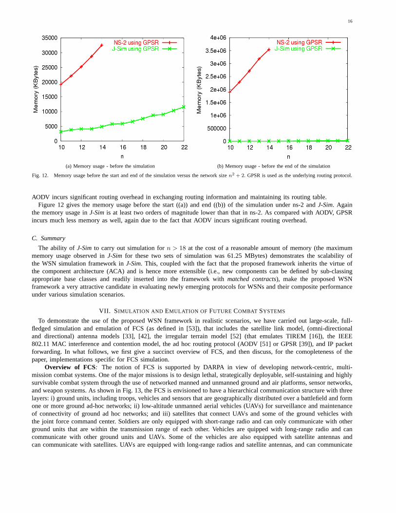
Fig. 12. Memory usage before the start and end of the simulation versus the network sizen2 + 2. GPSR is used as the underlying routing protocol.

AODV incurs significant routing overhead in exchanging routing information and maintaining its routing table.Figure 12 gives the memory usage before the start ((a)) and end ((b)) of the simulation under ns-2 andJ-Sim. Again

the memory usage inJ-Simis at least two orders of magnitude lower than that in ns-2. As compared with AODV, GPSRincurs much less memory as well, again due to the fact that AODV incurs significant routing overhead.

C. Summary

The ability of J-Simto carry out simulation forn > 18 at the cost of a reasonable amount of memory (the maximummemory usage observed inJ-Sim for these two sets of simulation was 61.25 MBytes) demonstrates the scalability ofthe WSN simulation framework inJ-Sim. This, coupled with the fact that the proposed framework inherits the virtue ofthe component architecture (ACA) and is hence more extensible (i.e., new components can be defined by sub-classingappropriate base classes and readily inserted into the framework withmatched contracts), make the proposed WSNframework a very attractive candidate in evaluating newly emerging protocols for WSNs and their composite performanceunder various simulation scenarios.

VII. S IMULATION AND EMULATION OF FUTURE COMBAT SYSTEMS

To demonstrate the use of the proposed WSN framework in realistic scenarios, we have carried out large-scale, full-fledged simulation and emulation of FCS (as defined in [53]), that includes the satellite link model, (omni-directionaland directional) antenna models [33], [42], the irregular terrain model [52] (that emulates TIREM [16]), the IEEE802.11 MAC interference and contention model, the ad hoc routing protocol (AODV [51] or GPSR [39]), and IP packetforwarding. In what follows, we first give a succinct overview of FCS, and then discuss, for the comopleteness of thepaper, implementations specific for FCS simulation.

Overview of FCS: The notion of FCS is supported by DARPA in view of developing network-centric, multi-mission combat systems. One of the major missions is to design lethal, strategically deployable, self-sustaining and highlysurvivable combat system through the use of networked manned and unmanned ground and air platforms, sensor networks,and weapon systems. As shown in Fig. 13, the FCS is envisioned to have a hierarchical communication structure with threelayers: i) ground units, including troops, vehicles and sensors that are geographically distributed over a battlefield and formone or more ground ad-hoc networks; ii) low-altitude unmanned aerial vehicles (UAVs) for surveillance and maintenanceof connectivity of ground ad hoc networks; and iii) satellites that connect UAVs and some of the ground vehicles withthe joint force command center. Soldiers are only equipped with short-range radio and can only communicate with otherground units that are within the transmission range of each other. Vehicles are quipped with long-range radio and cancommunicate with other ground units and UAVs. Some of the vehicles are also equipped with satellite antennas andcan communicate with satellites. UAVs are equipped with long-range radios and satellite antennas, and can communicate

17

Fig. 13. A typical FCS scenario. Also shown is how network emulation is performed by transporting real-life images captured by a WebCam (thatemualtes the view of a soldier) through theJ-Simvirtual environment to a real-life device PDA (that emulates the command center) and virtual nodesin J-Sim.

with both the ground vehicles and satellites. The satellites connects the UAVs and some of the ground vehicles with thecommand center. In addition, sensors self-organize themselves into a WSN, serve to track enemy vehicles (with differentsignatures of acoustic sounds), and relay sensor information to one or more of the ground vehicles.

All the ground/air platforms, sensor networks, and systems are prohibitively expensive to be readily deployed in trialtests. Moreover, tuning of systems parameters to optimize the performance is extremely time-consuming in real life. Asa result, there has been a pressing need to carry out high-fidelity (and preferrably real-time) simulation of a full-fledgedFCS based on real-life traces.

Classes implemented for FCS simulation: To faithfully simulate the FCS scenario, several components have tobe implemented: (1) a full-fledged networking stack including MAC, routing, transport and application layer protocols;(2) detailed radio propagation models and interference models to accurately model the physical characteristics of wirelesschannels; (3) (irregular) terrain model to take into account of the physical signal attenuation effect due to terrains; and(4) interfaces to allow input of real-life traces that give the movement characteristics of military units in the battlefield.Furthermore, in order to emulate different types of military wireless links (ground-to-ground, ground-UAV, ground-to-satellite, and UAV-to-UAV), each warfare entity must be equipped with different parameters (e.g. sending power, frequency,bandwidth, receiving threshold, carrier sense threshold, and interference threshold). We have leveraged both the wirelessnetwork extension and the proposed WSN framework to define and implement ground ad hoc networks (composed ofground units) and suvelliance sensor networks. We have also devised RTI-compliant trace interfaces inJ-Simto read real-lifemovement traces of ground entities provided by SAIC, Inc. In addition, we have completed the following implementation:

UAV Placement: One of the major functions of UAVs is to maintain the connectivity of the ground ad hoc networks.To this end, we have designed and implemented a UAV placement algorithm that continuously optimizes, based on themovement information of ground entities and the path loss information the altitudes and the flight paths of UAVs, so as

18

to maintain network connectivity and to recover from temporary network partition [45]. The UAV placement algorithmis periodically execuated in the simulation. In each run, the algorithm first builds connected components of ground unitsbased on the Irregular Terrain Model (ITM) [52]. It then sorts the connected components in the decreasing order of theirsizes (where the size of a componenet is the number of ground units in the component) and then searches for (near)optimal locations for UAVs to connect components in this order. Finally, for each UAV location newly determined, theUAV that is closest to the new location in the last run is dispatch to fly to that location.

Network emulation: To demonstrate the capability of network emulation, we have ported a real-life WebCamapplication on top ofJ-Simand transported real-life images captured by WebCam through theJ-Simvirtual simulationenvironment to another real-life device, a PDA. The WebCam is associated with a (virtual) vehicle node inJ-Sim, andis used to emulate the view of a soldier that operates the vehicle. The PDA, on the other hand, is associated with the(virtual) command center in the simulation scenario. Network emulation is then used to demonstrate how the view of asoldier in the battlefield can be transported, with the use of the top-down approach (Section V), to the remote commandcenter, and how its quality is subject to the mobility of ground entities, the terrain effect, and the paramter setting in theprotocol stack.

J-Sim 3D terrain visualization: We have also implemented, based on Java3D [4] technology, a 3D terrain visual-ization tool (Fig. 14) as a component inJ-Sim. The terrain visualization tool reads the altitude data of any location onthe earth from the GLOBE (Global Land One-km Base Elevation [11]) database, and renders the terrain. It also displaysthe movement of all the ground vehicles, soldiers, and UAVs. The 3D terrain images can be zoomed in/out, translated,and/or rotated. Performance statistics (such as the number of packets sent/received) pertaining to a node can be displayin real-time by clicking on the particular node.

Use of wireless sensor networks in target tracking in FCS: With the above implementation, we are able tosimulate various FCS scenarios. One scenario that pertains to the use of WSNs is to simulate how WSNs can be usedto facilitate target tracking in a FCS scenario. The FCS contains 121 sensors that are evenly distributed over a11 × 11square mile region, 40 ground vehicles, three UAVs, and one command center. The sensors are equipped with acousticsensors to detect enemy vehicles (that generates accoustics sound of supposedly different signatures). The radio frequencyis chosen to be 900MHz for short-range radio and 2GHz for long-range radio to avoid collision between the two types ofradios. The transmission power is set to be 0.2818W and the receiving threshold is set to be1.58× 10−10W for shortrange radios and2.7 × 10−11W for long range radios. The wireless bandwidth of each sensor is set to 20Kbps and theradio bandwidth of all the other entities is set to 2Mbps. The carrier sense threshold is set to be the receiving thresholddivided by 10.

In the simulation, two enemy tanks enter this battlefield. The sensors detect their exitence, continuously monitor theirmovement and send their locations and moving directions to one of the ground vehicles (that acts as the sink). After beingrelayed the information, the ground vehicle sends control messages to several ground vehicles to chase after the enemyvehicles, while the UAVs continuously adjust their altitudes and fly paths to maintain connectivity of ground vehicles.Figure 15 shows a snapshot of the movement information of the two enemy tanks received at the sink node. A videodemo of the entire simulation can be downloaded at [2].

VIII. R ELATED WORK

In this section, we give an overview of existing network simulators that support wireless network simulation and/orsensor network simulation. Examples of network simulators that support wireless network simulation are GloMoSim [8]and OPNET [12]. Examples of network simulators that support both wireless network simulation and sensor networksimulation are ns-2 [6] and Ptolemy [7].

GloMoSim (Global Mobile Information System Simulator) [21], [8] is a simulation environment for wireless mobilenetworks. GloMoSim is designed as a set of modules in the layered architecture; each module simulates a specific protocolin the protocol stack. GloMoSim has been designed using the parallel discrete-event simulation capability provided byPARSEC (Parallel Simulation Environment for Complex Systems) [20], [13]. PARSEC is a C-based sequential and parallelsimulation language, which can be used to program new modules that can be added to GloMoSim.

OPNET [12] is a commercial network modeler and simulator provided by OPNET Technologies, Inc. In OPNET, anetwork is modeled in a hierarchical approach that closely matches the hierarchical architecture of the Internet: networks,subnets and nodes (fixed, mobile or satellite). Each node is modeled as a set of processes where each process is modeledas a finite state machine (FSM). The entire network is simulated using a discrete-event simulator. OPNET supports threetypes of links: point-to-point, bus and wireless. A wireless link is used in wireless, mobile or satellite network simulation.Each stage in the 14-stage transceiver pipeline models an aspect of the channel’s behavior (e.g., line-of-sight, signal

19

Fig. 14. A snapshot of the terrain and warefare entity visualization tool that shows a FCS scenario in San Diego, CA. Each circle denotes the coveragearea of an UAV.

strength or bit errors). The transceiver pipeline stages calculate the received signal power in order to determine whetherthe signal can be received by the receiver.

Ns-2 [22] began as a variant of the REAL network simulator [41], and has evolved substantially over the past few years.It provides substantial support for simulation of TCP, routing, and multicast protocols. The support for wireless and mobilenetwork simulation was included in ns-2 by the Rice University Monarch (Mobile Networking Architectures) Project [14]2.The Monarch project provides various modules for (mobile) wireless network simulation; e.g., radio propagation models,the IEEE 802.11 MAC protocol, mobility models, different ad-hoc routing protocols (e.g., AODV and DSR) and MobileIP. The latest version of ns-2 supports the simulation of pure wireless LANs, multihop ad-hoc networks and the combinedsimulation of wired and wireless (known as “wired-cum-wireless”) networks. SensorSim [49], [48], [15], from UCLA,has further extended ns-2 by including the support for sensor network simulation. Similar to our simulation framework,SensorSim also includes the definition of target, sensor and sink nodes, sensor and wireless communication channels,physical media, mobility model and the power model. However, at the time of this writing, the public release of SensorSimis no longer available at [15].

Ptolemy [7] is an ongoing project at UC Berkeley that studies modeling, discrete-event simulation, and design of

2formerly known as The CMU Monarch Project (http://www.monarch.cs.cmu.edu/).

20

Fig. 15. Movement information of the two enemy tanks received by the sink node.

concurrent, real-time, embedded systems. The key underlying principle in Ptolemy is the ability to use multiple modelsof computation (e.g., continuous-time, dataflow, finite-state machine) in a hierarchical heterogeneous design environment.VisualSense [23] is a modeling and simulation framework that builds on and leverages Ptolemy to support design, simulationand visualization of sensor networks. In VisualSense, a sensor node can be modeled either in Java or by using conventionaldiscrete-event models (e.g., block diagrams) or Ptolemy models (e.g., continuous-time or dataflow models). Similar toour simulation framework, VisualSense supports sensor and wireless channels, antenna gains, terrain models and batterymodels. However, Ptolemy does not support network emulation. On the other hand,J-Simsupports network emulation asexplained in the Future Combat System (FCS) simulation presented in this paper.

TOSSIM [17] is a bit-level simulator for TinyOS[34] wireless sensor networks. The goal of TOSSIM is to provide anaccurate, scalable simulator that bridge the gap between algorithms and implementations. TOSSIM can compile unchangedTinyOS applications directly into its framework, which means most of the codes written for TOSSIM can be directly usedin TinyOS. It only replaces a few low-level TinyOS systems that touch hardware and thus maintains the accuracy ofthe simulation. The link layer is modeled using an independent bit error model. The packet is encoded with CRC andcan correct one-bit error and detect two-bit error. TOSSIM models the wireless network with a directed graph, whereeach vertex is a node and each edge has a bit error probability. This simple abstraction increases its scalability. However,TOSSIM is very specific to TinyOS and Berkeley motes. It may not be appropriate for simulating a general sensor network.

IX. CONCLUSIONS ANDFUTURE WORK

In this paper, we have defined and implemented a simulation and emulation framework for wireless sensor networks(WSNs) in J-Sim— an open-source, component-based compositional network simulation environment. The frameworkprovides an object-oriented definition of (i) target, sensor and sink nodes, (ii) sensor and wireless communication channels,and (iii) physical media such as seismic channels, mobility models and power models (both energy-producing and energy-consuming components). Customized application-specific models can be readily defined and implemented by sub-classingappropriate classes the simulation framework and customizing their behaviors. We have also included inJ-Sima set ofclasses and mechanisms to realize network emulation [40], [29], [60]. We leverage packet capturing tools (such as pcap[5] in Linux and Windows and SerialForwarder in TinyOS [34]) and devise mechanisms to synchronize the virtual timeand the wall time.

We have demonstrated the use of the proposed WSN simulation framework by implementing several well-known local-ization, geographic routing, and directed diffusion protocols. We have also performed detailed performance comparisons

21

(in terms of execution time incurred, and the memory used) in simulating several typical WSN scenarios inJ-Simandns-2. The simulation study indicatesJ-Simandns-2 incur comparable execution time, but the memory allocated to carryout simulation (of length≥ 1000 in J-Sim is at least two orders of magnitude lower than that inns-2. As a result, whilens-2often suffers from out-of-memory exceptions and was unable to carry out large-scale WSN simulation, the proposedWSN framework inJ-Sim exhibits good scalability. Finally, we have demonstrated the use of the WSN framework incarrying out real-life, full-fledged future combat system simulation and emulation.

We have also identified several research avenues for future work. First, the proposed framework did not explicitly modelthe lateration mechanism by which sensor nodes determine the location of a target node. As part of our future work, wewill lay out classes to model how sensors cooperate to determine the location of a target node. Second, we will defineand implement inJ-Simgeneric classes for several newly emerging WSN functions, such as coverage [61], [59], timeindexing [62], and power management [63], [25].

REFERENCES

[1] Evaluation of J-Sim. http://www.j-sim.org/comparison.html.[2] Future Combat System (FCS) simulation and demo. http://lion.cs.uiuc.edu/demo/demo.html.[3] Irregular Terrain Model (ITM). http://elbert.its.bldrdoc.gov/itm.html.[4] Java 3D API. http://java.sun.com/products/java-media/3D/.[5] The libpcap packet capture library. ftp://ftp.ee.lbl.gov/libpcap.tar.z.[6] Ns-2. http://www.isi.edu/nsnam/ns/.[7] Ptolemy. http://ptolemy.eecs.berkeley.edu.[8] GloMoSim. http://pcl.cs.ucla.edu/projects/glomosim/.[9] J-Sim. http://www.j-sim.org/.

[10] J-Sim wireless extension tutorial. http://www.j-sim.org/v1.3/wireless/wirelesstutorial.htm.[11] NGDC-GLOBE Project. http://www.ngdc.noaa.gov/seg/topo/globe.shtml.[12] OPNET. http://www.opnet.com.[13] PARSEC. http://pcl.cs.ucla.edu/projects/parsec/.[14] The Rice University Monarch Project. http://www.monarch.cs.rice.edu/.[15] SensorSim: A simulation framework for sensor networks. http://nesl.ee.ucla.edu/projects/sensorsim/.[16] Terrain Integrated Rough Earth Model (TIREM). TIREM/SEM handbook, ECAC-handbook-93-076.[17] TOSSIM: Accurate and scalable simulation of entire TinyOS applications, 2003.[18] I. F. Akyildiz, W. Su, Y. Sankarasubramaniam, and E. Cayirci. Wireless sensor networks: A survey.Computer Networks,

38(4):393–422, March 2002.[19] G. Asada, M. Dong, T. S. Lin, F. Newberg, G. Pottie, and W. Kaiser. Wireless integrated network sensors: Low power systems

on a chip. InProc. of the 1998 European Solid State Circuits Conference, 1998.[20] R. Bagrodia, R. Meyer, M. Takai, Y.-A. Chen, X. Zeng, J. Martin, and H. Y. Song. Parsec: a parallel simulation environment for

complex systems.IEEE Computer Magazine, 31(10):77–85, October 1998.[21] L. Bajaj, M. Takai, R. Ahuja, K. Tang, R. Bagrodia, and M. Gerla. GloMoSim: A scalable network simulation environment.

Technical Report 990027, Computer Science Department, University of California, Los Angeles, May 1999.[22] S. Bajaj, L. Breslau, D. Estrin, K. Fall, S. Floyd, P. Haldar, M. Handley, A. Helmy, J. Heidemann, P. Huang, S. Kumar, S. McCanne,

R. Rejaie, P. Sharma, K. Varadhan, Y. Xu, H. Yu, and D. Zappala. Improving simulation for network research. Technical Report

99-702, University of Southern California, 1999.[23] P. Baldwin, S. Kohli, E. A. Lee, X. Liu, and Y. Zhao. Modeling of sensor nets in Ptolemy II. InProc. of the ACM/IEEE

International Symposium on Information Processing in Sensor Networks (ACM/IEEE IPSN’04), April 2004.[24] N. Bulusu, J. Heidemann, and D. Estrin. GPS-less low-cost outdoor localization for very small devices.IEEE Personal

Communications, pages 28–34, 2000.[25] B. Chen, K. Jamieson, H. Balakrishnan, and R. Morris. Span: An energy-efficient coordination algorithm for topology maintenance

in ad hoc wireless networks. InProc. of MobiCom, July 2001.[26] J. Cowie, H. Liu, J. Liu, D. Nicol, and A. Ogielski. Towards realistic million-node Internet simulations. InProc. of International

Conference on Parallel and Distributed Processing Techniques and Applications (PDPTA’99), June 1999.[27] L. Doherty, K. Pister, and L. Ghaoui. Convex position estimation in wireless sensor networks. InProceedings of IEEE INFOCOM,

2001.[28] D. Estrin, R. Govindan, J. S. Heidemann, and S. Kumar. Next century challenges: Scalable coordination in sensor networks. In

Proc. of the ACM International Conference on Mobile Computing and Networking (ACM MobiCom’99), August 1999.[29] K. Fall. Network emulation in the vint/ns simulator. InProceedings IEEE ISCC99, July 1999.

22

[30] T. He, C. Huang, B. M. Blum, J. A. Stankovic, and T. Abdelzaher. Range-free localization schemes for large scale sensor networks.

In Proceedings of ACM MOBICOM, 2003.[31] J. Heidemann, F. Silva, and D. Estrin. Matching data dissemination algorithms to application requirements. InProc. of the ACM

Conference on Embedded Networked Sensor Systems (ACM SenSys’03), 2003.[32] W. Heinzelman, J. Kulik, and H. Balakrishnan. Adaptive protocols for information dissemination in wireless sensor networks. In

Proc. 5th ACM MobiCom, August 1999.[33] A. Higgins, G. Lehtola, R. Meyer, and K. Peterson. A quasi-optical adaptive antenna communications system for 37 GHz. In

Proc. of the IEEE Military Communications Conference (IEEE MILCOM’01), October 2001.[34] J. Hill, R. Szewczyk, A. Woo, S. Hollar, D. Culler, and K. S. Pister. System architecture directions for networked sensors. In

Architectural Support for Programming Languages and Operating Systems, pages 93–104, Boston, MA, USA, Nov. 2000.[35] C. Intanagonwiwat, R. Govindan, and D. Estrin. Directed diffusion: A scalable and robust communication paradigm for sensor

networks. InProc. of the ACM International Conference on Mobile Computing and Networking (ACM MobiCom’00), 2000.[36] C. Intanagonwiwat, R. Govindan, D. Estrin, J. Heidemann, and F. Silva. Directed diffusion for wireless sensor networking.

IEEE/ACM Transactions on Networking, 11(1):2–16, February 2003.[37] J. Kahn, R. Katz, and K. Pister. Next century challenges: Mobile networking for “Smart Dust. InProc. of the ACM International

Conference on Mobile Computing and Networking (ACM MobiCom’99), 1999.[38] J. M. Kahn, R. H. Katz, and K. S. J. Pister. Next century challenges: mobile networking for small dusts. InProc. of the ACM

International Conference on Mobile Computing and Networking (ACM MobiCom’99), August 1999.[39] B. Karp and H. Kung. Greedy perimeter stateless routing for wireless networks. InProceedings of the Sixth Annual ACM/IEEE

International Conference on Mobile Computing and Networking (MobiCom 2000), pages 243–254, Boston, MA, August 2000.[40] Q. Ke, D. Maltz, and D. B. Johnson. Emulation of multi-hop wireless ad hoc networks. InProc. of the Seventh International

Workshop on Mobile Multimedia Communications, October 2000.[41] S. Keshav. REAL: A network simulator. Technical Report 88/472, University of California, Berkeley, 1988.[42] W. Kishaba, G. Vardakas, J. J. Garcia-Luna-Aceves, L. Bao, and Y. Kang. Adhoc networking with beam-forming antennas. In

Proc. of the IEEE Military Communications Conference (IEEE MILCOM’01), October 2001.[43] F. Kuhn, R. Wattenhofer, Y. Zhang, and A. Zollinger. Geometric ad-hoc routing: of theory and practice. InProc. of the ACM

Symposium on Principles of Distributed Computing (ACM PODC’03), July 2003.[44] F. Kuhn, R. Wattenhofer, and A. Zollinger. Worst-case optimal and average-case efficient geometric ad-hoc routing. InProc. of

the ACM International Conference on Mobile Computing and Networking (ACM MobiHoc’03), June 2003.[45] N. Li and J. C. Hou. Improving connectivity of wireless ad-hoc networks. Submitted to IEEE Int’l Conf. on Distributed Computing

Systems (ICDCS’05), October.[46] R. Nagpal, H. Shrobe, and J. Bachrach. Organizing a global coordinate system from local information on an ad hoc sensor

network. InProceedings of IPSN, 2003.[47] D. Niculescu and B. Nath. Ad hoc positioning system (APS). InProceedings of IEEE GLOBECOM, 2001.[48] S. Park, A. Savvides, and M. Srivastava. Simulating networks of wireless sensors. InProc. of the 2001 Winter Simulation

Conference, 2000.[49] S. Park, A. Savvides, and M. Srivastava. SensorSim: A simulation framework for sensor networks. InProc. of the ACM international

Workshop on Modeling, Analysis and Simulation of Wireless and Mobile Systems, 2000.[50] S. Park, A. Savvides, and M. Srivastava. Battery capacity measurement and analysis using lithium coin cell battery. InProc. of

the ACM International Symposium on Low power Electronics and Design (ACM ISLPED’01), 2001.[51] C. Perkins, E. Royer, and S. Das. Ad hoc on demand distance vector (aodv) routing. IETF Draft, January 2002.[52] K. Sarabandi, I. Koh, G. Liang, and H. Bertoni. Propagation modeling for FCS. InProc. of the IEEE Military Communications

Conference (IEEE MILCOM’01), October 2001.[53] P. Sass and J. Freebersyser. FCS communications technology for the objective force.[54] A. Savvides, C. C. Han, and M. B. Srivastava. Dynamic fine-grained localization in ad-hoc wireless sensor networks. InProceedings

of ACM MOBICOM, 2001.[55] D. J. Schwartz, Y. Yemini, and D. Bacon. NEST: A network simulation and prototyping testbed.Communications of the ACM,

33(10):63–74, October 1990.[56] A. Sobeih and J. C. Hou. A simulation framework for sensor networks in J-Sim. Technical Report UIUCDCS-R-2003-2386,

Department of Computer Science, University of Illinois at Urbana-Champaign, November 2003.[57] H.-Y. Tyan. Design, Realization and Evaluation of a Component-based Compositional Software Architecture for Network

Simulation. PhD thesis, Department of Electrical Engineering, The Ohio State University, 2002.[58] H.-Y. Tyan and J. C. Hou.JavaSim: A component-based compositional network simulation environment. InProc. of Western

23

Simulation Multiconference, CNDS’01, January 2001.[59] X. Wang, G. Xing, Y. Zhang, C. Lu, R. Pless, and C. Gill. Integrated coverage and connectivity configuration in wireless sensor

networks. InACM Sensys’03, Nov. 2003.[60] B. White, J. Lepreau, and S. Guruprasad. Lowering the barrier to wireless and mobile experimentation.ACM SIGCOMM Computer

Communications Review, 33(1), January 2003.[61] F. Ye, G. Zhong, S. Lu, and L. Zhang. Peas: A robust energy conserving protocol for long-lived sensor networks. InThe 23nd

International Conference on Distributed Computing Systems (ICDCS), 2003.[62] R. Zheng, G. He, I. Gupta, J. Hou, and L. Sha. Time indexing in sensor networks. InProc. 1st IEEE International Conf. on

Mobile Ad Hoc and Sensor Systems (MASS’04), October 2004.[63] R. Zheng and R. Kravets. On-demand power management for ad hoc network. InProc. of IEEE INFOCOM, 2003.

24

I. Wired networksTraffic model Packet scheduler Routing algorithm/protocol Resource reservation

Periodic message FCFS Unicast shortest path RSVPPeak rate model RM Unicast minimum load path

Leaky bucket model EDF Unicast QoS routingToken bucket model stop-and-go Multicast shortest path

IETF/Intserv Flowspec DCTS Multicast minimum load tree(r, t)-smooth model VirtualClock Multicast spanning tree

(C, D)-smooth model LFVC Multicast steiner treeSCFQ Distance vector routingPGPS OSPFv2STFQ QoS-enhanced OSPFv2WF2Q Dist. Unicast QoS routing

Leave-in-time DVMRPFIFO-r MOSPF

CBTQoS-enhanced CBT

Data transport Socket layer Tagger/marker Buffer management

TCP-Reno Java-compliant Token bucket model REDTCP-Tahoe TSW FREDTCP-Vegas ETSW SRED

TCP with delayed ack option BREDTCP with ECN

UDP

PGPS: packet-by-packet generalized processing sharing. WF2Q: worst-case fair weighted fair queuing.STFQ: start time fair queuing. SCFQ: self-clocked fair queuing.LFVC: leap forward virtual clock. OSPFv2: open shortest path first protocol (Version 2).DVMRP: distance vector multicast routing protocol. MOSPF: multicast extension to open shortest path first.CBT: core based tree protocol. TCP: transport control protocol.ECN: explicit congestion notification. UDP: user datagram protocol.TSW: time sliding window. ETSW: enhanced time sliding window.RED: random early drop. FRED: fair random early drop.SRED: stable random early drop. BRED: balanced random early drop.

II. Wireless networksAntenna model Signal propagation Datalink model Ad hoc routing

Parabolic reflective antenna Free space model IEEE 802.11 DSRDirectional antenna Two-ray ground model IEEE 802.11 with PSM AODV

Irregular terrain model Military link emulation with different send-ing powers, frequencies, bandwidth, receiv-ing/ carrier sense/ interference thresholds

AODV multicast extension

Satellite link Mobility modelSatellite link with detailed wireless errormodel and propagation delay

Random way-point

SDF trace-based model

DSR: dynamic source routing. AODV: ad hoc on-demand distance vector.PSM: power saving mode.

TABLE I

NETWORK AND COMMUNICATIONS ENTITIES SUPPORTED INJ-Sim.