International Journal of Engineering Science xxx (2011) xxx–xxx

Contents lists available at ScienceDirect

International Journal of Engineering Science

journal homepage: www.elsevier .com/locate / i jengsci

Isothermal two-phase flow of a vapor–liquid systemwith non-negligible inertial effects

Iacopo Borsi, Lorenzo Fusi ⇑, Fabio Rosso Alessandro SperanzaDipartimento di Matematica, ‘‘U. Dini’’, Viale Morgagni 67/a, 50134 Firenze, Italy

a r t i c l e i n f o

Article history:Received 15 July 2010Accepted 5 May 2011Available online xxxx

Keywords:Flow in porous mediaLiquid–gas two-phase flowsNonlinear constitutive equationsNumerical simulation

0020-7225/$ - see front matter � 2011 Elsevier Ltddoi:10.1016/j.ijengsci.2011.05.003

⇑ Corresponding author.E-mail address: fusi@math.unifi.it (L. Fusi).

a b s t r a c t

In this paper we consider the problem of gas/liquid extraction near the bottom well in thecontext of geothermal energy exploitation. In particular we develop a mathematical modelfor the isothermal two-phase flow of a mono-component fluid in an undeformable porousmedia taking into account inertial effects. We use the so-called Forchheimer’s equation tomodel the relation between the fluid velocity and the pressure gradient in the region of co-existence of the two phases. We formulate the problem in cylindrical geometry assumingsteady state and isothermal conditions. We take into account capillary pressure and westudy its influence on the whole system. We derive important formulas that allow to pre-dict the main thermodynamical quantities in the region of co-existence of the liquid andgaseous phase and we determine constraints on the physical parameters in order to predictthe behavior of the fluid in the domain of the problem. Finally, we perform some numericalsimulations to investigate the dependence on the physical parameters involved in themodel.

� 2011 Elsevier Ltd. All rights reserved.

1. Introduction

It is known that flows through porous media can be modeled within the theory of mixture that allows to take into accountthe numerous mechanisms occurring during the flow (see Rajagopal, 2007, Rajagopal & Tao, 1995). Popular models such asBrinkman (1947a, 1947b), Biot (1956a, 1956b), and Forchheimer (1901) and the most famous Darcy (1856) can be obtainedfrom classical balance laws under specific assumptions in the context of mixture theory. Recently Rajagopal (2007) hasdeveloped a hierarchy of approximate models in which Darcy’s law represents the simplest of the models considered.Depending on which effects one wants to model (frictional effects, drag effects, inertial effects, compressibility, etc.) a seriesof assumptions which lead to particular constitutive equations must be made. For example, Darcy’s law is obtained assumingthat the porous matrix is rigid, that the interaction forces between the solid and the fluid are only due to the friction betweenthe fluid and the pore surface (expressed by a drag-like term proportional to the velocity of the fluid), that the frictional ef-fects within the fluid due to its viscosity can be neglected, that the flow is sufficiently slow that inertial terms can be ignoredand that the partial stress is the one of an Euler fluid.

When relaxing some assumptions one gets more complex models. For instance, assuming that the frictional effects in thefluid are not negligible one gets the Brinkman model (Brinkman, 1947a, 1947b). Further, if one relaxes the hypothesis of neg-ligible inertial effects one gets a series of nonlinear models (Dupuit–Forchheimer of second or third grade or power law, seeAulisa, Bloshanskaya, Hoang, & Ibragimov (2009)), depending on the way interaction forces are modeled. In other situations(e.g. oil recovery) the effects of pressure on viscosity cannot be neglected or, as in the case developed by Munaf, Lee, and

. All rights reserved.

916 I. Borsi et al. / International Journal of Engineering Science xxx (2011) xxx–xxx

Rajagopal (1993), liquid compressibility is taken into account. Other models may include the solid matrix undergoing smallor large deformations (see Rajagopal & Tao (2005) for a detailed derivation of the Biot’s equation in the context of theory ofmixture).

It is clear that mixture theory is a powerful tool to derive the constitutive equation one needs to develop a specific model.Of course it is not the only way to derive constitutive equations for the flow through porous media (e.g. Darcys equation hasalso been obtained rigorously within the context of homogenization and other averaging/upscaling techniques, see Sanchez-Palencia (1980)).

In the model we are going to present, the constitutive equations stem from specific assumptions within the context ofmixture theory. Indeed, as shown in Rajagopal (2007), a hierarchy of equations that govern the flow through porous mediacan be developed with each equation obtained by making rigorous assumptions on the physical processes one is considering.

In particular we propose a nonlinear one-dimensional macroscopic model for the isothermal compressible flow of a two-phase (mono-component) fluid in a porous medium where inertial effects cannot be neglected. Within the framework dis-cussed in Rajagopal (2007), the main physical assumptions under which the model is derived are the following.

� The solid composing the matrix of the porous medium is rigid (balance of linear momentum can be neglected)� The sole interaction forces between the fluid and the matrix are due to the friction exerted by the fluid on the boundary of

the pore and such forces are modeled as a drag-like term proportional to the velocity of the fluid (as in Darcy’s law)� The frictional effects within the fluid due to its viscosity are neglected� The flow is sufficiently fast so that non-linearities due to inertia cannot be ignored� The fluid is compressible� The fluid can be found in two different phases (gaseous and liquid)� There is non mass exchange between the fluid and the solid matrix

The main motivation of this work is the development of a mathematical model for describing a geothermal reservoir inthe vicinity of a wellbore.

It is well known that, for low pore-scale Reynolds numbers, the flow of fluid through a porous media can be described byDarcy’s law Darcy (1856), which assumes that the fluid velocity in the pores is linearly related to the pressure drop throughthe so-called permeability coefficient. In this framework the contribution of inertial effects is neglected and the mass balanceequation for each phase is written exploiting Darcy’s law Bear (1972).

Unlike one dimensional viscous flows in channels or pipes, where the transition from laminar (no inertial effects) to tur-bulent regimes occurs when the Reynolds number is above a critical threshold, in flows through porous media inertial effectsmay play a non negligible role even if the Reynolds number is below the critical value at which turbulent effects are observedDullien (1979).

In this situation the transition from laminar to turbulent regimes is more gradual so that the influence of inertia must betaken into account even before turbulence has fully developed Andrade, Costa, Almeida, Makse, and Stanley (1999) and Has-sanizadehm and Gray (1987). This fact, which has been verified experimentally Dullien (1979), has also been confirmed bynumerical simulations Edwards, Shapiro, Bar-Yoseph, and Shapira (1990) and Koch and Ladd (1997).

In this optic we develop a mathematical model that accounts for inertial effects assuming that the mass transport is gov-erned by the so-called Forchheimer’s equation Bear (1972). The linear Darcian model then becomes a limit case which can beobtained by letting the inertial parameter appearing in the Forchheimer’s equation tend to zero.

Since we are dealing with a two-phase flow for a mono-component fluid, the pores in which the fluid flows are filled bygas and liquid (for instance water and vapour). The combination of surface tension and curvature at the interface betweenthe gas and the liquid in the pores causes the two phases to experience different pressures. The difference between these twopressure is known as the capillary pressure Bear (1972). Capillary pressure is defined as the pressure difference between thenon-wetting phase and the wetting phase and it is represented as a function of the wetting phase saturation. As the relativesaturation between the phases changes, the capillary pressure also changes, so that a constitutive relationship linking sat-uration and capillary pressure has to be prescribed (saturation curve). In reservoir rocks that are significantly wettable1 andin which the fractures are filled by water (wetting) and vapour (non-wetting), capillary pressure is defined as a decreasing func-tion of the liquid saturation.

In isothermal conditions, when the effects of capillary pressure are negligible, the pressures experienced by the twophases at the separation interface are equal to the saturation vapour pressure of the fluid for the fixed temperature. Inthe case capillary pressure is significant, the saturation vapour pressure becomes lower that the value assumed when cap-illary effects are not present.2 The exact amount of this reduction is obtained through Kelvin’s law Coussy (1995).

The model we are going to present is derived in a general 3D setting, but we will focus on a cylindrical geometry in whichthe domain is the outer region of a cylinder with fixed radius (see Fig. 1). This choice is motivated by the fact that the mainpractical application of the model is the process of gas/liquid extraction in geothermal power plants in which a well (thecylinder) is drilled in a geothermal reservoir (the external part of the cylinder) for withdrawal purposes. The set of equations

1 Wettability can be described as the relative tendency of a rock to be covered by the liquid phase.2 This phenomenon is also known as vapour pressure lowering, Bear (1972).

Fig. 1. Sketch of the cylindrical domain.

I. Borsi et al. / International Journal of Engineering Science xxx (2011) xxx–xxx 917

that defines the flow is composed by mass balance equation, the equations of state of the fluid in the two phases and theconstitutive relations that define which kind of transport is taking place (Darcy, Forchheimer, etc.).

We will limit ourselves to consider the stationary state (an assumption justified by the typical time scales of a geothermalsystem) and we will derive the differential equations that define the liquid saturation as a function of the distance from theboundary of the domain (the wall of the cylinder). We will take into account the effects due to capillary pressure and finally,we will present some numerical simulations to illustrate how the evolution of the system depends from the physical param-eters involved in the model.

In particular we shall see that, when the simulations are performed using parameters that are typical of a geothermalreservoir, the Darcian model and the Forchheimer’s model provide results that are significantly different. This is a veryimportant outcome, since it clearly indicates that in the modeling of a geothermal fluid flow inertial effects cannot beneglected.

Far from being exhaustive, this model is an attempt to describe the macroscopic two-phase flow in a porous medium withnon-negligible inertial effects in order to get quantitative informations that can be useful to predict the potential productiv-ity of a geothermal plant.

2. The general model

Let us consider a domain X � R3 representing an undeformable porous medium where pores are filled by liquid and va-pour of the same fluid (for instance water). Mass balance is expressed by

@

@t/X

aSaqa

!þr �

Xa

qa~ua

!¼ �Q ; ð1Þ

where Sa; qa; ~ua are the saturation, density, superficial velocity of the ath phase, respectively (a = l liquid, a = g vapour) andwhere Q represents the sink/source term due to extraction or injection of the fluid. The coefficient / represents the porosityof the porous medium. Since we are dealing with a two-phase flow, the saturations Sg, Sl are such that

Sg þ Sl ¼ 1: ð2Þ

If we assume that mass exchange with X occurs only at the boundary oX (i.e. Q = 0) and we assume cylindrical geometry(which is the natural setting for application purposes) and stationary state, Eq. (1) becomes

@

@rrX

aqa~ua

" #¼ 0; r 2 ½rw;1Þ; ð3Þ

where rw > 0 is the radius of the cylinder which represents, for instance, the radius of the well in a geothermal reservoir. Forsimplicity, we suppose that mass is extracted (and not injected) from X and that the extraction rate is constant. The exten-sion to the case of injection is straightforward. In this setting the amount of fluid crossing the lateral surface of a cylinder ofradius r P rw and fixed height H is independent from r. Therefore if we denote with w the amount of fluid per unit time ex-tracted at r = rw we have

½qlul þ qgug �2prH ¼ �w; 8r 2 ½rw;1Þ ð4Þ

and (3) becomes

qlul þ qgug ¼ � w2pH

� �1r; r 2 ½rw;1Þ: ð5Þ

2.1. The fluid flow

As stated in the introduction, for small Reynolds pore-scale numbers where only viscous effects are relevant, the two-phase flow is well described by Darcy’s law

3 Thephase c

918 I. Borsi et al. / International Journal of Engineering Science xxx (2011) xxx–xxx

la

ka ~ua ¼ �rðPa � qag~zÞ; ð6Þ

where Pa, la, ka are the pressure, viscosity, effective permeability3 of the ath phase and where g is gravity. When inertial ef-fects are significant Eq. (6) is no longer apt to describe the flow. In this situation a good experimental law that describes the flow(as confirmed by several laboratory measurements Venkataraman & Rao (1998)) is given by the Forchheimer or Forchheimer–Dupuit equation

la

ka ~ua þ bqaj~uaj~ua ¼ �r Pa � qag~k

� �; ð7Þ

where b is the so-called Forchheimer parameter ([b] = [L�1]) which can be safely considered the same for both the liquid andgaseous phase, since it depends on some structural properties of the solid matrix Bear (1972). A typical way of estimating b is

b � dk; ð8Þ

where k is the absolute permeability and d is the typical dimension of the pores. Neglecting the effects of gravity and con-sidering cylindrical geometry (Fig. 1) Eq. (7) becomes

la

ka ua þ bqajuajua ¼ � dPa

dr; r 2 ½rw;1Þ: ð9Þ

Recalling the expression Bear (1972)

ka ¼ kkar ðS

aÞ ð10Þ

which defines the relation between the relative ðkar Þ, absolute (k) and effective (ka) permeability, Eq. (9) can be rewritten as

la

kkar ðS

lÞua þ bqajuajua ¼ � dPa

dr; r 2 ½rw;1Þ: ð11Þ

where we have exploited the fact that Sl = 1 � Sg, that allows to write kar ðS

lÞ for a = l, g.

2.2. Equations of state

In order to model the two-phase flow, we must specify the equation of state in both phases. Assuming that the gaseousphase is constituted by a perfect gas we write

qg ¼ MwPg

RT¼:

cPg

T; ð12Þ

where Mw is the molar mass (mass divided by the number of moles), R is the universal gas constant and T is temperature([c] = [T � t2 � L�2]). For the liquid phase we assume the exponential law

ql ¼ qo exp kðPl � PoÞh i

; ð13Þ

where qo and Po are a reference density and a reference pressure respectively and where k is the compressibility coefficient([k] = [P]�1). For most compressible liquids, Eq. (13) can be approximated by

ql ¼ qo½1þ kðPl � PoÞ�; ð14Þ

since the compressibility coefficient k is sufficiently small. In our model we will consider (12) and (14) as equations of statefor the gaseous and liquid phase.

2.3. The capillary pressure

In the model we are going to present we will include the effects due to capillary pressure. From a microscopic point ofview, in the interstices of the porous medium, the two phases of the fluid are separated by an interface (Fig. 2) where thefluid pressure exhibits a jump whose magnitude depends on the interface curvature. The latter, in turn, depends on thechemical, physical and topological characteristics of the solid matrix and in particular on the tendency to attract or rejectthe liquid phase (wettability/non-wettability). Because of the impossibility to describe the geometrical shape of each poreit is useful to imagine the interstices as short capillary tubes. The capillary pressure is then the pressure required to draina wetting liquid (or conversely to force a non-wetting liquid) out of a capillary tube ad is defined as

Pc ¼2rd

cos h; ð15Þ

effective permeability of each phase depends on the structural features of the porous medium and specifically on the absolute permeability k of a singleompletely saturating it.

Fig. 2. Microscopic sketch of a porous medium where the pores are filled by liquid and gas.

I. Borsi et al. / International Journal of Engineering Science xxx (2011) xxx–xxx 919

where r > 0 is the interfacial tension ([r] = [P � L]), d > 0 is the radius of the capillary tube (averaged value of the pores diam-eter) and h is the contact angle (h 2 (0,90�) wetting, h > 90� non-wetting). The equilibrium between the two phases at theinterface in the pores is expressed by the relation

4 In w

Pc ¼ Pg � Pl; ð16Þ

where Pg is the pressure of the non-wetting phase (gas) and Pl is the pressure of the wetting phase (liquid). When consideringgeothermal system it is reasonable to assume that h 2 (0,90o], which implies Pc P 0, since the liquid is water and rocks arecommonly highly wettable. When capillary effects are negligible we set h = 90o and Pc = 0, since Pg = Pl = Psat, where Psat is thesaturation vapour pressure.

When switching to the macroscopic level we will no longer be dealing with pores and interfaces, but simply assume thateach point of the spatial domain is co-occupied by the gaseous and liquid phase. The capillary pressure then will be consti-tutively defined as a function of the volume fraction occupied by the liquid Sl and we will assume that it is experimentallygiven, i.e. Pc = Pc(Sl).

Remark 1. The curve in the (P,T) plane that describes the thermodynamical equilibrium between the vapour phase and theliquid phase in an isolated system is called the saturation pressure curve, which is a function of the temperature, i.e.Psat = Psat(T). The dependence on temperature is expressed through the so-called Clausius–Clapeyron relation Bear (1972)

Psat ¼ K exp �DHRT

� �; ð17Þ

where K is a constant ([K] = [P]) and DH is the specific enthalpy of vaporization ([DH] = [L2 � t�2]). In case the mono-compo-nent fluid is water a good approximation of (17) is given Tsypkin (1997)

Psat ¼ Pa exp 12;512� 4611;73T

� �; ð18Þ

where Pa = 105 Pa and T is expressed in �K.

Remark 2. When capillary pressure is not zero, experimental results have shown a phenomenon known as vapour pressurelowering Coussy (1995), where the saturation vapour pressure of the gaseous phase for a given temperature is lower than theone experienced in the case capillary pressure is zero. The measure of this reduction is obtained by means of the so-calledKelvin’s equation4 Coussy (1995)

hat follows we consider the wettable case with Pc P 0.

920 I. Borsi et al. / International Journal of Engineering Science xxx (2011) xxx–xxx

Pg ¼ Psat exp � PccqlT

� �: ð19Þ

In this case the pressure Pl is lower than Pg and thermodynamical equilibrium is between Pc + Pl and Pg, as expressed by (16).

3. The mathematical problem

The equations that define the mathematical problem are

qg ¼ cPg

T ;

ql ¼ qo½1þ kðPl � PoÞ�;qlul þ qgug ¼ � w

2pH

� 1r ; r 2 ½rw;1Þ;

la

kkar ðS

aÞua þ bqajuajua ¼ � dPa

dr ; r 2 ½rw;1Þ;

8>>>>><>>>>>:ð20Þ

with a = l, g. It is useful to work with nondimensional variables and to this aim we rescale the problem introducing

qg ¼ q�~qg ; ql ¼ q�~ql; Pg ¼ P�ePg ; Pl ¼ P�ePl ð21Þ

Pc ¼ P�ePc; ug ¼ u�~ug ; ul ¼ u�~ul; r ¼ r�~r; ð22Þ

where we set

q� ¼ qo; P� ¼ Po; r� ¼ rw; u� ¼ w2prwHqo

: ð23Þ

The reference pressure and density of the liquid phase are taken as

Po ¼ Psat ; qo ¼ qsat ; ð24Þ

where Psat is given by (17) and qsat is the liquid density corresponding to Psat. In the non-dimensional form problem (20)becomes

~qg ¼ wePg ;

~ql ¼ 1þ gðePl � 1Þ;~qg ~ug þ ~ql~ul ¼ � 1

~r ; ~r 2 ½1;1Þ

ha þ e~qa ~uaj jð Þua ¼ � dePa

d~r ; ~r 2 ½1;1Þ; a ¼ l; g:

8>>>>>><>>>>>>:ð25Þ

where the coefficients

w ¼ cPsat

qsatT; g ¼ kPsat; ð26Þ

ha ¼ wla

2pHqsatPsatkkar ðS

aÞ; e ¼ bw2

ð2pHÞ2qsatPsatrw

; ð27Þ

have positive sign. Exploiting 12, 14, 16, 19, it is easy to check that

ePgðSlÞ ¼ exp �ePcw~ql

� �;

ePlðSlÞ ¼ exp �ePcw~ql

� �� ePc;

~qgðSlÞ ¼ w exp �ePcw~ql

� �;

~ql ¼ 1þ g exp �ePcw~ql

� �� ePc � 1

�:

8>>>>>>>>>>>><>>>>>>>>>>>>:ð28Þ

Remark 3. The liquid pressure must satisfy the inequalities

0 < Pl6 Pg : ð29Þ

The r.h.s. inequality is fulfilled because of the definition (16) and because of the assumption Pc P 0. The l.h.s. inequality, onthe other hand, poses a constraint on the liquid density ql. Indeed ePl ¼ ePg � ePc and, by means of (28)1 and (28)4 we getgePl ¼ ~ql � 1þ g > 0. Therefore

I. Borsi et al. / International Journal of Engineering Science xxx (2011) xxx–xxx 921

~ql > 1� g: ð30Þ

Further, since from (28)1 Pg6 0, we can write

0 < ePl6 ePg

6 1; ð31Þ

that implies

~ql � 1þ gg

6 1; ð32Þ

which holds if and only if

~ql6 1: ð33Þ

Coupling (30) and (33)

1� g < ~ql6 1: ð34Þ

To avoid pathological situations we will assume that g < 1, since typical values of g are O(10�3–10�4) and the oscillation of~ql is close to one. For the sake of simplicity in what follows we shall omit the tilde.

3.1. The differential equation for the saturation Sl

From (25)4 we notice that dPa

dr � ua < 0, a = l, g, meaning that the velocity and the pressure gradient have opposite signs inboth phases. Assume for instance that ua < 0 and dPa

dr > 0. Eq. (25)4 can be rewritten as

qaeðuaÞ2 � haua � dPa

dr¼ 0; ð35Þ

where (notice that the discriminant is positive)

ua ¼ha

ffiffiffiffiffiffiffiffiffiffiffiffiffiffiffiffiffiffiffiffiffiffiffiffiffiffiffiffiffiffiffiffiffiffiðhaÞ2 þ 4 dPa

dr eqaq

2qae: ð36Þ

The only acceptable solution is

ua ¼ha �

ffiffiffiffiffiffiffiffiffiffiffiffiffiffiffiffiffiffiffiffiffiffiffiffiffiffiffiffiffiffiffiffiffiffiðhaÞ2 þ 4 dPa

dr eqaq

2qae; ð37Þ

since the one with the positive sign in front of the square root gives a positive ua, which is in contradiction with the assump-tion ua < 0. Using the same argument we can prove that, if we assume ua > 0 and dPa

dr < 0, the only acceptable solution is

ua ¼�ha þ

ffiffiffiffiffiffiffiffiffiffiffiffiffiffiffiffiffiffiffiffiffiffiffiffiffiffiffiffiffiffiffiffiffiffiðhaÞ2 � 4 dPa

dr eqaq

2qae: ð38Þ

Expressions (37) and (38) can be written as the unique expression

qaua ¼ sgndPa

dr

� � ha �ffiffiffiffiffiffiffiffiffiffiffiffiffiffiffiffiffiffiffiffiffiffiffiffiffiffiffiffiffiffiffiffiffiffiffiðhaÞ2 þ 4 dPa

dr

eqa

r2e

26643775; a ¼ l; g: ð39Þ

From (39) and (25)3, we get

Xa¼l;g

sgndPa

dr

� � ha �ffiffiffiffiffiffiffiffiffiffiffiffiffiffiffiffiffiffiffiffiffiffiffiffiffiffiffiffiffiffiffiffiffiffiffiðhaÞ2 þ 4 dPa

dr

eqa

r2e

26643775 ¼ �1

r: ð40Þ

Recalling, from (28), that Pg and Pl are functions of the liquid saturation Sl, we can introduce

FdSl

dr; Sl; r

!¼:Xa¼l;g

sgn Pað Þha �

ffiffiffiffiffiffiffiffiffiffiffiffiffiffiffiffiffiffiffiffiffiffiffiffiffiffiffiffiffiffiffiffiffiffiffiffiðhaÞ2 þ 4 Paj jeqa

q2e

24 35þ 1r¼ 0; ð41Þ

922 I. Borsi et al. / International Journal of Engineering Science xxx (2011) xxx–xxx

where

Pa ¼ dPa

dSl

dSl

dr: ð42Þ

Eq. (41) is the non-linear differential equation that must be solved to obtain the function Sl(r) that describes the saturation ofthe liquid phase in the domain of the problem. The initial datum Sl(1) 2 [0,1] specifies the relative saturation at the wall ofthe drilled well. From (40) it is easy to see that the derivative dSl

dr – 0 because otherwise r�1 = 0, which is absurd. Therefore dSl

dr

keeps the same sign as dSl

dr ð1Þ. Eq. (41) is too complex to treat, even numerically because of its highly nonlinear structure. Inthe next section we will show that, under suitable assumptions, (41) can be approximated by a simpler equation for whichwe can find analytical and numerical solutions.

3.2. An approximated problem

Due to the high complexity of (41) we look for a solution that can be expressed in the following form

Sl ¼ Slo þ eSl

1 þe2

2!Sl

2 þ � � � ¼X1i¼0

ei

i!Sl

i: ð43Þ

where Sli ¼ Sl

iðrÞ. Of course such an expansion is valid only if e is sufficiently small. All the main quantities involved in themodel are functions of the saturation Sl and we can expand such functions around e = 0 by means of (43). In particularwe get

PaðSlÞ ¼ PaðSoÞ þdPa

dSlðSoÞeSl

1 þd2Pa

dSl2Sl

o

� �ðSl

1Þ2 þ dPa

dSlðSl

oÞSl2

" #e2

2!þ � � � ; ð44Þ

uaðSlÞ ¼ uaðSoÞ þdua

dSlðSoÞeSl

1 þd2ua

dSl2ðSl

oÞðSl1Þ

2 þ dua

dSlðSl

oÞSl2

" #e2

2!þ � � � ; ð45Þ

qaðSlÞ ¼ qaðSoÞ þdqa

dSlðSoÞeSl

1 þd2qa

dSl2ðSl

oÞðSl1Þ

2 þ dqa

dSlðSl

oÞSl2

" #e2

2!þ . . . ; ð46Þ

haðSlÞ ¼ haðSoÞ þdha

dSlðSoÞeSl

1 þd2ha

dSl2ðSl

oÞðSl1Þ

2 þ dha

dSlðSl

oÞSl2

" #e2

2!þ � � � : ð47Þ

We shall consider here only the zero and first order approximation and for simplicity of notation we write

PaðSlÞ ¼ Pao þ Pa

1eSl1; uaðSlÞ ¼ ua

o þ ua1eSl

1; ð48Þ

qaðSlÞ ¼ qao þ qa

1eSl1; haðSlÞ ¼ ha

o þ ha1eSl

1; ð49Þ

where

Pao ¼ PaðSoÞ; Pa

1 ¼dPa

dSlðSoÞ; ð50Þ

uao ¼ uaðSoÞ; ua

1 ¼dua

dSlðSoÞ ð51Þ

qao ¼ qaðSoÞ; qa

1 ¼dqa

dSlðSoÞ; ð52Þ

hao ¼ haðSoÞ; ha

1 ¼dha

dSlðSoÞ: ð53Þ

We plug expressions (48) and (49) in (25) 3,4 and we get

qgo þ qg

1eSl1

� �ug

o þ eug1Sl

1

h iþ ql

o þ ql1eSl

1

� �ul

o þ eul1Sl

1

h i¼ �1

r; ð54Þ

hao þ ha

1eSl1 þ eðqa

o þ qa1eSl

1Þjuao þ eua

1Sl1j

� �ua

o þ eua1Sl

1

� �¼ � dPa

o

dr� e

ddr

Pa1Sl

1

� �; ð55Þ

I. Borsi et al. / International Journal of Engineering Science xxx (2011) xxx–xxx 923

where a = l, g. Neglecting nonlinear terms the saturation is approximated by

5 Not

Sl ¼ Slo þ �S

l1: ð56Þ

3.2.1. Zero order approximation: Darcian flowIf we neglect all the terms containing e in (54) and (55), we get

qgoug

o þ qloul

o ¼ �1r; a ¼ l; g; ð57Þ

hao ua

o ¼ �dPa

o

dr; a ¼ l; g ð58Þ

and the problem is governed by Darcy’s law. Eliminating ulo and ug

o from the expressions above we get the first order non-linear ODE

qgo

hgo

dPgo

dSlo

þ qlo

hlo

dPlo

dSlo

!dSl

o

dr¼ 1

r: ð59Þ

The above can be integrated with the initial datum Sloð1Þ ¼ S�o 2 ½0;1� to obtain

r ¼ expZ Sl

o

S�o

qgo

hgo

dPgo

dyþ ql

o

hlo

dPlo

dy

" #dy

( ): ð60Þ

Expression (60) defines SloðrÞ but does not provide an explicit expression for the saturation as a function of r. Nevertheless,

once capillary pressure is known, expressions (59) or (60) can be used to compute (numerically) the function SloðrÞ (upon

which all the physical quantities describing the system in the zero order approximation depend).

3.2.2. First order approximation: simplified Forchheimer’s flowNeglect all the zero order terms in (54) and (55), we get

qgoug

1 þ qg1ug

o þ qloul

1 þ ql1ul

o ¼ 0; ð61Þ

hao ua

1Sl1 þ ha

1uao Sl

1 þ qao jua

o juao ¼ �

ddrðPa

1Sl1Þ; a ¼ l; g; ð62Þ

so that

ua1 ¼ �

1

hao Sl

1

ha1ua

o Sl1 þ qa

o juao jua

o þddrðPa

1Sl1Þ

�a ¼ l; g: ð63Þ

Eliminating ug1 and ul

1 from (61) and (63) we get

dSl1

dr¼ Sl

1qg

1ugoh

goh

lo þ ql

1uloh

goh

lo � qg

ohg1h

loug

o

qgoPg

1hlo þ ql

oPl1h

go

� qloh

l1h

goul

o þ qgoh

loPg

1r þ qloh

goPl

1r

qgoPg

1hlo þ ql

oPl1h

go

" #� qg2

o jugojug

o þ ql2o jul

ojulo

qgoPg

1hlo þ ql

oPl1h

go

" #; ð64Þ

which is a linear first order ODE in Sl1ðrÞ that must be integrated with the initial datum S�1 2 ½0;1�, where

S� ¼ S�o þ eS�1 2 ½0;1�: ð65Þ

For simplicity of notation we set5

F 1ðrÞ ¼qg

1ugoh

goh

lo þ ql

1uloh

goh

lo � qg

ohg1h

loug

o

qgoPg

1hlo þ ql

oPl1h

go

� qloh

l1h

goul

o þ qgoh

loPg

1r þ qloh

goPl

1r

qgoPg

1hlo þ ql

oPl1h

go

" #; ð66Þ

F 2ðrÞ ¼ �qg2

o jugojug

o þ ql2o jul

ojulo

qgoPg

1hlo þ ql

oPl1h

go

" #; ð67Þ

so that the Cauchy problem we must solve is the following

dSl1

dr ¼ F 1ðrÞSl1 þ F 2ðrÞ;

Sl1ð1Þ ¼ S�1:

(ð68Þ

The solution of (68) is given by

e that the dependence of the coefficients F1 and F 2 on r is through the function Slo which is obtained with the zero order approximation.

Fig. 3. Capillary pressure.

924 I. Borsi et al. / International Journal of Engineering Science xxx (2011) xxx–xxx

Table 1Data used for numerical simulations.

Po 7�106 Pa qo 733 Kg m�3

T 563.15�K rw 10�1 mc 2.2 � 103�K s2 m�2 k 2 � 10�9 Pa�1

lg 2 � 10�5 Pa s ll 9 � 10�5 Pa sk 10�14 m2 w 19 Kg s�1

g 0.0140 w 0.0373S�1 0.5

Fig. 4. Sl with e = 0.5, d = 0.1, S�o ¼ 0:1.

Fig. 5. Sl with e = 0.5, d = 0.01, S�o ¼ 0:1.

Fig. 6. Pg: e = 0.5, d = 0.1, S�o ¼ 0:1.

I. Borsi et al. / International Journal of Engineering Science xxx (2011) xxx–xxx 925

Sl1ðrÞ ¼

Z r

1F 2ðsÞ exp

Z r

sF 1ðtÞdt

� �dsþþS�1 exp

Z r

1F 1ðsÞds

� �ð69Þ

and saturation is therefore given by

SlðrÞ ¼ SloðrÞ þ eSl

1ðrÞ: ð70Þ

The functions SloðrÞ and Sl

1ðrÞ can be determined only numerically, due to the complexity of the functions appearing in theintegrals in (60) and (69). This will be done in Section 4 where Sl

oðrÞ and Sl1ðrÞ are obtained solving numerically Eqs. (59)

and (68).

Fig. 7. Pg: e = 0.5, d = 0.01, S�o ¼ 0:1.

Fig. 8. Pl: e = 0.5, d = 0.1, S�o ¼ 0:1.

926 I. Borsi et al. / International Journal of Engineering Science xxx (2011) xxx–xxx

3.3. Capillary pressure effects

In order to perform the numerical simulations that will provide the saturation Sl(r) (upon which all the physical quantitiesdescribing the system depend), we need to specify the capillary pressure of the system.

As we have previously noticed, such a function must be given experimentally. The dependence of the capillary pressure Pc

on the liquid saturation Sl is evaluated measuring the capacity of the non-wetting phase to displace the wetting phase (drain-age) or measuring the capacity of the wetting phase to displace the non-wetting phase (imbibition). The capillary pressurecurves in these two phenomena are different because of hysteresis (the contact angle h is a function of the direction ofthe displacement), meaning that the capillary pressure depends on the history of the flow, Bear (1972) and Coussy(1995). Moreover, for sufficiently large velocity, relaxation phenomena may occur and dynamical effects should be taken intoaccount defining a differential equation linking Pc and Sl, Hassanizadeh, Celia, and Dahle (2002).

Fig. 9. Pl: e = 0.5, d = 0.01, S�o ¼ 0:1.

Fig. 10. Sl: e = 0.12, d = 0.1, S�o ¼ 0:1.

I. Borsi et al. / International Journal of Engineering Science xxx (2011) xxx–xxx 927

For simplicity here we neglect hysteresis and relaxation phenomena and we suppose that there is an experimentally gi-ven curve Pc(Sl) : [0,1] ? [0,d] (Fig. 3) which describes the nonlinear relationship between capillary pressure and saturation.We assume that the function Pc is smooth and in particular we assume that is satisfies the following hypotheses.

(HY1) Pc(Sl) 2 C1[0,1],(HY2) P0cðS

lÞ 6 0,(HY3) Pc(0) = d > 0, Pc(1) = 0.

where d = sup[0, 1]Pc. For the numerical simulations we have assumed that

PcðSlÞ ¼ d2þ

d � arctanh B 12� Sl� �h i

2 � arctanh B2

� ; ð71Þ

Fig. 11. Sl: e = 0.12, d = 0.5, S�o ¼ 0:07.

Fig. 12. Pg: e = 0.12, d = 0.1, S�o ¼ 0:1.

928 I. Borsi et al. / International Journal of Engineering Science xxx (2011) xxx–xxx

dPcðSlÞdSl

¼ � 2Bd

arctanh B2

� � 4� B2ð1� 2SlÞ2h i < 0; ð72Þ

setting B = 1.95 and taking different values of d. Such a choice is motivated by the fact that, changing the parameters B and d,we can obtain a set of curves that satisfy hypotheses (HY1)–(HY3), reproducing the typical behavior of a capillary pressurecurve obtained through experiments (notice that when B ? 2 the derivatives P0cð0Þ ¼ P0cð1Þ ¼ �1).

Remark 4. We notice that d must be such that d < 1. Indeed

d ¼ sup Pc ¼ sup Pg � inf Pl < 1; ð73Þ

where the inequality is due to (28)1 and (31).

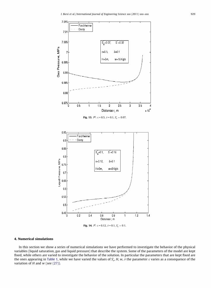
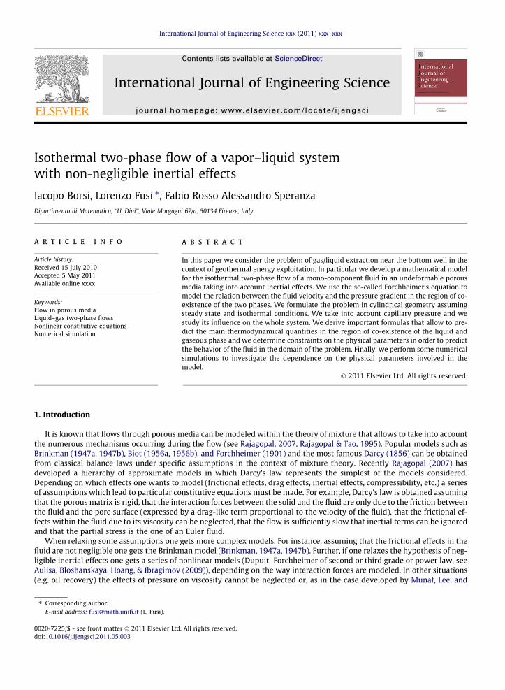
Fig. 13. Pg: e = 0.5, d = 0.1, S�o ¼ 0:07.

Fig. 14. Pl: e = 0.12, d = 0.1, S�o ¼ 0:1.

I. Borsi et al. / International Journal of Engineering Science xxx (2011) xxx–xxx 929

4. Numerical simulations

In this section we show a series of numerical simulations we have performed to investigate the behavior of the physicalvariables (liquid saturation, gas and liquid pressure) that describe the system. Some of the parameters of the model are keptfixed, while others are varied to investigate the behavior of the solution. In particular the parameters that are kept fixed arethe ones appearing in Table 1, while we have varied the values of S�o, H, w, d the parameter e varies as a consequence of thevariation of H and w (see (27)).

Fig. 15. Pl: e = 0.5, d = 0.1, S�o ¼ 0:07.

Fig. 16. Sl: e = 0.05, d = 0.1, S�o ¼ 0:07.

930 I. Borsi et al. / International Journal of Engineering Science xxx (2011) xxx–xxx

Figs. 4–21 represent the plots of the functions SloðrÞ; Sl

oðrÞ þ eSl1ðrÞ; Pg

oðrÞ; PgoðrÞ þ ePg

1ðrÞ; PloðrÞ; Pl

oðrÞ þ ePl1ðrÞ, that is the

liquid saturation and the gas/liquid pressures for the zero and first order approximation. The numerical procedure usedto obtain such functions can be outlined as follows:

1. we determine the function ql(Sl) from (28)4;2. we solve (59) to get Sl

oðrÞ, i.e. the saturation in the Darcian (zero order) case;3. we compute the coefficients defined in (48) and (49) exploiting Sl

oðrÞ and we use them to solve (64) which provides thesaturation Sl

1ðrÞ for the first order approximation (Forchheimer);4. we plot the functions Sl

oðrÞ; SloðrÞ þ eSl

1ðrÞ; PgoðrÞ; Pg

oðrÞ þ ePg1ðrÞ; Pl

oðrÞ; PloðrÞ þ ePl

1ðrÞ using the values shown in Table 1and taking different values of S�o, H, w, d.

Fig. 17. Sl: e = 0.05, d = 0.1, S�o ¼ 0:1.

I. Borsi et al. / International Journal of Engineering Science xxx (2011) xxx–xxx 931

Looking at Figs. 4–15 we can infer the following conclusions:

(i) for most of the co-existence domain the liquid saturation Sl (as well as liquid pressure and gas pressure) does not sig-nificantly detach from the value assumed at the wall of the well (in practice, as we depart from the wellbore, the pres-sures and the saturation oscillations are not remarkable). This is valid for both the Darcian and the Forchheimer case.The portion of the domain in which Sl grows to its saturation value Sl = 1 is quite small if compared to the whole co-existence domain.

(ii) when e is not overly small - more precisely for e P 0.1 (which is the range obtained using typical reservoir values) –the Darcian and Forchheimer models differ significantly in the domain of co-existence. This fact, which is due to the

Fig. 18. Pg: e = 0.05, d = 0.1, S�o ¼ 0:07.

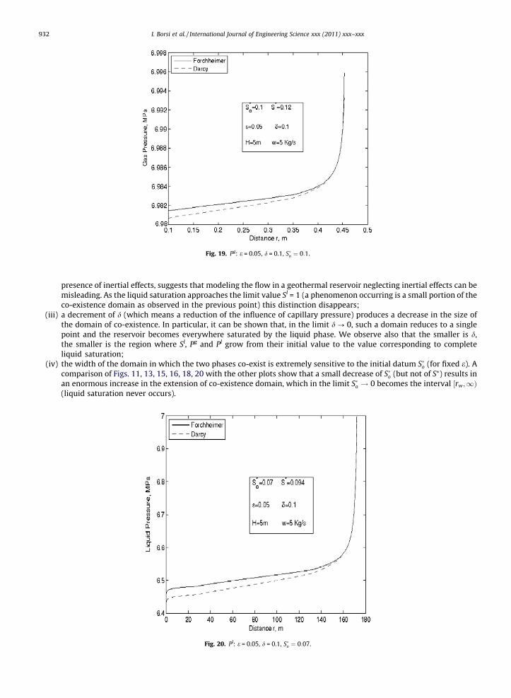
Fig. 19. Pg: e = 0.05, d = 0.1, S�o ¼ 0:1.

932 I. Borsi et al. / International Journal of Engineering Science xxx (2011) xxx–xxx

presence of inertial effects, suggests that modeling the flow in a geothermal reservoir neglecting inertial effects can bemisleading. As the liquid saturation approaches the limit value Sl = 1 (a phenomenon occurring is a small portion of theco-existence domain as observed in the previous point) this distinction disappears;

(iii) a decrement of d (which means a reduction of the influence of capillary pressure) produces a decrease in the size ofthe domain of co-existence. In particular, it can be shown that, in the limit d ? 0, such a domain reduces to a singlepoint and the reservoir becomes everywhere saturated by the liquid phase. We observe also that the smaller is d,the smaller is the region where Sl, Pg and Pl grow from their initial value to the value corresponding to completeliquid saturation;

(iv) the width of the domain in which the two phases co-exist is extremely sensitive to the initial datum S�o (for fixed e). Acomparison of Figs. 11, 13, 15, 16, 18, 20 with the other plots show that a small decrease of S�o (but not of S⁄) results inan enormous increase in the extension of co-existence domain, which in the limit S�o ! 0 becomes the interval ½rw;1Þ(liquid saturation never occurs).

Fig. 20. Pl: e = 0.05, d = 0.1, S�o ¼ 0:07.

Fig. 21. Pl: e = 0.05, d = 0.1, S�o ¼ 0:1.

I. Borsi et al. / International Journal of Engineering Science xxx (2011) xxx–xxx 933

Acknowledgments

This work was partially supported by the project MACGEO funded by the Tuscany RegionGovernment, September 2008–2010.

References

Andrade, J. S., Costa, U. M. S., Almeida, M. P., Makse, H. A., & Stanley, H. E. (1999). Inertial effects on fluid flow through disordered porous media. PhysicalReview Letters, 82(26), 5249–5252.

Aulisa, E., Bloshanskaya, L., Hoang, L., & Ibragimov, A. (2009). Analysis of generalized Forchheimer flows of compressible fluids in porous media. Journal ofMathematical Physics, 50, 103102.

Bear, J. (1972). Dynamics of fluids in porous media. New York: American Elsevier Publishing.Biot, M. A. (1956a). Theory of elastic waves in a fluid-saturated porous solid. I: Low frequency range. The Journal of Acoustical Society of America, 28, 168–178.Biot, M. A. (1956b). Theory of elastic waves in a fluid-saturated porous solid. II: High frequency range. The Journal of Acoustical Society of America, 28,

179–191.Brinkman, H. C. (1947a). A calculation of the viscous force exerted by a flowing fluid on a dense swarm of particles. Applied Scientific Research, A1, 27–34.Brinkman, H. C. (1947b). On the permeability of media consisting of closely packed porous particles. Applied Scientific Research, A1, 81–86.Coussy, O. (1995). Mechanics of porous continua. Wiley.Darcy, H. (1856). Les fontaines publiques de la Ville de Dijon. Paris: Dalmont.Dullien, F. A. L. (1979). Porous media fluid transport and pore structure. New York: Academic.Edwards, D. A., Shapiro, M., Bar-Yoseph, P., & Shapira, M. (1990). The influence of Reynolds number upon the apparent permeability of spatially periodic

arrays of cylinders. Physics of Fluids, 2, 45.Forchheimer, P. (1901). Wasserbewegung durch Boden Zeit. Zeitschrift des Vereins Deutscher Ingenieure, 45, 1782–1788.Hassanizadeh, S. M., Celia, M. A., & Dahle, H. K. (2002). Dynamic effect in the capillary pressure-saturation relationship and its impacts on unsaturated flow.

Vadose Zone Journal, 1, 38–57.Hassanizadehm, S. M., & Gray, W. G. (1987). High velocity flow in porous media. Transport Porous Media, 2, 521–531.Koch, D. L., & Ladd, A. J. C. (1997). Moderate Reynolds number flows through periodic and random arrays of aligned cylinders. The Journal of Fluid Mechanics,

349, 31.Munaf, D., Lee, D., & Rajagopal, K. R. (1993). boundary value problem in ground water motion analysis-comparison of predictions based on Darcys law and

continuum theory of mixtures. Mathematical Models and Methods in Applied Sciences, 3, 231–248.Rajagopal, K. R. (2007). On a hierarchy of approximate models for flows of incompressible fluids through porous solids. Mathematical Models and Methods in

Applied Sciences, 17(2), 215–252.Rajagopal, K. R., & Tao, L. (1995). Mechanics of mixtures. Singapore: World Scientific.Rajagopal, K. R., & Tao, L. (2005). On the propagation of waves through porous solids. International Journal of Non-Linear Mechanics, 40, 373–380.Sanchez-Palencia, E. (1980). Non-Homogeneous Media and Vibration Theory. Lecture Notes in Physics. Springer-Verlag.Tsypkin, G. G. (1997). On water-steam phase transition front in geothermal reservoirs USA. In Proceedings of stanford geotherm, workshop (Vol. 22, pp. 359–

367).Venkataraman, P., & Rao, P. R. M. (1998). Darcian, transitional and turbulent flow through porous media. Journal of Hydraulic Engineering (ASCE), 124,

840846.