Jean-Marc Bernard, Teddy Seidenfeld, & Marco Zaffalon(Editors)

ISIPTA ’03

Proceedings of the Third International Symposium onImprecise Probabilities and Their Applications

Lugano, Switzerland

PROCEEDINGS IN INFORMATICS 18

Contents c

2003 Carleton ScientificPublished by: Carleton ScientificCover design by: Steve IzmaPrinted and bound in Canada

Canadian Cataloguing in Publication (pending)

International Symposium on Imprecise Probabilities and Their Applications (3rd: 2003 : Lugano, Switzerland)

ISIPTA ’03 : proceedings of the 3rd International Symposium on ImpreciseProbabilities and Their Applications, Lugano, Switzerland)

(Proceedings in informatics ; 18)Conference held Jul. 14-17, 2003.Includes bibliographical references.ISBN 1-894145-17-8

1. Computer networks–Congresses. 2. Electronic data processing–Distributedprocessing–Congresses. I. Bernard, Jean-Marc II. Title. III. Series.

This book was processed using the LATEX 2ε macro package with the Carleton Scientificstyle package, cs.sty.

Table of Contents

Jean-Marc Bernard, Teddy Seidenfeld, & Marco ZaffalonPreface . . . . . . . . . . . . . . . . . . . . . . . . . . . . . . . . . . . . . . . . . . . . . . . . . . . . . . . . . . . . vii

J. Abellan & S. MoralMaximum Entropy in Credal Classification . . . . . . . . . . . . . . . . . . . . . . . . . . . . . 1

J.P. Arias, J. Hernandez, J.R. Martın, & A. SuarezBayesian Robustness with Quantile Loss Functions . . . . . . . . . . . . . . . . . . . . 16

Th. AugustinOn the Suboptimality of the Generalized Bayes Rule and RobustBayesian Procedures from the Decision Theoretic Point of View —A Cautionary Note on Updating Imprecise Priors . . . . . . . . . . . . . . . . . . . . . . 31

J.-M. BernardAnalysis of Local or Asymmetric Dependencies in Contingency

Tables using the Imprecise Dirichlet Model . . . . . . . . . . . . . . . . . . . . . . . . . . . 46

V. Biazzo, A. Gilio, & G. SanfilippoSome Results on Generalized Coherence of ConditionalProbability Bounds . . . . . . . . . . . . . . . . . . . . . . . . . . . . . . . . . . . . . . . . . . . . . . . . . 62

A.G. BronevichThe Maximal Variance of Fuzzy Interval . . . . . . . . . . . . . . . . . . . . . . . . . . . . . . 77

D.V. Budescu & T.M. KarelitzInter-Personal Communication of Precise and Imprecise SubjectiveProbabilities . . . . . . . . . . . . . . . . . . . . . . . . . . . . . . . . . . . . . . . . . . . . . . . . . . . . . . . . 91

A. CapotortiRelevance of Qualitative Constraints in Diagnostic Processes . . . . . . . . . . 106

E. Castagnoli, F. Maccheroni, & M. MarinacciExpected Utility with Multiple Priors . . . . . . . . . . . . . . . . . . . . . . . . . . . . . . . . 121

M. CattaneoCombining Belief Functions Issued from Dependent Sources . . . . . . . . . . 133

F.P.A. Coolen & K.J. YanComparing Two Groups of Lifetime Data . . . . . . . . . . . . . . . . . . . . . . . . . . . . 148

iii

iv ISIPTA ’03

G. de Cooman & M.C.M. TroffaesDynamic Programming for Discrete-Time Systems withUncertain Gain . . . . . . . . . . . . . . . . . . . . . . . . . . . . . . . . . . . . . . . . . . . . . . . . . . . . 162

Fabio CozmanComputing Lower Expectations with Kuznetsov’s IndependenceCondition . . . . . . . . . . . . . . . . . . . . . . . . . . . . . . . . . . . . . . . . . . . . . . . . . . . . . . . . . 177

F. CuzzolinGeometry of Upper Probabilities . . . . . . . . . . . . . . . . . . . . . . . . . . . . . . . . . . . . 188

M. Danielson, L. Ekenberg, J. Johansson, & A. LarssonThe DecideIT Decision Tool . . . . . . . . . . . . . . . . . . . . . . . . . . . . . . . . . . . . . . . . 204

James M. DickeyConvenient Interactive Computing for Coherent ImprecisePrevision Assessments . . . . . . . . . . . . . . . . . . . . . . . . . . . . . . . . . . . . . . . . . . . . . 218

Serena DoriaIndependence with Respect to Upper and Lower ConditionalProbabilities Assigned by Hausdorff Outer and Inner Measures . . . . . . . . . 231

P.I. Fierens & T.L. FineTowards a Chaotic Probability Model for Frequentist Probability:The Univariate Case . . . . . . . . . . . . . . . . . . . . . . . . . . . . . . . . . . . . . . . . . . . . . . . 245

M. Ha-Duong, E. Casman, & M.G. MorganBounding Analysis of Lung Cancer Risks Using ImpreciseProbabilities . . . . . . . . . . . . . . . . . . . . . . . . . . . . . . . . . . . . . . . . . . . . . . . . . . . . . . 260

M. HutterRobust Estimators under the Imprecise Dirichlet Model . . . . . . . . . . . . . . . 274

J.-Y. Jaffray & M. JelevaHow to Deal with Partially Analyzed Acts? A Proposal . . . . . . . . . . . . . . . . 290

R. JirousekOn Approximating Multidimensional Probability Distributionsby Compositional Models . . . . . . . . . . . . . . . . . . . . . . . . . . . . . . . . . . . . . . . . . . 305

George J. KlirAn Update on Generalized Information Theory . . . . . . . . . . . . . . . . . . . . . . . 321

Table of Contents v

I. Kozine & V. KrymskyReducing Uncertainty by Imprecise Judgements on ProbabilityDistributions: Application to System Reliability . . . . . . . . . . . . . . . . . . . . . . 335

E. Kriegler & H. HeldGlobal Mean Temperature Projections for the 21st Century UsingRandom Sets . . . . . . . . . . . . . . . . . . . . . . . . . . . . . . . . . . . . . . . . . . . . . . . . . . . . . . 345

R. Lazar & G. MeedenExploring Imprecise Probability Assessments Based onLinear Constraints . . . . . . . . . . . . . . . . . . . . . . . . . . . . . . . . . . . . . . . . . . . . . . . . . 360

S. MaaßContinuous Linear Representation of Coherent Lower Previsions . . . . . . . 371

Enrique Miranda, Ines Couso, & Pedro GilStudy of the Probabilistic Information of a Random Set . . . . . . . . . . . . . . . 382

D.R. Morrell & W.C. StirlingAn Extended Set-valued Kalman Filter . . . . . . . . . . . . . . . . . . . . . . . . . . . . . . 395

R. NauThe Shape of Incomplete Preferences . . . . . . . . . . . . . . . . . . . . . . . . . . . . . . . . 406

R. Pelessoni & P. VicigConvex Imprecise Previsions: Basic Issues and Applications . . . . . . . . . . . 421

G.M. Peschl & H.F. SchweigerReliability Analysis in Geotechnics with Finite Elements —Comparison of Probabilistic, Stochastic and Fuzzy Set Methods . . . . . . . . 435

E. Quaeghebeur, G. de CoomanGame-Theoretic Learning Using the Imprecise Dirichlet Model . . . . . . . . 450

H . Reynaerts & M. VanmaeleA Sensitivity Analysis for the Pricing of European Call Optionsin a Binary Tree Model . . . . . . . . . . . . . . . . . . . . . . . . . . . . . . . . . . . . . . . . . . . . . 465

Jose Rocha & Fabio CozmanInference in Credal Networks with Branch-and-Bound Algorithms . . . . . 480

vi ISIPTA ’03

M.J. Schervish, T. Seidenfeld, J.B. Kadane, & I. LeviExtensions of Expected Utility Theory and Some Limitations ofPairwise Comparisons . . . . . . . . . . . . . . . . . . . . . . . . . . . . . . . . . . . . . . . . . . . . . . 494

G. Shafer, P.R. Gillett, & R.B. ScherlSubjective Probability and Lower and Upper Prevision:A New Understanding . . . . . . . . . . . . . . . . . . . . . . . . . . . . . . . . . . . . . . . . . . . . . 509

Damjan SkuljProducts of Capacities Derived from Additive Measures . . . . . . . . . . . . . . . 524

L.V. UtkinA Second-Order Uncertainty Model of Independent RandomVariables: An Example of the Stress-Strength Reliability . . . . . . . . . . . . . . 530

L.V. Utkin & Th. AugustinDecision Making with Imprecise Second-Order Probabilities . . . . . . . . . . . 545

B. VantaggiGraphical Representation of Asymmetric Graphoid Structures . . . . . . . . . 560

Jirina VejnarovaDesign of Iterative Proportional Fitting Procedure for PossibilityDistributions . . . . . . . . . . . . . . . . . . . . . . . . . . . . . . . . . . . . . . . . . . . . . . . . . . . . . . 575

A. WallnerBi-elastic Neighbourhood Models . . . . . . . . . . . . . . . . . . . . . . . . . . . . . . . . . . . 591

K. Weichselberger & Th. AugustinOn the Symbiosis of Two Concepts of Conditional IntervalProbability . . . . . . . . . . . . . . . . . . . . . . . . . . . . . . . . . . . . . . . . . . . . . . . . . . . . . . . . 606

Preface

The ISIPTA meetings are one of the primary international forums to presentand discuss new results on the theory and applications of imprecise probabili-ties. Imprecise probability has a wide scope, being a generic term for the manymathematical or statistical models that measure chance or uncertainty withoutsharp numerical probabilities. These models include belief functions, Choquet ca-pacities, comparative probability orderings, convex sets of probability measures,fuzzy measures, interval-valued probabilities, possibility measures, plausibilitymeasures, and upper and lower expectations or previsions. Imprecise probabilitymodels are needed in inference problems where the relevant information is scarce,vague or conflicting, and in decision problems where preferences may also be in-complete.

A total of 44 papers were presented at ISIPTA ’03, covering a wide range oftopics, including: new model based inference with imprecise probabilities; com-putations and foundations of inference with imprecise probabilities; applicationsof imprecise probabilities in engineering, finance, and medicine; connections withgraph theory, belief functions, and fuzzy random variables; and the introductionof new principles and tools for decision theory.

To help promote the exchange of novel ideas, at ISIPTA ’03 we continued theconference format begun at ISIPTA ’01. Each of the 44 papers were presentedboth in a 20 minute plenary overview and as part of a poster session. Authors pre-senting at the plenary sessions were encouraged to use some of their 20 minutesto identify the context for their research, in addition to giving an overview of theresearch paper appearing in the proceedings. In this way the poster sessions serve,again, as a forum for extended discussions of the papers.

This ISIPTA meeting included three invited contributions from Terrence L.Fine, Irving J. Good, and Patrick Suppes. Copies of their papers were distributedat the conference and are included in the electronic version of the proceedings.

Each paper appearing in these printed proceedings has been the subject of acareful refereeing process. We feel confident that the selection process has re-sulted in a symposium and proceedings with contributions displaying both veryhigh quality and unusual originality.

We want to thank the contributors for their diligence in preparing their sub-missions, and for their patience with our selection process. The Program Com-mittee members discharged their refereeing responsibilities effectively and con-structively, with the result that all the papers have been improved by the review-ing process. We are grateful to the tutorial leaders (Jean-Marc Bernard: “Impre-cise Dirichlet model for multinomial data,” Gert de Cooman: “A gentle introduc-tion to imprecise probability models and their behavioral interpretation,” FabioG. Cozman: “Graph-theoretical models for multivariate modeling with impreciseprobabilities,” Charles F. Manski: “Partial identification of probability distribu-

vii

viii ISIPTA ’03

tions,” Sujoy Mukerji: “Imprecise probabilities and ambiguity aversion in eco-nomic modeling”), who have contributed their time and talents in such a generousfashion. As with ISIPTA ’01, the Board is exceptionally thankful to Serafın Moral,who has overseen the electronic management of these papers, their submissionsand reviews, and who has tirelessly given his time to fixing the inevitable break-downs that happen in a complicated web-based system. These proceedings simplywould not be possible without his expertise.

Jean-Marc BernardTeddy Seidenfeld

Marco Zaffalon

ISIPTA ’03 Sponsors

http://www.antoptima.com/

City of Luganohttp://www.lugano.ch/

Dipartimento dell’educazione, della cultura e dello sport del Canton Ticinohttp://www.ti.ch/DECS

The research programme NCCR FINRISK is gratefully acknowledged.http://www.nccr-finrisk.unizh.ch/

Grants: 20CO21-101209 and, in part, 2100-067961.02.http://www.snf.ch/

Preface ix

ISIPTA ’03Program Committee Board

Jean-Marc Bernard, FranceTeddy Seidenfeld, USA

Marco Zaffalon, Switzerland

Program Committee MembersThomas Augustin, Germany

Salem Benferhat, FranceDavid V. Budescu, USAFrank P. A. Coolen, UKFabio G. Cozman, Brazil

Luis M. de Campos, SpainGert de Cooman, Belgium

Dieter Denneberg, GermanyJames M. Dickey, USADidier Dubois, France

Love Ekenberg, SwedenEnrico Fagiuoli, Italy

Scott Ferson, USATerrence L. Fine, USAItzhak Gilboa, IsraelAngelo Gilio, Italy

Michel Grabisch, FranceJoseph Y. Halpern, USA

David Harmanec, Czech RepublicManfred Jaeger, GermanyJean-Yves Jaffray, France

Edi Karni, USAEtienne E. Kerre, Belgium

Gernot Kleiter, AustriaGeorge J. Klir, USA

Jurg Kohlas, SwitzerlandIgor Kozine, DenmarkHenry Kyburg, USA

Isaac Levi, USAThomas Lukasiewicz, Italy

Fabio Maccheroni, ItalyCharles F. Manski, USA

Alfio Marazzi, SwitzerlandGlen Meeden, USA

Kalled Mellouli, Tunisia

Serafın Moral, SpainSujoy Mukerji, UKRobert Nau, USA

Klaus Nehring, USAJohn Norton, USA

Michael Oberguggenberger, AustriaEndre Pap, Yugoslavia

Andrzej Pownuk, PolandHenri Prade, France

Urho Pulkkinen, FinlandMarco Ramoni, USAGiuliana Regoli, Italy

Peter Reichert, SwitzerlandLuca Rigotti, USA

David Rios Insua, SpainFabrizio Ruggeri, ItalyPaola Sebastiani, USA

Glenn Shafer, USAPrakash P. Shenoy, USAPhilippe Smets, Belgium

Michael Smithson, AustraliaPaul Snow, USA

Claudio Sossai, ItalyWynn Stirling, USA

Milan Studeny, Czech RepublicFabio Trojani, Switzerland

Lev V. Utkin, RussiaPaolo Vanini, Switzerland

Barbara Vantaggi, ItalyJirina Vejnarova, Czech Republic

Paolo Vicig, ItalyFrans Voorbraak, The Netherlands

Kurt Weichselberger, GermanyNic Wilson, UK

Robert L. Wolpert, USA

x ISIPTA ’03

Organizing InstitutionsIDSIA (USI-SUPSI): Dalle MolleInstitute for Artificial Intelligence

(www.idsia.ch)IFin USI: Institute of Finance, Lugano

(www.lu.unisi.ch/istfin)SIPTA: Society for Imprecise

Probability Theory and Applications(www.sipta.ch)

SUPSI: University of AppliedSciences of Southern Switzerland

(www.supsi.ch)USI: University of Lugano

(www.unisi.ch)

Local OrganizationAlessandro Antonucci

Marco Zaffalon

Electronic OrganizationSerafın Moral

Steering CommitteeJean-Marc Bernard

Gert de CoomanSerafın Moral

Teddy SeidenfeldMarco Zaffalon

Maximum of Entropy in CredalClassification

J. ABELLANUniversidad de Granada, Spain

S. MORALUniversidad de Granada, Spain

Abstract

We present an application of the measure of maximum entropy for credalsets: as a branching criterion for classification trees based on imprecise prob-abilities. We also justify the use of maximum entropy as a global uncertaintymeasure for credal sets, and a deduction of this measure, based on the bestlower expectation of the logarithmic score, is presented. We have also carriedout several experiments in which credal classification trees are built taking aglobal uncertainty measure as a basis. The results show that there is a lowerdegree of error when maximum entropy is used as a global uncertainty mea-sure.

Keywords

imprecise probabilities, uncertainty, maximum entropy, imprecision, non-specificity,classification, classification trees, credal sets

1 Introduction

Classification is an important problem in the area of machine learning in whichclassical probability theory has been extensively used. Basically, we have an in-coming set of observations, called the training set, and we want to obtain a set ofrules to assign a value of the variable to be classified to any new case. The set usedto assess the quality of this set of rules is also called the test set. Classification hasnotable applications in medicine, recognition of hand-written characters, astron-omy, banks, etc. The learned classifier can be represented as a Bayesian network,a neural network, a classification tree, etc. These methods normally use the The-ory of Probability to estimate the parameters with a stopping criterion to limit thecomplexity of the classifier and to avoid overfitting.

This work has been supported by the Spanish Ministry of Science and Technology, project ElviraII (TIC2001-2973-C05-01).

1

2 ISIPTA ’03

In some previous papers [4, 5, 6], we have introduced a new procedure to buildclassification trees based on the use of imprecise probabilities. Classification treeshave their origin in Quinlan’s ID3 algorithm [18], and a basic reference is the bookby Breiman et al. [8]. We also applied decision trees for classification, but as inZaffalon [25], the imprecise Dirichlet model is used to estimate the probabilitiesof belonging to the respective classes defined by the variable to be classified. Inclassical probabilistic approaches, information gain is used to build the tree, butthen other procedures must subsequently be used to prune it, since informationgain tends to build structures which are too complex. We have shown that if im-precise probabilities are used and the information gain is computed by measuringthe total amount of uncertainty of the associated credal sets (a closed and convexset of probability distributions), then the problem of overfitting disappears andresults improve.

In Abellan and Moral [1, 2, 3], we studied how to measure the uncertainty of acredal set by generalizing the measures used in the Theory of Evidence, Dempster[10] and Shafer [20]. We considered two main sources of uncertainty: entropyand non-specificity. We proved that the proposed functions verify the most basicproperties of these types of measures (Abellan and Moral [2], Dubois and Prade[12], Klir and Wierman [15]).

We previously proved that by using a global uncertainty measure which is theresult of adding an entropy measure and a non-specificity measure, classificationresults are better than those obtained by the C4.5 classification method, based onQuinlan’s ID3 algorithm. In this paper, we have carried out some experiments inwhich the maximum entropy of the probability distributions of a credal set is usedto measure its uncertainty, and we show that the results obtained are even bet-ter. We consider two methods of building classification trees. In the first method,Abellan and Moral [4], we start with an empty tree and in each step, a node anda variable are selected for branching which give rise to a greater decrease in thefinal entropy of the variable to be classified. In classical probability, a branchingalways implies a decrease in the entropy. It is necessary to include an additionalcriterion so as not to create models which are too complex and therefore over-fit the data. With credal sets, a branching will produce a lower entropy but, atthe same time, a greater non-specificity. Under these conditions, we follow thesame procedure as in probability theory, but measuring the total uncertainty of abranching. The stopping criterion is very simple: when every possible branchingproduces an increment of the total uncertainty.

Finally, in order to carry out the classification given a set of observations, weuse a strong dominance criterion to obtain the value of the variable to be classifiedand a maximum frequency criterion when we want to classify all the cases.

The extended method quantifies the uncertainty of each individual variable ineach node in the same way, but also considers the results of adding two variablesat the same time. In this way, we aim to discover relationships involving morethan two variables that were not seen when investigating the relationships of a

Abellan & Moral: Maximum Entropy in Credal Classification 3

single variable with the variable to be classified.In Section 2, we present the necessary previous concepts on uncertainty on

credal sets. We place special emphasis on the maximum of entropy as a globaluncertainty measure. In Section 3, we introduce the necessary notation and defi-nitions for our procedure of building classification trees. In Section 4, we describethe methods based on imprecise probabilities. In Section 5, we test our procedurewith known data sets used in classification by comparing the use of two globaluncertainty measures.

2 Total Uncertainty on Credal Sets

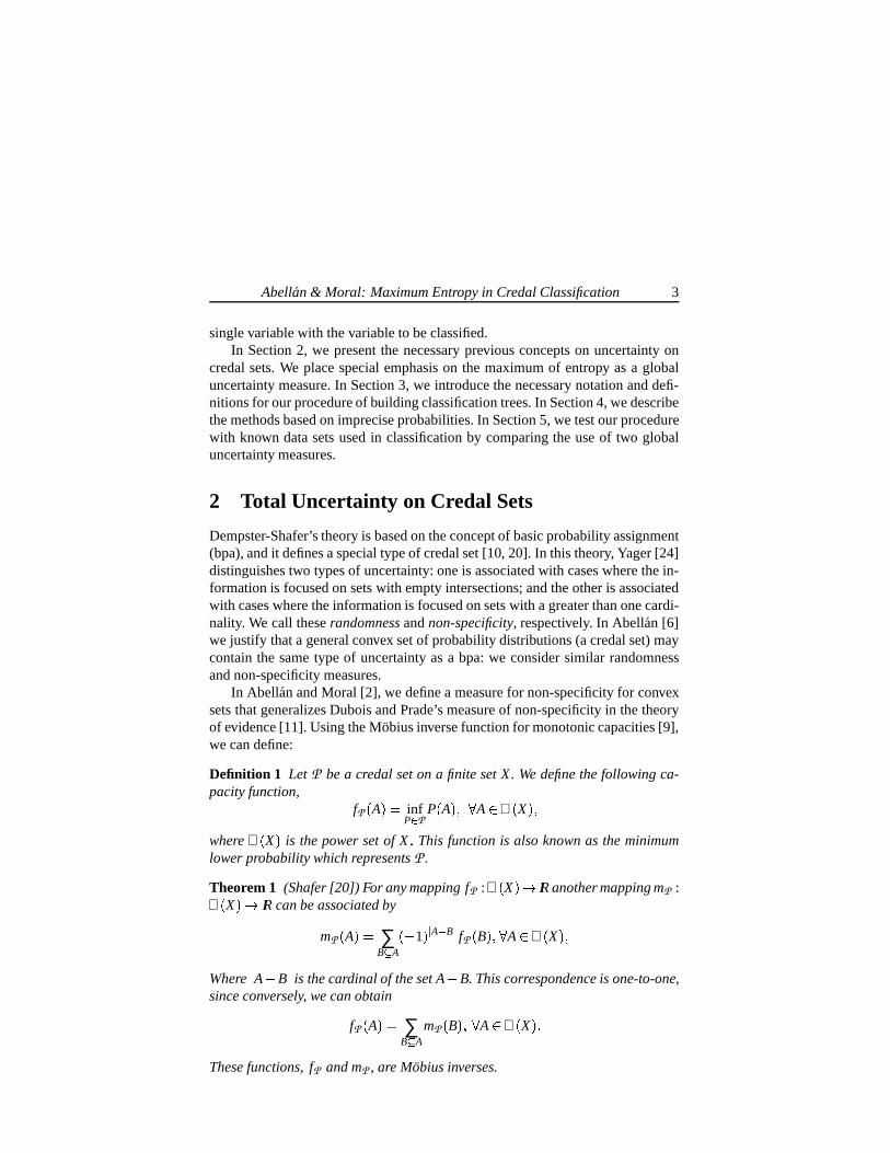
Dempster-Shafer’s theory is based on the concept of basic probability assignment(bpa), and it defines a special type of credal set [10, 20]. In this theory, Yager [24]distinguishes two types of uncertainty: one is associated with cases where the in-formation is focused on sets with empty intersections; and the other is associatedwith cases where the information is focused on sets with a greater than one cardi-nality. We call these randomness and non-specificity, respectively. In Abellan [6]we justify that a general convex set of probability distributions (a credal set) maycontain the same type of uncertainty as a bpa: we consider similar randomnessand non-specificity measures.

In Abellan and Moral [2], we define a measure for non-specificity for convexsets that generalizes Dubois and Prade’s measure of non-specificity in the theoryof evidence [11]. Using the Mobius inverse function for monotonic capacities [9],we can define:

Definition 1 Let P be a credal set on a finite set X. We define the following ca-pacity function,

fP A infP P

P A A ℘ X where ℘ X is the power set of X This function is also known as the minimumlower probability which represents P .

Theorem 1 (Shafer [20]) For any mapping fP :℘ X IR another mapping mP :℘ X IR can be associated by

mP A ∑B A

1 A B fP B A ℘ X Where A B is the cardinal of the set A B. This correspondence is one-to-one,since conversely, we can obtain

fP A ∑B A

mP B A ℘ X These functions, fP and mP , are Mobius inverses.

4 ISIPTA ’03

Definition 2 Let P be a credal set on a frame X, fP its minimum lower probabilityas in Definition 1 and let mP be its Mobius inverse. We say that function mP is anassignment of masses on P . Any A X such that mP A 0 will be called a focalelement of mP .

We can now define a general function of non-specificity.

Definition 3 Let P be a credal set on a frame X. Let mP be its associated as-signment of masses on P . We define the following function of non-specificity onP :

IG P ∑A X

mP A ln A In Abellan and Moral [3], we proposed the following measure of randomness

for general credal sets:

G P Max

∑x X

px ln px where the maximum is taken over all probability distributions on P and P is ageneral credal set. This measure generalizes the classical Shannon’s measure [21]verifying similar properties. It can be used either as one of the components of ameasure of total uncertainty, or as a total uncertainty measure, Harmanec and Klir[14]. We have proved that this function is also a good randomness measure forcredal sets and possesses all the basic properties required in Dempster-Shafer’stheory [3].

We define a measure of total uncertainty as TU P G P ! IG P . Thismeasure could be modified by the factor introduced in Abellan and Moral [1],but this will not be considered here, due to its computational difficulties (it is asupremum that is not easy to compute). The properties of this measure are studiedin Abellan and Moral [2, 3] and these are similar to the properties verified by totaluncertainty measures in Dempster-Shafer’s theory [17].

In this paper, we shall also consider G P as a measure of total uncertainty.In the particular case of belief functions, Harmanec and Klir [14] consider thatmaximum entropy is a measure of total uncertainty. They justify it by using anaxiomatic approach: it possesses some basic properties. However, uniqueness isnot proved. But perhaps the most compelling reason is given in Walley’s book[22]. Walley calls this measure the upper entropy. We start by explaining the caseof a single probability distribution, P. If You are subject to the logarithmic scor-ing rule, that means that You are forced to select a probability distribution Q onX that if the true value is x, then You must pay log Q x . For example, if Yousay that Q x is very small and finally x is the true value, You must pay a lot. IfQ x is close to one, then you must pay a small amount. Of course, You shouldchoose Q so that EP " log Q x $# is minimum, where EP is the mathematical ex-pectation with respect to P. This minimum is obtained when Q P and the value

Abellan & Moral: Maximum Entropy in Credal Classification 5

of EP " log P x $# is the entropy: the expected loss or the amount that You couldaccept to be subject to the logarithmic scoring rule. In the case of a credal set,P , we can also have the logarithmic scoring rule, but now we choose Q in sucha way that the upper loss E P " log Q x %&# (the supremum of the expectationswith respect to the probabilities in P ) is minimum. Walley shows that this mini-mum is obtained for the distribution P0 P with maximum entropy. Furthermore,E P " log P0 x $# is equal to the maximum entropy in P : G P . This is the min-imum payment You require before being subject to the logarithmic scoring rule.This argument is completely analogous with the probabilistic one, except that wechange the expectation for the upper expected loss. This is really a measure ofuncertainty, as the better we know the true value of x, then the less we shouldneed to accept the logarithmic scoring rule (lower value of G P ). We are notsaying that P can be replaced by the distribution of maximum entropy, only thatits uncertainty can be measured by considering maximum entropy in the credalset.

3 Notation and Previous Definitions

For a classification problem we shall consider that we have a data set D withvalues of a set L of discrete and finite variables ' Xi ( n

1. Each variable will take

values on a finite set ΩXi )' x1i x2

i *+* x ΩXi i ( . Our aim will be to create a clas-

sification tree on the data set D of one target variable C, with values in ΩC ' c1 c2 **+ c ΩC ( .Definition 4 A configuration of ' Xi ( n

1 is any m-tuple Xr1 xtr1r1 Xr2 x

tr2r2 *+* Xrm x

trmrm

where xtr jr j Ωr j , j ,' 1 *+* m ( , r j -' 1 %+** n ( and r j rh with j h. That is, a

configuration is an assignment of values for some of the variables in ' Xi ( n1.

If D is a data set and σ is a configuration, then D " σ # will denote the subset ofD given by the cases which are compatible with configuration σ (cases in whichthe variables in σ have the same values as the ones assigned in the configuration).

Definition 5 Given a data set and a configuration σ of variables ' Xi ( n1 we con-

sider the credal set P σC for variable C with respect to σ defined by the set of

probability distributions, p, such that

p j /. nσc j

N ! s nσ

c j ! s

N ! s 0

6 ISIPTA ’03

for every j 1' 1 **+2ΩC ( , where for a generic state c j ΩC, nσc j is the number of

occurrences of ' C c j ( in D " σ # , N is the number of cases in D " σ # , and s 3 0 isa parameter.

We denote this interval as 4P c j σ P c j σ $56

This credal set is the one obtained on the basis of the imprecise Dirichletmodel, Walley [23], applied to the subsample D " σ # .

The parameter s determines how quickly the lower and upper probabilitiesconverge as more data become available; larger values of s produce more cautiousinferences. Walley [23] suggests a candidate value for s between s 1 and s 2,but no definitive statement is given.

4 Classification Procedure

We have proposed two methods to build a classification tree: the simple method[4] and the double method [5]. Here we describe the double procedure and givethe simple as a particular case.

A classification tree is a tree where each interior node is labeled with a variableof the data set X j with a child for each one of its possible values: X j xt

j ΩX j .In each leaf node, we shall have a credal set for the variable to be classified, P σ

C ,as defined above, where σ is the configuration with all the variables in the pathfrom the root node to this leaf node, with each variable assigned to the value cor-responding to the child followed in the path. We use a measure of total uncertaintyto determine how and when to carry out a branching of the tree. The method startswith a tree with a single node, which will have an empty configuration associated.This node will be open. In this node the set of variables L is equal to the list ofvariables in the database.

I. For each open node already generated, we compute the total uncertainty ofthe credal set associated with the configuration, σ, of the path from the rootnode to that node: TU P σ

C . Then we calculate the values of α and β with

α minXi L 879 ∑

r ;: 1 < = = < ΩXi > ρ : xri > σTU P σ ?A@ Xi B xr

i CC $DE

β minXi < X j L 7F9 ∑

r ;: 1 < = = < ΩXi > < t G: 1 < = = <IHHHΩXj HHH > ρ : xri < xt

j > σTU P σ ?@ Xi B xri < X j B xt

j CC DKJE

where L is the set of variables of the data set minus those that appearon the path from the actual node to the root node, ρ : xr

i > σ is the relative

Abellan & Moral: Maximum Entropy in Credal Classification 7

frequency with which Xi takes the value xri in D " σ # , ρ : xr

i < xtj > σ is the relative

frequency with which Xi and X j take values xri and xt

j, respectively, in D " σ # ,and σ L Xi xr

i is the result of adding the value Xi xri to configuration

σ (analogously for σ L Xi xri X j xt

j ).II. If the minimum of ' α β ( is greater or equal than TU P σ

C (including the casein which L is empty), then the node is closed and the credal set P σ

C isassigned to it.

III. If the minimum of ' α β ( is smaller than TU P σC , then if α M β, we choose

the variable that attains the minimum in α as branching variable for thisnode; and if α 3 β we consider the pair of variables Xi X j for which thevalue of β is attained, and select as branching variable that from Xi X j witha minimum value of uncertainty (calculated in an individual way as in αcomputation).

If Xi0 is the branching variable we add to this node a child for each one ofits possible values. All the children are open nodes.

The simple method does not need β, Abellan and Moral [4]. It only considersα and it carries out a branching if this value is less than or equal to the uncer-tainty of the actual node (TU P σ

C ). As above, the branching variable is the onefor which the value α is attained. In the double method, we demand that the uncer-tainty is reduced. However, the double method looks for relationships of two vari-ables with C at the same time. The simple method only considers the informationof a single variable about C. In some cases, some multidimensional relationshipsdo not give rise to pairwise relationships between the implied variables, and thenthey will not be detected by the simple method.

4.1 Decision in the Leaves

In order to classify a new case with observations of all the variables except inthe variable to be classified C, we start at the root of the tree and follow the pathcorresponding to the observed values of the variables in the interior nodes of thetree, i.e. if we are at a node with variable Xi and this variable takes the valuexr

i in this particular case, then we choose the child corresponding to this value.This process is followed until we arrive at a leaf node. We then use the associatedcredal set about C, P σ

C , to obtain a value for this variable.We will use a strong dominance criterion on C. This criterion generally im-

plies only a partial order, and in some situations, no possible precise classificationcan be done. We will choose an attribute of the variable C ch if i h

P ci σ ON P ch σ

8 ISIPTA ’03

When there is no value dominating all other possible values of C, the outputis the set of non-dominated cases (cases ci for which there is no other case ch

verifying inequality). In this way, we obtain what Zaffalon [26] calls a credalclassifier, in which, for a set of observations, we obtain a set of possible valuesfor the variable to classify, non-dominated cases, instead of unique prediction.In the experiments, when there is no dominant value, we simply do not classify,without calculating the set of non-dominated attributes. This implies a loss ofsome valuable information in certain situations.

We want to compare our methods with existing classification methods. Thesemethods classify all the records of the training and test sets, without rejecting anyof the cases. In order to carry out a fair comparison with such complete proce-dures, we also use the maximum frequency criterion based on frequency of thedata, i.e. we will choose the case with maximum frequency in D " σ # as the attributeof the variable to be classified.

5 Experimentation

We have applied this method to some known data sets, obtained from the UCIrepository of machine learning databases, which can be found on the follow-ing website: http://www.sgi.com/Technology/mlc/db. We use the less conserva-tive parameter s 1, since with s 3 1, we obtained a high degree of non-classifieddata in some databases (although with a greater percentage of correct classifica-tions).

We plan to compare the behavior of the two total uncertainty measures wehave previously defined:P TU1 G ! IGP TU2 G

The data sets are: Breast, Breast Cancer, Heart, Hepatitis, Cleveland, Cleve-land nominal and Pima(medical); Australian (banking); Monks1 (artificial) andSoybean-small (botanical).

These databases were used by Acid [7]. Some of the original data sets haveobservations with missing values and in some cases, some of the variables arenot discrete. The cases with missing values were removed and the continuousvariables have been discretized using MLC++ software, available at the websitehttp://www.sgi.com/Technology/mlc. The measure used to discretize them is theentropy. The number of intervals is not fixed and it is obtained following theFayyad and Irani procedure [13]. Only the training part of the database is used todetermine the discretization procedure. In Table 1 there is a brief description ofthese databases.

In general, when there is no case dominating all the other possible values ofthe variable to be classified, we simply do not classify this individual.

Abellan & Moral: Maximum Entropy in Credal Classification 9

Data set N. Tr N. Ts N. variables N. classesBreast Cancer 184 93 9 2Breast 457 226 10 2Heart 180 90 13 2Hepatitis 59 21 19 2Cleveland nominal 202 99 7 5Cleveland 200 97 13 5Pima 512 256 8 2Vote1 300 135 15 2Australian 460 230 14 2Monks1 124 432 6 2Soybean-small 31 16 21 4

Table 1: Description of the databases. The column N. Tr contains the number ofcases of the training set, the column N. Ts is the number of cases of the test set,the column N. variables is the number of variables in the database and the columnN. classes is the number of different values of the variable to be classified

Algorithms have been implemented using Java language version 1.1.8. In or-der to obtain the value of G for probability intervals we have used the algorithmproposed in Abellan and Moral [3].

The percentages obtained of correct classifications with the simple model andTU1 can be seen in Table 2.

In Table 2, the training column is the percentage of correct classifications inthe data set that was used for learning. The UC Tr column shows the percentageof rejected cases, i.e. the observations that were not classified by the method dueto the fact that no value verifies the strong dominance criterion, and the UC Ts column shows the rejected cases in the test set.

In the results presented in Table 2 (Abellan and Moral [4]) there is no overfit-ting (one of the most common problems of learning procedures): the success ofthe training set and the test set are very similar.

Only the Cleveland database has a high rate of non-classified data. This is thecase with the highest number of cases of the variable to be classified and then itis more difficult to obtain a class dominating all the other classes. In this case, wewould have obtained more information by changing the output to a set of non-dominated cases. In most of the other databases, the variable to be classified hastwo possible states and in this situation our classification is equivalent to the setof non-dominated values.

In Table 3, we see the success of other known methods on the same databases,Acid [7]. The NB-columns correspond to the results of the Naive Bayesian clas-sifier on the training set and the test set. Similarly, the C4.5-columns correspondto Quinlan’s method [19], based on the ID3 algorithm [18], where a classification

10 ISIPTA ’03

Data set Training UC(Tr) Test UC(Ts)Breast Cancer 75.5 0.0 81.7 0.0Breast 98.0 1.3 96.9 0.9Heart 92.2 7.2 95.2 6.7Hepatitis 96.4 5.0 94.7 9.5Cleveland nominal 62.7 4.4 66.0 5.0Cleveland 72.8 21.0 69.9 24.7Pima 79.7 0.2 80.5 0.0Australian 92.3 3.4 91.0 3.4Vote1 96.1 6.6 96.9 5.9Soybean-small 100.0 0.0 100.0 0.0

Table 2: The measured experimental percentages of the simple method and TU1.The columns UC(Tr) and UC(Ts) are the percentages of the rejected cases ob-tained with the training and the test set respectively.

tree with classical precise probabilities is used. We report the results obtainedby Acid [7]. We can see that there is overfitting in these methods, principally inC4.5, being especially notable in certain data sets (Cleveland nominal, Cleveland,Hepatitis).

In Table 4 we can see the results of the simple method with TU2 and strongdominance. We have a higher percentage of success and a higher percentage ofunclassified cases. This total uncertainty measure obtains larger trees as we canobserve for the number of leaves presented in Table 5.

The success of the simple method with all cases classified (0% of rejectedcases) with the frequency criterion are presented in Table 6 for the test set, tocompare it with the models C4.5 and Naive Bayes. Table 7 shows the results ofsimilar experiments with the double method. We can see the high percentages ofcorrect classifications with TU2. These are a little higher than those obtained withTU1 and notably higher than the other methods (C4.5 and Naive Bayes).

The results of the simple and double methods are similar (slightly better inthe double method). In order to see the potential of the double method we use anartificial database: Monks1.

Monks1 is a database with six variables. The variable to be classified has twopossible states: a0 and a1, being a1 when the first and the second variables areequal or the fourth variable has the first of its possible four states. This type ofdependency is very difficult to find for some classification methods, as this is adeterministic relationship involving more than two variables. The double methodshould be much better than the simple one.

Table 8 shows the success of the methods C4.5 and Naive Bayes. Table 9shows the success of the simple and double method with all cases classified.

Abellan & Moral: Maximum Entropy in Credal Classification 11

Data set NB(Tr) NB(Ts) C4.5(Tr) C4.5(Ts)Breast Cancer 78.2 74.2 81.5 75.3Breast 97.8 97.3 97.6 95.1Cleveland nominal 63.9 57.6 69.3 51.5Cleveland 78.0 50.5 73.5 54.6Pima 76.4 74.6 79.9 75.0Heart 87.8 82.2 83.3 75.6Hepatitis 96.2 81.5 96.2 85.2Australian 87.6 86.1 89.3 83.0Vote1 87.6 88.9 94.5 88.3Soybean-small 100 93.8 100 100

Table 3: Percentages of another methods

Data set Training UC(Tr) Test UC(Ts)Breast Cancer 89.0 16.3 93.5 17.2Breast 99.1 2.6 98.6 2.6Cleveland nominal 73.6 21.2 74.4 13.1Cleveland 82.6 34.0 80.3 31.9Pima 86.6 15.6 86.2 15.2Heart 93.9 8.8 93.8 10.0Hepatitis 96.4 5.0 94.7 9.5Australian 95.3 6.5 94.4 6.5Vote1 98.2 5.3 98.4 4.4Soybean-small 100.0 0.0 100.0 0.0

Table 4: Simple method with TU2 and strong dominance

Data set TU1 TU2 N of possible leavesBreast 10 17 512Cleveland 17 112 635904

Table 5: Number of leaves of the trees obtained with the simple method and TU1and TU2

12 ISIPTA ’03

Data set TU1(Ts) TU2(Ts) NB(Ts) C4.5(Ts)Breast Cancer 81.7 90.3 74.2 75.3Breast 96.9 97.8 97.3 95.1Cleveland nominal 65.7 75.8 57.6 51.5Cleveland 67.0 80.4 50.5 54.6Pima 80.5 80.9 74.6 75.0Heart 93.3 92.2 82.2 75.6Hepatitis 95.2 95.2 81.5 85.2Australian 90.9 93.5 86.1 83.0Vote1 94.8 97.8 88.9 88.3Soybean-small 100 100 93.8 100

Table 6: Success of the simple method with TU1 and TU2 with the frequencycriterion on the test set

Database TU1(Ts) TU2(Ts) NB(Ts) C4.5(Ts)Breast Cancer 81.7 91.4 74.2 75.3Breast 96.9 98.7 97.3 95.1Cleveland nominal 68.7 74.7 57.6 51.5Cleveland 67.0 80.4 50.5 54.6Pima 80.5 82.4 74.6 75.0Heart 93.3 94.4 82.2 75.6Hepatitis 95.2 95.2 81.5 85.2Australian 89.1 91.7 86.1 83.0Vote1 94.8 98.5 88.9 88.3Soybean-small 100 100 93.8 100

Table 7: Success of the double method with TU1 and TU2 with the frequencycriterion on the test set

Data set NB(Tr) NB(Ts) C4.5(Tr) C4.5(Ts)Monks1 79.8 71.3 83.9 75.7

Table 8: C4.5 and Naive Bayes on Monks1

Abellan & Moral: Maximum Entropy in Credal Classification 13

Simple method Double methodFunction Tr Ts Tr TsTU1 81.5 80.6 94.4 91.7TU2 89.5 80.6 96.7 94.4

Table 9: Percentages on Monks1 of the methods with TU1 and TU2 and all casesclassified

We can see some interesting things. There is an appreciable overfitting in C4.5and Naive Bayes but not in our methods. The percentage obtained with the test setis better in the extended method than in the simple method and there is a differenceof 23 1% of the extended method and TU2 with respect to Naive Bayes success.

6 Conclusions

In this paper, we have discussed the role of maximum entropy as a total uncer-tainty measure in credal sets. First, we have revised some decision theoretic jus-tification based on the logarithmic scoring rule. We have carried out a series ofexperiments in which we compare this measure with the one we had previouslyused in our experiments. The main conclusion is that, in general, the results arealways the same or better when only the maximum entropy is used than when anon-specificity value is added to it (the other total uncertainty measure). And insome cases, the percentages of success are notably better.

Other conclusions from the experiments can be summarized in the followingpoints:Q

Imprecise probability methods are outstandingly better than classical prob-abilistic methods, and also have the option of not classifying difficult cases.QIn general, the double method produces slightly better results than the singleone, but in some particular cases the differences can be remarkable.QMaximum entropy (TU2) produces larger trees than the other uncertaintymeasure (TU1), but even this classifier does not suffer from overfitting.

Acknowledgements

We are very grateful to the anonymous referees for their valuable comments andsuggestions.

14 ISIPTA ’03

References

[1] J. Abellan and S. Moral. Completing a Total Uncertainty Measure inDempster-Shafer Theory. Int. J. General Systems, 28:299–314, 1999.

[2] J. Abellan and S. Moral. A Non-specificity Measure for Convex Sets ofProbability Distributions. International Journal of Uncertainty, Fuzzinessand Knowledge-Based Systems, 8:357–367, 2000.

[3] J. Abellan and S. Moral. Maximum entropy for credal sets. To appear in In-ternational Journal of Uncertainty, Fuzziness and Knowledge-Based Sys-tems, 2003.

[4] J. Abellan and S. Moral. Using the Total Uncertainty Criterion for BuildingClassification Trees. Proceeding of the International Symposium of Impre-cise Probabilities and Their Applications, 1-8, 2001.

[5] J. Abellan and S. Moral. Construccion de arboles de clasificacion con prob-abilidades imprecisas. Actas de la Conferencia de la Asociacion Espanolapara la Inteligencia Artificial, 2:1035-1044, 2001.

[6] J. Abellan. Medidas de entropıa y distancia en conjuntos convexos de prob-abilidad: definiciones y aplicaciones. PhD thesis, Universidad de Granada,2003.

[7] S. Acid. Metodos de aprendizaje de Redes de Creencia. Aplicacion a laClasificacion. PhD thesis, Universidad de Granada, 1999.

[8] L. Breiman, J.H. Friedman, R.A. Olshen, and C.J. Stone. Classification andRegression Trees. Wadsworth Statistics, Probability Series, Belmont, 1984.

[9] G. Choquet. Theorie des Capacites. Ann. Inst. Fourier, 5:131–292,1953/54.

[10] A.P. Dempster. Upper and Lower Probabilities Induced by a MultivaluatedMapping, Ann. Math. Statistic, 38:325–339, 1967.

[11] D. Dubois and H. Prade. A Note on Measure of Specificity for Fuzzy Sets.BUSEFAL, 19:83–89, 1984.

[12] D. Dubois and H. Prade. Properties and Measures of Information in Evi-dence and Possibility Theories. Fuzzy Sets and Systems, 24:183–196, 1987.

[13] U.M. Fayyad and K.B. Irani. Multi-valued Interval Discretization ofContinuous-valued Attributes for Classification Learning. Proceeding ofthe 13th International Joint Conference on Artificial Intelligence, MorganKaufmann, San Mateo, 1022-1027, 1993.

Abellan & Moral: Maximum Entropy in Credal Classification 15

[14] D. Harmanec and G.J. Klir. Measuring Total Uncertainty in Dempster-Shafer Theory: a Novel Approach, Int. J. General System, 22:405–419,1994.

[15] G.J. Klir and M.J. Wierman. Uncertainty-Based Information, Phisica-Verlag, 1998.

[16] S. Kullback. Information Theory and Statistics, Dover, 1968.

[17] Y. Maeda and H. Ichihashi. A Uncertainty Measure with Monotonicity un-der the Random Set Inclusion, Int. J. General Systems 21:379–392, 1993.

[18] J.R. Quinlan. Induction of decision trees, Machine Learning, 1:81–106,1986.

[19] J.R. Quinlan. Programs for Machine Learning. Morgan Kaufmann seriesin Machine Learning, 1993.

[20] G. Shafer. A Mathematical Theory of Evidence. Princeton University Press,Princeton, 1976.

[21] C.E. Shannon. A mathematical theory of communication. The Bell SystemTechnical Journal, 27:379–423,623–656, 1948.

[22] P. Walley. Statistical Reasoning with Imprecise Probabilities. Chapmanand Hall, New York, 1991.

[23] P. Walley. Inferences from Multinomial Data: Learning about a Bag ofMarbles. J.R. Statist. Soc. B, 58:3–57, 1996.

[24] R.R. Yager. Entropy and Specificity in a Mathematical Theory of Evidence.Int. J. General Systems, 9:249–260, 1983.

[25] M. Zaffalon. A Credal Approach to Naive Classification. Proceedings ofthe First International Symposium on Imprecise Probabilities and their Ap-plications, 405-414, 1999.

[26] M. Zaffalon. The Naive Credal Classifier. Journal of Statistical Planningand Inference, 105:5–21, 2002.

J. Abellan is with the Universidad de Granada, Spain.

S. Moral is with the Universidad de Granada, Spain.

Bayesian Robustness with Quantile LossFunctions

J.P. ARIASUniversidad de Extremadura, Spain

J. HERNANDEZUniversidad de Extremadura, Spain

J. MARTINUniversidad de Extremadura, Spain

A. SUAREZUniversidad de Cadiz, Spain

Abstract

Bayes decision problems require subjective elicitation of the inputs: beliefsand preferences. Sometimes, elicitation methods may not perfectly representthe Decision Maker’s judgements. Several foundations propose to overlaythis problem using robust approaches. In these models, beliefs are modelledby a class of probability distributions and preferences by a class of loss func-tions. Thus, the solution concept is the set of non-dominated alternatives. Inthis paper we focus on the computation of the efficient set when the pref-erences are modelled by a class of convex loss functions, specifically thequantile loss functions. We illustrate the idea with examples and introducethe use of stochastic dominance in this context.

Keywords

Bayesian robustness, non-dominated alternatives, Bayes alternatives, quantile lossfunctions, stochastic orders, quantile class of prior distributions

1 Introduction

Robust Bayesian analysis arises to avoid demanding an excessively precision inthe decision maker’s judgements concerning his beliefs and preferences. Thus, the

This work has been supported in part by a grant of Junta de Extremadura IPR00A075. We thankthe referees for their fruitful comments

16

Arias et al.: Bayesian Robustness with Quantile Loss Functions 17

imprecision in preferences leads to a class of loss functions while the imprecisionin beliefs is modelled by a class of prior probability distributions which wouldbe actualized via Bayes Theorem. For some interesting revisions on BayesianRobustness axiomatic systems see e.g. Rıos Insua and Martın [13], Nau [11],Seidenfeld et al [18] and Weber [19].

In summary, using a class Γ of prior distributions over the set of states Θ anda class L of loss functions, given a b A , set of alternatives, we say that b R aif and only if

T a L π OM T b L π π Γ S L L where T a L π is the posterior expected loss for the action a, L is the loss func-tion, π is the prior and R is the preference relationship between alternatives:

T a L π UT ΘL a θ l θ dπ θ T Θ

l θ dπ θ l θ being the likelihood for an experiment x.

This model is similar to a multicriteria optimization problem. The optimalsolution is the one that minimizes T P L π for every pair π Γ L L . Unfortu-nately, in general, that optimal solution does not exist. Thus, the non-dominatedset is taken as an starting point. Any dominated alternative must be discarded. SeeCoello [6] for an excellent discussion on multiobjective optimization. We say thata dominates b if and only if a V b, (that is, a R b and W b R a ). A non-dominatedalternative a is such that there is no other alternative b which dominates a. Arias[1] and Arias and Martın [2] provide theoretic results about the existence of sucha set and its relationship with the set of Bayes alternatives. Martın and Arias [8]provide a method based on comparing pairs to approximate the non-dominatedset. Some references for Bayesian sensitivity are Berger [4], Rıos Insua and Rug-geri [14] and Rıos et al [15].

We study the calculus of the non-dominated set for problems in which theimprecision in preferences is modelled by quantile loss functions. We give generalresults that we will particularize for classes of quantile prior distributions, seeMoreno and Cano [9]. Since we are interested in Bayesian inference, we willconsider A YX although the results will be easily applicable when A is an intervalof X .

We organize this work as follows. We begin with some results concerningconvex loss functions and their implications in the calculus of the non-dominatedset. Secondly, we particularize for quantile loss functions, indicating the relation-ship with the Bayes alternatives in this case. We also consider a quantile class forprior distributions giving some results and an example. Third part of the paper isdedicated to various stochastic orders, only those that hold for the posterior dis-tributions once the priors have been ordered, and how they can be used in orderto calculate the non-dominated set.

18 ISIPTA ’03

2 Bayesian Robustness with convex loss functions

We will denote LC the class of all convex loss functions in A Every loss functionL LC, verifies for all θ, a b A and λ " 0 1 # that

L λa ! 1 λ b θ 6M λL a θ A! 1 λ L b θ (1)

A first useful result, easy to prove, is:

Lemma 1 Let Γ be any class of prior distributions and LC the class of convexloss functions. The function T P L π : A ZX is convex for every pair L π OLC [ Γ.

A well known result is that every convex function is continuous in the interior,see Roberts and Varberg [16]. Then considering the set of alternatives, X , thefunction T P L π is continuous in X and if it exists the set of Bayes alternatives,this will be a closed interval in X . In the case that, for some pair L π \ LC [ Γthe set of Bayes alternatives is empty, the function T P L π will be increasingor decreasing in X (strictly increasing or strictly decreasing if the functions arestrictly convex).

If the set of Bayes alternatives is not empty, then the function T P L π isstrictly decreasing in ] ∞ a @ L < π C and strictly increasing in a @ L < π C &! ∞ , being

a @ L < π C mina B ^ L _ π ` a and

a @ L < π C maxa B ^ L _ π ` a

Note that the alternatives a @ L < π C and a @ L < π C are also Bayes for L π .An immediate result is that the set of non-dominated alternatives is included

in the closed interval " µ µ # , being µ and µ , respectively, the infimum and thesupremum of the Bayes alternatives, that is,

µ inf@ L < π C L a Γa @ L < π C and

µ sup@ L < π C L a Γa @ L < π C

In the Bayesian literature the range of this interval is considered as the ro-bustness measure of the problem, see Berger [4]. However, if we are interestedin calculating exactly the set of non-dominated alternatives, we can give a moreaccurate approximation using the following result due to Arias et al [3]:

Theorem 1 Let L b LC be a family of convex loss functions, Γ a class of priorprobability distributions, so that, for every pair L π L [ Γ, the set of Bayes

Arias et al.: Bayesian Robustness with Quantile Loss Functions 19

alternatives B @ L < π C is not empty and let

a inf@ L < π C L a Γa @ L < π C

a sup@ L < π C L a Γa @ L < π C

We have

1. If a N a , then a a Ob N D A b " a a # .2. If a \c a , then N D A d " a a # .In order to study the robustness of the problem, it is not necessary to deter-

mine whether the alternatives a and a are dominated or not. Nevertheless, it isinteresting to calculate the efficient set in an accurate way. In this paper we willsee inference problems modelled by particular classes of loss functions and priordistributions in which we can assure that the extremes of the interval a and/or a are non-dominated alternatives. If the set of Bayes alternatives is empty for somepair L π L [ Γ then the result is valid considering a ∞ (when T P L π is increasing) or a ∞ (decreasing).

3 Quantile loss functions

Let us consider the case where preferences are modelled by quantile loss func-tions. A particular case of this type is the absolute value loss function. The classof quantile loss functions is defined as

L e' Lp : Lp a θ f a θ a 2p 1 p " 0 1 # ( (1) Functions equivalent to these have been used in Economy, such as the ones

studied by Geweke [7]

L a θ c1 a θ I @+ ∞ < a g θ ! c2 θ a I @ a < h ∞ C θ (2)

where I is the indicator function. Bayes alternatives for this type of functionare the quantiles of order c2 i c1 ! c2 (If c1 c2, it coincides with the median)Thus, they are asymmetric functions with different weights on the positive andnegative errors. Next example shows the use of this type of functions.

Example 1 Noortwijt and Gelder [12] studied the Bayes estimators of the opti-mal dyke height under asymmetric linear loss function. Let us suppose we haveto decide the height of the dykes to prevent flooding. The height of the dyke h willbe the decision variable and h0 3 25 the initial height at the moment when thedecision has to be taken. Inundation will occur as soon as the sea water level

20 ISIPTA ’03

exceeds the hight of the dyke. We assume that the maximal sea levels per year Xi

i 1 %j n are conditionally independent, exponentially distributed, with a knownlocation parameter x0 1 96 meters and an unknown parameter λ with expectedvalue 0.33 meters. Therefore the likelihood function is

l x λ n

∏i B 1

f xi λ 6 n

∏i B 1

1λ

exp ' xi x0

λ ( The prior density of λ is assumed to be an inverted gamma distribution with scaleparameter µ 3 0 and shape parameter ν 3 0

Ig λ ν µ " µν i Γ ν &# λ @ ν h 1 C exp ' µ i λ ( λ 3 0 The loss function is (2) with c1 5 37 P 107 and c2 1 94 P 107. k

This type of loss function have also been used in Forecast Theory, see Capistran[5] and references therein.

We will use the functions defined in (1) as they only depend on a single pa-rameter. Quantile loss functions are convex in A . The posterior expected loss is

T a Lp π Dθ x a a 2p 1 and their Bayes alternatives are the quantiles of order p of the posterior distribu-tions, since

T l a Lp π 6 2Fθ x a 2p for every point a where the distribution function is continuous.

Let us recall that it is called quantile of order p of a random variable X , thevalue QX p such that

P " X M QX p &# c p and

P " X c QX p &# c 1 p As it happened with the absolute value loss function, when using quantile loss

functions, the posterior distribution quantiles may not be unique.Based on theorem 1 we have the following result, when there is precision in

DM’s beliefs.

Proposition 1 Let L be the class of quantile loss functions

L e' Lp : Lp a θ m a θ a 2p 1 p " p0 p1 # (and π a prior distribution so that the posterior distribution quantiles are unique,then

N Dπ A 6 "Qπ p0 Qπ p1 &#nwhere Qπ p0 and Qπ p1 are, respectively, the quantiles of order p0 and p1 ofthe posterior distribution of π.

Arias et al.: Bayesian Robustness with Quantile Loss Functions 21

This result can be generalized in the case that we also have imprecision in thedecision maker’s beliefs.

Proposition 2 Let L be the class of quantile loss functions

L e' Lp : Lp a θ ) a θ a 2p 1 p " p0 p1 # ( a class of distributions

Γ o' π : π θ x with posterior quantiles Qπ p unique p " 0 1 # (and the values

a µ infπ Γ

Qπ p0 and

a O µ d supπ Γ

Qπ p1 then µ µ Ob N D A Ob " µ µ #p

If posterior quantiles are not unique we must appeal to theorem 1 with

a infπ Γ

' supQπ p0 (a sup

π Γ' infQπ p1 (

and a a 2Ob N D A Ob " a a #pIn general it can not be assured that µ or µ are non-dominated alternatives

as we illustrate with the following example.

Example 2 Let us consider the class of absolute value loss functions and a classof discrete posterior distributions with probability distribution: n rqO

πn θ tsuuuuv uuuuw2n ! 3

4 n ! 1 if θ 1n

2n ! 14 n ! 1 if θ 1

The Bayes alternative for each distribution πn would be its posterior median1 i n and the set of non-dominated alternatives is the interval 0 1 # . The alternative0 is dominated by the alternative 1, since for every n rq

T 0 L πn 2n2 ! 3n ! 34n n ! 1 3 2n2 ! n 3

4n n ! 1 T 1 L πn A k

22 ISIPTA ’03

Obviously if µ and µ are unique Bayes alternatives, then they are also non-dominated alternatives.

Note that, if having precision in beliefs, then the range of the non-dominatedset is the range between the quantile p0 and the quantile p1. Sometimes the non-dominated set can be the same as the (HPD), as in next example. However, so thatthis happens the elicitation of the class should depend on the posterior distribution.

Example 3 Let us consider the class of loss functions

L e' Lp : Lp a θ m a θ a 2p 1 p " 0 0 8 # (and a Pareto prior distribution with parameters α and β.

We take a sample ' X1 %j Xn ( of a population which is distributed followingan uniform distribution with mean θ i 2. Therefore, the posterior distribution is

P α ! n max x β X @ n Czy with X @ n C max ' X1 %j Xn (Then, the posterior quantiles of π are

Qπ p 1α n|

pmax x β X @ n C y

Thus, the set of non-dominated alternatives would be the closed interval

ND A 4max x β X @ n C&y Qπ 0 8 5

This means than the non-dominated set coincides with the confidence intervalHPD for the parameter θ at a confidence level of 80% .

The table 1 shows the non-dominated set when α 2 and β 5 for varioussamples.

n X @ n C ND A range10 3 2 " 5 5 0938 # 0.093850 4 5 " 5 5 0215 # 0.0215

100 4 8 " 5 5 011 # 0.011500 5 9 " 5 9 5 9026 # 0.0026

1000 4 7 " 5 5 0011 # 0.0011

Table 1: Non-dominated set for the example 3. k3.1 Relationship with the non-dominated set

An important question is the relationship between the Bayes set and the non-dominated set. It is easy to prove that, in general, they are different, see Arias etal [1]. In this case, we have the following result:

Arias et al.: Bayesian Robustness with Quantile Loss Functions 23

Proposition 3 Let L be the class of quantile loss functions with p " p0 p1 # . Ifthe class Γ of prior distributions is convex and Qπ p are unique for every π Γand p p0 p1 , then the set of non-dominated alternatives is the closure of theset of Bayes actions, and the interiors of both sets are the same.

Proof.If the set of prior distributions is convex, then the set of posterior distributions

is convex as well, see Arias et al[1]. As the quantiles are unique for any π, allbayes actions are non-dominated. So, we only have to prove that given a and bbayes actions for π L1 and π L2 , αa ! 1 α b is also bayes for α 0 1 .Consider a Qπ1 p l and b Qπ2 p l l with p l p l l " p0 p1 # and a N b p l N p l l .

Then T αa h@ 1 α C b ∞π1 θ x dθ 3 p l

T αa h6@ 1 α C b ∞π2 θ x dθ N p l l

so, there is β such that

β T αa h@ 1 α C b ∞π1 θ x dθ ! 1 β T αa h@ 1 α C b ∞

π2 θ x dθ p p l p l l Then αa ! 1 α b is the Qπ p with π P x 6 βπ1 P x A! 1 β π2 P x

4 Quantile prior distributions

We now consider some classes of prior distributions to model imprecision in be-liefs. Let Ai ~ θi θi h 1 1 be a partition of the parameter space and the class ofprior distributions:

ΓQ o' π : π Ai qi i 1 % n qi c 0 i ∑i

qi 1 (This is a particular case of the quantile class, see Moreno and Cano [9] and

Moreno and Pericchi [10] and Martın and Rıos Insua [13] among others.A well known result states that the suprema and the infima of functionals over

Γ are attained for discrete distributions. So, we have

Lemma 2 We have

maxπd Γd

π ij B 1

Ai x ∑ij B 1 maxθ A j l x θ p j

∑ij B 1 maxθ A j l x θ p j ! ∑n

k B i h 1 minθ Ak l x θ pk

1by a b we denote any type of interval in

24 ISIPTA ’03

Let us denote ri the second term in (8). Lemma 2 lead us to the followingiterative scheme to calculate µ

r0 0 i 0while ri N p0 i i ! 1compute ri

Let Ak be the first interval for which rk c p0. We define now

rk θ ∑i 1j B 1 maxλ A j l x λ p j ! l x θ pk

∑i 1j B 1 maxλ A j l x λ p j ! l x θ pk ! ∑n

j B k h 1 minλ A j l x λ p j θ Ak

thenµ inf ' θ Ak : rk θ c p0 (

By Theorem 1, for the calculus of a , we will distinguish two cases, if the lastinequality is strict then µ a which is the only quantile of order p. Otherwise,there are several quantiles. For the calculus of a we proceed as follows. In Ak wewill search a point a 3 µ for which the inequality is strict. If such point existsthen a inf ' a Ak : rk a \3 p0 ( . If there is no point a 3 µ in Ak such thatthis is verified then a inf ' a Ak h 1 : rk h 1 a d3 p0 ( and so on.

Example 4 The decision maker considers that negative errors are more impor-tant than positive, so he uses the class of loss functions:

L e' Lp : Lp a θ 6) a θ a 2p 1 p " 0 45 0 48 # ( For believes representation he adopts a quantile class with quantiles given in

Table 2.

Ai ∞ 16 44 16 44 5 22 5 24 2 53 2 53 1 25 1 25 0 pi 0 05 0 25 0 1 0 05 0 05

Ai 0 1 25 1 25 2 53 2 53 5 24 5 24 16 44 16 44 ∞ pi 0 05 0 05 0 1 0 25 0 05

Table 2: Probabilities for some intervals

Applying the proposed iterative scheme to obtain infQπ 0 45 we get the ri

values showed table 3. Therefore minπ Γ Qπ 0 45 d A4 " 2 533 1 257 # andsolving min ' θ Ai such that rk θ c 0 45 ( we obtain infQπ 0 45 2 533.Moreover, rk ] 2 5333 3 0 45 so a 2 533.

We apply the equivalent algorithm for supπ ΓQπ 0 48 obtaining 2.533. ThenN D A " 2 533 2 533 #

Arias et al.: Bayesian Robustness with Quantile Loss Functions 25

i 1 2 3 4 5 6 7 8 9 10ri 0 0001 0 28 0 44 0 54 0 65 0 76 0 87 0 99 1 1

Table 3: ri values

The class of quantiles ΓQ can be generalized considering bounds over the sets Ai

obtaining the class

ΓQG e' π : αi M π Ai OM βi 0 M αi M βi M 1 (In this case the proposed scheme can be modified taking into account that

ΓQG α p β

' π : π Ai 6 pi ∑i

pi 1 (where α α1 %j αn p p1 %j pn β β1 %% βn and α M p M β indi-

cates αi M pi M βi i 1 %j n.Thus, to calculate rk it is enough to consider sequently the linear problems:

maxk

∑i B 1

maxθi Ai

l x θi pi

s a n

∑i B 1

pi 1

αi M pi M βi i 1 % nwith optimum p 1 %j p k and

minn

∑i B k h 1

minθi Ai

l x θi pi

s a k

∑i B 1

p i ! n

∑i B k h 1

pi 1

αi M pi M βi i 1 % nwith optimum p k h 1 %j p n and we replace in the algorithm pi for p i . A similarmodification give us the values µ and a .

A natural extention of the quantile class for continuous parameters is the class

ΓLU o' π : L A OM π A dM U A A β (where β is a σ-field on the state set Θ. This is the class studied, among others, byMoreno and Pericchi [10] who provide the following result for posterior proba-bilities of sets in β.

26 ISIPTA ’03

Theorem 2 Let A be an arbitrary set in β. Suppose that l x θ , L and U satisfyU " l x θ 8 z # L " l x θ z # 0 for any z c 0 where " l x θ 8 z #6' θ :l x θ z ( . Then, we have

(i) if U A A! L Ac d3 1 then supπ ΓLU

Pπ A x 6 Pπ0 A x where π0 dθ U dθ IA l @ x θ C zA g θ A! L dθ IA l @ x θ C zA g Ac θ

zA being such that πo Θ 6 1

(ii) if U A A! L Ac 1 then supπ ΓLU

Pπ A x Pπ0 A x where π0 dθ U dθ IA θ A! L dθ IAc θ

(iii) if U A A! L Ac dN 1 then supπ ΓLU

Pπ A x 6 Pπ0 A x where πo dθ U dθ IA Ac f @ x θ C zA g θ ! L dθ IAc f @ x θ CS zA g θ

zA being such that πo Θ 6 1

This resuls allow us to compute N D A .Theorem 3 Let be the class ΓLU ' π : L A M π A M U A A β ( andL ' Lp : Lp a θ e a θ ! a 2p 1 p " p0 p1 # ( and l x θ , L and U satisfyU " l x θ z #SA! L " l x θ z # 0 z c 0 then

µ inf ' θ Θ : supπ ΓLU

Pπ ∞ θ c p0 ( where Pπ denotes the posterior probability.

Proof. Let θ inf ' θ Θ : supπ ΓLUPπ ] ∞ θ c p0 ( . If θ N θ then

Pπ ∞ θ 8N p0 π. Then by Theorem 1, θ is a dominated alternative. More-over, if θ satisfies supπ ΓLU

' Pπ ] ∞ θ c p0 ( then there is π ΓLU such thatθ Qπ p0 . In other case, by previous Theorem 2 there is a sequence of valuesθn such that is exists πθn ΓLU θn Qπθn p0 with θn θ so θ µ . Theorem 4 If L and U verify that L A \3 0 U A \3 0 A with µ A \3 0then µ a .Proof. It is easy to prove that π0 of theorem 2 has unique quantiles.

These results can be applied using searching methods based on simulation

schemes.

Arias et al.: Bayesian Robustness with Quantile Loss Functions 27

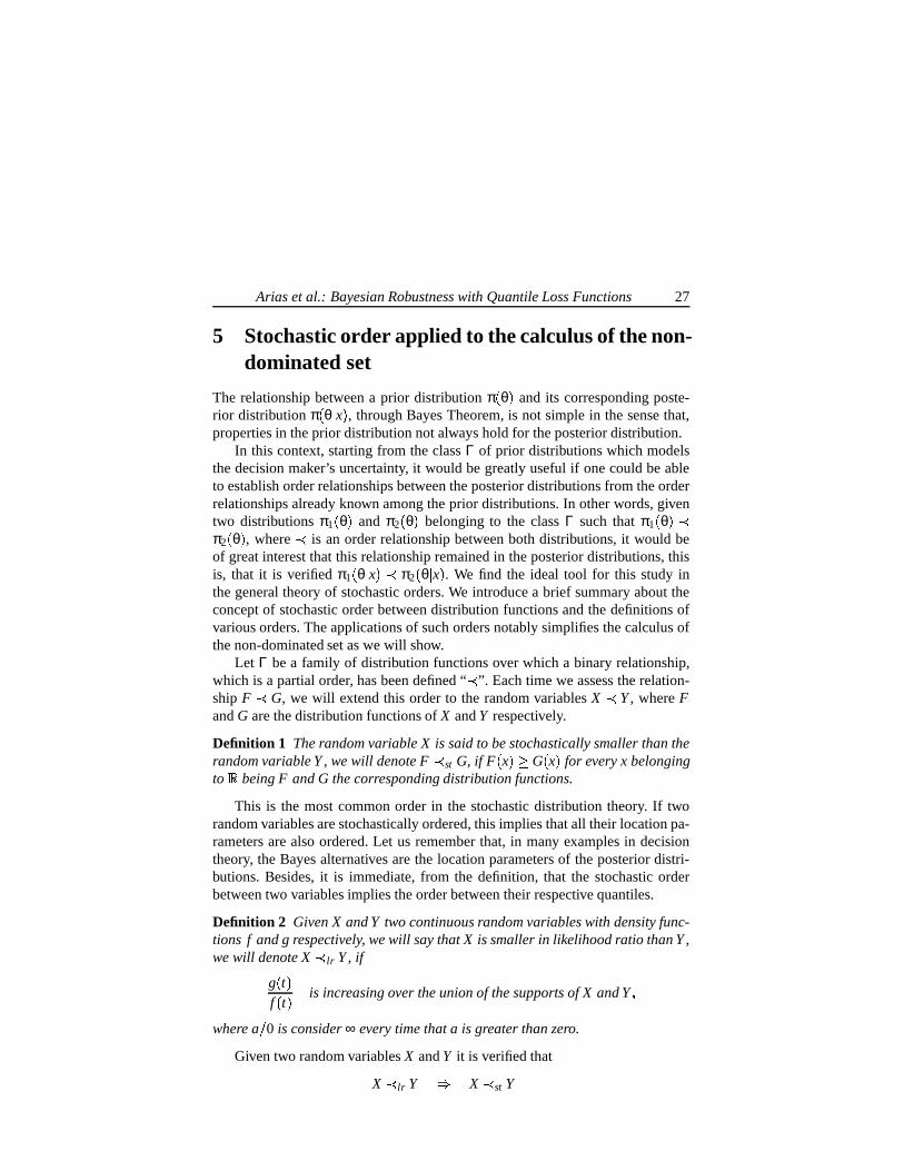
5 Stochastic order applied to the calculus of the non-dominated set

The relationship between a prior distribution π θ and its corresponding poste-rior distribution π θ x , through Bayes Theorem, is not simple in the sense that,properties in the prior distribution not always hold for the posterior distribution.

In this context, starting from the class Γ of prior distributions which modelsthe decision maker’s uncertainty, it would be greatly useful if one could be ableto establish order relationships between the posterior distributions from the orderrelationships already known among the prior distributions. In other words, giventwo distributions π1 θ and π2 θ belonging to the class Γ such that π1 θ Vπ2 θ , where V is an order relationship between both distributions, it would beof great interest that this relationship remained in the posterior distributions, thisis, that it is verified π1 θ x V π2 θ x . We find the ideal tool for this study inthe general theory of stochastic orders. We introduce a brief summary about theconcept of stochastic order between distribution functions and the definitions ofvarious orders. The applications of such orders notably simplifies the calculus ofthe non-dominated set as we will show.

Let Γ be a family of distribution functions over which a binary relationship,which is a partial order, has been defined “ V ”. Each time we assess the relation-ship F V G, we will extend this order to the random variables X V Y , where Fand G are the distribution functions of X and Y respectively.

Definition 1 The random variable X is said to be stochastically smaller than therandom variable Y , we will denote F V st G, if F x c G x for every x belongingto X being F and G the corresponding distribution functions.

This is the most common order in the stochastic distribution theory. If tworandom variables are stochastically ordered, this implies that all their location pa-rameters are also ordered. Let us remember that, in many examples in decisiontheory, the Bayes alternatives are the location parameters of the posterior distri-butions. Besides, it is immediate, from the definition, that the stochastic orderbetween two variables implies the order between their respective quantiles.

Definition 2 Given X and Y two continuous random variables with density func-tions f and g respectively, we will say that X is smaller in likelihood ratio than Y ,we will denote X V lr Y, if

g t f t is increasing over the union of the supports of X and Y

where a i 0 is consider ∞ every time that a is greater than zero.

Given two random variables X and Y it is verified that

X V lr Y X V st Y

28 ISIPTA ’03

see Shaked and Shantikumar [17] and Whitt [20].As indicated in the beginning of this section, the relationship between the

density function of the prior distribution and the posterior distribution is not eas-ily treatable from a mathematic point of view; although, this relationship is moreintuitive when we study properties associated to the quotient of two prior distri-butions. Due to the form of the posterior density function, it is not difficult totranslate these properties to the quotient of the respective posterior distributions.In this way we give the following two propositions, easy to prove, but of great useas we show later with various examples.

Proposition 4 Let π1 θ and π2 θ be two prior distributions for an unknownparameter of interest. Let π1 θ x and π2 θ x be the respective posterior dis-tributions of the parameter once the sampling experiment information has beenincorporated. Then if π1 θ \V lr π2 θ it is verified that π1 θ x \V lr π2 θ x . Par-ticularly, it is verified that π1 θ x OV st π2 θ x .Example 5 Let us consider a decision problem where the decision maker’s be-liefs are modelled by a parametric class of Pareto distributions with unknownparameter α

Γ e' π P α β : α "α1 α2 #p α1 β 3 0 (and the preferences are modelled by the class of quantile loss functions

L e' Lp : Lp a θ ) a θ a 2p 1 p " p1 p2 # ( The class of Pareto distributions can be ordered in the sense of likelihood ratio,since, for any two distributions P α1 β , P α2 β ,

π2 θ π1 θ α2

α1 βθ ¡ α2 α1

is an increasing function in " β &! ∞ , as long as α1 3 α2. Then, it is stochasti-cally ordered and, therefore, all the location parameters are ordered, in particu-lar, the quantiles are ordered. If we take a sample of size n of a population thatis distributed according to an uniform distribution of mean θ i 2, we have that, byproposition 4, the non-dominated set coincides with the closed interval4

QP @ α2 < β C p1 QP @ α1 < β C p2 5 Table 4 shows the non-dominated set for some samples and supposing that β 4 α1 2 α2 4 p1 1

3 and p2 13 .

References

[1] Arias. J.P., El conjunto no dominado en la teorıa de la decision bayesianarobusta, Ph.D. Thesis, Universidad de Extremadura, 2002.

Arias et al.: Bayesian Robustness with Quantile Loss Functions 29

n X @ n C ND A range4 3 2 " 4 208 4 489 # 0.281950 4 5 " 4 534 4 560 # 0.0264

100 4 8 " 4 819 4 833 # 0.0139500 5 9 " 5 905 5 908 # 0.0034

1000 4 7 " 4 702 4 703 # 0.001310000 6 1 " 6 1002 6 1004 # 0.00017

Table 4: Non-dominated set for the example 5.

[2] Arias, J.P. and Martın, J., Uncertainty in beliefs and preferences: Conditionsfor optimal alternatives, Annals of Mathematics and Artificial Intelligence,35, 1-4, 3-10, 2002.

[3] Arias, J.P., Martın, J.R., Suarez, A., Bayesian Robustness with convexloss functions, Technical Paper, Universidad de Extremadura, avaliable atjparias@unex.es, 2003.

[4] Berger, J., An overview of robust Bayesian analysis (with discussion), Test,3, 5-124, 1994.

[5] Capistran Carmona, C., A review of Forecast Theory using generalized lossfunctions, Working paper, University of California, San Diego, 2003.

[6] Coello Coello, C. A., Van Veldhuizen, D. A. and Lamont, G. B., Evolution-ary Algorithms for Solving Multi-Objetive Problems, Kluber A.P., 2002.

[7] Geweke, J., A brief digression on ancillarity and nuisance parameters, Lec-ture Notes in Economics, Applies Econometrics II 8-205, 1997.

[8] Martın, J. and Arias, J.P., Computing the efficient set in Bayesian decisionproblems, Robust Bayesian Analysis, eds. D. Rıos Insua and F. Ruggeri,Lectures Notes in Statistics, vol 152, Springer, 2000.

[9] Moreno, E. and Cano, J.A., Robust Bayesian analysis for ε-contaminationspartially known, Journal Royal Statistical Society B 53, 143-155, 1991.

[10] Moreno E. and Pericchi R., Bands of probability measures: a robust bayesiananalysis, Bayesian Statistics 4, Oxford O.P.707-713 (eds. Bernardo et al) ,1992.

[11] Nau, Robert F., The shape of incomplete preferences Working Paper, FuquaSchool of Bussines, Duke University, 1996.

30 ISIPTA ’03

[12] Van Noortwijk, J. and van Gelder, P., Bayesian estimation of quantiles forthe purpose of flood prevention. B.L. Edge, ed., Proceedings of the 26thInternational Conference on Coastal Engineering, Copenhagen, Denmark,3529-3541, 1998.

[13] Rıos Insua, D. and Martın J., On the foundations of robust Decision MakingDecision Theory and Decision Analysis: Trends and Challenges Rios, S.,Kluwer A.P., 1994.

[14] Rıos Insua, D. and Ruggeri, F., Robust Bayesian Analysis, Springer, 2000.

[15] Rıos Insua, D., Ruggeri, F. and Martın, J., Bayesian sensitivity analysis: areview, Sensitivity Analysis, (eds. Saltelli et al), New York: Wiley, 2000.

[16] Roberts, A.W. and Varberg, A.D., Convex Functions, Academic Press. NewYork, 1973.

[17] Shaked, M. and Shanthikumar, J.G., Stochastic orders and their applica-tions, Academic Press, New York, 1994.

[18] Seidenfeld, T., Shervish, M.J., and Kadane, J., A representation of partiallyordered preferences, Annals of Statistics, 23, 2168-2217, 1995.

[19] Weber, M., Decision Making with incomplete information, European Jour-nal of Operations Research, 28, 4-57, 1987.

[20] Whitt, W. Uniform conditional variability ordering of probability distribu-tions, Journal of Applied Probability, 22, 619-633, 1985.

Pablo Arias belongs to the Department of Mathematics, Universidad de Extremadura,caceres, 10071, Spain. E-mail: jparias@unex.es

Javier Hernandez belongs to the Department of Mathematics, Universidad de Ex-tremadura, Badajoz, 06006, Spain. E-mail: javierhs@materiales.unex.es

Jacinto Martın belongs to the Department of Mathematics, Universidad de Extremadura,Caceres, 10071, Spain. E-mail: jrmartin@unex.es

Alfonso Suarez belongs to the Department of Statistics, Universidad de Cadiz, SpainE-mail: alfonso.suarez@uca.es

On the Suboptimality of the GeneralizedBayes Rule and Robust Bayesian

Procedures from the Decision TheoreticPoint of View: A Cautionary Note on

Updating Imprecise Priors

THOMAS AUGUSTINLudwig-Maximilians University of Munich, Germany

Abstract

This paper discusses fundamental aspects of inference with imprecise prob-abilities from the decision theoretic point of view. It is shown why the equiv-alence of prior risk and posterior loss, well known from classical Bayes-ian statistics, is no longer valid under imprecise priors. As a consequence,straightforward updating, as suggested by Walley’s Generalized Bayes Ruleor as usually done in the Robust Bayesian setting, may lead to suboptimaldecision functions. As a result, it must be warned that, in the framework ofimprecise probabilities, updating and optimal decision making do no longercoincide.

Keywords

decision making, generalized risk, generalized expected loss, imprecise prior risk andposterior loss, robust Bayesian analysis, Generalized Bayes rule

1 Introduction

A powerful method of inference has to provide answers to (at least) the followingthree questions:Q

What is updating?QHow to learn from data? (inference)QHow to make optimal decisions?

31

32 ISIPTA ’03

The classical Bayesian statistical theory, based on precise probabilities, claimsto provide a comprehensive framework to deal with all these aspects simultane-ously. For a Bayesian, inference and decision making coincide, and the solutionto both tasks is essentially based on updating prior probabilities by means of theBayes rule. More precisely, Bayesian statistics is based on two paradigms [P1]and [P2], where

[P1] Every uncertainty can adequately be described by a classical probabilitydistribution. This in particular allows to assign a prior distribution π P onparameter spaces in inferential problems and on the space of states of naturein decision problems.

[P2] After having observed the sample ' x ( , the posterior π P x contains all therelevant information. Every inference procedure depends on π P x , andonly on π P x .

There are several strong arguments for [P2], see, for instance, the discussionin [25]. Among them is the decision theoretic foundation by the often so-called‘main theorem of Bayesian decision theory’: As discussed below, it says that de-cision functions with minimal risk under a prior π P can be constructed fromconsidering optimal actions with respect to the posterior probability π P x as an‘updated prior’.

In the last decade a rapidly increasing number of researches have objectedagainst " P1 # , and so theories of imprecise probabilities and interval probabilityemerged (see, e.g., the monographs by Walley [33], Kuznetsov [22], Weichsel-berger [39], the conference proceedings de Cooman, Fine, Moral and Seiden-feld [6] and the web page de Cooman and Walley [7]), offering a comprehensiveframework to deal with a more realistic and reliable description of uncertainty. Inthis context also concepts generalizing conditional probability have been devel-oped, suggesting the straightforward extension of " P2 # , namely to use impreciseposteriors to update imprecise priors. This approach is discussed, among others,by Levi ([23],[24]), and is rigorously justified by general coherence axioms inWalley’s theory ([33]). Moreover, it is even often understood as self-evident, andapplied in many cases without a moment of hesitation, for instance, in the robustBayesian Analysis (e.g., [35, 26]) and in economic applications following Koflerand Menges’ [21] approach of decision making under linear partial information.1

The self-evidence of this way to proceed is questioned here. From a rigorousdecision theoretic point of view, which is taken up in this paper, it is becom-ing clear without any ifs and buts that – quite surprisingly – such a proceduremay be suboptimal: the resulting decision function may have higher risk than theoptimal decision function. The present paper wants to illuminate this aspect. Toachieve this goal, it proceeds as follows: Section 2 collects basic notions needed

1For further references see, e.g., Cozman’s survey ([8]) on computational aspects and the refer-ences in [41, Section 1].

Augustin: Generalized Bayes Rule and Robust Bayesian Procedures 33

later from classical decision theory. After recalling some general aspects and ter-minology from the theory of interval probability in Section 3.1, both ingredientsare melt together in Section 3.2, where the general framework for decision mak-ing under interval probability developed in [1, 2] is described briefly. Behind thisbackground Section 4 explores the suboptimality of decision functions based onimprecise posteriors, while Section 5 returns to the fundamental questions formu-lated above and concludes with a short reflection on the consequences to be drawnfrom the observation made here.

2 Classical Decision Theory

2.1 The Basic Decision Problem and the Data Problem

Classical decision theory provides a formal framework for decision situations un-der uncertainty. The decision maker aims at choosing an action from of a non-empty, finite set IA m' a1 ¢j ai ¢% an ( of possible actions. Apart from trivialborder cases, the consequences of every action depend on the true, but unknownstate of nature ϑ Θ ' ϑ1 ¢% ϑ j ¢j ϑm ( The corresponding outcome isevaluated by a loss function

l : IA [ Θ £ IR a ϑ ¤ l a ϑ and by the associated random variable l a on Θ P o Θ % taking the values l a ϑ .For brevity of reference, the relevant components, the set IA of actions, the set Θof states of nature and the precise loss function2 l P , is collected in the triple IA Θ l P , which is called basic decision problem.

For many applications it will prove of value to extend the problem by allowingfor randomized actions. Formally, every randomized action can be identified witha classical probability λ P on IA P o IA % where λ ' a ( a IA is interpretedas the probability to choose action a. The set of all randomized actions will bedenoted by Λ IA . Pure actions, i.e. elements a of IA itself, are identified with theDirac measure in the point ' a ( , and therefore are also understood to be elementsof Λ IA . The loss function is extended to the domain Λ IA [ Θ by l λ ϑ j : ∑n

i B 1 λ ai P l ai ϑ j Analogously to l a , l λ is that random variable which givesthe loss of λ in dependence on the true state ϑ.

Quite often it is possible to obtain some information on the states of natureby collecting additional data. Formally, this can be described by an additional‘experiment’ where the probability pϑ P of the outcomes depends on the truestate ϑ of nature. Let X be the sample space of this experiment, and assume

2Throughout the paper it is assumed that a (precise) loss function is given. On the constructionof loss functions in the presence of ambiguity, generalizing the Neumann Morgenstern approach, see,e.g., [14] and the references therein.)

34 ISIPTA ’03

throughout the paper X to be finite, so that X ¥' x1 %j xs %j xk ( . The triple X P o X pϑ P ϑ Θ is called sample information, the basic decision problemtogether with the sample information data problem.

Now the decision problem consists in the choice between decision functions(strategies)

d : ' x1 G%j xk ( Λ IA x ¤ d x λ

i.e. functions which map every observation x into a (randomized) action λ whichhas to be chosen if x occurs. Let ID be the set of all decision functions. Deci-sion functions are compared via their overall expected loss under pϑ P , i.e. oneconsiders the so called risk function

R d ϑ : k

∑s B 1

l d xs ϑ P pϑ xs (1)

which produces, analogous to above, the random variable R d .2.2 Optimality Criteria

If the states of nature are produced by a perfect random mechanism (e.g. anideal lottery), and the corresponding probability measure π P on Θ P o Θ iscompletely known, the Bernoulli principle is nearly unanimously favored. Onechooses that action λ which minimizes the expected loss

IEπl λ 6 m

∑j B 1

l λ ϑ j P π ' ϑ j ( (2)

among all λ Λ IA , and that decision function which minimizes the expectedrisk

IEπR d m

∑j B 1

R d ϑ j P π ' ϑ j ( (3)

among all d ID, respectively.

In most practical applications, however, the true state of nature can not beunderstood as arising from an ideal random mechanism. And even if so, the cor-responding probability distribution will be not known exactly. There are two maindirections to proceed in this situation:

Since for a classical subjectivist, or Bayesian, according to " P1 # , every situa-tion under uncertainty can be described by a single, precise probability measureπ P , the lack of such a known random mechanism does not make any impor-tant difference to the decision maker. (S)he acts according to subjective expectedloss/risk. In this context a special terminology became quite common: π P iscalled prior probability, and the expression in (3) prior risk.

Augustin: Generalized Bayes Rule and Robust Bayesian Procedures 35

In contrast, from the viewpoint of an ‘objectivist’ it does not make any senseat all to assign a probability on Θ P o Θ . Therefore, the objectivist concludesthat the decision maker is completely ignorant about which state of nature willoccur; (s)he has to act according to a criterion based on complete ignorance. Themost common criterion is the minimax rule, which concentrates on the worst stateof nature, leading in the basic decision problem to

maxϑ Θ

l λ ϑ min (4)

and in the data problem to

maxϑ Θ

R d ϑ min (5)

2.3 The Main Theorem of Bayesian Decision Theory

It is quite an essential characteristic of Bayesian decision theory that an optimaldecision function d P minimizing the prior risk (3) can be obtained by minimiz-ing, for every observation ' x ( , the posterior loss,

IEπ @+¦ x C l λ m

∑j B 1

l λ ϑ j P π ' ϑ j ( x (6)

where, compared to (2), the prior π P is replaced by the ’updated prior’, i.e., theposterior π P x . This is the decision theoretic foundation for the usual Bayesianupdating (see also "P2 # from the Introduction). More precisely this fundamentalrelation is formulated in

Proposition 1 (“Main theorem of Bayesian decision theory”) 3 Consider adata problem, consisting of a basic decision problem IA Θ l P , a sample in-formation X P o X pϑ P ϑ Θ and a prior probability π P . For every s 1 %% k, let π P xs be the corresponding posterior given xs, and λ s be an opti-mal solution to the basic decision problem with respect to π P xs , i.e. an actionminimizing (6).

Then d : λ 1 %j λ s %% λ k is an optimal decision function minimizing (3).

Remark 1 The property formulated in Proposition 1 is constitutive for Bayesiandecision making. In particular, an analogous reduction of the data problem tobasic decision problems is not possible for the maximin criterion (4) and (5).

3 Decision Making under Interval Probability

It has often been complained that both classical ways to proceed – relying onsubjective expected loss as well as acting according to a criterion based on com-plete ignorance – are inappropriate, because they both distort the partial nature of

3Compare, for instance, [4, p. 159, Result 1].

36 ISIPTA ’03

the knowledge on the decision maker’s hand: The objectivist’s criteria treat par-tial knowledge like complete ignorance, often leading to unsatisfactory, overpes-simistic solutions. Subjective utility/loss theory on the other hand identifies partialknowledge with complete probabilistic knowledge. This conflicts with Ellsberg’s[11] experiments, which made it perfectly clear that ambiguity (i.e. the deviationfrom ideal stochasticity) plays a constitutive role in decision making — neglectingit may lead to deceptive conclusions.

Imprecise probabilities and related concepts are understood to provide a pow-erful language which is able to reflect the partial nature of the knowledge suitablyand to express the amount of ambiguity adequately. (See [7] and [39, Ch. 1] forrecent reviews on the development in this field.)

3.1 Basic Terminology of Interval Probability

With respect to the intended application the whole consideration is restricted hereto the case of a finitely generated algebra A based on a sample space Ω. Then,without loss of generality, Ω is finite, and A is the power set of Ω e' ω1 %j ωk ( .

To distinguish in terminology, every probability measure in the usual sense,i.e. every set function p P satisfying Kolmogorov’s axioms is called a classicalprobability. The set of all classical probabilities on the measurable space Ω A will be denoted by K Ω A .

Axioms for interval-valued probabilities P P \ " L P U P $# can be obtainedby looking at the relation between the non-additive set-function L P and U P and the set of classical probabilities being in accordance with them. On a finitesample space, as considered throughout this paper, several concepts of intervalprobability coincide. They all are concerned with set-functions

P P : A Z0 : o' " L U # 0 M L M U M 1(A ¤ P A 6 " L A U A $#

with

M : o' p P d K Ω A L A OM p A dM U A § A A ( /0 (7)

andinf

p @+¦ C Mp A 6 L A

supp @+¦ C M

p A 6 U A ©¨ ª« A A (8)

Such P P , and the corresponding set functions L P and U P , are called lowerand upper probability ([17]), envelopes ([34, 9]), coherent probability ([33]) andF-probability ([37, 38, 39]). In the game theoretic setting M is the ‘core’. HereWeichselberger’s terminology is used calling M structure. Note that, by (8), thereis a one-to-one correspondence between P P and the structure M .

Augustin: Generalized Bayes Rule and Robust Bayesian Procedures 37

Two-monotone capacities ([17], also called supermodular capacities ([9]) orconvex capacities ([18]), as well as belief functions ([28, 42]) are special cases.More general sets of classical probabilities are obtained by the theory of co-herent previsions ([33]), i.e. by assigning interval-valued expectations IEM P : " LIEM P UIEM P &# on a set K of random variables on Ω A . By the lower en-velope theorem ([33, p.134]) and the fact that classical expectation and classicalprobabilities uniquely correspond with each other, the definition of coherence canbe rewritten in a way similar to (8). Since Walley [33] did not coin a name for theresulting set of classical probabilities, it will be called structure, too.

The interval-valued functions or functionals and the structure are dual con-cepts, they uniquely determine each other. The results obtained in this paper willbe given in terms of the structure.

Many concepts of classical probability theory can be generalized appropri-ately. For decision making the notion of expectation is the most important one.Looking at the structure M , one way how to define expectation for interval prob-ability and how to extend the functional IEM to random variables X K suggestsitself (see also the natural extension in [33]): Given a structure M b K Ω A

IEM X : 4LIEM X UIEM X 5 : 4

infp @+¦ C M

IEpX supp @¬¦ C M

IEpX 5 (9)

is the (interval-valued) expectation of X (with respect to F ).4

3.2 Generalized Expected Loss and Risk

In this section the decision problem as described in the Introduction will be an-alyzed in the situation where the decision maker’s knowledge on the states ofnature is ambiguous, expressed by a structure M of classical probabilities on Θ P o Θ . To focus the argumentation on the essential ideas, it is assumed thatthe sampling information consists of classical probabilities.5

The generalization of the concept of probability now allows to consider gen-eralized prior probabilities describing the decision maker’s state of knowledge.With the notion of interval-valued expectation from (9) one immediately obtainsthe basic element of a generalized decision theory:

Definition 1 Consider the basic decision problem IA Θ l P , a structure M bK Θ P o Θ % , and a sample information X P o X pϑ P ϑ Θ . For every (ran-domized action) λ Λ IA , and every decision function d ID the expectations

4An alternative way to define expectation for non-additive set functions is the Choquet integral(or fuzzy integral) (c.f., e.g., [9]). For the case of two-monotone and totally monotone capacities bothnotions are equivalent (cf., e.g., [9, Prop. 10.3, p. 126]). Therefore, the results developed below arethen valid for the Choquet integral, too.

5The whole framework can be extended to imprecise sample information without substantial diffi-culties (cf., also the brief outline in [1]).

38 ISIPTA ’03

IEM l λ and IEM R d are the generalized expected loss and the generalized ex-pected risk (with respect to the prior information M ), respectively.

Note that IEM l λ and IEM R d are interval-valued quantities. In most cases,comparing the generalized expected loss of actions directly will lead only to par-tial orderings on IA and Λ IA . If a linear (complete) ordering of actions is de-sired, an appropriate representation is needed. This is a mapping from IR [ IR toIR which evaluates intervals by real numbers to use the natural ordering on IR fordistinguishing optimal actions.

Expressing the probabilistic knowledge by a structure means that inside thestructure there is complete ignorance: none of the elements of the structure is‘more likely’ than another one. Therefore several authors (see the literature citedbelow) suggested to apply ‘the maximin criterion to the structure’. Then the interval-valued expectations are represented by the upper interval limit alone. Accordingly,an action λ or a decision function d is optimal iff

UIEM l λ M UIEM l λ %­ λ Λ IA (10)

andUIEM R d M UIEM R d ­ d ID (11)

respectively. The criterion (10) corresponds, among others, to the Maxmin ex-pected utility model ([15]) and to the MaxEMin criterion considered by Koflerand Menges ([21]; cf. also [20] and the references therein)). (11) is also calledGamma-Minimax principle (e.g. [4, Section 4.7.6],[32]). These criteria will beused in this paper, too.6

Remark 2 It should be noted that the criterion considered here contains the twomain classical decision criteria as border cases: If there is perfect probabilisticinformation and therefore no ambiguity, then M consists of one single classicalprior probability π P only; (10) and (11) coincide with Bayes optimality withrespect to π P . On the other hand, in the case of completely lacking information,the prior information consists of all classical probabilities on Θ P o Θ (‘non-selective’ or ’vacuous’ prior). Then it is easily derived that

UIEM l λ minj G: 1 < = = = <m > l d ϑ j and UIEM R d % max

j ;: 1 < = = = <m > R d ϑ j and (10) as well as (11) lead to the minimax criterion.

6This is done, however, without claiming that this is the only appropriate choice. Indeed, alreadyin the seminal paper by Ellsberg [11] there are strong arguments for additionally taking into accountother criteria. A convenient and nevertheless flexible choice is a linear combination of lower and upperlimits (compare, e.g., with [11, p. 664], [18],[40], [39, Ch. 2.6]).

Augustin: Generalized Bayes Rule and Robust Bayesian Procedures 39

4 Robust Bayesian Analysis and Generalized BayesRule

4.1 Posterior Loss Analysis

The search for a decision function is much more costly than the calculation ofoptimal actions. Therefore, a natural attempt to solve (11) relies on the idea of themain theorem of Bayesian decision theory (compare Proposition 1): after havingobserved ' x ( , calculate the (now imprecise) posterior to update the impreciseprior, and then determine the action minimizing posterior loss.

Before discussing properties of this way to proceed in detail, the informaldescription just given has to be made precise:

Definition 2 Consider the basic decision problem IA Θ l P , a structure M bK Θ P o Θ % , and a sample information X P o X pϑ P ϑ Θ . Assume thatπ ' ϑ ( d3 0 ϑ Θ A π M .

i) Then, for every x X , call

M ¦ x o' π P x ® π M ( (12)

the imprecise posterior given x, and λ Λ IA with

UIEM ¦ x l λ p ϑ j OM UIEM ¦ x l λ ϑ j %O­ λ Λ IA (13)

an optimal action with respect to the posterior loss given x.7

ii) A decision function d d x1 %j d xs where, for every s 1 %j k theaction d xs is optimal with respect to the posterior loss given xs, is calledposterior loss optimal decision function.

The imprecise posterior from (12) is the main tool in robust Bayesian analysis(e.g., [35]), and its use is understood as self-evident in the decision theoretic workbased on the theory of linear partial information ([21] and subsequent work).Moreover, a strong justification is provided by Walley’s [33] theory. The cal-culation of M ¦ x is equivalent to applying his generalized Bayes rule, which isthoroughly derived from general axioms on coherent updating (cf. [33]). And in-deed next to its intuitive plausibility working with the imprecise posteriorhas many further appealing properties. For instance, it is a vivid tool to reflectprior-data conflict ([33, p.6]) and it is naturally applied in successive updatingwhere the imprecise posterior serves as an imprecise prior, once additional dataare available.8

7Vidakovic [32] calls such optima conditional Gamma-Minimax solutions.8See, however, [41, Section 6].

40 ISIPTA ’03

4.2 Suboptimality of Posterior Loss Optimal Decision Func-tions

Though this procedure seems to suggest itself, it must, however, be noted that itsdecision theoretic foundation is lost. As has to be discussed here, the decisionfunction constructed along the lines of Part ii) of Definition 2 may be suboptimalwith respect to the criterion (11).

A very simple counterexample can be obtained from a border case: Considerthe vacuous prior information K Θ P o Θ . Then, independent of x, also the im-precise posterior is vacuous9. Using it as the ‘updated prior’ yields, for every x,according to Remark 2, the maximin solution λmm of the basic decision problemas the optimal randomized action. In contrast, the optimal decision function coin-cides with the maximin decision function dmm P of the data problem. Typically,dmm P has lower risk than the decision function d λmm λmm %% λmm . Othercounterexamples can be obtained, for instance, by considering situations, wherethe posterior probabilities are dilated (for this phenomenon see: [31, 36]).

The relation to minimax solutions goes far beyond the border case counterex-ample just given. Indeed, the following representation theorem even shows thatoptimal actions in the sense of (10) and optimal decision functions according to(11) are minimax solutions (in a different decision problem, where the structureserves as the set of states of nature) — except in the case of classical probabil-ity where the structure consists of a single element only. Therefore, the optimalsolution must share all the (un)pleasant properties of minimax solutions, and soa reduction of the data problem to smaller basic decision problems cannot be ex-pected; the equivalence of optimality with respect to posterior loss and to priorrisk has to be given up.10

Theorem 1 (Representation Theorem) Consider the basic decision problem IA Θ l P , the prior structure M b K Θ P o Θ % , and a sample information X P o X pϑ P ϑ Θ . Then the following equivalences hold:

i) An action λ is optimal with respect to the criterion (10), iff it is minimaxaction in the basic decision problem Λ IA M l P % with

l : Λ IA [ M ¯ IR λ π ¤ l λ π : IEπ l λ ϑ %ii) A decision function d P is optimal with respect to the criterion (11), iff

d P is minimax solution in the basic decision problem D M R P with

R : D [ M ¯ IR d π ¤ R d π : IEπ R d ϑ %9See, for instance, [33, p.308].

10For the same reason also the essential completeness of unrandomized actions, known from clas-sical Bayesian theory, is no longer valid.

Augustin: Generalized Bayes Rule and Robust Bayesian Procedures 41

Sketch of the proof: For Part i) read the criterion (10)

maxπ °+± ²´³ M IEπ µ l µ λ ϑ &A¶ min

from the viewpoint of the minimax criterion (4), where Θ has been replaced by M . Toshow Part ii), analogously rewrite (11) in the light of (5).

The basic idea of this theorem is similar to Schneeweiß’ [27] representation ofa basic decision problem. A closer study of the proof shows that this theorem canalso be directly extended to imprecise sample information and to the Hurwicz-like optimality criteria briefly mentioned in Footnote 6. Moreover, the fact thatin this representation the structure M now serves as the set of states of natureprovides straightforwardly a framework for decision making with second orderprobabilities: in this setting, a prior weighing the states of nature is nothing but asecond order distribution.

5 Concluding Remarks

The paper showed that, for imprecise probability, optimality with respect to priorrisk and to posterior loss need no longer coincide. Decision functions constructedby collecting, for every potential observation x X , the optimal actions giventhe corresponding imprecise posterior structure may have higher risk than thedirect solution to (11). From the computational point of view this means that, inorder to calculate the risk minimizing solution, the reduction to small, easy tosolve basic decision problems, which is characteristic for the Bayesian approachin the classical setting, is not possible any more; it is indispensable to go the costlyway, fraught with difficulty, via the optimal decision function. Efficient algorithmssolving this challenge in contexts of optimal design and testing are provided byFandom Noubiap and Seidel [12, 13]. Augustin [1, 3] gives a general algorithmwhich is, in principle, applicable to arbitrary decision problems on finite spaces.

Concerning the foundations of statistics it is remarkable that, in the area ofimprecise probabilities, the intensive debate between frequentists and Bayesianson topics like counterfactual effects and the principle of conditionality, obtainsnew importance. Should inference be based only on the concrete observation x, orshould one take all potential observations x X into account, i.e., evaluate the de-cision function as a whole? There are sound arguments for both views and, quiteevidently, the author is not the one to decide the question definitely. But, at least, itcan be said that one should be aware of the fact that in the area of imprecise proba-bility, in contrast to classical theory, now the standpoint matters; it may influencethe results substantially. The imprecise posterior does no longer contain all therelevant information to produce optimal decisions. Inference and decision do notcoincide any more — just as in every day life, there is a difference between ac-cumulating as much information as possible (inference and updating knowledge)and making optimal decisions. This may lead to a number of paradoxes, since

42 ISIPTA ’03

statisticians up to now have been used to phrase estimating and testing problemsequivalently as inference as well as decision problems.

Important further insights into the topic should arise from a deeper under-standing of the relationship between the result obtained here and the phenomenonof dilation in conditioning imprecise probabilities as described by Seidenfeld andWasserman [31] and Wasserman and Seidenfeld [36]. There should also be a closeand illuminating connection to Jaffray’s [19] observations on sequential decisionmaking, and to Seidenfeld’s paper ([29]) on incoherence in sequential decisionmaking when preferences fail the independence axiom.11

Further research may also attempt at reconciling the conditional and the so-to-say global point of view, the more as the debate on appropriately defining con-ditional imprecise probabilities is far from being closed. An increasing number ofresults supports the idea that there should be a symbiosis of several concepts ofconditional interval probability ([10, 16, 41] and the references provided there.).There may be some hope to find a notion of conditional probability or a mean-ingful optimality criterion under which both ways to proceed coincide. In such asetting there would be unanimity on the meaning of terms like ‘updating’, ‘infer-ence’ and ‘optimal decision making’, because then, and only then, the posteriorwould contain all the relevant information for decision making.

Acknowledgement

I am very grateful to numerous colleagues for clarifying discussions on this topic,which has haunted me for quite a long time. Special thanks go to Kurt Weichsel-berger, Franz Ferschl, Toni Wallner, Bernhard Ruger, Frank Coolen, Gert de Coo-man and Teddy Seidenfeld. My appreciation extends to an anonymous member ofthe program board and to three anonymous referees.

References

[1] Augustin, T. (2001): On decision making under ambiguous prior and sam-pling information. In [6], 9-16.

[2] Augustin, T. (2002): Expected utility within a generalized concept of proba-bility — a comprehensive framework for decision making under ambiguity.Statistical Papers 43, 5-22.

[3] Augustin, T. (2003): Optimal decisions under complex uncertainty —basic notions and a general algorithm for data-based decision makingwith partial prior knowledge described by interval probability. Submitted.www.stat.uni-muenchen.de/ · thomas/augustin2003d.pdf

11Concerning the relation between the independence axiom and dilation see [30, Section 3.1].

Augustin: Generalized Bayes Rule and Robust Bayesian Procedures 43

[4] Berger, J.O. (1984): Statistical Decision Theory and Bayesian Analysis. (2ndedition). Springer. New York.

[5] de Cooman, G.,Cozman, F.G., Moral, S. and Walley, P. (Eds.) (1999):ISIPTA’99: Proceedings of the First International Symposium on ImpreciseProbabilities and their Applications. Ghent.

[6] de Cooman, G., Fine, T.L., Moral, S., and Seidenfeld, T. (Eds.) (2001):ISIPTA 01: Proceedings of the Second International Symposium on Impre-cise Probabilities and their Applications. Cornell University, Ithaca (N.Y.),Shaker, Maastricht.

[7] de Cooman, G., and Walley, P. (Eds.) (2003): The Imprecise ProbabilityProject. http://www.sipta.org.

[8] Cozman, F.G. (2000): Computing posterior upper expectations. Internatiop-nal Journal of Approximate Reasoning 24, 191-205.

[9] Denneberg, D. (1994): Non-Additive Measure and Integral. Kluwer. Dor-drecht.

[10] Dubois, D., and Prade, H. (1994): Focusing versus updating in belief func-tion theory. In: R.R. Yager, M. Fedrizzi and J. Kacprzyk (Eds.), Advances inthe Dempster-Shafer Theory of Evidence. Wiley, New York, 71-95.

[11] Ellsberg, D. (1961): Risk, ambiguity, and the Savage axioms. QuarterlyJournal of Economics 75, 643-669.

[12] Fandom Noubiap, R., and Seidel, W. (2001a): An algorithm for calculatingΓ-minimax decision rules under generalized moment conditions. Annals ofStatistics 29, 1094-1116.

[13] Fandom Noubiap, R., and Seidel, W. (2001b): An efficient algorithm forconstructing Γ-minimax tests for finite parameter spaces. ComputationalStatistics and Data Analysis 36, 145-161.

[14] Ghirardato, P. and Marinacci, M. (2001): Risk, ambiguity, and the separationof utility and beliefs. Mathematics of Operations Research 26, 864-890.

[15] Gilboa, I., and Schmeidler, D. (1989): Maxmin expected utility with non-unique prior. Journal of Mathematical Economics 18, 141–153.

[16] Halpern, J.Y., and Fagin, R. (1992): Two views of belief: belief as general-ized probability and belief as evidence. Artificial Intelligence 54, 275-317.

[17] Huber, P.J., and Strassen, V. (1973): Minimax tests and the Neyman-Pearsonlemma for capacities. Annals of Statistics 1, 251-263; Correct.: 2, 223-224.

44 ISIPTA ’03

[18] Jaffray, J.Y. (1989): Linear utility theory and belief functions. OperationsResearch Letters 8, 107–122.

[19] Jaffray, J.Y. (1999): Rational decision making with imprecise probabilities.In [5], 183-188.

[20] Kofler, E. (1989): Prognosen und Stabilitat bei unvollstandiger Information.Campus. Frankfurt/Main.

[21] Kofler, E., and Menges, G. (1976): Entscheidungen bei unvollstandiger In-formation. Springer. Berlin.

[22] Kuznetsov, V.P. (1991): Interval Statistical Methods. Radio i Svyaz Publ.,(in Russian).

[23] Levi, I. (1974): On indeterminate probabilities. Journal of Philosophy 71,391-418.

[24] Levi, I. (1980): The Enterprise of Knowledge. An Essay on Knowledge,Credal Probability and Chance. MIT Press, Cambridge (MA).

[25] Levi, I. (1990): Consequentialism and sequential choice. In: Bacharch, M.and Hurley, S. (Eds.): Foundations of Decision Theory. Blackwells, Oxford;92-122.

[26] Rios Insua, D.R., and Ruggeri, F. (Eds.) (2000): Robust Bayesian Analysis.Springer (Lecture Notes in Statistics 152), New York.

[27] Schneeweiß, H. (1964): Eine Entscheidungsregel im Fall partiell bekannterWahrscheinlichkeiten. Unternehmensforschung 10, 86-95.

[28] Shafer, G. (1976): A Mathematical Theory of Evidence. Princeton UniversityPress. Princeton.

[29] Seidenfeld, T. (1988): Decision theory without ’independence’ or without’ordering’. Waht is the difference?. Economics and Philosophy 4, 267-290.

[30] Seidenfeld, T. (1994): When normal and extensive form decisions differ. In:Prawitz, D., Skyrms, B. and Westerstahl, D. (Eds.): Logic, Methodology andPhilosophy of Science IX (Uppsala, 1991). Elsevier, Amsterdam, 451-463

[31] Seidenfeld, T., and Wasserman, L. (1993): Dilation for sets of probabilities.Annals of Statistics 21, 1139-1154.

[32] Vidakovic, B. (2000): Γ-minimax: A paradigm for conservative robustBayesians. In: Insua, D.R., and Ruggeri, F. (Eds.): Robust Bayesian Anal-ysis. Springer (Lecture Notes in Statistics 152), New York, 241-259.

Augustin: Generalized Bayes Rule and Robust Bayesian Procedures 45

[33] Walley, P. (1991): Statistical Reasoning with Imprecise Probabilities. Chap-man & Hall. London.

[34] Walley, P., and Fine, T.L. (1982): Towards a frequentist theory of upper andlower probability. The Annals of Statistics 10, 741-761.

[35] Wasserman, L. (1997): Bayesian robustness. In: S. Kotz, C.B. Read, D.L.Banks (Eds.): Encyclopedia of Statistical Sciences. Update Volume 1. Wiley,New York, pp. 45-51.

[36] Wasserman, L., and Seidenfeld, T. (1994): The dilation phenomenon in ro-bust Bayesian inference. (With discussion). Journal of Statistical Planningand Inference 40, 345-356.

[37] Weichselberger, K. (1995): Axiomatic foundations of the theory of interval-probability. In: V. Mammitzsch, and H. Schneeweiß (Eds.): Symposia Gaus-siana Conference B. de Gruyter, Berlin, 47-64.

[38] Weichselberger, K. (2000): The theory of interval-probability as a unifyingconcept for uncertainty. International Journal of Approximate Reasoning 24,149-170.

[39] Weichselberger, K. (2001): Elementare Grundbegriffe einer allgemeinerenWahrscheinlichkeitsrechnung I. Intervallwahrscheinlichkeit als umfassendesKonzept. Physika, Heidelberg.

[40] Weichselberger, K., and Augustin, T. (1998): Analysing Ellsberg’s Paradoxby means of interval-probability. In: R. Galata, and H. Kuchenhoff (Eds.):Econometrics in Theory and Practice. (Festschrift for Hans Schneeweiß.)Physika. Heidelberg, 291–304.

[41] Weichselberger, K., and Augustin, T. (2003): On the symbiosis of twoconcepts of conditional interval probability. Conditionally accepted for:Bernard, J.M., Seidenfeld, T., and Zaffalon, M. (Eds.): ISIPTA 03: Proceed-ings of the Third International Symposium on Imprecise Probabilities andtheir Applications, Lugano.

[42] Yager, R.R., Fedrizzi, M., and Kacprzyk, J. (Eds.) (1994): Advances in theDempster-Shafer Theory of Evidence. Wiley. New York.

T. Augustin is with the Department of Statistics, Ludwig-Maximilians Universityof Munich, Ludwigstr. 33, D-80539 Munchen, Germany. E-mail: augustin@stat.uni-muenchen.de

Analysis of Local or AsymmetricDependencies in Contingency Tables using

the Imprecise Dirichlet Model

J.-M. BERNARDUniversite de Paris 5 & CNRS, France

AbstractWe consider the statistical problem of analyzing the association between twocategorical variables from cross-classified data. The focus is put on mea-sures which enable one to study the dependencies at a local level and toassess whether the data support some more or less strong association model.Statistical inference is envisaged using an imprecise Dirichlet model.

Keywords

association, logical model, directional association model, statistical inference, upper andlower probabilities, IDM, prior ignorance, Bayesian inference

1 Introduction

1.1 The problem of association in contingency tables

The problem of measuring association in two-way contingency tables arising fromcross-classifications has a long tradition in statistical research (see, e.g.,the numer-ous association measures reviewed by Goodman & Kruskal [6]). Though everyone agrees on the meaning of “independence”, the opposite notion of “completeassociation” is felt more ambiguous, because there are several directions in whichthe data may depart from independence. For the simplest case of 2 [ 2 tables,Kendall & Stuart [9] make the distinction between “complete association” (oneempty cell) and “absolute association” (two empty cells on either diagonal of thetable). Although such distinctions are occasionally mentioned in the literature,most statistical research appears to have focused on proposing global measures ofassociation.

The motivation behind this article arise from two (apparently) independentgoals. The first one is to provide a local and/or asymmetric approach to the anal-ysis of contingency tables and to define well-suited descriptive indices for thatpurpose. The second one is to build the inferential part of the analysis on a gen-eralization of the Bayesian framework, the imprecise Dirichlet model (IDM). Letus comment on these two aspects.

46

Bernard: Analysis of Contingency Tables Using the IDM 47

1.2 Analysis of local/asymmetric dependencies: two examples

The first aim of this article is to address two related types of statistical issues, thatwe shall illustrate by two psychological examples.

Example 1 (Stages data, Logical model) Jamison [8] studied several cognitivetasks related to the Piaget’s stage concept. Table 1 gives the levels attained bya group of children in two tasks, A and B, with three levels each. One modelpredicts that attaining a given level in task A is a prerequisite for attaining thesame level in task B, i.e., predicts that cells a1b2, a1b3 and a2b3 should be empty.This model can also be expressed as the logical expression M " b3 6 a3 ¸b2 6 a2 ¹ a3 $# . The issue here is to assess whether a conclusion of quasi-agreement of the data with model M , can be reached or not.

Table 1: “Stages” example. Observed counts xxx for n º 101 children cross-classified ac-cording to their performance level in Seriation of lengths (A) and Inclusion of lengths (B),from [8, p. 248]. For each task, children were classified as “preoperational” (a1 and b1),“transitional” (a2 and b2) or “operational” (a3 or b3). Shaded cells are error cells associ-ated to the logical model M º µ b3 º» a3 ¼ b2 º» µ a2 ½ a3 & .

b1 b2 b3

a1 14 0 0

a2 15 5 2

a3 19 20 26

Example 2 (Dyad data, Directional association model) Another type of prob-lem is the study of local dependencies within an A [ B table, which aims at show-ing that a specified group of cells is over- or under-represented. For example,Danis et al. [5] analyzed data about adult-child verbal interactions in a situationof book reading. Each statement produced by either actor was categorized intoone of four levels of increasing complexity. Table 2(left) gives one transition ma-trix (child statement followed by adult statement) for one dyad. One hypothesisof interest here is that some regions of Table 2(left) should be over- or under-represented according to the pattern shown in Table 2(right): over-representationof statements of the adult at the same level as the child’s (denoted “ ! ”), mod-erate under-representation of statements at an higher level (denoted “ ”), andhigh under-representation of statements at a lower level (denoted “ ¾ ”).

The two types of questions raised by these examples, either asymmetric andexpressed in terms of quasi-agreement with a logical model, or local and ex-pressed in terms of over-/under-representation, can be answered using indices of

48 ISIPTA ’03

Table 2: Dyad data. Counts of transitions from the child’s statement level (A) to the adultstatement level (B) for one dyad (left). Expected pattern of over-representations ( ¿ ) andunder-representations ( or ) (right). Levels correspond to increasing cognitive com-plexity: “perceptual identification” (a1 and b1), “perceptual relationship” (a2 and b2), “dis-placed reference” (a3 and b3), and “inferential statement” (a4 and b4); categories a0 andb0 indicate cases in which one of the actors did not speak.

b0 b1 b2 b3 b4a0 0 25 2 8 0a1 6 27 1 3 2a2 2 0 2 0 0a3 13 0 0 20 2a4 0 2 0 0 0

b0 b1 b2 b3 b4a0a1 ! a2 ¾ ! a3 ¾ ¾ ! a4 ¾ ¾ ¾ !

the same family. Hildebrand et al. [7], beside the main trend of research sketchedpreviously, proposed a general index, named Del, which measures the degree ofagreement of cross-classified data to a specified logical model. The building blockof the Del index is what [10] call the association rate between modalities. Ourmethod will be based on these two indices.

1.3 Inference for local/asymmetric analyses

Several difficulties arise when it comes to making inferences about these indices.The inferential methods that were initially proposed were based on the frequentistframework, and, due to the presence of nuisance parameters, relied on asymptoticarguments (see e.g., [7, Chp. 6]), so that the validity conditions of these methodsare satisfied neither for small samples, nor for extreme data sets in which somecells are empty or nearly so. These difficulties come in addition to some funda-mental shortcomings of the frequentist methods, and, in particular, the fact thatthey do not obey the likelihood principle (LP).

The Bayesian approach to inference answers most of these problems. How-ever, it also encounters some difficulties when one wants to make inferences froma prior state of ignorance. None of the various solutions which were proposed forthat goal simultaneously satisfies some general desirable principles (see [11]), i.e.,the LP, and the representation invariance principle (RIP) (invariance with respectto how categories are distinguished).

A generalization of the Bayesian framework, involving imprecise probabili-ties, allows one to overcome most, if not all, of the difficulties of the Bayesianapproach, while keeping its attractive features (see [11]). In particular, Walley[12] proposed a new method of inference for categorical data based on the im-precise Dirichlet model (IDM). In the IDM, prior uncertainty about the cells’ true

Bernard: Analysis of Contingency Tables Using the IDM 49

frequencies is described by a set of Dirichlet priors, each of which being updatedinto a Dirichlet posterior using Bayes’ theorem. Posterior uncertainty is describedby the set of these Dirichlet posteriors. The IDM has several desirable propertiesas a model for making inferences from a prior state of near ignorance. Firstly,it satisfies both the LP and the RIP. Secondly, the IDM distinguishes betweena relative lack of information (high imprecision) and a more substantial state ofknowledge (low imprecision). The IDM can also be viewed as a method for mak-ing robust inferences.

Our purpose here is to apply the IDM to the problem of studying the associ-ation in contingency tables. This article contains relatively few new results aboutthe IDM itself, but we think it is important to face the IDM with several types ofapplications and data sets, in order to develop more insights about its propertiesand the scope of its application.

This article is structured as follows. Section 2 defines local or asymmetric as-sociation measures. Sections 3 and 4 review the usual Bayesian Dirichlet modelsand the IDM, respectively. Our main contribution is the study of inferences aboutassociation measures from the IDM which is presented in Sections 5 and 6.

2 Descriptive analysis: defining relevant indices

Consider a data set of size n categorized in K categories, with observed countsxxx x1 %j xK , with n ∑k xk. The observed (relative) frequencies are denotedfff f1 %% fK , with fk xk i n. The data xxx will be considered as a samplefrom a larger population, characterized by the parent or true frequencies θθθ θ1 %% θK , which are the population counterparts of fff . Both fff and θθθ belongto the K-dimensional unit simplex S 1 K . Throughout this paper, the generic ex-pression “association model” (or simply “model”) denotes some summary state-ment about a frequency-vector,either fff or θθθ, i.e., a statement saying that it belongsto some subset R À S 1 K . The qualifiers “descriptive” and “inductive” are usedfor models bearing on fff and θθθ respectively. At the descriptive level, a model iseither true or false, whereas, at the inductive level, the model’s truth can only beassessed with some probability.

In this section, we define various indices in terms of which the associationmodels considered in this paper will be defined. Here, these indices are definedas functions of fff , but each one has its inductive counterpart as a function of θθθ.The problem of making inferences about parameters θθθ (and indices derived fromthem) will be envisaged in later sections.

2.1 Notation and preliminary definitions

The K categories are obtained here as combinations of modalities of the A andB variables, so we shall use more specific notations: ab or a b for a cell of the

50 ISIPTA ’03

contingency table, xab for its observed count, fab for its observed frequency; wenote fa ∑b fab and fb ∑a fab the marginal frequencies of categories a A orb B, and Áfab fa fb the product-frequency of cell ab.1

Definition 1 (Local independence) There is local independence between modal-ities a and b, noted a ÂK b, whenever fab ¥Áfab.

Definition 2 (Global independence) There is global independence between vari-ables A and B, noted A ® B, whenever a A b B a ÂK b.

2.2 The association rates as measures of local association

Being interested in the association between variables A and B amounts to beinginterested in the departures from global independence, i.e., all departures fromlocal independence. This is done by introducing a measure of local association.

Definition 3 (Association rate, [10]) The association rate between a and b is de-fined as tab fab Áfab i Áfab .

The sign of tab indicates whether there is an attraction (case tab 3 0), a localindependence (case tab 0), or a repulsion (case tab N 0) between a and b. Themaximum repulsion is obtained when tab 1, i.e., when fab 0, but there isno a priori upper limit for tab. The index tab can also be interpreted as a over- orunder-representation rate of cell ab with respect to the a ® b case: for example,tab f! 0 50 (resp. 0 50), indicates that cell ab contains 50% more (resp. less)observations than in the a ® b case.

2.2.1 Properties of association rates

As should be clear from properties given below (see also [10, Chp. 7]), the product-frequencies à fff Áfab a A < b B must be considered as a canonical set of weights for

ttt tab a A < b B. In the following, we denote MeanR ttt à fff the weighted mean of ttt

(with weights à fff ) over R À A [ B (R being omitted when R A [ B).

Property 1 The marginal weighted average of ttt, for any a A or any b B, isequal to 0, i.e., Mean :2@ a < b C < b B > ttt zà fff 0 and Mean :j@ a < b C < a A > ttt zà fff 0.

Corollary 1 If in any row a (resp. column b) some tab is positive, then some othertab Ä (resp. ta Ä b) is negative: over-representation of some cells implies the existenceof some under-represented cells. In particular, for a 2 [ 2 table, a ® b impliesA ® B.

1Throughout this paper, we use K to denote both the set of categories and its cardinal, and similarlyfor A and B, the distinction being always clear from the context. Unless otherwise stated, all sums overk (resp. a, b) run from 1 to K (resp. A, B).

Bernard: Analysis of Contingency Tables Using the IDM 51

Property 2 (Pooling) Consider two applications A A and B B and thepooled table, A [ B , then, a A , b B , ta b Mean :2@ ab C < a a

< b b > ttt à fff .

In particular, consider cell ab and the pooled table A [ B , where A m' a a l (and B e' b b l ( . Then tab is unchanged, whether it is defined from table A [ B orfrom A [ B .Note 1 (Global independence and ttt) From Definitions 2 and 3, A ÂKÂ B occursif and only if the tab’s are all equal to 0. Conversely, the departure of any tab from0 indicates a departure from independence. What is important here is that theprecise pattern of the tab’s departures from 0 points to the direction of association.

2.2.2 Example: Dyad data (continued)

Table 3 gives the tab’s for all cells of Table 2(left). Descriptively, (i) all diagonalcells but one are over-represented, (ii) all cells below the diagonal but one aremaximally under-represented, and (iii) four of the six cells above the diagonal areunder-represented (two maximally). Several of these results go in the directionof the pattern of Table 2(right), but this model, if taken at the cell level, is notdescriptively satisfied.

2.3 Mean association rate over a region R: index tR

In order to express the idea that some region R À A [ B is over- or under-represented,we shall have recourse to a more global index as in [5].

Definition 4 (Mean association rate) Given a region R À A [ B, the mean asso-ciation rate over R is defined as, tR MeanR ttt zà fff .

The index tR varies from 1 (all cells in R are empty), to negative values(under-representation of R), to 0 (independence on average in R), to positive val-ues (over-representation of R) without any a priori upper bound.

Table 3: Dyad data. Observed association rates tab from data of Table 2.

b0 b1 b2 b3 b4a0 -1.00 0.52 0.31 -0.15 -1.00a1 -0.16 0.47 -0.41 -0.71 0.47a2 1.74 -1.00 10.50 -1.00 -1.00a3 1.03 -1.00 -1.00 1.12 0.64a4 -1.00 1.13 -1.00 -1.00 -1.00

52 ISIPTA ’03

2.3.1 Example: Dyad data (continued)

Consider the Dyad data and the pattern of over-/under-representation of Table2(right). One possible way to confront the data to this model, at a descriptivelevel, is to compute the observed mean association rates for the three regions, Dfor cells on the diagonal, U for cells above and L for cells below it. This yieldstD 0 75, tU 0 50 and tL 0 91. A global descriptive summary of the data,which goes in the direction of the expected pattern, is thus: tD 3 0 3 tU 3 tL.

2.4 The Del index, a measure of agreement with a logical model

2.4.1 Quasi-implication for a 2 [ 2 table

Consider a 2 [ 2 table, with binary variables A ' a a l ( and B ' b b l ( . Weassimilate a and b to logical propositions, and denote negation by priming, con-junction by concatenation, implication by 6 , and the false proposition by /0.Then the statement a 6 b (i.e., any observation of type a is necessarily of typeb) is equivalent to ab l 6 /0, i.e., that cell ab l is empty (cell ab l is an error cellfor model a 6 b, see [7]). Bernard [4] weakened the notion of a strict impli-cation a b into that of a quasi-implication, denoted by a b, by definingthe descriptive index da BpÅ b tab Ä as a measure of the degree of agreement withthe logical model a 6 b. For a given threshold dquasi 3 0, quasi-implication wasdefined by: a b ÆÇ da B®Å b c dquasi.

2.4.2 Generalization to any logical model, the Del index

Definition 5 (Del index, [7]) More generally, consider a logical model M rela-tive to an A [ B table, and denote by EM , or E for short, the set of all error cellsthat contradict M , i.e., such that M mÈ ab 6 /0 @ a < b C E . Let tE be the meanassociation rate over region E . Then a global measure of the degree of agreementof the data with M is the Del index, dM tE .

Properties of dM flow from those of (mean) association rates. The index dMvaries in the range # ∞ 1 # ; dM 0 in case of independence on average in regionE and dM 1 when M is verified. A value of dM between 0 and 1 can thus beinterpreted as a quasi-agreement of the data with M at degree dM ; the closer to 1its value is, the better the quasi-agreement is.

Property 3 (Equivalent logical models) Consider two logical models M1, de-fined on A [ B, and M2, defined on a table A [ B obtained by coarsenings ofthe A and B classifications, such that M1 and M2 are logically equivalent. Then,dM1

dM2. This property follows from Property 2.

As seen from Definition 5, dM and tR are equivalent indices. In using tR, wewant to stress the over-/under-representation interpretation and the independence

Bernard: Analysis of Contingency Tables Using the IDM 53

case as a privileged reference (tR 0), whereas, in using dM , we stress the inter-pretation in terms of quasi-agreement with a strong/logical model and we pointmodel M as a privileged reference (dM 1).

2.4.3 Example: Stages data (continued)

Consider the Stages data in Table 1 and the logical model M associated withE ' a1 b2 a1 b3 a2 b3 ( . We see that only two observations fall in regionE and we find dM 0 851. Descriptively, at threshold, say, dquasi 0 80, we mayconclude that the data quasi-agree with model M .

3 Bayesian inference

We now assume that the data xxx x1 %j xK is a multinomial sample (with K A [ B categories) of size n from a population characterized by the unknown pa-rameters θθθ θ1 %j θK , the true frequencies of the K categories: xxx Mn n θθθ .We now want to make inferences about θθθ, and, more precisely here, about derivedparameters such as τab, τR and δM which are the population counterparts of thedescriptive indices tab, tR and dM .

3.1 Dirichlet model for θθθIn the usual Bayesian conjugate analysis, prior uncertainty about θθθ is describedby a Dirichlet prior distribution, θθθ Diri ααα , where ααα α1 %j αK and eachhyper-parameter αk 3 0. We call the αk’s the prior strengths and ν ∑k αk the to-tal prior strength. We shall use an alternative parameterization of the Dirichlet interms of the prior frequencies ϕϕϕ ααα i ν, where ϕϕϕ S É 1 K and S É 1 K denotesthe interior of simplex S 1 K .2 The prior expectations are simply E θk ϕk.The posterior distribution on θθθ is then an updated Dirichlet distribution, θθθ xxx Diri xxx ! ααα 6 Diri xxx ! νϕϕϕ , with posterior expectations given by,

E θk xxx ¯ xk ! νϕk

n ! ν (1)

3.2 Objective Bayesian models

For multinomial data, four Dirichlet priors have been proposed as models for priorignorance about θθθ. All are symmetric Dirichlet, that is ϕk 1 i K for any k, andthey only differ in their respective total prior strength ν: ν 0 (Haldane), ν 1(Perks), ν K i 2 (Jeffreys) and ν K (Bayes-Laplace’s uniform prior).

Haldane’s improper prior leads to some undesirable inferences: when xk 0,it leads to infer that θk 0, even when n is small. A major difficulty with the other

2Walley [12] uses symbols s and tk in place of ν and ϕk respectively.

54 ISIPTA ’03

three objective Bayesian priors is that inferences they produce depend on how theK categories are distinguished, which is partly arbitrary, and thus they do notsatisfy the RIP (see [12]). Jeffreys’ prior does not satisfy the LP either. Althoughit is often claimed that inferences from these priors differ in a negligible waywhen n is not small, large discrepancies can be obtained for statements bearingon unobserved or rare cells, even with large n.

4 Imprecise Dirichlet model

4.1 Presentation of the model

Walley [12] proposed the imprecise Dirichlet model (IDM) as a model for priorignorance in the case of categorical data. The model consists in describing prioruncertainty about θθθ θ1 %j θK by a set of Dirichlet priors. The prior IDM(ν)is defined as the set of all Dirichlet priors on θθθ with a fixed total prior strengthν 3 0, i.e., the set ' Diri ααα : αk 3 0 for all k, ∑k αk ν ( , or equivalently' Diri νϕϕϕ : ϕϕϕ S É 1 K ( (2)

where S É 1 K is the interior of the simplex S 1 K .Let Pνϕϕϕ P and Eνϕϕϕ P be respectively a prior probability and a prior expecta-

tion provided by a particular Diri νϕϕϕ in the set (2). The uncertainty about anyevent Z concerning θθθ is described by prior lower and upper probabilities, de-noted by P Z and P Z , and calculated by minimizing and maximizing Pνϕϕϕ Z with respect to ϕϕϕ S É 1 K . Similarly, for any real-valued function λ g θθθ ,prior lower and upper expectations E λ and E λ are calculated by minimizingor maximizing the expectation Eνϕϕϕ λ with respect to ϕϕϕ. Inferences about λ canbe summarized by the prior lower and upper cumulative distribution functions(cdf’s), Fλ l P λ 3 l and Fλ l P λ 3 l .

Each Dirichlet prior in the prior IDM(ν) is updated into a Dirichlet posteriorusing Bayes’ theorem. This updating procedure guarantees coherence of the infer-ences [11]. Hence the posterior uncertainty about θθθ from the IDM(ν) is expressedby the set ' Diri xxx ! νϕϕϕ : ϕϕϕ S É 1 K ( (3)

As for the prior IDM, posterior lower and upper probabilities, expectations andcdf’s are obtained by minimization or maximization with respect to ϕϕϕ S É 1 K .

The IDM satisfies several desirable principles of inference, and in particularboth the LP and the RIP (see [12]). The RIP states that posterior inferences aboutany derived parameter λ g θθθ should not depend on the number of categoriesK used for defining λ. The RIP is satisfied by the IDM in so far as the total priorstrength ν is specified independently of K.

Bernard: Analysis of Contingency Tables Using the IDM 55

4.2 Prior and posterior inferences about θk from the IDM

The posterior lower and upper expectations of θk are given by

E θk xxx xk i n ! ν and E θk xxx xk ! ν i n ! ν (4)

and are obtained as ϕk 0 and ϕk 1 respectively. The two same limiting valueslead to the posterior upper and lower cdf’s respectively, P θk 3 l xxx which is theBeta xk n xk ! ν cdf, and P θk 3 l xxx which is the Beta xk ! ν n xk cdf.

By setting n xk 0 in (4), we see that prior uncertainty about θk is maximal.We have E θk 0 and E θk 1, and P θK 3 l d 0 and P θk 3 l 1 for any0 N l N 1, that is vacuous lower and upper probabilities.

4.3 Choice of νThe IDM as defined in (2) and (3) depends on the choice of ν. The constant νdetermines how fast the lower and upper probabilities converge one towards theother as n increases, and can thus be interpreted as a measure of the caution ofthe inferences. The larger ν is, the more cautious the inferences are. The mostimportant criterion for the choice of ν is the requirement that the IDM shouldbe cautious enough to encompass frequentist or objective Bayesian alternatives,while not being too cautious to avoid too weak inferences.

The first researches about the IDM lead to several convincing arguments forchoosing 1 M ν M 2, but most of these arguments are relative to the binary case(K 2) only (see [2, ?]. More recent work provides some support for ν 2 in thecase of large K, for non-parametric inference about a mean [3]. In the following,we shall use ν 2, a value which is also supported by results in Section 5.4.

4.4 Two conjectures about the IDM

Conjecture 1 (Expectation of a derived parameter) Let λ g θθθ be a real-va-lued function of θθθ, and Eνϕϕϕ θθθ the prior (resp. posterior) expectation of θθθ underthe prior Diri νϕϕϕ (resp. posterior Diri xxx ! νϕϕϕ ). Then the upper and lower ex-pectations of θθθ under the IDM(ν) are obtained from the (or one of the) Dirichletprior which maximizes (resp. minimizes) g Eνϕϕϕ θθθ with respect to ϕϕϕ.

Conjecture 2 (Cdf of a real-valued derived parameter) Let λ g θθθ be a real-valued function of θθθ. Let Diri νϕϕϕ be a Dirichlet prior which provides the lower(resp. upper) prior or posterior expectation of λ under the IDM(ν), then it alsoprovides the prior or posterior upper (resp. lower) cdf of λ.

The two conjectures hold if g is a linear function of the θk’s. We don’texpect them to be true in the general case (there are simple counter-examples toConjecture 1). Nevertheless, we suggest that these conjectures actually provide

56 ISIPTA ’03

reasonable approximations for the lower and upper expectations and cdf’s of λfor most functions g . In any case, the procedures they induce necessarily leadto an upper (resp. lower) bound for E λ and Fλ (resp. E λ and Fλ ).5 Inference about a single association rate τi j

We first investigate the properties of the inferences about a single association rateτab from the IDM. The following lemma shows that inferences about τab can becarried out from the analysis of a simple 2 [ 2 table.

Lemma 1 Consider the pooled table A [ B , with A o' a a l ( and B e' b b l (and denote τ ab the association rate of cell ab from the pooled table. From Property2, τ ab τab. Further, inferences from the IDM are invariant by such a pooling,since the IDM obeys the RIP. Thus, inferences about any single τab only involvethe relevant 2 [ 2 table, A [ B .5.1 Prior upper and lower expectation and cdf

The prior lower and upper expectation of τab are given by E τab 1 andE τab Ê! ∞, and are attained respectively by ϕab ϕa Ä b Ä 1

2 , and by ϕab λ,ϕa Ä b Ä 1 λ, with λ 0. The same limiting values of ϕϕϕ also lead to the priorupper and lower cdf’s respectively, P τab 3 t \ 0 and P τab 3 t O 1, for any0 N t N 1. These results show that prior inferences about τab are vacuous. Theprior IDM thus expresses a state of prior ignorance about parameter τab.

5.2 Posterior upper and lower expectation and cdf

As in [4], we have recourse to Conjecture 1 in order to find approximate valuesfor the posterior upper and lower expectations of τab. Write τab g θθθ where g is such that tab g fff and g is given by Definition 3. Under a single Dirichletprior, Diri νϕϕϕ , the posterior expectation Eνϕϕϕ τab xxx is approximated by replacingeach θk in g by E θk xxx given in (1), that is

E Éνϕϕϕ τab xxx ¯ xab ! νϕab xa ! νϕa xb ! νϕb 1 (5)

where xa and xb are the marginal counts of cell ab, and ϕa and ϕb its marginal priorfrequencies. Conjecture 1 suggests then to minimize (resp. maximize) E Éνϕϕϕ τab xxx with respect to ϕϕϕ, in order to estimate the posterior lower (resp. upper) expecta-tions of τab under the IDM(ν). The minimum value is attained by letting ϕab Ä 1,ϕa Ä b 1, or ϕab Ä ϕa Ä b 1 i 2, whether fab Ä is lower than, greater than, or equal tofa Ä b respectively. The maximum value is attained by letting ϕab 1 or ϕa Ä b Ä 1whether xaxb 3 xab xa ! xb ! ν or not. Following Conjecture 2, we use the samevalues for finding approximate posterior lower and upper cdf’s of τab.

Bernard: Analysis of Contingency Tables Using the IDM 57

5.3 Dyad data: Summary of local inferences

Table 4 gives the lower and upper probabilities of a positive association rate fromthe IDM with ν 2, for each cell ab concerned by the prediction given in Table2(right). Three of the four diagonal cells, a1 b1 , a2 b2 and a3 b3 , can beassessed to be inductively over-represented with a high guarantee, P τab 3 0 being at least 0 99 for any of them. For cell a4 b4 , the probability interval," 0 00;1 00 # is almost vacuous; uncertainty still dominates, even after observing115 observations. For the regions off the diagonal, only cells a1 b3 and a3 b1 are guaranteed to be under-represented, since, in both cases, P τab N 0 1 P τab 3 0 1 00; cells a2 b1 and a3 b2 have a probability of at least 0 79and 0 61 to be under-represented; uncertainty concerning the 8 remaining off-diagonal cells is even larger, since P τab N 0 dN 0 50 for each cell.

The first overall conclusion that may be drawn from these results is that themodel shown in Table 2(right) cannot not be inductively assessed at the cell level.

Of course, any other reference value for τab than 0 can be used in a similarway. For instance, the probability intervals for event τab 3 0 50 for diagonal cellsare: " 0 30;0 50 # for a1 b1 , " 0 98;1 00 # for a2 b2 , " 0 99 1 00 # for a3 b3 and" 0 00 0 99 # for a4 b4 . Both cells a2 b2 and a3 b3 can be assessed to beover-represented by at least 50% with a high lower probability.

Table 4: Dyad data. Lower and upper posterior probabilities for event τab Ë 0, P µ τab Ë 0 Ì xxx and P µ τab Ë 0 Ì xxx , for cells indexed by a1 &&z$ a4 and b1 &&&$ b4 only, using the IDM(ν º 2).

b0 b1 b2 b3 b4a0a1 1.00;1.00 0.09;0.65 0.00;0.00 0.45;0.95a2 0.00;0.21 0.99;1.00 0.00;0.57 0.00;0.99a3 0.00;0.00 0.00;0.39 1.00;1.00 0.53;0.97a4 0.56;1.00 0.00;0.99 0.00;0.81 0.00;1.00

5.4 Comparison with frequentist and Bayesian approaches

Let us consider the test of the hypothesis H0 : τab M 0 versus H1 : τab 3 0. Due toCorollary 1, this test is equivalent to H0 : Φ M 0 versus H1 : Φ 3 0, where Φ is theusual contingency coefficient for a 2 [ 2 table.

In the frequentist framework, the usual corresponding test is Fisher’s exact testfor a 2 [ 2 table. The one-sided level pinc of this test is usually computed as theprobability of the observations or more extreme cases (inclusive test) under H0.However, as argued by [2], this choice is a matter of convention and one could alsoenvisage the exclusive alternative with level pexc involving more extreme cases

58 ISIPTA ’03

only. The following lemma shows that both these frequentist tests can actually bereinterpreted in a Bayesian way.

Lemma 2 Let pexc and pinc by the exclusive and the inclusive levels (one-sided)of Fisher’s exact test of H0 : Φ M 0 versus H1 : Φ 3 0 for a 2 [ 2 table with countsxxx. Let Pνϕϕϕ be a Bayesian probability obtained from the prior Diri νϕϕϕ on θθθ.Then, pexc Pνϕϕϕ H1 xxx with ν 2 and ϕϕϕ 0 1

2 12 0 , and pinc Pνϕϕϕ H1 xxx

with ν 2 and ϕϕϕ 12 0 0 1

2 . The former prior allocates non-null strengthsevenly to cells a b l and a l b , the latter to cells a b and a l b l .Lemma 3 Under the same assumptions, the probability Pνϕϕϕ τab 3 0 xxx from anyof the four symmetric (ϕϕϕ constant) objective Bayesian priors, i.e., ν 0, ν 1,ν 2 and ν 4, are in the interval " pexc; pinc # .Proof. Lemmas 2 and 3 can be readily deduced from results in [1, Sec. 3].

Theorem 1 For any cell a b , the posterior lower and probabilities of eventτab M 0 from the IDM with ν 2 encompass (i) Fisher’s exact probabilities for H0 :τab M 0 versus H1 : τab 3 0 using either the exclusive or the inclusive conventionand (ii) the Bayesian posterior probabilities of the same event under the objectivepriors of Haldane, Perks, Jeffreys and Bayes-Laplace (the latter two being definedon the relevant specific 2 [ 2 table).

Proof. The proof follows from (i) the equivalence between τab 3 0 and Φ 3 0for the pooled ' a a l ([ ' b b l ( table, (ii) the two Lemmas 2 and 3, and (iii) fromthe fact that the two Bayesian priors equivalent to pexc and pinc are such that ν 2and thus belong to the IDM(ν 2).

Note 2 In analyzing a 2 [ 2 table, Walley et al. [13, Sec. 5.4] advocate the useof two independent IDM’s with same prior strength ν1, one for each line of thetable. They note that the value ν1 1 leads to P H0 xxx O pinc, a result which isonly half of what Lemma 2 says. Here, we propose a more cautious model, a singleIDM with ν 2ν1 2 for the whole table, which encompasses Walley’s model.As Theorem 1 implies, our model has the advantage of producing inferences thatencompass inferences from alternative objective models for all cells of the tablesimultaneously. The IDM(ν 2) is the smallest IDM having this property.

5.5 Absent or rare cells

For some cells, posterior uncertainty is still quite large. As an example, considerthe unobserved cell a2 b4 for which the posterior probability interval for τab 3 0is almost vacuous, " 0 00;0 986 # (see Table 4). Such a wide interval results fromthe rareness of both a2 and b4 ( fa2 fb4 4 i 115 . Even if a2 and b4 werelocally independent, the expected number of observations in cell a2 b4 would

Bernard: Analysis of Contingency Tables Using the IDM 59

be extremely small, Íxa2b4 n Ífa2b4 16 i 115, far less than one observation. Thus,despite the extreme descriptive result ta2b4 1, both the hypotheses a2 ÂKÂ b4(τa2b4 0) and a2b4 6 /0 (τa2b4 1) are compatible with the data. A similarresult was found by [4]. This uncertainty is also reflected in the large differencesbetween the alternative objective models: P τa2b4 3 0 ranges from 0 (Haldane),0 350 (Perks), 0 571 (Jeffreys), to 0 802 (Bayes-Laplace), and the correspondingprobability from Fisher’s exact tests are 0 (exclusive) and 0 866 (inclusive).

6 Inference about a mean association rate τR

Without loss of generality (see Property 1), we consider a non-empty region Rwhich does not contain any full row or a full column of the A [ B table. It is easyto find a Dirichlet prior within the IDM for which the prior lower expectation ofτR is 1 ( a b R ϕab 0 with strengths of cells outside R carefully chosen).This limiting value for ϕϕϕ also provides the prior upper cdf, P τR 3 t 1 for0 N t N 1. We believe that the prior upper expectation and lower cdf of τR lead tovacuous inferences about τR, but we have no formal proof of that.

6.1 Posterior inferences about a single τR

Let τR g θθθ , with tR g fff as given in Definition 4. We shall assume that al-locating ν to a single cell suffices to attain the lower or upper expectation or cdfof τR. This assumption actually appears to be true in most cases we tested, but iscertainly not true in all cases. However, we shall consider that it provides a rea-sonable approximation for inferences about τR from the IDM. As a second levelof approximation, we use the same argument as in Section 5.2 using Conjectures1 and 2. Define E Éνϕϕϕ τR xxx g Eνθθθ θθθ xxx % and Eνθθθ θθθ xxx is given by (1).

Theorem 2 Denote by rab the indicator variable of a b d R and R l the comple-ment of R in A [ B. Compute mab ∑A

i B 1 ribxi ! ∑ j B 1 = = = B ra jx j for each cell a b .Then EÉνϕϕϕ τR xxx is minimized by letting ϕab 1 for cell a b R l maximizingmab. (We have no simple formula for maximization of E Éνϕϕϕ τR xxx .) Proof involvestedious but rather simple algebra.

6.2 Stages data: Inference on δM

Consider the Stages data (Table 1) and the model M defined therein. We founddM 0 851 and we now want to make inferences about parameter δM usingthe IDM(ν 2). For various statements about δM , we find the following proba-bility intervals: " 1 00;1 00 # for δM 3 0, " 0 95;1 00 # for δM 3 0 50, " 0 84;0 98 #for δM 3 0 60 and " 0 62;0 93 # for δM 3 0 70. We thus may assess that the dataquasi-agree with M at threshold dquasi 0 50, with probability at least 0 95.

60 ISIPTA ’03

6.3 Inferences about a complex directional association model

The IDM can be applied to study any kind of complex model expressed as aconjunction of constraints about association rates of specific cells or regions ofan A [ B table. Consider the Dyad data in Table 2(left) and the two models M1 τL N τU N 0 N τD and M2 τL N 0 70 N τU N 0 N 0 50 N τD. Both try toexpress the expected pattern shown in Table 2(right), in a more or less strong way.Computing the posterior lower and upper probabilities of M1 or M2 can be donenumerically by minimization/maximization over the set of Dirichlet posteriors.Using the IDM with ν 2, we find P M1 0 98, P M1 1 00, and P M2 0 84, P M2 d 0 96. Model M1 only is supported by the data with a sufficientlyhigh lower probability.

Of course, models M1 and M2 are only two candidates amongst the possibleinductive summaries of the data. The task of model selection (which is not ad-dressed here) would require taking into account, not only the (lower) probabilityof each model, but also the degree of specificity or generality of each model.

7 Concluding remarks

This paper proposes a method for analyzing local or asymmetric dependenciesin a contingency table, by focusing on previously suggested indices — (mean)association rates [5, 10] and Del index [7] —, which, we believe, are simple andnatural, and yet provide means to define a wide variety of association models.

We showed how the imprecise Dirichlet model (IDM) can be applied to assesswhether the data support such association models or not. Several results provideapproximate solutions to the minimizing/maximizing problems required by theIDM. Further research would be needed to develop exact solutions or to measurethe accuracy of our approximate procedures.

The exact comparison between the IDM and alternative frequentist or objec-tive Bayesian models, carried out in Section 5.4 (see especially Theorem 1), pro-vides a new argument for choosing ν 2 in the IDM, for a problem involving apossibly large number of categories (see also [4]). The large discrepancies whichcan be obtained in the inferences from these various alternative models are trans-lated as a high imprecision in the IDM (see an example in Section 5.5). Section5.4 shows that this phenomenon occurs whenever the frequentist probability ofthe observed data (under some particular null hypothesis) is not negligible.

References

[1] ALTHAM, P. M. E. Exact Bayesian analysis of a 2 [ 2 contingency tableand Fisher’s exact significance test. J. Roy. Statist. Soc. Ser. B 31, 2 (1968),261–269.

Bernard: Analysis of Contingency Tables Using the IDM 61

[2] BERNARD, J.-M. Bayesian interpretation of frequentist procedures for aBernoulli process. The American Statistician 50, 1 (1996), 7–13.

[3] BERNARD, J.-M. Non-parametric inference about an unknown mean us-ing the imprecise Dirichlet model. In Proceedings of the 2nd InternationalSymposium on Imprecise Probabilities and their Applications (ISIPTA’01)(Maastricht, 2001), G. de Cooman, T. Fine, and T. Seidenfeld, Eds., ShakerPublishing BV, pp. 40–50.

[4] BERNARD, J.-M. Implicative analysis for multivariate binary data using animprecise Dirichlet model. J. Statist. Plann. Inference 105 (2002), 83–103.

[5] DANIS, A., BERNARD, J.-M., AND LEPROUX, C. Shared picture-bookreading: A sequential analysis of adult-child verbal interactions. BritishJournal of Developmental Psychology 18 (2000), 369–388.

[6] GOODMAN, L. A., AND KRUSKAL, W. H. Measures of association forcross classifications. II: Further discussion and references. J. Amer. Statist.Assoc. 54 (1959), 123–163.

[7] HILDEBRAND, D. K., LAING, J. D., AND ROSENTHAL, H. PredictionAnalysis of Cross Classifications. John Wiley & sons, 1977.

[8] JAMISON, W. Developmental inter-relationships among concrete opera-tional tasks: An investigation of Piaget’s stage concept. Journal of Experi-mental Child Psychology 24 (1977), 235–253.

[9] KENDALL, M. G., AND STUART, A. The Advanced Theory of Statistics,Vol. 2: Inference and Relationship, 3rd ed. Griffin, 1973.

[10] ROUANET, H., BERT, M.-P., AND LE ROUX, B. Statistique en SciencesHumaines: Procedures Naturelles. Dunod, Paris, 1987.

[11] WALLEY, P. Statistical reasoning with imprecise probabilities. In Mono-graphs on Statistics and Applied Probability, vol. 42. Chapman & Hall,London, 1991.

[12] WALLEY, P. Inferences from multinomial data: learning about a bag ofmarbles. J. Roy. Statist. Soc. Ser. B 58 (1996), 3–57.

[13] WALLEY, P., GURRIN, L., AND BURTON, P. Analysis of clinical data usingimprecise prior probabilities. The Statistician 45 (1996), 457–485.

Jean-Marc Bernard is with the Laboratoire de Psychologie Environnementale, Universitede Paris 5 & CNRS UMR 8069, 71 avenue Edouard Vaillant, 92774 Boulogne-BillancourtCedex, France. E-mail: jmbernard@psycho.univ-paris5.fr

Some Results on Generalized Coherence ofConditional Probability Bounds

V. BIAZZOUniversita di Catania, Italy

A. GILIOUniversita “La Sapienza,” di Roma, Italy

G. SANFILIPPOUniversita di Catania, Italy

Abstract

Based on the coherence principle of de Finetti and a related notion of gener-alized coherence (g-coherence), we adopt a probabilistic approach to uncer-tainty based on conditional probability bounds. Our notion of g-coherence isequivalent to the ”avoiding uniform loss” property for lower and upper prob-abilities (a la Walley). Moreover, given a g-coherent imprecise assessmentby our algorithms we can correct it obtaining the associated coherent assess-ment (in the sense of Walley and Williams). As is well known, the problemsof checking g-coherence and propagating tight g-coherent intervals are NP and FPNP complete, respectively, and thus NP hard. Two notions whichmay be helpful to reduce computational effort are those of non relevant gainand basic set. Exploiting them, our algorithms can use linear systems withreduced sets of variables and/or linear constraints. In this paper we give someinsights on the notions of non relevant gain and basic set. We consider severalfamilies with three conditional events, obtaining some results characterizingg-coherence in such cases. We also give some more general results.

Keywords

uncertain knowledge, coherence, g-coherence, imprecise probabilities, conditionalprobability bounds, lower and upper probabilities, non relevant gains, basic sets

1 Introduction

Among the many symbolic or numerical approaches to the management of uncer-tain knowledge, the probabilistic treatment of uncertainty by means of precise orimprecise assessments is a well known formalism often applied in real situations.

62

Biazzo et al.: Some Results on G-Coherence of Probability Bounds 63

A general framework which allows a consistent management of probabilistic as-sessments is obtained by resorting to de Finetti’s coherence principle ([2], [7],[8], [11]), or suitable generalizations of it given for upper and lower probabilities([20], [19]). In our approach we adopt the notion of g-coherence (i.e. general-ized coherence) introduced in [1] (see also [10]), which is weaker than the notionof coherence given in [19]. Actually, the notion of g-coherence is equivalent tothe property of ”avoiding uniform loss” given in [19]. Within our framework, agiven g-coherent assessment can be corrected, obtaining the associated coherentone, and possibly extended to further conditional events. As is well known, if wediscard the case of conditioning events with zero probability the probabilistic rea-soning can be reduced to a linear optimization problem (we also point out thatg-coherent probabilistic reasoning generally does not coincide with probabilis-tic reasoning as in, e.g., [12], [14], when the conditioning event has a non-zeroprobability). When conditioning events may have zero lower/upper probability,the methods presented in the literature (our one too) usually exploit sequences oflinear programs. Among them, a ”dual” approach for the extension of lower andupper previsions, explicitly based on random gains, has been developed in [20].With the aim of improving the method given in [20], an interesting technique forcomputing lower conditional expectations through sequences of pivoting oper-ations has been proposed in [9]. Roughly speaking, probabilistic reasoning canbe developed by local approaches, based on the iteration of suitable inferencerules, and global ones (the issue of local versus global approaches has been ex-amined especially in [17], [18]). We recall that probabilistic reasoning based on aglobal approach tends to become intractable. Hence, it is worthwhile to examineany method which try to eliminate or reduce computational difficulties, possiblyfinding efficient special-case algorithms. This problem has been faced by manyauthors (see, e.g., [5], [7], [8], [9], [12], [14], [20]). Many aspects concerningthe complexity of probabilistic reasoning under coherence have been studied in[3]. The relationship between coherence-based and model-theoretic probabilis-tic reasoning has been widely explored in [4]. In [16] an efficient procedure hasbeen proposed for families of conjunctive conditional events. Such procedure canbe characterized in the framework of coherence introducing suitable notions ofnon relevant gains and basic sets ([2]). Exploiting such notions, our algorithmsfor g-coherence checking and propagation of conditional probability bounds canuse linear systems with reduced sets of variables and/or constraints. In this pa-per we illustrate the notions of non relevant gain and basic set, by examiningseveral examples of families constituted by three conditional events. We obtainsome theoretical results which characterize g-coherence in such particular cases.In this way, the characterization of g-coherence in the case of larger familiesof conditional events should be facilitated. We obtain some necessary and suf-ficient conditions for the g-coherence of lower probability bounds. We also givesome more general results. Notice that the case of families with three conditionalevents may have a specific importance, e.g., in the field of default reasoning where

64 ISIPTA ’03

many inference rules consist of two premises and one consequence. We also recallthat coherence-based probabilistic reasoning can be reduced to standard reasoningtasks in model-theoretic probabilistic logic, using concepts from default reason-ing ([4]). The rest of the paper is organized as follows. In Section 2 we recallsome preliminary concepts. In Section 3 we illustrate the notions of non relevantgain and basic set and we recall some theoretical results. In Section 4 we con-sider several cases of families constituted by three conditional events and we givesome necessary and sufficient conditions of g-coherence. In Section 5 we givesome more general results. Finally, in Section 6 we give some conclusions and anoutlook on further developments.

2 Some preliminary concepts

For each integer n, we set Jn m' 1 %% n ( . Given any event E, we denote by thesame symbol its indicator and by Ec its negation. Given a further event H, we de-note by EH (resp. E ¹ H) the conjunction (resp. disjunction) of E and H. Let P bea conditional probability assessment defined on a family of conditional eventsK .Given a finite subfamily Fn Î' E1 H1 %j En Hn ( b K , let Pn be the vector p1 % pn , where pi P Ei Hi i Jn. With the pair Fn Pn we associate therandom quantity Gn ∑i Jn siHi Ei pi with s1 %j sn arbitrary real numbers.Moreover, we denote by Gn Hn the restriction of Gn to Hn H1 ¹ P%PP ¹ Hn. Then,based on the betting scheme, we have

Definition 1 The probability assessment P on K is said coherent if, for everyinteger n 1 2 % , for every subfamily Fn b K and for every real numberss1 %j sn, the condition Max Gn Hn c 0 is satisfied.

We denote by An a vector α1 %j αn of lower probability bounds on Fn. We saythat the pair Fn An is associated with the set Jn.

Definition 2 The vector of lower bounds An is g-coherent iff there exists a coher-ent probability assessment Pn p1 %j pn on Fn such that pi c αi 2 i Jn.

By expanding the expression È i Jn EiHi ¹ Eci Hi ¹ Hc

i we obtain the constituentsassociated with Fn. We denote by C1 %%% Cm, where m M 3n 1, the constituentscontained in Hn ÐÏ j Jn

H j. A further constituent (if it is not impossible) is C0 H c

n Hc1PP%P Hc

n .Remark: With the family Fn we associate a set L which describe the logicalrelationships among the events Ei Hi i Jn. Then, the set of constituents is the setof those conjunctions χ1

PP%P χn, with χi Ñ' EiHi Eci Hi Hc

i ( i Jn, which satisfythe set of logical relations L. Notice that, if L /0, then m 3n 1 and C0 /0,i.e. the number of constituents is 3n.

For each constituentCr r Jm, we introduce a vectorVr vr1 %% vrn , wherefor each i Jn it is respectively vri 1, or vri 0, or vri αi, according to

Biazzo et al.: Some Results on G-Coherence of Probability Bounds 65

whether Cr b EiHi, or Cr b Eci Hi, or Cr b Hc

i . With the pair Fn An we associatethe random gain Gn ∑i Jn siHi Ei αi , where si c 0 Ò i Jn Moreover, wedenote by

gh Gn Vh 6 ∑i Jn

si vhi αi ∑i:Ch Hi

si vhi αi (1)

the value of Gn Hn associated with Ch. We denote by Sn the following systemin the unknowns λr’s.

∑r Jm

λrvri c αi i Jn; ∑r Jm

λr 1; λr c 0 Ó r Jm (2)

Remark: The solvability of Sn means that there exists a non negative vector λr ; r Jm , with ∑r Jm λr 1, such that ∑r Jm λrVr c An. In other words, inthe convex hull of the points Vr’s there exists a point V ∑r Jm λrVr such thatV c An (this geometrical approach will be used in the proof of Theorem 4).

As shown in [10], a set of lower bounds A defined on K is g-coherent iff, forevery n and for every Fn b K , the system (2) is solvable. Moreover, based on asuitable alternative theorem, it can be shown ([2]) that the solvability of system(2) is equivalent to the following condition

Max Gn Hn c 0 (3)

Then, we have

Proposition 1 A set of lower bounds A defined on a family of conditional eventsK is g-coherent iff n S Fn b K and si c 0 i Jn , it is Max Gn Hn c 0.

We remark that, if the case of zero probability for conditioning events is dis-carded, then to check g-coherence of the assessment An on Fn it is enough tocheck solvability of system (2). However, in our coherence-based approach, some(or possibly all) conditioning events may have zero probability. Then, to checkg-coherence we should study the solvability of a very large number of systems,like (2). Actually, we can exploit algorithms which only check (the solvability of)a small number of linear systems (see, e.g., [1], [2], [5]).

3 Non relevant gains and basic sets

In this section we illustrate the notions of non relevant gain and basic set. Ex-ploiting such notions, the algorithms for g-coherence checking and propagationof conditional probability bounds can use linear systems with reduced sets of vari-ables and/or constraints. We recall some theoretical conditions given in [2].

Definition 3 Let G m' g j ( j Jm be the set of possible values of the random gainGn Hn. Then, a value gr G is said ”not relevant for the checking of condition(3)”, or in short ”not relevant”, if there exists a set Tr b Jm Ô ' r ( such that:

Max ' g j ( j Tr N 0 6 gr N 0 (4)

66 ISIPTA ’03

Remark: Notice that, in the previous definition, it wouldn’t be equivalent to usethe condition Tr Jm Ô ' r ( instead of Tr b Jm Ô ' r ( . In fact, it may happen that (4)holds with Tr À Jm Ô ' r ( , so that gr is not relevant, while at the same time it maybe Max ' g j ( j Jm Õ : r > 3 0.

Definition 4 A set GΓ /' gr ( r Γ, with Γ À Jm, is said not relevant if, r Γ,there exists a set Tr b Jm Ô Γ such that (4) is satisfied.

Definition 5 A set T À Jm is said basic if the following property holds:Basic Property. For every r Jm Ô T there exists a set Tr b T such that the con-dition (4) is satisfied.A basic set T is said minimal if, for every T À T , the set T is not basic.

We observe that Max Gn Hn Max ' g j ( j Jm . Then, we have

Theorem 1 Let T À Jm be a basic set. Then

Max ' g j ( j Jm c 0 ÆÖ Max ' g j ( j T c 0 (5)

Remark: We point out that, given a subset T , if there exists r i T such that, forevery Tr b T , the condition (3) is not satisfied, then T is not a basic set. Moreover,we observe that the condition (5) is trivially satisfied for T Jm. Then, as forT Jm the set Jm Ô T is empty, we can enlarge the class of basic sets by includingin it Jm too.

Given r Jm and a set Tr b Jm Ô ' r ( , let us consider the following condition

gr M ∑j Tr

a jg j ; a j 3 0 j Tr (6)

By Definition 3 one has that, if the above condition is satisfied, then gr is notrelevant. The condition (6) can be exploited in general to reduce the number ofvariables. The basic idea is illustrated by the following theorem ([2], [5]).

Theorem 2 Let T be a strict subset of the set Jm such that for every r i T thereexists Tr b T satisfying the condition (6). Then:

Max ' g j ( j Jm c 0 ÆÖ Max ' g j ( j T c 0 (7)

Based on the previous result and on suitable alternative theorems, in order tocheck g-coherence we can replace Sn by an equivalent system S T

n , which hasa reduced vector of unknowns ΛT λr; r T . We denote by ST the set ofsolutions of S T

n . Moreover, for each j Jn, we consider the function ΦTj ΛT

∑r T :Cr H jλr. We denote by IT

0 the (strict) subset of Jn defined as

IT0 e' j Jn : M j MaxΛT ST ΦT

j ΛT 0 ( (8)

and by F T0 AT

0 the pair associated with IT0 . Then, to check g-coherence of An,

we can exploit the following result ([2]).

Biazzo et al.: Some Results on G-Coherence of Probability Bounds 67

Theorem 3 The imprecise assessment An on Fn is g-coherent if and only if:1) the system S T

n is solvable; 2) if IT0 /0, then AT

0 is g-coherent.

Note that, if IT0 ® 1, say IT

0 f' h ( , then AT0 αh and the g-coherence of AT

0simply amounts to the condition: αh M 1.

4 Some results on g-coherence of lower probabilitybounds for families of three conditional events

In this section we will illustrate the notions of non relevant gain and basic setby examining several examples which concern particular families of three condi-tional events.Remark: We recall that such kind of families may be relevant in the field ofdefault reasoning, where many inference rules are associated with two premisesand one conclusion. As an example, with the following basic inference rules ofSystem P ([15])

A B A C 6 A BC And A C A B 6 AB C Cautious Monotonicity A C B C A ¹ B C Or

are associated, respectively, the following families of conditional events' B A C A BC A ( ; ' C A B A C AB ( ; ' C A C B C A ¹ B ( We also note that the theoretical results obtained in the case n 3 may be usefulin establishing more general results when n 3 3.

In what follows, to avoid the analysis of trivial or particular cases, we assume

/0 À EiHi À Hi 0 N αi N 1 × i Then, for each r Jm, as αi N 1, if vri 1 for some i, it follows Cr b EiHi.Let A3 α1 α2 α3 be a vector of lower bounds on F3 Ø' E1 H1 E2 H2 E3 H3 ( .Given the set V e' V1 %j Vm ( , we define

W e' Vr V : vri 0 S i Jn ( (9)

and, for each Vr W ,Nr e' i Jn : Cr b Hc

i ( (10)

Of course, Nr À Jn. Then, we define

Vh e' Vr W : Nr ® h ( h 0 1 %j n 1 (11)

68 ISIPTA ’03

With each Vr V r Jm we associate the set Nr defined in (10) and the set

Mr e' i Jn : vri 0 ( (12)

Then, introducing the set I f' h k : h 0 %j n 1; k 1 %j n ( , we definethe sets

Uh < k o' Vr V : Nr K h Mr ® k ( h k d I (13)

We observe that, if the sets Uh < 0 were defined, then recalling (11) we would haveVh Uh < 0. Then, recalling (9), we have

V W L @ h < k C IUh < k n 1

h B 0

Vh §L h < k Uh < k (14)

As n 3, the set of vectors V Ù' V1 %%% Vm ( , where m M 26, is a subset of the set' 1 1 1 1 1 α3 1 α2 1 α1 1 1 %j α1 0 0 0 α2 0 0 0 α3 0 0 0 ( By (14), we have

V V0 L V1 L V2 L U0 < 1 L U1 < 1 L U0 < 2 L U2 < 1 L U1 < 2 L U0 < 3 (15)

where

V0 bÙ' 1 1 1 ( V1 b' 1 1 α3 1 α2 1 α1 1 1 ( V2 bÙ' 1 α2 α3 α1 1 α3 α1 α2 1 ( U0 < 1 bÙ' 1 1 0 1 0 1 0 1 1 ( U1 < 1 b' 1 α2 0 1 0 α3 α1 1 0 0 1 α3 α1 0 1 0 α2 1 ( U0 < 2 b' 1 0 0 0 1 0 0 0 1 ( U2 < 1 b' α1 α2 0 α1 0 α3 0 α2 α3 ( U1 < 2 b' α1 0 0 0 α2 0 0 0 α3 ( U0 < 3 bÙ' 0 0 0 (

Remark: Notice that each given set of logical relationships L among the eventsEi Hi i 1 2 3 determines a particular representation (15) for the set of vectorsV . Then, in what follows, instead of assigning the set L, we directly assume somehypotheses on the subsets Vh’s and Uh < k’s. We list below some sufficient condi-tions, proved in [6], for g-coherence of the vector of lower bounds A3 on F3.1 ØV0 ® 1; 2 V0 /0 V1 c 1; 3 V0 V1 /0 jV2 c 2;4 V0 V1 /0 V2 o' 1 α2 α3 ( E2H2E3H3 ¹ E2H2Hc

3 ¹ Hc2E3H3 /0

Some further conditions obtained in [6] are given below.5 If V0 V1 /0 V2 o' 1 α2 α3 ( E2H2E3H3 E2H2Hc

3 Hc2 E3H3 /0

then A3 is g-coherent iff α2 ! α3 M 1 6 V0 V1 V2 /0 α1 ! α2 ! α3 3 2 6 A3 not g-coherent.

Biazzo et al.: Some Results on G-Coherence of Probability Bounds 69

7 If V0 V1 V2 /0 U0 < 1 ® 3 αi N 1 i then: a) there exists a basic setT , with T p 3; b) A3 is g-coherent iff α1 ! α2 ! α3 M 2 8 If V0 V1 V2 U0 < 1 U1 < 1 /0 U0 < 2 e' 1 0 0 0 1 0 0 0 1 ( αi N 1 2 i, then:a) if α1 ! α2 M 1 α1 ! α3 M 1 α2 ! α3 M 1, then T o' 1 2 3 ( is a basic set;b) A3 is g-coherent iff α1 ! α2 ! α3 M 1.

Now we give further results concerning the case n 3. Besides providinga better understanding of the notions of basic set and non relevant gain, theseresults permit in particular the deepening of the condition (6). In next theorem thehypotheses concerning the set of logical relations L specify that the conjunctions

E1H1E2H2E3H3 E1H1E2H2Hc3 E1H1Hc

2 E3H3 Hc1E2H2E3H3

E1H1Hc2Hc

3 Hc1E2H2Hc

3 Hc1Hc

2E3H3 Ec1H1E2H2E3H3

are impossible, while the conjunctions

E1H1E2H2Ec3H3 E1H1Ec

2H2E3H3 Ec1H1E2H2Hc

3 Ec1H1Hc

2 E3H3

are possible. Then, concerning the number m of unknowns in the system S3 , onehas: 4 M m M 18. Actually, we will use a system S T

3 with only 3 or 4 unknowns.

Theorem 4 If V0 V1 V2 /0 U0 < 1 Ð' V1 V2 ( Ð' 1 1 0 1 0 1 ( 2' V3 V4 ( ' 0 1 α3 0 α2 1 ( b U1 < 1 0 N αi N 1 2 i, then one has:a) for every r 3 4, the gain gr is not relevant;b) if α1 ! α2 M 1, or α2 ! α3 M 1, or α1 ! α3 M 1, then there exists a basic set T ,with T nM 3, and A3 is g-coherent;c) if α1 ! α2 3 1 α2 ! α3 3 1 α1 ! α3 3 1, then A3 is g-coherent iff

α1α3 ! α2 M 1 or α1α2 ! α3 M 1 Proof. a) by the hypotheses, it follows that for each Vr V , with r 3 4,there exists h Ø' 1 2 3 4 ( such that Vr M Vh; hence gr is not relevant. Then,T o' 1 2 3 4 ( is a basic set.In order to study the g-coherence of A3, we first determine the gains associatedwith the vectors V1 V2 V3 V4. Recalling (1), these gains are respectively

g1 s1 1 α1 A! s2 1 α2 s3α3 g2 s1 1 α1 s2α2 ! s3 1 α3 g3 s1α1 ! s2 1 α2 g4 s1α1 ! s3 1 α3

We also need the equations of the planes π1 π2 π3 π4, containing respectivelythe triangles V1V2V3 V1V2V4 V1V3V4 V2V3V4, which are given below

π1 : α3x ! y ! z 1 ! α3 ; π3 : α3 1 α2 x ! 1 α3 y ! 1 α2 z 1 α2α3 ;π2 : α2x ! y ! z 1 ! α2 ; π4 : α2 1 α3 x ! 1 α3 y ! 1 α2 z 1 α2α3

70 ISIPTA ’03

The intersection points of the segment x α2 α3 0 M x M 1 with the planes π1

and π2, are respectively V x 1 α2α3

α2 α3 and V ]x 1 α3α2

α2 α3 . Moreover,

V x c A3 ÆÇ α1α3 ! α2 M 1 ; V ]x c A3 ÆÇ α1α2 ! α3 M 1 The intersection point of the segment α1 y α3 0 M y M 1 with the plane π3 is

V y α1 1 α3 α1α3 @ 1 α2 C1 α3

α3 c A3 α2 " 0 1 #The intersection point of the segment α1 α2 z 0 M z M 1 with the plane π4 is

V z α1 α2 1 α2 α1α2 @ 1 α3 C1 α2

c A3 α3 " 0 1 #b.1) assume that α1 ! α2 M 1 and consider the set

S e' a b : a c 1 α2

1 α1 α2 1 ! α2

1 α2a M b M 1 α1

α1a 1 α1

α1(

We have: a 3 0 b 3 0 ag2 ! bg3 c g1 Y a b S Then, g1 is not relevantand T e' 2 3 4 ( is a basic set. Moreover, V z λ2V2 ! λ3V3 ! λ4V4 with

λ2 α1 λ3 α1α2

1 α2 λ4 1 α1 α2

1 α2

We recall that 0 N αi N 1 i 1 2 3, so that λ2 3 0 λ3 3 0 λ4 c 0 Then, thevector λ2 λ3 λ4 is a solution of the system S T

3 , with IT0 GM 1, and hence, by

Theorem 3, A3 is g-coherent.b.2) assume that α2 ! α3 M 1 and consider the sets

S1 Ð' a b : 0 N a M 1 α2 α3 ! α2α3

1 α2 α3 α3

1 α3a M b M 1 α2

α2a 1 α2

α2( ;

S2 o' γ δ : 0 N γ M α2α3 1 α3 1 α2 α3

1 ! α3

1 α3γ M δ M 1 α2

α2γ (

For each a b O S1 γ δ \ S2 , one has

a 3 0 b 3 0 γ 3 0 δ 3 0 ag1 ! bg2 c g3 γg1 ! δg2 c g4 Then, g3 and g4 are not relevant and T Ú' 1 2 ( is a basic set. Moreover, definingV 1 α2 1 α2 λ1 α2 λ2 1 α2, one has

V c 1 α2 α3 c A3 ; V d λ1V1 ! λ2V2 λ1 3 0 λ2 3 0 λ1 ! λ2 1 Then, the vector λ1 λ2 is a solution of the system S T

3 , with IT0 /0, and hence,

by Theorem 3, A3 is g-coherent.b.3) assume that α1 ! α3 M 1 and consider the set

S e' a b : a c 1 α3

1 α1 α3 1 ! α3

1 α3a M b M 1 α1

α1a 1 α1

α1(

Biazzo et al.: Some Results on G-Coherence of Probability Bounds 71

We have: a 3 0 b 3 0 ag1 ! bg4 c g2 Û a b 6 S Then, g2 is not relevantand T e' 1 3 4 ( is a basic set. Moreover, V y λ1V1 ! λ3V3 ! λ4V4 with

λ1 α1 3 0 λ3 1 Y α1 ! α3 1 α3 c 0 λ4 α1α3

1 α33 0

Then, the vector λ1 λ3 λ4 is a solution of the system S T3 , with IT

0 GM 1, andhence, by Theorem 3, A3 is g-coherent. Therefore, under the condition

α1 ! α2 M 1 or α2 ! α3 M 1 or α1 ! α3 M 1 A3 is g-coherent.c) assume that α1 ! α2 3 1 α2 ! α3 3 1 α1 ! α3 3 1.c.1) if α1α3 ! α2 M 1, then V x c A3. Moreover, V x λ1V1 ! λ2V2 ! λ3V3, with

λ1 1 α2 1 α3 α3

3 0 λ2 1 α2 3 0 λ3 α2 ! α3 1α3

3 0 Then, considering the basic set T Ù' 1 2 3 4 ( , the vector λ1 λ2 λ3 0 is a solu-tion of the system S T

3 , with IT0 /0, and hence, by Theorem 3, A3 is g-coherent.

c.2) if α1α2 ! α3 M 1, then V x c A3. Moreover, V x λ1V1 ! λ2V2 ! λ4V4, with

λ1 1 α3 3 0 λ2 1 α2 1 α3 α2

3 0 λ4 α2 ! α3 1α2

3 0 Then, considering the basic set T Ù' 1 2 3 4 ( , the vector λ1 λ2 0 λ4 is a solu-tion of the system S T

3 , with IT0 /0, and hence, by Theorem 3, A3 is g-coherent.

c.3) assume that α1α2 ! α3 3 1 α1α3 ! α2 3 1 and let us make the (absurd) hy-pothesis that A3 were g-coherent. Then, considering the basic set T Ú' 1 2 3 4 ( ,the system S T

3 should be solvable and hence, for suitable non negative valuesλ1 %% λ4, with λ1 ! PP%P ! λ4 1 defining

V λ1V1 ! λ2V2 ! λ3V3 ! λ4V4 λ1 ! λ2 λ1 ! λ3 ! α2λ4 λ2 ! α3λ3 ! λ4 it should be: V c A3 , that is

λ1 ! λ2 c α1 ; λ1 ! λ3 c α2 α2λ4 ; λ2 ! λ4 c α3 λ1 ! λ2 ! λ4 A (16)

or, equivalently

λ1 ! λ2 c α1 ; λ1 ! λ3 c α2 λ1 ! λ2 ! λ3 ; λ2 ! λ4 c α3 α3λ3 (17)

Then, assuming α3 α2 c 0 and recalling that α1α3 ! α2 3 1, by summing thelast two inequalities in (16) we would obtain

1 c α3 λ1 ! λ2 ! α2 ! α3 α2 λ4 c α1α3 ! α2 ! α3 α2 λ4 3 1

72 ISIPTA ’03

which is absurd. On the other hand, assuming α3 α2 N 0 and recalling thatα1α2 ! α3 3 1, by summing the last two inequalities in (17) we would obtain

1 c α2 λ1 ! λ2 ! α3 ! α2 α3 λ3 c α1α2 ! α3 ! α2 α3 λ3 3 1 which is absurd too. Hence, S T

3 is not solvable and A3 is not g-coherent.

We observe that the hypotheses concerning the set of logical relations L can bemodified in many ways. Then, by the same reasoning as in Theorem 4, we obtainmany similar results, which we give without proof in the remaining part of thissection (the proofs of these results can be found in [6]).

Theorem 5 If V0 V1 V2 /0 U0 < 1 ¥' V1 V2 ( Ü' 1 1 0 1 0 1 ( V3 0 1 α3 d U1 < 1 0 α2 1 i U1 < 1 αi N 1 S i, then one has:a) for every r 3 3, the gain gr is not relevant;b) if α2 ! α3 M 1, then there exists a basic set T , with T 2, and A3 isg-coherent;c) if α2 ! α3 3 1, then A3 is g-coherent iff α1α3 ! α2 M 1.

Theorem 6 If V0 V1 V2 /0 U0 < 1 e' V1 ( o' 1 1 0 ( ' V2 V3 V4 V5 ( ' α1 0 1 0 α2 1 1 0 α3 0 1 α3 ( b U1 < 1 αi N 1 S i, then one has:a) for every r 3 5, the gain gr is not relevant;b) if α1 ! α2 M 1, then there exists a basic set T , with T 4, and A3 isg-coherent.c) if α1 ! α2 3 1, then A3 is g-coherent iff

α3 M Max ' α1 ! α2 2α1α2

α1 ! α2 α1α2 1 α1 ! α1α3 α1α2α3 1 α1α3 (

Remark: We observe that, by suitably modifying the hypotheses in Theorems 4,5, and 6, we obtain similar results on non relevant gains and basic sets, with fur-ther conditions characterizing the g-coherence of the assessment A3 on F3. As anexample, by Theorem 4, still assuming V0 V1 V2 /0, under the hypotheses

U0 < 1 e' V1 V2 ( e' 1 1 0 0 1 1 ( Ý' V3 V4 ( e' 1 0 α3 α1 0 1 ( b U1 < 1 we obtain a new result, which is similar to such theorem, and so on.

Theorem 7 If V0 V1 V2 U0 < 1 /0 U1 < 1 o' V1 V2 V3 V4 V5 V6 ( ' 1 α2 0 1 0 α3 α1 1 0 0 1 α3 α1 0 1 0 α2 1 ( αi N 1 2 i, then onehas:a) for every r 3 6, the gain gr is not relevant;b) if α1 ! α2 M 1, or α1 ! α3 M 1, or α2 ! α3 M 1, then there exists a basic set T ,with T K 4, and A3 is g-coherent.c) if α1 ! α2 3 1 α1 ! α3 3 1 α2 ! α3 3 1, then A3 is not g-coherent.

Biazzo et al.: Some Results on G-Coherence of Probability Bounds 73

Theorem 8 If V0 V1 V2 U0 < 1 /0 U1 < 1 Þ' V1 V2 V3 V4 ( ' 1 α2 0 α1 1 0 α1 0 1 0 α2 1 % ( αi N 1 i, then one has:a) for every r 3 4, the gain gr is not relevant;b) if α1 ! α3 M 1, or α2 ! α3 M 1, then there exists a basic set T , with T p 2,and A3 is g-coherent.c) if α1 ! α3 3 1 α2 ! α3 3 1, then A3 is not g-coherent.

Theorem 9 If V0 V1 V2 U0 < 1 /0 U1 < 1 Þ' V1 V2 V3 V4 ( ' 1 0 α3 0 1 α3 α1 1 0 α1 0 1 ( αi N 1 i, then one has:a) for every r 3 4, the gain gr is not relevant;b) if α1 ! α2 M 1, or α2 ! α3 M 1, then there exists a basic set T , with T p 2,and A3 is g-coherent.c) if α1 ! α2 3 1 α2 ! α3 3 1, then A3 is not g-coherent.

Theorem 10 If V0 V1 V2 U0 < 1 /0 U1 < 1 £' V1 V2 V3 V4 ( ' 1 0 α3 0 1 α3 1 α2 0 0 α2 1 % ( αi N 1 i, then one has:a) for every r 3 4, the gain gr is not relevant;b) if α1 ! α2 M 1, or α1 ! α3 M 1, then there exists a basic set T , with T p 2,and A3 is g-coherent.c) if α1 ! α2 3 1 α1 ! α3 3 1, then A3 is not g-coherent.

5 Some general results

In this section we give some theorems on g-coherence of a vector of lower prob-ability bounds An defined on a family of n conditional events Fn. Notice thatdetailed proofs of all theorems presented in this section are given in [6].In the next theorem we generalize the condition 6 in Remark 4. In such theoremthe set of logical relations L specifies that the conjunctions

E1H1PP%P EnHn E1H1

P%PP En 1Hn 1Hcn )%ß Hc

1E2H2PP%P EnHn

E1H1PP%P En 2Hn 2Hc

n 1Hcn m%¢ Hc

1Hc2E3H3

PP%P EnHn )%Ç%¢E1H1Hc

2P%PP Hc

n )%¢ Hc1P%PP Hc

n 1EnHn

are impossible. Then, under such hypotheses, the condition α1 ! PP%P ! αn M n 1is necessary for the g-coherence of An.

Theorem 11 If V0 V1 PP%P Vn 1 /0 and α1 ! PP%P ! αn 3 n 1, then An isnot g-coherent.

In the next theorem we generalize the condition 7 given in Remark 4.

Theorem 12 If V0 P%PP Vn 1 /0 U0 < 1 p n 0 N αi N 1 i then one has:a) there exists a basic set T , with T K n;b) An is g-coherent iff α1 ! PP%P ! αn M n 1.

74 ISIPTA ’03

We denote by Z the set defined as

Z e' h k : h ! k n 1 h 3 0 ( LÛ' h k : h ! k N n 1 ( Then, we have

Theorem 13 If V0 P%PP Vn 1 /0, Uh < k /0 for each h k Z, andα1 ! PP%P ! αn 3 1, then An is not g-coherent.

The next result generalizes the condition 8 in Remark 4.

Theorem 14 If V0 PPP Vn 1 /0, Uh < k /0, for each pair h k Z, U0 < n 1 jn 0 N αi N 1 i then one has:a) if, for every j Jn it is ∑i Jn Õ : j > αi M 1, then T Jn is a basic set;b) An is g-coherent iff α1 ! PP%P ! αn M 1.

6 Conclusions

Exploiting the coherence principle of de Finetti and the related notion of g-coherence,we illustrated a probabilistic approach to uncertain reasoning based on lowerprobability bounds. We examined the notions of non relevant gain and basic setwhich may be helpful, in g-coherence checking and propagation of conditionalprobability bounds, to reduce the sets of variables and/or constraints in the linearsystems used in our algorithms. We observe that such notions and in particularthe condition (6), in the form gr ∑ j Tr g j, have been used in ([3], Theorem 5.6)to characterize in term of random gains an efficient procedure proposed in [16]for families of conjunctive conditional events. To provide a better understandingof these notions, we examined several examples of families constituted by threeconditional events. This case may have a specific importance, e.g., in default rea-soning where many inference rules consist of two premises and one conclusion.We obtained some necessary and sufficient conditions of g-coherence and we alsogeneralized some theoretical results. Further work should allow to extend the re-sults of this paper to the case of families of n conditional events, with n 3 3.

AcknowledgmentsThe authors are grateful to the referees for the valuable criticisms and suggestions.

References

[1] Biazzo V., and Gilio A.: A generalization of the fundamental theorem of deFinetti for imprecise conditional probability assessments. International Jour-nal of Approximate Reasoning 24: 251-272 (2000)

Biazzo et al.: Some Results on G-Coherence of Probability Bounds 75

[2] Biazzo V., Gilio A.: On the linear structure of betting criterion and the check-ing of coherence. Annals of Mathematics and Artificial Intelligence 35: 83-106 (2002)

[3] Biazzo V., Gilio A., Lukasiewicz T., and Sanfilippo G.: Probabilistic Logicunder Coherence: Complexity and Algorithms. Proc. of The Second Interna-tional Symposium on Imprecise Probabilities and their Applications (ISIPTA’01), Ithaca, USA, June 26 - 29, 51-61 (2001)

[4] Biazzo V., Gilio A., Lukasiewicz T., and Sanfilippo G.: Probabilistic Logicunder Coherence, Model-Theoretic Probabilistic Logic, and Default Reason-ing in System P. Journal of Applied Non-Classical Logics 12(2): 189-213(2002)

[5] Biazzo V., Gilio A., and Sanfilippo G.: Coherence Checking and Propagationof Lower Probability Bounds. Soft Computing 7: 310-320 (2003)

[6] Biazzo V., Gilio A., and Sanfilippo G.: On the checking of g-coherence of conditional probability bounds. Preprint (2002) (available athttp://www.dmmm.uniroma1.it/ gilio/publications/BGS-1.pdf).

[7] Capotorti A., and Vantaggi B.: Locally strong coherence in inference pro-cesses. Annals of Mathematics and Artificial Intelligence 35: 125-149 (2002)

[8] Coletti G., and Scozzafava R.: Conditioning and inference in intelligent sys-tems. Soft Computing 3(3): 118-130 (1999)

[9] Cozman F. G.: Algorithms for Conditioning on Events of Zero Probabil-ity. Fifteenth International Florida Artificial Intelligence Society Conference.Pensacola, Florida, 248-252 (2002)

[10] Gilio A.: Probabilistic consistency of conditional probability bounds. Ad-vances in Intelligent Computing, Lecture Notes in Computer Science 945(B. Bouchon-Meunier, R. R. Yager, and L. A. Zadeh, Eds.), Springer-Verlag,Berlin Heidelberg, 200-209 (1995)

[11] Gilio A.: Probabilistic reasoning under coherence in System P. Annals ofMathematics and Artificial Intelligence 34: 5-34 (2002)

[12] Hansen, P.; Jaumard, B.; Nguetse, G.-B. D.; and de Aragao M. P.: Modelsand algorithms for probabilistic and Bayesian logic. Proc. of IJCAI-95, 1862-1868 (1995)

[13] Hansen P., Jaumard B., de Aragao M.P., Chauny F., and Perron S.: Proba-bilistic satisfiability with imprecise probabilities. International Journal of Ap-proximate Reasoning 24(2-3): 171-189 (2000)

76 ISIPTA ’03

[14] Jaumard, B.; Hansen, P.; and de Aragao, M. P.: Column generation methodsfor probabilistic logic. ORSA J. Comput. 3: 135-147 (1991)

[15] Kraus, K.; Lehmann, D.; and Magidor, M.: Nonmonotonic reasoning, pref-erential models and cumulative logics. Artificial Intelligence 44: 167-207(1990)

[16] Lukasiewicz T.: Efficient Global Probabilistic Deduction from Taxonomicand Probabilistic Knowledge-Bases over Conjunctive Events. Proc. of the 6thInternational Conference on Information and Knowledge Management, ACMPress, 75-82 (1997)

[17] Lukasiewicz, T.: Local probabilistic deduction from taxonomic and proba-bilistic knowledge-bases over conjunctive events. Intern. J. Approx. Reason.21: 23-61 (1999)

[18] Lukasiewicz, T.: Probabilistic deduction with conditional constraints overbasic events. Journal of Artificial Intelligence Research 10: 199-241 (1999)

[19] Walley P.: Statistical reasoning with imprecise probabilities, Chapman andHall, London (1991)

[20] Walley P., Pelessoni R., and Vicig P.: Direct Algorithms for CheckingCoherence and Making Inferences from Conditional Probability Assess-ments. Quaderni del Dipartimento di Matematica Applicata alle Scienze Eco-nomiche, Statistiche e Attuariali ”B. de Finetti” 6 (1999)

V. Biazzo & G. Sanfilippo are with the Dipartimento di Matematica e Informatica, Uni-versita di Catania, Italy. E-mail: vbiazzo@dmi.unict.it, gsanfilippo@dmi.unict.it

A. Gilio is with the Dipartimento di Metodi e Modelli Matematici, Universita“La Sapienza,” Roma, Italy. E-mail: gilio@dmmm.uniroma1.it

The Maximal Variance of Fuzzy Interval A.G. BRONEVICH

Taganrog State University of Radio-Engineering, RussiaBremen University, Germany

Abstract

The paper gives the solution of calculating maximal variance of fuzzy inter-val in the scope of the theory of imprecise probabilities. As it appears, thisproblem is more difficult than analogous one connected with evaluation oflower and upper expectations of fuzzy interval. This paper gives some con-tribution to possibility theory in the framework of probability approach.

Keywords

possibility measure, upper and lower probabilities, maximal variance

1 Introduction

There is a well-known interpretation of fuzzy interval in the framework of thetheory of imprecise probabilities [1, 2]. To get this, we associate with any fuzzyinterval a possibility or necessity measure, and then consider that values of thepointed measures give us lower or upper assessments of probabilities. This inter-pretation was discussed in detail in [3], and there it is proposed to use upper andlower expectations for evaluating uncertainty of such intervals. These character-istics and other crude moments of order k can be easily calculated by Choquetintegral. However, to calculate upper and lower central moments is more difficultas it is shown in investigations, presented below.

Throughout the paper we will use the following notations: 1) E " ξ # is an or-

dinary expectation of the random variable ξ, i.e. E " ξ #Ò h ∞à ∞xdP x , where P is a

probability measure associated with the random variable ξ; 2) σ2 " ξ # is an ordinaryvariance of the random variable ξ, i.e. σ2 " ξ # E

4ξ2 5 Y E " ξ # 2.

I would like to express my sincere thanks to the German Academic Exchange Service (DAAD),Bremen University and Prof. Dr. Dieter Denneberg for the research opportunity provided.

77

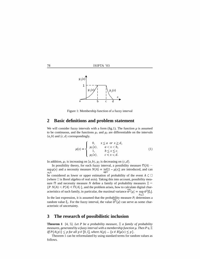
78 ISIPTA ’03

a b c d

1

x

µ 1 ( x ) µ 2 ( x )

µ 1 ( x )

Figure 1: Membership function of a fuzzy interval

2 Basic definitions and problem statement

We will consider fuzzy intervals with a form (fig.1). The function µ is assumedto be continuous, and the functions µ1 and µ2 are differentiable on the intervals a b and c d correspondingly.

µ x suuv uuw0 x M a or x c d

µ1 x a N x N b 1 b M x M c

µ2 x c N x N d 1 In addition, µ1 is increasing on a b , µ2 is decreasing on c d .

In possibility theory, for each fuzzy interval, a possibility measure Π A \supx A

µ x and a necessity measure N A \ infx á A

" 1 µ x &# are introduced, and can

be considered as lower or upper estimation of probability of the event A ℑ(where ℑ is Borel algebra of real axis). Taking this into account, possibility mea-sure Π and necessity measure N define a family of probability measures Ξ ' P N A OM P A dM Π A ( , and the problem arises, how to calculate digital char-acteristics of such family, in particular, the maximal variance σ2 µ sup

Pi Ξσ2 " ξi # .

In the last expression, it is assumed that the probability measure Pi determines arandom value ξi. For the fuzzy interval, the value σ2 µ can serve as some char-acteristic of uncertainty.

3 The research of possibilistic inclusion

Theorem 1 [4, 5]. Let P be a probability measure, Ξ a family of probabilitymeasures, generated by a fuzzy interval with a membership function µ. Then P Ξiff P ' A p ( M p for all p " 0 1 # , where A p 6o' x R µ x OM p ( .

Theorem 1 can be reformulated by using standard terms for random values asfollows.

Bronevich: The Maximal Variance of Fuzzy Interval 79

Theorem 1*. Let we use the same notations as in theorem 1, and the randomvalue ξ is described by the probability measure P on ℑ. Consider also a randomvalue η µ ξ d " 0 1 # . Then P Ξ iff Fη y dM y, where Fη y P ' η M y .

Remark. The function Fη is a distribution function of η, whenever η is con-tinuous.

4 The solution of the optimization problem

Theorem 2. Let ξ be a random value, described by a probability measure P Ξ,in addition, σ2 " ξ #A σ2 µ . Then we have P ' b c ( 0 for fuzzy interval (1).

Proof. Suppose that the coordinate system has been chosen in a way thatE " ξ #Ý 0. Assume also that b N 0, and the condition of the theorem is not ful-filled, i.e. P b 0 #3 0. The theorem is valid if one can find such a measure P thatP Ξ and σ2 " ξ #3 σ2 " ξ # . We will search the probability measure P in a form:

P A 6 sv wP A ε

P ' b ( ! P b 0 # 1 ε P A A b b 0 #&

A o' b ( A â " b 0 #ß /0

It is obvious that P extends on ℑ uniquely and P Ξ. Calculate derivative of

σ2 " ξ %# h ∞T ∞

x2dP x äãå h ∞T ∞

xdP x zæç 2

w.r.t. ε at the point ε 1. Sinceh ∞à ∞

xdP x 0 at the point ε 1,

ddε

x σ2 " ξ %# y ε B 1 ddε ãå h ∞T ∞

x2dP x $æçε B 1

Describe the last expression in detail.h ∞T ∞

x2dP x TR Õ b < 0 g x2P x ! b2 P ' b ( ! P b 0 # 1 ε è§! ε T@ b < 0 g x2dP x KTherefore,

ddε

x σ2 " ξ # y ε B 1 b2P b 0 #p! T@ b < 0 g x2dP x ON 0 It means that there exists ε N 1 that σ2 " ξ #3 σ2 " ξ # . For the complete proof of thetheorem, we must consider also a case, where c 3 0 and P " 0 c d3 0.

80 ISIPTA ’03

Corollary. Let P Ξ, σ2 " ξ #Ý σ2 µ as in theorem 2, in addition, E " ξ # 0.Then

1) P " 0 c 6 0 if c 3 0;2)P b 0 0 if b N 0.Theorem 3. Let P Ξ, σ2 " ξ #§ σ2 µ as in theorem 2. Then the random value

η has a distribution function Fη y y.Proof. We will assume that the coordinate system has been chosen in a way

that E " ξ # 0. Suppose the contrary assumption, that for ξ from the theorem,Fη y é y. The theorem will be proved, if under this condition, there exists arandom value ξ associated with a probability measure P Ξ for which σ2 " ξ #A3σ2 " ξ # . The random value ξ will be searched for a certain α " 0 1 # , using theexpression:

ξ OÜê µ 11 " αFη µ ξ %! 1 α µ ξ è#®

µ 12 " αFη µ ξ %! 1 α µ ξ è#® ξ " a b #&

ξ " c d #zHence, we need to find α " 0 1 # such that σ2 " ξ #3 σ2 " ξ # . But at first, check thatξ generates the probability measure P Ξ. To do this, we need to confirm thatthe inequality

Fη y P ' µ ξ dM y ( M y

is valid. Actually,

η µ ξ αFη µ ξ A! 1 α µ ξ Fη y 6 P ' αFη µ ξ A! 1 α µ ξ M y (

Since Fη y OM y, then ' αFη µ ξ ]A! 1 α µ ξ M y ( bÐ' Fη µ ξ dM y ( There-fore,

Fη y OM P ' Fη µ ξ M y ( P ë µ ξ dM F 1η y ®ì Fη x F 1

η y y y Thus, it has been shown that P Ξ. Further we will prove that σ2 " ξ #3 σ2 " ξ # fora certain α " 0 1 # . To do this, calculate derivative of

ddα

σ2 " ξ %#A ddα í E î ξ 2 ï Û E " ξ # 2 ð

α B 0

at the point α 0. Since E " ξ # α B 0 E " ξ # 0,

ddα

σ2 " ξ #2ññññ α B 0 d

dαE î ξ 2 ï ññññ α B 0

d

dα 79 bTa 4µ 1

1 "αFη µ x A! 1 α µ x è# 5 2dP x DE

α B 0

!

Bronevich: The Maximal Variance of Fuzzy Interval 81

! ddα 79 dTc 4

µ 12 "αFη µ x A! 1 α µ x è#*5 2 dP x ]DE

α B 0

Taking derivative w.r.t. α at the point α 0, we get

ddα

σ2 " ξ #2ññññ α B 0 bTa 2x

ddy

µ 11 y ;ññññ y B µ @ x C Fη µ x µ x ] dP x j!

! dTc 2xddy

µ 12 y ññññ y B µ @ x C Fη µ x % µ x ] dP x

Analyze signs of factors stating in the integrands.1) Fη µ x % µ x ÝM 0, in addition, since according to our supposition Fη y O

y, y " 0 1 # , there exists a non-empty set of points, in which Fη µ x µ x dN 0.Since Fη is continuous, increasing function, P ' Fη µ ξ µ ξ N 0 ( 3 0

2) The function µ1 is increasing on " a b # , therefore, ddy µ 1

1 y ñññ y B µ @ x C 3 0 if

x a b .3) According to the corollary of theorem 2, P " 0 c Ý 0. It enables to exchange

the area of integration to a min ' b 0 ( . Notice that 2x 6N 0 if x is in this interval.

4) The function µ2 is decreasing on " c d # , thus, ddy µ 1

2 y ñññ y B µ @ x C N 0, whenever

x c d .5) According to the corollary of theorem 2, P " d 0 Ý 0. It enables to exchange

the area of integration to max ' c 0 ( d in the second integral. Note that the factor 2x d3 0 in this interval.Analyzing signs of integrals, one can confirm that value of each of them is

non-negative; in addition, one of them is strictly positive. Hence, ddα σ2 " ξ # ññ α B 0 3

0. It means that one can find α 3 0 that σ2 " ξ #63 σ2 " ξ # , i.e. the supposition hasbeen made is wrong, and it implies Fη y y.

The proved theorems enable to make some simplifying of our optimizationproblem. To do this, introduce into consideration the functions

Fη1 y P ' µ1 ξ M y ξ " a b # ( Fη2 y P ' µ2 ξ OM y ξ " c d # ( It is clear that η1 µ ξ1 , η2 µ ξ2 , and also the random value ξ1 is associatedwith the probability measure P 'nò\ ξ " a b # ( , ξ2 with the probability measureP 'nò ξ " c d # ( . Let P Ξ and σ2 " ξ # σ2 µ , then P ' R Ô" a b #®L " c d # ( 0, and,using formula of composite probability, one can write:

Fη y Fη1 y P ' ξ " a b # ( ! Fη2 y P ' ξ " c d # (

82 ISIPTA ’03

By theorem 3, Fη y O y. Assume that functions Fη1 y and Fη2 y are differen-tiable, then the calculation of probability is transformed to Riemannian integral:

P ' ξ A ( P ' ξ " a b # ( Tµ : A ó§ a < b g > dFη1 y ! P ' ξ " c d # ( Tµ : A óß c < d g > dFη2 y 2 By analogy, using the expression ξ ê µ 1

1 η1 ξ " a b #zµ 1

2 η2 ξ " c d #z one can write the

formula for calculating moments:

E î ξk ï P ' ξ " a b # ( 1T04µ 1

1 y 5 kdFη1 y A! P ' ξ " c d # ( 1T0

4µ 1

2 y 5 kdFη2 y

Introduce the following notations:

h1 y 6 P ' ξ " a b # ( F lη1 y h2 y P ' ξ " c d # ( F lη2 y Then

E î ξk ï 1T04µ 1

1 y 5 kh1 y dy ! 1T0

4µ 1

2 y 5 kh2 y dy 3

It is clear, that functions h1, h2 have to be non-negative in " 0 1 # , in addition,h1 y ! h2 y 1 by theorem 3.

Theorem 4. Let ξ be associated with a probability measure P, P Ξ, σ2 " ξ #§σ2 µ , E " ξ # 0, and E

4ξk 5 is calculated by formula (3). In addition, functions

h1, h2 are piecewise continuous. Then in the range of hi continuity the followingformula is valid:

h1 y ê 1 ññ µ 11 y ññ 3 ññ µ 1

2 y ññ 0 ññ µ 11 y ññ N ññ µ 1

2 y ññ h2 y 1 h1 y 4 Proof. Assume, on the contrary, that the condition of the theorem takes place,

but formula (4) is not valid at least for one point of hi y continuity. The theorem isvalid if, for this case, we can find a random value ξ , associated with a probabilitymeasure P Ξ such that σ2 " ξ #Ò3 σ2 " ξ # . To do this, introduce into considerationthe following functions:

g1 y sv w1 0

h1 y ññ µ 11 y ññ 3 ññ µ 1

2 y ññ ññ µ 11 y ññ N ññ µ 1

2 y ññ ññ µ 11 y ññ ññ µ 1

2 y ññ g2 y 1 g1 y and also

h 1 y 6 g1 y α ! h1 y 1 α h 2 y 6 g2 y α ! h2 y 1 α y " 0 1 #z

Bronevich: The Maximal Variance of Fuzzy Interval 83

It is assumed that functions h 1, h 2 generate the probability distribution of ξ bythe formula:

P ' ξ A ( Tµ : A óß a < b g > h 1 y dy ! Tµ : A óß c < d g > h 2 y dy It is clear that the last formula is an analog of formula (2), and the random valueξ generates the probability measure P Ξ for all values α " 0 1 # . Calculate

derivative of ddα σ2 " ξ #A d

dα í E î ξ 2 ï Û E " ξ # 2 ðα B 0

at the point α 0. Since

E " ξ # 0 for α 0, we get ddα σ2 " ξ # ññ α B 0 d

dα E î ξ 2 ï ñññ α B 0. Then

ddα

E î ξ 2 ï ddα

1T04µ 1

1 y 5 2 " g1 y α ! h1 y 1 α z# dy !! d

dα

1T04µ 1

2 y 5 2 " g2 y α ! h2 y 1 α &# dy 1T0

4µ 1

1 y $5 2 " g1 y h1 y $# dy ! 1T04µ 1

2 y &5 2 " g2 y h2 y &# dy Since g1 y h1 y 6 h2 y g2 y , we get at last

ddα

σ2 " ξ # ññññ α B 0 1T0 í 4 µ 1

1 y $5 2 4µ 1

2 y &5 2 ð " g1 y h1 y $# dy Analyze signs of integrands factors.1) Let g1 y O3 h1 y , then g1 y 1, i.e. µ 1

1 y O3 µ 12 y by formula (4).

2) Let g1 y ON h1 y , then g1 y 0. i.e. µ 11 y ON µ 1

2 y by formula (4).From this, one can make a conclusion that the integrand on " 0 1 # is non-

negative. In addition, by our assumption, there is a point in the range of h1 y continuity such that g1 y h1 y . It implies d

dα σ2 " ξ # ññ α B 0 3 0. It means, thereis a point α 3 0 such that σ2 " ξ #63 σ2 " ξ # , i.e. the assumption made is wrong. Itproves the theorem in the whole.

Theorem 5. Let a set ' ξi ( of random values with maximal variance σ2 " ξi #σ2 µ , E " ξi # 0, be in a fuzzy interval F with the membership function µ. Thenthere is a random value ξ o' ξi ( such that

h 1 y sv w1 ññ µ 1

1 y ññ 3 ññ µ 12 y ññ 0 ññ µ 1

1 y ññ N ññ µ 12 y ññ α ññ µ 1

1 y ññ ññ µ 12 y ññ h 2 y 1 h 1 y α " 0 1 #z

84 ISIPTA ’03

Proof. By theorem 4, the set ' ξi ( includes a random value ξ such that

h1 y ê 1 ññ µ 11 y ññ 3 ññ µ 1

2 y ññ 0 ññ µ 11 y ññ N ññ µ 1

2 y ññ h2 y 1 h1 y Denote A Uë y " 0 1 #] ññ µ 1

1 y ññ ññ µ 12 y ññ ì . For the random value ξ , choose

parameter α " 0 1 # as follows. Under the condition, E " ξ # E " ξ #Ò 0, in addi-tion, hi y h i y if y A. Therefore,

E " ξ # E " ξ # TA µ 11 y h1 y dy ! TA µ 1

2 y h2 y dy 79 TA µ 1

1 y h 1 y dy ! TA µ 12 y h 2 y dy DE

For y A, µ 11 y µ 1

2 y , thus,

TA µ 11 y h1 y dy ! TA µ 1

2 y h2 y dy TA µ 1

1 y h1 y h2 y % dy β TA µ 11 y dy

where β " 0 1 # . The last equality is obtained with the help of mean-value theo-rem. By analogy,

TA µ 11 y h 1 y dy ! TA µ 1

2 y h 2 y dy TA µ 1

1 y h 1 y h 2 y dy 2α 1 TA µ 11 y dy

Thus, E " ξ #ß E " ξ #¢ 0 if β 2α 1. Let us show that σ2 " ξ #¢ σ2 " ξ # in this case.Actually,

σ2 " ξ # σ2 " ξ # E

4ξ2 5 E î ξ 2 ï 79 TA

4µ 1

1 y 5 2h 1 y dy ! TA

4µ 1

2 y 5 2 h 2 y dy DE TA

4µ 1

1 y 5 2dy TA

4µ 1

2 y 5 2dy 0

The theorem is proved.

Bronevich: The Maximal Variance of Fuzzy Interval 85

5 The practical calculation of maximal variance

Theorem 6. Let the function µ 11 ! µ 1

2 be increasing. Then functions hi for cal-culating the maximal variance have a form:

h1 y /ê 1 y N α 0 y 3 α h2 y 1 h1 y y α " 0 1 #& 5

Proof. Let ξ be associated with a probability measure P Ξ and σ2 " ξi #6σ2 µ . Suppose that E " ξ # m, then by theorem 4,

h1 y Üê 1 ññ µ 11 y m ññ 3 ññ µ 1

2 y m ññ 0 ññ µ 11 y m ññ N ññ µ 1

2 y m ññ Thus, we need to solve the inequality, ññ µ 1

1 y m ññ 3 ññ µ 12 y m ññ . One can con-

sider that µ 11 y m N 0 and µ 1

2 y m 3 0 (see corollary of theorem 2). There-fore, the last inequality is transformed to a form:

µ 11 y A! µ 1

2 y dN 2m Let the number 2m belong to the range of values of the function µ 1

1 ! µ 12 , g be

an inverse function to this median, then, since g is increasing function, we getthat y N g 2m 6 α. The cases, where 2m does not belong to the range of medianvalues, are also described by formula (5).

Corollaries of theorem 6. Let we use notations of theorem 6. Then

1) h1 y 6¥ê 1 µ 11 y A! µ 1

2 y ON 0 0 µ 1

1 y A! µ 12 y O3 0 h2 y 6 1 h1 y , if E " ξ # 0.

2) Let the function µ 11 ! µ 1

2 be increasing on " 0 1 # , then there is a certain

α " 0 1 # such that h1 y ê 1 y 3 α 0 y N α h2 y 1 h1 y , y α " 0 1 #&

Theorem 7. Let ξ belong to a fuzzy interval F with a membership function µand σ2 " ξ #A σ2 µ . Then E " ξ #ôë µ 1

1 y ! µ 12 y y " 0 1 #Gì .

Proof. Assume that the condition of the theorem is not satisfied. Then, usingcorollary 1 of theorem 6, we get that either h1 y õ 1 or h2 y õ 1. For the sake ofdeterminacy, let E " ξ # 0. 1) Let h1 y 6õ 1, then E " ξ #N b. It means that P " 0 c 30, but this contradicts to the corollary of theorem 2. 2) Let h2 y Òõ 1, then E " ξ #§3 c.It means that P b 0 #3 0, but this contradicts to the corollary of theorem 2. Thecontradictions found prove the truth of the theorem.

Corollary. Let a fuzzy interval F be symmetric, i.e. µ 11 y A! µ 1

2 y const,

and, for the sake of determinacy, const 0. Then σ2 µ 6 1à0

4µ 1

1 y 5 2dy.

Proof. According to theorem 7, for ξ with maximal variance, the value E " ξ #

86 ISIPTA ’03

belongs to the range of µ 11 ! µ 1

2 values, i.e. E " ξ #A const 0. Therefore,

σ2 " ξ # 1T04µ 1

1 y 5 2h1 y dy ! 1T0

4µ 1

2 y 5 2h2 y dy

Since

4µ 1

1 y 5 2 4µ 1

2 y 5 2and h1 y ;! h2 y 1, we get σ2 " ξ #G 1à

0

4µ 1

1 y 5 2dy.

The corollary is proved.Theorem 8. Let functions hi y in the formula (3) for calculating maximal

variance have a form:

h1 y 6Üê 1 y N α 0 y 3 α h2 y 1 h1 y y α " 0 1 #& 6

Then α can be found from the equality:

µ 11 α A! µ 1

2 α 2

! αT04µ 1

2 y µ 11 y ]5 dy 1

2

1T04µ 1

2 y µ 11 y &5 dy 0 7

if the coordinate system is chosen such that1à0

4µ 1

2 y ! µ 11 y 5 dy 0. There is

a unique solution if the function µ 11 ! µ 1

2 is increasing.Proof. Let the functions hi have a form (6). Then

σ2 " µ #A E

4ξ2 5 E2 " ξ # αT0

4µ 1

1 y 5 2h1 y dy !

! 1Tα 4µ 1

2 y 5 2h2 y dy 79 αT0 µ 1

1 y dy ! 1Tα µ 12 y dy DE 2

Taking derivative w.r.t. α and using the necessity condition for extremum, we getthe equality:4µ 1

1 α ]5 2 4 µ 12 α $5 2 2

4µ 1

1 α µ 12 α &5 ãå αT0 µ 1

1 y dy ! 1Tα µ 12 y dy æç 0

Since α N 1 and µ 11 α µ 1

2 α \N 0, then we can reduce this factor. As result,

µ 11 α A! µ 1

2 α 2 ãå αT0 µ 11 y dy ! 1Tα µ 1

2 y dy æç 0 8

Bronevich: The Maximal Variance of Fuzzy Interval 87

Transform the expression:

2 ãå αT0 µ 11 y dy ! 1Tα µ 1

2 y dyæç αT0 µ 11 y dy αT0 µ 1

2 y dy ! 1T0 µ 12 y dy

! 1T0 µ 11 y dy 1Tα µ 1

1 y dy !-! 1Tα µ 12 y dy 79 1Tα 4

µ 12 y µ 1

1 y 5 dy αT0

4µ 1

2 y µ 11 y $5 dy DE ! 1T0

4µ 1

2 y A! µ 11 y &5 dy

By the supposition,1à0

4µ 1

2 y A! µ 11 y 5 dy 0, in addition, the first item in the

last expression can be transformed to a form:

1T04µ 1

2 y µ 11 y $5 dy 2

αT04µ 1

2 y µ 11 y $5 dy

Taking this into account, the equality (8) is written as follows:

µ 11 α ! µ 1

2 α A! 2

αT04µ 1

2 y µ 11 y $5 dy ö 1T0

4µ 1

2 y µ 11 y $5 dy 0 9

i.e. we really prove the truth of equation (7).Denote the left part of equation (9) by f α . Let the function µ 1

1 ! µ 12 be

increasing, then, since by supposition1à0

4µ 1

2 y ! µ 11 y 5 dy 0, it is obvious

that µ 11 0 A! µ 1

2 0 OM 0 and µ 11 1 A! µ 1

2 1 c 0. Taking this into our account,analyze signs of f α at the ends of " 0 1 # :

f 0 µ 11 0 ! µ 1

2 0 S f 1 µ 1

1 1 ! µ 12 1 A! S

where S is an area of the fuzzy interval. Therefore, f 0 N 0 and f 1 d3 0, i.e. theequation has at least one root. Analyze the sign of

f l α ddα

4µ 1

1 α A! µ 12 α ]5! 2

4µ 1

2 α µ 11 α $5

It is obvious, that f l α 3 0 for α " 0 1 # . Thus, the equality f α 0 has only oneroot, and this root is a point of maximum (you should remind, that for obtaining

88 ISIPTA ’03

equality (8), we reduce the expression by the negative factor x µ 11 α µ 1

2 α y ).Thus, the theorem is proved in the whole.

Remarks.1) Theorem 8 is easily generalized for the case, where

h1 y Üê 1 y 3 α 0 y N α h2 y 1 h1 y y α " 0 1 #z

and the function µ 11 ! µ 1

2 is decreasing. In this case α can be found from theequation:

µ 11 α A! µ 1

2 α 2 αT0

4µ 1

2 y µ 11 y 5 dy ! 1

2

1T04µ 1

2 y µ 11 y 5 dy 0

We also suppose that1à0

4µ 1

2 y ! µ 11 y $5 dy 0.

2) The equation (7) has a geometrical interpretation (fig. 2).

a b c d

1

x

µ 1 -1 (y)

y

µ 2 -1 (y)

0.5[ µ 1 −1 (y) + µ 2

−1 (y) ]

α

Figure 2: Fuzzy interval: inverse functions

a) 0 5 µ 11 ! µ 1

2 is the median of the fuzzy interval;

b)1à0

4µ 1

2 y µ 11 y &5 dy is the area of the fuzzy interval;

c)αà0

4µ 1

2 y µ 11 y 5 dy is the area of the part of the fuzzy interval that is

below of α level ;d) µ 1

2 α µ 11 α is the length of the level line y α for the fuzzy interval.

3) Introduce into consideration functions

m y Ò µ 11 y A! µ 1

2 y 2

w y Ò µ 12 y µ 1

1 y 2

F α Ò αT0 . w y A! m l y 2 0 dy

Then equation (7) can be transformed to a form:

2F α F 1 0 7

Bronevich: The Maximal Variance of Fuzzy Interval 89

Example. Consider, how to calculate the maximal variance for the fuzzy inter-val having a form of trapezium (fig. 3). In this case, the functions m, w are linear.

A

B C

D

y

x

m ( y )

0.5

Figure 3: Fuzzy interval with a form of trapezium

We assume that m is increasing and1à0

m y dy 0. In this case, one can easily

show that m y d k y 0 5 , where k 3 0. The function w is expressed throughlengths of the trapezium sides l1 ÜBC and l2 AD . Since w 0 0 5l2 andw 1 0 5l1, then w y 0 5 " l2 - l2 l1 y # . The parameter α can be found fromequation (7*). Then F α 6 0 5 k ! l2 α 0 25 l2 l1 α2 , and we need to solvethe equation: l2 l1 α2 2 k ! l2 α ! l1 ! l2 ! 2k

2 0

Solving it, we get

α k ! l2 Y÷ 0 5 î k ! l2 2 ! k ! l1 2 ïl2 l1

in addition, α " 0 1 # . The precise value of σ2 µ can be calculated by formula(3). Namely, according to the form of h1 h2 we can write

σ2 µ 6 αT04µ 1

1 y 5 2dy ! 1Tα 4

µ 12 y 5 2

dy 79 αT0 µ 11 y dy ! 1Tα µ 1

2 y dy DE 2 where

µ 11 y " k ! 0 5 l2 l1 &# y 0 5 0 25 l2 ! l1

µ 12 y " k 0 5 l2 l1 &# y 0 5 A! 0 25 l2 ! l1

Let l1 1 l2 3 k 0 5, then α 0 404, σ2 µ 1 342. Fig. 4 shows this fuzzyinterval, and probability distribution function F of the extreme random value ξ,being in the fuzzy interval, for which σ2 µ 6 σ2 " ξ # .

90 ISIPTA ’03

µ x( )

F x( )

x

2 1 0 1 2

0

1

Figure 4: Numerical example

References

[1] P. Walley. Statistical reasoning with imprecise probabilities. Chapman andHall, London, 1991.

[2] D. Dubois, and H. Prade. Possibility theory. Plenum Press, New-York, 1988.

[3] D. Dubois, and H. Prade. The mean value of fuzzy number. In Fuzzy setsand systems, 24: 279-300, 1987.

[4] D. Dubois, and H. Prade. When upper probabilities are possibility measures.In Fuzzy sets and systems, 49: 65-74, 1992.

[5] A.G. Bronevich, and A.N. Karkishchenko. Statistical classes and fuzzy settheoretical classification of possibility distributions. In Statistical modelling,analysis and management of fuzzy data. Heidelberg. New-York: Physica-Verl., 173-195, 2002.

Andrew G. Bronevich is with the Laboratory of Mathetimatical Problems in Artificial In-telligence, Taganrog State University of Radio-Engineering, Nekrasovskiy street, 44, Rus-sia, 347928. E-mail: brone@mail.ru

Inter-personal Communication of Preciseand Imprecise Subjective Probabilities

D. V. BUDESCUUniversity of Illinois at Urbana-Champaign, USA

T. M. KARELITZUniversity of Illinois at Urbana-Champaign, USA

Abstract

We analyze communication of uncertainty among individuals as a function ofthe parties’ preference for modes of communication. We assume that differ-ent individuals may prefer precise Numerical probabilities, Ranges of proba-bilities or Verbal descriptions of probabilities, and consider all possible pair-ings of communicators and receivers under this classification. We proposea general criterion of optimal conversion among the various modalities, de-scribe several instantiations tailored to fit the special features of the variousmodalities, and illustrate the efficacy of the proposed procedures with empir-ical results from several experiments.

Keywords

subjective probability, judgment, inter-personal translation, verbal probabilities

1 Introduction

Consider a situation where two individuals communicate about stochastic events.The two are equally interested and motivated to communicate as efficiently andprecisely as possible. This paper is concerned with procedures that can be em-ployed to address the individuals’ different preferences for modality of commu-nicating probabilistic opinions. Although many decision analysts and orthodoxBayesians consider precise numerical probabilities to be the language of uncer-tainty, many people (layman and experts, alike) prefer to use probability phrases(e.g. review by Budescu and Wallsten [6]) or other imprecise variants of probabil-ity. In this paper we propose ways to achieve the highest possible level of accuracyin communication while accommodating these individual preferences.

This work has been supported by the US National Science Foundation under Award No. SES9975360. Any opinions, findings, and conclusions or recommendations expressed in this publicationare those of the authors and do not necessarily reflect the views of the US National Science Foundation.

91

92 ISIPTA ’03

1.1 Reasons for preferences of specific communication modes

Spontaneous preferences for one particular mode may be due to several factors:The perceived nature of the uncertainty to be communicated–Budescu and

Wallsten [6] have speculated, and Olson and Budescu [14] have documented em-pirically that most individuals prefer to use precise numerical estimates to com-municate uncertainty about repeated events with aleatory uncertainty, but tendto use more imprecise methods when communicating the probabilities of uniqueevents with epistemic uncertainty.

The perceived strength of the available information–The responses to the sur-vey conducted by Wallsten, Budescu, Zwick, and Kemp [18], indicate that peoplewould gravitate towards more precise modes of communication, if they perceivethe available information to be firmer, reliable and valid.

The person’s role in the communication–In the same survey Wallsten et al.[18] have found that most people prefer to use imprecise terms when they com-municate to others, but prefer others to communicate to them in precise terms, ifpossible (see also, Brun and Teigen [2] and Erev and Cohen [8]).

In addition to these systematic factors, preferences may be due to plain in-dividual differences that reflect one’s lifetime experiences in dealing with, andcommunicating, uncertainties.

1.2 The problem

The need to communicate probabilities arises in a variety of situations. A commoncase is when both individuals have prior opinions, have access to some relevant(possibly overlapping) information, and wish to exchange information to furtherrefine their respective estimates. In this symmetric case the designation of commu-nicator and receiver is arbitrary, as the two individuals can act in both capacities.For example, think of two friends who talk about the chances of their favorite teamto win a game. The other prototypical case involves asymmetric communication:only one individual, the Forecaster (F for short), has access to, or possesses thenecessary expertise to make sense of, the relevant information for the probabilityestimation. The second individual, the Decision Maker (or DM) needs to make achoice or decision on the basis of the F’s estimate, and without the benefit of his,or her, own probability assessment. For example, think of an investor (the DM)who gets from his, or her, favorite financial advisor estimates of the likelihoodthat certain investment policies will succeed.

The two situations are similar in many respects but the former is more com-plex because a complete analysis should take into account the processes that gov-ern the combination of one’s own opinions with estimates obtained form oth-ers (Yaniv and Kleinberger [19]). To simplify the analysis, we will focus on thesecond case. In the same spirit, we will not consider the case where one needsto aggregate multiple forecasts from various sources (Budescu, Rantilla, Yu and

Budescu & Karelitz: Inter-personal Communication of Probabilities 93

Karelitz [5], Wallsten, Budescu and Tsao [17]).To summarize, we analyze an asymmetric dyadic communication situation

where one F and one DM share a common interest in optimizing communication,but they may have different preferences for modality of communicating proba-bilistic opinions.

1.3 A typology of communication preferences in a dyad

We distinguish between three modes of communication: precise (point) Numericalprobability estimates (e.g., 0.45), precise Ranges of numerical values (e.g., 0.3 -0.55), and Verbal phrases (e.g., good chance). Ranges with precise end points ex-clude implicit vague ranges such as ”in the forties” or ”at least 0.80”, but suchexpressions can be analyzed as verbal terms.

The three modes can be ranked from the most precise (N) to the most vague(V). In fact, the more precise modes can be represented as special cases of themore vague modes: clearly an N is an R where the lower and upper limit coincide,and we will show later how N and R can be viewed as special cases of V undera particular representation of the probability phrases. This typology implies 9distinct dyadic patterns of dyadic preferences for modes of communication thatwill be denoted by ordered pairs, where the first character in the pair refers to theF’s preference.

2 The translation process

The problem we wish to address is deceptively simple – How to best convert ajudgment originally expressed in the F’s favorite response mode (N, R or V), toan estimate in the DM’s favorite mode (N, R or V).

The criterion of optimality is the level of (dis)similarity between the F’s judg-ments translated into the DM’s favorite mode, and the DM’s spontaneous (andindependent) judgments of the same events in his, or her, favorite mode. For ex-ample, assume that the F prefers numbers and the DM prefers verbal terms (i.e.,an [N,V] dyad). If both had the same prior probability distribution and could ac-cess the same information pertaining to the target event, Xi, their spontaneous andindependent judgments would be nF Xi , and vDM Xi , respectively.

Any mapping of the F’s spontaneous judgment into the DM’s favorite commu-nication mode is a translation. For example, vDM " nF Xi $# is the verbal translationof the F’s original numerical judgments. An optimal translation is one that maxi-mizes the similarity between the translation of the F’s term into the DM’s favoritemode, and the DM’s spontaneous judgment of the target event (assuming he/shehas the same priors and could access the same information).

Note that (dis)similarity is measured in the scale of the target modality (i.e.,the one that is favored by the DM), so it always relies on commeasurable units or

94 ISIPTA ’03

entities. On the other hand, these entities vary as a function of the DM’s favoritemodality. Next we describe some sensible choices for the dissimilarity metrics.Our goal in this paper is to provide a general framework for the translation processand illustrate the feasibility of the approach. We make no claim of optimality, oruniqueness on behalf of these choices, and realize that other metrics could be usedin this context.

Dissimilarity between two numbers, nDM and nF , is defined as the distancebetween them:

DSn ' nDM nF ( m nDM nF I (1)

Dissimilarity between two ranges, rDM and rF , is a function of their respectivelengths, and their overlap. Consider two ranges, r1 (ranging from l1 to u1) andr2 (from l2 to u2). The width of the range over which the two overlap is OV12 Max ' 0 "Min u1 u2 Max l1 l2 &# ( , and the joint range of values they span isJR12 "Max u1 u2 Min l1 l2 &# . We define the dissimilarity between the tworanges as:

DSr ' rDM rF ( JRDM < F OVDM < F (2)

This measure is zero if, and only if, the two ranges coincide. For any pair ofranges, rDM and rF , the index is maximal when they are disjoint.

Dissimilarity between two verbal terms, vDM and vF , is defined in the con-text of a particular representation of such phrases. Wallsten, Budescu, Rapoport,Zwick, and Forsyth [16] suggested that probability phrases are fuzzy concepts andproposed using Membership Functions (MFs) over the " 0 1 # probability intervalto represent their vague meanings (see Zadeh [20]). A phrase’s MF assigns to eachprobability a real number that represents the (non-negative) degree of its member-ship in the concept defined by the phrase. These values are scaled between 0 and1 (Norwich and Turksen [13]), such that memberships of 0 denote probabilitiesthat are absolutely not in the concept and memberships of 1 denote elements thatare perfect exemplars of the concept. All other positive values represent interme-diate degrees of membership. MFs can be estimated directly (non-parametrically)based on the participants’ direct or indirect judgments (see Budescu and Wall-sten [6], Wallsten et al. [16]). Alternatively, one can fit MF using specific familiesof functions, such as polynomials (Budescu, Karelitz and Wallsten [4]), or trape-zoidal functions.

Let µvDM p and µvF p be the MFs representing the two words being com-pared. The similarity between the two words should reflect the closeness betweentheir respective MFs. There are many possible single-valued indices of closenessbetween the two functions (see review by Zwick, Carlstein, and Budescu [21]),and we will only list two of them here (these are not necessarily monotonically re-lated). The first measure is the total absolute distance between the two functions.

Budescu & Karelitz: Inter-personal Communication of Probabilities 95

Formally, we can write1:

DSvµ ' vDM vF ( T 1

p B 0 µvDM p µvF p K dp (3)

The second index is the distance between the peaks of the two functions. Assumethat both µvDM p and µvF p are single peaked (see Budescu and Wallsten [6] onthis point). Let π v be the probability (or the center of the range of probabili-ties) at which the function µv p reaches its maximal value. We define, a secondmeasure of dissimilarity as:

DSvπ ' vDM vF ( ) π vDM π vF ®I (4)

2.1 General comments on the measures of dissimilarity

The various measures may appear at first glance to be unrelated and, somewhatarbitrary, so a few comments and clarifications are in order. First, we should pointout that all the dissimilarity indices are distances. In all cases they assign to everypair of (N,R or V) judgments a non-negative real number DS 0 only if thetwo members of the pair are identical). The measures are symmetric, satisfy thetriangle inequality and induce a weak order over all pairs.

One could invoke other metrics for these comparisons. A particularly elegantapproach would be to use the same metric for all modalities. Technically, thisis feasible since numbers can be represented by point MFs (membership of 0everywhere, and 1 for the chosen number) and ranges can be represented by flatMFs (membership of 0 everywhere outside, and 1 everywhere within the chosenrange), and treated in the same fashion as the MFs obtained for verbal terms.However, we believe that the metrics identified above are better suited for ourpurposes because they are more in line with the particular level of (im)precisionimplied by the three modalities.

The last comment is subtler. Our definition of similarity relies on a counter-factual scenario that gives rise to a hypothetical entity - the DM’s spontaneousjudgment of the target event if he, or she, had the same prior probability distri-bution and could access the same information that was used by the F as a ba-sis for his/her judgment. Strictly speaking, this definition is meaningful only inthose cases where it makes sense to assume that a person’s judgment depends onlyon the specific information presented. This implies that the relevant informationis unambiguous and does not lend itself to different (subjective) interpretations.In other words, the observed variability among probabilities assigned to a targetevent by different individuals can be attributed solely to different response stylesand/or random factors within the judges. This formulation makes perfect sense

1In most empirical applications the MFs are approximated by a set of n points over ø 0 1 ù , so adiscrete version of this measure can be used to approximate it.

96 ISIPTA ’03

for repeatable and exchangeable events, but not for unique events where subjec-tive probabilities rely on internal epistemic uncertainty that can vary systemati-cally across individuals. (Ariely, Au, Bender, Budescu, Dietz, Gu, Wallsten andZauberman [1] and Wallsten, Budescu, Erev and Diederich [15], discuss variousfacets of this key distinction).

For example, it is quite unlikely that if we were to present anti-smoking ac-tivists and tobacco lobbyists with the results of a new study on the effects ofsecond-hand smoking, they would agree in their estimation of the probabilitiesthat second-hand smoking has serious public health consequences. The differ-ences between their estimates would reflect (a) their different prior probabilities,and (b) their differential assessment of the quality, reliability and validity of thenew data. Clearly, no translation method can be expected to reconcile disagree-ments of this type. Despite these irreconcilable differences in their opinions, wecan still take advantage of optimal translation schemes derived for various pairsof communicators based on their judgments of a standard set of exchangeableevents. When these translation methods are applied they can reduce the effect ofother sources of variability among the participants and provide the most accuraterepresentation of the F’s assessment in the DM’s favorite communication mode,where accuracy is measured by one of the dissimilarity metrics discussed above.

2.2 Methods of translation

We return now to our original question: how to best convert a judgment originallyexpressed in the F’s favorite response mode (N, R or V), to an estimate in theDM’s favorite mode (N, R or V). Before we discuss translation schemes for eachof the 9 cases, it makes sense to classify them into three distinct groups:

Common modalities - In three cases ([N,N], [R,R] and [V,V]) both individualsshare a common preference for mode of communication, so there is no need toworry about differential precision. Conversions may be employed to account forinter-personal differences in the way the relevant terms are chosen and used.

Resolving vagueness - In three cases ([R,N], [V,R] and [V,N]) the DM prefersa more precise mode of communication than the F. Thus, the challenge is to find atranslation that resolves the vagueness implicit in the F’s judgment to achieve thehigher level of precision required by the DM.

Imputing vagueness - In the other three cases ([N,R], [N,V] and [R,V]) theDM prefers a more vague mode of communication than the F. Thus, the challengeis to find a translation that replaces the precision implicit in the F’s judgment toreflect the higher level of vagueness expected by the DM.

We will discuss the three classes separately. In each case we describe andjustify a translation method designed to optimize our stated goal and, when ap-propriate, we review and discuss relevant results from several empirical studiesthat are described in the next section.

Budescu & Karelitz: Inter-personal Communication of Probabilities 97

2.3 The data

Over the last two years we have conducted four experiments designed to test theefficacy and accuracy of various translation methods of probability phrases (V).The studies vary in many specific details (Budescu and Karelitz [3] and Kare-litz and Budescu [11]) but they share a set of common features that allow us toanalyze some of their results jointly. The focus on the N and V responses is nei-ther accidental, nor arbitrary. Subjects rarely communicate their probabilities bymeans of ranges even when offered the opportunity (e.g. references in Budescuand Wallsten [6]). For example, in one of the studies analyzed below when thisoption was present, it was used in less that 7.5% of the cases. Thus, we will notpresent any empirical results concerning translations involving Rs.

The four studies involved a total of 128 individuals (all students at the Univer-sity of Illinois in Urbana Champaign, and most of them native English speakers2).All the experiments were computer controlled, and included the following threetasks: (1) Selection of a personal verbal probability lexicon including 5-11 phrases(In a few cases some, or all, the phrases were selected by the experimenters basedon previous research); (2) Elicitation of MFs for all the phrases; and (3) Numericaland verbal estimation of probabilities of a common set of events.

Subjects created their lists by selecting combinations of words and semanticoperators (modifiers, intensifiers, etc.) from two lists, or typing in phrases. Theywere instructed to select phrases that span the whole probability range, and theytend to use regularly. Membership functions were elicited using a method vali-dated by Budescu et al. [4]. Each phrase was presented with a set of eleven proba-bilities ranging from 0 to 1 in increments of 0 1. The subjects judged the degree towhich the target phrase captured the intended meaning of each of the eleven nu-merical probabilities by using a bounded scale, anchored by the terms ’not at all’and ’absolutely’. In the last task, the participants saw a series of circular, partiallyshaded, targets. Their task was to assess the likelihood that a dart, aimed at thecenter of the target, would hit the shaded area. The shaded areas varied from onetrial to another and covered the full (0,1) range. On separate presentations theseprobabilities were judged numerically (by selecting one value from a list of 21probabilities, ranging from 0 to 1 in increments of 0 05), or verbally by selecting(in some cases up to four) phrases from their lexicons.

2.4 Common modalities

[N,N] This is the ”gold standard” case of Bayesian decision analysis. Pre-sumably numbers are universal and everyone understands, interprets and usesthem in identical fashion. Therefore, no transformation is required. There is, how-ever, evidence that people’s mapping of their internal feelings of uncertainty into

2One of the studies was concerned with translation of probability phrases across languages and werecruited native speakers of French, German, Spanish, Russian and Turkish.

98 ISIPTA ’03

numbers is imperfect. In particular, most people over-(under-) estimate low(high)probabilities (e.g. references in Erev, Wallsten and Budescu [9]), and it is con-ceivable that there are systematic differences in the degree to which individualstend to avoid (or favor) the extreme values. In principle, one could quantify thistendency and apply appropriate stretching (or contracting) transformations. Toillustrate this point consider multiple judges (1 2 %% j j l %j J) who judge a setof stochastic events (1 2 %] i %%j I). Assume that: (1) All judges have access tothe same amount of information, implying that differences in their judgments aredue only to (a) differences in their use of the response scales and (b) randomcomponents. (2) All judges spontaneously recognize events that are impossible(probability = 0), certain (probability = 1), and as likely as not (probability = 0 5).(3) Assume an ”ideal judge” who is perfectly calibrated (no biases) and accurate(no random component). Thus his/her judgments, p1 p2 % pi, coincide with theevents’ ”objective probabilities”.

The probability assigned by judge j to event i is denoted by pi j, and can beexpressed as a function of the objective probability, pi, his/her bias parameter, α j,and the random component, ei j which we assume is distributed with µe 0 and(finite) σe. We use a variation of Karmarkar’s [10] model, that assumes that thelogit of the judged probabilities is a linear function of the logit of their objectivecounterparts:

Log . pi j 1 pi j n0 α jP Log . pi 1 pi n0 ! ei j (5)

Individual differences between judges are captured by the parameter α j , whichis bounded from below by 0 (when all events are assigned a probability of 0 5).An unbiased judge should have an α j of 1, but we expect that most individu-als would have parameters between 0 and 1 that are consistent with the regressivemodel described above. We used a least-squares procedure to estimate the individ-ual parameter, α j, in model 5. The model fits the data well for almost all subjects(median R2 0 98, median MSE 0 13). The distribution of the individual pa-rameters matches our expectations: 64 values (50%) are between 0 55 and 0 98,45 participants (35 2%) are almost perfectly calibrated (0 99 M α j M 1 01), andonly 19 individuals (14 8%) have parameters values above 1. To verify that thesedifferences reflect systematic individual differences rather than pure random error,we performed two additional analyses: (a) we compared these results with a modelwhere the parameter, α j, was constrained to be 1 (thus the model includes onlyrandom error). A comparison of the two models in terms of R2

ad j favors slightlythe fitted model. The modal difference (34% of the cases) is 0, but there is a clearmajority (43% vs. 23%) of cases where the fitted model fits better (mean differ-ence in fit = 0 02), even after we account for its extra parameter. Significance testscomparing the fit of the two models (separately for each subject) revealed that thisdifferences was significant at the traditional 0 05 level, for 25 2% of the subjects.(b) We re-analyzed two of the studies in which all subjects judged all the displays

Budescu & Karelitz: Inter-personal Communication of Probabilities 99

twice, so we could obtain two estimates of the parameter, α j , for each person.In both studies (involving a total of 55 subjects) the between-subjects variancecomponent was considerably larger than the within-subject component (in factthe within-subject component was not significantly greater then 0).

In principle, one could convert numerical estimates from one person to anotherin an optimal fashion by applying simple stretching (contracting) transformationbased on the estimates of the individual parameters, α j, α j l .[R,R] The use of precise ranges instead of simple point estimates reflectsone’s perceived level of imprecision in his or her estimate of the probability of thetarget event. Clearly, the arguments invoked in the [N,N] case regarding the natureof the numbers, apply here as well. This would suggest that no transformationsare indicated. It is conceivable, however, that there are systematic differences inthe degree of imprecision perceived by different individuals and this would in-duce systematic differences in the widths of their ranges. One could quantify thistendency and apply appropriate imprecision equating transformations.[V,V] This situation is, probably, the most interesting and it has been thefocus of much of our recent research. This case is qualitatively different fromthe previous two for several reasons. There is a large literature indicating that (a)spontaneously, people tend to use highly different and diverse lexicons, and (b)the numerical meanings (as well as other forms of representation) associated withthese words vary dramatically across people (e.g. review in Budescu and Wall-sten [6]). Thus, one cannot assume that everyone is equally comfortable with, orinterprets identically terms such as ”likely”, ”poor chance”, etc. For this case weadvocate the following multi-stage procedure that is sensitive to these empiricalfindings: (a) each participant selects his/her own subjective lexicon; (b) MFs areelicited for all the terms in the list; (c) the MFs of the words selected by the Fand the DM are placed on a common probability scale and are matched accord-ing to the criterion of choice (DSvµ or DSvp). Occasionally this procedure doesnot yield a unique solution, i.e., one of the F’s words can be translated equallywell into several of the DM’s words. Of course, all these words are equally validtranslations of the F’s judgment. If practical considerations prevent one-to-manytranslations, one of them can be selected randomly (or by some other sensibletie-breaking procedure).

We have done quite a lot of empirical work documenting the efficacy of thisapproach (Karelitz and Budescu [11], Karelitz, Dhami, Budescu, and Wallsten[12]). In each of our studies we compared the level of agreement in assignmentof verbal phrases to the same events among numerous pairs of distinct individu-als. We hypothesized that the lowest level of agreement would be observed withspontaneous (un-aided), verbal discourse, and the best level of agreement wouldbe found in the case of numerical communication. Most importantly, we expectthat communication with converted phrases would be superior to un-aided verbalcommunication, and closer in quality to the numerical case. To quantify the levelof inter-personal agreement we defined two indices of co-assignment. We use two

100 ISIPTA ’03

measures because some of the events were judged more than once and yieldeddifferent responses from the subjects. Both measures range from 0 to 1 (highervalues indicate stronger agreement), and can be interpreted as measures of theaccuracy of inter-personal communication of imprecise opinions.PIA- Proportion of Identical Assignments- the proportion of comparisons whereboth participants assigned the same phrase to a given event.PMA- Proportion of Minimal Agreement - the proportion of stimuli for whichboth participants assigned at least one common phrase to a given event.

In the interest of brevity we only report results based on PIA, which is a morestringent measure than PMA (PIA M PMA) because it weighs the agreement bythe number of comparisons made (The PMA results are very similar in a quali-tative sense). Table 1 summarizes the results of 4 studies (details in Karelitz andBudescu [11]). Each cell presents the mean (and SD) PIA in the various modes,and across all pairs of subjects analyzed.

Table 1: Summary of agreement indices from 4 studies

Translation CriterionStudy No. of VJ: Unaided DSvµ DSvπ NJ: Unaided

pairs Verbal Judgments (Eq. 3) (Eq. 4) Numerical Judgments1 306 0.05 (0.03) 0.23 (0.12) 0.22 (0.10) 0.29 (0.07)2 90 0.04 (0.04) 0.22 (0.11) 0.19 (0.09) 0.36 (0.09)3 86 0.04 (0.07) 0.35 (0.16) 0.35 (0.16) 0.40 (0.15)4* 509 0.06 (0.09) 0.34 (0.15) 0.35 (0.14) 0.40 (0.13)

* Experiment 4 involves translations of words across various languages. VJ is based of the subjects’

spontaneous translation of words from their native languages to English.

The results clearly support our predictions: unaided VJ had the lowest valuesfor both indices in all the studies and NJ had the largest values. The two translationcriteria clearly outperformed the unaided verbal communication3.

2.5 Resolving vagueness

[R,N] In principle, any sensible person should be able to infer a single Nvalue from his/her partner range without invoking any translation scheme. Theindividual differences discussed in the [N,N] and [R,R] cases apply here as well.In principle, one could improve the quality of communication by (a) inferring theF’s best guess (presumably, the center of the reported range) and, if necessary, (b)applying the appropriate stretching (or contracting) transformation.[V,N] Recall that every word in the F’s lexicon has a (single-peaked) MFdefined over the [0,1] interval that describes the degree to which the various prob-

3Dhami and Wallsten [7] and Karelitz and Budescu [11] report similar results with several othertranslation methods.

Budescu & Karelitz: Inter-personal Communication of Probabilities 101

abilities match the intended meaning of that particular word. The MF’s peak,π v , is the single numerical probability that is most representative of the word’smeaning and is the translation of choice. Occasionally, the MF does not have aunique maximum, so all probabilities within a given range can be considered tobe equally good representations of the word’s meaning. In these cases it is conve-nient to translate the word into the mid-range of these probabilities. To illustratethe potential accuracy of this approach we compared the peaks of the 977 verbalphrases used by 113 of the subjects in our experiments with the mean of theirnumerical judgments when judging the same events. We found a remarkable sim-ilarity between the two sets: (a) the median within-subject difference betweenthe two is 0.006 and the median absolute difference between them is 0.097; (b)the median within-subject rank order correlation between the peaks of the wordsand the mean numerical judgments is 0.89; and (c) the two sets are almost per-fectly related linearly with a median within-subject intercept of 0 022, a medianwithin subject slope of 1.06, and a median R2

ad j of 0.90. These results indicatethat the translation procedure can map with high accuracy the intended meaningof the words and predict accurately the numerical probabilities used to describethe same events.[V,R] Every MF is, essentially, a collection of ranges since every level ofmembership, ν (0 M ν M 1), defines a range of values, R ν , such that µ(v) c ν.Typically, as ν increases, R ν becomes narrower indicating the range of valuesthat possess that (higher) level of membership is more restrictive. Thus, the trans-lation from a V to a R boils down to the issue of which threshold, ν, to choose.Presumably, there are systematic differences in the ”typical” threshold that indi-viduals tend to use in these circumstances, so one could quantify this tendencyand identify the most appropriate range for each individual. We are not aware ofany studies that have collected both verbal and upper and lower numerical boundsof the probabilities of the same events, so we are not in a position to assess theefficacy of the proposed approach.

2.6 Imputing vagueness

[N,R] If numbers are the universal language of uncertainty and everyoneinterprets them identically, any sensible DM would infer that the F’s single N isthe center of a range that describes his/her opinions, but there is no clue regardingthe implied imprecision of the F’s opinion. One could improve the quality ofcommunication by reversing the procedure described for [R,N], i.e., (a) applyingthe appropriate stretching (or contracting) transformation for the DM, and (b)imputing the DM’s typical band of imprecision. We are not familiar with anyempirical work along these lines.[N,V] Recall that all the words in the F’s lexicon have single-peaked MFsdefined over the [0,1] interval. These functions describe the degree to which anygiven probability matches the intended meaning of the various phrases. The pro-

102 ISIPTA ’03

posed translation rule calls for the choice of that phrase that has the highest mem-bership at the N in question. This procedure is not guaranteed to yield a uniquesolution, i.e. there could be several words with equally high membership at thatprobability, and all these words should be considered equally valid translationsof the numerical judgment. If necessary, one of these words can be selected ran-domly (or by some other tie-breaking procedure). In analyzing our studies welooked at responses from 118 subjects who used an average of 14.85 distinct nu-merical judgments. We analyzed the verbal responses that were assigned by thesubjects to the events to which they assigned a certain numerical response. Onthe average, each set of events that were judged to be equally probable (in thenumerical mode) generated 1.81 distinct verbal phrases, and in 68% of the casesat least one4 of these verbal responses had, indeed, the maximal membership forthat probability. Another look at the same data indicates that for 59.7% of the nu-merical judgments at least one of the verbal terms used was predicted from theMFs. Interestingly, we found large individual differences: 30 subjects (25.4%)are at, or below a 40% success rate, while for 27 subjects (22.9%) the rate of ac-curate translation is greater than, or equal to 75%. Not surprisingly, the level ofagreement is considerably higher for the extreme (0 and 1), and the central (0.5)numerical probabilities.[R,V] All the words in the F’s lexicon have (single-peaked and continuous)MFs defined over the [0,1] interval. For any fixed range of numerical probabilitythese functions describe the degree to which the probabilities in that range matchthe intended meaning of the various phrases. The proposed translation rule callsfor the choice of that verbal term that has the highest average membership over theR in question. It is possible that there would be several words with equally highmembership over that range probabilities. All these words should be consideredequally valid translations. We are not aware of studies that have collected therelevant data for the empirical evaluation of this procedure.

3 General Discussion

In this paper we proposed a unifying conceptual framework for optimal interper-sonal translation of probabilistic information for the 9 distinct cases we identified.We discussed the 9 scenarios at different levels of details, and provided extensiveempirical support for some of them. Although the cases are not encountered withsimilar frequency in applied settings, we decided to review all of them to illustratethe generality, feasibility and flexibility of the overall approach.

This line of research is part of an effort to create a general Linguistic Probabil-ity Translator (LiProT, for short) that could serve both as a useful research tool,and a general decision aid. LiProT would facilitate communication of subjec-

4In 14.5% of the cases more than one word tied for the highest membership at a given probability.The mean number of words tied for maximal membership was 1.14.

Budescu & Karelitz: Inter-personal Communication of Probabilities 103

tive uncertainties between participants in various decision situations - forecasters,judges, experts and decision makers - by reducing the dangers of miscommunica-tion of probabilities among the various members of the group.

To fix ideas consider a group of experts (physicians, intelligence officers, fi-nancial forecasters, etc.) who communicate with each other, possibly electroni-cally form various locations. As part of this process they need to exchange prob-abilistic information based on the evidence available to them and reflecting theirown unique expertise. If various people in this group have differential preferencesfor modes of communicating probabilities to others and receiving informationfrom others, then each of the 9 cases discussed above may be relevant for someof the pairs. The procedures described and partially tested in this paper providea foundation for such a system. Before the meeting, the participants’ preferredmodes of communication are ascertained, their verbal probability lexicons aremapped, and LiProT derives the appropriate translation scheme for each dyad.During the meeting, every probability (N, R or V) used by each of the experts isinstantly converted optimally to the favorite modality (N, R or V) of each of theother participants.

For example, assume that participant A prefers to communicate and to re-ceive numbers, participant B has a universal preference for Vs, and participant Cprefers to communicate with V, but to receive Ns (the modal pattern according toWallsten et al. [18]). Every uncertainty judgment provided by A (using Ns) willbe translated by LiProT into the closest V in judge B lexicon (using the [N,V]module), and into the most appropriate N for judge C (using the [N,N] module).Similarly, the verbal uncertainty judgments provided by C will be translated intothe closest N for judge A (using the [V,N] module), and into the most appropriateV in B’s lexicon (using the [V,V] module). Thus, all judges communicate theiropinions and receive information in their respective preferred modes. This ap-proach may be too restrictive, since preferences for a particular mode may varyas a function of the situation, the nature of the target event and its underlyinguncertainty. A good translator should allow the receiver of the communication tochoose the mode of communication. For example, judge B may choose to havejudge A numerical translated by LiProT into the closest V in judge in most cases,but occasionally he/she may opt for a simpler, and more direct, translation intothe most appropriate N.

In closing we emphasize that this work has focused on communication of un-certainty, and has not addressed the issue of the efficacy of the proposed transla-tions in the context of specific decision situations. We are now conducting empiri-cal work that seeks to determine the degree to which these translation rules, whichwere shown to improve the inter-personal communication of uncertainties, couldalso improve the quality of the ultimate decisions involving these uncertainties.

104 ISIPTA ’03

4 Acknowledgements

We thank Professor Thomas S. Wallsten for many insightful comments on anearlier version of this paper.

References

[1] D. Ariely, W. T. Au, R. H. Bender, D. V. Budescu, C. Dietz, H. Gu, T. S.Wallsten, and G. Zauberman. The effects of averaging subjective probabilityestimates between and within judges. Journal of Experimental Psychology:Applied, 6:130–147, 2000.

[2] W. Brun, and K. H. Teigen. Verbal probabilities: Ambiguous, context-dependent, or both? Organizational Behavior and Human Decision Pro-cesses, 41:390–414, 1988.

[3] D. V. Budescu, and T. M. Karelitz Improving the quality of decisionsthrough interpersonal translation of probability phrases. In preparation.

[4] D. V. Budescu, T. M. Karelitz, and T. S. Wallsten. Predicting the direc-tionality of probability words from their membership functions. Journal ofBehavioral Decision Making, in press, 2003.

[5] D. V. Budescu, A. K. Rantilla, H. Yu, and T. M. Karelitz. The effects ofasymmetry among advisors on the aggregation of their opinions. Organiza-tional Behavior and Human Decision Processes, in press, 2003.

[6] D. V. Budescu, and T. S. Wallsten. Processing linguistic probabilities: Gen-eral principles and empirical evidence. In Decision Making from a Cogni-tive Perspective, J. Busemeyer, D. L. Medin, and R. Hastie (Eds.), 275-318,1995. San Diego, CA: Academic Press.

[7] M. K. Dhami, and T. S. Wallsten. Interpersonal comparison of subjectiveprobability and subjective probability phrases. Submitted for publication.

[8] I. Erev, and B. L. Cohen. Verbal versus numerical probabilities: Efficiency,biases, and the preference paradox. Organizational Behavior and HumanDecision Processes, 45:1–18, 1990.

[9] I. Erev, T. S. Wallsten, and D. V. Budescu. Simultaneous over- and under-confidence: The role of error in judgment processes. Psychological Review,101:519–527, 1994.

[10] U. S. Karmarkar. Subjectively weighted utility: A descriptive extension ofexpected utility model. Organizational Behavior and Human Performance21:61–72, 1978.

Budescu & Karelitz: Inter-personal Communication of Probabilities 105

[11] T. M. Karelitz, and D. V. Budescu. You say probable and I say likely: Im-proving interpersonal communication with probability phrases. Submittedto publication.

[12] T. M. Karelitz, M. K. Dhami, D. V. Budescu., and T. S. Wallsten. Toward auniversal translator of verbal probabilities. In Proceedings of the 15th Inter-national Florida Artificial Intelligence Research Society (FLAIRS) Confer-ence, 298-503, 2002.

[13] A. M. Norwich, and I. B. Turksen. A model for the measurement of mem-bership and the consequences of its empirical implementation. Fuzzy Setsand Systems, 12:1–25, 1984.

[14] M. J. Olson, and D. V. Budescu. Patterns of preference for numerical andverbal probabilities. Journal of Behavioral Decision Making, 10:117–131,1997.

[15] T. S. Wallsten, D. V. Budescu, I. Erev, and A. Diederich. Evaluating andcombining subjective probability estimates. Journal of Behavioral DecisionMaking, 10:189–209, 1997.

[16] T. S. Wallsten, D. V. Budescu, A. Rapoport, R. Zwick, and B. Forsyth. Mea-suring the vague meanings of probability terms. Journal of ExperimentalPsychology: General, 115:348–365, 1986.

[17] T. S. Wallsten, D. V. Budescu, and C-Y. Tsao. Combining linguistic proba-bilities. Psychologische Beitraege, 39:27–55, 1997.

[18] T. S. Wallsten, D. V. Budescu, R. Zwick, and S. M. Kemp. Preferences andreasons for communicating probabilistic information in numerical or verbalterms. Bulletin of the Psychonomic Society, 31:135–138, 1993.

[19] I. Yaniv, and E. Kleinberger. Advice taking in decision-making: Egocentricdiscounting and reputation formation. Organizational Behavior and HumanDecision Processes, 83:260–281, 2000.

[20] L. A. Zadeh. Fuzzy sets. Information and Control, 8:338–353, 1965.

[21] R. Zwick, E. Carlstein, and D. V. Budescu. Measures of similarity amongfuzzy concepts: A comparative analysis. International Journal of Approxi-mate Reasoning, 1:221–242, 1987.

David V. Budescu is a Professor in the Quantitative division of the Department ofPsychology, University of Illinois, Urbana-Champaign, IL, USA 61820. E-mail: dbude-scu@uiuc.edu

Tzur M. Karelitz is a graduate student in the Quantitative division of the Departmentof Psychology, University of Illinois, Urbana-Champaign, IL, USA 61820. E-mail: kare-litz@uiuc.edu

Relevance of Qualitative Constraints inDiagnostic Processes

A. CAPOTORTIUniversita di Perugia, Italy

Abstract

This paper reviews recent results obtained in the medical diagnosis field byadding to a coherent inference process qualitative constraints. Such furtherconsiderations turn out to be significant whenever a basic lower-upper con-ditional probability assessment induces extension bounds too vague to takeany decision. Three general types of qualitative judgements are proposed andfully described. They do not constitute a “panacea” to solve any problematicsituation, but their application can considerably improve inferences resultsin specific fields, as two practical applications show.

Keywords

coherent inference, conditional exchangeability, qualitative constraints, diagnosisprocedures

1 Introduction

In many practical applications, and in particular in the medical field, there is theproblem that the information at hand is not so fully detailed and sound to adoptsophisticated statistical tools. This happens especially whenever information isbased on data collected from different sources or by heterogenous samples. Inthese cases a genuinely probabilistic reasoning can anyway help to reach con-siderable results about relevant statements. Of course, with such approach, an-swers differ from usual uniquely determined statistical results, having, in general,interval-based conclusions. Unluckily, there is the widespread bad habit of avoid-ing not unique answers by forcing in the model artificial assumptions, such asindependence, and this can bring to misleading inferences. On the other hand, itis true that, especially if information is very limited , results could be so vaguethat it is impossible to make any reasonable decision. Hence, it is reasonable tosearch for further properties that can help us to reach sharper conclusions. Thiscan be obtained by a deeper analysis of the problem and also by further quali-tative judgements. Of particular importance are conditional exchangeability as-sumptions, which are more general and reasonable than those of independence,

106

Capotorti: Relevance of Qualit. Constraints in Diagnostic Processes 107

comparisons between conditional probabilities, which are apt to capture expertconvictions not numerically expressible, and restrictions on the admissible classof agreeing conditional measures, which are induced by indirect considerationson some statement not considered at the beginning.

In this paper we will explicitly show how such further considerations can beformalized and operationally adopted in general inference processes. Moreoverwe will have an idea of their relevance by applying them on two medical diag-nostic procedures: a median decision process for the asbestosis diagnosis basedon X-ray film’s readings and a reliability judgement of a GIST (gastrointestinalstromal tumor) diagnosis based on istochemical results.

2 Coherent Inferences with Limited Information

As already sketched out in the Introduction, whenever a problem does not al-low a description by usual statistical models, a simple probabilistic approach cananyway be adopted to extrapolate which are the bounds induced by the availableinformation. This is possible by embedding the problem at hand in a coherentsetting, i.e. representing the relevant entities through conditional events endowedwith numerical values or bounds and looking for some class of conditional mea-sures agreeing with them. Once a class has been detected, it can be used to makeinference on relevant quantities (usually called “indexes”).

With such approach, we have, on one side, the peculiarity of a direct intro-duction of conditional probability assessments, hence they are not derived assub-products of joints and marginal evaluations, on the other hand we are awareof working with imprecise tools (interval assessments, classes of distributions,bounds for conclusions, etc.). The wide range of subjects covered in the previousISIPTAs symposia ([8, 9]) testifies of the meaningfulness and soundness of thelast aspect, while appropriateness and usefulness, both from a theoretical and apractical point of view, of the first are contained in the work started in [6] andrecently fully described in Coletti & Scozzafava’s book [7].

2.1 Preliminaries

Let us now introduce a proper formalization to operate with the framework de-picted before. For the sake of simplicity we will use conditional and unconditionalevents, but everything can be easily generalized to (finite) random variables, con-ditional or not (see for example what it has been done about conditional previ-sions in [4]). The initial information, usually a knowledge and/or rule base, isrepresented trough a conditional lower-upper probability assessment. Hence wewill have a generic list of n conditional events F S1 C1 %j Sn Cn , where eachSi Ci represents some macro-situation Si (i.e. some combination of events) consid-ered in some particular hypothetical circumstances Ci (usually the Cis represent

108 ISIPTA ’03

different scenarios).Incompleteness of the information can have two origins: the Sis do not de-

scribe all possible combinations and the different circumstances Cis can overlapor do not cover all possibilities. For this, it is crucial to know which are the re-lationships of incompatibility, implication, coincidence or whatever, among theevents UF m' C1 %%% Cn S1 %j Sn ( because they represent constraints that anymodel must fulfill. Moreover they limit which are the possible atoms. The atomsare elementary events obtained by full combinations of affirmed or negated eventsin UF

1.We will generally denote by LC the set of such logical constraints and we will

refer only to atoms Ar, with r 1 %% a, spanned by UF and inside the disjunc-tion Ï n

i B 1 Ci. In the sequel we will also need to use the characteristic vectors of theevents, i.e. vectors whose components are 1 or 0 depending if the correspondingatom implies or not the event, and we will denote them with the same letter ofthe event but in boldface lower-cases. Hence, for example, si and ci will denotethe characteristic vectors of Si and Ci, respectively, while their juxtaposition siciwill represent the characteristic vector of the conjunction SiCi (for the sake ofsimplicity we will omit the usual conjunction operator ¸ ). To complete this nota-tional parenthesis, in the following we will use the logical operator W to denotenegations.

The last component of an assessment is represented by numerical boundsp " lb1 ub1 #&%% " lbn ubn # , each closed interval " lbi ubi # associated to the cor-responding conditional event Si Ci, and usually estimated by expert believes, lit-erature reports or by collected data.

Note that some Si Ci could be actually unconditional (i.e. the situation Si isconsidered independently from any specific circumstance) and in such case Ci

will coincide with the sure event Ω. Moreover some of the numerical bounds" lbi ubi # could degenerate in a single value pi, representing a precise assessment.

2.2 Coherence

If we don’t want, or we cannot, adopt for the domain F LC p a unique proba-bilistic model, it is just possible to search for a class ú F of conditional probabilitydistributions, such that p coincides with the restriction to F of the closed envelopof ú F . This can be operationally checked by the satisfiability of a class of se-quences of linear systems. Sequences of linear systems are necessary to allowthe possibility that conditioning events Cis have induced probability not boundedaway from 0. Hence there could be the need of classifying the conditional eventsin different zero layers. On the other hand, a class of linear systems is requiredbecause, to be sure p agrees with a closed envelope, each bound lb j or ub j mustbe cyclically forced to be strictly fulfilled as an equality (for a deeper exposition

1In some discipline atoms are called possible worlds.

Capotorti: Relevance of Qualit. Constraints in Diagnostic Processes 109

of both aspects refer again to [7], in particular to chapt. 12 and 15).Such linear systems will anyway have a common structure like

suuv uuwE P x 0L P x c 0U P x M 0

x c 0 x 0

(1)

where P represents the row-column matrix product, x is a column vector of un-knowns, with each component xr associated to an atom Ar, r 1 %j a, while E,L and U are matrices that reflect the numerical constraints induced by p. Hencein E a generic row is of the form sici pici for each Si Ci with a precise assessment pi and cyclically for one Sk Ck with animprecise assessment and forcing pk to be equal to lbk or to ubk. On the otherhand, in L and U there are, respectively, rows like sjcj lb jcj and sjcj ub jcj for each S j C j with probability bounds lb j and ub j different from the chosen pk.

Through the set of solutions x, it is possible to represent the searched classú F .

2.3 Extension

Once coherence of the assessment F LC p has been assured, and in practicalapplication this turns out to be a compulsory step whenever information comesfrom different sources, it is possible to perform inference on any conditional eventH E judged important to reach conclusions on the problem. Usually H representssome hypothesis to test on the basis of some fact E.

In this context, inference reduces to compute the coherent extension of p toH E, obtainable as the closed envelop " lbH E ubH E # of the values P H E withP ¾ú F . Operationally we need to perform sequences of optimizations of the form

minimize/maximize he P xs.t.

E P x 0L P x c 0U P x M 0e P x 1

x c 0

(2)

110 ISIPTA ’03

where the normalization constraint e P x 1 permits the optimization problem tobe linear instead of fractional.

The main difficulty of such procedure is the usually huge number a of atomsbut, thanks to a smart use of null probabilities, in [2, 5] this complexity problemhas been tackled and mainly solved for practical applications.

3 Results Improvement by Qualitative Constraints

Extension bounds " lbH E ubH E # are what, from a pure probabilistic point of view,our information implies on H E but, sometimes, they could result too wide totake any decision. Anyway, it is possible, maintaining a model free approach, toshrink the reference conditional probability class ú F adding qualitative (i.e. notnumerically expressed) considerations to the numerical constraints p. Of coursethere are several possible different kinds of constraints to introduce, but we willfocus on few of them, either because they are quite natural or because by them wehave reached quite satisfactory results.

3.1 Conditional Exchangeability vs Independence

As already mentioned, a widespread tool for restricting the variability of the con-clusions is to adopt some assumption of independence. And it is actually a pow-erful restriction, but usually it is a too strong assumption, not supported by theproblem. It is in fact usually confused with the information that some evalua-tions are made independently (i.e. one given without knowing the others), while itshould be used to model situations whose measure of uncertainty cannot be mod-ified by simply taking into account some other aspect. Moreover its formalizationand use in a context of partial information should be done with the awarenessof all its implications, that are deeper then the simple factorization of some jointprobabilities (for more details see once more [7], chapt. 17).

In the presence of strong symmetries, like for example assessment on the samestatement made independently by different experts with similar skills (see for ex-ample Lad et al. [11]), it is more suitable to introduce some kind of exchangeabil-ity. This is opportune whenever it is relevant how many instead of which eventsrealize, or, in other words, whenever it possible to identify a sum as a sufficientstatistic (for a detailed explanation refer to [10], sect. 3.9). In particular, wheneverthe assessment is mainly conditional, the judgement of conditional exchangeabil-ity could be the more suitable and it is formulated as follows:if there is a group of k events E1 %% Ek regarded exchangeable under a specificscenario C j, then any conjunction of the Eis with the same number of affirmed andnegated events must be equally evaluated. In other words, for any fixed numbers û' 0 %% k ( there must be a constant cs such that

P Ei1 % Eis W Eis 1 %&W Eik C j cs (3)

Capotorti: Relevance of Qualit. Constraints in Diagnostic Processes 111

for any permutation of the indexes i1 %j ik.Conditions like (3) actually reduce the “degree of freedom” for the unknowns

x respect the constraints (1) of the original assessment, restricting “de facto” theadmissible class of conditional measures ú F and, possibly, shrinking some exten-sion bounds.

Since (3) refers to a fixed conditioning event C j, restriction of this type are eas-ily reported as linear constraints. In fact, denoting with πs and π ls the characteristicvectors of two different permutations of the combination Ei1 % Eis W Eis 1 %$W Eik ,extensions with the further conditional exchangeability requirement obtain byadding to (2) pairwise equalities of the form πscj π lscj P x 0 (4)

for each pair of permutations πs and π ls and each s 1 %% k 1 (note that extremecases s 0 and s k do not actually constitute any constraint).

3.2 Conditional Probabilities Comparison

Sometimes there are conditional events which an expert believes more than someother, but he/she cannot express neither precise nor imprecise probability assess-ments on them, being only capable to compare them.

This is immediately interpretable as

P Si Ci c k h P S j C j (5)

for some constant value k h .Anyway, if none of the conditional probabilities present in (5) is uniquely

constrained, its direct representation by vectors would be

xT P " sici T P cj Y k h sjcj T P ci # P x c 0 (6)

that has the drawback of being quadratic. This increases the difficulties for thecomputation of the extension bounds. In fact, to deal with quadratically con-strained optimization problems there are specific Operational Research’s tech-niques, like interior-point algorithms [13] or duality bound methods [14], but theyare not so safe and confirmed like those for linear programming problems.

That is why we propose an approximation of (5) that, even being a weakerconstraint, has the advantage of leaving the extension problem in a linear form.The idea is of expressing (5) in a parametric way and introducing further un-knowns that can capture the basic structure of the parameterization.

If we focus our attention on one of the two conditional probabilities in (5), letus say P S j C j , we can take it as an inference target and compute its extensionbounds " lbS j C j

ubS j C j# as it has been illustrated in Subsection 2.3. We can now

introduce new variables yi, i 1 %j a, representing the quantities P S j C j xi, so

112 ISIPTA ’03

that the inequality (5) can be represented by

siciP x k h ci

P y c 0; (7)

the link by new and old variables by

sjcjP x cj

P y 0; (8)

while the variability bounds for P S j C j imply the constraints

lbS j C jxi M yi M ubS j C j

xi for i 1 %j a (9)

These constraints are all implied by (5), while the vice versa does not hold ingeneral. Hence, if the minimization/maximization of he P x is performed with con-straints (2), (7), (8) and (9) we are not guaranteed to have obtained the coherentextension for P H E of p plus (5), but just an interval containing it. However,once such optimal solutions x are obtained, they can be substituted in (6) to checkif the interval " lbH E ubH E # is coherent. If not, the left-hand-side of (6) will resulta negative value that can be adopted as a measure of violation of (5).

Of course it is not needed to add sequences of optimizations to cyclicallyimpose equalities in (7) and (9) because they must be fulfilled as they are by eachP Çú F .

Anyway, (7), (8) and (9) increase significantly the space complexity of theoptimization procedure. Hence, before to adopt them it would be better to checkif the optimal solutions of the original linear program (2) already satisfy (6). Ifit is the case, it means that the qualitative comparison (5) is redundant because itactually does not restrict the class ú F .

3.3 Selectors Restriction

We introduce now a consideration that will result more technical than the previousones. It will be less intuitive and also more debatable, hence it should be usedmore carefully and it will anyway need an interpretation process before beingpresented to a field’s expert for its acceptance.

Analyzing the inference procedure for some conditional event H E, it couldhappen to notice that results are mainly influenced by the possible variability ofsome other K F. As usual K F can be conditioned to a proper F or unconditional,i.e. with F Ω. If K F does not belong to the initial list of conditional eventsF , the induced bounds " lbK F ubK F # for its conditional probability could be ex-tremely vague, and usually this is not noted at the beginning because K F couldbe of no direct interest.

However, it could be impossible to assess bounds for P K F either becausethe data on which p was built are not available anymore or because there is notdirect information on K F . Anyway, an indirect consideration is possible.

Capotorti: Relevance of Qualit. Constraints in Diagnostic Processes 113

Variability range " lbK F ubK F # results from the union of all the extensions, say" lb jK F ub j

K F # , with 1 M j M n, of the extreme conditional distributions P j ÀÛú F .With extreme distribution we mean those P üú F that reach at least one the loweror upper bounds (lb j or ub j) of the assessment p. It could happen that some of the" lb j

K F ub jK F # is narrow enough to drastically influence P H E , showing that not

all the admissible distributions play the same role for the inference.Hence, adopting a more restrictive attitude and thanks also to some extra con-

sideration, it is possible to select only some of the admissible P j Àöú F by choos-ing more informative lower-upper bounds for P K F (possibly coinciding withthe narrower interval " lb j

K F ub jK F # ) so that the initial assessment can be updated

and a new inference on H E performed.

4 Two Medical Applications

We will show now how the procedures described before can be applied on prac-tical problems. In particular we will illustrate the results we recently attained fortwo different medical diagnostic processes. The first problem will show how toapply and the relevance of the conditional exchangeability assumptions and of theconditional probabilities comparisons as depicted in subsections 3.1 and 3.2. Onthe contrary, with the second one we will show the importance of a preliminarycheck of coherence whenever information comes from different sources and theinfluence in the results of selector restrictions, in line with subsections 2.2 and3.3, respectively.

4.1 Accuracy Rates for an Asbestosis Median Decision Proce-dure

In [3] we re-examined the procedure of median decision making in the context ofradiological determination of asbestosis. Median decision applies whenever thereis a pool of experts, usually equivalent in skill, examining the same patients andeach single case is finally diagnosed on the basis of the agreement of the majorityof judgments.

In particular, in a recent paper [12], Tweedie and Mergersen analyze a pre-vious case-report about incidence of asbestosis among a group of people with asimilar history of asbestos exposure. Opinions of three radiologists are based onX-ray films readings, and the authors have rather limited information about themedian decision procedure. Anyway, they are able to propose a tricky method-ology to retrieve some conclusion about the probability of the diagnosis beingcorrect.

However, the authors’ analysis deeply relies on a assumption of independencefor the experts’ assessments and they adopt it because X-ray films are read in-

114 ISIPTA ’03

dependently by the radiologists. But this consideration should pertain to experts’assessment procedure, not to our belief about information’s influence one expertopinion could have on an other. Actually, since the experts have similar skills, theresponse of one of them is already a significant indicator of what we could expectfrom an other.

Tweedie and Mergersen are aware of the inadequacy of the independence pre-sumption, but they wonder how it could be replaced. The fact is that they ”need” tointroduce independence to maintain uniqueness of the agreeing conditional prob-ability distribution. On the other hand, the information that the three experts arejudged equivalently because of their similar skill cannot be ignored. As we haveunderlined in Subsection 3.1, assumptions of conditional exchangeabilities couldbe an appropriate answer to this need.

To make a synthesis (a full description can be obviously found in the citedpapers), we can formalize the problem as it follows.

First of all we introduce events that refer to a generic patient with a X-ray filmavailable:

label description

F asbestosis (fibrosis) presenceDi i 1 2 3 i-th expert positive asbestosis judgmentD positive median decision diagnosisS positive median decision with a splitting vote

Since the similarity among radiologists, their sensitivities for the films’ read-ing process P Di F , i 1 2 3, are thought to be equal.

On the basis of recorded data on 642 patients and of specific literature refer-ences, the following conditional probability assessment p onF D1 F D2 F D3 F D S D is considered2:

P Di F o 82 i 1 2 3P D f 12P S D f 42

The first probability P Di F comes from literature results on sensitivity anal-yses performed by comparing radiological and histopathological evaluations. Theother two P D and P S D derives from the only data reported in [12]. Inparticular, P D is directly estimated by the ratio 77 i 642 of positive median di-agnoses, while P S D is attained indirectly by the three individual 82%, 86%and 90% positive assessments through the formula

P S nD 100 82 % ! 100 86 % ! 100 90 % 42% To complete the assessment we must explicitly give which are the possible

logical relations LC among the unconditional events UF Ð' F D1 D2 D3 D S ( .2In [12] and [3] several assessments with different sensitivity values are examined, here we report

only the first one as prototype

Capotorti: Relevance of Qualit. Constraints in Diagnostic Processes 115

By the problem description we can pick out logical dependencies among the me-dian decisions, with or without splitting vote, and individual experts’ diagnosis

S D1D2 W D3 ý¹ D1 W D2D3 ¹ W D1D2D3 D þ S ý¹ D1D2D3

It is easy to check that the numeric assessment p is coherent and that, evenbeing a precise conditional probability assessment, the admissible class ú F is nota single conditional distribution, as it will appear in the sequel.

We can consider the assessment F LC p as a partial knowledge base whosemain “lack” is the absence of an estimate for the expert’s specificity P W Di W F .Anyhow, thanks to the conditional independence assumptions

P Di D jF 6 P Di F and P Di D j W F P Di W F (10)

and thanks to some algebraic manipulation involving Bayes’ Theorem, Tweedieand Mergersen uniquely determine probability values for the usual accuracy in-dexes specificity, positive predictive value, negative predictive value and estimatethe true positive proportion. We can compare their results with what we obtainedfirstly without any assumption, secondly adopting the method of Subsection 3.1to incorporate the following conditions of conditional exchangeability3

P D1D2 W D3 F P D1 W D2D3 F P W D1D2D3 F P D1 W D2 W D3 F P W D1 W D2D3 F P W D1D2 W D3 F

(11)

P D1D2 W D3 W F P D1 W D2D3 W F P W D1D2D3 W F P D1 W D2 W D3 W F P W D1 W D2D3 W F ¯ P W D1D2 W D3 W F

and finally using considerations of Subsection 3.2 to consider the following condi-tional probabilities’ comparisons that arise from the formalization of an interviewwith a further physician4:

3With respect to the notation of Subs.3.1 we have k ÿ 3, Ei ÿ Di and C j equal at first to F and afterto F

4These comparisons are the result of the formalization of a long and detailed analysis of the in-fluence of the knowledge of the answers of some expert on the behaviors of the others. It has beenperformed with a physician extraneous to the rest of the work

116 ISIPTA ’03

PD3 D1D2F

P D3 D1D2F 3 2 P

D1 F

P ^ D1 F PD3 D1 D2F

P D3 D1 D2F 2 3 P

D3 F

P D3 F

(linear) (linear)

PD3 D1 D2 F

P D3 D1 D2 F 2 3 P

D3 F

P D3 F P

D3 D1 D2F Óø 5 5

PD3 F 5 *ù

(quadratic) (linear)

PD3 D1 D2 F ø 5

PD3 F 5 5 ù P

D2 D1F P

D2 F

(linear) (linear)

PD3 D2D1F P

D3 D1F P

D2 D1 F P

D2 F

(quadratic) (quadratic)

PD3 D2 D1 F P

D3 D1 F

(quadratic)

Note that such relations, even being similar in structure (the first three actu-ally reflect odds ratios comparisons), are distinguished, by labels, between thoseof them that are actually linear constraints since some quantity is uniquely deter-mined and those that are properly quadratic and need the proposed linear approx-imation.

We cannot go into technical details, but it is important to mention just onecomputational feature: the number of atoms in this problem is 16, but condi-tional independence assumptions (10) reduce at two the degrees of freedom fortheir probabilities, i.e. everything is fully determined once the experts’ sensitiv-ity P Di F and specificity P W Di W F could be selected, while with conditionalexchangeabilities (11) we have only a reduction at 8 degrees of freedom.

Here we report the different inferences performed on several accuracy in-dexes, specifying the particular assumptions adopted

extension bounds underindex description ———————–

cond. idep. no ass. cond. exch. qual. comp.

P Di F experts’ specificity .957 [0 , 1] [.603 , 1] [.820 , .970]PF D positive predict. val. .961 [0 , 1] [0 , 1] [0 , .779]

P F D

negative predict. val. .988 [.970 , 1] [.971 , 1] [.979 , 1]PF asbestosis incidence .126 [0 , .130] [0 , .130] [0 , .106]

PD F med. dec. sensitivity .994 [.730 , 1] [.730 , 1] [.820 , .878]

P D

F med. dec. specificity .995 [.880 , 1] [.880 , 1] [.954 , .970]

Whenever conditional exchangeability cannot help on limiting vague infer-ence bounds, the further qualitative probabilistic comparisons are determinant. Infact, apart from the positive predictive value, all the intervals in the last columnare tight enough to judge the procedure. About the only ”vague” interval " 0 % 779 # ,even it does not bound from below the positive predictive value, it gives an inter-esting upper limitation for such index.

Capotorti: Relevance of Qualit. Constraints in Diagnostic Processes 117

Moreover, note that some interval of the last column do not contain the cor-responding values obtained by Tweedie and Mergersen. This because the furtherconstraints go in the opposite direction of independence, bringing some kind ofcorrelation but leaving ”untouched” the conditional exchangeability framework.

Our computations needed to solve several liner programming problems, butwhat we obtained is really based on reasonable probabilistic statements and noton tricky manipulation that have the only justification of bringing to single valuesinstead of intervals.

4.2 Reliability of GIST Diagnosis Based on Partial Informa-tion

Other prototypes of applications of inference with a not fully detailed model arethe medical diagnostic procedures where there is not a golden standard protocolto follow. This happens when new advances in the understanding of the biologyare done or new techniques are discovered. In such situations, different opinionsappear in scientific literature and they are based on disparate case studies, eachone with its peculiarity and heterogeneity of data.

In particular, in [1] we analysed a diagnostic process for gastrointestinal stro-mal tumors (GISTs) where only recently a new and reliable phenotypic marker(the KIT protein CD117) for these neoplasm has been introduced.

The diagnosis path consist mainly of two stages: at first a histological analysisis done and later an immunohistochemical schema is adopted to confirm cases pre-viously suspected to be GISTs. What we have done was to numerically evaluatethe quality of the first discrimination and it was possible by matching informationfrom a personal case study5 and immunohistochemical behaviors reported in therelevant literature.

The problem can be synthesized as it follows: we have selected as relevant fora lesion the events

label description

DIAGNOSIS lesion is histologically suspected to be a GISTGIST lesion is really a GISTCD117 KIT protein expressionCD34 Hematopoietic progenitor cell antigen expressionSMA Muscle actin expressionDESM Desmin expressionS100 S-100 protein expression

where the first two distinguish the suspected tumors by those actually belongingto the GIST’s family, while the others represent the positivity for specific im-munohistochemical markers.

5Data was collected at Istituto di Anatomia e Istologia Patologica - Divisione di ricerca sul cancro- Universit degli Studi di Perugia - Italy during the period Jan.1998–Sept.2002

118 ISIPTA ’03

We had only the following logical restriction due to the extreme specificity ofthe KIT marker

CD117 b GIST By the personal case study we estimated (by observed frequencies) the fol-

lowing “knowledge base”

statement cond. prob.

DIAGNOSIS .510CD117 CD34 W DESM W S100 DIAGNOSIS .308W SMA W CD117 CD34 DESM W S100 DIAGNOSIS .077W SMA CD117 CD34 W DESM S100 DIAGNOSIS .077

SMA W CD117 CD34 W DESM W S100 DIAGNOSIS .077SMA CD117 W CD34 W S100 DIAGNOSIS .231

SMA CD117 W CD34 W DESM S100 DIAGNOSIS .077W SMA CD117 W CD34 W DESM S100 DIAGNOSIS .077

but it turned out to be incoherent with the “rule base” we derived by collectingdifferent literature sources

statement expected frequencies bounds

CD34 CD117 [.60 , .70]SMA CD117 [.30 , .40]S100 CD117 [.096 , .105]

DESM CD117 [.01 , .02]

A deeper analysis of the observed results has shown that there were two caseswith dubious S100 positivity and they have judged as the cause of the inconsis-tency. In fact, performing an inference based only on the knowledge base, weobtain that the percentage for S100 CD117 results between 13% and 70%, whileit should be around 10% as indicated in the rule base.

Revising these two judgements, we have obtained a different knowledge baseconsistent with the literature rule base

statement cond. prob.

DIAGNOSIS .510CD117 CD34 W DESM W S100 DIAGNOSIS .380W SMA W CD117 CD34 DESM W S100 DIAGNOSIS .077

SMA W CD117 CD34 W DESM W S100 DIAGNOSIS .077SMA CD117 W CD34 W S100 DIAGNOSIS .077

SMA CD117 W CD34 W DESM S100 DIAGNOSIS .077W SMA CD117 W CD34 W DESM W S100 DIAGNOSIS .077

Further considerations has induced us to add the further constraintP CD117 GIST O " 0 95 0 99 # for the sensitivity of the KIT marker.

Putting together all these assessments, they force the usual accuracy indexesto be in the following bounds

Capotorti: Relevance of Qualit. Constraints in Diagnostic Processes 119

index description extension bounds

P(DIAGNOSIS GIST) sensitivity [.47 , .76]P( W DIAGNOSIS nW GIST) specificity [0 , .88]

P(GIST DIAGNOSIS) positive predictive value [.85 , .94]P( W GIST pW DIAGNOSIS) negative predictive value [0 , 69]

that, apart from the positive predictive value, reflect a weak ”influence” of theconstraint considered.

Adding to the assessment the probabilistic comparisonP DIAGNOSIS GIST c P DIAGNOSIS GW GIST we have not obtained ap-preciable improvements.

On the contrary, reasoning as described in Subsection 3.3, we have focusedthe attention on the ”a priori” values of GIST’s incidence. In fact, its coherentbounds result P GIST " 59 % 97 # while one extreme sub-class of the admissi-ble conditional probabilities induce the more restrictive lower bound of 81. Sincethe pathologist judged as reasonable a variability around 81% of the GISTS’s inci-dence, we have added to the whole assessment the restrictionP GIST O " 806 815 # obtaining the more relevant results

index description extension bounds

P(DIAGNOSIS GIST) sensitivity [.53 , .59]P( W DIAGNOSIS nW GIST) specificity [.58 , .80]

P(GIST DIAGNOSIS) positive predictive value [.85 , .93]P( W GIST pW DIAGNOSIS) negative predictive value [.22 , .32]

that confirm a good positive predictive performance of the diagnostic procedure,while they express a really bad reliability in the case of a negative diagnosis. This,in a way, reverses the role that the KIT marker should have. Instead of being usedas a confirmatory tool in already suspected cases, it should have a crucial role forthe right diagnosis of lesion at first not suspected to be GISTs.

References

[1] A. Capotorti, S. Fagundes Leite. Reliability of GIST diagnosis based onpartial information. accepted for the pubblication on Statistical Inferencein Human Biology, (M. Di Bacco, G. D’Amore, F. Scalfari editors), KluwerAcademic Publishers, Norwell, MA (USA), 2003.

[2] A. Capotorti, L. Galli and B. Vantaggi. How to use locally strong coherencein an inferential process based on upper-lower probabilities. Soft Computing,7(5), 280-87, 2003.

[3] A. Capotorti, F. Lad. Reassessing accuracy rates from median decision pro-cedures. submitted to The American Statistician, 2003.

120 ISIPTA ’03

[4] A. Capotorti, T. Paneni. An operational view of coherent conditional previ-sions. Symbolic and Quantitative Approaches to Reasoning with Uncer-tainty, Benferhat, S., Besnard, P. (eds): ECSQUARU 2001, LNAI 2143,132–143, 2001.

[5] A. Capotorti, B. Vantaggi. Locally strong coherence in an inference process.Annals of Mathematics and Artificial Intelligence, 35(1-4), 125- 149, 2002.

[6] G. Coletti, R. Scozzafava. Characterization of Coherent Conditional Proba-bilities as a Tool for their Assessment and Extension. Int. Journ. of Uncer-tainty, Fuzziness and Knowledge-Based Systems, 4(2): 103-127, 1996.

[7] G. Coletti, R. Scozzafava. Probabilistic Logic in a Coherent Setting, Dor-drecht: Kluwer, Series “Trends in Logic”, 2002.

[8] ISIPTA’99. Proocedings of the First International Symposium on ImpreciseProbabilities and Their Applications. de Cooman, G., Cozman, F.G., Moral,S., Walley, P. (eds.), Imprecise Probabilities Project, Universiteit Gent, Bel-gium, 1999.

[9] ISIPTA’01. Proocedings of the Second International Symposium on Impre-cise Probabilities and Their Applications. held at the Robert Purcell Com-munity Center of Cornell University Ithaca, NY, USA, 26-29 June 2001, deCooman, G., Fine, T. L., Seinfeld, T. (eds.), The Nederlands: Shaker Pub-lishing.

[10] F. Lad. Operational Subjective Statistical Methods: a mathematical, philo-sophical, and historical introduction, New York: John Wiley, 1996.

[11] F. Lad, M. Di Bacco. Assessing the value of a second opinion: the role andstructure of exchangeability. Annals of Mathematics and Artificial Intelli-gence, 35:227–252, 2002.

[12] R. Tweedie, K. Mengersen. Calculating accuracy rates from multiple as-sessors with limited information. The American Statistician , 53, 233–238,1999.

[13] R.J. Vanderbei, D.F. Shanno. An interior-point algorithm for nonconvexnonlinear programming. Tecnical report SOR-97-21, Statistics and Opera-tions Research, Princeton University, 1997.

[14] N.V. Thoai. Duality bound method for the general quadratic programmingproblem with quadratic constraints. Jour. of Optimization Theory and Ap-plications, 107(2): 331–354, 2000.

Andrea Capotorti is with the Dipartimento di Matematica e Informatica at Uni-versita degli Studi di Perugia, via Vanvitelli 1, 06123 Perugia, Italy. E-mail:capot@dipmat.unipg.it

Expected Utility with Multiple Priors E. CASTAGNOLI

Universita Bocconi, Italy

F. MACCHERONIUniversita Bocconi and ICER, Italy

M. MARINACCIUniversita di Torino and ICER, Italy

Abstract

Let be a preference relation on a convex set F . Necessary and sufficientconditions are given that guarantee the existence of a set ul of affine util-ity functions on F such that is represented by U µ f º ul µ f if f Fl;where each Fl is a convex subset of F . The interpretation is simple: facing a“non-homogeneous” set F of alternatives, a decision maker splits it into “ho-mogeneous” subsets Fl , and acts as a standard expected utility maximizer oneach of them.

In particular, when F is a set of simple acts, each ul corresponds to asubjective expected utility with respect to a finitely additive probability Pl;while when F is a set of continuous acts, each probability Pl is countablyadditive.

Keywords

preference representation, subjective probability, nonexpected utility, integralrepresentation, multiple priors, countable additivity

1 Introduction

Given a preference relation on a convex set F, we provide necessary and suffi-cient conditions that guarantee the existence of a set ' ul ( of affine utility functionson F such that is represented by

U f ul f if f Fl We gratefully acknowledge the financial support of CNR and MIUR. First version: November

1999.

121

122 ISIPTA ’03

where each Fl is a convex subset of F . This representation has a simple interpre-tation: facing a “non-homogeneous” set of alternatives F , a decision maker splitsit into “homogeneous” subsets Fl and, on each of them, she behaves as a standardexpected utility maximizer. For example, the Fl can be commodities traded in alocal market l and F be the global market, or the Fl can be sets of lotteries onwhich the decision maker feels she has the same information.

The idea underlying these results is close to the one of Castagnoli and Mac-cheroni (2000), but the difference of setups heavily reflects on the techniques weuse in the proofs.

In particular, if F is a convex set of objective lotteries, the model falls in theclass of lottery dependent utility (see, e.g., Maccheroni, 2002, and the referencestherein).

While, when F is a set of simple (resp. continuous) acts, each ul correspondsto a subjective expected utility with respect to a finitely additive (resp. countablyadditive) probability Pl. This time we are in the spirit of multiple priors mod-els: for example, Choquet Expected Utility of Schmeidler (1989) and MaxminExpected Utility of Gilboa and Schmeidler (1989) are particular cases of the pro-posed model when the family ' Fl ( l L consists of sets of comonotone and affinelyrelated acts, respectively. In fact, many recent papers focus on specific cases of themodel obtained here, and provide interesting interpretations on the derived familyof probabilities. See, e.g. Nehring (2001), Ghirardato, Maccheroni, and Marinacci(2002), Kopylov (2002), Siniscalchi (2003). In particular, the latter work buildson a similar idea and looks for conditions ensuring the uniqueness of the sub-jective probability used to evaluate the expected utility of each act; furthermore,differently from us, the sets Fl are elicited from the preference.

2 A general representation result

Let F be a convex subset of a vector space, X a nonempty convex subset of F ,' Fl ( l L a family of convex subsets of F such that F l L Fl and X b l L Fl ,and a binary relation on F . As usual, we denote by and the asymmetricand the symmetric parts of . In the sequel we will make use of the followingassumptions on .

Weak Order (WO): For all f1 and f2 in F : f1 f2 or f2 f1. For all f1 f2,and f3 in F : if f1 f2 and f2 f3, then f1 f3.

Local Independence (LI): For all l L, all f1 f2, and f3 in Fl , and all α in 0 1 : f1 f2 implies α f1 ! 1 α f3 α f2 ! 1 α f3. When L is a singletonthis property is the standard Independence (I).

Local Continuity (LC): For all l L and all f1 f2, and f3 in Fl : if f1 f2

and f2 f3, then there exist α and β in 0 1 such that α f1 ! 1 α f3 f2

Castagnoli et al.: Expected Utility with Multiple Priors 123

and f2 β f1 ! 1 β f3. When L is a singleton this property is the standardContinuity (C).

Boundedness (B): For all f in F : there exist x1 x2 X such that x1 f andf x2.

Quasiconcavity (Q): For all f1 and f2 in F and all α in 0 1 : f1 f2 impliesα f1 ! 1 α f2 f1.

As suggested by Siniscalchi (2003), a natural way to elicit the sets Fl from thepreference is to look for the maximal convex subsets of F on which it satisfies thestandard assumptions of expected utility. Next theorem shows that the first fourproperties are necessary and sufficient to yield a piecewise affine representationof .

Theorem 1 Given a binary relation on F, the following conditions are equiv-alent:

(i) satisfies WO, LI, LC, and B.

(ii) There exists a family ' ul ( of affine functionals on F such that the functional

U f ul f if f Fl (1)

represents on F and U X 6 U F .Moreover, U is unique up to positive affine transformations.

Ghirardato, Maccheroni, and Marinacci (2002), show that under suitable topo-logical assumptions, the closed and convex hull of the family ' ul ( is the Clarkesubdifferential of U .

Next we show that the quasiconcavity assumption Q implies concavity of therepresentation.

Corollary 1 Let be a binary relation represented by (1). Then, satisfies Q ifand only if ' ul ( can be chosen such that

U f minl L

ul f for all f F.

It is easy to see that the assumptions WO, LI, LC, B, and Q are indepen-dent. Moreover, the Example on page 216 of Castagnoli and Maccheroni (2000)with F eX 2 and X )' 0 ( shows that WO, LI, and LC are not sufficient to ob-tain a representation like (1). Further notice that U α f ! 1 α x αU f Ò! 1 α U x for all α " 0 1 # , f F and x X . We call this property X-affinity.

124 ISIPTA ’03

A special case of interest is the one in which only F and X are a priori givenand, for all f F X , Ff is the convex hull co ' f X ( of ' f ( and X . In this caseLI and LC can be restated with no explicit reference to the family Ff , moreoverthey can be replaced by

X-Independence (X-I): For all f1 f2 in F , all x in X , and all α in 0 1 : f1 f2

iff α f1 ! 1 α x α f2 ! 1 α x.

X-Continuity (X-C): For all x1 x2 X and all f in F: if x1 f and f x2,then there exist α and β in 0 1 such that αx1 ! 1 α x2 f and f βx1 ! 1 β x2.

The previous Theorem takes the following form.

Corollary 2 Let be a binary relation on F, and Ff co ' f X ( for all f F X. The following statements are equivalent:

(i) satisfies WO, LI, LC, and B.

(ii) satisfies WO, X-I, X-C, and B.

(iii) There exists an X-affine functional U : F X representing and such thatU X 6 U F .

Moreover, U is unique up to positive affine transformations.In this case, satisfies Q iff there exists a family U of affine functionals on F,

all of which are concordant on X, such that

U f minu U

u f ÒWe think that the above general results shed some light on the common traits

of several well-known particular results in the literature. As an exemplification inthe next section we apply them to a problem of choice under uncertainty. We areconfident that they can be fruitfully employed to the study of different problems;e.g., decision models in which F is the convex set of all (closed and convex) setsof lotteries over a finite set Z of outcomes, and its elements are considered asmenus of alternatives available to a decision maker (see, e.g., Dekel, Lipman, andRustichini, 2001).

3 The Anscombe - Aumann setup

We now consider the special case in which F is a set of acts; more precisely, wefocus on two possible settings.

The first one is the classical Anscombe - Aumann setup. S is a nonempty setof states of the world, Σ an algebra of subsets of S called events, X a convex set

Castagnoli et al.: Expected Utility with Multiple Priors 125

of outcomes. A simple act is just an X-valued, simple and Σ-measurable function;F Fs is the set of all simple acts. In this setting a probability on Σ is a finitelyadditive set function P : Σ " 0 1 # such that P /0 6 0 and P S 6 1.

The second one is a topological variation of the first. S is a compact metricset, Σ its Borel σ-field, and X a finite dimensional simplex. A continuous act isjust an X-valued, continuous function; F Fc is the set of all continuous acts. Inthis setting a probability on Σ is a countably additive set function P : Σ " 0 1 #such that P /0 6 0 and P S 6 1.

For every f1 f2 F and α " 0 1 # we denote by α f1 ! 1 α f2 the act inF which yields α f1 s A! 1 α f2 s \ X for every s S. With a slight abuse ofnotation, we identify X with the set of all constant acts (thus making it a convexsubset of F).

We will replace assumption B with the mildly stronger conditions:

Monotonicity (M): For all f1 and f2 in F: if f1 s f2 s on S, then f1 f2.

Nondegeneracy (N): Not for all f1 and f2 in F , f1 f2.

Let G X be a subset of F , a functional U : G X is said to be mono-tone if g1 s g2 s on S implies U g1 c U g2 ; automonotone if U g1 s j cU g2 s on S implies U g1 c U g2 (that is, if U is monotone with respect tothe pointwise dominance relation it induces on G). Next lemma is a little variationon the von Neumann - Morgenstern Theorem to yield a subjective probability re-sult a la Anscombe and Aumann (1963). In particular, the lemma guarantees anexpected utility representation for any preference on G that satisfies WO, I, C,M, and N.

Lemma 1 Let G X be a convex subset of F, U : G X a nonconstant, au-tomonotone, affine functional, and u the restriction of U to X.1 There exists aprobability P on Σ such that

U g 6 T S u g dP

for all g G.

We are now ready to state the anticipated result.

Theorem 2 Given a binary relation on F, the following conditions are equiv-alent:

(i) satisfies WO, LI, LC, M, and N.

1More precisely: denoted by xS the constant act taking value x for all s S, u is the function definedby u

x ßÿ U

xS ; the shorter expression we adopted derives from the identification of X with the set

of all constant acts.

126 ISIPTA ’03

(ii) There exists a family ' Pl ( l L of probabilities on Σ, and an affine noncon-stant function u on X, such that the functional

U f d T S u f dPl if f Fl (2)

represents on F and it is monotone.

Moreover, U is unique up to positive affine transformations.

In the next corollary we consider the special case when the quasiconcavityaxiom Q holds.

Corollary 3 Let be a binary relation represented by (2). Then, satisfies Q ifand only if ' Pl ( l L can be chosen such that

U f minl L T S

u f dPl

for all f F.

The counterpart of Corollary 2 for F F s is Theorem 1 of Gilboa and Schmei-dler (1989), and we explicitly state it only in the case F F c. Here, the set of allprobability measures is endowed with the weak* topology.

Corollary 4 A binary relation on F c satisfies WO, X-I, X-C, M, N, and Qiff there exist an affine function u : X ©X and a compact and convex set C ofprobability measures, such that

f g minP C T S

u f dP c minP C T S

u g dP

for all f g Fc. C is unique and u is unique up to a positive linear transformation.

Differently from the Gilboa and Schmeidler (1989) result, the set of priors Cconsists of countably additive probability measures. This way of obtaining count-able additivity is alternative to that used by Marinacci, Maccheroni, Chateauneuf,and Tallon (2002); in fact, we add assumptions on the structure of the model ratherthan assumptions on the preference.

4 Proofs

Next Lemma is a minor variation on the Hahn - Banach Extension Theorem. Itsproof is part of the one of Lemma 4 p. 829-830 in Maccheroni (2002).

Lemma 2 Let F G X be nonempty convex subsets of a vector space. If afunctional U : F X is X-affine, concave, and U G is affine, then there exists anaffine functional u : F ZX such that u c U and u G U G.

Castagnoli et al.: Expected Utility with Multiple Priors 127

The following is a topological version of the previous one. We refer to Alipran-tis and Border (1999) Chapter 5 for the basic notation and results on topologicalvector spaces’ theory.

Lemma 3 Let E be a vector space, E l be a total subspace of its algebraic dual,and K be a σ E l E -compact subset of E l . Set

I e mine Ĭ K

e e l

for all e E. If I is affine on a convex subset C of E, there exists an extreme pointe lC of K such that I C e lC, i.e.

e lC Argmine Ä K

e e l

for all e C.

Proof of Lemma 3. For all e C, Argmine Ä K ! e e l#" is a σ E l E -closed subset ofK. By compactness of K, it is enough to show that n

j B 1 Argmine Ä K

e j e l /0

for any e1 e2 **+ en C. Choose w l Argmine Ĭ K $ Σnj B 1

1n e j e l %

I x Σnj B 1e j y nI Σn

j B 11n

e j ¡ n & Σnj B 1

1n

e j w l('Y Σnj B 1

e j w l

but, since I is affine on C

I x Σnj B 1e j y nI Σn

j B 11n

e j ¡ nΣnj B 1

1n

I e j 6 Σnj B 1 min

e Ä K

e j e l

We can conclude that w l K and

Σnj B 1

e j w l Σn

j B 1 mine Ä K

e j e l

Hence e j w l min

e Ĭ K

e j e l

for all j 1 2 %+** n, that is w l ) nj B 1 Argmine Ä K

e j e l .

Moreover, e C Argmine Ä K ! e e l " is a nonempty intersection of compact ex-treme sets, hence it is a compact extreme set, and it contains an extreme point.Q.E.D.

Proof of Theorem 1 and Corollary 1.2 By the von Neumann - MorgensternTheorem for all l L there exists an affine functional

ul : Fl ×X2The proofs are not separated to avoid duplicate notation.

128 ISIPTA ’03

representing on Fl . We still denote by ul an arbitrarily fixed affine extension oful to F . Since ul X is an affine representation of on X , it is unique up to positiveaffine transformations. Fix arbitrarily m L and set u um X . For all l L chooseul so that ul X u.

By B, for all f F there exist x1 x2 X such that x1 f x2. Thereforeu x1 6 ul x1 c ul f c ul x2 6 u x2 , for all l L such that f Fl , and thereexists α " 0 1 # such that

ul f Þ αu x1 ! 1 α u x2 u αx1 ! 1 α x2 ul αx1 ! 1 α x2 Atherefore ul f does not depend on the choice of l L such that f Fl . Moreover,the argument above shows that there exists x f X (i.e. αx1 ! 1 α x2) such thatx f f and

ul f u x f for all l L such that f Fl .

We setU f ul f if f Fl

What precedes guarantees that U is well defined, and U f 8 u x f U x f implies U F 6 U X . For all f1 f2 F , let fi xi X to obtain

f1 f2 x1 x2 u x1 c u x2 U f1 c U f2 If U l : F X is affine on Fl for all l L and represents , then u l U lX au ! bfor some a 3 0 and b rX ; for all f F , let f x f X to obtain

U l f u l x f au x f A! b aU f A! b This concludes the proof of Theorem 1.

For any α " 0 1 # , f F, and x X , choose l L such that f Fl to obtain

U α f ! 1 α x Þ ul α f ! 1 α x αul f A! 1 α ul x αU f A! 1 α U x Athis shows that U is X-affine.

Next we prove Corollary 1. If U is constant, the result is trivial. If U is notconstant, there exist f1 f2 F such that f1 f2 and, by B, there exist x 1 x 1 Xsuch that x 1 x 1. W.l.o.g. assume x 1 x 1 (so that 0 X) and U x 1 1,U x x 1 y 1, whence U 0 U x 1

2 x 1 ! 12 x 1 y 0. Then U is positively homo-

geneous. The (unique) positively homogeneous extension of U to the convex coneH generated by F is the functional defined by

V γ f γU f

Castagnoli et al.: Expected Utility with Multiple Priors 129

if f F and γ 3 0. Let h H and y in the convex cone Y generated by X , thereexist γ 3 0, f F and x X such that h γ f and y γx, whence

12

V h ! y £ 12

V γ f ! x ] γV 12 f ! x ¡ γU 12

f ! 12

x ¡ γ 12

V f ! 12

V x ¡ 12 V h §! V y

that is V h ! y Ý V h ! V y .Let h1 h2 H; there exist γ 3 0, f1 f2 F such that hi γ fi. If V h1 \

V h2 , U f1 V f1 V f2 O U f2 , so that f1 f2 and U x 12 f1 ! 1

2 f2 y cU f1 1

2U f1 ¢! 12U f2 , that is V h1 ! h2 c V h1 §! V h2 . Else if V h1 3

V h2 , there exists y Y such that V y Ò V h1 V h2 (take V h1 V h2 x 1),then

V h1 ! h2 §! V y ¯ V h1 ! h2 ! y c V h1 A! V h2 ! y V h1 A! V h2 A! V y That is, V is superlinear and U is concave. Now using Lemma 2 for each Fl wecan choose vl such that vl : F ÊX is affine, vl c U and vl Fl

U Fl. Replace the

ul chosen at the beginning of the proof with vl to obtain

U f vl f mini L

vi f if f Fl . The rest is trivial. Q.E.D.

Given Theorem 1 and Corollary 1, the proof of Corollary 2 is a long, simpleexercise.

We denote by B0 S Σ the vector space of all real valued, simple and Σ-measurable functions, endowed with the supnorm topology. If S is a compactmetric set, we denote by C S the vector space of all real valued, continuousfunctions, endowed with the supnorm topology. It is well known that the topo-logical dual of B0 S Σ (resp. C S ) is the vector space ba S Σ of all bounded,finitely additive set functions on Σ (resp. the vector space ca S of all countablyadditive set functions on Σ): the duality being

! ϕ µ " T Sϕdµ

130 ISIPTA ’03

for all ϕ B0 S Σ and µ ba S Σ (resp. ϕ C S and µ ca S ). If k X , theconstant element of B0 S Σ or C S taking value k on S will be denoted again byk. A functional I on a subset of B0 S Σ or C S is monotone if ϕ1 c ϕ2 impliesI ϕ1 c I ϕ2 . A monotone linear functional I on B0 S Σ or C S correspondsto a positive set function µ.

Proof of Lemma 1. Let u U X ; obviously u is affine, (and continuous if F F c).For all g G, let x g S be such that u x c u g s % for all s S and x g S be such that u x OM u g s for all s S. The existence of such x and x descendsfrom the finiteness of g S if F F s, from the continuity of g and u if F Fc.Then U x M U g M U x , and there exists xg X such that U xg U g .Hence U G U X and there exists x x intU X with U x ÓN U x .Assume first U x U x 6 1. Automonotonicity of U yields that g1 g2 Gand u g1 u g2 imply U g1 U g2 . It is easy to see that Φ ' u g : g G (is a convex subset of B0 S Σ or C S containing the constant functions 1 and 1.

Define I : Φ ÊX byI ϕ U g

if ϕ u g. I is monotone, affine, I 0 Ý 0 and I 1 Ý 1. It is routine to extend I tothe vector subspace ! Φ " of B0 S Σ or C S generated by Φ and obtain a linear,monotone functional I : ! Φ " X such that I 0 O 0 and I 1 1. A classicalextension result of Kantorovich (see, e.g., Aliprantis and Border, 1999, Lemma7.31) guarantees that there exists a linear, monotone extension I of I to the wholeB0 S Σ or C S . We can conclude that there exists a probability P on Σ such that

U g 6 I u g T S u g dP

for all g G.Finally, if it is not the case that U x O U x O 1, there exist a 3 0 and

b ÇX such that , aU x ! b aU x ! b 1, and the proposed techniqueyields

aU g ! b T S a u g ¢! b dP

for all g G, as wanted. Q.E.D.

Proof of Theorem 2 and Corollary 3.3 M implies B. If F Fs, for any act ftake x f S such that x f s for all s S and x f S such that f s * xfor all s S to obtain x f and f x. If F Fc, let v : X X be an affinefunction that represents on X ; for any act f , there exists s and s such thatv f s j c v f s % c v f s for all s S, then M guarantees that f s + f f s . By Theorem 1 there exists a functional U : F X , affine on Fl for alll L, that represents (and for all f F there exists x f X such that x f f ).

3The proofs are not separated to avoid duplicate notation.

Castagnoli et al.: Expected Utility with Multiple Priors 131

M also implies that U is automonotone on F (a fortiori on Fl for all l L). Infact, U f1 s c U f2 s on S implies f1 s , f2 s on S and f1 f2, whenceU f1 c U f2 . M and N imply that U is nonconstant on Fl for all l L (just takef 1 f 1, and x 1 x 1 X with x i fi to have U x 1 O3 U x x 1 y ). Apply Lemma1 to Fl for each l L to obtain a family ' Pl ( l L of probabilities on Σ such that

U f T S u f dPl if f Fl

where u : X ×X is the restriction of U to X . This proves Theorem 2.Next we prove Corollary 3. Assuming Q holds, then U is concave.If F Fs, w.l.o.g. u X - " 1 1 # , and ' u f : f F ( is the set B0 S Σ u X ]

of simple, Σ measurable functions from S to u X .Else if F Fc, w.l.o.g. u X Ò " 1 1 # , and ' u f : f F ( is the set C S u X ]

of continuous functions from S to u X .4For all ϕ B0 S Σ u X % or C S u X , set

I ϕ U f if ϕ u f . I is monotone, u X -affine, concave, I 0 0 and I 1 1. There-fore, its positive homogeneous extension I to B0 S Σ or C S is monotone, su-perlinear, and such that I ϕ ! k d I ϕ A! k for all ϕ B0 S Σ or C S and allk rX . Moreover, being bounded on B0 S Σ " 1 1 #´ or C S " 1 1 #´ , I is contin-uous in the supnorm. Standard convex analysis results guarantee that there existsa unique convex and weak* compact set C of probabilities such that

I ϕ minP C T S

ϕdP

(just take as C the superdifferential of I at 0). The functional I is affine on theconvex set Φl ' u f : f Fl ( for all l L. In fact, for all l L and all ϕi u fi

with fi Fl , and α " 0 1 # we have

I αϕ1 ! 1 α ϕ1 ¯ I u α f1 ! 1 α f2 % U α f1 ! 1 α f2 αU f1 A! 1 α U f2 αI ϕ1 A! 1 α I ϕ2 ABy Lemma 3, there exist P ll C such that

I ϕ T SϕdP ll

4Let x1 u . 1

1 and x . 1 u . 1 1 . The restriction ν of u to / x . 1 x 1 0 is an homeomorphism

between / x . 1 x 1 0 and ø 1 1 ù ; so if ϕ : S 1Úø 1 1 ù is continuous, f ÿ ν . 1 2 ϕ : S 13/ x . 1 x 1 054 X isa continuous act such that

ufs Gÿ u 6 ν . 1

ϕs 7Òÿ ν 6 ν . 1

ϕs 897Òÿ ϕ

s :

132 ISIPTA ’03

for all ϕ Φl . Therefore for all l L and all f Fl

U f I u f 6 minP C T S

u f dP T S u f dP ll min

m L T S u f dP lm

The rest is trivial. Q.E.D.

The proof of Corollary 4 is immediate.

References

[1] Aliprantis, C.D., and K.C. Border (1999). Infinite Dimensional Analysis, 2ndedition. Springer, New York.

[2] Anscombe, F.J., and R.J. Aumann (1963). A definition of subjective proba-bility, Annals of Mathematical Statistics 34, 199-205.

[3] Castagnoli, E., and F. Maccheroni (2000). Restricting independence to con-vex cones, Journal of Mathematical Economics 34, 215-223.

[4] Dekel, E., B.L. Lipman, and A. Rustichini (2001). Representing preferenceswith a unique subjective state space, Econometrica 69, 891-934.

[5] Ghirardato, P., F. Maccheroni, and M. Marinacci (2002). Ambiguity fromthe differential viewpoint, ICER Working Paper 2002/17.

[6] Gilboa, I., and D. Schmeidler (1989). Maxmin expected utility with non-unique prior, Journal of Mathematical Economics 18, 141-153.

[7] Kopylov, I. (2002). α-maxmin expected Utility, mimeo, University ofRochester, Department of Economics.

[8] Maccheroni, F. (2002). Maxmin under risk, Economic Theory 19, 823-831.

[9] Marinacci, M., F. Maccheroni, A. Chateauneuf, and J-M. Tallon (2002).Monotone continuous multiple priors, mimeo, Universita di Torino, Dipar-timento di Statistica e Matematica Applicata.

[10] Nehring, K. (2001). Ambiguity in the context of probabilistic beliefs,mimeo, University of California, Davis, Department of Economics.

[11] Siniscalchi, M. (2003). A behavioral characterization of plausible priors,mimeo, Northwestern University, Department of Economics.

[12] Schmeidler, D. (1989), Subjective probability and expected utility withoutadditivity, Econometrica 57, 571–587.

Combining Belief Functions Issued fromDependent Sources

MARCO E.G.V. CATTANEOETH Zurich, Switzerland

Abstract

Dempster’s rule for combining two belief functions assumes the indepen-dence of the sources of information. If this assumption is questionable, Isuggest to use the least specific combination minimizing the conflict amongthe ones allowed by a simple generalization of Dempster’s rule. This in-creases the monotonicity of the reasoning and helps us to manage situationsof dependence. Some properties of this combination rule and its usefulnessin a generalization of Bayes’ theorem are then considered.

Keywords

belief functions, propositional logic, combination, Dempster’s rule, independence,conflict, monotonicity, nonspecificity, idempotency, associativity, Bayes’ theorem

1 Introduction

In the theory of belief functions, Dempster’s rule allows us to pool the informationissued from several sources, if we assume that these are independent. In his orig-inal work [2], Dempster based the independence concept on the usual statisticalone and underlined the vagueness of its real world meaning. Shafer reinterpretedDempster’s work and in his monograph [8] defined a belief function without as-suming an underlying probability space, making so the independence assumptioneven more problematic.

In probability theory, the independence concept refers to classes of events orto random variables, with respect to a single probability distribution (this kind ofindependence for belief functions is studied for instance in Ben Yaghlane, Smetsand Mellouli [1]). On the contrary, the concept considered here refers to severalsources of information issuing several belief functions over the same frame ofdiscernment. The assumption of the independence of the sources can be justifiedonly by analogies with other situations in which this assumption proved to besensible (cf. Smets [10]).

Following Dubois and Prade [3], I consider a generalization of Dempster’srule which allows the sources of information to be dependent. This general rule

133

134 ISIPTA ’03

just assigns to a pair of belief functions a set of possible combinations, compellingus to make a choice. If the independence of the sources of information is doubtful(that is, we cannot adequately justify its assumption), I suggest to choose the leastspecific combination minimizing the conflict. This increases the monotonicity ofthe reasoning (in particular, complete monotonicity is assured if it does not en-tail incoherence) and helps us to manage situations of dependence (in particular,idempotency is assured).

2 Setting and Notation

It is assumed that the reader has a basic knowledge of the Dempster-Shafer the-ory and of classical propositional logic (refer for instance to Shafer [8] and toEpstein [4], respectively).

Let U be a finite set of propositional variables, which represents the topicconsidered. LU denotes the language of propositional logic built over the alphabetU L1'<; zW8&¹8z¸8$ ( , where ; is the tautology. VU denotes the set of (classical)valuations of LU , i.e. the consistent assignments v : LU ' t f ( of truth valuesto the formulas of LU (thus VU K 2 U ). The mapping

TU : LU 2VU

ϕ ¤ ' v VU : v ϕ t (assigns to each formula of LU the set of its models, i.e. the valuations for whichthe formula is true.1

Definition 1 A basic belief assignment (bba) is a function

m : 2VU " 0 1 # such that m /0 6 0 and ∑A VU

m A 6 1.2

MU is the set of bbas on 2VU .The belief and the plausibility about U with bba m are the functions

bel : LU " 0 1 #ϕ ¤ ∑

A TU @ ϕ C m A ,pl : LU " 0 1 #

ϕ ¤ ∑A ó TU @ ϕ C(=B /0

m A .1TU is not injective (LU is redundant) but it is surjective (LU is sufficient).2The beliefs are normalized, since the “open-world assumption” (see for instance Smets [9]) does

not make sense in the setting of classical propositional logic: a formula and its negation cannot bothbe false.

Cattaneo: Combining Belief Functions Issued from Dependent Sources 135

Consider two finite sets of propositional variables U b V . If bel is a beliefabout V , the belief bel > U about U is the restriction of bel to LU . If bel is a beliefabout U, the belief bel ? V about V is the vacuous extension of bel to LV , i.e. theminimal belief about V whose restriction to LU is bel (where minimal means thatif bel l is a belief about V satisfying bel l > U bel, then bel ? V M bel l ).3Definition 2 A joint belief assignment (jba) with marginal bbas m1 m2 MU isa function

m : 2VU [ 2VU " 0 1 # such that

∑B VU

m A B 6 m1 A for all A b VU and

∑A VU

m A B 6 m2 B for all B b VU .

M m1 <m2U is the set of jbas with marginal bbas m1 m2 MU .The conflict of a jba m is the quantity

c m 6 ∑A ó B B /0

m A B .For any m1 m2 MU , the function mD on 2VU [ 2VU defined by

mD A B m1 A m2 B is a jba with marginal bbas m1 and m2 (it is the jba which corresponds to theindependence assumption). Thus M m1 <m2

U cannot be empty.In the following, bel1 and bel2 will denote two beliefs about U with bbas m1

and m2, respectively (and pl1 and pl2 will denote the respective plausibilities). Ifm M m1 <m2

U with c m ON 1, the function m on 2VU defined by m /0 6 0 and

m A 11 c m ∑

B ó C B A

m B C if A /0

is a bba. The belief about U with bba m is called combination of bel1 and bel2 withrespect to m, and is denoted by bel1 @ m bel2. The rule @ generalizes Dempster’sone A , since the latter is the combination with respect to the particular jba mD , orsymbolically AÙ @ mD

.

3 Monotonicity and Conflict

A reasoning process is called monotonic if the acquisition of new informationdoes not compel us to give up some of our beliefs; otherwise it is called non-monotonic. In the Dempster-Shafer theory, the reasoning process consists in the

3If m is the bba associated with bel, then the bba associated with bel B V is the function m Ä on 2VV

defined by m Ä TVϕ ¢ÿ m

TU

ϕ for all ϕ LU , and m Ä A ;ÿ 0 if A TV

LU .

136 ISIPTA ’03

combination of beliefs. That is, the reasoning would be monotonic only if

bel1 @ m bel2 c max bel1 bel2 ,which does not always hold (cf. Yager [12]). Proposition 1 gives the best possiblelower bound for bel1 @ m bel2 ϕ based only on the knowledge of bel1 ϕ , bel2 ϕ and c m .Proposition 1 If m M m1 <m2

U with c m ON 1, and ϕ LU , then

bel1 @ m bel2 ϕ c max bel1 ϕ c m 1 c m bel2 ϕ c m

1 c m 0 ¡ .

Proof. 1 c m % bel1 @ m bel2 ϕ ∑/0 =B @ A ó B C TU @ ϕ C m A B cc ∑

A TU @ ϕ C ∑B VU

m A B ∑A ó B B /0

m A B bel1 ϕ c m .Similarly, 1 c m bel1 @ m bel2 ϕ c bel2 ϕ c m . From Proposition 1 it follows that if m has no conflict (i.e. c m 0), then

we have monotonicity. But if m has some conflict (i.e. c m d3 0), then the mono-tonicity is assured only for the formulas ϕ such that max bel1 ϕ A bel2 ϕ 1.In general we can affirm that the more m has conflict, the more we have nonmono-tonicity.

The monotonicity is admissible only if there is a belief bel about U withbel c max bel1 bel2 . If there is a formula ϕ with bel1 ϕ 3 pl2 ϕ ,4 then themonotonicity is not admissible, since bel c max bel1 bel2 implies that

bel ; c bel ϕ ! bel W ϕ c bel1 ϕ A! bel2 W ϕ O3 1.

Proposition 2 assures that if the monotonicity is admissible, then it is feasible (thatis, there is a jba without conflict).

Proposition 2min

m M m1 _m2U

c m maxϕ LU

bel1 ϕ pl2 ϕ .Proof. Let m be a jba minimizing the conflict (such a jba certainly exists since

M m1 <m2U ÀÛX 22 VU is compact and not empty).If A1 A2 B1 B2 b VU with A1 â B1 /0, A1 â B2 /0, A1 A2, m A1 B1 d3 0

and m A2 B2 O3 0, then A2 â B1 /0 and A2 â B2 /0, and without loss of gener-ality we may assume that m A2 B1 d3 0.

4Notice that bel2ψ C pl1

ψ ;ÿ bel1

ϕ pl2

ϕ with ϕ ÿD ψ.

Cattaneo: Combining Belief Functions Issued from Dependent Sources 137

To prove this, consider the function m l on 2VU [ 2VU defined by

m l A B sv wm A B ε if A B dÑ' A1 B1 A A2 B2 ( ,m A B A! ε if A B dÑ' A1 B2 A A2 B1 ( ,m A B otherwise,

for an ε such that 0 N ε N min m A1 B1 m A2 B2 % . It is easily verified thatm l M m1 <m2

U and c m l M c m , with equality only if A2 â B1 /0 and A2 â B2 /0.

Let A o' A b VU : E B b VU A â B /0 m A B O3 0 ( and A A A

A.

If B â A /0, then m2 B 6 ∑A A < A ó B =B /0

m A B .This can be proven as follows. Since B â A /0, there is an A1 A with

A1 â B /0. Since A1 A , there is a B1 b VU with A1 â B1 /0 and m A1 B1 3 0.If A2 b VU with A1 A2 and m A2 B 3 0, then we are in the situation consideredabove (with B2 B). Therefore A2 A (since A2 â B1 /0 and m A2 B1 3 0)and A2 â B /0. Thus m A B d3 0 implies A A and A â B /0.

Let ϕ LU with TU ϕ A . Then

c m ∑A A < A ó B B /0

m A B 6 ∑A A

m1 A ∑A A < A ó B =B /0

m A B ∑A A

m1 A ∑B ó A =B /0

m2 B OM bel1 ϕ pl2 ϕ .On the other hand, for any ψ LU (let C TU ψ and C VU Ô C),

c m c ∑A C < B C

m A B 6 ∑A C

m1 A ∑A C < B F C

m A B cc ∑A C

m1 A ∑B F C

m2 B 6 bel1 ψ pl2 ψ Let cm1 <m2

min denote the value of minm M m1 _m2

U

c m , and let bel1 and bel2 be called

compatible if bel1 M pl2. Proposition 2 enables us to determine cm1 <m2min and to prove

Corollary 1.

Corollary 1 The following assertions are equivalent.QThe monotonicity of the combination of bel1 and bel2 is admissible.Qbel1 and bel2 are compatible.Qcm1 <m2

min =0.

138 ISIPTA ’03

4 The Choice of a Combination Rule

The only case in which the marginal bbas uniquely determine the jba is the con-ditioning of a belief. The conditioning on ϕ LU of a belief bel about U is theresult of its combination with belϕ

U , where belϕU denotes the minimal belief about

U assigning the value 1 to the formula ϕ.5 It is easily verified that if one of thetwo beliefs which have to be combined has the form belϕ

U , then the jba is unique(i.e. M m1 <m2

U ' mD ( ). Thus in the case of conditioning the general rule @ reducesitself to Dempster’s one.

Generally, in order to combine two beliefs bel1 and bel2 about U, we mustchoose a jba m M m1 <m2

U . Sometimes we can analyse in detail the situation andbase our choice on specific assumptions about the nature of the dependence of thesources of information, but usually we can at most assume their independence.Thus there is little loss of generality in considering only the two usual cases:the one in which the independence is assumed, and the one in which nothingis assumed about the sources. In both cases we need a combination rule; thatis, we need an operator G assigning to every pair of bbas m1 m2 MU a jbam1 G m2 M m1 <m2

U , for any finite set of propositional variables U. Such an operatorcan be sensible only if it satisfies the following basic requirements (the first twomake the combination rule independent of the particular logical formalization,whereas the third one is a technical necessity).Q

The influence of U on G must be limited to the cardinality of VU . That is, ifV is a set of propositional variables and f : VV VU is a bijection, then m1 f G m2 f A B 6 m1 G m2 f A f B % for all A B b VV .QThe operator G must be “equivariant” with respect to the vacuous exten-sions. That is, if V is a finite set of propositional variables with U b V andm l1 m l2 are the bbas associated with bel1 ? V and bel2 ? V , respectively, then

m l1 G m l2 TV ϕ TV ψ 6 m1 G m2 TU ϕ TU ψ % for all ϕ ψ LU .QThe combination with respect to m1 G m2 must be defined as often as possi-ble. That is, if cm1 <m2

min N 1, then c m1 G m2 ON 1.

It is easily verified that the operator which corresponds to Dempster’s rule(m1 G m2 mD) satisfies these basic requirements. Thus if in the considered situa-tion the assumption of the independence of the sources of information is sensible,we should employ Dempster’s rule. But if the independence is doubtful, employ-ing this rule can be hazardous, since the conflict is in general pretty high (even if

5The bba associated with belϕU is the function m on 2VU defined by m

TU

ϕ 8Gÿ 1 and m

A Gÿ 0

if A Hÿ TUϕ . In particular, bel IU is the vacuous belief about U.

Cattaneo: Combining Belief Functions Issued from Dependent Sources 139

the combined beliefs are exactly the same) and this means unnecessary nonmono-tonicity.

In order to reduce the unnecessary nonmonotonicity, I suggest to choose thejba which minimizes the conflict (with this choice the monotonicity is assured if itis admissible). If this is not unique, it seems natural to me to choose the least spe-cific one. This is the jba whose respective combination of beliefs maximizes thewell established measure of nonspecificity (see for instance Klir and Wierman [7])among the combinations with respect to the jbas with minimal conflict.

Definition 3 If bel is a belief about U with bba m, the measure of nonspecificityof bel is the quantity

N bel 6 ∑A =B /0

m A log2 A .Thus if cm1 <m2

min N 1, I suggest to choose as m1 G m2 a jba m maximizingN x bel1 @ m bel2 y among the m M m1 <m2

U with c m cm1 <m2min (if cm1 <m2

min 1, thechoice of a jba is useless, since anyway we cannot combine bel1 and bel2). FromProposition 3 follows that the task of finding such a m is a problem of linearprogramming.6

Proposition 3 If m1 m2 MU , cm1 <m2min N 1 and f : q X with f 0 N U

and f n 6 log2 n for all n 3 0, then

arg maxm M m1 _ m2

Uc @ m C B c

m1 _m2min

N x bel1 @ m bel2 y arg maxm M m1 _m2

U∑

A < B VU

m A B f A â B .Proof. Let F m 6 ∑

A < B VU

m A B f A â B . If c m cm1 <m2min , then

F m 6 cm1 <m2min f 0 ! x 1 cm1 <m2

min y N x bel1 @ m bel2 y .

Therefore it suffices to show that if m maximizes F m , then c m d cm1 <m2min .

In the proof of Proposition 2 it is shown that c m cm1 <m2min is implied by the

following property: if A1 A2 B1 B2 b VU with A1 â B1 /0, A1 â B2 /0, A1 A2,m A1 B1 d3 0 and m A2 B2 O3 0, then A2 â B1 /0 and A2 â B2 /0.

Assume that m maximizes F m and consider the transformation m ¤ m ldefined in the proof of Proposition 2. If the hypothesis of the property statedabove holds, we have

F x m l y F m §! ε f A1 â B2 A! f A2 â B1 f A1 â B1 f A2 â B2 jd33 F m §! ε f A2 â B1 A!U f A2 â B2 % .6The proof of Proposition 3 suggests an iteration algorithm for solving this problem: start for

instance from mD and recursively apply a transformation of the form m J 1 m Ä in order to increasethe value of the linear functional ∑m

A B f

A K B . I have not studied the properties of such analgorithm yet.

140 ISIPTA ’03

Therefore F m l M F m implies f A2 â B1 N 0 and f A2 â B2 c 0; that is,A2 â B1 /0 and A2 â B2 /0.

The least specific jba minimizing the conflict is not always unique, thus

m1 G m2 is not always defined. Consider first the set S of pairs m1 m2 for whichthe operator G is defined: the following properties can be easily verified. In Sthe operator G satisfies the three basic requirements stated above (notice that if m1 m2 S , then m1 f m2 f S and m l1 m l2 \ S ). If m1 m2 \ S , then m2 m1 S and m1 G m2 A B m2 G m1 B A for all A B b VU . If m MU ,then m m O S and m G m A A m A for all A b VU . The last two propertiesimply commutativity and idempotency for the respective combinations of beliefs.

Commutativity is a necessary requirement in symmetrical situations wherethe two sources of information have the same importance and credibility. In othersituations we can prefer that one of the two beliefs has a prominent role in thecombination: since these cases can be worked out with other methods (such asdiscounting), I shall consider commutativity as necessary.

For any pair of bbas m1 m2 MU , the least specific jbas minimizing the con-flict form a convex polytope (i.e. the bounded intersection of a finite number of

closed half-spaces) in X 22 VU . Therefore the completion of the definition of theoperator G consists in a rule for assigning to every pair of bbas a point of therespective convex polytope, in such a way that commutativity and the first twobasic requirements remain satisfied (the third one being trivially satisfied). Sym-metry considerations could lead to the choice of the centre of the polytope (thatis, the barycentre with respect to the uniform mass density): this choice fulfillsthe requirements. Another possibility fulfilling them is for instance the selectionof the point of the polytope which minimizes the Euclidean distance from mD . Ithink that the choice of a rule should be based not only on its theoretical prop-erties, but also on considerations about the computational complexity of possibleimplementations of this rule; since I have not analysed this aspect yet, I leave thequestion of the completion of the definition of G open. The contents of the restof this paper are independent of any particular completion of this definition (suchthat the above requirements are fulfilled): simply let G be the obtained operatorand let L be the respective rule for the combination of beliefs.

Both rules A and L satisfy the three basic requirements (to be precise, thecorresponding operators satisfy them) and commutativity; A is associative, whileL is idempotent. Dempster’s one is perhaps the only rule of the form @ withthe four common properties and associativity;7 anyway, Example 1 shows thatassociativity and idempotency are two incompatible properties for rules of thisform, even if we abandon every other assumption.

7The axiomatic derivations of Dempster’s rule in Klawonn and Schwecke [5] and Smets [9] donot allow an answer to this question, since both sets of axioms contain a property which is strongerthan the ones considered here; while Klawonn and Smets [6] consider a framework which is morerestrictive than the one used here.

Cattaneo: Combining Belief Functions Issued from Dependent Sources 141

Example 1 Let q U and 12 N α N 1. Let bel1 and bel2 be the minimal beliefs

with bel1 q α and bel2 W q α, respectively. That is, m1 Q m2 x Q y αand m1 VU m2 VU 6 1 α, with Q TU q and Q VU Ô Q.

Then the bba m associated with bel1 @ bel2 satisfies m Q d m x Q y β andm VU 1 2β, for a β such that 0 M β M 1

2 (the value of β depends on the choiceof a jba).

If we assume idempotency and associativity, we obtain

bel1 @ bel2 bel1 @ bel1 @ bel2 bel1 @ bel1 @ bel2 .That is, there is a jba m M m1 <m

U with

m x Q y m x VU Q y1 c m m x Q y m x Q Q y

1 m x Q Q y .

Therefore c m m x Q Q y 0, and from Proposition 1 follows that

β bel1 @ bel2 q c bel1 q α,

which is a contradiction to β M 12 N α. Thus idempotency and associativity are

incompatible (if U c 1).

In order to combine two beliefs without assuming the independence of thesources, I suggest the rule L . This can be considered as the most conservativerule of the form @ : it conserves as much as possible of both beliefs (it has mini-mal conflict, i.e. maximal monotonicity) without adding anything (it has minimalspecificity among the rules with minimal conflict). It is idempotent, thus it can-not be associative. It can be easily verified (for instance by considering epistemicprobabilities, defined in Example 3) that associativity is incompatible also withthe minimization of the conflict (which is the basic feature of the rule L ).

Idempotency is only a particular case of the following property of the rule L :if bel2 is a specialization of bel1 (i.e. m2 can be obtained through redistribution ofm1 A to the non-empty sets B b A, for all A b VU ), then bel1 L bel2 bel2. Thisproperty is important if strong dependence is possible: if bel2 is a specializationof bel1, the information encoded by bel1 can be part of the information encodedby bel2, in which case the result of pooling the information is actually bel2.

Associativity is important because (with commutativity) it implies that the re-sult of the combination of n beliefs is independent of the order in which thesebeliefs are combined. In a sense, this independence of the order can be obtainedalso for the rule L : if we have to combine n beliefs simultaneously, we can con-sider the set of n-dimensional jbas and extend our rule for the selection of a jbato the n-dimensional case. An interesting problem could be the search for an ana-logue of Proposition 2 for the n-dimensional case.

Example 2 and Example 3 illustrate the differences between the two rules Aand L in two simple situations.

142 ISIPTA ’03

Example 2 Consider the situation of Example 1. Since bel1 and bel2 are not com-patible, the monotonicity of their combination is not admissible. In fact, for bothϕ ' q &W q ( we have max bel1 bel2 ϕ 6 α 3 1

2 , while bel1 @ bel2 ϕ 6 β M 12 .

Using A we obtain β αα h 1 N 1

2 , whereas using L we obtain β 12 . Thus, unlike

the rule A , the rule L allows only the necessary nonmonotonicity.In Example 1 we have seen that no rule of the form @ can satisfy both equa-

tions bel1 @ bel1 bel1 and bel1 @ bel1 @ bel2 bel1 @ bel1 @ bel2 . Obviously,A satisfies the second one, whereas L satisfies the first one. If we want to combinethe three beliefs of the second equation in a unique way with the rule L , we canextend it to the 3-dimensional case. The 3-dimensional jba minimizing the con-flict is unique and the respective combination of the three beliefs is the one thatwe obtain by using the rule L in the left-hand side of the equation: bel1 L bel2.

Example 3 The beliefs bel1 and bel2 considered in Example 2 are consonant. Insome senses, at the opposite extreme from consonant beliefs we find the epistemicprobabilities. A belief about U with bba m is an epistemic probability if m A 0for all A b VU with A 1. Such a belief is completely defined by the r ¥VU values p1 %%% pr that m assigns to the A b VU with A n 1 (it suffices to decidean order for the elements of VU).

Let bel1 and bel2 be two epistemic probabilities defined by p @ 1 C1 %% p @ 1 Cr and

p @ 2 C1 %% p @ 2 Cr , respectively. Then their combination bel1 @ bel2 is still an epistemicprobability; let it be defined by p1 %j pr. The monotonicity is admissible only ifbel1 bel2, and to assure this monotonicity a rule must be idempotent. Using Awe obtain that pi bp @ 1 Ci p @ 2 Ci for each i ô' 1 %j r ( , where b c 1 is a normaliz-

ing constant. Using L we obtain that pi cmin M p @ 1 Ci p @ 2 Ci N c min M p @ 1 Ci p @ 2 Ci Nfor each i Û' 1 % r ( , where c c 1 is a normalizing constant (notice that theinequality is strict unless bel1 bel2).

If we want to simultaneously combine n epistemic probabilities defined, re-

spectively, by p @ j C1 %% p @ j Cr (for each j ' 1 %% n ( ), we can easily extend therule L to the n-dimensional case. The result of the combination is the epis-

temic probability defined by p1 %j pr, with pi d min M p @ 1 Ci %j p @ n Ci N for each

i Ñ' 1 %% r ( , where d c 1 is a normalizing constant.

5 A Generalization of Bayes’ Theorem

Now I present a situation in which a combination rule minimizing the conflictis especially sensible and in which we can get many results without need to con-sider the whole combination of beliefs: it suffices to know the value of the conflictbetween them (which for a combination rule minimizing the conflict can be de-termined thanks to Proposition 2).

Cattaneo: Combining Belief Functions Issued from Dependent Sources 143

Consider a hypothesis h implying a belief bel about U (with h i U). If wehave a belief belH about H m' h ( , we can combine these two beliefs in the fol-lowing way. We first expand bel to the belief about U l U L H which containsnothing more than the implication h bel: let h bel be the minimal beliefabout U l assigning for all ϕ LU the value bel ϕ to the formula h ϕ.8 Thenwe can combine h bel with the vacuous extension of belH to LU Ä , obtaining

belH ? U Ä A h bel .The use of Dempster’s rule is justified in the sense that this is only a formal con-struction to apply a “metabelief” belH about H to the consequence bel of thehypothesis h (in particular, there can be no conflict). The resulting belief about Uis í belH ? U Ä A h bel ð > U belH h bel ! 1 belH h ] bel OU ;

that is, the discounting of bel with discount rate 1 belH h . This is sensible,since plH W h 1 belH h measures the amount of our uncertainty about thehypothesis h.

If we get some information in the form of a belief bel l about U, we can com-bine its vacuous extension to LU Ä with our belief about U l , obtaining in particulara new belief bel lH about H :

bel lH íÝí belH ? U Ä A h bel ð @ m bel l ? U Ä´ð > H .

Thus in order to get bel lH , we must choose a jba m. If we reason on the form ofthe marginal bbas, we can see that m is sensible only if it is “naturally” based ona jba mh for the combination of bel and bel l .9 Then c m \ belH h c mh , sothe combination is possible unless we are sure of the hypothesis and this totallyconflicts with the new information (i.e. belH h Ý 1 and c mh Ý 1). The changesin the belief about H are entirely determined by the conflict c mh :

bel lH h 6 belH h c m 1 c m M belH h and

bel lH W h belH W h 1 c m c belH W h .

8If m is the bba associated with bel, then the bba associated withh P bel is the func-

tion m Ä on 2VU Q defined by m Ä TU Q h 1 ϕ 6ÿ m

TU

ϕ for all ϕ LU , and m Ä A ÿ 0 if

A TU Q 9R h 1 ϕ : ϕ LU S .9If mH and m Ä are the bbas associated with belH and bel Ä , respectively, then m is the jba which

satisfies (for all ϕ ψ LU )

mTU Q h T ϕ 2 TU Q ψ ÿ mH

TH

h mh

TU

ϕ 2 TU

ψ ,

mTU Q h 1 ϕ j TU Q ψ ÿ mH

VH mh

TU

ϕ 2 TU

ψ and

mTU Q h 2 TU Q ψ ÿ mH

TH

h m Ä TUψ .

144 ISIPTA ’03

If 0 N belH h ON 1, then bel lH h is a strictly decreasing function of c mh , andin particular we maintain our belief in h only if c mh O 0. Thus c mh (that is,the conflict between the implications of the hypothesis h and the new information)is clearly a measure of disagreement. Therefore it is especially sensible to choosea jba mh minimizing the conflict (and if we are only interested in the new beliefabout H , then knowing the minimal conflict suffices). With such a choice weobtain in particular that if bel and bel l are compatible, then we maintain our beliefin h (this is in general not true if mh mD, even if bel bel l ).

Consider now the general case with n hypotheses h1 %j hn implying, respec-tively, the beliefs bel1 %% beln about U (with h1 %j hn i U). Given an “a priori”belief belH about H e' h1 %% hn ( and an “observation” belief bel l about U, wecan combine these beliefs to obtain an “a posteriori” belief bel lH about H :

bel lH VUWU belH ? U Ä A nXi B 1

hi beli Y? U Ä#Z @ m bel l ? U Ä[Z > H .

As before, U l U L H and the use of Dempster’s rule in the first combination

can be justified as a formal construction. The new element isnX

i B 1 hi beli ? U Ä ,

which is any combination of the n beliefs hi beli \? U Ä using the general rule @(we can obtain it by n 1 applications of the binary rule or with a n-dimensionaljba). This allows the hypotheses to be dependent (for instance if two hypothesesdiffer only by a detail and the two implied beliefs are almost the same), and it isimportant to notice that anyway there can be no conflict among the n ! 1 beliefsbelH ? U Ä and hi beli -? U Ä .

This way to update a belief about H is a broad generalization of Bayes’ the-orem for epistemic probabilities and of Smets’ generalized Bayesian theorem(gBt) for normalized beliefs (see for instance Smets [11]). The construction of

nXi B 1

hi beli ]? U Ä allows a lot of freedom, which of course can be limited by

some additional assumptions. Before introducing two such assumptions, I con-sider a simple special case.

Let belH be a belief about H satisfying

n

∑i B 0

belH ϕi 1, where

ϕ0 W h1 ¸r%¸ W hn andϕi ÙW h1 ¸1¸ W hi 1 ¸ hi ¸üW hi h 1 %¸üW hn if i Ñ' 1 % n ( ;

that is, belH is an epistemic probability on ϕ0 %j ϕn. Then

belH ? U Ä A nXi B 1

hi beli ? U Ä

Cattaneo: Combining Belief Functions Issued from Dependent Sources 145

is independent of the choice ofnX

i B 1 hi beli -? U Ä , and its restriction to LU is

n

∑i B 1

belH hi beli ! belH ϕ0 bel OU .

This shows that ϕ0 can be considered as an additional hypothesis h0 implying thevacuous belief bel0 bel OU , and belH can be seen as an epistemic probability onthe mutually exclusive and exhaustive hypotheses h0 %j hn. As before, in orderto get bel lH , we must choose a jba m. And as before, if we reason on the formof the marginal bbas, we can see that m is sensible only if it is “naturally” basedon the jbas mi of the combinations of beli and bel l (for each i Û' 0 %% n ( ).10

Then c m \ n

∑i B 1

belH hi c mi (notice that c m0 O 0), so the combination is

possible unless we are sure that the truth is among some hypotheses and these to-tally conflict with the new information. The belief about H remains an epistemicprobability on ϕ0 % ϕn, and as before, the changes are entirely determined bythe conflicts c m1 A%%% c mn :

bel lH hi 1 c mi 1 c m belH hi for each i Ñ' 0 %% n ( .

Thus the belief in a hypothesis hi increases if and only if the respective conflictc mi is less than c m , which is a weighted average of the conflicts of the n ! 1hypotheses (h0 included). Therefore the conflicts c m1 A%j c mn measure thedisagreement between the respective hypotheses and the new information, andthus it is especially sensible to choose jbas m1 %j mn minimizing the conflict.With such a choice we obtain in particular that if beli and bel l are compatible,then the belief in hi does not decrease (and it increases if c m 83 0); this is ingeneral not true if mi mD, even if beli bel l .

I now consider the two announced assumptions which limit the freedom in the

construction ofnX

i B 1 hi beli Y? U Ä . The first one is that the hypotheses h1 %j hn

are mutually exclusive (i.e. belH ϕ0 ¹r%¹ ϕn 1), but not necessarily exhaus-tive (which would mean belH ϕ1 ¹r%¹ ϕn 1). The second one is that thebeliefs bel1 %j beln are issued from independent sources of information (thesources can be identified with the respective hypotheses h1 %j hn). Since the hy-potheses are mutually exclusive, this simply means that the belief about U implied

10m is the jba which satisfies (for all ϕ ψ LU and i R0 z n S )

mTU Q ϕi T ϕ TU Q ψ ;ÿ belH

ϕi mi

TU

ϕ 2 TU

ψ .

146 ISIPTA ’03

by a disjunction of hypotheses is the disjunctive combination of the respective be-liefs (the disjunctive rule of combination is defined for instance in Smets [11]).With these two additional assumptions, we obtain

bel lH VUWU belH ? U Ä A n^i B 1

hi beli Y? U Ä#Z @ m bel l ? U Ä[Z > H .

This is a generalization of Smets’ gBt for normalized beliefs (which correspondsto the special case with m mD), and thus also of Bayes’ theorem for epistemicprobabilities. If bel l has the form belϕ

U (in the literature the gBt is usually re-stricted to this case), the jba m is unique and the updated belief bel lH is the onethat we would obtain by applying the gBt to the n ! 1 hypotheses h0 %j hn (withbel0 bel OU). But if bel l has not the form belϕ

U , we must choose a jba m; and asbefore, m can be sensible only if it is “naturally” based on the jbas of the combina-tions of the new information bel l with the beliefs implied by the hypotheses or byany disjunction of hypotheses. Since also in this more general case the conflictsmeasure the disagreement between the respective hypotheses (or disjunctions ofhypotheses) and the new information, it is especially sensible to choose jbas min-imizing the conflict. With such a choice we obtain in particular that if the beliefsimplied by some hypotheses are compatible with the new information, then thevalues of the belief in these hypotheses and in their disjunctions do not decrease(and they increase if c m d3 0). If instead we use Dempster’s rule (that is, we usethe gBt), we can get very bad results, since the conflict between the new infor-mation bel l and a hypothesis h implying the belief bel can be very high, even ifbel l bel (i.e. the prevision of h is perfect). In fact, if a hypothesis is correct, canwe assume that the belief which is a theoretical consequence of the hypothesis andthe belief which is a practical consequence of the correctness of the hypothesis areindependent?

6 Conclusion

In this paper a rule has been proposed to combine two belief functions issuedfrom sources of information whose independence is doubtful. This rule increasesthe monotonicity of the reasoning, assuring in particular complete monotonicity ifthis is admissible. The proposed combination rule is commutative and idempotent.It is not associative, but it can be easily extended to a rule for the simultaneouscombination of any number of belief functions.

The proposed combination rule leads to sensible results in a generalization ofBayes’ theorem for epistemic probabilities and of Smets’ generalized Bayesiantheorem. This generalization allows the new information to be any belief function:in this situation the use of Dempster’s rule (that is, the independence assumption)leads to questionable results.

Cattaneo: Combining Belief Functions Issued from Dependent Sources 147

References

[1] B. Ben Yaghlane, P. Smets and K. Mellouli. Belief Function Independence: I. TheMarginal Case. International Journal of Approximate Reasoning, 29:47–70, 2002.

[2] A. P. Dempster. Upper and Lower Probabilities Induced by a Multivalued Mapping.The Annals of Mathematical Statistics, 38:325–339, 1967.

[3] D. Dubois and H. Prade. On the Unicity of Dempster Rule of Combination. Inter-national Journal of Intelligent Systems, 1:133–142, 1986.

[4] R. L. Epstein. Propositional Logics. The Semantic Foundations of Logic, 2nd edi-tion, Wadsworth, 2001.

[5] F. Klawonn and E. Schwecke. On the Axiomatic Justification of Dempster’s Rule ofCombination. International Journal of Intelligent Systems, 7:469–478, 1992.

[6] F. Klawonn and P. Smets. The Dynamic of Belief in the Transferable Belief Modeland Specialization-Generalization Matrices. In Dubois, Wellman, D’Ambrosio andSmets, editors, Proceedings of the 8th Conference on Uncertainty in Artificial Intel-ligence, 130–137, Morgan Kaufmann, 1992.

[7] G. J. Klir and M. J. Wierman. Uncertainty-Based Information: Elements of General-ized Information Theory. Studies in Fuzziness and Soft Computing, 15, 2nd edition,Physica-Verlag, 1999.

[8] G. Shafer. A Mathematical Theory of Evidence. Princeton University Press, 1976.

[9] P. Smets. The Combination of Evidence in the Transferable Belief Model. IEEETransactions on Pattern Analysis and Machine Intelligence, 12:447–458, 1990.

[10] P. Smets. The Concept of Distinct Evidence. In Bouchon-Meunier, Valverde andYager, editors, Proceedings of the 4th Conference on Information Processing andManagement of Uncertainty in Knowledge-Based Systems, 789–794, Lecture Notesin Computer Science, 682, Springer, 1993.

[11] P. Smets. Belief Functions: The Disjunctive Rule of Combination and the General-ized Bayesian Theorem. International Journal of Approximate Reasoning, 9:1–35,1993.

[12] R. R. Yager. Nonmonotonic Reasoning with Belief Structures. In Yager, Kacprzykand Fedrizzi, editors, Advances in the Dempster-Shafer Theory of Evidence, Chapter24, 533–554, Wiley, 1994.

Marco E.G.V. Cattaneo is with the Seminar for Statistics, Department of Mathematics,ETH Zurich, Switzerland. E-mail: cattaneo@stat.math.ethz.ch

Nonparametric Predictive Comparison ofTwo Groups of Lifetime Data

F.P.A. COOLENUniversity of Durham, United Kingdom

K.J. YANUniversity of Durham, United Kingdom

Abstract

We present the application of a recently introduced nonparametric predictiveinferential method to compare two groups of data, consisting of observedevent times and right-censoring times. Comparison is based on impreciseprobabilities concerning one future observation per group.

Keywords

censored data, exchangeability, nonparametrics, prediction, survival analysis

1 Introduction

We apply a recently introduced method for statistical inference, called ‘nonpara-metric predictive inference’ (NPI) [1, 6], to the problem of comparing two groupsof data, or, if one prefers to use such terminology, two underlying populations,where the data include right-censored observations. This generalizes the resultspresented by Coolen [3], who did not allow censoring. Right-censoring typicallyoccurs in study of event times, e.g. survival times of patients in medical applica-tions, or periods without failures of technical systems in reliability engineering,where a right-censoring at a time t just implies that the event of interest has notyet happened before or at time t. Throughout, we assume that no further infor-mation is available about the random quantities corresponding to right-censoredobservations, an assumption often called ‘noninformative censoring’ [6, 11, 13].We also assume that the two populations compared are independent, in the sensethat any information about the random quantities from one population does notinfluence our inferences on random quantities from the other population.

The method of statistical inference used here is based on quite minimal mod-elling assumptions, and is directly in terms of random quantities representingfuture observations. We assume that either a well-specified event happens, at a

148

Coolen & Yan: Comparing Two Groups of Lifetime Data 149

particular time, to each item for which, or individual for who, we have an obser-vation, or that a time is reported at which such an event has not yet occurred. Alldata are referred to as ‘observation (time)’, if it is a time at which the event ofinterest actually occurred we call it ‘event (time)’, else ‘(right-)censoring (time)’.Speaking in terms of ‘time’, we restrict attention to non-negative random quanti-ties, so to random quantities and observations on the time-axis " 0 ∞ . However,the method presented is more widely applicable, as only a finite partition of (partof) the real line is required.

In Section 2, the basics of nonparametric predictive inference are briefly sum-marized. Section 3 presents the main result on predictive comparison of twogroups of lifetime data, which is illustrated, and briefly compared with an alterna-tive nonparametric method, via two examples in Section 4. For ease of notation,we assume that there are no ties of any kind in the data, so no two observations areequal. In Section 5, we briefly discuss how the method can be adapted for dealingwith tied observations, and we add a few concluding remarks about the presentedmethod and results, including some attention to when this method might be used.

2 Nonparametric predictive inference

In this section, we summarize NPI for data including right-censored observations,as recently presented by Coolen and Yan [6], to which we refer for the theoreticaljustification and further detailed discussion of this method.

Let a single group of data consist of n observations, of which u are event times,0 N t1 NØ;N tu, and v n u right-censoring times, 0 N c1 NÐ%pN cv. Let t0 0and tu h 1 ∞, and let the right-censoring times in ti ti h 1 be ci

1 NoN cili. We

assume that there are no ties among the data, the method is easily adapted for ties[6]. Let nt be the number of items with observation time greater than or equal tot. We call this the number of items ‘at risk just prior to time t’, at an observationtime the corresponding item is included in nt .

Based on such data, Coolen and Yan [6] introduce, and justify, the assumption‘right-censoring A @ n C ’ (rc-A @ n C ) for NPI, for the random quantity Xn h 1 representingthe lifetime of a future item, or the survival time of a future individual. Right-censoring A @ n C generalizes Hill’s A @ n C [7], which underlies NPI if the data do notinclude right-censored observations [1, 3]. Description of rc-A @ n C requires notationfor partial specification of probability distributions, called ‘M-function’.

Definition 1 (M-function) [6]A partial specification of a probability distribution for a real-valued randomquantity X can be provided via probability masses assigned to intervals, withoutany further restriction on the spread of the probability mass within each interval.A probability mass assigned, in such a way, to an interval a b , is denoted byMX a b , and referred to as M-function value for X on a b .

150 ISIPTA ’03

Clearly, all M-function values for X on all intervals should sum up to one,and each M-function value should be in " 0 1 # .Definition 2 (rc-A @ n C ) [6]The assumption ‘right-censoring A @ n C ’ (rc-A @ n C ) is that the probability distributionfor a nonnegative random quantity Xn h 1, based on u event times and v right-censoring times, as described above, is partially specified by (i 0 % u; k 1 %% li)

MXn 1 ti ti h 1 ¯ 1n ! 1 ∏: r:cr ti > ncr ! 1

ncr

MXn 1 ci

k ti h 1 ¯ 1 n ! 1 ncik

∏: r:cr cik > ncr ! 1

ncr

The product terms are defined as one if the product is taken over an empty set.

The M-function values for Xn h 1 on other intervals are zero. This implicitly as-sumes non-informative censoring, as a post-data assumption related to exchange-ability of all items known to be at risk at any time t, see Coolen and Yan [6], whoalso justify rc-A @ n C . We illustrate the M-function values in rc-A @ n C via an example,followed by a brief explanation of the key ideas behind rc-A @ n C .Example 1Table 1 gives the data for group A which are part of Example 2 in Section 4, wherethe data are introduced in more detail. For this group, there are 10 observed eventtimes and 6 right-censoring times. Table 1 also presents the M-function values,with corresponding intervals, according to rc-A @ n C for these data.

These M-function values sum up to one (subject to a minor rounding effect),and illustrate the effects of right-censoring. Notice, for example, that there is someprobability mass defined on each interval from a right-censoring time to the nextobserved event time, and that a right-censored observation also leads to largerM-function values between two later observed event times.

This assumption rc-A @ n C is generalizing Hill’s assumption A @ n C [7], the idea isroughly as follows. If n ! 1 real-valued random quantities are exchangeable, andwe assume that ties occur with probability zero, then the n ! 1-st of these ran-dom quantities has equal probability 1 i n ! 1 to fall in each of the intervals thatform the partition created by the values of the other n random quantities, beforeany of these random quantities are actually observed. Hill [7] proposed this sameproperty as a posterior predictive distribution, calling it A @ n C , and later he [8, 9]discussed further properties of this assumption and its use as an inferential proce-dure, and presented a prior process that leads to A @ n C in the Bayesian framework(under finite additivity). Generally speaking, use of A @ n C makes sense in case ofvery vague prior information, or indeed if one explicitly wishes not to use any

Coolen & Yan: Comparing Two Groups of Lifetime Data 151

Table 1: Cervical cancer example ( 3 t: right-censoring at t)

data valueM 0 90 0.05882

90 M 90 142 0.05882142 M 142 150 0.05882150 M 150 269 0.05882269 M 269 291 0.05882291 M 291 680 0.058823 468 M 468 680 0.00535680 M 680 837 0.06417837 M 837 1037 0.064173 890 M 890 1037 0.00802

1037 M 1037 1297 0.072193 1090 M 1090 1297 0.012033 1113 M 1113 1297 0.016843 1153 M 1153 1297 0.025271297 M 1297 1429 0.126341429 M 1429 ∞ 0.126343 1577 M 1577 ∞ 0.12634

such prior information. Our generalization adopts the same idea for the situationof right-censored data, using the extra assumption that a right-censored item, atthe moment the censoring takes place, had an exchangeable residual time till eventwith all those items for which the event had not yet taken place, and which hadnot been censored previously. This exchangeability at time of censoring is indeeda proper form of ‘noninformative censoring’, and the probabilities as specified byrc-A @ n C , via M-function values, for a single future observation are then derived viaconditioning on possible values for the right-censored items. Further details of thederivation and justification of rc-A @ n C are given by Yan [16] and Coolen and Yan[6].

Berliner and Hill [2] also presented the use of A @ n C for right-censored data,but instead of adding an assumption to deal with the exact censoring information,they replaced each censored observation by just survival past the largest observedevent time smaller than the censoring time, in which case no assumptions need tobe added to A @ n C . This implies that at observed event times, our method coincideswith the Berliner-Hill method, but these two methods differ in between eventtimes if there are censoring times. In addition, Berliner and Hill assumed that theprobability mass per interval is uniformly distributed (except for the last intervalif there is no finite right-end point), whereas we use imprecise probabilities, as wediscuss next.

152 ISIPTA ’03

It should be mentioned that, of course, imprecise probabilities have been usedbefore for situations where not all data are complete, in the sense that not eachevent of interest has actually been observed. For example, Manski [12] considersthe logical bounds on conditional probabilities based on censored samples alone.This would relate to our approach if we had not added any further assumptionabout the right-censored data, the novelty of rc-A @ n C is the extra exchangeability-related assumption about the residual time till event for each censored observa-tion, which has the effect of keeping imprecision relatively small, which is partic-ularly useful if there are relatively many censored observations in the data set.

The partial specification of the probability distribution of Xn h 1, via M-functionvalues as specified by rc-A @ n C , enables NPI if the problems considered can beformulated in terms of a future observation Xn h 1. However, for many problemsof interest, the M-function values only imply bounds for predictive probabilities,where optimal bounds are imprecise probabilities [15].

As a consequence of the M-function values defined in rc-A @ n C , the events' Xn h 1 ti ti h 1 ( , for i 0 % u, have precise probabilities [6]

P Xn h 1 ti ti h 1 r MXn 1 ti ti h 1 ! li

∑k B 1

MXn 1 cik ti h 1

3 Comparing two groups of lifetime data

For the comparison of two groups of lifetime data we use the notation as intro-duced above, but consistently add an index a or b, corresponding to the groupswhich we call A and B. For example, for group A we have na observations, con-sisting of the event times 0 N ta < 1 NØ%pN ta < ua and right-censoring times 0 N ca < 1 N;N ca < va , and the right-censoring times in the interval ta < i ta < i h 1 are denoted byci

a < 1 Nm%N cia < la _ i , et cetera. Throughout we assume that there are no ties at all

among the observations (see Section 5), and that information on one group doesnot have any effect on probabilities of random quantities corresponding to theother group, so that Xa < na h 1 and Xb < nb h 1 are independent and that data from groupA does not influence our probabilities for Xb < nb h 1, and vice versa. We summarizethis by stating that the groups are independent.

We require some additional notation, effectively counting the number of ob-served event times from group B to the left of observations from group A:

sb ta < i Þ # ' tb < j tb < j N ta < i j 1 % ub ( sb ci

a < k Þ # ' tb < j tb < j N cia < k j 1 %% ub (

for i 1 %% ua and k 1 %% la < i. Similarly, we need notation for the number ofright-censoring times from group B in the interval tb < sb @ ta _ i C ta < i :

scb ta < i 6 # ' cb < j cb < j tb < sb @ ta _ i C ta < i j 1 %% ub (

Coolen & Yan: Comparing Two Groups of Lifetime Data 153

for i 1 %% ua ! 1.The main results of this paper, namely the lower and upper probabilities for

events Xa < na h 1 3 Xb < nb h 1, based on the assumptions rc-A @ na C and rc-A @ nb C , are pre-sented as a theorem below. The proof of the theorem is simplified via a lemma,which we present first, and which justifies the use of a variety of the theorem oftotal probability with conditioning on nested intervals, with probability distribu-tions partially specified via M-function values.

Lemma 1 For s c 2, let Jl jl r , with j1 N j2 NØpN js N r, so we have nestedintervals J1 _ J2 _ % _ Js with the same right end-point r (which may be infinity).We consider two independent real-valued random quantities, say X and Y . Let theprobability distribution for X be partically specified via M-function values, withall probability mass P X J1 described by the s M-function values MX Jl , so∑s

l B 1 MX Jl P X J1 . Then, without additional assumptions, we have

s

∑l B 1

P Y N jl MX Jl M P Y N X X J1 OM P Y N r P X J1 and these bounds are optimal, so they are the maximum lower and minimum upperbounds that generally hold.

Proof. For any number s of nested intervals, the proof follows the same princi-ple, so for ease of notation we present it for s 3. We use the theorem of totalprobability to condition further on the partition ' J3 J2 Ô J3 J1 Ô J2 ( of J1 for therandom quantity X . The probability distribution of X on J1 is partially specifiedvia M-function values for X defined on J1 J2 J3. Let Ml

X J denote the (unknown)part of the M-function value MX Jl that is actually in J À Jl , so we have

P X J3 ¯ M3X J3 A! M2

X J3 A! M1X J3

P X J2 Ô J3 ¯ M2X J2 Ô J3 A! M1

X J2 Ô J3 P X J1 Ô J2 ¯ M1

X J1 Ô J2 MX J1 ¯ M1

X J1 Ô J2 A! M1X J2 Ô J3 A! M1

X J3 MX J2 ¯ M2

X J2 Ô J3 A! M2X J3

MX J3 ¯ M3X J3

These M-function values are not further specified, but we can now use the theoremof total probability, and then derive bounds by solving the constrained optimiza-

154 ISIPTA ’03

tion problems. The lower bound follows from (with J4 /0 for ease of notation)

P Y N X X J1 ¯ 3

∑l B 1

P Y N X X Jl Ô Jl h 1 3

∑l B 1

P Y N X X Jl Ô Jl h 1 P X Jl Ô Jl h 1 P Y N X X J1 Ô J2 M1X J1 Ô J2 A!

P Y N X X J2 Ô J3 "M2X J2 Ô J3 A! M1

X J2 Ô J3 $#p!P Y N X X J3 "M3

X J3 A! M2X J3 A! M1

X J3 &#&With the constraints on these M-function values as given above, the lower boundis achieved by effectively putting the probability masses for X at the infimums ofthe intervals on which they are defined, so setting

M1X J2 Ô J3 M1

X J3 M2X J3 0

and taking the lower bounds for the conditional probabilities for Y N X , givenX I, for the relevant I above, by replacing X I by X inf I , leading to theterms Y N jl in the lower bound. The upper bound can be derived simultaneously,but is rather trivial as these nested intervals have the same right end-point. Thefact that these bounds are optimal, without additional assumptions, follows easilyfrom this construction.

Bounds for the probability of Xa < na h 1 3 Xb < nb h 1, based on rc-A @ na C and rc-A @ nb C ,

are presented in the following theorem. As these bounds are optimal, without anyadditional assumptions, they are lower and upper probabilities [15], which wedenote by P Xa < na h 1 3 Xb < nb h 1 and P Xa < na h 1 3 Xb < nb h 1 , respectively.

Theorem 1 Assume that data are available from two independent groups, A andB, following the notation presented above. Based on the assumptions rc-A @ na C andrc-A @ nb C , predictive comparison of these two groups can be based on the followinglower and upper probabilities for Xa < na h 1 3 Xb < nb h 1,

Coolen & Yan: Comparing Two Groups of Lifetime Data 155

P Xa < na h 1 3 Xnb h 1 ua

∑i B 0

a`sb @ ta _ i C 1

∑j B 0

P Xb < nb h 1 tb < j tb < j h 1 %cb MXa _ na 1 ta < i ta < i h 1 ! la _ i

∑k B 1

79 ãå sb @ cia _ k C

∑j B 0

P Xb < nb h 1 tb < j tb < j h 1 æç MXa _ na 1 cia < k ta < i h 1 ]DE ¨ ª«

P Xa < na h 1 3 Xb < nb h 1 ua

∑i B 0

a`sb @ ta _ i 1 C 1

∑j B 0

P Xb < nb h 1 tb < j tb < j h 1 ! P Xb < nb h 1 tb < sb @ ta _ i 1 C 1 tb < sb @ ta _ i 1 C ! scb @ ta _ i 1 C∑l B 1

MXb _ nb 1 cscb @ ta _ i 1 C tb < sb @ ta _ i 1 C h 1 b P Xa < na h 1 ta < i ta < i h 1

Proof. These lower and upper probabilities are derived by first writing

P Xa < na h 1 3 Xb < nb h 1 ua

∑i B 0

P Xb < nb h 1 N Xa < na h 1 Xa < na h 1 ta < i ta < i h 1 and then applying the above lemma for each of the terms within this sum, andusing the intervals on which the M-function values for Xa < na h 1 are defined accord-ing to rc-A @ na C . Then, bounds for the resulting probabilities (compare the lemmaabove) for Xb < nb h 1 are determined, based on the corresponding M-function valuesaccording to rc-A @ nb C , where a lower bound is derived by including only the M-function values on intervals that are fully included in the interval in the event of in-terest, and the upper bound is derived by including all M-function values on inter-vals that have non-empty intersection with the interval in the event of interest. Fur-ther details are relatively straightforward (see Yan [16] for a complete proof).

These lower and upper probabilities are not available in a nice closed form.

However, calculation is relatively easy as the individual terms are all productforms following from the definition of rc-A @ n C . If the data do not include anyright-censorings, these lower and upper probabilities are identical to those pre-sented by Coolen [3]. Although these formulae become fairly complex, the un-derlying idea for these optimal bounds is straightforward. The lower probabilityfor Xa < na h 1 3 Xb < nb h 1, based on the rc-A @ n C assumptions per group, puts the prob-ability masses as specified by the M-function values for Xa < na h 1 at the infimumsof the intervals on which corresponding M-function values are specified, and forXb < nb h 1 at the supremums of the intervals, so at this bound the probability masses

156 ISIPTA ’03

are effectively least supportive for this event, given the partial specifications viaM-function values. Of course, the upper probability just relates to these probabil-ity masses being put at the other end-points per interval.

We have presented the lower and upper probabilities for Xa < na h 1 3 Xb < nb h 1.Similar results are available for the complementary event Xb < nb h 1 3 Xa < na h 1, whichcan be derived by interchanging the indices for the groups above. However, it isnot necessary to calculate lower and upper probabilities for both these events, be-cause the well-known conjugacy property for imprecise probabilities [15], P E Ò1 P Ec , holds, where Ec is the complementary event of E. Informally, thisholds because our bounds are optimal, and correspond to the same assessmentsbased on the rc-A @ n C assumptions per group. Alternatively, one could only com-pute either the lower or upper probabilities for both these events, requiring only asingle algorithm, and using this relation to derive the other imprecise probabilitiesof interest.

Implicit in our results is that the probability of Xa < na h 1 Xb < nb h 1 is zero, whichis reasonable for our method as long as there are no ties among the event timesof different groups (it would become a problem if a particular event time hadbeen observed twice or more in each group, we discuss ties briefly in Section 5),and which is a consequence of our method of comparison, where effectively wealways put probability masses at end-points of different intervals. It should beremarked, however, that a positive upper probability for Xa < na h 1 Xb < nb h 1 couldalso be justified on the basis of these rc-A @ n C assumptions, but doing so consis-tently would have made the analysis presented here more awkward, with littlerelevance for most practical situations.

4 Examples

We illustrate our nonparametric predictive method for comparison of two groupsof lifetime data via two examples. We also compare our method with Mantel’stwo-sample test for censored data (see Section 11.7 of Hollander and Wolfe [10]for details), an established nonparametric method for such comparison, and dis-cuss the important difference between our predictive approach and Mantel’s hy-pothesis test.

Coolen & Yan: Comparing Two Groups of Lifetime Data 157

Example 2The data for this example are given in Table 2, and were also used by Parmar andMachin [14] to illustrate nonparametric methods for survival data. It is a subsetof data obtained from 183 patients entered into a randomised Phase III trial con-ducted by the Medical Research Council Working Party on Advanced Carcinomaof the Cervix.

Table 2: Cervical cancer survival data ( 3 t: right-censoring at t).

Control (A) New (B)90 272

142 362150 373269 3 383291 3 5193 468 3 563680 3 650837 8273 890 3 919

1037 3 9783 1090 3 11003 1113 13073 1153 3 13601297 3 147614293 1577

The data are on survival of 30 patients with cervical cancer, recruited to arandomised trial aimed at analysing the effect of addition of a radiosensitiser toradiotherapy (‘new treatment’, B), via comparison to the use of radiotherapy alone(‘control treatment’, A). Of these 30 patients, na 16 received the control treat-ment A, and nb 14 received the new treatment B. The data are in days since startof the study, the event of interest is death of the patient caused by this cancer. Fur-ther variables recorded for patients in the original study are not taken into account(see Parmar and Machin [14] for further references to the original study), we onlyuse this subset of all the data to illustrate our new method for comparison of twosuch groups of data.

Using the method presented in Section 3, we compare these two groups ofdata predictively, by focussing on future observations Xa < 17, assuming rc-A @ 16 C ,and Xb < 15, assuming rc-A @ 14 C . The corresponding lower and upper probabilitiesare

P Xa < 17 3 Xb < 15 0 226 and P Xa < 17 3 Xb < 15 6 0 473

158 ISIPTA ’03

which, by the conjugacy property for imprecise probability, imply

P Xb < 15 3 Xa < 17 0 527 and P Xb < 15 3 Xa < 17 6 0 774 These imprecise probabilities indicate that a preference for the new treatmentB over the control treatment A would be reasonable, if no further information(e.g. on side-effects) is taken into account, and if one aims at surviving longer. Inparticular from an individual’s perspective, this seems to be a natural inference ifchoice between two treatments is possible.

Although we do not discuss it explicitly here, such a choice could also takefurther aspects into account via our general rc-A @ n C -based inferential method. Forexample, a patient may prefer the treatment with maximum lower probability ofsurviving a particular length of time, it is fairly straightforward to calculate suchlower probabilities per treatment in our approach [6].

From a classical nonparametric point of view, inference on the difference be-tween survival chances for the two treatments could, for example, be based onapplication of Mantel’s two-sample test for censored data, which is a rank-basedtest of a null-hypothesis of two equal survival functions, using asymptotic nor-mality of the relevant test statistic. Applying this test for these cervical cancersurvival data leads to a one-sided p-value of 0.1020, which may not be regardedas strong enough evidence against the null-hypothesis.

Example 3The data for this example are given in Table 3, and were also used by Hollanderand Wolfe [10] to illustrate Mantel’s test. These data are from a clinical trial onHodgkin’s disease, a cancer of the lymph system. Two treatments were consid-ered, a radiation treatment of the affected node (Treatment A; 25 patients), anda radiation treatment of the affected node plus all nodes in the trunk of the body(Treatment B; 24 patients). The data represent the relapse-free survival times indays. If a relapse had not occurred before the end of the study, then the observationfor that patient is right-censored.

Our method, as presented in Section 3, applied to these data, leads to predic-tive imprecise probabilities

P Xb < 25 3 Xa < 26 0 557 and P Xb < 25 3 Xa < 26 6 0 893 These values indicate that the data suggest pretty strongly that Tb < 25 3 Ta < 26, henceit seems to be in a patient’s best interest to opt for Treatment B. Applying Man-tel’s test to these data leads to an approximate one-sided p-value of 0 0006, whichsuggests very strongly that the survival functions corresponding to these two treat-ments are not equal.

Coolen & Yan: Comparing Two Groups of Lifetime Data 159

Table 3: Hodgkin’s disease survival data ( 3 t: right-censoring at t).

Treatment A Treatment B86 822 173 3 1726

107 836 498 3 1763141 3 1309 615 3 1807296 1375 950 3 1879312 3 1378 3 1190 3 1889330 3 1446 3 1242 3 1897346 3 1540 1408 3 1968364 3 1645 3 1493 3 1972401 3 1818 3 1572 3 2022419 3 1910 3 1576 3 2070505 3 1953 3 1585 3 2177570 3 2052 3 1684688 3 1699

Clearly, testing equality of survival functions is quite a different inference thanour predictive comparison, and it is not unreasonable to consider the outcomeof both when trying to get more insight into the different survival chances pertreatment. In Example 2, our method suggests that the new treatment would bebetter for a future patient than the control treatment, although Mantel’s test doesnot strongly reject the hypothesis that both survival functions could be equal. InExample 3, the conclusions from both methods seem to agree more.

In general, it could also happen that Mantel’s test would reject the null hy-pothesis, while we would end up with lower and upper probabilities both closeto 0.5, so care should be taken on interpretation of the results of our method andMantel’s test. In situations where the real problem of interest is naturally in termsof comparison of next observations, we believe that our new method should bepreferred.

The imprecision in our upper and lower probabilities in Examples 2 and 3 isnot unreasonably large, in particular when considering the relatively large numberof right-censored observations. This is explicitly due to our assumption rc-A @ n C ,without this exchangeability-related assumption for the residual times till eventfor the right-censored items, logical bounds on the relevant conditional probabil-ities would be much wider.

5 Concluding remarks

We suggest that our new method for comparison of two groups of survival data isparticularly useful in situations where such comparison takes place from a single

160 ISIPTA ’03

individual’s perspective, e.g. when a person has a choice between the two treat-ments. If one has more relevant information, e.g. covariates or prior knowledge,some established statistical methods will be more appropriate. Our method canthen still serve as a sort of base method, which can provide insight into the effectof further information or model assumptions, used with those alternative meth-ods, by comparing the ultimate inferences. Extending our approach to possibleinclusion of covariates is an interesting and relevant topic for future research.

Generalization of this approach to more than two groups of data is feasible,in a way similar to Coolen and van der Laan [5], who considered this problemwithout censored observations. It is also possible to extend attention to multiplefuture observations per group, but this would lead to rather complex computationsdue to dependence of such future observations for the same group [4, 7].

Throughout, we have assumed that there are no ties in the data. If there are ties,these can relatively easily be taken into account by breaking the ties, so assumingthat tied values are only nearly identical, applying our method, and then letting thedifferences decrease to zero. For ties between the groups, one should break theminto all possible orderings among the groups, calculate lower (upper) probabilitiesfor each such ordering, and then take the minimum (maximum) of all these lower(upper) probabilities as the actual lower (upper) probability to be used for thecomparison.

Acknowledgements

We are grateful to the referees for thoughtful comments and suggestions that haveled to better presentation.

References

[1] T. Augustin, and F.P.A. Coolen. Nonparametric predictive inference andinterval probability. Journal of Statistical Planning and Inference, to appear,2003.

[2] L.M. Berliner, and B.M. Hill. Bayesian nonparametric survival analysis(with discussion). Journal of the American Statistical Association, 83:772-784, 1988.

[3] F.P.A. Coolen. Comparing two populations based on low stochastic structureassumptions. Statistics & Probability Letters, 29:297-305, 1996.

[4] F.P.A. Coolen. Low structure imprecise predictive inference for Bayes’problem. Statistics & Probability Letters, 36:349-357, 1998.

Coolen & Yan: Comparing Two Groups of Lifetime Data 161

[5] F.P.A. Coolen, and P. van der Laan. Imprecise predictive selection based onlow structure assumptions. Journal of Statistical Planning and Inference,98:185-203, 2001.

[6] F.P.A. Coolen, and K.J. Yan. Nonparametric predictive inference with right-censored data. Journal of Statistical Planning and Inference, to appear,2003.

[7] B.M. Hill. Posterior distribution of percentiles: Bayes’ theorem for samplingfrom a population. Journal of the American Statistical Association, 63:677-691, 1968.

[8] B.M. Hill. De Finetti’s theorem, induction, and An, or Bayesian nonpara-metric predictive inference (with discussion). In Bayesian Statistics 3,J.M. Bernardo, M.H. DeGroot, D.V. Lindley, and A.F.M. Smith, Eds. Ox-ford University Press, 211-241, 1988.

[9] B.M. Hill. Parametric models for A @ n C : splitting processes and mixtures.Journal of the Royal Statistical Society B, 55:423-433, 1993.

[10] M. Hollander, and D.A. Wolfe. Nonparametric Statistical Methods (2nded.). Wiley, New York, 1999.

[11] J.F. Lawless. Statistical Models and Methods for Lifetime Data. Wiley, NewYork, 1982.

[12] C.F. Manski. Identification Problems in the Social Sciences. Harvard Uni-versity Press, Cambridge, Massachusetts, 1995.

[13] W.Q. Meeker, and L.A. Escobar. Statistical Methods for Reliability Data.Wiley, New York, 1998.

[14] M.K.B. Parmar, and D. Machin. Survival Analysis: a Practical Approach.Wiley, Chichester, 1995.

[15] P. Walley. Statistical Reasoning with Imprecise Probabilities. Chapman andHall, London, 1991.

[16] K.J. Yan. Nonparametric predictive inference with right-censored data.PhD-thesis, University of Durham (available from the corresponding au-thor), 2002.

Frank Coolen is Reader in Statistics at the Department of Mathematical Sciences, Uni-versity of Durham, Durham 3LE, United Kingdom. E-mail: Frank.Coolen@durham.ac.uk

Ke-Jian Yan finished his PhD studies, under supervision of Frank Coolen, at the Depart-ment of Mathematical Sciences, University of Durham, in August 2002.

Dynamic Programming for Discrete-TimeSystems with Uncertain Gain

G. DE COOMANGhent University, Belgium

M. C. M. TROFFAESGhent University, Belgium

Abstract

We generalise the optimisation technique of dynamic programming for discrete-time systems with an uncertain gain function. We assume that uncertaintyabout the gain function is described by an imprecise probability model, whichgeneralises the well-known Bayesian, or precise, models. We compare vari-ous optimality criteria that can be associated with such a model, and whichcoincide in the precise case: maximality, robust optimality and maximinity.We show that (only) for the first two an optimal feedback can be constructedby solving a Bellman-like equation.

Keywords

optimal control, dynamic programming, uncertainty, imprecise probabilities

1 Introduction to the Problem

The main objective in optimal control is to find out how a system can be influ-enced, or controlled, in such a way that its behaviour satisfies certain require-ments, while at the same time maximising a given gain function. A very effectivemethod for solving optimal control problems for discrete-time systems is the re-cursive dynamic programming method, introduced by Richard Bellman [1].

To explain the ideas behind this method, we refer to Figures 1 and 2. In Fig-ure 1 we depict a situation where a system can go from state a to state c throughstate b in three ways: following the paths αβ, αγ and αδ. We denote the associatedgains by Jαβ, Jαγ and Jαδ respectively. Assume that path αγ is optimal: Jαγ 3 Jαβand Jαγ 3 Jαδ. Then it follows that path γ is the optimal way to go from b to c. To

This paper presents research results of project G.0139.01 of the Fund for Scientific Research,Flanders (Belgium), and of the Belgian Programme on Interuniversity Poles of Attraction initiated bythe Belgian state, Prime Minister’s Office for Science, Technology and Culture.

162

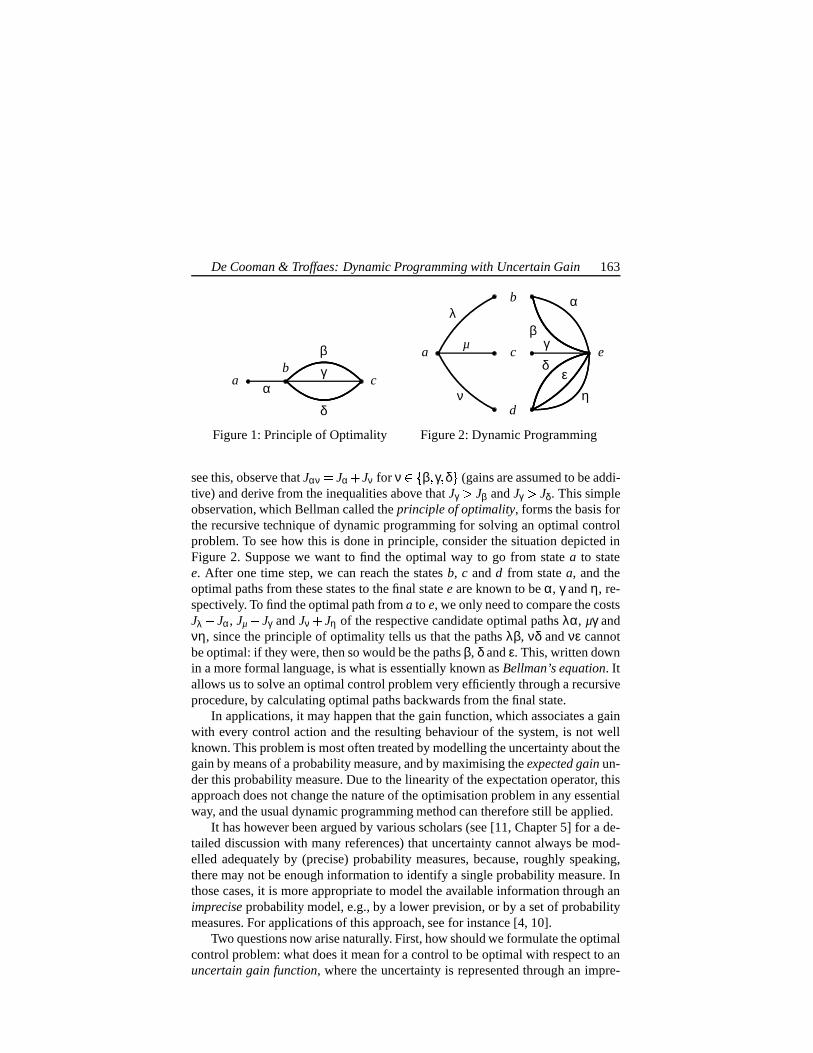
De Cooman & Troffaes: Dynamic Programming with Uncertain Gain 163

a cb

α

βγ

δ

Figure 1: Principle of Optimality

b

c

d

a e

λα

µ

ν

βγ

δε

η

Figure 2: Dynamic Programming

see this, observe that Jαν Jα ! Jν for ν û' β γ δ ( (gains are assumed to be addi-tive) and derive from the inequalities above that Jγ 3 Jβ and Jγ 3 Jδ. This simpleobservation, which Bellman called the principle of optimality, forms the basis forthe recursive technique of dynamic programming for solving an optimal controlproblem. To see how this is done in principle, consider the situation depicted inFigure 2. Suppose we want to find the optimal way to go from state a to statee. After one time step, we can reach the states b, c and d from state a, and theoptimal paths from these states to the final state e are known to be α, γ and η, re-spectively. To find the optimal path from a to e, we only need to compare the costsJλ ! Jα, Jµ ! Jγ and Jν ! Jη of the respective candidate optimal paths λα, µγ andνη, since the principle of optimality tells us that the paths λβ, νδ and νε cannotbe optimal: if they were, then so would be the paths β, δ and ε. This, written downin a more formal language, is what is essentially known as Bellman’s equation. Itallows us to solve an optimal control problem very efficiently through a recursiveprocedure, by calculating optimal paths backwards from the final state.

In applications, it may happen that the gain function, which associates a gainwith every control action and the resulting behaviour of the system, is not wellknown. This problem is most often treated by modelling the uncertainty about thegain by means of a probability measure, and by maximising the expected gain un-der this probability measure. Due to the linearity of the expectation operator, thisapproach does not change the nature of the optimisation problem in any essentialway, and the usual dynamic programming method can therefore still be applied.

It has however been argued by various scholars (see [11, Chapter 5] for a de-tailed discussion with many references) that uncertainty cannot always be mod-elled adequately by (precise) probability measures, because, roughly speaking,there may not be enough information to identify a single probability measure. Inthose cases, it is more appropriate to model the available information through animprecise probability model, e.g., by a lower prevision, or by a set of probabilitymeasures. For applications of this approach, see for instance [4, 10].

Two questions now arise naturally. First, how should we formulate the optimalcontrol problem: what does it mean for a control to be optimal with respect to anuncertain gain function, where the uncertainty is represented through an impre-

164 ISIPTA ’03

cise probability model? In Section 2 we identify three different optimality criteria,each with a different interpretation (although they coincide for precise probabilitymodels), and we study the relations between them. Secondly, is it still possible tosolve the corresponding optimal control problems using the ideas underlying Bell-man’s dynamic programming method? We show in Section 3 that this is the casefor only two of the three optimality criteria we study: only for these a generalisedprinciple of optimality holds, and the optimal controls are solutions of suitablygeneralised Bellman-like equations. To arrive at this, we study the properties thatan abstract notion of optimality should satisfy for the Bellman approach to work.

We recognise that other authors (see for instance [8]) have extended the dy-namic programming algorithm to systems with imprecise gain and/or imprecisedynamics. However in doing so, none of them seems to have questioned in whatsense their generalised dynamic programming method leads to optimal paths. Inthis article we approach the problem from the opposite, and in our opinion, morelogical side: one should first define a notion optimality and investigate whetherthe dynamic programming argument holds for this notion of optimality, insteadof blindly “generalising” Bellman’s algorithm. In the remainder of this section,we introduce the basic terminology and notation that will allow us to give a pre-cise formulation of the problems under study. We have omitted proofs of technicalresults that do not contribute to a better understanding of the main ideas.

1.1 Preliminaries

1.1.1 The System

For a and b in q , the set of natural numbers c that satisfy a M c M b is denotedby " a b # . Let xk h 1 f xk uk k describe a discrete-time dynamical system withk Öq , xk X and uk U. The set X is the state space (e.g., X n , n Çq Ô ' 0 ( ), andthe set U is the control space (e.g., X m , m éq Ô ' 0 ( ). The map f : X [ U [ q, Xdescribes the evolution of the state through time: given the state xk X and thecontrol uk U at time k ôq , it returns the next state xk h 1 of the system. Forpractical reasons, we impose a final time N beyond which we are not interested inthe dynamics of system. Moreover, it may happen that not all states and controlsare allowed at all times: we demand that xk should belong to a set of admissiblestates Xk at every instant k " 0 N # , and that uk should belong to a set of admissiblecontrols Uk at every instant k " 0 N 1 # , where Xk b X and Uk b U are given.The set XN may be thought of as the set we want the state to end up in at time N.

1.1.2 Paths

A path is a triple x k u ¦ , where x X is a state, k " 0 N # a time instant, andu ¦ : " k N 1 #A U a sequence of controls. A path fixes a unique state trajectoryx ¦ : " k N # X , which is defined recursively through xk x and xi h 1 f xi ui i for every i " k N 1 # . It is said to be admissible if x d X d for every e " k N #

De Cooman & Troffaes: Dynamic Programming with Uncertain Gain 165

and u d\ U d for every eÓ " k N 1 # . We denote the unique map from /0 to U byu /0. If k N, the control u ¦ does nothing: it is equal to u /0.

The set of admissible paths starting in the state x Xk at time k " 0 N # isdenoted by U x k , i.e., U x k Om' x k u ¦ : x k u ¦ admissible path ( . For ex-ample, U x N e' x N u /0 ( whenever x XN and U x N /0 otherwise.

If we consider a path with final time M different from N, then we write x k u ¦ M (assume k M M M N). Observe that x k u ¦ k can be identified with x k u /0 k; it is the unique path (of length zero) starting and ending at time k inx. Let 0 M k MfeM m. Two paths x k u ¦ d and y eG v ¦ m can be concatenated ify x d . The concatenation is denoted by x k u ¦ 8eG v ¦ m or x k u ¦ gd5A y eG v ¦ m,and represents the path that starts in state x at time k, and results from applyingcontrol ui for times i " k 8e 1 # and control vi for times i " eG m 1 # . In particular, x k u ¦ d x k u ¦ k A x k u ¦ d x k u ¦ d A x d 8eG u ¦ d The set of admissible paths starting in state x Xk at time k " 0 N # and endingat time eý " k N # is denoted by U x k gd . In particular we have that U x k k ' x k u /0 k ( if x Xk, and U x k k /0 otherwise. Moreover, for any x k u ¦ gddU x k gd and any V b U x d e® , we use the notation x k u ¦ hdiA V for the set' x k u ¦ d A x d eG v ¦ : x d eG v ¦ O V ( 1.1.3 The Gain Function

Applying the control action u U to the system in state x X at time k " 0 N 1 #yields a real-valued gain g x u k ω . Moreover, reaching the final state x X attime N also yields a gain h x ω . The parameter ω Ω represents the (unknown)state of the world, used to model uncertainty of the gains. If we knew that thereal state of the world was ωo, we would know the gains to be g x u k ωo andh x ωo . As it is, the real state of the world is uncertain, and so are the gains,which could be considered as random variables. It is important to note that theparameter ω only influences the gains; it has no effect on the system dynamics,which are assumed to be known perfectly well.

Assuming gain additivity, we can also associate a gain with a path x k u ¦ :J x k u ¦ ω ∑N 1

i B k g xi ui i ω ! h xN ω for any ω Ω. If M N N, we also use the notation

J x k u ¦ ω M ∑M 1i B k g xi ui i ω

It will be convenient to associate a zero gain with an empty control action: fork " 0 N # we let J x k u ¦ ω k 0.

The main objective of optimal control can now be formulated as follows: giventhat the system is in the initial state x X at time k " 0 N # , find a control se-quence u ¦ : " k N 1 #A U resulting in an admissible path x k u ¦ such that the

166 ISIPTA ’03

corresponding gain J x k u ¦ ω is maximal. Moreover, we would like this controlsequence u ¦ to be such that its value uk at the time instant k is a function of x andk only, since in that case the control can be realised through state feedback.

If ω is known, then the problem reduces to the classical problem of dynamicprogramming, first studied and solved by Bellman [1]. We assume here that theavailable information about the true state of the world is modelled through a co-herent lower prevision P defined on the set L Ω of gambles, or bounded real-valued maps, on Ω. A special case of this obtains when P is a linear previsionP. Linear previsions are the precise probability models; they can be interpreted asexpectation operators associated with (finitely additive) probability measures, andthey are previsions or fair prices in the sense of de Finetti [6]. We assume that thereader is familiar with lower previsions and coherence (see [11] for more details).

For a given path x k u ¦ , the corresponding gain J x k u ¦ ω can be seen as areal-valued map on Ω, which is denoted by J x k u ¦ and called the gain gambleassociated with x k u ¦ .1 In the same way we define the gain gambles g xk uk k ,h xN and J x k u ¦ M . There is gain additivity: J x k u ¦ eG v ¦ m J x k u ¦ d !J x d 8eG v ¦ m for k MjeÓM m M N, and J x k u ¦ k 0. We denote by J x k the setof gain gambles for admissible paths from initial state x Xk at time k " 0 N # :

J x k o' J x k u ¦ : x k u ¦ O U x k ( For fixed k " 0 N 1 # and x Xk, the gain J x k u ¦ ω can also be interpreted asa map from U x k to L Ω ; this map is denoted by J x k .2 Optimality Criteria

2.1 P-Maximality

The lower prevision P X of a gamble X has a behavioural interpretation as asubject’s supremum acceptable price for buying the gamble X : it is the highestvalue of µ such that the subject accepts the gamble X x (i.e., accepts to buy Xfor a price x) for all x N µ. The conjugate upper prevision P X P ] X of Xis then the subject’s infimum acceptable price for selling X . This way of lookingat a lower prevision P defined on the set L Ω of all gambles allows us to definea strict partial order 3 P on L Ω whose interpretation is that of strict preference.

Definition 1 For any gambles X and Y in L Ω we say that X strictly dominatesY, or X is strictly preferred to Y (with respect to P), and write X 3 P Y , if

P X Y O3 0 or X c Y and X Y Indeed, if X c Y and X Y , then the subject should be willing to exchange

Y for X , since this transaction can only improve his gain. On the other hand,

1To simplify the discussion, we assume this map is bounded.

De Cooman & Troffaes: Dynamic Programming with Uncertain Gain 167

P X Y 3 0 expresses that the subject is willing to pay a strictly positive priceto exchange Y for X , which again means that he strictly prefers X to Y .

It is clear that we can also use the lower prevision P to express a strict pref-erence between any two paths x k u ¦ and x k v ¦ , based on their gains: ifJ x k u ¦ d3 P J x k v ¦ this means that the uncertain gain J x k u ¦ is strictly pre-ferred to the uncertain gain J x k v ¦ . We then say that the path x k u ¦ is strictlypreferred to x k v ¦ , and we use the notation x k u ¦ O3 P x k v ¦ .3 P is anti-reflexive and transitive, and therefore a strict partial order on L Ω ,and in particular also on J x k and on U x k . But it is generally not linear: anytwo paths need not be comparable with respect to this order, and it does not alwaysmake sense to look for greatest elements, i.e., for paths that strictly dominate allthe others. Rather, we should look for maximal, or undominated, elements: pathsthat are not dominated by any other path. Observe that a maximal gamble X ina set K with respect to 3 P is a maximal element of K with respect to c (i.e., itis point-wise undominated) such that P X Y c 0 for all Y K . In case P isa linear prevision P, maximal gambles with respect to 3 P are just the point-wiseundominated gambles whose prevision is maximal; they maximise expected gain.

Definition 2 Let k " 0 N # , x Xk and V b U x k . A path x k u ¦ in V iscalled P-maximal, or 3 P-optimal, in V if no path in V is strictly preferred to x k u ¦ , i.e., x k u ¦ ;3 P x k u ¦ for all x k u ¦ V . We denote the set of theP-maximal paths in V by opt k

P V . The operator opt kP

is called the optimalityoperator induced by 3 P, associated with U x k .

The P-maximal paths in U x k are just those admissible paths starting attime k in state x for which the associated gain gamble is a maximal element ofJ x k with respect to the strict partial order 3 P. If we denote the set of these 3 P-maximal gain gambles in J x k by opt k

P J x k , then for all x k u ¦ U x k : x k u ¦ d opt kP U x k 1ÆÇ J x k u ¦ d opt k

P J x k ÒP-maximal paths do not always exist: not every partially ordered set has maximalelements. A fairly general sufficient condition for the existence of P-maximal el-ements in J x k (and hence in U x k ) is that J x k should be compact2 (andof course non-empty). This follows from a general result mentioned in [11, Sec-tion 3.9.2]. In fact, Theorem 1 is a stronger result, whose Corollary 1 turns out tobe very important in proving that the dynamic programming approach works forP-maximality (see Section 3.2). Its proof is based on Zorn’s lemma.

Theorem 1 For every element X of a compact subset K of L Ω that is not amaximal element of K with respect to 3 P there is some maximal element Y of Kwith respect to 3 P such that Y 3 P X.

2In this paper, we always assume that LΩ is provided with the supremum-norm topology.

168 ISIPTA ’03

Corollary 1 Let k " 0 N # and let x Xk. If J x k is compact then for everyadmissible, non-P-maximal path x k u ¦ in U x k there is a P-maximal path x k u ¦ in U x k that is strictly preferred to it.

2.2 P-Maximinity

We now turn to another optimality criterion that can be associated with a lowerprevision P. We can use P to define another strict order on L Ω :Definition 3 For any gambles X and Y in L Ω we write X l P Y if

P X O3 P Y or X c Y and X Y l P induces a strict partial order on U x k , since it is anti-reflexive and tran-sitive on L Ω . A maximal element X of a subset K of L Ω with respect to l P

is easily seen to be a point-wise undominated element of K that maximises thelower prevision: P X c P Y for all Y K .

We can consider as optimal in U x k those admissible paths x k u ¦ forwhich the associated gain gamble J x k u ¦ is a maximal element of J x k withrespect to l P; they are the paths x k u ¦ that maximise the ‘lower expected gain’P J x k u ¦ % and whose gain gambles J x k u ¦ are point-wise undominated.

Definition 4 Let k " 0 N # , x Xk and V b U x k . A path x k u ¦ in V iscalled P-maximin, or l P-optimal, in V if no path in V is strictly preferred to x k u ¦ , i.e., x k u ¦ l P x k u ¦ for all x k u ¦ \ V . We denote the set of theP-maximin paths in V by opt m

P V . The operator opt mP

is called the optimalityoperator induced by l P, associated with U x k .Proposition 1 P-maximinity implies P-maximality. For a linear prevision P, P-maximinity is equivalent to P-maximality.

The existence of maximal elements with respect to l P in an arbitrary set ofgambles K is obviously not guaranteed. But if K is compact, then we may easilyinfer from the continuity of any coherent lower prevision P, that the counterpartsof Theorem 1 and Corollary 1 hold for l P.

2.3 M -Maximality

There is a tendency, especially among robust Bayesians, to consider an impreciseprobability model as a compact convex set of linear previsions M b P Ω , whereP Ω is the set of all linear previsions on L Ω . M is assumed to contain the true,but unknown, linear prevision PT that models the available information [2, 7].

A gamble X is then certain to be strictly preferred to a gamble Y under thetrue linear prevision PT if and only if it is strictly preferred under all candidatemodels P M . This leads to a ‘robustified’ strict partial order 3 M on L Ω .

De Cooman & Troffaes: Dynamic Programming with Uncertain Gain 169

Definition 5 X 3 M Y if X 3 P Y for all P M .

Since M is assumed to be compact and convex, it is not difficult to showthat the strict partial orders 3 M and 3 P are one and the same, where the coher-ent lower prevision P is the so-called lower envelope of M , defined by P X dinf ë P X : P M ì for all X L Ω .3 Conversely, given a coherent lower previ-sion P, the strict partial orders 3 M @ P C and 3 P are identical, where

M P 6o' P P Ω : X L Ω P X c P X (is the set of linear previsions that dominate P. These strict partial orders thereforehave the same maximal elements, and lead to the same notion of optimality.

But there is in the literature yet another notion of optimality that can be associ-ated with a compact convex set of linear previsions M : a gamble X is consideredoptimal in a set of gambles K if it is a maximal element of K with respect tothe strict partial order 3 P for some P M . This notion of optimality is called‘E-admissibility’ by Levi [9, Section 4.8]. It does not generally coincide with theones associated with the strict partial orders 3 M and 3 P, unless the set K is con-vex [11, Section 3.9]. We are therefore led to consider a third notion of optimality:

Definition 6 Let x X , k " 0 N # and V b U x k . A path x k u ¦ O V is saidto be M -maximal in V if it is P-maximal in V for some P in M , or in other wordsif it is c -maximal in V and maximises P J x k u ¦ % over V for some P M . Theset of all M -maximal elements of V is denoted by optM V .

Interestingly, for any set of paths V b U x k :optM V 6

P Mopt k

P V (1)

3 Dynamic Programming

3.1 A General Notion of Optimality

We have discussed three different ways of associating optimal paths with a lowerprevision P, all of which occur in the literature. We now propose to find outwhether, for these different types of optimality, we can use the ideas behind thedynamic programming method to solve the corresponding optimal control prob-lems. To do this, we take a closer look at Bellman’s analysis as described in Sec-tion 1, and we investigate which properties a generic notion of optimality mustsatisfy for his method to work. Let us therefore assume that there is some prop-erty, called ò -optimality, which a path in a given set of paths P either has or doesnot have. If a path in P has this property, we say that it is ò -optimal in P . We

3Since M is compact, this infimum is actually achieved.

170 ISIPTA ’03

b

c

d

a e

λα

µ

ν

βγ

δε

η

Figure 3: A More General Type of Dynamic Programming

shall denote the set of the ò -optimal elements of P by opt P . By definition,opt P b P . Further on, we shall apply our findings to the various instances ofò -optimality described above.

Consider Figure 3, where we want to find the ò -optimal paths from state ato state e. Suppose that after one time step, we can reach the states b, c and dfrom state a. The ò -optimal paths from these states to the final state e are knownto be α, γ, and δ and η, respectively. For the dynamic programming approach towork, we need to be able to infer from this a generalised form of the Bellmanequation, stating essentially that the ò -optimal paths from a to e, a priori given byopt ' λα λβ µγ νδ νε νη ( , are actually also given by opt ' λα µγ νδ νη ( ,i.e., the ò -optimal paths in the set of concatenations of λ, µ and ν with the respec-tive ò -optimal paths α, γ, and δ and η. It is therefore necessary to exclude that theconcatenations λβ and νε with the non- ò -optimal paths β and ν can be ò -optimal.This amounts to requiring that the operator opt should satisfy some appropriategeneralisation of Bellman’s principle of optimality that will allow us to concludethat λβ and νε cannot be ò -optimal because then β and ε would be ò -optimal aswell. Definition 8 below provides a precise general formulation.

But, perhaps surprisingly for someone familiar with the traditional form ofdynamic programming, opt should satisfy an additional property: the omissionof the non- ò -optimal paths λβ and νε from the set of candidate ò -optimal pathsshould not have any effect on the actual ò -optimal paths: we need that

opt ' λα λβ µγ νδ νε νη ( opt ' λα µγ νδ νη ( This is obviously true for the simple type of optimality that we have looked atin Section 1, but it need not be true for the more abstract types that we want toconsider here. Equality will be guaranteed if opt is insensitive to the omission ofnon- ò -optimal elements from ' λα λβ µγ νδ νε νη ( , in the following sense.

Definition 7 Consider a set S /0 and an optimality operator opt defined on theset ℘ S of subsets of S such that opt T b T for all T b S. Elements of opt T are called ò -optimal in T. opt is called insensitive to the omission of non- ò -optimal elements from S if opt S Ò opt T for all T such that opt S b T b S.

De Cooman & Troffaes: Dynamic Programming with Uncertain Gain 171

The following proposition gives an interesting sufficient condition for this in-sensitivity in case optimality is associated with a (family of) strict partial order(s):it suffices that every non-optimal path is strictly dominated by an optimal path.

Proposition 2 Let S be a non-empty set provided with a family of strict partialorders 3 j, j J. Define for T b S, opt k

j T ë a T : b T b 3 j a ì as theset of maximal elements of T with respect to 3 j, and let optJ T Òj j J opt k

j T .Then opt k

j, j J and optJ are optimality operators. If for some j J, a S Ô opt k

j S ] E b opt kj S b 3 j a (2)

then opt kj

is insensitive to omission of non- 3 j-optimal elements from S. If (2)holds for all j J, then optJ is insensitive to omission of non-J-optimal elementsfrom S.

Proof. Consider j in J, and assume that (2) holds for this j. Let opt kj S b

T b S, then we must prove that opt kj S opt k

j T . First of all, if a opt kj S

then b 3 j a for all b in S, and a fortiori for all b in T , so that a opt kj T .

Consequently, opt kj S 8b opt k

j T . Conversely, let a opt kj T and assume

ex absurdo that a opt kj S . It then follows from (2) that there is some c in

opt kj S and therefore in T such that c 3 j a, which contradicts a opt k

j T .Next, assume that (2) holds for all j J. Let optJ S Ob T b S, then we must

prove that optJ S optJ T . Consider any j J, then opt kj S b optJ S b

T b S, so we may infer from the first part of the proof that opt kj S opt k

j T .By taking the union over all j J, we find that indeed optJ S 6 optJ T .

We are now ready for a precise formulation of the dynamic programmingapproach for solving optimal control problems associated with general types ofoptimality. We assume that we have some type of optimality, called ò -optimality,that allows us to associate with the set of admissible paths U x k starting at timek in initial state x, an optimality operator opt defined on the set ℘ U x k % ofsubsets of U x k . For each such subset V , opt V is then the set of admissiblepaths that are ò -optimal in V . The principle of optimality states that the optimalityoperators associated with the various U x k should be related in a special way.

Definition 8 (Principle of Optimality) ò -optimality satisfies the principle of op-timality if it holds for all k " 0 N # , x Xk, e8 " k N # and x k u ¦ in U x k thatif x k u ¦ is ò -optimal in U x k , then x d 8eG u ¦ is ò -optimal in U x d e® .

This may also be expressed as:

opt U x k Ob @ x < k < u n C[o U @ x < k C[o x k u ¦ hdiA opt U x d28e®The Bellman equation now states that applying the optimality operator to the righthand side suffices to achieve equality. (Usually this is stated with e\ k ! 1.)

172 ISIPTA ’03

Theorem 2 (Bellman Equation) Let k " 0 N # and x Xk. Assume that ò -opti-mality satisfies the principle of optimality, and that the optimality operator opt for U x k is insensitive to the omission of non- ò -optimal elements from U x k .Then for all e8 " k N # :

opt U x k opt @ x < k < u C o U @ x < k C o x k u gdpA opt U x d e®Athat is, a path is ò -optimal if and only if it is a ò -optimal concatenation of anadmissible path x k u ¦ d and a ò -optimal path of U x d e® .Proof. Fix k in " 0 N # , e " k N # and x Xk. Define

V1 @ x < k < u C[o U @ x < k C[o x k u d A opt U x d e®%A and,

V2 @ x < k < u C o U @ x < k C o x k u d A U x d e® Ô opt U x d e®%Obviously, U x k Ç V1 L V2 and V1 â V2 /0. We have to prove thatopt U x k %8 opt V1 . By the principle of optimality, no path in V2 is ò -optimal in U x k , so V2 â opt U x k d /0. This implies that opt U x k bV1 b U x k , and since opt is assumed to be insensitive to the omission of non-ò -optimal elements from U x k , it follows that opt U x k % opt V1 . 3.2 P-Maximality

Let us now apply these general results to the specific types of optimality intro-duced before. We first consider the optimality operator opt k

Pthat selects from a

set of gambles (or paths) S those gambles (or paths) that are the maximal elementsof S with respect to the strict partial order 3 P. The following lemma roughly statesthat the preference amongst paths with respect to 3 P is preserved under concate-nation and truncation. It yields a sufficient condition for the principle of optimalitywith respect to P-maximality to hold. Moreover, the lemma, and the principle ofoptimality, do not necessarily hold for preference with respect to P-maximinity.

Lemma 1 Let k " 0 N # and eÓ " k N # . Consider the paths x k u ¦ d in U x k dand x d eG v ¦ , x d eG w ¦ in U x d 8e® . Then x d eG v ¦ Ó3 P x d eG w ¦ if and only if x k u ¦ gdpA x d8eG v ¦ d3 P x k u ¦ hdiA x d8eG w ¦ .Proof. Let X , Y and Z be gambles on Ω. The statement is proven if we can showthat Y 3 P Z implies X ! Y 3 P X ! Z. Assume that Y 3 P Z. If P Y Z d3 0, thenP X ! Y ö X ! Z 6 P Y Z d3 0. If Y c Z, then X ! Y c X ! Z, and finally,if Y Z, then X ! Y X ! Z. It follows that X ! Y 3 P X ! Z.

De Cooman & Troffaes: Dynamic Programming with Uncertain Gain 173

Proposition 3 (Principle of Optimality) Let k " 0 N # , x Xk and x k u ¦ U x k . If x k u ¦ is P-maximal in U x k then x d eG u ¦ is P-maximal in U x d 8e®for all e8 " k N # .Proof. If x d 8eG u ¦ is not P-maximal, there is a path x d eG u ¦ such that x d 8eG u ¦ O3 P x d 8eG u ¦ . By Lemma 1 we find that x k u ¦ hdpA x d eG u ¦ d3 P x k u ¦ hdpA x d28eG u ¦ x k u ¦ This means that x k u ¦ d A x d 8eG u ¦ is preferred to x k u ¦ , and therefore x k u ¦ cannot be P-maximal, a contradiction.

As a direct consequence of Corollary 1 and Proposition 2, we see that if J x k

is compact, then the optimality operator opt kP

associated with U x k is insen-sitive to the omission of non- 3 P-optimal elements. Together with Proposition 3and Theorem 2, this allows us to infer a Bellman equation for P-maximality.

Corollary 2 Let k " 0 N # and x Xk. If J x k is compact, then for all e " k N #opt k

P U x k opt kP

@ x < k < u C o U @ x < k C o x k u d A opt kP U x d e®%A (3)

that is, a path is P-maximal if and only if it is a P-maximal concatenation of anadmissible path x k u ¦ d and a P-maximal path of U x d e® .

Corollary 2 results in a procedure to calculate all P-maximal paths. Indeed,opt k

P U x N %ÝÐ' u /0 ( for every x XN , and opt kP U x k can be calculated re-

cursively through Eq. (3). It also provides a method for constructing a P-maximalfeedback: for every x Xk, choose any x k u ¦ x k % opt k

P U x k % . Thenφ x k u k x k realises a P-maximal feedback.

3.3 M -Maximality

We now turn to the optimality operator optM , satisfying (1). By Proposition 2and (1), it follows that optM is insensitive to the omission of non-M -maximalelements of U x k whenever J x k is compact. By Proposition 3, optM satisfiesthe principle of optimality (indeed, if a path is M -maximal, then it must be P-maximal for some P M , and by the proposition any truncation of it is alsoP-maximal, hence also M -maximal). This means that the Bellman equation alsoholds for M -maximality under similar conditions as for P-maximality. As alreadymentioned in Section 2.3, both types of optimality coincide if J x k is convex.

3.4 P-Maximinity

Finally, we come to the type of optimality associated with the strict partial orderl P. It follows from Proposition 2 and the discussion at the end of Section 2.2

174 ISIPTA ’03

ab

c

d

αβ

γ

Figure 4: A Counterexample

that if J x k is compact, the optimality operator opt mP

for U x k is insensi-tive to the omission of non- l P-optimal paths from U x k . But, as the followingcounterexample shows, we cannot guarantee that the principle of optimality holdsfor l P-optimality, and therefore dynamic programming may not work here—noteven with a vacuous uncertainty model. Essentially, this is because the partial or-der l P is not a vector ordering on L Ω —it is not compatible with gain additivity:contrary to expected gain, lower expected gains are not additive.

Example 1 Consider the dynamical system depicted in Figure 4. Let Ω e'<qcr ( ,let P be the vacuous lower prevision on Ω, and denote the gamble q¤ x, rO¤ yby ! x y " . Assume that J α ! 2 0 " , J β ! 0 1 " and J γ ! 2 0 " (there iszero gain associated with the final state). Then αβ l P αγ: indeed, ! 2 1 " doesnot dominate ! 0 0 " point-wise, and inf ! 2 1 " 3 inf ! 0 0 " or equivalently ! 0 0 "maximises the worst expected gain. Hence, we find that αγ is P-maximin. Butβ l P γ: indeed, inf ! 0 1 " 3 inf ! 0 2 " which means that γ is not P-maximin.Thus the “principle of P-maximin optimality” does not hold here.

3.5 Yet Another Type of Optimality

We end this discussion with another type of optimality associated with a strict par-tial order, introduced by Harmanec in [8, Definition 3.4]. In our setting (preciselyknown system dynamics), its definition basically reduces to

X 3 ÉP Y if P X d3 P Y or X c Y and X Y It can be shown easily that if J x k is compact, the optimality operator inducedby 3ÉP for U x k is insensitive to the omission of non- 3ÓÉP-optimal paths fromU x k . But, as the following counterexample shows, we cannot guarantee thatthe principle of optimality holds for 3ÉP-optimality, and therefore the dynamicprogramming approach may not work here—not even with a vacuous uncertaintymodel. Again, this is because the partial order l P is not compatible with gain ad-ditivity. It also indicates that the solution of the Bellman-type equation advocatedin [8] will not necessarily lead to optimal paths, in the sense we described above.

Example 2 Consider the dynamical system depicted in Figure 4. Let Ω e'<qcr ( ,let P be the vacuous lower prevision on Ω, and denote the gamble q¤ x, rO¤ y

De Cooman & Troffaes: Dynamic Programming with Uncertain Gain 175

by ! x y " . Assume that J α ! 2 0 " , J β ! 0 0 " and J γ d ! 1 1 " (there iszero gain associated with the final state). Then αβ 3ÓÉP αγ: indeed, ! 2 0 " does notdominate ! 1 1 " point-wise, and, inf ! 2 0 " 3 sup ! 1 1 " . Hence, we find that αγis 3ÉP-maximal. But β 3ÉP γ: indeed, ! 0 0 " dominates ! 1 1 " point-wise, whichmeans that γ is not 3ÉP-maximal. Thus the “principle of 3ÓÉP-maximal optimality”does not hold for this example.

4 Conclusion

The main conclusion of our work is that the method of dynamic programming canbe extended to systems with imprecise gain. Our general study of what conditionsa generalised notion of optimality should satisfy for the Bellman approach to workis of some interest in itself too. In particular, besides an obvious extension ofthe well-known principle of optimality, another condition emerges that relates tothe nature of the optimality operators per se: the optimality of a path should beinvariant under the omission of non-optimal paths from the set of paths underconsideration. If optimality is induced by a strict partial ordering of paths, thenthis second condition is satisfied whenever the existence of dominating optimalpaths for non-optimal ones is guaranteed.

Another important observation is that, in contradistinction to P-maximalityand M -maximality, the dynamic programming method cannot be used to solveoptimisation problems corresponding to P-maximinity: for this notion the princi-ple of optimality does not hold in general.

Throughout the paper we assumed the system dynamics to be deterministic,that is, independent of ω. This greatly simplifies the discussion, still encompassesa large number of interesting applications, and does not suffer from the compu-tational issues often encountered when dealing with non-deterministic dynamicalsystems—simply because in general the number of possible (random) paths tendsto grow exponentially with the size of the state space X . However, we should notethat dropping this assumption still leads to a Bellman-type equation, connectingoperators of optimality associated with random states x : Ω X . A discussion ofthese matters has been omitted from the present paper due to limitations of space.

Acknowledgements

This paper presents research results of project G.0139.01 of the Fund for ScientificResearch, Flanders (Belgium), and of the Belgian Programme on InteruniversityPoles of Attraction initiated by the Belgian state, Prime Minister’s Office for Sci-ence, Technology & Culture. The scientific responsibility rests with the authors.

176 ISIPTA ’03

References

[1] BELLMAN, R. Dynamic Programming. Princeton University Press, Prince-ton, 1957.

[2] BERGER, J. O. The robust Bayesian viewpoint. In Robustness of BayesianAnalyses, J. B. Kadane, Ed. Elsevier Science, Amsterdam, 1984.

[3] BERNARDO, J. M., H., D. J., V., L. D., AND SMITH, A. F. M., Eds.Bayesian Statistics. University Press, Valencia, 1980.

[4] CHEVE, M., AND CONGAR, R. Optimal pollution control under impreciseenvironmental risk and irreversibility. Risk Decision and Policy 5 (2000),151–164.

[5] DE COOMAN, G., COZMAN, F. G., MORAL, S., AND WALLEY, P., Eds.ISIPTA ’99 – Proceedings of the First International Symposium on ImpreciseProbabilities and Their Applications (Ghent, 1999), Imprecise ProbabilitiesProject.

[6] DE FINETTI, B. Theory of Probability: a Critical Introductory Treatment.Wiley, London, 1975.

[7] GIRON, F. J., AND RIOS, S. Quasi-Bayesian behaviour: A more realisticapproach to decision making? In Bernardo et al. [3], pp. 17–38.

[8] HARMANEC, D. Generalizing Markov decision processes to impreciseprobabilities. Journal of Statistical Planning and Inference 105, 1 (June2002), 199–213.

[9] LEVI, I. The Enterprise of Knowledge. An Essay on Knowledge, CredalProbability, and Chance. MIT Press, Cambridge, 1983.

[10] UTKIN, L. V., AND GUROV, S. V. Imprecise reliability models for thegeneral lifetime distribution classes. In de Cooman et al. [5], pp. 333–342.

[11] WALLEY, P. Statistical Reasoning with Imprecise Probabilities. Chapmanand Hall, London, 1991.

Gert de Cooman is a member of the SYSTeMS research group of Ghent University.Address: Technologiepark – Zwijnaarde 914, B-9052, Zwijnaarde, Belgium.E-mail: gert.decooman@ugent.be

Matthias Troffaes is a member of the SYSTeMS research group of Ghent University.Address: Technologiepark – Zwijnaarde 914, B-9052, Zwijnaarde, Belgium.E-mail: matthias.troffaes@ugent.be

Computing Lower Expectations withKuznetsov’s Independence Condition

FABIO GAGLIARDI COZMANEscola Politecnica, University of Sao Paulo, Brazil

Abstract

Kuznetsov’s condition says that variables X and Y are independent when anyproduct of bounded functions f µ X and g µ Y behaves in a certain way: theinterval of expected values s f µ X g µ Y 8t must be equal to the interval products f µ X 8tvu+s g µ Y 8t . The main result of this paper shows how to compute lowerexpectations using Kuznetsov’s condition. We also generalize Kuznetsov’scondition to conditional expectation intervals, and study the relationship be-tween Kuznetsov’s conditional condition and the semi-graphoid properties.

Keywords

sets of probability distributions, lower expectations, probability intervals, expectationintervals, independence concepts

1 Introduction

Kuznetsov’s condition says that two variables X and Y are independent if, for anytwo bounded functions f X and g Y , we havew " f X g Y &# w " f X &# [ w " g Y $#® (1)

wherew " P # denotes an interval of expected values and the product is understood as

interval multiplication [8].Kuznetsov’s condition is geared towards models that represent uncertainty

through sets of probability measures and expectation intervals. In those models,Kuznetsov’s condition is seen to be more general than the standard definition ofstochastic independence. The condition can be viewed as a definition of inde-pendence, and also as a constraint to be used when building models that involveimprecise beliefs. The relationship between Kuznetsov’s condition and other con-cepts of independence was analyzed in a previous paper [5]; several results fromthat publication are used in this paper.

This work has been supported in part by CNPq through grant 300183/98-4, and in part by HPLabs through “Convenio Aprendizado de Redes Bayesianas”.

177

178 ISIPTA ’03

This paper shows how to compute minima and maxima of expected valuesusing Kuznetsov’s condition. The main result is a characterization of the largestcredal set that complies with Kuznetsov’s condition — the “Kuznetsov’s exten-sion” of marginal sets. We discuss the computation of lower expectations fromKuznetsov’s extensions, and investigate the connection between Kuznetsov’s ex-tensions and other extensions used in the literature. Section 4 contains these de-velopments.

We then generalize Kuznetsov’s condition to conditional beliefs (Section 5).To clarify the behavior of the resulting condition, we investigate its complianceto the semi-graphoid properties. We show that Kuznetsov’s conditional conditionsatisfies symmetry, redundancy, decomposition and weak union, but fails the con-traction property.

Kuznetsov’s condition is an interesting tool for modeling independence withimprecise beliefs. This paper provides the basic machinery to manipulate the con-dition in practice. Section 6 presents our conclusions.

2 Credal sets, lower expectations, extensions

In this section we review the basic concepts necessary for later developments.Consider two random variables X and Y . In this paper all variables have finitelymany values. The probability density for X is denoted by p X , and Ep " f X $#denotes the expectation of function f X with respect to p X . A non-empty setof probability measures is called a credal set [9]; a credal set consisting of den-sities p X is denoted by K X . A credal set K X Y consisting of joint den-sities p X Y is called a joint credal set. The lower and upper expectations offunction f X are respectively E " f X &# minp@ X C K @ X C Ep " f X &# and E " f X &#maxp@ X C K @ X C Ep " f X &# . The lower probability and the upper probability of eventA are defined similarly. A credal set produces an expectation interval for anybounded function h X : w " h X $# 4

E " h X &#® E " h X &# 5 .There are several concepts of independence that can be applied to credal sets

[2, 7]; here we focus on epistemic independence and strong independence. Vari-able Y is epistemically irrelevant to X if K X y and K X have the same con-vex hull for all possible values of Y (equivalently, E " f X K y #Ý E " f X $# for anybounded function f X and all possible values of Y ). Variables X and Y are epis-temically independent if X is irrelevant to Y and Y is irrelevant to X . Strong in-dependence focuses instead on decomposition of probability measures [1, 2, 4]:Variables X and Y are strongly independent when every extreme point of K X Y satisfies standard stochastic independence of X and Y .

Given marginal credal sets K X and K Y , there may be several credal setsK X Y for which X and Y are independent. Each one of these sets is called anextension of K X and K Y . Given marginal sets K X and K Y , their epistemicextension (called the independent natural extension by Walley) is the largest joint

Cozman: Kuznetsov’s Extensions 179

credal set that satisfies epistemic independence with marginals K X and K Y [13]. Their strong extension is the largest joint credal set that satisfies strong in-dependence with marginals K X and K Y [2, 4]. The term natural extensionis used to indicate the largest possible extension given whatever constraints onprobability and independence are adopted [13].

A credal set K X Y is finitely generated when it is a polytope in the space ofprobability measures — the convex hull of a finite number of probability distri-butions. Such a set is defined by a finite collection of linear inequalities such as∑X <Y h X Y p X Y c 0. In the remainder of this paper, f indicates a function ofX , g indicates a function of Y and h indicates a function of X and Y . Similarly,p indicates a density for X , q indicates a density for Y ; other densities, such asp X Y , are indicated explicitly. We can view functions and probability densitiesas vectors, so we can write f g P pq c 0 instead of ∑X <Y f X g Y p X q Y c0, using the dot product to produce summation.

Note that any hyperplane h P p X Y O 0 goes through the origin. The func-tion/vector h is the normal vector of the hyperplane. If E " h # 0, then h defines asupporting hyperplane for the credal set. If E " h #A 0, then h is a supporting hy-perplane. A face of a polytope is the intersection of the polytope with a supportinghyperplane; a facet is a maximal face distinct of the polytope [11].

To simplify notation, we use the same letter ( f , for instance) for a function,a vector (containing the values of a function), a normal vector (orthogonal to anhyperplane), an hyperplane (with the normal vector), or a facet (contained in thehyperplane with the normal vector), depending on the circumstances.

Any function/vector h can be written as h l ! E " h # or as h l l ! E " h # , where h land h l l are supporting hyperplanes that are parallel to h. Consider any supportinghyperplane h l that goes through a vertex V . Take the facets intersecting at V , andthe normal vectors to these facets. Then it must be possible to write h l as a linearof these normal vectors.

3 Kuznetsov’s condition and Kuznetsov’s extension

Kuznetsov’s condition is a condition for independence operating on expectationsof independent variables [8]. The condition can be expressed either in terms ofexpectation intervals (Expression (1)), or as

E " f X g Y &#A min E " f X &# E " g Y &#n E " f X &# E " g Y &#pE " f X $# E " g Y $#® E " f X &# E " g Y &# ¡ (2)

To obtain (2) from (1), we recall that the interval product " a b # [Ñ" c d # is equal to"min ac ad bc bd max ac ad bc bd $#KThe following result is used later:

180 ISIPTA ’03

Theorem 1 For any bounded functions f X and g Y , any extension that satis-fies Kuznetsov’s condition must contain densities that attain E " f # E " g # , E " f # E " g # ,E " f # E " g # , and E " f # E " g # .Proof. Suppose we have a credal set that satisfies Kuznetsov’s condition. Con-sider a function h1 f E " f #n! α g E " g #K! β , where α β 3 0; then E " h1 # E " f E " f #*#p! α E " g E " g #+#p! β αβ for any α, β. But for this to happen, wemust have a density p1 X Y such that Ep1 " f #6 E " f # and Ep1 " g #Ý E " g # at thesame time. The proof can be completed by taking functions h2 f E " f #ß!α g E " g #G! β , h3 é f E " f #¢! α g E " g #;! β and h4 é f E " f #¢!α g E " g #®! β .

We can use Kuznetsov’s condition to construct credal sets. Suppose we haveK X and K Y , and we obtain the information that X and Y satisfy Kuznetsov’scondition, without further information on K X Y . What can we say about thejoint credal set K X Y ? A reasonable strategy is to focus on the largest jointcredal set that satisfies Kuznetsov’s condition and has the marginals K X andK Y . This set is referred to as Kuznetsov’s extension of K X and K Y . It shouldbe noted that a Kuznetsov’s extension always exists [5].

Kuznetsov’s extensions are smaller than epistemic extensions when all eventshave positive probability, as in this case Kuznetsov’s independence implies epis-temic independence — and even when all lower probabilities are larger than zeroKuznetsov’s extensions can be strictly smaller than epistemic extensions [5]. Astrong extension always satisfies Kuznetsov’s condition and is contained in thecorresponding Kuznetsov’s extension (however, the Kuznetsov’s extension canbe strictly larger than the strong extension; also, it is possible that a credal setsatisfies strong independence but does not satisfy Kuznetsov’s condition) [5].

4 Characterizing Kuznetsov’s extensions

Suppose we have two binary variables X and Y , and we construct the strong ex-tension of K X and K Y . In this case, it is known that the strong extension andthe Kuznetsov’s extension of K X and K Y are identical [5]. A more generalresult can actually be proved:

Theorem 2 Consider a binary variable X with credal set K X , and a variableY with N values and credal set K Y with M vertices; the strong extension andKuznetsov’s extension of K X and K Y are identical.

Proof. The strong extension is composed of vertices of the form pi X q j Y ,where pi indicates a vertex of K X and q j indicates a vertex of K Y . If K X contains a single point, the result is immediate; suppose that K X has two ver-tices p1 and p2 (so there is a function f1 X such that f1

P p1 0, and a functionf2 X such that f2

P p2 0). The strong extension can have at most 2M vertices,

Cozman: Kuznetsov’s Extensions 181

all of them with 2N components (thus the strong extension lives in 2N 1 di-mensional space). Any facet of the strong extension is contained in an hyperplanethat is defined by selecting 2N 1 vertices of the strong extension plus the ori-gin. Take a facet and divide its vertices (other than the origin) in two sets:(i) the set C1 containing points of the form p1q j,(ii) the set C2 containing points of the form p2qk,where q j, qk are vertices of K Y . Suppose that C1 contains more points than C2.Then we have at most N 1 points in C2; we can always find an hyperplane de-fined by a function g Y that goes through all these points. Thus we can constructa function f1 X g Y such that

∑X <Y f1 X g Y p1 X q j Y U ∑

X

f1 X p1 X Z U ∑Y

g Y q j Y Z 0

for every point in C1 and every point in C2. So the facet is represented by a de-composable function f1g. The same construction can be followed if C2 has moreelements than C1, in which case we will arrive at a decomposable function of theform f2g l for some g l Y . Thus, any facet of the strong extension is defined by adecomposable hyperplane and consequently is a valid constraint for Kuznetsov’sextension. The strong extension must then contain Kuznetsov’s extension, and soboth are equal.

The facets generated in the proof of Theorem 2 are of the form f X g Y . Alittle reflection shows that this function g Y must define a supporting hyperplaneof K Y : If g were not a supporting hyperplane of K Y , there should be a pointqc such that ∑Y gqc c 0 and a point qd such that ∑Y gqd M 0. But g P qc c 0 wouldimply f g P p1qc c 0 and g P qd M 0 would imply f g P p1qd M 0, contradictingthe fact that f g is a supporting hyperplane for the strong extension. Consequently,the facets of the strong extension in Theorem 2 are defined by decomposablefunctions that factorize into facets of K X and K Y .

Consider now a more general situation where we have categorical variables Xand Y and finitely generated marginal credal sets K X and K Y . Suppose that,instead of trying to compute Kuznetsov’s extensions, someone simply constructedthe following inequalities:

∑X <Y fi X p X Y c 0 ∑X <Y g j Y p X Y c 0 (3)

∑X <Y fi X g j Y % p X Y c 0

which can be written as

fiP p X Y c 0 g j

P p X Y c 0 fig j P p X Y c 0 (4)

182 ISIPTA ’03

for all combinations of i and j, where fi is a facet of K X and g j is a facetof K Y . Note that any set of densities that satisfies these inequalities will alsosatisfy f l g l P p X Y c 0, where f l and g l are supporting hyperplanes of K X and K Y respectively.

The next theorem is the main result: it shows how to explicitly constructKuznetsov’s extensions. The proof essentially consists of showing that any in-equality required by Kuznetsov’s condition is already implied by inequalities (4).

Theorem 3 Consider a variable X with finitely generated credal set K X , de-fined by facets fi, and a variable Y with finitely generated credal set K Y , definedby facets g j. The Kuznetsov’s extension is entirely defined by the facets fi, g j, and fig j , for all combinations of i and j.

Proof. Denote by Kk X Y the credal set constructed in the theorem. Every ver-tex of the strong extension is of the form p X q Y and consequently satisfies fig j P pq c 0. We conclude that the strong extension is contained in Kk X Y ,thus the expectation intervals generated by the strong extension are containedin the expectation intervals generated by Kk X Y . Furthermore, for every de-composable function f X g Y , there is a density in Kk X Y that attains thevalue prescribed by Kuznetsov’s condition, as the strong extension is contained inKk X Y .Now take two arbitrary bounded functions f X and g Y . There are seven differ-ent situations to consider:

1. E " f # c 0, E " g # c 0: Kuznetsov’s condition requires that E " f g #A E " f # E " g # .Write f as f l ! E " f # ( f l is a supporting hyperplane of K X ) and writeg as g l ! E " g # (g l is a supporting hyperplane of K Y ). Then we have:f g P p X Y 8 f l ! E " f # g l ! E " g #´ P p X Y 8 f l g l P p X Y ! E " f # g l Pp X Y ! E " g # f l P p X Y ! E " f # E " g # , an expression that is equal to orlarger than E " f # E " g # given that p X Y satisfies inequalities (4). This im-plies that Ep " f g # c E " f # E " g # for every p X Y and we obtain E " f g #E " f # E " g # (because the inclusion of the strong extension in Kk X Y guar-antees that the equality obtains).

2. E " f #6M 0, E " g #M 0: Kuznetsov’s condition requires E " f g # E " f # E " g # . Toshow that Ep " f g # c E " f # E " g # for every p X Y , write f as f l ! E " f # andg as g l ! E " g # (where f l and g l are appropriate supporting hyperplanes),and then: f g P p X Y 6 ] f l ! E " f # ] g l ! E " g #´ P p X Y , a quantity thatis equal to or larger than E " f # E " g # given inequalities (4).

3. E " f # c 0, E " g #¢M 0: Kuznetsov’s condition requires E " f g #G E " f # E " g # . Writef f l ! E " f # , f f l l ! E " f # , and g g l ! E " g # (where f l , f l l and g lare appropriate supporting hyperplanes; note that f is written in two differ-ent ways) and then f g P p X Y f g l ! E " g #S P p X Y 6 % f l ! E " f #S g l !] f l l ! E " f # E " g #S P p X Y , which that is equal to or larger than E " f # E " g # .

Cozman: Kuznetsov’s Extensions 183

4. E " f #M 0, E " f # c 0, E " g #\M 0: Kuznetsov’s condition requires E " f g #dE " f # E " g # . Write f f l ! E " f # , g g l ! E " g # , and g g l l ! E " g # , andthen f g P p X Y ] f l g l l ! E " g #Ò! E " f # g l ! E " g #S% P p X Y , whichis equal to or larger than E " f # E " g # .

5. E " f #M 0, E " g # c 0: Kuznetsov’s condition requires E " f g #G E " f # E " g # . Writef f l ! E " f # , g g l ! E " g # , and g g l l ! E " g # , and then f g P p X Y d f l g l ! E " g #SÝ! E " f # g l l ! E " g #´% P p X Y , which is equal to or largerthan E " f # E " g # .

6. E " f #M 0, E " g #ÝM 0, E " g # c 0: Kuznetsov’s condition requires that E " f g #E " f # E " g # . Write f f l ! E " f # , f f l l ! E " f # , and g g l ! E " g # , andf g P p X Y 8 ] g l ] f l l ! E " f #Ý! E " g # f l ! E " f # P p X Y f l l g l !E " g # f l E " f # g l P p X Y ! E " f # E " g # , equal to or larger than E " f # E " g # .

7. E " f # M 0, E " f # c 0, E " g #OM 0, E " g # c 0: Kuznetsov’s condition requiresE " f g # min E " f # E " g #® E " f # E " g #´ . Divide Kk X Y into two sets. DefineK1 X Y to contain the distributions in Kk X Y such that f P p X Y c 0,and K2 X Y to contain the distributions in Kk X Y such that f P p X Y M0. The value of E " f g # with respect to Kk X Y is the minimum of E " f g # withrespect to K1 X Y and K2 X Y . Following the previous cases, we obtainE " f # E " g # as E " f g # with respect to K1 X Y , and E " f # E " g # as E " f g # withrespect to K2 X Y . We finally obtain E " f g #A min E " f # E " g #K E " f # E " g #S .

Thus Kk X Y satisfies Kuznetsov’s condition, and Kuznetsov’s extension mustcontain Kk X Y — however Kuznetsov’s extension cannot be larger than the setKk X Y , as every inequality (4) is directly required by Kuznetsov’s condition.

Once we know how to construct Kuznetsov’s extensions, we can computeE " h X Y &# for a non-decomposable function h X Y :

E " h X Y &# min h X Y P p X Y (5)

subject to p X Y c 0, ∑X <Y p X Y 1, and inequalities (4).The linear program (5) provides the solution to the question, Which (decom-

posable) constraints to use when computing a lower expectation for Kuznetsov’sextension? Theorem 3 proves that inequalities (4) contain all the relevant con-straints. Kuznetsov himself seems to have obtained different results, using his con-dition and additional factorization conditions to define extensions — a frameworkthat led him to prescribe linear programs with infinitely many constraints [8].

Finally, note that we can also use linear programming if we need to computea conditional lower expectation such as E " h A # for some event A where P A d3 0.The computation of E " h A # requires the solution of a fractional linear programthat can be performed using the Charnes-Cooper transformation and linear pro-gramming [3], using inequalities (4) as the starting point.

184 ISIPTA ’03

5 Kuznetsov’s conditional condition and the semi-graphoid properties

Kuznetsov’s condition does not deal with the concept of conditional indepen-dence, but it can certainly be extended to do so. Say that two variables X and Yare independent conditional on Z if, for bounded functions f X and g Y ,w " f g z # w " f z # [ w " g z #&for any value of Z (we assume that conditioning events have positive lower prob-ability).

How appropriate is Kuznetsov’s conditional condition as a concept of con-ditional independence? One way to study concepts of independence is to ver-ify the semi-graphoid properties satisfied by the concept [6, 10, 12]. A relation X ÂK Y Z is called a semi-graphoid when it satisfies the following axioms:Symmetry: X ÂK Y Z d Y ÂK X Z Redundancy: X ® Y X Decomposition: X ÂK W Y Z d X ÂK Y Z Weak union: X ÂK W Y Z X ® Y W Z Contraction: X ® Y Z & X ÂK W Y Z X ÂK W Y Z .

Denote by X ÂKÂ K Y Z the fact that X and Y satisfy Kuznetsov’s conditionconditional on Z. The notation E " f # is used to indicate either E " f # or E " f # , what-ever value is required by Kuznetsov’s condition. We have:

Theorem 4 Kuznetsov’s conditional condition satisfies symmetry, redundancy,weak union and decomposition when applied to credal sets where no event haszero lower probability.

Proof. Symmetry is immediate, and redundancy follows fromw " f X g Y ® x0 #Ò

f x0 w " g Y ® x0 #Ý w " f X ® x0 # [ w " g Y K x0 # for any f X , g Y , and any x0. De-composition follows from the fact that any function of Y is also a function of Y andW , so we have

w " f X g Y K z #A w " f X ® z # [ w " g Y K z # when X ÂK K W Y Z .To simplify the proof of the weak union property, the conditioning variable Zis suppressed. What must be shown is that E " f g w #6 E " f # E " g w # follows fromE " f h #§ E " f # E " h # , where h is any function of W and Y (note that E " f # E " f w # byhypothesis, as events have positive lower probability). Theorem 1 can be easilymodified to prove that any credal set satisfying Kuznetsov’s condition must con-tain densities that attain E " f # E " g w # , E " f # E " g w # , E " f # E " g w # and E " f # E " g w # ;thus, there is always a density p in a set that satisfies Kuznetsov’s conditionsuch that Ep " f g w #d E " f g w # , where E " f g w # follows Kuznetsov’s condition.Take Kuznetsov’s extension of K X and K W Y , denoted by Kk W X Y . Thisextension must be equal to or larger than any set satisfying X ® K W Y . Ifwe determine that E " f g w # c E " f # E " g w # for Kk W X Y , then automatically weobtain E " f g w # E " f # E " g w # for any set satisfying X ÂK K W Y % , and weak

Cozman: Kuznetsov’s Extensions 185

union follows. The Kuznetsov’s extension Kk W X Y satisfies any inequalityh W X Y P p W X Y c 0, and so it satisfies f X g Y Iw W P p W X Y c 0for any f X , g Y and w. If we consider the conditional distributions p X Y w obtained from Kk W X Y , they must satisfy f X g Y P p X Y w c 0 as thislast inequality is obtained by normalizing the previous one. If we were to con-struct the Kuznetsov’s extension of K X and K Y w , where K Y w is obtainedfrom K W X by conditioning, then this Kuznetsov’s extension would also sat-isfy any inequality f X g Y P p X Y w c 0. So, every inequality constrainingthe Kuznetsov’s extension of K X and K Y w is also a constraint for the con-ditional set obtained from Kk W X Y . Thus the former set is equal to or largerthan the latter set. Now notice that, for the Kuznetsov’s extension of K X andK Y w , E " f g w # E " f # E " g w # , and so we must have E " f g w # c E " f # E " g w # forKk W X Y .

Kuznetsov’s condition does not imply the contraction property, as the nextexample shows.

Example 1 Consider binary variables W , X, and Y , and a credal set K W X Y with eight vertices such that each vertex decomposes as p W Y p X p Y . Val-ues of p w0 y0 , p w0 y1 , p x0 and p y0 are:

Vertex " p w0 y0 p w0 y1 p x0 p y0 &# Vertex " p w0 y0 A p w0 y1

p x0 p y0 &#1 [0.7,0.4,0.3,0.2] 5 [0.7,0.4,0.3,0.3]2 [0.7,0.5,0.2,0.2] 6 [0.7,0.5,0.3,0.3]3 [0.8,0.4,0.2,0.2] 7 [0.8,0.4,0.3,0.3]4 [0.8,0.5,0.2,0.2] 8 [0.8,0.5,0.2,0.3]

It can be verified that the set of marginal densities K X Y contains every com-bination of p x0 and p y0 , so K X Y is the Kuznetsov’s extension for X and Y(Theorem 2). Likewise, K W X y0 is the Kuznetsov’s extension of W and X condi-tional on y0, and K W X y1 is the Kuznetsov’s extension of W and X conditionalon y1. Thus the credal set K W X Y satisfies X ÂK K Y and X ® K W Y , butit is not true that X ® K W Y . Take the function f X " 1 2 # and the func-tion h W Y " 2 1 1 2 # . Then E " f h # 2 652 for K W X Y , but E " f # E " h #1 7 [ 1 54 2 61 — violating Kuznetsov’s condition.

Despite the failure of contraction for generic credal sets, there is an importantsituation where contraction holds with Kuznetsov’s condition.

Theorem 5 Kuznetsov’s conditional condition satisfies the contraction propertywhen applied to credal sets where no events have zero lower probability, and suchthat the sets K X , K Y , and K W Y are separately specified.

Proof. As the relevant sets are separately specified, minimization can occur sepa-rately within each set, so E " f X h W Y $#¢ minEp " Ep " f h Y #+#ß minEp "E " f h Y #*# .

186 ISIPTA ’03

As we have X ® K W Y , E " f X h W Y &#ß minEp

4E " f Y # E " h Y #*5 , and because

X ® K Y , E " f X h W Y &# minE " f # Ep

4E " h Y # 5 E " f # E " h # .

6 Conclusion

A Kuznetsov’s extension can be viewed as a set that “wraps” a strong extensionusing decomposable hyperplanes. In fact, there is an interesting duality betweenthese two extensions; while the former is constructed with decomposable hyper-planes, the latter is constructed with decomposable measures.

Kuznetsov’s extensions can have complex structures, except when binary vari-ables are present. The fact that the conditional version of Kuznetsov’s conditionfails the contraction property is troubling. This failure suggests that it may behard to simplify multivariate models using only judgements of conditional inde-pendence (according to Kuznetsov’s condition), as these judgements are coupledwith the contraction property in traditional multivariate probabilistic models [10].

The challenges for the future are to determine when Kuznetsov’s extensions(and derived concepts) are applicable in practice and how to manipulate themefficiently.

References

[1] J. Cano, M. Delgado, and S. Moral. An axiomatic framework for propagat-ing uncertainty in directed acyclic networks. Int. Journal of ApproximateReasoning, 8:253–280, 1993.

[2] I. Couso, S. Moral, and P. Walley. Examples of independence for impreciseprobabilities. First Int. Symp. on Imprecise Probabilities and Their Applica-tions, pages 121–130, Ghent, Belgium, 1999.

[3] F. G. Cozman. Calculation of posterior bounds given convex sets of priorprobability measures and likelihood functions. Journal of Computationaland Graphical Statistics, 8(4):824–838, 1999.

[4] F. G. Cozman. Separation properties of sets of probabilities. XVI Conf. onUncertainty in Artificial Intelligence, pages 107–115, San Francisco, July2000. Morgan Kaufmann.

[5] F. G. Cozman. Constructing sets of probability measures throughKuznetsov’s independence condition. In Second Int. Symp. on ImpreciseProbabilities and Their Applications, pages 104–111, Ithaca, New York,2001.

Cozman: Kuznetsov’s Extensions 187

[6] A. P. Dawid. Conditional independence. Encyclopedia of Statistical Sci-ences, Update Volume 2, pages 146–153. Wiley, New York, 1999.

[7] L. de Campos and S. Moral. Independence concepts for convex sets ofprobabilities. XI Conf. on Uncertainty in Artificial Intelligence, pages 108–115, San Francisco, California, United States, 1995. Morgan Kaufmann.

[8] V. P. Kuznetsov. Interval Statistical Methods. Radio i Svyaz Publ., (inRussian), 1991.

[9] I. Levi. The Enterprise of Knowledge. MIT Press, Cambridge, Mas-sachusetts, 1980.

[10] J. Pearl. Probabilistic Reasoning in Intelligent Systems: Networks of Plau-sible Inference. Morgan Kaufmann, San Mateo, California, 1988.

[11] A. Schrijver. Theory of Linear and Integer Programming. John Wiley andSons Ltd., New York, 1986.

[12] M. Studeny. Semigraphoids and structures of probabilistic conditional inde-pendence. Annals of Mathematics and Artificial Intelligence, 21(1):71–98,1997.

[13] P. Walley. Statistical Reasoning with Imprecise Probabilities. Chapman andHall, London, 1991.

Fabio Gagliardi Cozman is with the Engineering School (Escola Politecnica), Universityof Sao Paulo, Av. Prof. Mello Moraes, 2231, Cidade Universitaria, Sao Paulo, SP, Brazil,CEP 05508-900. E-mail: fgcozman@usp.br

Geometry of Upper Probabilities F. CUZZOLIN

Universita di Padova, ItalyPolitecnico di Milano, Italy

Abstract

In this paper we adopt the geometric approach to the theory of evidence tostudy the geometric counterparts of the plausibility functions, or upper prob-abilities. The computation of the coordinate change between the two naturalreference frames in the belief space allows us to introduce the dual notionof basic plausibility assignment and understand its relation with the classicalbasic probability assignment. The convex shape of the plausibility space Π isrecovered in analogy to what was done for the belief space, and the pointwisegeometric relation between a belief function and the corresponding plausi-bility vector is discussed. The orthogonal projection of an arbitrary belieffunction s onto the probabilistic subspace is computed and compared withother significant entities, such as the relative plausibility and mean probabil-ity vectors.

Keywords

theory of evidence, belief space, basic plausibility assignment, plausibility space,orthogonal projection

1 Introduction

Uncertainty measures are assuming a mayor role in fields like artificial intelli-gence and computer vision, where problems requiring formalized reasoning arecommon. However, during the last decades a number of different descriptions ofuncertain state of knowledge have been proposed, as alternatives or extensions ofthe classical probability theory. The theory of evidence is one of the most popularformalisms, thanks perhaps to its nature of quite natural extension of the classicalBayesian methodology.

In a series of recent works ([7], [6]) we have proposed a geometric interpre-tation of the theory of evidence based on the notion of belief space, the set of all

This work has been supported by the Autonomous Navigation and Computer Vision Lab, Depart-ment of Information Engineering, led by professor R. Frezza.

188

Cuzzolin: Geometry of Upper Probabilities 189

the b.f.s defined on a fixed domain. It is well known that upper and lower proba-bilities, belief functions, possibility measures, fuzzy sets can be all thought of asfuzzy measures. Hence, it would be highly desirable to find a common environ-ment where to discuss and compare all these uncertainty descriptions in an unifiedfashion.

In this perspective, this paper proposes a geometric picture of the connectionsbetween upper and lower probabilities in the belief space framework. After re-calling the basic notions of the theory of evidence, we will briefly introduce thegeometric approach to the ToE. After computing the change of coordinates be-tween the orthogonal and oblique reference frames in the belief space, the notionof basic plausibility assignment will be defined and its analytic relation with thebasic probability assignment unveiled (Section 3). This will allow us to describethe space of all the plausibility vectors as a simplex, called plausibility space, andgive a natural interpretation of its vertices in terms of degrees of belief.

Next (Section 4) we will try and understand the pointwise geometry of upperprobabilities by noticing that the line connecting a belief function s and the corre-sponding plausibility function P s is orthogonal to the Bayesian subspace P . Thiswill allow us to compute the orthogonal projection s x P of s onto P and prove thatit is a probability distribution. We will also find the position of the mean proba-bility vector s h P

s

2 and the condition under which P s is the reflection of s throughthe probabilistic subspace.

Finally, we will express the credal set of the probabilities consistent with s asa simplex, noticing that its center of mass is the geometric counterpart of the socalled pignistic transformation, and discuss the geometry of these points in theperspective of the probabilistic approximation problem. To improve the readabil-ity of the paper the proofs of the major results have been moved to an appendix.

1.1 Previous work

The geometric approach to the theory of evidence and generalized probabilities isdue to the author, even if close references can be the works of Ha and Haddawy[9] and Wang et al. [17]. Anyway, some interesting papers have been recentlypublished on the geometry of lower probabilities and plausibilities of singletons.P. Black, in particular, has dedicated its doctoral thesis to the study of belief func-tions [2]. An abstract of his results on the geometry of belief functions and othermonotone capacities can be found in [3], where he uses shapes of geometric locito give a direct visualization of the distinct classes of monotone capacities. Inparticular a number of results about lengths of edges of convex sets representingmonotone capacities are given, together with their size meant as the sum of thoselengths.

A number of papers, on the other side, have been published on the approxi-mation of belief functions (see [1] for a review), mainly in order to find efficientimplementations of the rule of combination aiming to reduce the number of focal

190 ISIPTA ’03

elements (see for instance the works of Tessem [16] and Lowrance et al. [11]).

2 Geometric approach to the Theory of Evidence

The theory of evidence [13] has been introduced in the late Seventies by GlennShafer as a way of representing epistemic knowledge, starting from a sequenceof seminal works of Arthur Dempster [8]. In this formalism the best representa-tion of chance is a belief function (b.f.) rather than a Bayesian mass distribution.Following Shafer [13] let us call the finite set of possible outcomes for a decisionproblem frame of discernment or simply frame. In the following we will denoteby Ac the complement of an arbitrary set A, by A Ô B

A â Bc the difference oftwo sets A and B, and by A the cardinality (number of elements) of A.

A basic probability assignment (b.p.a.) over a frame Θ is a function m : 2Θ " 0 1 # on its power set 2Θ e' A À Θ ( such that

m /0 6 0 ∑A Θ

m A 1 m A c 0 A À Θ The subsets of Θ associated with non-zero values of m are called focal elementsand their union C core.The belief function s : 2Θ " 0 1 # associated with a basic probability assignmentm is defined as s A ∑B A m B , while m can be uniquely recovered from s bymeans of the Moebius formula

m A 6 ∑B A

] 1 A Õ B s B (1)

In particular, a Bayesian belief function s is a belief function such that ms A 6 0for all A s.t. A K3 1. Hence, finite probabilities are nothing more than special b.f.s.

Belief functions representing distinct bodies of evidence can be combined bymeans of the Dempster’s rule of combination [8]. The orthogonal sum s1 A s2

of two belief functions is a new belief function whose focal elements are all thepossible intersections between the combining focal elements and whose b.p.a. isgiven by

m C ∑i < j:Ai ó B j B C m1 Ai m2 B j 1 ∑i < j:Ai ó B j B /0 m1 Ai m2 B j (2)

where ' Ai ( and ' B j ( are the focal elements of s1 s2 respectively.When all the intersections between focal elements of the two functions are empty,the denominator of Equation (2) goes to zero and we say that s1 and s2 are notcombinable.

A dual representation of the evidence encoded by a belief function s is calledupper probability1, and expresses the amount of evidence not against a proposi-

1The name comes from the fact that belief values and upper probability values are respectivelylower and upper bounds for the probabilities of the events.

Cuzzolin: Geometry of Upper Probabilities 191

tion AP A 1 s Ac 6 1 ∑

B Acm B 6 ∑

B ó A =B /0m B c s A (3)

Now, consider a frame of discernment Θ and introduce in the Euclidean spaceX 2Θ 1 an orthonormal reference frame ' XA ( A Θ < A =B /0 such that each coordinatefunction xA measures the belief value associated with the i-th subset of Θ.

Definition 1 The belief space associated with Θ is the set of points SΘ of X 2Θ 1

corresponding to a belief function.

We usually assume the domain Θ fixed, and denote the belief space by S . Let uscall A-th basis belief function

PA s S s t ms A 6 1 ms B 0 B A

the unique belief function assigning all the mass to a single subset A of Θ. It canbe proved that (see [7], [6]), calling Es the list of focal elements of s,

Theorem 1 The set of all the belief functions with focal elements in a given col-lection X is closed and convex in S : ' s : Es À X ( Cl ' PA : A X ( .The shape of S follows immediately from Theorem 1.

Corollary 1 The belief space S coincides with the convex closure of all the basisbelief functions, S Cl PA A À Θ A /0 .Moreover, any belief function s S can be written as a convex sum as follows:

s ∑A Θ < A =B /0

ms A P PA (4)

Clearly, since a probability is a belief function assigning non zero massesto singletons only, Theorem 1 implies that the set P of all the Bayesian belieffunctions is a subset of the border of S , precisely P Cl P: θi > i 1 *+*jΘ .3 Geometry of Plausibility Functions

Analogously to what done for the vectors of X N (Ne 2Θ 1) representing belief

functions, we would like to understand the geometric properties of the plausibilityvectors " P s A A À Θ # l . A plausibility vector can indeed be expressed as

P s ∑A Θ

P s A P XA (5)

where ' XA A À Θ ( is the orthogonal reference frame of the belief space.The basis belief functions PA form a set of independent vectors in X N , so that the

192 ISIPTA ’03

collections ' XA ( and ' PA ( form two distinct coordinate frames in the belief space.To understand the place a plausibility vector takes in the belief reference frame' PA ( we then need to compute the coordinate change between these frames. Wefirst notice that basis b.f.s can be expressed as PA ∑E y A XE .

Proposition 1 The coordinate change between the two coordinate frames ' XA (and ' PA ( is given by

XA ∑B y A

PBP 1 B Õ A (6)

3.1 Basic Plausibility Assignment

Let us now replace expression (6) in Equation (5), obtaining for P s 2

∑A Θ

P s A P XA ∑A Θ

P s A P ∑B y A

PBP 1 B Õ A ∑

B ΘPBP ∑A B

] 1 B A P s A and after introducing the quantity

µ A ∑B A

1 A B P s B (7)

we can writeP s ∑

A Θµ A P PA (8)

We call the function µ : 2Θ X defined by expression (7) basic plausibility as-signment. It is easy to recognize the Moebius equation for plausibilities, whichimplies P s A O ∑B A µ B . A few calculations allow us to understand the rela-tion between basic probabilities and plausibilities.

Theorem 2

µ A 6¥ê 1 A h 1 ∑E y A m E A /00 A /0 (9)

It is easy to see that basic plausibility assignments meet the normalization con-straint. In fact

∑A Θ

µ A 6 ∑A Θ < A =B /0

1 A ∑E y A

m E 6 ∑E Θ

m E P ∑A E < A =B /0

1 A 1

since ∑A E < A =B /0 ] 1 A é 0 ] 1 0 1 for the expression of Newton’sbinomial ∑n

k B 0 x nk y pkqn k p ! q n, where in this case k ¥A , p 1, q 1.However, µ A is not always positive, so we can just infer that any plausibilityvector lies on the affine subspace generated by the basis belief functions ' PA ( .

2Note that Ps/0 ;ÿ 0 so the expression is correct even if X /0 does not exist.

Cuzzolin: Geometry of Upper Probabilities 193

3.2 Plausibility Space

Analogously to what done for belief functions, let us call plausibility space theregion Π of X N whose points correspond to admissible plausibility functions. Itis not difficult to prove that

Theorem 3 Π is a simplex

Π Cl ΠA A À Θ A /0 ΠA ∑B A

] 1 B PB (10)

Proof. We just need to re-assemble expression (8) as a convex combination ofpoints, getting (through Equation (9))

P s ∑A Θ

µ A P PA ∑A Θ < A =B /0

1 A h 1 P ∑E y A

m E P PA ∑A Θ < A =B /0

∑E y A

1 A h 1m E P PA ∑E Θ < E =B /0

m E P ∑A E < A =B /0

] 1 A h 1PA ∑E =B /0 m E ΠE , that is a convex combination since basic probability assign-ments have unitary sum.

It is easy to notice that Π : θ > é 1 : θ > P P: θ > P: θ > θ Θ, so that P À

S â Π. The inverse relation between basis belief functions and basis plausibilitieshas the same form of Equation (10):

Theorem 4PA ∑

B A] 1 B P ΠB (11)

Proof. The proof follows the sketch of Proposition 1. Replacing expression (11)in Equation (10) yields for ΠA ∑

B A 1 B PB ∑

B A 1 B P ∑

E B 1 E ΠE ∑

E A] 1 E ΠE

P ∑E B A

] 1 B but then, analogously to what previously done (see the Appendix),

∑E B A

] 1 B ê ] 1 A E A0 E A

and the thesis easily follows.

The vertices of the plausibility space have a natural interpretation.

Theorem 5 The vertex ΠA of the plausibility space is the plausibility vector as-sociated with the basis belief function PA, ΠA P PA

.

194 ISIPTA ’03

*

sP),(

~*

yxs ppP =

s

yyP P=

xxP P=

QP

QP

÷÷ø

öççè

æ

x

y

p

p,1

÷÷ø

öççè

æ0,

x

y

p

p

S

P

Figure 1: Geometric relations between upper and lower probabilities in the be-lief space for a binary frame Θ m' x y ( . The belief space S and the plausibilityspace Π are both simplices with vertices ' PΘ 0 0 Px 1 0 Py 0 1 ( and' ΠΘ 1 1 Πx Px Πy Py ( respectively. In the picture a belief function s andthe corresponding plausibility function P s are indicated, showing that they are insymmetric positions with respect to the common subspace P . The location of therelative plausibility of singletons P s is also shown, as intersection of the proba-bilistic subspace with the line joining P s and PΘ 0 0 . A dual line joining sand ΠΘ also appears.

Figure 1 shows the relation between belief and plausibility space for a the bi-nary frame Θ Ù' x y ( . Without reporting the calculations, we may notice anotherfew interesting facts. The two simplices are perfectly symmetric with respect tothe probabilistic subspace. Furthermore, upper and lower probability vectors de-termine a line that is orthogonal to P , and they also lie on symmetric positionswith respect to the Bayesian region. Notice that the relative plausibility vector P s(normalized version of P s ) does not coincide at all with the orthogonal projectionof s (or P s ) onto P . In the following we will try and understand what of thosefeatures retain their validity in the general case.

4 Upper and lower probability vectors

It is in fact natural to wonder what is the pointwise relation between vectors rep-resenting upper and lower probability functions generated by the same evidence.

Cuzzolin: Geometry of Upper Probabilities 195

Luckily enough, orthogonality turns out to be an actual property of those uncer-tainty descriptions.

4.1 Orthogonal projection

Let us first denote with Px the basis belief function for A ' x ( . Being P Cl Px x Θ an affine subspace, it can be written as the translated version ofa vector space as P Px ! span Py Px y Θ y x , where the n 1 vectorsPy Px form a basis of this vector space. They show a peculiar symmetry

Py Px A 6 sv w1 A _ ' y ( A _ ' x (0 A _ ' x ( ' y ( or A _ ' x ( ]' y ( 1 A _ ' y ( A _ ' x (

that can be usefully exploited for our goals. In particular, we can appreciate that Py Px A 1 A _ ' y ( A _ ' x ( Ac _ ' x ( Ac _ ' y ( Py Px Ac 1

and vice-versa, while Py Px A 0 A _ ' y ( A _ ' x ( or A _ ' y ( A _ ' x (so that in the first case Ac _ ' x ( ' y ( , in the second one Ac _ ' x ( ]' y ( but in bothsituations Py Px Ac 0. Summarizing we can write Py Px Ac é Py Px A A À Θ

which directly implies that

Theorem 6 The line connecting P s and s is orthogonal to the probabilistic sub-space, i.e.

s P s  P It is then clear that the orthogonal projection of s onto P is simply the intersectionof this line with the probabilistic subspace,

s x P zsP s â P We just have to find the value of α such that s ! α P s s d P .

Theorem 7 The coordinates of the orthogonal projection of s onto P with respectto the basis ' PA ( can be expressed in terms of the basic probability assignment mof s as follows:

ms P ' x ( 6 m ' x ( A! ∑A |: x > m A P ∑ A k 1 m A

∑ A k 1 m A KA (12)

Equation (12) ensures that ms P ' x ( is always positive for each x Θ, so that

196 ISIPTA ’03

Corollary 2 The orthogonal projection s x P of any arbitrary belief function s ontothe probabilistic subspace P is a Bayesian belief function.

This fact is not just a trivial consequence of its definition, since the probabilitysimplex is a small region of span P in general. A symmetric version of the for-

mula can be obtained after realizing that∑ A ~ 1 m @ A C

∑ A ~ 1 m @ A C A 1, so that we can write

ms P ' x ( 6 s ' x ( P ∑ A B 1 m A ∑ A B 1 m A ®A ! " P s s # ' x ( P ∑ A k 1 m A

∑ A k 1 m A ®A (13)

It is natural to wonder whether the upper probability vector is actually thereflection of the lower probability vector through the probabilistic subspace as in

the binary case, i.e. if s x P s ! P s2

. In [5] we will show that

Proposition 2 Orthogonal projection and mean probability coincide iff

∑A k 1

m A KA K 2 ∑A k 1

m A This apparently arid result is strictly related to the duality isuue concerning thegeometric counterparts of upper and lower probabilities. Is this duality associatedwith some kind of symmetry through the probabilistic subspace? Further analysis[5] seem to hint that the situation is a bit more complex.

4.2 Simplex of Consistent Probabilities

It is well known, on the other side, that belief functions can be formally interpretedin terms of classes of unknown probabilities. Given the nature of basic probabilityassignments, it is natural to conjecture that the set of probabilities P s consistentwith a given belief function s has also the shape of a simplex. Is there any relationbetween the orthogonal projection of s onto P and this simplex?

Following Shafer [13] we can think of m A as a probability free to moveinside A. If we assign the mass of each focal element Ai to one of its elementsai, intuitively we should get an extremum of the region of consistent probabili-ties. More formally, to each focal element A corresponds a mass m A distributedamong its elements, m A P Cl Pa a A , so that P s can be expressed as

P s ∑A Θ

m A P Cl Pa a A Then, given an arbitrary belief function s with focal elements A1 *+* Am, we candefine for each choice of m representatives ' a1 *+* am ( , ai Ai i,

Pa1 = = = am m

∑i B 1

m Ai P Pai (14)

It can be proved that [5] (as suggested by our intuition)

Cuzzolin: Geometry of Upper Probabilities 197

Proposition 3

P s Cl Pa1 = = = am ' a1 %+** am ( A1 [ +* [ Am Accordingly, the center of mass P s of P s gets the form

1

∏i Ai P ∑: a1 < = = = < am > A1 a= = =Ia Am

Pa1 = = = am 1

∏i Ai P ∑: a1 < = = = < am > A1 a= = =Ia Am

m

∑i B 1

m Ai Pai 1

∏i Ai ∑a Cs

Pa ∑A j y: a > m A j ∏i Ai A j ∑

a Cs

Pa ∑A j y: a > m A j A j ∑

x ΘPx ∑

A yÒ: x > m A A (15)

since no focal elements include points outside the core. Equation (15) possessesseveral interesting interpretations.

4.2.1 Center of mass and pignistic transformation

In his popular transferable belief model [15] Philippe Smets has proposed an ap-proach to the theory of evidence in which beliefs are represented at credal level(as convex sets of probabilities or belief functions), while decisions are made byresorting to a probabilistic approximation of belief function called pignistic trans-formation (see for instance [4]). Smets justifies his transformation by means of aso-called “rationality” requirement, which mathematically translates into a linear-ity constraint (see Theorem 3 of [14]).

It is pretty surprising to see that the pignistic transformation Pign " s # of a belieffunction s is exactly expressed by Equation (15)

Pign " s # x 6 ∑A yÒ: x > m A A

making clear that the geometric counterpart of the pignistic transformation coin-cides with the center of mass of the simplex P s of consistent probabilities. Thefull implications of this fact are still unclear, and deserve further investigations.

4.2.2 Consistency and Epsilon Contamination

The geometric analysis of the convex region of the consistent probabilities canbe also related to a popular technique in robust statistics, the Epsilon Contam-ination Model. For a fixed 0 N ε N 1 and a probability distribution P , the as-sociated ε-contamination model is a convex class of distributions of the form' 1 ε P ! εQ ( where Q is arbitrary.Teddy Seidenfeld has proved that (for discrete domains) any ε-contaminationmodel is equivalent to a belief function, whose corresponding consistent prob-abilities form the largest convex set induced by the collection of coherent lower

198 ISIPTA ’03

probabilities the model specifies for the elements of the domain (see [12], The-orem 2.10). It is worth noticing that in this special case P has the meaning ofbarycenter of the convex set, providing then another interesting interpretation ofEquation (15).

5 Comments

What we have learned about the pointwise geometry of upper and lower proba-bilities can then be eventually depicted as in Figure 2. Each belief function s isassociated with a simplex of consistent probabilities (the shaded triangle) P s in the probabilistic subspace P (the larger triangle), whose center of mass P s (representing the pignistic transformation of s) is in general different from the or-thogonal projection of s onto P . The line sP s is orthogonal to P but s and P s arenot on symmetric positions in general.

s

*

sP

P

)(sP

1xP

2xP

n

xP

Ps^

)(sP

A

X

Figure 2: Geometric relation between upper and lower probability vectors.

The binary case turns out to be rather peculiar, since, recalling the definition

Cuzzolin: Geometry of Upper Probabilities 199

of basic plausibility assignment (Section 3.1),

P s ∑x Θ2Px ∑A y x

m @ A CA PxP m x A! m @ Θ C

2 A! PyP m y A! m @ Θ C

2 s h P

s

2 PxP m @ x C h m @ x C h m @ Θ C

2 ! PyP m @ y C h m @ y C h m @ Θ C

2 !! PΘ P m @ Θ C m @ Θ C2 Px

P m x ! m @ Θ C2 A! Py

P m y A! m @ Θ C2

s x P PxP "m x A! 1 m y m x % P m @ Θ C

2m @ Θ C #p! PyP "m y A! 1 m @ x C m @ y C

2 # PxP m x A! m @ Θ C

2 A! PyP m y A! m @ Θ C

2 and these three quantities coincide.

In our vision this knowledge could represent a step towards a more compre-hensive understanding of the various uncertainty measures that can be introducedon finite domains: classical probabilities, upper and lower probabilities, belieffunctions, possibility measures, fuzzy sets. A number of papers have been re-cently published, for instance, on the connection between fuzzy measures andbelief functions ([10] among the others). The belief space framework could pro-vide a unifying environment where those connections may emerge more clearlyand lead to a better comprehension of the field.In this paper, in particular, we have seen how the dual concept of plausibility func-tion or upper probability transfer into a dual convex geometry. The analogous ofbasis belief functions and probability assignments have been developed and theirgeometric interpretation exposed. We concentrated our efforts on understandingthe pointwise relation between lower and upper probability vectors, proving theirorthogonality with respect to the probabilistic subspace.We also analyzed the comparative geometry of relative plausibility, orthogonalprojection and center of mass of the set of consistent probabilities. This can beseen as a preliminary work in the perspective of a geometric solution to the proba-bilistic approximation problem. Coherently, we are also working on the geometryof finite fuzzy sets and possibility measures, to investigate more closely the ideaof duality between probabilistic and possibilistic measures and discuss possiblealternative consonant approximations of belief functions.

From a purely technical viewpoint, it is not clear yet what is the exact posi-tion in the belief space of a generic plausibility vector, and its geometric relationwith other significant points like the relative plausibility of singletons P s . In thenext future [5] we will show how this quantity turns out to be the best Bayesianapproximation of a belief function in the framework of Dempster’s combinationrule, and “perfectly” represents (in a very precise way) the original belief func-tion in probabilistic subspace. It will be interesting to compare these findings withthe results of a recent working paper Cobb and Shenoy [4], where they describesome properties of the relative plausibility of singletons and discuss its nature ofprobability function that is equivalent to the original belief function.

The study of consistent probabilities could play as well an important role inthe search for an alternative to Dempster’s rule of combination, for their descrip-tion in terms of convex sets opens the way to the application of our commutativity

200 ISIPTA ’03

results [6]. Understanding their behavior in an inference process could give us ahint of the properties a combination rule should possess to guarantee coherencyin terms of the corresponding credal sets.

Appendix: Mathematical Proofs

Proof. (Proposition 1) If the thesis is true we have, by replacing XA with expres-sion (6),

PA ∑E y A

XE ∑E y A

∑B y E

PBP ] 1 B E ∑

B y A

PBP ∑B y E y A

] 1 B E Let us consider the factor ∑A E B 1 B E . When A B then E A B andthe coefficient becomes 1. On the other side, when B A we have

∑A E B

1 B E ∑F B Õ A ] 1 B Õ A Õ F 0

for Newton’s binomial. Hence PA PA.

Proof. (Theorem 2) The definition (3) of upper probability yields

µ A 6 ∑B A

1 A B P s B 6 ∑B A

] 1 A B 1 s Bc % ∑B A

] 1 A B ∑B A

1 A B s Bc (16)

where for Newton’s binomial ∑B A 1 A Õ B 0 if A /0, ] 1 A otherwise. IfB À A then Bc _ Ac, so that the second addendum becomes ∑

B A < B =B /0 1 A B ∑

E Bcm E 6 ∑

E Θm E P ∑

B:B A < Bc y E 1 A B ∑

E Θm E P ∑

B A ó Ec 1 A B (17)

for Bc _ E B À A is equivalent to B À Ec B À A õ B À A â Ec .Let us now analyze the function of E

f E ∑B A ó Ec

1 A B If A â Ec /0 then B /0 and the sum is 1 A . If A â Ec /0, instead, we canwrite F

Ec â A and obtain (since B À F À A and A B mA F ]!F B )f E ∑

B F 1 A B ∑

B F] 1 A F h F B 1 A F P ∑

B F 1 F B 0

Cuzzolin: Geometry of Upper Probabilities 201

given that ∑B F 1 F B 0 for Newton’s binomial again. Eventually

f E ê 0 Ec â A /0] 1 A Ec â A /0 We can then rewrite expression (17) as follows ∑

E Θm E f E ∑

E:Ec ó A =B /0m E P 0 ∑

E:Ec ó A B /0m E P ] 1 A ] 1 A h 1 ∑

E:Ec ó A B /0m E 6 ] 1 A h 1 ∑

E y A

m E and replacing it in Equation (16) yields Equation (9), after distinguishing the twocases A /0, A /0.

Proof. (Theorem 5) Expression (10) is equivalent to ΠA X o ∑

B A < B =B /0 1 B PB X X À Θ. But since PB X 1 if X _ B and 0 oth-

erwise we have that

ΠA X ∑B A < B X < B =B /0

] 1 B K ∑B A ó X < B =B /0

1 B Now, if A â X /0 there is no addenda in the above sum, that goes to zero. Other-wise, for Newton’s binomial, we have ΠA X ' " 1 ! ] 1 &# A ó X - 1 0 ( 1.But then the definition of upper probability yields exactly

P PA X ∑B ó X =B /0

mPA B Üê 1 A â X /00 A â X /0

Proof. (Theorem 6) Clearly P s s ∑A Θ XAP " P s A s A &# , where " P s

s # Ac 6 P s Ac s Ac 6 1 s A s Ac 6 1 s Ac s A P s A s A Ý"P s s # A . Hence,

! P s s Py Px " ∑A Θ " P s s # A P "Py Px # A ∑ A Θ á 2 "P s s # A P " Py Px A Y Py Px Ac &# 0

since Py Px A é Py Px Ac . Proof. (Theorem 7) The desired condition implies that, for any subset A À Θ,s A ! α P " P s A s A &# s A ! α P " 1 s Ac s A &# P . In particular, whenA o' x ( is a singleton,

s ' x ( ! α P " 1 s ' x ( c s ' x ( &# P (18)

202 ISIPTA ’03

This point belongs to P iff the normalization criterion for singletons is met, i.e.

∑x Θ

s ' x ( G! α P ∑x Θ

1 s ' x ( c s ' x ( 1 α 1 ∑x Θ s ' x ( ∑x Θ 1 s ' x ( c s ' x (

and after replacing this value of α into Equation (18) we get

s x P ' x ( 6 s ' x ( ! 1 ∑y Θ s ' y ( ∑y Θ 1 s ' y ( c s ' y ( P 1 s ' x ( c s ' x (

s ' x ( P "∑y Θ 1 s ' y ( c s ' y ( % Y 1 ∑y Θ s ' y ( $#∑y Θ 1 s ' y ( c s ' y ( % !

! 1 s ' x ( c % P 1 ∑y Θ s ' y ( ∑y Θ 1 s ' y ( c s ' y (

s ' x ( P "∑y Θ 1 s ' y ( c % 1 #p! 1 s ' x ( c P 1 ∑y Θ s ' y ( ∑y Θ 1 s ' y ( c s ' y (

that using the definition of plausibility function can be rewritten as

s x P ' x ( 6 s ' x ( P ∑y =B x P s ' y ( 1 A! P s ' x ( P 1 ∑y =B x s ' y ( ∑y Θ "P s ' y ( s ' y ( &# (19)

Equation (19) determines the coordinate of the orthogonal projection of a belieffunction s onto P . The expression for the basic probability assignment associatedwith this projection (Equation (12)) can be found after a few passages, extensivelyreported in [5].

References[1] BAUER, M. Approximation algorithms and decision making in the Dempster-Shafer

theory of evidence–an empirical study. International Journal of Approximate Rea-soning 17 (1997), 217–237.

[2] BLACK, P. An examination of belief functions and other monotone capacities. PhDdissertation, Department of Statistics, Carnegie Mellon University, 1996. Pgh. PA15213.

[3] BLACK, P. Geometric structure of lower probabilities. In Random Sets: Theory andApplications, Goutsias, Malher, and Nguyen, Eds. Springer, 1997, pp. 361–383.

[4] COBB, B., AND SHENOY, P. On transforming belief function models to probabilitymodels. Tech. rep., University of Kansas, School of Business, Working Paper No.293, February 2003.

[5] CUZZOLIN, F. Probabilistic approximations of belief functions. in preparation.

Cuzzolin: Geometry of Upper Probabilities 203

[6] CUZZOLIN, F. Geometrical structure of belief space and conditional subspaces. sub-mitted to the IEEE Transactions on Systems, Man and Cybernetics part C (November2002).

[7] CUZZOLIN, F., AND FREZZA, R. Geometric analysis of belief space and condi-tional subspaces. In Proceedings of the 2nd International Symposium on ImpreciseProbabilities and their Applications (ISIPTA2001) (26-29 June 2001).

[8] DEMPSTER, A. Upper and lower probabilities generated by a random closed interval.Annals of Mathematical Statistics 39 (1968), 957–966.

[9] HA, V., AND HADDAWY, P. Theoretical foundations for abstraction-based proba-bilistic planning. In Proc. of the 12th Conference on Uncertainty in Artificial Intelli-gence (August 1996), pp. 291–298.

[10] HEILPERN, S. Representation and application of fuzzy numbers. Fuzzy Sets andSystems 91 (1997), 259–268.

[11] LOWRANCE, J. D., GARVEY, T. D., AND STRAT, T. M. A framework for evidential-reasoning systems. In Proceedings of the National Conference on Artificial Intelli-gence (1986), A. A. for Artificial Intelligence, Ed., pp. 896–903.

[12] SEIDENFELD, T. Some static and dynamic aspects of rubust Bayesian theory. In Ran-dom Sets: Theory and Applications, Goutsias, Malher, and Nguyen, Eds. Springer,1997, pp. 385–406.

[13] SHAFER, G. A Mathematical Theory of Evidence. Princeton University Press, 1976.

[14] SMETS, P. Constructing the pignistic probability function in a context of uncertainty.In Uncertainty in Artificial Intelligence, 5, M. Henrion, R. Shachter, L. Kanal, andJ. Lemmer, Eds. Elsevier Science Publishers, 1990, pp. 29–39.

[15] SMETS, P., AND KENNES, R. The transferable belief model. Artificial Intelligence66 (1994), 191–234.

[16] TESSEM, B. Approximations for efficient computation in the theory of evidence.Artificial Intelligence 61:2 (1993), 315–329.

[17] WANG, C.-C., AND DON, H.-S. A geometrical approach to evidential reasoning. InProceedings of IEEE (1991), pp. 1847–1852.

Fabio Cuzzolin is with the Department of Information Engineering, University of Padova,35131 Padova Italy. E-mail: cuzzolin@dei.unipd.it

The DecideIT Decision Tool

M. DANIELSONOrebro University, Sweden

L. EKENBERGStockholm University and Mid Sweden University, Sweden

J. JOHANSSONMid Sweden University, Sweden

A. LARSSONMid Sweden University, Sweden

Abstract

The nature of much information available to decision makers is vague andimprecise, be it information for human managers in organisations or for pro-cess agents in a distributed computer environment. Several models for han-dling vague and imprecise information in decision situations have been sug-gested. In particular, various interval methods have prevailed, i.e. methodsbased on interval estimates of probabilities and, in some cases, interval util-ity estimates. Even if these approaches in general are well founded, little hasbeen done to take into consideration the evaluation perspective and, in partic-ular, computational aspects and implementation issues. The purpose of thispaper is to demonstrate a tool for handling imprecise information in decisionsituations. The tool is an implementation of our earlier research focussingon finding fast algorithms for solving bilinear systems of equations togetherwith a graphical user interface supporting the interpretation of evaluations ofimprecise data.

Keywords

decision analysis, interval probabilities, utility theory, decision tools

1 Introduction

The idea of using computers to support decision making has been around almostas long as computers have been available for humans in usable form. The pastdecades have witnessed a tremendous development in the graphical user inter-face, which facilitates the use of more advanced computational techniques to

204

Danielson et al.: The DecideIT Decision Tool 205

a wider group of users. As a consequence, several decision analytic tools haveemerged during the last decade. Decision software based on classical decisiontheory, such as Standard & Poor’s DPL (www.dpl.adainc.com), Palisades’ Pre-cisionTree (www.palisade.com), and TreeAge’s DATA (www.treeage.com), havesuccessfully been commercialised and are used by various professional decisionanalysts and decision makers to aid them in their work.

However, most classical decision models and software based on them con-sist of some straightforward set of rules applied to precise numerical estimates ofprobabilities and values. Matrix, tree, and influence diagram models have prolif-erated, but since they mostly handle precise numeric figures, sensitivity analysisis often not easy to carry out in more than a few dimensions at a time. The require-ment to provide numerically precise information in such models has often beenconsidered unrealistic in real-life decision situations, and a number of modelswith representations allowing imprecise statements have been suggested. Some ofthem use standard probability theory while others contain some specialised for-malism. Most of them focus more on representation and probabilistic inference,and less on evaluation [15], [21], [22], [23], [24].

The purpose of this paper is to present a new decision tool currently beingdeveloped, called DecideIT. It allows the decision maker to be as deliberatelyimprecise as he feels is natural and provides him with the means of expressingvarying degrees of imprecision in the input sentences, facilitating both the use ofdecision trees and influence diagrams as decision models. The application takesadvantage of a set of algorithms defined as the DELTA method [4], [5], [8], [9],combined with a user-friendly interface which provides an intuitive graphical rep-resentation of evaluation results.

Pre-release versions of DecideIT have been used in a number of various ar-eas and situations, such as contract formulations [1], investment decisions [7],and insurance policies and flood management [10]. DecideIT is currently in abeta-stage of the development phase and will be distributed by Doctor Decide(www.doctordecide.com). Academic licenses will be available for a symbolic fee.

2 The DELTA Method

The main concern of the DELTA method is evaluation of decision problems, withprobability and utility intervals to express numerically imprecise information. Themethod originates from research on handling decision problems involving a finitenumber of alternatives and consequences [16].

Interval sentences are of the form: “The probability of ci j lies between thenumbers ak and bk” and are translated into pi j " ak bk # . Comparative sentencesare of the form: “The probability of ci j is greater than the probability of ckl”.Such a sentence is translated into an inequality pi j c pkl . The conjunction ofconstraints of the types above together with ∑ j pi j 1 for each alternative Ai

206 ISIPTA ’03

involved is called the probability base P . The value base V consists of similartranslations of vague and numerically imprecise value estimates.

A collection of interval constraints concerning the same set of variables iscalled a constraint set. For such a set of constraints to be meaningful, there mustexist some vector of variable assignments that simultaneously satisfies each in-equality, i.e., the system must be consistent. The orthogonal hull is a concept thatin each dimension signals which parts are incompatible with the constraint set,thus it consists of consistent value assignments for each variable.

Definition 1: Given a consistent constraint set X in ' xi ( i I I f' 1 % n ( , and afunction f , X max f x d de f sup a I' f x O3 a ( L X is consistent).Similarly, X min f x % de f inf a I' f x ON a ( L X is consistent).

Definition 2: Given a consistent constraint set X in ' xi ( i I I o' 1 %% n ( , the setof pairs ' ! X min xi X max xi " ( is the orthogonal hull of the set and is denoted! X min xi X max xi " n.

The orthogonal hull greatly simplifies the computational effort and can be picturedas the result of wrapping the smallest orthogonal hyper-cube around the constraintset. For the probability base P, such a wrapping of a consistent system yieldsfeasible interval probabilities, in the sense that none of the lower and upper boundsof the probability assignments are inconsistent [24].

2.1 Strength of Alternatives

An information frame contains the probability and value bases. In an informationframe, an alternative Ai is represented by its consequence set Ci o' ci1 %j cihi ( .Definition 3: Given an information frame ! ' C1 %%% Cn ( P V " the strength, δi j,denotes the expression E Ci E C j , i.e., ∑k pik

P vik ∑k p jkP v jk, over all con-

sequences in the consequence sets Ci and C j.

To analyse the strength of the alternatives, PVmax δi j is calculated. This meansthat we choose the feasible solutions to the constraints in P and V that are mostfavourable to E Ci and demeaning to E C j . This means that if there are no de-pendencies1 between the alternatives, PVmax δi j Ò PVmax E Ci % PVmin E C j and PVmin δi j Ò PVmin E Ci % PVmax E C j % . The concept of strength expressesthe maximum differences between the alternatives under consideration. It is how-ever used in a comparative way so that formally the maximum and minimum iscalculated. In this way, we get a measure about the proportions of the informationframe, where the respective alternatives are dominant. When applying the hull

1cf. [4] for details when there are various dependencies between the alternatives.

Danielson et al.: The DecideIT Decision Tool 207

cut operation (see section 2.2), we also receive a measure of the stability of thesedifferences.

This is, however, not enough. Sometimes, the decision maker wants to putmore emphasis on the maximal difference (displaying a difference-prone behaviour).At other times, the minimal difference is of more importance. This is captured inthe medium difference.

Definition 4: Given an information frame ! ' C1 %j Cn ( P V " , let α " 0 1 # bea real number. The α-medium difference of δi j in the frame is PV "α # mid δi j \α P PVmax δi j ! 1 α P PVmin δi j .The α can be considered a precedence parameter that indicates if one boundaryshould be given more weight than the other. It is, consequently, a measure ofdifference in strength between the consequence sets. This view duality is a key tounderstanding the selection process. This is further discussed in [6].

For the pairwise evaluation of our alternatives, [4] suggests the two algorithmsPBOpt and VBOpt. The first algorithm (probability bilinear optimisation) can han-dle any statement except comparisons between value variables from different Ci’s,and is described as follows.

Definition 5: Given an information frame ! ' C1 %j Cn ( P V " , let Ci be the set' ci1 %% cihi ( . Then VEmaxi is pi1

P ai1 !%! pihiP aihi , where ain, 1 M n M hi, is

sup b I' b vin ( Lr' ai @ n 1 C vi @ n 1 C ( Lr%]LÇ' ai1 vi1 ( is consistent with V ).

Further, VEmini is pi1

P ai1 !%K! pihiP aihi , where ain 1 M n M hi, is inf b I' b c

vin ( Lr' ai @ n 1 C vi @ n 1 C ( Lr%]LÇ' ai1 vi1 ( is consistent with V ).Let C j be the set ' c j1 %j c jh j ( . Then V δi j is VEmax

i V Eminj .

The idea behind this is to transform a bilinear expression into a linear expres-sion with the property of having the same extremal value under specific condi-tions. Under conditions satisfied by a majority of information frames, maxδi j maxV δi j and minδi j minV δi j. When comparisons between value variables fromdifferent Ci’s are important, the VBOpt algorithm should be considered instead.VBOpt is a twin algorithm to PBOpt, working essentially in the same way, but forother preconditions [4].

2.2 Cutting the Orthogonal Hull

A problem with evaluating interval statements is that the results could be overlap-ping, i.e., an alternative might not be dominating2 for all instances of the feasiblevalues in the probability and value bases. A suggested solution to this is to furtherinvestigate in which regions of the bases the respective alternatives are dominat-ing. For this purpose, the hull cut is introduced in the framework. The hull cut

2Alternative i dominates alternative j iff PVminδi j 0.

208 ISIPTA ’03

can be seen as generalised sensitivity analyses to be carried out to determine thestability of the relation between the consequence sets under consideration. Thehull cut avoids the complexity in combinatorial analyses, but it is still possible tostudy the stability of a result by gaining a better understanding of how importantthe interval boundary points are.

If dominance is evaluated on a sequence of ever-smaller sub-bases, a goodappreciation of the strength’s dependency on boundary values can be obtained.This is taken into account by cutting off the dominated regions indirectly usingthe hull cut operation. This is denoted cutting the bases, and the amount of cuttingis indicated as a percentage p, which can range from 0 % to 100 %. For a 100 %cut, the bases are transformed into single points, and the evaluation becomes thecalculation of the ordinary expected value.

Definition 6: X is a base with the variables x1 %%% xn, π " 0 1 # is a variablereferred to as the cut level. ! ai bi " n is the orthogonal hull, and k k1 %% kn is a consistent point in X . A π-cut of X is to add the interval statements ' xi " ai ! π P ki ai bi π P bi ki &# : i 1 %% n ( to the base X . k is called thecontraction point.

If no consistent contraction point is given explicitly by the decision maker, De-cideIT suggests one by minimising the distance to the orthogonal hull midpoints.The choice of the calculated contraction point is motivated by being the centroidin the (non-explicit) second-order belief distributions over the intervals [12]. In-tuitively, the hull cuts in DecideIT are based on values closer to the centre ofthe interval being more reliable, i.e., there is an underlying assumption that thesecond-order distributions have a mass concentrated to the centre. Since the be-lief in peripheral values is somewhat less, the interpretation of the cut is to zoomin on more believable values that are more centrally located. The centroid of adistribution is exactly this point where this geometrical property of the distribu-tion can be regarded as concentrated. Furthermore, it has very attractive propertiesfrom computational as well as intuitive view-points [12].

By co-varying the cutting of an arbitrary set of intervals, it is possible to gainmuch better insight into the influence of the structure of the information frameon the solutions. Contrary to volume estimates, hull cuts are not measures of thesizes of the solution sets but rather of the strength of statements when the origi-nal solution sets are modified in controlled ways. Both the set of intervals underinvestigation and the scale of individual hull cuts can be controlled.

2.3 Risk Constraints and Security Levels

It is reasonable to extend the framework based on the principle of maximising theexpected utility with other decision rules. A number of rules have been suggested,

Danielson et al.: The DecideIT Decision Tool 209

see, e.g., [14], [18] and [20], but these are mostly applicable to decisions understrict uncertainty.

A more general approach is to introduce risk constraints that provide thresh-olds beyond which a strategy is undesirable. However, when the information isnumerically imprecise, the meaning of such thresholds is not obvious. In [11] it issuggested that the interval limits together with stability analyses should be consid-ered in such cases. In DecideIT, such thresholds are referred to as security levels,and the exclusion of undesirable consequence sets takes the following form,

S Ci r s ∑vi j r

pi j M s where r denotes the lowest acceptable value and s the highest acceptable proba-bility of ending up with a lower value than r. This means that the sum of the prob-abilities, where the consequences violate the security level r, must not exceed s.When dealing with interval statements it is not obvious what r and s represents,but one approach is to study the worst and best case by using lower and upperbounds. The contraction points can be used to study the normal case. The con-cept of security levels is of general use when implementing risk constraints, assuggested in [8].

3 The Tool

The decision tools currently available on the market (e.g., DPL, PrecisionTree,DATA etc.) have set a useful de facto standard for how users may interact with thesoftware, and construct models of their decision problems. Therefore, DecideIThas about the same look-and-feel as these tools.

210 ISIPTA ’03

Figure 1: Screenshot of DecideIT holding an influence diagram that has been convertedto a decision tree.

Currently, three types of nodes may be used in the application: decision nodes,chance nodes, and consequence nodes. Work is carried out on deterministic nodesfor influence diagrams.

3.1 Decision Trees

A decision tree is graphically illustrated on the screen, showing explicitly theprobabilities and values for all nodes. Interaction with the model is performedthrough the GUI. Editing probabilities, values, and other properties of a certainnode is performed through a node property frame.

Figure 2: Entering imprecise probabilities, using a probability template for the outcomeleading to E6. For the outcome C12, we explicitly set the contraction point to 0.55.

Danielson et al.: The DecideIT Decision Tool 211

3.2 Influence Diagrams

Influence diagrams are, when evaluated, transformed into a corresponding sym-metric decision tree using a conversion algorithm that creates a total ordering ofall connected nodes in the diagram, barren nodes discarded. This conversion algo-rithm traverses along the directed arcs, and orders the nodes according to a set ofrules. In some cases, when only the topology of the graph is not enough to orderthe nodes, a node placed to the left is converted before a node to the right. It isalso possible to convert an influence diagram into an instance of a decision tree,and continue the modelling work on this tree.

Editing the properties of a node in an influence diagram is analogous to thesame procedure for a decision tree. There is, however, some differences betweenthe node property frames of the two models. In an influence diagram, the usergets an overview of the conditional expansion order when editing properties of aconditionally dependent chance node.

Figure 3: Entering conditional probabilities for a conditionally dependent chance nodein an influence diagram.

Reversal of arcs is possible between two chance nodes in an influence diagram,who shares a common information state and have no other directed path betweenthem. Thus, according to Shachter, the two chance nodes must inherit each other’sconditional predecessors before reversal of an arc between them [19]. Bayes’ the-orem is invoked, and to determine the lower bound we maximise the denominatorand minimise the numerator, and vice versa for the upper bound. This means thatas of today reversal of arcs in DecideIT simply employ the intuitive concept ofconditional probability, and a re-flip of the arc will not restore the values for in-terval probabilities as they do in the precise case. One solution is to implementthe Fertig and Breese algorithm [13], but since we do not wish to lose the up-per bounds this solution seems less interesting. There does not exist one superioralgorithm for this problem taking both lower and upper bounds in account [2],

212 ISIPTA ’03

[3].Because of this drawback, development of DecideIT will focus on employing

the canonical concept of conditional probabilities [24], but this is a matter offurther research regarding the computational aspects. The user of DecideIT mayhowever choose not to let the software automatically suggest any new conditionalprobabilities when flipping an arc.

3.3 Probability and Value Statements

In a chance node in a tree or influence diagram, it is possible to set comparativestatements between the probabilities of different outcomes. These statements arethen added to the constraint sets. Value statements are set in an analogous fashion.

Figure 4: Setting a comparative probability statement, that the probability of the out-come leading to C5 is at least 0.05 higher than the probability of ending up with C3.

Note that by using this feature, it is possible to handle qualitative probabilities andutilities in a common framework together with the interval approach. Such state-ments let both decision trees and influence diagrams handle both quantitative andqualitative information, as a step towards evaluation of more qualitative modelsdefined in [17].

3.4 Presentation of Evaluation Results

Results are presented as a graph. Along the x-axis we have the cut in per centranging from 0% to 100%, and along the y-axis the possible differences of theexpected values between a pair of alternatives. It is also possible to compare onealternative against an average of a set of alternatives. In Figure 5, the upper line ismax δ13 , the middle is PV " 0 5 # mid δ13 , and the lower is min δ13 . The shrink-ing area depicts the expected value under different degrees of cutting. As can beseen, the higher cut level that is used, the more equal the alternatives seem to be,according to the principle of maximising the expected utility. For a 100% cut,where the results from the algorithms coincide with the ordinary expected value,the result implies that A3 is the better alternative. However, taking imprecisenessin account, it may not be that simple.

Danielson et al.: The DecideIT Decision Tool 213

Figure 5: Pairwise comparison of two alternatives, using the DELTA method. Afterabout 75% cut, we see that PV 0 5 t mid µ δ13 0.

3.5 Security Levels

In Figure 6, we investigate at which cut level a given security level will hold in theworst case3. An all-green (light grey) alternative can then from this perspectivebe considered as completely safe.

Figure 6: A security analysis with a security level of -100 as the lowest acceptable valueand 0.02 as the highest acceptable probability.

A3 does not violate the security levels for any cut level and seems to be the de-sired course of action for a risk avoidant decision maker. This is represented bygreen (brighter) in the figure above. After a 70% cut level, A2 does not violatethe given security level. If the decision maker is eager for choosing A1 or A3, thesecurity analysis imply that A1 is more risky than A3, leaving the decision makerto seriously consider choosing A3 over A1.

3It is possible to investigate best and normal cases as well.

214 ISIPTA ’03

3.6 Preference Ordering Among Consequences

In complex decision situations with large sets of consequences, it might be time-consuming to identify the preference ordering of consequences, and DecideIToffers a graphical overview of such a relation on a set of consequences. The or-dering is easily determined by checking whether vi j vkl 3 0 is consistent withthe value base. If not, vi j is before vkl in the partial ordering. Thereafter, obvioustransitive relationships are removed.

Figure 7: Preference order among consequences, where C1 is the most preferred conse-quence.

3.7 Critical Values

Even though the concept of hull cut is a general form of sensitivity analysis, amodel may be further investigated through identifying the most critical elementsof a decision problem. By varying each event’s probability and utility valueswithin their intervals, it is possible to identify the elements with highest impacton the expected value. This feature lets a decision maker identify where to put hisefforts in the information gathering procedure in order to make more safe deci-sions.

Danielson et al.: The DecideIT Decision Tool 215

Figure 8: Identifying the critical elements of a decision problem, illustrated as a tornadodiagram.

For probability variation, the event E6 has the highest impact on the expectedvalue. By varying the probabilities for this uncertain event, the expected valuemay differ 397.9 value units. For value variation, the impreciseness in the valueof consequence C6 affects the expected value the most.

4 Concluding Remarks

Based on our earlier research on fast algorithms for solving bilinear problems, wehave presented a tool integrating various procedures for handling vague and nu-merically imprecise probabilities and utilities. The tool has been tested in severalreal-life applications, and provides means for evaluating decision situations usingalternative evaluation principles beside the conventional pointwise maximisationof the expected utility. The latter has turned out to be too limited in many situ-ations. Thus, we also suggest that the alternatives should be further investigatedwith respect to their relative strengths and also to the number of values consistentwith the given domain. Furthermore, the alternatives can also be evaluated rela-tive to a set of security parameters considering how risky they are. To refine theevaluations, we have also shown how hull cut procedures can be introduced in themodel. These indicate the effects of choosing different degrees of reliability of theinput data. In this way, it is possible to investigate critical variables and the sta-bility of the evaluations. The result of such an analysis often point out reasonablestrategies, but also what aspects are crucial to consider for a reliable and stableresult.

216 ISIPTA ’03

References

[1] N-P. Andersson, L. Ekenberg, and A Larsson. A Bayesian Approach to Op-erational Decisions in Transportation Businesses. In Proc. of 15th Interna-tional FLAIRS Conference, 514–518, AAAI Press, 2002.

[2] A. Cano and S. Moral. A Review of Propagation Algorithms for ImpreciseProbabilities. In Proc. of 1st International Symposium on Imprecise Proba-bilities and their Applications, 1999.

[3] F.G. Cozman. Computing Posterior Upper Expectations. In Proc. of 1st In-ternational Symposium on Imprecise Probabilities and their Applications,1999.

[4] M. Danielson and L. Ekenberg. A Framework for Analysing Decisions Un-der Risk. In European Journal of Operational Research, vol. 104/3, 474–484, 1998.

[5] M. Danielson. Generalized Evaluation in Decision Analysis. To appear inEuropean Journal of Operational Research, 2003.

[6] M. Danielson and L. Ekenberg. Symmetry in Decision Evaluation. In Proc.of 14th International FLAIRS Conference, 575–579, AAAI Press, 2001.

[7] M. Danielson, L. Ekenberg, J. Johansson and A. Larsson. Investment Deci-sion Analysis – A Case Study at SCA Transforest. To appear in Proc. of The2003 International Conference on Information and Knowledge Engineering,CSREA Press, 2003.

[8] L. Ekenberg. Risk Constraints in Agent Based Decisions. In A. Kent &J.G. Williams (Eds) Encyclopaedia of Computer Science and Technology,vol. 23/48, 263–280, Marcel Dekker nc., 2000.

[9] L. Ekenberg, M. Boman, and J. Linneroth-Bayer. General Risk Constraints.In Journal of Risk Research 4/1, 31–47, 2001.

[10] L. Ekenberg, L. Brouwers, M. Danielson, K. Hansson, A. Riabacke, J. Jo-hansson, and A. Vari. Simulations and Analysis of Three Flood ManagementStrategies. International Institute for Applied Systems Analysis (IIASA),2003.

[11] L. Ekenberg, M. Danielson, and M. Boman. Imposing Risk Constraints onAgent-Based Decision Support. In Decision Support Systems, vol. 20/1, 3–15, 1997.

[12] L. Ekenberg and J. Thorbiornson. Second-Order Decision Analysis. In Inter-national Journal of Uncertainty, Fuzziness and Knowledge-Based Systems,vol. 9/1, 13–38, 2001.

Danielson et al.: The DecideIT Decision Tool 217

[13] K.W. Fertig and J.S. Breese. Probability Intervals Over Influence Diagrams.In IEEE Transactions on Pattern Analysis and Machine Intelligence 15,280–286, 1993.

[14] L. Hurwicz. Optimality Criteria for Decision Making under Ignorance.Cowles Commission Discussion Paper, vol. 370, 1951.

[15] H.E. Kyburg. Semantics for Interval Probabilities. In Proc. of 15th Interna-tional FLAIRS Conference, 253–257, AAAI Press, 2002.

[16] P-E. Malmnas. Towards a Mechanization of Real Life Decisions. In Logicand Philosophy of Science in Uppsala, 231–243, 1994.

[17] S. Renooij and L. van der Gaag. Decision Making in Qualitative InfluenceDiagrams. In Proc. of 11th International FLAIRS Conference, 410–414,AAAI Press, 1998.

[18] L. Savage. The Theory of Statistical Decision. In Journal of the AmericanStatistical Association, vol. 46, 55–67, 1951.

[19] R.D. Shachter. Evaluating Influence Diagrams. In Operations Research 34,871–882, 1986.

[20] A. Wald. Statistical Decision Functions, John Wiley and Sons, 1950.

[21] P. Walley. Statistical Reasoning with Imprecise Probabilities, Chapman andHall, 1991.

[22] P. Walley. Imprecise Probabilities. From The Imprecise ProbabilitiesProject, http://ippserv.rug.ac.be, 1997.

[23] K. Weichselberger and S. Pohlman. A Methodology for Uncertainty inKnowledge-Based Systems, Springer-Verlag, 1990.

[24] K. Weichselberger. The Theory of Interval-Probability as a Unifying Con-cept for Uncertainty. In Proc. of 1st International Symposium on ImpreciseProbabilities and their Applications, 1999.

Mats Danielson is with the Department of Informatics / ESI at Orebro University, Orebro,Sweden. E-mail: mad@dsv.su.se

Love Ekenberg is with the Department of Computer and Systems Sciences at StockholmUniversity and KTH, Stockholm, Sweden, and the Department of Information Technologyand Media at Mid Sweden University, Sundsvall, Sweden. E-mail: lovek@dsv.su.se

Jim Johansson is with the Department of Information Technology and Media at Mid Swe-den University, Sundsvall, Sweden. E-mail: jim.johansson@mh.se

Aron Larsson is with the Department of Information Technology and Media at Mid Swe-den University, Sundsvall, Sweden. E-mail: aron.larsson@mhs.studit.com

Convenient Interactive Computing forCoherent Imprecise Prevision Assessments

JAMES DICKEYUniversity of Minnesota, USA

Abstract

A generalization of deFinetti’s Fundamental Theorem of Probability facili-tates coherent assessment, by iterated natural extension, of imprecise proba-bilities or expectations, conditional and unconditional. Point values are gen-eralized to assessed bounds, accepted under weak coherence, that is, allow-ing the input of redundant loose bounds. The method is realized in a conve-nient interactive computer program, which is demonstrated here, and madeavailable as open source code. This work suggests that a consulting expert’sfees should not be paid unless his/her assessed probabilities cohere.

Keywords

assessment, imprecise probabilities, previsions, coherence, natural extension, interactivecomputing

1 Introduction

We consider previsions of random quantities, loosely, expectations of randomvariables, a probability being the prevision of an event, or 0-1 random quantity.Prevision assessments can either be intended as estimates of frequencies, moregenerally averages, or they can be intended as mere quantitative expressions ofhuman uncertainty. In either case, they should be coherent, that is, extendible toat least one full probability distribution. For estimates of frequencies or averagesto be taken seriously, this says that their values must not be impossible when in-terpreted together as limiting frequencies or limiting averages in an experiment.They can describe a conceivable, possibly infinite, population. For previsions in-tended as expressions of uncertainty, coherence is a kind of rationality, a directgeneralization of non-contradiction for statements of fact, a self-consistency inthe sense that, if taken as a person’s betting prices, the person could not be madea sure-loser merely by combining a finite number of bets at such prices.

218

Dickey: Coherent Imprecise Prevision Assessments 219

2 Coherent Assessment by Iterated Natural Exten-sion

It is becoming more widely known that deFinetti’s Fundamental Theorem of Prob-ability [12, 13] provides a dynamic for interactive computational assessment ofcoherent previsions. For a sequence of mathematically related random quantities(including logically related events), if coherent prevision values are given for aninitial segment of the sequence, the available cohering values for the prevision ofthe next quantity comprise an interval whose endpoints can be computed by lin-ear programming (first noted by Boole [2], Hailperin [14], and Bruno and Gilio[6] ). Walley [22] calls this interval the “natural extension” of the given coherentprevisions.

The linear-programming variables are interpretable as the probabilities of the“constituent” events, the events of the joint-range points of the random quantities.Coherence restricts the prevision vector of the quantities to the convex hull of thejoint- range set, that is, the prevision point must be some weighted average of thejoin-range points. The assessed previsions impose additional linear constraints.

In textbook-type problems, where a probability is determined by given proba-bilities, the extension interval reduces to a single value. If the given values, them-selves, are not coherent, the linear programming calculation will so indicate byreporting that there are “no feasible solutions,” which implies an empty extensioninterval. Coherent previsions are always capable of being extended coherentlywith the value for any further random quantity assignable in an extend-assess cy-cle. If supplementary calculations are made of the extension interval for a randomquantity of special interest, the interval will be seen to shrink to a subintervalwhenever a further coherent prevision is assessed.

The method generalizes to include conditional previsions, as inputs and/oroutputs. In addition, since prevision is a linear operator, a linear combination ofprevisions can be assessed directly as the prevision of a linear combination of ran-dom quantities. For example, if the assessor defines the difference of two eventsas a random quantity, then the difference of their probabilities can be assessedas a prevision, and so included in the analysis. The convenience of the methodsuggests that any consulting expert should not be paid unless her/his probabilityassessments cohere.

3 Coherence for Imprecise Assessments

An interval, or even a single bound, generalizes a point value, and experts mayonly be willing to report such imprecise previsions. So how do the coherenceconcept and the iterated extend-assess algorithm generalize to handle impreciseprevisions?

If mere bounds are input, instead of precise values, the output extension in-

220 ISIPTA ’03

terval consists of all the available values for the further prevision for which thereexists at least one mutually coherent list of precise values satisfying the inputbounds. And, of course, for each such precise list, the corresponding coheringvalues for the further random quantity would form a subinterval of the outputinterval. This was defined as the problem of probability logic by Hailperin [15](following Boole [2]), included as “natural extension” by Walley [22], and pre-sented in a generalization of deFinetti’s Fundamental Theorem by Lad, Dickey,and Rahman [18, 19]. The latter two papers are the basis for the algorithm codedin the present program. A prototype program written in Mathematica in 1991 hashad limited distribution.

So, what assessed further bounds should one say “cohere” with the outputextension interval?

Definition 1 (Weak Coherence) Assessed bounds that do not contradict the out-put bounds will be said to cohere weakly with the given input bounds. An assessedlower (upper) bound must not lie above (below) the output upper (lower) bound,that is, the assessed interval must overlap the extension interval. Also, of course,an assessed lower (upper) bound must not be higher (lower) than the correspond-ing assessed upper (lower) bound. Weak coherence is directly equivalent to theprevention of sure-loss combined bets.

Definition 2 (Strong Coherence) Assessed bounds that neither contradict, in theweak-coherence sense, nor relax the output bounds will be said to cohere stronglywith the given input bounds. So, in addition, an assessed lower (upper) boundmust not lie below (above) the output lower (upper) bound, that is, the assessedinterval must be a subinterval of the extension interval.

P. Walley [22] uses the term “coherence” to refer to strong coherence, withthe interpretation that an assessed lower (upper) value is asserted as the highest(lowest) agreeable relative purchase (selling) price for the random quantity scaledin monetary units, an interpretation under which dynamic refinement of assessedprevisions would seem less than natural. Whereas, weakly coherent buying (sell-ing) prices can be interpreted as conservative purchase offers (offers to sell) thatcan be refined upward (downward). The weak version of coherence was termed“g-coherence” by Biazzo and Gilio [3]. Weak coherence is relevant to our pro-gram, for if a user chooses a bound that is a relaxation of the latest extensioninterval, it has no effect on any subsequent computed interval. Being subject tolater refinement, it need not be the tightest bound, now.

In a trivial mathematical sense, the order in which assessments are made doesnot matter. If an expert asserts the same coherent bounds in a different order, thenthe same coherent joint bounds will result. (The tightest implied bounds prevail,of course.) In a practical sense, however, ones psychological reaction to encoun-tering different computed intervals for a different order can make a substantialdifference in ones assessed values or bounds.

Dickey: Coherent Imprecise Prevision Assessments 221

Relevant further references on coherence and coherence methods for impre-cise unconditional and conditional previsions, as suggested by referees, include[1], [7], [8], [9], [10], [11], [16].

4 Implementation

This is to introduce an interactive computer program for coherent assessment ofimprecise previsions by iterated coherent extension, in which the user communi-cates with the program through a combined input-output text file. The interactionproceeds as a series of steps, each in the form of an extend-assess cycle:

1. Based on all the prevision bounds assessed so far, the program computesnatural extensions, the implied extension interval(s), for the previsions ofone or more user-selected quantities.

2. The user assesses a lower and/or upper bound (or a point value) for a pre-vision, cohering with its computed extension interval.

4.1 Algorithm

To calculate the extension interval for the unspecified prevision of a quantity, saypn P Xn , the program must determine the convex hull of the joint range set ofthe considered quantities, and then impose the linear constraints of the assessedprevision values and bounds. Denote by X n [ 1 the vector of n quantities, R n [N the matrix of N joint-range points, and C N [ 1 the vector of N “constituent”events (joint point-value events). Then C is a partition, and X RC. The convexhull of the set of columns of R is the set of all convex combinations,

p Rq (1)

where q c 0 and 1Tq 1. Now, suppose our assessments impose the further con-straints,

Ap M b some of the inequalities of which may be equalities. The prevision variable tobe optimized is pn rT

n q, from Eq. (1). This fully defines the relevant linear-programming calculations.

The steps to achieve this construction and calculation are:

1. Define the product quantities needed for any conditional previsions consid-ered.

2. Define subroutines to reject the potential columns of R that do not satisfythe logical and mathematical constraints on X.

222 ISIPTA ’03

3. Border R for any new random quantities, or start over to reconstruct R fromscratch if any old quantities are omitted or redefined.

4. For each prevision to be optimized, form a linear-programming input fileand run the routine lp-solve. (Perform a change-of-variables if a conditionalprevision is to be optimized.)

4.2 Zero Probabilties

A coherent prevision conditional on an event of zero probability is not determinedby the usual unconditional previsions: if P A 0, then P XA Ý 0 and P X A Ý0 i 0, which is indeterminate. Nor can such a conditional prevision have any co-herent effect on unconditional prvisions: if P A 0, then P X Ý P X A P A ß!P X nA P nA P X nA . So, although the program can accept, as input, previ-sion assessments that are conditional on an event of probability zero, as presentlycoded, it will not respond to a request to calculate extension bounds on such aprevision. The practical reason for this is that the program solves the fractional-programming problem for a bound on conditional prevision by a change-of-variablethat divides by P A . Improvements in this aspect of the program are contem-plated.

4.3 Input/Output

The combined input/output file is organized as a sequence of records, or lines,separated by carriage returns. The following two types of records represent utter-ances about previsions.

1. Assessed lower and/or upper bound(s) (or point value) on the prevision ofa quantity. (Input.)

2. A computed extension interval for the prevision of a quantity. (Output.)

In each type of utterance about a prevision, the case of equal lower and up-per bounds, a single point value, is handled by special notation. (A pair of equalbounds are optional on input.)

In order to keep track of what assessed bounds are assumed as the bases forcomputed intervals, and to promote the stepwise coherence-preserving use of themethod, a step number is assigned to a new assessment the first time it is imposedin the calculation of an extension interval. That step number is also assigned toall extension intervals that are subsequently calculated before any further assess-ments are introduced.

It should be noted that a computed interval will only guarantee coherenceof an assessment one new quantity at a time. If more than one quantity’s newassessment is uttered in the same step, the linear programming routine could find

Dickey: Coherent Imprecise Prevision Assessments 223

that they are not coherent, even though each new assessment would be coherentif added singly. The program will issue a warning, yet it will not prevent the userfrom introducing multiple new assessments in a single step. The user may happento know that coherence will be preserved, or may just wish to take a chance.

A third type of record provides the framework for prevision utterances:

3. A definition of a random quantity, stated with identifying name, description,range set, and relation(s) (if any) to preceding random quantities. An eventis a quantity with the range set ' 0, 1 ( .

The records that define random quantities are spaced out in the file in the orderthey are introduced, and each is immediately followed by its corresponding previ-sion utterances, with step numbers. This format seems an important contribution,lending great convenience to the use of the program. The program actually allowsthe prevision utterances to be placed arbitrarily, but arranging them by quantityseems helpful. What the program requires for quantities is that they be definedand listed in a logical order that facilitates the computation of the joint range set.

4.4 Relations and the Joint Range

Hailperin [14, 15] seems not to have noticed that logical and other mathematicalrelations among random quantities can substantially reduce the size of their jointrange set and, hence, diminish computing costs. It is not necessary, first, to definea full product space and then discard all the points made impossible by the rela-tions. The program brings in only the possible points during the formation of thejoint range set. Each definition of a quantity, imposing constraints relating it topreviously defined quantities, enables the program to construct only those pointsthat are possible as each quantity is introduced to the joint range. Any referenceto a quantity that has not yet been introduced will raise an exception. Of course,the user can wait until the very last quantity defined in the file to impose all therelations, but this can be very inefficient, hence even nonfeasible.

Consider, for example, a partition, A1 %%% An The relation A1 !Û%! An 1,meaning mutually exclusive and exhaustive (for 0 1 quantities), can be moreefficiently imposed piecemeal, as A1 ! %j! Ak M 1 at each definition of Ak k 1 %% n 1 and then 1 at k n However, a more convenient approach, alsoefficient, is to define the Ak’s as the value events of an artificial random quantity Xwith the arbitrary range ' 1 % n ( After first defining X with that range, let Ak :X k for k 1 %% n Then A1 %j An will automatically comprise a partition.

4.5 Availability

The program, a moderately large Perl script wrapper on a publicly available open-source linear programming routine, lp-solve, currently runs under unix/linux. Usercontrol is through a program command line and the vi editor. The menu for the

224 ISIPTA ’03

MENUFILE: ACTION:

n New a Assesso Open au Undo Assessments Save e Extendp Print eu Undo Extensionq Quit t Option

Figure 1: Program menu.

command line is shown in Fig. 1. To obtain the program via e-mail or ftp transfer,contact the author at dickey@stat.umn.edu. A tutorial file is also available.

5 Example: A Medical Screening Test

We demonstrate the use of the program with a simplified example of medicaldiagnosis. The assessed probability values here will help introduce the program,but they are not necessarily appropriate to the real problem, nor is the problemclaimed to be a typical use of the program. Interaction with the program in theexample will be described by showing the progressive states of the input/outputfile.

Suppose a person from the general population receives a positive test result,event S in a screening skin test for tuberculosis. What is the conditional probabil-ity of the event T that she/he has tuberculosis, P T S ? This is a classic Bayes’Theorem problem, but the program does not see it as such, treating it more directlyas a problem of implied bounds on conditional probability.

Assuming, first, the bounds on the prior probability, 5 [ 10 5 M P T M 10 4,and the test-performance probabilities, P S T d 1, 1 i 20 M P S nT OM 1 i 10, wewill obtain the implied bounds on the marginal symptom probability, 05005 MP S M 10001, and the posterior-probability bounds, 0004998 M P T S M 001996.This posterior probability, following a positive symptom, is small; but of course,it lies between about ten and twenty times the prior probability.

We will then use the computed extension interval of the marginal probabil-ity, 0 05005 M P S M 0 1001, as a coherent guide for a further, precise assess-ment, P S 8 0 07 It could be known, for example, that the relevant empiri-cal frequency of positive test readings is equal to this value. The program thenoutputs the corresponding step-2 extension intervals. The interval for the con-ditional false-positive probability will shrink almost to a single point, 06991 MP S nT MÛ 06995, and the posterior probability of having the disease will be con-fined to the subinterval, 0 0007143 M P T S M 0 001429. Again, this is small;but it’s about 15 times the prior probability.

Dickey: Coherent Imprecise Prevision Assessments 225

* TITLE/DESCR: - 3 SCREENING TEST FOR TB N -* Separate fields by “; ” (semicolon space(s)). Records (lines) by N Enter 3 .* EVENT/QUANT DEFN FIELDS: xname; descr; rangeSet(or”fun”); relation(orexpr)* PROB/EXPEC FIELDS: (Indent)P(xname); bdL; bdU; “a”(assess) or“e”(extend)stepN

T; Patient has TB; (0, 1); noneP(T); 5.00e-05; 1.00e-04; a

nT; Doesn’t have TB; fun; not $T

S; Pos skin test; (0, 1); noneP(S T); eq; 1; aP(S nT); 1/20; 1/10; aP(S); ; ; e

Figure 2: Initial input file.

6 Using the Program

The initial input file is given in Fig. 2. Four automatic header lines, each startingwith a star “*”, consist of: title/description of the problem (as entered by user),a line giving formats, and two lines defining the fields of the quantity-definitionlines and the fields of the prevision-utterance lines. (We drop these header linesin the subsequent figures.) The user-input lines of the three types follow.

The three left-justified lines here define the events, T nT (for notT ), and S The ranges of T and S are given as the Perl list “ 0 1 ”, followed by “none” (forno relation). The event nT is defined as the function (“fun”), not T , of the 0-1event quantity T (The dollar sign in the expression “not $T” signifies a variablein Perl.) Alternatively, nT could be defined as an event subject to a relation, withthe fields, “ 0 1 ; $T or $nT ¾ 1”.

The remaining indented lines are prevision utterances. The second and thirdfields are for lower and upper bounds, respectively, or for a point value when “eq”is entered in the second field followed in the third field by a single number. In thefourth field of a prevision utterance, the user indicates whether an assessment isbeing asserted (“a”) or an extension requested (“e”). Perpetual calculation, at eachstep, of the current extension interval for a quantity is the default action triggeredby “e”. (To prevent the automatic later extensions, enter “e!”.) For a check onthe effectiveness of assessed bounds, “a” also, by default, triggers the perpetualcalculation of extension intervals. (Use “a!” to prevent it.) After an interval iscalculated, the current step number is automatically appended to the fourth field.

Fig. 3 shows the file updated to report the calculation of three extension inter-

226 ISIPTA ’03

T; Patient has TB; (0, 1); noneP(T); 5.00e-05; 1.00e-04; a1; [5e-05; 0.0001]; e1

nT; Doesn’t have TB; fun; not $T

S; Pos skin test; (0, 1); noneS T; S and T; fun; $S and $TS nT; S and nT; fun; $S and $nT

P(S T); eq; 1; a1P(S nT); 1/20; 1/10; a1; [0.05; 0.1]; e1P(S); [0.05005; 0.1001]; e1

Figure 3: First output

P(T S); [0.0004998; 0.001996]; e1

Figure 4: Second output (fragment)

vals: for P T ; for P S nT , both as checks; and for P S , the marginal probabil-ity of a positive skin test result. Note the new events, Sand T and Sand nT automatically defined by the program as needed to work with bounds on the condi-tional probabilities, P S T Ò P Sand T i P T and P S nT Ò P Sand nT i P nT .

After including a new request for the conditional (“posterior”) probabilityP T S , we obtain the output as given in Fig. 4, differing only in this one linefrom the output in Fig. 3. Note that, because no additional assessments were in-put, the assigned step number remains at 1.

Finally, we use the computed extension interval of the marginal probability0 05005 M P S M 0 1001, as a coherent guide for a further, precise assessment,P S 0 07 Then the program outputs the corresponding step-2 extension inter-vals as given in Fig. 5.

7 Relevance of the Method

It seems to the author that these interactive methods could potentially be em-ployed to advantage by real-time decision makers, such as physicians or militarycommanders. In personal discussion, Glen Meeden has suggested simultaneouscooperative use by a group of experts as an aid to achieving a jointly agreeablecoherent assessment.

Dickey: Coherent Imprecise Prevision Assessments 227

T; Patient has TB; (0, 1); noneP(T); 5.00e-05; 1.00e-04; a1; [5e-05; 0.0001]; e1; [5e-05; 0.0001]; e2P(T S); [0.0004998; 0.001996]; e1; [0.0007143; 0.001429]; e2

nT; Doesn’t have TB; fun; not $T

S; Pos skin test; (0, 1); noneS T; S and T; fun; $S and $TS nT; S and nT; fun; $S and $nT

P(S T); eq; 1; a1P(S nT); 1/20; 1/10; a1; [0.05; 0.1]; e1; [0.06991; 0.06995]; e2P(S); [0.05005; 0.1001]; e1; eq; 0.07; a2; EQ; [0.07]; e2

Figure 5: Third output

Because of the convenience of this coherent assessment algorithm and its in-teractive implementation, and the flexibility afforded by imprecise assessments,the method would seem destined for heavy use. However, the need for and advan-tage of such a method hinges on the recognition of logical and other mathemat-ical relations among the quantities whose previsions are subject to assessment.It seems still an open question whether such relations are rare or common inpractice. Early Wittgenstein, in what has been called his Logical IndependenceThesis, might be interpreted as claiming that such relations tend not to be basic inan analyses. Quoting from the Tractatus [23]:

The world divides into facts [Prop. 1.2]

Each can be the case or not the case, while the others remain the same[Prop. 1.21]

(See also [Props. 2.061, 2.062].)

In the opinion of a referee, this is no longer an open question, “We simply haveapplications where logical independence holds and other cases where the randomquantities are not logically independent.”

228 ISIPTA ’03

8 Further Developments

1. Events or quantities having special properties are amenable to special cod-ing:

(a) Exchangeable events. Logical independence is usually assumed. Di-rect definition of variables representing the common invariant jointprobabilities seems preferable to imposing the equality constraintsfor exchangeability on probability variables for a large number ofevents: n ! 1 variables with 1 constraint, versus 2n variables with2n n constraints.

(b) Interval events on a random quantity. These can usefully accommo-date envelope and other statements regarding the c.d.f.

2. Various upper and lower probability systems (C.A.B. Smith, Dempster-Shafer, etc.) can be incorporated as special program modes. Comparisonscan be made in such applications as the use of multiple messages withspecifiable reliabilities.

3. Reconciliation of incoherent previsions, by minimum distance under weightedleast squares, or other, metric. See, for example, Nau [20, 21].

4. A graphical user interface (Perl/Tk) is being put onto the current function-ality, for unix/linux and win32.

5. Charles Geyer has suggestied integration of the program into the emacseditor environment with separate simultaneous displays for the menu andinput/output file.

6. Charles Geyer suggested that the program be recast as an ad hoc computinglanguage, for possible inclusion in rweb, or other general system.

9 A Plea

The author would like to hear from conference participants and others interestedin using or improving the program. Advice is welcome on what to do or how todo it better, and collaborative and coding help is especially welcome.

Acknowledgement

The author is grateful to anonymous referees for valuable suggestions that im-proved the paper.

Dickey: Coherent Imprecise Prevision Assessments 229

References

[1] M.Baioletti, A.Capotorti, S.Tulipani, B.Vantaggi. Simplification rules forthe coherent probability assessment problem, Annals of Mathematics andArtificial Intelligence, 35 (2002), 11-28.

[2] G. Boole. An Investigation of the Laws of Thought. Walton and Maberly,London, 1854.

[3] V. Biazzo, A. Gilio. “A generalization of the fundamental theorem of deFinetti for imprecise conditional probability assessments”. InternationalJournal of Approximate Reasoning 24, 251-272, 2000.

[4] V. Biazzo, A. Gilio. “On the linear structure of betting criterion and thechecking of coherence”, Annals of Mathematics and Artificial Intelligence35: 83-106, 2002.

[5] V. Biazzo, A. Gilio, G. Sanfilippo. “Coherence checking and propagation oflower probability bounds”, Soft Computing 7 (2003), 310-320.

[6] G. Bruno and A. Gilio. Applicazione del metodo del simplesso al teoremafondamentale per le probabilita nella concezione soggettivistica. Statistica,Vol. 40, 1980, No. 3, pp 337-344.

[7] A.Capotorti, B.Vantaggi. A simplified algorithm for inference by lower con-ditional probabilities, Proc. ?2nd ISIPTA? (2001) Ithaca (New York), 68-76;

[8] A.Capotorti, B.Vantaggi. Locally strong coherence in inferential processes,Annals of Mathematics and Artificial Intelligence, 35 (2002), 125-149.

[9] G.Coletti. Coherent numerical and ordinal probabilistic assessments, IEEETrans. on Systems, Man, and Cybernetics, 24(12) (1994), 1747-1754.

[10] G.Coletti, R.Scozzafava. The Role of Coherence in Eliciting and HandlingImprecise Probabilities and its Application to Medical Diagnosis. Informa-tion Science, 130 (2000), 41-65.

[11] G.Coletti, R.Scozzafava. Probabilistic logic in a coherent setting. Trends inlogic n.15, Kluwer, Dordrecht/Boston/London 2002.

[12] B. deFinetti. La prevision, ses lois logiques, ses sources subjectives. Annalesde L’Institute Henri Poincare, Vol. 7, 1937, pp 1-68. H. Kyburg (tr.) Fore-sight, its logical laws, its subjective sources, in Kyburg, H., and Smokler,H. (eds.) Studies in Subjective Probability, Wiley, New York, 1964; 2nd ed.,Krieger, NewYork, 1980.

[13] B. deFinetti. Theory of Probability, Vol. 1. English translation of Teoria delleProbabilita (1970). Wiley, London, 1974.

230 ISIPTA ’03

[14] T. Hailperin. Best possible inequalities for the probability of a logical func-tion of events. American Mathematical Monthly, Vol. 72, 1965, pp. 343-359.

[15] T. Hailperin. Sentential Probability Logic. Lehigh University Press, Bethle-hem, PA, 1996.

[16] B. Jaumard; P. Hansen; M. Poggi de Aragao. Column generation methodsfor probabilistic logic, ORSA J. Comput. 3 (1991) 135-148.

[17] F. Lad. Operational Subjective Statistical Methods. Wiley, New York, 1996.

[18] F. Lad; J. Dickey; M. Rahman. The fundamental theorem of prevision. Sta-tistica, Vol. 50, 1990, No. 1, pp 15-38.

[19] F. Lad; J. Dickey; M. Rahman. Numerical application of the fundamentaltheorem of prevision. J. of Statistical Computation and Simulation, Vol 40,1992, pp 135-151.

[20] R. Nau. Decision Analysis with Indeterminate or Incoherent Probabilities.Annals of Operations Research, 1989.

[21] R. Nau. Indeterminate Probabilities on Finite Sets. Annals of Statistics,1992.

[22] P. Walley. Statistical Reasoning with Imprecise Probabilities. Chapman andHall, London, 1991.

[23] L. Wittgenstein. Tractatus Logico-Philosophicus. English translation by D.F. Pears and B. F. McGuiness from the German, in Annalen der Natur-pholosophie (1921). Routledge & Kegan Paul Ltd, London, 1961.

James Dickey is with the School of Statistics of the University of Minnesota.

Independence with Respect to Upper andLower Conditional Probabilities Assignedby Hausdorff Outer and Inner Measures

SERENA DORIAUniversita “G.d’Annunzio,” Italy

Abstract

Upper and lower conditional probabilities assigned by Hausdorff outer andinner measures are given; they are natural extensions to the class of all sub-sets of Ω=[0,1] of finitely additive conditional probabilities, in the sense ofDubins, assigned by a class of Hausdorff measures. A weak disintegrationproperty is introduced when conditional probability is defined by a class ofHausdorff dimensional measures. Moreover the definition of s-independenceand s-irrelevance are given to assure that logical indepedence is a necessarycondition of independence. The interpretation of commensurable events inthe sense of de Finetti as sets with finite and positive Hausdorff measure andwith the same Hausdorff dimension is proposed.

Keywords

upper and lower conditional probabilities, Hausdorff measures, disintegration property,independence

1 Introduction

The necessity to introduce a new tool to assess conditional probabilities is due tosome problems related to the aximatic definition of regular conditional probabil-ity (or regular conditional distribution) Q(A,ω) on a σ-field F given a sub σ-fieldG. A regular conditional probability can not exist [7]; moreover even if it exists,if F is a σ-field countably generated and G is sub σ-field of F not countably gen-erated, than there exists no regular, proper conditional probability Q(A,ω) on Fgiven G, that is Q(H,ω) =1 for ω H G ([2], [3]). In a recent paper of Seidenfeld,Schervish and Kadane [16] improper regular conditional distributions are stud-ied. The authors established that when regular conditional probability exists andthe sub σ-field G is countably generated almost surely it is proper, but when thesub σ-field G is not countable generated the regular conditional probability can bemaximally improper, that is Q(H,ω) =0 for ω H G, almost surely. Alternative

231

232 ISIPTA ’03

probabilistic approaches that always assure the existence of a proper conditionalprobability are those proposed by de Finetti [5, 6], Dubins [9] and Walley [17].In [8] finitely additive conditional probabilities in the sense of Dubins are givenby a class of Hausdorff dimensional measures. Their natural extensions are givenin Section 2 of this paper by outer and inner Hausdorff measures. In particularthe case where the σ-field of the conditioning events is not countable generated isanalysed. In fact we consider G equal to the σ-field of countable or co-countablesets, to the tail σ-field and equal to the σ-field of symmetric events. A problemrelated to the theory of finitely additive conditional probability is that it does notalways satisfy the disintegration property. In section 3 we analyse the meaningof the disintegration property when conditional probability is assigned by a classof Hausdorff dimensional measures. In particular a weak disintegration propertyis introduced and it is proved that this property is verified by conditional prob-ability assigned by a class of Hausdorff measures. There is an other reason toinvestigate coherent conditional probabilities: it is that, some paradoxical situ-ations about stochastic independence, can be solved if a stronger definition ofindependence, tested with respect upper and lower conditional probabilities as-signed by outer and inner Hausdorff measure, is given. To this aim in section 4we introduce the definitions of s-independence and s-irrelevance that are based onthe fact that epistemic independence and irrelevance, introduce by Walley, mustbe tested for events A and B such that the intersection A â B and the events Aand B have the same Hausdorff dimension. With this further condition we provethat s-independence implies logical independence. The results proposed in thispaper are based on the idea that commensurable events in the sense of de Finetti[4], are subsets of Ω with the same Hausdorff dimension when conditional prob-ability is assigned by a class of Hausdorff measures. At the end of this paper weput in evidence the possibility to use conditional probabilities, assigned by Haus-dorff dimensional measures, to deal uncertainty in complex natural phenomenaand to give hazard assessments. In fact in different fields of science (geology, bi-ology, architecture) many data sets are fractal sets, i.e. are sets with non-integerHausdorff dimension. So conditional probabilities, assigned by a Hausdorff di-mensional measures, can be used as tool to make inference given fractal sets ofdata.

2 Upper and Lower Conditional Probabilities As-signed by Hausdorff Outer and Inner Measures

In Walley [17] (Chap. 6) coherent conditional probabilities are considered as aspecial case of coherent conditional previsions, that are characterized in the casewhere conditioning events form a partition B of Ω The real number P X B arespecified for B in B and all gambles X in some domain H(B). Conditional pre-visions P X B , defined for B in B and all gambles X in H(B), are separately

Doria: Independence with Upper and Lower Conditional Probabilities 233

coherent when for every conditioning event B, P P B is a coherent upper previ-sion on the domain H(B) and P B B 1.

When the domain H(B) is a class of events, that can be regarded as a classof 0-1 valued gambles, P X B is a coherent upper conditional probability. Inparticular when P P B is a countably additive probability defined on a σ-field, itsnatural extensions to the class of all subsets of Ω, called coherent upper and lowerprobabilities are the outer and inner measures generated by it (see Theorem 3.1.5of [17]).

In the standard theory, conditional previsions P( G) are defined with respectto a σ-field of events G, rather then a partition B. The two approches are closelyrelated when G is the σ-field made up of all unions of sets in B.

In this section coherent upper and lower conditional probabilities are given bythe inner and outer measures generated by the Hausdorff dimensional measures.They are natural extensions to the class of all subsets of Ω=[0,1] of finitely ad-ditive conditional probabilities, in the sense of Dubins [9] assigned by a class ofHausdorff measures.

Let F and G be two fields of subsets of Ω, with G b F, P* is a finitely additiveconditional probability [9] on (F,G) if it is a real function defined on F [ G0,where G0= G- ' /0 ( such that the following conditions hold:

I) given any H G0 and A1,...,An F with Ai â A j /0 for i j, the functionP*( P H) defined on F is such that

P ò A H c 0 P ò nk B 1

Ak H n

∑k B 1

P Ak H P ò H 6 1

II) P*(H H)=1 if H F â G0

III) given E F, H F, EH F with A G0 and EA G0 thenP*(EH A)=P*(E A)P*(H EA).From conditions I) and II) we haveII’) P*(A H)=1 if A F, H G0and H À A.These conditional probabilities are coherent in the sense of de Finetti, since

conditions I), II), III) are sufficient [14] for the coherence of P* on C=F [ G0 whenF and G are fields of subsets of Ω with G b F or when G is an additive subclassof F; otherwise if F and G are two arbitrary families of subsets of Ω, such thatΩ F the previous conditions are necessary for the coherence [11, 14], but notsufficient.

Now we recall some definitions about Hausdorff dimensional outer measuresthat we use as tool to give upper conditional probabilities (for more details aboutHausdorff measures see for example [10]).

Let (Ω,d) be the Euclidean metric space with Ω=[0,1]. The diameter of anonempty set U of Ω is defined as U =sup 'A x-y : x,y U ( and if a subset A of Ω issuch that A Àj

iUi and 0 NÚUi pN δ for each i, the class ' Ui ( is called a δ-cover of

234 ISIPTA ’03

A. Let s be a non-negative number. For δ 3 0 we define hs(A)=inf∞∑

i B 1Ui s, where

the infimum is over all (countable) δ-covers ' Ui ( . The Hausdorff s-dimensionalouter measure of A, denoted by hs(A), is defined as hs(A)=lim

δ 0hs

δ(A). This limit

exists, but may be infinite, since hsδ(A) increases as δ decreases.

The Hausdorff dimension of a set A, dimH(A), is defined as the unique value,such that hs(A)=∞ if 0 M s N dimHA and hs(A)=0 if dimHA N s N ∞. We can ob-serve that if 0 N hs(A) N ∞ then dimH(A)=s, but the converse is not true. Weassume the Hausdorff dimension of the empty set equal to -1. So no event hasHausdorff dimension equal to the empty set.Remark: It is important to note the link between the Hausdorff dimension ofan event and the Hausdorff dimension of its complement. In fact, denoted bydimH(A) the Hausdorff dimension of A we have [10] that

dimH A L B 6 max ' dimH A dimH B ( ;in particular if A=Bcwe obtain that 1=dimH(Ω)=max ' dimH(B), dimH(Bc) ( ; so ifdimH(B) ¡ dimH(Bc) then dim(Bc)=1.

Upper conditional probabilities are given by outer Hausdorff dimensional mea-sures, firstly in the case where conditioning events have finite and positive Haus-dorff outer measure.

Theorem 1 Let Ω=[0,1] and let F be the σ-field of all subsets of [0,1] and let Gbe an additive subclass of F of sets such that for every H in G we have 0 N hs (H) N∞, where s is the Hausdorff dimension of H and hs is the Hausdorff s-dimensionalouter measure. Then for each H in G the real function P( P H) defined on F, suchthat

P A H hs AH hs H

verifies the following properties:

a) 0 M P(A H) M 1;b) P(A L B H) M P(A H)+ P(B H) and P(A L B H) = P(A H)+ P(B H) whenever

A and B are positively separated, that is d(A,B)= inf ' d(x,y): x A, y B ( 3 0;c) for each H G P( P H) is a coherent upper probability.

Proof. For each H belonginig to G we have, for the monotony of the Hausdorffouter measures, that

0 M P A H hs(AH)hs(H)

M hs(H)hs(H)

1;

Moreover, since hs is an outer measure for every s then it is subadditive.For every s the Hausdorff outer measure hs is a metric outer measure that ishs(A L B)=hs(A)+hs(B) whenever A and B are positively separated.

Doria: Independence with Upper and Lower Conditional Probabilities 235

Property c) follows from Theorem 3.1.5. of [17].

In the general case, when conditioning events can have infinite or zero Haus-dorff measure, conditional probability is defined by a 0-1 valued finitely additive(but not countable additive) probability measure m; this assures condition III) ofa finitely conditional probability in the sense of Dubins, is verified.

Theorem 2 Let Ω=[0,1], let F be the σ-field of all subsets of [0,1] and let Gbe an additive sub-class of F. Let us denoted by hs the Hausdorff s-dimensionalouter measure, by s the Hausdorff dimension of H and by t Hausdorff dimension ofAH; let m be a 0-1 valued finitely additive (but not countable additive) probabilitymeasure. Then the function P defined on C=F [ G0 such that

P A H 6 hs @ AH Chs @ H C i f 0 N hs H dN ∞

m AH i f hs H 0 ∞is an upper conditional probability.

Proof. Firstly we prove that the restriction of P to the Catersian product ofB [ G0, where B is the Borel σ-field of [0,1] is a coherent conditional probability.The restriction of the Hausdorff s-dimensional outer measure to the σ-field of theborelian sets of [0,1] is a measure for every s so, by definition, we have, that P( P H) verifies condition I) and II).

To prove condition III), that is P(EH A)=P(E A)P(H EA), for E B, H BEH B with A G0 and EA G0, we distinguish the following cases:

a) conditioning events A and EA have positive and finite Hausdorff measures,then condition III) can be written as

hs(EAH)hs(A)

hs(EA)hs(A)

ht (EAH)ht (EA)

(1)

Two cases are possible: i) s t or ii) s 3 t.If i) holds than (1) is obviously satisfied. If ii) holds than hs(EA)=0 and also,

by the monotony of hs, hs(EAH)=0; so equation (1) is satisfied.b) conditioning events A and EA have both infinite or zero Hausdorff mea-

sures then condition III) becomes m(EAH)=m(EAH)m(EA) and it is always sat-isfied because m is monotone;

c) conditioning event A has infinite Hausdorff measure and conditioning eventEA has positive and finite Hausdorff measure then from the definition of m itfollows that condition III) becomes 0=0 , and it is obviously satisfied.

Then from Theorem 3.1.5 of [16] we have that if 0 N hs(H) N ∞ then P is thenatural extension to C=F [ G0 moreover if hs(H)=0 or ∞ then m can be extendedto C=F [ G0 since m is finitely additive, but not countable additive.

The upper conditional probability defined in the previous Theorem 2 can

be used to assess conditional upper probabilities when the class of conditioning

236 ISIPTA ’03

events is not a countably generated σ-field. In particular if G is equal to the σ-fieldof countable or co-countable sets, to the tail σ-field or to the σ-field of symmetricevents. In all these cases conditioning events have Lebesgue measure equal to oneor zero. So upper conditional probability can be defined as in Theorem 2.

Example 1 Let (Ω,F,P) be a probability space where Ω=[0,1], F is the σ-fieldof Borel of Ω and P is the Lebesgue measure on F. Let G be the sub σ-field ofF of sets that are either countable or co-countable. Since the probability of theevents of the σ-field G is either 0 or 1, we have that the probability of A givenG is equal to P(A), with probability 1, if conditional probability is defined by theRadon-Nikodym derivative. That is

P "A *G # ω P A except on a P zero subset of [0,1].Given A=[a,b] with 0 N a N b N 1 let P be the real function defined on

C=F [ G0 such that the restriction P r to E= ' (A, ' ω ( :ω " 0 1 # ( is equal, withprobability 1, to the Radon-Nikodym derivative P[A +G] ω. We have that P* is notcoherent on C, since it does not satisfy the property that P*(A, ' ω ( ) is equal to 1or 0 according to whether ω belongs to A or not.

A finitely additive conditional probability on C=F [ G0 can be defined by

P A H suuv uuwh1 @ AH Ch1 @ H C H co-countable

h0 @ AH Ch0 @ H C H finite

m AH H countable

where m is a 0-1 valued finitely additive (but not countably additive) proba-bility measure.

The function P is a coherent conditional probability since it verifies the axiomsof a finitely additive probability in the sense of Dubins as proved in Theorem 2.

The lower conditional probability P(A H) can be define as in the previoustheorems if hs denotes the Hausdorff s-dimensional inner measure.

3 The Disintegration Property

In this section we analyse the meaning of the disintegration property when con-ditional probability is assigned by a class of Hausdorff dimensional measures. Inparticular a weak disintegration property is introduced. If conditional probabilityis defined by the Radon-Nikodym derivative P[A +G]ω, it verifies the disintegra-tion property, that is the functional equation P(A â H)=

àH

P[A +G]ωdP with H G.

This property is not always satisfied in the theory of finitely additive probabilityof Dubins. In fact with a finitely additive probability P it is not assured that P(A)=

Doria: Independence with Upper and Lower Conditional Probabilities 237àΩ

P[A *G]ωdP for A in F. In the paper of Schervish, Seidenfeld and Kadane [15]

has been shown that each finitely but not countably additive probability P will failto be disintegrable on some denumerable partition of Ω.

Let Ω=[0,1], let F be the σ-field of the Borel subsets of [0,1], G a sub σ-fieldof F and let P be equal to h1, that is the Lebesgue measure. We recall that sincethe class of subsets of Ω measurable with respect to hs, for every s, is the classof Borel subsets of [0,1], than each hs is a measure (σ-additive) on F. We denoteby P* the restriction to F [ G0, of the upper conditional probability assigned inTheorem 2. For each H in G0P A H is a function on H.

The starting point is that when the conditioning event H has Hausdorff dimen-sion s less then 1, the equation P(A â H)=

àH

P*(A H)dP is obviously verified since

dim(A â H) M dim(H) N 1 then P(A â H)=0=P(H) andàH

P*(A H)dP=0. So it can be

interesting to investigate if an analogous equation holds with respect to the mea-sure hs. We observe that, if hs(H)=∞ then the functions P*(A H), defined in theprevious section, are not integrable since no constant different from zero is inte-grable on H with respect to hs; so we introduce the following definition

Definition 1. Let Ω=[0,1], let F be the σ-field of the Borel subsets of [0,1]and let P be equal to h1, that is the Lebesgue measure. Let G be a sub-σ field ofF. Denoted by hs the Hausdorff s-dimensional measure where s is the Hausdorffdimension of H. A coherent conditional probability P* verifies the weak disinte-gration property if the following functional equation hs(A â H)=

àH

P*(A H)dhs is

verified for every H in G0 with hs(H) N ∞.Remark: If dim(A â H) N dim(H)=s and hs(H) N ∞ then the equation

hs A â H 6 TH P ò A H dhs

is satisfied since both members are equal to zero. So to verify that a given coherentconditional probability satisfied the weak disintegration property we have to provethat the equation is verified for every pair of event A, H with dim(AH)=dim(H).

Theorem 3 Let Ω=[0,1], let F be the σ-field of the Borel subsets of [0,1] andlet P be equal to h1, that is the Lebesgue measure. Let G be a sub-σ-field of F.Having fixed A in F, let us denoted by hs the Hausdorff s-dimensional measure,by s the Hausdorff dimension of H; let m be a 0-1 valued finitely additive (but notcountable additive) probability measure. The coherent conditional probability P*defined on C=F [ G0 such that

P A H 6 hs @ AH Chs @ H C i f 0 N hs H ON ∞

m AH i f hs H 0 ∞verifies the weak disintegration property.

238 ISIPTA ’03

Proof. We have to prove that the equation

hs A â H 6 TH P A H dhs (2)

is verified for every H in G0 with hs(H) N ∞.Firstly we suppose hs(H) positive and finite; for each A and H, the function

P*(A H) is nonnegative and less or equal to 1, so it is integrable with respect tohs; then we observe that the equation (2) is always satisfied since

TH P A H dhs TH hs A â H hs H dhs hs A â H

Moreover if hs(H) is equal to zero, then equation (2) vanishes to 0=0.

4 Independence

In this section we introduce a new definition of independence for events, called s-independence, based on the fact that the relative events and their intersection musthave the same Hausdorff dimension. This notion does not require any assumptionof positivity for the probability of the conditioning event. This is one of the differ-ence with the concepts of confirmational irrelevance and strong confirmationalirrelevance, proposed by Levi [12].

We prove that s-independence between events implies their logical indepen-dence when both events have Hausdorff dimension less than 1. Moreover alsowhen the events have Hausdorff dimension equal to 1 and positive and finiteLebesgue outer measure then logical dependence is a necessary condition forthe s-independence. Firstly we analyse the concept of epistemic independencefor events proposed by Walley [17] with respect to conditional upper and lowerprobabilities defined by Hausdorff dimensional outer and inner mesures. The con-cept of epistemic independence is based on the notion of irrelevence; given twoevents A and B, we say that B is irrelevant to A when P(A B)=P(A Bc)=P(A) andP(A B)=P(A Bc)=P(A).

A and B are epistemic independent when B is irrelevant to A and A is irrel-evant to B. As a consequence of this definition we can obtain the factorisationproperty P(A â B)=P(A)P(B) that constitutes the standard definition of indepen-dence for events. Let Ω=[0,1] and let P and P be the upper and lower conditionalprobabilities defined by the outer and inner Hausdorff measures. The uncondi-tional upper and lower probabilities can be obtained from the conditional ones bythe equalities P(A)=P(A Ω)= and P(A)=P(A Ω).

When the events A and B or their complements have not upper probabilityequal to zero, epistemic independence implies logical independence, (i.e. each of

Doria: Independence with Upper and Lower Conditional Probabilities 239

four sets A â B, A â Bc, Ac â B, Ac â Bc are non-empty). Otherwise logically depen-dent events can be epistemically independent.

Example 2 Let Ω=[0,1], let F be the σ-field of all subsets of [0,1] and let G bethe additive sub-class of F of sets that are finite and co-finite. Let A and B twofinite subsets of [0,1] such that A â B= /0. If conditional probability is defined as inTheorem 2 we have that

P A B 6 P A B 6 h0(AB)

h0(B) 0

P A Bc 6 P A Bc h1(ABc)

h1(Bc) 0

P A P A P A Ω 6 h 1(A)

h1(Ω) 0

So A and B are logical dependent but epistemically independent.

The previous example puts in evidence the necessity to introduce the follow-ing definition.

Definition 2. Let Ω=[0,1], let F be the σ-field of all subsets of [0,1] and letG=F. Denoted by P and P be the upper and lower conditional probabilities definedby the outer and inner Hausdorff measures and given A and B in G0, then theyare s-independent if the following conditions hold:

1) dimH(AB)=dimH(B)=dimH(A)2) P(A B)=P(A Bc)=P(A) and P(A B)=P(A Bc)=P(A).3) P(B A)=P(A Ac)=P(B) and P(B A)=P(B Ac)=P(B).

Remark: Two disjoint events A and B are s-dependent since the Hausdorff di-mension of the empty set can not be equal to that one of any other set so condition1) is never satisfied. In particular the events A and B of Example 1, that are logicaldependent but epistemically independent, are not s-independent.

We prove that logical independence between two events A and B is a neces-sary condition for s-independence when dimH(A) and dimH(B) are both less then1.

Theorem 4 Let Ω=[0,1], let F be the σ-field of all subsets of [0,1], let G=F andlet us denoted by P and P be the upper and lower conditional probabilities definedby the outer and inner Hausdorff as in Theorem 2. Then two events A and B of G0,s-independent and with Hausdorff dimension less then 1, are logical independent.

Proof. Since dimH(A) and dimH(B) are both less then 1 if A and B are s-independent then the following conditions hold:

1) dimH(AB)=dimH(B)=dimH(A)

240 ISIPTA ’03

2) P(A B)=P(A Bc)=P(A)=h1(A)=0 and P(B A)=P(A Ac)=P(B)=h1(B)=0

3) P(A B)=P(A Bc)=P(A)=h1(A)=0 and P(B A)=P(B Ac)=P(B)=h

1(B)= 0.

From 1) we have that A â B /0 since the Hausdorff dimension of the emptyset can not be equal to that one of any other set, from 3) we have P(A B)=0 thenB is not contained in A and P(B A)=0 then A is not contained in B. Moreoversince dimHA and dimHB are both less then 1 then h1(A L B)=0 while h1(Ω)=1 soΩ A L B.

We prove that logical independence is a necessary condition for the s-independence

when the events have Hausdorff dimension equal to 1 and positive and finiteLebesgue outer measure.

Theorem 5 Let Ω=[0,1], let F be the σ-field of all subsets of [0,1], let G=F andlet us denoted by P and P be the upper and lower conditional probabilities definedby the outer and inner Hausdorff as in Theorem 2. Two events A and B of G0, s-

independent, with Hausdorff dimension equal to 1 and such that 0 N h1(A) N 1 and

0 N h1(B) N 1, are logically independent.

Proof. Since A and B are s-independent, from condition 1) wehave dimHA â B=1, that implies A â B /0; from condition 3) we have

P(A B)=P(A Bc)=P(A)=h1(A) 1 so B is not contained in A and Bc is not con-

tained in A; moreover P(B A)=P(B Ac)=P(B)= h1(B) 1 so A is not contained in

B and Ac is not contained in B.Then A and B are logically independent.

We can observe that the converse of Theorems 3) and 5) is not true; in factlogical independence is not a sufficient condition for the s-independence.

Example 3 Let Ω=[0,1], let F be the σ-field of all subsets of [0,1], let G=Fand let us denoted by P and P be the upper and lower conditional probabilitiesdefined by the outer and inner Hausdorff measures as in Theorem 2. Let A and Btwo finite subsets of [0,1] such that each of four sets A â B, A â Bc, Ac â B, Ac â Bc isnon-empty, that is A and B are logical independent. We have that A and B are nots-independent since conditions 2) and 3) of Definition 1 is never satisfied.

If G is properly contained in F and A belong to F-G, for any H in G0 wecannot test the s-independence between A and H because epistemic independenceis symmetric, so it requires that also A belongs to G0; in this case we introducethe following definition.

Definition 2. Let Ω=[0,1], let F be the σ-field of all subsets of [0,1] and let G asub field of F. Denoted by P and P be the upper and lower conditional probabilitiesdefined by the outer and inner Hausdorff measures and given A in F and B in G0,then B is s-irrelevant to A if the following conditions hold:

1) dimH(AB)=dimH(B)=dimH(A)2) P(A B)=P(A Bc)=P(A) and P(A B)=P(A Bc)=P(A).

Doria: Independence with Upper and Lower Conditional Probabilities 241

Proposition 1 Let Ω=[0,1], let F be the σ-field of all subsets of [0,1] and G asub field properly contained in F. Given A in F and B in G0 such that dimH(A) N 1,dimH(B) N 1 and B is s-irrelevant to A then the following conditions hold:

1a) A â B /0;2a) B is not contained in A and Bc is not contained in A;3a) Ω A L B;

Proof. The result follows from Theorem 5.

Definition 3. Let Ω=[0,1], let F be the σ-field of all subsets of [0,1] and let Gan additive subclass contained in F. Given A in F we say that G is s-irrelevant toA if any event H of G such that dimH(A)=dimH(H) is irrelevant to A.

The previous results can be used to solve paradoxical situations proposed inliterature that show that the interpretation of conditional probability in terms ofpartial knowledge breaks down in certain cases. A conditional probability can beused to represent partial information as proposed by Billingsley [1]. A probabilityspace (Ω,F,P) can be use to represent a random phenomenon or an experimentwhose outcome is drown from Ω according to the probability given by P. Partialinformation about the experiment can be represented by a sub σ-field G of F inthe following way: an observer does not know which ω has been drawn but heknows for each H in G, if ω belongs to H or if ω belongs to Hc.

A sub σ-field G of F can be identified as partial information about the randomexperiment, and, fixed A in F, conditional probability can be used to representpartial knowledge about A given the information on G. By standard definition,an event A is independent from the σ-field G if it is independent from each Hin G, that is, if conditional probability is defined by the Radon-Nikodym deriva-tive, P[A *G]ω=P(A) with probability 1. Example 3 shows that the interpretationof conditional probability in terms of partial knowledge breaks down in certaincases. In fact the event A is independent from the information represented by Gand this is a contradiction according to the fact that the information representedby G is complete since G contains all the singletons of Ω. The contradiction canbe dissolved if s-irrelevance is tested with respect to conditional probabilities as-signed by a class of Hausdorff dimensional measures.

Example 4 Let (Ω,F,P) be a probability space where Ω=[0,1], F is the σ-fieldof Borel of Ω and P is the Lebesgue measure on F. Let G be the sub σ-field ofF of sets that are either countable or co-countable. Let P be the finitely additiveconditional probability defined on C=F [ G0 by

P A H 6 suuv uuwh1 @ AH Ch1 @ H C H co-countable

h0 @ AH Ch0 @ H C H finite

m AH H countable

(3)

242 ISIPTA ’03

where m is a 0-1 valued finitely additive (but not countably additive) proba-bility measure.

Given A=[a,b] with 0 N a N b N 1, we have that G is not s-irrelevant to A, sincecondition 2) of the definition of s-irrelevance is not satisfied.

In fact for every H= [0,1]- ' ω ( we have that P(A)=P(A Ω)=h1(A) is differentfrom 0 and 1, while P*(A Hc)=P*(A ' ω ( ) must be, for the coherence, equal to 1or 0 according to the fact that ω belongs to A or not.

5 Conclusions and Applications

The results proposed in this paper would be an attempt to show that Hausdorffdimensional measures can be used as a tool to define coherent conditional prob-abilities. This approach is based on the idea that commensurable events [4] withrespect to the given coherent conditional probability, are subsets of Ω with thesame Hausdorff dimension. Given a coherent conditional probabilities P* definedon C =F [ G0, any pair of events A and B of G0 can be compare as proposed byde Finetti. In fact

P A A L B A! P B A L A c 1

so the above conditional probabilities cannot be both zero and their ratio canbe used to introduce an ordering between A and B. In fact this ratio is finite ifeither P (A A L B) and P (B A L B) are finite and in this case A and B are calledcommensurable. Otherwise if one of the conditional probability is zero the corre-sponding event has a probability infinitely less then the other and the two eventsA and B belong to different layers [5]. We can observe that when conditionalprobability P is countably additive there can be only finitely many layers abovea given layer, but not so when P is only finitely additive.

Two events A and B of G0, commensurable with respect to the coherent con-ditional probability defined by (3) of Example 4, are subsets of Ω with the sameHausdorff dimension. The converse is not true, in fact if A is countable and Bfinite then the two events have Hausdorff dimension equal to 0, but they are notcommensurable with respect to the previous conditional probability, since coher-ence requires that P (B A L B)=0. Two events are commensurable in the sense ofde Finetti if and only if they have both finite and positive Hausdorff measure andthe same Hausdorff dimension.

Also from a practical point of view there are some advantages to assess co-herent conditional probabilities, by a class of Hausdorff dimensional measures. Infact they can be used as a tool to assess probability to an event given a data setcoming from a real problem. In different fields of science (geology, biology, archi-tecture, economics) many data sets are fractal sets, i.e. are sets with non-integerHausdorff dimension; for example the hypocentre distribution of earthquakes isa fractal set so if we want to assess the probability that a given place will be the

Doria: Independence with Upper and Lower Conditional Probabilities 243

hypocentre of a future earthquake knowing the set of the previous ones, we needto have a tool able to handling fractal sets. Moreover the classification of severalsoils can be done by their Hausdorff dimensions. A future aim of this researchis to implement these results to dealing uncertainty in natural hazard and riskassessment.

6 Acknowledgements.

I wish to thank Prof. Teddy Seidenfeld of Carnegie Mellon University for hisvaluable remarks and insightful comments.

References

[1] P.Billingsley. (1985), Probability and measure, John Wiley, New York.

[2] D. Blackwell and L.Dubins, (1975), On existence and non-existence ofproper, regular, conditional distributions, The Annals of Probability, Vol 3,No5, 741-752.

[3] D. Blackwell and C. Ryll-Nardzewski, (1963), Non-existence of everywhereproper conditional distributions, Ann.Math.Statist., 34, 223-225.

[4] B.de Finetti, (1936), Les probabilits nulles, in Bulletin de Sciences Matem-atiques, Paris, pp. 275-288.

[5] B.de Finetti, (1970), Teoria della Probabilita’, Einaudi Editore, Torino.

[6] B.de Finetti. (1972), Probability, Induction, Statistics, Wiley, London.

[7] J.L. Doob Stochastic Processes, John Wiley, 1953.

[8] S.Doria (2001), Conditional Upper Probabilities Assigned by a Class ofHausdorff Outer Measures, in ISIPTA 01, Proceedings of the Second In-ternational Symposium on Imprecise Probabilites and Their Applications,Edited by G.de Cooman, T.L.Fine, T.Seidenfeld, Ithaca, NY,USA, pp.147-151.

[9] L. Dubins. (1975), Finitely additive conditional probabilities, conglomer-ability and disintegrations, The Annals of Probability, VOL. 3, No.1,89-99.

[10] K.J.Falconer. (1986), The geometry of the fractal sets, Cambridge UniversityPress.

[11] S. Holzer. (1985), On coherence and conditional prevision, Bollettino U.M.I.Serie VI, vol IV-C-N.1, 441-460.

244 ISIPTA ’03

[12] Levi, I (1980), The Enterprise of knowledge. MIT Press.

[13] E. Regazzini. (1987), de Finetti coherence and statistical inference, The An-nals of Statistics, vol 15, No.2, 845-864.

[14] E. Regazzini. (1985), Finitely additive conditional probabilities, Rend. Sem.Mat. Fis. Milano, 55, 69-89.

[15] M. Schervish, T. Seidenfeld and J.B. Kadane. (1984), The extent of non-conglomerability of finitely additive probability. Z.War. 66 205-226.

[16] T. Seidenfeld, M. Schervish and J.B. Kadane. (2001), Improper regular con-ditional distributions, The Annals of Probability, Vol. 29, No 4,1612-1624.

[17] P.Walley. (1991), Statistical Reasoning with Imprecise Probabilities, Chap-man and Hall.

Serena Doria is with the Facolta di Scienze Matematiche Fisiche e Naturali, Universita“G.d’Annunzio,” Via dei Vestini, 31 66013 Chieti, Italy. E-mail: s.doria@dst.unich.it

Towards a Chaotic Probability Model forFrequentist Probability:

The Univariate Case P.I. FIERENS

Cornell University, U.S.A.

T.L. FINECornell University, U.S.A.

Abstract

We adopt the same mathematical model of a set M of probability measuresas is central to the theory of coherent imprecise probability. However, weendow this model with an objective, frequentist interpretation in place ofa behavioral subjective one. We seek to use M to model stable physicalsources of time series data that have highly irregular behavior and notto model states of belief or knowledge that are assuredly imprecise. The ap-proach we present in this paper is to understand a set of measures model Mnot as a traditional compound hypothesis, in which one of the measures inM is a true description, but rather as one in which none of the individualmeasures in M provides an adequate description of the potential behavior ofthe physical source as actualized in the form of a long time series.

We provide an instrumental interpretation of random process measuresconsistent with M and the highly irregular physical phenomena we intend tomodel by M. This construction provides us with the basic tools for simulationof our models.

We present a method to estimate M from data which studies any givendata sequence by analyzing it into subsequences selected by a set of com-putable rules. We prove results that help us to choose an adequate set of rulesand evaluate the performance of the estimator.

Keywords

imprecise probability, sets of measures, objective, frequentist interpretationResearch of both authors partially supported by AFOSR Grant F30602-00-2-0558

245

246 ISIPTA ’03

1 Introduction

1.1 Orientation

We adopt the same mathematical model of a set M Ù' ν ( of probability measuresas is central to the theory of coherent imprecise probability (e.g., see Walley [18]).However, we endow this model with an objective, frequentist interpretation inplace of a behavioral subjective one, and ask completely different questions ofthis model. While the mathematical model M is the same in the two theories ofprobability (as it is in a variety of interpretations that have been offered for con-ventional probability), on our account there is no focus on imprecision as is ap-propriate in the behavioral account. In order to signal the distinction between thetwo theories sharing the same mathematical model, we do not use the descriptor“imprecise” and instead use “chaotic”. Although we remain interested in alterna-tives to this term, it does connote a highly irregular sequence of physical (typicallymechanical) origin. We seek to use M to model stable (although not stationary inthe traditional stochastic sense) physical sources of time series data that havehighly irregular behavior and not to model states of belief or knowledge that areassuredly imprecise. Support for the existence of such chaotic sources is lent bythe following quotation from Kolmogorov [9]:

In everyday language we call random those phenomena where we cannot find a reg-

ularity allowing us to predict precisely their results. Generally speaking, there is no

ground to believe that random phenomena should possess any definite probability.

Therefore, we should distinguish between randomness proper (as absence of any reg-

ularity) and stochastic randomness (which is the subject of probability theory). There

emerges the problem of finding reasons for the applicability of the mathematical theory

of probability to the real world.

1.2 Previous Work

Previous work focused on asymptotics or laws of large numbers for interval-valued probability models can be found in Fine et al. [10][12][7][15]. Cozmanand Chrisman [1] estimate credal sets by looking at the limiting relative frequen-cies along several subsequences of a time series. Our current work focussed onmodelling finite length time series.

Our previous attempt at supplying an objective frequentist interpretation for aset of measures M, reported at ISIPTA ’01 in Fierens and Fine [3], was based uponthe use of Kolmogorov complexity to enable us to simulate highly complex timeseries data from the model and then to estimate the model from such data throughthe sequence of alternating minima and maxima of relative frequencies calculatedalong a given sequence. The underlying motivation was an attempt at an analogof the i i d standard probability model; the model M gave us the marginal orunivariate description and the high complexity was meant to ensure that there was

Fierens & Fine: Towards a Chaotic Prob. Model for Frequentist Prob. 247

no further exploitable structure in the time evolution. We subsequently judged thisapproach to be inadequate, in part after considering the performance of martingalebetting systems on such time series as advocated by the then newly-publishedShafer and Vovk [16].

1.3 Overview

As in our previous work, we focus on a description of univariate or marginalevents and not on descriptions of k-tuples of outcomes. This restriction is intendedonly to simplify our search for a meaningful interpretation and not because wedeny the importance of an extension to k-tuples. In Section 2.1, we provide aninstrumental interpretation of random process measures consistent with M andthe highly irregular physical phenomena we intend to model by M. Although wedo not offer this description as an explanation for real world data, we develop itbecause it helps us to better understand chaotic probability models by reference towell-known standard stochastic processes, and, at the same time, this descriptionprovides us with the basic tools for simulation of our models (see Section 2.2).Essentially, our instrumental interpretation consists of a decision mechanism thatat each time instant chooses a probability measure ν M from which the nextoutcome of a sequence will be generated. This measure selection function hasboth properties of being highly complex so that it is difficult to discover it fromany given data sequence, and having enough simple structure to allow for theestimation of M (see Theorems 1-3). The approach we present in this paper is tounderstand a set of measures model M not as a traditional compound hypothesis,in which one of the measures in M is a true description, but rather as one in whichnone of the individual measures in M provides an adequate description of thepotential behavior of the physical source as actualized in the form of a long timeseries. Instead, it is the whole set M that describes the potential behavior, andthis distinction has operational significance in terms of the time series data that isanticipated from the physical source.

As explained in Section 3, we estimate M from a data sequence by com-puting the relative frequencies along some of its subsequences. Subsequenceselection is a well-entrenched method of exposing behavioral patterns in timeseries. It formed the basis of Richard von Mises’ pioneering definition of ran-domness ([17],[4],[11],[13]) for infinitely long sequences and the seminal workof A.N. Kolmogorov on randomness of finite strings ([8]). Cozman and Chris-man [1] estimate credal sets by looking at the relative frequencies along severalsubsequences. In a similar way, we also study a given sequence by analyzing itinto subsequences selected by rules in some set Ψ. Technically, we use causalsubsequence selection rules, also known as Church place selection rules (seeDefinition 1 and also Li and Vitanyi [11]). For any given model M, we expect tofind some set of rules ΨV for which M becomes “visible”, that is, a set of rulessuch that all measures in M can be estimated by the relative frequencies along the

248 ISIPTA ’03

selected subsequences (see Definition 2 and Theorems 2 and 3). Although sucha set ΨV may exist, identifying it will not be easy. Furthermore, there are setsof rules ΨT for which a chaotic source may appear to be “temporally homoge-neous”, that is, for a certain set ΨT there may exist a chaotic source generatingsequences such that the relative frequencies along subsequences selected by rulesin ΨT cannot expose more than a small neighborhood of a single measure con-tained in the convex hull of M (see Definition 3, Lemma 1 and Theorem 4).

Proofs have been omitted in what follows. However, they are available in theappendices of Fierens [2].

2 From the Model to Data

2.1 An Instrumental Interpretation of the Model

Let X ' z1 z2 PP%P zξ ( be a finite sample space. We denote by X the set ofall finite sequences of elements taken in X. A particular sequence of n samplesfrom X is denoted by xn )' x1 x2 PPP xn ( . P denotes the set of all measures onthe power set of X. A chaotic probability model M is a subset of P and modelsthe “marginals” of some process generating sequences in X . In this section, wepresent an instrumental (that is, without commitment to reality) interpretation ofsuch a process.

Consider the generation of a sequence xn by the following pseudo-algorithm:

FOR k = 1 TO k = n

1. Choose ν M.

2. Generate xk according to ν.

If the decision mechanism in 1 is very complex1, say, random, with decisionsmade in an i i d manner according to some distribution on M, we would not beable to distinguish whether xn was produced by an i i d process according tosome measure in ch M , the convex hull of M, or by the algorithm in question.On the other hand, if the decision rule were very simple and deterministic, wewould possibly be able to make such a distinction. For example, consider thesimple choice mechanism that alternates between two measures ν1 ν2 M. Inthis case, for sufficiently large n, we expect to discover the alternating-measurerule and to be able to estimate ν1 and ν2. However, if the choice mechanism in 1were neither too complex (as in the first example) nor too simple (as in the secondexample), we may still be able to estimate M (or part of it), but we would probably

1Although Kolmogorov complexity captures part of the complexity to which we make referencehere, it seems not to suffice. Thus, the discussion in this paragraph follows at a more intuitive level.

Fierens & Fine: Towards a Chaotic Prob. Model for Frequentist Prob. 249

find it difficult (if not impossible given our computational resources) to discoverthe choice mechanism itself. It is in this case that we believe chaotic probabilitymodels to be useful: when dealing with chaotic sources, the measure selectionfunction F has both properties of being highly complex so that it is difficult todiscover it from any given data sequence, and having enough simple structure toallow for the estimation of M.

We formalize the decision in 1 of the previous algorithm by means of a func-tion F : X M. Furthermore, we restrict ourselves to causally made decisions,ones dependent only upon the past:

FOR k = 1 TO k = n

1. Choose ν º F µ xk 1 M.

2. Generate xk according to ν.

Let νk F xk 1 . For any k M n, F determines the probability distribution ofthe potential kth outcome Xk of the sequence, A b X P Xk A Xk 1 xk 1 6 νk Xk A An actual data sequence xn is assessed by the graded potential of the realizationof a sequence of random variables X n described by

P X1 x1 %j Xn xn n

∏k B 1

νk Xk xk We denote by M the family of all such process measures P. From the analysis ofdata, we do not expect in general to be able to pinpoint a single P M or evena small subset of M , what we call a fine-grained picture of the source. On thecontrary, we expect our knowable operational quantities to be (large) subsetsof M which provide an appropriate coarse-grained description of the source.These ideas are related to those of coarse grainedness and fine grainedness inphysics. For example, in classical physics we commonly have situations, say, ki-netic theory, in which a coarse description suffices even though we have accessin principle to a more detailed quantum mechanical one. Unlike the case of clas-sical physics, there need be no more than instrumental reality in the fine detailsof our model M . A similar situation may be found in quantum mechanics wherethere are fine-grained pictures that have no empirical reality (see Gell-Mann [6],Chapter 11, especially pp. 143-147).

2.2 Simulation

Simulation of sequences coming from a source modelled by a set of measuresM can be achieved by simply choosing an appropriate function F and applying

250 ISIPTA ’03

the algorithm presented above. Since we expect not to know F in general, thechoice of the measure selection functions used for simulation depends on ourjudgment, based on our knowledge of the physical phenomenon being modelled,the intended use of the simulated sequences, etc.

In the typical case where M has infinite cardinality, we need a notion of ap-proximation to the measures in M by finitely many other measures in (or closeto) M. Given a distance or metric d on P, a particular form of approximation isprovided by an ε-covering of M, that is, by a covering of the set M by open ballsof radius ε (according to d) and centers in some set Mε À P (perhaps a subset ofM). Note that, if P is compact with respect to d, we can find a finite ε-coveringof M. Choose a minimal set Mε so that each ball has a non-empty intersectionwith M and call B ε ν the ball with center ν Mε and radius ε. Then, given anappropriate measure selection function F : X Mε, the following algorithm canbe used for simulation.

FOR k = 1 TO k = n

1. Choose ν º F µ xk 1 Mε.

2. Choose any ν B µ ε ν v M.

3. Use a pseudo-random number generator togenerate xk according to ν .

Since we want to expose all of M in a single, but sufficiently long, simulatedsequence, we require F to visit, many times, each measure in Mε. Theorems 1-2in Section 3 can help us choose the minimum number of times that each measureshould be visited. Examples of simulation algorithms based on the basic strategypresented above are available in the appendices of Fierens [2] (see, e.g., the proofof Theorem 4) and in Section 3.5

3 From Data to the Model

3.1 Subsequence Analysis

We begin the study of a sequence xn X by analyzing it into several subse-quences. These subsequences are selected by rules that satisfy the following

Definition 1 (Causal Subsequence Selection Rule)An effectively computable function ψ is a causal subsequence selection rule

(also known as a Church place selection rule) if

ψ : X ' 0 1 (

Fierens & Fine: Towards a Chaotic Prob. Model for Frequentist Prob. 251

and, for any xn X , xk is the j-th term in the generated subsequence xψ < n, oflength λψ < n, if

ψ xk 1 6 1 k

∑i B 1

ψ xi 1 j λψ < n n

∑k B 1

ψ xk 1 Let Ψ Ù' ψα ( be a set of causal subsequence selection rules. For each ψ Ψ,

we study the behavior of the relative frequency of (only) marginal events along thechosen subsequence. That is, given xn and a selection rule ψ Ψ we determine thefrequentist empirical (relative frequency) measure µψ < n along the subsequencexψ < n through A À X µψ < n A 1

λψ < n n

∑k B 1

IA xk ψ xk 1 where IA P is the ' 0 1 ( -valued indicator function of the event A. In a similarmanner, for any such rule ψ, we may compute the time average conditionalmeasure νψ < n defined by A À X νψ < n A 1

λψ < n n

∑k B 1

E î IA Xk ñññ Xk 1 xk 1 ï ψ xk 1 Rewritten in terms of our instrumental understanding of the measure selectionfunction F ,

νψ < n A 1λψ < n n

∑k B 1

νk A ψ xk 1 where νk F xk 1 .

Since we want to expose some of the structure of the chaotic probability modelM by means of the rules in Ψ, we are interested in how good an estimator of νψ < nis µψ < n. Introduce the norm-based metric µ µ l P d µ µ l max

z X ññ µ z µ l z ññ which quantifies the “closeness” between two probability measures on X. We calla rule ψ applied to xn causally faithful if the resulting subsequence yields a smallvalue of d νψ < n µψ < n . The existence of such rules is guaranteed by

Theorem 1 Let ξ be the cardinality of X and denote the cardinality of Ψ by Ψ .Let m M n. If Ψ 8M tn, then for any process measure P M

P maxψ Ψ

ë d µψ < n νψ < n : λψ < n c m ì c ε ¡ M 2ξtne ε2m2

2n

252 ISIPTA ’03

Hence, so long as we restrict to a family of causal selection rules of size tn andexamine discrepancies of size ε only over subsequences of length at least m, withm large, we can with high probability avoid uncontrollably imposing our ownpatterns through some of the selected subsequences and instead exhibit only thepatterns that have inductive validity. If, to the contrary, we allow the set of subse-quence selection rules to be too large, we will observe with non-negligible proba-bility measures that are outside the convex hull of M. For example, if we enlargethe set of subsequence selection rules by including all possible subsequences, thenwe will observe measures that concentrate all the mass on a single atom (outcomein X).

3.2 Visibility and Estimation

The possibility of exposing all of M by means of the rules in Ψ is expressed inthe following

Definition 2 (Visibility)(a) M is made visible Ψ θ δ m n by P M if

P Uµ M

ψ Ψ

' Xn : λψ < n Xn c m d µψ < n µ OM θ ( Z c 1 δ (b) A subset of M renders M uniformly visible Ψ θ δ m n if M is made

visible Ψ θ δ m n by each of its elements. The maximal such subset is denotedMV Ψ and MV Ψ may be empty.

The non-triviality of Definition 2(a), and, hence, of Definition 2(b), is assertedin

Theorem 2 Let 0 N 2ε N θ and Mε b M be the centers of a minimal covering ofM by Nε balls of radius ε (according to the metric d as defined above2). Then, forlarge n, there exists a process measure P and a family Ψ of size Nε such that M ismade visible Ψ θ δ m n with

δ 2 ξ ! 1 Nεe @ θ 2ε C 2m2

2n Theorem 2 asserts the existence of a set of rules Ψ such that MV Ψ is not empty.

The following theorem shows how it is possible to estimate M by means of anappropriate set of rules Ψ.

2According to our choice of d, although M is not necessarily compact, P certainly is. Therefore,as a subset of compact P, M will always have a finite open covering.

Fierens & Fine: Towards a Chaotic Prob. Model for Frequentist Prob. 253

Theorem 3 Let Mα be a subset of the non-empty maximal MV Ψ b M thatrenders M uniformly visible Ψ θ δ m n . Let "A # ε denote the ε-enlargement ofa set A defined by A b P ε 3 0 "A # ε o' µ : E µ Ä A d µ µ Ä ON ε ( Let Mθ <Ψ be an estimator of M defined by xn X Mθ <Ψ xn ' ψ:ψ Ψ < λψ _ n @ xn C m ( B θ µψ < n Then the estimator Mθ <Ψ satisfies P Mα P í " ch M $# θ h ε _ Mθ <Ψ _ M ð c 1 δ τn where ch M is the convex hull of M and

τn 2ξ Ψ e ε2m2

2n 3.3 Temporal Homogeneity

Not every set of rules Ψ can expose all of M. The following definition dealswith some sets of rules that can only expose a small neighborhood of a singleprobability measure in ch M .Definition 3 (Temporal Homogeneity)

(a) P M is temporally homogeneous Ψ θ δ m n if

P maxψ1 <ψ2 Ψ

ë d µψ1 < n µψ2 < n : λψ1 < n Xn λψ2 < n Xn c m ìéM θ ¡ c 1 δ (b) A subset of M is uniformly temporally homogeneous Ψ θ δ m n if

each of its elements is temporally homogeneous Ψ θ δ m n . The maximal suchsubset is denoted MT Ψ .

The non-triviality of Definition 3(a), and, hence, of Definition 3(b), is estab-lished by

Lemma 1 Choose µ0 P and 0 N 2ε N θ and constrain the measure selectionmechanism F so that x \ X F x O B ε µ0

254 ISIPTA ’03

where B ε µ0 is a ball with center µ0 and radius ε; that is, every P inducedby F is approximately i i d µ0. Then each such P is temporally homogeneous Ψ θ δ m n provided that δ satisfies

δ 2ξtne @ θ 2ε C m g 28n

where tn Ψ .

3.4 Consistency between Visibility and Temporal Homogene-ity

We can better appreciate the difficulty of choosing an appropriate set of rules forestimation of M by means of the next theorem, which in some sense complementsTheorem 2 and Lemma 1.

Theorem 4 Let ε 3 1m . Assume that there is an ε-cover of M by Nε open balls with

centers in a set Mε o' µ1 µ2 P%PP µNε ( such that, for each µi, there is a recursiveprobability measure ν B ε µi Aâ M. Let Ψ0 be a set of (causal deterministic)place selection rules. Then, there are a process measure P and a family Ψ1 suchthat, for large enough n, P will both render M visible Ψ1 3ε δ m n and ensuretemporal homogeneity Ψ0 6ε δ m n with

δ 2ξtne ε2m22n

wheretn max ' Ψ0 ; Ψ1 (

A more transparent version of Theorem 4, given in terms of an analyzing setΨ0 formed by finite history rules defined as follows

Definition 4 Finite History RulesWe say that ψ is a finite history rule if there is a positive integer L, called the

history length of ψ, and a function Γ : XL ' 0 1 ( such that for all xn X wehave

ψ xk 1 Γ xk L xk L h 1 PP%P xk 1 if k 3 L,

0 otherwise.

The next theorem is similar to Theorem 4:

Theorem 5 Assume that M makes all atoms possible, i.e., there is φ 3 0 such that

infµ M

minz X

µ ' z ( c φ

Fierens & Fine: Towards a Chaotic Prob. Model for Frequentist Prob. 255

Let Ψ0 consist of finite history rules with length smaller than a given L. Then, forε 3 0, there are a process measure P and a family Ψ1 such that P will both renderM visible Ψ1 2ε δ m n and ensure temporal homogeneity Ψ0 4ε δ m n with

δ 4ξtne ε2m22n

wheretn max ' Ψ0 ; Ψ1 (

Although we do not present a complete proof here (it can be found in Fierens[2]), we give the basic idea behind the construction of P in Section 3.5 because itprovides a simple example of several ideas in this paper.

Put picturesquely, the results in this section show that Ψ determines the re-solving power of the analytical microscope with which we examine M. Whenone prepares a sample to be put under the lenses of the microscope, little or noth-ing is seen of the structure of the sample, e.g., it may just look like some waterysolution. Similarly, in the case of a chaotic probability model, the temporal homo-geneity property tells us that M looks just like the traditional single measure. Aswe explore M with a large numbers of more complex selection rules, say, underthe more powerful lenses of the microscope, we begin to see or isolate differentrelative frequency measures and begin to see M as a set of measures. However,we do not know in advance the final scale at which M exhibits all of its structureand do not know in advance how to choose Ψ to render all of M visible. Ourabilities at progressive exploration are, of course, limited both by the increasingcomputational burden, and by considerations of extracting faithful subsequences.Preserving the faithful subsequence property requires a relation between Ψ andthe resulting confidence level 1 δ. As Ψ increases, maintaining confidencelevels requires longer subsequences (larger m) and in turn more data (larger n).These considerations make good traditional statistical sense.

3.5 Simulation Example

Let Mε ' µ1 µ2 P%PP µNε ( b M be the centers of a finite ε-cover of M by Nε openballs. Let γ be defined as

γ logξ Nε Let B1 P%PP BNε be a partition of Xγ, the histories of length γ, into Nε subsetsand consider the memory-γ Markov process defined by the following transitionprobabilities: A b X P x Xk A Xk 1 xk 1 PPP Xk γ xk γ y µi Xk A (1)

iff xk γ PP%P xk 1 Bi. It can be proved that this Markov process has a uniquestationary probability measure µS (see Fierens [2]).

256 ISIPTA ’03

Let R be an integer greater than a given L and consider the construction ofa process measure P M by an algorithm that: a) initializes R i i d Markovprocesses (as described by Eqn. 1) at the stationary measure; b) generates thesequence xn by choosing outcomes from the R Markov processes in a round-robinfashion. A more detailed description of this algorithm follows.

FOR l = 1 TO l = R

1. Generate µ xl 1 xl 2 chhK xl γ according to µS.

2. FOR k = γ ¿ 1 TO k = n R (a) Find the set Bi such that µ xk γ hhh® xk 1 Bi.

(b) Generate xk according to µi.

Set R counters i1 i2 hhhK iR to 1.

FOR k = 1 TO k = n

1. Let l º µ k 1 mod R t%¿ 1.

2. Let xk º xl il.3. Let il º il ¿ 1.

We now sketch the proof that the previous algorithm succeeds in constructinga process measure P M satisfying the conditions stated in Theorem 5. By theprevious algorithm, for k 3 Rγ, the outcome Xk depends on Xk Rγ, Xk R @ γ 1 C , PP%P ,Xk R, but it does not depend on Xk R h 1, Xk R h 2, PP%P , Xk 1. Let ψ be any rule inΨ0. Since ψ has a limited time horizon L which is strictly smaller than R, we havefor all A À X

En

∑k B 1

ψ Xk 1 î E î IA Xk ñññ Xk 1 ï µS A ï n

∑k B 1

P í ψ Xk 1 1 ð E î IA Xk µS A ñññ ψ Xk 1 1 ï (by memory L) n

∑k B 1

P í ψ Xk 1 6 1 ð E î IA Xk µS A ñññψ Xk L:k 1 1 ï (by indep.) n

∑k B 1

P í ψ Xk 1 1 ð E " IA Xk µS A $#A 0 It can be shown, by means of the same techniques used in the proof of Theorem1, that this fact implies that

P maxψ Ψ0

ë d νψ < n µS : λψ < n c m ì c ε ¡ M 2ξ Ψ0 e ε2m2

2n

Fierens & Fine: Towards a Chaotic Prob. Model for Frequentist Prob. 257

Finally, this statement together with Theorem 1 imply that M is Ψ0-temporalhomogeneous.

Let Ψ1 e' ψ1 P%PP ψNε ( be a set of rules such that

ψi xk 1 1 if k 3 Rγ and xk Rγ xk R @ γ 1 C P%PP xk R d Bi 0 otherwise

Then, it is easy to see that A b X νψi < n A 1λψi < n n

∑k B 1

E î IA Xk ñññ Xk 1 xk 1 ï ψi xk 1 6 µi A This fact together with Theorem 1 ensure Ψ1-visibility.

4 Conclusions and Future Work

As is well known in cognitive psychology (see, e.g., [5]), perception is intimatelyrelated to expectation: in many cases, we see what we expect to see. In a similarmanner, our capacity to recognize new phenomena is conditioned by our exist-ing mathematical constructs (see Fierens and Fine [3]). In the words of Meno toSocrates3:

And how will you enquire, Socrates, into that which you do not know? What will you

put forth as the subject of enquiry? And if you find what you want, how will you ever

know that this is the thing which you did not know? (From [14]).

We have presented here a new way of “seeing” time series by introducing chaoticprobability models. Although we have not shown real-world data supporting ourmodels, we have provided the basic tools needed to recognize and study suchdata. We have developed a basic understanding of chaotic sources by means ofthe instrumental interpretation in Section 2 and we have presented methods toestimate the model from data and to simulate it given the model in Section 3.

Bridge-building provides a metaphor for our approach to the development ofan objective theory based on sets of probability models M. The two piers of thebridge are: the model M as a set of probability measures on all subsets of X (seeSection 2) representing potential; time series data in the form of a sequence xn offinite length n with terms in the sequence all drawn from a finite sample spaceX (see Section 3) representing the actualization of potential. Our models needto show consistent descriptions of both piers and methods to traverse this bridgein both directions. In estimation we have many ways to proceed from a uniquedata sequence to an approximate model. In simulation we have many ways toproceed from a model to multiple data sequences that are typical of the model.

3We owe this quote to an anonymous referee.

258 ISIPTA ’03

Structural soundness of the bridge amounts to self-consistency of estimation andsimulation, in the sense that a model M estimated from a simulated sequence xn

must be similar to the original model M being simulated:

M ]Ò source gen.

xn GÒ estimation

M xn c M §Ò simulation

xn ¢Ò estimation

M xn M More work remains to be done on estimation and simulation before being able toevaluate fairly this kind of consistency in our chaotic probability models. Also,we need to find a way of quantifying such consistency. Do the models obtainedfrom simulated sequences look similar to the models used for simulation? Howdo we quantify these similarities? These questions need an answer if we want theframework of chaotic probability models to be consistent.

In view of the instrumental interpretation in Section 2.1, it may be argued thata set of probability measures M provides only an unfinished picture of a chaoticsource, the description of F being needed for a complete model. However, webelieve that M provides, not an incomplete picture of the source, but a coarsegrained one. As thermodynamics in physics provides good (complete) enoughmodels of gases for many practical purposes, we believe sets of measures M maybe good (complete) enough models of chaotic sources in many cases. Althoughexamples of the successful use of chaotic models in applied probability have yetto be provided, the main elements needed for the application of our models havebeen given in this paper.

References

[1] COZMAN, F., AND CHRISMAN, L. Learning convex sets of probabilityfrom data. Tech. Rep. CMU-RI-TR-97-25, Robotics Institute, Carnegie Mel-lon University, 1997.

[2] FIERENS, P. I. Towards a Chaotic Probability Model for FrequentistProbability. PhD thesis, Cornell University, August 2003. Available athttp://www.people.cornell.edu/pages/pif1/thesis.pdf.

[3] FIERENS, P. I., AND FINE, T. L. Towards a frequentist interpretation ofsets of measures. In Proceedings of the Second International Symposiumon Imprecise Probabilities and Their Applications (The Netherlands, 2001),G. de Cooman, T. L. Fine, and T. Seidenfeld, Eds., Shaker Publishing.

[4] FINE, T. L. Theories of Probability: An Examination of Foundations. Aca-demic Press, 1973.

[5] GALOTTI, K. M. Cognitive Science In and Out of the Laboratory.Brooks/Cole, 1994.

Fierens & Fine: Towards a Chaotic Prob. Model for Frequentist Prob. 259

[6] GELL-MANN, M. The Quark and The Jaguar. W. H. Freeman and Com-pany, 1994.

[7] GRIZE, Y.-L., AND FINE, T. L. Continuous lower probability-based mod-els for stationary processes with bounded and divergent time averages. An-nals of Probability 15 (1987), 783–803.

[8] KOLMOGOROV, A. N. On tables of random numbers. Sankhya: The IndianJournal of Statistics, Series A (1963), 369–376.

[9] KOLMOGOROV, A. N. On logical foundations of probability theory. InProbability Theory and Mathematical Statistics, K. Ito and J. Prokhorov,Eds., vol. 1021 of Lecture Notes in Mathematics. Springer-Verlag, 1983.

[10] KUMAR, A., AND FINE, T. L. Stationary lower probabilities and unstableaverages. Zeitschrift fur Wahrscheinlichkeitstheorie und verwandte Gebiete69 (1985), 1–17.

[11] LI, M., AND VITANYI, P. An Introduction to Kolmogorov Complexity andIts Applications, second ed. Graduate Texts in Computer Science. Springer,1997.

[12] PAPAMARCOU, A., AND FINE, T. L. A note on undominated lower proba-bilities. Annals of Probability 14 (1986), 710–723.

[13] PAPAMARCOU, A., AND FINE, T. L. Unstable collectives and envelopes ofprobability measures. Annals of Probability (1991), 893–906.

[14] PLATO. Meno. Translated by Bengamin Jowett. Available athttp://textkit.com.

[15] SADROLHEFAZI, A., AND FINE, T. L. Finite-dimensional distribution andtail behavior in stationary interval-valued probability models. Annals ofStatistics 22 (1994), 1840–70.

[16] SHAFER, G., AND VOVK, V. Probability and Finance. It’s Only a Game!Wiley Series in Probability and Statistics. John Wiley & Sons, 2001.

[17] VON MISES, R. Probability, Statistics and Truth. Dover, 1981.

[18] WALLEY, P. Statistical Reasoning with Imprecise Probabilities. Chapmanand Hall, 1991.

Bounding Analysis of Lung Cancer RisksUsing Imprecise Probabilities

MINH HA-DUONGCentre National de la Recherche Scientifique, France

ELIZABETH CASMANCarnegie Mellon University, USA

M. GRANGER MORGANCarnegie Mellon University, USA

Abstract

For cancers with more than one risk factor, the sum of probabilistic estimatesof the number of cancers attributable to each individual factor may exceedthe total number of cases observed when uncertainties about exposure anddose-response for some factors is high. In this study we outline a methodto bound the fraction of lung cancer fatalities not attributed to specific well-studied causes in which available data and expert judgment are used to at-tribute portions of the observed lung cancer mortality to known causes suchas smoking, residential radon, and asbestos fibers. An upper bound on theresidual risk due to other causes is then inferred using a coherence constrainton the total number of deaths, a maximum uncertainty principle, and impre-cise probabilities.

Keywords

bounding analysis, lung cancer, belief functions, assessment methods, medicine

1 Introduction

Usually, the health risk of exposure to an environmental contaminant is calcu-lated using a “front-to-back” procedure, which involves estimating toxic releases,modeling environmental and physiological transformations, and then employingexposure models and dose-response functions, see for example [6]. That method-ology works best when the relevant science is well developed; however, when

This work has been supported by CNRS of France, and by the National Science Foundationunder grants SES-0216897 and SRB-9521914. A similar paper has been submitted for publication inthe journal Risk Analysis.

260

Ha-Duong et al.: Bounding Analysis of Lung Cancer Risks 261

Well characterized factors Less well characterized factorsCigarette smoking Occupational exposures:Passive smoking AsbestosIndoor radon Arsenic

ChromatesChloromethyl ethersDiesel exhaustNickel

Polycyclic aromatic hydrocarbons (PAHs)Ambient air pollution

Table 1: Examples of environmental risk factors for lung cancer

there are several risk factors (as the expression is used in the epidemiology liter-ature), and uncertainty about some of the science is large, such a procedure canlead to estimates for the numbers of cancers attributable to the various factors that,summed, exceed the total number of cases actually observed.

Morgan [12] argued that methods of bounding analysis could be used forenvironmental risk analysis. For health risks with multiple external causes, theavailable knowledge constrains the magnitude of the poorly characterized risks.If most risks were known with precision, this would be a simple subtraction prob-lem. However disease risks from environmental causes are often estimated frommodels or inferred from studies involving limited numbers of subjects and incon-sistent notions of controls or have other methodological problems that contributeto the uncertainty of the results. It is common to see the central tendencies of suchrisk estimates expressed as ranges, especially when there are competing plausiblemodels. Sometimes the sum of the individual risks exceeds the total risk. How toquantify and bound the residual “unclaimed” risk is the subject of this paper.

Using lung cancer mortality from environmental factors as an illustrative ex-ample, this paper presents a method for bounding the remaining uncertainty whenonly some of the risk factors are well characterized. The result is an upper boundon the mortality that can be attributed to all other, less well-characterized fac-tors. Some of the major environmental risk factors for lung cancer are shown inTable 1. “Well characterized” here means that population-wide longitudinal attri-butional studies exist.

In the method presented, expert judgment is used to attribute a portion ofthe observed cancers to known causes such as smoking, radon and asbestos. In-formation about the risks from unspecified causes is inferred using a coherenceconstraint on the total number of deaths, and a principle we term maximum un-certainty.

Our method builds upon the work of Walley [23, chapter 4]. Mathematically,this is an application of Smets’ Transferable Belief Model [20], which was de-

262 ISIPTA ’03

veloped to solve some paradoxes in combining expert opinion in the theory ofevidence [19]. We elicit information about a finite set of variables (risk factorsfor cancer) and represent this information as constraints on a linear programmingproblem involving a convex family of probabilities. We invoke the maximum un-specificity criterion in order to estimate the upper bound for the less well-studiedmembers of the set.

Ours is not the first combination of linear programming, expert elicitation,and imprecise probabilities. Lins combined these elements [10] to assess priorprobabilities for a single continuous parameter.

The paper is organized as follows. Section 2 presents the conceptual model,which is an application of the mathematical Transferable Beliefs Model to riskassessment. Based on this, Section 3 discusses our method to elicit and validateexpert opinion using a maximum unspecificity criterion. From our reading of theliterature, we then provide a tentative attribution among the causes (because theexpert elicitation phase of this project is currently incomplete), and in Section 4illustrate the method with a numerical application.

2 Model

2.1 Multiple pollutants may cause lung cancer

Let N denote the magnitude of the health end-point, in this case, the total annualnumber of lung cancer deaths. Let Ω denote the set of all possible causes of lungcancer deaths. For example, Ω Ð' C R A X ( where C means tobacco smokeprimarily from cigarettes, R means indoor exposure to radon, A means asbestosand X is the group of all other more poorly understood environmental factors ofinterest.

The model assumes that N is readily observable and therefore known withprecision. While this is not strictly true in the case of lung cancer [3, 2] the as-sumption is not limiting, since the results of the method can be stated in percent-age terms and then applied to a range of possible numerical values of N. We alsoassume exposure to be binary, which is of course not true, but the assumption isconsistent with the exposure definitions used in the supporting epidemiologicalstudies. With these two assumptions, each death can be linked to zero or morepossible causes in Ω. Most lung cancer deaths are caused by smoking alone, butthere are synergistic cases in which more than one cause is involved, such assmoking and radon.

Figure 1 shows one way to subdivide N by causes that includes synergisticeffects. We denote the number of deaths linked to cause s as n s , where s is anysubset of Ω. In our example we consider four possible causes in Ω, so there couldbe sixteen ( 24) possible s, but to simplify the analysis and to be consistent withthe cancer literature, we will consider only the two-factor interactions involving

Ha-Duong et al.: Bounding Analysis of Lung Cancer Risks 263

n c n C n R n CR n X n XC n XR n Ω N = All lung cancer cases

Figure 1: The basic statistic n, simplified to include only the risk factors cigarettes(C), radon (R), and all other causes (X). N is the total number of lung cancer fatal-ities. n is the number of fatalities attributable to each risk factor, or combinationof factors. n c is the background number of lung cancer deaths that would occurabsent all the various risk factors. n Ω = n CRX , those cases for which no riskfactor can be excluded.

cigarette smoke.To adopt a more precise and cautious definition, n s is the number of cases

not caused by pollutants not in s. This implies that causes not in s are known tobe non-contributing to that lung cancer. For deaths in n s , any cause in s mayhave caused the lung cancer, but which one is uncertain and there may have beensynergies.

Our intuitive interpretation for this definition of “ambiguous causality” is thatn s represents the number of cases that were exposed to the possibly multiplerisk factors in s.

The number of lung cancer deaths where all causes of Ω have been positivelyexcluded is n c shown to the left of the bar in Figure 1. Cases that could not belinked to any pollutant in Ω are considered spontaneous lung cancer. It is impor-tant to underline that n h does not have the same status as n X , which will bededuced as a residual. It corresponds to the background rate of lung cancer thatoccurs in a population without exposure to any environmental, dietary, occupa-tional or other carcinogen.

The function n does not come from real data. Direct measurement of the basicstatistic n is impossible, since exposure to a pollutant does not necessarily resultin a cancer fatality and because retrospectively, lifetime exposures to the variouscarcinogens can only be roughly estimated. It is only a mathematical tool used into support expert elicitation of consistent bounds, as discussed next.

2.2 Bounding the risk attributable to single and joint pollu-tants

The basic statistic n can be used to bound the number of cases attributable tosmoking C as follows, where n C and n C denote the upper and lower boundson n C , respectively:Q

The lower bound is the number of cases attributed only to smoking (we

264 ISIPTA ’03

n C n CX n X n h

Lower bound on C Upper bound on X

Upper bound on C

Lower bound on X

Synergistic effects

Figure 2: Upper and lower bounds on the number of lung cancer deaths at-tributable to C and X

lump both passive and active smoking together). That is n C =n C .QThe upper bound is the number of cases exposed to smoke and possiblyother factors. That is n C O n C ! n XC ! n CR ! n XCR ! n CA !n XCA A! n CRA A! n XCRA or:

n C ∑E

n E for all subsets E of Ω containing C

Figure 2 illustrates this definition of the upper and lower bounds of the num-ber of lung cancer deaths attributable to X and C. For clarity the figure is drawnshowing only two causes, with Ω o' C X ( .

In epidemiologists’ terms, the attributable fraction of pollutant C is the pro-portion of all cases that could be avoided if this pollutant were eliminated, denoteda f C . The model suggests the following bounds for smoking attributable frac-tion:

n C N 1 r0 dM a f C M n C

N 1 r0 (1)

The lower bound accounts for the 1 r0 share of spontaneous lung cancercases in those cases exposed to cigarettes. The upper bound attributes all cigarette-exposed deaths to this factor.

For this paper we will assume that the background rate of lung cancer mor-tality in the U.S., r0, is 3 deaths per 100 000 people. This background rate is thenumber of lung cancer deaths in the unexposed population divided by the unex-posed population. Denoting pC, pR and pA as the exposure probabilities of C R A;and T as the total population; assuming independence (meaning that people whosmoke are no more or less likely to be exposed to radon or to asbestos):

r0 n c 1 pC 1 pR 1 pA T (2)

Ha-Duong et al.: Bounding Analysis of Lung Cancer Risks 265

Consider now the bounds on deaths attributed to multiple synergistic causes.Denote these causes s, a subset of Ω, for example s CR. For the lower boundon the number of deaths attributable to these causes acting jointly, we continue toadopt the number of cases exposed only to these causes, that is:

n s n s (3)

And as the upper bound, we continue to adopt the number of cases exposed tos and possibly other factors, that is:

n s ∑E

n E for all subsets E of Ω containing s (4)

This n corresponds to the commonality function in the Transferable BeliefModel [20]. Bounds on the attributable fraction can be computed as in equation 1.

2.3 Unspecificity, a measure of uncertainty

Structurally, the only uncertainty in this bounding analysis model comes from thesynergistic causes, because it is not possible to attribute the cancer to any one ofthese causes. Consider these two (of the three) extreme cases:Q

If each death were attributed to exactly one cause, then there would be nouncertainty, and all lower bounds would coincide with their upper coun-terpart. We would have n C A! n R A! n A A! n X N n h . Note thatsince n is a positive function that sums up to N, this implies that n s d 0for all other subsets.QIf no information were available, each death would be attributed to the syn-ergy of all factors. We would have all the lower bounds at 0 and all upperbounds at N. Mathematically, this is n Ω d N. Note that this constitutesa proper uninformative distribution: it is not the Bayesian uniform priorprobability distribution on Ω. It represents the family of all probability dis-tributions that can be defined on Ω.

Unspecificity is an numeric indicator that equals one in the first case, and inthe second case equals the number of elements of Ω. It is the expected value of thenumber of elements of s with respect to the probability distribution m s n @ s C

N ,that is:

U n C A! n R A! n A A! n X A! 2 n CR ! n RA ! A! 3 %]! 4n Ω N

(5)

In this paper unspecificity is a kind of generalized cardinality, that specifiesthe number of alternatives. The reason for using this word is that when a death is

266 ISIPTA ’03

attributed to the synergy of k factors, it can be said that the unspecificity of thisinformation is k. See [16] for an extensive discussion of this concept.

A lower unspecificity measure corresponds to better information, so a thirdextreme case needs discussion: unspecificity is zero when and only when n c N. This is the case when for all deaths, all non-spontaneous causes of Ω have beenpositively excluded. It means that all the substances in Ω are actually safe (withrespect to lung cancer). This is the highest level of information achievable, to thepoint that it makes Ω irrelevant.

Regarding unspecificity as a measure of information allows to implement nu-merically the general principle of maximum uncertainty, also known as Laplace’sprinciple of “raison insuffisante”. The principle states that one should select thestatistic that is the most unspecific, compatible with existing information. This isthe principle that we use in the next section to estimate the bounds on the unknowncause, given information about all others.

3 Expert elicitation

3.1 Procedure

When we apply this procedure, we will elicit a set of judgments regarding n s from a number of leading health scientists using methods previously developedfor expert elicitation in domains in which there is considerable scientific evi-dence [13, 14, 15]

The results from an elicitation will be interpreted as linear constraints on n.These constraints determine a set B of basic statistics, that is a set of n that are allcompatible with the expert’s judgments. The most unspecific n in B is chosen torepresent the expert judgment, according to the maximum uncertainty principle.This amounts to solving a linear program in a space with 2 Ω dimensions.

Other ways of translating judgments into constraints are possible, for exam-ple using relative risk, but are not used in this introductory paper. Note that bothquantitative and comparative judgments are possible, which may ultimately beimportant because some of the pollutants have been well studied, but we are in-terested in the less well-known pollutants.

In addition to elicited information, we impose these constraints:QIt is understood that all n s are non-negative, summing up to N.QThree-way interactions and higher are not allowed. That is, n s 0 if s has3 or more elements.

The constraint on three-way interaction is a zero-order approximation. We as-sume that that the number of deaths caused by multiple interactions are a verysmall number that can be neglected. In a more sophisticated approach, this as-sumption could be replaced by explicit considerations about causes interactivity

Ha-Duong et al.: Bounding Analysis of Lung Cancer Risks 267

and independence. But there is little scientific empirical knowledge about theseinteractions.

3.2 Ensuring consistency

Maximizing unspecificity is possible only if B is not empty. This means that thedifferent items of information given by the expert should be coherent with eachother. For example, one could not allow the expert to say that the lower boundfor C is 90 percent, and the lower bound for R is 20 percent at the same time,because that would exceed 100 percent. Walley has shown [23] that the coherencecondition is:

a f si A! ∑j =B i

a f s j OM 1 M a f si A! ∑j =B i

a f s j The double inequality should hold for all causes i in ' 1 %%jΩ ( .Besides mathematical consistency, it is also important to provide safeguards

so that the expert can check that formal implications of the elicited n are consistentwith its informal understanding of the problem. We propose two checks.

The first check on n is to make sure that the results in terms of bounds onrelative risks and on interactions between pollutants make sense. The definitionof relative risk for smoking cigarettes rr C , for example, is the lung cancer rateassociated with exposure to tobacco smoke divided by the background lung cancerrate. Given exposure probabilities in the general population, we will assess thebounds on the relative risk for the various pollutants using the formula in [6,appendix C p. 229].

The second check on n is to make sure that the risk-ranking it implies makessense. We will ask experts to rank risks during the elicitation process. The con-sistency of results will be assessed by comparing the partial order derived from nwith the expert’s a priori risk ranking.

Informally, this partial order says that the lung cancer risk related to R is notlarger than the risk related to C when we know with certainty that R causes fewerlung cancer deaths than C. For example, one sufficient condition for this is thatthe lower bound on C is greater than the upper bound on R. But the mathematicaldefinition of the natural partial order relation associated with a basic statistic nrequires more explanations.

Let P denote a function such that P C G! P R G! P A G! P X N. It is a basicstatistic with unspecificity one, describing an hypothetical world where each lungcancer death is attributed to one and only one cause. For such a P, the number ofdeaths caused by any set of causes s is ∑x P x , for all causes x in s. We say that Pis compatible with the basic statistic n if and only if for all s, that number respectsthe bound determined by n in the following way:

268 ISIPTA ’03

s À Ω ∑x s

P x OM ∑y < s ó y =B\ n y (6)

The right hand side of Equation 6 can be interpreted in the present model asthe upper bound on the number of deaths related to the causes in s acting eitherjointly or separately. This function of s corresponds to the belief function in theTransferable Belief Model.

The heart of the problem is that P is hypothetical. Because there are inter-actions, more than one P is compatible with n. Denote P the family of all Pcompatible with n. The natural partial order is mathematically defined by:

R R C P P P R dM P C (7)

Numerically, this is determined by checking the sign of the minimum ofP C P R under constraint 6. It is tractable to work with the full partial or-der, since there is at most Ω Ω 1 i 2 comparisons. Assuming Ω ß 7 forexample, there are no more than 21 information items, which can be presentednaturally in the diagonal half of a table. Moreover, practically there will be fewerthan 21 items, since not all risks can be compared. It is to be expected, for exam-ple, that some experts may prefer to find that some of the less-known risks are notcomparable, because of missing scientific information.

4 Application

Our numerical simulations were performed using a Mathematica notebook1. Thecode directly implements matrix calculus for belief functions as outlined in [21].This is the most straightforward method given that Ω remains small, but it wouldnot scale well to tens of pollutants, since it involves square matrices with 22 Ω elements. For example, 10 pollutants implies storing in memory arrays with 1Mnumbers.

In our illustration Ω, the set of possible causes of lung cancer, consists of:C SmokingR RadonA Asbestos, glass wool, ceramic fibersX All other environmental risk factors

Based on our own review of the literature [6, 7, 4, 18, 22, and others] we haveconstructed a set of judgments attributing lung cancer deaths among the majorcauses, as the expert elicitations have not at this time been performed. We offerthe following breakdown: Cigarette smoking combined with passive smoking ac-counts for 70 to 95 percent of lung cancer mortality; indoor radon exposures for02 to 21 percent; asbestos, 1 to 5 percent.

1Available on the web at http://www.andrew.cmu.edu/user/mduong, or upon request,under the GNU General Public License.

Ha-Duong et al.: Bounding Analysis of Lung Cancer Risks 269

Bounds C R A Xa f 95% 21% 5% 3.2%a f 70% 02% 1% 0%

Exposure probability 45% 50% 5% 5%rr 43.2 1.53 2.05 1.66rr 6.19 1.04 1.20 1.

Table 2: Results of optimization: Upper and lower bounds on attributable fractionsand relative risks

We used a 3% background rate [1, 5, 11, 9, 17]. With our assumptions onexposure probabilities, equation 2 implies that n c 6 0 013N.

The next table shows the implications for bounds of a f and rr of the mostunspecific imprecise probability distribution compatible with these constraints.The exposure probabilities needed to compute rr are exogenous: radon exposureis defined as living in a home with radon concentration at or above 25 Bqm 1,and exposure to X is our estimate. The effect of this calculation on the boundsof rr would serve as a calibration/validation reference for the expert who may bemore familiar with small sample studies than population effects, and might adjusthis or her initial responses in light of seeing their mathematical implications.

This result attributes between 0 and 3.2 percent of lung cancer deaths to X ,the group of unknown environmental pollutants. For the group of known and sus-pected lung carcinogens other than C, A and R, the risk analyst concludes that, ifone is confident in the bounds assigned to the well understood risk factors, thesum of the effects of the other factors accounts for no more than 3.2% of totallung cancer mortality.

The implication for judging future risk assessments of members of X is that,if the assessment projects the lung cancer risk in the U. S. population from thesepollutants to be in excess of 3.2% of the annual lung cancer mortality, then theassumptions of the model should be re-examined and the upper bound on theresulting estimate constrained.

5 Concluding remarks

5.1 Discussion

With less than ten pollutants, computing time is not a problem. Expert elicitationcould be done interactively, solving for n after each expert’s reply. This would al-low the interviewer to point out and resolve inconsistency when there is no solu-tion. But assuming that experts were willing to form judgments on a wider range

270 ISIPTA ’03

of pollutants, the curse of dimensionality can be addressed along the followinglines. Rather than using matrix calculus, it is possible to use faster algorithms(namely the Fast Mobius transform) for belief function computations. If this isnot enough, further simplifications can be made if additional assumptions on n,for example disallowing 3-way or higher interactions, are accepted.

The proposed method takes all information items provided by the expert withequal force. A potential advance of this research could be to ask experts to rankthe reliability of each information item, or even to give an estimate of confidencefor them.

Further research could deal with inter-expert validation, a question linked withthe unresolved issue of judgment fusion. The Transferable Belief Model under-lying this work offers a measure of contradiction between different sources ofinformation: it reinterprets n c , the number of spontaneous lung cancer deathsfound when one combines the opinion of all experts. The problem is how to com-bine the experts.

Each expert’s judgment determines a set B of coherent basic statistics. If theintersection of all these sets is non-empty, then experts agree on this intersection.The principle of maximum unspecificity can be used to form a group judgment.

If the intersection is empty, the experts contradict each other. Studying whichinformation items cause the contradiction (which constraints make the LP infeasi-ble) can identify the substantive sources of disagreement, and in that way informboth future research priorities as well as the decision-making process. How (orif) to fuse the judgments and quantify the degree of contradiction is still an activeresearch question, see [8] for example.

5.2 Conclusion

This paper has proposed an application of the Transferable Belief Model [20] toestimate an upper bound on the number of lung cancers caused annually by thegroup of causes for which comprehensive longitudinal studies are lacking. Such aresult is interesting from a risk management perspective, as it gives an indicationof the level of effort control of these pollutants deserve.

This was done by attributing a portion of the observed cancers to knowncauses such as smoking, radon and asbestos, and then deducing information aboutthe residual using maximum unspecificity. The critical aspects of this procedureare:

1. Uncertainty in the known causes is explicitly stated, using statements onupper and lower bounds.

2. Synergistic effects in the known causes are part of the framework.

3. Consistency between known causes and poorly understood agents is re-quired. (As Figure 2 illustrates, it is the lower bound on smoking that mostly

Ha-Duong et al.: Bounding Analysis of Lung Cancer Risks 271

constrains the upper bound on the residual.)

This paper presents the methodology. The results revealed by future expertelicitation will be the subject of another paper.

References

[1] ALAVANJA, M. C. R., BROWNSON, R. C., BENICHOU, J., SWANSON, C.,AND BOICE, J. D. J. Attributable risk of lung cancer in lifetime nonsmokersand long-term ex-smokers (missouri, united states). Cancer Causes andControl 6 (1995), 209–216.

[2] AMERICAN CANCER INSTITUTE. Cancer facts & figures. Tech. rep., Amer-ican Cancer Society, Inc. Surveillance Research, 2003.

[3] ARCHER, V. E., AND LYON, J. L. Errors and biases in the diagnosis ofcancer of the lung and their influence on risk estimates. Medical hypotheses54(3) (2000), 400–407.

[4] AXELSON, O. Alternative for estimating the burden of lung cancer from oc-cupational exposures – some calculations based on data from swedish men.Scandinavian Journal of Work, Environment, and Health 28, 1 (2002), 58–63.

[5] AXELSON, O., DAVIS, D. L., FORESTIERE, F., SCHNEIDERMAN, M.,AND WAGENER, D. Lung cancer not attributable to smoking. Annals ofthe New York Academy of Sciences 609, 78 (1990), 165–178.

[6] BEIR VI, C. Health effects of exposure to radon. National Academy Press,1999.

[7] CENTERS FOR DISEASE CONTROL AND PREVENTION. Smoking-attributable mortality, morbidity, and economic costs (SAMMEC): adultSAMMEC and maternal and child health (MCH) SAMMEC software, 2002.

[8] ISIF (INTERNATIONAL SOCIETY ON INFORMATION FUSION). Fusion2000 Conference (Paris, 10–13 July 2000).

[9] KOO, L. C., AND HO, J. H. Worldwide epidemiological patterns of lungcancer in nonsmokers. International Journal of Epidemiology 19, Suppl. 1(1990), s14–s23.

[10] LINS, G. C. N., AND DE SOUZA, F. M. C. A protocol for the elicitation ofprior distributions. In Second International Symposium on Imprecise Prob-ability and their Applications (New York, USA, 26–29 June 2001), CornellUniversity.

272 ISIPTA ’03

[11] LYON, J. L., GARDNER, J. W., AND WEST, D. W. Cancer in utah: risk byreligion and place of residence. J Natl Cancer Inst 65, 5 (1980), 1063–71.

[12] MORGAN, M. G. The neglected art of bounding analysis. EnvironmentalScience and Technology 35, 7 (Apr.1 2001), 162A–164A.

[13] MORGAN, M. G., AND HENRION, M. Uncertainty: A guide to dealing withuncertainty in quantitative risk and policy analysis. Cambridge UniversityPress, 1990.

[14] MORGAN, M. G., AND KEITH, D. Subjective judgments by climate ex-perts. Environmental Science and Technology 29, 10 (Oct. 1995), 468A–476A.

[15] MORGAN, M. G., PITELKA, L. F., AND SHEVLIAKOVA, E. Elicitation ofexpser judgments of climate change impact on forest ecosystems. ClimaticChange 49 (2001), 279–307.

[16] ROCHA, L. M. Relative uncertainty and evidence sets: a constructivistframework. International Journal of General Systems 26, 1–2 (1997), 35–61.

[17] SAMET, J. M., BRENNER, D., BROOKS, A. L., ELLETT, W. H., GILBERT,E. S., GOODHEAD, D. T., HALL, E. J., HOPKE, P. K., KREWSKI, D.,LUBIN, J. H., MCCLELLAN, R. O., AND ZIEMER, P. L. Health effects ofexposure to radon, 1999.

[18] SCHOENBERG, J. B., STEMHAGEN, A., MASON, T. J., PATTERSON, J.,BILL, J., AND ALTMAN, R. Occupation and lung cancer risk among newjersey white males. Journal of the National Cancer Institute 79, 1 (1987),13–21.

[19] SHAFER, G. A Mathematical Theory of Evidence. Princeton UniversityPress, Princeton (NJ), 1976.

[20] SMETS, P. Belief functions and the transferable belief model, 2000.

[21] SMETS, P. Matrix calculus for belief functions, 2001.

[22] VINEIS, P., AND SIMONATO, L. Proportion of lung and bladder cancers inmales resulting from occupation: a systematic approach. Archives of Envi-ronmental Health 46, 1 (1991), 6–15.

[23] WALLEY, P. Statistical Reasoning with Imprecise Probabilities. Chapmanand Hall, London, 1991.

Ha-Duong et al.: Bounding Analysis of Lung Cancer Risks 273

Minh Ha-Duong is Visiting Professor at the Engineering and Public Policy Depart-ment, Carnegie Mellon University, 5000 Forbes Avenue, Pittsburgh PA 15213. E-mail:minh.ha.duong@cmu.edu

Elizabeth Casman is Research Engineer at the Engineering and Public Policy Depart-ment, Carnegie Mellon University.

M. Granger Morgan is Lord Chair Professor in Engineering; Professor and DepartmentHead, Engineering and Public Policy; Professor, Electrical and Computer Engineering,and The H. John Heinz III School of Public Policy and Management, Carnegie MellonUniversity.

Robust Estimators under theImprecise Dirichlet Model

MARCUS HUTTERIDSIA, Switzerland

Abstract

Walley’s Imprecise Dirichlet Model (IDM) for categorical data overcomesseveral fundamental problems which other approaches to uncertainty sufferfrom. Yet, to be useful in practice, one needs efficient ways for computingthe imprecise=robust sets or intervals. The main objective of this work isto derive exact, conservative, and approximate, robust and credible intervalestimates under the IDM for a large class of statistical estimators, includingthe entropy and mutual information.

1 Introduction

This work derives interval estimates under the Imprecise Dirichlet Model (IDM)[Wal96] for a large class of statistical estimators. In the IDM one considers ani.i.d. process with unknown chances1 πi for outcome i. The prior uncertaintyabout πππ 2 is modeled by a set of Dirichlet priors3

p πππ ∝ ∏i πsti 1i : ttt ∆ ,

where4 ∆ : ttt : ti 0 ∑i ti 1 , and s is a hyper-parameter, typically cho-

sen between 1 and 2. Sets of probability distributions are often called Impreciseprobabilities, hence the name IDM for this model. We avoid the term impreciseand use robust instead, or capitalize Imprecise. IDM overcomes several funda-mental problems which other approaches to uncertainty suffer from [Wal96]. Forinstance, IDM satisfies the representation invariance principle and the symmetryprinciple, which are mutually exclusive in a pure Bayesian treatment with properprior [Wal96]. The counts ni for i form a minimal sufficient statistic of the dataof size n ∑i ni. Statistical estimators F nnn usually also depend on the chosen

1Also called objective or aleatory probabilities.2We denote vectors by xxx : x1 xd for xxx nnn ttt uuu πππ .3Also called second order or subjective or belief or epistemic probabilities.4Strictly speaking, ∆ should be the open simplex [Wal96], since p πππ is improper for ttt on the

boundary of ∆. For simplicity we assume that, if necessary, considered functions of ttt can and arecontinuously extended to the boundary of ∆, so that, for instance, minima and maxima exist. All con-siderations can straightforwardly, but cumbersomely, be rewritten in terms of an open simplex. Notethat open/closed ∆ result in open/closed robust intervals, the difference being numerically/practicallyirrelevant.

274

Hutter: Robust Estimators under the Imprecise Dirichlet Model 275

prior: so a set of priors leads to a set of estimatorsFttt nnn : ttt ∆ . For instance,

the expected chances Ettt πi ni stin s : ui ttt lead to a robust interval estimate ni

n s ni sn s Ettt πi . Robust intervals for the variance Var πi [Wal96] and for the

mean and variance of linear-combinations ∑i αiπi have also been derived [Ber01].Bayesian estimators (like expectations) depend on ttt and nnn only through uuu (andn s which we suppress), i.e. Fttt nnn F uuu . The main objective of this work is toderive approximate, conservative, and exact intervals minttt ∆ F uuu maxttt ∆ F uuu for general F uuu , and for the expected (also called predictive) entropy and theexpected mutual information in particular. These results are key building blocksfor applying IDM. Walley suggests, for instance, to use minttt Pttt F c α forinference problems and minttt Ettt F c for decision problems [Wal96], where Fis some function of πππ. One application is the inference of robust tree-dependencystructures [Zaf01, ZH03], in which edges are partially ordered based on Imprecisemutual information.

Section 2 gives a brief introduction to IDM and describes our problem setup.In Section 3 we derive exact robust intervals for concave functions F , such as theentropy. Section 4 derives approximate robust intervals for arbitrary F. In Section5 we show how bounds of elementary functions can be used to get bounds forcomposite function, especially for sums and products of functions. The resultsare used in Section 6 for deriving robust intervals for the mutual information. Theissue of how to set up IDM models on product spaces is discussed in Section 7.Section 8 addresses the problem of how to combine Bayesian credible intervalswith the robust intervals of the IDM. Conclusions are given in Section 9.

2 The Imprecise Dirichlet Model

Random i.i.d. processes. We consider discrete random variables ı 1 ! d and

an i.i.d. random process with outcome i 1 ! d having probability πi. The

chances πππ form a probability distribution, i.e. πππ ∆ : xxx IRd : xi 0 " i x #$

1 , where we have used the abbreviation xxx % x1 ! xd and x # : ∑di & 1 xi. The

likelihood of a specific data set DDD with ni observations i and total sample sizen n #' ∑i ni is p DDD (πππ ) ∏i πni

i . The chances πi are usually unknown and haveto be estimated from the sample frequencies ni. The frequency estimate ni

n for πi

is one possible point estimate.

Second order p(oste)rior. In the Bayesian approach one models the initial un-certainty in πππ by a (second order) prior “belief” distribution p πππ with domain

πππ ∆. The Dirichlet priors p πππ ∝ ∏i πn *i 1i , where n +i comprises prior informa-

tion, represent a large class of priors. n +i may be interpreted as (possibly frac-tional) virtual number of “observation”. High prior belief in i can be modeled bylarge n +i. It is convenient to write n +i s , ti with s : n + , hence ttt ∆. Havingno initial bias one should choose a prior in which all ti are equal, i.e. ti 1

d " i.

276 ISIPTA ’03

Examples for s are 0 for Haldane’s prior [Hal48], 1 for Perks’ prior [Per47], d2

for Jeffreys’ prior [Jef46], and d for Bayes-Laplace’s uniform prior [GCSR95].From the prior and the data likelihood one can determine the posterior p πππ (DDD -p πππ (nnn ∝ ∏i πni sti 1

i .The posterior p πππ (DDD summarizes all statistical information available in the

data. In general, the posterior is a very complex object, so we are interested insummaries of this plethora of information. A possible summary is the expectedvalue or mean Ettt πi ni sti

n s which is often used for estimating πi. The accuracymay be obtained from the covariance of πππ.

Usually one is not only interested in an estimation of the whole vector πππ, butalso in an estimation of scalar functions F : ∆ . IR of πππ, such as the entropyH πππ 0/ ∑i πi logπi, where log denotes the natural logarithm. Since F is it-self a random variable we could determine the posterior distribution p F0 (nnn 12

∆ δ F πππ / F0 p πππ (nnn dπππ of F , which may further be summarized by the poste-rior mean Ettt F 2

∆ F πππ p πππ (nnn dπππ and possibly the posterior variance Varttt F .A simple, but crude approximation for the mean can be obtained by exchangingE with F (exact only for linear functions): Ettt F πππ 3 F Ettt πππ . The approxi-mation error is typically of the order 1

n .

The Imprecise Dirichlet Model. The classical approach, which consists of se-lecting a single prior, suffers from a number of problems. Firstly, choosing forexample a uniform prior ti 1

d , the prior depends on the particular choice of thesampling space. Secondly, it assumes exact prior knowledge of p πππ . The solu-tion to the second problem is to model our ignorance by considering sets of priorsp πππ , often called Imprecise probabilities. The specific Imprecise Dirichlet Model(IDM) [Wal96] considers the set of all ttt ∆, i.e.

p πππ (nnn : ttt ∆ which solves

also the first problem. Walley suggests to fix the hyperparameter s somewherein the interval 1 2 . A set of priors results in a set of posteriors, set of expectedvalues, etc. For real-valued quantities like the expected entropy Ettt H the sets aretypically intervals, which we call robust intervals

Ettt F minttt ∆

Ettt F maxttt ∆

Ettt F Problem setup and notation. Consider any statistical estimator F . F is a functionof the data DDD and the hyperparameters ttt. We define the general correspondence

u 4 4 4i ni st 4 4 4i

n s where 5 5 5 can be various superscripts (1)

F can, hence, be rewritten as a function of uuu and DDD. Since we regard DDD as fixed, wesuppress this dependence and simply write F F uuu . This is further motivatedby the fact that all Bayesian estimators of functions F of πππ only depend on uuu andthe sample size n s. It is easy to see that this holds for the mean, i.e. Ettt F F uuu ; n s , and similarly for the variance and all higher (central) moments. The

Hutter: Robust Estimators under the Imprecise Dirichlet Model 277

main focus of this work is to derive exact and approximate expressions for upperand lower F values

F : maxttt ∆

F uuu and F : minttt ∆

F uuu 6 F : F F ttt ∆ 7 uuu ∆ + , where ∆ + :

uuu : ui nin s u #$ 1 . We define uuuF as the uuu ∆ +

which maximizes F , i.e. F F uuuF , and similarly tttF through relation (1). If themaximum of F is assumed in a corner of ∆ + we denote the index of the corner byiF , i.e. tF

i δiiF , where δi j is Kronecker’s delta function. Similarly uuuF , tttF , iF .

3 Exact Robust Intervals for Concave Estimators

In this section we derive exact expressions for F if F : ∆ . IR is of the form

F uuu ) d

∑i & 1

f ui and concave f : 0 1 . IR (2)

The expected entropy is such an example (discussed later). Convex f are treatedsimilarly (or simply take / f ).

The nature of the solution. The approach to a solution of this problem is moti-vated as follows: Due to symmetry and concavity of F , the global maximum isattained at the center ui 1

d of the probability simplex ∆, i.e. the more uniform uuuis, the larger F uuu . The nearer uuu is to a vertex of ∆, i.e. the more unbalanced uuu is,the smaller is F uuu . The constraints ti 0 restrict uuu to the smaller simplex

∆ + uuu : ui u0

i u #' 1 with u0i : ni

n s

which prevents setting uFi 1

d and uFi δi1. Nevertheless, the basic idea of choos-

ing uuu as uniform / as unbalanced as possible still works, as we will see.

Greedy F uuu minimization. Consider the following procedure for obtaining uuuF .We start with ttt 8 000 (outside the usual domain ∆ of F, which can be extended to 0 1 d via (2)) and then gradually increase ttt in an axis-parallel way until t #9 1.With axis-parallel we mean that only one component of ttt is increased, whichone possibly changes during the process. The total zigzag curve from tttstart 000to tttend has length tend# 1. Since all possible curves have the same (Manhattan)length 1, F uuuend is minimized for the curve which has (on average) smallest F-gradient along its path. A greedy strategy is to follow the direction i of currentlysmallest F-gradient ∂F

∂ti f + ui s

n s . Since f + is monotone decreasing ( f + +;: 0), ∂F∂ti

is smallest for largest ui. At tttstart 000, ui nin s is largest for i imin : argmaxi ni.

Once we start in direction imin, uimin increases even further whereas all other ui

(i < imin) remain constant. So the moving direction is never changed and finally

278 ISIPTA ’03

we reach a local minimum at tendi δiimin . In [Hut03] we show that this is a global

minimum, i.e.tFi δiiF with iF : argmax

ini (3)

Greedy F uuu maximization. Similarly we maximize F uuu . Now we increase ttt indirection i i1 of maximal ∂F

∂ti, which is the direction of smallest ui ∝ ni sti.

Again, (only) ui1 increases, but possibly reaches a value where it is no longer thesmallest one. We stop if it becomes equal to the second smallest ui, say i i2.We now have to increase ui1 and ui2 with same speed (or in an ε-zigzag fashion)until they become equal to ui3 , etc or until u #= 1 t # is reached. Assume theprocess stops with direction im and minimal u being u, i.e. finally uik u fork > m and tik 0 for k ? m. From the constraint 1 u #@ ∑k A m uik ∑k B m uik mu ∑k B m

nikn s we obtain u m C 1

m 1 / ∑k B mnikn s s ∑k A m nik EDF m n s .

One can show that u m has one global minimum (no local ones) and that thefinal m is the one which minimizes u, i.e.

u minm HG 1 5 5 5 d I s ∑k A m nik

m n s where ni1 > ni2 >J !K> nid uFi max

u0

i u K (4)

If there is a unique minimal ni1 with gap s to the second smallest ni2 (whichis quite likely for not too small n), then m 1 and the maximum is attained at acorner of ∆ (∆ + ).Theorem 1 (Exact extrema for concave functions on simplices) Assume F :∆ +L. IR is a concave function of the form F uuu M ∑d

i & 1 f ui . Then F attains theglobal maximum F at uuuF defined in (4) and the global minimum F at uuuF definedin (3).

Proof. What remains to be shown is that the solutions obtained in the last para-graphs by greedy minimization/maximization of F uuu are actually global min-ima/maxima. For this assume that ttt is a local minimum of F uuu . Let j : argmaxi ui

(ties broken arbitrarily). Assume that there is a k < j with non-zero tk. Define ttt + ast +i ti for all i < j k, and t +j t j ε, t +k tk / ε, for some 0 : ε > tk. From uk > u j

and the concavity of f we get5

F ttt + / F ttt N f u + j O f u +k / f u j F f uk f u j σε P/ f u j / f uk / f uk / σε : 0

where σ : sn s . This contradicts the minimality assumption of ttt. Hence, ti 0 for

all i except one (namely j, where it must be 1). (Local) minima are attained in thevertices of ∆. Obviously the global minimum is for tF

i δiiF with iF : argmaxi ni.This solution coincides with the greedy solution. Note that the global minimum

5Slope f Q u # ε R S f Q u Rε is a decreasing function in u for any ε T 0, since f is concave.

Hutter: Robust Estimators under the Imprecise Dirichlet Model 279

may not be unique, but since we are only interest in the value of F uuuF and not itsargument this degeneracy is of no further significance.

Similarly for the maximum, assume that ttt is a (local) maximum of F uuu . Letj : argmini ui (ties broken arbitrarily). Assume that there is a k < j with non-zero tk and uk ? u j. Define ttt + as above with 0 : ε : min

tk tk / t j . Concavity of

f implies

F ttt + / F ttt ) f u j σε / f u j / f uk / f uk / σε ? 0 which contradicts the maximality assumption of ttt. Hence ti 0 if ui is not minimal(u). The previous paragraph constructed the unique solution uuuF satisfying thiscondition. Since this is the only local maximum it must be the unique globalmaximum (contrast this to the minimum case). UTheorem 2 (Exact extrema of expected entropy) Let H πππ 1%/ ∑i πi logπi bethe entropy of πππ and the uncertainty of πππ be modeled by the Imprecise Dirich-let Model. The expected entropy H uuu : Ettt H for given hyperparameter ttt andsample nnn is given by

H uuu V ∑i

h ui with h u W u , ψ n s 1 P/ ψ n s u 1 u ,n s

∑k &X n s Y u 1

k 1 (5)

where ψ x - d logΓ x D dx is the logarithmic derivative of the Gamma functionand the last expression is valid for integral s and n s u. The lower H and upperH expected entropies are assumed at uuuH and uuuH given in (3) and (4) (with F Z H,see also (1)).

A derivation of the exact expression (5) for the expected entropy can be foundin [WW95, Hut02]. The only thing to be shown is that h is concave. This may bedone by exploiting special properties of the digamma function ψ (see [AS74]).

There are fast implementations of ψ and its derivatives and exact expressionsfor integer and half-integer arguments

Example. For d 2, n1 3, n2 6, s 1 we have n 9, u1 3 t110 , u2 6 t2

10 ,

ttt0 0, uuu0 \[ 5 35 6 ] , see (1). From (3), iH 2, tttH 0[ 01 ] , uuuH ^[ 5 35 7 ] . From (4), i1 1,

i2 2, u min 1 3

9 1 1 3 62 4 X 9 1 Y @ 4

10 , uuuH maxuuu0 u @_[ 5 45 6 ]a` tttH b[ 1

0 ] is in

corner. From (5), h 310 - 2761

8400 , h 410 c 2131

6300 , h 610 c 1207

4200 , h 710 - 847

3600 , hence

H H uuuH H uuuH h 310 K h 7

10 O h 410 K h 6

10 0 5639 ! 0 6256 ! , soH / H O 1

10 .4 Approximate Robust Intervals

In this section we derive approximations for F suitable for arbitrary, twice dif-ferentiable functions F uuu . The derived approximations for F will be robust in

280 ISIPTA ’03

the sense of covering set F (for any n), and the approximations will be “good”if n is not too small. In the following, we treat σ : s

n s as a (small) expansionparameter. For uuu uuu de ∆ + we have

ui / u di σ ,f ti / t di and ( ui / u di (C σ ( ti / t di (> σ with σ : sn s (6)

Hence we may Taylor-expand F uuu around uuu d , which leads to a Taylor seriesin σ. This shows that F is approximately linear in uuu and hence in ttt. A linearfunction on a simplex assumes its extreme values at the vertices of the simplex.This has already been encountered in Section 3. The consideration above is asimple explanation for this fact. This also shows that the robust interval F is ofsize F / F O σ .6 Any approximation to F should hence be at least O σ2 . Theexpansion of F to O σ is

F uuu F0 & O X 1 Yg hi jF uuu d k FR & O X σ Yg h6i j

∑i

∂iF uuu ui / u di (7)

where ∂iF uuu is the partial derivative ∂iF X uuu Y∂ui

of F uuu w.r.t. ui. For suitable uuu uuu uuu uuu d6) ∆ + this expansion is exact (FR is the exact remainder). Natural points forexpansion are t di 1

d in the center of ∆, or possibly also t di nin u di . See [Hut03]

for such a general expansion. Here, we expand around the improper point t di : t0i 8 0, which is outside(!) ∆, since this makes expressions particularly simple.7

(6) is still valid in this case, and FR is exact for some uuu in

∆ +e : uuu : ui u0

i " i u # > 1 K where u0i ni

n s

Note that we keep the exact condition uuu ∆ + . F is usually already defined on ∆ +eor extends from ∆ + to ∆ +e without effort in a natural way (analytical continuation).We introduce the notation

F l G : 7 F > G and F G O σ2 (8)

stating that G is a “good” upper bound on F . The following bounds hold forarbitrary differentiable functions. In order for the bounds to be “good,” F has tobe Lipschitz differentiable in the sense that there exists a constant c such that( ∂iF uuu m(;> c and ( ∂iF uuu / ∂iF uuu + n(o> c (uuu / uuu + (" uuu uuu + ∆ +e and " 1 > i > d (9)

6 f nnn ttt s O σk : prq c s nnn INd0 ttt ∆ s T 0 : t f nnn ttt s tu cσk , where σ s

n # s .7The order of accuracy O σ2 we will encounter is for all choices of uuu v the same. The concrete

numerical errors differ of course. The choice ttt v 000 can lead to O d smaller FR than the naturalcenter point ttt v 1

d , but is more likely a factor O 1 larger. The exact numerical values depend on thestructure of F.

Hutter: Robust Estimators under the Imprecise Dirichlet Model 281

If F depends also on nnn, e.g. via σ or uuu0, then c shall be independent of them.

The Lipschitz condition is satisfied, for instance, if the curvature ∂2F is uniformlybounded. This is satisfied for the expected entropy H (see (5)), but violated forthe approximation Ettt H F3 H uuu if ni 0 for some i.

Theorem 3 (Approximate robust intervals) Assume F : ∆ +e . IR is a Lipschitzdifferentiable function (9). Let F F be the global [minimum,maximum] of Frestricted to ∆ + . Then

F uuu1 wl F l F0 FubR where Fub

R maxi

FubiR and Fub

iR σmaxuuu ∆ *e ∂iF uuu

F0 F lbR l F l F uuu2 where F lb

R mini

F lbiR and F lb

iR σ minuuu ∆ *e ∂iF uuu

F0 F uuu0 , and u1i δii1 with i1 argmaxi Fub

iR , and u2i δii2 with i2 argmini F lb

iR ,and l defined in (8) means > and x O σ2 , where σ 1 / u0# .

For conservative estimates, the lower bound on F and the upper bound on F arethe interesting ones.

Proof. We start by giving an O σ2 bound on FR maxuuu ∆ * FR uuu . We first insert(6) with ttt d1 ttt0 8 000 into (7) and treat uuu and ttt as separate variables:

FR uuu ttt σ∑i

∂iF uuu , ti l maxuuu ∆ *e y

σ∑i

∂iF uuu , ti z l ∑i

FubiR , ti

with FubiR : σmax

uuu ∆ *e ∂iF uuu (10)

The first inequality is obvious, the second follows from the convexity of max.From assumption (9) we get ∂iF uuu / ∂iF uuu +!c O σ for all uuu uuu + ∆ +e, since ∆ +ehas diameter O σ . Due to one additional σ in (10) the expressions in (10) changeonly by O σ2 when introducing or dropping maxuuu anywhere. This shows that theinequalities are tight within O σ2 and justifies l . We now upper bound FR uuu :

FR maxuuu ∆ * FR uuu Ml max

ttt ∆maxuuu ∆ *e FR uuu ttt Ml max

ttt ∆ ∑i

FubiR , ti max

iFub

iR : FubR (11)

A linear function on ∆ is maximized by setting the ti component with largestcoefficient to 1. This shows the last equality. The maximization over uuu in (10) canoften be performed analytically, leaving an easy O d time task for maximizingover i.

We have derived an upper bound FubR on FR. Let us define the corner ti δii1

of ∆ with i1 : argmaxi FubiR . Since FR FR uuu for all uuu, FR uuu1 in particular

is a lower bound on FR. A similar line of reasoning as above shows that thatFR uuu1 e FR O σ2 . Using F const | F const we get O σ2 lower andupper bounds on F , i.e. F uuu1 )l F l F0 Fub

R . F is bound similarly with all max’sreplaced by min’s and inequalities reversed. Together this proves the Theorem 3.U

282 ISIPTA ’03

5 Error Propagation

Approximation of F (special cases). For the special case F uuu ∑i f ui wehave ∂iF uuu f +~ ui . For concave f like in case of the entropy we get particularlysimple bounds

FubiR σmax

uuu ∆ *e f + ui ) σ f + u0i 6 Fub

R σmaxi

f + u0i σ f + mini ni

n s F lb

iR σ minuuu ∆ *e f + ui - σ f + u0

i σ F lbR σmin

if + u0

i σ V σ f + maxi ni sn s 6

where we have used maxuuu ∆ *e f +~ ui 1 maxui ; u0i u0

i σ f +E ui 1 f +~ u0i , and simi-

larly for min. Analogous results hold for convex functions. In case the maximumcannot be found exactly one is allowed to further increase ∆ +e as long as its diam-eter remains O σ . Often an increase to U+ :

uuu : u0i > ui > u0

i σ ' ∆ +e ∆ +makes the problem easy. Note that if we were to perform these kind of crudeenlargements on maxuuu F uuu directly we would loose the bounds by O σ .Example (continued). σ 1

10 , h +f 310 V 13051

2520 / 12 Π2, h +f 7

10 V 917178400 / 7

6 Π2, H0 H uuu0 h 3

10 V h 610 , Hub

R 110 h +E 3

10 , H lbR 1

10 h +f 710 ` H0 H lb

R H0 Hub

R 0 5564 ! ! 0 6404 ! , hence H0 HubR / H 0 0148 O 1

102 , H / H0 /H lb

R 0 0074 !m O 1102 .

Error propagation. Assume we found bounds for estimators G uuu and H uuu andwe want now to bound the sum F uuu : G uuu W H uuu . In the direct approachF > G H we may lose O σ . A simple example is G uuu - ui and H uuu -/ ui

for which F uuu V 0, hence 0 F > G H u0i σ / u0

i σ, i.e. F <l G H. Wecan exploit the techniques of the previous section to obtain O σ2 approximations.

FubiR σmax

uuu ∆ *e ∂iF uuu l σmaxuuu ∆ *e ∂iG uuu F σmax

uuu ∆ *e ∂iH uuu GubiR Hub

iR

Theorem 4 (Error propagation: Sum) Let G uuu and H uuu be Lipschitz differ-entiable and F uuu c αG uuu O βH uuu , α β 0, then F l F0 Fub

R and F F0 F lb

R , where F0 αG0 βH0, and FubiR l αGub

iR βHubiR , and F lb

iR αGlbiR βH lb

iR.

It is important to notice that FubR <l Gub

R HubR (use previous example), i.e.

maxi GubiR Hub

iR <l maxi GubiR maxi Hub

iR . maxi can not be pulled in and it is im-portant to propagate Fub

iR , rather than FubR .

Every function F with bounded curvature can be written as a sum of a concavefunction G and a convex function H. For convex and concave functions, determin-ing bounds is particularly easy, as we have seen. Often F decomposes naturallyinto convex and concave parts as is the case for the mutual information, addressedlater. Bounds can also be derived for products.

Hutter: Robust Estimators under the Imprecise Dirichlet Model 283

Theorem 5 (Error propagation: Product) Let G H : ∆ +e . 0 ∞ be non-nega-tive Lipschitz differentiable functions (9) with non-negative derivatives ∂iG ∂iH 0 " i and F uuu c G uuu , H uuu , then F l F0 Fub

R , where F0 G0 , H0, and FubiR l

GubiR H0 Hub

R F G0 GubR Hub

iR , and similarly for F.

Proof. We have

FubiR σmax∂iF σmax∂i G , H σmax ∂iG H G ∂iH l

σ max∂iG m maxH F σ maxG max∂iH cl GubiR H0 Hub

R F G0 GubR Hub

iR

where all functions depend on uuu and all max are over uuu ∆ +e. There is one subtletyin the last inequality: maxG < G l G0 Gub

R . The reason for the < being that themaximization is taken over ∆ +e, not over ∆ + as in the definition of G. The correctline of reasoning is as follows:

maxuuu ∆ *e GR uuu 1l max

ttt ∆e∑

iGub

iR , ti max0 max

iGub

iR GubR ` maxG l G0 Gub

R

The first inequality can be proven in the same way as (11). In the first equalitywe set the ti 1 with maximal Gub

iR if it is positive. If all GubiR are negative we set

ttt 8 000. We assumed G 0 and ∂iG 0, which implies GR 0. So, since GR 0anyway, this subtlety is ineffective. Similarly for maxHR. U

It is possible to remove the rather strong non-negativity assumptions. Propa-gation of errors for other combinations like ratios F G D H may also be obtained.

6 Robust Intervals for Mutual Information

Mutual Information. We illustrate the application of the previous results onthe Mutual Information between two random variables ı

1 ! d1 and j 1 ! d2 . Consider an i.i.d. random process with outcome i j

1 ! ! d1 1 ! d2 having joint probability πi j, where πππ ∆ :

xxx IRd1 d2 : xi j 0 " i j x #o# 1 . An important measure of the stochastic dependence of ı and jis the mutual information

I πππ d1

∑i & 1

d2

∑j & 1

πi j logπi j

πi # π # j ∑

i jπi j logπi j / ∑

iπi # logπi #C/ ∑

jπ # j logπ # j (12) H πππı #LF H πππ # j / H πππı j

πi #9 ∑ j πi j and π # j ∑i πi j are row and column marginal chances. Again, weassume a Dirichlet prior over πππı j, which leads to a Dirichlet posterior p πππı j (nnn ∝∏i j πni j sti j 1

i j with ttt ∆. The expected value of πi j is

Ettt πi j ni j sti j

n s : ui j

284 ISIPTA ’03

The marginals πππi # and πππ # j are also Dirichlet with expectation ui # and u # j. Theexpected mutual information I uuu : Ettt I can, hence, be expressed in terms ofthe expectations of three entropies H uuu : Ettt H (see (5))

I uuu H uuuı #OO H uuu # j P/ H uuuı j Hrow Hcol / H joint ∑i

h ui # F ∑j

h u # j / ∑i j

h ui j where here and in the following we index quantities with joint, row, and col todenote to which distribution the quantity refers.

Crude bounds for I uuu . Estimates for the robust IDM interval minttt ∆ Ettt I maxttt ∆ Ettt I can be obtained by [minimizing,maximizing] I uuu . A crude upperbound can be obtained as

I : maxttt ∆

I uuu max Hrow Hcol / H joint >maxHrow maxHcol / minH joint Hrow Hcol / H joint

where exact solutions to Hrow, Hrow and H joint are available from Section 3. Sim-ilarly I Hrow Hcol / H joint . The problem with these bounds is that, althoughgood in some cases, they can become arbitrarily crude. The following O σ2 bound can be derived by exploiting the error sum propagation Theorem 4.

Theorem 6 (Bound on lower and upper Mutual Information) The followingbounds on the expected mutual information I uuu Ettt I are valid:

I uuu1 Ml I l I0 IubR and I0 Ilb

R l I l I uuu2 6 where

I0 I uuu0 - H0row H0col / H0 joint h u0i # F h u0# j / h u0

i j 6Iubi jR l Hub

iRrow HubjRcol / H lb

i jR joint h + u0i # O h + u0# j / h + u0

i j σ 6Ilbi jR H lb

iRrow H lbjRcol / Hub

i jR joint h + u0i # σ F h + u0# j σ P/ h + u0

i j 6with h defined in (5), and t0

i j 0, and t1i j δ X i j Y~X i j Y 1 with i j 1 argmaxi j Iub

i jR, and

t2i j δ X i j YEX i j Y 2 with i j 2 argmini j Ilb

i jR.

7 IDM for Product Spaces

Product spaces Ω Ω1 n Ωm with Ωk 1 ! dk occur frequently in practi-

cal problems, e.g. in the mutual information (m 2), in robust trees (m 3), or inBayesian nets in general (m large). Without loss of generality we only discuss them 2 case in the following. Ignoring the underlying structure in Ω, a Dirichletprior in case of unknown chances πı j and an IDM as used in Section 6 with

ttt ∆ : ttt IRd1 d2 8 IRd1 IRd2 : ti j 0 " i j t #o#' 1 (13)

Hutter: Robust Estimators under the Imprecise Dirichlet Model 285

seems natural. On the other hand, if we take into account the structure of Ω andgo back to the original motivation of IDM this choice is far less obvious. Recallthat one of the major motivations of IDM was its reparametrization invariancein the sense that inferences are not affected when grouping or splitting eventsin Ω. For unstructured spaces like Ωk this is a reasonable principle. For illus-tration, let us consider objects of various shape and color, i.e. Ω Ω1 Ω2,Ω1

ball pen die !! , Ω2 yellow red green !! in generalization to Wal-

leys bag of marbles example. Assume we want to detect a potential dependencybetween shape and color by means of their mutual information I. If we have noprior idea on the possible kind of colors, a model which is independent of thechoice of Ω2 is welcome. Grouping red and green, for instance, corresponds to xi1, xi2, xi3, xi4 !FZ xi1, xi2 xi3, xi4 for all shapes i, where xxx

nnn πππ ttt uuu .Similarly for the different shapes, for instance we could group all round or all an-gular objects. The “smallest IDM” which respects this invariance is the one whichconsiders all

ttt ∆ : ∆d1 ∆d2 ∆ (14)

The tensor or outer product is defined as vvv www i j : viw j and V W : vvv www :

vvv V www W . It is a bilinear (not linear!) mapping. This “small tensor” IDMis invariant under arbitrary grouping of columns and rows of the chance matrix πππi j 1 A i A d1 1 A j A d2 . In contrast to the larger ∆ IDM model it is not invariant underarbitrary grouping of matrix cells, but there is anyway little motivation for thenecessity of such a general invariance. General non-column/row cross groupingswould destroy the product structure of Ω and with that the mere concepts of shapeand color, and their correlation. For m ? 2 as in Bayes-nets cross groupings lookeven less natural. Whether the ∆ or the larger simplex ∆ is the more appropriateIDM model depends on whether one regards the structure Ω1 Ω2 of Ω as anatural prior knowledge or as an arbitrary a posteriori choice. The smaller IDMhas the potential advantage of leading to more precise predictions (smaller robustsets).

Let us consider an estimator F : ∆ . IR and its restriction F : ∆=. IR. Robustintervals F F for ∆ are generally wider than robust intervals F F for ∆ . For-tunately not much. Although ∆ is a lower-dimensional subspace of ∆, it containsall vertices of ∆. This is possible since ∆ is a nonlinear subspace. The set of “ver-tices” in both cases is

ttt : ti j δii0 δ j j0 i0 Ω1 j0 Ω2 . Hence, if the robust

interval boundaries F are assumed in the vertices of ∆ then the interval for the ∆IDM model is the same (F F ). Since the condition is “approximately” true,the conclusion is “approximately” true. More precisely:

Theorem 7 (IDM bounds for product spaces) The O σ2 bounds of Theorem 3on the robust interval F in the full IDM model ∆ (13), remain valid for F in theproduct IDM model ∆ (14).

Proof.

286 ISIPTA ’03

F uuu1 1> F > F > F0 FubR F uuu1 F O σ2 6

where F : maxttt ∆ F uuu and uuu1 was the “FR maximizing” vertex as definedin Theorem 6 (F uuu1 l F). The first inequality follows from the fact that all∆ vertices also belong to ∆ , i.e. ttt1 ∆ . The second inequality follows from∆ ∆. The remaining (in)equalities follow from Theorem 3. This shows that( F / F (o O σ2 , hence F0 Fub

R is also an O σ2 upper bound to F . This im-plies that to the approximation accuracy we can achieve, the choice between ∆and ∆ is irrelevant. U8 Robust Credible Intervals

Bayesian credible sets/intervals. For a probability distribution p : IRd . 0 1 , anα-credible region is a measurable set A for which p A : 2

p x χ A x ddx α,where χA x M 1 if x A and 0 otherwise, i.e. x A with probability at least α.For given α, there are many choices for A. Often one is interested in “small” sets,where the size of A may be measured by its volume Vol A : 2

χA x ddx. Let usdefine a/the smallest α-credible set

Amin : argminA:p X A Yf α

Vol A with ties broken arbitrarily. For unimodal p, Amin can be chosen as a connected set.For d 1 this means that Amin a b with

2 ba p x dx α is a minimal length α-

credible interval. If, additionally p is symmetric around E x , then Amin E x /a E x a is also symmetric around E x .Robust credible sets. If we have a set of probability distributions

pt x , t T ,

we can choose for each t an α-credible set At with pt At α, a minimal one beingAmin

t : argminA:pt X A Yf α Vol A . A robust α-credible set is a set A which containsx with pt -probability at least α for all t. A minimal size robust α-credible set is

Amin : argminA & t At :pt X At Yf α t T

Vol A (15)

It is not easy to deal with this expression, since Amin is not a function ofAmin

t :t T , and especially does not coincide with t Amin

t as one might expect.

Robust credible intervals. This can most easily be seen for univariate symmetricunimodal distributions, where t is a translation, e.g. pt x Normal Et x t σ 1 with 95% credible intervals Amin

t t / 2 t 2 . For, e.g. T / 1 1 we get t Amint / 3 3 . The credible intervals move with t. One can get a smaller union

if we take the intervals Asymt / at at symmetric around 0. Since Asym

t is a non-central interval w.r.t. pt for t < 0, we have at ? 2, i.e. Asym

t is larger than Amint , but

one can show that the increase of at is smaller than the shift of Amint by t, hence

Hutter: Robust Estimators under the Imprecise Dirichlet Model 287

we save something in the union. The optimal choice is neither Asymt nor Amin

t ,but something in-between. In the extended version [Hut03] this is illustrated forthe triangular distribution pt x ) max

0 1 /a( x / t ( with t T : / γ γ , where

closed form solutions can be given.An interesting open question is under which general conditions we can expect

Amin t Amint . In any case, t At can be used as a conservative estimate for a

robust credible set, since pt t * At * pt At α for all t.A special (but important) case which falls outside the above framework are

one-sided credible intervals, where only At of the form a ∞ are considered. Inthis case Amin t Amin

t , i.e. Amin amin ∞ with amin maxa : pt a ∞

α " t .

Approximations. For complex distributions like for the mutual information wehave to approximate (15) somehow. We use the following notation for shortestα-credible intervals w.r.t. a univariate distribution pt x :

x t 8 x t xt 8 Et x / ∆x t Et x ∆xt : argmin a b :pt X! a b Yf α

b / a 6where ∆

xt :

xt / Et x (∆x t : Et x / x t) is the distance from the right boundaryxt (left boundary x t ) of the shortest α-credible interval

x t to the mean Et x of

distribution pt . We can usex 8 x x : t

x t as a (conservative, but not shortest)

robust credible interval, since pt x pt x t α for all t. We can upper boundx

(and similarly lower bound x ) byx max

t Et x ∆

xt w> max

tEt x max

t∆

xt E x ∆

x (16)

We have already intensively discussed how to compute upper and lower quanti-ties, particularly for the upper mean E x for x

F H I ! ! , but the lineariza-tion technique introduced in Section 4 is general enough to deal with all in tdifferentiable quantities, including ∆

xt . For example for Gaussian pt with vari-

ances σt we have ∆xt κσt with κ given by α erf κ DK 2 , where erf is the error

function (e.g. κ 2 for α 3 95% . We only need to estimate maxt σt .For non-Gaussian distributions, exact expression for ∆

xt are often hard or im-

possible to obtain and to deal with. Non-Gaussian distributions depending onsome sample size n are usually close to Gaussian for large n due to the centrallimit theorem. One may simply use κσt in place of ∆

xt also in this case, keeping

in mind that this could be a non-conservative approximation. More systemati-cally, simple (and for large n good) upper bounds on ∆

xt can often be obtained

and should preferably be used.Further, we have seen that the variation of sample depending differentiable

functions (like Et x Et x (nnn ) w.r.t. t ∆ are of order sn s . Since in such cases

the standard deviation σt n 1 2 ∆xt is itself suppressed, the variation of ∆

xt

288 ISIPTA ’03

with t is of order n 3 2. If we regard this as negligibly small, we may simply fixsome t de ∆:

maxt

∆xt κσt v O n 3 2

Since ∆xt is “nearly” constant, this also shows that we lose at most O n 3 2

precision in the bound (16) (equality holds for ∆xt independent of t). Expressions

for the variance of I , for instance, have been derived in [WW95, Hut02].

9 Conclusions

This is the first work, providing a systematic approach for deriving closed formexpressions for interval estimates in the Imprecise Dirichlet Model (IDM). Weconcentrated on exact and conservative robust interval ([lower,upper]) estimatesfor concave functions F ∑i fi on simplices, like the entropy. The conservativeestimates widened the intervals by O n 2 , where n is the sample size. Here is adilemma, of course: For large n the approximations are good, whereas for smalln the bounds are more interesting, so the approximations will be most usefulfor intermediate n. More precise expressions for small n would be highly in-teresting. We have also indicated how to propagate robust estimates from sim-ple functions to composite functions, like the mutual information. We arguedthat a reduced IDM on product spaces, like Bayesian nets, is more natural andshould be preferred in order to improve predictions. Although improvement isformally only O n 2 , the difference may be significant in Bayes nets or for verysmall n. Finally, the basics of how to combine robust with credible intervals havebeen laid out. Under certain conditions O n 3 2 approximations can be derived,but the presented approximations are not conservative. All in all this work hasshown that IDM has not only interesting theoretical properties, but that explicit(exact/conservative/approximate) expressions for robust (credible) intervals forvarious quantities can be derived. The computational complexity of the derivedbounds on F ∑i fi is very small, typically one or two evaluations of F or relatedfunctions, like its derivative. First applications of these (or more precisely, verysimilar) results, especially the mutual information, to robust inference of treeslook promising [ZH03].

Acknowledgements. I want to thank Peter Walley for introducing IDM to meand Marco Zaffalon for encouraging me to investigate this topic. This work wassupported by SNF grant 2000-61847.00 to Jurgen Schmidhuber.

References[AS74] M. Abramowitz and I. A. Stegun, editors. Handbook of mathematical functions.

Dover publications, inc., 1974.

Hutter: Robust Estimators under the Imprecise Dirichlet Model 289

[Ber01] J.-M. Bernard. Non-parametric inference about an unknown mean using theImprecise Dirichlet Model. In G. de Cooman, T. Fine, and T. Seidenfeld, editors,Proceedings of the 2nd International Symposium on Imprecise Probabilities andTheir Application (ISIPTA-2001), pages 40–50, The Netherlands, 2001. ShakerPublishing.

[GCSR95] A. Gelman, J. B. Carlin, H. S. Stern, and D. B. Rubin. Bayesian Data Analysis.Chapman, 1995.

[Hal48] J. B. S. Haldane. The precision of observed values of small frequencies.Biometrika, 35:297–300, 1948.

[Hut02] M. Hutter. Distribution of mutual information. In T. G. Dietterich, S. Becker, andZ. Ghahramani, editors, Advances in Neural Information Processing Systems 14,pages 399–406, Cambridge, MA, 2002. MIT Press.

[Hut03] M. Hutter. Robust estimators under the Imprecise Dirichlet Model (ex-tended version). Technical report, IDSIA, Manno(Lugano), Switzerland, 2003.http://www.idsia.ch/ marcus/ai/idmx.ps.

[Jef46] H. Jeffreys. An invariant form for the prior probability in estimation problems.In Proc. Royal Soc. London (A), volume 186, pages 453–461, 1946.

[Per47] W. Perks. Some observations on inverse probability. J. Inst. Actuar., 73:285–312,1947.

[Wal96] P. Walley. Inferences from multinomial data: Learning about a bag of marbles.Journal of the Royal Statistical Society B, 58(1):3–57, 1996.

[WW95] D. H. Wolpert and D. R. Wolf. Estimating functions of distributions from a finiteset of samples. Physical Review E, 52(6):6841–6854, 1995.

[Zaf01] M. Zaffalon. Robust discovery of tree-dependency structures. In G. de Cooman,T. Fine, and T. Seidenfeld, editors, Proceedings of the 2nd International Sym-posium on Imprecise Probabilities and Their Application (ISIPTA-2001), pages394–403, The Netherlands, 2001. Shaker Publishing.

[ZH03] M. Zaffalon and M. Hutter. Robust inference of trees. Technical Report IDSIA-11-03, IDSIA, Manno (Lugano), CH, 2003.

Marcus Hutter is with the AI research institute IDSIA, Galleria 2, CH-6928 Manno-Lugano, Switzerland. E-mail: marcus@idsia.ch, HP: http://www.idsia.ch/ marcus/idsia

How to Deal with Partially Analyzed Acts?A Proposal

JEAN-YVES JAFFRAYUniversite Paris 6, France

MEGLENA JELEVAUniversite de Nantes et EUREQua, France

Abstract

In some situations, a decision is best represented by an incompletely an-alyzed act: conditionally to a certain event, the consequences of the deci-sion on sub-events are perfectly known and uncertainty becomes expressablethrough probabilities, whereas the plausibility of this event itself remainsvague and the decision outcome on the complementary event is impreciselyknown. In this framework, we study an axiomatic decision model and prove arepresentation theorem. Decision criteria must aggregate partial evaluationsconsisting in: i) the conditional expected utility associated with the analyzedpart of the decision and ii) the best and worst outcomes of its non-analyzedpart.

Keywords

decision making under uncertainty, partially analyzed decision

1 Introduction

Consider the famous oil wildcatter problem of decision analysis textbooks. Its de-scription only involves geophysical data and results of seismic tests, which makesit quite convincingly expressible in a Savagean setting where decisions are actsand events are endowed with subjective probabilities. However, it may well bethat the relevance of that analysis is only contingent on local political stability.A complete description of the problem would require introducing this factor ex-plicitly. The likelihood of political events being generally difficult to assess andtheir impact on the wildcatter profits difficult to evaluate, the standard Savageanapproach reveals itself unsuitable for taking this aspect into account.

As another example, consider the question of the use of genetically modi-fied organisms (GMO) in agriculture. Without GMO, farmers’ income depend

290

Jaffray & Jeleva: How to Deal with Partially Analyzed Acts? 291

basically on climatic and market variables. Available data allow to estimate theirprobability distribution and their impact on income. With GMO, expected incomeremains assessable conditionally on the absence of cross-fertilization and contam-ination of other plants. However, neither the plausibility of the contamination, norits consequences on the farmers’ income, can be precisely evaluated. Here again,the standard approach appears unsatisfactory.

In these situations, and many others (introduction of new technologies, mar-keting of new medicines,...) decisions seem best represented by incompletely ana-lyzed acts: conditionally to some events consequences of decisions on sub-eventsare perfectly known and uncertainty becomes expressable through probabilities,whereas the plausibility of these events themselves remains vague and the deci-sion outcomes on complementary events are imprecisely known.

The axiomatic model proposed below is an attempt at formalizing such situa-tions and at justifying adapted decision criteria.

2 The Model

Decisions.Consider: Ω, set of states of nature; E σ / algebra of events; C , a set of conse-

quences; G , σ / algebra of subsets of C containing singletons. A decision probleminvolves a particular set of decisions, D which are (measurable) acts in the senseof Savage1, i.e., mappings Ω E k/. C G However, in the decision modelbelow, these acts are not completely known by the decision maker. Specifically,the decisions are only partially analyzed, i.e., for any decision a D there is anevent A such that the restriction of a to A - the analyzed part of a - denoted a ( A isexactly known but the only information about a ( Ac - the non-analyzed part of a -is its range Ma a Ac 6 Thus, preferences will depend on pairs a ( A Ma O

A specific feature of the model is that D is not assumed to contain all con-ceivable pairs a ( A Ma F The reason is that decision makers cannot be expectedto meaningfully evaluate unrealistic decisions. Thus the range M on an ”unfavor-able” event (such as a natural catastrophe) should not include any blissful con-sequence. Similarly, in some situations, major ignorance about the relevant eventwill necessarily imply much uncertainty about outcomes i. e. a wide consequencerange M on this event.

Completely analyzed decisions, denoted by a ( Ω , , can exist. In particular,for evaluation purposes, we shall assume the existence of completely analyzed R -measurable acts, where subalgebra R of E can be interpreted as events associatedwith sequences of heads and tails (see Savage [6, p. 38-39] and de Finetti [2,p.199-202]).

1More precisely, we use Savage’s remark [6, ¡ 3.4, p. 42] that the results in his model remain validwith events, consequences and acts defined in the present way.

292 ISIPTA ’03

A decision a analyzed on an event A is called an A - act. It generates a σ -

algebra of subsets of A : ¢ a ( 1A G 6 G G £ , which we embed into a richer one,

the σ - algebra Aa of subsets of A generated by ¢ a ( 1A G L¤ R G G R R £

Ma

A Ac

¥@¥@¥@¥@¥@¥@¥@¥@¥@¥@¥¥@¥@¥@¥@¥@¥@¥@¥@¥@¥@¥¥@¥@¥@¥@¥@¥@¥@¥@¥@¥@¥¦@¦@¦@¦@¦@¦@¦@¦@¦@¦¦@¦@¦@¦@¦@¦@¦@¦@¦@¦¦@¦@¦@¦@¦@¦@¦@¦@¦@¦a

Figure 1: A partially analyzed act

We denote by Fa the set of all pairs g § g ( A Ma where g ( A is any conceiv-able Savagean act A Aa e/.¨ C , G . Thus, g Fa implies Mg Ma There isone such set corresponding to each a D and their union is denoted by F Wedenote by AF the set of all events A such that F contains at least one A-act.

Note that the fact that two acts a + and a + + are both A-acts, i.e., are analyzed onthe same event A does not imply the identity of Aa * and Aa * * nor that of Fa * andFa * * Example 1 Acts a a +f a + + characterize various oil field management strategies inthe same country. Political risk (event Ac) may imply partial or complete loss ofthe investment. Act a + involves the same investment level I as a but concerns theexploitation of a different oil field, whereas act a + + corresponds to a more intensiveexploitation of the same field as a. Thus, it is likely that Ma * Ma 0 / I butAa * < Aa (oil yields depend on different events), whereas Ma * * 0 / I + + < Ma

and Aa * * Aa Hence, although the three acts are analyzed on the same event A,Fa Fa * and Fa * * all differ from one another.

Preferences.Preferences on F are expressed by a binary relation ©ª We assume:

Axiom 1 © is a weak order on F .

We want to endow © with standard properties and, moreover, to establish linksbetween its restrictions © a to the various Fa For this, we need in particular anappropriate version of Savage’s Sure Thing Principle.

Jaffray & Jeleva: How to Deal with Partially Analyzed Acts? 293

Due to the partial information on the decisions, the common part Com a b of two acts a and b analyzed on events A and B respectively, is defined as

Com a b V y ω A ¤ B : a ω ) b ω « if Ma < Mbω A ¤ B : a ω ) b ω « Ac ¤ Bc if Ma Mb

Axiom 2 (Sure Thing Principle for partially analyzed decisions)Let a ­¬a b ¬b F where ¬a results from a and ¬b from b by a common modifica-

tion in the sense that Com a b V Com ®¬a ¬b .Then a © b ¯ ` ¬a © ¬b Note that the feasible common modifications of a given pair of acts are strongly

limited by the fact that the modified acts must still belong to F .Note also that Fa F °a Fb F°b may differ.

Example 2 Suppose there are three countries: ±k~² and ³ Country ± (resp. ²may possibly face an economic crisis (event Ac (resp. Bc which however is un-likely in country ³ A firm has to take a decision concerning a productive invest-ment of amount I The decision a of investing I in country ± will generate salesshared out among countries ±k®² and ³ in proportions 45% in country ± , 5%in country ² and 50% in country ³ , unless economic crisis (event Ac happensin ± in which case I may be partially or completely lost, independently of crisisoccurring or not in country ²M

On the other hand, consider a + with the same amount of investment in ± as abut generating a different sales sharing, namely 70%, 30% and 0% respectively incountries ±kE² and ³ if there is no economic crisis. With this investment decision,the firm may loose up to I if crisis occurs only in ± , but is sure to loose theinvestment completely if the crisis takes place simultaneously in ± and ² (eventAc ¤ Bc 6

Decisions b and b + have similar characteristics with the roles of countries ±and ² exchanged. We assume moreover that the countries are ”similar”, in thesense that the return from sales is the same in ± as in ²M that is a ( A c andb ( B c with c C

Thus, a and b are respectively an A / act and a B / act with

Com a b § A ¤ B K Ac ¤ Bc and Ma Mb 0 / I .

294 ISIPTA ’03

A B A Bc A Bc A Bcc

´ ´ ´ ´´ ´ ´ ´´ ´ ´ ´´ ´ ´ ´´ ´ ´ ´´ ´ ´ ´´ ´ ´ ´µ µ µ µµ µ µ µµ µ µ µµ µ µ µµ µ µ µµ µ µ µ

¶@¶@¶@¶@¶¶@¶@¶@¶@¶¶@¶@¶@¶@¶¶@¶@¶@¶@¶·@·@·@·@··@·@·@·@··@·@·@·@··@·@·@·@·

¸ ¸ ¸¸ ¸ ¸¸ ¸ ¸¸ ¸ ¸¹ ¹ ¹¹ ¹ ¹¹ ¹ ¹¹ ¹ ¹ a

b

0

−I

Figure 2: Original acts a and b.

a + and b + are A ¤ B L Ac ¤ Bc / acts resulting from a and b by a modifica-tion of their common part. More precisely,

a ( A º B b ( A º B a +¼»» A º B b +¼»» A º B ,

Ma * Mb * 0 / I and a + »» Ac º Bc b + »» Ac º Bc ½/ I

A B A Bc A Bc A Bcc

¾ ¾ ¾ ¾¾ ¾ ¾ ¾¾ ¾ ¾ ¾¾ ¾ ¾ ¾¾ ¾ ¾ ¾¾ ¾ ¾ ¾¿ ¿ ¿ ¿¿ ¿ ¿ ¿¿ ¿ ¿ ¿¿ ¿ ¿ ¿¿ ¿ ¿ ¿¿ ¿ ¿ ¿

À@À@À@À@ÀÀ@À@À@À@ÀÀ@À@À@À@ÀÁ@Á@Á@Á@ÁÁ@Á@Á@Á@ÁÁ@Á@Á@Á@Á

a’

b’

0

−I

Figure 3: Modified acts a + and b + .3 Preferences on Analyzed Events and SEU

From preferences © a on Fa, we can now derive, ”a la Savage”, © Ea conditional

preferences given event E, where E Aa, by

g © Ea h 7 g + © a h + where g +»» E g ( E h +»» E h ( E and g +¼»» A à E h +¼»» A à E

Jaffray & Jeleva: How to Deal with Partially Analyzed Acts? 295

Axiom 2 ensures that the ordering of g + and h + is independent from their commonvalues on A Ä E

Note that © Aa is the same as © a

More generally, given an A-act, a D and a B-act, b D where B Aa (henceB A , orderings © B

a on Fa and © b on Fb are related as shown by the followinglemma.

Lemma 1 Let a +;§ a +~( A Ma O a + +|½ a + +~( A Ma with a +E a + +O Fa Suppose that,for some B Aa, b is a B / act and b +o½ a +~( B Mb b + +;Å a + +~( B Mb c Fb Then

a + © Ba a + + 7 b + © b b + +

Proof. Consider g + and g + + resulting from b + and b + + by the common modificationconsisting in giving them a constant common consequence g +f ω e g + +~ ω cfor ω A Ä B and the same range Ma on Ac. By Axiom 2, g +© g + +O7 b +P© b b + +fMoreover, g + and g + + also belong to Fa and can be obtained by modifying a + anda + + on A Ä B and giving them the constant value c. By definition, a +n© B

a a + +7 g +n© g + + .Hence a +;© B

a a + +H7 b +;© b b + + . UAs a direct consequence of Lemma 1, conditional preferences given E are

intrinsic in the sense that they do not depend on which Aa containing E (hence onwhich a in F ) is considered, and can be defined by g © B h 7 there is a such thatg © E

a h We also need slightly modified versions of the other Savage’s definitions and

axioms.A constant A-act f c

a in Fa is defined by: f ca A W

c with c C and f ca Ac V

Ma.Savage’s P3 becomes:

Axiom 3 For c +f c + +W C let f c *a f c * *

a be constant A-acts in Fa and f c *b f c * *

b beconstant B-acts in Fb

Then f c * © f c * * ¯ ` f c *b © f c * *

b Preferences among consequences can now be defined byc +PÆ C c + +¯ ` there exist a D and constant A-acts f c *

a f c * *a in Fa such that

f c *a © f c * *

a Since C can always be replaced by its quotient, we henceforth assume w.l.o.g.

that Æ C is an order (i.e. is antisymmetric) which justifies the use of symbol Æ C .We moreover assume the existence of c c respectively the worst and the best

consequence in C .We now require Savage’s P4 (irrelevance of the values of the prizes on the

events) in every Fe, where e D is an E-act.

296 ISIPTA ’03

Axiom 4 Let A B Ae where e D is an E-act; let c1 c +1 c2 c +2 C be such thatc1 Ç C c +1 and c2 Ç C c +2. Define acts f f +® g g +O Fe by:

i) f Ec - f +® Ec g Ec ) g +f Ec Me;ii) f ω ) c1 f +E ω ) c +1 for ω A;

f ω ) c2 f +® ω - c +2 for ω E Ä A;iii) g ω c1 g +f ω ) c +1 for ω B;

g ω c2 g + ω ) c +2 for ω E Ä B;then f © g 7 f +K© g +Whenever f © g holds for f g defined as in Axiom 4, we can write A © E

e B However, if A B Ae v for some other e d D which is also an E / act, it resultsfrom Axiom 2 ( f Ec 1 f +® Ec C g Ec 1 g +E Ec 1 Me above can be replacedby f Ec C f +~ Ec C g Ec C g +~ Ec C Me v ) that: A © E

e B 7 A © Ee v B. We can

therefore drop the subscript e and simply write A © E B and read “event A is qual-itatively more probable than B conditionally to event E”.

The next axiom is Savage’s P5.

Axiom 5 There exists a pair c + c + + C such that c + Ç C c + + We also introduce a version of Savage’s P6. It makes it clear that one of the

roles of the coin-toss related subalgebra of events R is to make all Aa © a atom-less.

Axiom 6 Let f g Fa, where a D is an A-act, with f Ç g and c C . Thereexists a partition of A consisting of events R ¤ A R R such that if f ( resp. g)is modified on any element of the partition and given constant outcome c on thiselement, then the modified act f + ( resp. g + ) also satisfies f + Ç g (resp. f Ç g +È .

We also need Savage’s P7 for each © a Axiom 7 Let f g Fa, where a D is an A-act and let E Aa. If f © E

a resp.É Ea g ω for all ω E then f © E

a resp É Ea g

Axioms 1-7 imply the validity of Savage’s P1-7 in every Fa, where thus hismain result holds: preferences in Fa can be represented by a subjective expectedutility (SEU) criterion with respect to an atomless probability on Aa

Moreover, due to the explicit introduction of σ-algebra R A A ¤ R R R

in the statement of Axiom 6, it is clear that this result still holds if Fa is replacedby its restriction to R A - measurable acts. We can thus state:

Proposition 1 For every a D there exist a bounded utility ua and an additiveprobability Pa such that

f © g 7ËÊAua Ì f dPa Ê

Aua Ì g dPa " f g Fa

Jaffray & Jeleva: How to Deal with Partially Analyzed Acts? 297

whereua is unique up to an affine transformation;Pa is unique and for every ρ 0 1 there exists B Aa such that Pa B ) ρ.Moreover, these existence and uniqueness statements are also valid when Fa

is replaced by its restriction to R A - measurable acts and thus Aa by R A 64 Intrinsic Utility and Probability Consistency

It is well known that Savage’s axioms do not imply the existence of certaintyequivalents for the acts. However, this property is easily acceptable for sufficientlyrich consequence sets (for instance when C is a real interval) and, although notnecessary, will be technically helpful later in the paper. So, we assume:

Axiom 8 For any a F there exist c C such that the constant A-act f ca

satisfiesf c

a a a

The next assumption and the lemma that follows assert that coin-toss relatedevents are ”qualitatively” independent and thus ”quantitatively” independent fromevents in E Axiom 9 For every A B AF conditional preferences on events © A and © B sat-isfy, for all R +E R + +L R :

A ¤ R + © A A ¤ R + + ¯ ` B ¤ R + © B B ¤ R + + Lemma 2 Let a b D. For every R R Pa A ¤ R Pb B ¤ R .Proof. For any R +f R + + R , Pa A ¤ R +È Pa A ¤ R + +Èc7 A ¤ R +F© A A ¤ R + +L¯ `B ¤ R +K© B B ¤ R + +;7 Pb B ¤ R +Í Pb B ¤ R + +Í6 Thus, the mapping R A Î /. 0 1 defined by A ¤ R Î /. Pb B ¤ R is a probability measure representing © A whichhowever is uniquely represented by Pa. Therefore Pa A ¤ R V Pb B ¤ R for everyR R U

Whenever A ¤ R +;© A A ¤ R + + holds for R +f R + +F R and some A AF , we shallsimply write R + © R R + + and read ”event R + is qualitatively more probable than R + +” Qualitative probability © R is uniquely represented by probability PR definedby PR R Pa A ¤ R for some A

Thus, Axiom 8 ensures the existence of an intrinsic probability PR on R We shall use this result to derive properties of utilities. That far, all we know

about the ua a D is that they represent the same ordering Æ C and are therefore

298 ISIPTA ’03

increasing transforms from one another. We would like functions ua to be identical(after calibration).

According to Proposition 1 for every triple c +|Æ C c Æ C c + + , with c + Ç C c + +f thereis an event R R such that act g Fa with g ω c +f for ω A ¤ R and g ω c + +for ω A ¤ Rc is indifferent to the constant A / act f c

a in Fa In other terms, thereis R R such that Pa A ¤ R satisfies:

ua c ) Pa A ¤ R ua c + F 1 / Pa A ¤ R ua c + + 6 (1)

hence, according to the definition that follows Lemma 2

ua c - PR R ua c + F 1 / PR R ua c + + 6Thus, all we need is an axiom ensuring that the event R in (1) only depends

on c Axiom 10 For every triple c +Æ C c Æ C c + + , with c + Ç C c + +f there exist an eventR R such that for every a D act g Fa with g ω c c +E for ω A ¤ R andg ω c + + for ω A ¤ Rc is indifferent to the constant A / act f c

a in Fa If follows immediately that:

Proposition 2 Utilities ua (a D are affine transforms from one another.

Thus, after calibration ua’s are identical and we will write from now on uinstead of ua Note that u is a utility function representing Æ C

Next proposition guarantees the existence of intrinsic conditional probabil-ities in the sense that they are independent from the context in which they areevaluated.

Proposition 3 Let a b D be analyzed on A and B, respectively, with B Aa

and let moreover E Ab (hence E B A Then Pa E D B Pb E 6Proof. By Proposition 2, there exists R R such that R ¤ B b E, and thus, byLemma 1, R ¤ B B

a E, implying

Pb R ¤ B Pb E and Pb R ¤ B D B W Pa E D B 6 (2)

Moreover, by applying Lemma 1 to acts offering prizes on events R +Ϥ B andR + +m¤ B, where R + R + +W R , we get R +¤ B © b R + +6¤ B 7 R +m¤ B © B

a R + +m¤ B Thus,the same ordering (say © b) on set of events

R ¤ B R R is representable by

(restrictions of) probabilities Pb and Pa ¼ D B ; by uniqueness of such a representa-tion (see Proposition 2), Pb R ¤ B Pa R ¤ B D B , for all R R Then accordingto (2) Pb E - Pa E D B 6 U

Thus, as for conditional preferences, intrinsic conditional probabilities can bedefined by P E D B V Pa E D B where E B Aa and E B

Jaffray & Jeleva: How to Deal with Partially Analyzed Acts? 299

5 Preferences on Non-analyzed Events

We now turn to the non-analyzed part of the decisions.Let M denote the set of ranges corresponding to all the decisions:M

Ma VÐ a D such that a § a ( A Ma «)We assume that every M M has a Æ C - greatest and a Æ C - lowest conse-

quence, respectively denoted g M and l M We define a partial preference relation over M . For this, two axioms are

needed: Axiom 11 ensures the existence of the relation and Axiom 12 its tran-sitivity.

Axiom 11 Let a + a + + be A / acts such that a +\ a +E( A Ma * O a + +Ñ a + +E( A Ma * * with a +E( A a + +E( Aand let b +f b + + be B / acts such that b +mJ b +E( B Mb * O b + +mJ b + +E( B Mb * * with b +E( B b + +~( B Mb * Ma * and Mb * * Ma * * Then

a + © a + + 7 b + © b + + Preferences among ranges can now be defined by the transitive closure © M

of the relation © 0M given by:

M + © 0M M + + ¯ ` there exist A / acts a + a + + D such that Ma * M + Ma * * M + + ,

a +E( A a + +~( A and a +|© a + +© M is automatically a partial order if:

Axiom 12 © 0M is acyclic i.e. there is no sequence Mi i 1 n in M such that

Mi © 0M Mi 1 i 1 n / 1 and Mn Ç 0

M M1 Let’s now turn to the representation of the preference relation © M The following requirement will allow us to extend a result of Barbera, Barrett

and Pattanaik [1].

Axiom 13 (1) " M c KÐ A and two A / acts a + a + + such that Ma * M and Ma * * M

c (2) Let c1 c2 C be such that c1 Ç C c2. Then, for any M0 M such that

c1 c2 D M0, c1 ) M0 © M

c1 c2 V M0 © M

c2 M0

Moreover, if c Ç C c2 for all c M0, then:c1 ) M0 Ç M

c1 c2 M0

and if c1 Ç C c for all c M0, thenc1 c2 M Ç M

c2 V M0

Note that, if M0 /0, we getc1 Ç M

c1 c2 Ç M

c2 )

300 ISIPTA ’03

Note that Axiom 16 makes both existence and comparability requirements.

Lemma 3 (i) For all finite M M such that g M Ç C l M M Mg M 6 l M «c

(ii) For finite M +f M + +F M:

g M +!MÆ C g M + +!l M + MÆ C l M + + z ` M + © M M + + (3)

Moreover,g M +! Ç C g M + +!l M + Ç C l M + + z ` M + Ç M M + + (4)

Proof. (i) For c M Ä g M 6 l M «c by Axiom 13, g M Ç C c implies

M Ä c © M M (take M0 M Ä

g M 6 c o and symmetrically c Ç C l M impliesM © M M Ä

c ; hence M M M Ä c K

Let M g M 6 c1 c2 ! ! cn l M « where g M Ç C c1 Ç C c2 Ç C Ç C cn Ç C

l M 6 Then, by repeated application of last relation:M M M Ä

c1 M M Ä c1 c2 M ! M M Ä

c1 c2 ! ! cn g M l M 6-

(ii) From (i) of the Lemma, we have M + Mg M +!6 l M +« and M + + M

g M + + 6 l M + +« . © M being transitive (Axiom 12), we just need to prove thatg M + l M +Í«e© M

g M + +!6 l M + +Í«) Assume that in the left side of (3) there is at

least one strict preference, for instance g M + Ç C g M + +! (if it is not the case, theresult is straightforward). By Axiom 13 (point (2)) with M0

l M + «K we haveg M + l M +Í«e© M

g M + +!6 l M + 6) If l M +Í Ç C l M + + , by the same Axiom with

M0 g M + + «K

g M + +! l M +«Ò© Mg M + +!6 l M + +Í« . Else l M + C l M + +! ,

from the proof of (i)Óg M + + l M + 6 l M + + mÔ M

Óg M + + 6 l M + mÔ M

Óg M + + 6 l M + + mÔC

The proof of the second part of (ii) is similar and uses the second part of point(2) in Axiom 13 (strict inequalities). U

Lemma 3 directly implies that, for a finite sequence Mi ni & 1 of finite Mi with

g Mi and l Mi independent of i H nj & 1M j M Mi i 1 n We extend this prop-

erty to infinite unions in the following axiom.

Axiom 14 For any family Mi i I , of finite Mi M such that g Mi and l Mi are independent of i ; j IM j M Mi i I

We can then prove the following proposition:

Jaffray & Jeleva: How to Deal with Partially Analyzed Acts? 301

Proposition 4 For all M M such that g M Ç C l M M Mg M 6 l M «M

Proof. It is sufficient to note that any M in M is the infinite union of finitesubsets of it also in M and with the same greatest and lowest elements. UProposition 5 There exists a mapping v : M .ÖÕ such that

M + Ç M M + + ` v M + M? v M + + M + M M + + ` v M + ) v M + +

with M Î. v M ) ϕ g M l M and

g M +! Ç C g M + +! l M +cÆ C l M + + or

g M +!MÆ C g M + +! l M + Ç C l M + + × ØÙ ` v M + M? v M + + 6

Proof. Let the elements of C be indexed as c1 Ç C c2 Ç C ! Ç C cN and mappingϕ defined:

for i : j by ϕ ci c j ) ∑X r s Yf Ei j

12r s

where Ei j Ó r s : r : s andÓci c j Ô Ç M

cr cs Ô

for i j by ϕ ci ci ) ∑X r s Yf Fi

12r s

where Fi r s : r : s andci Ç M

cr cs K

Then, v defined by v M 1 ϕ g M l M has the required properties sinceif g M Ç M l M then M M

Óci c j Ô for some ci g M and c j l M and if

g M ) l M M Mci for ci g M 6 U

6 Representation Theorem

We now want to construct a utility representation of preferences © in F that in-corporates the results obtained so far concerning its restrictions © a to the variousFa as well as those concerning © M

This construction will be based on the existence of certainty equivalent forthe acts which is directly required by the following axiom, where f k denotes theconstant act: f k Ω -

k .

Axiom 15 For any act a F there exists k C such that f k a.

302 ISIPTA ’03

Proposition 6 The weak order © on F is representable by a utility function V :Ú For an A-act a such that A < Ω a § a ( A Ma )Î /. V a Φ Û A Ê

Au Ì a dPa g Ma l Ma ÂÜ

where

Pa is a subjective conditional probability on the σ-algebra Aa;g Ma 6 l Ma are the Æ C - greatest and the Æ C - lowest consequences in Ma;

and Φ is increasing in ÊA

u Ì a dPa, g Ma l Ma 6Ú Otherwise, for A Ω a ½ a ( Ω V,)Î /. V a ) Ψ Û Ê

Ωu Ì a dPa Ü

with Ψ increasing in ÊΩ

u Ì a dPa Proof. Any a in F has a certainty equivalent k in C (by Axiom 15) and Æ C isrepresentable by utility function u. A priori consequence k, hence number u k ,depends on all the elements characterizing a namely A Aa a ( A and Aa

Since, by Axiom 8, there exist c in C such that a a f ca

then

a A Aa f ca

»» A Ma (5)

The constant A-act f ca

being measurable with respect to any σ-algebra Aa ofsubsets of A we have, for any A-acts a +f a + + such that Ma * Ma * * and f c

a * f ca * *

a + a + +E Thus, the preference between a + and a + + does not explicitly depend on Aa *and Aa * * and (5) becomes:

a A f ca

»» A Ma 6 (6)

Moreover, the certainty equivalent k depends on a ( A only through ÊAu Ì a dPa (by

Proposition 1) and on Ma only through g Ma l Ma (by Proposition 4). UExample 3 A common practice in international borrowing consists in classify-ing countries into various groups according to their insolvency risk. The ratingis generally based on a check-list of economic indicators through a multiple cri-teria decision model; probability evaluations are rarely involved (Cf: Saini andBates [5]). A given country is then allowed to borrow money at an interest rate

Jaffray & Jeleva: How to Deal with Partially Analyzed Acts? 303

equal to the LIBOR, i plus a risk spread ∆i which depends on its group. Thus, thenet expected present value of a one period investment I is

EV ½/ I ER 1 i ∆i Å/ I ER 1 i / ∆i ER 1 i ∆i ; (7)

the risk premium, given by the last term, is proportional to the expected returnER On the contrary, a particular, additive, instance of our model would evaluatethe preceding investment according to formula:

V d ª/ I ER 1 i / k I

i. e. require the risk premium to be proportional to the maximal possible loss, hereI which seems to make more sense.

7 Discussion

The family of criteria described by the representation theorem is still rather wideand various behavioural assumptions could be added and lead to more specificcriteria. On the other hand, the building blocks of the model, SEU for the ana-lyzed part and “(max, min)” for the non-analyzed one could easily be replacedby other theories for instance the analyzed part would still be be endowed withprobabilities but Quiggin’s Rank Dependent Utility [4] would replace EU or in-formation on the non-analyzed part of the acts would not be quantified in termsof consequence sets but according to symbolic categories.

The model is consistent with various generalizations of SEU. For instancepartially analyzed acts are a special case of multivalued acts; once restricted to thisspecial class, the criteria of Ghirardato’s model [3], become a subfamily of ours.Moreover, our model allows the expression of various types of beliefs concerningthe relative plausibility of the analyzed and the non analyzed events ranging fromprobabilities (P A P Ac e 1 to complete ignorance that include capacities(v A O v Ac e< 1 , and in particular necessities for instance N A α N Ac 0 6References

[1] S. Barbera, C. R. Barrett, P. K. Pattanaik. On Some Axioms for RankingSets of Alternatives. Journal of Economic Theory, 33:301–308, 1984.

[2] B. de Finetti. Theory of Probability (vol. 1), Wiley, 1974.

304 ISIPTA ’03

[3] P. Ghirardato. Coping with Ignorance: Unforeseen Contingencies and Non-Additive Uncertainty. Economic Theory, 17:247–276, 2001.

[4] J. Quiggin. A Theory of Anticipated Utility. Journal of Economic Behaviorand Organization, 3:324–343, 1982.

[5] K. G. Saini, P. S. Bates. A survey of the quantitative approaches to countryrisk analysis. Journal of Banking and Finance, 8-2:341–356, 1984.

[6] L. J. Savage. The Foundations of Statistics, Wiley, New York, 1954.

Jean-Yves Jaffray is a Professor at Universite Paris 6. LIP6, pole IA, 8, rue du capitaineScott, F-75015 Paris, France. E-mail: Jean-Yves.Jaffray@lip6.fr

Meglena Jeleva is an Associate Professor at Universite de Nantes. Member of EUREQua,Maison des Sciences Economiques, 106-112 boulevard de l’Hopital, F-75647 Paris cedex13, France. E-mail: Meglena.Jeleva@univ-paris1.fr

On Approximating MultidimensionalProbability Distributions by

Compositional Models ÝR. JIROUSEK

Academy of Science, Czech Republic

Abstract

Because of computational problems, multidimensional probability distribu-tions must be approximated by distributions which can be defined by a rea-sonable number of parameters. As a rule, distributions with a special depen-dence structure (i.e., complying with a system of conditional independencerelations) are considered; graphical Markov models and especially Bayesiannetworks are often used. This paper proposes application of compositionalmodels for this puropose. In addition to a theoretical background, a heuris-tic algorithm solving one part of a model learning process is presented. Itsbasic idea, construction of an approximation exploiting informational con-tent of given low-dimensional distributions in a maximal possible way, wasproposed by Albert Perez as early as in 1977.

Keywords

multidimensional distributions, approximations, conditional independence, operator ofcomposition

1 Introduction

Data-driven methods for probability model construction usually suffer from a lackof data. This is why one must always keep in mind that any probability estimate isimprecise and the more probabilities, the less precise their estimates. Moreover,it would be absurd to try to get estimates of (let us say) 250 probabilities defininga 50-dimensional distribution (of binary variables) from a file whose size is onlyseveral Mbytes. Such an effort would also be in contradiction with the MinimumDescription Length principle often employed in the field of AI. Therefore, appli-cation of probabilistic models to problems of practice, when the dimensionalityv This work has been supported in part by GA AV CR, under grant A2075302.

305

306 ISIPTA ’03

of considered multidimensional probability distributions is expressed in hundredsrather than tens, quite naturally leads to the necessity of approximations.

The present paper proposes to look for an approximation of a probability dis-tribution in a class of so-called compositional models (CM), which is an alterna-tive apparatus to that usually called Graphical Markov Modeling (GMM). GMMis used as a general term describing any of the approaches representing multidi-mensional probability distributions by means of graphs and systems of quantita-tive parameters like Bayesian networks (BN), decomposable and graphical mod-els, influence diagrams and chain graph models.

The main idea of CM is the same as that of GMM: not to strive for esti-mating multidimensional distribution but only its oligo-dimensional marginals,from which the multidimensional model is subsequently composed. In a way thismodel resembles a jigsaw puzzle that has a great number of parts, each bear-ing a local piece of a picture, and the goal is to find how to assemble them in away that the global picture makes sense, reflecting all the individual small parts.Naturally, the whole task can be split into two subproblems: how to find whicholigo-dimensional distributions are to be estimated and how to compose them intoa multidimensional model. Though the present paper concentrates exclusively onthe latter one, let us mention that, to be consistent with the apparatus employedin this paper, the problem of selection of oligodimensional distributions shouldbe solved with the help of information theoretic quantities; distributions with thehighest informational content (see section 5) should be selected.

Before introducing the apparatus of CM let us mention that both GMM andCM are based on the very idea published by Albert Perez as early as 1977 inhis unfortunately neglected paper [10]. In this paper Perez calls these probabilitydistributions dependence structure simplification approximations and studies in-crease of risk connected with statistical decision problem when, instead of Bayesoptimal solution, ε-Bayes optimal solution (ie., Bayes optimal with respect toε-approximation) is accepted.

2 Notation

In this text, we will deal with a finite system of finite-valued random variables. LetN be an arbitrary finite index set, N < /0. Each variable from

Xi i N is assumed

to have a finite (non-empty) set of values Xi. Distributions of these variables willbe denoted by Greek letters (π κ); thus for K N, we can consider a distributionπ Xi i K . To make the formulae more lucid, the following simplified notationwill be used. Symbol π xK will denote both a ( K ( -dimensional distribution and avalue of a probability distribution π (when several distributions are considered, weshall distinguish between them by indices), which is defined for variables Xi i K

at a combination of values xK ; xK thus represents a ( K ( -dimensional vector ofvalues of variables

Xi i K . Analogously, we shall also denote the set of all these

Jirousek: On Approximating Distributions by Compositional Models 307

vectors XK :XK ßÞ i KXi

For a probabilistic distribution π xK and J K we will often consider amarginal distribution π xJ of distribution π xK , which can be computed by

π xJ ) ∑xK à J XK à J

π xK - ∑xK à J XK à J

π xK Ã J xJ 6In this simple formula we have introduced a notation used throughout this article:a vector xK is composed of two subvectors xK Ã J and xJ , where xJ is a projectionof xK into XJ , and, analogously xK Ã J is a projection of xK into XK Ã J . For com-putation of marginal distributions we need not exclude situations when J /0. Inaccordance with the above-introduced formula we get π x /0 1.

In some situations we will want to stress that we are dealing with a marginaldistribution of a distribution π; we will use symbol π X J Y to denote the marginaldistribution of π for variables Xi i J . That is, for J K and a distribution π xK ,

π X J Y π xJ 6For a distribution π xK and two disjoint subsets J L K we will also speak

about a conditional distribution π xJ ( xL , which is, for each fixed xL XL, a ( J ( -dimensional probability distribution, for which π xJ ( xL π xL - π xJ á L . (Noticethat this definition is ambiguous if π xL c 0 for some combination(s) of valuesxL XL.) The reader can immediately see that if J /0 then π xJ ( xL c 1, and ifL /0 then π xJ ( xL ) π xJ .

Consider K L N and a probability distribution π xK . With Π X L Y we shalldenote the set of all probability distributions defined for variables XL. Similarly,Π X L Y π will denote the system of all extensions of the distribution π to L-di-mensional distributions:

Π X L Y π ¢ κ Π X L Y : κ xK ) π xK £ (where κ xK naturally denotes the marginal distribution of κ for variables XK).Having a system

Ξ π1 xK1 6 π2 xK2 6 πn xKn «-

of oligo-dimensional distributions (K1 =~ Kn L), the symbol Π X L Y Ξ denotes

the system of distributions that are extensions of all the distributions from Ξ:

Π X L Y Ξ ¢ κ Π X L Y : κ X Ki Y πi " i 1 n £ nâi & 1

Π X L Y πi

308 ISIPTA ’03

3 Operator of composition

To be able to compose low-dimensional distributions to get a distribution of ahigher dimension we will introduce an operator of composition.

To make this construction clear from the very beginning, let us stress that it isjust a generalization of the idea of computing the three-dimensional distributionfrom two two-dimensional ones introducing the conditional independence:

π x1 x2 Lã κ x2 x3 ) π x1 x2 κ x2 x3 κ x2 π x1 x2 κ x3 ( x2 6

Consider two probability distributions π xK and κ xL , such that κ xL º K dominates1 π xL º K ; in symbol: π xL º K 1ä κ xL º K . The composition of thesetwo distributions is defined by the formula

π xK Lã κ xL π xK κ xL κ X L º K Y

Since we assume π X L º K Y ä κ X L º K Y , if for any x X X L º K Y κ X L º K Y x 0 then thereis a product of two zeros in the nominator and we take 0 0 D 0 0. If L ¤ K /0then κ X L º K Y 1 and the formula degenerates to a simple product of π and κ.

Let us stress that in the case π X L º K Y <ä κ X L º K Y , the expression π ã κ remainsundefined.

Thus, the formal definition of the operator ã is as follows.

Definition 1 For two arbitrary distributions π Π X K Y and κ Π X L Y their compo-sition is given by the following formula

π xK Lã κ xL åæ ç π X xK Y κ X xL Yκ X xK è L Y if π xK º L ä κ xK º L

undefined otherwise The following simple assertion proven in [5] answers the question: what is the

result of the composition of two distributions?

Theorem 1 If π xL º K ä κ xL º K (i.e., if π xK 1ã κ xL is defined) thenπ xK Fã κ xL is a probability distribution from Π X L á K Y π , i.e., it is a probabil-ity distribution of XK á L and its marginal distribution for variables XK equals π: π ã κ xK ) π xK .

An importance of this operator arises from the fact that, when applied itera-tively, it defines a multidimensional distribution from a system of low-dimensionalones.

1The concept of dominance (or absolute continuity) π é κ in finite case simplifies tos x X κ x 0 ;ê π x 0

Jirousek: On Approximating Distributions by Compositional Models 309

4 Generating sequences

Let us now consider a system of n low-dimensional distributions π1 xK1 , π2 xK2 πn xKn , and start studying a distribution π1 ã π2 ãk¼ã πn, which (if defined)is a distribution of variables XK1 á K2 á 5 5 5 á Kn . Regarding the fact that the operator isneither commutative nor associative, let us stress that we always apply the opera-tors from left to right:

π1 ã π2 ãÂã πn §¼« π1 ã π2 Kã π3 LãÂã πn 6Therefore, in order to construct a multidimensional distribution it is sufficient

to determine a sequence – we call it a generating sequence – of low-dimensionaldistributions.

Example 1 In agreement with what has just been said, the generating sequence

π1 x1 x3 π2 x3 x5 6 π3 x1 x4 x5 x6 6 π4 x2 x5 x6 defines distribution π1 ã π2 ã π3 ã π4 m x1 x2 x3 x4 x5 x6 [ π1 x1 x3 Lã π2 x3 x5 )ã π3 x1 x4 x5 x6 ] ã π4 x2 x5 x6 π1 x1 x3 π2 x5 ( x3 π3 x4 x6 ( x1 x5 π4 x2 ( x5 x6 6 ë

Not all generating sequences are equally efficient in their representations ofmultidimensional distributions. Among them, the so-called perfect sequences holdan important position.

Definition 2 A generating sequence of probability distributions π1 π2 ì πn iscalled perfect if for all k 2 n distributions π1 ãÂã πk are defined and

π1 ã­ã πk πk ãk π1 ãÂã πk 1 6This definition enables us to check whether a generating sequence is perfect2

but one can hardly see from it the importance of perfect sequences. This impor-tance becomes clearer from the following characterization theorem (Theorem 2in [7]).

Theorem 2 A sequence of distributions π1 π2 πn is perfect iff all the distri-butions from this sequence are marginals of the distribution π1 ã π2 ãÂã πn 6

What is the main message conveyed by this characterization theorem? Consid-ering that low-dimensional distributions πk are carriers of local information, theconstructed multidimensional distribution represents global information, faith-fully reflecting all of the local input.

Let us briefly summarize the main properties of distributions represented byperfect sequences and their relation to the well-known concepts of GMM.

2A sequence is perfect iff for all k 2 ~ n, π1 íK Íí πk S 1 Q Kn è«Q K1 î«ï ï ï î Ki ð 1 R R π Q Kn è«Q K1 î«ï ï ï î Ki ð 1 R Rk .

310 ISIPTA ’03

(i) It was shown that perfect sequences are equivalent to BNs in the sense thatany distribution representable by a perfect sequence can be represented byBN (and vice versa) and both of these strucures are defined with the samenumber of parameters – probabilities (for details see [7]) .

(ii) In analogy to BN, for each distribution represented by a perfect sequence alist of conditional independence relations holds true. For a BN, one can readall these relations from its graph by the famous d-separation criterion. Howto determine them for CM was shown in [8].

(iii) Let us stress that whether a generating sequence is perfect does not dependonly on structural properties (those corresponding to sets K1 Kn andtheir ordering), but also on probabilities. To make this remark clearer noticethe two extreme sufficient conditions, guaranteeing perfecness of a gener-ating sequence:

(a) if distributions π1 xK1 πn xKn are pairwise consistent (π X Ki º K j Yi

π X K1 º K j Yj ) and the sequence K1 ì Kn meets the running intersection

property3 then π1 xK1 ì πn xKn is perfect;

(b) if all the distributions πk xKk are uniform then π1 xK1 ì πn xKn isalways perfect.

(iv) Distributions represented by perfect sequences are unique in the followingsense: if two permutations πi1 ì πin and π j1 ì π jn of a system of oligodi-mensional distributions are perfect then πi1 ã¼ã πin π j1 ã¼ã π jn . Thisproperty, somehow resembling decomposable distributions, is especiallyimportant for designing computational procedures.

(v) Notice that we have not imposed any conditions on sets Kk. For example,considering a generating sequence where one distribution is defined for asubset of variables of another distribution (ie., K j Kk) is fully sensibleand may enrich a system of considered multidimensional distributions (cf.Algorithm in Section 6.3).

5 Information-theoretic notions

In Section 6 several notions characterizing probability distributions and their re-lationship will be used. The first is the well-known Shannon entropy defined (forπ Π X N Y )

H π ª/ ∑x XN

π x logπ x 63 s k 2 ~ n q j 1 u j ñ k Kk ò K1 óc ®ó Kk S 1 Kô K j

Jirousek: On Approximating Distributions by Compositional Models 311

Recall that for two disjoint index sets K L N one can also define a conditionalentropy H π xK ( xL using the expression:

H π xK ( xL õ / ∑x XK î L

π x logπ xK ( xL To compare two distributions defined for the same system of variables (i.e.

π κ ΠN) we will use Kullback-Leibler divergence (in literature sometimes calledI-divergence, or cross-entropy). It is in fact a relative entropy of the first distribu-tion with respect to the other:

Div π ö κ Wåæ ç ∑x XN

π x log π X x Yκ X x Y if π ä κ ∞ otherwise

The reader can immediately see that if π κ then Div π ö κ 0. It is a well-knownproperty of Kullback-Leibler divergence (and not too difficult to be proven) thatits value is always non-negative and equals 0 if and only if π κ. (Recall also thatthis divergence is not symmetric, i.e., generally Div π ö κ < Div κ ö π .)

One of the fundamental notions of information theory is a mutual information.Having a distribution π xN and two disjoint subsets K L N, it expresses howmuch one group of variables XK influences the other one – XL. It is defined

MIπ XK ;XL - ∑xK î L XK î L

π xK á L logπ xK á L

π xK π xL and equals 0 if and only if the groups of variables XK and XL are independentunder the distribution π. Otherwise, it is always positive.

The last notion, which will be of great importance, but which is not as fa-mous as Shannon entropy or mutual information, is an informational content of adistribution defined by the formula:

I π ∑x XN

π x logπ x

∏j N

π x j Notice that this formula is nothing but a Kullback-Leibler divergence of two

distributions: π xN and ∏ j N π x j . Therefore, it is always non-negative andequals 0 if and only if π xN k ∏ j N π x j . In fact, this value expresses howmuch individual variables are dependent under the distribution π. Therefore thehigher this value, the more dependent the variables, and consequently, the greateramount of information carried by the distribution.

One can also immediately see that for a 2-dimensional distribution π x1 x2 I π MIπ X1;X2 6

312 ISIPTA ’03

6 Approximations

Let us consider an arbitrary multidimensional distribution κ Π X N Y and assumethat for one reason or another we are looking for its approximation in the form ofa compositional model. Such situations appear quite often in practical problems;κ can be, for example, a sample distribution of a large database, or it can be anunknown theoretical distribution, from which some data file has been generated.In any case, we need its approximation.

Criterion function.For a candidate compositional distribution π π1 ã π2 ãìã πn Π X N Y , the

Kull- back-Leibler divergence Div κ ö π will be used as a criterion function. Nat-urally, the smaller the value of the Kullback-Leibler divergence, the better approx-imation π.

For compositional models this divergence can be expressed in a special form,which enables us to analyze individual factors of the divergence. To make theformulae more transparent we will use the following notation: for each i 1 nset Ki is split into two disjoint parts

Ri Ki Ä K1 Ki 1 Si Ki ¤ K1 Ki 1 6(Naturally, R1 K1 and S1 /0.) In the following computations we shall use astandard trick, according to which

∑x XN

κ x logκ xK N ∑xK XK

κ xK logκ xK ∑xN à K XN à K

κ xN Ã K ( xK ∑

xK XK

κ xK logκ xK because ∑xN à K XN à K

κ xN Ã K ( xK 1 1. Thus, assuming Div κ ö π is finite, we cancompute

Div κ ö π W ∑x XN

κ x logκ x

π1 xK1 LãÂã πn xKn ∑x XN

κ x logκ x / ∑x XN

κ x logn

∏i & 1

πi xRi ( xSi ª/ H κ / n

∑i & 1

∑x XN

κ x logπi xRi ( xSi ª/ H κ / n

∑i & 1

∑xKi XKi

κ xKi logπi xRi ( xSi

Jirousek: On Approximating Distributions by Compositional Models 313

ª/ H κ F n

∑i & 1

∑xKi XKi

κ xKi logκ xRi ( xSi πi xRi ( xSi / n

∑i & 1

∑xKi XKi

κ xKi logκ xRi ( xSi ª/ H κ F n

∑i & 1

Div κ xRi ( xSi mö πi xRi ( xSi O n

∑i & 1

H κ xRi ( xSi 6Now, let us have a look at the meaning of the expression

n

∑i & 1

H κi xRi ( xSi / H κ 6First, for each i 1 ì n we get

H κi xRi ( xSi ÷ / ∑xKi XKi

κ xKi logκ xRi ( xSi / ∑

xKi XKi

κ xKi logκ xKi κ xSi ∏

j Ki

κ x j ∏

j Ki

κ x j / I κ xKi F I κ xSi F ∑j Ri

H κ x j Since all sets Ri are mutually disjoint and their union is the whole set N we aregetting

n

∑i & 1

H κi xRi ( xSi / H κ _ n

∑i & 1

I κ xSi / I κ xKi F ∑j N

H κ x j P/ H κ n

∑i & 1

I κ xSi / I κ xKi F I κ 6In this way we have deduced that

Div κ ö π n

∑i & 1

Div κ xRi ( xSi mö πi xRi ( xSi F n

∑i & 1

I κ xSi / I κ xKi I κ 6 (1)

which is a result that is worth being formulated as a theorem.

Theorem 3 Let a distribution κ Π X N Y and a sequence of distributions π1 xK1 π2 xK2 6 πn xKn , for which

ni & 1

Ki N, be such that Div κ ö π1 ãø6ã πn is

finite. Then, denoting π π1 ã π2 ãk«ã πn, for the Kullback-Leibler divergenceDiv κ ö π the equation (1) holds true.

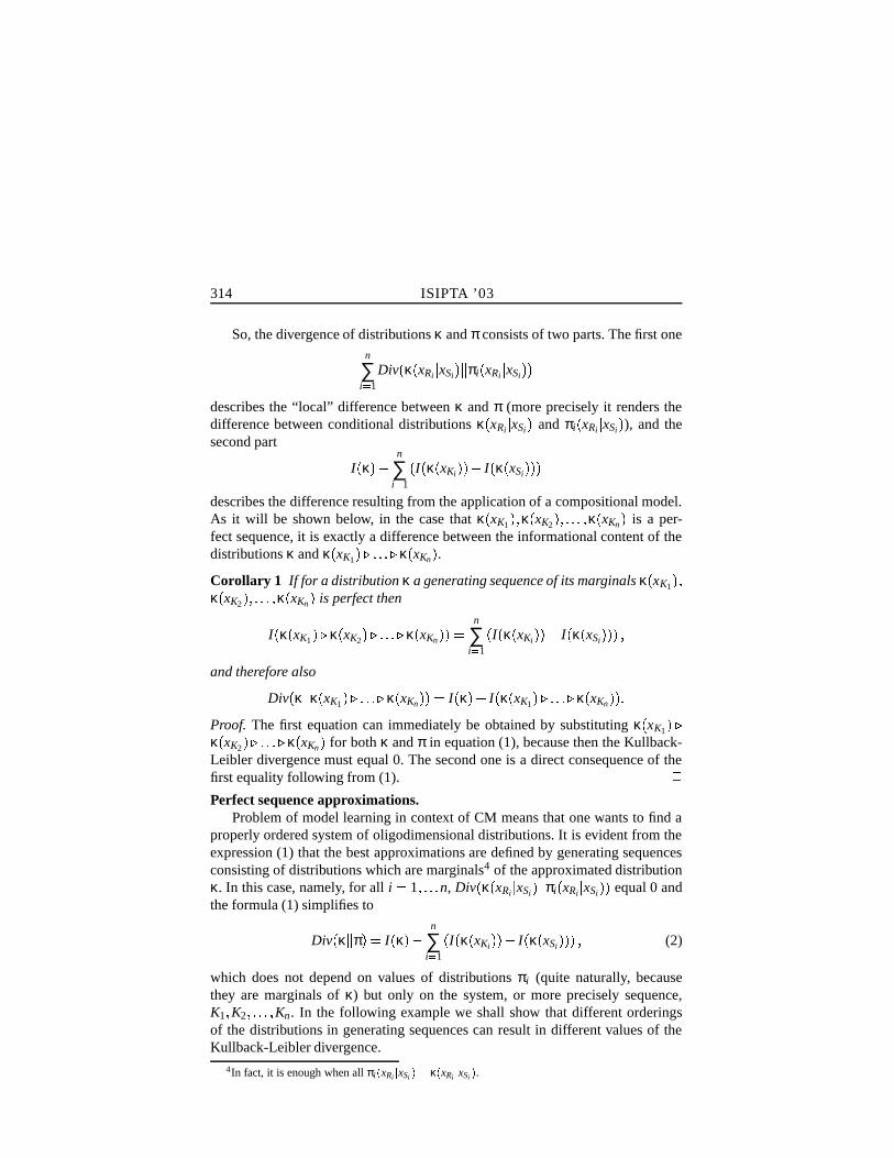
314 ISIPTA ’03

So, the divergence of distributions κ and π consists of two parts. The first onen

∑i & 1

Div κ xRi ( xSi nö πi xRi ( xSi describes the “local” difference between κ and π (more precisely it renders thedifference between conditional distributions κ xRi ( xSi and πi xRi ( xSi ), and thesecond part

I κ / n

∑i & 1

I κ xKi P/ I κ xSi describes the difference resulting from the application of a compositional model.As it will be shown below, in the case that κ xK1 κ xK2 « κ xKn is a per-fect sequence, it is exactly a difference between the informational content of thedistributions κ and κ xK1 Lã­ã κ xKn .Corollary 1 If for a distribution κ a generating sequence of its marginals κ xK1 κ xK2 6 κ xKn is perfect then

I κ xK1 Lã κ xK2 Lã­ã κ xKn ) n

∑i & 1

I κ xKi / I κ xSi and therefore also

Div κ ö κ xK1 KãÂã κ xKn ) I κ / I κ xK1 Lã®ã κ xKn 6Proof. The first equation can immediately be obtained by substituting κ xK1 ãκ xK2 Lãã κ xKn for both κ and π in equation (1), because then the Kullback-Leibler divergence must equal 0. The second one is a direct consequence of thefirst equality following from (1). UPerfect sequence approximations.

Problem of model learning in context of CM means that one wants to find aproperly ordered system of oligodimensional distributions. It is evident from theexpression (1) that the best approximations are defined by generating sequencesconsisting of distributions which are marginals4 of the approximated distributionκ. In this case, namely, for all i 1 n, Div κ xRi ( xSi mö πi xRi ( xSi equal 0 andthe formula (1) simplifies to

Div κ ö π V I κ / n

∑i & 1

I κ xKi / I κ xSi (2)

which does not depend on values of distributions πi (quite naturally, becausethey are marginals of κ) but only on the system, or more precisely sequence,K1 K2 ì Kn. In the following example we shall show that different orderingsof the distributions in generating sequences can result in different values of theKullback-Leibler divergence.

4In fact, it is enough when all πi xRi t xSi κ xRi t xSi .

Jirousek: On Approximating Distributions by Compositional Models 315

Example 2 Consider a 4-dimensional distribution κ x1 x2 x3 x4 and its threemarginal distributions denoted π1 π2 π3:

π1 x1 x2 κ x1 x2 π2 x2 x3 κ x2 x3 6 π3 x3 x4 κ x3 x4 6Compute Div κ ö π and Div κ ö π for π π1 ã π2 ã π3 and π π1 ã π3 ã π2. For thefirst distribution it is

Div κ ö π ù I κ /ú[ I κ x G 1 2 I F I κ x G 2 3 I F I κ x G 3 4 I ]J[ I κ x /0 F I κ x G 2 I F I κ x G 3 I ] I κ / I κ x G 1 2 I / I κ x G 2 3 I / I κ x G 3 4 I whereas for π we get

Div κ ö π N I κ / [ I κ x G 1 2 I O I κ x G 3 4 I O I κ x G 2 3 I ] [ I κ x /0 F I κ x /0 F I κ x G 2 3 I ] I κ / I κ x G 1 2 I / I κ x G 3 4 I / I κ x G 2 3 I F I κ x G 2 3 I Div κ ö π F I κ x G 2 3 I 6The reader probably noticed that, for the sake of simplicity, we introduced a situa-tion corresponding to a decomposable model. It is perhaps worth mentioning thateven in this case it may happen that both of the sequences defining distributionsπ and π are perfect. In correspondence with the assertion mentioned in Section 4(item (iv)), it happens only when π π and therefore also Div κ ö π W Div κ ö π ,from which we get that I κ x G 2 3 I ) 0. This means that variables X2 and X3 areindependent. ë

In the example we have shown that a quality of a compositional approximationdepends not only on the selected system of low-dimensional distributions (possi-bly marginals of the approximated distribution) but also on their ordering. Wecould see that κ was better approximated by perfect sequence π1 π2 π3 than byπ1 π3 π2, in case that the latter one was not perfect. From the following assertionwe will see that perfect sequences are always, in a sense, the best approximations.

Theorem 4 If π1 π2 πn is a perfect sequence of marginal distributions of κ(κ Π X K1 á 5 5 5 á Kn Y ) then

Div κ ö π1 ã π2 ãÂã πn c> Div κ ö πi1 ã πi2 ãÂã πin for any permutation i1 i2 ì in of indices 1 2 n.

Proof. Since π1 π2 ì πn is a perfect sequence of marginals of κ, we get fromCorollary 1

Div κ ö π1 ã π2 ã­ã πn - I κ / I π1 ã π2 ãÂã πn

316 ISIPTA ’03

and, because the Kullback-Leibler divergence is always nonnegative,

I κ I π1 ã π2 ã­ã πn 6We assume that π1 π2 ì πn are marginals of κ, and since they form a perfect

sequence (due to Theorem 2) they are also marginals of π1 ã π2 ãk¼ã πn. There-fore, equation (2) can be applied to both Div κ ö πi1 ãûã πin andDiv π1 ãÂã πn ö πi1 ãÂã πin :Div κ ö πi1 ã­ã πin I κ / n

∑ü & 1 ý I κ xKiþ / I κ xSiþ ¼ÿ$ (3)

Div π1 ãÂã πn ö πi1 ãÂã πin ) I π1 ãÂã πn / n

∑ü & 1 ý I κ xKi þ / I κ xSiþ ÿ The latter equality gives (respecting again the fact that the Kullback-Leibler di-vergence value must be nonnegative)

I π1 ã­ã πn n

∑ü & 1 ý I κ xKi þ / I κ xSi þ ÿ Combining this with equality (3) we get

Div κ ö πi1 ã­ã πin I κ / I π1 ãÂã πn where the right-hand side part of the inequality equals, as mentioned at the verybeginning of the proof, Div κ ö π1 ãÂã πn . UHeuristic algorithm.

Regarding the above-mentioned fact that perfect sequence models are equiva-lent to Bayesian networks, it is obvious that all the methods for Bayesian networklearning can be adapted to CM construction (see eg. [1]). Another very simpleand effective possibility, though far from being optimal, is the process discussedin the rest of the paper.

We split the model construction process into two steps. The first one, whichis not discussed in this paper, is selection of oligodimensional distributions, fromwhich the model will be constructed. In some situations one can be quite natu-rally relieved of necessity to perform this step. For example, when the data fileis too small and only 2-dimensional distributions can be estimated, then all these2-dimensional distributions can be considered. In other situations, an expert canselect the distributions from which the model should be constructed. Otherwise,informational content of low-dimensional distributions should be taken as a crite-rion for selection of a system of oligodimensional distributions.

The second step of the model construction process is to find a proper orderingof the selected oligodimensional distributions. The properties presented in the

Jirousek: On Approximating Distributions by Compositional Models 317

above sections theoretically support a heuristic algorithm, which arranges low-dimensional distributions into a generating sequence in a manner that utilizes itsinformational content as much as possible. In this section its simplest version ispresented that enables the reader to understand the basic principle of exploitingthe informational content of individual input low-dimensional distributions.

The reader will see that the procedure considers not only the given system ofdistributions but also their marginals; this can, in some situations, improve ex-ploitation of the informational content of distributions, since it considers a greatervariety of conditional independence structures.

Algorithm

Input: System of low-dimensional distributions π1 xK1 6 πn xKn .Initialization: Select a variable Xm and a distribution π j such that m K j.

Set κ1 : π j xm , L : m and k : 1.

Computational Cycle: While K1 û Kn Ä L < /0 perform the following3 steps:

1. for all j 1 n and all m K j Ä L compute the mutualinformation

MIπ j Xm;XK j º L 62. Fix j and m for which MIπ j Xm;XK j º L achieved its maximal

value.

3. Increase k by 1. Set κk : π j X X K j º L Y áKG m I and L : L m .

Output: Generating sequence κ1 κ2 κk.

What can be said about the resulting generating sequence κ1 κ2 κk? Dis-tribution κ dC κ1 ã κ2 ãkã κk is a probability distribution of XK1 á K2 á 5 5 5 á Kn . Thegoal of the algorithm is to get a distribution with the highest possible informa-tional content I κ d6 (we know that the higher informational content, the lower thecriterion function – Kullback-Leibler divergence). Important questions concernthe facts whether the resulting sequence κ1 κ2 ì κk is perfect and contains allthe distributions from π1 π2 πn. Unfortunately, answers to both these ques-tions are negative.

Though the heuristics employed in the algorithm do not guarantee that a per-fect sequence will always be found when it does exist, the advantage is in itsefficiency and in the fact that it always suggests a subset of distributions thatmay form a perfect sequence, exploiting the available information in a subopti-mal way5. One should realize, however, that a distribution from such a perfect

5Any generating sequence can be converted into a perfect sequence according to the following

318 ISIPTA ’03

sequence, though defined for groups of variables for which some input distribu-tion π j is defined, can differ from this input distribution π j. In such a case, weemploy a process of verification and refinement.

The detailed description of this process is beyond the scope (and extent) ofthis paper. Briefly said, verification consists of computation of Kullback-Leiblerdivergence of model distributions and the respective input distributions (or theirmarginals). If we find that some of the distributions defining the perfect modelare too far from the required marginals (assuming that input distributions aremarginals of the approximated distribution), then refinement is applied. This isrealized by substituting a group of input marginal distributions by one distribu-tion defined for all of the variables which are arguments of the deleted distribu-tions. Naturally, this must be applied carefully, to avoid too much increase in thedimension of input distributions. New, more-dimensional input distributions areeither estimated from data, or often computed from the original input distributionsby the well-known Iterative Proportional Fitting Procedure ([3]). Then, having anew group of input distributions, the process starts from the very beginning byapplication of Algorithm.

The same process of verification and refinement is also applied when some ofthe input distributions are not included in the model.

Let us illustrate this process by a simple example.

Example 3 Let us consider the following 10 3-dimensional distributions (theirvalues were estimated from a data file):

π1 x1 x2 x4 6 π2 x1 x2 x6 6 π3 x1 x4 x6 π4 x3 x6 x11 6 π5 x3 x10 x11 π6 x4 x6 x11 6π7 x5 x6 x8 6 π8 x6 x8 x11 π9 x7 x10 x11 6

π10 x9 x10 x11 The algorithm (starting with variable X1 and distribution π1) produced the

sequence

π1 x1 6 π1 x1 x4 π3 x1 x4 x6 6 π6 x4 x6 x11 π8 x6 x8 x11 6 π4 x3 x6 x11 π7 x5 x6 x8 6 π5 x3 x10 x11 π10 x9 x10 x11 6 π9 x7 x10 x11 6 π1 x1 x2 x4 6

There are two points that can be made about this sequence. First, since all the dis-tributions were estimated from one data file (with no missing values), all the distri-butions were pairwise consistent, and thus both π1 x1 - π3 x1 and π1 x1 x4 -π3 x1 x4 , and therefore also

π1 x1 Lã π1 x1 x4 Lã π3 x1 x4 x6 ) π3 x1 x4 x6 assertion ([5, 6]).Theorem 5 Let π1 íK í πn be defined and let the sequence κ1 ® κn be: κ1 π1, κ2 κ Q K2 è K1 R

1 í π2,

and generally κ j κ1 íL Eí κ j S 1 Q K j èìQ K1 îìï ï ï î K j ð 1 R R í π j . Then κ1 ® κn is perfect and π1 íL Eí πn κ1 íO Eí κn.

Jirousek: On Approximating Distributions by Compositional Models 319

Therefore, the result of the algotihm was, in fact, a generating sequence

π3 π6 π8 π4 π7 π5 π10 π9 π1 which was perfect (see assertion (iiia) in Section 4).

The negative property of this result was the fact that the algorithm finishedbefore exploiting distribution π2 x1 x2 x6 . Since we are looking for an approx-imation of a distribution from which the data file was generated, (following theverification and refinement process) we have to assess how much omitting π2

influences the quality of the achieved result. This is done by considering theKullback-Leibler divergence Div π2 x1 x2 x6 mö πappr x1 x2 x6 , for

πappr π3 ã π6 ã π8 ã π4 ã π7 ã π5 ã π10 ã π9 ã π1

(let us mention that in this case πappr x1 x2 x6 - π3 ã π1 x1 x2 x6 ). If we arenot satisfied, refinement results in getting a distribution π11 x1 x2 x4 x6 and sub-stituting it for π1 π2 and π3. Subsequent application of the algorithm to the setof distributions π4 π5 π6 π7 π8 π9 π10 π11 resulted in obtaining the perfect se-quence

π11 π6 π8 π4 π7 π5 π10 π9 ë7 Conclusions

We have presented theoretical results showing that if an approximation of a prob-ability distribution is looked for in a family of compositional distributions thenthe Kullback-Leibler divergence representing a quality of the approximation canbe expressed as a sum of two contributions. The first one, which can easily besuppressed by considering only marginals of the approximated distribution, de-scribes “local” differences, while the other one corresponds to the loss of infor-mation resulting from the compositional model (from introducing the respectiveconditional independence relations). This knowledge was exploited for designinga heuristic algorithm based on an effort to maximize informational content of theconstructed approximation.

Let us conclude the paper by a brief comment advocating CMs. Based onde Cooman approach to conditionning [2], J. Vejnarova introduced the operatorof composition also in possibility theory [11], which made it possible to extendthe whole approach beyond probabilistic framework.

References

[1] R.R. Boukaert, Bayesian belief networks – from construction to inference,PhD. thesis, University of Utrecht (Netherlands), 1995.

320 ISIPTA ’03

[2] G. de Cooman, Possibility theory I – III International Journal of GeneralSystems 25 (1997), pp. 291–371.

[3] W.E. Deming and F.F. Stephan, On a least square adjustment of a sampledfrequency table when the expected marginal totals are known, Ann. Math.Stat. 11 (1940), pp. 427-444.

[4] F. V. Jensen, Introduction to Bayesian Network, UCL Press 1996.

[5] R. Jirousek, Composition of probability measures on finite spaces. In: Proc.of the 13th Conf. Uncertainty in Artificial Intelligence UAI’97 (D. Geigerand P. P. Shenoy, eds.), Morgan Kaufmann Publ., San Francisco, California,1997, pp. 274-281.

[6] Jirousek, R. Graph Modelling without Graphs. In Proc. of the 17th Int. Conf.on Information Processing and Management of Uncertainty in Knowledge-based Systems IPMU’98 (B. Bouchon-Meunier, R.R. Yager, eds.), EditionsE.D.K. Paris, 1998, pp. 809-816.

[7] R. Jirousek, Marginalization in composed probabilistic models. In: Proc. ofthe 16th Conf. Uncertainty in Artificial Intelligence UAI’00 (C. Boutilier andM. Goldszmidt eds.), Morgan Kaufmann Publ., San Francisco, California,2000, pp. 301-308.

[8] Jirousek, R. Detection of independence relations from persegrams. In: Pro-ceedings of the 9th Int. Conf. on Information Processing and Managementof Uncertainty in Knowledge Based Systems (Bernadette Bouchon-Meunier,Ronald R. Yager (ed)), ESIA, Annecy, France, 2002, pp. 1261-1267.

[9] S.L. Lauritzen, Graphical Models. Clarendon Press, Oxford, 1996.

[10] A. Perez, ε-admissible simplification of the dependence structure of a set ofrandom variables, Kybernetika 13 (1977), pp. 439–450.

[11] J. Vejnarova, Possibilistic independence and operators of composition ofpossibility measures. In Prague Stochastics’98 (M. Huskova, J. A. Vısekand P. Lachout eds.), JCMF 1998, pp. 575–580.

Radim Jirousek is with the Institute of Information Theory and Automation of theAcademy of Sciences of the Czech Republic. He is also a visiting Professor at Facultyof Management, Jindrichuv Hradec, Czech Republic. E-mail: radim@utia.cas.cz

An Update on GeneralizedInformation Theory

GEORGE J. KLIRBinghamton University (SUNY), USA

Abstract

The purpose of this paper is to survey recent developments and trends inthe area of generalized information theory (GIT) and to discuss some of theissues of current interest in GIT regarding the measurement of uncertainty-based information for imprecise probabilities on finite crisp sets.

Keywords

uncertainty, uncertainty-based information, generalized information theory

1 Introduction

The term “Generalized Information Theory” (GIT) was introduced in the early1990s to name a research program whose objective was to develop a broadertreatment of uncertainty-based information, not restricted to the classical notionsof uncertainty [6]. In GIT, the primary concept is uncertainty, and information isdefined in terms of uncertainty reduction.

The basic tenet of GIT is that uncertainty can be formalized in many differentways, each based on some specific assumptions. To develop a fully operationaltheory for some conceived type of uncertainty, we need to address issues at fourlevels:Ú LEVEL 1 – we need to find an appropriate mathematical representation of

the conceived type of uncertaintyÚ LEVEL 2 – we need to develop a calculus by which this type of uncertaintycan be properly manipulatedÚ LEVEL 3 – we need to find a meaningful way of measuring the amount ofrelevant uncertainty in any situation formalizable in the theoryÚ LEVEL 4 – we need to develop methodological aspects of the theory

321

322 ISIPTA ’03

GIT is an outgrowth of two classical uncertainty theories. The older one,which is also simpler and more fundamental, is based on the notion of possibility.The newer one, which has been considerably more visible, is based on the notionof probability. Proper ways of measuring uncertainty in these classical theorieswere established, respectively, by Hartley [5] and Shannon [12]. Basic features ofthe theories are outlined in [8].

The various nonclassical uncertainty theories in GIT are obtained by expand-ing the conceptual framework upon which the classical theories are based. Atthis time, the expansion is two-dimensional. In one dimension, the formalizedlanguage of the classical set theory is expanded to a more expressive languageof fuzzy set theory, where further distinctions are based on various special typesof fuzzy sets [10]. In the other dimension, the classical (additive) measures the-ory [4] is expanded to a less restrictive fuzzy measure theory [14], within whichfurther distinctions are made by using fuzzy measures with various special prop-erties. This expanded conceptual framework is a broad base for formulating anddeveloping various theories of imprecise probabilities.

The subject of this paper is to discuss some of the issues of current interestregarding the measurement of uncertainty for imprecise probabilities on finitecrisp sets. The various issues of possible fuzzifications of imprecise probabilitiesand of imprecise probablities on infinite sets are not addressed here. To facilitatethe discussion, some common characteristics of imprecise probabilities on finitecrisp sets are introduced in Section 2.

2 Imprecise Probabilities: Some Common Charac-teristics

One of the common characteristics of imprecise probabilities on finite crisp sets isthat evidence within each theory is fully described by a lower probability function(or measure), g, or, alternatively, by an upper probability function (or measure)g. These functions are always regular fuzzy measures that are superadditive andsubadditive [14], respectively, and

∑x X

g x oc> 1 ∑x X

g x o 1 (1)

In the various special theories of uncertainty, they possess additional special prop-erties.

When evidence is expressed (at the most general level) in terms of an arbitraryclosed and convex set D of probability distribution functions p on a finite set X ,functions gD and gD associated with D are determined for each A P X by theformulas

gD A ) infp D ∑

x A

p x and gD A supp D

∑x A

p x

Klir: An Update on Generalized Information Theory 323

Since

∑x A

p x O ∑x A

p x 1 for each p D and each A P X , it follows that

gD A 1 / gD A 6 (2)

Due to this property, functions gD and gD are called dual (or conjugate). One ofthem is sufficient for capturing given evidence; the other one is uniquely deter-mined by (2). It is common to use the lower probability function gD to capturethe evidence.

As is well known [2, 3], any given lower probability function gD is uniquelyrepresented by a set-valued function mD for which mD /0 0 and

∑A P X X Y mD A 1 (3)

Any set A P X for which mD A '< 0 is often called a focal set, and thefamily of all focal sets, F , with the values assigned to them by function mD iscalled a body of evidence. Function mD is called a Mobius representation of gDwhen it is obtained for all A P X via the Mobius transform

mD A ) ∑B B A

¼/ 1 A B gD B (4)

where ( A / B ( denotes the cardinality of the finite set A / B. The inverse transformis defined for all A P X by the formula

gD A ∑B B A

mD B (5)

It follows directly from (2) that

gD A ) ∑B B º A

& /0mD B (6)

for all A P X .Assume now that evidence is expressed in terms of a given lower probability

function g. Then, the set of probability distribution functions that are consistentwith g, D g , which is always closed and convex, is defined as follows:

D g ) p x m( x X p x c 0 1 ∑

x Xp x ) 1 and

g A M> ∑x A

p x for all A P X «K (7)

That is, each given function g is associated with a unique set D and vice-versa.

324 ISIPTA ’03

3 Measures of Uncertainty

A measure of uncertainty of some conceived type in a given theory of impreciseprobabilities is a functional, U , that assigns to each lower probability function inthe theory a nonnegative real number. This number is supposed to measure, in anintuitively meaningful way, the amount of uncertainty of the considered type thatis embedded in the lower probability function. To be acceptable as a measure ofthe amount of uncertainty, the functional U must satisfy several intuitively essen-tial axiomatic requirements. Considering the most general level, when evidenceis represented in terms of an arbitrary closed and convex set D of probability dis-tribution functions p on finite set X Y , function U must satisfy the followingrequirements:

1. Subadditivity: U D M> U DX F U DY , where

DX pX ( pX x ) ∑

y Yp x y for some p D K

DY pY ( pY y ) ∑

x Xp x y for some p D L

2. Additivity: U D U DX V U DY if and only if DX and DY are notinteractive, which means that for all A P X and all B P X , mD A B ) mDX A , mDY B and mD R ) 0 for all R < A B.

3. Monotonicity: if D D + , then U D U D + ; and similarly for DX andDY .

4. Range: if uncertainty is measured in bits, then U D - 0 log2 ( X Y ( , andsimilarly for DX and DY .

The requirement of subadditivity and additivity, as stated here, are general-ized counterparts of the classical requirements of subadditivity and additivity forprobabilistic and possibilistic measures of uncertainty. The requirement of mono-tonicity (not applicable to classical probabilistic uncertainty) means that reducingthe set of probability distributions consistent with a given lower (or upper) prob-ability function cannot increase uncertainty. The requirement of range, which de-pends on the choice of measurement units, is defined by the two extreme cases:the full certainty and the total ignorance.

When distinct types of uncertainty coexist in a given uncertainty theory, itis not necessary that these requirements be satisfied by each uncertainty type.However, they must be satisfied by an overall uncertainty measure, which appro-priately aggregates measures of the individual uncertainty types.

It is well established that two types of uncertainty coexist in all theories ofimprecise probabilities [8, 9]. They are generalized counterparts of the classicalpossibilistic and probabilistic uncertainties. They are measured, respectively, byappropriate generalizations of the Hartley and Shannon measures.

Klir: An Update on Generalized Information Theory 325

4 Generalized Hartley Measures

An historical overview of efforts to generalize the classical Hartley measure ofuncertainty can be found in [9]. Its full generalization (to arbitrary closed andconvex sets of probability distributions) was completed fairly recently by Abellanand Moral [1]. They showed that the functional

GH mD ∑A F

mD A log2 ( A ( (8)

where mD is the Mobius representation of the lower probability associated witha given closed and convex set D of probability distributions, satisfies all the es-sential axiomatic requirements defined in Sec. 3 (subadditivity, additivity, etc.).Moreover, this functional is also directly connected with the classical Hartleymeasure: it is the weighted average of the Hartley measure for each given body ofevidence F mD .

It is fairly obvious that the functional GH defined by (8) measures the lackof specificity in evidence. Large focal elements result in less specific predictions,diagnoses, etc., than their smaller counterparts. The type of uncertainty measuredby GH is thus well characterized by the term nonspecificity.

Observe that GH mD e 0 for precise probabilities, where D consists of asingle probability distribution function, which is expressed in (8) by function mD .All focal sets are in this case singletons. Evidence expressed by precise probabil-ities is thus fully specific.

Eq. (8) is clearly applicable only to functions mD defined on finite sets. It mustbe properly modified when mD is defined on the n-dimensional Euclidean spacefor some n 1, as shown in [9]. However, this modification is not a subject of thispaper.

5 Generalized Shannon Measures

There have been many promising, but eventually unsuccessful efforts to general-ize the classical Shannon measure (usually referred to as the Shannon entropy).Virtually all these efforts were based on the recognition that the Shannon entropymeasures the mean (expected) value of the conflict among evidential claims ex-pressed by a single probability distribution function on a finite set of mutuallyexclusive alternatives [9]. An historical overview of most of these efforts is givenin [9].

All the proposed generalizations of the Shannon entropy were intuitively promis-ing as measures of conflict among evidential claims in general bodies of evidence,but each of them was eventually found to violate the essential requirement of sub-additivity. In fact, no generalized Shannon entropy can be subadditive on its own,as is shown in [13]. The subadditivity may be obtained only in terms of the total

326 ISIPTA ’03

uncertainty — an aggregate of the two coexisting types of uncertainty (nonspeci-fivity and conflict). However, when the total uncertainty is viewed as the sum ofthe generalized Hartley measure with the various candidates for the generalizedShannon entropy, none of these aggregated uncertainty measures is still subaddi-tive, as demonstrated by relevant counterexamples in each case [13].

The latest promising candidate (not previously analyzed in terms of the re-quirement of subadditivity) is based on the so-called Shapley index, which playsan important role in game theory [11, 15]. For any given finite universal set X ,this candidate for the generalized Shannon entropy, GS, is defined as the averageShannon entropy of differences in a given lower probability (or, alternatively, anupper probability) for all maximal chains in the lattice P X 6 . Unfortunately,the sum GH GS does not satisfy in this case again the requirement of subaddi-tivity. This can be demonstrated by the following counterexample.

Let X x1 x2 and Y y1 y2 , and let us consider a body of evidence onX Y whose Mobius representation is:

m x1 y1 6ì x2 y2 x2 y1 «HN a m X Y 1 / a

where a 0 1 . Then, mX X mY Y W 1, and, hence, GSX mX V GSY mY W0 and GHX mX F GHY mY ) 2. Furthermore,

GS m / a log2 a / 1 / a log2 1 / a ED 4 GH m N alog23 2 / 2a

For subadditivity of GH GS, the difference

∆ § GHX GHY GSX GSY P/ GH GS a log2 a 1 / a log2 1 / a ED 4 2a / alog23

is required to be nonnegative for all values a 0 1 . However, ∆ is negative inthis case for any value a 0 0 58 and it reaches its minimum, ∆ \/ 0 1, ata 0 225.

6 Total Uncertainty Measures

Generalized Shannon measure, GS, was eventually defined indirectly, via an ag-gregated uncertainty, AU , covering both nonspecificity and conflict, and the wellestablished generalized Hartley measure of nonspecificity, GH, defined by (8).Since it must be that GH GS AU , the generalized Shannon measure can bedefined as

GS AU / GH (9)

Klir: An Update on Generalized Information Theory 327

Using this definition, the unsuccessful effort to find GS directly is replaced withthe effort to find AU and define GS indirectly via Eq. (9). The latter effort wassuccessful in the mid 1990s, when a functional AU satisfying all essential re-quirements was established in evidence theory [9]. However, this functional isapplicable to all the other theories of imprecise probabilities as well, which fol-lows from the common properties shared by these theories (Sec. 2). Given anylower probability function gD associated with a closed convex set D of probabil-ity distributions (or vice versa), AU gD is defined by the formula

AU gD ) maxp D

/ ∑x X

p x log2 p x (10)

It is the maximum Shannon entropy within D. An efficient algorithm for com-puting this maximum, which was proven correct for belief functions of evidencetheory [9], is applicable without any change when belief functions are replacedwith arbitrary lower probability functions of any other kind.

Given an arbitrary lower probability function g on P x , the generalized ver-sion of this algorithm consists of the following seven steps:

Step 1. Find a non-empty set A X , such that g A D ( A ( is maximal. If there aremore such sets than one, take the one with the largest cardinality.

Step 2. For all x A, put p x ) g A D ( A ( .Step 3. For each B X / A, put g B g B A / g A .Step 4. Put X X / A.

Step 5. If X < /0 and g X c? 0, then go to Step 1.

Step 6. If g X W 0 and X < /0, then put p x 0 for all x X and m X W 1 / na.

Step 7. Calculate AU ª/ ∑x X p x log2 p x .Although functional AU is a well-justified measure of total uncertainty in the

various theories of uncertainty, it is highly insensitive to changes in evidence dueto its aggregated nature. It is an aggregate of the two coexisting types of uncer-tainty, nonspecificity and conflict. It is thus desirable to express the total uncer-tainty, TU , in a disaggregated form

TU § GH GS (11)

where GH is defined by (8) and GS is defined by (9) and (10). It is assumedhere that the axiomatic requirements are defined in terms of the sum of the twofunctionals involved, which is always the well-justified aggregate measure AU .In this sense the measure satisfies trivially all the requirements. Its advantage

328 ISIPTA ’03

is that measures of both types of uncertainty that coexist in uncertainty theoryemployed (nonspecificity and conflict) are expressed explicitly and, consequently,the measure is sensitive to changes in evidence.

To appreciate the difference between AU and TU , let us consider three sim-ple examples of given evidence within a finite universal set X and let ( X (n n forconvenience: (i) in the case of total ignorance (when m X 1), we obtain AU log2 n and TU ª log2 n 0 ; (ii) when evidence is expressed by the uniform prob-ability distribution on X , then again we have AU log2 n, but TU ^ 0 log2 n ;(iii) when evidence is expressed by m x o a for all x X and m X 1 / na,then again AU log2 n for all values a > 1 D n, while

TU § 1 / na log2 n na log2 n 6It is clear that TU defined by (11) possesses all the required properties in

terms of the sum of its components, since GH GS AU . Moreover, as provenby Smith [13], GS 0 for all bodies of evidence. Additional properties of GSdefined by (9) can be determined by employing the algorithm for computing AU ,as shown for some properties in Section 7.

It is also reasonable to express the generalized Shannon entropy by the inter-val S S , where S and S are, respectively, the minimum and maximum values ofthe Shannon entropy within the set of all probability distributions that are consis-tent with a given lower probability function. Clearly S AU and S is defined byreplacing max with min in Eq. (10). Then, the total uncertainty, TU + , has the form

TU + § GH S S (12)

Let us define a partial ordering of these total uncertainties as follows:

TU +1 > TU +2 iff GH1 > GH2 and S1 S1 S2 S2 Then, due to subadditivity of S, subadditivity of TU + is guaranteed. Indeed, SX SY SX SY < S S for any joint and associated marginal bodies of evidence. However, no algorithmfor computing S that has been proven correct is available as yet.

7 Some Properties of Generalized Shannon Entropy

The purpose of this section is to examine the generalized Shannon entropy definedby (9). To facilitate this examination, let

F Ai ( Ai P X 6 i q

Klir: An Update on Generalized Information Theory 329

denote the family of all focal sets of a given body of evidence, where q 1 2 ¼ q for some integer q, and let mi m Ai for convenience. Moreover,

letE

i q

Ai The algorithm for computing S ® AU produces a partition,

E Ek ( k r r > q

of E. For convenience, assume that block Ek of this partition was produced in k-thiteration of the algorithm and let ek §( Ek ( . Then

S m )½/ ∑k r

gk

log2 gk D ek

where gk

denotes the lower probability of Ek in k-th iteration of the algorithm,where ak §( Ak ( . This equation can be rewritten as

S m ½/ ∑k r

gklog2 g

k ∑

k r

gklog2 ek

It follows from this equation and from Eq. (9) that

GS m S gk( k r F GH g

k( k r P/ GH m (13)

where S denotes the Shannon entropy.Assume now that F consists of pair-wise disjoint focal sets. Then, the Mobius

representation, m, is a positive function since any negative value mi for some Ai F would clearly violate in this case the requirement that values of the associatedlower probability function must be in 0 1 . When applying the algorithm forcomputing S to our case, it turns out that the values mi for all Ai F are uniformlydistributed among elements of each focal set Ai. This only requires to prove that

∑i I

mi D ∑i I

ai > mk D ak

for each k I and all nonempty sets I q , where ak %( Ak ( . The proof of thisinequality, which is omitted here due to limited space, can be obtained by themethod of contradiction. The maximum entropy probability distribution function,p, for the given body of evidence is thus defined for all xik Ai k Ai and all

330 ISIPTA ’03

Ai F . by the formula p xik - mi D ai where ai ( Ai ( . Hence,

S m õª/ n

∑i & 1

ai

∑k & 1

p xik log2 p xik ½/ n

∑i & 1

mi log2 mi D ai ½/ n

∑i & 1

mi log2 mi n

∑i & 1

mi log2 ai½/ n

∑i & 1

mi log2 mi GH m 6Consequently,

GS m ½/ n

∑i & 1

mi log2 mi This is clearly a property that we would expect, on intuitive grounds, the general-ized Shannon entropy to satisfy.

To examine some properties of the generalized Shannon entropy for nestedbodies of evidence, let X

xi ( i n and assume that elements of X are orderedin such a way that the family

A Ai

x1 x2 xi F( i n contains all focal sets. That is, F A . For convenience, let mi m Ai for alli n .

To express GS m , we need to express GH m and S m . Clearly,

GH m ª/ n

∑i & 1

mi log2 i (14)

To express S m , three cases must be distinguished in terms of values mi:

(a) mi mi 1 for all i n 1 ;

(b) mi > mi 1 for all i n 1 ;

(c) neither (a) nor (b).

Following the algorithm for computing S, we obtain the formula

GSa m )ª/ n

∑i & 1

mi log2 mii (15)

Klir: An Update on Generalized Information Theory 331

for any function m that conforms to Case (a). By applying the method of Lagrangemultipliers, we can readily find out that the maximum, GS da n , of this functionalfor some n is obtained for

mi § 1 D i 2 X 1 ln2 α Y i n 6 (16)

where the value of α is determined by solving the equation

2 X 1 ln2 α Y n

∑i & 1

1 D i 1 Let sn ∑n

i & 1 1 D i . Then,

α ½/ log2 1 D sn / 1 D ln2 and, hence,

mi § 1 D i 2log2 X 1 sn Y 1 D isn 6Substituting this expression for mi in (15), we obtain

GS da n N n

∑i & 1

1 D i 1 D sn log2 sn 1 D sn log2 sn n

∑i & 1

1 D i Consequently,

GS da n ) log2 sn (17)

In Case (b), S log2 n and GH is given by (8). Hence,

GSb m log2 n / n

∑i & 1

mi log2 i The maximum, GS db n , of this functional for some n subject to the inequali-ties that are assumed in Case (b), is obtained for mi 1 D n. Hence,

GS db n - log2n

n!1 n (18)

Employing Stirling’s formula for approximating n!, it can be shown that

limn ∞ log2n

n!1 n log2 e 1 442695

332 ISIPTA ’03

GS db is thus bounded, contrary to GS da n . Moreover, GS db n : GS da n for alln .

Case (c) is more complicated for a general analytic treatment since it covers agreater variety of bodies of evidence with respect to the computation of GS. Thisfollows from the algorithm for computing S . For each given body of evidence,the algorithm partitions the universal set in some way, and distributes the value ofthe lower probability in each block of the partition uniformly. For nested bodiesof evidence, the partitions preserve the induced order of elements of X . There are2n 1 order preserving partitions. The most refined partition and the least refinedone are represented by Cases (a) and (b), respectively. All the remaining 2n 1 / 2partitions are represented by Case (c). A conjecture, based on a complete analysisfor n 3 and extensive simulation experiments for n ? 3, is that the maxima of GSfor all these partitions are for all n smaller than the maximum GS da for Case(a). According to this plausible conjecture, whose proof is an open problem, thedifference between the maximum nonspecificity, GH d n , and maximum conflict,GS da n , grows rapidly with n. For example, GH dn 2 e 1 and GS da 2 C 0 585,while GH do 104 C 13 29 and GS da 104 e 3 29. Similarly, the maximum valueof conflict is 36.9% of the maximum value of total uncertainty for n 2, but itreduces to 19.8% for n 104. For nested (consonant) bodies of evidence, thisfeature makes intuitively a good sense.

8 Conclusions

For the last two decades or so, research in GIT has been focusing on developingjustifiable ways of measuring uncertainty and the associated uncertainty-basedinformation in the various emerging uncertainty theories. This objective is now,by and large, achieved. However, some research in this direction is still neededto improve our understanding of the generalized Shannon entropy, defined eitherby (9) or by the interval S S . Results presented in this paper are intended tocontribute a little to this understanding.

In the years ahead, the focus of GIT will likely divide into two branches ofresearch. One of them will focus on developing methodological tools based onour capability to measure uncertainty in the various established theories of uncer-tainty. Methodological tools for making the principles of uncertainty maximiza-tion, minimization, and invariance operational will in particular be sought due tothe broad utility of these principles [7, 9]. The other branch of research will pursuethe development of additional uncertainty theories. One direction in this researcharea will undoubtedly include a comprehensive investigation of the various waysof fuzzifying existing uncertainty theories.

Klir: An Update on Generalized Information Theory 333

References

[1] Abellan, J. and S. Moral, “A non-specificity measure for convex sets of prob-ability distributions.” Intern. J. of Uncertainty, Fuzziness, and Knowledge-Based Systems, 8(3): 357–367, 1999.

[2] Chateauneuf, A. and Jaffray, J. Y., “Some characterizations of lower proba-bilities and other monotone capacities through the use of Mobius inversion.”Mathematical Social Sciences, 17: 263–283, 1989.

[3] Grabisch, M. “The interaction and Mobius representations of fuzzy mea-sures on finite spaces, k-additive measures: a survey.” Grabish, M. et al.,eds., Fuzzy Measures and Integrals: Theory and Applications. Springer-Verlag, New York, pp. 70–93.

[4] Halmos, P. R., Measure Theory. D. Van Nostrand, Princeton, NJ, 1950.

[5] Hartley, R. V. L., “Transmission of information.” The Bell System TechnicalJ., 7(3): 535–563, 1928.

[6] Klir, G. J., “Generalized information theory.” Fuzzy Sets and Systems, 40(1):127–142, 1991.

[7] Klir, G. J., “Principles of uncertainty: What are they? Why do we needthem?” Fuzzy Sets and Systems, 74(1): 15–31, 1995.

[8] Klir, G. J., “Uncertainty-based information.” Teodorescu, H. and P. Melo,eds, Systemic Organization of Information in Fuzzy Systems. IOS Press, Am-sterdam, pp. 21–52, 2003.

[9] Klir, G. J. and Wierman M. J., Uncertainty-Based Information: Ele-ments of Generalized Information Theory (Second Edition). Physica-Verlag/Springer-Verlag, Heidelberg and New York, 1999.

[10] Klir, G. J. and Yuan, B., Fuzzy Sets and Fuzzy Logic: Theory and Applica-tions. Prentice Hall, PTR, Upper Saddle River, NJ, 1995.

[11] Marichal, J. and Roubens, M., “Entropy of discrete fuzzy measures.” Intern.J. of Uncertainty, Fuzziness, and Knowledge-Based Systems, 8(6): 625–640,2000.

[12] Shannon, C. E., “The mathematical theory of communication.” The Bell Sys-tem Technical J., 27(3&4): 379–423, 623–656, 1948.

[13] Smith, R. M., Generalized Information Theory: Resolving Some Old Ques-tions and Opening Some New Ones. PhD. Dissertation, Binghamton Univer-sity (SUNY), Binghamton, NY, 2000.

334 ISIPTA ’03

[14] Wang, Z. and Klir, G. J., Fuzzy Measure Theory. Plenum Press, New York,1992.

[15] Yager, R. R., “On the entropy of fuzzy measures.” IEEE Trans. on FuzzySystems, 8(4): 453–461, 2000.

George J. Klir is with the Center for Intelligent Systems, Binghamton University (SUNY),Binghamton, New York, 13902 USA

Reducing Uncertainty by ImpreciseJudgements on Probability Distributions:

Application to System Reliability ÝI.KOZINE

Risø National Laboratory, Denmark

V.KRYMSKYUfa State Aviation Technical University, Russia

Abstract

In this paper the judgement consisting in choosing a function that is believedto dominate the true probability distribution of a continuous random variableis explored. This kind of judgement can significantly increase precision inconstructed imprecise previsions of interest, which of great importance forapplications. New formulae for computing system reliability are derived onthe basis of the technique developed.

Keywords

imprecise probabilities, probability density function, reliability

1 Introduction

Natural extension, a tool to extend statistical knowledge to other domains and tomake a set of available statistical partial evidence coherent, can appear and beused in different forms. In [1] four equivalent forms of the natural extension werereported. They are all nothing other than properly stated optimisation problemsfor obtaining lower and upper coherent bounds of probability characteristics ofinterest. The primal form suggests seeking coherent bounds defined by a set offeasible probability distributions, and this set, in turn, is formed by the availableevidence expressed as constraints in the optimisation task. If no evidence is avail-able (the state of complete ignorance), then the solution is sought over the set ofall possible probability distributions, which brings us to the vacuous probability ofthe event of interest A, i.e., P A c 0 1 . The crux of such optimisation problemsv Participation of V. Krymsky in this work has been supported by NATO grant #26-02-0001.

335

336 ISIPTA ’03

is that their solutions are defined on the family of degenerate probability distribu-tions1, which are included on equal footing in the set of all possible probabilitydistributions. As proven in [1], solving these optimisation problems, on the set ofall possible probability distributions, gives the same solution as that obtained ononly the set of degenerate distributions. This issue is closely related to the centraltheorems and methods of Chebychev systems as described in [2]. All this wouldsimply be mathematical subtlety, that is, far from practitioners’ interest, if this didnot give us a clue for deriving more precise previsions of interest for continuousrandom variables. For these variables it is often not realistic to assume that theprobability masses are concentrated in a few points as opposed to being contin-uously distributed over the set of possible outcomes. The existence of solutionson degenerate distributions often results in high imprecision, negating the prag-matic value of the assessments of interest. For example, in reliability applicationsthe time to failure of a system/component can not admit (except for very specialcases) the concentration of probability masses in a very few points of the positivereal line. Not being able to utilise such evidence leads to the fact that imprecisionin the reliability of a system grows rapidly as the number of components in thesystem increases, making the results rather practically useless [3].

This feature of the natural extension was found disturbing and precluded widerimplementation of imprecise statistical reasoning into reliability analysis. An at-tempt to mitigate the influence of degenerate probability distributions on the so-lutions was undertaken in [4]. No significant effect was attained through the in-troduction of judgements on the skewness and unimodality of the distributionsas, in this case, the peaks of degenerate distributions simply become repositionedand probability masses become redistributed among the peaks. The nature of thedistributions defining the solutions stays the same.

In this paper we explore a more drastic and, as it will be demonstrated, effec-tive way to exclude the family of degenerate distributions from the set of proba-bility distributions, which, as was expected, results in more precise previsions ofinterest. This is attained through judgements on a value (or a function, in general)that dominates the probability density function ρ x of a continuous random vari-able X . That is, we introduce judgements of the form ρ x c> Ψ x , where Ψ x isa real-valued positive function satisfying the inequalities 1 > 2

R # Ψ x dx : ∞, and

demonstrate a way of their utilisation. In particular, Ψ x can be set as Ψ x MK , I a b x where a b R and a > b, I a b x is the indicator function such thatI a b x c 1 if x a b , and I a b x c 0 otherwise, and K b / a 1 is a con-stant.

Similar ideas of utilising bounds on density functions were explored in [5].The tool of their utilisation was dynamic programming which gives us numerical

1The probability distribution of a continuous random variable is referred to as degenerate if theprobability masses are concentrated in a finite number of points belonging to the continuous set ofpossible states

Kozine & Krymsky: Imprecise Judgements on Probability Distributions 337

solutions of the stated problems, while we suggest an approach to solving theproblems analytically.

Breaking down a multidimensional case, X= X1 ì Xn , provides a theoreti-cal basis for system reliability computations, which is a subject of the second partof the paper.

2 Relevant basics of the approach

Comprehensive coverage of the foundation of the theory of imprecise previsionscan be found in the books [6] and [7]. In this section we briefly describe onlythose concepts that are necessary to understand the approach developed.

Consider a system consisting of n components. Let fi j xi be j / th function ofthe i-th component lifetime xi, i 1 n, and j 1 mi. Suppose that reliabil-ity characteristics of the components are not known precisely and represented asa set of lower and upper previsions ai j M fi j xi ai j M fi j xi 6 i 1 n and j 1 mi, which means that there exist mi interval-valued judgements forthe i-th component formally represented as expected values. The functions f i j xi can be regarded as gambles, where a gamble is a real-valued function on a pos-sibility space whose value is uncertain [6]. If, for instance, fi j xi 1 x, then thelower prevision ai j is the lower bound of the mean time to failure of the i-th com-ponent; or if fi j xi e I t ∞ Y xi , where I t ∞ Y xi =1 if xi t ∞ and I t ∞ Y xi =0otherwise, then the lower prevision ai j is the lower bound of the probability of afailure occurrence within t ∞ .

Denote X= X1 ì Xn a random vector and x % x1 ì xn is the vector ofnumerical values for X1 ! Xn. Then, there exists a function g(X) of the compo-nent lifetimes that characterises the system’s reliability. The function g(X) is alsoa gamble.

In order to compute the coherent lower and upper previsions M g and M g of interest characterising the system reliability, a proper optimisation problem(also referred to as the natural extension in its primal form) can be posed

M g M gt ) infℜn

supℜn Ê

Rn# g x ρ x dx (1)

subject to

0 > ρ x 6 2Rn# ρ x dx 1

ai j > 2Rn# fi j xi ρ x dx > ai j i 1 ! n j 1 ! ! mi

× ØÙ (2)

Here the minimum and maximum are taken over the set ℜn of all possible n-dimensional density functions

ρ(x) satisfying conditions (2). That is, each con-

straint in (2) is associated with a subset of ℜn and the intersection of those subsets,

338 ISIPTA ’03

if not empty, defines the solutions of the above optimisation problems. If the ini-tial interval-valued data, forming the constraints, are not consistent, then some ofthe subsets of ℜn associated with the constraints are disjoint and the solution doesnot exist. The requirement of the existence of a non-empty set of probability dis-tributions associated with the set of constraints is the only consistency principleimposed on the initial interval-valued data. This requirement is equivalent to theprinciple of avoiding sure loss [6] and is easily subject to technical checks.

If the components of a system are independent, then ρ(x) = ρ1 x1 ,. . . ,ρn xn .In some cases the duals of optimisation problems (1)-(2) can be stated, which

makes it technically easy to solve them [1]. The duals of (1)-(2) are

M g supc0 ci j di j c0 n

∑i & 1

mi

∑j & 1

ci jai j / di jai j (3)

subject to c0 R ci j di j R and for any xi 0, i 1 2 ! n j 1 2 ! mi c0 n

∑i & 1

mi

∑j & 1

ci j / di j I t ∞ Y xi c> g x (4)

And

M g infc0 ci j di j c0 n

∑i & 1

mi

∑j & 1

ci jai j / di jai j (5)

subject to c0 R ci j di j R and for any xi 0, i 1 2 ! n, j 1 2 ! mi,

c0 n

∑i & 1

mi

∑j & 1

ci j / di j I t ∞ Y xi g x (6)

The validity of the transition from a primal form similar to (1)-(2) to the dual formis explained in [1], [8].

Problems (3)-(4) and (5)-(6) are linear optimisation problems and and havetechnically straightforward solutions.

In some cases dual problems do not exist. This takes place if a primal op-timisation problem is not linear. For example, the judgement of independenceamong system components, which is equivalent to the introduction of ρ(x) =ρ1 x1 ,. . . ,ρn xn , makes the problem non-linear, and, as a consequence, it leadsto the non-existence of the dual optimisation problem.

3 Extending knowledge: one-dimensional case

Let us consider first a one-dimensional case of extending partial statistical infor-mation to probability characteristics of interest. That is, we will be focusing inthis section on the construction of new imprecise characteristics provided some

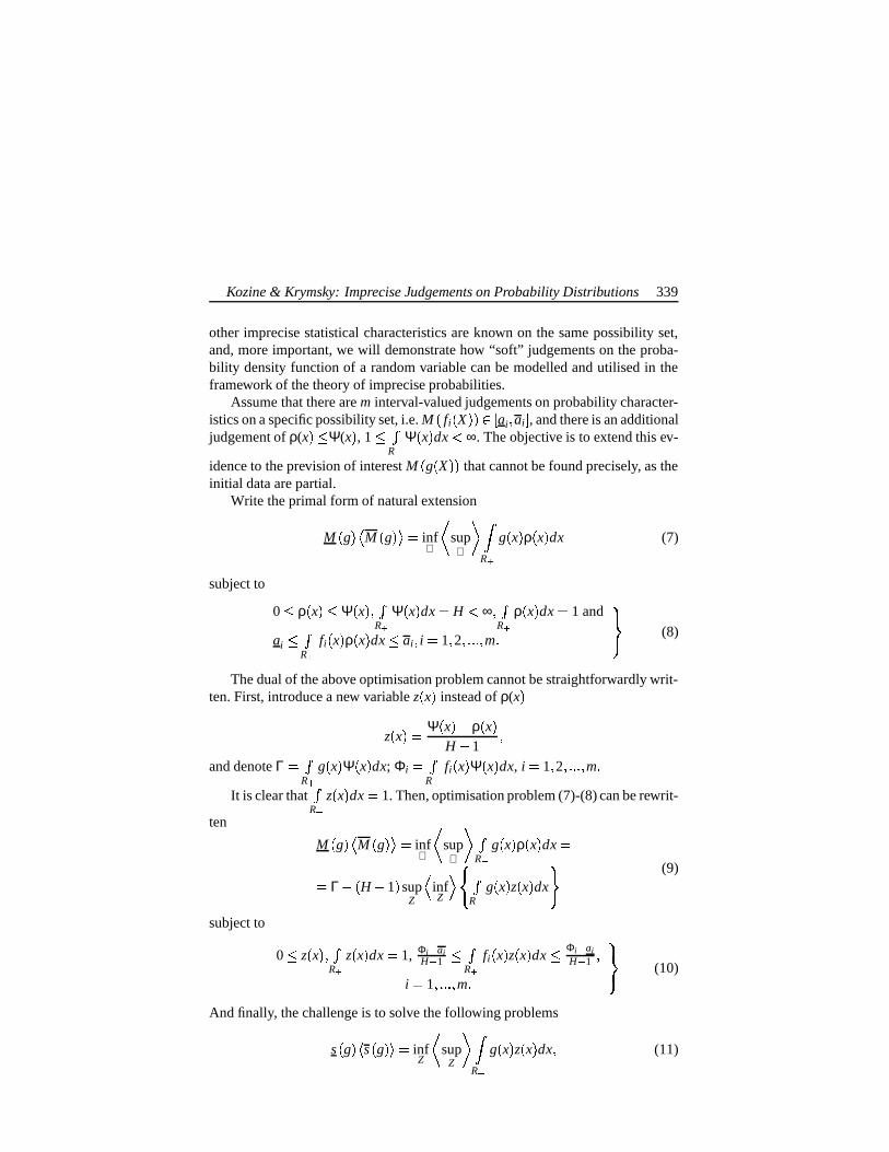
Kozine & Krymsky: Imprecise Judgements on Probability Distributions 339

other imprecise statistical characteristics are known on the same possibility set,and, more important, we will demonstrate how “soft” judgements on the proba-bility density function of a random variable can be modelled and utilised in theframework of the theory of imprecise probabilities.

Assume that there are m interval-valued judgements on probability character-istics on a specific possibility set, i.e. M fi X V ai ai , and there is an additionaljudgement of ρ(x c> Ψ(x , 1 > 2

R # Ψ x dx : ∞. The objective is to extend this ev-

idence to the prevision of interest M g X ¼ that cannot be found precisely, as theinitial data are partial.

Write the primal form of natural extension

M g M g 1 infℜ

sup

ℜ ÊR # g x ρ x dx (7)

subject to

0 > ρ x c> Ψ x 6 2R # Ψ x dx H : ∞ 2

R # ρ x dx 1 and

ai > 2R # fi x ρ x dx > ai i 1 2 ! m × ØÙ (8)

The dual of the above optimisation problem cannot be straightforwardly writ-ten. First, introduce a new variable z x instead of ρ(x

z x ) Ψ x / ρ x H / 1

and denote Γ 2

R # g x Ψ x dx; Φi 2R # fi x Ψ x dx, i 1 2 ! m

It is clear that2

R # z x dx 1. Then, optimisation problem (7)-(8) can be rewrit-

ten

M g M g e infℜ

sup

ℜ 2R # g x ρ x dx

Γ / H / 1 supZ inf

Z !#" 2R # g x z x dx $ (9)

subject to

0 > z x 2R # z x dx 1, Φi ai

H 1 > 2R # fi x z x dx > Φi ai

H 1 i 1 ! ! m

× ØÙ (10)

And finally, the challenge is to solve the following problems

s g s g % infZ

sup

Z ÊR # g x z x dx (11)

340 ISIPTA ’03

subject to (10).Before we go on to the duals, one consistency condition must be fulfilled. It

is of avoiding sure loss [6] and is transparent from the stand of common senseand can be written as inf f x ì1> M f x ì1> M f x C> sup f x ì . Applied toobjective functions (9), it appears as

inf g c> Γ / H / 1 supZ " 2

R # g x z x dx $>Γ / H / 1 inf

Z " 2R # g x z x dx $ > sup g

Optimisation problems (11) subject to (10) have their duals

s g ) supc0 ci di

" c0 m

∑i & 1 & ci Û Φi / ai

H / 1Ü / di Û Φi / ai

H / 1Ü(' $ (12)

subject to c0 R ci di R and for any x 0 c0 m∑

i & 1 ci / di fi x M> g x 6 And

s g ) infc0 ci di " c0 m

∑i & 1 & ci Û Φi / ai

H / 1Ü / di Û Φi / ai

H / 1Ü(' $ (13)

subject to c0 R ci di R and for any x 0 c0 m∑

i & 1 ci / di fi x g x 6

Thus, having derived the dual optimisation problems (12) and (13), we havegot a tool for utilising “soft” judgements concerning probability density functionsand extending them to other probability characteristics of interest defined on aone-dimensional possibility set.

Example 1. The information concerning a continuous random variable X isthat of ρ x > Ψ x K , I 0 T x : ∞, where T K are fixed positive numbers.What are the bounds for the expectation M X ?

The above approach brings us to the following results

M X ) KT 2

2/ KT / 1 T T Û 1 / KT

2Ü and M X KT 2

2

Example 2. Assume now that besides the information stated in example 1 weknow precisely the probability P

a > X > a ' p, where 0 > a : a > T . How

would the given information change the bounds for the expectation M X ?The result is

M X ) T [ 1 / KT2 ] T / a K a / a P/ p

M X ) KT 2

2 / a K a / a / p

Kozine & Krymsky: Imprecise Judgements on Probability Distributions 341

4 Computation of system reliability

Extending knowledge on multidimensional possibility sets, taking into accountimprecise judgements on probability density functions, is undertaken in a similarway to the one-dimensional case described above. The multidimensional case isbroken down in detail in [9]. In this section we represent the results concerningsystem reliability computations that follow from this case.

As it has been found earlier (see elsewhere [3], [10], [11]), the reliability of asystem, PSeries, the components of which are connected in series given the lowerand upper bounds of the components’ reliabilities and the state of complete igno-rance concerning their dependence, is calculated according to the formulae

PSeries M Û I t ∞ Y mini

xi Ü max 0;n

∑i & 1

pi/ n / 1

and

PSeries M Û I t ∞ Y mini

xi Ü mini

pi where PSeries > PSeries > PSeries, and p

iand pi i 1 ! n are the lower and upper

reliabilities of the components.By applying the above described approach, the formulas for the calculation

of the reliability of series systems become updated in the light of the evidenceconcerning the probability density function of time to failure

PSeries Γ / H / 1 mini

Û Φi / ai

H / 1Ü Γ / min

i Φi / ai 6

PSeries Γ / H / 1 max Û 0;n∑

i & 1 ý Φi aiH 1 ÿ / n / 1 Ü Γ / max Û 0;

n∑

i & 1 Φi / ai / H / 1 P, n / 1 Ü

The reliability of a system, PParallel , the components of which are connected inparallel given the lower and upper bounds of the components’ reliabilities and thestate of ignorance concerning their independence, is calculated according to theformulas (see elsewhere [3], [10], [11])

PParallel M Û I t ∞ Y maxi

xi Ü maxi

pi

PParallel M Û I t ∞ Y maxi

xi ¼ÜJ min Û 1;n∑

i & 1pi Ü

342 ISIPTA ’03

Their update in the light of the new evidence appears as follows

PParallel Γ / H / 1 min Û 1;n∑

i & 1 ý Φi aiH 1 ÿ Ü Γ / min Û H / 1 ; n

∑i & 1

Φi / ai Ü and

PParallel Γ / H / 1 maxi

Û Φi / ai

H / 1ÜJ Γ / max

i Φi / ai 6

For a system of an arbitrary structure the reliability bounds satisfy the inequalities[3], [10], [11]:

PArbStruct max1 A j A r

max 0 L j 6where r is a number of system minimal paths π1 π2 ! πr, L j ∑

i π j

pi/ µ j / 1 ,

and µ j is the number of components belonging to path π j, and

PArbStruct > min1 A j A s

min ∑i K j

pi;1 where s is a number of system minimal cut sets denoted by K1 K2 ! Ks

Now by applying the approach developed and using the substitutions pi Φi aiH 1 , p

i Φi ai

H 1 , we obtain

PArbStruct Γ / min1 A j A s

min ∑i K j

Φi / ai ; H / 1 PArbStruct > Γ / max

1 A j A rmax 0 L d j 6

where L d j ∑i π j

Φi / ai / H / 1 , µ j / 1 6Example 3. A system consists of two components (n=2) connected in se-

ries, and the reliability of the first component is p1 a1 a1 and the secondis p2 a2 a2 . One more judgement is of the form ρ x1 x2 > Ψ x1 x2 1 K ,I G¼ 0 T ; 0 T I x1 x2 , where K andT are constants and I G¼ 0 T ; 0 T I x1 x2 is a two-dimensional indicator function. What is system reliability?

The reliabilities of the components for an arbitrary time tare to be written inthe form (2)

a1 > T20

I t T x1 T20

ρ x1 x2 dx1dx2 > a1,

a2 > T20

I t T x2 T20

ρ x1 x2 dx1dx2 > a2

Kozine & Krymsky: Imprecise Judgements on Probability Distributions 343

Note that in this case H KT 2, Γ K T / t 2, hence

PSeries Γ / mini

Φi / ai - Γ / T2t

T20

Ψ x1 x2 dx1dx2 maxi

ai maxi

ai / Kt T / t ;PSeries Γ / max Û 0;

n∑

i & 1 Φi / ai / H / 1 , n / 1 EÜÖ min Û K T / t 2; Kt2 2

∑i & 1

ai / 1 Ü 5 Concluding remarks

Judgements concerning the function Ψ x , which is believed to dominate the trueprobability distribution of a continuous variable, are practically elicitable and maybe unambiguously understood by those inexperienced in probabilistic reasoning.So, a sample probability density function is defined by the totality of the valuesρi ni) N∆x , i 1 2 ! where ni is the number of observed realisations of acontinuous random variable X falling in the i / th bin with a width of ∆x, andN is the size of the sample. For example, in reliability analysis the continuousrandom variable is time to failure or time between failures, and usually reliabilitycharacteristics are counted for a time period of 1 year. That is, the width of thebins is equal to 1 year for any i except for the last bin which is an open interval [xk,∞). As a matter of fact, any reliability calculation and failure reporting systemsare scaled to one-year assessments so that the experts in the field are used to thinkof reliability characteristics as values scaled to a year. A question of “what wouldbe the maximum percentage of failures per year for a specified component overits lifetime?” or alike would be quite easy to answer for an expert or to assessbased on even scarce failure evidence.

References

[1] Utkin L. and Kozine I. Different faces of the natural extension. In: Proc. ofthe Second International Symposium on Imprecise Probabilities and TheirApplications, ISIPTA ’01, 316-323, 2001.

[2] Karlin S. and Studden W.J. Tchebycheff systems: With applications in anal-ysis and statistics. Interscience Publishers. A division of John Willey & Sons,(1966).

[3] Kozine I. Prior reliability assessments based on coherent imprecise proba-bilities. Int. J. General Systems, 30(3):283-307, 2001.

344 ISIPTA ’03

[4] Utkin L. Imprecise calculation with the qualitative information about proba-bility distributions. In Proc. of the conference on Soft Methods in Probabilityand Statistics. Eds. P.Grzegorzewski, O.Hryniewicz and M.A.Gil, 164-169,2002.

[5] Smith E.J. Generalized Chebychev inequalities: theory and applications indecision analysis. Operations Research, Vol. 43(5) (1995), pp. 807-825.

[6] Walley P. Statistical reasoning with imprecise probabilities. Chapman andHall, 1991.

[7] Kuznetsov V. Interval statistical models. Radio and Sviaz, 1991(in Russian).

[8] Kuznetsov V. Interval methods for processing statistical characteristics. In:Proceedings of International Workshop on Applications of Interval Compu-tations, 116-122, 1995.

[9] Kozine I. and Krymsky V. Widening the scope of statistical judgements inreliability analysis. In: Proceedings of 25 Symposium i Anvendt Statistik,Frederiksberg, Denmark, 27-28 January, 137-148, 2003.

[10] Kozine I. and Filimonov Y. Imprecise reliabilities: experiences and ad-vances. Reliability Engineering & System Safety, 67:75-83, 2000.

[11] Utkin L. and Gurov S. Imprecise reliability of general structures. Knowledgeand Information Systems, 1:459-480, 1999.

Igor O.Kozine is with the System Analysis Department, Risø National Laboratory,P.O.Box 49 DK-4000 Roskilde, Denmark. E-mail: igor.kozine@risoe.dk

Victor G.Krymsky is with the Ufa State Aviation Technical University, Industrial Elec-tronics Department, 12 K.Marx Street, Ufa, 450000, Russia. E-mail: kvg@mail.rb.ru

Climate Projections for the 21st CenturyUsing Random Sets Ý

E. KRIEGLERPotsdam Institute of Climate Impact Research, Germany

H. HELDPotsdam Institute of Climate Impact Research, Germany

Abstract

We apply random set theory to an analysis of future climate change. Boundson cumulative probability are used to quantify uncertainties in natural andsocio-economic factors that influence estimates of global mean temperature.We explore the link of random sets to lower envelopes of probability fami-lies bounded by cumulative probability intervals. By exploiting this link, arandom set for a simple climate change model is constructed, and projectedonto an estimate of global mean warming in the 21st century. Results showthat warming estimates on this basis can generate very imprecise uncertaintymodels.

Keywords

climate change, climate sensitivity, imprecise probability, random sets, belief functions

1 Introduction

It is widely acceped by now that a discernible influence of anthropogenic emis-sions of greenhouse gases (GHGs) on the earth’s climate exists. Greenhouse gasconcentrations in the atmosphere have risen by, to name just a few, 30% (car-bon dioxide), 250% (methane) and 15% (nitrous oxide) in the industrial era since1750, mainly due to human activity. Empirical evidence for a growing climatechange signal is mounting, and nearly all climate models need the increased ra-diative forcing due to growing GHG concentrations to reproduce this signal. Still,uncertainty abounds. How sensitive is the climate to growing GHG concentra-tions? What amount of greenhouse gases will humankind put into the atmospherein the 21st century?v This work has been supported in part by the Deutsche Bundesstiftung Umwelt (German FederalFoundation of the Environment).

345

346 ISIPTA ’03

We believe that the application of imprecise probability concepts carries thepotential to greatly improve the situation in climate change forecasting and inte-grated assessment of climate change policies. However, an obstacle might be thedynamical nature of climate change models, and the large number of uncertainvariables which mostly range over continuous possibility spaces. In this paper,we present an application of random set methods to the estimation of global meantemperature (GMT) change in the 21st century. We interprete the correspond-ing belief functions as a lower envelope of a set of probability measures, andtry to respect this interpretation throughout the reasoning process. The uncertainmodel parameters are initially quantified by lower and upper cumulative proba-bility distribution functions (CDF) on the real line. In section 2, we discuss howthis information can be converted into a random set, combined for independentmodel parameters, and projected onto the model output. In section 3, we presentthe simple temperature change model, and construct a random set for its uncertainparameters. In section 4, the uncertainty in the input values is projected onto anestimate of global mean temperature change.

2 Methods

Random Sets of Imprecise CDF Models.Consider an uncertain quantity X that enters a model of some causal relation-

ship, e.g. of the link between GHG emissions and GMT. The imprecise uncer-tainty about X shall be described by a lower bound FX : Õ. 0 1 and an upperbound FX : ÕJ. 0 1 for a set of CDFs FX x : P X > x on the real line Õ .In the following, such an uncertainty assessment will be called an imprecise CDFmodel

MX F F : P ( " x Õ F x M> P ¼/ ∞ x > F x L (1)

A monotone set function P : R . 0 1 , P /0 1 0, P EÕC 1 is a lower en-velope or coherent lower probability on the Borel algebra R of the real line, ifit defines a non-empty set of countably additive probability measures M P :

P ( " A R P A M> P A 6 , and " A R P A ) infP M X P Y P A [13, theorem3.3.3]. An ∞-monotone lower envelope is a belief function Bel.

In the theory of Dempster [4], belief functions are generated by a multi-valuedmapping from an underlying space Ψ

ψ1 ! ψn onto a field of sets, in ourcase the Borel algebra R . By means of the multi-valued mapping, a probabil-ity mass assignment m on Ψ can be transferred to R , i.e. there exists m : R . 0 1 , with m A C? 0 for only a finite number of sets F

E1 ! En @ R and∑A R m A c 1. The pair F m is called a (finite support) random set, and thesets Ei F focal elements. A belief function Bel and its conjugate plausibility

Kriegler & Held: Climate Projections for the 21st Century 347

function Pl are connected to a random set by [4, 11]

Bel A - ∑B A

m B ∑i Ei A

mi Pl A ) ∑B º A

& /0m A ∑

i Ei º A& /0

mi

Thus, knowledge of the random set F m suffices to determine Bel and Pl on R .

We explore the relationship between the lower envelope of an imprecise CDFmodel and a belief function that can be represented by a finite support random set(In the following, the reference to the finiteness of the random set will be omitted).The goal is to capture the information content of an imprecise CDF model with arandom set.

Proposition 1 Let MX F F be an imprecise CDF model as defined in (1). LetA be the algebra generated by the set of half-closed intervals a b a : b of thereal line Õ . Let F m be a random set, and BelF , PlF the corresponding beliefand plausibility functions, respectively.

If (I) F m contains only closed intervals Ei xi xi ,(II) F m includes no pair of focal elements Ei E j with xi : x j : x j : xi, and(III) " x Õ BelF / ∞ x F x , PlF ¼/ ∞ x F x ,

then " A A BelF A ) PX A : infP MX X F F Y P A

Proof. Step 1: Consider an arbitrary a b A a : b. We have to showPX a b BelF a b and PX a b PlF a b . Since PX A C 1 / PX Ac andBelF A - 1 / PlF Ac , this implies that the equalities hold for the complement a b c as well.

1a PX a b F b / F a ∑i Ei ºOX ∞ b & /0

mi / ∑j E j WX ∞ a m j ∑

s X i Y Es Q i R WX ∞ a ms X i Y ∑t X i Y Et Q i R ºOX a b & /0

mt X i Y / ∑j E j WX ∞ a m j PlF a b

1b PX a b max 0 F b / F a max 0 ∑i Ei VX ∞ b mi / ∑

j E j ºOX ∞ a & /0m j

If F b : F a , there exists E d x d x d F with E d ¤a¼/ ∞ a < /0 and E d <¼/ ∞ b . Assume an arbitrary E +; x +f x + F with x +L? a x d . By condition (II),x + x d ? b. Thus, E +W< a b , and BelF a b 0.

Assume there exists E d F with E d ¤¼/ ∞ a < /0 and E d=< /9 ∞ b . Bycondition (I)+(II), all Ei

/ ∞ b F intersect ¼/ ∞ a , and F b : F a .

348 ISIPTA ’03

Thus, if F b F a , there is no such focal element E d F . In other words," Ei F Ei < / ∞ b ` Ei ¤¼/ ∞ a /0.` PX a b ∑s X i Y Es Q i R WX a b ms X i Y ∑

t X i Y Et Q i R ºOX ∞ a mt X i Y / ∑j E j ºOX ∞ a & /0

m j BelF a b Step 2: Consider an arbitrary union of k disjoint half-closed intervals Ak a1 b1 ak bk a1 : b1 : ! : ak : bk.

Choose a CDF F d : Õú. 0 1 with F d a1 C min F a1 F b1 F d b1 1F b1 , ..., F do ak w min F ak 6 F bk F do bk F bk . Since F do a1 >F do b1 >0! W> F do ak > F dÏ bk , such a CDF does exist, and is contained inMX F F .

P d Ak N F d bk / F d ak F ! F d b1 / F d a1 max 0 F bk / F ak ! max 0 F b1 / F a1 PX ak bk ! PX a1 b1 Since the lower envelope PX is super-additive on a union of disjoint sets

[13, Ch. 2.7.4], PX Ak P dn Ak . Thus, PX kl & 1

al bl k∑

l & 1PX al bl . Since

PX al bl Bel al bl as shown in step 1:

2a PX Ak N k

∑l & 1

∑i Ei WX al bl mi ∑

i Ei k*l + 1

X al bl mi BelF Ak 2b PX Ak N PX ¼/ ∞ bk / PX / ∞ a1 b1 a2 bk 1 ak F bk / F a1 / PX b1 a2 / ! 6/ PX bk 1 ak ∑

i Ei ºOX a1 bk & /0mi / ∑

j E j k S 1*l + 1

X bl al # 1 m j PlF Ak Every element of A is either /0 PÕ , a union of k disjoint half-closed inter-

vals, or its complement. For the latter, PX A - BelF A has been shown in step1 and 2. For /0 Õ , PX /0 BelF /0 0 and PX EÕ1 BelF EÕ1e 1. U

Since the random set F m contains only a finite number of focal elements,its corresponding belief and plausibility function cannot fulfil condition (III) ofproposition 1 for continuous F and/or F. For application purposes, however, thisdefect is not disturbing. Every imprecise CDF model with continuous lower andupper bound can be approximated by two step functions approaching the lower

Kriegler & Held: Climate Projections for the 21st Century 349

bound from below and the upper bound from above [7, 12]. Consider two stepfunctions SFd SF d : Õ . 0 1 of the form 0 SF x1 : ! : SF xk - 1,

SFd x P åæ ç SFd x d i x d i > x : x d i 1

0 x : x d 1

SFd x d k x d k > xSF d x P åæ ç SF do x d j 1 x d j : x > x d j 1

0 x > x d1SF do x dk x dk * : x

If " x ûÕ SF do x SFd x , the two step functions define an imprecise CDFmodel M SFd SF d6 :

P (Í" x Õ SFd x ø> P ¼/ ∞ x > SF do x L . The fol-lowing algorithm can be used to construct a random set F m , which fulfils therequirements of proposition 1, from two arbitrary SFd > SF d . Let the lower boundhave cumulative probability SFd x d i at the “step” points x d 1 : : x d n, and theupper bound have cumulative probability SF d x d j at x d1 : ! : x dm.

Algorithm 1 1. Initialize indices k 1 (running over the focal elements ofthe random set to be constructed), i 1 (running over x d i), j 1 (runningover x d j ). Let pk denote the cumulative probability already accounted for instep k. Assign p0 0.

2. Construct random set Ek x d j x d i .3. (a) SFd x d i : SF d x d j : mk SFd x d i V/ pk 1 pk SFd x d i . Raise

indices k . k 1, i . i 1. Return to step 2.

(b) SFd x d i e? SF do x d j : mk SF do x d j V/ pk 1 pk SF dÏ x d j . Raiseindices k . k 1, j . j 1. Return to step 2.

(c) SFd x d i SF do x d j : mk SF do x d j / pk 1 . If SFd x d i V SF do x d j V1 abort the algorithm.

If SFd x d i SF d x d j : 1, set pk SF d x d j . Raise indices k . k 1,i . i 1, j . j 1. Return to step 2.

Algorithm 1 is well defined. For each step k, x d j > x d i, mk ? 0, and the al-gorithm will always reach the points x d n x dm with SFd x d n C SF dÏ x dm C 1 andabort. It constructs a random set F m with k > n m focal elements. The Ek

are either closed intervals ak bk or singletonsa ak ak . The algorithm is

also applicable to the case of a precise probability, where SFd SF dc SF.

Combining and Extending Random Sets.In almost all assessments of climate change, uncertainty accumulates from

different sources. In general, we need to consider a multivariate uncertainty modelthat arises from a vector of uncertain quantities X

X1 ! Xn , each of whichis described by an imprecise CDF model MXi F F on the real line Õ . There aredifferent ways to construct a joint lower envelope PX from the lower envelopes ofindependent marginals PXi

. They depend on the concept of independence that isemployed to generate the joint envelope [2, 13]. In general, the resulting envelopesagree only on product sets A1 w! H An Ai

Õ .

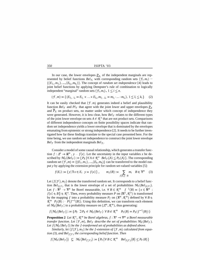
350 ISIPTA ’03

In our case, the lower envelopes PXiof the independent marginals are rep-

resented by belief functions BelFi with corresponding random sets Fi mi k E1i m1i 6! Eki mki « . The concept of random set independence [4] leads tojoint belief functions by applying Dempster’s rule of combination to logicallyindependent “marginal” random sets Fi mi O 1 > i > n. F m El1 5 5 5 ln El1 H Eln ml1 5 5 5 ln ml1 ,6 !6, mln 1 > li > ki (2)

It can be easily checked that F m generates indeed a belief and plausibilityfunction BelF and PlF that agree with the joint lower and upper envelopes PXand PX on product sets, no matter under which concept of independence theywere generated. However, it is less clear, how BelF relates to the different typesof the joint lower envelope on sets A R n that are not product sets. Comparisonsof different independence concepts on finite possibility spaces indicate that ran-dom set independence yields a lower envelope that is dominated by the envelopesemanating from epistemic or strong independence [2]. It needs to be further inves-tigated how far these findings translate to the special case presented here. For thetime being, we use random set independence to construct the joint lower envelopeBelF from the independent marginals BelFi .

Consider a model of some causal relationship, which generates a transfer func-tion f : Õ n . Õ m y f x . Let the uncertainty in the input variables x be de-scribed by MX BelF :

PX ( " A R n BelF A )> PX A O . The correspondingrandom set F m ) E1 m1 6 !ì Ek mk « can be transferred to the model out-put y by applying the extension principle for random set-valued variables [5]:

f Ei : y (EÐ x Ei y f x Lø m f B : ∑

f X Ei YÍ& B

mi B Õ m (3)

Let f F 6 m f denote the transferred random set. It corresponds to a belief func-tion Bel f X F Y that is the lower envelope of a set of probabilities MY Bel f X F Y .Let f : Õ n .¨Õ m be Borel measurable, i.e. " B R m f 1 B

x Õ m :f x C B @ R n. Then, every probability measure P on ~Õ n R n is transformedby the mapping f into a probability measure Pf on ~Õ m R m defined by " B R m Pf B : P f 1 B . Using this definition, we can transform each elementof MX BelF to a probability measure on EÕ m R m , thus generating:

f MX BelF : PY (EÐ PX MX BelF 9" B R m PY B PX f 1 B L

Proposition 2 Let R n R m be Borel algebras, f : Õ n . Õ m a Borel measurabletransfer function. Let F m , BelF describe the set of probabilities MX BelF .Let f MX BelF be the f -tranformed set of probabilities as defined above.

Similarly, let f F 6 m f be the f -extension of F m calculated from equa-tion (3), and Bel f X F Y the corresponding belief function. Then

f MX BelF MY Bel f X F Y : PY (Í" B R m Bel f X F Y B c> PY B L

Kriegler & Held: Climate Projections for the 21st Century 351

Proof. Consider an arbitrary PY f MX BelF . There exists a PX MX BelF with " B R m PY B ) PX f 1 B . For a particular, yet arbitrary B R m

PY B % PX f 1 B BelF f 1 B % ∑Ei f S 1 X B Y mi ∑

f X Ei Y, B

mi Bel f X F Y B U

3 A Random Set for a Simple Climate Model

Global Mean Temperature Model.We use a simple dynamical model to link radiative forcing F t to a change

∆T in global mean temperature (GMT) since preindustrial times [14].

Ce , ∆T + t õ F t / F2x , ∆T t T2x

(4)

Ce effective ocean heat capacity

F2x radiative forcing for a doubling of atmospheric CO2

T2x climate sensitivity

Differential equation (4) is the simplest type of energy balance model. It equatesthe net radiative flux into the system at the top of the atmosphere to oceanic heatuptake Ce∆T + . If the radiative forcing was kept constant at a value F t F2x, thesystem would undergo an equilibrium temperature change of ∆T T2x. Climatesensitivity T2x is a crucial parameter to characterize the response of the climatesystem to an increase in GHG concentrations.

The Intergovernmental Panel on Climate Change (IPCC) gives an estimateof climate sensitivity T2x 1 5 K 4 5 K [3]. The panel explicitely refrains fromspecifying probabilistic information. Recently, models of intermediate complex-ity (EMICs) were used to establish probability distributions from a comparisonof model results with historical atmosphere, surface and deep ocean temperaturedata [1, 6, 8]. Efforts are hampered by the presence of natural variability, the lackof long-term data and the multitude of forcings.

In this analysis, we use the probability distributions of [1, 6] to generate animprecise CDF model for T2x (fig. 1). The estimates of [1] are shifted to consider-ably higher values of climate sensitivity compared to [6], ranging up to values ofT2x 22 K. One reason could be that [1] does not compare their results with deepocean temperature data. [6] requires the ocean record to restrict T2x from above.However, [8] considers ocean heat uptake, and fails to discriminate between cli-mate sensitivity in the range T2x 1 K 10 K . In this situation, we simply cut of

352 ISIPTA ’03

Figure 1: Imprecise CDF model for T2x: Shown are 5%, 25%, 50%, 75% and 95% quantiles ofprobability distributions from [1, 6]. Estimates of [6] depend on a prior probability for T2x. Estimatesof [1] depend on whether solar forcing (S), volcanic aerosol forcing (V) and tropospheric ozone (T)was added to greenhouse gas (G) and aerosol forcing (A). The capital letters G, A, T, S, V in the figurekey specify the radiative forcing components that were considered for the particular estimate of [1].

the probability distributions of [1] at T2x 10 K, and allocate their total probabil-ity mass P T2 10 K to this value.

Fig. 1 depicts the resulting ranges for 5%, 25%, 50%, 75% and 95% quantileestimates in [1, 6]. We interpolate the extreme values of the ranges to generatea lower and upper CDF, and approximate the resulting imprecise CDF modelwith two step functions SFd and SF d (Fig. 1). There is some arbitrariness here.It could be resolved by fixing the number of “step” points T2x i d and T d2x j, andcalculating the optimal approximation according to some accuracy measure [7,12]. Algorithm 1 is applied to construct a random set FT2x mT2x that correspondsto MT2x SFd SF d« :

P ( " T2x Õ SFd T2x -> P / ∞ T2x > SF dÏ T2x L (in thesense of proposition 1). MT2x SFd SF d6 can be compared with the IPCC estimate[1.5 K, 4.5 K] for climate sensitivity. The probability for T2x [1.5 K, 4.5 K] liesin the interval 0 1 , for T2x : 1 5K in 0 0 25 , and for T2x ? 4 5 K in 0 0 75 . Thenumbers show that MT2x SFd SF d6 does not support the IPCC estimate, especiallyfor high climate sensitivities T2x ? 4.5 K. This reflects the fact that the upperbound of the IPCC estimate is not supported by [1, 6, 8].

Effective ocean heat capacity Ce is an artificial quantity that arises from thesimple form of the energy balance model (4). It depends on ocean characteristics,but also on climate sensitivity [3]. A comparison of model (4) with emulationsof different AOGCMs suggest a functional dependence of Ce on T2x of the formCe T γc

2x with 0 : γc > 1. We specify an interval uncertainty for the parametersC Ce T2x 3 K and γc, which is an adequate choice in the light of the large

Kriegler & Held: Climate Projections for the 21st Century 353

uncertainty surrounding ocean characteristics like vertical diffusivity [6]. Intervaluncertainty is the simplest form of an imprecise CDF model. Lower and upperCDF are either 0 or 1. The model can be immediately captured by a random set FC γc

mC γc containing just one focal element E [40 Wa/m2K, 50 Wa/m2K]

[0.6,1] with probability mass assignment m E - 1.An additional uncertainty concerns the present day global mean warming ∆To

since 1860, which enters model (4) as initial value. Estimates of ∆To lie in therange 0 6 - 0 2 K. We adopt the interval uncertainty [0.4 K, 0.8 K] for ∆To, sinceits small influence on future GMT projections does not justify a more complicatedimprecise CDF model.

Radiative Forcing Model.We group the anthropogenic sources of radiative forcing F t into carbon

dioxide, which is the most important GHG, the “other” greenhouse gases (OGHG)including both the remaining direct as well as indirect GHGs, and aerosols. So-lar and volcanic sources are neglected since we are interested in estimating theanthropogenic climate change signal.

F t N F2x ln Û CCO2 t CCO2 1750 Ü D ln2 FAer g EAer t F FOGHG h t (5)

CCO2 atmospheric CO2 concentration

EAer anthropogenic sulfate aerosol emissions

FAer Total aerosol forcing in the period 1990-2000

FOGHG Total OGHG forcing in the period 1990-2000

The radiative properties of aerosol particles are most uncertain. Aerosols in-fluence the radiation balance not only directly, but also indirectly by altering cloudformation processes. The IPCC estimates that the negative forcing of aerosols hasbeen in the range [-0.8 W/m2, -0.2 W/m2] (direct effect) and [-2 W/m2, 0 W/m2](indirect effect) for the period 1990-2000 [10]. [1, 6, 8] have investigated FAer intheir comparison of model results with historical data. Fig. 2 shows the rangesfor the 5%, 25%, 50%, 75% and 95% quantile estimates from [1, 6]. [8] presentsa histogram probability which can be converted into two step functions for thelower and upper bound on the CDFs that are supported by the probability massesallocated to the bins of the histogram. Analogous to the case of climate sensitivity,we construct a lower CDF SFd and upper CDF SF d (solid lines in fig. 2). Algo-rithm 1 is used to generate the random set MFAer mFAer that corresponds to theimprecise CDF model MFAer SFd SF d .

The probability that FAer is contained in the IPCC estimate [-2.8 K, -0.2 K](direct and indirect effect combined) lies in the range 0 95 1 . In contrast to cli-mate sensitivity, the IPCC range includes MFAer SFd SF d6 almost entirely. Theresults in [1, 6, 8] support a more narrow range, where in particular the potentialof a very strong negative aerosol forcing contribution is discarded.

354 ISIPTA ’03

Figure 2: Imprecise CDF model for FAer : Shown are 5%, 25%, 50%, 75% and 95% quantiles ofprobability distributions from [1, 6], and a histogram probability from [8]. See Fig. 1 for additionalexplanation of the figure key.

Estimates for the radiative forcing contributions of indirect GHGs, in particu-lar troposheric and stratospheric ozone, exhibit relative errors between 40%-70%.The indirect GHGs have contributed around 30-40% to FOGHG in the last decade.We capture the uncertainty by the interval FOGHG 0 8 W/m2 1 2 W/m2 .

We link the uncertainty in the time-dependent paths of atmospheric CO2 con-centration CCO2 t , future changes in the radiative forcing of the OGHG h t , andanthropogenic aerosol emissions EAer t directly to the socio-economic sphere.Thereby, we neglect any uncertainty about the response of the biogeochemicalcycles to anthropogenic emissions. In a special report on emissions scenarios(SRES) [9], the IPCC has formulated a range of scenarios describing future path-ways of society and economy on a global scale. The major branching points ofthese scenarios are globalization vs. regionalization and sustainability orienta-tion vs. growth orientation. In this analysis, we specify just two parameters G(“Growth”) and S (“Shift”), with CCO2 t O h t eGt St2

. We restrict S >G D 200, so that the growth in atmospheric CO2 concentration and radiative forcingof OGHGs can be dampened, but not reversed by a “shift” S in the 21st century.

As the future socio-economic development is entirely uncertain, it is appropri-ate to specify interval uncertainties for G 0 004 D a 0 012 D a and S 0 G D 200 .Growth rates from 0.4% to 1.2% per year lead to atmospheric CO2 concentrationsfrom 480 ppmv to 1230 ppmv in 2100 (present day: 370 ppmv), and to a forcingcontribution of the OGHG from 1 W/m2 to 4 W/m2. This covers the full range ofthe SRES scenarios including uncertainty in the biogeochemical cycles [3].

Combining the Random Set Information.

Kriegler & Held: Climate Projections for the 21st Century 355

Most parameter pairs are physically and epistemically independent. Presentday warming To depends physically on climate sensitivity and ocean heat capac-ity, but knowledge of To alone does not constrain the assessment of T2x and Ce. Amore critical issue is the epistemic dependence of FAer and T2x. Although physi-cally independent, comparisons of model results with historical data will have atendency to produce high estimates of T2x for a large negative radiative forcingFAer of aerosols, and vice versa [6]. Neglecting this dependence will yield a moreimprecise estimate of future GMT change, since the probability weight of com-binations with large negative FAer and low T2x leading to a weak GMT increase,and with small negative FAer and high T2x leading to a strong rise of GMT, will beoverestimated. This issue needs to be investigated in further studies. For the timebeing, we use equation (2) based on random set independence to combine the ran-dom sets for all eight parameters par : ∆T0 T2x C γc FAer FOGHG G S to ajoint random set Fpar m .4 Estimation of Global Mean Temperature Change

Differential equation (4) and radiative forcing model (5) generate a continuoustransfer function that maps the uncertain model parameters to an increase ∆Tin GMT since 1860. The extension principle for random sets ([5], equation 3)transfers the random set Fpar m for the uncertain parameters to a random set F∆T m for GMT increase. In our specific case, the images f Ei par ∆T i t 6 ∆T i t can be calculated with standard gradient-based optimization meth-ods. After discretizing time in sufficiently small time steps ∆t, the boundaries ofthe range at time tk k ∆t to are found by solving

∆T i tk N minX ∆T0 T2x C γc FAer FOGHG G S YH Ei . par

∆T tk (6)

subject to ∆T tl ) ∆T tl 1 F ∆t ,Û F tl 1 Ce

/ F2x

Ce, ∆T tl 1

T2xÜ 1 > l > k

∆T i tk N maxX ∆T0 T2x C γc FAer FOGHG G S YH Ei . par

∆T tk (7)

subject to ∆T tl ) ∆T tl 1 F ∆t ,Û F tl 1 Ce

/ F2x

Ce, ∆T tl 1

T2xÜ 1 > l > k

It can be checked that ∆T t is monotone in ∆To C γc FAer FOGHG G S andconvex in T2x. The latter is due to the fact that T2x influences ∆T both directlyand indirectly through its connection to effective ocean heat capacity. Thus, pro-gram (7) is a well-defined convex optimization problem. Care has to be taken withprogram (6). The solution will be a boundary point of the focal element Ei par, andwe have to check both for the lower and upper bound of T2x.

Fig. 3 shows the image ∆T t 6 ∆T t of a single focal element. The range

356 ISIPTA ’03

Figure 3: Image / ∆T t ∆T t 10 of a single focal element E v [1.8 K, 6.0 K] 2 [-1.37 W/m2,-0.62W/m2] 2W ∆To C γc FOGHG G S Fpar for the years 2025, 2050, 2075 and 2100. Shown are also thecases with solely socio-economic or solely forcing and climate uncertainty.

of the image grows considerably in time. We performed a sensitivity analysiswith partly resolved uncertainty. Uncertainty in the radiative forcing and climateparameters dominates the overall uncertainty in the first half of the 21st century,but socio-economic uncertainty becomes equally important in the second half ofthe 21st century. Most strikingly, the uncertainties on the subspaces combine in anonlinear way. A much larger overall uncertainty is found in particular for caseswhere the natural systems and socio-economic uncertainties are of similar size.

The projected random set F∆T m for GMT increase can be used to constructthe lower CDF F∆T and upper CDF F∆T . It is important to note that the corre-sponding imprecise CDF model M∆T F F :

P ( " x Õ F∆T x W> P / ∞ x >F∆T x L can be more imprecise than M∆T BelF∆T :

P (Í" A A BelF∆T A ->P A O , i.e. M∆T F F 43 M∆T BelF∆T . This is due to the fact, that after applyingthe extension principle, the focal elements Ei ∆T ∆T i t 6 ∆T i t F∆T mightviolate condition (II) of proposition 1. In this case, the lower envelope P∆T ofM∆T F F is strictly smaller than BelF∆T for some A A . Recalling proposi-tion 2, it can be seen that M∆T F F does not contain more information than Fpar m , which captures the uncertainty in the model parameters, would allow.

M∆T F F 53 M∆T BelF∆T 63 Mpar BelFpar Fig. 4 shows the lower and upper CDFs that are generated by the random set F∆T m . We consider the area between lower and upper CDF as an indicator for

the imprecision in the uncertainty. It can be seen that the imprecision in the GMT

Kriegler & Held: Climate Projections for the 21st Century 357

a. Full uncertainty b. Forcing and climate uncertainty only

c. Climate uncertainty only d. Forcing uncertainty only

Figure 4: Lower and upper CDFs for GMT increase ∆T in the years 2025, 2050, 2075, 2100

estimate for the case of full uncertainty in the model parameters is enormous.This is partly due to the large number of uncertain parameters, as a comparisonwith the other cases shows. However, the cases (4.b) and (4.c) also exhibit largeimprecision. This reflects the fact that the underlying imprecise CDF models forthe climate parameters are already very imprecise. Certainly, they are conservativeestimates, as the results of different studies were not weighed against each other.Some imprecision is also induced by the combination of the uncertainty for singleparameters using random set independence (sec. 3).

The results can be compared with the IPCC estimate [1.8 K, 6.6 K] for GMTincrease in 2100 relative to 1860 [3]. The probability for ∆T [1.8 K, 6.6 K] liesin the interval 0 1 , for ∆T : 1.8 K in 0 0 95 , and for ∆T ? 6.6 K in 0 0 965 .Despite the large range of the IPCC estimate, the uncertainty in GMT increaseis too imprecise to discriminate against values outside this range. The probabilitymass allocated to values smaller than 1.8 K stems from random sets allowing forclimate sensitivity values that are below the IPCC estimate for climate sensitivity.Similarly, the probability mass allocated to GMT increases higher than 6.6 Kis due to climate sensitivity values above the IPCC estimate. As a comparison

358 ISIPTA ’03

of (4.c) and (4.d) underlines, the uncertainty in climate parameters is the mostinfluential factor on the uncertainty in GMT increase.

5 Conclusion

Imprecise probability concepts carry the potential to consistently capture the dif-ferent types of uncertainties and different degrees of knowledge that are encoun-tered in climate change analysis. However, they need to be applicable to dynam-ical problems with a large number of continuous uncertain variables. We suggestthat imprecise CDF models are conceptually flexible and mathematically tractableenough to fulfil these competing requirements to some extent. When the impre-cise CDF model is bounded by lower and upper step functions on the real line, theinformation about the encompassed set of additive probabilities can be condensedin a random set F m . The corresponding belief function BelF is the lower en-velope of the imprecise CDF model on the algebra generated by the half-closedintervals of the real line. Moreover, if the random set extension principle is usedto project a random set onto the range of a measurable function, no information isadded in the sense that every additive probability dominating BelF is transferredinto a probability dominating the “extended” belief function.

We have constructed a random set for a simple climate model, and projected itonto an estimate for global mean temperature increase. The resulting estimate isvery imprecise, with uncertainties about socio-economic development, radiativeforcing and climate characteristics combining in a nonlinear way. The large im-precision of the estimate has different reasons and implications. Firstly, we incor-porated a very broad range of factors in the analysis. Imprecision will be reducedif the range of factors is limited by formulating more specific questions. Secondly,we combined the random sets of single uncertain factors by assuming random setindependence. This has increased the imprecision in the overall estimate, sinceaerosol forcing and climate sensitivity are not epistemically independent, whenestimated from the present day climate change signal. Thirdly, the CDF modelsfor the single parameters should be considered conservative estimates, which canbe improved upon, when more comparisons of model results with historical databecome available. Imprecision can be reduced in particular, if it is discriminatedbetween the reliability of different models and methods.

Nevertheless, the results show that uncertainty is a key issue in the integratedassessment of climate change. Random set methods provide new insights into thestructure of the uncertainty, particularly into its imprecision. The link to impreciseCDF models seems to be an important yardstick for assessing information losseswhen combining random sets, and applying the extension principle. More theo-retical work is needed here to enhance the applicability of random sets to climatechange analysis. In addition, methods need to be developed to determine impre-cise CDF models directly from a comparison of model results with historical data.

Kriegler & Held: Climate Projections for the 21st Century 359

References[1] Andronova, N. G., and Schlesinger, M. E. Objective estimation of the probability

density function for climate sensitivity. Journal of Geophysical Research 106 (2001),22605–22611.

[2] Couso, I., Moral, S., and Walley, P. Examples of independence for imprecise proba-bilities. In Proceedings of the First International Symposium on Imprecise Probabil-ities and Their Applications (1999), pp. 121–130.

[3] Cubasch, U., and Meehl, G. Projections of future climate change. In Climate Change2001: The Scientific Basis, J. Houghton and Y. Ding, Eds. Cambridge UniversityPress, Cambridge, 2001, pp. 525–582.

[4] Dempster, A. P. Upper and lower probabilities induced by a multivalued mapping.Ann. Math. Statist. 38 (1967), 325–339.

[5] Dubois, D., and Prade, H. Random sets and fuzzy interval analysis. Fuzzy Sets andSystems 42 (1991), 87–101.

[6] Forest, C. E., Stone, P. H., Sokolow, A. P., Allen, M. R., and Webster, M. D. Quanti-fying uncertainties in climate system properties with the use of recent climate obser-vations. Science 295 (2002), 113–117.

[7] Hall, J., and Lawry, J. Generation, combination and extension of random set ap-proximations to coherent lower and upper probabilities. Reliability Engineering andSystem Safety (2003), in press.

[8] Knutti, R., Stocker, T. F., Joos, F., and Plattner, G. K. Constraints on radiative forcingand future climate change from observations and climate model ensembles. Nature416 (2002), 719–723.

[9] Nakicenovic, N., and Swart, R. Emissions Scenarios. Special Report of the IPCC.Cambridge University Press, Cambridge, 2000.

[10] Ramaswamy, V. Radiative forcing of climate change. In Climate Change 2001:The Scientific Basis, J. Houghton and Y. Ding, Eds. Cambridge University Press,Cambridge, 2001, pp. 289–348.

[11] Shafer, G. A Mathematical Theory of Evidence. Princeton U. Press, Princeton, 1976.

[12] Tonon, F. Using random set theory to propagate uncertainty through a mechanicalsystem. Reliability Engineering and System Safety (2003), in press.

[13] Walley, P. Statistical Reasoning with Imprecise Probabilities. Chapman and Hall,London, 1991.

[14] Watterson, I. G. Interpretation of simulated global warming using a simple model.Journal of Climate 13 (2000), 202–215.

H. Held is with the Potsdam Institute of Climate Impact Research, Germany. E-mail:kriegler@pik-potsdam.de

E. Kriegler is with the Potsdam Institute of Climate Impact Research, Germany. E-mail:kriegler@pik-potsdam.de

Exploring Imprecise ProbabilityAssessments Based on Linear Constraints

RADU LAZARUniversity of Minnesota, USA

GLEN MEEDENUniversity of Minnesota, USA

Abstract

For many problems there is only sufficient prior information for a Bayesiandecision maker to identify a class of possible prior distributions. In such casesit is of interest to find the range of possible values for the prior expectationfor some real valued function of the parameter of interest. Here we showhow this can be done when the imprecise prior assessment is based on linearconstraints. In particular we find the joint range of possible values for a pairof such functions. We also study the joint range of the posterior expectationfor a pair of functions.

Keywords

linear constraints, probability assessment, Bayesian inference, Metropolis-Hastingsalgorithm

1 Introduction

Consider the usual statistical inference problem where a subjective Bayesian mustselect a prior probability distribution which reflects their prior knowledge and be-liefs about the unknown state of nature. Often one is unable to actually choose asingle prior even though some prior information is present. When this occurs theBayesian often selects a family of possible prior distributions. In such cases onecould be interested in the range of possible values for some function defined onthe the family of possible priors. More generally one could be interested in the setof possible values for a pair of functions. By judiciously selecting different pairsof functions such a graphical representation could help the Bayesian assess howsensible their initial choice for the family of priors really is. These graphical rep-resentations could help a pair of experts resolve possible conflicting prior beliefs.It could be used to check for areas of disagreement and to see how adjustments ofsome of their beliefs could lead to a merging of opinions.

360

Lazar & Meeden: Exploring Imprecise Probability Assessments 361

In section two we assume that the parameter space contains only a finite num-ber of points, say k. If p \ p1 pk denotes a typical prior distribution weassume that the prior information can be expressed through linear equalities andinequalities involving the pi’s. This restricts the class of possible priors to a con-vex subset, C say, of the k / 1 dimensional simplex of possible probability vectorsof length k. Note C must be a convex polytope generated by a finite number ofextreme points or vertices. Let φ denote a real valued function defined on the pa-rameter space. Then its prior expectation is a linear function on C . Dickey (seeDickey (2003)) has developed an interactive computing environment which com-putes the minimum and maximum of its expectation over C . This programs allowsthe statistician to incorporated their prior information in stages and see how therange of φ changes. Here we are interested in finding the range of a pair of suchfunctions. Because the prior expectations of the two functions are linear functionsof p the range of possible values must be a convex set. Moreover, its extremepoints must be contained in set of points which are images of the extreme pointsof C . Hence, this problem is easily solved if one knows the extreme points of C .But these can be found using a program that developed by Fuduka. See Fuduka(2003).

When considering the posterior expectation of such functions our problembecomes much more difficult analytically since the posterior expectation is nolonger a linear function over C . However, knowing the extreme points of C letsone find an approximate solution quite easily. Using these points one can generaterandom values in C by assigning random weights to them. Then one finds thevalues of the two functions at each of the realizations and plots these pairs ofvalues.

In section three we consider the situation where the parameter is a r dimen-sional vector. We assume that it belongs to a convex polytope in r-dimensionalEuclidean space defined by some known linear equalities and inequalities whichreflect some of prior information of the statistician. A Bayesian needs to selecta prior or possibly a family of prior distributions over this set to further reflecttheir uncertainty. For a given prior one is interested in computing prior and pos-terior expectations of some function of the parameter. In practice, it is usually notpossible to make independent draws from a probability density defined on such aset. In such cases statisticians often employ Markov chain Monte Carlo methodsto generate dependent samples from the posterior from which expectations can becomputed approximately. Here, we use the Metropolis-Hastings algorithm to con-struct dependent samples drawn from a prior of interest. If the statistician selectsas their family of priors all possible convex combinations of some finite collectionof priors defined on the parameter space then for any pair of functions defined onthe parameter space one can find the range of all possible values of their prior orposterior expectations.

As far as we know statisticians have not really addressed problems whereimprecise knowledge is expressed through linear constraints. In section four we

362 ISIPTA ’03

will note examples of somewhat similar problems that have been studied in theoperations research literature. Finally, we will point out some of the difficultieswhen either the dimension of C or the parameter space gets too large.

2 The parameter space is finite

We begin by assuming that the parameter space contains only finitely many points,say k. In k-dimensional Euclidean space let Λ denote the k / 1 dimensional sim-plex of p vectors with pi 0 and ∑k

i & 1 pi 1. We assume that the known relationsamong the pi’s can be expressed by

Ap a (1)

where A is a known r k matrix and a is a known vector of length r and

Bp > b (2)

p 0 (3)

where B is a known s k matrix and b is a known vector of length s. The set ofp Λ which satisfy the above equations form a closed convex subset of Λ whichwe will denote by C .

Note that the interior of C is empty but we assume that properly consideredC will have a nonempty interior in some smaller dimensional Euclidean spacewith a dimension of at least two. If φ1 and φ2 are two functions defined on theparameter space we let C φ1 φ2 denote their range of possible values over C . Ourproblem is to find this set. To see what could happen in practice we consideredthe following simple example.

Example 1 We let k 10 and imposed two equality constraints and two inequal-ity constraints. The equality constraints were p5 p6 and ∑10

i & 1 ipi 5 5 while theinequality constraints were p1 > p2 and ∑4

i & 1 pi > 0 5. When doing the posteriorcalculations we assumed that the probabilities of seeing the observed data underthe 10 possible parameter values were 0.1, 0.15, 0.09, 0.2, 0.3, 0.2, 0.1, 0.05, 0.07and 0.02.

As we noted in the introduction C φ1 φ2 is a convex set whose extreme pointsare contained in the image of all the extreme points of C . Hence, this becomes aneasy problem once we know the extreme points of C .

Fortunately for many problems the extreme points of C can be found easilyusing a program that is available over the Internet. See Fuduka (2003). It turns outfor our example that C has 28 extreme points.

For definiteness we let φ1 i c i / 5 5 2 for i 1 10 and φ2 be the indi-cator function of the set

2 3 4 5 .

Lazar & Meeden: Exploring Imprecise Probability Assessments 363

Plotting φ1 and φ2 at the extreme points of C we found the seven extremepoints of C φ1 φ2 .

Since we know the extreme points of C we can use the Dirichlet family ofdistributions to generate a fairly flexible class of distributions which take values inC and from which one can simulate directly. If q1 qm are the extreme points ofC and W is Dirichlet α where α ½ α1 αm then ∑M

i & 1 Wiqi defines a randomdistribution on C . In some cases one may be able to make a judicious choice ofα if some partial information about the φ’s are available. For our example wegenerated 1,000 random values using the Dirichlet distribution with each of the10 parameter values set equal to 0.1.

In the upper plot of Figure 1 we plotted the posterior expectations of theφ’s for these 1,000 pairs of values along with the seven extreme points for theprior expectations. The prior expectations are darker and four of these points areclearly visible. They form the lower boundary of C φ1 φ2 . Another, (14.03,0.56),is clearly visible as well but maybe hard to identify because the plot is quite small.The other two, (3.82,0.64) and (4.58,0.67), are totally obscured by the posteriorexpectations. As to be expected the posterior expectations form a smaller set thanthe prior expectations.

Being able to find the extreme points of C is a powerful tool. In our somewhatlimited experience the program we used seems quite good. In one constrainedproblem we considered in a different context it found over 28,000 extreme points.Using the Dirichlet distribution on the set of weights associated with the extremepoints is a convenient distribution to sample from. These distributions are knownas multivariate B-splines and are well studied. See for example Dahmen and Mic-chelli (1983). If one had a closed form expression for their densities then onecould use importance sampling to approximate expectations under other densi-ties. Unfortunately this can only be done in practice for very small problems. Seefor example Choudhuri (2003).

In practice one would use a much larger sample that 1,000 when studying theposterior expectations. But if the dimension of C gets to large one may not beable to take a large enough sample to get a reasonable approximation. In suchcases one can find the minimum or maximum of the posterior expectation of aparticular φ using a random search. The basic idea underlying random searches iswell know and is quite simple. See for example Swann (1974).

3 The parameter space is a convex polytope

Here we will consider cases where the parameter space is no longer finite. Wewill assume that the parameter is a m dimensional vector, θ and that any possiblechoice for θ must satisfy

Aθ a (4)

364 ISIPTA ’03

where A is a known r m matrix and a is a known vector of length r and

Bθ > b (5)

where B is a known s m matrix and b is a known vector of length s.These constraints represent some of the statistician’s prior information about

θ. The parameter space, Θ, is the set of all θ which satisfy the above two equations.It is a convex polytope in m dimensional Euclidean space with an empty interior.

We begin by assuming that the statistician can select a prior density f overthe parameter space to reflect the rest of their prior information. After discussingthis case we will consider the situation where the statistician can only determinea family of possible prior densities.

Let φ denote some function defined on Θ. Then we are interested in finding

µ ÊΘ

φ θ h θ dθ (6)

approximately. Interesting choices of h include f and the posterior density of θunder f given the data.

For most cases of interest this means employing Markov chain Monte Carlomethods. Here we will use the Metropolis-Hastings algorithm. With the Metropolis-Hastings algorithm one generates dependent observations, Y1 Y2 from a suit-able chosen Markov chain with values in Θ and then calculates

µn 1n

n

∑i & 1

φ Yi In nice situations µn . µ almost surely.

If the current value of the chain is θ d then one selects a proposal value for thenext possible value in the sequence, θ + , according to some probability distribution.Whether or not this new value is used depends on this probability distribution andthe value of h at the two points. If q u v denotes the probability of selecting v asthe proposal point when u is the current value we let

R h v q v u h u q u v (7)

and accept the proposal with probability min 1 R . From this equation we see thatthe density h needs to be know only up to a constant since the value of R does notdepend on this value.

We now explain how this can be done for our problem. Suppose θ d is ourcurrent state which is assumed to lie in the relative interior of Θ. In particular,this means that it yields a strict inequality in all the equations in 5. There is anintuitive two step process by which we can choose the proposal. First, we select arandom direction, d, in Θ. Remember that even though d is a vector of length m

Lazar & Meeden: Exploring Imprecise Probability Assessments 365

it must remain in Θ which is essentially a lower dimensional set. The distributionfor choosing d will not depend on the value θ d Next, we find the set of points inΘ which lie either in the direction d or / d from θ d and choose the proposal atrandom from this set.

It is important to note that for this scheme if θ + is the proposal then

q θ d θ + q θ + θ d This follows because if d is the direction from θ d to θ + then the only way to movefrom θ d to θ + is if the directions d or / d were selected in the first step. Of coursethe same is true if we are moving from θ + to θ d . Clearly, the second step hasthe same distribution no matter which of the two points was chosen as the initialpoint.

To implement this scheme we proceed as follows. To get our direction d wechoose at random a vector from S , the unit sphere in m dimensional Euclideanspace and then project it onto the null space of A. Next, we normalize this vectorso that its length is one and denote it by d. Remember that d S . Let S A denotethe the subset S consisting of all vectors which can be generated in this way. Sincewe use the uniform distribution on the surface of S to choose the first vector,the distribution of d must be uniform on S A . This follows by symmetry. Theprobability of d falling in any region of some fixed shape is independent of thelocation of the region in S A .

Let θ d denote a point which lies in the relative interior of Θ and considervectors of the form

θ d αd (8)

where α is a real number. Note if d does not belong to the null space of A thispoint cannot belong to Θ whenever α < 0. On the other hand if Ad 0 and αis sufficiently close to zero then this point will belong to Θ. Hence, α should beselected from the set of possible values that satisfy all the constraints of equation5. This is a total of s constraints. Each constraint will result in either an upper orlower bound for α. Consider the interval formed by the maximum of these lowerbounds to the minimum of these upper bounds. This is the range of possible valuesfor α for which the vector in equation 8 will belong to Θ. Given a θ d and a d inthis equation then one just selects a value for α from the uniform distribution onits interval of possible values resulting in the proposal

θ + θ d αd

To recap, this is essentially a very simple procedure. Given a current value inthe interior of Θ we first pick a random direction in Θ and then find how far we canmove either in this or the opposite direction and still remain in Θ. Note that thismethod of selecting a proposal point does not depend in any way on the functionh although from equation 7 the probability of it being accepted does depend on h.When h is the uniform distribution then the proposal is always accepted.

366 ISIPTA ’03

Suppose now the statistician does not have enough prior information to selecta single prior density over Θ but can only specify a family of possible priors onΘ. A convenient and often sensible choice for such a family is all possible convexcombinations of some finite set of densities. Let f1 ì fn denote such a finite setof densities and Π the be the family of all possible convex combinations of thefi’s. For a function φ define on Θ let Π φ be the range of possible values of theprior expectation of φ as the prior ranges over all members of Π. Since for each f i

we can find its φ expectation approximately we can find Π φ approximately. It isjust the interval from the minimum to the maximum of these n prior expectations.Suppose instead we wished to find the joint range of the prior expectations of twofunctions as the prior ranged over Π, say Π φ1 φ2 . This is easily done since itis just the convex hull of all points of the form 2 φ1 fi 2 φ2 fi for i 1 n.Posterior calculations are handled in exactly the same way since for any priorin Π the posterior is just a convex combination of the n posteriors. Finally, weemphasize the importance of only needing to know any probability density up toa constant since for most of these kind of problems the normalizing constant willbe unknown.

Example 2 We let m 5 and supposed θ is the parameter for the multinomialdistribution. We imposed the constraints θ1 > θ2, θ1 θ2 D 2 >ú θ3 θ4 θ5 D 3and θ4 > θ5 to get the parameter space Θ. We assumed the class of possible priorsis all possible convex combinations of three Dirichlet distributions restricted toΘ. These were taken to be Dirichlet(2,2,2,2,2), Dirichlet(0.5,0.5,0.5,0.5,0.5) andDirichlet(0.5,1.0,1.5,2,2.5). The two functions of interest were φ θ W θ4 / θ3 andφ2 θ e θ5 / θ3. To compare the prior and posterior expectations we assumedthat a random sample of size 20 had been observed with the observed counts ofstates 1, 2, 3, 4 and 5 being 2, 3, 4, 3 and 8 respectively.

Using our methods we found approximately the three extreme points of Π φ1 φ2 and the corresponding extreme points for the posterior problem. As we noted be-fore it is crucial that the densities on Θ need only be known up to a constant to findthese integrals approximately. The results are given in the lower plot of Figure 1.The prior expectations are marked by 0 and the posterior expectations are markedby x. As to be expected the posterior range is much smaller than the prior range.Using our approach and considering various sets of constraints, families of priors,choices of φ1 and φ2 and hypothetical samples can be useful in helping one selecta sensible representation of their prior beliefs for a particular problem.

We end this section by noting that our method of picking a proposal point canbe adapted to the random search method we mentioned in section 2. Formally, thetwo spaces C and Θ are essentially the same. In the random search algorithm givena point in the interior of C one needs to be able to choose a point at random froma small neighborhood that contains it. Hence after a direction has been selectedat random rather than allowing a move that is as far as possible in either direction

Lazar & Meeden: Exploring Imprecise Probability Assessments 367

0 5 10 15

0.2

0.3

0.4

0.5

0.6

0.7

0.8

−0.20 −0.15 −0.10 −0.05

0.15

0.20

0.25

0.30

0.35

x

x

x

Figure 1: The upper plot contains the seven extreme points for the prior expecta-tions and the plot of 1,000 posterior expectations for the functions φ1 and φ2 inExample 1. The lower plot gives the extreme points for prior (marked by 0) andposterior (marked by x) expectations of φ1 φ2 for Example 2. In both cases thehorizonal and vertical axes are the φ1 and φ2 expectations respectively.

368 ISIPTA ’03

one restricts the new point to be no more than ε away in either direction from thecurrent point where ε ? 0 is fixed.

4 Discussion

Although constraints seem a natural way to incorporate prior information into aninference problem they have not been widely considered in the statistical litera-ture. The main reason seems to be that they are difficult to deal with both theo-retically and practically. Betro and Guglielmi (2000) considered robust Bayesiananalysis under moment constraints in a fairly abstract setting and concluded thatnone of the current algorithms were good enough to be adopted for routine use.Generating random samples from distributions defined over bounded subsets of mdimensional Euclidean has been considered in a variety of contexts. Smith (1984)considers the problem of generating independent uniform observations from abounded region while Belisle, Romeijin and Smith (1993) considers algorithmsfor generating observations from a general multivariate distribution. They assumethat the region of interest is open with a nonempty interior which will not workhere. Boender et al. (1991) and Chen and Schmeiser (1993) consider somewhatrelated problems.

At the present time Markov chain Monte Carlo methods seem to be the bestway to handle the types of problems considered in section 3. They come with noguarantees however. If run long enough they will converge to the correct answerbut in a given example it can be very difficult to know when to stop. When m islarge it is impossible to visualize Θ. From our experience, it seems one shouldselect a starting value for θ that is somewhere in the “center” of Θ. In some casesit seems that it is possible for the chain to spend long periods trapped in a cornernear the boundary of Θ. If you start in the center then any region of Θ you even-tually reach you will also eventually leave. When trying to compute equation 6approximately it is not necessary to visit every niche and corner of Θ especiallythose where h puts little weight. But in examples we have studied we have seenthat it can take a very long time to reach certain regions very near the boundary.As be noted by many authors when m increases we must deal with the “curse ofdimensionality”. For a helpful discussion on the convergence of Markov chainMonte Carlo simulations see Geyer (1992) and Gelman and Rubin (1992).

The methods discussed here not only can help a single statistician evaluatethe consequences of their prior assessments but could help a pair of experts re-solve possibly conflicting prior beliefs. It can be used to check how areas of dis-agreement will effect their inferences. It could help them study how adjustmentsof some of their beliefs could lead to a merging of opinions. Clearly this is nota theory of how to readjust one beliefs when face with new information but away to explore the consequences of readjustments of linear constraints. Here wehave emphasized exploring jointly the prior or posterior expectations for a pair of

Lazar & Meeden: Exploring Imprecise Probability Assessments 369

functions. The methods work for jointly exploring three and even more functionshowever convenient graphical representations are no longer possible.

Our simulations were done using R. We are preparing a small package thatwould make it easy for others to implement these methods. Once it is finished wewill submit it to the R archives for public distribution. We hope to complete thissometime this year.

Finally, the authors wish to thank Charles Geyer for many helpful discussions.

References

[1] C. J. P. Belisle, H. E. Romeijn and R. L. Smith. Hit-and-Run Algorithmsfor Generating Multivariate Distributions. Mathematics of Operations Re-search, 18:255-266, 1993.

[2] B. Betro and A. Gugliemi. Methods for Global Prior Robustness underGeneralized Moment Conditions. In Robust Bayesian Analysis (D. R. Insuaand F. Ruggeri eds.) 273-293, Springer 2000.

[3] C. G. E. Boender, R. J. Caron, J. F. McDonald, A. H. G Rinnooy Kan, H. E.Romejin and R. L. Smith. Shake-and-Bake Algorithms for Generating Uni-form Points on the Boundary of Bounded Polyhedra. Operations Research39: 945-954, 1991.

[4] M. Chen and B. Schmeiser. Performance of the Gibbs, Hit-and-Run andMetropolis Samplers. Journal of Computational and Graphical Statistics,2, 251-272, 1993.

[5] N. Choudhuri. Computing Multivariate B-splines: A Simulation Based Ap-proach. Technical Report, Case Western Reserve University, 2003.

[6] W. Dahmen and C. A. Micchelli. Recent Progress in Multivariate Splines.In Approximation Theory IV (C. K. Chui, L. L. Schumaker and J. D. Ward,eds.) 17-121. Academic Press, New York 1983.

[7] J. M. Dickey. Convenient Interactive Computing for Coherent ImprecisePrevision Assessment. submitted to ISIPTA ’03, 2003.

[8] K. Fuduka. cdd and cddplus Homepage for locating vertices.http://www.cs.mcgill.ca/ fukuda/soft/cdd home/cdd.html, 2003.

[9] A. Gelman and D. B. Rubin. Inference from Iterative Simulation UsingMultiple Sequences. Statistical Science, 7, 457:472, 1992.

[10] C. J. Geyer. Practical Markov Chain Monte Carlo. Statistical Science, 7,473-483, 1992.

370 ISIPTA ’03

[11] W. H. Swann. Constrained Optimization by Direct Search. In NumericalMethods for Constrained Optimization (P. E. Gill and W. Murray, eds.) 191-217. Academic Press, New York 1974.

[12] R. L. Smith. Efficient Monte Carlo Procedures for Generating Points Uni-formly Distributed over Bounded Regions. Operations Research 32:1296-1308, 1984.

Radu Lazar is a graduate student in the School of Statistics at the University of Minnesota,Minneapolis, MN 55455, USA. E-mail: lazar@stat.umn.edu

Glen Meeden is with the School of Statistics at the University of Minnesota, Minneapolis,MN 55455, USA. E-mail: glen@stat.umn.edu

Continuous Linear Representation ofCoherent Lower Previsions

SEBASTIAN MAASSUniversitat Bremen, Germany

Abstract

This paper studies the possibility of representing lower previsions by con-tinuous linear functionals. We prove the existence of a linear isomorphismbetween the linear space spanned by the coherent lower previsions and thatof an appropriate space of continuous linear functionals. Moreover, we showthat a lower prevision is coherent if and only if its transform is monotone. Wealso discuss the interpretation of these results and the new light they shed onthe theory of imprecise probabilities.

Keywords

coherent lower previsions, Mobius transform, Choquet’s theorem, Bishop-de Leeuwtheorem, Dempster-Shafer-Shapley representation theorem

1 Introduction

The theory of imprecise probabilities especially that of coherent lower previsionshas been designed to mathematically cope with subjective behavior in decisionsituations (cf. Walley [11]). It has evolved so extensively that coherent lower pre-visions have been repeatedly reinvented under different names like e.g. “coherentrisk measures” (cf. Delbaen [4]) or “maxmin expected utility” (cf. Gilboa andSchmeidler [7]).

From an applicational and often also mathematical point of view nonlinearfunctionals like coherent lower previsions cannot as nice be handled as (mono-tone) continuous linear functionals. So, in this paper, we are interested in repre-senting the former functionals by the latter. For nonadditive set functions such arepresentation is well-known as Dempster-Shafer-Shapley Representation Theo-rem in the discrete case or as Mobius transform in the general case (cf. Denneberg[5], Gilboa and Schmeidler [6] and Marinacci [10]).

The main steps of constructing such a transformed set function run as follows.First, given a totally monotone set function ν on an algebra A , to every set A Ais assigned a function A on the extreme points of the convex set of normalized

371

372 ISIPTA ’03

totally monotone set functions and defined by A η : η A . Since the extremepoints are the filter games and therefore

0 1 -valued (cf. Choquet [3] p. 260 f.)

all A can be interpreted as characteristic functions of the setsη ( η A e 1 .

Then, by different methods, it can be shown that there exists a bijective mappingfrom the set of totally monotone set functions to the set of (positive) measures onthe σ-algebra generated by the A, A A . Finally, this bijective mapping can beextended to the linear spaces each spanned by the respective class of set functions.

In this paper we will show that the main results of these theorems do notpresuppose the functions being totally monotone set functions. Even a structureddomain like an algebra is not necessary to obtain analogous results for coherentlower previsions. In our main theorem (Theorem 2) we provide a representationtheorem for coherent lower previsions which contains results analogously to thosesketched in the preceding paragraph for totally monotone set functions.

2 Preliminaries

Let Ω be a nonempty set, B 2Ω the linear space of bounded (w.r.t. the supremumnorm) real-valued functions on Ω and K B 2Ω be nonempty. To avoid laboriousconsiderations of special cases, we will assume that there is at least one nonzerofunction in K. A lower prevision on K is a real-valued functional P : K . Õ . Alower prevision P is called coherent, if P f ∑n

i & 1 λiP fi λ0 whenever f ∑n

i & 1 λi fi λ0 with f fi K, λi ? 0, λ0 =Õ , n . This definition is not the usualone (cf. Walley [11, Definition 2.5.1]) but it follows immediately from Proposition3.1.2 (d) and Lemma 3.1.3 (b) in Walley’s book and it will be of use to prove afunctional being not coherent. Furthermore, this characterization of coherence cannicely be interpreted in the following way. As usual, Ω denotes a possibility space,K a set of gambles, i.e. positive or negative rewards depending on the uncertainstate ω Ω. A lower prevision P of a gamble f is then the supremum buyingprice for f one is willing to pay. Since the system of buying prices have to fulfillsome justified consistency properties, Walley introduced the notion of coherencewhich, using the characterization given above, means that, whenever a gamble fis dominating a portfolio of other gambles (possibly including a sure gain or lossλ0) independently of the state ω, one should be willing to pay at least as much forf as one is willing to pay for the individual gambles included in the portfolio (notfor the portfolio as whole - this would be considered as one gamble).

If K consists of characteristic functions then P can be interpreted as a set func-tion and then is called a coherent lower probability. We have shown in [8] that thenormalized exact games in cooperative game theory are the coherent lower proba-bilities. Simple examples of coherent lower probabilities are unanimity games, i.e.set functions uA on an algebra A with A A and uA B W 1 if B A and 0 else. IfK is a linear space containing constant functions then P is a coherent lower previ-sion if and only if it is monotone, positively homogeneous, superadditive, normal-

Maaß: Linear Representation of Lower Previsions 373

ized (i.e. P 1 1) and constant additive (i.e. P f c V P f | P c ). This char-acterization is almost equivalent to that of “coherent risk measures” (cf. Delbaen[4] and Maaß [9]). It is well-known (cf. Walley [11], Chapter 3) that every coher-ent lower prevision can be extended coherently to the linear space of all boundedreal-valued functions. The minimum of all such extensions exists and is called thenatural extension. Since coherence implies that every function f K is mappedinto the bounded interval inf f sup f , CLP K is contained in BLP K . Denote byBLP K the linear space of all lower previsions on K which are bounded w.r.t. the

operator norm öV,6ö , ö P ö : sup f K f & 0P X f Y78

f8∞

, and by CLP K the convex set of allcoherent lower previsions on K.

The linear space BLP K will additionally be considered as a topologicalspace endowed with the topology T having as subbase the sets B P f ε :

P +LBLP K -(m( P + f L/ P f m( : ε , with P BLP K , f K, ε ? 0. The definition of Tis similar to that of the weak d topology and it is the smallest making all functions

f : BLP K .xÕ f P : P f continuous for all f K. The set of all such f will be denoted by K, the linearspace spanned by K will be denoted by span K . The topology T is also known asthe topology of pointwise convergence and, by definition of the product topology,T is identical with the relative topology of BLP K as a subset of the productspace Π f K Õ f , Õ f : Õ for all f K.

We start with some topological results that will serve as technical basis for thefollowing analysis.

Proposition 1 Under the topology T the linear space BLP K is a locally convexand Hausdorff topological linear space.

Proof. We have to show that T possesses a base consisting of convex sets. Sinceconvexity is preserved under forming intersections it suffices to show that thegiven subbase of T consists of convex sets. Therefore, suppose P1 P2 B P f ε with P BLP K , f K and ε ? 0 and let λ 0 1 . Then( λP1 f O 1 / λ P2 f / P f n(;> λ ( P1 f P/ P f m(¼ 1 / λ m( P2 f / P f m( : ε i.e. B P f ε is convex since P1 P2 and λ were chosen arbitrarily. Hence, allelements of the subbase are convex since P f and ε were chosen arbitrarily. UProposition 2 The unit ball in BLP K ìö-,möm , B :

P BLP K e(|ö P ö> 1 , isT -compact.

Proof. Let I : Π f K / 1 1 . By Tychonoff’s Theorem, I is compact w.r.t. the

product topology. Let τ : B . I be the injective mapping τ P : Π f KP X f Y8

f8∞

. Since

374 ISIPTA ’03

the sets B P f ε : P +O B (|( P +~ f P/ P f n( : ε with P B, f K, ε ? 0 form

a subbase for the relative topology TB of B generated by T and sinceΠ f KU f (

U f ªÕ " f K Ä f +L U f * x / ε x ε f + K x Õ ε ? 0 is a subbase of

the product topology in Õ K , the images of the TB-subbase elements of TB forma subbase of the relative product topology in τ B . Thus τ is a homeomorphismbetween B endowed with the relative T -topology, and τ B endowed with therelative product topology. Therefore, to prove that B is T -compact, it sufficesto show that B is T -closed. This is easily done since for any P BLP K withö P öM? 1 there exist a f K and a ε ? 0 with ( P f m(n?Öö f ö ∞ ε such that B P f ε is an open neighborhood of P disjoint from B, i.e. B is T -closed. UProposition 3 The set CLP K is T -compact in BLP K .Proof. Obviously, CLP K is a subset of the T -compact set B. So, it remainsto prove that CLP K is T -closed. Suppose P is a noncoherent lower previ-sion. Then there exist f fi K, λi ? 0, λ0 Õ , i

1 n and ε ? 0 withf ∑n

i & 1 λi fi λ0 and P f F ε : ∑ni & 1 λiP fi F λ0. Setting εi : ε D 2∑n

k & 1 λk ,the set B P f 1

2 ε F¤9 ni & 1 B P fi εi is an open neighborhood of P which is dis-

joint from CLP K . Hence, CLP K is T -compact. UThe main result of this paper will heavily base on the Bishop-de Leeuw

Theorem (cf. Alfsen [1, Theorem I.4.14]) which, like Choquet’s Theorem, be-longs to a group of results generalizing the famous Krein-Milman Theorem. Werecall that the Baire σ-algebra is the smallest σ-algebra for which all continuousreal-valued functions are measurable, with, as usual, the Borel σ-algebra on therange space Õ . Furthermore, denote by ex X the set of extreme points of X .

Theorem 1 (Bishop-de Leeuw) Suppose E is a locally convex Hausdorff spaceover Õ and X a nonempty compact convex subset of E. Denote by A X the linearspace of continuous real-valued functions a : X . Õ which are affine, i.e. a λx 1 / λ y M λa x Ö 1 / λ a y for x y X, 0 > λ > 1 and by B0 the Baire σ-algebra on X. Then for every x X there exists a probability measure µx on theσ-algebra ex X O¤ B0, such that

a x -ÖÊ adµx for all a A X (1)

Generally, it is not possible to replace the Baire σ-algebra by the more usualBorel σ-algebra (cf. Alfsen [1, p. 39 f.]).

3 Main Results

In this section, we present the announced isomorphism between the linear spacespanned by CLP K and a linear space of continuous linear functionals and char-

Maaß: Linear Representation of Lower Previsions 375

acterize the previsions in CLP K by monotonicity of their transform. As a prepa-ration, we start with a simple application of the Bishop-de Leeuw Theorem.

Lemma 1 For every coherent lower prevision P on K there exists a probabilitymeasure µP on the σ-algebra ex CLP K L¤ B0, such that

P f )ÖÊ f dµP for all f K (2)

Proof. The assertion made in the lemma follows directly from Theorem 1 usingProposition 1 and 3 and from f A CLP K for all f K. U

We obviously have found that the continuous linear functional2 , dµP repre-

sents the coherent lower prevision P via the nonlinear application f Î. f . Un-fortunately, the representing measure µP needs not to be unique as the followingexample shows.

Example 1 Let Ω 1 2 3 and ν : 2Ω . Õ be the coherent lower probability

defined by ν A : 12 iff ( A (H 2 and ν A : 0 iff ( A ( : 2. Then ν is an extreme

point of the set of coherent lower probabilities on 2Ω, CLP 2Ω 1. Suppose ν isa convex combination of two coherent lower probabilities ν1 and ν2 Obviously,ν1 A ν2 A ν A for all A with ν A V

0 1 , i.e. ( A (o< 2. Therefore, supposeν1 1 2 o)? ν 1 2 oW 1

2 . By coherence of ν1, 1 G 1 I 1 G 1 2 I 1 G 1 3 I / 1 implies

ν1 1 H ν1 1 2 oF ν1 1 3 H/ 1 such that ν1 1 3 H : 12 . Analogously, we

conclude ν1 2 3 o : 12 . The same argument applied to ν2 implies that both ν1

and ν2 are at least for two of three sets A with ( A (H 2 smaller than or equal toν A . Hence, ν1 ν2 ν.Further on, it is easy to see that all unanimity games on 2Ω are extreme points ofCLP 2Ω .The coherent lower probability ν + : 2Ω . Õ defined by ν + A : 1

3 iff ( A (m 2 andν +E A : 0 iff ( A ( : 2 can be obtained by two different convex combinations ofextreme points of CLP 2Ω , ν +L 1

3 u G 1 2 I 13 u G 1 3 I 1

3 u G 2 3 I and ν +L 23 ν 1

3 uΩ.Since the coefficients of the extreme points used in the convex combinations arethe masses of the transform µν * of ν + , we obtain that uniqueness of the representingmeasure cannot be guaranteed.

To obtain uniqueness, we have to draw our attention to the integrals becausefor two representing measures µP and µ +P of P we have, by Lemma 1,Ê f dµP Ê f dµ +P for all f K (3)

So, if we just restrict the continuous linear functional2 , dµP to the linear space

span K we get the desired uniqueness.

1It can be shown that ν is the only non-unanimity game in the set of extreme points of CLP 2Ω .

376 ISIPTA ’03

The subsequent lemma (cf. Maaß [9, Proposition 6]) is mainly for technicaluse in the proof of the following theorem. As will be discussed after Lemma 3, itcan be of practical use.

Lemma 2 LetPi i I be a nonempty indexed set of coherent lower previsions on

K B 2Ω and the lower prevision P : B 2I P.ßÕ be coherent. Then the functional

K .rÕ f Î. P i Î. Pi f (4)

is a coherent lower prevision.

Proof. The functional defined in (4) is well defined since coherence of the Pi im-plies / ∞ : inf f > Pi f )> sup f : ∞ such that the function i Î. Pi f is boundedfor every f K. By considering the natural extensions E i of Pi, coherence is eas-ily verified for the functional B 2Ω M.xÕ , f Î. P i Î. E i f by using the char-acterization of coherence on linear spaces, and therefore for its restriction to K asdefined in (4). U

This rather abstract lemma can be used to prove results which were formulatedas individual theorems in Walley’s book (cf. Walley [11, 2.6.3 - 2.6.7] and Maaß[8, Corollary 4.2]). The following lemma generalizes one of these results, namelythat convex combinations of coherent lower previsions are again coherent.

Lemma 3 Let X CLP K , A be a σ-algebra over X making all f measurableand µ be a probability measure on A . Then the lower prevision

P : K . Õ P f : JÊ f dµ (5)

is coherent.

Proof. The integral2 , dµ is of course coherent and applies to functions X . Õ ,

P +KÎ. f P +!) P +E f . Applying Lemma 2 yields the desired result. UBefore proceeding with the main issue of this paper, a possible application of

Lemma 2 should be sketched. Suppose I is a nonempty set of persons assigningvalues in a coherent way to all gambles f K, i.e.

Pi i I is an indexed set of

coherent lower previsions. Furthermore, suppose we also want to assign valuescoherently to all f K just by incorporating the Pi. Using the already cited well-known theorems (cf. Walley [11, 2.6.3 - 2.6.7]), we could take the lower envelopeof all Pi, infi I Pi, as our coherent lower prevision if we were very cautious. If wehad certain opinions on the coherent lower previsions of all persons we also couldassign weights λi to every Pi and take ∑i I λiPi as our coherent lower prevision(cf. Lemma 3). But using Lemma 2 we can go even further. We can assign weightsµ J to “coalitions” J I in order to express that if certain persons agree on theevaluation of some gamble f this should count more than the evaluations of other

Maaß: Linear Representation of Lower Previsions 377

persons. If this set function µ is supermodular then the Choquet integral2 , dµ is

coherent and, by Lemma 2, so is the lower prevision f Î. 2 i Î. Pi dµBy merely collecting the results from Lemma 1, the remarks following Exam-

ple 1 (especially Equation (3)) and Lemma 3, we obtain the subsequent proposi-tion which contains the essential mathematical part of the main theorem of thispaper (Theorem 2).

Proposition 4 The mapping

CLP K . ¢ [oÊ, dµ ] span X K Y ( µ : ex CLP K O¤ B0 .rÕ probability measure £ P Î. [ÏÊ, dµP ] span X K Y (6)

with P f - 2f dµP for all f K is bijective.

We now expand this first result to the linear spaces spanned by the respectivesets used in Proposition 4. Thus, denote by

V1 : ¢ λ1P1 / λ2P2 ( λ1 λ2 0 P1 P2 CLP K £ (7)

the linear space of functionals spanned by CLP K and by

V2 : ¢ [ Ê, dµ ] span X K Y ( µ : ex CLP K O¤ B0 . Õ of bounded variation £ (8)

the linear space of restricted integrals w.r.t. signed measures on ex CLP K L¤ B0

of bounded variation. Let V1 be endowed with TV1 , the relative topology of V1

generated by T , i.e. the smallest topology making all f restricted to V1 continuousand let V2 be endowed with TV2 , the weak d topology, i.e. the smallest topology

making all natural embeddings ˜f : V2 .bÕ , ˜f 2 , dµ span X K Y : 2f dµ continuous.

Further on, let the norm ö),mö V1 be defined byö P ö V1 : infλ1 λ2 ( P λ1P1 / λ2P2 λ1 λ2 0 P1 P2 CLP K « (9)

and the norm ö-,mö V2 be analogously to ö),mö V1 defined byö[ Ê , dµ ] span X K Y ö V2

: infÓλ1 λ2 (F[nÊ, dµ ] span X K Y λ1 [nÊ, dµ1 ] span X K Y / λ2 [nÊ, dµ2 ] span X K Y

λ1 λ2 0 µ1 µ2 probability measures Ô (10)

We defer the easy but technical proof of ö-,mö V1 and ö),mö V2 really being normsto the end of this section and just proceed with the main result.

378 ISIPTA ’03

Theorem 2 There is a linear isomorphism J d between the linear spaces V1 andV2. The isomorphism is determined by the identity

P f )JÊ f dµ for all f K (11)

The isomorphism J d is topological, i.e. a homeomorphism, between the topolog-ical spaces V1 TV1 and V2 TV2 . The isomorphism J d is isometric between thenormed spaces V1 ìö),6ö V1 and V2 «ö,ö V2 . Moreover, P is coherent if and only ifits transformed is monotone.

Proof. To prove that J d is well defined, it suffices to show that for every P V1

there is a measure µ : ex CLP K F¤ B0 .ËÕ of bounded variation with P f 12f dµ for all f K because uniqueness of the image is guaranteed by Equation

(11). Suppose P λ1P1 / λ2P2 with λ1 λ2 0 and P1 P2 CLP K . Then, byProposition 4, there exist probability measures µ1 µ2 on ex CLP K F¤ B0 satis-fying P1 f - 2

f dµ1 and P2 f ) 2f dµ2 for all f K. Thus,

P f λ1P1 f L/ λ2P2 f W λ1 Ê f dµ1 / λ2 Ê f dµ2 Ê f d λ1µ1 / λ2µ2 (12)

for all f K, i.e. J d is well defined. Injectivity of J d directly follows from Equa-tion (11) since P1 < P2, P1 P2 V1, implies

2f dµ1 < 2

f dµ2 for all f K withP1 f $< P2 f and µ1 resp. µ2 satisfying Equation (11) for P1 resp. P1. Since,by the Hahn-Jordan Decomposition Theorem, every measure µ of bounded varia-tion can be decomposed into a difference µ λ1µ1 / λ2µ2, λi 0, µi probabilitymeasures, i

1 2 , we obtain surjectivity of J d simply by reading Equation (12)from right to left, again using Proposition 4. Linearity of J d is rather obvious. So,we have shown that J d is a linear isomorphism between the linear spaces V1 andV2.By setting X : K and V : V1 in the subsequent Proposition 5, it follows imme-diately that J d also is a homeomorphism between the topological spaces V1 TV1 and V2 TV2 .For proving isometry of J d , we observe that any decomposition of J do P ,J dÏ P 1 λ1 [ 2 , dµ1 ] span X K Y / λ2 [ 2 , dµ2 ] span X K Y , with λ1 λ2 0, µ1 µ2 probabil-ity measures, directly corresponds to a decomposition of P by Proposition 4,P λ1Pµ1

/ λ2Pµ2. Therefore, the infima in the respective definitions of ö1,Ïö V1

and ö-,mö V2 are taken over the same sets, i.e. ö J dÏ P nö V2 §ö P ö V1 for all P V1. UWe now provide the deferred, fairly general proposition used in Theorem 2.2

2This proposition can also be used to prove that the isomorphism between the linear spaces re-spectively spanned by the totally monotone set functions and the signed bounded Borel measures(cf. Marinacci [10, Theorem 3]) is a homeomorphism. Marinacci proved homeomorphy only for therespective unit balls (w.r.t. the norm which is not compatible to the topology) instead of the wholespaces.

Maaß: Linear Representation of Lower Previsions 379

Proposition 5 Let X be a nonempty set and V a linear space of real-valued func-tions on X. Define

X : x : V . ÕÅ( x v : v x x X K (13)

V : v : X .rÕª( v x : x v v V K (14)

˜X : ˜x : V .rÕª( ˜x v : v x x X ! (15)

Endow TV with the smallest topology on V making all x X continuous andendow TV with the smallest topology on V making all ˜x ˜X continuous.Then J : V . V , v Î. v is a linear topological isomorphism.

Proof. Linearity and injectivity of J is easily verified by successively applyingthe definitions of V and X . Additionally, by definition of V , J is surjective. Forproving J being a homeomorphism it suffices to show that the elements of therespective subbase of TV ,

x 1 O -( O Õ open and TV ,

˜x 1 O -( O Õ open ,

are mapped onto each other as preimages under J and J 1. This follows almostdirectly from the above definitions since

J 1 ˜x 1 O N J 1 v ( ˜x v c O o J 1 v ( x v c O o J 1 v ( v x 1 O «H x 1 O and analogously J x 1 O ) ˜x 1 O . U

We end this section with a lemma proving the function öM,oö V1 and öM,oö V2 infact being norms.

Lemma 4 The functions ö-,mö V1 and ö),mö V2 are norms on the respective spaces.

Proof. Obviously, ö 0 ö V1 0. Now suppose ö P ö- 0 for a P V1. Since all f Kare bounded and since every coherent lower prevision maps f into the boundedinterval inf f sup f , we obtain ( P f n( : ε for every ε ? 0, i.e. P 0. Further on,for all P V1 and c Õ , c < 0,ö cP ö inf

Óλ1 λ2 ( cP λ1P1 / λ2P2 λ1 λ2 0 P1 P2 CLP K Ô inf

Ó ( c ( λ1 λ2 c ( P λ1c P1 / λ2

c P2 λ1 λ2 0 P1 P2 CLP K Ô ( c ( infÓ λ1 c λ2 c ( P λ1 c P1 / λ2 c P2 λ1 λ2 0 P1 P2 CLP K Ô ( c (ì,mö P öH

Finally, the triangle inequality holds because whenever P P1 P2 withP P1 P2 V1, P1 λ1 1P1 1 / λ1 2P1 2, P2 λ2 1P2 1 / λ2 2P2 2, Pi j CLP K

380 ISIPTA ’03

and λi j 0 with i j 1 2 then P ú λ1 1P1 1 λ2 1P2 1 O/ λ1 2P1 2 λ2 2P2 2

holds whereat λ1 1P1 1 λ2 1P2 1 6 λ1 2P1 2 λ2 2P2 2 CLP K . Therefore,ö P1 P2 ö>Åö P +~öVö P+ +Eö . U4 Summary, Outlook and Open Problems

In this paper we have presented a linear isomorphism between the linear spaceV1, spanned by the coherent lower previsions on an arbitrary nonempty set K andan appropriate linear space V2 of continuous linear functionals. Thereby, we haveshown that the famous representation theorems for totally monotone set functionsdo not depend on this special class, not even on the structure of the domain.

For applications, we are heavily interested in transformations of coherentlower previsions that can practically be handled. It is well-known that the set ofextreme points of the set of normalized totally monotone set functions on a finitealgebra is finite and consists of all unanimity games which is a finite set. There-fore, every totally monotone set function on a finite domain can be representedas a convex combination of unanimity games. It remains as an open problem todetermine the set of extreme points of CLP K for a given K. Additionally, forpossible application of Theorem 2, it remains as an open problem what conditionK has to meet in order to make ex CLP K finite.

Theorem 2 can be used to construct coherent lower previsions in the followingway. After determining the extreme points of the convex set of coherent lowerprevisions any coherent lower prevision can be obtained by assigning weights toall extreme points. There is an analogous situation in Dempster-Shafer Theorywhere these weights are called “basic probability assignments”. So, by workingon the set of extreme points of CLP K with linear functionals, things are gettingeasier and often more applicable.

Finally, we will outline why the transform given in Theorem 2 should not becalled “Mobius transform” like in the case of totally monotone set functions. Onan algebra A the zeta function can be expressed in terms of unanimity games,ζ A B : uA B . In the case of considering totally monotone set functions on afinite algebra instead of coherent lower previsions (cf. Denneberg [5], Gilboa andSchmeidler [6] and Marinacci [10]), the integrand of Equation (11) is always azeta function because the set of extreme points of the set of normalized totallymonotone set functions consists of all unanimity games. This gives rise to callthe two set functions appearing in the transformation equation the zeta transformresp., since the zeta function and the Mobius function are mutually inverse, theMobius transform of the respective other set function. Since we have seen in Ex-ample 1 that the set of extreme points of CLP A contains more than unanimitygames the interpretation of using zeta functions can not be preserved such that theterm “Mobius transform” can not be justified in our case.

Maaß: Linear Representation of Lower Previsions 381

Acknowledgements

The author is indebted to D. Denneberg for valuable discussions and to the anony-mous referees for their helpful suggestions and comments.

References

[1] E. M. Alfsen. Compact Convex Sets and Boundary Integrals. Springer,Berlin, 1971.

[2] E. Bishop and K. de Leeuw. The Representation of Linear Functionals byMeasures on Sets of Extreme Points. Annales de l’Institut Fourier, 9:305–331, 1959.

[3] G. Choquet. Theory of Capacities. Annales de l’Institut Fourier, 5:131–295,1953/54.

[4] F. Delbaen. Coherent Risk Measures on General Probability Spaces. 1–37 inK. Sandmann and P. J. Schonbucher. Advances in Finance and Stochastics,Springer, Berlin, 2002.

[5] D. Denneberg. Representation of the Choquet Integral with the σ-additiveMobius Transform. Fuzzy Sets and Systems, 92:139–156, 1997.

[6] I. Gilboa and D. Schmeidler. Canonical Representation of Set Functions.Mathematics of Operations Research, 20:197–212, 1995.

[7] I. Gilboa and D. Schmeidler. Maxmin Expected Utility with non-uniquePrior. Journal of Mathematical Economics, 18:141–153, 1989.

[8] S. Maaß. Coherent Lower Previsions as Exact Functionals and their(Sigma-)Core. In ISIPTA’01: Proceedings of the Second InternationalSymposium on Imprecise Probabilitics and their Applications, Shaker,Maastricht, 230–236, 2001.

[9] S. Maaß. Exact Functionals and their Core. Statistical Papers, 43:75–93,2002.

[10] M. Marinacci. Decomposition and Representation of Coalitional Games.Mathematics of Operations Research, 21:1000–1015, 1996.

[11] P. Walley. Statistical Reasoning with Imprecise Probabilities. Chapman andHall, London, 1991.

Sebastian Maaß is with the Department of Mathematics, Universitat Bremen, Germany.E-mail: Sebastian.Maass@web.de

Study of the Probabilistic Informationof a Random Set Ý

ENRIQUE MIRANDAUniversity of Oviedo, Spain

INES COUSOUniversity of Oviedo, Spain

PEDRO GILUniversity of Oviedo, Spain

Abstract

Given a random set coming from the imprecise observation of a randomvariable, we study how to model the information about the distribution of thisrandom variable. Specifically, we investigate whether the information givenby the upper and lower probabilities induced by the random set is equivalentto the one given by the class of the distributions of the measurable selections;together with sufficient conditions for this, we also give examples showingthat they are not equivalent in all cases.

Keywords

random sets, upper and lower probabilities, measurable selections, Choquet integral

1 Introduction

Random sets have been successfully applied in such different fields as economy([11]) or stochastic geometry ([14]), and they have been studied under differentinterpretations, like the behavioral ([19]) or the evidential one ([7]). In this pa-per, we will interpret a random set as the result of the imprecise observation of arandom variable ([13]). Under this interpretation, our information about the prob-ability distribution of the random variable is given by the class of distributionsof the measurable selections of the random set. This class of distributions is asubset of the class of probability measures bounded between the upper and lowerprobabilities ([7]) of the random set. These functions satisfy Walley’s axioms ofv This paper has been partially funded by FEDER-MCYT, grant number BFM2001-3515, and Fun-dacion Banco Herrero.

382

Miranda et al.: Probabilistic Information of a Random Set 383

coherence ([21]), and are moreover ∞-alternating and ∞-monotone, respectively([20]).

Although working with the upper and lower probabilities leads to a number ofmathematical simplifications ([20, 21]), the information they provide is in generalmore imprecise than the one given by the set of distributions of the measurable se-lections ([16, 18]). In this paper, we will investigate under which conditions thesetwo models are equivalent. The results we obtain will show when it is advisableto model our information through the upper and lower probabilities and when thisproduces a loss of precision.

In Section 2, we introduce some concepts and notations that we will use in therest of the paper, and recall some previous works on the subject. In Section 3, weinvestigate the information that the upper and lower probabilities give about thedistribution of the original random variable, and about the value of this distribu-tion on an arbitrary set. Finally, in Section 4 we give some additional commentsand remarks.

2 Preliminary concepts

We will consider a probability space Ω A P , a measurable space X A +! and amulti-valued mapping Γ : Ω . P X . If X is a topological space, we will denoteβX its Borel σ-field. A topological space is said to be Polish when it is separableand complete for some compatible metric d, and it is called Souslin if it is thebijective image of a Polish space. The multi-valued mapping will be called open(resp. complete, closed, compact) if Γ ω is an open (resp. complete, closed, com-pact) subset of X for every ω Ω.

Formally, a random set is a multi-valued mapping satisfying some measura-bility condition. There are different conditions, such as the weak, the strong, orthe graph-measurability ([12]). Most of them are based on the notion of upper andlower inverse:

Definition 1 Let Ω A P be a probability space, X A +! be a measurable spaceand Γ : Ω . P X a multi-valued mapping. Given A A + , its upper inverse isΓ do A

ω Ω ( Γ ω L¤ A < /0 , and its lower inverse is Γ d A ω Ω ( /0 <

Γ ω A .

When there is no possible confusion about the multi-valued mapping we areworking with, we will use the notation A d : Γ do A and A d : Γ d A . By a ran-dom set we will mean throughout a strongly measurable multi-valued mapping.The strong measurability is necessary for the upper and lower probabilities of therandom set to be defined on A + .Definition 2 A multi-valued mapping is called strongly measurable if A d A" A A + .

384 ISIPTA ’03

Note that A d X dO¤ Ac d6 c " A A + , whence if Γ is strongly measurable, wealso have A d A " A A + . The concepts of upper and lower probabilities inducedby a random set were introduced by Dempster in [7]:

Definition 3 Given a random set Γ : Ω . P X , the upper probability of A A +is P dΓ A - P X A v Y

P X X v Y , and its lower probability is Pd Γ A - P X A v YP X X v Y .

When there is no ambiguity about which random set is inducing the upper andlower probability, we will denote P d : P dΓ and Pd : Pd Γ.

As we said in the introduction, we will regard a random set as the result ofthe imprecise observation of a random variable U0 : Ω . X (which we will calloriginal random variable), in the sense that for every ω in the initial space allwe know about U0 ω is that it belongs to the set Γ ω . As a consequence, Γ ω will be assumed to be non-empty for every ω, and hence P dÏ A P A d« andPd A C P A d for all A A + . The upper and lower probabilities induced by arandom set are conjugate functions, and they are moreover ∞-alternating and ∞-monotone capacities, respectively ([20]). This means in particular that they satisfyWalley’s axioms of coherence ([21]).

If Γ is the imprecise observation of U0, all we know about this variable is thatit belongs to the class of measurable selections (or selectors) of Γ,

S Γ : U : Ω . X measurable ( U ω c Γ ω W" ω K

The probability distribution of U0 belongs to

P Γ : PU ( U S Γ 6K

and our information about PU0 A is given by the set of values

P Γ A : PU A 1( U S Γ 6K

There are two other classes of probabilities that may be useful in some situations.The first one is

∆ Γ : Q probability ( Q A c P Γ A W" A A + K

This is the set of distributions whose values are compatible with the informationgiven by the random set. It is clear that P Γ ∆ Γ . If they coincide, the infor-mation about the distribution of the original random variable is equivalent to theinformation about the values it takes. On the other hand, we can also consider theclass

M P d : Q probability ( Q A M> P d A V" A A +

of distributions dominated by P d , or credal set generated by P d . This class isconvex and easier to handle in practice than P Γ . Using the inequalities Pd A c>

Miranda et al.: Probabilistic Information of a Random Set 385

PU A 1> P do A , valid for any U S Γ A A + , we deduce that ∆ Γ M P d .We see then that P Γ ∆ Γ M P d6 . As we showed in [16], both inclusionscan be strict, and in some cases the use of the upper and lower probabilities canproduce a loss of precision, which in turn can cause some misjudgements. It istherefore interesting to see in which cases it is reasonable to use P d and Pd .

Although the class of the distributions of the selectors of a random set ([1, 9])and the upper probability it induces ([14, 20]) have been thoroughly studied inthe literature, the connection between them has not received much attention. Itwas investigated for the case of X finite in [16], and for some particular infinitespaces in [3, 6, 10, 15, 18]. Our goal in this paper is to somewhat fill this gap.Specifically, we will study two different problems:Ú First, we will investigate the relationship between ∆ Γ and M P d6 , which

tells us if the upper and the lower probabilities are informative enough aboutthe value PU0 A for some arbitrary A A + .Ú Then, we will study when P Γ - M P dm , i.e., under which conditions theupper probability keeps all the information about PU0 .

3 Study of the probabilistic models for PU0

P d A Pd A as a model for PU0 A . Let us start investigating the relationshipbetween ∆ Γ and M P d6 . As we mentioned before, ∆ Γ models the informationthat Γ gives about the probability values of the elements in A + . Therefore, by in-vestigating its equality with M P d6 we will see whether P d and Pd are informativeenough about the ‘true’ probability of an arbitrary set A. This is formally stated inthe following proposition.

Proposition 1 Let Ω A P be a probability space, X A +! a measurable spaceand Γ : Ω . P X a random set. Then,

∆ Γ ) M P d V7 P Γ A ) Pd A P d A " A A + Let us consider then some arbitrary A A + , and let us study the relationship

between P Γ m A and Pd A P do A . It is clear that the latter is a superset ofthe former. In order to give conditions for the equality, we must see if the maxi-mum and minimum values of P Γ m A coincide with P do A and Pd A , and also ifP Γ m A is convex.

This problem was studied in [18]. We showed there that P Γ A has a max-imum and a minimum value (it is indeed a closed subset of 0 1 ), and that thesevalues do not coincide in all cases with P do A Pd A , even in the non-trivialcase of S Γ @< /0. Moreover, P Γ A is not convex in general. The followingtheorem gives sufficient conditions for the equalities P do A M maxP Γ m A andPd A ) minP Γ m A . It generalizes previous results from [6].

386 ISIPTA ’03

Theorem 1 [18] Consider Ω A P a probability space, X τ a topologicalspace and Γ : Ω . P X a random set. Under any of the following conditions:

1. Ω is complete, X is Souslin and Gr Γ M A βX ,

2. X is a separable metric space and Γ is compact,

3. X is a separable metric space and Γ is open,

4. X is a Polish space and Γ is closed,

5. X is a σ-compact metric space and Γ is closed,

we have P do A maxP Γ A and Pd A ) minP Γ A W" A βX . Moreover, if

6. X is a separable metric space and Γ is complete,

then P dn A P maxP Γ A 6 Pd A P minP Γ A " A Q Bn n , whereBn n

B xi;q j ( i q j :' is a countable basis of τ d associated to a countabledense set

xn n and Q Bn n is the field generated by

Bn n.

This theorem gives sufficient conditions for the equalities P dM maxP Γ andPd minP Γ . The coherence of P d implies ([21]) that it is the upper envelopeof the set of the finitely additive probabilities it dominates. We have proven that,under conditions (1) to (5) from Theorem 1, it is indeed the upper envelope ofthe class of countably additive probabilities induced by the selectors. A similar(symmetrical) remark can be made for Pd .

Let us remark in passing that results established in Theorem 1 guarantee theexistence of a selector of Γ whose distribution coincides with P d on a finite chain.Indeed, in [5] Couso showed that the equality P do A ) supP Γ m A )" A A + im-plies the equality between the Choquet integral of a bounded random variablerespect to the upper probability of a random set ([8]) and the supremum of classof the integrals respect to the distributions of the measurable selections. This al-lows us to deduce the following result, which generalizes theorem 1 from [3].

Theorem 2 Let Γ : Ω . P X be a random set and V : X .ËÕ a bounded ran-dom variable. Under any of the conditions (1) to (5) from the previous theo-rem, C 2

VdP dM sup 2

V dPU ( U S Γ « and C 2VdPd inf

2VdPU ( U

S Γ 6KOn the other hand, we have already remarked that the equality between ∆ Γ

and M P d6 relies on the equalities P dÏ A ) maxP Γ m A and on the convexity ofP Γ m A for every A A + . Concerning the latter, we have proven the following:

Proposition 2 [18] Let Γ : Ω . P X be a random set, and consider A A + . LetU1 U2 S Γ satisfy PU1 A ) maxP Γ A , PU2 A ) minP Γ A . Then,

Miranda et al.: Probabilistic Information of a Random Set 387

P Γ A is convex 7 U 11 A FÄ U 1

2 A is not an atom 1.

In particular, P Γ A is convex " A A + if the initial space is non-atomic;this condition holds for instance if we have some additional information statingthat PU0 is continuous. Nevertheless, the non-atomicity of Ω A P is not neces-sary for P Γ A to be convex, as we showed in [16]. If we join Theorem 1 andProposition 2, we derive the following corollary:

Corollary 1 Let Γ : Ω . P X be a random set satisfying any of the conditions(1) to (5) from Theorem 1. If A dFÄ A d is not an atom for any A βX , ∆ Γ W M P d .P dn Pd as a model for PU0 . Let us study now the equality between P Γ and M P d ,which tells whether the upper probability keeps all the available information aboutthe distribution of the original random variable, PU0 . The class of the distributionsof the selectors has been studied for some types of random sets (see for instance[1, 9, 10]). However, its relationship with the credal set generated by the upperprobability has not been investigated in detail. In [16], we studied this problemfor the case of X finite, and in [15] the attention was focused on random intervals.On the other hand, Castaldo and Marinacci proved in [3] a result for compactrandom sets on Polish spaces.

The equality between ∆ Γ and M P d does not guarantee that P Γ M P d ,and neither does the equality between P Γ and ∆ Γ ([16]). Then, a possibleapproach for our problem would be determining sufficient conditions for P Γ )∆ Γ , and join them with the ones stated in Corollary 1. Unfortunately, it doesnot seem easy (except in trivial situations) to characterize this last equality. Weare going to show that a reasoning based on the extreme points of M P d willbe more fruitful in our context: it allows us to easily characterize the equalitybetween P Γ and M P d in the finite case, and we can use this to derive someresults for the case of X separable metric. When X is finite, the extreme pointsof M P d are in correspondence with the permutations on X , in the followingmanner2:

Theorem 3 [4] Consider X x1 ì xn finite and µ a 2-alternating capacity

on P X . For any π Sn, define a probability Qπ on P X satisfying

Qπ xπ X 1 Y ì xπ X j Y o- µ xπ X 1 Y ì xπ X j Y o­" j 1 n Then, Ext M µ )

Qπ ( π Sn and M µ ) Conv Qπ ( π Sn H .We can see ([16]) that given X finite and Γ : Ω . P X a random set, it is

Ext M P d6 P Γ , and as a consequence P Γ M P d6C7 P Γ is convex.

1By this we mean that for every α ø 0 1 there is some measurable B ; U S 11 A < U S 1

2 A withP B αP U S 1

1 A < U S 12 A f .

2This theorem is an extension, for 2-alternating capacities, of a result given by Dempster ([7]) forrandom sets on finite spaces.

388 ISIPTA ’03

This equivalence does not hold for the case of X infinite, as the following exampleshows:

Example 1 (sketch) Let Γ : 0 1 c. P 0 1 be defined between the probabil-ity space 0 1 β X 0 1 Y λ X 0 1 Y and the measurable space 0 1 β 0 1 by Γ ω - 0 ω V" ω 0 1 . It is easy to see that this mapping is strongly measurable.Ú Given U S Γ , it can be checked that PU 0 HW 0 PU 0 x x " x, and

λ X 0 1 Y x 0 1 1( PU 0 x ) x H 0.Ú Conversely, consider a probability measure Q : β 0 1 . 0 1 satisfying thethree previous properties. This implies that it also satisfies Q 0 x xand Q 0 x M? x for all but a null subset of 0 1 , that we will denote NQ.The quantile function U of Q is a measurable mapping satisfying PU Q U ω k Γ ω k" ω D NQ. We can modify U on NQ without affecting itsmeasurability so that all its values are included in those of Γ, whence wededuce that Q P Γ .Ú We deduce that P Γ is the class of probability measures with Q 0 oM0 Q 0 x x " x and Q 0 x ? x for all but a null subset of 0 1 , andwe can easily check that this class is convex.Ú The Lebesgue measure λ 0 1 on β 0 1 satisfies λ 0 1 A -> P do A P" A β 0 1 ;hence, it belongs to M P dm , and clearly it does not satisfy λ 0 1 0 x 1? xwith probability 1. As a consequence, P Γ M P d6 .

In [17], we investigated the form of the extreme points of M µ for the case ofµ 2-alternating and upper continuous, and for X d a separable metric space. Theidea in that paper was to approximate a distribution Q : βX . 0 1 by distributionscoinciding with Q on some finite fields. We will use a similar reasoning in ournext theorem, where we consider the upper probability P d induced by a randomset (and hence not necessarily upper continuous). We will work in this paper withthe topology of the weak convergence, whose main properties can be found in[2]. Together with the well-known Portmanteau’s theorem, we will also use thefollowing result:

Proposition 3 [2] Let X d be a separable metric space, and consider a classU βX such that (i) it is closed under finite intersections and (ii) every openset is a finite or countable union of elements from U. Let

Pn n P be a family of

probability measures on βX such that Pn A . P A W" A U. Then, the sequencePn n converges weakly to P.

Letxn n be a countable set dense on X d , and define

Bn n :

B xi;q j C(i q j :' a countable basis of τ d . Let us denote Q Bn n the field gener-ated by

Bn n, Qn the field generated by

B1 Bn . Then, Q Bn n -ú nQn,

Miranda et al.: Probabilistic Information of a Random Set 389

and it can easily be checked that Q Bn n satisfies the hypotheses (i) and (ii)stated in the previous proposition. Any element of Qn is a (finite and disjoint)union of elements from Dn :

C1 ¤ C2 ¤a,,,¤ Cn ( Ci Bi Bc

i " i : 1 n . Letus denote this class Dn :

En1 ì En

kn .

Theorem 4 Let Ω A P be a probability space, X d a separable metric spaceand Γ : Ω . P X a random set such that P dÏ A V maxP Γ A " A Q Bn n .Then,

1. M P d Conv P Γ .2. P Γ - M P d 7 P Γ is convex.

Proof.

1. It is clear that Conv P Γ M P d . Conversely, consider Q1 M P d ,and fix n . Consider the finite measurable space Dn P Dn , and let usdefine the multi-valued mapping

Γn : Ω . P Dn ω = .

Eni ( Γ ω O¤ En

i < /0 LÚ Given I 1 kn K Γ dn En

i i I ω (Ð i I En

i Γn ω « ω (Ð i I Γ ω F¤ En

i < /0 Γ do® i I Eni A ` Γn is strongly measur-

able.Ú Define a probability measure Q : P Dn @. 0 1 by Q Eni o@

Q1 Eni V" i. Then, given I

1 ¼ kn ,

Q Eni i I ) Q1 ® i IE

ni c> P dΓ ® i IE

ni P dΓn

Eni i I 6

whence Q M P dΓn .

Now, from Theorem 3 M P dΓnM Conv Qπ ( π Skn o , where the proba-

bility measure Qπ : P Dn c. 0 1 is defined by Qπ Enπ X 1 Y En

π X j Y ocP dΓn

Enπ X 1 Y ì En

π X j Y o P dΓ ~ ji & 1En

π X j Y V" j 1 kn.

For any of these extreme points, there is some Pπ P Γ with Pπ Enj 1

Qπ Enj oC" j 1 ì kn: it suffices to take into account that, as we have

seen in Theorem 2, we can approximate P dΓ on a finite chain. As a conse-quence, for the probability Q Conv Qπ ( π Sn o defined above, thereis some Pn Conv P Γ such that Pn En

j k Q Enj ok Q1 En

j '" j 1 kn. The sequence

Pn n

Conv P Γ satisfies Pn A 1. Q1 A forall A Q Bn n . Applying Proposition 3, we conclude that

Pn n con-

verges weakly to Q1, whence M P d6 Conv P Γ and we deduce the de-sired equality.

390 ISIPTA ’03

2. For the direct implication, it suffices to see that M P d is convex. Con-sider P1 P2 M P d 6 α w 0 1 ; then, there are

P1

n n P2n n M P d6 con-

verging weakly to P1 P2, respectively. Let A βX be a αP1 1 / α P2 -continuity set. It is 0 b αP1 ª 1 / α P2 δ A 3 αP1 δ A ½ 1 /α P2 δ A , and therefore A is also a P1 P2-continuity set. From Portman-teau’s theorem (see for instance [2]), P1

n A c. P1 A and P2n A c. P2 A ,

whence αP1n Ö 1 / α P2

n A e. αP1 J 1 / α P2 m A , and again usingPortmanteau’s theorem we deduce that the sequence

αP1

n 1 / α P2n n

M P d converges weakly to αP1 J 1 / α P2. Hence, this probability be-longs to M P d .For the converse implication, assume that P Γ is convex. Then, applyingthe first point of this theorem, it is

M P d - Conv P Γ Conv P Γ ¼ P Γ ) P Γ ` P Γ ) M P d UThe second part of this theorem extends a result mentioned before for the

finite case (it can be checked that in that case both P Γ and M P d are closed).We deduce that a way to determine conditions for the equality M P d M P Γ isto give sufficient conditions for the convexity of P Γ . We have done this in ournext theorem. It uses the following supporting result.

Lemma 1 Let Ω A P be a non-atomic probability space, X d a separablemetric space and Γ : Ω . P X a random set. Then, the class of probabili-ties Hn :

Q : P Dn . 0 1 probability (FÐ Q +) P Γ such that Q Eni ok

Q +E Eni W" En

i Dn is convex for every n.

Proof. Fix n > , and consider P1 P2 Hn α ½ 0 1 . Then, there existU1 U2 S Γ with PU1 En

i ) P1 Eni o6 PU2 En

i ) P2 Eni HV" i 1 ì kn. Let

us consider the measurable partition of Ω given byCi j ( i j 1 ì kn with

Ci j U 11 En

i H¤ U 12 En

j ; from the non-atomicity of Ω A P , there is, for everyi j, some measurable Di j

Ci j such that P Di j c αP Ci j . Define C Å i jCi j,and

U : U1IC U2ICc Then, U is a measurable combination of selectors of Γ, whence U S Γ .Moreover,

3δ A denotes here the boundary of the set A.

Miranda et al.: Probabilistic Information of a Random Set 391

PU Enl ) P U 1

1 Enl O¤ C F P U 1

2 Enl O¤ Cc kn

∑i & 1

P Dli F kn

∑j & 1

P C jl / P D jl kn

∑i & 1

αP Cli F kn

∑j & 1

1 / α P C jl αPU1 Enl F 1 / α PU2 En

l V" l 1 ì kn and we deduce that αP1 1 / α P2 Hn. UTheorem 5 Let Ω A P be a non-atomic probability space, X d a separablemetric space and Γ : Ω . P X a random set. Then, P Γ is convex.

Proof. Let us show first that Conv P Γ P Γ . Consider P1 P2 P Γ 6 α 0 1 . Applying the previous lemma, for every n there is Qn P Γ with Qn A W αP1 1 / α P2 m A M" A Qn, where Qn is the field generated byB1 ì Bn .

Now, applying Proposition 3 we deduce thatQn n converges weakly to αP1 1 / α P2 and this probability belongs to P Γ . From this, we deduce in particular

the equality Conv P Γ C P Γ . The first set in this equality is the closure ofa convex set of probabilities defined on a separable metric space. Following thecourse of reasoning from the proof of point 2 from Theorem 4, we can deducethat Conv P Γ (and hence P Γ is convex. U

A similar proof would allow us to deduce that ∆ Γ is convex when Ω A P is non-atomic and X d separable. Now, using Theorems 1, 4 and 5, we derivethe following result:

Corollary 2 Let Ω A P be a probability space, X d be a separable metricspace, and Γ : Ω . P X a random set. Under any of the following conditions:

1. Γ is open,

2. Γ is complete,

3. X is σ-compact and Γ is closed,

M P d W Conv P Γ . If in addition Ω A P is non-atomic, then M P d V P Γ .Proof. The first part follows from Theorem 1 and the first point of Theorem4. For the second part, it suffices to apply the second point of Theorem 4 andTheorem 5. U

392 ISIPTA ’03

This corollary extends results from [3, 16], and tells us that under fairly gen-eral conditions, the upper probability can be used to model the available infor-mation without producing a (big) loss of precision. It also extends some resultsfrom [10]: it is proven there that given two closed random sets Γ1 Γ2 on a separa-ble Banach space, the equality between P dΓ1

and P dΓ2implies that Conv P Γ1 is

equal to Conv P Γ2 . Similar results can be seen in [1, 9]. We have proven thatit is indeed P dΓ1

P dΓ2 ` Conv P Γ1 - Conv P Γ2 c M P dΓ1- M P dΓ2

, andonly requiring Γi to be complete on a separable metric space " i 1 2. On theother hand, we deduce that under the hypotheses of the second part of Corollary2, if P Γ is weakly closed, it is also convex, and M P d6 is closed. The conversesare not true in general. The following example shows that P Γ is not necessarilyclosed when M P d6 is closed:

Example 2 [15] Consider Γ : 0 1 . P 0 1 defined by Γ ω / ω ω " ω 0 1 . Then, it can be proven that M P d6 is closed (indeed, this holds for anycompact random set on a Polish space). However, given the selectors A B S Γ defined by A ω c§/ ω B ω - ω " ω, it can be checked that PA PB

2 D P Γ . Thisshows that P Γ is not convex. As a consequence, it is not closed either: if it were,it would be P Γ P Γ ) M P d ) M P d6 convex, a contradiction.

On the other hand, Example 1 shows that P Γ is not closed either if it isconvex. Indeed, that implication does not hold even if P Γ M P d :Example 3 Consider Ω A P 1\ 0 1 β X 0 1 Y λ X 0 1 Y a non-atomic probabilityspace, and let Γ : Ω . P EÕC be constant on 0 1 . Then, M P d 1

Q : β?w. 0 1 probability ( Q 0 1 e 1 . Given a probability measure Q M P d , itsquantile function U : 0 1 -.ËÕ is a selector of Γ and satisfies PU Q, whenceP Γ M P d6 convex. However, the sequence of degenerate probability measureson 1

n ,δ 1

n n

P Γ , converges weakly to δ0 D P Γ . Hence, this set is not closed.

4 Conclusions and open problems

In this paper, we have compared the different models of the probabilistic informa-tion given by a random set, when this random set is the imprecise observation of arandom variable. We have considered three different sets of probability measures,and through them we have investigated whether an imprecise probability modelin terms of the upper and lower probabilities is useful in this context.

The results we have established allow us to conclude that under fairly generalconditions, the upper and lower probabilities induced by a random set can be usedto summarize the information on the distribution of the original random variablewithout a substantial loss of precision. Nevertheless, there are still a number ofparticular cases of random sets which are worth a detailed study. We would alsolike to study the topological structure of P Γ and M P d6 under other than the

Miranda et al.: Probabilistic Information of a Random Set 393

topology of the weak convergence, and derive other sufficient conditions for theequalities ∆ Γ M P d and P Γ ) M P d . Finally, it would also be interesting(though we are not very optimistic in this respect) to obtain sufficient conditionsfor the equality P Γ M P d6 in terms of the images of the random set, as it wasdone in [15] for the particular case of random intervals.

References

[1] Z. Arstein and S. Hart. Law of large numbers for random sets and allocationprocesses. Mathematics of Operations Research, 6:485–492, 1981.

[2] P. Billingsley. Convergence of probability measures. Wiley, New York,1968.

[3] A. Castaldo and M. Marinacci. Random correspondences as bundles of ran-dom variables. In Proceedings of the 2nd ISIPTA Conference, Ithaca (NewYork), 2001.

[4] A. Chateauneuf and J.-Y. Jaffray. Some characterizations of lower proba-bilities and other monotone capacities through the use of Mobius inversion.Mathematical Social Sciences, 17:263–283, 1989.

[5] I. Couso. Teorıa de la Probabilidad para datos imprecisos. Algunos aspec-tos. Ph.D. Thesis, University of Oviedo, 1999. In Spanish.

[6] I. Couso, S. Montes and P. Gil. Second order possibility measure induced bya fuzzy random variable. In C. Bertoluzza, M. A. Gil and D. A. Ralescu, ed-itors, Statistical modeling, analysis and management of fuzzy data. Springer,2002.

[7] A. P. Dempster. Upper and lower probabilities induced by a multivaluedmapping. Annals of Mathematical Statistics, 38:325–339, 1967.

[8] D. Denneberg. Non-additive measure and integral. Kluwer Academic Pub-lishers, 1994.

[9] S. Hart and E. Kohlberg. Equally distributed correspondences. Journal ofMathematical Economics, 1:167–674, 1974.

[10] C. Hess. The distribution of unbounded random sets and the multivaluedstrong law of large numbers in nonreflexive banach spaces. Journal of Con-vex Analysis, 6:163–182, 1999.

[11] W. Hildenbrand. Core and Equilibria of a Large Economy. Princeton Uni-versity Press, Princeton, 1974.

394 ISIPTA ’03

[12] C. J. Himmelberg. Measurable relations. Fundamenta Mathematicae,87:53–72, 1975.

[13] R. Kruse and K. D. Meyer. Statistics with vague data. D. Reidel PublishingCompany, Dordretch, 1987.

[14] G. Matheron. Random sets and integral geometry. Wiley, New York, 1975.

[15] E. Miranda. Estudio de la informacion probabilıstica de los intervalosaleatorios. In Proceedings of the 27th SEIO conference, Lerida (Spain),2003. In Spanish.

[16] E. Miranda, I. Couso and P. Gil. Upper probabilities and selectors of randomsets. In P. Grzegorzewski, O. Hryniewicz and M. A. Gil, editors, Advancesin soft computing. Physica-Verlag, 2002.

[17] E. Miranda, I. Couso and P. Gil. Extreme points of credal sets generated by2-alternating capacities. International Journal of Approximate Reasoning,33:95-115, 2003.

[18] E. Miranda, I. Couso and P. Gil. Upper probabilities attainable by distribu-tions of measurable selections, 2002, submitted.

[19] E. Miranda, G. de Cooman and I. Couso. Imprecise probabilities inducedby multi-valued mappings. In Proceedings of the 9th IPMU Conference,Annecy (France), 2002.

[20] H. T. Nguyen. On random sets and belief functions. Journal of MathematicalAnalysis and Applications, 63:531–542, 1978.

[21] P. Walley. Statistical reasoning with imprecise probabilities. Chapman andHall, London, 1991.

Enrique Miranda is with the Department of Statistics and O. R. of the University ofOviedo, C-Calvo Sotelo s/n, 33007, Oviedo. E-mail:emiranda@correo.uniovi.es

Ines Couso is with the Department of Statistics and O. R. of the University of Oviedo, E. S.de Marina Civil, Ctra. de Villaviciosa s/n 33203, Gijon. E-mail:couso@pinon.ccu.uniovi.es

Pedro Gil is with the Department of Statistics and O. R. of the University of Oviedo,C-Calvo Sotelo s/n, 33007, Oviedo. E-mail:pedro@pinon.ccu.uniovi.es

An Extended Set-valued Kalman Filter

D. R. MORRELLArizona State University, USA

W. C. STIRLINGBrigham Young University, USA

Abstract

Set-valued estimation offers a way to account for imprecise knowledge of theprior distribution of a Bayesian statistical inference problem. The set-valuedKalman filter, which propagates a set of conditional means corresponding toa convex set of conditional probability distributions of the state of a lineardynamic system, is a general solution for linear Gaussian dynamic systems.In this paper, the set-valued Kalman filter is extended to the non-linear caseby approximating the non-linear model with a linear model that is chosen tominimize the error between the non-linear dynamics and observation modelsand the linear approximation. An application is presented to illustrate andinterpret the estimator results.

Keywords

imprecise probabilities, statistical inference, dynamic systems, convex sets of probabilitymeasures, set-valued estimation

1 Introduction

In this paper we address the statistical inference problem of estimating a setof time-varying parameters of a discrete-time dynamical system that is moni-tored with discrete-time observations of its behavior. Such a real-time estimatoris called a filter. For example, consider an aircraft flight for which radar data arecollected as functions of its kinematic parameters (position and velocity). Thefiltering problem is to obtain instantaneous estimates of its trajectory.

A reasonable model structure for this class of problems is for the system dy-namics to be modeled as a finite-dimensional Markov process that is characterizedby a stochastic difference equation of the form

xk 1 f xk F wk (1)

for k 0 1 , where the p-dimensional vector xk is the state of the system attime k, and is the time-varying parameter set to be estimated. The p-dimensional

395

396 ISIPTA ’03

vector function f is the dynamical model for the system, and the p-dimensionalvector wk is an uncorrelated process termed the process noise, with covariancematrix Qk. The process noise represents random disturbances to the system.

The observation model for this system is of the form

yk h xk F vk (2)

for k 1 2 , where the q-dimensional vector function h models the observa-tions as a function of the state. The q-dimensional vector vk is an uncorrelatedprocess, termed the observation noise, with covariance matrix R. The observationnoise represents random measurement errors.

The general filtering problem for this class of systems is to determine theconditional distribution of

xk k ? 0 , given

y j j > k . This problem is easily

solved formally: densities are propagated forward via the Chapman-Kolmogorovequation and observations are incorporated using Bayes theorem. However, thereare very few system models that lead to closed form solutions. An important spe-cial case for which the solution is well known is the linear Gaussian system withprecise probability distributions. According to this model, the dynamical and ob-servational equations are linear functions of the state, i.e. ,

xk 1 Fkxk wk (3)

andyk Hkxk vk (4)

where the processes wk and vk and the initial state x0 are all assumed to be jointlynormally distributed and mutually uncorrelated. For this special case, the sub-sequent states xk, being linear combinations of normally distributed random vari-ables, are also normally distributed, and the problem is solved by directly comput-ing the conditional expectation and covariance of the state. The stationary linearfiltering problem (that is, when Fk and Hk are constant matrices) was solved byWiener [14, 4], and the nonstationary case was solved by Kalman [5], Kalmanand Bucy [7], and Kalman [6], resulting in the well-known Kalman filter.

Since the normal distribution is not preserved under non-linear transforma-tions, it is not straightforward to compute the conditional mean and variance fornon-linear systems. The set-valued estimation problem was addressed for the non-linear case by Kenney and Stirling [8], who provide an approximate solution forthe propagation for a set of conditional densities of the state based upon Galerkinapproximations to Kolmogorov’s equations. Unfortunately, however, this latterapproach, although theoretically elegant, is very computationally intensive andhas not yet proven to be a practical solution. Practical non-linear estimation tech-niques include linearization approaches such as the extended Kalman filter [3],Monte Carlo particle filters [2], and interacting multiple-model filtering [1]. Al-though our approach is essentially Kalman filter based, alternative approaches to

Morrell & Stirling: An Extended Set-valued Kalman Filter 397

set-valued filtering are possible topics of future research. Our preliminary assess-ment, however, is that extending a particle filter to the imprecise case would becomputationally very demanding.

Kalman filter-based approaches (both linear and extended) typically employa precise prior distribution for the initial state. This is a strict Bayesian approachthat is often assumed out of convenience. If this assumption is unwarranted, theprecision attributed to the resulting state estimates will not be a realistic indica-tion of their accuracy. Of course, if the system is observable, the influence of theinitial conditions will become asymptotically negligible as more and more dataare processed. But, for systems with limited data, or if accuracy assessments aftera few observations are of interest, then the effect of the initial conditions will becritical.

Imprecise probability theory [13] has emerged as a way to account for igno-rance as well as uncertainty in decision making. For the problem here considered,we are concerned with situations where we are unable to specify with confidencethe prior distribution of x0. One way to approach this problem is to character-ize the prior as a convex set of distributions, rather than a singleton. This convexBayesian approach is advocated by Levi [9, 10] as a way of suspending judgmentbetween choices when there is insufficient information to choose a single distri-bution. Thus, if p1 x and p2 x are possible prior distributions for x0, then sois every convex combination αp1 x F 1 / α p2 x , where α 0 1 . The filter-ing problem is then to propagate and update this convex set of distributions. Thisproblem was solved for the linear case by Morrell and Stirling [12], resulting inthe set-valued Kalman filter.

This paper presents an alternative approach to set-valued non-linear filtering.In Section 2 we review linear set-valued Kalman filtering, which we then extendto deal with non-linear systems in Section 3. Finally, we provide an example inSection 4, and we finish with a discussion in Section 5.

2 Linear Set-Valued Filtering

Consider the system dynamics and observation equations presented in (3) and(4). The set-valued Kalman filter computes a sequence of estimate sets and acorresponding sequence of estimate covariances [12]. An estimate set is denotedXk j, the set of estimates of the system state at time k given the observations y1

through y j, and is represented in terms of the p-dimensional vector ck j and thep p matrix Kk j as

Xk j ¢ x: [ x / ck j ] T S 1k j [ x / ck j ] > 1 £ (5)

where Sk j Kk jKk jT . The set-valued Kalman filtering equations provide a two-stage recursion for computing ck j , Kk j, and the estimation error covariance Pk j

398 ISIPTA ’03

for j k / 1 (prediction between observations) and j k (updating new observa-tions, or filtering).

Initialization: We assume that the initial state of the dynamic system is charac-terized by a distribution that lies in the set

X Óx N [ m P0 0 ] : m X0 0 Ô

where N [ m P0 0 ] denotes the normal distribution with mean m and positive-definite covariance matrix P0 0, and X0 0 denotes a hyper-ellipsoid definedby

X0 0 ¢ x: [ x / c0 0 ] T S 10 0 [ x / c0 0 ] > 1 £ (6)

where S0 0 K0 0K0 0T .

Prediction Step:ck k 1 Fk 1ck 1 k 1 (7)

Pk k 1 Fk 1Pk 1 k 1Fk 1T Qk 1 (8)

Kk k 1 Fk 1Kk 1 k 1 (9)

The predicted set-valued state estimate is given by

Xk k 1 ¢ x: [ x / ck k 1 ] T S 1k k 1 [ x / ck k 1 ] > 1 £ (10)

with Sk k 1 Kk k 1Kk k 1T .

Filter Step:ck k ck k 1 Wk @ yk / Hkck k 1 A (11)

Pk k I / WkHk Pk k 1 (12)

Kk k I / WkHk Kk k 1 (13)

where Wk is the Kalman gain:

Wk Pk k 1HkT @HkPk k 1Hk

T R A 1 (14)

The filtered set-valued estimate is then given by

Xk k ¢ x: [ x / ck k ] T S 1k k [ x / ck k ] > 1 £ (15)

It is shown in [12] that, if the linear system defined by (3) and (4) is uniformlyobservable and controllable (e.g. , see [3]), then Kk k . 0 as k . ∞. Thus, in thelimit, the set-valued estimates converge to a point, and the imprecise probabilitydistributions converge to a precise distribution. For systems that are not uniformlyobservable and controllable, or if the time sequence is not infinite, then impreci-sion cannot be eliminated. Observability and controllability guarantee only thatPk k will be bounded [3]. This does not mean, however, that the estimation errorcovariance Pk k tends to zero as k . ∞.

Morrell & Stirling: An Extended Set-valued Kalman Filter 399

Figure 1: Approximation points for the extended set-valued Kalman filter.

3 Extension to Non-linear System Models

We desire to apply the set-valued Kalman filter to non-linear systems using alinear approximation to the system model. In an extended Kalman filter, such anapproximation is made by computing a first-order Taylor series expansion of thenon-linear functions about a point-valued state estimate. Unfortunately, becausewe have a set of state estimates, the set-valued Kalman filter cannot be extendedin the same way, and we instead choose approximations that best fit the non-linearfunctions over the estimate set.

We propose the following approach to finding approximations of the systemdynamic and observation functions over the entire estimate set. A set of approx-imation points is chosen; the parameters of affine approximations to the dynam-ics and observation functions are computed to minimize the weighted squarederrors between the function values and approximation values evaluated at the ap-proximation points. Our method of choosing approximation points relies on thehyper-ellipsoidal shape of the estimation sets. Figure 1 illustrates our method for atwo-dimensional estimate set (i.e., p 2). Specifically, we form the set of approx-imation points from the centroid of the estimate set, each point where an axis ofthe hyper-ellipse intersects the ellipse, and all points equidistant from the centroidand boundary points. Since the estimate set is a p-dimensional hyper-ellipse, theset of approximation points will require 4p 1 elements. The set-valued Kalmanfilter requires (approximate) linear dynamics and observation models in which theapproximations are good over the entire estimate set.

Approximating the Dynamics and Observation Functions. We choose approx-

400 ISIPTA ’03

imations of the following form:

f xk 3 Fkxk f0k (16)

andh xk 3 Hkxk h0

k (17)

The linearizations are obtained by solving the following problems for Fk and

f0k and for Hk and h0

k . Let x X 0 Yk k through x X N 1 Y

k k be values in Xk k, denoted the filtered

approximation points, and let x X 0 Yk k 1 through x X N 1 Y

k k 1 be values in Xk k 1, denoted

the predicted approximation points. Let d X n Yk be the error between the actual dy-

namics function and the linear approximation evaluated at x X n Yk k :

d X n Yk f ý x X n Y

k k ÿ / Fkx X n Yk k / f0

k Also, let e X n Y

k be the error between the actual observation function and the linear

approximation evaluated at x X n Yk k 1:

e X n Yk h ý x X n Y

k k 1 ÿ / Hkx X n Yk k 1 / h0

k We choose Fk, f0

k and Hk, h0k to minimize the sums, respectively, of weighted

squared dynamics and observation errors evaluated at the approximation points:

Fk f0k argmin

F f0

N 1

∑n & 0 B X n Y

k C d X n Yk D T C d X n Y

k Dand

Hk h0k argmin

H h0

N 1

∑n & 0 B X n Y

k C e X n Yk D T C e X n Y

k D where B X n Y

k is a weight associated with the nth approximation point.This is a simple weighted least squares problem [11]. We define the following

matrices:Lk diag ý B X 0 Y

k B X N 1 Yk ÿ

Ak FE x X 0 Yk k x X N 1 Y

k k1 1 G Bk FE x X 0 Y

k k 1 x X N 1 Yk k 1

1 1 GCk HIIIJ fT ý x X 0 Y

k k ÿ...

fT ý x X N 1 Yk k ÿ

KMLLLN Dk OHIIIJ hT ý x X 0 Yk k 1 ÿ...

hT ý x X N 1 Yk k 1 ÿ

KMLLLN

Morrell & Stirling: An Extended Set-valued Kalman Filter 401

The solution to the weighted least squares problem is& FkT

f0k

T ' 0[ AkLkAkT ] 1

AkLkCk

and & HkT

h0k

T '9 [ BkLkBkT ] 1

BkLkDk An example of choosing approximation points is given in Section 4 in the

context of a target tracking problem. Once these quantities are defined, the set-valued Kalman filter is applied to the equations

xk 1 Fkxk f0k wk (18)

andyk Hkxk h0

k vk (19)

Initialization: The extended set-valued Kalman filter is initialized in the sameway the set-valued Kalman filter is initialized.

Prediction Step:ck k 1 f ck 1 k 1 (20)

Pk k 1 Fk 1Pk 1 k 1Fk 1T Qk 1 (21)

Kk k 1 Fk 1Kk 1 k 1 (22)

Filter Step:ck k ck k 1 Wk @ yk / h ck k 1 A (23)

Pk k I / WkHk Pk k 1 (24)

Kk k I / WkHk Kk k 1 (25)

where Wk is the Kalman gain as given by (14). The filtered set estimate isthen given by (15).

4 Example: Target Tracking using Range Measure-ments

In this section, we present an example of this linearization technique for the set-valued filter. We track a moving target using measured range from one or two fixedsensors; one or both sensors may operate at any point in time. The target movesin a two-dimensional Cartesian coordinate system. Figure 2 illustrates the targetmotion, sensor locations, and range measurements. The set-valued filter estimates

402 ISIPTA ’03

Figure 2: The tracking scenario for application of the set-valued Kalman filter.The target moves in a straight line from left to right. Sensors 1 and 2 measuretheir range to the target at each time.

the target position and velocity in both dimensions as a function of time from therange measurements.

We use a linear model of the form (3) for the target dynamics. The target statexk consists of four elements: the target position in the x and y directions, denotedxk 0 and xk 1 , and the target velocity in the x and y directions, denoted xk 2 and xk 3 . The system dynamics matrix is the following:

F & HIIJ 1 0 ∆t 00 1 0 ∆t0 0 1 00 0 0 1

KMLLN where ∆t is the time between observations. The process noise covariance matrixis

Qk σ2 HIIIJ ∆t3

3 0 ∆t2

2 0

0 ∆t3

3 0 ∆t2

2∆t2

2 0 ∆t 0

0 ∆t2

2 0 ∆t

KMLLLN where σ2 is the intensity of a white continuous-time Gaussian noise process mod-eling the target acceleration.

For this example, we locate Sensor 1 at coordinates 0 20 and Sensor 2 atcoordinates 20 0 . The ranges from the sensors to the target at time k are denoted

Morrell & Stirling: An Extended Set-valued Kalman Filter 403

as rk 1 and rk 2 . These ranges are computed as

rk 1 QP xk 0 P/ 0 2 xk 1 / 20 2

rk 2 )QP xk 0 / 20 2 xk 1 / 0 2 Since one or both sensors may be in use at any given k, the observation func-tion h xk will be either a one- or two- dimensional vector function of the statexk. When only Sensor 1 is in use, h xk M rk 1 When both sensors are in use,

h xk ) & rk 1 rk 2 '

In this problem, the system dynamics are linear; thus, we need to approximate

only the observation function. We select the predicted approximation points x X n Yk k 1

as follows. The observations depend only on the target position and not on itsvelocity, so we select approximation points to cover the range of position valuesin the estimate set Xk k 1. These position values lie in an ellipse defined by theupper left sub-matrix of Sk k 1. We use the centroid of the ellipse, the four pointsat the intersection of the boundary of the ellipse with its axes, and the four pointsequidistant between the centroid and boundary points. We use weights of 1.0 forthe centroid point, 0.5 for the midpoints, and 0.1 for the boundary points.

In the example scenario, the target starts at the point (10,10) with a velocityof one unit/second to the right. The time ∆t between observations is 2 seconds.Only Sensor 1 provides range measurements from time k 1 to k 4; after k 4, both sensors provide range measurements. Figure 3 shows the set estimatesof the target position for this scenario. The initial estimate set is circular. Therange observations from Sensor 1 quickly reduce the size of the estimate set in thedirection of the target from the sensor, but do not provide information about thetarget location along the perpendicular direction. When range information fromSensor 2 becomes available at time k 5, the set of estimates becomes muchsmaller, since now there is enough information in the observations to locate thetarget. In other words, during the first 4 time units, when the system is not fullyobservable, the set of estimates does not shrink in the unobservable direction, butthereafter, the system is fully observable and the set of means shrinks in bothdirections.

It must be emphasized that the ellipses in Figure 3 do not correspond to like-lihood contours (contours of constant value of probability density); rather, theydefine a set of position estimates, each of which has a legitimate claim to being avalid assessment of the true state of the system. If time were to increase withoutbound with both sets of observations available, the system would be observableand, in the limit, it would converge to a singleton representing the mean valueof a unique limiting distribution (a precise probability). The covariance of thisdistribution, however, would converge to a steady-state, but non-zero, level, such

404 ISIPTA ’03

Figure 3: Estimate sets.

that no increase in the accuracy of the (now point-valued) state estimates can beachieved.

5 Discussion

For time-varying estimation scenarios that are either not uniformly observable andcontrollable or, even if they are observable and controllable, are of such short du-ration that transients in the estimator dynamics do not have time to damp out, set-valued estimation provides a realistic means of accounting for imprecise knowl-edge of the mean of the prior distribution.

Non-linear filtering requires the propagation of the entire distribution, in con-trast to the need to propagate only the first two moments with linear filtering. Thisaccounts for the difficulty associated with non-linear estimation. The conventionalextended Kalman filter is a well-accepted and practical solution for point-valuedestimates, but it does not apply to the set-valued case. The extended set-valuedKalman filter provides an approximate solution to the non-linear set-valued dy-namic state estimation problem that is computationally feasible. As with the con-ventional extended Kalman filter, however, it is not possible to prove global con-vergence of the extended set-valued Kalman filter.

Morrell & Stirling: An Extended Set-valued Kalman Filter 405

References

[1] Blom, H. A. P., and Bar-Shalom, Y. The interacting multiple model algo-rithm for systems with markovian switching coefficients. IEEE Trans. onAutomatic Control AC-33, 8 (1988), 780–783.

[2] Doucet, A. N., de Freitas, N., and Gordon, N. J., Eds. Sequential MonteCarlo Methods in Practice. Springer-Verlag, New York, 2001.

[3] Jazwinski, A. H. Stochastic Processes and Filtering Theory. AcademicPress, New York, 1970.

[4] Kailath, T. Lectures on Wiener and Kalman Filtering. Springer-Verlag, NewYork, 1981.

[5] Kalman, R. E. A new approach to linear filtering and prediction problems.Trans. ASME, Ser. D: J. Basic Eng 82 (1960), 35–45.

[6] Kalman, R. E. New methods in Wiener filtering theory. In Proc. Symp.Appl. Random Function Theory and Probability (New York, 1963), J. L.Bogdanoff and F. Kozin, Eds., Wiley.

[7] Kalman, R. E., and Bucy, R. S. New results in linear filtering and predictiontheory. Trans. ASME, Ser. D: J. Basic Eng 83 (1961), 95–108.

[8] Kenney, J. D., and Stirling, W. C. Nonlinear filtering of convex sets of prob-ability distributions. J. Stat. Plann. Inference 105 (2002), 123–137.

[9] Levi, I. The Enterprise of Knowledge. MIT Press, Cambridge, MA, 1980.

[10] Levi, I. Imprecision and indeterminacy in probability judgement. Philoso-phy of Science 52, 3 (1985), 390–409.

[11] Moon, T. K., and Stirling, W. C. Mathematical Methods and Algorithms inSignal Processing. Prentice-Hall, Upper Saddle River, NJ, 2000.

[12] Morrell, D. R., and Stirling, W. C. Set-valued filtering and smoothing. IEEETrans. Systems, Man, Cybernet. 21, 1 (January/February 1991), 184–193.

[13] Walley, P. Statistical Reasoning with Imprecise Probabilities. Chapman andHall, London, 1991.

[14] Wiener, N. The extrapolation, Interpolation and Smoothing of StationaryTime Series. Wiley, New York, 1949.

Darryl R. Morrell is with the Department of Electrical Engineering, Arizona State Uni-versity, Tempe, Arizona, USA. E-mail Morrell@asu.edu

Wynn C. Stirling is with the Department of Electrical and Computer Engineering,Brigham Young University, Provo, Utah, USA. E-mail wynn@ee.byu.edu

The Shape of Incomplete Preferences ÝROBERT NAU

Duke University, USA

Abstract

The emergence of robustness as an important consideration in Bayesian sta-tistical models has led to a renewed interest in normative models of incom-plete preferences represented by imprecise (set-valued) probabilities and util-ities. This paper presents a simple axiomatization of incomplete preferencesand characterizes the shape of their representing sets of probabilities andutilities. Deletion of the completeness assumption from the axiom system ofAnscombe and Aumann yields preferences represented by a convex set ofstate-dependent expected utilities, of which at least one must be a probabil-ity/utility pair. A strengthening of the state-independence axiom is needed toobtain a representation purely in terms of a set of probability/utility pairs.

Keywords

axioms of decision theory, Bayesian robustness, state-dependent utility, coherence, partialorder, imprecise probabilities and utilities

1 Introduction

In the Bayesian theory of choice under uncertainty, a decision maker holds ra-tional preferences among acts, which are mappings from states of nature

s to

consequencesc . It is typically assumed that rational preferences are complete,

meaning that for any two acts X and Y, either X R Y (“X is weakly preferred toY) or else Y R X, or both. This assumption, together with other rationality axiomssuch as transitivity and independence, leads to a representation of preferences bya unique subjective probability distribution on states p s and a unique utilityfunction u c on consequences, such that X R Y if and only if the subjective ex-pected utility of X is greater than or equal to that of Y (Savage 1954, Anscombeand Aumann 1963, Fishburn 1982). However, the completeness assumption maybe inappropriate if we have only partial information about the decision maker’spreferences, or if realistic limits on her powers of discrimination are assumed, orif there are actually many decision makers whose preferences may disagree.v This research was supported by the Fuqua School of Business and by the National Science Foun-dation. The author is grateful to David Rios Insua, Teddy Seidenfeld, Jim Smith, and Peter Wakkerfor comments on earlier drafts.

406

Nau: The Shape of Incomplete Preferences 407

Incomplete preferences are generally represented by indeterminate (i.e., set-valued) probabilities and/or utilities. Varying degrees of such indeterminacy havebeen modeled previously in the literature of statistical decision theory and rationalchoice:

i. If probabilities alone are considered to be indeterminate, then preferencescan be represented by a set of probability distributions

p s « and a unique

(perhaps linear) utility function u c . The set of probability distributionsis typically convex, so the representation can be derived by separating hy-perplane arguments (e.g., Smith (1961), Suppes (1974), Williams (1976),Giron and Rios (1980), Nau (1992).) Representations of this kind are arewidely used in robust Bayesian statistics; an extensive treatment is given byWalley (1991).

ii. If utilities alone are considered to be indeterminate, preferences can be rep-resented by a set of utility functions

u c « and a unique (perhaps objec-

tively specified) probability distribution p s , a representation that has beenaxiomatized and applied to economic models by Aumann (1962). The setof utility functions in this case is also typically convex, so that separatinghyperplane arguments are again applicable.

iii. If both probabilities and utilities are allowed to be indeterminate, they canbe represented by separate sets of probability distributions

p s « and util-

ity functionsu c « whose elements are paired up arbitrarily. This repre-

sentation of preferences preserves the traditional separation of informationabout beliefs from information about values when both are indeterminate(Rios Insua 1990, 1992), but lacks a natural axiomatic basis. Rather, it arisesonly as a special case of more general representations when probability andutility assessments are carried out independently.

iv. More generally, we can represent incomplete preferences by sets of prob-ability distributions paired with state-independent utility functions

p s u c 6 , a.k.a. “probability/utility pairs.” This representation has an appeal-ing multi-Bayesian interpretation and provides a normative basis for tech-niques of robust decision analysis (Moskowitz, Preckel and Yang, 1993)and asset pricing in incomplete financial markets (Staum 2002). It has beenaxiomatized by Seidenfeld, Schervish, and Kadane (1995, henceforth SSK),starting from the “horse lottery” formalization of decision theory intro-duced by Anscombe and Aumann (1963). However, as pointed out by SSK,the set of probability/utility pairs is typically nonconvex and may even beunconnected, so that separating hyperplane arguments are not directly ap-plicable. Instead, SSK rely on methods of transfinite induction and indirectreasoning to obtain their results.

408 ISIPTA ’03

The objective of this paper is to derive a simple representation of incompletepreferences for the elementary case of finite state and reward spaces, and to char-acterize the shape of the resulting sets of probabilities and utilities. We begin bydeleting both completeness and state-independence from the horse-lottery axiomsystem of Anscombe and Aumann, showing that this leads immediately to a repre-sentation of preferences by a set of probabilities paired with state-dependent util-ity functions

p s 6 u s c « . Such pairs will be called state-dependent expectedutility (s.d.e.u.) functions. State-dependent utilities have been used in economicmodels by Karni (1985) and Dreze (1987) and are also discussed by Schervish etal. (1990). A set of s.d.e.u. functions is typically convex—unlike a set of prob-ability/utility pairs—so that separating-hyperplane methods are still applicableat this stage. We then re-introduce Anscombe and Aumann’s state-independenceassumption and show that it imposes (only) the further requirement that the rep-resenting set should contain at least one probability/utility pair. Finally, we con-sider the additional assumptions that must be imposed in order to shrink the rep-resentation to (the convex hull of) a set of probability/utility pairs, and presenta constructive alternative to SSK’s indirect reasoning method. We show that al-though the representing set of probability/utility pairs is nonconvex, it nonethelesshas a simple configuration: it is merely the intersection of a convex set of s.d.e.u.functions with the nonconvex surface of state-independent utilities.

The organization of the paper is as follows. Section 2 introduces basic nota-tion and derives a representation of preferences by convex sets of s.d.e.u. functionswhen neither completeness nor state-independence is assumed. Section 3 incorpo-rates Anscombe and Aumann’s state-independence assumption and shows that itrequires (only) the existence of at least one agreeing state-independent utility. Sec-tion 4 discusses an example of SSK to highlight the implications of different con-tinuity and strictness conditions. Section 5 gives the additional constructive axiomthat is needed to obtain a representation purely in terms of probability/utility pairs,illustrated by another example. Section 6 briefly discusses the results.

2 Representation of incomplete preferences

Let S denote a finite set of states and let C denote a finite set of consequences.Let B

B : S C Î. ℜ . An element X B is a horse lottery if X 0 and" s ∑c X s c c 1, with the interpretation that X s c is the objective probabilityof receiving consequence c when state s occurs. Henceforth, the symbols W, X,Y, Z, and H will be used to denote horse lotteries; the symbol B will denote an el-ement of B that is not necessarily a horse lottery (e.g., B may represent the differ-ence between two horse lotteries). A horse lottery X is constant if the probabili-ties it assigns to consequences are constant across states—i.e., if X s c X s + c for all s s +~ c. The symbol R will denote non-strict preference between horse lot-teries: X R Y means that X is preferred or indifferent to Y, which is considered

Nau: The Shape of Incomplete Preferences 409

as the behavioral primitive. The domain of R is the set of all horse lotteries. Theasymmetric part of R will be denoted by Ç .

An event is a subset of S. The symbol E will be used interchangeably as thename for an event and for its indicator function on S C. That is, E s c W 1 0 forall c if the event E includes [does not include] state s. Es will denote the indicatorvector for state s. That is, Es s +E c - 1 for all c if s s + and zero otherwise. If αis a scalar between 0 and 1, then αX 1 / α Y is an objective mixture of X andY: it yields consequence c in state s with probability αX s c Ö 1 / α Y s c .If E is an event, then EX ú 1 / E Y is a subjective mixture of X and Y: ityields consequence c in state s with probability X s c if E s c C 1, and withprobability Y s c otherwise.

Assume that C contains a “worst” and a “best” consequence, labeled 0 and 1respectively.1 Other consequences are labeled 2 3 K. The symbols Hc, for c

0 1 2 ¼ K , and Hu, for u 0 1 , will be used to denote special “reference”horse lotteries. First, for all c

0 1 2 ¼ K , let Hc denote the horse lotterythat yields consequence c with probability 1 in every state. That is, Hc s c + - 1if c c + and Hc s c + C 0 otherwise. For example, H2 is the horse lottery thatyields consequence 2 with probability 1 in every state. Next, for all u 0 1 ,let Hu denote the horse lottery that yields the best and worst consequences withprobabilities u and 1 / u in every state, which is the objective mixture:

Hu 8 uH1 1 / u H0 For example, H0 5 5 is the horse lottery that yields consequences 0 and 1 with equalprobability. Later on, consequences 0 and 1 will be assigned utilities of 0 and 1,respectively, so that Hu will have an expected utility of u by definition.

The reference-lottery notation can be stretched further to define HE as thehorse lottery that yields the best consequence if event E occurs and the worstconsequence otherwise, i.e., the subjective mixture:

HE 8 EH1 1 / E H0 Bounds on subjective probabilities are expressible as preferences between subjec-tive and objective mixtures of H0 and H1. For example, a preference of the formHE R Hp for some event E and p 0 1 means that “the probability of E is atleast p,” i.e., that p is a lower probability for E. Upper probabilities are definedanalogously. If X is a horse lottery and u is a scalar between 0 and 1, a preference

1Our assumption of a priori best and worst consequences follows Luce and Raiffa (1957) andAnscombe and Aumman (1963), and it is technically without loss of generality in the sense that thepreference order can always be extended to a larger domain that includes two additional consequenceswhich by construction are better and worse, respectively, than all the original consequences. (Such anextension is demonstrated by SSK, Theorem 2.) The best and worst consequences ultimately serveto calibrate the definition and measurement of subjective probabilities, but even so the probabilitiesremain somewhat arbitrary, as will be shown.

410 ISIPTA ’03

of the form X R Hu means that “the expected utility of X is at least u.” Equiva-lently, we will say that u is a lower expected utility for X. Upper expected utilitiesare defined analogously. Using the terms defined above, we now introduce the firstgroup of axioms that are assumed to govern rational preference:A1 (Quasi order): R is transitive and reflexive.A2 (Mixture-independence): X R Y 7 αX 1 / α Z R αY 1 / α Z " α 0 1 .A3 (Continuity in probability): If

Xn and

Yn are convergent sequences such

that Xn R Yn, then limXn R limYn.A4 (Existence of best and worst): For all c ? 1, H1 R Hc R H0.A5 (Coherence, or non-triviality): H1 Ç H0 (i.e., not H0 R H1).

A1 and A2 are von Neumann and Morgenstern’s first two axioms of expectedutility, minus completeness2, as applied to horse lotteries by Anscombe and Au-mann (1963); see also Fishburn (1982). A3 is a strong continuity condition usedby Garcia del Amo and Rios Insua (2002) that also works in infinite-dimensionalspaces. A4 and A5 ensure non-triviality and provide reference points for proba-bility measurement, as noted earlier.DEFINITION: A collection of preferences

Xn R Yn is a basis3 for R under

an axiom system if every preference X R Y can be deduced fromXn R Yn by

direct application of those axioms.The primal geometric representation of R is now given by:

Theorem 1 R satisfies A1–A5 if and only if there exists a closed convex coneB de B , receding from the origin, such that for any horse lotteries X and Y:

X R Y 7 X / Y B d In particular, if

Xn R Yn is a basis for R under A1–A5, then the cone B d is the

closed convex hull of the rays whose directions areXn / Yn for all n together

withH1 / Hc and

Hc / H0 for all c.4

Because the direction of preference between two horse lotteries X and Y dependsonly on the direction of the vector X / Y, it follows that if EX 1 / E Z R EY 1 / E Z where E is an event, then EX Ö 1 / E Z + R EY Ö 1 / E Z + for anyZ + . Consequently, we will simply write EX R EY to indicate that EX ú 1 /E Z R EY 1 / E Z for all Z, or in other words, “X is preferred to Y conditionalon the event E.” This result enables us to give a simple definition of conditionalprobability or expected utility: if E is an event and X is a horse lottery, then thepreference EX R EHu means that “the conditional expected utility of X given Eis at least u.”

2The completeness assumption asserts that for any X and Y, either X ST Y or Y ST X, or both. Here,it is permitted that neither of these conditions holds—i.e., X and Y may be incomparable.

3Use of the term “basis” in this context is due to SSK.4Proofs have been suppressed in the conference version of the paper but are available in the com-

plete version on the author’s web site at http://www.duke.edu/ T rnau.

Nau: The Shape of Incomplete Preferences 411

Now let a state dependent expected utility (s.d.e.u.) function be defined as afunction v : S C Î. ℜ, with the interpretation that v s c is the expected utilityof receiving consequence c with probability 1 if state s obtains and receivingconsequence 0 with probability 1 otherwise. Let Uv X denote the expected utilityassigned to a horse lottery X by the s.d.e.u. function v:

Uv X 8 ∑s S c C

X s c v s c 6DEFINITIONS: A s.d.e.u. function v is a probability/utility pair if it can be

expressed as the product of a probability distribution on S and a state-independentutility function on C—i.e., if v s c e p s u c for some functions p and u. As.d.e.u. function v agrees (one way) with R if X R Y ` Uv X Uv Y . A setV of s.d.e.u. functions represents R if X R Y 7 Uv X / Uv Y 0 " v V .

We now have, as the dual to Theorem 1:

Theorem 2 R satisfies A1–A5 if and only if it is represented by a non-emptyclosed convex set V d of s.d.e.u. functions satisfying (w.l.o.g.) Uv H0 e 0 andUv H1 1.

(The proof relies on a separating hyperplane argument. For a similar result on amore general space, see Rios 1992.) If

Xn R Yn is a basis for R , then V d is

merely the intersection of the linear constraintsUv Xn Uv Yn « , Uv H0 V 0,

Uv H1 ) 1, and 0 > Uv Hc C> 1 for all c 2. If the basis is finite, then V d is aconvex polytope, whose elements need not be probability/utility pairs. Subsequentsections of the paper will discuss the additional assumptions needed to ensure thatsome points of V d —especially its extreme points—are probability/utility pairs.

3 The state-independence axiom

We now explore the implications, in the context of incompleteness, of the addi-tional axiom introduced by Anscombe and Aumann5 to provide the usual sep-aration of subjective probability from utility. First, define the concept of a not-potentially-null event:DEFINITION: An event E is not potentially null if HE R Hp for some p ? 0.

Thus, an event that is not potentially null is precluded from having zero as anupper probability in any extension of R satisfying A1–A5. The final axiom isthen:A6 (State-independence): If X and Y are constant and E is not potentially null,

then EX R EY ` E + X R E + Y for every other event E + .An immediate contribution of A6, in light of A4, is to guarantee that conse-

quences 0 and 1 are best and worst in every state. Thus, if A6 holds, any s.d.e.u.

5Anscombe-Aumann refer to this assumption as “monotonicity in the prizes” or “substitutability.”

412 ISIPTA ’03

function agreeing with R may be considered to belong to the set V V de-fined by:

V 8 v : 0 v s 0 @> v s c @> v s 1 @> 1 " s S c 2; ∑

s S

v s 1 ) 1 LHenceforth it will be assumed (arbitrarily but w.l.o.g.) that consequences 0 and1 have the same numerical utilities, namely 0 and 1, in every state as well asunconditionally. Then, regardless of whether v is a probability/utility pair, define

pv s )8 v s 1 as “the” probability assigned to state s by v, since it is the expected utility of ahorse lottery that yields a utility of 1 if state s obtains and 0 otherwise.6 Corre-spondingly, if E is an event,

pv E )8 Uv HE ) ∑s E

pv s is the probability assigned to E by v. Next define:

uv s c -8 v s c D v s 1 if v s 1 M? 0 as the utility assigned to consequence c in state s by v. This utility is state-independent if v is a probability/utility pair, otherwise it is state-dependent. Inthese terms, the expected utility assigned to X by v can be rewritten as:

Uv X ) ∑s

pv s ∑c

uv s c X s c We can now give a dual definition of conditional expected utility in terms of v inthe obvious way:

Uv X ( E ) Uv XE D pv E If the conditional expected utility of X given E is at least u by our primal definition—i.e., if EX R EHu—then dually we have Uv X ( E u for any v agreeing with Rand satisfying pv E M? 0, because for any agreeing v:

EX R EHu ` Uv EX Uv EHu upv E P7 Uv X ( E u or else pv E W 0 Another consequence of A6, in light of Theorem 1, is the property of stochas-

tic dominance. In particular, if X is obtained from Y by shifting probability mass

6The same method of defining probabilities is used by Karni (1993). Since this definition is basedon the arbitrary assignment of equal utilities to the best and worst outcomes in all states, it should notbe interpreted as the “true” probability of a hypothetical decision maker whose preferences are rep-resented by v. The classic definitions of subjective probability given by Savage, Anscombe-Aumann,and others, are all afflicted with the same arbitrariness. The intrinsic impossibility of inferring “true”probabilities from material preferences is discussed by Kadane and Winkler (1988), Schervish et al.(1990), Karni and Mongin (2000) and Nau (1995, 2002).

Nau: The Shape of Incomplete Preferences 413

to consequence 1 from any other consequence, and/or from consequence 0 toany other consequence, in any state, then X R Y. To see this, note that A6 to-gether with A4 implies that EsH1 R EsHc and EsHc R EsH0 for state s and anyc ? 1. Hence B d contains all vectors of the form Es H1 / Hc and Es Hc / H0 .If X / Y can be expressed as a non-negative linear combination of these vectors,then X / Y B d and hence X R Y. To make this result more precise, let the min

(“minimum s.d.e.u.”) operation be defined on B as follows: B min 8 minv V # Uv B ) min

s S B s 1 F ∑

c 2min

0 B s c 6

This quantity is the minimum possible state-dependent expected utility that couldbe assigned to B: it is achieved by assigning, within each state, a utility of 0 tothose consequences c 2 for which B is positive and a utility of 1 to those conse-quences c 2 for which B is negative, then assigning a subjective probability of 1to the state in which the conditional expected utility of B is minimized. Stochasticdominance and the negative orthant in B can now be defined in a natural way:DEFINITIONS: X d ?ød Y (“X [strictly] dominates Y”) if X / Y min ? 0.The open negative orthant B consists of those B that are strictly dominated bythe zero vector, i.e., B

B B : 0 ? d B .A6 in conjunction with A1–A5 then implies that X d ?ød Y ` X R ÈÇk Y.

If preferences are complete (i.e., if for any horse lotteries X and Y, either X R Yor Y R X or both), then the primal representation B d is a half-space, the dualrepresentation V d consists of a unique s.d.e.u. function v d , and axiom A6 re-quires the latter to be a probability/utility pair, which is the same result obtainedby Anscombe and Aumann (1963). (A6 implies that Uv v Hc ( Es Uv v Hc inde-pendent of the state s.) In the absence of completeness, the contribution of A6 tothe separation of probability and utility is weaker, as summarized by:

Theorem 3 . R satisfies A1–A6 if and only if it is represented by a nonemptyconvex set V dd V of s.d.e.u. functions of which at least one element is aprobability/utility pair.

IfXn R Yn is a basis for R under axioms A1–A6, then any probability/utility

pair v that satisfies Uv Xn Uv Yn for all n, v V , belongs to the set V d¼d .Apart from this fact, it is not easy to characterize the set V d¼d in terms of proba-bility/utility pairs, as will be illustrated in the sequel.

4 Strict vs. non-strict preference: an example

The results of the preceding section establish that a preference relation satisfyingA1–A6 is represented by a closed set of s.d.e.u. functions of which at least one isa probability/utility pair. The closedness of the representing set is attributable tothe use of non-strict preference as the behavioral primitive, together with a strong

414 ISIPTA ’03

continuity assumption. In contrast, SSK use strict preference as the behavioralprimitive, together with a weaker continuity assumption, to explicitly allow forthe representation of incomplete preferences by open sets that may fail to containprobability/utility pairs.

The differences in these approaches are illustrated by an example of SSK(Example 4.1) comprising two states and three consequences, i.e., S

1 2 andC

0 1 2 . Consequences 0 and 1 have state-independent utilities of 0 and 1 byassumption, so that a probability/utility pair is completely parameterized by theprobability assigned to state 1 and the utility assigned to consequence 2. Consider,then, the two probability/utility pairs pi ui in which p0 1 M 0 1 and p1 1 M0 3, and u0 2 C 0 1 and u1 2 e 0 4. Let v0 and v1 denote the correspondings.d.e.u. functions—i.e., vi s c ) pi s ui c for i 0 1. Then Uvi X denotes theexpected utility assigned to horse lottery X by pi ui . In particular,Uv0 H2 0 1and Uv1 H2 c 0 4. Now let Ç be defined as the preference relation that satisfiesa weak Pareto condition with respect to these two probability/utility pairs—i.e.,X Ç Y 7

Uv0 X )? Uv0 Y and Uv1 X V? Uv1 Y 6 . Any s.d.e.u. function that isa convex combination of v0 and v1 also agrees with Ç , so the representing set V ddis the closed line segment whose endpoints are v0 and v1, but none of its interiorpoints are probability/utility pairs.

Next SSK extend Ç to obtain a new preference relation Ç + + by imposing theadditional strict preferences H0 5 4 Ç + + H2 Ç + + H0 5 1. The effect of this extension isto chop off the two endpoints of the representing set of s.d.e.u. functions, so thatÇ + + is represented by the open line segment connecting v0 with v1. SSK point outthat, although Ç + + satisfies all their axioms, there is no agreeing probability/utilitypair for it, since the only two candidates have been deliberately excluded. Theyproceed to axiomatize the concept of “almost state- independent” utilities, whichagree with a strict preference relation and are “within ε” of being state- inde-pendent. Clearly, Ç + + has an almost-state-independent representation, containingpoints arbitrarily close to v0 and v1.

In our framework, where the language of preference is non-strict, there isno way to implement a constraint such as H2 Ç H0 5 1 (i.e., to chop off v0) ex-cept by asserting that H2 R H0 5 1 ε for a specific positive ε. And if this asser-tion is made, an interesting thing happens: axiom A6 begins to nibble on thev0 end of the line segment and continues nibbling until the representation col-lapses to the v1 end. To illustrate this process, let the non-zero elements of eachv be written out as v v s c «Hc v 1 1 v 2 1 ;v 1 2 v 2 2 . Thus, v0 0 1 0 9;0 01 0 09 and v1 ^ 0 3 0 7;0 12 0 28 . (Note that because these areprobability/utility pairs, the first two numbers in parentheses are the probabilitiesof states 1 and 2, and the last two numbers are the same probabilities multipliedby the utility of consequence 2.) Next, let the line segment from v0 to v1 be pa-rameterized by vα 8§ 1 / α v0 αv1 for α û 0 1 . In these terms we obtain:

vα § 0 1 0 2α 0 9 / 0 2α;0 01 0 11α 0 09 0 19α 6

Nau: The Shape of Incomplete Preferences 415

whence:Uvα H2 - vα 1 2 O vα 2 2 0 1 0 3α 4 1

Uvα H2 ( E1 ) vα 1 2 vα 1 1 0 01 0 11α

0 1 0 2α 4 2

Uvα H2 ( E2 ) vα 2 2 vα 2 1 0 09 0 19α

0 9 / 0 2α 4 3

These are all monotone functions of α for α between 0 and 1, and they all areequal to 0.1 at α 0 and 0.4 at α 1. However, for intermediate values of α,(4.1) is greater than (4.3) and less than (4.2), and by invoking axiom A6, we canplay the last two off against each other. In particular, it follows from monotonicityof (4.2) that

α α d ` Uvα H2 ( E1 0 01 0 11α d0 1 0 2α d 4 4

whereas it follows from monotonicity of (4.3) that

Uvα H2 ( E2 u d ` α 0 9u d/ 0 090 2u d 0 19

4 5 Let the set V dd representing the original relation Ç henceforth be parameterizedas V d¼d-

vα ( α 0 1 . Suppose that we now increase the lower utility of H2 byε 0 01 by adding the preference assertion H2 R H0 5 11 to the basis for Ç . Thisadditional assertion imposes the constraint Uvα H2 0 11 for all vα agreeingwith the extended relation, thus excluding v0 as an agreeing s.d.e.u. function. Byapplication of A6, we may conclude that Uvα H2 ( E2 0 11 as well. Substitutingu dV 0 11 in (4.5), it follows that the representing set must consist only of those vαsatisfying α 0 042453. But now, substituting α d) 0 042453 back into (4.4), wefind that it must also satisfy Uvα H2 ( E1 0 135217. Since E1 is not potentiallynull, A6 may be applied again to obtain Uvα H2 0 135217. Thus, if we take onebite out of the line segment by imposing the constraint Uvα H2 0 11, we endup concluding that a larger bite Uvα H2 0 135217 may be taken! If we now re-peat the process by substituting u d 0 135217 in (4.5), we obtain α d- 0 146034,which yields Uvα H2 ( E1 0 201721 when substituted in (4.4). Successive itera-tions yield u d values of 0.299288, 0.365247, 0.390144, 0.397381, 0.399317, andso on with rapid convergence to 0.4, which is realized (only) at v1. The continuityaxiom then allows us to assert that H2 R H0 5 4, which together with the originalconstraint H0 5 4 R H2, establishes that the utility of consequence 2 is precisely 0.4.

If instead we start at the other endpoint, adding the constraint H0 5 4 ε R H2

for ε ? 0, the collapse occurs to the 0.1 value. If both constraints are added—i.e.,if both endpoints are chopped off by finite margins, the entire interval is annihi-lated, yielding incoherence (a violation of A5). Hence, this example is unstablein the sense that any finite extension of the original preference relation leads toa collapse to one or the other of the original probability/utility pairs, or else toincoherence.

416 ISIPTA ’03

5 The need for stronger state-independence

The original preference relation in SSK’s example is represented by a set ofs.d.e.u. functions whose extreme points are both probability/utility pairs. In ourframework, if either of these points is excluded, then the intervening points mustbe excluded as well. Thus, in extending that relation, it is impossible to retain anyagreeing state-dependent utilities that are not convex combinations of agreeingstate-independent utilities. A second example shows that this is not always thecase under axioms A1–A6. In other words, a preference relation can satisfy theseaxioms and yet not be represented by utilities that are state-independent or even“almost” state-independent.

Let there be three states and three consequences, and let X denote the horselottery that satisfies X 1 0 X 2 2 e X 3 1 e 1. That is, X yields conse-quences 0, 2, and 1 with certainty in states 1, 2, and 3 respectively. Suppose thatall states are judged to have probability at least 0.1, and X is judged to have anunconditional expected utility of at least 0.5. Furthermore, a coin flip between Xand

consequence 2 if state 1, otherwise Z is preferred to a coin flip between

utility 0.5 andutility 0.9 if state 1, otherwise Z , but also a coin flip between X

andutility 0.1 if state 2, otherwise Z is preferred to a coin flip between utility

0.5 andconsequence 2 given state 2, otherwise Z . (The common alternative Z

is arbitrary by Theorem 1.) Thus, the basis for R is as follows:

HE R H0 5 1 for E E1 E2 E3 5 1 12

X 12

Z R 12

H0 5 5 12

Z 5 2 12

X 12

E1H2 1 / E1 Z R 12

H0 5 5 12

E1H0 5 9 1 / E1 Z 6 5 3 12

X 12

E2H0 5 1 1 / E2 Z R 12

H0 5 5 12

E2H2 1 / E2 Z 6 5 4 Notice that (5.3) and (5.4) are obtained from (5.2) by replacing Z by subjectivemixtures of Z with different constant lotteries on the LHS and RHS. These lasttwo preferences imply that the lower bound on the expected utility of X amongall probability/utility pairs agreeing with R must be strictly greater than 0.5.To understand this implication, note that under any s.d.e.u. function that agreeswith R , the differences in expected utility between the LHS’s and RHS’s of(5.2), (5.3), and (5.4), must all be non-negative. Moreover, if the s.d.e.u. functionis a probability/utility pair, then in at least one of the two comparisons (5.3) and(5.4), the difference in expected utility between LHS and RHS must be strictlyless than it is in (5.2), a situation that occurs when consequence 2 has a utilitystrictly greater than 0.1 and/or strictly less than 0.9. If the difference in expectedutility between LHS and RHS is non-negative in all cases, then the difference cannever be zero in (5.2)—i.e., X cannot have a lower expected utility as small as

Nau: The Shape of Incomplete Preferences 417

0.5. In fact, the minimum expected utility of X among all probability/utility pairsagreeing with (5.1–5.4) is 0.564314.

The question is whether, by direct application of axioms A1–A6, we can inferthat the expected utility of X is strictly greater than 0.5. The answer is: we cannot.The problem is that axiom A6 is useless here because of the common nonconstantterm X in (5.2)–(5.4). In order to apply A6, we must first find non- negative lin-ear combinations of the differences between the LHS’s and RHS’s of (5.1)–(5.4)that are conditionally constant—i.e., of the form EB, where E is an event and Bis constant across states. But the search for such conditionally constant terms isconstrained here by the presence of a common nonconstant term X / H0 5 5 in thedifferences between LHS’s and RHS’s of (5.2)–(5.4). Furthermore, in order forA6 to “bite,” B needs to have a negative lower expected utility when conditionedon some other event E + . The effect of applying A6 will then be to raise this lowerexpected utility to zero, which shrinks the set of s.d.e.u. functions representingR . In the example, the few conditionally-constant lottery differences EB thatcan be constructed from (5.1)–(5.4) all turn out to satisfy B d 0, which is com-pletely uninformative. The lower expected utility of X therefore remains at 0.5despite the fact that this value is not realized, or even closely approached, by anyprobability/utility pair agreeing with R .

This example shows that when preferences are incomplete, axiom A6 is insuf-ficient to guarantee that they are represented by a set of probability/utility pairs(or their convex hull). Evidently, an additional state-independence condition isneeded, such as:A7 (Stochastic substitution): If

αX 1 / α m EX + 1 / E Z R αY 1 / α m EY + 1 / E Z for some α 0 1 where X + and Y + and Z are constant lotteries and E is notpotentially null, then

αX 1 / α m pX + 1 / p Z R αY 1 / α m pY + 1 / p Z for some p û 0 1 .

In other words, the subjective mixtures of the constant lotteries X + and Y + withZ can be replaced with objective mixtures against the background of a compari-son between the nonconstant lotteries X and Y. In terms of the primal representa-tion B d , this assumption means that if B EB +F B d , where B + is constant acrossstates and E is not potentially null, then B pB + B d for some p ? 0.7 Note thatif a collection of preferences

Xn R Yn satisfies A1–A6, then the imposition of

A7 cannot produce a contradiction. A1–A6 require the existence of at least oneprobability/utility pair agreeing with

Xn R Yn , and any probability/utility pair

that agrees with the original preferences will also agree with any new preferencesgenerated from them by A7.

7A2 and A6 imply only that this substitution may be performed in the nonstochastic case B 0.

418 ISIPTA ’03

The new axiom does affect the counterexample discussed above. (5.3) and(5.4) can now be replaced by

12

X 12

pH2 1 / p Z R 12

H0 5 5 12

pH0 5 9 1 / p Z 12

X 12

p + H0 5 1 1 / p + Z R 12

H0 5 5 12

p + H2 1 / p + Z for some p p +|? 0. A mixture of these two comparisons in a ratio of p + to p yields:

12

X 12

αH0 5 1 αH2 1 / 2α Z R 12

H0 5 5 12

αH0 5 9 αH2 1 / 2α Z where α pp + D p p + . The LHS must have greater-or-equal expected utilitythan the RHS, which (because of the H0 5 1 term on the left and the H0 5 9 term onthe right, and cancellation of the common terms H2 and Z) means that X musthave strictly greater expected utility than 0.5.

The main result, which generalizes this example, can now be stated as:

Theorem 4 R satisfies A1–A7 if and only if it is represented by a nonempty setV d¼d¼d of s.d.e.u. functions that is the convex hull of a set of probability/utility pairs.

IfXn R Yn is a basis for R under A1–A7, then V d¼d¼d is merely the con-

vex hull of the set of probability/utility pairs that satisfyUv Xn Uv Yn « .

If the basis is finite, the construction of V d¼d¼d can be carried out as follows.First, form the convex polyhedron consisting of the intersection of the constraintsUv Xn Uv Yn 6 , v V . Now take the intersection of this polyhedron with

the nonconvex surface consisting of all probability/utility pairs. (If the latter in-tersection is empty, the preferences do not satisfy A1–A7: they are incoherent.)Finally, take the convex hull of what remains: this is the set V d¼dd .6 Discussion

It has been shown that, in order to obtain a convenient representation of incom-plete preferences by sets of probability/utility pairs, it does not suffice merely todelete the completeness axiom from the standard axiomatic framework of Anscombeand Aumann. This finding is not due to technical problems with limits or nullevents, but rather to a fundamental weakness of the traditional state-independenceaxiom in the absence of completeness. Our approach is to introduce an additionalstate-independence postulate (A7) that has “bite” in the absence of completeness.SSK follow a different approach in their axiomatization of incomplete strict pref-erences. Instead of directly strengthening the state-independence property, they“fill in the missing preferences” by indirect reasoning, namely, they assume thepreference relation has the property that Uk X R Y ` Y Ç X, where “ U ” stands

Nau: The Shape of Incomplete Preferences 419

for “it is precluded that,” meaning that there is no extension of R satisfyingthe other axioms in which X R Y (p. 2204 ff.). SSK’s assumption requires thatwherever a weak preference is precluded, the opposite strict preference must beaffirmed. In our framework, this property of R is not implied by axioms A1–A6,hence it amounts to an additional axiom of rationality. The lack of this property isillustrated by the example of the preceding section, in which it is precluded thatHu R X for any u : 0 5643 ! , yet it is not implied by A1–A6 that X Ç Hu forany u ? 0 5. If the “axiom” of indirect reasoning is added to A1–A6, in lieu ofA7, the representation of Theorem 4 follows immediately from Theorem 3.

References

[1] Anscombe, F. and R. Aumann. A Definition of Subjective Probability. Ann.Math. Statist. 34 199–205, 1963.

[2] Aumann, R. Utility Theory Without the Completeness Axiom. Economet-rica 30 445–462, 1962.

[3] Dreze, J. Decision Theory with Moral Hazard and State-Dependent Prefer-ences. In Essays on Economic Decisions Under Uncertainty. CambridgeUniversity Press, 1987.

[4] Fishburn, P.C. The Foundations of Expected Utility D. Reidel, Dordrecht,1982.

[5] Del Amo, A. and D Rios Insua A Note on an Open Problem in the Founda-tions of Statistics. Rev. R. Acad. Cinc. Serie A. Mat. 96:1 55–61, 2002.

[6] Giron, F.J., and S. Rios. Quasi-Bayesian Behavior: A More Realistic Ap-proach to Decision Making? In J.M. Bernardo et. al. (eds.), Bayesian Statis-tics. University Press, Valencia, Spain, 1980.

[7] Kadane, J.B. and R.L. Winkler. Separating Probability Elicitation from Util-ities. J. Amer. Statist. Assoc. 83:402 357–363, 1988.

[8] Karni, E. and P. Mongin. On the Determination of Subjective Probability byChoices. Management Science 46 233–248, 2000.

[9] Karni, E., Schmeidler, D. and K. Vind. On State-Dependent Preferences andSubjective Probabilities. Econometrica 511021–1031, 1983.

[10] Karni, E. Decision Making Under Uncertainty: The Case of State-Dependent Preferences. Harvard University Press, Cambridge, 1985.

[11] Karni, E. A Definition of Subjective Probabilities with State-DependentPreferences. Econometrica 61187–198, 1993.

420 ISIPTA ’03

[12] Luce, R.D. and H. Raiffa. Games and Decisions: Introduction and CriticalSurvey. Wiley, New York, 1957.

[13] Moskowitz, Preckel and Yang. Decision Analysis with Incomplete Proba-bility and Utility Information. Operns. Res 41 864–879, 1993.

[14] Nau, R. Indeterminate Probabilities on Finite Sets. Ann. Statist. 20:41737–1767, 1992.

[15] Nau, R. Coherent Decision Analysis with Inseparable Probabilities and Util-ities. J. Risk and Uncertainty 10 71–91, 1995.

[16] Nau, R. De Finetti Was Right: Probability Does Not Exist. Theory andDecision 51 89–124, 2002.

[17] Rios Insua, D. Sensitivity Analysis in Multiobjective Decision Making.Springer-Verlag, 1990.

[18] Rios Insua, D. On the Foundations of Decision Making under Partial Infor-mation. Theory and Decision 33 83–100, 1992.

[19] Schervish, M.J, T. E. Seidenfeld and J.B. Kadane. State- Dependent Utili-ties. J. Amer. Statist. Assoc. 85:411 840–847, 1990.

[20] Seidenfeld, T., M. J. Schervish and J. B. Kadane. Decisions Without Order-ing. In W. Sieg (ed.) Acting and Reflecting, Reidel, Dordrecht, 1990.

[21] Seidenfeld, T.E., M.J. Schervish and J.B. Kadane. A Representation of Par-tially Ordered Preferences. Ann. Statist. 23 2168–2174, 1995.

[22] Smith, C.A.B. Consistency in Statistical Inference and Decision. J. Roy.Stat. Soc. B 23 1–25, 1961.

[23] Staum, J. Pricing and Hedging in Incomplete Markets: Fundamental Theo-rems and Robust Utility Maximization. Math. Finance, forthcoming.

[24] Suppes, P. The Measurement of Belief. J. Roy. Stat. Soc. B 36 160–175,1974.

[25] Walley, P. Statistical Reasoning with Imprecise Probabilities. Chapmanand Hall, London, 1991.

[26] Williams, P.M. Indeterminate Probabilities. In M. Przełecki, K. Szaniawski,and R. Wojcicki (eds.), Formal Methods in the Methodology of EmpiricalSciences Ossolineum and D. Reidel, Dordecht, Holland 229–246, 1976.

Robert Nau is with the Fuqua School of Business, Duke University, Durham, NC 27708-0120 USA. E-mail: robert.nau@duke.edu

Convex Imprecise Previsions:Basic Issues and Applications

R. PELESSONIUniversity of Trieste, Italy

P. VICIGUniversity of Trieste, Italy

Abstract

In this paper we study two classes of imprecise previsions, which we termedconvex and centered convex previsions, in the framework of Walley’s the-ory of imprecise previsions. We show that convex previsions are related witha concept of convex natural estension, which is useful in correcting a largeclass of inconsistent imprecise probability assessments. This class is char-acterised by a condition of avoiding unbounded sure loss. Convexity furtherprovides a conceptual framework for some uncertainty models and devices,like unnormalised supremum preserving functions. Centered convex previ-sions are intermediate between coherent previsions and previsions avoidingsure loss, and their not requiring positive homogeneity is a relevant featurefor potential applications. Finally, we show how these concepts can be ap-plied in (financial) risk measurement.

Keywords

imprecise previsions, convex imprecise previsions, convex natural extension, riskmeasures

1 Introduction

Imprecise probability theory is developed by P. Walley in [14] in terms of twomajor classes of (unconditional) imprecise previsions, relying upon reasonableconsistency requirements: avoiding sure loss and coherent previsions. The condi-tion of avoiding sure loss is less restrictive than coherence but is often too weak.

Coherent imprecise previsions have been studied more extensively, while im-precise previsions that avoid sure loss received less attention, and it is an interest-ing problem to state whether some special class of previsions avoiding sure losscan be identified, which is such that

421

422 ISIPTA ’03

(a) its properties are not too far from those of coherent previsions;

(b) it gives further insight into the theory of imprecise previsions or generalisessome of its basic aspects;

(c) it may express beliefs which do not match with coherence but which areuseful in formalising and dependably modelling certain kinds of problems.

The main aim of this paper is to discuss the properties and some applications oftwo classes of imprecise previsions, which we termed convex and centered convexprevisions and which let us provide some answers to points (a), (b), (c). The paperpartly summarises and complements [12], where proofs may be found for thoseresults which are stated without proof here.

After recalling some basic notions in Section 2, we study the larger class ofconvex lower previsions in Section 3. Although our conclusion is that convex-ity is an unsatisfactory consistency requirement – for instance, convex previsionsdo not necessarily avoid sure loss – it is however important as far as (b) is con-cerned. That is seen in Section 3, where a notion of convex natural extension isdiscussed which formally parallels the basic concept of natural extension in [14].We characterise lower previsions whose convex natural extension is finite as thosecomplying with the (mild) requirement of avoiding unbounded sure loss. In thiscase the convex natural extension indicates a canonical (least-committal) way ofcorrecting them into a convex assessment. As discussed in Section 3.0.1, it is theneasy to make a further correction to achieve the stronger (and more satisfactory)property of centered convexity.

Centered convex previsions are discussed in Section 3.0.1, together with gen-eralisations of the important envelope theorem. Centered convex lower previsionsare a special class of previsions avoiding sure loss, retaining several properties ofcoherent imprecise previsions, and hence they appear to fulfil requirement (a).

Section 4 gives some answers to point (c). Here convex previsions provide aconceptual framework for certain kinds of uncertainty models, as shown in Ex-amples 1 (overly prudential assessments) and 2 (supremum preserving functions).These models are sometimes employed in practice, although they cannot usuallybe regarded as satisfactory. Centered convex previsions do not require the positivehomogeneity condition P λX - λP X , " λ ? 0, and hence seem appropriate tocapture risk aversion. In Section 4 we focus in particular on risk measurementproblems, showing that the results in Section 3 may be used to define convex riskmeasures (centered or not) for an arbitrary set of random variables D. In particu-lar, the definition of convex risk measure coincides, when D is a linear space, withthe concept of convex risk measure recently introduced in the literature to considerliquidity risks [4, 5, 7]. It appears here that results from the risk measurement areacan profitably contribute to the development of imprecise probability theory andviceversa. Section 5 concludes the paper.

Pelessoni & Vicig: Convex Imprecise Previsions 423

2 Preliminaries

Unless otherwise specified, in the sequel we shall denote with D an arbitrary setof bounded random variables (or gambles, in the notation of [14]) and with L¼ D the set of all bounded random variables (on a possibility space). A lowerprevision P (an upper prevision P, a prevision P) on D is a real-valued functionwith domain D. In particular, if D contains only indicator functions of events, P(P, P) is termed lower probability (upper probability, probability).

Lower (and upper) previsions should satisfy some consistency requirements:the condition of avoiding sure loss and the stronger coherence condition [14].

Definition 1 P : D . IR is a lower prevision on D that avoids sure loss iff, forall n N , " X1 ì Xn D, " s1 ì sn real and non-negative, defining G ∑n

i & 1 si Xi / P Xi , supG 0.

Definition 2 P : D . IR is a coherent lower prevision on D if and only if, forall n N , " X0 X1 Xn D, " s0 s1 sn real and non-negative, definingG ∑n

i & 1 si Xi / P Xi / s0 X0 / P X0 , supG 0.

The condition of avoiding sure loss is too weak under many respects: for instance,it does not require that P X infX , nor does it impose monotonicity. On theother hand, it is simpler to assess and to check than coherence.

Behaviourally, a lower prevision assessment P X may be viewed as a supre-mum buying price for X [14], and s X / P X represents an elementary gainfrom a bet on X , with stake s. We shall say that the bet is in favour of X if s 0,whilst / s X / P X (s 0) is an elementary gain from a bet against X . Defini-tions 1 and 2 both require that no admissible linear combination G of elementarygains originates a sure loss bounded away from zero. The difference is that theconcept of avoiding sure loss considers only bets in favour of the Xi, while coher-ence considers also (at most) one bet against a random variable in D.

We recall the following properties of coherent lower previsions, which holdwhenever the random variables involved are in D:

(a) P λX λP X , " λ ? 0 (positive homogeneity)(b) infX > P X M> supX (internality)(c) P X Y P X F P Y (superlinearity).

Coherent precise previsions may be defined by modifying Definition 2 to allown 0 bets in favour of and m 0 bets against random variables in D (m n IN).A coherent precise prevision P is necessarily linear and homogeneous: P aX bY aP X O bP Y , " a b IR. In particular P 0 0.

Coherent lower previsions may be characterised using precise previsions [14]:

Theorem 1 (Lower envelope theorem) A lower prevision P on D is coherent iffP is the lower envelope of some set M of coherent precise previsions on D, i.e. iff

P X ) infP M

P X «-" X D (inf is attained).

424 ISIPTA ’03

Upper and lower previsions are customarily related by the conjugacy relationP X ú/ P / X . An upper prevision P X may be viewed as an infimum sellingprice for X and an elementary gain from a bet concerning X is written as s P X L/X . The definitions of coherence and of the condition of avoiding sure loss aremodified accordingly.

3 Convex Lower Previsions

Convex Previsions.

Definition 3 P : D . IR is a convex lower prevision on D iff, for all n N ," X0 X1 ì Xn D, " s1 ì sn real and non-negative such that ∑ni & 1 si 1 (con-

vexity condition), defining G ∑ni & 1 si Xi / P Xi / X0 / P X0 , supG 0.1

Any coherent lower prevision is convex, since Definition 3 is obtained fromDefinition 2 adding the constraint ∑n

i & 1 si s0 1 (note that we would get adefinition equivalent to Definition 3 requiring only ∑n

i & 1 si s0 ? 0). Conversely,a convex lower prevision does not even necessarily avoid sure loss:

Proposition 1 Let P be a convex lower prevision on D and let 0 D. Then Pavoids sure loss iff P 0 c> 0.

Convexity is characterised by a set of axioms if D has a special structure:

Theorem 2 Let P : D . IR.

(a) If D is a linear space containing real constants, P is a convex lower previ-sion iff it satisfies the following axioms:2

(T) P X c P X O c " X D " c IR (translation invariance)

(M) " X Y D, if Y > X then P Y M> P X (monotonicity)

(C) P λX ½ 1 / λ Y λP X )§ 1 / λ P Y " X Y D " λ 0 1 (concavity).

(b) If D is a convex cone, P is a convex lower prevision iff it satisfies (C) and

(M1) " µ IR, " X Y D, if X Y µ then P X P Y F µ.

Proposition 2 Some properties of convex lower previsions.

1The term ‘convex’ in ‘convex prevision’ refers to the convexity condition ∑ni + 1 si 1 si V 0 ,

which distinguishes convex lower (upper) previsions from coherent lower (upper) previsions (cf. Def-initions 2, 3 and 7) and convex natural extensions from natural extensions (cf. Definition 4 and Sec-tion 3.0.1). The term ‘convex prevision’ is therefore unrelated with convexity or concavity propertiesof previsions as real functions.

2(T) and (M) can be replaced by P X W P Y u sup X W Y s X Y D.

Pelessoni & Vicig: Convex Imprecise Previsions 425

(a) (Convergence theorem) LetP j ∞

j & 1 be a sequence of lower previsions,convex on D and such that " X D there exists lim j ∞ P j X C P X .Then P is convex on D.

(b) (Convexity theorem) If P1 and P2 are convex lower previsions on D, so isP X λP1 X O 1 / λ P2 X , " λ 0 1 .

Let P be a convex lower prevision on D. The following properties hold (wheneverall random variables involved are in D):

(c) If P 0 0, P λX λP X , " λ 0 1 and P λX c> λP X , " λ ? 1

(d) P 0 F infX > P X c> P 0 O supX

(e) " µ IR, P d X - P X F µ is convex on D.

Properties (a) and (b), which are quite analogous to corresponding properties ofcoherent previsions and previsions avoiding sure loss [14], point out ways of ob-taining new convex lower previsions from given ones. Property (c) shows thatconvexity is compatible with lack of positive homogeneity, but requires the con-dition P 0 0. Property (d) highlights a sore point of convexity: P X need notbelong to the closed interval infX supX (internality may fail).3

Property (d) suggests that internality could be restored imposing P 0 c 0, if0 D D; by (e), if 0 D and P 0 < 0, then P dH X c P X / P 0 is convex andP do 0 c 0. Requiring P 0 ) 0 is also the only choice to make P avoid sure loss(Proposition 1), while assuring that (c) holds.

Thinking of the meaning of a lower prevision, it appears extremely reasonableto add condition P 0 0 to convexity: it would be at least weird to give anestimate (even imprecise) of the non-random variable 0 which is other than zero.

Convex Natural Extension. Before considering the stronger class of centeredconvex previsions, we introduce the notion of convex natural extension, which isstrictly related to convexity.

Definition 4 Let P : D . IR be a lower prevision, Z an arbitrary (bounded) ran-dom variable. Define gh sh Xh / P Xh , L

α : Z / α ∑ni & 1 gi for some

n 1 Xi D si 0 with ∑ni & 1 si 1 . Ec Z c supL is termed convex natural

extension4 of P on Z.

It is clear that L is always non-empty (putting n 1, s1 1, X1 X D in itsdefinition, α L for α > infZ / supX P X ), while Ec Z can in general beinfinite. This situation is characterised in the following Proposition 3.

3Non-internality cannot anyway be two-sided: if there exists X D such that P X T supX(P X ñ infX), then P Y T infY (P Y ñ supY ), s Y D. This is easily seen applying Definition 3,with n 2, X0 X1 9 X Y .

4The reason why Ec is termed ‘extension’ appears from the later Theorem 3, especially (d).

426 ISIPTA ’03

Definition 5 P : D . IR is a lower prevision that avoids unbounded sure loss onD iff there exists k IR such that, for all n N , " X1 ì Xn D, " s1 ì sn realand non-negative with ∑n

i & 1 si 1, defining G ∑ni & 1 si Xi / P Xi , supG k.

Remark 1 Definition 5 generalises Definition 1: P avoids unbounded sure lossif and only if P k avoids sure loss for some k IR, since the last inequality inDefinition 5 may be written as sup∑n

i & 1 si Xi / P Xi | k 0 and the constraint∑n

i & 1 si 1 is not restrictive for Definition 1. Note also that if P k avoids sureloss, then so does P h, " h > k. Therefore, when P avoids unbounded sure loss,defining k sup

k IR : P k avoids sure loss , P avoids sure loss too whenever

k 0. As a further remark, it can be seen that the constraint ∑ni & 1 si 1 is essential

in Definition 5: wiping it out would make Definition 5 equivalent to Definition 1.

Proposition 3 Ec Z is finite, whatever is Z, iff P avoids unbounded sure loss.

Proof. Suppose first that P avoids unbounded sure loss and for an arbitrary Z letα L. Then Z / α ∑n

i & 1 si Xi / P Xi for some X1 ì Xn D and s1 ì sn 0with ∑n

i & 1 si 1, and hence supZ / α sup∑ni & 1 si Xi / P Xi k, using Defi-

nition 5 at the last inequality. Therefore Ec Z M> supZ / k.Conversely, suppose now that P does not avoid unbounded sure loss. There-

fore, for each k IR there are X1 Xn D and s1 sn 0 with ∑ni & 1 si 1

such that ∑ni & 1 si Xi / P Xi : k > Z /¼/ k infZ . This implies, for any Z,/ k infZ L and, by the arbitrariness of k, Ec Z )J ∞. U

The condition of avoiding unbounded sure loss is rather mild. For instance, itclearly holds whenever D is finite. It is also implied by convexity, as shown bythe following proposition, while the converse implication is generally not true.

Proposition 4 If P : D . IR is convex, it avoids unbounded sure loss.

Proof. Choose arbitrarily X1 Xn D and s1 sn 0 such that∑n

i & 1 si 1 in Definition 5. Given X0 D, use convexity to write 0 >sup

∑n

i & 1 si Xi / P Xi / X0 / P X0 6@> sup∑n

i & 1 si Xi / P Xi 6e/ infX0 /P X0 , and hence sup

∑n

i & 1 si Xi / P Xi 6 k infX0 / P X0 . UWe state now some properties of the convex natural extension. An indirect char-acterisation of the convex natural extension will be given in Theorem 5.

Theorem 3 Let P : D . IR be a lower prevision which avoids unbounded sureloss and Ec its convex natural extension. Then

(a) Ec is a convex prevision on L and Ec X P X 6f" X D

(b) P is convex if and only if Ec P on D

(c) If P d is a convex prevision on L such that P do X P X " X D, thenP do Z Ec Z " Z L

Pelessoni & Vicig: Convex Imprecise Previsions 427

(d) If P is convex, Ec is the minimal convex extension of P to L

(e) P avoids sure loss on D if and only if Ec avoids sure loss on L .

3.0.1 The Role of the Convex Natural Extension

The properties of Ec closely resemble those of the natural extension E [14] of alower prevision P, whose definition differs from that of Ec only for the lack ofthe constraint ∑n

i & 1 si 1. In particular, as E characterises coherence of P (P iscoherent iff E coincides with P on D), Ec characterises convexity of P.

Property (d) lets us extend P to any D + D (maintaining convexity) by con-sidering the restriction of Ec to D + . Moreover, (e) guarantees that Ec inherits thecondition of avoiding sure loss when P satisfies it.

It is well known that the natural extension is finite iff P avoids sure loss,and when finite it can correct P into a coherent assessment in a canonical way.Analogously, the convex natural extension is finite iff P avoids unbounded sureloss, and can be used to correct P into a convex assessment, although property (e)warns us that Ec will still incur sure loss if P does so. This problem can be solvedusing Proposition 2, (e): P dH X Ec X F/ Ec 0 is a correction of P which avoidssure loss by Proposition 1, as P do 0 1 0. This also means that P d is a centeredconvex prevision by Definition 6 in the next section.

Alternatively, the convex natural extension may be employed to correct anassessment P which avoids unbounded sure loss (but not sure loss) into P + , whichavoids sure loss but is not necessarily convex. In fact, P h avoids sure loss " h >k : 0 (cf. Remark 1). Since it can be shown that k Å/ Ec 0 , it ensues that Ec 0 is the minimum k to be subtracted from P to make P + P / k avoid sure loss.

Hence, the convex natural extension points out ways of correcting an assess-ment incurring (bounded) sure loss into one avoiding sure loss, a problem whichcannot be answered using the natural extension. These corrections can be appliedin several interesting situations, including, as already noted, the case of a finite D.

Centered Convex Previsions and Envelope Theorems. The considerations atthe end of Section 3 lead us naturally to the following stronger notion of centeredconvexity:

Definition 6 A lower prevision P on domain D 0 D is centered convex (C-convex, in short) iff it is convex and P 0 ) 0.5

Proposition 5 Let P be a centered convex lower prevision on D. Then

(a) P has a convex natural extension (hence at least one centered convex exten-sion) on any D +F D

(b) P λX λP X , " λ 0 1 , P λX c> λP X , " λ / ∞ 0 1 ­ ∞ 5As shown in [12], we obtain an equivalent definition of centered convex lower prevision by re-

quiring P 0 0 and relaxing the convexity condition ∑ni + 1 si s0 T 0 to ∑n

i + 1 si u s0.

428 ISIPTA ’03

(c) infX > P X M> supX, " X D

(d) P avoids sure loss.

Besides, the convergence and convexity theorems hold for C-convex previsions too(replacing ‘convex’ with ‘centered convex’ in Proposition 2, (a) and (b)).

Properties (a) X (d) show that centered convexity is significantly closer to co-herence than convexity: C-convex lower previsions are a special class of previ-sions avoiding sure loss, retaining several properties of coherence and the exten-sion property of convexity, but not requiring positive homogeneity.

A convex prevision P which is not centered may still be avoiding sure loss, ifP 0 : 0 (Proposition 1), but in general it is only warranted by Proposition 4 thatit avoids unbounded sure loss, a very weak consistency requirement.

Remark 2 (Convexity and n-coherence) The consistency notion of n-coherenceis discussed in [14], Appendix B, illustrating how it can be appropriate for certain‘bounded rationality’ models. If the model does not require positive homogeneity,n-coherence alone is inadequate: 1-coherence is too weak, being equivalent to theinternality condition (c) in Proposition 5, 2-coherence is too strong, as on linearspaces it is equivalent to two axioms, one of which is positive homogeneity [14].As a matter of fact, C-convex previsions are a special class of 1-coherent (but notnecessarily 2-coherent) previsions.

An indirect comparison among convexity, centered convexity and coherence isgiven by their corresponding envelope theorems. We firstly recall that it wasproved in [14] that any lower envelope of coherent lower previsions is coherent.Here is the parallel statement for convex lower previsions, while the generalisa-tion of Theorem 1 (lower envelope theorem) comes next.

Proposition 6 Let P be a set of convex lower previsions all defined on D. IfP X ) infQ P

ÓQ X Ô is finite " X D, P is convex on D.

Theorem 4 (Generalised envelope theorem) P is convex on D iff there exist a setP of coherent precise previsions on D and a function α : P . IR such that:

(a) P X infP PP X O α P « , " X D (inf is attained).

Moreover, P is centered convex iff (0 D and) both (a) and the following (b) hold:

(b) infP Pα P 6 0 (inf is attained).

A result similar to Theorem 4 was proved in risk measurement theory [4], requir-ing D to be a linear space. The proof of Theorem 4, given in [12] in the frameworkof imprecise prevision theory, is simpler and imposes no structure on D.

Pelessoni & Vicig: Convex Imprecise Previsions 429

Remark 3 In particular, the constructive implication of the theorem (for convexprevisions) enables us to obtain convex previsions as lower envelopes of trans-lated precise previsions. Its proof follows easily from Proposition 6 and Proposi-tion 2, (e): every precise prevision P is convex and so is P α P , by Proposi-tion 2, (e); infP P

P X F α P « is a convex prevision by Proposition 6.

Remark 4 Let P be a lower prevision and S the set of all coherent precise pre-visions on L . Define also M P Q r 1 S IR : Q X F r P X 6f" X D .It ensues from Theorem 4 that convexity of P can be equivalently characterised bythe condition P X - inf

ÓQ X F r : Q r M M P mÔû" X D; C-convexity can

be characterised by adding the constraint infÓr : Ð Q S : Q r 1 M P nÔ9 0

(cf. also the following Theorem 5, where the lower envelope concerns all X L).

The envelope theorem characterisations of convexity, centered convexity andcoherence differ about the role of function α, which is unconstrained with con-vexity, non-negative and such that minα 0 with centered convexity, identicallyequal to zero with coherence (in this case Theorem 4 reduces to Theorem 1).

The result in the next theorem characterises the convex natural extension asthe lower envelope of a set of translated coherent precise previsions and can beproved in a way similar to the natural extension theorem in [14], Section 3.4.

Theorem 5 Let P be a lower prevision on D which avoids unbounded sure lossand define S and M P as in Remark 4. Then, M P C M E c and Ec X Cinf

ÓQ X F r : Q r 1 M P Ô " X L .

4 Some Applications

We have seen so far that convexity may help in correcting several inconsistentassessments. As noted in Section 3.0.1, its usefulness in this problem is essentiallyinstrumental: we may easily go further and arrive at a centered convex correction,which guarantees a more satisfactory degree of consistency.

Turning to other problems, some uncertainty modelisations give rise to convexprevisions, as in the examples which follow. We emphasise that we do not main-tain that these models are reasonable, but simply that they are sometimes adoptedin practice, and that convexity supplies a conceptual framework for them.

Example 1 (Overly prudential assessments) Persons or institutions which haveto evaluate the random variables in a set D are often unfamiliar with uncer-tainty theories. In this case, a solution is to gather n experts and ask each ofthem to formulate a precise prevision (or an expectation) for all X D. ChoosingP X mini & 1 5 5 5 n Pi X 6f" X (where Pi is expert i’s evaluation) as one’s own opin-ion is an already prudential way of pooling the experts’opinions, and originates acoherent lower prevision. Some more caution or lack of confidence toward someexperts may lead to replacing every Pi with P di Pi / αi before performing the

430 ISIPTA ’03

minimum, where αi 0 measures in some way the final assessor’s personal cau-tion or his/her (partially) distrusting expert i. By Theorem 4, P dc mini & 1 5 5 5 n P di isconvex (cf. Remark 3). More generally, P d is of course convex also when the signof the αi is unconstrained (αi : 0 if, for instance, expert i’s opinion is believed tobe biased and below the ‘real’ prevision). It is interesting to observe that if αi 0for at least one i, P d avoids sure loss too (since then Ec 0 > 0 by Theorem 5,hence Ec avoids sure loss by Proposition 1, and so does P d by Theorem 3, (e)).In particular, the following situation may be not unusual with an unexperiencedassessor: αi ? 0 for some i, and 0 D D, because the assessor thinks that no expertis needed to evaluate 0, he himself can assign, of course, P d| 0 1 0. If such isthe case, the extension of P d on D

0 keeps on avoiding sure loss, as is eas-ily seen, but is generally not convex (to see this with a simple example, supposeX D, P dÏ X : infX and use the result in footnote 3 to obtain that P do 0 : 0 isthen necessary for convexity).

In the following example and in Section 4 we shall refer to upper previsions, towhich the theory developed so far extends with mirror-image modifications. Wereport the conjugates of Definition 3 and Theorem 4.

Definition 7 P : D . IR is a convex upper prevision on D iff, for all n N ," X0 X1 ì Xn D, " s1 ì sn real and non-negative such that ∑ni & 1 si 1 (con-

vexity condition), defining G ∑ni & 1 si P Xi P/ Xi / P X0 / X0 , supG 0.

Theorem 6 P is convex on its domain D iff there exist a set P of coherent preciseprevisions (all defined on D) and a function α : P . IR such that:

(a) P X supP PP X F α P 6 , " X D (sup is attained).

Moreover, P is centered convex iff (0 D and) both (a) and the following (b) hold:

(b) supP Pα P 6 0 (sup is attained).

Example 2 (Supremum preserving functions) Let IP ωi i I be a (not neces-

sarily finite) set of exhaustive non-impossible elementary events or atoms, i.e.ωi <ZYJ" i I, i Iωi Ω, ωi ¤ ω j [Y if i < j. Given a function π : IP . 0 1 ,define Π : 2IP / Y=e. 0 1 (2IP is the powerset of IP) by

Π A supωi A

π ωi «-" A 2IP / Y= (1)

As well-known, if π is normalised (i.e., supπ 1) and extended to Y puttingπ 7Y$m® Π \Y$) 0, Π is a normalised possibility measure, a special case of co-herent upper probability [3]. Without these additional assumptions, Π is a convexupper probability. To see this, define for i I, Pi ωi 1, Pi ω j e 0 " j < i,αi π ωi / 1, and extend (trivially) each Pi to 2IP. It is not difficult to see thatΠ A supi I

Pi A F αi )F" A 2IP and therefore Π is convex by Theorem 6. If

Pelessoni & Vicig: Convex Imprecise Previsions 431

supπ : 1, Π has the unpleasant property that Π Ω : 1, and also Π \Y$ : 0 (thismeans that Π incurs sure loss and is not C-convex). Functions similar to thesekinds of unnormalised possibilities were considered in the literature relating pos-sibility and fuzzy set theories, and their unsatisfactory properties were alreadypointed out (see e.g. [9], Section 2.6 and the references quoted therein).

Convex Risk Measures. Further applications of convex imprecise previsions aresuggested by the fact that they do not necessarily require positive homogeneity,as appears from Proposition 5, (b). Considering the well-known behavioural in-terpretation of lower (and upper) previsions [14], it is intuitively clear that appli-cations could be generally related to situations of risk aversion, because of whichan agent’s supremum buying price for the random quantity λX might be less thanλ times his/her supremum buying price for X , when λ ? 1.

In this section we shall discuss an application to (financial) risk measurement.The literature on risk measures is quite large, as this topic is very important inmany financial, banking or insurance applications. Formally, a risk measure is amapping ρ from a set D of random variables into IR. Therefore ρ associates areal number ρ X to every X D, which should determine how ‘risky’ X is, andwhether it is acceptable to buy or hold X . Intuitively, X should be acceptable (notacceptable) if ρ X M> 0 (if ρ X 1? 0), and ρ X should determine the maximumamount of money which could be subtracted from X , keeping it acceptable (theminimum amount of money to be added to X to make it acceptable).

Traditional risk measures, like Value-at-Risk (VaR) – probably the most wide-spread – require assessing (at least) a distribution function for each X D; often,a joint normal distribution is assumed [8]. Quite recently, other risk measureswere introduced, which do not require assessing exactly one precise probabilitydistribution for each X D, and are therefore appropriate also in situations whereconflicting or insufficient information is available. Precisely, coherent risk mea-sures were defined in a series of papers (including [1, 2]) using a set of axioms(among these positive homogeneity), and assuming that D is a linear space. Inthese papers, coherent risk measures were not related with imprecise previsionstheory, while this was done in [11, 13]; see also [10] for a general approach tothese and other theories. Convex risk measures were introduced in [4, 5, 7] asa generalisation of coherent risk measures which does not require the positivehomogeneity axiom. We report the definition in [5]:

Definition 8 Let V be a linear space of random variables which contains realconstants. ρ : V . IR is a convex risk measure iff it satisfies the following axioms:

(T1) " X V , " α IR, ρ X α ρ X / α (translation invariance)

(M2) " X Y V , if X > Y then ρ Y M> ρ X (monotonicity)

(C1) ρ λX 1 / λ Y -> λρ X K 1 / λ ρ Y P" X Y V λ 0 1 (convexity).

432 ISIPTA ’03

Convex risk measures are also discussed in [6] and their potential capability ofcapturing risk aversion is pointed out in [5]. In a risk measurement environment,a motivation for not assuming positive homogeneity is that ρ λX may be largerthan λρ X for λ ? 1 also because of liquidity risks: if we were to sell immedi-ately a large amount λX of a financial investment, we might be forced to accept asmaller reward than λ times the current selling price for X .

It was shown in [11] that risk measures can be encompassed into the theory ofimprecise previsions, because a risk measure for X can be interpreted as an upperprevision for / X :6

ρ X P ¼/ X (2)

This fact was used in [11, 13] to generalise the notion of coherent risk measuresto an arbitrary domain D. An analogue generalisation can be done for convex riskmeasures [12], as we shall now illustrate.

Definition 9 ρ : D . IR is a convex risk measure on D if and only if for all n N , " X0 X1 ì Xn D, " s1 ì sn real and non-negative such that ∑n

i & 1 si 1,defining G ∑n

i & 1 si Xi ρ Xi P/ X0 ρ X0 , supG 0.

Note that Definition 9 may be obtained from Definition 7 referring to / X ratherthan X , for all X D.

If D is a linear space containing real constants, the notion in Definition 9reduces to that in [4, 5], by the next theorem (cf. also Theorem 2, (a)):

Theorem 7 Let V be a linear space of bounded random variables containingreal constants. A mapping ρ from V into IR is a convex risk measure according toDefinition 9 iff it is a convex risk measures according to Definition 8.

Definition 9 applies to any set D of random variables, unlike Definition 8, which,if D is arbitrary, requires embedding it in a larger linear space.

Results specular to those presented in Section 3 apply to convex risk measures.In particular, the convergence and convexity theorems (Proposition 2, (a) and (b))hold; convex risk measures can be extended on any D +K D, preserving convexity;they avoid sure loss iff ρ 0 0 (we say that ρ avoids sure loss on D iff P ¼/ X Wρ X avoids sure loss on D / X : X D ).

Like the general case in Section 3, it appears quite appropriate to put ρ 0 0,and hence to use centered convex risk measures: 0 is the unquestionably reason-able selling or buying price for X 0.

Definition 10 A mapping ρ from D 0 D into IR is a centered convex riskmeasure on D iff ρ is convex and ρ 0 0.

6We assume that the time gap between the buying and selling time of X is negligible (if not, weshould introduce a discounting factor in (2)). This simplifies the sequel, without substantially alteringthe conclusions.

Pelessoni & Vicig: Convex Imprecise Previsions 433

Centered convex risk measures have further nice additional properties, corre-sponding to those of centered convex lower previsions: they always avoid sureloss, and are such that / supX > ρ X c>J/ infX " X D.

This condition corresponds to internality ((c) of Proposition 5), and is a ra-tionality requirement for risk measures: for instance, ρ X -?Ö/ infX would meanthat to make X acceptable we require adding to it a sure number (ρ X ) higherthan the maximum loss X may cause.

A centered convex risk measures ρ is not necessarily positively homogeneous:

ρ λX λρ X 6f" λ 1 (3)

A notion of convex natural extension may also be given for centered convex (orconvex) risk measures and its properties correspond to those listed in Theorem 3.When finite, it gives in particular a standard way of ‘correcting’ other kinds ofrisk measures into convex risk measures.7

The generalised envelope theorem is obtained from the statement of Theo-rem 6 replacing P X and P X with, respectively, ρ X and P / X .

Examples of convex risk measures may be found in [4, 5, 12].

5 Conclusions

In this paper we studied convex and centered convex previsions in the frameworkof Walley’s theory of imprecise previsions. Convex previsions do not necessarilysatisfy minimal consistency requirements, but are useful in generalising naturalextension-like methods of correcting inconsistent assessments and in providing aconceptual framework for some uncertainty models. Centered convex previsionsare in a sense intermediate between avoiding sure loss and coherence: their prop-erties are closer to coherence than those of a generic prevision that avoids sureloss, but are also compatible with lack of positive homogeneity. Because of this,they are potentially useful at least in models which incorporate some forms of riskaversion. We outlined a risk measurement application, where they lead to definingconvex risk measures, and believe that several applications of convex impreciseprevisions are still to be explored. It might also be interesting to investigate if andhow convex previsions can be generalised in a conditional environment, or whenallowing unbounded random variables.

References

[1] P. Artzner. Application of coherent risk measures to capital requirements ininsurance. North American Actuarial Journal, 3:11–26, 1999.

7Note that this is always possibile if D is finite (cf. Section 3.0.1).

434 ISIPTA ’03

[2] P. Artzner, F. Delbaen, S. Eber, and D. Heath. Coherent measures of risk.Mathematical Finance, 9:203–228, 1999.

[3] G. de Cooman, D. Aeyels. Supremum preserving upper probabilities. Infor-mation Sciences, 118:173–212, 1999.

[4] H. Follmer, A. Schied. Convex measures of risk and trading constraints.Finance and Stochastics, 6:429–447, 2002.

[5] H. Follmer, A. Schied. Robust preferences and convex measures of risk. InAdvances in Finance and Stochastics, K. Sandmann, K., P. J. Schonbucher(eds.), Springer-Verlag, 39–56, 2002.

[6] M. Frittelli, E. R. Gianin. Putting order in risk measures. Journal of Bankingand Finance, 26:1473–1486, 2002.

[7] D. Heath, H. Ku. Market equilibrium with coherent measures of risk.Preprint, Dept. Math. Sciences, Carnegie Mellon University, 2001.

[8] J. C. Hull. Options, Futures and other Derivatives. 4th ed., Prentice HallInc., Upper Saddle River, NJ, USA, 2000.

[9] G. J. Klir, M. J. Wierman. Uncertainty-Based Information. Physica-Verlag,Heidelberg, 1998.

[10] S. Maaß. Exact functionals and their core. Statistical Pap., 43:75–93, 2002.

[11] R. Pelessoni, P. Vicig. Coherent risk measures and imprecise previsions. InProc. ISIPTA’01, Ithaca, NY, 307–315, 2001.

[12] R. Pelessoni, P. Vicig. Convex imprecise previsions for risk measurement.Quad. Dip. Mat. Appl. ‘B. de Finetti’, 5/02, Universita di Trieste, availableat http://www.univ.trieste.it/ matappl/quaderni.htm, 2002.

[13] R. Pelessoni, P. Vicig. Imprecise previsions for risk measurement. Int. Jour-nal of Uncertainty, Fuzziness and Knowledge-Based Systems, to appear.

[14] P. Walley. Statistical Reasoning with Imprecise Probabilities. Chapman andHall, 1991.

Renato Pelessoni and Paolo Vicig are with the Department of Applied Mathematics ‘B.de Finetti’, University of Trieste, Piazzale Europa 1, I-34127 Trieste, Italy. E-mails: re-nato.pelessoni@econ.units.it, paolo.vicig@econ.units.it

Reliability Analysis in Geotechnics withFinite Elements — Comparison of

Probabilistic, Stochastic and Fuzzy SetMethods

G.M. PESCHLGraz University of Technology, Austria

H.F. SCHWEIGERGraz University of Technology, Austria

Abstract

The finite element method is widely used for solving various problems ingeotechnical engineering practice. The input parameters required for the cal-culations are generally imprecise. The paper is devoted to a comparison ofprobabilistic, stochastic and fuzzy set method for reliability analysis with re-spect to its applicability for practical problems in geotechnical engineering.Emphasis will be given by comparing the effects of modelling uncertaintyusing different methods, with special reference to the role of spatial correla-tion. After introducing some basic notions about the approaches, this articleshows that the results obtained with the fuzzy set method for a simple bearingcapacity problem agree with the outcomes by a probabilistic and a stochas-tic method. Advantages and shortcomings of either approach with respect topractical applications will be discussed.

Keywords

finite element method, probabilistic, fuzzy set, stochastic modelling, random field, spatialcorrelation

1 Introduction

It is well known that material parameters of geomaterials may scatter within aconsiderable range. Thus, a high degree of uncertainty may be introduced in anytype of analysis if material parameters are treated as deterministic values. Thereis no agreement about what method should be used, to account for these uncer-tainties especially in practical geotechnical problems where usually not sufficient

435

436 ISIPTA ’03

information is available for a rigorous stochastic analysis, because site investiga-tion and laboratory testing are restricted due to financial und time constraints.

It is still possible to use probabilistic methods in these problems by makingsuitable assumptions on the statistics of the uncertainties, at least to some extent,by combining different sources of information via Bayes’ theorem. However, thenumerical values obtained by probabilistic analysis (e.g. probability of failure) arequite sensitive to changes in the input distribution parameters ([1, 13]), but playan important rule in comparative and qualitative studies [14]. On the other hand,Fuzzy set methods provide an appropriate mathematical model which can be usedfor quantitative assessment.

In the developed methodology point estimate methods (PEM) for probabilis-tic analyses and fuzzy set method for possibilistic analyses together with a finiteelement model is used. Emphasis will be given to comparison with methods em-ploying a stochastic model, which means that the parameters are described by spa-tial random fields (e.g. [7]). This stochastic approach employs the Monte-Carlomethod and is used in this paper as a reference.

Both variability and spatial correlation lengths of material properties can af-fect the reliability of geotechnical systems. In this article, elasto-plastic finite el-ement analysis has been combined with theories mentioned above to investigatethe influence of material variability and spatial correlation lengths on the com-putation of the bearing capacity of a smooth rigid strip footing on a weightlesssoil with shear strength parameters c and ϕ under plane strain conditions [14].The soil stratum is compressed by incrementally displacing the top surface verti-cally downwards. Geometry and boundary conditions of the problem are shownin figure 1.

Figure 1: Geometry and boundary conditions

Peschl & Schweiger: Reliability Analysis in Geotechnics ... 437

In the simulations, the mean cohesion (µc) and mean angle of friction (µϕ)have been held constant at 100 kN/m2 and 25 ] while the coefficient of variation,(COV=σc/µc), and the spatial correlation length, (Θ), are varied systematically.For this investigation, it is assumed that when the variability in the cohesion islarge, the variability in the friction angle will also be large. The material param-eters required for the model used are: Young’s modulus (E), Poisson’s ratio (ν),dilatancy angle (ψ), cohesion (c), and friction angle (ϕ). In the present study, E,ν and ψ are held constant (at 100.000 kN/m2, 0.3, and 0, respectively) while cand ϕ are basic variables. It has to be pointed out that the interaction and cross-correlation between the shear strength parameters is neglected in this study.

The question is how the variability of the shear strength parameters c andϕ affects the response given by the dimensionless bearing capacity factor, N c,and consequently the reliability of the structure. The bearing capacity factor istraditionally defined by Nc = q f / c where q f is the computed bearing capacityand c is the cohesion of the soil. The theoretical bearing capacity factor, Nc, for aspatially constant friction angle is given by Sokolovski [19]:

Nc 1tanϕ C eπ tanϕ tan2 ý 45 ϕ

2ÿ / 1 D

2 Spatial variability of soil properties

In principle, the spatial variation of a soil layer can be characterized in detail, butonly if a large number of tests can be performed. Thus, for geotechnical purposesa simplification is introduced in which spatial variability is subdivided into twoparts, i.e. a linear trend, and a residual variability (stochastic description) aboutthat trend [15]. Figure 2 depicts the value of the soil property, u, at a boring loca-tion as a function of depth, z, where µu(z) describes the trend which is representedby a depth-dependent mean value. The stochastic description of the soil prop-erty, u(z), consists of the standard deviation, σu(z), and the scale of fluctuation orautocorrelation length, Θu, of u(z).

The spatial correlation length measures the distance within which the prop-erty shows relatively strong correlation from point to point. The soil is modelledas a random field ([21, 16]), which is a stochastic process defined by three co-ordinates in space. This means that the properties of the soil in a specific point aredescribed as a random variable. Rather than a characterization of soil propertiesat every point, data are used to estimate a smooth trend, and remaining variationsare described statistically because of the lack of data.

Spatial averaging.The mean of large volumes remains the same as the mean of small volumes,

but the standard deviation of the average property from one large volume to thenext is smaller than the standard deviation of the average property from one small

438 ISIPTA ’03

Figure 2: Spatial variability of a soil layer

volume to the next [21]. The extent of averaging of soil properties, u(z), withina large volume depends on the structure of spatial variation. More precisely, theextent of averaging depends on the standard deviation of properties, σu, from pointto point and on the autocorrelation function. Similarly, the standard deviationsof the spatial averages, u∆z and uV, are σu∆z and σuV , respectively. Therefore, thelarger the length ∆z or the volume V over which the property is averaged, the morevariations of u tends to produce a reduction in the process of spatial averaging.This tends to originate a reduction in standard deviation as the size of the averagedlength or volume increases. The so-called reduction factor Γu(V) is defined as thedimensionless ratio between σuV and σu (Γu V = σuV / σu).

The square of the reduction factor, Γ2u, will be called the variance function,

whereas for the two-dimensional case it will take the form: Γ2u ∆z) = Θu / ∆z

for ∆z Θu. This relationship in fact defines the scale Θu, and provides a basisfor estimating this parameter of u(z) (figure 2). A useful interpretation of thisrelationship is that Θu is the elementary distance that can be used to measure∆z. Other assumptions for the determination of this variance reduction factor arepresented in e.g. [10, 22].

3 Probabilistic approach

The point estimate method.An alternative approach for calculating the statistical moments of the limit

state function, denoted by G(X), where X is the collection of random input vari-ables, is the point estimate method (PEM). The method is essentially a weighted

Peschl & Schweiger: Reliability Analysis in Geotechnics ... 439

average method similar to numerical integration formulas involving samplingpoints and weighting parameters. The method seeks to replace a given contin-uous probability density function, with a discrete function having the same firstthree central moments (mean value µ, standard deviation σ and skewness ν). Thepoint estimate method is able to account for up to three moments.

The most common point estimate method was developed by Rosenblueth [17].In addition to Rosenblueth’s method, there are many other PEMs developed byvarious researchers, including the methods of Evans [6], Zhou and Nowak [24],Harr [9] and of Li [11]. In the present study the point estimate methods by Rosen-blueth, Harr and Zhou and Nowak are used to obtain the statistical moments ofthe bearing capacity factor Nc. A brief description of the methods is given below.

PEM by Rosenblueth: Rosenblueth [17] developed a point estimate methodwhich concentrates the probability density of a continuous random variable X intotwo estimate points. If G(X) is a function of n basic variables whose skewness iszero but which may be correlated, 2n points are chosen to include all possiblecombinations so that the value of each variable is one standard deviation above orbelow its mean value.

PEM by Harr: In particular the point estimate method by Harr [9] extendsRosenblueth’s PEM. Harr proposed an alternative method which starts from thecorrelation matrix of the data. This matrix is a real symmetric matrix of ordern, the number of random variables which can be diagonalized by an orthogonaleigenvector matrix. The correlation matrix can be represented by a hypersphere ofradius n centered at the corresponding expected values of xn in the standardizedcoordinate system. The eigenvector starts from the origin of expected values intheir respective directions and each eigenvector intersects the sphere at two points.These points of intersections provide the 2n point estimates for calculating thestatistical moments of G(X).

PEM by Zhou and Nowak: In the approach proposed by Zhou and Nowak [24]predetermined points in the standard normal space are used to compute the statisti-cal parameters of a function of multiple random variables X. These points must betransformed in the typically correlated and non standard normal distributed space.The integration of G(X) can be achieved using a non-product formula. Zhou andNowak provide a set of numerical integration formulas. In this work the 2n2+1formula (ZN III) is used which leads to 2n2+1 realizations of G(X).

Stochastic modelling of soil properties.The finite element code [2] used in the proposed approach to calculate the

bearing capacity q f , require the soil profile to be modelled using homogeneouslayers with constant soil properties. For this reason soil properties have to bedefined not only for a certain point in space, but also for the entire domain whichis used in the calculation process. Due to the fact of spatial averaging of soilproperties the coefficient of variation is reduced significantly as described above.In this study, the variance reduction factor Γ by Vanmarcke [22] is used and can

440 ISIPTA ’03

be obtained by

Γ2 & ΘLu

Û 1 / Θ4Lu

Ü^'for Θ/Lu > 2, where Θ is the autocorrelation length and Lu is the length of the

potential failure surface. For µϕ = 25 ] the length of the failure surface Lu yields avalue of approximately 10.5 m.

4 Stochastic approach

The model of Fenton and Griffiths [7] combines random field theory with anelasto-plastic finite element algorithm in a Monte-Carlo framework (RFEM). Thespatially varying and cross-correlated random fields are generated using the so-called Local Average Subdivision (LAS) method which produces local arithmeticaverages of the lognormally distributed random field over each element. Thus,each element is assigned a random value of ln c (c is the soil cohesion) as a localaverage, over the element size, of the continuously varying random field havingpoint statistics. The element values thus correctly reflect the variance reductiondue to arithmetic averaging over the element as well as the cross-correlation struc-ture dictated by spatial correlation length, Θln c. For the correlation structure of theunderlying generated fields an exponentially decaying isotropic correlation func-tion is assumed, ρ τ = exp(-2τ / Θln c) where τ is the absolute distance betweenany two points in the field. A typical deformed finite element mesh at failure isshown in figure 3. Lighter regions in the illustration indicate stronger materialand darker regions indicate weaker material, which have triggered quite irregularfailure mechanisms.

The soil cohesion, c, is assumed to be lognormally distributed with mean µc,standard deviation σc, and spatial correlation length Θln c. For the friction angle,ϕ, a bounded distribution is selected. For each set of statistical properties given inTable 1 according to [7], Monte-Carlo simulations have been performed, whichinvolves 1000 repetitions of the soil property random fields and the subsequentfinite element analysis. A different value for the bearing capacity, and after nor-malization by the mean cohesion µc, a different value for the bearing capacityfactor, Nci, is obtained for each of the n Monte-Carlo simulations by Nci = q f i /µc, i = 1,2,...,n. These values are then analysed statistically leading to an expectedvalue E[Nc], and standard deviation, s[Nc].

5 Fuzzy set approach

Zadeh [23] used the theory of fuzzy sets as a basis for possibility to model un-certainties. Although possibility distributions seem to be similar to probability

Peschl & Schweiger: Reliability Analysis in Geotechnics ... 441

Figure 3: Typical deformed finite element mesh at failure from [7]

distributions, possibility calculus, which is used to derive the membership func-tion of the performance of a system from the membership functions of the un-certain variables, is fundamentally different than probability calculus. The maindifference between the axioms of possibility and probability measures is that thepossibility of a union of events (disjoint or not) is equal to the maximum of thepossibilities of the individual events, whereas the probability of a union of disjointevents is equal to the sum of the probabilities of these events (see e.g. discussionin [4]). Therefore, fuzzy set approach is an alternative to probability.

Fuzzy numbers._ X denotes the collection of fuzzy subsets of a set X. A fuzzy set A _ X is characterized by (and can be identified with) its membership function mA(x),0 > mA(x) > 1, describing the degree of possibility that the variable A takes thevalue x of X. The fuzzy sets [A]α = x X : mA(x) α are the so-called α-levelsets of A, i.e. the variable A fluctuates in the range [A]α with possibility degreeα. Given a function f : X . Y, the extension principles by Zadeh [23] allows toextend it to a function f :

_ X M. _ Y by m f X A Y y supmA x 6 x f 1 y 6 .

A _ [ Õ d ] is called a fuzzy vector, if each of its α-level sets is convex andcompact (0 : α : 1), and [A]1 contains exactly one point. In the case of d = 1, Ais referred to as a fuzzy number. If f : Õ d .rÕ is continuous and A a fuzzy vector,the function value f (A) is a fuzzy number, whose level sets are computed by settheoretic evaluation: [f (A)]α = f ([A]α).

Fuzzification Method .Dubois and Prade [5] have proposed methods, which are based on judgement

and/or on statistical data but there is no commonly accepted procedure for es-timating the possibility distribution of a variable. To compare probabilistic andfuzzy set-based methods, we first construct a fuzzy set of an uncertain variableon the basis of a given probability distribution by means of the least conservativeprinciple [12]. In this way, we ensure that both models are constructed using thesame data. In this paper, the principle is applied to construct a fuzzy set on the

442 ISIPTA ’03

basis of a given lognormal probability distribution in such a way that the rangebetween the 5% and the 95%-fractile represents the support (the upper and lowerbound value corresponds to α = 0) of the triangular fuzzy number where the ulti-mate value, the core, respectively is at the modal value, which is the most frequentvalue (figure 4 and 5). Since the data is based on the lognormal distributions ac-cording to section 3.3, it has to be pointed out that autocorrelation is consideredalready.

Figure 4: Fuzzy input parameter c, for a) COV of 0.2 and b) COV of 0.5

Figure 5: Fuzzy input parameter ϕ, for a) COV of 0.2 and b) COV of 0.5

Fuzzy finite element analysis.When the input variables are defined as fuzzy numbers, the computation of

the fuzzy response quantity has to be performed. This is achieved by constructinga possibility distribution for the response quantity which is based on the exten-sion principle mentioned above. The principle relates the possibility distributionof fuzzy input variables to the possibility distribution of the fuzzy response func-

Peschl & Schweiger: Reliability Analysis in Geotechnics ... 443

tion, whereas the α-level concept is used to numerically implement the extensionprinciple. In this approach, the fuzzy function is a finite element model that trans-forms input fuzzy data to a desired fuzzy output quantity. By replacing the fuzzynumbers in the solution model with intervals, the fuzzy computation reduces to aseries of interval analyses, where the minimum and the maximum of the 2n valuesdefine the resulting interval (n is the number of fuzzy input variables). Repeatingthis process for all selected α-levels, a set of resulting intervals corresponding tothe selected α-levels is obtained and define the final output, the response mem-bership function of the dimensionless bearing capacity factor, Nc (figure 6). Thehigher the number of α-levels under consideration, the greater the accuracy of thepossibility distribution of the response. The total number of finite element runsthat is involved is N , 2n, where N is the number of α-levels.

Figure 6: Possibility distribution of the bearing capacity factor, Nc, for a) COV of0.2 and b) COV of 0.5

Defuzzification Method.For defuzzification a method based on weighted possibilistic mean and vari-

ance of fuzzy numbers is used in this paper. Carlsson and Fuller [3] suggested thenotations of weighted possibilistic mean value and variance of fuzzy numbers,which are consistent with the extension principle. Furthermore, they showed thatthe weighted variance of linear combinations of fuzzy numbers can be computedin a similar manner as in probability theory:

E X r N

∑i & 1

αi xrαi

N

with xrαi

= 1/2 ( xrαi . L xr

αi .U ), where E[Xr] represents the level-weighted rth mo-ment of all α-level sets. αi denotes the α-level, N the number of α-levels con-sidered and xr

αithe arithmetic means of all α-level sets, that is, the weight of the

arithmetic mean of xrαi . L and xαi .U is just α.

444 ISIPTA ’03

6 Results and discussion

Figure 7 depicts the influence of Θ and COVc on the sample coefficient of vari-ation of the estimated bearing capacity factor, COVNc = sNc /E[Nc] computed bythe random field model (RFEM) and by using the probabilistic and the fuzzy setapproach.

Figure 7: Coefficient of variation of Nc, a) Θ=0.5 and b) Θ=4.0

To have an assessment on the performance of all the approaches, the resultsfrom the fuzzy solution are also included in those plots. The figure shows howthe bearing capacity factor varies with soil variability, and the spatial correlationlength. The plots indicate that COVNc is positively correlated with both COVc

and Θ, i.e. the variability in E[Nc] increases with the variability in the soil (thehigher the spatial correlation length the higher the increase). The results comparewell with the COVNc by the random field method, which represents a more so-phisticated method. The PEM methods as well as the fuzzy set method capturethe overall behaviour of the analysed ratio and is fairly accurate for moderatemagnitudes of the variability in the soil, i.e. COV : 0.5.

Dubois and Prade [5] have shown that a possibility distribution (fuzzy set A)constructed starting from few statistical data may be used to represent a wideclass of probability distributions (compatible with the available information) andto consistently define upper and lower probability distributions, FL(x) and FU (x).These bounds may be rewritten in terms of the membership function of the fuzzyset A as FL(x) = sup

mA x 6 x > ω and FU (x) = inf

1-mA x x ? ω , where ω

describes the value x with the degree of possibility, mA(x)=1 [8].Figure 8 shows the possibility and probability of the bearing capacity factor

Nc. It can be seen that the possibility is always greater than the probability. Alsonote that, for this case, the possibility is 1.0 when the probability is 0.5. Theseresults are in line with other studies, e.g. Smith et al. [18] showed that if the fuzzymembership function for a random variable is based on the mean and standard

Peschl & Schweiger: Reliability Analysis in Geotechnics ... 445

Figure 8: Cumulative distribution functions of E[Nc] assumed as lognormally dis-tributed and membership function of Nc, for a) COV of 0.2 and b) COV of 0.5

deviation of a probabilistic random variable, the possibility of failure is one whenthe probability of failure is fifty-percent. Therefore, fuzzy set theory may be usedto obtain conservative bounds for probability [13].

From a practical point of view, it would be of interest to estimate the proba-bility of design failure [7], defined here as occurring when the computed bearingcapacity factor, Nc, is less than the deterministic value based on the mean angleof friction divided by a factor of safety F, i.e. 20.7/F (the mean angle of friction ϕ= µϕ = 25 degrees, then the deterministic value of Nc yields approximately 20.7).

With the obtained mean value and standard deviation of the performance func-tion based on the PEM assuming a lognormal distribution the probability of designfailure (P[Nc : 20.7/F]) can be evaluated. For the case where Θ=4.0 figure 9 com-pares the probability of design failure for two different factors of safety F obtainedby probabilistic methods and random field method [14]. The results indicate thatthe higher the variability (COV) the higher the probability of design failure andshow that the proposed method predicts the basic behaviour of relatively simplefunctions of random variables, but the accuracy is significantly reduced for largecoefficients of variation of the input variables.

In order to determine a possibility of design failure the membership functionsfor the response bearing capacity factor, Nc, are compared with the allowable re-sponses, i.e. 20.7/F as already mentioned. Figure 10 illustrates how the possibilityof design failure varies as a function of COVNc and the ratio of the target value20.7/F. The fuzzy set method also captures the basic behaviour in terms of thepossibility of design failure for the given problem. The outcomes show that thehigher the variability (COV) the higher the possibility of design failure. Similarobservations can be made about the relations between possibility and probabilityas described by figure 8, i.e. that the possibility of failure is one when the prob-ability of failure is fifty-percent. However, Stroud et al. [20] reported that even

446 ISIPTA ’03

Figure 9: Probabilistic and stochastic approach with Θ=4.0: Influence of factor ofsafety for a) F=2 and b) F=4

though the possibility of failure was always greater than the probability of failurefor a particular problem with two failure modes, the assumption that possibilis-tic design is conservative is not a valid assumption when there are many failuremodes.

Figure 10: Fuzzy set approach: Influence of factor of safety for a) F=2 and b) F=4

7 Concluding remarks

The general objective of this paper is to study the differences between probabilis-tic, stochastic and fuzzy set methods for modelling uncertainties with respect to asimple practical problem for geotechnical engineering. It is argued that the uncer-tainties associated with material and model parameters are covered in a rationalway in the probabilistic and fuzzy set approach. The true probability distributions

Peschl & Schweiger: Reliability Analysis in Geotechnics ... 447

of the uncertain soil parameters, c (cohesion), and, ϕ (friction angle), are usedas the scale to compare the probabilistic and fuzzy set based methods. Generallyspeaking the outcome of point estimate methods and the fuzzy set method agreedreasonably well with the results obtained by the random field method. An advan-tage of the fuzzy set approach, from a practical point of view, is the determinationof an upper and lower bound to the probability in an efficient way. The resultsare in line with other studies, even for membership functions as simple as the tri-angular functions employed here. For the given system and the given data aboutuncertainties, probabilistic and stochastic analysis yields the probability of failureand fuzzy set analysis yields the possibility of failure, which also varies betweenzero and one. However, the two measures are not directly comparable, but theresults considered were intended to be of easy comprehension and to allow theestablishment of a comparison and a correspondence between the methods.

It is acknowledged that the comparisons presented are not rigorous in a math-ematical sense and the authors are aware of the discussion on whether the assump-tions made in these methods allow a comparison at all. However, from a practicalpoint of view this type of uncertainty can be accepted, because it is a significantstep forward to be able to account for uncertainties in material parameters usinghigh level numerical methods and keeping the computational effort acceptable. Inpractice there will always be a trade off between mathematical rigour and prac-tical benefits achievable, which is true in particular in geotechnical engineering.The work presented here should be seen as a step towards a more realistic mod-elling in geotechnical engineering by demonstrating the applicability of variousapproaches and should not be seen as a recommendation for one or the othermethod, at least not at the present stage of developments.

References

[1] Y. Ben-Haim, I. Elishakoff. Convex Models of Uncertainty in AppliedMechanics. Elsevier, Amsterdam, 1990.

[2] R.B.J. Brinkgreve. PLAXIS, Finite element code for soil and rock analyses.Users manual, Rotterdam, Balkema, 2002.

[3] C. Carlsson, R. Fuller. On possibilistic mean value and variance of fuzzynumbers. Fuzzy Sets and Systems, 122:315-326, 2001.

[4] S. Chen, E. Nikolaidis, H.H. Cudney. Comparison of Probabilistic andFuzzy Set Methods for Designing under Uncertainty. American Institute ofAeronautics and Astronautics, AIAA-99-1579, 1999.

[5] D. Dubois, H. Prade. Possibility Theory. An Approach to ComputerizedProcessing of Uncertainty. Plenum Press, New York, 1988.

448 ISIPTA ’03

[6] D.H. Evans. An application of numerical integration techniques to statisticaltolerancing. Technometrics, 9:441-456, 1967.

[7] G.A. Fenton, D.V. Griffiths. Bearing capacity of spatially random c - φ soils.In Proc. Int. Conf. on Computer Methods and Advances in Geomechanics,1411-1415, Balkema, 2001.

[8] P. Ferrari, M. Savoia. Fuzzy number theory to obtain conservative resultswith respect to probability. Comput. Methods Appl. Mech. Engrg., 160:205-222, 1998.

[9] M.E. Harr. Probabilistic estimates for multivariate analyses. Appl. Math.Modelling, 13(5):313-318, 1989.

[10] S. Lacasse, F. Nadim. Uncertainties in characterising soil properties. NGI-Publication 201, 1997.

[11] K.S. Li. Point-estimate method for calculating statistical moments. J. Engrg.Mech., 118(7):1506-1511, 1992.

[12] E. Nikolaidis, R. Haftka, R. Rosca. Comparison of Probabilistic and Possi-bility Theory-Based Methods for Designing against Uncertainty. Aerospaceand Ocean Engineering Department, Virginia Tech, Blacksburg, VA 24061-0203, 1997.

[13] M. Oberguggenberger, W. Fellin. From probability to fuzzy sets: The strug-gle for meaning in geotechnical risk assessment. In Proc. of Int. Conf. onProbabilistics in Geotechnics - Technical and Economic Risk Estimation,29-38, 2002.

[14] G.M. Peschl, H.F. Schweiger. Reliability analysis in geotechnics with de-terministic finite elements - a comparison of two methods. In Proc. of 5thEuropean Conference on Numerical Methods in Geotechnical Engineering,299-304, 2002.

[15] K.-K. Phoon, F.H. Kulhawy. Characterization of geotechnical variability.Canadian Geotechnical Journal, 36:612-624, 1994.

[16] R. Rackwitz. Reviewing probabilistic soils modelling. Computers andGeotechnics, 26:199-223, 2000.

[17] E. Rosenblueth. Two-point estimates in probabilities. Appl. Math. Mod-elling, 5(2):329-335, 1981.

[18] S.A. Smith, T. Krishnamurthy, B.H. Mason. Optimized Vertex Methodand Hybrid Reliability. American Institute of Aeronautics and Astronautics,AIAA-2002-1465, 2002.

Peschl & Schweiger: Reliability Analysis in Geotechnics ... 449

[19] V.V. Sokolovski. Statics of Granular Media. Pergamon Press, London,England, 1965.

[20] W.J. Stroud, T. Krishnamurthy, S.A. Smith. Probabilistic and PossibilisticAnalyses of the Strength of a Bounded Joint. American Institute of Aero-nautics and Astronautics, AIAA-2001-1238, 2001.

[21] E.H. Vanmarcke. Probabilistic Modelling of Soil Profiles. Journal of theGeotechnical Engineering Division, ASCE, 103:1227-1246, 1977.

[22] E.H. Vanmarcke. Random Fields - Analysis and Syntesis. MIT-Press, Cam-bridge, Massachusetts, 1983.

[23] L.A. Zadeh. Fuzzy Sets as a Basis for a Theory of Possibility. Fuzzy Setsand Systems, 1:3-28, 1978.

[24] J. Zhou, A.S. Nowak. Integration formulas to evaluate functions of randomvariables. Structural safety, 5:267-284, 1988.

Gerd M. Peschl is with the Institute for Soil Mechanics and Foundation Engineering, GrazUniversity of Technology, Graz, Austria. E-mail: peschl@tugraz.at

Helmut F. Schweiger is with the Institute for Soil Mechanics and Foundation Engineering,Graz University of Technology, Graz, Austria. E-mail: helmut.schweiger@tugraz.at

Game-Theoretic Learning Using theImprecise Dirichlet Model

E. QUAEGHEBEURGhent University, Belgium

G. DE COOMANGhent University, Belgium

Abstract

We discuss two approaches for choosing a strategy in a two-player game. Wesuppose that the game is played a large number of rounds, which allows theplayers to use observations of past play to guide them in choosing a strategy.

Central in these approaches is the way the opponent’s next strategy isassessed; both a precise and an imprecise Dirichlet model are used. The ob-servations of the opponent’s past strategies can then be used to update themodel and obtain new assessments. To some extent, the imprecise probabil-ity approach allows us to avoid making arbitrary initial assessments.

To be able to choose a strategy, the assessment of the opponent’s strategyis combined with rules for selecting an optimal response to it: a so-calledbest response or a maximin strategy. Together with the updating procedure,this allows us to choose strategies for all the rounds of the game.

The resulting playing sequence can then be analysed to investigate if thestrategy choices can converge to equilibria.

Keywords

game theory, fictitious play, equilibria, imprecise Dirichlet model, learning

1 Introduction

In [4] and [5], Fudenberg et al. have proved a number of convergence results con-cerning methods for learning optimal strategies in a game-theoretic context. Theyshow that these results hold in particular for fictitious play in strictly competitivetwo-player games in strategic form. In this context, a player bases his learningmethod on the assumption that his opponent uses a fixed, but unknown, mixedstrategy. The pure strategies that his opponent actually plays are consequentlyassumed to be iid observations of the random multinomial process that has thismixed strategy as its probability mass function. The player then uses a Bayesian

450

Quaeghebeur and De Cooman: Game-theoretic learning using the IDM 451

statistical updating scheme, where the prior is chosen from among a class of mod-els that is conjugate with the multinomial likelihood function, namely the Dirich-let priors, mainly because such a choice allows for simple updating rules.

In the present work, we investigate how this learning method is influenced byreplacing the Dirichlet priors by so-called imprecise Dirichlet priors, first intro-duced by Walley [9], and we provide generalisations for Fudenberg’s convergenceresults that can be applied to the new learning method.

The Game. We consider strictly competitive two-player games in the strategicform; [3, Chapter 2], [5, Chapter 1]. One player is denoted by i and his opponentby / i, where i / 1 1 .

Player i has a finite set Si 1 N i of pure strategies si. After each round

of the game, he receives a (possibly negative) pay-off ui si s i , with si Si ands i S i. This pay-off is assumed to be expressed in units of some predeterminedlinear utility, e.g. probability currency; [7, Sections 13 and 14], [8, Section 2.2.2].

Instead of choosing a pure strategy, player i can also choose a so-called mixedstrategy σi, which is a probability mass function on the set Si. This amounts tousing a randomisation device that chooses a pure strategy from Si, with the prob-abilities for each pure strategy defined by the mixed strategy σi. These can bewritten as a vector of length N i with ∑si σi si C 1. We denote the set of thesemixed strategies by Σi. In what follows, unless otherwise indicated, si will alwaysbe an element of Si and σi will always be an element of Σi.

When using mixed strategies, only the expected pay-off can be calculated,

ui σi σ i ) ∑si Si

∑s S i S S i

ui si s i σi si σ i s i 6 (1)

It should be clear that pure strategies can be considered as border-case, or degen-erate, mixed strategies. The set of all mixed strategies Σ i can be represented asthe unit simplex in Õ N S i

. Pure strategies correspond to the vertices of the simplex.The distance between two strategies is measured using the sup-norm,1

d σ i τ i sups S i S S i ( σ i s i / τ i s i m(ÈObserve that the convex unit simplex is compact under this norm.

Our Objective. We wish to formulate a procedure that guides the players in theirstrategy choices in such a way, that, using the information they have at their dis-posal, their expected pay-off is in some sense optimal.

2 Assessing the Opponent’s Strategy

It is essential that the information player i has about the strategy σ i that hisopponent will play, is modelled in a manner that is useful, in light of the objective

1This allows for a nice interpretation, but any norm generating the usual topology could be used.

452 ISIPTA ’03

above, for choosing a strategy σi in response to σ i. In this section we describetwo uncertainty models for representing such information. The first is a preciseprobability model, the second is imprecise.

Gambles. The available information about his opponent’s strategy σ i will leadplayer i to accept or reject gambles whose outcome depends on σ i. Both theuncertainty models described later intend to model player i’s behavioural disposi-tions toward such gambles. A gamble X on Σ i is a bounded real-valued map onΣ i. It represents an uncertain reward: it yields the amount X σ i if player / idecides to play the mixed strategy σ i. The set of all gambles on Σ i is denotedby L Σ i ; [8, Section 1.5.6]. Two types of gambles are of special interest.

If player i decides to play strategy σi, then the game will result in an ex-pected pay-off that still depends on the strategy σ i that his opponent will play.Thus, we can associate the strategy gamble Xσi on Σ i with this strategy σi bydefining Xσi σ i c ui σi σ i for all σ i in Σ i. It represents the uncertain ex-pected pay-off for player i if he chooses strategy σi. Every gamble in the subsetK i

Xσi : σi Σi of L Σ i is thus an uncertain expected pay-off. The distancebetween two strategy gambles is measured using the sup-norm,

d Xσi Xτi ) supσ S i Σ S i

( Xσi σ i / Xτi σ i m(ÈProposition 1 The set of strategy gambles K i is convex and compact under thesup-norm topology on Σ i.

Another type of gamble on Σ i, specifically associated with a pure strategys i, is the evaluation gamble Ys S i : Σ i . 0 1 defined by Ys S i σ i c σ i s i .This definition implies that ∑s S i Ys S i 1. Each of these gambles yields the un-known probability mass of the pure strategy s i defined by (the unknown) prob-ability mass function σ i. Using this notation, the vector Y i Y1 YN S i ofevaluation gambles returns to the unknown mixed strategy σ i Y i σ i itself.

Using Eq. (1), it is possible to write each strategy gamble as a linear combi-nation of evaluation gambles,

Xσi ∑s S i S S i

Û ∑si Si

ui si s i σi si ÂÜ Ys S i (2)

The Precise Dirichlet Model. First we consider a model that specifies the infor-mation available to player i as a linear prevision P on some subset of L Σ i ;[2, Chapter 3], [8, Section 2.8]. P X is player i’s fair price, or prevision, for thegamble X , i.e., the unique real number such that he is disposed to buy the gambleX for all prices p : P X and to sell X for all prices p ? P X .

If we define πP P Y i ª P Y1 6ì P YN S i , then the properties of linearprevisions allow us to conclude that ∑s S i πP s i C 1 and 0 > πP s i > 1. Wesee that πP is a possible mixed strategy for the opponent. It is player i’s prevision

Quaeghebeur and De Cooman: Game-theoretic learning using the IDM 453

of the strategy that his opponent will play. Using Eq. (2) and the linearity of theoperator P, we can write for the prevision of the strategy gamble Xσi :

P Xσi ∑s S i S S i

Û ∑si Si

ui si s i σi si ¼Ü πP s i ) Xσi πP (3)

i.e., the expected pay-off if the opponent were actually to play strategy πP.The linear prevision P we shall use here is a precise Dirichlet model (PDM)

P ¼,;( βt ρt , where βt ? 0 and ρt is a mixed strategy in the interior int Σ i of Σ i,i.e., ρt s i -? 0 for all s i S i. This PDM is defined for all measurable gamblesX on Σ i by

P X ( βt ρt ) 1B βt ρt Ê

Σ S iX σ i f σ i ( βt ρt dσ i (4)

where f and the normalisation constant B define the parametrised2 Dirichlet prob-ability density function,

f σ i ( βt ρt ) ∏s S i S S i

σ i s i βt ρt X s S i Y 1 and B βt ρt ∏s S i Γ βt ρt s i Γ βt

When using such a PDM, the prevision πP of the strategy his opponent will playcoincides with ρt :

πP πP X 4 βt ρt Y P Y i ( βt ρt ) ρt This means that for the calculation of P Xσi ( βt ρt we don’t need to use Eq. (4),but that we can use Eq. (3), replacing πP by ρt :

P Xσi ( βt ρt ) ∑s S i S S i

Û ∑si Si

ui si s i σi si ÂÜ ρt s i ) Xσi ρt 6The Imprecise Dirichlet Model. Next, we consider an imprecise probabilitymodel for the information player i has about his opponent’s strategy. This canalways be made to take the form of a coherent lower prevision P on some sub-set of L Σ i ; [8, Section 2.3]. P X specifies player i’s supremum acceptableprice for buying the gamble X , i.e., it is the greatest real number p such that he isdisposed to buying the gamble X for all prices strictly smaller than p.

The lower prevision P we shall use here is an imprecise Dirichlet model (IDM)P ¼,( βt Mt , where βt ? 0 and Mt

int Σ i ; [9]. This IDM is defined for allmeasurable gambles X on Σ i as the lower envelope of a set of PDM’s (with acommon βt , but each with their own ρt),

P X ( βt Mt ) infP X ( βt ρt : ρt Mt Σ i L (5)

2We use a non-standard parametrisation, because it is more convenient in this context; [9].

454 ISIPTA ’03

3 Choosing an Optimal Strategy

When choosing an optimal strategy, it is important to be clear on what definesoptimality. In this game-theoretic context, it is desirable to attain a pay-off thatis as high as possible, but on the other hand it may also be important to limitpossible losses. These are the guiding criteria in our search for optimal strategies[6, Section 3.8].

Admissible Strategies, Maximin Strategies, Best Replies. If for two strategiesτi and σi, the pay-off for τi is always at least as high as that for σi, i.e., Xτi Xσi

or in other words " σ i Σ i Xτi σ i Xσi σ i , we say that τi dominatesσi—or that Xτi dominates Xσi ; [5, Section 1.7.2].

A strategy σi Σi, or its corresponding strategy gamble Xσi K i, is calledinadmissible if there is another strategy τi that strictly dominates it: Xτi Xσi andXσi < Xτi . Otherwise, it is called admissible. We consider an admissible strategyto be more optimal than an inadmissible strategy. However, the discussion of, andthe results deduced for, the learning models below is not essentially affected whenthis distinction is not made.

Now suppose that player i knows that his opponent will play some strategy inM Σ i, but nothing more. When playing σi, his expected pay-off will at leastbe infσ S i M Xσi σ i . An M-maximin strategy τi maximises this minimal pay-off:

τi argmaxσi Σi

infσ S i M

Xσi σ i Proposition 2 There are admissible M-maximin strategies for any compact sub-set M of Σ i.

When M Σ i, player i doesn’t have a clue about his opponent’s strategy choice,and the corresponding Σ i-maximin strategy is simply called a maximin strategy.

Corollary 1 There are always admissible maximin strategies.

At the other extreme, player i knows his opponent will play a strategy σ i. Anycorresponding

σ i -maximin strategy is called a best reply to σ i. The set of all

best replies to σ i is denoted by BRi σ i .Corollary 2 There are always admissible best replies to any strategy σ i in Σ i.

This set of best replies has some interesting properties.

Proposition 3 For all σ i in Σ i, BRi σ i is a compact and convex subset of Σi.Moreover, if σi BRi σ i and σi si M? 0 for some si Si, then si BRi σ i .

For M Σ i, the collection of best replies to strategies in M is denoted byBRi M and given by

BRi M ) σ S i M

BRi σ i

Quaeghebeur and De Cooman: Game-theoretic learning using the IDM 455

Proposition 4 For any subset M of Σ i that is convex and closed, the M-maximinstrategies make up a subset of BRi M .Corollary 3 There are always admissible best replies to any convex and closedsubset M of Σ i.

Optimal Strategies and the PDM. When using a linear prevision P, any admissi-ble strategy σi that maximises P Xσi is called a Bayes strategy. This name refersto the fact that it is an optimal strategy in the usual Bayesian sense of maximisingexpected utility; [8, Section 3.9].

Eq. (3) tells us that P Xσi - Xσi πP . This means that τi is a Bayes strategywhenever τi argmaxσi Xσi πP . This gives the following result.

Proposition 5 The set of the Bayes strategies corresponding to a linear previsionP is given by the admissible strategies of BRi πP .

If player i’s model for his opponent’s strategy is a PDM P ,O( βt ρt , we findthat his optimal (Bayes) strategies are simply the admissible strategies of BRi ρt .Optimal Strategies and the IDM. When using a coherent lower prevision P, amaximal strategy is any admissible strategy σi for which minτi Σi P Xσi / Xτi 0; see [8, Section 3.9] for motivation.3

We shall use the notation M P for the set of linear previsions P that dominateP on its domain.

Proposition 6 A strategy σi is maximal under P7 σi is a Bayes strategy under some P in M P ;7 σi is an admissible best reply to πP for some P M P , i.e., the admissibleσi BRi MP , where MP

πP : P M P « Σi.

Corollary 4 There are maximal strategies under P.

There is another optimality criterion associated with a lower prevision P: anadmissible mixed strategy σi is called P-maximin if it maximises the lower pre-vision P Xτi of all strategy gambles Xτi , i.e., if σi argmaxτi Σi P Xτi ; [8, Sec-tion 3.9]. Since a coherent lower prevision P is the lower envelope of its set ofdominating linear previsions (see [8, Theorem 3.3.3]), we see that

P Xτi minP M X P Y P Xτi ) min

σ S i MP

Xτi σ i 63To see that this definition generalises that of a Bayes strategy, consider that

σi argmaxτi ` Σi

P Xτi p P Xσi V maxτi ` Σi

P Xτi p minτi ` Σi

P Xσi W Xτi V 0

456 ISIPTA ’03

and consequently, the admissible mixed strategy σi is P-maximin if and only ifσi argmaxτi Σi minσ S i MP

Xτi σ i , i.e., if it is MP-maximin. We know from

Section 3 that all the MP-maximin strategies also belong to BRi MP .Corollary 5 For any coherent lower prevision P, there are P-maximin strategies.They coincide with the admissible MP-maximin strategies, and are in particularalso maximal strategies under P.

If player i models his uncertainty about his opponent’s strategy by an IDMP ¼,( βt Mt , we have proved the following results, using the continuity of Y i

and the properties of M P ¼,O( βt Mt .Theorem 1 If Mt is a subset of int Σ i , then the set MP X 4 βt Mt Y is the closedconvex hull co Mt of Mt .

We thus find that the optimal strategies in this imprecise model are the admissibleelements of BRi co Mt . Moreover, if player i wants to play it safe (maximise hisminimal expected gains), he can use admissible co Mt -maximin strategies.

4 Playing the Game Over and Over Again

We now turn our attention to how the proposed models, the PDM and the IDM,can be used when a number of rounds of the game are played. We specificallylook at the way observations of past play can change the assessments of a playerand we formulate an algorithm to guide the players in their strategy choices.

Learning from Past Play. After playing t rounds of the game, player i has ob-served a so-called history ζ i

t Z it % S i t of the pure strategies ζ i

t k , k 1 t, that his opponent has played.

If player i supposes that his opponent plays a fixed mixed strategy σ i,4 whichis of course not necessarily the case, the order of the strategies in the historydoes not matter and the observed strategies can be considered as outcomes ofa multinomial iid process. As a sufficient statistic for σ i he can then use theN i-tuple n i of observed occurrences for which each component n i s i is thenumber of times his opponent has played s i S i, and which is consequently arandom variable with the multinomial distribution. The total number t of roundsplayed is also equal to ∑s S i n i s i . The N i-tuple of observed frequencies n S i

tis denoted by κ i

t and can be considered to be an element of Σ i.The likelihood function for n i is

Ln S i σ i t!

∏s S i n i s i ! ∏s S i S S i

σ i s i n S i X s S i Y 4This corresponds to the underlying assumption used in so-called fictitious play; [5, Chapter 2].

Quaeghebeur and De Cooman: Game-theoretic learning using the IDM 457

Using Bayes’ rule, we can now update (see e.g. [5, Chapter 2]) a prior Dirichletdensity function f σ i ( β0 ρ0 with the observations n i,

f σ i ( β0 ρ0 n i 1P Ln S i ( β0 ρ0 f σ i ( β0 ρ0 Ln S i σ i f σ i ( β0 t β0ρ0 n i

β0 t f σ i ( βt ρt

We see that the posterior density function f σ i ( βt ρt is still a Dirichlet densityfunction. This means that that the Dirichlet density functions constitute a conju-gate family of density functions for the multinomial sampling likelihood functionLn S i . Observe that P Ln S i ( β0 ρ0 has to be non-zero, which is guaranteed byβ0 ? 0 and ρ0 int Σ i .Updating a Dirichlet model. When updating a prior PDM P ,( β0 ρ0 after trounds, we find that we simply have to update the parameters,

β0 . βt β0 t and ρ0 . ρt β0ρ0 n i

β0 t (6)

to obtain the posterior PDM P ¼,( βt ρt . It is clear that first updating with n i

and then updating the new model with m i is equivalent to updating the originalmodel with n i m i.

When updating a prior IDM P ,( β0 M0 after t rounds, the answer is a bitmore complicated. It is possible that there are n i for which P Ln S i ( β0 M0 - 0even with M0

int Σ i , i.e., for P Ln S i ( β0 M0 ? 0 we need P Ln S i ( β0 ρ0 V? 0for all ρ0 co M0 . However, using the notion of regular extension, we can finda unique posterior IDM that is coherent with P ¼,P( β0 M0 and that satisfies theadditional rationality axiom of regularity; [8, Appendix J]. This posterior lowerprevision turns out to be the lower envelope of the updated PDM’s,

infρ0 M0

P X ( β0 t β0ρ0 n i

β0 t inf

ρt MtP X ( βt ρt ) P X ( βt Mt

where βt and Mt are the parameters of the updated IDM,

β0 . βt β0 t and M0 . Mt β0ρ0 n i

β0 t: ρ0 M0 K (7)

Iterative Playing Algorithm: Assess, Decide and Update. Our generic guidingalgorithm for player i playing multiple rounds of a strictly competitive two-playergame consists of three steps; [4, Section 3]. Assume that t rounds have alreadybeen played, and that the history ζ i

t of the pure strategies played by the opponentduring these rounds is available to player i. He is about to play a new round anduses some model to describe the information he has.

458 ISIPTA ’03

1. Player i has to make an assessment µi ζ it about the data that are relevant

for his strategy choice: to this end, he uses an assessment rule µi.

2. Player i has to use a decision rule φi to choose a strategy φi ζ it to play,

using his assessments µi ζ it .

3. After the round is played, player i should use the observation of his oppo-nent’s strategy to update his information.

Let us now see what this algorithm becomes for the two types of uncertaintymodels described above.

When using a PDM P ,K( βt ρt , we can formulate the following implementa-tion of the algorithm.

1. Let µi ζ it ρt πP X 4 βt ρt Y , the prevision of the opponent’s strategy.

2. Let φi ζ it be some (admissible) element of BRi ρt .

3. Update the PDM to P ¼,L( βt 1 ρt 1 using Eq. (6).

Initially, player i has to choose a ρ0 and β0. The parameter β0 can be interpretedas the number of pseudocounts5 associated with the initial prevision of his oppo-nent’s strategy ρ0, for which any choice is arbitrary (if it is not based on someinformation).

When using an IDM P ¼,F( βt Mt , we can formulate two different implemen-tations of the algorithm, different only in their choice of behaviour rule.

1. Let µi ζ it co Mt ) MP X 4 βt Mt Y .

2. (a) If we consider maximality as the optimality criterion, then let φi ζ it

be some (admissible) element of BRi co Mt .(b) If we consider maximinity as the optimality criterion, then let φi ζ i

t be some (admissible) co Mt -maximin strategy.

3. Update the IDM to P ,L( βt 1 Mt 1 using Eq. (7).

Initially, player i has to choose an M0 and a number of pseudocounts β0. Whenhe has no information available, an obvious choice for M0 is int Σ i , which cor-responds to so-called near-ignorance [8, Section 4.6.9]. The choice for the bestreply behaviour rule or the maximin behaviour rule will not influence the resultsof Section 5 in any way.

5In the literature, the values 1 and 2 are found for prior models that are not based on any informa-tion; [9].

Quaeghebeur and De Cooman: Game-theoretic learning using the IDM 459

5 Equilibria and Convergence

Now that we have two learning models, the PDM and the IDM, at our disposal,we can investigate the game-play that results from using them. We start by givingsome definitions that are essential for the ensuing analysis.

Strategy Profiles and Equilibria. To be able to analyse the game-play that resultsfrom the assessment and behaviour rules discussed in Section 4, we introducesome new notation and recall the concept of an equilibrium.

A couple of strategies of the players is called a strategy profile, which canbe pure s 0 si s i S Si S i, or mixed σ 0 σi σ i Σ Σi Σ i. Acorresponding profile history after t rounds of play is denoted by ζt Zt St .

The notation σ s corresponds to σi si 6 σ i s i . Likewise, we write

BR σ ) BRi σ i - BR i σi Σ µ ζt ) µi ζ i

t - µ i ζit Σ

φ ζt )½ φi ζ it φ i ζi

t 1 Σ An equilibrium is a strategy profile for which the pay-off for both players

cannot be increased if one of them changes his strategy, while his opponent’sstrategy remains unchanged; [3]. This means that

σ d is an equilibrium 7 Í" i ý ui σ d ) maxτi Σi

ui τi σ id ¼ÿ 7 σ d BR σ d If s d BR s d , then s d is a strict equilibrium.6 A game can have multiple (strict)equilibria.7

Assessment Rules. The definitions in this section and in the next are generalisa-tions of the definitions given by Fudenberg and Kreps in [4] to learning modelswith assessments µi ζ i

t that are set-valued rather than point-valued.An important characterisation of possible assessment rules can be made by

looking at what the influence is of different parts of a history.We say that a assessment rule µi is adaptive if it attaches diminishing im-

portance to earlier parts of the history, as the number of rounds t increases. Thismeans that for all t and all ε ? 0,~Ð T ? t |[" t + ? T / t ] [f" ζ i

t t * Z it t * ] [" σi µi ζ i

t t * ] [ σi si : ε ] for every pure strategy si that was not played in the last t + rounds (did not appearin the t + last components of ζ i

t t * ).A specific subcategory of the adaptive assessment rules can be defined using

the observed frequencies κ it of strategies played by the opponent. An assessment

6By Proposition 3, only pure strategy profiles can be strict equilibria.7When only admissible strategies are considered optimal, some equilibria might not be playable.

There is always at least one admissible equilibrium.

460 ISIPTA ’03

rule µi is called asymptotically empirical if for every infinite history ζ i∞ Z i

∞ itholds that limt ∞ supσ S i µi X ζ S i

t Y d σ i κ it W 0, where the ζ i

t are partial histories

of the selected infinite history ζ i∞ .

Using the updating formulae (6) and (7), we obtain the following result.

Theorem 2 The assessment rules of the PDM and the IDM are asymptoticallyempirical, and thus adaptive.

Behaviour Rules. It is clear that the behaviour rules φ determine which historiesare possible. A history is called compatible with the behaviour rules φ used bythe players if it can be generated (with non-zero probability) by these behaviourrules. Explicitly, this means that for every pure profile ζt k , k 1 t, that isa component of a compatible profile history, both components of φ ζk 1 ζt k are strictly positive, so the randomisation devices used by the players can selectthe pure strategies ζi

t k and ζ it k with non-zero probability.

It is useful to know to what degree the behaviour rules φ used by the playerssucceed in attaining the objective of optimality (see Section 1). The characterisa-tions in this section do just this, and give a clear interpretation of this objective,keeping in mind that the players suppose that their opponent plays an unknown,but fixed, mixed strategy.

We call a behaviour rule φi set-myopic relative to the assessment rule µi if, forall t and histories ζ i

t , it holds that φi ζ it c BRi µi ζ i

t . When the assessmentsµi ζ i

t are point-valued, the prefix ‘set’ in set-myopic is dropped.We now define a weakening of the notion of a set-myopic behaviour rule. We

call a behaviour rule φi strongly asymptotically set-myopic relative to the assess-ment rule µi if, for some sequence εt ? 0 with limt ∞ εt 0 and for all t andhistories ζ i

t , it holds that[ " σ i µi ζ it ] [ " si Si such that φi ζ i

t si M? 0 ]ý ui si σ i F εt maxsi Si

ui si σ i ¼ÿMUsing the definitions from Section 4 the next result is immediate.

Theorem 3 The behaviour rules for the IDM are set-myopic and the behaviourrule for the PDM is myopic.

Convergence to equilibria. An interesting theorem about strict equilibria followsdirectly from the definitions of a strict equilibrium and of a myopic behaviour rule;[4].

Theorem 4 (absorption to a strict equilibrium) If there is a strict equilibriums d that is played in some round t of a profile history ζt compatible with a myopicbehaviour rule φ, then s d will be played during all subsequent rounds t +L? t.

Quaeghebeur and De Cooman: Game-theoretic learning using the IDM 461

This theorem holds for the PDM (with myopic behaviour rules), due to Theo-rem 3, but not for the IDM (with set-myopic behaviour rules), because we havebeen able to show that the selected mixed strategy φi ζ i

t under both optimisationcriteria can still be different from sid due to the fact that µi ζ i

t ) co Mt is a set.It is possible to tighten the conditions, to obtain a result that also works for theIDM, i.e., to make sure that best reply only contains s d .

Theorem 5 (conditional absorption to a strict equilibrium) If, for some profilehistory ζt compatible with set-myopic behaviour rules φ, the strategy profile φ ζt cannot be different from the strict equilibrium s d , then s d will be played during allsubsequent rounds t +O? t.

For equilibria s d of pure strategies that aren’t necessarily strict, the followingresult is found.

Theorem 6 (repeated play of a pure strategy profile) Consider an infinite his-tory ζ∞ in Z∞ such that for some t, a pure strategy profile s d is played in allsubsequent rounds. If ζ∞ is compatible with behaviour rules φ that are stronglyasymptotically set-myopic relative to the adaptive assessment rules µ, then s d isan equilibrium.

This theorem can be used for both the PDM and the IDM, due to Theorems 2 and3, even if both players don’t use the same model. For example, one player can usethe IDM and his opponent the PDM, or two players can use the IDM, each usinga different optimality criterion.

For mixed equilibria σ d , the following result about the convergence of theobserved game-play to a mixed equilibrium, is found.

Theorem 7 (repeated play of a mixed strategy profile) Let the infinite historyζ∞ in Z∞ be such that for some mixed strategy profile σ d , it holds that for bothplayers i / 1 1

limt ∞

κ it σ id

If the infinite history ζ∞ is compatible with behaviour rules φ that are stronglyasymptotically set-myopic relative to the assessment rules µ that are asymptoti-cally empirical, then σ d is an equilibrium.

As before, due to Theorems 2 and 3, this theorem can be used for both the PDMand the IDM.

Theorems 6 and 7 can only say that convergence has occurred, but do notindicate when convergence will occur. They could be useful for finding equilibriain large games. As these theorems are generalisations to set-valued assessmentrules of theorems found in [4], their proofs are (not always trivial) modificationsof the ones found there.

462 ISIPTA ’03

6 Conclusions

General Remarks. Both the learning models discussed above accomplish our ob-jective of optimality of the expected pay-off quite well. Their convergence prop-erties also favour their use in game theory, notably in the search for equilibria.

The PDM has already been studied in the literature and the learning modelbased on it is often called fictitious play in a game-theoretic setting. The IDM hasalso been used in different contexts; see [9] for the presentation of the IDM itselfand [1], [10], [11] and [12] for examples of possible applications in other areas.

In Section 5 we have in fact generalised the results of Fudenberg and Krepsin [4, Sections 3 and 4], where point-valued assessments µi ζ i

t are used, to set-valued assessments. This is why we formulated Theorems 6 and 7 for a broaderclass of learning models than our Dirichlet models, which allows Section 5 to beseen as a generalisation of [4, Sections 3 and 4], and not only as a group of resultsfor the PDM and IDM.

We haven’t discussed the choice of a specific strategy φi ζ it from among

the optimal ones. But, if for a specific application other, additional, criteria areavailable, then using them at this stage will not influence the convergence resultsin any way.

PDM vs. IDM. If we compare the PDM to the IDM, the first thing to be said isthat the PDM is a special case of the IDM, where M0

ρ0 . This immediatelyindicates the most important advantage of the IDM over the PDM, the possibilityof not having to make an arbitrary initial choice, as there is no need to choose onespecific prior.

The second advantage of the learning model using the IDM is that it reflects,in its assessment µi ζ i

t , the amount of information on which it is based. Thiscorresponds to the fact that the distances between elements of Mt shrink withincreasing t. So the model becomes more precise as more observations come in,in the sense that all elements of Mt will lie closer and closer to the ρt of any PDMthat could have been used.8

One disadvantage of the IDM is that it is a more complex model (the playerhas to work with sets of strategies instead of one strategy). This difference couldbe reflected by the calculation load for both models.

Acknowledgements

This paper presents research results of the Belgian Programme on InteruniversityPoles of Attraction initiated by the Belgian state, Prime Minister’s Office for Sci-ence, Technology and Culture. It was also financed by a Ph.D. grant of the Insti-

8It is interesting to note that the successive Mt are similar to one another, because the updatingprocedure of Eq. (7) corresponds to a contraction and a translation of Mt on the simplex Σ S i.

Quaeghebeur and De Cooman: Game-theoretic learning using the IDM 463

tute for the Promotion of Innovation through Science and Technology in Flanders(IWT-Vlaanderen). The scientific responsibility rests with the authors.

References

[1] BERNARD, J.-M. Non-parametric inference about an unknown mean usingthe imprecise dirichlet model. In ISIPTA ’01 – Proceedings of the Second In-ternational Symposium on Imprecise Probabilities and Their Applications,G. de Cooman, T. L. Fine, and T. Seidenfeld, Eds. Shaker Publishing, Maas-tricht, 2000, pp. 40–50.

[2] DE FINETTI, B. Theory of Probability, vol. 1. John Wiley & Sons, Chich-ester, 1974. English Translation of Teoria delle Probabilita.

[3] FRIEDMAN, J. W. Game Theory with Applications to Economics. OxfordUniversity Press, New York, 1989.

[4] FUDENBERG, D., AND KREPS, D. M. Learning mixed equilibria. Gamesand Economic Behaviour 5 (1993), 320–367.

[5] FUDENBERG, D., AND LEVINE, D. K. The Theory of Learning in Games,vol. 2 of The MIT Press Series on Economic Learning and Social Evolution.The MIT Press, Cambridge, Massachusets and London, England, 1998.

[6] MYERSON, R. B. Game Theory: Analysis of Conflict. Harvard UniversityPress, Cambridge, Massachusetts, 1991.

[7] SMITH, C. A. B. Consistency in statistical inference and decision. Journalof the Royal Statistical Society, Series A 23 (1961), 1–37.

[8] WALLEY, P. Statistical Reasoning with Imprecise Probabilities. Chapmanand Hall, London, 1991.

[9] WALLEY, P. Inferences from multinomial data: learning about a bag ofmarbles. Journal of the Royal Statistical Society, Series B 58 (1996), 3–57.With discussion.

[10] WALLEY, P., AND BERNARD, J.-M. Imprecise probabilistic prediction forcategorical data. Tech. Rep. CAF-9901, Laboratoire Cognition et ActivitesFinalisees, Universite de Paris 8, Paris, January 1999.

[11] ZAFFALON, M. Statistical inference of the naive credal classifier. In ISIPTA’01 – Proceedings of the Second International Symposium on ImpreciseProbabilities and Their Applications, G. de Cooman, T. L. Fine, and T. Sei-denfeld, Eds. Shaker Publishing, Maastricht, 2000, pp. 384–393.

464 ISIPTA ’03

[12] ZAFFALON, M. The naive credal classifier. Journal of Statistical Planningand Inference 105 (2002), 5–21.

Erik Quaeghebeur is a member of the SYSTeMS research group at Ghent University.address: Technologiepark – Zwijnaarde 914, 9052 Zwijnaarde, Belgium.e-mail: erik.quaeghebeur@ugent.be

Gert de Cooman is a member of the SYSTeMS research group at Ghent University.address: Technologiepark – Zwijnaarde 914, 9052 Zwijnaarde, Belgium.e-mail: gert.decooman@ugent.be

A Sensitivity Analysis for the Pricing ofEuropean Call Options in a Binary Tree

Model ÝH. REYNAERTS

Ghent University, Belgium

M. VANMAELEGhent University, Belgium

Abstract

The European call option prices have well-known formulae in the Cox-Ross-Rubinstein model [2], depending on the volatility of the underlying asset.Nevertheless it is hard to give a precise estimate of this volatility. S. Muzzioliand C. Toricelli [6] handle this problem by using possibility distributions. Inthe first part of our paper we make some critical comments on their work. Inthe second part we present an alternative solution to the problem by perform-ing a sensitivity analysis for the pricing of the option. This method is verygeneral in the sense that it can be applied if one describes the uncertainty inthe volatility by confidence intervals as well as if one describes it by fuzzynumbers. The conclusion is that the price of the option is not necessarily astrictly increasing function of the volatility.

Keywords

fuzzy sets, option pricing, sensitivity analysis

1 Introduction

In the first section of this paper we introduce the Cox-Ross-Rubinstein model [2]for the pricing of a European call option and the assumptions which are made.The well-known formula for the option price depends on the volatility of the un-derlying asset. However in practice it is hard to give a precise estimate of thisvolatility. S. Muzzioli and C. Toricelli [6] handle this problem by using possibil-ity distributions. In the first part of our paper we make some critical comments ontheir work. In the second part we present an alternative solution to the problemv This work has been supported by the BOF-project 001104599 of Ghent University

465

466 ISIPTA ’03

by performing a sensitivity analysis for the pricing of the option. This method isvery general in the sense that it can be applied if one describes the uncertainty inthe volatility by confidence intervals as well as if one describes it by fuzzy num-bers. Indeed, in both approaches the imprecise volatility results in imprecise upand down factors. Those factors are modelled by a fuzzy quantity or are said tobelong to a confidence interval.We consider the case where the down factor is the inverse of the up factor. Thelifetime of the option is divided into N steps of length T D N. Then we need tostudy the behaviour of the option price as a function of the up factor in an inter-val, which is a subset of 1 r T N ­ ∞ , where r stands for the risk-free interestrate. Therefore we study the functional behaviour of the option price for all pos-sible values of the up factor.Finally, we illustrate the method by an example with a fuzzy up factor.

2 The binary tree model

The binary tree model of Cox-Ross-Rubinstein [2] can be considered as a discrete-time version of the Black & Scholes model [1]. The following assumptions aremade:Ú The markets have no transaction costs, no taxes, no restrictions on short

sales, and assets are infinitely divisible.Ú The lifetime T of the option is divided into N steps of length T D N.Ú The market is complete.Ú No arbitrage opportunities are allowed which implies for the risk-free rateof interest r, that d : 1 r T N : u, where u is the up factor and d thedown factor.

The European call option price at time zero, has a well-known formula in thismodel:

EC K T ) 1 1 r T

N

∑j & 0

Û NjÜ p j

u 1 / pu N j [ S0u jdN j / K ] (1)

where K is the exercise (or strike) price, S0 is the price of the underlying assetat time the contract begins, pu the risk-neutral probability that the price goes upwith the factor u exp σ a T D N , with σ the volatility of the underlying asset.Let pd be the risk-neutral probability that the price goes down with the factor d.We assume that d 1 D u. It is known that pu and pd are solutions to the system:" pu pd 1

dpd upu ½ 1 r T N (2)

Reynaerts et al.: Pricing of European Call Options 467

The solutions are:

pu 1 r T N / du / d

1 r T Nu / 1u2 / 1

(3)

pd u / 1 r T N

u / d u2 / 1 r T Nu

u2 / 1 (4)

3 Critical Analysis of the paper ‘A Multiperiod Bi-nomial Model for Pricing Options in an UncertainWorld’ by S. Muzzioli and C. Torricelli

S. Muzzioli and C. Torricelli [6] state: ‘There are different methods for estimatingvolatility either from historical data, or from option prices. Sometimes it is hardto give a precise estimate of the volatility of the underlying asset and it may beconvenient to let it take interval values. Moreover, it may be the case that not allmembers of the interval have the same reliability, as central members are morepossible then the ones near the borders. This is exactly the idea behind our model,but instead of modelling volatility as a fuzzy quantity, we directly model the upand down jumps of the stock price.’Instead of modelling the volatility as a fuzzy quantity, S. Muzzioli and C. Tor-ricelli model directly the up and down factors u and d as the fuzzy numbers u1 u2 u3 and d1 d2 d3 , where u1 (resp d1) is the minimum possible value,u3 (resp d3) is the maximum possible value and u2 (resp d2) is the most possiblevalue. A triangular fuzzy number a1 a2 a3 can alternatively be defined by itsα-cuts a1 α2 a3 α2 , α 0 1 : a1 α2 a3 α2 a1 α a2 / a1 a3 / α a3 / a2 In fact a fuzzy quantity is completely defined by its α-cuts. Consider intervals a1 α a3 α , α 0 1 , where

α1 > α2 : a1 α1 6 a3 α1 a1 α2 6 a3 α2 then the intervals a1 α a3 α are the α-cuts of the fuzzy quantity a,

a x supα ; 0 1 min

α 1 a1 X α Y a3 X α Y! x «L x Õ

Since the α-cuts of a triangular fuzzy number are compact intervals of the set ofreal numbers, the interval calculus of Moore [5] can be applied to them. Thusevery binary operation in Õ can be extended to a binary operation on the set offuzzy numbers.S. Muzzioli and C. Torricelli consider a binary tree with 1 period, i.e. T N 1.

468 ISIPTA ’03

A fuzzy version of the two equations of the system (2) should be introduced. Thiscan be done (for each equation) in two different ways:

pu pd § 1 1 1 pu § 1 1 1 / pd

respectively

dpd upu § 1 r 1 r 1 r upu § 1 r 1 r 1 r / dpd

where pu and pd are the fuzzy up and down probabilities pu 1 pu 2 pu 3 and pd 1 pd 2 ì pd 3 .S. Muzzioli and C. Torricelli choose for both equations the first form. However,one has to take into account that pu and pd are fuzzy probabilities and thereforeone should use the second form for the first equation. For the second equation in(2) the first form should be taken since the left-hand side is an expectation.Thus the correct solution is obtained by extending the system (2) to" pu § 1 1 1 / pd

dpd upu § 1 r 1 r 1 r Expressed in α-cuts and keeping in mind that the operations are binary operationson fuzzy numbers, see e.g. E. Kerre [3], this leads to the system:

åæ ç pu 1 α 6ì pu 3 α 1 1 / pd 1 α 6ì pd 3 α d1 α 6 d3 α Â pd 1 α 6 pd 3 α u1 α 6 u3 α Â pu 1 α 6ì pu 3 α 1 r 1 r or åæ ç pu 1 α c 1 / pd 3 α pu 3 α c 1 / pd 1 α

d1 α m pd 1 α F u1 α pu 1 α - 1 r

d3 α m pd 3 α F u3 α pu 3 α - 1 rThe correct solution to this system is:

åæ ç pu 1 α - d1 X α Y~X d3 X α Y u3 X α YÍY X 1 r Y~X d1 X α Y u3 X α Y Yd1 X α Y d3 X α Y u1 X α Y u3 X α Y pu 3 α - d3 X α Y~X d1 X α Y u1 X α YÍY X 1 r Y~X d3 X α Y u1 X α Y Yd1 X α Y d3 X α Y u1 X α Y u3 X α Y pd 1 α ) X 1 r Y~X d3 X α Y u1 X α YÍY u1 X α Y~X d3 X α Y u3 X α YÍYd1 X α Y d3 X α Y u1 X α Y u3 X α Y pd 3 α ) X 1 r Y~X d1 X α Y u3 X α YÍY u3 X α Y~X d1 X α Y u1 X α YÍYd1 X α Y d3 X α Y u1 X α Y u3 X α Y

Reynaerts et al.: Pricing of European Call Options 469

One can easily prove that for α 1:" pu 2 X 1 r Y d2u2 d2 pd 2 u2 X 1 r Yu2 d2

and for α 0: åæ ç pu 1 d1 X d3 u3 Y X 1 r YEX d1 u3 Yd1d3 u1u3 pu 3 d3 X d1 u1 Y X 1 r YEX d3 u1 Yd1d3 u1u3 pd 1 X 1 r YEX d3 u1 Y u1 X d3 u3 Yd1d3 u1u3 pd 3 X 1 r YEX d1 u3 Y u3 X d1 u1 Yd1d3 u1u3

Next S. Muzzioli and C. Torricelli calculate the price of the option in the oneperiod model. They assume that the exercise price is between the highest value ofthe underlying asset in state down and the lowest value of the underlying asset instate up,

S0d3 > K > S0u1 (5)

in which case the calculations are very simple. The aim of their next section is toextend the pricing methodology to a two period and then to a multi period binarymodel. The condition (5) is extended as follows:

S0d j 13 uN j 1

3 > K > S0d j1uN j

1 j 0 N / 1

which is impossible since K can not be an element of those N intervals. Even ifone changes the condition toÐ j

0 N / 1 : S0d j 13 uN j 1

3 > K > S0d j1uN j

1

the condition is not always fulfilled since one can easily prove (for example inthe crisp case with d 1 D u) that S0d j 1

3 uN j 13 is not always less then S0d j

1uN j1 .

Even if this is the case, there are no economic reasons why the exercise pricewould not be out of the mentioned intervals.Finally, they calculate the price of the option in one special situation of the twoperiod model and remark that the extension to N periods is straightforward, whichis not the case as we will see in what follows.A last remark concerns the number of periods. S. Muzzioli and C. Torricelli ex-tend the number of periods without explicitly mentioning that at the same timeone should fix the lifetime of the option. Otherwise when the lifetime equals thenumber N of periods and N is increased, another option is considered at each step.Hence, if one models one and the same option, one has to fix the lifetime T anddivide T in N subperiods of length T D N. Then increasing the number N of stepsimplies at the same time a decrease of the steplength.This is also the way to proceed in order to be able to consider the important limitproblem.

470 ISIPTA ’03

4 Imprecise volatility and the pricing of a EuropeanCall Option

The change of the price St of the underlying asset at time t can be modelled as in[4] by

St 1 ξt 1St

where ξt 1 is a sequence taking values in a compact set M. We are interestedin the special case where M consists only of two elements, its upper and lowerbounds u and d. Those up and down factors depend on the volatility σ. As wealready mentioned, it is often hard to give a precise estimate of the volatility. Thisproblem can be avoided either by giving a confidence interval of the volatility orby modelling the volatility by a fuzzy quantity.Imprecise volatility implies imprecision in the up (and down) factors. Under theassumptions of section 2 the (confidence or α-cut) intervals, to which the up fac-tor, belongs, are subsets of 1 r T N ­ ∞ . We study the behaviour of the priceof a European call option for all possible values of the up factor. In sections5, 6 and 7 we also need to include the border case where the up factor equals 1 r T N . Therefore we define the up factor as uλ:

uλ ½ 1 r T N λ λ Õ If we invoke (3), the risk-neutral probability, pλ, that the price goes up, is

pλ 1 r T Nuλ / 1

u2λ / 1

The price Cλ K of the option is:

Cλ K õ 1 1 r T E STλ / K 1 1 r T

N

∑j & 0

S0u2 j Nλ / K , P XN

λ j 1 1 r T

N

∑j & j vλ S0u2 j N

λ / K PÛ NjÜ p j

λ 1 / pλ N j (6)

where XNλ is the number of ups in the lifetime T and S0u2 j N

λ / K is positive forj j dλ.Consider a confidence interval, u0 u1 1 r T N Â ∞ , of the up factor with

u0 1 r T N λ0

u1 1 r T N λ1

Reynaerts et al.: Pricing of European Call Options 471

If uµ u0 u1 µ 0 1 then

uµ µu0 1 / µ u1 µ 1 r T N λ0 O 1 / µ 1 r T N λ1 1 r T N µλ0 1 / µ λ1 1 r T N λ d µ 6The price of the option belongs to the interval min

µ ; 0 1 Cλ v X µ Y K 6 maxµ ; 0 1 Cλ v X µ Y K

Suppose the imprecise volatility is described by using a fuzzy quantity, u1 u2 u3 ,u1 u2 u3 1 r T N Â ∞ , with

u1 1 r T N λ1

u2 1 r T N λ2

u3 1 r T N λ3 for the up factor. An α-cut, α 0 1 is the interval: u1 u2 / u1 α u3 u2 / u3 α 1 r T N λ1 α λ2 / λ1 1 r T N λ3 α λ2 / λ3 An element of this interval can be described by

µ 1 r T N λ1 α λ2 / λ1 1 / µ 1 r T N λ3 α λ2 / λ3 § 1 r T N µ λ1 α λ2 / λ1 F 1 / µ m λ3 α λ2 / λ3 § 1 r T N λ dα µ 6 µ 0 1 The α-cut, α 0 1 , of the option price is: min

µ | 0 1 Cλ vα X µ Y K 6 maxµ ; 0 1 Cλ vα X µ Y K (7)

It is clear that, for the method with confidence intervals as well as for the methodusing fuzzy quantities, the behaviour of Cλ K as function of uλ should be studied.This is the subject of the following sections.

5 Definitions, notations and lemmas

The function is broken up in its basic elements: first the (up and down) probabili-ties are considered, then their products and finally their products with the up and

472 ISIPTA ’03

down factors. The risk-neutral probability, pλ, is a decreasing function of uλ. Foruλ § 1 r T N this probability is one and

limuλ ∞

pλ 0 And one obtains p d 0 5 for

uλ u d ½ 1 r T N P 1 r 2T N / 1 The probability 1 / pλ is an increasing function of uλ.The function pλ 1 / pλ has a maximum for uλ u d . It is zero for uλ ú 1 r T N

and in the limit for uλ .x ∞.The function uλpλ attains a minimum for uλ u d . It is equal to 1 r T N foruλ § 1 r T N and in the limit for uλ .x ∞.The function u 1

λ 1 / pλ attains a maximum for uλ u d . It is zero for uλ 1 r T N and in the limit for uλ .x ∞.One can prove that uλ pλ + 1 / 2pλ

u2λ / 1

½/9 u 1λ 1 / pλ +

6 Functional behaviour of the functions C1 b λ c j d andC2 b λ c j c K d

In the next section we will examine the functional behaviour of each term in thesum (6). Those terms consist of two parts, namely C1 λ j c S0u2 j N

λ [ Nj ] p j

λ 1 /pλ N j and C2 λ j K c§/ K [ N

j ] p jλ 1 / pλ N j. Those functions are first exam-

ined separately, regardless the sign of their sum.The derivative of the function C1 λ j with respect to uλ, uλ 1 r T N ­ ∞ ,is: C1 λ j + (8) S0 [ N

j ]uλ

uλpλ j 1 u 1λ 1 / pλ N j 1 j 1 / pλ u2

λpλ / Nu2λpλ 1 / 2pλ

u2λ / 1

which implies that:Ú If j > N D 2 then j 1 / pλ u2λpλ W/ Nu2

λpλ : 0 and the function C1 λ j attains a maximum for uλ u d . It is zero for uλ \ 1 r T N and in thelimit for uλ . ∞.Ú If N D 2 : j : N then the expression j 1 / pλ u2

λpλ / Nu2λpλ

Reynaerts et al.: Pricing of European Call Options 473

– is negative for all uλ if moreover 1 r T N > N2 X N j Y j

and the func-

tion C1 λ j attains a maximum for uλ u d .– if 1 r T N ? N

2 X N j Y j j floor N D 2 1

(a) the expression is negative for j ? Nu v2 X 1 r Y T N and the functionC1 λ j

attains a maximum for uλ u d(b) the expression has two roots for j > Nu v

2 X 1 r Y T NThose roots are:

u1 j ÷ N a N2 / 4 N / j j 1 r 2T N

2 N / j m 1 r T N

u2 j ÷ N / a N2 / 4 N / j j 1 r 2T N

2 N / j m 1 r T N

with u1 j u d u2 j 1 r T N

and if u1 j - u2 j then u1 j - u2 j ) u d .The function C1 λ j attains a maximum for uλ u2 j and for uλ u1 j . It attains a minimum for uλ u d .

– The function C1 λ j is zero for uλ 1 r T N and in the limit foruλ .x ∞.Ú if j N then the function equals S0 uλpλ N and it attains a minimum for

uλ u d . The function C1 λ j is equal to S0 1 r T for uλ % 1 r T N

and in the limit for uλ . ∞.

The derivative of the function C2 λ j K 6 0 : j : N, with respect to uλ is: C2 λ j K + ª/ K Û NjÜÒ j / N pλ p j 1

λ 1 / pλ N j 1 pλ + (9)

The factor j / N pλ has two roots for all j:

u d1 j õ N 1 r T N a N2 1 r 2T N / 4 j N / j 2 j

u d2 j õ N 1 r T N / a N2 1 r 2T N / 4 j N / j 2 j

but u d2 j : 1 r T N .The function attains a minimum for uλ u d1 j . If j > N D 2 then u d1 j 1? u d andif j N D 2 then u d1 j : u d . The function is zero for uλ % 1 r T N and in thelimit for uλ .x ∞.The function is decreasing for j 0. It is zero for uλ % 1 r T N and equal to

474 ISIPTA ’03/ K in the limit for uλ .x ∞.The function C2 λ j K increases for j N. It is equal to / K for uλ ª 1 r T N

and zero in the limit for uλ .x ∞.

7 The branches of the binary tree considered sepa-rately

Each term in the sum corresponds to a branch in the binary tree. Such a termdepends on j j 0 ì N, and K, and is function of λ:

Cλ j K )§ S0u2 j N / K Û NjÜ p j

λ 1 / pλ N j The functional behaviour of Cλ j K is examined regardless of its sign.Noting that

Cλ j K ) C1 λ j F C2 λ j K the derivative of Cλ j K with respect to uλ can be calculated by invoking (8) and(9):

S0 Û NjÜ uλpλ j 1 u 1

λ 1 / pλ N j 1u 1λ j 1 / pλ u2

λpλ / Nu2λpλ 1 / 2pλ

u2λ / 1/ K Û N

jÜ j / N pλ p j 1

λ 1 / pλ N j 1 pλ + In those intervals where both derivatives (8) and (9) have the same sign or forthose values of uλ where one of the derivatives is zero, one can immediately con-clude from section 6 if the term is decreasing or increasing.On the other hand we can draw conclusions about the functional behaviour of theterm by remarking that we studied the functional behaviour of S0u2 j N

λ multiplied

by [ Nj ] p j

λ 1 / p j Nλ and that the term can be calculated in two steps: first subtract

K from S0u2 j Nλ and then multiply the result by [ N

j ] p jλ 1 / p j N

λ .This leads to the following conclusions:

j 0Ú C0 0 K ) 0 and Cλ 0 0 c? 0,lim

uλ ∞Cλ 0 K ½/ K.Ú If K S0 1 r T then Cλ 0 K is negative for all uλ.

Reynaerts et al.: Pricing of European Call Options 475Ú If 0 : K : S0 1 r T then Cλ 0 K has a root, u do 0 ª S0k 1

N . The func-tion is negative for all uλ ? u dÏ 0 , it attains a maximum in the interval 1 r T N u d . The root and the maximum decrease as K increases.

0 : j : N2Ú C0 j K - 0 and Cλ j 0 M? 0,

limuλ ∞

Cλ j K ) 0Ú If K S0 1 r Q 2 j S N R TN then Cλ j K is negative for all uλ.Ú If K : S0 1 r Q 2 j S N R T

N then Cλ j K has a root, u dÏ j k KS0

12 j S N . The

function is negative for all uλ ? u do j , it attains a maximum in the interval 1 r T N u d . The root and the maximum decrease as K increases.Ú Since the function converges to zero it attains a minimum in the interval u d j 6Â ∞ .j N D 2 , j is odd

Since Cλ j K c½ S0 / K [ Nj ] pλ 1 / pλ N 2,Ú C0 j K - 0 and limuλ ∞

Cλ j K - 0.Ú The function is positive for all uλ if S0 ? K and negative for all uλ if S0 : K.Ú The function attains a maximum for uλ u d if S0 ? K and a minimum foruλ u d if S0 : K.

N2

: j : NÚ C0 j K - 0 and limuλ ∞

Cλ j K - 0Ú If 1 r T N > N2 X N j Y j

or 1 r T N ? N2 X N j Y j

and N2 : j > Nu v

2 X 1 r Y T Nthen

– If K > S0 1 r Q 2 j S N R TN the function is positive for all uλ and attains a

maximum, larger then u d . The maximum increases as K increases.

476 ISIPTA ’03

– If K ? S0 1 r Q 2 j S N R TN the function has a root, u dÏ j )½ K

S0 1

2 j S N . Thefunction is positive for all uλ ? u d j . It attains a maximum, largerthen u d . The maximum and the root increase as K increases. It attainsa minimum, smaller then u d1 j , between 1 r T N and the root.Ú 1 r T N ? N

2 X N j Y jand Nu v

2 X 1 r Y T N : j : N

– If K > S0 1 r T Q 2 j S N RN then the function is positive for all uλ. It attains

a maximum and a minimum in u2 j 6 u d . If K increases the differ-ence between the maximum and the minimum becomes insignificant.It also attains a maximum which is larger then u1 j .

– If S0 1 r T Q 2 j S N RN : K then the function has a root, u do j Å K

S0 1

2 j S N ,and is negative for all uλ : u do j . It attains a minimum, smaller thenu d1 j , between 1 r T N and the root.

j NÚ C0 N K - S0 1 r T / K and limuλ ∞

Cλ N K - S0 1 r T .Ú If K S0 1 r T then Cλ N K has a root, u d N c KS0

1N . The function

is positive for all uλ ? u do j . The root decreases when K decreases. Thefunction increases.Ú If S0 1 r T 2T

N > K : S0 1 r T then the function is positive and increas-ing for all uλ.Ú If 0 > K : S0 1 r T 2T

N then the function is positive for all uλ and attainsa minimum in 1 r T N u d . The minimum decreases as K increases.

Reynaerts et al.: Pricing of European Call Options 477

8 Procedure for the Pricing of the European CallOption

Suppose that K is such that Cλ j K is positive for all j, then the price EC K T (1) or (6) reads

Cλ K N 1 1 r T

N

∑j & 0

S0u2 j Nλ / K Û N

jÜ p j

λ 1 / pλ N j

S0 1 r T

N

∑j & 0

uλ pλ j u 1λ 1 / pλ N j

/ K 1 r T

N

∑j & 0

p jλ 1 / pλ N j

S0 1 r T uλpλ u 1λ 1 / pλ N / K 1 r T S0 / K 1 r T

where in the last equality we applied (2).This case is only possible if K : S0, since otherwise the terms for j : N D 2 arenot in the sum. If this condition is fulfilled for K, then all terms for j N D 2 arein the sum. Therefore we concentrate on the terms with j : N D 2. The expression

Cλ j K is positive for all uλ : S0K 1

N S 2 j .

The smallest root is S0K 1

N . This root is larger then 1 r T N if 0 : K > S0 1 r T N . If, in this case, 1 r T N : uλ : S0

K 1

N

then all terms are in the sum and Cλ K is constant for those values of uλ, namelyCλ K - S0 1 r T N / K.If uλ increases: S0

K 1

N > uλ : S0

K 1

N S 2

then Cλ 0 K : 0 and the corresponding term is not in the sum. Thus Cλ K 1S0 / K 1 r T / Cλ 0 K 1 r T . Since Cλ 0 K is negative and decreasing

for S0K 1

N > uλ : S0K 1

N S 2 , Cλ K increases for those values of uλ.This procedure can be extended for all values of uλ and K.Finally, we illustrate the procedure by an example in the case the imprecise volatil-ity is described by a fuzzy quantity.

478 ISIPTA ’03

Let 0 : K > S0 1 r T N and

u1 1 r T N S0

K 1

N u2 S0

K 1

N

u3 S0

K 1

N S0

K 1

N S 2 then, by applying (7), the α-cuts of the option price are S0 / K 1 r T S0 / K 1 r T / Cλ vα X 1 Y 0 K 1 r T 9 Conclusions

In the continuous Black & Scholes model, of which the binary tree model is adiscrete time version, the price of a European call option is a strictly increasingfunction of the volatility, since the hedging parameter vega, i.e. the derivative ofthe price with respect to the volatility, is strictly positive.In the discrete case we studied the functional behaviour of the price in order tomodel the uncertainty in the volatility. We can conclude that in the binary treemodel the price is not necessarily a strictly increasing function of the volatility.As further research we will investigate the functional behaviour when this discretetime model converges to the Black & Scholes model.

References

[1] F. Black and M. Scholes. The Pricing of Options and Corporate Liabilities.Journal of Political Economics, 7:637–659, 1973.

[2] C. Cox and M. Rubinstein. Option pricing. A simplified approach. Journalof Financial Economics, 81:229–263, 1979.

[3] E. Kerre. Fuzzy Sets and Approximate Reasoning. Xian Jiaotong UniversityPress, pp 254, 1998.

[4] V. Kolokotsov. Nonexpansive maps and option pricing theory. Kibernetica,34:713–724, 1998.

[5] R. Moore. Interval Analysis. Prentice-Hall, 1966.

[6] S. Muzzioli and C. Torricelli. A Multiperiod Binomial Model for PricingOptions in an Uncertain World. Proceedings of the Second InternationalSymposium on Imprecise Probabilities and Their Applications, 255–264,2001.

Reynaerts et al.: Pricing of European Call Options 479

Huguette Reynaerts is with the Ghent University, Ghent, Belgium. E-mail:huguette.reynaerts@rug.ac.be

Michele Vanmaele is with the Ghent University, Ghent, Belgium. E-mail:michele.vanmaele@rug.ac.be

Inference in Credal Networks withBranch-and-Bound Algorithms Ý

JOSE CARLOS FERREIRA DA ROCHAEscola Politecnica, Universidade de Sao PauloUniversidade Estadual de Ponta Grossa, Brazil

FABIO GAGLIARDI COZMANEscola Politecnica, Universidade de Sao Paulo, Brazil

Abstract

A credal network associates sets of probability distributions with directedacyclic graphs. Under strong independence assumptions, inference with credalnetworks is equivalent to a signomial program under linear constraints, aproblem that is NP-hard even for categorical variables and polytree mod-els. We describe an approach for inference with polytrees that is based onbranch-and-bound optimization/search algorithms. We use bounds gener-ated by Tessem’s A/R algorithm, and consider various branch-and-boundschemes.

Keywords

credal networks, strong independence, probability intervals, inference, branch-and-boundalgorithms

1 Introduction

A credal network provides a representation for imprecise probabilistic knowledgethrough direct acyclic graphs (DAGs) [1]. In this formalism, each node in a DAGrepresents a random variable, and each variable is associated with convex sets ofprobability distributions. The structure of the graph indicates relations of proba-bilistic independence between variables. In this paper we interpret independencerelations as statements of strong independence [1, 2].

A credal network can be viewed as a Bayesian network [3] with relaxednumerical statements. Credal networks can be used to study the robustness ofv The first author is supported in part by CAPES. The work has received substantial support fromHP Labs through “Convenio Redes Bayesianas para Aprendizado.”

480

Rocha & Cozman: Inference in Credal Nets 481

Bayesian networks [4], or to represent vague or incomplete probability state-ments.

An inference with a credal network is the computation of upper and lowerprobability values for each category of a query variable. This computation is NP-hard even for polytrees [5], and it can be viewed as a signomial program underlinear constraints [6]. Exact and approximate inference algorithms have been pro-posed in the literature, but no algorithm can handle large credal networks exactly.

In this article we propose new algorithms for inferences in polytrees. The ideais to use branch-and-bound search/optimization techniques to produce inferences.We explore Tessem’s A/R algorithm [7] as a bound generation mechanism. Weshow how this approach can generate exact and approximate inferences, illustrat-ing the main ideas with of examples.

The organization of the text is as follows. Sections 2 and 3 present a sum-mary of credal networks and branch-and-bound techniques. Section 4 describeshow exact and approximate inference can be performed with branch-and-boundtechniques and the A/R algorithm. Section 5 shows how exact and approximatetechniques can be combined through decomposition of networks. Section 6 dis-cusses the proposed algorithms and results.

2 Credal sets, credal networks and inference

A convex set of probability distributions is called a credal set [8].1 Denote theprobability density of a categorical random variable X by p X . A credal set forX is denoted by K X ; we assume that every credal set has a finite number ofvertices. We can represent such a set just enumerating its vertices. A conditionalcredal set is a set of conditional distributions. We obtain a conditional credal setapplying Bayes rule to each distribution in a joint credal set.

Given a number of marginal and conditional credal sets, an extension of thesesets is a joint credal set with the given marginal and conditional credal sets. A col-lection of marginal and conditional credal sets can have more than one extension.In this paper we are always interested in computing the largest possible extensionfor a given collection of marginal and conditional credal sets.

Credal networks associate credal sets with a direct acyclic graph. In analogyto Bayesian networks, in a credal network every node of a directed acyclic graphis associated with a variable,2 and every variable is associated with a collection oflocal credal sets K X ( pa X , where pa X denotes the parents of variable X inthe graph. That is, a node stores the credal sets

K X ( pa X - π1 F K X ( pa X πm «L1We deal only with convex sets.2To simplify the text, we represent a node and its variable with the same symbol.

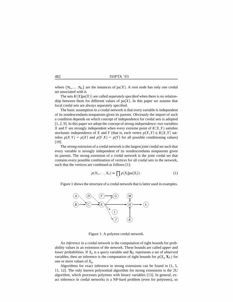
482 ISIPTA ’03

whereπ1 πm are the instances of pa X . A root node has only one credal

set associated with it.The sets K X ( pa X are called separately specified when there is no relation-

ship between them for different values of pa X . In this paper we assume thatlocal credal sets are always separately specified.

The basic assumption in a credal network is that every variable is independentof its nondescendants nonparents given its parents. Obviously the import of sucha condition depends on which concept of independence for credal sets is adopted[1, 2, 9]. In this paper we adopt the concept of strong independence: two variablesX and Y are strongly independent when every extreme point of K X Y satisfiesstochastic independence of X and Y (that is, each vertex p X Y e K X Y sat-isfies p X (Y e p X and p Y ( X C p Y for all possible conditioning values)[10].

The strong extension of a credal network is the largest joint credal set such thatevery variable is strongly independent of its nondescendants nonparents givenits parents. The strong extension of a credal network is the joint credal set thatcontains every possible combination of vertices for all credal sets in the network,such that the vertices are combined as follows [1]:

p X1 Xn ) ∏i

p Xi ( pa Xi O (1)

Figure 1 shows the structure of a credal network that is latter used in examples.

A

B C

D

E

F G

H

I

J K

M

Lef f e g fe hf ij f

Figure 1: A polytree credal network.

An inference in a credal network is the computation of tight bounds for prob-ability values in an extension of the network. These bounds are called upper andlower probabilities. If Xq is a query variable and XE represents a set of observedvariables, then an inference is the computation of tight bounds for p Xq ( XE forone or more values of Xq.

Algorithms for exact inference in strong extensions can be found in [1, 5,11, 12]. The only known polynomial algorithm for strong extensions is the 2Ualgorithm, which processes polytrees with binary variables [13]. In general, ex-act inference in credal networks is a NP-hard problem (even for polytrees), so

Rocha & Cozman: Inference in Credal Nets 483

approximate algorithms are a natural solution. We distinguish outer approxima-tions from inner ones; the former are produced when the correct interval betweenlower and upper probabilities is enclosed in the approximate interval; the latterapproximations are produced when the correct interval encloses the approximateinterval. Outer approximations can be found in [7, 14, 15], and inner approximatealgorithms can be found in [4, 16, 17]. Generally speaking, inner algorithms areobtained by local optimization methods.

In this paper we are interested in inferences with strong extensions. The diffi-culty faced by inference algorithms is the potentially enormous number of verticesthat a strong extension can have — even a relatively small network can dwarf thebest exact algorithms. Consider the following example, taken from [5]:

Example 1 Consider a network with four variables X, Y , Z and W; W is the solechild of X, Y and Z, and there are no other arrows in the network. Suppose that allvariables have three values and that every local credal set has only three vertices.The vertices of the strong extension K X Y Z W factorize as p W X Y Z p W ( X Y Z p X p Y p Z . Now, W is associated with 27 credal sets; thereforethere are 327 ways to combine the vertices of these credal sets. These 327 verticesmust be combined with every combination of vertices of K X , K Y and K Z .So, the potential number of vertices in K X Y Z W is 330.

We note that inference in credal networks is an optimization problem. Con-sider the computation of an upper probability:Ú The goal is to find a distribution p Xi ( pa Xi in K Xi ( pa Xi , for each

variable Xi, so as to maximize the probability value p Xq ( XE .Ú The objective function p Xq ( XE is a fraction of multilinear expressions:

p Xq ( XE ) ∑X1 5 5 5 Xn ÃG Xq XE I ∏i p Xi ( pa Xi ∑X1 5 5 5 Xn à XE ∏i p Xi ( pa Xi Ú The maximization is subject to linear constraints, given our assumption of

credal sets with finitely many vertices.

This maximization problem belongs to the field of signomial programming [6], asobserved independently by [4, 12, 18]. Signomial programs are generally solveddividing the feasible set (“branching” on various subsets) and obtaining outer ap-proximations (“bounding” the objective function in each subset) [6, 19]. Thatis, signomial programming is solved by branch-and-bound procedures. The greatadvantage of signomial programming over more general optimization problemsis that it is possible to obtain bounds for signomial programs using geometricprogramming — a well establish field that can be tackled efficiently through con-vex programming [20]. However, direct application of geometric programming

484 ISIPTA ’03

bounds to strong extensions seems to face difficulties. First, the inference prob-lem is an “implicit” signomial programming, as the objective function is encodedin the graph through Expression (1); each combination of variables in the credalnetwork would be a maximizer in the geometric program. Second, and perhapsmore importantly, the “degree of difficulty” of a geometric program depends onthe number of polynomial terms in the program — note that Expression (1) sum-marizes a large number of terms.

In this paper we adopt the basic idea of branching and bounding to computelower and upper probabilities, but instead of relying on properties of geometricprogramming, we use bounds that have been specifically developed for strongextensions.

3 Branch-and-bound search and optimization

Branch-and-bound techniques appear in artificial intelligence, optimization andconstraint satisfaction [21, 22]. The basic purpose of a branch-and-bound algo-rithm is to optimize a function. For example, take a problem P stated as: P max f w

s.t. g w M> 0 w W where W ℜn, f is a real valued function, and the image of g is contained in ℜm.A branch-and-bound technique is suitable for P whenever it is possible to divide Pin sub-instances that are easier to solve or approximate than P itself, and such thatthe solution for P is present in one of these sub-instances [23, 24]. Additionally, abranch-and-bound technique requires a bound r (overestimation) for the solutionof P. This upper bound is usually obtained from a relaxed version of P, indicatedby R. Obviously, R must be easier and faster to solve than P, and must give a goodapproximation for P. The relaxed bound for P is denoted by r P .

In our implementation we use the following version of branch-and-bound[25]; several variants exist for it [23].

Algorithm 1 - Depth-first branch-and-boundÚ Input: a problem P.Ú Output: the value of max f w , denoted by p.

1. Initialize p with a small value (necessarily smaller than p).

2. If W contains a single value w then: update p with f w when f w 1? p;

3. else:

Rocha & Cozman: Inference in Credal Nets 485

(a) using decomposition, obtain a list L of sub-instances of P; each sub-instance is denoted by Ph and has feasible region Wh.

(b) for each Ph do

i. if Wh is feasible in the original problem and r Ph C? p, call re-cursively depth-first branch-and-bound over Ph.

4. Take the last p as p.

This algorithm can be viewed as a search in a tree where the root node con-tains P and descendant nodes contain sub-instances of P. The leaf nodes containproblems that can be exactly solved. When a leaf node l is reached, the value forf at l is computed; if this value is the largest one up to that moment, it is retained.Non-leaf nodes are processed by relaxing the original problem and producingbounds. Every non-leaf node is expanded by decomposition into sub-instances, aslong as its bound is larger than the current best value.

4 Branch-and-bound inference in strong extensions

This section contains the central ideas in this paper. We use a branch-and-boundprocedure whereÚ branching occurs at every vertex of credal sets, andÚ bounding is achieved by Tessem’s A/R algorithm [7].

Given a query variable X and a credal network N , a single run of the branch-and-bound procedure computes the lower or upper probability for a single stateof X , denoted by x.

The first step is to discard variables that are not used to compute the inference;this can be done using d-separation [26]. The resulting network is denoted by N0.

Branching.The root node in the branch-and-bound search tree is N0. The root node N0

is then divided into several simpler credal networksN01 ì N0q . Each one of

these networks is obtained as follows. We select one credal set in N0, and produceas many networks as there are vertices in this credal set — each network is associ-ated with a single vertex of the selected credal set. This decomposition procedureis then applied recursively, following the branch-and-bound algorithm. At eachstep, a credal set is “expanded”. Using this decomposition strategy, a leaf nodecontains a Bayesian network, obtained by a particular selection of vertices in allcredal sets in the credal network. When a leaf node is reached, a variable elimi-nation algorithm is used to perform inference in the Bayesian network defined bythe leaf [27]. Such an algorithm produces a probability value p x ( XE ; if p x ( XE is greater than the current maximum probability, the latter value is updated.

486 ISIPTA ’03

We always select the non-expanded credal set nearest to the queried variable,but we always keep the query variable to be processed at last (a similar criterionis used in [28] to deal with partial evaluation of belief nets). We have tried severalcriteria for the selection of the credal sets that are expanded, and we found thatthe procedure just described is quite appropriate.

Bounding.For non-leaf nodes in the search tree, we run the A/R algorithm as a relax-

ation of exact inference [7], because this algorithm produces outer bounds ratherquickly. The A/R algorithm focuses on polytrees, even though it can be modifiedto handle more general networks [14].

The A/R algorithm assumes that every credal set is approximated by a collec-tion of probability intervals. So we must convert the credal network to an interval-based Bayesian network (conditional probability tables contain intervals). Obvi-ously the replacement of credal sets by probability intervals introduces potentialinaccuracies into the process.

The A/R algorithm mimics the dynamics of Pearl’s belief propagation algo-rithm [3]. The functions λ, π and the messages used in BP are still defined withidentical purposes, but they are now interval-valued functions. The idea is to ma-nipulate these intervals using interval arithmetic and two additional techniquescalled by Tessem annihilation and reinforcement.

We can understand the basic ideas in the A/R algorithm by looking at thecomputation of the interval-valued message π X — this message is computedat a node X with parents Y0 ì Yk. Consider then the computation of π d x j , thelower bound of π x j for a particular value x j:

1. Construct a interval-valued function β Y0 ì Yk by interval-multiplicationof the messages πX Yi received by X (these messages are also interval-valued).

2. Construct a distribution p Y0 ì Yk that is consistent with the intervals inβ Y0 ì Yk , such that p Y0 Yk minimizes the sum

∑Y0 5 5 5 Yk

p x j (Y0 ì Yk p Y0 Yk Fwhere p x j (Y0 Yk is the lower value for p x j (Y0 Yk ; the minimumof the sum is π d x j .

These operations are efficient because it is not hard to find p Y0 ì Yk in step 2:sort p x j (Y0 Yk in increasing order, and distribute probability mass (consis-tently with β Y0 ì Yk ) from the smallest to the largest value of p x j (Y0 Yk .The same operations can be adapted to compute the upper bound π dn x j .

The A/R algorithm prescribes similar operations for computation of λX Yi and πZi X (where Zi is a child of X). The function λ X is obtained by directinterval multiplication. Finally, the algorithm uses annihilation or reinforcement

Rocha & Cozman: Inference in Credal Nets 487

UjV

p k v0 lnm p m 0 o 45

1p mqp ∞r m 0 o 45r a0 ea1

2p mqp ∞r m 0 o 45r b0 eb1

7p m 0 o 45r m 0 o 43

3p mqp ∞r m 0 o 45r b2 eb3

6p m 0 o 45r m 0 o 35

4p m 0 o 45r m 0 o 45

5p m 0 o 45r m 0 o 35

Figure 2: An example of branch-and-bound based inference. Left: a simple credalnetwork, where K U is the convex hull of

a0 a1 , with a0 Ñ 0 5 0 5 and

a1 % 0 3 0 7 ; K V ( u0 is the convex hull ofb0 b1 , with b0 0 5 0 5 and

b1 % 0 3;0 7 ; K V ( u1 is the convex hull ofb2 b3 , with b2 0 4 0 6 and

b3 ½ 0 2 0 8 . Right: Search tree for computation of p v0 .operations to “normalize” the functions λX Yi , πZi X , and the product π X λ X — “normalization” means simply computing bounds that take into account thefact that probability distributions add up to one.

In our branch-and-bound procedure, the deeper a node is in the search tree,the more point probabilities are manipulated by the A/R algorithm.

Example 2 Figure 2 shows a very simple network and the the basic steps of ourbranch-and-boundalgorithm when computing p v0 . Nodes in the search tree rep-resent credal networks; the numbering inside nodes indicates the order in whichnodes are visited. The value r is obtained by the A/R algorithm. Close to eacharc in the search tree we indicate which vertex (and for which credal set) wasexpanded.

Experiments.We have implemented the branch-and-bound scheme in a Java program, using

Pentium IV machines to run tests. We ran experiments with networks containingvariables with three and four states. Each configuration was tested against severalrandomly generated credal nets [29]. Experiments discussed in this section haveno evidence (XE /0); this restriction simplifies the presentation with no loss ingenerality.

488 ISIPTA ’03

Table 1: Cost for exact inference for E in the network of Figure 1.

# states # vertices Potential size Visited nodes Samplesper per credal of the strong (mean) (networks)

variable sets extension03 02 221 5499 3503 03 321 284912 1004 02 235 559255 10

We have observed that the size of the search tree explored by branch-and-bound is usually a small fraction of the potential vertices of the strong extension.As an example, consider the network in Figure 1. Table 1 shows relevant resultsfor query variable E, indicating the number of states for variables, the number ofvertices for each credal set in the network, and the potential number of vertices ofthe strong extension. The table indicates how many networks of each type weretested, and the mean number of visited nodes during branch-and-bound. Note theenormous difference between the potential number of vertices and the number ofeffectively expanded nodes.

As another instructive example, we applied the branch-and-bound scheme tothe network described in Example 1. We tested thirty randomly generated credalnetworks with the same structure and different credal sets; in each one of themwe computed the lower and upper probabilities for w0. These sample networkshad ternary variables and three distributions in each credal set. The branch-and-bound search was always able to quickly compute the exact inference, on averageexploring 243 nodes per inference.

Consider another example. We took the polytree structure of the well-knownBayesian network called “Car Starts”3 and set all of its variables as ternary. Weassumed that in practice it would be unusual to have credal sets associated toall variables in a credal network — some distributions could be obtained withgreater precision, and in any case the specification of dozens of credal sets is notan easy matter. We therefore introduced credal sets in all root nodes and in thenode called BatteryState, using ε-contaminated models with ε 0 2 [30]. Theresulting strong extension has 318 potential vertices (about 387 million potentialvertices). We ran branch-and-bound inference for all states of the variable Startsand obtained exact values after evaluating 1,139,717 nodes (less than 0.3% ofthe number of potential vertices were explored). An interesting test was madewith the branching strategy. We ran the same inference using a “reverse ordering”for branching; that is, we first expanded the credal sets that were farthest awayfrom the query node. Using this strategy, the branch-and-bound algorithm found

3Microsof Research: http://www.research.microsoft.com/research/dtg/bnformat/autoxml.html.

Rocha & Cozman: Inference in Credal Nets 489

Table 2: The probability error in underestimated approximate reasoning for E inthe network of Figure 1.

# states # vertices Fixed number Meanper variable per credal set of visited nodes relative error

03 03 150000 0.001303 03 30000 0.006704 02 200000 0.006104 02 50000 0.0097

the exact values after expanding 4,546,943 nodes. This simple test reinforces theintuition that the most relevant probability values in an inference are the valuesthat are “close” to the query variable.

It is also possible to look at the branch-and-bound scheme not only as an exactalgorithm, but also as an algorithm that can be stopped at any time to generate ap-proximate results. We tested this idea by running the branch-and-bound algorithmwith a fixed number of nodes. Table 2 shows the mean relative error in inferences(each row is the mean of ten random networks). The relative error is computedusing the approximate and the exact values for P E e0 .5 Inference with network fragments

If the credal network N is large, it may not be possible to run the branch-and-bound algorithm to optimality. In this section we propose strategies to handlesuch problems. The basic idea is to divide the credal network in parts and to runbranch-and-bound in these sub-networks, in some suitable order. We illustrate thisidea through an example.

Consider the network in Figure 1, with ternary variables and two vertices ineach credal set. Suppose that we want to compute exact lower and upper proba-bilities for variable G and that our space and time constraints allow us to performan exact inference just for E, but not for G. We then run branch-and-bound andobtain lower and upper probabilities for E. In a particular instance of the networkshown in Figure 1, we obtained p e0 ) 0 199;0 587 , p e1 - 0 084;0 375 andp e2 c 0 212;0 604 . We can easily generate the largest credal set that is consis-tent with these intervals. We obtain K E defined by the vertices 0 413;0 375;0 212 6ì 0 312;0 084;0 604 6 0 587;0 084;0 329 0 199;0 197;0 604 6 0 587;0 201;0 212 0 199;0 375;0 426 «KNow we can remove E and its antecedents from the network, and replace E bya new node E + that has the marginal credal set of E as its marginal credal set.

490 ISIPTA ’03

The transformed network is displayed in Figure 3. We then run exact branch-and-bound based inference for G, obtaining the intervals p g0 e 0 091;0 447 ,p g1 1 0 157;0 564 and p g2 C 0 208;0 591 . Incidentally, we computed thesame inferences with an exhautive algorithm in the JavaBayes system4 and gotthe same values.

E sF G

H

I

J K

Lg fe hf i f

Figure 3: Transformed polytree credal network.

If inferences in the transformed credal network are still unfeasible, we can runan approximate inference algorithm in the transformed credal network. Considerrunning Tessem’s algorithm in the network in Figure 3. We obtain the intervalsp g0 M 0 053 0 502 , p g1 c 0 116 0 663 and p g2 M 0 128 0 644 .

In closing, we note that Tessem’s algorithm alone in the complete examplenetwork produced the intervals p g0 c 0 040 0 524 , p g1 - 0 106 0 698 andp g2 M 0 097 0 667 .6 Discussion

Any branch-and-boundalgorithm is highly dependent on the quality of the boundsit employs. We have found that Tessem’s bounds, while fast to compute and rea-sonably accurate, are quite wide — usually the search tree is expanded to a largedepth before some of its branches are discarded. To give an example, in the com-putation of inferences for variable E in our samples with ternary variables andthree vertices, the branch-and-bound algorithm explored the search tree almostcompletely down to levels 12 or 13 (the complete search tree has 21 levels).

As an aside, we have also implemented a breadth-first version of branch-and-bound [22], but we have found that the need to store the expanded frontier insuch algorithms makes them unfeasible. Breadth-first branch-and-bound will onlybecome a reality if better bounds than Tessem’s are found.

Generally speaking, we can say that the branch-and-bound algorithm needs toexplore a tiny fraction of potential vertices of the strong extension, and is fasterthan the best existing exact algorithms [5]. For really small credal networks (with

4Free software, site http://www.cs.cmu.edu/ javabayes.

Rocha & Cozman: Inference in Credal Nets 491

a few thousand potential vertices in the strong extension), the overhead of branch-ing and bounding can be significant, and in those cases enumeration algorithmsmay be faster.

Clearly, the branch-and-bound algorithm with Tessem bounds cannot copewith arbitrarily large problems, and it can face difficulties even in seemingly sim-ple situations. In the network in Figure 1, inferences for variable L could not befound exactly, even after extensive tests.

7 Conclusion

This paper can be best understood as proposing a family of solutions for inferencein strong extensions, using branch-and-bound algorithms as a unifying idea insuch solutions. We have restricted ourselves to polytrees, but branch-and-boundtechniques can be used for general inference; we have stressed the use of Tessembounds, but any bounding scheme can be used.

We believe that our ideas are the first explicit formulation and implementa-tion of inference in credal networks as a search procedure that runs to optimality.Branch-and-bound techniques are rather suitable for this purpose; the experimentsshow that inference with branch-and-bound and Tessem bounds is a definite im-provement over existing algorithms.

We also would like to emphasize the possibility that a network is processedin pieces, using different levels of accuracy in each one of the partial inferences.Such a strategy seems to be appropriate for large networks. Our future researchwill be focused on developing and implementing general algorithms for decom-posing networks and processing fragments with different strategies.

References

[1] Cozman, F.G.: Credal Networks. Artificial Intelligence 120 (2000) 199–233

[2] Couso, I. Moral, S., Walley, P.: Examples of Independence for ImpreciseProbabilities. Proc. of the 1st ISIPTA, Ghent Belgium (1999) 121–130

[3] Pearl, J.: Probabilistic Reasoning in Intelligent Systems. Networks of Plau-sible Inference. Morgan Kaufmann Publishers, San Mateo CA (1988)

[4] Cozman, F.G.: Robustness Analysis of Bayesian Networks with Local Con-vex Sets of Distributions. Proc. of the 13th Annual Conference on Un-certainty in Artificial Intelligence, Morgan Kaufmann, San Francisco, CA,(1997) 393-405

[5] Rocha, J.C.F.; Cozman, F.G.: Inference with Separately Specified Sets ofProbabilities in Credal Networks. Proc. of the 18th Annual Confence on Un-

492 ISIPTA ’03

certainty in Artificial Intelligence, Morgan Kaufmann, San Francisco, CA ,(2002) 430-437

[6] Avriel, M.: Advances in Geometric Programming, Plenum Press, New York,1980.

[7] Tessem, B.: Interval Probability Propagation. Int. Journal of ApproximateReasoning 7, (1992) 95–120

[8] Levi, I. The Enterprise of Knowledge. MIT Press, Cambridge, Mass, (1980)

[9] Campos, L. M. de, Moral, S.: Independence Concepts for Convex Sets ofProbabilities. Proc. of the XI Conference on Artificial Intelligence, MorganKaufmann, San Francisco, CA, (1995) 108–115

[10] Walley, P.: Statistical Reasoning with Imprecise Probabilities. Chapman andHall, London, (1991)

[11] Cano, J.E., Delgado, M., Moral, S.: An Axiomatic Framework for the Prop-agation of Uncertainty in Directed Acyclic Networks. Int. Journal of Ap-proximate Reasoning 8, (1993) 253–280.

[12] Zaffalon, M.: Inferenze e Decisioni in Condizioni di Incertezza con ModelliGrafici Orientati. Ph.D. Thesis, Universita di Milano, Milan, Italy, (1997)(in Italian)

[13] Fagiuoli, E., Zaffalon, M. (1998).: 2U - An Exact Interval Propagation Al-gorithm for Polytrees with Binary Variables. Artificial Intelligence 106(1),77-107

[14] Ha, V.A. et al: Geometric Foundations for Interval-Based Probabilities. An-nals of Mathematics and Artificial Intelligence, Vol.24, 1-4 (1998) 1–21

[15] Cano, A., Moral, S.: Using Probabilistic Trees to Compute Marginals withImprecise Probabilities. TR-DECSAI-00-02-14, University of Granada,(2000)

[16] Cano, A., Moral, S.: A Genetic Algorithm to Approximate Convex Sets ofProbabilities. 7th Int. Conf. IPMU-96, (Paris, France, July, 1994), (1994) pp859–864

[17] Cano, A., Moral, S.: Convex Sets of Probabilities Propagation by SimulatedAnnealing. 5th Int. Conf. IPMU-94, (Paris, France, July, 1994), (1994) pp4–8

[18] Andersen, K.A., Hooker, J.N.: Bayesian Logic. Decision Support Systems11, (1994) 191-210.

Rocha & Cozman: Inference in Credal Nets 493

[19] Duffin R.J., Peterson, E.L.: Geometric Programming with Signomials. Jour-nal of Optimization Theory and Applications, 11(1), (1973) 3–35”

[20] Duffin, R.J., Peterson, E.L., Zener, C.: Geometric Programming, Theory andApplication. John Willey and Sons, New York, (1967)

[21] Norvig, P., Russell, S.: Artificial Intelligence: a Modern Approach. PrenticeHall, Englewoods, (1995)

[22] Bertsekas, D.P.: Dynamic Programming, Deterministic and Stochastic Mod-els. Prentice Hall, Englewoods, (1987)

[23] Papadimitriou, C., Steiglitz, I.: Combinatorial Optimization, Algorithms andComplexity. Prentice-Hall, Englewood Cliffs, New Jersey, (1982)

[24] Sahinidis, N.V.: BARON, Branch and Reduce Optimization Navigator,User’s manual 4.0. University of Illinois at Urbana-Champaign, (2000)

[25] Preiss, B.R.: Data Structures and Algorithms with Object-Oriented DesignPatterns in Java. Wiley, New York, (2000)

[26] Cozman, F.G.: Irrelevance and Independence in Quasi-Bayesian Networks.Proc. XIV Conference on Uncertainty in Artificial Intelligence, MorganKaufmann, San Francisco, CA, (1998) 86–96

[27] Cozman, F.G.: Generalizing Variable Elimination in Bayesian Networks.Workshop on Probabilistic Reasoning in Artificial Intelligence, Editora TecArt, Sao Paulo, (2000) 27–32

[28] Draper, D.L., Hanks, S.: Localized Partial Evaluation of Belief Networks.XV Conference on UAI, (1995) 170-177

[29] Ide, J.S., Cozman, F.G.: Random Generation of Bayesian Networks. Proc. ofthe XVI Braziliam Symposium on Artificial Intelligence, Springer-Verlag,(2002)

[30] Berger, J.O.: Statistical Decision Theory and Bayesian Analysis. Springer,Berlin, (1985)

Jose Carlos Ferreira da Rocha is a PhD student at the Engineering School (EscolaPolitecnica), University of Sao Paulo, and a teaching assistant at UEPG, Deinfo, PontaGrossa, PR, Brasil, CEP 84030-900 E-mail: jrocha@uepg.br

Fabio Gagliardi Cozman is with the Engineering School (Escola Politecnica), Universityof Sao Paulo, Sao Paulo, SP, Brazil, CEP 05508-900. E-mail: fgcozman@usp.br

Extensions of Expected Utility Theory andSome Limitations of Pairwise Comparisons Ý

M. J. SCHERVISHCarnegie Mellon University, USA

T. SEIDENFELDCarnegie Mellon University, USA

J. B. KADANECarnegie Mellon University, USA

I. LEVIColumbia University, USA

Abstract

We contrast three decision rules that extend Expected Utility to contextswhere a convex set of probabilities is used to depict uncertainty: Γ-Maximin,Maximality, and E-admissibility. The rules extend Expected Utility theoryas they require that an option is inadmissible if there is another that carriesgreater expected utility for each probability in a (closed) convex set. If theconvex set is a singleton, then each rule agrees with maximizing expectedutility. We show that, even when the option set is convex, this pairwise com-parison between acts may fail to identify those acts which are Bayes for someprobability in a convex set that is not closed. This limitation affects two ofthe decision rules but not E-admissibility, which is not a pairwise decisionrule. E-admissibility can be used to distinguish between two convex sets ofprobabilities that intersect all the same supporting hyperplanes.

1 Introduction

This paper offers a comparison among three decision rules for use when uncer-tainty is depicted by a non-trivial, convex set of probability functions P . Thissetting for uncertainty is different from the canonical Bayesian decision theoryof expected utility, which uses a singleton set, just one probability function, torepresent a decision maker’s uncertainty. Justifications for using a non-trivial setof probabilities to depict uncertainty date back at least a half century [4] and av The research of the first three authors is supported by NSF grant DMS-0139911

494

Schervish et al.: Extensions of Expected Utility Theory 495

foreshadowing of that idea can be found even in [7], where he allows that not allhypotheses may be comparable by qualitative probability – in accord with, e.g.,the situation where the respective intervals of probabilities for two events merelyoverlap with no further (joint) constraints, so that neither of the two events ismore, or less, or equally probable compared with the other.

We study decision rules that are extensions of canonical Subjective ExpectedUtility [SEU] theory, using sets of probabilities, in the following sense. The deci-sion rules we consider all satisfy the following pairwise comparison between twooptions.

Criterion 1 For a pair of options f and g, if for each probability P P , f hasgreater expected utility than g, then g is inadmissible whenever f is available.

This pairwise comparison itself creates a strict partial order. It (or a similarrelation) has been the subject of representation theorems by, e.g., [3, 14, 15].Note that when P is a singleton set, then the partial order is a weak order thatsatisfies SEU theory. In this sense, a decision rule that embeds this partial orderextends SEU theory.

Here, we avail ourselves of four simplifying assumptions:

1. The decision maker’s values for outcomes are determinate and are depictedby a (cardinal) utility function.

Reason: We use circumstances under which convexity of P is not con-troversial. 1

2. The algebra of uncertainty is finite, with finite state space Ω ω1 ω2 ! ωk .

Reason: We avoid the controversies surrounding countable versus fi-nite additivity, which arise with infinite algebras.

3. Acts (or options) are gambles, i.e. functions from states to utilities, f :Ω /. IR.

Reason: This assumption is commonplace and affords us an opportu-nity to contrast a variety of decision rules.

4. Each decision problem presents the decision maker a uniformly boundedchoice set A of gambles.

Reason: We avoid complications with unbounded utilities. Moreover,by considering the convex hull of a family of such gambles, we are as-sured of achieving the infimum and supremum operations with respect toexpected utilities calculated with respect to the set P .

1The issue of convexity of P is controversial. See [14] for a representation of partially ordered strictpreferences that does not require convexity unless the decision maker has a determinate (cardinal)utility for outcomes. Rebuttal is presented in Section 7 of [11].

496 ISIPTA ’03

Of the three decision rules we discuss, perhaps the most familiar one is Γ-Maximin2. This rule requires that the decision maker ranks a gamble by its lowerexpected value, taken with respect to a closed, convex set of probabilities, P , andthen to choose an option from A whose lower expected value is maximum. Thisdecision rule (as simplified by the assumptions, above) was given a representationin terms of a binary preference relation over Anscombe-Aumann horse lotteries[2], has been discussed by, e.g., Section 4.7.6 of [1] and recently by [5], who de-fend it as a form of Robust Bayesian decision theory. The Γ-Maximin decisionrule creates a preference ranking of options independent of the alternatives avail-able in A : it is context independent in that sense. But Γ-Maximin corresponds toa preference ranking that fails the so-called (von Neumann-Morgenstern’s) “In-dependence” or (Savage’s) “Sure-thing” postulate of SEU theory. In Section 2 of[15], we note that such theories suffer from sequential incoherence in particularsequential decision problems.

The second decision rule that we consider, called E-admissibility (‘E’ for“expectation”), was formulated in [8, 9]. E-admissibility constrains the decisionmaker’s admissible choices to those gambles in A that are Bayes for at least oneprobability P P . That is, given a choice set A , the gamble f is E-admissibleon the condition that, for at least one P P , f maximizes subjective expectedutility with respect to the options in A .3 Section 7.2 of [12]4 defends a precursorto this decision rule in connection with cooperative group decision making. E-admissibility does not support an ordering of options, real-valued or otherwise,so that it is inappropriate to characterize E-admissibility by a ranking of gamblesindependent of the set A of feasible options. However, the distinction betweenoptions that are and are not E-admissible does support the “Independence” pos-tulate. For example, if neither option f nor g is E-admissible in a given decisionproblem A , then the convex combination, the mixed option h = α f t (1-α)g (0> α > 1) likewise is E-inadmissible when added to A This is evident from thebasic SEU property: the expected utility of a convex combination of two gamblesis the corresponding weighted average of their separate expected utilities; hence,for a given P P the expected utility of the mixture of two gambles is boundedabove by the maximum of the two expected utilities. The assumption that neitherof two gambles is E-admissible entails that their mixture has P-expected utilityless than some E-admissible option in A .

The third decision rule we consider is called Maximality by Walley in [17]5,

2When outcomes are cast in terms of a (statistical) loss function, the rule is then Γ-Minimax:rank options by their maximum expected risk and choose an option whose maximum expected risk isminimum.

3Levi’s decision theory is lexicographic, in which the first consideration is E-admissibility, fol-lowed by other considerations, e.g. what he calls a Security index. Here, we attend solely to E-admissibility.

4Savage’s analysis of the decision problem depicted by his Figure 1, p. 123, and his rejection ofoption b, p. 124 is the key point.

5There is, for our discussion here, a minor difference with Walley’s formulation of Maximality

Schervish et al.: Extensions of Expected Utility Theory 497

who appears to endorse it (p. 166). Maximality uses the strict partial order (above)to fix the admissible gambles from A to be those that are not strictly preferred byany other member of A . That is, f is a Maximal choice from A provided thatthere is no other element g A that, for each P P , carries greater expectedutility than f does. Maximality (under different names) has been studied, forexample, in [6, 8, 10, 13, 16]. Evidently, the E-admissible gambles in a decisionproblem are a subset of the Maximally admissible ones.

The three rules have different sets of admissible options. Here is a heuristicillustration of that difference.

Example 1 Consider a binary-state decision problem, Ω =ω1, ω2 , with three

feasible options. Option f yields an outcome worth 1 utile if state ω1 obtains andan outcome worth 0 utiles if ω2 obtains. Option g is the mirror image of f andyields an outcome worth 1 utile if ω2 obtains and an outcomes worth 0 utiles ifω1 obtains. Option h is constant in value, yielding an outcome worth 0.4 utilesregardless whether ω1 or ω2 obtains. Figure 1 graphs the expected utilities forthese three acts. Let P =

P: 0.25 u P(ω1) u 0.75 . The surface of Bayes solutions

is highlighted. The expected utility for options f and g each has the interval ofvalues [0.25, 0.75], whereas h of course has constant expected utility of 0.4. Fromthe choice set of these three options A =

f , g, h the Γ-Maximin decision rule

determines that h is (uniquely) best, assigning it a value of 0.4, whereas f and geach has a Γ-Maximin value of 0.25. By contrast, under E-admissibility, only theoption h is E-inadmissible from the trio. Either of f or g is E-admissible. And, asno option is strictly preferred to any other by expectations with respect to P , allthree gambles are admissible under Maximality.

What normative considerations can be offered to distinguish among thesethree rules? For example, all three rules are immune to a Dutch Book, in thefollowing sense:

Definition 1 Call an option favorable if it is uniquely admissible in a pairwisechoice against the status-quo of “no bet,” which we represent as the constant 0.

Proposition 1 For each of the three decision rules above, no finite combinationof favorable options can result in a Dutch Book, i.e., a sure loss.

Proof. Reason indirectly. Suppose that the sum of a finite set of favorable gam-bles is negative in each state ω. Choose an element P from P . The probabilityP is a convex combination of the extreme (0-1) probabilities, corresponding to aconvex combination of the finite partition by states. The expectation of a convex

involving null-events. Walley’s notion of Maximality requires, also, that an admissible gamble beclassically admissible, i.e., not weakly dominated with respect to state-payoffs. This means that, e.g.,our Theorem 1(i) is slightly different in content from Walley’s corresponding result.

498 ISIPTA ’03

Figure 1: Expected utilities for three acts in Example 1. The thicker line indicatesthe surface of Bayes solutions.

combination of probabilities is the convex combination of the individual expec-tations. This makes the P-expectation of the sum of the finite set of favorableoptions negative. But the P-expectation of the sum cannot be negative unless atleast one of the finitely many gambles has a negative P-expectation. Then thatgamble cannot be favorable under any of the three decision rules. Thus, none ofthese three decision rules is subject to sure loss. U

In this paper, we develop an additional criterion for contrasting these deci-sion rules. In Section 2 we address the question of what operational content therules give to distinguishing among different (convex) sets of probabilities. That is,we are concerned to understand which convex sets of probabilities are treated asequivalent under a given decision rule. When do two convex sets of probabilitieslead to all the same admissible options for a given decision rule? Γ-Maximin andMaximality are based solely on pairwise comparisons. Not so for E-admissibility.Even when the choice set A of feasible options is convex (e.g., closed under mixedstrategies), these rules have distinct classes of admissible options.

Schervish et al.: Extensions of Expected Utility Theory 499

2 Gambles and pairwise choice rules

It is evident that for Γ-Maximin generally to satisfy Criterion 1, the convex set ofprobabilities P must be closed. For an illustration why, if Example 1 is modifiedso that P +

P : 0 4 : P ω1 ^u 0 75 then, even though f and h both havethe same infimum, 0.4, of expectations with respect to P + , for each P P + f hasgreater expected utility than does h. Thus, from the perspective of operationalcontent, the Γ-Maximin rule fails to distinguish between different convex sets ofprobabilities that differ with respect to Criterion 1, although each of Maximalityand E-admissibility does distinguish the two sets P and P + .

In order to contrast Maximality and E-admissibility, first we ask when do theylead to the same choices? Walley’s Theorem 3.9.5 of [17] shows that, when theoption space A is convex and the convex set of probabilities P is closed, the tworules are equivalent, i.e. both E-admissibility and Maximality reduce to a pairwisecomparison of options according to Criterion 1. In this circumstance, an optionis admissible, under either rule, just in case there is no other option that makes itinadmissible under Criterion 1. Then, with decision problems using convex setsof options, the two rules are capable of distinguishing between any two closedconvex sets of probabilities, since distinct closed convex sets have distinct sets ofsupporting hyperplanes.

In Corollary 1 we re-establish Walley’s result, and we extend the equivalenceto decision problems in which P is open and A is finitely generated. The examplefollowing Theorem 1 establishes that for part (ii), the restriction to a finite (orfinitely generated) option set, A , is necessary. More important, however, we thinkis the second example following Theorem 1. That example is of a finite decisionproblem with a convex set of probabilities P (neither closed nor open) where,even though the option set is made convex, some Maximal options are not Bayeswith respect to P . Hence, even when the option space is convex, E-admissibilitydoes not in general reduce to pairwise comparisons.

We preface Theorem 1 with a restatement of the structural assumptions fordecision problems that we use in this paper. Let Ω be a finite state space with kstates. Let A be a uniformly bounded collection of acts or gambles (real-valuedfunctions from Ω). Let C be the convex hull of A . For each probability vector P= p1 pk @ P and each f C there is a point p1 ì pk 1 Ep f IRk,where Ep f ) ∑k

j & 1 p j f ω j . For each f C there is a hyperplane that containsall of the points of the form p1 pk 1 Ep f . For each f C , the halfspaceat or above its corresponding hyperplane is

x IRk : α v f x c f Lwhere

α f ½ f ωk / f ω1 6 f ωk P/ f ωk 1 6 1 and c f f ωk .

500 ISIPTA ’03

Definition 2 Let P be a convex set of probability vectors. We say that f A isBayes with respect to P if there exists p P such that Ep f Ep g for allg A .

Theorem 1 Let B be the set of all f A such that f is Bayes with respect to P .Suppose that g A Ä B . Assume either

(i) that P is closed, or

(ii) that A is finite and that P is open. That is, p1 pk 1 : p1 ì pk M P is an open subset of IRk 1.

Then there exists h in the convex hull of B such that Ep h c? Ep g for all p P .

Corollary 1 Assume that A is closed and convex. Let B be the set of all f Asuch that f is Bayes with respect to P . Suppose that g A Ä B is not Bayes withrespect to P . Assume either

(i) that P is closed, or

(ii) that A is the convex hull of finitely many acts and that P is open.

Then there exists h B such that Ep h c? Ep g for all p P .

The proofs of Theorem 1 and Corollary 1 rely on a series of results about convexsets and are given in Appendix A.

Example 2 The following example illustrates that Theorem 1(ii) does not holdif A is allowed to be infinite. Let Ω have only k 2 states. Let A consist of thegambles

fθ : 0 > θ > π D 4 where

fθ ½ 0 4 0 8tan θ / 0 2sec θ 6 0 4 / 0 2tan θ P/ 0 2sec θ FNotice that f0 § 0 2 0 2 . Let

P p1 p2 : p1 ? 0 2 KFor each p1 0 2 0 3 , the act fθ is Bayes with respect to P when θ 0 5sin 1 10 p1 /0 2 . For p1 0 3, fπ 4 is Bayes with respect to P . Let g f0, which is not Bayeswith respect to P . Notice that, for every θ,

Ep fθ )½ p1 / 0 2 tan θ F 0 4 / 0 2sec θ 6So, Ep fθ : 0 2 when p1 0 2. Since Ep fθ is a continuous function of p,Ep fθ : 0 2 for p in an open set around 0 2 0 8 , which includes part of P .It follows that every convex combination h of fθ’s has Ep h : 0 2 somewhereinside of P .

Schervish et al.: Extensions of Expected Utility Theory 501

Example 3 This example illustrates why we assume that P is closed in Theo-rem 1(i). Let Ω consist of three states. Let

P p1 p2 p3 : p2 : 2p1 for p1 > 0 2 p1 p2 p3 : p2 > 2p1 for 0 2 : p1 > 1 D 3 KThe set of acts A contains only the following three acts (each expressed as avector of its payoffs in the three states):

f1 0 2 0 2 0 2 f2 1 0 0 6g ¼/ 1 8 1 2 2 6

Notice that Ep f2 is the highest of the three whenever p1 0 2, Ep f1 is thehighest whenever p1 > 0 2, and Ep g is never the highest. So, B

f1 f2 andg is not Bayes with respect to A . For each 0 > α > 1, we compute

Ep α f1 1 / α f2 N p1 1 / α F 0 2α Ep g N / 2p1 p2 0 2

Notice that Ep α f1 1 / α f2 is strictly greater than Ep g if and only if p2 : 3 / α p1 / 0 2 1 / α . There is no α such that this inequality holds for all p P .

Remark 1 Note that is it irrelevant to this example that p2 0 for some p P .

Definition 3 Say that two convex sets intersect all the same supporting hyper-planes if they have the same closure and a supporting hyperplane intersects oneconvex set if and only if it intersects the other.

In addition to showing that E-admissibility does not reduce to pairwise com-parisons even when the option set is convex, this example also brings out theimportant point the E-admissibility (but not Maximality) can distinguish betweensome convex sets that intersect all the same supporting hyperplanes. As we notedsome years ago (Section III of [15]), the strict preference relation induced by Cri-terion 1 cannot distinguish between pairs of convex sets that intersect all the samesupporting hyperplanes. Of course, Γ-Maximin does even worse than Maximality,as it cannot distinguish open convex sets from their closure.

Figure 2 illustrates Example 3 and that the presence or absence of probabilitypoint D Å 0 2 0 2 0 4 determines whether or not act g is Bayes from the choiceset A

f1 f2 g . The closure of the convex set P is the triangle with extremepoints A 1 D 3 0 2 D 3 , B 1 D 3 2 D 3 0 , and C 0 0 1 . In Example 3, setP is the result of removing the closed line segment C D from the left face B C of the triangle ABC, leaving the half-open line segment B D along that face.The convex set P d is the set of probabilities that results by adding point D to

502 ISIPTA ’03

o

o

(0,0,1)

(0,1,1)

(1,0,0)

(1,0,1)

(1,1,1)

(1,1,0)

(0,1,0)

A

B

C

D

o

Figure 2: Illustration for Example 3. The set of p1 p2 such that p1 p2 1 / p1 /p2 V P is the diagonally shaded set inside the probability triangle at the bottom ofthe figure with the points A, B, C, and D that are discussed in the text labeled. Thediagonally shaded surface is the surface of Bayes solutions for all probabilities(not just those in P ). The solid shaded set is

p1 p2 Ep g : p P . The points 0 2 0 4 , 0 0 , and 0 2 0 4 Ep g are indicated by open circles.

set P . Point D then is an extreme but not exposed point in P d . Evidently, P andP d intersect all the same supporting hyperplanes. Next, we indicate how to useE-admissibility to distinguish between these two convex sets of probabilities.

For this exercise, we bypass the details of what can easily be done with pair-wise comparisons to fix the common boundaries of P and P d . Specifically, binarycomparisons suffice to fix the closed interval [A,B] belongs to both sets, as the up-per probability P(ω1) = 1/3; they suffice to fix that point C does not belong toeither set, as the lower probability P ω1 ? 0; they suffice to fix the half-openinterval A C belongs to both sets, as the lower probability P ω2 c 0, and theysuffice to fix the half open interval B C as a boundary for both sets, as the uppercalled-off (conditional) odds ratio P ω1 ( ω1 ω2 o1? 1 D 3. But pairwise compar-isons according to Criterion 1, alone, cannot determine how much of the half-openinterval B C belongs to either set P or P d . For that, we use non-binary choiceproblems and E-admissibility.

In order to establish that the half open line segment [C, D) does not belong to

Schervish et al.: Extensions of Expected Utility Theory 503

either set P or P d , consider the family of decision problems defined by the three-way choices: A ε

f1 f2 g ε , where g ε is the act with payoffs 1 8 1 2 /ε 0 2 . For each ε ? 0, only the pair

f1 f2 is E-admissible from such a three-

way choice, with respect to each of the two convex sets of probabilities.Likewise, in order to establish that the half-open line segment D B belongs

to both sets, P and P d , consider the family of decision problems defined bythe three-way choices: A ε

f1 f2 g ε , where g ε is the act with payoffs 1 8 1 2 ε 2 . For each ε ? 0, all three options are E-admissible with respectto each of the two convex sets of probabilities.

However, in the decision problem with options A f1 f2 g , as shown

above, only the pair

f1 f2 is E-admissible with respect to the convex set P ,whereas all three options are E-admissible with respect to the convex set P d .

By contrast, given a choice set, Maximality makes the same ruling aboutwhich options are admissible from that choice set, regardless whether convex setP or convex set P d is used. That is, Maximality cannot distinguish between thesetwo convex sets of probabilities in terms of admissibility of choices, as the twoconvex sets of probabilities intersect all the same supporting hyperplanes.

3 Summary

The discussion here contrasts three decision rules that extend Expected Utilityand which apply when uncertainty is represented by a convex set of probabilities,P , rather than when uncertainty is represented only by a single probability distri-bution. The decision rules are: Γ-Maximin, Maximality, and E-admissibility. Weshow that these decision rules have different operational content in terms of theirability to distinguish different convex sets of probabilities. When do the admis-sible choices differ for different convex sets of probabilities? Γ-Maximin is leastsensitive among the three in this regard. We show that, even when the option setis convex, one decision rule (E-admissibility) distinguishes among more convexsets than the other two. This is because it alone among these three is not based onpairwise comparisons among options. The upshot it that it, but neither of the othertwo rules, can distinguish between two convex sets of probabilities that intersectall the same supporting hyperplanes.

A Proofs of Theorem 1 and Corollary 1

The proofs rely on some lemmas about convex sets.

Lemma 1 Let k be a positive integer. Let C be a closed convex subset of IRk thatcontains the origin. There exists a unique closed convex subset D of IRk 1 withthe following properties:

504 ISIPTA ’03Ú C x IRk : α v x c for all α c C D .Ú α c C D implies aα ac c D for all a 0,Ú α c C D implies α c / a - D for all a ? 0,

Also, for each α c 1 D, c > 0.

Proof. To see that α c ) D implies c > 0, let 0 be the origin. Then α v 0 0 c.Define the following set

D0 α c : α v x c for all x C K (1)

To see that D0 is convex, let γ1 d1 and γ2 d2 be in D0 and 0 > β > 1. Then,for all x C, βγ1 1 / β γ1 v x βd1 1 / β d2 This means that β γ1 d1 L 1 / β γ2 d2 M D0, and D0 is convex. To see that D0

is closed, notice that D0 9 x C Dx, where Dx α c : α v c c and each Dx

is closed. It is clear that D0 has the last two properties in the itemized list. Forthe first condition, let E be the set defined in the first condition. It is clear thatC E. Suppose that there is x0 E such that x0 < C. Then there is a hyperplanethat separates

x0 from C. That is, there is γ IRk and d such that γ v x d for all

x C and γ v x0 : d. It follows that γ d C D0, but then x0 < E, a contradiction.To see that the set that satisfies the conditions is unique, suppose that D and F

are both sets satisfying the listed conditions. If F < D, then there is α c eitherin D Ä F or in F Ä D. We will show, by way of contradiction, that neither of thesecases can occur. The two cases are handled the same way. We will do only thefirst. In the first case, there is a hyperplane separating

α c 6 from F. That is,there is γ d f with γ IRk and d f IR such that

γ v δ dg f for all δ g M F (2)

and γ v α dc : f . It follows that aγ v δ da g / b f for all δ g M F and alla b ? 0. As a . 0, we see that f > 0 is required. As b . ∞, we see that d > 0is required. As a . ∞ we see that γ v δ dg 0 for all δ g C F , hence we canassume that f 0. Because d c > 0 and γ v α dc : 0 it follows that γ v α : 0 andthere exists d0 : 0 such that γ v α d0c : 0. Because g > 0 for all δ g M F , wesee that, even if d 0, γ v δ d0g 0 for all δ g F . Hence, we can assume thatthe separating hyperplane has the form γ d0 0 with d0 : 0. Define γ0 γ D / d0 .It follows from (2) that δ v γ0 g for all δ g c F and so γ0 C. Hence α v γ0 cwhich contradicts γ v α d0c : 0. ULemma 2 Let V be a closed convex subset of IRk 1, and express elements of V as α d where α IRk and d is real. Define

A x IRk : α v x d for all α d M V K

Schervish et al.: Extensions of Expected Utility Theory 505

Assume that A is nonempty. Define D to be the set of all vectors in IRk 1 of theform aα ad / b with a b 0 and α d c V. Then D α d - IRk 1 : α v x d for all x A .

Proof. Let x0 A, and define

C x / x0 : x A K

V + α d / α v x0 : α d M V LIt follows that

C x IRk : α v x c for all α c M V +K (3)

and C contains the origin and is a closed convex set. Define D1 α d / α v x0 : α d C D . In other words, D1 is the convex closed convex set of all vectors inIRk 1 of the form aα ac / b with a b 0 and α c C V + . The definitions of Dand D1 were rigged so that D1 satisfies all the conditions required of the set calledD in Lemma 1 except possibly the first condition in the itemized list. To verifythis condition, define

C + x IRk : α v x c for all α c M D1 K

To see that C C + , let x C. Then aα v x ac / b for all α c V + and alla b 0. Hence, α v x c for all α c C D1. To see that C + C, let x C + . Since α c M V + implies α c 1 D1, we have α v x c for all α c C D1 and x C. Itfollows from Lemma 1 that D1 is the set D0 defined in (1) and D is the claimedset as well. UProof of Theorem 1. (i) Let

U " x IRk : x1 ì xk 1 1 / k 1

∑j & 1

x j P $Let C + be the convex hull of B . Let V consist of all points of the form α f c f where f C + . Let A be as defined in the statement of Lemma 2. Since g is notBayes with respect to P , the set Hg

x U : α vg x cg does not intersectA. Now, notice that Hg and A are disjoint closed convex sets, hence there is aseparating hyperplane. That is, there exists a nonzero γ IRk and c such thatγ v x c for all x A and γ v y : c for all y Hg. Because γ v x c for all x A,it follows from Lemma 2 that γ c is in the set D defined in the statement ofLemma 2. Hence, γ aα and c ad / b for some α c C V and some a b 0.Because γ is nonzero, we have a ? 0 and we can assume without loss of generalitythat a 1 and γ d / b M V . So, γ αh for some h C + and c ch / b, and wecan assume without loss of generality that b 0 and c ch. Now, for all real t,

α vh p1 pk 1 t ) h ωk P/ Ep h F t ch / Ep h O t

506 ISIPTA ’03

So, for all x Hg,ch ? α vh x ch / Ep h O Ep g

It follows that, for all p P , Ep h M? Ep g .(ii) Define U , C + , V , A, and Hg exactly as in the proof of part (i). It is

still true that Hg and A are convex, that A is closed, and that Hg does not intersectA. But Hg is now relatively open. That is, it is the intersection of the hyperplaneH +g

x : α vg x cg with an open set. For this reason, H +g is the unique hyperplanethat contains Hg. Of course, if the closure of Hg fails to intersect A, the rest of theproof of part (i) continues to work. So, suppose that the closure Hg of Hg intersectsA. Even so, there is a weakly separating hyperplane γ c , i.e., there is a γ IRk

and c such that γ v x c for all x A and γ v y > c for all y Hg. We need toshow that among all such separating hyperplanes, there is at least one such thatthe second inequality is strict, i.e., at least one of the separating hyperplanes failsto intersect Hg. Then the rest of the proof of part (i) will finish the proof.

Because A is finite, A is the intersection of finitely many closed halfspaces,and each of these halfspaces is of the form

x : α v f x c f for some f B . Now,

Hg intersects A in some convex subset of the union of the hyperplanes that de-termine these halfspaces. No subset of the union of finitely many distinct hyper-planes can be convex unless it is contained in the intersection of one or more ofthe hyperplanes. (Just check that αx Ö 1 / α y is in the same hyperplane with xif and only if y is as well.) Hence, A ¤ Hg is a subset of the intersection of one ormore of the hyperplanes of the form H +f

x : α v f x c f for some f B . Define

W f B : A ¤ Hg H +f L

If W B , then Hg A, a contradiction. Let f0 B Ä W be such that H +f0 is closest

to A ¤ Hg. Such f0 exists because B is finite. Let ε be one-half of the distance fromH +f0 to A ¤ Hg, and define

O x : ö x / A ¤ Hg ö : ε K

Then

T O ¤ âf W

x : α v f x c f A

For each f W , define M f x Hg : α v f x c f . If at least one M f /0, then

H +f fails to intersect Hg, and the proof is complete. So assume, to the contrary,

that every M f < /0. Then for each f , the closure M f of M f contains A ¤ Hg. It fol-lows that each M f contains points in every neighborhood of A ¤ Hg, including O.Hence, for each f , there exists x T ¤ M f . Each such x Hg ¤ A, a contradiction.UProof of Corollary 1. Let C be the convex hull of B . Either assumption (i) or(ii) is strong enough to imply that Theorem 1 applies, hence there is h +F C such

Schervish et al.: Extensions of Expected Utility Theory 507

that Ep h +Èk? Ep g for all p P . If h +c< B let h1 h + , and apply Theorem 1repeatedly in a transfinite induction as follows. At each successor ordinal γ 1,find hγ 1 C such that Ep hγ 1 ? Ep hγ for all p P . At a countable limitordinal γ choose any countable sequence

γn ∞

n & 1 of ordinals that is cofinal withγ. By the induction hypothesis, Ep hγi : Ep hγ j for all p P if i : j. Thesequence

hγn ∞

n & 1 belongs to the closed bounded set A , hence it has a limit hγand

Ep hγ ) limn ∞

Ep hγn - supn

Ep hγn 6for all p, and hence does not depend on which limit point we take. Also, supn Ep hγ W?Ep hα for all α : γ, so we continue to satisfy the induction hypothesis. Since Ais bounded, there cannot exist an uncountable increasing sequence of Ep hγ val-ues, hence the transfinite induction terminates at some countable ordinal γ0 withhγ0 B .

References

[1] Berger, J. O. Statistical Decision Theory and Bayesian Analysis, 2 ed.Springer-Verlag, New York, 1985.

[2] Gilboa, I., and Schmeidler, D. Maxmin expected utility with non-uniqueprior. Journal of Mathematical Economics 18 (1989), 141–153.

[3] Giron, F. J., and Rios, S. Quasi-Bayesian behavior: A more realistic ap-proach to decision making? In Bayesian Statistics, e. a. J. M. Bernardo, Ed.University of Valencia Press, Valencia, 1980, pp. 17–38.

[4] Good, I. J. Rational decisions. Journal of the Royal Statistical Society 14(1952), 117–114.

[5] Grunwald, P. D., and Dawid, A. P. Game theory, maximum entropy, min-imum discrepancy, and robust bayesian decision theory. Tech. Rep. 223,University College London, 2002.

[6] Herzberger, H. Ordinal preferences and rational choice. Econometrica 41(1973).

[7] Keynes, J. M. A Treatise on Probability. MacMillan and Co., London, 1921.

[8] Levi, I. On indeterminate probabilities. Journal of Philosophy 71 (1974),391–418.

[9] Levi, I. The Enterprise of Knowledge. MIT Press, Cambridge, MA, 1980.

508 ISIPTA ’03

[10] Levi, I. Imprecise and indeterminate probabilities. In Proceedings of the 1stInternational Symposium on Imprecise Probabilities and Their Applications.University of Ghent, Ghent, Belgium, 1999.

[11] Levi, I. Value commitments, value conflict, and the separability of beliefand value. Philosophy of Science 66 (1999), 509–533.

[12] Savage, L. J. The Foundations of Statistics. Wiley, New York, 1954.

[13] Seidenfeld, T. Comment on “Probability, evidence, and judgment” by A.P. Dempster. In Bayesian Statistics 2: Proceedings of the Second Valen-cia International Meeting, 1983, e. a. J. M. Bernardo, Ed. North-Holland,Amsterdam, 1985, pp. 127–129.

[14] Seidenfeld, T., and Schervish, M. J.and Kadane, J. A representation of par-tially ordered preferences. Annals of Statistics 23 (1995), 2168–2217.

[15] Seidenfeld, T., Schervish, M. J., and Kadane, J. Decisions without order-ing. In Acting and Reflecting, W. Sieg, Ed. Kluwer Academic Publishers,Dordrecht, 1990, pp. 143–170.

[16] Sen, A. K. Social choice theory: a re-examination. Econometrica 45 (1977),53–89.

[17] Walley, P. Statistical Reasoning with Imprecise Probabilities. Chapman andHall, London, 1990.

M. J. Schervish is with Carnegie Mellon University, USA

T. Seidenfeld is with Carnegie Mellon University, USA

J. B. Kadane is with Carnegie Mellon University, USA

I. Levi is with Columbia University, USA

Subjective Probability and Lower andUpper Prevision: A New Understanding Ý

G. SHAFERRutgers Business School, USA

P. R. GILLETTRutgers Business School, USA

R. B. SCHERLMonmouth University, USA

Abstract

This article introduces a new way of understanding subjective probability andits generalization to lower and upper prevision. Instead of asking whether aperson is willing to pay given prices for given risky payoffs, we ask whetherthe person believes he can make a lot of money at those prices. If not—if theperson is convinced that no strategy for exploiting the prices can make himvery rich in the long run—then the prices measure his subjective uncertaintyabout the events involved.

This new understanding justifies Peter Walley’s updating principle, whichapplies when new information is anticipated exactly. It also justifies a weakerprinciple that is more useful for planning because it applies even when newinformation is not anticipated exactly. This weaker principle can serve as abasis for flexible probabilistic planning in event trees.

Keywords

subjective probability, upper and lower prevision, updating, event trees

1 Introduction

In the established understanding of subjective probability, set out by Bruno deFinetti [2] and his followers, a person’s beliefs are revealed by the bets he iswilling to make. The odds at which he is willing to bet define his probabilities.

We develop a somewhat different understanding of subjective probability, us-ing Shafer and Vovk’s game-theoretic framework [8]. In this framework, proba-bility is understood in terms of two players: one who offers bets, and one to whomv Research for this article was supported by NSF grant SES-9819116.

509

510 ISIPTA ’03

the bets are offered. We call these two players House and Gambler, respectively.The established understanding seems to be concerned with House’s uncertainty,since he is the one stating odds and offering to bet. But following Shafer andVovk, we take Gambler’s point of view. Gambler is trying to beat the odds, andShafer and Vovk’s work suggests that what makes odds expressions of a person’suncertainty is his conviction that he cannot beat them.

We briefly introduce our new understanding of subjective probability in Sec-tion w 2 and immediately generalize it to lower and upper prevision in Section w 3.

2 Subjective Probability

Suppose House states odds p : 1 / p and offers Gambler the opportunity to betany amount he chooses for or against E at these odds. This means that Houseoffers Gambler the payoff y

α 1 / p if E happens/ αp if E fails(1)

for any real number α, which Gambler must choose immediately, before any otherinformation becomes available. The absolute value of α is the total stakes for thebet, and the sign of α indicates which side Gambler is taking:Ú If α is positive, then Gambler is betting on E happening. Gambler puts up

αp, which he loses to House if E fails, while House puts up α 1 / p , whichhe loses to Gambler if E happens. The total stakes are αp α 1 / p , or α.Ú If α is negative, then Gambler is betting against E happening. Gamblerputs up / α 1 / p , which he loses to House if E happens, while Houseputs up / αp, which he loses to Gambler if E fails. The total stakes are/ α 1 / p / αp, or / α.

No principle of logic requires House to state odds at which Gambler can take ei-ther side. But mathematical probability has earned our attention by its practicalsuccesses over several centuries, and if we follow de Finetti in rejecting as de-fective all past attempts to provide objective interpretations of probability, thenwe seem to be left with (1) as the only viable way of interpreting this successfulmathematical theory.

De Finetti developed this interpretation from the viewpoint of the player weare calling House. The principle that House should avoid sure loss to Gambler wasfundamental to this development. If we agree that House should offer Gambler (1)for some p, then the principle that House should avoid sure loss leads immediatelyto the conclusion that p should be unique. If House offers (1) for both p1 and p2,where p1 : p2, then Gambler can accept the p1-offer with α 1 and the p2-offerwith α %/ 1, and this produces a sure gain of p2 / p1 for Gambler, no matterwhether E happens or fails.

Shafer et al.: Subjective Probability and Lower and Upper Prevision 511

Protocols.From a thoroughly game-theoretic point of view, the game between House and

Gambler also involves a third player, who decides the outcomes on which they arebetting. Calling this third player Reality, we can lay out an explicit protocol forthe game in the style of Shafer and Vovk [8].

PROBABILITY FORECASTING

House announces p 0 1 .Gambler announces α aÕ .Reality announces x

0 1 .K1 : K0 α x / p .

This is a perfect-information protocol; the players move in the order indicated(not simultaneously), and each player sees the other players’ moves as they aremade. We have written K0 for Gambler’s initial capital and K1 for his final capital.Reality’s announcement indicates the happening or failure of E: x 1 meansE happens, and x 0 means E fails. Thus α x / p is the same as (1). This isGambler’s net gain, which we can think of as the result of his paying αp for αx;Gambler buys α units of x for p per unit.

We may, for example, present de Finetti’s argument for Additivity in this for-mat. Consider the following protocol, where House gives probabilities for thethree events E, F , and E F , where E and F are disjoint:

MULTIPLE PROBABILITY FORECASTING

House announces pE pF pE á F 0 1 .Gambler announces αE αF αE á F Õ .Reality announces xE xF xE á F

0 1 .K1 : K0 αE xE / pE F αF xF / pF O αE á F xE á F / pE á F .

Constraint on Reality: Reality must make xE á F xE xF (this expresses theassumptions that E and F are disjoint and that E F is their disjunction).

The constraint on Reality is part of the rules of the game. Like the other rules, itis known to the players at the outset.

To see that House must make pE á F pE pF in order to avoid sure loss inthis protocol, set

δ : åæ ç 1 if pE á F ? pE pF

0 if pE á F pE pF/ 1 if pE á F : pE pF

and consider the strategy for Gambler in which αE and αF are equal to δ andαE á F is equal to / δ. Gambler’s net gain with this strategy is

δ xE / pE F δ xF / pF / δ xE á F / pE á F δ pE á F / pE pF which is positive unless pE pF pE á F .

512 ISIPTA ’03

This argument readily generalizes to an argument for the rule that relates theexpected value (or prevision) of a payoff to the probability of the events thatdetermine the payoff.

Cournot’s Principle.The rules of probability can be derived from House’s motivation to avoid sure

loss. But a clear understanding of how subjective probabilities should be updatedover time requires that we shift to Gambler’s viewpoint and invoke Cournot’sprinciple. When we assert that certain numbers are valid as objective probabili-ties, we are asserting that they do not offer anyone any opportunity to get veryrich. When we advance them as our subjective probabilities, we are saying some-thing only a little different: we are asserting that they do not offer us, with theknowledge we have, any opportunity to get very rich. When we say this, we putourselves in the role of Gambler, not in the role of House. The point is not howwe got the numbers: the point is what we think we can do with them.

A probability for a single event, if it is not equal to 0 or 1, can hardly berefuted. Even if Gambler chooses the winning side, with stakes high enough tomake a lot of money, we will hesitate to conclude that the probability was wrong.Gambler may simply have been lucky. On the other hand, if House announcesprobabilities for a sequence of events, and Gambler consistently manages to makemoney, then the validity of the probabilities will be cast in doubt.

Shafer and Vovk [8] have shown that we can make this notion of testing pre-cise within the following protocol, where House announces probabilities p1 p2 for a series of events E1 E2 with indicator variables x1 x2 :SEQUENTIAL PROBABILITY FORECASTING

K0 : 1.For n 1 2 :

House announces pn 0 1 .Gambler announces αn Õ .Reality announces xn

0 1 .Kn : Kn 1 αn xn / pn .

In this protocol, Gambler can test House’s probabilities by trying to get infinitelyrich (limn ∞ Kn ∞) without ever risking bankruptcy (without giving Reality anopportunity to make Kn negative for any n). If Gambler succeeds in doing this, hehas refuted an infinite subset of the set of given probabilities.

Shafer and Vovk use the name Cournot’s principle for the hypothesis that Re-ality will not allow Gambler to become infinitely rich without risking bankruptcy.This principle says that no matter what bankruptcy-free strategy for Gambler wespecify (in addition to House’s and Reality’s previous moves, such a strategy mayalso use other information available to Gambler), we can be confident that Realitywill move in such a way that the strategy will not make Gambler infinitely rich.This is an empirical hypothesis—a hypothesis about how Reality will behave, not

Shafer et al.: Subjective Probability and Lower and Upper Prevision 513

a rule of the game.If given probabilities satisfy Cournot’s principle for any potential gambler, no

matter how much information that gambler has, then we might call them objectiveor causal probabilities [5, 6]. On the other hand, if they satisfy Cournot’s principleonly for gamblers with a certain level of information, then we might call themsubjective probabilities for that level of information. An individual who believesthat the probabilities provided to him by some source or method do not permitany bankruptcy-free strategy to make him very rich might reasonably call themhis personal subjective probabilities.

Under this interpretation, a person with subjective probabilities is not merelysaying that he does not know how to get very rich betting at these probabilities.He is saying that he is convinced that there is no bankruptcy-free strategy that willmake him very rich.

3 Subjective Lower and Upper Prevision

In recent decades, there has been great interest in supplementing subjective prob-ability with more flexible representations of uncertainty. Some of the represen-tations studied emphasize evidence rather than gambling [4, 9, 12]; others use aconcept of partial possibility [3]. But many scholars prefer to generalize the storyabout betting that underlies subjective probability. The first step of such a gen-eralization is obvious. Instead of requiring a person to set odds at which he willtake either side of a bet, allow him to set separate odds for the two sides. Thisleads to lower and upper probabilities and lower and upper previsions rather thanadditive probabilities and expected values. See the early work of C. A. B. Smith[10, 11] and Peter Williams [17, 18, 19], the influential work of Peter Walley[13, 14, 15, 16], and the recent work of the imprecise probabilities project [1].

In this section, we look at lower and upper previsions from the point of viewdeveloped in the preceding section. This leads to a better understanding of howthese measures of subjective uncertainty should change with new information,both when the new information is exact (i.e., when it is the only additional infor-mation) and when it is not.

Pricing Events and Payoffs.Whereas probabilities for events determine expected values for payoffs that

depend on those events (see w 2), lower and upper probabilities are not so infor-mative. The rates at which a person is willing to bet for or against given events donot necessarily determine the prices at which he is willing to buy or sell payoffsdepending on those events. We need more than a theory of lower and upper prob-abilities for events: we need a theory of lower and upper previsions for payoffs.

514 ISIPTA ’03

3.0.1 Lower and Upper Probabilities

Suppose House expresses his uncertainty about E by specifying two numbers, p1

and p2. He offers to pay Gambler/ α1 x / p1 y / α1 1 / p1 if E happensα1 p1 if E fails

(2)

for any α1 0, and he also offers to pay Gambler

α2 x / p2 yα2 1 / p2 if E happens/ α2 p2 if E fails

(3)

for any α2 0. In (2), Gambler sells α1 units of x for p1 per unit, while in (3), hebuys α2 units of x for p2 per unit. Here is the protocol for this:

FORECASTING WITH LOWER AND UPPER PROBABILITIES

House announces p1 p2 0 1 .Gambler announces α1 α2 0 ∞ .Reality announces x

0 1 .K1 : K0 / α1 x / p1 F α2 x / p2 .

To avoid sure loss, House must make p1 > p2. If p1 ? p2, then Gambler can makemoney for sure by making α1 and α2 strictly positive and equal.

House would presumably be willing to increase his own payoffs by decreasingp1 in (2) and increasing p2 in (3). The natural remaining question is how highHouse will make p1 and how low he will make p2. We may call p1 and p2 House’slower and upper probabilities, respectively, if House will not offer (2) for anyvalue higher than p1 and will not offer (3) for any value lower than p2.

When we model our beliefs by putting ourselves in the role of House, wehave some flexibility in the meaning we give our refusal to offer higher valuesof p1 or lower values of p2. Perhaps we are certain that we do not want to makeadditional offers, perhaps we are hesitating, or perhaps we are providing merelyan incomplete model of our beliefs (Walley [14], pp. 61–63).

When we instead model our beliefs by putting ourselves in the role of Gam-bler, the question is what values of p1 and p2 we believe will satisfy Cournot’sprinciple. In the context of a sequence of forecasts, we might call p1 and p2 Gam-bler’s lower and upper probabilities when (1) Gambler believes that no strategyfor buying and selling will make him very rich in the long run when he can sellx for p1 or buy it for p2 but (2) Gambler is not confident about this in the casewhere he is allowed to sell x for more than p1 or buy it for less than p2.

Clause (2) can be made precise in more than one way. Gambler might beunsure about whether he can get very rich with better values of p1 or p2, or hemight believe that a strategy available to him would succeed with such values.

Shafer et al.: Subjective Probability and Lower and Upper Prevision 515

3.0.2 Lower and Upper Previsions

The following protocol allows us to price a payoff x that depends on the outcomeof more than one event:

FORECASTING WITH LOWER AND UPPER PREVISIONS

House announces p1 p2 Õ .Gambler announces α1 α2 0 ∞ .Reality announces x aÕ .K1 : K0 / α1 x / p1 F α2 x / p2 .

Again, Gambler is allowed to sell x for p1 and buy it for p2. If p1 is the highestprice at which Gambler can sell x (either the highest price House will offer or thehighest price at which Gambler believes Cournot’s principle, depending on ourviewpoint), we may call it the lower prevision of x. Similarly, if p2 is the lowestprice at which Gambler can buy x, we may call it the upper prevision of x.

House may have more to say about x than the lower and upper previsionsp1 and p2, and even the statement that these are lower and upper previsions isnot exactly a statement about the protocol itself. We now turn to a more abstractapproach, better suited to general discussion.

Forecasting in General.Consider a set R, and consider a set H of real-valued functions on R. We call

H a belief cone on R if it satisfies these two conditions:

1. If g is a real-valued function on R and g r )> 0 for all r R, then g is in H.

2. If g1 and g2 are in H and a1 and a2 are nonnegative numbers, then a1g1 a2g2 is in H.

We write CR for the set of all belief cones on R.Intuitively, a belief cone is a set of payoffs that House might offer Gambler.

Thus if α / g c H, House is willing to buy g for α; and if g / α M H, Houseis willing to sell g for α. Condition 1 says that House will at least offer any con-tract that does not require him to risk a loss. Condition 2 says House will allowGambler to combine any two of his offers, in any amounts. These conditions are,of course, closely related to Walley’s concept of desirability.

The following abstract protocol is adapted from p. 90 of [8].

FORECASTING

Parameters: R and C CRProtocol:

House announces H C .Gambler announces g H.Reality announces r R.K1 : K0 g r .

516 ISIPTA ’03

We call any protocol obtained by a specific choice of R and C a forecasting pro-tocol. We call R the sample space.

We call a real-valued function on the sample space R a variable. House’smove H, itself a set of variables, determines lower and upper previsions for allvariables. The lower prevision for a bounded variable x isx

H x : supα (| α / x c H L (4)

and the upper prevision isxH x : inf

α (H x / α c H K (5)

These definitions are similar to those given by Walley ([14], pp. 64–65), with adifference in sign because Walley considers a collection D of payoffs that Houseis willing to accept for himself rather than a collection H that House offers.

The condition α / x k H in (4) means that Gambler can sell x for α. Soroughly speaking, the lower prevision

xH x is the highest price at which Gambler

can sell x. We say “roughly speaking” because (4) tells us only that Gamblercan obtain α / x for α arbitrarily close to

xH x, not that he can obtain x H x / x.

Similarly, the upper previsionx

H x is roughly the lowest price at which Gamblercan buy x.

Once we know lower previsions for all variables, we also know upper previ-sions for all variables, and vice versa, becausex

H x ª/ x H ¼/ x for every variable x. For additional general properties of lower and upper previ-sions, see Chapter 2 of Walley [14] and Chapters 1 and 8 of [8].

3.0.3 Regular Protocols

Given H CR, setH d :

x : R Î.xÕú( x H x > 0 KThe following facts can be verified straightforwardly:Ú H d is also a belief cone (H d CR),Ú H H d ,Ú x

H x x H v x andx

H x x H v x for every variable x, andÚ H d6d1 H d .Intuitively, if House offers Gambler all the payoffs in H, then he might as wellalso offer the other payoffs in H d , because for every payoff in H d , there is one inH that is arbitrarily close.

Shafer et al.: Subjective Probability and Lower and Upper Prevision 517

We call a forecasting protocol regular if H H d for every H in C . Becauseany forecasting protocol can be replaced with a regular one with the same lowerand upper previsions (enlarge each H in C to H d ), little generality is lost when weassume regularity. This assumption allows us to remove the “roughly speaking”from the statements that the lower prevision of x is the highest price at whichGambler can sell x and the upper prevision the lowest price at which he can buyit. It also allows us to say that H is completely determined by its upper previsions(and hence also by its lower previsions):

x H if and only ifx

H x > 0 The condition x H says that House will give x to Gambler. The condition

xH x >

0 says that House will sell x to Gambler for 0 or less.

3.0.4 Interpretation

Both interpretations of lower and upper previsions we discussed in w 3 generalizeto forecasting protocols in general. We can put ourselves in the role of Houseand say that our beliefs are expressed by the prices we are willing to pay—ourlower and upper previsions. Or, as we prefer, we can put ourselves in the role ofGambler and subscribe to these prices in the sense of believing that they will notallow us to become very rich in the long run, no matter what strategy we follow.

The reference to the long run in the second interpretation must be understoodin terms of a sequential version of our abstract protocol. If we suppose, for sim-plicity, that Reality and House have the same choices of belief cones and payoffson every move, this sequential protocol can be written as follows:

SEQUENTIAL FORECASTING

Parameters: R and C CRProtocol:

K0 : 1.For n 1 2 :

House announces Hn C .Gambler announces gn Hn.Reality announces rn R.Kn : Kn 1 gn rn .

The ambiguities we discussed in w 3 also arise here. If we take House’s pointof view, we may or may not be categorical about our unwillingness to offer riskierpayoffs than those in Hn. If we take Gambler’s point of view, we may be more orless certain about whether larger Hn would also satisfy Cournot’s principle.

Walley’s Updating Principle.

518 ISIPTA ’03

We turn now to Peter Walley’s updating principle. This principle can be shownto entail the rule of conditional probability when it is applied to subjective proba-bility. Here we apply it to our abstract framework for lower and upper previsions.

TWO-STAGE FORECASTING

Parameters: R, a disjoint partition B1 Bk of R, C CRProtocol:

At time 0:House announces H0 C .Gambler announces g0 H0.Reality announces i

1 2 k .At time t:

House announces Ht CBi .Gambler announces gt Ht .Reality announces rt Bi.

Kt : K0 g0 rt F gt rt .Because we are considering here how House should make his second move, weleave this move unconstrained by the protocol. In Sections 3.0.4 and 3.0.4 belowwe consider two specific alternatives for this choice. Here, House can choose anybelief cone on the reduced sample space Bi.

Walley’s updating principle says that if House knows at time 0 that Reality’sannouncement of i will be House’s only new information when he moves at timet, then at time 0, as he makes his move H0, House should intend for his move Ht

to be the belief cone wit on Bi given by

wit :

g : Bi Î.rÕª( g y H0 K (6)

where g y is defined by

g yo r : yg r if r Bi

0 if r D Bi (7)

In words: House should intend to offer a given payoff at the second stage afterReality announces i if and only if he is already offering that payoff at the firststage contingent on that value of i. This produces simple formulae relating thenew lower and upper previsions to the old ones:x

witx sup

α ( x H0

x / α y 0 (8)

and xwi

tx inf

α ( x H0 x / α y> 0 (9)

for every variable x on the reduced sample space Bi.

Announcing Future Beliefs in Advance.

Shafer et al.: Subjective Probability and Lower and Upper Prevision 519

We now consider House’s second move being constrained by announcing hisfuture beliefs in advance. The rule of conditional probability can be shown tobe mandated by the principle of House’s avoiding sure loss when he announcesfuture subjective probabilities in advance. What if House announces in advancefuture beliefs that determine only lower and upper previsions?

ADVANCE FORECASTING

Parameters: R, a disjoint partition B1 Bk of R, C CR.Protocol:

At time 0:House announces H0 C and H j

t CB j for j 1 k.Gambler announces g0 H0.Reality announces i

1 2 k .At time t:

Gambler announces gt Hit .

Reality announces rt Bi.Kt : K0 g0 rt F gt rt .Consider House’s H0 and his H j

t for some particular j. Suppose the variableg is in H j

t , but g y is not in H0. Then it would make no difference in what Gamblercan do if House were to enlarge H0 by adding g y to it. He can already get theeffect of g y at time 0 by planning in advance to announce g at time t.

So we can assume, without changing what Gambler can accomplish, that ifg H j

t , then g y H0. This assumption implies H jt

w jt by (6) and thenx

H jt

> x w jt

(10)

by (4). The lower prevision at time t that is foreseen and announced at time 0should not exceed the lower prevision given by Walley’s updating principle. Writ-ing simply

x0 x for

xH0

x andx

t x forx

Hitx (the lower previsions that House’s

time-0 announcements imply for time 0 and t, respectively) and recalling (8), wecan write (10) in the formx

t x > supα ( x 0 x / α y 0 K (11)

where x is a variable on the reduced sample space Bi.The argument for (11) relies on the new viewpoint developed in this article,

according to which a person’s uncertainty is measured by prices he believes hecannot beat, not by prices he is disposed to offer. We expect (11) to hold becauseif it did not, the time 0 lower previsions would need to be increased to reflectstronger betting offers that Gambler cannot beat. Strictly speaking, of course, talkabout Gambler not being able to beat given prices is talk about the long run, andso a complete exposition of the argument would involve a sequential protocol. Weleave this further elaboration of the argument to the reader.

520 ISIPTA ’03

The argument does not rely on any assumption about exact information. Pos-sibly House and Gambler will learn more than Bi by time t.

xt x, in (11), is not

necessarily the lower prevision at time t. It is merely the lower prevision at time tto which House commits himself at time 0. This commitment does not exclude thepossibility that House and Gambler will acquire additional unanticipated informa-tion and that House will thus offer Gambler more variables at time t than those towhich he committed himself at time 0. In this case, the actual lower prevision forx at time t may come out higher than

xHi

tx and even higher than

xwi

tx.

For planning at time 0, we are interested in what we can count on already attime 0. This is why the upper bound in (11) is interesting. When time t comesaround, positive unanticipated information may lead us to give x a lower pre-vision exceeding this upper bound, but there is also the possibility of negativeunanticipated information, and the upper bound can be thought of as telling ushow conservative we need to be in our advance commitments in order to hedgeagainst the possible negative information.

Updating with Exact Information.Although the case in Section 3.0.4 above where commitments are made in

advance in the face of possible unanticipated new information seems to us tohave greater practical importance, it is also of interest to consider the case wherenew information is anticipated exactly. This is where Walley’s principle applies.

Extending the protocol of w 3.0.4, we obtain the following sequential protocol:

SEQUENTIAL TWO-STAGE FORECASTING

K0 : 1 For n 1 2

At time n:House announces Hn0 C .Gambler announces gn0 Hn0.Reality announces in

1 2 k .At time n 1 D 2:

House announces Hn1 CBin.

Gambler announces gn1 Hn1.Reality announces rn Bin .

Kn : Kn 1 gn0 rn F gn1 rn .First, we make the following assumptions:

1. House’s Hn0 satisfy Cournot’s principle.

2. House agrees in advance to follow Walley’s updating principle: Hn1 winn ,

where w jn :

g : B j Î. ÕÅ( g y Hn0 .

3. The only new information Gambler acquires between his move at time nand his move at time n 1 D 2 is Reality’s choice of of in. (By the precedingassumption, he already knows House’s move Hn1.)

Shafer et al.: Subjective Probability and Lower and Upper Prevision 521

4. Reality disregards Gambler’s moves when she chooses her own moves.

Will all of House’s announcements (the Hn0 and Hn1) satisfy Cournot’s principleas a group? It is reasonable to conclude that they will. If they did not, then Gam-bler would have a bankruptcy-free strategy S that would make him infinitely rich.This strategy would specify gn0 C for n 1 2 and g j

n1 w jn for n 1 2

and j 1 ì k. Because Reality’s moves do not depend on what Gambler does(Assumption 4) and House will follow Walley’s recommendation for Hn1 (As-sumption 2), Gambler has a strategy S + for choosing the gn0 alone that makes hiscapital grow exactly as S does: to duplicate the effect of S ’s move gn1, he adds g j

n1 y to S ’s gn0 for j 1 ì k. This strategy does not require knowledge of in,and so Gambler would have the information needed to implement it (Assumption3). So S + would also make Gambler infinitely rich, contradicting Assumption 1.

This result is a long-run justification for Walley’s updating principle in its fullgenerality.

4 Summary and Prospects

In this article, we set forth a new way of understanding probabilities and previ-sions in which we considered Gambler’s viewpoint, and adopted Cournot’s prin-ciple, in a series of game-theoretic protocols.

The proper handling of updating depends on whether we can exactly antici-pate new information.Ú We learned in w 3.0.4 that if we can exactly anticipate new information—i.e.,

if we have an exhaustive advance list B1 ì Bk of possibilities for exactlywhat all our new information will be, then we can follow Walley’s updatingprinciple, deriving new lower previsions from old ones using the formulax

t x supα ( x 0 x / α y 0 L (12)Ú We learned in w 3.0.4 that if we cannot exactly anticipate new information,

but we do know that we will learn which of the mutually exclusive eventsB1 Bk has happened, and we commit ourselves in advance to lower pre-visions that depend on which Bi happens, then these preannounced lowerprevisions should satisfy the upper boundx

t x > supα ( x 0 x / α y 0 L (13)

The requirement of exact new information is very strong. The inequality (13) de-pends only on the weaker condition that we learn which of the B1 ì Bk happens.There is no requirement that this be all we learn. On the other hand, the inequalityonly bounds the new lower prevision that can be guaranteed at the outset, at theplanning stage. Unanticipated information may produce a higher lower prevision.

522 ISIPTA ’03

In this article, we have invoked Cournot’s principle using a relatively simpleprotocol, in which Reality has a binary choice at each step. This principle can alsobe adopted, however, when Reality sometimes has more than two choices, andwhen the choices available to her may depend on what she has done previously.This brings us to the generality of an event tree [5], offering additional flexibilitythat is needed in planning. Here it may be convenient to suppress the role of Housein favor of a formal rule for determining the probabilities offered to Gambler, andto allow for unanticipated information and the refinement of beliefs. We explorethese questions in [7].

References

[1] DE COOMAN, G., AND WALLEY, P. The imprecise probabilities project.http://ippserv.rug.ac.be/home/ipp.html.

[2] DE FINETTI, B. Teoria Delle Probabilita. Einaudi, Turin, 1970. An Englishtranslation, by Antonio Machi and Adrian Smith, was published as Theory ofProbability by Wiley (London, England) in two volumes in 1974 and 1975.

[3] DUBOIS, D., AND PRADE, H. Possibility Theory: An Approach to Comput-erized Processing of Uncertainty. Plenum Press, New York, 1988.

[4] SHAFER, G. A Mathematical Theory of Evidence. Princeton UniversityPress, Princeton, New Jersey, 1976.

[5] SHAFER, G. The Art of Causal Conjecture. The MIT Press, Cambridge,Massachusetts, 1996.

[6] SHAFER, G. Causality and responsibility. Cardozo Law Review 22 (2001),101–123.

[7] SHAFER, G., GILLETT, P. R., AND SCHERL, R. B. A new understandingof subjective probability and its generalization to lower and upper prevision.International Journal of Approximate Reasoning 33 (2003), 1–49.

[8] SHAFER, G., AND VOVK, V. Probability and Finance: It’s Only aGame! Wiley, New York, 2001. For more information on this book, seehttp://www.cs.rhul.ac.uk/˜vovk/book/.

[9] SMETS, P. Varieties of ignorance. Information Sciences 57–58 (1991), 135–144.

[10] SMITH, C. A. B. Consistency in statistical inference and decision. Journalof the Royal Statistical Society, Series B 23 (1961), 1–25.

Shafer et al.: Subjective Probability and Lower and Upper Prevision 523

[11] SMITH, C. A. B. Personal probabilities and statistical analysis. Journal ofthe Royal Statistical Society, Series A 128 (1965), 469–499.

[12] SRIVASTAVA, R. P., AND MOCK, T. J., Eds. Belief Functions in BusinessDecisions. Springer Verlag, New York, 2002.

[13] WALLEY, P. Coherent lower (and upper) probabilities. Tech. Rep. 22, De-partment of Statistics, University of Warwick, Coventry, UK, 1981.

[14] WALLEY, P. Statistical Reasoning with Imprecise Probabilities. Chapmanand Hall, London, 1991.

[15] WALLEY, P. Inferences from multinomial data: learning about a bag ofmarbles (with discussion). Journal of the Royal Statistical Society, Series B58 (1996), 3–57.

[16] WALLEY, P. Towards a unified theory of imprecise probability. Interna-tional Journal of Approximate Reasoning 24 (2000), 125–148.

[17] WILLIAMS, P. M. Coherence, strict coherence and zero probabilities. InFifth International Congress of Logic, Methodology and Philosophy of Sci-ence (1975), pp. VI, 29–33.

[18] WILLIAMS, P. M. Notes on conditional previsions. Research Report,School of Mathematical and Physical Sciences, University of Sussex, Febru-ary 1975.

[19] WILLIAMS, P. M. Indeterminate probabilities. In Formal Methods inthe Methodology of Empirical Sciences, M. Przełecki, K. Szaniawski, andR. Wojcıckı, Eds. Ossolineum & Reidel, 1976, pp. 229–246.

Glenn Shafer is on the faculty of the Rutgers Business School—Newark and NewBrunswick, NJ, USA. E-mail: gshafer@andromeda.rutgers.edu.

Peter R. Gillett is on the faculty of the Rutgers Business School—Newark and NewBrunswick, NJ, USA. E-mail: gillett@business.rutgers.edu.

Richard B. Scherl is on the faculty of Monmouth University’s Department of ComputerScience, NJ, USA. E-mail: rscherl@monmouth.edu.

Products of Capacities Derived fromAdditive Measures

Extended abstract

DAMJAN SKULJUniversity of Ljubljana, Slovenia

Abstract

A new approach to define a product of capacities is presented. It works forcapacities that are in a certain relation with additive measures, most often thismeans that they are somehow derived from additive measures. The productobtained is not unique, but rather, lower and upper bound are given.

Keywords

products of capacities, capacities, non-additive measures, increasing capacities, distortedmeasures

1 Introduction

It is a well known fact that there is no straightforward unique way to generalizethe product of additive measures to the non-additive case. Several approaches todefine a product for a specific family of non-additive measures, also called capac-ities, have already been proposed (see [3, 4, 6]). In this paper a new approach ispresented to define a product for a family of capacities related to additive mea-sures. The product of capacities defined here is in a close relation with the productof the corresponding additive measures.

Let us first explain the terminology used in this paper. Let S be a nonempty setand A a σ-algebra of its subsets. A capacity is a monotone function v : A .ËÕ ,such that v /0 C 0 and v S : ∞. Additive measures used here are assumed tobe finite and defined on the same algebras as the capacities. We will also use thestandard terminology for the products in additive case. So µ λ will be the usualadditive product of two additive measures µ and λ, and A B will be the usualproduct algebra.

A product of capacities u and v on σ-algebras A and B respectively, is anycapacity w : A B .xÕ such that

w A B V u A v B (1)

524

Skulj: Products of Capacities Derived from Additive Measures 525

In additive measure theory the above condition uniquely determines the productof measures. Uniqueness crucially depends on additivity, moreover, without addi-tivity requirement uniqueness of product can in general not be achieved. However,there always exist product capacities that satisfy (1), as shown in [4] where thelower and the upper bound are also given. But the set of all products if mono-tonicity of the product alone is required is far too big and their values differ toomuch on non-rectangular sets.

In order to reduce the set of all possible product capacities, the products aresought within some class of capacities with some additional properties that arepreserved by multiplication. In [4] Hendon et al. define a product of belief func-tions using the idea of Mobius representation of capacities. Another definition ofa product was proposed by Koshevoy in [6] using triangulation of geometricalrealizations of distributive lattices. Denneberg in [3] joins both ideas to obtain adefinition of a product for general monotone capacities which coincides with theMobius product for the class of belief functions.

Instead of restricting to a special class of capacities Ghirardato in [5] re-stricts to a special class of functions for which the Fubini theorem for capaci-ties holds. This class contains characteristic functions for a family of sets that hecalls comonotonic sets. For these sets the double integral of their characteristicfunctions is a natural definition of a product of the capacities.

Although the existing definitions of products cover a very general class ofcapacities, most of them are still limited to discrete capacities. In this paper Ipresent a definition of a product of capacities that seems to work better for con-tinuous capacities, however, the results are valid for discrete case as well. Theclass of capacities it covers is rather restricted, but I think there are ways open togeneralize this idea.

2 Increasing Capacities

The product of capacities defined here works for a family of capacities that arein a certain way related to additive measures. Before defining this relation, wewill observe it in the case of a supermodular distorted measure. A capacity v isa distorted measure if it can be expressed as a composite f Ì µ, where µ is anadditive measure and the distortion f is an increasing real function with f 0 W 0.It is well known that a distorted measure is submodular or supermodular if thedistortion is concave or convex respectively (see [2]). Suppose now that v is asupermodular distorted measure with distortion f applied to measure µ. Since fis a convex function, graph of a linear function intersects its graph in at mosttwo different points. Using this fact, one can easily observe that for each pair ofsubsets A B v A D µ A c> v B D µ B holds. This leads to the next definition.

Definition 1 Let µ be an additive measure on a σ-algebra A and v a capacity onthe same algebra. The capacity v is increasing with respect to µ if the following

526 ISIPTA ’03

is true: If A B and µ A c? 0 then v A D µ A c> v B D µ B and if µ A ) 0 thenalso v A 0.

If µ : A .rÕ is an additive measure, I µ will denote the set of all increasingcapacities with respect to µ.

Further, we define quotient mv A : v A D µ A , where mv A c 0 for all A

with v A M µ A c 0, and for each t wÕ Av t : ¢ A »» t > v X A Yµ X A Y £ . According to

Definition 1, mv : A . Õ is an increasing set function and it will be used to definethe product of capacities. Thus, the product of two increasing capacities u and vwill be defined by defining the corresponding mu v.

We will also generalize the concept of comonotonicity for the case of increas-ing capacities. (For definition of comonotonicity for real functions see e.g. [2]).If v1 and v2 are capacities on a σ-algebra A , increasing with respect to an addi-tive measure µ, then we say v1 and v2 are comonotonic if the union

Av1 t ( t Õ

Av2 s ( s Õ forms a chain of subsets of A . Equivalently, capacities v1 and v2

are comonotonic exactly when mv1 and mv2 are comonotonic as real functions onA in the usual sense.

3 Products of Increasing Capacities

Given a set C A B , we will first define two Borel measurable sets in Õ 2 whoseLebesgue measures are the minimum and the maximum value for the functionmu v. These sets can be considered as some kind of products of mu and mv.

Definition 2 Let u and v be increasing capacities with respect to measures µ andλ respectively and defined on σ-algebras A and B . Let A B be the algebra ofall measurable sets with respect to the product measure µ λ. Define functionsϕ

u v and ϕu v : A B . 2 ? 2with x y M ϕ

u v C ¯ ` If there exist A Au x and B Bv ysuch that A B C x ? 0 y ? 0 x y M ϕu v C ¯ ` If for all A A and B B such that A B 3 C

A Au x and B Bv y holds, x ? 0 y ? 0

It is easy to see that ϕu v C and ϕu v C are Borel measurable sets in Õ 2

for all C A B . However, there is a substantial asymmetry between both sets.While ϕu v C is only a rectangle that represents the smallest rectangular set (withrespect to mu and mv) that contains C ϕ

u v C is a union of rectangles representingthe family of the largest rectangular sets that are contained in C. Clearly, the latterset therefore characterizes C much more precisely, in general, than the former one.

The definition of the lower and the upper bound for a product follows.

Skulj: Products of Capacities Derived from Additive Measures 527

Definition 3 Let u and v be increasing capacities with respect to measures µ andλ. We define the lower product of u and v as u v m C - µ ? 2 ý ϕ

u v C ¼ÿ µ λ C and their upper product as u v m C ) µ ? 2 [ ϕu v C ] µ λ m C

The products u v and u v turn out to be the lower and the upper bound fora product of capacities under some additional natural assumptions. But first westate some properties of the products just defined.

Proposition 1 The following statements hold for u u + ui I µ and v I λ .(i) If u > u + then u v > u + v.

(ii) u u + - v > u v u + v, equality holds if u and u + are comonotonic.

(iii) If ui z u then ui v z u v.

and

(i)’ If u > u + then u v > u + v.

(ii)’ u u + - v u v u + v

(iii)’ If ui z u then ui v z u v.

Because of symmetry of the product all of the above properties also hold for thesecond term.

The above properties also show that the upper and the lower product are notsymmetric, as one might expect. While the upper product is additive, the lower isonly comonotonically additive.

In order to prove that the lower and the upper product are indeed lower and up-per bound in a family of product operators, we define operators Φ and Φ : I µ )I λ . I µ λ with Φ u v ) u v and Φ u v - u v.

Proposition 1 implies that the operators Φ and Φ are monotonic and contin-uous from below (in the sense of [2]) in both terms. The upper product operatorΦ is also biadditive, while the lower product operator Φ is subadditive in bothterms, however, when applied to sum of comonotonic capacities it is additive aswell. Usually such operators are said to be comonotonically additive.

The following two theorems are the main results of this paper.

528 ISIPTA ’03

Theorem 1 Let µ and λ be positive measures on σ-algebras A and B respec-tively. Let Φ : I µ C I λ . I µ λ be an operator that is comonotonicallyadditive, positively homogeneous and continuous in both terms and such that

Φ u v A B u A v B for all A A and B B . Then Φ > Φ > Φ holds.

Proof Sketch. To prove this and also the next theorem, we define a family ofsimple increasing capacities that we call cut measures. Let A + A be a family ofsets such that for each pair of sets A B A A + implies B A + . Then we definecut measure µ ( A * by

µ ( A * A : " µ A if A A +0 otherwise

The first step of proof is to verify that u v and u v are the smallest andthe greatest product measures in case where u and v are cut measures, sayu µ ( A * and v λ ( B * . It turns out that cut measures µ λ m( C * and µ λ n( C * *are their smallest and largest product capacities increasing with respect to µ λ, where C +P

C ( there exist A A and B B such that A B C and C + +PC ( if for all A B 3 C A A and B B holds . These two cut measures turn

out to be equal to u v and u v respectively.The second step is to show that an increasing capacity can be uniformly ap-

proximated by sums of comonotonic cut measures. Using first step, comonotonicadditivity and continuity of Φ we get the desired inequality. U

Next important property that a product should have is associativity.

Theorem 2 Let u v and w be increasing capacities, with respect to µ λ and η.Then the following equalities hold:

u v w u v w : u v w

andu v w u v w : u v w

The proof of this theorem also consists of two steps, the first being proof thatit holds for the case of cut measures and the second one is extension to generalcase, using comonotonic additivity and continuity of Φ.

4 Conclusion

The results presented here, should be extended to more general families of ca-pacities. One idea is to extend the product to differences of increasing measures.

Skulj: Products of Capacities Derived from Additive Measures 529

That is, if capacities u and v can be written as u u1 / u2 and v v1 / v2, whereu1 u2 v1 v2 are increasing with respect to some additive measure µ and λ re-spectively, an obvious way to extend present definition of the product would be,to define the lower product u v u1 v1 u2 v2 / u1 v2 / u2 v1. Such adefinition unfortunately does not provide uniqueness of the product. A topic offurther study is therefore searching for alternative generalizations.

The main disadvantage of the product defined here is, that it depends on theunderlying additive measure. If we, on the other hand, modified the definition toallow all additive measures and apply minimum or maximum on it, we wouldprobably obtain a trivial result. A compromise would be, to consider a properfamily of additive measures. Such a family could depend on the type of consideredcapacities.

References

[1] A. Chateauneuf, Decomposable Capacities, Distorted Probabilities and Con-cave Capacities, Mathematical Social Sciences 31, (1996), 19–37.

[2] D. Denneberg, Non-Additive Measure and Integral, Kluwer Academic Pub-lishers, Dordrecht, 1997.

[3] D. Denneberg, Totally Monotone Core and Products of Monotone Measures,International Journal of Approximate Reasoning 24, (2000), 273–281.

[4] E. Hendon, H. J. Jacobsen, B. Sloth and T. Trana.e.s, The Product of Capaci-ties and Belief Functions, Mathematical Social Sciences 32, (1996), 95–108.

[5] P. Ghirardato, On independence for non-additive measures, with a Fubini the-orem, Journal of Economic Theory 73, (1997), 261–291.

[6] G. A. Koshevoy, Distributive Lattices and Products of Capacities, Journal ofMathematical Analysis and Applications 219, (1998), 427–441.

Damjan Skulj Faculty of Social Sciences, University of Ljubljana, Slovenia, E-Mail:Damjan.Skulj@Uni-lj.si

A Second-Order Uncertainty Model ofIndependent Random Variables: An

Example of the Stress-Strength Reliability

L.V. UTKINUniversity of Munich, Germany

St.Petersburg State Forest Technical Academy, Russia

Abstract

A second-order hierarchical uncertainty model of a system of independentrandom variables is studied in the paper. It is shown that the complex non-linear optimization problem for reducing the second-order model to the first-order one can be represented as a finite set of simple linear programmingproblems with a finite number of constraints. The stress-strength reliabilityanalysis by unreliable information about statistical parameters of the stressand strength exemplifies the model. Numerical examples illustrate the pro-posed algorithm for computing the stress-strength reliability.

Keywords

stress-strength reliability, imprecise probabilities, second-order uncertainty, naturalextension, previsions, linear programming

1 Introduction

By processing unreliable information, much attention have been focused on thesecond-order uncertainty models (hierarchical uncertainty models) due to theirquite commonality. These models describe the uncertainty of a random quantityby means of two levels. Various second-order models and their applications canbe found in the literature [4, 6, 7, 12, 13, 22], and a comprehensive review ofhierarchical models is given in [5], where it is argued that the most common hi-erarchical model is the Bayesian one [2, 8, 14]. At the same time, the Bayesianhierarchical model is unrealistic in problems where there is available only partialinformation about the system behavior.

The main shortcoming of most proposed second-order hierarchical models(from the informational point of view) is the necessity to assume the certain typeof the second-order probability or possibility distributions defined on the first-order level. This information is usually absent in many applications and additional

530

Utkin: Uncertainty Model of Independent Random Variables 531

assumptions may lead to some inaccuracy in results. The study of some tasks re-lated to homogeneous second-order models without any assumptions about prob-ability distributions has been illustrated by Kozine and Utkin [10]. However, thesemodels are of limited use due to the homogeneity of gambles considered on thefirst-order level, i.e., the initial information is restricted by previsions of identicalgambles. A new hierarchical uncertainty model for combining different types ofevidence was proposed by Utkin [17, 16], where the second-order probabilitiescan be regarded as confidence weights and the first-order uncertainty is modelledby lower and upper previsions of different gambles [21]. However, the proposedmodel [17, 16] supposes that initial information is given only for one random vari-able. At the same time, many applications use a set of random variables describedby a second-order uncertainty model, and it is necessary to find a model for somefunction of these variables. For example, reliability analysis demands to computethe reliability of a system under uncertain information about its components. Animprecise hierarchical model of a number of random variables has been studiedby Utkin [18], but this model supposes that there is no information about indepen-dence of random variables. It should be noted that the condition of independencetakes place in many applications. This condition makes the natural extension tobe non-linear and, as a result, the corresponding hierarchical model becomes verycomplex.

An efficient approach to solve this problem is proposed in the paper. In orderto show the practical relevance of the proposed approach, it is applied to the stress-strength reliability analysis by the independent stress and strength.

2 Imprecise Stress-Strength Reliability

A probabilistic model of structural reliability can be formulated as follows. Let Yrepresent a random variable describing the strength of a system and let X representa random variable describing the stress or load placed on the system. Systemfailure occurs when the stress on the system exceeds the strength of the system.Then the reliability of the system is determined as R Pr

X > Y . A general

approach to the structural reliability analysis based on the imprecise probabilitytheory [11, 21, 23] was proposed in [19, 20]. Let us briefly consider this approach.Suppose that available information about the random stress X and the randomstrength Y is given as a set of n lower

xhi and upper

xhi previsions of gambles

hi X Y (unbounded gambles are considered in [15]) such thatxhi > x p X x y Y hi X Y c> x hi i 1 ! n

Here p x y is a joint density of the stress and strength. It is assumed that thereexist a set of density functions such that linear previsions

xp X x y Y hi can be regarded

as expectations of hi. Taking into account that

R PrX > Y x p X x y Y I 0 ∞ Y Y / X (1)

532 ISIPTA ’03

we can write the following optimization problems (natural extension) for comput-ing the lower R and upper R stress-strength reliability as follows:

R R infp

sup

p Ê ? 2# I 0 ∞ Y y / x p x y dxdy (2)

subject to xhi > Ê ? 2# hi x y p x y dxdy > x hi i 1 ! n (3)

Here the infimum and supremum are taken over the set of all possible densitiesp x y « satisfying conditions (3), I 0 ∞ Y Y / X is the indicator function taking

the value 1 if Y X and 0 otherwise. If random variables X and Y are independent,then the constraint p x y V pX x pY y is added to constraints (3), where pX andpY are densities of X and Y , respectively.

The natural extension is a powerful tool for analyzing the reliability on the ba-sis of available partial information. However, it has a shortcoming. Let us imaginethat two experts provide the following judgements about the stress: (i) mean valueof the stress is not greater than 10; (ii) mean value of the stress is not less than 10hours. The natural extension produces the resulting mean value 0 10 ¤ 10 ∞ 10. In other words, the absolutely precise measure is obtained from too impreciseinitial data. This is unrealistic in practice of reliability analysis. The reason ofsuch results is that probabilities of judgements are assumed to be 1. If we assignsome different probabilities to judgements, then we obtain more realistic assess-ments. For example, if the belief to each judgement is 0 5, then, according to [9],the resulting mean value is greater than 5 hours. Therefore, in order to obtain theaccurate and realistic reliability assessments, it is necessary to take into accountsome vagueness of information about characteristics of the stress and strength.

3 Second-Order Model. Problem Statement

Suppose that there exist n judgements about the stress X :xf j X M Tj t j t j j 1 ! n

and l judgements about the strength Y :xh j Y M S j s j s j j 1 ! l

Here f j and h j are gambles corresponding to the available judgements about Xand Y . Moreover, it is known that

α j > PrÓ x

f j Tj Ô > α j j 1 ! ! n β

j> Pr

Ó xh j S j Ô > β j j 1 ! l

Utkin: Uncertainty Model of Independent Random Variables 533

The second-order probabilities α j α j and β j β j are interpreted as a model for

uncertainty about “correct” values of partially known measures of X and Y . Letus briefly discuss the sense of beliefs to the expert judgements. If we know thatan expert provides 100 , α% of “correct” judgements, this means that, by givingfinitely many intervals, say n, for an unknown parameter, approximately nα inter-vals cover some “correct” value of the parameter. But if we have only the n 1 -stinterval and do not know anything about previous n intervals, then we can only saythat the “correct” value of the parameter lies in this interval with probability α andoutside this interval with probability 1 / α. If we would have all aforementionedn intervals, some probability distribution of the parameter could be constructedand well-known Bayesian methods could be used. In this case, there is no need toapply imprecise probabilities.

The term “expert information” may be used in a more general sense. In partic-ular, confidence intervals of parameters elicited as a result of statistical inferencewith corresponding confidence probabilities may be regarded as “beliefs to ex-perts”. For example, if we have one confidence interval for the expectation of aprobability distribution, then we can only assert, that the “correct” value of theexpectation is in the interval with the confidence interval probability α 1 andoutside the confidence interval with the probability 0 1 / α .

How to find average values of R and R, i.e., to reduce the second-order modelto the first-order one? Roughly speaking, if we have second-order probabilitiesdefined for different intervals of

xf j and

xh j , then there exist a set of second-

order distributions ofx

f j ,x

h j , andx

I 0 ∞ Y Y / X produced an interval of lowerand upper expectations of

xI 0 ∞ Y Y / X , i.e., R and R. We will call this interval

”average” to distinguish expectations (previsions) on the first and second levelsof the considered second-order uncertainty model. In fact, the ”average” intervalallows us to get rid of the more complex second-order model and to deal with thefirst-order model. This problem is especially difficult if the stress and strength areindependent. At that, a special type of independence called by the free product[11] is studied in the paper. This type of independence is like to the epistemicirrelevance [3] and, generally, is asymmetric.

In order to give the reader the essence of the subject analyzed and make allthe formulas more readable, we will mainly consider only the lower bound R.

Let vi x fi and wi x hi be values of random variables Vi and Wi defined onsample spaces Ωi and Λi, respectively. Let V § V1 ! Vn , W ½ W1 ! Wn andV % v1 ! vn 6 W ^ w1 ! wl be the vectors of random variables Vi, Wi andtheir values, respectively. Denote N

1 ! n and L 1 ! l . Then the natu-

ral extension for computing R can be written as a sequence of lower expectations:

R x W ¢ x V W [ x I 0 ∞ Y Y / X ] £by given lower and upper previsionsx

ITi vi ) αi x ITi vi αi x ISi wi - βi x ISi wi ) βi (4)

534 ISIPTA ’03

By introducing a random variable Z having values z V W c x I 0 ∞ Y Y / X and assuming that there exists a set of densities ϕ V and ψ W of vectors V andW , respectively, we can write

R infψ

ÊΛ

Û infϕ

ÊΩ

z V W ϕ V dV Ü ψ W dW (5)

subject to

αi > ÊΩ

ITi vi ϕ V dV > αi i N βi> Ê

ΛISi wi ψ W dW > βi i L (6)

Here Ω Ω1 û,m,n,| Ωn, Λ Λ1 û,m,m,K Λl. The sample spaces Ωi and Λ j aredetermined by sets of values

xfi and

xh j , i.e.,

Ωi infx

fi supx

fi Λ j infx

h j supx

h j A dual optimization problem can not be written as it has been made in [18] be-cause the initial problem is non-linear. Our aim is to find R, i.e., to solve (5)-(6).

4 Solution of Problem (5)-(6)

A Set of Linear Programming Problems.Let W dM§ w d1 ! w dn c Λ be a realization of the vector W. Denote R W d6x

ϕ z V W d . Problem (5)-(6) can be represented as follows:

R infψ

ÊΛ

Û infϕ

ÊΩ

z V W ϕ V dV Ü ψ W dW infψ

ÊΩ

infϕ

R W d ψ W dW infψ

ÊΩ

R W d ψ W dW (7)

subject toβ

i> x ψ ISi wi > βi i L (8)

HereR W d - inf

ϕ

xϕ z V W d 6 (9)

subject toαi > x ϕ ITi vi 6> αi i 1 ! n (10)

Problems (7)-(8) and (9)-(10) are linear and dual optimization problems canbe written, i.e., we have a set of the following problems for each W de Λ:

R W d sup c0 ∑i N

ciαi / diαi (11)

Utkin: Uncertainty Model of Independent Random Variables 535

subject to ci di aÕ , c0 aÕ , i N, and " V Ω,

c0 ∑i N

ci / di ITi vi M> z V W d 6 (12)

and one linear programming problem

R sup c0 ∑i L ý ciβi

/ diβi ÿ (13)

subject to ci di aÕ , c0 aÕ , i L, and " W dC Λ,

c0 ∑i L

ci / di ISi wi M> R W d (14)

The dual problems have been introduced in order to get rid of densities ϕ V and ψ W .Solution of Problem (11)-(12).

An algorithm and an approach to solving a problem similar to (11)-(12) aregiven in [16, 17]. But problem (11)-(12) has some difference. To solve this prob-lem, it is necessary to define what z V W d is.

Let J be a set of indices and J N. Introduce the following sets of constraints:

TJ Ti i J T c

J T c

i i J ) T ci Ωi Ä Ti

Then constraints (12) can be rewritten as

c0 n

∑i & 1

ci / di ITi x pX fi c> z V W d 6 pX P (15)

Here P is the set of all densities

pX . Let us consider these constraints in detailand define z V W d . Note that

z V W d x pX pY I 0 ∞ Y Y / X 6 (16)

However, we fixed the vector W d% x d h1 ! x d hl . This means that the set ofprobability densities pY y is restricted as follows:x dpY

h1 w d1 ! x dpYhl w dl (17)

So, z V W d can be found by solving the optimization problem with objectivefunction (16), constraints (17), and constraints for pX , which will be consideredbelow.

In order to compute the indicator functions in (15), it is necessary to substitutedifferent functions pX from P and to calculate the corresponding values of

xpX fi

and ITi x pX fi . Moreover, it is necessary to solve problem (16)-(17) for each pX

536 ISIPTA ’03

P . Obviously, this task can not be practically solved. Therefore, another way forsolving the optimization problem is proposed.

We call the set T cN Ã J TJ consistent if there is at least one density pX such thatx

pX fi Ti, i J,x

pX f j T cj , j N Ä J. Now we can see that if the set TJ T c

N Ã J

is consistent, then ITi x pX fi - 1 if i J, and ITi x pX fi c 0 if i N Ä J. In otherwords, if the set T c

N Ã J TJ is consistent, then there exists at least one density pX

such that all linear previsionsx

pX fi, i J, are in intervals Ti and their indicatorfunctions are equal to 1, all linear previsions

xpX f j, j N Ä J, do not belong to

intervals Ti and their indicator functions are equal to 0. In this case, we will saythat pX belongs to a set PJ . So, to simplify constraints (15), it is necessary to lookover all consistent sets T c

N Ã J TJ . Then constraints (15) can be rewritten for allJ N, such that T c

N Ã J TJ are consistent, as follows:

c0 ∑i J

ci / di c> z V W d 6 (18)

If T cN Ã J TJ is inconsistent, then corresponding inequality (18) is excluded from

the list of all constraints.But how to determine the consistency of sets T c

N Ã J TJ? The set T cN Ã J TJ is

consistent if an optimization problem with constraints produced by T cN Ã J TJ has

any solution. At that, the objective function may be arbitrary. In other words, fordetermining the consistency of T c

N Ã J TJ , it is necessary to solve the followingoptimization problem:

infpX

Û suppX

Ü x pX u x subject to

xpX fi Ti i J x pX f j T c

j j N Ä J. Here u is an arbitrary function.

Let p X 1 YX PJ and p X 2 Y

X PJ . Then

ITi x pQ 1 RX

fi ) ITi x pQ 2 RX

fi 6Let

z X 2 Y V W d ) xpQ 2 RX pY

I 0 ∞ Y Y / X -> xpQ 1 RX pY

I 0 ∞ Y Y / X V z X 1 Y V W d 6Then the constraint

c0 ∑i N

ci / di ITi x pQ 1 RX

fi M> z X 1 Y V W d follows from the constraint

c0 ∑i N

ci / di ITi x pQ 2 RX

fi M> z X 2 Y V W d

Utkin: Uncertainty Model of Independent Random Variables 537

and can be removed. This implies that (15) is equivalent to

c0 ∑i J

ci / di M> infPJ

z V W d 6 (19)

whereinfPJ

z V W d ) infpX pY

xpX pY I 0 ∞ Y Y / X (20)

subject to xpX fi y

Ti i JT c

i i N Ä J i N (21)x

pY hi w di i L (22)

So, an infinite number of constraints has been reduced to at most 2n constraints(19). Since the function u is arbitrary, then infPJ z V W d may be used in place ofu. There exist exact analytical solutions to problem (20)-(22) for various types ofinitial information [19].

Solution of Problem (13)-(14).Now we have the values of R W d6 for each W dC Λ. Let us introduce the sets

SK Si i K ) S c

K Sc

i i K K L 1 2 ! l K

For solving problem (13)-(14), we apply an algorithm which is similar to theconsidered one in the previous subsection, i.e.,

R sup c0 ∑i L ý ciβi

/ diβi ÿ (23)

subject to ci di aÕ , c0 aÕ , i L, and " K L, " W de Λ,

c0 ∑i K

ci / di c> infW v S c

L à K á SK

R W d (24)

This is a simple linear programming problem with at most 2l constraints.

5 Exact Bounds for the Reliability

It can be seen from results of the previous section that complex non-linear opti-mization problem (5)-(6) is reduced to a set of linear programming problems withfinitely many constraints and non-linear problems (20)-(22) which can be numer-ically solved or have exact solutions [19] for the most important types of initialinformation (points of probability distribution functions of X and Y , moments ofX and Y , probabilities defined on nested intervals). However, these optimization

538 ISIPTA ’03

problems have to be solved for all values of W d Λ whose number may be infi-nite. This leads only to the approximate solution and makes the task to be ratherdifficult from the computational point of view even by a small number of initialjudgements. It turns out that optimization problem (5)-(6) can be exactly solved.Therefore, an interesting and efficient solution of the problem is proposed in thissection.

Let us consider constraints (24). Suppose that R W d achieves its minimumat W dk W do K S c

L Ã K SK . Then all vectors W d S cL Ã K SK except W do K

are not used in constraints to problem (23)-(24). This implies that we do not needto look over all possible vectors W d . By returning to problem (11)-(12), it isnecessary to solve it only for W do K , K L. This implies that the number ofsolved optimization problems is finite and depends on numbers n and l of initialjudgements about X and Y . Moreover, we can obtain exact bounds for the stress-strength reliability in this case. However, we do not know points W do K beforesolving problem (11)-(12). Let us show how to overcome this difficulty.

It follows from (11)-(12) that R W d6 decreases as z V W d decreases. More-over, the left sides of constraints (19) and (24) do not depend on special valuesof W d and are determined only by the set S c

L Ã K SK . This implies that we do notneed to know an optimal value of the vector W dC W do K . It is enough to knowthat this value belongs to the set S c

L Ã K SK (this allows us to construct the K-thconstraint in (24)) and makes z V W d and R W d6 to be minimal for at least oneW de S c

L Ã K SK . Therefore, constraints (22) have to be replaced by constraintsxpY hi Y 1 y

Si i KSc

i i L Ä K i L (25)

where intervals Si, Sci are defined by the set S c

L Ã K SK .Indeed, infW v S c

L à K á SK R W d corresponds to infW v S cL à K á SK infPJ z V W d At

the same time, this is equivalent to the problem infPJ z V K subject toxpX fi y

Ti i JT c

i i N Ä J i N x pY hi y

Si i KSc

i i L Ä K i L

because constraints (25) contain all points W d S cL Ã K SK and infPJ z V W d is

achieved at pY satisfying one of the values W d .So, z V W d and R W d6 can be replaced by z J K and R K . This means that

values of V and W are taken from the sets T cN Ã J TJ and S c

L Ã K SK , respectively.It is worth noticing that this subtle technique allows us to solve a problem

of consistency of judgements (22). It is obvious that constraints (22) may be in-consistent by some values of w di , and it is not clear what to do in this case. Afterintroducing constraints (25), the inconsistency means that the corresponding con-straint in (24) is removed from the list of constraints to problem (23)-(24).

Utkin: Uncertainty Model of Independent Random Variables 539

6 Algorithm for Computing R

Let us write a final algorithm for computing R.Step 1. Choosing a set S c

L Ã Ki SKi from the possible sets S c

L Ã K SK , K L.Step 2. Choosing a set T c

N Ã J j TJ j from the possible sets T c

N Ã J TJ , J N.

Step 3. Solving the optimization problem with objective function (20) andconstraints (21) and (25) by Ti and Si taken from sets T c

N Ã Ji TJi and S c

L Ã Ki SKi

defined on Steps 1 and 2, respectively. The result of this step is the value z J j Ki .If z J Ki are obtained for all possible J N, then go to Step 4, else go to Step 2.

Step 4. Solving linear programming problem (11)-(12) by using the consistentvalues of z J Ki computed on Step 3. The result of this step is the value R K . IfR K are obtained for all possible K L, then go to Step 5, else go to Step 1.

Step 5. Solving linear programming problem (23)-(24) by using the consistentvalues of R K computed on Step 4. The result of this step is R.

According to the algorithm, it is necessary to solve 2l 1 linear programmingproblems (Steps 4 and 5) and 2nl non-linear optimization problems (Step 3). Step3 can be realized by means of results given in [19]. For solving this non-linearproblem in a case of arbitrary judgements, a software program has been devel-oped.

7 Numerical Example 1

Suppose that two experts provide probabilities of events concerning the stress andstrength. The first expert: 0 9 and 1 are bounds for the probability that the stressis less than x1 18. The second expert: 0 and 0 2 are bounds for the probabilitythat the strength is less than y1 14; 0 75 and 1 are bounds for the probabilitythat the strength is less than y2 20. The beliefs to experts are 0 9 and 0 6 0 8 ,respectively. The beliefs a b mean that the expert provides between a% and b%of true judgements. This information can be formally represented as

Pr0 9 > x I 0 18 X M> 1 0 9

Pr0 > x I 0 14 Y M> 0 2 k 0 6 0 8

Pr0 75 > x I 0 20 Y M> 1 0 6 0 8

Here N 1 , L

1 2 . Let us find R x x I 0 ∞ Y Y / X . Define sets

K 1 2 L S c

L Ã K SK S1 S2 0 0 2 0 75 1

K 1 L S c

L Ã K SK S1 Sc

2 0 0 2 0 0 75 WK

2 L S cL Ã K SK

Sc1 S2 0 2 1 0 75 1 W

K Y=L S cL Ã K SK

Sc1 Sc

2 0 2 1 0 0 75

540 ISIPTA ’03

and

J 1 L T c

N Ã J TJ T1 0 9 1 V

J Y=K T cN Ã J TJ

T c1 0 0 9 V

Let us compute z J K for each K and J. According to [19], there holds

z t1 1 / s j X 1 Y j i - min

j : xi > y j KHence j 1 ) 2, and the following hold for J

1 1

K 1 2 K z J K - 0

K 1 L z J K ) 0 225

K 2 L z J K ) 0

K Y=K z J K - 0 225 If J Y= , then z J K c 0 for all K

1 2 because infT c1 0. Let us solve

problem (11)-(12) for each K L. For example, if K 1 , then

R 1 oV sup c0 0 9c1 / 0 9d1 Osubject to c1 d1 aÕ , c0 Õ , c0 c1 / d1 c> 0 225, c0 > 0.

Hence R 1 oC 0 2025. Similarly, we can get R 1 2 HM 0, R 2 o1 0,R Y=H 0 2025. Let us solve problem (23)-(24)

R sup c0 0 6c1 / 0 8d1 0 6c2 / 0 8d2 subject to c1 d1 c2 d2 Õ , c0 Õ ,

c0 c1 / d1 F c2 / d2 c> 0 c0 c1 / d1 c> 0 2025 c0 c2 / d2 c> 0 c0 > 0 2025

Hence R 0 0405. The upper stress-strength reliability R 0 9996 can be com-puted in the same way by taking into account that there holds z 1 / s1 1 / t1 .

How to use the obtained interval? This depends on a decision maker and thesystem purposes (consequences of failures). The values 0 0405 and 0 9996 can beinterpreted as pessimistic and optimistic assessments of the stress-strength relia-bility, respectively. If consequences of the system failure are catastrophic (trans-port systems, nuclear power plants), then the lower bound (pessimistic decision)for the system reliability has to be determinative and is compared with a requiredlevel of the system reliability. If the system failure does not imply major con-sequences, then the upper bound (optimistic decision) can be used. Generally,the decision maker may use a caution parameter η [1] on the basis of his (her)

Utkin: Uncertainty Model of Independent Random Variables 541

own experience, various conditions of the system functioning, etc. In this case,the precise value of the system reliability is determined as the linear combina-tion ηR J 1 / η R. At the same time, it can be seen from the example that theobtained interval R R is very wide and the results are too imprecise to make auseful decision concerning the reliability.

8 Numerical Example 2

Suppose that information about the stress and strength is represented as the fol-lowing set of confidence intervals for two moments: the first and second momentsof the stress are in intervals 7 8 and 40 50 , respectively, with the confidenceprobability 0 95; the first and second moments of the strength are in intervals 12 13 and 150 160 , respectively, with the confidence probability 0 9. By as-suming that all values of the stress and strength are in the interval 0 50 (thesample space), this information can be formally represented as

Pr7 > x X > 8 0 95 1 Pr

40 > x X2 > 50 k 0 95 1

Pr12 > x Y > 13 0 9 1 Pr

150 > x Y 2 > 160 k 0 9 1

Here N 1 2 , L

1 2 . Results of computing z J K for each K and J areshown in Table 1.

Table 1: Values of z J K K

1 2 K 1 K

2 K Y=J

1 2 0 62 0 122 0 04 0J

1 0 265 0 085 0 03 0J

2 0 5 0 12 0 042 0J Y= 0 0 0 0

Let us solve (11)-(12) for each K L. For example, if K 1 2 , then

R 1 2 HW sup c0 0 95c1 / 1d1 0 95c1 / 1d1 Fsubject to c1 d1 c2 d2 Õ , c0 Õ ,

c0 c1 / d1 F c2 / d2 c> 0 62 c0 c1 / d1 c> 0 265 c0 c2 / d2 c> 0 5 c0 > 0

Hence R 1 2 H 0 589. Similarly, we can get R 1 o 0 116, R 2 o 0 038,R Y=H 0. Let us solve problem (23)-(24)

R sup c0 0 9c1 / 1d1 0 9c2 / 1d2 F

542 ISIPTA ’03

subject to c1 d1 c2 d2 Õ , c0 Õ ,

c0 c1 / d1 F c2 / d2 M> 0 589 c0 c1 / d1 M> 0 116 c0 c2 / d2 M> 0 038 c0 > 0

Hence R 0 487. The upper bound is R 1. If we assume that the intervals formoments of the stress and strength have probabilities 1 (the first-order model),then lower and upper bounds for the stress-strength reliability are 0 62 and 1,respectively.

9 Conclusion

The efficient algorithm for computing the stress-strength reliability by the second-order initial information about the stress and strength has been proposed in the pa-per. This algorithm uses the imprecise stress-strength reliability models obtainedin [19]. Its main virtue is that complex non-linear optimization problem (5)-(6) isreduced to a finite set of simple problems whose solution presents no difficulty.Therefore, this approach might be a basis for developing similar algorithms forreliability analysis of various systems where random variables describing the sys-tem reliability behavior are independent. The upper bound for the stress-strengthreliability can be similarly computed. In this case, the “inf” is replaced by “sup”in optimization problems and vice versa.

It should be noted also a shortcoming of the algorithm. The joint judgementsabout the stress and strength can not be used because optimization problem (5)-(6) in this case can not be decomposed into a set of linear programming problems.Therefore, further study is needed to develop methods and efficient algorithms forprocessing the second-order imprecise probabilities by this type of initial infor-mation.

Acknowledgement

This work was supported by the Alexander von Humboldt Foundation. I am verygrateful to Prof. Dr. Kurt Weichselberger (Munich University, Germany) for hisscientific support and help. I have would like to thank Dr. Anton Wallner (Mu-nich University, Germany) for a very useful discussion and comments related tothe independence conditions. I also thank three referees for useful and detailedsuggestions that improved the paper.

Utkin: Uncertainty Model of Independent Random Variables 543

References

[1] T. Augustin. On decision making under ambiguous prior and sampling in-formation. In G. de Cooman, T.L. Fine, and T. Seidenfeld, editors, Impre-cise Probabilities and Their Applications. Proc. of the 2nd Int. SymposiumISIPTA’01, pages 9–16, Ithaca, USA, June 2001. Shaker Publishing.

[2] J.O. Berger. Statistical Decision Theory and Bayesian Analysis. Springer-Verlag, New York, 1985.

[3] I. Couso, S. Moral, and P. Walley. Examples of independence for impreciseprobabilities. In G. de Cooman, F.G. Cozman, S. Moral, and P. Walley,editors, ISIPTA ’99 - Proceedings of the First International Symposium onImprecise Probabilities and Their Applications, pages 121–130, Zwijnaarde,Belgium, 1999.

[4] G. de Cooman. Precision–imprecision equivalence in a broad class of im-precise hierarchical uncertainty models. Journal of Statistical Planning andInference, 105(1):175–198, 2002.

[5] G. de Cooman and P. Walley. A possibilistic hierarchical model for be-haviour under uncertainty. Theory and Decision, 52(4):327–374, 2002.

[6] L. Ekenberg and J. Thorbiornson. Second-order decision analysis. Inter-national Journal of Uncertainty, Fuzziness and Knowledge-Based Systems,9:13–38, 2 2001.

[7] P. Gardenfors and N.-E. Sahlin. Unreliable probabilities, risk taking, anddecision making. Synthese, 53:361–386, 1982.

[8] I.J. Good. Some history of the hierarchical Bayesian methodology. In J.M.Bernardo, M.H. DeGroot, D.V. Lindley, and A.F.M. Smith, editors, BayesianStatistics, pages 489–519. Valencia University Press, Valencia, 1980.

[9] I.O. Kozine and L.V. Utkin. Constructing coherent interval statistical mod-els from unreliable judgements. In E. Zio, M. Demichela, and N. Piccini,editors, Proceedings of the European Conference on Safety and ReliabilityESREL2001, volume 1, pages 173–180, Torino, Italy, September 2001.

[10] I.O. Kozine and L.V. Utkin. Processing unreliable judgements with an im-precise hierarchical model. Risk Decision and Policy, 7(3):325–339, 2002.

[11] V. P. Kuznetsov. Interval Statistical Models. Radio and Communication,Moscow, 1991. in Russian.

[12] R. F. Nau. Indeterminate probabilities on finite sets. The Annals of Statistics,20:1737–1767, 1992.

544 ISIPTA ’03

[13] H.T. Nguyen, V. Kreinovich, and L. Longpre. Second-order uncertainty asa bridge between probabilistic and fuzzy approaches. In Proceedings of the2nd Conference of the European Society for Fuzzy Logic and TechnologyEUSFLAT’01, pages 410–413, England, September 2001.

[14] C.P. Robert. The Bayesian Choice. Springer, New York, 1994.

[15] M.C.M. Troffaes and G. de Cooman. Lower previsions for unbounded ran-dom variables. In P. Grzegorzewski, O. Hryniewicz, and M.A. Gil, editors,Soft Methods in Probability, Statistics and Data Analysis, pages 146–155.Phisica-Verlag, Heidelberg, New York, 2002.

[16] L.V. Utkin. A hierarchical uncertainty model under essentially incompleteinformation. In P. Grzegorzewski, O. Hryniewicz, and M.A. Gil, editors,Soft Methods in Probability, Statistics and Data Analysis, pages 156–163.Phisica-Verlag, Heidelberg, New York, 2002.

[17] L.V. Utkin. Imprecise second-order hierarchical uncertainty model. Inter-national Journal of Uncertainty, Fuzziness and Knowledge-Based Systems,11(3), 2003. To Appear.

[18] L.V. Utkin. A second-order uncertainty model for the calculation of theinterval system reliability. Reliability Engineering and System Safety,79(3):341–351, 2003.

[19] L.V. Utkin and I.O. Kozine. Stress-strength reliability models under incom-plete information. International Journal of General Systems, 31(6):549 –568, 2002.

[20] L.V. Utkin and I.O. Kozine. Structural reliability modelling under partialsource information. In H. Langseth and B. Lindqvist, editors, Proceedingsof the Third Int. Conf. on Mathematical Methods in Reliability (Methodologyand Practice), pages 647–650, Trondheim, Norway, June 2002. NTNU.

[21] P. Walley. Statistical Reasoning with Imprecise Probabilities. Chapman andHall, London, 1991.

[22] P. Walley. Statistical inferences based on a second-order possibility distri-bution. International Journal of General Systems, 9:337–383, 1997.

[23] K. Weichselberger. Elementare Grundbegriffe einer allgemeineren Wahr-scheinlichkeitsrechnung, volume I Intervallwahrscheinlichkeit als umfassen-des Konzept. Physika, Heidelberg, 2001.

Lev Utkin is with the Department of Computer Science, St.Petersburg Forest TechnicalAcademy, Institutski per. 5, 194021 St.Petersburg, Russia.Phone +7/812/2476937E-mail: lvu@utkin.usr.etu.spb.ru

Decision Making with ImpreciseSecond-Order Probabilities

L.V. UTKINSt.Petersburg State Forest Technical Academy, Russia

TH. AUGUSTINUniversity of Munich, Germany

Abstract

In this paper we consider decision making under hierarchical imprecise un-certainty models and derive general algorithms to determine optimal actions.Numerical examples illustrate the proposed methods.

Keywords

decision making, generalized expected utility, imprecise probabilities, second-orderuncertainty, natural extension, linear programming

1 Introduction

Consider the basic model of decision theory: One has to choose an action from anon-empty, finite set ±

a1 ! an of possible actions. The consequences of ev-ery action depend on the true, but unknown state of nature ϑ Θ

ϑ1 ! ! ϑm .The corresponding outcome is evaluated by the utility function

u : f± Θ C. Õ a ϑ )Î /W. u a ϑ and by the associated random variable u a on Θ P o Θ taking the valuesu a ϑ . Often it makes sense to study randomized actions, which can be under-stood as a probability measure λ ª λ1 ! λn on f±k P o E± . Then u ¼, and u ¼,are extended to randomized actions by defining u λ ϑ : ∑n

s & 1 u as ϑ λs.This model contains the essentials of every (formalized) decision situation

under uncertainty and is applied in a huge variety of disciplines. If the statesof nature are produced by a perfect random mechanism (e.g. an ideal lottery),and the corresponding probability measure π ¼, on Θ P o Θ is completelyknown, the Bernoulli principle is nearly unanimously favored. One chooses that

545

546 ISIPTA ’03

action λ d which maximizes the expected utilityx

π u λ : ∑mj & 1 u λ ϑ j P, π ϑ j

among all λ.In most practical applications, however, the true state of nature can not be

understood as arising from an ideal random mechanism. And even if so, the cor-responding probability distribution will be not known exactly. An efficient ap-proach for solving this problem in the framework of imprecise probability theory(Kuznetsov [13], Walley [18], Weichselberger [20]) has been proposed by Au-gustin in [1, 2].

A related, quite commonly used, way to deal with complex uncertainty is toapply second-order uncertainty models (hierarchical uncertainty models). Thesemodels describe the uncertainty of a random quantity by means of two levels.Many papers are devoted to the theoretical [4, 5, 11, 14, 19] and practical [7, 9, 12]aspects of second-order uncertainty models. A comprehensive review of hierar-chical models is given in [6] where it is argued that the most common hierarchicalmodel is the Bayesian one [3, 10, 21]. At the same time, the Bayesian hierarchicalmodel is unrealistic in applications where there is available only partial informa-tion about the system behavior.

Most proposed second-order uncertainty models assume that there is a precisesecond-order probability distribution (or possibility distribution). Unfortunately,such information is often absent and making additional assumptions may lead towrong results. A new hierarchical uncertainty model for combining different typesof evidence was proposed by Utkin [15, 16], where the second-order probabilitiescan be regarded as confidence weights and the first-order uncertainty is modelledby lower and upper previsions of different gambles. We will call these hierarchicalmodels second-order probabilities of type 1.

It is worth noticing that there are cases when the type of the probability distri-bution of the states of nature is known, for example, from their physical nature, butparameters or a part of the parameters of the distribution are defined by experts.In reality, there is some degree of our belief to each expert’s judgement whosevalue is determined by experience and competence of the expert. Therefore, it isnecessary to take into account the available information about experts to obtainmore credible decisions. This model can be also considered in the framework ofhierarchical models and will be called second-order probabilities of type 2.

Decision making for both models of type 1 and type 2 are studied in the pa-per. In particular, we give general and efficient algorithms for calculating optimalactions and illustrate them in detailed examples.

One should note explicitly that throughout the paper we assume the utilityand the description of the uncertainty on the state of nature are given. Alterna-tively, there are quite sophisticated approaches directly extending the Neumann-Morgenstern point of view. They construct separated utility and imprecise prob-ability from axioms on behaviour and preferences (see, e.g., the work of [8] andthe references therein).

Utkin & Augustin: Decision Making with Second-Order Probabilities 547

2 Second-Order Probabilities of Type 1

Suppose that there is a set of weighted expert judgements related to some mea-sures of the states of nature

xfi ϑ j , i 1 ! ! r, i.e., there are values bi, bi of lower

and upper previsions. Suppose that the credibility of each of r experts is charac-terized by a subjective probability γi or interval of probabilities γi

γi , i 1 ! r.It should be noted that the second-order probabilities γ

iand γi form an imprecise

probability, described by a set N of distributions on the set M of all distribu-tions π on Θ P o Θ . We assume that the second-order imprecise probabilityis avoiding sure loss, i.e., N is not empty. Denote for any gamble f the lower(upper) second-order expectations by L x

N f (U xN f ), respectively. Generally, the

judgements can be written as follows:

PrÓbi > x π fi > bi Ô γi

γi i 1 ! ! r (1)

orL x

N IBi x π fi K γi U x

N IBi x π fi ) γi i 1 ! rHere the set

bi, bi contains the first-order previsions, Bi bi bi , the set

γ

i γi

contains the second-order probabilities andx

π fi ∑mj & 1 fi ϑ j π ϑ j .

The problem here is that the resulting set of distributions may be rather com-plex because the functions fi are different, especially, if the value of m is large.

Decision Making.Since there exists the set N of distributions on the set M of all distribu-

tions π, the expected utilityx

π u λ can be considered as a random variable de-scribed by distributions from N , and there exist lower L x

N x π u λ and upperU x

N x π u λ expectations of this random variable, which depend on the ac-tion λ. These expectations can be roughly called also by lower and upper “av-erage” expected utilities. With this respect, we can assert that every action isevaluated by its minimal “average” expected utility. By representing the interval L x N x π u λ O U x N x π u λ by the lower interval limit alone, we can writethe criterion of decision making.

Throughout the paper we evaluate interval-valued expectations by their lowerinterval-limits only — more complex interval orderings are a topic of further re-search, see also Section 4. Therefore, an action λ d is optimal iff for all λ

L xN x πu λ d L x

N x π u λ (2)

Then the optimal action λ d can be obtained by maximizing L xN x π u λ subject

to ∑ns & 1 λs 1, λs 0, s 1 ! ! n. In other words, the following optimization

problem has to be solved:

L xN x π u λ ). max

λs

548 ISIPTA ’03

under the constraints

n

∑s & 1

λs 1 λs 0 s 1 ! n Due to arguments similar to those used in [17], this problem can be rewritten as

L xN x π u λ d - max

c ? ck ? # dk ? # λs ? # " c r

∑k & 1 ý ckγ

k/ dkγk ÿ$ (3)

subject to

c r

∑k & 1

ck / dk IBk x π fk c> x π u λ 6 (4)

n

∑s & 1

λs 1 (5)

By substituting the expressions forx

π fi andx

π u λ d6 into the constraints, we get

c r

∑k & 1

ck / dk IBk m

∑j & 1

fk ϑ j π ϑ j %> m

∑j & 1

u λ ϑ j , π ϑ j FP" π M (6)

It is worth noticing that the maximal number of different expressions for the leftsides of the constraints (6) is 2r because they involve indicator functions. Letus write a vector i Ñ i1 ! ir , i j

0 1 , whose values correspond to thosesituations. In accordance with possible values of the binary vector i, the set Mcan be divided into 2r subsets M1 ! M2r such that the i-th subset is formed bythe set of constraints x

π fk yBk ik 1Bc

k ik 0 k 1 ! ! r (7)

Here Bck inf

xπ fk sup

xπ fk Ä Bk is the (relative) complement of the interval Bk.

Introduce the set K j

1 ! ! r corresponding to the set M j such that forany π M j and k K j there holds IBk x π fk e 1, and for l D K j there holdsIBl x π fl - 0.

Let π ^ π ϑ1 6! ! π ϑm be a probability distribution belonging to M j. Itshould be noted that some elements from the set

M j j 1 ! ! 2r may be empty,

i.e., there are no such distributions π that satisfy all constraints (7). This meansthat the corresponding vector of indices i provides inconsistent judgements (7)and corresponding constraints (4) must be removed from the list of 2r constraints.Therefore, as the first step, it is necessary to determine the consistency of judge-ments. The consistency of the set of constraints, corresponding to a realization ofthe vector i, can be determined by solving a linear programming problem withan arbitrary objective function and constraints (7). If any solution exists, then the

Utkin & Augustin: Decision Making with Second-Order Probabilities 549

feasible region is non-empty and there exists at least one probability distributionπ satisfying all constraints (7), i.e., M j < /0. Otherwise, M j /0 and the corre-sponding constraint (4) must be removed.

Let L 1 ! 2r be a set of indices for all consistent constraints or all non-

empty sets. Suppose that π1 M j and π2 M j are two distributions from M j, j L, such that

xπ1 u λ x π2 u λ . Since π1 M j and π2 M j, then the constraint

c ∑k K j

ck / dk M> x π1 u λ follows from the constraint

c ∑k K j

ck / dk M> x π2 u λ because the left sides of constraints are the same. This implies that from all con-straints, corresponding to the set M j , we have to keep only one constraint

c ∑k K j

ck / dk M> minπ M j

xπ u λ

So, problem (3)-(5) becomes

L xN x π u λ d - max

c ? ck ? # dk ? # λs ? # " c r

∑k & 1 ý ckγ

k/ dkγk ÿ$ (8)

subject toc ∑

k K j

ck / dk M> minπ M j

xπu λ 6O" j L (9)

n

∑s & 1

λs 1 (10)

Write G j minπ M j

xπ u λ , j L. Then there holds

L xN x π u λ d ) max

c ? ck ? # dk ? # λs ? # G j " c r

∑k & 1 ý ckγ

k/ dkγk ÿ$ (11)

subject toc ∑

k K j

ck / dk c> G j (12)xπ u λ G j π M j O" j L n

∑s & 1

λs 1 (13)

One can see that the variables Gk are linear for all k L. This implies that theoptimization problem (11)-(13) is linear, but, in the way it is written, it contains

550 ISIPTA ’03

infinitely many constraints. In order to overcome this difficulty, note, however,that the set of distributions M j for every j can be viewed as a simplex in a finitedimensional space. According to some general results from linear programmingtheory, an optimal solution to the above problem is achieved at extreme points ofthe simplex, and the number of its extreme points is finite. This implies, similarto the solution in the first-order decision problem [1, 2], that the infinite set ofconstraints (13) is reduced to some finite number, and standard routines for linearprogramming can be used to determine optimal actions. If one wants to concen-trate on unrandomized actions (pure actions), where λs

0 1 , then Booleanoptimization can be used.

Numerical Example.Suppose that 2 experts evaluate 3 states

1 2 3 of nature as follows: the

probability that either the first state or the second one is true is less than 0 4; themean value of states is between 1 and 2. The belief to the first expert is 0 5. Thismeans that he (she) provides 50% of true judgements. The belief to the secondexpert is between 0 3 and 1. This means that he (she) provides more than 30% oftrue judgements. Values of the utility function u as ϑ j are given in Table 1.

Table 1: Values of the utility function u as ϑ j ϑ1 ϑ2 ϑ3

a1 6 3 1a2 2 7 4

Table 2: Consistency of constraintsi set consistent 1 1 x

π I G 1 2 I ϑ M 0 0 4 x π ϑ 1 2 no 1 0 xπ I G 1 2 I ϑ M 0 0 4 x π ϑ 2 3 yes 0 1 xπ I G 1 2 I ϑ M 0 4 1 x π ϑ 1 2 yes 0 0 xπ I G 1 2 I ϑ M 0 4 1 x π ϑ 2 3 yes

The above judgements can be written in the formal form as follows:

PrÓ0 > x π I G 1 2 I ϑ M> 0 4 Ô 0 5 Pr

1 > x π ϑ > 2 0 3 1

Let us find the set L 1 2 3 4 . It can be seen from Table 2 that L

2 3 4 .Let us find the optimal strategies λ d1, λ d2. For doing so, it is necessary to findextreme points for subsets M2, M3, M4.

Utkin & Augustin: Decision Making with Second-Order Probabilities 551

Subset 2: π1 0 π2 0 π3 1 π1 0 π2 0 4 π3 0 6 π1 0 4 π2 0 π3 0 6

Subset 3: π1 1 π2 0 π3 0 π1 0 π2 1 π3 0 π1 0 5 π2 0 π3 0 5

Subset 4: π1 0 π2 1 π3 0 π1 0 5 π2 0 π3 0 5 π1 0 π2 0 4 π3 0 6 π1 0 4 π2 0 π3 0 6

So, the following optimization problem has to be considered:L x

N x π u λ d maxc ck dk λs G j

c 0 5c1 / 0 5d1 0 3c2 / 1d2

subject to ci 0 di 0 λi 0, i 1 2,

c 1 , c1 / d1 F 0 , c2 / d2 c> G2 c 0 , c1 / d1 F 1 , c2 / d2 c> G3 c 0 , c1 / d1 F 0 , c2 / d2 c> G4 λ1 4λ2 , 1 G2 3λ1 7λ2 , 0 4 λ1 4λ2 , 0 6 G2 6λ1 2λ2 , 0 4 λ1 4λ2 , 0 6 G2 6λ1 2λ2 , 1 G3 3λ1 7λ2 , 1 G3 6λ1 2λ2 , 0 5 λ1 4λ2 , 0 5 G3 3λ1 7λ2 , 1 G4 6λ1 2λ2 , 0 5 λ1 4λ2 , 0 5 G4 3λ1 7λ2 , 0 4 λ1 4λ2 , 0 6 G4 6λ1 2λ2 , 0 4 λ1 4λ2 , 0 6 G4

λ1 λ2 1 Solution of the problem: c 3 143, G2 G3 G4 3 143, c1 c2 d1

d2 0, λ1 0 2857, λ2 0 7143.

552 ISIPTA ’03

3 Second-Order Probabilities of Type 2

Suppose that the states of nature are described by a discrete probability distribu-tion of a certain type, for example, binomial, hypergeometric or Poisson distri-butions. The certain type of the distribution is often known from some physicalproperties of the considered object. However, the parameters of the correspondingdistribution may be uncertain. Denote by α α1 ! ! αh a vector of parametersfor some discrete distribution π ϑ α . Consider a case of continuous real param-eters, i.e., αi ûÕ . If we suppose that the experts provide some evidence aboutparameters, then the vector α can be considered, just as in classical Bayesianstatistics, as a random variable. This is due to the following reasons: First, expertsmay provide some information about statistical characteristics of parameters, forexample, about intervals of mean values or about some probability that the i-th parameter is in an interval. Second, even if experts provide only informationabout intervals of possible values of parameters, we can not totally believe in theexperts because they may be unreliable. This implies that every expert is charac-terized by a probability or by an interval-valued probability of producing correctjudgements. Generally, if we suppose that the vector of parameters is governedby some unknown joint density ρ, then the expert judgements can be formallywritten as follows:

γi j

> x ρ fi j αi M> γi j i 1 ! h j 1 ! ri (14)

Here ri is a number of judgements related to i-th parameter; fi j is a functioncorresponding to information about the i-th parameter provided by the j-th expert.For example, if an expert offers information about the probability that the i-thparameter is in an interval B, then fi j αi is the indicator function of the event B,i.e., fi j αi - IB αi . If the expert provides the mean value of the i-th parameter,then there holds fi j αi αi. The values γ

i jand γi j are the bounds for the provided

characteristicx

ρ fi j αi of the i-th parameter1.

Decision Making.We assume that there are some bounds for all parameters αi αi , i 1 ! ! h.

This means that the i-th parameter belongs to the interval αi αi with probabil-ity 1. Inside this interval, the parameter is distributed according to an unknownprobability density ρi.

So, we have some infinite set of discrete probability distributions π ϑ j α defined by different parameters. Then the expected utility corresponding to one

1For simplicity, it is assumed that either experts with weights provide intervals for unknown pa-rameters or experts without weights provide some statistical characteristics of random parameters. Ofcourse, we could consider more complex cases when experts with weights provide statistical charac-teristics of random parameters, but the study of these, so-to-say third-order level, cases may hide themain results behind complex notation.

Utkin & Augustin: Decision Making with Second-Order Probabilities 553

realization of the vector α isxπ u λ α ) m

∑j & 1

u λ ϑ j , π ϑ j α FBy averaging the expected utilities

xπ u λ α over all possible vectors α, we getx

ρx

π u λ α -ÖÊΩh m

∑j & 1

u λ ϑ j , π ϑ j α % ρ α dα Here Ωh is a sample space and Ωh α1 α1 !H αh αh .

Now we define an optimal action. An action λ d is optimal iff

L xP x π u λ d α L x

P x π u λ α P (15)

Here P is a set of all possible density functions ρ α satisfying the constraints

γi j

> x ρ fi j αi M> γi j i 1 ! h j 1 ! ri or

γi j

> Ê αi

αi

fi j αi ρi αi dαi > γi j i 1 ! h j 1 ! ri Then the optimal action λ d can be obtained by maximizing L x

P x π u λ α subject to ∑n

s & 1 λs 1, λs 0, s 1 ! n. In other words, the following optimiza-tion problem has to be solved:

L xP x π u λ d α c. max

λs

(16)

under the constraintsn

∑s & 1

λs 1 λs 0 s 1 ! n (17)

If we assume that there is no information about independence of parameters, i.e.,the joint density ρ α can not be represented as a product of marginal ones, thenproblem (16)-(17) can be rewritten as

L xP x π u λ d α c max

c ? ck j ? # dk j ? # λs " c h

∑k & 1

rk

∑j & 1 ý ck jγk j

/ dk jγk j ÿ|$ (18)

subject to

c h

∑k & 1

rk

∑j & 1

[ ck j / dk j ] fk j αi M> x π u λ α 6O" α Ωh (19)

n

∑s & 1

λs 1 λs 0 (20)

554 ISIPTA ’03

This is a linear programming problem having an infinite number of con-straints. However, for many special cases problem (18)-(20) can be simplified. Letus consider the most important and realistic case when experts provide h intervalsB1 ! Br for unknown parameters and each expert is characterized by some prob-ability γk j or interval-valued probability γi j

γi j . Moreover, in order to give the

reader the essence of the subject analyzed and make all the formulas more read-able, we will also assume that h 1 and α ½ α , i.e., there is only one parameterof the distribution π ϑ j α . We also denote r1 by r. In other words, constraints(14) are represented as

γj

> Ê α

αIB j α ρ α dα > γ j j 1 ! r (21)

Then problem (18)-(20) can be rewritten as

L xP x π u λ d α ) max

c ? ck ? # dk ? # λs " c r

∑k & 1 ý ckγ

k/ dkγk ÿ|$ (22)

subject to

c r

∑k & 1

ck / dk IBk α 1> x π u λ α F" α α α (23)

n

∑s & 1

λs 1 λs 0 (24)

Denote i ^ i1 ! ir , i j 0 1 . In accordance with possible values of the

binary vector i, the interval B α α of all values α can be divided into 2r subin-tervals B X 1 Y ! ! B X 2r Y such that the i-th subinterval is formed by

B X i Y râk & 1

yBk ik 1Bc

k ik 0 (25)

Let L 1 ! 2r be a set of indices for all non-empty subintervals B X j Y < /0.

Then from all constraints corresponding to the subinterval B X j Y , we have to keeponly one constraint

c r

∑k & 1

ck / dk ik > minα B Q j R x π u λ α

So, problem (22)-(24) becomes

L xP x π u λ d α ) max

c ? ck ? # dk ? # λs " c r

∑k & 1 ý ckγ

k/ dkγk ÿ $ (26)

Utkin & Augustin: Decision Making with Second-Order Probabilities 555

subject to

c r

∑k & 1

ck / dk ik > minα B Q j R x πu λ α F" i (27)

n

∑s & 1

λs 1 λs 0 (28)

Let us introduce the variable G j minα B Q j R x π u λ α . Then problem (26)-(28) can be rewritten as

L xP x π u λ d α - max

c ? ck ? # dk ? # λs G j " c r

∑k & 1 ý ckγ

k/ dkγk ÿ|$ (29)

subject to

c r

∑k & 1

ck / dk ik > G j P" i (30)xπ u λ α G j P" α B X j Y " i (31)

n

∑s & 1

λs 1 λs 0 (32)

In this case, we obtain the linear programming problem with infinite numberof constraints. However, if it is known that the function

xπ u λ α is monotone

with α, then it is sufficient to consider only boundary points of intervals B X j Y .Constraints (31) can be written as

m

∑j & 1 n

∑s & 1

u as ϑ j λs P, π ϑ j > G j or

n

∑s & 1 m

∑j & 1

u as ϑ j π ϑ j λs > G j Hence it is obvious that the constraints are linear with λs.

Numerical Example.Suppose that 3 states

1 2 3 of nature are governed by the binomial distri-

bution

π ϑ j α )bÛ 3 / 1j / 1

Ü α j 1 1 / α 3 j 1 j 1 2 3 Two experts provide their judgements about the parameter α 0 1 as follows:

1. the parameter α is in interval 0 8 1 ;

556 ISIPTA ’03

2. the parameter α is in interval 0 7 1 .The belief in the correctness of the first expert is 0 5. The belief in the second

expert is between 0 3 and 1 (see Section 2). The above judgements can be writtenin the formal form as follows:Ê 1

0I 0 5 8 1 α ρ α dα 0 5 Ê 1

0I 0 5 7 1 α ρ α dα 0 3 1

Let us find the set L 1 2 3 4 .

i intervals non-empty 1 1 0 8 1 ¤ 0 7 1 yes 1 0 0 8 1 ¤ 0 0 7 no 0 1 0 0 8 ¤ 0 7 1 yes 0 0 0 0 8 ¤ 0 0 7 yes

Table 3: Intersections of intervals

It can be seen from Table 3 that L 1 3 4 .

Let us find λ1, λ2. In this case, there holds

L xP x π u λ d α - max

c ? ck ? # dk ? # λs G j

c 0 5c1 / 0 5d1 0 3c2 / 1d2

subject to

c 1 , c1 / d1 O 1 , c2 / d2 c> G1 c 0 , c1 / d1 O 1 , c2 / d2 c> G3 c 0 , c1 / d1 O 0 , c2 / d2 c> G4 [ α2 / 6α 6 ] λ1 [ 10α / 8α2 2 ] λ2 G1 α 0 8 1 [ α2 / 6α 6 ] λ1 ª[ 10α / 8α2 2 ] λ2 G3 α 0 7 0 8 [ α2 / 6α 6 ] λ1 ª[ 10α / 8α2 2 ] λ2 G3 α 0 0 7

λ1 λ2 1 λ1 0 λ2 0 By solving this problem approximately (for a finite number of values of α), weget c 3 636, G1 2 773, G3 G4 3 636, c1 c2 d2 0, d1 0 864,λ1 0 409, λ2 0 591.

4 Concluding Remarks

Two models of decision making based on different types of initial hierarchicalinformation about states of nature have been studied in the paper. We have shown

Utkin & Augustin: Decision Making with Second-Order Probabilities 557

that both models can be brought into a form which allows us to give generalalgorithms to determine optimal solutions.

It should be noted that we have focused in this paper on the basic decisionproblem. However, the fundamental ideas of this paper should be also applicableto more complex decision problems, like multi-criteria decision making and data-based decision problems. Another topic of furhter research is to extend the resultsobtained here to other optimality criteria which are more sophisticated than thecriteria from (2) and (15), which take into account only the lower interval limits.

Acknowledgement

The first author gratefully acknowledges financial support of the Alexander vonHumboldt Foundation. We both thank Kurt Weichselberger, Franz Ferschl, Mar-tin Gumbel, Bernhard Ruger, Heinrich Strecker and Anton Wallner for numerouscomments and stimulating discussions during the Munich weekly seminar on in-terval probability.

References

[1] AUGUSTIN, T. On decision making under ambiguous prior and samplinginformation. In Imprecise Probabilities and Their Applications. Proc. of the2nd Int. Symposium ISIPTA’01 (Ithaca, USA, June 2001), G. de Cooman,T. Fine, and T. Seidenfeld, Eds., Shaker Publishing, pp. 9–16.

[2] AUGUSTIN, T. Expected utility within a generalized concept of probability- a comprehensive framework for decision making under ambiguity. Statis-tical Papers 43 (2002), 5–22.

[3] BERGER, J. Statistical Decision Theory and Bayesian Analysis. Springer-Verlag, New York, 1985.

[4] DE COOMAN, G. Possibilistic previsions. In Proceedings of IPMU’98(Paris, 1998), vol. 1, Editions EDK, pp. 2–9.

[5] DE COOMAN, G. Precision–imprecision equivalence in a broad class ofimprecise hierarchical uncertainty models. Journal of Statistical Planningand Inference 105, 1 (2002), 175–198.

[6] DE COOMAN, G., AND WALLEY, P. A possibilistic hierarchical model forbehaviour under uncertainty. Theory and Decision 52, 4 (2002), 327–374.

[7] EKENBERG, L., AND THORBIORNSON, J. Second-order decision analy-sis. International Journal of Uncertainty, Fuzziness and Knowledge-BasedSystems 9 (2 2001), 13–38.

558 ISIPTA ’03

[8] GHIRARDATO, P., AND MARINACCI, M. Risk, ambiguity, and the separa-tion of utility and beliefs. Mathematics of Operations Research 26 (2001),864–890.

[9] GILBERT, L., DE COOMAN, G., AND KERRE, E. Practical implementa-tion of possibilistic probability mass functions. In Proceedings of FifthWorkshop on Uncertainty Processing (WUPES 2000) (Jindvrichouv Hradec,Czech Republic, June 2000), pp. 90–101.

[10] GOOD, I. Some history of the hierarchical Bayesian methodology. InBayesian Statistics, J. Bernardo, M. DeGroot, D. Lindley, and A. Smith,Eds. Valencia University Press, Valencia, 1980, pp. 489–519.

[11] GOODMAN, I. R., AND NGUYEN, H. T. Probability updating using secondorder probabilities and conditional event algebra. Information Sciences 121,3-4 (1999), 295–347.

[12] KOZINE, I., AND UTKIN, L. Processing unreliable judgements with animprecise hierarchical model. Risk Decision and Policy 7, 3 (2002), 325–339.

[13] KUZNETSOV, V. P. Interval Statistical Models. Radio and Communication,Moscow, 1991. in Russian.

[14] NAU, R. F. Indeterminate probabilities on finite sets. The Annals of Statis-tics 20 (1992), 1737–1767.

[15] UTKIN, L. A hierarchical uncertainty model under essentially incompleteinformation. In Soft Methods in Probability, Statistics and Data Analysis,P. Grzegorzewski, O. Hryniewicz, and M. Gil, Eds. Phisica-Verlag, Heidel-berg, New York, 2002, pp. 156–163.

[16] UTKIN, L. Imprecise second-order hierarchical uncertainty model. Interna-tional Journal of Uncertainty, Fuzziness and Knowledge-Based Systems 11,3 (2003). To Appear.

[17] UTKIN, L., AND KOZINE, I. Different faces of the natural extension. InImprecise Probabilities and Their Applications. Proc. of the 2nd Int. Sym-posium ISIPTA’01 (Ithaca, USA, June 2001), G. de Cooman, T. Fine, andT. Seidenfeld, Eds., Shaker Publishing, pp. 316–323.

[18] WALLEY, P. Statistical Reasoning with Imprecise Probabilities. Chapmanand Hall, London, 1991.

[19] WALLEY, P. Statistical inferences based on a second-order possibility dis-tribution. International Journal of General Systems 9 (1997), 337–383.

Utkin & Augustin: Decision Making with Second-Order Probabilities 559

[20] WEICHSELBERGER, K. Elementare Grundbegriffe einer allgemeinerenWahrscheinlichkeitsrechnung, vol. I Intervallwahrscheinlichkeit als umfas-sendes Konzept. Physika, Heidelberg, 2001.

[21] ZELLNER, A. An introduction to Bayesian Inference in Econometrics. Wi-ley, New York, 1971.

Lev Utkin is with the Department of Computer Science, St.Petersburg Forest TechnicalAcademy, Institutski per. 5, 194021 St.Petersburg, Russia.Phone +7/812/247693E-mail: lvu@utkin.usr.etu.spb.ru

Thomas Augustin is with the Department of Statistics, Ludwig-Maximilians-Universityof Munich, Ludwigstr. 33, D-80539 Munich, Germany.Phone +49/89/2180-3520 Fax +49/89/2180-5044E-mail: augustin@stat.uni-muenchen.de

Graphical Representation of AsymmetricGraphoid Structures

B. VANTAGGIUniversita “La Sapienza,” Roma, Italy

Abstract

Independence models induced by some uncertainty measures (e.g. condi-tional probability, possibility) do not obey the usual graphoid properties,since they do not satisfy the symmetry property. They are efficiently rep-resentable through directed acyclic l-graphs by using L-separation criterion.

In this paper, we show that in general there is not a l-graph which de-scribes completely all the independence statements of a given model; hencewe introduce in this context the notion of minimal I-map and we show howto build it, given an ordering on the variables. In addition, we prove that, forany ordering, there exists an I-map for any asymmetric graphoid structure.

Keywords

conditional independence models, directed acyclic graph, L-separation criterion, I-map

1 Introduction

The use of graphs to describe conditional independence structures (the set of con-ditional independence statements “X is independent of Y given Z”) induced byprobability distributions has a long and rich tradition; one can distinguish threemain classic approaches based on undirected graphs [12], directed acyclic graphs[14], or chain graphs [15]. These graphical structure obey graphoid properties(symmetry, decomposition, weak union, contraction, intersection). On the otherhand, the independence models based on the classic definition of stochastic in-dependence in the usual probabilistic setting, have semi-graphoid structure (theysatisfy all graphoid properties except intersection). However, if the probabilitydistribution is strictly positive, the independence model has a graphoid structure.Hence, the lack of intersection property is due to zero probability on some ofthe possible events. Actually, it is well-known (see, for example, [4, 6]) that theclassic definition of stochastic independence presents counter-intuitive situationswhen zero or one probability events are involved: for example, a possible eventwith zero or one probability is independent of itself.

560

Vantaggi: Graphical Representation of Asymmetric Graphoid Structures 561

We stress that zero probability values are interesting not only from a merelytheoretical point of view, but they are met in many real problems, for example inmedical diagnosis [7] , statistical mechanics, physics, etc. [11].

The counter-intuitive situations cannot be avoided within the usual frameworkof conditional probability. In the more general framework (de Finetti [8], Du-bins [9]), a definition of stochastic independence (called cs-independence), whichavoids these critical situations, has been introduced in [4] and the main propertieshave been studied. We recall that the aforementioned definition agrees with theclassic one when the probabilities of the relevant events are different from 0 and 1.

The main properties connected with graphoid structures were proved in [16]:these independence models generally are not closed with respect to the symmetryproperty. Hence, the classic separation criterion are not apt to represent asym-metric independence statements, so in [17] a new separation criterion (called L-separation) for directed acyclic l-graphs has been introduced. It has been shownalso that L-separation criterion satisfy asymmetric graphoid properties (graphoidproperties except symmetry).

In this paper we deepen the problem of representing such cs-independencemodel, together with the logical constraints, using L-separation criterion in di-rected acyclic l-graphs. In particular, Example 1 shows that cs-independence struc-tures are richer than the graphical ones, i.e. for some independence model thereis no graph able to describe all the independence statements. Hence, in Section 5we define in this context (analogously to [14, 10]) the notion of minimal I-mapfor a given independence model M : a directed acyclic l-graph such that everystatement represented by it is in M , while the graph obtained by removing anyarrow from it would represent an independence statement not in M .

Moreover, in Section 5 we show how to build such minimal I-maps underlingthe differences arising from the lack of symmetry property, and, in addition, weprove that any ordering on the variables gives rise to an I-map for any indepen-dence model M obeying to asymmetric graphoid properties.

On the other hand, the ordering has a crucial role: in fact, if a perfect I-map(able to describe all the independence statements) exists, it can be built using onlysome specific ordering on the variables.

2 Independence in a coherent probability setting

It is well known that the classic definition of stochastic independence of twoevents

P A B W P A P B (1)

gives rise to counter-intuitive situations when one of the events has probability 0or 1. For instance an event A with P A V 0 is stochastically independent of itself,while it is natural (due to the intuitive meaning of independence) to require for anyevent to be dependent on itself. Other classic formulations are P A ( B W P A and

562 ISIPTA ’03

P A ( B c P A ( Bc , that are equivalent to (1) for events such that the probabilityof B is different from 0 and 1, but in that “extreme” cases (without positivityassumption) they may even lack meaning in the Kolmogorovian approach.

Anyway, some critical situations related to logical dependence continue toexist (see [16]) also considering the last stronger formulation in the more generalframework of de Finetti [8]:

Definition 1 Given a Boolean algebra A , a conditional probability on A A 0

(with A0 A Ä /0 ) is a function P ¼,( , into 0 1 , which satisfies the following

conditions:(i) P ,Í( H is a finitely additive probability on A for any H A0

(ii) P H ( H 1 for every H A0

(iii) P E A ( H P E ( H P A ( E H 6 whenever E A A and H E H A0

Note that iii reduces, when H Ω (where Ω is the certain event), to the classic“chain rule” for probability P E A c P E P A ( E In the case P0 , c P ¼,( Ω is strictly positive on A0, any conditional probability can be derived as a ratio(Kolmogorov’s definition) by this unique “unconditional” probability P0.

As proved in [6], in all other cases to get a similar representation we need toresort to a finite family P

P0 ì Pk of unconditional probabilities:- every Pα is defined on a proper set of events (taking A0 A)

Aα E Aα 1 : Pα 1 E ) 0

- for each event B A0 there exists an unique α such that Pα B -? 0 and for every

conditional event E ( H one has P E ( H Pα X E ~ H YPα X H Y with Pα H M? 0.

The class of probabilities P P0 ì Pk is said to agree with the condi-

tional probability P ¼,(È, .Such theory of conditional probability allows to handle also partial probabil-

ity assessment on an arbitrary set of conditional events F E1 ( H1 ì En ( Hn

through the concept of coherence: an assessment is coherent if it is the restrictionof a conditional probability defined on A A0, where A is the algebra generatedby

E1 H1 En Hn . A characterization of coherence was proven in [3]:

Theorem 1 Let F be an arbitrary finite family of conditional events and C denotethe set of atoms Cr generated by the events E1 H1 ì En Hn. For a real functionP on F the following two statements are equivalent:(i) P is a coherent conditional probability on F ;(ii) there exists a class of unconditional probabilities

P0 Pk , with P0 de-

fined on A0 and Pα (α ? 0) being defined on Aα E Aα 1 : Pα 1 E M 0 ,

such that for any Ei ( Hi F there is a unique Pα, with Pα Hi M? 0 and

P Ei ( Hi ∑Cr Ei ~ Hi

Pα Cr ∑

Cr Hi

Pα Cr

Vantaggi: Graphical Representation of Asymmetric Graphoid Structures 563

The class of probabilities P P0 Pk agreeing with the given coherent as-

sessment P is not unique. But, given one class P P0 ì Pk , for each event H

there is a unique α such that Pα H 1? 0 and α is said zero-layer of H accordingto P , and it is denoted by the symbol Ì H . In particular, for every probability wehave Ì Ω c 0, while we define Ì /0 ) ∞. The zero-layer of a conditional eventE ( H is defined (see [4]) as Ì E ( H Ì E H / Ì H 6In the sequel, to avoid cumbersome notation, the conjunction symbol amongevents is omitted.

In this framework the following definition of stochastic independence hasbeen proposed in [4] and extended to conditional independence in [16]:

Definition 2 Given a coherent conditional probability P, defined on a family Fcontaining D

A ( BC A ( BcC Ac ( BC Ac ( BcC B ( AC B ( AcC Bc ( AC Bc ( AcC , A isconditionally independent of B given C with respect to P (in symbol A csB (C) ifboth the following conditions hold:

(i) P A ( BC ) P A ( BcC ;(ii) there exists a class

Pα of probabilities agreeing with the restriction of P

to the family D, such thatÌ A ( BC Ì A ( BcC and Ì Ac ( BC Ì Ac ( BcC FNote that if 0 : P A ( BC ) P A ( BcC : 1 (so 0 : P Ac ( BC c P Ac ( BcC : 1),then both equalities in condition (ii) are trivially satisfiedÌ A ( BC 0 Ì A ( BcC and Ì Ac ( BC 0 Ì Ac ( BcC Hence, in this case condition (i) completely characterizes conditional cs-indepen-dence, and, in addition, this definition coincides with the classic formulationswhen also P B (C and P C are in 0 1 . However, in the other cases (whenP A ( BC is 0 or 1) condition (i) needs to be “reinforced” by the requirement thatalso their zero-layers must be equal, otherwise we can meet critical situations(see, e.g. [6]).

Observation 1 Even if different agreeing classes generated by the restriction ofP on D may give rise to different zero-layers, it has been proved in [5, 6] thatcondition ii of Definition 2 either holds for all the agreeing classes of P or fornone of them.

Notice that for every event A this notion of stochastic independence is alwaysirreflexive (also when the probability of A is 0 or 1) because Ì A ( A M 0, whileÌ A ( Ac V ∞. Moreover, conditional independence of two possible events A and Bimply the logical independence of A and B, i.e. all the events of the kind A d B dis possible, with A d - analogously B d - is either A or Ac. (see [4]).

In [4, 16] theorems characterizing stochastic and conditional independence oftwo logically independent events A and B in terms of probabilities P B (C 6 P B ( AC and P B ( AcC is given, giving up any direct reference to the zero-layers.

564 ISIPTA ’03

Theorem 2 Let A B be two events logically independent with respect to the eventC. If P is a coherent conditional probability such that P A ( BC P A ( BcC , thenA csB ( C if and only if one of the following conditions holds:

(a) 0 : P A ( BC : 1;

(b) P A ( BC 1 0 and the extension of P to B (C and B ( AC satisfies one of thefollowing conditions

1. P B (C 0, P B ( AC 0,2. P B (C 1, P B ( AC 1,3. 0 : P B (C : 1, 0 : P B ( AC : 1;

(c) P A ( BC - 1 and the extension of P to B (C and B ( AcC satisfies one of thefollowing conditions

1. P B (C 0, P B ( AcC ) 0,2. P B (C 1, P B ( AcC ) 1,3. 0 : P B (C : 1, 0 : P B ( AcC : 1.

Indeed, in [16] the definition of cs-independence has been extended to the case offinite sets of events and to finite random variables.

Definition 3 Let E1 E2 E3 be three different partitions of Ω such that E2 is nottrivial. The partition E1 is stochastically independent of E2 given E3 with re-spect to a coherent conditional probability P (in symbols E1 csE2 ( E3 P ) iffCi1 csCi2 (Ci3 P for every Ci1 E1 Ci2 E2 Ci3 E3 such that Ci2 Ci3 < /0 Let X ½ X1 ì Xn be a random vector with values in RX

IRn. The partition Eof the sure event Ω generated by X is denoted by EX

X x : x RX .

Definition 4 Let X Y Z be a finite discrete random vector with values in R RX RY RZ and EX , EY , EZ be the partitions generated by X Y and Z, respec-tively. Let P be a coherent conditional probability on F containing

A ( BC : A

EX B EY C EZ : then X is stochastically cs-independent of Y given Z withrespect to P (in symbol X csY ( Z P ) iff EX csEY ( EZ P Note that in Definition 4 it is not required that the domain of the random vector X Y Z must be R RX RY RZ , so logical constraints among the variablescan be considered.

The set MP of cs-independence statements induced by a coherent conditionalprobability P of the form XI csXJ ( XK , where I, J and K are three disjoint subsets,is called cs-independence model.

Every cs-independence model induced by P is closed with respect to the fol-lowing properties (for the proof see [16]):

Decomposition property

XI cs XJ XK ( XW P ` XI csXJ ( XW P ;

Vantaggi: Graphical Representation of Asymmetric Graphoid Structures 565

Reverse decomposition property XI XJ csXW ( XK P ` XI csXW ( XK P ;Weak union property

XI cs XJ XK ( XW P ` XI csXJ ( XW XK o P ;Contraction property

XI csXW ( XJ XK Ï P &XI csXJ ( XK P ` XI cs XJ XW ( XK Ï P ;Reverse contraction property

XI csXW ( XJ XK Ï P &XJ csXW ( XK P ` XI XJ csXW ( XK Ï P ;Intersection property

XI csXJ ( XW XK Ï P &XI csXW ( XJ XK Ï P ` XI cs XJ XW ( XK Ï P ;Reverse intersection property

XI csXW ( XJ XK Ï P &XJ csXW ( XI XK P ` XI XJ csXW ( XK Ï P .Hence, these models satisfy all graphoid properties (see [14],[15]) except the

symmetry propertyXI csXJ ( XK P ` XJ csXI ( XK P

and reverse weak union property XJ XW csXI ( XK W P ` XJ csXI ( XW XK P In [16] the models closed with respect to reverse weak union property, but not

necessarily with respect to symmetry, (called a-graphoid) were classified. Thepossible lack of symmetry is not counterintuitive (see [4, 6]). Obviously, whenthe probability P is strictly positive on possible events, the cs-independence modelinduced by P is closed with respect to graphoid properties.

3 Basic graphical concepts

A l-graph G is a triplet V E B , where V is a finite set of vertices, E is a set ofedges (i.e. a subset of ordered pairs of distinct vertices of V V Ä v v : v V )and B is a family (possibly empty) of subsets of vertices. The elements of the fam-ily B

B B V are represented graphically by boxes enclosing the verticesin B. If B is empty, then the l-graph is a graph.

The attention in the sequel will be focused on directed acyclic l-graphs, andto introduce this kind of l-graphs we need to recall some basic notion from graphtheory. A directed l-graph is a l-graph whose set of vertices E satisfies the follow-ing property: u v c E ` v u e< E. A directed edge u v - E is represented byan arrow pointing from u to v, u . v. We say that u is a parent of v and v a childof u. The set of parents of v is denoted by pa v and the set of children of u bych u .

566 ISIPTA ’03

A path from u to v is a sequence of distinct vertices u u1 un v, n 1such that either ui . ui 1 or ui 1 . ui for i 1 n / 1. A directed path fromu to v is a sequence u u1 ì un v of distinct vertices such that ui . ui 1

for all i 1 n / 1. If there is a directed path from u to v, we say that u is anancestor of v or v a descendant of u and we write u Î. v. The symbols an v andds u denote the set of ancestors of v and the set of descendants of u (verticesthat u an v and v ds u , respectively. Note that, according to our definition,a sequence consisting of one vertex is a directed path of length 0, and thereforeevery vertex is its own descendent and ancestor, i.e. u an u u ds u .

A reverse directed path from u to v is a sequence u u1 un v of distinctvertices such that ui ui 1 for all i 1 ì n / 1.

A n-cycle is a sequence of u1 ì un, with n ? 3, such that un . u1 andu1 ì un is a directed path. A directed graph is acyclic if it contains no cycles.

Given an acyclic directed graph G, the relation Î. defines a partial orderingG on the set of vertices, in particular for any u v V we have that if u an v ,

then u G v, while if u ds v , then v G u.

L-graphs and logical constraints. In Section 2 the relationship between logi-cal independence and stochastic cs-independence has been shown, so we needto visualize which variables are linked by a logical constraint, and for this pur-pose we refer to the family B of subsets of vertices. Since, given a random vectorX § X1 Xn , a vertex i is associated with each random variable Xi, by meansof the boxes B B , we visualize the sets of random variables linked by a logicalconstraint (more precisely, a logical constraint involves the events of the parti-tions generated by the random variables). Recall that the partitions E1 En arelogically independent if for every choice Ci Ei, with i 1 ! n, the conjunctionC1 % Cn < /0

Obviously, if n partitions are logically independent, then arbitrary subsets ofthese partitions are logically independent.

However, n partitions E1 En need not be logically independent, even ifevery n / 1 partitions can be logically independent; it follows that there is a log-ical constraint such that an event of the kind C1 Cn is impossible, withCi Ei. For example, suppose E1

A Ac , E2 B Bc and E3

C Cc arethree distinct partitions of Ω with A B C /0. All the couples of that partitionsare logically independent, but they are not logically independent. Actually, thepartition E1 is not logically independent of the partition generated by

E2 E3 .

The same conclusion is reached replacing E1 by E2 or E3.Given n partitions and some logical constraints among such partitions, it is

possible, for each constraint, to find the minimal subsetE1 Ek of partitions

generating it. Actually, E1 ì Ek are such that C1 w Ck /0, with Ci Ei,and, in addition, for all j 1 ì k, C1 C j 1 C j 1 Ck < /0. Such setof partitions

E1 ì Ek is said the minimal set generating the given logical con-

straint, and it is singled-out graphically by the box B 1 k , which includes

Vantaggi: Graphical Representation of Asymmetric Graphoid Structures 567

exactly the vertices associated to the corresponding random variables X1 ì Xk.Then, in the sequel we call the boxes B B logical components.

4 Separation criterion for directed acyclic graphs

To represent conditional cs-independence models we need to recall L-separationcriterion . In fact, the classic separation criterion for directed acyclic graphs (see[14]), known as d-separation (where d stands for directional), is not suitable forour purposes, because it induces a graphoid structure, and so it is not useful todescribe a model where symmetry property may not hold (see Example 1).

Definition 5 Let G be an acyclic directed graph. A path u1 un n 1 in G isblocked by a set of vertices S V, whenever there exists 1 : i : n such that oneof the following three condition holds:

1. ui 1 . ui . ui 1 (i.e. ui 1 ui ui 1 is the reverse directed path) and ui S

2. ui 1 ui . ui 1 and ui S

3. ui 1 . ui ui 1 and ds ui < S

The three conditions of Definition 5 are illustrated by Figure 1 (the grey verticesbelong to S).

i

iu

u

i+1

i−1u

i+1 u u

uuu

uds(u )

i

ii−1

i−1

i+1

Figure 1: Blocked paths

Note that the definition of blocked path strictly depends on the direction ofthe path, in fact the main difference between our notion and that used in d-separation criterion [14] consists essentially in condition 1 of Definition 5. Thepath ui 1 ui ui 1 drawn in the left-side of Figure 1 is blocked by ui, while itsreverse is not blocked by ui because of the direction. Hence, the reverse path of ablocked one is not necessarily blocked according to our definition, so the blockingpath notion does not satisfy the symmetry property.

The second and third cases of Definition 5 are like in d-separation criterion.

568 ISIPTA ’03

Definition 6 Let G be a directed acyclic l-graph and let U, W and S be threepairwise disjoint sets of vertices of V . We say that U is L-separated from W byS in G and write symbol U W ( S l

G, whenever every path in G from U to W isblocked by S and moreover, the following “logical separation” condition holds" B B s.t. B U W S one has either B ¤ U /0 or B ¤ W /0 (2)

Figure 2 clarifies when condition (2) holds (the set of vertices Vi and S are repre-sented as ovals).

V1V2S

B1

B2

V1 S V2

B

Figure 2: Representation of logical components: in the left-side V1 and V2 are notconnected, in the right-side they are connected by B

Since the notion of blocked path is not necessarily symmetric, it follows that U W ( S lG <` W U ( S l

G. Actually, the lack of symmetry property depends on thenotion of blocked path and not on the condition of logical separation (2).

Theorem 3 [17] Let G § V E B be a graph. The following properties hold1. (Decomposition property) U W Z ( S l

G ` U W ( S lG

2. (Reverse decomposition property) U Z W ( S lG ` U W ( S l

G

3. (Weak union property) U W Z ( S lG ` U W ( Z S l

G

4. (Reverse weak union property) U Z W ( S lG ` U W ( Z S l

G 5. (Contraction property) U W ( S l

G & U Z (W S lG ` U W Z ( S l

G

6. (Reverse contraction property) U W ( S lG & Z W ( U S l

G ` U Z W ( S lG

7. (Intersection property) U W ( Z S lG & U Z (W S l

G ` U W Z ( S lG

8. (Reverse intersection property) U W ( Z S lG & Z W (U S l

G ` U Z W ( S lG

Vantaggi: Graphical Representation of Asymmetric Graphoid Structures 569

5 Minimal I-map

Given an independence model M over a set of variables (possibly) linked by aset of logical constraints, we look for a directed acyclic l-graph G describing allthe statements T in M and localizing the set of variables involved in some logi-cal constraint. But, generally, it is not always feasible to have such graph G (i.e.describing all the independence statements) for a given M as shown by the fol-lowing example.

Example 1. Let X1 X2 X3 X4 be a random vector such that the range of Xi is0 1 , let us denote Ai ½ Xi 1 (so Ac

i § Xi 0 ), and suppose that A1 A2.Consider the following coherent conditional probability

P A1A2 - 15 P Ac

1A2 ) 310 P Ac

1Ac2 1

2 P A3A4 ( A1A2 ) P A3A4 ( Ac

1A2 ) P A3Ac4 ( A1A2 ) P A3Ac

4 ( Ac1A2 - 0

P Ac3A4 ( A1A2 ) 2

5 P Ac3A4 ( Ac

1A2 6P Ac

3Ac4 ( A1A2 ) 3

5 P Ac3Ac

4 ( Ac1A2 6

P A4 ( A2A3 ) 25 P A4 ( Ac

2A3 ) 320 P A2 ( A3 ) 1

5 P A1 ( A2A3A4 ) 1

2 P A1 ( A2A3Ac4 ) 2

5 Since P A1 ( A2 2

5 , it follows from condition (b) 3. of Theorem 2 the validity ofthe statements A3A4 csA1 ( A2 and A3Ac

4 csA1 ( A2; moreover from condition (a)of the same theorem it follows that also Ac

3A4 csA1 ( A2 and Ac3Ac

4 csA1 ( A2 hold,so we have (by Definition 3 and Definition 4) that X3 X4 csX1 ( X2.

While, the statement X1 cs X3 X4 n( X2 does not hold under P, in fact we haveP A1 ( A2A3A4 ) 1

2 < P A1 ( A2 .The validity of the two conditional independence statements X3 csX4 ( X2 and

X4 csX3 ( X2 follows from these equalities P A3 ( A2A4 0 P A3 ( A2Ac4 and

P A4 ( A2 ) 0 4 P A4 ( A2A3 P A4 ( A2Ac3 .

Note that P A3 ( A4 W 0 P A3 ( Ac4 and P A4 W 0 2 P A4 ( A3 P A4 ( Ac

3 ,so X4 csX3 and its symmetric statement hold under P.

Therefore, the independence model MP (which has a-graphoid structure)contains the statements X3 X4 csX1 ( X2 X3 csX4 ( X2 X3 csX4 (È X1 X2 ;X4 csX3 ( X2 X4 csX3 (È X1 X2 O X3 csX4 X4 csX3

Note that MP is not completely representable by a directed acyclic l-graph.

Hence, we need to introduce, analogously as in [14], the notion of I-map.

Definition 7 A directed acyclic l-graph G is an I-map for a given independencemodel M iff every independence statement represented by means of L-separationcriterion in G is also in M .

Thus an I-map G for M may not represent every statement of M , but the ones

570 ISIPTA ’03

it represents are actually in M , it means that the set MG of statements describedby G is contained in M .

An I-map G for M is said minimal if removing any arrow from the l-graph Gthe obtained l-graph will no longer be an I-map for M .

Given an independence model M over a random vector X1 ! Xn , letπ % π1 ! πn be any ordering of the given variables, and, in addition, for anyj, let Uπ j

π1 ! π j 1 be the set of indexes before π j, and Dπ j the minimalsubset of Uπ j such that Xπ j csXRπ j

( XDπ jwhere Rπ j Uπ j Ä Dπ j ; moreover, let

Wπ j v Uπ j : v Dπk ¤ Dπi i < k i > j k > j and Sπ j the maximal subset

of Uπ j such that XSπ j csXπ j ( XWπ j

.

The subset Θπ Xπ j csXRπ j

( XDπ j XSπ j

csXπ j ( XWπ j: j 1 ! n is said

the basic list of M relative to π. From the basic list Θπ and the set of logicalcomponents B , a directed acyclic l-graph G (related to π) is obtained by draw-ing the boxes B B and designating Dπ j as parents of vertex π j (for any vertexv Dπ j , an arrow goes from v to π j), moreover, for any vertex πi Uπ j Ä Sπ j suchthat πi ds w , with w Wπ j , but πi < an π j draw an arrow from πi to π j.

This construction of G from the basic list differs from the classic construc-tion given for directed acyclic graphs with d-separation [14] essentially for thesecond part, which is useful to avoid the introduction of symmetric statementsnot in the given independence model. For example, consider the independencemodel M

X1 csX3 ( X2 and considering the ordering π ½ 2 3 1 , the relateddirected acyclic l-graph is obtained following these steps: draw an arrow from 2 to3, then consider the vertex 1 and draw an arrow from 2 to 1; now since 3 ds 2 (i.e. D3

2 ), but 3 < an 1 and, since the statement X3 csX1 ( X2 is not in M ,we must draw an arrow from 3 to 1.

Now, we must prove that such directed acyclic l-graph obtained from the basiclist Θπ is an I-map for M .

Theorem 4 Let M be an independence model over a set of random variableslinked by a set of logical constraints. Given an ordering π on the random vari-ables, if M is an a-graphoid, then the directed acyclic l-graph G generated by thebasic list Θπ is an I-map for M .

Proof: For an a-graphoid of one variable it is obvious that the directed acyclicl-graph is an I-map. Suppose for a-graphoid structure with less than k variablesthat the directed acyclic l-graph is an I-map.

Let M be an independence model under k variables. Given an ordering π onthe variables, let Xn be the last variable according to π (n denotes the vertex in Gassociated to Xn), M + the a-graphoid formed by removing all the independencestatements involving Xn from M and G + the directed acyclic l-graph formed byremoving n and all the arrows going to n (they cannot depart from n because isthe last vertex) in G.

Since Xn is the last variable in the ordering π, it cannot appear in any set of

Vantaggi: Graphical Representation of Asymmetric Graphoid Structures 571

parents Dπ j (with j : k), and the basic list Θ +O Θ Ä Xn csXRn ( XDn generates

G + . Since M + has k / 1 variables, G + is an I-map of it.G is an I-map of M iff the set MG of the independence statements represented

in G by L-separation criterion is also in M .If Xn does not appear in T , then, being T ½ XI csXJ ( XK C MG , T must be

represented also in G + , if it were not, then there would be a path in G + from I toJ that is not blocked (according to L-separation) by K. But then it must be notblocked also in G, since the addition of a vertex and some arrows going to thenew vertex cannot block a path. Since G + is an I-map for of M + , T must be anelement of it, but M + M , so T M .

Otherwise (if Xn appears in T ), T falls into one of the following three situa-tions:

1. suppose that T ^ XI Xn csXJ ( XK MG, let Xn csXRn ( XDn M (byconstruction). Obviously J and Dn have no vertices in common, otherwisewe would have a path from a vertex in j J ¤ Dn pointing to n, so byL-separation n would not be separated from J given K in G.

Since there is an arrow from every vertex in Dn to n and every path from nto J is blocked by K in G, then every path from Dn to J must be blocked byK in G. Therefore, every path from both Dn and I to J are blocked by K inG. Now, if there is a logical component B B such that B Dn I J Kand both B ¤ Dn I and B ¤ J are not empty, then remove a suitable vertexin B from Dn, w.l.g. Hence, the statement XI XDn csXJ ( XK belongs toMG. This statement does not contain the variable Xn, hence, being G + anI-map for M +F M , then XI XDn csXJ ( XK M .

Since M is closed under a-graphoid properties, (by weak union property)Xn csXJ (! XI XDn XK W M and it follows XI XDn Xn csXJ ( XK M (us-ing reverse contraction property), so XI Xn csXJ ( XK M by decompo-sition property.

2. suppose that T XI cs XJ Xn m( XK e MG, it means, by definition of L-separation and from the assumption that n is the last vertex in the ordering,that every path going from I to J n is L-separated by K. Therefore, if thereis no path as in condition 1. of Definition 5, then in the remaining two cases,also the statement T1 § XJ Xn csXI ( XK M MG, so the proof goes in thesame line of that in step 1.

Otherwise, (if there is a path as in condition 1 of Definition 5), thenI < an n . Therefore, there is a subset Wn

Un such that every path betweenn and I K is blocked by Wn. Note that, Wn W 1 W 2 (W 1 or W 2 can beempty) with W 2 Dn and W 1 an Dn . Moreover, let J J1 J2 J3

(J1 or J2 or J3 can be empty) with J1 ds W ¤ an K , while J2 Wand J3 J Ä J1 J2 , so for any j J3 one has that either j an W or j ds W O¤ an n .By construction, one has that every path between n J3 and I K J1 is

572 ISIPTA ’03

blocked by Wn. Hence, one has that XI XK XJ1 cs Xn XJ3 m( XWn and itssymmetric statement belong to M .

Therefore, one has XI cs Xn XJ3 n(È XWn XK XJ1 W M by weak union prop-erty. Since also T2 XI cs XWn XJ1 m( XK 1 MG and since that statementT2 does not involve n, T2 M , so the statement XI cs Xn XWn XJ1 XJ3 m( XK belong to M (by contraction property), and it follows that XI cs Xn XJ n( XK

belongs to M (by reverse decomposition).

3. suppose that T ^ XI csXJ (È XK Xn MG. It must be the case that I isL-separated by J given K in G for if it were not, then there would be a pathfrom some vertex in I to some vertex in J not passing trough K. But I isseparated by J given n and K, so this path would pass through n; but n isthe last vertex in the ordering, so all arrows go on it. Hence, it cannot blockany unblocked path, and so T1 ½ XI csXJ ( XK c MG.

The statements T1 and T imply that either XI Xn csXJ ( XK orXI cs XJ Xn n( XK holds in G: in fact, if both I and J are connected to n,since n is the last vertex (from n an arrow cannot leave), then there is adirected path from I to n and another from J to n, so that one would getXI csXJ (È XK Xn k< MG. So, the conclusion follows by step 1 and 2. U

Example 1 (continued) – The following pictures show the minimal I-map ob-tained by means of the proposed procedure for two possible orderings: 1 2 3 4 on the left-side and 3 4 1 2 on the right-side

2

4

1

4

3 3

12

Figure 3: Two possible I-Maps for the independence model MP of Example 1

Actually, the picture in the left-side represents the independence statements X3 X4 csX1 ( X2 X3 csX4 ( X2 X4 csX3 ( X2 and those implied by a-graphoidproperties; while that one on the right-side describes the statement X3 csX4 andits symmetric one. Note that these two graphs actually are minimal I-maps; in factremoving any arrow from them, we may read independence statements not in MP.The block B

1 2 localizes the logical constraint A1 A2.If for a given independence model over n variables there exists a perfect map

G, then (at least) one of n! orderings among the variables will generate the l-graphG. More precisely, such orderings, which give rise to G, are all the orderingscompatible with the partial order induced by G.

Vantaggi: Graphical Representation of Asymmetric Graphoid Structures 573

6 Conclusions

The L-separation criterion for directed acyclic graphs has been recalled togetherwith its main properties. This is very useful for effective description of indepen-dence models induced by different uncertainty measures [1, 2, 4, 5, 6, 13, 16,18, 19]. In fact, these models cannot be represented efficiently by the well-knowngraphical models [12, 14], because the related separation criteria satisfy the sym-metry property.

In this paper, we have considered the L-separation criterion introduced in [16],which satisfies asymmetric graphoid properties. We have shown that for someindependence models there is not a perfect map even using L-separation criterion.

Therefore, the notion of minimal I-map has been redefined in this context andwe have shown how to build it given an ordering on the variables. In addition, wehave proved that for any ordering on the variables there is a minimal I-map for agiven independence model obeying to asymmetric graphoid properties.

References

[1] B. Bouchon-Meunier, G. Coletti, C. Marsala. Independence and PossibilisticConditioning. Annals of Mathematics and Artificial Intelligence, 35:107–124, 2002.

[2] L. de Campos, S. Moral. Independence Concepts for Convex Sets of Prob-abilities. In Proc. XI Conference on Uncertainty in Artificial Intelligence,Morgan Kaufmann, San Francisco, CA, 108-115, 1995.

[3] G. Coletti. Coherent numerical and ordinal probabilistic assessments. IEEETrans. on Systems, Man, and Cybernetics, 24(12):1747-1754, 1994.

[4] G. Coletti, R. Scozzafava. Zero probabilities in stochastic independence. InInformation, Uncertainty, Fusion (Eds. B. Bouchon-Meunier, R. R. Yager,and L. A. Zadeh), Kluwer, Dordrecht 185-196, 2000. (Selected papers fromIPMU ’98).

[5] G. Coletti, R. Scozzafava. Stochastic Independence in a Coherent Setting.Annals of Mathematics and Artificial Intelligence, 35:151–176, 2002.

[6] G. Coletti, R. Scozzafava. Probabilistic logic in a coherent setting (Trendsin logic n.15, Kluwer, Dordrecht/Boston/London) 2002.

[7] F.T. de Dombal, F. Gremy. Decision Making and Medical Care. North Hol-land, 1976.

[8] B. de Finetti. Sull’impostazione assiomatica del calcolo delle probabilita.Annali dell’Universita di Trieste, 19:3-55, 1949. (Eng. transl.: Ch. 5 in Prob-ability, Induction, Statistics, London: Wiley, 1972).

574 ISIPTA ’03

[9] L.E. Dubins. Finitely additive conditional probabilities, conglomerabilityand disintegration. Annals of Probability, 3:89-99, 1975.

[10] D. Geiger, T. Verma, J. Pearl. Identifying Independence in Bayesian Net-works. Networks, 20:507-534, 1990.

[11] J.R. Hill. Comment on “Graphical models”. Statistical Science, 8:258-261,1993.

[12] S.L. Lauritzen. Graphical models, Clarendon Press, Oxford, 1996.

[13] S.Moral. Epistemic irrelevance on sets of desiderable gambles. In Proc. ofthe Fird Int. Symposium on Imprecise Probabilities and Their Applications(Eds. G. de Cooman, T.L. Fine, T. Seidenfeld), 247-254, 2001.

[14] J. Pearl. Probabilistic Reasoning in Intelligent Systems: Networks of Plau-sible Inference. Morgan Kaufmann, 1988.

[15] M. Studeny, R.R. Bouckaert. On chain graph models for description of con-ditional independence structures. The Annals of Statistics, 26(4):1434-1495,1998.

[16] B. Vantaggi. Conditional Independence in a Coherent Finite Setting. Annalsof Mathematic and Artificial Intelligence, 32:287-314, 2001.

[17] B. Vantaggi. The L-separation criterion for description of cs-independencemodels. International Journal of Approximate Reasoning, 29:291-316,2002.

[18] B. Vantaggi. Graphical models for conditional independence structures. InProc. of the Fird Int. Symposium on Imprecise Probabilities and Their Ap-plications (Eds. G. de Cooman, T.L. Fine, T. Seidenfeld), 332-341, 2001.

[19] J. Vejnarova. Conditional Independence Relations in Possibility Theory.International Journal of Uncertainty, Fuzziness and Knowledge-based Sys-tems, 8(3):253-269, 2000.

Barbara Vantaggi is with the Department of Metodi e Modelli Matematici perle Scienze Applicate at Universita “La Sapienza” di Roma, Italy. E-mail: van-taggi@dmmm.uniroma1.it

Design of Iterative Proportional FittingProcedure for Possibility Distributions Ý

JIRINA VEJNAROVALaboratory for Intelligent Systems, Prague, Czech Republic

Abstract

We design an iterative proportional fitting procedure (parameterized by acontinuous t-norm) for computation of multidimensional possibility distri-butions from its marginals, and discuss its basic properties.

Keywords

multidimensional possibility distributions, marginal problem, triangular norm, iterativeproportional fitting procedure

1 Introduction

The complexity of practical problems that are of primary interest in the field ofartificial intelligence usually results in the necessity to construct models with theaid of a great number of variables: more precisely, hundreds or thousands ratherthan tens. However, distributions of such dimensionality are usually not available;the global knowledge (joint distribution) must be integrated on the basis of itslocal pieces (marginal distributions). This problem type is often referred to as amarginal problem. More precisely, the marginal problem addresses the question ofwhether or not a common extension exists for a given set of marginal distributions.

In [14] we introduced a possibilistic marginal problem and found necessaryand sufficient conditions, respectively. This contribution is a natural continuationof our work — it tries to solve a practical problem: how to compute the values ofan extension. Its aim is to introduce a possibilistic version of Iterative ProportionalFitting Procedure and to discuss its basic properties.

Iterative Proportional Fitting Procedure (IPFP) was originally designed byDeming and Stephan [3] in 1940 for adjustment of frequencies in contingencytables. Later, IPFP was applied to several problems in different domains; e.g. forv This work has been partially supported by the GACR Grant No. 201/02/1269 and the GA AV CRGrant No. A1075104.

575

576 ISIPTA ’03

maximum likelihood estimate in a hierarchical model, or for computation of val-ues of joint probability distributions in a probabilistic expert system [6] (for otherapplications see [9]).

This contribution is organized as follows. First an overview, followed by thebasic notions (Section 2); then in Section 3 we briefly recall a possibilistic marginalproblem, introduce possibilistic IPFP and demonstrate, on a simple example, howits computations are performed. In Section 4 we find a sufficient condition for itsconvergence and present two counterexamples.

2 Basic Notions

The purpose of this section is to give, as briefly as possible, an overview of basicnotions of De Cooman’s measure-theoretical approach to possibility theory [2],necessary for understanding the paper. We will start with the notion of a triangularnorm, since most notions in this paper are parameterized by it.

Triangular Norms.A triangular norm (or a t-norm) T is an isotonic, associative and commutative

binary operator on 0 1 (i.e. T : 0 1 2 . 0 1 ) satisfying the boundary condition:for any x 0 1

T 1 x x Let x y 0 1 and T be a t-norm. We will call an element z 0 1

T-inverse of x w.r.t. y ifT z x ) T x z ) y (1)

It is obvious that if x > y then there are no T -inverses of x w.r.t. y. The T -residualy T x of y by x is defined as

y T x supz 0 1 : T z x M> y L

A t-norm T is called continuous if T is a continuous function. Within thispaper, we will only deal with continuous t-norms, since for continuous t-normsy T x is the greatest solution of the equation (1) in z (if it exists).

Example 1 The most important examples of continuous t-norms are:

(i) Godel’s t-norm: TG x y ) min x y ;(ii) product t-norm: TΠ x y - x , y;

(iii) Lukasziewicz’s t-norm: TL x y ) max 0 x y / 1 ;and the corresponding residuals for x ? y (otherwise y T x 1 for any t-norm):

(i) y TGx y;

(ii) y TΠx yx ;

Vejnarova: Iterative Proportional Fitting for Possibility Distributions 577

(iii) y TLx y / x 1.

Because of its associativity, any t-norm T can be extended to an n-ary operatorT n : 0 1 n . 0 1 , namely in the following way

T 2 a1 a2 N T a1 a2 6T n a1 ì an N T T n 1 a1 an 1 an

for n 3.

Possibility Measures and Distributions.Let X be a finite set called universe of discourse which is supposed to contain

at least two elements. A possibility measure Π is a mapping from the power setP X of X to the real unit interval 0 1 satisfying the following requirement: forany family

A j j J of elements of P X

Π j J

A j ) maxj J

Π A j 1 Π is called normal if Π X c 1 Within this paper we will always assume that Πis normal.

For any Π there exists a mapping π : X . 0 1 , called a distribution of Π,such that for any A P X , Π A ) maxx A π x . This function is a possibilisticcounterpart of a density function in probability theory. In the remaining part ofthis contribution we will deal with distributions rather than with measures.

Let X1 and X2 denote two finite universes of discourse provided by possibilitymeasures Π1 and Π2 (with distributions π1 and π2), respectively. The possibilitydistribution π on X1 X2 is called T -product possibility distribution of π1 and π2

if for any x1 x2 M X1 X2

π x1 x2 ) T π1 x1 6 π2 x2 (2)

Considering an arbitrary possibility distribution π defined on a product uni-verse of discourse X Y, its marginal possibility distribution on X is defined bythe equality

πX x ) maxy Y

π x y (3)

for any x X.

Conditioning.Let T be a t-norm on 0 1 . For any possibility measure Π on X with distribu-

tion π, we define the following binary relation on the set G X h : X /. 0 1

of all fuzzy variables on X: For h1 and h2 in G X we say that h1 and h2 are Π T -equal almost everywhere (and write h1X Π T Y h2) if for any x X

T h1 x π x c T h2 x π x 1max must be substituted by sup if X is not finite.

578 ISIPTA ’03

This notion is very important for the definition of conditional possibility dis-tribution, which is defined (in accordance with [2]) as any solution of the equation

πXY x y ) T πY y πX T

Y x (T

y 6 (4)

for any x y M X Y. Continuity of a t-norm T guarantees the existence of a so-lution of this equation. This solution is not unique (in general), but the ambiguityvanishes when almost-everywhere equality is considered. We are able to obtain arepresentative of these conditional possibility distributions (if T is a continuoust-norm) by taking the residual πXY x , T πY , since

πX T

Y x (T

, X ΠY T Y πXY x , T πY ¼,6 (5)

This way of conditioning brings a unifying view on several conditioning rules[4, 5, 7], i.e., its importance from the theoretical viewpoint is obvious. On theother hand, its practical meaning is not so substantial. Although De Cooman [2]claims that conditional distributions are never used per se, there exist situationsin which it is necessary to be careful to choose an appropriate representative ofthe set of solutions (cf. Example 5 in [14]). Therefore, in this contribution we alsouse residuals rather than general conditionals.

Independence.Two variables X and Y (taking their values in X and Y, respectively) are pos-

sibilistically T -independent [2] if for any FX X 1 P X , FY Y 1 P Y ,Π FX ¤ FY N T Π FX 6 Π FY 6Π FX ¤ FC

Y N T Π FX 6 Π FCY 6

Π FCX ¤ FY N T Π FC

X Π FY 6Π FC

X ¤ FCY N T Π FC

X Π FCY 6

where AC denotes the complement of A.From this definition it immediately follows that the independence notion is

parameterized by T . More specifically, it means that if X and Y are independentwith respect to Godel’s t-norm, they need not be, for example, independent withrespect to product t-norm. This fact is reflected in most definitions and assertionsthat follow.

In [11] we generalized this notion and in the following way: Given a possibil-ity measure Π on X Y Z with the respective distribution π x y z , variablesX and Y are possibilistically conditionally T -independent2 given Z (in symbolsIT X Y ( Z ) if, for any pair x y c X Y,

πXY T

Z x y (T

, X ΠZ T Y T πX T

Z x (T

,6 πY T

Z y (T

, (6)

2Let us note that a similar definition of conditional independence can be found in [8].

Vejnarova: Iterative Proportional Fitting for Possibility Distributions 579

Let us stress again that we do not deal with the pointwise equality but with thealmost everywhere equality. This definition unifies, in a sense, several notionsof conditional noninteractivity and that of conditional independence (for moredetails see [12]). Although it may seem to be controversial from the epistemicpoint of view [1], it is very suitable for our purpose, since it is closely connected(for more details see [13]) with a principal notion of multidimensional models —the notion of factorization.

We will say that a possibility distribution π factorizes3 with respect to a systemA and a t-norm T , if, for all complete subsets A A , there exist fuzzy variablesfA of xA such that π has the form

π x T A fA1 xA1 6ì fA A xA A 6 (7)

The functions fA are not uniquely determined (in general), since they can be “mul-tiplied” in several ways, cf. Example 14 in [13].

3 Iterative Proportional Fitting Procedure

In this section we define (in the most general way) an iterative proportional fittingprocedure for possibility distributions and show, on a simple example, how itworks.

Before doing that, let us recall what is possiblistic marginal problem.

Possibilistic Marginal Problem.Let us assume that Xi, i N, 1 >( N ( : ∞ are finite universes of discourse,

K is a system of nonempty subsets of N and S πK K K is a family of

possibility distributions, where each πK is a distribution on a product space

XK i KXi The problem we are interested in is the existence of an extension, i.e., a distribu-tion π on

X i NXi whose marginals are distributions from S ; or, more generally, the set

P π x : π xK ) πK xK 6 K K

is of interest.The necessary condition (but not sufficient, as shown in [14]) for the existence

of an extension is the pairwise projectivity of distributions from S . Let us recall

3Factorization is usually defined with respect to a graph, but this definition is more appropriate forthe purpose of this contribution.

580 ISIPTA ’03

that two possibility distributions πI and πJ are projective if they have commonmarginals, i.e. if

πI xI º J ) πJ xI º J Since IPFP is able to solve a marginal problem (if a solution exists) within a

probabilistic setting, it seems to be useful to design an analogous procedure forpossibility distributions.

Design of Iterative Proportional Fitting Procedure.Let S

πi i 1 m be a sequence of low-dimensional normal possibilitydistributions, which will be referred to as an input sequence. Let

ρ X 0 Y R ρ : X /. 0 1 ;max

x Xρ x - 1

be an initial possibility distribution.The iterative proportional fitting procedure with respect to a t-norm T

(IPFP(T )) is a computational process defined for x X and for j 1 2 andk ½ j / 1 mod m F 1 by the following formula:

ρ X j Y x N T ρ X j 1 Y x T ρ X j 1 Y xKk 6 πk xKk 6 (8)

Formula (8) has the following meaning: at every step j we udate distributionρ X j 1 Y simply by “multiplying” the marginal πk, k ^ j / 1 mod m 1 bythe residual of ρ X j 1 Y in order to obtain distribution ρ X j Y such that

ρ X j Y xKk - πk xKk 6It is completely analogous to probability theory, where (8) has form

Q X j Y x ) Pk xKk Q X j 1 Y x Q X j 1 Y xKk

which is a generalization of the original procedure by Deming and Stephan [3].

Example.The following simple example illustrates how the computations of IPFP(T )

are performed.

Example 2 Let X1 X2 and X3 be three binary variables with values in X1, X2

and X3, respectively (X1 X2 X3 0 1 ), and let the input sequence con-

sist of two possibility distributions π1 x1 x2 and π2 x2 x3 on X G 1 2 I and X G 2 3 I ,respectively.Ú The initial distribution ρ X 0 Y R is the least informative distribution on

X G 1 2 3 I , i.e. ρ X 0 Y 8 1 (initial and input distributions can be found at Fig-ure 1).

Vejnarova: Iterative Proportional Fitting for Possibility Distributions 581

ρ X 0 Y x1 x2 x3 1

1 1

1 1

1

1 1

π1 x1 x2 1 5 8 3

π2 x2 x3 71 8

4

Figure 1: Initial and input distributions of IPFP(T )Ú The operation of fitting the first input distribution π1 x1 x2 brings jointpossibility distribution ρ X 1 Y such that

ρ X 1 Y x1 x2 ) π1 x1 x2 6as can be seen from Figure 2.

ρ X 1 Y x1 x2 x3 1

1 5 8 3 5 8 3

ρ X 1 Y x1 x2 1 5 8 3

ρ X 1 Y x2 x3 1

1 8 8

Figure 2: Joint distribution ρ X 1 Y and its marginals after fitting π1Ú Fitting the second input distribution π2 x2 x3 gives the joint possibilitydistribution

ρ2 x1 x2 x3 T π2 x2 x3 6 ρ X 1 Y x1 x2 x3 T ρ X 1 Y x2 x3 with the property ρ X 2 Y x2 x3 ) π2 x2 x3 (cf. Figure 3).

From Figure 3 one can see that due to the projectivity of π1 and π2, ρ X 2 Ypreserves its marginal from previous step, i.e.

ρ X 2 Y x1 x2 - ρ X 1 Y x1 x2 - π1 x1 x2 6

582 ISIPTA ’03

ρ X 2 Y x1 x2 x3 1

7 5 8 3 5 4 3

ρ X 2 Y x1 x2 1 5 8 3

ρ X 2 Y x2 x3 71 8

4

Figure 3: Joint distribution ρ X 2 Y (with respect to Godel’s t-norm) and its marginalsafter fitting π1 and π2

1

7 35

8 3 5 4 15

1

7 2 8 3 5 4 0

Figure 4: Joint distribution ρ X 2 Y (with respect to product and Lukasziewicz’ t-norms, respectively) after fitting π1 and π2

Vejnarova: Iterative Proportional Fitting for Possibility Distributions 583

It is evident that there is no reason to fit π1 x1 x2 again, since it cannot bring anychange to ρ X 2 Y .

From this simple example, one can conclude that if the input set consists oftwo projective possibility distributions and the initial possibility distribution isρ X 0 Y 8 1, IPFP(T ) stops after one cycle for any continuous t- norm T . Neverthe-less, the resulting distribution depends on the choice of the t-norm, which can beseen from Figures 3 and 4.

4 On Convergence of Possibilistic IPFP

In this section we will generalize the observation from the end of the foregoingsection and find a sufficient condition for the convergence of possibilistic IPFP.Before doing that, let us briefly recall the notions of operators of composition ofpossibility distributions (introduced in [10]), which seem to be a useful technicaltool for proofs.

Operators of Composition.Considering a continuous t-norm T , two subsets K1 K2 of N and two normal

possibility distributions π1 xK1 and π2 xK2 ,4 we define the operator of rightcomposition of these possibilistic distributions by the expression

π1 xK1 Kã T π2 xK2 - T π1 xK1 F π2 xK2 T π2 xK1 º K2 ì ;

analogously the operator of left composition is defined by the expression

π1 xK1 T π2 xK2 - T π1 xK1 T π1 xK1 º K2 π2 xK2 ìOIf K1 ¤ K2 /0 then obviously

π1 xK1 Lã T π2 xK2 ) π1 xK1 T π2 xK2 T π1 xK1 O π2 xK2 Fwhich means that the operators of composition generalize, in a sense, T - productpossibility distributions defined by (2).

It is evident that both π1 ã T π2 and π1 T π2 are (generally different) possibilitydistributions of variables Xi i K1 á K2 . In fact, the first one is an extension of π1,while the second of π2, in a special case of both, as the following lemma suggests.

Lemma 1 Consider two distributions π1 xK1 and π2 xK2 . Then π1 ã T π2 m xK1 á K2 § π1 T π2 m xK1 á K2 for any continuous t-norm T if and only if π1and π2 are projective.

4Let us stress that for the definition of these operators we do not require projectivity of distributionsπ1 and π2.

584 ISIPTA ’03

The following lemma (proven in [14]) expresses the relationship between theoperators of composition and conditional T -independence.

Lemma 2 Let T be a continuous t-norm and π1 and π2 be projective possibilitydistributions on XK1 and XK2 , respectively. Then the distribution π of XK1 á K2

π xK1 á K2 π1 xK1 Kã T π2 xK2 ) π1 xK1 T π2 xK2 if and only if XK1 Ã K2

and XK2 Ã K1are conditionally independent, given XK1 º K2 .

Perfect Sequences. Now, we will recall how to apply the operators iteratively.Consider a sequence of distributions π1 xK1 6 π2 xK2 ì πm xKm and the ex-pression

π1 ã T π2 ã T ¼ã T πm Before presenting its properties, let us note that in the part that follows, we alwaysapply the operators from left to right, i.e.,

π1 ã T π2 ã T π3 ã T ¼ã T πm ½ì π1 ã T π2 Lã T π3 Lã T ¼ã T πm 6This expression defines a multidimensional distribution on XK1 á 5 5 5 á Km . There-

fore, for any permutation i1 i2 ì im of indices 1 m the expression

πi1 ã T πi2 ã T ¼ã T πim

determines a distribution on the same universe of discourse. However, for differentpermutations these distributions can differ from one another. Some of them seemto possess the most advantageous properties.

An ordered sequence of possibility distributions π1 π2 πm is said to beT-perfect if for any j 2 m

π1 ã T ,,,¼ã T π j π1 T ,,, T π j The notion of T -perfectness suggests that a sequence perfect with respect to

one t-norm needn’t be perfect with respect to another t-norm, similarly to (condi-tional) T -independence.

Let us present two assertions, which will be used later.

Lemma 3 Let T be a continuous t-norm. The sequence π1 π2 ì πm is T -perfect,if and only if the pairs of distributions π1 ã T ,,,­ã T πk 1 and πk are projective forall k 2 3 m.

Theorem 1 The sequence π1 π2 πm is T -perfect if and only if all the distri-butions π1 π2 Oì πm are marginal to distribution π1 ã T π2 ã T ¼ã πm.

Vejnarova: Iterative Proportional Fitting for Possibility Distributions 585

Now, let us recall the notion of running intersection property (RIP) and therelated results from [14]. A sequence of sets K1 K2 Kn is said to meet RIP if" i 2 n Ð j 1 > j : i Ki ¤ K1 Ki 1 K j Lemma 4 If π1 π2 ì πm is a sequence of pairwise projective low-dimensionaldistributions such that K1 ì Km meets RIP, then this sequence is T -perfect forany continuous t-norm T .

Convergence of IPFP(T ).

Theorem 2 If there is an ordering π1 ì πm of possibility distributions from Ssuch that π1 ì πm form a T-perfect sequence for some continuous t-norm Tand ρ X 0 Y 8 1, then IPFP(T) converges in one cycle. Furthermore, distribution ρ X m Yfactorizes with respect to K and T .

Proof. First, let us note that (8) for π1 ì πm can be rewritten using an operatorof left composition, i.e.,

ρ X j Y x õ T ρ X j 1 Y x T ρ X j 1 Y xKk πk xKk ρ X j 1 Y x T πk xKk for any j 1 ; especially for j 1 n (which means that k j) we obtain

ρ j k x lm ρ j 1 k x l T π j k xK j lm k ρ j 2 k x l T π j 1 k xK j ð 1 l\l T π j k xK j l\\m k7o\o\ok ρ 0 k x l T π1 k xK1 l7l T o7o\o T π j 1 k xK j ð 1 l\l T π j k xK j lm k7o\o\o T k ρ 0 k xN 7 jk 1Kk

l% π1 k xK1 l\l T o\o\o T π j 1 k xK j ð 1 l\l T π j k xK j l%since ρ X 0 Y 8 1. In particular we have

ρ m k x lm k7o\o\ok π1 k xK1 l T π2 k xK2 l o\o\o T πm 1 k xKm ð 1 l7l T πm k xKm l o (9)

Since π1 ì πm is a T -perfect sequence of possibility distributions, every πk is amarginal to the distribution on the right-hand side of (9). Therefore,

ρ X m Y xKk πk xKk for all k 1 m, which implies

ρ X j Y xKk ρ X m Y xKk for any j m 1 . To prove factorization it is enough to find fuzzy variablesfK1 fKm such that

ρ X m Y x ) T m fK1 xK1 ì fKm xKm

586 ISIPTA ’03

But, due to T -perfectness of π1 ì πm

ρ X m Y x ) π1 xK1 Lã T π2 xK2 Lã T ¼ã πm xKm which can be rewritten in the form

ρ X m Y x - T m π1 xK1 π2 xK2 T π2 xK2 º K1 πm xKm T πm xKm ºOX K1 á 5 5 5 á Km S 16

which concludes the proof.First, let us stress that perfectness with respect to a t-norm implies conver-

gence with respect to the same t-norm (and not with respect to any) as can beseen from the following simple example.

Example 3 Let X1 X2 and X3 be three binary variable as in Example 2 and π1 π2

and π3 on X G 1 2 I X G 2 3 I and X G 1 3 I be defined by Table 1.

π1 X2 0 1X1 0 1 8X1 1 6 4 π2 X3 0 1

X2 0 1 5X2 1 3 8 π3 X3 0 1

X1 0 1 8X1 1 6 5

Table 1: Distributions forming min-perfect sequence

ρ X j Y j x1 x2 x3 0 1 2 3 4 5 6 0 0 0 1 1 1 1 1 1 1 0 0 1 1 1 .5 .5 .5 .5 .5 0 1 0 1 .8 .8 .8 .8 .8 .8 0 1 1 1 .8 .8 .8 .8 .8 .8 1 0 0 1 .6 .6 .6 .6 .6 .6 1 0 1 1 .6 .5 .5 .5 .5 .5 1 1 0 1 .4 .3 .3 .3 .3 .3 1 1 1 1 .4 .4 .4 .4 .4 .4

Table 2: Convergence of IPFP with respect to Godel’s t-norm

Sequence π1 π2 π3 is min-perfect (due to Lemma 3), since π1 x2 M π2 x2 and π1 ã TG π2 x1 x3 c π3 x1 x3 6 Starting from ρ X 0 Y 8 1, IPFP(TG) convergesafter one cycle as can be seen from Table 2 while IPFP(TΠ) and IPFP(TL) convergeafter four and five cycles, respectively (cf. Tables 3 and 4).

Corollary 1 If there is a permutation Ki1 ì Kin of sets from K such that Ki1 ì Kinmeets RIP,

πi1 ì πin is an input sequence of pairwise projective possibility

distributions and ρ X 0 Y 8 1 then IPFP(T) converges in one cycle for any continu-ous t-norm T and ρ X m Y factorizes with respect to the corresponding t-norm T .

Vejnarova: Iterative Proportional Fitting for Possibility Distributions 587

ρ X j Y j x1 x2 x3 0 1 2 3 4, 5 6 7, 8 9 10 11 12 0 0 0 1 1 1 1 1 1 1 1 1 0 0 1 1 1 .5 .5 .5 .5 .5 .5 .5 0 1 0 1 .8 .3 .3 .3 .3 .3 .3 .3 0 1 1 1 .8 .8 .8 .8 .8 .8 .8 .8 1 0 0 1 .6 .6 .6 .6 .6 .6 .6 .6 1 0 1 1 .6 .3 .375 .375 .46875 .46875 .5 .5 1 1 0 1 .4 .15 .15 .12 .096 .096 .096 .09 1 1 1 1 .4 .4 .5 .4 .5 .4 .427 .4

Table 3: Convergence of IPFP with respect to product t-norm

ρ X j Y j x1 x2 x3 0 1 2 3 4, 5 6 7, 8 9 10, 11 12 13, 14, 15(0,0,0) 1 1 1 1 1 1 1 1 1 1 1(0,0,1) 1 1 .5 .5 .5 .5 .5 .5 .5 .5 .5(0,1,0) 1 .8 .3 .3 .3 .3 .3 .3 .3 .3 .3(0,1,1) 1 .8 .8 .8 .8 .8 .8 .8 .8 .8 .8(1,0,0) 1 .6 .6 .6 .6 .6 .6 .6 .6 .6 .6(1,0,1) 1 .6 .1 .2 .2 .3 .3 .4 .4 .5 .5(1,1,0) 1 .4 .0 .0 .0 .0 .0 .0 .0 .0 .0(1,1,1) 1 .4 .4 .5 .4 .5 .4 .5 .4 .5 .4

Table 4: Convergence of IPFP with respect to Lukasziewicz’ t-norm

Proof follows directly from Theorem 2 and Lemma 4.

Let us also mention that ρ X 0 Y 8 1 is not only a technical requirement thatmakes the proof of Theorem 2 so simple; it may be substantial for convergence ascan be seen from the following example.

Example 4 Let X1 X2 X3 and π1 x1 x2 , π2 x2 x3 be as in Example 2 and ρ X 0 Ybe defined as follows:

ρ X 0 Y 0 0 0 ρ X 0 Y 0 1 1 ρ X 0 Y 1 0 1 V ρ X 0 Y 1 1 0 W 1 values of remaining combinations being equal to α 0 1 . The convergence de-pends on the value of α — the results of our experiments can be found in Table 5.

The reason for this behaviour lies in the tendency of IPF procedure to find adistribution with given marginals which, moreover, factorizes with respect to thesystem K and is “as close as possible” to ρ X 0 Y . It is evident that ρ X 0 Y 8 1 factorizeswith respect to any system of cliques. Therefore, it is the “safe”, although perhaps

588 ISIPTA ’03

α Convergence of IPFP(T )TG TΠ TL

1 1 1 1.5 2 2 2.1 cycles 4 30 cycles cycles 3

Table 5: Convergence of IPFP(T ) depends on α

not always an optimal, initial distribution. The more “distant” the structure ofthe starting distribution is from factorization with respect to K and T , the moreproblematic the convergence of IPFP(T ) is.

5 Conclusions

We introduced a possibilistic version of IPF procedure with the aim of using itas a tool for marginal problem solving. This procedure is parameterized by acontinuous t-norm and its behaviour (convergence) is strongly dependent on it.Another important finding is that convergence of IPFP(T ) substantially dependson the choice of an input distribution.

Nevertheless, there are still many problems that remain to be solved. The mostimportant is the proof of the convergence of IPFP(T ) in a general case. Anotherquestion is whether the resulting distribution is independent of the ordering ofinput distributions. We should also study the behaviour of IPFP(T ) in inconsistentcases.

Acknowledgements

The author wishes to express her gratitude to Jirı Vomlel for writing the programin Mathematica and for his invaluable help when performing the experiments.

References

[1] B. Bouchon-Meunier, G. Coletti and C. Marsala, Independence and possi-bilistic conditioning Annals of Mathematics and Artificial Intelligence, 35(2002), pp. 107-123.

[2] G. de Cooman, Possibility theory I – III. Int. J. General Systems 25 (1997),pp. 291–371.

Vejnarova: Iterative Proportional Fitting for Possibility Distributions 589

[3] W.E. Deming and F.F. Stephan, On a least square adjustment of a sampledfrequency table when the expected marginal totals are known. Ann. Math.Statist. 11 (1940), pp. 427–444.

[4] A. Dempster, Upper and lower probabilities induced by multivalued map-pings. Ann. Math. Statist. 38 (1967), pp. 325–339.

[5] D. Dubois and H. Prade, Possibility theory. Plenum Press, New York, 1988.

[6] P. Hajek, T. Havranek and R. Jirousek, Uncertain information processing inexpert systems. CRC Press, Boca Raton, Ann Arbor, London, Tokyo, 1992.

[7] E. Hisdal, Conditional possibilities independence and noninteraction, FuzzySets and Systems, 1 (1978), pp. 299–309.

[8] H. Janssen, G. de Cooman and E. E. Kerre, First results for a mathematicaltheory of possibilistic Markov processes, Proceedings of IPMU’96, volumeIII (Information Processing and Management of Uncertainty in Knowledge-Based Systems), Granada, Spain, 1996, pp. 1425–1431. (1988),

[9] L. Ruschendorf, Convergence of the iterative proportional fitting procedure.Ann. Statist. 24 (1995), pp. 1160–1174.

[10] J. Vejnarova, Composition of possibility measures on finite spaces: prelimi-nary results. In: Proceedings of IPMU’98, Paris, 1998, pp. 25–30.

[11] J. Vejnarova, Possibilistic independence and operators of composition ofpossibility measures. In: M. Huskova, J. A. Vısek, P. Lachout (eds.) PragueStochastics’98, JCMF, 1998, pp. 575–580.

[12] J. Vejnarova, Conditional independence relations in possibility theory. Int.J. Uncertainty, Fuzziness and Knowledge-Based Systems 8 (2000), pp. 253–269.

[13] J. Vejnarova, Markov properties and factorization of possibility distribu-tions. Annals of Mathematics and Artificial Intelligence, 35 (2002), pp. 357-377.

[14] J. Vejnarova, A partial solution of possibilistic marginal problem. In: G. deCooman, T. L. Fine and T. Seidenfeld (eds.), ISIPTA’01 (2nd Int. Symposiumon Imprecise Probabilities and Their Applications), Shaker Publishing BV,Maastricht, 2001, pp. 342–351.

[15] L. A. Zadeh, Fuzzy sets as a basis for theory of possibility, Fuzzy Sets andSystems, 1 (1978), pp. 3–28.

590 ISIPTA ’03

Jirina Vejnarova is with the Laboratory for Intelligent Systems of the University of Eco-nomics, Prague, Czech Republic. She is also a senior research fellow of the Institute forInformation Theory and Automation of the Academy of Sciences of the Czech Republic.E-mail: vejnar@vse.cz

Bi-elastic Neighbourhood Models

A. WALLNERLudwig-Maximilians-University Munich, Germany

Abstract

We extend Buja’s concept of “pseudo-capacities”, which comprises theneighbourhood models for classical probabilities commonly used in robuststatistics. Although systematically developing various directions for general-izing that model, we especially show that robust statistics can be freed fromthe severe restriction to 2-monotone capacities by employing the more natu-ral framework of coherent or F-probabilities. Our main new tool for doingthis is to use bi-elastic instead of convex functions.

Keywords

interval probability, robust statistics, neighbourhood models, distorted probability,pseudo-capacity, convex and bi-elastic functions

1 Introduction

The major concept in robust statistics for “robustifying” statements concerningclassical distributions is to construct neighbourhoods of precise probabilities,which are called central distributions in this context. There is a famous method,due to Buja, accommodating, up to now, many of the corresponding neighbour-hood models: Let p be some fixed classical probability, let f : 0; 1 . 0; 1 be afunction with f 0 ) 0 and f 1 c 1, and define

L f Ì p (1)

By Denneberg (see [4], p. 17), a set function L constructed like this, is called adistorted probability, if f is increasing. In case f x )> x, " x 0; 1 , L can be seenas the lower bound of an interval probability, which creates a neighbourhood ofp in the sense that L A M> p A c> U A : 1 / L 7U A for all events A.

Now in robust statistics the standard requirement concerning f is to be indeedconvex. We suspect that nobody knows a reasonable philosophical argument, whythis strong assumption is made. Instead it seems to have mere mathematical ori-gins: “Only if f is convex, then L becomes an algebraic pushover.” We want toconvince the reader that not even this technical argument is true. Strictly speaking,the word “Only” should be replaced by “Not only”.

591

592 ISIPTA ’03

If f is convex, then by Buja (cf. [3]) a set function L constructed in accordancewith (1) is called a pseudo-capacity.1 Now every pseudo-capacity is a 2-monotoneset function (see Theorem 1, model 5, and also [4], p. 17), and this fact seemsto be the technical advantage. But from a philosophical point of view there areno visible reasons to restrict the frameworks of interval probability as well asof robust statistics to 2-monotonicity. Instead it is more natural to consider thewider class of Walley’s coherent probabilities (cf. [8]), which are closely relatedto F-probabilities in the sense of Weichselberger (see [10] or [11]).

We will show that the formulation (1) is also useable for constructing thelower bound L of an F-probability, which is not necessarily 2-monotone. For thiswe have to weaken the condition of convexity for f and replace it by a new as-sumption: bi-elasticity.

Just as there exist 2-monotone set functions L, which cannot be describedby (1) using convex functions f , we, of course, are not able to produce the wholeclass of F-probabilities by only employing the definition (1), letting p vary over allclassical probabilities and f vary over all bi-elastic functions. But we will explainthat bi-elasticity is exactly the appropriate requirement when defining F-proba-bilities via (1) (see Section 6). Moreover, from an algebraical point of view thegenerated subclass of F-probabilities is as easy manageable as the correspondingsubclass of 2-monotone set functions, i.e. the class of pseudo-capacities.

In Section 2 we introduce the notion of bi-elasticity. In Section 3 a languagefor interval probability is fixed: As far as needed, we outline Weichselberger’sformal and methodological framework. But this should be no restriction. Since,in particular, σ-additivity (instead of additivity) of classical probabilities does notplay any role, the concepts developed could also be applied to other theories ofimprecise probabilities, especially to Walley’s theory. In Section 4 we go intothe details of the convex and bi-elastic neighbourhood models described above,resulting in Theorem 1. There we, in fact, will not use the phrasing of equation(1): Since sometimes it is necessary to apply methods of robustness to intervalprobability itself2 and, anyway, it is a natural mathematical task to look for closureproperties, we consider the more generalized form

L f Ì L0 (2)

where L0 is the lower bound of some given interval-valued central distribution.Learning from Theorem 1, we also deal with a modified version of it, which isstated in Theorem 2. Its formulation serves, in essence, as a motivation for Section5, i.e. for Theorems 3 and 4, which significantly generalize the neighbourhoodmodels developed before. Section 6 is reserved for concluding remarks.

To give reasons for the successive steps, the structure of this technical paperis rather heuristic. Hence the proofs are postponed repeatedly — until the proofof the last theorem.

1See [2] for more detailed information.2See [1], pp. 229ff, for a discussion of this topic.

Wallner: Bi-elastic Neighbourhood Models 593

2 Convex and Bi-elastic Functions

What is bi-elasticity? Suppose we concentrate on a function f : 0; 1 . 0; 1 with f 0 1 0 and f 1 M 1 and imagine that three points of f ’s graph, namely x f x K y f y , and z f z with 0 > x : y : z > 1, are standing in convexposition. Obviously, by this terminology we mean that the following local com-parison of quotients of differences is valid:

f y / f x y / x

> f z / f y z / y

(3)

If this inequality is globally true, i.e. for all such x y z, we usually say that f isconvex. Now fix x 0, and let just y and z vary. Then it is easily seen that we getequivalently

f y y

> f z z

" y z with 0 : y > z > 1 (4)

i.e. that the average of f is increasing. In economic sciences this behaviour of fis called elastic (e.g. see [5]).

So, what’s bi-elasticity? For this new concept (introduced in [9], Chapter 6),let first f be elastic, and secondly set z 1 in (3) and let x and y vary. After simpletransformations we get

1 / f x 1 / x

> 1 / f y 1 / y

" x y with 0 > x > y : 1 (5)

as an equivalent form, which, in turn, is equivalent to

1 / f 1 / y y

> 1 / f 1 / x x

" x y with 0 : x > y > 1 (6)

Thus, additionally, the conjugate function of f , i.e. x Î. 1 / f 1 / x , has to havedecreasing average. We summarize:

Definition 1 Let f : 0; 1 . 0; 1 with f 0 ) 0 and f 1 ) 1. Then f is called1. convex, if (3) holds for all x y z with 0 > x : y : z > 1,

2. bi-elastic, if (4) and (6) are valid. UCorollary 1 Let f : 0; 1 . 0; 1 with f 0 ) 0 and f 1 ) 1.

1. f is convex iff f 1 / λ x λy V>Å 1 / λ f x F λ f y , " x y λ 0; 1 .2. f is bi-elastic iff f λx V> λ f x and λ 1 / f 1 / x P> 1 / f 1 / λx , " x λ 0; 1 .3. If f is convex, then f is bi-elastic.

4. If f is bi-elastic, then f x 1> x, " x 0; 1 .3 UProof. 1.) and 2.) can be shown straightforwardly. For 3.) see above, for 4.) put y m x andz m 1 in (4).

3Moreover, every bi-elastic function is monotone in / 0; 1 0 and continuous in / 0; 1 / .

594 ISIPTA ’03

Figure 1: An example of a bi-elastic function f . Bi-elasticity of f can be described equiva-lently as follows: For each point A m k xA f k xA l\l on the graph of f , the graph of f between0 and xA nowhere is lying above the line between k 0 0 l and A, and between xA and 1 itnowhere is lying above the line between A and k 1 1 l .3 Basic Definitions of Interval Probability accord-

ing to Weichselberger

Here we report the main concepts of Weichselberger’s theory of interval proba-bility (see [10] or [11]), adding some slight modifications. For the following let Ωbe a fixed sample space and A a fixed σ-algebra over Ω. Hence Ω; A is fixedmeasurable space.

Definition 2 A set function p: A . 0; 1 is called a K-function (classical proba-bility) on Ω; A , if it satisfies the axioms of Kolmogorov. The set of all K-func-tions on Ω; A is denoted by K Ω; A . UDefinition 3

1. A triple O Å Ω; A ; L is called an adjusted O-field, if L: A . 0; 1 is a setfunction, which is normed, i.e. L /0 M 0 and L Ω 1 1. The set M O c

p K Ω; A 1( L A M> p A " A A is called the structure of O.

2. An adjusted O-field R is called an adjusted R-(probability) field, ifM R < /0.

Wallner: Bi-elastic Neighbourhood Models 595

3. An adjusted R-field F \ Ω; A ; L is called an F-(probability) field, if itsatisfies the axiom L A ) infp M X F Y p A , " A A .4

4. An adjusted R-field F Ω; A ; L is called an F0-(probability) field, if itsatisfies the axiom L A ) minp M X F Y p A , " A A .

5. An adjusted O-field Ω; A ; L is called a CA-field, if L is 2-monotone, i.e.L A F L B c> L A B F L A ¤ B , " A B A .

6. A CA-field is called a C-(probability) field, if it is an F-field.

7. A CA-field is called a C0-(probability) field, if it is an F0-field.

8. A triple Ω; A ; p is called a K-(probability) field, if p is a K-function. USince Ω; A is fixed, every adjusted O-field O § Ω; A ; L is determined by

the “lower bound” L. Subsequently we always “associate” the “upper bound” Uof O via conjugation of L, i.e. U 1 / L 7U .

Some comments on Definition 3 are useful:Ú Weichselberger’s original definition of an R-field is that of a quadrupleR ª Ω; A ; L U having a non-empty structure M R W

p K Ω; A 1(L A C> p A C> U A 6W" A A . In this setting neither L is normed neces-sarily, nor L and U have to be conjugate, what both is not appropriate forour purposes.Ú In [1], Corollary 2.13, it is shown that every continuous F-field is anF0-field. (Hence, in particular, every F-field on a finite measurable spacehas the F0-property.) Since, on the one hand, we don’t want to discusstopological features here, but, on the other hand, intend to deal with clo-sure properties concerning F-fields as well as F0-fields, we distinguish bothcases by introducing these two terms.Ú It is known that every CA-field is a C0-field, and hence a C-field, in case thesample space Ω is finite. For the general case, usually additional topolog-ical assumptions are made to enforce the F-(or F0-)property, in particular,for defining 2-monotone capacities (cf. [7]). But, as mentioned above, wewant to abstain from topological aspects here. So the CA-property, i.e., es-sentially, the 2-monotonicity of the lower bound, should be considered asthe extracted pure algebraic part of the definition of C-(or C0-)fields. Thereare some closure properties, we want to emphasize later, only concerningthis algebraic part. Therefore the definitions of CA-, C-, and C0-fields areorganized as stated.

4The definitions of adjusted R-fields and of F-fields are closely related to Walley’s avoiding sureloss and coherence respectively (cf. [8]).

596 ISIPTA ’03

For later use we record the following corollary, which can be proven straight-forwardly.

Corollary 2

1. If O ú Ω; A ; L is an adjusted O-field and U 1 / L 7U , then M O p K Ω; A 1( p A c> U A " A A .

2. If Ω; A ; L is an F- or a CA-field, then L and its conjugate U are mono-tone, i.e., for Ψ

L U we have " A B A: A B ` Ψ A c> Ψ B .3. If O1 § Ω; A ; L1 and O2 ½ Ω; A ; L2 are adjusted O-fields, then

L1 ¼M> L2 ¼) ` M O2 M O1 6 UAs a mnemonic device concerning the definitions above, we get the following

clear picture:

CA-f. F0-f. ` F0-field K-field ` C0-field F-field ` adj. R-field ` adj. O-field.

C-field 7 CA-f. F-f.

4 Convex and Bi-elastic Neighbourhood Models

For constructing neighbourhoods of classical probabilities, in robust statisticsmainly metrics are used to define appropriate topologies over the space K Ω;A (e.g. see [6]). Here we do not rely on the term “neighbourhood” in some topolog-ical sense, and that is why we give the trivial

Definition 4 For adjusted O-fields O0 J Ω; A ; L0 , O J Ω; A ; L and a K-func-tion p, we say thatÚ O is a neighbourhood of O0, if L ¼M> L0 ¼ ,Ú O is a neighbourhood of p, if O is a neighbourhood of Ω; A ; p . U

Therefore, O is a neighbourhood of the K-function p iff simply p is an elementof the structure of O, and hence O is an adjusted R-field. In general, we haveM O0 M O , if O is a neighbourhood of O0 (cf. Corollary 2, 3.)).

Now we come to a first category of neighbourhood models motivated in Sec-tion 1. Inspired by the notions of pseudo-capacities (the starting point of our de-velopments), bi-elastic functions (generalizing convex functions), and interval-valued central distributions (including precise central distributions as a specificcase), we get

Wallner: Bi-elastic Neighbourhood Models 597

Theorem 1 (First class of neighbourhood models) Let L0: A . 0; 1 be a setfunction, f : 0; 1 . 0; 1 a function with f 0 C 0 and f 1 e 1, L f Ì L0,O0 § Ω; A ; L0 , and O § Ω; A ; L . Then we have:5

1. If O0 is an adjusted O-field, then so is O.

2. If f x 1> x, " x 0; 1 , and O0 is an adjusted R-field, then so is O.

3. If f is bi-elastic, and O0 is an F-field, then so is O.

4. If f is bi-elastic, and O0 is an F0-field, then so is O.

5. If f is convex, and O0 is a CA-field, then so is O.

6. If f is convex, and O0 is a C-field, then so is O.

7. If f is convex, and O0 is a C0-field, then so is O.

Moreover, in the cases 2.)–7.) O is a neighbourhood of O0. UProof. 1.) and 2.) are obvious. For 3.)–7.) see Theorem 2 below.6 The “Moreover”-statement follows from Corollary 1, 3.) and 4.).

From now on we concentrate on the most interesting cases, namely F-, F0-,CA-, C-, and C0-fields. Our goal is to generalize models 3–7 of Theorem 1 in twosteps, which leads to Theorems 2, 3, and 4.

The first step is just a small one and is based on an elementary observation.Let us for the moment consider model 5 of Theorem 1: In order to maintain the2-monotonicity, we, in essence, made two assumptions: the definition of L, i.e.L f Ì L0, and the convexity of f . By Definition 1, 1.), this implies

L B / L A L0 B / L0 A > L C / L B

L0 C / L0 B (7)

for all A, B, C A with L0 A : L0 B : L0 C . Now it is natural to suspectthat it doesn’t matter, how f is defined on 0; 1 Ä

L0 A ø( A A . It shouldbe sufficient for our CA-model to presuppose the inequalities (7). Similarly, weexpect that models 3 and 4 of Theorem 1 could be modified analogously: Thecorresponding inequalities given by bi-elasticity are (cf. (4) and (5))

L A L0 A f L0 A

L0 A > f L0 B L0 B L B

L0 B for all A, B A with 0 : L0 A > L0 B , and, additionally, using U0 ¼C 1 /L0 U and U ¼ 1 / L U ,U B U0 B 1 / L U B

1 / L0 7U B 1 / f L0 7U B 1 / L0 U B > 1 / f L0 U A

1 / L0 7U A 1 / L U A 1 / L0 7U A U A

U0 A for all A, B A with L0 U B > L0 U A : 1, i.e., equivalently, 0 : U0 A > U0 B .

These considerations are summed up in5Models 5–7 reflect the concept of pseudo-capacities, in case of a precise central distribution O0.6For the moment, we can say that 6.) is a consequence of 3.) and 5.), and 7.) is a consequence of

4.) and 5.), since convexity implies bi-elasticity (cf. Corollary 1, 3.)).

598 ISIPTA ’03

Theorem 2 (Second class of neighbourhood models) Let O0 Ω; A ; L0 andO ½ Ω; A ; L be adjusted O-fields, U0 ¼) 1 / L0 7U , and U ¼ 1 / L U .

1. Suppose that O0 is an F-field and that the following two conditions hold:

(a) L A P, L0 B M> L0 A , L B " A B A with L0 A M> L0 B ; (8)

(b) U0 A , U B c> U A , U0 B " A B A with U0 A M> U0 B (9)

Then O is an F-field, too.

2. Suppose that O0 is an F0-field and that conditions (8) and (9) hold. Then Ois an F0-field, too.

3. Suppose that O0 is a CA-field and that the following condition holds:7 L B / L A , L0 C / L0 B @>Ñ L0 B P/ L0 A , L C / L B " A B C A with L0 A 1> L0 B c> L0 C 6 (10)

Then O is a CA-field, too.

4. Suppose that O0 is a C-field and that condition (10) holds. Then O is aC-field, too.

5. Suppose that O0 is a C0-field and that condition (10) holds. Then O is aC0-field, too.

Moreover, in all five cases we have: O is a neighbourhood of O0, and the“functional connection”" A B A : L0 A ) L0 B ) ` L A ) L B (11)

between L0 and L is valid. UProof. It is straightforward that from condition (10) we can derive conditions (8) and (9)(for (8) put A m /0 in (10), for (9) set C m Ω in (10)8). Hence, on the one hand, 4.) is a directconsequence of 1.) and 3.), and 5.) is a consequence of 2.) and 3.). On the other hand, the“Moreover”-statement can be deduced from (8): By putting B m Ω, we get

L k A l L0 k A l% A ¡ A (12)

which is the statement that O is a neighbourhood of O0. To prove (11), let L0 k A lm L0 k B l .By (12), we can assume L0 k B ln¢ 0. But then, two applications of (8) lead to L k A l L0 k B l£mL0 k A l L k B lm L0 k B l L k B l , thus L k A lm L k B l .

Summarizing, we have shown all parts of Theorem 2 — with the exception of its heart:statements 1.), 2.), and 3.). For this we refer to Theorem 3 below, since in the situationsof 1.), 2.), and 3.) the set functions L0 and U0 are monotone (cf. Corollary 2, 2.)). To becomplete, we have to prove the additional premise (15) in Theorem 3. But this is an easyresult of (11) (just set B m Ω), which is proved already.

7In (10) it’s not sufficient to use quotients as above, excluding the possibility that the denominatoris 0.

8We can argue in a manner similar to the proof sketch, given at the beginning of Section 2, wherewe deduced bi-elasticity from convexity.

Wallner: Bi-elastic Neighbourhood Models 599

Clearly, the most important case of Theorem 2 is that the central distributionO0 is some K-field Ω; A ; p0 . For this we give an example, which — historically— led to all generalized neighbourhood models presented here.

Example 1 Let Ω; A @ Ωk; P Ωk be a finite measurable space, where( Ωk ( k IN and P Ωk is the power set of Ωk. We consider the consequences ofTheorem 2 for the case O0 J Ωk; P Ωk ; pk

0 , in which pk0 is the classical uniform

probability on Ωk; P Ωk , i.e. pk0 A c A

k , " A Ωk. Let O Ωk; P Ωk ; L be some adjusted O-field. From (11) we conclude" A B Ωk : ( A (n( B ( ` L A ) L B (13)

which means that the only possibility in generating O as a neighbourhood of pk0

with the methods of Theorem 2, we have to restrict ourselves to uniform intervalprobability. Hence we assume (13) and write for i 0 ;ì k: L X i Y L A , if i J( A (for some A Ωk, and consistently U X i Y 1 / L X k i Y . Additionally, we concentrateon considering models 1 and 2 of Theorem 2, the F- and the F0-model, which arethe same, since Ωk is finite. Conditions (8) and (9) are equivalent to the chain

L X 1 Y1

> L X 2 Y2

>J,,,;> L X k 1 Yk / 1

> 1k

> U X k 1 Yk / 1

>J,,,K> U X 2 Y2

> U X 1 Y1

(14)

Therefore, model 1 of Theorem 2 says: Every adjusted uniform O-field O Ωk; P Ωk ; L is an F-field — an “uniform F-field” —, if it obeys the chain (14).In [11], Lemma 4.3.5, it is shown over and above that, that (14) is also necessaryfor O to be an uniform F-field on Ωk; P Ωk . U

Theorem 2 is only a very slight generalization of the models 3–7 in Theorem1. For example, if condition (10) holds, it always is possible to construct a convexfunction f : 0; 1 . 0; 1 with f 0 k 0 and f 1 1 such that L f Ì L0.Similarly for (8) and (9) on the one hand and bi-elastic functions defined on 0; 1 on the other hand.

Theorem 2 should rather be seen as a motivation for Theorem 3 given in thenext section.

5 Generalized Convex and Bi-elastic Neighbour-hood Models

The inequalities, working as premises in conditions (8), (9), and (10) do not seemto be very natural. For example, in (8) it would be nice to replace “L0 A V> L0 B ”by “A B”, since then, e.g., we would have a connection to conditional intervalprobability (see Section 6).

Let us formulate this big second step of generalizing the neighbourhood mod-els, fundamentally first presented in [9], Chapter 6:

600 ISIPTA ’03

Theorem 3 (Third class of neighbourhood models, part 1) Let O0 ª Ω; A ; L0 and O Ö Ω; A ; L be adjusted O-fields, U0 1 / L0 U , and U P 1 / L 7U .Assume additionally that we have9" A A : L0 A - 1 ` L A ) 1 (15)

1. Suppose that O0 is an F-field and that the following two conditions hold:

(a) L A P, L0 B M> L0 A , L B " A B A with A B; (16)

(b) U0 A , U B -> U A , U0 B " A B A with A B (17)

Then O is an F-field, too.

2. Suppose that O0 is an F0-field and that conditions (16) and (17) hold. ThenO is an F0-field, too.

3. Suppose that O0 is a CA-field and that the following condition holds: L B / L A , L0 C / L0 B @>Ñ L0 B P/ L0 A , L C / L B " A B C A with A B C (18)

Then O is a CA-field, too.

4. Suppose that O0 is a C-field and that condition (18) holds. Then O is aC-field, too.

5. Suppose that O0 is a C0-field and that condition (18) holds. Then O is aC0-field, too.

Moreover, in all five cases we have: O is a neighbourhood of O0, and the“functional connection”" A B A : A B L0 A - L0 B ` L A ) L B (19)

between L0 and L is valid. UProof. Let O0 and O be adjusted O-fields as denoted. First we prove:

1. (16) m¤ L k A l L0 k A l%¥ A ¡ A .

2. (16) m¤§¦¨ A B ¡ A : A © B ª L0 k A l L0 k B l5mn¤ L k A l L k B l7« .3. (15) ª (16) ª (17) mn¤ (19).

9It can easily be seen that the models don’t work, if we drop this additional condition. (15) isequivalent with s A A : U0 A 0 ê U A 0, and hence withs A A : s p0 M O0 p0 A 0 ;êús p M O p A 0 which means that O is absolutely continuous with respect to O0.

Wallner: Bi-elastic Neighbourhood Models 601

For a), just let B m Ω in (16). For b) assume A © B and L0 k A l4 L0 k B l , where bya) w.l.o.g. L0 k A l4¢ 0. Together with (16) we get L k A l L0 k A l4 L k A l L0 k B l4 L0 k A l L k B l , hence L k A l L k B l . For c) suppose (15), (16), (17), A © B, and L0 k A lm L0 k B l , thusalso ¬ B ©­¬ A and U0 k®¬ A lm U0 k®¬ B l . By (15), w.l.o.g. we can assume L0 k B l°¯ 1, henceU0 k®¬ B l°¢ 0. Now (17) gives U0 k®¬ B l U k®¬ A l U k®¬ B l U0 k,¬ A lm U k®¬ B l U0 k®¬ B l , thusU k®¬ A l U k®¬ B l , i.e. L k B l L k A l . Together with b) we infer L k A lm L k B l .

Now we give the proof of Theorem 3. First it can easily be seen that (18) implies(16) and (17) (let A m /0 or C m Ω in (18)). Therefore, on the one hand, the “Moreover”-statement is a trivial conclusion of a) and c), and, on the other hand, 4.) is a consequenceof 1.) and 3.), and 5.) is a consequence of 2.) and 3.).

For 1.) and 2.) we refer to Theorem 4 (see below).So here we just have to prove 3.), i.e., we have to show that condition (18) transfers

2-monotonicity from L0 to L. For this, let (18) be valid and L0 be 2-monotone. Then,according to Corollary 2, 2.), L0 is monotone 2, and by b) we also infer the monotonicityof L. Now let A B ¡ A be given. We have to show that

L k A l± L k B l L k A ² B l³± L k A ´ B l o (20)

If L0 k A ´ B lnm L0 k A l , then by (19) L k A ´ B lm L k A l , hence (20) follows from the mono-tonicity of L. Thus we assume L0 k A ´ B l¯ L0 k A l and, symmetrically, L0 k A ´ B l¯ L0 k B l .But then, by the 2-monotonicity of L0 we have L0 k A l¯ L0 k A ² B l and L0 k B ln¯ L0 k A ² B l .Together with (18), we infer for X ¡#µ A B ¶ :

0 x k X l : m L k X l·p L k A ´ B lL0 k X l·p L0 k A ´ B l L k A ² B l·p L k X l

L0 k A ² B l·p L0 k X l m : y k X l oNow, by symmetric reasons, we suppose that y k A l4 y k B l , hence x k A l5 y k B l . Finally,the 2-monotonicity of L0 leads to L k A l£p L k A ´ B lnm x k A l k L0 k A lp L0 k A ´ B l\l¸ x k A l k L0 k A ² B l·p L0 k B l\l y k B l k L0 k A ² B l·p L0 k B l\lm L k A ² B l·p L k B l , thus (20) holds.

The proof of Theorem 3 is not complete, because models 1 and 2 are waitingfor verification. The reason for this is that we want to emphasize that these modelsare, in fact, local models with respect to the F- and F0-property respectively.10

This is the content of the following Theorem 4, the last one in the sequence oftheorems.

Definition 5 Let A A be fixed. An adjusted R-field R § Ω; A ; L is called

1. an F(A)-field, if it satisfies the axiom L A - infp M X R Y p A ,2. an F0 A -field, if it satisfies the axiom L A ) minp M X R Y p A . UThe trivial connection with Definition 3, 3.) and 4.), is given by

Corollary 3 Let R § Ω; A ; L be an adjusted R-field. Then we have:

1. R is an F-field iff for all A A , R is an F(A)-field.

2. R is an F0-field iff for all A A , R is an F0 A -field. U10This also is true for the F- and F0-models in Theorems 1 and 2.

602 ISIPTA ’03

Theorem 4 (Third class of neighbourhood models, part 2) Let A A be fixed.Let O0 ½ Ω; A ; L0 and O ª Ω; A ; L be adjusted O-fields, U0 ¼ 1 / L0 U ,and U ¼ 1 / L U . Assume that (15), (16), and (17) hold. Then we have:

1. If O0 is an F(A)-field, then so is O.

2. If O0 is an F0 A -field, then so is O.Moreover, in both cases O is a neighbourhood of O0, and the “functional

connection” (19) between L0 and L is valid. UProof. The “Moreover”-statement can be shown like a) and c) in the proof of Theorem 3.So we only have to prove statements 1.) and 2.), where we restrict ourselves to model 1.11

For this let all the corresponding premises be given, especially let A ¡ A be fixed and O0be an F(A)-field. Since O is a neighbourhood of O0, we have

L k7o l L0 k7o l and U0 k7o l U k7o l% and thus M k O0 l © M k O l o (21)

(Hence the R-property moves from O0 to O.) Now we concentrate on proving the F(A)-pro-perty of O, where by (21) w.l.o.g. we assume L k A l¯ L0 k A l . Together with (15) we infer

U k®¬ A l¢ U0 k,¬ A l¢ 0 o (22)

Let ε ¢ 0, w.l.o.g.ε ¯ U k,¬ A l¥p U0 k,¬ A l o (23)

We have to show that there exists p ¡ M k O l with p k A l¸ L k A l³± ε. Define

δ m U0 k,¬ A lU k®¬ A l ε o (24)

Then, by (22), δ ¢ 0. Since O0 is an F(A)-field, there is

p0 ¡ M k O0 l with p0 k A l L0 k A l± δ o (25)

Together with (22), (23), and (24) we get by easy calculations

0 ¯ U0 k,¬ A l¥p δ p0 k®¬ A l¹ U0 k®¬ A lº¯ U k®¬ A l·p ε 1 o (26)

Therefore

1 U k®¬ A l·p εp0 k®¬ A l U k®¬ A l·p ε

U0 k®¬ A l·p δ m U k®¬ A lU0 k,¬ A l (27)

where (24) is used for the equality. In addition, (26) implies that p0 k A l and p0 k®¬ A l havepositive values, and hence it is possible to define the classical conditional probabilities

p0 k7o¼» A l5m p0 k A ´½o lp0 k A l and p0 k7o³»·¬ A l4m p0 k®¬ A ´½o l

p0 k®¬ A l oNow we let

p k7o l5m k L k A l³± ε l p0 k7o³» A l³± k U k®¬ A l·p ε l p0 k7o¼»¥¬ A l% (28)

which (using (26)) is a convex combination of p0 k7on» A l and p0 k7o»¬ A l . Hence p is awell-defined K-function on k Ω; A l . Moreover, we have p k A lm L k A l³± ε.

To verify that p is an element of the structure of O, let B ¡ A . We have to provethat p k B l°¾ L k B l , where w.l.o.g. L k B l¿¢ 0. But then, by (21) we also have L0 k B l¸¢ 0. In

addition, L0 k A ² B l¢ 0 o 12 From (16) we derive L A B L0 A B ¾ L B

L0 B , thus with (25),

11Modifying the following arguments by setting ε δ 0, we also get a proof of model 2.12Note that we are not able to infer this inequality from L0 B T 0 by monotonicity of L0, since

Wallner: Bi-elastic Neighbourhood Models 603

p0 k B l L k A ² B lL0 k A ² B l ¾ L k B l o (29)

Furthermore, using the abbreviation

∆ m U0 k®¬ A ´(¬ B l·p p0 k®¬ A ´(¬ B l^m p0 k A ² B l¿p L0 k A ² B l% (30)

we get the following inequalities, where (31) follows from (27) and (17), (32) is a conse-quence of (25), and (33) is implied by (27) and (21):

U0 k,¬ A ´(¬ B l U k®¬ A l·p εp0 k®¬ A l U k®¬ A ´(¬ B l¼ (31)

∆ ¾ 0 (32)

U k®¬ A l·p εp0 k®¬ A l ¾ L k A ² B l

L0 k A ² B l o (33)

If L A ¨À εp0 A ¢ L A B

L0 A B ,13 we calculate

p k B l (28)m p0 k A ´ B l L k A l³± εp0 k A l ± p0 k®¬ A ´ B l U k®¬ A l·p ε

p0 k®¬ A l(33)¾ p0 k A ´ B l L k A ² B l

L0 k A ² B l ± p0 k®¬ A ´ B l L k A ² B lL0 k A ² B lm p0 k B l L k A ² B l

L0 k A ² B l (29)¾ L k B l oTherefore, we can assume

L k A l³± εp0 k A l L k A ² B l

L0 k A ² B l o (34)

Now we receive

p k B l m 1 p p k®¬ B l(28)m 1 p k L k A l³± ε l p0 k A ´(¬ B l

p0 k A l p k U k®¬ A l·p ε l p0 k®¬ A ´(¬ B lp0 k®¬ A l

(30)m 1 p U0 k®¬ A ´(¬ B l U k,¬ A l·p εp0 k,¬ A l ± ∆ U k,¬ A l·p ε

p0 k,¬ A l p p0 k A ´(¬ B l L k A l³± εp0 k A l

(31)–(34)¾ 1 p U k®¬ A ´(¬ B l± ∆ L k A ² B lL0 k A ² B l p p0 k A ´(¬ B l L k A ² B l

L0 k A ² B l(30)m p0 k B l L k A ² B l

L0 k A ² B l (29)¾ L k B l oHence Theorem 4 is proven. we did not presuppose this monotonicity. But we can argue as follows: Assume L0 A ó B 0. ThenU0 ¨Á A ò Á B 1, thus by (21), U 1Á A ò Á B 1. Using (17), we get U ¨Á A U0 ¨Á A ò Á B  U 1Á A uU ¨Á A ò Á B  U0 ¨Á A U0 ¨Á A , contradicting (22).

13Concerning the modified proof of model 2 mentioned above, note that due to (16) this case doesnot occur, if ε 0.

604 ISIPTA ’03

6 Concluding Remarks

To start with a topic raised in Section 1, consider again equation (2), that isL f Ì L0, with the standard assumption that f : 0; 1 . 0; 1 is a function withf 0 1 0 and f 1 1 1. Already in [2], Proposition 5.2, it is shown that via (2)every convex f transfers any given F-field O0 % Ω; A ; L0 to a neighbourhoodO Ω; A ; L , which is an F-field too. But in a strict sense, this neighbourhoodmodel is not “appropriate”, since by Theorem 1, model 3, there is a weaker con-dition on f doing the same — namely the condition of bi-elasticity. The questionarises, whether this requirement is “appropriate” instead. Indeed, bi-elasticity iseven the weakest assumption on f ensuring that via (1), i.e. L f Ì p, everyK-function p K Ω; A is transfered to an F-neighbourhood O % Ω; A ; L , ifwe are allowed to vary the underlying measurable space Ω; A . For this, there isa quick argument, if additionally it is assumed that our functions f are continuouson 0; 1 . In this case it is even sufficient to consider all finite measurable spacesand, for each of them, only one central distribution p “testing” equation (1):

Let f be fixed, being continuous on 0; 1 and having the above-mentionedproperty of generating F-neighbourhoods via (1). We restrict ourselves in derivingcondition (4), where, by continuity, it is possible to assume that in there y and zare rational numbers: y i

k and z jk for 0 : i > j > k. Now, for this k IN, we

walk up to the finite measurable space Ωk; P Ωk and employ the correspondingclassical uniform probability p pk

0 as central distribution, generating via (1) anF-neighbourhood O \ Ωk; P Ωk ; L (cf. Example 1). Hence O is an uniformF-field on Ωk; P Ωk , which — according to the last sentence in Example 1 —obeys the chain (14), especially its left part. Finally, an easy transformation leadsto the desired inequality in (4).

Apart from this — last — positive result given here, many questions concern-ing the role of bi-elasticity within the theory of interval probability remain open.For example, the concept of conditional interval probability is still debated (see[10] or [12] and the references therein). In particular, Weichselberger’s notion ofthe canonical concept has the disadvantage that some constructions are not closedw.r.t. the F-property. Using the corresponding notation Ψ A ( B Ψ X A Y

Ψ X B Y for every

A, B A with A B such that Ψ B < 0, where Ψ can be a K-function as well asthe lower or the upper bound of a probability field, it is possible to rephrase sen-sitively Theorem 3, models 1 and 2, and Theorem 4. Considering the outcome, itperhaps is feasible to modify these theorems in a way, which is profitable for abetter understanding of the phenomenon of conditional interval probability.

Summarizing, the results presented in this article can be seen as the formal ba-sis for joining together robust statistics and interval probability in its most expres-sive form, i.e., the concept of coherent or F-probabilities. The systematic develop-ment of distorted probabilities should be able to initiate a variety of applicationsin robust statistics and beyond.

Wallner: Bi-elastic Neighbourhood Models 605

Acknowledgements

I thank Thomas Augustin and three anonymous referees for their valuable re-marks.

References[1] T. Augustin. Optimale Tests bei Intervallwahrscheinlichkeit. Vandenhoeck

& Ruprecht, Gottingen, 1998.

[2] T. Augustin. Neyman-Pearson testing under interval probability by globallyleast favorable pairs — Reviewing Huber-Strassen theory and extending it togeneral interval probability. Journal of Statistical Planning and Inference,105: 149–173, 2002.

[3] A. Buja. On the Huber-Strassen theorem. Probability Theory and RelatedFields, 73: 149–152, 1986.

[4] D. Denneberg. Non-Additive Measure and Integral. Kluwer, Dordrecht,1994.

[5] D. Greenwald. The McGraw-Hill Dictionary of Modern Economics.McGraw-Hill Book Company, New York, 1973.

[6] P.J. Huber. Robust Statistics. Wiley, New York, 1981.

[7] P.J. Huber and V. Strassen. Minimax tests and the Neyman-Pearson lemmafor capacities. Annals of Statistics, 1: 251–263, 1973. Correction: 2: 223–224, 1974.

[8] P. Walley. Statistical Reasoning with Imprecise Probabilities. Chapman andHall, London, New York, 1991.

[9] A. Wallner. Beitrage zur Theorie der Intervallwahrscheinlichkeit — DerBlick uber Kolmogorov und Choquet hinaus. Dr. Kovac, Hamburg, 2002.

[10] K. Weichselberger. The theory of interval-probability as a unifying conceptfor uncertainty. International Journal of Approximate Reasoning, 24: 149–170, 2000.

[11] K. Weichselberger. Elementare Grundbegriffe einer allgemeineren Wahr-scheinlichkeitsrechnung I — Intervallwahrscheinlichkeit als umfassendesKonzept, in cooperation with T. Augustin and A. Wallner, Physica, Hei-delberg, 2001.

[12] K. Weichselberger and T. Augustin. On the Symbiosis of Two Conceptsof Conditional Interval Probability. www.stat.uni-muenchen.de/Ã thomas/weichselberger-augustin-isipta03long.pdf,2003.

Anton Wallner is with the Department of Statistics, Ludwig-Maximilians-University Mu-nich, Ludwigstr. 33, 80539 Munchen, Germany. E-mail: toni@stat.uni-muenchen.de

On the Symbiosis of Two Concepts ofConditional Interval Probability Ý

KURT WEICHSELBERGERLudwig-Maximilians-University Munich, Germany

THOMAS AUGUSTINLudwig-Maximilians-University Munich, Germany

Abstract

This paper argues in favor of the thesis that two different concepts of con-ditional interval probability are needed, in order to serve the huge variety oftasks conditional probability has in the classical setting of precise probabili-ties. We compare the commonly used intuitive concept of conditional intervalprobability with the canonical concept, and see, in particular, that the canon-ical concept is the appropriate one to generalize the idea of transition kernelsto interval probability: only the canonical concept allows reconstruction ofthe original interval probability from the marginals and conditionals, as wellas the powerful formulation of Bayes Theorem.

Keywords

conditional interval probability, intuitive concept of conditional interval probability,canonical concept of conditional interval probability, conditioning, updating, theorem of

total probability, Markov chains, Bayes theorem, decision theory

1 Introduction

In the last years a comprehensive theory of interval probability has been devel-oped which systematically generalizes Kolmogorov’s axiomatic approach to clas-sical probability. Just as in Kolmogorov’s approach, the basic axioms have to besupplemented by appropriate concepts of independence and by a definition ofconditional probability.

The goal of the theory of interval probability is not only the creation of meth-ods for dealing with imprecise probability but also a systematic one: the establish-ment of a body of definitions and results comparable to the analogous elements ofv We thank Anton Wallner for his valuable remarks and his support.

606

Weichselberger & Augustin: Concepts of Conditional Interval Probability 607

the classical theory with respect to rigidity and efficiency but with a much widerfield of appropriate application.

While the system of axioms describing the properties of probability assign-ments is thoroughly discussed in [27] (see also [25] and [26]), the necessary sup-plements concerning independence and conditional probability are not included inthat volume. A report summarizing basic aspects results in the statement that thereis need for two different definitions of conditional probability associated with dif-ferent roles in employing interval probability: the intuitive concept of conditionalprobability and the canonical concept of conditional probability ([26]).

The intuitive concept of conditional probability is widely used as the only gen-eralization of classical conditional probability to imprecise probability in general(for a recent study in the context of numerical possibility theory, see [8], section6). This way of generalizing conditional probability was rigorously justified byWalley [22], who derived it from coherence considerations between gambles andcontingent gambles. It is almost exclusively used in statistical inference with im-precise probabilities: In particular, it underlies Walley’s imprecise Dirichlet model(cf. [23], see also, e.g., [3] and [31]), and it is often understood as self-evident inrobust Bayesian inference (e.g. [24], [18]).

Mainly in the area of artificial intelligence, often another definition of condi-tional interval probability is applied. It dates back to Dempster [10] and his pro-posed method of statistical inference. Since Shafer [19] it is often used isolatedfrom its original motivation as Dempster’s rule of conditioning. It has experiencedmany modifications, see [30] for a comparison of different proposals.

Only very few authors have argued in favor of a symbiosis of different con-cepts of conditional probabilities. Dubois and Prade [11] use the intuitive conceptfor what they call ‘focusing’, and Dempster’s rule for ‘conditioning’. Halpern andFagin [12] stress that there are different ways to understand belief functions, afact which naturally leads to different concepts of conditional probability.

Weichselberger argues that the intuitive concept has to be supplemented bythe canonical concept, which in rare situations produces the same result as theconcept proposed by Dempster. Although in many situations the canonical con-cept does not qualify for being interpreted as an assignment of interval probabilityitself, it serves as the inevitable bearer of information for solving important prob-lems. This is not surprising, since even in classical theory conditional probabilityhas two different roles: sometimes as an information of its own value, but in othercases as a tool allowing the derivation of other quantities. In the theory of intervalprobability canonical conditional probability and canonical conditional expecta-tion can be used for such purposes, irrespective of their qualification as intervalprobability or as interval expectation. The relation between the two concepts ofconditional interval probability with respect to different situations is the subject ofthe present article. After introducing basic requirements in Section 2, in Sections3 to 6 we compare the consequences of the employment of each concept with re-spect to some relevant aspect of conditioning. Section 7 contains the conclusions

608 ISIPTA ’03

which can be drawn.

2 Basic Concepts

Every probability measure in the usual sense, i.e. every set function p satisfy-ing Kolmogorov’s axioms, is called a classical probability. The set of all classicalprobabilities on a measurable space Ω;A will be denoted by K Ω;A . Ac-cording to [27] axioms for interval probability P L ¼6 U ¼ can be obtainedby describing the relation between the non-additive set functions L and U ¼and the set of classical probabilities being in accordance with them. Set functionsP ¼ : A . Z0 : L;U ( 0 > L > U > 1 , A Î. P A V L A ;U A , with M :

p ¼k K Ω;A ( L A M> p A c> U A 66" A A < /0 are called R-probabilitywith structure M . If additionally infp X 5 Yf M p A 1 L A , and supp X 5 Yf M p A MU A , " A A , hold, then P is F-probability. (With allowance to the differentattitudes of Kolmogorov and de Finetti towards σ-additivity R-probability mate-rially corresponds to a probability assignment ‘avoiding sure loss’ described byinterval limits and F-probability to a ‘coherent’ assignment by interval limits.)The triple F ½ Ω;A ;L is called an F-probability field.

A non-empty subset V of M is called a prestructure of F Ñ Ω; A ; L ¼if the following equations hold: infp X 5 Yf V p A 1 L A , supp X 5 Yf V p A C U A ," A A . The concept of independence1 is introduced by

Definition 1 Let F 0 Ω; A ; L ¼ be an F-probability field with structure Mand let Ci, i 1 2, be partitions of Ω. Then C1 and C2 are mutually independent,if the set MI

p ) M ( p A1 ¤ A2 W p A1 O, p A2 , " Ai Ci i 1 2 servesas a prestructure of the field F . U

In [26] this definition is illustrated in the case of a fourfold-table. As alsomentioned there, apart from cases for which at least one of the marginal prob-abilities is a classical probability, the structure M will always contain classicalprobabilities with some dependence of C1 and C2 in the classical sense.

The classical concept of conditional probability can be generalized to intervalprobability in two different ways, generating on the one hand the intuitive concept,on the other hand the canonical concept of conditional probability, two conceptswith different properties in many respects.

1The question how to generalize the notion of independence has received considerable attention(see, e.g., [4] for a survey and [13] for a comprehensive treatment in the context of random sets).Recently, in particular the concepts of epistemic irrelevance and independence, introduced by Walley[22], have been investigated in detail (see, among others, [7], [14], [16], [17], [21], [20]).

In the context studied here the most natural definition is to call two partitions independent if thestructure of the underlying F-probability field is generated by the set of independent classical probabil-ities (cf. [25], [26]). This way of defining independence corresponds to the notion of strong extension([4], [6]).

Weichselberger & Augustin: Concepts of Conditional Interval Probability 609

Definition 2 Let F 0 Ω; A ; L ¼ be an F-probability field with structure M ,and C be a partition of Ω where U C e? 0, " C C . With MC :

p e M (p C k? 0 the intuitive concept of conditional probability is given by definingiPC A ( C iLC A ( C ; iUC A ( C , where

iLC A ( C ) infp X 5 Yf MC

p A ¤ C p C iUC A ( C ) sup

p X 5 Yf MC

p A ¤ C p C f" A A 6" C C U

It can be demonstrated that this definition generates a conditional F-field forevery C with U C ? 0. The motivation of employing the intuitive concept isstraightforward: As long as L C 1? 0 it may be understood as the transition fromthe structure M to the structure iMC ¼L( C

p ¼|( C C( p ¼M M , which con-sists exactly of all classical conditional probabilities corresponding to elementsof the original structure M . The conditional interval expectation of any gainfunction G — defined for all elements E of Ω — therefore is calculated asix G ( C - i ÄC G ¼ø( C ; i Å' G ¼( C

Ep G ¼C( p ¼M iMC ¼O( C 6 .Weichselberger ([25], [26]) argues that the intuitive concept has to be supple-

mented by a concept, which is derived from a canon of desirable properties, andtherefore is called the canonical concept of conditional interval probability.

Definition 3 Let F § Ω; A ; L ¼ be an F-probability field and C be a partitionof Ω where L C $? 0, " C C . The canonical concept of conditional probability

is given by LC A ( C : L X A º C YL X C Y and UC A ( C : U X A º C Y

U X C Y , " A A , " C C .

The canonical concept of conditional expectation of the gain function G foreach C C with L C M? 0 is defined as

x G '( C : Ä1 G ¼( C ; Å' G k( C with Äe G ¼ø( C : ÇÆ X G X 5 Y º C Y

L X C Y , Å' G k( C : ÉÈ X G X 5 Y º C YU X C Y and Äe G O¤ C e

infp M ∑E A G E , p E , Å@ G ¼O¤ C c supp M ∑E A G E , p E . UThree simple examples demonstrate the different types of conditional proba-

bility according to the canonical concept. Each is constructed from an F-prob-ability field on Ω E1 E2 E3 with A P Ω , and the same partitionC r C1 C2 with C1 E1 E2, C2 E3 is considered. Example 1 describesa constellation F ; C with conditional F-probability according to the canonicalconcept.

Example 1 An F-probability field F X 1 Y is given by

P E1 M 0 10; 0 30 P E2 M 0 20; 0 45 P E3 M 0 40; 0 60 P E1 E2 c 0 40; 0 60

P E1 E3 c 0 55; 0 80 P E2 E3 c 0 70; 0 90

Because of L C1 0 40, U C1 k 0 60 the conditional probability according to

610 ISIPTA ’03

the canonical concept is given by

PC E1 ( C1 M 0 25; 0 50 PC E2 ( C1 M 0 50; 0 75 PC E3 ( C1 M 0 PC E1 ( C2 M 0

PC E2 ( C2 M 0 PC E3 ( C2 M 1

It is easily seen that in this case both conditional probability fields are F-prob-ability. In addition the results may be compared with those from applying theintuitive concept:

iPC E1 ( C1 c 0 182; 0 600 iPC E2 ( C1 c 0 400; 0 818 iPC E3 ( C1 c 0 iPC E1 ( C2 M 0

iPC E2 ( C2 M 0 iPC E3 ( C2 M 1 U

It can be shown that interval limits resulting from the intuitive concept cannotbe narrower than those arising from the canonical one (cf., e.g., [22], p. 301). Ingeneral for all C C , iPC Ei ( C ºÊ PC Ei ( C holds. Both concepts coincide ifthe marginals consist of classical probabilities.2 Example 2 shows a constellation F ; C for which the conditional probability according to the canonical conceptpossesses R-quality but not F-quality.

Example 2 The F-field F X 2 Y is given by

P E1 M 0 10; 0 25 P E2 M 0 20; 0 40 P E3 M 0 40; 0 60 P E1 E2 c 0 40; 0 60

P E1 E3 c 0 60; 0 80 P E2 E3 c 0 75; 0 90

The conditional probability according to the canonical concept now reads as fol-lows:

PC E1 ( C1 c 0 250; 0 417 PC E2 ( C1 c 0 500; 0 667 PC E3 ( C1 c 0 PC E1 ( C2 M 0

PC E2 ( C2 M 0 PC E3 ( C2 M 1

The fact, that LC E1 ( C1 L UC E2 ( C1 < 1 and LC E2 ( C1 O UC E1 ( C1 < 1makes it clear, that PC ¼F( C1 is not F-probability. On the other hand the assign-ment pC E1 ( C1 M 0 4, pC E2 ( C1 c 0 6, pC E3 ( C1 1 0 0 is an element ofthe structure of this field: The canonical concept here produces an R-field, but notan F-field. Again the intuitive concept produces an F-probability-field with widerinterval limits: iPC E1 ( C1 M 0 200; 0 556 and iPC E2 ( C1 c 0 444; 0 800 completed by the same trivial interval limits as in Example 1. U

Example 3 describes a constellation for which canonical conditional probabil-ity has not even R-quality, since it contains intervals for which L ? U holds.

2For an attractive example for this special situation see the nonparametric predictive inferencediscussed in [2].

Weichselberger & Augustin: Concepts of Conditional Interval Probability 611

Example 3 The F-field F X 3 Y is given through

P E1 M 0 16; 0 18 P E2 M 0 22; 0 42 P E3 M 0 40; 0 60 P E1 E2 c 0 40; 0 60

P E1 E3 c 0 58; 0 78 P E2 E3 c 0 82; 0 84

The canonical concept produces: PC E1 ( C1 M 0 40; 0 30 and PC E2 ( C1 M 0 55; 0 70 and the same trivial interval limits as the foregoing examples. SinceLC E1 ( C1 ? UC E1 ( C1 , it is impossible to find K-functions in accordancewith the interval limits: A structure does not exist. Concerning the intuitive con-cept, there are no problems: iPC E1 ( C1 C 0 276; 0 450 and iPC E2 ( C1 C 0 550; 0 724 . U

It is obvious that in a case like this the outcome of the canonical conceptcannot be interpreted as interval probability in the usual sense. In order to allowthe employment of the word probability, the usage of this expression has to beextended.

Definition 4 Given a sample space Ω and a σ-field A of random events in Ω,P A C L A ; U A , " A A , is named O-probability, if 0 > L A 6 U A > 1," A A . UP A , A A , need not be intervals, L A may be larger than U A . It will be shownin the following sections that the canonical concept produces results which arebearers of important information, even they do not qualify for being interpretedas R-probability or as interval expectation.

3 Independence and Conditional Probability

In the classical theory mutual independence of two partitions C1 and C2 can becharacterized by

p A1 ( A2 ) p A1 6 " A1 C1 «" A2 C2 : p A2 k< 0 (1)

If the intuitive concept of conditional interval probability and the definition ofindependence along the lines of Definition 1 are applied, this appealing propertydoes not hold in general. This fact led to the introduction of the notions of epis-temic irrelevance and epistemic independence (see the references in footnote 1),which use variants of (1) to define independence.

In contrast, (1) extends to interval probability if the canonical concept ofconditional probability is employed (and L A2 ø< 0). According to Definition 1L A1 ¤ A2 ) L A1 , L A2 and U A1 ¤ A2 ) U A1 , U A2 hold. This leads to

Theorem 1 If F Ñ Ω; A ; L ¼ is an F-probability field and C1, C2 A are

partitions of Ω, the statements a) and b) are equivalent:

612 ISIPTA ’03

1. PC2 A1 ( A2 ) P A1 " A1 C1 A2 C2 : L A2 < 0.

2. C1 and C2 are mutually independent. UIt is, therefore, in this case guaranteed that the canonical concept produces

conditional F-probability fields. On the other hand: Since the interval limits of theintuitive concept are generally wider than that of the canonical one, in the caseof mutual independence iPC2 A1 ( A2 ºÊ P A1 must be expected. Employing themodel of double-dichotomy this phenomenon is demonstrated in Example 4.

Example 4 Let F Ω; A ; L ¼ be an F-probability field with Ω4 E1 E2 E3 E4, A P Ω4 and

P E1 M 0 08; 0 21 P E2 M 0 06; 0 18 P E3 M 0 28; 0 49 P E4 M 0 21; 0 48

P E1 E2 c 0 20; 0 30 P E1 E3 c 0 40; 0 70 P E1 E4 c 0 33; 0 66

(The remaining components of this F-field follow from L A U 7U A M 1 " A A .) Let two partitions be given by C1 \ A1 U A1 , where A1 \ E1 E2 , andC2 ^ A2 U A2 , where A2 ^ E1 E3 . By means of a four-fold table indepen-dence of C1 and C2 is directly controlled:

P E1 ì 0 08; 0 21 P E1 0 06; 0 18 P E1 E2 0 20; 0 30 P E3 ì 0 28; 0 49 P E4 0 21; 0 48 P E3 E4 0 70; 0 80

P E1 E3 ì 0 40; 0 70 P E2 E4 0 30; 0 60 P Ω4 1 L E1 E4 max L E1 F L E4 6 1 / U E2 / U E3 « 0 33

U E1 E4 min U E1 F U E4 6 1 / L E2 / L E3 0 66 The canonical concept of conditional probability produces:

LC2 A1 ( A2 LC2 E1 E2 ( E1 E3 ; L X E1 YL X E1 á E3 Y 0 5 08

0 5 40 0 20 L E1 E2 UC2 A1 ( A2 UC2 E1 E2 ( E1 E3 U X E1 Y

U X E1 á E3 Y 0 5 210 5 70 0 30 U E1 E2 6

The intuitive concept leads to

iLC2 A1 ( A2 infM p E1 ( E1 E3 C 0 5 080 5 08 0 5 49 0 140 : 0 20

iUC2 A1 ( A2 supM p E1 ( E1 E3 0 5 210 5 21 0 5 28 0 429 ? 0 30 U

The conclusion from these results is evident: If it is of importance, that in thecase of mutual independence conditional and marginal probability are equal, thenthe canonical concept of conditional probability must be employed.

Weichselberger & Augustin: Concepts of Conditional Interval Probability 613

4 Updating with Conditional Probability

The essential aspects concerning updating by means of conditional interval prob-ability already become clear in the simple case of two states, A1 and A2, and two(or later, three) possible diagnoses, B1 and B2 (and later, B3). If the overall prob-ability is given by an F-field F § Ω; P Ω ; L with ( Ω (m 4, one has

P A1 ¤ B1 « L11; U11 P A1 ¤ B2 L12; U12 P A1 L1 5 ; U1 5 P A2 ¤ B1 « L21; U21 P A2 ¤ B2 L22; U22 P A2 L2 5 ; U2 5

P B1 « L 5 1; U 5 1 P B2 L 5 2; U 5 2 P Ω4 1 While the prior probability of state A1 is given by P A1 , updating in case of diag-nosis B1 produces the conditional probability of A1 ¤ B1 given B1. If more thantwo diagnoses are possible, it is important to ensure that the process of updatingis associative: Does stepwise learning lead to the same result as instantaneouslearning? In the case of classical probability the answer is affirmative.

An F-probability field F ½ Ω; P Ω ; L with ( Ω (m 6 is given by:

P11 P12 P1S P13 P1 5P21 P22 P2S P23 P2 5P5 1 P5 2 P5 S P5 3 1 where

Pi j : P Ai ¤ B j Pi 5 : P Ai i 1 2P5 j : P B j 6 j 1 2 3PiS : P Ai ¤ B1 B2 P5 S : P B1 B2

and in an analogous way for L and U .Let instantaneous learning immediately transfer the information from Ω to B1,

while stepwise learning leads from Ω to B1 B2 and from there to B1. A methodof updating can only be accepted, if the final result is equal in both cases.

For the intuitive concept it is sufficient to remember that for classical proba-bility the equation p A ( B1 ) p X A º B1 B1 á B2 Y

p X B1 B1 á B2 Y is valid. This is not only the reason,why associativity holds for updating with the classical conditional probability; italso means that iM ¼( B1 1 Ó

p ¼L( B1 C( p ¼c iM ¼O( B1 B2 Ô must be trueand updating with the intuitive concept of conditional probability produces thesame results for instantaneous and for stepwise learning.

With respect to the canonical concept the first step of information (“B1 B2”)produces the conditional probability field with the following interval limits:& L11

L 5 S ;U11

U 5 S ' & L12

L 5 S ;U12

U 5 S ' & L1S

L 5 S ;U1S

U 5 S '& L21

L 5 S ;U21

U 5 S ' & L22

L 5 S ;U22

U 5 S ' & L2S

L 5 S ;U2S

U 5 S '& L 5 1L 5 S ;

U 5 1U 5 S ' & L 5 2

L 5 S ;U 5 2U 5 S ' 1

614 ISIPTA ’03

The second step of information (“B1”) leads to the interval limits L11L ï S : L ï 1

L ï S L11L ï 1 ,

U11U ï S : U ï 1

U ï S U11U ï 1 , which are the same as if the information “B1” had been given at

once. Therefore the canonical concept satisfies the necessary condition for rea-sonable updating as well.

It may be concluded that in principle each of the two concepts can be em-ployed for updating. Since the intuitive concept guarantees the F-property of theoutcome it should be preferred under usual circumstances.

5 Transfer of Information

The idea of conditional probability often is employed in designing new mod-els, combining marginal probability derived from one source of information, withconditional probability gained from another source. In particular the theory ofMarkov chains relies on this principle: The dynamic evolution is completely de-scribed by specifying an initial distribution and a matrix of transition probabilities,consisting of the conditional probabilities to reach a state i given state j.

A necessary condition for the qualification of any concept of conditional prob-ability with respect to such transfer obviously is the possibility to reconstruct anF-probability field by means of marginal probability and conditional probabil-ity. It was demonstrated in [26], that this reconstruction need not be possible ifthe intuitive concept is employed: different F-fields may be equal with respect tomarginal probability and to intuitive conditional probability for a certain partition.This phenomenon is quite common for the intuitive concept: There are very rareborderline cases where it is possible to determine an F-field uniquely by means ofmarginal probability and the respective intuitive conditional probability.

On the other hand, reconstruction of an F-probability field using the marginalprobability of a partition together with the canonical conditional probability ispracticable, if a so called laminar constellation in the following sense is given.

Definition 5 i) AL AU is named a support of the F-field F Ω; A ; L ¼with structure M , if the set of equations: L A > p A " A AL and p A k>U A 6f" A AU is sufficient to determine M .

ii) A constellation F C , consisting of an F-field F b Ω; A ; L anda partition C of Ω, is named a laminar constellation, if there exists a support AL AU of F , so that for each A AL AU one of the two following conditionsis satisfied:

1. Ð C X 1 Y C X q Y C : A qi & 1 C X i Y .

2. Ð C C : A C. UThis definition characterizes constellations, where all information about the struc-ture M — and therefore about F itself — is contained only in the marginal prob-ability on C or in events which are subsets of single elements of the partition.

Weichselberger & Augustin: Concepts of Conditional Interval Probability 615

If laminarity of the constellation is given, reconstruction of the original F-fieldby means of marginal probability of C and the canonical conditional probabilitiesfor all C C is possible, irrespective of the quality of the canonical conditionalprobabilities, since for each A satisfying condition a) the interval limits are de-termined by the marginal probability and for each A satisfying condition b) theinterval limits are to be reconstructed by L A C LC A ( C V, L C C L X A Y

L X C Y , L C and U A ) UC A ( C , U C U X A Y

U X C Y , U C .The reconstruction of an F-field using conditional O-probability is demon-

strated in Example 5 for a sample space of size 3.

Example 5 Let an F-field F § Ω3; P Ω3 ; L be given by:

P E1 ) 0 16; 0 21 P E2 ) 0 22; 0 42 P E3 ) 0 40; 0 60 The partition C C1 C2 with C1 E1 E2 and C2 E3 leads to P C1 0 40; 0 60 , P C2 c 0 40; 0 60 . It is obvious, that this is a laminar constella-tion: E1 and E2 obey condition b), E3 satisfies condition a). The interval limits ofconditional probability according to the canonical concept are:

LC E1 ( C1 0 40 UC E1 ( C1 ì 0 35LC E2 ( C1 0 55 UC E2 ( C1 ì 0 70LC E3 ( C2 1 UC E3 ( C2 ì 1

Therefore PC E1 ( C1 0 40; 0 35 , PC E2 ( C1 0 55; 0 70 is an assignmentwhich can not be interpreted as a generalization of classical probability, but it isuseful for reconstructing F :

L E1 ì LC E1 ( C1 , L C1 0 40 , 0 40 0 16

U E1 ì UC E1 ( C1 P, U C1 ì 0 35 , 0 60 0 21

L E2 ì LC E2 ( C1 , L C1 0 55 , 0 40 0 22

U E2 ì UC E2 ( C1 P, U C1 ì 0 70 , 0 60 0 42

L E3 ì LC E3 ( C2 , L C2 1 , 0 40 0 40

U E3 ì UC E3 ( C2 P, U C1 ì 1 , 0 60 0 60 Because of the laminarity of the constellation F C these interval limits aresufficient to reconstruct F . U

The Theorem of Total Probability can be formulated as

Corollary 1 If F ; C is a laminar constellation, the F-field F is uniquely de-termined by the marginal probability field for C and by the canonical conditionalprobability fields resulting for each C C , irrespective of the F- or R- or O-qualityof the conditional fields. U

616 ISIPTA ’03

This result allows interpretations:

1. If the conditional probabilities do not possess F-(R-)quality, there cannotbe any set of conditional F-(R-)probabilities which allows to reconstructthe given F-field through the given marginal F-probability.

2. If the process of matching a given marginal F-probability with given canon-ical conditionals results in a field not possessing F-(R-)quality, it is impos-sible to find an F-(R-)field with this marginal and with these conditionals.

Therefore, the results of transfer of information from one model to another tosome extent can be foreseen:

1. If PC ¼P(- describes an F-field, matching with marginal F-probability al-ways produces an F-field.

2. If PC L(W describes an R-field, matching with marginal F-probability pro-duces either an F-field or an R-field which does not possess the F-quality.

3. If PC K(W does not fit to an R-field, nothing can be predicted about qualityof the outcome, if it is matched with marginal F-probability.

6 The Theorem of Bayes

The Theorem of Bayes is an important result of classical probability theory. Whileit is of highest significance for any subjectivistic school, even the objectivisticview sometimes finds conditions, under which it is legitimate to accept a certainprior information which is described by classical probability. On the other handeven the subjectivist cannot deny that in most practically relevant cases the choiceof a particular classical prior is at least highly debatable.

Therefore this is a situation inviting to propose the employment of intervalprobability. If a successful transfer of the Theorem of Bayes into the theory ofinterval probability can be achieved, a strong argument favouring the efficiencyof this theory is presented.3 Ambiguity, however, — distinguishing interval andclassical probability — does not obey to those laws which are the basis of theTheorem of Bayes in the classical theory. It should therefore not be expected thatthe roles of this theorem in classical probability and in generalized probabilityare the same. References to the obvious limitations for the efficiency of particulartypes of this theorem have been given only recently ([29], [1]).

In classical probability the Theorem of Bayes results from the properties ofthe concept of conditional probability. Therefore it has to be expected that in the

3The Theorem of Bayes and the problem of computing posterior probabilities or posterior expec-tations is a frequent subject in literature dealing with generalized probability: In his fundamental book[22], Walley derived the ‘Generalized Bayes Rule’, which also is used in the robust Bayesian approach(see, f.i., [5], [24], [15], [18]).

Weichselberger & Augustin: Concepts of Conditional Interval Probability 617

theory of interval probability the role of conditional probability — and especiallyof the concept employed — proves to be decisive. The transition from prior prob-ability to posterior probability necessarily consists of two steps:

1. Derivation of an F-probability field for which the prior is marginal proba-bility and the conditional probability is given.

2. Derivation of conditional probability relative to the actual observation.

For the first step the method to be applied in case of interval probability isobvious: Marginal probability and conditional probability (due to the canonicalconcept) have to be combined by means of the Cartesian product of two structures.This generates the product rules L A ¤ Z L A O, L A ( Z and U A ¤ Z V U A O,U A ( Z . In Example 6 this procedure is demonstrated introducing a special caseof double-dichotomy which will be employed in all of the examples to come.

Example 6 Let the F-field describing the probability for a dichotomy of states ofnature be given by P Z1 1 0 2; 0 3 , P Z2 1 0 7; 0 8 , and the probability ofthe outcome of a certain trial in case of state Z1 be given by the F-field P A1 (Z1 c 0 6; 0 7 , P A2 ( Z1 M 0 3; 0 4 in case of state Z2 by the F-field P A1 (Z2 1 0 1; 0 2 , P A2 ( Z2 1 0 8; 0 9 . Interpreting the first of the three fieldsas marginal probability and the two others as conditional probability accordingto the canonical concept one arrives at the following components of an F-fielddescribing the combined probability of the states and outcomes:

P A1 ¤ Z1 ì 0 12; 0 21 P A2 ¤ Z1 ì 0 06; 0 12 P Z1 0 2; 0 3 P A1 ¤ Z2 ì 0 07; 0 16 P A2 ¤ Z2 ì 0 56; 0 72 P Z2 0 7; 0 8

P A1 P A2 P Ω4 1 This is partial determinate F-probability and the process of normal completionhas to be employed in order to calculate the components P A1 and P A2 . Inthe present situation the results are gained easily: Let p Z1 - a be a K-functionbelonging to the structure of the prior probability, p A1 ( Z1 b and p A1 (Z2 ) c be K-functions belonging to the structures of two marginal probabilities.Therefore: 0 2 > a > 0 3; 0 6 > b > 0 7; 0 1 > c > 0 2. The possible values ofa , b produce P A1 ¤ Z1 , those of 1 / a W, c produce P A1 ¤ Z2 and the valuesof a , b Ö 1 / a , c produce P A1 . It is easily controlled, that a 0 2, b 0 6,c 0 1 render the minimum of a , b J 1 / a V, c, so that L A1 e 0 20 results,and a 0 3, b 0 7, c 0 2 render U A1 1 0 35. Since an F-field possessesconjugate interval limits, one arrives for A1 QU A2 at L A2 C 0 65, U A2 C0 80. The last line of the table above reads:

P A1 0 20; 0 35 P A2 ) 0 65; 0 80 P Ω4 ) 1 The results of the procedure described are those components of the combined F-field which are relevant with respect to posterior probability. The components still

618 ISIPTA ’03

lacking would be calculated in an analogous manner, for instance P A1 ¤ Z1 F A2 ¤ Z2 0 76; 0 86 . UWhile the canonical concept is inevitable for step 1, there is a possibility to

choose between the concepts as far as step 2 is concerned: the calculation of theposterior probability for each observation. The decision in favour of the intuitiveconcept is quite common and promises some remarkable advantages:

1. The F-quality of the posterior probability is guaranteed.

2. The structure of this F-field can be interpreted as the Cartesian product ofthe structures of the marginal probability and of the conditional F-probabi-lity belonging to the actual observation.

On the other hand, use of the canonical concept includes the risk that theoutcome cannot be interpreted as a generalization of a classical probability, sincethe resulting intervals do not define a structure.

It is therefore advisable to calculate posterior probability by means of the in-tuitive concept, if this posterior constitutes the only and final goal of the analysis.However, in the following it will be demonstrated, that there are good reasons forthe opposite decision, if the posterior probability is to be employed as a basis forfurther analysis. Two situations will be considered:

1. The posterior probability of one trial is used as prior probability for anothertrial which is independent from the first one.

2. The posterior probability is the basis of a decision between different ac-tions.

As to the first of the two aspects: In classical theory it is seen as one of themost important merits attributed to the employment of Bayes’ theorem that thetransition from the prior probability to the posterior is a definitive one: After thetrial the posterior takes over the role of the prior. If a next trial is independent fromthe first one the posterior of the former trial, therefore, is the prior of the next.Obviously the following must be seen as a substantial criterion for a successfultransfer of Bayes’ theorem to interval probability: The results have to be the same,whether two mutually independent trials are combined to one trial, or the posteriorof the first one is used as prior for the second one. It can be shown that theserequirements are met, provided that the Theorem of Bayes is executed by meansof the canonical concept of conditional probability. For brevity the proof will belimited to the case of two states of nature and two possible observations.

Proposition 1 Let Z1 Z2 be a dichotomy of the states of nature with the priorF-probability given by P Z1 ) L; U .

A first trial with possible outcome A1 or A2 is characterized by F-probabilitiesgiven by P A1 ( Z1 k l11; u11 , P A1 ( Z2 l21; u21 . A second trial which

Weichselberger & Augustin: Concepts of Conditional Interval Probability 619

is independent from the first one, has the outcomes B1 and B2. The ruling F-probabilities are given by P B1 ( Z1 ) l12; u12 , P B1 ( Z2 c l22; u22 . If in theTheorem of Bayes the canonical concept of conditional probability is employed,a trial which originates from a combination of the observations A. and B. rendersthe same posterior probability as the procedure, in which the posterior probabilityof the first trial is taken as prior probability for the second one. UFor the proof of this proposition it is sufficient to show that both procedures produce thesame probability components P k Ai ´ B j ´ Zr l and P k Ai ´ B j l , since the final probability isderived from the interval limits of these components. The demonstration will be given forP k A1 ´ B1 ´ Zr l , r m 1 2, and P k A1 ´ B1 l .

1. In case of a combined trial, because of mutual independence of the trials one arrivesat P k A1 ´ B1 » Z1 l¸mZË l11

l12; u11 u12 Ì , P k A1 ´ B1 » Z2 l¿mZË l21

l22; u21 u22 Ì and

together with the marginal probability of the states of nature: P k A1 ´ B1 ´ Z1 l¿mË l11 l12

L; u11 u12

U Ì , P k A1 ´ B1 ´ Z2 l¿m[Ë l21 l22

k 1 p U l ; u21 u22

k 1 p L l Ì .These two components are sufficient to calculate P k A1 ´ B1 l .

2. If the first trial is executed separately, conditional probability and marginal probabil-ity produce P k A1 ´ Z1 lnmÍË l11

L; u11 U Ì , P k A1 ´ Z2 lmÎË l21

k 1 p U l ; u21 k 1 p L l Ì .

The component of the union of these events4 is designated by P k A1 lmÏË L1; U1 Ì . Theposterior probability of the first trial in case of observation A1 — which will be usedas prior for the second trial — is defined by the canonical conditional probability as

P k Z1 » A1 lmÑÐ l11 Ò LL1

; u11 ÒUU1 Ó , P k Z2 » A1 lmÔÐ l21 Ò 1 U

L1; u21 Ò 1 L

U1 Ó . Hence, conditional

to A1 the probability-components for the observation B1 of the second trial read as

P k B1 ´ Z1 » A1 l·m Ð l12 Ò l11 Ò LL1

; u12 Ò u11 ÒUU1 Ó , P k B1 ´ Z2 » A1 lm Ð l22 Ò l21 Ò 1 U

L1; u22 Ò u21 Ò 1 L

U1 Ó .In order to arrive at the components of the events A1 ´ B1 ´ Z1 and A1 ´ B1 ´ Z2,canonical conditional and marginal probability must be combined:L k A1 ´ B1 ´ Z1 lm L k B1 ´ Z1 » A1 l L k A1 lm l11 Ò l12 Ò L

L1 L1 m l11

l12 L,

U k A1 ´ B1 ´ Z1 lnm U k B1 ´ Z1 » A1 l U k A1 lm u11 Ò u12 ÒUU1

U1 m u11 u12

Uand corresponding procedures for Z2. Both components are equal to those result-ing from the combined trial and consequently as well P k A1 ´ B1 l as the canonicalconditional probability are alike: Both methods produce the same posterior.

In Example 7 this equivalence is demonstrated in the case of the F-probabilityfield introduced in Example 6.

Example 7 For the prior probability and the conditional probability ofExample 6 the posterior probability — defined by the canonical concept resultsas

P Z1 ( A1 N @ 0 5 120 5 20 ; 0 5 21

0 5 35 A 0 60; 0 60 P Z2 ( A1 N @ 0 5 07

0 5 20 ; 0 5 160 5 35 A 0 35; 0 46

These two components can be interpreted as R-probability, sincep Z1 ( A1 - 0 60, p Z2 ( A1 ø 0 40, is a K-function in accordance with all

4The appropriate method of calculation is demonstrated in Example 6.

620 ISIPTA ’03

interval limits. It will be seen that despite the lack of F-quality this assignmentcan be used as a prior for a next trial. Let

P B1 ( Z1 c 0 7; 0 9 P B1 ( Z2 c 0 2; 0 4 P B2 ( Z1 M 0 1; 0 3

P B2 ( Z2 M 0 6; 0 8 Combined with the new prior produced by observation A1:

P k B1 ´ Z1 » A1 l\mÕË 0 o 42; 0 o 54 Ì P k B2 ´ Z1 » A1 l\mÖË 0 o 06; 0 o 18 Ì P k Z1 » A1 l\mÖË 0 o 60; 0 o 60 ÌP k B1 ´ Z2 » A1 l\mÕË 0 o 07; 0 o 184 Ì P k B2 ´ Z2 » A1 l\mÖË 0 o 21; 0 o 37 Ì P k Z2 » A1 l\mÖË 0 o 35; 0 o 46 Ì

In order to calculate components of the absolute probability, the componentP A1 0 20; 0 35 according to Example 6 has to be multiplied — which isexecuted only for the events produced by observation B1:

L k A1 ´ B1 ´ Z1 l°m 0 o 42 0 o 20 m 0 o 084L k A1 ´ B1 ´ Z2 l°m 0 o 07 0 o 20 m 0 o 014

U k A1 ´ B1 ´ Z1 l°m 0 o 54 0 o 35 m 0 o 189U k A1 ´ B1 ´ Z2 l°m 0 o 184 0 o 35 m 0 o 064 o

If, on the other hand, the mutually independence trials were combined, the com-ponents of A1 ¤ B1 would be:

P A1 ¤ B1 ( Z1 N 0 6 , 0 7; 0 7 , 0 9 0 42; 0 63 P A1 ¤ B1 ( Z2 N 0 1 , 0 2; 0 2 , 0 4 0 02; 0 08

With respect to the marginal probability P Z1 V 0 2; 0 3 , P Z2 V 0 7; 0 8 theoutcome of the combined trial is partially described by the components

P A1 ¤ B1 ¤ Z1 N 0 42 , 0 2; 0 63 , 0 3 0 084; 0 189 P A1 ¤ B1 ¤ Z2 N 0 02 , 0 7; 0 08 , 0 8 0 014; 0 064

demonstrating the conformity of the two procedures with regard to probability ofthe observations. U

It should be noted that the procedure described in Proposition 1 and demon-strated in Example 7 is not a mere transfer of the procedures customary in clas-sical theory. The posterior probability resulting from the first trial is conditionalprobability relative to the actual observation. Prior probability is always marginalprobability, hence total probability, not a conditional one. Therefore total proba-bility has to be reconstructed by means of the marginal component of the actualobservation in the first trial. This step does not influence the result in classicaltheory — and is left out therefore — but it is inevitable for interval probability!

Concerning the decision-theoretic approach it has been shown recently ([1])that with regard to the optimization of decisions in the general case of intervalprobability the Theorem of Bayes — at least as far as it employs the intuitive con-cept — does not render what its counterpart for classical probability renders: thatthe Bernoulli-optimal action with respect to the posterior probability generated by

Weichselberger & Augustin: Concepts of Conditional Interval Probability 621

the actual observation produces the corresponding branch of the optimal decisionfunction. Hence the so called ‘Main Theorem of Bayesian Decision Analysis’does not hold for interval probability.

It can be demonstrated that in the general case of interval probability this phe-nomenon is inevitable — beyond all questions about the methodology of Bayes’theorem. In classical theory the branch of a decision function attributed to a cer-tain observation produces an expected gain not depending on the circumstancesrelated to the other possible observations. Therefore this expectation can be com-pared directly with those of respective branches belonging to other — competing— decision functions, a task, which is achieved easily via the Theorem of Bayes.

In presence of ambiguity the situation is different: If the expected gain of adecision function is calculated, each of the partial sums generated by an observa-tion can be influenced by circumstances which originally refer to any of the otherpossible observations.This is a rule of thumb for decision functions:

Classical probability — only the actual observation counts.Interval probability — all possible observations count.Example 8, related to Examples 6 and 7, shows: If two gain functions differ

only for observation A2, nevertheless the contribution of observation A1 to theinterval expectation of the total gain may be influenced by this difference.

Example 8 Z1, Z2 are two states of nature and A1, A2 are two possible obser-vations, where the marginal probability P Z1 , P Z2 and the canonical condi-tional probabilities P A1 ( Z1 , P A2 ( Z1 , P A1 ( Z2 , P A2 ( Z2 are given inExample 1. Remember, that for K-functions of the respective structures

p Z1 - a p A1 ( Z1 ) b p A1 ( Z2 ) c

the interval limits are given by

0 2 > a > 0 3 0 6 > b > 0 7 0 1 > c > 0 2 The structure of the resulting F-field then consists of K-functions with the compo-nents given by

p k A1 ´ Z1 lnm a b p k A2 ´ Z1 lnm a k 1 p b l p k Z1 lm ap k A1 ´ Z2 lnm k 1 p a l c p k A2 ´ Z2 lnm k 1 p a l k 1 p c l p k Z2 lm 1 p ap k A1 lnm a b ± k 1 p a l c p k A2 lnm a k 1 p b l± k 1 p a l k 1 p c l p k Ω4 lnmÎË 1 Ì

producing the interval limits of these components as

P k A1 ´ Z1 lmË 0 o 12; 0 o 21 Ì P k A2 ´ Z1 lmË 0 o 06; 0 o 12 Ì P k Z1 lmË 0 o 2; 0 o 3 ÌP k A1 ´ Z2 lmË 0 o 07; 0 o 16 Ì P k A2 ´ Z2 lmË 0 o 56; 0 o 72 Ì P k Z2 lmË 0 o 7; 0 o 8 Ì

P k A1 lmË 0 o 20; 0 o 35 Ì P k A2 lmË 0 o 65; 0 o 80 Ì P k Ω4 lmË 1 ÌA first decision function D1 ¼ is characterized by the following gains

D1 A1 ¤ Z1 M 4D1 A1 ¤ Z2 M 8

D1 A2 ¤ Z1 c 6D1 A2 ¤ Z2 c 2

622 ISIPTA ’03

The expected gain e D1 ¼ for a K-function described by a, b and c is given as

e D1 P 4ab 8 1 / a c 6a 1 / b H 2 1 / a m 1 / c P 2 2a 2 / b / 3c H 6c Since e D1 ¼ is minimal for a 0 2, b 0 7, c 0 1 and

x D1 3 0; 3 68 .For every K-function, e D1 ¼ can be divided into the two branches: e D1 ¼ce D1 O¤ A1 O e D1 O¤ A2 where

e D1 O¤ A1 - 4ab 8 1 / a c e D1 ¼L¤ A2 ) 6a 1 / b F 2 1 / a m 1 / c 6With respect to the roles of the two branches in determining e D1 ¼ they haveto be evaluated in the same way as e D1 itself, i.e., using a 0 2, b 0 7,c 0 1 to produce the two parts of Äe D1 3 0: Ä-dO D1 V¤ A1 1 20,Äd D1 ¼¤ A2 1 1 80, and a 0 3, b 0 6, c 0 2 to produce the respectiveparts of Å@ D1 ¼c 3 68: ÅdK D1 O¤ A1 - 1 84, ÅdK D1 O¤ A2 ) 1 84. As faras comparisons with other decision functions are concerned, the branch of D1 ¼determined by the observation A1 therefore is represented by 1 20; 1 84 . Now leta second decision function D2 be given by

D2 A1 ¤ Z1 M 4D2 A1 ¤ Z2 M 8

D2 A2 ¤ Z1 c 3D2 A2 ¤ Z2 c 2

This leads to

e D2 4ab 8 1 / a c 3a 1 / b | 2 1 / a 1 / c L 2 a 1 b / 6c K 6c

and this is minimal for a 0 2, b 0 6, c 0 1 and maximal for a 0 3, b 0 7,c 0 2, producing

x D2 ¼1 2 8; 3 35 . If this interval expectation is dividedinto the two branches generated by the observation of A1 and A2, one arrives at

e D2 O¤ A1 - 4ab 8 1 / a c e D2 O¤ A2 - 3a 1 / b O 2 1 / a 1 / c together with the results for a 0 2, b 0 6, c 0 1: Ä d D2 ¼P¤ A1 C 1 12,Äd D2 ¼L¤ A2 1 68, and for a 0 3, b 0 7, c 0 2: ÅdK D2 L¤ A1 1 96,ÅdK D2 ¼O¤ A2 ) 1 39.

There are two striking findings:

1. ÅdK D2 =¤ A2 : Ä-dO D2 ¼9¤ A2 . Obviously Ä)d D2 ¼O¤ A2 andÅdK D2 -¤ A2 may not be confounded with the lower and upper in-terval limits for the expectation of D2 ¼¤ A2, which can be calculatedas ÄC D2 ¼V¤ A2 1 39 (produced by a 0 3, b 0 7, c 0 2) andÅ' D2 O¤ A2 - 1 68 (produced by a 0 2, b 0 6, c 0 1). In the caseof decision function D2 therefore that constellation of K-functions, whichleads to the maximal e D2 ¼ , results in the smallest possible value ofe D2 ¼P¤ A2 , and that constellation, which minimizes e D2 ¼ , happensto maximize the value of e D2 O¤ A2 .

Weichselberger & Augustin: Concepts of Conditional Interval Probability 623

2. Ä-dF D2 ¼¤ A1 <×Ä-dO D1 ¼W¤ A1 and Åkd| D2 ¼¤ A1 <QÅdK D1 ¼¤ A1 .Both interval limits describing the contribution of branch A1 to the expectedgain are different for decision function D1 ¼ and decision function D2 ¼— although all of the data describing branch A1 are equal for both deci-sion functions. The differences between the contributions of branch A1 arecaused by differences concerning the gains in case of observation A2. U

This phenomenon demonstrates the impossibility of qualifying the contribu-tion of the branch attributed to the actual observation only by the circumstances ofthis observation without consideration of data related to other possible observa-tions. In interval probability a decision function can only be judged or comparedwith others as a whole — not piecewise for each branch separately. Any kindof Theorem of Bayes, however, bases its calculation of the posterior probabil-ity only upon the circumstances of the actual observation — irrespective of thecircumstances relating to other observations. Therefore no posterior probabilitycontains enough information to qualify a branch of a decision function in com-parison with the corresponding branches of competing decision functions.

The situation is different, if the problem considered is characterized by a veryspecial type of gain function: Gains different from zero are supposed to be pos-sible only if the actual observation is A1. Therefore decision functions D ¼6¤w are admissible for competition only if satisfying the requirements D Ai ¤ Z j 10 -" i < 1 " j. In this case the expected total gain and the expected gain for thebranch A1 are identical for every K-function: e D e D ¼V¤ A1 . Conse-quently the following relations hold: Ä1 D ¼K¤ A1 ÍÄ1 D ¼ and Å@ D ¼|¤ A1 VÅ' D . While at first this assumption seems to be very unrealistic, its systematicapplication to every actual observation Ai — instead of A1 — generates a strat-egy which obviously is suboptimal in the general case, but may be understood asa kind of approximation to the optimal strategy: For each actual observation Ai

that action D ¤ Ai is chosen, which is best w.r.t. ÄC D ¤ Ai ; Å@ D ¤ Ai ,irrespective of all observations which could have been made and the gains whichwould have been possible, if this observations had occured.

This strategy is much simpler than that founded on the complete decisionfunction. It is an imitation of the proceeding in classical probability. In Example9 it is demonstrated using the data of Example 8.

Example 9 In the case of observation A1 for the branch D1 A1 ¤ Z1 - D2 A1 ¤Z1 4, D1 A1 ¤ Z1 W D2 A1 ¤ Z2 8 the decisive interval-expectation is givenby Äe D1 O¤ A1 cØÄe D2 ¼O¤ A1 k 1 12 a 0 2 b 0 6 c 0 1 Å' D1 O¤ A1 cÙÅ@ D2 ¼L¤ A1 M 1 96 a 0 3 b 0 7 c 0 2 In case of observation A2: For D1 A2 ¤ Z1 6, D1 A2 ¤ Z2 ) 2 one arrives atÄC D1 ¼O¤ A2 M 1 64 a 0 2 b 0 7 c 0 2 Å@ D1 ¼O¤ A2 M 1 98 a 0 3 b 0 6 c 0 1 6

624 ISIPTA ’03

for D2 A2 ¤ Z1 - 3, D2 A2 ¤ Z2 ) 2:ÄC D2 ¼O¤ A2 M 1 39 a 0 3 b 0 7 c 0 2 Å@ D2 ¼O¤ A2 M 1 68 a 0 2 b 0 6 c 0 1 6 UTwo remarks are useful:Expectations belonging to different observations are based on contradictory

assumptions. Therefore they are not suitable for being combined.Comparison of actions which are characterized by means of interval expec-

tation depends on the attitude of the decision-maker towards ambiguity. It maybe described by the choice of ηL G Ö 1 / η U G , 0 > η > 1, as the decisivequantity. Since it can be understood, that the larger value of gain G always ispreferred, η is interpreted as a measure of caution.

Because of the goal of this section it is asked whether a posterior probabilitygenerated by the Theorem of Bayes can be employed in calculating the expecta-tion ÄC D F¤ A1 ; Å' D O¤ A1 produced by the actual observation A1.

Using again the data of Example 9 it will be demonstrated in Example 10that with respect to that type of Theorem of Bayes, which employs the intuitiveconcept of conditional probability, the answer to this question must be negative.

Example 10 The intuitive conditional probability iP Z1 ( A1 , iP Z2 ( A1 obvi-ously is determined by iL Z1 ( A1 ) min

Mab

ab X 1 a Y c , iU Z1 ( A1 ) maxM

abab X 1 a Y c

withM

pa b c ¼ ; 0 2 > a > 0 3; 0 6 > b > 0 7; 0 1 > c > 0 2 LIt is easily seen, that the minimum is produced by a 0 2, b 0 6, c 0 2 and themaximum by a 0 3, b 0 7, c 0 1. The resulting i-conditional F-probabilityfield is given by iP Z1 ( A1 1 0 429; 0 750 , iP Z2 ( A1 1 0 250; 0 571 . Thei-conditional expectation of the gain function produced by the decision functionD ¼) D1 ) D2 ¼ with D A1 ¤ Z1 ) 4, D A1 ¤ Z2 ) 8 is determined by

i Äe D ¼ø( A1 c 0 750 , 4 0 250 , 8 5i Å' D ¼( A1 c 0 429 , 4 0 571 , 8 7 429

To achieve the interval-expectation of D ¼L¤ A1, conditional expectation must becombined with the corresponding component of marginal probability: P A1 C 0 20; 0 35 . Therefore i ÄC D L¤ A1 5 , 0 20, i Å' D L¤ A1 7 429 , 0 35 andix D H¤ A1 1 00; 2 60 instead of the true interval expectation, as calculated

in Example 9:x D ¤ A1 - 1 12; 1 96 . Like in other situations, employment

of the intuitive concept generates a loss in sharpness of the result. UIf, however, the canonical concept is applied, the conditional expectation of

the gain produced by the decision function D ¼ for the observation A1, due to the

definition described in Section 2, reads asx D ¼( A1 C Æ X D X 5 Yͺ A1 Y

L X A1 Y ; È X D X 5 Y º A1 YU X A1 Y D .

Weichselberger & Augustin: Concepts of Conditional Interval Probability 625

Combined with the component L A1 ; U A1 of the marginal probability thisconditional expectation produces

x D M¤ A1 ÄC D F¤ A1 ; Å' D O¤ A1 ,due to the simplified optimal strategy, as it was described above (Example 11).

It is, therefore, justified to use the designation ‘Interval Bayes-Strategy’ forthe method of selecting in case of observation A1 that action which produces thelargest expected gain — judged by means of the individual caution — with respectto the posterior probability generated by the Theorem of Bayes with the canonicalconcept of conditional probability.

Example 11 Because ofx D ¤ A1 1 1 12; 1 96 (Example 9) and P A1 M 0 20; 0 35 (Example 8), the conditional expectation results as ÄC D =( A1 C

1 5 120 5 20 , Å' D ( A1 ) 1 5 96

0 5 35 orx D ¼ø( A1 ) 5 60; 5 60 . The quality of the result

is not affected by the fact, that this interval possesses length zero. UHence, use of the canonical concept allows the Interval Bayes-Strategy, dis-

tinguished from the strategy based upon the optimal decision function only byneglecting any information concerning observations which did not occur. If theomission of such ‘counterfactual information’ is accepted on principle, the Inter-val Bayes-Strategy must be regarded as optimal.

7 Conclusions

This paper contributes to the question of defining conditional interval probabilityappropriately. A symbiosis of the intuitive and the canonical concept of condi-tional probability is proposed, resulting in recommendations which of the con-cepts should be used for what propose.

The results of Sections 3–6 can for short be interpreted to favour the em-ployment of the intuitive concept in any situation where conditional probabilityis seen as a goal in itself, therefore in updating, whether it is achieved directly orby means of the Theorem of Bayes: the final result should be described by theintuitive concept of conditional probability.

The canonical concept proves to be superior always when conditional prob-ability is used as a tool for further analysis. This applies to the transfer of infor-mation from one model to another and to the derivation of a posterior probabilityby means of the Theorem of Bayes, if this posterior is employed as prior for anindependent trial, or as basis for decisions between possible actions. Additionallythis concept produces a Theorem of Total Probability and the consistency withmarginal probability in the case of independence as defined by strong extension.

While the intuitive concept guarantees that its outcome describing the finalresult of an analysis always can be interpreted as interval probability or as intervalexpectation, it is possible that the outcome of the canonical concept, which isemployed as a tool for further calculations, does not possess the F- or even R-quality, resp., the quality of interval expectation, without loss of usefulness: an

626 ISIPTA ’03

obvious analogy to the role of complex numbers in algebra.

References[1] T. Augustin. On the suboptimality of the Generalized Bayes Rule and ro-

bust Bayesian procedures from the decision theoretic point of view — a cau-tionary note on updating imprecise priors. www.stat.uni-muenchen.de/˜thomas/robust-bayes-suboptimal.pdf, 2003.

[2] T. Augustin and F. Coolen. Nonparametric predictive inference and interval proba-bility. To appear in: Journal of Statistical Planning and Inference, 2003.

[3] J.M. Bernard. Non-parametric inference about an unknown mean using the impreciseDirichlet model. In: [9], 40–50.

[4] I. Couso, S. Moral, and P. Walley. A survey of concepts for imprecise probabilities.Risk Decision and Policy, 5: 165–181, 2000.

[5] F.G. Cozman. Computing posterior upper expectations. In: G. de Cooman, F.G. Coz-man, S. Moral, and P. Walley (eds.), ISIPTA ’99: Proceedings of the First Interna-tional Symposium on Imprecise Probabilities and their Applications. University ofGhent, 131–140, 1999.

[6] F.G. Cozman. Constructing sets of probability measures through Kuznetsov’s inde-pendence condition. In: [9], 104–111.

[7] F. Cozman and P. Walley. Graphoid properties of epistemic irrelevance and indepen-dence. In: [9], 112–121.

[8] G. de Cooman. Integration and conditioning in numerical possibility theory. Annalsof Mathematics and Artificial Intelligence, 32: 87–123, 2001.

[9] G. de Cooman, T. Fine, S. Moral, and T. Seidenfeld (eds.). ISIPTA01: Proceedingsof the Second International Symposium on Imprecise Probabilities and their Appli-cations. Cornell University, Ithaca (N.Y.). Shaker, Maastricht, 2001.

[10] A.P. Dempster. Upper and lower probabilities induced by a multivalued mapping.The Annals of Mathematical Statistics, 38: 325–339, 1967.

[11] D. Dubois and H. Prade. Focusing versus updating in belief function theory. In:R.R. Yager, M. Fedrizzi, and J. Kacprzyk (eds.), Advances in the Dempster-ShaferTheory of Evidence. Wiley, New York, 71–95, 1994.

[12] J.Y. Halpern and R. Fagin. Two views of belief: belief as generalized probability andbelief as evidence. Artificial Intelligence, 54: 275–317, 1992.

[13] T. Fetz. Sets of joint probability measures generated by random sets. DoctoralThesis, University of Innsbruck, 2002.

[14] V.P. Kuznetsov. Interval Statistical Methods (in Russian). Radio i Svyaz Publ.,Moscow, 1991.

Weichselberger & Augustin: Concepts of Conditional Interval Probability 627

[15] M. Lavine. Sensitivity in Bayesian statistics, the prior and the likelihood. Journal ofthe American Statistical Association, 86 (414): 396–399, 1991.

[16] E. Miranda and G. de Cooman. Independent products of numerical possibility mea-sures. In: [9], 237–246.

[17] S. Moral. Epistemic irrelevance on sets of desirable gambles. In: [9], 247–254.

[18] D. Rios Insua and F. Ruggeri (eds.). Robust Bayesian Analysis. Lecture Notes inStatistics 152, Springer, New York, 2000.

[19] G. Shafer. A Mathematical Theory of Evidence. Princeton University Press, Prince-ton, 1976.

[20] B. Vantaggi. Graphical models for conditional independence structures. In: [9],332–341.

[21] P. Vicig. Epistemic independence for imprecise probabilities. International Journalof Approximate Reasoning, 24: 235–250, 2000.

[22] P. Walley. Statistical Reasoning with Imprecise Probabilities. Chapman and Hall,London, New York, 1991.

[23] P. Walley. Inferences from multinomial data: Learning from a bag of marbles (withdiscussion). Journal of the Royal Statistical Society, B 58: 3–57, 1996.

[24] L. Wasserman. Bayesian robustness. In: S. Kotz, C.B. Read, and D.L. Banks (eds.),Encyclopedia of Statistical Sciences, Update Volume 1. Wiley, New York, 45–51,1997.

[25] K. Weichselberger. Axiomatic foundations of the theory of interval-probability. In:V. Mammitzsch and H. Schneeweiß (eds.), Symposia Gaussiana, Proceedings of the2nd Gauss-Symposium, Conference B. De Gruyter, Berlin, 47–64, 1995.

[26] K. Weichselberger. The theory of interval probability as a unifying concept for un-certainty. International Journal of Approximate Reasoning, 24: 149–170, 2000.

[27] K. Weichselberger. Elementare Grundbegriffe einer allgemeineren Wahrschein-lichkeitsrechnung I — Intervallwahrscheinlichkeit als umfassendes Konzept, in co-operation with T. Augustin and A. Wallner. Physica, Heidelberg, 2001.

[28] K. Weichselberger. Elementare Grundbegriffe einer allgemeineren Wahrschein-lichkeitsrechnung II — Die Theorie von Intervallwahrscheinlichkeit. In preparation.

[29] N. Wilson. Modified upper and lower probabilities based on imprecise likelihoods.In: [9],

[30] C. Yu and F. Arasta. On conditional belief functions. International Journal of Ap-proximate Reasoning, 10: 155–172, 1994.

[31] M. Zaffalon. Statistical inference of the naive credal classifier. In: [9], 384–393.

K. Weichselberger and T. Augustin are with the Department of Statistics, Ludwig-Maximilians-University Munich, Ludwigstr. 33, 80539 Munchen, Germany. E-mail:Ú

weichsel, augustin Û @stat.uni-muenchen.de

628 ISIPTA ’03

Author Index

Abellan, J., 1

Arias, J.P., 16

Augustin, Th., 31, 545, 606

Bernard, J.-M., 46

Biazzo, V., 62

Bronevich, A.G., 77

Budescu, D.V., 91

Capotorti, A., 106

Casman, E., 260

Castagnoli, E., 121

Cattaneo, M., 133

Coolen, F.P.A., 148

Cooman, G. de, 162, 450

Couso, Ines, 382

Cozman, Fabio, 177, 480

Cuzzolin, F., 188

Danielson, M., 204

Dickey, James M., 218

Doria, Serena, 231

Ekenberg, L., 204

Fierens, P.I., 245

Fine, T.L., 245

Gil, Pedro, 382

Gilio, A., 62

Gillett, P.R., 509

Ha-Duong, M., 260

Held, H., 345

Hernandez, J., 16

Hutter, M., 274

Jaffray, J.-Y., 290

Jeleva, M., 290

Jirousek, R., 305

Johansson, J., 204

Kadane, J.B., 494

Karelitz, T.M., 91

Klir, George J., 321

Kozine, I., 335

Kriegler, E., 345

Krymsky, V., 335

Larsson, A., 204

Lazar, R., 360

Levi, I., 494

Maaß, S., 371

Maccheroni, F., 121

Marinacci, M., 121

Martın, J.R., 16

Meeden, G., 360

Miranda, Enrique, 382

Moral, S., 1

Morgan, M.G., 260

Morrell, D.R., 395

Nau, R., 406

Pelessoni, R., 421

Peschl, G.M., 435

Quaeghebeur, E., 450

Reynaerts, H ., 465

Rocha, Jose, 480

Sanfilippo, G., 62

Scherl, R.B., 509

629

630 ISIPTA ’03

Schervish, M.J., 494

Schweiger, H.F., 435

Seidenfeld, T., 494

Shafer, G., 509

Skulj, Damjan, 524

Stirling, W.C., 395

Suarez, A., 16

Troffaes, M.C.M., 162

Utkin, L.V., 530, 545

Vanmaele, M., 465

Vantaggi, B., 560

Vejnarova, Jirina, 575

Vicig, P., 421

Wallner, A., 591

Weichselberger, K., 606

Yan, K.J., 148

Keyword Index

Page numbers refer to the first page of a paper containing the keyword or keyword phraselisted here.

approximations, 305

assessment, 218

assessment methods, 260

association, 46

associativity, 133

axioms of decision theory, 406

basic plausibility assignment, 188

basic sets, 62

Bayes alternatives, 16

Bayes’ theorem, 133, 606

Bayesian inference, 46, 360

Bayesian robustness, 16, 406

belief functions, 133, 260, 345

belief space, 188

Bishop-de Leeuw theorem, 371

bounding analysis, 260

branch-and-bound algorithms, 480

canonical concept of conditional intervalprobability, 606

capacities, 524

censored data, 148

Choquet integral, 382

Choquet’s theorem, 371

classification, 1

classification trees, 1

climate change, 345

climate sensitivity, 345

coherence, 62, 218, 406

coherent inference, 106

coherent lower previsions, 371

combination, 133

conditional exchangeability, 106

conditional independence, 305

conditional independence models, 560

conditional interval probability, 606

conditional probability bounds, 62

conditioning, 606

conflict, 133

convex and bi-elastic functions, 591

convex imprecise previsions, 421

convex natural extension, 421

convex sets of probability measures, 395

countable additivity, 121

credal networks, 480

credal sets, 1

decision analysis, 204

decision making, 31, 545

decision making under uncertainty, 290

decision theory, 606

decision tools, 204

Dempster’s rule, 133

Dempster-Shafer-Shapley representationtheorem, 371

diagnosis procedures, 106

directed acyclic graph, 560

631

632 ISIPTA ’03

directional association model, 46

disintegration property, 231

distorted measures, 524

distorted probability, 591

dynamic programming, 162

dynamic systems, 395

equilibria, 450

event trees, 509

exchangeability, 148

expectation intervals, 177

fictitious play, 450

finite element method, 435

frequentist interpretation, 245

fuzzy sets, 435, 465

g-coherence, 62

game theory, 450

Generalized Bayes rule, 31

generalized expected loss, 31

generalized expected utility, 545

generalized information theory, 321

generalized risk, 31

Hausdorff measures, 231

I-map, 560

idempotency, 133

IDM, 46

imprecise Dirichlet model, 450

imprecise previsions, 421

imprecise prior risk and posterior loss, 31

imprecise probabilities, 1, 62, 162, 218,245, 335, 345, 395, 530, 545

imprecise probabilities and utilities, 406

imprecision, 1

increasing capacities, 524

independence, 133, 177, 231

inference, 480

integral representation, 121

inter-personal translation, 91

interactive computing, 218

interval probabilities, 204, 591

intuitive concept of conditional intervalprobability, 606

iterative proportional fitting procedure, 575

judgment, 91

L-separation criterion, 560

learning, 450

linear constraints, 360

linear programming, 530, 545

logical model, 46

lower and upper probabilities, 62

lower expectations, 177

lung cancer, 260

Mobius transform, 371

marginal problem, 575

Markov chains, 606

maximal variance, 77

maximum entropy, 1

measurable selections, 382

medicine, 260

Metropolis-Hastings algorithm, 360

monotonicity, 133

multidimensional distributions, 305

multidimensional possibility distributions,575

multiple priors, 121

natural extension, 218, 530, 545

neighbourhood models, 591

non-additive measures, 524

non-dominated alternatives, 16

non-relevant gains, 62

non-specificity, 1, 133

Keyword Index 633

nonexpected utility, 121

nonparametrics, 148

objective, 245

operator of composition, 305

optimal control, 162

option pricing, 465

orthogonal projection, 188

partial order, 406

partially analyzed decision, 290

plausibility space, 188

possibility measure, 77

prediction, 148

preference representation, 121

previsions, 218, 530

prior ignorance, 46

probabilistic, 435

probability assessment, 360

probability density function, 335

probability intervals, 177, 480

products of capacities, 524

propositional logic, 133

pseudo-capacity, 591

qualitative constraints, 106

quantile class of prior distributions, 16

quantile loss functions, 16

random field, 435

random sets, 345, 382

reliability, 335

risk measures, 421

robust Bayesian analysis, 31

robust statistics, 591

second-order uncertainty, 530, 545

sensitivity analysis, 465

set-valued estimation, 395

sets of measures, 245

sets of probability distributions, 177

spatial correlation, 435

state-dependent utility, 406

statistical inference, 46, 395

stochastic modelling, 435

stochastic orders, 16

stress-strength reliability, 530

strong independence, 480

subjective probability, 91, 121, 509

survival analysis, 148

theorem of total probability, 606

theory of evidence, 188

triangular norm, 575

uncertain knowledge, 62

uncertainty, 1, 162, 321

uncertainty-based information, 321

updating, 509, 606

upper and lower conditional probabilities,231

upper and lower prevision, 509

upper and lower probabilities, 46, 77, 382

utility theory, 204

verbal probabilities, 91

Proceedings in Informatics

Carleton Scientific publishes the series Proceedings in Informatics as a contribution tothe rapid dissemination of high quality results in all aspects and all areas of Informatics,including Computing, Communication, Discrete Mathematics, Algorithms, Complexity,and Networking.

It has as its mandate the publishing of proceedings of conferences, colloquia, work-shops and symposia that focus on research themes of scientific importance and relevance.In particular, reflecting the continuous changes in the domain, it actively pursues thosemeetings devoted to new research topics, emerging areas of scientific investigation, andmutation and integration of existing fields.

The goal of this series is to provide an invaluable working tool for researchers active in(or entering) the specific area covered by each volume, for scientists who want to discoverthe current directions in Informatics, and for application designers and software engineerswho want to keep up to date with the latest results and problems being investigated by theresearch community.

To achieve this goal and fulfill its mandate, Carleton Scientific has established an in-ternational editorial board of scholars working in the area of Informatics.

If you are interested in publishing the proceedings of your meeting in this series,please contact any of the members of the Editorial Board. For any other informationcontact: editor@carleton-scientific.com

Series Editorial BoardJose Rolim (Jose.Rolim@cui.unige.ch)

Nicola Santoro (santoro@scs.carleton.ca)

Managing EditorSteve Izma (editor@carleton-scientific.com)