Embed Size (px)
Citation preview
Investigations on Organochlorine Pesticide
Residues in Soils from Cotton Growing Areas of
Pakistan
By
AZHAR RASHID
Department of Plant Sciences
Quaid–i–Azam University
Islamabad–Pakistan
2011
Investigations on Organochlorine Pesticide
Residues in Soils from Cotton Growing Areas of
Pakistan
By
AZHAR RASHID
A thesis submitted in partial fulfillment of the requirements for the degree of
DOCTOR OF PHILOSOPHY
IN
PLANT SCIENCES
Department of Plant Sciences Quaid–i–Azam University
Islamabad–Pakistan 2011

IN THE NAME OF ALLAH,
THE MOST MERCIFUL,
THE MOST COMPASSIONATE

Dedicated to
my parents for
inspiring me towards higher ideals of life
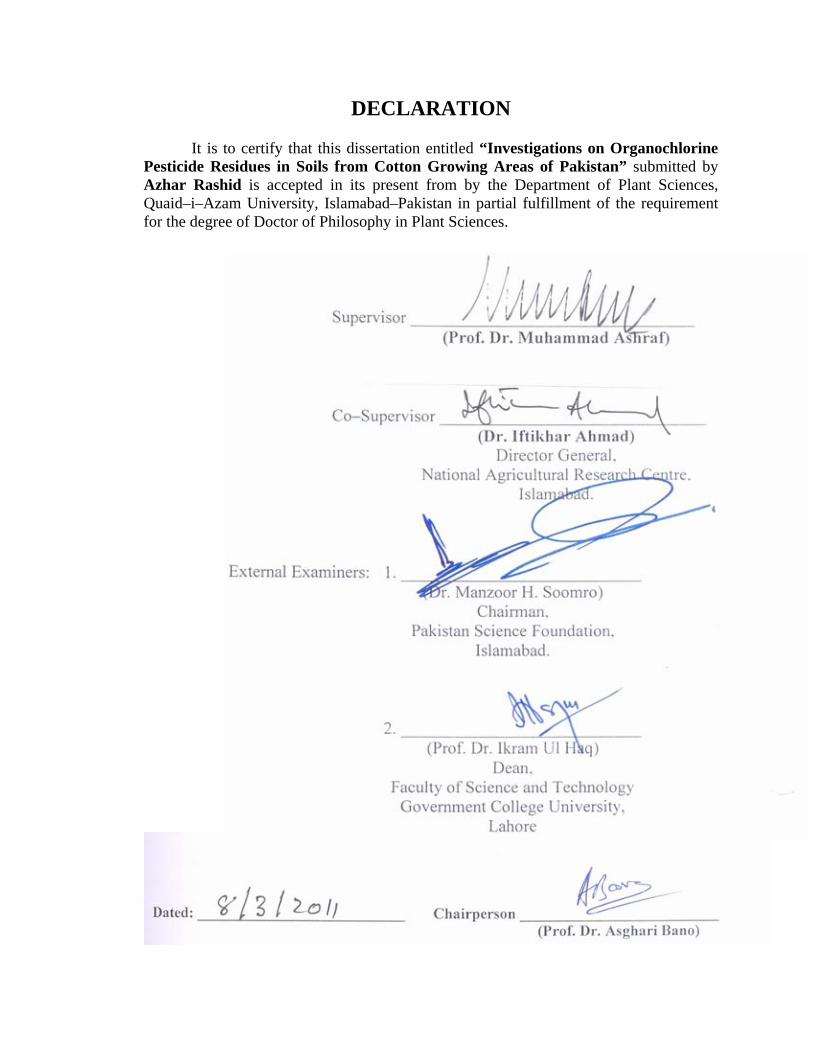
DECLARATION
It is to certify that this dissertation entitled “Investigations on Organochlorine Pesticide Residues in Soils from Cotton Growing Areas of Pakistan” submitted by Azhar Rashid is accepted in its present from by the Department of Plant Sciences, Quaid–i–Azam University, Islamabad–Pakistan in partial fulfillment of the requirement for the degree of Doctor of Philosophy in Plant Sciences.
CONTENTS LIST OF TABLES........................................................................................... i LIST OF FIGURES ....................................................................................... iii ACKNOWLEDGMENTS ...............................................................................v ABSTRACT ................................................................................................. vii LIST OF ABREVIATIONS .......................................................................... ix Chapter 1..........................................................................................................1 INTRODUCTION ...........................................................................................1
1.1 BACKGROUND OF THE STUDY ......................................................................... 1 1.2 ORGANOCHLORINE PESTICIDES...................................................................... 3
1.2.1 Dichlorodiphenyltrichloroethane (DDT) ........................................................... 3 1.2.2 Dicofol ............................................................................................................... 4 1.2.3 Heptachlor.......................................................................................................... 5 1.2.4 Aldrin ................................................................................................................. 6 1.2.5 Dieldrin .............................................................................................................. 7 1.2.6 Chlordane........................................................................................................... 8 1.2.7 Endosulfan ......................................................................................................... 9 1.2.8 Endrin............................................................................................................... 10 1.2.9 Hexachlorohexane (HCH) ............................................................................... 11 1.2.10 Hexachlorobenzene (HCB)............................................................................ 13
1.3 PESTICIDE USE IN PAKISTAN.......................................................................... 13 1.4 PESTICIDE USE IMPLICATIONS....................................................................... 14 1.5 PESTICIDES IN SOIL ........................................................................................... 16 1.6 OBJECTIVES......................................................................................................... 17 1.7 ORGANIZATION OF THESIS ............................................................................. 18 1.8 REFERENCES ....................................................................................................... 20
Chapter 2........................................................................................................25 STUDIES ON SOIL SAMPLE PROCESSING METHODS FOR DETERMINATION OF ORGANOCHLORINE PESTICIDE RESIDUES FROM SOIL MATRIX BY GAS CHROMATORGAPHY .........................25
2.1 INTRODUCTION .................................................................................................. 25 2. 2 MATERIALS AND METHODS........................................................................... 31
2.2.1 Chemicals and Reagents .................................................................................. 31 2.2.2 Instrumentation ................................................................................................ 32 2.2.3 Soil Samples..................................................................................................... 32
2.2.3.1 Preparation of Spike Samples ................................................................... 35 2.2.4 Extraction of Soil Samples............................................................................... 35
2.2.4.1 Ultrasonic Extraction ................................................................................ 36 2.2.4.2 Vortex Extraction...................................................................................... 36 2.2.4.3 Soxtec Extraction ...................................................................................... 36
2.2.4.4 QuEChERS Extraction.............................................................................. 37 2.2.4.5 Modified QuEChERS Method (with cleanup step) .................................. 37
2.2.5 Analytical Conditions ...................................................................................... 38 2.2.6 Method Performance Parameters..................................................................... 38
2.3. RESULTS AND DISCUSSION............................................................................ 42 2.3.1 Chromatographic Performance of GC-ECD- Ni63 ............................................ 42
2.3.1.1 Linearity.................................................................................................... 42 2.3.1.2 Limits of Detection and Quantification .................................................... 42 2.3.1.3 Reproducibility ......................................................................................... 43
2.3.2 Comparison of Existing Method...................................................................... 43 2.3.3 Method Development....................................................................................... 47
2.3.3.1 Comparison of Hydration Steps in QuEChERS Extraction...................... 47 2.3.3.2 QuEChERS Modifications........................................................................ 47 2.3.3.3 Chromatographic Performance of GC-MS/MS ........................................ 49
2.3.3.3.1 Linearity............................................................................................. 49 2.3.3.3.2 Chromatographic Reproducibility ..................................................... 49 2.3.3.3.3 Limits of Detection and Quantification ............................................. 49 2.3.3.3.4 Specificity .......................................................................................... 49
2.3.3.4 Method Validation .................................................................................... 50 2.3.3.5 Scope of the Method ................................................................................. 51
2.3.4 QuEChERS vs. Soxtec..................................................................................... 54 2.4 CONCLUSION....................................................................................................... 58 2.5 REFERENCES ....................................................................................................... 59
Chapter 3........................................................................................................64 STATUS AND SPATIAL VARIATIONS OF ORGANOCHLORINE PESTICIDE RESIDUES IN SOILS OF COTTON GROWING AREAS OF PAKISTAN....................................................................................................64
3.1 INTRODUCTION .................................................................................................. 64 3.1.1 Organochlorine Pesticide Residues in International Perspective..................... 64 3.1.2 Organochlorine Pesticide Residues in Pakistan............................................... 66
3.2 MATERIALS AND METHODS............................................................................ 68 3.2.1 Profile of Study Areas...................................................................................... 68
3.2.1.1 Nawabshah................................................................................................ 69 3.2.1.2 Ghotki ....................................................................................................... 69 3.2.1.3 Jhang ......................................................................................................... 70 3.2.1.4 Multan ....................................................................................................... 73
3.2.2 Soil Sampling................................................................................................... 73 3.2.3 Chemicals and Reagents .................................................................................. 74 3.2.4 Sample Preparation and Cleanup ..................................................................... 74 3.2.5 Chemical Analysis ........................................................................................... 75 3.2.6 Quality Control and Quality Assurance........................................................... 76 3.2.7 Statistical Analysis........................................................................................... 79
3.2.7.1 Hierarchical Cluster Analysis (HCA) ....................................................... 79 3.2.7.2 Discriminant Function Analysis (DFA).................................................... 80
3.3 RESULTS AND DISCUSSION............................................................................. 81
3.3.1 Quality Control / Quality Assurance................................................................ 81 3.3.1.1 Sampling ................................................................................................... 81 3.3.1.2 Extraction.................................................................................................. 81 3.3.1.3 Analysis..................................................................................................... 82
3.3.2 Organochlorine Residues in Different Soil Depths ......................................... 85 3.3.3 Organochlorine Pesticide Residue Status ........................................................ 87
3.3.3.1 Hexachlorohexane (HCH) ........................................................................ 87 3.3.3.2 Hexachlorobenzene (HCB)....................................................................... 92 3.3.3.3 Dichlorodiphenyl trichloroethane (DDT) ................................................. 93 3.3.3.4 Heptachlor............................................................................................... 103 3.3.3.5 Chlordane................................................................................................ 106 3.3.3.6 Endosulfan .............................................................................................. 110 3.3.3.7 Aldrin and Dieldrin ................................................................................. 115 3.3.3.8 Endrin...................................................................................................... 116
3.3.4 Spatial Distribution of Organochlorine Pesticide Residues........................... 117 3.3.4.1 Hierarchical Cluster Analysis (HCA) ..................................................... 117 3.3.4.2 Discriminant Function Analysis (DFA).................................................. 122
3.4 CONCLUSION..................................................................................................... 134 3.5 REFERENCES ..................................................................................................... 137
Chapter 4......................................................................................................144RELATIONSHIP OF ORGANOCHLORINE PESTICIDE RESIDUES WITH PHYSICAL, CHEMICAL AND BIOLOGICAL PROPERTIES OF SOIL............................................................................................................ 144
4.1 INTRODUCTION ................................................................................................ 144 4.2 MATERIALS AND METHODS.......................................................................... 148
4.2.1 Physical Properties......................................................................................... 148 4.2.1.1 Soil Textural Class.................................................................................. 149
4.2.2 Chemical Properties ....................................................................................... 149 4.2.2.1 Soil pH .................................................................................................... 149 4.2.2.2 Electrical Conductivity (EC)................................................................... 149 4.2.2.3 Organic Matter Content .......................................................................... 150
4.2.3 Biological Properties...................................................................................... 151 4.2.3.1 Isolation of Microbes From Soil ............................................................. 151
4.2.3.1.1 Fungal isolation................................................................................ 151 4.2.3.1.2 Bacterial isolation ............................................................................ 151
4.2.3.2 Enumeration of Soil Microflora.............................................................. 151 4.2.3.3 Fungal Identification............................................................................... 152
4.2.3.3.1 Macroscopic and microscopic studies ............................................. 152 4.2.4 Statistical Analysis......................................................................................... 152
4.3 RESULTS AND DISCUSSION........................................................................... 154 4.3.1 Physicochemical Properties ........................................................................... 154
4.3.1.1 Soil pH .................................................................................................... 154 4.3.1.2 Electrical Conductivity (EC)................................................................... 155 4.3.1.3 Organic Matter Content .......................................................................... 155 4.3.1.4 Physical Properties of Soil ...................................................................... 156
4.3.1.5 Soil Textural Class.................................................................................. 158 4.3.2 Biological Properties...................................................................................... 159
4.3.2.1 Fungal Diversity...................................................................................... 162 4.3.3 Relationship of Spatial Groups and Soil Properties....................................... 165 4.3.4 Relationship of Physicochemical Properties with OCPs ............................... 169 4.3.5 Relationship of Fungal Diversity with OCPs................................................. 177
4.4 CONCLUSION..................................................................................................... 184 4.5 REFERENCES ..................................................................................................... 186
Chapter 5..................................................................................................... 192 SUMMARY AND CONCLUSIONS......................................................... 192 Chapter 6..................................................................................................... 197 RECOMMENDATIONS FOR FUTURE STUDIES................................. 197 Chapter 7..................................................................................................... 198 BROCHURE FOR POLICY MAKERS .................................................... 198 APPENDICES ............................................................................................ 200
Appendix A Cost estimation for batch of 20 soil samples by proposed QuEChERS and Soxtec methods ........................................................ 200 Appendix B Physicochemical properties of soil samples ....................................... 201 Appendix C Abundance (CFUs g-1) of different fungi in soil samples................... 204 Appendix D Concentration (µg kg-1) of 19 organochlorine compounds in soil
samples from study areas. ................................................................... 207 Appendix E Chromatogram of 19 organochlorine pesticides for matrix matched
calibration solution (0.1 µg ml-1 ≡ 28 µg kg-1). .................................. 212
LIST OF TABLES Table Page Chapter 2
2.1 Physicochemical properties of soil samples 33 2.2 Summary of multiple reaction monitoring transitions selected for
analysis of 19 organochlorine pesticides in electron ionization mode 41
2.3 Chromatographic performance of gas chromatograph with electron capture detector for a calibration range of 40 µg kg–1 – 200 µg kg–1
43
2.4 F–values calculated by two–way ANOVA with interaction (α = 0.05) to compare different extraction methods, at three spiking levels of organochlorine pesticides
44
2.5 Percent recovery of selected organochlorine pesticides from soil matrix by different extraction methods at three fortification levels (n = 5)
46
2.6 Recovery of OCPs from hydrated samples (n = 10) 48 2.7 Chromatographic performance of gas chromatograph tandem
quadrupole mass spectrometer (GC–MS/MS) 50
2.8 Recovery data for organochlorine pesticides (n = 10) using the proposed procedure
52
2.9 Recovery data (n = 5) for organochlorine pesticides from different types of soil
53
2.10 Comparison of modified QuEChERS (Quch) and Soxtec (Sox) method for analysis of organochlorine pesticide residues in soil samples (µg kg-1) by gas chromatograph tandem quadrupole mass spectrometer (GC–MS/MS)
56
2.11 Comparison of sensitivity of two methods for gas chromatograph tandem quadrupole mass spectrometer (GC–MS/MS) analysis
57
2.12 Comparison between QuEChERS and Soxtec extraction methods 57 Chapter 3
3.1 Detail of sampling in study areas 74 3.2 Summary of multiple reaction monitoring transitions selected for
analysis of 19 organochlorine pesticides in electron ionization mode 78
3.3 Organochlorine pesticide contaminations (µg kg–1) in control samples from study areas
83
3.4 Batch–wise recovery (%) of OCPs in quality assurance/quality control samples spiked at 5 µg kg–1 (Sp1) and 20 µg kg–1 (Sp2)
84
3.5 Comparison between two soil profiles by paired t–test at 95 % level of significance
86
3.6 Hexachlorohexane (HCH) residues (µg kg–1) in cotton soils from study areas
91
3.7 Hexachlorobenzene (HCB) residues (µg kg–1) in cotton soils from study areas
93
3.8 DDT residues (µg kg–1) in cotton soils from study areas 96 3.9 Heptachlor residues (µg kg–1) in cotton soils from study areas 105 3.10 Chlordane residues (µg kg–1) in cotton soils from study areas 109
i
3.11 Endosulfan residues (µg kg–1) in cotton soils from study areas 113 3.12 Correlation between endosulfan isomers and their breakdown product 114 3.13 Aldrin and dieldrin residues (µg kg–1) in cotton soils from study areas 116 3.14 Endrin residues (µg kg–1) in cotton soils from study areas 116 3.15 Classification functions and variance (%) explained by stepwise
discriminant function analysis for spatial variations between study areas of Punjab (Group A) and Sindh (Group B)
124
3.16 Classification functions and variance (%) explained by stepwise discriminant function analysis for spatial variations between study areas of Jhang (Group AI) and Multan (Group AII)
127
3.17 Classification functions and variance (%) explained by stepwise discriminant function analysis for spatial variations between subgroups BI, BII and BIII of sampling sites of Sindh
132
Chapter 4
4.1 F–values calculated by one-way ANOVA to compare different physical and chemical properties of soil in different study areas
157
4.2 Description of fungal and bacterial abundance (CFUs g–1) in soils of study areas
160
4.3 Correlation coefficients of total organochlorine pesticide residues with different spatial groups and soil properties
165
4.4 Eigenvalues and percentages of the variance, obtained with the canonical correspondence analysis performed for OCP residues and physicochemical properties of soil from study areas
169
4.5 Canonical coefficients and correlation coefficient of physicochemical properties of soil with the first two axes generated by canonical correspondence analysis of physicochemical properties of soils from study areas
169
4.6 Eigenvalues and percentages of the variance, obtained with the canonical correspondence analysis performed for OCP residues and soil fungi from study areas
177
4.7 Canonical coefficients and correlation coefficient of soil fungi with the first two axes generated by canonical correspondence analysis of fungal diversity of soils from study areas
177
ii
LIST OF FIGURES Table Page Chapter 2
2.1 Multiple reaction monitoring chromatogram of (a) sample 2, (b) sample 3, (c) sample 4, (d) sample 5, (e) sample 6 and (f) 1 µg ml–1 matrix matched calibration solution. For peak identification see Table 2.2.
34
Chapter 3
3.1 Map of selected study areas in cotton growing areas of Pakistan 72 3.2 Relationship between o,p′–DDT and p,p′–DDT in soil sample from
(a) Nawabshah, (b) Ghotki and (c) Multan study areas (r = coefficient of correlation)
100
3.3 Frequency (%) of soil samples with different p,p′–DDE / p,p′–DDD ratios in the study areas
102
3.4 Relationship between β–Endosulfan and endosulfan sulphate in (a) Nawabshah, (b) Ghotki, (c) Jhang and (d) Multan study areas. (r = correlation coefficient at p = 0.05)
114
3.5 Dendrogram showing the major grouping among soil samples from four cotton growing study areas using Ward’s method (minimum variance) and Euclidian distance
119
3.6 Dendrogram showing sub–groups AI and AII in Group A using Ward’s method (minimum variance) and Euclidian distance
120
3.7 Dendrogram showing the sub–grouping in Group B using Ward’s method (minimum variance) and Euclidian distance
121
3.8 Box and Whisker plots of (a) γ–HCH, (b) heptachlor, (c) chlordane (cis), (d) α–endosulfan and (e) p,p´–DDE separated by discriminant function analysis for spatial variation between study areas of Punjab and Sindh
125
3.9 Box and Whisker plots of (a) γ–HCH, (b) heptachlor, (c) β–endosulfan and (d) p,p´–DDE separated by discriminant function analysis for spatial variation between study areas of Jhang (AI) and Multan (AII)
128
3.10 Box and Whisker plots of (a) HCB, (b) γ–HCH, (c) heptachlor, (d) β–endosulfan, (e) endosulfan sulphate, (f) o,p´–DDT and p,p´–DDT separated by discriminant function analysis for spatial variation between subgroups BI, BII and BIII of sampling sites in Sindh
133
Chapter 4
4.1 Box and Whisker plots for comparison of soil pH in study areas 154 4.2 Box and Whisker plots for comparison of soil ECe (dSm–1) in study
areas 155
4.3 Box and Whisker plots for comparison of organic matter content in study areas
156
4.4 Box and Whisker plots for (a) sand, (b) silt and (c) clay contents in the 157
iii
study areas 4.5 Soil texture class of soil samples from (a) Nawabshah, (b) Ghotki, (c)
Jhang and (d) Multan area plotted on USDA triangle for textural class 159
4.6 Abundance (CFUs g–1) of bacteria and fungi in soils of study areas 161 4.7 Relationship of fungal and bacterial abundance in soil 161 4.8 Frequency (%) of soil borne fungi in study areas 164 4.9 Abundance of soil borne fungi in study areas (error bars = ± standard
error of mean) 164
4.10 Relation of cumulative organochlorine pesticide (OCP) residues in relation to mean (a) soil pH (1:1), (b) ECe, (c) organic matter content (%), sand (%), silt (%), clay (%) and soil mycoflora (cfu) in different spatial groups (Error bars = ± standard error of mean)
168
4.11 Ordination diagram of canonical correspondence analysis of the relationship between physicochemical parameter soil and sampling sites in four study areas in cotton growing areas of Pakistan. Physicochemical parameters are represented as arrows. Directions of arrows indicate correlation with canonical axes and gradient of maximum change. The lengths of arrows indicate strength of correlation with respect to canonical axes and sampling sites.
175
4.12 Ordination diagram of canonical correspondence analysis of the relationship between physicochemical parameter soil and OCPs in four study areas in cotton growing areas of Pakistan. Physicochemical parameters are represented as arrows. Directions of arrows indicate correlation with canonical axes and gradient of maximum change. The lengths of arrows indicate strength of correlation with respect to canonical axes and OCPs.
176
4.13 Ordination diagram of canonical correspondence analysis of the relationship between mycoflora and sampling sites in four study areas in cotton growing areas of Pakistan. Fungal genera are represented as arrows. Directions of arrows indicate correlation with canonical axes and gradient of maximum change. The lengths of arrows indicate strength of correlation with respect to canonical axes and sampling sites.
182
4.14 Ordination diagram of canonical correspondence analysis of the relationship between soil mycoflora and OCPs in four study areas in cotton growing areas of Pakistan. Fungal genera are represented as arrows. Directions of arrows indicate correlation with canonical axes and gradient of maximum change. The lengths of arrows indicate strength of correlation with respect to canonical axes and OCPs.
183
Chapter 5
5.1 Overview of (a) cumulative organochlorine pesticide residues, (b) physical properties, (c) chemical properties and (d) mycoflora in soils from different cotton growing areas of Pakistan
196
iv

ACKNOWLEDGMENTS
All glories be to Almighty Allah, the eternal Creator of this universe, the most Beneficent, the
Merciful, the Gracious and the Compassionate, Whose bounteous blessings gave me potential and
opportunity to make this humble contribution. Praises, respects and Derwood–o–Salam are due to the
Holy Prophet, Hazard Muhammad (Peace be upon him) whose blessings and exaltations flourished my
thoughts and thrived my ambitions to have this cherished fruit of my efforts in the form of this write
up.
I am cordially gratified to my supervisor Prof. Dr. Muhammad Ashraf Ex-Chairman Department of
Plant Sciences for his patience, trust, moral support, encouragement and able guidance all through the
study.
Heartiest gratitude, sincere thanks and appreciation to my co–supervisor Dr. Ifitikhar Ahmad,
Director General, National Agricultural Research Centre (NARC), Islamabad for his inspiration,
moral support, guidance and for providing research facilities at NARC.
I am highly indebted to Dr. Sadat Nawaz, Programme Manager, Pesticide Residue Team, The Food
and Environment Research Agency (FERA), York, UK for his cooperation and providing me an
opportunity to work under his able guidance and state of the art research facilities.
I am gratified to “Indigenous 5000 Ph.D. Fellowship Programme” and “International Research
Support Initiative Programme (IRSIP)” of Higher Education Commission for providing me funding to
peruse my Ph.D. inland and abroad.
I thank Dr. Mir Ajab Khan, Dean, Faculty of Biological Sciences and Dr. Asghari Bano, Chairperson,
Department of Plant Sciences, Quaid-i-Azam University, Islamabad for their support and
cooperation.
I am thankful to serving and previous, Chairs and Members of Pakistan Atomic Energy Commission;
Directors of Nuclear Institute of Agriculture (NIA), Tandojam and Heads of Plant Genetics Division
for their continued support and kind cooperation throughout my quest for Ph.D.
v

I am thankful to Mr. Afzal Arain (Director, NIA, Tandojam), Dr. Muhammad Mureed Kandhro and
Mr. Ghulam Hussain Kaleri from Nuclear Institute of Agriculture, Tandojam for their help in survey
and sampling in Sindh. I express my thanks to Mr. Karam Ahad and Dr. Ashiq Muhammad from Eco-
toxicology Research Programme, NARC, Islamabad for providing me expertise and facilities for
analytical work. Thanks to Dr. Javed Iqbal Mirza for providing facilities for microbiological studies
in his laboratory.
I am also thankful to my university colleagues Munawar Raza Kazmi, Sobia Tabassum, Hadi
Bakhsh, Ali Mustajab Naqvi, S. Tatheer Naqvi, Abdul Qadir and Muhammad Rizwan. I am also
thankful to my loving friends Muhammad Jabbar and Abdul Nadeem for their well wishes.
A non-payable debt to my loving parents, their wish motivated me in striving for higher education;
they prayed for me, shared the burden and made sure that I sailed through smoothly. I am also very
grateful to my in-laws for their support and wishes for my success. I am also thankful to my brother
Zahid Rashid and sisters for their well wishes.
Last but not the least, I acknowledge and thank my wife Sobia, son M. Qasim Azhar, Daughters
Fatima Azhar and Hafsa Azhar for their patience, love and cooperation.
May Allah shower all these people with His Blessings.
AZHAR RASHID
vi
ABSTRACT
Organochlorine pesticides have been used in agricultural as well as public health sectors
for many years in Pakistan. Cotton, for its importance as major cash crop and backbone
of agro–based economy of Pakistan, was major recipient of these pesticides. In view of
the historical application, organochlorine pesticide residues were investigated in cotton
growing areas. Residues of 19 organochlorines viz. hexachlorobenzene (HCB), α–HCH,
β–HCH, γ–HCH, heptachlor, heptachlor–epoxide (trans), aldrin, dieldrin, chlordane
(trans), chlordane (cis), oxychlordane, α–endosulfan, β–endosulfan, endosulfan sulfate,
endrin, p,p׳–DDT, o,p׳–DDT, p,p׳–DDD and p,p׳–DDE were studied in low and high
pesticide application areas of Punjab and Sindh. Sites were selected belonging to Miani
soil series. In Sindh, Nawabshah was low and Ghotki was high pesticide application area.
Similarly, in Punjab, Jhang was low and Multan was high pesticide intensity area. Prior
to soil sample analysis, extraction procedures were studied for accuracy and precision.
Among the existing soil processing methods, Soxtec was found with good accuracy and
precision but involved considerably long sample processing and high cost of solvents and
disposable accessories. In order to overcome these limitations, potential of quick,
efficient, cheap, easy, rugged and safe (QuEChERS) method was explored for soil matrix
with some modifications. The modified method was validated for different fortification
levels, different types of soils and was compared with Soxtec method using soil samples
with field incurred residues. The extracts produced by the proposed method were clean
with low background noise on gas chromatography with tandem quadrupole mass
spectrometry (GC-MS/MS). The method was cheap, safe and rugged requiring minimal
time and resources.
Henceforth, the newly developed method was used to study organochlorine pesticides in
selected sites of Sindh and Punjab. Higher concentrations of γ–HCH, heptachlor,
chlordane (cis), α–Endosulfan and p,p′–DDE were responsible for variation between
Sindh and Punjab. Mean concentration of organochlorine residues was 35.5 µg kg-1 in
Sindh and 5.23 µg kg-1 in Punjab. In Sindh, high pesticide use area of Ghotki had higher
amounts of γ–HCH, heptachlor, β–endosulfan and p,p′–DDE residues than Nawabshah.
vii
In Ghotki area, mean organochlorine residue concentration in soil samples was 26.7 µg
kg-1 compared with 20 µg kg-1 in Nawabshah. In Punjab, Multan area soils had higher
concentration and frequencies of hexachlorobenzene (HCB), γ–HCH, heptachlor, β–
endosulfan, endosulfan sulphate, o,p΄–DDT and p,p΄–DDD than in soils of Jhang. Mean
organochlorine concentration was 4.2 µg kg-1 in Multan and 2 µg kg-1 in Jhang soils.
Physicochemical and biological properties of soil were studied in relation to the
distribution and magnitude of organochlorine contaminants in soil. Soil salinity (ECe)
and clay content were positively associated with amount of organochlorine residues in
contaminated soils. Soil pH and organic matter content were identified as most important
variables in relation to organochlorine residues and had negative interaction with
dichlorodiphenyltrichloroethane (DDT), hexachlorohexane (HCH) and cyclodienes
except for endosulfan and positive association with breakdown products of these
compounds. This indicated instability or degradation of organochlorines under alkaline
and high organic matter soils. Association of some soil mycoflora was negative with
organochlorine compounds and positive with their breakdown products. It is therefore,
envisaged that these fungi showing sensitivity to the parent organochlorines and tolerance
for their breakdown products might have some role in bio-degradation.
viii
LIST OF ABREVIATIONS OC organochlorine OCP organochlorine pesticide DDT dichlorodiphenyltrichloroethane EPA Environmental Protection Agency HCH hexachlorohexane HCB hexachlorobenzene GDP gross domestic product POPs persistent organic pollutants MAE microwave assisted extraction ASE accelerated solvent extraction PLE pressurized liquid extraction SFE supercritical fluid extraction SPE solid phase extraction QuEChERS quick, efficient, cheap, easy, rugged, safe PSA primary secondary amine GC gas chromatography LC liquid chromatography MS mass spectrometry ECD electron capture detector MS/MS tandem quadruple mass spectrometry IPM integrated pest management NGOs non-governmental organizations QC quality control QA quality assurance OM organic matter EI electron ionization HCA hierarchical cluster analysis DFA discriminant function analysis MAC maximum allowable concentration EC electrical conductivity CCA canonical correspondence analysis
ix
Chapter 1
INTRODUCTION
1.1 BACKGROUND OF THE STUDY
Primary role of agriculture is to produce a reliable supply of wholesome food to feed the
burgeoning world population, safely and without adverse effects on the environment.
Intensified agriculture around the world has, therefore dictated increasing use of
agrochemicals to meet the growing food, feed and fiber demands. Modern era of
chemical pest control began around the time of World War II with the discovery of most
famous organochlorine DDT (Zhang et al., 2009). The DDT compound was rediscovered
as an insecticide in 1939 and its discoverer, Paul Müller was awarded the Nobel Prize for
medicine in 1948 (Banuri, 1999). Commercial production of DDT began in 1943 (Beatty,
1973). At that time, DDT was considered as blessing due to low cost production, high
toxicity to insects, and low toxicity to mammals and was used widely in public health and
agriculture sector as an all-purpose insecticide. Afterwards, many other compounds were
formulated between 1945 and 1953, including BHC, chlordane, toxaphene, aldrin,
dieldrin, endrin, heptachlor, parathion, methyl parathion, and tetraethyl paraphosphate
(Banuri, 1999). These pesticides had been used for many years in public health sector to
control mosquitoes and as broad-spectrum insecticide against insect pests of food and
fiber crops in agriculture sector. Over the years, use of pesticides and other agrochemical
has increased many folds in agriculture sector especially in the developing countries with
no or negative impact on crop yields (Khan et al., 2002).
Presently, over 500 compounds are registered worldwide as pesticides or metabolites of
pesticides (van der Hoff and van Zoonen, 1999). Pesticides are grouped according to
purpose of use, formulations and chemical structure of pesticides.
According to purpose of pesticide use, different groups include: insecticides (insect
killers), herbicides (plant killers), fungicides (controlling fungi), molluscicides
(controlling molluscs), nematicides (controlling nematodes), rodenticides (controlling
1
rodents), bactericides (bacteria killers), defoliants (removing plants leaves), acaricides
(killers of ticks and mites), wood preservatives, repellents (substances repugnant to pest),
attractants (substances attracting insects, rodents and other pests), and chemosterilants
(substances inhibiting reproduction of insects) (Skoglund et al., 2006).
A formulation is a mixture of the active ingredient in a pesticide with other inert
(inactive) substances. Different formulations may be used differently. These include,
aerosol, baits, dry flowable, dusts, emulsifiable concentrate, flowable, granule, low
concentrate solution, micro-encapsulation, soluble powder, solution, tracking powders,
water soluble packets and wettable powder (Buffington and McDonald, 2006).
Classification of the pesticides on the basis of chemical structure is another very
important criterion. Based on the chemical structure, there are three main classes of
pesticides viz. inorganic, botanical and synthetic organic pesticides. Inorganic pesticides
constitute elements, minerals or chemical compounds derived from deposits in nature.
Common inorganic pesticides are copper, mercury, sulfur silica aerogel, boric acid,
borates, diatomaceous earth and cryolite. Botanical pesticides are extracts of different
parts of plant species. These pesticides have a short residual activity and do not
accumulate in the biotic and abiotic environments. Common examples of botanical
pesticides are pyrethrins, rotenone, nicotine, neem, limonene etc. Synthetic organic
insecticides are synthesized having carbon and hydrogen atoms as the basis of their
molecule. Synthetic organic insecticides are grouped into six basic types viz.
organochlorines (hydrocarbon compounds containing multiple chlorine substitutions),
organophosphates (esters of phosphoric acid), carbamates (slats or esters of carbamic
acid), pyrethroids (synthetic compounds similar to naturally occurring pesticide
pyrethrin, which is found in chrysanthemum), insect growth regulators affecting the
normal growth and maturity of insects and microbial pesticides (formulations of
pathogens of insect pests).
2
1.2 ORGANOCHLORINE PESTICIDES
Organochlorine is an organic compound that contains carbon, hydrogen and through
sharing of electron pair forms covalent bond with one or more chlorine atoms. Several
groups of chemicals including industrial chemicals viz. polychlorinated biphenyls
(PCBs), chlorofluorocarbons (CFCs), polychlorinated dibenzodioxins (PCDDs), or
dioxins and many pesticides contain chlorinated hydrocarbons and are classified as
organochlorine. Organochlorine pesticides vary in their chemical structures and
mechanisms of toxicity. Persistence of organochlorine compounds in the environment is
well known. They are hydrophobic and lipophilic in nature and, tend to accumulate in the
fatty tissues of marine and wildlife animals. Beside persistence in the environment, some
organochlorine pesticides move considerable long distances and get accumulated in
vegetation, soil and bodies of water of high latitudes by global distillation phenomenon
(Simonich and Hites, 1995). Organochlorine pesticides can be classified into four
categories: diphenyl alephatic (e.g. DDT, dicofol), cyclodienes (e.g. heptachlor, dieldrin),
chlorinated benzenes (e.g. hexachlorobenzene [HCB]), and cyclohexanes (e.g.
hexachlorocyclohexane [HCH]).
1.2.1 Dichlorodiphenyltrichloroethane (DDT)
DDT (1, 1, 1-trichloro-2, 2-bis (p-chlorophenyl) ethane), most famous insecticide was the
first organochlorine pesticide developed and was discovered to be an insecticide in 1939
by Nobel laureate Paul Muller. It is persistent, non-systemic with contact and stomach
3
mode of action. After its wide use in World War II against mosquitoes in the malaria
eradication programme, DDT was introduced as insecticide in agricultural sector.
According to the estimates more than 2 million tons of DDT has been produced and
applied since 1940 for the management of insect pests throughout the world.
Commercially available DDT (technical grade) is white, crystalline, tasteless and almost
odorless solid and a mixture many isomers. The major component p,p´-DDT constitute
77% and o,p'-DDT is about 15% of the mixture and the rest contains o,o´-DDT and
sometime breakdown products.
DDT and its metabolites are highly toxic and can persist in the environment for several
decades after application and their affects could be magnified through the food chain.
Being lipophilic DDT gets accumulated into fatty tissues of birds and animals. In soil
environment due to hydrophobic properties, it remains adhered to soil particles and does
not reach ground water quickly. DDT is semi-volatile compound and enter atmosphere
through volatilization from plant, soil and water surfaces. Half-life of DDT ranges from
2–15 years and breaks down by the affects of sunlight or microorganisms in environment.
In environment DDT breaks down to more persistent compounds DDE (1,1-dichloro-2,2-
bis(p-chlorophenyl)ethylene) and DDD (1,1-dichloro-2,2-bis(p-chlorophenylethane). In
the residue analysis, the term "total DDT or Σ DDT" is used to refer to the sum of all
DDT related compounds (p,p´-DDT, o,p´-DDT, DDE, and DDD).
1.2.2 Dicofol
Dicofol (2,2,2-trichloro-1,1-bis (4-chlorophenyl) ethanol) is structurally similar to DDT.
The only difference is due to replacement of the hydrogen (H) on C-1 by a hydroxyl (-
4
OH) functional group in DDT. Technical DDT is used for synthesis of Dicofol. For this
purpose DDT is chlorinated to an intermediate, Cl-DDT, followed by hydrolyzing to
dicofol. Commercial dicofol contains 80% dicofol and the rest is mixture of DDT
isomers, DDT breakdown products DDD and DDE and Cl-DDT as impurities.
Dicofol is a non-systemic acaricide with contact action. It is used as foliar spray on
agricultural crops and ornamentals, and in or around agricultural and domestic buildings
for mite control. In 1986, the US Environmental protection Agency (EPA) temporarily
suspended the use of dicofol due to high levels of DDT contaminants in the final product.
According to World Health Organization (WHO), dicofol is Class III, 'slightly hazardous'
pesticide. Dicofol shows non-toxic effects to bees and is slightly toxic to birds. However,
it is highly toxic to fish and aquatic invertebrates.
In the environment dicofol is moderately persistent in soil, with a half-life of 60 days
(Johnson et al., 1998). Dicofol is practically insoluble in water and adsorption with soil
particles is very strong. It is nearly immobile in soils and unlikely to infiltrate
groundwater. It is possible for dicofol to enter surface waters when soil erosion occurs
where it can be adsorbed by the sediments. Soil with high moisture and exposure to UV
light at alkaline pH favors its breakdown.
1.2.3 Heptachlor
Heptachlor (1, 4, 5, 6, 7, 8, 8-heptachloro-3a, 4, 7, 7a-tetrahydro-4, 7-methanoindene) is
an insecticide in the form of white powder and sometimes due to impurities as tan color
powder. Commercial heptachlor (technical grade) contains 72% heptachlor and 28%
5
related compounds. It is a non-systemic insecticide with contact, stomach and to some
extent respiratory mode of action. Heptachlor resembles chlordane and was isolated from
technical chlordane. In efficacy as insecticide, heptachlor is 4-5 time more effective than
chlordane.
Heptachlor is one of the persistent organic pollutants (POPs) and is toxic and extremely
persistent in the environment. Through biomagnifications accumulates in the fatty tissues
of humans and animals and can move to remote locations after volatilization and can
deposit in high altitudes via global distillation. Heptachlor persists in soils for long time
and metabolizes into a more toxic compound heptachlor epoxide. Heptachlor epoxide
residues are more likely to occur in soil than its parent compound either due to rapid
degradation compared to heptachlor or accumulation from other sources like chlordane.
Heptachlor epoxide is solubilized in water easily and can get adsorbed with soil particle
to persist soil and water for longer periods.
Due to environmental persistence they can find routs into human food chain by
deposition in edible fish, dairy products, and meats exposed to the compounds, breast
milk, and drinking water. Direct inhalation and contact with contaminated soil at disposal
sites are some other human exposure routes.
1.2.4 Aldrin
Aldrin (1, 2, 3, 4, 10, 10-Hexachloro-1, 4, 4a, 5, 8, 8a-Hexahydro-exo-1, 4-endo-5, 8-
Dimethanonaphthalene) is used as an insecticide in agriculture sector. It was named after
the German chemist Kurt Alder. Aldrin has been effectively used against soil born insects
6
such as termites and grasshoppers to protect field crops such as cotton, corn and potatoes.
Aldrin itself is non-toxic to insects. In insect body, it is oxidized to dieldrin which is
neurotoxin and carries out insecticidal function. After agricultural application aldrin
either volatilizes from soil or is converted rapidly to dieldrin after oxidization.
Aldrin is also categorized as persistent organic pollutant (POP) due to persistence of
parent and breakdown products. After inhalation or some direct or indirect physical
contact, aldrin enters the body, and metabolizes to dieldrin. Dieldrin has the ability to
accumulate in the fatty tissues and its metabolites are excreted in bile and feces. It is also
excreted in breast milk.
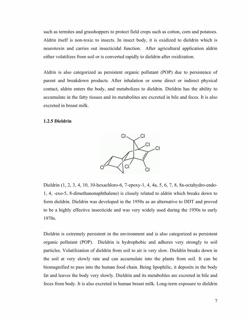
1.2.5 Dieldrin
Dieldrin (1, 2, 3, 4, 10, 10-hexachloro-6, 7-epoxy-1, 4, 4a, 5, 6, 7, 8, 8a-octahydro-endo-
1, 4, -exo-5, 8-dimethanonaphthalene) is closely related to aldrin which breaks down to
form dieldrin. Dieldrin was developed in the 1950s as an alternative to DDT and proved
to be a highly effective insecticide and was very widely used during the 1950s to early
1970s.
Dieldrin is extremely persistent in the environment and is also categorized as persistent
organic pollutant (POP). Dieldrin is hydrophobic and adheres very strongly to soil
particles. Volatilization of dieldrin from soil to air is very slow. Dieldrin breaks down in
the soil at very slowly rate and can accumulate into the plants from soil. It can be
biomagnified to pass into the human food chain. Being lipophilic, it deposits in the body
fat and leaves the body very slowly. Dieldrin and its metabolites are excreted in bile and
feces from body. It is also excreted in human breast milk. Long-term exposure to dieldrin
7

has proven toxic to a very wide range of animals including humans, far greater than to the
original insect targets. The elimination half-life of dieldrin is approximately 1 year. At
high doses, dieldrin affect central nervous system by blocking inhibitory
neurotransmitters which leads to symptoms like headache, confusion, muscle twitching,
nausea, vomiting, and seizures.
1.2.6 Chlordane
Chlordane (1, 2, 4, 5, 6, 7, 7, 8-octachloro-2, 3, 3a, 4, 7, 7a-hexahydro-4, 7-
methanoindene) is an insecticide used against termites and other insects on agricultural
crops and lawns. It is non-systemic with contact, stomach and respiratory mode of action.
Chlordane resembles heptachlor structurally and in mechanism of toxicity. Commercial
chlordane (technical grade) may contain more than 50 related chemicals including 50-
60% chlordane isomers and the rest constitutes stereoisomer and heptachlor. The main
chlordane isomers, chlordane (trans) and chlordane (cis) found in ratio of 4:5
approximately in the commercial chlordane. Chlordane metabolizes into oxy-chlordane
and trans-nonachlor while heptachlor into heptachlor epoxide. Therefore, heptachlor
epoxide residues in the absence of oxy-chlordane and trans-nonachlor cannot be taken as
from chlordane source.
Chlordane is highly persistent in the environment. It is strongly hydrophobic and remains
adsorbed to soil particles and are not likely to enter groundwater. Residues of chlordane
can be found even after 20 years of application in soil where it breaks down very slowly.
It has a reported half life of 1 year. In soil, residues of trans-chlordane are found
comparatively in higher amounts than those of chlordane (cis) either due to difference in
rate of degradation or difficulty in analysis of cis- compared to trans-chlordane during
8
sample processing. Chlordane can leave soil to enter atmosphere by volatilization.
Because of concern about damage to the environment and harm to human health, the US
Environmental protection Agency (EPA) banned chlordane for all purposes in 1988.
Chlordane is lipophilic and can bioaccumulate in the fatty tissues of fish, birds, and
mammals which can act as source of human exposure.
1.2.7 Endosulfan
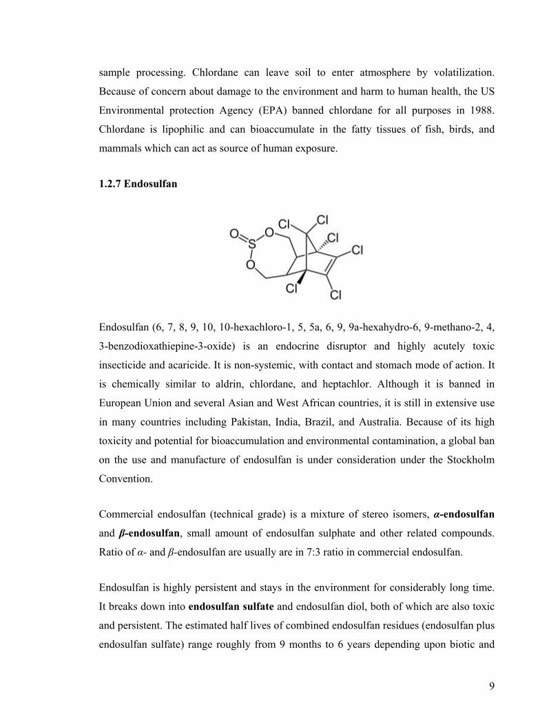
Endosulfan (6, 7, 8, 9, 10, 10-hexachloro-1, 5, 5a, 6, 9, 9a-hexahydro-6, 9-methano-2, 4,
3-benzodioxathiepine-3-oxide) is an endocrine disruptor and highly acutely toxic
insecticide and acaricide. It is non-systemic, with contact and stomach mode of action. It
is chemically similar to aldrin, chlordane, and heptachlor. Although it is banned in
European Union and several Asian and West African countries, it is still in extensive use
in many countries including Pakistan, India, Brazil, and Australia. Because of its high
toxicity and potential for bioaccumulation and environmental contamination, a global ban
on the use and manufacture of endosulfan is under consideration under the Stockholm
Convention.
Commercial endosulfan (technical grade) is a mixture of stereo isomers, α-endosulfan
and β-endosulfan, small amount of endosulfan sulphate and other related compounds.
Ratio of α- and β-endosulfan are usually are in 7:3 ratio in commercial endosulfan.
Endosulfan is highly persistent and stays in the environment for considerably long time.
It breaks down into endosulfan sulfate and endosulfan diol, both of which are also toxic
and persistent. The estimated half lives of combined endosulfan residues (endosulfan plus
endosulfan sulfate) range roughly from 9 months to 6 years depending upon biotic and
9

abiotic factors of soil (Anonymous, 2002). From soil it can be volatilized into air and can
move and deposit at far away places by global distillation.
Endosulfan has high potential of bio-accumulation in fish, birds and animals. Endosulfan
is toxic and can act as an endocrine disruptor, causing reproductive and developmental
damage in both animals and humans. Acute poisoning with endosulfan include
hyperactivity, tremors, convulsions, lack of coordination, staggering, suffocation, nausea,
vomiting, diarrhea and unconsciousness in severe cases.
1.2.8 Endrin
Endrin ((1aR, 2S, 2aS, 3S, 6R, 6aR, 7R, 7aS)-3, 4, 5, 6, 9, 9-hexachloro-1a, 2, 2a, 3, 6,
6a, 7, 7a-octahydro-2, 7:3, 6-dimethanonaphtho [2, 3-b] oxirene) is an insecticide used on
cotton, maize, and rice. It also acts as an avicide and rodenticide. It is a solid, cream to
light tan to white, almost odorless substance. Endrin is a stereoisomer of dieldrin and is
structurally similar to aldrin, and heptachlor epoxide. Due to high toxicity and
persistence, endrin was banned in many countries. It was mainly used as aerial spray to
control insect pests of cotton besides it was also used on rice, sugar cane, grain crops and
sugar beet, and tobacco.
Endrin is highly persistent in the environment and is likely to be absorbed into the
sediments in surface water. It is very toxic to aquatic organisms and has potential of
bioaccumulation into fatty tissues of aquatic animals. In soil its half life is over 10 years.
10
Human exposure is through skin adsorption or inhalation of dust or vapors. Endrin is
highly lipophilic and can deposit in fatty tissues for long time. Acute endrin poisoning in
humans affects primarily the nervous system.
1.2.9 Hexachlorohexane (HCH)
There are three isomers of HCH viz. α-hexachlorohexane (α-HCH), β-hexachlorohexane
(β-HCH), and γ-hexachlorohexane (γ-HCH) used as pesticides in agriculture and public
health sector. Of these isomers only γ-HCH has insecticidal properties and is also called
Lindane. Other isomers α-HCH and β-HCH are byproducts of commercial lindane (γ-
HCH) production.
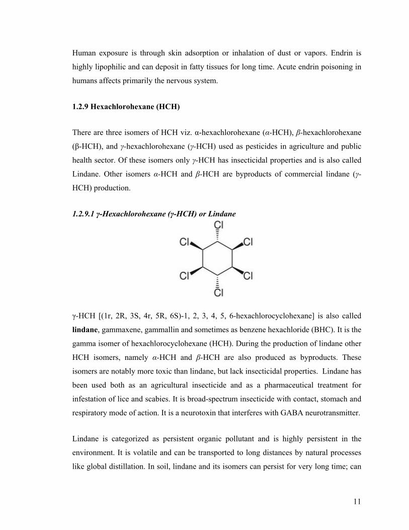
1.2.9.1 γ-Hexachlorohexane (γ-HCH) or Lindane
γ-HCH [(1r, 2R, 3S, 4r, 5R, 6S)-1, 2, 3, 4, 5, 6-hexachlorocyclohexane] is also called
lindane, gammaxene, gammallin and sometimes as benzene hexachloride (BHC). It is the
gamma isomer of hexachlorocyclohexane (HCH). During the production of lindane other
HCH isomers, namely α-HCH and β-HCH are also produced as byproducts. These
isomers are notably more toxic than lindane, but lack insecticidal properties. Lindane has
been used both as an agricultural insecticide and as a pharmaceutical treatment for
infestation of lice and scabies. It is broad-spectrum insecticide with contact, stomach and
respiratory mode of action. It is a neurotoxin that interferes with GABA neurotransmitter.
Lindane is categorized as persistent organic pollutant and is highly persistent in the
environment. It is volatile and can be transported to long distances by natural processes
like global distillation. In soil, lindane and its isomers can persist for very long time; can
11
leach to surface and even ground water. Over time, lindane and isomers can break down
in soil, sediment and water into less toxic substances by algae, fungi and bacteria.
However, this is very slow process depending upon the environmental conditions.
Lindane can bioaccumulate and enter into human food chain. Exposure of lindane to
general population is from agricultural uses and the intake of contaminated foods, such as
produce, meats and milk. In humans, lindane primarily affects the nervous system, liver
and kidneys, and may be a carcinogen and/or endocrine disruptor. It is categorized as
“moderately hazardous” by World Health Organization. It was included in the Stockholm
Convention on persistent organic pollutants, which bans its production and use
worldwide.
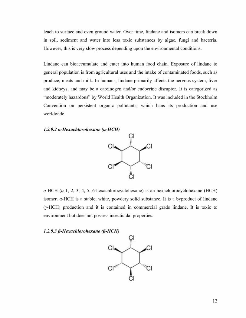
1.2.9.2 α-Hexachlorohexane (α-HCH)
α-HCH (α-1, 2, 3, 4, 5, 6-hexachlorocyclohexane) is an hexachlorocyclohexane (HCH)
isomer. α-HCH is a stable, white, powdery solid substance. It is a byproduct of lindane
(γ-HCH) production and it is contained in commercial grade lindane. It is toxic to
environment but does not possess insecticidal properties.
1.2.9.3 β-Hexachlorohexane (β-HCH)
12
β-HCH (β-hexachlorocyclohexane) is an also a hexachlorocyclohexane (HCH) isomer. It
is a byproduct of lindane (γ-HCH) production. It typically constitutes 5-14% of technical
grade lindane.
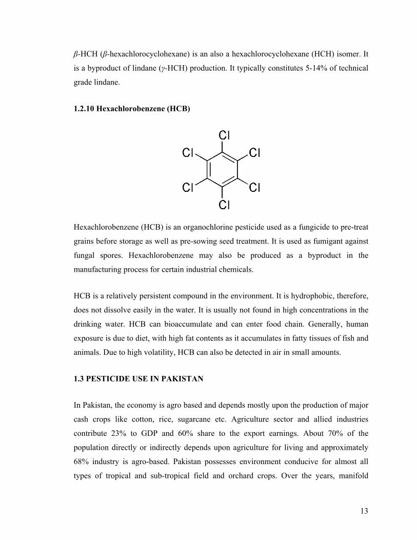
1.2.10 Hexachlorobenzene (HCB)
Hexachlorobenzene (HCB) is an organochlorine pesticide used as a fungicide to pre-treat
grains before storage as well as pre-sowing seed treatment. It is used as fumigant against
fungal spores. Hexachlorobenzene may also be produced as a byproduct in the
manufacturing process for certain industrial chemicals.
HCB is a relatively persistent compound in the environment. It is hydrophobic, therefore,
does not dissolve easily in the water. It is usually not found in high concentrations in the
drinking water. HCB can bioaccumulate and can enter food chain. Generally, human
exposure is due to diet, with high fat contents as it accumulates in fatty tissues of fish and
animals. Due to high volatility, HCB can also be detected in air in small amounts.
1.3 PESTICIDE USE IN PAKISTAN
In Pakistan, the economy is agro based and depends mostly upon the production of major
cash crops like cotton, rice, sugarcane etc. Agriculture sector and allied industries
contribute 23% to GDP and 60% share to the export earnings. About 70% of the
population directly or indirectly depends upon agriculture for living and approximately
68% industry is agro-based. Pakistan possesses environment conducive for almost all
types of tropical and sub-tropical field and orchard crops. Over the years, manifold
13
increase in the demand has pushed for more and more use of agrochemicals to produce
more yields. Present use of pesticides in Pakistan is concentrated on cotton, the most
important cash crop and the most important export commodity. Cotton production is
mostly concentrated in Punjab and Sindh provinces, constituting about 2.5 M.ha and
consumes major share of pesticides used in Pakistan (Khan, 1998). The pesticides applied
are mostly insecticides, used against a number of serious pest species e.g. white fly,
jassid, aphid and bollworms. These pests have direct as well as indirect affect on yield
reduction, besides also act as vectors for different contagious bacterial, fungal and viral
diseases.
In Pakistan, there was no concept of agro-chemical use before 1960s. However, to control
ever increasing problems of pests and diseases, traditional methods proved insufficient
and were supplemented by the use of pesticides from 1970s onwards. Initially, pesticides
were introduced by government on subsidized rates and even free of cost in some cases,
to promote productivity of agricultural sector. Since then use of pesticide in Pakistan has
increased from 665 metric tons (MT) at the inception of pesticide business in 1980 to
90676 MT in 2007. With the development of cotton industry, cotton became a major
recipient of pesticides with 80% share of the amount used in Pakistan (Tariq at el., 2007).
According to Ahmad and Poswal (2000), massive increase in the pesticide use has not
necessarily increased yields positively. In contrary, this indiscriminate use of pesticides
had serious implications on the environment and the populations of natural bio-control
agents and natural enemies of the insects and pests have declined up to 90% during the
last decade of 19th century especially, in cotton growing areas of the country (Hasnain,
1999). Furthermore, reliance on pesticide use for pest management has resulted in
changing the cotton pest complex thus becoming a never ending practice.
1.4 PESTICIDE USE IMPLICATIONS
An estimated 0.1% of the pesticides applied to crops reach their target pest, and rest of
them enter the environment, and contaminate soil, air and water (Pimentel et al., 1991).
Unfortunately, scientists learned after a while about the environmental implications of the
pesticides in the form of persistence and bioaccumulation in biotic and abiotic
14
components of the ecosystem. Realization about these affects came after some 20 years
of DDT usage through renowned book “Silent Spring” by Rachel Carson in 1962. She
reported DDT causing eggshell thinning in bird eggs leading to near extinction of bird
species such as peregrine falcons and bald eagles. Scientists took leaf out of Carson’s
book and started exploring the environmental aspects of pesticide use. Along with the
extensive use of pesticides, concerns regarding potential adverse environmental effects
have grown globally. Pesticides have been detected in surface and ground water bodies in
many parts of the world. Today most of the organochlorine pesticides have been banned
in the United States by the EPA because of the tendency of these compounds to persist in
the environment and bioaccumulate in animals. Several studies have shown accumulation
of pesticide especially organochlorine in soils, ground waters and food commodities
(Aubin et al., 1993; Masse et al., 1994; USEPA, 1998; Hébert and Rondeau, 2004; PAN
Europe, 2004). Pesticides accumulation in food and drinking water has been recognized
as dangerous throughout the world. Long-term persistence and toxicity of pesticides in
natural resources is responsible for causing various kinds of human illnesses (Peralta et
al., 1994; Mannion, 1995). This estimates over 0.22 million deaths throughout the world
and 3 million cases of severe pesticide poisonings each year (Stangil, 2001). Colborn et
al., (1997) reported that 35% of consumed food in US, contaminated with detectable
pesticide residues. Sometimes, laboratory analytical methods due to low sensitivity, can
detect only one-third of the total pesticides present in food. Therefore, the use of
pesticides and their potentially undesirable effects on the environment and human health
has been one of the leading research areas (Schumacher and Ward, 1987). This
emphasizes the need for validation of assessment procedures prior to any kind of
monitoring and surveillance studies.
Among classes of pesticides, organochlorine and organophosphorus are most important
and most widely used pesticides. Organochlorine pesticides are known to resist
biodegradation, therefore, are persistent and have high bioaccumulation potential along
food chains (Mbakaya et al., 1994; Sankararamakrishnan et al., 2005). Organophosphorus
compounds, on the other hand, are known to degrade rapidly depending upon their
formulation, method of application, climate and the growing stage of the plant
15
(Sankararamakrishnan et al., 2005). Realizing the carcinogenic and persistent nature of
organochlorine pesticides, and to protect the human health and environment, a
convention on twelve persistent organic pollutants (POPs) including eight pesticides viz.
DDT, aldrin, dieldrin, endrin, chlordane, heptachlor, mirex, and toxaphene for special
investigations and international attention has been reached in Durban, South Africa, in
2000 (Getenga et al., 2004; Tieyu et al., 2005). Despite these facts, organochlorine
compounds are cheap to produce and remain highly effective due to their broad-spectrum
nature. Due to these reasons, developing countries maintain that they cannot afford to ban
these older pesticides (Sankararamakrishnan et al., 2005). The dilemma of cost/efficacy,
verses ecological impacts, including long range impacts via atmospheric transport, and
access to modern pesticide formulations at low cost remain a continuous global issue.
Besides, social cost has also been reported due to externalities of pesticide use (Khan et
al., 2002). In Pakistan, exposure of pesticides in past resulted in the burden of pesticides
in soil, water, food, feed, fiber and other agricultural commodities (Ahmad and Abdullah,
1971; Parveen and Masud, 1988; Masud and Hasan, 1992; Parveen et al., 1994; Masud
and Hasan, 1995; Parveen et al., 1996; Anonymous, 2001; Hussain et al., 2001).
1.5 PESTICIDES IN SOIL
Pesticides reach soil through application, disposal, spill, runoff from plant surface or
through incorporation of pesticide applied crop residues into the soil (Brown and Hock,
1990). Soil acts as filter, buffer and exhibit degradation potentials for pollutant owing
mainly to the soil organic matter content (Burauel and Baßmann, 2005). According to
Brown and Hock (1990), these pesticides are either absorbed by soil components, move
away from point of intrusion or go through microbial, chemical and photo degradation.
Furthermore, degradation of pesticides is very slow in soil and can result in entry into
human food chain owing to runoff and subsurface drainage; interflow and leaching; and
translocation into the plant and animals (Tariq et al., 2007). Bhattacharya et al., (2003)
described chemical discharges from domestic and industrial sources, chemical
applications in the form of fertilizers and pesticides in agricultural and soil erosion due to
deforestation as sources of soil contaminants (Bhattacharya et al., 2003). As soil is the
most important agricultural resource next to water, therefore, it is important to study the
16
possible presence of pesticide residues in soil in relation to physical, chemical and
biological properties of soil.
In past, several studies have been conducted to monitor pesticide contamination and to
understand fate of pesticides in relation to soils of Pakistan. These contributions are
reviewed by Tariq et al., (2007). Pesticide contaminants have been monitored in crop
lands especially cotton and rice in Punjab, tobacco in Khyber Pakhtoonkhwa (formerly
NWFP) (Ali and Jabbar, 1992; Jabbar et al., 1993) and around different water bodies of
Punjab and Sindh (Bano and Siddique, 1991; Tehseen et al., 1994; Sanpera et al., 2002).
Studies related to sorption coefficients, pesticide half lives, hydrophobicity and pesticide
persistence have also been conducted in different types of soil (Tariq et al., 2004a; Tariq
et al., 2004b; Tariq et al., 2006; Tariq et al., 2007). Similarly, interaction and fate of
pesticide contaminants in relation to physical, chemical and biological properties of soil
have also been studied by different workers (Iqbal et al., 2001; Tariq et al., 2006, Tariq et
al., 2007). These studies clearly indicated contamination of OCPs and other pesticides in
the soil environment. However, these studies are mostly localized and relation of these
contaminants to different crop ecologies and intensity of pesticide use have not been
investigated.
Cotton crop cultivation in Pakistan has long history of pesticide use especially OCPs.
Some of these OCPs were banned a decade ago, while, other are still in use. Since, OCPs
persist in the soil environment for long periods of time compared to other types of
pesticide. Therefore, present study was planned to study OCP contaminants in soils under
cotton crop. The study aimed to comprehend status of OCP contaminants in relation to
the pesticide use intensities and agro-ecologies of cotton crop in Pakistan. Present study
was conducted in the major cotton growing districts of Punjab and Sindh. In each
province two sites were selected varying in pesticide use.
1.6 OBJECTIVES
Overall objective of the study was to investigate the status and spatial variations in OCP
residues in different cotton growing areas. For this purpose, different analytical
17

procedures were compared and validated to ensure realistic estimation of contaminants.
Occurrence and spatial variations of OCP residues were studied in relation to different
properties of soil. The specific objectives were as follows:
1. Evaluation and validation of sample processing methods for efficient, reliable and
robust assessment of OCPs from soil matrix at very low levels in minimal time
and resources.
2. Investigation of status and spatial variations of OCP residue in soils from cotton
growing areas.
3. Elucidation of factors responsible for the spatial variations.
4. Investigation for interaction of physical, chemical and biological properties of soil
with OCP contaminants in soils of different cotton areas.
1.7 ORGANIZATION OF THESIS
In this thesis, general background of the research including an overview of
organochlorine pesticides, pesticide use in Pakistan, and implications of pesticide use are
discussed along with objectives of research in Chapter 1.
Studies related to development, validation and comparison of different analytical
methods for analysis of OCP residues in soil matrix by gas chromatography are described
in Chapter 2.
Next, in Chapter 3, the newly developed analytical method was applied for assessment of
OCP residues in soils from different cotton growing areas of Pakistan. Occurrence,
concentration of OCP residues, source and age of these residues in the soil environment
are also discussed. Spatial variations for OCP residues in the study areas and factors
responsible for these variations are also discussed using different statistical tools.
18
In Chapter 4, study areas were compared for physical, chemical and biological properties
of soil. Relation of these soil properties with OCP contaminants was also studied using
multivariate statistical tools. This chapter also narrates spatial variations of OCP residues
with reference to soil properties of the study areas.
Overview of the whole study and outcomes is presented in Chapter 5 as Executive
Summary. Finally, recommendations for future studies based on the outcomes of this
research work are given in Chapter 6. Brochure for policy maker is set as Chapter 7.
19
1.8 REFERENCES
Ahmad, I., and A. Poswal. 2000. Cotton Integrated Pest Management in Pakistan: Current
Status. Country Report presented in Cotton IPM Planning and Curriculum
Workshop Organised by FAO, Bangkok, Thailand. February 28-March 2.
Ahmad, M., and A. Abdullah. 1971. Determination of residues of dimecron, endrin and
malathion on tobacco plants, using bioassay technique. Pakistan J Sci Res, 23(1-
2): 34-41.
Ali, M. and A. Jabbar. 1992. Effect of pesticides and fertilizers on shallow groundwater
Quality. Final technical report (Jan. 1990–Sep. 1991). Pakistan Council of
Research in Water Resources (PCRWR), Government of Pakistan, Islamabad.
Anonymous. 2001. Policy and strategy for rational use of pesticides in Pakistan-Building
consensus for action. FAO/Global IPM Facility, UNDP, Government of Pakistan.
Anonymous. 2002. Reregistration eligibility decision for endosulfan. US Environmental
Protection Agency (EPA) EPA 738-R-02-013. http://www.epa.gov/oppsrrd1/
reregistration/endosulfan/finalefed_riskassess.pdf
Aubin, E., S.O. Prasher and R.N. Yong. 1993. Impact of water table on metribuzin
leaching. Proc. Of the 1993 Joint CSCE-ASCE National conference on
Environmental Engineering. July 12-14, Montreal, Quebec, Canada. pp. 548-564.
Bano, A., and S.A. Siddique. 1991. Chlorinated hydrocarbons in the sediments from the
coastal waters of Karachi (Pakistan). Pak. J. Sci. Ind. Res., 34:70–4.
Burauel, P. and F. Baßmann. 2005. Soils as filter and buffer for pesticides: experimental
concepts to understand soil functions. Environmental Pollution, 133(1): 11-16.
Banuri, T. 1999. Pakistan: Environmental Impact of Cotton Production and Trade.
International Institute for Sustainable Development, Winnipeg, Manitoba Canada.
http://www.tradeknowledgenetwork.net/pdf/pk_Banuri.pdf
Beatty, R.G. 1973. The DDT myth: triumph of the amateurs. The John Day Company,
New York, USA.
Bhattacharya, B., S.K. Sarkar, and N. Mukherjee. 2003. Organochlorine pesticide
residues in sediments of a tropical mangrove estuary, India: implications for
monitoring. Environment International, 29:587–92.
20
Brown, C.L. and W.K. Hock. 1990. The Fate of Pesticides in the environment.
Agrichemical Fact Sheet #8, Penn State Cooperative Extension.
Buffington, E.J. and S.K. McDonald. 2006. Pesticide formulations. Colorado
Environmental Pesticide Education Program Pesticide Fact Sheet #105 CEPEP
5/00 Updated 6/06. http://wsprod.colostate.edu/cwis79/FactSheets/Sheets
/105Formulations.pdf
Colborn, T., D. Dumanoski, and J.P. Myers.1997. Our Stolen Future: are we threatening
our fertility, intelligence, and survival: A scientific detective story. New York:
Penguin Group.
Getenga, Z.M., F.O. Kengara, S.O. Wandiga. 2004. Determination of organochlorine
pesticide residues in soil and water from river Nyando Drainage System within
Lake Victoria basin, Kenya. Bull Environ Contam Toxicol, 72:335-343.
Hasnain, T. 1999. Pesticides-use and its impact on crop ecologies: issues and options.
Working Paper Series # 42. SDPI, Islamabad.
Hébert, S. and B. Rondeau. 2004. Saint Laurent Vision 2000 actions plan. Phase III: The
Water Quality of Lake Saint-Pierre and its Tributaries.
http://www.slv2000.qc.ca/plan_action/phase3/biodiversite/suivi_ecosysteme/ateli
er_20041203/presentations/SH_qual_eaux_a.htm.
van der Hoff, G. R. and P. van Zoonen. 1999. Trace analysis of pesticides by gas
chromatography. J. Chromatogr. A, 843, 301–322.
Hussain, A., Z. Iqbal, M.R. Asi. 2001. Impact of repeated pesticide application on the
binding and release of 14C-methameidophos to soil matrices under field
conditions. NIAB, Faisalabad.
Iqbal, Z., A. Hussain, A. Latif, M.R. Asi and J.A. Chaudhary. 2001. Impact of pesticide
applications in cotton agro ecosystem and soil bioactivity studies I: microbial
populations. J Biol Sci, 1:640–4.
Jabbar, A., S.Z. Masud, Z. Parveen, M. Ali. 1993. Pesticide residues in cropland soils and
shallow groundwater in Punjab Pakistan. Bull Environ Contam Toxicol, 51:268–
273.
21
Johnson, M. L., A. Salveson, L. Holmes, M. S. Denison and D. M. Fry. 1998.
Environmental Estrogens in Agricultural Drain Water from the Central Valley of
California. Bull. Environ. Contam. Toxicol., 60:609 - 614.
Khan, M.S.H. 1998. Pakistan crop protection market. PAPA Bulletin. 9:7-9.
Khan, M.A., M. Iqbal, I. Ahmad and M.H. Soomro. 2002. Economic Evaluation of
Pesticide Use Externalities in the Cotton Zones of Punjab, Pakistan. The Pakistan
Development Review, Pakistan Institute of Development Economics, 41(4): 683-
698.
Mannion, A.M. 1995. Agricultural and environmental change. New York, N.Y.: John
Wiley & Sons.
Masse, L., S.O. Prasher, S.U. Khan, D.S. Arjoon and S. Barrington. 1994. Leaching of
metolachlor, atrazine, and atrazine metabolites into ground water. Trans. ASAE,
37(3):801-806.
Masud, S.Z., and N. Hasan. 1992. Pesticide residues in foodstuffs in Pakistan:
organochlorine, organophosphorus and pyrethroid insecticides in fruits and
vegetables. Pak. J. Sci. Ind. Res. 35(12): 499-504.
Masud, S.Z., and N. Hasan. 1995. Study of fruits and vegetables in NWFP, Islamabad
and Balochistan for organochlorine, organophosphorus and pyrethroid pesticides
residues. Pak. J. Sci. Ind. Res., 38(2):47-80.
Mbakaya, C.F.l., G.J.A. Ohayo-Mitoko, V.A.F. Ngowi, R. Mbabazi, J.M. Simwa, D.N.
Maeda, J. Stephens and H. Hakuza. 1994. The status of pesticide usage in East
Africa. Afr J Health Sci., 1:37-41.
PAN Europe. 2004. Pesticide Action Network Europe: Pesticides in food - what’s the
problem? Briefing no. 3, September 2004, Facilitated by PAN Germany and PAN
UK. http://www.pan-europe.info/publications/index.shtm.
Parveen, Z., and S.Z. Masud. 1988. Monitoring of fresh milk for organochlorine pesticide
residues in Karachi. Pak. J. Sci. Ind. Res., 31(1): 49-56.
Parveen, Z., I.A.K. Afridi and S.Z. Masud. 1994. A multi-residue method for quantitation
of organochlorine, organophosphorus and synthetic pyrethroid pesticides in cotton
seed. Pak. J. Sci. Ind. Res., 37(12): 536-540.
22
Parveen, Z., I.A.K. Afridi, S.Z. Masud and M.M.H. Baig. 1996. Monitoring of multiple
pesticide residues in cotton seeds during three crop seasons. Pak. J. Sci. Ind. Res.,
39(5-8): 146-149.
Peralta, R.C., M.A. Hegazy and G.R. Musharrafieh. 1994. Preventing pesticide
contamination of ground water while maximizing irrigated crop yield. Water
Resource Res., 30(11): 3183-3193.
Pimentel, D., A. Greiner and T. Bashore. 1991. Economic and environmental costs of
pesticide use. Arch Environ Contam Toxicol, 21:84–90.
Sankararamakrishnan, N., A.K. Sharma and R. Sanghi. 2005. Organochlorine and
organophosphorus pesticide residues in ground and surface waters of Knpur, utter
Pradesh, India. Environment International, 31:113-120.
Sanpera, C., X. Ruiz, G.A. Llorente, L. Jover and R. Jabeen. 2002. Persistent
organochlorine compounds in sediment and biota from the Haleji Lake: a wildlife
sanctuary in south Pakistan. Bull Environ Contam Toxicol., 68:237–244.
Schumacher, B.A. and S.E. Ward. 1987. Quantitation reference compounds and VOC
recoveries from soils by purge-and-trap GC/MS. Environ. Sci. Technol. 31: 2287-
2291.
Simonich, S.L. and R.A. Hites. 1995 Organic pollutant accumulation in vegetation.
Environ. Sci. Technol, 29: 2905-2914.
Skoglund, L.G., S.K. McDonald and E.J. Buffington. 2006. What are pesticides?
Colorado Environmental Pesticide Education Program, Pesticide Fact Sheet #101
CEPEP 05/00, Updated 6/06. http://wsprod.colostate.edu/cwis79/
FactSheets/Sheets/101whatarepesticides.pdf
Stangil, P. 2001. Enjoy Vibrant Health in a Toxic World (Pamphlet). Charlottesville,
Virginia.
Tariq, M.I., S. Afzal, and I. Hussain. 2004a. Pesticides in shallow water table areas of
Bahawalnagar, Muzafargarh, D. G. Khan and Rajan Pur Districts of Punjab,
Pakistan. Environment International, 30:471–9.
Tariq, M.I., S. Afzal, and I. Hussain. 2004b. Adsorption of pesticides by salorthids and
camborthids of Punjab, Pakistan. Toxicological & Environmental Chemistry,
86:247–64.
23
Tariq, M.I., S. Afzal, and I. Hussain. 2006. Degradation and persistence of cotton
pesticides in sandy loam soils from Punjab, Pakistan. Environmental Research,
100:184–96.
Tariq, M.I., S. Afzal, I. Hussain, and N. Sultana. 2007. Pesticides exposure in Pakistan: a
review. Environment International, 33: 1107–1122.
Tehseen W.M., L.G. Hansen, S.G. Wood and M. Hanif. 1994. Assessment of chemical
contaminants in water and sediment samples from Degh Nala in the province of
Punjab, Pakistan. Arch Environ Contam Toxicol, 26:79–89.
Tieyu, W., L. Yonglong, S. Yajuan, and Z. Hong. 2005. Spatial distribution of
organochlorine pesticide residues in soils surrounding Guanting reservoir,
People’s Republic of China. Bull Environ Contam Toxicol., 74:623-630.
USEPA. 1988. Research program description-ground water research. EPA/600/9-88/005.
Washington D.C.: US Environment Protection Agency.
Zhang, P., J. Song and H. Yuan. 2009. Persistent organic pollutant residues in the
sediments and mollusks from the Bohai Sea coastal areas, North China: An
overview. Environment International, 35(3):632-646.
24

Chapter 2
STUDIES ON SOIL SAMPLE PROCESSING METHODS FOR DETERMINATION OF ORGANOCHLORINE PESTICIDE RESIDUES
FROM SOIL MATRIX BY GAS CHROMATORGAPHY
2.1 INTRODUCTION
Pesticide residue analysis from soil is very complex process and over the years efforts
have been made to develop simple, reliable and cost effective analytical method. The
soil-organochlorine (OC) interaction is intricate, ranging from weak electrostatic forces
(dipole-dipole) to ionic bonding that gives birth to the phenomenon of bound residues.
Adsorption of compounds by soil is influenced by diverse factors such as organic matter
content, soil type, and physical-chemical properties of pesticides like vapor pressure,
water solubility and n-octanol-water partition coefficient (Cheng, 1990). The interaction
between soil matrix and pesticide analytes is stronger than food and other matrices,
resulting in the formation of bound residues (Rissato et al., 2005). Organochlorine
pesticide (OCP) residues in soil are unenviable and many investigators have reported
different levels of residues in different soils.
In this regard, researchers have employed various sample processing techniques, like
shake flask (Vig et al., 2001), vortex extraction (Garimella et al., 2000), ultrasonic
extraction (Xia and Leidy, 2002; Tadeo et al., 2004; Goncalves and Alpendurada, 2005),
microwave assisted ultrasonic extraction (MAE) (Fuentes et al., 2006), Soxhlet extraction
or Soxtec (automated Soxhlet extraction) (Getenga et al., 2004; Garimella et al., 2000,
Sanghi and Kannamkumarath 2004; Hussen et al., 2006) and some more recently
developed methods like accelerated solvent extraction (ASE) or pressurized liquid
extraction (PLE) (Haib et al., 2003; Grana et al., 2004; Hussen et al., 2006; Pang et al.,
2006), supercritical fluid extraction (SFE) (Khan, 1995; Chester et al., 1998; Garimella et
al., 2000, Anitsecu and Tavlarides, 2006;); and solid phase extraction (SPE) (Garimella et
al., 2000, Haib et al., 2003). Preference of the method depends upon its availability,
efficacy, applicability, simplicity and cost effectiveness.
25
Shake flask method is simple and straight forward method of pesticide residue extraction
from environmental and food matrices. This has been used for organochlorines (Tor et
al., 2006) and herbicides (Cheng, 1990) from soil matrix. The only limitations are excess
use of organic solvents, long duration of extraction and need for post–extraction cleanup.
Vortex extraction method is similar to shake–flask method in working principles but
utilizes smaller amount of sample and organic solvent. However, reproducibility of the
method is not very good due to number of handling steps. Ultrasonic extraction involves
extraction of analytes from solid matrix by the use of sonication energy. The method is
used by U.S. Environmental Protection Agency (EPA) as Method 3550B for extraction of
non–volatile and semi–volatile organic compounds from solid matrices like soil, sludge
and wastes. Among the conventional methods ultrasonic extraction is less time
consuming, uses less solvent to produce good recoveries of residues from soil matrix (Tor
et al., 2006).
Among the modern extraction method Soxhlet extraction is considered as most
exhaustive of the extraction methods and is a standard extraction technique for
environmental analysis used for over 30 years (Rissato et al., 2005). This has been used
as reference method by U.S. Environmental Protection Agency (EPA) as EPA Method
3540C for non–volatile and semi–volatile organic compounds from solids such as soils,
sludges and wastes. Limitations of this approach are utilization of large volumes of
extraction solvent (s), long extraction time and interferences resulting from the
exhaustive extraction process (Handley, 1999). Soxtec or automated Soxhlet extraction
method works similar to Soxhlet extraction. This approach has similar extraction
efficiency but time of extraction is very short (3 hours) compared to Soxhlet extraction.
Soxtec extraction method is used by U.S. Environmental Protection Agency (EPA) as
Method 3541 for extraction of organic analytes from soil, sediment, sludges and solid
waste. Lopez–Avila et al., (1993) studied Soxtec extraction for extraction of
organochlorine compounds from soils with different physicochemical characteristics and
proposed Soxtec as an alternate to Soxhlet and sonication extraction techniques.
26
Microwave assisted extraction (MAE) utilizes microwave energy to produce high
temperature, under elevated pressure in closed vessel containing sample and organic
solvent (s). MAE is used for extraction of organophosphorus, organochlorine, and PCBs
from solid matrices by U.S. Environmental Protection Agency (EPA) under Method
3546. MAE has high extraction efficiency, requires small amount of organic solvent (s)
and is completely automated. The only drawback is high cost of instrumentation. Due to
exhaustive extraction further cleanup steps are usually required.
Pressurized liquid extraction (PLE) is also called pressurized fluid extraction (PFE) and
accelerated solvent extraction (ASE) as trade name by Dionex. PLE is an extraction
procedure that uses organic solvents under elevated pressure (1500–2000 psi) and
temperature (100°C) for extraction of organic analytes from samples contained in
stainless steel extraction cells and electronically controlled heaters and pumps. High
pressure keeps the solvent below boiling point and forces its penetration in the matrix.
Elevated temperature changes the distribution co–efficient of the solvent to increase the
solubilization of analytes in the solvent by decreasing its viscosity and diffusivity which
overcomes intermolecular interactions of the analyte and matrix (Grana et al., 2004).
Environmental Protection Agency (EPA) has given PFE as Method 3545A for extraction
for semi–volatile organic compounds, organochlorine and organophosphorus pesticides,
chlorinated herbicides and PCBs etc. from soils, sediments, sludges and solid wastes.
Supercritical fluid extraction (SFE) is somewhat similar to PLE, except that it involves
carbon dioxide liquefied above critical temperature (31°C) at high pressure and is used to
extract pesticides and their metabolites without the use of organic solvents. In PLE
extraction of thermo–labile compounds is problematic due to high temperature. In
contrary, SFE provides possibility of extraction of such compounds at moderate
temperature (around 30°C) with high level of selectivity (Haib et al., 2003). Method 3562
was described by U.S. Environmental Protection Agency (EPA) for extraction of
polychlorinated biphenyls, and organochlorine pesticides from solids such as soils,
sludges, and wastes by supercritical fluid extraction (SFE). Due to rather expensive
device, use of limited sample size and erratic recoveries due sample moisture content and
variations in polarity of the analytes (Vinas et al., 2003), it is not a widely used method.
27
Solid phase extraction (SPE) is basically a cleanup method for solid matrices rather than
an extraction method. It is used to isolate analytes of interest from aqueous matrix or
extracts of solid matrices like soil, sludges, food samples etc. SPE is based on selective
adsorption and desorption of components dissolved in a solvent (mobile phase) by solid
(stationary phase) through which sample is passed. In a recently developed method of
extraction, sorbent SPE material PSA (primary secondary amine) is incorporated directly
in the extract produced by QuEChERS in bulk to remove undesirable co–extracts is
called dispersive SPE (Anastassiades, et al., 2003).
Recently a new method was developed for multi–residue analysis highlighted for being
quick, easy, cheap, effective, rugged and safe and commonly called as “QuEChERS”
(Anastassiades et al., 2003). The methods have been widely used as reference method
especially for food related matrices in international laboratories for monitoring and
surveillance studies. QuEChERS method effectively covers analytes with wide range of
polarities as well as highly acidic and basic pesticides. The method involved extraction of
the homogenized samples by hand shaking or vortex for few seconds with acetonitrile
(MeCN). Residual moisture in the acetonitrile extract is removed by liquid–liquid
partitioning facilitated by addition of salts (4 gm anhydrous MgSO4 and 1 gm NaCl).
This is followed by addition of internal standard and centrifugation to physically separate
aqueous phase from organic MeCN phase. Further cleanup of the extract is carried out by
dispersive solid–phase extraction (dispersive–SPE). For this purpose solid phase
extraction sorbent viz. primary secondary amine (PSA) and anhydrous MgSO4 is
thoroughly mixed with MeCN extract aliquot and separated by centrifugation to remove
aqueous and polar contaminants. This method is considerably easy, produces good
recoveries of analytes in considerably clean extracts with minimal resources and very
short period of time.
Primarily the QuEChERS method was developed for high moisture and low fat matrices
like fruits and vegetable. Later intervention were made it suitable for intermediate as well
as for high fat matrices with added advantage of high sample throughput with minimal
involvement of solvents, glassware, bench space and instrumentation (Paya et al., 2007).
28
After introducing hydration step before MeCN extraction stage, the method was modified
and optimized for samples with low moisture contents like barley grains (Diez et al.,
2006), wheat flour (Paya et al., 2007), and for dry cereals and animal feeding stuff
including bran, whole ears, straw, hay, malt, starch and dry vegetables (Walorczyk,
2008). Luiz et al., (2008) successfully used QuEChERS to extract veterinary antibiotics
including quinolones, sulphonamides, macrolides, anthelmintics and one tetracycline
from milk for UPLC/MS analysis. They used 10 ml of 0.1M Na2–EDTA along with
buffered MeCN for extraction of antibiotics from full cream, semi–skim and skim milk
samples to avoid formation of chelating complexes by macrolides with cations present in
the solution. Very recently, Lesueur et al., (2008) further exploited application of
QuEChERS and included it in a comparative study along with three other well
established methods viz. liquid–liquid, pressurized liquid extraction and European Norm
Din 12393 for analysis of 24 pesticide from soil matrix by GC/MS and LC/MS.
QuEChERS was found superior in analyte recoveries, and was stated as most adapted
method for majority of analytes. QuEChERS method had shown flexibility and had gone
through many changes since its inception to become adaptable for different types of
matrices and analytes. The method is based on MeCN extraction which has also been
recommended for pesticide residue extraction especially those of organochlorine from
soil (Goncalves and Alpendurada, 2005).
Pesticide residue analysis in food and environmental samples has become a regulatory
and industrial requirement in many parts of the world. Modern residue monitoring
programmes are expected to be responsive to latest developments in agriculture and new
legislations. Therefore, development and application of modern analytical methods are
necessary to improve qualitative and quantitative performance of the laboratories. This is
also necessary for realistic and reliable estimation of contaminants in the samples.
Present study was aimed to investigate OCP residue status in the cotton growing areas of
Pakistan. Prior to sample analysis, studies were conducted to compare some conventional
extraction methods viz. vortex, sonication and Soxtec extraction for precision and
accuracy. Although, these methods are efficient and precise in recovery yield of analytes
29
from soil but generally, all of these methods are costly and cumbersome due to longer
sample processing time. Therefore, potential of QuEChERS extraction approach was also
exploited for soil matrix with the aim to achieve high accuracy and precision of OCP
analytes from soil in minimal time and resources.
The present study was conducted with following objectives:
1. Comparison of three conventional extraction techniques viz. vortex, ultrasonic
and Soxtec for analysis of selected OCs by gas chromatography equipped with
electron capture detection (GC/ECD) from soil. During the study, methods were
compared for precision, accuracy and sensitivity by using spiked soil samples.
2. Development and validation of quick, cheap and reliable procedure for analysis of
19 OCs from soil samples to achieve sensitivity at low levels. This was achieved
through use of QuEChERS extraction method, simultaneous clean–up and
concentration step followed by determination using gas chromatography tandem
quadruple mass spectrometry (GC–MS/MS).
3. Comparison of proposed method with Soxtec extraction method to study its
applicability.
30
2. 2 MATERIALS AND METHODS
Studies for comparison between three extraction methods viz. vortex, sonication and
Soxtec for OCs in soil matrix were conducted in Pesticide Residues Laboratory,
Ecotoxicology Research Prgramme, National Agricultural Research Centre, Islamabad,
Pakistan. Development and validation of QuEChERS extraction method for soil matrix
was carried out in Pesticide Residue Laboratory, Food and Environment Research
Agency (formerly Central Science Laboratory), Sand Hutton, York, United Kingdom.
2.2.1 Chemicals and Reagents
Pesticide reference standards (purity > 99.0 %) of aldrin, DDT, dicofol, dieldrin, α– and
β–endosulfan, endrin, HCH and heptachlor used during method comparison studies were
purchased from Dr. Ehrenstorfer Laboratories (Augsburg, Germany). Analytical grade
ethyl acetate, dichloromethane and reagent grade sodium sulphate anhydrous (Na2SO4)
from Merck Co. (Darmstadt, Germany).
For QuEChERS related studies, certified, high purity (> 99.0 %), reference standards of
α–HCH, γ–HCH, β–HCH, endrin, HCB, heptachlor, heptachlor epoxide (trans), aldrin,
dieldrin, chlordane (trans), chlordane (cis), oxychlordane, p,p΄–DDT, p,p΄–DDT, p,p΄–
DDD, p,p΄–DDE, α–endosulfan, β–endosulfan, endosulfan–sulphate were purchased
from Qmx (Thaxted, UK) and LGC–Promochem (Teddington, UK). Acetonitrile, water
(HPLC grade) and hexane (analytical reagent grade) were from Fisher Scientific
(Loughborough, UK), anhydrous magnesium sulphate and sodium acetate trihydrate
(analytical reagent grade) were purchase from York glassware (York, UK).
Individual stock solutions for OCs were prepared in hexane. The working standard
solutions containing each of the 19 OCs were prepared in hexane at 10 µg ml–1, 1.0 µg
ml–1, and 0.1 µg ml–1. The working standard solutions were used for spiking blank soil
samples and for the preparation of matrix matched calibration solutions.
31
32
2.2.2 Instrumentation
Method comparison involved Soxtec system HT2 (Tecator, Sweden) constituting 1045
extraction unit and 1046 service unit, Vortex Gyromixer TRA and Elma Transonic–T700.
For centrifugation Hettich Zentrifugen D–78532 (Tuttinggen, Germany), capable of
producing 4000g and for concentration step rotary evaporator Rotavapor R–114 (Buchi,
UK) was used. For pesticide residue analysis auto–system gas chromatograph (GC)
(Perkin Elmer, USA) equipped with an electron capture detector (ECD–63Ni) was used.
For chromatographic separation of the analytes, fused silica capillary column (PE–3,
phase methyl 10 % phenyl silicon, 25 m, 0.32 i.d., 0.5 mm o.d., 0.5 µ film thickness,
Perkin Elmer, USA) was used. Data acquisition and reprocessing steps were carried out
by Turbochrom4® data analysis hardware/software system.
Method development and validation involved vortex mixer (Clifton Cyclone) and
centrifuge (Jouan C/CR4.12 bench top centrifuge) capable of producing 5000 g.
Determination step was carried out using a Varian GC–MS/MS system comprising of
CP3800 gas chromatograph (GC) with a 1079 injector, a CP8400 auto–sampler and a
1200L triple quadrupole MS/MS (Varian, Walnut Creek, CA, USA). A fused silica
capillary column (Zebron ZB–50 phase, 50 % phenyl 50 % methylpolysiloxane, 30 m x
0.25 mm i.d., and 0.25 µm film thickness; Phenomenex, USA) was used. The column
was protected by a 7 mm CarboFrit insert (Restek, Bellefonte, PA, USA) placed in the
GC liner (Varian Split, Open, 5 mm OD × 54 mm × 3.4 mm ID). Data acquisition and
reprocessing were performed using a Star Workstation version 6.41.
2.2.3 Soil Samples
Method comparison study was carried out by using blank soil sample (Blank soil A)
collected from pesticide free area of National Agriculture Research Centre, Islamabad.
For method development and validation, pesticide free soil sample (Blank soil B) was
collected from a domestic garden in York, UK. Five samples (Blank soil B–F) were used
for performance evaluation of proposed method in relation to the soil types.

Table 2.1 Physicochemical properties of soil samples
Soil Sample Sampling Depth (cm)
Sand (w/w %)
Silt (w/w %)
Clay (w/w %)
Textural Class
Organic matter (%)
pH (1:1 soil:water)
Blank soil A 0–15 26.0 41.0 33.0 Clay loam 1.3 6.7 Blank soil B 0–15 17.5 47.1 35.4 Silty clay loam 4.4 6.4 Blank soil C 0–15 54.6 31.7 13.7 Sandy loam 6.4 4.3 Blank soil D 0–15 52.1 29.0 18.9 Sandy loam 9.8 4.8Blank soil E 0–15 18.0 43.0 39.0 Silty clay loam 8.6 6.0 Blank soil F 15–30 45.1 21.7 33.2 Sandy clay loam 3.8 6.0 Field sample a 0–15 19.5 48.1 32.4 Silty clay loam 1.5 7.7 Field sample b 15–30 19.5 47.5 33.0 Silty clay loam 1.1 7.7 Field sample c 0–15 21.6 39.2 39.2 Clay loam 1.5 7.7 Field sample d 0–15 20.6 40.0 39.4 Clay loam 1.4 7.4 Field sample e 15–30 21.1 45.5 33.4 Clay loam 1.0 7.2 Field sample f 0–15 22.1 35.3 42.6 Clay 1.3 7.4
33

Figure 2.1 Multiple reaction monitoring chromatogram of (a) Blank soil B, (b) Blank soil C, (c) Blank soil D, (d) Blank soil
E, (e) Blank soil F and (f) 1 µg ml–1 matrix matched calibration solution. For peak identification see Table 2.2.
34
The proposed method was also compared with an established method using soil samples
with field incurred residues (Field samples a–f). These soil samples were collected from
different cotton growing regions of Pakistan with history of intensive pesticide use.
Physicochemical properties of samples used during the study are given in Table 2.1. The
samples (Blank soil B–F) used for method development and validation were analysed
using GC–MS/MS to check for any residues or interferences (Figure 2.1).
2.2.3.1 Preparation of Spike Samples
Fortification of the soil sample was carried by the modified procedure of Tor et al.,
(2006). Soil sub–samples of 5 g were weighed in Erlenmeyer flasks or polypropylene
tubes for different extraction procedures. Soil was spiked at required levels by adding
appropriate volume of mixed standard solution containing OC pesticides. For
homogeneity fortified soil samples were mixed with acetone and swirled for few seconds.
Spiked soil samples were left uncovered for 5 days in fume hood to allow solvent
evaporation and aging before extraction. Control soil samples without spiking were also
treated with acetone in a similar way. For comparison among vortex, sonication and
Soxtec extraction methods three soil fortification levels i.e. 40 µg kg–1, 100 µg kg–1 and
200 µg kg–1were used. Method development and validation by QuEChERS approached
involved soil samples fortified at 1 µg kg–1, 2 µg kg–1, 5 µg kg–1, 50 µg kg–1 and 200 µg
kg–1.
2.2.4 Extraction of Soil Samples
Three pesticide residue extraction methods viz. ultrasonic, vortex, and Soxtec extraction
methods were compared for the recovery of γ–HCH, aldrin, dieldrin, heptachlor, α– and
β– endosulfan, endrin, o,p׳–DDT and p,p׳–DDT by using fortified soil samples. Spiked
soil samples were extracted in 5 replicates by each method.
35
2.2.4.1 Ultrasonic Extraction
An ultrasonic extraction procedure of Goncalves and Alpendurada, (2005) was followed.
Soil sample (5 g) was mixed with an equal amount of anhydrous sodium sulphate to
remove moisture in the samples. The mixture was extracted with 10ml ethyl acetate in
Erlenmeyer flasks. After manual swirling of the mixture, samples were subjected to
ultrasonic energy in ultrasonic bath for 15 min in three repeats. The extracts of each
repeat was decanted and pooled in a round bottom flask by using a funnel plugged with
pre–rinsed cotton wool and overlaid by anhydrous sodium sulphate pre–washed. Pooled
extracts were concentrated to near dryness by rotary evaporator and reconstituted with
1ml n–hexane for GC analysis.
2.2.4.2 Vortex Extraction
Method described by Garimella et al., (2000) was modified for the study. Fortified soil
sample (5 g) was mixed with anhydrous sodium sulphate in a polypropylene tube. Sample
was extracted by swirling tubes on vortex with 10 ml ethyl acetate for 2 min. Liquid solid
partitioning of the mixture was done by centrifugation for 5 min at 4000 g. The process
was repeated with fresh solvent three times. Extract was pooled and concentrated to near
dryness on rotary evaporator. Final extract was reconstituted with 1 ml n–hexane for GC
analysis.
2.2.4.3 Soxtec Extraction
Standard Soxtec (automated Soxhlet) extraction procedure US EPA Method 3541 was
used. Soil sample (5 g) was thoroughly mixed with an equal amount of anhydrous sodium
sulphate to form a free flowing powder in a solvent rinsed cellulose extraction thimble
(MN 645 Macherey–Nagel, Germany) of 30 × 100 mm dimensions. Samples were
extracted in three processing steps (boiling, extraction, and rinsing) of 60 min each with
50 ml of dichloromethane contained in collecting jar. In the final step, excess solvent was
evaporated and collected in the condenser. Concentrated extract was reconstituted with
1ml n–hexane for residue analysis by GC.
36
2.2.4.4 QuEChERS Extraction
Two extraction procedures based on QuEChERS method were compared using soil
samples fortified with OC pesticides at 50 µg kg–1 and 200 µg kg–1.
Method 1: The first procedure involved hydration of 5 g soil sample with 10 ml water for
30 min before extraction (Anastassiades et al., 2003; Fussel et al., 2002).
Method 2: The second procedure involved hydration of 5 g soil sample with 10 ml 1.0 M
Na2–EDTA solution for 30 min before extraction (Luiz et al., 2008).
After the hydration step, both procedures involved the same extraction procedure, as
follows. An aliquot (10 ml) of acetonitrile + acetic acid mixture (99:1 v/v) was added to
the 40 ml polypropylene centrifuge tube containing the hydrated sample. After 30 second
vortex, 4 g anhydrous MgSO4 and 1.66 g of NaAc.3H2O was added. The contents were
shaken vigorously and centrifuged at 5000 g for 5 min. The centrifuge step facilitated the
separation of acetonitrile from the aqueous layer. An aliquot (1 ml) of the upper
acetonitrile layer was transferred to 1.5 ml micro centrifuge tubes containing anhydrous
MgSO4. The mixture was shaken vigorously and then centrifuged at 5000 g for 1 min. An
aliquot of the supernatant was taken for residue determination using GC–MS/MS.
2.2.4.5 Modified QuEChERS Method (with cleanup step)
Soil sample (5 g) was hydrated for 30 min with 10 ml water. An aliquot (10 ml) of
acetonitrile + acetic acid mixture (99:1 v/v) was added to the 40 ml polypropylene
centrifuge tube containing the hydrated sample. After 30 second vortex, 4 g anhydrous
MgSO4 and 1.66 g of NaAc.3H2O were added. The contents were shaken vigorously and
then centrifuged at 5000 g for 5 min. The centrifuge step facilitated the separation of
acetonitrile from the aqueous layer. The simultaneous cleanup involved transfer of an
aliquot (8 ml) of the upper acetonitrile layer into a 10 ml glass test tube. The extract was
concentrated to approximately 1 ml under a gentle stream of nitrogen on a dry block at
30°C. The concentrated extract was mixed with water (1 ml) and n–hexane (5 ml) and
swirled on vortex mixer for 15 seconds. The mixture was allowed to stand and an aliquot
37
(4 ml) of the upper n–hexane layer was transferred into another glass tube. After addition
of 50µl of 10µg ml–1 δ–HCH solution as internal standard, the hexane extract was
concentrated to near dryness under a gentle stream of nitrogen on a dry block at 30°C and
reconstituted in 1 ml hexane for GC–MS/MS analysis.
2.2.5 Analytical Conditions
Sample extract (2.0 µl) produced by conventional extraction methods was injected by
auto–sampler in injector (splitless mode) at 225°C. For GC analysis initial oven
temperature was kept at 100°C for 0.5 min, ramped to 160°C at 15°C min–1, ramped to
190°C at 2°C min–1, and finally ramped to 220°C at 15°C min–1 and held for 1 min.
ECD–63Ni detector temperature was maintained at 350°C. High purity (99.999%)
nitrogen gas (N2) was used as carrier gas at flow rate 1.2 ml min–1.
An aliquot (3.0 µl) of QuEChERS extract was injected using an injector operated in
splitless mode at 225°C. The GC oven temperature programme was 100°C for 1 min
ramped to 200°C at 20°C min–1 (held for 6 min), ramped to 300°C at 10°C min–1 (held
for 3 min). Total GC run time was 25 min. Helium was used as carrier gas at 1 ml min–1.
The tandem quadrupole mass spectrometer (GC–MS/MS) was operated in electron
ionization (EI) mode. The MS/MS detector interface was set at 210°C, source
temperature at 300°C, electron energy at 70 eV, filament current at 150 µA and detector
voltage at 1600 V. Argon (137 kPa) was used as collision gas in collision cell. The mass
spectrometer was auto–tuned and calibrated using perflurotributylamine before the start
of each sample sequence. Data acquisition (6 min to 21 min) used multiple reaction
monitoring (MRM) detailed in Table 2.2.
2.2.6 Method Performance Parameters
Performance evaluation and validation of different extraction method was carried out by
using parameters viz. accuracy, precision, specificity, linearity and limits of detection
(LOD) and quantification (LOQ) (SANCO, 2006). Accuracy referred to percentage
recovery of analytes from the spiked sample where acceptable range is 70-110%
38
(SANCO, 2007). Precision is the measure of bias in reproducibility of the method and
was measured as percentage relative standard deviation (%RSD). According to SANCO,
(2007) the acceptable RSD is ≤ 20%. Specificity of the method is the ability of analytical
method to identify individual analytes without any effect of matrix or interferences. This
was achieved by MRM method (Table 2.2) in GC-MS/MS analysis. Linearity of the
method was measured to determine the ability of analytical system to measure the
analytes over a range of concentrations. For this purpose matrix matched calibration
solution of the analytes were used and linearity was measured as coefficient of
correlation. While, LOD is defined as the lowest detectable and LOQ as lowest
quantifiable analyte amount meeting the method performance acceptability criteria (mean
recoveries in the range 70-120%, with a RSD ≤ 20%). LOD was calculated by equation:
⎟⎠
⎜⎝
=m
SLOD 3 ⎞⎛ 1
LODLOQ 3
While, LOQ was calculated as:
=
Where S refers to mean standard deviation of detector response to the analytes
concentration and m is the slope or the co–efficient of regression (R2) of the calibration
curves plotted for range of matrix matched calibration solution. Matrix matched,
multilevel calibration solutions were used to bracket the fortified samples and δ–HCH
was used as internal standard for correction of volumetric errors.
Effect of different extraction methods and different spiking levels on percent analyte
recoveries were compared by employing two–way ANOVA with interaction (Ambrus
and Miller, 2003). For validation of analytical procedure matrix matched, multilevel
calibration solutions were used to bracket the fortified samples and quantification was
carried out by external standard method.
39
40
Scope and robustness of the proposed method was studied by using different types of
soil. Method performance for variety of soils was assessed by using accuracy (%
recovery) and precision (% RSD) criteria.
Applicability of the proposed method was assessed by comparing the results of OCP
residues in soil samples (Field sample a - f) with field incurred residues to the results
generated by Soxtec extraction method. The soil samples were extracted by Soxtec
method (section 2.2.4.3) and newly developed QuEChERS method (section 2.2.4.5).
Both types of extracts were analysed by GC–MS/MS using MRM described in section
2.2.5. Results were compared by paired t–test.

41
Table 2.2 Summary of multiple reaction monitoring transitions selected for analysis of 19 organochlorine pesticides
in electron ionization mode
Peak no.
Pesticide tR (min) Time segment (min)
First transition
m/z
CE (V) Second transition
m/z
CE (V) Quan. ions
1 HCB 8.21 284<214 40 284<249 30 2492 α–HCH
8.38 6.13–9.25
219<147 20 219<183 10 1833 γ–HCH 9.56
9.26–11.31 219<147 20 219<183 10 183
4 β–HCH 10.49 219<147 20 219<183 10 1835 heptachlor 10.52 272<237 20 274<239 40 2376 δ–HCH (IS) 11.50 219<147 20 219<183 10 1837 aldrin 11.82
11.32–13.01 263<191 40 293<257 10 191+257
8 oxychlordane 13.68 13.02–14.31 185<121 20 185<149 10 121+1499 heptachlor epoxide
(trans) 14.54 14.32–14.71 253<217 40 289<253 10 217+253
10 chlordane (trans) 14.83 373<264 40 373<266 30 266+26411 chlordane (cis) 15.28 373<264 40 373<266 30 266+26412 α–Endosulfan 15.33
14.72–15.85
195<124 30 195<159 10 124+15913 p,p΄–DDE 16.04
15.86–17.01 264<176 40 318<246 30 176
14 dieldrin 16.28 263<193 40 277<241 10 193+24115 endrin 17.17 17.02–17.36 263<191 40 281<245 20 191+24516 o,p΄–DDT 17.48
17.37–18.10 235<165 30 235<199 30 165
17 p,p΄–DDD 17.62 235<165 30 235<199 30 16518 β–Endosulfan 17.85 195<124 30 195<159 10 124+159
19 p,p΄–DDT 18.28 18.11–18.81 235<165 30 235<199 20 19920 endosulfan–
sulphate 18.97 18.82–20.51 272<236 10 387<252 10 236
IS: Internal standard
2.3. RESULTS AND DISCUSSION
2.3.1 Chromatographic Performance of GC-ECD-63Ni
Performance of chromatographic method on GC-ECD-63Ni was assessed by using matrix
matched calibration standard solutions bracketed in each sample run. For this purpose
multi-level, matrix matched calibration regime was used. Soil matrix extracts were used
for the preparation of calibration range of 0.2 µg ml–1 – 1.0 µg ml–1 that correspond to 40
µg kg–1 – 200 µg kg–1. Parameter viz. linearity, limits of detection and quantification and
reproducibility were used to assess the chromatographic performance. Summarized
chromatographic performance of OCs on GC–ECD-63Ni is given in Table 2.3.
2.3.1.1 Linearity
Calibration curves from three point calibration regimes (40 µg kg–1, 100 µg kg–1 and 200
µg kg–1) were linear for all the compounds with co-efficient of regression (R2) > 0.98.
Linearity data for each OCs analyzed on GC–ECD-63Ni is given in Table 2.3.
2.3.1.2 Limits of Detection and Quantification
Sensitivity of chromatographic method on GC–ECD-63Ni was assessed by limits of
detection (LOD) and quantification (LOQ) (Table 2.3). LOD and LOQ refer to the least
detectable and quantifiable amount respectively, independent of the chromatographic
background noise. LOD and LOQ of the analytical procedure were determined by the
method given by Tor et al., (2006). For this purpose mean standard deviation of the
instrument response (peak height) to lowest calibration level of 0.2 µg ml–1 ≡ 40 µg kg–1
was used. LODs and LOQs for selected organochlorine compounds are given in table
2.5. LOD and LOQ for studied organochlorine compounds are in agreement with those
given by (Tor et al., 2006).
42
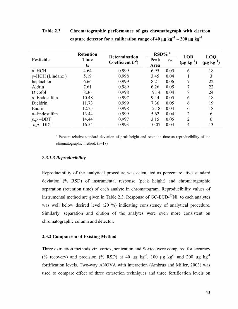
Table 2.3 Chromatographic performance of gas chromatograph with electron
capture detector for a calibration range of 40 µg kg–1 – 200 µg kg–1
RSD% aPesticide
Retention Time
tR
Determination Coefficient (r2) Peak
Area tR
LOD (µg kg–1)
LOQ (µg kg–1)
β–HCH 4.64 0.999 6.95 0.05 6 18 γ–HCH (Lindane ) 5.19 0.998 3.45 0.04 1 3 heptachlor 6.66 0.999 8.21 0.06 7 22 Aldrin 7.61 0.989 6.26 0.05 7 22 Dicofol 8.36 0.998 19.14 0.04 8 24 α–Endosulfan 10.48 0.997 9.44 0.05 6 18 Dieldrin 11.73 0.999 7.36 0.05 6 19 Endrin 12.75 0.998 12.18 0.04 6 18 β–Endosulfan 13.44 0.999 5.62 0.04 2 6 p,p΄–DDT 14.44 0.997 3.15 0.05 2 6 p,p΄–DDT 16.54 0.993 10.07 0.04 4 13
a Percent relative standard deviation of peak height and retention time as reproducibility of the
chromatographic method. (n=18)
2.3.1.3 Reproducibility
Reproducibility of the analytical procedure was calculated as percent relative standard
deviation (% RSD) of instrumental response (peak height) and chromatographic
separation (retention time) of each analyte in chromatogram. Reproducibility values of
instrumental method are given in Table 2.3. Response of GC-ECD-63Ni to each analytes
was well below desired level (20 %) indicating consistency of analytical procedure.
Similarly, separation and elution of the analytes were even more consistent on
chromatographic column and detector.
2.3.2 Comparison of Existing Method
Three extraction methods viz. vortex, sonication and Soxtec were compared for accuracy
(% recovery) and precision (% RSD) at 40 µg kg-1, 100 µg kg-1 and 200 µg kg-1
fortification levels. Two-way ANOVA with interaction (Ambrus and Miller, 2003) was
used to compare effect of three extraction techniques and three fortification levels on
43
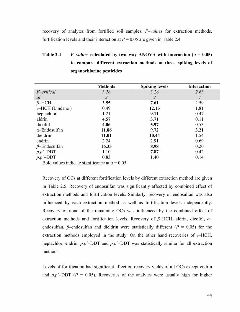
recovery of analytes from fortified soil samples. F–values for extraction methods,
fortification levels and their interaction at P = 0.05 are given in Table 2.4.
Table 2.4 F–values calculated by two–way ANOVA with interaction (α = 0.05)
to compare different extraction methods at three spiking levels of
organochlorine pesticides
Methods Spiking levels Interaction F–critical 3.26 3.26 2.63 df 2 2 4 β–HCH 3.55 7.61 2.59 γ–HCH (Lindane ) 0.49 12.15 1.81 heptachlor 1.21 9.11 0.47 aldrin 4.57 3.71 0.11 dicofol 4.06 5.97 0.53 α–Endosulfan 11.86 9.72 3.21 dieldrin 11.01 10.44 1.54 endrin 2.24 2.91 0.69 β–Endosulfan 16.35 8.98 0.20 p,p΄–DDT 1.10 7.87 0.42 p,p΄–DDT 0.83 1.40 0.14
Bold values indicate significance at α = 0.05
Recovery of OCs at different fortification levels by different extraction method are given
in Table 2.5. Recovery of endosulfan was significantly affected by combined effect of
extraction methods and fortification levels. Similarly, recovery of endosulfan was also
influenced by each extraction method as well as fortification levels independently.
Recovery of none of the remaining OCs was influenced by the combined effect of
extraction methods and fortification levels. Recovery of β–HCH, aldrin, dicofol, α–
endosulfan, β–endosulfan and dieldrin were statistically different (P = 0.05) for the
extraction methods employed in the study. On the other hand recoveries of γ–HCH,
heptachlor, endrin, p,p΄–DDT and p,p΄–DDT was statistically similar for all extraction
methods.
Levels of fortification had significant affect on recovery yields of all OCs except endrin
and p,p΄–DDT (P = 0.05). Recoveries of the analytes were usually high for higher
44
45
fortification levels compared to low ones. These results are also in agreement with a
similar study on trifluralin where vortex, Soxtec and SPE methods were used and the
workers concluded recoveries of some analyte as concentration dependent rather than
method dependent (Garimella et al., 2000).
Among three extraction methods, Soxtec extraction method was found better with
acceptable accuracy (76–106 %) in general and for precision in particular where RSD
was below 10 %. Vortex and ultrasonic extraction methods were comparable with Soxtec
for analyte recoveries but both the method were less consistent in terms of precision with
RSD values > 10%. Dean, (1998) also had similar results where, Soxhlet extraction was
found more reliable and accurate method than ultrasonic extraction for extraction of
PCBs from soil samples. Soxtec extraction system is automated; therefore, chances of
variation between the samples are minimal. On the other hand several steps and manual
handling in ultrasonic and vortex extraction methods can lead to low precision or
reproducibility.
Soxtec extraction method has been widely used for analysis of organic analytes from soil
and sediments around the world. It is obvious from the results that Soxtec is quite
accurate and precise method for these types of analyses. However, Soxtec method has
some limitations due to use of large solvent volumes and the sample extraction time is
too long usually 4-5 hrs. Furthermore, use of chlorinated solvent like dichloromethane is
also not safe for the health of analyst. Therefore, an effort was made to develop an
extraction method comparable to the established method to produce clean extracts with
minimal resources and in very short period of time. For this purpose potential of
QuEChERS extraction method commonly used for fruits and vegetables was exploited
for soil matrix. Interventions made in this regard are discussed in the subsequent sections.
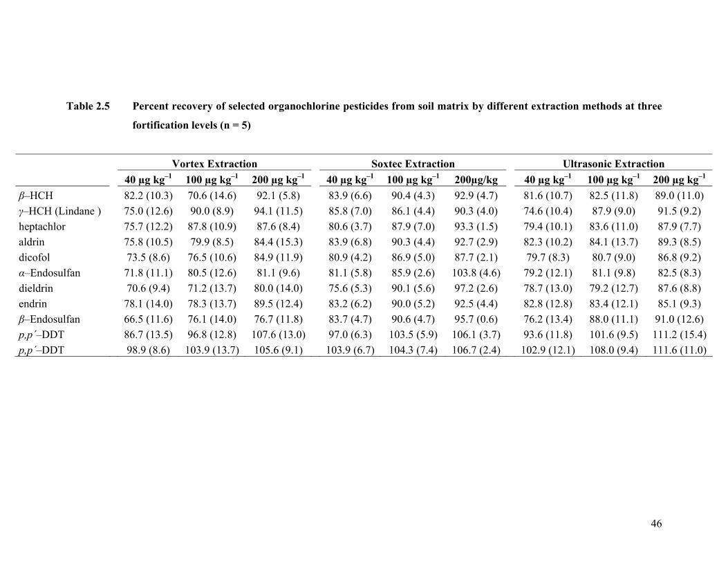
46
Vortex Extraction Soxtec Extraction Ultrasonic Extraction 40 µg kg–1 100 µg kg–1 200 µg kg–1 40 µg kg–1 100 µg kg–1 200µg/kg 40 µg kg–1 100 µg kg–1 200 µg kg–1
β–HCH 82.2 (10.3) 70.6 (14.6) 92.1 (5.8) 83.9 (6.6) 90.4 (4.3) 92.9 (4.7) 81.6 (10.7) 82.5 (11.8) 89.0 (11.0) γ–HCH (Lindane ) 75.0 (12.6) 90.0 (8.9) 94.1 (11.5) 85.8 (7.0) 86.1 (4.4) 90.3 (4.0) 74.6 (10.4) 87.9 (9.0) 91.5 (9.2) heptachlor 75.7 (12.2) 87.8 (10.9) 87.6 (8.4) 80.6 (3.7) 87.9 (7.0) 93.3 (1.5) 79.4 (10.1) 83.6 (11.0) 87.9 (7.7) aldrin 75.8 (10.5) 79.9 (8.5) 84.4 (15.3) 83.9 (6.8) 90.3 (4.4) 92.7 (2.9) 82.3 (10.2) 84.1 (13.7) 89.3 (8.5) dicofol 73.5 (8.6) 76.5 (10.6) 84.9 (11.9) 80.9 (4.2) 86.9 (5.0) 87.7 (2.1) 79.7 (8.3) 80.7 (9.0) 86.8 (9.2) α–Endosulfan 71.8 (11.1) 80.5 (12.6) 81.1 (9.6) 81.1 (5.8) 85.9 (2.6) 103.8 (4.6) 79.2 (12.1) 81.1 (9.8) 82.5 (8.3) dieldrin 70.6 (9.4) 71.2 (13.7) 80.0 (14.0) 75.6 (5.3) 90.1 (5.6) 97.2 (2.6) 78.7 (13.0) 79.2 (12.7) 87.6 (8.8) endrin 78.1 (14.0) 78.3 (13.7) 89.5 (12.4) 83.2 (6.2) 90.0 (5.2) 92.5 (4.4) 82.8 (12.8) 83.4 (12.1) 85.1 (9.3) β–Endosulfan 66.5 (11.6) 76.1 (14.0) 76.7 (11.8) 83.7 (4.7) 90.6 (4.7) 95.7 (0.6) 76.2 (13.4) 88.0 (11.1) 91.0 (12.6) p,p΄–DDT 86.7 (13.5) 96.8 (12.8) 107.6 (13.0) 97.0 (6.3) 103.5 (5.9) 106.1 (3.7) 93.6 (11.8) 101.6 (9.5) 111.2 (15.4) p,p΄–DDT 98.9 (8.6) 103.9 (13.7) 105.6 (9.1) 103.9 (6.7) 104.3 (7.4) 106.7 (2.4) 102.9 (12.1) 108.0 (9.4) 111.6 (11.0)
Table 2.5 Percent recovery of selected organochlorine pesticides from soil matrix by different extraction methods at three
fortification levels (n = 5)
2.3.3 Method Development
2.3.3.1 Comparison of Hydration Steps in QuEChERS Extraction
Pesticides and their metabolites may become bound to soil through physical or weak
chemical bonding depending upon the nature and properties of compounds and soil
(Gevao et al., 2000). Luiz et al., (2008) described the use of 1.0 M Na2–EDTA to
facilitate extraction of bound analytes from complex matrices. During the current study
two hydration methods, using either plain water or Na2–EDTA solution were compared.
The results are summarized in Table 2.6, which showed that there was no significant
difference in extraction efficiency for the two hydration methods (paired t–test p = 0.05).
Recovery values generally ranged between 70–100 % with the exception of HCB and %
RSD values were at or below 20 %. Low recovery of HCB was thought to be due to the
volatile nature of the analyte, resulting in some losses during the spiking, aging or
analysis. This initial evaluation was carried out at relatively high fortification level to
compare the effectiveness of two hydration steps to facilitate the extraction process. It
was concluded that there is no need to use EDTA solution for the hydration step as
hydration using plain water produced equally good recovery of analytes.
2.3.3.2 QuEChERS Modifications
The limit of detection (LOD) and limit of quantification (LOQ) were relatively high
when the standard QuEChERS method (Anastassiades et al., 2003) was used for
extraction without clean–up or concentration steps due to low sample concentration in the
extracts. In addition, it was only possible to inject l µl of the extract onto the GC–
MS/MS, as acetonitrile has a high expansion volume in the GC injector. It was not
desirable to concentrate these crude extracts, as this process was likely to lead to
concentration of co–extractives.
47
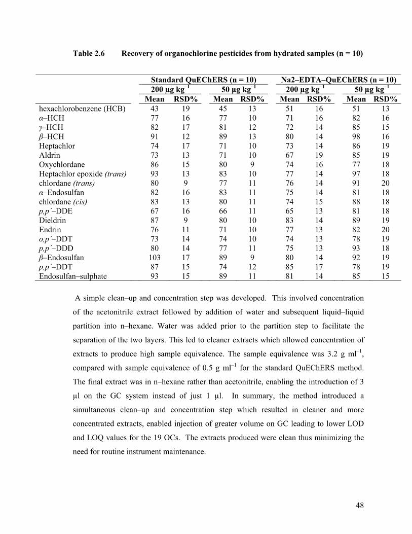
Table 2.6 Recovery of organochlorine pesticides from hydrated samples (n = 10)
Standard QuEChERS (n = 10) Na2–EDTA–QuEChERS (n = 10) 200 µg kg–1 50 µg kg–1 200 µg kg–1 50 µg kg–1
Mean RSD% Mean RSD% Mean RSD% Mean RSD%hexachlorobenzene (HCB) 43 19 45 13 51 16 51 13 α–HCH 77 16 77 10 71 16 82 16 γ–HCH 82 17 81 12 72 14 85 15 β–HCH 91 12 89 13 80 14 98 16 Heptachlor 74 17 71 10 73 14 86 19 Aldrin 73 13 71 10 67 19 85 19 Oxychlordane 86 15 80 9 74 16 77 18 Heptachlor epoxide (trans) 93 13 83 10 77 14 97 18 chlordane (trans) 80 9 77 11 76 14 91 20 α–Endosulfan 82 16 83 11 75 14 81 18 chlordane (cis) 83 13 80 11 74 15 88 18 p,p΄–DDE 67 16 66 11 65 13 81 18 Dieldrin 87 9 80 10 83 14 89 19 Endrin 76 11 71 10 77 13 82 20 o,p΄–DDT 73 14 74 10 74 13 78 19 p,p΄–DDD 80 14 77 11 75 13 93 18 β–Endosulfan 103 17 89 9 80 14 92 19 p,p΄–DDT 87 15 74 12 85 17 78 19 Endosulfan–sulphate 93 15 89 11 81 14 85 15
A simple clean–up and concentration step was developed. This involved concentration
of the acetonitrile extract followed by addition of water and subsequent liquid–liquid
partition into n–hexane. Water was added prior to the partition step to facilitate the
separation of the two layers. This led to cleaner extracts which allowed concentration of
extracts to produce high sample equivalence. The sample equivalence was 3.2 g ml–1,
compared with sample equivalence of 0.5 g ml–1 for the standard QuEChERS method.
The final extract was in n–hexane rather than acetonitrile, enabling the introduction of 3
µl on the GC system instead of just 1 µl. In summary, the method introduced a
simultaneous clean–up and concentration step which resulted in cleaner and more
concentrated extracts, enabled injection of greater volume on GC leading to lower LOD
and LOQ values for the 19 OCs. The extracts produced were clean thus minimizing the
need for routine instrument maintenance.
48
2.3.3.3 Chromatographic Performance of GC-MS/MS
2.3.3.3.1 Linearity: Linearity was assessed using matrix matched calibration solutions
over a wide range of concentrations. The GC–MS/MS response for the 19 pesticides was
linear over the range tested, namely 0.002 µg ml–1 – 1.0 µg ml–1 which corresponds to
0.63 µg kg–1 – 300 µg kg–1. The correlation coefficient (r2) was > 0.99 for all the
pesticides (Table 2.7).
2.3.3.3.2 Chromatographic Reproducibility: Reproducibility of retention time and
response were assessed using matrix matched calibration solutions (0.002 µg ml–1 – 1.0
µg ml–1). The relative standard deviation (% RSD) for response per unit concentration for
individual pesticides in matrix matched calibration solutions ranged from 5.6 to 18 % and
the % RSD for retention time of individual pesticides ranged between 0.13 % and 0.28%
(Table 2.7).
2.3.3.3.3 Limits of Detection and Quantification: The analytical limits were determined
experimentally by measuring the averages of chromatographic noise for blank soil
extracts taken at specific compound retention times over two different days. The limit of
detection (LOD) was 3 times the baseline noise for injected sample equivalent amount
(Patel et al., 2005; Brunete et al., 2004), while the limit of quantification (LOQ) was 10
times the baseline noise for injected sample equivalent amount (Brunete et al., 2004).
LODs and LOQs of 19 OCs are given in Table 2.7.
2.3.3.3.4 Specificity: The specificity of the GC–MS/MS method was assessed by
presence or absence of peaks above LOD at specific retention time of targeted pesticide
compounds in blank soil samples used during the study. The chromatograms of blank soil
samples showed no peak above the specified limit (Figure 2.1).
49
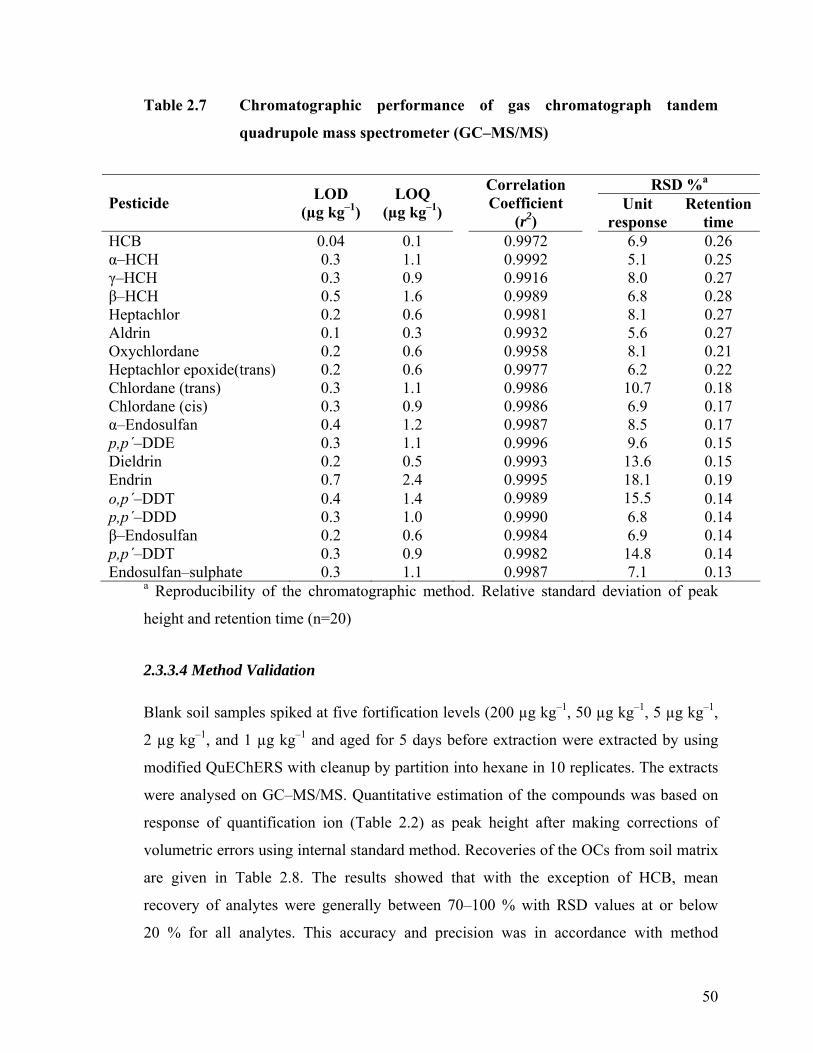
Table 2.7 Chromatographic performance of gas chromatograph tandem
quadrupole mass spectrometer (GC–MS/MS)
RSD %a
Pesticide LOD (µg kg–1)
LOQ (µg kg–1)
Correlation Coefficient
(r2)
Unit response
Retention time
HCB 0.04 0.1 0.9972 6.9 0.26 α–HCH 0.3 1.1 0.9992 5.1 0.25 γ–HCH 0.3 0.9 0.9916 8.0 0.27 β–HCH 0.5 1.6 0.9989 6.8 0.28 Heptachlor 0.2 0.6 0.9981 8.1 0.27 Aldrin 0.1 0.3 0.9932 5.6 0.27 Oxychlordane 0.2 0.6 0.9958 8.1 0.21 Heptachlor epoxide(trans) 0.2 0.6 0.9977 6.2 0.22 Chlordane (trans) 0.3 1.1 0.9986 10.7 0.18 Chlordane (cis) 0.3 0.9 0.9986 6.9 0.17 α–Endosulfan 0.4 1.2 0.9987 8.5 0.17 p,p΄–DDE 0.3 1.1 0.9996 9.6 0.15 Dieldrin 0.2 0.5 0.9993 13.6 0.15 Endrin 0.7 2.4 0.9995 18.1 0.19 o,p΄–DDT 0.4 1.4 0.9989 15.5 0.14 p,p΄–DDD 0.3 1.0 0.9990 6.8 0.14 β–Endosulfan 0.2 0.6 0.9984 6.9 0.14 p,p΄–DDT 0.3 0.9 0.9982 14.8 0.14 Endosulfan–sulphate 0.3 1.1 0.9987 7.1 0.13
a Reproducibility of the chromatographic method. Relative standard deviation of peak
height and retention time (n=20)
2.3.3.4 Method Validation
Blank soil samples spiked at five fortification levels (200 µg kg–1, 50 µg kg–1, 5 µg kg–1,
2 µg kg–1, and 1 µg kg–1 and aged for 5 days before extraction were extracted by using
modified QuEChERS with cleanup by partition into hexane in 10 replicates. The extracts
were analysed on GC–MS/MS. Quantitative estimation of the compounds was based on
response of quantification ion (Table 2.2) as peak height after making corrections of
volumetric errors using internal standard method. Recoveries of the OCs from soil matrix
are given in Table 2.8. The results showed that with the exception of HCB, mean
recovery of analytes were generally between 70–100 % with RSD values at or below
20 % for all analytes. This accuracy and precision was in accordance with method
50
51
performance acceptability criteria described by SANCO, (2007). At lower fortification
level, the number of analytes that met these criteria was lower (17 at 2 µg kg–1 and 10 at 1
µg kg–1). Recovery of HCB in fortified samples was low but consistent. The low HCB
recovery value is thought to be due to losses during the fortification, aging and analysis,
as this analyte is the most volatile of the OCs in this study. These results confirm the
findings of Lesueur et al., (2008) where QuEChERS method was found to produce more
consistent data for soil matrix compared to other established extraction methods.
2.3.3.5 Scope of the Method
The scope of the proposed method (robustness) was assessed using soil samples (Blank
soil B–F) with varying physicochemical properties (Table 2.1). Five aliquots each of the
soil samples were fortified at 5 µg kg–1 with the 19 OCs and aged for 5 days before
extraction. The analysis of these samples showed that the accuracy and precision were
not adversely affected regardless of the type of samples under investigation. As before,
the recovery values from all types of soil were generally between 70–100 % except for
HCB (Table 2.9). Method precision was calculated for each soil type as relative standard
deviation (% RSD). The % RSD values for OCs in different type of soil samples were
generally below 20 %. Therefore, the method has shown to produce good accuracy and
precision for soil samples with different physicochemical properties.
.

Table 2.8 Recovery data for organochlorine pesticides (n = 10) using the proposed procedure
200 µg kg–1 50 µg kg–1 5 µg kg–1 2 µg kg–1 1 µg kg–1
Mean %RSD Mean RSD% Mean RSD% Mean RSD% Mean %RSDhexachlorobenzene (HCB) 43 17 56 8 50 10 48 18 34 10α–HCH
79 11 70 4 76 16 75 4 68 6γ–HCH 73 9 74 10 71 18 79 15 69 6β–HCH 75 14 80 4 74 10 72 17 71 10heptachlor
80 15 83 10 80 17 79 9 66 7
aldrin 68 13 86 10 80 18 76 15 59 11oxychlordane 87 18 80 17 71 12 99 13 75 7heptachlor epoxide (trans)
89 16 76 5 78 9 70 13 78 10
chlordane (trans)
89 16 71 6 71 6 70 11 80 8α–endosulfan 90 16 73 5 79 10 76 12 77 7chlordane (cis)
89 16 72 4 76 7 76 15 72 7
p,p΄–DDE
75 20 90 11 72 11 80 16 62 12dieldrin 91 17 86 5 83 16 74 17 80 9endrin 92 16 86 5 84 19 77 16 76 7o,p΄–DDT 85 19 75 13 82 11 83 10 69 8p,p΄–DDD 84 12 83 14 82 15 75 11 77 10β–endosulfan
89 12 76 5 73 7 64 11 78 4
p,p΄–DDT 83 17 75 17 83 10 85 13 68 11endosulfan–sulphate 79 14 77 3 77 7 81 4 64 7
52
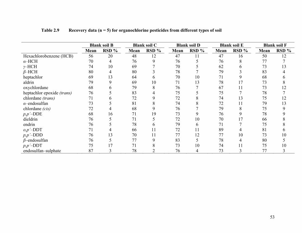
53
Table 2.9 Recovery data (n = 5) for organochlorine pesticides from different types of soil
Blank soil B Blank soil C Blank soil D Blank soil E Blank soil F Mean RSD % Mean RSD % Mean RSD % Mean RSD % Mean RSD %Hexachlorobenzene (HCB) 56 20 48 12 47 11 47 16 50 12α–HCH
70 4 76 9 76 5 76 8 77 7γ–HCH 74 10 69 7 70 5 62 6 73 13β–HCH 80 4 80 3 78 7 79 3 83 4heptachlor
69 13 64 6 70 10 71 9 68 6
aldrin 79 9 69 10 71 13 78 17 73 8oxychlordane 68 6 79 8 76 7 67 11 73 12heptachlor epoxide (trans)
76 5 83 4 75 5 75 7 78 7
chlordane (trans)
71 6 72 9 72 8 74 13 75 12α–endosulfan 73 5 81 8 74 8 72 11 79 13chlordane (cis)
72 4 68 9 76 7 79 8 75 9
p,p΄–DDE 68 16 71 19 73 9 76 9 78 9dieldrin 76 5 71 5 72 10 70 17 66 8endrin 76 5 78 6 79 6 71 7 75 8o,p΄–DDT 71 4 66 11 72 11 89 4 81 6p,p΄–DDD 76 13 70 11 77 12 77 10 73 10β–endosulfan
76 5 77 9 83 5 78 4 80 5
p,p΄–DDT 75 17 71 8 73 10 74 11 75 10endosulfan–sulphate 87 3 78 2 76 4 73 3 77 3
2.3.4 QuEChERS vs. Soxtec
Proposed QuEChERS extraction method was found quick, efficient, cheap, easy, robust
and safe for processing of soil samples. Applicability of the proposed method was studied
in comparison with Soxtec extraction method. For this purpose, soil samples (Field
sample a–f) with field–incurred residues were used to compare the extraction efficiencies
of modified QuEChERS method with Soxtec extraction method. Physicochemical
properties of the soil sample used are given in Table 2.1. GC–MS/MS determination was
used to analyze the extracts from both techniques. Residues were detected in all samples
studied by both the methods (Table 2.10). Both methods were comparable with each
other in qualitative and quantitative analysis of OCP residues in the soil samples.
However, proposed QuEChERS method was more sensitive and produced clean extracts
than Soxtec method. Higher detection and quantification limits (Table 2.11) for Soxtec
method emphasized further need for cleanup. The proposed method was less time
consuming. It was possible to prepare extracts for a batch of 20 samples in under 4 hours
using the proposed method. The Soxtec extraction procedure would require over 40 hours
to prepare a similar batch of soil samples. Besides, use of relatively safer solvents like
MeCN and n-hexane made the proposed method safer than Soxtec where
dichloromethane was used as extraction solvent. The residues detected above the
corresponding LOQs were α-HCH, γ-HCH, heptachlor, chlordane (trans), p,p׳-DDT, op׳-
DDT, p,p׳-DDD, p,p׳-DDE, β-endosulfan and endosulfan sulfate. Other residues were
detected in samples but not reported in Table 2.11 as these were below the LOQs. These
were β-HCH, heptachlor epoxide (trans), dieldrin, chlordane (cis) and α-endosulfan.
Chlordane (trans) was detected in all the samples (albeit some below LOQ), while
chlordane (cis) was detected in only one sample.
Proposed method and Soxtec method are compared for different parameters in Table
2.12. Proposed method besides having good accuracy and precision was found cheap due
to low operational cost in terms of solvent consumption and accessories. Furthermore, the
proposed method involved simple sample processing steps without much involvement of
instrumentation except for bench top centrifuge. Usually extraction of soil sample with
standard methods like Soxtec is very tedious and time consuming. The problem seemed
54
55
solved by the proposed method as batch of 20 soil samples along with one blank and two
quality control sample can be completely processed for GC analysis in merely 4 hrs. The
proposed method was also safe to execute due to involvement of relatively safer organic
solvents.
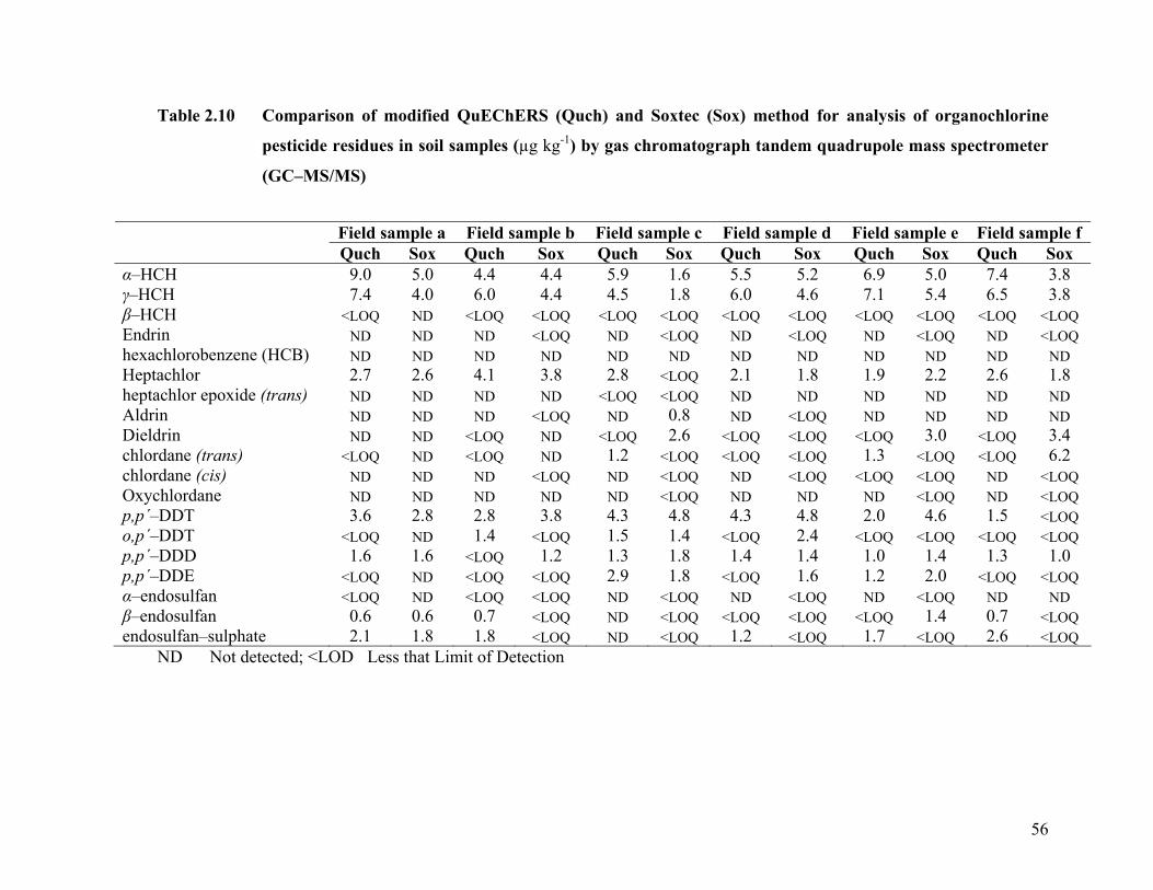
56
Table 2.10 Comparison of modified QuEChERS (Quch) and Soxtec (Sox) method for analysis of organochlorine
pesticide residues in soil samples (µg kg-1) by gas chromatograph tandem quadrupole mass spectrometer
(GC–MS/MS)
Field sample a Field sample b Field sample c Field sample d Field sample e Field sample f Quch Sox Quch Sox Quch Sox Quch Sox Quch Sox Quch Sox
α–HCH 9.0 5.0 4.4 4.4 5.9 1.6 5.5 5.2 6.9 5.0 7.4 3.8γ–HCH
7.4 4.0 6.0 4.4 4.5 1.8 6.0 4.6 7.1 5.4 6.5 3.8β–HCH <LOQ ND <LOQ <LOQ <LOQ <LOQ <LOQ <LOQ <LOQ <LOQ <LOQ <LOQ Endrin ND ND ND <LOQ ND <LOQ ND <LOQ ND <LOQ ND <LOQ hexachlorobenzene (HCB)
ND ND ND ND ND ND ND ND ND ND ND ND
Heptachlor 2.7 2.6 4.1 3.8 2.8 <LOQ 2.1 1.8 1.9 2.2 2.6 1.8heptachlor epoxide (trans) ND ND ND ND <LOQ <LOQ ND ND ND ND ND ND Aldrin ND ND ND <LOQ ND 0.8 ND <LOQ ND ND ND ND Dieldrin ND ND <LOQ ND <LOQ 2.6 <LOQ <LOQ <LOQ 3.0 <LOQ 3.4 chlordane (trans) <LOQ ND <LOQ ND 1.2 <LOQ <LOQ <LOQ 1.3 <LOQ <LOQ 6.2 chlordane (cis) ND ND ND <LOQ ND <LOQ ND <LOQ <LOQ <LOQ ND <LOQ Oxychlordane
ND ND ND ND ND <LOQ ND ND ND <LOQ ND <LOQ
p,p΄–DDT 3.6 2.8 2.8 3.8 4.3 4.8 4.3 4.8 2.0 4.6 1.5 <LOQ o,p΄–DDT <LOQ ND 1.4 <LOQ 1.5 1.4 <LOQ 2.4 <LOQ <LOQ <LOQ <LOQ p,p΄–DDD 1.6 1.6 <LOQ 1.2 1.3 1.8 1.4 1.4 1.0 1.4 1.3 1.0p,p΄–DDE <LOQ ND <LOQ <LOQ 2.9 1.8 <LOQ 1.6 1.2 2.0 <LOQ <LOQ α–endosulfan <LOQ ND <LOQ <LOQ
ND <LOQ ND <LOQ ND <LOQ ND ND
β–endosulfan 0.6 0.6 0.7 <LOQ
ND <LOQ <LOQ <LOQ <LOQ 1.4 0.7 <LOQ endosulfan–sulphate 2.1 1.8 1.8 <LOQ ND <LOQ 1.2 <LOQ 1.7 <LOQ 2.6 <LOQ
ND Not detected; <LOD Less that Limit of Detection

Table 2.11 Comparison of sensitivity of two methods for gas chromatograph tandem quadrupole mass spectrometer (GC–MS/MS) analysis
QuEChERS Soxtec LOD
(µg kg-1) LOQ
(µg kg-1) LOD
(µg kg-1) LOQ
(µg kg-1) α–HCH 0.3 1.1 0.3 0.9 γ–HCH 0.3 0.9 0.2 0.5 β–HCH 0.5 1.6 0.1 0.4 Endrin 0.7 2.4 0.6 2.1 hexachlorobenzene (HCB) 0.04 0.1 0.2 0.5 heptachlor 0.2 0.6 0.6 1.9 heptachlor epoxide (trans) 0.2 0.6 1.0 3.2 Aldrin 0.1 0.3 0.2 0.7 dieldrin 0.2 0.5 0.2 0.7 chlordane (trans) 0.3 1.1 0.7 2.4 chlordane (cis) 0.3 0.9 0.6 1.9 oxychlordane 0.2 0.6 0.4 1.2 p,p΄–DDT 0.3 1.0 1.2 3.8 o,p΄–DDT 0.4 1.4 0.5 1.7 p,p΄–DDD 0.3 1.0 0.2 0.8 p,p΄–DDE 0.3 1.1 0.4 1.3 α–endosulfan 0.4 1.2 0.4 1.4 β–endosulfan 0.2 0.6 0.3 1.0 endosulfan–sulphate 0.3 1.1 0.5 1.7
Table 2.12 Comparison between QuEChERS and Soxtec extraction methods
QuEChERS Soxtec
Solvents Less volume is required [10 ml MeCN for extraction and 10 ml n–hexane for cleanup]
Large volume is required [50 ml of methylene chloride]
Accessories No accessories required Cellulose thimbles are needed to hold soil sample
Instrumentation Centrifuge capable of producing 5000g for partitioning
Soxtec apparatus for extraction and concentration
Operational Time 4 hours for a batch of 20 soil samples 40 hours for batch of 20 soil samples
Safety Use of relatively safe solvents and processes
Use of relatively safe solvents but leaks can produce dangerous fumes in labs.
Additional inputs Salts are required for partitioning No salts are used Cost* Low cost (~ Rs.93 per sample) High cost (~Rs. 633 per sample)
*See Appendix A for cost calculation
57
2.4 CONCLUSION
Three conventional extraction methods viz. vortex, sonication and Soxtec were at par
with each other to yield good recoveries i.e. 70–110 % for almost all the OCs from spiked
soil. However, reproducibility of Soxtec was better than other methods due to low
precision (RSD %). Recovery yields of OCs were affected by extraction methods as well
as fortifications levels. Recovery of endosulfan was significantly affected by the methods
as well as fortification levels and their interaction. Recoveries of γ–HCH, heptachlor,
endrin, p,p΄–DDT and p,p΄–DDT were not influenced by method, however, recovery of
β–HCH, aldrin, dicofol, α–endosulfan, β–endosulfan, and dieldrin varied among different
extraction methods. Generally recoveries were low for lower fortification levels except
for endrin and p,p΄–DDT. Among three extraction methods, Soxtec extraction method
was found better among the three methods. Although Soxtec was effective and consistent
method but operation cost and sample processing time was very high. Therefore,
potential of QuEChERS extraction method was explored for extraction of OCs from soil
samples. Using this approach a rapid and efficient procedure for extraction and
simultaneous liquid–liquid partition cleanup was successfully developed and validated
for determination of 19 OCs in soil samples. The proposed method only needed a bench
top centrifuge and a vortex mixer for extraction and clean–up, therefore, set–up cost is
low. The proposed procedure was successful in analyzing OCs in spiked soil samples
with acceptable accuracy and precision, with low detection and quantification limits. The
method was robust and was equally effective for soil samples with different
physicochemical properties. The method was successfully compared with Soxtec
extraction method. The proposed method was equally efficient and sensitive with added
advantage of low sample processing time at low cost. The comparison involved analysis
of soil samples from cotton growing region of Pakistan. The proposed QuEChERS
method was found clean and did not require further cleanup. New proposed method was
found quick, efficient, cheap, easy, robust, and safe for analysis of OCs from soil
matrices. The comparison involved soil samples with low organic matter, therefore,
appropriate in-house QC checks are advised for the analysis of samples with high organic
matter content.
58
2.5 REFERENCES
Ambrus A. & J.N., Miller. 2003. Manual on Basic Statistics. IAEA Training Manual,
IAEA, Vienna, Austria.
Anastassiades, M., S.J. Lehotay, D. Stajnbaher and F.J. Schenck. 2003. Fast and easy
multiresidue method employing acetonitrile extraction/partitioning and
“dispersive solid–phase extraction” for the determination of pesticide residues in
produce. J. AOAC. Int. 86(2): 412–431.
Anitsecu, G., and L.L. Tavlarides. 2006. Supercritical extraction of contaminants from
soils and sediments. Journal of Supercritical Fluids, 38: 167–180.
Brunete, C.S., B. Albero and J.L. Tadeo. 2004. Multiresidue determination of pesticides
in soil by gas chromatography–mass spectrometry detection. J Agric Food Chem
52: 1445–1451.
Cheng, H.H. 1990. Pesticides in soil environment: processes, impacts and modeling. Soil
Society of America: Madison, WI, America.
Chester, T.L., J.D. Pinkston and D.E. Raynie. 1998. Supercritical Fluid Chromatography
and Extraction. Anal. Chem., 70: 301R–319R.
Dean, J.R. (Ed.). 1998. Extraction methods for environmental analysis. John Wiley &
Sons Ltd., England.
Diez, C., W.A. Traag, P. Zommer, P. Marinero and J. Atienza. 2006. Comparison of an
acetonitrile extraction/partitioning and “dispersive solid–phase extraction”
method with classical multi–residue methods for the extraction of herbicide
residues in barley samples. J. Chromatogr. A, 1131: 11–23.
Fuentes, E., M.E. Baez and D. Reyes. 2006. Microwave–assisted extraction through an
aqueous medium and simultaneous cleanup by partition on hexane for
determining pesticides in agricultural soils by gas chromatography: A critical
study. Analytica Chimica Acta, 578: 122–130.
Fussell, R.J., F. Smith, K. Patel and M. Sykes. 2003. An evaluation of a new, simple, low
cost acetonitrile extraction procedure for the multiresidue determination of
pesticides in apples. CSL report FD 02/33.
59
Garimella, U.I., G.K. Stearman and M.J.M. Wells. 2000. Comparison among soil series
and extraction methods for the analysis of Trifluralin. J. Agric. Food Chem. 48:
5874–5880.
Getenga, Z.M., F.O. Keng’ara and S.O. Wandiga. 2004. Determination of organochlorine
pesticide residues in soil and water from River Nyando drainage system within
Lake Victoria basin, Kenya. Bull Environ Contam Toxicol, 72: 335–343.
Gevao, B., K.T. Semple, and K.C. Jones. 2000. Bound pesticide residues in soils: a
review. Environmental Pollution 108: 3–14.
Goncalves, C. and M.F. Alpendurada. 2005. Assessment of pesticide contamination in
soil samples from an intensive horticulture area, using ultrasonic extraction and
gas chromatography–mass spectrometry. Talanta. 65:1179–1189.
Goncalves, C., J.J. Carvalho, M.A. Azenha and M.F. Alpendurada. 2006. Optimization of
supercritical fluid extraction of pesticide residues in soil by means of central
composite design and analysis by gas chromatography–tandem mass
spectrometry. J. Chromatogr. A, 1110: 6–14.
Graña C.E., M.I.T. Carou, S.M. Lorenzo, P.L. Mahía, D.P. Rodríguez and E.F.
Fernández. 2006. Evaluation of HCH isomers and metabolites in soils, leachates,
river water and sediments of a highly contaminated area. Chemosphere, 64:588–
595
Haib, J., I. Hofer and J.M. Renaud. 2003. Analysis of multiple pesticide residues in
tobacco using pressurized liquid extraction, automated solid–phase extraction
clean–up and gas chromatography–tandem mass spectrometry. J. Chromatogr. A,
1020: 173–187.
Handley, A.J. 1999. Extraction Methods in Organic Analysis, CRC Press LLC, Boca
Raton, Florida, pp 308.
Hussen, A., R. Westbom, N. Megersa, L. Mathiasson and E. Björklund. 2006.
Development of a pressurized liquid extraction and clean–up procedure for the
determination of α–endosulfan, β–endosulfan and endosulfan sulfate in aged
contaminated Ethiopian soils. J. Chromatogr. A, 1103: 202–210.
Khan, S.U. 1995. Supercritical fluid extraction of bound pesticide residues from soil and
food commodities. J. Agric. Food Chem, 43: 1718–1723.
60
Lesueur, C., M. Gartner, A. Mentler, and M. Fuerhacker. 2008. Comparison of four
extraction methods for the analysis of 24 pesticides in soil samples with gas
chromatography–mass spectrometry and liquid chromatography–ion trap–mass
spectrometry. Talanta, 75: 284–293.
Lopez–Avila, V., K. Bauer, J. Milanes and W.F. Beckert. 1993. J. JOAC Int., 76: 864.
Luiz, M.M.A., J.L.M. Vidal, R.R. González and A.G. Frenich. 2008. Multi–residue
determination of veterinary drugs in milk by ultra–high–pressure liquid
chromatography–tandem mass spectrometry. J. Chromatogr. A, 1205: 10–16.
Method 3540C, Soxhlet Extraction, Revision 3, US Environmental Protection Agency,
Washington, DC, December 1996.
Method 3541, Automated Soxhlet Extraction (Soxtec), Revision 0, US Environmental
Protection Agency, Washington, DC, January 1994.
Method 3541, Automated Soxhlet Extraction, Revision 0, US Environmental Protection
Agency, Washington, DC, September 1994.
Method 3545A, Pressurized Fluid Extraction (PFE), Revision 4B, US Environmental
Protection Agency, Washington, DC, November 2000.
Method 3546. Microwave extraction, Revision 0. US Environmental Protection Agency,
Washington DC 2000.
Method 3550B, Ultrasonic Extraction, Revision 2, US Environmental Protection Agency,
Washington, DC, December 1996.
Method 3562, Supercritical Fluid Extraction of Polychlorinated Biphenyls (PCBs) and
Organochlorine Pesticides, Revision 0, US Environmental Protection Agency,
Washington, DC, January 1998.
Pang, G.F., Y.M. Liu, C.L. Fan, J.J. Zhang, Y.Z. Cao, X.M. Li, Z.Y. Li, Y.P. Wu and
T.T. Guo. 2006. Simultaneous determination of 405 pesticide residues in grain by
accelerated solvent extraction then gas chromatography–mass spectrometry or
liquid chromatography–tandem mass spectrometry. Anal Bioanal Chem, 284:
1366–1408.
Patel, K., R.J. Fussell, M. Hetmanski, D.M. Goodall and B.J. Keely. 2005. Evaluation of
gas chromatography–tandem quadrupole mass spectrometry for the determination
of organochlorine pesticides in fats and oils. J. Chromatogr. A, 1068: 289–296.
61
Paya, P., M. Anastassiades, D. Mack, I. Sigalova, B. Tasdelen, J. Oliva and A. Barba.
2007. Analysis of pesticide residues using the Quick Easy Cheap Effective
Rugged and Safe (QuEChERS) pesticide multiresidue method in combination
with gas and liquid chromatography and tandem mass spectrometric detection.
Anal Bioanal Chem, 389:1697–1714
Rissato. S.R., M.S. Galhiane, B.M. Apon and M.S.P. Arruda. 2005. Multiresidue analysis
of pesticides in soil by supercritical fluid extraction/gas chromatography with
electron–capture detection and confirmation by gas chromatography–mass
spectrometry. J. Agric. Food Chem., 53:62–69.
SANCO. 2006. Quality control procedures for pesticide residue analysis. European
Commission, Directorate General Health and Consumer Protection, Document
No. SANCO/10232/2006.
SANCO. 2007. Method validation and quality control procedures for pesticide residues
analysis in food and feed. European Commission, Directorate General Health and
Consumer Protection, Document No. SANCO/2007/3131.
Sanghi, R. and S.S. Kannamkumarath. 2004. Comparison of Extraction Methods by
Soxhlet, Sonicator, and Microwave in the Screening of Pesticide Residues from
Solid Matrices. Journal of Analytical Chemistry, 59 (11): 1032–1036.
Tadeo, J.L., J. Castro and C.S. Brunete. 2004. Multiresidue determination in soil of
Pesticides used in tomato crops by Sonication–assisted extraction in small
Columns and gas chromatography. Int J Environ Anal Chem., 84 (1–3): 29–37.
Tor, A., M.E. Aydin and S. Ozcan. 2006. Ultrasonic solvent extraction of organochlorine
pesticides from soil. Analytica Chimica Acta, 559: 173–180.
Vig, K., D.K. Singh, H.C. Agarwal, A.K. Dhawan and P. Dureja. 2001. Insecticide
residues in cotton crop soil. J Environ Sci Health B, 36: 421–434.
Vinas, P., N. Campillo, I.L. Garcia, N. Aguinaga and M.H. Cordoba. 2003. Capillary gas
chromatography with atomic emission detection for pesticide analysis in soil
samples. J. Agric. Food Chem. 5: 3704–3708.
Walorczyk, S. 2008. Development of a multi–residue method for the determination of
pesticides in cereals and dry animal feed using gas chromatography–tandem
62
quadrupole mass spectrometry II. Improvement and extension to new analytes. J.
Chromatogr. A, 1208: 202–214.
Xia, X.R., and R.B. Leidy. 2002. A simplified liquid–solid extraction technique for the
analyses of pesticide residues in soil samples. Environ Monit Assess, 73: 179–
190.
63
Chapter 3
STATUS AND SPATIAL VARIATIONS OF ORGANOCHLORINE PESTICIDE RESIDUES IN SOILS OF COTTON GROWING AREAS
OF PAKISTAN
3.1 INTRODUCTION
Although most of the organochlorine pesticides (OCPs) have been banned in many
countries because of mutagenic and carcinogenic effects, they and their metabolites are
still present in the environment, especially in the soil and sediments, owing to their
persistence and lipophilic properties (Tor et al., 2006). OCPs such as cyclodiene
(heptachlor, aldrin, endrin, and dieldrin) are the most persistent with half lives ranging
from 0.3–2.8 years in temperate soils and can be detected in filed crop soils for long
period of time (Wandiga, 1995). Occurrence and formation of OCP residues depends
upon their historical application and contemporary anthropogenic activities, while spatial
variations are predominantly affected by structural factors, e.g. soil type, texture, parent
materials and topographic factors (Tieyu et al., 2005). Renaud et al., (2004) put forward
five physicochemical processes to explain the different patterns of pesticide leached loads
observed in the soils: (1) relative extent of preferential flow, (2) sorption capacity of the
compounds to the different soils, (3) extent of degradation of the compounds in the soil,
(4) variation in sorption kinetics between compounds associated with pesticide diffusion
into soil aggregates and (5) protection of the compounds by a combination of intra–
aggregate diffusion and the presence of preferential flow pathways. Cheng, (1990)
described influence of diverse factors such as organic matter content, soil type, and
physicochemical properties of pesticides, that is, vapor pressure, water solubility, and n-
octanol–water partition coefficient responsible for adsorption of compounds by soil.
3.1.1 Organochlorine Pesticide Residues in International Perspective
OCP residues have been detected in soils of almost every part of the world. Graña, et al.,
(2006) reported the presence of some natural degradation products of HCH and some
64
other OCPs in the soil samples analyzed. In a study conducted in the soils of Hong Kong,
Zhang et al., (2005) reported presence of five OCPs viz. HCH, DDT, HCB, Endrin and
α–endosulfan and found HCH isomer β–HCH and DDT metabolite p,p′–DDE dominating
occurrence and concentration. In a similar study on soils from organic farms of England,
Zohair et al., (2005) found the concentrations of PAHs, PCBs and OCPs in soils from
organic farms ranged from 590 to 2301 µg kg–1, 3.56 to 9.61 µg kg–1 and 52.2 to 478
µg kg–1, respectively. During 1999–2000 soils of farms in Alabama, Louisiana and Texas
were studied by Bidleman, (2004) to determine residues of OCPs and found DDT
isomers and breakdown products (p,p′–DDD, p,p′–DDE, o,p′–DDE) in every soil studied,
and toxaphene residues were found in most of soils while chlordane, dieldrin and HCH
isomers occurred less frequently. In another study conducted by Kim and Smith, (2001)
reported residues of γ–HCH and δ–HCH, heptachlor epoxide and dieldrin in soils of rice
and industrial areas of South Korea where OCP application had been discontinued almost
a decade ago. Nawab et al., (2003) collected soil samples from different agricultural
fields of Aligarh, India and through GC analysis found residues of γ–HCH at
concentration 47.35 ppb and that of α–HCH, β–HCH, p,p′–DDE, o,p′–DDT at 38.81,
1.79, 7.10 and 13.30 ppb, respectively, in these same soils.
Cavanagh et al., (1999) studied coastal alluvial flood–plains of the Herbert and Burdekin
Rivers in North Queensland where OCPs had been widely used in sugarcane cultivation.
Analysis of the marine surface sediment samples revealed absence of detectable OCP
residues, while soil samples contained detectable residues in range of 0.01–45 ng g–1.
Harner et al., (1999) made a survey of 36 Alabama agricultural soils to assess residues of
formerly used OCPs. Compounds determined comprised α– and γ–HCH, heptachlor,
heptachlor exo-epoxide, trans– and cis–chlordane, trans–nonachlor, dieldrin, toxaphene,
DDT and DDE. Concentrations varied by several orders of magnitude among farms and
appeared to be log–normally distributed. Kishimba et al., (2004) reviewed the research
carried out regarding the pesticide pollution in Tanzania and found out that generally, low
levels of residues were found in areas associated with agricultural pesticide use but the
levels in the former storage areas were substantially high. DDT and HCH were dominant
65
in all the studied areas. Kabbany et al., (2000) monitored pesticide residues in soil and
water samples collected from different locations in the El–Haram region Giza, Egypt and
reported variation in pesticide residue occurrence and concentration between different
locations.
3.1.2 Organochlorine Pesticide Residues in Pakistan
Agro based economy of Pakistan mostly depends upon production of major cash crops
like cotton, rice, sugarcane etc. Over the years manifolds increase in the demand has
pushed for more and more use of agrochemicals to produce more yields. In this context,
use of OCPs has been a very common feature for pest management in cotton production
for many years. After realization of harmful effects, some OCPs viz. DDT, HCH
(Lindane), Aldrin, Dieldrin and Endrin were banned for agricultural and domestic
purposes. However, some OCPs viz. Endosulfan, Heptachlor and Dicofol (DDT
substitute) are still recommended and used for pest management of cotton crop.
According to Hasnain (1999), despite the fact that some pesticides are banned in
Pakistan, these are still used at limited scale due to smuggling from neighboring
countries. The extensive use of pesticides has resulted in the burden of pesticides in soil
of areas under these crops (Hussain et al., 2001). Anonymous (2001), reported the
presence of residues of organochlorine (Lindane), Organophosphorus (azinophos–
methyl), and Pyrethroid (fenvalerate) pesticides in soil samples collected from cotton
zone of Punjab. In some previous studies DDT and its metabolites were detected from
soils of Kala Shah Kaku and Multan (Ali and Jabbar, 1992). In another study presence of
aldrin, dieldrin, endrin, DDT and its metabolites from soils of Samundri in Punjab was
reported (Jabbar et al., 1993). Similarly, there are also some scientific evidences that
OCP residues are found in many items of human consumption e.g. fruits and vegetables
(Masud and Hasan, 1992; Masud and Hasan, 1995); milk (Parveen and Masud, 1988),
cotton seed (Parveen et al., 1994; Parveen et al., 1996), tobacco (Ahmad and Abdullah
1971) etc. suggesting that organochlorine can intrude human food chain.
The present use of pesticides in Pakistan is concentrated on cotton, the most important
cash crop and the most important exportable commodity. Cotton production is mostly
66
concentrated in Punjab and Sindh provinces, constituting about 2.5 M.ha and 76 % of the
total pesticides consumed in Pakistan are used in cotton (Khan, 1998). The pesticides
applied are mostly insecticides; used against a number of serious pests, e.g. white fly,
jassid, aphid and bollworms. These pests have direct as well as indirect affect on yield
reduction, besides also act as vectors for different contagious bacterial, fungal and viral
diseases. Although pesticide residue monitoring studies have been conducted in cotton
areas in past but most of these address localized environments and do not provide any
information regarding different cotton growing areas. Cotton growing areas stretch across
Punjab and Sindh provinces where the microclimates are variable. This variation often
leads to different pest issues and management practices in these areas. Keeping in view
these factors, present study was planned to investigate OCP residues from different
cotton growing areas of Pakistan with history of OCP use for pest management. Study
aimed to investigate OCP residues in soils with varying pesticide uses. Both parent and
breakdown OCs were studied to determine source and age of these residues.
The specific objectives of the study were as follows:
1. Assessment of residue status of OCPs and their breakdown products in soils of
different cotton growing areas of Pakistan.
2. Investigations for spatial variation of OCP residues in the study areas.
3. Elucidation of basis for spatial variations of OCP residues in study areas.
67
3.2 MATERIALS AND METHODS
3.2.1 Profile of Study Areas
Present study was planned to investigate the OCP residue status in soils under cotton
cultivation in different cotton growing areas of Pakistan. Cotton belt of Pakistan covers a
long stretch of land, mainly in Punjab and Sindh provinces. During 2005–06 cotton was
cultivated on total areas of 3.1 million hectares. Of this 2.46 million hectares that
correspond to 78.2 % of the total cotton area, and 0.63 million hectares corresponding to
20.5 % of total cotton area were cultivated in Punjab and Sindh respectively. Cotton
cultivation practices vary in different areas depending upon the climate and cropping
pattern.
Present study was conducted in different agro-ecologies of cotton cultivation in cotton
growing areas of Sindh and Punjab. Spatial variations in OCP residues were studied in
areas with similar or closely related soil background. For this purpose study areas were
selected in Nawabshah, Ghotki, Jhang and Multan with soils belonging to Miani soil
series (Figure 3.1).
Miani soil series feature moderately deep and deep, well drained, calcareous and
moderately fine textured soils developed from sub–recent mixed alluvium derived from
rocks of Himalayas. These soils have been structurally classified as (combic) B horizon
or Typic Comborthids. These soils occur in an arid subtropical continental climate and
occupy slightly convex areas and level to nearly level channel in–fills in the recent and
Sub–recent floodplains. The soils have dark grayish brown, friable, massive, calcareous,
silty clay loam topsoil underlain by a brown/dark brown, friable, calcareous, silty clay
loam B horizon with weak coarse sub–regular blocky structure. The substratum is either
stratified or comprises a buried soil but may have layers of various colors and textures.
The horizon boundaries are gradual or clear and smooth. These soils are considered
suitable for crop cultivation especially for wheat, cotton, sugarcane, vegetables etc.
68

On the basis of preliminary survey, one of the sites in each province was considered high
pesticide use area and the other as low pesticide use area depending upon the pesticide
use intensity taken as number of sprays per cotton crop season. Nawabshah and Jhang
areas were low pesticide use areas; and Ghotki and Multan were high pesticide use areas.
3.2.1.1 Nawabshah
The site located in district Nawabshah was taken as low pesticide use area. The site is
located about 6.5 kilometers from Sakrand city on Sakrand Qazi Ahmad road. Samples
were collected from field with Miani series soil described by Anonymous, (1971) located
about 73 meters west from the main road. Study area constituted farmer fields around
villages Mangi Tarr, Khadam Hussain Khicchi and New–Dadh in Deh 21–Dadh, Tehsil
Sakrand. Interviewing with the growers and farmers suggested that pest pressure on
cotton crop is usually very low and normal cotton crop receives 0-3 sprays per season.
Therefore, this area was taken as low pesticide use area of Sindh.
Nawabshah is located 26°15′00″ North 68°25′00″ East and 26°25′00′′ North 68°41′66′′
East. It neighbors Naushero Feroz, Matiari in South, Sanghar in East and River Indus and
Dadu district in West. Nawabshah is famous for sugarcane and banana production. Its
climate is hot and dry but some time temperature fall below 0°C in winter. After
assassination of ex–prime minister and chairperson of Pakistan Peoples Party Mohtarima
Benazir Bhutto, Nawabshah was renamed as Banazirabad in 2007.
3.2.1.2 Ghotki
Other study site in Sindh was located in district Ghotki. Sampling site in Ghotki was
taken as high pesticide use area. The site with soil belonging to Miani series described by
Anonymous, (1969a) is located about 3.5 kilometers from Ghotki city on Ghotki Khanpur
road. Study area constituted fields located around villages Haji Khan Kolachi and
Muhammad Hashim Machchi in Deh Khunhara of Tehsil Ghotki.
69
Ghotki is a town of Northern Sindh, Pakistan. The town is located at 28°1'0N 69°19'0E
with an altitude of 72 m (239 ft) from sea level. Ghotki has very hot weather around the
year and winter only lasts for 3 months. Ghotki has very fertile land and main crops it
produces are cotton, wheat and rice. Farmers in the study area has small to medium
landholdings with average farm size of 20 acres. The site represents typical cotton–
wheat–cotton area. Other crops cultivated in this area are wheat, rice, sugarcane and
fodders. Sometimes, apart from fallowing, the lands especially located near the villages
are also used for vegetable production. Climate in this area is usually very hot and humid
making it very conducive for insect pest infestation. Farmers in the area were found very
inclined to use insecticides and correlate insecticide spray with yield increase.
Interviewing with farmers suggest use of 10–12 sprays in a cotton crop season. Farmers
had very little excess to research and extension personal working in public sector for
consultation. In contrary pesticide sector is well established in this area and often farmers
are influenced to use pesticides to meet the pesticide sale targets rather than to manage
pest infestation.
3.2.1.3 Jhang
In Punjab province, sampling site from Jhang district was considered low pesticide use
area. Miani series soil as described by Anonymous, (1968) were found about 300 feet
South of R.D. 39 on Manghani distributary situated 9.5 kilometers from Mochiwala town
near Jhang. Study area comprised of farmer fields around Chak–171, Chak–172, and
Chak–173 in Deh Manghani, Tehsil Jhang.
Jhang District is situated on the Chenab River at latitude 31.15° N and longitude 72.22°
E. The rivers of Jhelum and Chanab make their way through the district and Trimmu
Head–works is the pint of their convergence. Climate of the district is hot and dry during
summer and cold and dry in winter. Temperature of this area some time exceeds 50°C in
months of June and July. In Jhang study area cotton had been major Kharif crop but due
to heavy insect pest infestation and cotton leaf curl virus epidemic during 90s, cotton
suffered huge losses and cotton cultivation was suspended for many years. Very recently,
Government of Punjab has started cotton revival programme in this area and cotton is re–
70
71
gaining popularity. During survey and sampling in Jhang study area during June 2007,
more than 70 % of land was found under cotton cultivation. Sugarcane, fodder and
vegetable crops were among other cultivated crops in the area. Farmers in the area were
aware of the cotton production technologies and had good interaction with the trained
plant protection personal working in both public and private sectors. Due to break of
cotton cultivation for many years in this area, cotton pest population was not well
established and did not have much affects on cotton crop. Interviewing with farmers
suggest very little or no use of chemical pesticides required during crop season and for
last few years 0–3 number of sprays were used per cropping season.
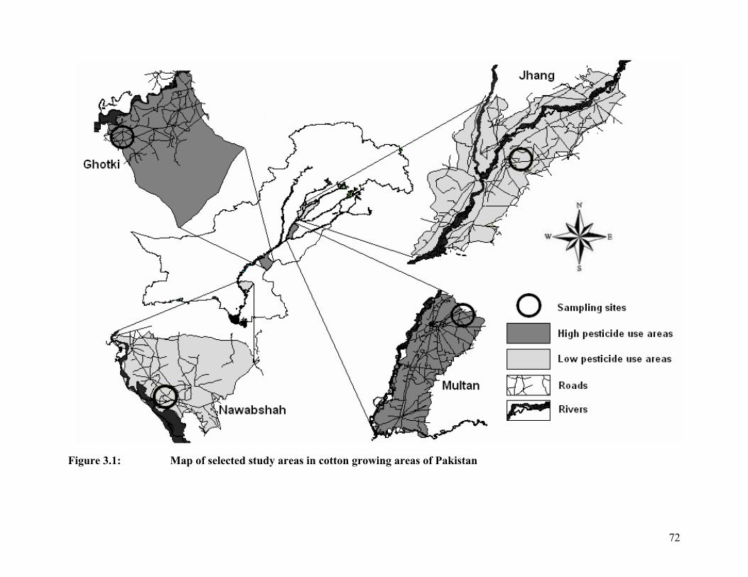
72
Figure 3.1: Map of selected study areas in cotton growing areas of Pakistan
3.2.1.4 Multan
Site located in districts Multan was selected as high pesticide use area of Punjab. The site
with soil of Miani series described by Anonymous, (1969b) is located about 5 km from
Kabirwala on Multan–Khanewal main matelled road and about 4 Km South–West of
village Kohiwala along Kohiwala–Mohni Sial kacha road near “Pirwala Khu”. Sampling
was done from cotton field around villages Mohni Sial and Pirwala.
Study area in Multan district was located at the periphery of the district close to
Khanewal district. This is predominantly cotton growing area, with wheat as following
crop and okra, fodders and sugarcane as alternate crops. The area also has mango
orchards and field crop often intercropped in the orchards. Farmers in this area have
updated knowledge about the pest, their management and are well aware of the direct and
indirect hazards of pesticide use. Due to different integrated pest management (IPM)
programmes organized by public, private sector and non–governmental organizations
(NGOs), farmers adopt integrated approaches of pest management rather than going for
chemical pesticides. This area has well established pest population due to successive
cotton and related crop cultivation year after year. Therefore, during cotton season
chemical pesticide use becomes obvious and 8–10 insecticide sprays are very common in
this area.
3.2.2 Soil Sampling
Soil sampling was carried out in June, 2006 and June, 2007 from study areas in Sindh and
Punjab provinces respectively. Total of 143 soil sample were collected across four study
areas. Sampling detail is given in Table 3.1.
Soil samples were collected from top soil (0–15 cm) and subsoil (16–30 cm) profiles by
using soil augur. Six soil samples were collected randomly from land block of 4 acre size.
Soil samples were thoroughly mixed and foreign materials like roots, stones, pebbles and
gravels etc. were removed and bulked. The bulk sample was reduced to about 1 kg by
dividing the thoroughly mixed sample into four equal parts. The two opposite quarters
73

were discarded and the remaining two quarters are remixed and the process was repeated
until the desired sample size was obtained. Samples were stored in labeled polythene
bags and transported to the laboratory. Collected soil samples were air dried in shade,
powdered by pastel and mortar, passed through 2 mm sieve, homogenized and stored at
room temperature for further analysis.
Table 3.1 Number of soil samples collected from study areas.
Punjab Sindh Multan Jhang Ghotki Nawabshah
Top soil 30 25 30 30 Subsoil 5 5 5 5 Control 2 2 2 2
3.2.3 Chemical and Reagents
Certified pesticide reference standards of high purity (> 98 %) were purchased from Qmx
(Thaxted, UK) and LGC–Promochem (Teddington, UK). Acetonitrile, water (HPLC
grade) and hexane (analytical reagent grade) were obtained from Fisher Scientific
(Loughborough, UK), anhydrous magnesium sulphate and sodium acetate trihydrate
(analytical reagent grade) were purchased from York glassware (York, UK).
Individual stock solutions for 19 OC pesticides were prepared in hexane. The working
standard solutions containing each of the 19 OC compounds were prepared in hexane at
10 µg ml–1, 1.0 µg ml–1, and 0.1 µg ml–1. The working standard solutions were used for
the preparation of matrix matched calibration solutions.
3.2.4 Sample Preparation and Cleanup
Newly developed QuEChERS extraction and cleanup method was used for processing of
soil samples. Soil sample (5 g) was hydrated for 30 minutes with 10 ml water. An aliquot
(10 ml) of acetonitrile + acetic acid mixture (99:1 v/v) was added to the 40 ml
polypropylene centrifuge tube containing the hydrated soil sample. After 30 second
vortex using Clifton Cyclone Vortex mixer, 4 g anhydrous MgSO4 and 1.66 g of
74
NaAc.3H2O were added. The contents were shaken vigorously and then centrifuged at
5000 g for 5 minutes using Jouan C/CR4.12 bench top centrifuge. The centrifuge step
facilitated the separation of acetonitrile from the aqueous layer. The simultaneous
cleanup involved transfer of an aliquot (8 ml) of the upper acetonitrile layer into a 10 ml
glass test tube. The extract was concentrated to approximately 1 ml under a gentle stream
of nitrogen on a dry block at 30°C. The concentrated extract was mixed with water (1 ml)
and n–hexane (5 ml) and swirled on vortex mixer for 15 seconds. The mixture was
allowed to stand and an aliquot (4 ml) of the upper n–hexane layer was transferred into
another glass tube. After addition of 50 µl of 10µg ml–1 δ–HCH solution as internal
standard, the hexane extract was concentrated to near dryness under a gentle stream of
nitrogen on a dry block at 30°C and reconstituted in 1 ml hexane for GC–MS/MS
analysis.
3.2.5 Chemical Analysis
Determination step was carried out using a Varian GC–MS/MS system comprising of
CP3800 gas chromatograph (GC) with a 1079 injector, a CP8400 auto–sampler and a
1200L triple quadrupole MS/MS (Varian, Walnut Creek, CA, USA). A fused silica
capillary column (Zebron ZB–50 phase, 50 % phenyl 50 % methylpolysiloxane, 30 m ×
0.25 mm i.d., and 0.25 µm film thickness; Phenomenex, USA) was used. The column
was protected by a 7 mm CarboFrit insert (Restek, Bellefonte, PA, USA) placed in the
GC liner (Varian Split, Open, 5 mm OD × 54 mm × 3.4 mm ID). Data acquisition and
reprocessing were performed using a Star Workstation version 6.41.
An aliquot (3.0 µl) of the sample extract was injected using an injector operated in
splitless mode at 225°C. The GC oven temperature programme was 100°C for 1 min
ramped to 200°C at 20°C min–1 (held for 6 min), ramped to 300°C at 10°C min–1 (held
for 3 min). Total GC run time was 25 minutes. Helium was used as carrier gas at 1 ml
min–1.
The tandem quadrupole mass spectrometer (GC–MS/MS) was operated in electron
ionization (EI) mode. The MS/MS detector interface was set at 210°C, source
75
temperature at 300°C, electron energy at 70 eV, filament current at 150 µA and detector
voltage at 1600 V. Argon (137 kPa) was used as collision gas in collision cell. The mass
spectrometer was auto–tuned and calibrated using perflurotributylamine before the start
of each sample sequence. Data acquisition (6 min to 21 min) used multiple reaction
monitoring detailed in Table 3.2. The MS/MS method included two transitions for each
analyte which allowed simultaneous quantification and confirmation of any residues
detected. Multi-level, matrix matched, bracketed calibration regime was used for
quantification. Calibration range from 0.005 µg ml-1 – 0.1µg ml-1 that corresponds to 1.4
µg kg-1 – 28 µg kg-1 were used for reference calibration curve to quantify analyte residues
against abundance of their quantification ions. Data acquisition and reprocessing were
performed by internal standard method for correction of volumetric errors using a Star
Workstation version 6.4.1.
3.2.6 Quality Control and Quality Assurance
Quality control (QC) and quality assurance (QA) procedures were used to determine and
maintain the quality of analytical data. QC and QA helped to identify deficiencies and
flaws in the analytical procedures. In response proper corrective measures were adopted
to ensure quality and precision in the interpretation of results. For this purpose method–
specific QC and QA procedures were adopted at sampling, extraction, and analytical
stages of the studies. These procedures were incorporated in the individual steps
according to the specificity and need of the methods.
During sampling stage control samples were collected from location with no agricultural
activities. For this purpose control samples were collected from the streets of village and
courtyard of houses in Nawabshah, courtyard of mosque in Ghotki, courtyards of houses
located near the sampling areas of Jhang and Multan. The samples were collected
randomly from top soil (0–15 cm) in 4 replicates and were combined to get composite
samples.
Processing and extraction of soil samples was carried out by validated method in batches
of 20–25 samples. Each batch included one blank soil sample and two spiked controls as
76
77
QC samples. The spiked soil (QC) samples were fortified with mix of standard solutions
to get 5 µg kg–1 and 20 µg kg–1 concentrations. Sample batch was treated and processed
in similar way to ensure and monitor quality of the extraction procedure. Accuracy of the
method was monitored in terms of % recovery of individual OC compounds included in
the study.
QC and QA during the pesticide residue analysis by GC–MS/MS were carried out by
using internal standard method. For this purpose 50 µl of 10 µg ml–1 δ–HCH standard
solutions was added in the extracts at the final stage of extraction just before
reconstitution of the extracts into 1 ml for GC–MS/MS analysis. After GC–MS/MS
analysis δ–HCH was used for correction of volumetric errors during the analytical
procedure.
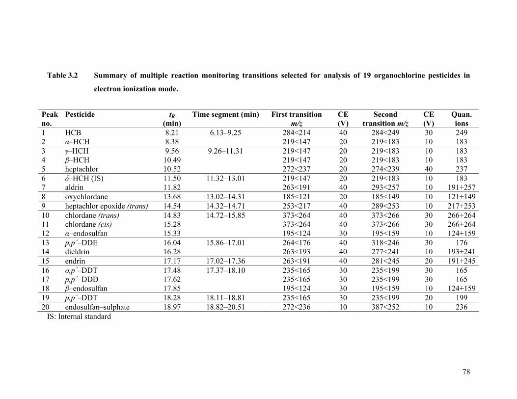
Peak no.
Pesticide tR (min)
Time segment (min) First transition m/z
CE (V)
Second transition m/z
CE (V)
Quan. ions
1 HCB 8.21 284<214 40 284<249 30 2492 α–HCH
8.38
6.13–9.25 219<147 20 219<183 10 183
3 γ–HCH 9.56 219<147 20 219<183 10 1834 β–HCH
10.49
9.26–11.31 219<147 20 219<183 10 183
5 heptachlor 10.52 272<237 20 274<239 40 2376 δ–HCH (IS) 11.50 219<147 20 219<183 10 183 7
aldrin 11.82
11.32–13.01 263<191 40 293<257 10 191+257
8 oxychlordane 13.68 13.02–14.31 185<121 20 185<149 10 121+1499 heptachlor epoxide (trans) 14.54 14.32–14.71 253<217 40 289<253 10 217+25310 chlordane (trans) 14.83 373<264 40 373<266 30 266+26411
chlordane (cis) 15.28 14.72–15.85
373<264 40 373<266 30 266+26412 α–endosulfan 15.33 195<124 30 195<159 10 124+15913 p,p΄–DDE 16.04 264<176 40 318<246 30 17614
dieldrin
16.28
15.86–17.01 263<193 40 277<241 10 193+241
15 endrin 17.17 17.02–17.36 263<191 40 281<245 20 191+24516 o,p΄–DDT 17.48 235<165 30 235<199 30 16517 p,p΄–DDD
17.62 17.37–18.10
235<165 30 235<199 30 16518 β–endosulfan 17.85 195<124 30 195<159 10 124+15919 p,p΄–DDT 18.28 18.11–18.81 235<165 30 235<199 20 19920 endosulfan–sulphate 18.97 18.82–20.51 272<236 10 387<252 10 236
Table 3.2 Summary of multiple reaction monitoring transitions selected for analysis of 19 organochlorine pesticides in
electron ionization mode.
78
IS: Internal standard
3.2.7 Statistical Analysis
Descriptive statistical parameters such as frequency (%) of positive soil samples, mean,
median and range of OCP residue levels; standard deviation, variance and data skewness
were calculated by Statistica version 5.5 (StatSoft, 1999). Ratios and percentages were
calculated for parent compounds, isomers and byproducts to determine the behavior of
compounds in soil, residue structure, age and source of residues.
Spatial variations and interpretation of important parameters responsible for these
variations, through multivariate statistical techniques had been widely used (Singh et al.,
2005; Qadir et al., 2008). In the present study two multivariate techniques hierarchical
cluster analysis (HCA) and discriminant function analysis (DFA) were used for
categorization among different study areas on the basis of OCP residues and for
assessment of basis of these spatial variations.
3.2.7.1 Hierarchical Cluster Analysis (HCA)
HCA is an unmanaged technique whereby unbiased inherent structure of data set is
discovered. The categorization or clustering of the data set is based on the nearness or
similarities between different data structures (Singh et al., 2005). HCA is a common
approach used in the environmental analysis in which clustering is formed sequentially,
by starting with the most similar pair of objects and forming bigger groups step by step
(Singh et al, 2005; Qadir et al., 2008). In the present study, HCA was performed on
normalized data set of OCP residues in different cotton growing areas of Pakistan by
means of Ward’s method, using Euclidian distance as measure of similarity. The
Euclidian distance usually gives the similarity between two samples and the difference of
analytical values between two samples can be represented as “distance”. Ward’s method
is a linkage rule that utilizes analysis of variance approach to evaluate the distances
between clusters with minimization of sum of squares of any two clusters that can be
formed at each step. HCA was applied on OCP residue data to group sites with similar
pattern of residues in the form of Dendrogram . The linkage distance between the groups
is described as (Dlink × Dmax) × 100 which represent quotient between the linkage
79
distances for a particular case divided by the maximal distance, multiplied by 100, to
standardize the linkage distance represented on y–axis (Singh et al., 2005).
3.2.7.2 Discriminant Function Analysis (DFA)
DFA was used to explain the basis for hierarchical classification between different
identified groups as a result of HCA. DFA determines the variables, responsible for
discrimination between groups. DFA determines whether groups differ with regard to the
mean of a variable, and then to use that variable to predict group membership. DFA is
applied on raw data and the technique works in standard, forward and backward stepwise
modes to give discriminate functions (DFs) for each group. In standard mode usually DFs
of all the variables included in the study area are given. Whereas in forward stepwise
mode, all variable are included step by step to review and evaluate their contribution to
discriminate between different groups and the ones with highest contribution are selected.
In backward stepwise mode, variable selected in the forward step are included and the
ones with least contributions towards discrimination between groups are eliminated
leaving behind the only the most important variable responsible for group discrimination
(Singh et al., 2005; Qadir et al., 2008).
In our study, DFA was used to describe spatial variations of OCP residues in cotton
growing areas of Pakistan by discrimination between the groups describing provincial
variations as well as site variations within each province. In DFA, sites were taken as
spatial grouping variable. These grouping variables (spatial) were used in the analysis as
dependent variables, while the residue data of 19 OCPs was considered independent
variable. DFA was carried out in standard, forward, and backward stepwise modes.
80
3.3 RESULTS AND DISCUSSION
3.3.1 Quality Control / Quality Assurance
3.3.1.1 Sampling
Soil sample collected from the locations in study areas with no agricultural activity were
used as control samples. Before using these samples as reference material for comparison
with soil samples from cotton fields, the control samples were analyzed for OCP
contaminants. Results were quite surprising and almost all the control samples were
found heavily contaminated with OCPs (Table 3.3). Residues of HCHs and DDTs along
with their breakdown products were present in almost all control samples. Residues of
cyclodienes were also present in these soil samples in varying concentrations and
frequencies. Control soil samples were collected from courtyards of the houses or village
streets. In villages usually people use soils from fields to make mud plaster for their
courtyards. Furthermore, these courtyards are also centre of household as well as
agricultural activities from seed preparation, handling of produce to formulation and
preparation of pesticide sprays. Furthermore, such soils remain un-altered for longer
period of time and therefore, lack activities for environmental and biological exposure of
these pesticides for breakdown or other kinds of losses.
Due to contamination of control soil samples with OCPs, these samples were not
considered for further use as reference blanks and preparation of matrix matched
calibration solutions. For this purpose Blank soil B (Chapter 2, section 2.2.3) used during
modification and validation of QuEChERS was used.
3.3.1.2 Extraction
Quality of the extraction procedures was monitored and maintained by including QA/QC
samples in each batch of real soil samples. QA/QC samples were prepared by spiking
blank soil at 5 µg kg–1 and 20 µg kg–1 concentration levels. These QA/QC soil samples
were extracted and treated similar to the real soil samples. After analyzing the QA/QC
81

82
samples for OCPs, percentage recovery of each was assessed to monitor losses during the
extraction procedure. Recovery results QA/QC samples used in different batches are
given in Table 3.4. Recoveries of all OCP in QA/QC were in range of 70–110 %. These
recoveries were in accordance with method performance acceptability criteria given by
SANCO, (2007).
3.3.1.3 Analysis
Quality of the analytical procedure on GC–MS/MS was ensured by the use of δ–HCH as
internal standard and multi–level, matrix matched, bracketed calibration regime was used
for quantification. The internal standard was used to identify and correct any sort of
volumetric errors occurred either at the sample processing or during the analytical stage.
Besides quantitative determination of unknowns in the sample extracts, multi–level
calibrations were also used to monitor the stability and sensitivity of MS/MS detection
system by estimation of linearity, limits of detection and limits of quantification of each
analyte.

Table 3.3 Organochlorine pesticide contaminations (µg kg–1) in control samples from study areas
Nawabshah Jhang Multan Ghotki 0–15 cm 16–30 cm 0–15 cm 16–30 cm 0–15 cm 16–30 cm 0–15 cm 16–30 cm
α–HCH 5.5 3.0 1.4 < LOQ 0.3 0.4 1.1 2.3γ–HCH
2.9 3.2 1.2 0.9 < LOQ < LOQ 1.7 3.4β–HCH 2.5 < LOQ < LOQ < LOQ ND ND < LOQ < LOQ Endrin < LOQ < LOQ
< LOQ
ND ND ND < LOQ < LOQ
HCB 2.1 0.4 1.1 ND 0.4 0.4 ND ND Heptachlor 1.4 1.4 < LOQ < LOQ ND ND 0.6 1.3heptachlor epoxide(trans)
< LOQ ND ND ND ND ND ND ND
Aldrin 0.5 ND < LOQ ND ND ND ND ND Dieldrin 0.7 1.7 < LOQ ND ND ND < LOQ ND chlordane (trans) 6.9 9.8 < LOQ < LOQ < LOQ ND < LOQ < LOQ chlordane (cis) < LOQ ND ND ND ND ND < LOQ < LOQ oxychlordane < LOQ ND ND ND ND ND < LOQ < LOQ p,p΄–DDT 63.4 16.4 ND ND ND ND ND 42.5 o,p΄–DDT 11.5 2.5 < LOQ ND ND ND 8.4 4.1p,p΄–DDD 12.8 6.2 < LOQ ND ND < LOQ 34.4 12.9p,p΄–DDE 4.3 4.1 1.5 1.3 4.2 7.4 52.0 35.2α–endosulfan < LOQ < LOQ < LOQ < LOQ ND ND < LOQ < LOQ β–endosulfan < LOQ ND ND 0.6 ND ND ND ND endosulfan sulfate ND ND < LOQ < LOQ ND ND ND ND
ND = not detected; <LOQ = less than limit of quantification
83
Batch 1 Batch 2 Batch 3 Batch 4 Batch 5 Batch 6 Sp1 Sp2 Sp1 Sp2 Sp1 Sp2 Sp1 Sp2 Sp1 Sp2 Sp1 Sp2
α–HCH 72 79 73 95 82 72 76 72 72 91 86 82γ–HCH
71 70 84 102 85 71 72 74 76 93 88 85β–HCH 73 73 92 99 87 74 78 71 74 86 84 86Endrin
76 91 81 98 74 73 89 75 71 89 82 79
HCB 76 97 81 79 102 75 95 98 77 80 75 79Heptachlor 77 102 78 94 97 77 89 94 88 87 75 74heptachlor epoxide(trans)
83 102 94 110 97 77 83 99 78 76 72 83
Aldrin 83 106 77 96 101 80 85 96 97 88 79 76Dieldrin 89 107 75 97 103 80 71 85 88 80 84 90chlordane (trans)
93 109 83 107 103 75 89 97 96 85 76 89
chlordane (cis) 86 107 81 103 110 79 99 89 79 99 77 93Oxychlordane
82 108 94 96 105 74 97 95 87 86 76 82
p,p΄–DDT 68 85 85 77 89 98 77 78 89 83 73 66o,p΄–DDT 68 80 72 88 76 98 87 76 84 84 84 72p,p΄–DDD 86 102 91 102 98 80 78 96 81 86 87 94p,p΄–DDE 82 107 89 95 102 79 96 87 70 94 86 83α–endosulfan 82 96 76 101 103 84 73 96 79 83 73 85β–endosulfan 55 71 93 89 99 72 84 93 77 88 89 84endosulfan sulfate 80 73 88 103 91 97 97 88 72 85 76 84
84
Table 3.4 Batch–wise recovery (%) of OCPs in quality assurance/quality control samples spiked at 5 µg kg–1 (Sp1) and 20
µg kg–1 (Sp2)
85
3.3.2 Organochlorine Residues in Different Soil Depths
Concentration of organochlorine pesticide residues were compared in different soil
depths. For his purpose, 5 soil samples were randomly collected from subsoil (16–30 cm)
from all four study areas for comparison with top soil (0–15 cm) in respective sampling
sites. Soil samples from both the profiles were extracted and analyzed in same batch to
avoid experimental errors. Concentrations of 19 OCP residues were compared between
the two soil depths by Student’s t–test. Results of statistical analysis are given in Table
3.5. Results indicate no statistical difference of residues between two soil depths for 95 %
level of significance at both one tail and two tail t–tests. This is probably due to
continuous overturning of soil by plowing and related activities. On this basis further
pesticide residue studies were carried out by using the top soil (0–15 cm) samples.
Generally, pesticide residues accumulate in the top 15 cm of soil (Alexander, 1961;
Harris and Sans, 1969). Ahmed et al., (1998) monitored residues of lindane, heptachlor,
heptachlor epoxide, aldrin, endrin, dieldrin, and DDT in rain water, soil profile, and
ground water in Turkey and reported wider spectrum and higher concentrations in top
soil (9.5 µg kg−1), than at 50 cm depth (8 µg kg−1) while at 1 m depth no detectable
residues were found. Zhu et al., (2005) determined the concentrations of HCH and DDT
in shallow subsurface (5–30 cm depth) and deep soil layers (150–180 cm depth) from the
outskirts of Beijing, China. Results revealed that the concentrations of total HCHs
(including α, β, γ, δ–isomers) and total DDTs (including p,p′–DDT, p,p′–DDE, p,p′–
DDD, o,p′–DDT) in shallow subsurface soils were relatively higher than those in the
deeper layers of the soil.
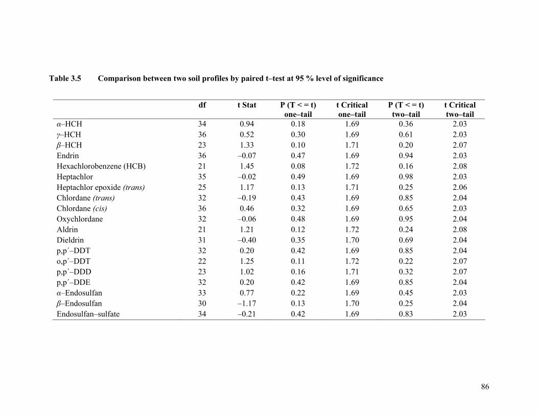
df t Stat P (T < = t) one–tail
t Critical one–tail
P (T < = t) two–tail
t Critical two–tail
α–HCH 34 0.94 0.18 1.69 0.36 2.03γ–HCH
36 0.52 0.30 1.69 0.61 2.03β–HCH 23 1.33 0.10 1.71 0.20 2.07Endrin 36 –0.07 0.47 1.69 0.94 2.03Hexachlorobenzene (HCB)
21 1.45 0.08 1.72 0.16 2.08
Heptachlor 35 –0.02 0.49 1.69 0.98 2.03Heptachlor epoxide (trans)
25 1.17 0.13 1.71 0.25 2.06
Chlordane (trans) 32 –0.19 0.43 1.69 0.85 2.04Chlordane (cis) 36 0.46 0.32 1.69 0.65 2.03Oxychlordane
32 –0.06 0.48 1.69 0.95 2.04
Aldrin 21 1.21 0.12 1.72 0.24 2.08Dieldrin 31 –0.40 0.35 1.70 0.69 2.04p,p΄–DDT 32 0.20 0.42 1.69 0.85 2.04o,p΄–DDT 22 1.25 0.11 1.72 0.22 2.07p,p΄–DDD 23 1.02 0.16 1.71 0.32 2.07p,p΄–DDE 32 0.20 0.42 1.69 0.85 2.04α–Endosulfan 33 0.77 0.22 1.69 0.45 2.03β–Endosulfan 30 –1.17 0.13 1.70 0.25 2.04Endosulfan–sulfate 34 –0.21 0.42 1.69 0.83 2.03
86
Table 3.5 Comparison between two soil profiles by paired t–test at 95 % level of significance
3.3.3 Organochlorine Pesticide Residue Status
Residues of OCPs were detected from soil samples collected from different study areas in
varying frequencies and magnitudes. Major pesticide residues in all the samples were
from HCH, DDT sub–groups of OCs. Residues from cyclodiene subgroup viz.
heptachlor, chlordane, endosulfan, aldrin, dieldrin and endrin were also detected from the
soil samples. This section of the chapter describes status of different OCP residues from
HCH, DDT and cyclodiene subgroups detected from different soil profiles, study areas
and chemometric studies for spatial variations in OCP residues in the study areas.
3.3.3.1 Hexachlorohexane (HCH)
Soil samples collected from different cotton growing areas were analyzed for different
HCH isomers including α–HCH, γ–HCH and β–HCH. HCH was completely banned in
Pakistan after de–registration in 1996 (Ahad et al., 2009). Residues of different HCH
isomers were detected in all the study areas. However, HCH residues varied both in
frequency and magnitude in different study areas.
3.3.3.1.1 HCH residues in study areas
Magnitude of HCH residues varied greatly among the study areas. Descriptive statistical
data for HCH residues is given in Table 3.6. The highest Σ HCH (α–HCH + γ–HCH + β–
HCH) residues were detected from Sindh sites compared to those in Punjab. In Ghotki
area highest Σ HCH residues were detected ranging 2.8–17.6 µg kg–1 with median 8.1 µg
kg–1. This was followed by Nawabshah area with range 2.4–15.1 µg kg–1 and median 7.9
µg kg–1. Sites from Punjab province had lower magnitude of Σ HCH residue than sites in
Sindh. In Multan area, Σ HCH residues range from 0.3–3.3 µg kg–1 with median 1.6 µg
kg–1 with the fact that no residues of β–HCH were found in this area. Lowest amount of Σ
HCH residues were detected from Jhang area soil samples with range 0.6–2.8 µg kg–1 and
median 1.3 µg kg–1. Threshold level for pesticide residues in soil are referred as
Maximum Allowable Concentration (MAC). MAC is defined as "The maximum
87
allowable concentration of a substance in soil is its concentration at which the substance
does not enter the plants, water or air in amounts that exceed the respective maximum
allowable concentration for these media and has no adverse effects on the composition
and biological properties of the soil" (Beyer, 1990). MAC for HCH residues in soil are
given as 100 µg kg–1 by former USSR environmental agency (Beyer, 1990). Results of
the study suggest that soils study areas were on safer side for HCH residues.
Highest frequency of HCH residues were detected in Nawabshah study area. Residues of
α–HCH and γ–HCH were detected in all the soil samples while those of β–HCH were
detected in only 10 % of the soil samples. In Ghotki area all the three isomers were
detected in majority of soil samples. About 97 % samples were found with α–HCH and
γ–HCH residues, and β–HCH residues were detected in 60 % of the samples. In the
Punjab, α–HCH residues were detected in all the samples from Jhang area while, γ–HCH
and β–HCH residues were detected form 76 % and 24 % samples respectively. In Multan
area 93 % soil samples were found with α–HCH and γ–HCH while β–HCH residues were
not detected from any of the samples.
3.3.3.1.2 Source and age of HCH residues
Ratios between different isomers of HCH are considered very important to predict the
source and age of HCH contaminations (Table 3.6). Commercial HCH applications, were
generally formulated as (i) technical grade HCH containing mixture of different isomers,
mainly α– (55–80 %), β– (5–14 %), γ– (8–15 %), and δ–HCH (7–16 %) and (ii) lindane
(almost pure γ–HCH) (Li et al., 2006). Among HCH isomers γ–HCH has insecticidal
properties while other isomers α and β are produced as byproducts during the commercial
production of γ–HCH or lindane. For commercial lindane production, γ–HCH is isolated
from technical grade HCH by crystallization (Turnbull, 1996). All HCH isomers are
acutely toxic to mammals and possess mutagenic, teratogenic and carcinogenic properties
and are highly persistent in environment (Kidd et al., 2008).
88
Keeping in view the isomeric composition of the two commercial formulation, ratio
between α– and γ– isomers can be used to predict possible use of HCH formulation.
Ratios of α– / γ– around ≥ 5 indicate HCH input from technical HCH application, and
low ratios (< 1) indicate possible use of lindane. During this study ratios of α– / γ– ranged
from 0.7–1.5 with median 1.1 in Nawabshah, from 0.2–1.3 with median 0.7 in Ghotki,
1.0–2.0 with median 1.3 in Jhang and from 0.5–1.9 with median 1.0 in Multan study area.
These ratios are not in accordance with either of the isomeric composition of commercial
HCH products. During HCH use, majority of α–HCH comes from technical HCH.
Furthermore, conversion of γ–HCH into α–HCH by sunlight and through biological
degradation in soil is another possible source (Li et al., 2006). Therefore, amounts of α–
HCH residues in the environment indicate use of technical HCH as well as possibility of
an historic γ–HCH use. In the present study residues of α–HCH in the soil environment
indicated use of technical HCH. However, comparison between α– and γ– isomers
suggested presence of γ–HCH isomer proportionately higher than expected from
technical HCH source. Therefore, it can be concluded that besides technical HCH, γ–
HCH residues also came from lindane application. Therefore, either of HCH formulations
cannot be singled out for γ–HCH residues, and indicate that the source of HCH residues
in the study areas were due to possible use of cocktail of both HCH commercial
formulations. Furthermore, proportionality higher levels of γ–HCH also suggest a recent
HCH use.
Although, β–HCH is considered more stable of the other isomers and degrades very
slowly due to very low vapor pressure. In this study, β–HCH was detected in least
amounts compared to other two isomers suggesting that HCHs in the soils were from
recent HCH use rather than from an historical input. These finding are in contrary to
findings of Gao et al., (2008) and Li et al., (2006) where β–HCH was predominant
among HCH isomers and was indicated as consequence of historical use rather than
recent one. The Majority of β–HCH residues occurred in study area from Sindh province.
Highest incidence of β–HCH (60 %) was detected in Ghotki with residues ranging from
0.5–1.6 µg kg–1 with median value 0.6 µg kg–1 followed by Nawabshah with incidence of
only 10 % and magnitude of residues ranging from 0.5–1.6 µg kg–1 with median value
89
90
0.6 µg kg–1. In Punjab province, residues of β–HCH were only detected from samples of
Jhang area with incidence 24 % and magnitude ranging from 0.6–0.9 µg kg–1 with
median value 0.7 µg kg–1 and no residues of β–HCH were detected in any of the soil
samples from Multan area. Major source of β–HCH isomer between commercial HCH
formulations is technical HCH. Between the two commercial sources of HCH, technical
HCH is major source of β–HCH. In technical HCH formulation ratio of β–HCH / γ–HCH
is 0.8 to 0.9. While in our study, this ratio was calculated in range of 0.1–0.3 with median
0.1 in Nawabshah and from 0.1–0.4 with median 0.1 in Ghotki. These ratios indicate
higher levels of γ–HCH isomer compared to β–HCH supporting claims of lindane use
besides technical HCH.
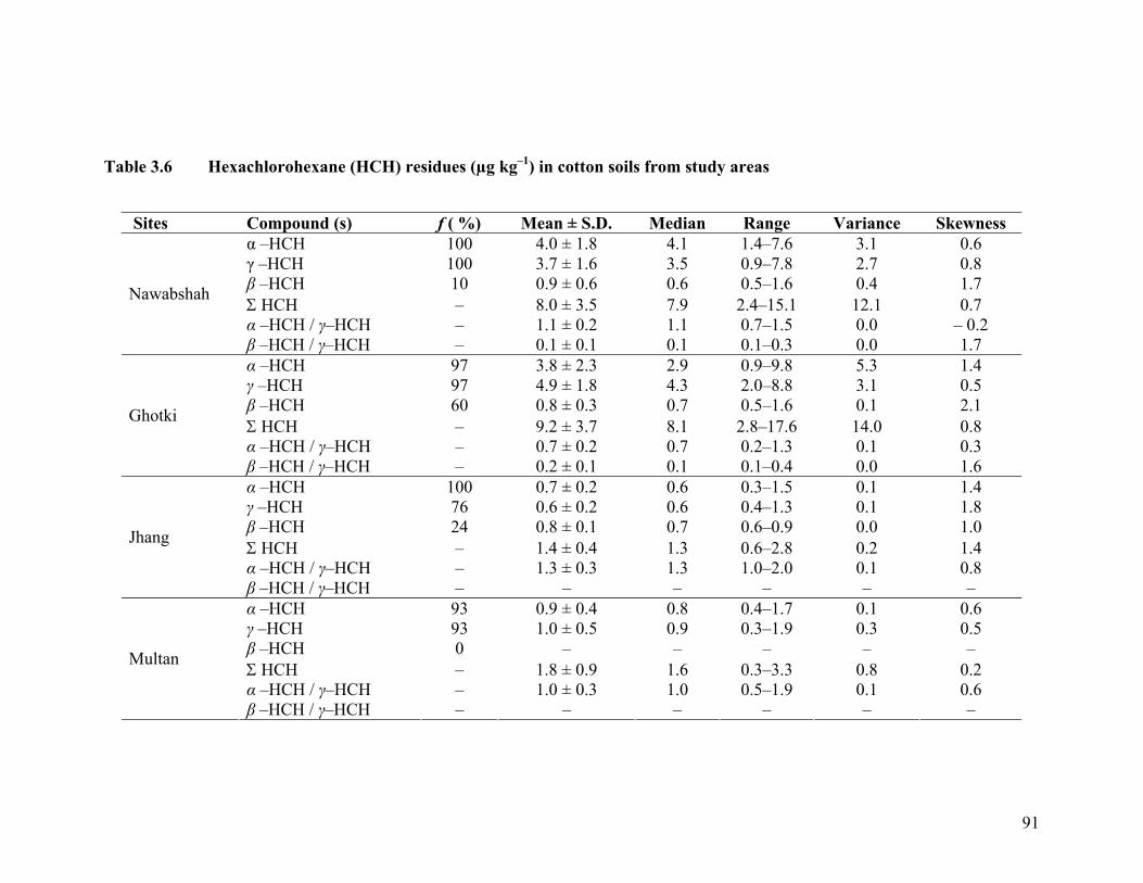
Sites Compound (s) f ( %) Mean ± S.D. Median Range Variance Skewness α –HCH 100 4.0 ± 1.8 4.1 1.4–7.6 3.1 0.6 γ –HCH 100 3.7 ± 1.6 3.5 0.9–7.8 2.7 0.8 β –HCH 10 0.9 ± 0.6 0.6 0.5–1.6 0.4 1.7 Σ HCH – 8.0 ± 3.5 7.9 2.4–15.1 12.1 0.7 α –HCH / γ–HCH – 1.1 ± 0.2 1.1 0.7–1.5 0.0 – 0.2
Nawabshah
β –HCH / γ–HCH – 0.1 ± 0.1 0.1 0.1–0.3 0.0 1.7 α –HCH 97 3.8 ± 2.3 2.9 0.9–9.8 5.3 1.4 γ –HCH 97 4.9 ± 1.8 4.3 2.0–8.8 3.1 0.5 β –HCH 60 0.8 ± 0.3 0.7 0.5–1.6 0.1 2.1 Σ HCH – 9.2 ± 3.7 8.1 2.8–17.6 14.0 0.8 α –HCH / γ–HCH – 0.7 ± 0.2 0.7 0.2–1.3 0.1 0.3
Ghotki
β –HCH / γ–HCH – 0.2 ± 0.1 0.1 0.1–0.4 0.0 1.6 α –HCH 100 0.7 ± 0.2 0.6 0.3–1.5 0.1 1.4 γ –HCH 76 0.6 ± 0.2 0.6 0.4–1.3 0.1 1.8 β –HCH 24 0.8 ± 0.1 0.7 0.6–0.9 0.0 1.0 Σ HCH – 1.4 ± 0.4 1.3 0.6–2.8 0.2 1.4 α –HCH / γ–HCH – 1.3 ± 0.3 1.3 1.0–2.0 0.1 0.8
Jhang
β –HCH / γ–HCH – – – – – –α –HCH 93 0.9 ± 0.4 0.8 0.4–1.7 0.1 0.6 γ –HCH 93 1.0 ± 0.5 0.9 0.3–1.9 0.3 0.5 β –HCH 0 – – – – – Σ HCH – 1.8 ± 0.9 1.6 0.3–3.3 0.8 0.2 α –HCH / γ–HCH – 1.0 ± 0.3 1.0 0.5–1.9 0.1 0.6
Multan
β –HCH / γ–HCH – – – – – –
91
Table 3.6 Hexachlorohexane (HCH) residues (µg kg–1) in cotton soils from study areas
3.3.3.2 Hexachlorobenzene (HCB)
Soil samples collected from different study areas were also analysed for HCB residues
(Table 3.7). Residues of HCB were detected in Nawabshah, Jhang and Multan areas.
None of the samples from Ghotki were found contaminated with HCB. Highest
frequency (22 %) was detected from Nawabshah soil samples followed by 21 % in Jhang
and only 3 % (1 sample) in Multan study area. Highest amount of HCB residues ranging
from 0.1–2.6 µg kg–1 with median 0.6 µg kg–1 were detected from Nawabshah area. Both
study areas in Punjab i.e. Jhang and Multan had almost same magnitude of HCB residues
with range 0.1–0.9 µg kg–1 and 0.2–0.6 µg kg–1 respectively and median value of 0.3 µg
kg–1 in both the study areas. Quebec government in Canada categorized 1000 µg kg–1 as
moderate and 10,000 µg kg–1 as threshold levels for HCB residues in soil (Beyer, 1990).
HCB residues detected from the study areas were far below these values.
Both industrial and agricultural sectors are considered responsible for HCB contaminants
in environment (Meijer et al., 2001). In agricultural sector, HCB had been used for seed
dressing to prevent fungal disease on grains especially to control Bunt (Tilletia caries, T.
tritici and T. foetida) in wheat, but this use was discontinued in most countries in the
1970s (Barber et al., 2005). According to Barber et al., (2005) an estimated 15390 tonnes
of HCB were imported by Pakistan during 1970–92 and 12162 tonnes was used (1979–
88). According to Jacoff et al, (1986), apart from agricultural use, HCB contamination
could come from manufacturing and use of chlorinated solvents, chlorinated aromatics
and chlorinated pesticides as well as during incomplete combustion of waste at disposal
sites. HCB breaks down very slowly in the environment and due to its lipophilic nature
accumulates through the food web to top predators where it can impair wildlife health.
Highest occurrence and magnitude of HCB residues was detected in Nawabshah study
area. The study area is located on National Highway very close to Sakrand town.
Furthermore, in and around the sampling area, many brick kilns are present. These units
are reported to use rubber tyres and other inflammable wastes along with coal and wood
to generate prolonged heating environment for brick baking. Therefore, in Nawabshah
study area besides agricultural use, these high amounts of HCB residues could be
92
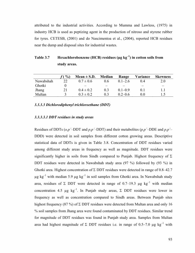
attributed to the industrial activities. According to Mumma and Lawless, (1975) in
industry HCB is used as peptizing agent in the production of nitroso and styrene rubber
for tyres. CETESB, (2001) and do Nascimentoa et al., (2004), reported HCB residues
near the dump and disposal sites for industrial wastes.
Table 3.7 Hexachlorobenzene (HCB) residues (µg kg–1) in cotton soils from
study areas.
f ( %) Mean ± S.D. Median Range Variance Skewness Nawabshah 22 0.7 ± 0.6 0.6 0.1–2.6 0.4 2.0 Ghotki 0 – – – – – Jhang 21 0.4 ± 0.2 0.3 0.1–0.9 0.1 1.1 Multan 3 0.3 ± 0.2 0.3 0.2–0.6 0.0 1.5
3.3.3.3 Dichlorodiphenyl trichloroethane (DDT)
3.3.3.3.1 DDT residues in study areas
Residues of DDTs (o,p΄–DDT and p,p΄–DDT) and their metabolites (p,p΄–DDE and p,p΄–
DDD) were detected in soil samples from different cotton growing areas. Descriptive
statistical data of DDTs is given in Table 3.8. Concentration of DDT residues varied
among different study areas in frequency as well as magnitude. DDT residues were
significantly higher in soils from Sindh compared to Punjab. Highest frequency of Σ
DDT residues were detected in Nawabshah study area (97 %) followed by (93 %) in
Ghotki area. Highest concentration of Σ DDT residues were detected in range of 0.8–42.7
µg kg–1 with median 5.9 µg kg–1 in soil samples from Ghotki area. In Nawabshah study
area, residues of Σ DDT were detected in range of 0.7–19.3 µg kg–1 with median
concentration 4.5 µg kg–1. In Punjab study areas, Σ DDT residues were lower in
frequency as well as concentration compared to Sindh areas. Between Punjab sites
highest frequency (87 %) of Σ DDT residues were detected from Multan area and only 16
% soil samples from Jhang area were found contaminated by DDT residues. Similar trend
for magnitude of DDT residues was found in Punjab study area. Samples from Multan
area had highest magnitude of Σ DDT residues i.e. in range of 0.5–7.0 µg kg–1 with
93

median concentration 1.5 µg kg–1 followed by range 0.3–0.6 µg kg–1 with median
concentration 0.5 µg kg–1.
Intensity of DDT isomers and their by–products also varied among study areas. In
Nawabshah, different DDT residues occurred in following order: p,p΄–DDD=p,p΄–
DDT> o,p΄–DDT> p,p΄–DDE. The magnitude of parent DDTs was higher than
breakdown products of DDTs. Concentration of p,p΄–DDT was highest with
concentration range 0.4–11.6 µg kg–1 with median 1.7 µg kg–1 followed by o,p΄–DDT
with concentration range 0.5–2.8 µg kg–1 and median 1.3 µg kg–1. Breakdown products of
DDTs, p,p΄–DDE and p,p΄–DDD were detected in almost similar concentrations with
ranges 0.4–3.0 µg kg–1 (median 0.9 µg kg–1) and 0.3–3.7 µg kg–1 (median 0.8 µg kg–1)
respectively.
In Ghotki study area, different DDT isomers and byproducts occurred in almost similar
order as in Nawabshah. Occurrence of different DDT residues were in order: p,p΄–
DDD>p,p΄–DDT> o,p΄–DDT> p,p΄–DDE. Concentration of parent DDT compounds was
higher or at par with the byproducts. Concentration of p,p΄–DDT was highest with range
0.4–22.8 µg kg–1 with median values 2.1 µg kg–1 followed by p,p΄–DDD, p,p΄–DDE and
o,p΄–DDT with concentrations in range 0.4–14.3 µg kg–1 (median 1.5 µg kg–1), 0.4–3.7
µg kg–1 (median 1.4 µg kg–1) and 0.4–3.9 µg kg–1 (median 1.2 µg kg–1) respectively.
In Punjab province, Multan area was more contaminated by DDT residues compared to
Jhang. In Multan, different DDT residues occurred in flowing order: p,p΄–DDE> o,p΄–
DDT> p,p΄–DDD>p,p΄–DDT. In magnitude, highest concentration of p,p΄–DDT was
detected with range 0.3–5.0 µg kg–1 with median 0.9 µg kg–1 followed by p,p΄–DDE 0.3–
4.2 µg kg–1 with median 0.8 µg kg–1. Residues of o,p΄–DDT and p,p΄–DDD were at par
with each other and their concentrations ranged from 0.4–1.0 µg kg–1 and 0.3–1.5 µg kg–1
respectively with median concentration of 0.6 µg kg–1 for each.
Among the study areas, Jhang soil samples were least contaminated by DDT residues. In
this area o,p΄–DDT was not detected from any soil sample. Residues of p,p΄–DDT and
p,p΄–DDE were detected in concentration of 0.5 µg kg–1 from only one sample each and
94
95
p,p΄–DDD was detected from two soil samples with concentration range 0.3–0.6 µg kg–1
and median 0.4 µg kg–1. MAC for DDT residues in soil given by USSR Committee of
Science and Technology was 1000 µg kg–1 (Beyer, 1990). None of the soil samples from
the study areas exceeded this critical limit for DDT residues and soils in the study areas
can be considered on safer side on this basis.
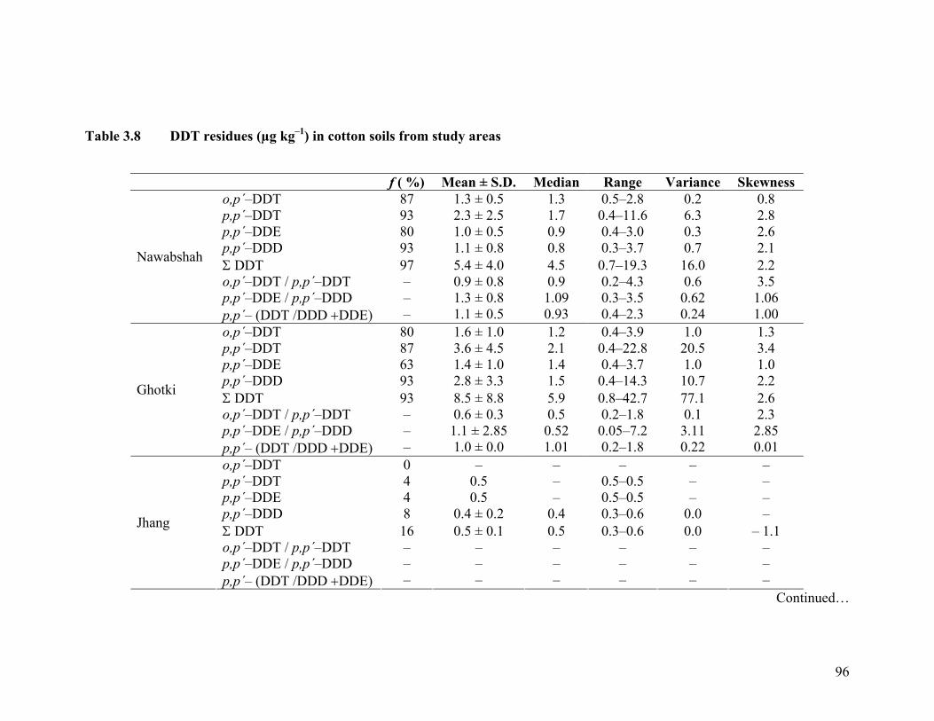
Table 3.8 DDT residues (µg kg–1) in cotton soils from study areas
f ( %) Mean ± S.D. Median Range Variance Skewness o,p΄–DDT 87 1.3 ± 0.5 1.3 0.5–2.8 0.2 0.8 p,p΄–DDT 93 2.3 ± 2.5 1.7 0.4–11.6 6.3 2.8 p,p΄–DDE 80 1.0 ± 0.5 0.9 0.4–3.0 0.3 2.6 p,p΄–DDD 93 1.1 ± 0.8 0.8 0.3–3.7 0.7 2.1 Σ DDT 97 5.4 ± 4.0 4.5 0.7–19.3 16.0 2.2 o,p΄–DDT / p,p΄–DDT – 0.9 ± 0.8 0.9 0.2–4.3 0.6 3.5 p,p΄–DDE / p,p΄–DDD – 1.3 ± 0.8 1.09 0.3–3.5 0.62 1.06
Nawabshah
p,p΄– (DDT /DDD +DDE) – 1.1 ± 0.5 0.93 0.4–2.3 0.24 1.00 o,p΄–DDT 80 1.6 ± 1.0 1.2 0.4–3.9 1.0 1.3 p,p΄–DDT 87 3.6 ± 4.5 2.1 0.4–22.8 20.5 3.4 p,p΄–DDE 63 1.4 ± 1.0 1.4 0.4–3.7 1.0 1.0 p,p΄–DDD 93 2.8 ± 3.3 1.5 0.4–14.3 10.7 2.2 Σ DDT 93 8.5 ± 8.8 5.9 0.8–42.7 77.1 2.6 o,p΄–DDT / p,p΄–DDT – 0.6 ± 0.3 0.5 0.2–1.8 0.1 2.3 p,p΄–DDE / p,p΄–DDD – 1.1 ± 2.85 0.52 0.05–7.2 3.11 2.85
Ghotki
p,p΄– (DDT /DDD +DDE) – 1.0 ± 0.0 1.01 0.2–1.8 0.22 0.01 o,p΄–DDT 0 – – – – –p,p΄–DDT 4
0.5 – 0.5–0.5 – –p,p΄–DDE 4 0.5 – 0.5–0.5 – –p,p΄–DDD 8 0.4 ± 0.2 0.4 0.3–0.6 0.0 – Σ DDT 16 0.5 ± 0.1 0.5 0.3–0.6 0.0 – 1.1 o,p΄–DDT / p,p΄–DDT – – – – – –p,p΄–DDE / p,p΄–DDD – – – – – –
Jhang
p,p΄– (DDT /DDD +DDE) – – – – – –Continued…
96
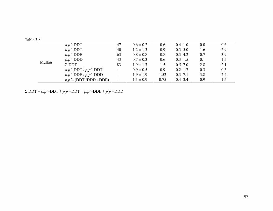
97
Table 3.8 o,p΄–DDT 47 0.6 ± 0.2 0.6 0.4–1.0 0.0 0.6 p,p΄–DDT 40 1.2 ± 1.3 0.9 0.3–5.0 1.6 2.9 p,p΄–DDE 63 0.8 ± 0.8 0.8 0.3–4.2 0.7 3.9 p,p΄–DDD 43 0.7 ± 0.3 0.6 0.3–1.5 0.1 1.5 Σ DDT 83 1.9 ± 1.7 1.5 0.5–7.0 2.8 2.1 o,p΄–DDT / p,p΄–DDT – 0.9 ± 0.5 0.9 0.2–1.7 0.3 0.3 p,p΄–DDE / p,p΄–DDD – 1.9 ± 1.9 1.52 0.3–7.1 3.8 2.4
Multan
p,p΄– (DDT /DDD +DDE) – 1.1 ± 0.9 0.75 0.4–3.4 0.9 1.5
Σ DDT = o,p΄–DDT + p,p΄–DDT + p,p΄–DDE + p,p΄–DDD
3.3.3.3.2 Source and age of DDT residues
Technical DDT consists of p,p΄–DDT (85 %) and o,p΄–DDT (15 %). However, besides
DDT, dicofol also contributes these isomers as its impurities into the environment.
Dicofol contains reasonably higher o,p΄–DDT than p,p΄–DDT and the ratio of o,p΄–DDT
/ p,p΄–DDT can be as high as 7.0 in commercial dicofol formulations (Yang et al., 2007).
In technical DDT, the ratio of o,p΄–DDT / p,p΄–DDT is ~0.2. The ratio between DDT
isomers can be used to predict the possible source of DDT residues in an environment
(Yang et al., 2007). In our study (Table 3.8), this ratio was calculated with range 0.2–4.3
and median 0.6 in Nawabshah, 0.2–1.8 with median 0.5 in Ghotki and 0.2–1.7 with
median 0.9 in Multan study area. These ratios of o,p΄–DDT / p,p΄–DDT were mostly
lower than dicofol but higher than that of technical DDT. As the relative quantities of
o,p΄–DDT and p,p΄–DDT are reasonably fixed in technical DDT and dicofol formulations
and that the environmental behavior of both the isomers is quite similar and they degrade
at almost similar rates (Yang et al., 2007). Therefore, the ratio of these isomers should
match either of the formulations. But in our study, ratio of o,p′–DDT / p,p′–DDT in
majority of soil samples in almost all the study areas does not match either source of
DDT isomers. Therefore, apart from technical DDT, a contribution of DDT residues from
some other source like dicofol is quite obvious. According to Li et al., (2006) ratios of
o,p′–DDT / p,p′–DDT between two source formulations could be due to mixing of
technical DDT and dicofol–type DDT. This ratio could not be calculated for Jhang
because of absence of o,p΄–DDT residues in this area.
Relationship between o,p΄–DDT and p,p΄–DDT in different study areas were studied by
correlation analysis (Figure 3.2). In Nawabshah and Ghotki areas there was a strong
correlation between two DDT isomers. The correlation coefficient (r2) for o,p΄–DDT and
p,p΄–DDT isomers was 0.7080 and 0.8058 in Nawabshah (Fig. 1a) and Ghotki (Fig 1b)
areas respectively. Though o,p΄–DDT / p,p΄–DDT ratio for Nawabshah (median = 0.9)
and Ghotki (median = 0.5) was quite different. But the correlation analysis show similar
environmental behavior of these isomers in these areas. o,p΄–DDT / p,p΄–DDT ratio
(median 0.9) in Multan suggests presence of both the isomers in almost similar amounts.
98
However, correlation studies show very poor relationship between o,p΄–DDT and p,p΄–
DDT Multan area. Correlation between the two (r = –0.2965) show negative association
between the two. Possible reason could be the fresh use of DDTs in this area or due to
different rates of degradation between two isomers. It is well established that components
of DDTs in technical DDT and dicofol are both the isomers show similar environmental
behavior. Therefore, both the components had been reported showing similar trend in
many studies (Yang et al., 2007).
In soil environment, degradation of DDTs is facilitated by microbes. DDT is biodegraded
into DDE under aerobic conditions and into DDD under anaerobic conditions (Gao et al.,
2008). Both DDD and DDE are more stable and highly toxic compounds. The rate of
transformation is dependent upon soil type, temperature, moisture and organic carbon
content of the soil (Li et al., 2006). Different isomers maintain their identity in
breakdown products. o,p′–DDT always breaks down into o,p′–DDD and o,p′–DDE,
similarly p,p′–DDT degrades into p,p′–DDD and p,p′–DDE.
99

(a)
-
2
4
6
8
10
12
14
- 2 4 6 8 10 12 14
(b)
-
5
10
15
20
25
- 5 10 15 20 25
p,p-
DD
T
(c)
-
0.50
1.00
1.50
2.00
- 0.50 1.00 1.50 2.00
o,p-DDT
r = 0.7080
r = 0.8058
r = –0.2965
Figure 3.2 Relationship between o,p′–DDT and p,p′–DDT in soil sample from
(a) Nawabshah, (b) Ghotki and (c) Multan study areas (r = coefficient
of correlation)
100
During the study both types of byproducts p,p′–DDE and p,p′–DDD were detected from
the study areas. Relative proportion of the breakdown products varied among different
areas. To compare type of biodegradation activities in different areas, p,p′–DDE and p,p′–
DDD ratios were used (Figure 3.3). Small value (< 1) of p,p′–DDE / p,p′–DDD ratio
indicates dominance of p,p′–DDD over p,p′–DDE, while large values (> 1) indicate
presence of higher amounts of p,p′–DDE. In Nawabshah, p,p′–DDE / p,p′–DDD ratios
ranged between 0.3–3.5 with median 1.09. Majority of the soil samples (57 %) had higher
p,p′–DDE / p,p′–DDD ratio indicating dominance of p,p′–DDE in the area and aerobic
degradation of DDTs. In contrast, p,p′–DDE / p,p′–DDD ratio were quite low in Ghotki
study area and ranged from 0.05–7.2 with median 0.52 indicating dominance of p,p′–
DDD in the area. Majority of soil samples (74 %) had ratios less than 1 and only 26 %
were found with ratios > 1, indicating dominance of anaerobic biodegradation of DDT in
the area. In Multan, p,p′–DDE / p,p′–DDD ratios ranged from 0.3–7.1 with median 1.52.
Majority of the soil samples (70 %) had higher (> 1) p,p′–DDE / p,p′–DDD ratio and only
30 % had ratio < 1 (Figure 3.3). These results are indicative of higher proportion of DDTs
biodegradation by aerobic microbial activities. Nawabshah and Multan study areas are
located in predominantly cotton growing regions. Besides cotton, agro–climate prevailing
in the area is suited for wheat, sugarcane, fodders and fruits orchards cultivation.
Therefore, majority of the soils are irrigated but well drained favoring aerobic microbial
activities. Although Ghotki area is regarded as cotton growing area but due to it
geographical location very close to rice belt and hot and humid climate, rice is also grown
as alternate crop in the area. Generally cotton growing areas in Pakistan were badly
affected by outbreak of cotton leaf curl virus and heavy insect pest infestation in 90s.
During this period cotton cultivation became economically unfeasible and growers and
farmers were forced to adopt alternate crops. In areas like Multan and Nawabshah, cotton
was mainly replaced by sugarcane while in Ghotki area rice crop along with sugarcane
was adopted by many growers. Therefore, soils of Ghotki area had experienced almost a
decade of anaerobic conditions. During the survey and sampling of the area, many farmer
fields were found with recent rice cultivation supporting presence of p,p′–DDD as a result
of anaerobic biodegradation of DDTs.
101
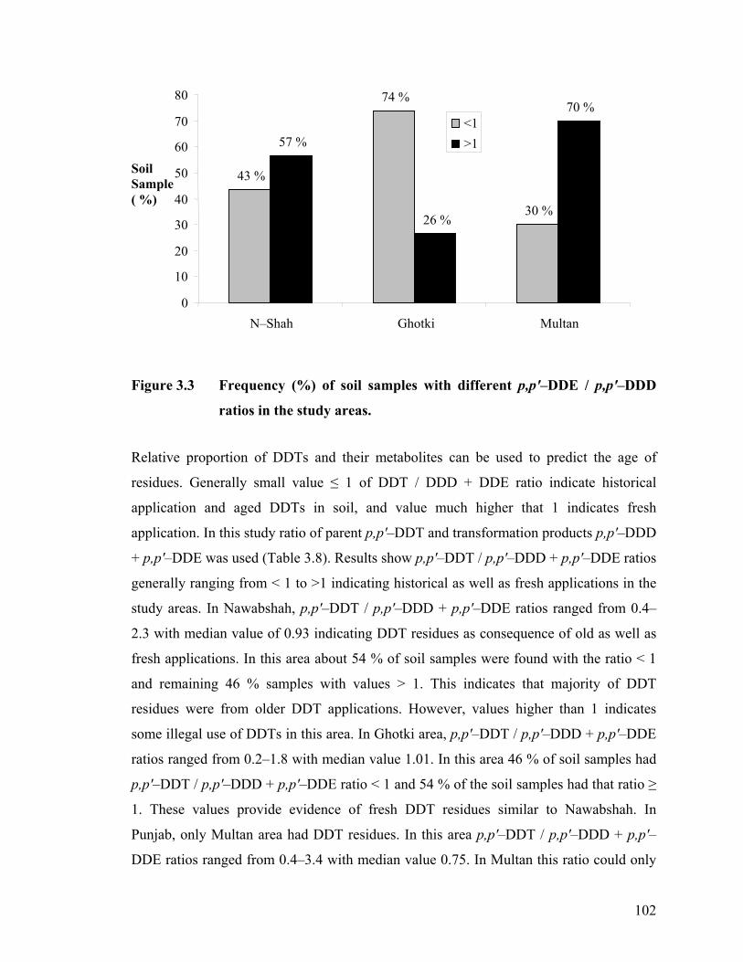
80
>1<1
57 %
26 %
70 %
43 %
74 %
30 %
70
60
40
50 Soil Sample ( %)
30
20
10
0N–Shah Ghotki Multan
Figure 3.3 Frequency (%) of soil samples with different p,p′–DDE / p,p′–DDD
ratios in the study areas.
Relative proportion of DDTs and their metabolites can be used to predict the age of
residues. Generally small value ≤ 1 of DDT / DDD + DDE ratio indicate historical
application and aged DDTs in soil, and value much higher that 1 indicates fresh
application. In this study ratio of parent p,p′–DDT and transformation products p,p′–DDD
+ p,p′–DDE was used (Table 3.8). Results show p,p′–DDT / p,p′–DDD + p,p′–DDE ratios
generally ranging from < 1 to >1 indicating historical as well as fresh applications in the
study areas. In Nawabshah, p,p′–DDT / p,p′–DDD + p,p′–DDE ratios ranged from 0.4–
2.3 with median value of 0.93 indicating DDT residues as consequence of old as well as
fresh applications. In this area about 54 % of soil samples were found with the ratio < 1
and remaining 46 % samples with values > 1. This indicates that majority of DDT
residues were from older DDT applications. However, values higher than 1 indicates
some illegal use of DDTs in this area. In Ghotki area, p,p′–DDT / p,p′–DDD + p,p′–DDE
ratios ranged from 0.2–1.8 with median value 1.01. In this area 46 % of soil samples had
p,p′–DDT / p,p′–DDD + p,p′–DDE ratio < 1 and 54 % of the soil samples had that ratio ≥
1. These values provide evidence of fresh DDT residues similar to Nawabshah. In
Punjab, only Multan area had DDT residues. In this area p,p′–DDT / p,p′–DDD + p,p′–
DDE ratios ranged from 0.4–3.4 with median value 0.75. In Multan this ratio could only
102
be calculated for only from 11 of the 30 soil samples. Of these soil samples, 64 % had
p,p′–DDT / p,p′–DDD + p,p′–DDE ratio < 1 and 36 % samples had ratio > 1. In two of
the samples viz. M03A and M12A this ratio was 2.06 and 3.35 respectively. These results
show main source of residues from older applications as well as some recent use of DDT
at isolated places. Cases of fresh application could be intentional or unintentional owing
to adulteration of recommended pesticides with DDTs.
3.3.3.4 Heptachlor
Residues of heptachlor and breakdown product heptachlor epoxide (trans) were studied
from different cotton growing study areas (Table 3.9). Heptachlor is transformed to
heptachlor epoxide in soil, plants and animals. The epoxide is more toxic, persistent and
can bio–accumulate in the biological systems (Singh et al., 2007). Highest frequency of
heptachlor residues were detected in study areas of Sindh province. Nawabshah was most
contaminated area with 97 % sample with heptachlor residues followed by Ghotki with
93 % contaminated samples. Comparatively very few samples were found with
heptachlor epoxide (trans) residues. Only 17 % samples from Nawabshah and merely 7
% samples from Ghotki were detected with heptachlor epoxide (trans) residues. In
Punjab, highest intensity (83 %) of heptachlor residues were found in Multan and only 12
% samples were found contaminated from Jhang area. Heptachlor epoxide (trans)
residues were also quite low in these areas and only 10 % soil samples from Multan and
none from Jhang area were found with heptachlor epoxide (trans) residues.
Magnitude of heptachlor and heptachlor epoxide (trans) residues also varied among
different study areas. Study areas of Sindh had higher magnitude of heptachlor residues
compared to Punjab. In Sindh, Ghotki soil samples had higher contamination of
heptachlor residues ranging from 0.4–4.7 µg kg–1 with median 2.0 µg kg–1 than
Nawabshah where residue concentration ranged from 0.5–2.8 µg kg–1 with median 1.6 µg
kg–1. In Punjab province, Multan area had higher concentration of heptachlor residues
ranging from 0.2–1.0 µg kg–1 with median 0.3 followed by concentration range 0.2–0.8
µg kg–1 with median 0.3 µg kg–1 in Jhang area. MAC for heptachlor residues in soil was
given as 50 µg kg–1 by USSR Committee of Science and Technology and 500 µg kg–1 by
103
104
Wisconsin Department of Natural Resources (Beyer, 1990). Heptachlor residues did not
exceed either of these levels in the study areas.
Alike occurrence, concentrations of heptachlor epoxide (trans) were quite low in the
study areas compared to parent heptachlor. Highest magnitude of heptachlor epoxide
(trans) was detected from Ghotki where residue concentration ranged from 0.7–1.0 µg
kg–1 and median 0.8 µg kg–1 followed by residue range 0.3–1.0 µg kg–1 with median 0.4
µg kg–1 in Multan area and 0.2–0.3 µg kg–1 and median 0.2 µg kg–1 in Nawabshah.
Heptachlor epoxide (trans) residues were not detected from Jhang.
The Heptachlor epoxide (trans) / Heptachlor ratio has been used by many workers to
predict the age of heptachlor residues. The metabolite/parental ratio < 1 is regarded as
fresh application or use of heptachlor while that > 1 is considered either, loss of
heptachlor due to volatilization or a higher conversion to the epoxide by biotic or abiotic
pathways (Gonzalez et al., 2005). Due to very low occurrence of heptachlor epoxide
(trans) from the study area, the ratio could only be calculated for 5, 2 and 3 soil samples
from Nawabshah, Ghotki and Multan areas (Table 3.9). Generally very low (< 1)
heptachlor epoxide (trans) ratio were detected from the study areas indicating fresh use
of heptachlor in cotton growing areas. The ratio ranged from 0.1–0.3 with median 0.1 in
Nawabshah, 0.3–0.4 with median 0.4 in Ghotki and 0.2–2.8 with median 0.8 in Multan.
Only one soil samples (M26A) from Multan had the ratio (2.27) indicating older
heptachlor use in that particular location.
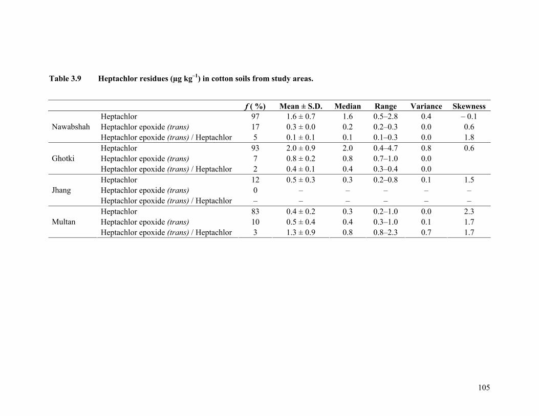
f ( %) Mean ± S.D. Median Range Variance Skewness Heptachlor 97 1.6 ± 0.7 1.6 0.5–2.8 0.4 – 0.1 Heptachlor epoxide (trans) 17 0.3 ± 0.0 0.2 0.2–0.3 0.0 0.6 Nawabshah Heptachlor epoxide (trans) / Heptachlor 5 0.1 ± 0.1 0.1 0.1–0.3 0.0 1.8 Heptachlor 93 2.0 ± 0.9 2.0 0.4–4.7 0.8 0.6 Heptachlor epoxide (trans) 7 0.8 ± 0.2 0.8 0.7–1.0 0.0 Ghotki Heptachlor epoxide (trans) / Heptachlor 2 0.4 ± 0.1 0.4 0.3–0.4 0.0 Heptachlor 12 0.5 ± 0.3 0.3 0.2–0.8 0.1 1.5 Heptachlor epoxide (trans) 0 – – – – –Jhang Heptachlor epoxide (trans) / Heptachlor – – – – – – Heptachlor 83 0.4 ± 0.2 0.3 0.2–1.0 0.0 2.3 Heptachlor epoxide (trans) 10 0.5 ± 0.4 0.4 0.3–1.0 0.1 1.7 Multan Heptachlor epoxide (trans) / Heptachlor 3 1.3 ± 0.9 0.8 0.8–2.3 0.7 1.7
105
Table 3.9 Heptachlor residues (µg kg–1) in cotton soils from study areas.
3.3.3.5 Chlordane
Chlordane has never been registered in Pakistan but still residues of different chlordane
isomers chlordane (trans) and chlordane (cis) and their breakdown products
oxychlordane were detected from cotton growing areas of Pakistan. Chlordane residues
varied both in intensity as well as magnitude in different study areas (Table 3.10). Both in
occurrence and magnitude, study areas from Sindh province had higher chlordane
contaminants than those in Punjab. Highest frequency (97 %) of Σ chlordane residues
was detected from Ghotki, followed by 93 % in Nawabshah, 52 % in Jhang and 43 % in
Multan. Highest concentration of Σ chlordane residues ranged from 0.4–3.5 µg kg–1 with
median 1.4 µg kg–1 in Ghotki followed by 0.3–2.5 µg kg–1 with median 0.9 µg kg–1 in
Nawabshah, 0.3–1.0 µg kg–1 with median 0.7 µg kg–1 in Jhang and least concentration in
range 0.3–0.9 µg kg–1 with median 0.4 µg kg–1 was detected from soil samples of Multan
study area. Critical residue levels for chlordane given by Wisconsin Department of
Natural Resources for sediments were 500 µg kg–1 (Beyer, 1990). Chlordane residues
detected from the study areas were far below this level. In soil chlordane (cis) and
chlordane (trans) is known to transforms into oxychlordane as a result of soil microbial
activities (Falconer et al., 1997). Residues of oxychlordane as breakdown of cis– and
trans– chlordane were studied. Highest frequency of oxychlordane residues occurred in
Nawabshah where 60 % soil samples were found with oxychlordane residues. This was
followed by 30 % oxychlordane frequency in Ghotki area. Study area from Punjab had
relatively low occurrence of oxychlordane like the parent cis and trans chlordane
residues. In Punjab, highest frequency (13 %) of oxychlordane residues was detected
from Multan followed by 8 % in Jhang area.
Concentration of cis and trans isomers of chlordane also varied in frequency and
magnitude among different study areas. In our study generally in all the areas, frequency
and concentration of chlordane (trans) (TC) was higher than chlordane (cis) (CC).
Commercial chlordane formulation technical–chlordane usually has CC and TC in
varying proportions. The TC/CC ratio in technical chlordane formulation has been given
ranging from 1.25–1.8 (Jantunen, et al., 2000; Singh et al., 2007). During the study
106
relative concentration of the two isomers was compared by TC/CC ratios in soil samples
from different areas (Table 3.10). The ratio could only be calculated for Sindh samples
due to the reason that only soil samples from Sindh area contained both the isomers. The
TC/CC ratio ranged from 0.9–2.5 with median 0.9 in Nawabshah and 0.4–3.5 with
median 1.4 in Ghotki area where majority of the samples had these ratios in accordance
with those in technical chlordane. In Nawabshah majority of the soil samples (66 %) had
TC/CC ratio above 1.8 while in rest of the 33 % samples the ratio was within that in
technical chlordane. In Ghotki majority of the soil samples (50 %) had less ratio, 31 %
sample had larger ratios and only 19 % had ratios according to technical chlordane.
Therefore, the results indicate variations between as well as within the study areas. The
locations with greater ratios indicate an older use of chlordane and depletion of CC
isomer due to degradation at possibly higher rates (Li et al., 2006). Areas/locations where
the TC/CC ratios match that of technical chlordane indicate fresh use and presence of
chlordane in its original composition. There were few locations where TC/CC ratios were
less than the range could be explained either as matter of chlordane composition with
lesser TC compared to CC or difference of TC degradation pattern under particular
factors related to soil environment. As described in an earlier section, unlike Nawabshah
where crop production is solely under aerobic soil environment, in Ghotki rice is also
cultivated that leads to anaerobic soil environment. Therefore, somewhat different
degradation pattern between TC and CC isomers existed in Ghotki area.
In Punjab, CC residues were detected in very low frequency. Only 17 % soil sample from
Multan were detected with CC residues and none of the samples from Jhang contained
CC residues. Due to this reason, TC/CC ratio could be calculated only for one sample
indicating equal amounts of both isomers from Multan and for none from Jhang area. In
Multan area concentration of TC was higher with range 0.3–0.8 µg kg–1 with median 0.4
µg kg–1 compared to CC that had concentration from 0.4–0.5 µg kg–1 with median 0.4 µg
kg–1. While in Jhang area only TC residues could be detected with range 0.3–1.0 µg kg–1
and median 0.7 µg kg–1 and no residues of CC above LOQ were detected. This low
detection or absence of CC residues in soils from Punjab area indicates older application
and losses of CC residues from soil with time. In another study, involving agricultural
107
108
soils Singh et al., (2007) found TC/CC ratio in range from 3.3–25 indicating very high
TC compared to CC and explained it as an earlier use of chlordane in the region.
Similarly, Li et al., (2006) detected TC/CC ratio in range 0.36–1.47 with median value of
1.04 and explained lower amounts of CC residues as consequence of higher rate of
degradation compared to TC residues.
Breakdown product of chlordane i.e. oxychlordane was also detected from the study
areas. Like chlordane, oxychlordane residues were also detected at higher frequency and
concentration from study areas in Sindh. Nawabshah had highest frequency 60 %
followed by 30 % in Ghotki area. Concentration of oxychlordane residues was almost
similar with range from 0.2–1.0 µg kg–1 and median 0.4 µg kg–1 in both the areas. In
Punjab only 8 % and 13 % samples were contaminated with oxychlordane residues in
Jhang and Multan study areas respectively. Concentration of oxychlordane residues was
higher in Multan with range 0.2–0.9 µg kg–1 and median concentration 0.8 µg kg–1 and
that in Jhang ranged from 0.3–0.6µg kg–1 with median 0.4 µg kg–1. To establish relation
between parent and breakdown product, Σ chlordane / oxychlordane ratio was calculated
(Table 3.10). Higher ratios (> 1) indicate recent application and low ratio (< 1) indicate
older application resulting in decrease in parent compound and increase in byproducts
due to degradation. In our study, Σ chlordane / oxychlordane ratio were quite high
indicating events of recent chlordane application. In Nawabshah, the ratio was in range
from 1.2–7.4 and median 2.5, 1.3–11.9 and median 2.5 in Ghotki, 0.5–3.6 with median
0.5 in Multan and for Jhang the ratio 1.3 could be calculated only for one sample. These
ratios further support the outcome from TC/CC ratios that Sindh samples indicate fresh as
well as older application of chlordane in the study areas. Similarly, low Σ chlordane /
oxychlordane ratio in Multan support earlier conclusion that chlordane related residue in
the area were from older applications.
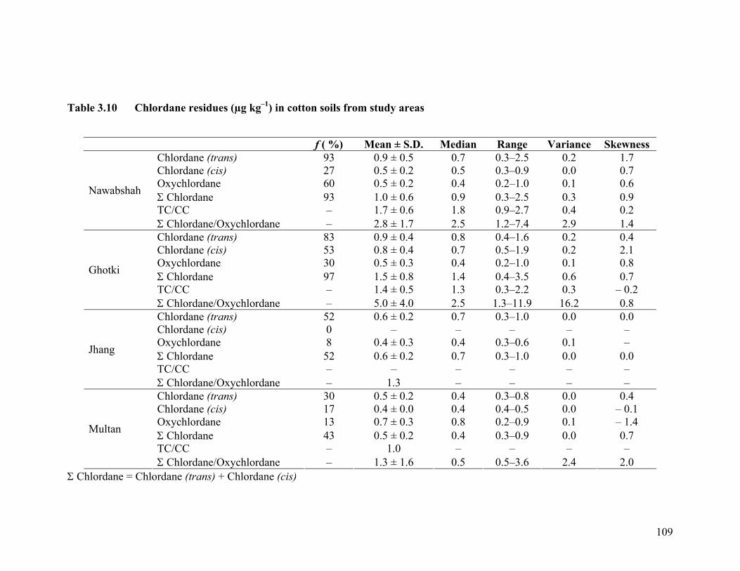
f ( %) Mean ± S.D. Median Range Variance Skewness Chlordane (trans) 93 0.9 ± 0.5 0.7 0.3–2.5 0.2 1.7 Chlordane (cis) 27 0.5 ± 0.2 0.5 0.3–0.9 0.0 0.7 Oxychlordane 60 0.5 ± 0.2 0.4 0.2–1.0 0.1 0.6 Σ Chlordane 93 1.0 ± 0.6 0.9 0.3–2.5 0.3 0.9 TC/CC – 1.7 ± 0.6 1.8 0.9–2.7 0.4 0.2
Nawabshah
Σ Chlordane/Oxychlordane – 2.8 ± 1.7 2.5 1.2–7.4 2.9 1.4 Chlordane (trans) 83 0.9 ± 0.4 0.8 0.4–1.6 0.2 0.4 Chlordane (cis) 53 0.8 ± 0.4 0.7 0.5–1.9 0.2 2.1 Oxychlordane 30 0.5 ± 0.3 0.4 0.2–1.0 0.1 0.8 Σ Chlordane 97 1.5 ± 0.8 1.4 0.4–3.5 0.6 0.7 TC/CC – 1.4 ± 0.5 1.3 0.3–2.2 0.3 – 0.2
Ghotki
Σ Chlordane/Oxychlordane – 5.0 ± 4.0 2.5 1.3–11.9 16.2 0.8 Chlordane (trans) 52 0.6 ± 0.2 0.7 0.3–1.0 0.0 0.0 Chlordane (cis)
0 – – – – –Oxychlordane 8 0.4 ± 0.3 0.4 0.3–0.6 0.1 – Σ Chlordane 52 0.6 ± 0.2
0.7
0.3–1.0
0.0 0.0
TC/CC – – – – – –
Jhang
Σ Chlordane/Oxychlordane – 1.3 – – – –Chlordane (trans) 30 0.5 ± 0.2 0.4 0.3–0.8 0.0 0.4 Chlordane (cis) 17 0.4 ± 0.0 0.4 0.4–0.5 0.0 – 0.1 Oxychlordane 13 0.7 ± 0.3 0.8 0.2–0.9 0.1 – 1.4 Σ Chlordane 43 0.5 ± 0.2 0.4
0.3–0.9
0.0 0.7
TC/CC – 1.0 – – – –
Multan
Σ Chlordane/Oxychlordane – 1.3 ± 1.6 0.5 0.5–3.6 2.4 2.0
109
Table 3.10 Chlordane residues (µg kg–1) in cotton soils from study areas
Σ Chlordane = Chlordane (trans) + Chlordane (cis)

3.3.3.6 Endosulfan
Endosulfan is one of the few organochlorine pesticides, still used in Pakistan and many
other countries for pest management. World health organization (WHO) has classified
endosulfan as moderately hazardous pesticide (Anonymous, 2002). It is the most
commonly used pesticide in recent years around the world and is ubiquitous in
environment. Endosulfan is used in rice crop against thrips, stem borer, whorl maggot,
case worm and against Helicoverpa armigera (Boll worm), Helicoverpa puncligera (Bud
worm) on cotton crops (Jayashree and Vasudevan, 2007). Commercially available,
technical endosulfan contains two isomers namely α– and β–endosulfan at 7:3 ratio with
a vapor pressure of 9×10⁻³ mm Hg (Goebel et al., 1982). According to Mathur et al.,
(2005) α–endosulfan is 3 times more toxic than the β–endosulfan. Endosulfan breaks
down into endosulfan sulfate due to microbial activities especially of fungi in soil and
into nontoxic endosulfan diol in water due to hydrolysis (Gonzalez et al., 2003).
Endosulfan sulfate is as toxic and persistent as parent endosulfan isomers (Gonzalez et
al., 2003).
Endosulfan residues varied among different study areas in frequency, magnitude as well
as isomeric composition (Table 3.11). Highest frequency of Σ endosulfan (α–endosulfan
+ β–endosulfan) residues (87 %) was detected in Multan followed by 77 % in Ghotki
area. Both of these areas were found contaminated with residues of α–endosulfan, β–
endosulfan their byproduct endosulfan sulphate. Nawabshah and Jhang areas had only β–
endosulfan residues along with endosulfan sulphate, while, α–endosulfan was not
detected from any soil sample from these areas. Frequency of Σ endosulfan residues was
37 % and 16 % in Nawabshah and Jhang areas respectively. Ghotki study area had
highest Σ endosulfan residue contamination in range of 0.3–2.9 µg kg–1 with median 1.1
µg kg–1 followed by 0.4–1.4 µg kg–1 and median 0.9 µg kg–1 in Multan. Σ Endosulfan
residues constituting only of β–endosulfan residues were high in Nawabshah with range
0.2–1.0 µg kg–1 and median 0.4 µg kg–1 compared to Jhang where β–endosulfan residues
ranged from 0.2–0.7 µg kg–1 with median concentration 0.3 µg kg–1. MAC for heptachlor
110
given by USSR Committee of Science and Technology was 100 µg kg–1 (Beyer, 1990).
On this basis soil of the study areas can be regarded on safer side.
In this study endo–α / endo–β ratio was calculated to compare relative contribution of
endosulfan isomers in Σ endosulfan residues in Ghotki and Multan areas (Table 3.11).
The ratio was high for Ghotki area ranging from 0.7–7.2 with median 2.5 indicating
presence of α–endosulfan at higher concentration than β–endosulfan. While, in Multan
area, α–endo / β–endo ratio was relatively low than Ghotki where it ranged from 0.8–3.9
with median 1.7 showing relatively low concentration of α–endosulfan. In Nawabshah
and Jhang areas, only β–endosulfan residues were detected and residues of α–endosulfan
were not detected from any of the samples. Reason for low incidence and magnitude of
α–endosulfan could be its high rate of volatilization influenced by environmental factors.
Technical endosulfan contains α–endosulfan and β–endosulfan isomers in ratio of 7:3.
According to Jayashree and Vasudevan, (2007) distribution and dissipation of endosulfan
occurs in two phases, firstly α–endosulfan volatilizes rapidly than β–endosulfan followed
by degradation of β–endosulfan into sulfate and α–endosulfan can only be detected from
soil immediately after its application, while β–endosulfan is less volatile and more
persistent than α–endosulfan. Gonzalez et al., (2003) found α–endosulfan / β–endosulfan
ratios ~1 in soil under tomato crop and described β–endosulfan and endosulfan sulfate as
more persist with the ability to adsorb in and on soil particles.
Relationship among α– and β–endosulfan and endosulfan sulphate was studied by
correlation analysis. Correlation coefficients of the parent and byproduct endosulfan are
given in (Table 3.12). Results show a very strong relationship between β–endosulfan and
endosulfan sulphate in all the study areas (Table 3.12; Figure 3.4). While, such
relationship was not observed between α–endosulfan and endosulfan sulfate. It is well
documented that in soil β–endosulfan and endosulfan sulfate are interrelated chemically
as well as in physical behavior (Gonzalez et al., 2003; Jayashree and Vasudevan, 2007).
β–endosulfan is known to oxidize into endosulfan sulphate and both the compounds get
adsorbed to soil particle and have more persistence than α–endosulfan (Jayashree and
Vasudevan, 2007).
111
112
During the study, endosulfan sulfate residues were also detected from all the study areas
in varying frequencies and magnitudes (Table 3.11). Highest frequency of endosulfan
sulfate was detected in Ghotki (83 %) followed by 47 % in Multan, 24 % in Jhang and 23
% in Nawabshah. Highest concentration of endosulfan sulfate residues were detected
from Ghotki ranging from 0.6–4.4 µg kg–1 with median 1.5 µg kg–1, followed by 0.8–2.6
µg kg–1 with median 0.9 µg kg–1 in Nawabshah, 0.3–1.1 µg kg–1 with median 0.6 µg kg–1
in Multan and 0.5–0.8 µg kg–1 with median 0.5 µg kg–1 in Jhang area. These results show
presence of endosulfan sulphate at higher concentration than Σ endosulfan in Nawabshah,
Ghotki and Jhang areas. Whereas, concentration of endosulfan sulphate residues was
lower than Σ endosulfan in Multan area. To compare relation between parent Σ
endosulfan and byproduct endosulfan, Σ endosulfan / endo–sulphate ratio was calculated
(Table 3.11). The higher Σ endosulfan / endo–sulphate ratio (> 1) indicated presence of
higher amounts of parent isomers than byproduct as a consequence of fresh application of
parent compounds. Lower Σ endosulfan / endo–sulphate ratio (< 1) indicates older
endosulfan residues where most of the parent isomers are lost or degraded. In our study
these ratios were low (< 1) for Nawabshah, Ghotki and Jhang areas where, it ranged from
0.3–0.5 with median 0.3, 0.2–1.6 with median 0.8, and 0.4–0.9 with median 0.6
respectively. This indicate majority of the endosulfan from older applications and very
low current use in the areas. The Σ endosulfan / endo–sulphate ratio was high compared
to other study areas in Multan ranging from 0.4–3.8 with median 1.6. These ratios for
Multan clearly suggest fresh use of endosulfan in the area.
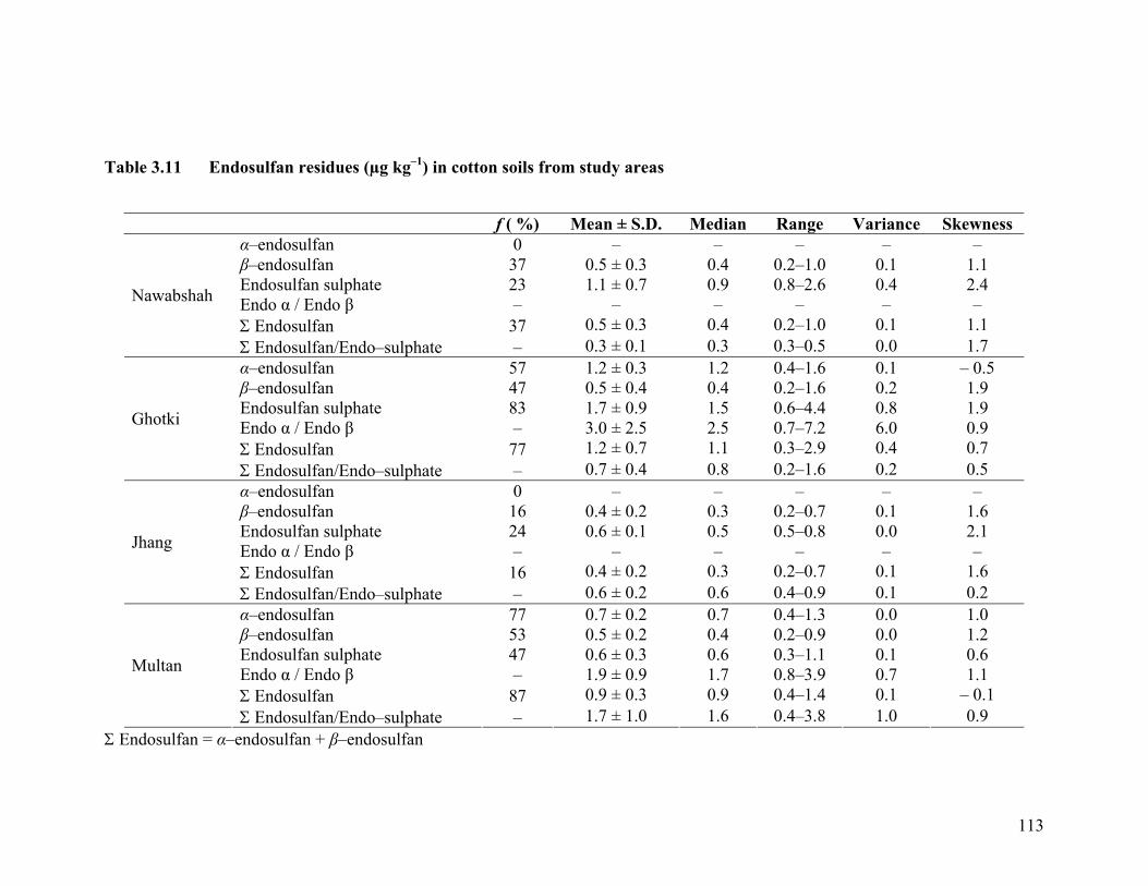
f ( %) Mean ± S.D. Median Range Variance Skewness α–endosulfan 0 – – – – –β–endosulfan 37 0.5 ± 0.3 0.4 0.2–1.0 0.1 1.1 Endosulfan sulphate 23 1.1 ± 0.7
0.9 0.8–2.6 0.4 2.4
Endo α / Endo β – – – – – –Σ Endosulfan 37 0.5 ± 0.3 0.4 0.2–1.0 0.1 1.1
Nawabshah
Σ Endosulfan/Endo–sulphate – 0.3 ± 0.1 0.3 0.3–0.5 0.0 1.7 α–endosulfan 57 1.2 ± 0.3 1.2 0.4–1.6 0.1 – 0.5 β–endosulfan 47 0.5 ± 0.4 0.4 0.2–1.6 0.2 1.9 Endosulfan sulphate 83 1.7 ± 0.9 1.5 0.6–4.4 0.8 1.9 Endo α / Endo β – 3.0 ± 2.5 2.5 0.7–7.2 6.0 0.9 Σ Endosulfan 77 1.2 ± 0.7 1.1 0.3–2.9 0.4 0.7
Ghotki
Σ Endosulfan/Endo–sulphate
– 0.7 ± 0.4 0.8
0.2–1.6
0.2 0.5 α–endosulfan 0 – – – – – β–endosulfan 16 0.4 ± 0.2 0.3 0.2–0.7 0.1 1.6 Endosulfan sulphate 24 0.6 ± 0.1
0.5 0.5–0.8 0.0 2.1
Endo α / Endo β – – – – – –Σ Endosulfan 16 0.4 ± 0.2 0.3 0.2–0.7 0.1 1.6
Jhang
Σ Endosulfan/Endo–sulphate – 0.6 ± 0.2 0.6 0.4–0.9 0.1 0.2 α–endosulfan 77 0.7 ± 0.2 0.7 0.4–1.3 0.0 1.0 β–endosulfan 53 0.5 ± 0.2 0.4 0.2–0.9 0.0 1.2 Endosulfan sulphate 47 0.6 ± 0.3 0.6 0.3–1.1 0.1 0.6 Endo α / Endo β – 1.9 ± 0.9 1.7 0.8–3.9 0.7 1.1 Σ Endosulfan 87 0.9 ± 0.3 0.9 0.4–1.4 0.1 – 0.1
Multan
Σ Endosulfan/Endo–sulphate – 1.7 ± 1.0 1.6 0.4–3.8 1.0 0.9
113
Table 3.11 Endosulfan residues (µg kg–1) in cotton soils from study areas
Σ Endosulfan = α–endosulfan + β–endosulfan
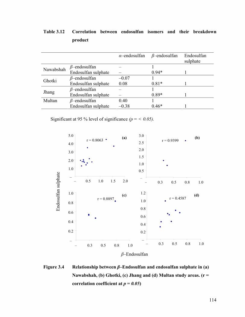
Table 3.12 Correlation between endosulfan isomers and their breakdown
product
α–endosulfan β–endosulfan Endosulfan sulphate
β–endosulfan – 1 Nawabshah Endosulfan sulphate – 0.94* 1 β–endosulfan –0.07 1 Ghotki Endosulfan sulphate 0.08 0.81* 1 β–endosulfan – 1 Jhang Endosulfan sulphate – 0.89* 1 β–endosulfan 0.40 1 Multan Endosulfan sulphate –0.38 0.46* 1
Significant at 95 % level of significance (p = < 0.05).
5.0 3.0
Endo
sulfa
n su
lpha
te
β–Endosulfan
Figure 3.4 Relationship between β–Endosulfan and endosulfan sulphate in (a)
Nawabshah, (b) Ghotki, (c) Jhang and (d) Multan study areas. (r =
correlation coefficient at p = 0.05)
(b)(a)r = 0.8063 r = 0.93992.54.02.03.01.5
2.01.0
1.0 0.5– –
– 0.5 1.0 1.5 2.0 – 0.3 0.5 0.8 1.0
1.21.0
– 0.3 0.5 0.8 1.0
(d)(c)r = 0.4587r = 0.8897 1.00.8
0.80.6
0.60.4
0.4
0.2 0.2
––– 0.3 0.5 0.8 1.0
114
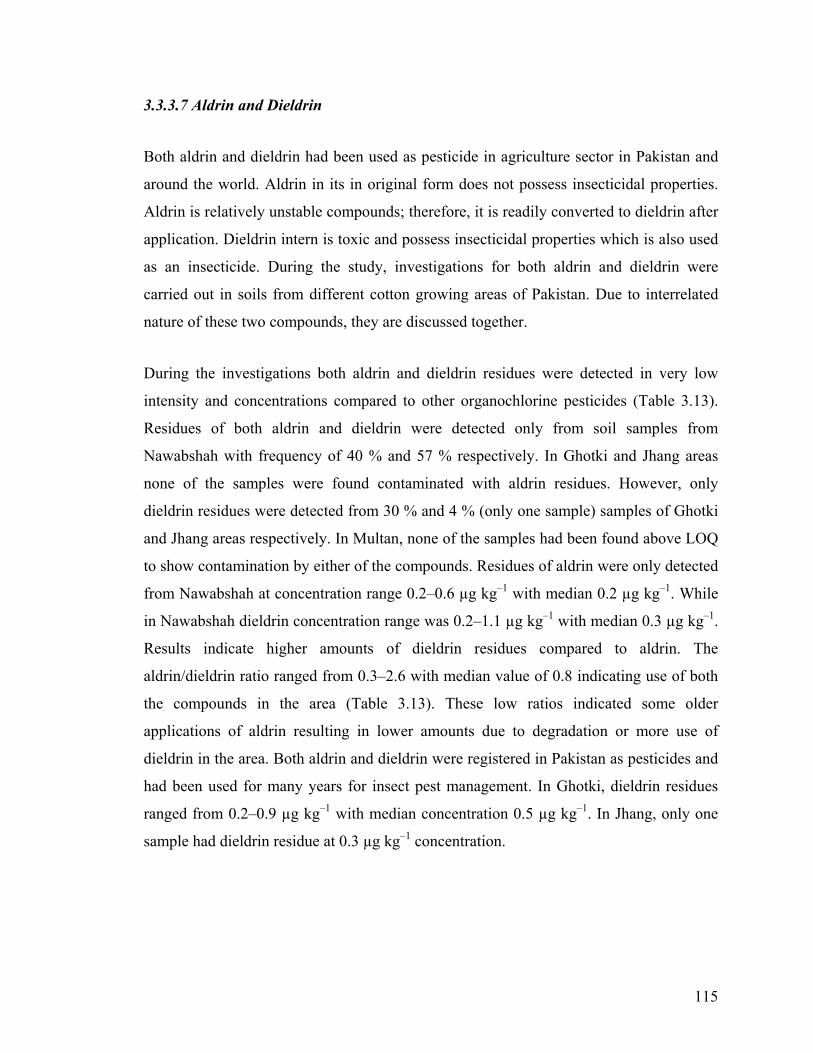
3.3.3.7 Aldrin and Dieldrin
Both aldrin and dieldrin had been used as pesticide in agriculture sector in Pakistan and
around the world. Aldrin in its in original form does not possess insecticidal properties.
Aldrin is relatively unstable compounds; therefore, it is readily converted to dieldrin after
application. Dieldrin intern is toxic and possess insecticidal properties which is also used
as an insecticide. During the study, investigations for both aldrin and dieldrin were
carried out in soils from different cotton growing areas of Pakistan. Due to interrelated
nature of these two compounds, they are discussed together.
During the investigations both aldrin and dieldrin residues were detected in very low
intensity and concentrations compared to other organochlorine pesticides (Table 3.13).
Residues of both aldrin and dieldrin were detected only from soil samples from
Nawabshah with frequency of 40 % and 57 % respectively. In Ghotki and Jhang areas
none of the samples were found contaminated with aldrin residues. However, only
dieldrin residues were detected from 30 % and 4 % (only one sample) samples of Ghotki
and Jhang areas respectively. In Multan, none of the samples had been found above LOQ
to show contamination by either of the compounds. Residues of aldrin were only detected
from Nawabshah at concentration range 0.2–0.6 µg kg–1 with median 0.2 µg kg–1. While
in Nawabshah dieldrin concentration range was 0.2–1.1 µg kg–1 with median 0.3 µg kg–1.
Results indicate higher amounts of dieldrin residues compared to aldrin. The
aldrin/dieldrin ratio ranged from 0.3–2.6 with median value of 0.8 indicating use of both
the compounds in the area (Table 3.13). These low ratios indicated some older
applications of aldrin resulting in lower amounts due to degradation or more use of
dieldrin in the area. Both aldrin and dieldrin were registered in Pakistan as pesticides and
had been used for many years for insect pest management. In Ghotki, dieldrin residues
ranged from 0.2–0.9 µg kg–1 with median concentration 0.5 µg kg–1. In Jhang, only one
sample had dieldrin residue at 0.3 µg kg–1 concentration.
115
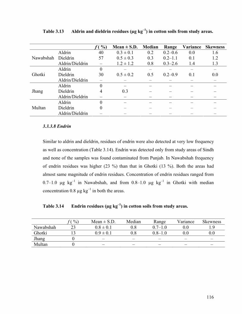
Table 3.13 Aldrin and dieldrin residues (µg kg–1) in cotton soils from study areas.
f ( %) Mean ± S.D. Median Range Variance SkewnessAldrin 40 0.3 ± 0.1 0.2 0.2–0.6 0.0 1.6 Dieldrin 57 0.5 ± 0.3 0.3 0.2–1.1 0.1 1.2 Nawabshah Aldrin/Dieldrin – 1.2 ± 1.2 0.8 0.3–2.6 1.4 1.3 Aldrin 0 – – – – – Dieldrin 30 0.5 ± 0.2 0.5 0.2–0.9 0.1 0.0 Ghotki Aldrin/Dieldrin – – – – – – Aldrin 0 – – – – – Dieldrin 4 0.3 – – – – Jhang Aldrin/Dieldrin – – – – – – Aldrin 0 – – – – – Dieldrin 0 – – – – – Multan Aldrin/Dieldrin – – – – – –
3.3.3.8 Endrin
Similar to aldrin and dieldrin, residues of endrin were also detected at very low frequency
as well as concentration (Table 3.14). Endrin was detected only from study areas of Sindh
and none of the samples was found contaminated from Punjab. In Nawabshah frequency
of endrin residues was higher (23 %) than that in Ghotki (13 %). Both the areas had
almost same magnitude of endrin residues. Concentration of endrin residues ranged from
0.7–1.0 µg kg–1 in Nawabshah, and from 0.8–1.0 µg kg–1 in Ghotki with median
concentration 0.8 µg kg–1 in both the areas.
Table 3.14 Endrin residues (µg kg–1) in cotton soils from study areas.
f ( %) Mean ± S.D. Median Range Variance Skewness Nawabshah 23 0.8 ± 0.1 0.8 0.7–1.0 0.0 1.9 Ghotki 13 0.9 ± 0.1 0.8 0.8–1.0 0.0 0.0 Jhang 0 – – – – – Multan 0 – – – – –
116
3.3.4 Spatial Distribution of Organochlorine Pesticide Residues
3.3.4.1 Hierarchical Cluster Analysis (HCA)
Spatial HCA rendered a Dendrogram (Figure 3.5) where all the 114 soil samples
collected from the top soil profile (0–15 cm) were grouped in two clusters at (Dlink/Dmax)
× 100 ≤ 100 where cluster “A” comprised of soil sample from study areas in Punjab and
cluster “B” comprised soil samples from study areas in Sindh. This grouping clearly
indicated the variations in OCP residues between the two provinces.
Both the groups A and B were further studied for subgroups to understand spatial
variation of OCP residues within each province. Group A from the Dendrogram is given
in Figure 3.6. In this group 55 soil sample mainly from Punjab study areas were grouped
into two sub–clusters at (Dlink/Dmax) × 100 < 10. The first sub–cluster designated as AI
predominantly comprised of soil samples from selected site of Jhang along with three soil
sample M11A, M07A and M04A from Multan and one sample N27A from Nawabshah.
The second sub–cluster of Group A designated as AII included majority of soil samples
from Multan. This sub–group also contained one soil sample each from Jhang (J19A) and
Ghotki (G53A).
Soil samples in Group B predominantly belonged to study areas of Sindh comprising 59
soil samples. The group was further categorized into three sub–clusters at (Dlink/Dmax) ×
100 ≤ 40 (Figure 3.7). The first sub–group designated as sub–group BI was
comparatively smaller in size with only six soil samples. This sub–group had 4 soil
samples from Ghotki and 2 samples from Nawabshah. The second cluster of Group B
was designated as sub–group BII containing 16 soil samples, 11 from Ghotki and 5 from
Nawabshah. Third subgroup BIII was the largest sub–group containing 37 soil samples
which entail 22 from Nawabshah, 13 from Ghotki and 2 from Multan study area.
Results of HCA clearly demonstrate spatial variations of OCP residues in different areas.
These variations existed between Punjab and Sindh provinces as well as between selected
study areas within each province. These results provide evidence that HCA technique
117
118
was useful in offering reliable information about the classification among different cotton
growing areas on the basis of OCP residues. This method was also usefully used for
previous environmental studies related to organic and inorganic pollutants in soils
(Goncalves et al., 2006; Luo et al., 2007; Qishlaqi et al., 2009), water (Goti et al., 1998;
Qadir et al., 2008) and sediments (Sarkar et al., 2008).
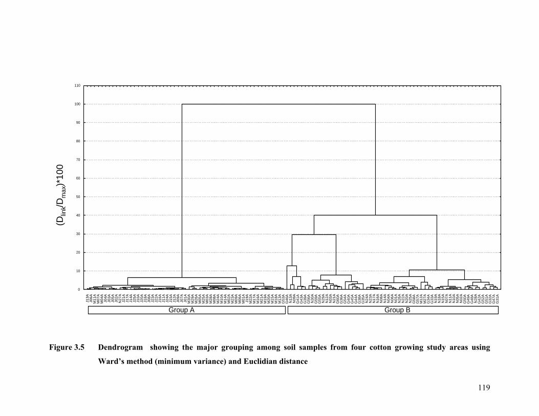
(Dlin
k/Dm
ax)*
100
0
10
20
30
40
50
60
70
80
90
100
110
J13
A
J06
A
M11
A
M07
A
M04
A
J04
A
J03
A
J05
A
J02
A
N27
A
J21
A
J17
A
J14
A
J25
A
J10
A
J20
A
J18
A
J08
A
J23
A
J22
A
J16
A
J11
A
J24
A
J15
A
J12
A
J09
A
J07
A
J01
A
M30
A
M29
A
M26
A
M05
A
M25
A
M03
A
M28
A
M08
A
M24
A
M10
A
M14
A
M02
A
M23
A
M09
A
M06
A
M01
A
J19
A
M22
A
M17
A
M16
A
M21
A
M19
A
M20
A
M15
A
M18
A
M13
A
G53
A
G46
A
N13
A
N09
A
G41
A
G43
A
G39
A
G56
A
N30
A
G59
A
G55
A
N29
A
N12
A
N03
A
N21
A
G60
A
G36
A
G54
A
G40
A
G45
A
G44
A
G38
A
G35
A
N24
A
N23
A
N17
A
N16
A
N08
A
N14
A
N04
A
N06
A
N01
A
N26
A
N22
A
N20
A
N25
A
G58
A
G57
A
M12
A
M27
A
G34
A
G33
A
N19
A
N18
A
N15
A
N07
A
N11
A
N10
A
N05
A
N02
A
G50
A
G49
A
G48
A
N28
A
G42
A
G52
A
G51
A
G32
A
G47
A
G31
A
Group A Group B
Figure 3.5 Dendrogram showing the major grouping among soil samples from four cotton growing study areas using
Ward’s method (minimum variance) and Euclidian distance
119
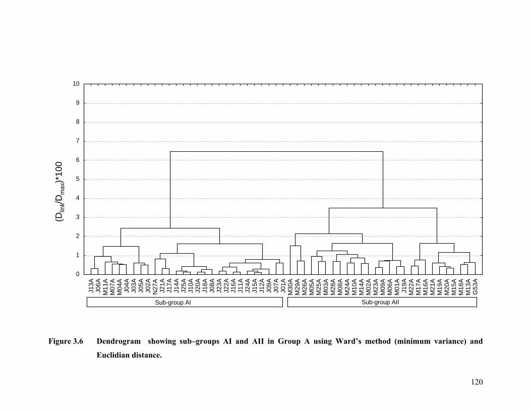
(Dlin
k/Dm
ax)*
100
0
1
2
3
4
5
6
7
8
9
10
J13
A
J06
A
M11
A
M07
A
M04
A
J04
A
J03
A
J05
A
J02
A
N27
A
J21
A
J17
A
J14
A
J25
A
J10
A
J20
A
J18
A
J08
A
J23
A
J22
A
J16
A
J11
A
J24
A
J15
A
J12
A
J09
A
J07
A
J01
A
M30
A
M29
A
M26
A
M05
A
M25
A
M03
A
M28
A
M08
A
M24
A
M10
A
M14
A
M02
A
M23
A
M09
A
M06
A
M01
A
J19
A
M22
A
M17
A
M16
A
M21
A
M19
A
M20
A
M15
A
M18
A
M13
A
G53
A
Sub-group AI Sub-group AII
Figure 3.6 Dendrogram showing sub–groups AI and AII in Group A using Ward’s method (minimum variance) and
Euclidian distance.
120

Figure 3.7 Dendrogram showing the sub–grouping in Group B using Ward’s method (minimum variance) and Euclidian
distance
(Dlin
k/Dm
ax)*
100
0
10
20
30
40
50
G46
A
N13
A
N09
A
G41
A
G43
A
G39
A
G56
A
N30
A
G59
A
G55
A
N29
A
N12
A
N03
A
N21
A
G60
A
G36
A
G54
A
G40
A
G45
A
G44
A
G38
A
G35
A
N24
A
N23
A
N17
A
N16
A
N08
A
N14
A
N04
A
N06
A
N01
A
N26
A
N22
A
N20
A
N25
A
G58
A
G57
A
M12
A
M27
A
G34
A
G33
A
N19
A
N18
A
N15
A
N07
A
N11
A
N10
A
N05
A
N02
A
G50
A
G49
A
G48
A
N28
A
G42
A
G52
A
G51
A
G32
A
G47
A
G31
A
Sub-group BII Sub-group BIIISub-gr. BI
121

3.3.4.2 Discriminant Function Analysis (DFA)
Discriminant function analysis (DFA) was used to understand the reasons for spatial
variations. Initially the DFA was applied to explain difference between Punjab and Sindh
provinces based on Group A and Group B clusters respectively (Figure 3.5). Discriminant
Functions (DFs) and classification matrices (CMs) obtained from standard, forward
stepwise and backward stepwise modes of spatial DFA are given in Table 3.15. All three
modes standard, forward stepwise and backward stepwise giving CMs with 96.01 %,
95.61 % and 94.73 % correct assignation in respective modes generated 19, 13 and 8
discriminant variables respectively. Spatial DFA showed that γ–HCH, heptachlor,
chlordane (cis), α–endosulfan, and p,p΄–DDE were the most important variables
responsible for discrimination between study areas of Punjab and Sindh. Box and whisker
plots of important variables identified by spatial DFA (backward stepwise mode) were
constructed to evaluate the trends of OCP residues in the two provinces (Figure 3.8). All
the OCPs responsible for provincial variation identified by DFA were in high
concentration in Sindh than in Punjab. These results indicated that OCPs were present at
higher concentration in areas of Sindh than areas of Punjab.
Concentration of γ–HCH residues ranged from 0.3–8.8 µg kg–1 with mean 4.3 µg kg–1 in
Sindh compared to 0.3–2.0 µg kg–1 with mean 0.9 µg kg–1 in study areas of Punjab.
Previous section (3.3.3.1.2) described technical–HCH and lindane (γ–HCH) as sources of
γ–HCH residues in cotton growing areas. Heptachlor residues were also categorized as
discriminating factor between Punjab and Sindh study areas by DFA. Heptachlor residues
were detected at high concentration in soil samples from Sindh compared to those from
Punjab. Heptachlor residues ranged from 0.4–4.7 µg kg–1 with mean 1.9 µg kg–1 in study
areas of Sindh that surpass 0.2–1.0 µg kg–1 with mean 0.3 µg kg–1 in soil samples from
Punjab. Besides cotton, heptachlor has been used for pest management in many other
fruits and field crops. In this regard sugarcane is very important where heptachlor use is
common against insect pests especially sugar cane borers etc. During the survey and
sampling of the study areas, it was observed that in cotton growing areas sugarcane was
frequently used as rotational or alternate crop. However, sugarcane cultivation is more
122

123
common in areas of Sindh compared to Punjab. Therefore, high levels of heptachlor
residues in the study areas of Sindh could be due to successive sugarcane cultivation in
these areas.
Backward stepwise DFA indicated contribution of chlordane (cis) in discriminating
between study areas of Sindh and Punjab. Chlordane has never been registered in
Pakistan. Despite the fact, residues of both chlordane (cis) and (trans) were detected in
soil samples from the study areas. In Sindh concentration of chlordane (cis) residues
ranged from 0.3–1.9 µg kg–1 with mean 0.7 µg kg–1 while, at relatively low concentration
range 0.3–0.5 µg kg–1 with mean 0.4 µg kg–1 in study areas of Punjab.
Backward stepwise DFA, also indicated α–endosulfan as differentiating factor between
the two provinces. α–endosulfan is reported to have less persistence in soils due to losses
mainly through volatilization and presence of α–endosulfan in the soil is often regarded
as consequence of fresh endosulfan applications (Jayashree and Vasudevan, 2007). The
concentration of α–endosulfan residues were relatively higher in Sindh with
concentration range from 0.4–1.6 µg kg–1 and mean 1.1 µg kg–1, compared to the
concentration range 0.4–1.3 µg kg–1 with mean 0.7 µg kg–1 in study areas of Punjab.
These results suggest relatively higher and fresh use of endosulfan as insecticide in the
study areas of Sindh.
According to the results of backward stepwise DFA, p,p′–DDE was also responsible for
difference between study areas of Punjab and Sindh. p,p′–DDE is the byproduct of p,p′–
DDT under aerobic conditions. Residues of p,p′–DDT were detected in order
Ghotki>Nawabshah>Multan>Jhang from the study areas. Similar trend was also found in
DDT breakdown products and the residues of p,p′–DDE in the study areas of Sindh
surpassed those in Punjab. Concentration of p,p′–DDE ranged from 0.4–4.2 µg kg–1 with
mean 1.3 µg kg–1 in study areas of Sindh and ranged from 0.3–0.9 µg kg–1 with mean 0.6
µg kg–1 in study areas of Punjab. These results mainly indicate higher DDT
contaminations in Sindh compared to Punjab. These results clearly indicate higher
concentration of OCP residues than study areas of Sindh than those in Punjab.
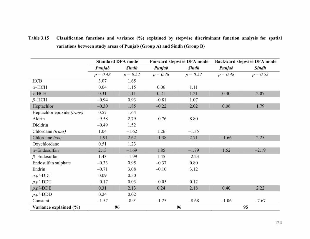
Standard DFA mode Forward stepwise DFA mode Backward stepwise DFA mode Punjab Sindh Punjab Sindh Punjab Sindh
p = 0.48 p = 0.52 p = 0.48 p = 0.52 p = 0.48 p = 0.52 HCB 3.07 1.65 α–HCH 0.04 1.15 0.06 1.11γ–HCH 0.31 1.11 0.21 1.21 0.30 2.07 β–HCH –0.94 0.93 –0.81 1.07Heptachlor –0.30 1.85
124
Table 3.15 Classification functions and variance (%) explained by stepwise discriminant function analysis for spatial
variations between study areas of Punjab (Group A) and Sindh (Group B)
–0.22 2.02 0.06 1.79 Heptachlor epoxide (trans)
0.57 1.64Aldrin –9.58 2.79 –0.76
8.80
Dieldrin –0.49 1.52Chlordane (trans) 1.04 –1.62 1.26 –1.35Chlordane (cis) –1.91 2.62 –1.38 2.71 –1.66 2.25 Oxychlordane 0.51 1.23α–Endosulfan 2.13 –1.69 1.85 –1.79 1.52 –2.19 β–Endosulfan
1.43 –1.99 1.45 –2.23Endosulfan sulphate
–0.33 0.95 –0.37 0.80
Endrin –0.71 3.08 –0.10
3.12o,p′–DDT 0.09 0.50p,p′–DDT –0.17 0.03 –0.05 0.12p,p′–DDE 0.31 2.13 0.24 2.18 0.40 2.22 p,p′–DDD
0.24 0.02
Constant –1.57 –8.91 –1.25 –8.68 –1.06 –7.67Variance explained (%) 96 96 95
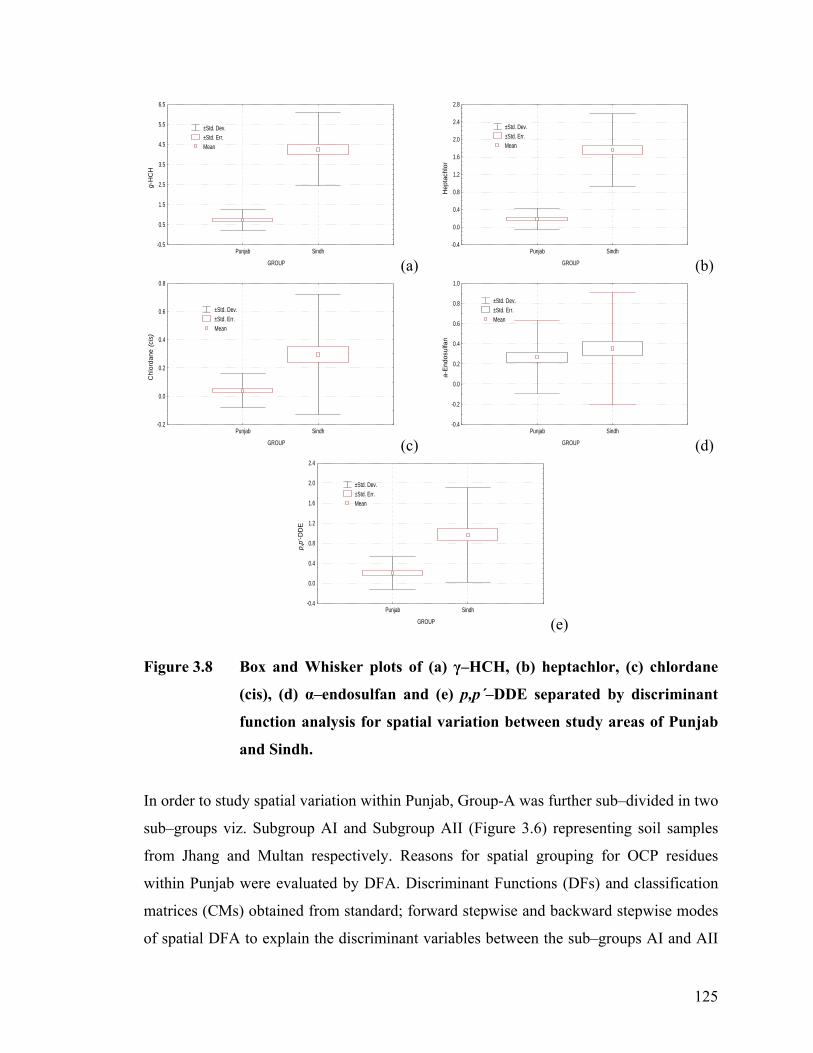
GROUP
g-H
CH
-0.5
0.5
1.5
2.5
3.5
4.5
5.5
6.5
Punjab Sindh
±Std. Dev.±Std. Err.Mean
(a) GROUP
Hep
tach
lor
-0.4
0.0
0.4
0.8
1.2
1.6
2.0
2.4
2.8
Punjab Sindh
±Std. Dev.±Std. Err.Mean
(b)
GROUP
Chl
orda
ne (
cis)
-0.2
0.0
0.2
0.4
0.6
0.8
Punjab Sindh
±Std. Dev.±Std. Err.Mean
(c) GROUPa-
End
osul
fan
-0.4
-0.2
0.0
0.2
0.4
0.6
0.8
1.0
Punjab Sindh
±Std. Dev.±Std. Err.Mean
(d)
GROUP
p,p'
-DD
E
-0.4
0.0
0.4
0.8
1.2
1.6
2.0
2.4
Punjab Sindh
±Std. Dev.±Std. Err.Mean
(e)
Figure 3.8 Box and Whisker plots of (a) γ–HCH, (b) heptachlor, (c) chlordane
(cis), (d) α–endosulfan and (e) p,p´–DDE separated by discriminant
function analysis for spatial variation between study areas of Punjab
and Sindh.
In order to study spatial variation within Punjab, Group-A was further sub–divided in two
sub–groups viz. Subgroup AI and Subgroup AII (Figure 3.6) representing soil samples
from Jhang and Multan respectively. Reasons for spatial grouping for OCP residues
within Punjab were evaluated by DFA. Discriminant Functions (DFs) and classification
matrices (CMs) obtained from standard; forward stepwise and backward stepwise modes
of spatial DFA to explain the discriminant variables between the sub–groups AI and AII
125
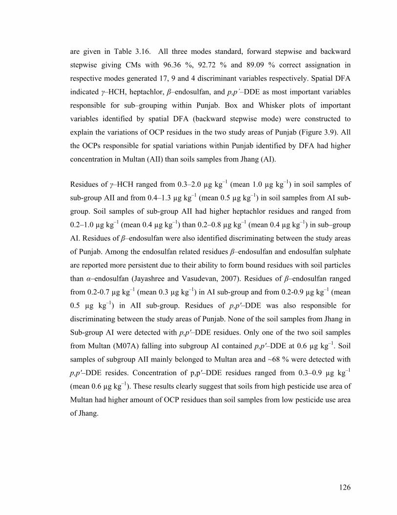
are given in Table 3.16. All three modes standard, forward stepwise and backward
stepwise giving CMs with 96.36 %, 92.72 % and 89.09 % correct assignation in
respective modes generated 17, 9 and 4 discriminant variables respectively. Spatial DFA
indicated γ–HCH, heptachlor, β–endosulfan, and p,p΄–DDE as most important variables
responsible for sub–grouping within Punjab. Box and Whisker plots of important
variables identified by spatial DFA (backward stepwise mode) were constructed to
explain the variations of OCP residues in the two study areas of Punjab (Figure 3.9). All
the OCPs responsible for spatial variations within Punjab identified by DFA had higher
concentration in Multan (AII) than soils samples from Jhang (AI).
Residues of γ–HCH ranged from 0.3–2.0 µg kg–1 (mean 1.0 µg kg–1) in soil samples of
sub-group AII and from 0.4–1.3 µg kg–1 (mean 0.5 µg kg–1) in soil samples from AI sub-
group. Soil samples of sub-group AII had higher heptachlor residues and ranged from
0.2–1.0 µg kg–1 (mean 0.4 µg kg–1) than 0.2–0.8 µg kg–1 (mean 0.4 µg kg–1) in sub–group
AI. Residues of β–endosulfan were also identified discriminating between the study areas
of Punjab. Among the endosulfan related residues β–endosulfan and endosulfan sulphate
are reported more persistent due to their ability to form bound residues with soil particles
than α–endosulfan (Jayashree and Vasudevan, 2007). Residues of β–endosulfan ranged
from 0.2-0.7 µg kg–1 (mean 0.3 µg kg–1) in AI sub-group and from 0.2-0.9 µg kg–1 (mean
0.5 µg kg–1) in AII sub-group. Residues of p,p′–DDE was also responsible for
discriminating between the study areas of Punjab. None of the soil samples from Jhang in
Sub-group AI were detected with p,p′–DDE residues. Only one of the two soil samples
from Multan (M07A) falling into subgroup AI contained p,p′–DDE at 0.6 µg kg–1. Soil
samples of subgroup AII mainly belonged to Multan area and ~68 % were detected with
p,p′–DDE resides. Concentration of p,p′–DDE residues ranged from 0.3–0.9 µg kg–1
(mean 0.6 µg kg–1). These results clearly suggest that soils from high pesticide use area of
Multan had higher amount of OCP residues than soil samples from low pesticide use area
of Jhang.
126
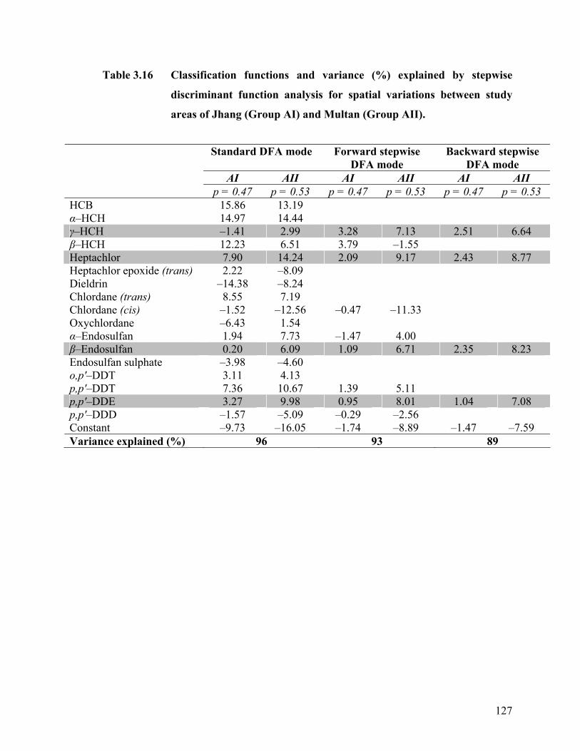
Table 3.16 Classification functions and variance (%) explained by stepwise
discriminant function analysis for spatial variations between study
areas of Jhang (Group AI) and Multan (Group AII).
Standard DFA mode Forward stepwise DFA mode
Backward stepwise DFA mode
AI AII AI AII AI AII
p = 0.47 p = 0.53 p = 0.47 p = 0.53 p = 0.47 p = 0.53 HCB 15.86 13.19 α–HCH 14.97 14.44 γ–HCH –1.41 2.99 3.28 7.13 2.51 6.64 β–HCH 12.23 6.51 3.79 –1.55 Heptachlor 7.90 14.24 2.09 9.17 2.43 8.77 Heptachlor epoxide (trans) 2.22 –8.09 Dieldrin –14.38 –8.24 Chlordane (trans) 8.55 7.19 Chlordane (cis) –1.52 –12.56 –0.47 –11.33 Oxychlordane –6.43 1.54 α–Endosulfan 1.94 7.73 –1.47 4.00 β–Endosulfan 0.20 6.09 1.09 6.71 2.35 8.23 Endosulfan sulphate –3.98 –4.60 o,p′–DDT 3.11 4.13 p,p′–DDT 7.36 10.67 1.39 5.11 p,p′–DDE 3.27 9.98 0.95 8.01 1.04 7.08 p,p′–DDD –1.57 –5.09 –0.29 –2.56 Constant –9.73 –16.05 –1.74 –8.89 –1.47 –7.59 Variance explained (%) 96 93 89
127
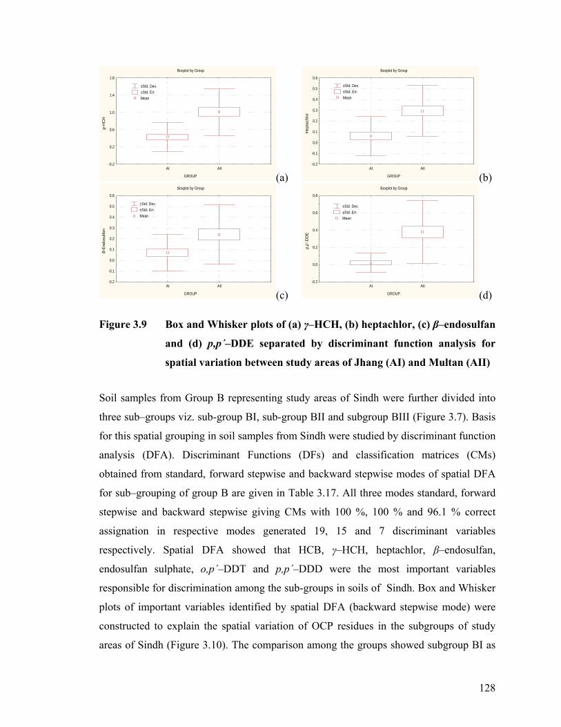
Boxplot by Group
GROUP
g-H
CH
-0.2
0.2
0.6
1.0
1.4
1.8
AI AII
±Std. Dev.±Std. Err.Mean
(a)
Boxplot by Group
GROUP
Hep
tach
lor
-0.2
-0.1
0.0
0.1
0.2
0.3
0.4
0.5
0.6
AI AII
±Std. Dev.±Std. Err.Mean
(b) Boxplot by Group
GROUP
B-E
ndos
ulfa
n
-0.2
-0.1
0.0
0.1
0.2
0.3
0.4
0.5
0.6
AI AII
±Std. Dev.±Std. Err.Mean
(c)
Boxplot by Group
GROUP
p,p'
-DD
E
-0.2
0.0
0.2
0.4
0.6
0.8
AI AII
±Std. Dev.±Std. Err.Mean
(d)
Figure 3.9 Box and Whisker plots of (a) γ–HCH, (b) heptachlor, (c) β–endosulfan
and (d) p,p´–DDE separated by discriminant function analysis for
spatial variation between study areas of Jhang (AI) and Multan (AII)
Soil samples from Group B representing study areas of Sindh were further divided into
three sub–groups viz. sub-group BI, sub-group BII and subgroup BIII (Figure 3.7). Basis
for this spatial grouping in soil samples from Sindh were studied by discriminant function
analysis (DFA). Discriminant Functions (DFs) and classification matrices (CMs)
obtained from standard, forward stepwise and backward stepwise modes of spatial DFA
for sub–grouping of group B are given in Table 3.17. All three modes standard, forward
stepwise and backward stepwise giving CMs with 100 %, 100 % and 96.1 % correct
assignation in respective modes generated 19, 15 and 7 discriminant variables
respectively. Spatial DFA showed that HCB, γ–HCH, heptachlor, β–endosulfan,
endosulfan sulphate, o,p΄–DDT and p,p΄–DDD were the most important variables
responsible for discrimination among the sub-groups in soils of Sindh. Box and Whisker
plots of important variables identified by spatial DFA (backward stepwise mode) were
constructed to explain the spatial variation of OCP residues in the subgroups of study
areas of Sindh (Figure 3.10). The comparison among the groups showed subgroup BI as
128

most contaminated site by o,p′–DDT and p,p′–DDD residues and subgroup BII was
characterized by highest concentration of HCB, γ–HCH, heptachlor, β–endosulfan and
endosulfan sulphate residues. While, subgroup BIII was least contaminated of the
subgroups and contained lowest amount of γ–HCH, heptachlor, endosulfan sulphate,
o,p′–DDT and p,p′–DDD residues.
Highest concentration of HCB residues was detected in subgroup BII with range 0.2–2.3
µg kg–1 (means 1.2 µg kg–1), followed by 0.1–2.6 µg kg–1 (mean 0.7 µg kg–1) in subgroup
BIII, and 0.3–0.4 µg kg–1 (mean 0.4 µg kg–1) in subgroup BI. HCB residues were present
in two samples each in sub-groups BI and BII each and in 17 soil samples of sub-group
BIII. All of these soil samples belonged to Nawabshah area. Both agricultural and
industrial sectors are considered sources of HCB residues in agricultural areas. As
discussed in earlier section (3.3.3.2), Nawabshah sampling site was in close vicinity of
brick making units where quite often rubber tyres and other waste is burnt to save
expensive coal fuel. Mumma and Lawless, (1975) has described use of HCB as peptizing
agent in the production of nitroso and styrene rubber for tyres. Therefore, release of HCB
from the burning tyres and their deposition on soil is quite possible. Despite the fact, that
Nawabshah was categorized as low pesticide use area, 70 % of the soil samples from this
area were contaminated with HCB residues and none of the samples from Ghotki were
found with HCB residues. This clearly suggests, HCB contaminants coming from non-
agricultural sources.
Subgroup BII also had highest concentration of γ–HCH (mean 6.7 µg kg–1) and
heptachlor (mean 2.3 µg kg–1). This was followed by mean concentration of γ–HCH and
heptachlor 4.5 µg kg–1 and 2.1 µg kg–1 in subgroup BI and 3.2 µg kg–1 and 1.5 µg kg–1 in
subgroup BIII respectively. Both the compounds had been used for pest management in
agriculture related activities. Frequency of both the compounds was 100 % in the three
subgroups indicating widespread use of these OCPs in Nawabshah and Ghotki study
areas.
Both β–endosulfan and endosulfan sulphate residues were detected from the soil samples
included in the three subgroups. Highest mean concentration of both β–endosulfan and
129

endosulfan sulphate residues 2.3 µg kg–1 and 0.7 µg kg–1 were detected respectively from
soil samples categorized in subgroup BII. In all the three subgroups, concentration of β–
endosulfan was higher than that of endosulfan sulphate indicating less breakdown of the
β–endosulfan either due to fresh applications or due to its high persistence in soil.
According to Jayashree and Vasudevan, (2007) β–endosulfan and endosulfan sulphate are
more important during the soil related studies because both the compounds are more
interrelated. Whereas, α–endosulfan gets volatilized after application and does not
persists in soils. Therefore, relationship of β–endosulfan and endosulfan sulphate in the
studies is obvious and indicates similar source of contamination and behavior in the study
areas.
In contrary to the other discriminating variable concentration of o,p′–DDT and p,p′–DDD
residues were very high in sub-group BI making it distinct from other two subgroups.
o,p′–DDT is one of the two parent DDT isomers, coming from both technical DDT and
dicofol insecticides. Sub-group BI had highest mean concentration of o,p′–DDT 3.1 µg
kg–1 followed by 1.4 µg kg–1 in subgroup BII and 1.1 µg kg–1 in subgroup BIII. Similar
trend was also observed for p,p′–DDD, breakdown product of p,p′–DDT under anaerobic
condition in the soil. Highest amount of p,p′–DDD residues with mean concentration 7.8
µg kg–1 were detected in subgroup BI, followed by 1.9 µg kg–1 in subgroup BII. Least
amount (mean 0.9 µg kg–1) of p,p′–DDD residues were detected in soil samples of
subgroup BIII.
Both subgroups BI and BII predominantly contained soil samples from Ghotki while in
sub-group BIII majority of the soil samples belonged to Nawabshah. These results
indicated higher amounts of DDT and their metabolites in Ghotki area. In both
Nawabshah and Ghotki areas, agricultural activities take place under irrigated condition.
Usually flood irrigation is practiced and water is allowed to stand for one to two days to
ensure retention of maximum soil moisture. During the survey and sampling of the areas,
and communications with farmers also revealed that rice cultivation as a replacement
crop was very common in the Ghotki area, especially, during high pest infestation and
cotton leaf curl virus epidemics. Therefore, higher amount of p,p′–DDD residues in
130

131
Ghotki areas of Sindh could be attributed to prolonged anaerobic soil conditions
especially during rice cultivation in Ghotki. Lower concentration of p,p′–DDD residues
in Nawabshah areas and in some soil samples from Ghotki areas indicate more aerobic
degradation of DDT compounds.
Spatial DFA for study areas of Sindh revealed generally higher OCP residues in sub-
group BI and BII with majority of soil samples from Ghotki area. Residues of o,p′–DDT
and breakdown product p,p′–DDD were in higher concentration in soil samples from sub-
group BI. On the other hand, concentration of γ–HCH, heptachlor, β–endosulfan and
endosulfan sulphate residues was higher in soil samples of sub-group BII. This clearly
suggested higher accumulation of OCP residues in high pesticide use area of Ghotki
compared to low pesticide use area of Nawabshah. The only exception was higher
occurrence and concentration of HCB residues in soil samples from Nawabshah. These
HCB residues were probably not related to agricultural activities in the area. Therefore,
these studies suggest more OCP contaminants in high pesticide use area of Ghotki than
those in the low pesticide use area of Nawabshah.
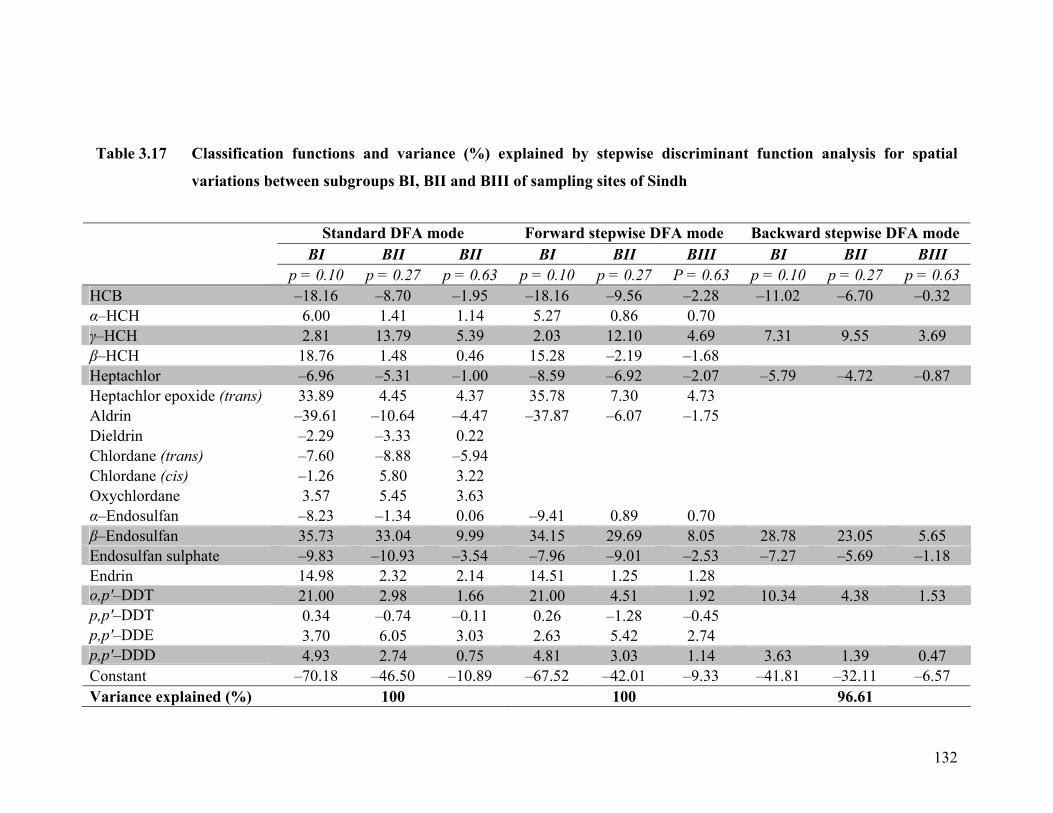
Standard DFA mode Forward stepwise DFA mode Backward stepwise DFA mode BI BII BII BI BII BIII BI BII BIII
p = 0.10 p = 0.27 p = 0.63 p = 0.10 p = 0.27 P = 0.63 p = 0.10 p = 0.27 p = 0.63 HCB –18.16 –8.70 –1.95 –18.16 –9.56 –2.28 –11.02 –6.70 –0.32 α–HCH 6.00 1.41 1.14 5.27 0.86 0.70 γ–HCH 2.81 13.79 5.39 2.03 12.10 4.69 7.31 9.55 3.69 β–HCH 18.76 1.48 0.46 15.28 –2.19 –1.68Heptachlor –6.96 –5.31 –1.00 –8.59 –6.92 –2.07 –5.79 –4.72 –0.87
Heptachlor epoxide (trans)
33.89 4.45 4.37 35.78 7.30 4.73 Aldrin –39.61 –10.64
–4.47
–37.87
–6.07 –1.75
Dieldrin –2.29 –3.33 0.22Chlordane (trans) –7.60 –8.88
–5.94
Chlordane (cis) –1.26 5.80 3.22Oxychlordane 3.57 5.45 3.63α–Endosulfan –8.23 –1.34 0.06 –9.41 0.89 0.70β–Endosulfan 35.73 33.04 9.99 34.15 29.69 8.05 28.78 23.05 5.65 Endosulfan sulphate –9.83 –10.93 –3.54 –7.96 –9.01 –2.53 –7.27 –5.69 –1.18
Endrin 14.98 2.32 2.14 14.51 1.25 1.28 o,p′–DDT 21.00 2.98 1.66 21.00 4.51 1.92 10.34 4.38 1.53 p,p′–DDT 0.34
–0.74 –0.11 0.26 –1.28 –0.45
p,p′–DDE 3.70 6.05 3.03 2.63 5.42 2.74p,p′–DDD 4.93 2.74 0.75 4.81 3.03 1.14 3.63 1.39 0.47 Constant –70.18 –46.50 –10.89 –67.52 –42.01 –9.33 –41.81 –32.11 –6.57Variance explained (%) 100 100 96.61
Table 3.17 Classification functions and variance (%) explained by stepwise discriminant function analysis for spatial
variations between subgroups BI, BII and BIII of sampling sites of Sindh
132
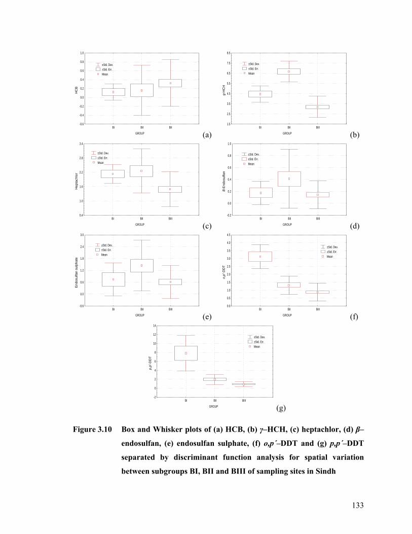
GROUP
HC
B
-0.6
-0.4
-0.2
0.0
0.2
0.4
0.6
0.8
1.0
BI BII BII
±Std. Dev.±Std. Err.Mean
(a) GROUP
g-H
CH
1.5
2.5
3.5
4.5
5.5
6.5
7.5
8.5
BI BII BIII
±Std. Dev.±Std. Err.Mean
(b)
GROUP
Hep
tach
lor
0.4
1.0
1.6
2.2
2.8
3.4
BI BII BIII
±Std. Dev.±Std. Err.Mean
(c) GROUPB
-End
osul
fan
-0.2
0.0
0.2
0.4
0.6
0.8
1.0
BI BII BIII
±Std. Dev.±Std. Err.Mean
(d)
GROUP
End
osul
fan
sulp
hate
-0.6
0.0
0.6
1.2
1.8
2.4
3.0
BI BII BIII
±Std. Dev.±Std. Err.Mean
(e) GROUP
o,p'
-DD
T
0.0
0.5
1.0
1.5
2.0
2.5
3.0
3.5
4.0
4.5
BI BII BIII
±Std. Dev.±Std. Err.Mean
(f)
GROUP
p,p'
-DD
T
-2
0
2
4
6
8
10
12
14
BI BII BIII
±Std. Dev.±Std. Err.Mean
(g)
Figure 3.10 Box and Whisker plots of (a) HCB, (b) γ–HCH, (c) heptachlor, (d) β–
endosulfan, (e) endosulfan sulphate, (f) o,p´–DDT and (g) p,p´–DDT
separated by discriminant function analysis for spatial variation
between subgroups BI, BII and BIII of sampling sites in Sindh
133
3.4 CONCLUSION
Status and spatial variations of 19 organochlorine pesticide residues was studied in soils
of four selected cotton growing areas of Pakistan. Site selection was made in areas under
cotton cultivation with similar soil background and varying pesticide use in Punjab and
Sindh provinces. For this purpose, areas with soils belonging to Miani soil series were
selected. Soil samples were extracted with the modified QuEChERS method for
organochlorine residues analysis by gas chromatography coupled with tandem
quadrupole mass spectrometry (GC-MS/MS). Consistency of different steps, from
sampling to analysis were ensured and monitored by proper quality control and quality
assurance procedures.
Residues of almost all the OCPs included in the study were detected in different
frequencies and magnitudes from the selected study area in Punjab and Sindh. Residues
of HCH were detected in almost all the study areas. Isomeric ratios suggested use of both
technical HCH and lindane in the study areas. Similarly, residues of DDT and their
metabolites were also detected from the study areas. Ratio of DDT isomers suggested
DDT residues coming from both technical DDT as well as from DDT impurities during
dicofol application. Study of metabolites suggested predominant anaerobic degradation of
DDT in Multan and Nawabshah areas and aerobic in Ghotki areas. DDT
parent/breakdown product ratios suggested residues of DDT from some older
applications. However, in some samples fresh DDT application was also evident due to
higher amounts of parent DDT isomers. Residues of HCB were usually very low in the
study areas except for Nawabshah where the source could be agricultural as well as
industrial. Heptachlor residues were detected from all the study areas at low frequency.
Frequency of heptachlor-epoxide was also very low in the study areas. The ratios for
heptachlor-epoxide (trans)/heptachlor could be calculated for few samples from
Nawabshah, Ghotki and Multan areas and suggested fresh use of the heptachlor in these
areas. Residues of an unregistered pesticides chlordane were also detected from almost
all the study areas. These residues were from recent chlordane applications in cotton
areas due to low conversion into oxychlordane. In contrary, endosulfan is still
134
recommended insecticide but the residues of endosulfan sulfate were present at higher
concentrations indicating mostly older applications of endosulfan in the study areas.
Residue of aldrin, dieldrin and endrin were found in very low frequencies and magnitudes
in soils of study areas. Almost all the OCP residues were below the critical limits defined
by various countries (Beyer, 1990)
Residues of OCPs were detected in all the study areas in varying frequencies and
magnitudes. Inter-provincial as well as intra-provincial variation existed for OCP
residues. Soils from Sindh were more contaminated than those of Punjab. OCPs viz. γ–
HCH, heptachlor, chlordane (cis), α–endosulfan and p,p´–DDE were found to contribute
significantly for variation between Sindh and Punjab. Mean concentration levels of γ–
HCH, heptachlor, chlordane (cis), α–endosulfan and p,p´–DDE in soils from Sindh were
4.3 µg kg-1, 1.9 µg kg-1, 0.7 µg kg-1, 1.1 µg kg-1 and 1.3 µg kg-1; and 0.9 µg kg-1, 0.3 µg
kg-1, 0.4 µg kg-1, 0.7 µg kg-1 and 0.6 µg kg-1 in Punjab respectively. Soils of Sindh were
found with relatively higher amounts of these OCPs than those of Punjab. Study areas
within Punjab viz. Jhang and Multan were also significantly different from each other.
Owing to γ–HCH, heptachlor, β–endosulfan and p,p´–DDE residues. Mean concentration
of γ–HCH, heptachlor, β–endosulfan was 0.5 µg kg-1, 0.4 µg kg-1, 0.3 µg kg-1 in Jhang
and 1.0 µg kg-1, 0.4 µg kg-1, 0.5 µg kg-1 in Multan respectively. p,p´–DDE residues were
detected from only one sample from Punjab in comparison to 68% sample in Multan.
This suggests that high pesticide use area of Multan was more contaminated than low
pesticide use area of Jhang. Soils from study areas of Sindh were sorted into three sub-
groups where residue of HCB, γ–HCH, heptachlor, β–endosulfan, endosulfan sulphate,
o,p´–DDT and p,p´–DDT were responsible for discriminating among groups. Highest
levels of o,p´–DDT and p,p´–DDD residues were detected in group BI mainly constituted
of soil samples from Ghotki area. Similarly, group BII with predominant soil samples
from Ghotki area contained highest levels of γ–HCH, heptachlor, β–endosulfan and
endosulfan sulphate. Whereas, group BIII mainly constituted of Nawabshah soil samples
was found with highest levels of HCB residues. This clearly suggested that soils of
Nawabshah were less contaminated than Ghotki. In Nawabshah and Ghotki areas, mean
concentration of γ–HCH was 3.7 µg kg-1 and 4.9 µg kg-1, heptachlor 1.6 µg kg-1 and 2.0
135

µg kg-1, endosulfan sulphate 0.9 µg kg-1 and 1.5 µg kg-1, o,p´–DDT 1.3 µg kg-1 and 1.6
µg kg-1, and that of p,p´–DDD were 1.1 µg kg-1 and 2.8 µg kg-1 respectively. Mean
concentration of β–endosulfan was 0.5 µg kg-1 in both Nawabshah and Ghotki. However,
frequency of β–endosulfan residues was high in Ghotki are than Nawabshah. The
accumulation has clear relation with the pesticide intensities. Higher accumulation of
OCP residues was observed in high pesticide use areas than those where pesticide are
used at relatively low intensity.
136
3.5 REFERENCES
Ahad, K., A. Mohammad, H. Khan, I. Ahmad and Y. Hayat. 2009. Monitoring Results for
Organochlorine Pesticides in Soil and Water from Selected Obsolete Pesticide
Stores in Pakistan. Environ. Monit. Assess., DOI: 10. 1007/s10661-009-0995-5.
Ahmad, M. and A. Abdullah. 1971. Determination of residues of dimecron, endrin and
malathion on tobacco plants, using bioassay technique. Pakistan J Sci Res, 23(1-
2): 34-41.
Ahmed, M.T., S.M.M. Ismail and S.S. Mabrouk. 1998. Residues of some chlorinated
hydrocarbon pesticides in rain water, soil and ground water, and their influence on
some soil microorganisms. Environment International, 24(5-6): 665-670.
Alexander, M. 1961. Introduction to soil microbiology. Wiley Press, New York. p.467.
Ali, M. and A. Jabbar. 1992. Effect of pesticides and fertilizers on shallow groundwater
Quality. Final technical report (Jan. 1990–Sep. 1991). Pakistan Council of
Research in Water Resources (PCRWR), Gov. of Pakistan, Islamabad.
Anonymous. 2002. The WHO recommended classification of pesticides by hazard and
guidelines to classification 2000–2002. International programme on chemical
safety. WHO/PCS/01.5. World Health Organization.
Anonymous. 1969a. Reconnaissance soil survey of Ghotki. Soil Survey Project of
Pakistan, Directorate of Soil Survey, West Pakistan, Lahore, Pakistan.
Anonymous. 2001. Policy and strategy for rational use of pesticides in Pakistan-Building
consensus for action. FAO/Global IPM Facility, UNDP, Gov. of Pakistan.
Anonymous. 1968. Reconnaissance soil survey of Jhang. Soil Survey Project of Pakistan,
Directorate of Soil Survey, West Pakistan, Lahore, Pakistan.
Anonymous. 1969b. Reconnaissance soil survey of Multan. Soil Survey Project of
Pakistan, Directorate of Soil Survey, West Pakistan, Lahore, Pakistan.
Anonymous. 1971. Reconnaissance soil survey of Nawabshah. Soil Survey Project of
Pakistan, Directorate of Soil Survey, West Pakistan, Lahore, Pakistan.
Barber, J., A. Sweetman and K. Jones. 2005. Hexachlorobenzene-sources, environmental
fate and risk characterization. Science dossier, Euro Chlor, Euro Chlor • Avenue
E. Van Nieuwenhuyse 4, box 2 • B-1160 Brussels, Belgium. www.eurochlor.org.
137
Beyer, W.N. 1990. Evaluating soil contamination. U.S. Fish Wildl. Serv., Biol. Rep. 90
(2). 25 pp.
Bidleman, T.F. and A.D. Leone. 2004. Soil-air exchange of organochlorine pesticides in
the Southern United States. Environmental Pollution, 128(1-2): 49-57.
Cavanagh, J.E., K.A. Burns, G.J. Brunskill and R.J. Coventry. 1999. Organochlorine
Pesticide Residues in Soils and Sediments of the Herbert and Burdekin River
Regions, North Queensland: Implications for Contamination of the Great Barrier
Reef. Marine Pollution Bulletin, 39(1-12): 367-375.
CETESB. 2001. Companhia de Technologia e Saneamento Basico de Sao Paulo.
www.cetesb.sp.gov.br.
Cheng, H.H. 1990. Pesticides in environment: processes, impacts and modeling. Soil
Society of America: Madison, WI, America.
do Nascimentoa, N.R., S.M.C. Nicolab, M.O.O. Rezendec, T.A. Oliveiraa and G. Öberg.
2004. Pollution by Hexachlorobenzene and pentachlorophenol in the coastal plain
of São Paulo state, Brazil. Geoderma, 121, 221–232.
Falconer, R.L., T.F. Bidleman and S.Y. Szeto. 1997. Chiral pesticides on soils of the
Fraser Valley, British Columbia. J. Agric. Food Chem., 45, 1946-1951.
Gao, F., J. Jia and X. Wand. 2008. Occurrence and ordination of
dichlorodiphenyltrichloroethane and hexachlorocyclohexane in agricultural soils
from Guangzhou, China. Arch Environ Contam Toxicol, 54:155–166.
Goebel, H., S. Gorbach, W. Knauf, R.H. Rimpau and H. Huttenbach. 1982. Properties,
effects, residues and analytics of the insecticide endosulfan. Research Review, 83:
5–16.
Goncalves, C., J.C.G. Esteves da Silva and M.F. Alpendurada. 2006. Chemometric
interpretation of pesticide occurrence in soil samples from an intensive
horticulture area in north Portugal. Analytica Chimica Acta, 560: 164–171.
DOI:10.1016/j.aca.2005.12.021.
Gonzalez, M., K.S.B. Miglioranza, J.E.A. De Moreno and V.J. Moreno. 2003.
Occurrence and distribution of organochlorine pesticides (OCPs) in tomato
(Lycopersicon esculentum) crops from organic production. J. Agric. Food Chem.,
51: 1353–1359.
138
Gonzalez, M., K.S.B. Miglioranza, J.E.A. de Moreno and V.J. Moreno. 2005. Evaluation
of conventionally and organically produced vegetables for high lipophilic
organochlorine pesticide (OCP) residues. Food and Chemical Toxicology, 43:
261–269.
Goti, R., B. Steiner, P. Friesel, K. Roth, F. Walkow, V. Maa, H. Reincke and B. Stachel.
1998. Dioxin (PCDD/F) in the river Elbe – Investigations of their origin by
multivariate Statistical methods. Chemosphere, 31 (9–12): 1987–2002.
Graña, E.C., M.I.T. Carou, S.M. Lorenzo, P.L. Mahía, D.P. Rodríguez and E.F.
Fernández. 2006. Evaluation of HCH isomers and metabolites in soils, leachates,
river water and sediments of a highly contaminated area. Chemosphere, 64 (4):
588-595.
Harner, T., J.L. Wideman, L.M.M. Jantunen, T.F. Bidleman and W.J. Parkhurst. 1999.
Residues of organochlorine pesticides in Alabama soils. Environmental Pollution,
106 (3): 323-332.
Harris, C.R. and H.J. Sans. 1969. Vertical distribution of residues of organochlorine
insecticides in soils collected fro six farms in Southwestern Ontario. Proc.
Entomol. Soc. Wash., 100: 156-164.
Hasnain, T. 1999. Pesticides-use and its impact on crop ecologies: issues and options.
Working Paper Series # 42. SDPI, Islamabad.
Hussain, H., Z. Iqbal and M.R. Asi. 2001. Impact of repeated pesticide application on the
binding and release of 14C-methameidophos to soil matrices under field
conditions. NIAB, Faisalabad.
Jabbar, A., S.Z. Masud, Z. Parveen and M. Ali. 1993. Pesticide residues in cropland soils
and shallow groundwater in Punjab Pakistan. Bull Environ Contam Toxicol,
51:268–273.
Jacoff, F.S., R. Scarberry and D. Rosa. 1986. Source assessment of hexachlorobenzene
from the organic chemical manufacturing industry. In: Morris, C.R. and J.R.P.
Cabral. Hexachlorobenzene: Proceedings of an International Symposium. Lyon,
IARC Sci. Publ. 77: 31–37.
139
Jantunen, L.M.M., T.F. Bidleman, T. Harner and W.J. Parkhurst. 2000. Toxaphene,
chlordane, and other organochlorine pesticides in Alabama air. Environ Sci
Technol, 34:5097–5105.
Jayashree, R. and N. Vasudevan. 2007. Persistence and Distribution of endosulfan under
Field Condition. Environ. Monit. Assess., 131:475–487.
Kabbany, S.E., M.M. Rashed and M.A. Zayed. 2000. Monitoring of the pesticide levels
in some water supplies and agricultural land in ElHaram, Giza. Journal of
Hazardous Materials, 72, 11–21.
Khan, M.S.H. 1998. Pakistan crop protection market. PAPA Bulletin. 9:7-9.
Kidd, P.S., A.P. Fernández, C. Monterroso and M.J. Acea. 2008. Rhizosphere microbial
community and hexachlorocyclohexane degradative potential in contrasting plant
species. Plant Soil, 302:233–247.
Kim, J.H. and A. Smith. 2001. Distribution of organochlorine pesticides in soils from
South Korea. Chemosphere, 43(2): 137-140.
Kishimba, M.A., L. Henry, H. Mwevura, A.J. Mmochi, M. Mihale and H. Hellar. 2004.
The status of pesticide pollution in Tanzania. Talanta, 64(1): 48-53.
Li, J., G. Zhang, S. Qi, X. Li and X. Peng. 2006. Concentrations, enantiomeric
compositions, and sources of HCH, DDT and chlordane in soils from the Pearl
River Delta, South China. Science of the Total Environment, 372: 215–224.
Luo, W., Y. Lu, J.P. Giesy, T. Wang, Y. Shi, G. Wang and Y. Xing. 2007. Effects of land
use on concentrations of metals in surface soils and ecological risk around
Guanting Reservoir, China. Environ Geochem Health, 29:459–471.
Masud, S.Z. and N. Hasan. 1992. Pesticide residues in foodstuffs in Pakistan:
organochlorine, organophosphorus and pyrethriod insecticides in fruits and
vegetables. Pak. J. Sci. Ind. Res., 35(12): 499-504.
Masud, S.Z. and N. Hasan. 1995. Study of fruits and vegetables in NWFP, Islamabad and
Balochistan for organochlorine, organophosphorus and pyrethroid pesticides
residues. Pak. J. Sci. Ind. Res., 38(2):47-80.
Mathur, H.B., H.C. Agarwal, S. Johnson and N. Saikia. 2005. Analysis of pesticide
residues in blood samples from villages of Punjab. Centre for Science and
Environment. CSE/PML/PR–21/2005.
140
Meijer, S.N., C.J. Halsall, T.H. Arner, A.J. Peters, W.A. Ockenden, A.E. Johnston and
K.C. Jones. 2001. Organochlorine pesticide residues in archived UK soil.
Environ. Sci. Technol., 35: 1989-1995.
Mumma, C.F. and E.W. Lawless. 1975. Survey of Industrial Processing Data. Task I –
Hexachlorobenzene and Hexachlorobutadiene Pollution for Chlorocarbon
Processes (EPA 56013–75–004), Washington D.C., US EPA.
Nawab, A., A. Aleem and A. Malik. 2003. Determination of organochlorine pesticides in
agricultural soil with special reference to γ-HCH degradation by Pseudomonas
strains. Bioresource Technology, 88(1): 41-46.
Parveen, Z. and S.Z. Masud. 1988. Monitoring of fresh milk for organochlorine pesticide
residues in Karachi. Pak. J. Sci. Ind. Res., 31(1): 49-56.
Parveen, Z., I.A.K. Afridi and S.Z. Masud. 1994. A multi-residue method for quantitation
of organochlorine, organophosphorus and synthetic pyrethroid pesticides in cotton
seed. Pak. J. Sci. Ind. Res., 37(12): 536-540.
Parveen, Z., I.A.K. Afridi, S.Z. Masud and M.M.H. Baig. 1996. Monitoring of multiple
pesticide residues in cotton seeds during three crop seasons. Pak. J. Sci. Ind. Res.,
39(5-8): 146-149.
Qadir, A., R.N. Malik and S.Z. Husain. 2008. Spatio–temporal variations in water quality
of Nullah Aik–tributary of the river Chenab, Pakistan. Environ. Monit. Assess.,
140:43–59.
Qishlaqi, A., F. Moore and G. Forghani. 2009. Characterization of metal pollution in soils
under two land use patterns in the Angouran region, NW Iran; a study based on
multivariate data analysis. Journal of Hazardous Materials, 172 (1): 374-384.
Renaud, F.G., C.D. Brown, C.J. Fryer and A. Walker. 2004. A lysimeter experiment to
investigate temporal changes in the availability of pesticide residues for leaching.
Environmental Pollution, 131(1): 81-91.
SANCO. 2007. Method validation and quality control procedures for pesticide residues
analysis in food and feed; The European Commission, Document No.
SANCO/2007/3131.
141

Sarkar, S.K., A. Binelli, C. Riva, M. Parolini, M. Chatterjee, A.K. Bhattacharya, B.D.
Bhattacharya and K.K. Satpathy. 2008. Organochlorine pesticide residues in
sediment cores of Sunderban Wetland, northeastern part of Bay of Bengal, India,
and their ecotoxicological significance. Arch Environ Contam Toxicol, 55:358–
371.
Singh, K.P., A. Malik and S. Sinha. 2007. Persistent organochlorine pesticide residues in
soil and surface water of northern Indo–Gangetic alluvial plains. Environ. Monit.
Assess., 125:147–155.
Singh, K.P., A. Malik and V.K. Singh. 2005. Chemometric analysis of hydro–chemical
data of an alluvial river– A case study. Water Air Soil Pollut, 170: 383–404.
StatSoft, Inc. 1999. STATISTICA for Windows [Computer program manual]. Tulsa, OK:
StatSoft, Inc., 2300 East 14th Street, Tulsa, OK 74104, phone: (918) 749–1119,
fax: (918) 749–2217, email: [email protected], WEB: http://www.statsoft.com.
Tieyu. W., L. Yonglong, S. Yajuan and Z. Hong. 2005. Spatial distribution of
organochlorine pesticide residues in soils surrounding Guanting reservoir,
People’s Republic of China. Bull Environ Contam Toxicol, 74:623-630.
Tor, A., M.E. Aydin and S. Ozcan. 2006. Ultrasonic solvent extraction of organochlorine
pesticides from soil. Analytica Chimica Acta. 559:173-180.
Turnbull, A. 1996. Chlorinated pesticides. In: Hester RE, Harrison RM (eds) Chlorinated
organic micropollutants. Issues in environmental science and technology. The
Royal Society of Chemistry, Cambridge, pp 113–135.
Wandiga, S.O. 1995. Organochlorine pesticides: curse or blessing to tropical agriculture?
Kenya National Academy of Sciences, Nairobi, Kenya, public lectures series, 80-
90.
Yang, X., S. Wang, Y. Bian, F. Chen, G. Yu, C. Gu and X. Jiang. 2007. Dicofol
application resulted in high DDTs residues in cotton fields from northern Jiangsu
province, China. Journal of Hazardous Materials, 150 (1): 92-98.
Zhang, H.B., Y.M. Luo, Q.G. Zhao, M.H. Wong and G.L. Zhang. 2005. Residues of
organochlorine pesticides in Hong Kong soils. Chemosphere, 63(4): 633-641.
Zhu, Y., H. Liu, Z. Xi, H. Cheng and X. Xu. 2005. Organochlorine pesticides (DDTs and
HCHs) in soils from the outskirts of Beijing, China. Chemosphere, 60: 770–778.
142

Zohair, A., A.B. Salim, A.A. Soyibo and A.J. Beck. 2005. Residues of polycyclic
aromatic hydrocarbons (PAHs), polychlorinated biphenyls (PCBs) and
organochlorine pesticides in organically-farmed vegetables. Chemosphere, 63 (4):
541-553.
143
Chapter 4
RELATIONSHIP OF ORGANOCHLORINE PESTICIDE RESIDUES WITH PHYSICAL, CHEMICAL AND BIOLOGICAL PROPERTIES OF
SOIL
4.1 INTRODUCTION
Soil health or soil quality refers to the capacity of soil to sustain biological productivity,
maintain environmental health and promote plant and animal health within boundaries of
an ecosystem. The soil health/quality is rather dynamic and can affect the sustainability
and productivity of a particular land area. It is the outcome of different soil degradation
or conserving processes controlled by physical, chemical and biological components of
soil and their interactions (Papendick and Parr, 1992). The physical parameters include
soil textural class dictated by distribution of sand, silt and clay particles in soil; chemical
factors include soil reaction (pH), electrical conductivity (EC) and distribution of
essential and nonessential nutrients and the biological components consist of both micro–
and macro–organisms. These factors influence and get affected by different external
influences and can result in binding and incorporation of both organic and inorganic
substances into soil complexes. In this way, soil sometimes accumulates harmful
pollutants besides useful nutrients (Lou et al., 2007).
Generally the agricultural soils are exposed to agro–chemicals especially the pesticides.
Pesticide exposure may be through direct application, accidental spillage, runoff from
plant surfaces or from incorporation of pesticide contaminated plant materials (Brown
and Hock 1990; Goncalves and Alpendurada, 2005). Pesticide behavior in soil is
influenced by physicochemical factors like soil pH, organic matter content and soil
texture (Hayar et al., 1997). The fate and behavior of pesticides in the soil environment
involve several different and often concurrent phenomena to determine the bioavailability
of pesticides and their redistribution from the point of application (Konda and Pasztor
2001). The pesticides persist or get transformed by the influence of physical, chemical
and biological processes. According to Vig et al., (2001) persistence of pesticides in soil
is influenced by soil moisture, organic matter content, redox status, soil pH, temperature,
144
sorption–desorption, and mineral constituents of soil and at the same time the pesticide
residues can affect the soil microorganisms, enzymes and hence the soil health.
Soil pH plays very important role in controlling chemical reactions taking place in the
soil environments and influences the fate of chemical compounds in soil (Muller et al.,
2007). In a study with organophosphorus pesticides Sattar, (1990) found lower rate of
degradation in neutral soil than that of acid soils while comparing silty clay acid and
sandy clay neutral soils. Similarly a clear pH–dependency of the partitioning of
dodemorph between solid and water phase was reported by Vorkamp et al., (2003) while
examining the stability and distribution of the fungicide dodemorph during anaerobic
digestion. Zhang et al., (2005) also associated pH and total organic carbon with
extractability of HCH from soil.
Behavior of pesticides in the soil environment is also greatly influenced by the soil
texture. Sandy soils are known to facilitate leaching whereas the clayey soils help
accumulation through colloid formation. Pesticide residue status varies with its residence
time in soil which in turn depends upon the soil texture (Boivin et al., 2005). Magnitudes
of pesticide losses varied from soil to soil, depending on structural development and the
organic carbon content (Renaud et al., 2004). Haria et al., (1994) studied the processes
and mechanisms that control pesticide transport from drained heavy clay catchments in
southern England. These studies demonstrated that the main mechanism for pesticide
translocation was by preferential flow via macropore system that effectively depends
upon soil matrix. This macropore system included worm holes, shrinkage cracks and
cracks resulting from ploughing. Jones et al., (1989) described loamy sand or sand
surface soils and sand subsoils as favorable for pesticide movement. The soil
heterogeneity can affect pesticide behavior in terms of adsorption, transport and
persistence, therefore, soil characterization is necessary in pesticide residue analysis to
determine sand, silt and clay content (Redondo, 1994) to understand pesticide behavior in
soil.
Among biological factors soil microbial mass and organic matter content plays a major
role in behavior of pesticides in soil, and this phenomenon is usually the most important
145
cause for interaction of pesticides in the soil environment (Tariq, et al., 2007; Naqvi et
al., 2009). Soil organic matter consists of living, partially to fully decomposed organic
materials. Soil organic matter is typically 1 to 5 % of the total dry weight of topsoil, with
lower amounts in the subsoil as the biological activities tend to decrease with soil depth
(Cruz et al., 2006). It also influences other soil characteristics like CEC (cation exchange
capacity) of a soil. Organic amendments used to enrich soils of low organic matter
contents can affect sorption and movement of pesticides in soils (Cox et al., 1997).
Binding can occur with the original pesticide or transformation products, the reaction
being caused by abiotic agents or biotic agents (microbial or plant enzymes) (Bollag et
al., 1992). Binding of pesticides to organic matter can occur by sorption (Van der Waal's
forces, hydrogen bonding, hydrophobic bonding), electrostatic interactions (charge
transfer, ion exchange or ligand exchange), covalent bonding or combinations of these
reactions (Bollag et al., 1992; Gevao et al., 2000). According to Burauel and Baßmann,
(2005), humification products of natural organic matter are reaction partners for binding
and re–mobilization of pesticides in soil. Hayar et al., (1997) found approximately 65 %
of bound residues associated with humus in soil with contamination history. Barraclough
et al., (2005) reviewed the evidences that residues are so tightly bound to soil organic
matter as essentially unavailable. They added that the existing knowledge of the
mechanisms by which residues bind to soil organic matter suggests that release might be
closely dependent on soil organic matter breakdown.
Pesticides also influence the microbial activities and some microorganisms may be
suppressed and others may proliferate in different ecological niches (Johnsen et al.,
2001). Some pesticides like carbofuran and 2,4–dichlorophenoxyacetic acid (2,4–D), and
atrazine can results in soil enrichment of microbial species, which use pesticide as source
of carbon and energy resulting in bio–degradation (Soulas and Lagacherie, 2001). On the
other hand pesticides can result in decrease of soil microbial mass to alter soil health and
thereby posing potential risk to the soil environment (Schwarzenbach et al., 2009).
According to Azam and Memon, (1996) among the soil microbes bacteria and fungi are
most important for their role in energy flow in soil ecosystem.
146
To reduce the risk of contaminations, it is essential to understand the factors that affect
their behavior in environment. According to Karlen et al., (1997), assessment of risks
associated with the application of pollutants like pesticides, need quantitative monitoring
of their presence as well as analysis of factors that may influence their persistence or
degradation. In the previous chapter, distinct spatial groups of OCP contaminated soils
from cotton areas were identified. These groups were differentiated for magnitude and
distribution of different OCP contaminants with each other. In present study relation of
physical, chemical and biological characteristics of soils were studied in relation to the
OCP contamination pattern in different spatial groups. Furthermore, interaction among
physicochemical and biological properties and their relation with the OCP residues in soil
was also investigated. The objectives of the study were as follows:
1. To study relation between OCP contamination in different study areas and soil
properties.
2. To establish relationship between different soil properties and organochlorine
pesticide residues in soil environment.
147
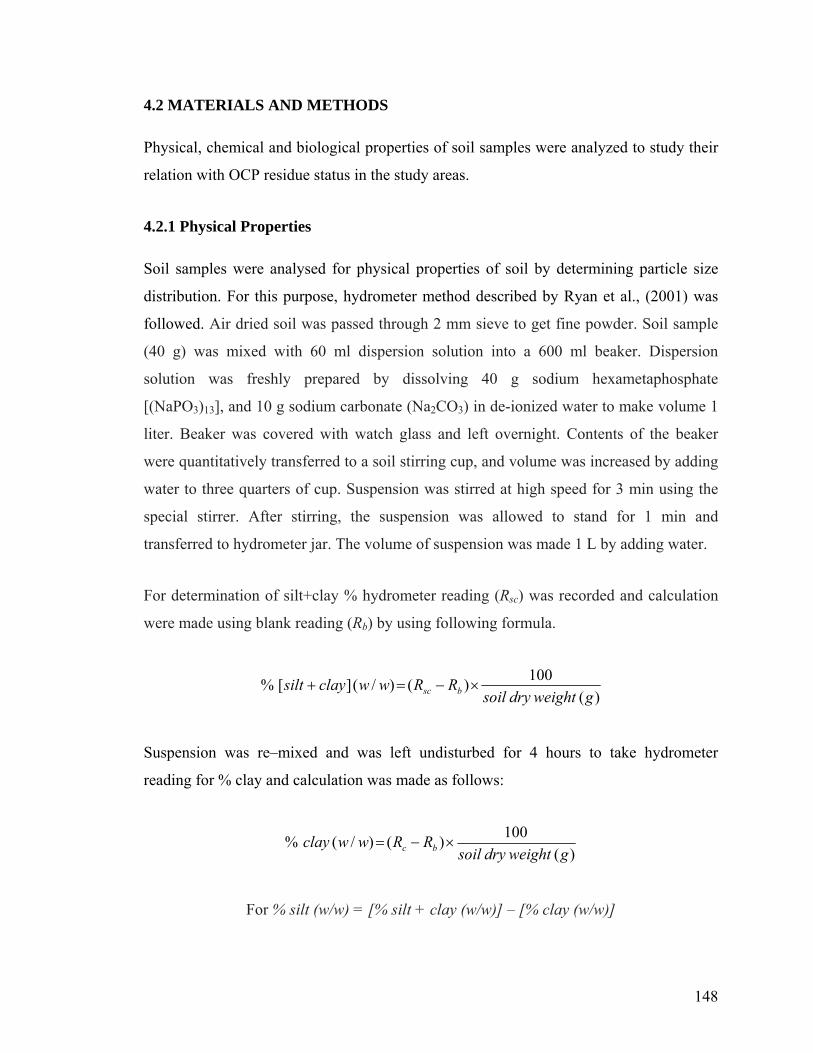
4.2 MATERIALS AND METHODS
Physical, chemical and biological properties of soil samples were analyzed to study their
relation with OCP residue status in the study areas.
4.2.1 Physical Properties
Soil samples were analysed for physical properties of soil by determining particle size
distribution. For this purpose, hydrometer method described by Ryan et al., (2001) was
followed. Air dried soil was passed through 2 mm sieve to get fine powder. Soil sample
(40 g) was mixed with 60 ml dispersion solution into a 600 ml beaker. Dispersion
solution was freshly prepared by dissolving 40 g sodium hexametaphosphate
[(NaPO3)13], and 10 g sodium carbonate (Na2CO3) in de-ionized water to make volume 1
liter. Beaker was covered with watch glass and left overnight. Contents of the beaker
were quantitatively transferred to a soil stirring cup, and volume was increased by adding
water to three quarters of cup. Suspension was stirred at high speed for 3 min using the
special stirrer. After stirring, the suspension was allowed to stand for 1 min and
transferred to hydrometer jar. The volume of suspension was made 1 L by adding water.
For determination of silt+clay % hydrometer reading (Rsc) was recorded and calculation
were made using blank reading (Rb) by using following formula.
)()()/(][%
gweightdrysoilRRwwclaysilt bsc ×−=+
100
Suspension was re–mixed and was left undisturbed for 4 hours to take hydrometer
reading for % clay and calculation was made as follows:
)()()/(%
gweightdrysoilRRwwclay bc ×−=
100
For % silt (w/w) = [% silt + clay (w/w)] – [% clay (w/w)]
148

For determination of sand, suspension was passed through 50 µm sieve. Sieve was
thoroughly washed to get clear water. Sand collected on sieve was transferred into a
beaker and was oven dried at 105°C. Sand was weighed and % sand was quantified with
the following formula:
)()/(%
gweightdrysoilweightsandwwsand ×=
100
4.2.1.1 Soil Textural Class
Soil textural class of the soil samples was determined based on proportional distribution
of sand, silt and clay particles in soil samples using the USDA textural triangle #2.
4.2.2 Chemical Properties
Soil pH, electrical conductivity (EC) and soil organic matter content were studied among
the chemical properties using methods described by Ryan et al., (2001).
4.2.2.1 Soil pH
Soil pH as negative log of hydrogen ion activity was determined by soil water (1:1 w/v)
suspension. Air dried soil (50 g) was thoroughly mixed with 50 ml water in a 100 ml
beaker with a glass rod. Suspension was stirred after every 10 minute interval. Pre–
calibrated pH meter for 4.0 and 7.0 pH buffers and temperature was used. Combined
Electrode was used to take pH reading by a pH meter after every 30 seconds. Readings
were made in triplicate to get the average pH reading. Soil pH reflects whether the soil is
acidic, neutral or alkaline in reaction.
4.2.2.2 Electrical Conductivity (EC)
EC refers to the concentration of soluble inorganic salts in the soil. Soil and water
suspension (1:1 w/v) similar to that for pH determination was prepared. After thorough
mixing the suspension was filtered through Whatman No. 42 filter paper. The filtration
process was facilitated by vacuum pump. The suction was continued until cracks
149

appeared in the soil. The filtrate was transferred to a 50 ml bottle and Conductivity Cell
was immersed in the solution to take reading. The readings were recorded in deci–
Siemens per meter (dS m–1).
4.2.2.3 Organic Matter Content
Soil organic matter content was determined in the soil samples following the procedure
given by Ryan et al., (2001). Soil sample (1 g) was mixed with 10 ml 1N potassium
dichromate solution and 20 ml concentrated sulphuric acid to make suspension. The
suspension was mixed thoroughly and allowed to stand. After 30 min 200 ml of de–
ionized water and then 10 ml of concentrated orthophosphoric acid was added to the
suspension. The mixture was allowed to cool down for some time. Then 10–15 drops of
diphenylamine indicator was added to the suspension and mixture was mixed thoroughly
on a magnetic stirrer. The suspension was titrated with 0.5M ferrous ammonium sulphate
solution, until the color of the suspension changes to violet blue to green. Soil organic
matter content was determined with respect to reagent blanks and quantification was done
using following formulae:
blankVM =
10
)()/(%
gweightdrySoilwwCarbonOrganicOxidizable =
3.0][ MVV sampleblank ××−
CarbonOrganicOxidizablewwcarbonorganicTotal %334.1)/(%
×=
CarbonOrganicTotalwwMatterOrganic %724.1)/(% ×=
Where M is molarity of ferrous ammonium sulphate; Vblank is volume of ferrous
ammonium sulphate in blank; Vsample is volume of ferrous ammonium sulphate in sample.
150

4.2.3 Biological Properties
Biological properties of soil samples were analyzed by determining microbial mass of the
soil samples.
4.2.3.1 Isolation of Microbes From Soil
Isolation of bacterial and fungal colony forming units (CFUs) from soil samples was
carried out by adopting serial dilution technique (Brown, 1958; Wicklow, 1973).
4.2.3.1.1 Fungal isolation: Isolation of fungal CFUs from soil samples was carried out
by following the procedure of Azaz, (2003). An aliquot (1 ml) from each 10–1, 10–2 and
10–3 dilution was inoculated in triplicate on a 9 cm petri dish containing Potato Dextrose
Agar (PDA) medium. PDA constituted 20 g potato starch, 20 g agar, 20 g glucose per
1000 ml of distilled water. PDA was autoclaved at 120oC and 15 psi for 15 minutes. To
avoid bacterial growth, Streptomycin was added @ 30 mg L–1 to the medium before
pouring. The inoculated plates were incubated at 25 ± 2oC till the fungal colonies started
appearing.
4.2.3.1.2 Bacterial isolation: Bacterial CFUs from soil samples were isolated by
following the procedure of Wollum, 1982. An aliquot (1 ml) from each 10–3, 10–4 and 10–
5 dilution was inoculated in triplicate on a 9 cm petri dish containing nutrient agar
medium. Inoculated plates were incubated at 28 ± 2oC till the fungal colonies started
appearing.
4.2.3.2 Enumeration of Soil Microflora
Enumeration of fungal and bacterial CFUs was carried out under stereomicroscope
(Wollum, 1982 ;Azaz, 2003). CFUs appearing first were counted and marked. The plates
were reincubated and rechecked for newly appeared unmarked colonies on each
consecutive day. The process was continued until no new colonies appeared on the plates.
Colony count for each dilution was averaged and concentration of fungal and bacterial
CFUs in the soil sample was calculated by using the respective dilution factor.
151
)(gweightdrySoilsoilgCFUs .1 factordilutionCFUsofNo ×
=−
4.2.3.3 Fungal Identification
Identification of fungal CFUs was carried out mainly from plates with 10–2 and 10–3 soil
dilutions. For identification purpose macroscopic and microscopic techniques described
by Waller et al., (1998) was followed.
4.2.3.3.1 Macroscopic and microscopic studies: Macroscopic identification of each
fungal CFU was made by naked eye or by stereoscope. Colonies were identified on the
basis of mycelial color, radial growth, colony color and growth pattern of the colonies
and formation of the fruiting bodies.
Microscopic study of fungal CFUs was done by making temporary and permanent slides
of the isolates. The slides were examined at 40×, 100× and 200× magnifications under a
compound microscope. Different fungal isolates were identified and categorized on the
basis of mycelial and spore characteristics. Guidelines of Waller et al., (1998) were used
for identification and characterization of fungi.
4.2.4 Statistical Analysis
Descriptive statistical parameters such as mean, standard deviation, and standard error of
mean were compared as Box and Whisker’s plots by using Statistica version 5.5
(StatSoft, 1999). Physical and chemical properties of soil were compared among selected
sites by signal factor ANOVA. Frequencies and abundance of fungi and bacteria in soils
were presented by simple bar diagram with error bars using Microsoft Excel. Correlation
between bacterial and fungal CFUs was studied to establish their relationship in the soil
environment. Relationship of OCP residues were studied with physicochemical and
biological properties in different spatial groups identified in previous chapter. For this
purpose Pearson correlation analysis was used and results were presented graphically on
two axes.
152

Canonical correspondence analysis (CCA) was used to examine the relationship between
physical, chemical and biological parameters of soil with organochlorine pesticide
residues status (ter Braak, 1986; ter Braak, 1994). CCA is a direct gradient analysis (ter
Braak, 1986) whereby the ordination of the main matrix by reciprocal averaging is
constrained by multiple regression on variables included in the second matrix. CCA had
been widely used in environmental analysis by many scientists in establishing relation
between different populations and environmental factors (Canete et al., 2004; Rosa et al.,
2008; Hoy et al., 2008; Qadir et al., 2009). CCA was performed by MVSP 3.1.
In this study, site data for OCP residues was used as main matrix and constrained by their
relationship to the physical, chemical and biological parameters of soil. A global Monte
Carlo permutation test was used to test the existence of multivariate relationship and a
dimensionless biplot was used to graphically examine the pattern of variation in OCPs
with respect to each soil parameter. Biplot axes were interpreted by examining the sign
and magnitude of respective intra–set correlations and using background knowledge
(Rosa et al., 2008). Length of the eigen–vectors (arrows) on the biplot was interpreted as
the strength of correlation between OCPs concentrations and soil parameters. Therefore,
soil parameters with longer eigen–vectors represent stronger relationship with OCP
residues. The position of OCPs points relative to the soil parameter vectors was used to
interpret their relationship. Each soil parameter was graphically represented and
explained by extending each representative eigenvector through the origin of the biplot.
Perpendiculars were drawn from each OCP point to the soil parameter eigen–vectors.
OCPs positioned near to the arrow head and blunt end of the eigen–vector were most
positively and negatively correlated respectively with the particular soil parameter.
Furthermore, the biplot was also used to examine relationship among different soil
parameters. Eigen–vectors lying close to each other indicate stronger association with
each other. Ordination of biplot with soil samples was used to examine the gradient of
soil parameters in different study areas.
153
4.3 RESULTS AND DISCUSSION
4.3.1 Physicochemical Properties
4.3.1.1 Soil pH
Soil pH levels in the four study areas are compared by Box and Whisker’s plots (Figure
4.1). Almost all the soil sample collected from these areas had alkaline pH (> 7.0).
However, variation existed among the areas and significant variations were observed by
one–way ANOVA at 95 % level of significance (Table 4.1). Soil samples from
Nawabshah and Ghotki were less alkaline than soils from Jhang and Multan. Nawabshah
soils were neutral to alkaline (7.0–8.3) with mean pH 7.8. Similarly soils of Ghotki area
had mean pH 7.6 with range 7.4 to 7.8. Soils of Jhang and Multan areas were generally
more basic in nature with mean soil pH 8.5 and 8.4 respectively. Majority of the soils in
Pakistan have pH range from 7.5 to 8.5. Alkaline nature of these soils is mainly due to
calcareous parent material, arid climate and low forest density in Pakistan (Khattak,
1996).
Study Areas
Soil
pH
7.4
7.6
7.8
8.0
8.2
8.4
8.6
8.8
Nawabshah Ghotki Jhang Multan
±Std. Dev.±Std. Err.Mean
Figure 4.1 Box and Whisker’s plots for comparison of soil pH in study areas
154

4.3.1.2 Electrical Conductivity (EC)
ECe of soil samples was measured to investigate the salinity status of the soils. Soil ECe
is a measure of dissolved salts in the soil. ECe levels in different areas were compared by
Box and Whisker’s plots (Figure 4.2). Significant variation was observed for ECe among
the study areas by one–way ANOVA at 95 % level of significance (Table 4.1). Soil
samples from Nawabshah area were found with wider range of ECe (0.4–4.3 dSm–1) than
other areas. These results indicate incidence of moderate salinity in the area. Similar to
Nawabshah, Ghotki area was also found with incidences of salinity in sporadic patches.
ECe of the soil samples collected from Ghotki ranged from 0.4–1.2 dSm–1 with 0.5 dSm–1
mean levels. In contrast, areas of Punjab were generally free from salinity with ECe < 0.5
dSm–1. Both the areas had 0.1 dSm–1 mean ECe. Soils with ECe of 4 or > 4 dSm–1 are
categorized as saline soils.
Study Areas
ECe
dSm
-1
-0.2
0.2
0.6
1.0
1.4
1.8
2.2
2.6
Nawabshah Ghotki Jhang Multan
±Std. Dev.±Std. Err.Mean
Figure 4.2 Box and Whisker’s plots for comparison of soil ECe (dSm–1) in study
areas
4.3.1.3 Organic Matter Content
Soil organic matter (OM) content is an important measure of soil health status indicating
degree of microbial activity in soil. Generally Pakistani soils are considered low in OM
155

due to arid climate. OM levels were compared by Box and Whisker’s plots (Figure 4.3).
Statistically significant variation existed for OM content among the study areas by one–
way ANOVA at 95 % level of significance (Table 4.1). OM levels in study areas of
Punjab were found better than those of Sindh. Soil of Multan areas were richest in OM
where the contents ranges from 2.0–4.5 % with mean 2.7 %. This was followed by OM
contents in Jhang, Nawabshah, and Ghotki where mean OM levels were 1.5 %, 1.4 % and
1.3 % respectively.
Study Areas
Org
anic
Mat
ter (
%)
0.4
1.0
1.6
2.2
2.8
3.4
4.0
Nawabshah Ghotki Jhang Multan
±Std. Dev.±Std. Err.Mean
Figure 4.3 Box and Whisker’s plots for comparison of organic matter content in
study areas
4.3.1.4 Physical Properties of Soil
Physical properties of soil samples were measured as distribution of sand, silt and clay
particles in the soil samples. Variations existed in the distribution pattern of almost all the
three particles in the study areas. Comparison of the distribution pattern of sand, silt and
clay particle in the study areas is summarized in Figure 4.4 and Table 4.1. Significant
variation for sand, silt and clay particles was observed among the study areas by one–way
ANOVA at 95 % level of significance. Highest clay and sand particles were found in
Multan area followed by Nawabshah, Ghotki and Jhang areas. Distribution of silt in these
areas was inverse to sand and clay. Highest quantity of silt (%) was detected in Jhang
156
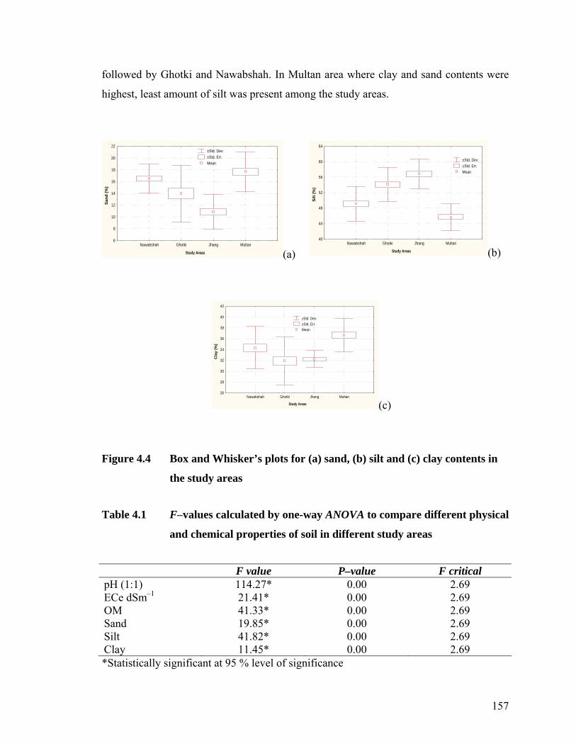
followed by Ghotki and Nawabshah. In Multan area where clay and sand contents were
highest, least amount of silt was present among the study areas.
Study Areas
Sand
(%)
6
8
10
12
14
16
18
20
22
Nawabshah Ghotki Jhang Multan
±Std. Dev.±Std. Err.Mean
(a) Study Areas
Silt
(%)
40
44
48
52
56
60
64
Nawabshah Ghotki Jhang Multan
±Std. Dev.±Std. Err.Mean
(b)
Study Areas
Cla
y (%
)
26
28
30
32
34
36
38
40
42
Nawabshah Ghotki Jhang Multan
±Std. Dev.±Std. Err.Mean
(c)
Figure 4.4 Box and Whisker’s plots for (a) sand, (b) silt and (c) clay contents in
the study areas
Table 4.1 F–values calculated by one-way ANOVA to compare different physical
and chemical properties of soil in different study areas
F value P–value F critical pH (1:1) 114.27* 0.00 2.69 ECe dSm–1 21.41* 0.00 2.69 OM 41.33* 0.00 2.69 Sand 19.85* 0.00 2.69 Silt 41.82* 0.00 2.69 Clay 11.45* 0.00 2.69 *Statistically significant at 95 % level of significance
157
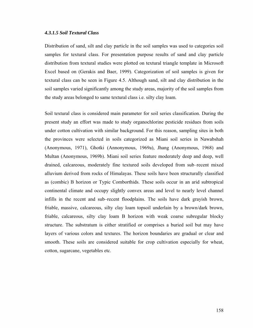
4.3.1.5 Soil Textural Class
Distribution of sand, silt and clay particle in the soil samples was used to categories soil
samples for textural class. For presentation purpose results of sand and clay particle
distribution from textural studies were plotted on textural triangle template in Microsoft
Excel based on (Gerakis and Baer, 1999). Categorization of soil samples is given for
textural class can be seen in Figure 4.5. Although sand, silt and clay distribution in the
soil samples varied significantly among the study areas, majority of the soil samples from
the study areas belonged to same textural class i.e. silty clay loam.
Soil textural class is considered main parameter for soil series classification. During the
present study an effort was made to study organochlorine pesticide residues from soils
under cotton cultivation with similar background. For this reason, sampling sites in both
the provinces were selected in soils categorized as Miani soil series in Nawabshah
(Anonymous, 1971), Ghotki (Annonymous, 1969a), Jhang (Anonymous, 1968) and
Multan (Anonymous, 1969b). Miani soil series feature moderately deep and deep, well
drained, calcareous, moderately fine textured soils developed from sub–recent mixed
alluvium derived from rocks of Himalayas. These soils have been structurally classified
as (combic) B horizon or Typic Comborthids. These soils occur in an arid subtropical
continental climate and occupy slightly convex areas and level to nearly level channel
infills in the recent and sub–recent floodplains. The soils have dark grayish brown,
friable, massive, calcareous, silty clay loam topsoil underlain by a brown/dark brown,
friable, calcareous, silty clay loam B horizon with weak coarse subregular blocky
structure. The substratum is either stratified or comprises a buried soil but may have
layers of various colors and textures. The horizon boundaries are gradual or clear and
smooth. These soils are considered suitable for crop cultivation especially for wheat,
cotton, sugarcane, vegetables etc.
158
(a) (b)
(c) (d)
0
10
20
30
40
50
60
70
80
90
100
0 10 20 30 40 50 60 70 80 90 100
% sand
% c
lay clay
siltyclay
siltyclay loam
silt loam
silt
loam
sandy loam loamysand
sand
sandy clay loam
sandy clay
clay loam
0
10
20
30
40
50
60
70
80
90
0
0 10 20 30 40 50 60 70 80 90 100
% sand
% c
la
10
y clay
siltyclay
siltyclay loam
silt loam
silt
loam
sandy loam loamysand
sand
sandy clay loam
sandy clay
clay loam
0
10
20
30
40
50
60
70
80
90
0
0 10 20 30 40 50 60 70 80 90 100
% sand
% c
la
10
y clay
siltyclay
siltyclay loam
silt loam
silt
loam
sandy loam loamysand
sand
sandy clay loam
sandy clay
clay loam
0
10
20
30
40
50
60
70
80
90
0
0 10 20 30 40 50 60 70 80 90 100
% sand
% c
lay clay
siltyclay
siltyclay loam
silt loam
silt
loam
sandy loam loamysand
sand
sandy clay loam
sandy clay
clay loam
10
Figure 4.5 Soil texture class of soil samples from (a) Nawabshah, (b) Ghotki, (c)
Jhang and (d) Multan area plotted on USDA triangle for textural
class
4.3.2 Biological Properties
Soil quality is strongly influenced by microbial mediated processes like nutrient cycling,
nutrient capacity, and aggregate stability. Therefore, identification of biological
indicators of soil health is regarded as critically important (Abawi and Widmer, 2000)
particularly the components sensitive to changes in soil quality (Romig et al., 1995).
Commonly measured biological parameters of soil health include soil organic matter,
respiration, microbial biomass (total bacteria and fungi,) and mineralizable nitrogen.
During this study soil microbial mass was measured as abundance of bacteria and fungi
159
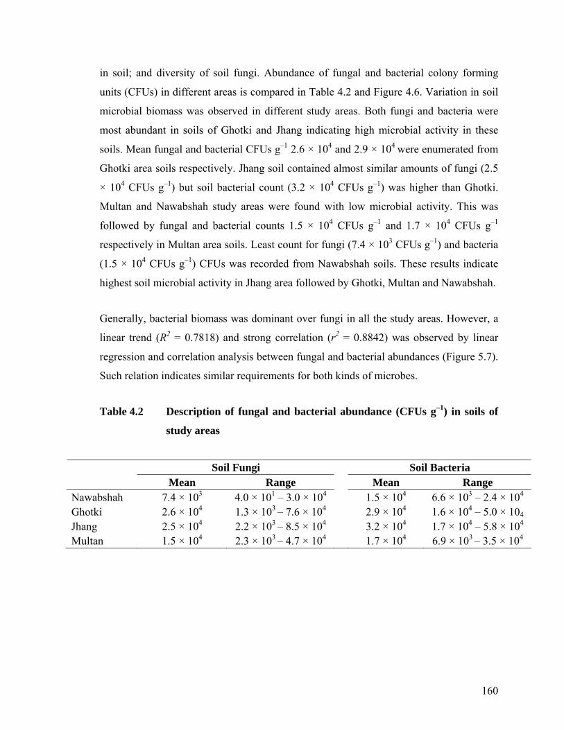
in soil; and diversity of soil fungi. Abundance of fungal and bacterial colony forming
units (CFUs) in different areas is compared in Table 4.2 and Figure 4.6. Variation in soil
microbial biomass was observed in different study areas. Both fungi and bacteria were
most abundant in soils of Ghotki and Jhang indicating high microbial activity in these
soils. Mean fungal and bacterial CFUs g–1 2.6 × 10⁴ and 2.9 × 10⁴ were enumerated from
Ghotki area soils respectively. Jhang soil contained almost similar amounts of fungi (2.5
× 104 CFUs g–1) but soil bacterial count (3.2 × 10⁴ CFUs g–1) was higher than Ghotki.
Multan and Nawabshah study areas were found with low microbial activity. This was
followed by fungal and bacterial counts 1.5 × 10⁴ CFUs g–1 and 1.7 × 10⁴ CFUs g–1
respectively in Multan area soils. Least count for fungi (7.4 × 10³ CFUs g–1) and bacteria
(1.5 × 10⁴ CFUs g–1) CFUs was recorded from Nawabshah soils. These results indicate
highest soil microbial activity in Jhang area followed by Ghotki, Multan and Nawabshah.
Generally, bacterial biomass was dominant over fungi in all the study areas. However, a
linear trend (R2 = 0.7818) and strong correlation (r2 = 0.8842) was observed by linear
regression and correlation analysis between fungal and bacterial abundances (Figure 5.7).
Such relation indicates similar requirements for both kinds of microbes.
Table 4.2 Description of fungal and bacterial abundance (CFUs g–1) in soils of
study areas
Soil Fungi Soil Bacteria Mean Range Mean Range
Nawabshah 7.4 × 10³ 4.0 × 101 – 3.0 × 10⁴ 1.5 × 10⁴ 6.6 × 10³ – 2.4 × 10⁴
Ghotki 2.6 × 10⁴ 1.3 × 10³ – 7.6 × 10⁴ 2.9 × 10⁴ 1.6 × 10⁴ – 5.0 × 10⁴
Jhang 2.5 × 10⁴ 2.2 × 10³ – 8.5 × 10⁴ 3.2 × 10⁴ 1.7 × 10⁴ – 5.8 × 10⁴
Multan 1.5 × 10⁴ 2.3 × 10³ – 4.7 × 10⁴ 1.7 × 10⁴ 6.9 × 10³ – 3.5 × 10⁴
160
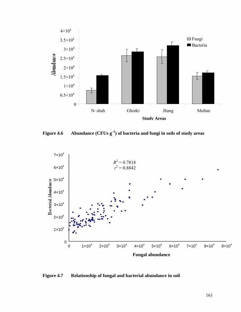
4×10⁴
Figure 4.6 Abundance (CFUs g–1) of bacteria and fungi in soils of study areas
Figure 4.7 Relationship of fungal and bacterial abundance in soil
Fungi 3.5×10⁴
Bacteria 3×10⁴
2.5×10⁴
2×10⁴
1.5×10⁴
1×10⁴
0.5×10⁴
0 N–shah Ghotki Jhang Multan
Study Areas
7×10⁴
R2 = 0.7818 r2 = 0.88426×10⁴
5×10⁴
4×10⁴
3×10⁴
2×10⁴
1×10⁴
01×104 2×10⁴ 3×10⁴ 4×10⁴ 5×10⁴ 6×10⁴ 7×10⁴ 8×10⁴ 9×1040
Fungal abundance
161
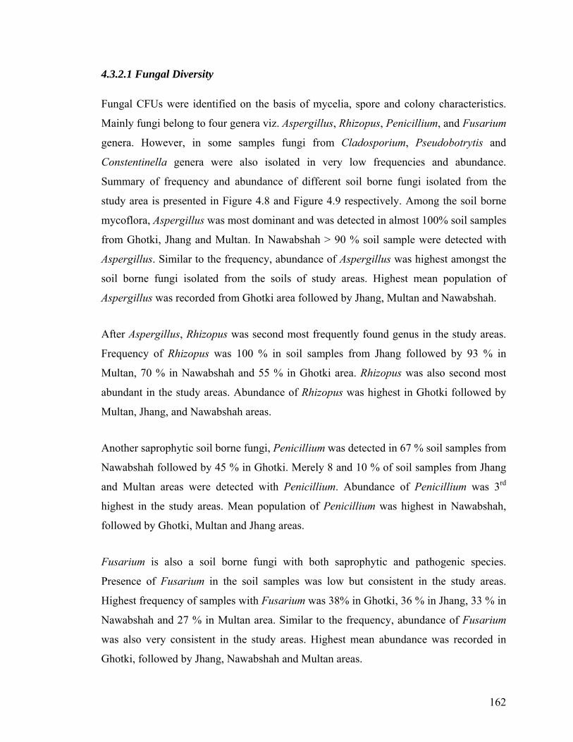
4.3.2.1 Fungal Diversity
Fungal CFUs were identified on the basis of mycelia, spore and colony characteristics.
Mainly fungi belong to four genera viz. Aspergillus, Rhizopus, Penicillium, and Fusarium
genera. However, in some samples fungi from Cladosporium, Pseudobotrytis and
Constentinella genera were also isolated in very low frequencies and abundance.
Summary of frequency and abundance of different soil borne fungi isolated from the
study area is presented in Figure 4.8 and Figure 4.9 respectively. Among the soil borne
mycoflora, Aspergillus was most dominant and was detected in almost 100% soil samples
from Ghotki, Jhang and Multan. In Nawabshah > 90 % soil sample were detected with
Aspergillus. Similar to the frequency, abundance of Aspergillus was highest amongst the
soil borne fungi isolated from the soils of study areas. Highest mean population of
Aspergillus was recorded from Ghotki area followed by Jhang, Multan and Nawabshah.
After Aspergillus, Rhizopus was second most frequently found genus in the study areas.
Frequency of Rhizopus was 100 % in soil samples from Jhang followed by 93 % in
Multan, 70 % in Nawabshah and 55 % in Ghotki area. Rhizopus was also second most
abundant in the study areas. Abundance of Rhizopus was highest in Ghotki followed by
Multan, Jhang, and Nawabshah areas.
Another saprophytic soil borne fungi, Penicillium was detected in 67 % soil samples from
Nawabshah followed by 45 % in Ghotki. Merely 8 and 10 % of soil samples from Jhang
and Multan areas were detected with Penicillium. Abundance of Penicillium was 3rd
highest in the study areas. Mean population of Penicillium was highest in Nawabshah,
followed by Ghotki, Multan and Jhang areas.
Fusarium is also a soil borne fungi with both saprophytic and pathogenic species.
Presence of Fusarium in the soil samples was low but consistent in the study areas.
Highest frequency of samples with Fusarium was 38% in Ghotki, 36 % in Jhang, 33 % in
Nawabshah and 27 % in Multan area. Similar to the frequency, abundance of Fusarium
was also very consistent in the study areas. Highest mean abundance was recorded in
Ghotki, followed by Jhang, Nawabshah and Multan areas.
162

Among the least frequent fungi isolated from the soil samples, Cladosporium was
detected in only 13 % and 7 % soil samples from Nawabshah and Ghotki respectively.
Mean abundance of Cladosporium from the two areas was 1.5 × 10³ CFUs g–1 soil in
Ghotki and 5.0 × 10² CFUs g–1 soil in Nawabshah. Cladosporium was not isolated from
any of the soil samples from Jhang and Multan. Pseudobotrytis and Constentinella were
isolated from only one sample each from Jhang and Ghotki areas. Abundance of
Pseudobotrytis was 1.8 × 10² CFUs g–1 soil in Jhang and that of Constentinella was 1.8 ×
103 CFUs g–1 soil in Ghotki.
Most of the fungi viz. Aspergillus, Penicillium, Fusarium, and Cladosporium belong to
phylum Ascomycota. All of these genera have cosmopolitan distribution and found
almost anywhere, including soil, plant debris, wood and both outdoor and indoor air.
Each of the genera has many species ranging from saprophytic to pathogenic for plants,
animals and human beings especially due to their toxin production. However, some
species are also useful and used for fermentation of various food items and drug
production in pharmaceuticals industry. Rhizopus falls into phylum Zygomycota and
order Mucorales. Rhizopus is a cosmopolitan filamentous fungus found in soil, decaying
fruit and vegetables, animal feces, and old bread. Genus Rhizopus is versatile and has
both saprophytic as well as pathogenic species.
163
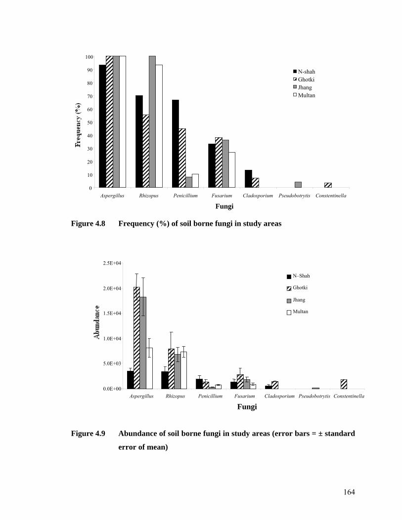
N-shah Ghotki Jhang
10
100
90
80
30
40
50
60
70 Multan
20
0 Aspergillus Rhizopus Penicillium Fusarium Cladosporium Pseudobotrytis Constentinella
Fungi
Figure 4.8 Frequency (%) of soil borne fungi in study areas
2.5E+04
N–Shah
Ghotki2.0E+04
Jhang
Multan 1.5E+04
1.0E+04
5.0E+03
0.0E+00Aspergillus Rhizopus Penicillium Fusarium Cladosporium Pseudobotrytis Constentinella
Fungi
Figure 4.9 Abundance of soil borne fungi in study areas (error bars = ± standard
error of mean)
164
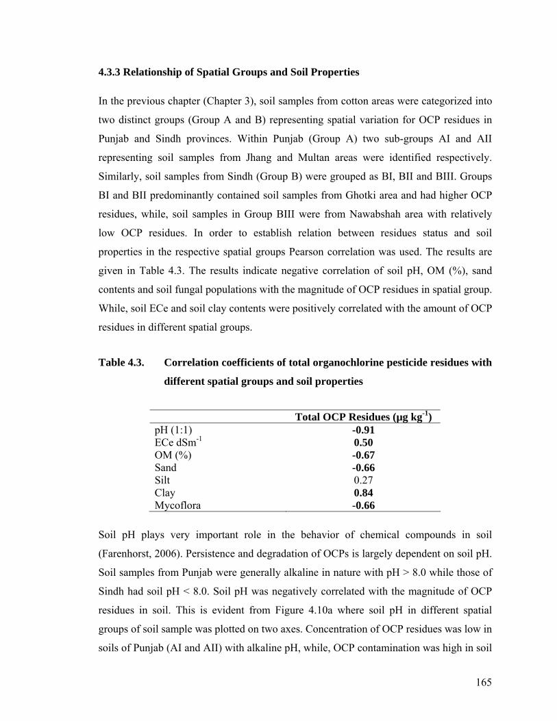
4.3.3 Relationship of Spatial Groups and Soil Properties
In the previous chapter (Chapter 3), soil samples from cotton areas were categorized into
two distinct groups (Group A and B) representing spatial variation for OCP residues in
Punjab and Sindh provinces. Within Punjab (Group A) two sub-groups AI and AII
representing soil samples from Jhang and Multan areas were identified respectively.
Similarly, soil samples from Sindh (Group B) were grouped as BI, BII and BIII. Groups
BI and BII predominantly contained soil samples from Ghotki area and had higher OCP
residues, while, soil samples in Group BIII were from Nawabshah area with relatively
low OCP residues. In order to establish relation between residues status and soil
properties in the respective spatial groups Pearson correlation was used. The results are
given in Table 4.3. The results indicate negative correlation of soil pH, OM (%), sand
contents and soil fungal populations with the magnitude of OCP residues in spatial group.
While, soil ECe and soil clay contents were positively correlated with the amount of OCP
residues in different spatial groups.
Table 4.3. Correlation coefficients of total organochlorine pesticide residues with
different spatial groups and soil properties
Total OCP Residues (µg kg-1) pH (1:1) -0.91 ECe dSm-1 0.50 OM (%) -0.67 Sand -0.66 Silt 0.27 Clay 0.84 Mycoflora -0.66
Soil pH plays very important role in the behavior of chemical compounds in soil
(Farenhorst, 2006). Persistence and degradation of OCPs is largely dependent on soil pH.
Soil samples from Punjab were generally alkaline in nature with pH > 8.0 while those of
Sindh had soil pH < 8.0. Soil pH was negatively correlated with the magnitude of OCP
residues in soil. This is evident from Figure 4.10a where soil pH in different spatial
groups of soil sample was plotted on two axes. Concentration of OCP residues was low in
soils of Punjab (AI and AII) with alkaline pH, while, OCP contamination was high in soil
165
groups of Sindh (BI, BII and BIII) where soil samples had lower pH (≈ 7). Similar trend
was also observed within each province. Soil samples from Jhang (AI) and Nawabshah
(BIII) with low concentration of OCP residues had relatively high pH than Multan (AII)
and Ghotki (BI and BII) where residues of OCPs were detected at higher concentration in
the respective provinces. Soil salinity (ECe) had positive but weak relation with OCP
residues in soil (Figure 4.10 b). Generally soils from Jhang, Multan and Nawabshah were
free of soil salinity. Only Nawabshah soils had sporadic incidence of moderate to low
levels of salinity. Relation of soil organic matter content was found negative with the
OCP residues in different spatial groups (4.10 c). Generally, OM content was high in
both Jhang and Multan areas of Punjab and than soils of Sindh However, variation in soil
organic matter content in study areas within two provinces was non-significantly
different.
Trend of physical properties of soil in different spatial groups categorized on the basis of
OCP residues is given in Figures 4.10 d, e and f. Sand content in soils was negatively
associated with the concentration of OCP residues in different spatial groups. Generally
sand content was high in Punjab where OCP were low than areas of Sindh. Sand has no
role in accumulation of pesticide residues. In contrary, sandy soils are reported to
facilitate leaching and removal of pesticide residues from surface soil (Csutoras and
Kiss, 2007). Silt content was poorly associated with the OCP concentration in different
spatial groups. Relation of clay content with OCP concentration in spatial groups was
strongly positive. In contrast to sand, clay content was high in areas of Punjab than in
Sindh. Soil clay contents play very important role in the retention or accumulation of
OCPs. OCPs are known to bind with clay to form bound residues (Fuentes, 2006). Clay
content was high in Multan (AII) than Jhang area (AII). Similarly, in Sindh soil clay
content was high in more contaminated areas of Ghotki (BI, BII) than those of
Nawabshah (BIII).
Soil mycoflora was negatively associated with OCP contaminants in spatial groups. This
indicates sensitivity of microbes to organic pollutants and their populations tend to
decrease at high levels. Decline in fungal population due to insecticide was also reported
166
by Omar, (1998). Higher fungal populations were observed in low contaminated soils of
Punjab and lower in Sindh where OCP residues were relatively high. In Punjab spatial
group AI representing Jhang area had higher fungal population than in high OCP
contaminated group AII representing Multan area. Similarly, fungal population was
considerably low in highly contaminated spatial groups BI and BII where majority of soil
samples were from Ghotki area. Fungal population in BIII, where majority of soil sample
were from Nawabshah had moderate fungal population. Although BIII soils were least
contaminated by DDTs, HCHs and cyclodienes but in this area highest amounts of HCB
residues were detected. Therefore, HCB residues could be responsible for low microbial
populations in Nawabshah soils.
167

(a)
0.0
5.0
10.0
15.0
20.0
25.0
30.0
35.0
40.0
45.0
AI AII BI BII BIII
Spatial Groups
ΣOC
P re
sidue
s (ug
6.80
7.00
7.20
7.40
7.60
7.80
8.00
8.20
8.40
8.60
8.80
Soil
(pH
1:
OCP ResiduespH (1:1)
(b)
0.0
5.0
10.0
15.0
20.0
25.0
30.0
35.0
40.0
45.0
AI AII BI BII BIII
Spatial Groups
ΣOC
P re
sidue
s (ug
(0.50)
-
0.50
1.00
1.50
2.00
2.50
ECe
(dS/
m
OCP ResiduesECe dS/m
(c)
0.0
5.0
10.0
15.0
20.0
25.0
30.0
35.0
40.0
45.0
AI AII BI BII BIII
Spatial Groups
ΣOC
P re
sidue
s (ug
-
0.50
1.00
1.50
2.00
2.50
3.00
3.50
4.00
O.M
(%
OCP ResiduesO.M. (%)
(d)
0.0
5.0
10.0
15.0
20.0
25.0
30.0
35.0
40.0
45.0
AI AII BI BII BIII
Spatial Groups
ΣOC
P re
sidue
s (ug-
10
20
30
40
50
60
70
80
90
100
Sand
(%
OCP ResiduesSand
(e)
0.0
5.0
10.0
15.0
20.0
25.0
30.0
35.0
40.0
45.0
AI AII BI BII BIII
Spatial Groups
ΣOC
P re
sidue
s (ug
-
5
10
15
20
25
30
Silt
(%
OCP Residuessilt
(f)
0.0
5.0
10.0
15.0
20.0
25.0
30.0
35.0
40.0
45.0
AI AII BI BII BIII
Spatial Groups
ΣOC
P re
sidue
s (ug
-
5
10
15
20
25
Cla
y (%
OCP ResiduesClay
(g)
0.0
5.0
10.0
15.0
20.0
25.0
30.0
35.0
40.0
45.0
AI AII BI BII BIII
Spatial Groups
ΣOC
P re
sidue
s (ug
0.0E+00
5.0E+03
1.0E+04
1.5E+04
2.0E+04
2.5E+04
3.0E+04
Σ So
il m
ycof
lora
(
OCP ResiduesMycoflora
Figure 4.10. Relation of cumulative organochlorine pesticide (OCP) residues in relation to
mean (a) soil pH (1:1), (b) ECe, (c) organic matter content (%), sand (%), silt (%), clay (%) and soil mycoflora (cfu) in different spatial groups (Error bars = ± standard error of mean)
168

4.3.4 Relationship of Physicochemical Properties with OCPs
Interaction between physical and chemical properties of soil with OCP residues status
was examined by employing CCA on OCP data matrix (114 soil samples × 19 OCPs) and
soil physicochemical data matrix (114 soil samples × 6 parameters). Global Monte Carlo
permutation test was applied on data normalized by Hill’s method. Results of CCA
analysis were explained by dimensionless ordination diagrams. The ordination diagram
featured two axes, and vectors representing physicochemical properties of soil. The
length of arrows represents the relative contribution of each soil variable to the axis, to
the OCPs and study areas. The direction on the arrow represents the correlation between
each soil variable and the canonical axis, and each other.
Table 4.4 Eigen-values and percentages of the variance, obtained with the canonical correspondence analysis performed for OCP residues and physicochemical properties of soil from study areas
Axis 1 Axis 2 Eigen values 0.05 0.03 Variance Explained (%) 5.02 3.57 Cumulative Variance Explained (%) 5.02 8.59 Cumulative Constrained Variance Explained (%) 41.61 71.21 OCPs × Physicochemical parameter correlations 0.60 0.48
Table 4.5 Canonical coefficients and correlation coefficient of physicochemical properties of soil with the first two axes generated by canonical correspondence analysis of physicochemical properties of soils from study areas
Canonical coefficients Correlation Coefficient Spec. Axis 1 Spec. Axis 2 Envi. Axis 1 Envi. Axis 2 pH (1:1) 0.15 –0.17 0.89 –0.26 ECe dSm–1 –0.02 –0.13 –0.29 –0.52 OM (%) 0.11 0.13 0.80 0.34 *Silt 0 0 –0.09 –0.12 Sand –0.03 0.015 0.08 –0.22 Clay –0.05 0.09 0.04 0.34
*Ignored in analysis due to multi co–linearity detected in data
169
The eigen values and variance explained by the first two axes is given in Table 4.4.The
first two axes were able to explain cumulative variance of 8.59 % where the first axis
contributed 5.02 % and the second axis 3.57 % for OCPs distribution in soil samples. The
interaction between OCPs and soil parameters was also explained by the same two axes.
The two axes explained a cumulative 71.21 % variability in the interaction between OCP
residues and soil parameters. Where, the first and second axes contributed 41.61 % and
29.6 % in explaining the variability in interaction. The intra–set correlations (Table 4.5)
and the ordination diagrams (Figure 4.11 and Figure 4.12) explained the relationship of
soil parameters with ordination axes. Soil pH and OM contents were the most important
soil parameters in the study followed by ECe. Soil pH and OM were strongly correlated
but ECe was negatively correlated with first axis. The physical parameter viz. sand, silt
and clay had weak association with axis 1. Association with second axis was rather weak
for pH, OM, sand, silt and clay but strong and negative for ECe with second axis. Only
OM and clay were positively associated with the second axis. Soil parameters–OCPs
residues correlation was strong for axis 1 (r2 = 0.60) as well as for axis 2 (r2 = 0.48) with
each other at 95 % level of significance. Association between pH and OM was positive
while both had negative association with ECe. Generally, soil microbial activities
decompose organic matter into CO2 and different acids to lower soil pH. Therefore, OM
is considered to have negative association with soil pH. According to Khattak, (1996), in
calcareous soils with high CaCO3 contents as of Pakistan, equilibrium between CaCO3
and HCO3 is very important. CO2 released due to different biological processes in soil
results in dissolution of CaCO3 to form HCO3– which intern is dissociated into OH– ions
to increase soil pH. Addition of organic matter in the soil improves the physical condition
of the soil by aggregation of exchangeable inorganic salts, by improving soil microbial
activity and by decreasing the bulk density of soils (Richards, 1954). ECe is the measure
of exchangeable sodium percentage in a saturated extract for soil salinity classification.
According to Richards (1954), pH of saturated soil paste is influenced by the composition
of the exchangeable cations, nature of cation–exchange materials, the composition and
concentration of soluble salts, and the presence or absence of gypsum and alkaline–earth
carbonates. Soil pH of 8.5 or greater indicate higher amounts of exchangeable–sodium–
percentage (> 15%) and the presence of alkaline–earth carbonates; the pH value < 8.5
170
indicate presence of low amounts (< 15%) exchangeable–sodium; and soils with pH
values < 7.5 are almost free of alkaline–earth carbonates and those having values of less
than 7.0 contain significant amounts of exchangeable hydrogen. This shows that soil pH
and ECe are closely related to each other. However, at more alkaline pH (> 8.5) the rate
of change of soil ECe may not be as linear as at the lower pH levels due to precipitation
of salts. However, some soils with considerably high amounts (> 15%) of exchangeable
sodium in soil and soil pH as low as 6.0 were regarded as degraded alkali soils (Richards,
1954) indicating negative association between ECe and pH under some specific
conditions.
CCA ordination of sampling sites from four cotton growing areas with soil parameters is
given in Figure 4.11. The sampling sites mainly from Multan and partly from Ghotki area
were associated and grouped together on the upper right side of CCA axis 1. This group
of soil samples was also associated with OM indicating a developing gradient in this area.
Soils of Multan area had highest amount of organic matter contents among the study
areas. Average OM content of Multan soil samples was 2.8 % ranging from 2.1 to 3.5 %.
Like–wise another group of soil sample mainly from Jhang area was prominent on the
lower right side of axis 1. This group of soil samples was closely associated with pH
suggesting an increasing trend in soil pH in soil samples from Jhang area. Soils samples
from Jhang areas were found alkaline in nature with mean pH 8.5 ranging from 8.3 to 8.8.
Some soil samples from Ghotki and majority from Nawabshah area were either located
on upper left of axis 1or concentrated on the centroid of the ordination axes. These soil
samples indicate low levels of soil pH as well as OM contents due to negative association
with these parameters. These groups were positively associated with ECe indicating
incidences of soil salinity in these areas. Soil ECe ranged from 0.4–4.3 dSm–1 in
Nawabshah and from 0.4–1.2 dSm–1 in Ghotki area. Soils of Nawabshah were more
saline than Ghotki area but both the areas were poor in organic matter content and soil pH
was also relatively lower than Jhang and Multan areas.
CCA ordination for OCP residues in the soil samples with soil parameters is given in
Figure 4.12. The position of OCP points relative to the soil parameter vectors was used to
171
interpret their relationship. For interpretation each vector for soil parameters was
extended backwards through the central origin of two axes. The soil parameters viz. pH,
OM content and soil ECe with long vectors were most closely correlated in the ordination
and more important in influencing the community variation than sand, silt and clay with
shorter arrows. For interaction between OCPs and soil parameters, each point
corresponding to OCP compound on the biplot was related to soil parameter by drawing
perpendicular on arrow representing particular soil parameter. The order in which the
OCP points project onto the arrow from the tip of the arrow downwards through the
origin indicated degree of association with the soil parameter. OCPs with their
perpendiculars anticipated near to or beyond the tip of the arrow were strongly correlated
and their presence in the soil was positively influenced by that soil parameter. Those at
the opposite side of centroid and towards the end of the vector were negatively correlated
with OCP residues in soil.
Among the OCPs endosulfan residues were found positively correlated with soil pH, OM
and clay content (Figure 4.12). This association was stronger for α–endosulfan compared
to β–endosulfan. During the study endosulfan isomers were detected in varying
frequencies and magnitudes from the study areas. Residues of α–endosulfan were not
detected in any of the soil samples from Nawabshah and Jhang areas while Endo α– /
Endo β– ratios ranged from 0.7–7.2 in Ghotki and 0.8–3.9 in Multan area. This suggests
accumulation of α–endosulfan and β–endosulfan residues at different rates depending
upon pH, OM and clay content in the micro–environments. α–endosulfan was more
stable under higher pH and have stronger association with OM than β–endosulfan.
Endosulfan degrades to more stable and toxic endosulfan sulphate. Association of
endosulfan sulphate with pH and OM was relatively weak compared to the parent
isomers. Endosulfan sulphate residues were detected at lower frequency and
concentration in Nawabshah, Jhang and Multan areas while they were somewhat higher
in Ghotki areas. Soil properties of these areas may be more conducive for parent
compounds and degradation to produce endosulfan sulphate takes place at lower rates. In
Ghotki areas soil pH and OM was lowest among the study areas, therefore, endosulfan
172
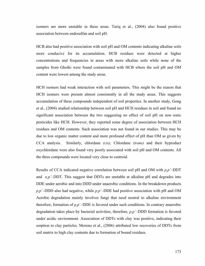
isomers are more unstable in these areas. Tariq et al., (2004) also found positive
association between endosulfan and soil pH.
HCB also had positive association with soil pH and OM contents indicating alkaline soils
more conducive for its accumulation. HCB residues were detected at higher
concentrations and frequencies in areas with more alkaline soils while none of the
samples from Ghotki were found contaminated with HCB where the soil pH and OM
content were lowest among the study areas.
HCH isomers had weak interaction with soil parameters. This might be the reason that
HCH isomers were present almost consistently in all the study areas. This suggests
accumulation of these compounds independent of soil properties. In another study, Gong
et al., (2004) studied relationship between soil pH and HCH residues in soil and found no
significant association between the two suggesting no effect of soil pH on non–ionic
pesticides like HCH. However, they reported some degree of association between HCH
residues and OM contents. Such association was not found in our studies. This may be
due to low organic matter content and more profound effect of pH than OM as given by
CCA analysis. Similarly, chlordane (cis), Chlordane (trans) and their byproduct
oxychlordane were also found very poorly associated with soil pH and OM contents. All
the three compounds were located very close to centroid.
Results of CCA indicated negative correlation between soil pH and OM with p,p´–DDT
and o,p´–DDT. This suggest that DDTs are unstable at alkaline pH and degrades into
DDE under aerobic and into DDD under anaerobic conditions. In the breakdown products
p,p´–DDD also had negative, while p,p´–DDE had positive association with pH and OM
Aerobic degradation mainly involves fungi that need neutral to alkaline environment
therefore, formation of p,p´–DDE is favored under such conditions. In contrary anaerobic
degradation takes place by bacterial activities, therefore, p,p´–DDD formation is favored
under acidic environment. Association of DDTs with clay was positive, indicating their
sorption to clay particles. Moreno et al., (2006) attributed low recoveries of DDTs from
soil matrix to high clay contents due to formation of bound residues.
173
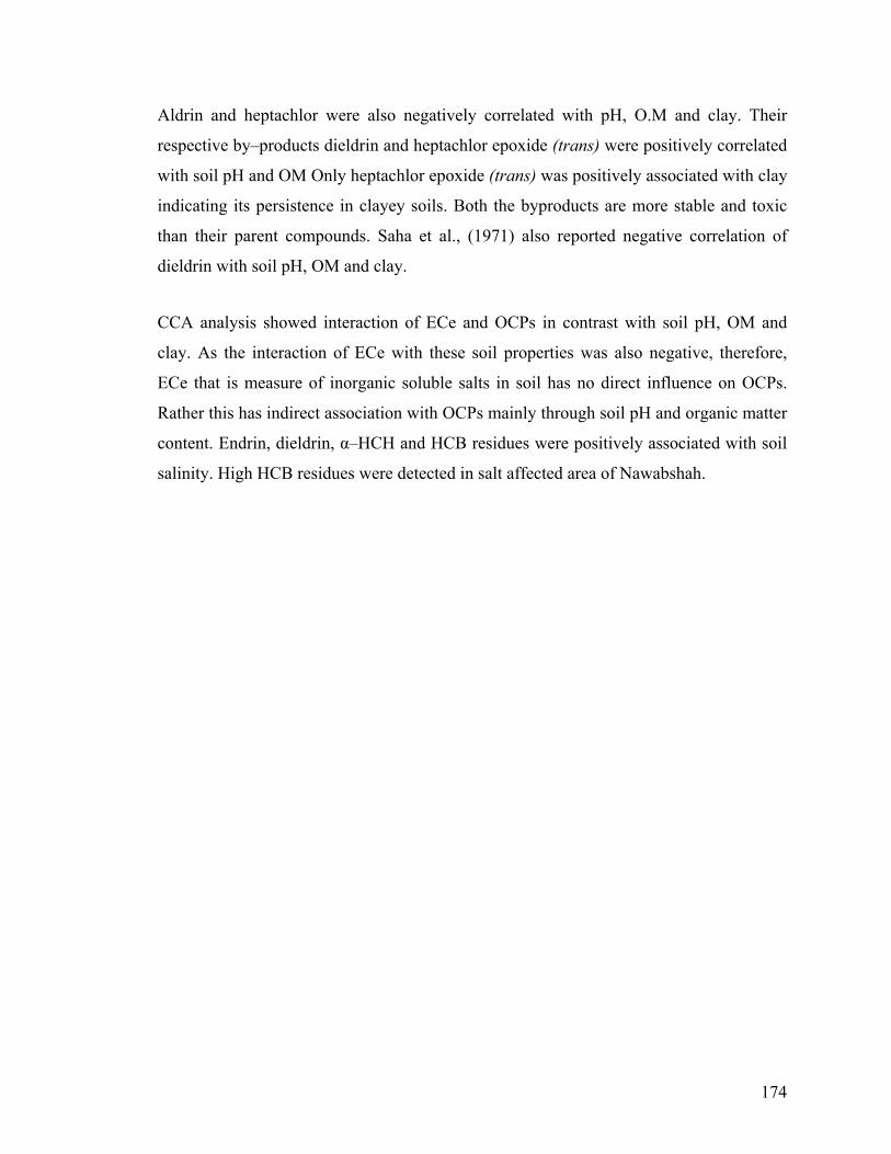
174
Aldrin and heptachlor were also negatively correlated with pH, O.M and clay. Their
respective by–products dieldrin and heptachlor epoxide (trans) were positively correlated
with soil pH and OM Only heptachlor epoxide (trans) was positively associated with clay
indicating its persistence in clayey soils. Both the byproducts are more stable and toxic
than their parent compounds. Saha et al., (1971) also reported negative correlation of
dieldrin with soil pH, OM and clay.
CCA analysis showed interaction of ECe and OCPs in contrast with soil pH, OM and
clay. As the interaction of ECe with these soil properties was also negative, therefore,
ECe that is measure of inorganic soluble salts in soil has no direct influence on OCPs.
Rather this has indirect association with OCPs mainly through soil pH and organic matter
content. Endrin, dieldrin, α–HCH and HCB residues were positively associated with soil
salinity. High HCB residues were detected in salt affected area of Nawabshah.
175
Figure 4.11 Ordination diagram of canonical correspondence analysis of the relationship between physicochemical parameter soil and sampling sites in four study areas in cotton growing areas of Pakistan. Physicochemical parameters are represented as arrows. Directions of arrows indicate correlation with canonical axes and gradient of maximum change. The lengths of arrows indicate strength of correlation with respect to canonical axes and sampling sites.
3.1
3.1
Axis 2 -2.5
Axis 1
G31AG32AG33A
G34A
G35A
G36AG38A
G39AG40A
G41A
G42A
G43A
G44AG45A
G46A
G47A
G48AG49AG50AG51AG52A
G53A
G54A G55A G56AG57AG58AG59AG60A
J01AJ02A
J03A
J04A
J05A
J06A J07A
J08A
J09A J10A
J11A
J12AJ13A
J14A
J15A
J16AJ17AJ18A
J19AJ20AJ21A
J22A
J23A
J24A
J25A
M01A
M02AM03A
M04A
M05A
M06A M07A
M08A
M09A M10A M11AM12A
M13A M14A
M15A M16A M17A M18A M19A M20A
M21A
M22A
M23A
M24AM25A
M26AM27AM28A
M29A
M30A
N01A
N02AN03AN04AN05AN06AN07A
N08A
N09AN10AN11A
N12AN13A
N14AN15AN16AN17AN18AN19A
N20AN21AN22A
N23AN24AN25A
N26A N27AN28AN29A
N30A
-0.6
-1.3
-1.9
-2.5
0.6
1.3
1.9
2.5
-0.6-1.3-1.9 0.6 1.3 1.9 2.5
pH (1:1)
ECe dSm–1
OM (%) Clay
Vector scaling: 14.06
Figure 4.12 Ordination diagram of canonical correspondence analysis relationship between physicochemical parameter soil and OCPs in four study areas in cotton growing areas o istan. Physicochemical parameters are represented as arrows. Directions of arrows indicate correlation with ical axes and gradient of maximum change. The lengths of arrows indicate strength of correlation with respe canonical axes and OCPs.
176
B
Heptachlor–epoxide (trans
Dieldrin
t–chlordane
Oxychlordane
α–Endosulfan
sulfan
En indr
p,p´-DDE
-1.40
.81
.21
0
1
1
1
17.0
5.6
4.2
-2
-4
1.4
2.8
o, p´–DDT
β–HCH
p, p´–DDT
p, p´–DDD
Chlordane (cis)
OM (%)
7.01-1.40.81 .21 -2-4 1.40 1 4.21 5.61
ECe dSm–1
Clay
Heptachlor
Aldrin
γ–HCH
Sand ndosulfan sulphate
α–HCH
pH (1:1)
Axis 1Vector scaling: 31.32
Axis 2
of thef Pakcanonct to
HC
)
β–Endo
2.8
E
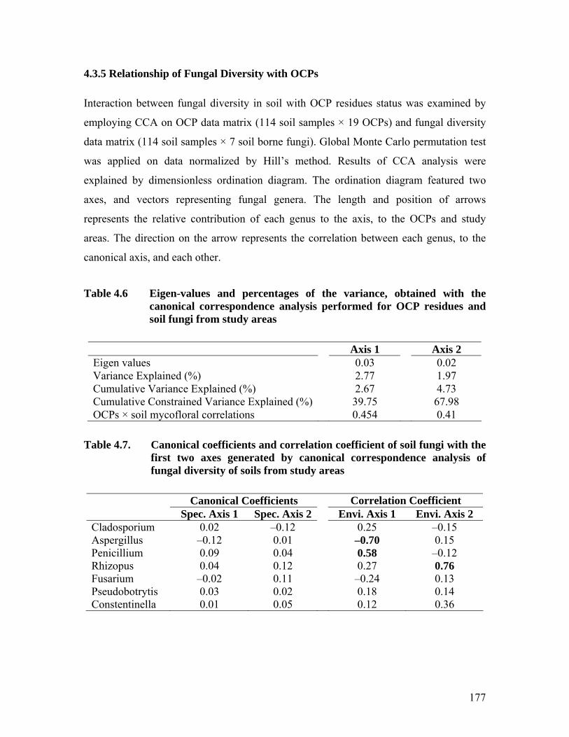
4.3.5 Relationship of Fungal Diversity with OCPs
Interaction between fungal diversity in soil with OCP residues status was examined by
employing CCA on OCP data matrix (114 soil samples × 19 OCPs) and fungal diversity
data matrix (114 soil samples × 7 soil borne fungi). Global Monte Carlo permutation test
was applied on data normalized by Hill’s method. Results of CCA analysis were
explained by dimensionless ordination diagram. The ordination diagram featured two
axes, and vectors representing fungal genera. The length and position of arrows
represents the relative contribution of each genus to the axis, to the OCPs and study
areas. The direction on the arrow represents the correlation between each genus, to the
canonical axis, and each other.
Table 4.6 Eigen-values and percentages of the variance, obtained with the canonical correspondence analysis performed for OCP residues and soil fungi from study areas
Axis 1 Axis 2 Eigen values 0.03 0.02 Variance Explained (%) 2.77 1.97 Cumulative Variance Explained (%) 2.67 4.73 Cumulative Constrained Variance Explained (%) 39.75 67.98 OCPs × soil mycofloral correlations 0.454 0.41
Table 4.7. Canonical coefficients and correlation coefficient of soil fungi with the first two axes generated by canonical correspondence analysis of fungal diversity of soils from study areas
Canonical Coefficients Correlation Coefficient Spec. Axis 1 Spec. Axis 2 Envi. Axis 1 Envi. Axis 2 Cladosporium 0.02 –0.12 0.25 –0.15 Aspergillus –0.12 0.01 –0.70 0.15 Penicillium 0.09 0.04 0.58 –0.12 Rhizopus 0.04 0.12 0.27 0.76 Fusarium –0.02 0.11 –0.24 0.13 Pseudobotrytis 0.03 0.02 0.18 0.14 Constentinella 0.01 0.05 0.12 0.36
177
The eigen values and variance explained by the first two axes is given in Table 4.6. The
first two axes were able to explain cumulative variance of 4.7 % where the first axis
contributed 2.8 % and the second axis 1.96 % for explaining the variability of OCPs in
the study areas. The interaction between OCPs and fungal myco–flora was also explained
by the same two axes. The two axes explained a cumulative 68 % variability in the
interaction between OCP residues and soil parameters. Where, the first and second axes
contributed 40 % and 28 % respectively in explaining the variability. The intra–set
correlations (Table 4.7) and the ordination diagrams (Figure 4.13 and Figure 4.14)
explain the relationship of soil borne fungi with ordination axes. Aspergillus, Penicillium
and Rhizopus were the most important genera in the study followed by Cladosporium,
Constentinella, Fusarium and Pseudobotrytis. Penicillium was strongly correlated but
Aspergillus was negatively correlated with first axis. Fusarium also had negative but
weak correlation with first axis. Association of other genera was weak but positive with
first axis. Association of majority of fungi with second axis was also weak. Only
Rhizopus had strong positive association with the second axis. Correlation coefficient of
fungi–OCPs residues interaction was moderate with axis 1 (r2 = 0.45) as well as for axis
2 (r2 = 0.41) at 95% level of significance. Among fungal genera, association between
Aspergillus and Penicillium was strongly negative. Eigenvectors of both the fungi were in
opposite direction to each other. Rhizopus had positive association with both Aspergillus
and Penicillium. Aspergillus and Penicillium belong to same order and most of their
species are saprophytic. As both have almost similar living requirements, therefore, the
negative interaction between the two may be due to inter–genus competition in soil or
due to their dominance over each other in the laboratory cultures. Fusarium was more
closely associated with Rhizopus than other fungi. Rest of the fungi were in positive
association with Rhizopus and Penicillium.
CCA ordination for OCP residues in the soil samples with fungal genera is given in
Figure 4.13. The position of OCP points relative to the fungal vectors was used to
interpret their relationship. For interpretation each vector for fungal genus was extended
backwards through the central origin of two axes. The fungal genera viz. Aspergillus,
Penicillium and Rhizopus with long vectors were most closely correlated in the ordination
178
and considered most important in influencing the community variation than Fusarium,
Cladosporium, Constentinella and Pseudobotrytis with shorter arrows. For interaction
between OCPs and fungal genera, each point corresponding to OCP compound on the
biplot was related to each genus by drawing perpendicular on arrow representing
particular fungi. The order in which the OCP points project on to the arrow from the tip
of the arrow downwards through the origin indicated degree of association with the fungi.
OCPs with their perpendiculars anticipated near to or beyond the tip of the arrow were
strongly correlated and their presence in soil was positively influenced by that genus.
Those at the opposite side of centroid and towards the end of the vector were negatively
correlated with the fungi.
CCA ordination of sampling sites from four cotton growing areas with soil borne fungi is
given in Figure 4.14. As discussed in earlier section 4.3.3.1, the abundance of Aspergillus
and Fusarium was almost similar in the study areas. Therefore, both the fungi were
closely associated with each other in the ordination. Among other genera, association of
Rhizopus was relatively stronger with Jhang and Multan areas. Soil samples from Jhang,
followed by soil samples from Multan are positioned close to head–end of eigen–vector
representing Rhizopus. Penicillium was also found important in the ordination.
Association of Penicillium was relatively stronger with Sindh areas than those of Punjab.
Gradient for Penicillium was observed stronger with Nawabshah area than Ghotki area by
CCA ordination. The other genera viz. Cladosporium, Constentinella and Pseudobotrytis
were isolated from individual soil samples in different areas; therefore, no meaningful
relation could be established with any soil population.
CCA ordination showed weak OCPs–fungi interaction. Aspergillus was strongest factors
influencing community variations. Due to closer association of Fusarium with
Aspergillus, both had almost similar relation with OCPs. Different HCH isomers had
different relation with Aspergillus and Fusarium. β–HCH positioned closer to head–end
of Aspergillus and Fusarium was positively associated. α–HCH was located on the other
side of centroid indicated negative correlation with Aspergillus and Fusarium. While, γ–
HCH was located very close to the centroid on positive axis indicated very weak
179
association with both Aspergillus and Fusarium. HCH isomers had reverse relation with
Penicillium. Association of β–HCH was positive but that for α–HCH was negative. γ–
HCH also had negative but weak association with Penicillium. Association of HCH
isomers with Rhizopus was quite different from that with other fungi. Both α–HCH and
γ–HCH were positively correlated, while, β–HCH was negatively correlated with
Penicillium. From these results we can conclude that different fungal genera have
different tolerance for different isomers of HCH. Aspergillus and Fusarium had tolerance
for β– and γ–HCH, Rhizopus had tolerance for α– and γ–HCH, and Penicillium had
tolerance for only α–HCH. Transformation of γ-HCH into α-HCH in soil is also attributed
to sunlight exposure as well as biological activities (Li et al., 2006). Therefore, fungi
positively associated with α-HCH may have some role in degradation of γ-HCH.
Both the isomers α–endosulfan and β–endosulfan were located very close to the centroid,
therefore had weak association with different fungi. However, endosulfan sulphate was
positively correlated with Aspergillus and Fusarium. This indicate role of Aspergillus and
Fusarium in breakdown of endosulfan and formation of endosulfan sulphate. Hussain et
al., (2007) isolated different soil borne fungi from different agro–ecologies of Pakistan
and found Chaetosartorya stromatoides, Aspergillus terricola and Aspergillus terreus
capable of degrading both α– and β–endosulfan upto 75% in cultures. Similarly, Bhalerao
and Puranik (2007) had reported the ability of Aspergillus niger to tolerate upto 400 ppm
of technical grade of endosulfan in cultures. In another study Siddique et al., (2003)
described the ability of Fusarium ventricosum to degrade α– and β–endosulfan into less
toxic endosulfan diol and endosulfan ether.
Aspergillus and Fusarium were positively correlated with p,p´–DDD and p,p´–DDT and
negatively associated with o,p´–DDT and p,p´–DDE. The relation of these DDT isomers
and byproducts was opposite with Penicillium. However, all DDTs and their breakdown
products were negatively correlated with Rhizopus. This indicates sensitivity of Rhizopus
to the presence of DDTs in the environment. In nature, conversion of p,p´–DDE is the
byproduct of p,p´–DDT under aerobic conditions. Negative association of Penicillium
with p,p´–DDT and positive with p,p´–DDE indicate some role of Penicillium in
180
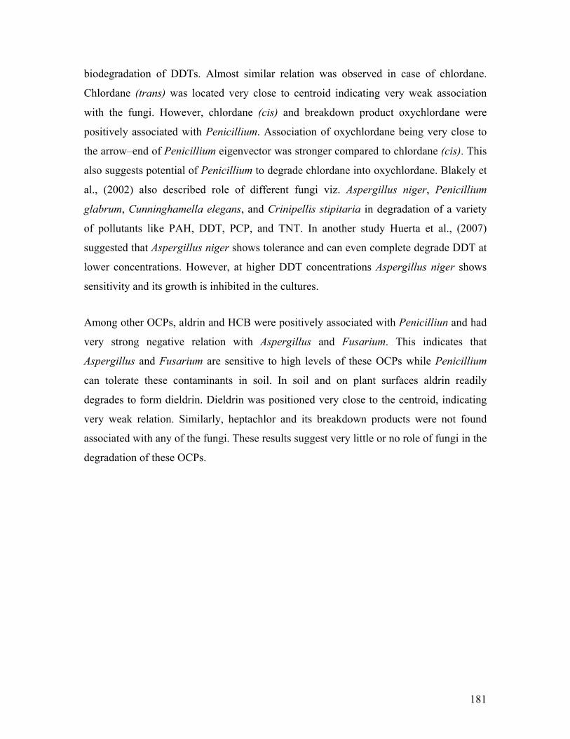
181
biodegradation of DDTs. Almost similar relation was observed in case of chlordane.
Chlordane (trans) was located very close to centroid indicating very weak association
with the fungi. However, chlordane (cis) and breakdown product oxychlordane were
positively associated with Penicillium. Association of oxychlordane being very close to
the arrow–end of Penicillium eigenvector was stronger compared to chlordane (cis). This
also suggests potential of Penicillium to degrade chlordane into oxychlordane. Blakely et
al., (2002) also described role of different fungi viz. Aspergillus niger, Penicillium
glabrum, Cunninghamella elegans, and Crinipellis stipitaria in degradation of a variety
of pollutants like PAH, DDT, PCP, and TNT. In another study Huerta et al., (2007)
suggested that Aspergillus niger shows tolerance and can even complete degrade DDT at
lower concentrations. However, at higher DDT concentrations Aspergillus niger shows
sensitivity and its growth is inhibited in the cultures.
Among other OCPs, aldrin and HCB were positively associated with Penicilliun and had
very strong negative relation with Aspergillus and Fusarium. This indicates that
Aspergillus and Fusarium are sensitive to high levels of these OCPs while Penicillium
can tolerate these contaminants in soil. In soil and on plant surfaces aldrin readily
degrades to form dieldrin. Dieldrin was positioned very close to the centroid, indicating
very weak relation. Similarly, heptachlor and its breakdown products were not found
associated with any of the fungi. These results suggest very little or no role of fungi in the
degradation of these OCPs.
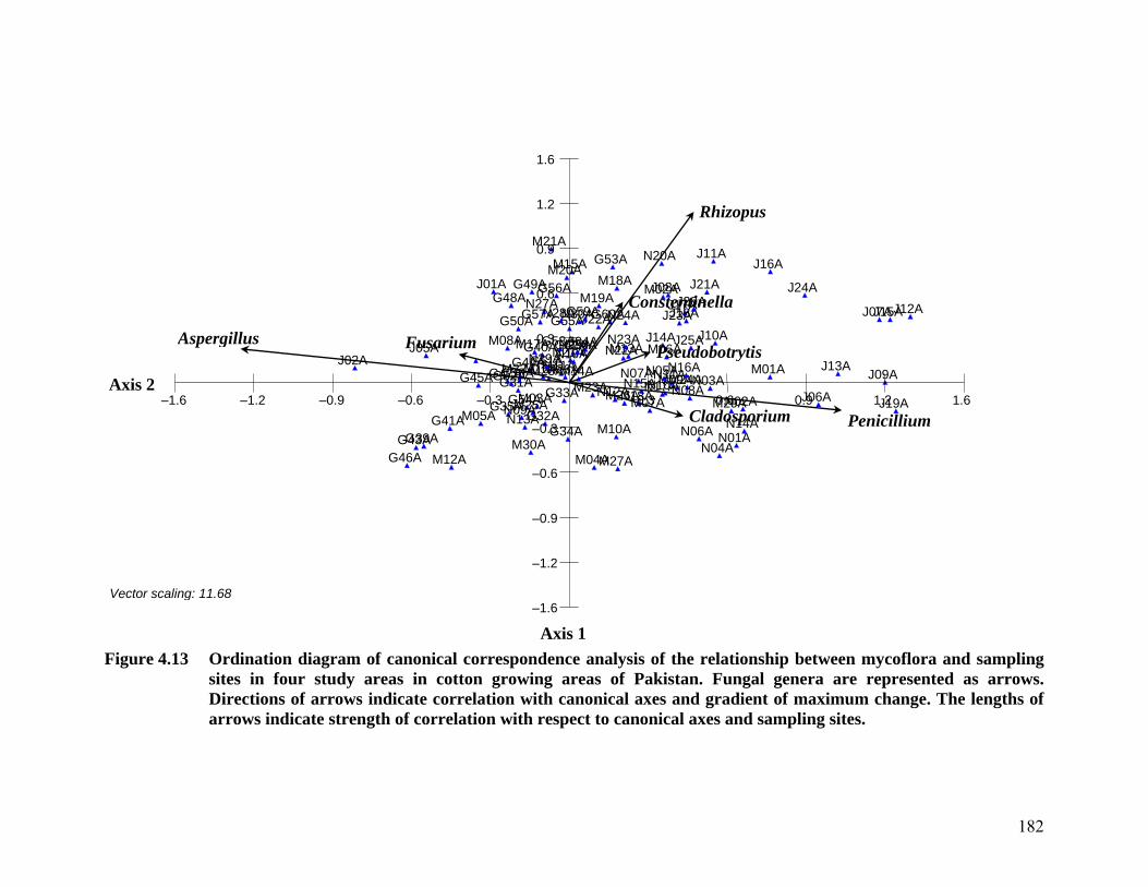
182
Figure 4.13 Ordination diagram of canonical correspondence analysis of the relationship between mycoflora and sampling sites in four study areas in cotton growing areas of Pakistan. Fungal genera are represented as arrows. Directions of arrows indicate correlation with canonical axes and gradient of maximum change. The lengths of arrows indicate strength of correlation with respect to canonical axes and sampling sites.
Axis 2
Axis 1
G31A
G32A
G33A
G34A
G35A
G36A
G38A
G39A
G40A
G41A
G42A
G43A
G44AG45A
G46A
G47A
G48AG49A
G50A
G51AG52A
G53A
G54A
G55A
G56A
G57A
G58A
G59AG60A
J01A
J02AJ04AJ05A
J06A
J07A
J08A
J09A
J 0A1
J11A
J12A
J13A
J14A J15A
J16A
J17A J18A
J19A
J20A J21A
J22A J23A J24A
J25A
M01A
M02A
M03A
M04A
M05A
M 06A
M07A
M08A
M09A
M10A
M11A
M12A
M13A
M14A
M15A
M16A
M17A
M18AM19A
M20A
M21A
M22AM23A M24A
M25AM26A
M27A
M28A
M29A
M30A N01A
N02AN03A
N04A
N05A
N06A
N07AN08A
N09A
N10A N11A N12A
N13A N14A
N15AN16A
N17A N18A
N19A
N20A
N21A N22AN23A
N24A
N25A
N26A
N27AN28A
N29A
N30A
–0.3
–0.6
–0.9
–1.2
–1.6
0.3
0.6
0.9
1.2
1.6
–0.3–0.6–0.9 –1.2 –1.6 0.3 0.6 0.9 1.2 1.6Cladosporium
Aspergillus
Penicillium
Rhizopus
Fusarium Pseudobotrytis
Constentinella
Vector scaling: 11.68
Figure 4.14 Ordination diagram of canonical correspondence analys he relationship between soil mycoflora and OCPs in four study areas in cotton growing areas of Pakistan. l genera are represented as arrows. Directions of arrows indicate correlation with canonical axes and grad maximum change. The lengths of arrows indicate strength of correlation with respect to canonical axes and s.
183
7.4
Vector scaling: 55.49 Axis 1
–1.5
–3.0
–4.4
–5.9
–7.4
1.5
3.0
4.4
5.9
–1.5–3.0–4.4 –5.9
β–HCH
p,p–DDD
p,p–DDT
t–Chlordane
Dieldrin
–7.4 3.0 4.4 5.9Cladosporium
Aspergillus
Rhizopus
Pseudobotrytis
tentinella
β–Endosulfan
Heptachlor
α–HCH
Fusarium
Endosulfan–sulphate
Heptachlor epoxide (trans)
a–Endosulfan
γ–HCH
Penicillium
Endrin
HCB
Oxychlordane
p,p–DDE
Aldrin
c–Chlordane
o,p–DDT
Axis 2
7.4
is of tFungaient of OCP
1.5
Cons
4.4 CONCLUSION
Relationship between OCP contaminants and physical, chemical and biological properties
of the soils from study areas were studied. Significant variations existed for physical,
chemical and biological properties among the study areas. Generally the soils of study
areas were alkaline and poor in organic matter content. However, study areas of Punjab
were more alkaline and rich in OM contents than those of Sindh. ECe of the soil samples
suggested occurrence of salinity in areas of Sindh, while, study areas of Punjab were
generally free of salinity. Significant variations also existed in sand, silt and clay
distribution among the study areas. However, almost all the soil samples were
categorized as silty clay loam representing Miani series soils. Spatial groups identified
for OCP residues in the study areas were studied in relation to physicochemical and
biological properties. Soil pH, organic matter content, sand content and soil fungal
populations were negatively correlated with the magnitude of OCP residues in different
spatial groups. Sandy, alkaline soils rich in organic matter content and with higher fungal
populations were associated with areas of Jhang and Multan where OCP residues were
present in relatively lower concentrations. Soil ECe and soil clay contents were positively
correlated with magnitude of OCP residues. Generally higher amounts of OCP residues
were found in clayey soils of Ghotki and among OCPs higher HCB residues were
associated with soil salinity especially in Nawabshah.
In order to study OCPs in relation to the soil properties, canonical correspondence
analysis (CCA) was found very useful. Relationship between OCP contaminants in soil
samples and physical and chemical properties of soil was studied by CCA. OCPs and
physicochemical properties had strong association with each other. In this regard, soil pH
and OM content were identified as most important variables and were positively
associated with each other. Role of sand, silt and clay particle distribution in soil samples
was very low in relation to OCP residues. Results indicated accumulation of endosulfan
in alkaline and high OM content soils i.e. Ghotki and Multan areas. However, the study
suggested less persistence of DDTs, chlordane, heptachlor, aldrin and γ–HCH residues in
alkaline soil. Therefore, these soil conditions may favor degradation of these OCPs and
OCP metabolites were detected at higher levels. Due to these reasons residues of these
184
OCPs were low in high alkaline areas of Punjab than those of Sindh. Soil salinity was
also found important in the study and was negatively affecting endosulfan but
accumulation of other OCPs like HCB was favored under saline soils like that of
Nawabshah. Similarly, endosulfan residues were relatively lower and higher of other
OCPs in Sindh than Punjab.
Soil microbial populations also varied among the study areas. Soils of Jhang and Ghotki
area were rich in microbial population than Nawabshah and Multan. Abundance and
frequency of bacterial and fungal populations were positively correlated with each other.
The study area also varied in fungal diversity. Aspergillus was most abundantly and most
frequently isolated fungus followed by Rhizopus, Penicillium, Fusarium, Cladosporium,
Pseudobotrytis and Constentinella. Aspergillus, Penicllium and Rhizipus were found
most important genera by CCA analysis in relation to PCPs. Different fungi showed
different behavior in relation to different OC compounds. Negative association of
Aspergillus with Aldrin, endosulfan, chlordane, HCB, heptachlor and o,p´–DDT and
p,p´–DDE suggest its intolerance to these OCPs. Positive association of Aspergillus with
the breakdown products viz. endosulfan sulphate, and p,p´–DDD and negative
association with endosulfan and DDT indicate its role in degradation. Penicillium had
opposite role to that of Aspergillus and was positively associated with aldrin, endosulfan,
chlordane, HCB, heptachlor and o,p´–DDT and p,p´–DDE indicating tolerance to these
OCPs. Rhizopus indicated tolerance for HCHs, heptachlor, endosulfan and their
breakdown products. However, Rhizopus was found sensitive to DDTs, chlordane,
endrin, aldrin and dieldrin. This study indicates role of different physicochemical and
biological properties in the behavior of OCPs in soil environment.
185
4.5 REFERENCES
Abawi, G.S. and T.L. Widmer. 2000. Impact of soil health management practices on soil
borne pathogens, nematodes and root diseases of vegetables crops. Applied Soil
Ecology, 15: 37–47.
Anonymous. 1968. Reconnaissance soil survey of Jhang. Soil Survey Project of Pakistan,
Directorate of Soil Survey, West Pakistan, Lahore, Pakistan.
Anonymous. 1969a. Reconnaissance soil survey of Ghotki. Soil Survey Project of
Pakistan, Directorate of Soil Survey, West Pakistan, Lahore, Pakistan.
Anonymous. 1969b. Reconnaissance soil survey of Multan. Soil Survey Project of
Pakistan, Directorate of Soil Survey, West Pakistan, Lahore, Pakistan.
Anonymous. 1971. Reconnaissance soil survey of Nawabshah. Soil Survey Project of
Pakistan, Directorate of Soil Survey, West Pakistan, Lahore, Pakistan.
Azam, F. and G.H. Memon. 1996. Soil organisms. In: Bashir, E. and R. Bantel (Eds.).
Soil science. National Book Foundation, Islamabad.
Azaz, A.D. 2003. Isolation and Identification of Soil borne Fungi in Fields Irrigated by
GAP in Harran Plain Using Two Isolation Methods. Turk J Bot, 27: 83–92.
Barraclough, D., T. Kearney and A. Croxford. 2005. Bound residues: environmental
solution or future problem? Environmental Pollution, 133: 85-90.
Bhalerao T.S. and P.R. Puranik. 2007. Biodegradation of organochlorine pesticide,
endosulfan, by a fungal soil isolate, Aspergillus niger, Int. Biodeter. Biodegr., 59
(2007) 315–321.
Blakely, J.K., D.A. Neher and A.L. Spongberg. 2002. Soil invertebrate and microbial
communities, and decomposition as indicators of polycyclic aromatic
hydrocarbon contamination. Applied Soil Ecology, 21: 71–88.
Boivin, A., S. Amellal, M. Schiavon and M.T. van Genuchten. 2005. 2,4–
Dichlorophenoxyacetic acid (2,4–D) sorption and degradation dynamics in three
agricultural soils. Environmental Pollution, 138(1): Pages 92–99.
Bollag, J.M., C.J. Myers and R.D. Minard. 1992. Biological and chemical interactions of
pesticides with soil organic matter. Science of Total Environment, 123–124: 205–
217.
186
Brown, C.L. and W.K. Hock. 1990. The Fate of Pesticides in the environment.
Agrichemical Fact Sheet #8, Penn State Cooperative Extension.
Brown, J.C. 1958. Soil fungi of some British sand dunes in relation to soil type and
succession. Journal of Ecology, 46: 641–664.
Burauel, P. and F. Baßmann. 2005. Soils as filter and buffer for pesticides: experimental
concepts to understand soil functions. Environmental Pollution, 133(1): 11–16.
Cañete, R., M. Yong, J. Sánchez, L. Wong and A. Gutiérrez. 2004. Population Dynamics
of Intermediate Snail Hosts of Fasciola hepatica and Some Environmental
Factors in San Juan y Martinez Municipality, Cuba. Mem Inst Oswaldo Cruz, Rio
de Janeiro, 99(3): 257-262.
Cox, L., R. Celis, M.C. Hermosin, A. Becker and J. Cornejo. 1997. Porosity and
herbicide leaching in soils amended with olive–mill wastewater. Agriculture,
Ecosystems & Environment, 65(2): 151–161.
Cruz, M.S.R., J.E. Jones and G.D. Bending. 2006. Field–scale study of the variability in
pesticide biodegradation with soil depth and its relationship with soil
characteristics. Soil Biology and Biochemistry, 38: 2910–2918.
Csutoras, C.S. and A. Kiss. 2006. Efficient method for the characterization of the
interaction of pesticides with different soil samples. Microchemical Journal,
85:21–24.
Farenhorst, A. 2006. Importance of Soil Organic Matter Fractions in Soil-Landscape and
Regional Assessments of Pesticide Sorption and Leaching in Soil. Soil Sci. Soc.
Am. J., 70:1005–1012.
Fuentes, E., M.E. Baez and D. Reyes. 2006. Microwave-assisted extraction through an
aqueous medium and simultaneous cleanup by partition on hexane for
determining pesticides in agricultural soils by gas chromatography: A critical
study. Analytica Chimica Acta, 578: 122–130.
Gerakis, A. and B. Baer. 1999. A computer programme for soil textural classification.
Soil Sci. Soc. Am. J., 63:807–808.
Gevao, B., K.T. Semple and K.C. Jones. 2000. Bound pesticide residues in soils: a
review. Environmental Pollution, 108: 3–14.
187
Goncalves, C. and M.F. Alpendurada. 2005. Assessment of pesticide contamination in
soil samples from an intensive horticulture area, using ultrasonic extraction and
gas chromatography–mass spectrometry. Talanta, 65:1179–1189.
Gong, Z.M., F.L. Xu, R. Dawson, J. Cao, W.X. Liu, B.G. Li, W.R. Shen, W.J. Zhang,
B.P. Qin, R. Sun and S. Tao. 2004. Residues of Hexachlorocyclohexane isomers
and their distribution characteristics in soils in the Tianjin area, China. Arch.
Environ Contam Toxicol., 46: 432–437.
Haria, A.H., A.C. Johnson, J.P. Bell and C.H. Batchelor. 1994. Water movement and
isoproturon behavior in a drained heavy clay soil: 1. Preferential flow processes.
Journal of Hydrology, 163(3–4): 203–216.
Hayar, S., C. Munier–Lamy, T. Chone and M. Schiavon. 1997. Physicochemical versus
microbial release of 14c–atrazine bound residues from a loamy clay soil incubated
in laboratory microcosms. Chemosphere, 34(12): 2683–2697.
Hoy, C.W., P.S. Grewal, J.L. Lawrence, G. Jagdale and N. Acosta. 2008. Canonical
correspondence analysis demonstrates unique soil conditions for
entomopathogenic nematode species compared with other free-living nematode
species. Biological Control, 46: 371–379.
Huerta, B.E.B., C.C. Pérez, J.P. Cruz, J.B. Cortés, F.E. García and R.R. Vázquez. 2007.
Biodegradation of organochlorine pesticides by bacteria grown in microniches of
the porous structure of green bean coffee. Int. Biodeter. Biodegr., 59 : 239–244.
Hussain, S., M. Arshad, M. Saleem and Z.A. Zahir. 2007. Screening of soil fungi for in
vitro degradation of endosulfan. World J. Microbiol. Biotechnol., 23:939–945.
Johnsen, K., C.S. Jacobsen, V. Torsvik and J. Sørensen. 2001. Pesticide effects on
bacterial diversity in agricultural soils – a review. Biol Fertil Soils, 33:443–453.
Jones, R.L., T.W. Hunt, F.A. Norris and C.F. Harden. 1989. Field research studies on the
movement and degradation of thiodicarb and its metabolite methomyl. Journal of
Contaminant Hydrology, 4(4): 359–371.
Karlen, D.L., M.J. Mausbach, J.W.Doran, R.G. Cline, R.F. Harris and G.E. Schuman.
1997. Soil quality: a concept, definition, and framework for evaluation. Soil Sci.
Soc. Am. J., 61: 4–10.
188
Khattak, R.A. 1996. Chemical properties of soil. In: Bashir, E. and R. Bantel (Eds.). Soil
Science. National Book Foundation, Islamabad.
Konda, L.N. and Z. Pasztor. 2001. Environmental distribution of acetochlor, atrazine,
chlorpyrifos, and propisochlor under field conditions. J. Agric. Food Chem., 49:
3859–3863.
Li, J., G. Zhang, S. Qi, X. Li and X. Peng. 2006. Concentrations, enantiomeric
compositions, and sources of HCH, DDT and chlordane in soils from the Pearl
River Delta, South China. Science of Total Environment, 372: 215–224.
Luo, W., Y. Lu, J.P. Giesy, T. Wang, Y. Shi, G. Wang, and Y. Xing. 2007. Effects of
land use on concentrations of metals in surface soils and ecological risk around
Guanting Reservoir, China. Environ Geochem Health, 29:459–471.
Moreno, D.V., Z.S. Ferrera and J.J.S. Rodriguez. 2006. Use of polyoxyethylene
surfactants for the extraction of organochlorine pesticides from agricultural soils.
J. Chromatogr. A, 1104: 11–17.
Muller, K., G.N. Magesan and N.S. Bolan. 2007. A critical review of the influence of
effluent irrigation on the fate of pesticides in soil. Agriculture, Ecosystems &
Environment, 120: 93–116.
Naqvi, T., M.J. Cheesman, M.R. Williams, P.M. Campbell, S. Ahmed, R.J. Russell, C.
Scott and J.G. Oakesshott. 2009. Heterologus expression of methyl carbamate-
degrading hydrolase MCD. J Biotechnol, 144 (2): 89-95.
Omar, S.A. 1998. Availability of phosphorus and sulfur of insecticide origin by fungi.
Biodegradation, 9: 327–336.
Papendick, R.I. and J. Parr. 1992. Soil quality–the key to a sustainable agriculture.
American Journal of Alternative Agriculture, 7: 2–3.
Qadir, A., R.N. Malik, T. Ahmad and A.M. Sabir. 2009. Patterns and Distribution of Fish
Assemblage in Nullah Aik and Nullah Palkhu Sialkot, Pakistan. Biodivers
Conserv, 2 (2): 110-124.
Redondo, M.J., M.J. Ruiz, R. Boluda and G. Font. 1994. Persistence of pesticide residues
in orchard soil. Science of Total Environment, 156(3): 199–205.
189
Renaud F.G., C.D. Brown, C.J. Fryer and A. Walker. 2004. A lysimeter experiment to
investigate temporal changes in the availability of pesticide residues for leaching.
Environmental Pollution, 131(1): 81–91.
Richards, L.A. (Ed.) 1954. Diagnosis and improvement of saline and alkali soils.
Handbook No. 60. USDA, Washington, USA.
Romig, D.E., M.J. Garlynd, R.F. Harris and K. McSweeney. 1995. How farmers assess
soil health and quality. Journal of Soil and Water Conservation, 50: 229–236.
Rosa, C., J. E. Blake, G.R. Bratton, L.A. Dehn, M.J. Gray and T.M. O’Hara. 2008. Heavy
metal and mineral concentrations and their relationship to histopathologcal
findings in bowhead whale (Balaena mysticetus). Science of Total Environment,
399: 165–178.
Ryan, J., G. Estefan and A. Rashid. Soil and Plant Analysis Laboratory Manual (Second
Edition). Jointly published by the International Center for Agricultural Research
in the Dry Areas (ICARDA) and the National Agricultural Research Center
(NARC). Available from ICARDA, Aleppo, Syria 2001.
Saha, J.G., J.C. Karapally and W.K. Janzen. 1971. Influence of the type of mineral soil
on the uptake of dieldrin by wheat seedlings. J. Agr. Food Chem., 19 (5):842–
845.
Sattar, M.A. 1990. Fate of organophosphorus pesticides in soils. Chemosphere, 20(3–4):
387–396
Schwarzenbach, K., J. Enkerli and F. Widmer. 2009. Effects of biological and chemical
insect control agents on fungal community structures in soil microcosms. Applied
Soil Ecology., 42: 54–62.
Siddique, T., B.C. Okeke, M. Arshad and Jr. W.T. Frankenberger. 2003. Biodegradation
kinetics of endosulfan by Fusarium ventricosum and a Pandoraea species. J.
Agric. Food Chem., 51: 8015–8019.
Soulas, G. and B. Lagacherie. 2001. Modelling of microbial degradation of pesticides in
soils. Biol Fertil Soils, 33:551–557.
StatSoft, Inc. 1999. STATISTICA for Windows [Computer program manual]. Tulsa, OK:
StatSoft, Inc., 2300 East 14th Street, Tulsa, OK 74104.WEB:
http://www.statsoft.com.
190
Tariq, M.I., S. Afzal and I. Hussain. 2004. Adsorption of pesticides by salorthids and
camborthids of Punjab, Pakistan. Toxicol Environ Chem, 86 (4): 247–264.
Tariq, M. Ilyas, S. Afzal, I. Hussain and N. Sultana. 2007. Pesticides exposure in
Pakistan: a review. Environment International, 33: 1107–1122.
ter Braak, C.J. 1986. Canonical Correspondence Analysis; a new eigenvector technique
for multivariate direct gradient analysis. Ecology, 67: 1167–1179.
ter Braak, C.J. 1994. Canonical community ordination. Part I: basic theory and linear
methods. Ecoscience, 1: 127–140.
Vig, K., D.K. Singh, H.C. Agarwal, A.K. Dhawan and P. Dureja. 2001. Insecticide
residues in cotton crop soil. J. Environ. Sci. Health B, 36 (4), 421– 434.
Vorkamp, K., J. Taube, J. Dilling, E. Kellner and R. Herrmann. 2003. Fate of the
fungicide dodemorph during anaerobic digestion of biological waste.
Chemosphere, 53(5): 505–514
Waller, J.M., B.J. Ritchie and M. Holderness. 1998. IMI Technical Handbook No. 3:
Plant Clinic Handbook. CAB Intenational, Wallingford.
Wicklow, D.T. 1973. Microfungal populations in surface soils of manipulated prairie
stands. Ecology, 54: 1302–1310.
Wollum II, A.G. 1982. Cultural methods for soil microorganisms. In: A. L. Page, R. H.
Miller and D.R. Keeney (ed.). Methods of soil analysis, Part 2. Chemical and
microbiological properties. Agron. Monograph 9(2): 781–802.
Zhang, H.B., Y.M. Luo, Q.G. Zhao, M.H. Wong and G.L. Zhang. 2005. Residues of
organochlorine pesticides in Hong Kong soils. Chemosphere, 63 (4): 633-641.
191
Chapter 5
SUMMARY AND CONCLUSIONS
In Pakistan, organochlorine pesticides (OCPs) had been extensively used for pest
management especially in cotton crop and by public health sector in vector management
programmes in past. The majority of OCPs viz. DDT, heptachlor, aldrin, dieldrin and
chlordane were banned for their negative effects on biotic and abiotic components of
environment. Some of organochlorine compounds like endosulfan, HCH and dicofol
(DDT substitute) are still recommended and used for insect pests of cotton crop.
Accumulation of OCPs in soil due to repeated long-term application has risen
environmental and health concerns. In Pakistan, cotton growing areas stretch along the
River Indus in Punjab and Sindh provinces. Crop management across these areas differs
due to variations in environment, pest pressure and local practices. Some previous studies
suggest accumulation of OCPs in agricultural soils. However, so far no information is
available regarding the occurrence and concentration of OCPs in relation to pesticide use
intensities. The present study was conducted in cotton areas of Punjab and Sindh with
similar soils and variable pesticide use intensities. For this purpose, Miani series soils
were selected in two cotton growing areas each of Punjab and Sindh. Among these areas,
Multan and Ghotki were high pesticide use areas with 10-12 sprays per cotton crop;
while, Jhang and Nawabshah were low pesticide use areas where only 0-3 sprays were
used in a cotton cropping season. Soils of these areas were investigated for OCPs
contaminants in relation to pesticide use as well as physical, chemical and biological
properties of soil.
Assessment of the OCPs in soil was done by newly developed procedure based on
QuEChERS extraction and a simultaneous liquid-liquid partition clean-up. The procedure
involved extraction of hydrated soil samples using acetonitrile and clean-up by liquid-
liquid partition into n-hexane. The hexane extracts produced were clean and suitable for
OCP determination using gas chromatography tandem mass spectrometry (GC-MS/MS).
The method was validated by analysis of soil samples, spiked at five levels between 1 and
192
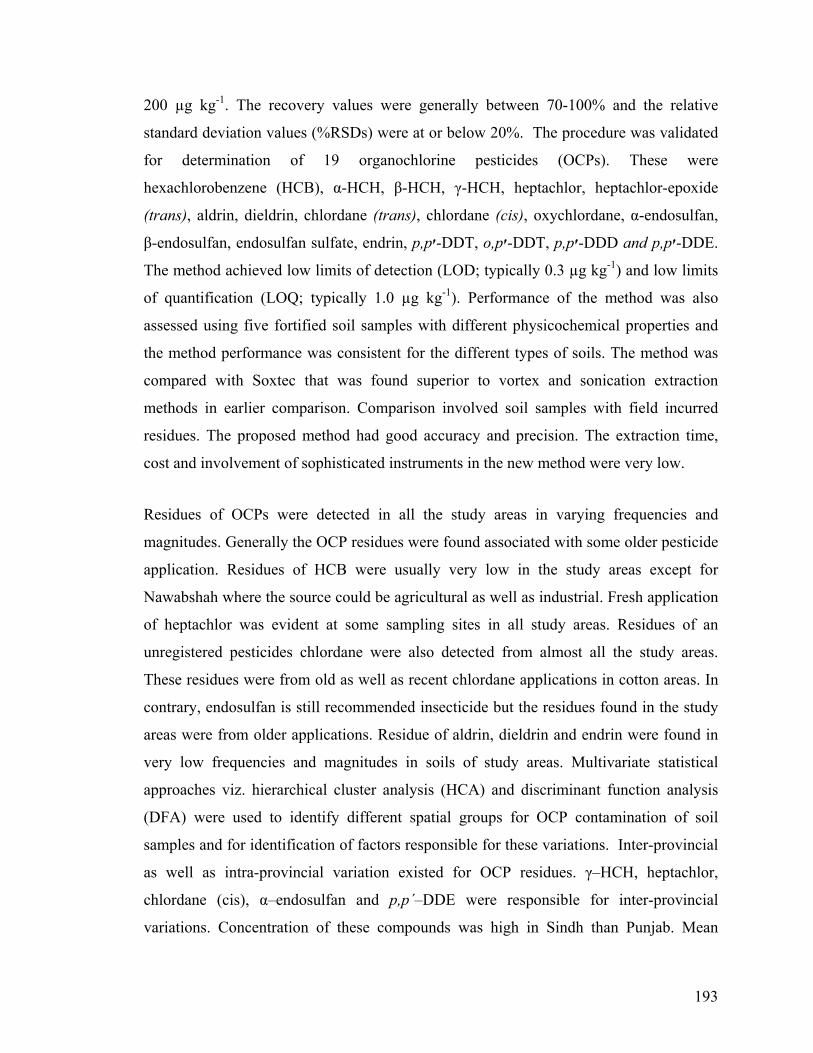
200 µg kg-1. The recovery values were generally between 70-100% and the relative
standard deviation values (%RSDs) were at or below 20%. The procedure was validated
for determination of 19 organochlorine pesticides (OCPs). These were
hexachlorobenzene (HCB), α-HCH, β-HCH, γ-HCH, heptachlor, heptachlor-epoxide
(trans), aldrin, dieldrin, chlordane (trans), chlordane (cis), oxychlordane, α-endosulfan,
β-endosulfan, endosulfan sulfate, endrin, p,p׳-DDT, o,p׳-DDT, p,p׳-DDD and p,p׳-DDE.
The method achieved low limits of detection (LOD; typically 0.3 µg kg-1) and low limits
of quantification (LOQ; typically 1.0 µg kg-1). Performance of the method was also
assessed using five fortified soil samples with different physicochemical properties and
the method performance was consistent for the different types of soils. The method was
compared with Soxtec that was found superior to vortex and sonication extraction
methods in earlier comparison. Comparison involved soil samples with field incurred
residues. The proposed method had good accuracy and precision. The extraction time,
cost and involvement of sophisticated instruments in the new method were very low.
Residues of OCPs were detected in all the study areas in varying frequencies and
magnitudes. Generally the OCP residues were found associated with some older pesticide
application. Residues of HCB were usually very low in the study areas except for
Nawabshah where the source could be agricultural as well as industrial. Fresh application
of heptachlor was evident at some sampling sites in all study areas. Residues of an
unregistered pesticides chlordane were also detected from almost all the study areas.
These residues were from old as well as recent chlordane applications in cotton areas. In
contrary, endosulfan is still recommended insecticide but the residues found in the study
areas were from older applications. Residue of aldrin, dieldrin and endrin were found in
very low frequencies and magnitudes in soils of study areas. Multivariate statistical
approaches viz. hierarchical cluster analysis (HCA) and discriminant function analysis
(DFA) were used to identify different spatial groups for OCP contamination of soil
samples and for identification of factors responsible for these variations. Inter-provincial
as well as intra-provincial variation existed for OCP residues. γ–HCH, heptachlor,
chlordane (cis), α–endosulfan and p,p´–DDE were responsible for inter-provincial
variations. Concentration of these compounds was high in Sindh than Punjab. Mean
193
concentration of OCP residues was 35.5 µg kg-1 in Sindh and 5.23 µg kg-1 in Punjab.
Study areas within Punjab viz. Jhang and Multan were also significantly different from
each other. Owing to γ–HCH, heptachlor, β–endosulfan and p,p´–DDE, where
concentration of these compounds was high in high pesticide use area of Multan and low
in low pesticide use area of Jhang. Multan soils had higher OCP residues with mean 4.2
µg kg-1 than mean OCP residues 2 µg kg-1less in Jhang area soils. Soils from study areas
of Sindh were categorized into three group where residue of HCB, γ–HCH, heptachlor,
β–endosulfan, endosulfan sulphate, o,p´–DDT and p,p´–DDT were responsible for
discriminating among groups. Residue levels were generally high in high pesticide use
areas of Ghotki than those of Nawabshah. In Ghotki area, mean OCP concentration was
26.7 µg kg-1 compared with 20 µg kg-1 in soil samples from Nawabshah.
Magnitude of OCP residues in different spatial groups was also studied in relation to
physicochemical and biological properties of soil. Soil pH, organic matter, sand content
and soil fungal population were negatively associated with amount of OCP residues in
soil. Soils of spatial groups with high OCP residues had relatively lower soil pH, low
organic matter and sand contents and lower fungal populations were observed in these
soils. Soil ECe describing soil salinity and soil clay content were positively associated
with the magnitude of OCP residues in spatial groups. High pesticide spatial groups were
relatively more saline and had high clay content. Interaction of OCP compounds and
breakdown products with different soil properties was also studied. Accumulation of
DDTs, chlordane, heptachlor, aldrin and γ–HCH residues was high in relatively high pH
soils. Due to these reasons residues of these OCPs were low in high alkaline areas of
Punjab than those of Sindh. Soil salinity was also found important in the study and was
negatively associated with endosulfan but accumulation of other OCPs was favored under
saline soil possibly due to relatively low soil pH. Due to this reason, endosulfan residues
were relatively lower and were higher of other OCPs in Sindh than Punjab. Similarly soil
microbial mass also influenced OCPs in soil. Soils of Jhang and Ghotki area were rich in
microbial population than Nawabshah and Multan. Abundance and frequency of bacterial
and fungal populations were positively correlated with each other. The study areas varied
in fungal diversity. Aspergillus was most abundantly and most frequently isolated fungus
194

followed by Rhizopus, Penicillium, Fusarium, Cladosporium, Pseudobotrytis and
Constentinella. Aspergillus was found sensitive to aldrin, endosulfan, chlordane, HCB,
heptachlor and o,p´–DDT and p,p´–DDE. However, positive association of Aspergillus
with the breakdown products of these OCPs suggested its tolerance to the breakdown
products or role in biodegradation of parent OCPs into breakdown products. In contrast,
Penicillium was tolerant to aldrin, endosulfan, chlordane, HCB, heptachlor and o,p´–
DDT and p,p´–DDE. Rhizopus indicated tolerance for HCHs, heptachlor, endosulfan and
sensitive to DDTs, chlordane, endrin, aldrin and dieldrin.
Comparison for pesticide residue status and physicochemical and biological properties of
soil are given in Figure 5.1. The study suggested contamination of soils under cotton
cultivation with OCPs applied over the years for pest management. The occurrence and
concentration of these residues varied depending upon pesticide use intensities in
different areas. Accumulation of these residues was also found dependent upon physical,
chemical and biological properties of soil.
195
(a) (b)
(c) (d)
Figure 5.1 Overview of (a) cumulative organochlorine pesticide residues, (b) physical
properties, (c) chemical properties and (d) mycoflora in soils from different cotton growing areas of Pakistan
196
Chapter 6
RECOMMENDATIONS FOR FUTURE STUDIES
Although, the study was conducted successfully in the cotton growing areas of Pakistan
and status and spatial variations in organochlorine residues with respect to pesticide use,
soil’s physicochemical and biological properties in different areas was studied by using
newly developed analytical approach. Present work can be a way forward for very useful
future studies for the sustainability of agro-ecosystem. In this context, future
recommendations are as follows:
i. Newly developed analytical approach worked well for OCPs in soil matrix. It
is recommended that the new analytical method should also be applied and
validated for other pesticide groups in soil and sediment matrices.
ii. The study was conducted in Miani soil series and cotton growing areas of
Pakistan. It is recommended to conduct similar studies for other soil types and
agro-ecologies. Furthermore, similar studies for other pesticide groups and
other crops are also suggested for future investigations.
iii. Spatial variations of OCPs were fond influenced by many factors. Therefore,
it is suggested that future monitoring studies should be planned keeping in
view various environmental variables.
iv. During the study various microbes with their role in biodegradation of
potentially lethal OCPs. It is recommended that full fledge bioremediation
studies should be planned for pesticides by exploring the potential of these
microbes present in contaminated soils.
197
INVESTIGATIONS ON ORGANOCHLORINE PESTICIDE RESIDUES IN SOILS FROM
COTTON GROWING AREAS OF PAKISTAN
INTRODUCTION
The economy of Pakistan is agro based. Agriculture sector and allied industries contribute 23% to GDP and 60% share to export earnings. About 70% of population directly or indirectly depends upon agriculture for living. Pesticide use in Pakistan has increased from 665 metric tons (MT) at the inception of pesticide business in 1980 to 90676 MT in 2007. According to Ahmad and Poswal, (2000), massive increase in the pesticide use has not necessarily increased yields positively and only estimated 0.1% of the pesticides applied reach their target pest (Pimentel et al., 1991). Pesticides reach soil and water bodies through application, disposal, spill and runoff from plant surface or through incorporation of contaminated crop leftovers (Brown and Hock, 1990). These pesticides are either absorbed by soil components, move away from point of intrusion or go through microbial, chemical and photo degradation. Pesticides can also reach into human food chain by translocation into plant and animals (Tariq et al., 2007).
With the development of cotton industry, cotton became a major recipient of pesticides with 80% share in Pakistan (Tariq at el., 2007). Cotton production is mostly concentrated in Punjab and Sindh provinces, constituting about 2.5 M.ha and consumes major share of pesticides used in Pakistan (Khan, 1998). Among pesticides, organochlorine pesticides (OCPs) have high
environmental persistence and have been used in pest management in Pakistan. Therefore, OCP contaminants in soils under cotton crop were studied. The study aimed to comprehend status of OCP contaminants in relation of pesticide use intensities and agro-ecologies of cotton crop in Pakistan.
OBJECTIVES
1. Investigation of status and spatial variations of OCP residues in soils from cotton growing areas of Pakistan.
2. Investigation for interaction of physical, chemical and biological properties of soil with OCP contaminants in soils of different cotton areas.
RESEARCH PLAN
Residues of 19 OCPs (hexachlorobenzene (HCB), α–HCH, β–HCH, γ–HCH, heptachlor, heptachlor–epoxide (trans), aldrin, dieldrin, chlordane (trans), chlordane (cis), oxychlordane, α–endosulfan, β–endosulfan, endosulfan sulfate, endrin, p,p׳–DDT, o,p׳–DDT, p,p׳–DDD and p,p׳–DDE) were studied in low and high pesticide use intensity areas of Punjab and Sindh. To minimize the effects of soil variation, samples were collected from Miani series soils of Jhang and Multan in Punjab and Nawabshah and Ghotki in Sindh. Jhang and Nawabshah were low pesticide use areas with 0-3 sprays and Multan and Ghotki were high pesticide use areas with 10-12 sprays per cropping season.
Soil samples were analyzed by gas chromatography tandem quadruple mass spectrometry (GC-MS/MS). Multivariate statistical approaches, hierarchical cluster analysis (HCA) and discriminant function analysis (DFA) were used to identify spatial variations and the factors responsible for these variations. Physicochemical and biological properties of soil were also studied in relation to the distribution and magnitude of OCP contaminants in soil.
Chapter 7 BROCHURE FOR POLICY MAKERS
MAJOR OUTCOMES
1. OCP residues were detected in majority of soil samples. High pesticide use areas were more contaminated than low pesticide use areas. Soils of Sindh were more contaminated with OCP residues than soils of Punjab. Mean concentration OCP residues was 35.5 µg kg-1 in Sindh and 5.23 µg kg-1 in Punjab. In Sindh, Ghotki area was more contaminated with mean OCP concentration of 26.7 µg kg-1 compared with 20 µg kg-1 in soil samples from Nawabshah. In Punjab, Multan soils had more OCP residues with mean 4.2 µg kg-1 and less in Jhang soils where mean OCP level was 2 µg kg-1.
2. Generally, higher OCP residues were detected in areas where more pesticides are applied. Soils with high salinity and high clay content favor OCP accumulation. On the other hand low levels of OCPs were found in soils with higher pH, organic matter and sand content.
3. Soil microbial population was low in high contaminated areas. Association of Aspergillus and Penicillium with the parent and breakdown products indicated some possible role of these fungi in the biodegradation of OCP compounds.
198
RECOMMENDATIONS
i. Comprehensive monitoring of pesticide residues should be conducted in different crop ecologies keeping in view biotic and abiotic environmental variables.
ii. High pesticide contaminated areas should be identified and cultivation of food crop, especially exportable food commodities should be avoided in these areas.
iii. Proper regulatory measures should be implemented to avoid further deterioration of these areas and for reclamation of the contaminated lands.
REFERENCES
Ahmad, I. and A. Poswal. 2000. Cotton Integrated Pest Management in Pakistan: Current Status. Country Report presented in Cotton IPM Planning and Curriculum Workshop Organised by FAO, Bangkok, Thailand. February 28-March 2.
Brown, C.L. and W.K. Hock. 1990. The Fate of Pesticides in the environment. Agrichemical Fact Sheet #8, Penn State Cooperative Extension.
Khan, M.S.H. 1998. Pakistan crop protection market. PAPA Bulletin. 9:7-9.
Pimentel, D., A. Greiner and T. Bashore. 1991. Arch Environ Contam Toxicol 21:84–90.
Tariq, M. I., S. Afzal, I. Hussain and N. Sultana. 2007. Environment International 33: 1107–1122.
(a)
(c)
(b)
(d) Figure 7.1: Overview of (a) organochlorine pesticide residues, (b) physical, (c) chemical and (d)
biological properties of soils from different cotton growing areas of Pakistan
199
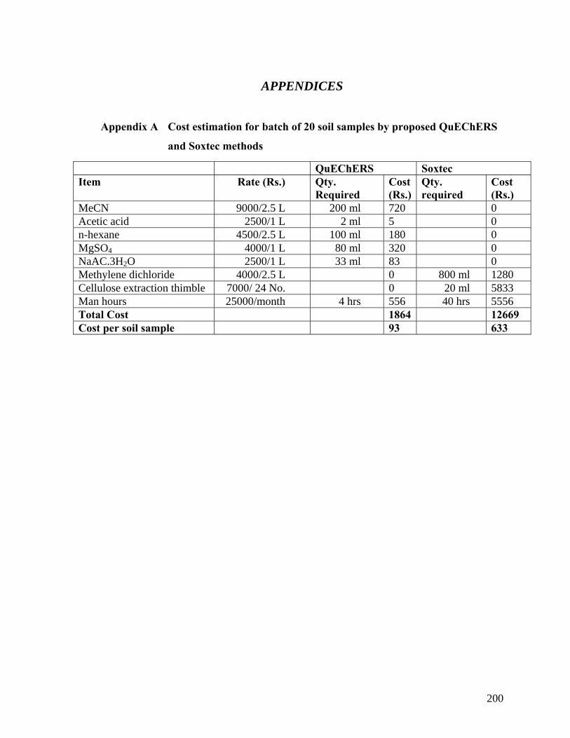
APPENDICES
Appendix A Cost estimation for batch of 20 soil samples by proposed QuEChERS
and Soxtec methods
QuEChERS Soxtec Item Rate (Rs.) Qty.
Required Cost (Rs.)
Qty. required
Cost (Rs.)
MeCN 9000/2.5 L 200 ml 720 0 Acetic acid 2500/1 L 2 ml 5 0 n-hexane 4500/2.5 L 100 ml 180 0 MgSO4 4000/1 L 80 ml 320 0 NaAC.3H2O 2500/1 L 33 ml 83 0 Methylene dichloride 4000/2.5 L 0 800 ml 1280 Cellulose extraction thimble 7000/ 24 No. 0 20 ml 5833 Man hours 25000/month 4 hrs 556 40 hrs 5556 Total Cost 1864 12669 Cost per soil sample 93 633
200
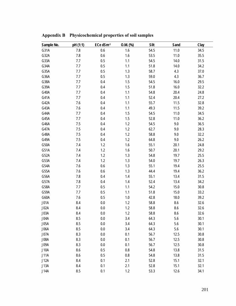
Appendix B Physicochemical properties of soil samples
Sample No. pH (1:1) ECe dSm-1 O.M. (%) Silt Sand Clay G31A 7.8 0.6 1.6 54.5 11.0 34.5 G32A 7.8 0.6 1.6 53.5 11.0 35.5 G33A 7.7 0.5 1.1 54.5 14.0 31.5 G34A 7.7 0.5 1.1 51.8 14.0 34.2 G35A 7.7 0.5 1.3 58.7 4.3 37.0 G36A 7.7 0.5 1.3 59.0 4.3 36.7 G38A 7.7 0.4 1.5 54.5 16.0 29.5 G39A 7.7 0.4 1.5 51.8 16.0 32.2 G40A 7.7 0.4 1.1 54.8 20.4 24.8 G41A 7.7 0.4 1.1 52.4 20.4 27.2 G42A 7.6 0.4 1.1 55.7 11.5 32.8 G43A 7.6 0.4 1.1 49.3 11.5 39.2 G44A 7.7 0.4 1.5 54.5 11.0 34.5 G45A 7.7 0.4 1.5 52.8 11.0 36.2 G46A 7.5 0.4 1.2 54.5 9.0 36.5 G47A 7.5 0.4 1.2 62.7 9.0 28.3 G48A 7.5 0.4 1.2 58.8 9.0 32.2 G49A 7.5 0.4 1.2 64.8 9.0 26.2 G50A 7.4 1.2 1.6 55.1 20.1 24.8 G51A 7.4 1.2 1.6 50.7 20.1 29.2 G52A 7.4 1.2 1.3 54.8 19.7 25.5 G53A 7.4 1.2 1.3 54.0 19.7 26.3 G54A 7.6 0.6 1.3 55.1 19.4 25.5 G55A 7.6 0.6 1.3 44.4 19.4 36.2 G56A 7.8 0.4 1.4 55.1 13.4 31.5 G57A 7.8 0.4 1.4 52.4 13.4 34.2 G58A 7.7 0.5 1.1 54.2 15.0 30.8 G59A 7.7 0.5 1.1 51.8 15.0 33.2 G60A 7.6 0.5 1.0 42.8 18.0 39.2 J01A 8.4 0.0 1.2 58.8 8.6 32.6 J02A 8.4 0.0 1.2 58.8 8.6 32.6 J03A 8.4 0.0 1.2 58.8 8.6 32.6 J04A 8.5 0.0 3.4 64.3 5.6 30.1 J05A 8.5 0.0 3.4 64.3 5.6 30.1 J06A 8.5 0.0 3.4 64.3 5.6 30.1 J07A 8.3 0.0 0.1 56.7 12.5 30.8 J08A 8.3 0.0 0.1 56.7 12.5 30.8 J09A 8.3 0.0 0.1 56.7 12.5 30.8 J10A 8.6 0.5 0.8 54.8 13.8 31.5 J11A 8.6 0.5 0.8 54.8 13.8 31.5 J12A 8.4 0.1 2.1 52.8 15.1 32.1 J13A 8.4 0.1 2.1 52.8 15.1 32.1 J14A 8.5 0.1 1.2 53.3 12.6 34.1
201
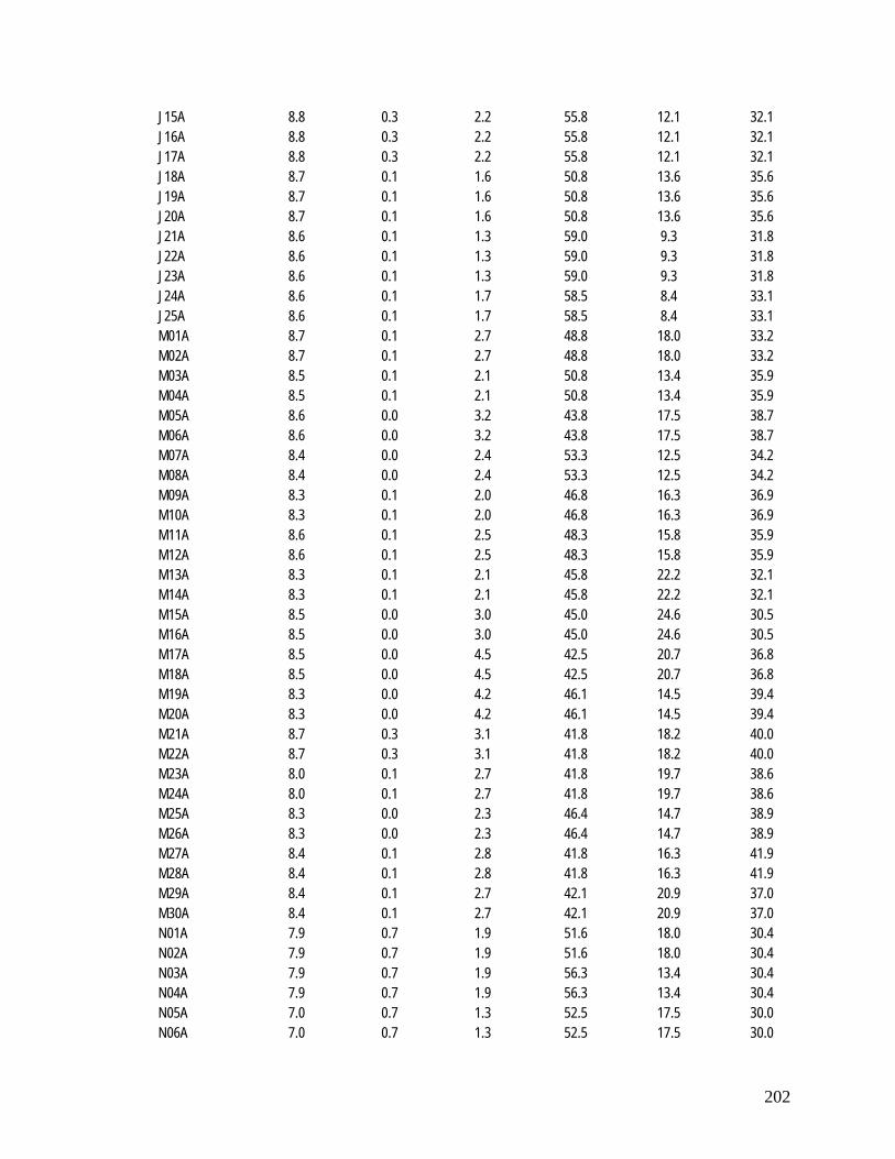
J15A 8.8 0.3 2.2 55.8 12.1 32.1 J16A 8.8 0.3 2.2 55.8 12.1 32.1 J17A 8.8 0.3 2.2 55.8 12.1 32.1 J18A 8.7 0.1 1.6 50.8 13.6 35.6 J19A 8.7 0.1 1.6 50.8 13.6 35.6 J20A 8.7 0.1 1.6 50.8 13.6 35.6 J21A 8.6 0.1 1.3 59.0 9.3 31.8 J22A 8.6 0.1 1.3 59.0 9.3 31.8 J23A 8.6 0.1 1.3 59.0 9.3 31.8 J24A 8.6 0.1 1.7 58.5 8.4 33.1 J25A 8.6 0.1 1.7 58.5 8.4 33.1 M01A 8.7 0.1 2.7 48.8 18.0 33.2 M02A 8.7 0.1 2.7 48.8 18.0 33.2 M03A 8.5 0.1 2.1 50.8 13.4 35.9 M04A 8.5 0.1 2.1 50.8 13.4 35.9 M05A 8.6 0.0 3.2 43.8 17.5 38.7 M06A 8.6 0.0 3.2 43.8 17.5 38.7 M07A 8.4 0.0 2.4 53.3 12.5 34.2 M08A 8.4 0.0 2.4 53.3 12.5 34.2 M09A 8.3 0.1 2.0 46.8 16.3 36.9 M10A 8.3 0.1 2.0 46.8 16.3 36.9 M11A 8.6 0.1 2.5 48.3 15.8 35.9 M12A 8.6 0.1 2.5 48.3 15.8 35.9 M13A 8.3 0.1 2.1 45.8 22.2 32.1 M14A 8.3 0.1 2.1 45.8 22.2 32.1 M15A 8.5 0.0 3.0 45.0 24.6 30.5 M16A 8.5 0.0 3.0 45.0 24.6 30.5 M17A 8.5 0.0 4.5 42.5 20.7 36.8 M18A 8.5 0.0 4.5 42.5 20.7 36.8 M19A 8.3 0.0 4.2 46.1 14.5 39.4 M20A 8.3 0.0 4.2 46.1 14.5 39.4 M21A 8.7 0.3 3.1 41.8 18.2 40.0 M22A 8.7 0.3 3.1 41.8 18.2 40.0 M23A 8.0 0.1 2.7 41.8 19.7 38.6 M24A 8.0 0.1 2.7 41.8 19.7 38.6 M25A 8.3 0.0 2.3 46.4 14.7 38.9 M26A 8.3 0.0 2.3 46.4 14.7 38.9 M27A 8.4 0.1 2.8 41.8 16.3 41.9 M28A 8.4 0.1 2.8 41.8 16.3 41.9 M29A 8.4 0.1 2.7 42.1 20.9 37.0 M30A 8.4 0.1 2.7 42.1 20.9 37.0 N01A 7.9 0.7 1.9 51.6 18.0 30.4 N02A 7.9 0.7 1.9 51.6 18.0 30.4 N03A 7.9 0.7 1.9 56.3 13.4 30.4 N04A 7.9 0.7 1.9 56.3 13.4 30.4 N05A 7.0 0.7 1.3 52.5 17.5 30.0 N06A 7.0 0.7 1.3 52.5 17.5 30.0
202
N07A 7.7 0.4 1.5 53.5 12.5 34.0 N08A 7.7 0.4 1.5 53.5 12.5 34.0 N09A 7.4 0.8 1.4 53.0 16.3 30.7 N10A 7.4 0.8 1.4 53.0 16.3 30.7 N11A 7.6 0.6 1.2 42.2 15.8 42.0 N12A 7.6 0.6 1.2 42.2 15.8 42.0 N13A 7.8 0.5 0.9 47.8 14.2 38.0 N14A 7.8 0.5 0.9 48.1 13.9 38.0 N15A 7.9 4.3 1.6 43.5 17.8 38.7 N16A 7.9 4.3 1.6 47.0 14.3 38.7 N17A 8.2 0.6 1.4 50.0 19.3 30.7 N18A 8.2 0.6 1.4 48.6 20.7 30.7 N19A 8.3 0.6 1.2 55.5 14.5 30.0 N20A 8.3 0.6 1.2 55.5 14.5 30.0 N21A 8.2 0.7 1.4 42.7 18.2 39.1 N22A 8.2 0.7 1.4 43.1 18.2 38.7 N23A 8.3 1.3 1.1 47.4 19.7 33.0 N24A 8.3 1.3 1.1 47.4 19.7 33.0 N25A 7.8 2.5 1.9 48.1 14.7 37.2 N26A 7.8 2.5 1.9 50.1 14.7 35.2 N27A 8.0 0.7 1.3 47.6 16.3 36.1 N28A 8.0 0.7 1.3 45.6 16.3 38.1 N29A 7.7 3.5 1.9 44.0 20.9 35.1 N30A 7.7 3.5 1.9 44.0 20.9 35.1
203
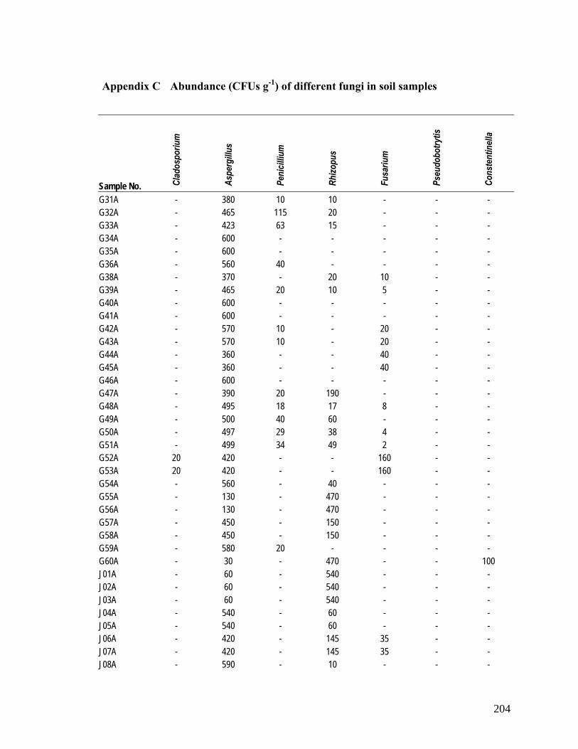
Appendix C Abundance (CFUs g-1) of different fungi in soil samples
Sample No. Clad
ospo
rium
Aspe
rgillu
s
Peni
cilliu
m
Rhizo
pus
Fusa
rium
Pseu
dobo
trytis
Cons
tent
inell
a
G31A - 380 10 10 - - - G32A - 465 115 20 - - - G33A - 423 63 15 - - - G34A - 600 - - - - - G35A - 600 - - - - - G36A - 560 40 - - - - G38A - 370 - 20 10 - - G39A - 465 20 10 5 - - G40A - 600 - - - - - G41A - 600 - - - - - G42A - 570 10 - 20 - - G43A - 570 10 - 20 - - G44A - 360 - - 40 - - G45A - 360 - - 40 - - G46A - 600 - - - - - G47A - 390 20 190 - - - G48A - 495 18 17 8 - - G49A - 500 40 60 - - - G50A - 497 29 38 4 - - G51A - 499 34 49 2 - - G52A 20 420 - - 160 - - G53A 20 420 - - 160 - - G54A - 560 - 40 - - - G55A - 130 - 470 - - - G56A - 130 - 470 - - - G57A - 450 - 150 - - - G58A - 450 - 150 - - - G59A - 580 20 - - - - G60A - 30 - 470 - - 100 J01A - 60 - 540 - - - J02A - 60 - 540 - - - J03A - 60 - 540 - - - J04A - 540 - 60 - - - J05A - 540 - 60 - - - J06A - 420 - 145 35 - - J07A - 420 - 145 35 - - J08A - 590 - 10 - - -
204
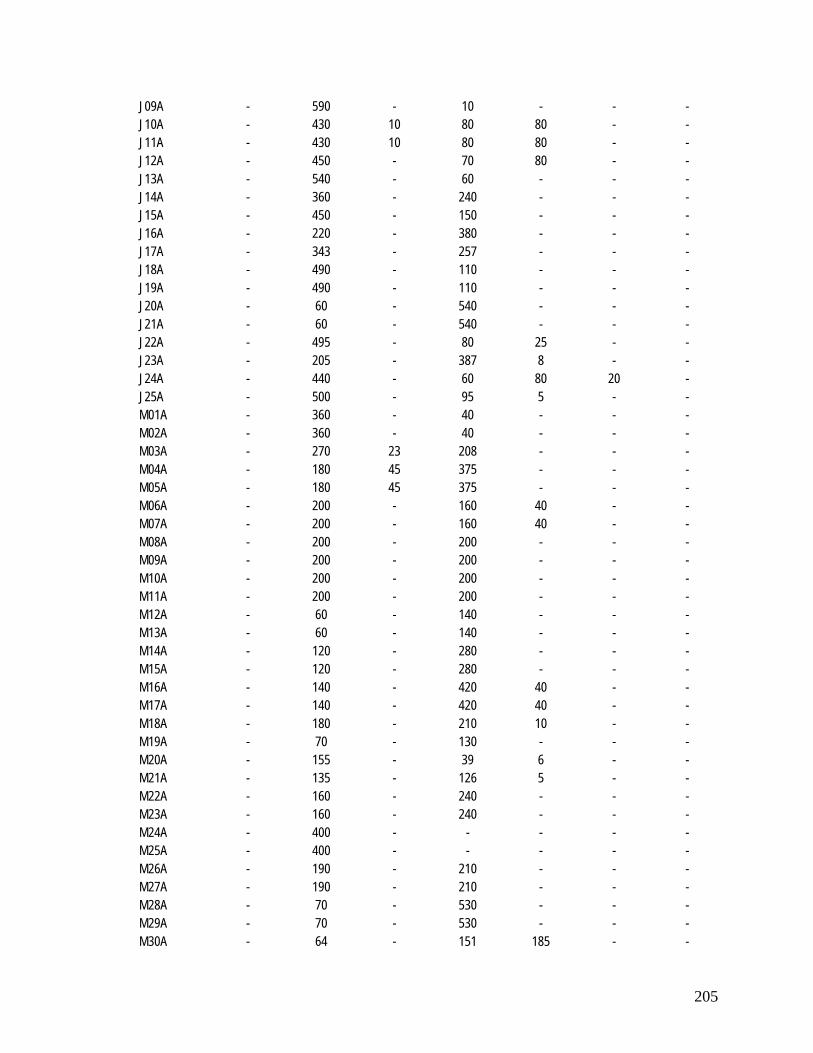
J09A - 590 - 10 - - - J10A - 430 10 80 80 - - J11A - 430 10 80 80 - - J12A - 450 - 70 80 - - J13A - 540 - 60 - - - J14A - 360 - 240 - - - J15A - 450 - 150 - - - J16A - 220 - 380 - - - J17A - 343 - 257 - - - J18A - 490 - 110 - - - J19A - 490 - 110 - - - J20A - 60 - 540 - - - J21A - 60 - 540 - - - J22A - 495 - 80 25 - - J23A - 205 - 387 8 - - J24A - 440 - 60 80 20 - J25A - 500 - 95 5 - - M01A - 360 - 40 - - - M02A - 360 - 40 - - - M03A - 270 23 208 - - - M04A - 180 45 375 - - - M05A - 180 45 375 - - - M06A - 200 - 160 40 - - M07A - 200 - 160 40 - - M08A - 200 - 200 - - - M09A - 200 - 200 - - - M10A - 200 - 200 - - - M11A - 200 - 200 - - - M12A - 60 - 140 - - - M13A - 60 - 140 - - - M14A - 120 - 280 - - - M15A - 120 - 280 - - - M16A - 140 - 420 40 - - M17A - 140 - 420 40 - - M18A - 180 - 210 10 - - M19A - 70 - 130 - - - M20A - 155 - 39 6 - - M21A - 135 - 126 5 - - M22A - 160 - 240 - - - M23A - 160 - 240 - - - M24A - 400 - - - - - M25A - 400 - - - - - M26A - 190 - 210 - - - M27A - 190 - 210 - - - M28A - 70 - 530 - - - M29A - 70 - 530 - - - M30A - 64 - 151 185 - -
205
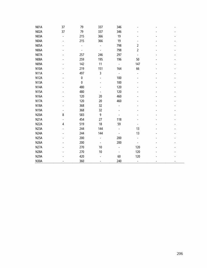
206
N01A 37 79 337 346 - - - N02A 37 79 337 346 - - - N03A - 215 366 19 - - - N04A - 215 366 19 - - - N05A - - - 798 2 - - N06A - - - 798 2 - - N07A - 257 246 297 - - - N08A - 259 195 196 50 - - N09A - 142 11 - 147 - - N10A - 219 151 164 66 - - N11A - 497 3 - - - - N12A - 0 - 100 - - - N13A - 0 - 100 - - - N14A - 480 - 120 - - - N15A - 480 - 120 - - - N16A - 120 20 460 - - - N17A - 120 20 460 - - - N18A - 368 32 - - - - N19A - 368 32 - - - - N20A 8 583 9 - - - - N21A - 454 27 118 - - - N22A 4 519 18 59 - - - N23A - 244 144 - 13 - - N24A - 244 144 - 13 - - N25A - 200 - 200 - - - N26A - 200 - 200 - - - N27A - 270 10 - 120 - - N28A - 270 10 - 120 - - N29A - 420 - 60 120 - - N30A - 360 - 240 - - -
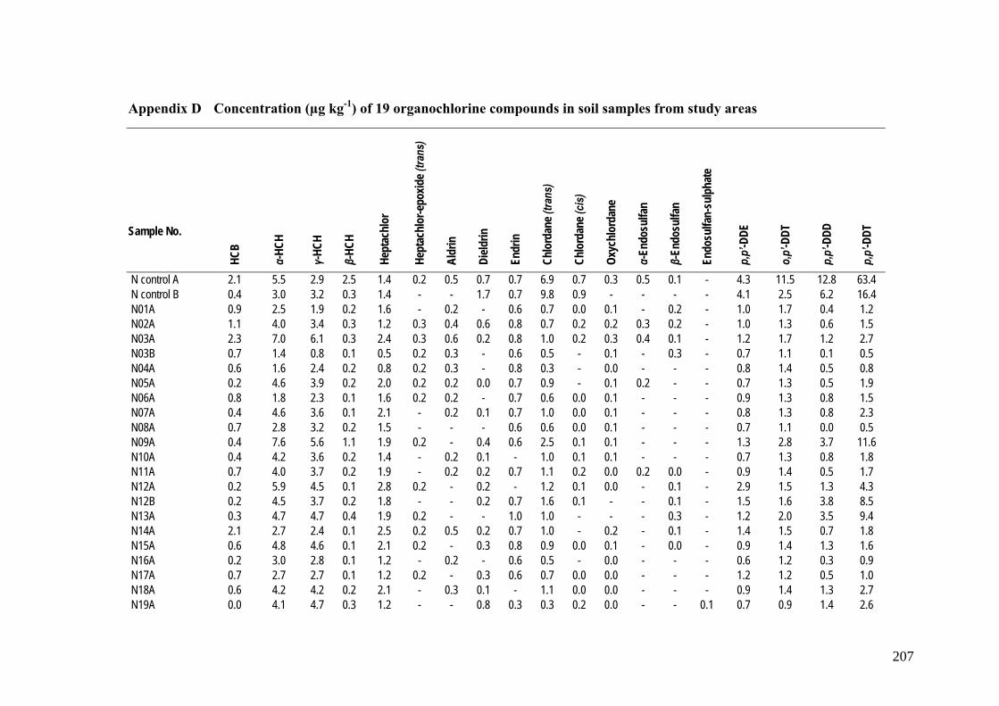
Appendix D Concentration (µg kg-1) of 19 organochlorine compounds in soil samples from study areas
Sample No.
HCB
α-HC
H
γ-HC
H
β-HC
H
Hept
achl
or
Hept
achl
or-e
poxid
e (tra
ns)
Aldr
in
Dield
rin
Endr
in
Chlo
rdan
e (tra
ns)
Chlo
rdan
e (cis
)
Oxyc
hlor
dane
α-En
dosu
lfan
β-En
dosu
lfan
Endo
sulfa
n-su
lpha
te
p,p’
-DDE
o,p’
-DDT
p,p’
-DDD
p,p’
-DDT
N control A 2.1 5.5 2.9 2.5 1.4 0.2 0.5 0.7 0.7 6.9 0.7 0.3 0.5 0.1 - 4.3 11.5 12.8 63.4 N control B
0.4 3.0 3.2 0.3 1.4 - - 1.7 0.7 9.8 0.9 - - - - 4.1 2.5 6.2 16.4
N01A 0.9 0.7
2.5 1.9 0.2 1.6 - 0.2 - 0.6 0.7 0.0 0.1 - 0.2 - 1.0 1.7 0.4 1.2 N02A 1.1 4.0 3.4 0.3 1.2 0.3 0.4 0.6 0.8 0.7 0.2 0.2 0.3 0.2 - 1.0 1.3 0.6 1.5 N03A 2.3 7.0 6.1 0.3 2.4 0.3 0.6 0.2 0.8 1.0 0.2 0.3 0.4 0.1 - 1.2 1.7 1.2 2.7 N03B 0.7 1.4 0.8 0.1 0.5 0.2 0.3 - 0.6 0.5 - 0.1 - 0.3 - 0.7 1.1 0.1 0.5 N04A 0.6 1.6 2.4 0.2 0.8 0.2 0.3 - 0.8 0.3 - 0.0 - - - 0.8 1.4 0.5 0.8 N05A 0.2 4.6 3.9 0.2 2.0 0.2 0.2 0.0
0.7 0.9 - 0.1 0.2
- - 0.7 1.3 0.5 1.9
N06A 0.8 1.8 2.3 0.1 1.6 0.2
0.2 - 0.7 0.6 0.0 0.1 - - - 0.9 1.3 0.8 1.5 N07A 0.4 4.6 3.6 0.1 2.1 - 0.2 0.1 0.7 1.0 0.0 0.1 - - - 0.8 1.3 0.8 2.3 N08A 0.7 2.8 3.2 0.2 1.5 - - - 0.6 0.6 0.0 0.1 - - - 0.7 1.1 0.0 0.5 N09A 0.4 7.6 5.6 1.1 1.9 0.2
- 0.4 0.6
2.5 0.1 0.1 - - - 1.3 2.8 3.7 11.6
N10A 0.4 4.2 3.6 0.2 1.4 - 0.2 0.1 - 1.0 0.1 0.1 - - - 0.7 1.3 0.8 1.8 N11A 0.7 4.0 3.7 0.2 1.9 - 0.2 0.2 0.7 1.1 0.2 0.0 0.2 0.0 - 0.9 1.4 0.5 1.7 N12A 0.2 5.9 4.5 0.1 2.8 0.2 - 0.2 - 1.2 0.1 0.0 - 0.1 - 2.9 1.5 1.3 4.3 N12B 0.2 4.5 3.7 0.2 1.8 - - 0.2 0.7 1.6 0.1 - - 0.1 - 1.5 1.6 3.8 8.5 N13A 0.3 4.7 4.7 0.4 1.9 0.2 - - 1.0 1.0 - - - 0.3 - 1.2 2.0 3.5 9.4 N14A 2.1 2.7 2.4 0.1 2.5 0.2 0.5
0.2 0.7 1.0 - 0.2 - 0.1 - 1.4 1.5 0.7 1.8
N15A 0.6 4.8 4.6 0.1 2.1 0.2 - 0.3 0.8 0.9 0.0 0.1 - 0.0 - 0.9 1.4 1.3 1.6 N16A 0.2 3.0 2.8 0.1 1.2 - 0.2
- 0.6 0.5 - 0.0 - - - 0.6 1.2 0.3 0.9
N17A 0.7 2.7 2.7 0.1 1.2 0.2
- 0.3 0.6
0.0 0.0 - - - 1.2 1.2 0.5 1.0 N18A 0.6 4.2 4.2 0.2 2.1 - 0.3
0.1 - 1.1 0.0 0.0 - - - 0.9 1.4 1.3 2.7
N19A 0.0 4.1 4.7 0.3 1.2 - - 0.8 0.3 0.3 0.2 0.0 - - 0.1 0.7 0.9 1.4 2.6
207
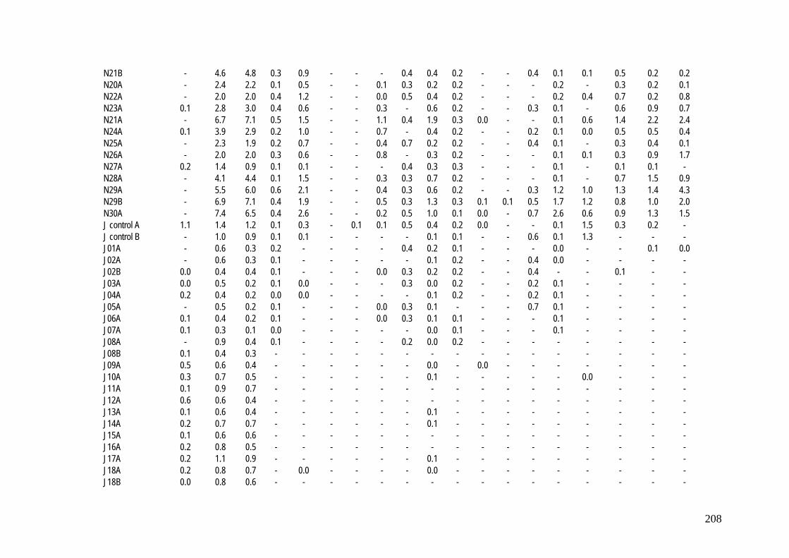
N21B
- 4.6 4.8 0.3 0.9 - - - 0.4 0.4 0.2 - - 0.4 0.1 0.1 0.5 0.2 0.2 N20A - 2.4 2.2 0.1 0.5 - - 0.1 0.3 0.2 0.2 - - - 0.2 - 0.3 0.2 0.1 N22A - 2.0 2.0 0.4 1.2 - - 0.0 0.5 0.4 0.2 - - - 0.2 0.4 0.7 0.2 0.8 N23A 0.1
2.8 3.0 0.4 0.6 - - 0.3 - 0.6 0.2 - - 0.3
0.1 - 0.6 0.9 0.7
N21A - 6.7 7.1 0.5 1.5 - - 1.1 0.4 1.9 0.3 0.0 - - 0.1 0.6 1.4 2.2 2.4 N24A 0.1 3.9 2.9 0.2 1.0 - - 0.7 - 0.4 0.2 - - 0.2 0.1 0.0 0.5 0.5 0.4 N25A - 2.3 1.9 0.2 0.7 - - 0.4 0.7 0.2 0.2 - - 0.4 0.1 - 0.3 0.4 0.1 N26A - 2.0 2.0 0.3 0.6 - - 0.8 - 0.3 0.2 - - - 0.1 0.1 0.3 0.9 1.7 N27A 0.2 1.4 0.9 0.1 0.1 - - - 0.4 0.3 0.3 - - - 0.1 - 0.1 0.1 - N28A - 4.1 4.4 0.1 1.5 - - 0.3 0.3 0.7 0.2 - - - 0.1 - 0.7 1.5 0.9 N29A - 5.5 6.0 0.6 2.1 - - 0.4 0.3 0.6 0.2 - - 0.3 1.2 1.0 1.3 1.4 4.3 N29B - 6.9 7.1 0.4 1.9 - - 0.5 0.3 1.3 0.3 0.1 0.1
0.5 1.7 1.2 0.8 1.0 2.0
N30A - 7.4 6.5 0.4 2.6 - - 0.2 0.5 1.0 0.1 0.0 - 0.7 2.6 0.6 0.9 1.3 1.5 J control A 1.1 1.4 1.2 0.1 0.3 - 0.1 0.1 0.5 0.4 0.2 0.0 - - 0.1 1.5 0.3 0.2 - J control B
- 1.0 0.9 0.1 0.1 - - - - 0.1 0.1 - - 0.6 0.1 1.3 - - -
J01A - 0.6 0.3 0.2 - - - - 0.4 0.2 0.1 - - - 0.0 - - 0.1 0.0 J02A - 0.6 0.3 0.1 - - - - - 0.1 0.2 - - 0.4 0.0 - - - - J02B 0.0 0.4 0.4 0.1 - - - 0.0 0.3 0.2 0.2 - - 0.4 - - 0.1 - - J03A 0.0 0.5 0.2 0.1 0.0 - - - 0.3 0.0 0.2 - - 0.2 0.1 - - - - J04A 0.2 0.4 0.2 0.0 0.0 - - - - 0.1 0.2 - - 0.2 0.1 - - - - J05A - 0.5 0.2 0.1 - - - 0.0 0.3 0.1 - - - 0.7 0.1 - - - - J06A 0.1 0.4 0.2 0.1 - - - 0.0 0.3 0.1 0.1 - - - 0.1 - - - - J07A 0.1 0.3 0.1 0.0 - - - - - 0.0 0.1 - - - 0.1 - - - - J08A - 0.9 0.4 0.1 - - - - 0.2 0.0 0.2 - - - - - - - - J08B 0.1 0.4 0.3 - - - - - - - - - - - - - - - - J09A 0.5 0.6 0.4 - - - - - - 0.0 - 0.0 - - - - - - - J10A 0.3 0.7 0.5 - - - - - - 0.1 - - - - - 0.0 - - - J11A 0.1 0.9 0.7 - - - - - - - - - - - - - - - - J12A 0.6 0.6 0.4 - - - - - - - - - - - - - - - - J13A 0.1 0.6 0.4 - - - - - - 0.1 - - - - - - - - - J14A 0.2 0.7 0.7 - - - - - - 0.1 - - - - - - - - - J15A 0.1 0.6 0.6 - - - - - - - - - - - - - - - - J16A 0.2 0.8 0.5 - - - - - - - - - - - - - - - - J17A 0.2 1.1 0.9 - - - - - - 0.1 - - - - - - - - - J18A 0.2 0.8 0.7 - 0.0 - - - - 0.0 - - - - - - - - - J18B 0.0 0.8 0.6 - - - - - - - - - - - - - - - -
208
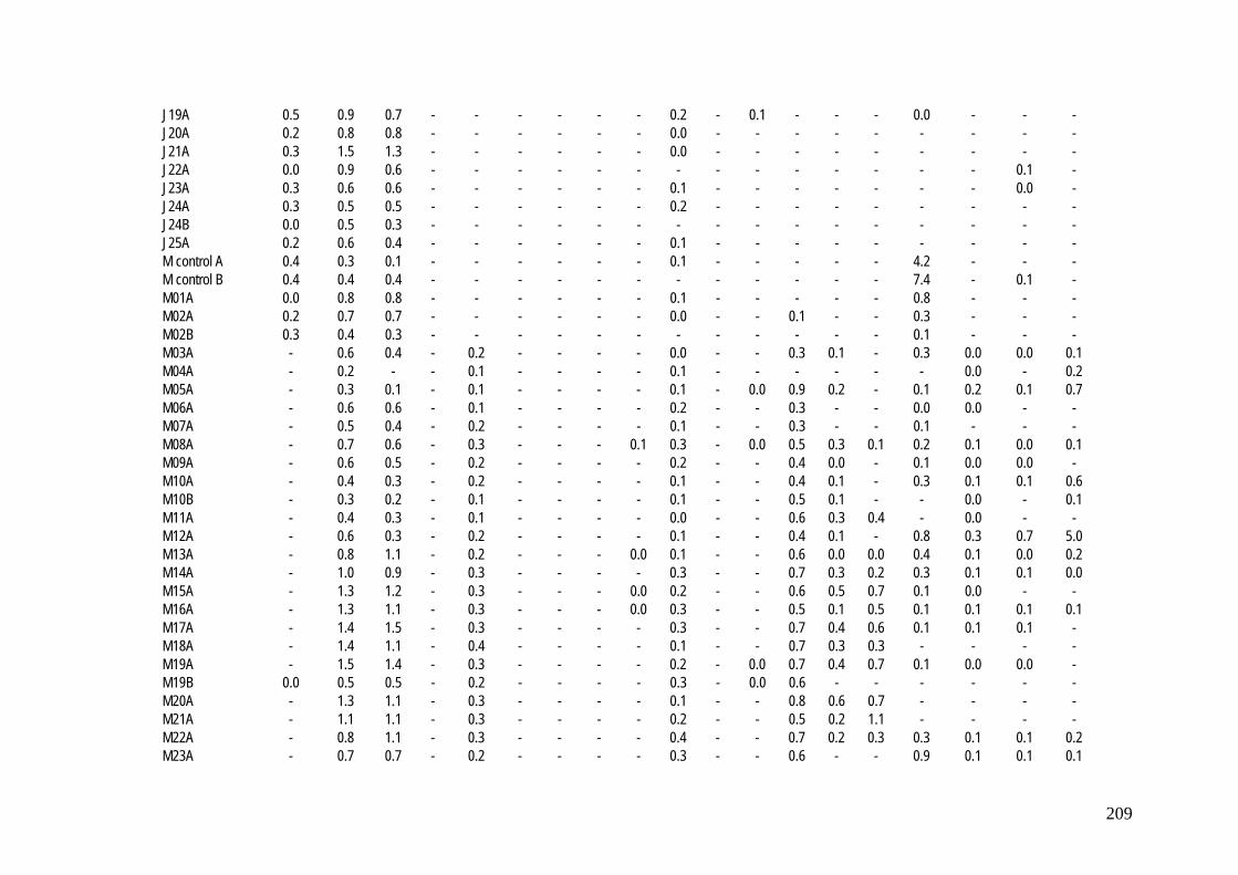
J19A
0.5 0.9 0.7 - - - - - - 0.2 - 0.1 - - - 0.0 - - - J20A 0.2 0.8 0.8 - - - - - - 0.0 - - - - - - - - - J21A 0.3 1.5 1.3 - - - - - - 0.0 - - - - - - - - - J22A 0.0 0.9 0.6 - - - - - - - - - - - - - - 0.1 - J23A 0.3 0.6 0.6 - - - - - - 0.1 - - - - - - - 0.0 - J24A 0.3 0.5 0.5 - - - - - - 0.2 - - - - - - - - - J24B 0.0 0.5 0.3 - - - - - - - - - - - - - - - - J25A 0.2 0.6 0.4 - - - - - - 0.1 - - - - - - - - - M control A 0.4 0.3 0.1 - - - - - - 0.1 - - - - - 4.2 - - - M control B
0.4 0.4 0.4 - - - - - - - - - - - - 7.4 - 0.1 -
M01A 0.0 0.8 0.8 - - - - - - 0.1 - - - - - 0.8 - - - M02A 0.2 0.7 0.7 - - - - - - 0.0 - - 0.1 - - 0.3 - - - M02B 0.3 0.4 0.3 - - - - - - - - - - - - 0.1 - - - M03A - 0.6 0.4 - 0.2 - - - - 0.0 - - 0.3 0.1 - 0.3 0.0 0.0 0.1 M04A - 0.2 - - 0.1 - - - - 0.1 - - - - - - 0.0 - 0.2 M05A - 0.3 0.1 - 0.1 - - - - 0.1 - 0.0 0.9 0.2 - 0.1 0.2 0.1 0.7 M06A - 0.6 0.6 - 0.1 - - - - 0.2 - - 0.3 - - 0.0 0.0 - - M07A - 0.5 0.4 - 0.2 - - - - 0.1 - - 0.3 - - 0.1 - - - M08A - 0.7 0.6 - 0.3 - - - 0.1 0.3 - 0.0 0.5 0.3 0.1 0.2 0.1 0.0 0.1 M09A - 0.6 0.5 - 0.2 - - - - 0.2 - - 0.4 0.0 - 0.1 0.0 0.0 - M10A - 0.4 0.3 - 0.2 - - - - 0.1 - - 0.4 0.1 - 0.3 0.1 0.1 0.6 M10B - 0.3 0.2 - 0.1 - - - - 0.1 - - 0.5 0.1 - - 0.0 - 0.1 M11A - 0.4 0.3 - 0.1 - - - - 0.0 - - 0.6 0.3 0.4 - 0.0 - - M12A - 0.6 0.3 - 0.2 - - - - 0.1 - - 0.4 0.1 - 0.8 0.3 0.7 5.0 M13A - 0.8 1.1 - 0.2 - - - 0.0 0.1 - - 0.6 0.0 0.0 0.4 0.1 0.0 0.2 M14A - 1.0 0.9 - 0.3 - - - - 0.3 - - 0.7 0.3 0.2 0.3 0.1 0.1 0.0 M15A - 1.3 1.2 - 0.3 - - - 0.0 0.2 - - 0.6 0.5 0.7 0.1 0.0 - - M16A - 1.3 1.1 - 0.3 - - - 0.0 0.3 - - 0.5 0.1 0.5 0.1 0.1 0.1 0.1 M17A - 1.4 1.5 - 0.3 - - - - 0.3 - - 0.7 0.4 0.6 0.1 0.1 0.1 - M18A - 1.4 1.1 - 0.4 - - - - 0.1 - - 0.7 0.3 0.3 - - - - M19A - 1.5 1.4 - 0.3 - - - - 0.2 - 0.0 0.7 0.4 0.7 0.1 0.0 0.0 - M19B 0.0 0.5 0.5 - 0.2 - - - - 0.3 - 0.0 0.6 - - - - - - M20A - 1.3 1.1 - 0.3 - - - - 0.1 - - 0.8 0.6 0.7 - - - - M21A - 1.1 1.1 - 0.3 - - - - 0.2 - - 0.5 0.2 1.1 - - - - M22A - 0.8 1.1 - 0.3 - - - - 0.4 - - 0.7 0.2 0.3 0.3 0.1 0.1 0.2 M23A - 0.7 0.7 - 0.2 - - - - 0.3 - - 0.6 - - 0.9 0.1 0.1 0.1
209
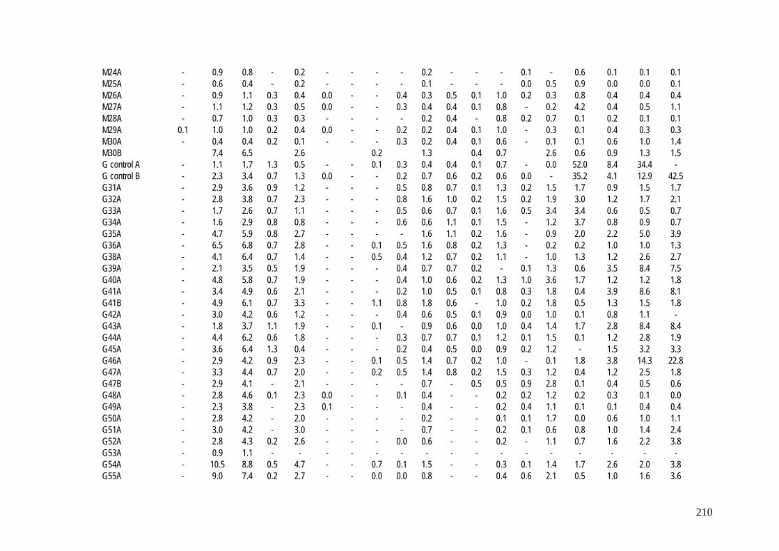
M24A
- 0.9 0.8 - 0.2 - - - - 0.2 - - - 0.1 - 0.6 0.1 0.1 0.1 M25A - 0.6 0.4 - 0.2 - - - - 0.1 - - - 0.0 0.5 0.9 0.0 0.0 0.1 M26A - 0.9 1.1 0.3 0.4 0.0 - - 0.4 0.3 0.5 0.1 1.0 0.2
0.3 0.8 0.4 0.4 0.4
M27A - 1.1 1.2 0.3 0.5 0.0
- - 0.3
0.4 0.4 0.1
0.8 - 0.2 4.2 0.4 0.5 1.1 M28A - 0.7 1.0 0.3 0.3 - - - - 0.2 0.4 - 0.8 0.2
0.7 0.1 0.2 0.1 0.1
M29A 0.1
1.0 1.0 0.2 0.4 0.0
- - 0.2 0.2 0.4 0.1 1.0 - 0.3 0.1 0.4 0.3 0.3 M30A - 0.4 0.4 0.2
0.1 - - - 0.3 0.2 0.4 0.1 0.6 - 0.1 0.1 0.6 1.0 1.4
M30B 7.4 6.5 2.6 0.2 1.3 0.4 0.7 2.6 0.6 0.9 1.3 1.5 G control A - 1.1 1.7 1.3 0.5 - - 0.1 0.3 0.4 0.4 0.1 0.7 - 0.0 52.0 8.4 34.4 - G control B
- 2.3 3.4 0.7 1.3 0.0
- - 0.2 0.7 0.6 0.2 0.6 0.0 - 35.2 4.1 12.9 42.5
G31A - 2.9 3.6 0.9 1.2 - - - 0.5 0.8 0.7 0.1 1.3 0.2 1.5 1.7 0.9 1.5 1.7 G32A - 2.8 3.8 0.7 2.3 - - - 0.8 1.6 1.0 0.2 1.5 0.2 1.9 3.0 1.2 1.7 2.1 G33A - 1.7 2.6 0.7 1.1 - - - 0.5 0.6 0.7 0.1 1.6 0.5
3.4 3.4 0.6 0.5 0.7
G34A - 1.6 2.9 0.8 0.8 - - - 0.6 0.6 1.1 0.1 1.5 - 1.2 3.7 0.8 0.9 0.7 G35A - 4.7 5.9 0.8 2.7 - - - - 1.6 1.1 0.2 1.6 - 0.9 2.0 2.2 5.0 3.9 G36A - 6.5 6.8 0.7 2.8 - - 0.1 0.5 1.6 0.8 0.2 1.3 - 0.2 0.2 1.0 1.0 1.3 G38A - 4.1 6.4 0.7 1.4 - - 0.5
0.4 1.2 0.7 0.2 1.1
- 1.0 1.3 1.2 2.6 2.7
G39A - 2.1 3.5 0.5 1.9 - - - 0.4 0.7 0.7 0.2 - 0.1 1.3 0.6 3.5 8.4 7.5 G40A - 4.8 5.8 0.7 1.9 - - - 0.4 1.0 0.6 0.2 1.3 1.0 3.6 1.7 1.2 1.2 1.8 G41A - 3.4 4.9 0.6 2.1 - - - 0.2 1.0 0.5 0.1
0.8 0.3 1.8 0.4 3.9 8.6 8.1
G41B - 4.9 6.1 0.7 3.3 - - 1.1
0.8 1.8 0.6 - 1.0 0.2 1.8 0.5 1.3 1.5 1.8 G42A - 3.0 4.2 0.6 1.2 - - - 0.4
0.6 0.5 0.1 0.9 0.0 1.0 0.1 0.8 1.1 -
G43A - 1.8 3.7 1.1 1.9 - - 0.1
- 0.9 0.6 0.0 1.0 0.4 1.4 1.7 2.8 8.4 8.4 G44A - 4.4 6.2 0.6 1.8 - - - 0.3 0.7 0.7 0.1 1.2 0.1 1.5 0.1
1.2 2.8 1.9
G45A - 3.6 6.4 1.3 0.4 - - - 0.2 0.4 0.5 0.0 0.9 0.2
1.2 - 1.5 3.2 3.3 G46A - 2.9 4.2 0.9 2.3 - - 0.1 0.5 1.4 0.7 0.2 1.0 - 0.1 1.8 3.8 14.3 22.8 G47A - 3.3 4.4 0.7 2.0 - - 0.2 0.5 1.4 0.8 0.2 1.5 0.3 1.2 0.4 1.2 2.5 1.8 G47B - 2.9 4.1 - 2.1 - - - - 0.7 - 0.5 0.5 0.9 2.8 0.1 0.4 0.5 0.6 G48A - 2.8 4.6 0.1 2.3 0.0 - - 0.1 0.4 - - 0.2 0.2 1.2 0.2 0.3 0.1 0.0 G49A - 2.3 3.8 - 2.3 0.1 - - - 0.4 - - 0.2 0.4 1.1 0.1 0.1 0.4 0.4 G50A - 2.8 4.2 - 2.0 - - - - 0.2 - - 0.1 0.1 1.7 0.0 0.6 1.0 1.1 G51A - 3.0 4.2 - 3.0 - - - - 0.7 - - 0.2 0.1 0.6 0.8 1.0 1.4 2.4 G52A - 2.8 4.3 0.2 2.6 - - - 0.0 0.6 - - 0.2 - 1.1 0.7 1.6 2.2 3.8 G53A - 0.9 1.1 - - - - - - - - - - - - - - - - G54A - 10.5 8.8 0.5 4.7 - - 0.7 0.1 1.5 - - 0.3 0.1 1.4 1.7 2.6 2.0 3.8 G55A - 9.0 7.4 0.2 2.7 - - 0.0 0.0 0.8 - - 0.4 0.6 2.1 0.5 1.0 1.6 3.6
210
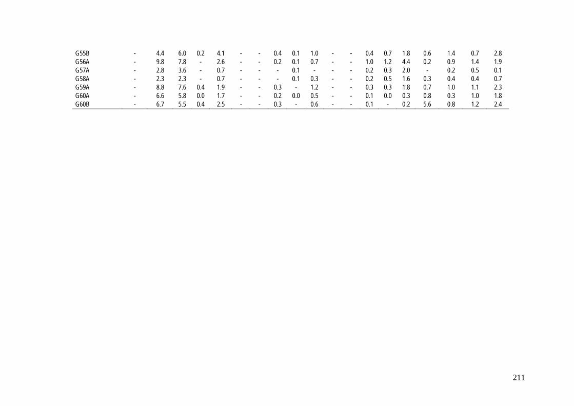
G55B
- 4.4 6.0 0.2
4.1 - - 0.4 0.1 1.0 - - 0.4 0.7 1.8 0.6 1.4 0.7 2.8 G56A - 9.8 7.8 - 2.6 - - 0.2 0.1 0.7 - - 1.0 1.2 4.4 0.2 0.9 1.4 1.9 G57A - 2.8 3.6 - 0.7 - - - 0.1 - - - 0.2 0.3 2.0 - 0.2 0.5 0.1 G58A - 2.3 2.3 - 0.7 - - - 0.1 0.3 - - 0.2 0.5 1.6 0.3 0.4 0.4 0.7 G59A - 8.8 7.6 0.4 1.9 - - 0.3 - 1.2 - - 0.3 0.3 1.8 0.7 1.0 1.1 2.3 G60A - 6.6 5.8 0.0 1.7 - - 0.2 0.0 0.5 - - 0.1 0.0 0.3 0.8 0.3 1.0 1.8 G60B - 6.7 5.5 0.4 2.5 - - 0.3 - 0.6 - - 0.1 - 0.2 5.6 0.8 1.2 2.4
211

212
Appendix E Chromatogram of 19 organochlorine pesticides for matrix matched calibration solution (0.1 µg ml-1 ≡ 28 µg kg-1)


