Embed Size (px)
Citation preview
1
NATIONAL OPEN UNIVERSITY OF NIGERIA
INTRODUCTION TO ECONOMETRICS I ECO 355
SCHOOL OF ARTS AND SOCIAL SCIENCES
COURSE GUIDE
Course Developer:
Samuel Olumuyiwa Olusanya
Economics Department,
National Open University of Nigeria
And
Adegbola Benjamin Mufutau Part time Lecturer
Lagos State University,
Lagos State.
2
CONTENT
Introduction
Course Content
Course Aims
Course Objectives
Working through This Course
Course Materials
Study Units
Textbooks and References
Assignment File
Presentation Schedule
Assessment
Tutor-Marked Assignment (TMAs)
Final Examination and Grading
Course Marking Scheme
Course Overview
How to Get the Most from This Course
Tutors and Tutorials
Summary
Introduction
Welcome to ECO: 355 INTRODUCTION TO ECONOMETRICS I.
ECO 355: Introduction to Econometrics I is a three-credit and one-semester
undergraduate course for Economics student. The course is made up of nineteen units
spread across fifteen lectures weeks. This course guide gives you an insight to
introduction to econometrics and how it is applied in economics. It tells you about the
course materials and how you can work your way through these materials. It suggests
some general guidelines for the amount of time required of you on each unit in order to
achieve the course aims and objectives successfully. Answers to your tutor marked
assignments (TMAs) are therein already.
Course Content
This course is basically an introductory course on Econometrics. The topics covered
include the econometrics analysis, single-equation (regression models), Normal linear
regression model and practical aspects of statistics testing.
Course Aims
The aims of this course is to give you in-depth understanding of the macroeconomics as
regards
Fundamental concept of econometrics
To familiarize students with single-equation of regression model
3
To stimulate student‘s knowledge on normal linear regression model
To make the students to understand some of the practical aspects of econometrics
test.
To expose the students to rudimentary analysis of simple and multiple regression
analysis.
Course Objectives
To achieve the aims of this course, there are overall objectives which the course is out to
achieve though, there are set out objectives for each unit. The unit objectives are included
at the beginning of a unit; you should read them before you start working through the
unit. You may want to refer to them during your study of the unit to check on your
progress. You should always look at the unit objectives after completing a unit. This is to
assist the students in accomplishing the tasks entailed in this course. In this way, you can
be sure you have done what was required of you by the unit. The objectives serves as
study guides, such that student could know if he is able to grab the knowledge of each
unit through the sets of objectives in each one. At the end of the course period, the
students are expected to be able to:
to understand the basic fundamentals of Econometrics
distinguish between Econometrics and Statistics.
know how the econometrician proceed in the analysis of an economic problem.
know how the econometrician make use of both mathematical and statistical
analysis in solving economic problems.
understand the role of computer in econometrics analysis
identify/explain the types of econometrics analysis.
understand the basic Econometrics models
differentiate between Econometrics theory and methods
know the meaning of Econometrics and why Econometrics is important within
Economics.
know how to use Econometrics for Assessing Economic Model
understand what is Financial Econometrics.
examine the linear regression model
understand the classical linear regression model
be able to differentiate the dependant and independent variables.
prove some of the parameters of ordinary least estimate.
4
know the alternative expression for
understand the assumptions of classical linear regression model.
know the properties that our estimators should have
know the proofing of the OLS estimators as the best linear unbiased estimators
(BLUE).
examine the Goodness fit
understand and work through the calculation of coefficient of multiple
determination
identify and know how to calculate the probability normality assumption for Ui
understand the normality assumption for Ui
understand why we have to conduct the normality assumption.
identify the properties of OLS estimators under the normality assumption
understand what is probability distribution
understand the meaning of Maximum Likelihood Estimation of two variable
regression Model.
understand the meaning of Hypothesis
know how to calculate hypothesis using confidence interval
analyse and interpret hypothesis result.
understand the meaning of accepting and rejecting an hypothesis
identify a null and alternative hypothesis.
understand the meaning of Level of significance
understand the Choice between confidence-interval and test-of-significance
Approaches to hypothesis testing
understand the meaning of regression analysis and variance
know how to calculate the regression analysis and analysis of variance
Working Through The Course
To successfully complete this course, you are required to read the study units, referenced
books and other materials on the course.
Each unit contains self-assessment exercises called Student Assessment Exercises (SAE).
At some points in the course, you will be required to submit assignments for assessment
purposes. At the end of the course there is a final examination. This course should take
about 15weeks to complete and some components of the course are outlined under the
course material subsection.
5
Course Material
The major component of the course, What you have to do and how you should allocate
your time to each unit in order to complete the course successfully on time are listed
follows:
1. Course guide
2. Study unit
3. Textbook
4. Assignment file
5. Presentation schedule
Study Unit
There are 19 units in this course which should be studied carefully and diligently.
MODULE ONE ECONOMETRICS ANALYSIS
Unit 1 Meaning Of Econometrics
Unit 2 Methodology of Econometrics
Unit 3 Computer and Econometrics
Unit 4 Basic Econometrics Models: Linear Regression
Unit 5 Importance Of Econometrics
MODULE TWO SINGLE- EQUATION (REGRESSION MODELS)
Unit One: Regression Analysis
Unit Two: The Ordinary Least Square (OLS) Method Estimation
Unit Three: Calculation of Parameter and the Assumption of Classical Least
Regression Method (CLRM)
Unit Four: Properties of the Ordinary Least Square Estimators
Unit Five: The Coefficient of Determination (R2): A measure of ―Goodness of fit‖
MODULE THREE NORMAL LINEAR REGRESSION MODEL (CNLRM)
Unit One: Classical Normal Linear Regression Model
Unit Two: OLS Estimators Under The Normality Assumption
Unit Three: The Method Of Maximum Likelihood (ML)
Unit Four: Confidence intervals for Regression Coefficients and
Unit Five: Hypothesis Testing
6
MODULE FOUR PRACTICAL ASPECTS OF ECONOMETRICS TEST
Unit One Accepting & Rejecting an Hypothesis
Unit Two The Level of Significance
Unit Three Regression Analysis and Analysis of Variance
Unit Four Normality tests
Each study unit will take at least two hours, and it include the introduction, objective,
main content, self-assessment exercise, conclusion, summary and reference. Other areas
border on the Tutor-Marked Assessment (TMA) questions. Some of the self-assessment
exercise will necessitate discussion, brainstorming and argument with some of your
colleges. You are advised to do so in order to understand and get acquainted with
historical economic event as well as notable periods.
There are also textbooks under the reference and other (on-line and off-line) resources for
further reading. They are meant to give you additional information if only you can lay
your hands on any of them. You are required to study the materials; practice the self-
assessment exercise and tutor-marked assignment (TMA) questions for greater and in-
depth understanding of the course. By doing so, the stated learning objectives of the
course would have been achieved.
Textbook and References
For further reading and more detailed information about the course, the following
materials are recommended:
Adesanya, A.A., (2013). Introduction to Econometric, 2nd
edition, Classic Publication
limited, Lagos Nigeria.
Adekanye, D. F., (2008). Introduction to Econometrics, 1st edition, Addart Publication
limited, Lagos Nigeria.
Begg, Iain and Henry, S. G. B. Applied Economics and Public Policy. Cambridge
University Press, United Kingdom: 1998.
Bello, W.L., (2015). Applied Econometrics in a large Dimension, Fall Publication,
Benini, Nigeria.
Cassidy, John. The Decline of Economics.
Dimitrios, A & Stephen, G., (2011). Applied Econometrics, second edition 2011, first
edition 2006 and revised edition 2007.
Emmanuel, E.A., (2014). Introduction to Econometrics, 2nd
edition, World gold
Publication limited.
Faraday, M.N., (2014) Applied Econometrics, 1st Edition, Pentagon Publication limited.
7
Friedland, Roger and Robertson, A. F., eds. Beyond the Marketplace: Rethinking
Economy and Society. Walter de Gruyter, Inc. New York: 1990
Gordon, Robert Aaron. Rigor and Relevance in a Changing Institutional Setting.
Kuhn, Thomas. The Structure of Scientific Revolutions.
Gujarat, D. N. (2007) Basic Econometrics, 4th
Edition, tata Mcgraw – Hill publishing
company limited, New Delhi.
Hall, S. G., & Asterion, D. (2011) Applied Econometrics, 2nd
Edition, Palgrave
Macmillian, New York city, USA
Medunoye, G.K., (2013). Introduction to Econometrics, 1st edition, Mill Publication
limited.
Olusanjo, A.A. (2014). Introduction to Econometrics, a broader perspective, 1st edition,
world press publication limited, Nigeria.
Parker, J.J., (2016). Econometrics and Economic Policy, Journal vol 4, pg 43-73, Parking
& Parking Publication limited.
Warlking, F.G., (2014). Econometrics and Economic theory, 2nd
edition, Dale Press
limited.
Assignment File
Assignment files and marking scheme will be made available to you. This file presents
you with details of the work you must submit to your tutor for marking. The marks you
obtain from these assignments shall form part of your final mark for this course.
Additional information on assignments will be found in the assignment file and later in
this Course Guide in the section on assessment.
There are four assignments in this course. The four course assignments will cover:
Assignment 1 - All TMAs‘ question in Units 1 – 5 (Module 1)
Assignment 2 - All TMAs' question in Units 6 – 10 (Module 2)
Assignment 3 - All TMAs' question in Units 11 – 15 (Module 3)
Assignment 4 - All TMAs' question in Unit 16 – 19 (Module 4).
Presentation Schedule
The presentation schedule included in your course materials gives you the important
dates for this year for the completion of tutor-marking assignments and attending
tutorials. Remember, you are required to submit all your assignments by due date. You
should guide against falling behind in your work.

8
Assessment
There are two types of the assessment of the course. First are the tutor-marked
assignments; second, there is a written examination.
In attempting the assignments, you are expected to apply information, knowledge and
techniques gathered during the course. The assignments must be submitted to your tutor
for formal Assessment in accordance with the deadlines stated in the Presentation
Schedule and the Assignments File. The work you submit to your tutor for assessment
will count for 30 % of your total course mark.
At the end of the course, you will need to sit for a final written examination of three
hours' duration. This examination will also count for 70% of your total course mark.
Tutor-Marked Assignments (TMAs)
There are four tutor-marked assignments in this course. You will submit all the
assignments. You are encouraged to work all the questions thoroughly. The TMAs
constitute 30% of the total score.
Assignment questions for the units in this course are contained in the Assignment File.
You will be able to complete your assignments from the information and materials
contained in your set books, reading and study units. However, it is desirable that you
demonstrate that you have read and researched more widely than the required minimum.
You should use other references to have a broad viewpoint of the subject and also to give
you a deeper understanding of the subject.
When you have completed each assignment, send it, together with a TMA form, to your
tutor. Make sure that each assignment reaches your tutor on or before the deadline given
in the Presentation File. If for any reason, you cannot complete your work on time,
contact your tutor before the assignment is due to discuss the possibility of an extension.
Extensions will not be granted after the due date unless there are exceptional
circumstances.
Final Examination and Grading
The final examination will be of three hours' duration and have a value of 70% of the
total course grade. The examination will consist of questions which reflect the types of
self-assessment practice exercises and tutor-marked problems you have previously
encountered. All areas of the course will be assessed
Revise the entire course material using the time between finishing the last unit in the
module and that of sitting for the final examination to. You might find it useful to review
your self-assessment exercises, tutor-marked assignments and comments on them before
the examination. The final examination covers information from all parts of the course.

9
Course Marking Scheme
The Table presented below indicates the total marks (100%) allocation.
Assignment Marks
Assignments (Best three assignments out of four that is
marked)
30%
Final Examination 70%
Total 100%
Course Overview
The Table presented below indicates the units, number of weeks and assignments to be
taken by you to successfully complete the course, Introduction to Econometrics (ECO
355).
Units Title of Work Week’s
Activities
Assessment
(end of unit)
Course Guide
Module 1 ECONOMETRICS ANALYSIS
1 Meaning Of Econometrics Week 1 Assignment 1
2 Methodology of Econometrics Week 1 Assignment 1
3 Computer and Econometrics Week 2 Assignment 1
4. Basic Econometrics Models: Linear
Regression.
Week 2 Assignment 1
5. Importance Of Econometrics
Module 2 SINGLE- EQUATION (REGRESSION MODELS)
1. Regression Analysis Week 3 Assignment 2
2. The Ordinary Least Square (OLS)
Method Estimation
Week 3 Assignment 2
3. Calculation of Parameter and the
Assumption of Classical Least
Regression Method (CLRM)
Week 4 Assignment 2
4. Properties of the Ordinary Least
Square Estimators
Week 5 Assignment 2
5. The Coefficient of Determination
(R2): A measure of ―Goodness of fit‖
Week 6 Assignment 3
Module 3 NORMAL LINEAR REGRESSION MODEL (CNLRM)
1. Classical Normal Linear Regression
Model
Week 7 Assignment 3
2. OLS Estimators Under The
Normality Assumption
Week 8 Assignment 3

10
3. The Method Of Maximum Likelihood
(ML)
Week 9 Assignment 3
4. Confidence intervals for Regression
Coefficients and
Week 10 Assignment 4
5. Hypothesis Testing Week 11
Module 4 PRACTICAL ASPECTS OF ECONOMETRICS TEST
1. Accepting & Rejecting an Hypothesis Week 12 Assignment 4
2. The Level of Significance Week 13 Assignment 4
3. Regression Analysis and Analysis of
Variance
Week 114 Assignment 4
4. Normality tests Week 15 Assignment 4
Total 15 Weeks
How To Get The Most From This Course
In distance learning the study units replace the university lecturer. This is one of the great
advantages of distance learning; you can read and work through specially designed study
materials at your own pace and at a time and place that suit you best.
Think of it as reading the lecture instead of listening to a lecturer. In the same way that a
lecturer might set you some reading to do, the study units tell you when to read your
books or other material, and when to embark on discussion with your colleagues. Just as
a lecturer might give you an in-class exercise, your study units provides exercises for you
to do at appropriate points.
Each of the study units follows a common format. The first item is an introduction to the
subject matter of the unit and how a particular unit is integrated with the other units and
the course as a whole. Next is a set of learning objectives. These objectives let you know
what you should be able to do by the time you have completed the unit.
You should use these objectives to guide your study. When you have finished the unit
you must go back and check whether you have achieved the objectives. If you make a
habit of doing this you will significantly improve your chances of passing the course and
getting the best grade.
The main body of the unit guides you through the required reading from other sources.
This will usually be either from your set books or from a readings section. Some units
require you to undertake practical overview of historical events. You will be directed
when you need to embark on discussion and guided through the tasks you must do.
The purpose of the practical overview of some certain historical economic issues are in
twofold. First, it will enhance your understanding of the material in the unit. Second, it
will give you practical experience and skills to evaluate economic arguments, and
understand the roles of history in guiding current economic policies and debates outside
your studies. In any event, most of the critical thinking skills you will develop during
11
studying are applicable in normal working practice, so it is important that you encounter
them during your studies.
Self-assessments are interspersed throughout the units, and answers are given at the ends
of the units. Working through these tests will help you to achieve the objectives of the
unit and prepare you for the assignments and the examination. You should do each self-
assessment exercises as you come to it in the study unit. Also, ensure to master some
major historical dates and events during the course of studying the material.
The following is a practical strategy for working through the course. If you run into any
trouble, consult your tutor. Remember that your tutor's job is to help you. When you need
help, don't hesitate to call and ask your tutor to provide it.
1. Read this Course Guide thoroughly.
2. Organize a study schedule. Refer to the `Course overview' for more details. Note
the time you are expected to spend on each unit and how the assignments relate to
the units. Important information, e.g. details of your tutorials, and the date of the
first day of the semester is available from study centre. You need to gather
together all this information in one place, such as your dairy or a wall calendar.
Whatever method you choose to use, you should decide on and write in your own
dates for working breach unit.
3. Once you have created your own study schedule, do everything you can to stick to
it. The major reason that students fail is that they get behind with their course
work. If you get into difficulties with your schedule, please let your tutor know
before it is too late for help.
4. Turn to Unit 1 and read the introduction and the objectives for the unit.
5. Assemble the study materials. Information about what you need for a unit is given
in the `Overview' at the beginning of each unit. You will also need both the study
unit you are working on and one of your set books on your desk at the same time.
6. Work through the unit. The content of the unit itself has been arranged to provide
a sequence for you to follow. As you work through the unit you will be instructed
to read sections from your set books or other articles. Use the unit to guide your
reading.
7. Up-to-date course information will be continuously delivered to you at the study
centre.
8. Work before the relevant due date (about 4 weeks before due dates), get the
Assignment File for the next required assignment. Keep in mind that you will
learn a lot by doing the assignments carefully. They have been designed to help
you meet the objectives of the course and, therefore, will help you pass the exam.
Submit all assignments no later than the due date.
9. Review the objectives for each study unit to confirm that you have achieved them.
If you feel unsure about any of the objectives, review the study material or consult
your tutor.
12
10. When you are confident that you have achieved a unit's objectives, you can then
start on the next unit. Proceed unit by unit through the course and try to pace your
study so that you keep yourself on schedule.
11. When you have submitted an assignment to your tutor for marking do not wait for
it return `before starting on the next units. Keep to your schedule. When the
assignment is returned, pay particular attention to your tutor's comments, both on
the tutor-marked assignment form and also written on the assignment. Consult
your tutor as soon as possible if you have any questions or problems.
12. After completing the last unit, review the course and prepare yourself for the final
examination. Check that you have achieved the unit objectives (listed at the
beginning of each unit) and the course objectives (listed in this Course Guide).
Tutors and Tutorials
There are some hours of tutorials (2-hours sessions) provided in support of this course.
You will be notified of the dates, times and location of these tutorials. Together with the
name and phone number of your tutor, as soon as you are allocated a tutorial group.
Your tutor will mark and comment on your assignments, keep a close watch on your
progress and on any difficulties you might encounter, and provide assistance to you
during the course. You must mail your tutor-marked assignments to your tutor well
before the due date (at least two working days are required). They will be marked by your
tutor and returned to you as soon as possible.
Do not hesitate to contact your tutor by telephone, e-mail, or discussion board if you need
help. The following might be circumstances in which you would find help necessary.
Contact your tutor if.
• You do not understand any part of the study units or the assigned readings
• You have difficulty with the self-assessment exercises
• You have a question or problem with an assignment, with your tutor's comments on an
assignment or with the grading of an assignment.
You should try your best to attend the tutorials. This is the only chance to have face to
face contact with your tutor and to ask questions which are answered instantly. You can
raise any problem encountered in the course of your study. To gain the maximum benefit
from course tutorials, prepare a question list before attending them. You will learn a lot
from participating in discussions actively.
Summary
The course, Introduction to Econometrics II (ECO 355), expose you to the field of
Econometrics analysis such as Meaning of Econometrics, Methodology of Econometrics,
Computer and Econometrics, and Basic Econometrics Models: Linear Regression,
13
Importance of Econometrics etc. This course also gives you insight into Single- Equation
(Regression Models) such as; Regression Analysis, the Ordinary Least Square (OLS)
Method Estimation, Calculation of Parameter and the Assumption of Classical Least
Regression Method (CLRM), Properties of the Ordinary Least Square Estimators and the
Coefficient of Determination (R2): A measure of ―Goodness of fit‖. The course shield
more light on the Normal Linear Regression Model (CNLRM) such as Classical Normal
Linear Regression Model, OLS Estimators Under The Normality Assumption, the
Method Of Maximum Likelihood (ML). However, Confidence intervals for Regression
Coefficients and and Hypothesis Testing were also examined. Furthermore the
course shall enlighten you about the Practical Aspects of Econometrics Test such
accepting & Rejecting an Hypotheses, the Level of Significance, regression Analysis and
Analysis of Variance and Normality tests.
On successful completion of the course, you would have developed critical thinking skills
with the material necessary for efficient and effective discussion on Econometrics
Analysis, Single- Equation (Regression Models), Normal Linear Regression Model (CNLRM)
and Practical Aspects of Econometrics. However, to gain a lot from the course please try to
apply anything you learn in the course to term papers writing in other economic
development courses. We wish you success with the course and hope that you will find it
fascinating and handy.

14
MODULE ONE: ECONOMETRICS ANALYSIS
Unit One: Meaning of Econometrics
Unit Two: Methodology of Econometrics
Unit Three: Computer and Econometrics
Unit Four: Basic Econometrics Models: Linear Regression
Unit Five: Importance of Econometrics
Unit One: Meaning of Econometrics
CONTENTS
1.0 Introduction
2.0 Objectives
3.0 Main content
3.1 Definition/Meaning of Econometrics
3.2 Why is Econometrics a Separate Discipline
4.0 Conclusion
5.0 Summary
6.0 Tutor-Marked Assignment
7.0 References/Further Readings
1.0 INTRODUCION
The study of econometrics has become an essential part of every undergraduate course in
economics, and it is not an exaggeration to say that it is also an essential part of every
economist‘s training. This is because the importance of applied economics is constantly
increasing and the ability to quantity and evaluates economic theories and hypotheses
constitutes now, more than ever, a bare necessity. Theoretical economies may suggest
that there is a relationship between two or more variables, but applied economics
demands both evidence that this relationship is a real one, observed in everyday life and
quantification of the relationship, between the variable relationship using actual data is
known as econometrics.
2.0 OBJECTIVES
At the end of this unit, you should be able to:
understand the basic fundamentals of Econometrics
distinguish between Econometrics and Statistics.
15
3.0 MAIN CONTENT
3.1 Definition/Meaning of Economics
Literally econometrics means measurement (the meaning of the Greek word metrics) in
economic. However econometrics includes all those statistical and mathematical
techniques that are utilized in the analysis of economic data. The main aim of using those
tools is to prove or disprove particular economic propositions and models.
Econometrics, the result of a certain outlook on the role of economics consists of the
application of mathematical statistics to economic data to tend empirical support to the
models constructed by mathematical economics and to obtain numerical results.
Econometrics may be defined as the quantitative analysis of actual economic phenomena
based on the concurrent development of theory and observation, related by appropriate
methods of inferences.
Econometrics may also be defined as the social sciences in which the tools of economic
theory, mathematics and statistical inference are applied to the analysis of economic
phenomena.
Econometrics is concerned with the empirical determination of economic laws.
3.2 Why Is Econometrics A Separate Discipline?
Based on the definition above, econometrics is an amalgam of economic theory,
mathematical economics, economic statistics and mathematical statistics. However, the
course (Econometrics) deserves to be studied in its own right for the following reasons:
1. Economic theory makes statements or hypotheses that are mostly qualitative in
nature. For example, microeconomics they states that, other thing remaining the
same, a reduction in the price of a commodity is expected to increase the quantity
demanded of that commodity. Thus, economic theory postulates a negative or
inverse relationship between the price and quantity demanded of a commodity.
But the theory itself does not provide any numerical measure of the relationship
between the two\; that is it does not tell by how much the quantity will go up or
down as a result of a certain change in the price of the commodity. It is the job of
econometrician to provide such numerical estimates. Stated differently,
econometrics gives empirical content to most economic theory.
2. The main concern of mathematical economics is to express economic theory in
mathematical form (equation) without regard to measurability or mainly interested
in the empirical verification of the theory. Econometrics, as noted in our
discussion above, is mainly interested in the empirical verification of economic
theory. As we shall see in this course later on, the econometrician often uses the
mathematical equations proposed by the mathematical economist but puts these
equations in such a form that they lend themselves to empirical testing and this
conversion of mathematical and practical skill.
16
3. Economic statistics is mainly concerned with collecting, processing and presenting
economic data in the form of charts and tables. These are the jobs of the economic
statistician. It is he or she who is primarily responsible for collecting data on gross
national product (GNP) employment, unemployment, price etc. the data on thus
collected constitute the raw data for econometric work, but the economic
statistician does not go any further, not being concerned with using the collected
data to test economic theories and one who does that becomes an econometrician.
4. Although mathematical statistics provides many tools used in the trade, the
econometrician often needs special methods in view of the unique nature of the
most economic data, namely, that the data are not generated as the result of a
controlled experiment. The econometrician, like the meteorologist, generally
depends on data that cannot be controlled directly.
4.0 CONCLUSION
In econometrics, the modeler is often faced with observational as opposed to
experimental data. This has two important implications for empirical modeling in
econometrics. The modeler is required to master very different skills than those needed
for analyzing experimental data and the separation of the data collector and the data
analyst requires the modeler familiarize himself/herself thoroughly with the nature and
structure of data in question.
5.0 SUMMARY
The units vividly look at the meaning of econometrics which is different from the modern
day to day calculation or statistical analysis we are all familiar with. However, the units
also discuss the reasons why econometrics is studied differently from other disciplines in
economics and how it is so important in formulating and forecasting the present to the
future.
6.0 TUTOR MARKED ASSIGNMENT
1. Differentiate between mathematical equation and models.
2. Explain the term ‗Econometrics‘.
7.0 REFERENCES/FURTHER READINGS
Gujarat, D. N. (2007) Basic Econometrics, 4th
Edition, tata Mcgraw – Hill publishing
company limited, New Delhi.
Hall, S. G., & Asterion, D. (2011) Applied Econometrics, 2nd
Edition, Palgrave
Macmillian, New York city, USA.
17
UNIT 2 METHODOLOGY OF ECONOMETRICS
CONTENTS
1.0 Introduction
2.0 Objectives
3.0 Main content
3.1. Traditional Econometrics Methodology
4.0 Conclusion
5.0 Summary
6.0 Tutor-Marked Assignment
7.0 References/Further Readings
1.0 INTRODUCTION
One may ask question that how economists justifies their argument with the use of
statistical, mathematic and economic models to achieve prediction and policy
recommendation to economic problems. However, econometrics may also come inform
of applied situation, which is called applied econometrics. Applied econometrics works
always takes (or, at least, should take) as its starting point a model or an economic theory.
From this theory, the first task of the applied econometrician is to formulate an
econometric model that can be tested empirically and the next task is to collect data that
can be used to perform the test and after that, to proceed with the estimation of the model.
After this estimation, an econometrician performs specification tests to ensure that the
model used was appropriate and to check the performance and accuracy of the estimation
procedure. So these process keep on going until you are satisfied that you have a good
result that can be used for policy recommendation.
2.0 OBJECTIVES
At the end of this unit, you should be able to:
know how the econometrician proceed in the analysis of an economic problem.
know how the econometrician make use of both mathematical and statistical
analysis in solving economic problems.
18
3.0 MAIN CONTENT
3.1 Traditional Econometrics Methodology
The traditional Econometrics methodology proceeds along the following lines:
1. Statement of theory or hypothesis.
2. Specification of the mathematical model of the theory.
3. Specification of statistical, or econometric, model.
4. Obtaining the data.
5. Estimation of parameters of the econometric model.
6. Hypothesis testing.
7. Forecasting or prediction.
8. Using the model for control or policy purposes.
However, to illustrate the proceeding steps, let us consider the well-known Keynesian
theory of consumption.
1. Statement of the theory Hypothesis
Keynes stated:
The fundamental psychological law is that Men (Women) are disposed as a rule and on
average, to increase their consumption as their income increases, but not as much as the
increase in their income.
In short, Keynes postulated that the marginal propensity to consume (MPC), the rate of
change of consumption for a unit change income is greater than zero but less than 1.
2. Specification of the mathematical model of consumption
Although Keynes postulated a positive relationship between consumption and income, he
did not specify the precise form of the functional relationship between the two. However,
a mathematical economist might suggest the following form of the Keynesian
consumption function:
where .
Where Y = consumption expenditure and X = income and where , known as
the parameters of the model, are respectively, the intercept and slope coefficients. The
slope coefficient measures the MPC. In equation (1) above, which states that
consumption is linearly related to income, is an example of a mathematical model of the
relationship between consumption and income that is called consumption function in
economics. A model is simply a set of mathematical equations, if the model had only one
equation, as in the proceeding example, it is called a single equation model, whereas if it
has more than one equation, it is known as a multiple-equation model. In equation (1), the
variable appearing on the left side of the equality sign is called the ‗dependent variable‘
19
and the variable(s) on the right side are called the independent or explanatory variables.
Moreover, in the Keynesian consumption function in equation (1), consumption
(expenditure) is the dependent variable and income is the explanatory variable.
3. Specification of the Econometric Model of Consumption
The purely mathematical model of the consumption function given in equation (1) is of
limited interest to econometrician, for it assures that there is an exact or deterministic
relationship between consumption and income. But relationships between economic
variables are generally inexact. Thus, if we were to obtain data on consumption
expenditure and disposable (that is after tax) income of a sample of, say, 500 Nigerians
families and plot these data on a graph paper with consumption expenditure on the
vertical axis And disposable income on the horizontal axis we would not expect all 500
observations to lie exactly on the straight line of equation (1) above, because, in addition
to income other variables affect consumption expenditure. For example size of family,
ages of the members in the family, family religion etc are likely to exert some influence
on consumption.
To allow for the inexact relationships between economic variables, the econometrician
would modify the deterministic consumption function in equation (1) as follows:
Where u, known as the disturbance, or error term, is a random (Stochastic) variable that
has well-defined probabilistic properties. The disturbance term ‗u‘ may well represent all
those factors that affect consumption but are not taken into account explicitly.
Equation (2) is an example of an econometric model. More technically, it is an example
of a linear regression model, which is the major concern in this course.
4. Obtaining Data
To estimate the econometric model in equation (2), that is to obtain the numerical values
of , we need data. Although will have more to say about the crucial importance
of data for economic analysis. The data collection is used to analysis the equation (2) and
give policy recommendation.
5. Estimation of the Econometric Model
Since from ‗obtaining the data‘ we have the data we needed, our next point of action is to
estimate the parameters of the say consumption function. The numerical estimates of the
parameters give empirical content to the consumption function. The actual mechanics of
estimating the parameters will be discussed later in this course. However, note that the
statistical technique of regression analysis is the main tool used to obtain the estimates.
For example assuming the data collected was subjected to calculation and we obtain the
following estimates of , namely Thus, the estimated
consumption function is:
20
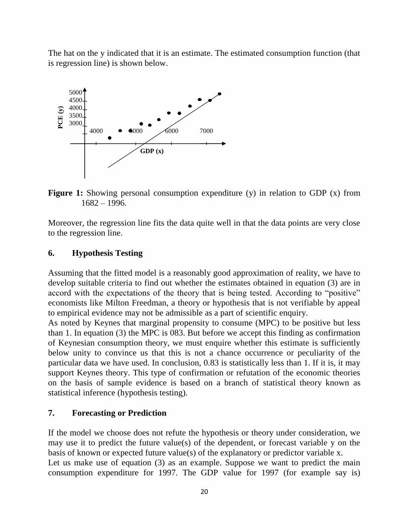
The hat on the y indicated that it is an estimate. The estimated consumption function (that
is regression line) is shown below.
Figure 1: Showing personal consumption expenditure (y) in relation to GDP (x) from
1682 – 1996.
Moreover, the regression line fits the data quite well in that the data points are very close
to the regression line.
6. Hypothesis Testing
Assuming that the fitted model is a reasonably good approximation of reality, we have to
develop suitable criteria to find out whether the estimates obtained in equation (3) are in
accord with the expectations of the theory that is being tested. According to ―positive‖
economists like Milton Freedman, a theory or hypothesis that is not verifiable by appeal
to empirical evidence may not be admissible as a part of scientific enquiry.
As noted by Keynes that marginal propensity to consume (MPC) to be positive but less
than 1. In equation (3) the MPC is 083. But before we accept this finding as confirmation
of Keynesian consumption theory, we must enquire whether this estimate is sufficiently
below unity to convince us that this is not a chance occurrence or peculiarity of the
particular data we have used. In conclusion, 0.83 is statistically less than 1. If it is, it may
support Keynes theory. This type of confirmation or refutation of the economic theories
on the basis of sample evidence is based on a branch of statistical theory known as
statistical inference (hypothesis testing).
7. Forecasting or Prediction
If the model we choose does not refute the hypothesis or theory under consideration, we
may use it to predict the future value(s) of the dependent, or forecast variable y on the
basis of known or expected future value(s) of the explanatory or predictor variable x.
Let us make use of equation (3) as an example. Suppose we want to predict the main
consumption expenditure for 1997. The GDP value for 1997 (for example say is)
5000
4500
4000
3500
3000
4000 5000 6000 7000
PC
E (
y)
GDP (x)
21
6158.7billion dollars. Putting this GDP figure on the right-hand side of equation (3), we
obtain
Therefore
or about 4944 billion naira. Thus given the value of the GDP, the mean or average,
forecast consumption expenditure is about 4944 billion naira. The actual value of the
consumption expenditure reported in 1997 was 4913.5 billion naira. The estimated model
(in equation 3) thus over predicted the actual consumption expenditure by about 30.76
billion naira. We could say that forecast error is about 30.76 billion naira, which is about
0.74 percent of the actual GDP value for 1997.
8. Use of the Model for Control or Policy Purpose
Let us assume that we have already estimated a consumption function given in equation
(3). Suppose further the government believes that consumer expenditure of about say
4900 (billion of 1992 naira) will keep the unemployment rate at its current level of about
4.2 percent (early 2000). What level of income will guarantee the target amount of
consumption expenditure? If the regression result given in equation (3) seem reasonable,
sample arithmetic will show that 4900 = – 144.06 + 0.8262x ______________ (5).
Which gives x = 6105, approximately. That is, an income levels of about 6105 (billion)
naira, given an MPC of about 0.83, will produce (10) an expenditure of about 4900
billion naira.
From the analysis above, an estimated model may be used for control or policy purposes.
By appropriate fiscal and monetary policy mix, the government can manipulate the
control variable x to produce the desired level of the target variable y.
4.0 CONCLUSION
Stages of econometrics analysis are the process of getting on economic theory, subject it
to empirical model, and then make use of data, estimation, and hypothesis and policy
recommendation.
5.0 SUMMARY
The unit has discussed attentively the stages econometrics analysis from the economic
theory, mathematical model of theory, econometric model of theory, collecting the data,
estimation of econometric model, hypothesis testing, forecasting or prediction and using
the model for control or policy purposes. Therefore at this end I belief you must have
understand the stages of econometrics analysis.
6.0 TUTOR MARKED ASSIGNMENT
Discuss the stages of econometrics analysis
22
7.0 REFERENCES/FURTHER READINGS
Adekanye, D. F., (2008). Introduction to Econometrics, 1st edition, Addart Publication
limited, Lagos Nigeria.
Dimitrios, A & Stephen, G., (2011). Applied Econometrics, second edition 2011, first
edition 2006 and revised edition 2007.
23
UNIT 3 COMPUTER AND ECONOMETRICS
CONTENTS
1.0 Introduction
2.0 Objectives
3.0 Main content
3.1. Definition of Macroeconomics
3.2. Types of Econometrics Basic
3.3. Theoretical versus Applied Economics
3.4. The Differences between Econometrics Modeling and
Machine Learning
4.0 Conclusion
5.0 Summary
6.0 Tutor-Marked Assignment
7.0 References/Further Readings
1.0 INTRODUCTION
In this unit, we are going to know briefly the role computer application in econometrics
analysis and to be able to convinced people that are not economists that computer help in
bringing the beauty of economic model to reality and prediction. The computer
application are peculiar to social sciences techniques/analysis and economics in
particular.
2.0 OBJECTIVES
At the end of this unit, you should be able to:
understand the role of computer in econometrics analysis
identify/explain the types of econometrics analysis.
3.0 MAIN CONTENT
3.1 The Role of Computer
Regression analysis, the bread-and-better tool of econometrics, these days is unthinkable
without the computer and some access to statistical software. However, several excellent
regression packages are commercially available, both for the mainframe and the
microcomputer and the lot is growing by the day.
Regression software packages such as SPSS, EVIENS, SAS, STATA etc. are few of the
economic software packages use in conducting estimation analysis on economic-
equations and models.
24
3.2 TYPES OF ECONOMETRICS
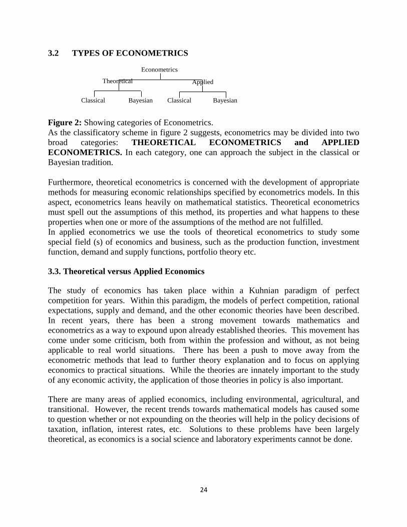
Figure 2: Showing categories of Econometrics.
As the classificatory scheme in figure 2 suggests, econometrics may be divided into two
broad categories: THEORETICAL ECONOMETRICS and APPLIED
ECONOMETRICS. In each category, one can approach the subject in the classical or
Bayesian tradition.
Furthermore, theoretical econometrics is concerned with the development of appropriate
methods for measuring economic relationships specified by econometrics models. In this
aspect, econometrics leans heavily on mathematical statistics. Theoretical econometrics
must spell out the assumptions of this method, its properties and what happens to these
properties when one or more of the assumptions of the method are not fulfilled.
In applied econometrics we use the tools of theoretical econometrics to study some
special field (s) of economics and business, such as the production function, investment
function, demand and supply functions, portfolio theory etc.
3.3. Theoretical versus Applied Economics
The study of economics has taken place within a Kuhnian paradigm of perfect
competition for years. Within this paradigm, the models of perfect competition, rational
expectations, supply and demand, and the other economic theories have been described.
In recent years, there has been a strong movement towards mathematics and
econometrics as a way to expound upon already established theories. This movement has
come under some criticism, both from within the profession and without, as not being
applicable to real world situations. There has been a push to move away from the
econometric methods that lead to further theory explanation and to focus on applying
economics to practical situations. While the theories are innately important to the study
of any economic activity, the application of those theories in policy is also important.
There are many areas of applied economics, including environmental, agricultural, and
transitional. However, the recent trends towards mathematical models has caused some
to question whether or not expounding on the theories will help in the policy decisions of
taxation, inflation, interest rates, etc. Solutions to these problems have been largely
theoretical, as economics is a social science and laboratory experiments cannot be done.
Econometrics
Bayesian
Classical
Bayesian
Classical
Applied Theoretical
25
However, there are some concerns with traditional theoretical economics that are worth
mentioning. First, Ben Ward describes "stylized facts," or false assumptions, such as the
econometric assumption that "strange observations do not count."
[1] While it is vital that anomalies are overlooked for the purpose of deriving and
formulating a clear theory, when it comes to applying the theory, the anomalies could
distort what should happen. These stylized facts are very important in theoretical
economics, but can become very dangerous when dealing with applied economics. A
good example is the failure of economic models to account for shifts due to deregulation
or unexpected shocks.
[2] These can be viewed as anomalies that are unable to be accounted for in a model, yet
is very real in the world today.
Another concern with traditional theory is that of market breakdowns. Economists
assume things such as perfect competition and utility maximization. However, it is easily
seen that these assumptions do not always hold. One example is the idea of stable
preferences among consumers and that they act efficiently in their pursuit. However,
people's preferences change over time and they do not always act rational nor efficient.
[3] Health care, for another example, chops down many of the assumptions that are
crucial to theoretical economics. With the advent of insurance, perfect competition is no
longer a valid assumption. Physicians and hospitals are paid by insurance companies,
which assures them of high salaries, but which prevents them from being competitive in
the free market. Perfect information is another market breakdown in health economics.
The consumer (patient) cannot possibly know everything the doctor knows about their
condition, so the doctor is placed in an economically advantaged position. Since the
traditional assumptions fail to hold here, a manipulated form of the traditional theory
needs to be applied. The assumption that consumers and producers (physicians,
hospitals) will simply come into equilibrium together will not become a reality because
the market breakdowns lead to distortions. Traditional theorists would argue that the
breakdown has to be fixed and then the theory can applied as it should be. They stick to
their guns even when there is conflicting evidence otherwise, and they propose that the
problem lies with the actors, not the theory.
[4] The third concern to be discussed here ties in with the Kuhnian idea of normal
science. The idea that all research is done within a paradigm and that revolutions in
science only occur during a time of crisis. However, this concerns a "hard" science, and
economics is a social science. This implies that economics is going to have an effect on
issues, therefore, economists are going to have an effect on issues. Value-neutrality is
not likely to be present in economics, because economists not only explain what is
happening, predict what will happen, but they prescribe the solutions to arrive at the
desired solution. Economics is one of the main issues in every political campaign and
26
there are both liberal and conservative economists. The inference is that economists use
the same theories and apply them to the same situations and recommend completely
different solutions. In this vein, politics and values drive what solutions economists
recommend. Even though theories are strictly adhered to, can a reasonably economic
solution be put forth that is not influenced by values? Unfortunately, the answer is no.
Theoretical economics cannot hold all the answers to every problem faced in the "real
world" because false assumptions, market breakdowns, and the influence of values
prevent the theories from being applied as they should. Yet, the Formalist Revolution or
move towards mathematics and econometrics continues to focus their efforts on theories.
Economists continue to adjust reality to theory, instead of theory to reality.
[5] This is Gordon's "Rigor over Relevance." The concept that mathematical models and
the need to further explain a theory often overrides the sense of urgency that a problem
creates. There is much literature about theories that have been developed using
econometric models, but Gordon's concern is that relevance to what is happening in the
world is being overshadowed.
[6] This is where the push for applied economics has come from over the past 20 years or
so. Issues such as taxes, movement to a free market from a socialist system, inflation,
and lowering health care costs are tangible problems to many people. The notion that
theoretical economics is going to be able to develop solutions to these problems seems
unrealistic, especially in the face of stylized facts and market breakdowns. Even if a
practical theoretical solution to the problem of health care costs could be derived, it
would certainly get debated by economists from the left and the right who are sure that
this solution will either be detrimental or a saving grace.
Does this mean that theoretical economics should be replaced by applied economics?
Certainly not. Theoretical economics is the basis from which economics has grown and
has landed us today. The problem is that we do not live in a perfect, ideal world in which
economic theory is based. Theories do not allow for sudden shocks nor behavioral
changes.
[7] This is important as it undercuts the stable preferences assumption, as mentioned
before. When the basic assumptions of a theory are no longer valid, it makes very
difficult to apply that theory to a complex situation. For instance, if utility maximization
is designed as maximizing my income, then it should follow that income become the
measuring stick for utility. However, if money is not an important issue to someone, then
it may appear as if they are not maximizing their utility nor acting rationally. They may
be perfectly happy giving up income to spend time with their family, but to an economist
they are not maximizing their utility. This is a good example of how theory and reality
come into conflict.
27
The focus in theoretical economics has been to make reality fit the theory and not vice-
versa. The concern here is that this version of problem-solving will not actually solve
any problems. Rather, more problems may be created in the process. There has been
some refocusing among theoreticians to make their theories more applicable, but the
focus of graduate studies remains on econometrics and mathematical models. The
business world is beginning to take notice of this and is often requiring years away from
the academic community before they will hire someone. They are looking for economists
who know how to apply their knowledge to solve real problems, not simply to expound
upon an established theory. It is the application of the science that makes it important
and useful, not just the theoretical knowledge.
This is not to say that theoretical economics is not important. It certainly is, just as
research in chemistry and physics is important to further understand the world we live in.
However, the difference is that economics is a social science with a public policy aspect.
This means that millions of people are affected by the decisions of policy-makers, who
get their input from economists, among others. Legislators cannot understand the
technical mathematical models, nor would they most likely care to, but they are interested
in policy prescriptions. Should health care be nationalized? Is this the best solution
economically? These are the practical problems that face individuals and the nation
every day. The theoreticians provide a sturdy basis to start from, but theory alone is not
enough. The theory needs to be joined with practicality that will lead to reasonable
practical solutions of difficult economic problems. Economics cannot thrive without
theory, and thus stylized facts and other assumptions. However, this theory has to
explain the way the world actually is, not the way economists say it should be.
[8] Pure economic theory is a great way to understand the basics of how the market
works and how the actors should act within the market. False assumptions and market
breakdowns present conflict between theory and reality. From here, many economists
simply assume is not the fault of the theory, but rather the economic agents in play.
However, it is impossible to make reality fit within the strict guidelines of a theory; the
theory needs to be altered to fit reality. This is where applied economics becomes
important. Application of theories needs to be made practical to fit each situation. To
rely simply on theory and models is not to take into account the dynamic nature of human
beings. What is needed is a strong theoretical field of economics, as well as a strong
applied field. This should lead to practical solutions with a strong theoretical basis.
28
3.4. THE DIFFERENCE BETWEEN ECONOMETRICS MODELING AND
MACHINE LEARNING
Econometric models are statistical models used in econometrics. An econometric
model specifies the statistical relationship that is believed to be held between the various
economic quantities pertaining to a particular economic phenomenon under study.
On the other hand- Machine learning is a scientific discipline that explores the
construction and study of algorithms that can learn from data. So that makes a clear
distinction right? If it learns on its own from data it is machine learning. If it is used for
economic phenomenon it is an econometric model. However the confusion arises in the
way these two paradigms are championed. The computer science major will always say
machine learning and the statistical major will always emphasize modeling. Since
computer science majors now rule at face book, Google and almost every technology
company, you would think that machine learning is dominating the field and beating poor
old econometric modeling.
But what if you can make econometric models learn from data?
Lets dig more into these algorithms. The way machine learning works is to optimize
some particular quantity, say cost. A loss function or cost function is a function that maps
a value(s) of one or more variables intuitively representing some ―cost‖ associated with
the event. An optimization problem seeks to minimize a loss function. Machine learning
frequently seek optimization to get the best of many alternatives.
Now, cost or loss holds different meanings in econometric modeling. In econometric
modeling we are trying to minimize the error (or root mean squared error). Root mean
squared error means root of the sum of squares of errors. An error is defined as the
difference between actual and predicted value by the model for previous data.
The difference in the jargon is solely in the way statisticians and computer scientists are
trained. Computer scientists try to compensate for both actual error as well as
computational cost – that is the time taken to run a particular algorithm. On the other
hand statisticians are trained primarily to think in terms of confidence levels or error in
terms or predicted and actual without caring for the time taken to run for the model.
That is why data science is defined often as an intersection between hacking skills (in
computer science) and statistical knowledge (and math). Something like K Means
clustering can be taught in two different ways just like regression can be based on these
two approaches. I wrote back to my colleague in Marketing – we have data scientists.
They are trained in both econometric modeling and machine learning. I looked back and
had a beer. If university professors don‘t shed their departmental attitudes towards data
29
science, we will have a very confused set of students very shortly arguing without
knowing how close they actually are.
4.0 CONCLUSION
Computer and Econometrics have a long history in econometrics analysis. The use of
software to calculate data in economics analysis is very important in econometrics
analysis and it has shown and gives the way forward in forecasting and policy
recommendations to the stakeholders, private companies and government.
5.0 SUMMARY
The unit discussed extensively on the role of computer in econometrics. When equations
in economics are turn to mathematical equations and becomes a model in economics, the
computer software or what are ‗economists‘ called econometrics packages to solve/run
the analysis for forecast and policy recommendation.
6.0 TUTOR MARKED ASSIGNMENT
Discuss the role of computer in econometrics analysis
7.0 REFERENCES/FURTHER READINGS
Begg, Iain and Henry, S. G. B. Applied Economics and Public Policy. Cambridge
University Press, United Kingdom: 1998.
Cassidy, John. The Decline of Economics.
Dimitrios, A & Stephen, G., (2011). Applied Econometrics, second edition 2011, first
edition 2006 and revised edition 2007.
Friedland, Roger and Robertson, A. F., eds. Beyond the Marketplace: Rethinking
Economy and Society. Walter de Gruyter, Inc. New York: 1990
Gordon, Robert Aaron. Rigor and Relevance in a Changing Institutional Setting.
Kuhn, Thomas. The Structure of Scientific Revolutions.
30
UNIT 4: BASIC ECONOMETRICS MODELS: LINEAR REGRESSION
CONTENTS
1.0. Introduction
2.0. Objectives
3.0. Main content
3.1. Econometrics Theory
3.2. Econometrics Methods
3.3. Examples of a Relationship in Econometrics
3.4. Limitations and Criticism
4.0 Conclusion
5.0 Summary
6.0 Tutor-Marked Assignment
7.0 References/Further Readings
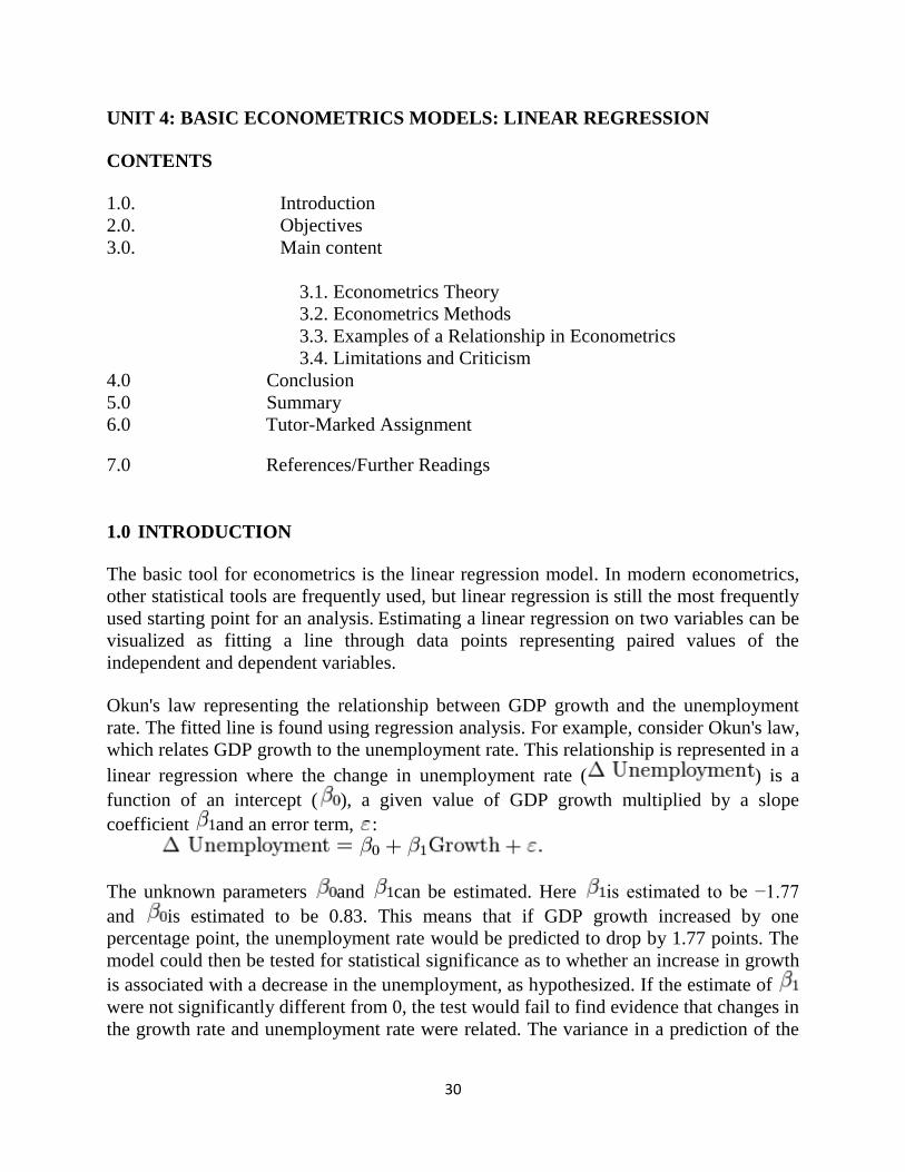
1.0 INTRODUCTION
The basic tool for econometrics is the linear regression model. In modern econometrics,
other statistical tools are frequently used, but linear regression is still the most frequently
used starting point for an analysis. Estimating a linear regression on two variables can be
visualized as fitting a line through data points representing paired values of the
independent and dependent variables.
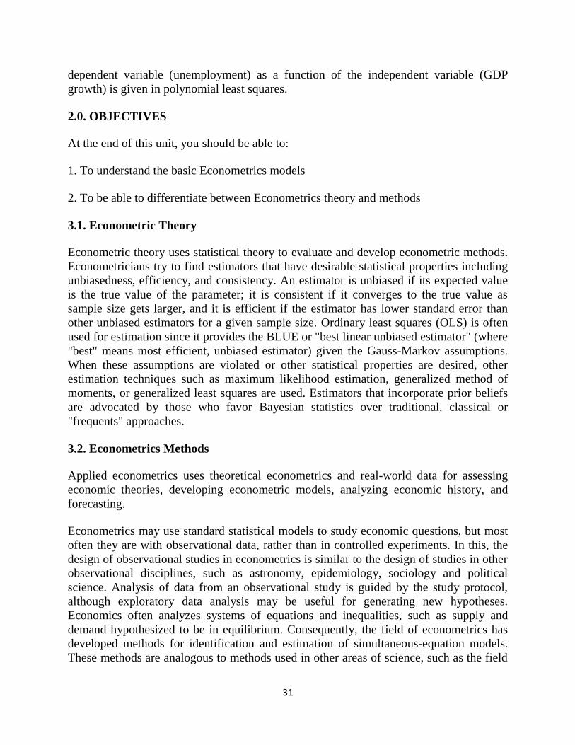
Okun's law representing the relationship between GDP growth and the unemployment
rate. The fitted line is found using regression analysis. For example, consider Okun's law,
which relates GDP growth to the unemployment rate. This relationship is represented in a
linear regression where the change in unemployment rate ( ) is a
function of an intercept ( ), a given value of GDP growth multiplied by a slope
coefficient and an error term, :
The unknown parameters and can be estimated. Here is estimated to be −1.77
and is estimated to be 0.83. This means that if GDP growth increased by one
percentage point, the unemployment rate would be predicted to drop by 1.77 points. The
model could then be tested for statistical significance as to whether an increase in growth
is associated with a decrease in the unemployment, as hypothesized. If the estimate of
were not significantly different from 0, the test would fail to find evidence that changes in
the growth rate and unemployment rate were related. The variance in a prediction of the
31
dependent variable (unemployment) as a function of the independent variable (GDP
growth) is given in polynomial least squares.
2.0. OBJECTIVES
At the end of this unit, you should be able to:
1. To understand the basic Econometrics models
2. To be able to differentiate between Econometrics theory and methods
3.1. Econometric Theory
Econometric theory uses statistical theory to evaluate and develop econometric methods.
Econometricians try to find estimators that have desirable statistical properties including
unbiasedness, efficiency, and consistency. An estimator is unbiased if its expected value
is the true value of the parameter; it is consistent if it converges to the true value as
sample size gets larger, and it is efficient if the estimator has lower standard error than
other unbiased estimators for a given sample size. Ordinary least squares (OLS) is often
used for estimation since it provides the BLUE or "best linear unbiased estimator" (where
"best" means most efficient, unbiased estimator) given the Gauss-Markov assumptions.
When these assumptions are violated or other statistical properties are desired, other
estimation techniques such as maximum likelihood estimation, generalized method of
moments, or generalized least squares are used. Estimators that incorporate prior beliefs
are advocated by those who favor Bayesian statistics over traditional, classical or
"frequents" approaches.
3.2. Econometrics Methods
Applied econometrics uses theoretical econometrics and real-world data for assessing
economic theories, developing econometric models, analyzing economic history, and
forecasting.
Econometrics may use standard statistical models to study economic questions, but most
often they are with observational data, rather than in controlled experiments. In this, the
design of observational studies in econometrics is similar to the design of studies in other
observational disciplines, such as astronomy, epidemiology, sociology and political
science. Analysis of data from an observational study is guided by the study protocol,
although exploratory data analysis may be useful for generating new hypotheses.
Economics often analyzes systems of equations and inequalities, such as supply and
demand hypothesized to be in equilibrium. Consequently, the field of econometrics has
developed methods for identification and estimation of simultaneous-equation models.
These methods are analogous to methods used in other areas of science, such as the field
32
of system identification in systems analysis and control theory. Such methods may allow
researchers to estimate models and investigate their empirical consequences, without
directly manipulating the system.
One of the fundamental statistical methods used by econometricians is regression
analysis. Regression methods are important in econometrics because economists typically
cannot use controlled experiments. Econometricians often seek illuminating natural
experiments in the absence of evidence from controlled experiments. Observational data
may be subject to omitted-variable bias and a list of other problems that must be
addressed using causal analysis of simultaneous-equation models.
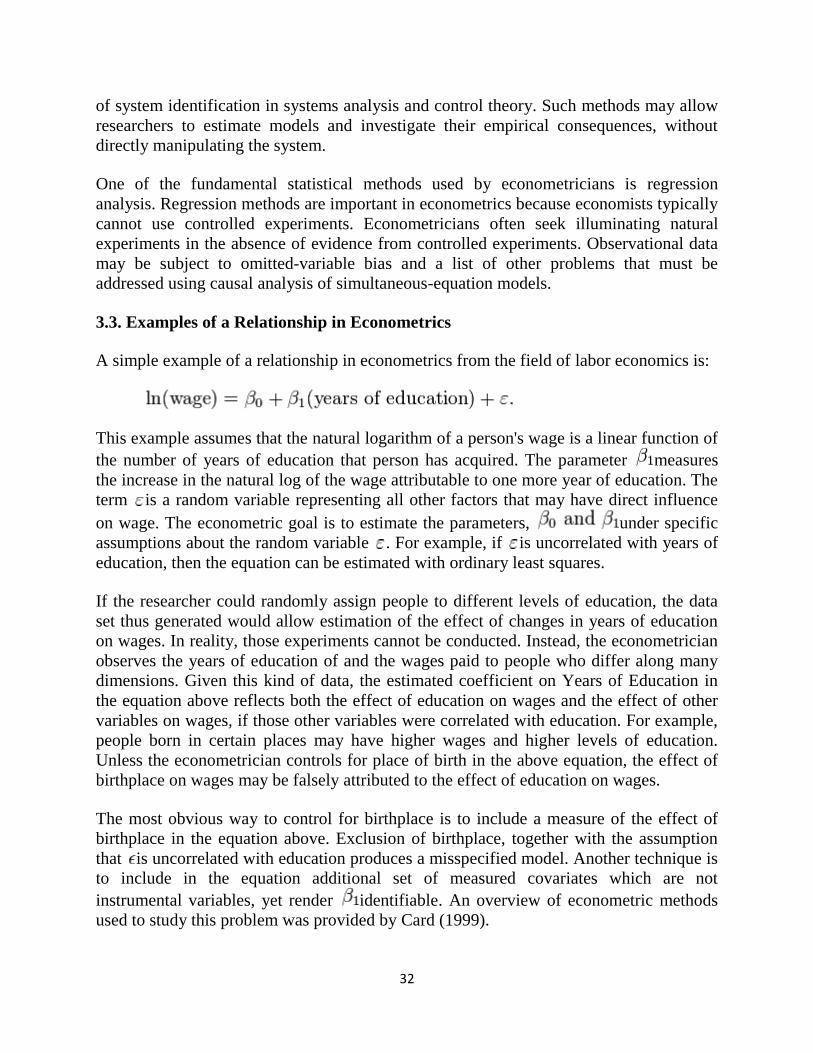
3.3. Examples of a Relationship in Econometrics
A simple example of a relationship in econometrics from the field of labor economics is:
This example assumes that the natural logarithm of a person's wage is a linear function of
the number of years of education that person has acquired. The parameter measures
the increase in the natural log of the wage attributable to one more year of education. The
term is a random variable representing all other factors that may have direct influence
on wage. The econometric goal is to estimate the parameters, under specific
assumptions about the random variable . For example, if is uncorrelated with years of
education, then the equation can be estimated with ordinary least squares.
If the researcher could randomly assign people to different levels of education, the data
set thus generated would allow estimation of the effect of changes in years of education
on wages. In reality, those experiments cannot be conducted. Instead, the econometrician
observes the years of education of and the wages paid to people who differ along many
dimensions. Given this kind of data, the estimated coefficient on Years of Education in
the equation above reflects both the effect of education on wages and the effect of other
variables on wages, if those other variables were correlated with education. For example,
people born in certain places may have higher wages and higher levels of education.
Unless the econometrician controls for place of birth in the above equation, the effect of
birthplace on wages may be falsely attributed to the effect of education on wages.
The most obvious way to control for birthplace is to include a measure of the effect of
birthplace in the equation above. Exclusion of birthplace, together with the assumption
that is uncorrelated with education produces a misspecified model. Another technique is
to include in the equation additional set of measured covariates which are not
instrumental variables, yet render identifiable. An overview of econometric methods
used to study this problem was provided by Card (1999).
33
3.4. LIMITATIONS AND CRITICISMS
Like other forms of statistical analysis, badly specified econometric models may show a
spurious relationship where two variables are correlated but causally unrelated. In a study
of the use of econometrics in major economics journals, McCloskey concluded that some
economists report p values (following the Fisherian tradition of tests of significance of
point null-hypotheses) and neglect concerns of type II errors; some economists fail to
report estimates of the size of effects (apart from statistical significance) and to discuss
their economic importance. Some economists also fail to use economic reasoning for
model selection, especially for deciding which variables to include in a regression. It is
important in many branches of statistical modeling that statistical associations make some
sort of theoretical sense to filter out spurious associations (e.g., the collinearity of the
number of Nicolas Cage movies made for a given year and the number of people who
died falling into a pool for that year).
In some cases, economic variables cannot be experimentally manipulated as treatments
randomly assigned to subjects. In such cases, economists rely on observational studies,
often using data sets with many strongly associated covariates, resulting in enormous
numbers of models with similar explanatory ability but different covariates and
regression estimates. Regarding the plurality of models compatible with observational
data-sets, Edward Leamer urged that "professionals ... properly withhold belief until an
inference can be shown to be adequately insensitive to the choice of assumptions"
4.0 CONCLUSION
The unit critically conclude that basic econometrics models is the basis of econometrics
and from the simple straight line graph we can see that a simple/linear regression
equation is derived from the graph and from there, the model of econometrics started to
emanate to becomes higher level of econometrics model which is called multiple
regression analysis.
5.0 SUMMARY
The unit discussed extensively on basic Econometrics models of linear regression
analysis such as Econometrics theory, Econometrics Methods, Examples of econometrics
modeling and the limitations and criticism of the models.
6.0 TUTOR MARKED ASSIGNMENT
Discuss the theory and methods of Econometrics modeling
34
7.0 . REFERENCES/FURTHER READINGS
Olusanjo, A.A. (2014). Introduction to Econometrics, a broader perspective, 1st edition,
world press publication limited, Nigeria.
Warlking, F.G., (2014). Econometrics and Economic theory, 2nd
edition, Dale Press
limited.
35
UNIT FIVE: IMPORTANCE OF ECONOMETRICS
CONTENTS
1.0. Introduction
2.0. Objectives
3.0. Main content
3.1. Why is Econometrics important within economics
3.2. Meaning of Modern Econometrics
3.3. Using Econometrics for Assessing Economic Model
3.4. Financial Economics
3.4.1. Relationship with the capital Asset pricing model
3.4.2. Co integration
3.4.3. Event Study
4.0 Conclusion
5.0 Summary
6.0 Tutor-Marked Assignment
7.0 References/Further Readings
1.0. INTRODUCTION
Econometrics contains statistical tools to help you defend or test assertions in economic
theory. For example, you think that the production in an economy is in Cobb-Douglas
form. But do data support your hypothesis? Econometrics can help you in this case.
To be able to learn econometrics by yourself, you need to have a good
mathematics/statistics background. Otherwise it will be hard. Econometrics is the
application of mathematics, statistical methods, and computer science to economic data
and is described as the branch of economics that aims to give empirical content to
economic relations.
2.0. OBJECTIVES
At the end of this unit, you should be able to:
know the meaning of Econometrics and why Econometrics is important within
Economics.
know how to use Econometrics for Assessing Economic Model
understand what is Financial Econometrics.
3.0. MAIN CONTENT
36
3.1. WHY IS ECONOMETRICS IMPORTANT WITHIN ECONOMICS?
So Econometrics is important for a couple of reasons though I would strongly urge you to
be very wary of econometric conclusions and I will explain why in a minute.
1. It provides an easy way to test statistical significance so in theory, if we specify our
econometric models properly and avoid common problems (i.e. heteroskedasticity or
strongly correlated independent variables etc.), then it can let us know if we can say
either, no there is no statistical significance or yes there is. That just means that for the
data set we have at hand, we can or cannot rule out significance. Problems with this:
Correlation does not prove causality. It is theory which we use to demonstrate causality
but we most definitely cannot use it to "discover" new relationships (only theory can be
used to tell us what causes what, for example, we may find a strong statistical
significance between someone declaring red is their favorite color and income, but this
obviously not an important relationship just chance)
Another problem is that many times people run many regressions until they find one that
"fits" their idea. So think about it this way, you use confidence intervals in economics, so
if you are testing for a 95% confidence interval run 10 different regressions and you have
a 40% chance of having a regression model tell you there is statistical significance when
there isn't. Drop this number to 90% and you have a 65% chance. Alot of shady
researchers do exactly this, play around with data series and specifications until they get
something that says their theory is right then publish it. So remember, be wary of
regression analysis and really only use it to refute your hypotheses and never to "prove"
something.
Regression analysis is your friend and you will see how people love to use it. If you don't
understand econometrics very well, particularly how to be able to sift through the
different specifications so that you rule out any poorly specified models, and so that you
understand what all these crazy numbers they are throwing at you mean. If you don't
know econometrics yet try reading some papers using regression analysis and notice how
you don't know what any of the regression analysis means. This should give you an idea
of why you need to learn it.
However, many people use it, and believe me many people get undergraduate degrees in
economics without knowing econometrics and this makes you less capable then those
peers of yours who did learn it.
3.2. MEANING OF MODERN ECONOMETRICS
Modern econometrics is the use of mathematics and statistics as a way to analyze
economic phenomena and predict future outcomes. This is often done through the use of
complex econometric models that portray the cause and effect of past or current
37
economic stimuli. Econometric analysts can plug new data into these models as a means
of predicting future results. One of the distinguishing features of modern econometrics is
the use of complex computer algorithms that can crunch tremendous amounts of raw data
and create a concise and coherent overview of some aspect of the economy.
For a long period of time in the past, economists could make hypotheses and guesses
about the economy but couldn‘t prove their theories without some sort of obvious sea
change in the economy as an indicator. As a result, many started to use mathematics and
statistics to give proof about their different ideas. Some began to realize that these same
tools could actually give accurate assessments about future economic events, which is
how the field of modern econometrics first came into being.
Although it can be defined in many different ways, modern econometrics essentially boils
down to plugging statistical information about an economy into mathematical formulas.
When that happens, the results can show cause and effect about certain economic
characteristics. For example, when interest rates rise, it might affect employment levels,
inflation, economic growth, and so on. Using econometrics, an analyst might be able to
pinpoint exactly how and to what extent this occurs.
Economic models are a huge part of the field of modern econometrics. This is where the
leaps and bounds made by computer technology in the modern era come into play.
Sophisticated programs devised by analysts can take all of the information that is entered,
analyze the relationships between the numerical data, and come up with specific
information about how certain economic stimuli affect the overall picture. It is an
effective way for those practicing econometrics to use the past to predict the future.
Proponents of modern econometrics should factor in those unforeseen circumstances that
can trigger huge negative changes in an economy. One way to do this is to simulate
worst-case scenarios for an economy. By doing this, analysts can see what the potential
damage done by hypothetical economic catastrophes might be. In addition, models can be
used to show the ways out of such dire occurrences. The boundaries for econometrics are
practically limitless, but using them can be fruitless without sound economic theories as
their basis.
3.3. USING ECONOMETRICS FOR ASSESSING ECONOMIC MODELS
Econometrics is often used passively to provide the economist with some parameter
estimates in a model which from the outset is assumed to be empirically relevant. In this
sense, econometrics is used to illustrate what we believe is true rather than to find out
whether our chosen model needs to be modified or changed altogether. The econometric
analyses of this special issue should take its departure from the latter more critical
approach. We would like to encourage submissions of papers addressing questions like
whether a specific economic model is empirically relevant in general or, more
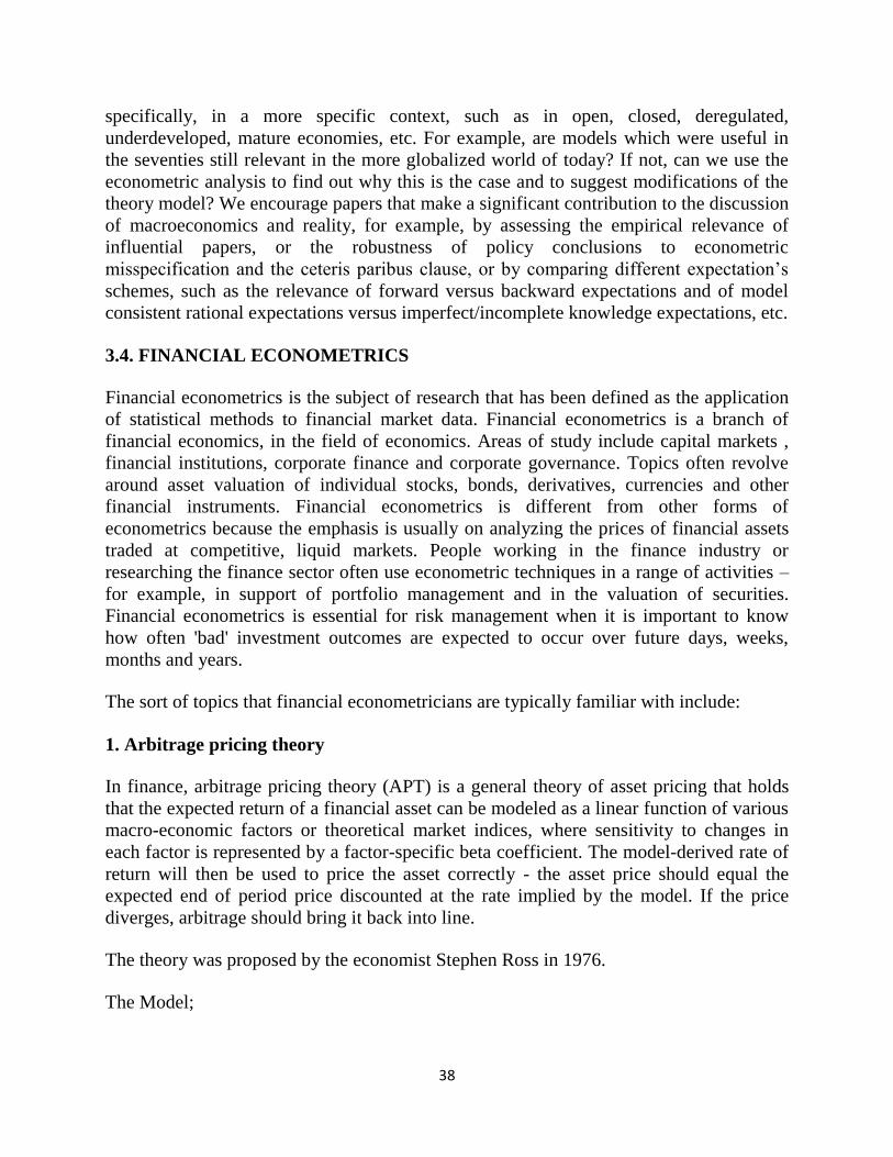
38
specifically, in a more specific context, such as in open, closed, deregulated,
underdeveloped, mature economies, etc. For example, are models which were useful in
the seventies still relevant in the more globalized world of today? If not, can we use the
econometric analysis to find out why this is the case and to suggest modifications of the
theory model? We encourage papers that make a significant contribution to the discussion
of macroeconomics and reality, for example, by assessing the empirical relevance of
influential papers, or the robustness of policy conclusions to econometric
misspecification and the ceteris paribus clause, or by comparing different expectation‘s
schemes, such as the relevance of forward versus backward expectations and of model
consistent rational expectations versus imperfect/incomplete knowledge expectations, etc.
3.4. FINANCIAL ECONOMETRICS
Financial econometrics is the subject of research that has been defined as the application
of statistical methods to financial market data. Financial econometrics is a branch of
financial economics, in the field of economics. Areas of study include capital markets ,
financial institutions, corporate finance and corporate governance. Topics often revolve
around asset valuation of individual stocks, bonds, derivatives, currencies and other
financial instruments. Financial econometrics is different from other forms of
econometrics because the emphasis is usually on analyzing the prices of financial assets
traded at competitive, liquid markets. People working in the finance industry or
researching the finance sector often use econometric techniques in a range of activities –
for example, in support of portfolio management and in the valuation of securities.
Financial econometrics is essential for risk management when it is important to know
how often 'bad' investment outcomes are expected to occur over future days, weeks,
months and years.
The sort of topics that financial econometricians are typically familiar with include:
1. Arbitrage pricing theory
In finance, arbitrage pricing theory (APT) is a general theory of asset pricing that holds
that the expected return of a financial asset can be modeled as a linear function of various
macro-economic factors or theoretical market indices, where sensitivity to changes in
each factor is represented by a factor-specific beta coefficient. The model-derived rate of
return will then be used to price the asset correctly - the asset price should equal the
expected end of period price discounted at the rate implied by the model. If the price
diverges, arbitrage should bring it back into line.
The theory was proposed by the economist Stephen Ross in 1976.
The Model;
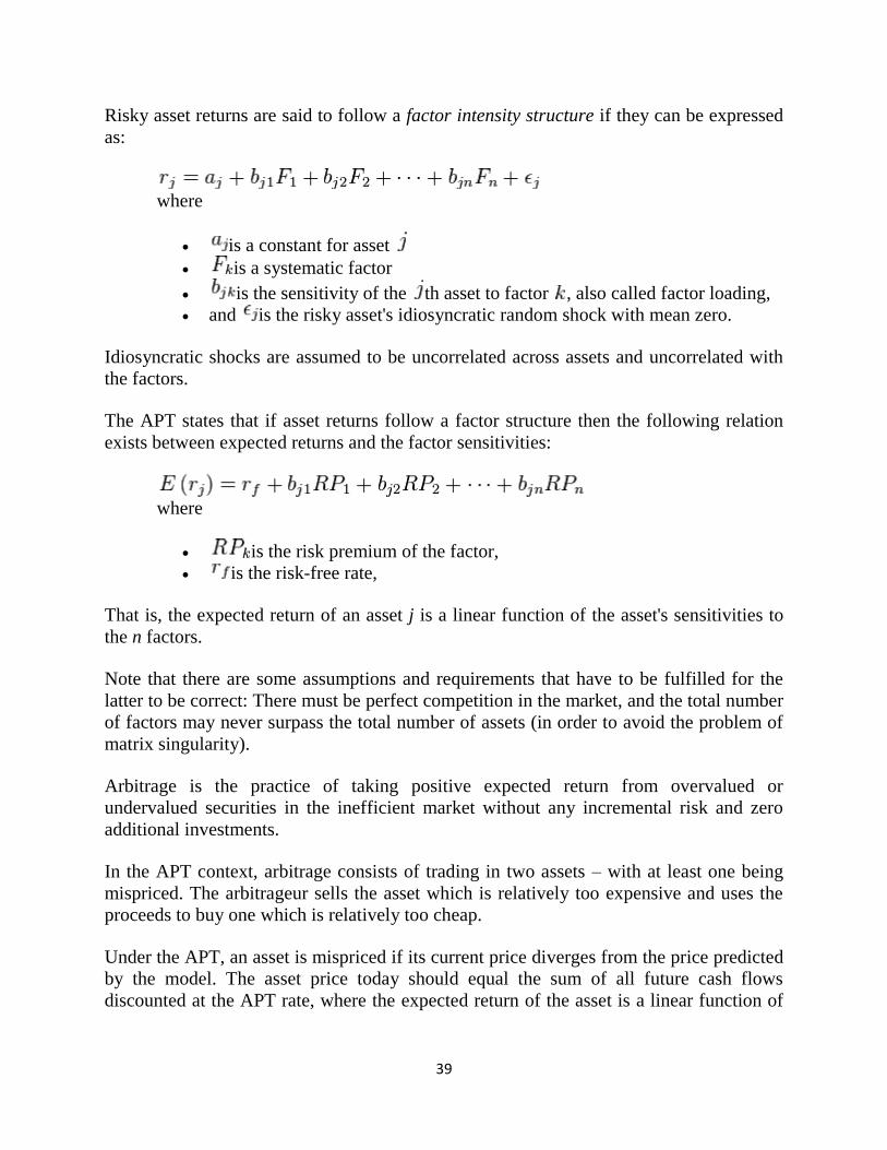
39
Risky asset returns are said to follow a factor intensity structure if they can be expressed
as:
where
is a constant for asset
is a systematic factor
is the sensitivity of the th asset to factor , also called factor loading,
and is the risky asset's idiosyncratic random shock with mean zero.
Idiosyncratic shocks are assumed to be uncorrelated across assets and uncorrelated with
the factors.
The APT states that if asset returns follow a factor structure then the following relation
exists between expected returns and the factor sensitivities:
where
is the risk premium of the factor,
is the risk-free rate,
That is, the expected return of an asset j is a linear function of the asset's sensitivities to
the n factors.
Note that there are some assumptions and requirements that have to be fulfilled for the
latter to be correct: There must be perfect competition in the market, and the total number
of factors may never surpass the total number of assets (in order to avoid the problem of
matrix singularity).
Arbitrage is the practice of taking positive expected return from overvalued or
undervalued securities in the inefficient market without any incremental risk and zero
additional investments.
In the APT context, arbitrage consists of trading in two assets – with at least one being
mispriced. The arbitrageur sells the asset which is relatively too expensive and uses the
proceeds to buy one which is relatively too cheap.
Under the APT, an asset is mispriced if its current price diverges from the price predicted
by the model. The asset price today should equal the sum of all future cash flows
discounted at the APT rate, where the expected return of the asset is a linear function of
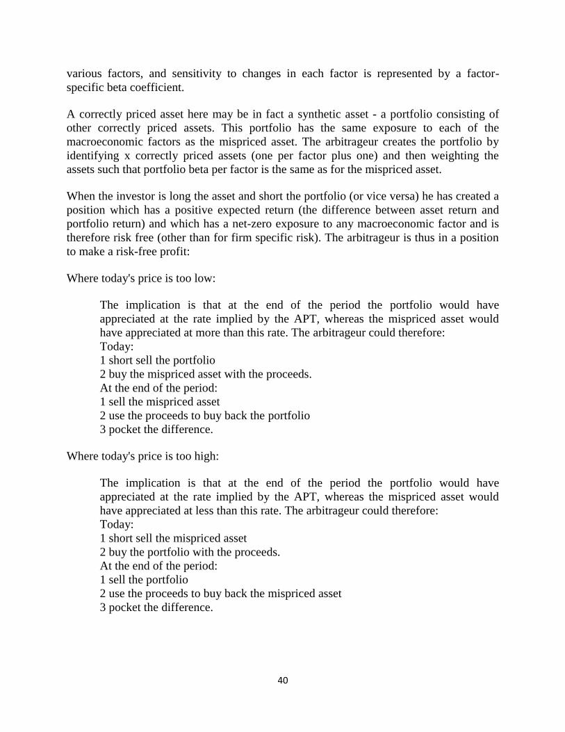
40
various factors, and sensitivity to changes in each factor is represented by a factor-
specific beta coefficient.
A correctly priced asset here may be in fact a synthetic asset - a portfolio consisting of
other correctly priced assets. This portfolio has the same exposure to each of the
macroeconomic factors as the mispriced asset. The arbitrageur creates the portfolio by
identifying x correctly priced assets (one per factor plus one) and then weighting the
assets such that portfolio beta per factor is the same as for the mispriced asset.
When the investor is long the asset and short the portfolio (or vice versa) he has created a
position which has a positive expected return (the difference between asset return and
portfolio return) and which has a net-zero exposure to any macroeconomic factor and is
therefore risk free (other than for firm specific risk). The arbitrageur is thus in a position
to make a risk-free profit:
Where today's price is too low:
The implication is that at the end of the period the portfolio would have
appreciated at the rate implied by the APT, whereas the mispriced asset would
have appreciated at more than this rate. The arbitrageur could therefore:
Today:
1 short sell the portfolio
2 buy the mispriced asset with the proceeds.
At the end of the period:
1 sell the mispriced asset
2 use the proceeds to buy back the portfolio
3 pocket the difference.
Where today's price is too high:
The implication is that at the end of the period the portfolio would have
appreciated at the rate implied by the APT, whereas the mispriced asset would
have appreciated at less than this rate. The arbitrageur could therefore:
Today:
1 short sell the mispriced asset
2 buy the portfolio with the proceeds.
At the end of the period:
1 sell the portfolio
2 use the proceeds to buy back the mispriced asset
3 pocket the difference.
41
3.4.1. Relationship with the capital asset pricing model
The APT along with the capital asset pricing model (CAPM) is one of two influential
theories on asset pricing. The APT differs from the CAPM in that it is less restrictive in
its assumptions. It allows for an explanatory (as opposed to statistical) model of asset
returns. It assumes that each investor will hold a unique portfolio with its own particular
array of betas, as opposed to the identical "market portfolio". In some ways, the CAPM
can be considered a "special case" of the APT in that the securities market line represents
a single-factor model of the asset price, where beta is exposed to changes in value of the
market.
Additionally, the APT can be seen as a "supply-side" model, since its beta coefficients
reflect the sensitivity of the underlying asset to economic factors. Thus, factor shocks
would cause structural changes in assets' expected returns, or in the case of stocks, in
firms' profitabilities.
On the other side, the capital asset pricing model is considered a "demand side" model.
Its results, although similar to those of the APT, arise from a maximization problem of
each investor's utility function, and from the resulting market equilibrium (investors are
considered to be the "consumers" of the assets).
3.4.2. Co integration
Co integration is a statistical property of a collection (X1,X2,...,Xk) of time series
variables. First, all of the series must be integrated of order 1 (see Order of Integration).
Next, if a linear combination of this collection is integrated of order zero, then the
collection is said to be co-integrated. Formally, if (X,Y,Z) are each integrated of order 1,
and there exist coefficients a,b,c such that aX+bY+cZ is integrated of order 0, then X,Y,
and Z are co integrated. Co integration has become an important property in
contemporary time series analysis. Time series often have trends — either deterministic
or stochastic. In an influential paper, Charles Nelson and Charles Plosser (1982) provided
statistical evidence that many US macroeconomic time series (like GNP, wages,
employment, etc.) have stochastic trends — these are also called unit root processes, or
processes integrated of order 1 — I(1). They also showed that unit root processes have
non-standard statistical properties, so that conventional econometric theory methods do
not apply to them.
If two or more series are individually integrated (in the time series sense) but some linear
combination of them has a lower order of integration, then the series are said to be
cointegrated. A common example is where the individual series are first-order integrated
(I(1)) but some (co integrating) vector of coefficients exists to form a stationary linear
combination of them. For instance, a stock market index and the price of its associated
futures contract move through time, each roughly following a random walk. Testing the
42
hypothesis that there is a statistically significant connection between the futures price and
the spot price could now be done by testing for the existence of a co integrated
combination of the two series.
3.4.3. Event study
An Event study is a statistical method to assess the impact of an event on the value of a
firm. For example, the announcement of a merger between two business entities can be
analyzed to see whether investors believe the merger will create or destroy value. The
basic idea is to find the abnormal return attributable to the event being studied by
adjusting for the return that stems from the price fluctuation of the market as a whole.
As the event methodology can be used to elicit the effects of any type of event on the
direction and magnitude of stock price changes, it is very versatile. Event studies are thus
common to various research areas, such as accounting and finance, management,
economics, marketing, information technology, law, and political science.
One aspect often used to structure the overall body of event studies is the breadth of the
studied event types. On the one hand, there is research investigating the stock market
responses to economy-wide events (i.e., market shocks, such as regulatory changes, or
catastrophic events). On the other hand, event studies are used to investigate the stock
market responses to corporate events, such as mergers and acquisitions, earnings
announcements, debt or equity issues, corporate reorganisations, investment decisions
and corporate social responsibility (MacKinlay 1997; McWilliams & Siegel, 1997
4.0 CONCLUSION
The unit critically concludes that Econometrics is very important in Economics and
financial analysis. Econometrics is the basis of using economics theories to justify a real
life situation in the micro and macro economy of any nation.
5.0 SUMMARY
The unit discussed extensively on the importance of Econometrics and why econometrics
is very useful in our day to day activities and how the financial analyst also makes use of
it to financial forecast and analysis.
6.0 TUTOR MARKED ASSIGNMENT
Differentiate between Modern and Financial Econometrics
43
7.0. REFERENCES/FURTHER READINGS
Medunoye, G.K., (2013). Introduction to Econometrics, 1st edition, Mill Publication
limited.
Parker, J.J., (2016). Econometrics and Economic Policy, Journal vol 4, pg 43-73, Parking
& Parking Publication limited.

44
MODULE TWO – SINGLE- EQUATION (REGRESSION MODELS)
Unit One: Regression Analysis
Unit Two: The Ordinary Least Square (OLS) Method Estimation
Unit Three: Calculation of Parameter and the Assumption of Classical Least
Regression
Method (CLRM)
Unit Four: Properties of the Ordinary Least Square Estimators
Unit Five: The Coefficient of Determination (R2): A measure of “Goodness of fit”
Unit One: Regression Analysis
CONTENTS
1.0 . Introduction
2.0. Objectives
3.0. Main content
3.1. The Linear Regression Model
3.2. The Classical Linear Regression Model
3.3. Regression Vs Causation
3.4. Regression Vs Correlation
4.0 Conclusion
5.0 Summary
6.0 Tutor-Marked Assignment
7.0 References/Further Readings
45
1.0 INTRODUCTION
The term regression was introduced by Francis Galton. In a famous paper, Galton found
that, although there was a tendency for tall parents to have tall children and for short
parents to have short children, the average height of children born of parents of a given
height tended to move to ―regress‖ toward the average height in the population as a
whole. In other words, the height of the children of unusually tall or unusually short
parents tends to move toward the average height of the population. Galton‘s law of
universal regression was confirmed by his friend Karl Pearson who collected more than a
thousand records of heights of members of family groups. He found that the average
height of sons of a group of tall fathers was less than their father‘s height and the average
height of sons of a group of short fathers was greater than their fathers‘ height, thus
―regressing‖‖ tall and short sons alike toward the average height of all men. In the word
of Galton, this was ―regression to mediocrity‖.
2.0. OBJECTIVES
At the end of this unit, you should be able to:
examine the linear regression model
understand the classical linear regression model
3.0 MAIN CONTENT
3.1 The Linear Regression Model
We can ask ourselves a question that why do we regress? Econometric methods such as
regression can help to overcome the problem of complete uncertainty and guide planning
and decision-making. Of course, building a model is not an easy task. Models should
meet certain criteria (for example a model should not suffer from serial correlation) in
order to be valid and a lot of work is usually needed before we achieve a good model.
Furthermore, much decision making is required regarding which variables to include in
the model. Too many may cause problems (unneeded variables misspecification), while
too few may cause other problems (omitted variables misspecification or incorrect
functional form).
3.2 The classical linear regression model
The classical linear regression is a way of examining the nature and form of the
relationships among two or more variables. In this aspect we will consider the case of
only two variables. One important issue in the regression analysis is the direction of
causation between the two variables; in other words, we want to know which variable is
affecting the other. Alternatively, this can be stated as which variable depends on the
other. Therefore, we refer to the two variables as the dependent variable (usually denoted
by Y) and the independent or explanatory variable (usually denoted by X). We want to
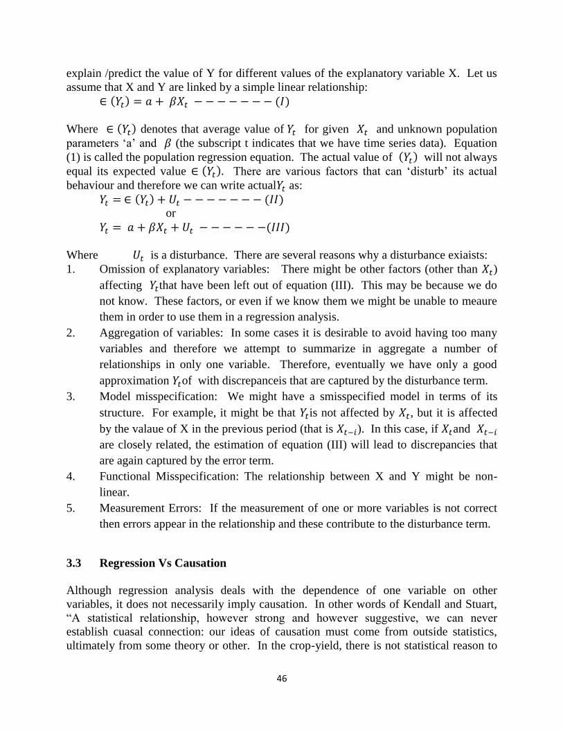
46
explain /predict the value of Y for different values of the explanatory variable X. Let us
assume that X and Y are linked by a simple linear relationship:
Where denotes that average value of for given and unknown population
parameters ‗a‘ and (the subscript t indicates that we have time series data). Equation
(1) is called the population regression equation. The actual value of will not always
equal its expected value There are various factors that can ‗disturb‘ its actual
behaviour and therefore we can write actual as:
or
Where is a disturbance. There are several reasons why a disturbance exiaists:
1. Omission of explanatory variables: There might be other factors (other than )
affecting that have been left out of equation (III). This may be because we do
not know. These factors, or even if we know them we might be unable to meaure
them in order to use them in a regression analysis.
2. Aggregation of variables: In some cases it is desirable to avoid having too many
variables and therefore we attempt to summarize in aggregate a number of
relationships in only one variable. Therefore, eventually we have only a good
approximation of with discrepanceis that are captured by the disturbance term.
3. Model misspecification: We might have a smisspecified model in terms of its
structure. For example, it might be that is not affected by , but it is affected
by the valaue of X in the previous period (that is ). In this case, if and
are closely related, the estimation of equation (III) will lead to discrepancies that
are again captured by the error term.
4. Functional Misspecification: The relationship between X and Y might be non-
linear.
5. Measurement Errors: If the measurement of one or more variables is not correct
then errors appear in the relationship and these contribute to the disturbance term.
3.3 Regression Vs Causation
Although regression analysis deals with the dependence of one variable on other
variables, it does not necessarily imply causation. In other words of Kendall and Stuart,
―A statistical relationship, however strong and however suggestive, we can never
establish cuasal connection: our ideas of causation must come from outside statistics,
ultimately from some theory or other. In the crop-yield, there is not statistical reason to
47
assume that rainfall does not depend on crop yeild. The fact that we treat crop yeeld as
dependent on rainfall (among other things) is due to nonstatistical considerations:
common sense suggests that the relationship cannot be reversed for we cannot control
rainfall by barying crop yield.
3.4 Regression Vs Correlation
Closely related to but conceptually very much different from regression analysis is
correlation analysis, where the primary objective is to measure the strength or degree of
linear association between two variables. The correlation coefficient measures the
strength of (Linear) association. For example, we may be interested in finding the
correlation (coefficient) between smoking and lung cancer, between scores on statistics
and mathematics examinations, between high school grades and college grades and so on.
In regression analysis, as already noted, we are not primarily interested in such a
measure. Instead, we try to estimate or predict the average value of one variable on the
basis of the fixed values of other variables. Thus, we may want to know whether we can
predict the average score on a statistics examination by knowing a students‘ score on a
mathematics examination.
4.0 SUMMARY
The key idea behind regression analysis is the statistical dependence of one variable, the
dependent variable , on one or more of the variables, the explanatory variable. So, I
believe in this unit you must have known the differences between regression and
correlation and the classical linear regression anlysis.
5.0 CONCLUSION
In any research, the researcher should clearly state the sources of the data used in the
analysis, their definitions, their methods of collection and amy gaps or omissions in the
data as well as any revisions in the data.
6.0 TUTOR MARKED ASSESSMENT EXERCISE
1. Discuss the term ―Regression Analysis‖
2. Differentiate between regression and correlation
7.0 REFERENCES/Further Reading
Dimitrios, A & Stephen, G., (2011). Applied Econometrics, second edition 2011, first
edition 2006 and revised edition 2007.
48
Emmanuel, E.A., (2014). Introduction to Econometrics, 2nd
edition, World gold
Publication limited.
UNIT 2 THE ORDINARY LEAST SQUARE (OLS) METHOD OF
ESTIMATION
CONTENTS
1.0. Introduction
2.0. Objectives
3.0. Main content
3.1. The Method of Ordinary Least Square (OLS)
3.2. Properties of OLS
4.0 Conclusion
5.0 Summary
6.0 Tutor-Marked Assignment
7.0 References/Further Readings
1.0 INTRODUCTION
Ordinary Least Square (OLS) method is used extensively in regression analysis primarily
because it is intuitively appealing and mathematically much simplier than the method of
maximum likelihood.
2.0. OBJECTIVES
At the end of this unit, you should be able to:
differentiate the dependant and independent variables.
prove some of the parameters of ordinary least estimate.
3.0 MAIN CONTENT
3.1 The method of Ordinary Least Squares (OLS)
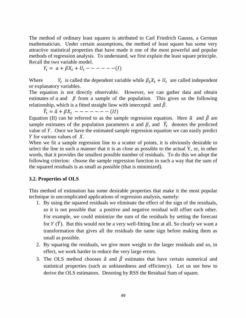
49
The method of ordinary least squares is attributed to Carl Friedrich Gausss, a German
mathematician. Under certain assumptions, the method of least square has some very
attractive statistical properties that have made it one of the most powerful and popular
methods of regression analysis. To understand, we first explain the least square principle.
Recall the two variable model.
Where is called the dependent variable while are called independent
or explanatory variables.
The equation is not directly observable. However, we can gather data and obtain
estimates of and from a sample of the population. This gives us the following
relationship, which is a fitted straight linw with intercept and .
Equation (II) can be referred to as the sample regression equation. Here and are
sample estimates of the population parameters and , and denotes the predicted
value of . Once we have the estimated sample regression equation we can easily predict
for various values of .
When we fit a sample regression line to a scatter of points, it is obviously desirable to
select the line in such a manner that it is as close as possible to the actual Y, or, in other
words, that it provides the smallest possible number of residuals. To do this we adopt the
following criterion: choose the sample regression function in such a way that the sum of
the squared residuals is as small as possible (that is minimized).
3.2. Properties of OLS
This method of estimation has some desirable properties that make it the most popular
technique in uncomplicated applications of regression analysis, namely:
1. By using the squared residuals we eliminate the effect of the sign of the residuals,
so it is not possible that a positive and negative residual will offset each other.
For example, we could minimize the sum of the residuals by setting the forecast
for ( ). But this would not be a very well-fitting line at all. So clearly we want a
transformation that gives all the residuals the same sign before making them as
small as possible.
2. By squaring the residuals, we give more weight to the larger residuals and so, in
effect, we work harder to reduce the very large errors.
3. The OLS method chooses and estimates that have certain numerical and
statistical properties (such as unbiasedness and efficiency). Let us see how to
derive the OLS estimators. Denoting by RSS the Residual Sum of square.
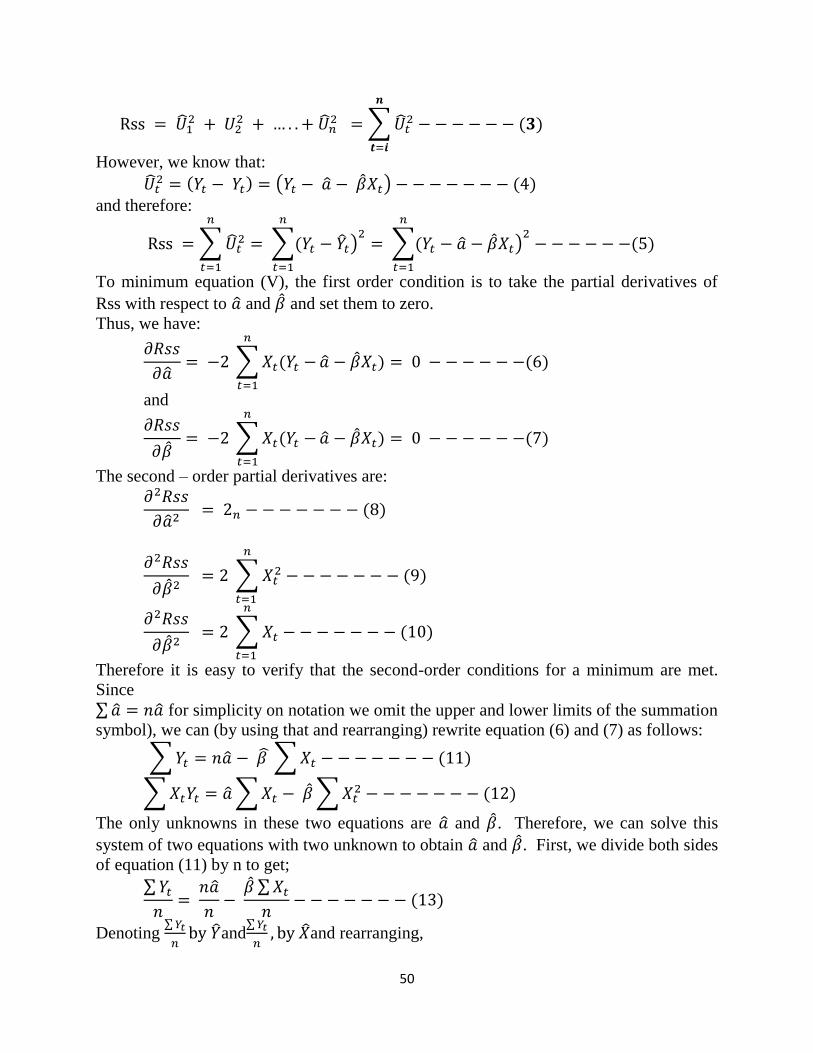
50
∑
However, we know that:
( )
and therefore:
∑
∑ ) ∑ )
To minimum equation (V), the first order condition is to take the partial derivatives of
Rss with respect to and and set them to zero.
Thus, we have:
∑
and
∑
The second – order partial derivatives are:
∑
∑
Therefore it is easy to verify that the second-order conditions for a minimum are met.
Since
∑ for simplicity on notation we omit the upper and lower limits of the summation
symbol), we can (by using that and rearranging) rewrite equation (6) and (7) as follows:
∑ ∑
∑ ∑ ∑
The only unknowns in these two equations are and . Therefore, we can solve this
system of two equations with two unknown to obtain and . First, we divide both sides
of equation (11) by n to get;
∑
∑
Denoting ∑
and
∑
and rearranging,
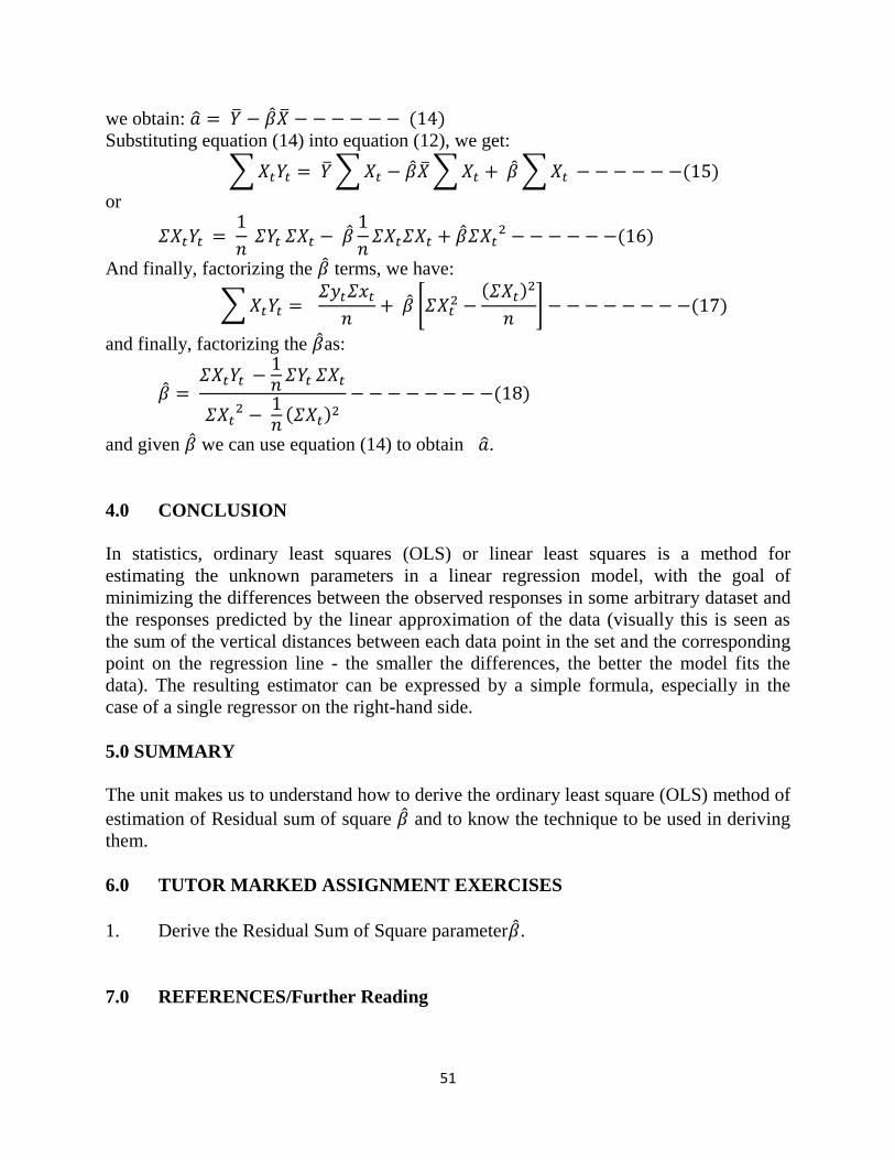
51
we obtain: Substituting equation (14) into equation (12), we get:
∑ ∑ ∑ ∑
or
And finally, factorizing the terms, we have:
∑
*
+
and finally, factorizing the as:
and given we can use equation (14) to obtain .
4.0 CONCLUSION
In statistics, ordinary least squares (OLS) or linear least squares is a method for
estimating the unknown parameters in a linear regression model, with the goal of
minimizing the differences between the observed responses in some arbitrary dataset and
the responses predicted by the linear approximation of the data (visually this is seen as
the sum of the vertical distances between each data point in the set and the corresponding
point on the regression line - the smaller the differences, the better the model fits the
data). The resulting estimator can be expressed by a simple formula, especially in the
case of a single regressor on the right-hand side.
5.0 SUMMARY
The unit makes us to understand how to derive the ordinary least square (OLS) method of
estimation of Residual sum of square and to know the technique to be used in deriving
them.
6.0 TUTOR MARKED ASSIGNMENT EXERCISES
1. Derive the Residual Sum of Square parameter .
7.0 REFERENCES/Further Reading
52
Dimitrios, A & Stephen, G., (2011). Applied Econometrics, second edition 2011, first
edition 2006 and revised edition 2007.
UNIT 3 CALCULATION OF PARAMETER AND THE ASSUMPTION OF
CLRM
CONTENTS
1.0. Introduction
2.0. Objectives
3.0. Main content
3.1. Alternative Expression for
3.2. The Assumptions of CLRM
3.2.1. The Assumptions
4.0 Conclusion
5.0 Summary
6.0 Tutor-Marked Assignment
7.0 References/Further Readings
1.0 INTRODUCTION
Based on Unit 2 we just discussed, we can also make an alternative expression for
parameter for residual sum of square and it can also be expressed further as co-variance
analysis. In this unit, the assumptions of classical linear regression model will also be
examined and you will be able to differentiate these assumptions from other economic
analysis assumptions.
2.0. OBJECTIVES
At the end of this unit, you should be able to:
know the alternative expression for
understand the assumptions of classical linear regression model.
3.0 MAIN CONTENT
3.1 Alternative Expression for
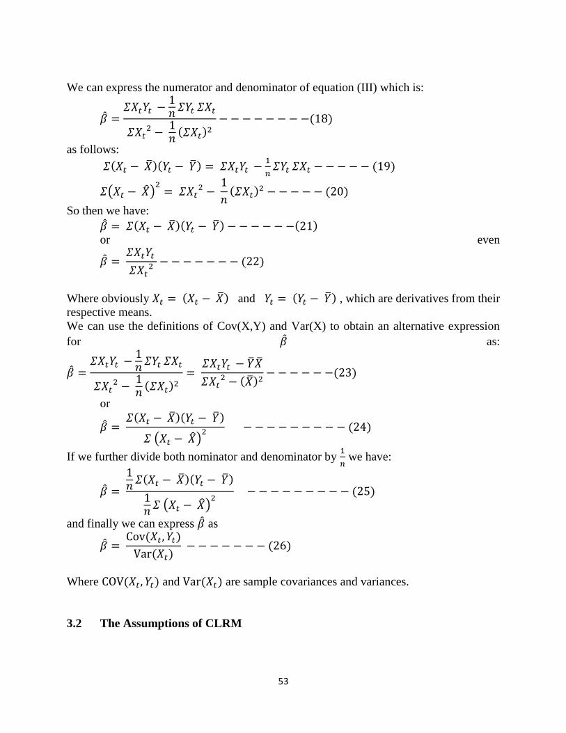
53
We can express the numerator and denominator of equation (III) which is:
as follows:
( )
So then we have:
or even
Where obviously and , which are derivatives from their
respective means.
We can use the definitions of Cov(X,Y) and Var(X) to obtain an alternative expression
for as:
or
( )
If we further divide both nominator and denominator by
we have:
( )
and finally we can express as
Where and are sample covariances and variances.
3.2 The Assumptions of CLRM
54
In a general term, when we calculate estimators of population parameters from sample
data we are bound to make some initial assumptions about the population distribution.
Usually, they amount to a set of statements about the distribution of the bariables we are
investigating, without which our model and estimates cannot be justified. Therefore it is
important not only to present the assumptions but also to move behond them, to the
extent that we will at least study what happens when they go wrong and how we may test
whether they have gone wrong.
3.2.1 The Assumptions
The CLRM consists of eight basic assumptions about the ways in which the observations
are generated:
1. Linearity: The first assumption is that the dependent variable can be calculated as
a linear function of a specific set of independent variables, plus a disturbance term.
This can be expressed mathematically as follows: The regression model is linear
in the unknown coefficients so that
2. has some variation: By this assumption we mean that not all observations of
are the same, at least one has to be different so that the sample is not 0. It
is important to distinguish between the sample variance, which simply shows how
much X varies over the particular sample, and the stochastic nature of X. in
course, we shall make the assumption that X is non-stochastic. This means that
the variance of X at any point in time is zero, so is not 0. It is important
to distinguish between the sample variance, which simply shows how much X
varies over the particular sampl, and the stochastice nature of X. In course, we
shall make the assumption that X is non-stochastic. This means that the variance
of X at any point in time is zero, so , and if we could somehow repeat
the world over againX would always take exactly the same values. But of course,
over any sample there will (indeed must) be some variations in X.
3. is non-stochastic and fixed in repeated samples. By these assumptions we
mean first that is a variable whose value are not determined by some chance
mechanism, that is they are determined by an experimenter or investigator, and
seen that it is possible to repeat the sample with the same independent variable
values. This implies that for all s, and t =1, 2 ……., n: that is
and are uncorrelated.
4. The expected value of the disturbance term is zero: - This means that the
disturbance is a genuine disturbance, so that if we took a large number of samples
the mean disturbance would be zero. This can be denoted as . We
need this assumption in order to interpret the deterministic part of a regression
model, as a statistical average relation.
55
5. Homoskedasticity: This requires that all disturbance terms have the same
variance, so that = = constant for all t.
6. Serial independence: This requires that all disturbance terms are independently
distributed, or, more easily, are not correlated with one another, so that
for all s. This
assumption has a special significance in economics to grasp what it means in
practice, recall that we nearly always obtain our data from time series in which
each t is one year, or one quarter, or one week ahead of the last. The condition
means, therefore, that the disturbance is one period should not be related to a
disturbance in the next or previous periods. This condition is frequently violated
since, if there is a disturbing effect at one time, it is likely to persist.
7. Normality of Residuals: The disturbance are assumed to be
independently and identically normally distributed, with mean zero and common
variance .
8. n>2 and multicollinearity: This assumption says that the number of observations
must be greater than two or in general than the relationships among the variables.
4.0 CONCLUSION
Classical linear regression model statistical-tool used in predicting future values of a
target (dependent) variable on the basis of the behavior of a set of explanatory factors
(independent variables). A type of regression analysis model, it assumes the target
variable is predictable, not chaotic or random.
5.0 SUMMARY
In this unit, we have vividly discuss the classical linear regression model and its
assumptions and various calculation of . So i think from this unit, you should be able to
work through the calculation of CLRM and the assumptions.
6.0 Tutor Marked Assessment Exercise.
1. Discuss extensively the assumption of classical linear regressions model.
7.0 REFERENCES/Further Reading
Dimitrios, A & Stephen, G., (2011). Applied Econometrics, second edition 2011, first
edition 2006 and revised edition 2007.
56
UNIT 4 PROPERTIES OF THE ORDINARY LEAST SQUARE
ESTIMATORS
CONTENTS
1.0. Introduction
2.0. Objectives
3.0. Main content
3.1. Properties of the OLS Estimators
4.0 Conclusion
5.0 Summary
6.0 Tutor-Marked Assignment
7.0 References/Further Readings
1.0 INTRODUCTION
The ordinary least square (OLS) estimator is consistent when the regressors are
exogenous and there is no perfect multicollinearity, and optimal in the class of linear
unbiased estimators when the errors are homoscedastic and serially uncorrelated. Under
these conditions, the method of OLS provides minimum-variance mean-unbiased
estimation when the errors have finite variances. Under the additional assumption that the
errors be normally distributed, OLS is the maximum likelihood estimator. OLS is used in
economics (econometrics), political science and electrical engineering (control theory and
signal processing), among many areas of application. The Multi-fractional order
estimator is an expanded version of OLS.
57
2.0. OBJECTIVES
At the end of this unit, you should be able to:
know the properties that our estimators should have
know the proofing of the OLS estimators as the best linear unbiased estimators
(BLUE).
3.0 MAIN CONTENT
3.1 Properties of the OLS Estimators
We now return to the properties that we would like our estimators to have. Based on the
assumptions of the CLRM can prove that the OLS estimators are best linear unbiased
estimators (BLUE). To do so, we first have to decompose the regression coefficients
estimated under OLS into their random and non-random components.
As a starting point, not that has a non-random component , as well as a
random component, captured by the residual . Therefore cov(X,Y) that is which
depends on values of – will have a random and non-random component.
[ ]
However, because are constants we have that and that
Thus
and substituting that in equation (26) yields:
which says that the OLS coefficient estimated from any sample has a non-random
component, random component which depends on .
(i). Linearity
Based on assumption 3, we have that X is non-stochastic and fixed in repeated samples.
Therefore, the x values can be treated as cosntants and we need merely to concentrate on
the Y values. If the OLS estimators are linear functions of the Y values then they are
linear estimators.
From equation (22) we have that:
58
Since the are regarded as constants, then the are regarded as constants as well, we
have that:
but because , we have that:
Where can also be regarded as constant and therefore is indeed a linear
estimator of the .
(ii) Unbiasedness.
(1) Unbiasedness of
To prove that is an unbiased estimator of we need to show that
( ) *
+
However, is a constant, and using assumptions, that is is non-random- we can take
as a fixed constant to take them out of the expectation expression and have:
[( )]
Therefore, it is enough to show that [( )]
[( )]
∑
Where
is constant, so we can take it out of the expectation expression and we can also
break the sum down into the sum of its expectations to give:
[( )]
[ [ ] ]
∑ [ ]
Furthermore, because is non-random (again from assumption 3) we can take it out of
the expression term to give:
[( )]
∑ [ ]
Finally, using assumption 4, we have that and therefore So
[( )] and this proves that:
( )
or, to put it in words, that is an unbiased estimator of the true population parameter .
(b) Unbiasedness of . We know that
59
( )
But we also have that:
Where we eliminated the
Substituting equation (40) into equation (38) gives:
( )
We have proved before that ( ) ; therefore:
( )
Which proves that is an unbiased estimator of
(iii) Efficiency and BLUEness
Under assumptions 5 and 6, we can then make a prove that the OLS estimators are the
most efficient among all unbiased linear estimators. However, we can say that the OLS
procedure yields BLU estimators.
The proof that the OLS estimators are BLU estimators is relatively complicated. It
entails a procedure which goes the opposite way from that followed so far. We start the
estimation from the beginning, trying to derive a BLU estimator of based on the
properties of linearity, unbiasedness and minimum variance one by one, and we will then
check whether the BLU estimator derived by this procedure is the same as the OLS
estimator. Thus, we want to derive the BLU estimator of , say , concentrating first on
the property of linearity. For to be linear we need to have:
∑
Where the terms are constants, the values of which are to be determined proceeding
with the property of unbiasedness, for to be unbiased, we must be able to have ( )
. However, we know that;
( ) (∑ ) ∑
Therefore, let us substitute , and also
because is non-stochastic and , given by the basic assumptions of the
model, we get;
( ) ∑ ∑ ∑
And therefore, in order to have unbiased , we need;
∑ ∑
I think you are learning through the process and you should know that econometric
notation might show as if they are abstract but they have different meaning. Therefore,
60
we can then proceed by deriving an expression for the variance (which we need to
minimize) of :
( ) [ ( )]
*∑ (∑ )+
*∑ ∑ +
*∑ +
From equation 47 above, we can use and
respectively. Then:
( ) (∑ )
(
) (
) (
) (
)
Let us use the assumptions and we obtain that:
( ) ∑
We then need to choose in the linear estimator (equation 44 to be such as to minimize
the variance (equation 49 subject to the constraints (equation 46) which ensure
unbiasedness (with this then having a linear, unbiased minimum variance estimator). We
formulate the Langrangian function:
Where and are Langrangian multipliers.
However, following the regular procedure, which is to take the first-order conditions (that
is the portal derivatives of Lwith respect to , and ) and set them equal to zero and
after re-arrangement and mathematical manipulations (we omit the mathematical details
of the derivation because it is very lengthy and tedious and because it does not use any of
the assumptions of the model in any case), we obtain the optimal as:
We can say that of the OLs expression given by Equation (32). so, substituting
this into our linear estimators we have:
61
Therefore we can conclude that of the OLs is BLU. Let us then talk more about the
advantage of the BLUEness: The advantages of the BLUEness condition is that it
provides us with an expression for the variance by substituting the optional given in
equation (51) into equation (49) and that will gives:
( ) ( ) ∑(
)
(iv) CONSISTENCY
Consistency is the idea that, as the sample becomes infinitely large, the parameter
estimate given by a procedure such as OLs converges on the true parameter value. This is
obviously true when estimator is unbiased, as shown in our previous discussion above, as
consistency is really just a weaker form of unbiasedness. However, the proof above rests
on our assumption 3, that the X variables are fixed. If we relax this assumption it is no
longer possible to prove the unbiasedness of OLs but we can still establish that it is a
consistent estimator. That is, when we relax assumption 3, OLS is no longer a BLU
estimator but it is still consistent. We showed in equation (29) in this module that
Let us divide the top and the bottom of the last term by n, we
have:
Finally, using the law of large numbers, we know that coverages to its
expectation, which is . Similarly converges to . So as n
tend to infinity (i.e. n , which is equal to the true
population parameter if (that is if uncorrelated). Thus
is a consistent estimator of the true population parameter .
4.0 CONCLUSION
The unit has critically examines assumption 5 and 6 of the CLRM and we can concludes
that efficiency and consistency of CLRM as shown that is the best property of the model
the value of
respectively.
5.0 SUMMARY
It should be noted by all the students that this unit make a continuation of the classical
linear regression model (CLRM) and it is also called the GAUSS-MARKOV
62
THEOREM. However, the unit try to proof the efficiency and consistency of classical
linear regression model (CLRM) in one case while the unit also make a difference
between the efficiency and BLUEness.
6.0 TUTOR MARKED ASSESSMENT EXERCISE
1. Discuss the differences between Efficiency and BLUEness.
2. Proof the consistency property of classical linear regression model.
7.0 REFERENCES
Dimitrios, A & Stephen, G., (2011). Applied Econometrics, second edition 2011, first
edition 2006 and revised edition 2007.
63
UNIT 5 : THE COEFFICIENT OF DETERMINATION : A MEASURE OF
“GOODNESS OF FIT”.
CONTENTS
1.0. Introduction
2.0. Objectives
3.0. Main content
3.1. Goodness of fit
4.0 Conclusion
5.0 Summary
6.0 Tutor-Marked Assignment
7.0. References/Further Readings
1.0. INTRODUCTION
In statistics, the coefficient of determination denoted R2 or r
2 and pronounced R squared,
is a number that indicates the proportion of the variance in the dependent variable that is
predictable from the independent variable.
It is a statistic used in the context of statistical models whose main purpose is either the
prediction of future outcomes or the testing of hypotheses, on the basis of other related
information. It provides a measure of how well observed outcomes are replicated by the
model, based on the proportion of total variation of outcomes explained by the model
(pp. 187, 287).
There are several definitions of R2 that are only sometimes equivalent. One class of such
cases includes that of simple linear regression where r2 is used instead of R
2. In this case,
if an intercept is included, then r2 is simply the square of the sample correlation
coefficient (i.e., r) between the outcomes and their predicted values. If additional
explanator are included, R2 is the square of the coefficient of multiple correlations. In
both such cases, the coefficient of determination ranges from 0 to 1.
Important cases where the computational definition of R2 can yield negative values,
depending on the definition used, arise where the predictions that are being compared to
the corresponding outcomes have not been derived from a model-fitting procedure using
those data, and where linear regression is conducted without including an intercept.
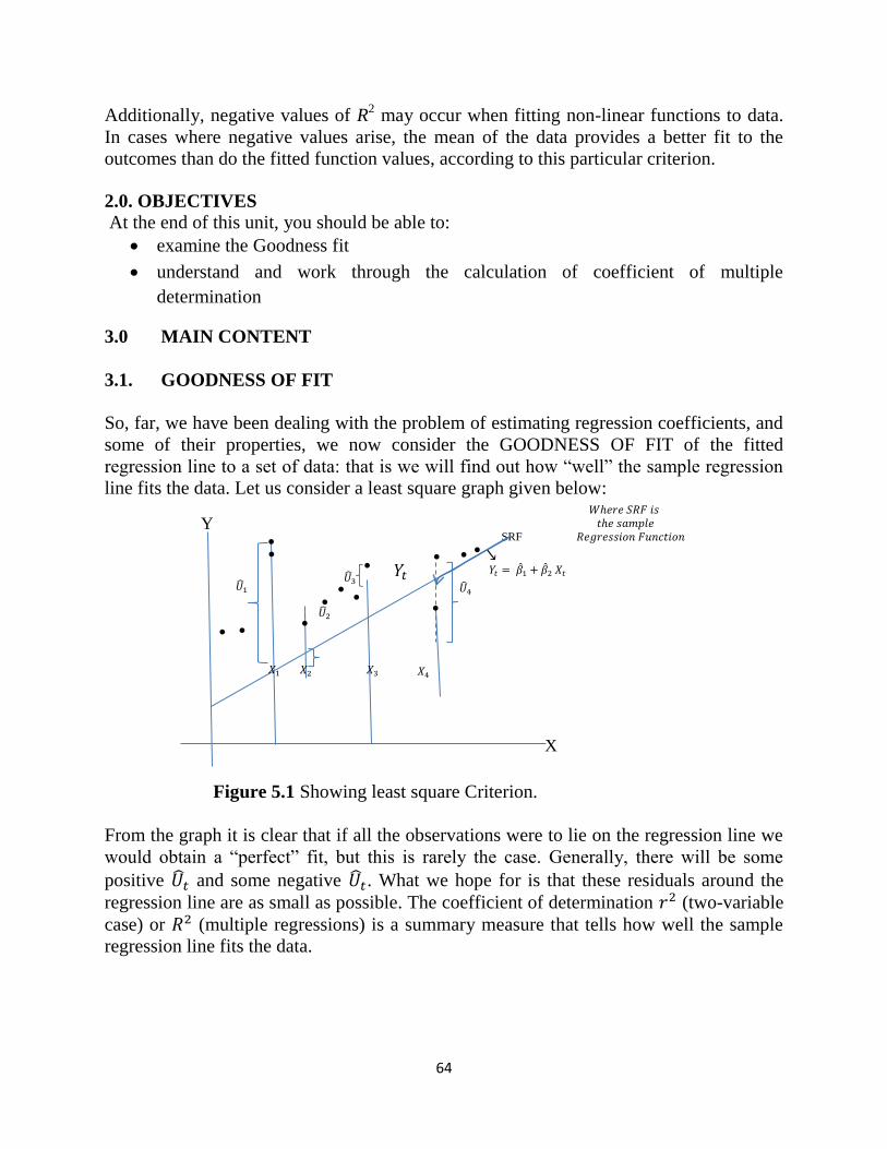
64
Additionally, negative values of R2 may occur when fitting non-linear functions to data.
In cases where negative values arise, the mean of the data provides a better fit to the
outcomes than do the fitted function values, according to this particular criterion.
2.0. OBJECTIVES
At the end of this unit, you should be able to:
examine the Goodness fit
understand and work through the calculation of coefficient of multiple
determination
3.0 MAIN CONTENT
3.1. GOODNESS OF FIT
So, far, we have been dealing with the problem of estimating regression coefficients, and
some of their properties, we now consider the GOODNESS OF FIT of the fitted
regression line to a set of data: that is we will find out how ―well‖ the sample regression
line fits the data. Let us consider a least square graph given below:
Figure 5.1 Showing least square Criterion.
From the graph it is clear that if all the observations were to lie on the regression line we
would obtain a ―perfect‖ fit, but this is rarely the case. Generally, there will be some
positive and some negative . What we hope for is that these residuals around the
regression line are as small as possible. The coefficient of determination (two-variable
case) or (multiple regressions) is a summary measure that tells how well the sample
regression line fits the data.
Y
X
SRF
𝑈
𝑈
𝑈4
𝑈
𝑌𝑡
𝑌𝑡 �� �� 𝑋𝑡
𝑋
𝑋
𝑋
𝑋4
𝑊ℎ𝑒𝑟𝑒 𝑆𝑅𝐹 𝑖𝑠 𝑡ℎ𝑒 𝑠𝑎𝑚𝑝𝑙𝑒
𝑅𝑒𝑔𝑟𝑒𝑠𝑠𝑖𝑜𝑛 𝐹𝑢𝑛𝑐𝑡𝑖𝑜𝑛
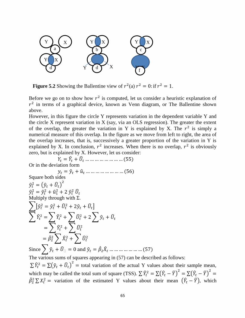
65
Figure 5.2 Showing the Ballentine view of (a) .
Before we go on to show how is computed, let us consider a heuristic explanation of
in terms of a graphical device, known as Venn diagram, or The Ballentine shown
above.
However, in this figure the circle Y represents variation in the dependent variable Y and
the circle X represent variation in X (say, via an OLS regression). The greater the extent
of the overlap, the greater the variation in Y is explained by X. The is simply a
numerical measure of this overlap. In the figure as we move from left to right, the area of
the overlap increases, that is, successively a greater proportion of the variation in Y is
explained by X. In conclusion, increases. When there is no overlap, is obviously
zero, but is explained by X. However, let us consider:
Or in the deviation form
Square both sides
( )
Multiply through with .
∑[
]
∑ ∑
∑ ∑
∑ ∑
∑
∑
∑
The various sums of squares appearing in (57) can be described as follows:
∑ ∑( )
total variation of the actual Y values about their sample mean,
which may be called the total sum of square (TSS). ∑ ∑( )
∑( )
∑
variation of the estimated Y values about their mean ( ) which
a
Y X Y X
b
Y X
c
d
Y X
Y X
d Y=X f
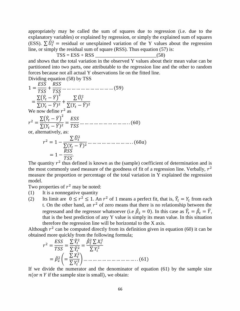
66
appropriately may be called the sum of squares due to regression (i.e. due to the
explanatory variables) or explained by regression, or simply the explained sum of squares
(ESS). ∑ residual or unexplained variation of the Y values about the regression
line, or simply the residual sum of square (RSS). Thus equation (57) is:
TSS = ESS + RSS ________________________(58)
and shows that the total variation in the observed Y values about their mean value can be
partitioned into two parts, one attributable to the regression line and the other to random
forces because not all actual Y observations lie on the fitted line.
Dividing equation (58) by TSS
∑( )
∑
∑
∑
We now define as
∑( )
∑
or, alternatively, as:
∑
∑
The quantity thus defined is known as the (sample) coefficient of determination and is
the most commonly used measure of the goodness of fit of a regression line. Verbally,
measure the proportion or percentage of the total variation in Y explained the regression
model.
Two properties of may be noted:
(1) It is a nonnegative quantity
(2) Its limit are An of 1 means a perfect fit, that is, from each
t. On the other hand, an of zero means that there is no relationship between the
regressand and the regressor whatsoever (i.e . In this case as ,
that is the best prediction of any Y value is simply its mean value. In this situation
therefore the regression line will be horizontal to the X axis.
Although can be computed directly from its definition given in equation (60) it can be
obtained more quickly from the following formula;
∑
∑
∑
∑
(
∑
∑ )
If we divide the numerator and the denominator of equation (61) by the sample size
, we obtain:
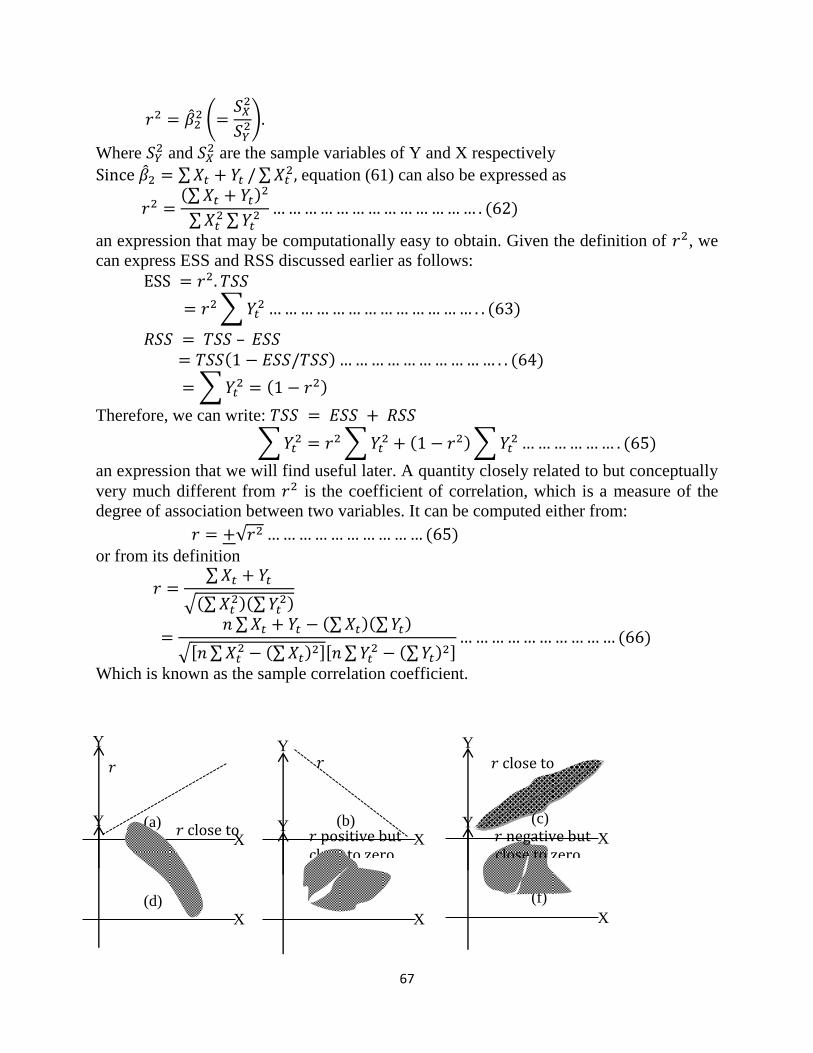
67
(
)
Where and
are the sample variables of Y and X respectively
∑ ∑ equation (61) can also be expressed as
∑
∑ ∑
an expression that may be computationally easy to obtain. Given the definition of , we
can express ESS and RSS discussed earlier as follows:
∑
–
∑
Therefore, we can write:
∑ ∑
∑
an expression that we will find useful later. A quantity closely related to but conceptually
very much different from is the coefficient of correlation, which is a measure of the
degree of association between two variables. It can be computed either from:
√
or from its definition
∑
√ ∑ ∑
∑ ∑ ∑
√[ ∑ ∑
][ ∑ ∑
]
Which is known as the sample correlation coefficient.
Y Y Y
X X X
𝑟
𝑟
(a) (b) (c)
𝑟
Y Y Y
X X X
𝑟
(d) (e) (f)
f
𝑟
𝑟 g
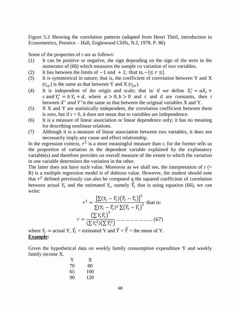
68
Figure 5.3 Showing the correlation patterns (adapted from Henri Theil, introduction to
Econometrics, Prentice – Hall, Englewood Cliffs, N.J, 1978. P. 86)
Some of the properties of r are as follows:
(1) It can be positive or negative, the sign depending on the sign of the term in the
numerator of (66) which measures the sample co variation of two variables.
(2) It lies between the limits of | | (3) It is symmetrical in nature; that is, the coefficient of correlation between Y and X
( ) is the same as that between Y and X ( ).
(4) It is independent of the origin and scale; that is/ if we define
where and c and d are constants, then r
between is the same as that between the original variables X and Y.
(5) If X and Y are statistically independent, the correlation coefficient between them
is zero, but if r = 0, it does not mean that to variables are independence.
(6) It is a measure of linear association or linear dependence only; it has no meaning
for describing nonlinear relations.
(7) Although it is a measure of linear association between two variables, it does not
necessarily imply any cause and effect relationship.
In the regression context, is a more meaningful measure than r, for the former tells us
the proportion of variation in the dependent variable explained by the explanatory
variable(s) and therefore provides on overall measure of the extent to which the variation
in one variable determines the variation in the other.
The latter does not have such value. Moreover as we shall see, the interpretation of r (=
R) is a multiple regression model is of dubious value. However, the student should note
that defined previously can also be computed q the squared coefficient of correlation
between actual and the estimated , namely that is using equation (66), we can
write:
[∑ ( )]
∑ ∑( )
(∑ )
∑ (∑
)
where actual Y, = estimated Y and = = the mean of Y.
Example:
Given the hypothetical data on weekly family consumption expenditure Y and weekly
family income X.
Y X
70 80
65 100
90 120
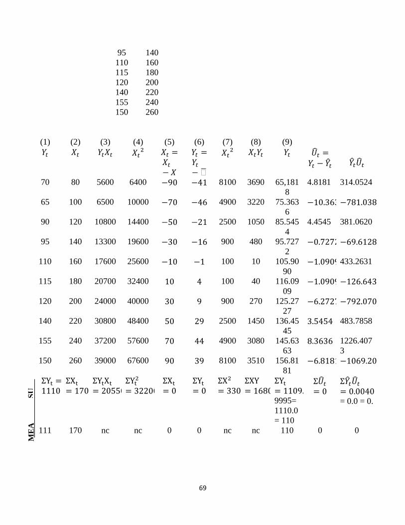
69
95 140
110 160
115 180
120 200
140 220
155 240
150 260
(1)
(2)
(3)
(4)
(5)
(6)
(7)
(8)
(9)
70 80 5600 6400 8100 3690 65,181
8
4.8181 314.0524
65 100 6500 10000 4900 3220 75.363
6
90 120 10800 14400 2500 1050 85.545
4
4.4545 381.0620
95 140 13300 19600 900 480 95.727
2
110 160 17600 25600 100 10 105.90
90 433.2631
115 180 20700 32400 100 40 116.09
09
120 200 24000 40000 900 270 125.27
27
140 220 30800 48400 2500 1450 136.45
45 483.7858
155 240 37200 57600 4900 3080 145.63
63 1226.407
3
150 260 39000 67600 8100 3510 156.81
81
9995=
1110.0
= 110
= 0.0 = 0.
111 170 nc nc 0 0 nc nc 110 0 0
ME
A
N
SU
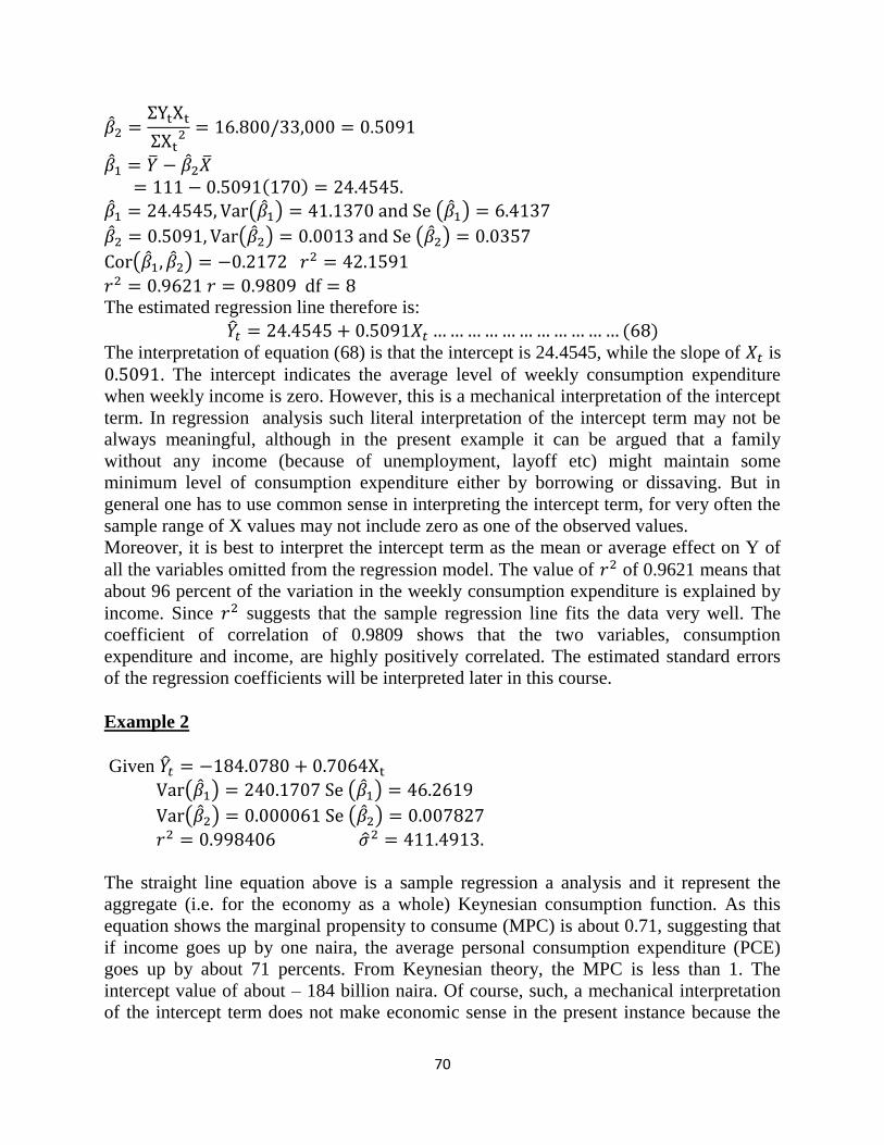
70
( ) ( )
( ) ( )
( )
The estimated regression line therefore is:
The interpretation of equation (68) is that the intercept is 24.4545, while the slope of is
. The intercept indicates the average level of weekly consumption expenditure
when weekly income is zero. However, this is a mechanical interpretation of the intercept
term. In regression analysis such literal interpretation of the intercept term may not be
always meaningful, although in the present example it can be argued that a family
without any income (because of unemployment, layoff etc) might maintain some
minimum level of consumption expenditure either by borrowing or dissaving. But in
general one has to use common sense in interpreting the intercept term, for very often the
sample range of X values may not include zero as one of the observed values.
Moreover, it is best to interpret the intercept term as the mean or average effect on Y of
all the variables omitted from the regression model. The value of of 0.9621 means that
about 96 percent of the variation in the weekly consumption expenditure is explained by
income. Since suggests that the sample regression line fits the data very well. The
coefficient of correlation of 0.9809 shows that the two variables, consumption
expenditure and income, are highly positively correlated. The estimated standard errors
of the regression coefficients will be interpreted later in this course.
Example 2
Given
( ) ( )
( ) ( )
The straight line equation above is a sample regression a analysis and it represent the
aggregate (i.e. for the economy as a whole) Keynesian consumption function. As this
equation shows the marginal propensity to consume (MPC) is about 0.71, suggesting that
if income goes up by one naira, the average personal consumption expenditure (PCE)
goes up by about 71 percents. From Keynesian theory, the MPC is less than 1. The
intercept value of about – 184 billion naira. Of course, such, a mechanical interpretation
of the intercept term does not make economic sense in the present instance because the
71
zero income value is out of range of values we are working with and does not represent a
likely outcome. As we will see on many occasion, very often the intercept term may not
make much economic sense.
Therefore, in practice the intercept term may not be very meaningful although on
occasions it can be very meaningful, in some analysis. The more meaningful value is the
slope coefficient MPC in the present case.
The value of 0.9984 means approximately 99 percent of the variation in the PCE is
explained by variation in the GDP. Since at most can be 1, we can say that the
regression line in the equation above fit our data extremely well; as you can see from that
figure the actual data points are very tightly clustered around the estimated regression
line.
4.0 CONCLUSION
Coefficient of multiple determinations ( as been seen as an area of economic analysis
that try to explain the variation in the dependent and independent variable in a
simple/multiple regression analysis of ordinary least square method and it is one of the
best instrument use to know whether a regression is spurious or not.
5.0 SUMMARY
The unit has vividly looked at the analysis of coefficient of determination and this
measures the goodness of fit.
However the unit also make some proof of and its component which is total sum of
squares, which is equal to residual sum of square and error sum of squares.
The interpretation of simple equation of a straight was also analysis which is called the
simple regression analysis.
6.0 TUTOR MARKED ASSESSMENT EXERCISE
Given
. Interpret the equation critically.
7.0 REFERENCES/FURTHER READINGS
Gujarat, D. N. (2007) Basic Econometrics, 4th
Edition, tata Mcgraw – Hill publishing
company limited, New Delhi.
Hall, S. G., & Asterion, D. (2011) Applied Econometrics, 2nd
Edition, Palgrave
Macmillian, New York city, USA.
72
MODULE THREE: NORMAL LINEAR REGRESSION MODEL (CNLRM)
UNIT ONE: Classical Normal Linear Regression Model
UNIT TWO: OLS Estimators Under the Normality Assumption
UNIT THREE: The Method of Maximum Likelihood (ML)
UNIT FOUR: Confidence Intervals for Regression Coefficients AND
UNIT FIVE: Hypothesis Testing
UNIT ONE : CLASSICAL NORMAL LINEAR REGRESSION MODEL
CONTENTS
1.0 Introduction
2.0 Objectives
3.0 Main content
3.1. The Probability Distribution of Disturbances Ui
3.2. The Normality Assumption for Ui
3.2.1. Why the Normality Assumption
4.0 Conclusion
5.0 Summary
4.0 Tutor-Marked Assignment
7.0. References/Further Readings
1.0. INTRODUCTION
What is known as the classical theory of statistical inference consists of two branches,
namely, estimation and hypothesis testing. We have thus far covered the topic of
estimation of the parameters of the (two variable) linear regression model. Using the
method of OLS we were able to estimate the parameters , and . Under the
assumptions of the classical linear regression model (CLRM), we were able to show that
the estimators of these parameters, , and , satisfy several desirable statistical
properties, such as unbiasedness, minimum variance, etc. (Recall the BLUE property.)
Note that, since these are estimators, their values will change from sample to sample.
Therefore, these estimators are random variables.
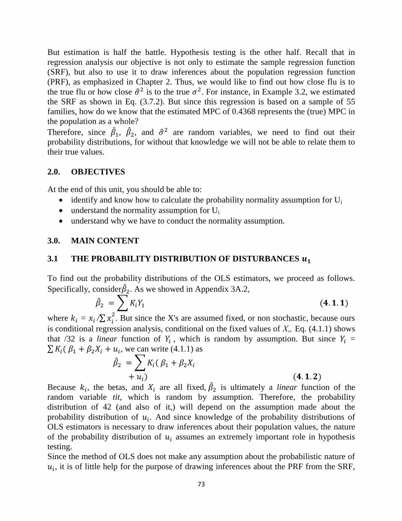
73
But estimation is half the battle. Hypothesis testing is the other half. Recall that in
regression analysis our objective is not only to estimate the sample regression function
(SRF), but also to use it to draw inferences about the population regression function
(PRF), as emphasized in Chapter 2. Thus, we would like to find out how close flu is to
the true flu or how close is to the true . For instance, in Example 3.2, we estimated
the SRF as shown in Eq. (3.7.2). But since this regression is based on a sample of 55
families, how do we know that the estimated MPC of 0.4368 represents the (true) MPC in
the population as a whole?
Therefore, since , , and are random variables, we need to find out their
probability distributions, for without that knowledge we will not be able to relate them to
their true values.
2.0. OBJECTIVES
At the end of this unit, you should be able to:
identify and know how to calculate the probability normality assumption for Ui
understand the normality assumption for Ui
understand why we have to conduct the normality assumption.
3.0. MAIN CONTENT
3.1 THE PROBABILITY DISTRIBUTION OF DISTURBANCES
To find out the probability distributions of the OLS estimators, we proceed as follows.
Specifically, consider . As we showed in Appendix 3A.2,
∑
where = /∑ . But since the X's are assumed fixed, or non stochastic, because ours
is conditional regression analysis, conditional on the fixed values of X„ Eq. (4.1.1) shows
that /32 is a linear function of , which is random by assumption. But since = ∑ , we can write (4.1.1) as
∑
Because , the betas, and are all fixed, is ultimately a linear function of the
random variable tit, which is random by assumption. Therefore, the probability
distribution of 42 (and also of it,) will depend on the assumption made about the
probability distribution of . And since knowledge of the probability distributions of
OLS estimators is necessary to draw inferences about their population values, the nature
of the probability distribution of assumes an extremely important role in hypothesis
testing.
Since the method of OLS does not make any assumption about the probabilistic nature of
, it is of little help for the purpose of drawing inferences about the PRF from the SRF,
74
the Gauss-Markov theorem notwithstanding. This void can be filled if we are willing to
assume that the u's follow some probability distribution. For reasons to be explained
shortly, in the regression context it is usually assumed that the u's follow the normal
distribution. Adding the normality assumption for it to the assumptions of the classical
linear regression model (CLRM) discussed in Chapter 3, we obtain what is known as the
classical normal linear regression model (CNLRM).
3.2 THE NORMALITY ASSUMPTION FOR
The classical normal linear regression model assumes that each is distributed normally
with
Mean: (4.2.1)
Variance: [ ]
(4.2.2)
cov ( ): {[ ][ ]} ( ) (4.2.3)
The assumptions given above can be more compactly stated as
(4.2.4)
where the symbol — means distributed as and N stands for the normal distribution, the
terms in the parentheses representing the two parameters of the normal distribution,
namely, the mean and the variance.
As noted in Appendix A, for two normally distributed variables, zero covariance or
correlation means independence of the two variables. Therefore, with the normality
assumption, (4.2.4) means that , and are not only uncorrelated but are also
independently distributed.
Therefore, we can write (4.2.4) as
(4.2.5) where NID stands for normally and independently distributed.
3.2.1. Why the Normality Assumption?
Why do we employ the normality assumption? There are several reasons:
1. represent the combined influence (on the dependent variable) of a large number
of independent variables that are not explicitly introduced in the regression model.
As noted, we hope that the influence of these omitted or neglected variables is
small and at best random. Now by the celebrated central limit theorem (CLT) of
statistics (see Appendix A for details), it can be shown that if there are a large
number of independent and identically distributed random variables, then, with a
few exceptions, the distribution of their sum tends to a normal distribution as the
number of such variables increase indefinitely.' It is the CLT that provides a
theoretical justification for the assumption of normality of .
2. A variant of the CLT states that, even if the number of variables is not very large
or if these variables are not strictly independent, their sum may still be normally
distributed.2
75
3. With the normality assumption, the probability distributions of OLS estimators
can be easily derived because, as noted in Appendix A, one property of the normal
distribution is that any linear function of normally distributed variables is itself
normally distributed. OLS estimators , and are linear functions of .
Therefore, if are normally distributed, so are , and , which makes our task
of hypothesis testing very straightforward.
4. The normal distribution is a comparatively simple distribution involving only two
parameters (mean and variance); it is very well known and its theoretical
properties have been extensively studied in mathematical statistics. Besides, many
phenomena seem to follow the normal distribution.
5. Finally, if we are dealing with a small, or finite, sample size, say data of less than
100 observations, the normality assumption assumes a critical role. It not only
helps us to derive the exact probability distributions of OLS estimators but also
enables us to use the t, F, and statistical tests for regression models. The
statistical properties of t, F, and probability distributions are discussed in
Appendix A. As we will show subsequently, if the sample size is reasonably large,
we may be able to relax the normality assumption.
A cautionary note: Since we are "imposing" the normality assumption, it behooves us to
find out in practical applications involving small sample size data whether the normality
assumption is appropriate. Later, we will develop some tests to do just that. Also, later we
will come across situations where the normality assumption may be inappropriate. But
until then we will continue with the normality assumption for the reasons discussed
previously.
4.0 CONCLUSION
In this unit we conclude that the normality assumption is one of the most misunderstood
in all of statistics. In multiple regressions, the assumption requiring a normal distribution
applies only to the disturbance term, not to the independent variables as is often
believed. Perhaps the confusion about this assumption derives from difficulty
understanding what this disturbance term refers to – simply put, it is the random error in
the relationship between the independent variables and the dependent variable in a
regression model. Each case in the sample actually has a different random variable
which encompasses all the ―noise‖ that accounts for differences in the observed and
predicted values produced by a regression equation, and it is the distribution of this
disturbance term or noise for all cases in the sample that should be normally distributed.
5.0 SUMMARY
In this unit, we must have been able to understand the normality assumption and the
assumption of normality is just the supposition that the underlying random variable of
interest is distributed normally, or approximately so. Intuitively, normality may be
understood as the result of the sum of a large number of independent random events.
76
4.0 TUTOR MARKED ASSESSMENT EXERCISE
Critically discuss why we employ Normality assumption.
7.0 REFERENCES/FURTHER READINGS
Gujarat, D. N. (2007) Basic Econometrics, 4th
Edition, tata Mcgraw – Hill publishing
company limited, New Delhi.
Hall, S. G., & Asterion, D. (2011) Applied Econometrics, 2nd
Edition, Palgrave
Macmillian, New York city, USA.
UNIT TWO: OLS ESTIMATORS UNDER THE NORMALITY ASSUMPTION
CONTENTS
1.0 Introduction
2.0 Objectives
3.0 Main content
3.1. Properties of OLS Estimators under the Normality Assumption
4.0 Conclusion
5.0 Summary
2.0 Tutor-Marked Assignment
7.0. References/Further Readings
1.0. INTRODUCTION
The OLS estimators that we create through linear regression give us a relationship
between the variables. However, performing a regression does not automatically give us a
reliable relationship between the variables. In order to create reliable relationships, we
77
must know the properties of the estimators and show that some basic assumptions about
the data are true under the normality assumption. One must understand that having a
good dataset is of enormous importance for applied economic research. Therefore, in this
unit we will vividly discuss the OLS estimators under the normality assumption.
2.0. OBJECTIVES
At the end of this unit, you should be able to:
identify the properties of OLS estimators under the normality assumption
understand what is probability distribution
3.0. MAIN CONTENT
3.1. PROPERTIES OF OLS ESTIMATORS UNDER THE NORMALITY
ASSUMPTION
With the assumption that u, follow the normal distribution as in (4.2.5), the OLS
estimators have the following properties; Appendix A provides a general discussion of
the desirable statistical properties of estimators.
1. They are unbiased.
2. They have minimum variance. Combined with 1, this means that they are
minimum-variance unbiased, or efficient estimators.
3. They have consistency; that is, as the sample size increases indefinitely, the
estimators converge to their true population values.
4 (being a linear function of u,) is normally distributed with
Mean: (4.3.1)
∑
∑
= (3.3.3) (4.3.2)
Or more compactly,
Then by the properties of the normal distribution the variable Z, which is defined as
(4.3.3)
follows the standard normal distribution, that is, a normal distribution with zero mean and
unit variance, or
5. (being a linear function of ) is normally distributed with
Mean: E( ) = (4.3.4)
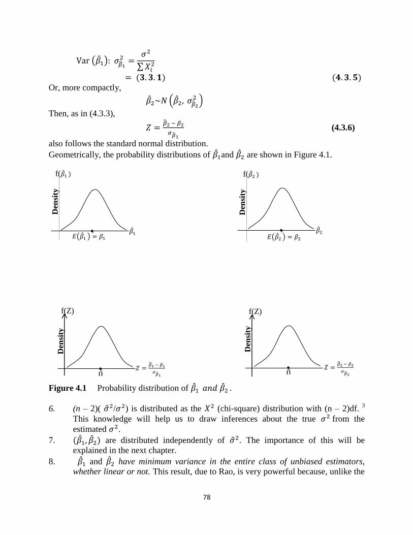
78
( )
∑
Or, more compactly,
(
)
Then, as in (4.3.3),
(4.3.6)
also follows the standard normal distribution.
Geometrically, the probability distributions of and are shown in Figure 4.1.
Figure 4.1 Probability distribution of
6. (n – 2)( / ) is distributed as the (chi-square) distribution with (n – 2)df. 3
This knowledge will help us to draw inferences about the true from the
estimated .
7. are distributed independently of . The importance of this will be
explained in the next chapter.
8. and have minimum variance in the entire class of unbiased estimators,
whether linear or not. This result, due to Rao, is very powerful because, unlike the
f(Z) f(Z)
𝑍 �� 𝛽
𝜎��
𝑍 �� 𝛽
𝜎��
Den
sity
Den
sity
f(�� f(��
�� ��
Den
sity
Den
sity
𝐸(�� ) 𝛽 𝐸(�� ) 𝛽
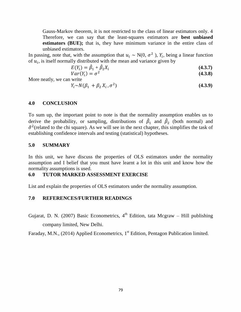
79
Gauss-Markov theorem, it is not restricted to the class of linear estimators only. 4
Therefore, we can say that the least-squares estimators are best unbiased
estimators (BUE); that is, they have minimum variance in the entire class of
unbiased estimators.
In passing, note that, with the assumption that N(0, ), , being a linear function
of , is itself normally distributed with the mean and variance given by
+ (4.3.7)
(4.3.8) More neatly, we can write
) (4.3.9)
4.0 CONCLUSION
To sum up, the important point to note is that the normality assumption enables us to
derive the probability, or sampling, distributions of and (both normal) and
(related to the chi square). As we will see in the next chapter, this simplifies the task of
establishing confidence intervals and testing (statistical) hypotheses.
5.0 SUMMARY
In this unit, we have discuss the properties of OLS estimators under the normality
assumption and I belief that you must have learnt a lot in this unit and know how the
normality assumptions is used.
6.0 TUTOR MARKED ASSESSMENT EXERCISE
List and explain the properties of OLS estimators under the normality assumption.
7.0 REFERENCES/FURTHER READINGS
Gujarat, D. N. (2007) Basic Econometrics, 4th
Edition, tata Mcgraw – Hill publishing
company limited, New Delhi.
Faraday, M.N., (2014) Applied Econometrics, 1st Edition, Pentagon Publication limited.
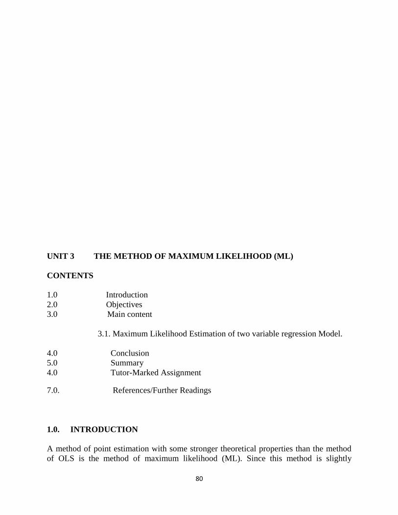
80
UNIT 3 THE METHOD OF MAXIMUM LIKELIHOOD (ML)
CONTENTS
1.0 Introduction
2.0 Objectives
3.0 Main content
3.1. Maximum Likelihood Estimation of two variable regression Model.
4.0 Conclusion
5.0 Summary
4.0 Tutor-Marked Assignment
7.0. References/Further Readings
1.0. INTRODUCTION
A method of point estimation with some stronger theoretical properties than the method
of OLS is the method of maximum likelihood (ML). Since this method is slightly
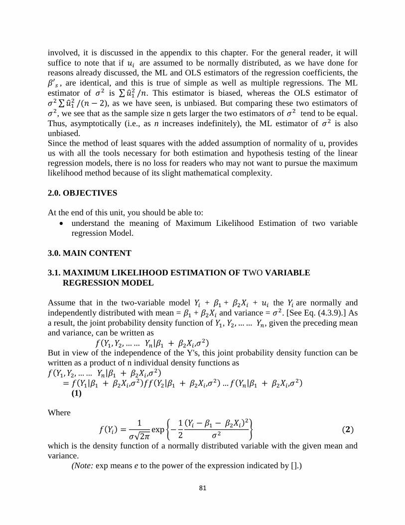
81
involved, it is discussed in the appendix to this chapter. For the general reader, it will
suffice to note that if are assumed to be normally distributed, as we have done for
reasons already discussed, the ML and OLS estimators of the regression coefficients, the
, are identical, and this is true of simple as well as multiple regressions. The ML
estimator of is ∑ . This estimator is biased, whereas the OLS estimator of
∑ ), as we have seen, is unbiased. But comparing these two estimators of
, we see that as the sample size n gets larger the two estimators of tend to be equal.
Thus, asymptotically (i.e., as n increases indefinitely), the ML estimator of is also
unbiased.
Since the method of least squares with the added assumption of normality of u, provides
us with all the tools necessary for both estimation and hypothesis testing of the linear
regression models, there is no loss for readers who may not want to pursue the maximum
likelihood method because of its slight mathematical complexity.
2.0. OBJECTIVES
At the end of this unit, you should be able to:
understand the meaning of Maximum Likelihood Estimation of two variable
regression Model.
3.0. MAIN CONTENT
3.1. MAXIMUM LIKELIHOOD ESTIMATION OF TWO VARIABLE
REGRESSION MODEL
Assume that in the two-variable model + + + the are normally and
independently distributed with mean = + and variance = . [See Eq. (4.3.9).] As
a result, the joint probability density function of , , given the preceding mean
and variance, can be written as
|
But in view of the independence of the Y's, this joint probability density function can be
written as a product of n individual density functions as
|
| |
|
(1)
Where
√ ,
-
which is the density function of a normally distributed variable with the given mean and
variance.
(Note: exp means e to the power of the expression indicated by [].)
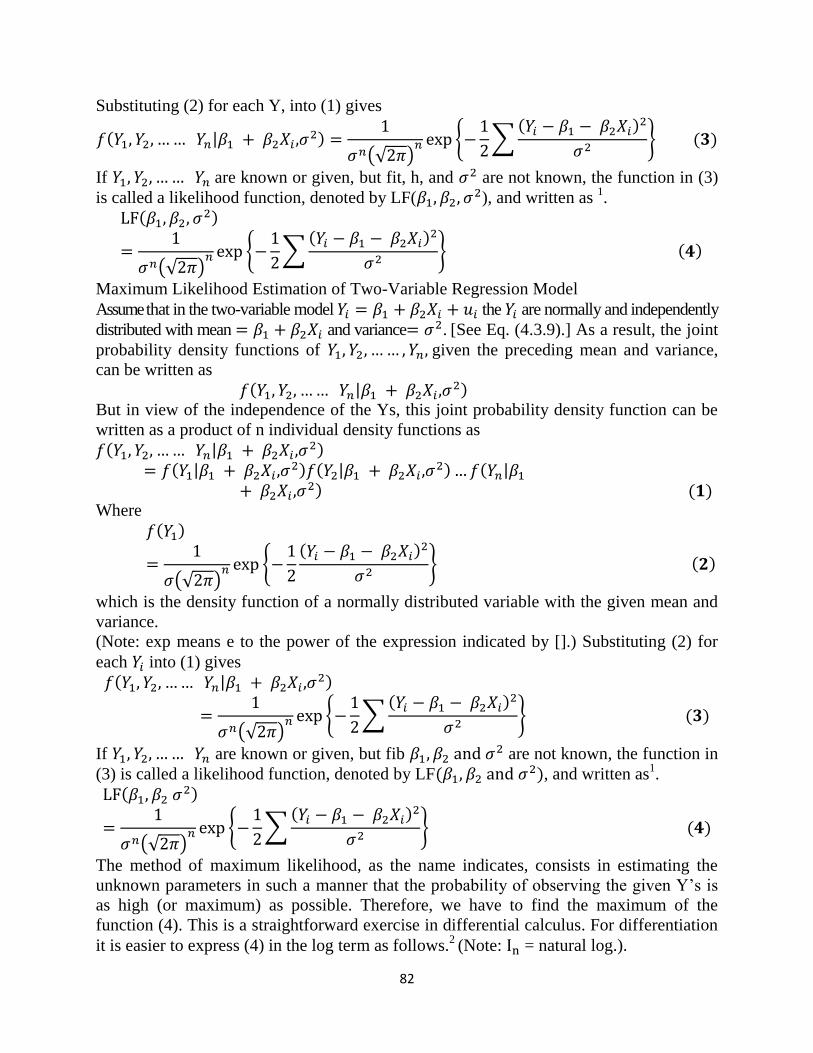
82
Substituting (2) for each Y, into (1) gives
|
(√ ) ,
∑
-
If are known or given, but fit, h, and are not known, the function in (3)
is called a likelihood function, denoted by LF( ), and written as
1.
(√ ) ,
∑
-
Maximum Likelihood Estimation of Two-Variable Regression Model
Assume that in the two-variable model the are normally and independently
distributed with mean and variance . [See Eq. (4.3.9).] As a result, the joint
probability density functions of given the preceding mean and variance,
can be written as
|
But in view of the independence of the Ys, this joint probability density function can be
written as a product of n individual density functions as
|
| |
|
Where
(√ ) ,
-
which is the density function of a normally distributed variable with the given mean and
variance.
(Note: exp means e to the power of the expression indicated by [].) Substituting (2) for
each into (1) gives
|
(√ ) ,
∑
-
If are known or given, but fib are not known, the function in
(3) is called a likelihood function, denoted by LF , and written as
1.
(√ ) ,
∑
-
The method of maximum likelihood, as the name indicates, consists in estimating the
unknown parameters in such a manner that the probability of observing the given Y‘s is
as high (or maximum) as possible. Therefore, we have to find the maximum of the
function (4). This is a straightforward exercise in differential calculus. For differentiation
it is easier to express (4) in the log term as follows.2
(Note: = natural log.).
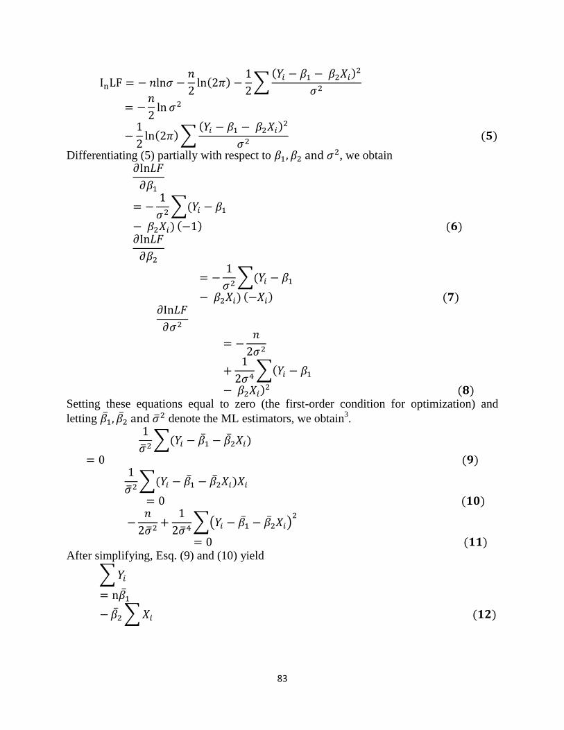
83
∑
∑
Differentiating (5) partially with respect to , we obtain
∑
∑
4∑
Setting these equations equal to zero (the first-order condition for optimization) and
letting denote the ML estimators, we obtain
3.
∑
∑
4∑( )
After simplifying, Esq. (9) and (10) yield
∑
∑
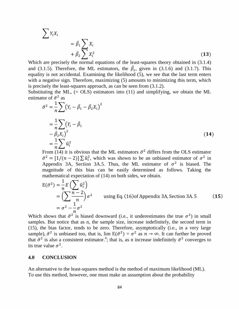
84
∑
∑
∑
Which are precisely the normal equations of the least-squares theory obtained in (3.1.4)
and (3.1.5). Therefore, the ML estimators, the , given in (3.1.6) and (3.1.7). This
equality is not accidental. Examining the likelihood (5), we see that the last term enters
with a negative sign. Therefore, maximizing (5) amounts to minimizing this term, which
is precisely the least-squares approach, as can be seen from (3.1.2).
Substituting the ML, (= OLS) estimators into (11) and simplifying, we obtain the ML
estimator of as
∑( )
∑(
)
∑
From (14) it is obvious that the ML estimators differs from the OLS estimator
[ ]∑ , which was shown to be an unbiased estimator of in
Appendix 3A, Section 3A.5. Thus, the ML estimator of is biased. The
magnitude of this bias can be easily determined as follows. Taking the
mathematical expectation of (14) on both sides, we obtain.
(∑
)
(∑
) g
Which shows that is biased downward (i.e., it underestimates the true ) in small
samples. But notice that as n, the sample size, increase indefinitely, the second term in
(15), the bias factor, tends to be zero. Therefore, asymptotically (i.e., in a very large
sample), is unbiased too, that is, lim E( = as . It can further be proved
that is also a consistent estimator.4; that is, as n increase indefinitely converges to
its true value .
4.0 CONCLUSION
An alternative to the least-squares method is the method of maximum likelihood (ML).
To use this method, however, one must make an assumption about the probability
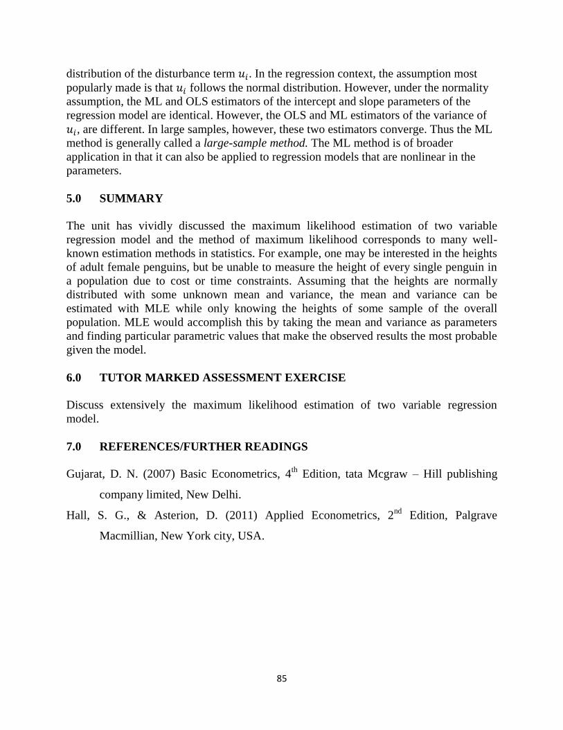
85
distribution of the disturbance term . In the regression context, the assumption most
popularly made is that follows the normal distribution. However, under the normality
assumption, the ML and OLS estimators of the intercept and slope parameters of the
regression model are identical. However, the OLS and ML estimators of the variance of
, are different. In large samples, however, these two estimators converge. Thus the ML
method is generally called a large-sample method. The ML method is of broader
application in that it can also be applied to regression models that are nonlinear in the
parameters.
5.0 SUMMARY
The unit has vividly discussed the maximum likelihood estimation of two variable
regression model and the method of maximum likelihood corresponds to many well-
known estimation methods in statistics. For example, one may be interested in the heights
of adult female penguins, but be unable to measure the height of every single penguin in
a population due to cost or time constraints. Assuming that the heights are normally
distributed with some unknown mean and variance, the mean and variance can be
estimated with MLE while only knowing the heights of some sample of the overall
population. MLE would accomplish this by taking the mean and variance as parameters
and finding particular parametric values that make the observed results the most probable
given the model.
6.0 TUTOR MARKED ASSESSMENT EXERCISE
Discuss extensively the maximum likelihood estimation of two variable regression
model.
7.0 REFERENCES/FURTHER READINGS
Gujarat, D. N. (2007) Basic Econometrics, 4th
Edition, tata Mcgraw – Hill publishing
company limited, New Delhi.
Hall, S. G., & Asterion, D. (2011) Applied Econometrics, 2nd
Edition, Palgrave
Macmillian, New York city, USA.
86
UNIT 4 CONFIDENCE INTERVALS FOR REGRESSION COEFFICIENTS
AND
CONTENTS
1.0 Introduction
2.0 Objectives
3.0 Main content
3.1. Confidence intervals for regression Coefficients
3.2. Confidence interval for
4.0 Conclusion
5.0 Summary
2.0 Tutor-Marked Assignment
7.0. References/Further Readings
1.0. INTRODUCTION
Interval estimates can be contrasted with point estimates. A point estimate is a single
value given as the estimate of a population parameter that is of interest, for example the
mean of some quantity. An interval estimate specifies instead a range within which the
parameter is estimated to lie. Confidence intervals are commonly reported in tables or
87
graphs along with point estimates of the same parameters, to show the reliability of the
estimates.
For example, a confidence interval can be used to describe how reliable survey results
are. In a poll of election voting-intentions, the result might be that 40% of respondents
intend to vote for a certain party. A 99% confidence interval for the proportion in the
whole population having the same intention on the survey might be 30% to 50%. From
the same data one may calculate a 90% confidence interval, which in this case might be
37% to 43%. A major factor determining the length of a confidence interval is the size of
the sample used in the estimation procedure, for example the number of people taking
part in a survey.
In statistics, a confidence interval (CI) is a type of interval estimate of a population
parameter. It is an observed interval (i.e., it is calculated from the observations), in
principle different from sample to sample, that frequently includes the value of an
unobservable parameter of interest if the experiment is repeated. How frequently the
observed interval contains the parameter is determined by the confidence level or
confidence coefficient. More specifically, the meaning of the term "confidence level" is
that, if CI are constructed across many separate data analyses of replicated (and possibly
different) experiments, the proportion of such intervals that contain the true value of the
parameter will match the given confidence level. Whereas two-sided confidence limits
form a confidence interval, their one-sided counterparts are referred to as lower/upper
confidence bounds (or limits). The confidence interval contains the parameter values that,
when tested, should not be rejected with the same sample. Greater levels of variance yield
larger confidence intervals, and hence less precise estimates of the parameter. Confidence
intervals of difference parameters not containing 0 imply that there is a statistically
significant difference between the populations.
In applied practice, confidence intervals are typically stated at the 95% confidence level.
However, when presented graphically, confidence intervals can be shown at several
confidence levels, for example 90%, 95% and 99%.
Certain factors may affect the confidence interval size including size of sample, level of
confidence, and population variability. A larger sample size normally will lead to a better
estimate of the population parameter.
Confidence intervals were introduced to statistics by Jerzy Neyman in a paper published
in 1937
2.0. OBJECTIVES
At the end of this unit, you should be able to:
understand confidence interval for and
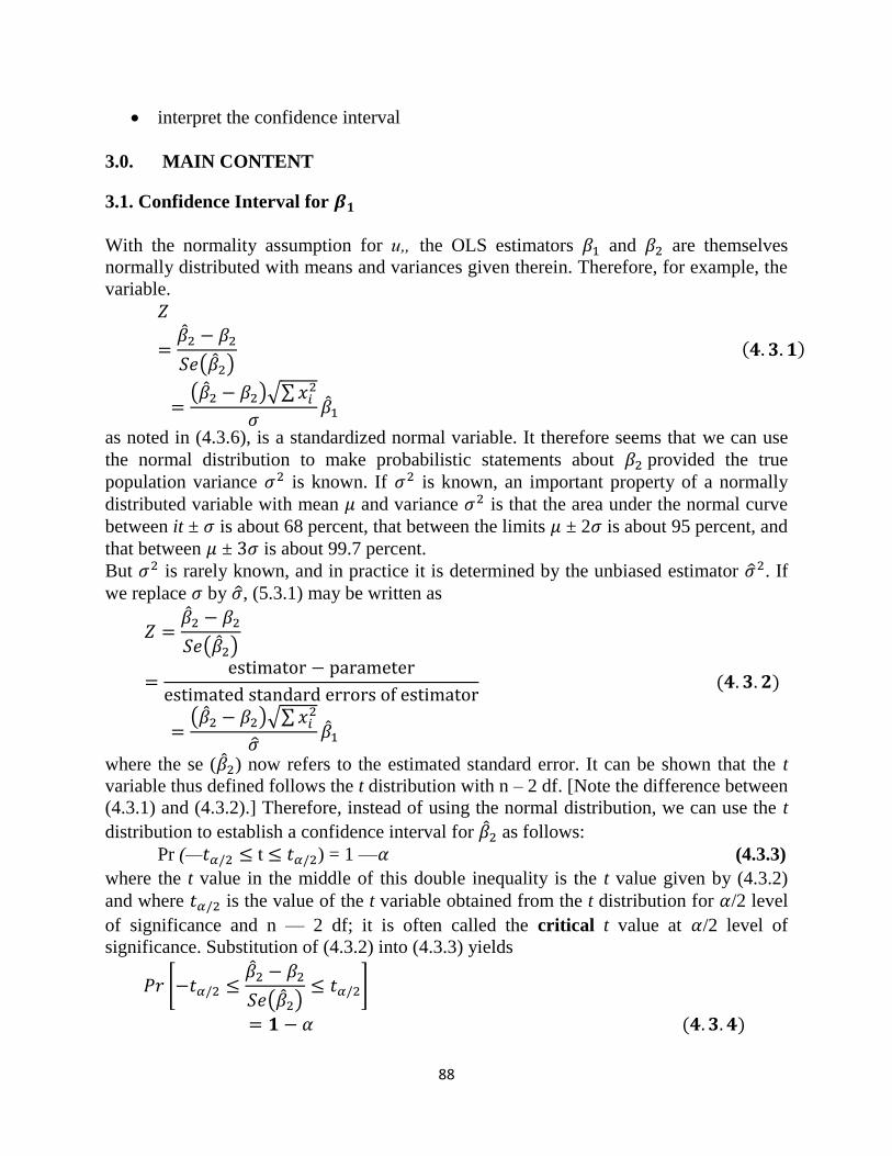
88
interpret the confidence interval
3.0. MAIN CONTENT
3.1. Confidence Interval for
With the normality assumption for u„ the OLS estimators and are themselves
normally distributed with means and variances given therein. Therefore, for example, the
variable.
( )
( )√∑
as noted in (4.3.6), is a standardized normal variable. It therefore seems that we can use
the normal distribution to make probabilistic statements about provided the true
population variance is known. If is known, an important property of a normally
distributed variable with mean and variance is that the area under the normal curve
between it ± is about 68 percent, that between the limits ± 2 is about 95 percent, and
that between ± is about 99.7 percent.
But is rarely known, and in practice it is determined by the unbiased estimator . If
we replace by , (5.3.1) may be written as
( )
( )√∑
where the se ( ) now refers to the estimated standard error. It can be shown that the t
variable thus defined follows the t distribution with n – 2 df. [Note the difference between
(4.3.1) and (4.3.2).] Therefore, instead of using the normal distribution, we can use the t
distribution to establish a confidence interval for as follows:
Pr (— t ) = 1 — (4.3.3)
where the t value in the middle of this double inequality is the t value given by (4.3.2)
and where is the value of the t variable obtained from the t distribution for /2 level
of significance and n — 2 df; it is often called the critical t value at /2 level of
significance. Substitution of (4.3.2) into (4.3.3) yields
*
( ) +
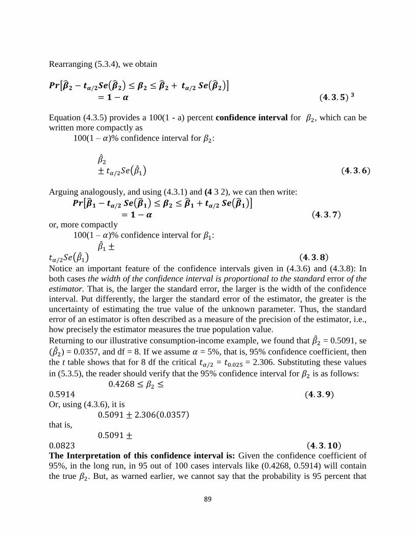
89
Rearranging (5.3.4), we obtain
[ ( ) ( )]
Equation (4.3.5) provides a 100(1 - a) percent confidence interval for , which can be
written more compactly as
100(1 – )% confidence interval for :
( )
Arguing analogously, and using (4.3.1) and (4 3 2), we can then write:
[ ( ) ( )]
or, more compactly
100(1 – )% confidence interval for :
( )
Notice an important feature of the confidence intervals given in (4.3.6) and (4.3.8): In
both cases the width of the confidence interval is proportional to the standard error of the
estimator. That is, the larger the standard error, the larger is the width of the confidence
interval. Put differently, the larger the standard error of the estimator, the greater is the
uncertainty of estimating the true value of the unknown parameter. Thus, the standard
error of an estimator is often described as a measure of the precision of the estimator, i.e.,
how precisely the estimator measures the true population value.
Returning to our illustrative consumption-income example, we found that = 0.5091, se
) = 0.0357, and df = 8. If we assume = 5%, that is, 95% confidence coefficient, then
the t table shows that for 8 df the critical = = 2.306. Substituting these values
in (5.3.5), the reader should verify that the 95% confidence interval for is as follows:
Or, using (4.3.6), it is
that is,
The Interpretation of this confidence interval is: Given the confidence coefficient of
95%, in the long run, in 95 out of 100 cases intervals like (0.4268, 0.5914) will contain
the true . But, as warned earlier, we cannot say that the probability is 95 percent that
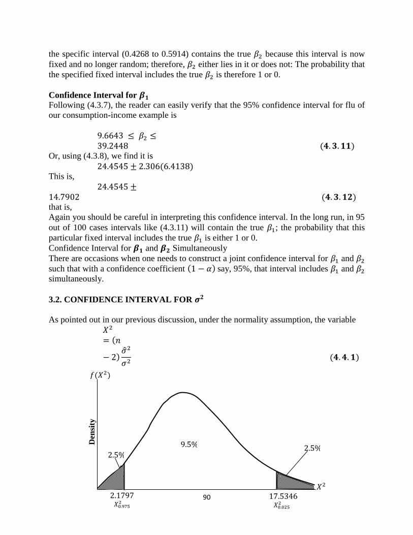
90
the specific interval (0.4268 to 0.5914) contains the true because this interval is now
fixed and no longer random; therefore, either lies in it or does not: The probability that
the specified fixed interval includes the true is therefore 1 or 0.
Confidence Interval for
Following (4.3.7), the reader can easily verify that the 95% confidence interval for flu of
our consumption-income example is
Or, using (4.3.8), we find it is
This is,
that is,
Again you should be careful in interpreting this confidence interval. In the long run, in 95
out of 100 cases intervals like (4.3.11) will contain the true ; the probability that this
particular fixed interval includes the true is either 1 or 0.
Confidence Interval for and Simultaneously
There are occasions when one needs to construct a joint confidence interval for and
such that with a confidence coefficient say, 95%, that interval includes and
simultaneously.
3.2. CONFIDENCE INTERVAL FOR
As pointed out in our previous discussion, under the normality assumption, the variable
𝑋
𝑋
%
𝑋
%
𝑓 𝑋
% Den
sity
91
Figure 5.1 The 95% confidence interval for (8 df).
follows the distribution with n – 2 df.5 Therefore, we can use the distribution to
establish a confidence interval for .
where the value in the middle of this double inequality is as given by (5.4.1) and
where and
are two values of (the critical values) obtained from the
chi-square table for n – 2 df in such a manner that they cut off 100( /2) percent tail areas
of the distribution, as shown in Figure 5.1. Substituting from (5.4.1) into (5.4.2)
and rearranging the terms, we obtain
*
+
which gives the 100(1 - a)% confidence interval for a 2 .
To illustrate, consider this example, when = 42.1591 and df = 8. If is chosen at 5
percent, the chi-square table for 8 df gives the following critical values: = 17.5346,
and = 2.1797. These values show that the probability of a chi-square value
exceeding 17.5346 is 2.5 percent and that of 2.1797 is 97.5 percent. Therefore, the
interval between these two values is the 95% confidence interval for .
Substituting the data of our example into (4.4.3), the students should verify that the 95%
confidence interval for 5 2 is as follows:
(4.4.4) The interpretation of this interval is: If we establish 95% confidence limits on a2 and
if we maintain a priori that these limits will include true a 2 , we shall be right in the long
run 95 percent of the time.
4.0 CONCLUSION
Confidence intervals consist of a range of values (interval) that act as good estimates of
the unknown population parameter; however, the interval computed from a particular
sample does not necessarily include the true value of the parameter. When we say, "we
are 99% confident that the true value of the parameter is in our confidence interval", we
express that 99% of the hypothetically observed confidence intervals will hold the true
value of the parameter. After any particular sample is taken, the population parameter is
either in the interval, realized or not; it is not a matter of chance. The desired level of
confidence is set by the researcher (not determined by data). If a corresponding
hypothesis test is performed, the confidence level is the complement of respective level
of significance, i.e. a 95% confidence interval reflects a significance level of 0.05.
92
5.0 . SUMMARY
In this unit we have learnt a lot on Confidence intervals and confident interval are
frequently misunderstood, and published studies have shown that even professional
scientists often misinterpret them. A 95% confidence interval does not mean that for a
given realized interval calculated from sample data there is a 95% probability the
population parameter lies within the interval, nor that there is a 95% probability that the
interval covers the population parameter. Once an experiment is done and an interval
calculated, this interval either covers the parameter value or it does not, it is no longer a
matter of probability. The 95% probability relates to the reliability of the estimation
procedure, not to a specific calculated interval.
6.0 TUTOR MARKED ASSESSMENT EXERCISE
Discuss the term ―Confidence interval‖.
7.0 REFERENCES/FURTHER READINGS
Gujarat, D. N. (2007) Basic Econometrics, 4th
Edition, tata Mcgraw – Hill publishing
company limited, New Delhi.
Hall, S. G., & Asterion, D. (2011) Applied Econometrics, 2nd
Edition, Palgrave
Macmillian, New York city, USA.
93
UNIT FIVE: HYPOTHESIS TESTING
CONTENTS
1.0 Introduction
2.0 Objectives
3.0 Main content
3.1. Analysis of Hypothesis
3.2. Hypothesis testing: the confidence interval Approach
3.3. Hypothesis testing: the test-of-significance Approach
3.4. Testing the significance of : the Chi Square ( Test
4.0 Conclusion
5.0 Summary
3.0 Tutor-Marked Assignment
7.0. References
1.0. INTRODUCTION
A hypothesis test is a statistical test that is used to determine whether there is enough
evidence in a sample of data to infer that a certain condition is true for the entire
population. A hypothesis test examines two opposing hypotheses about a population: the
null hypothesis and the alternative hypothesis. The null hypothesis is the statement being
tested. Usually the null hypothesis is a statement of "no effect" or "no difference". The
alternative hypothesis is the statement you want to be able to conclude is true.
94
Based on the sample data, the test determines whether to reject the null hypothesis. You
use a p-value, to make the determination. If the p-value is less than or equal to the level
of significance, which is a cut-off point that you define, then you can reject the null
hypothesis.
2.0. OBJECTIVES
At the end of this unit, you should be able to:
understand the meaning of Hypothesis
know how to calculate hypothesis using confidence interval
analyse and interpret hypothesis result.
3.0. MAIN CONTENT
3.1. ANALYSIS OF HYPOTHESIS
Having discussed the problem of point and interval estimation, we shall now consider the
topic of hypothesis testing. In this unit we will discuss briefly some general aspects of
this topic.
The problem of statistical hypothesis testing may be stated simply as follows: Is a given
observation or finding compatible with some stated hypothesis or not? The word
"compatible," as used here, means "sufficiently" close to the hypothesized value so that
we do not reject the stated hypothesis. Thus, if some theory or prior experience leads us
to believe that the true slope coefficient of the consumption-income example is unity,
is the observed = 0.5091 from the statistical table consistent with the stated
hypothesis? If it is, we do not reject the hypothesis; otherwise, we may reject it.
In the language of statistics, the stated hypothesis is known as the null hypothesis and is
denoted by the symbol . The null hypothesis is usually tested against an alternative
hypothesis (also known as maintained hypothesis) denoted by , which may state, for
example, that true is different from unity. The alternative hypothesis may be simple or
composite.6 For example, = 1.5 is a simple hypothesis, but 0 1.5 is a
composite hypothesis.
The theory of hypothesis testing is concerned with developing rules or procedures for
deciding whether to reject or not reject the null hypothesis. There are two mutually
complementary approaches for devising such rules, namely, confidence interval and test
of significance. Both these approaches predicate that the variable (statistic or estimator)
under consideration has some probability distribution and that hypothesis testing involves
making statements or assertions about the value(s) of the parameter(s) of such
distribution. For example, we know that with the normality assumption is normally
distributed with mean equal to and variance. If we hypothesize that = 1, we are
making an assertion about one of the parameters of the normal distribution, namely, the
mean. Most of the statistical hypotheses encountered in this text will be of this type-
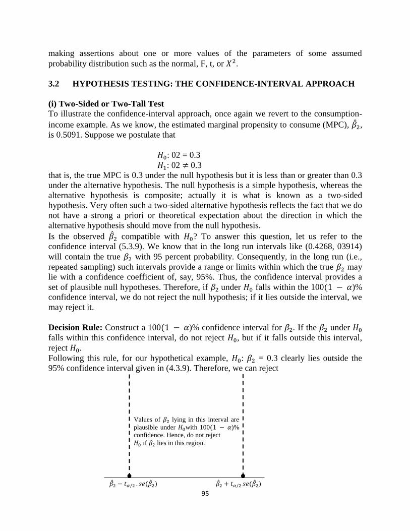
95
making assertions about one or more values of the parameters of some assumed
probability distribution such as the normal, F, t, or .
3.2 HYPOTHESIS TESTING: THE CONFIDENCE-INTERVAL APPROACH
(i) Two-Sided or Two-Tall Test To illustrate the confidence-interval approach, once again we revert to the consumption-
income example. As we know, the estimated marginal propensity to consume (MPC), ,
is 0.5091. Suppose we postulate that
: 02 = 0.3
: 02 0.3
that is, the true MPC is 0.3 under the null hypothesis but it is less than or greater than 0.3
under the alternative hypothesis. The null hypothesis is a simple hypothesis, whereas the
alternative hypothesis is composite; actually it is what is known as a two-sided
hypothesis. Very often such a two-sided alternative hypothesis reflects the fact that we do
not have a strong a priori or theoretical expectation about the direction in which the
alternative hypothesis should move from the null hypothesis.
Is the observed compatible with ? To answer this question, let us refer to the
confidence interval (5.3.9). We know that in the long run intervals like (0.4268, 03914)
will contain the true with 95 percent probability. Consequently, in the long run (i.e.,
repeated sampling) such intervals provide a range or limits within which the true may
lie with a confidence coefficient of, say, 95%. Thus, the confidence interval provides a
set of plausible null hypotheses. Therefore, if under falls within the 100 )%
confidence interval, we do not reject the null hypothesis; if it lies outside the interval, we
may reject it.
Decision Rule: Construct a 100 )% confidence interval for . If the under
falls within this confidence interval, do not reject , but if it falls outside this interval,
reject .
Following this rule, for our hypothetical example, : = 0.3 clearly lies outside the
95% confidence interval given in (4.3.9). Therefore, we can reject
Values of 𝛽 lying in this interval are
plausible under 𝐻 with 100 𝛼)%
confidence. Hence, do not reject
𝐻 if 𝛽 lies in this region.
�� 𝑡𝛼 𝑠𝑒 ��
�� 𝑡𝛼 𝑠𝑒 ��
96
Figure 4.2 A 100 )% confidence interval for .
the hypothesis that the true MPC is 0.3, with 95% confidence. If the null hypothesis were
true, the probability of our obtaining a value of MPC of as much as 0.5091 by sheer
chance or fluke is at the most about 5 percent, a small probability.
In statistics, when we reject the null hypothesis, we say that our finding is statistically
significant. On the other hand, when we do not reject the null hypothesis, we say that our
finding is not statistically significant.
Some authors use a phrase such as "highly statistically significant." By this they usually
mean that when they reject the null hypothesis, the probability of committing a Type I
error (i.e., a) is a small number, usually 1 percent. it is better to leave it to the researcher
to decide whether a statistical finding is "significant," "moderately significant," or
"highly significant."
(ii) One-sided or One-Tall Test
Sometimes we have a strong a priori or theoretical expectation (or expectations based on
some previous empirical work) that the alternative hypothesis is one-sided or
unidirectional rather than two-sided, as just discussed. Thus, for our consumption-income
example, one could postulate that
and
Perhaps economic theory or prior empirical work suggests that the marginal propensity to
consume is greater than 0.3. Although the procedure to test this hypothesis can be easily
derived from (4.3.5), the actual mechanics are better explained in terms of the test-of-
significance approach discussed next.
3.3. HYPOTHESIS TESTING: THE TEST-OF-SIGNIFICANCE APPROACH
(i) Testing the Significance of Regression Coefficients: The t Test
An alternative but complementary approach to the confidence-interval method of testing
statistical hypotheses is the test-of-significance approach developed along independent
lines by R. A. Fisher and jointly by Neyman and Pearson.' Broadly speaking, a test of
significance is a procedure by which sample results are used to verify the truth or falsity
of a null hypothesis. The key idea behind tests of significance is that of a test statistic
(estimator) and the sampling distribution of such a statistic under the null hypothesis. The
decision to accept or reject Ho is made on the basis of the value of the test statistic
obtained from the data at hand.
As an illustration, recall that under the normality assumption the variable
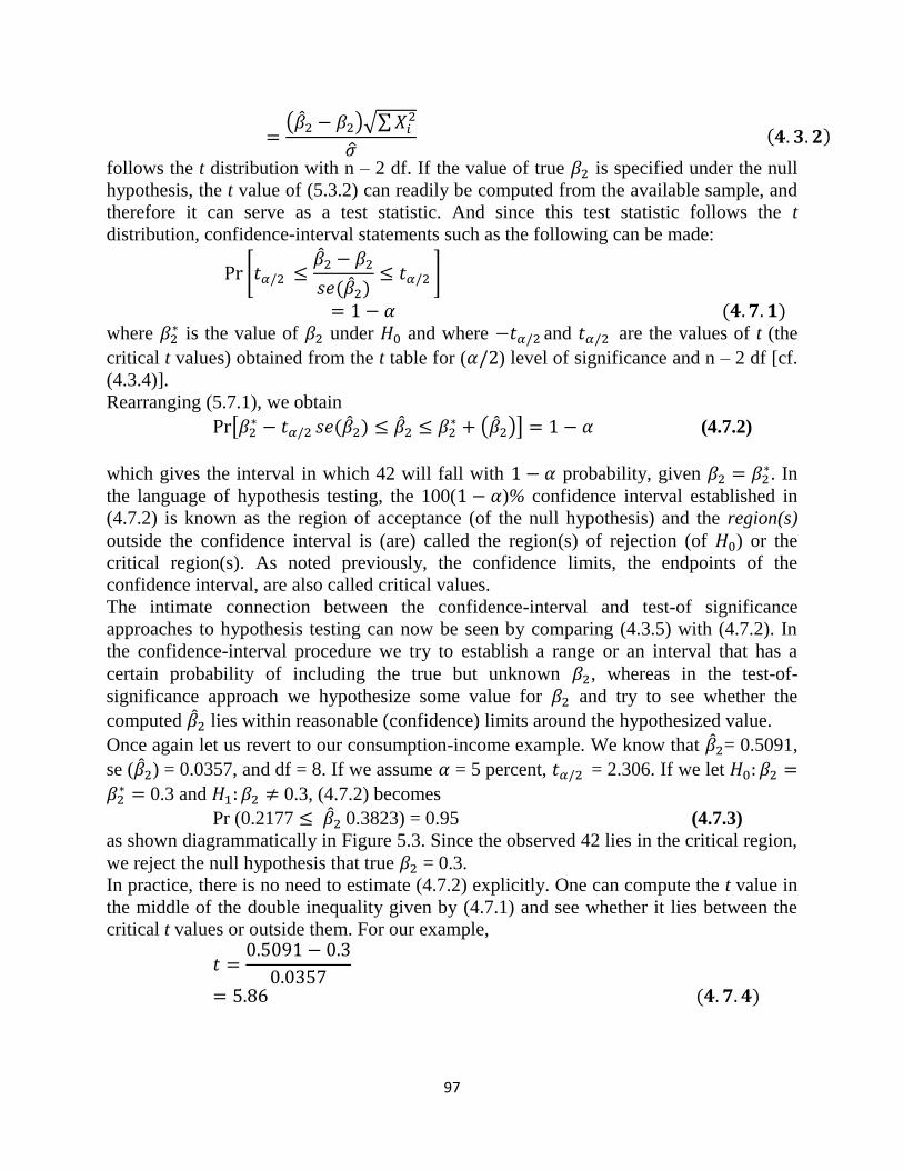
97
( )√∑
follows the t distribution with n – 2 df. If the value of true is specified under the null
hypothesis, the t value of (5.3.2) can readily be computed from the available sample, and
therefore it can serve as a test statistic. And since this test statistic follows the t
distribution, confidence-interval statements such as the following can be made:
*
+
where is the value of under and where and are the values of t (the
critical t values) obtained from the t table for ( ) level of significance and n – 2 df [cf.
(4.3.4)].
Rearranging (5.7.1), we obtain
[
( )] (4.7.2)
which gives the interval in which 42 will fall with probability, given . In
the language of hypothesis testing, the 100( )% confidence interval established in
(4.7.2) is known as the region of acceptance (of the null hypothesis) and the region(s)
outside the confidence interval is (are) called the region(s) of rejection (of ) or the
critical region(s). As noted previously, the confidence limits, the endpoints of the
confidence interval, are also called critical values.
The intimate connection between the confidence-interval and test-of significance
approaches to hypothesis testing can now be seen by comparing (4.3.5) with (4.7.2). In
the confidence-interval procedure we try to establish a range or an interval that has a
certain probability of including the true but unknown , whereas in the test-of-
significance approach we hypothesize some value for and try to see whether the
computed lies within reasonable (confidence) limits around the hypothesized value.
Once again let us revert to our consumption-income example. We know that = 0.5091,
se ( ) = 0.0357, and df = 8. If we assume = 5 percent, = 2.306. If we let
0.3 and 0.3, (4.7.2) becomes
Pr (0.2177 0.3823) = 0.95 (4.7.3)
as shown diagrammatically in Figure 5.3. Since the observed 42 lies in the critical region,
we reject the null hypothesis that true = 0.3.
In practice, there is no need to estimate (4.7.2) explicitly. One can compute the t value in
the middle of the double inequality given by (4.7.1) and see whether it lies between the
critical t values or outside them. For our example,
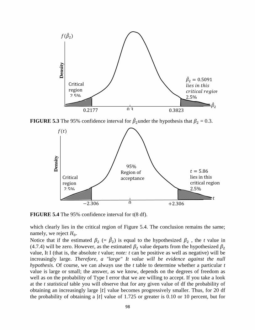
98
FIGURE 5.3 The 95% confidence interval for under the hypothesis that = 0.3.
FIGURE 5.4 The 95% confidence interval for t(8 df).
which clearly lies in the critical region of Figure 5.4. The conclusion remains the same;
namely, we reject .
Notice that if the estimated (= ) is equal to the hypothesized , the t value in
(4.7.4) will be zero. However, as the estimated value departs from the hypothesized
value, It I (that is, the absolute t value; note: t can be positive as well as negative) will be
increasingly large. Therefore, a "large" It value will be evidence against the null
hypothesis. Of course, we can always use the t table to determine whether a particular t
value is large or small; the answer, as we know, depends on the degrees of freedom as
well as on the probability of Type I error that we are willing to accept. If you take a look
at the t statistical table you will observe that for any given value of df the probability of
obtaining an increasingly large | | value becomes progressively smaller. Thus, for 20 df
the probability of obtaining a | | value of 1.725 or greater is 0.10 or 10 percent, but for
𝑡
𝑡
g
%
g
%
𝑓 𝑡
Den
sity
%
g
𝑓 ��
��
��
𝑙𝑖𝑒𝑠 𝑖𝑛 𝑡ℎ𝑖𝑠
𝑐𝑟𝑖𝑡𝑖𝑐𝑎𝑙 𝑟𝑒𝑔𝑖𝑜𝑛
%
g
%
Den
sity
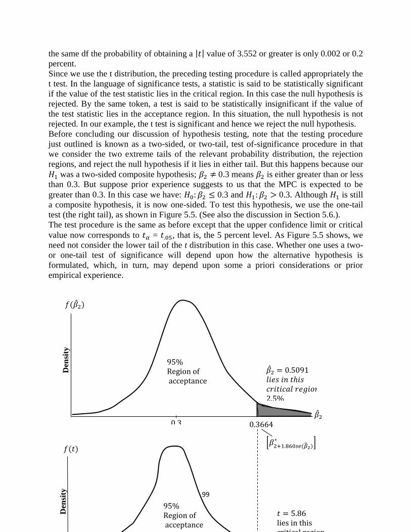
99
the same df the probability of obtaining a | | value of 3.552 or greater is only 0.002 or 0.2
percent.
Since we use the t distribution, the preceding testing procedure is called appropriately the
t test. In the language of significance tests, a statistic is said to be statistically significant
if the value of the test statistic lies in the critical region. In this case the null hypothesis is
rejected. By the same token, a test is said to be statistically insignificant if the value of
the test statistic lies in the acceptance region. In this situation, the null hypothesis is not
rejected. In our example, the t test is significant and hence we reject the null hypothesis.
Before concluding our discussion of hypothesis testing, note that the testing procedure
just outlined is known as a two-sided, or two-tail, test of-significance procedure in that
we consider the two extreme tails of the relevant probability distribution, the rejection
regions, and reject the null hypothesis if it lies in either tail. But this happens because our
was a two-sided composite hypothesis; 0.3 means is either greater than or less
than 0.3. But suppose prior experience suggests to us that the MPC is expected to be
greater than 0.3. In this case we have: 0.3 and 0.3. Although is still
a composite hypothesis, it is now one-sided. To test this hypothesis, we use the one-tail
test (the right tail), as shown in Figure 5.5. (See also the discussion in Section 5.6.).
The test procedure is the same as before except that the upper confidence limit or critical
value now corresponds to = , that is, the 5 percent level. As Figure 5.5 shows, we
need not consider the lower tail of the t distribution in this case. Whether one uses a two-
or one-tail test of significance will depend upon how the alternative hypothesis is
formulated, which, in turn, may depend upon some a priori considerations or prior
empirical experience.
𝑓 ��
��
��
𝑙𝑖𝑒𝑠 𝑖𝑛 𝑡ℎ𝑖𝑠
𝑐𝑟𝑖𝑡𝑖𝑐𝑎𝑙 𝑟𝑒𝑔𝑖𝑜𝑛
%
Den
sity
%
g
𝑡
g
𝑓 𝑡
Den
sity
%
g
*𝛽 + 86 𝑠𝑒 �� +
100
3.4. Testing the significance of The Chi Square ( Test As another illustration of the test-of-significance methodology, consider the following
variables
which, as noted previously, follows the x 2 distribution with n – 2 df. For the hypothetical
example, = 42.1591 and df = 8. If we postulate that = 85 vs.
, Eq.
(4.4.1) provides the test statistic for . Substituting the appropriate values in (4.4.1), it
can be found that under = 3.97. If we assume = 5%, the critical values are
2.1797 and 17.5346. Since the computed lies between these limits, the data support
the null hypothesis and we do not reject it. This test procedure is called the chi-square test
of significance.
1. The Logic of Hypothesis Testing
As just stated, the logic of hypothesis testing in statistics involves four steps. We
expand on those steps in this section:
First Step: State the hypothesis Stating the hypothesis actually involves stating two opposing hypotheses about the value
of a population parameter.
Example: Suppose we have are interested in the effect of prenatal exposure of alcohol on
the birth weight of rats. Also, suppose that we know that the mean birth weight of the
population of untreated lab rats is 18 grams.
Here are the two opposing hypotheses:
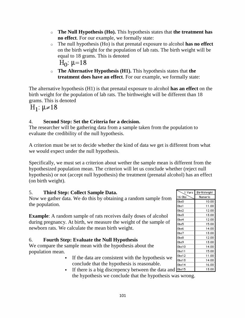
101
o The Null Hypothesis (Ho). This hypothesis states that the treatment has
no effect. For our example, we formally state:
o The null hypothesis (Ho) is that prenatal exposure to alcohol has no effect
on the birth weight for the population of lab rats. The birth weight will be
equal to 18 grams. This is denoted
o The Alternative Hypothesis (H1). This hypothesis states that the
treatment does have an effect. For our example, we formally state:
The alternative hypothesis (H1) is that prenatal exposure to alcohol has an effect on the
birth weight for the population of lab rats. The birthweight will be different than 18
grams. This is denoted
4. Second Step: Set the Criteria for a decision. The researcher will be gathering data from a sample taken from the population to
evaluate the credibility of the null hypothesis.
A criterion must be set to decide whether the kind of data we get is different from what
we would expect under the null hypothesis.
Specifically, we must set a criterion about wether the sample mean is different from the
hypothesized population mean. The criterion will let us conclude whether (reject null
hypothesis) or not (accept null hypothesis) the treatment (prenatal alcohol) has an effect
(on birth weight).
5. Third Step: Collect Sample Data. Now we gather data. We do this by obtaining a random sample from
the population.
Example: A random sample of rats receives daily doses of alcohol
during pregnancy. At birth, we measure the weight of the sample of
newborn rats. We calculate the mean birth weight.
6. Fourth Step: Evaluate the Null Hypothesis We compare the sample mean with the hypothesis about the
population mean.
If the data are consistent with the hypothesis we
conclude that the hypothesis is reasonable.
If there is a big discrepency between the data and
the hypothesis we conclude that the hypothesis was wrong.
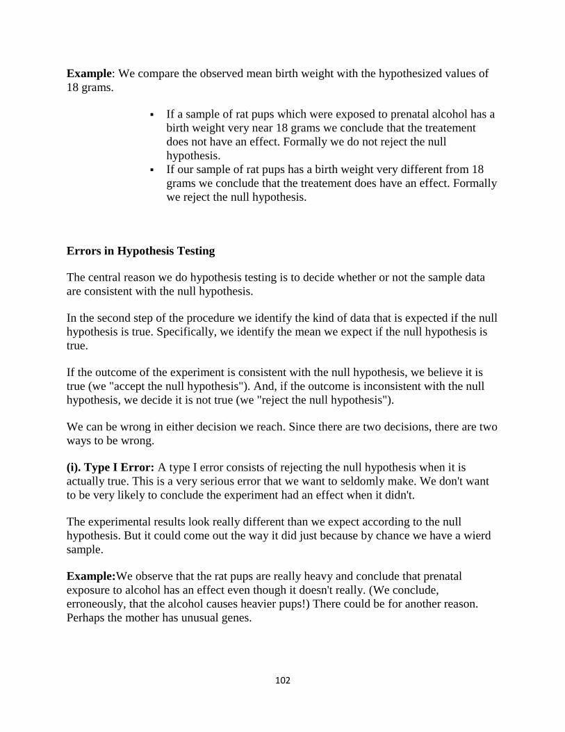
102
Example: We compare the observed mean birth weight with the hypothesized values of
18 grams.
If a sample of rat pups which were exposed to prenatal alcohol has a
birth weight very near 18 grams we conclude that the treatement
does not have an effect. Formally we do not reject the null
hypothesis.
If our sample of rat pups has a birth weight very different from 18
grams we conclude that the treatement does have an effect. Formally
we reject the null hypothesis.
Errors in Hypothesis Testing
The central reason we do hypothesis testing is to decide whether or not the sample data
are consistent with the null hypothesis.
In the second step of the procedure we identify the kind of data that is expected if the null
hypothesis is true. Specifically, we identify the mean we expect if the null hypothesis is
true.
If the outcome of the experiment is consistent with the null hypothesis, we believe it is
true (we "accept the null hypothesis"). And, if the outcome is inconsistent with the null
hypothesis, we decide it is not true (we "reject the null hypothesis").
We can be wrong in either decision we reach. Since there are two decisions, there are two
ways to be wrong.
(i). Type I Error: A type I error consists of rejecting the null hypothesis when it is
actually true. This is a very serious error that we want to seldomly make. We don't want
to be very likely to conclude the experiment had an effect when it didn't.
The experimental results look really different than we expect according to the null
hypothesis. But it could come out the way it did just because by chance we have a wierd
sample.
Example:We observe that the rat pups are really heavy and conclude that prenatal
exposure to alcohol has an effect even though it doesn't really. (We conclude,
erroneously, that the alcohol causes heavier pups!) There could be for another reason.
Perhaps the mother has unusual genes.
103
(ii). Type II Error: A type II error consists of failing to reject the null hypothesis when it
is actually false. This error has less grevious implications, so we are will to err in this
direction (of not concluding the experiment had an effect when it, in fact, did).
The experimental results don't look different than we expect according to the null
hypothesis, but they are, perhaps because the effect isn't very big.
Example: The rat pups weigh 17.9 grams and we conclude there is no effect. But "really"
(if we only knew!) alcohol does reduce weight, we just don't have a big enough effect to
see it.
3. Hypothesis Testing Techniques
There is always the possibility of making an inference error --- of making the wrong
decision about the null hypothesis. We never know for certain if we've made the right
decision. However:
The techniques of hypothesis testing allow us to know the probability of making a type I
error.
We do this by comparing the sample mean and the population mean hypothesized
under the null hypothesis and decide if they are "significantly different". If we
decide that they are significantly different, we reject the null hypothesis that
.
To do this we must determine what data would be expected if Ho were true, and what
data would be unlikely if Ho were true. This is done by looking at the distribution of all
possible outcomes, if Ho were true. Since we usually are concerned about the mean, we
usually look at the distribution of sample means for samples of size n that we would
obtain if Ho were true.
Thus, if we are concerned about means we:
o Assume that Ho is true
o Divide the distribution of sample means into two parts:
1. Those sample means that are likely to be obtained if Ho is true.
2. Those sample means that are unlikely to be obtained if Ho is true.
104
To divide the distribution into these two parts -- likely and unlikely -- we define a cutoff
point. This cutoff is defined on the basis of the probability of obtaining specific sample
means. This (semi-arbitrary) cutoff point is called the alpha level or the level of
significance. The alpha level specifies the probability of making a Type I error. It is
denoted . Thus:
= the probability of a Type I error.
By convention, we usually adopt a cutoff point of either:
or or occasionally . If we adopt a cutoff point of
then we know that the obtained sample of data is likely to be obtained in less than 5 of
100 samples, if the data were sampled from the population in which Ho is true.
We decide: "The data (and its sample mean) are significantly different than the value of
the mean hypothesized under the null hypothesis, at the .05 level of significance."
This decision is likely to be wrong (Type I error) 5 times out of 100. Thus, the probability
of a type I error is .05.
The obtained sample of data is likely to be obtained in less than 1 of 100 samples, if the
data were sampled from the population in which Ho is true.
We decide: "The data (and its sample mean) are significantly different than the value of
the mean hypothesized under the null hypothesis, at the .01 level of significance."
This decision is likely to be wrong (Type I error) 1 time out of 100. Thus, the probability
of a type I error is .05.
The obtained sample of data is likely to be obtained in less than 1 of 1000 samples, if the
data were sampled from the population in which Ho is true.
We decide: "The data (and its sample mean) are significantly different than the value of
the mean hypothesized under the null hypothesis, at the .001 level of significance."
This decision is likely to be wrong (Type I error) 1 time out of 1000. Thus, the
probability of a type I error is .05.
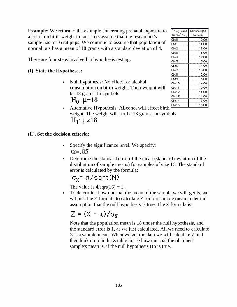
105
Example: We return to the example concerning prenatal exposure to
alcohol on birth weight in rats. Lets assume that the researcher's
sample has n=16 rat pups. We continue to assume that population of
normal rats has a mean of 18 grams with a standard deviation of 4.
There are four steps involved in hypothesis testing:
(I). State the Hypotheses:
Null hypothesis: No effect for alcohol
consumption on birth weight. Their weight will
be 18 grams. In symbols:
Alternative Hypothesis: ALcohol will effect birth
weight. The weight will not be 18 grams. In symbols:
(II). Set the decision criteria:
Specify the significance level. We specify:
Determine the standard error of the mean (standard deviation of the
distribution of sample means) for samples of size 16. The standard
error is calculated by the formula:
The value is 4/sqrt(16) = 1.
To determine how unusual the mean of the sample we will get is, we
will use the Z formula to calculate Z for our sample mean under the
assumption that the null hypothesis is true. The Z formula is:
Note that the population mean is 18 under the null hypothesis, and
the standard error is 1, as we just calculated. All we need to calculate
Z is a sample mean. When we get the data we will calculate Z and
then look it up in the Z table to see how unusual the obtained
sample's mean is, if the null hypothesis Ho is true.
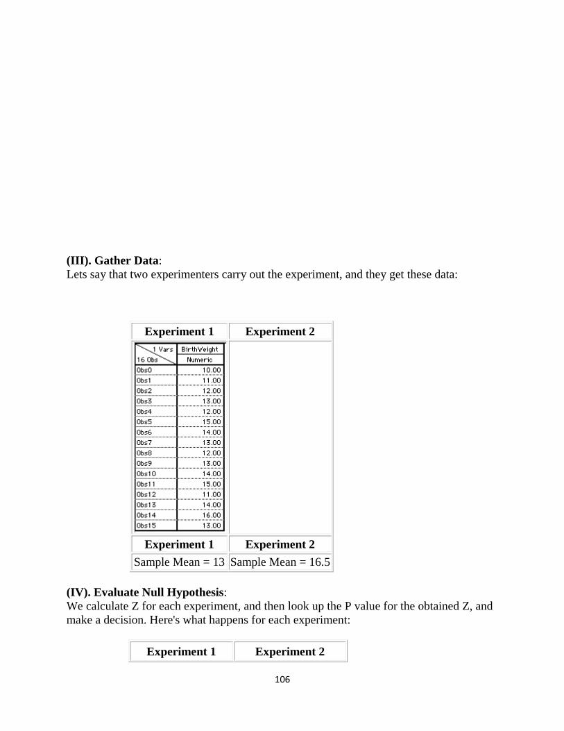
106
(III). Gather Data:
Lets say that two experimenters carry out the experiment, and they get these data:
Experiment 1 Experiment 2
Experiment 1 Experiment 2
Sample Mean = 13 Sample Mean = 16.5
(IV). Evaluate Null Hypothesis:
We calculate Z for each experiment, and then look up the P value for the obtained Z, and
make a decision. Here's what happens for each experiment:
Experiment 1 Experiment 2
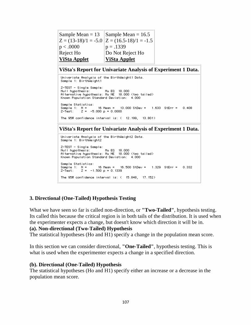
107
Sample Mean = 13
Z = (13-18)/1 = -5.0
p < .0000
Reject Ho
ViSta Applet
Sample Mean = 16.5
Z = (16.5-18)/1 = -1.5
p = .1339
Do Not Reject Ho
ViSta Applet
ViSta's Report for Univariate Analysis of Experiment 1 Data.
ViSta's Report for Univariate Analysis of Experiment 1 Data.
3. Directional (One-Tailed) Hypothesis Testing
What we have seen so far is called non-direction, or "Two-Tailed", hypothesis testing.
Its called this because the critical region is in both tails of the distribution. It is used when
the experimenter expects a change, but doesn't know which direction it will be in.
(a). Non-directional (Two-Tailed) Hypothesis The statistical hypotheses (Ho and H1) specify a change in the population mean score.
In this section we can consider directional, "One-Tailed", hypothesis testing. This is
what is used when the experimenter expects a change in a specified direction.
(b). Directional (One-Tailed) Hypothesis The statistical hypotheses (Ho and H1) specify either an increase or a decrease in the
population mean score.
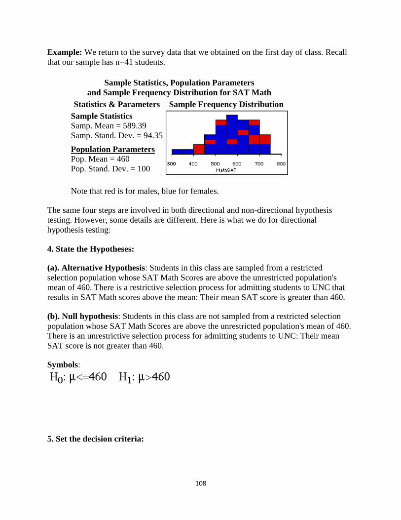
108
Example: We return to the survey data that we obtained on the first day of class. Recall
that our sample has n=41 students.
Sample Statistics, Population Parameters
and Sample Frequency Distribution for SAT Math
Statistics & Parameters Sample Frequency Distribution
Sample Statistics Samp. Mean = 589.39
Samp. Stand. Dev. = 94.35
Population Parameters Pop. Mean = 460
Pop. Stand. Dev. = 100
Note that red is for males, blue for females.
The same four steps are involved in both directional and non-directional hypothesis
testing. However, some details are different. Here is what we do for directional
hypothesis testing:
4. State the Hypotheses:
(a). Alternative Hypothesis: Students in this class are sampled from a restricted
selection population whose SAT Math Scores are above the unrestricted population's
mean of 460. There is a restrictive selection process for admitting students to UNC that
results in SAT Math scores above the mean: Their mean SAT score is greater than 460.
(b). Null hypothesis: Students in this class are not sampled from a restricted selection
population whose SAT Math Scores are above the unrestricted population's mean of 460.
There is an unrestrictive selection process for admitting students to UNC: Their mean
SAT score is not greater than 460.
Symbols:
5. Set the decision criteria:

109
Specify the significance level. We specify:
Determine the standard error of the mean (standard deviation of the distribution of
sample means) for samples of size 41. The standard error is calculated by the formula:
The value is
To determine how unusual the mean of the sample we will get is, we will use the Z
formula to calculate Z for our sample mean under the assumption that the null hypothesis
is true. The Z formula is:
Note that the population mean is 460 under the null hypothesis, and the standard error is
15.6, as we just calculated. All we need to calculate Z is a sample mean. When we get the
data we will calculate Z and then look it up in the Z table to see how unusual the obtained
sample's mean is, if the null hypothesis Ho is true.
6. Gather Data:
We gathered the data on the first day of class and observed that the class's mean on SAT
Math was 589.39.
7. Evaluate Null Hypothesis:
We calculate Z and then look up the P value for the obtained Z, and make a decision.
Here's what happens:
The P value is way below .00001, so we reject the null hypothesis that there is an
unrestrictive selection process for admitting students to UNC. We conclude that the
selection process results in Math SAT scores for UNC students that are higher than the
population as a whole.
8. Statistical Power
110
As we have seen, hypothesis testing is about seeing if a particular treatment has an effect.
Hypothesis testing uses a framework based on testing the null hypothesis that there is no
effect. The test leads us to decide whether or not to reject the null hypothesis.
We have examined the potential for making an incorrect decision, looking at Type I and
Type II errors, and the associated significance level for making a Type I error.
We now reverse our focus and look at the potential for making a correct decision. This is
referred to as the power of a statistical test.
However, the power of a statistical test is the probability that the test will correctly reject
a false null hypothesis. The more powerful the test is, the more likely it is to detect a
treatment effect when one really exists.
9. Power and Type II errors:
When a treatment effect really exists the hypothesis test:
(i). can fail to discover the treatment effect (making a Type II error). The
probability of this happening is denoted:
= P[Type II error]
(ii) can correctly detect the treatment effect (rejecting a false null
hypothesis). The probabililty of this happening, which is the power of
the test, is denoted:
= power = P[rejecting a false Ho].
Here is a table summarizing the Power and Significance of a test and their relationship to
Type I and II errors and to "alpha" and "beta" the probabilities of a Type I and Type II
error, respectively:
10. How to we determine power? Unfortunately, we don't know "beta", the exact value of the power of a test. We do know,
however, that the power of a test is effected by:
(i). Alpha Level: Reducing the value of alpha also reduces the power. So if we wish to be
less likely to make a type I error (conclude there is an effect when there isn't) we are also
less likely to see an effect when there is one.
(ii). One-Tailed Tests: One tailed tests are more powerful. They make it easier to reject
null hypotheses.
111
(iii). Sample Size: Larger samples are better, period. Tests based on larger samples are
more powerful and are less likely to lead to mistaken conclusions, including both Type I
and Type II errors.
4.0. CONCLUSION
The unit concludes that hypothesis testing is an act in statistics whereby an analyst tests
an assumption regarding a population parameter. The methodology employed by the
analyst depends on the nature of the data used and the reason for the analysis. Hypothesis
testing is used to infer the result of a hypothesis performed on sample data from a larger
population.
5.0 SUMMARY
We then summaries that Procedure for deciding if a null hypothesis should be accepted or
rejected in favor of an alternate hypothesis. A statistic is computed from a survey or test
result and is analyzed to determine if it falls within a preset acceptance region. If it does,
the null hypothesis is accepted otherwise rejected.
6.0. TUTOR MARKED ASSESSMENT EXERCISE
List the stages of hypothesis testing in statistical analysis
7.0 REFERENCES/FURTHER READINGS
Gujarat, D. N. (2007) Basic Econometrics, 4th
Edition, tata Mcgraw – Hill publishing
company limited, New Delhi.
Hall, S. G., & Asterion, D. (2011) Applied Econometrics, 2nd
Edition, Palgrave
Macmillian, New York city, USA.
112
MODULE FOUR: PRACTICAL ASPECTS OF ECONOMETRICS TEST:
Unit One Accepting & Rejecting an Hypothesis
Unit Two The Level of Significance
Unit Three Regression Analysis and Analysis of Variance
Unit Four Normality tests
UNIT ONE: ACCEPTING AND REJECTING AN HYPOTHESIS
CONTENTS
1.0 Introduction
2.0 Objectives
3.0 Main content
3.1. The meaning of ―accepting‖ or ―rejecting‖ an hypothesis
3.2. The ―zero‖ null hypothesis and the ―2-t‖ rule of thumb
3.3. Forming the null and Alternative hypothesis
4.0 Conclusion
5.0 Summary
6.0 Tutor-Marked Assignment
7.0. References
113
1.0. INTRODUCTION
In order to undertake hypothesis testing you need to express your research hypothesis as a
null and alternative hypothesis. The null hypothesis and alternative hypothesis are
statements regarding the differences or effects that occur in the population. You will use
your sample to test which statement (i.e., the null hypothesis or alternative hypothesis) is
most likely (although technically, you test the evidence against the null hypothesis). So,
with respect to our teaching example, the null and alternative hypothesis will reflect
statements about all statistics students on graduate management courses.
The null hypothesis is essentially the "devil's advocate" position. That is, it assumes that
whatever you are trying to prove did not happen (hint: it usually states that something
equals zero). For example, the two different teaching methods did not result in different
exam performances (i.e., zero difference). Another example might be that there is no
relationship between anxiety and athletic performance (i.e., the slope is zero). The
alternative hypothesis states the opposite and is usually the hypothesis you are trying to
prove (e.g., the two different teaching methods did result in different exam
performances). Initially, you can state these hypotheses in more general terms (e.g., using
terms like "effect", "relationship", etc.).
2.0. OBJECTIVES
At the end of this unit, you should be able to:
understand the meaning of accepting and rejecting an hypothesis
identify a null and alternative hypothesis.
3.0. MAIN CONTENT
3.1. The meaning of "Accepting" or "Rejecting" an Hypothesis
If on the basis of a test of significance, say, the t test, we decide to "accept" the null
hypothesis, all we are saying is that on the basis of the sample evidence we have no
reason to reject it; we are not saying that the null hypothesis is true beyond any doubt.
Why? To answer this, let us revert to our consumption-income example and assume that
(MPC) = 0.50. Now the estimated value of the MPC is = 0.5091 with a
. Then on the basis of the t test we find that , which is insignificant, say, at = 5%. Therefore, we say
"accept" . But now let us assume = 0.48. Applying the t test, we obtain t =
( , which too is statistically insignificant. So now we
say "accept" this . Which of these two null hypotheses is the "truth"? We do not know.
Therefore, in "accepting" a null hypothesis we should always be aware that another null
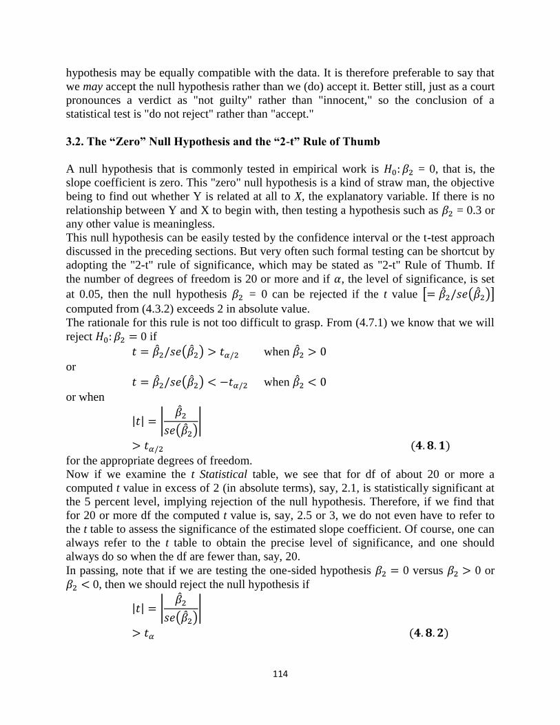
114
hypothesis may be equally compatible with the data. It is therefore preferable to say that
we may accept the null hypothesis rather than we (do) accept it. Better still, just as a court
pronounces a verdict as "not guilty" rather than "innocent," so the conclusion of a
statistical test is "do not reject" rather than "accept."
3.2. The “Zero” Null Hypothesis and the “2-t” Rule of Thumb
A null hypothesis that is commonly tested in empirical work is = 0, that is, the
slope coefficient is zero. This "zero" null hypothesis is a kind of straw man, the objective
being to find out whether Y is related at all to X, the explanatory variable. If there is no
relationship between Y and X to begin with, then testing a hypothesis such as = 0.3 or
any other value is meaningless.
This null hypothesis can be easily tested by the confidence interval or the t-test approach
discussed in the preceding sections. But very often such formal testing can be shortcut by
adopting the "2-t" rule of significance, which may be stated as "2-t" Rule of Thumb. If
the number of degrees of freedom is 20 or more and if , the level of significance, is set
at 0.05, then the null hypothesis = 0 can be rejected if the t value [ ( )] computed from (4.3.2) exceeds 2 in absolute value.
The rationale for this rule is not too difficult to grasp. From (4.7.1) we know that we will
reject 0 if
( ) when
or
( ) when
or when
| | |
( )|
for the appropriate degrees of freedom.
Now if we examine the t Statistical table, we see that for df of about 20 or more a
computed t value in excess of 2 (in absolute terms), say, 2.1, is statistically significant at
the 5 percent level, implying rejection of the null hypothesis. Therefore, if we find that
for 20 or more df the computed t value is, say, 2.5 or 3, we do not even have to refer to
the t table to assess the significance of the estimated slope coefficient. Of course, one can
always refer to the t table to obtain the precise level of significance, and one should
always do so when the df are fewer than, say, 20.
In passing, note that if we are testing the one-sided hypothesis 0 versus 0 or
0, then we should reject the null hypothesis if
| | |
( )|

115
If we fix at 0.05, then from the t table we observe that for 20 or more df a t value in
excess of 1.73 is statistically significant at the 5 percent level of significance (one-tail).
Hence, whenever a t value exceeds, say, 1.8 (in absolute terms) and the df are 20 or more,
one need not consult the t table for the statistical significance of the observed coefficient.
Of course, if we choose at 0.01 or any other level, we will have to decide on the
appropriate t value as the benchmark value. But by now the reader should be able to do
that.
3.3. Forming the Null and Alternative Hypotheses
Given the null and the alternative hypotheses, testing them for statistical significance
should no longer be a mystery. But how does one formulate these hypotheses? There are
no hard-and-fast rules. Very often the phenomenon under study will suggest the nature of
the null and alternative hypotheses. For example, consider the capital market line (CML)
of portfolio theory, which postulates that , where E = expected return on
portfolio and a = the standard deviation of return, a measure of risk. Since return and risk
are expected to be positively related–the higher the risk, the higher the return–the natural
alternative hypothesis to the null hypothesis that 0 would be 0. That is, one
would not choose to consider values of less than zero.
But consider the case of the demand for money. As we shall show later, one of the
important determinants of the demand for money is income. studies of the money demand
functions have shown that the income elasticity of demand for money (the percent change
in the demand for money for a 1 percent change in income) has typically ranged between
0.7 r, 1.3. Therefore, in a new study of demand for money, if one postulates t the income-
elasticity coefficient is 1, the alternative hypothesis could he that 1, a two-sided
alternative hypothesis.
Thus, theoretical expectations or prior empirical work or both can be relied upon to
formulate hypotheses. But no matter how the hypotheses are formed, it is extremely
important that the researcher establish these hypotheses before carrying out the
empirical investigation. Otherwise, he or she will be guilty of circular reasoning or self-
fulfilling prophesies. That is, if one were to formulate hypotheses after examining the
empirical results, there may be the temptation to form hypotheses that justify one's
results. Such a practice should be avoided at all costs, at least for the sake of scientific
objectivity. Keep in mind the Stigler quotation given at the beginning of this chapter!
4.0. CONCLUSION
The unit conclude that in stage one of the hypothesis-testing process, we formulate a
hypothesis called the null hypothesis. This has some special characteristics. It is a
specific statement about population parameters and it provides the basis for calculating
what is called a p-value. The null hypothesis is often shortened to H₀. The null hypothesis
represents your current belief. If the data is consistent with it, you do not reject the null
hypothesis (H₀). But if the data provides enough evidence against it, then you do reject
116
H₀. The result of the hypothesis test is either: to reject or not to reject the null hypothesis
and you might be wondering, why not just accept H₀ instead of 'not rejecting' it? This is
because statistical hypothesis testing is not geared towards proving that H₀ is true, but to
disproving it instead.
5.0 SUMMARY
This unit has vividly discuss at length in accepting and rejecting an hypothesis and we
can see that the process of how we can accept and reject an hypothesis was discuss in
Module three, unit five and in this unit you must have learn more on how you are to
accept and reject an hypothesis.
6.0. TUTOR MARKED ASSESSMENT EXERCISE
Differentiate between a Null and Alternative hypothesis
7.0 REFERENCES/FURTHER READINGS
Adesanya, A.A., (2013). Introduction to Econometric, 2nd
edition, Classic Publication
limited, Lagos Nigeria.
Gujarat, D. N. (2007) Basic Econometrics, 4th
Edition, tata Mcgraw – Hill publishing
company limited, New Delhi.
Hall, S. G., & Asterion, D. (2011) Applied Econometrics, 2nd
Edition, Palgrave
Macmillian, New York city, USA.
117
UNIT TWO: The Level of Significance
CONTENTS
1.0 Introduction
2.0 Objectives
3.0 Main content
3.1. Analysis of Level of significance
3.2. The exact level of significance: the P value
3.3. Significance Analysis
3.4. The Choice between confidence-interval and test-of-significance
Approaches to hypothesis testing
4.0 Conclusion
5.0 Summary
6.0 Tutor-Marked Assignment
7.0. References
1.0. INTRODUCTION
The significance level, also denoted as alpha or α, is the probability of rejecting the null
hypothesis when it is true. For example, a significance level of 0.05 indicates a 5% risk of
concluding that a difference exists when there is no actual difference. However, a type I
118
error occurs when the researcher rejects a null hypothesis when it is true. The probability
of committing a Type I error is called the significance level, and is often denoted by α.
2.0. OBJECTIVES
At the end of this unit, you should be able to:
understand the meaning of Level of significance
understand the Choice between confidence-interval and test-of-significance
Approaches to hypothesis testing
3.0. MAIN CONTENT
3.1. LEVEL OF SIGNIFICANCE
It should be clear from the discussion so far that whether we reject or do not reject the
null hypothesis depends critically on a, the level of significance or the probability of
committing a Type I error–the probability of rejecting the true hypothesis. But even then,
why is a commonly fixed at the 1, 5, or at the most 10 percent levels? As a matter of fact,
there is nothing sacrosanct about these values; any other values will do just as well.
In an introductory book like this it is not possible to discuss in depth why the chooses the
1, 5, or 10 percent levels of significance, for that will take us into the field of statistical
decision making, a discipline unto itself. A brief summary, for a given sample size, if we
try to reduce a Type I error, a Type II error increases, and vice versa. That is, given the
sample size, if we try to reduce the probability of rejecting the true hypothesis, we at the
same time increase the probability of accepting the false hypothesis. So there is a tradeoff
involved between these two types of errors, given the sample size. Now the only way we
can decide about the tradeoff is to find out the relative costs of the two types of errors.
Then,
If the error of rejecting the null hypothesis which is in fact true (Error Type I) is
costly relative to the error of not rejecting the null hypothesis which is in fact false
(Error Type II), it will be rational to set the probability of the first kind of error
low. If, on the other hand, the cost of making Error Type I is low relative to the
cost of making Error Type II, it will pay to make the probability of the first kind of
error high (thus making the probability of the second type of error low).13
Of course, the rub is that we rarely know the costs of making the two types of errors.
Thus, applied econometricians generally follow the practice of setting the value of at a
1 or a 5 or at most a 10 percent level and choose a test statistic that would make the
probability of committing a Type II error as small as possible. Since one minus the
probability of committing a Type II error is known as the power of the test, this
procedure amounts to maximizing the power of the test.
119
But this entire problem with choosing the appropriate value of a can be avoided if we use
what is known as the p value of the test statistic, which is discussed next.
3.2. The Exact Level of Significance: The p Value
As just noted, the Achilles heel of the classical approach to hypothesis testing is its
arbitrariness in selecting . Once a test statistic (e.g., the t statistic) is obtained in a given
example, why not simply go to the appropriate statistical table and find out the actual
probability of obtaining a value of the test statistic as much as or greater than that
obtained in the example? This probability is called the p value (i.e., probability value),
also known as the observed or exact level of significance or the exact probability of
committing a Type I error. More technically, the p value is defined as the lowest
significance level at which a null hypothesis can be rejected.
To illustrate, let us return to our consumption–income example. Given the null hypothesis
that the true MPC is 0.3, we obtained a t value of 4.86 in (4.7.4). What is the p value of
obtaining a t value of as much as or greater than 5.86? Looking up the t table, we observe
that for 8 df the probability of obtaining such a t value must be much smaller than 0.001
(one-tail) or 0.002 (two-tail). By using the computer, it can be shown that the probability
of obtaining a t value of 5.86 or greater (for 8 df) about 0.000189." This is the p value of
the observed t statistic. This observed, or exact, level of significance of the t statistic is
much smaller than the conventionally, and arbitrarily, fixed level of significance, such as
1, 5, or 10 percent. As a matter of fact, if we were to use the p value just computed, and
reject the null hypothesis that the true MPC is 0.3, the probability of our committing a
Type I error is only about 0.02 percent, that is, only about 2 in 10,000.
As we noted earlier, if the data do not support the null hypothesis, | | obtained under the
null hypothesis will be "large" and therefore the p value of obtaining such a | |value will
be "small." In other words, for a given sample size, as | | increases, the p value decreases,
and one can therefore reject the null hypothesis with increasing confidence.
What is the relationship of the p value to the level of significance a? If we make the habit
of fixing a equal to the p value of a test statistic (e.g., the t statistic), then there is no
conflict between the two values. To put it differently, it is better to give up fixing fi
arbitrarily at some level and simply choose the p value of the test statistic. It is preferable
to leave it to the reader to decide whether to reject the null hypothesis at the given p
value. If in an application the p value of a test statistic happens to be, say, 0.145, or r 14.5
percent, and if the reader wants to reject the null hypothesis at this (exact) level of
significance, so be it. Nothing is wrong with taking a chance of being wrong 14.5 percent
of the time if you reject the true null hypothesis. Similarly, as in our consumption-income
example, there is nothing wrong if the researcher wants to choose a p value of about 0.02
percent and not take a chance of being wrong more than 2 out of 10,000 times. After all,
some investigators may be risk-lovers and some risk-averters.
3.3. SIGNIFICANCE ANALYSIS
120
Let us revert to our consumption-income example and now hypothesize t the true MPC is
0.61 ( : = 0.61). On the basis of our sample result 0.5091, we obtained the interval
(0.4268, 0.5914) with 95 percent confidence. Since this interval does not include 0.61, we
can, with 95 percent confidence, say that our estimate is statistically significant, that is,
significantly different from 0.61.
But what is the practical or substantive significance of our finding? That is, what
difference does it make if we take the MPC to be 0.61 rather than 0.5091? Is the 0.1009
difference between the two MPCs that important practically?
The answer to this question depends on what we really do with these estimates. For
example, from macroeconomics we know that the income multiplier is 1/(1 – MPC).
Thus, if MPC is 0.5091, the multiplier is 2.04, but it is 2.56 if MPC is equal to 0.61. That
is, if the government were to increase its expenditure by N1 to lift the economy out of a
recession, income will eventually increase by N2.04 if the MPC is 0.5091 but by N2.56 if
the MPC is 0.61. And that difference could very well be crucial to resuscitating the
economy.
The point of all this discussion is that one should not confuse statistic significance with
practical, or economic, significance. As Goldberger notes:
When a null, say, = 1, is specified, the likely intent is that is close to 1, so close that
for all practical purposes it may be treated as if it were 1. But whether 1.1 is "practically
the same as" 1.0 is a matter of economics, not of statistics. One cannot resolve the matter
by relying on a hypothesis test, because the test statistic [t =]( 1)/ measures the
estimated coefficient in standard error units, which are not meaningful units in which to
measure the economic parameter . It may be a good idea to reserve the term
"significance" for the statistical concept, adopting "substantial" for the economic concept.
The point made by Goldberger is important. As sample size becomes very large, issues of
statistical significance become much less important but issues of economic significance
become critical. Indeed, since with very large samples almost any null hypothesis will be
rejected, there may be studies which the magnitude of the point estimates may be the only
issue.
3.4. The Choice between Confidence-Interval and Test-of-Significance Approaches
to Hypothesis Testing
In most applied economic analyses, the null hypothesis is set up as a straw man and the
objective of the empirical work is to knock it down, that is, reject the null hypothesis.
Thus, in our consumption–income example, the null hypothesis that the MPC is
patently absurd, but we often use it to dramatize the empirical results. Apparently editors
of reputed journals do not find it exciting to publish an empirical piece that does not
reject the null hypothesis. Somehow the finding that the MPC is statistically different
from zero is more newsworthy than the finding that it is equal to, say, 0.7.
Thus, J. Bradford De Long and Kevin Lang argue that it is better for economists.
121
4.0 CONCLUSION
In this unit we conclude that in the study of statistics, a statistically significant result (or
one with statistical significance) in a hypothesis test is achieved when the p-value is less
than the defined significance level. The p-value is the probability of obtaining a test
statistic or sample result as extreme as or more extreme than the one observed in the
study whereas the significance level or alpha tells a researcher how extreme results must
be in order to reject the null hypothesis.
5.0 SUMMARY
The unit has discussed extensively the analysis of level of significance and the exact p
value, in addition to how to interpret the level of significance in hypothesis testing. I
belief at this junction that you must have learn through this unit of level of significance
and it‘s rudimentary.
6.0 TUTOR MARKED ASSESSMENT EXERCISE
Write short note on ―Level of Significance‖
7.0 REFERENCES/FURTHER READINGS
Bello, W.L., (2015). Applied Econometrics in a large Dimension, Fall Publication,
Benini, Nigeria.
Gujarat, D. N. (2007) Basic Econometrics, 4th
Edition, tata Mcgraw – Hill publishing
company limited, New Delhi.
Hall, S. G., & Asterion, D. (2011) Applied Econometrics, 2nd
Edition, Palgrave
Macmillian, New York city, USA.
122
UNIT 3 REGRESSION ANALYSIS AND ANALYSIS OF VARIANCE
CONTENTS
1.0 Introduction
2.0 Objectives
3.0 Main content
1. Regression Analysis
2. Application of Regression Analysis The problem of prediction.
3.2.1. Mean Prediction
3.2.2. Reporting the results of regression analysis
3.2.3. Individual Prediction
3.2.4. Evaluating the results of regression analysis
3.2.5. Evaluating the results of regression of regression analysis
4.0 Conclusion
5.0 Summary
6.0 Tutor-Marked Assignment
7.0. References
1.0. INTRODUCTION
123
In statistical modeling, regression analysis is a statistical process for estimating the
relationships among variables. It includes many techniques for modeling and analyzing
several variables, when the focus is on the relationship between a dependent variable and
one or more independent variables (or 'predictors'). More specifically, regression analysis
helps one understand how the typical value of the dependent variable (or 'criterion
variable') changes when any one of the independent variables is varied, while the other
independent variables are held fixed. Most commonly, regression analysis estimates the
conditional expectation of the dependent variable given the independent variables – that
is, the average value of the dependent variable when the independent variables are fixed.
Less commonly, the focus is on a quantile, or other location parameter of the conditional
distribution of the dependent variable given the independent variables. In all cases, the
estimation target is a function of the independent variables called the regression function.
In regression analysis, it is also of interest to characterize the variation of the dependent
variable around the regression function which can be described by a probability
distribution.
Regression analysis is widely used for prediction and forecasting, where its use has
substantial overlap with the field of machine learning. Regression analysis is also used to
understand which among the independent variables are related to the dependent variable,
and to explore the forms of these relationships. In restricted circumstances, regression
analysis can be used to infer causal relationships between the independent and dependent
variables. However this can lead to illusions or false relationships, so caution is
advisable; for example, correlation does not imply causation.
Many techniques for carrying out regression analysis have been developed. Familiar
methods such as linear regression and ordinary least squares regression are parametric, in
that the regression function is defined in terms of a finite number of unknown parameters
that are estimated from the data. Nonparametric regression refers to techniques that allow
the regression function to lie in a specified set of functions, which may be infinite-
dimensional.
The performance of regression analysis methods in practice depends on the form of the
data generating process, and how it relates to the regression approach being used. Since
the true form of the data-generating process is generally not known, regression analysis
often depends to some extent on making assumptions about this process. These
assumptions are sometimes testable if a sufficient quantity of data is available.
Regression models for prediction are often useful even when the assumptions are
moderately violated, although they may not perform optimally. However, in many
applications, especially with small effects or questions of causality based on
observational data, regression methods can give misleading results.
variance is the expectation of the squared deviation of a random variable from its mean,
and it informally measures how far a set of (random) numbers are spread out from their
124
mean. The variance has a central role in statistics. It is used in descriptive statistics,
statistical inference, hypothesis testing, goodness of fit, Monte Carlo sampling, amongst
many others. This makes it a central quantity in numerous fields such as physics, biology,
chemistry, economics, and finance. The variance is the square of the standard deviation,
the second central moment of distribution, and the covariance of the random variable
with itself.
2.0. OBJECTIVES
At the end of this unit, you should be able to:
understand the meaning of regression analysis and variance
know how to calculate the regression analysis and analysis of variance
3.0. MAIN CONTENT
3.1. Regression Analysis
In this unit we will study regression analysis from the point of view of the analysis of
variance and introduce the reader to an illuminating and complementary way of looking
at the statistical inference problem.
In previous discussion, we developed the following identity:
∑ ∑
∑
∑
∑
that is, TSS = ESS + RSS, which decomposed the total sum of squares (TSS) into two
components: explained sum of squares (ESS) and residual sum of squares (RSS). A study
of these components of TSS is known as the analysis of variance (ANOVA) from the
regression viewpoint.
Associated with any sum of squares is its df, the number of independent observations on
which it is based. TSS has df because we lose 1 df in computing the sample mean
. RSS has n – 2 df. (Why?) (Note: This is true only for the two-variable regression
model with the intercept present.) ESS has 1 df (again true of the two-variable case
only), which follows from the fact that ESS ∑
is a function of only, since
∑ is known.
However, we can also state that;
125
∑
∑
∑
If we assume that the disturbances u, are normally distributed, which we do under the
CNLRM, and if the null hypothesis ( ) is that = 0, then it can be shown that the F
variable of (4.9.1) follows the F distribution with 1 df in the numerator and (n – 2) df in
the denominator.
What use can be made of the preceding F ratio? It can be shown that
( ∑
)
∑
and
∑
(Note that and appearing on the right sides of these equations are the true
parameters.) Therefore, if is in fact zero, Eqs. (4.9.2) and (4.9.3) both provide us with
identical estimates of true . In this situation, the explanatory variable X has no linear
influence on Y whatsoever and the entire variation in Y is explained by the random
disturbances . If, on the other hand, is not zero, (4.9.2) and (4.9.3) will be different
and part of the variation in Y will be ascribable to X. Therefore, the F ratio of (4.9.1)
provides a test of the null hypothesis . Since all the quantities entering into this
equation can be obtained from the available sample, this F ratio provides test statistic to
test the null hypothesis that true is zero. All that needs to be done is to compute the F
ratio and compare it with the critical F value obtained from the F tables at the chosen
level of significance, or obtain the p value of the computed F statistic.
To illustrate, let us continue with our consumption-income example.
Looking at the ANOVA value and the F statistics; therefore, the computed F value is seen
to be 202.87. The p value of this F statistic corresponding to 1 and 8 degree of freedom
(df) cannot be obtained from the F table, but by using electronic statistical tables it can be
shown that the p value 0.0000001, an extremely small probability indeed. If you decide to
choose the level-of-significance approach to hypothesis testing and fix at 0.01, or a 1
percent level, you can see that the computed F of 202.87 is obviously significant at this
level. Therefore, if we reject the null hypothesis that = 0, the probability of
committing a Type I error is very small. For all practical purposes, our sample could not
126
have come from a population with zero value and we can conclude with great
confidence that X, income, does affect Y, consumption expenditure.
Thus, the t and the F tests provide us with two alternative but complementary ways of
testing the null hypothesis that . If this is the case, why not just rely on the t test
and not worry about the F test and the accompanying analysis of variance? For the two-
variable model there really is no need to resort to the F test. But when we consider the
topic of multiple regressions we will see that the F test has several interesting
applications that make it a very useful and powerful method of testing statistical
hypotheses.
3.2. APPLICATION OF REGRESSION ANALYSIS: THE PROBLEM OF
PREDICTION
For example let say we have a sample regression result:
where is the estimator of true E(Y,) corresponding to given X. What use can be made
of this historical regression? One use is to "predict" or "forecast" the future consumption
expenditure Y corresponding to some given level of income X. Now there are two kinds
of predictions: (1) prediction of the conditional mean value of Y corresponding to a
chosen X, say, , that is the point on the population regression line itself and (2)
prediction of an individual Y value corresponding to . We shall call these two
predictions the mean prediction and individual prediction.
3.2.1. Mean Prediction
To fix the ideas, assume that = 100 and we want to predict E( | = 100). Now it can
be shown that the historical regression (3.6.2) provides the point estimate of this mean
prediction as follows:
where = estimator of E( | ). It can be proved that this point predictor is a best linear
unbiased estimator (BLUE).
Since is an estimator, it is likely to be different from its true value. The difference
between the two values will give some idea about the prediction or forecast error. To
assess this error, we need to find out the sampling distribution of . It is shown in
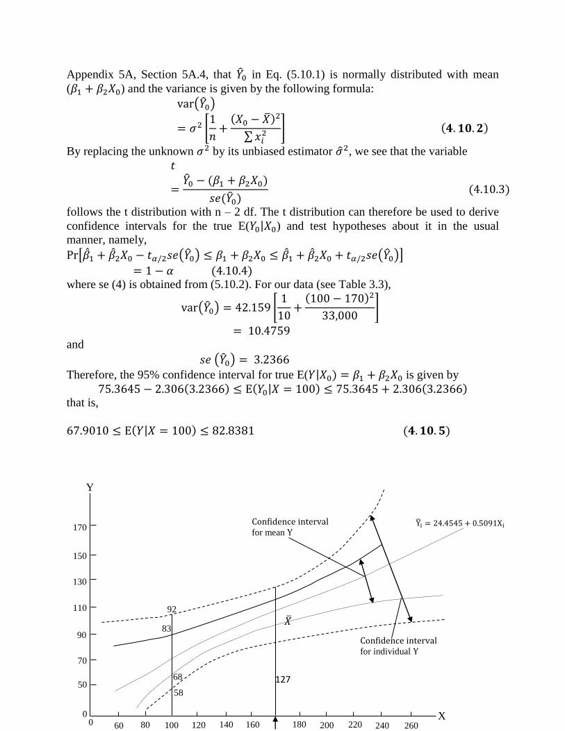
127
Appendix 5A, Section 5A.4, that in Eq. (5.10.1) is normally distributed with mean
( ) and the variance is given by the following formula:
( )
*
∑ +
By replacing the unknown by its unbiased estimator , we see that the variable
follows the t distribution with n – 2 df. The t distribution can therefore be used to derive
confidence intervals for the true E( | ) and test hypotheses about it in the usual
manner, namely,
[ ( ) ( )]
where se (4) is obtained from (5.10.2). For our data (see Table 3.3),
( ) *
+
and
( )
Therefore, the 95% confidence interval for true E( | is given by
| that is,
|
��
Y
X
150
130
0 0 60 80 100 120 140 160
for mean
200 220 260 240
50
70
90
110
170
92
83
68
58
for individual
i i
180
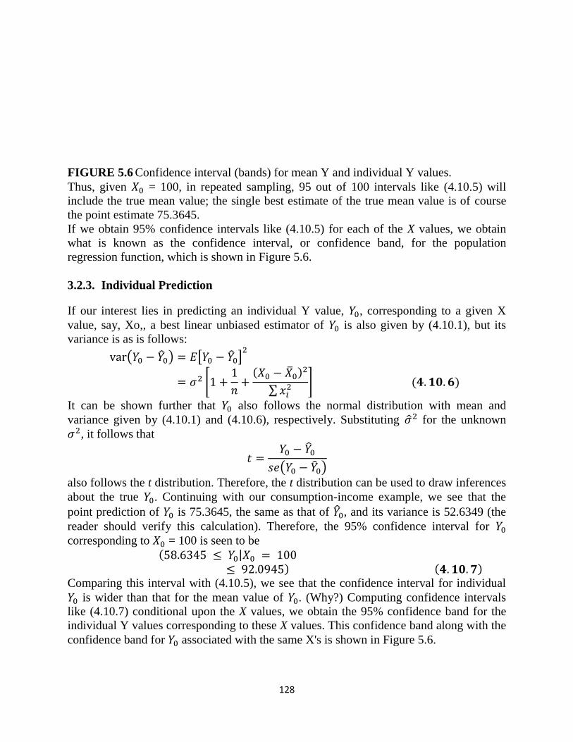
128
FIGURE 5.6 Confidence interval (bands) for mean Y and individual Y values.
Thus, given = 100, in repeated sampling, 95 out of 100 intervals like (4.10.5) will
include the true mean value; the single best estimate of the true mean value is of course
the point estimate 75.3645.
If we obtain 95% confidence intervals like (4.10.5) for each of the X values, we obtain
what is known as the confidence interval, or confidence band, for the population
regression function, which is shown in Figure 5.6.
3.2.3. Individual Prediction
If our interest lies in predicting an individual Y value, , corresponding to a given X
value, say, Xo,, a best linear unbiased estimator of is also given by (4.10.1), but its
variance is as is follows:
( ) [ ]
*
∑ +
It can be shown further that also follows the normal distribution with mean and
variance given by (4.10.1) and (4.10.6), respectively. Substituting for the unknown
, it follows that
( )
also follows the t distribution. Therefore, the t distribution can be used to draw inferences
about the true . Continuing with our consumption-income example, we see that the
point prediction of is 75.3645, the same as that of , and its variance is 52.6349 (the
reader should verify this calculation). Therefore, the 95% confidence interval for
corresponding to = 100 is seen to be
|
Comparing this interval with (4.10.5), we see that the confidence interval for individual
is wider than that for the mean value of . (Why?) Computing confidence intervals
like (4.10.7) conditional upon the X values, we obtain the 95% confidence band for the
individual Y values corresponding to these X values. This confidence band along with the
confidence band for associated with the same X's is shown in Figure 5.6.
129
Notice an important feature of the confidence bands shown in Figure 5.6. The width of
these bands is smallest when = X. (Why?) However, the width widens sharply as
moves away from X. (Why?) This change would suggest that the predictive ability of the
historical sample regression line falls markedly as departs progressively from X.
Therefore, one should exercise great caution in "extrapolating" the historical regression
line to predict E | or associated with a given that is far removed from the
sample mean X.
3.2.4 REPORTING THE RESULTS OF REGRESSION ANALYSIS
There are various ways of reporting the results of regression analysis, but in this text we
shall use the following format, employing the consumption income example of Chapter 3
as an illustration:
8 In Eq. (4.11.1) the figures in the first set of parentheses are the estimated standard errors
of the regression coefficients, the figures in the second set are estimated t values
computed from (4.3.2) under the null hypothesis that the true population value of each
regression coefficient individually is zero (e.g., 3.8128 = 24.4545 6.4138), and the
figures in the third set are the estimated p values. Thus, for 8 df the probability of
obtaining a t value of 3.8128 or greater is 0.0026 and the probability of obtaining a t
value of 14.2605 or larger is about 0.0000003.
By presenting the p values of the estimated t coefficients, we can see at once the exact
level of significance of each estimated t value. Thus, under the null hypothesis that the
true population intercepts value is zero, the exact probability (i.e., the p value) of
obtaining a t value of 3.8128 or greater is only about 0.0026. Therefore, if we reject this
null hypothesis, the probability of our committing a Type I error is about 26 in 10,000, a
very small probability indeed. For all practical purposes we can say that the true
population intercept is different from zero. Likewise, the p value of the estimated slope
coefficient is zero for all practical purposes. If the true MPC were in fact zero, our
chances of obtaining an MPC of 0.5091 would be practically zero. Hence we can reject
the null hypothesis that the true MPC is zero.
Earlier we showed the intimate connection between the F and t statistics, namely,
. Under the null hypothesis that the true , (4.11.1) shows that the F value
is 202.87 (for 1 numerator and 8 denominator df ) and the t value is about 14.24 (8 df );
130
as expected, the former value is the square of the latter value, except for the roundoff
errors.
3.2.5. EVALUATING THE RESULTS OF REGRESSION ANALYSIS
Now that we have presented the results of regression analysis of our consumption-income
example in (4.11.1), we would like to question the adequacy of the fitted model. How
"good" is the fitted model? We need some criteria with which to answer this question.
First, are the signs of the estimated coefficients in accordance with theoretical or prior
expectations? A priori, , the marginal propensity to consume (MPC) in the
consumption function, should be positive. In the present example it is. Second, if theory
says that the relationship should be not only positive but also statistically significant, is
this the case in the present application? The MPC is not only positive but also statistically
significantly different from zero; the p value of the estimated t value is extremely small.
The same comments apply about the intercept coefficient. Third, how well does the regression model explain variation in the consumption expenditure? One can use to answer this question. In the present example is about 0.96, which is a
very high value considering that can be at most 1.
Thus, the model we have chosen for explaining consumption expenditure behavior
seems quite good. But before we sign off, we would like to find out whether our
model satisfies the assumptions of CNLRM. We will not look at the various assumptions
now because the model is patently so simple. But there is one assumption that we would
like to check, namely, the normality of the disturbance term, . Recall that the t and F
tests used before require that the error term follow the normal distribution. Otherwise, the
testing procedure will not be valid in small, or finite, samples.
4.0 CONCLUSION
The unit conclude that statistical approach to forecasting change in a dependent variable
(sales revenue, for example) on the basis of change in one or more independent variables
(population and income, for example). Known also as curve fitting or line fitting because
a regression analysis equation can be used in fitting a curve or line to data points, in a
manner such that the differences in the distances of data points from the curve or line are
minimized. Relationships depicted in a regression analysis are, however, associative only,
and any cause-effect (causal) inference is purely subjective and that variance is the
difference between an expected and actual result, such as between a budget and actual
expenditure.
5.0 SUMMARY
131
In this unit we have discuss the meaning of regression analysis and analysis of variance.
However, some of the calculation of regression analysis and variance was also examine
in this unit, therefore I belief you must have learn a lot in this unit.
6.0 TUTOR MARKED ASSESSMENT EXERCISE
Differentiate between regression analysis and variance analysis.
7.0 REFERENCES/FURTHER READINGS
Gujarat, D. N. (2007) Basic Econometrics, 4th
Edition, tata Mcgraw – Hill publishing
company limited, New Delhi.
Hall, S. G., & Asterion, D. (2011) Applied Econometrics, 2nd
Edition, Palgrave
Macmillian, New York city, USA.
UNIT FOUR: Normality Tests
CONTENTS
1.0 Introduction
2.0 Objectives
3.0 Main content
3.1. Normality test analysis
3.1.1. Histogram of Residuals
3.1.2. Normal Probability Plot
3.1.3. Jarque-Bera (JB) test of Normality
4.0 Conclusion
5.0 Summary
6.0 Tutor-Marked Assignment
7.0. References
1.0. INTRODUCTION
132
In statistics, normality tests are used to determine if a data set is well-modeled by a
normal distribution and to compute how likely it is for a random variable underlying the
data set to be normally distributed.
Before applying statistical methods that assume normality, it is necessary to perform a
normality test on the data (with some of the above methods we check residuals for
normality). We hypothesize that our data follows a normal distribution, and only reject
this hypothesis if we have strong evidence to the contrary.
While it may be tempting to judge the normality of the data by simply creating a
histogram of the data, this is not an objective method to test for normality – especially
with sample sizes that are not very large. With small sample sizes, discerning the shape
of the histogram is difficult. Furthermore, the shape of the histogram can change
significantly by simply changing the interval width of the histogram bars.
2.0. OBJECTIVES
At the end of this unit, you should be able to:
understand the meaning of histogram residuals
understand the analysis of normal probability plot and Jarque-Bera test of
normality.
3.0. MAIN CONTENT
3.1. NORMALITY TEST ANALYSIS
Although several tests of normality are discussed in the literature, we will consider just
three: (1) histogram of residuals; (2) normal probability plot (NPP), a graphical device;
and (3) the Jarque-Bera test.
3.1.1. Histogram of Residuals.
A histogram of residuals is a simple graphic device that is used to learn something about
the shape of the PDF of a random variable. On the horizontal axis, we divide the values
of the variable of interest (e.g., OLS residuals) into suitable intervals, and in each class
interval we erect rectangles equal in height to the number of observation (i.e., frequency)
in that class interval. If you mentally superimpose the bell-shaped normal distribution
curve on the histogram, you will get some idea as to whether normal (PDF)
approximation may be appropriate. It is always a good practice to plot the histogram of
the residuals as a rough and ready method of testing for the normality assumption.
3.1.2. Normal Probability Plot.
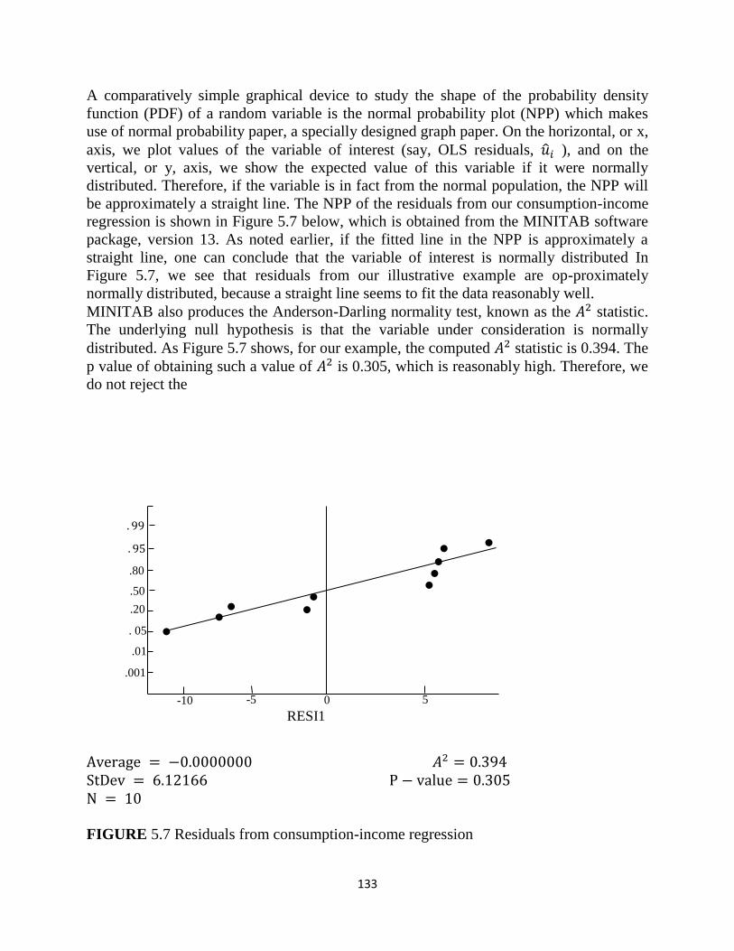
133
A comparatively simple graphical device to study the shape of the probability density
function (PDF) of a random variable is the normal probability plot (NPP) which makes
use of normal probability paper, a specially designed graph paper. On the horizontal, or x,
axis, we plot values of the variable of interest (say, OLS residuals, ), and on the
vertical, or y, axis, we show the expected value of this variable if it were normally
distributed. Therefore, if the variable is in fact from the normal population, the NPP will
be approximately a straight line. The NPP of the residuals from our consumption-income
regression is shown in Figure 5.7 below, which is obtained from the MINITAB software
package, version 13. As noted earlier, if the fitted line in the NPP is approximately a
straight line, one can conclude that the variable of interest is normally distributed In
Figure 5.7, we see that residuals from our illustrative example are op-proximately
normally distributed, because a straight line seems to fit the data reasonably well.
MINITAB also produces the Anderson-Darling normality test, known as the statistic.
The underlying null hypothesis is that the variable under consideration is normally
distributed. As Figure 5.7 shows, for our example, the computed statistic is 0.394. The
p value of obtaining such a value of is 0.305, which is reasonably high. Therefore, we
do not reject the
g
FIGURE 5.7 Residuals from consumption-income regression
.80
.50
.20
. 05
.01
.001
-10 -5 0 5
RESI1
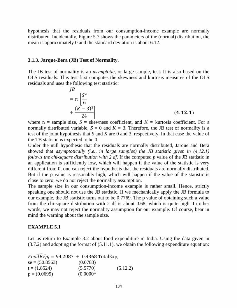
134
hypothesis that the residuals from our consumption-income example are normally
distributed. Incidentally, Figure 5.7 shows the parameters of the (normal) distribution, the
mean is approximately 0 and the standard deviation is about 6.12.
3.1.3. Jarque-Bera (JB) Test of Normality.
The JB test of normality is an asymptotic, or large-sample, test. It is also based on the
OLS residuals. This test first computes the skewness and kurtosis measures of the OLS
residuals and uses the following test statistic:
*
+
where n = sample size, S = skewness coefficient, and K = kurtosis coefficient. For a
normally distributed variable, S = 0 and K = 3. Therefore, the JB test of normality is a
test of the joint hypothesis that S and K are 0 and 3, respectively. In that case the value of
the TB statistic is expected to be 0.
Under the null hypothesis that the residuals are normally distributed, Jarque and Bera
showed that asymptotically (i.e., in large samples) the JB statistic given in (4.12.1)
follows the chi-square distribution with 2 df. If the computed p value of the JB statistic in
an application is sufficiently low, which will happen if the value of the statistic is very
different from 0, one can reject the hypothesis that the residuals are normally distributed.
But if the p value is reasonably high, which will happen if the value of the statistic is
close to zero, we do not reject the normality assumption.
The sample size in our consumption-income example is rather small. Hence, strictly
speaking one should not use the JB statistic. If we mechanically apply the JB formula to
our example, the JB statistic turns out to be 0.7769. The p value of obtaining such a value
from the chi-square distribution with 2 df is about 0.68, which is quite high. In other
words, we may not reject the normality assumption for our example. Of course, bear in
mind the warning about the sample size.
EXAMPLE 5.1
Let us return to Example 3.2 about food expenditure in India. Using the data given in
(3.7.2) and adopting the format of (5.11.1), we obtain the following expenditure equation:
se = (50.8563) (0.0783)
t = (1.8524) (5.5770) (5.12.2)
p = (0.0695) (0.0000*
135
= 0.3698; df = 53
31.1034 (p value = 0.0000)*
where * denotes extremely small.
First, let us interpret this regression. As expected, there is a positive relationship between
expenditure on food and total expenditure. If total expenditure went up by a rupee, on
average, expenditure on food increased by about 44 paise. If total expenditure were zero,
the average expenditure on food would be about 94 rupees. Of course, this mechanical
Interpretation of the intercept may not make much economic sense. The value of about
0.37 means that 37 percent of the variation in food expenditure is explained by total
expenditure, a proxy for income.
Suppose we want to test the null hypothesis that there is no relationship between food
expenditure and total expenditure, that Is, the true slope coefficient = 0. The estimated
value of is 0.4368. If the null hypothesis were true, what is the probability of obtaining
a value of 0.4368? Under the null hypothesis, we observe from (5.12.2) that the t value is
5.5770 and the p value of obtaining such a t value is practically zero. In other words we
can reject the null hypothesis resoundingly. But suppose the null hypothesis were that
= 0.5. Now what?
Using the t test we obtain:
The probability of obtaining a | | of 0.8071 is greater than 20 percent. Hence we do not
reject the hypothesis that the true is 0.5.
Notice that, under the null hypothesis, the true slope coefficient is zero, the F value is
31.1034, as shown in (5.12.2). Under the same null hypothesis, we obtained a t value of
5.5770. If we square this value, we obtain 31.1029, which is about the same as the F
value, again showing the close relationship between the t and the Fstatistic. (Note: The
numerator df for the F statistic must be 1, which is the case here.)
Using the estimated residuals from the regression, what can we say about the probability
distribution of the error term? The information is given in Figure 5.8. As the figure
shows, the residuals from the food expenditure regression seem to be symmetrically
distributed. Application of the Jarque-Bera test shows that the JB statistic is about 0.2576,
and the probability of obtaining such a statistic under the normality assumption is about
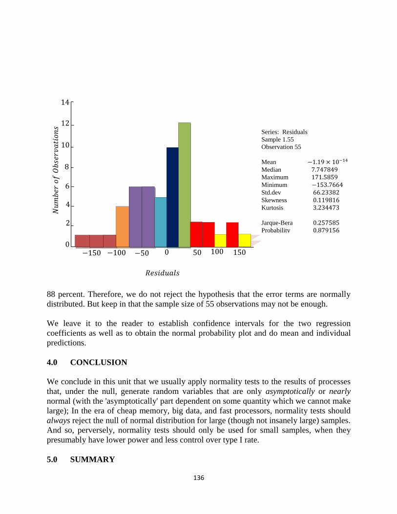
136
88 percent. Therefore, we do not reject the hypothesis that the error terms are normally
distributed. But keep in that the sample size of 55 observations may not be enough.
We leave it to the reader to establish confidence intervals for the two regression
coefficients as well as to obtain the normal probability plot and do mean and individual
predictions.
4.0 CONCLUSION
We conclude in this unit that we usually apply normality tests to the results of processes
that, under the null, generate random variables that are only asymptotically or nearly
normal (with the 'asymptotically' part dependent on some quantity which we cannot make
large); In the era of cheap memory, big data, and fast processors, normality tests should
always reject the null of normal distribution for large (though not insanely large) samples.
And so, perversely, normality tests should only be used for small samples, when they
presumably have lower power and less control over type I rate.
5.0 SUMMARY
𝑅𝑒𝑠𝑖𝑑𝑢𝑎𝑙𝑠
Series: Residuals
Sample 1.55
Observation 55
Mean × 4
Median
Maximum
Minimum
Std.dev
Skewness
Kurtosis
Jarque-Bera
Probability
𝑁𝑢𝑚𝑏𝑒𝑟
𝑜𝑓 𝑂𝑏𝑠𝑒𝑟𝑣𝑎𝑡𝑖𝑜𝑛𝑠
137
The unit discusses at length the normality test analysis such as the histogram of residuals,
probability plot and Jraque Bera test of normality. Therefore, we can say that you must
have learn through the test of normality at length.
6.0 TUTOR MARKED ASSESSMENT EXERCISE
Discuss the differences between Normal probability plot and Jarque-Bera test of
normality
7.0 REFERENCES/FURTHER READINGS
Gujarat, D. N. (2007) Basic Econometrics, 4th
Edition, tata Mcgraw – Hill publishing
company limited, New Delhi.
Hall, S. G., & Asterion, D. (2011) Applied Econometrics, 2nd
Edition, Palgrave
Macmillian, New York city, USA.


![Introduction to Open Access [Open Access for Library Schools, Module 1]](https://img.dokumen.tips/doc/110x75/632bafb3de0a35b8fa0ad761/introduction-to-open-access-open-access-for-library-schools-module-1.jpg)


