I

I I

I .

i J

, /

/

I !

Introduction to Behavioral Research Methods

J

I

THIRD EDITION

Introduction to Behavioral Research Methods

Mark R. Leary Wake Forest University

Allyn and Bacon Boston • London • Toronto • Tokyo • Sydney • Singapore

Executive Editor: Rebecca Pascal Series Editorial Assistant: Whitney C. Brown Marketing Manager: Caroline Crowley Production Editor: Christopher H. Rawlings Editorial-Production Service: Omegatype Typography, Inc. Composition and Prepress Buyer: Linda Cox Manufacturing Buyer: Megan Cochran Cover Administrator: Jennifer Hart Electronic Composition: Omega type Typography, Inc.

Copyright © 2001 by Allyn & Bacon A Pearson Education Company 160 Gould Street Needham Heights, MA 02494

Internet: www.abacon.com

All rights reserved. No part of the material protected by this copyright notice may be reproduced or utilized in any form or by any means, electronic or mechanical, including photocopying, recording, or by any information storage and retrieval system, without written permission from the copyright owner.

Library of Congress Cataloging-in-Publication Data

Leary, Mark R. Introduction to behavioral research methods / Mark Leary.-3rd ed.

p. em. Includes bibliographical references and indexes. ISBN 0-205-32204-2 1. Psychology-Research-Methodology. I. Title.

BF76.5 .L39 2001 105'.7' 2-dc21

Printed in the United States of America

10 9 8 7 6 5 4 3 2 1 05 04 03 02 01 00

00-020422

! !

J I

I I

r I

CONTENTS

Preface xiii

1 Research in the Behavioral Sciences 1

The Beginnings of Behavioral Research 2

Goals of Behavioral Research 4 Describing Behavior 4 Explaining Behavior 4 Predicting Behavior 5 Solving Behavioral Problems 5 Four Goals or One? 5

The Value of Research to the Student 6

The Scientific Approach 7 Systematic Empiricism 8 Public Verification 8 Solvable Problems 9

Behavioral Science and Common Sense 10

Philosophy of Science 11

The Role of Theory in Science 13

Research Hypotheses 14

A Priori Predictions and Post Hoc Explanations 16

Conceptual and Operational Definitions 16

Proof and Disproof in Science 19 The Logical Impossibility of Proof 19 The Practical Impossibility of Disproof 20 If Not Proof or Disproof, Then What? 20

Strategies of Behavioral Research 23 Descriptive Research 23 Correlational Research 23 Experimental Research 24 Quasi-Experimental Research 24

Domains of Behavioral Science

A Preview 27

Summary 28

25

v

vi CONTENTS

2 Behavioral Variability and Research 33

Variability and the Research Process 34

Variance: An Index of Variability 37 A Conceptual Explanation of Variance 38 A Statistical Explanation of Variance 39

Systematic and Error Variance 42 Systematic Variance 42 Error Variance 43 Distinguishing Systematic from Error Variance 45

Assessing the Strength of Relationships 46

Meta-Analysis: Systematic Variance Across Studies 47

Summary 49

3 The Measurement of Behavior 53

Types of Measures 54

Scales of Measurement 56

Estimating the Reliability of a Measure 57 Measurement Error 58 Reliability as Systematic Variance 59 Assessing Reliability 60 Increasing the Reliability of Measures 64

Estimating the Validity of a Measure 65 Assessing Validity 65

Fairness and Bias in Measurement 71

Summary 73

4 Approaches to Psychological Measurement 77

Observational Methods 78 Naturalistic Versus Contrived Settings 78 Disguised Versus Nondisguised Observation 80 Behavioral Recording 82 Increasing the Reliability of Observational Methods 85

Physiological Measures 85

Self-Report: Questionnaires and Interviews 86 Writing Questions 86

I

) !

j

CONTENTS vii

Questionnaires 91 Interviews 93 Advantages of Questionnaires Versus Interviews 94 Biases in Self-Report Measurement 94

Archival Data 97

Content Analysis 99

Summary 100

5 Descriptive Research 104

Types of Descriptive Research 105 Surveys 105 Demographic Research 107 Epidemiological Research 108 Summary 108

Sampling 109 Probability Samples Nonprobability Samples

109 116

Describing and Presenting Data 119 Criteria of a Good Description 119 Frequency Distributions 120 Measures of Central Tendency 125 Measures of Variability 126 Standard Deviation and the Normal Curve 127 The z-Score 130

Summary 131

6 Correlational Research 136

The Correlation Coefficient 138

A Graphic Representation of Correlations 139

The Coefficient of Determination 142

Statistical Significance of r 146

Factors That Distort Correlation Coefficients 148 Restricted Range 148 Outliers 150 Reliability of Measures 152

Correlation and Causality 152

Partial Correlation 155

viii CONTENTS

Other Correlation Coefficients 156

Summary 157

7 Advanced Correlational Strategies 162

Predicting Behavior: Regression Strategies Linear Regression 163 Types of Multiple Regression Multiple Correlation 170

165

162

Assessing Directionality: Cross-Lagged and Structural Equations Analysis 171

Cross-Lagged Panel Design Structural Equations Modeling

171 172

Uncovering Underlying Dimensions: Factor Analysis 175 An Intuitive Approach 176 Basics of Factor Analysis 176 Uses of Factor Analysis 178

Summary 179

8 Basic Issues in Experimental Research 184

Manipulating the Independent Variable 186 Independent Va.riables 186 Dependent Variables 190

Assignment of Participants to Conditions 191 Simple Random Assignment 191 Matched Random Assignment 192 Repeated Measures Designs 193

Experimental Control 197 Systematic Variance 197 Error Variance 198 An Analogy 199

Eliminating Confounds 200 Internal Validity 200 Threats to Internal Validity 201 Experimenter Expectancies, Demand Characteristics, and Placebo Effects 205

Error Variance 208 Sources of Error Variance 208

CONTENTS ix

Experimental Control and Generalizability: The Experimenter's Dilemma 211

Summary 212

9 Experimental Design 218

One-Way Designs 219 Assigning Participants to Conditions 220 Posttest and Pretest-Posttest Designs 221

Factorial Designs 224 Factorial Nomenclature 225 Assigning Participants to Conditions 228

Main Effects and Interactions 230 Main Effects 230 Interactions 231 Higher-Order Designs 234

Combining Independent and Subject Variables 235

Summary 239

10 Analyzing Experimental Data 243

An Intuitive Approach to Analysis 244 The Problem: Error Variance Can Cause Mean Differences 245 The Solution: Inferential Statistics 245

Hypothesis Testing 246 The Null Hypothesis 246 Type I and Type II Errors 247 Effect Size 250 Summary 250

Analysis of Two-Group Experiments: The t-Test 250 Conducting a t-Test 251 Back to the Droodles Experiment 255

/ Analyses of Matched-Subjects and Within-Subjects Designs 256

Summary 257

11 Analyzing Complex Designs 262

The Problem: Multiple Tests Inflate Type I Error 263

X CONTENTS

The Rationale Behind ANOVA 264

How ANOVA Works 265 Total Sum of Squares 265 Sum of Squares Within-Groups 266 Sum of Squares Between-Groups 267 The F-Test 267 Extension of ANOVA to Factorial Designs 268

Follow-Up Tests 271 Main Effects 271 Interactions 272

Between-Subjects and Within-Subjects ANOVAs 274

Multivariate Analysis of Variance 274 Conceptually Related Dependent Variables 275 Inflation of Type I Error 275 How MANOVA Works 276

Experimental and Nonexperimental Uses of Inferential Statistics 277

Computer Analyses 278

Summary 279

12 Quasi-Experimental Designs 282

Pretest-Posttest Designs 284 How NOT to Do a Study: The One-Group Pretest-Posttest Design 285 Nonequivalent Control Group Design 286

Time Series Designs 291 Simple Interrupted TIme Series Design 291 Interrupted TIme Series with a Reversal 294 Control Group Interrupted Tl1Ile Series Design 295 l

Longitudinal Designs 296

Program Evaluation 298

Evaluating Quasi-Experimental Designs 300 Threats to Internal Validity 300 Increasing Confidence in Quasi-Experimental Results 302

Summary 303

13 Single-Case Research 306

Single-Case Experimental Designs 308

f

J

CONTENTS xi

Criticisms of Group Designs and Analyses 309 Basic Single-Case Experimental Designs 312 Data from Single-Participant Designs 316 Uses of Single-Case Experimental Designs 318 Critique of Single-Participant Designs 320

Case Study Research 321 Uses of the Case Study Method 322 Limitations of the Case Study Approach 323

Summary 325

14 Ethical Issues in Behavioral Research 329

Approaches to Ethical Decisions 330

Basic Ethical Guidelines 332 Potential Benefits 333 Potential Costs 334 Balancing Benefits and Costs 334 The Institutional Review Board 334

The Principle of Informed Consent 335 Obtaining Informed Consent 335 Problems with Obtaining Informed Consent 336

Invasion of Privacy 338

Coercion to Participate 339

Physical and Mental Stress 339

Deception in Research Objections to Deception Debriefing 341

340 340

Confidentiality in Research 342

Common Courtesy 344

Ethical Principles in Research with Animals

Scientific Misconduct 347

A Final Note 350

Summary 350

15 Scientific Writing 353

345

How Scientific Findings Are Disseminated 353

xii CONTENTS

Journal Publication 354 Presentations at Professional Meetings 355 Personal Contact 356

Elements of Good Scientific Writing 357 Organization 357 Clarity 358 Conciseness 360 Proofreading and Rewriting 361

Avoiding Biased Language 362 Gender-Neutral Language 362 Other Language Pitfalls 364

Parts of a Manuscript 364 Title Page 365 Abstract 366 Introduction 367 Method 367 Results 368 Discussion 369

Citing and Referencing Previous Research 370 Citations in the Text 370 The Reference List 371

Other Aspects of APA Style 373 Optional Sections 373 Headings, Spacing, Pagination, and Numbers 374

Sample Manuscript 377 r

Glossary 399

Appendix A Statistical Tables 411

Appendix B Computational Formulas for ANOVA 418

References 427

Index 435

i i

f

PREFACE

Regardless of how good a particular class is, the students' enthusiasm for the course material is rarely, if ever, as great as the professor's. No matter how inter­esting the material, how motivated the students, or how skillful the professor, those who take a course are seldom as enthralled with the content as those who teach it. We've all taken courses in which an animated, nearly zealous professor faced a classroom of only mildly interested students.

In departments founded on the principles of behavioral science-psychology, communication, human development, education, marketing, social work, and the like-this discrepancy in student and faculty interest is perhaps most pronounced in courses that deal with research design and analysis. On one hand, the faculty members who teach courses in research methods are usually quite enthused about research. They typically enjoy the research process. Many have contributed to the research literature in their own areas of expertise, and some are highly regarded researchers within their fields. On the other hand, despite these instruc­tors' best efforts to bring the course alive, students often dread taking methods courses. They find these courses dry and difficult and wonder why such courses are required as part of their curriculum. Thus, the enthused, involved instructor is often confronted by a class of disinterested, even hostile students who begrudge the fact that they must study research methods at all.

These attitudes are understandable. After all, students who choose to study psychology, education, human development, and other areas that rely on behav­ioral research rarely do so because they are enamored with research. Rather, they either plan to enter a profession in which knowledge of behavior is relevant (such as professional psychology, social work, teaching, or public relations) or are intrin­sically interested in the subject matter. Although some students eventually come to appreciate the value of research to behavioral science, the helping professions, and society, others continue to regard it as an unnecessary curricular diversion im­posed by misguided academicians. For many students, being required to take courses in methodology and statistics supplants other courses in which they are more interested.

In addition, the concepts, principles, analyses, and ways of thinking central to the study of research methods are new to most students and, thus, require extra effort to comprehend, learn, and retain. Add to that the fact that the topics covered in research methods courses are, on the whole, inherently less interesting than those covered in most other courses in psychology and related fields. If the instructor and textbook authors do not make a special effort to make the material interesting and relevant, students are unlikely to derive much enjoyment from studying research methods.

I wrote Introduction to Behavioral Research Methods because, as a teacher and as a researcher, I wanted a book that would help counteract students' natural tendencies

xiii

xiv PREFACE

to dislike and shy away from research-a book that would make research method­ology as understandable, palatable, useful, and interesting for my students as it was for me. Thus, my primary goal was to write a book that is readable. Students should be able to understand most of the material in a book such as this without the course instructor having to serve as an interpreter. Enhancing comprehensibility can be achieved in two ways. The less preferred way is simply to dilute the material by omitting complex topics and by presenting material in a simplified, "dumbed­down" fashion. The alternative that I chose to pursue in this text is to present the material with sufficient elaboration, explanation, and examples to render it under­standable. The feedback that I have received on the two previous editions of the book make me optimistic that I have succeeded in my goal to create a rigorous yet readable book.

A second goal was to integrate the various topics covered in the book to a greater extent than is done in most methods texts, using the concept of variability as a unifying theme. From the development of a research idea, through measure­ment issues, to design and analysis, the entire research process is an attempt to understand variability in behavior. Because the concept of variability is woven throughout the research process, I've used it as a framework to provide coherence to the various topics in the book. Having taught research methods courses centered around the theme of variability for 20 years, I can attest that students find the uni­fying theme very useful.

Third, I tried to write a book that is interesting-that presents ideas in an engaging fashion and uses provocative examples of real and hypothetical research. This edition of the book has even more interesting examples of real research, tidbits about the lives of famous researchers, and intriguing controversies that have arisen in behavioral science. Far from being icing on the cake, these features help to enliven the research enterprise. Like most researchers, I am enthusiastic about the research process, and I hope that some of my fervor will be contagious.

Courses in research methods differ widely in the degree to which statistics are incorporated into the course. My personal view is that students' understanding of research methodology is enhanced by familiarity with basic statistical principles. Without an elementary grasp of statistical concepts, students will find it very diffi­cult to understand the research articles they read. Although this book is decidedly focused on research methodology and design, I've sprinkled essential statistical top­ics throughout the book that emphasize conceptual foundations and provide calcu­lation procedures for a few basic analyses. My goal is to help students understand statistics conceptually without asking them to actually complete the calculations. With a better understanding of what becomes of the data they collect, students should be able to design more thorough and reliable research studies. Furthermore, knowing that instructors differ widely in the degree to which they incorporate sta­tistics into their methods courses, I have made it easy for individual instructors to choose whether students will deal with the calculational aspects of the analyses that appear. For the most part, presentation of statistical calculations are confined to a few within-chapter boxes, Chapters 10 and 11, and Appendix B. These sections may eas­ily be omitted if the instructor prefers.

I

,'-1

I r

)

l , i I

'"

PREFACE XV

This edition of Introduction to Behavioral Research Methods has benefitted from the feedback I have received from many instructors who have used it in their courses, as well as my experiences of using the previous editions in my own course for over 10 years. In addition to editing the entire text and adding many new exam­ples of real research throughout the book, I have changed the third edition from the previous edition in five primary ways. First, the coverage of measurement has been reorganized and broadened. Following Chapter 3, which deals with basic mea­surement issues, Chapter 4 now focuses in detail on specific types of measures, in­cluding observational, physiological, self-report, and archival measures. Second, a new chapter on descriptive research (Chapter 5) has been added that deals with types of descriptive studies, sampling, and basic descriptive statistics. (This new chapter is a hybrid of Chapters 5 and 6 in the previous edition, along with new mate­rial.) Third, the section on regression analysis in Chapter 7 has been expanded; given the prevalence of regression in the published research, I felt that students needed to understand regression in greater detail. Fourth, a new sample manuscript has been included at the end of the chapter on scientific writing (Chapter 15), and this manuscript has been more heavily annotated in terms of APA style than the one in the previous edition. Fifth, at the request of several instructors who have used pre­vious editions of the book, the number of review questions at the end of each chap­ter has been expanded to increase students' ability to conquer the material and test their own knowledge. I should also mention that an expanded Instructor's Manual is available for this edition.

As a teacher, researcher, and author, I know that there will always be some discrepancy between professors' and students' attitudes toward research methods, but I hope that the new edition of this book will help to narrow the gap.

Acknowledgments

I would like to thank the following reviewers: Danuta Bukatko, Holy Cross College; Tracy Giuliano, Southwestern University; Marie Helweg-Larsen, Transylvania Uni­versity; Julie Stokes, California State University, Fullerton; and Linda Vaden-Goad, University of Houston-Downtown Campus.

1

,I I ,

,I i

! i

I I

! )

) :4

.'

Introduction to Behavioral Research Methods

I

t' , l \

j

! ,,;

CHAPTER

1 Research in the Behavioral Sciences

The Beginnings of Behavioral Research Goals of Behavioral Research The Value of Research to the Student

The Scientific Approach Behavioral Science and Common Sense

Philosophy of Science The Role of Theory in Science

Research Hypotheses

A Priori Predictions and Post Hoc Explanations Conceptual and Operational Definitions

Proof and Disproof in Science

Strategies of Behavioral Research

Domains of Behavioral Science

A Preview

Stop for a moment and imagine, as vividly as you can, a scientist at work. Let your imagination fill in as many details as possible regarding this scene. What does the imagined scientist look like? Where is the person working? What is the scientist doing?

When I asked a group of undergraduate students to imagine a scientist and to tell me what they imagined, their answers were quite intriguing. First, virtually every student said that their imagined scientist was male. This in itself is interest­ing given that a high percentage of scientists are, of course, women.

Second, most of the students reported that they imagined that the scientist was wearing a white lab coat and working indoors in some kind of laboratory. The details regarding this laboratory differed from student to student, but the lab nearly always contained technical scientific equipment of one kind or another. Some students imagined a chemist, surrounded by substances in test tubes and beakers. Other students thought of a biologist peering into a microscope. Still others conjured up a physicist working with sophisticated electronic equipment. One or two students even imagined an astronomer peering through a telescope. Most in­teresting to me was the fact that although these students were members of a psy­chology class (in fact, most were psychology majors), not one of them thought of any kind of a behavioral scientist when I asked them to imagine a scientist.

1

2 CHAPTER 1

Their responses were probably typical of what most people would say if asked to imagine a scientist. For most people, the prototypic scientist is a man wearing a white lab coat working in a laboratory filled with technical equipment. Most people do not think of psychologists and other behavioral researchers as scientists in the same way that they think of physicists, chemists, and biologists as scientists.

Instead, people tend to think of psychologists primarily in their roles as men­tal health professionals. If I had asked you to imagine a psychologist, you probably would have thought of a counselor talking with a client about his or her problems. You probably would not have imagined a behavioral researcher, such as a physio­logical psychologist studying startle responses, a social psychologist conducting an experiment on aggression, or an industrial psychologist interviewing the line supervisors at an automobile assembly plant.

Psychology, however, not only is a profession that promotes human welfare through counseling, education, and other activities, but also is a scientific disci­pline that studies behavior and mental processes. Just as biologists study living or­ganisms and astronomers study the stars, behavioral scientists conduct research involving behavior and mental processes.

The Beginnings of Behavioral Research

People have asked questions about the causes of behavior throughout written his­tory. Aristotle (384-322 BCE) is sometimes credited for being the first individual to address systematically basic questions about the nature of human beings and why they behave as they do, and within Western culture this claim may be true. How­ever, more ancient writings from India, including the Upanishads and the teachings of Gautama Buddha (563-483 BCE), offer equally sophisticated psychological in­sights into human thought, emotion, and behavior.

For over two millennia, however, the approach to answering these questions was entirely speculative. People would simply concoct explanations of behavior based on everyday observation, creative insight, or religious doctrine. For many centuries, people who wrote about behavior tended to be philosophers or theolo­gians, and their approach was not scientific. Even so, many of these early insights into behavior were, of course, quite accurate.

However, many of these explanations of behavior were also completely wrong. These early thinkers should not be faulted for having made mistakes, for even modem researchers sometimes draw incorrect conclusions. Unlike behavioral sci­entists today, however, these early "psychologists" (to use the term loosely) did not rely on scientific research to provide answers about behavior. As a result, they had no way to test the validity of their explanations and, thus, no way to discover whether or not their interpretations were accurate.

Scientific psychology (and behavioral science more broadly) was born during the last quarter of the nineteenth century. Through the influence of early researchers such as Wilhelm Wundt, William James, John Watson, G. Stanley Hall, and others,

( ,

( .1

/

t

-::

Research in the Behavioral Sciences 3

people began to realize that basic questions about behavior could be addressed using many of the same methods that were used in more established sciences, such as biology, chemistry, and physics.

Today, more than 100 years later, the work of a few creative scientists has blos­somed into a very large enterprise, involving hundreds of thousands of researchers around the world who devote part or all of their working lives to the scientific study of behavior. These include not only research psychologists but also researchers in other disciplines such as education, social work, family studies, communication, management, health and exercise science, marketing, and a number of medical fields (such as nursing, neurology, psychiatry, and geriatrics). What researchers in all of these areas of behavioral science have in common is that they apply scientific methodologies to the study of behavior, thought, and emotion.

i!!I! !m!l CONTRIBUTORS TO BEHAVIORAL RESEARCH

Wilhelm Wundt and the Founding of Scientific Psychology Wilhelm Wundt (1832-1920) was the first bonafide research psychologist. Most of those be­fore him who were interested in behavior identified themselves primarily as philosophers, theologians, biologists, physicians, or phYSiologists. Wundt, on the other hand, was the first to view himself as a research psychologist.

Wundt, who was born near Heidelberg, Germany, began studying medicine but switched to physiology after working with Johannes Muller, the leading physiologist of the time. Although his early research was in physiology rather than psychology, Wundt soon became interested in applying the methods of physiology to the study of psychology. In 1874, Wundt published a landmark text, Principles of Physiological Psychology, in which he boldly stated his plan to "mark out a new domain of science. II

In 1875, Wundt established one of the first two psychology laboratories in the world at the University of Leipzig. Although it has been customary to cite 1879 as the year in which his lab was founded, Wundt was actually given laboratory space by the university for his laboratory equipment in 1875 (Watson, 1978). William James established a laboratory at Harvard University at about the same time, thus establishing the first psychologicallabora­tory in the United States (Bringmann, 1979).

Beyond establishing the Leipzig laboratory, Wundt made many other contributions to behavioral science. He founded a scientific journal in 1881 for the publication of research in experimental psychology-the first journal to devote more space to psychology than to phi­losophy. (At the time, psychology was viewed as an area in the study of philosophy.) He also conducted a great deal of research on a variety of psychological processes, including sensa­tion, perception, reaction time, attention, emotion, and introspection. Importantly, he also trained many students who went on to make their own contributions to early psychology: G. Stanley Hall (who founded the American Psychological Association and is considered the founder of child psychology), Lightner Witmer (who established the first psycholOgical clinic), Edward Titchener (who brought Wundt's ideas to the United States), and Hugo Munsterberg (a pioneer in applied psychology). Also among Wundt's students was James

4 CHAPTER 1

McKeen Cattell who, in addition to conducting early research on mental tests, was the first to integrate the study of experimental methods into the undergraduate psychology curriculwn (Watson, 1978). In part, you have Cattell to thank for the importance that colleges and uni­versities place on courses in research methods.

Goals of Behavioral Research

Psychology and the other behavioral sciences are thriving as never before. Theo­retical and methodological advances have led to important discoveries that have not only enhanced our understanding of behavior but also improved the quality of human life. Each year, behavioral researchers publish the results of tens of thou­sands of studies, each of which adds incrementally to what we know about the be­havior of human beings and other animals.

As behavioral researchers design and conduct all of these studies, they gen­erally do so with one of four goals in mind-description, explanation, prediction, or application. That is, they design their research with the intent of describing be­havior, explaining behavior, predicting behavior, or applying knowledge to solve behavioral problems.

Describing Behavior

Some behavioral research focuses primarily on describing patterns of behavior, thought, or emotion. Survey researchers, for example, conduct large studies of ran­domly selected respondents to determine what people think, feel, and do. You are un­doubtedly familiar with public opinion polls, such as those that dominate the news during elections, which describe people's attitudes. Some research in clinical psychol­ogy and psychiatry investigates the prevalence of certain psychological disorders. Marketing researchers conduct descriptive research to study consumers' preferences and buying practices. Other examples of descriptive studies include research in de­velopmental psychology that describes age-related changes in behavior and research in industrial psychology that describes the behavior of effective managers.

Explaining Behavior

Most behavioral research goes beyond studying what people do to attempting to understand why they do it. Most researchers regard explanation as the most im­portant goal of scientific research. Basic research, as it is often called, is conducted to understand behavior regardless of whether the knowledge is immediately ap­plicable. This is not to say that basic researchers are not interested in the applica­bility of their findings. They usually are. In fact, the results of basic research can be quite useful, often in ways that were not anticipated by the researchers themselves. For example, basic research involving brain function has led to the development of drugs that control some symptoms of mental illness, and basic research on cogni-

;

j

, i ~ ,

, ~

I

J

)

)

(

Research in the Behavioral Sciences 5

tive development in children has led to educational innovations in schools. How­ever, the immediate goal of basic research is to explain a particular psychological phenomenon rather than to solve a particular problem.

Predicting Behavior

Many behavioral researchers are interested in predicting people's behavior. For ex­ample, personnel psychologists try to predict employees' job performance using employment tests and interviews. Similarly, educational psychologists develop ways to predict academic performance using scores on standardized tests to identify students who might have learning difficulties in school. Likewise, some forensic psychologists are interested in predicting which criminals are likely to be dangerous if released from prison. Developing ways to predict job performance, school grades, or violent tendencies requires considerable research. The appropri­ate tests (such as employment or achievement tests) must be administered, ana­lyzed, and refined to meet certain statistical criteria. Then, data are collected and analyzed to identify the best predictors of the target behavior. Prediction equations are calculated on other samples of participants to validate whether they predict the behavior well enough to be used. Throughout this process, scientific prediction of behavior involves behavioral research methods.

Solving Behavioral Problems

The goal of applied research is to find solutions for certain problems rather than to understand basic psychological processes per se. For example, industrial-organiza­tional psychologists are hired by businesses to study and solve problems related to employee morale, satisfaction, and productivity. Similarly, community psycholo­gists are sometimes asked to investigate social problems such as racial tension, lit­tering, and violence, and researchers in human development and social work study problems such as child abuse and teenage pregnancy. These behavioral researchers use scientific approaches to understand and solve some problem of immediate con­cern (such as employee morale or prejudice). Other applied researchers conduct evaluation research (also called program evaluation) using behavioral research meth­ods to assess the effects of social or institutional programs on behavior. When new programs are implemented-such as when new educational programs are intro­duced into the schools, when new laws are passed, or when new employee policies are started in a business organization-program evaluators are sometimes asked to determine whether the new program is effective in achieving its intended purpose. If so, the evaluator often tries to determine precisely why the program works; if not, the evaluator tries to uncover why the program is unsuccessful.

Four Goals or One?

The four goals of behavioral research-description, explanation, prediction, and application-overlap considerably. For example, much basic research is immediately

6 CHAPTER 1

applicable, and much applied research provides information that enhances our basic understanding of behavior. Furthermore, because prediction and application often require an understanding of how people act and why, descriptive and basic research provide the foundation on which predictive and applied research rests. In return, in the process of doing behavioral research to predict behavior and of doing applied research to solve problems, new questions and puzzles often arise for basic researchers. Importantly, researchers rely largely on the same general re­search strategies whether their goal is to describe, explain, predict, or solve prob­lems. Methodological and statistical innovations that are developed in one context spread quickly to the others. Thus, although researchers may approach a particu­lar study with one of these goals in mind, behavioral science as a,:\"hole benefits from the confluence and integration of all kinds of research. .P~~'

The Value of Research to the Student

The usefulness of research for understanding behavior and improving the quality of life is rather apparent, but it may be less obvious that a firm grasp of basic research methodology has benefits for students such as yourself. After all, most students who take courses in research methods have no intention of becoming re­searchers. Understandably, such students may wonder how studying research benefits them.

A background in research has at least four important benefits. First, knowl­edge about research methods allows people to understand research that is relevant to their professions. Many professionals who deal with people-not only psychol­ogists, but also those in social work, nursing, education, management, medicine, public relations, communication, advertising, and the ministry-must keep up with advances in their fields. For example, people who become counselors and therapists are obligated to stay abreast of the research literature that deals with therapy and related topics. Similarly, teachers need to stay informed about recent research that might help improve their teaching. In business, many decisions that executives and managers make in the workplace must be based on the outcomes of research studies. However, most of this information is published in professional re­search journals, and as you may have learned from experience, journal articles can be nearly incomprehensible unless the reader knows something about research methodology and statistics. Thus, a background in research provides you with knowledge and skills that may be useful in professional life.

Related to this outcome is a second: A knowledge of research methodology makes one a more intelligent and effective "research consumer" in everyday life. In­creasingly, we are asked to make everyday decisions on the basis of scientific re­search findings. When we try to decide which new car to buy, how much we should exercise, which weight-loss program to select, whether to enter our children in pub­lic versus private schools, whether to get a flu shot, or whether we should follow the latest fad to improve our happiness or prolong our life, we are often confronted with research findings that argue one way or the other. For example, the Surgeon

r I r , r

!

..

Research in the Behavioral Sciences 7

General of the United States and the tobacco industry have long been engaged in a debate on the dangers of cigarette smoking. The Sw.t:geon General maintains that cigarettes are hazardous to your health, whereas cigarette manufacturers claim that no conclusive evidence exists that shows cigarette smoking causes lung cancer and other diseases in humans. Furthermore, both sides present scientific data to support their arguments. Who is right? As you'll see later in this book, even a basic knowl­edge of research methods will allow you to resolve this controversy. When we read or hear about the results of research in the media, how do we spot shoddy studies, questionable statistics, and unjustified conclusions? People who have a basic knowledge of research design and analysis are in a better position to evaluate the scientific evidence they encounter in everyday life than those who don't.

A third outcome of research training involves the development of critical thinking. Scientists are a critical lot, always asking questions, considering alterna­tive explanations, insisting on hard evidence, refining their methods, and cri­tiquing their own and others' conclusions. Many people have found that a critical, scientific approach to solving problems is useful in their everyday lives.

Finally, a fourth benefit of learning about and becoming involved in research is that it helps one become an authority, not only on research methodology, but also on particular topics. In the process of reading about previous studies, wrestling with issues involving research strategy, collecting data, and interpreting the re­sults, researchers grow increasingly familiar with their topics. For this reason, fac­ulty members at many colleges and universities urge their students to become involved in research, such as class projects, independent research projects, or a fac­ulty member's research. This is also one reason why many colleges and universi­ties insist that their faculty maintain ongoing research programs. By remaining active as researchers, professors engage in an ongoing learning process that keeps them at the forefront of their fields.

Many years ago, science fiction writer H. G. Wells predicted: "Statistical thinking will one day be as necessary for efficient citizenship as the ability to read and write." Although we are not at the point where the ability to think like a scien­tist and statistician is as important as reading or writing, knowledge of research methods and statistics is becoming increasingly important for successful living.

The Scientific Approach

I noted earlier that most people have greater difficulty thinking of psychology and other behavioral sciences as science than regarding chemistry, biology, physicS, or astronomy as science. In part, this is because many people misunderstand what science is. Most people appreciate that scientific knowledge is somehow special, but they judge whether a discipline is scientific on the basis of the topics it studies. Research involving molecules, chromosomes, and sunspots seems more scientific than research involving emotions, memories, or social interactions, for example.

Whether an area of study is scientific has little to do with the topics it studies, however. Rather, science is defined in terms of the approaches used to study the

8 CHAPTER 1

topic. Specifically, three criteria must be met for an investigation to be considered sci­entific: systematic empiricism, public verification, and solvability (Stanovich, 1996).

Systematic Empiricism

Empiricism refers to the practice of relying on observation to draw conclusions about the world. The story is told about two scientists who saw a flock of sheep stand­ing in a field. Gesturing toward the sheep, one scientist said, "Look, all of those sheep have just been shorn." The other scientist narrowed his eyes in thought, then replied, "Well, on the side faCing us anyway." Scientists insist that conclusions be based on what can be objectively observed, and not on assumptions, hunches, unfounded be­liefs, or the product of people's imaginations. Although most people today would agree that the best way to find out about something is to observe it directly, this was not always the case. Until the late sixteenth century, experts relied more heavily on reason, intuition, and religious doctrine than on observation to answer questions.

But observation alone does not make something a science. After all, everyone draws conclusions about human nature from observing people in everyday life. Scientific observation is systematic. Scientists structure their observations in sys­tematic ways so that they can draw valid conclusions from them about the nature of the world. For example, a behavioral researcher who is interested in the effects of exercise on stress is not likely simply to chat with people who exercise about how much stress they feel. Rather, the researcher is likely to design a carefully con­trolled study in which people are assigned randomly to different exercise pro­grams, then measure their stress using reliable and valid techniques. Data obtained through systematic empiricism allow researchers to draw more confident conclu­sions than they can draw from casual observation alone.

Public Verification

The second criterion for scientific investigation is that it be available for public ver­ification. In other words, research must be conducted in such a way that the find­ings of one researcher can be observed, replicated, and verified by others.

There are two reasons for this. First, the requirement of public verification en­sures that the phenomena scientists study are real and observable, and not one per­son's fabrications. Scientists disregard claims that cannot be verified by others. For example, a person's claim that he or she was captured by Bigfoot makes interesting reading, but it is not scientific if it cannot be verified.

Second, public verification makes science self-correcting. When research is open to public scrutiny, errors in methodology and interpretation can be discov­ered and corrected by other researchers. The findings obtained from scientific re­search are not always correct, but the requirement of public verification increases the likelihood that errors and incorrect conclusions will be detected and corrected.

Public verification requires that researchers report their methods and their findings to the scientific community, usually in the form of journal articles or pre­sentations of papers at professional meetings. In this way, the methods, results,

I \

r

Research in the Behavioral Sciences 9

and conclusions of a study can be examined and, possibly, challenged by others. And, as long as researchers report their methods in full detail, other researchers can attempt to repeat, or replicate, the research. Not only does replication catch er­rors, but it allows researchers to build on and extend the work of others.

Solvable Problems

The third criterion for scientific investigation is that science deals only with solvable problems. Researchers can investigate only those questions that are answerable given current knowledge and research techniques.

This criterion means that many questions fall outside the realm of scientific investigation. For example, the question /I Are there angels?/I is not scientific: No one has yet devised a way of studying angels that is empirical, systematic, and publicly verifiable. This does not necessarily imply that angels do not exist or that the question is unimportant. It simply means that this question is beyond the scope of scientific investigation.

t!!t!!#l§4'l!i!WOlill IN DEPTH

Pseudoscience: Believing the Unbelievable

Many people are willing to believe in things for which there is little, if any, empirical proof. They readily defend their belief that extraterrestrials have visited Earth; that some people can read others' minds; that they have been visited by the dead; or that Bigfoot was sighted recently.

From the perspective of science, such beliefs present a problem because the evidence that is marshaled to support them is usually pseudoscientific. Pseudoscientific evidence in­volves claims that masquerade as science but in fact violate the basic assumptions of scien­tific investigation (Radner & Radner, 1982). It is not so much that people believe things that have not been confirmed; even scientists do that. Rather, it is that pseudoscientists present evidence to support such beliefs that pretend to be scientific but are not. Pseudoscience is easy to recognize because it violates the basic criteria of science discussed above: systematic empiricism, public verification, and solvability.

Nonempirical Evidence Scientists rely on observation to test their hypotheses. Pseudoscientific evidence, however, is often not based on observation, but rather on myths, opinions, and hearsay. For example, von Daniken (1970) used biblical references to "chariots of fire"in Chariots of the Gods? as ev­idence for ancient spacecrafts. However, because biblical evidence of past events is neither systematic nor verifiable, it cannot be considered scientific. This is not to say that such evi­dence is necessarily inaccurate; it is Simply not permissible in scientific investigation be­cause its veracity cannot be determined conclusively. Similarly, pseudoscientists often rely on people's beliefs rather than on observation or accepted scientific fact to bolster their ar­guments. Scientists wait for the empirical evidence to come in rather than basing their con­clusions on what others think might be the case.

10 CHAPTER 1

Furthermore, unlike science, pseudoscience tends to be highly biased in the evi­dence presented to support its case. For example, those who believe in precognition­telling the future-point to specific episodes in which people seemed to know in advance that something was going to happen. A popular tabloid once invited its readers to send in their predictions of what would happen during the next year. When the 1,500 submissions were opened a year later, one contestant was correct in all five of her predictions. The tabloid called this a "stunning display of psychic ability." Was it? Isn't it just as likely that, out of 1,500 en­tries, some people would, just by chance, make correct predictions? Scientific logic requires that the misses be considered evidence along with the hits. Pseudoscientific logic, on the other hand, is satisfied with a single (perhaps random) occurrence.

Unverifiability Much pseudoscience is based on individuals' reports of what they have experienced, reports that are essentially unverifiable. If Mr. Smith claims to have spent last Thursday in an alien spacecraft, how do we know whether he is telling the truth? If Ms. Brown says she "knew" beforehand that her uncle had been hurt in an accident, who's to refute her? Of course, Mr. Smith and Ms. Brown might be telling the truth. On the other hand, they might be playing a prank, mentally disturbed, trying to cash in on the publicity, or sin­cerely confused. Regardless, because their claims are unverifiable, they cannot be used as scientific evidence.

Irrefutable Hypotheses As we will discuss in detail below, scientific hypotheses must be potentially falsifiable. If a hypothesis cannot be shown to be false by empirical data, we have no way to determine its validity. Pseudoscientific beliefs, on the other hand, are often stated in such a way that they can never be disconflrmed. Those who believe in extrasensory perception (ESP), for exam­ple, sometimes argue that ESP cannot be tested empirically because the conditions neces­sary for the occurrence of ESP are violated under controlled laboratory conditions. Thus, even though "not a single individual has been found who can demonstrate ESP to the satis­faction of independent investigators" (Hansel, 1980, p. 314), believers continue to believe. Similarly, some advocates of creationism claim that the Earth is much younger than it ap­pears from geological evidence. When the Earth was created in the relatively recent past, they argue, God put fossils and geological formations in the rocks that only make it appear to be millions of years old. In both these examples, the hypothesis is irrefutable and untestable, and thus is pseudoscientific.

Behavioral Science and Common Sense

Unlike research in the physical and natural sciences, research in the behavioral sci­ences often deals with topics that are familiar to most people. For example, although few of us would claim to have personal knowledge of subatomic particles, cellular structure, or chloroplasts, we all have a great deal of experience with memory, preju­dice, sleep, and emotion. Because they have personal experience with many of the

I ~.

.. r I

I

l I I

1

j

r

r

( r

f

r

r 1

Research in the Behavioral Sciences 11

topics of behavioral science, people sometimes maintain that the findings of behav­ioral science are mostly common sense-things that we all knew already.

In some instances, this is undoubtedly true. It would be a strange science indeed whose findings contradicted everything that laypeople believed about behavior, thought, and emotion. Even so, the fact that a large percentage of the population believes something is no proof of its accuracy. After all, most people once believed that the sun revolved around the Earth, that flies generated sponta­neously from decaying meat, and that epilepsy was brought about by demonic possession-all formerly "commonsense" beliefs that were disconfirmed through scientific investigation.

Likewise, behavioral scientists have discredited many widely held beliefs about behavior: For example, parents should not respond too quickly to a crying infant because doing so will make the baby spoiled and difficult (in reality, greater parental responsiveness actually leads to less demanding babies); geniuses are more likely to be crazy or strange than people of average intelligence (on the con­trary, exceptionally intelligent people tend to be more emotionally and socially ad­justed); paying people a great deal of money to do a job increases their motivation to do it (actually high rewards can undermine intrinsic motivation); and most dif­ferences between men and women are purely biological (only in the past 40 years have we begun to understand fully the profound effects of socialization on gender­related behavior). Only through scientific investigation can we test popular beliefs to see which are accurate and which are myths.

To look at another side of the issue, common sense can interfere with scien­tific progress. Scientists' own commonsense assumptions about the world can blind them to alternative ways of thinking about the topics they study. Some of the great­est advances in the physical sciences have occurred when people realized that their commonsense notions about the world needed to be abandoned. The Newtonian revolution in physics, for example, was the "result of realizing that commonsense notions about change, forces, motion, and the nature of space needed to be re­placed if we were to uncover the real laws of motion" (Rosenberg, 1995, p. 15).

Social and behavioral scientists rely heavily on commonsense notions re­garding behavior, thought, and emotion. When these notions are correct, they guide us in fruitful directions, but when they are wrong, they prevent us from un­derstanding how psychological processes actually operate. Scientists are, after all, just ordinary people who, like everyone else, are subject to bias that is influenced by culture and personal experience. However, scientists have a special obligation to question their commonsense assumptions and to try to minimize the impact of those assumptions on their work.

Philosophy of Science

The decisions that researchers make in the course of designing and conducting re­search are guided by their assumptions about the world and about the nature of scientific investigation. Researchers hold many assumptions that directly impinge

12 CHAPTER 1

on their work-for example, assumptions about topics that are worthy of study, about the role of theories in designing research, about the best methods for study­ing particular phenomena, and about whether research can ever lead to general laws about behavior. Sometimes, researchers think carefully about these funda­mental, guiding assumptions, but without careful analysis they may be implicitly taken for granted.

Philosophers of science (many of whom are behavioral researchers them­selves) help scientists articulate their guiding beliefs, turning uncritical, implicit assumptions into an explicit appreciation of how their beliefs affect their work. Careful attention to these issues helps researchers to do better work, and, for this reason, many researchers take courses in the philosophy of science.

One of the fundamental assumptions that affects how we approach research deals with the question of whether scientists are in the business of discovering the truth about the world. What do you think: Is the job of scientists to uncover the truth? Your answer to this question reveals something about your own implicit as­sumptions about science and the nature of truth, and how you might conceptual­ize and conduct research.

Most scientists would deny that they are uncovering the truth about the world. Of course, the empirical findings of specific studies are true in some limited sense, but the goal of science is not the collection of facts. Rather, most scientists see their job as developing, testing, and refining theories, models, and explanations that provide a viable understanding of how the world works. As one writer put it:

The scientist, in attempting to explain a natural phenomenon, does not look for some underlying true phenomenon but tries to invent a hypothesis or model whose behavior will be as close as possible to that of the observed natural phenomenon. As his techniques of observation improve, and he realizes that the natural phenome- r non is more complex than he originally thought, he has to discard his first hypoth-esis and replace it with another, more sophisticated one, which may be said to be "truer" than the first, since it resembles the observed facts more closely. (powell, 1962,pp.122-123) (

But there will never be a point where scientists decide that they know the truth, the whole truth, and nothing but the truth. The reason is that, aside from difficulties in defining precisely what it means for something to be "true," no intellectual system of understanding based on words or mathematical equations can ever really cap­ture the whole Truth about how the universe works. Any explanation, conclusion, or generalization we develop is, by necessity, too limited to be really true. All we can do is develop increasingly sophisticated perspectives and explanations that help us to make sense out of things the best we can.

For me, this is the exciting part of scientific investigation. Developing new ideas, explanations, and theories that help us to understand things just a bit better, then testing those notions in research, is an enjoyable challenge. The process of sci­ence is as much one of intellectual creativity as it is one of discovery; both processes are involved.

I

j

)

Research in the Behavioral Sciences 13

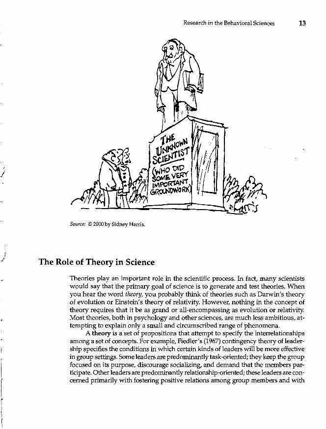
Source: © 2000 by Sidney Harris.

The Role of Theory in Science

Theories play an important role in the scientific process. In fact, many scientists would say that the primary goal of science is to generate and test theories. When you hear the word theory, you probably think of theories such as Darwin's theory of evolution or Einstein's theory of relativity. However, nothing in the concept of theory requires that it be as grand or all-encompassing as evolution or relativity. Most theories, both in psychology and other sciences, are much less ambitious, at­tempting to explain only a small and circumscribed range of phenomena.

A theory is a set of propositions that attempt to specify the interrelationships among a set of concepts. For example, Fiedler's (1967) contingency theory of leader­ship specifies the conditions in which certain kinds of leaders will be more effective in group settings. Some leaders are predominantly task-oriented; they keep the group focused on its purpose, discourage socializing, and demand that the members par­ticipate. Other leaders are predominantly relationship-oriented; these leaders are con­cerned primarily with fostering positive relations among group members and with

14 CHAPTER 1

group satisfaction. The contingency theory proposes three factors that determine whether a task-oriented or relationship-oriented leader will be more effective: the quality of the relationship between the leader and group members, the degree to which the group's task is structured, and the leader's power within the group. In fact, the theory specifies quite precisely the conditions under which certain leaders are more effective than others. The contingency theory of leadership fits our defini­tion of a theory because it attempts to specify the interrelationships among a set of concepts (the concepts of leadership effectiveness, task versus interpersonal leaders, leader-member relations, task structure, and leader power).

Occasionally, people use the word theory in everyday language to refer to hunches or unsubstantiated ideas. For example, in the debate on whether to teach creationism as an alternative to evolution in public schools, creationists dismiss evolution because it's "only a theory." This use of the term theory is very mislead­ing: Scientific theories are not wild guesses or unsupported hunches. On,the con­trary, theories are accepted as valid only to the extent that they are supp~rted by empirical findings. Science insists that theories be consistent with the facts as they are currently known. Theories that are not supported by data are usually replaced by other theories.

Theory construction is very much a creative exercise, and ideas for theories can come from virtually anywhere. Sometimes, researchers immerse themselves in the research literature and purposefully work toward developing a theory. In other instances, researchers construct theories to explain patterns they observe in data they have collected. Other theories have been developed on the basis of case stud­ies or everyday observation. At other times, a scientist may get a fully developed theoretical insight at a time when he or she is not even working on research. Re­searchers are not constrained in terms of where they get their theoretical ideas, and there is no single way to formulate a theory.

Closely related to theories are models. In fact, researchers occasionally use the terms theory and model interchangeably, but we can make a distinction between them. Whereas a theory specifies both how and why concepts are interrelated, a model describes only how they are related. Put differently, a theory has more ex­planatory power than a model, which is somewhat more descriptive. We may have a model that specifies that X causes Y and Y then causes Z, without a theory about why these effects occur.

Research Hypotheses

On the whole, scientists are a skeptical bunch, and they are not inclined to accept theories and models that have not been supported by empirical research. (Remem­ber the scientists and the sheep.) Thus, a great deal of their time is spent testing theories and models to determine their usefulness in explaining and predicting be­havior. Although theoretical ideas may come from anywhere, scientists are much more constrained in the procedures they use to test their theories.

. ~ r

I ..,

r

I I

Research in the Behavioral Sciences 15

The process of testing theories is an indirect one. Theories themselves are not tested directly. The propositions in a theory are usually too broad and complex to be tested directly in a particular study. Rather, when researchers set about to test a theory, they do so indirectly by testing one or more hypotheses that are derived from the theory.

A hypothesis is a specific proposition that logically follows from the theory. Deriving hypotheses from a theory involves deduction, a process of reasoning from a general proposition (the theory) to specific implications of that proposition (the hypotheses). Hypotheses, then, can be thought of as the logical implications of a theory. When deriving a hypothesis, the researcher asks, If the theory is true, what would we expect to observe? For example, one hypothesis that can be de­rived from the contingency model of leadership is that relationship-oriented lead­ers will be more effective when the group's task is moderately structured rather than unstructured. If we do an experiment to test the validity of this hypothesis, we are testing part, but only part, of the contingency theory of leadership.

You can think of hypotheses as if-then statements of the general form, If a, then b. Based on the theory, the researcher hypothesizes that if certain conditions occur, then certain consequences should follow. Although not all hypotheses are actually expressed in this manner, virtually all hypotheses are reducible to an if­then statement.

Not all hypotheses are derived deductively from theory. Often, scientists ar­rive at hypotheses through induction-abstracting a hypothesis from a collection of facts. Hypotheses that are based solely on previous observed patterns of results are sometimes called empirical generalizations. Having seen that certain variables repeatedly relate to certain other variables in a particular way, we can hypothesize that such patterns will occur in the future. In the case of an empirical generalization, we often have no theory to explain_.why the variables are related but nonetheless can make predictions about them.

Whether derived deductively from theory or inductively from observed facts, hypotheses must be formulated precisely in order to be testable. Specifically, hypotheses must be stated in such a way that leaves them open to falsifiability. A hypothesis is of little use unless it has the potential to be found false (Popper, 1959). In fact, some philosophers of science have suggested that empirical falsification is the hallmark of science-the characteristic that distinguishes it from other ways of seeking knowledge, such as philosophical argument, personal experience, casual observation, or religious insight. In fact, one loose definition of science is that sci­ence is "knowledge about the universe on the basis of explanatory principles sub­ject to the possibility of empirical falsification" (Ayala & Black, 1993).

One criticism of Freud's psychoanalytic theory, for example, is that researchers have found it difficult to generate hypotheses that can be falsified by research. Al­though psychoanalytic theory can explain virtually any behavior after it has oc­curred, researchers have found it difficult to derive specific falsifiable hypotheses from the theory that predict how people will behave under certain circumstances. For example, Freud's theory relies heavily on the concept of repression-the idea

16 CHAPTER 1

that people push anxiety-producing thoughts into their unconscious-but such a claim. is exceptionally difficult to falsify. According to the theory itself, anything that people can report to a researcher is obviously not unconscious, and anything that is unconscious cannot be reported. So how can the hypothesis that people repress un­desirable thoughts and urges ever be falsified? Because parts of the theory do not easily generate falsifiable hypotheses, most behavioral scientists regard aspects of psychoanalytic theory as inherently nonscientific.

A Priori Predictions and Post Hoc Explanations

People can usually find reasons for almost anything after it happens. In fact, we sometimes find it equally easy to explain completely opposite occurrences. Con­sider Jim and Marie, a married couple I know. If I hear in 5 years that Jim and Marie are happily married, I'll be able to look back and find clear-cut reasons why their relationship worked out so well. If, on the other hand, I learn in 5 years that they're getting divorced, I'll undoubtedly be able to recall indications that all was not well even from the beginning. As the saying goes, hindsight is 20/20. Nearly everything makes sense after it happens.

The ease with which we can retrospectively explain even opposite occur­rences leads scientists to be skeptical of post hoc explanations-explanations that are made after the fact. In light of this, a theory's ability to explain occurrences in a post hoc fashion provides little evidence of its accuracy or usefulness. More telling is the degree to which a theory can successfully predict what will happen. Theories that accurately predict what will happen in a research study are regarded more positively than those that can only explain the findings afterwards.

This is one reason that researchers seldom conduct studies just "to see what happens." If they have no preconceptions about what should happen in their study, they can easily explain whatever pattern of results they obtain in a post hoc fashion. To provide a more convincing test of a theory, researchers usually make a priori predictions, or specific research hypotheses, before collecting the data. By making specific predictions about what will occur in a study, researchers avoid the pitfalls associated with purely post hoc explanations.

Conceptual and Operational Definitions

I noted above that scientific hypotheses must be potentially falsifiable by empirical data. For a hypothesis to be falsifiable, the terms used in the hypothesis must be clearly defined. In everyday language, we usually don't worry about how precisely we define the terms we use. If I tell you that the baby is hungry, you understand what I mean without my specifying the criteria I'm using to conclude that the baby is, indeed, hungry. You are unlikely to ask detailed questions about what I mean ex­actly by baby or hunger; you understand well enough for practical purposes.

Research in the Behavioral Sciences 17

More precision is required of the definitions we use in research, however. If the terms used in research are not defined precisely, we may be unable to deter­mine whether the hypothesis is supported. Suppose that we are interested in studying the effects of hunger on attention in infants. Our hypothesis is that ba­bies' ability to pay attention decreases as they become more hungry. We can study this topic only if we define clearly what we mean by hunger and attention. Without clear definitions, we won't know whether the hypothesis has been supported.

Researchers use two distinct kinds of definitions in their work. On one hand, they use conceptual definitions. A conceptual definition is more or less like the de­finition we might find in a dictionary. For example, we might define hunger as hav­ing a desire for food. Although conceptual definitions are necessary, they are seldom specific enough for research purposes.

A second way of defining a concept is by an operational definition. An oper­ational definition defines a concept by specifying precisely how the concept is mea­sured or manipulated in a particular study. For example, we could operationally define hunger in our study as being deprived of food for 12 hours. An operational defi­nition converts an abstract conceptual definition into concrete, situation-specific terms.

There are potentially many operational definitions of a single construct. For example, we could operationally define hunger in terms of hours of food depriva­tion. Or we could define hunger in terms of responses to the question: How hun­gry are you at this moment? Consider a scale composed of the follOWing responses: (1) not at all, (2) slightly, (3) moderately, and (4) very. We could classify people as hun­gry if they chose to answer moderately or very on this scale.

A recent study of the incidence of hunger in the United States defined hungry people as those who were eligible for food stamps but who didn't get them. This particular operational definition is a poor one, however. Many people with low in­come living in a farming area would be classified as hungry, no matter how much food they raised on their own.

Operational definitions are essential so that researchers can replicate one an­other's studies. Without knowing precisely how hunger was induced or measured in a particular study, other researchers have no way of replicating the study in pre­cisely the same manner that it was conducted originally. In addition, using opera­tional definitions forces researchers to clarify their concepts precisely (Underwood, 1957), thereby allowing scientists to communicate clearly and unambiguously.

Occasionally, you will hear people criticize the use of operational definitions. In most cases, they are not criticizing operational definitions per se but rather a perspective known as operationism. Proponents of operationism argue that oper­ational definitions are the only legitimate definitions in science. According to this view, concepts can be defined only in terms of specific measures and operations. Conceptual definitions, they argue, are far too vague to serve the needs of a precise science. Most contemporary behavioral scientists reject the assumptions of strict operationism. Conceptual definitions do have their uses, even though they are ad­mittedly vague.

L

20 CHAPTER 1

hypotheses derived from both theories. Yet, for the reasons we discussed above, this support did not prove either theory.

The Practical Impossibility of Disproof

Unlike proof, disproof is a logically valid operation. If I deduce Hypothesis H from Theory A, then find that Hypothesis H is not supported by the data, Theory A must be false by logical inference. Imagine again that we hypothesize that, if Jake is the murderer, then Jake must have been at the party. If our research subsequently shows that Jake was not at the party, our theory that Jake is the murderer is logi­cally disconfirmed.

However, testing hypotheses in real-world research involves a number of practical difficulties that may lead a hypothesis to be disconfirmed even when the theory is true. Failure to find empirical support for a hypothesis can be due to a number of factors other than the fact that the theory is incorrect. For example, using poor measuring techniques may result in apparent disconfirmation of a hy­pothesis, even though the theory is actually valid. (Maybe Jake slipped into the party, undetected, for only long enough to commit the murder.) Similarly, obtain­ing an inappropriate or biased sample of participants, failing to account for or con­trol extraneous variables, and using improper research designs or statistical analyses can produce negative findings. Much of this book focuses on ways to eliminate problems that hamper researchers' ability to produce strong, convincing evidence that would allow them to disconfirm hypotheses.

Because there are many ways in which a research study can go wrong, the failure of a study to support a particular hypothesis seldom, if ever, means the death of a theory (Hempel, 1966). With so many possible reasons why a particular study might have failed to support a theory, researchers typically do not abandon a theory after only a few disconfirmations (particularly if it is their theory). This is the reason that scientific journals are reluctant to publish the results of studies that fail to support a theory (see box on "Publishing Null Findings" on p. 22). The fail­ure to confirm one's research hypotheses can occur for many reasons other than the invalidity of the theory.

If Not Proof or Disproof, Then What?

If proof is logically impossible and disproof is pragmatically impossible, how does science advance? How do we ever decide which theories are good ones and which are not? This question has provoked considerable interest among philosophers and scientists alike (Feyerabend, 1965; Kuhn, 1962; Popper, 1959).

In practice, the merit of theories is judged, not on the basis of a single research study, but on the accumulated evidence of several studies. Although any particu­lar piece of research that fails to support a theory may be disregarded, the failure to obtain support in many studies provides evidence that the theory has problems. Similarly, a theory whose hypotheses are repeatedly corroborated by research is considered supported by the data.

I

I i

Research in the Behavioral Sciences 21

Importantly, the degree of support for a theory or hypothesis depends not only on the number of times it has been supported but on the stringency of the tests it has survived. Some studies provide more convincing support for a theory than other studies do (Ayala & Black, 1993; Stanovich, 1996). Not surprisingly, seasoned re­searchers try to design studies that will provide the strongest, most stringent tests of their hypotheses. The findings of tightly conceptualized and well-designed studies are simply more convincing than the findings of poorly conceptualized and weakly designed ones. In addition, the greater the variety of the methods and measures that are used to test a theory in various experiments, the more confidence we can have in their accumulated findings. Thus, researchers often aim for methodological pluralism-using many different methods and designs-as they test theories.

Some of the most compelling evidence in science is obtained from studies that directly pit the predictions of one theory against the predictions of another theory. Rather than simply testing whether the predictions of a particular theory are supported, researchers often design studies to test simultaneously the oppos­ing predictions of two theories. Such studies are designed so that, depending on how the results turn out, the data will confirm one of the theories while discon­firming the other. This head-to-head approach to research is sometimes called the strategy of strong inference because the findings of such studies allow researchers to draw stronger conclusions about the relative merits of competing theories than do studies that test a single theory (Platt, 1964).

An example of the strategy of strong inference comes from recent research on self-evaluation. For many years, researchers have disagreed regarding the pri­mary motive that affects people's perceptions and evaluations of themselves: self­enhancement (the motive to evaluate oneself favorably), self-assessment (the motive to see oneself accurately), and self-verification (the motive to maintain one's existing self-image). And, over the years, a certain amount of empirical support has been obtained for each of these motives and for the theories on which they are based. Sedikides (1993) conducted six experiments that placed each of these theo­ries in direct opposition with one another. In these studies, participants indicated the kinds of questions they would ask themselves if they wanted to know whether they possessed a particular characteristic (such as whether they were open-minded, greedy, or selfish). Participants could choose questions that varied according to the degree to which the question would lead to information about themselves that was (1) favorable (reflecting a self-enhancement motive), (2) accurate (reflecting a desire for accurate self-assessment), or (3) consistent with their current self-views (reflect­ing a motive for self-verification). Results of the six studies provided overwhelming support for the precedence of the self-enhancement motive. When given the choice, people tend to ask themselves questions that allow them to evaluate themselves positively rather than choosing questions that either support how they already per­ceive themselves or lead to accurate self-knowledge. By using the strategy of strong inference, Sedikides was able to provide a stronger test of these three theories than would have been obtained from research that focused on anyone of them alone.

Throughout this process of scientific investigation, theory and research interact to advance science. Research is conducted explicitly to test theoretical propositions,

22 CHAPTER 1

then the findings obtained in that research are used to further develop, elaborate, qualify, or fine-tune the theory. Then more research is conducted to test hypotheses derived from the refined theory, and the theory is further modified on the basis of new data. This process typically continues until researchers tire of the theory (usu­ally because most of the interesting and important issues seem to have been ad­dressed) or until a new theory, with the potential to explain the phenomenon more fully, gains support.

Science advances most rapidly when researchers work on the fringes of what is already known about a phenomenon. Not much is likely to come of devoting oneself to continuous research on topics that are already reasonably well under­stood. As a result, researchers tend to gravitate toward areas in which we have more questions than answers. As Homer and Gorman (1988), the paleontologists who firs! discovered evidence that some dinosaurs cared for their young, ob­served,tIn some ways, scientific research is like taking a tangled ball of twine and trying to unravel it. You look for loose ends. When you find one, you tug on it to see if it leads to the heart of the tangle"(p. 34) . ..J

This is one reason that researchers often talk more about what they don't know rather than what is already known (Stanovich, 1996). Because they live in a world of "tangles" and "loose ends," scientists sometimes seem uncertain and in­decisive, if not downright incompetent, to the lay public. However, as McCall (1988) noted, we must realize that,

by definition, professionals on the edge of knowledge do not know what causes what. Scientists, however, are privileged to be able to say so, whereas business ex­ecutives, politicians, and judges, for example, sometimes make decisions in auda­cious ignorance while appearing certain and confident. (p. 88)

_!!II 'e IN DEPTH

Publishing Null Findings Students often are surprised to learn that scientific journals are reluctant, if not completely unwilling, to publish studies that fail to obtain effects. You might think that results showing certain variables are not related to behavior-so-called null findings-would provide im­portant information. After all, if we predict that certain psychological variables are related, but our data show that they are not, haven't we learned something important?

The answer is no, for as we have seen, data may fail to support our research hypothe­ses for reasons that have nothing to do with the validity of a particular hypothesis. As a re­sult, null findings are usually uninformative regarding the hypothesis being tested. Was the hypothesis disconfirmed, or did we simply design a lousy study? Because we can never know for certain, journals generally will not publish studies that fail to obtain effects.

One drawback of this policy, however, is that researchers may design studies to test a theory, unaware of the fact that the theory has already been disconfirmed in dozens of ear­lier studies. However, because of the difficulties in interpreting null findings (and journals' reluctance to publish them), none of those previous studies were published. ~y scientists

_have expressed the need for the dissemination of information about unsuccessful studi~

;

I

, /

Research in the Behavioral Sciences· 23

Strategies of Behavioral Research

Roughly speaking, behavioral research can be classified into four broad categories: descriptive, correlational, experimental, and quasi-experimental. Although we will return to each of these research strategies in later chapters, it will be helpful for you to understand the differences among them from the beginning.

Descriptive Research

Descriptive research describes the behavior, thoughts, or feelings of a particular group of individuals. Perhaps the most common example of purely descriptive re­search is public opinion polls, which describe the attitudes of a particular group of people. Similarly, in developmental psychology, the purpose of some studies is to describe the typical behavior of children of a certain age. Along the same lines, nat­uralistic observation describes the behavior of nonhuman animals in their natural habitats. In descriptive research, researchers make little effort to relate the behav­ior under study to other variables or to examine or explain its causes systemati­cally. Rather, the purpose is, as the term indicates, to describe.

Some research in clinical psychology, for example, is conducted to describe the prevalence, severity, or symptoms of certain psychological problems. In a descrip­tive study of the incidence of emotional and behavioral problems among high school students (Lewinsohn, Hops, Roberts, Seeley, & Andrews, 1993), researchers obtained a representative sample of students from high schools in Oregon. Through personal interviews and the administration of standard measures of psycho­pathology, the researchers found that nearly 10% of the students had a recognized psychiatric disorder at the time of the study, most commonly depression. Further­more, 33% of the respondents had experienced a disorder at some time in their lives. Female respondents were more likely than male respondents to experience unipolar depression, anxiety disorders, and eating disorders, whereas males had higher rates of problems related to disruptive behavior.

Descriptive research, which we will cover in greater detail in Chapter 5, provides the foundation on which all other research rests. However, it is only the beginning.

Correlational Research

If behavioral researchers only described how human and nonhuman animals think, feel, and behave, they would provide us with little insight into the complexities of psychological processes. Thus, most research goes beyond mere description to an ex­amination of the correlates or causes of behavior. Correlational research investigates the relationships among various psychological variables. Is there a relationship be­tween self-esteem and shyness? Does parental neglect in infancy relate to particular problems in adolescence? Do certain personality characteristics predispose people to abuse drugs? Is the ability to cope with stress related to physical health? Each of these questions asks whether there is a relationship-a correlation-between two variables.

Health psychologists have known for many years that people who are Type A-highly achievement-oriented and hard-driving-have an exceptionally high

24 CHAPTER 1

risk of heart disease. More recently, research has suggested that Type A people are most likely to develop coronary heart disease if they have a tendency to become hostile when their goals are blocked. In a correlational study designed to explore this issue, Kneip et al. (1993) asked the spouses of 185 cardiac patients to rate these patients on their tendency to become hostile and angry. They also conducted scans of the patients' hearts to measure the extent of their heart disease. The data showed not only that spouses' ratings of the patients' hostility correlated with heart disease, but that hostility predicted heart disease above and beyond tradi­tional risk factors such as age, whether the patient smoked, and high blood pres­sure. Thus, the data supported the hypothesis that hostility is correlated with coronary heart disease.

Correlational studies provide valuable information regarding the relation­ships between variables. However, although correlational research can establish that certain variables are related to one another, it cannot tell us whether one vari­able actually causes the other. We'll return to a full discussion of correlational re­search strategies in C~apters 6 and 7.

(

Experimental Research

When researchers are interested in determining whether certain variables cause changes in behavior, thought, or emotion, they turn to experimental research. In an experiment, the researcher manipulates or changes one variable (called the in­dependent variable) to see whether changes in behavior (the dependent variable) occur as a consequence. If behavioral changes do occur when the independent variable is manipulated, we can conclude that the independent variable caused changes in the dependent variable (assuming certain conditions are met).

For example, Terkel and Rosenblatt (1968) were interested in whether mater­nal behavior in rats is caused by hormones in the bloodstream. They injected virgin female rats with either blood plasma from rats who had just given birth or blood plasma from rats who were not mothers. They found that the rats who were injected with the blood of mother rats showed more maternal behavior toward rat pups than those who were injected with the blood of nonmothers, suggesting that the presence of hormones in the blood of mother rats is partly responsible for maternal behavior. In this study, the nature of the injection (blood from mothers versus blood from non­mothers) was the independent variable, and maternal behavior was the dependent variable. We'll spend four chapters (Chapters 8-11) on the design and analysis of ex­periments such as this one.

Note that the term experiment applies to only one kind of research-a study in which the researcher controls an independent variable to assess its effects on behav­ior. Thus, it is incorrect to use the word experiment as a synonym for research or study.

Quasi-Experimental Research

When behavioral researchers are interested in understanding cause-and-effect re­lationships, they prefer to use experimental designs. However, as noted above, ex-

r

/

Research in the Behavioral Sciences 25

perimental research requires that the researcher vary an independent variable to assess its effects on the dependent variable. In many cases, researchers are not able to vary the independent variable. When this is the case, researchers sometimes use quasi-experimental research. In a quasi-experimental design, such as those we'll study in Chapter 12, the researcher studies the effects of some variable or event that occurs naturally.

Many parents and teachers worry that students' schoolwork will suffer if stu­dents work at a job each day after school. Indeed, previous research has shown that part-time employment in adolescence is associated with a number of problems, in­cluding lower academic achievement. What is unclear, however, is whether em­ployment causes these problems, or whether students who choose to have an after-school job tend to be those who are already doing poorly in school. Re­searchers would find it difficult to conduct a true experiment on this question be­cause they would have to manipulate the independent variable of employment by randomly requiring certain students to work after school while prohibiting other students from having a job.

Because a true experiment was not feasIble, Steinberg, Fegley, and Dorn­busch (1993) conducted a quasi-experiment. They tested high school students dur­ing the 1987-88 school year and the same students again in 1988-89. They then compared those students who had started working during that time to those who did not take a job. As they expected, even before starting to work, students who later became employed earned lower grades and had lower academic expectations than those who later did not work. Even so, the researchers found clear effects of working above and beyond these preexisting differences. Compared to students who did not work, those who took a job subsequently spent less time on home­work, cut class more frequently, and had lower academic expectations. Although quasi-experiments do not allow the same degree of confidence in interpretation as do true experiments, the data from this study appear to show that after-school em­ployment can have deleterious effects on high school students.

Each of these basic research strategies-descriptive, correlational, experi­mental, and quasi-experimental-has its uses. One task of behavioral researchers is to select the strategy that will best address their research questions given the lim­itations imposed by practical concerns (such as time, money, and control over the situation) as well as ethical issues (the manipulation of certain independent vari­ables would be ethically indefensible). By the time you reach the end of this book, you will have the background to make informed decisions regarding how to choose the best strategy for a particular research question.

Domains of Behavioral Science

The breadth of behavioral science is staggering, ranging from researchers who study microscopic biochemical processes in the brain to those who investigate the broad influence of culture. What all behavioral scientists have in common, how­ever, is an interest in behavior, thought, and emotion.

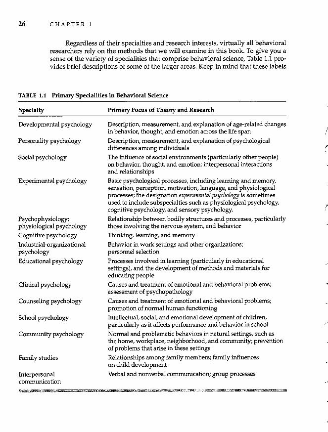
26 CHAPTER 1

Regardless of their specialties and research interests, virtually all behavioral researchers rely on the methods that we will examine in this book. To give you a sense of the variety of specialities that comprise behavioral science, Table 1.1 pro­vides brief descriptions of some of the larger areas. Keep in mind that these labels

TABLE 1.1 Primary Specialities in Behavioral Science

Specialty

Developmental psychology

Personality psychology

Social psychology

Experimental psychology

Psychophysiology; physiological psychology

Cognitive psychology

Industrial-organizational psychology

Educational psychology

Clinical psychology

Counseling psychology

School psychology

Community psychology

Family studies

Interpersonal communication

Primary Focus of Theory and Research

Description, measurement, and explanation of age-related changes in behavior, thought, and emotion across the life span

Description, measurement, and explanation of psychological differences among individuals

The influence of social environments (particularly other people) on behavior, thought, and emotion; interpersonal interactions and relationships Basic psychological processes, including learning and memory, sensation, perception, motivation, language, and physiological processes; the designation experimental psychology is sometimes used to include subspecialties such as physiological psychology, cognitive psychology, and sensory psychology.

Relationship between bodily structures and processes, particularly thos~ involving the nervous system, and behavior

1hinking, learning, and memory

Behavior in work settings and other organizations; personnel selection

Processes involved in learning (particularly in educational settings), and the development of methods and materials for educating people Causes and treatment of emotional and behavioral problems; assessment of psychopathology

Causes and treatment of emotional and behavioral problems; promotion of normal human functioning

Intellectual, social, and emotional development of children, particularly as it affects performance and behavior in school

Normal and problematic behaviors in natural settings, such as the home, workplace, neighborhood, and community; prevention of problems that arise in these settings

Relationships among family members; family influences on child development

Verbal and nonverbal communication; group processes

-

/ ,

!

; J

{

I

r f

Research in the Behavioral Sciences 27

often tell us more about particular researchers' academic degrees or the depart­ment in which they work than about their research interests. Researchers in differ­ent domains often have very similar research interests whereas those within a domain may have quite different interests.

A Preview

The research process is a complex one. In every study researchers must address many questions:

• HQw should I measure participants' thoughts, feelings, or behavior in this study?

• How do I obtain a sample of participants for my research? • Given my research question, what is the most appropriate research strategy? • How can I be sure my study is as well designed as possible? • What are the most appropriate and useful ways of analyzing the data? • How should my findings be reported? • What are the ethical issues involved in conducting this research?

Each chapter in this book deals with an aspect of the research process. Now that you have an overview of the research process, Chapter 2 sets the stage for the remainder of the book by discussing what is perhaps the central concept in re­search design and analysis-variability. Armed with an understanding of behav­ioral variability, you will be better equipped to understand many of the issues we'll address in later chapters. Chapters 3 and 4 deal with how researchers measure be­havior and psychological processes. Chapter 3 focuses on basic issues involved in psychological measurement, and Chapter 4 examines specific types of measures used in behavioral research.

After covering basic topics that are relevant to all research in Chapters 1 through 4, we turn to specific research strategies. Chapter 5 deals with descriptive re­search, including how researchers select samples of participants. In Chapters 6 and 7, you will learn about correlational research strategies-not only correlation per se, but also regression, partial correlation, factor analysis, and other procedures that are used to investigate how naturally occurring variables are related to one another.

Chapters 8 and 9 will introduce you to experimental design; Chapters 10 and 11 will then go into greater detail regarding the design and analysis of experi­ments. In these chapters, you'llieam not only how to design experiments, but also how to analyze experimental data.

Chapter 12 deals with quasi-experimental designs, and Chapter 13 with single­case designs. The complex ethical issues involved in conducting behavioral re­search are discussed in Chapter 14. Finally, in Chapter 15 we'll take a look at how research findings are disseminated and discuss how to write research reports.

At the end of the book are two appendixes containing statistical tables and formulas, along with a glossary and a list of references.

28 CHAPTER 1

Summary

1. Psychology is both a profession that promotes human welfare through coun­seling, education, and other activities, as well as a scientific discipline that is devoted to the study of behavior and mental processes.

¥.- 2. Interest in human behavior can be traced to ancient times, but the study of be­havior became scientific only in the late 1800s, stimulated in part by the labo­ratories established by Wundt in Germany and by James in the United States.

3. Behavioral scientists work in many disciplines, including psychology, educa­tion, social work, family studies, communication, management, health and exercise science, marketing, psychiatry, neurology, and nursing.

4. Behavioral scientists conduct research to describe, explain, and predict be­havior, as well as to solve applied problems.

5. To be considered scientific, observations must be systematic and empirical, research must be conducted in a manner that is publicly verifiable, and the questions addressed must be potentially solvable given current knowledge.

6. Pseudoscience involves evidence that masquerades as science but that fails to meet one or more of the three criteria used to define scientific.

7. Although the findings of behavioral researchers often coincide with com­mon sense, many commonly held beliefs have been disconfirmed by behav­ioral science.

8. Research is not designed to find the truth as much as it is designed to test hy­potheses and models about behavior.

9. Much research is designed to test the validity of theories. A theory is a set of propositions that attempts to specify the interrelationships among a set of concepts.

10. Researchers assess the usefulness of a theory by testing hypotheses-the propositions that are deduced logically from a theory. To be tested, hypothe­ses must be stated in a manner that is potentially falsifiable.

11. By stating their hypotheses a priori, researchers avoid the risks associated with post hoc explanations.

12. Researchers use two distinct kinds of definitions in their work. Conceptual de­finitions are much like dictionary definitions. Operational definitions, on the other hand, define concepts by specifying precisely how they are measured or manipulated in the context of a particular study. Operational definitions are essential for replication, as well as for nonambiguous communication among scientists.

13. Strictly speaking, theories can never be proved or disproved by research. Proof is logically impossible because it is invalid to prove the antecedent of an argument by showing that the consequent is true. Disproof, though logically possible, is impossible in a practical sense; failure to obtain support for a theory may reflect more about the research procedure than about the accuracy of the hypothesis. Because of this, the failure to obtain hypothesized findings (null findings) are often uninformative regarding the validity of a hypothesis.

14. Behavioral research falls into roughly four categories: descriptive, correla­tional, experimental, and quasi-experimental.

/

--

f j

I J

IS'

Research in the Behavioral Sciences 29

KEY TERMS

applied research (p. 5) experimental research (p. 24) falsifiability (p. 15) hypothesis (p. 15)

operationism (p. 17) a priori prediction (p. 16) basic research (p. 4) conceptual definition (p. 17) correlational research (p. 23) deduction (p. 15)

induction (p. 15) methodological pluralism

(p.21) model (p. 14)

post hoc explanation (p. 16) pseudoscience (p. 9) public verification (p. 8) quasi-experimental research

(p.25) descriptive research (p. 23) empirical generalization (p. 15) empiricism (p. 8)

null finding (p. 22) operational definition (p. 17)

strategy of strong inference (p.21)

theory (p. 13) evaluation research (p. 5)

QUESTIONS FOR REVIEW

1. In what sense is psychology both a science and a profession?

2. Describe the development of psychology as a science.

3.

4.

5.

6.

7.

8.

9.

10.

11.

12.

13.

14.

15.

16.

What was WIlhelm Wundt's primary contribution to behavioral research?

Name at least ten academic disciplines in which behavioral scientists do research.

What are the four basic goals of behavioral research?

Distinguish between basic and applied research. In what ways are basic and ap­plied research interdependent?

In what ways is the study of research methods valuable to students such as you?

Discuss the importance of systematic empiricism, public verification, and solvabil­ity to the scientific method.

In what ways does pseudoscience differ from true science?

Is it true that most of the findings of behavioral research are just common sense?

Why is the philosophy of science important to behavioral researchers?

Distinguish between theory, model, and hypothesis.

Describe how researchers use induction versus deduction to generate research hypotheses.

Describe the process by which hypotheses are developed and tested.

Why must hypotheses be falsifiable?

One theory suggests that people feel socially anxious or shy in social situations when two conditions are met: (a) they are highly motivated to make a favorable im-pression on others who are present, but (b) they doubt that they will be able to do so. Suggest at least three research hypotheses that can be derived from this theory. Be sure your hypotheses are falsifiable.

17. Why are scientists skeptical of post hoc explanations?

18. Why are operational definitions important in research?

30 CHAPTER 1

19. Suggest three operational definitions for each of the following constructs: a. aggression b. patience c. test anxiety d. memory e. smiling

20. What are some ways in which scientists get ideas for their research?

21. Why can theories not be proved or disproved by research?

22. Given that proof and disproof are impossible in science, how does scientific knowl­edge advance?

23. Why are journals reluctant to publish null findings?

24. Distinguish among descriptive, correlational, experimental, and quasi-experimental research.

25. Distinguish between an independent and dependent variable.

26. Tell what researchers study in each of the following fields: a. developmental psychology b. experimental psychology c. industrial-organizational psychology d. social psychology e. cognitive psychology f. personality psychology g. family studies h. interpersonal communication i. psychophysiology j. school psychology

k. counseling psychology 1. community psychology

m. clinical psychology n. educational psychology

QUESTIONS FOR DISCUSSION

1. Why do you think behavioral sciences such as psychology developed later than other sciences such as chemistry, physics, astronomy, and biology?

2. Why do you think many people have difficulty seeing psychologists and other be­havioral researchers as scientists?

3. How would today's world be different if the behavioral sciences had not developed?

4. Develop your own idea for research. If you have trouble thinking of a research idea, use one of the tactics described in the box, "Getting Ideas for Research." Choose your idea carefully as if you were actually going to devote a great deal of time and effort to carrying out the research.

j

Research in the Behavioral Sciences 31

5. After researchers formulate an idea, they must evaluate its quality to decide whether the idea is really worth pursuing. Evaluate the research idea you devel­oped in Question 4 using the following four criteria. If your idea fails to meet one or more of these criteria, think of another idea. • Does the idea have the potential to advance our understanding of behavior?

Assuming that the study is conducted and the expected patterns of results are ob­tained, will we have learned something new about behavior?

• Is the knowledge that may be gained potentially important? Importance is, of course, in the eye of the beholder. A study can be important in several ways: (a) It tests hypotheses derived from a theory (thereby providing evidence for or against the theory); (b) it identifies a qualification to a previously demonstrated finding; (c) it demonstrates a weakness in a previously used research method or technique; (d) it documents the effectiveness of procedures for modifying a be­havioral problem (such as in counseling, education, or industry, for example); (e) it demonstrates the existence of a phenomenon or effect that had not been pre­viously recognized. Rarely does a single study provide earthshaking information that revolutionizes the field, so don't expect too much. Ask yourself whether this idea is likely to provide information that other behavioral researchers or practi­tioners (such as practicing psychologists) would find interesting or useful.

• Do I find the idea interesting? No matter how important an idea might be, it is difficult to do research that one finds boring. This doesn't mean that you have to be fascinated by the topic, but if you really don't care about the area and aren't in­terested in the answer to the research question, consider getting a different topic.

• Is the idea researchable? Many research ideas are not viable because they are ethically questionable or because they require resources that the researcher can­not possibly obtain.

6. We noted that research falls into four basic categories, depending on whether the goal is to describe patterns of behavior, thought, or emotion (descriptive research); to examine the relationship among naturally occurring variables (correlational re­search); to test cause-and-effect relationships by experimentally manipulating an independent variable to examine its effects on a dependent variable (experimental research); or to examine the possible effects of an event that cannot be controlled by the researcher (quasi-experimental research). For each of the following research questions, indicate which kind of research-descriptive, correlational, experimen­tal, or quasi-experimental-would be most appropriate. a. What percentage of college students attend church regularly? b. Does the artificial sweetener aspartame cause dizziness and confusion in some

people? c. What personality variables are related to depression? d. What is the effect of a manager's style on employees' morale and performance? e. Do SAT scores predict college performance? f. Do state laws that mandate drivers to wear seat belts reduce traffic fatalities? g. Does Prozac (a popular antidepression medication) help insomnia? h. Does getting married make people happier? i. Do most U.S. citizens support stronger gun control laws?

7. Go to the library and locate several journals in psychology or other behavioral sciences. A few journals that you might look for include the Journal of Experimental

32 CHAPTE R 1

Psychology, Journal of Personality and Social Psychology, Developmental Psychology, Journal of Abnormal Psychology, Health Psychology, Journal of Applied Psychology, Jour­nal of Clinical and Consulting Psychology, Journal of Counseling Psychology, and Journal of Educational Psychology. Look through the table of contents in several of these jour­nals to see the diversity of the research that is currently being published. If an arti­cle title looks interesting, read the abstract (the article summary) that appears at the beginning of the article.

8. Read one entire article. You will undoubtedly find parts of the article difficult (if not impossible) to understand, but do your best to understand as much as you can. As you stumble on the methodological and statistical details of the study, tell yourself that, by the time you are finished with this book, you will understand the vast ma­jority of what you read in an article such as this. (You might even want to copy the article so that you can underline the methodological and statistical items that you do not understand. Then, after finishing this book, read the article again to see how much you have learned.)

r I

J

J

)

CHAPTER

2 Behavioral Variability and Research

Variability and the Research Process

Variance: An Index of Variability

Systematic and Error Variance

Assessing the Strength of Relationships

Meta-Analysis: Systematic Variance Across Studies

Rychologists use the word schema to refer to a cognitive generalization that orga­nizes and guides the processing of information. You have schemas about many cat­egories of events, people, and other stimuli that you have encountered in life. For example, you probably have a schema for the concept leadership. Through your ex­periences with leaders of various sorts, you have developed a generalization of what a good leader is. Similarly, you probably have a schema for big cities. What do you think of when I say, "New York, Los Angeles, and Atlanta?" Some people's schemas of large cities include generalizations such as "crowded and dangerous," whereas other people's schemas include attributes such as "interesting and excit­ing." We all have schemas about many categories of stimuli.

Researchers have found that people's reactions to particular stimuli and events are strongly affected by the schemas they possess. For example, if you were a business executive, your decisions about who to promote to a managerial posi­tion would be affected by your schema for leadership. You would promote a very different kind of employee to manager if your schema for leadership included at­tributes such as caring, involved, and people-oriented than if you saw effective leaders as autocratic, critical, and aloof. Similarly, your schema for large cities would affect your reaction to receiving a job offer in Miami or Dallas.

Importantly, when people have a schema, they more easily process and orga­nize information relevant to that schema. Schemas provide us with frameworks for organizing, remembering, and acting on the information we receive. It would be difficult for executives to decide who to promote to manager if they didn't have schemas for leadership, for example. Even though schemas sometimes lead us to wrong conclusions when they are not rooted in reality (as when our stereotypes about a particular group bias our perceptions of a particular member of that group),

33

34 CHAPTER 2

they are essential for effective information processing. If we could not rely on the generalizations of our schemas, we would have to painstakingly consider every new piece of information when processing information and making decisions.

By now you are probably wondering how schemas relate to research methods. Having taught courses in research methods and statistics for several years, I have come to the conclusion that, for most students, the biggest stumbling block to un­derstanding behavioral research is their failure to develop a schema for the mater­ial. Many students have little difficulty mastering specific concepts and procedures, yet they complete their first course in research methods without seeing the big pic­ture. They learn many concepts, facts, principles, designs, and analyses, but they do not develop an overarching framework for integrating and organizing all of the in­formation they learn. Their lack of a schema impedes their ability to organize, pro­cess, remember, and use information about research methods. In contrast, seasoned researchers have a well-articulated schema for the research process that facilitates their research activities and helps them to make methodological decisions.

The purpose of this chapter is to provide you with a schema for thinking about the research process. By giving you a framework for thinking about research, I hope that you will find the rest of the book easier to comprehend and remember. In essence, this chapter will give you pegs on which to hang what you learn about behavioral research. Rather than dumping all of the new information you learn in a big heap on the floor, we'll put schematic hooks on the wall for you to use in or­ganizing the incoming information.

The essence of this schema is that, at the most basic level, all behavioral re­search attempts to answer questions about behavioral variability-that is, how and why behavior varies across situations, differs among individuals, and changes over time. The concept of variability underlies many of the topics we will discuss in later chapters and provides the foundation on which much of this book rests. The better you understand this basic concept now, the more easily you will grasp many of the topics we will discuss later in the book.

Variability and the Research Process

All aspects of the research process revolve around the concept of variability. The concept of variability runs through the entire enterprise of designing and analyz­ing research. To show what I mean, let me offer five propositions that involve the relationship between variability and behavioral research.

Proposition 1. Psychology and other behavioral sciences involve the study of behav­ioral variability. Psychology is often defined as the study of behavior and mental processes. Specifically, what psychologists and other behavioral researchers study is behavioral variability; they want to know how and why behavior varies across situations, among people, and over time. Put differently, understanding behavior and mental processes really means understanding what makes behavior and men­tal processes vary.

t !

)

I

Behavioral Variability and Research 35

Think about the people you interact with each day and about the variation you see in their behavior. First, their behavior varies across situations. People feel and act differently on sunny days than when it is cloudy and differently in dark settings than when it is light. College students are often more nervous when interacting with a person of the other sex than when interacting with a person of their own sex. Children behave more aggressively after watching violent TV shows than they did before watching them. A hungry pigeon who has been reinforced for pecking when a green light is on pecks more in the presence of a green light than a red light. In brief, people and other animals behave differently in different situations. Behav­ioral researchers are interested in how and why situational factors cause this vari­ability in behavior, thought, and emotion.

Second, behavior varies among individuals. Even in similar situations, not every­one acts the same. At a party, some people are talkative and outgoing whereas others are quiet and shy. Some people are more conscientious and responsible than others. Some individuals generally appear confident and calm whereas others seem nervous. And certain animals, such as dogs, display marked differences in behavior depending on their breed. Thus, because of differences in their biological makeup and previous experience, different people and different animals behave differently. A great deal of behavioral research focuses on understanding this variability across individuals.

Third, behavior also varies over time. A baby who could barely walk a few months ago can run today. An adolescent girl who two years ago thought boys were If gross" now has romantic fantasies about them. A task that was interesting an hour ago has become boring. Even when the situation remains constant, behavior may change as time passes. Some of these changes, such as developmental changes that occur with age, are permanent; other changes, such as boredom or sexual drive, are temporary. Behavioral researchers are often interested in understanding how and why behavior varies over time.

Proposition 2. Research questions in all behavioral sciences are questions about behav­ioral variability. Whenever behavioral scientists design research, they are interested in answering questions about behavioral variability (whether they think about it that way or not). For example, suppose we want to know the extent to which sleep deprivation affects performance on cognitive tasks (such as deciding whether a blip on a radar screen is a flock of geese or an incoming enemy aircraft). In essence, we are asking how the amount of sleep people get causes their performance to change or vary. Or imagine that we're interested in whether a particular form of counseling reduces family conflict. Our research centers on the question of whether counseling causes changes or variation in a family's interactions. Any specific research ques­tion we might develop can be phrased in terms of behavioral variability.

Proposition 3. Research should be designed in a manner that best allows the researcher to answer questions about behavioral variability. Given that all behavioral research in­volves understanding variability, research studies must be designed in a way that allows us to identify, as unambiguously as possible, factors related to the behav­ioral variability we observe. Viewed in this way, a well-designed study is one that

36 CHAPTER 2

permits researchers to describe and account for the variability in the behavior of their research participants. A poorly designed study is one in which researchers have difficulty answering questions about the source of variability they observe.

As we'll see in later chapters, flaws in the design of a study can make it im­possible for a researcher to determine why participants behaved as they did. At each step of the design and execution of a study, researchers must be sure that their research will permit them to answer their questions about behavioral variability.

Proposition 4. The measurement of behavior involves the assessment of behavioral vari­ability. All behavioral research involves the measurement of some behavior, thought, emotion, or physiological process. Our measures may involve the number of times a rat presses a bar, a participant's heart rate, the score a child obtains on a memory test, or a person's rating of how tired he or she feels on a scale of 1 to 7. In each case, we're assigning a number to a person's or animal's behavior: 15 bar presses, 65 heartbeats per minute, a test score of 87, a tiredness rating of 5, or whatever.

No matter what is being measured, we want the number we assign to a partic­ipant's behavior to correspond in a meaningful way to the behavior being measured. Put another way, we would like the variability in the numbers we assign to various par­ticipants to correspond to the actual variability in participants' behaviors, thoughts, emo­tions, or physiological reactions. We must have confidence that the scores we use to capture participants' behavior reflect the true variability in the behavior we are mea­suring. If the scores do not correspond, at least roughly, to the attribute we are mea­suring, the measurement technique is worthless and our research is doomed.

Proposition 5. Statistical analyses are used to describe and account for the observed variability in the behavioral data. No matter what the topic being investigated or the research strategy being used, one phase of the research process always involves an­alyzing the data that are collected. Thus, the study of research methods necessarily involves an introduction to statistics. Unfortunately, many students are initially in­timidated by statistics and sometimes wonder why they are so important. The rea­son is that statistics are necessary for us to understand behavioral variability.

After a study is completed, all we have is a set of numbers that represent the responses of our research participants. These numbers vary, and our goal is to un­derstand something about why they vary. The purpose of statistics is to summarize and answer questions about the behavioral variability we observe in our research. Assuming that the research was competently designed and conducted, statistics help us account for or explain the behavioral variability we observed. Does a new treatment for depression cause an improvement in mood? Does a particular drug enhance memory in mice? Is self-esteem related to the variability we observe in how hard people try when working on difficult tasks? We use statistics to answer questions about the variability in our data.

As we'll see in greater detail in later chapters, statistics serve two general purposes for researchers. Descriptive statistics are used to summari~e and de­scribe the behavior of participants in a study. They are ways of reducmg a large number of scores or observations to interpretable numbers such as averages and percentages.

I

-:

I

Behavioral Variability and Research 37

Inferential statistics, on the other hand, are used to draw conclusions about the reliability and generalizability of one's findings. They are used to help answer questions such as, How likely is it that my findings are due to random extraneous factors rather than to the variables of central interest in my study? How represen­tative are my findings of the larger population from which my sample of partici­pants came?

Descriptive and inferential statistics are simply tools that researchers use to in­terpret the behavioral data they collect. Beyond that, however, understanding sta­tistics provides insight into what makes some research studies better than others. As you learn about how statistical analyses are used to study behavioral variability, you'll develop a keener sense of how to design powerful, well-controlled studies.

In brief, the concept of variability accompanies us through the entire research process: Our research questions concern the causes and correlates of behavioral variability. We try to design studies that best help us to describe and understand variability in a particular behavior. The measures we use are an attempt to capture numerically the variability we observe in participants' behavior. And our statistics help us to analyze the variability in our data to answer the questions we began with. Variability is truly the thread that runs throughout the research process. Un­derstanding variability will provide you with a schema for understanding, re­membering, and applying what you learn about behavioral research. For this reason, we will devote the remainder of this chapter to the topic of variability and return to it continually throughout the book.

Variance: An Index of Variability

Given the importance of the concept of variability in designing and" analyzing be­havioral research, researchers need a way of expressing how much variability there is in a set of data. Not only are researchers interested simply in knowing the amount of variability in their data, but they need a numerical index of the vari­ability in their data to conduct certain statistical analyses that we'll examine in later chapters. Researchers use a statistic known as variance to indicate the amount of observed variability in participants' behavior. We will confront variance in a vari­ety of guises throughout this book, so we need to understand it well.

Imagine that you conducted a very simple study in which you asked 6 par­ticipants to describe their attitudes about capital punishment on a scale of 1 to 5 (where 1 indicates strong opposition and 5 indicates strong support for capital punishment). Suppose you obtained these responses:

Participant 1 2 3 4 5 6

Response 4 1 2 2 4 3

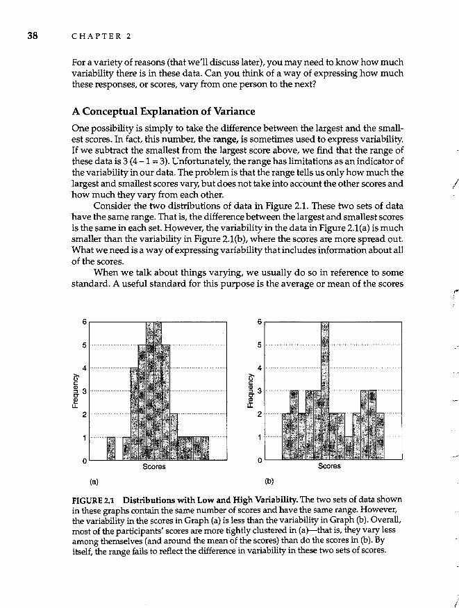
38 CHAPTER 2

For a variety of reasons (that we'll discuss later), you may need to know how much variability there is in these data. Can you think of a way of expressing how much these responses, or scores, vary from one person to the next?

A Conceptual Explanation of Variance

One possibility is simply to take the difference between the largest and the small­est scores. In fact, this number, the range, is sometimes used to express variability. If we subtract the smallest from the largest score above, we find that the range of these data is 3 (4 -1 = 3). Unfortunately, the range has limitations as an indicator of the variability in our data. The problem is that the range tells us only how much the largest and smallest scores vary, but does not take into account the other scores and how much they vary from each other.

Consider the two distributions of data in Figure 2.1. These two sets of data have the same range. That is, the difference between the largest and smallest scores is the same in each set. However, the variability in the data in Figure 2.1(a) is much smaller than the variability in Figure 2.1(b), where the scores are more spread out. What we need is a way of expressing variability that includes information about all of the scores.

When we talk about things varying, we usually do so in reference to some standard. A useful standard for this purpose is the average or mean of the scores

6.------

5

4 g ~ 3 C" I!! u.

2

o Scores

(a)

6.------

5 ............................ .

4 ............................ ..

~ c ~ 3 ..

I 2

o Scores

(b)

FIGURE 2.1 Distributions with Low and High Variability. The two sets of data shown in these graphs contain the same number of scores and have the same range. However, the variability in the scores in Graph (a) is less than the variability in Graph (b). Overall, most of the participants' scores are more tightly clustered in (a)-that is, they vary less among themselves (and around the mean of the scores) than do the scores in (b). By itself, the range fails to reflect the difference in variability in these two sets of scores.

/

;

I

I

I

Behavioral Variability and Research 39

in our data set. Researchers use the term mean as a synonym for what you proba­bly call the average-the sum of a set of scores divided by the number of scores you have.

The mean stands as a fulcrum around which all of the other scores balance. So, we can express the variability in our data in terms of how much the scores vary. around the mean. If most of the scores in a set of data are tightly clustered around the mean (as in Figure 2.1[aD, then the variance of the data will be small. If, how­ever, our scores are more spread out (as in Figure 2.1[bD, they will vary a great deal around the mean, and the variance will be large. So, the variance is nothing more than an indication of how tightly or loosely a set of scores clusters around the mean of the scores. As we will see, this provides a very useful indication of the amount of variability in a set of data.

A Statistical Explanation of Variance

You'll understand more precisely what the variance tells us about our data if we consider how variance is expressed statistically. At this point in our discussion of variance, the primary goal is to help you to better understand what variance is from a conceptual standpoint, not to teach you how to calculate it statistically. The following statistical description will help you get a clear picture of what variance tells us about our data.

We can see what the variance is by following five simple steps. We will refer here to the scores or observations obtained in our study of attitudes on capital punishment.

Step 1. As we saw above, variance refers to how spread out the scores are around the mean of the data. So, to begin, we need to calcwate the mean of our data. Just sum the numbers (4 + 1 + 2 + 2 + 4 + 3 = 16) and divide by the number of scores you have (16/6 = 2.67). Note that statisticians usually use the symbol iJ or x to represent the mean of a set of data. In short, all we do on the first step is calculate the mean of the six scores.

Step 2. Now we need a way of expressing how much the scores vary around the mean. We do this by subtracting the mean from each score. This difference is called a deviation score.

Let's do this for our data involving people's attitudes toward capital punish­ment:

Participant 1 2 3 4 5 6

Deviation Score 4 - 2.67 = 1.33 1- 2.67 = -1.67 2 - 2.67 = -0.67 2 - 2.67 = -0.67 4 - 2.67 = 1.33 3 - 2.67 = 0.33

40 CHAPTER 2

Step 3. By looking at these deviation scores, we can see how much each score varies or deviates from the mean. Participant 2 scores furthest from the mean (1.67 units below the mean), whereas Participant 6 scores closest to the mean (0.33 unit above it). Note that a positive number indicates that the person's score fell above the mean, whereas a negative sign (-) indicates a score below the mean. (What would a deviation score of zero indicate?)

You might think we could add these six deviation scores to get a total variabil­ity score for the sample. However, if we sum the deviation scores for all of the par­ticipants in a set of data, they always add up to zero. So we need to get rid of the negative signs. We do this by squaring each of the deviation scores.

Participant 1 2 3 4 5 6

Deviation Score 1.33

-1.67 -0.67 -0.67

1.33 0.33

Deviation Score Squared 1.77 2.79 0.45 0.45 1.77 0.11

Step 4. Now we add the squared deviation scores. If we add all of the squared deviation scores obtained in Step 3 above, we get

1.77 + 2.79 + 0.45 + 0.45 + 1.77 + 0.11 = 7.34.

As we'll see in later chapters, this number-the sum of the squared deviations of the scores from the mean-is central to the analysis of much research data. We have a shorthand way of referring to this important quantity; we call it the total sum of squares.

Step 5. In Step 4 we obtained an index of the total variability in our data-the total sum of squares. However, this quantity is affected by the number of scores we have; the more participants in our sample, the larger the total sum of squares will be. However, just because we have a larger number of participants does not neces­sarily mean that the variability of our data will be greater.

Because we do not want our index of variability to be affected by the size of the sample, we divide the sum of squares by a function of the number of partici­pants in our sample. Although you might suspect that we would divide by the ac­tual number of participants from whom we obtained data, we usually divide by one less than the number of participants. (Don't concern yourself with why this is the case.) This gives us the variance of our data, which is indicated by the symbol 52. If we do this for our data, the variance (52) is 1.47.

To review, we calculate variance by (1) calculating the mean of the data, (2) subtracting the mean from each score, (3) squaring these differences or devia­tion scores, (4) summing these squared deviation scores (this, remember, is the total sum of squares), and (5) dividing by the number of scores minus 1. By fol-

/

(

J I j

"

(

I

) I

I' /" .r

I

, ,

) I

,

( r r (

Behavioral Variability and Research 41

lowing these steps, you should be able to see precisely what the variance is. It is an index of the average amount of variability in a set of data expressed in terms of how much the scores differ from the mean in squared units. Again, variance is important because virtually every aspect of the research process will lead to the analysis of be­havioral variability, which is expressed in the statistic known as variance.

Statistical Notation Statistical formulas are typically written using statistical notation. Just as we commonly use symbols such as a plus sign (+) to indicate add and an equal sign (=) to indicate i5 equal to, we'll be using special symbols-such as l:, n, and 52-to indicate statistical terms and oper­ations. Although some of these symbols may be new to you, they are nothing more than sym­bolic representations of variables or mathematical operations, all of which are elementary.

For example, the formula for the mean, expressed in statistical notation, is

y=l:yJn.

The uppercase Greek letter sigma (l:) is the statistical symbol for summation and tells us to add what follows. The symbol Yi is the symbol for each individual participant's score. So the operation l:Yi simply tells us to add up all of the scores in our data. That is,

l:Yi = Yl + Y2 + Y3 + ... + Yn

where n is the number of participants. Then, the formula for the mean tells us to divide l:Yi by n, the number of participants. Thus, the formula y = l:yJn indicates that we should add all of the scores and divide by the number of participants.

Similarly, the variance can be expressed in statistical notation as

Look back at the steps for calculating the variance on the preceding pages and see whether you can interpret this formula for 52.

Step 1. Calculate the mean, y. Step 2. Subtract the mean from each participant's score to obtain the deviation

scores, (Yi - y). Step 3. Square each participant's deviation score, (Yi - y)2. Step 4. Sum the squared deviation scores, l:(Yi _ y)2.

Step 5. Divide by the number of scores minus 1, n -1.

As we will see throughout the book, statistical notation will allow us to express certain sta­tistical constructs in a shorthand and unambiguous manner.

42 CHAPTER 2

Systematic and Error Variance

So far, our discussion of variance has dealt with the total variance in the responses of participants in a research study. However, the total variance in a set of data can be split into two parts:

Total variance = systematic variance + error variance.

The distinction between systematic and error variance will be maintained through­out the chapters of this book. Because systematic and error variance are important to the research process, developing a grasp of the concepts now will allow us to use them as needed throughout the book. We'll explore them in greater detail in later chapters.

Systematic Variance

Most research is designed to test the hypothesis that there is a relationship between two or more variables. For example, a researcher may wish to test the hypothesis that self-esteem is related to drug use, or that changes in office illumination cause systematic changes in on-the-job performance. Put differently, researchers usu­ally are interested in whether variability in one variable (self-esteem, illumination) is related in a systematic fashion to variability in other variables (drug use, on-the­job performance).

Systematic variance is that part of the total variability in participants' behav­ior that is related in an orderly, predictable fashion to the variables the researcher is investigating. If the participants' behavior varies in a systematic way as certain other variables change, the researcher has evidence that those variables are related to behavior. In other words, when some of the total variance in participants' be­havior is found to be associated with certain variables in an orderly, systematic fashion, we can conclude that those variables are related to participants' behavior. The portion of the total variance in participants' behavior that is related systemat­ically to the variables under investigation is systematic variance. Two examples may help clarify the concept of systematic variance.

Temperature and Aggression. In an experiment that examined the effects of tem­perature on aggression, Baron and Bell (1976) led participants to believe that they would administer electric shocks to another person. (In reality, that other person was an accomplice of the experimenter and was not actually shocked.) Participants performed this task in a room in which the ambient temperature was 73 degrees, 85 degrees, or 95 degrees F. To determine whether temperature did, in fact, affect ag­gression, the researchers had to determine how much of the variability in partici­pants' aggression was related to temperature. That is, they needed to know how much of the total variance in the aggression scores was systematic variance due to temperature. We wouldn't expect all of the variability in participants' aggression to be a function of temperature. After all, participants entered the experiment already

, i f r

! (

r I

j i

r 1 f

,.

Behavioral Variability and Research 43

differing in their tendencies to respond aggressively. In addition, other factors in the experimental setting may have affected aggressiveness. What the researchers wanted to know was whether any of the variance in how aggressively participants responded was due to differences in the temperatures in the three experimental conditions (73°, 85°, and 95°). If systematic variance related to temperature was ob­tained, they could conclude that changes in temperature affected aggressive behav­ior. Indeed, this and other research has shown that the likelihood of aggression is greater when the temperature is moderately hot than when it is cool, but that ag­gression decreases under extremely high temperatures (Anderson, 1989).

Optimism and Health. In a correlational study of the relationship between opti­mism and health, Scheier and Carver (1985) administered to participants a measure for optimism. Four weeks later, the same participants completed a checklist on which they indicated the degree to which they had experienced each of 39 physical symptoms. Of course, there was considerable variability in the number of symp­toms that participants reported. Some indicated that they were quite healthy, whereas others reported many symptoms. Interestingly, participants who scored high on the optimism scale reported fewer symptoms than did less optimistic par­ticipants; that is, there was a correlation between optimism scores and the number of symptoms that participants reported. In fact, approximately 7% of the total vari­ance in reported symptoms was related to optimism; in other words, 7% of the vari­ance in symptoms was systematic variance related to participants' optimism scores. Thus, optimism and symptoms were related in an orderly, systematic fashion.

In both of these studies, the researchers found that some of the total variance was systematic variance. Baron and Bell found that some of the total variance in aggression was systematic variance related to temperature; Scheier and Carver found that some of the total variance in physical symptoms was systematic vari­ance related to optimism. Finding evidence of systematic variance indicates that variables are related to one another-that room temperature is related to aggres­sion, and optimism is related to physical symptoms, for example. Uncovering rela­tionships in research is always a matter of seeing whether part of the total variance in participants' scores is systematic variance.

As we'll see in detail in later chapters, researchers must design their studies so that they can tell how much of the total variance in participants' behavior is sys­tematic variance associated with the variables they are investigating. If they don't, the study will fail to detect relationships among variables that are, in fact, related. Poorly designed studies do not permit researchers to conclude confidently which variables were responsible for the systematic variance they obtained. We'll return to this important point in later chapters as we learn how to design good studies.

Error Variance

Not all of the total variability in participants' behavior is systematic variance. Fac­tors that the researcher is not investigating may also be related to participants' be­havior. In the Baron and Bell experiment, not all of the variability in aggression

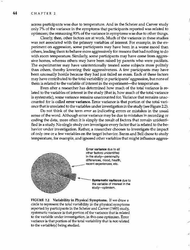
44 CHAPTER 2

across participants was due to temperature. And in the Scheier and Carver study only 7% of the variance in the symptoms that participants reported was related to optimism; the remaining 93% of the variance in symptoms was due to other things.

Clearly, then, other factors are at work. Much of the variance in these studies was not associated with the primary variables of interest. For example, in the ex­periment on aggression, some participants may have been in a worse mood than others, leading them to behave more aggressively for reasons that had nothing to do with room temperature. Similarly, some participants may have come from aggres­sive homes, whereas others may have been raised by parents who were pacifists. The experimenter may have unintentionally treated some subjects more politely than others, thereby lowering their aggressiveness. A few participants may have been unusually hostile because they had just failed an exam. Each of these factors may have contributed to the total variability in participants' aggression, but none of them is related to the variable of interest in the experiment-the temperature.

Even after a researcher has determined how much of the total variance is re­lated to the variables of interest in the study (that is, how much of the total variance is systematic), some variance remains unaccounted for. Variance that remains unac­counted for is called error variance. Error variance is that portion of the total vari­ance that is unrelated to the variables under investigation in the study (see Figure 2.2).

Do not think of the term error as indicating errors or mistakes in the usual sense of the word. Although error variance may be due to mistakes in recording or coding the data, more often it is simply the result of factors that remain unidenti­fied in a study. No single study can investigate every factor that is related to the be­havior under investigation. Rather, a researcher chooses to investigate the impact of only one or a few variables on the target behavior. Baron and Bell chose to study temperature, for example, and ignored other variables that might influence aggres-

Error variance due to all other factors unidentified in the study-personality differences, mood, health,

____ recent experiences, etc.

---- SystematiC variance due to the variable of interest in the study-optimism.

FIGURE 2.2 Variability in Physical Symptoms. If we draw a circle to represent the total variability in the physical symptoms reported by participants in the Scheier and Carver (1985) study, systematic variance is that portion of the variance that is related to the variable under investigation, in this case optimism. Error variance is that portion of the total variability that is not related to the variable(s) being studied.

-,

(

( i

J

Behavioral Variability and Research 45

sion. Carver and Scheier focused on optimism but not on the myriad of other vari­ables related to physical symptoms. All those other, unidentified variables contribute to variance in participants' responses, but we cannot identify precisely what the error variance is due to.

Distinguishing Systematic from Error Variance

As we have seen, researchers must determine whether any of the total variance in the data they collect is related in a systematic fashion to the variables they are in­vestigating. If the participants' behavior varies in a systematic way as certain other variables change, systematic variance is present, providing evidence that those variables are related to the behavior under investigation.

The task researchers face, then, is one of distinguishing the systematic vari­ance from the error variance in their data. In order to determine whether variables are related to one another, they must be able to tell how much of the total variabil­ity in the behavior being studied is systematic variance versus error variance. This is the point at which statistics are indispensable. Researchers use certain statistical analyses to partition the total variance in their data into components that reflect systematic versus error variance. These analyses allow them not only to calculate how much of the total variance is systematic versus error variance, but also to test whether the amount of systematic variance in the data is enough to conclude that the effect is real (as opposed to being due to random influences). We will return to some of these analyses later in the book. For now, the important point to remember is that, in order to draw conclusions from their data, researchers must statistically separate systematic from error variance.

Unfortunately, error variance can mask or obscure the effects of the variables in which researchers are primarily interested. The more error variance in a set of data, the more difficult it is to determine whether the variables of interest are re­lated to variability in behavior. For example, the more participants' aggression in an experiment is affected by extraneous factors, such as their mood or how the re­searcher treats them, the more difficult it is to determine whether room tempera­ture affected their aggression.

The reason that error variance can obscure the systematic effects of other vari­ables is analogous to the way in which noise or static can cover up a song that you want to hear on the radio. In fact, if the static is too loud (because you are sitting be­side an electrical device, for example), you might wonder whether a song is play­ing at all. Similarly, you can think of error variance as noise or static-unwanted, annoying variation that, when too strong, can mask the real "signal" produced by the variables in which the researcher is interested.

In the same way that we can more easily hear a song when the static is re­duced, researchers can more easily detect systematic variance produced by the variables of interest when error variance is mirtimized. They can rarely eliminate error variance entirely, both because the behavior being studied is almost always influenced by unknown factors and because the procedures of the study itself can create error variance. But researchers strive to reduce error variance as much as

46 CHAPTER 2

possible. A good research design is one that minimizes error variance so that the re­searcher can detect any systematic variance that is present in the data.

To review, the total variance in a set of data contains both systematic variance due to the variables of interest and error variance due to everything else (that is, total variance = systematic variance + error variance). The analysis of data from a study always requires us to separate systematic from error variance and thereby determine whether a relationship between our variables exists.

Assessing the Strength of Relationships

Researchers are interested not only in whether certain variables are related to partic­ipants' responses, but also in how strongly they are related. Sometimes, variables are associated only weakly with particular cognitive, emotional, behavioral, or physio­logical responses, whereas other variables are strongly related to thoughts, emotions, and behavior. For example, in a study of variables that predict workers' reactions to losing their jobs, Prussia, Kinicki, and Bracker (1993) found that the degree to which respondents were emotionally upset about losing their jobs was strongly related to how much effort they expected they would have to exert to find a new job but only weakly related to their expectations of actually finding a new job. Knowing about the strength or magnitude of relationships among variables can be very informative.

Researchers assess the strength of the empirical relationships they discover by determining the proportion of the total variability in participants' responses that is systematic variance related to the variables under study. As we saw, the total variance of a set of data is composed of systematic variance and error variance. Once we calculate these types of variance, we can easily determine the proportion of the total variance that is systematic (that is, the proportion of total variance that is systematic variance = systematic variance/total variance).

The statistics that express the strength of relationships are sometimes called measures of strength of association (Maxwell, Camp, & Avery, 1981). How re­searchers calculate these statistics is a topic for later chapters. For now, it is enough to understand that the proportion of total variance that is systematic variance will tell us how strong the relationships are between the variables studied.

At one extreme, if the proportion of the total variance that is systematic vari­ance is .00, none of the variance in participants' responses in a study is systematic variance. When this is the case, we know there is absolutely no relationship be­tween the variables under study and participants' responses. At the other extreme, if all of the variance in participants' responses is systematic variance (that is, if sys­tematic variance/total variance = 1.00), then all of the variability in the data can be attributed to the variables under study. When this is the case, the variables are as strongly related as they possibly can be (in fact, this is called a perfect relationship). When the ratio of systematic to total variance is between .00 and 1.00, the larger the proportion, the stronger the relationship between the variables.

Because measures of the strength of association are proportions, we can com­pare the strength of relationships directly. For example, in the study of reactions to

j

I

i ~

Behavioral Variability and Research 47

job loss described earlier, 26% of the total variance in emotional upset after being fired was related to how much effort the respondents expected they would have to exert to find a new job. In contrast, only 5% of the variance in emotional upset was related to their expectations of finding a new job. Taken together, these findings suggest that, for people who lose their jobs, it is not the possibility of being forever unemployed that is most responsible for their upset, but rather the expectation of how difficult things would be in the short run while seeking reemployment. In fact, by comparing the strength of association for the two findings, we can see that the person's expectations about the effort involved in looking for work (which ac­counted for 26% of the total variance in distress) was over five times more strongly related to their emotional upset than their expectation of finding a new job (which accounted for only 5% of the variance).

The strength of the relationships between variables varies a great deal across studies. In some studies, as little as 1 % of the total variance may be systematic vari­ance, whereas in other contexts, the proportion of the total variance that is system­atic variance may exceed .40 or .50. Although researchers differ in the standards they use to interpret the strength of relationships, Cohen's (1977) criteria are often used. Cohen stated that the association between two variables should be regarded as small if the proportion of systematic to total variance is around .01, medium if the proportion is around .06, and large if the proportion of systematic to total variance exceeds .15. (Keep in mind that these are just rules of thumb that differ across re­search areas.) (See Keppel, 1982.)

You may be surprised that researchers regard .15 as indicating a relatively strong relationship. After all, only 15% of the total variance is systematic variance, and 85% of the variance is error variance that remains unaccounted for. However, most psychological phenomena are multiply determined-the result of a large number of factors. In light of this, we should not be surprised that any single vari­able investigated in a particular study is systematically related to only a small por­tion of the total variance in the phenomenon being investigated. Viewed in this way, explaining even a small percentage of the variance in a particular behavior in terms of only one variable may be an impressive finding.

Meta-Analysis: Systematic Variance Across Studies

As we've seen, researchers are typically interested in the strength of the relation­ships they uncover in a particular study. However, any particular piece of research can provide only a rough estimate of the "true" proportion of the total variance in a particular behavior that is systematically related to other variables. This limita­tion exists because the strength of the relationship obtained in a particular study is affected not only by the relationship between the variables, but also by the charac­teristics of the study itself-the sample of participants who were studied, the par­ticula~ measures used, and the research procedures, for example. Thus, although PruSSIa et al. (1993) found that 26% of the variance in their respondents' emotional

48 CHAPTER 2

upset was related to their expectations of how much effort they would need to exert to find a new job, the strength of the relationship between expectations and emotional upset in this study may have been affected by the particular partici­pants, measures, and procedures the researchers used. We may find a somewhat stronger or weaker relationship if we conducted a similar study using different participants, measures, or methods.

For this reason, behavioral scientists have become increasingly interested in examining the strength of relationships between particular variables across many studies. Although any given study provides only a rough estimate of the strength of a particular relationship, averaging these estimates over many studies that used different participants, measures, and procedures should provide a more accurate indication of how strongly the variables are "really" related.

A procedure known as meta-analysis is used to analyze and integrate the results from a large set of individual studies (Cooper, 1990; Glass, 1976). When re­searchers conduct a meta-analysis, they examine every study that has been con­ducted on a particular topic to assess the relationship between whatever variables are the focus of their analysis. Using information provided in the journal article or re­port of each study, the researcher calculates an index of the strength of the relation­ship between the variables (this is often called the effect size). These data are then statistically integrated to obtain a general estimate of the strength of the relationship between the variables. By combining information from many individual studies, re­searchers assume that the resulting estimate of the average strength of the relation­ship will be more accurate than the estimate provided by any particular study.

In most meta-analyses, researchers not only determine the degree to which certain variables are related, but also explore the factors that affect their relation­ship. For example, in looking across many studies, they may find that the relation­ship was generally stronger for male than for female participants, that it was stronger when certain kinds of measures were used, or that it was weaker when particular experimental conditions were present. Thus, not only is meta-analysis used to document relationships across studies, but it also can be used to explore factors that affect those relationships.

BEHAVIORAL RESEARCH CASE STUDY

Meta-Analyses of Gender Differences In recent years, meta-analyses have been conducted on many areas of the research literature, including expectancy effects, mood and helping inclinations, factors that influence the ef­fectiveness of psychotherapy, gender differences in sexuality, and employees' commitment to work organizations. However, by far, the most popular topic for meta-analysis has been gender differences.

Although many studies have found that men and women differ on a variety of cogni­tive, emotional, and behavioral variables, researchers have been quick to point out that the dif­ferences obtained in these studies are often quite small (and typically smaller than popular stereotypes of men and women assume). Researchers have conducted meta-analyses of re-

)

/

Behavioral Variability and Research 49

search on gender differences to answer the question of whether men and women really differ in regard to certain behaviors and, if so, to document the strength of the relationship between gender and these behaviors. Using the concepts we have learned in this chapter, we can rephrase these questions as: Is any of the total variability in people's behavior related to their gender, and, if so, what proportion of the total variance is systematic variance due to gender?

Hyde, Fennema, and Lamon (1990) conducted a meta-analysis to examine gender dif­ferences in mathematics performance. Based on analyses of 100 individual studies (that in­volved over 3 million participants), these researchers concluded that, overall, the relationship between gender and math performance is very weak. Analyses showed that girls slightly outperformed boys in mathematic computation in elementary and middle school, but that boys tended to outperform girls in math problem solving in high school. By statistically com­paring the effect sizes for studies that were conducted before versus after 1974, they also found that the relationship between gender and math ability has weakened over the past 20 years.

In another meta-analysis, Eagly and Johnson (1990) reviewed previous research on male-female differences in leadership style. Contrary to the stereotypes that women adopt relationship-oriented leadership styles and men task-oriented ones, their analysis found that men and women did not differ in leadership style in studies conducted in actual busi­ness organizations. That is, none of the variability in managers' leadership styles was sys­tematic variance due to gender. However, in laboratory studies of leadership style, some variance was associated with gender, with men being more task-oriented and women being more relationship-Oriented. In studies conducted both in organizational settings and in lab­oratories, female leaders tended to adopt a more democratic style than did male leaders.

Summary

1. Psychology and other behavioral sciences involve the study of behavioral variability. Most aspects of behavioral research are aimed at explaining vari­ability in behavior: (a) Research questions are about the causes and correlates of behavioral variability; (b) researchers try to design studies that will best explain the variability in a particular behavior; (c) the measures used in re­search attempt to capture numerically the variability in participants' behav­ior; (d) and statistics are used to analyze the variability in our data.

2. Descriptive statistics summarize and describe the behavior of research par­ticipants. Inferential statistics analyze the Variability in the data to answer questions about the reliability and generalizability of the findings.

3. Variance is a statistical index of variability. Variance is calculated by subtract­ing the mean of the data from each participant's score, squaring these differ­ences, summing the squared difference scores, and dividing this sum by the number of participants minus 1. In statistical notation, the variance is ex­pressed as: 52 = 1:(Yi - y)2/ (n - 1).

4. The total variance in a set of data can be broken into two components. Sys­tematic variance is that part of the total variance in participants' responses

50 CHAPTER 2

that is related in an orderly fashion to the variables under investigation in a particular study. Error variance is variance that is due to unidentified sources and, thus, remains unaccounted for in a study.

5. To examine the strength of the relationships they study, researchers deter­mine the proportion of the total variability in behavior that is systematic vari­ance associated with the variables under study. The larger the proportion of the total variance that is systematic variance, the stronger the relationship be­tween the variables. Statistics that express the strength of relationships are called measures of strength of association.

6. Meta-analysis is used to examine the nature and strength of relationships be­tween variables across many individual studies. By averaging effect sizes across many studies, a more accurate estimate of the relationship between variables can be obtained.

KEY TERMS

descriptive statistics (p. 36) effect size (p. 48) error variance (p. 44) inferential statistics (p. 37) mean(p.39)

measures of strength of association (p. 46)

meta-analysis (p. 48) range (p. 38) statistical notation (p. 41)

QUESTIONS FOR REVIEW

systematic variance (p. 42) total sum of squares (p. 40) total variance (p. 42) variability (p. 34) variance (p. 37)

1. Discuss how the concept of behavioral variability relates to the following topics: a. the research questions that interest behavioral researchers b. the design of research studies c. the measurement of behavior d. the analysis of behavioral data

2. Why do researchers care how much variability exists in a set of data?

3. Distinguish between descriptive and inferential statistics.

4. Conceptually, what does the variance tell us about a set of data?

5. What is the range, and why is it not ideal as an index of variability?

6. Give a definition of variance, then explain how you would calculate it.

7. How does variance differ from the total sum of squares?

8. What do each of the following symbols mean in statistical notation? a. I b. x c. s2 d. IyJn e. I(Yi-y)2

r t !

('

i

)

Behavioral Variability and Research 51

9. The total variance in a set of scores can be partitioned into two components. What are they, and how do they differ?

10. What are some factors that contribute to error variance in a set of data?

11. Generally, do researchers want systematic variance to be large or small? Explain.

12. Why are researchers often interested in the proportion of total variance that is sys­tematic variance?

13. What would the proportion of total variance that is systematic variance indicate if it were .25? .OO? .98?

14. Why do researchers want the error variance in their data to be small?

15. If the proportion of systematic variance to error variance is .08, would you character­ize the relationship as small, medium, or large? What if the proportion were .72? .OO?

16. Why do researchers use meta-analysis?

17. In a meta-analysis, what does the effect size indicate?

QUESTIONS FOR DISCUSSION

1. Restate each of the following research questions as questions about behavioral variability. a. Does eating too much sugar increase children's activity level? b. Do continuous reinforcement schedules result in faster learning than intermit­

tent reinforcement schedules? c. Do people who are depressed sleep more or less than those who are not

depressed? d. Are people with low self-esteem more likely than those with high self-esteem to

join cults? e. Does caffeine increase the startle response to loud noise?

2. Simply from inspecting the three data sets below, which would you say has the largest variance? Which has the smallest? a. 17,19, 17,22, 17,21,22,23,18,18,20 b. 111,132, 100, 122, 112,99,138,134, 116 c. 87,42,99,27,35,37,92,85,16,22,50

3. A researcher conducted an experiment to examine the effects of distracting noise on people's ability to solve anagrams (scrambled letters that can be unscrambled to make words). Participants worked on anagrams for 10 minutes while listening to the sound of jackhammers and dissonant music that was played at one of four vol­ume levels (quiet, moderate, loud, or very loud). After analyzing the number of anagrams that participants solved in the four conditions, the researcher concluded that loud noise did, in fact, impede participants' ability to solve anagrams. In fact, the noise conditions accounted for 23% of the total variance in the number of ana­grams that participants solved. a. Is this a small, medium, or large effect? b. What proportion of the total variance was error variance? c. List at least 10 things that might have contributed to the error variance in this

study.

52 CHAPTER 2

4. Several years ago, Mischel (1968) pointed out that, on average, only about 10% of the total variance in a particular behavior is systematic variance associated with an­other variable being studied. Reactions to Mischel's observation were of two vari­eties. On one hand, some researchers concluded that the theories and methods of behavioral science must somehow be flawed; surely, if our theories and methods were better we would obtain stronger relationships. However, others argued that accounting for an average of 10% of the variability in behavior with any single vari­able is not a bad track record at all. Where do you stand on this issue? How much of the total variability in a particular phenomenon should we expect to explain with some other variable?

r (

I

,.. I

r

CHAPTER

3 Types of Measures

Scales of Measurement

The Measurement of Behavior

Estimating the Validity of a Measure

Fairness and Bias in Measurement

Estimating the Reliability of a Measure

In 1904, the French minister of public education decided that children of lower in­telligence required special education, so he hired Alfred Binet to design a proce­dure to identify children in the Paris school system who needed special attention. Binet faced a complicated task. Previous attempts to measure intelligence had been notably unsuccessful. Earlier in his career, Binet had experimented with craniome­try, which involved estimating intelligence (as well as personality characteristics) from the size and shape of people's heads. Craniometry was an accepted practice at the time, but Binet became skeptical about its usefulness as a measure of intelli­gence. Other researchers had tried using other aspects of physical appearance, such as facial features, to measure intelligence, but these also were unsuccessful. Still others had used tests of reaction time under the assumption that more intelligent people would show faster reaction times than would less intelligent people. How­ever, evidence for a link between intelligence and reaction time also was weak.

Thus, Binet rejected the previous methods and set about designing a new technique for measuring intelligence. His approach involved a series of short tasks requiring basic cognitive processes such as comprehension and reasoning. For ex­ample, children would be asked to name objects, answer commonsense questions, and interpret pictures. Binet published the first version of his intelligence test in 1905 in collaboration with one of his students, Theodore Simon.

When he revised the test three years later, Binet proposed a new index of intel­ligence that was based on an age level for each task on the test. The various tasks were arranged sequentially in the order in which a child of average intelligence could pass them successfully. For example, average 4-year-olds know their sex, are able to indicate which of two lines is longer, and can name familiar objects (such as a key), but cannot say how two abstract terms (such as the pair pride and pretension)

53

54 CHAPTER 3

differ. By seeing which tasks a child could or could not complete, one could esti­mate the "mental age" of a child-the intellectual level at which the child is able to perform. Later, the German psychologist William Stern recommended dividing a child's mental age (as measured by Binet's test) by his or her chronological age to create the intelligence quotient, or IQ.

Binet's work provided the first useful measure of intelligence and set the stage for the widespread use of tests in psychology and education. Furthermore, it developed the measurement tools behavioral researchers needed to conduct re­search on intelligence, a topic that continues to attract a great deal of research at­tention today. Although contemporary intelligence tests continue to have their critics, the development of adequate measures was a prerequisite to the scientific study of intelligence.

All behavioral research involves the measurement of some behavioral, cogni­tive, emotional, or physiological response. Indeed, it would be inconceivable to conduct a study in which nothing was measured. Importantly, a particular piece of research is only as good as the measuring techniques that are used; poor measure­ment can doom a study. In this and the following chapters, we will look at how re­searchers measure behavioral and mental events by examining the types of measures that behavioral researchers commonly use, the numerical properties of such measures, and the characteristics that distinguish good measures from bad ones. In addition, we will discuss ways to develop the best possible measures for research purposes.

Types of Measures

The measures used in behavioral research fall roughly into three categories: obser­vational measures, physiological measures, and self-reports. Observational mea­sures involve the direct observation of behavior. Observational measures therefore can be used to measure anything an animal or person does that researchers can ob­serve-a rat pressing a bar, eye contact between people in conversation, fidgeting by a person giving a speech, aggression in children on the playground, the time it takes a worker to complete a task. In each case, researchers observe either directly or from audio- or videotape recordings and record the participant's behavior.

Behavioral researchers who are interested in the relationship between bodily processes and behavior use physiological measures. Internal processes that are not directly observable-such as heart rate, brain activity, and hormonal changes-can be measured with sophisticated equipment. Some physiological processes, such as facial blushing and muscular reflexes, are potentially observable with the naked eye, but specialized equipment is needed to measure them accurately.

Self-report measures involve the replies people give to questionnaires and interviews. The information that self-reports provide may involve the respon­dent's thoughts, feelings, or behavior. Cognitive self-reports measure what people think about something. For example, a developmental psychologist may ask a child which of two chunks of clay is larger-one rolled into a ball or one formed in the

;

r·

I

I )

The Measurement of Behavior 55

shape of a hot dog. Or a survey researcher may ask people about their attitudes about a political issue. Affective self-reports involve participants' responses regard­ing how they feel. Many behavioral researchers are interested in emotional reac­tions, such as depression, anxiety, stress, grief, and happiness, and in people's evaluations of themselves and others. The most straightforward way of assessing these kinds of affective responses is to ask participants to report on them. Behavioral self-reports involve participants' reports of how they act. Participants may be asked how often they read the newspaper, go to the dentist, or have sex, for example. Similarly, many personality inventories ask participants to indicate how fre­quently they engage in certain behaviors.

As I noted, the success of a particular piece of research depends heavily on the quality of the measures used. Measures of behavior that are flawed in some way can distort our results and lead us to draw erroneous conclusions about the data. Be­cause measurement is so important to the research process, an entire speciality known as psychometrics is devoted to the study of psychological measurement. Psychometricians investigate the properties of the measures used in behavioral re­search and work toward improving psychological measurement.

BEHAVIORAL RESEARCH CASE STUDY

Converging Operations in Measurement

Because any particular measurement procedure may provide only a rough and imperfect measure of a given construct, researchers sometimes measure a given construct in several different ways. By using several types of measures-each coming at the construct from a dif­ferent angle-researchers can more accurately assess the variable of interest. When different kinds of measures provide the same results, we have more confidence in their validity. This approach to measurement is called converging operations or triangulation. (In the vernacu­lar of navigation and land surveying, triangulation is a technique for determining the posi­tion of an object based on its relationship to three points whose positions are known.)

A case in point involves Pennebaker, Kiecolt-Glaser, and Glaser's (1988) research on the effects that writing about one's experiences has on health. On the basis of previous stud­ies, these researchers hypothesized that people who wrote about traumatic events they had personally experienced would show an improvement in their physical health. To test this idea, they conducted an experiment in which 50 university students were instructed to write for 20 minutes a day for 4 days about either a traumatic event they had experienced (such as the death of a loved one, child abuse, rape, or intense family conflict) or superficial topics.

Rather than rely on any single measure of physical health-which is a complex and multifaceted construct-Pennebaker and his colleagues used converging operations to as­sess the effects of writing on participants' health. First, they obtained observational measures involving participants' visits to the university health center. Second, they used physiological measures to assess directly the functioning of participants' immune systems. Specifically, they collected samples of participants' blood three times during the study and tested the lymphocytes, or white blood cells. Third, they used self-report measures to assess how dis­tressed participants later felt-1 hour, 6 weeks, and 3 months after the experiment.

56 CHAPTER 3

Together, these triangulating data supported the experimental hypothesis. Compared to participants who wrote about superficial topics, those who wrote about traumatic expe­riences visited the health center less frequently, showed better functioning of their immune systems (as indicated by the action of the lymphocytes), and reported they felt better. This and other studies by Pennebaker and his colleagues were among the first to demonstrate empirically the beneficial effects of expressing one's thoughts and feelings about troubling events (Pennebaker, 1990).

Scales of Measurement

Regardless of what kind of measure is used-observational, physiological, or self­report-the goal of measurement is to assign numbers to participants' responses so that they can be summarized and analyzed. For example, a researcher may convert participants' marks on a questionnaire to a set of numbers (from 1 to 5, perhaps) that meaningfully represent the participants' responses. These numbers are then used to describe and analyze participants' answers.

However, in analyzing and interpreting research data, not all numbers can be treated the same way. As we'll see, some numbers used to represent participants' behaviors are, in fact, "real" numbers that can be added, subtracted, multiplied, and divided. Other numbers, however, have special characteristics and require special treatment.

Researchers distinguish between four different levels or scales of measure­ment. These scales of measurement differ in the degree to which the numbers being used to represent participants' behaviors correspond to the real number sys­tem. Differences between these scales of measurement are important because they have implications for what a particular number indicates about a participant and how one's data may be analyzed.

The simplest type of scale is a nominal scale. With a nominal scale, the num­bers that are assigned to participants' behaviors or characteristics are essentially la­bels. For example, for purposes of analysis, we may assign all boys in a study the number 1 and all girls the number 2. Or we may indicate whether participants are married by designating 1 if they have never been married, 2 if they are currently mar­ried, 3 if they were previously married but are not married now, or 4 if they were married but their spouse is deceased. Numbers on a nominal scale indicate attributes of our participants, but they are labels or names rather than real numbers. Thus, it usually makes no sense to perform mathematical operations on these numbers.

An ordinal scale involves the rank ordering of a set of behaviors or charac­teristics, and it conveys more information than a nominal scale does. Measures that use ordinal scales tell us the relative order of our participants on a particular di­mension but do not indicate the distance between participants on the dimension being measured. Imagine being at a talent contest where the winner is the contes­tant who receives the loudest applause. Although we might be able to rank the con­testants by the applause they receive, we would find it difficult to judge precisely how much more the audience liked one contestant than another.

.r

r-/ .'

;

I i ,

r , ,

The Measurement of Behavior 57

When an interval scale of measurement is used, equal differences between the numbers reflect equal differences between participants in the characteristic being measured. On an IQ test, for example, the difference between scores of 90 and 100 (10 points) is the same as the difference between scores of 130 and 140 (10 points). However, an interval scale does not have a true zero point that indicates the absence of the quality being measured. An IQ score of 0 does not necessarily in­dicate that no intelligence is present, just as on the Fahrenheit thermometer (which is an interval scale), a temperature of zero degrees does not indicate the absence of temperature. Because an interval scale has no true zero point, the numbers on it cannot be multiplied or divided. It makes no sense to say that a temperature of 100 degrees is twice as hot as a temperature of 50 degrees, or that a person with an IQ of 60 is one third as intelligent as a person with an IQ of 180.

The highest level of measurement is the ratio scale. Because a ratio scale has a true zero point, ratio measurement involves real numbers that can be added, subtracted, multiplied, and divided. Many measures of physical characteristics, such as weight, are on a ratio scale. Because weight has a true zero point (indi­cating no weight), it makes sense to talk about 100 pounds being twice as heavy as 50 pounds.

Scales of measurement are important to researchers for two reasons. First, the measurement scale determines the amount of information provided by a particu­lar measure. Nominal scales provide less information than ordinal, interval, or ratio scales. When asking people about their opinions, for example, simply asking whether they agree or disagree with particular statements (which is a nominal scale) does not capture as much information as an interval scale that asks how much they agree or disagree. In many cases, choice of a measurement scale is determined by the characteristic being measured; it would be difficult to measure gender on anything other than a nominal scale, for example. However, given a choice, re­searchers prefer to use the highest level of measurement scale possible because it will provide the most pertinent and precise information about participants' re­sponses or characteristics.

The second important feature of scales of measurement involves the kinds of statistical analyses that can be performed on the data. Certain mathematical oper­ations can be performed only on numbers that conform to the properties of a par­ticular measurement scale. The more useful and powerful statistical analyses, such as t-tests and F-tests (which we'll meet in later chapters), generally require that numbers be on interval or ratio scales. As a result, researchers try to choose scales that allow them to use the most informative statistical tests.

Estimating the Reliability of a Measure

The goal of measurement is to assign numbers to behaviors, objects, or events so that they correspond in some meaningful way to the attribute we are trying to mea­sure. Researchers want the variability in the numbers assigned to reflect, as accu­rately as possible, the variability in the attribute being measured. A perfect measure

58 CHAPTER 3

would be one for which the variability in the numbers provided by the measure per­fectly matched the true variability in the event being assessed. But how do we know whether a particular measurement technique does, in fact, produce meaningful and useful scores that accurately reflect what we want to measure?

The first characteristic that any good measure must possess is reliability. Relia­bility refers to the consistency or dependability of a measuring technique. If you weigh yourself on a bathroom scale three times in a row, you expect to obtain the same weight each time. If, however, you weigh 140 pounds the first time, 108 pounds the second time, and 162 pounds the third time, then the scales are unreliable-they can't be trusted to provide consistent weights. Similarly, measures used in research must be reliable. When they aren't, we can't trust them to provide meaningful data regarding the behavior of our participants.

Measurement Error

A participant's score on a particular measure consists of two components: the true score and measurement error. We can portray this by the equation:

Observed score = True score + Measurement error.

The true score is the score that the participant would have obtained if our mea­sure were perfect and we were able to measure without error. If researchers were omniscient beings, they would know exactly what a participant's score should be-that Susan's IQ was exactly 138 or that the rat pressed the bar precisely 52 times, for example.

However, the measures used in research are seldom that precise. Virtually all measures contain measurement error. This component of the participant's ob­served score is the result of factors that distort the score so that it isn't precisely what it should be (that is, it doesn't perfectly equal the participant's true score). If Susan was anxious and preoccupied when she took the IQ test, for example, her observed IQ score might be lower than 138. If the counter on the bar in a Skinner box malfunctioned, it might record that the rat pressed the bar only 50 times in­stead of 52.

The many factors that can contribute to measurement error fall into five major categories. First, measurement error is affected by transient states of the par­ticipant. For example, a participant's mood, health, level of fatigue, and anxiety level can all contribute to measurement error so that the observed score on some measure does not perfectly reflect the participant's true characteristics or reactions.

Second, stable attributes of the participant can lead to measurement error. For example, paranoid or suspicious participants may distort their answers, and less intelligent participants may misunderstand certain questions. Individual differ­ences in motivation can affect test scores; on tests of ability, motivated participants will score more highly than unmotivated participants regardless of their real level of ability. Both transient and stable characteristics can produce lower or higher ob­served scores than participants' true scores would be.

The Measurement of Behavior 59

Third, situational factors in the research setting can create measurement error. If the researcher is particularly friendly, a participant might try harder; if the researcher is stern and aloof, participants may be intimidated, angered, or un­motivated. Rough versus tender handling of experimental animals can introduce changes in their behavior. Room temperature, lighting, and crowding also can ar­tificially affect scores.

Fourth, characteristics of the measure itself can create measurement error. For example, ambiguous questions create measurement error because they can be in­terpreted in more than one way. And measures that induce fatigue (such as tests that are too long) or fear (such as intrusive or painful physiological measures) also can affect scores.

Finally, actual mistakes in recording participants' responses can make the ob­served score different from the true score. If a researcher sneezes while counting the number of times a rat presses a bar, he may lose count; a careless researcher may write 3s that look like 5s; the person entering the data into the computer may enter a participant's score incorrectly. In each case, the observed score that is ulti­mately analyzed contains error.

Whatever its source, measurement error undermines the reliability of the measures researchers use. In fact, the reliability of a measure is an inverse function of measurement error: The more measurement error present in a measuring tech­nique, the less reliable the measure is. Anything that increases measurement error decreases the consistency and dependability of the measure.

Reliability as Systematic Variance

Unfortunately, researchers never know for certain precisely how much measure­ment error is contained in a particular participant's score nor what the partici­pant's true score really is. In fact, in many instances, researchers have no way of knowing for sure whether their measure is reliable and, if so, how reliable it is. However, for certain kinds of measures, researchers have ways of estimating the reliability of the measures they use. If they find that a measure is not acceptably re­liable, they may take steps to increase its reliability. If the reliability cannot be in­creased, they may decide not to use it at all.

Assessing a measure's reliability involves an analysis of the variability in a set of scores. We saw earlier that each participant's observed score is composed of a true-score component and a measurement-error component. If we combine the scores of many participants and calculate the variance, the total variance of the set of scores is composed of the same two components:

Total variance in a set of scores =

Variance due to true scores +

Variance due to measurement error.

Stated differently, the portion of the total variance in a set of scores that is associated with participants' true scores is called systematic variance, and the variance due to measurement error is called error variance. (See Chapter 2 for a review of systematic

60 CHAPTER 3

and error variance.) To assess the reliability of a measure, researchers estimate the proportion of the total variance in the data that is true-score (systematic) variance versus measurement error. Specifically,

Reliability = True-score variance / Total variance.

Thus, reliability is the proportion of the total variance in a set of scores that is sys­tematic variance associated with participants' true scores.

The reliability of a measure can range from .00 (indicating no reliability) to 1.00 (indicating perfect reliability). As the equation above shows, the reliability is .00 when none of the total variance is true-score variance. When the reliability co­efficient is zero, the scores reflect nothing but measurement error, and the measure is totally worthless. At the other extreme, a reliability coefficient of 1.00 would be obtained if all of the total variance were true-score variance. A measure is perfectly reliable if there is no measurement error. As a rule of thumb, a measure is consid­ered sufficiently reliable for research purposes if at least 50% of the total variance in scores is systematic, or true-score, variance.

Assessing Reliability

Researchers use three methods to estimate the reliability of their measures: test­retest reliability, interitem reliability, and interrater reliability. All three methods are based on the same general lOgic. To the extent that two measurements of the same behavior, object, or event yield similar scores, we can assume that both mea­surements are tapping into the same true score. However, if two measurements of something yield very different scores, the measures must contain a high degree of measurement error. Thus, by statistically testing the degree to which the two mea­surements yield similar scores, we can estimate the proportion of the total variance that is systematic true-score variance versus measurement-error variance, thereby estimating the reliability of the measure.

Most estimates of reliability are obtained by examining the correlation be­tween what are supposed to be two measures of the same behavior, attribute, or event. We'll discuss correlation in considerable detail in Chapter 6. For now, all you need to know is that a correlation coefficient is a statistic that expresses the strength of the relationship between two measures on a scale from .00 (no relation­ship between the two measures) to 1.00 (a perfect relationship between the two measures). Correlation coefficients can be positive, indicating a direct relationship between the measures, or negative, indicating an inverse relationship.

If we square a correlation coefficient, we obtain the proportion of the total variance in one set of scores that is systematic variance related to another set of scores. As we saw in Chapter 2, the proportion of systematic variance to total vari­ance (that is, systematic variance/total variance) is an index of the strength of the relationship between the two variables. Thus, the higher the correlation (and its square), the more closely related are the two variables. In light of this relationship, correlation is a useful tool in estimating reliability because it reveals the degree to which two measurements yield similar scores.

/

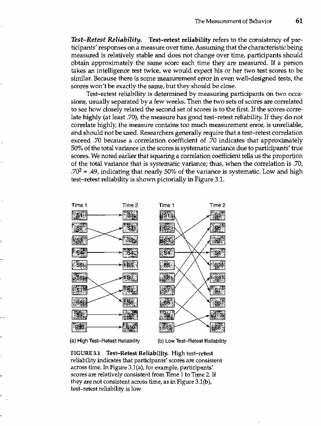
The Measurement of Behavior 61

Test-Retest Reliability. Test-retest reliability refers to the consistency of par­ticipants' responses on a measure over time. Assuming that the characteristic being measured is relatively stable and does not change over time, participants should obtain approximately the same score each time they are measured. If a person takes an intelligence test twice, we would expect his or her two test scores to be similar. Because there is some measurement error in even well-designed tests, the scores won't be exactly the same, but they should be close.

Test-retest reliability is determined by measuring participants on two occa­sions, usually separated by a few weeks. Then the two sets of scores are correlated to see how closely related the second set of scores is to the first. If the scores corre­late highly (at least .70), the measure has good test-retest reliability. If they do not correlate highly, the measure contains too much measurement error, is unreliable, and should not be used. Researchers generally require that a test-retest correlation exceed .70 because a correlation coefficient of .70 indicates that approximately 50% of the total variance in the scores is systematic variance due to participants' true scores. We noted earlier that squaring a correlation coefficient tells us the proportion of the total variance that is systematic variance; thus, when the correlation is .70, .702 = .49, indicating that nearly 50% of the variance is systematic. Low and high test-retest reliability is shown pictorially in Figure 3.1.

Time 1 Time 2 Time 1 Time 2

(a) High Test-Retest Reliability (b) Low Test-Retest Reliability

FIGURE 3.1 Test-Retest Reliability. High test-retest reliability indicates that participants' scores are consistent across time. In Figure 3.1(a), for example, participants' scores are relatively consistent from Time 1 to Time 2. If they are not consistent across time, as in Figure 3.1(b), test-retest reliability is low.

62 CHAPTER 3

Assessing test-retest reliability makes sense only if the attribute being mea­sured would not be expected to change between the two measurements. We would generally expect high test-retest reliability on measures of intelligence, attitudes, or personality, for example, but not on measures of hunger or fatigue.

Interitem Reliability. A second kind of reliability is relevant for measures that consist of more than one item. Interitem reliability assesses the degree of consis­tency among the items on a scale. Personality inventories, for example, typically consist of several questions that are summed to provide a single score that reflects the respondent's extraversion, self-esteem, shyness, or whatever. Similarly, on a scale used to measure depression, participants may be asked to rate themselves on several mood-related items (sad, unhappy, blue, helpless) that are then added to­gether to provide a single depression score. Scores on attitude scales are also cal­culated by summing a respondent's responses to several questions.

When researchers sum participants' responses to several questions or items to obtain a single score, they must be sure that all of the items are tapping into the same construct (such as a particular trait, emotion, or attitude). On an inventory to mea­sure extraversion, for example, researchers want all of the items to measure some aspect of extraversion. Including items that don't measure the construct of interest on a test increases measurement error. Researchers check to see that the items on such a scale measure the same general construct by examining interitem reliability.

Researchers examine interitem reliability by computing item-total correla­tions, split-half reliability, and Cronbach's alpha coefficient. First, researchers look at the item-total correlation for each question or item on the scale. Does each item correlate with the sum of all other items? If a particular item measures the same construct as the rest of the items, it should correlate with them. If not, the item only adds measurement error to the observed score and doesn't belong on the scale. Generally, the correlation between each item on a questionnaire and the sum of the other items should exceed .30.

Researchers also use split-half reliability as an index of interitem reliability. With split-half reliability, the researcher divides the items on the scale into two sets. Sometimes the first and second halves of the scale are used, sometimes the odd­numbered items form one set and even-numbered items form the other, or some­times items are randomly put into one set or the other. Then, a total score is obtained for each set by adding the items within each set, and the correlation between these two sets of scores is then calculated. If the items on the scale hang together well and estimate the true score consistently, scores obtained on the two halves of the test should correlate highly (> .70). If the split-half correlation is small, however, it indi­cates that the two halves of the scale are not measuring the same thing and, thus, the total score contains a great deal of measurement error.

There is one drawback to the use of split-half reliability, however. The relia­bility coefficient one obtains depends on how the items are split. Using a first­half/ second-half split is likely to provide a slightly different estimate of reliability than an even/ odd split. What, then, is the real interitem reliability? To get around this ambiguity, researchers often use Cronbach's alpha coefficient (Cronbach,

The Measurement of Behavior 63

1970). Cronbach's alpha is equivalent to the average of all possible split-half relia­bilities (although it can be calculated directly from a simple formula). As a rule of thumb, researchers consider a measure to have adequate interitem reliability if Cronbach's alpha coefficient exceeds .70. As with test-retest reliability, an alpha co­efficient of greater than .70 indicates that at least 50% of the total variance in the scores on the measure is systematic, true-score variance.

!@§ 11M BEHAVIORAL RESEARCH CASE STUDY

Interitem Reliability and the Construction of Multi-Item Measures As noted, whenever researchers calculate a score by summing respondents' answers across a number of questions, they must be sure that all of the items on the scale measure the same construct. Thus, when researchers develop new multi-item measures, they use item-total correlations to help them select items for the measure. Several years ago, I decided to de­velop a new measure of the degree to which people tend to feel nervous in social interac­tions (Leary, 1983). I started this process by writing 87 self-report items (such as "I often feel nervous even in casual get-togethers," "Parties often make me feel anxious and uncomfort­able," and "In general, I am a shy person"). Then, with the help of two students, these were narrowed down to what seemed to be the best 56 items. We administered those 56 items to 112 respondents, asking them to rate how characteristic or true each statement was of them on a 5-point scale (where 1 = not at all, 2 = slightly, 3 = moderately, 4 = very, and 5 = extremely). We then calculated the item-total correlation for each item-the correlation between the re­spondents' answers on each item and their total score on all of the other items. Because a low item-total correlation indicates that an item is not measuring what the rest of the items are measuring, we eliminated all items for which the item-total correlation was less than .40. A second sample then responded to the reduced set of items, and we looked at the item-total correlations again. Based on these correlations, we retained 15 items for the final version of our Interaction Anxiousness Scale (lAS).

To be sure that our final set of items was sufficiently reliable, we administered these 15 items to a third sample of 363 respondents. AllIS items on the scale had item-total corre­lations greater than .50, demonstrating that all items were measuring aspects of the same construct. Furthermore, we calculated Cronbach's alpha coefficient to examine the interitem reliability of the scale as a whole. Cronbach's alpha was .89, which exceeded the minimum criterion of .70 that most researchers use to indicate acceptable reliability. (If we square .89, we get .7921, showing that apprOximately 79% of the variance in scores on the lAS is sys­tematic, true-score variance.)

Because social anxiety is a relatively stable characteristic, we examined the test-retest reliability of the lAS as well. Eight weeks after it had been completed the first time, the lAS was readministered to 74 of the participants from our third sample, and we correlated their scores on the two administrations. The test-retest reliability was .80, again above the desired minimum of .70. Together, these data showed us that the new measure of social anxiety was sufficiently reliable to use in research.

64 CHAPTER 3

Interrater Reliability. Interrater reliability (also called inter judge or interob­server reliability) involves the consistency among two or more researchers who ob­serve and record participants' behavior. Obviously, when two or more observers are involved, we would like consistency to be maintained among them. If one ob­server records 15 bar presses and another observer records 18 bar presses, the dif­ference between their observations represents measurement error.

For example, Gottschalk, Uliana, and Gilbert (1988) analyzed presidential de­bates for evidence that the candidates were cognitively impaired at the time of the debates. They coded what the candidates said during the debates using the Cogni­tive Impairment Scale. In their report of the study, the authors presented data to sup­port the interrater reliability of their procedure. The reliability analysis demonstrated that the raters agreed sufficiently among themselves and that measurement error was acceptably low. (By the way, their results showed that Ronald Reagan was signifi­cantly more impaired than Jimmy Carter in 1980, or Walter Mondale in 1984, and that Reagan was more impaired during the 1984 debates than he had been 4 years earlier.)

Researchers use two general methods for assessing interrater reliability. If the raters are simply recording whether a behavior occurred, we can calculate the per­centage of times they agreed. Alternatively, if the raters are rating the participants' behavior on a scale (an anxiety rating from 1 to 5, for example), we can correlate their ratings across participants. If the observers are making similar ratings, we should obtain a relatively high correlation (at least .70) between them.

Increasing the Reliability of Measures

Unfortunately, it is not always possible to assess the reliability of measures used in research. For example, if we ask a person to rate on a scale of 1 to 7 how happy he or she feels at the moment, we have no direct way of testing the reliability of the re­sponse. Test-retest reliability is inappropriate because the state we are measuring changes over time; interitem reliability is irrelevant because there is only one item; and, because others cannot observe and rate the participant's feelings of happi­ness, we cannot assess interrater reliability. Even though researchers assess the re­liability of their measuring techniques whenever possible, the reliability of some measures cannot be determined.

In light of this, often the best a researcher can do is to make every effort to maximize the reliability of his or her measures by eliminating possible sources of measurement error. The following list offers a few ways of increasing the reliabil­ity of behavioral measures.

• Standardize administration of the measure. Ideally, every participant should be tested under precisely the same conditions. Differences in how the measure is given can contribute to measurement error. If possible, have the same re­searcher administer the measure to all participants in precisely the same setting.

• Clarify instructions and questions. Measurement error results when some participants do not fully understand the instructions or questions. When pos­sible, questions to be used in interviews or questionnaires should be pilot tested to be sure they are understood properly.

The Measurement of Behavior 65

• Train observers. If participants' behavior is being observed and rated, train the observers carefully. Observers should also be given the opportunity to practice using the rating technique .

• Minimize errors in coding data. No matter how reliable a measuring tech­nique is, error is introduced if researchers make mistakes in recording, cod­ing, tabulating, or computing the data.

In summary, reliable measures are a prerequisite of good research. A reliable measure is one that is relatively unaffected by sources of measurement error and thus is consistent and dependable. More specifically, reliability reflects the propor­tion of the total variance in a set of scores that is systematic, true-score variance. The reliability of measures is estimated in three ways: test-retest reliability, in­teritem reliability, and interrater reliability. Even in instances in which the reliabil­ity of a technique cannot be determined, steps should be taken to minimize sources of measurement error.

Estimating the Validity of a Measure

The measures used in research not only must be reliable but also must be valid. Va­lidity refers to the extent to which a measurement procedure actually measures what it is intended to measure rather than measuring something else (or nothing at all). Validity is the degree to which variability in participants' scores on a particu­lar measure reflects variability in the characteristic we want to measure. Do scores on the measure relate to the behavior or attribute of interest? Are we measuring what we think we are measuring? If a researcher is interested in the effects of a new drug on obsessive-compulsive disorder, for example, the measure for obsession­compulsion must reflect actual differences in the degree to which participants ac­tually have the disorder. That is, to be valid, the measure must assess what it is supposed to measure.

It is important to note that a measure can be highly reliable but not valid. For example, the cranial measurements that early psychologists used to assess intelli­gence were very reliable. When measuring a person's skull, two researchers would arrive at similar, though not always identical, measurements-that is, interrater re­liability was quite high. Skull size measurements also demonstrate high test-retest reliability; they can be recorded consistently over time with little measurement error. However, no matter how reliable skull measurements may be, they are not a valid measure of intelligence. They are not valid because they do not measure the construct of intelligence. Thus, researchers need to know whether measures are re­liable as well as whether they are valid.

Assessing Validity

When researchers refer to a measure as valid, they do so in terms of a particular scientific or practical purpose. Validity is not a property of a measuring technique per se but rather an indication of the degree to which the technique measures a

66 CHAPTER 3

particular entity in a particular context. Thus, a measure may be valid for one purpose but not for another. Cranial measurements, for example, are valid measures of hat size, but they are not valid measures of intelligence. Researchers often refer to three different types of validity: face validity, construct validity, and criterion validity.

Face Validity. Face validity refers to the extent to which a measure appears to measure what it's supposed to measure. Rather than being a technical or statistical procedure, face validation involves the judgment of the researcher or of research participants. A measure has face validity if people think it does.

In general, a researcher is more likely to have faith in an instrument whose content obviously taps into the construct he or she wants to measure than in an in­strument that is not face valid. Furthermore, if a measuring technique, such as a test, does not have face validity, participants, clients, job applicants, and other laypeople are likely to doubt its relevance and importance (Cronbach, 1970). In ad­dition, they are likely to be resentful if they are affected by the results of a test whose validity they doubt. A few years ago, a national store chain paid $1.3 million dollars to job applicants who sued the company because they were required to take a test that contained bizarre personal items such as "I would like to be a florist" and "Evil spirits possess me sometimes." The items on this test were from commonly used, well-validated psychological measures, such as the Minnesota Multiphasic Personality Inventory (MMPI) and the California Personality Inventory (CPI), but they lacked face validity. Thus, all other things being equal, it is usually better to have a measure that is face valid than one that is not; it simply engenders greater confidence by the public at large.

Although face validity is often desirable, three qualifications must be kept in mind. First, just because a measure has face validity doesn't necessarily mean that it is actually valid. There are many cases of face-valid measures that do not mea­sure what they appear to measure. For researchers of the nineteenth century, skull size measurements were a face-valid measure of intelligence.

Second, many measures that lack face validity are, in fact, valid. For example, the MMPI and CPI mentioned earlier-measures of personality that are used in practice, research, and business--<:ontain many items that are not face valid, yet scores on these measures predict various behavioral patterns and psychological problems. For example, responses indicating an interest in being a florist or believ­ing that one is possessed by evil spirits are, when combined with responses to other items, valid indicators of certain attributes, even though these items are by no means face valid.

Third, researchers sometimes want to disguise the purpose of their tests. If they think that respondents will hesitate to answer honestly sensitive questions, they may design instruments that lack face validity and thereby conceal the pur­pose of the test.

Construct Validity. Much behavioral research involves the measurement of hy­pothetical constructs-entities that cannot be directly observed but are inferred on the basis of empirical evidence. Behavioral science abounds with hypothetical con-

The Measurement of Behavior 67

structs such as intelligence, attraction, status, schema, self-concept, moral maturity, motivation, satiation, learning, and so on. None of these entities can be observed di­rectly, but they are hypothesized to exist on the basis of indirect evidence. In study­ing these kinds of constructs, researchers must use valid measures. But how does one go about validating the measure of a hypothetical (and invisible) construct?

In an important article, Cronbach and Meehl (1955) suggested that the valid­ity of measures of hypothetical constructs can be assessed by studying the relation­ship between the measure of the construct and scores on other measures. We can specify what the scores on any particular measure should be related to if that mea­sure is valid. For example, scores on a measure of self-esteem should be positively related to scores on measures of confidence and optimism, but negatively related to measures of insecurity and anxiety. Thus, we assess construct validity by seeing whether a particular measure relates as it should to other measures.

Researchers typically examine construct validity by calculating correlations be­tween the measure they wish to validate and other measures. Because correlation co­efficients describe the strength and direction of relationships between variables, they can tell us whether a particular measure is related to other measures as it should be. Sometimes we expect the correlations between one measure and measures of other constructs to be high, whereas in other instances we expect only moderate or weak relationships or none at all. Thus, unlike in the case of reliability (where we want cor­relations to exceed .70), no general criteria can be specified for evaluating the size of correlations when assessing construct validity. The size of each correlation coefficient must be considered relative to the correlation we would expect to find if our measure were valid and measured what it was intended to measure.

To have construct validity, a measure should both correlate with other mea­sures that it should correlate with (convergent validity) and not correlate with measures that it should not correlate with (discriminant validity). When measures correlate highly with measures they should correlate with, we have evidence of convergent validity. When measures correlate weakly (or not at all) with concep­tually unrelated measures, we have evidence of discriminant validity. Thus, we can examine the correlations between scores on a test and scores from other mea­sures to see whether the relationships converge and diverge as predicted. In brief, evidence that the measure is related to other measures as it should be supports its construct validity.

BEHAVIORAL RESEARCH CASE STUDY

Construct Validity Earlier I described the development of a measure of social anxiety-the Interaction Anx­iousness Scale-and data attesting to the scale's interitem and test-retest reliability. Before such a measure can be used, its construct validity must be assessed by seeing whether it cor­relates with other measures as it should. To examine the construct validity of the lAS, we de­termined what scores on our measure should be related to if it was a valid measure of social anxiety. Most obviously, scores on the lAS should be related to scores on existing measures

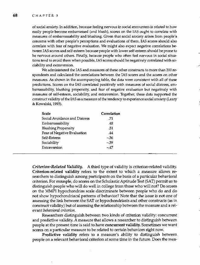
68 CHAPTER 3

of social anxiety. In addition, because feeling nervous in social encounters is related to how easily people become embarrassed (and blush), scores on the lAS ought to correlate with measures of embarrassability and blushing. Given that social anxiety arises from people's concerns with other people's perceptions and evaluations of them, lAS scores should also correlate with fear of negative evaluation. We might also expect negative correlations be­tween lAS scores and self-esteem because people with lower self-esteem should be prone to be nervous around others. Finally, because people who often feel nervous in social situa­tions tend to avoid them when possible, lAS scores should be negatively correlated with so­ciability and extraversion.

We administered the lAS and measures of these other constructs to more than 200 re­spondents and calculated the correlations between the lAS scores and the scores on other measures. As shown in the accompanying table, the data were consistent with all of these predictions. Scores on the lAS correlated pOSitively with measures of social distress, em­barrassability, blushing propensity, and fear of negative evaluation but negatively with measures of self-esteem, SOciability, and extraversion. Together, these data supported the construct validity of the lAS as a measure of the tendency to experience social anxiety (Leary & Kowalski, 1993).

Scale Social Avoidance and Distress Embarrassability Blushing Propensity Fear of Negative Evaluation Self-Esteem Sociability Extraversion

Correlation .71 .48 .51 .44

-.36 -.39 -.47

Criterion-Related Validity. A third type of validity is criterion-related validity. Criterionarelated validity refers to the extent to which a measure allows re­searchers to distinguish among participants on the basis of a particular behavioral criterion. For example, do scores on the Scholastic Aptitude Test (SAT) permit us to distinguish people who will do well in college from those who will not? Do scores on the MMPI hypochondrias scale discriminate between people who do and do not show hypochondriacal patterns of behavior? Note that the issue is not one of assessing the link between the SAT or hypochondriasis and other constructs (as in construct validity) but of assessing the relationship between the measure and a rel­evant behavioral criterion.

Researchers distinguish between two kinds of criterion validity: concurrent and predictive validity. A measure that allows a researcher to distinguish between people at the present time is said to have concurrent validity. Sometimes we want scores on a particular measure to be related to certain behaviors right now.

Predictive validity refers to a measure's ability to distinguish between people on a relevant behavioral criterion at some time in the future. Does the mea-

(

The Measurement of Behavior 69

sure predict future behavior? For the SAT, for example, the issue is one of predic­tive validity. No one really cares whether high school seniors who score high on the SAT are better prepared for college than low scorers at the time they take the test (concurrent validity). Instead, college admissions officers want to know whether SAT scores predict academic performance 1 to 4 years later (predictive validity).

_ BEHAVIORAL RESEARCH CASE STUDY

Criterion-Related Validity Establishing criterion-related validity involves showing that scores on a measure are related to people's behaviors as they should be. In the case of the Interaction Anxiousness Scale de­scribed earlier, scores on the lAS should be related to people's reactions in real social situa­tions. For example, as a measure of the general tendency to feel socially anxious, scores on the lAS should be correlated with how nervous people feel in actual interpersonal encounters. In several laboratory studies, participants completed the lAS, then interacted with another in­dividual. Participants' reported feelings of anxiety before and during these interactions cor­related with lAS scores as expected. Furthermore, lAS scores correlated with how nervous the participants were judged to be by people who observed them during these interactions.

We also asked participants who completed the lAS to keep track of all social interac­tions they had that lasted more than 10 minutes for about a week. For each interaction, they completed a brief questionnaire that assessed, among other things, how nervous they felt. Not only did participants' scores on the lAS correlate with how nervous they felt in every­day interactions, but participants who scored high on the lAS had fewer interactions with people whom they did not know well (presumably because they were uncomfortable in in­teractions with people who were unfamiliar) than did people who scored low on the lAS. These data showed that scores on the lAS related to people's real reactions and behaviors as they should, thereby supporting the criterion-validity of the scale.

Criterion-related validity is often of interest to researchers in applied research settings. In educational research, for example, researchers are often interested in the degree to which tests predict academic performance. Similarly, before using tests to select new employees, personnel psychologists must demonstrate that the tests successfully predict future on-the-job performance-that is, that they possess predictive validity.

!!W!tti'k11!1!Ell IN DEPTH

The Reliability and Validity of College Admission Exams Most colleges and universities use applicants' scores on one or more entrance examinations as one criterion for making admissions decisions. By far the most frequently used exam for this purpose is the Scholastic Aptitude Test (SAT), developed by the Educational Testing Service.

70 CHAPTER 3

Many students are skeptical of the SAT and similar exams. Many claim, for example, that they don't perform well on standardized tests and that their scores indicate little, if any­thing, about their ability to do well in college. No doubt, there are many people for whom the SAT does not predict performance well. Like all tests, the SAT contains measurement error and thus underestimates and overestimates some people's true aptitude scores. (Inter­estingly, I've never heard anyone derogate the SAT because they scored higher than they should have. From a statistical perspective, measurement error should lead as many people to obtain scores that are higher than their true ability as to obtain scores lower than their ability.) However, a large amount of data attests to the overall reliability and validity of the SAT. The psychometric data regarding the SAT are extensive, based on tens of thousands of scores over a span of many years.

The reliability of the SAT is impressive in comparison with most psychological tests. The SAT possesses high test-retest reliability as well as high interitem reliability. Reliability coefficients average around .90 (Kaplan, 1982), easily exceeding the standard criterion of .70. In fact, over 80% of the total variance in SAT scores is systematic, true-score variance.

In the case of the SAT, predictive validity is of paramount importance. Many studies have examined the relationship between SAT scores and college grades. These studies have shown that the criterion-related validity of the SAT depends, in part, on one's major in col­lege; SAT scores predict college performance better for some majors than for others. In gen­eral, however, the predictive validity of the SAT is fairly good. On the average, about 16% of the total variance in first-year college grades is systematic variance accounted for by SAT scores (Kaplan, 1982). Sixteen percent may not sound like a great deal until one considers all of the other factors that contribute to variability in college grades, such as motivation, health, personal problems, the difficulty of one's courses, the academic ability of the student body, and so on. Given everything that affects performance in college, it is not too surpris­ing that a single test score does not predict with greater accuracy.

Of course, most colleges and universities also use criteria other than entrance exams in the admissions decision. The Educational Testing Service advises admissions offices to consider high school grades, activities, and awards, as well as SAT scores, for example. Using these other criteria further increases the validity of the selection process.

This is not to suggest that the SAT and other college entrance exams are infallible or that certain people do not obtain inflated or deflated scores. But such tests are not as unreli­able or invalid as many students suppose.

To sum up, validity refers to the degree to which a measuring technique mea­sures what it's intended to measure. Although face-valid measures are often desir­able, construct and criterion-related validity are much more important. Construct validity is assessed by seeing whether scores on a measure are related to other measures as they should be. A measure has criterion-related validity if it correctly distinguishes between people on the basis of a relevant behavioral criterion either at present (concurrent validity) or in the future (predictive validity).

I I

The Measurement of Behavior 71

Fairness and Bias in Measurement

In recent years, a great deal of public attention and scientific research has been de­voted to the possibility that certain psychological and educational measures, par­ticularly tests of intelligence and academic ability, are biased against certain groups of individuals. Test bias occurs when a particular meaSUre is not equally valid for everyone who takes the test. That is, if test scores more accurately reflect the true ability or characteristics of one group than another, the test is biased.

Identifying test bias is difficult. Simply showing that a certain gender, racial, or ethnic group performs worse on a test than other groups does not necessarily in­dicate that the test is unfair. The observed difference in scores may reflect a true dif­ference between the groups in the attribute being measured. Bias exists only if groups that do not differ on the attribute or ability being measured obtain different scores on the test.

Bias can creep into psychological measures in very subtle ways. For example, test questions sometimes refer to objects or experiences that are mOre familiar to members of one group than to those of another. If those objects or experiences are not relevant to the attribute being measured (but rather are being used only as ex­amples), some individuals may be unfairly disadvantaged. Consider, for example, this sample analogy from the SAT:

STRAWBERRY:RED (A) peach:ripe (D) orange:round

(B) leather:brown (E) lemon:yellow

(C) grass:green

The correct answer is (E) because a strawberry is a fruit that is red, and a lemon is a fruit that is yellow. However, statistical analyses showed that Hispanic test takers missed this particular item notably more often than members of other groups. Fur­ther investigation suggested that the difference occurred because some Hispanic test takers were familiar with green rather than yellow lemons. As a result, they chose grass:green as the analogy to strawberry:red, a very reasonable response for an individual who does not associate lemons with the color yellow ("What's the DIP?," 1999). Along the same lines, a geometry question on a standardized test was identified as biased when it became clear that women missed it mOre often than did men because it referred to the dimensions of a football field. In these two cases, the attributes being measured (analogical reasoning and knowledge about geome­try) had nothing to do with one's experience with yellow lemons or football, yet those experiences led some test takers to perform better than others.

Test bias is hard to demonstrate because it is often difficult to determine whether the groups truly differ on the attribute in question. One way to document the presence of bias is to examine the predictive validity of a measure separately for different groups. A biased test will predict future outcomes better for one group than another. For example, imagine that we find that Group X performs worse on

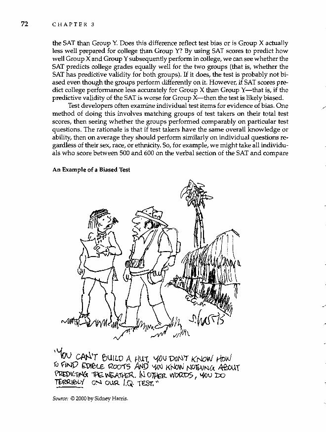
72 CHAPTER 3

the SAT than Group Y. Does this difference reflect test bias or is Group X actually less well prepared for college than Group Y? By using SAT scores to predict how well Group X and Group Y subsequently perform in college, we can see whether the SAT predicts college grades equally well for the two groups (that is, whether the SAT has predictive validity for both groups). If it does, the test is probably not bi­ased even though the groups perform differently on it. However, if SAT scores pre­diet college performance less accurately for Group X than Group Y-that is, if the predictive validity of the SAT is worse for Group X-then the test is likely biased.

Test developers often examine individual test items for evidence of bias. One method of doing this involves matching groups of test takers on their total test scores, then seeing whether the groups performed comparably on particular test questions. The rationale is that if test takers have the same overall knowledge or ability, then on average they should perform similarly on individual questions re­gardless of their sex, race, or ethnicity. So, for example, we might take all individu­als who score between 500 and 600 on the verbal section of the SAT and compare

An Example of a Biased Test

Source: © 2000 by Sidney Harris.

.. ",,-

--

The Measurement of Behavior 73

how different groups performed on the strawberry:red analogy described earlier. If the item is unbiased, an approximately equal proportion of each group should get the analogy correct. However, if the item is biased, we would find that a dis­proportionate number of one group got it "wrong."

All researchers and test developers have difficulty setting aside their own ex­periences and biases. However, they must make every effort to reduce the impact of their biases on the measures they develop. By collaborating with investigators of other genders, races, ethnic groups, and cultural backgrounds, potential sources of bias can be identified as tests are constructed. And by applying their understanding of validity, they can work together to identify biases that do creep into their measures.

Summary

1. Measurement lies at the heart of all research. Behavioral researchers have a wide array of measures at their disposal, including observational, physiolog­ical, and self-report measures. Psychometrics is a specialty devoted to the study and improvement of psychological tests and other measures.

2. Because no measure is perfect, researchers sometimes use several different measures of the same variable, a practice known as converging operations (or triangulation).

3. Whatever types of measure they use, researchers must consider whether the measure is on a nominal, ordinal, interval, or ratio scale of measurement. A measure's scale of measurement has implications for the kind of information that the instrument provides, as well as for the statistical analyses that can be performed on the data.

4. Reliability refers to the consistency or dependability of a measuring tech­nique. Three types of reliability can be assessed: test-retest reliability (consis­tency of the measure across time), interitem reliability (consistency among a set of items intended to assess the same construct), and interrater reliability (con­sistency between two or more researchers who have observed and recorded the participant's behavior).

5. All observed scores consist of two components-the true score and measure­ment error. The true-score component reflects the score that would have been obtained if the measure were perfect; measurement error reflects the effects of factors that make the observed score lower or higher than it should be. The more measurement error, the less reliable the measure.

6. Factors that increase measurement error include transient states (such as mood, fatigue, health), stable personality characteristics, situational factors, the measure itself, and researcher mistakes.

7. A correlation coefficient is a statistic that expresses the direction and strength of the relationship between two variables.

8. Reliability is tested by examining correlations between (a) two administra­tions of the same measure (test-retest), (b) items on a questionnaire (interitem), or (c) the ratings of two or more observers (interrater).

74 CHAPTER 3

9. Reliability can be enhanced by standardizing the administration of the mea­sure, clarifying instructions and questions, training observers, and minimiz­ing errors in coding and analyzing data.

10. Validity refers to the extent to which a measurement procedure measures what it's intended to measure.

11. Three types of validity were discussed: face validity (does the measure appear to measure the construct of interest?), construct validity (does the measure cor­relate with measures of other constructs as it should?), and criterion-related va­lidity (does the measure correlate with measures of current or future behavior as it should?).

12. Test bias occurs when scores on a test reflect the true ability or characteristics of one group of test takers more accurately than the ability or characteristics of another group-that is, when validity is better for one group than another.

KEY TERMS

concurrent validity (p. 68) construct validity (p. 67) convergent validity (p. 67) converging operations (p. 55) correlation coefficient (p. 60) criterion-related validity

(p.68) Cronbach's alpha coefficient

(p.62) discriminant validity (p. 67) face validity (p. 66)

hypothetical construct (p. 66) interitem reliability (p. 62) interrater reliability (p. 64) interval scale (p. 57) item-total correlation (p. 62) measurement error (p. 58) nominal scale (p. 56) observational measure (p. 54) ordinal scale (p. 56) physiological measure (p. 54) predictive validity (p. 68)

QUESTIONS FOR REVIEW

psychometrics(p.55) ratio scale (p. 57) reliability (p. 58) scales of measurement (p. 56) self-report measure (p. 54) split-half reliability (p. 62) test bias (p. 71) test-retest reliability (p. 61) true score (p. 58) validity (p. 65)

1. Distinguish among observational, physiological, and self-report measures.

2. What do researchers interested in psychometrics study?

3. Why do researchers use converging operations?

4. Distinguish among nominal, ordinal, interval, and ratio scales of measurement. Why do researchers prefer to use measures that are on interval and ratio scales when possible?

5. Why must researchers use reliable measures?

6. Why is it virtually impossible to eliminate all measurement error from the measures we use in research?

7. What is the relationship between the reliability of a measure and the degree of mea­surement error it contains?

; I

)

/

, i

The Measurement of Behavior 75

8. What does the reliability coefficient of a measure indicate if it is .60? .OO? 1.00?

9. What does a correlation coefficient tell us? Why are correlation coefficients useful when assessing reliability?

10. What are the three ways in which researchers assess the reliability of their mea­sures? Be sure that you understand the differences among these three approaches to reliability.

11. What is the minimum reliability coefficient that researchers consider acceptable? Why do researchers use this minimum criterion for reliability?

12. For what kind of measure is it appropriate to examine test-retest reliability? In-teritem reliability? Interrater reliability?

13. What value of Cronbach's alpha coefficient indicates acceptable interitem reliability?

14. Why are researchers sometimes not able to test the reliability of their measures?

15. What steps can be taken to increase the reliability of measuring techniques?

16. What is validity?

17. Distinguish between face validity, construct validity, and criterion-related validity. In general, which kind of validity is least important to researchers?

18. Can a measurement procedure be valid but not reliable? Reliable but not valid? Explain.

19. Distinguish between construct and criterion-related validity.

20. Distinguish between convergent and discriminant validity. Do these terms refer to types of construct validity or criterion-related validity?

21. Distinguish between concurrent and predictive validity. Do these terms refer to types of construct validity or criterion-related validity?

22. How can we tell whether a particular measure is biased against a particular group?

23. How do researchers identify biased test items on tests of intelligence or ability?

QUESTIONS FOR DISCUSSION

1. Many students experience a great deal of anxiety whenever they take tests. Imagine that you conduct a study of test anxiety in which participants take tests and their re­actions are measured. Suggest how you would apply the idea of converging opera­tions using observational, physiological, and self-report measures to measure test anxiety in such a study.

2. For each measure listed below, indicate whether it is measured on a nominal, ordi­nal, interval, or ratio scale of measurement. a. body temperature b. sexual orientation c. the number of times that a baby smiles in 5 minutes d. the order in which 150 runners finish a race

76 CHAPTER 3

e. the number of books on a professor's shelf f. ratings of happiness on a scale from 1 to 7 g. religious preference

3. If the measures used in research had no measurement error whatsoever, would re­searchers obtain weaker or stronger findings in their studies? (This one may require some thought.)

G Hypochondriacs are obsessed with their health, talk a great deal about their real and imagined health problems, and visit their physician frequently. Imagine that you developed an 8-item self-report measure of hypochondriacal tendencies. Tell how you would examine the (a) test-retest reliability and (b) interitem reliability of your measure.

C9 Imagine that the test-retest reliability of your hypochondriasis scale was .50, and Cronbach's alpha coefficient was .62. Comment on the reliability of your scale.

@ Now explain how you would test the validity of your hypochondriasis scale. Dis­cuss how you would examine both construct validity and criterion-related validity.

I7.l Imagine that you calculated the item-total correlations for the eight items on your \ U scale and obtained the correlations:

Item 1 .42 ltem2 .50 ltem3 .14 ltem4.45

itemS .37 Item 6 -.21 ltem7 .30 ltem8 .00

Discuss these item-total correlations, focusing on whether any of the items on the scale are problematic.

(j) Some scientists in the physical sciences (such as physics and chemistry) argue that . hypothetical constructs are not scientific because they cannot be observed directly.

Do you agree or disagree with this position? Why?

f9\, Imagine that we found that women scored significantly lower than men on a par­"-;I ticular test. Would you conclude that the test was biased against women? Why or

why not?

10. Imagine that you want to know whether the SAT is biased against Group X and in favor of Group Y. You administer the SAT to members of the two groups; then, 4 years later, you examine the correlations between SAT scores and college grade point aver­age (GPA) for the two groups. You find that SAT scores correlate .45 with GPAfor both Group X and Group Y. Would you conclude that the test was biased? Explain.

r' I

/

r

CHAPTER

4 Observational Methods

Physiological Measures

Approaches to Psychological Measurement

Archival Data Content Analysis

Self-Report: Questionnaires and Interviews

EVidence suggests that certain people who are diagnosed as schizophrenic (though by no means all) want other people to view them as psychologically disturbed be­cause being perceived as "crazy" has benefits for them. For example, being regarded as mentally incompetent frees people from normal responsibilities at home and at work, provides an excuse for their failures, and may even allow people living in poverty to improve their living conditions by being admitted to a mental institution. Indeed, Braginsky, Braginsky, and Ring (1982) suggested that some very poor people use mental institutions as "resorts" where they can rest, relax, and escape the stresses of everyday life. This is not to say that people who display symptoms of schizophre­nia are not psychologically troubled, but it suggests that psychotic symptoms some­times reflect patients' attempts to manage the impressions others have of them rather than underlying psychopathology per se (Leary, 1995).

Imagine that you are a member of a research team that is investigating the hy­pothesis that some patients use psychotic symptoms as an impression-management strategy. Think for a moment about how you would measure these patients' behav­ior to test your hypothesis. Would you try to observe the patients' behavior directly and rate how disturbed it appeared? If so, which of their behaviors would you focus on, and how would you measure them? Or would you use questionnaires or inter­views to ask patients how disturbed they are? If you used questionnaires, would you design them yourself or rely on existing scales? Would hospitalized schizo­phrenics be able to complete questionnaires, or would you need to interview them instead? Alternatively, would it be useful to ask other people who know the patients well-such as family members and friends-to rate the patients' behavior, or per­haps use ratings of the patients made by physicians, nurses, or therapists? Could you obtain useful information by examining transcripts of what the patients talked

77

78 CHAPTER 4

about during psychotherapy sessions or by examining medical records and case re­ports? Could you assess how disturbed the patients were trying to appear by look­ing at the pictures they drew or the letters they wrote? If so, how would you convert their drawings and writings to data that could be analyzed? Would physiological measures-of heart rate, brain waves, or autonomic arousal, for example-be use­ful to you?

Researchers face many such decisions each time they design a study. They have at their disposal a diverse array of techniques to assess behavior, thought, emotion, and phYSiological responses, and the decision regarding the best, most ef­fective measures to use is not always easy. In this chapter, we will examine four gen­eral types of psychological measures in detail: observational methods (in which participants' overt behaviors are observed and recorded), physiological measures (that record activity in the body), self-report measures (in which participants re­port on their own behavior), and archival methods (in which existing data, not col­lected specifically for the study, are used). Because some of these measures involve things that research participants say or write, we will also delve into content analy­sis, which converts spoken or written text to numerical data.

Observational Methods

A great deal of behavioral research involves the direct observation of human or nonhuman behavior. Behavioral researchers have been known to observe and record behaviors as diverse as eating, arguing, bar pressing, blushing, smiling, helping, food salting, hand clapping, eye blinking, mating, yawning, conversing, and even urinating. Roughly speaking, researchers who use observational meth­ods must make three decisions about how they will observe and record partici­pants' behavior in a particular study: (1) Will the observation occur in a natural or contrived setting? (2) Will the participants know they are being observed? and (3) How will participants' behavior be recorded?

Naturalistic Versus Contrived Settings

In some studies, researchers observe and record behavior in real-world settings. Naturalistic observation involves the observation of ongoing behavior as it occurs naturally with no intrusion or intervention by the researcher. In naturalistic stud­ies, the participants are observed as they engage in ordinary activities in settings that have not been arranged specifically for research purposes. For example, re­searchers have used naturalistic observation to study behavior during riots and other mob events, littering, nonverbal behavior, and parent-child interactions on the playground.

Researchers who are interested in the behavior of nonhuman animals in their natural habitats-ethologists and comparative psychologists-also use naturalis­tic observation methods. Animal researchers have studied a wide array of behav­iors under naturalistic conditions, including tool use by elephants, mating among

1

7

/ r" ,

i ,'1

"

Approaches to Psychological Measurement 79

iguana lizards, foraging in squirrels, and aggression among monkeys (see, for ex­ample, Chevalier-Skolnikoff & Liska, 1993). Jane Goodall and Dianne Fossey used naturalistic observation of chimpanzees and gorillas, respectively, in their well­known field studies.

Participant observation is one special type of naturalistic observation. In participant observation, the researcher engages in the same activities as the people he or she is observing. In a classic example of participant observation, social psy­chologists infiltrated a doomsday group that prophesied that much of the world would soon be destroyed (Festinger, Riecken, & Schachter, 1956). The researchers, who were interested in how such groups react when their prophecies are discon­firmed (as the researchers assumed they would be in this case), concocted fictitious identities to gain admittance to the group, then observed and recorded the group members' behavior as the time for the cataclysm came and went. In other studies involving participant observation, researchers have posed as cult members, home­less people, devil worshipers, homosexuals, African Americans (in this case, a white researcher tinted his skin and passed as black for several weeks), salespeo­ple, and street gang members.

Participating in the events he or she studies can raise special problems for researchers who use participant observation. To the extent that researchers become

Professor Wainwright's painstaking field research to decode the language of bears comes to a

sudden and horrific end.

Source: THE FAR SIDE. Copyright © 1994. FARWORKS, INC. All rights re­served. Reprinted with permission.

80 CHAPTER 4

immersed in the group's activities and come to identify with the people they study, they may lose their ability to observe and record others' behavior objectively. In ad­dition, in all participant observation studies, the researcher runs the risk of influenc­ing the behavior of the individuals being studied. To the extent that the researcher interacts with the participants, helps to make decisions that affect the group, and otherwise participates in the group's activities, he or she may unwittingly affect par­ticipants' behavior in ways that make it unnatural. (1 am not aware of any study that has involved participant observation of nonhuman animals, although the accompa­nying cartoon shows what might happen to a researcher who tries it.)

In contrast to naturalistic observation, contrived observation involves the ob­servation of behavior in settings that are arranged specifically for observing and recording behavior. Often such studies are conducted in laboratory settings in which participants know they are being observed, although the observers are usually con­cealed, such as behind a one-way mirror. For example, to study parent-child rela­tionships, researchers often observe parents interacting with their children in laboratory settings. In one such study (Rosen & Rothbaum, 1993), parents brought their children to a laboratory "playroom." Both parent and child behaviors were videotaped as the child explored the new environment with the parent present, as the parent left the child alone in the lab for a few minutes, and again when the par­ent and child were reunited. In addition, parents and their children were video­taped playing, reading, cleaning up toys in the lab, and solving problems. Analyses of the videotapes provided a wealth of information about the relationship between the quality of the care parents provided their children and the nature of the parent­child bond.

In other cases, researchers use contrived observation in the "real world." In these studies, researchers set up situations outside of the laboratory to observe people's reactions. For example, field experiments on determinants of helping be­havior have been conducted in everyday settings. In one such study, researchers interested in factors that affect helping staged an "emergency" on a New York City subway (Piliavin, Rodin, & Piliavin, 1969). Over more than two months, re­searchers staged 103 accidents in which a research confederate staggered and col­lapsed on a moving subway car. Sometimes the confederate carried a cane and acted as if he were injured or infirm; at other times he carried a bottle in a paper bag and pretended to be drunk. Two observers then recorded bystanders' reactions to the "emergency."

Disguised Versus Nondisguised Observation

The second decision a researcher must make when using observational methods is whether to let participants know they are being observed. Sometimes the individ­uals who are being studied know that the researcher is observing their behavior (undisguised observation). As you might guess, the problem with undisguised observation is that people often do not respond naturally when they know they are being scrutinized. When they react to the researcher's observation, their behaviors are affected. Researchers refer to this phenomenon as reactivity.

/

/

I

J

Approaches to Psychological Measurement 81

When they are concerned about reactivity, researchers may conceal the fact that they are observing and recording participants' behavior (disguised observa­tion). Festinger and his colleagues (1956) used disguised observation when study­ing the doomsday group because they undoubtedly would not have been allowed to observe the group otherwise. Similarly, the subway passengers studied by Pilli­avin et al. (1969) did not know their reactions to the staged emergency were being observed. However, disguised observation raises ethical issues because researchers may invade participants' privacy as well as violate participants' right to decide whether to participate in the research (the right of informed consent). As long as the behaviors under observation occur in public and the researcher does not unneces­sarily inconvenience or upset the participants, the ethical considerations are small. However, if the behaviors are not public or the researcher intrudes uninvited into participants' everyday lives, then disguised observation may be problematic.

In some instances, researchers compromise by letting participants know they are being observed while withholding information regarding precisely what as­pects of the participants' behavior are being recorded. This partial concealment strat­egy (Weick, 1968) lowers, but does not eliminate, the problem of reactivity while avoiding ethical questions involving invasion of privacy and informed consent. We'll return to these ethical issues in Chapter 14.

Because people often behave unnaturally when they know they are being watched, researchers sometimes measure behavior indirectly rather than actu­ally observing it. For example, researchers occasionally recruit knowledgeable informants-people who know the participants well-to observe and rate their be­havior (Moscowitz, 1986). Typically, these individuals are people who playa signif­icant role in the participants' lives, such as best friends, parents, romantic partners, coworkers, or teachers. For example, in a study of factors that affect the degree to which people's perceptions of themselves are consistent with others' perceptions of them, Cheek (1982) obtained ratings of 85 college men by three of their fraternity brothers. Because the participants are being observed during the course of everyday life, they are more likely to behave naturally.

Along the same lines, researchers sometimes measure things that indicate the occurrence of a behavior rather than observe the behavior itself. For example, be­cause he was concerned that people might lie about how much alcohol they drink, Sawyer (1961) counted the number of empty liquor bottles in neighborhood garbage cans rather than asking residents to report on their alcohol consumption directly or trying to observe them actually drinking. Unobtrusive measures such as this are useful when direct observation would lead to unnatural behavior.

§ BEHAVIORAL RESEARCH CASE STUDY

Disguised Observation in Laboratory Settings Researchers who use observation to measure participants' behavior face a dilemma. On one hand, they are most likely to obtain accurate, unbiased data if participants do not know they are being observed. In studies of interpersonal interaction, for example, participants have a

82 CHAPTER 4

great deal of difficulty acting naturally when they know their behavior is being observed or videotaped for analysis. On the other hand, failing to obtain participants' prior approval to be observed violates their right to choose whether they wish to participate in the research and, possibly, their right to privacy.

Researcher William Ickes has devised an ingenious solution to this dilemma (Ickes, 1982). His approach has been used most often to study dyadic, or two-person, social inter­actions (hence, it is known as the dyadic interaction paradigm), but it could be used to study other behavior as well. Pairs of participants reporting for an experiment are escorted to a waiting room and seated on a couch. The researcher excuses him- or herself to complete preparations for the experiment and leaves the participants alone. Unknown to the partici­pants, their behavior is then recorded by means of a concealed videotape recorder.

But how does this subterfuge avoid the ethical issues we just posed? Haven't we just observed participants' behavior without their consent and thereby invaded their privacy? The answer is no because, although the participants' behavior was recorded, no one has yet observed their behavior or seen the videotape. Their conversation in the waiting room is still as private and confidential as if it hadn't been recorded at all.

After a few minutes, the researcher returns and explains to the participants that their behavior was videotaped. The purpose of the study is explained, and the researcher asks the participants for permission to code and analyze the tape. However, participants are free to deny their permission, in which case the tape is erased in the participants' presence or, if they want, given to them. Ickes reports that most participants are willing to let the re­searcher analyze their behavior.

This observational paradigm has been successfully used in studies of sex role behav­ior, empathy, shyness, Machiavellianism, interracial relations, social cognition, and birth­order effects. Importantly, this approach to disguised observation in laboratory settings can be used to study not only overt social behavior but also covert processes involving thoughts and feelings. In some studies, researchers have shown participants the videotapes of their own behavior and asked them to report the thoughts or feelings they had at certain points during their interaction in the waiting room (see Ickes, Bissonnette, Garcia, & Stinson, 1990).

Behavioral Recording

The third decision facing the researcher who uses observational methods involves precisely how the participants' behavior will be recorded. When researchers ob­serve behavior, they must devise ways of recording what they see and hear. Some­times the behaviors being observed are relatively simple and easily recorded, such as the number of times a pigeon pecks a key or the number of M&Ms eaten by a participant (which might be done in a study of social influences on eating).

In other cases, the behaviors are more complex. When observing complex, mul­tifaceted reactions such as embarrassment, group discussion, or union-management negotiations, researchers spend a great deal of time designing and pretesting the system they will use to record their observations. Although the specific tech­niques used to observe and record behavioral data are nearly endless, most fall

I !

/

Approaches to Psychological Measurement 83

into four general categories: narrative records, checklists, temporal measures, and rating scales.

Narratives. Although rarely used in psychological research, narrative records (sometimes called specimen records) are common in other social and behavioral sci­ences. A narrative or specimen record is a full description of a participant's behav­ior. The intent is to capture, as completely as possible, everything the participant said and did during a specified period of time. Although researchers once wrote handwritten notes as they observed participants in person, researchers today are more likely to produce written narratives from audio- or videotapes, or to record a spoken narrative into a tape-recorder as they observe participants' behavior; the taped narrative is then transcribed.

One of the best known uses of narrative records is Piaget's ground-breaking studies of children's cognitive development. As he observed children, Piaget kept a running account of precisely what the child said and did. For example, in a study of Jacqueline, who was about to have her first birthday, Piaget (1951) wrote

... when I seized a lock of my hair and moved it about on my temple, she suc­ceeded for the first time in imitating me. She suddenly took her hand from her eye­brow, which she was touching, felt above it, found her hair and took hold of it, quite deliberately. (p. 55)

Narrative records differ in their explicitness and completeness. Sometimes re­searchers try to record verbatim virtually everything the participant says or does. More commonly, researchers take field notes that include summary descriptions of the participant's behaviors, but with no attempt to record behavior verbatim.

Although narrative records provide the most complete description of a re­searcher's observations, they cannot be analyzed quantitatively until they are content analyzed. As we'll discuss later in this chapter, content analysis involves classifying or rating behavior so that it can be analyzed.

Checklists. Narrative records are classified as unstructured observation methods because of their open-ended nature. In contrast, most observation methods used by behavioral researchers are structured. A structured observation method is one in which the observer records, times, or rates behavior on dimensions that have been decided upon in advance.

The simplest structured observation technique is a checklist (or tally sheet) on which the researcher records attributes of the participants (such as sex, age, and race) and whether particular behaviors were observed. In some cases, researchers are interested only in whether a single particular behavior occurred. For example, in a study of helping, Bryan and Test (1967) recorded whether passersby donated to a Salvation Army kettle at Christmas time. In other cases, researchers record when­ever one of several behaviors is observed. For example, many researchers have used the Interaction Process Analysis (Bales, 1970) to study group interaction. In this checklist system, observers record whenever any of 12 behaviors is observed: seems

84 CHAPTER 4

friendly, dramatizes, agrees, gives suggestion, gives opinion, gives information, asks for information, asks for opinion, asks for suggestion, disagrees, shows tension, and seems unfriendly.

Although checklists may seem an easy and straightforward way of recording behavior, researchers often struggle to develop clear, explicit operational definitions of the target behaviors. Whereas we may find it relatively easy to determine whether a passerby dropped money into a Salvation Army kettle, we may have more difficulty defining explicitly what we mean by "seems friendly" or "shows tension." As we dis­cussed in Chapter I, researchers use operational definitions to define unambiguously how a particular construct will be measured in a particular research setting.

Temporal Measures: Latency and Duration. Sometimes researchers are inter­ested not only in whether a behavior occurred but also in when it occurred and how long it lasted. Researchers are often interested in how much time elapsed between a particular event and a behavior, or between two behaviors (latency). The most ob­vious and commonplace measure of latency is reaction time-the time that elapses between the presentation of a stimulus and the participant's response (such as pressing a key). Reaction time is used by cognitive psychologists as an index of how much processing of information is occurring in the nervous system; the longer the reaction time, the more internal processing must be occurring.

Another measure of latency is task completion time-the length of time it takes participants to solve a problem or complete a task. In a study of the effects of altitude on cognitive performance, Kramer, Coyne, and Strayer (1993) tested climbers before, during, and after climbing Mount Denali in Alaska. Using portable computers, the researchers administered several perceptual, cognitive, and sensori­motor tasks, measuring both how well the participants performed and how long it took them to complete the task (i.e., task completion time). Compared to a control group, the climbers showed deficits in their ability to learn and remember informa-

_ .tion, and they performed more slowly on most of the tasks. Other measures of latency involve interbehavior latency-the time that elapses

between the performance of two behaviors. For example, in a study of emotional ex­pressions, Asendorpf (1990) observed the temporal relationship between smiling and gaze during embarrassed and nonembarrassed smiling. Observation of different smiles showed that nonembarrassed smiles tend to be followed by immediate gaze aversion (people look away briefly right as they stop smiling), but when people are embarrassed, they avert their gaze 1.0 to 1.5 seconds before they stop smiling.

In addition to latency measures, a researcher may be interested in how long a particular behavior lasted-in its duration. For example, researchers interested in social interaction often measure how long people talk during a conversation or how long people look at one another when they interact (eye contact). Researchers interested in infant behavior have studied the temporal patterns in infant crying­for example, how long bursts of crying last (duration) and how much time elapses between bursts (interbehavior latency) (Zeskind, Parker-Price, & Barr, 1993).

Observational Rating Scales. For some purposes, researchers are interested in measuring the quality or intensity of a behavior. For example, a developmental psy-

./

/

Approaches to Psychological Measurement 85

chologist may want to know not only whether a child cried when teased but how hard he or she cried. Or a counseling psychologist may want to assess how anxious speech-anxious participants appeared while giving a talk. In such cases, observers often go beyond recording the presence of a behavior to judging its intensity or quality. The observer may rate the child's crying on a 3-point scale (1 = slight, 2 = moderate, 3 = extreme) or how nervous a public speaker appeared on a 5-point scale (1 = not at all, 2 = slightly, 3 = moderately, 4 = very, 5 = extremely).

Because these kinds of ratings necessarily entail a certain degree of subjec­tive judgment, special care must be devoted to defining clearly the rating scale categories. Unambiguous criteria must be established so that observers know what distinguishes "slight crying" from "moderate crying" from "extreme crying," for example.

Increasing the Reliability of Observational Methods

To be useful, observational coding strategies must demonstrate adequate interrater reliability. As we saw in the previous chapter, interrater reliability refers to the de­gree to which the observations of two or more independent raters or observers agree. Low interrater reliability indicates that the raters are not using the observa­tion system in the same manner and that their ratings contain excessive measure­menterror.

The reliability of observational systems can be increased in two ways. First, as noted earlier, clear and precise operational definitions must be provided for the behaviors that will be observed and recorded. All observers must use precisely the same criteria in recording and rating participants' behaviors.

Second, raters should practice using the coding system, comparing and dis­cussing their practice ratings with one another before observing the behavior to be analyzed. In this way, they can resolve differences in how they are using the obser­vation system. This also allows researchers to check the interrater reliability to be sure that the observational coding system is sufficiently reliable before the ob­servers observe the behavior of the actual participants.

Physiological Measures

All behavior, thought, and emotion arise from events occurring within the brain and other parts of the nervous system. Physiological psychologists, psychophysiologists, neuropsychologists, and other behavioral researchers study these physiological pro­cesses and how they relate to behavior, thought, and subjective experience.

Physiological measures can be classified into four general types. First, mea­sures of neural activity are used to investigate activity within the nervous system. For example, researchers who study sleep, dreaming, and other states of conscious­ness use the electroencephalogram (EEG) to measure brain wave activity. Elec­trodes are attached to the outside of the head to record the brain's patterns of electrical activity. Other researchers implant electrodes directly into areas of the ner­vous system to measure the activity of specific neurons or groups of neurons. The

86 CHAPTER 4

electromyograph (EMG) measures electrical activity in muscles and thus provides an index of physiological activity related to emotion, stress, and other reactions in­volving muscular tension such as reflexes.

Second, physiological techniques are used to measure activity in the auto­nomic nervous system, that portion of the nervous system that controls involun­tary responses of the visceral muscles and glands. For example, measures of heart rate, respiration, blood pressure, skin temperature, and electrodermal response all reflect activity in the autonomic nervous system.

Third, some researchers study physiological processes by drawing and analyz­ing participants' blood. For example, certain hormones, such as adrenaline and cor­tisol, are released in response to stress; other hormones, such as testosterone, are related to activity level and aggression. In their research on the beneficial effects of writing about personally traumatic experiences (see Chapter 3), Pennebaker, Kiecolt­Glaser, and Glaser (1988) analyzed white blood cells to assess the functioning of par­ticipants' immune systems.

Finally, other physiological measures are used to measure precisely bodily re­actions that, though sometimes observable, require specialized equipment for quantification. For example, special sensors are used to measure facial blushing (in response to embarrassment) and sexual arousal (the plethysmograph for women and the penile strain gauge for men).

Often, physiological measures are used not because the researcher is inter­ested in the physiological reaction per se, but because the measures are a known marker or indicator for some other phenomenon. For example, because the startle response to loud noise is mediated by the brainstem, a researcher may use physio­lOgical measures designed to measure startle to study processes occurring in the brainstem. Similarly, a researcher might use an EMG to measure muscle activity in the face not because he was interested in facial activity but to tell whether the per­son was tense, angry, or happy (Cacioppo & Tassinary, 1990).

Self-Report: Questionnaires and Interviews

Behavioral researchers generally prefer to observe behavior directly rather than to rely on participants' reports of how they behave. However, practical and ethical is­sues often make direct observation implausible or impossible. Furthermore, some information-such as about past experiences, feelings, and attitudes-is most di­rectly assessed through self-report measures such as questionnaires and interviews. On questionnaires, participants respond to written questions or statements; in in­terviews, an interviewer asks the questions and the participant responds orally. Be­cause both questionnaires and interviews involve asking questions, we will first discuss general guidelines for writing good questions.

Writing Questions

Researchers spend a great deal of time working on the wording of the questions that they use in their questionnaires and interviews. Misconceived and poorly

1 ,;

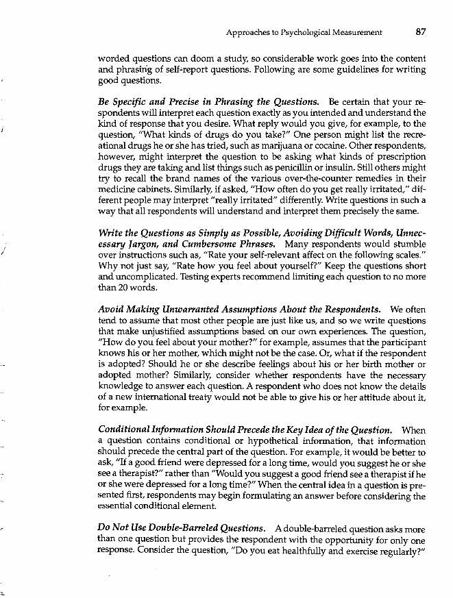
i I'

Approaches to Psychological Measurement 87

worded questions can doom a study, so considerable work goes into the content and phrasirig of self.:.report questions. Following are some guidelines for writing good questions.

Be Specific and Precise in Phrasing the Questions. Be certain that your re­spondents will interpret each question exactly as you intended and understand the kind of response that you desire. What reply would you give, for example, to the question, "What kinds of drugs do you take?" One person might list the recre­ational drugs he or she has tried, such as marijuana or cocaine. Other respondents, however, might interpret the question to be asking what kinds of prescription drugs they are taking and list things such as penicillin or insulin. Still others might try to recall the brand names of the various over-the-counter remedies in their medicine cabinets. Similarly, if asked, "How often do you get really irritated," dif­ferent people may interpret "really irritated" differently. Write questions in such a way that all respondents will understand and interpret them precisely the same.

Write the Questions as Simply as Possible, Avoiding Difficult Words, Unnec­essary Jargon, and Cumbersome Phrases. Many respondents would stumble over instructions such as, "Rate your self-relevant affect on the following scales." Why not just say, "Rate how you feel about yourself?" Keep the questions short and uncomplicated. Testing experts recommend limiting each question to no more than 20 words.

Avoid Making Unwarranted Assumptions About the Respondents. We often tend to assume that most other people are just like us, and so we write questions that make unjustified assumptions based on our own experiences. The question, "How do you feel about your mother?" for example, assumes that the participant knows his or her mother, which might not be the case. Or, what if the respondent is adopted? Should he or she describe feelings about his or her birth mother or adopted mother? Similarly, consider whether respondents have the necessary knowledge to answer each question. A respondent who does not know the details of a new international treaty would not be able to give his or her attitude about it, for example.

Conditional Information Should Precede the Key Idea of the Question. When a question contains conditional or hypothetical information, that information should precede the central part of the question. For example, it would be better to ask, "If a good friend were depressed for a long time, would you suggest he or she see a therapist?" rather than "Would you suggest a good friend see a therapist if he or she were depressed for a long time?" When the central idea in a question is pre­sented first, respondents may begin formulating an answer before considering the essential conditional element.

Do Not Use Double-Barreled Questions. A double-barreled question asks more than one question but provides the respondent with the opportunity for only one response. Consider the question, "Do you eat healthfully and exercise regularly?"

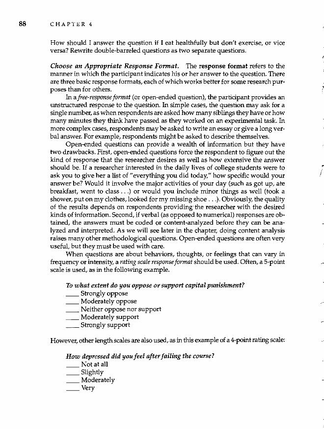
88 CHAPTER 4

How should I answer the question if I eat healthfully but don't exercise, or vice versa? Rewrite double-barreled questions as two separate questions.

Choose an Appropriate Response Format. The response format refers to the manner in which the participant indicates his or her answer to the question. There are three basic response formats, each of which works better for some research pur­poses than for others.

In a free-response format (or open-ended question), the participant provides an unstructured response to the question. In simple cases, the question may ask for a single number, as when respondents are asked how many siblings they have or how many minutes they think have passed as they worked on an experimental task. In more complex cases, respondents may be asked to write an essay or give a long ver­bal answer. For example, respondents might be asked to describe themselves.

Open-ended questions can provide a wealth of information but they have two drawbacks. First, open-ended questions force the respondent to figure out the kind of response that the researcher desires as well as how extensive the answer should be. If a researcher interested in the daily lives of college students were to ask you to give her a list of "everything you did today," how specific would your answer be? Would it involve the major activities of your day (such as got up, ate breakfast, went to class ... ) or would you include minor things as well (took a shower, put on my clothes, looked for my missing shoe ... ). Obviously, the quality of the results depends on respondents providing the researcher with the desired kinds of information. Second, if verbal (as opposed to numerical) responses are ob­tained, the answers must be coded or content-analyzed before they can be ana­lyzed and interpreted. As we will see later in the chapter, doing content analysis raises many other methodolOgical questions. Open-ended questions are often very useful, but they must be used with care.

When questions are about behaviors, thoughts, or feelings that can vary in frequency or intensity, a rating scale response format should be used. Often, as-point scale is used, as in the following example.

To what extent do you oppose or support capital punishment? __ Strongly oppose __ Moderately oppose __ Neither oppose nor support __ Moderately support __ Strongly support

However, other length scales are also used, as in this example of a 4-point rating scale:

How depressed did you feel after failing the course? Not at all

_Slightly _. _ Moderately __ Very

1

i"

!

)

,/

, ;/

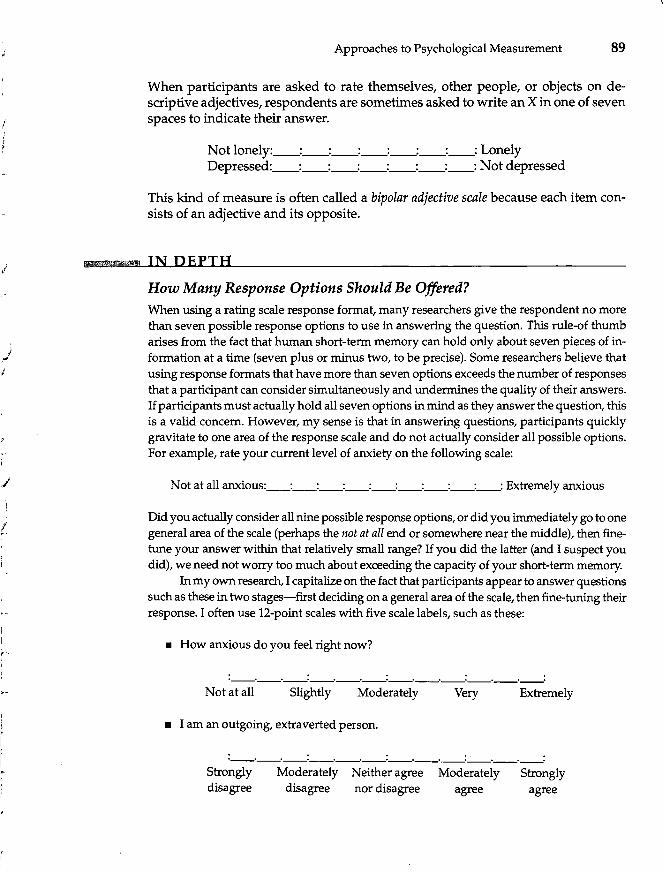
r­i I

.... I I

Approaches to Psychological Measurement 89

When participants are asked to rate themselves, other people, or objects on de­scriptive adjectives, respondents are sometimes asked to write an X in one of seven spaces to indicate their answer,

Not lonely: __ : __ : __ : __ : __ : __ : __ : Lonely Depressed: __ : __ : __ : __ : __ : __ : __ : Not depressed

This kind of measure is often called a bipolar adjective scale because each item con­sists of an adjective and its opposite,

IN DEPTH

How Many Response Options Should Be Offered? When using a rating scale response format, many researchers give the respondent no more than seven possible response options to use in answering the question, This rule-of thumb arises from the fact that human short-term memory can hold only about seven pieces of in­formation at a time (seven plus or minus two, to be precise), Some researchers believe that using response formats that have more than seven options exceeds the number of responses that a participant can consider simultaneously and undermines the quality of their answers, If participants must actually hold all seven options in mind as they answer the question, this is a valid concern, However, my sense is that in answering questions, participants quickly gravitate to one area of the response scale and do not actually consider all possible options, For example, rate your current level of anxiety on the following scale:

Not at all anxious: __ : __ : __ : __ : __ : __ : __ : __ : __ : Extremely anxious

Did you actually consider all nine possible response options, or did you immediately go to one general area of the scale (perhaps the not at all end or somewhere near the middle), then fine­tune your answer within that relatively small range? If you did the latter (and I suspect you did), we need not worry too much about exceeding the capacity of your short-term memory,

In my own research, I capitalize on the fact that participants appear to answer questions such as these in two stages-first deciding on a general area of the scale, then fine-tuning their response, I often use 12-point scales with five scale labels, such as these:

• How anxious do you feel right now?

. . . . . '--'--'--'--'--'--'--'--'--'--'--'--'

Not at all Slightly Moderately Very Extremely

• I am an outgoing, extraverted person,

. . . . . '--'--'--'--'--'--'--'--'--'--'--'--'

Strongly disagree

Moderately Neither agree Moderately Strongly disagree nor disagree agree agree

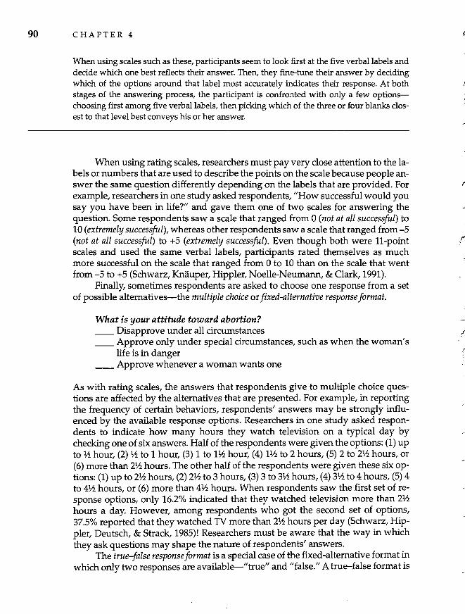
90 CHAPTER 4

When using scales such as these, participants seem to look first at the five verbal labels and decide which one best reflects their answer. Then, they fine-tune their answer by deciding which of the options around that label most accurately indicates their response. At both stages of the answering process, the participant is confronted with only a few options­choosing first among five verbal labels, then picking which of the three or four blanks clos­est to that level best conveys his or her answer.

When using rating scales, researchers must pay very close attention to the la­bels or numbers that are used to describe the points on the scale because people an­swer the same question differently depending on the labels that are provided. For example, researchers in one study asked respondents, "How successful would you say you have been in life?" and gave them one of two scales for answering the question. Some respondents saw a scale that ranged from 0 (not at all successful) to 10 (extremely successful), whereas other respondents saw a scale that ranged from-5 (not at all successful) to +5 (extremely successful). Even though both were ll-point scales and used the same verbal labels, participants rated themselves as much more successful on the scale that ranged from 0 to 10 than on the scale that went from -5 to +5 (Schwarz, Knauper, Hippler, Noelle-Neumann, & Clark, 1991).

Finally, sometimes respondents are asked to choose one response from a set of possible alternatives-the multiple choice or fixed-alternative response format.

What is your attitude toward abortion? __ Disapprove under all circumstances __ Approve only under special circumstances, such as when the woman's

life is in danger __ Approve whenever a woman wants one

As with rating scales, the answers that respondents give to multiple choice ques­tions are affected by the alternatives that are presented. For example, in reporting the frequency of certain behaviors, respondents' answers may be strongly influ­enced by the available response options. Researchers in one study asked respon­dents to indicate how many hours they watch television on a typical day by checking one of six answers. Half of the respondents were given the options: (1) up to 1h hour, (2) 1h to 1 hour, (3) 1 to 11h hour, (4) 11h to 2 hours, (5) 2 to 21h hours, or (6) more than 21h hours. The other half of the respondents were given these six op­tions: (1) up to 21h hours, (2) 21h to 3 hours, (3) 3 to 31h hours, (4) 31h to 4 hours, (5) 4 to 41h hours, or (6) more than 41h hours. When respondents saw the first set of re­sponse options, only 16.2% indicated that they watched television more than 21h hours a day. However, among respondents who got the second set of options, 37.5% reported that they watched TV more than 21h hours per day (Schwarz, Hip­pler, Deutsch, & Strack, 1985)! Researchers must be aware that the way in which they ask questions may shape the nature of respondents' answers.

The true-false response format is a special case of the fixed-alternative format in which only two responses are available-"true" and "false." A true-false format is

f

r

Approaches to Psychological Measurement 91

most useful for questions of fact (for example, "I attended church last week") but is not recommended for measuring attitudes and feelings. In most cases, people's subjective reactions are not clear-cut enough to fall neatly into a true or false cate­gory. For example, if asked to respond true or false to the statement, "I feel nervous in social situations," most people would have difficulty answering either true or false and would probably say, "It depends."

Researchers should consider various options when deciding upon a response format, then choose the one that provides the most useful information for their re­search purposes. Perhaps most importantly, researchers should be on guard for ways in which the questions themselves influence the nature of respondents' an­swers (Schwarz, 1999).

Pretest the Questions. Whenever possible, researchers pretest their questions before using them in a study. Questions are pretested by administering the ques­tionnaire or interview and instructing respondents to tell the researcher what they think each question is asking, report on difficulties they have understanding the questions or using the response formats, and express other reactions to the items. Based on participants' responses during pretesting, the questions can be revised before they are actually used in research.

Questionnaires

Questionnaires are perhaps the most ubiquitous of all psychological measures. Many dependent variables in experimental research are assessed via question­naires on which participants provide information about their cognitive or emo­tional reactions to the independent variable. Similarly, many correlational studies ask participants to complete questionnaires about their thoughts, feelings, and be­haviors, and questionnaires (called personality scales or inventories) are usually used to measure personality traits. Likewise, survey researchers often ask respon­dents to complete questionnaires about their attitudes, lifestyles, or behaviors. Even researchers who typically do not use questionnaires to measure dependent variables, such as physiological psychologists, may use them to ask about partic­ipants' reactions to the study. Questionnaires are used at one time or another not only by most researchers who study human behavior, but also by clinical psy­chologists to obtain information about their clients, by companies to collect data on applicants and employees, by members of Congress to poll their constituents, by restaurants to assess the quality of their food and service, and by colleges to ob­tain students' evaluations of their teachers. You have undoubtedly completed many questionnaires.

Although researchers must often design their own questionnaires, they usu­ally find it worthwhile to look for existing questionnaires before investing time and energy into designing their own. Existing measures often have a strong track record that gives us confidence in their psychometric properties. Particularly when using questionnaires to measure attitudes or personality, the chances are good that rele­vant measures already exist, although it sometimes takes a little detective work to track down measures that are relevant to a particular research topic. Keep in mind,

92 CHAPTER 4

however, that just because a questionnaire has been published does not necessarily indicate that it has adequate reliability and validity. Be sure to examine the available psychometric data for any measures you plan to use.

Four sources of information about existing measures are particularly useful. First, many psychological measures were initially published in journal articles, and you can locate these measures using the same kinds of strategies you use to search for articles on any topic (such as the computerized search service PsycInfo). Second, several books have been published that describe and critically evaluate measures used in behavioral and educational research. Some of these compendia of question­naires and tests-such as Mental Measurements Yearbook, Tests in Print, and the Direc­tory of Unpublished Experimental Mental Measures-include many different kinds of measures; other books focus on measures that are used primarily in certain kinds of research, such as personality psychology or health psychology (Robinson, Shaver, & Wrightsman, 1991). Third, several databases can be found on the World Wide Web that describe psychological tests and measures, such as ERIC's Clearing House on Assessment and Education, and Educational Testing Service's Test Collecting Catalog. Fourth, some questionnaires may be purchased from commercial publish­ers. In the case of commercially published scales, be aware that you must have cer­tain professional credentials to purchase many measures, and you are limited in how you may use them.

Although they often locate existing measures for their research, researchers sometimes must design measures "from scratch" either because appropriate measures do not exist or because they believe that the existing measures will not adequately serve their research purpose. But because new measures are time­consuming to develop and risky to use (in the sense that we do not know how well they will perform), researchers usually check to see whether relevant measures have already been published.

!!l1!'f!l!?!!!! BEHAVIORAL RESEARCH CASE STUDY

Self-Report Diaries

One shortcoming with some self-report questionnaires is that respondents have difficulty remembering the details needed to answer the questions accurately. Suppose, for example, that you are interested in whether lonely people have fewer contacts with close friends than nonlonely people. The most accurate way to examine this question would be to administer a measure of loneliness, then follow participants around for a week and directly observe whom they interact with. Obviously, practical and ethical problems preclude such an ap­proach, not to mention the fact that people would be unlikely to behave naturally with a re­searcher trailing them 24 hours a day.

Alternatively, you could measure participants' degree of loneliness, and then ask par­ticipants to report how many times (and for how long each time) they interacted with certain friends and acquaintances during the past week. If participants' memories were infallible, this would be a reasonable way to address the research question, but people's memories are simply not that good. Can you really recall everyone you interacted with during the past

I ;

Approaches to Psychological Measurement 93

seven days, and how long you interacted with each? Thus, neither observational methods nor retrospective self-reports are likely to yield valid data in a case such as this.

An approach that has seen increased use during the past 20 years involves diary methodology. Several different kinds of diary methodologies have been developed, but all of them ask participants to keep a daily record of information pertinent to the researcher's ques­tion. For example, Wheeler, Reis, and Nezlek (1983) used a diary approach to study the ques­tion posed above involving the relationship between loneliness and social interaction. In this study, participants completed a standard measure of loneliness and kept a daily record of their social interactions for about 2 weeks. For every interaction they had that lasted 10 minutes or longer, the participants filled out a short form on which they recorded whom they had inter­acted with, how long the interaction lasted, the gender of the other interactant(s), and other in­formation such as who had initiated the interaction and how pleasant the encounter was. By having participants record this information soon after each interaction, the researchers de­creased the likelihood that the data would be contaminated by participants' faulty memories.

The results showed that, for both male and female participants, loneliness was nega­tively related to the amount of time they interacted with women; that is, spending more time with women was associated with lower loneliness. Furthermore, although loneliness was not associated with the number of different people participants interacted with, lonely participants rated their interactions as less meaningful than less lonely participants did. In fact, the strongest predictor of loneliness was how meaningful participants found their daily interactions.

Diary methods have been used to study the relationship between everyday interaction and a variety of variables, including academic performance, gender, social support, alcohol use, self-presentation, physical attractiveness, and friendship (see Reis & Wheeler, 1991).

Interviews

For some research purposes, participants' answers to questions are better obtained in face-ta-face or telephone interviews rather than on questionnaires. Each of the guide­lines for writing questionnaire items discussed above is equally relevant for design­ing an interview schedule-the series of questions that are used in an interview.

In addition, the researcher must consider how the interview process itself­the interaction between the interviewer and respondent-will affect participants' responses. Following are a few suggestions of ways for interviewers to improve the quality of the responses they receive from interviewees.

Create a Friendly Atmosphere. The interviewer's first goal should be to put the re­spondent at ease. Respondents who like and trust the interviewer will be more open and honest in their answers than those who are intimidated or angered by the interviewer's style.

Maintain an Attitude of Friendly Interest. The interviewer should appear truly in­terested in the respondent's answers, rather than mechanically recording the re­sponses in a disinterested manner.

94 CHAPTER 4

Conceal Personal Reactions to the Respondent's Answers. At the same time, however, the interviewer should not react to the respondents' answers. The interviewer should never show surprise, approval, disapproval, or other reactions to what the respondent says.

Order the Sections of the Interview to Facilitate Building Rapport and to Create a Logical Sequence. Start the interview with the most basic and least threatening topics, then move slowly to more specific and sensitive questions as the respondent be­comes more relaxed.

Ask Questions Exactly as They Are Worded. In most instances, the interviewer should ask each question in precisely the same way to all respondents. Impromptu wordings of the questions introduces differences in how various respondents are interviewed, thereby increasing measurement error and lowering the reliability of participants' responses.

Don't Lead the Respondent. In probing the respondent's answer-asking for clarifi­cation or details-one must be careful not to put words in the respondent's mouth.

Advantages of Questionnaires Versus Interviews

Both questionnaires and interviews have advantages and disadvantages, and re­searchers must decide which strategy will best serve a particular research purpose. On one hand, because questionnaires require less extensive training of researchers and can usually be administered to groups of people simultaneously, they are often less expensive and time-consuming than interviews. Furthermore, if the topic is a sensitive one, participants can be assured that their responses to a questionnaire will be anonymous, whereas anonymity is impossible in a face-to-face interview. Thus, participants may be more honest on questionnaires than in interviews.

On the other hand, if respondents are drawn from the general population, questionnaires are inappropriate for those who are functionally illiterate-approx­imately 10% of the adult population of the United States. Similarly, interviews are necessary for young children, people who are cognitively impaired, severely dis­turbed individuals, and others who are incapable of completing questionnaires on their own. Also, interviews allow the researcher to be sure respondents understand each question before answering. We have no way of knowing whether respondents understand all of the questions on a questionnaire. Perhaps the greatest advantage of interviews is that detailed information can be obtained about complex topics. A skilled interviewer can probe respondents for elaboration of details in a way that is impossible on a questionnaire. Table 4.1 presents a comparison of the advantages of questionnaires and interviews.

Biases in Self-Report Measurement

Although measurement in all sciences is subject to biases of various sorts (for ex­ample, all scientists are prone to see what they expect to see), the measures used in

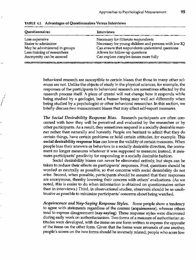
i j

Approaches to Psychological Measurement 95

TABLE 4.1 Advantages of Questionnaires Versus Interviews

Questionnaires

Less expensive Easier to administer May be administered in groups Less training of researchers Anonymity can be assured

Interviews

Necessary for illiterate respondents Necessary for young children and persons with low IQ Can ensure that respondents understand questions Allows for follow-up questions Can explore complex issues more fully

behavioral research are susceptible to certain biases that those in many other sci­ences are not. Unlike the objects of study in the physical sciences, for example, the responses of the participants in behavioral research are sometimes affected by the research process itself. A piece of crystal will not change how it responds while being studied by a geologist, but a human being may well act differently when being studied by a psychologist or other behavioral researcher. In this section, we briefly discuss two measurement biases that may affect self-report measures.

The Social Desirability Response Bias. Research participants are often con­cerned with how they will be perceived and evaluated by the researcher or by other participants. As a result, they sometimes respond in a sOcially desirable man­ner rather than naturally and honestly. People are hesitant to admit that they do certain things, have certain problems or hold certain attitudes, for example. This social desirability response bias can lower the validity of certain measures. When people bias their answers or behaviors in a socially desirable direction, the instru­ment no longer measures whatever it was supposed to measure; instead, it mea­sures participants' proclivity for responding in a socially desirable fashion.

Social desirability biases can never be eliminated entirely, but steps can be taken to reduce their effects on participants' responses. First, questions should be worded as neutrally as possible, so that concerns with social deSirability do not arise. Second, when possible, participants should be assured that their responses are anonymous, thereby lowering their concern with others' evaluations. (As we noted, this is easier to do when information is obtained on questionnaires rather than in interviews.) Third, in observational studies, observers should be as unob­trusive as possible to minimize participants' concerns about being watched.

Acquiescence and Nay-Saying Response Styles. Some people show a tendency to agree with statements regardless of the content (acquiescence), whereas others tend to express disagreement (nay-saying). These response styles were discovered during early work on authoritarianism. Two forms of a measure of authoritarian at­titudes were developed, with the items on one form written to express the opposite of the items on the other form. Given that the forms were reversals of one another, people's scores on the two forms should be inversely related; people who score low

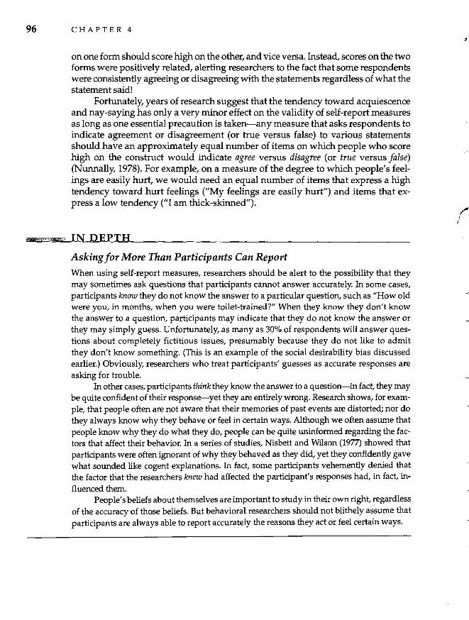
96 CHAPTER 4

on one form should score high on the other, and vice versa. Instead, scores on the two forms were positively related, alerting researchers to the fact that some respondents were consistently agreeing or disagreeing with the statements regardless of what the statement said!

Fortunately, years of research suggest that the tendency toward acquiescence and nay-saying has only a very minor effect on the validity of self-report measures as long as one essential precaution is taken-any measure that asks respondents to indicate agreement or disagreement (or true versus false) to various statements should have an approximately equal number of items on which people who score high on the construct would indicate agree versus disagree (or true versus false) (Nunnally, 1978). For example, on a measure of the degree to which people's feel­ings are easily hurt, we would need an equal number of items that express a high tendency toward hurt feelings (liMy feelings are easily hurt") and items that ex­press a low tendency ("I am thick-skinned").

IN DEPTH

Asking for More Than Participants Can Report

When using self-report measures, researchers should be alert to the possibility that they may sometimes ask questions that participants cannot answer accurately. In some cases, participants know they do not know the answer to a particular question, such as "How old were you, in months, when you were toilet-trained?" When they know they don't know the answer to a question, participants may indicate that they do not know the answer or they may simply guess. Unfortunately, as many as 30% of respondents will answer ques­tions about completely fictitious issues, presumably because they do not like to admit they don't know something. (This is an example of the social desirability bias discussed earlier.) Obviously, researchers who treat participants' guesses as accurate responses are asking for trouble.

In other cases, participants think they know the answer to a question-in fact, they may be quite confident of their response-yet they are entirely wrong. Research shows, for exam­ple, that people often are not aware that their memories of past events are distorted; nor do they always know why they behave or feel in certain ways. Although we often assume that people know why they do what they do, people can be quite uninformed regarding the fac­tors that affect their behavior. In a series of studies, Nisbett and WIlson (1977) showed that participants were often ignorant of why they behaved as they did, yet they confidently gave what sounded like cogent explanations. In fact, some participants vehemently denied that the factor that the researchers knew had affected the participant's responses had, in fact, in­fluenced them.

People's beliefs about themselves are important to study in their own right, regardless of the accuracy of those beliefs. But behavioral researchers should not blithely assume that participants are always able to report accurately the reasons they act or feel certain ways.

(

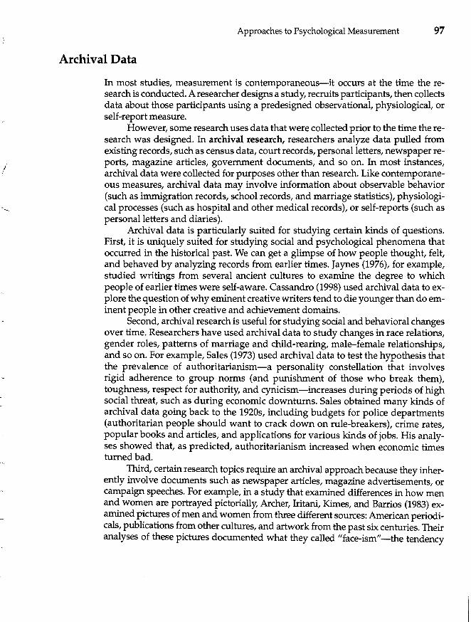
l

--

,.

Approaches to Psychological Measurement 97

Archival Data

In most studies, measurement is contemporaneous-it occurs at the time the re­search is conducted. A researcher designs a study, recruits participants, then collects data about those participants using a predesigned observational, physiological, or self-report measure.

However, some research uses data that were collected prior to the time the re­search was designed. In archival research, researchers analyze data pulled from existing records, such as census data, court records, personal letters, newspaper re­ports, magazine articles, government documents, and so on. In most instances, archival data were collected for purposes other than research. Like contemporane­ous measures, archival data may involve information about observable behavior (such as immigration records, school records, and marriage statistics), physiolOgi­cal processes (such as hospital and other medical records), or self-reports (such as personal letters and diaries).

Archival data is particularly suited for studying certain kinds of questions. First, it is uniquely suited for studying social and psychological phenomena that occurred in the historical past. We can get a glimpse of how people thought, felt, and behaved by analyzing records from earlier times. Jaynes (1976), for example, studied writings from several ancient cultures to examine the degree to which people of earlier times were self-aware. Cassandro (1998) used archival data to ex­plore the question of why eminent creative writers tend to die younger than do em­inent people in other creative and achievement domains.

Second, archival research is useful for studying social and behavioral changes over time. Researchers have used archival data to study changes in race relations, gender roles, patterns of marriage and child-rearing, male-female relationships, and so on. For example, Sales (1973) used archival data to test the hypothesis that the prevalence of authoritarianism-a personality constellation that involves rigid adherence to group norms (and punishment of those who break them), toughness, respect for authority, and cynicism-increases during periods of high social threat, such as during economic downturns. Sales obtained many kinds of archival data going back to the 1920s, including budgets for police departments (authoritarian people should want to crack down on rule-breakers), crime rates, popular books and articles, and applications for various kinds of jobs. His analy­ses showed that, as predicted, authoritarianism increased when economic times turned bad.

Third, certain research topics require an archival approach because they inher­ently involve documents such as newspaper articles, magazine advertisements, or campaign speeches. For example, in a study that examined differences in how men and women are portrayed pictorially, Archer, Iritani, Kimes, and Barrios (1983) ex­amined pictures of men and women from three different sources: American periodi­cals, publications from other cultures, and artwork from the past six centuries. Their analyses of these pictures documented what they called "face-ism"-the tendency

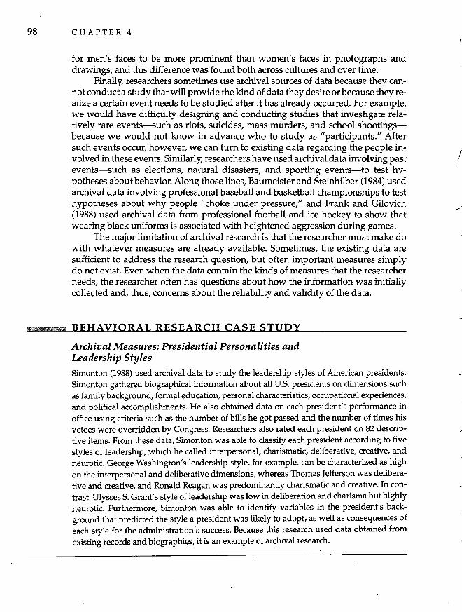
98 CHAPTER 4

for men's faces to be more prominent than women's faces in photographs and drawings, and this difference was found both across cultures and over time.

Finally, researchers sometimes use archival sources of data because they can­not conduct a study that will provide the kind of data they desire or because they re­alize a certain event needs to be studied after it has already occurred. For example, we would have difficulty designing and conducting studies that investigate rela­tively rare events-such as riots, suicides, mass murders, and school shootings­because we would not know in advance who to study as "participants." After such events occur, however, we can tum to existing data regarding the people in­volved in these events. Similarly, researchers have used archival data involving past events-such as elections, natural disasters, and sporting events-to test hy­potheses about behavior. Along those lines, Baumeister and Steinhilber (1984) used archival data involving professional baseball and basketball championships to test hypotheses about why people "choke under pressure," and Frank and Gilovich (1988) used archival data from professional football and ice hockey to show that wearing black uniforms is associated with heightened aggression during games.

The major limitation of archival research is that the researcher must make do with whatever measures are already available. Sometimes, the existing data are sufficient to address the research question, but often important measures simply do not exist. Even when the data contain the kinds of measures that the researcher needs, the researcher often has questions about how the information was initially collected and, thus, concerns about the reliability and validity of the data.

m BEHAVIORAL RESEARCH CASE STUDY

Archival Measures: Presidential Personalities and Leadership Styles Simonton (1988) used archival data to study the leadership styles of American presidents. Simonton gathered biographical information about all U.S. presidents on dimensions such as family background, formal education, personal characteristics, occupational experiences, and political accomplishments. He also obtained data on each president's performance in office using criteria such as the number of bills he got passed and the number of times his vetoes were overridden by Congress. Researchers also rated each president on 82 deSCrip­tive items. From these data, Simonton was able to classify each president according to five styles of leadership, which he called interpersonal, charismatic, deliberative, creative, and neurotic. George Washington's leadership style, for example, can be characterized as high on the interpersonal and deliberative dimensions, whereas Thomas Jefferson was delibera­tive and creative, and Ronald Reagan was predominantly charismatic and creative. In con­trast, Ulysses S. Grant's style of leadership was low in deliberation and charisma but highly neurotic. Furthermore, Simonton was able to identify variables in the president's back­ground that predicted the style a president was likely to adopt, as well as consequences of each style for the administration's success. Because this research used data obtained from existing records and biographies, it is an example of archival research.

t /

)

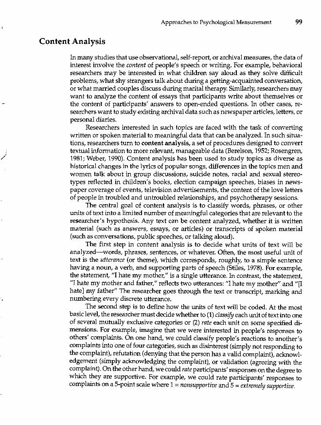
Approaches to Psychological Measurement 99

Content Analysis

In many studies that use observational, self-report, or archival measures, the data of interest involve the content of people's speech or writing. For example, behavioral researchers may be interested in what children say aloud as they solve difficult problems, what shy strangers talk about during a getting-acquainted conversation, or what married couples discuss during marital therapy. Similarly, researchers may want to analyze the content of essays that participants write about themselves or the content of participants' answers to open-ended questions. In other cases, re­searchers want to study existing archival data such as newspaper articles, letters, or personal diaries.

Researchers interested in such topics are faced with the task of converting written or spoken material to meaningful data that can be analyzed. In such situa­tions, researchers turn to content analysis, a set of procedures designed to convert textual information to more relevant, manageable data (Berelson, 1952; Rosengren, 1981; Weber, 1990). Content analysis has been used to study topics as diverse as historical changes in the lyrics of popular songs, differences in the topics men and women talk about in group discussions, suicide notes, racial and sexual stereo­types reflected in children's books, election campaign speeches, biases in news­paper coverage of events, television advertisements, the content of the love letters of people in troubled and untroubled relationships, and psychotherapy sessions.

The central goal of content analysis is to classify words, phrases, or other units of text into a limited number of meaningful categories that are relevant to the researcher's hypothesis. Any text can be content analyzed, whether it is written material (such as answers, essays, or articles) or transcripts of spoken material (such as conversations, public speeches, or talking aloud).

The first step in content analysis is to decide what units of text will be analyzed-words, phrases, sentences, or whatever. Often, the most useful unit of text is the utterance (or theme), which corresponds, roughly, to a simple sentence having a noun, a verb, and supporting parts of speech (Stiles, 1978). For example, the statement, "I hate my mother," is a single utterance. In contrast, the statement, "I hate my mother and father," reflects two utterances: "I hate my mother" and "[I hate] my father" The researcher goes through the text or transcript, marking and numbering every discrete utterance.

The second step is to define how the units of text will be coded. At the most basic level, the researcher must decide whether to (1) classify each unit of text into one of several mutually exclusive categories or (2) rate each unit on some specified di­mensions. For example, imagine that we were interested in people's responses to others' complaints. On one hand, we could classify people's reactions to another's complaints into one of four categories, such as disinterest (simply not responding to the complaint), refutation (denying that the person has a valid complaint), acknowl­edgement (simply acknowledging the complaint), or validation (agreeing with the complaint). On the other hand, we could rate participants' responses on the degree to which they are supportive. For example, we could rate participants' responses to complaints on a 5-point scale where 1 = nonsupportive and 5 = extremely supportive.

100 CHAPTER 4

Whichever system is used, clear rules must be developed for classifying or rating the text. These rules must be so explicit and clear that two raters using the system will rate the material in the same way. To maximize the degree to which their ratings agree, raters must discuss and practice the system before actually cod­ing the textual material from the study. Also, researchers assess the interrater reli­ability of the system by determining the degree to which the raters' classifications or ratings are consistent with one another (see Chapter 3). If the reliability is low, the coding system is clarified or redesigned.

After the researcher is convinced that interrater reliability is sufficiently high, raters code the textual material for all participants. They must do so independently and without conferring with one another so that interrater reliability can again be assessed based on ratings of the material obtained in the study.

Although researchers must sometimes design a content analysis coding sys­tem for use in a particular study, they should always explore whether a system al­ready exists that will serve their purposes. Coding schemes have been developed for analyzing everything from newspaper articles to evidence of inner psycholog­ical states (such as hostility and anxiety) to group discussions and conversations (Bales, 1970; Rosengren, 1981; Stiles, 1978; Viney, 1983). A growing number of com­puter software programs also content analyze textual material.

Summary

1. Most measures used in behavioral research involve either observations of overt behavior, measures of physiological responses, self-report questions (on questionnaire or in interviews), or archival data.

2. Researchers who use observational measures must decide whether the obser­vation will occur in a natural or contrived setting. Naturalistic observation in­volves observing behavior as it occurs naturally with no intrusion by the researcher. Contrived observation involves observing behavior in settings that the researcher has arranged specifically for observing and recording behavior.

3. Participant observation is a special case of naturalistic observation in which researchers engage in the same activities as the people they are studying.

4. When researchers are concerned that behaviors may be reactive (affected by participants' knowledge that they are being observed), they sometimes con­ceal from participants the fact they are being observed. However, because disguised observation sometimes raises ethical issues, researchers often use undisguised observation or partial concealment strategies, rely on the obser­vations of knowledgeable informants, or use unobtrusive measures.

5. Researchers record the behaviors they observe in four general ways: narra­tive records (relatively complete descriptions of a participant's behavior), checklists (tallies of whether certain behaviors were observed), temporal measures (such as measures of latency and duration), and observational rating scales (on which researchers rate the intensity or quality of partici­pants'reactions).

f" (

,I

r ( I

Approaches to Psychological Measurement 101

6. Interrater reliability can be increased by developing precise operational defi­nitions of the behaviors being observed and by giving observers the oppor­tunity to practice using the observational coding system.

7. Physiological measures are used to measure processes occurring in the par­ticipant's body. Such measures can be used to assess neural activity (such as brain waves and the activity of specific neurons), autonomic arousal (such as heart rate and blood pressure), biochemical processes involving hormones and neurotransmitters, and observable physical reactions (such as blushing or reflexes).

8. Participants' self-reports can be obtained using either questionnaires or in­terviews, each of which has its advantages and disadvantages.

9. To write good questions for questionnaires and interviews, researchers should use precise terminology, write the questions as simply as possible, avoid making unwarranted assumptions about the respondents, put conditional information before the key part of the question, avoid double-barreled ques­tions, choose an appropriate response format, and pretest the questions.

10. Self-report measures may use one of three general response formats: free­response, rating scale, and fixed-alternative (or multiple choice).

11. Before designing questionnaires from scratch, researchers should always in­vestigate whether measures already exist that will serve their research needs.

12. When a self-report diary methodology is used, respondents keep a daily record of certain target behaviors.

13. When interviewing, researchers must structure the interview setting in a way that enhances the respondents' comfort and that promotes the honesty and accuracy of their answers.

14. Whenever self-report measures are used, researchers must guard against the social desirability response bias (the tendency for people to respond in ways that convey a socially desirable impression), and acquiescence and nay-saying response styles.

15. Archival data is obtained from existing records, such as census data, news­paper articles, research reports, and personal letters.

16. If spoken or written textual material is collected, it must be content analyzed. The goal of content analysis is to classify units of text into meaningful cate­gories or to rate units of text along specified dimensions.

KEY TERMS

acquiescence (p. 95) archival research (p. 97) checklist (p. 83) content analysis (p. 99) contrived observation (p. 80) diary methodology (p. 93) disguised observation (p. 81)

duration (p. 84) field notes (p. 83) interbehavior latency (p. 84) interview (p. 86) interview schedule (p. 93) knowledgeable informant

(p.81)

latency (p. 84) narrative record (p. 83) naturalistic observation

(p.78) nay-saying (p. 95) observational method (p. 78) participant observation (p. 79)

102 CHAPTER 4

physiological measure (p. 85) questionnaire (p. 86) reaction time (p. 84) reactivity (p. 80)

response format (p. 88) social desirability response

bias (p. 95) task completion time (p. 84)

QUESTIONS FOR REVIEW

undisguised observation (p.80)

unobtrusive measure (p. 81)

1. Discuss the pros and cons of using naturalistic versus contrived observation.

2. What special opportunities and problems does participant observation create for researchers?

3. What does it mean if a behavior is reactive?

4. What are three ways in which researchers minimize reactivity?

5. What is the right of informed consent?

6. Explain how Ickes' dyadic interaction paradigm helps to avoid the problem of re­activity.

7. What are the advantages and disadvantages of using narrative records in observa­tional research?

8. Distinguish between a structured and unstructured observation method.

9. Distinguish between checklists and observational rating scales as ways to record behavior. When do researchers use each one?

10. Define reaction time, task completion time, and interbehavior latency.

11. Give three examples (other than those in the chapter) of measures of duration.

12. What is interrater reliability, and what are some ways in which you can increase the interrater reliability of observational methods?

13. Give five examples of physiological measures.

14. What considerations must a researcher keep in mind when writing the questions to be used on a questionnaire or in an interview?

15. What is a double-barreled question?

16. Describe the three basic types of response formats-free-response, rating scale, multiple choice.

17. Which of the three response formats would be most useful in obtaining the follow­ing information? a. to ask whether the respondent's maternal grandfather is still living b. to measure the degree to which participants liked another person with whom

they had just interacted c. to find out whether the participant was single, married, divorced, or widowed d. to find out how happy the participants felt e. to ask participants to describe why a recent romantic breakup had occurred

I

r ..

-'

. i

Approaches to Psychological Measurement 103

18. How might you find information about measures that have been developed by ofllerresearchers?

19. What are diary mefllodologies, and why are flley used?

20. Discuss ways in which interviewers can increase flle reliability and validity of flle information flley obtain from respondents.

21. Discuss flle advantages and disadvantages of using questionnaires versus inter­views to obtain self-report data.

22. How can researchers minimize flle effects of flle social desirability response bias on participants' self-reports?

23. List as many sources of archival data as you can.

24. What four kinds of research questions are particularly suited for flle use of archi­val data?

25. Describe how you would conduct a content analysis .

QUESTIONS FOR DISCUSSION

1. Design a questionnaire fllat assesses people's eating habits. Your questions could ad­dress topics such as what flley eat, when flley eat, how much flley eat, wifll whom flley eat, where flley eat, how healflly flleir eating habits are, and so on. In designing your questionnaire, be sure to consider flle issues discussed throughout fl1is chapter.

2. Pretest your questionnaire by giving it to fl1ree peQple. Ask for flleir reactions to each question, looking for potential problems in how flle questions are worded and in flle response formats that you used.

3. Do you fl1ink fllat people's responses on your questionnaire might be affected by re­sponse biases? If so, what steps could you take to minimize fllem?

4. Obtain two textbooks-one in a social or behavioral science (such as psychology, so­ciology, communication, or anthropology) and flle ofller in a natural science (such as biology, chemistry, or physics). Pick a page from each at random (but be sure to choose a page fllat is all text, wifll no figures or tables). Do a content analysis of flle text on fllese pages that will address flle question, "Are textbooks in behavioral and social science written in a more personal style fl1an textbooks in natural science?" You will need to (a) decide what unit of text will be analyzed, (b) operationally de­fine what it means for somefl1ing to be written in a "personal style," (c) develop your coding system, (d) code flle material on flle two pages of text, and (e) describe flle differences you discovered between flle two texts. (Note: Because fllere will likely be a different number of units of text on flle two pages, you will need to adjust flle scores for the two pages by flle number of units on that page.)

5. Using flle approaches discussed in fl1is chapter, identify as many existing scales as possible that measure attitudes toward members of ofller races. Locate two or three of fllese scales (in your library, for example).

CHAPTER

5 Descriptive Research

Types of Descriptive Research

Sampling Describing and Presenting Data

104

Each year, the Federal Interagency Forum on Child and Family Statistics releases a report that describes the results of studies dealing with crime, smoking, illicit drug use, nutrition, and other topics relevant to the well-being of children and ado­lescents in the United States. The most recent report painted a mixed picture of how American youth are faring at the start of the new millennium. On one hand, studies showed that many American high school students engage in behaviors that may have serious consequences for their health. For example, 22% of high school seniors in a nationwide survey reported that they smoked daily, 32% indicated that they had drunk heavily in the past two weeks, and 26% said that they had used il­licit drugs in the previous 30 days. The percentages for younger adolescents, al­though lower, also showed a high rate of risky behavior: the data for eighth grade students showed that 9% smoked regularly, 14% drank heavily, and 15% had used illicit drugs in the previous month. On the other hand, the studies also showed im­provements in the well-being of young people. In particular, the number of young people who were victims of violent crime (such as robbery, rape, aggravated as­sault, and homicide) was at a 20-year low.

The studies that provided these results involved descriptive research. The purpose of descriptive research is to describe the characteristics or behaviors of a given population in a systematic and accurate fashion. Typically, descriptive research is not designed to test hypotheses but rather is conducted to provide in­formation about the physical, social, behavioral, economic, or psychological char­acteristics of some group of people. The group of interest may be as large as the population of the world or as small as the students in a particular school. Descriptive research may be conducted to obtain basic information about the group of interest or to provide to government agencies and other policy-making groups specific data concerning social problems.

I

j

Descriptive Research 105

Types of Descriptive Research

Although several kinds of descriptive research may be distinguished, we will ex­amine three that psychologists and other behavioral researchers often use-sur­vey, demographic, and epidemiological research.

Surveys

Surveys are, by far, the most common type of descriptive research. They are used in virtually every area of social and behavioral science. For example, psychologists use surveys to inquire about people's attitudes, lifestyles, behaviors, and prob­lems; sociologists use surveys to study political preferences and family systems; political scientists use surveys to study political attitudes and predict the outcomes of elections; government researchers do surveys to understand social problems; and advertisers conduct survey research to understand consumers' attitudes and buying patterns. In each case, the goal is to provide a description of people's be­haviors, thoughts, or feelings.

In survey research, respondents provide ~ormation about themselves by completing a questionnaire or answering an interviewer's questions. (We dis­cussed the relative advantages and disadvantages of questionnaires versus inter­views in Chapter 4.) Many surveys are conducted face-to-face, as when people are recruited to report to a survey center or pedestrians are stopped on the street to an­swer questions, but some are conducted by phone or through the mail.

Most surveys involve a cross-sectional survey design in which a single group of respondents--a "cross section" of the population-is surveyed. These one-shot studies can provide important information about the characteristics of the group and, if more than one group is surveyed, about how various groups differ in their attitudes or behaviors.

Changes in attitudes or behavior can be examined if a cross section of the pop­ulation is studied more than once. In a successive independent samples survey de­sign, two or more samples of respondents answer the same questions at different points in time. Even though the samples are composed of different individuals, conclusions can be drawn about how people have changed if the respondents are selected in the same manner each time. For example, since 1939 the Gallup organi­zation has asked successive independent random samples of Americans, "Did you happen to attend a church or synagogue service in the last seven days?" As the data in Table 5.1 show, the percentage of Americans who attend religious services has re­mained remarkably constant over a 60-year span. The validity of a successive inde­pendent samples design depends on the samples being comparable, so researchers must be sure that each sample is selected in precisely the same way.

In a longitudinal or panel survey design, a single group of respondents is questioned more than once. If the same sample is surveyed on more than one occa­sion, changes in their behavior can be studied. However, problems arise with a panel survey design when, as usually happens, not all respondents who were surveyed

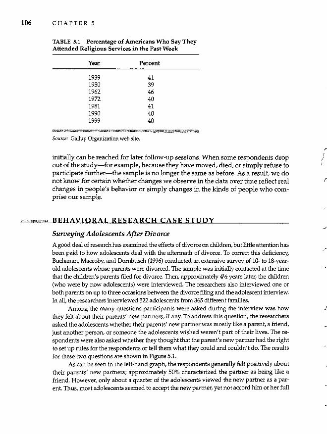
106 CHAPTER 5

TABLE 5.1 Percentage of Americans Who Say They Attended Religious Services in the Past Week

Source: Gallup Organization web site.

initially can be reached for later follow-up sessions. When some respondents drop out of the study-for example, because they have moved, died, or simply refuse to participate further-the sample is no longer the same as before. As a result, we do not know for certain whether changes we observe in the data over time reflect real changes in people's behavior or simply changes in the kinds of people who com­prise our sample.

f%,,,*_re BEHAVIORAL RESEARCH CASE STUDY

Surveying Adolescents After Divorce

A good deal of research has examined the effects of divorce on children, but little attention has been paid to how adolescents deal with the aftennath of divorce. To correct this deficiency, Buchanan, Maccoby, and Dornbusch (1996) conducted an extensive survey of 10- to 18-year­old adolescents whose parents were divorced. The sample was initially contacted at the time that the children's parents filed for divorce. Then, approximately 4lh years later, the children (who were by now adolescents) were interviewed. The researchers also interviewed one or both parents on up to three occasions between the divorce filing and the adolescent interview. In all, the researchers interviewed 522 adolescents from 365 different families.

Among the many questions participants were asked during the interview was how they felt about their parents' new partners, if any. To address this question, the researchers asked the adolescents whether their parents' new partner was mostly like a parent, a friend, just another person, or someone the adolescents wished weren't part of their lives. The re­spondents were also asked whether they thought that the parent's new partner had the right to set up rules for the respondents or tell them what they could and couldn't do. The results for these two questions are shown in Figure 5.l.

As can be seen in the left-hand graph, the respondents generally felt positively about their parents' new partners; approximately 50% characterized the partner as being like a friend. However, only about a quarter of the adolescents viewed the new partner as a par­ent. Thus, most adolescents seemed to accept the new partner, yet not accord him or her full

r' /

i

r

--

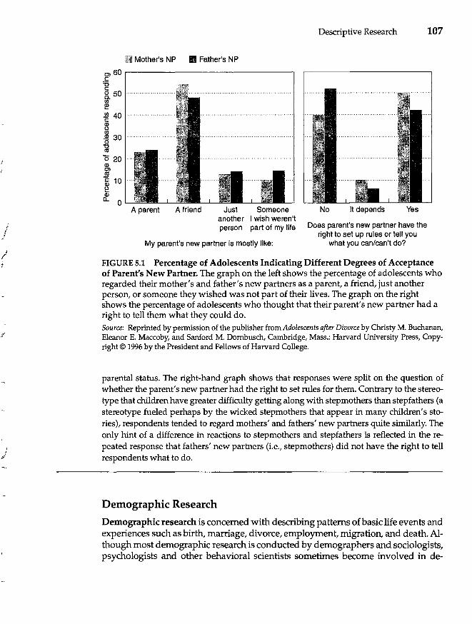
i i

)

j ;I

• Mother's NP • Father's NP

Cl 60 ,-----------------, c: =g o 50 ~ I!? -El 40

~ .!!! 30

~ '0 20 Q)

i 10 ~ 8? o

A parent A friend Just Someone another I wish weren't person part of my life

My parent's new partner is mostly like:

Descriptive Research 107

No It depends Yes

Does parent's new partner have the right to set up rules or tell you

what you can/can't do?

FIGURE 5.1 Percentage of Adolescents Indicating Different Degrees of Acceptance of Parenfs New Partner. The graph on the left shows the percentage of adolescents who regarded their mother's and father's new partners as a parent, a friend, just another person, or someone they wished was not part of their lives. The graph on the right shows the percentage of adolescents who thought that their parent's new partner had a right to tell them what they could do. Source: Reprinted by permission of the publisher from Adolescents after Divorce by Christy M. Buchanan, Eleanor E. Maccoby, and Sanford M. Dornbusch, Cambridge, Mass.: Harvard University Press, Copy­right © 1996 by the President and Fellows of Harvard College.

parental status. The right-hand graph shows that responses were split on the question of whether the parent's new partner had the right to set rules for them. Contrary to the stereo­type that children have greater difficulty getting along with stepmothers than stepfathers (a stereotype fueled perhaps by the wicked stepmothers that appear in many children's sto­ries), respondents tended to regard mothers' and fathers' new partners quite similarly. The only hint of a difference in reactions to stepmothers and stepfathers is reflected in the re­peated response that fathers' new partners (Le., stepmothers) did not have the right to tell respondents what to do.

Demographic Research

Demographic research is concerned with describing patterns of basic life events and experiences such as birth, marriage, divorce, employment, migration, and death. Al­though most demographic research is conducted by demographers and sociologists, psychologists and other behavioral scientists sometimes become involved in de-

108 C HAP T E R 5

mography because they are interested in the psychological processes that underlie major life events. For example, a psychologist may be interested in understanding differences in family size, marriage patterns, or divorce rates among various popu­lation groups.

Epidemiological Research

Epidemiological research is used to study the occurrence of disease in different groups of people. Most epidemiological research is conducted by medical re­searchers who study patterns of health and illness, but psychologists are often in­terested in epidemiology for two reasons. First, many illnesses and injuries are affected by people's behavior and lifestyles. For example, skin cancer is directly related to how much people expose themselves to the sun, and one's chances of contracting a sexually transmitted disease is related to practicing safe sex. Thus, epidemiological data can provide information regarding groups that are at risk of illness or injury, thereby helping health psychologists target certain groups for in­terventions to reduce their risk.

Second, some epidemiological research deals with describing the prevalence and incidence of psychological disorders. (Prevalence refers to the proportion of a population that has a particular disease or disorder at a particular point in time; in­cidence refers to the rate at which new cases of the disease or disorder occur over a specified period.) Behavioral researchers are interested in documenting the occur­rence of psychological problems-such as depression, alcoholism, child abuse, and schizophrenia; they conduct epidemiological studies to do so.

For example, data released by the National Institute of Mental Health (1999) showed that approximately 31,000 people died from suicide in the United States in 1996. Of those, the vast majority had a diagnosable psychological disorder, most commonly depression or substance abuse. Men were four times more likely to com­mit suicide than were women, and the highest suicide rate in the United States is among white men over the age of 65. Of course, many young people also commit sui­cide; in 1998, the most recent year for which statistics are available, suicide was the third leading cause of death among 15- to 24-year olds. Descriptive, epidemiological data such as these provide important information about the prevalence of psycho­logical problems in particular groups, thereby raising questions for future research and suggesting groups to which mental health programs should be targeted.

Summary

Although psychologists are less likely to conduct descriptive research than other kinds we will discuss in this book (correlational, experimental, and quasi­experimental research), descriptive research plays an important role in behavioral science. Survey, demographic, and epidemiological research provide a picture of how large groups of people tend to think, feel, and behave. Thus, descriptive data can help point researchers to topics and problems that need attention and suggest hypotheses that can be examined in future research. For example, if descriptive re-

I

I !

!

-,. i

j

I

Descriptive Research 109

search shows that the attitudes, behaviors, or experiences of people in different groups differ in important ways, researchers can begin to explore the psychological processes that are responsible for those differences. Importantly, the quality of the results obtained from descriptive research depends greatly on how the researcher obtained his or her sample of participants. Thus, we now turn our attention to the topic of sampling.

Sampling

In 1936, the magazine Literary Digest surveyed more than 2 million voters regarding their preference for Alfred Landon versus Franklin Roosevelt in the upcoming pres­idential election. Based on the responses they received, the Digest predicted that Landon would defeat Roosevelt by approximately 15 percentage points. When the election was held, however, not only was Roosevelt elected president, but his mar­gin of victory was overwhelming. Roosevelt received 62% of the popular vote, com­pared to 38% for Landon. As we will see later, the problem with the Literary Digest survey involved how the researchers selected respondents for the survey.

Among the decisions that researchers face each time they design a study is se­lecting research participants. Researchers can rarely examine every individual in the population who is relevant to their interests-all newborns, all paranoid schiz­ophrenics, all color-blind adults, all registered voters, all female porpoises, or who­ever. Fortunately there is absolutely no need to study every individual in the population of interest. Instead, researchers collect data from a subset, or sample, of individuals in the population. Just as a physician can learn a great deal about a pa­tient by analyzing a small sample of the patient's blood (and need not drain every drop of blood for analysis), researchers can learn about a population by analyzing a relatively small sample of individuals. Sampling is the process by which a re­searcher selects a sample of participants for a study from the population of interest. In this section, we focus on ways in which researchers select samples of participants to study.

Probability Samples

When the purpose of a study is to accurately describe the behavior, thoughts, or feel­ings of a particular group-as it is with most descriptive research-researchers must ensure that the sample they select is representative of the population at large. A rep­resentative sample is one from which we can draw accurate, unbiased estimates of the characteristics of the larger population. We can draw accurate inferences about the population from data obtained from a sample only if it is representative.

The E"or of Estimation. Unfortunately, samples rarely mirror their parent pop­ulations in every respect. The characteristics of the individuals selected for the sample always differ somewhat from the characteristics of the general population. This difference, called sampling error, causes results obtained from the sample to

110 C HAP T E R 5

differ from what would have been obtained had the entire population been stud­ied. If you calculate the average grade point average of a representative sample of 200 students at your college or university, the mean for this sample will not per­fectly match the mean you would obtain based on all students in your school. If the sample is truly representative, however, the value obtained on the sample should be very close to what would be obtained if the entire population were studied.

Fortunately, when probability sampling techniques are used, researchers can estimate how much their results are affected by sampling error. The error of esti­mation (also called the margin of error) indicates the degree to which the data ob­tained from the sample is expected to deviate from the population as a whole. For example, you may have heard newscasters report the results of a political opinion poll, then add that the results "are accurate within 3 percentage points." What this means is that if 45% of the respondents in the sample endorsed Smith for president, we know that there is a 95% probability that the true percentage of people in the population who support Smith is between 42% and 48% (that is, 45% ± 3%). Byal­lowing researchers to estimate the sampling error in their data, probability sam­ples permit them to specify how confident they are that the results obtained on the sample accurately reflect the behavior of the population. Their confidence is ex­pressed in terms of the error of estimation.

The smaller the error of estimation, the more closely the results from the sam­ple estimate the behavior of the larger population. For example, if the limits on the error of estimation are only ±1 %, the sample data are a better indicator of the population than if the limits on the error of estimation are ±10%. Obviously, re­searchers prefer the error of estimation to be as small as possible.

The error of estimation is a function of three things: sample size, population size, and variance of the data. First, the larger a probability sample, the more simi­lar to the population the sample tends to be (that is, the smaller the sampling error) and the more accurately the sample data estimate the population. In light of this, you might expect that researchers always obtain as large a sample as possible. This is not the case, however. Rather, researchers opt for an economic sample-one that provides a reasonably accurate estimate of the population (within a few percent­age points) at reasonable effort and cost. After a sample of a certain size is obtained, collecting additional data adds little to the accuracy of the results.

For example, if we are trying to estimate the percentage of voters in a population of 10,000 who will vote for a particular candidate in a close election, interviewing a sample of 500 will allow us to estimate the percentage of voters in the population who will support each candidate within nine percentage points. Increasing the sam­ple size to 1,000 (an increase of 500 respondents) lowers the error of estimation from ±9% to only ±3%, a rather substantial improvement in accuracy. However, adding an additional 500 participants beyond that to the sample helps relatively little; with 1,500 respondents in the sample, the error of estimation drops only to 2.3%. In this in­stance, it may make little practical sense to increase the sample size beyond 1,000.

The error of estimation also is affected by the size of the population from which the sample was drawn. Imagine we have two samples of 200 respondents. The first was drawn from a population of 400, the second from a population of 10 million. Which sample would you expect to mirror more closely the behavior of

r

" i

J 1

I' I

I

I ./

( i ; (

Descriptive Research 111

the population? I think you can guess that the error of estimation will be lower when the population contains 400 cases than when it contains 10 million cases.

The third factor that affects the error of estimation is the variance of the data. The greater the variability in the data, the more difficult it is to estimate accurately the population values. We saw in earlier chapters that the larger the variance, the less representative the mean is of the scores as a whole. As a result, the larger the variance in the data, the larger must be the sample from which to draw accurate in­ferences about the population.

Researchers can calculate the error of estimation only if they know the prob­ability that a particular individual in the population was included in the sample, and they can do this only when they use a probability sample. With a probability sample, the researcher can specify the probability that any individual in the popu­lation will be included in the sample. Typically, researchers use an epsem design, which specifies that all cases in the population have an equal probability of being chosen for the sample (Schuman & Kalton, 1985). (Epsem stands for equal proba­bility selection method.) Knowing the probability that a particular case will be in­cluded in the sample allows researchers to calculate how representative of the population the sample is because they can estimate the sampling error. Probability samples may be obtained in several ways, but three basic methods involve simple random sampling, stratified random sampling, and cluster sampling.

Simple Random Sampling. When a sample is chosen in such a way that every possible sample of the desired size has the same chance of being selected from the population, the sample is a simple random sample. For example, suppose we want to select a sample of 200 participants from a school district that has 5,000 students. If we wanted a simple random sample, we would select our sample in such a way that every possible combination of 200 students has the same probability of being chosen.

To obtain a simple random sample, the researcher must have a sampling frame-a list of the population from which the sample will be drawn. Then partic­ipants are chosen randomly from this list. If the population is small, one approach is to write the name of each case in the population on a slip of paper, shuffle the slips of paper, then pull slips out until a sample of the desired size is obtained. For example, we could type each of the 5,000 students' names on cards, shuffle the cards, then randomly pick 200. However, with larger populations, pulling names "out of a hat" becomes unwieldy. One common procedure is to use a table of ran­dom numbers. A portion of such a table is shown in Table 5.2, along with an ex­planation of how to use it.

@~ DEVELOPING YOUR RESEARCH SKILLS

Using a Table of Random Numbers

When researchers want to obtain a random sample from a larger population, they often use a table of random numbers. The numbers on such a table are generated in a random order. A small portion of a table of random numbers is shown below for demonstrational pur­poses. A complete table of random numbers appears in Appendix A-I.

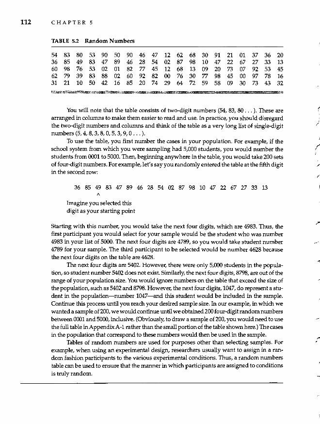
112 CHAPTER 5

TABLE 5.2 Random Numbers

54 83 80 53 90 50 90 46 47 12 62 68 30 91 21 01 37 36 20 36 85 49 83 47 89 46 28 54 02 87 98 10 47 22 67 27 33 13 60 98 76 53 02 01 82 77 45 12 68 13 09 20 73 07 92 53 45 62 79 39 83 88 02 60 92 82 00 76 30 77 98 45 00 97 78 16 31 21 10 50 42 16 85 20 74 29 64 72 59 58 09 30 73 43 32

You will note that the table consists of two-digit numbers (54, 83, 80 ... ). These are arranged in columns to make them easier to read and use. In practice, you should disregard the two-digit numbers and columns and think of the table as a very long list of single-digit numbers (5,4,8,3,8,0,5,3,9,0 ... ).

To use the table, you first number the cases in your population. For example, if the school system from which you were sampling had 5,000 students, you would number the students from 0001 to 5000. Then, beginning anywhere in the table, you would take 200 sets of four-digit numbers. For example, let' s say you randomly entered the table at the fifth digit in the second row:

%~fi~~~46~54m~%lO~22~V~~ A

Imagine you selected this digit as your starting point

Starting with this number, you would take the next four digits, which are 4983. Thus, the first participant you would select for your sample would be the student who was number 4983 in your list of 5000. The next four digits are 4789, so you would take student number 4789 for your sample. The third participant to be selected would be number 4628 because the next four digits on the table are 4628.

The next four digits are 5402. However, there were only 5,000 students in the popula­tion, so student number 5402 does not exist. Similarly, the next four digits, 8798, are out of the range of your population size. You would ignore numbers on the table that exceed the size of the population, such as 5402 and 8798. However, the next four digits, 1047, do represent a stu­dent in the population-number 1047-and this student would be included in the sample. Continue this process until you reach your desired sample size. In our example, in which we wanted a sample of 200, we would continue until we obtained 200 four-digit random numbers between 0001 and 5000, inclusive. (Obviously, to draw a sample of 200, you would need to use the full table in Appendix A-1 rather than the small portion of the table shown here.) The cases in the population that correspond to these numbers would then be used in the sample.

Tables of random numbers are used for purposes other than selecting samples. For example, when using an experimental design, researchers usually want to assign in a ran­dom fashion participants to the various experimental conditions. Thus, a random numbers table can be used to ensure that the manner in which participants are assigned to conditions is truly random.

,/

/

Descriptive Research 113

Stratified Random Sampling. Stratified random sampling is a variation of simple random sampling. Rather than selecting cases directly from the population, we first divide the population into two or more strata. A stratum is a subset of the population that shares a particular characteristic. For example, we might divide the population into men and women or into six age ranges (20-29,30-39,40-49, 50-59,60-69, over 69). Then, cases are randomly sampled from each of the strata.

By first dividing the population into strata, we sometimes increase the prob­ability that the participants we select will be representative of those in the popula­tion. In addition, stratification ensures that researchers have adequate numbers of participants from each strata so that they can examine differences in responses among the various strata. For example, the researcher might want to compare younger respondents (20-29 years old) with older respondents (60-69 years old). By first stratifying the sample, the researcher ensures that there will be an ample number of both young and old respondents in the sample.

Cluster Sampling. Although they provide us with very accurate pictures of the population, simple and stratified random sampling have a major drawback: They re­quire that we have a sampling frame of all cases in the population before we begin. Obtaining a list of small, easily identified populations is no problem. You would find it relatively easy to obtain a list of all students in your college or all members of the American Psychological Society, for example. Unfortunately, not all populations are easily identified. Could we, for example, obtain a list of every person in the United States or, for that matter, in New York City? Could we get a sampling frame of all His­panic three-year-olds, all people who are deaf who know sign language, or all single­parent families in Canada headed by the father? In cases such as these, random sampling is not possible because without a list we cannot locate potential partici­pants or specify the probability that a particular case will be included in the sample.

In such instances, cluster sampling is typically used. To obtain a cluster sam­ple, the researcher first samples not participants but rather groupings or clusters of participants. These clusters are often based on naturally occurring groupings, such as geographical areas or particular institutions. For example, if we wanted a sam­ple of elementary school children in West VIrginia, we might first randomly sam­ple from the 55 county school systems in West Virginia. Perhaps we would pick 15 counties at random. Then, after selecting this small random sample of counties, we could get lists of students for those counties and obtain random samples of stu­dents from the selected counties.

Often, cluster sampling involves a multistage sampling process in which we begin by sampling large clusters, then we sample smaller clusters from within the large clusters, then we sample even smaller clusters, and finally we obtain our sam­ple of participants. For example, we could randomly pick counties, then randomly choose several particular schools from the selected counties. We could then ran­domly select particular classrooms from the schools we selected, and finally ran­domly sample students from each classroom.

Cluster sampling has two advantages. First, a sampling frame of the popu­lation is not needed to begin sampling, only a list of the clusters. In this example,

114 CHAPTER 5

all we would need to start is a list of counties in West Virginia-a list that would be far easier to obtain than a census of all children enrolled in West VIrginia schools. Then, after sampling the clusters, we can get lists of students within each cluster (that is, county) that was selected, which is much easier than getting a census for the entire population of students in West Virginia. The second advantage is that, if each cluster represents a grouping of participants that are close together geographi­cally (such as students in a certain county or school), less time and effort are required to contact the participants. Focusing on only 15 counties would require consider­ably less time, effort, and expense than sampling students from all 55 counties in the state.

IN DEPTH

To Sample or Not to Sample: The Census Debate

Since the first U.S. census in 1790, the Bureau of the Census has struggled to find ways to ac­count for every individual in the country. For a variety of reasons, many citizens are missed by census-takers; in the 1990 census, for example, an estimated 8 million people were not counted. To combat this problem, the Census Bureau made plans to rely on sampling pro­cedures rather than to try to track down each and every person for the 2000 census.

Their plan was to count directly by mail or in person 90% of the population. Then, in­stead of trying to visit every one of the millions of households that did not respond to the mailed questionnaire or follow-up call, census-takers would visit a representative sample of the addresses that did not respond. The rationale was that, by focusing their time and effort on this representative sample rather than trying to contact all households unaccounted for (which the 1990 census showed was fruitless), they could greatly increase their chances of obtaining the missing information from these individuals. Then, using the data from the representative sample of nomesponding households, researchers could estimate the size and demographic characteristics of other households not accounted for.

Statisticians overwhelmingly agree that sampling will improve the accuracy of the cen­sus. A representative sample of nomesponding individuals provides far more accurate data than an incomplete set of households that is biased in unknown ways. However, despite its statistical merit, the plan met stiff opposition in Congress. Many people have trouble be­lieving that contacting a sample of nonresponding households provides more accurate data than trying (and failing) to locate them all, though you should now be able to see that this is the case. In addition, many politicians worried that the sample would be somehow biased (resulting perhaps in losses of federal money to their districts), would underestimate mem­bers of certain groups, or would undermine public trust in the census. Such concerns reflect misunderstandings about probability sampling.

Despite the fact that sampling promised to both improve the accuracy of the census and lower its cost, Congress denied the Bureau's plan to use sampling in the 2000 census. However, although the Census Bureau was forced to attempt a full-scale enumeration of every individual in the country as in previous years, a compromise allowed it to also study sampling procedures to validate their usefulness.

,. (

f

I I I

) ,

(

Descriptive Research 115

The Problem of Non response. The nonresponse problem is the failure to obtain responses from individuals that researchers select for their sample. In practice, re­searchers are rarely able to obtain perfectly representative samples. Imagine, for example, that we wish to obtain a representative sample of family physicians for a study of professional burnout. We design a survey to assess burnout and, using a professional directory to obtain names, mail this questionnaire to a random sample of family physicians in our state. To obtain a truly representative sample, every physician we choose for our sample must complete and return the questionnaire. If our return rate is less than 100%, the data we obtain may be biased in ways that are impossible to determine. For example, physicians who are burned out may be unlikely to take the time to complete and return our questionnaire. Or perhaps those who do return it are highly conscientious or have especially positive atti­tudes toward behavioral research. In any case, the representativeness of our sam­ple is compromised.

A similar problem arises when telephone surveys are used. Aside from the fact that a telephone sample is not representative of the country at large (only about 93% of American households have telephones), the nonresponse rate is often high in tele­phone surveys. We will find it difficult, if not impossible, to contact some of the people who were randomly selected for our sample. People who travel frequently, who work at odd hours, who live somewhere other than where their phone is, or who screen their calls may be inaccessible. Furthermore, we are likely to encounter many people who are unwilling to answer our questions. Given these limitations, the final set of respondents we contact may not be representative of the population.

Researchers can tackle the nonresponse problem in at least two ways. First, they can take steps to increase the response rate. When mail surveys are used, for example, researchers often follow up the initial mailing of the questionnaire with telephone calls or postcards to urge the respondents to complete and return them. Although we rarely get 100% of the sample to respond, we can be more confident of our findings the higher the response rate.

Second, to whatever extent possible, researchers try to determine whether re­spondents and nonrespondents differ in any systematic ways. Based on what they know about the sample they select, researchers can see whether those who did and did not respond differ. For example, the professional directory we use to obtain a sample of physicians may provide their birthdates, the year in which they obtained their medical degrees, their workplaces (hospital versus private practice), and other information. Using this information, we may be able to show that those who re­turned the survey did not differ from those who did not. (Of course, they may dif­fer on dimensions about which we have no information.)

e! IN DEPTH

The Literary Digest Survey

As noted earlier, pollsters hired by the Literary Digest failed miserably in their attempt to pre­dict the outcome of the 1936 presidential election between Roosevelt and Landon, misjudging

116 C HAP T E R 5

the margin of victory by 39 points in the wrong direction! The problem in this poll was entirely due to sampling. The names of the respondents contacted for the survey were taken from telephone directories and automobile registration lists. This sampling procedure had yielded accurate predictions in the presidential elections of 1920, 1924, 1928, and 1932. However, un­like in the previous polls, the people who had telephones and automobiles in 1936 were not representative of voters in the country at large. In the aftermath of the Great Depression, many voters had neither cars nor phones, and those voters overwhelmingly supported Roosevelt. Because individuals who were accessible by phone tended to be wealthier (and more likely to be Republican) than the population at large, the sample was not representative and the re­sults of the survey were biased.

Nonprobability Samples

Having seen the importance of a probability sample in descriptive research, it may now surprise you to learn that, in most research contexts, it is impossible, imprac­tical, or unnecessary for a researcher to obtain a probability sample. In such cases, nonprobability samples are used. With a nonprobability sample, researchers have no way of knowing the probability that a particular case will be chosen for the sam­ple. As a result, they cannot calculate the error of estimation to determine precisely how representative of the population at large the sample is. However, in many re­search contexts, this does not necessarily create a problem for the interpretation of our results, though it does limit our ability to generalize them.

When a researcher is interested in accurately describing the behavior of a par­ticular population from a sample-as in most descriptive research-probability sampling is a necessity. Without probability sampling, we cannot be sure of the de­gree to which the data provided by the sample approximate the behavior of the larger population. Unfortunately, probability sampling is time-consuming, expen­sive, and difficult. For example, a developmental psychologist who is interested in studying language development will find it difficult to obtain a probability sample of all preschool children in the United States. As a result, probability samples are virtually never used in experimental research. Instead, much psychological re­search is conducted on samples (such as college students) that are clearly not rep­resentative of all people. Similarly, the animals used in research are never sampled randomly from all animals of that species but instead consist of individuals that are raised for laboratory use. You might wonder, then, about the validity of research that does not use probability samples.

Contrary to what you might expect, nonprobability samples are perfectly ac­ceptable for many kinds of research. The goal of most behavioral research is not to describe how a population behaves but rather to test hypotheses regarding how particular variables relate to behavior. Hypotheses are derived from theories; then research is conducted to see whether the predicted effects of the independent vari­ables are obtained. If the data are consistent with the hypotheses, they provide ev­idence in support of the theory regardless of the nature of the sample. Of course,

(

(

I"

/'

/

j .}

./

/

r

Descriptive Research 117

we may wonder whether the results generalize to other kinds of samples, but this question does not undermine the quality of our particular study.

In the case of experimental studies that use nonprobability samples, the exter­nal validity (or generalizability) of the findings can be assessed through replication. The same experiment can be conducted using other samples of participants who differ in age, education level, socioeconomic status, geographic region, and so on. If similar findings are obtained using several different samples, faith in the validity of the results is increased. Furthermore, to the extent that many basic psychological processes are universal, there is often little reason to expect different samples to re­spond differently. If this is true, then it matters little what kind of sample one uses; the processes involved will be similar. Of course, we cannot assume that certain psychological processes are, in fact, universal; only replication can show whether findings generalize across samples. But it is erroneous to assume that research con­ducted on nonprobability samples tells us nothing about people in general.

The three primary types of nonprobability samples are convenience, quota, and purposive samples.

Convenience Sampling. In a convenience sample, researchers use whatever par­ticipants are readily available. For example, we could stop the first 150 shoppers we encounter on a downtown street, sample people waiting in an airport or bus station, contact patients at a local hospital, or use convenience samples of psychology stu­dents. No one argues that students are representative of people in general or even of young adults. Even so, such samples are often used because they are easy to obtain.

Although using students as participants does not invalidate the results of a study, certain biases are common in student samples. For example, college students tend to be more intelligent than the general population. They also tend to come from middle- and upper-class backgrounds and to hold slightly more liberal atti­tudes than the population at large. Additional sampling biases are introduced when students are asked to volunteer to participate in research. Compared to students who choose not to volunteer, volunteers tend to be more unconventional, more self­confident, more extraverted, and higher in need for achievement (Bell, 1962).

In the early days of psychology, when a disproportionate number of college students were men, researchers commonly used only convenience samples of male participants (Grady, 1981), and today about one-fourth of behavioral research uses only one sex. In many instances, single-sex samples are justified by the researcher's interest; a study of postpartum depression necessarily involves a female sample, for example. Furthermore, many findings that occur in one sex generalize to the other; studies that look for potential sex differences often find none. However, because many findings are specific to one sex or the other, researchers are never justified in generalizing from the behavior of one sex to the behavior of the other sex (Reardon & Prescott, 1977). Only by using samples composed of both men and women can conclusions be drawn about whether the sexes do or do not differ from one another.

Quota Sampling. A quota sample is a convenience sample in which the researcher takes steps to ensure that certain kinds of participants are obtained in particular

118 C HAP T E R 5

proportions. The researcher specifies in advance that the sample will contain cer­tain percentages of particular kinds of participants. For example, if researchers wanted to obtain an equal proportion of male and female participants, they might decide to obtain 20 women and 20 men in a sample from a psychology class rather than simply select 40 people without regard to gender.

Purposive Sampling. For a purposive sample, researchers use their judgment to decide which participants to include in the sample, trying to choose respondents who are typical of the population. Unfortunately, researchers' judgments cannot be relied on as a trustworthy basis for selecting samples. One area in which purposive sampling has been used successfully, however, involves forecasting the results of national elections. Based on previous elections, researchers have identified partic­ular areas of the country that tend to vote like the country as a whole. Voters from these areas are then interviewed and their political preferences used to predict the outcome of an upcoming election.

!!!Mj~ BEHAVIORAL RESEARCH CASE STUDY

Sampling and Sex Surveys

People appear to have an insatiable appetite for information about other people's sexual lives. The first major surveys of sexual behavior were conducted by Kinsey and his colleagues in the 19405 and '50s (Kinsey, Pomeroy, & Martin, 1948; Kinsey, Pomeroy, Martin, & Gebhard, 1953). Kinsey's researchers interviewed more than 10,000 American men and women, asking about their sexual practices. You might think that with such a large sample, Kinsey would have ob­tained valid data regarding sexual behavior in the United States. Unfortunately, although Kin­sey's data were often cited as if they reflected the typical sexual experiences of Americans, his sampling techniques do not permit us to draw conclusions about people's sexual behavior.

Rather than using a probability sample that would have allowed him to calculate the error of estimation in his data, Kinsey relied on convenience samples (or what he called "100 percent samples"). His researchers would contact a particular group, such as a professional organization or sorority, then obtain responses from 100% of its members. However, these groups were not selected at random (as they would be in the case of cluster sampling). As a re­sult, there were a disproportionate number of respondents from Indiana in the sample, as well as an overabundance of college students, Protestants, and well-educated people (Kirby, 1977). In an analysis of Kinsey's sampling technique, Cochran, Mosteller, and Tukey (1953) con­cluded that because he had not used a probability sample, Kinsey's results "must be regarded as subject to systematic errors of unknown magnitude due to selective sampling" (p. 711).

Other surveys of sexual behavior have encountered similar difficulties. In the Hunt (1974) survey, names were chosen at random from the phone books of 24 selected American cities. This technique produced three sampling biases. First, the cities were not selected ran­domly. Second, by selecting names from the phone book, the survey overlooked people without phones and those with unlisted numbers. Third, only 20% of the people who were contacted agreed to participate in the study; how these respondents differed from those who

declined is impossible to judge.

(

,..

l I

I

.t

/

)

Descriptive Research 119

Several popular magazines-such as McCall's, Psychology Today, and Redbook-have also conducted large surveys of sexual behavior. Again, probability samples were not ob­tained and thus the accuracy of their data is questionable. The most obvious sampling bias in these surveys is that only people who can read respond to questionnaires in magazines, thereby eliminating the estimated 10% of the adult population who is illiterate. Also, read­ers of particular magazines are unlikely to be representative of the population at large.

In 1987, Hite published a book, Women and Love, that describes the findings of a na­tionwide study of women and their relationships with men. To ensure anonymity, ques­tionnaires were sent to organizations rather than to individuals, with the idea that the organizations would distribute the questionnaires to their members, who would then return them anonymously. Thus, the sample included primarily women who belonged to some kind of organization. Furthermore, out of the 100,000 questionnaires that were sent out, only 4,500 completed surveys were retumed-a return rate of only 4.5%. How respondents dif­fered from nonrespondents is impossible to determine, but the nonresponsiveness of the sample should make us very hesitant to generalize the findings to the population at large.

In fairness to all of these studies, obtaining accurate information about sexual behav­ior is a difficult and delicate task. Aside from the problems associated with obtaining any probability sample, the fact that a high percentage of people refuse to answer questions about sexuality biases the findings. The bottom line is that although the results of such sur­veys are interesting, we should not regard them as accurate indicators of sexual behavior in the general population.

Describing and Presenting Data

An important part of all research involves describing and presenting the results to other people. Even when description is not the primary goal, researchers must al­ways decide how to summarize and describe their data in the most meaningful and useful fashion possible.

Criteria of a Good Description

To be useful, descriptions of data should meet three criteria: accuracy, conciseness, and understandability. Obviously, data must be summarized and described accu­rately. Some ways of describing the findings of a study are more accurate than others. For example, as we'll see later, certain ways of graphing data may be mis­leading. Similarly, depending on the nature of the data (whether extreme scores exist, for example), certain statistics may summarize and describe the data more accurately than others. Researchers should always present their data in ways that most accurately represent the data.

Unfortunately, the most accurate descriptions of data are often the least use­ful because they overwhelm the reader with information. Strictly speaking, the most accurate description of a set of data would involve a table of the raw data­all participants' scores on all measures. There is virtually no possibility that data in

120 C HAP T E R 5

this raw form will be distorted. However, to be interpretable, data must be sum­marized in a concise and meaningful form. It is during this process that distortion can occur. Researchers must be selective in the data they choose to present, pre­senting only the data that most clearly describe the results.

Third, the description of one's data must be easily understood. Overly com­plicated tables, graphs, or statistics can obscure the findings and lead to confusion. Having decided which aspects of the data best portray the findings of a study, re­searchers must then choose the clearest, most straightforward manner of describ­ing the data.

Methods of summarizing and describing sets of numerical data can be classified as either numerical methods or graphical methods. Numerical methods summarize data in the form of numbers such as percentages or means. Graphical methods in­volve the presentation of data in graphical or pictorial form, such as graphs.

Frequency Distributions

The starting point for many data descriptions is the frequency distribution. A fre­quency distribution is a table that summarizes raw data by showing the number of scores that fall within each of several categories.

Simple Frequency Distributions. One way to summarize data is to construct a simple frequency distribution of the data. A simple frequency distribution indi­cates the number of participants who obtained each score. The possible scores are arranged from lowest to highest. Then, in a second column, the number of scores, or frequency of each score, is shown. For example, Table 5.3 presents the answers of 168 university students when asked to tell how many friends they had. From the frequency distribution, it is easy to see the range of answers (1-40) and to see which answer occurs most frequently (7).

Grouped Frequency Distributions. In many instances, simple frequency distrib­utions provide a meaningful, easily comprehended summary of the data. However, when there are many possible scores, it is difficult to make much sense out of a sim­ple frequency distribution. In these cases researchers use a grouped frequency dis­tribution that shows the frequency of subsets of scores. To make a grouped frequency distribution, you first break the range of scores into several subsets, or class inter­vals, of equal size. For example, to create a grouped frequency distribution of the data in Table 5.3, we could create eight class intervals: 1-5,6-10, 11-15, 16-20,21-25, 26-30,31-35, and 36-40. We could then indicate the frequency of scores in each of the class intervals, as shown in Table 5.4.

Often, researchers also include relative frequencies in a table such as this. The relative frequency of each class is the proportion of the total number of scores that falls in each class interval. It is calculated by dividing the frequency for a class in­terval by the total number of scores. For example, the relative frequency for the class interval 1-5 in Table 5.4 is 31/168 or 18.5%. If you'll compare the grouped fre­quency distribution (Table 5.4) to the simple frequency distribution (Table 5.3), you

I

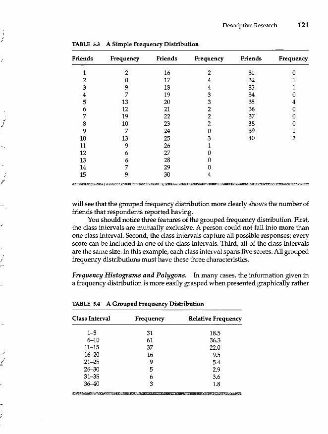
" I

I

.f

i ,J

/

)

I ..

Descriptive Research 121

TABLE 5.3 A Simple Frequency Distribution

Friends Frequency Friends Frequency Friends Frequency

1 2 16 2 31 0 2 0 17 4 32 1 3 9 18 4 33 1 4 7 19 3 34 0 5 13 20 3 35 4 6 12 21 2 36 0 7 19 22 2 37 0 8 10 23 2 38 0 9 7 24 0 39 1

10 13 25 3 40 2 11 9 26 1 12 6 27 0 13 6 28 0 14 7 29 0 15 9 30 4

gem;m"eH!Pla:a-~€ mm1~!iI!'il~~m.12!!~!!I!lml.!m".-..,~~- I!m i~ I ill !im.iiEilitiif'2, i1Ilml_S!FI!!fiI1'J1lJilB

will see that the grouped frequency distribution more clearly shows the number of friends that respondents reported having.

You should notice three features of the grouped frequency distribution. First, the class intervals are mutually exclusive. A person could not fall into more than one class interval. Second, the class intervals capture all possible responses; every score can be included in one of the class intervals. Third, all of the class intervals are the same size. In this example, each class interval spans five scores. All grouped frequency distributions must have these three characteristics.

Frequency Histograms and Polygons. In many cases, the information given in a frequency distribution is more easily grasped when presented graphically rather

TABLE 5.4 A Grouped Frequency Distribution

Oass Interval Frequency Relative Frequency

1-5 31 18.5 6-10 61 36.3

11-15 37 22.0 16-20 16 9.5 21-25 9 5.4 26-30 5 2.9 31-35 6 3.6 36-40 3 1.8 ..

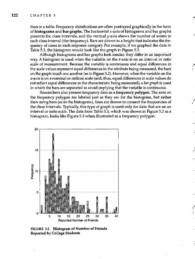
122 CHAPTER 5

than in a table. Frequency distributions are often portrayed graphically in the form of histograms and bar graphs. The horizontal x-axis of histograms and bar graphs presents the class intervals, and the vertical y-axis shows the number of scores in each class interval (the frequency). Bars are drawn to a height that indicates the fre­quency of cases in each response category. For example, if we graphed the data in Table 5.3, the histogram would look like the graph in Figure 5.2.

Although histograms and bar graphs look similar, they differ in an important way. A histogram is used when the variable on the x-axis is on an interval or ratio scale of measurement. Because the variable is continuous and equal differences in the scale values represent equal differences in the attribute being measured, the bars on the graph touch one another (as in Figure 5.2). However, when the variable on the x-axis is on a nominal or ordinal scale (and, thus, equal differences in scale values do not reflect equal differences in the characteristic being measured), a bar graph is used in which the bars are separated to avoid implying that the variable is continuous.

Researchers also present frequency data as a frequency polygon. The axes on the frequency polygon are labeled just as they are for the histogram, but rather than using bars (as in the histogram), lines are drawn to connect the frequencies of the class intervals. Typically, this type of graph is used only for data that are on an interval or ratio scale. The data from Table 5.3, which was shown in Figure 5.2 as a histogram, looks like Figure 5.3 when illustrated as a frequency polygon.

20.---------------------------------,

15

Ci' c::: ~ 10 CT ~ U.

o 5 1 0 15 20 25 30 35 40

Reported Number of Friends

FIGURE 5.2 Histogram of Number of Friends Reported by College Students

r I

r ,

I /

/" ,

!

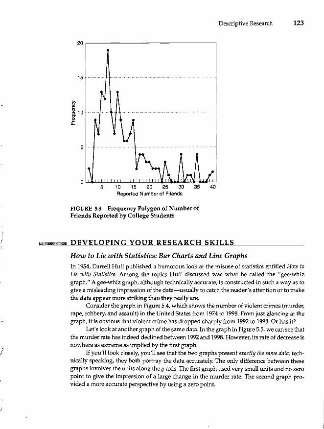
j I

"'

20r--------------------------------,

15 ................................................................................................. .

r; c: ~ 10 ............................................................................................. .

I

5 10 15 20 25 30 35 40 Reported Number of Friends

FIGURE 5.3 Frequency Polygon of Number of Friends Reported by College Students

Descriptive Research 123

7 DEVELOPING YOUR RESEARCH SKILLS

How to Lie with Statistics: Bar Charts and Line Graphs

In 1954, Darrell Huff published a humorous look at the misuse of statistics entitled How to Lie with Statistics. Among the topics Huff discussed was what he called the "gee-whiz graph." A gee-whiz graph, although technically accurate, is constructed in such a way as to give a misleading impression of the data-usually to catch the reader's attention or to make the data appear more striking than they really are.

Consider the graph in Figure 5.4, which shows the number of violent crimes (murder, rape, robbery, and assault) in the United States from 1974 to 1998. From just glancing at the graph, it is obvious that violent crime has dropped sharply from 1992 to 1998. Or has it?

Let's look at another graph of the same data. In the graph in Figure 5.5, we can see that the murder rate has indeed declined between 1992 and 1998. However, its rate of decrease is nowhere as extreme as implied by the first graph.

If you'll look closely, you'll see that the two graphs present exactly the same data; tech­nically speaking, they both portray the data accurately. The only difference between these graphs involves the units along the y-axis. The first graph used very small units and no zero point to give the impression of a large change in the murder rate. The second graph pro­vided a more accurate perspective by using a zero point.

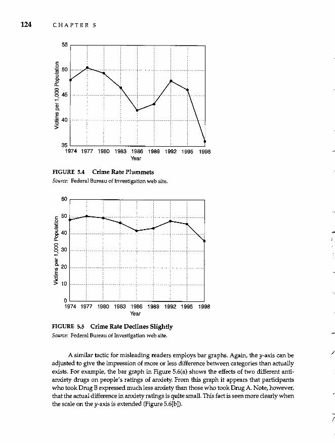
124 CHAPTER 5

55r---~--~--~--~--~----~--~--~

.... , .................................. : ......... .

~ Co i ~ ........... , ........... , ........... ; ........... , ........... ; .......... , ........... , .......... . 35~--~--~--~--~--~--~--~ __ -J

1~1m1~1~1~1~1~1~1~

Year

FIGURE 5.4 Crime Rate Plummets Source: Federal Bureau of Investigation web site.

60r---~--~--~--~--~----~--~--~

c: 50 o ··········t···········~···········t···········~···········t···········

~ ! ~ .........,', ......... ;........, ... . ! 30 ............ " ....................... _ ..................... ···1··.· ................... ,,············

i 20 ............ ( ....................... : ............ ; ........... -:- ........................ : ........... .

5 10 ···········t···········!···········t···········,······ ·····t···········!···········t············

. . . : : : o : : :

1~1m1~1~1~1~1~1~1~

Year

FIGURE 5.5 Crime Rate Declines Slightly Source: Federal Bureau of Investigation web site.

A similar tactic for misleading readers employs bar graphs. Again, the y-axis can be adjusted to give the impression of more or less difference between categories than actually exists. For example, the bar graph in Figure 5.6(a) shows the effects of two different anti­anxiety drugs on people's ratings of anxiety. From this graph it appears that participants who took Drug B expressed much less anxiety than those who took Drug A. Note, however, that the actual difference in anxiety ratings is quite small. This fact is seen more clearly when the scale on the y-axis is extended (Figure 5.6[b]).

(

,

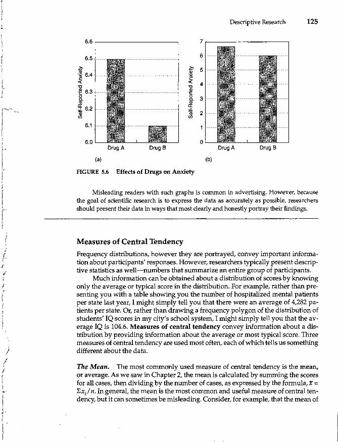
, I

}

( I f J

f-~;-

I } t

r j f

t r 1 1

/

r -'

,--:'-

i 1_

I • i

)

(' I \

f' r

1

---

Descriptive Research 125

6.6 7,------------,

6.5

i 6.4 ~ 'x

5·

~ I:: c(

"C "C

~ 6.3 ~ 8. 0

Co 3· Q) Q)

5: 6.2 0::

i iii 2 en en

1 .

6.0 o Drug A Drug B Drug A Drug B

(a) (b)

FIGURE 5.6 Effects of Drugs on Anxiety

Misleading readers with such graphs is common in advertising. However, because the goal of scientific research is to express the data as accurately as possible, researchers should present their data in ways that most clearly and honestly portray their findings.

Measures of Central Tendency

Frequency distributions, however they are portrayed, convey important informa­tion about participants' responses. However, researchers typically present descrip­tive statistics as well-numbers that summarize an entire group of participants.

Much information can be obtained about a distribution of scores by knowing only the average or typical score in the distribution. For example, rather than pre­senting you with a table showing you the number of hospitalized mental patients per state last year, I might simply tell you that there were an average of 4,282 pa­tients per state. Or, rather than drawing a frequency polygon of the distribution of students' IQ scores in my city's school system, I might simply tell you that the av­erage IQ is 104.6. Measures of central tendency convey information about a dis­tribution by providing information about the average or most typical score. Three measures of central tendency are used most often, each of which tells us something different about the data.

The Mean. The most commonly used measure of central tendency is the mean, or average. As we saw in Chapter 2, the mean is calculated by summing the scores for all cases, then dividing by the number of cases, as expressed by the formula, X = l:Xj / n. In general, the mean is the most common and useful measure of central ten­dency, but it can sometimes be misleading. Consider, for example, that the mean of

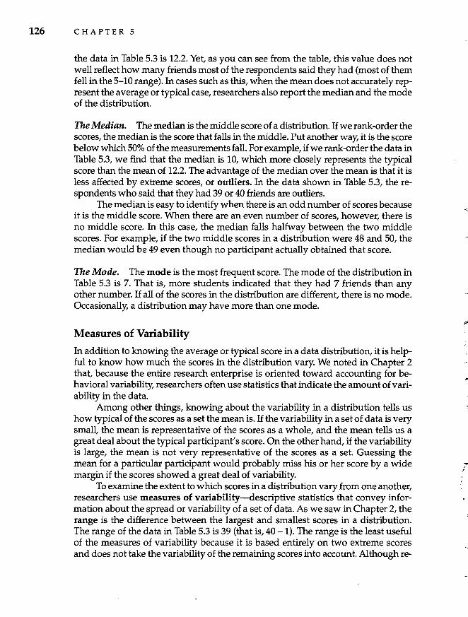
126 CHAPTER 5

the data in Table 5.3 is 12.2. Yet, as you can see from the table, this value does not well reflect how many friends most of the respondents said they had (most of them fell in the 5-10 range). In cases such as this, when the mean does not accurately rep­resent the average or typical case, researchers also report the median and the mode of the distribution.

The Median. The median is the middle score of a distribution. If we rank-order the scores, the median is the score that falls in the middle. Put another way, it is the score below which 50% of the measurements fall. For example, if we rank-order the data in Table 5.3, we find that the median is 10, which more closely represents the typical score than the mean of 12.2. The advantage of the median over the mean is that it is less affected by extreme scores, or outliers. In the data shown in Table 5.3, the re­spondents who said that they had 39 or 40 friends are outliers.

The median is easy to identify when there is an odd number of scores because it is the middle score. When there are an even number of scores, however, there is no middle score. In this case, the median falls halfway between the two middle scores. For example, if the two middle scores in a distribution were 48 and 50, the median would be 49 even though no participant actually obtained that score.

The Mode. The mode is the most frequent score. The mode of the distribution in Table 5.3 is 7. That is, more students indicated that they had 7 friends than any other number. If all of the scores in the distribution are different, there is no mode. Occasionally, a distribution may have more than one mode.

Measures of Variability

In addition to knowing the average or typical score in a data distribution, it is help­ful to know how much the scores in the distribution vary. We noted in Chapter 2 that, because the entire research enterprise is oriented toward accounting for be­havioral variability, researchers often use statistics that indicate the amount of vari­ability in the data.

Among other things, knowing about the variability in a distribution tells us how typical of the scores as a set the mean is. If the variability in a set of data is very small, the mean is representative of the scores as a whole, and the mean tells us a great deal about the typical participant's score. On the other hand, if the variability is large, the mean is not very representative of the scores as a set. Guessing the mean for a particular participant would probably miss his or her score by a wide margin if the scores showed a great deal of variability.

To examine the extent to which scores in a distribution vary from one another, researchers use measures of variability-descriptive statistics that convey infor­mation about the spread or variability of a set of data. As we saw in Chapter 2, the range is the difference between the largest and smallest scores in a distribution. The range of the data in Table 5.3 is 39 (that is, 40 - 1). The range is the least useful of the measures of variability because it is based entirely on two extreme scores and does not take the variability of the remaining scores into account. Although re-

,.

,"

... , (

!

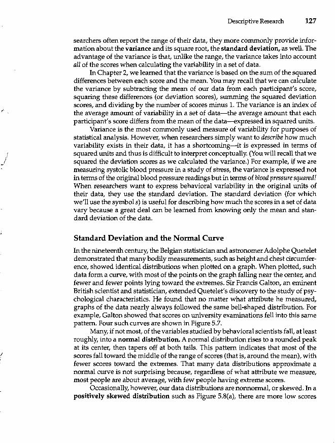
Descriptive Research 127

searchers often report the range of their data, they more commonly provide infor­mation about the variance and its square root, the standard deviation, as well. The advantage of the variance is that, unlike the range, the variance takes into account all of the scores when calculating the variability in a set of data.

In Chapter 2, we learned that the variance is based on the sum of the squared differences between each score and the mean. You may recall that we can calculate the variance by subtracting the mean of our data from each participant's score, squaring these differences (or deviation scores), summing the squared deviation scores, and dividing by the number of scores minus 1. The variance is an index of the average amount of variability in a set of data-the average amount that each participant's score differs from the mean of the data-expressed in squared units.

Variance is the most commonly used measure of variability for purposes of statistical analysis. However, when researchers simply want to describe how much variability exists in their data, it has a shortcoming-it is expressed in terms of squared units and thus is difficult to interpret conceptually. (You will recall that we squared the deviation scores as we calculated the variance.) For example, if we are measuring systolic blood pressure in a study of stress, the variance is expressed not in terms of the original blood pressure readings but in terms of blood pressure squared! When researchers want to express behavioral variability in the original units of their data, they use the standard deviation. The standard deviation (for which we'll use the symbol s) is useful for describing how much the scores in a set of data vary because a great deal can be learned from knowing only the mean and stan­dard deviation of the data.

Standard Deviation and the Normal Curve

In the nineteenth century, the Belgian statistician and astronomer Adolphe Quetelet demonstrated that many bodily measurements, such as height and chest circumfer­ence, showed identical distributions when plotted on a graph. When plotted, such data form a curve, with most of the points on the graph falling near the center, and fewer and fewer points lying toward the extremes. Sir Francis Galton, an eminent British scientist and statistician, extended Quetelet's discovery to the study of psy­chological characteristics. He found that no matter what attribute he measured, graphs of the data nearly always followed the same bell-shaped distribution. For example, Galton showed that scores on university examinations fell into this same pattern. Four such curves are shown in Figure 5.7.

Many, if not most, of the variables studied by behavioral scientists fall, at least roughly, into a normal distribution. A normal distribution rises to a rounded peak at its center, then tapers off at both tails. This pattern indicates that most of the scores fall toward the middle of the range of scores (that is, around the mean), with fewer scores toward the extremes. That many data distributions approximate a normal curve is not surprising because, regardless of what attribute we measure, most people are about average, with few people having extreme scores.

Occasionally, however, our data distributions are nonnormal, or skewed. In a positively skewed distribution such as Figure 5.S(a), there are more low scores

128 CHAPTER 5

~ c: 0) ::l

1

X Height in Inches

X Average High Temperature in Washington. DC in July

x IQ Scores

X Finish Times

in 5-Mile Race

FIGURE 5.7 Normal Distributions. Figure 5.7 shows four idealized normal distributions. In normal distributions such as these, most scores fall toward the middle of the range, with the greatest number of scores falling at the mean of the distribution. As we move in both directions away from the mean, the number of scores tapers off symmetrically, indicating an equal number of low and high scores.

than high scores in the data; if data are positively skewed, one observes a cluster­ing of scores toward the lower, left-hand end of the scale, with the tail of the distri­bution extending to the right. (The distribution of the data involving students' self-reported number of friends is also positively skewed; see Figure 5.3.) In a neg­atively skewed distribution such as Figure 5.8(b), there are more high scores than low scores; the hump is to the right of the graph, and the tail of the distribution ex­tends to the left.

g-O) ::l

I Scores

(a) Positively Skewed

Scores

(b) Negatively Skewed

FIGURE 5.S Skewed Distributions. In skewed distributions, most scores fall toward one end of the distribution. In a positively skewed distribution (a), there are more low scores than high scores. In a negatively skewed distribution (b), there are more high scores than low scores.

I'

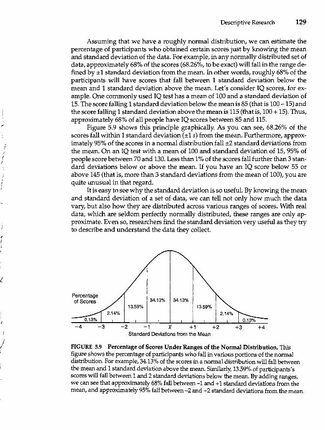
j

j

~

I

/ j

Descriptive Research 129

Assuming that we have a roughly normal distribution, we can estimate the percentage of participants who obtained certain scores just by knowing the mean and standard deviation of the data. For example, in any normally distributed set of data, approximately 68% of the scores (68.26%, to be exact) will fall in the range de­fined by ±1 standard deviation from the mean. In other words, roughly 68% of the participants will have scores that fall between 1 standard deviation below the mean and 1 standard deviation above the mean. Let's consider IQ scores, for ex­ample. One commonly used IQ test has a mean of 100 and a standard deviation of 15. The score falling 1 standard deviation below the mean is 85 (that is 100 -15) and the score falling 1 standard deviation above the mean is 115 (that is, 100 + 15). Thus, approximately 68% of all people have IQ scores between 85 and 115.

Figure 5.9 shows this principle graphically. As you can see, 68.26% of the scores fall within 1 standard deviation (±1 s) from the mean. Furthermore, approx­imately 95% of the scores in a normal distribution fall ±2 standard deviations from the mean. On an IQ test with a mean of 100 and standard deviation of 15, 95% of people score between 70 and 130. Less than 1% of the scores fall further than 3 stan­dard deviations below or above the mean. If you have an IQ score below 55 or above 145 (that is, more than 3 standard deviations from the mean of 100), you are quite unusual in that regard.

It is easy to see why the standard deviation is so useful. By knowing the mean and standard deviation of a set of data, we can tell not only how much the data vary, but also how they are distributed across various ranges of scores. With real data, which are seldom perfectly normally distributed, these ranges are only ap­proximate. Even so, researchers find the standard deviation very useful as they try to describe and understand the data they collect.

Percentage of Scores 34.13% 34.13%

13.59% 13.59%

-2 -1 x +1 +2 Standard Deviations from the Mean

FIGURE 5.9 Percentage of Scores Under Ranges of the Normal Distribution. 'This figure shows the percentage of participants who fall in various portions of the normal distribution. For example, 34.13% of the scores in a normal distribution will fall between the mean and 1 standard deviation above the mean. Similarly, 13.59% of participants's scores will fall between 1 and 2 standard deviations below the mean. By adding ranges, we can see that approximately 68% fall between -1 and +1 standard deviations from the mean, and approximately 95% fall between -2 and +2 standard deviations from the mean.

130 CHAPTER 5

DEVELOPING YOUR RESEARCH SKILLS

Calculating the Variance and Standard Deviation Although most researchers rely heavily on computers to conduct statistical analyses, you may occasionally have reason to calculate certain statistics by hand using a calculator. A de­scription of how to calculate the variance and the standard deviation by hand follows.

The formula for the variance, expressed in statistical notation, is

Remember that l: is summation, Yi refers to each participant's score, and n reflects the num­ber of participants.

To use this formula, you first square each score (Yl) and add these squared scores to­gether (l:yl). Then, add up all of the original scores (l:Yi) and square the sum [(l:Yi)2]. Finally, plug these numbers into the formula, along with the sample size (n), to get the variance. It simplifies the calculations if you set up a table with two columns-one for the raw scores and one for the square of the raw scores. If we do this for the data we analyzed in Chapter 2 dealing with attitudes about capital punishment, we get:

Participant # Yi yl 1 4 16 2 1 1 3 2 4 4 2 4 5 4 16 6 3 9

l:Yi = 16 l:yl=50 (l:Yi)2 = 256

Then,

52= 50-256/6 _ 50-42.67 1.47. 6-1 5

Thus, the variance (52) of these data is 1.47. To obtain the standard deviation (5), we simply take the square root of the variance. The standard deviation of these data is the square root of 1.47, or 1.21.

The z-Score

In some instances, researchers need a way to describe where a particular partici­pant falls in the data distribution. Just knowing that a certain participant scored 47

/

/

(

f

)

I /

I ; , i

I

I j I

J ,

t

Descriptive Research 131

on a test does not tell us very much. Knowing the mean of the data tells us whether the participant's score was above or below average, but without knowing some­thing about the variability of the data, we still cannot tell how far above or below the mean the participant's score was, relative to other participants.

The z-score, or standard score, is used to describe a particular participant's score relative to the rest of the data. A participant's z-score indicates how far from the mean in terms of standard deviations the participant's score varies. For exam­ple, if we find that a participant has a z-score of -1.00, we know that his or her score is 1 standard deviation below the mean. By referring to Figure 5.9 we can see that only about 16% of the other participants scored lower than this person. Similarly, a z-score of +2.9 indicates a score nearly 3 s's above the mean-one that is in the up­permost ranges of the distribution.

H we know the mean and standard deviation of a sample, a participant's z-score is easy to calculate:

z = (Yj-y)/s

where Yj is the participant's score, y is the mean of the sample, and s is the standard deviation of the sample.

Sometimes researchers standardize an entire set of data by converting all of the participants' raw scores to z-scores. This is a useful way to identify extreme scores or outliers. An outlier can be identified by a very low or very high z-score-one that falls below -3.00 or above +3.00, for example. Also, certain statistical analyses require standardization prior to the analysis. When a set of scores is standardized, the new set of z-scores always has a mean equal to 0 and a standard deviation equal to 1 re­gardless of the mean and standard deviation of the original data.

Summary

1. Descriptive research is designed to describe the characteristics or behaviors of a particular population in a systematic and accurate fashion.

2. Survey research uses questionnaires and interviews to collect information about people's attitudes, beliefs, feelings, behaviors, and lifestyles. Cross­sectional survey designs survey a single group of respondents, whereas a suc­cessive independent samples survey design surveys different samples at two or more points in time. A longitudinal or panel survey design surveys a single sample of respondents on more than one occasion.

3.

4.

5.

Demographic research describes patterns of basic life events, such as births, marriages, divorces, migration, and deaths. Epidemiological research studies the occurrence of physical and mental health problems. Sampling is the process by which a researcher selects a group of participants (the sample) from a larger population. When a probability sample is used, the researcher can specify the probability that any individual in the population will be included in the sample. With a

132 C HAP T E R 5

probability sample, the error of estimation can be calculated, allowing re­searchers to know how accurately their sample data describe the population.

6. The error of estimation is a function of the size of the sample, the size of the population, and the variance of the data. Researchers usually opt for an eco­nomical sample that provides an acceptably low error of estimation at rea­sonable cost and effort.

7. Most probability samples are selected in such a way that each individual in the population has an equal probability of being chosen for the sample. Sim­ple random samples, for example, are selected in such a way that every pos­sible sample of the desired size has an equal probability of being chosen.

8. A stratified random sample is chosen by first dividing the population into subsets or strata that share a particular characteristic. Then participants are sampled randomly from each stratum.

9. In cluster sampling, the researcher first samples groupings or clusters of par­ticipants, then samples participants from the selected clusters. In multistage sampling, the researcher sequentially samples clusters from within clusters before choosing the final sample of participants.

10. When the response rate for a probability sample is less than 100%, the find­ings of the study may be biased in unknown ways.

11. When nonprobability samples-such as convenience, quota, and purposive samples-are used, the researcher has no way of determining the degree to which they are representative of the population. Even so, nonprobability sam­ples are used far more often in behavioral research than are probability samples.

12. Researchers attempt to describe their data in ways that are accurate, concise, and easily understood.

13. A simple frequency distribution is a table that indicates the number (fre­quency) of participants who obtained each score. Often, the relative frequency (the proportion of participants who obtained each score) is also included. A grouped frequency distribution indicates the frequency of scores that fall in each of several mutually exclusive class intervals.

14. Histograms, bar graphs, and frequency polygons (line graphs) are common graphical methods for describing data.

15. A full statistical description of a set of data usually involves measures of both central tendency (mean, median, mode) and variability (range, variance, standard deviation).

16. The mean is the numerical average of a set of scores, the median is the middle score when a set of scores is rank-ordered, and the mode is the most frequent score. The mean is the most commonly used measure of central tendency, but it can be misleading if the data are skewed or outliers are present.

17. The range is the difference between the largest and smallest scores. The vari­ance and its square root (the standard deviation) indicate the total variability in a set of data. Among other things, the variability in a set of data indicates how representative of the scores as a whole the mean is.

18. When plotted, distributions may be either normally distributed or skewed. 19. A z-score describes a particular participant's score relative to the rest of the

data in terms of its distance from the mean in standard deviations.

,I

J .'

r ,

f )

) ,

! / (

( \

.; , ;

r r

) I

i

(

r \ r I r

KEY TERMS

bar graph (p. 122) class interval (p. 120) cluster sampling (p. 113) convenience sample (p. 117) cross-sectional survey design

(p.10S) demographic research (p. 107) descriptive research (p. 104) economic sample (p. 110) epidemiological research

(p.108) epsem design (p. 111) error of estimation (p. 110) frequency (p. 120) frequency distribution (p. 120) frequency polygon (p. 122) graphical method (p. 120) grouped frequency

distribution (p. 120) histogram (p. 122) longitudinal (or panel) survey

design (p. 105)

margin of error (p. 110) mean (p. 125) measures of central tendency

(p.12S) measures of variability (p. 126) median (p. 126) mode (p. 126) multistage sampling (p. 113) negatively skewed

distribution (p. 128) nonprobability sample (p. 116) nonresponse problem (p. 115) normal distribution (p. 127) numerical method (p. 120) outlier (p. 126) positively skewed

distribution (p. 127) probability sample (p. 111) purposive sample (p. 118) quota sample (p. 117) range (p. 126)

QUESTIONS FOR REVIEW

Descriptive Research 133

raw data (p. 119) relative frequency (p. 120) representative sample (p. 109) sample (p. 109) sampling (p. 109) sampling error (p. 109) sampling frame (p. 111) simple frequency distribution

(p.120) simple random sample (p. 111) standard deviation (p. 127) stratified random sampling

(p.113) stratum (p. 113) successive independent

samples survey design (p.10S)

table of random numbers (p.111)

variance (p. 127) z-score (p. 131)

1. How does descriptive research differ from other kinds of research strategies, such as correlational, experimental, and quasi-experimental research?

2. What is a cross-sectional survey design, and how does it differ from a successive in­dependent samples survey design?

3. A successive independent survey design and a longitudinal survey design both ex-amine changes in responses over time. How do they differ in their approach?

4. Distinguish between demographic and epidemiological research.

5. Why are psychologists sometimes interested in epidemiology?

6. Why do researchers use probability rather than nonprobability samples when doing descriptive research?

7. What does the error of estimation tell us about the results of a study conducted using probability sampling?

8. What happens to the error of estimation as one's sample size increases?

9. What is the central difficulty involved in obtaining simple random samples from large populations?

10. How does cluster sampling solve the practical problems involved in simple ran­dom sampling?

134 CHAPTER 5

11. What is the difference between a stratum and a cluster?

12. What is the drawback of obtaining random samples by telephone?

13. In what way would the use of sampling improve the accuracy of the United States census?

14. What type of sample is used most frequently in behavioral research?

15. Is it true that valid conclusions cannot be drawn from studies that are conducted on convenience samples? Why or why not?

16. Distinguish between a quota sample and a purposive sample.

17. What three criteria characterize good descriptions of data?

18. Under what conditions is a grouped frequency distribution more useful as a means of describing a set of scores than a simple frequency distribution? Why do re­searchers often add relative frequencies to their tables?

19. What three rules govern the construction of a grouped frequency distribution?

20. What is the difference between a histogram and a bar graph?

21. Distinguish among the median, mode, and mean.

22. Under what conditions is the median a more meaningful measure of central ten­dency than the mean?

23. Why do researchers prefer the standard deviation as a measure of variability over the range?

24. In a normal distribution, what percentage of scores fall between -1 and +1 standard deviations from the mean? Between the mean and -2 standard deviations? Between the mean and +3 standard deviations?

25. Draw a negatively skewed distribution.

26. What does it indicate if a participant has a z-score of 2.5? -.80? .OO?

QUESTIONS FOR DISCUSSION

1. Discuss the advantages and disadvantages of using a successive independent sam­ples survey design versus a longitudinal design to measure changes in people's at­titudes over time.

2. Suppose that you wanted to obtain a simple random sample of kindergarten chil­dren in your state. How might you do it?

3. Suppose that you wanted to study children who have Down syndrome. How might you use cluster sampling to obtain a probability sample of children with Down syn­drome in your state?

4. In defending the sampling methods used for Women and Love, Hite (1987) wrote: "Does research that is not based on a probability or random sample give one the right to generalize from the results of the study to the population at large? If a study

" /

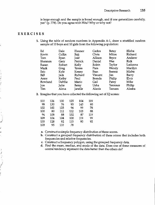
,J

.;

/

I )'

Descriptive Research 135

is large enough and the sample is broad enough, and if one generalizes carefully, yes" (p. 778). Do you agree with Hite? Why or why not?

EXERCISES

1. Using the table of random numbers in Appendix A-I, draw a stratified random sample of 10 boys and 10 girls from the following population:

Ed Dale Eleanor Carlos Betsy Elisha Kevin Collin Raji Chris Milou Richard Tom Ryan Jose Allison Bryce Andrew Shannon Gary Patrick Daniel Wes Rick Susan Robert Kelly Robin Taylor Ladonna Mark Greg Teresa Pam Wendy Marilyn Eric Kyle Kenny Stan Serena Misha Bill Jack Richard Vincent Jim Barry Anne Kathy Paul Brenda Philip Elvis Rowland Debbie Mario Gail Patsy Mike Jon Julie Betsy Usha Terrence Philip Tim Alexa Janelle Alanis Tamara Alesha

2. Imagine that you have collected the following set of IQ scores:

110 124 100 125 104 119 98 130 76 95 143 90

132 102 125 96 99 78 100 80 112 112 103 88 94 108 88 132 87 119

109 104 104 100 119 99 135 128 92 110 90 92 120 95 110 78

a . Construct a simple frequency distribution of these scores. b. Construct a grouped frequency distribution of these scores that includes both

frequencies and relative frequencies. c. Construct a frequency polygon, using the grouped frequency data. d. Find the mean, median, and mode of the data. Does one of these measures of

central tendency represent the data better than the others do?

CHAPTER

6 Correlational Research

The Correlation Coefficient Factors That Distort Correlation Coefficients

Correlation and Causality A Graphic Representation of Correlations

The Coefficient of Determination

Statistical Significance of r Partial Correlation

Other Correlation Coefficients

136

My grandfather, a farmer for over 50 years, told me on several occasions that the color and thickness of a caterpillar's coat is related to the severity of the coming winter. When "woolly worms" have dark, thick, furry coats, he had said that we can expect an unusually harsh winter.

Whether this bit of folk wisdom is true, I don't know. But like my grandfather, we all hold many beliefs about associations between events in the world. Many people believe, for instance, that hair color is related to personality-that people with red hair have fiery tempers and that blondes are of less-than-average intelli­gence. Others think that geniuses are particularly likely to suffer from mental dis­orders or that people who live in large cities are apathetic and uncaring. Those who believe in astrology claim that the date on which a person is born is associated with the person's personality later in life. Sailors capitalize on the relationship between the appearance of the sky and approaching storms, as indicated by the old saying: Red sky at night, sailor's delight; red sky at morning, sailors take warning. You probably hold many such beliefs about phenomena that tend to go together.

Like all of us, behavioral researchers also are interested in whether certain vari­ables are related to each other. Is outside temperature related to the incidence of urban violence? To what extent are children's IQ scores related to the IQs of their parents? Is shyness associated with low self-esteem? What is the relationship between the degree to which students experience test anxiety and their performance on exams? Are SAT scores related to college grades? Each of these questions asks whether two variables (such as SAT scores and grades) are related and, if so, how strongly they are related.

We determine whether one variable is related to another by seeing whether scores on the two variables covary-whether they vary together. If self-esteem is re­lated to shyness, for example, we should find that scores on measures of self-esteem

po

/ ,

J (

r , I ~ i

(' I

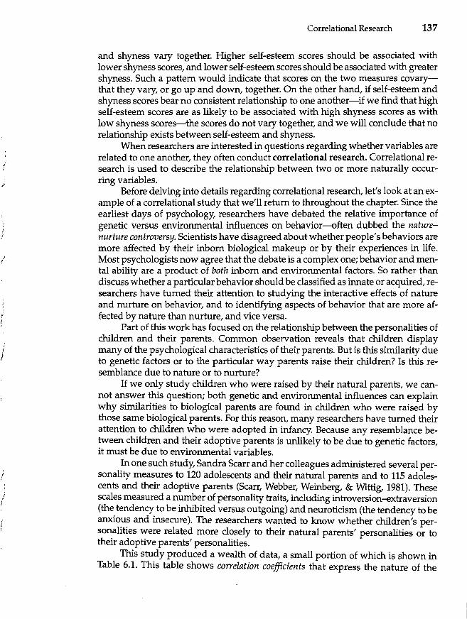
i' f -

I t I

r j

i

I

Correlational Research 137

and shyness vary together. Higher self-esteem scores should be associated with lower shyness scores, and lower self-esteem scores should be associated with greater shyness. Such a pattern would indicate that scores on the two measures covary­that they vary, or go up and down, together. On the other hand, if self-esteem and shyness scores bear no consistent relationship to one another-if we find that high self-esteem scores are as likely to be associated with high shyness scores as with low shyness scores-the scores do not vary together, and we will conclude that no relationship exists between self-esteem and shyness.

When researchers are interested in questions regarding whether variables are related to one another, they often conduct correlational research. Correlational re­search is used to describe the relationship between two or more naturally occur­ring variables.

Before delving into details regarding correlational research, let's look at an ex­ample of a correlational study that we'll return to throughout the chapter. Since the earliest days of psychology, researchers have debated the relative importance of genetic versus environmental influences on behavior-often dubbed the nature­nurture controversy. Scientists have disagreed about whether people's behaviors are more affected by their inborn biological makeup or by their experiences in life. Most psychologists now agree that the debate is a complex one; behavior and men­tal ability are a product of both inborn and environmental factors. So rather than discuss whether a particular behavior should be classified as innate or acquired, re­searchers have turned their attention to studying the interactive effects of nature and nurture on behavior, and to identifying aspects of behavior that are more af­fected by nature than nurture, and vice versa.

Part of this work has focused on the relationship between the personalities of children and their parents. Common observation reveals that children display many of the psychological characteristics of their parents. But is this similarity due to genetic factors or to the particular way parents raise their children? Is this re­semblance due to nature or to nurture?

If we only study children who were raised by their natural parents, we can­not answer this question; both genetic and environmental influences can explain why similarities to biological parents are found in children who were raised by those same biological parents. For this reason, many researchers have turned their attention to children who were adopted in infancy. Because any resemblance be­tween children and their adoptive parents is unlikely to be due to genetic factors, it must be due to environmental variables.

In one such study, Sandra Scarr and her colleagues administered several per­sonality measures to 120 adolescents and their natural parents and to 115 adoles­cents and their adoptive parents (Scarr, Webber, Weinberg, & Wittig, 1981). These scales measured a number of personality traits, including introversion--extraversion (the tendency to be inhibited versus outgoing) and neuroticism (the tendency to be anxious and insecure). The researchers wanted to know whether children's per­sonalities were related more closely to their natural parents' personalities or to their adoptive parents' personalities.

This study produced a wealth of data, a small portion of which is shown in Table 6.1. This table shows correlation coefficients that express the nature of the

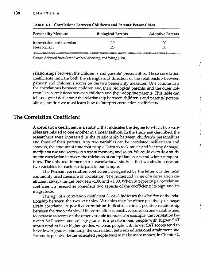
138 CHAPTER 6

TABLE 6.1 Correlations Between Children's and Parents' Personalities

Personality Measure

Introversion-extraversion Neuroticism

Biological Parents

.19

.25 w

Source: Adapted from Scarr, Webber, Weinberg, and Wittig (1981).

3 ¥@

Adoptive Parents

.00

.05

-!ItMtfit

relationships between the children's and parents' personalities. These correlation coefficients indicate both the strength and direction of the relationship between parents' and children's scores on the two personality measures. One column lists the correlations between children and their biological parents, and the other col­umn lists correlations between children and their adoptive parents. This table can tell us a great deal about the relationship between children's and parents' person­alities, but first we must learn how to interpret correlation coefficients.

The Correlation Coefficient

A correlation coefficient is a statistic that indicates the degree to which two vari­ables are related to one another in a linear fashion. In the study just described, the researchers were interested in the relationship between children's personalities and those of their parents. Any two variables can be correlated: self-esteem and shyness, the amount of time that people listen to rock music and hearing damage, marijuana use and scores on a test of memory, and so on. We could even do a study on the correlation between the thickness of caterpillars' coats and winter tempera­tures. The only requirement for a correlational study is that we obtain scores on two variables for each participant in our sample.

The Pearson correlation coefficient, designated by the letter r, is the most commonly used measure of correlation. The numerical value of a correlation co­efficient always ranges between -1.00 and +1.00. When interpreting a correlation coefficient, a researcher considers two aspects of the coefficient: its sign and its magnitude.

The sign of a correlation coefficient (+ or -) indicates the direction of the rela­tionship between the two variables. Variables may be either positively or nega­tively correlated. A positive correlation indicates a direct, positive relationship between the two variables. If the correlation is positive, scores on one variable tend to increase as scores on the other variable increase. For example, the correlation be­tween SAT scores and college grades is a positive one; people with higher SAT scores tend to have higher grades, whereas people with lower SAT scores tend to have lower grades. Similarly, the correlation between educational attainment and income is positive; better educated people tend to make more money. In Chapter 2,

t ,.

!

I ! ,

(

/

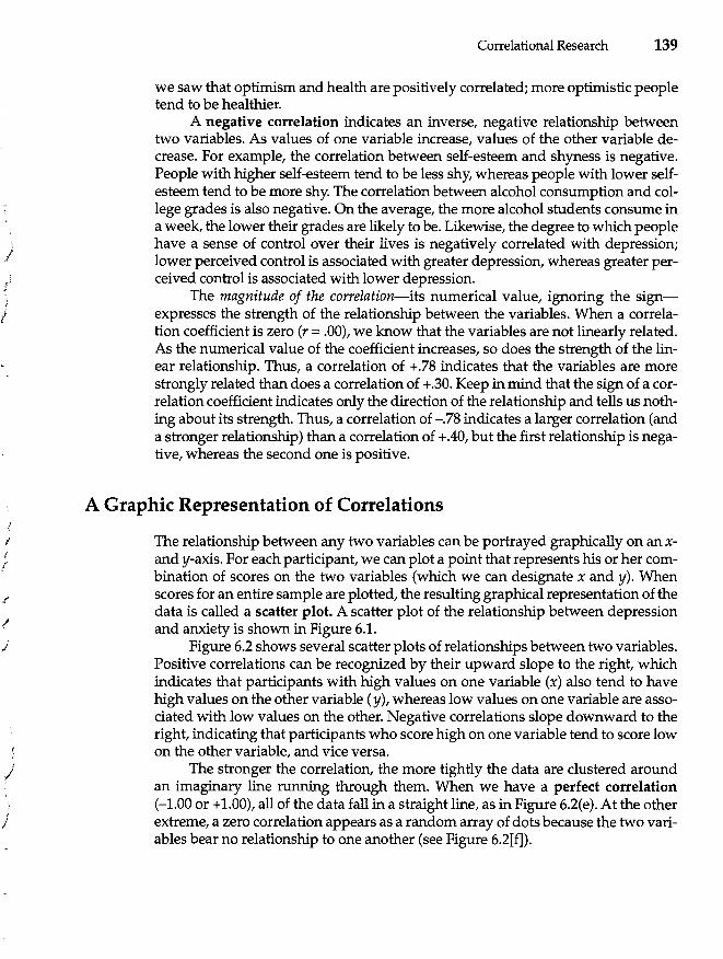
i t

I i l

;

I

;

I l ;

I

Correlational Research 139

we saw that optimism and health are positively correlated; more optimistic people tend to be healthier.

A negative correlation indicates an inverse, negative relationship between two variables. As values of one variable increase, values of the other variable de­crease. For example, the correlation between self-esteem and shyness is negative. People with higher self-esteem tend to be less shy, whereas people with lower self­esteem tend to be more shy. The correlation between alcohol consumption and col­lege grades is also negative. On the average, the more alcohol students consume in a week, the lower their grades are likely to be. Likewise, the degree to which people have a sense of control over their lives is negatively correlated with depression; lower perceived control is associated with greater depression, whereas greater per­ceived control is associated with lower depression.

The magnitude of the correlation-its numerical value, ignoring the sign­expresses the strength of the relationship between the variables. When a correla­tion coefficient is zero (r = .00), we know that the variables are not linearly related. As the numerical value of the coefficient increases, so does the strength of the lin­ear relationship. Thus, a correlation of +.78 indicates that the variables are more strongly related than does a correlation of +.30. Keep in mind that the sign of a cor­relation coefficient indicates only the direction of the relationship and tells us noth­ing about its strength. Thus, a correlation of -.78 indicates a larger correlation (and a stronger relationship) than a correlation of +.40, but the first relationship is nega­tive, whereas the second one is positive.

A Graphic Representation of Correlations

The relationship between any two variables can be portrayed graphically on an x­and y-axis. For each participant, we can plot a point that represents his or her com­bination of scores on the two variables (which we can designate x and y). When scores for an entire sample are plotted, the resulting graphical representation of the data is called a scatter plot. A scatter plot of the relationship between depression and anxiety is shown in Figure 6.1.

Figure 6.2 shows several scatter plots of relationships between two variables. Positive correlations can be recognized by their upward slope to the right, which indicates that participants with high values on one variable (x) also tend to have high values on the other variable (y), whereas low values on one variable are asso­ciated with low values on the other. Negative correlations slope downward to the right, indicating that participants who score high on one variable tend to score low on the other variable, and vice versa.

The stronger the correlation, the more tightly the data are clustered around an imaginary line running through them. When we have a perfect correlation (-1.00 or +1.00), all of the data fall in a straight line, as in Figure 6.2(e). At the other extreme, a zero correlation appears as a random array of dots because the two vari­ables bear no relationship to one another (see Figure 6.2[f]).

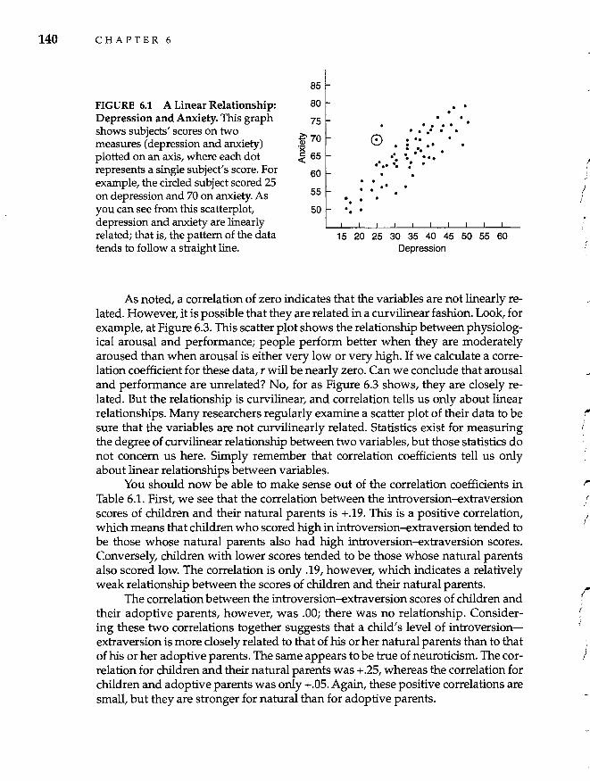
140 CHAPTER 6

FIGURE 6.1 A Linear Relationship: Depression and Anxiety. This graph shows subjects' scores on two measures (depression and anxiety) plotted on an axis, where each dot represents a single subject'S score. For example, the circled subject scored 25 on depression and 70 on anxiety. As you can see from this scatterplot, depression and anxiety are linearly related; that is, the pattern of the data tends to follow a straight line.

85

80

75

~70 ·x ~ 65

60

55

50

o

. . . .. .. ... -. . o " . .' . '. . . .

. ... ... .-.- -. : . . . . . .-

o. •

o. •

15 20 25 30 35 40 45 50 55 60 Depression

As noted, a correlation of zero indicates that the variables are not linearly re­lated. However, it is possible that they are related in a curvilinear fashion. Look, for example, at Figure 6.3. This scatter plot shows the relationship between physiolog­ical arousal and performance; people perform better when they are moderately aroused than when arousal is either very low or very high. If we calculate a corre­lation coefficient for these data, r will be nearly zero. Can we conclude that arousal and performance are unrelated? No, for as Figure 6.3 shows, they are closely re­lated. But the relationship is curvilinear, and correlation tells us only about linear relationships. Many researchers regularly examine a scatter plot of their data to be sure that the variables are not curvilinearly related. Statistics exist for measuring the degree of curvilinear relationship between two variables, but those statistics do not concern us here. Simply remember that correlation coefficients tell us only about linear relationships between variables.

You should now be able to make sense out of the correlation coefficients in Table 6.1. First, we see that the correlation between the introversion-extraversion scores of children and their natural parents is +.19. This is a positive correlation, which means that children who scored high in introversion-extraversion tended to be those whose natural parents also had high introversion-extraversion scores. Conversely, children with lower scores tended to be those whose natural parents also scored low. The correlation is only .19, however, which indicates a relatively weak relationship between the scores of children and their natural parents.

The correlation between the introversion-extraversion scores of children and their adoptive parents, however, was .00; there was no relationship. Consider­ing these two correlations together suggests that a child's level of introversion­extraversion is more closely related to that of his or her natural parents than to that of his or her adoptive parents. The same appears to be true of neuroticism. The cor­relation for children and their natural parents was +.25, whereas the correlation for children and adoptive parents was only +.05. Again, these positive correlations are small, but they are stronger for natural than for adoptive parents.

I ;

) i

!

f'

i

(

" !

!' , ; I

!

j

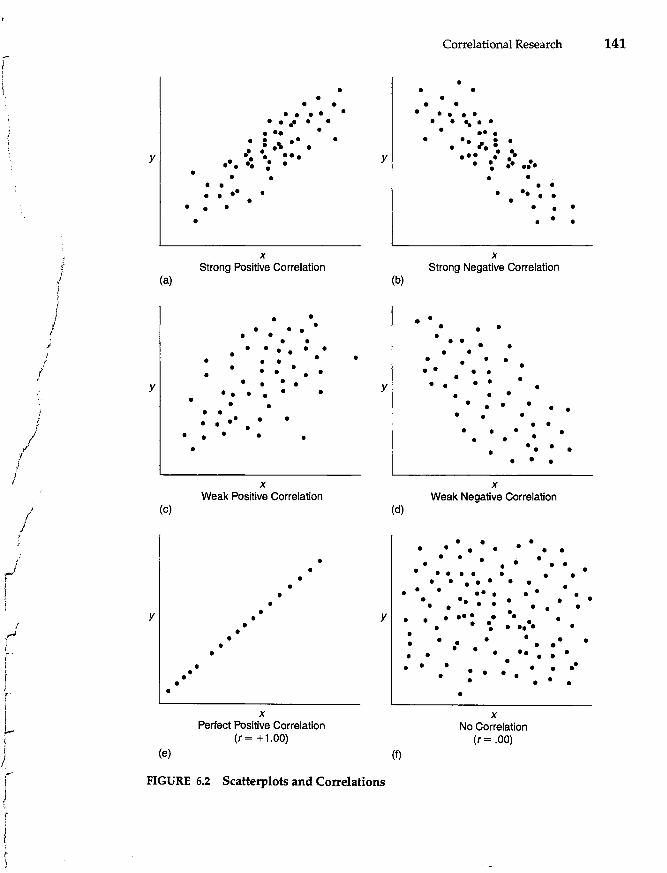
r \

J l i

j ! ; J

/

i

/ / /

J

i

( r­I

I r-

} r "

f

y

•

• •

(a)

y •

• •

(c)

• • · . , • ••

• • • • • • • . :., ... ".. . .. . -.. : : .

• • • • • ••••• • •

x Strong Positive Correlation

• • • • • • • • • •

• •

• ••• • • • • • • • • •

• • •• • • • • • • • •••••

• • •

x

• • • •

•

• • •

•

Weak Positive Correlation

• • •

• • •

• y

(b)

•

y

(d)

Correlational Research 141

• • • • •

•

• • • • • • •

• • .... •• •

•• , I • . ...... .. · ~ : . •

.: . • • • . . -... • • • •

x Strong Negative Correlation

• •

•

• • • • • • • • • • • • • • • • •

• • • •

• • • • • •

• • • •

•

• • • •

x

•

• • •

•

• • • • • •

•• •

• •

Weak Negative Correlation

• • • • • • • • • • •

• •

• • •

• • • • • •

• • • • • • • • • • • • • •

• • • • • • •• •••

• •• • • • • • • •

• y

• • • • •

• • • • •

• •

x

•

Perfect Positive Correlation (r= +1.00)

y

(e) (f)

FIGURE 6.2 Scatterplots and Correlations

• • • • •

• • •

• •

• •

•

• ••• • • • • •

• •• • • • ••••

• •

• • • •

•

• • • • • ••••••

••

• • • • • •

x No Correlation

(r= .00)

• • • • •

•

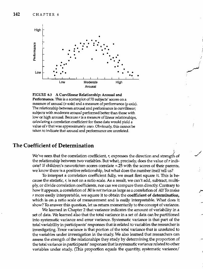
142 CHAPTER 6

High

• • • • • • • • • • • • • • • • • • • • • • •• • • • • •

• • • • • • • • • • • • • • • • • • • ••• • • • • • •

Low •• •• • • • • • • • •

Low Moderate High Arousal

FIGURE 6.3 A Curvilinear Relationship: Arousal and Performance. This is a scatterplot of 70 subjects' scores on a measure of arousal (x-axis) and a measure of performance (y-axis). The relationship between arousal and performance is curvilinear; subjects with moderate arousal performed better than those with low or high arousal. Because r is a measure of linear relationships, calculating a correlation coefficient for these data would yield a value of r that was approximately zero. Obviously, this cannot be taken to indicate that arousal and performance are unrelated.

The Coefficient of Determination

•

I

We've seen that the correlation coefficient, r, expresses the direction and strengt& of the relationship between two variables. But what, precisely, does the value of r indi­cate? If children's neuroticism scores correlate +.25 with the scores of their parents, we know there is a positive relationship, but what does the number itself tell us?

To interpret a correlation coefficient fully, we must first square it. This is be­cause the statistic, r, is not on a ratio scale. As a result, we can't add, subtract, multi­ply, or divide correlation coefficients, nor can we compare them directly. Contrary to how it appears, a correlation of .80 is not twice as large as a correlation of .4O! To make r more easily interpretable, we square it to obtain the coefficient of determination, which is on a ratio scale of measurement and is easily interpretable. What does it show? To answer this question, let us return momentarily to the concept of variance.

We learned in Chapter 2 that variance indicates the amount of variability in a set of data. We learned also that the total variance in a set of data can be partitioned into systematic variance and error variance. Systematic variance is that part of the total variability in participants' responses that is related to variables the researcher is investigating. Error variance is that portion of the total variance that is unrelated to the variables under investigation in the study. We also learned that researchers can assess the strength of the relationships they study by determining the proportion of the total variance in participants' responses that is systematic variance related to other variables under study. (This proportion equals the quantity, systematic variance/

i I

r

f ;

/

i'

i I

!

/ :'

I,

Correlational Research 143

total variance.) The higher the proportion of the total variance in one variable that is systematic variance related to another variable, the stronger will be the relationship between them.

The squared correlation coefficient (or coefficient of determination) tells us the proportion of variance in one of our variables that is accounted for by the other variable. Viewed another way, the coefficient of determination indicates the pro­portion of the total variance in one variable that is systematic variance shared with the other variable. For example, if we square the correlation between children's neuroticism scores and those of their biological parents (.25 x .25), we obtain a co­efficient of determination of .0625. This tells us that 6.25% of the variance in chil­dren's neuroticism scores can be accounted for by their parents' scores, or, to say it differently, 6.25% of the total. variance in children's scores is systematic variance, which is variance related to the parents' scores.

When two variables are uncorrelated-when r is .OO-they are totally inde­pendent, and we cannot account for any of the variance in one variable by the other variable. To say it differently, there is no systematic variance in the data. However, to the extent that two variables are correlated with one another, scores on one vari­able are related to scores on the other variable, and systematic variance is present. The existence of a correlation (and, thus, systematic variance) means that we can account for, or explain, some of the variance in one variable by the other variable.

If we knew everything there is to know about neuroticism, we would know all of the factors that account for the variance in children's neuroticism scores, such as genetic factors, the absence of a secure home life, neurotic parents who provide models of neurotic behavior, low self-esteem, and so on. If we knew everything about neuroticism, we could account for 100% of the variance in children's neu­roticism scores.

But we are not all-knowing. The best we can do is to conduct research that looks at the relationship between neuroticism and a handful of other variables. In the case of the research conducted by Scarr and her colleagues (1981) described earlier, we can account for only a relatively small portion of the variance in chil­dren's neuroticism scores-that portion that is associated with the neuroticism of their natural parents. Given the myriad of factors that influence neuroticism, it is really not surprising that one particular factor, such as parental neuroticism, is re­lated only weakly to children's neuroticism.

In summary, the square of a correlation coefficient-its coefficient of determi­nation-indicates the proportion of variance in one variable that can be accounted for by another variable. If r is zero, we account for none of the variance. If r equals - 1.00 or + 1.00, we can perfectly account for 100% of the variance. And if r is in be­tween, the more variance we account for, the stronger the relationship.

!!I!I DEVELOPING YOUR RESEARCH SKILLS

Calculating the Pearson Correlation Coefficient

Now that we understand what a correlation coefficient tells us about the relationship be­tween two variables, let's take a look at how it is calculated. To calculate the Pearson corre­lation coefficient (r), we must sample several individuals and obtain two measures on each.

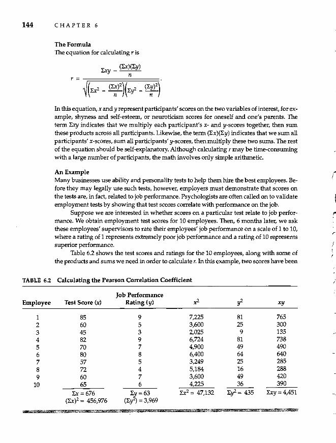
144 CHAPTER 6

TABLE 6.2

Employee

1 2 3 4 5 6 7 8 9

10

The Formula The equation for calculating r is

r.xy _ (u)(l:y) n

In this equation, x and y represent participants' scores on the two variables of interest, for ex­ample, shyness and self-esteem, or neuroticism scores for oneself and one's parents. The term r.xy indicates that we multiply each participant's x- and y-scores together, then sum these products across all participants. Likewise, the term (l:x)(l:y) indicates that we sum all participants' x-scores, sum all participants' y-scores, then multiply these two sums. The rest of the equation should be self-explanatory. Although calculating r may be time-consuming with a large number of participants, the math involves only simple arithmetic.

An Example Many businesses use ability and personality tests to help them hire the best employees. Be­fore they may legally use such tests, however, employers must demonstrate that scores on the tests are, in fact, related to job performance. PsycholOgists are often called on to validate employment tests by showing that test scores correlate with performance on the job.

Suppose we are interested in whether scores on a particular test relate to job perfor­mance. We obtain employment test scores for 10 employees. Then, 6 months later, we ask these employees' supervisors to rate their employees' job performance on a scale of 1 to 10, where a rating of 1 represents extremely poor job performance and a rating of 10 represents superior performance.

Table 6.2 shows the test scores and ratings for the 10 employees, along with some of the products and sums we need in order to calculate r. In this example, two scores have been

Calculating the Pearson Correlation Coefficient

Job Performance Test Score (x) Rating (y) x2 y2 xy

85 9 7,225 81 765 60 5 3,600 25 300 45 3 2,025 9 135 82 9 6,724 81 738 70 7 4,900 49 490 80 8 6,400 64 640 57 5 3,249 25 285 72 4 5,184 16 288 60 7 3,600 49 420 65 6 4,225 36 390

u=676 l:y = 63 u 2 = 47,132 l:y2 = 435 r.xy =4,451 (l:,x)2 = 456,976 (:Ey2) = 3,969

, (

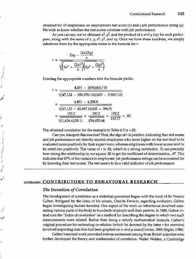
j

I

j

J

-, , I , j I

I

J

;'

Correlational Research 145

obtained for 10 employees: an employment test score (x) and a job performance rating (y). We wish to know whether the test scores correlate with job performance.

As you can see, we've obtained x2, i, and the product of x and y (xy) for each partici­pant, along with the sums of x, y, x2, y2, and xy. Once we have these numbers, we simply substitute them for the appropriate terms in the formula for r:

I.xy _ (Lx}(I:y) n

Entering the appropriate numbers into the formula yields:

4,451 - (676)(63)/10

r = ~r(=47=,1=32::::=::::::-=45=6=,9=76=/=10=)(43==5 =-=3=,9=69=/=10)

4,451 - 4,258.8 =r============== V(47,132 - 45,697.6)(435 - 396.9)

= 192.2 = 192.2 = 192.2 = .82

V(1,434.4}(38.1} V54,650.64 233.77

The obtained correlation for the example in Table 6.2 is +.82. Can you interpret this number? First, the sign of r is positive, indicating that test scores

and job performance are directly related; employees who score higher on the test tend to be evaluated more positively by their supervisors, whereas employees with lower scores tend to be rated less positively. The value of r is .82, which is a strong correlation. To see precisely how strong the relationship is, we square .82 to get the coefficient of determination, .67. This indicates that 67% of the variance in employees' job performance ratings can be accounted for by knowing their test scores. The test seems to be a valid indicator of job performance.

CONTRIBUTORS TO BEHAVIORAL RESEARCH

The Invention of Correlation The development of correlation as a statistical procedure began with the work of Sir Francis Galton. Intrigued by the ideas of his cousin, Charles Darwin, regarding evolution, Galton began investigating human heredity. One aspect of his work on inheritance involved mea­suring various parts of the body in hundreds of people and their parents. In 1888, Galton in­troduced the "index of co-relation" as a method for describing the degree to which two such measurements were related. Rather than being a strictly mathematical formula, Galton's original procedure for estimating co-relation (which he denoted by the letter r for reversion) involved inspecting data that had been graphed on x- and y-axes (Cowles, 1989; Stigler, 1986).

Galton's seminal work provoked intense excitement among three British scientists who further developed the theory and mathematics of correlation. Walter Weldon, a Cambridge

146 CHAPTER 6

zoologist, began using Galton's ideas regarding correlation in his research on shrimps and crabs. In the context of his work examining correlations among various crustacean body parts, Weldon first introduced the concept of negative correlation. (Weldon tried to name r after Galton, but the term Galton's function never caught on; Cowles, 1989.)

In 1892 Francis Edgeworth published the first mathematical formula for calculating the coefficient of correlation directly. Unfortunately, Edgeworth did not initially recognize the importance of his work, which was buried in a more general, "impossibly difficult to fol­low paper" on statistics (Cowles, 1989, p.139).

Thus, when Galton's student Karl Pearson derived a formula for calculating r in 1895, he didn't know that Edgeworth had obtained an essentially equivalent formula a few years earlier. Edgeworth himself notified Pearson of this fact in 1896, and Pearson later acknowl­edged that he had not carefully examined others' previous work. Even so, Pearson recog­nized the importance of the discovery and went ahead to make the most of it, applying his formula to research problems in both biology and psychology (Pearson & Kendall, 1970; Stigler, 1986). Because Pearson was the one to popularize the formula for calculating r, the coefficient became known as the Pearson correlation coefficient, or Pearson r.

Statistical Significance of r

When calculating a correlation between two variables, researchers are interested not only in the value of the correlation coefficient, but also in whether the value of r they obtain is statistically significant. Statistical significance exists when a corre­lation coefficient calculated on a sample has a very low probability of being zero in the population.

To understand what this means, let's imagine for a moment that we are all­knowing beings, and that, as all-knowing beings, we know for certain that if we tested every human being on the face of the earth, we would find that the correla­tion between two particular variables, x and y, was absolutely zero (that is, r = .00). Now, imagine that a mortal behavioral researcher wishes to calculate the correla­tion between these two variables. Of course, as a mortal, this researcher cannot col­lect data on millions of people around the world, so she obtains a sample of 200 respondents, measures x and y for each respondent, and calculates r. Will the value of r she obtains be .OO? I suspect that you can guess that the answer is probably not. Because of sampling error, measurement error, and other sources of error variance, she will likely obtain a nonzero correlation coefficient even though the true correla­tion in the population is zero.

Of course, this discrepancy creates a problem. When we calculate a correlation coefficient, how do we know whether we can trust the value we obtain or whether the true value of r in the population may, in fact, be zero? As it turns out, we can't know for certain, but we can estimate the probability that the value of r we obtain in our re­search would really be zero if we had tested the entire population from which our sample was drawn. And, if the probability that our correlation is truly zero in the pop­ulation is sufficiently low (usually less than .05), we refer to it as statistically significant.

I i

I

/

;

)

-I

" r-'

I

I' t

,..!

I

I

I (

,; r \

r I

Correlational Research 147

The statistical significance of a correlation coefficient is affected by three fac­tors. First is our sample size. Assume that, unbeknown to each other, you and I in­dependently calculated the correlation between shyness and self-esteem and that we both obtained a correlation of -.50. However, your calculation was based on data from 300 participants, whereas my calculation was based on data from 30 partici­pants. Which of us should feel more confident that the true correlation between shy­ness and self-esteem in the population is not .OO? You can probably guess that your sample of 300 should give you more confidence in the value of r you obtained than my sample of 30. Thus, all other things being equal, we are more likely to conclude that a particular correlation is statistically significant the larger our sample is.

Second, the statistical significance of a correlation coefficient depends on the magnitude of the correlation. For a given sample size, the larger the value of r we obtain, the less likely it is to be .00 in the population. Imagine you and I both calcu­lated a correlation coefficient based on data from 300 participants; your calculated value of r was .75, whereas my value of r was .20. You would be more confident that your correlation was not truly .00 in the population than I would be.

Third, statistical significance depends on how careful we want to be not to draw an incorrect conclusion about whether the correlation we obtain could be zero in the population. The more careful we want to be, the larger the correlation must be to be declared "significant." Typically, researchers decide that they will consider a correlation to be significantly different from zero if there is less than a 5% chance (that is, less than 5 chances out of 100) that a correlation as large as the one they ob­tained could have come from a population with a true correlation of zero.

Formulas and tables for testing the statistical significance of correlation coef­ficients can be found in many statistics books (see, for example, Minium, 1978). Table 6.3 shows part of one such table. This table shows the minimum value of r that would be considered statistically significant if we set the chances of making an incorrect decision at 5%. For example, imagine that you obtained a value of r = .32 based on a sample of 100 participants. Looking down the left-hand column, find the number of participants (100). Looking at the other column, we see that the min­imum value of r that is significant with 100 participants is .16. Because our correla­tion coefficient (.32) exceeds .16, we conclude that the population correlation is very unlikely to be zero (in fact, there is less than a 5% chance that the population correlation is zero).

If the correlation coefficient we calculated had been less than .16, however, we would have concluded that it could have easily come from a population in which the correlation between our variables was zero. Thus, it is regarded as sta­tistically nonsignificant, and we must treat it as if it were zero.

Keep in mind that, with large samples, even very small correlations are sta­tistically significant. Thus, finding that a particular r is significant tells us only that it is very unlikely to be .00 in the population; it does not tell us whether the rela­tionship between the two variables is a strong or an important one. The strength of a correlation is assessed only by its magnitude, not whether it is statistically signif­icant. Although only a rule of thumb, behavioral researchers tend to regard corre­lations at or below about .10 as weak in magnitude (they account for only 1 % of the

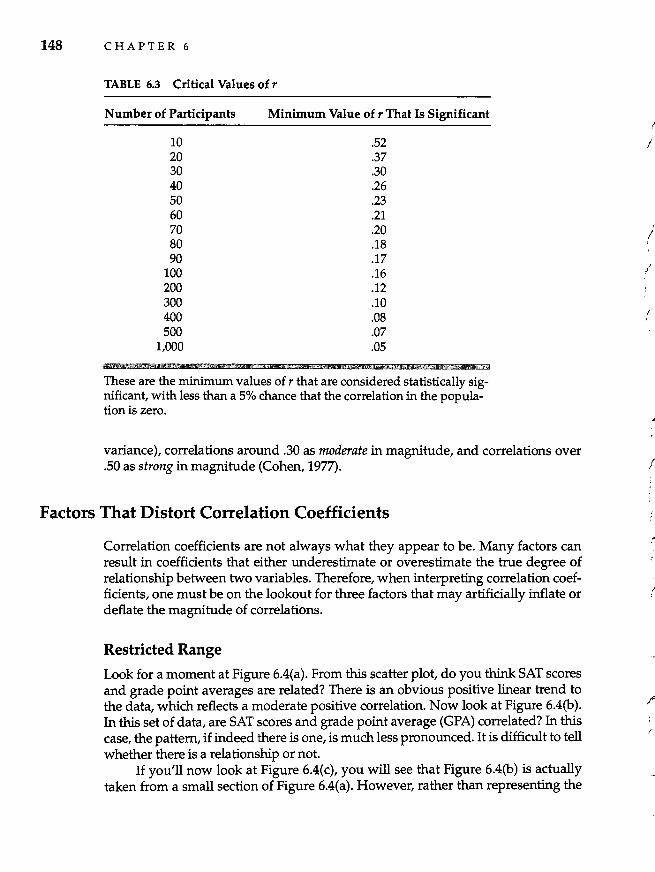
148 CHAPTER 6

TABLE 6.3 Critical Values of r

Number of Participants

10 20 30 40 50 60 70 80 90

100 200 300 400 500

1,000

Minimum Value of r That Is Significant

.52

.37

.30

.26

.23

.21

.20

.18

.17

.16

.12

.10

.08

.07

.05

These are the minimum values of r that are considered statistically sig­nificant, with less than a 5% chance that the correlation in the popula­tion is zero.

variance), correlations around .30 as moderate in magnitude, and correlations over .50 as strong in magnitude (Cohen, 1977).

Factors That Distort Correlation Coefficients

Correlation coefficients are not always what they appear to be. Many factors can result in coefficients that either underestimate or overestimate the true degree of relationship between two variables. Therefore, when interpreting correlation coef­ficients, one must be on the lookout for three factors that may artificially inflate or deflate the magnitude of correlations.

Restricted Range

Look for a moment at Figure 6.4(a). From this scatter plot, do you think SAT scores and grade point averages are related? There is an obvious positive linear trend to the data, which reflects a moderate positive correlation. Now look at Figure 6.4(b). In this set of data, are SAT scores and grade point average (GPA) correlated? In this case, the pattern, if indeed there is one, is much less pronounced. It is difficult to tell whether there is a relationship or not.

If you'll now look at Figure 6.4(c), you will see that Figure 6.4(b) is actually taken from a small section of Figure 6.4(a). However, rather than representing the

I

; ,

./

I ,

/

/

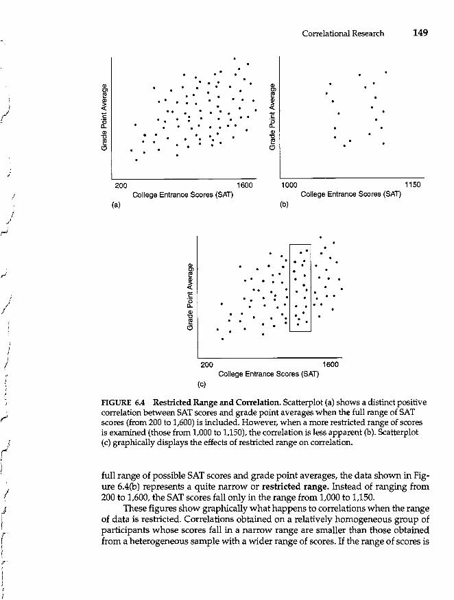
i i

/'

/ /

r'

I'"

/

l ( )

,r

\ \ ,

G)

~ G)

~ 1: ~ G) 'C I!! (!l

o 0

o 0 0 o 0

o • 0 o

. . . . ... . o 0 0

.. . :. ... . • 0

o 0

o o o

. . .. o

o

200 1600 College Entrance Scores (SAT)

(a)

G) Cl I!! G) 0 0

~ 00

1: 0

~ 0

G) . 0 'C I!! 0 0

(!l

200

0

0

Correlational Research 149

1000 1150 College Entrance Scores (SAn

(b)

0 . 0 0

0 0 0 0 0

0 0 . 0 0

0 0 0 0 0

0 0 0 0 0

0 0 0 0

0 0 0 0 0

1600 College Entrance Scores (SAT)

(c)

FIGURE 6.4 Resbicted Range and Correlation. Scatterplot (a) shows a distinct positive correlation between SAT scores and grade point averages when the full range of SAT scores (from 200 to 1,600) is included. However, when a more restricted range of scores is examined (those from 1,000 to 1,150), the correlation is less apparent (b). Scatterplot (c) graphically displays the effects of restricted range on correlation.

full range of possible SAT scores and grade point averages, the data shown in Fig­ure 6.4(b) represents a quite narrow or restricted range. Instead of ranging from 200 to 1,600, the SAT scores fall only in the range from 1,000 to 1,150.

These figures show graphically what happens to correlations when the range of data is restricted. Correlations obtained on a relatively homogeneous group of participants whose scores fall in a narrow range are smaller than those obtained from a heterogeneous sample with a wider range of scores. If the range of scores is

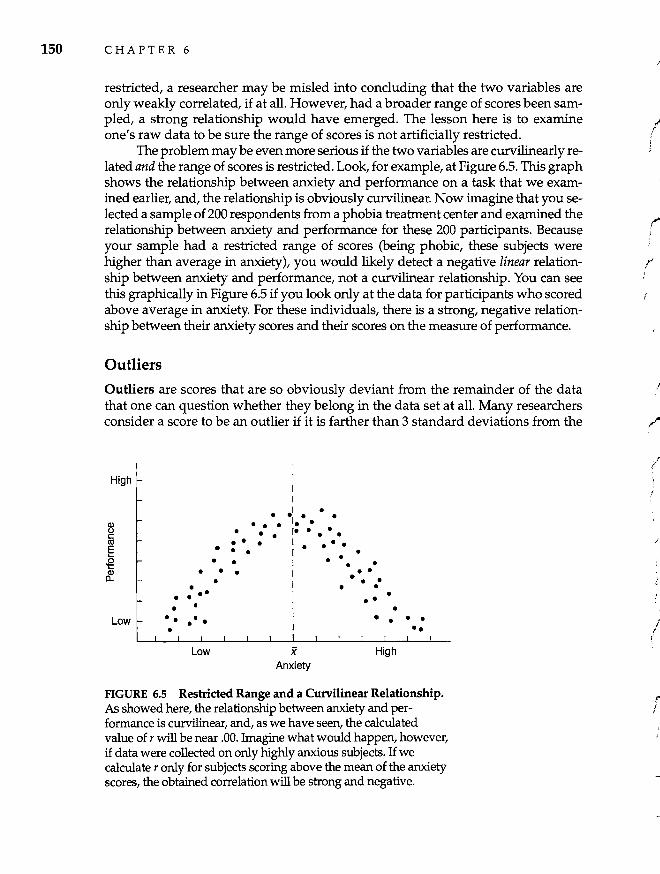
150 C HAP T E R 6

restricted, a researcher may be misled into concluding that the two variables are only weakly correlated, if at all. However, had a broader range of scores been sam­pled, a strong relationship would have emerged. The lesson here is to examine one's raw data to be sure the range of scores is not artificially restricted.

The problem may be even more serious if the two variables are curvilinearly re­lated and the range of scores is restricted. Look, for example, at Figure 6.5. This graph shows the relationship between anxiety and performance on a task that we exam­ined earlier, and, the relationship is obviously curvilinear. Now imagine that you se­lected a sample of 200 respondents from a phobia treatment center and examined the relationship between anxiety and performance for these 200 participants. Because your sample had a restricted range of scores (being phobic, these subjects were higher than average in anxiety), you would likely detect a negative linear relation­ship between anxiety and performance, not a curvilinear relationship. You can see this graphically in Figure 6.5 if you look only at the data for participants who scored above average in anxiety. For these individuals, there is a strong, negative relation­ship between their anxiety scores and their scores on the measure of performance.

Outliers

Outliers are scores that are so obviously deviant from the remainder of the data that one can question whether they belong in the data set at all. Many researchers consider a score to be an outlier if it is farther than 3 standard deviations from the

High

Low

• • • • ••

• • ••••• •

Low

• I • ·1. • • • • • ••• - Ie •• • • ... I.. ..

• • • I • • • I. e. •

• • • I··

I • • • .. I • I • • I I

X Anxiety

• • •

High

• • ••

FIGURE 6.5 Reshicted Range and a Curvilinear Relationship. As showed here, the relationship between anxiety and per­formance is curvilinear, and, as we have seen, the calculated value of r will be near .00. Imagine what would happen, however, if data were collected on only highly anxious subjects. If we calculate r only for subjects scoring above the mean of the anxiety scores, the obtained correlation will be strong and negative.

/

! ! ;

(' I ;

r I

/

I

r /

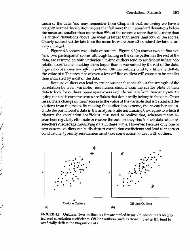
/ j

I

I

!

Correlational Research 151

mean of the data. You may remember from Chapter 5 that, assuming we have a roughly normal distribution, scores that fall more than 3 standard deviations below the mean are smaller than more than 99% of the scores; a score that falls more than 3 standard deviations above the mean is larger than more than 99% of the scores. Clearly, scores that deviate from the mean by more than ±3 standard deviations are very unusual.

Figure 6.6 shows two kinds of outliers. Figure 6.6(a) shows two on-line out­liers. Two participants' scores, although falling in the same pattern as the rest of the data, are extreme on both variables. On-line outliers tend to artificially inflate cor­relation coefficients, making them larger than is warranted by the rest of the data. Figure 6.6(b) shows two off-line outliers. Off-line outliers tend to artificially deflate the value of r. The presence of even a few off-line outliers will cause r to be smaller than indicated by most of the data.

Because outliers can lead to erroneous conclusions about the strength of the correlation between variables, researchers should examine scatter plots of their data to look for outliers. Some researchers exclude outliers from their analyses, ar­guing that such extreme scores are flukes that don't really belong in the data. Other researchers change outliers' scores to the value of the variable that is 3 standard de­viations from the mean. By making the outlier less extreme, the researcher can in­clude the participant's data in the analysis while minimizing the degree to which it distorts the correlation coefficient. You need to realize that, whereas many re­searchers regularly eliminate or rescore the outliers they find in their data, other re­searchers discourage modifying data in these ways. However, because only one or two extreme outliers can badly distort correlation coefficients and lead to incorrect conclusions, typically researchers must take some action to deal with outliers.

y

(a)

• .. .. , • ••• • • ••• • ••• • • • ••• e.... . .

• • • • • • • • •• • • • • • •

• • •

x On-Line Outliers

•

® @

y

(b)

•

•

• • • ••• • • ••• •

• •• . : ~ .. • •• • e.. . ..

•••• e. : • • • • • ... - . • • •

x Off-Line Outliers

•

• • •

•

FIGURE 6.6 Outliers. Two on-line outliers are circled in (a). On-line outliers lead to inflated correlation coefficients. Off-line outliers, such as those circled in (b), tend to artificially deflate the magnitude of r.

152 C HAP T E R 6

Reliability of Measures

Unreliable measures attenuate the magnitude of correlation coefficients. All other things being equal, the less reliable our measures, the lower the correlation coefficients we will obtain. (You may wish to review the section on reliability in Chapter 3.)

To understand why this is so, let us again imagine that we are omniscient. In our infinite wisdom, we know that the real correlation between a child's neuroti­cism and the neuroticism of his or her parents is, say, +.45. However, let's also as­sume that a poorly trained, fallible researcher uses a measure of neuroticism that is totally unreliable. That is, it has absolutely no test-retest or interim reliability. If the researcher's measure is completely unreliable, what value of r will he or she obtain between parents' and children's scores? Not +.45 (the true correlation), but rather .00. Of course, researchers seldom use measures that are totally unreliable. Even so, the less reliable the measure, the lower the correlation will be.

Correlation and Causality

Perhaps the most important consideration in interpreting correlation coefficients is that correlation does not imply causality. Often people will conclude that because two phenomena are related, they must be causally related in some way. This is not nec­essarily so; one variable can be strongly related to another yet not cause it. The thickness of caterpillars' coats may correlate highly with the severity of winter weather, but we cannot conclude that caterpillars cause blizzards, ice storms, and freezing temperatures. Even if two variables are perfectly correlated (r = -1.00 or + 1.00), we cannot infer that one of the variables causes the other. This point is ex­ceptionally important, so I will repeat it: A correlation can never be used to conclude that one of the variables causes or influences the other. Put simply, correlation does not imply causality.

For us to conclude that one variable causes or influences another variable, three criteria must be met: covariation, directionality, and elimination of extrane­ous variables. However, most correlational research satisfies only the first of these criteria unequivocally.

First, to conclude that two variables are causally related, they first must be found to covary, or correlate. If one variable causes the other, then changes in the values of one variable should be associated with changes in values of the other variable. Of course, this is what correlation means by definition, so if two variables are found to be correlated, this first criterion for inferring causality is met.

Second, to infer that two variables are causally related, we must show that the presumed cause precedes the presumed effect in time. However, in most correlational research, both variables are measured at the same time. For example, if a researcher correlates participants' scores on two personality measures that were collected at the same time, there is no way to determine the direction of causality. Does variable x cause variable y, or does variable y cause variable x (or, perhaps, neither)?

r

('

r {

/

)

(

,J

,I

)

t'

l )

)

Correlational Research 153

The third criterion for inferring causality is that all extraneous factors that might influence the relationship between the two variables are controlled or elim­inated. Correlational research never satisfies this requirement completely. Two variables may be correlated not because they are causally related to one another, but because they are both related to a third variable. For example, Levin and Stokes (1986) were interested in correlates of loneliness. Among other things, they found that loneliness correlated +.60 with depression. Does this mean that being lonely makes people depressed or that being depressed makes people feel lonely? Perhaps neither. Another option is that both loneliness and depression are due to a third variable, such as the quality of a person's social network. Having a large number of friends and acquaintances, for example, may reduce both loneliness and depression.

The inability to draw conclusions about causality from correlational data is the basis of the tobacco industry's insistence that no research has produced evi­dence of a causal link between smoking and lung cancer in humans. Plenty of re­search shows that smoking and the incidence of cancer are correlated in humans; more smoking is associated with a greater likelihood of getting lung cancer. But be­cause the data are correlational, we cannot infer a causal link between smoking and health. Research has established that smoking causes cancer in laboratory animals, however, because animal research can use experimental designs that allow us to infer cause-and-effect relationships. However, conducting experimental research on human beings would require randomly assigning people to smoke heavily. Not only would such a study be unethical, but would you volunteer to participate in a study that might give you cancer? Because we are limited to doing only correla­tional research on smoking in humans, we cannot infer causality from our results.

BEHAVIORAL RESEARCH CASE STUDY

Correlates of Satisfying Relationships

Although relationships are an important part of most people's lives, behavioral researchers did not begin to study processes involved in liking and loving seriously until the 1970s. Since that time, we have learned a great deal about factors that affect interpersonal attrac­tion, relationship satisfaction, and people's decisions to end their romantic relationships. However, researchers have focused primarily on the relationships of adults and have tended to ignore adolescent love experiences.

To remedy this shortcoming in the research, Levesque (1993) conducted a correla­tional study of the factors associated with satisfying love relationships in adolescence. Using a sample of more than 300 adolescents between the ages of 14 and 18 who were in­volved in dating relationships, Levesque administered measures of relationship satisfaction and obtained other information about the respondents' perceptions of their relationships.

A small portion of the results of the study is shown in Table 6.4. This table shows the correlations between respondents' ratings of the degree to which they were having certain experiences in their relationships and their satisfaction with the relationship.

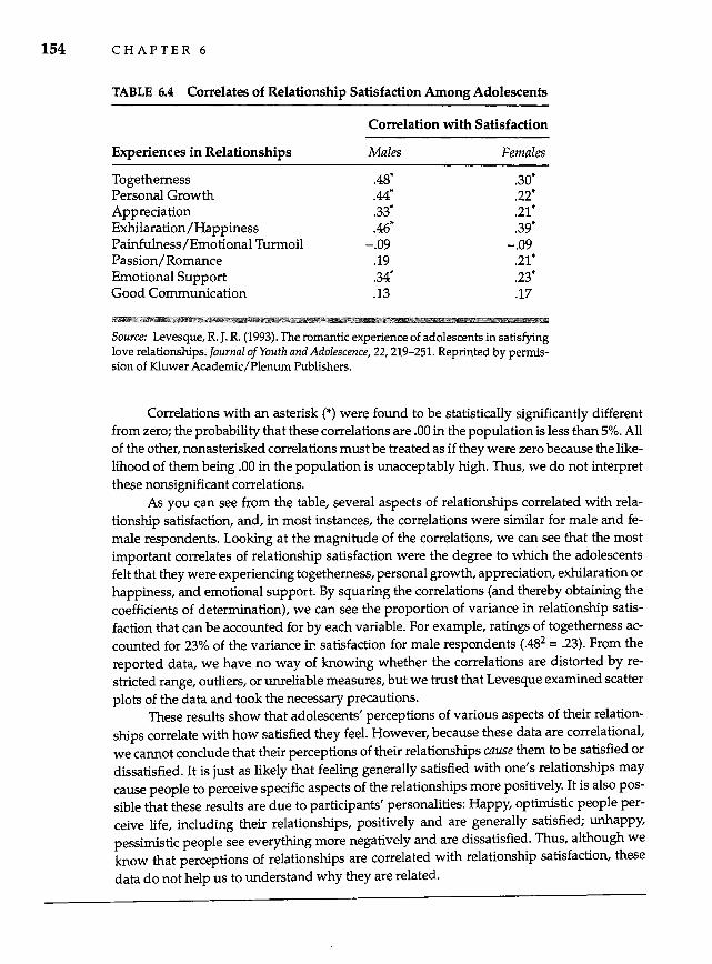
154 C HAP T E R 6

TABLE 6.4 Correlates of Relationship Satisfaction Among Adolescents

Correlation with Satisfaction

Experiences in Relationships Males Females

Togetherness .48* .30* Personal Growth .44* .22' Appreciation .33* .21* Exhilaration/Happiness .46* .39* Painfulness/Emotional Turmoil -.09 -.09 Passion/Romance .19 .21' Emotional Support .34' .23' Good Communication .13 .17

Source: Levesque, R. J. R. (1993). The romantic experience of adolescents in satisfying love relationships. Journal of Youth and Adolescence, 22, 219-251. Reprinted by permis­sion of Kluwer Academic/Plenum Publishers.

Correlations with an asterisk (*) were found to be statistically significantly different from zero; the probability that these correlations are .00 in the population is less than 5%. All of the other, nonasterisked correlations must be treated as if they were zero because the like­lihood of them being .00 in the population is unacceptably high. Thus, we do not interpret these nonsignificant correlations.

As you can see from the table, several aspects of relationships correlated with rela­tionship satisfaction, and, in most instances, the correlations were similar for male and fe­male respondents. Looking at the magnitude of the correlations, we can see that the most important correlates of relationship satisfaction were the degree to which the adolescents felt that they were experiencing togetherness, personal growth, appreciation, exhilaration or happiness, and emotional support. By squaring the correlations (and thereby obtaining the coefficients of determination), we can see the proportion of variance in relationship satis­faction that can be accounted for by each variable. For example, ratings of togetherness ac­counted for 23% of the variance in satisfaction for male respondents (.482 = .23). From the reported data, we have no way of knowing whether the correlations are distorted by re­stricted range, outliers, or unreliable measures, but we trust that Levesque examined scatter plots of the data and took the necessary precautions.

These results show that adolescents' perceptions of various aspects of their relation­ships correlate with how satisfied they feel. However, because these data are correlational, we cannot conclude that their perceptions of their relationships cause them to be satisfied or dissatisfied. It is just as likely that feeling generally satisfied with one's relationships may cause people to perceive specific aspects of the relationships more positively. It is also pos­sible that these results are due to participants' personalities: Happy, optimistic people per­ceive life, including their relationships, positively and are generally satisfied; unhappy, pessimistic people see everything more negatively and are dissatisfied. Thus, although we know that perceptions of relationships are correlated with relationship satisfaction, these data do not help us to understand why they are related.

/ j

(

/

, j

-.-1 I

,/

Correlational Research 155

Partial Correlation

Although we can never conclude that two correlated variables cause one another, researchers have at their disposal research strategies that allow them to make in­formed guesses about whether correlated variables might be causally related. These strategies cannot provide definitive causal conclusions, but they can give us evi­dence that either does or does not support a particular causal explanation of the relationship between two correlated variables. Although researchers can never con­clude that one correlated variable absolutely causes another, they may be able to conclude that a particular causal explanation of the relationship between the vari­ables is more likely to be correct than are other causal explanations.

If we find that two variables, x and y, are correlated, there are three general causal explanations of their relationship: x may cause y, y may cause x, or some other variable or variables (z) may cause both x and y. Imagine that we find a negative cor­relation between alcohol consumption and college grades-the more alcohol stu­dents drink per week, the lower their grades are likely to be. Such a correlation could be explained in three ways. On one hand, excessive alcohol use may cause students' grades to go down (because they are drinking instead of studying, missing class be­cause of hangovers, or whatever). Alternatively, obtaining poor grades may cause students to drink (to relieve the stress of failing, for example).

A third possibility is that the correlation between alcohol consumption and grades is due to some third variable. Perhaps depression is the culprit: Students who are highly depressed do not do well in class, and they may try to relieve their depression by drinking. Thus, alcohol use and grades may be correlated only indirectly-by virtue of their relationship with depression. Alternatively, the relationship between alcohol and grades may be caused by the value that students place on social relationships versus academic achievement. Students who place a great deal of importance on their social lives may study less and party more. As a result, they coincidentally receive lower grades and drink more alcohol, but the grades and drinking are not directly related. (Can you think of third variables other than depression and sociability that might mediate the relationship between alcohol consumption and grades?)

Researchers can test hypotheses about the possible effects of third variables on the correlations they obtain by using a statistical procedure called partial corre­lation. Partial correlation allows researchers to examine a third variable's possible influence on the correlation between two other variables. Specifically, a partial cor­relation is the correlation between two variables with the influence of one or more other variables statistically removed.

Imagine that we obtain a correlation between x and y, and we want to know whether the relationship between x and y is due to the fact that x and yare both caused by some third variable, z. We can statistically remove the variability in x and y that is associated with z and see whether x and yare still correlated. If x and y still correlate after we partial out the influence of z, we can conclude that the re­lationship between x and y is unlikely to be due to z. Stated differently, if x and y are correlated even when systematic variance due to z is removed, z is unlikely to be causing the relationship between x and y.

156 C HAP T E R 6

However, if x and yare no longer correlated after the influence of z is statisti­cally removed, we have evidence that the correlation between x and y is due to z or to some other variable that is associated with z. That is, systematic variance associ­ated with z must be responsible for the relationship between x and y.

Let's return to our example involving alcohol consumption and college grades. If we wanted to know whether a third variable, such as depression, was responsible for the correlation between alcohol and grades, we could calculate the partial corre­lation between alcohol use and grade point average while statistically removing (partialing out) the variability related to depression scores. If the correlation between alcohol use and grades remains unchanged when depression is partialed out, we will have good reason to conclude that the relationship between alcohol use and grades is not due to depression. However, if depression were removed from the cor­relation and the partial correlation between alcohol and grades was substantially lower than their true correlation, we would conclude that depression-or something else associated with depression-mediated the relationship.

The formulas used to calculate partial correlations do not concern us here. The important thing is to recognize that, although we can never infer causality from correlation, we can tentatively test causal hypotheses using partial correla­tion as well as other techniques that we will discuss in Chapter 7.

~ BEHAVIORAL RESEARCH CASE STUDY

Partial Correlation: Depression, Loneliness, and Social Support Earlier I mentioned a study by Levin and Stokes (1986) that found a correlation of .60 be­tween loneliness and depression. These researchers hypothesized that one reason that lonely people tend to be more depressed is that they have smaller social support networks; people who have fewer friends are more likely to feel lonely and are more likely to be de­pressed (because they lack social and emotional support). Thus, the relationship between loneliness and depression may be due to a third variable, lack of social support.

To test this possibility, Levin and Stokes calculated the partial correlation between loneliness and depression, removing the influence of participants' social networks. When they removed the variability due to social networks, the partial correlation was .39, some­what lower than the correlation between loneliness and depression without variability due to social networks partialed out. This pattern of results suggests that some of the relation­ship between loneliness and depression may be mediated by social network variables. However, even with the social network factor removed, loneliness and depression were still correlated, which suggests that factors other than social network also contribute to the rela­tionship between them.

Other Correlation Coefficients

We focused in this chapter on the Pearson correlation coefficient because it is the most commonly used index of correlation. The Pearson correlation is appropriate

f

r

I

(

/ /

/

I

J

I

;

/

/

('

Correlational Research 157

when both variables, x and y, are on an interval or ratio scale of measurement (as most variables studied by behavioral researchers are). Recall from Chapter 3 that for both interval and ratio scales, equal differences between the numbers assigned to participants' responses reflect equal differences between participants in the characteristic being measured. (Interval and ratio scales differ in that ratio scales have a true zero point, whereas interval scales do not.)

When one or both variables are measured on an ordinal scale-in which the numbers reflect the rank ordering of participants on some attribute-the Spear­man rank-order correlation coefficient is used. For example, suppose that we want to know how well teachers can judge the intelligence of their students. We ask a teacher to rank the 30 students in the class from 1 to 30 in terms of their general in­telligence. Then we obtain students' IQ scores on a standardized intelligence test. Because the teacher's judgments are on an ordinal scale of measurement, we cal­culate a Spearman rank-order correlation coefficient to examine the correlation be­tween the teacher's rankings and the student's real IQ scores.

Other kinds of correlation coefficients are used when one or both of the vari­ables are dichotomous, such as gender (male vs. female), handedness (left- vs. right­handed), or whether a student has passed a course (yes vs. no). (A dichotomous variable is measured on a nominal scale but has only two levels.) When correlations are calculated on dichotomous variables, the variables are assigned arbitrary num­bers, such as male = 1 and female = 2. When both variables being correlated are di­chotomous, a phi coefficient correlation is used; if only one variable is dichotomous (and the other is on an interval or ratio scale), a point biserial correlation is used. Thus, if we were looking at the relationship between gender and virginity, a phi co­efficient is appropriate because both variables are dichotomous. However, if we were correlating gender (a dichotomous variable) with height (which is measured on a ratio scale), a point biserial correlation would be calculated. Once calculated, the Spearman, phi, and point biserial coefficients are interpreted precisely like a Pearson coefficient.

Summary

1. Correlational research is used to describe the relationship between two variables.

2. A correlation coefficient (r) indicates both the direction and magnitude of the relationship.

3. If the scores on the two variables tend to increase and decrease together, the variables are positively correlated. If the scores vary inversely, the variables are negatively correlated.

4. The magnitude of a correlation coefficient indicates the strength of the rela­tionship between the variables. A correlation of zero indicates that the variables are not related; a correlation of ±1.00 indicates that they are perfectly related.

5. The square of the correlation coefficient, the coefficient of determination (r2), reflects the proportion of the total variance in one variable that can be ac­counted for by the other variable.

158 C HAP T E R 6

6. Researchers test the statistical significance of correlation coefficients to gauge the likelihood that the correlation they obtained in their research might have come from a population in which the true correlation was zero. A correlation is usually considered statistically significant if there is less than a 5% chance that the true population correlation is zero. Significance is affected by the sample size, magnitude of the correlation, and degree of confidence the re­searcher wishes to have.

7. When interpreting correlations, researchers look out for factors that may artificially inflate and deflate the magnitude of the correlation coefficient­restricted range, outliers, and low reliability.

8. Correlational research seldom if ever meets all three criteria necessary for in­ferring causality-covariation, directionality, and elimination of extraneous variables. Thus, the presence of a correlation does not imply that the vari­ables are causally related to one another.

9. A partial correlation is the correlation between two variables with the influ­ence of one or more other variables statistically removed. Partial correlation is used to examine whether the correlation between two variables might be due to certain other variables.

10. The Pearson correlation coefficient is most commonly used, but the Spearman, phi, and point biserial coefficients are used under special circumstances.

KEY TERMS

coefficient of determination Pearson correlation coefficient positive correlation (p. 138) restricted range (p. 149) scatter plot (p. 139) Spearman rank-order

(p.142) (p.138) correlational research (p. 137) correlation coefficient (p. 138) negative correlation (p. 139) outlier (p. 150)

perfect correlation (p. 139) phi coefficient (p. 157) point biserial correlation

(p.157) correlation (p. 157)

statistical significance (p. 146) partial correlation (p. 155)

QUESTIONS FOR REVIEW

1. The correlation between self-esteem and shyness is -.50. Interpret this correlation.

2. Which is larger-a correlation of +.45 or a correlation of -.60? Explain.

3. Tell whether each of the following relationships reflects a positive or a negative correlation: a. the amount of stress in people's lives and the number of colds they get in the

winter b. the amount of time that people spend suntanning and a dermatological index of

skin damage c. happiness and suicidal thoughts

(

i

,/

" !

/

/'

" , I

/

j

Correlational Research 159

d. blood pressure and a person's general level of hostility e. the number of times that a rat has run a maze and the time it takes to run it again

4. Why do researchers often examine scatter plots of their data when doing correla­tional research?

5. The correlation between self-esteem and shyness is -.50, and the correlation be­tween self-consciousness and shyness is +.25. How much stronger is the first rela­tionship than the second? (Be careful on this one.)

6. Why do researchers calculate the coefficient of determination?

7. What does a coefficient of determination of .40 indicate?

8. Why can it be argued that the formula for calculating r should be named the Edge­worth, rather than the Pearson, correlation coefficient?

9. Why may we not interpret or discuss a correlation coefficient that is not statistically significant?

10. Using Table 6.3 ("Critical Values of r"), indicate whether each of the following cor­relation coefficients is statistically significant: a. r = .42, n = 112 b. r = .00, n = 1,000 c. r = -.25, n = 50 d. r = -.15, n = 100 e. r = .05, n = 300 f. r = .25, n = 60

11. What is a restricted range, and what effect does it have on correlation coefficients? How would you detect and correct a restricted range?

12. How do we know whether a particular score is an outlier?

13. Do outliers increase or decrease the magnitude of correlation coefficients?

14. What impact does reliability have on correlation?

15. Why can't we infer causality from correlation?

16. How can partial correlation help researchers explore possible causal relationships among correlated variables?

17. When is the Spearman rank-order correlation used?

18. What is a dichotomous variable? What correlations are used for dichotomous variables?

QUESTIONS FOR DISCUSSION

1. Imagine that you predicted a moderate correlation between people's scores on a measure of anxiety and the degree to which they report having insomnia. You ad­ministered measures of anxiety and insomnia to a sample of 30 participants, and obtained a correlation coefficient of .28. Because this correlation is not statistically

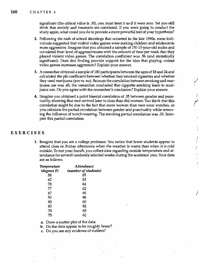
160 C HAP T E R 6

significant (the critical value is .30), you must treat it as if it were zero. Yet you still think that anxiety and insonmia are correlated. If you were going to conduct the study again, what could you do to provide a more powerful test of your hypothesis?

2. Following the rash of school shootings that occurred in the late 1990s, some indi­viduals suggested that violent video games were making children and adolescents more aggressive. Imagine that you obtained a sample of 150 15-year-old males and correlated their level of aggressiveness with the amount of time per week that they played violent video games. The correlation coefficient was .56 (and statistically significant). Does this finding provide support for the idea that playing violent video games increases aggression? Explain your answer.

3. A researcher obtained a sample of 180 participants between the ages of 18 and 24 and calculated the phi coefficient between whether they smoked cigarettes and whether they used marijuana (yes vs. no). Because the correlation between smoking and mar­ijuana use was .45, the researcher concluded that cig~ette smoking leads to mari­juana use. Do you agree with the researcher's conclusion? Explain your answer.

4. Imagine you obtained a point biserial correlation of .35 between gender and punc­tuality, showing that men arrived later to class than did women. You think that this correlation might be due to the fact that more women than men wear watches, so you calculate the partial correlation between gender and punctuality while remov­ing the influence of watch-wearing. The resulting partial correlation was .35. Inter­pret this partial correlation.

EXERCISES

1. Imagine that you are a college professor. You notice that fewer students appear to attend class on Friday afternoons when the weather is warm than when it is cold outside. To test your hunch, you collect data regarding outside temperature and at­tendance for several randomly selected weeks during the academic year. Your data are as follows:

Temperature (degrees F)

58 62 78 77 67 50 80 85 70 75

Attendance (number of students)

85 83 64 62 66 86 60 82 65 62

a. Draw a scatter plot of the data. b. Do the data appear to be roughly linear? c. Do you see any evidence of outliers?

j ~/

r' f

r

I /

r /

)

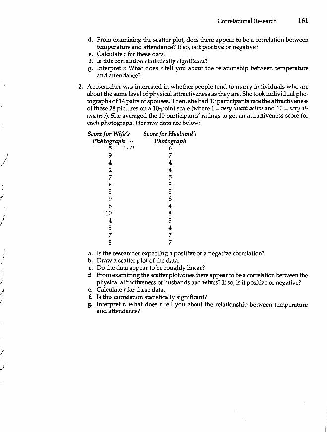
, I

I ,. , )

i /

l l

/ i

I ,.i

Correlational Research 161

d. From examining the scatter plot, does there appear to be a correlation between temperature and attendance? H so, is it positive or negative?

e. Calculate r for these data. f. Is this correlation statistically significant? g. Interpret r. What does r tell you about the relationship between temperature

and attendance?

2. A researcher was interested in whether people tend to marry individuals who are about the same level of physical attractiveness as they are. She took individual pho­tographs of 14 pairs of spouses. Then, she had 10 participants rate the attractiveness of these 28 pictures on a 10-point scale (where 1 = very unattractive and 10 = very at­tractive). She averaged the 10 participants' ratings to get an attractiveness score for each photograph. Her raw data are below:

Score for Wife'S Score for Husband's Ph'iJtograph· /; Photograph

a. b. c. d.

e. f. g.

5 '",/! 6 9 7 4 4 2 4 7 5 6 5 5 5 9 8 8 4

10 8 4 3 5 4 7 7 8 7

Is the researcher expecting a positive or a negative correlation? Draw a scatter plot of the data. Do the data appear to be roughly linear? From examining the scatter plot,.does there appear to be a correlation between the physical attractiveness of husbands and wives? H so, is it positive or negative? Calculate r for these data. Is this correlation statistically significant? Interpret r. What does r tell you about the relationship between temperature and attendance?

CHAPTER

7 Advanced Correlational Strategies

Predicting Behavior: Regression Strategies

Assessing Directionality: Cross-Lagged and Structural Equations Analysis

Uncovering Underlying Dimensions: Factor Analysis

Knowing whether variables are related to one another provides the cornerstone for much scientific investigation. 'TYPically, the first step in understanding any be­havioral phenomenon is to document that certain variables are somehow related; correlational research methods are indispensable for this purpose. However, as we saw in Chapter 6, correlational research can provide only tentative conclusions about cause-and-effect relationships, and simply demonstrating that variables are correlated has only limited usefulness. Once they know that variables are corre­lated, researchers usually want to understand how and why they are related.

In this chapter we take a look at three advanced correlational strategies that are used to explore how and why variables are related to one another. These methods allow researchers to go beyond simple correlations to a fuller and more precise un­derstanding of how particular variables are related to one another. Specifically, these methods allow researchers to (1) develop equations that describe how variables are related and that allow prediction of one variable from one or more other variables (re­gression analysis), (2) explore the likely direction of causality between two or more variables that are correlated (cross-lagged panel and structural equations analysis), and (3) identify basic dimensions that underlie sets of correlations (factor analysis).

Our emphasis in this chapter is on understanding what each of these meth­ods can tell us about the relationships among correlated variables and not on how to actually use them. Each of these strategies utilizes relatively sophisticated statis­tical analyses that would take us beyond the scope of this book.

Predicting Behavior: Regression Strategies

162

Imagine you are an industrial-organizational psychologist who works for a large company. One of your responsibilities is to develop better ways of selecting em-

....

.... !

(

/

i

J t r

;

! .

"..

, /

Advanced Correlational Strategies 163

ployees from the large number of people who apply for jobs with this company. You have developed a job aptitude test that is administered to everyone who ap­plies for a job. When you looked at the relationship between scores on this test and how employees were rated by their supervisors after working for the company for six months, you found that scores on the aptitude test correlated positively with ratings of job performance.

Armed with this information, you should be able to predict applicants' future job performance, allowing you to make better decisions about whom to hire. One consequence of two variables being correlated is that knowing a person's score on one variable allows us to predict his or her score on the other variable. Our predic­tion is seldom perfectly accurate, but if the two variables are correlated, we can predict scores at better than chance levels.

Linear Regression

This ability to predict scores on one variable from one or more other variables is ac­complished through regression analysis. The goal of regression analysis is to de­velop a regression equation from which we can predict one score on the basis of one or more other scores. This procedure is quite useful in situations where psy­chologists must make predictions. For example, regression equations are used to predict students' college performance from entrance exams and high school grades. They are also used in business and industrial settings to predict a job applicant's po­tential job performance on the basis of test scores and other factors. Regression analysis is also widely used in basic research settings to describe how variables are related to one another. Understanding how one variable is predicted by other vari­ables can help us understand the psychological processes that are involved. The precise manner in which a regression equation is calculated does not concern us here. What is important is that you know what a regression analysis is and the ra­tionale behind it, should you encounter it in the research literature.

Remember that correlation indicates a linear relationship between two vari­ables. If the relationship between two variables is linear, a straight line can be drawn through the data to represent the relationship between the variables. For example, Figure 7.1 shows the scatter plot for the relationship between the employees' test scores and job performance ratings that we analyzed in Chapter 6. (Remember that we found that the correlation between the test scores and job performance was +.82; see page 144.) The line drawn through the scatter plot portrays the nature of the re­lationship between test scores and performance ratings. In following the trend in the data, this line reflects how test scores and job performance tend to be related.

The goal of regression analysis is to find the equation for the line that best fits the pattern of the data. If we can find the equation for the line that best portrays the relationship between the two variables, this equation will provide us with a useful mathematical description of how the variables are related and also allow us to pre­dict one variable from the other.

You may remember from high school geometry class that a line can be rep­resented by the equation y = mx + b, where m is the slope of the line and b is the

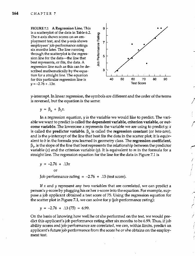
164 CHAPTER 7

FIGURE 7.1 A Regression Line. This 9 is a scatterplot of the data in Table 6.2. 01

The x-axis shows scores on an em- e: ~

ployment test, and the y-axis shows a: 7

employees' job performance ratings ~ e: six months later. The line running as

E through the scatterplot is the regres- ... .g 5 sion line for the data-the line that If. best represents, or fits, the data. A .Q

0 regression line such as this can be de- -,

scribed mathematically by the equa- 3

tion for a straight line. The equation for this particular regression line is 40 50 60 70 80 90 Y = -2.76 + .13x. Test Score

y-intercept. In linear regression, the symbols are different and the order of the terms is reversed, but the equation is the same:

In a regression equation, y is the variable we would like to predict. The vari­able we want to predict is called the dependent variable, criterion variable, or out­come variable. The lowercase x represents the variable we are using to predict y; x is called the predictor variable. Po is called the regression constant (or beta-zero), and is the y-intercept of the line that best fits the data in the scatter plot; it is equiv­alent to b in the formula you learned in geometry class. The regression coefficient, PI' is the slope of the line that best represents the relationship between the predictor variable (x) and the criterion variable (y). It is equivalent to m in the formula for a straight line. The regression equation for the line for the data in Figure 7.1 is

y = -2.76 + .13x

or

Job performance rating = -2.76 + .13 (test score).

If x and y represent any two variables that are correlated, we can predict a person's y-score by plugging his or her x-score into the equation. For example, sup­pose a job applicant obtained a test score of 75. Using the regression equation for the scatter plot in Figure 7.1, we can solve for y Gob performance rating):

y = -2.76 + .13 (75) = 6.99.

On the basis of knowing how well he or she performed on the test, we would pre­dict this applicant's job performance rating after six months to be 6.99. Thus, if job ability scores and job performance are correlated, we can, within limits, predict an applicant's future job performance from the score he or she obtains on the employ­menttest.

/

r' r

./

,I , ( ,

/

i'

{ i

!

j I / :I

t J

I ; \

*

Advanced Correlational Strategies 165

We can extend the idea of linear regression to include more than one predic­tor variable. For example, you might decide to predict job performance on the basis of four variables: aptitude test scores, high school grade point average (GPA), a measure of work motivation, and an index of physical strength. Using multiple re­gression analysis, you could develop a regression equation that includes all four predictors. Once the equation is determined, you could predict job performance from an applicant's scores on the four predictor variables. Typically, using more than one predictor improves the accuracy of our prediction over using only one.

Types of Multiple Regression

Researchers distinguish among three primary types of multiple regression proce­dures: standard, stepwise, and hierarchical multiple regression. These types of analyses differ with respect to how the predictor variables are entered into the re­gression equation as the equation is constructed. The predictor variables may be entered all at once (standard), based on the strength of their ability to help predict the criterion variable (stepwise), or in an order predetermined by the researcher (hierarchical).

Standard Multiple Regression. In standard multiple regression (also called si­multaneous multiple regression), all of the predictor variables are entered into the regression at the same time. So, for example, we could create a regression equation to predict job performance by entering simultaneously into the analysis employees' aptitude test scores, high school GPA, a measure of work motivation, and an index of physical strength. The resulting regression equation would provide a regression constant, as well as separate regression coefficients for each predictor. For example, the regression equation might look something like this:

Job performance rating = -2.79 + .17 (test score) + 1.29 (GPA) + .85 (work motivation) + .04 (physical strength).

By entering into the equation particular applicants' scores, we will get a predicted value for their job performance rating.

BEHAVIORAL RESEARCH CASE STUDY

Standard Multiple Regression Analysis: Do You Know How Smart You Are?

Researchers sometimes use standard or simultaneous multiple regression simply to see whether a set of predictor variables is related to some outcome variable. Paulhus, Lysy, and Yik (1998) used it in a study that examined the usefulness of self-report measures of intelli­gence. Because administering standardized IQ tests is time-consuming and expensive, Paulus et al. wondered whether researchers could simply rely on participants' ratings of how intelli­gent they are; if so, self-reported intelligence could be used instead of real IQ scores in some

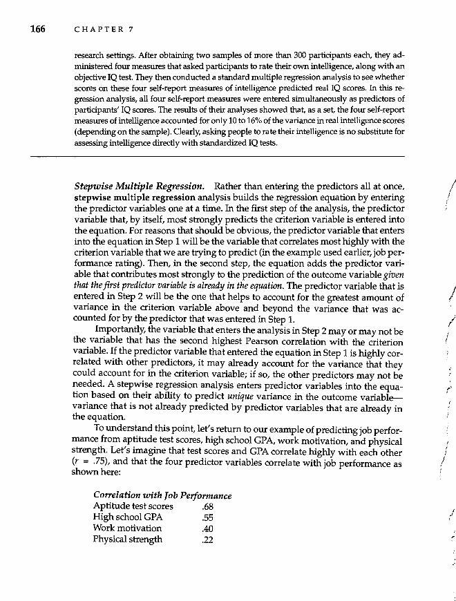
166 CHAPTER 7

research settings. After obtaining two samples of more than 300 participants each, they ad­ministered four measures that asked participants to rate their own intelligence, along with an objective IQ test. They then conducted a standard multiple regression analysis to see whether scores on these four self-report measures of intelligence predicted real IQ scores. In this re­gression analYSis, all four self-report measures were entered simultaneously as predictors of participants' IQ scores. The results of their analyses showed that, as a set, the four self-report measures of intelligence accounted for only 10 to 16% of the variance in real intelligence scores (depending on the sample). Clearly, asking people to rate their intelligence is no substitute for assessing intelligence directly with standardized IQ tests.

Stepwise Multiple Regression. Rather than entering the predictors all at once, stepwise multiple regression analysis builds the regression equation by entering the predictor variables one at a time. In the first step of the analysis, the predictor variable that, by itself, most strongly predicts the criterion variable is entered into the equation. For reasons that should be obvious, the predictor variable that enters into the equation in Step 1 will be the variable that correlates most highly with the criterion variable that we are trying to predict (in the example used earlier, job per­formance rating). Then, in the second step, the equation adds the predictor vari­able that contributes most strongly to the prediction of the outcome variable given that the first predictor variable is already in the equation. The predictor variable that is entered in Step 2 will be the one that helps to account for the greatest amount of variance in the criterion variable above and beyond the variance that was ac­counted for by the predictor that was entered in Step l.

Importantly, the variable that enters the analysis in Step 2 mayor may not be the variable that has the second highest Pearson correlation with the criterion variable. If the predictor variable that entered the equation in Step 1 is highly cor­related with other predictors, it may already account for the variance that they could account for in the criterion variable; if so, the other predictors may not be needed. A stepwise regression analysis enters predictor variables into the equa­tion based on their ability to predict unique variance in the outcome variable­variance that is not already predicted by predictor variables that are already in the equation.

To understand this point, let's return to our example of predicting job perfor­mance from aptitude test scores, high school GPA, work motivation, and physical strength. Let's imagine that test scores and GPA correlate highly with each other (r = .75), and that the four predictor variables correlate with job performance as shown here:

Correlation with lob Performance Aptitude test scores .68 High school GPA .55 Work motivation .40 PhYSical strength .22

/ , r "

I ( /

!

! { ,

i

l

, )

I )

. "

I f­!

Ii

Advanced Correlational Strategies 167

In a stepwise regression analysis, aptitude test scores would enter the equation in Step 1 because this predictor correlates most highly with job performance; by itself, aptitude test scores account for the greatest amount of variance in job performance ratings. But which predictor will enter the equation in the second step? Although GPA has the second highest correlation with job performance, it might not enter the equation in Step 2 because it correlates highly with aptitude test scores. If apti­tude test scores have already accounted for the variance in job performance that GPA can predict, GPA is no longer a useful predictor. Put differently, if we calcu­lated the partial correlation between GPA and job performance while statistically removing (partialing out) the influence of aptitude test scores (see Chapter 6), we would find that the partial correlation would be small or nonexistent, showing that GPA is not needed to predict job performance if we are already using aptitude test scores as a predictor.

The stepwise regression analysis will proceed step by step, entering predictor variables according to their ability to add uniquely to the prediction of the criterion variable. The stepwise process will stop when one of two things happens. On one hand, if each of the predictor variables can make a unique contribution to the pre­diction of the criterion variable, all of them will end up in the equation. On the other hand, the analysis may reach a point at which, with only some of the predic­tors in the equation, the remaining predictors cannot uniquely predict any remain­ing variance in the criterion variable. If this happens, the analysis stops without entering all of the predictors (and this may happen even if those remaining predic­tors are correlated with the variable being predicted). To use our example, perhaps after aptitude test scores and work motivation are entered into the regression equa­tion, neither GPA nor physical strength can further improve the prediction of job performance. In this case, the final regression equation would include only two predictors because the remaining two variables do not enhance our ability to pre­dict job performance .

BEHAVIORAL RESEARCH CASE STUDY

Stepwise Multiple Regression: Predictors of Blushing I once conducted a study in which we were interested in identifying factors that predict the degree to which people blush (Leary & Meadows, 1991). We administered a Blushing Propensity Scale to 220 subjects, along with measures of 13 other psychological variables. We then used stepwise multiple regression analysis, using the 13 variables as predictors of blushing propensity.

The results of the regression analysis showed that blushing propensity was best pre­dicted by embarrassability (the ease with which a person becomes embarrassed), which en­tered the equation in the first step. Social anxiety (the tendency to feel nervous in social situations) entered the equation in Step 2 because, with embarrassability in the equation, it made the greatest unique contribution of the remaining 12 predictors to the prediction of blushing scores. Self-esteem entered the equation in Step 3, followed in Step 4 by the degree to which a person is repulsed or offended by crass and vulgar behavior. After four steps, the

168 C HAP T E R 7

analysis stopped and entered no more predictors even though six additional predictor vari­ables (such as fear of negative evaluation and self-consciousness) correlated significantly with blushing propensity. These remaining variables did not enter the equation because, with the first four variables already in the equation, none of the others predicted unique variance in blushing propensity scores.

Hierarchical Multiple Regression. In hierarchical multiple regression, the pre­dictor variables are entered into the equation in an order that is predetermined by researchers, based on hypotheses that they want to test. As predictor variables are entered one by one into the regression analysis, their unique contributions to the prediction of the outcome variable can be assessed at each step. That is, by entering the predictor variables in some prespecified order, the researcher can determine whether particular predictors can account for unique variance in the outcome vari­able with the effects of other predictor variables statistically removed. Hierarchical multiple regression partials out the effects of the predictor variables entered on ear­lier steps to see whether predictors that are entered later make unique contributions to the outcome variable. Hierarchical multiple regression is a very versatile analysis that can be used to answer many kinds of questions. Two common uses are to elim­inate confounding variables and to test mediational hypotheses.

One of the reasons that we cannot infer causality from correlation is that, be­cause correlational research cannot control or eliminate extraneous variables, corre­lated variables are naturally confounded. Confounded variables are variables that tend to occur together, making their distinct effects on behavior difficult to separate. For example, we know that depressed people tend to blame themselves for bad things that happen more than nondepressed people; that is, depression and self­blame are correlated. For all of the reasons discussed earlier, we cannot conclude from this correlation that depression causes people to blame themselves or that self­blame causes depression. One explanation of this correlation is that depression is confounded with low self-esteem. Depression and low self-esteem tend to occur to­gether, so it is difficult to determine whether things that are correlated with depres­sion are a function of depression per se or whether they might be due to low self-esteem. A hierarchical regression analysis could provide a partial answer to this question. We could conduct a two-step hierarchical regression analysis in which we entered self-esteem as a predictor of self-blame in the first step. Of course, we would find that self-esteem predicted self-blame. More importantly, however, the relation­ship between self-esteem and self-blame would be partialed out in Step 1. Now, when we add depression to the regression equation in Step 2, we can see whether depression predicts self-blame above and beyond low self-esteem. If depression pre­dicts self-blame even after self-esteem was entered in the equation (and its influence on self-blame was statistically removed), we can conclude that the relationship be­tween depression and self-blame is not likely due to the fact that depression and low self-esteem are confounded. However, if depression no longer predicts self­blame when it is entered in Step 2, with self-esteem in the equation, the results will

!

, I'

/

I i

r ;

" i j

Advanced Correlational Strategies 169

suggest that the relationship between depression and self-blame may be due to its confound with self-esteem.

A second, related use of hierarchical multiple regression is to test mediational hypotheses. Many hypotheses specify that the effects of a predictor variable on a criterion variable are mediated by one or more other variables. Mediation effects occur when the effect of x on y occurs because of an intervening variable, z. For ex­ample, we know that regularly practicing yoga reduces stress and promotes a sense of calm. To understand why yoga has these effects, we could conduct hierar­chical regression analyses in which we enter possible mediators of the effect in Step 1. For example, we might hypothesize that some of the beneficial effects of yoga are mediated by its effects on the amount of mental"chatter" that goes on in the person's mind. That is, yoga helps to reduce mental chatter, which then leads to greater relaxation (because the person isn't thinking as much about worrisome things). To test whether mental chatter does, in fact, mediate the relationship be­tween yoga and relaxation, we would enter measures of mental chatter (such as in­dices of obsessional tendencies, self-focused thinking, and worry) in Step 1 of the analysis. Of course, these measures will probably predict low relaxation, but that's not our focus. Rather, we are interested in what happens when we enter the amount of time that people practice yoga in Step 2 of the analysis. If the variables entered in Step 1 mediate the relationship between yoga and relaxation, then yoga should no longer predict relaxation when it is entered in the second step. Remov­ing variance that is due to the mediators in Step 1 would eliminate yoga's ability to predict relaxation. However, if yoga practice predicts relaxation just as strongly with the influence of the hypothesized mediator variables removed in Step 1, then we conclude that yoga's effects are not mediated by reductions in mental chatter. Researchers are often interested in the processes that mediate the influence of one variable on another, and hierarchical regression can help them to test hypotheses about these mediators.

Me M BEHAVIORAL RESEARCH CASE STUDY

Hierarchical Regression: Personal and Interpersonal Antecedents of Peer Victimization

Hodges and Perry (1999) conducted a study to investigate factors that lead certain children to be victimized-verbally or physically assaulted-by their peers at school. Data were col­lected from 173 preadolescent children who completed several measures of personality and behavior, some of which involved personal factors (such as depression) and other measures involved interpersonal factors (such as difficulty getting along with others). They also pro­vided information regarding the victimization of other children they knew. The participants completed these measures two times spaced one year apart.

Multiple regression analyses were used to predict victimization from the various per­sonal and interpersonal factors. Of course, personal and interpersonal factors are likely to be confounded because certain personal difficulties may lead to social problems, and vice versa. Thus, the researchers wanted to test the separate effects of personal and interpersonal

170 CHAPTER 7

factors on victimization while statistically removing the effects of the other set. They used hierarchical regression to do this because it allowed them to enter predictors into the re­gression analysis in any order they desired. Thus, one hierarchical regression analysis was conducted to predict victimization scores at Time 2 (the second administration of the mea­sures) from personal factors measured at TIme 1, while removing the influence of interper­sonal factors (also at Time 1). To do this, interpersonal factors were entered as predictors (and their influence on victimization removed) before the personal factors were entered. Another regression analysis reversed the order in which predictors were entered, putting personal factors in the equation first, then testing the unique effects of interpersonal factors. In this way, the effects of each set of predictors could be tested while eliminating the con­founding influence of the other set.

Results showed that both personal and interpersonal factors measured at Time 1 pre­dicted the degree to which children were victimized a year later. Personal factors such as anxiety, depression, social withdrawal, and peer hovering (standing around without joining in) predicted victimization, as did scoring low on a measure of physical strength (presum­ably because strong children are less likely to be bullied). The only interpersonal factor that predicted victimization after personal problems were partialed out was the degree to which the child was rejected by his or her peers. In contrast, being aggressive, argumentative, dis­ruptive, and dishonest were unrelated to victimization. Using hierarchical regression analy­ses allows researchers to get a clearer picture of the relationships between particular predictors and a criterion variable, uncontaminated by confounding variables.

Multiple Correlation

When researchers use multiple regression analyses, they not only want to develop an equation for predicting people's scores, but also need to know how well the predictor, or x, variables predict y. After all, if the predictors do a poor job of pre­dicting the outcome variable, we wouldn't want to use the equation to make de­cisions about job applicants, students, or whomever. To express the usefulness of a regression equation for predicting, researchers calculate the multiple correlation coefficient, symbolized by the letter R. R describes the degree of relationship be­tween the criterion variable (y) and the set of predictor variables. Unlike the Pear­son " multiple correlation coefficients only range from .00 to 1.00. The larger R is, the better job the equation does of predicting the outcome variable from the pre­dictor variables.

Just as a Pearson correlation coefficient can be squared to indicate the per­centage of variance in one variable that is accounted for by another, a multiple cor­relation coefficient can be squared to show the percentage of variance in the criterion variable (y) that can be accounted for by the set of predictor variables. In the study of blushing described above, the multiple correlation, R, between the set of four predictors and blushing propensity was .63. Squaring R (.63 x .63) gives us .40, indicating that 40% of the variance in subjects' blushing propensity scores was accounted for by the set of four predictors.

Advanced Correlational Strategies 171

Assessing Directionality: Cross-Lagged and Structural Equations Analysis

We've stressed several times that researchers cannot infer causality from correla­tion. In Chapter 6, we saw how partial correlation can be used to tentatively test whether certain third variables are responsible for the correlation between two variables, and in this chapter, we discussed how hierarchical regression analysis can help disentangle confounded variables. But even if we conclude that the cor­relation between x and y is unlikely to be due to certain other variables, we still cannot determine from a correlation whether x causes y or y causes x. Fortunately, researchers have developed procedures for testing the viability of their causal hy­potheses. Although these procedures cannot tell us for certain whether x causes y or y causes x, they can give us more or less confidence in one causal direction than the other.

Cross-Lagged Panel Design

A simple case involves the cross-lagged panel correlation design (Cook & Camp­bell, 1979). In this design, the correlation between two variables, x and y, is calcu­lated at two different points in time. Then, correlations are calculated between measurements of the two variables across time. For example, we would correlate the scores on x taken at Time 1 with the scores on y taken at Tune 2. Likewise, we would calculate the scores on y at Time 1 with those on x at Time 2. H x causes y, we should find that the correlation between x at Time 1 and y at Time 2 is larger than the correlation between y at Time 1 and x at Time 2. This is because the relationship between a cause (variable x) and its effect (variable y) should be stronger if the causal variable is measured before rather than after its effect.

A cross-lagged panel design was used to study the link between violence on television and aggressive behavior. More than 30 years of research has demon­strated that watching violent television programs is associated with aggression. For example, the amount of violence a person watches on TV correlates positively with the person's level of aggressiveness. However, we should not infer from this corre­lation that television violence causes aggression. It is just as plausible to conclude that people who are naturally aggressive simply like to watch violent programs.

Eron, Huesmann, Lefkowitz, and Walder (1972) used a cross-lagged panel correlation design to examine the direction of the relationship between television violence and aggressive behavior. These researchers studied a sample of 427 par­ticipants twice: once when the participants were in the third grade and again 10 years later. On both occasions, participants provided a list of their favorite TV shows, which were later rated for their violent content. In addition, participants' aggressiveness was rated by their peers.

Correlations were calculated between TV violence and participants' aggres­siveness across the two time periods. The results for the male participants are shown in Figure 7.2. The important correlations are on the diagonals of Figure 7.2-the

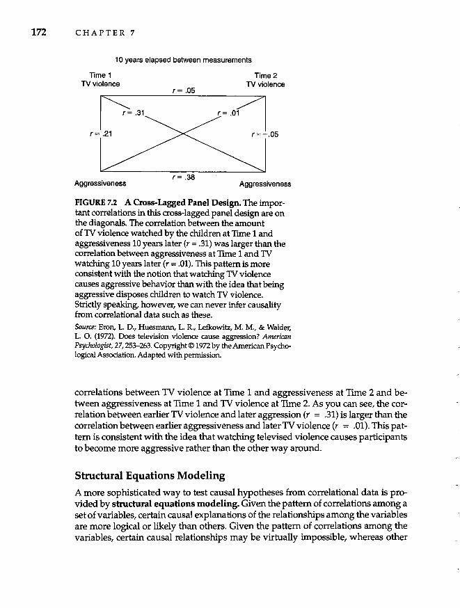
172 CHAPTER 7

10 years elapsed between measurements

Time 1 TV violence

Aggressiveness

r= .05

r= .38

Time 2 TV violence

Aggressiveness

FIGURE 7.2 A Cross-Lagged Panel Design. The impor­tant correlations in this cross-lagged panel design are on the diagonals. The correlation between the amount of TV violence watched by the children at Time 1 and aggressiveness 10 years later (r = .31) was larger than the correlation between aggressiveness at Time 1 and TV watching 10 years later (r = .01). This pattern is more consistent with the notion that watching TV violence causes aggressive behavior than with the idea that being aggressive disposes children to watch TV violence. Strictly speaking, however, we can never infer causality from correlational data such as these. Source: Eron, L. D., Huesmann, L. R., Lefkowitz, M. M., & Walder, L. O. (1972). Does television violence cause aggression? American Psychologist, 27, 253-263. Copyright © 1972 by the American Psycho­logical Association. Adapted with permission.

correlations between TV violence at Time 1 and aggressiveness at Time 2 and be­tween aggressiveness at Time 1 and TV violence at Time 2. As you can see, the cor­relation between earlier TV violence and later aggression (r = .31) is larger than the correlation between earlier aggressiveness and later TV violence (r = .01). This pat­tern is consistent with the idea that watching televised violence causes participants to become more aggressive rather than the other way around.

Structural Equations Modeling

A more sophisticated way to test causal hypotheses from correlational data is pro­vided by structural equations modeling. Given the pattern of correlations among a set of variables, certain causal explanations of the relationships among the variables are more logical or likely than others. Given the pattern of correlations among the variables, certain causal relationships may be virtually impossible, whereas other

Advanced Correlational Strategies 173

causal relationships are plausible. To use a simple example, imagine that we are try­ing to understand the causal relationships among three variables-X, Y, and Z. If we predict that X causes Y and then Y causes Z, then we should find not only that X and Yare correlated but that the relationship between X and Y is stronger than the correlation between X and Z. (Variables that are directly linked in a causal chain should correlate more highly than variables that are more distally related.) If either of these findings do not occur, then our hypothesis that X -7 Y -7 Z would appear to be false.

To perform structural equations modeling, the researcher makes precise predictions regarding how three or more variables are causally related. (In fact, researchers often devise two or more competing predictions based on different theories.) Each prediction (or model) implies that the variables should be corre­lated in a particular way. Imagine that we have two competing predictions about the relationships among X, Y, and Z. Hypothesis A says that X causes Y and then Y causes Z. In contrast, Hypothesis B predicts that Z causes X, then X causes Y. We would expect X, Y, and Z to correlate differently if Hypothesis A were true than if Hypothesis B were true. Thus, Hypothesis A predicts that the correlation matrix for X, Y, and Z will show a different pattern of correlations than Hypoth­esis B.

Structural equations modeling mathematically compares the correlation matrix implied by a particular hypothesized model to the real correlation ma­trix based on the data that we collect. The analysis examines the degree to which the pattern of correlations generated from our predicted model matches or fits the correlation matrix based on the data. If the correlation matrix predicted by our model closely resembles the real correlation matrix, then we have a cer­tain degree of support for the hypothesized model. Structural equations analy­ses provide a fit index that indicates how well the hypothesized model fits the data. By comparing the fit indexes for different predicted models, we can deter­mine whether one of our models fits the data better than other, alternative mod­els. Structural equations models can get very complex, adding not only more variables but also multiple measures of each variable to improve our measure­ment of the constructs we are studying. When multiple measures of each con­struct are used in the analysis, researchers sometimes call structural equations analysis latent variable modeling (because the various measures of a particular construct are assumed to assess a single underlying, or latent variable). In con­trast, when single measures of each construct are used, researchers sometimes call it path analysis.

It is important to remember that structural equations modeling cannot provide us with confident conclusions about causality. We are, after all, still dealing with cor­relational data, and as we've stressed again and again, we cannot infer causality from correlation. However, structural equations modeling can provide information re­garding the plausibility of causal hypotheses. If the analysis indicates that the model fits the data, then we have reason to regard that model as a reasonable causal expla­nation (though not necessarily the one-and-only correct explanation). Conversely, if

174 CHAPTER 7

the model does not fit the data, then we can conclude that the hypothesized model is not likely to be correct.

fIl!l!!IjJi!)i'!!!f!!*'i¥'i!!! BEHAVIORAL RESEARCH CASE STUDY

Structural Equations Modeling: Partner Attractiveness and Intention to Practice Safe Sex Since the beginning of the AIDS epidemic in the 1980s, health psychologists have devoted a great deal of attention to ways of increasing condom use. Part of this research has fo­cused on understanding how people think about the risks of having unprotected sexual intercourse. Agocha and Cooper (1999) were interested specifically in the effects of a po­tential sexual partner's sexual history and physical attractiveness on people's willingness to have unprotected sex. In this study, 280 college-age participants were given informa­tion about a member of the other sex that included a deSCription of the person's sexual his­tory (indicating that the person had between 1 and 20 previous sexual partners) as well as a yearbook-style color photograph of either an attractive or unattractive individual. Par­ticipants then rated the degree to which they were interested in dating or having sexual intercourse with the target person, the likelihood of getting AIDS or other sexually trans­mitted diseases from this individual, the likelihood that they would discuss sex-risk issues with the person prior to having sex, and the likelihood of using a condom if intercourse were to occur.

Among many other analyses, Agocha and Cooper conducted a path analYSis (a struc­tural equations model with one measure of each variable) to examine the effects of the tar­get's sexual history and physical attractiveness on perceived risk and intention to use a condom. The path diagram shown in Figure 7.3 fit the data well, indicating that it is a plau­sible model of how these variables are related. The arrows in the diagram indicate the pres­ence of statistically significant relationships. The numbers beside each arrow are path coefficients; they are analogous to the regression coefficients discussed earlier and reflect the strength of the relationship for each effect.

Examine the path diagram as I describe a few of the findings. First, participants' in­terest in dating or having sex with the target were predicted by both gender (male partici­pants were more interested than females) and, not surprisingly, the target's physical attractiveness. However, the target's sexual history did not predict interest in dating or sex (there is no arrow going from Target's Sexual History to Interest in Target). Second, perceived risk of getting AIDS was predicted by gender (women were more concerned than men), target's sexual history (more sexually active targets were regarded as greater risks), and participants' interest in the target. The latter finding is particularly interesting: Participants rated having sex with targets in whom they were interested as less risky, which is, of course, fallacious.

If we look at predictors of the intention to use condoms, we see that the intention to practice safe sex is predicted not only by perceived risk but also by the degree to which the participant was interested in the target. Regardless of the perceived risk, participants were less likely to intend to use a condom the more interested they were in the target and the

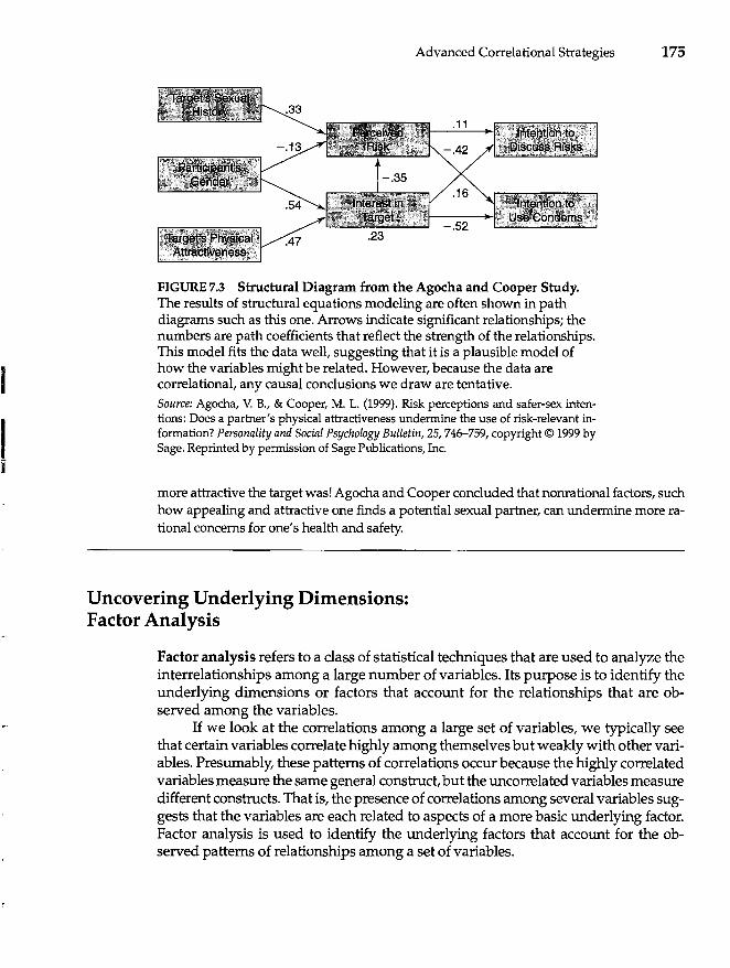
I

Advanced Correlational Strategies 175

FIGURE 7.3 Structural Diagram. from the Agocha and Cooper Study. The results of structural equations modeling are often shown in path diagrams such as this one. Arrows indicate significant relationships; the numbers are path coefficients that reflect the strength of the relationships. This model fits the data well, suggesting that it is a plausible model of how the variables might be related. However, because the data are correlational, any causal conclusions we draw are tentative. Source: Agocha, V. B., & Cooper, M. L. (1999). Risk perceptions and safer-sex inten­tions: Does a partner's physical attractiveness undermine the use of risk-relevant in­formation? Personality and Social Psychology Bulletin, 25, 746-759, copyright © 1999 by Sage. Reprinted by permission of Sage Publications, Inc.

more attractive the target was! Agocha and Cooper concluded that nonrational factors, such how appealing and attractive one finds a potential sexual partner, can undermine more ra­tional concerns for one's health and safety.

Uncovering Underlying Dimensions: Factor Analysis

Factor analysis refers to a class of statistical techniques that are used to analyze the interrelationships among a large number of variables. Its purpose is to identify the underlying dimensions or factors that account for the relationships that are ob­served among the variables.

If we look at the correlations among a large set of variables, we typically see that certain variables correlate highly among themselves but weakly with other vari­ables. Presumably, these patterns of correlations occur because the highly correlated variables measure the same general construct, but the uncorrelated variables measure different constructs. That is, the presence of correlations among several variables sug­gests that the variables are each related to aspects of a more basic underlying factor. Factor analysis is used to identify the underlying factors that account for the ob­served patterns of relationships among a set of variables.

176 CHAPTER 7

An Intuitive Approach

Suppose for a moment that you obtained participants' scores on five variables that we'll call A, B, C, D, and E. When you calculated the correlations among these five variables, you obtained the following correlation matrix:

A B C D E A 1.00 .78 .85 .01 -.07 B 1.00 .70 .09 .00 C 1.00 -.02 .04 D 1.00 .86 E 1.00

Look closely at the pattern of correlations. Based on the pattern, what conclusions would you draw about the relationships among variables A, B, C, D, and E? Which variables seem to be related to each other?

As you can see, variables A, B, and C correlate highly with each other, but each correlates weakly with variables D and E. Variables D and E, on the other hand, are highly correlated. This pattern suggests that these five variables may be measuring only two different constructs: A, B, and C seem to measure aspects of one construct, whereas D and E measure something else. In the language of factor analysis, two factors underlie these data and account for the observed pattern of correlations among the variables.

Basics of Factor Analysis

Although identifying the factor structure may be relatively easy with a few vari­ables, imagine trying to identify the factors in a data set that contained 20 or 30 or even 100 variables! Factor analysis identifies and expresses the factor structure by using mathematical procedures rather than by eyeballing the data, as we have just done.

The mathematical details of factor analysis are complex and don't concern us here, but let us look briefly at how factor analyses are conducted. The grist for the factor analytic mill consists of correlations among a set of variables. Factor analy­sis attempts to identify the minimum number of factors or dimensions that will do a reasonably good job of accounting for the observed relationships among the vari­ables. At one extreme, if all of the variables are highly correlated with one another, the analysis will identify a single factor; in essence, all of the observed variables are measuring aspects of the same thing. At the other extreme, if the variables are to­tally uncorrelated, the analysis will identify as many factors as there are variables. This makes sense; if the variables are not at all related, there are no underlying fac­tors that account for their interrelationships. Each variable is measuring something different, and there are as many factors as variables.

The solution to a factor analysis is presented in a factor matrix. Table 7.1 shows the factor matrix for the variables we examined in the preceding correlation

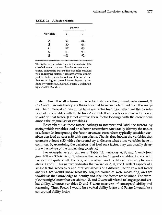
TABLE 7.1 A Factor Matrix

Factor

Variable 1 2

A .97 -.04 B .80 .04 C .87 .00 D .03 .93 E -.01 .92

4

This is the factor matrix for a factor analysis of the correlation matrix above. Two factors were ob­tained, suggesting that the five variables measure two underlying factors. A researcher would inter­pret the factor matrix by looking at the variables that loaded highest on each factor. Factor 1 is de­fined by variables A, B, and C. Factor 2 is defined by variables D and E.

Advanced Correlational Strategies 177

matrix. Down the left column of the factor matrix are the original variables-A, B, e, D, and E. Across the top are the factors that have been identified from the analy­sis. The numerical entries in the table are factor loadings, which are the correla­tions of the variables with the factors. A variable that correlates with a factor is said to load on that factor. (Do not confuse these factor loadings with the correlations among the original set of variables.)

Researchers use these factor loadings to interpret and label the factors. By seeing which variables load on a factor, researchers can usually identify the nature of a factor. In interpreting the factor structure, researchers typically consider vari­ables that load at least ±.30 with each factor. That is, they look at the variables that correlate at least ±.30 with a factor and try to discern what those variables have in common. By examining the variables that load on a factor, they can usually deter­mine the nature of the underlying construct.

For example, as you can see in Table 7.1, variables A, B, and e each load greater than .30 on Factor 1, whereas the Factor loadings of variables D and E with Factor 1 are quite small. Factor 2, on the other hand, is defined primarily by vari­ables D and E. This pattern indicates that variables A, B, and e reflect aspects of a single factor, whereas D and E reflect aspects of a different factor. In a real factor analysis, we would know what the original variables were measuring, and we would use that knowledge to identify and label the factors we obtained. For exam­ple, we might know that variables A, B, and e were all related to language and ver­bal ability, whereas variables D and E were measures of conceptual ability and reasoning. Thus, Factor 1 would be a verbal ability factor and Factor 2 would be a conceptual ability factor.

178 CHAPTER 7

Uses of Factor Analysis

Factor analysis has two basic uses. First, it is used to study the underlying structure of psychological constructs. Many questions in behavioral science involve the struc­ture of behavior and experience. How many distinct mental abilities are there? What are the basic traits that underlie human personality? What are the primary emotional expressions? What factors underlie job satisfaction? Factor analysis is used to answer such questions, thereby providing a framework for understanding behavioral phe­nomena. This use of factor analysis is portrayed in the accompanying Behavioral Re­search Case Study box, "Factor Analysis: The Five-Factor Model of Personality."

Researchers also use factor analysis to reduce a large number of variables to a smaller, more manageable set of data. Often, a researcher measures a large num­ber of variables, knowing that these variables measure only a few basic constructs. For example, participants may be asked to rate their current mood on 40 mood­relevant adjectives (such as happy, hostile, pleased, nervous). Of course, these do not reflect 40 distinct moods; instead, several items are used to measure each mood. So, a factor analysis may be performed to reduce these 40 scores to a small number of factors that reflect basic emotions. Once the factors are identified, com­mon statistical procedures may be performed on the factors themselves rather than on the original items. Not only does this approach eliminate the redundancy in­volved in analyzing many measures of the same thing, but analyses of factors are usually more powerful and reliable than measures of individual items.

~ BEHAVIORAL RESEARCH CASE STUDY

Factor Analysis: The Five-Factor Model of Personality

How many basic personality traits are there? Obviously, people differ on dozens, if not hun­dreds, of attributes, but presumably many of these variables are aspects of broader and more general traits. Factor analysis has been an indispensable tool in the search for the basic dimensions of personality. By factor-analyzing people's ratings of themselves, researchers have been able to identify the basic dimensions of personality and to see which specific traits load on these basic dimensions. In several studies of this nature, factor analyses have obtained five fundamental personality factors: extraversion, agreeableness, conscientious­ness, emotional stability, and openness.

In a variation on this work, McCrae and Costa (1987) asked whether the same five fac­tors would be obtained if we analyzed other people's ratings of an individual rather than the individual's self-reports. Some 274 participants were rated on 80 adjectives by a person who knew them well, such as a friend or coworker. When these ratings were factor ana­lyzed, five factors were obtained that closely mirrored the factors obtained when people's self-reports were analyzed.

A portion of the factor matrix is shown below. (Although the original matrix con­tained factor loadings for all 80 dependent variables, the portion of the matrix shown below involves only 15 variables.) Recall that the factor loadings in the matrix are correlations be­tween each item and the factors.

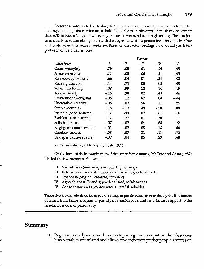
r

Advanced Correlational Strategies 179

Factors are interpreted by looking for items that load at least ±.30 with a factor; factor loadings meeting this criterion are in bold. Look, for example, at the items that load greater than ±.30 in Factor l---calm-worrying, at ease-nervous, relaxed-high-strung. These adjec­tives clearly have something to do with the degree to which a person feels nervous. McCrae and Costa called this factor neuroticism. Based on the factor loadings, how would you inter­pret each of the other factors?

Factor Adjectives I II III IV V Calm-worrying .79 .05 -.01 -.20 .05 At ease-nervous .77 -.08 -.06 -.21 -.05 Relaxed-high-strung .66 .04 .01 -.34 -.02 Retiring-sociable -.14 .71 .08 .08 .08 Sober-fun-Ioving -.08 .59 .12 .14 -.15 Aloof-friendly -.16 .58 .02 .45 .06 Conventional-original -.06 .12 .67 .08 -.04 Uncreative-creative -.08 .03 .56 .11 .25 Simple-complex .16 -.13 .49 -.20 .08 Irritable-good-natured -.17 .34 .09 .61 .16 Ruthless-soft-hearted .12 .27 .01 .70 .11 Selfish-selfless -.07 -.02 .04 .65 .22 Negligent-<:onscientious -.01 .02 .08 .18 .68 Careless-careful -.08 -.07 -.01 .11 .72 Undependable-reliable -.07 .04 .05 .23 .68

Source: Adapted from McCrae and Costa (1987).

On the basis of their examination of the entire factor matrix, McCrae and Costa (1987) labeled the five factors as follows:

I Neuroticism (worrying, nervous, high-strung) II Extraversion (sociable, fun-loving, friendly, good-natured)

III Openness (original, creative, complex) IV Agreeableness (friendly, good-natured, soft-hearted) V Conscientiousness (conscientious, careful, reliable)

These five factors, obtained from peers' ratings of participants, mirror closely the five factors obtained from factor analyses of participants' self-reports and lend further support to the five-factor model of personality.

Summary

1. Regression analysis is used to develop a regression equation that describes how variables are related and allows researchers to predict people's scores on

180 C HAP T E R 7

one variable based on their scores on other variables. A regression equation provides a regression constant (equivalent to the y-intercept) as well as a re­gression efficient for each predictor variable.

2. When constructing regression equations, a researcher may enter all of the predictor variables at once (simultaneous or standard regression), allow pre­dictor variables to enter the equation based on their ability to account for unique variance in the criterion variable (stepwise regression), or enter the variables in a manner that allows him or her to test particular hypotheses (hi­erarchical regression).

3. Multiple correlation expresses the strength of the relationship between one variable and a set of other variables. Among other things, it provides infor­mation about how well a set of predictor variables can predict scores on a cri­terion variable in a regression equation.

4. Cross-lagged panel correlation designs and structural equations modeling are used to test the plausibility of causal relationships among a set of corre­lated variables. Both analyses can provide evidence for or against causal hy­potheses, but our conclusions are necessarily tentative because the data are correlational.

5. Factor analysis refers to a set of procedures for identifying the dimensions or factors that account for the observed relationships among a set of variables. A factor matrix shows the factor loadings for each underlying factor, which are the correlations between each variable and the factor. From this matrix, re­searchers can identify the basic factors in the data.

KEY TERMS

criterion variable (p. 164) cross-lagged panel correlation

design (p. 171) dependent variable (p. 164) factor (p. 176) factor analysis (p. 175) factor loadings (p. 177) factor matrix (p. 176) fit index (p. 173) hierarchical multiple

regression (p. 168)

multiple correlation coefficient (p. 170)

multiple regression analysis (p.165)

outcome variable (p. 164) predictor variable (p. 164) regression analysis (p. 163) regression coefficient

(p.I64) regression constant (p. 164)

QUESTIONS FOR REVIEW

1. When do researchers use regression analysis?

regression equation (p. 163) simultaneous multiple

regression (p. 165) standard multiple regression

(p.165) stepwise multiple regression

(p.166) structural equations modeling

(p.I72)

2. Write the general form of a regression equation that has a single predictor variable. Identify the criterion variable, the predictor variable, the regression constant, and the regression coefficient.

Advanced Correlational Strategies 181

3. A regression equation is actually the equation for a straight line. What line is de­scribed by a regression equation?

4. Imagine that the equation for predicting y from x is y = 1.12 - .47x. How would you use this equation to predict a particular individual's score?

5. What is multiple regression analysis?

6. Distinguish among simultaneous (or standard), stepwise, and hierarchical regression.

7. Of the three kinds of regression analyses, which would you use to a. build the best possible prediction equation from the least number of predictor

variables? b. test a mediational hypothesis? c. determine whether a set of variables predicts a criterion variable? d. eliminate a confounding variable as you test the effects of a particular predictor

variable?

8. In stepwise regression, why might a predictor variable that correlates highly with the criterion variable not enter into the regression equation?

9. Explain how you would use regression analysis to see whether variable Z mediates the effect of variable X on variable Y.

10. When would you calculate a multiple correlation coefficient? What do you learn if you square a multiple correlation?

11. How does a cross-lagged panel correlation design provide evidence to support a causal link between two variables?

12. Describe how structural equations modeling works.

13. Distinguish between latent variable modeling and path analysis as types of struc­tural equations modeling.

14. Why do researchers use factor analysis?

15. Imagine that you conducted a factor analysis on a set of variables that were uncor­related with one another. How many factors would you expect to find? Why?

QUESTIONS FOR DISCUSSION

1. In one of the exercises at the end of Chapter 6, you calculated the correlation be­tween outside temperature and class attendance. The regression equation for the data in that exercise is

Attendance = 114.35 - .61 (temperature).

Imagine that the weather forecaster predicts that next Friday's temperature will be 82 degrees F. How many students would you expect to attend class on that day?

2. One of the Behavioral Research Case Studies in this chapter involved Agocha and Cooper's (1999) study of partner characteristics and intentions to practice safe sex. Below are the Pearson correlations between the likelihood that participants would discuss risks before having sex and several other variables.

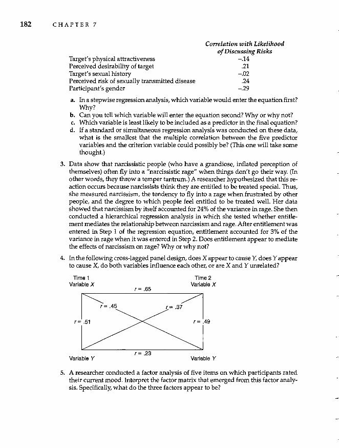
182 C HAP T E R 7

Target's physical attractiveness Perceived desirability of target Target's sexual history

Correlation with Likelihood of Discussing Risks

-.14 .21

-.02 Perceived risk of sexually transmitted disease Participant's gender

.24 -.29

a. In a stepwise regression analysis, which variable would enter the equation first? Why?

b. Can you tell which variable will enter the equation second? Why or why not? c. Which variable is least likely to be included as a predictor in the final equation? d. If a standard or simultaneous regression analysis was conducted on these data,

what is the smallest that the multiple correlation between the five predictor variables and the criterion variable could possibly be? (This one will take some thought.)

3. Data show that narcissistic people (who have a grandiose, inflated perception of themselves) often fly into a "narcissistic rage" when things don't go their way. (In other words, they throw a temper tantrum.) A researcher hypothesized that this re­action occurs because narcissists think they are entitled to be treated special. Thus, she measured narcissism, the tendency to fly into a rage when frustrated by other people, and the degree to which people feel entitled to be treated well. Her data showed that narcissism by itself accounted for 24% of the variance in rage. She then conducted a hierarchical regression analysis in which she tested whether entitle­ment mediates the relationship between narcissism and rage. After entitlement was entered in Step 1 of the regression equation, entitlement accounted for 3% of the variance in rage when it was entered in Step 2. Does entitlement appear to mediate the effects of narcissism on rage? Why or why not?

4. In the following cross-lagged panel deSign, does X appear to cause Y, does Yappear to cause X, do both variables influence each other, or are X and Y unrelated?

Time 1 Variable X

Variable Y

r= .65

r= .23

Time 2 Variable X

Variable Y

5. A researcher conducted a factor analysis of five items on which participants rated their current mood. Interpret the factor matrix that emerged from this factor analy­sis. Specifically, what do the three factors appear to be?

,-

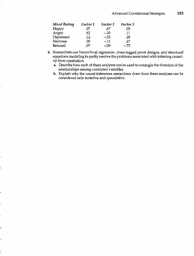
Mood Rating Happy Angry Depressed Nervous Relaxed

Factor 1 .07 .82 .12 .00 .07

Advanced Correlational Strategies 183

Factor 2 .67

-.20 -.55 -.12 -.09

Factor 3 .03 .11 .20 .67

-.72

6. Researchers use hierarchical regression, cross-lagged panel designs, and structural equations modeling to partly resolve the problems associated with inferring causal­ity from correlation. a. Describe how each of these analyses can be used to untangle the direction of the

relationships among correlated variables. b. Explain why the causal inferences researchers draw from these analyses can be

considered only tentative and speculative.

CHAPTER

8 Basic Issues in Experimental Research

Manipulating the Independent Variable

Assignment of Participants to Conditions

Experimental Control

Error Variance

Experimental Control and Generalizability: The Experimenter's Dilemma

Eliminating Confounds

184

Students in one of my courses once asked whether I would postpone for one week an exam that was scheduled for the next Monday. From my perspective as the in­structor, postponing the exam would have disrupted the course schedule, and I felt that delaying the test a week was too much to ask. So I told them, "No, I think it would be better to have the test as scheduled." After a moment of silence, a student asked, "Well, if you won't postpone the test a week, will you postpone it at least until next Friday?" I was still reluctant but finally agreed.

In retrospect, I think I was a victim of the" door-in-the-face" effect. The door-in­the-face phenomenon works like this: By first making an unreasonably large request, a person increases the probability that a second, smaller request will be granted. Re­fusing the students' request to postpone the test until Monday increased the chance that I would agree to postpone it until the preceding Friday.

This interesting phenomenon was studied by Robert Cialdini and his col­leagues in a series of experiments (Cialdini, Vmcent, Lewis, Catalan, Wheeler, & Darby, 1975). In one experiment, researchers approached people walking on the campus of Arizona State University and made one of three requests. Participants in one group were first asked whether they would be willing to work as a nonpaid counselor for the County Juvenile Detention Center for two hours per week for two years. Not surprisingly, no one agreed to such an extreme request. However, after the participant had turned down this request, the researcher asked whether the participant would be willing to chaperone a group of children from the Juve­nile Detention Center for a two-hour triP to the zoo.

Participants in a second group were asked only the smaller request-to chap­erone the trip to the zoo-without first being asked the more extreme request. For a

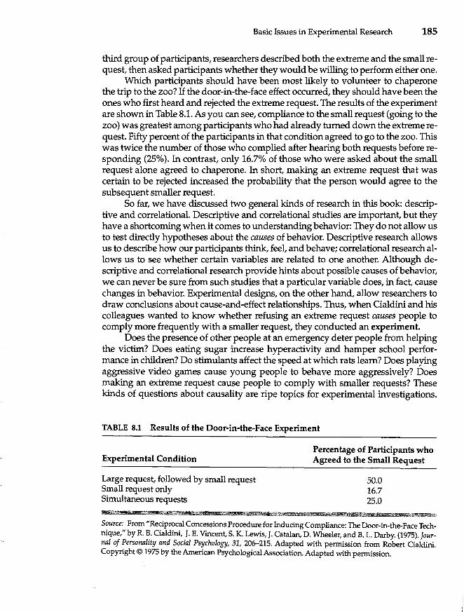
Basic Issues in Experimental Research 185

third group of participants, researchers described both the extreme and the small re­quest, then asked participants whether they would be willing to perform either one.

Which participants should have been most likely to volunteer to chaperone the trip to the zoo? If the door-in-the-face effect occurred, they should have been the ones who first heard and rejected the extreme request. The results of the experiment are shown in Table 8.1. As you can see, compliance to the small request (going to the zoo) was greatest among participants who had already turned down the extreme re­quest. Fifty percent of the participants in that condition agreed to go to the zoo. This was twice the number of those who complied after hearing both requests before re­sponding (25%). In contrast, only 16.7% of those who were asked about the small request alone agreed to chaperone. In short, making an extreme request that was certain to be rejected increased the probability that the person would agree to the subsequent smaller request.

So far, we have discussed two general kinds of research in this book: descrip­tive and correlational. Descriptive and correlational studies are important, but they have a shortcoming when it comes to understanding behavior: They do not allow us to test directly hypotheses about the causes of behavior. Descriptive research allows us to descnbe how our participants think, feel, and behave; correlational research al­lows us to see whether certain variables are related to one another. Although de­scriptive and correlational research provide hints about possible causes of behavior, we can never be sure from such studies that a particular variable does, in fact, cause changes in behavior. Experimental designs, on the other hand, allow researchers to draw conclusions about cause-and-effect relationships. Thus, when Cialdini and his colleagues wanted to know whether refusing an extreme request causes people to comply more frequently with a smaller request, they conducted an experiment.

Does the presence of other people at an emergency deter people from helping the victim? Does eating sugar increase hyperactivity and hamper school perfor­mance in children? Do stimulants affect the speed at which rats learn? Does playing aggressive video games cause young people to behave more aggressively? Does making an extreme request cause people to comply with smaller requests? These kinds of questions about causality are ripe topics for experimental investigations.

TABLE 8.1 Results of the Door-in-the-Face Experiment

Experimental Condition

Large request, followed by small request Small request only Simultaneous requests

Percentage of Participants who Agreed to the Small Request

50.0 16.7 25.0

.... @WA M i1

Source: From "Reciprocal Concessions Procedure for Inducing Compliance: The Door-in-the-Face Tech­nique," by R. B. Cialdini, J. E. Vincent, S. K. Lewis, J. Catalan, D. Wheeler, and B. L. Darby. (1975). Jour­nal of Personality and Social Psychology, 31, 206-215. Adapted with permission from Robert Cialdini. Copyright © 1975 by the American Psychological Association. Adapted with permission.

186 C HAP T E R 8

This chapter deals with the basic ingredients of a well-designed experiment. Chap­ter 9 will examine specific kinds of experimental designs; Chapter 10 will study how data from experimental designs are analyzed.

A well-designed experiment has three essential properties: (1) The researcher must vary at least one independent variable to assess its effects on participants' be­havior; (2) the researcher must have the power to assign participants to the various experimental conditions in a way that assures their initial equivalence; and (3) the re­searcher must control extraneous variables that may influence participants' behavior. We discuss each of these elements of an experiment below.

Manipulating the Independent Variable

The logic of experimentation stipulates that researchers vary conditions that are under their control to assess the effects of those different conditions on partici­pants' behavior. By seeing how participants' behavior varies with changes in the conditions controlled by the experimenter, we can then determine whether those variables affect participants' behavior.

Independent Variables

In every experiment, the researcher varies or manipulates one or more indepen­dent variables to assess their effects on participants' behavior. For example, a re­searcher interested in the effects of caffeine on memory would vary how much caffeine participants receive in the study; some participants might get capsules containing 100 milligrams (mg) of caffeine, some might get 300 mg, some 600 mg, and others might get capsules that contained no caffeine. After allowing time for the caffeine to enter the bloodstream, the participants' memory for a list of words could be assessed. In this experiment the independent variable is the amount of caffeine participants received.

An independent variable must have two or more levels. The levels refer to the different values of the independent variable. For example, the independent variable in the experiment described in the preceding paragraph had four levels: Participants received doses of 0,100,300, or 600 mg of caffeine. Often researchers refer to the different levels of the independent variable as the experimental condi­tions. There were four conditions in this experiment. Cialdini's door-in-the-face experiment, on the other hand, had three experimental conditions (see Table 8.1).

Sometimes the levels of the independent variable involve quantitative differ­ences in the independent variable. In the experiment on caffeine and memory, for example, the four levels of the independent variable reflect differences in the quan­tity of caffeine participants received: 0, 100, 300, or 600 mg. In other experiments, the levels involve qualitative differences in the independent variable. In the experi­ment involving the door-in-the-face effect, participants were treated qualitatively differently by being given different sequences of requests.

Basic Issues in Experimental Research 187

Types of Independent Variables. Independent variables in behavioral research can be roughly classified into three types: environmental, instructional, and inva­sive. Environmental manipulations involve experimental modifications of the par­ticipant's physical or social environment. For example, a researcher interested in visual perception might vary the intensity of illumination; a study of learning might manipulate the amount of reinforcement a pigeon receives; and an experiment in­vestigating attitude change might vary the characteristics of a persuasive message. In social and developmental psychology, confederates-accomplices of the re­searcher who pose as other participants or as uninvolved bystanders-are some­times used to manipulate the participant's social environment.

Instructional manipulations vary the independent variable through the ver­bal instructions that participants receive. For example, participants in a study of creativity may be given one of several different instructions regarding how they should go about solving a particular task. In a study of how people's expectancies affect their performance, participants may be led to expect that the task will be ei­ther easy or difficult.

Third, invasive manipulations involve creating physical changes in the par­ticipant's body through surgery or the administration of drugs. In studies that test the effects of chemicals on emotion and behavior, for example, the independent variable is often the amount of drug given to the participant. In physiolOgical psy­chology, surgical procedures may be used to modify participants' nervous systems to assess the effects of such changes on behavior.

BEHAVIORAL RESEARCH CASE STUDY

Emotional Contagion

Few experiments use all three types of independent variables described above. One well­known piece of research that used environmental, instructional, and invasive indepen­dent variables in a single study was a classic experiment on emotion by Schachter and Singer (1962).

In this study, participants received an injection of either epinephrine (which causes a state of physiological arousal) or an inactive placebo (which had no physiological effect). Participants who received the epinephrine injection then received one of three explanations about the effect of the injection. Some participants were accurately informed that the injec­tion would cause temporary changes in arousal such as shaking hands and increased heart rate. Other participants were misinformed about the effects of the injection, being told either that the injection would cause, among other things, numbness and itching, or that it would have no effects at all.

Participants then waited for the injection to have an effect in a room with a confeder­ate who posed as another participant. This confederate was trained to behave in either a playful, euphoric manner or an upset, angry manner. Participants were observed during this time, and they completed self-report measures of their mood as well.

188 C HAP T E R 8

Results of the study showed that participants who were misinformed about the effects of the epinephrine injection (believing it would either cause numbness or have no effects at all) tended to adopt the mood of the happy or angry confederate. In contrast, those who re­ceived the placebo or who were accurately informed about the effects of the epinephrine in­jection showed no emotional contagion. The researchers interpreted this pattern of results in terms of the explanations that participants gave for the way they felt. Participants who re­ceived an injection of epinephrine but did not know that the injection caused their arousal seemed to infer that their feelings were affected by the confederate's behavior. As a result, when the confederate was happy, they inferred that the confederate was causing them to feel happy, whereas when the confederate was angry, they labeled their feelings as anger. Participants who knew the injection caused physiological changes, on the other hand, at­tributed their feelings to the injection rather than to the confederate and, thus, showed no mood change. And, those who received the placebo did not feel aroused at all.

As you can see, this experiment involved an invasive independent variable (injection of epinephrine vs. placebo), an instructional independent variable (information that the in­jection would cause arousal, numbness, or no effect), and an environmental independent variable (the confederate acted happy or angry).

Experimental and Control Groups. In some experiments, one level of the inde­pendent variable involves the absence of the variable of interest. In the caffeine and memory study above, some participants received doses of caffeine, whereas other participants received no caffeine at all. Participants who receive a nonzero level of the independent variable compose the experimental groups, and those who re­ceive a zero level of the independent variable make up the control group. In this study, there were three experimental groups (those participants who received 100, 300, or 600 mg of caffeine) and one control group (those participants who received no caffeine).

Although control groups are useful in many experimental investigations, they are not always necessary. For example, if a researcher is interested in the ef­fects of audience size on performers' stage fright, she may have participants per­form in front of audiences of I, 3, or 9 people. In this example, there is no control group of participants performing without an audience. The door-in-the-face study also did not have a control group-there was no control group of participants re­ceiving no sort of request.

Researchers must decide whether a control group will help them interpret the results of a particular study. Control groups are particularly important when the researcher wants to know the baseline level of a behavior. For example, if we are in­terested in the effects of caffeine on memory, we would probably want a control group to determine how well participants remember words when they do not have any caffeine in their systems.

Assessing the Impact of Independent Variables. Many experiments fail, not be­cause the hypotheses being tested are incorrect, but because the independent vari-

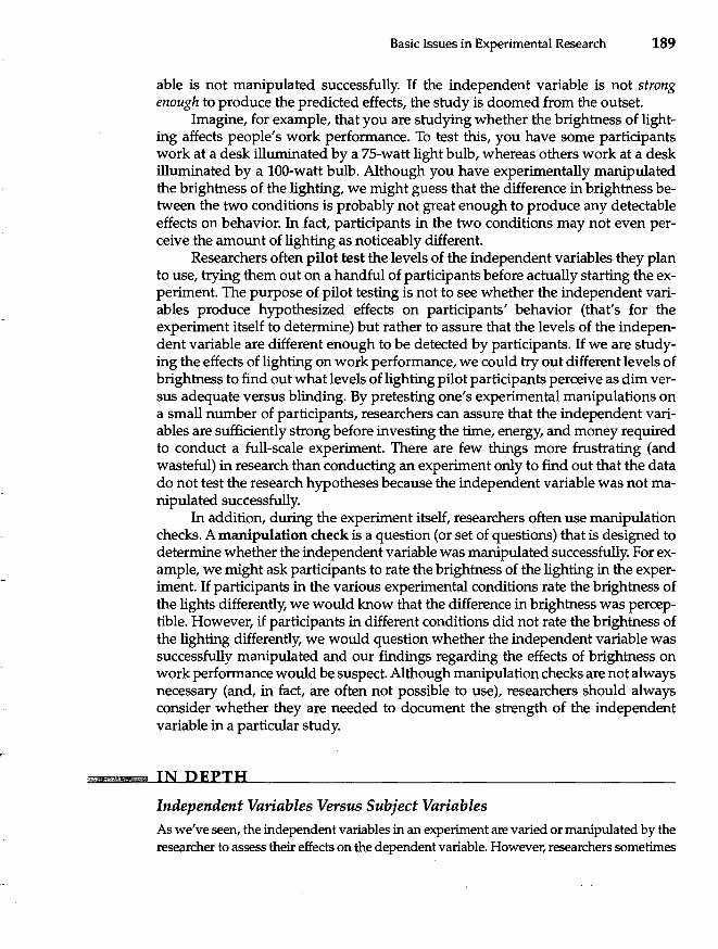
Basic Issues in Experimental Research 189

able is not manipulated successfully. If the independent variable is not strong enough to produce the predicted effects, the study is doomed from the outset.

Imagine, for example, that you are studying whether the brightness of light­ing affects people's work performance. To test this, you have some participants work at a desk illuminated by a 75-watt light bulb, whereas others work at a desk illuminated by a IOO-watt bulb. Although you have experimentally manipulated the brightness of the lighting, we might guess that the difference in brightness be­tween the two conditions is probably not great enough to produce any detectable effects on behavior. In fact, participants in the two conditions may not even per­ceive the amount of lighting as noticeably different.

Researchers often pilot test the levels of the independent variables they plan to use, trying them out on a handful of participants before actually starting the ex­periment. The purpose of pilot testing is not to see whether the independent vari­ables produce hypothesized effects on participants' behavior (that's for the experiment itself to determine) but rather to assure that the levels of the indepen­dent variable are different enough to be detected by participants. If we are study­ing the effects of lighting on work performance, we could try out different levels of brightness to find out what levels of lighting pilot participants perceive as dim ver­sus adequate versus blinding. By pretesting one's experimental manipulations on a small number of participants, researchers can assure that the independent vari­ables are sufficiently strong before investing the time, energy, and money required to conduct a full-scale experiment. There are few things more frustrating (and wasteful) in research than conducting an experiment only to find out that the data do not test the research hypotheses because the independent variable was not ma­nipulated successfully.

In addition, during the experiment itself, researchers often use manipulation checks. A manipulation check is a question (or set of questions) that is designed to determine whether the independent variable was manipulated successfully. For ex­ample, we might ask participants to rate the brightness of the lighting in the exper­iment. If participants in the various experimental conditions rate the brightness of the lights differently, we would know that the difference in brightness was percep­tible. However, if participants in different conditions did not rate the brightness of the lighting differently, we would question whether the independent variable was successfully manipulated and our findings regarding the effects of brightness on work performance would be suspect. Although manipulation checks are not always necessary (and, in fact, are often not possible to use), researchers should always consider whether they are needed to document the strength of the independent variable in a particular study.

!l!!!iM!¥1!$&l!j@I IN DEPTH

Independent Variables Versus Subject Variables

As we've seen, the independent variables in an experiment are varied or manipulated by the researcher to assess their effects on the dependent variable. However, researchers sometimes

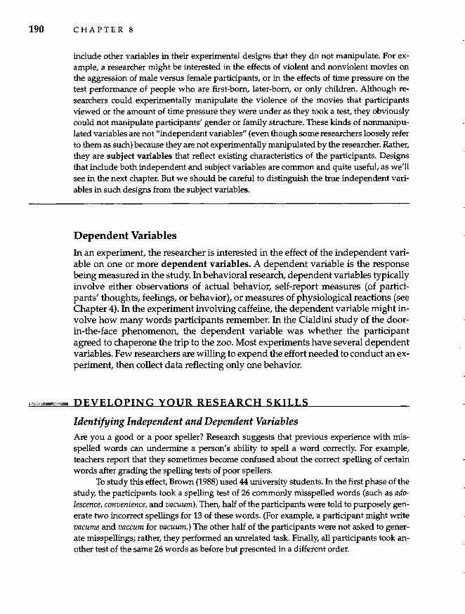
190 C HAP T E R 8

include other variables in their experimental designs that they do not manipulate. For ex­ample, a researcher might be interested in the effects of violent and nonviolent movies on the aggression of male versus female participants, or in the effects of time pressure on the test performance of people who are first-born, later-born, or only children. Although re­searchers could experimentally manipulate the violence of the movies that participants viewed or the amount of time pressure they were under as they took a test, they obviously could not manipulate participants' gender or family structure. These kinds of nonmanipu­lated variables are not "independent variables" (even though some researchers loosely refer to them as such) because they are not experimentally manipulated by the researcher. Rather, they are subject variables that reflect existing characteristics of the participants. Designs that include both independent and subject variables are common and quite useful, as we'll see in the next chapter. But we should be careful to distinguish the true independent vari­ables in such designs from the subject variables.

Dependent Variables

In an experiment, the researcher is interested in the effect of the independent vari­able on one or more dependent variables. A dependent variable is the response being measured in the study. In behavioral research, dependent variables typically involve either observations of actual behavior, self-report measures (of partici­pants' thoughts, feelings, or behavior), or measures of physiological reactions (see Chapter 4). In the experiment involving caffeine, the dependent variable might in­volve how many words participants remember. In the Cialdini study of the door­in-the-face phenomenon, the dependent variable was whether the participant agreed to chaperone the trip to the zoo. Most experiments have several dependent variables. Few researchers are willing to expend the effort needed to conduct an ex­periment, then collect data reflecting only one behavior.

__ DEVELOPING YOUR RESEARCH SKILLS

Identifying Independent and Dependent Variables Are you a good or a poor speller? Research suggests that previous experience with mis­spelled words can undermine a person's ability to spell a word correctly. For example, teachers report that they sometimes become confused about the correct spelling of certain words after grading the spelling tests of poor spellers.

To study this effect, Brown (1988) used 44 university students. In the first phase of the study, the participants took a spelling test of 26 commonly misspelled words (such as ado­lescence, convenience, and vacuum). Then, half of the participants were told to purposely gen­erate two incorrect spellings for 13 of these words. (For example, a participant might write vacume and vaccum for vacuum.) The other half of the participants were not asked to gener­ate misspellings; rather, they performed an unrelated task. Finally, all participants took an­other test of the same 26 words as before but presented in a different order.

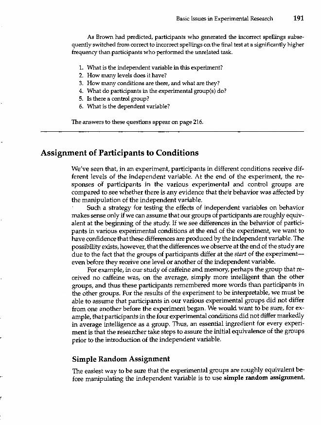
Basic Issues in Experimental Research 191

As Brown had predicted, participants who generated the incorrect spellings subse­quently switched from correct to incorrect spellings on the final test at a significantly higher frequency than participants who performed the unrelated task.

1. What is the independent variable in this experiment? 2. How many levels does it have? 3. How many conditions are there, and what are they? 4. What do participants in the experimental group(s) do? 5. Is there a control group? 6. What is the dependent variable?

The answers to these questions appear on page 216.

Assignment of Participants to Conditions

We've seen that, in an experiment, participants in different conditions receive dif­ferent levels of the independent variable. At the end of the experiment, the re­sponses of participants in the various experimental and control groups are compared to see whether there is any evidence that their behavior was affected by the manipulation of the independent variable.

Such a strategy for testing the effects of independent variables on behavior makes sense only if we can assume that our groups of participants are roughly equiv­alent at the beginning of the study. If we see differences in the behavior of partici­pants in various experimental conditions at the end of the experiment, we want to have confidence that these differences are produced by the independent variable. The possibility exists, however, that the differences we observe at the end of the study are due to the fact that the groups of participants differ at the start of the experiment­even before they receive one level or another of the independent variable.

For example, in our study of caffeine and memory, perhaps the group that re­ceived no caffeine was, on the average, simply more intelligent than the other groups, and thus these participants remembered more words than participants in the other groups. For the results of the experiment to be interpretable, we must be able to assume that participants in our various experimental groups did not differ from one another before the experiment began. We would want to be sure, for ex­ample, that participants in the four experimental conditions did not differ markedly in average intelligence as a group. Thus, an essential ingredient for every experi­ment is that the researcher take steps to assure the initial equivalence of the groups prior to the introduction of the independent variable.

Simple Random Assignment The easiest way to be sure that the experimental groups are roughly equivalent be­fore manipulating the independent variable is to use simple random assignment.

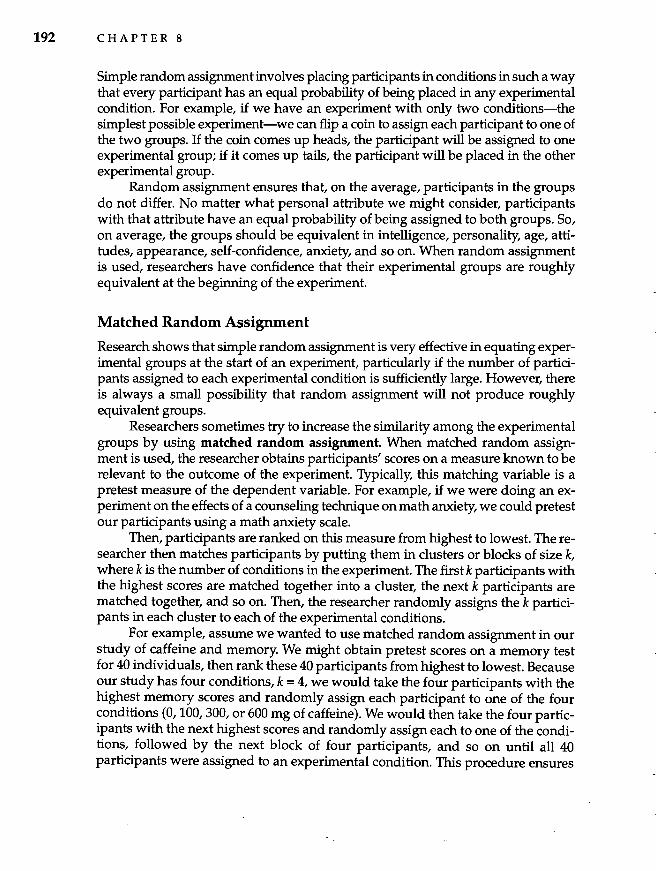
192 C HAP T E R 8

Simple random assignment involves placing participants in conditions in such a way that every participant has an equal probability of being placed in any experimental condition. For example, if we have an experiment with only two conditions-the simplest possible experiment-we can flip a coin to assign each participant to one of the two groups. If the coin comes up heads, the participant will be assigned to one experimental group; if it comes up tails, the participant will be placed in the other experimental group.

Random assignment ensures that, on the average, participants in the groups do not differ. No matter what personal attribute we might consider, participants with that attribute have an equal probability of being assigned to both groups. So, on average, the groups should be equivalent in intelligence, personality, age, atti­tudes, appearance, self-confidence, anxiety, and so on. When random assignment is used, researchers have confidence that their experimental groups are roughly equivalent at the beginning of the experiment.

Matched Random Assignment

Research shows that simple random assignment is very effective in equating exper­imental groups at the start of an experiment, particularly if the number of partici­pants assigned to each experimental condition is sufficiently large. However, there is always a small possibility that random assignment will not produce roughly equivalent groups.

Researchers sometimes try to increase the similarity among the experimental groups by using matched random assignment. When matched random assign­ment is used, the researcher obtains participants' scores on a measure known to be relevant to the outcome of the experiment. Typically, this matching variable is a pretest measure of the dependent variable. For example, if we were doing an ex­periment on the effects of a counseling technique on math anxiety, we could pretest our participants using a math anxiety scale.

Then, participants are ranked on this measure from highest to lowest. The re­searcher then matches participants by putting them in clusters or blocks of size k, where k is the number of conditions in the experiment. The first k participants with the highest scores are matched together into a cluster, the next k participants are matched together, and so on. Then, the researcher randomly assigns the k partici­pants in each cluster to each of the experimental conditions.

For example, assume we wanted to use matched random assignment in our study of caffeine and memory. We might obtain pretest scores on a memory test for 40 individuals, then rank these 40 participants from highest to lowest. Because our study has four conditions, k = 4, we would take the four participants with the highest memory scores and randomly assign each participant to one of the four conditions (0, 100,300, or 600 mg of caffeine). We would then take the four partic­ipants with the next highest scores and randomly assign each to one of the condi­tions, followed by the next block of four participants, and so on until all 40 participants were assigned to an experimental condition. This procedure ensures

r

Basic Issues in Experimental Research 193

that each experimental condition contains participants who possess comparable levels of memory ability.

Repeated Measures Designs

When different participants are assigned to each of the conditions in an experiment, as in simple and matched random assignment, the design is called a randomized groups design. This kind of study is also sometimes called a between-subjects or between-groups design because we are interested in differences in behavior be­tween different groups of participants.

In some studies, however, a single group of participants serves in all condi­tions of the experiment. For example, rather than randomly assigning participants into four groups, each of which receives one of four dosages of caffeine, a re­searcher may test a single group of participants under each of the four dosage levels. Such an experiment uses a within-subjects design in which we are inter­ested in differences in behavior across conditions within a single group of partici­pants. This is also commonly called a repeated measures design because each participant is measured more than once.

Using a within-subjects or repeated measures design eliminates the need for random assignment because every participant is tested under every level of the in­dependent variable. What better way is there to be sure the groups do not differ than to use the same participants in every experimental condition? In essence, each participant in a repeated measures design serves as his or her own control.

BEHAVIORAL RESEARCH CASE STUDY

A Within-Subjects Design: Sugar and Behavior

~ Many parents and teachers have become concerned in recent years about the effects of sugar '-...~n children's behavior. The popular view is that excessive sugar consumption results in be­

havioral problems ranging from mild irritability to hyperactivity and attention distur­bances. Interestingly, few studies have tested the effects of sugar on behavior, and those that

ve studied its effects have obtained inconsistent findings. . Against this backdrop of confusion, Rosen, Booth, Bender, McGrath, Sorrell, and

Drafunan (1988) used a within-subjects design to examine the effects of sugar on 45 pre­school and elementary school children. All 45 participants served in each of three experi­mental conditions. In the high sugar condition, the children drank an orange-flavored

. breakfast drink that contained 50 g of sucrose (approximately equal to the sucrose in two 'Candy bars)\. In the low sugar condition, the drink contained only 6.25 g of sucrose. And in

the control group, the drink contained aspartame (Nutrasweet™), an artificial sweetener. Each child was tested five times in each of the three conditions. Each morning for 15

days each child drank a beverage containing 0, 6.25, or 50 g of sucrose. To minimize order ef­fects, the order in which participants participated in each condition was randomized across " those 15 days.

194 CHAPTER 8

Several dependent variables were measured. Participants were tested each day on several measures of cognitive and intellectual functioning. In addition, their teachers (who did not know what each child drank) rated each student's behavior every morning. Obser­vational measures were also taken of behaviors that may be affected by sugar, such as activ­ity level, aggression, and fidgeting.

The results showed that high amounts of sugar caused a slight increase in activity, as well as a slight decrease in cognitive performance for girls. Contrary to the popular view, however, the effects of even excessive consumption of sugar were quite small in magnitude. The authors concluded that "the results did not support the view that sugar causes major changes in children's behavior" (Rosen et al., 1988, p. 583). Interestingly, parents' expecta­tions about the effects of sugar on their child were uncorrelated with the actual effects. Ap­parently, parents often attribute their children's misbehavior to excessive sugar consumption when sugar is not really the culprit.

Advantages of Within-Subjects Designs. The primary advantage of a within­subjects design is that it is more powerful than a between-subjects design. In statis­tical terminology, the power of a research design refers to its ability to detect effects of the independent variable. A powerful design is able to detect effects of the inde­pendent variable more easily than are less powerful designs. Within-subjects de­signs are more powerful because the participants in all experimental conditions are identical in every way (after all, they are the same individuals). When this is the case, none of the observed differences in responses to the various conditions can be due to preexisting differences between participants in the groups. Because we have repeated measures on every participant, we can more easily detect the effects of the independent variable on participants' behavior.

A second advantage of within-participants designs is that they require fewer participants. Because each participant is used in every condition, fewer are needed. ~.

/'

Disadvantages of Within-Subjects Designs. Despite their advantages, subjects designs create some special problems. The first involves order e cts. Be­cause each participant receives all levels of the independent variable, th ossibility arises that the order in which the levels are received affects particip. s' behavior.

For example, imagine that all participants in our memory'study are first tested with no caffeine, then with 100, 300, and 600 mg (in that order). Because of the opportunity to practice memorizing lists of words, participants' performance may improve as the experiment progresses. Because all participants receive in­creasingly higher doses of caffeine during the study, it may appear that,fueir mem­ory is best when they receive 600 mg of caffeine when, in fact, their memory may have improved as the result of practice alone.

To guard against the possibility of order effects, researchers use counterbal­ancing. Counterbalancing involves presenting the levels of the independent vari­able in different orders to different participants. When feasible, all possible orders

-

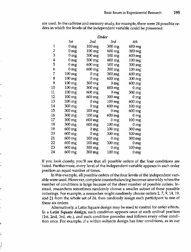
r

(

i ,

Basic Issues in Experimental Research 195

are used. In the caffeine and memory study, for example, there were 24 possible or-ders in which the levels of the independent variable could be presented:

Order 1st 2nd 3rd 4th

1 Omg 100mg 300mg 600mg 2 Omg 100mg 600mg 300mg 3 Omg 300mg 100mg 600mg 4 Omg 300mg 600mg 100mg 5 Omg 600mg 100mg 300mg 6 Omg 600mg 300mg 100mg 7 100mg Omg 300mg 600mg 8 100mg Omg 600mg 300mg 9 100mg 300mg Omg 600mg

10 100mg 300mg 600mg Omg 11 100mg 600mg Omg 300mg 12 100mg 600mg 300mg Omg 13 300mg Omg 100mg 600mg 14 300mg Omg 600mg 100mg 15 300mg 100mg Omg 600mg 16 300mg 100mg 600mg Omg 17 300mg 600mg Omg 100mg 18 300mg 600mg 100mg Omg 19 600mg Omg 100mg 300mg 20 600mg Omg 300mg 100mg 21 600mg 100mg Omg 300mg 22 600mg 100mg 300mg Omg 23 600mg 300mg Omg 100mg 24 600mg 300mg 100mg Omg

If you look closely, you'll see that all possible orders of the four conditions are listed. Furthermore, every level of the independent variable appears in each order position an equal number of times.

In this example, all possible orders of the four levels of the independent vari­able were used. However, complete counterbalancing becomes unwieldy when the number of conditions is large because of the sheer number of possible orders. In­stead, researchers sometimes randomly choose a smaller subset of these possible orderings. For example, a researcher might randomly choose orders 2,7,9,14,19, and 21 from the whole set of 24, then randomly assign each participant to one of these six orders.

Alternatively, a Latin Square design may be used to control for order effects. Ina Latin Square design, each condition appears once at each ordinal position (1st, 2nd, 3rd, etc.), and each condition precedes and follows every other condi­tion once. For example, if a within-subjects design has four conditions, as in our

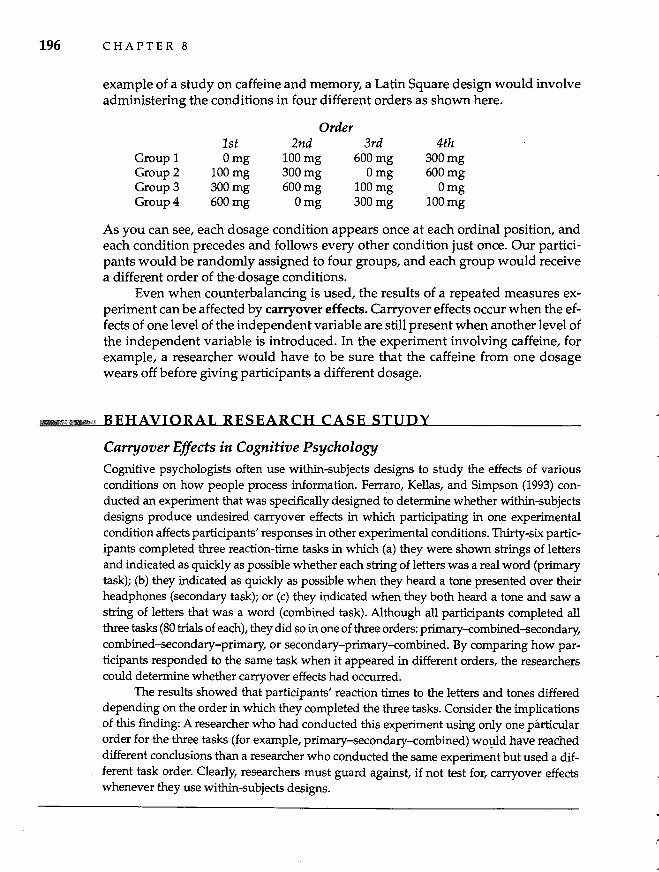
196 CHAPTER 8

example of a study on caffeine and memory, a Latin Square design would involve administering the conditions in four different orders as shown here.

Order 1st 2nd 3rd 4th

Group 1 Omg 100mg 600mg 300mg Group 2 100mg 300mg Omg 600mg Group 3 300mg 600mg 100mg Omg Group 4 600mg Omg 300mg 100mg

As you can see, each dosage condition appears once at each ordinal position, and each condition precedes and follows every other condition just once. Our partici­pants would be randomly assigned to four groups, and each group would receive a different order of the dosage conditions.

Even when counterbalancing is used, the results of a repeated measures ex­periment can be affected by carryover effects. Carryover effects occur when the ef­fects of one level of the independent variable are still present when another level of the independent variable is introduced. In the experiment involving caffeine, for example, a researcher would have to be sure that the caffeine from one dosage wears off before giving participants a different dosage.

BEHAVIORAL RESEARCH CASE STUDY

Carryover Effects in Cognitive Psychology Cognitive psychologists often use within-subjects designs to study the effects of various conditions on how people process information. Ferraro, Kellas, and Simpson (1993) con­ducted an experiment that was specifically designed to determine whether within-subjects designs produce undesired carryover effects in which participating in one experimental condition affects participants' responses in other experimental conditions. Thirty-six partic­ipants completed three reaction-time tasks in which (a) they were shown strings of letters and indicated as quickly as possible whether each string of letters was a real word (primary task); (b) they indicated as quickly as possible when they heard a tone presented over their headphones (secondary task); or (c) they indicated when they both heard a tone and saw a string of letters that was a word (combined task). Although all participants completed all three tasks (80 trials of each), they did so in one of three orders: primary-combined-secondary, combined-secondary-primary, or secondary-primary-combined. By comparing how par­ticipants responded to the same task when it appeared in different orders, the researchers could determine whether carryover effects had occurred.

The results showed that participants' reaction times to the letters and tones differed depending on the order in which they completed the three tasks. Consider the implications of this finding: A researcher who had conducted this experiment using only one particular order for the three tasks (for example, primary-secondary-combined) w~¢d have reached different conclusions than a researcher who conducted the same experiment but used a dif­ferent task order. Clearly, researchers must guard against, if not test for, carryover effects whenever they use within-subjects designs.

Basic Issues in Experimental Research 197

Experimental Control

The third critical ingredient of a good experiment is experimental control. Experi­mental control refers to eliminating or holding constant extraneous factors that might affect the outcome of the study. If the effects of such factors are not elimi­nated, it will be difficult, if not impossible, to determine whether the independent variable had an effect on participants' responses.

Systematic Variance

To understand why experimental control is important, let's return to the concept of variance. You will recall from Chapter 2 that variance is an index of how much par­ticipants' scores differ or vary from one another. Furthermore, you may recall that the total variance in a set of data can be broken into two components-systematic variance and error variance.

In the context of an experiment, systematic variance (often called between­groups variance) is that part of the total variance that reflects differences among the experimental groups. The question to be addressed in any experiment is whether any of the total variability we observe in participants' scores is systematic variance due to the independent variable. If the independent variable affected par­ticipants' responses, then we should find that some of the variability in partici­pants' scores is associated with the manipulation of the independent variable.

Put differently, if the independent variable had an effect on behavior, we should observe systematic differences between the scores in the various experimen­tal conditions. If scores differ systematically between conditions-if participants remember more words in some experimental groups than in others, for example-­systematic variance exists in the scores. This systematic or between-groups vari­ability in the scores may come from two sources: the independent variable (in which case it is called treatment variance) and extraneous variables (in which case it is called confound variance).

Treatment Variance. The portion of the variance in participants' scores that is due to the independent variable is called treatment variance (or sometimes pri­mary variance). If nothing other than the independent variable affected partici­pants' responses in an experiment, then all of the variance in the data would be treatment variance. This is rarely the case, however. As we will see, participants' scores typically vary for other reasons as well. Specifically, we can identify two other sources of variability in participants' scores: confound variance (which we must eliminate from the study) and error variance (which we must minimize).

Confound Variance. Ideally, other than the fact that participants in different con­ditions receive different levels of the independent variable, all participants in the various experimental conditions should be treated in precisely the same way. The only thing that may differ between the conditions is the independent variable. Only when this is so can we conclude that changes in the dependent variable were caused by manipulation of the independent variable.

198 C HAP T E R 8

Unfortunately, researchers sometimes design faulty experiments in which something other than the independent variable differs among the conditions. For example, if in a study of the effects of caffeine on memory, all participants who re­ceived 600 mg of caffeine were tested at 9:00 A.M. and all participants who received no caffeine were tested at 3:00 P.M., the groups would differ not only in how much caffeine they received, but also in the time at which they participated in the study. In this experiment, we would be unable to tell whether differences in memory be­tween the groups were due to the fact that one group ingested caffeine and the other one didn't, or to the fact that one group was tested in the morning and the other in the afternoon.

When a variable other than the independent variable differs between the groups, confound variance is produced. Confound variance, which is sometimes called secondary variance, is that portion of the variance in participants' scores that is due to extraneous variables that differ systematically between the experi­mental groups.

Confound variance must be eliminated at all costs. The reason is clear: It is im­possible for researchers to distinguish treatment variance from confound variance. Although we can easily determine how much systematic variance is present in our data, we cannot tell how much of the systematic variance is treatment variance and how much, if any, is confound variance. As a result, the researcher will find it im­possible to tell whether differences in the dependent variable between conditions were due to the independent variable or to this unwanted, confounding variable. As we'll discuss in detail later in the chapter, confound variance is eliminated through careful experimental control in which all factors other than the indepen­dent variable are held constant or allowed to vary nonsystematically between the experimental conditions.

Error Variance

Error variance (also called within-groups variance) is the result of unsystematic differences among participants. Not only do participants differ at the time they enter the experiment in terms of ability, personality, mood, past history, and so on, but chances are that the experimenter will treat individual participants in slightly different ways. In addition, measurement error contributes to error variance by in­troducing random variability into the data (see Chapter 3).

In our study of caffeine and memory, we would expect to see differences in the number of words recalled by participants who were in the same experimen­tal condition; not all of the participants in a particular experimental condition will remember precisely the same number of words. This variability in scores within an experimental condition is not due to the independent variable because all participants in a particular condition receive the same level of the indepen­dent variable. Nor is this within-groups variance due to confounding variables because all participants within a group would experience any confound that ex­isted. Rather, this variability-the error variance-is due to differences among participants within the group, to random variations in the experimental setting

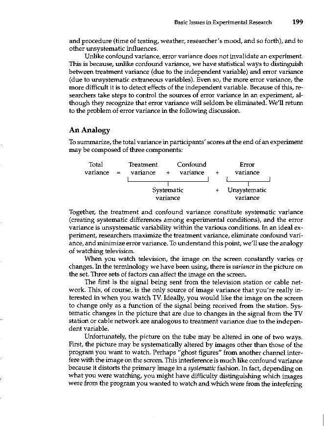
Basic Issues in Experimental Research 199

and procedure (time of testing, weather, researcher's mood, and so forth), and to other unsystematic influences.

Unlike confound variance, error variance does not invalidate an experiment. This is because, unlike confound variance, we have statistical ways to distinguish between treatment variance (due to the independent variable) and error variance (due to unsystematic extraneous variables). Even so, the more error variance, the more difficult it is to detect effects of the independent variable. Because of this, re­searchers take steps to control the sources of error variance in an experiment, al­though they recognize that error variance will seldom be eliminated. We'll return to the problem of error variance in the following discussion.

An Analogy

To summarize, the total variance in participants' scores at the end of an experiment may be composed of three components:

Total Treatment Confound Error variance variance + variance + variance

I I I

Systematic + Unsystematic variance variance

Together, the treatment and confound variance constitute systematic variance (creating systematic differences among experimental conditions), and the error variance is unsystematic variability within the various conditions. In an ideal ex­periment, researchers maximize the treatment variance, eliminate confound vari­ance, and minimize error variance. To understand this point, we'll use the analogy of watching television.

When you watch television, the image on the screen constantly varies or changes. In the terminology we have been using, there is variance in the picture on the set. Three sets of factors can affect the image on the screen.

The first is the signal being sent from the television station or cable net­work. This, of course, is the only source of image variance that you're really in­terested in when you watch TV. Ideally, you would like the image on the screen to change only as a function of the signal being received from the station. Sys­tematic changes in the picture that are due to changes in the signal from the TV station or cable network are analogous to treatment variance due to the indepen­dent variable.

Unfortunately, the picture on the tube may be altered in one of two ways. First, the picture may be systematically altered by images other than those of the program you want to watch. Perhaps" ghost figures" from another channel inter­fere with the image on the screen. This interference is much like confound variance because it distorts the primary image in a systematic fashion. In fact, depending on what you were watching, you might have difficulty distinguishing which images were from the program you wanted to watch and which were from the interfering

200 CHAPTER 8

signal. That is, you might not be able to distinguish the true signal (treatment vari­ance) from the interference (confound variance).

The primary signal can also be weakened by static, fuzz, or snow. Static pro­duces unsystematic changes in the TV picture. It dilutes the image without actually distorting it. If the static is extreme enough, you may not be able to recognize the real picture at all. Similarly, error variance in an experiment clouds the signal pro­duced by the independent variable.

To enjoy Tv, you want the primary signal to be as strong as possible, to eliminate systematic distortions entirely, and to have as little static as possible. Only then will the true program come through loud and clear. In an analogous fashion, researchers want to maximize treatment variance, eliminate confound variance, and reduce error variance. The remainder of this chapter deals with the ways researchers use experi­mental control to eliminate confound variance and minimize error variance.

Eliminating Confounds

Internal Validity

At the end of every experiment, we would like to have confidence that any differ­ences we observe between the experimental and control groups resulted from our manipulation of the independent variable rather than from extraneous variables. In­ternal validity is the degree to which a researcher draws accurate conclusions about the effects of the independent variable. An experiment is internally valid when it eliminates all potential sources of confound variance. When an experiment has in­ternal validity, a researcher can confidently conclude that observed differences were due to variation in the independent variable.

To a large extent, internal validity is achieved through experimental control. The logic of experimentation requires that nothing can differ systematically between the experimental conditions other than the independent variable. If something other than the independent variable differs in some systematic way, we say that con­founding has occurred. When confounding occurs, there is no way to know whether the results were due to the independent variable or to the confound. Confounding is a fatal flaw in experimental designs, one that makes the findings nearly worthless .

. As a result, possible threats to internal validity must be eliminated at all costs. One well-publicized example of confounding involved the "Pepsi Chal­

lenge" (see Huck & Sandler, 1979). The Pepsi Challenge was a taste test in which people were asked to taste two cola beverages and indicate which they preferred. As it was originally designed, glasses of Pepsi were always marked with a letter M, and glasses of Coca-Cola were marked with a Q. People seemed to prefer Pepsi over Coke in these tests, but a confound was present. Do you see it? The letter on the glass was confounded with the beverage in it. Thus, we don't know for certain whether people preferred Pepsi over Coke or the letter Mover Q. As absurd as this possibility may sound, later tests demonstrated that participants' preferences were affected by the letter on the glass. No matter which cola was in which glass, people tended to indicate a preference for the drink marked M over the one marked Q.

Basic Issues in Experimental Research 201

Before discussing some common threats to the internal validity of experi­ments, see if you can find the threat to internal validity in the hypothetical experi­ment described in the following box.

-§lIt-" DEVELOPING YOUR RESEARCH SKILLS

Confounding: Can You Find It? A researcher was interested in how people's perceptions of others are affected by the pres­ence of a physical handicap. Research suggests that people may rate those with physical dis­abilities less positively than those without disabilities. Because of the potential implications of this bias for job discrimination against people with disabilities, the researcher wanted to see whether participants responded less positively to applicants who were disabled.

The participant was asked to play the role of an employer who wanted to hire a com­puter programmer, a job in which physical disability is largely irrelevant. Participants were shown one of two sets of bogus job application materials prepared in advance by the exper­imenter. Both sets of application materials included precisely the same information about the applicant's qualifications and background (such as college grades, extracurricular activ­ities, test scores, and so on). The only difference in the two sets of materials involved a pho­tograph attached to the application. In one picture, the applicant was shown seated in a wheelchair, thereby making the presence of a disability obvious to participants. The other photograph did not show the wheelchair; in this picture, only the applicant's head and shoulders were shown. Other than the degree to which the applicant's disability was ap­parent, the content of the two applications was identical in every respect.

In the experiment, 20 participants saw the photo in which the disability was apparent, and 20 participants saw the photo in which the applicant did not appear disabled. Partici­pants were randomly assigned to one of these two experimental conditions. After viewing the application materials, including the photograph, every participant completed a ques­tionnaire on which they rated the applicant on several dimensions. For example, partici­pants were asked how qualified for the job the applicant was, how much they liked the applicant, and whether they would hire him.

1. What was the independent variable in this experiment? 2. What were the dependent variables? 3. The researcher made a critical error in designing this experiment, one that introduced

confounding and compromised the internal validity of the study. Can you find the re­searcher's mistake?

4. How would you redesign the experiment to eliminate this problem?

Answers to these questions appear on page 217.

Threats to Internal Validity

The reason that threats to internal validity, such as in the Pepsi Challenge taste test, are so damaging to experiments is that they introduce alternative rival explanations

202 C HAP T E R 8

for the results of a study. Instead of confidently concluding that differences among the conditions are due to the independent variable, the researcher must concede that there are alternative explanations for the results. When this happens, the results are highly suspect, and no one is likely to take them seriously. Although it would be impossible to list all potential threats to internal validity, a few of the more common threats are discussed below. (For complete coverage of these and other threats to in­ternal validity, see Campbell and Stanley [1966] and Cook and Campbell [1979].)

Biased Assignment of Participants to Conditions. We've already discussed one common threat to internal validity. If the experimental conditions are not equal­ized before participants receive the independent variable, the researcher may con­clude that the independent variable caused differences between the groups when, in fact, those differences were due to biased assignment. Biased assignment of par­ticipants to conditions (which is often referred to as the selection threat to internal va­lidity) introduces the possibility that the effects are due to nonequivalent groups rather than to the independent variable. We've seen that this problem is eliminated through simple or matched random assignment or use of within-subjects designs.

This confound poses a problem for research that compares the effects of an in­dependent variable on preexisting groups of participants. For example, if researchers are interested in the effects of a particular curricular innovation in elementary schools, they might want to compare students in a school that uses the innovative curriculum with those in a school that uses a traditional curriculum. But, because the students are not randomly assigned to one school or the other, the groups will differ in many ways other than in the curriculum being used. As a result, the study pos­sesses no internal validity, and no conclusions can be drawn about the effects of the curriculum.

Differential Attrition. Attrition refers to the loss of participants during a study. For example, some participants may be unwilling to complete the experiment be­cause they find the procedures painful, difficult, objectionable, or embarrassing. When studies span a long period of time or involve people who are already very ill (as in some research in health psychology), participants may become unavailable due to death. (Because some attrition is caused by death, some researchers refer to this confound as subject mortality.)

When attrition occurs in a random fashion and affects all experimental con­ditions equally, it is only a minor threat to internal validity. However, when the rate of attrition differs across the experimental conditions, a condition known as dif­ferentialattrition, internal validity is weakened. If attrition occurs at a different rate in different conditions, the independent variable may have caused the loss of participants. The consequence is that the experimental groups are no longer equiv­alent; differential attrition has destroyed the benefits of random assignment.

For example, suppose we are interested in the effects of physical stressors on intellectual performance. To induce physical stress, participants in the experimental group will be asked to immerse their right arm to the shoulder in a container of ice water for 15 minutes, a procedure that is quite painful but not damaging. Partici-

Basic Issues in Experimental Research 203

pants in the control condition will put their arms in water that is at room tempera­ture. While their arms are immersed, participants in both groups will complete a set of mental tasks. For ethical reasons, we must let participants choose whether to par­ticipate in this study. Let's assume, however, that, whereas all of the participants who are randomly assigned to the room-temperature condition agree to participate, 15% of those assigned to the experimental ice-water condition decline. Differential attrition has occurred and the tWo groups are no longer equivalent.

If we assume that participants who drop out of the ice-water condition are more fearful than those who remain, then the average participant who remains in the ice-water condition is probably less fearful than the average participant in the room-temperature condition, creating a potential bias. If we find a difference in performance between the two conditions, how do we know whether the difference is due to differences in stress or to differences in the characteristics of the partici­pants who agree to participate in the two conditions?

Pretest Sensitization. In some experiments, participants are pretested to obtain a measure of their behavior before receiving the independent variable. Although pretests provide useful baseline data, they have a drawback. Taking a pretest may sensitize participants to the independent variable so that they react differently to the independent variable than they would react had they not been pretested. When pretest sensitization occurs, the researcher may conclude that the independent variable has an effect when, in reality, the effect is a combined result of the pretest and the independent variable.

For example, imagine that a teacher designs a program to raise students' de­gree of cultural literacy-their knowledge of common facts that are known by most literate, educated people within a particular culture (for example, what hap­pened in 1492 or who Thomas Edison was). To test the effectiveness of this pro­gram, the teacher administers a pretest of such knowledge to 100 students. Fifty of these students then participate in a 2-week course designed to increase their cul­turalliteracy, whereas the remaining 50 students take another course. Both groups are then tested again, using the same test they completed during the pretest.

Assume that the teacher finds that students who take the cultural literacy course show a significantly greater increase in knowledge than students in the con­trol group. Is the course responsible for this change? Possibly, but pretest sensiti­zation may also be involved. When students take the pretest, they undoubtedly encounter questions they can't answer. When this material is covered during the course itself, they may be more attentive to it because of their experience on the pretest. As a result, they learn more than they would have had they not taken the pretest. Thus, the pretest sensitizes them to the experimental treatment and thereby affects the results of the study.

When researchers are concerned about pretest sensitization, they sometimes include conditions in their design in which some participants take the pretest whereas other participants do not. If the participants who are pretested respond differently in one or more experimental conditions than those who are not pre­tested, pretest sensitization has occurred.

204 CHAPTER 8

History. The results of some studies are affected by extraneous events that occur outside of the research setting. As a result, the obtained effects are due not to the in­dependent variable itself but to an interaction of the independent variable and his­tory effects.

For example, imagine that we are interested in the effects of filmed aggres­sion toward women on attitudes toward sexual aggression. Participants in one group watch a 30-minute movie that contains a realistic depiction of rape whereas participants in another group watch a film about wildlife conservation. We then measure both groups' attitudes toward sexual aggression. Let's imagine, however, that a female student was sexually assaulted on campus the week before we con­ducted the study. It is possible that participants who viewed the aggressive movie would be reminded of the attack and that their subsequent attitudes would be af­fected by the combination of the film and their thoughts about the campus assault. That is, the movie may have produced a different effect on attitudes given the fact that a real rape had occurred recently. Participants who watched the wildlife film, however, would not be prompted to think about rape during their 30-minute film. Thus, the differences we obtain between the two groups could be due to this inter­action of history (the real assault) and treatment (the film).

Maturation. In addition to possible outside influences, changes within the par­ticipants themselves can create confounds. If the experiment occurs over a long span of time, for example, developmental maturation may occur in which partic­ipants go through age-related changes. If this occurs, we don't know whether the differences we observe between experimental conditions are due to the indepen­dent variable, or to the independent variable in combination with age-related changes. Obviously, maturation is more likely to be a problem in research involv­ing children.

These by no means exhaust all of the factors that can compromise the internal validity of an experiment, but they should give you a feel for unwanted influences that can undermine the results of experimental studies. When critiquing the qual­ity of an experiment, ask yourself, "Did the experimental conditions differ system­atically in any way other than the fact that they received different levels of the independent variable?" If so, confounding may have occurred.

Miscellaneous Design Confounds. Many of the confounds just described are difficult to control or even to detect. However, one common type of confound is en­tirely within the researcher's control and, thus, can always be eliminated if suffi­cient care is taken as the experiment is designed. Ideally, every participant in an experiment should be treated in precisely the same way, except that participants in different conditions will receive different levels of the independent variable. Of course, it is virtually impossible to treat each participant exactly the same. Even so, it is essential that no systematic differences be imposed other than the different levels of the independent variable. When participants in one experimental condi­tion are treated differently than those in another condition, confounding destroys our ability to identify effects of the independent variable and introduces an alter-

Basic Issues in Experimental Research 205

native rival explanation of the results. The study involving reactions to disabled job applicants provided a good example of a design confound, as did the case of the Pepsi Challenge.

Experimenter Expectancies, Demand Characteristics, and Placebo Effects

The validity of researchers' interpretations of the results of a study are also affected by the researcher's and participants' beliefs about what should happen in the ex­periment. In this section, I'll discuss three potential problems in which people's expectations affect the outcome of an experiment: experimenter expectancies, de­mand characteristics, and placebo effects.

Experimenter Expectancy Effects. Researchers usually have some idea about how participants will respond. Indeed, they usually have an explicit hypothesis regard­ing the results of the study. Unfortunately, experimenters' expectations can distort the results of an experiment by affecting how they interpret participants' behavior.

A good example of the experimenter expectancy effect (sometimes called the Rosenthal effect) is provided in a study by Cordaro and Ison (1963). In this experi­ment, psychology students were taught to classically condition a simple response in Planaria (flatworms). Some students were told that the planarias had been pre­viously conditioned and should show a high rate of response. Other students were told that the planarias had not been conditioned; thus they thought their worms would show a low rate of response. In reality, both groups of students worked with identical planarias. Despite the fact that their planarias did not differ in respon­siveness, the students who expected responsive planarias recorded 20 times more responses than the students who expected unresponsive planarias!

Did the student experimenters in this study intentionally distort their obser­vations? Perhaps; but more likely their observations were affected by their expec­tations. People's interpretations are often affected by their beliefs and expectations; people often see what they expect to see. Whether such effects involve intentional distortion or an unconscious bias, experimenters' expectancies may affect their perceptions, thereby compromising the validity of an experiment.

Demand Characteristics. Participants' assumptions about the nature of a study can also affect the outcome of research. If you have ever participated in research, you probably tried to figure out what the study was about and how the researcher expected you to respond.

Demand characteristics are aspects of a study that indicate to participants how they should behave. Because many people want to be good participants who do what the experimenter wishes, their behavior is affected by demand character­istics rather than by the independent variable itself. In some cases, experimenters unintentionally communicate their expectations in subtle ways that affect partici­pants' behavior. In other instances, participants draw assumptions about the study from the experimental setting and procedure.

206 CHAPTER 8

A good demonstration of demand characteristics was provided by Orne and Scheibe (1964). These researchers told participants they were participating in a study of stimulus deprivation. In reality, participants were not deprived of stimulation at all but rather simply sat alone in a small, well-lit room for 4 hours. To create demand characteristics, however, participants in the experimental group were asked to sign forms that released the researcher from liability if the experimental procedure harmed the participant. They also were shown a "panic button" they could push if they could not stand the deprivation any longer. Such cues would likely raise in par­ticipants' minds the possibility that they might have a severe reaction to the study. (Why else would release forms and a panic button be needed?) Participants in the control group were told that they were serving as a control group, were not asked to sign release forms, and were not given a panic button. Thus, the experimental setting would not lead control participants to expect extreme reactions.

As Orne and Scheibe expected, participants in the experimental group showed more extreme reactions during the deprivation period than participants in the control group even though they all underwent precisely the same experience of sitting alone for four hours. The only difference between the groups was the pres­ence of demand characteristics that led participants in the experimental group to ex­pect more severe reactions. Given that early studies of stimulus deprivation were plagued by demand characteristics such as these, Orne and Scheibe concluded that many so-called effects of deprivation were, in fact, the result of demand character­istics rather than of stimulus deprivation per se.

To eliminate demand characteristics, experimenters often conceal the pur­pose of the experiment from participants. In addition, they try to eliminate any cues in their own behavior or in the experimental setting that would lead partici­pants to draw inferences about the hypotheses or about how they should act.

Perhaps the most effective way to eliminate both experimenter expectancy effects and demand characteristics is to use a double-blind procedure. With a double-blind procedure, neither the participants nor the experimenters who in­teract with them know which experimental condition a participant is in at the time the study is conducted. The experiment is supervised by another researcher, who assigns participants to conditions and keeps other experimenters "in the dark." This procedure ensures that the experimenters who interact with the par­ticipants will not subtly and unintentionally influence participants to respond in a particular way.

Placebo Effects. Conceptually related to demand characteristics are placebo ef­fects. A placebo effect is a physiological or psychological change that occurs as a result of the mere suggestion that the change will occur. In experiments that test the effects of drugs or therapies, for example, changes in health or behavior may occur because participants think that the treatment will work.

Imagine that you are testing the effects of a new drug, Mintovil, on head­aches. One way you might design the study would be to administer Mintovil to one group of participants (the experimental group) but not to another group of

I

J

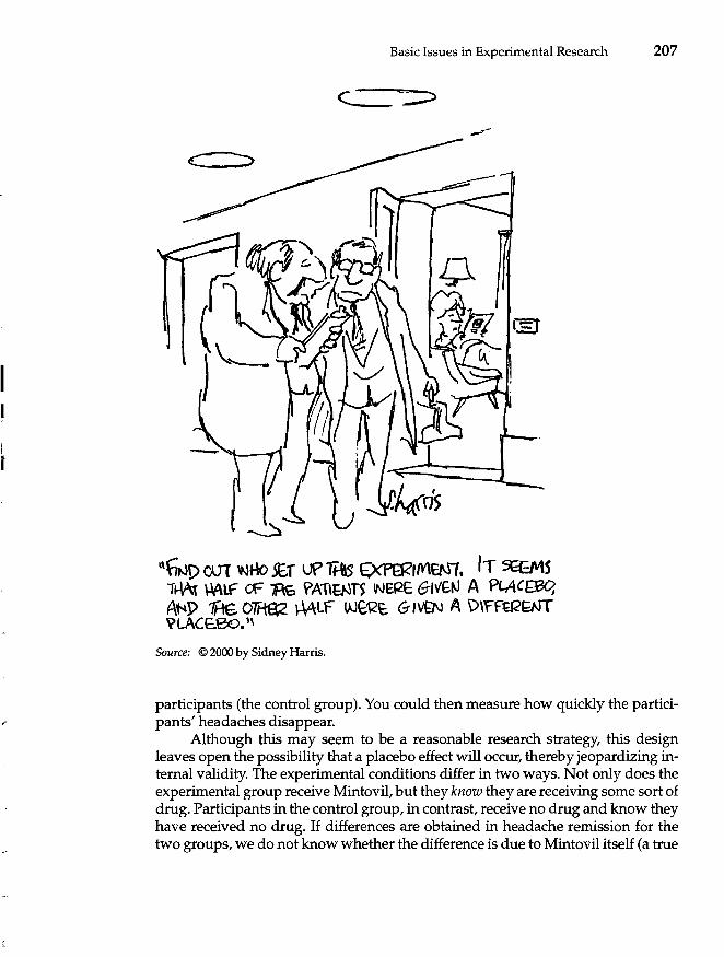
Basic Issues in Experimental Research 207

I'f}tJp 001 \'lHo.sE.r UP T1-\\5 ~1/V\EN1. IT %91S TW\l AAlf CF 1=\6 ~Al\g.lTS NERE GIv'£N A Pt..Ac£8q A~P 7Ft€. OTH€(2 AALf VJ~12t; G/Vf!\J A \)\rf~BJT ?LACE.eo. 1\

Source: © 2000 by Sidney Harris.

participants (the control group). You could then measure how quickly the partici­pants' headaches disappear.

Although this may seem to be a reasonable research strategy, this design leaves open the possibility that a placebo effect will occur, thereby jeopardizing in­ternal validity. The experimental conditions differ in two ways. Not only does the experimental group receive Mintovil, but they know they are receiving some sort of drug. Participants in the control group, in contrast, receive no drug and know they have received no drug. If differences are obtained in headache remission for the two groups, we do not know whether the difference is due to Mintovil itself (a true

208 CHAPTER 8

treatment effect) or to the fact that the experimental group receives a drug they ex­pect might reduce their headaches (a placebo effect).

When a placebo effect is possible, researchers use a placebo control group. Participants in a placebo control group are administered an ineffective treatment. For example, in the study above, a researcher might give the experimental group a pill containing Mintovil and the placebo control group a pill that contains an inac­tive substance. Both groups would believe they were receiving medicine, but only the experimental group would receive a pharmaceutically active drug. The chil­dren who received the aspartame-sweetened beverage in Rosen et al.'s (1988) study of the effects of sugar on behavior were in a placebo control group.

The presence of placebo effects can be detected by using both a placebo control group and a true control group in the experimental design. Whereas participants in the placebo control group receive an inactive substance (the placebo), participants in the true control group receive no pill and no medicine. If participants in the placebo control group (who received the inactive substance) improve more than those in the true control group (who received nothing), a placebo effect is operating. If this occurs but the researcher wants to conclude that the treatment was effective, he or she must demonstrate that the experimental group did improve more than the placebo con­trolgroup.

Error Variance

Error variance is a less "fatal" problem than confound variance, but it creates its own set of difficulties. By decreasing the power of an experiment, it reduces the re­searcher's ability to detect effects of the independent variable on the dependent variable. Error variance is seldom eliminated from experimental designs. How­ever, researchers try hard to minimize it.

Sources of Error Variance

Recall that error variance is the "static" in an experiment. It results from all of the unsystematic, uncontrolled, and unidentified variables that affect participants' be­havior in large and small ways.

Individual Differences. The most common source of error variance is preexisting individual differences among participants. When participants enter an experiment, they already differ in a variety of ways-cognitively, physiologically, emotionally, and behaviorally. As a result of their preexisting differences, even participants who are in the same experimental condition respond differently to the independent vari­able, creating error variance.

Of course, nothing can be done to eliminate individual differences among people. However, one partial solution to this source of error variance is to use a ho­mogeneous sample of participants. The more alike participants are, the less error variance is produced by their differences, and the easier it is to detect effects of the independent variable.

Basic Issues in Experimental Research 209

This is one reason that researchers who use animals as participants prefer samples composed of littermates. Littermates are genetically similar, are of the same age, and have usually been raised in the same environment. As a result, they differ little among themselves. Similarly, researchers who study human behavior often prefer homogeneous samples. For example, whatever other drawbacks they may have as research participants, college sophomores at a particular university are often a relatively homogeneous group.

Transient States. In addition to differing on the relatively stable dimensions al­ready mentioned, participants differ in terms of transient states. At the time of the experiment, some are healthy whereas others are ill. Some are tired; others are well rested. Some are happy; others are sad. Some are enthusiastic about participating in the study; others resent having to participate. Participants' current moods, atti­tudes, and physical conditions can affect their behavior in ways that have nothing to do with the experiment.

About all a researcher can do to reduce the impact of these factors is to avoid creating different transient reactions in different participants during the course of the experiment itself. If the experimenter is friendlier toward some participants than toward others, for example, error variance will increase.

Environmental Factors. Error variance is also affected by differences in the en­vironment in which the study is conducted. For example, participants who come to the experiment drenched to the skin are likely to respond differently than those who saunter in under clear skies. External noise may distract some participants. Collecting data at different times during the day may create extraneous variability in participants' responses.

To reduce error variance, researchers try to hold the environment as constant as possible as they test different participants. Of course, little can be done about the weather, and it may not be feasible to conduct the study at only one time each day. However, factors such as laboratory temperature and noise should be held con­stant. Experimenters try to be sure that the experimental setting is as invariant as possible while different participants are tested.

Differential Treatment. Ideally, researchers should treat each and every partici­pant within each condition exactly the same in all respects. However, as hard as they may try, experimenters find it difficult to treat all participants in precisely the same way during the study.

For one thing, experimenters' moods and health are likely to differ across participants. As a result, they may respond more positively toward some partici­pants than toward others. Furthermore, experimenters are likely to act differently toward different kinds of participants. Experimenters are likely to respond differ­ently toward participants who are pleasant, attentive, and friendly than toward participants who are unpleasant, distracted, and belligerent. Even the partici­pants' physical appearance can affect how they are treated by the researcher. Fur­thermore, experimenters may inadvertently modify the procedure slightly, by using slightly different words when giving instructions, for example. Also, male

210 C HAP T E R 8

and female participants may respond differently to male and female experimenters, and vice versa.

Even slight differences in how participants are treated can introduce error variance into their responses. One solution is to automate the experiment as much as possible, thereby removing the influence of the researcher to some degree. To eliminate the possibility that experimenters will vary in how they treat partici­pants, many researchers tape-record the instructions for the study rather than de­liver them in person. Similarly, animal researchers automate their experiments, using programmed equipment to deliver food, manipulate variables, and measure behavior, thereby minimizing the impact of the human factor on the results.

Measurement Error. We saw in Chapter 3 that all behavioral measures contain some degree of measurement error. Measurement error contributes to error vari­ance because it causes participants' scores to vary in unsystematic ways. Re­searchers should make every effort to use only reliable techniques and take steps to minimize the influence of factors that create measurement error.

'i"i"mrmr DEVELOPING YOUR RESEARCH SKILLS

Tips for Minimizing Error Variance

1. Use a homogeneous sample. 2. Aside from differences in the independent variable, treat all participants precisely the

same at all times. 3. Hold all laboratory conditions (heat, lighting, noise, and so on) constant. 4. Standardize all research procedures. 5. Use only reliable measurement procedures.

Many factors can create extraneous variability in behavioral data. Because the factors that create error variance are spread across all conditions of the design, they do not create confounding or produce problems with internal validity. Rather, they simply add static to the picture produced by the independent variable. They pro­duce unsystematic, yet unwanted, changes in participants' scores that can cloud the effects the researcher is studying. After reading Chapter 10, you'll understand more fully why error variance increases the difficulty of detecting effects of the indepen­dent variable. For now, simply understand what error variance is, the factors that cause it, and how it can be minimized through experimental control.

IN DEPTH

The Shortcomings of Experimentation Experimental designs are preferred by many behavioral scientists because they allow us to determine causal relationships. However, there are many topics in psychology for which ex-

Basic Issues in Experimental Research 211

perimental designs are inappropriate. Sometimes researchers are not interested in cause-and­effect relationships. Survey researchers, for example, often want only to describe people's at­titudes and aren't interested in why people hold the attitudes they do.

In other cases, researchers are interested in causal effects but find it impossible or un­feasible to conduct a true experiment. As we've seen, experimentation requires that the re­searcher be able to control carefully aspects of the research setting. However, researchers are often unwilling or unable to manipulate the variables they study. For example, to do an experiment on the effects of facial deformities on people's self-concepts would require randomly assigning some people to have their faces disfigured. Likewise, to conduct an experiment on the effects of oxygen deprivation during the birth process on later intellec­tual performance, we would have to experimentally deprive newborns of oxygen for varying lengths of time. As we saw in Chapter 6, experiments have not been conducted on the effects of smoking on humans because such studies would assign some nonsmokers to smoke heavily.

Despite the fact that experiments can provide clear evidence of causal processes, de­scriptive and correlational studies, as well as quasi-experimental designs (which we'll ex­amine in Chapter 12), are sometimes more appropriate and useful.

Experimental Control and Generalizability: The Experimenter's Dilemma

We've seen that experimental control involves treating all participants precisely the same, with the exception of giving participants in different conditions different levels of the independent variable. The tighter the experimental control, the more internally valid the experiment will be. And the more internally valid the experi­ment, the stronger, more definitive conclusions we can draw about the causal effects of the independent variables.

However, experimental control is a two-edged sword. Tight experimental control means that the researcher has created a highly specific and often artificial situation. The effects of extraneous variables that affect behavior in the real world have been eliminated or held at a constant level. The result is that the more con­trolled a study is, the more difficult it is to generalize the findings.

External validity refers to the degree to which the results obtained in one study can be replicated or generalized to other samples, research settings, and pro­cedures. External validity refers to the generalizability of the research results to other settings (Campbell & Stanley, 1966).

To some extent the internal validity and external validity of experiments are inversely related; high internal validity tends to produce lower external validity, and vice versa. The conflict between internal and external validity has been called the experimenter's dilemma Q"ung, 1971). The more tightly the experimenter con­trols the experimental setting, the more internally valid the results but the lower the external validity. Thus, researchers face the dilemma of choosing between in­ternal and external validity.

212 C HAP T E R 8

When faced with this dilemma, virtually all experimental psychologists opt in favor of internal validity. After all, if internal validity is weak, then they cannot draw confident conclusions about the effects of the independent variable, and the findings should not be generalized anyway.

Furthermore, in experimental research, the goal is seldom to obtain results that generalize to the real world. The goal of experimentation is not to make generaliza­tions but rather to test them (Mook, 1983). As we saw in Chapter 1, most research is designed to test hypotheses about the effects of certain variables on behavior. Re­searchers develop hypotheses, then design studies to determine whether those hy­potheses are supported by the data. If they are supported, evidence is provided that supports the theory. If they are not supported, the theory is called into question.

This approach is particularly pervasive in experimental research. The pur­pose of most experiments is not to discover what people do in real-life settings or to create effects that will necessarily generalize to other settings or to the real world. In fact, the findings of any single experiment should never be generalized­no matter how well the study is designed, who its participants are, or where it is conducted. The results of any particular study depend too strongly on the context in which it is conducted to allow us to generalize its findings.

Instead, the purpose of most experimentation is to test general propositions about the determinants of behavior. If the theory is supported by data, we may then try to generalize the theory, not the results, to other contexts. We determine the generalizability of a theory through replicating experiments in other contexts, with different participants, and using modified procedures. Replication tells us about the generality of our hypotheses.

Many people do not realize that the artificiality of many experiments is their greatest asset. As Stanovich (1996) noted, "contrary to common belief, the artifi­ciality of scientific experiments is not an accidental oversight. Scientists deliberately set up conditions that are unlike those that occur naturally because this is the only way to separate the many inherently correlated variables that determine events in the world" (p. 90). He described several phenomena that would have been impos­sible to discover under real-world, natural conditions-phenomena ranging from subatomic particles in physics to biofeedback in psychology.

In brief, although important, external validity is not a crucial consideration in most behavioral studies (Mook, 1983). The comment ''but it's not real life" is not a valid criticism of experimental research (Stanovich, 1996).

Summary

1. Of the four types of research (descriptive, correlational, experimental, and quasi-experimental), only experimental research provides conclusive evi­dence regarding cause-and-effect relationships.

2. In a well-designed experiment, the researcher varies at least one independent variable to assess its effects on participants' behavior, assigns participants to the experimental conditions in a way that assures their initial equivalence, and controls extraneous variables that may influence participants' behavior.

Basic Issues in Experimental Research 213

3. An independent variable must have at least two levels; thus, every experi­ment must have at least two conditions. The control group in an experiment, if there is one, gets a zero-level of the independent variable.

4. Researchers may vary an independent variable through environmental, in­structional, or invasive manipulations.

5. To assure that their independent variables are strong enough to produce the hypothesized effects, researchers often pilot test their independent variables and use manipulation checks in the experiment itself.

6. In addition to independent variables manipulated by the researcher, experi­ments sometimes include subject variables that reflect characteristics of the participants.

7. The logic of the experimental method requires that the various experimental and control groups be equivalent before the levels of the independent vari­able are introduced.

8. Initial equivalence of the various conditions is accomplished in one of three ways. In between-subjects designs, researchers use simple or matched ran­dom assignment. In within-subjects or repeated measures designs, all partici­pants serve in all experimental conditions, thereby ensuring their equivalence.

9. Within-subjects designs are more powerful and economical than between­subjects designs, but order effects and carryover effects are sometimes a problem.

10. Nothing other than the independent variable may differ systematically among conditions. When something other than the independent variable dif­fers among conditions, confounding occurs, destroying the internal validity of the experiment and making it difficult, if not impossible, to draw conclu­sions about the effects of the independent variable.

11. Researchers try to minimize error variance. Error variance is produced by un­systematic differences among participants within experimental conditions. Although error variance does not undermine the validity of an experiment, it makes detecting effects of the independent variable more difficult.

12. Researchers' and participants' expectations about an experiment can bias the results. Thus, efforts must be made to eliminate the influence of experimenter expectancies, demand characteristics, and placebo effects.

13. Attempts to minimize the error variance in an experiment may lower the study's external validity-the degree to which the results can be generalized. However, most experiments are designed to test hypotheses about the causes of behavior. If the hypotheses are supported, then they-not the particular re­sults of the study-are generalized.

KEY TERMS

attrition (p. 202) between-groups variance

(p.197)

between-subjects or between­groups design (p.193)

biased assignment (p. 202)

carryover effects (p. 196) condition (p. 186) confederate (p. 187)

214 CHAPTER 8

confounding (p. 200) confound variance (p. 198) control group (p. 188) counterbalancing (p. 194) demand characteristics

experimenter's dilemma (p.211)

external validity (p. 211) history effects (p. 204) independent variable (p. 186) instructional manipulation

placebo control group (p. 208) placebo effect (p. 206) power (p.194) pretest sensitization (p. 203) primary variance (p. 197) randomized groups design (p.205)

dependent variable (p. 190) differential attrition (p. 202) double-blind procedure

(p.187) internal validity (p. 200) invasive manipulation

(p.193) repeated measures design

(p.193) (p.206) (p.187)

environmental manipulation Latin Square design (p. 195) level (p. 186)

secondary variance (p. 198) simple random assignment

(p.187) (p.191) error variance (p. 198) experiment(p.185) experimental control (p. 197) experimental group (p. 188) experimenter expectancy

manipulation check (p. 189) matched random assignment

(p.192) maturation (p. 204) order effects (p. 194) pilot test (p. 189)

subject variable (p. 190) systematic variance (p. 197) treatment variance (p. 197) within-groups variance

(p.198) effect (p. 205) within-subjects design (p. 193)

QUESTIONS FOR REVIEW

1. What advantage do experiments have over descriptive and correlational studies? ...J

2. A well-designed experiment possesses what three characteristics?

..J 3. Distinguish between qualitative and quantitative levels of an independent variable:

4. True or false: Every experiment has as many conditions as there are levels of the in­dependent variable.

5. Give your own example of an environmental, instructional, and invasive experi­mental manipulation.

6. Must all experiments include a control group? Explain.

7. In what way do researchers take a risk if they do not pilot test the independent vari­able they plan to use in an experiment?

- 8. Explain how you would use a manipulation check to determine whether you suc­cessfully manipulated room temperature in a study of temperature and aggression.

9. Distinguish between an independent variable and a subject variable.

10. Why must researchers ensure that their experimental groups are roughly equiva­lent before manipulating the independent variable?

11. Imagine that you were conducting an experiment to examine the effect of generous role models on children's willingness to share toys with another child. Explain how you would use (a) simple random assignment and (b) matched random assignment to equalize your groups at the start of this study.

12. Explain how you would conduct the study in Question 11 as a within-subjects design.

-'

I

1 ..J

I ! i .....

.f ,I.

Basic Issues in Experimental Research 215

13. Discuss the relative advantages and disadvantages between within-subjects de-signs and between-subjects designs.

14. What are order effects, and how does counterbalancing help us deal with them?

15. Distinguish between treatment, confound, and error variance.

16. Which is worse--confound variance or error variance? Why?

17. What is the relationship between confounding and internal validity?

18. Define the confounds in the following list and tell why each confound undermines the internal validity of an experiment: a. biased assignment of participants to conditions b. differential attrition c. pretest sensitization d. history e. maturation f. miscellaneous design confounds

19. What are experimenter expectancy effects, and how do researchers minimize them?

20. Should demand characteristics be eliminated or strengthened in an experiment? Explain.

21. How do researchers detect and eliminate placebo effects?

22. What effect does error variance have on the results of an experiment?

23. What can researchers do to minimize error variance?

24. Discuss the trade-off between internal and external validity. Which is more impor­tant? Explain.

QUESTIONS FOR DISCUSSION

1. Psychology developed primarily as an experimental science. However, during the past 20 to 25 years, nonexperimental methods (such as correlational research) have become increasingly popular. Why do you think this change has occurred? Do you think an increasing reliance on nonexperimental methods is beneficial or detrimen­tal to the field?

2. Imagine that you are interested in the effects of background music on people's per­formance at work. Design an experiment in which you test the effects of classical music (played at various decibels) on employees' job performance. In designing the study, you will need to decide how many levels of loudness to use, whether to use a control group, how to assign participants to conditions, how to eliminate con­found variance and minimize error variance, and how to measure job performance.

3. For each experiment described below, identify any confounds that may be present. (Be careful not to identify things as confounds that are not.) Then, redesign each study to eliminate any confounds that you find. Write a short paragraph for each case below, identifying the confound and indicating how you would eliminate it.

216 CHAPTER 8

a. A pharmaceutical company developed a new drug to relieve depression and hired a research organization to investigate the potential effectiveness of the drug. The researchers contacted a group of psychiatric patients who were expe­riencing chronic depression and randomly assigned half of the patients to the drug group and half of the patients to the placebo group. To avoid any possible confusion in administering the drug or placebo to the patients, one psychiatric nurse always administered the drug and another nurse always administered the placebo. However, to control experimenter expectancy effects, the nurses did not know which drug they were administering. One month later the drug group had dramatically improved compared to the placebo group, and the pharmaceutical company concluded that the new antidepressant was effective.

b. An investigator hypothesized that people in a fearful situation desire to be with other individuals. To test her hypothesis, the experimenter randomly assigned 50 participants to either a high or low fear group. Participants in the low fear group were told that they would be shocked but that they would experience only a small tingle that would not hurt. Participants in the high fear group were told that the shock would be quite painful and might burn the skin, but would not cause any permanent damage. After being told this, eight participants in the high fear group declined to participate in the study. The experimenter released them (as she was ethically bound to do) and conducted the experiment. Each group of participants was then told to wait while the shock equipment was being prepared and that they could wait either in a room by themselves or with other people. No difference was found in the extent to which the high and low fear groups wanted to wait with others.

c. A study was conducted to investigate the hypothesis that watching televised vi­olence increases aggression in children. Fifty kindergarten children were ran­domly assigned to watch either a violent or a nonviolent television program. After watching the television program, the children were allowed to engage in an hour of free play while trained observers watched for aggressive behavior and recorded the frequency with which aggressive acts took place. To avoid the possibility of fatigue setting in, two observers observed the children for the first 30 minutes, and two other observers observed the children for the second 30 minutes. Results showed that children who watched the violent program be­haved more aggressively than those who watched the nonviolent show. (Be careful with this one!)

4. The text discusses the trade-off between internal and external validity, known as the experimenter's dilemma. Speculate on things a researcher can do to increase inter­nal and external validity simultaneously, thereby designing a study that ranks high on both.

s. Why is artificiality sometimes an asset when designing an experiment?

ANSWERS TO IN·CHAPTER QUESTIONS

Identifying Independent and Dependent Variables 1. The independent variable is whether participants generated incorrectly spelled

words.

Basic Issues in Experimental Research 217

2. It has two levels.

3. The experiment has two conditions-one in which participants generated incorrect spellings for 13 words and one in which participants performed an unrelated task.

4. They generate incorrectly spelled words.

5. Yes.

6. The frequency with which participants switched from correct to incorrect spellings on the final test.

Confounding: Can You Find It?

1. The independent variable was whether the applicant appeared to have a disability.

2. The dependent variables were participants' ratings of the applicant (such as ratings of how qualified the applicant was, how much the participant liked the applicant, and whether the participant would hire the applicant).

3. The experimental conditions differed not only in whether the applicant appeared to have a disability (the independent variable) but also in the nature of the photograph that participants saw. One photograph showed the applicant's entire body, whereas the other photograph showed only his head and shoulders. This difference creates a confound because participants' ratings in the two experimental conditions may be affected by the nature of the photographs rather than by the apparent presence or absence of a disability.

4. The problem could be corrected in many ways. For example, full-body photographs could be used in both conditions. In one photograph, the applicant could be shown seated in a wheelchair, whereas in the other photograph, the person could be shown in a chair. Alternatively, identical photographs could be used in both conditions, with the disability listed in the information that participants receive about the applicant.

CHAPTER

9 Experimental Design

One-Way Designs Factorial Designs

Combining Independent and Subject Variables

Main Effects and Interactions

218

People are able to remember verbal material better if they understand what it means than if they don't. For example, people find it difficult to remember seemingly mean­ingless sentences like The notes were sour because the seams had split. However, once they comprehend the sentence (it refers to a bagpipe), they remember it easily.

Bower, Karlin, and Dueck (1975) were interested in whether comprehension aids memory for pictures as it does for verbal material. These researchers designed an experiment to test the hypothesis that people remember pictures better if they comprehend them than if they don't comprehend them. In this experiment, partic­ipants were shown a series of "droodles." A droodle is a picture that, on first glance, appears meaningless but that has a humorous interpretation. An example of a ~oQSlle is shown in Figure 9.1. Participants were assigned randomly to one of two experimental conditions. Half of the participants were given an interpretation of the droodle as they studied each picture. The other half simply studied each pic­ture without being told what it was supposed to be.

After viewing 28 droodles for 10 seconds each, participants were asked to draw as many of the droodles as they could remember. Then, one week later, the participants returned for a recognition test. They were shown 24 sets of three pic­tures; each set contained one droodle that the participants had seen the previous week, plus two pictures they had not seen previously. Participants rated the three pictures in each set according to how similar each was to a picture they had seen the week before. The two dependent variables in the experiment, then, were the num­ber of droodles the participants could draw immediately after seeing them and the number of droodles that participants correctly recognized the following week.

The results of this experiment supported the researchers' hypothesis that people remember pictures better if they comprehend them than if they don't com-

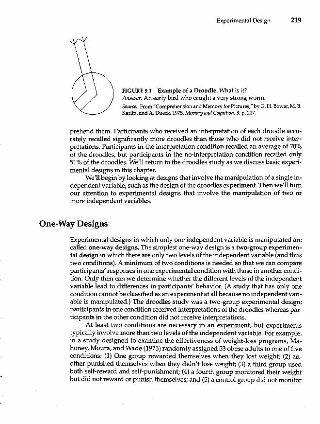
Experimental Design 219

FIGURE 9.1 Example of a Droodle. What is it? Answer: An early bird who caught a very strong worm. Source: From "Comprehension and Memory for Pictures," by G. H. Bower, M. B. Karlin, and A. Dueck, 1975, Memory and Cognition, 3, p. 217.

prehend them. Participants who received an interpretation of each droodle accu­rately recalled significantly more droodles than those who did not receive inter­pretations. Participants in the interpretation condition recalled an average of 70% of the droodles, but participants in the no-interpretation condition recalled only 51 % of the droodles. We'll return to the droodles study as we discuss basic experi­mental designs in this chapter.

We'll begin by looking at designs that involve the manipulation of a single in­dependent variable, such as the design of the droodles experiment. Then we'll turn our attention to experimental designs that involve the manipulation of two or more independent variables.

One-Way Designs

Experimental designs in which only one independent variable is manipulated are called one-way designs. The simplest one-way design is a two-group experimen­tal design in which there are only two levels of the independent variable (and thus two conditions). A minimum of two conditions is needed so that we can compare participants' responses in one experimental condition with those in another condi­tion. Only then can we determine whether the different levels of the independent variable lead to differences in participants' behavior. (A study that has only one condition cannot be classified as an experiment at all because no independent vari­able is manipulated.) The droodles study was a two-group experimental design; participants in one condition received interpretations of the droodles whereas par­ticipants in the other condition did not receive interpretations.

At least two conditions are necessary in an experiment, but experiments typically involve more than two levels of the independent variable. For example, in a study designed to examine the effectiveness of weight-loss programs, Ma­honey, Moura, and Wade (1973) randomly assigned 53 obese adults to one of five conditions: (1) One group rewarded themselves when they lost weight; (2) an­other punished themselves when they didn't lose weight; (3) a third group used both self-reward and self-punishment; (4) a fourth group monitored their weight but did not reward or punish themselves; and (5) a control group did not monitor

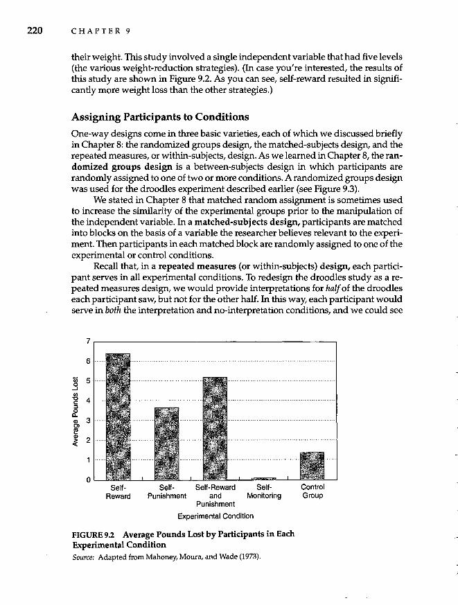
220 CHAPTER 9

their weight. This study involved a single independent variable that had five levels (the various weight-reduction strategies). (In case you're interested, the results of this study are shown in Figure 9.2. As you can see, self-reward resulted in signifi­cantly more weight loss than the other strategies.)

Assigning Participants to Conditions

One-way designs come in three basic varieties, each of which we discussed briefly in Chapter 8: the randomized groups design, the matched-subjects design, and the repeated measures, or within-subjects, design. As we learned in Chapter 8, the ran­domized groups design is a between-subjects design in which participants are randomly assigned to one of two or more conditions. A randomized groups design was used for the droodles experiment described earlier (see Figure 9.3).

We stated in Chapter 8 that matched random assignment is sometimes used to increase the similarity of the experimental groups prior to the manipulation of the independent variable. In a matched-subjects design, participants are matched into blocks on the basis of a variable the researcher believes relevant to the experi­ment. Then participants in each matched block are randomly assigned to one of the experimental or control conditions.

Recall that, in a repeated measures (or within-subjects) design, each partici­pant serves in all experimental conditions. To redesign the droodles study as a re­peated measures design, we would provide interpretations for half of the droodles each participant saw, but not for the other half. In this way, each participant would serve in both the interpretation and no-interpretation conditions, and we could see

7

6

'lii 5 .3 '" "C 4 c: :::l

~ Q) 3 Cl I!! Q)

~ 2

o Self­

Reward Self- Self-Reward Self-

Punishment and Monitoring Punishment

Experimental Condition

FIGURE 9.2 Average Pounds Lost by Participants in Each Experimental Condition Source: Adapted from Mahoney, Moura, and Wade (1973).

Control Group

, ,

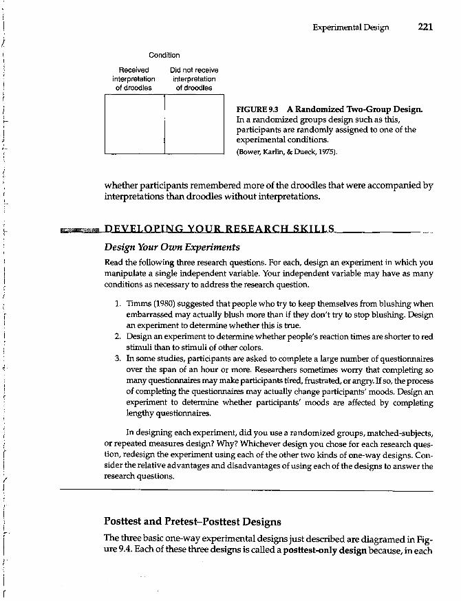
I f

I

I r-

~

I r i

! r r \ . r I

I

Condition

Received interpretation of droodles

Did not receive interpretation ofdroodles

Experimental Design 221

FIGURE 9.3 A Randomized Two-Group Design. In a randomized groups design such as this, participants are randomly assigned to one of the experimental conditions. (Bower, Karlin, & Dueck, 1975).

whether participants remembered more of the droodles that were accompanied by interpretations than droodles without interpretations.

.. I!!llff1I!5l!itl DEVELOPING YOUR RESEARCH SKILLS

Design Your Own Experiments

Read the following three research questions. For each, design an experiment in which you manipulate a single independent variable. Your independent variable may have as many conditions as necessary to address the research question.

1. Timms (1980) suggested that people who try to keep themselves from blushing when embarrassed may actually blush more than if they don't try to stop blushing. Design an experiment to determine whether this is true.

2. Design an experiment to determine whether people's reaction times are shorter to red stimuli than to stimuli of other colors.

3. In some studies, participants are asked to complete a large number of questionnaires over the span of an hour or more. Researchers sometimes worry that completing so many questionnaires may make participants tired, frustrated, or angry. If so, the process of completing the questionnaires may actually change participants' moods. Design an experiment to determine whether participants' moods are affected by completing lengthy questionnaires.

In designing each experiment, did you use a randomized groups, matched-subjects, or repeated measures design? Why? Whichever design you chose for each research ques­tion, redesign the experiment using each of the other two kinds of one-way designs. Con­sider the relative advantages and disadvantages of using each of the designs to answer the research questions.

Posttest and Pretest-Posttest Designs

The three basic one-way experimental designs just described are diagramed in Fig­ure 9.4. Each of these three designs is called a posttest-only design because, in each

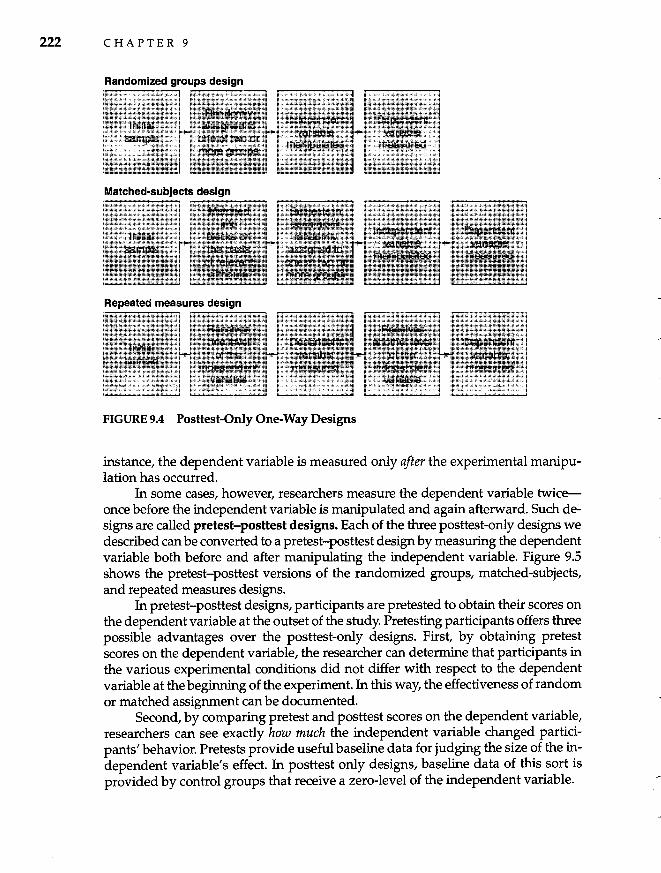
222 CHAPTER 9

Randomized groups design

Matched-subjects design

Repeated measures design

FIGURE 9.4 Posttest-Only One-Way Designs

instance, the dependent variable is measured only after the experimental manipu­lation has occurred.

In some cases, however, researchers measure the dependent variable twice­once before the independent variable is manipulated and again afterward. Such de­signs are called pretest-posttest designs. Each of the three posttest-only designs we described can be converted to a pretest-posttest design by measuring the dependent variable both before and after manipulating the independent variable. Figure 9.5 shows the pretest-posttest versions of the randomized groups, matched-subjects, and repeated measures designs.

In pretest-posttest designs, participants are pretested to obtain their scores on the dependent variable at the outset of the study. Pretesting participants offers three possible advantages over the posttest-only designs. First, by obtaining pretest scores on the dependent variable, the researcher can determine that participants in the various experimental conditions did not differ with respect to the dependent variable at the beginning of the experiment. In this way, the effectiveness of random or matched assignment can be documented.

Second, by comparing pretest and posttest scores on the dependent variable, researchers can see exactly how much the independent variable changed partici­pants' behavior. Pretests provide useful baseline data for judging the size of the in­dependent variable's effect. In posttest only designs, baseline data of this sort is provided by control groups that receive a zero-level of the independent variable.

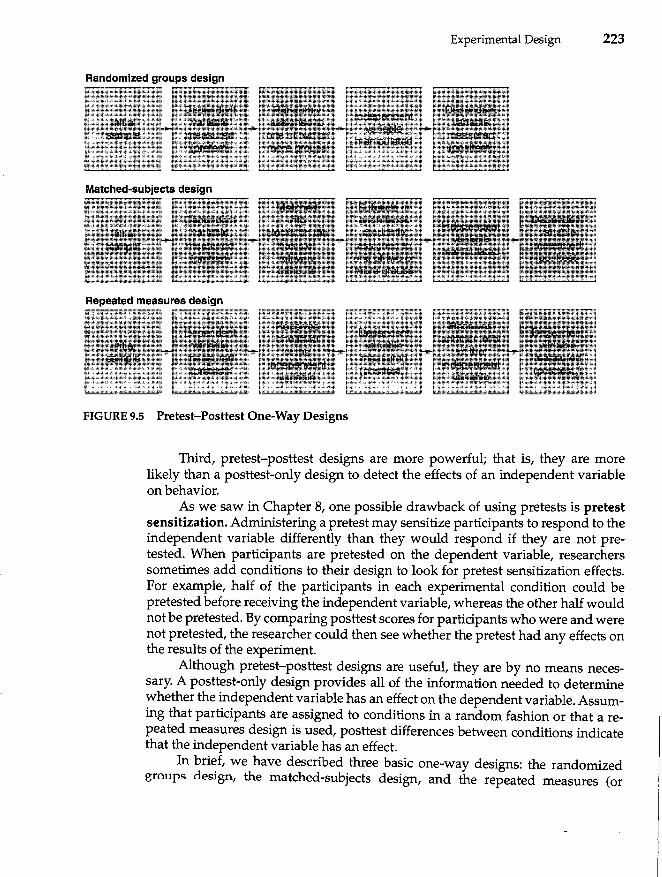
Experimental Design 223

Randomized groups design

Matched-subjects design

Repeated measures design

FIGURE 9.5 Pretest-Posttest One-Way Designs

Third, pretest-posttest designs are more powerful; that is, they are more likely than a posttest-only design to detect the effects of an independent variable on behavior.

As we saw in Chapter 8, one possible drawback of using pretests is pretest sensitization. Administering a pretest may sensitize participants to respond to the independent variable differently than they would respond if they are not pre­tested. When participants are pretested on the dependent variable, researchers sometimes add conditions to their design to look for pretest sensitization effects. For example, half of the participants in each experimental condition could be pretested before receiving the independent variable, whereas the other half would not be pretested. By comparing posttest scores for participants who were and were not pretested, the researcher could then see whether the pretest had any effects on the results of the experiment.

Although pretest-posttest designs are useful, they are by no means neces­sary. A posttest-only design provides all of the information needed to determine whether the independent variable has an effect on the dependent variable. Assum­ing that participants are assigned to conditions in a random fashion or that a re­peated measures design is used, posttest differences between conditions indicate that the independent variable has an effect.

In brief, we have described three basic one-way designs: the randomized groups design, the matched-subjects design, and the repeated measures (or

224 CHAPTER 9

within-subjects) design. Each of these designs can be employed as a posttest-only design or as a pretest-posttest design, depending on the requirements of a partic­ular experiment.

Factorial Designs

With the growth of urban areas during the 1960s, psychologists became interested in the effects of crowding on behavior, emotion, and health. In early work on crowd­ing, researchers assumed that increasing the density of a situation-decreasing the amount of space or increasing the number of people in it-typically leads to nega­tive effects such as aggression and stress. Freedman (1975) questioned this view, proposing instead that, rather than evoking exclusively negative reactions, high­density situations simply intensify whatever reactions people are experiencing at the time. If people are in an unpleasant situation, increasing density will make their experience even more unpleasant. Feeling crowded during a boring lecture only makes things worse, for example. But if people are enjoying themselves, Freed­man predicted, higher density will intensify their positive reactions. The larger the crowd at an enjoyable concert, the more you might enjoy it (within reasonable limits, of course).

Think for a moment about how you might design an experiment to test Freed­man's density-intensity hypothesis. According to this hypothesis, people's reac­tions to social settings are a function of two factors: the density of the situations and the quality of people's experiences in them. Thus, testing this hypothesis requires studying the combined effects of two independent variables simultaneously.

The one-way experimental designs we discussed earlier in the chapter would not be particularly useful in this regard. A one-way design allows us to examine the effects of only one independent variable. To test Freedman's hypothesis re­quires a design that involves two or more variables simultaneously. Such a design, in which two or more independent variables are manipulated, is called a factorial design. Often the independent variables are referred to as factors. (Do not confuse this use of the term factors with the use of the term in factor analysis.)

To test his density-intensity hypothesis, Freedman (1975) designed an exper­iment in which he manipulated two independent variables: the density of the room and the quality of the experience. In his study, participants delivered a brief speech to a small audience. The audience was instructed to provide the speaker with ei­ther positive or negative feedback about the speech. Thus, for participants in one condition the situation was predominately pleasant, whereas for participants in the other condition the situation was predominately unpleasant. Freedman also varied the size of the room in which participants gave their speeches. Some partic­ipants spoke in a large room (150 square feet), and some spoke in a small room (70 square feet). Thus, although audience size was constant in both conditions, the density was higher for some participants than for others. After giving their speeches and receiving either positive or negative feedback, participants completed a ques­tionnaire on which they indicated their reactions to the situation, including how

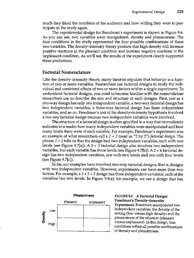
Experimental Design 225

much they liked the members of the audience and how willing they were to par­ticipate in the study again.

The experimental design for Freedman's experiment is shown in Figure 9.6. As you can see, two variables were manipulated: density and pleasantness. The four conditions in the study represented the four possible combinations of these two variables. The density-intensity theory predicts that high density will increase positive reactions in the pleasant condition and increase negative reactions in the unpleasant condition. As we'll see, the results of the experiment clearly supported these predictions.

Factorial Nomenclature

Like the density-intensity theory, many theories stipulate that behavior is a func­tion of two or more variables. Researchers use factorial designs to study the indi­vidual and combined effects of two or more factors within a single experiment. To understand factorial designs, you need to become familiar with the nomenclature researchers use to describe the size and structure of such designs. First, just as a one-way design has only one independent variable, a two-way factorial design has two independent variables, a three-way factorial design has three independent variables, and so on. Freedman's test of the density-intensity hypothesis involved a two-way factorial design because two independent variables were involved.

The structure of a factorial design is often specified in a way that immediately indicates to a reader how many independent variables were manipulated and how many levels there were of each variable. For example, Freedman's experiment was an example of what researchers call a 2 x 2 (read as "2 by 2") factorial design. The phrase 2 x 2 tells us that the design had two independent variables, each with two levels (see Figure 9.7[a]). A 3 x 3 factorial design also involves two independent variables, but each variable has three levels (see Figure 9.7[b]). A 2 x 4 factorial de­sign has two independent variables, one with two levels and one with four levels (see Figure 9.7[c]).

So far, our examples have involved two-way factorial designs, that is, designs with two independent variables. However, experiments can have more than two factors. For example, a 2 x 2 x 2 design has three independent variables; each of the variables has two levels. In Figure 9.8(a), for example, we see a design that has

~ Ul r::: CD o

Low

High

Pleasantness

Pleasant Unpleasant

FIGURE 9.6 A Factorial Design: Freedman's Density-Intensity Experiment. Freedman manipulated two independent variables: the density of the setting (low versus high density) and the pleasantness of the situation (pleasant versus unpleasant). In this design, four conditions reflect all possible combinations of density and pleasantness.

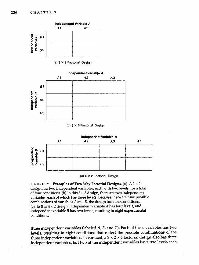
226 CHAPTER 9

Independent Variable A A1 A2

'Ell:! III 81 "Dill c-III..Q Do .!!! III .. "D~ 82 .E

(a) 2 x 2 Factorial Design

Independent Variable A A1 A2 A3

81 -5i1l:! "Dill c-

82 co..Q Do .!!! III .. "D~ .5

83

(b) 3 x 3 Factorial Design

Independent Variable A A1 A2 A3 A4

~II:! 81 "D III c-8.~ III .. "D~ 82 .5

(c) 4 x 2 Factorial Design

FIGURE 9.7 Examples of Two-Way Factorial Designs. (a) A 2 x 2 design has two independent variables, each with two levels, for a total of four conditions. (b) In this 3 x 3 design, there are two independent variables, each of which has three levels. Because there are nine possible combinations of variables A and B, the design has nine conditions. (c) In this 4 x 2 design, independent variable A has four levels, and independent variable B has two levels, resulting in eight experimental conditions.

three independent variables (labeled A, B, and C). Each of these variables has two levels, resulting in eight conditions that reflect the possible combinations of the three independent variables. In contrast, a 2 x 2 x 4 factorial design also has three independent variables, but two of the independent variables have two levels each

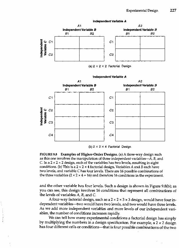
Experimental Design 227

Independent Variable A

A1 Independent Variable 8

81 82

C1

A2 Independent Variable 8

81 82

i ~ C1

8..!!! f------+----------1 CI) ..

"C ~ C2 .5

C1

... i U C2 "CCI) cjS 8. .!!! CI) .. "C~ C3 .5

C4

C2

(a) 2 x 2 x 2 Factorial Design

Independent Variable A

A1 Independent Variable 8

81 82

C1

C2

C3

C4

A2 Independent Variable 8

81 82

(b) 2 x 2 x 4 Factorial Design

FIGURE 9.8 Examples of Higher-Order Designs. (a) A three-way design such as this one involves the manipulation of three independent variables-A, B, and C. In a 2 x 2 x 2 design, each of the variables has two levels, resulting in eight conditions. (b) This is a 2 x 2 x 4 factorial design. Variables A and B each have two levels, and variable C has four levels. There are 16 possible combinations of the three variables (2 x 2 x 4 = 16) and therefore 16 conditions in the experiment.

and the other variable has four levels. Such a design is shown in Figure 9.8(b); as you can see, this design involves 16 conditions that represent all combinations of the levels of variables A, B, and C.

A four-way factorial design, such as a 2 x 2 x 3 x 3 design, would have four in­dependent variables-two would have two levels, and two would have three levels. As we add more independent variables and more levels of our independent vari­ables, the number of conditions increases rapidly.

We can tell how many experimental conditions a factorial design has simply by multiplying the numbers in a design specification. For example, a 2 x 2 design has four different cells or conditions-that is four possible combinations of the two

228 CHAPTER 9

independent variables (2 x 2 = 4). A 3 x 4 x 2 design has 24 different experimental conditions (3 x 4 x 2 = 24), and so on.

Assigning Participants to Conditions

Like the one-way designs we discussed earlier, factorial designs may include ran­domized groups, matched-subjects, or repeated measures designs. In addition, as we will see, the split-plot, or between-within, design combines features of the ran­domized groups and repeated measures designs.

Randomized Groups Factorial Design. In a randomized groups factorial de­sign (which is also called a completely randomized factorial design) participants are as­signed randomly to one of the possible combinations of the independent variables. In Freedman's (1975) test of the density-intensity hypothesis, participants were as­signed randomly to one of four combinations of density and pleasantness.

Matched Factorial Design. As in the matched-subjects one-way design, the matched-subjects factorial design involves first matching participants into blocks on the basis of some variable that correlates with the dependent variable. There will be as many participants in each matched block as there are experimental con­ditions. In a 3 x 2 factorial design, for example, six participants would be matched into each block (because there are six experimental conditions). Then the partici­pants in each block are randomly assigned to one of the six experimental conditions. As before, the primary reason for using a matched-subjects design is to equate more closely the participants in the experimental conditions before introducing the inde­pendent variable.

Repeated Measures Factorial Design. A repeated measures (or within-subjects) factorial design requires all participants to participate in every experimental con­dition. Although repeated measures designs are feasible with small factorial de­signs (such as a 2 x 2 design), they become unwieldy with larger designs. For example, in a 2 x 2 x 2 x 4 repeated measures factorial design, each participant would serve in 32 different conditions! With such large designs, order and carry­over effects can become a problem.

Mixed Factorial Design. Because one-way designs involve a single independent variable, they must involve random assignment, matched-subjects, or repeated measures. However, factorial designs involve more than one independent variable, and they can combine features of both randomized groups designs and repeated measures designs in a single experiment. Some independent variables in a factorial experiment may involve random assignment, whereas other variables involve a repeated measure. A design that combines one or more between-subjects vari­ables with one or more within-subjects variables is called a mixed factorial design, between-within design, or split-plot factorial design. (The odd name, split-plot, was adopted from agricultural research and actually refers an area of ground that has been subdivided for research purposes.)

,. I

! ! J

f

I i

!

J

/

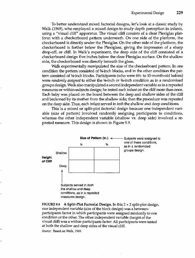
Experimental Design 229

To better understand mixed factorial designs, let's look at a classic study by Walk (1969), who employed a mixed design to study depth perception in infants, using a "visual cliff" apparatus. The visual cliff consists of a clear Plexiglas plat­form with a checkerboard pattern underneath. On one side of the platform, the checkerboard is directly under the Plexiglas. On the other side of the platform, the checkerboard is farther below the Plexiglass, giving the impression of a sharp drop-off, or cliff. In Walk's experiment, the deep side of the cliff consisted of a checkerboard design five inches below the clear Plexiglas surface. On the shallow side, the checkerboard was directly beneath the glass.

Walk experimentally manipulated the size of the checkerboard pattern. In one condition the pattern consisted of %-inch blocks, and in the other condition the pat­tern consisted of lA-inch blocks. Participants (who were 61h- to lS-month-old babies) were randomly assigned to either the lA-inch or %-inch condition as in a randomized groups design. Walk also manipulated a second independent variable as in a repeated measures or within-subjects design; he tested each infant on the cliff more than once. Each baby was placed on the board between the deep and shallow sides of the cliff and beckoned by its mother from the shallow side; then the procedure was repeated on the deep side. Thus, each infant served in both the shallow and deep conditions.

This is a mixed or split-plot factorial design because one independent vari­able (size of pattern) involved randomly assigning participants to conditions, whereas the other independent variable (shallow vs. deep side) involved a re­peated measure. This design is shown in Figure 9.9.

Height of Cliff

Shallow

Deep

1

Size of Pattern (in.) .... f---- Subjects were assigned to one of these conditions, as in a randomized groups design.

Subjects served in both the shallow and deep conditions, as in a repeated measures design.

FIGURE 9.9 A Split-Plot Factorial Design. In this 2 x 2 split-plot design, one independent variable (size of the block design) was a between­participants factor in which participants were assigned randomly to one condition or the other. The other independent variable (height of the visual cliff) was a within-participants factor. All participants were tested at both the shallow and deep sides of the visual cliff. Source: Based on Walk, 1969.

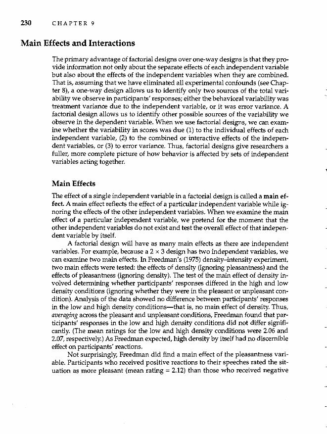
230 CHAPTER 9

Main Effects and Interactions

The primary advantage of factorial designs over one-way designs is that they pro­vide information not only about the separate effects of each independent variable but also about the effects of the independent variables when they are combined. That is, assuming that we have eliminated all experimental confounds (see Chap­ter 8), a one-way design allows us to identify only two sources of the total vari­ability we observe in participants' responses; either the behavioral variability was treatment variance due to the independent variable, or it was error variance. A factorial design allows us to identify other possible sources of the variability we observe in the dependent variable. When we use factorial designs, we can exam­ine whether the variability in scores was due (1) to the individual effects of each independent variable, (2) to the combined or interactive effects of the indepen­dent variables, or (3) to error variance. Thus, factorial designs give researchers a fuller, more complete picture of how behavior is affected by sets of independent variables acting together.

Main Effects

The effect of a single independent variable in a factorial design is called a main ef­fect. A main effect reflects the effect of a particular independent variable while ig­noring the effects of the other independent variables. When we examine the main effect of a particular independent variable, we pretend for the moment that the other independent variables do not exist and test the overall effect of that indepen­dent variable by itself.

A factorial design will have as many main effects as there are independent variables. For example, because a 2 x 3 design has two independent variables, we can examine two main effects. In Freedman's (1975) density-intensity experiment, two main effects were tested: the effects of density (ignoring pleasantness) and the effects of pleasantness (ignoring density). The test of the main effect of density in­volved determining whether participants' responses differed in the high and low density conditions (ignoring whether they were in the pleasant or unpleasant con­dition). Analysis of the data showed no difference between participants' responses in the low and high density conditions-that is, no main effect of density. Thus, averaging across the pleasant and unpleasant conditions, Freedman found that par­ticipants' responses in the low and high density conditions did not differ signifi­cantly. (The mean ratings for the low and high density conditions were 2.06 and 2.07, respectively.) As Freedman expected, high density by itself had no discernible effect on participants' reactions.

Not surprisingly, Freedman did find a main effect of the pleasantness vari­able. Participants who received positive reactions to their speeches rated the sit­uation as more pleasant (mean rating = 2.12) than those who received negative

Experimental Design 231

reactions (mean rating = 2.01). Of course, this main effect is not particularly surprising or interesting, but it serves as a manipulation check by showing that participants perceived the pleasant situation to be more pleasant than the un­pleasant situation.

Interactions

In addition to providing information about the main effects of each indepen­dent variable, a factorial design provides information about interactions between the independent variables. An interaction is present when the effect of one in­dependent variable differs across the levels of other independent variables. If one independent variable has a different effect at one level of another individual variable than it has at another level of that independent variable, we say that the independent variables interact and that an interaction between the independent variables is present. For example, imagine we conduct a factorial experiment with two independent variables, A and B. If the effect of variable A is different under one level of variable B than it is under another level of variable B, an in­teraction is present. However, if variable A has the same effect on participants' responses no matter what level of variable B they receive, then no interaction is present.

Consider, for example, what happens if you mix alcohol and drugs such as sedatives. The effects of drinking a given amount of alcohol vary depending on whether you've also taken sleeping pills. By itself, a strong mixed drink may result in only a mild "buzz." Similarly, taking one or two sleeping pills may make you sleepy but will have few other effects. However, that same strong drink may create pronounced effects on behavior if you've taken a sleeping pill. And mixing a strong drink with two or three sleeping pills will produce extreme, potentially fatal, re­sults. Because the effects of a given dose of alcohol depends on how many sleeping pills you've taken, alcohol and sleeping pills interact to affect behavior. This is an in­teraction because the effect of one variable (alcohol) differs depending on the level of the other variable (no pill, one pill, or three pills).

Similarly, the density-intensity hypothesis predicted an interaction of density and pleasantness on participants' reactions. According to the hypothesis, high density should have a different effect on participants who received positive feed­back than on those who received negative feedback. Freedman's data, shown in Figure 9.10, revealed the predicted interaction. High density resulted in more posi­tive reactions for participants in the pleasant condition but in less positive reactions for participants in the unpleasant condition. The effects of density were different under one level of pleasantness than under the other, so an interaction is present. Because the effect of one variable (density) differed under the different levels of the other variable (pleasantness), we say that density and pleasantness interacted to af­fect participants' responses to the situation.

232 C HAP T E R 9

~ Low

I/) c CD c

High

Means for the main effect of pleasantness

Pleasantness

Pleasant Unpleasant

2.01 2.10

2.22 1.92

, 2.12 2.01

Means for the main effect of density

j 2.06

2.07

FIGURE 9.10 Effects of Density and Pleasantness on Participants' Liking Other Participants. These numbers are participants' average ratings of how much they liked the members of the audience who observed their speeches. Higher numbers indicate greater liking. As the density-intensity hypothesis predicted, high density increased liking more than low density did when the situation was pleasant. However, high density decreased liking more than low density did when the situation was unpleasant. The fact that density had a different effect depending on whether the situation was pleasant or unpleasant indicates the presence of an interaction. Source: From Crowding and Behavior (p. 150) by J. L. Freedman, 1975, San Francisco: W. H. Freeman and Company. Copyright© 1975 by J. L. Freed­man. Adapted by permission of Jonathan Freedman and the publisher.

f¥OI&!!!!!I¥ffl!!!!!@jj! DEVELOPING YOUR RESEARCH SKILLS

Graphing Interactions Researchers often present the results of factorial experiments in tables of means such as that shown in Figure 9.10 for Freedman's density-intensity study. Although presenting tables of means provides readers with precise information about the results of an experiment, re­searchers sometimes graph the means for interactions because graphs show how indepen­dent variables interact more clearly and dramatically than tables. To graph a two-way interaction, the conditions for one independent variable are shown on the x-axis, and the conditions for the other independent variable are shown as lines. For example, we could graph the means from Figure 9.10 as shown in Figure 9.11(a).

When the means for the conditions of a factorial design are graphed, interactions ap­pear as nonparallel lines. The fact that the lines are not parallel shows that the effects of one independent variable differ depending on the level of the other independent variable. Look­ing at the graph of Freedman's data, we can easily see that low and high density produced different reactions to pleasant vs. unpleasant situations.

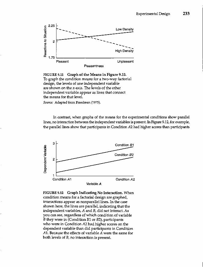
c: 2.25

~ :e en oS 2 ! o

--------Low Density

-------------... High Density ]

1.75 '------------------Pleasant Unpleasant

Pleasantness

FIGURE 9.11 Graph of the Means in Figure 9.10. To graph the condition means for a two-way factorial design, the levels of one independent variable are shown on the x-axis. The levels of the other independent variable appear as lines that connect the means for that level. Source: Adapted from Freedman (1975).

Experimental Design 233

In contrast, when graphs of the means for the experimental conditions show parallel lines, no interaction between the independent variables is present. In Figure 9.12, for example, the parallel lines show that participants in Condition A2 had higher scores than participants

3 Condition 81

Condition A 1 Condition A2 Variable A

FIGURE 9.12 Graph Indicating No Interaction. When condition means for a factorial design are graphed, interactions appear as nonparallel lines. In the case shown here, the lines are parallel, indicating that the independent variables, A and B, did not interact. As you can see, regardless of which condition of variable B they were in (Condition Bl or B2), participants who were in Condition A2 had higher scores on the dependent variable than did participants in Condition AI. Because the effects of variable A were the same for both levels of B, no interaction is present.

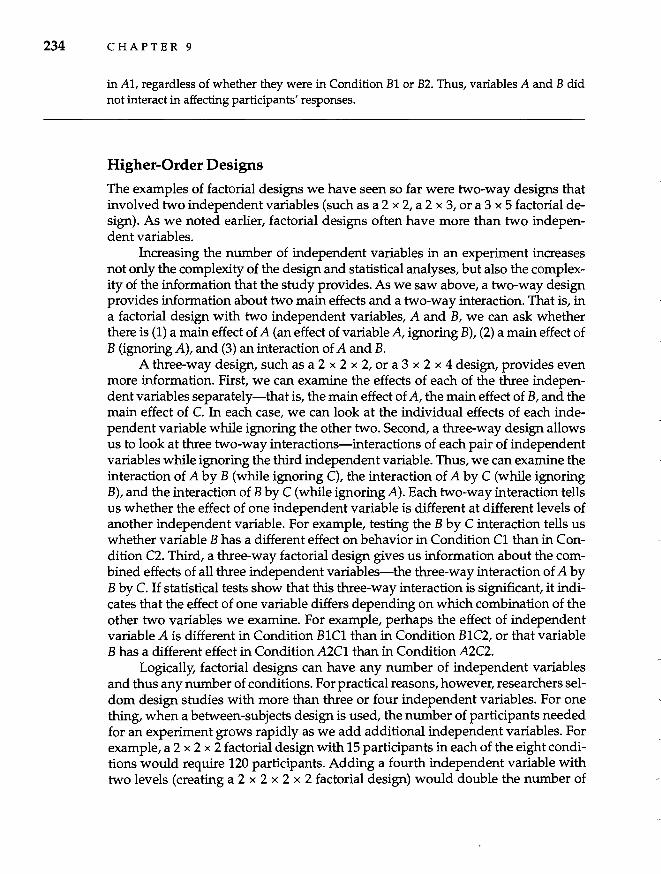
234 CHAPTER 9

in A1, regardless of whether they were in Condition B1 or B2. Thus, variables A and B did not interact in affecting participants' responses.

Higher-Order Designs

The examples of factorial designs we have seen so far were two-way designs that involved two independent variables (such as a 2 x 2, a 2 x 3, or a 3 x 5 factorial de­sign). As we noted earlier, factorial designs often have more than two indepen­dent variables.

Increasing the number of independent variables in an experiment increases not only the complexity of the design and statistical analyses, but also the complex­ity of the information that the study provides. As we saw above, a two-way design provides information about two main effects and a two-way interaction. That is, in a factorial design with two independent variables, A and B, we can ask whether there is (1) a main effect of A (an effect of variable A, ignoring B), (2) a main effect of B (ignoring A), and (3) an interaction of A and B.

A three-way design, such as a 2 x 2 x 2, or a 3 x 2 x 4 design, provides even more information. First, we can examine the effects of each of the three indepen­dent variables separately-that is, the main effect of A, the main effect of B, and the main effect of C. In each case, we can look at the individual effects of each inde­pendent variable while ignoring the other two. Second, a three-way design allows us to look at three two-way interactions-interactions of each pair of independent variables while ignoring the third independent variable. Thus, we can examine the interaction of A by B (while ignoring C), the interaction of A by C (while ignoring B), and the interaction of B by C (while ignoring A). Each two-way interaction tells us whether the effect of one independent variable is different at different levels of another independent variable. For example, testing the B by C interaction tells us whether variable B has a different effect on behavior in Condition C1 than in Con­dition C2. Third, a three-way factorial design gives us information about the com­bined effects of all three independent variables-the three-way interaction of A by B by C. If statistical tests show that this three-way interaction is significant, it indi­cates that the effect of one variable differs depending on which combination of the other two variables we examine. For example, perhaps the effect of independent variable A is different in Condition B1C1 than in Condition B1C2, or that variable B has a different effect in Condition A2C1 than in Condition A2C2.

LOgically, factorial designs can have any number of independent variables and thus any number of conditions. For practical reasons, however, researchers sel­dom design studies with more than three or four independent variables. For one thing, when a between-subjects design is used, the number of participants needed for an experiment grows rapidly as we add additional independent variables. For example, a 2 x 2 x 2 factorial design with 15 participants in each of the eight condi­tions would require 120 participants. Adding a fourth independent variable with two levels (creating a 2 x 2 x 2 x 2 factorial design) would double the number of

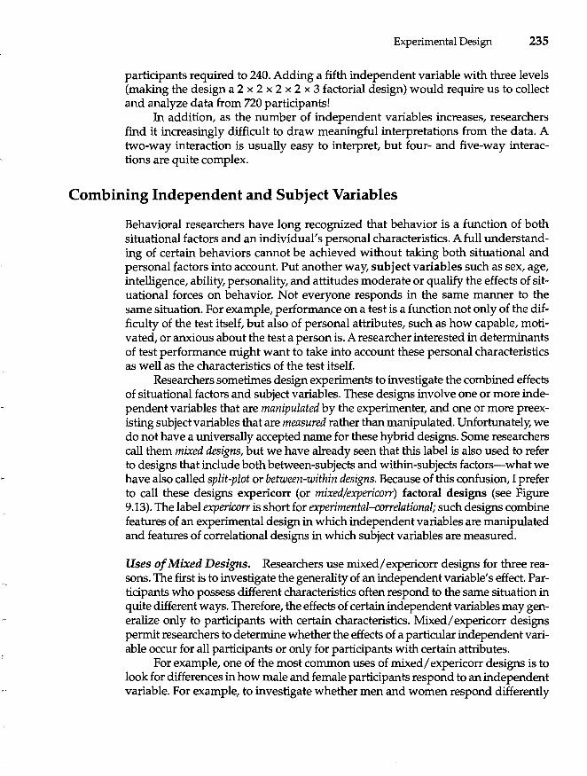
Experimental Design 235

participants required to 240. Adding a fifth independent variable with three levels (making the design a 2 x 2 x 2 x 2 x 3 factorial design) would require us to collect and analyze data from 720 participants!

In addition, as the number of independent variables increases, researchers find it increasingly difficult to draw meaningful interpretations from the data. A two-way interaction is usually easy to interpret, but four- and five-way interac­tions are quite complex.

Combining Independent and Subject Variables

Behavioral researchers have long recognized that behavior is a function of both situational factors and an individual's personal characteristics. A full understand­ing of certain behaviors cannot be achieved without taking both situational and personal factors into account. Put another way, subject variables such as sex, age, intelligence, ability, personality, and attitudes moderate or qualify the effects of sit­uational forces on behavior. Not everyone responds in the same manner to the same situation. For example, performance on a test is a function not only of the dif­ficulty of the test itself, but also of personal attributes, such as how capable, moti­vated, or anxious about the test a person is. A researcher interested in determinants of test performance might want to take into account these personal characteristics as well as the characteristics of the test itself.

Researchers sometimes design experiments to investigate the combined effects of situational factors and subject variables. These designs involve one or more inde­pendent variables that are manipulated by the experimenter, and one or more preex­isting subject variables that are measured rather than manipulated. Unfortunately, we do not have a universally accepted name for these hybrid designs. Some researchers call them mixed designs, but we have already seen that this label is also used to refer to designs that include both between-subjects and within-subjects factors-what we have also called split-plot or between-within designs. Because of this confusion, I prefer to call these designs expericorr (or mixed/expericorr) fadoral designs (see Figure 9.13). The label expericorr is short for experimental-correlational; such designs combine features of an experimental design in which independent variables are manipulated and features of correlational designs in which subject variables are measured.

Uses of Mixed Designs. Researchers use mixed/ expericorr designs for three rea­sons. The first is to investigate the generality of an independent variable's effect. Par­ticipants who possess different characteristics often respond to the same situation in quite different ways. Therefore, the effects of certain independent variables may gen­eralize only to participants with certain characteristics. Mixed/ expericorr designs permit researchers to determine whether the effects of a particular independent vari­able occur for all participants or only for participants with certain attributes.

For example, one of the most common uses of mixed/ expericorr designs is to look for differences in how male and female participants respond to an independent variable. For example, to investigate whether men and women respond differently

236 C HAP T E R 9

Subject Variable ...... i---- This is a characteristic

Independent Variable

Low High

Condition 1

Condition 2

1 This is a true independent variable that is manipulated by the researcher

of the participants that is measured before the study

FIGURE 9.13 A 2 x 2 Expericorr or Mixed Factorial Design

to success and failure, a researcher might use a 2 x 3 expericorr design. In this design, one factor would involve a participant variable with two levels, namely gender. The other factor would involve a manipulated independent variable that has three levels: Participants would each take a test and then receive either (1) success feed­back, (2) failure feedback, or (3) no feedback. When the data were analyzed, the re­searcher could examine the main effect of participant gender (whether, overall, men and women differ), the main effect of feedback (whether participants respond differently to success, failure, or no feedback), and, most important, the interaction of gender and feedback (whether men and women respond differently to success, failure, and/ or no feedback).

Second, researchers use expericorr designs in an attempt to understand how certain personal characteristics relate to behavior under varying conditions. The emphasis in such studies is on understanding the measured subject variable rather than the manipulated independent variable. For example, a researcher interested in self-esteem might expose persons who scored low or high in self-esteem to var­ious experimental conditions. Or a researcher interested in depression might con­duct an experiment in which depressed and nondepressed participants respond to various experimentally manipulated situations. Studying how participants with different characteristics respond to an experimental manipulation may shed light on that characteristic.

Third, by splitting participants into groups based on a participant variable, re­searchers make the participants within the experimental conditions more homo­geneous. This reduces the error variance (the variability within conditions), thereby increasing the sensitivity of the study in detecting effects of the independent variable.

Classifying Participants into Groups. When researchers use mixed designs, they typically classify participants into groups on the basis of the measured partic­ipant variable (such as gender or self-esteem), then randomly assign participants within those groups to levels of the independent variable. For discrete participant variables such as gender and race, it is usually easy to assign participants to two or more groups.

r

r

I I

\ J-

\ \

f I i I i

r /-t

~. ,e I t I I

r

j

I I I

L 1 r I ) (-

I r ,

,j I

Experimental Design 237

Sometimes, however, researchers are interested in subject variables that are continuous rather than discrete. For example, a researcher may be interested in how self-esteem moderates reactions to success and failure. Because scores on a measure of self-esteem are continuous, the researcher must decide how to classify participants into groups. Traditionally, researchers have typically used either the median-split procedure or the extreme groups procedure.

In the median-split procedure, the researcher identifies the median of the dis­tribution of participants' scores on the variable of interest (such as self-esteem). You will recall that the median is the middle score in a distribution, the score that falls at the 50th percentile. The researcher then classifies participants with scores below the median as low on the variable and those with scores above the median as high on the variable. It must be remembered, however, that the designations low and high are rel­ative to the researcher's sample. All participants could, in fact, be low or high on the attribute in an absolute sense. In a variation of the median-split procedure, some re­searchers split their sample into three or more groups rather than only two.

Alternatively, some researchers prefer the extreme groups procedure for classifying participants into groups. Rather than splitting the sample at the me­dian, the researcher pretests a large number of potential participants, then selects participants for the experiment whose scores are unusually low or high on the vari­able of interest. For example, the researcher may use participants whose scores fall in the upper and lower 25% of a distribution of self-esteem scores, discarding those with scores in the middle range.

Researchers interested in how independent variables interact with participant variables have traditionally classified participants into two or more groups using one of these splitting procedures. However, the use of median and extreme group splits is often criticized, and many researchers no longer use these approaches. One reason is that classifying participants into groups on the basis of a measured subject variable often throws away valuable information. When we use participants' scores on a continuous variable-such as age, self-esteem, or depression-to classify them into only two groups (old vs. young, low vs. high self-esteem, depressed vs. nonde­pressed), we discard information regarding the variability in participants' scores as we convert a rich set of data into a dichotomy.

Furthermore, studies have shown that splitting participants into groups on the basis of a subject variable, such as self-esteem or anxiety, can lead to biased re­sults. Depending on the nature of the data, the bias sometimes leads researchers to miss effects that were actually present, and at other times it leads researchers to ob­tain effects that are actually statistical artifacts (Bissonnette, Ickes, Bernstein, & Knowles, 1990; Cohen & Cohen, 1983; Maxwell & Delaney, 1993). In either case, ar­tificially splitting participants into groups can lead to erroneous conclusions.

Rather than splitting participants into groups, many researchers now use multiple regression procedures that allow them to analyze the data from mixed/ expericorr designs while maintaining the continuous nature of participants' scores on the measured subject variable (Aiken & West, 1991; Cohen & Cohen, 1983; Ko­walski, 1995). The details of such analyses are beyond the scope of this book, but you should be aware that researchers now recognize that median split and extreme group approaches can be problematic.

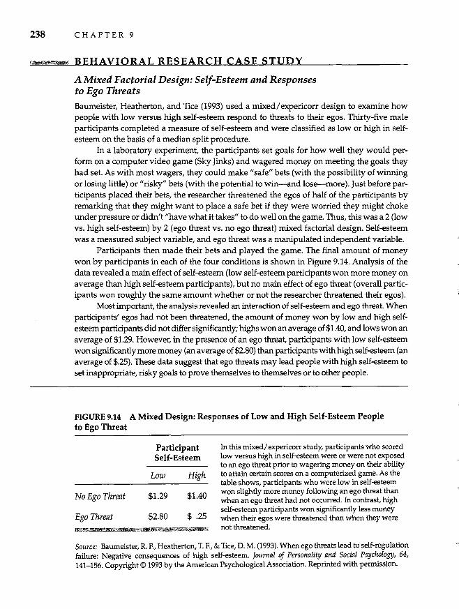
238 CHAPTER 9

BEHAVIORAL RESEARCH CASE STUDY

A Mixed Factorial Design: Self-Esteem and Responses to Ego Threats Baumeister, Heatherton, and Tice (1993) used a mixed/expericorr design to examine how people with low versus high self-esteem respond to threats to their egos. Thirty-five male participants completed a measure of self-esteem and were classified as low or high in self­esteem on the basis of a median split procedure.

In a laboratory experiment, the participants set goals for how well they would per­form on a computer video game (Sky Jinks) and wagered money on meeting the goals they had set. As with most wagers, they could make "safe" bets (with the possibility of winning or losing little) or "risky" bets (with the potential to win-and lose-more). Just before par­ticipants placed their bets, the researcher threatened the egos of half of the participants by remarking that they might want to place a safe bet if they were worried they might choke under pressure or didn't "have what it takes" to do well on the game. Thus, this was a 2 (low vs. high self-esteem) by 2 (ego threat vs. no ego threat) mixed factorial design. Self-esteem was a measured subject variable, and ego threat was a manipulated independent variable.

Participants then made their bets and played the game. The final amount of money won by participants in each of the four conditions is shown in Figure 9.14. Analysis of the data revealed a main effect of self-esteem (low self-esteem participants won more money on average than high self-esteem participants), but no main effect of ego threat (overall partic­ipants won roughly the same amount whether or not the researcher threatened their egos).

Most important, the analysis revealed an interaction of self-esteem and ego threat. When participants' egos had not been threatened, the amount of money won by low and high self­esteem participants did not differ significantly; highs won an average of $1.40, and lows won an average of $1.29. However, in the presence of an ego threat, participants with low self-esteem won significantly more money (an average of $2.80) than participants with high self-esteem (an average of $.25). These data suggest that ego threats may lead people with high self-esteem to set inappropriate, risky goals to prove themselves to themselves or to other people.

FIGURE 9.14 A Mixed Design: Responses of Low and High Self-Esteem People to Ego Threat

No Ego Threat

Ego Threat

Participant Self-Esteem

Low High

$1.29 $1.40

$2.80 $ .25

In this mixed/ expericorr study, participants who scored low versus high in self-esteem were or were not exposed to an ego threat prior to wagering money on their ability to attain certain scores on a computerized game. As the table shows, participants who were low in self-esteem won slightly more money following an ego threat than when an ego threat had not occurred. In contrast, high self-esteem participants won significantly less money when their egos were threatened than when they were not threatened.

Source: Baumeister, R. F., Heatherton, T. F., & lice, D. M. (1993). When ego threats lead to self-regulation failure: Negative consequences of high self-esteem. Journal of Personality and Social Psychology, 64, 141-156. Copyright © 1993 by the American Psychological Association. Reprinted with permission.

J

[

l I

r

Experimental Design 239

Cautions in Interpreting Results of a Mixed Design. Researchers must exer­cise care when interpreting results from mixed designs. Specifically, a researcher can draw causal inferences only about the true independent variables in the experiment-those that were manipulated by the researcher. As always, if effects are obtained for a manipulated independent variable, we can conclude that the in­dependent variable caused changes in the dependent variable.

When effects are obtained for the measured subject variable, however, the re­searcher cannot conclude that the participant variable caused changes in the depen­dent variable. Because the subject variable is measured rather than manipulated, the results are essentially correlational, and (recall from Chapter 6) we cannot infer causality from a correlation.

If a main effect of the subject variable is obtained, we can conclude that the two groups differed on the dependent variable, but we cannot conclude that the participant variable caused the difference. Rather, we say that the subject variable moderated participants' reactions to the independent variable and that the subject variable is a moderator variable. For example, we cannot conclude that high self­esteem caused participants to make risky bets in the ego-threat experiment (Bau­meister et al., 1993). Because people who score low versus high in self-esteem differ in many ways, all we can say is that differences in self-esteem were associated with different responses in the ego-threat condition. Or, more technically, self-esteem moderated the effects of ego threat on participants' behavior.

Summary

1. A one-way experimental design is an experiment in which a single indepen­dent variable is manipulated. The simplest possible experiment is the two­group experimental design.

2. Researchers use three general versions of the one-way design-the random­ized groups design (in which participants are assigned randomly to two or more groups), the matched-subjects design (in which participants are first matched into blocks, then randomly assigned to conditions), and the repeated measures or within-subjects design (in which each participant serves in all experimental conditions).

3. Each of these designs may involve a single measurement of the dependent variable after the manipulation of the independent variable, or a pretest and a posttest.

4. Factorial designs are experiments that include two or more independent vari­ables. (Independent variables are sometimes called factors, a term not to be confused with its meaning in factor analysis.)

5. The size and structure of factorial designs are described by specifying the num­ber of levels of each independent variable. For example, a 3 x 2 factorial design has two independent variables, one with three levels and one with two levels.

6. There are four general types of factorial design-the randomized groups, matched- participants, repeated measures, and mixed (also called split-plot or between-within) factorial designs.

240 CHAPTER 9

7. Factorial designs provide information about the effects of each independent variable by itself (the main effects) as well as the combined effects of the in­dependent variables.

8. An interaction between two or more independent variables is present if the ef­fect of one independent variable is different under one level of another inde­pendent variable than it is under another level of that independent variable.

9. Expericorr (sometimes called mixed) factorial designs combine manipulated independent variables and measured participant variables. Such designs are often used to study participant variables that qualify or moderate the effects of the independent variables.

10. Researchers using an expericorr design sometimes classify participants into groups using a median split or extreme groups procedure, but others use analyses that allow them to maintain the continuity of the measured partici­pant variable. In either case, causal inferences may be drawn only about the variables in the design that were experimentally manipulated.

KEY TERMS

between-within design (p.228)

expericorr factorial design (p.235)

extreme groups procedure (p.237)

factor (p. 224) factorial design (p. 224) interaction (p. 231) main effect (p. 230) matched-subjects design

(p.220)

matched-subjects factorial design (p. 228)

median-split procedure (p. 237) mixed factorial design (p. 228) moderator variable (p. 239) one-way design (p. 219) posttest-only design (p. 221) pretest-posttest design

(p.222) pretest sensitization (p. 223) randomized groups design

(p.220)

QUESTIONS FOR REVIEW

randomized groups factorial design (p. 228)

repeated measures design (p.220)

repeated measures factorial design (p. 228)

split-plot factorial design (p.228)

subject variable (p. 235) two-group experimental

design (p. 219)

1. How many conditions are there in the simplest possible experiment?

2. Describe how participants are assigned to conditions in randomized groups, matched-subjects, and repeated measures experimental designs.

3. What are the relative advantages and disadvantages of posttest-only versus pretest­posttest experimental designs?

4. What is a factorial design? Why are factorial designs used more frequently than one-way designs?

S. How many independent variables are involved in a 3 x 3 factorial design? How many levels are there of each variable? How many experimental conditions are there? Draw the design.

Experimental Design 241

6. Describe a 2 x 2 x 3 factorial design. How many independent variables are in­volved, and how many levels are there of each variable? How many experimental conditions are in a 2 x 2 x 3 factorial design?

7. Distinguish between randomized groups, matched-subjects, and repeated mea­sures factorial designs.

8. Describe a mixed, or split-plot, factorial design. This design is a hybrid of what two other designs?

9. What is a main effect?

10. How many main effects can be tested in a 2 x 2 design? In a 3 x 3 design? In a 2 x 2 x 3 design?

11. What is an interaction?

12. How many interactions can be tested in a 2 x 2 design? In a 3 x 3 design? In a 2 x 2 x 3 design?

- 13. H you want to have 20 participants in each experimental condition, how many par­ticipants will you need for a 2 x 3 x 3 completely randomized factorial design? How many participants will you need for a 2 x 3 x 3 repeated measures factorial design?

14. How do mixed/ expericorr designs differ from other experimental designs?

15. Why do researchers use expericorr designs?

16. Distinguish between an independent variable and a subject variable.

QUESTIONS FOR DISCUSSION

1. Design a randomized groups experiment to test the hypothesis that children who watch an hour-long violent television show subsequently play in a more aggressive fashion than children who watch a nonviolent TV show or who watch no show whatsoever.

2. Explain how you would conduct the study you designed in Question 1 as a matched-subjects design.

3. Build on the design you created in Question 1 to test the hypothesis that the effects of watching violent TV shows will be greater for boys than for girls. (What kind of design is this?)

4. What main effects and interaction could you test with the design you developed for Question 3? Are you predicting that you will obtain an interaction?

5. You have been asked to evaluate the effects of a new educational video that was de­veloped to reduce racial prejudice among adolescents. You plan to administer a pretest measure of racial attitudes to 60 adolescent participants, then randomly as­sign these participants to watch either the anti-prejudice video, an educational video about volcanoes, or no video. Afterwards, the participants will complete the measure of racial attitudes a second time. However, you are concerned that the first administration of the attitudes measure may create pretest sensitization, thereby

242 CHAPTER 9

directly affecting participants attitudes. Explain how you could redesign the exper­iment to see whether pretest sensitization occurred. (Hint: You will probably use a 3 x 2 factorial design.) What pattern of results would suggest that pretest sensitiza­tion had occurred?

6. Graph the means in Figure 9.14 for the interaction between self-esteem and ego threat. Does the graph look like one in which an interaction is present? Why or why not?

..,

CHAPTER

10 Analyzing Experimental Data

An Intuitive Approach to Analysis

Hypothesis Testing

Analyses of Matched-Subjects and Within­Subjects Designs

Analysis of Two-Group Experiments: The t-Test

Some of my students are puzzled (or, perhaps more accurately, horrified) when they discover that they must learn about statistics in a research methods course. More than one student has asked why we talk so much about statistical analyses in my class considering that the course is ostensibly about research methods and other courses on campus are devoted entirely to statistics. Given that the next two chapters are devoted to statistics, it occurred to me that you may be asking your­self the same question.

Statistical analyses are an integral part of the research process. A person who knew nothing about statistics would have difficulty not only conducting research but also understanding others' studies and findings. As a result, most seasoned re­searchers are quite knowledgeable about statistical analyses, although they some­times consult with statisticians when their research calls for analyses with which they are not already familiar.

Even if you, as a student, have no intention of ever conducting research, a basic knowledge of statistics is essential for understanding most journal articles. If you have ever read research articles published in scientific journals, you likely have encountered an assortment of mysterious analyses-t-tests, ANOVAs, MANOVAs, post hoc tests, simple effects tests, and the like-along with an endless stream of seemingly meaningless symbols and numbers, such as /IF (2, 328) = 6.78, P < .01." If you're like many of my students, you may have skimmed over these parts of the article until you found something that made sense. If nothing else, a knowledge of statistics is necessary to be an informed reader and consumer of sci­entific knowledge.

243

244 C HAP T E R 10

Even so, for our purposes here, you do not need a high level of proficiency with all sorts of statistical formulas and calculations. Rather, what you need is an understanding of how statistics work. Thus, Chapters 10 and 11 will focus on how experimental data are analyzed from a concep,.tual perspective. Along the way, you will see formulas for demonstrational purposes, but the calculational formulas re­searchers actually use to analyze data will generally take a back seat. At this point, it's more important to understand how data are analyzed and what the statistical analyses mean than to learn how to do a variety of analyses. That's what statistics courses are for.

An Intuitive Approach to Analysis

After an experiment is conducted, the researcher must analyze the data to deter­mine whether the independent variable had the predicted effect on the dependent variable(s). Did the manipulation of the independent variable cause systematic changes in participants' responses? Did providing participants with interpretations of the droodles they saw affect their memory of the pictures? Did different patterns of self-reward and self-punishment result in different amounts of weight loss? Was perceived crowding affected by a combination of density and pleasantness?

At the most general level, we can see whether the independent variable has an effect by determining whether the total variance in the data includes any systematic variance due to the manipulation of the independent variable (see Chapter 8). Specif­ically, the presence of systematic variance in a set of data is determined by compar­ing the means on the dependent variable for the various experimental groups.

If the independent variable has an effect on the dependent variable, we should find that the means for the experimental conditions differ. Different group aver­ages would suggest that the independent variable had an effect; it created differ­ences in the behavior of participants in the various conditions and thus resulted in systematic variance. Assuming that participants assigned to the experimental con­ditions do not differ systematically before the study and that no confounds are present, the only thing that can cause the means to differ at the end of the experi­ment is the independent variable. However, if the means of the conditions do not differ, then no systematic variance is present, and we will conclude that the inde­pendent variable had no effect.

In the droodles experiment we described in Chapter 9, for example, partici­pants who were given an interpretation of the droodles recalled an average of 19.6 of the pictures immediately afterwards. Participants in the control group (who re­ceived no interpretation) recalled an average of only 14.2 of the pictures (Bower et al., 1975). On the surface, then, inspection of the means for the two experimental conditions indicates that participants who were given an interpretation of the droodles remembered more pictures than those who were not given an interpreta­tion. Unfortunately, this conclusion is not as straightforward as it may appear; we cannot draw conclusions about the effects of an independent variable simply by looking only at the means of the experimental conditions.

,-

Analyzing Experimental Data 245

The Problem: Error Variance Can Cause Mean Differences

The problem with mean differences is that the means of the experimental condi­tions may differ even if the independent variable does not have an effect. We dis­cussed one possible cause of such differences in Chapter 8-confound variance. Recall that if something other than the independent variable differs in a systematic fashion between experimental conditions, the differences between the means may be due to this confounding variable rather than to the independent variable.

However, even assuming that the researcher successfully eliminated con­founding, the means may differ for yet another reason that is unrelated to the in­dependent variable. Suppose that the independent variable did not have an effect in the droodles experiment described earlier; that is, providing an interpretation did not enhance participants' memory for the droodles. What would we expect to find when we calculated the average number of pictures remembered by partici­pants in the two experimental conditions? Would we expect the mean number of pictures recalled in the two experimental groups to be exactly the same? Probably not. Even if the independent variable did not have an effect, it is unlikely that the means would be identical.

To understand this point, imagine that we randomly assigned participants to two groups, then showed them droodles while giving interpretations of the droo­dIes to all participants in both groups. Then we asked participants to recall as many of the droodles as possible. Would the average number of pictures recalled be ex­actly the same in both groups if participants in both groups received interpreta­tions? Probably not. Even if we created no systematic differences between the two conditions, we would be unlikely to obtain perfectly identical means.

Because of error variance in the data, the average recall of the two groups of participants is likely to differ slightly even if they are treated the same. You will re­call that error variance reflects the random influences of variables that remain unidentified in the study, such as individual differences among participants and slight variations in how the researcher treats different participants. These uncon­trolled and unidentified variables lead participants to respond differently whether or not the independent variable has an effect. As a result, the means of experimen­tal conditions typically differ even when the independent variable itself does not affect participants' responses.

But if we expect the means of the experimental conditions to differ somewhat even if the independent variable does not have an effect, how can we tell whether the difference between the means of the conditions is due to the independent vari­able (systematic treatment variance) or due to random differences between the groups (error variance)? How big a difference between the means of our conditions must we observe to conclude that the independent variable has an effect and that the difference between means is not simply due to error variance?

The Solution: Inferential Statistics

The solution to this problem is simple, at least in principle. If we can estimate how much the means of the conditions are expected to differ even if the independent variable

246 CHAPTER 10

has no effect, then we can determine whether the difference we observe between the means exceeds this estimate. Put another way, we can conclude that the indepen­dent variable has an effect when the difference between the means of the experi­mental conditions is larger than we expect it to be when that difference is due solely to the effects of error variance. We do this by comparing the difference we obtain between the means of the experimental conditions to the difference we ex­pect to obtain based on error variance alone.

Unfortunately, we can never be absolutely certain that the difference we ob­tain between group means is not just the result of error variance. Even large differ­ences between the means of the conditions can be due to error variance rather than to the independent variable. We can, however, specify the probability that the dif­ference we observe between the means is due to error variance.

Hypothesis Testing

The Null Hypothesis

Researchers use inferential statistics to determine whether observed differences between the means of the experimental conditions are greater than expected on the basis of error variance alone. If the observed difference between the group means is larger than expected given the amount of error variance in the data, researchers conclude that the independent variable caused the difference.

To make this determination, researchers statistically test the null hypothesis. The null hypothesis states that the independent variable did not have an effect on the dependent variable. Of course, this is usually the opposite of the researcher's actual experimental hypothesis, which states that the independent variable did have an effect. For statistical purposes, however, we test the null hypothesis rather than the experimental hypothesis. The null hypothesis for the droodles experiment was that participants provided with interpretations of droodles would remember the same number of droodles as those not provided with an interpretation. That is, the null hypothesis says that the mean number of droodles that participants re­membered would be equal in the two experimental conditions.

Based on the results of statistical tests, the researcher will make one of two de­cisions about the null hypothesis. If analyses of the data show that there is a high probability that the null hypothesis is false, the researcher will reject the null hy­pothesis. Rejecting the null hypothesis means that the researcher will conclude that the independent variable did indeed have an effect. The researcher will reject the null hypothesis if statistical analyses show that the difference between the means of the experimental groups is larger than would be expected given the amount of error variance in the data.

On the other hand, if the analyses show an unacceptably low probability of the null hypothesis being false, the researcher will fail to reject the null hypothesis. Failing to reject the null hypothesis means that the researcher will conclude that the independent variable had no effect. This would be the case if the statistical

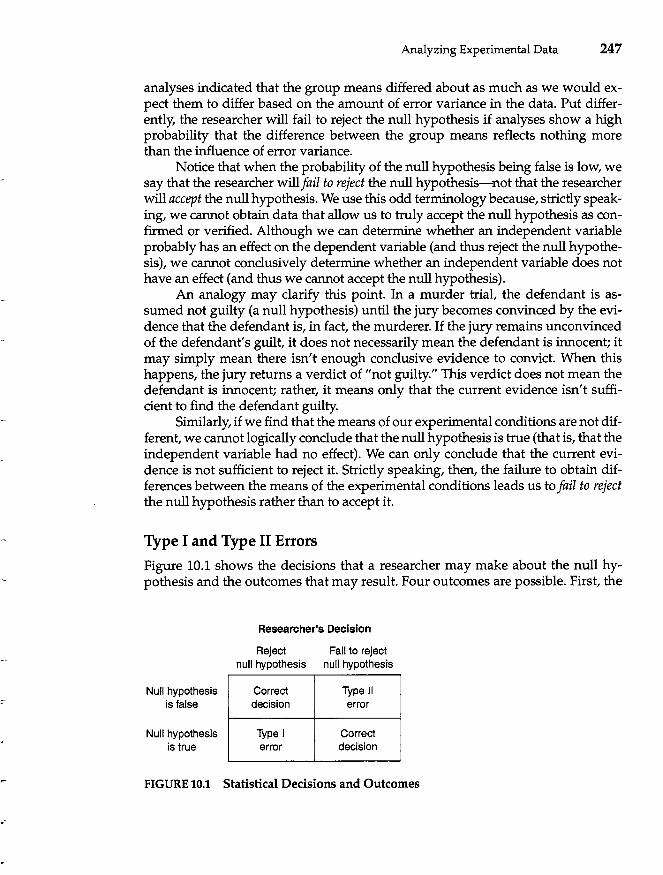
Analyzing Experimental Data 247

analyses indicated that the group means differed about as much as we would ex­pect them to differ based on the amount of error variance in the data. Put differ­ently, the researcher will fail to reject the null hypothesis if analyses show a high probability that the difference between the group means reflects nothing more than the influence of error variance.

Notice that when the probability of the null hypothesis being false is low, we say that the researcher will fail to reject the null hypothesis-not that the researcher will accept the null hypothesis. We use this odd terminology because, strictly speak­ing, we cannot obtain data that allow us to truly accept the null hypothesis as con­firmed or verified. Although we can determine whether an independent variable probably has an effect on the dependent variable (and thus reject the null hypothe­sis), we cannot conclusively determine whether an independent variable does not have an effect (and thus we cannot accept the null hypothesis).

An analogy may clarify this point. In a murder trial, the defendant is as­sumed not guilty (a null hypothesis) until the jury becomes convinced by the evi­dence that the defendant is, in fact, the murderer. If the jury remains unconvinced of the defendant's guilt, it does not necessarily mean the defendant is innocent; it may simply mean there isn't enough conclusive evidence to convict. When this happens, the jury returns a verdict of "not guilty." This verdict does not mean the defendant is innocent; rather, it means only that the current evidence isn't suffi­cient to find the defendant guilty.

Similarly, if we find that the means of our experimental conditions are not dif­ferent, we cannot logically conclude that the null hypothesis is true (that is, that the independent variable had no effect). We can only conclude that the current evi­dence is not sufficient to reject it. Strictly speaking, then, the failure to obtain dif­ferences between the means of the experimental conditions leads us to fail to reject the null hypothesis rather than to accept it.

Type I and Type II Errors

Figure 10.1 shows the decisions that a researcher may make about the null hy­pothesis and the outcomes that may result. Four outcomes are possible. First, the

Null hypothesis is false

Null hypothesis is true

Researcher's Decision

Reject Fail to reject null hypothesis null hypothesis

Correct Type II decision error

Type I Correct error decision

FIGURE 10.1 Statistical Decisions and Outcomes

248 CHAPTER 10

researcher may correctly reject the null hypothesis, thereby identifying a true effect of the independent variable. Second, the researcher may correctly fail to reject the null hypothesis, accurately concluding that the independent variable had no effect. In both cases, the researcher reached a correct conclusion.

The other two possible outcomes are the result of two kinds of errors that re­searchers may make when deciding whether to reject the null hypothesis: Type I and Type II errors. A Type I error occurs when a researcher erroneously concludes that the null hypothesis is false and, thus, rejects it. More straightforwardly, a Type I error occurs when a researcher concludes that the independent variable has an ef­fect on the dependent variable when, in fact, the observed difference between the means of the experimental conditions is actually due to error variance.

The probability of making a Type I error-of rejecting the null hypothesis when it is true-is called the alpha level. As a rule of thumb, researchers set the alpha level at .05: They reject the null hypothesis when there is less than a .05 chance (that is, fewer than 5 chances out of 100) that the difference they obtain be­tween the means of the experimental groups is due to error variance rather than to the independent variable. If statistical analyses indicate that there is less than a 5% chance that the difference between the means of our experimental conditions is due to error variance, we reject the null hypothesis, knowing there is only a small chance we are mistaken. Occasionally, researchers wish to lower their chances of making a Type I error even further and thus set a more stringent criterion for re­jecting the null hypothesis. By setting the alpha level at .01 rather than .05, for ex­ample, researchers risk only a 1% chance of making a Type I error.

When we reject the null hypothesis with a low probability of making a Type I error, we refer to the difference between the means as statistically significant. A statistically significant finding is one that has a low probability (usually < .05) of occurring as a result of error variance alone. We'll return to the important concepts of alpha level and statistical significance later.

Apart from making a Type I error, the researcher may mistakenly fail to reject the null hypothesis when, in fact, it is false; this is a Type II error. In this case, the researcher concludes that the independent variable does not have an effect when, in fact, it does. Just as the probability of making a Type I error is called alpha, the probability of making a Type II error is called beta.

Several factors can increase beta and lead to Type II errors. If researchers do not measure the dependent variable properly or if they use a measurement tech­nique that is unreliable, they might not detect the effects of the independent vari­able that occur. Mistakes may be made in collecting, coding, or analyzing the data, or the researcher may use too few participants to detect the effects of the indepen­dent variable. Excessively high error variance due to unreliable measures, very heterogeneous samples, or poor experimental control can also mask effects of the independent variable and lead to Type II errors. Many things can conspire to ob­scure the effects of the independent variable and, thus, lead researchers to make Type II errors.

To reduce the likelihood of making a Type II error, researchers try to design experiments that have high power. Power is the probability that a study will cor-

r

Analyzing Experimental Data 249

rectly reject the null hypothesis when the null hypothesis is false or, put another way, the probability that the study will obtain a significant result if the researcher's experimental hypothesis is, in fact, true. Power is a study's ability to detect anyef­fect of the independent variable that occurs. Stated differently, power is the oppo­site of beta-the probability of making a Type II error (that is, power = 1 - beta). Studies that are low in power may fail to detect the independent variable's effect on the dependent variable.

Among other things, power is related to the number of participants in a study. All other things being equal, the greater the number of participants, the greater the study's power and the more likely we are to detect effects of the independent vari­able on the dependent variable. Intuitively, you can probably see that an experiment with 100 participants will provide more definitive and clearcut conclusions about the effect of an independent variable than the same experiment conducted with only 10 participants. Because power is important to the success of an experiment, researchers often conduct a power analysis to determine the number of participants that are needed in order to detect the effect of a particular independent variable. If they can estimate (1) how strong the effect of the independent variable is likely to be (for example, how much the means of the conditions are likely to differ) and (2) how much error variance is likely to be present in the data, researchers can then calculate the number of participants they need to use in order to have a high probability of detecting the predicted effect of the independent variable. Generally, researchers aim for a study's power to exceed .80 (Cohen, 1988). An experiment with .80 power has an 80% chance of detecting an effect of the independent variable that is really there; or, stated another way, in a study with .80 power, the probability of making a Type II error (beta) is less than .20. The formulas for doing power analysis and cal­culating sample sizes can be found in many statistics books (see Hurlburt, 1998). Studies suggest that much research in the behavioral sciences is underpowered; sample sizes are often too small to detect effects of the independent variable easily. Conducting studies with inadequate power is obviously wasteful, so researchers must pay attention to the power of the experiments they design.

To be sure that you understand the difference between Type I and Type II er­rors, let us return to our example of a murder trial. After weighing the evidence, the jury is in the position of having to decide whether to reject the null hypothesis of "not guilty." In reaching their verdict, the jury hopes not to make either a Type I or a Type II error. In the context of a trial, a Type I error would involve rejecting the null hypothesis (not guilty) when it was true, or convicting an innocent person. A Type II error would involve failing to reject the null hypothesis when it was false­that is, not convicting a defendant who did, in fact, commit murder. Like scientists, jurors are generally more concerned about making a Type I than a Type II error when reaching a verdict: A greater injustice is done if an innocent person is con­victed than if a criminal goes free. In fact, jurors are explicitly instructed to convict the defendant (reject the null hypothesis) only if they are convinced ''beyond a rea­sonable doubt" that the defendant is guilty. In essence, using the criterion of "be­yond a reasonable doubt" is comparable to setting a relatively stringent alpha level of .01 or .05.

250 CHAPTER 10

Effect Size

When researchers reject the null hypothesis and conclude that the independent variable has an effect, they often want to know how strong the independent vari­able's effect is on the dependent variable. They determine this by calculating the effect size-the proportion of variability in the dependent variable that is due to the independent variable.

As a proportion, effect size can range from .00, indicating no relationship be­tween the independent variable and the dependent variable, to 1.00, indicating that 100% of the variance in the dependent variable is associated with the inde­pendent variable. For example, if we find that our effect size is .47, we know that 47% of the variability in the dependent variable is due to the independent variable. Several slightly different formulas for calculating effect size exist. The two most commonly used are called eta-squared and omega-squared.

Summary

In analyzing data collected in experimental research, researchers attempt to de­termine whether the means of the various experimental conditions differ more than they would if the differences were due only to error variance. If the differ­ence between means is large relative to the error variance, the researcher rejects the null hypothesis and concludes that the independent variable has an effect. Re­searchers draw this conclusion with the understanding that there is a low proba­bility (usually less than .05) that they have made a 'TYPe I error. If the difference in means is no larger than one would expect simply on the basis of the amount of error variance in the data, the researcher fails to reject the null hypothesis and concludes that the independent variable has no effect. When researchers reject the null hypothesis, they often calculate the effect size, which expresses the propor­tion of variability in the dependent variable that is associated with the indepen­dent variable.

Analysis of Two-Group Experiments: The t-Test

Now that you understand the rationale behind inferential statistics, we will look briefly at two statistical tests that are used most often to analyze data collected in ex­perimental research. We will examine t-tests in this chapter, and F-tests in Chapter 11.

Both of these analyses are based on the same rationale. The error variance in the data is calculated to provide an estimate of how much the means of the condi­tions are expected to differ when differences are due only to random error variance (and the independent variable has no effect). The observed differences between the means are then compared with this estimate. If the observed differences between the means are so large, relative to this estimate, that they are highly unlikely to be the result of error variance alone, the null hypothesis is rejected. As we saw earlier,

Analyzing Experimental Data 251

the likelihood of erroneously rejecting the null hypothesis is held at less than what­ever alpha level the researcher has stipulated, usually .05.

Conducting a t-Test Although the rationale behind inferential statistics may seem complex and convo­luted, conducting a t-test to analyze data from a two-group randomized groups experiment is straightforward. In this section, we will walk through the calculation of one kind of t-test to demonstrate how the rationale for comparing mean differ­ences to error variance described previously is implemented in practice.

To conduct a t-test, you calculate a value for t using a simple formula and then see whether this calculated value of t exceeds a certain critical value that you locate in a table. If it does, the group means differ by more than what we would ex­pect on the basis of error variance alone.

A t-test is conducted in the following five steps:

Step 1. Calculate the means of the two groups. Step 2. Calculate the standard error of the difference between the two means.

Step 3. Find the calculated value of t. Step 4. Find the critical value of t. Step 5. Determine whether the null hypothesis should be rejected by com­

paring the calculated value of t to the critical value of t.

Let's examine each of these steps in detail.

Step 1. To test whether the means of two experimental groups are different, we obviously need to know the means. These means will go in the numerator of the formula for a t-test. Thus, first we must calculate the means of the two groups, %1

and %2.

Step 2. To determine whether the means of the two experimental groups differ more than we would expect on the basis of error variance alone, we need an esti­mate of how much the means are expected to vary if the difference is due only to error variance. The standard error of the difference between two means provides an index of this expected difference.

This quantity is based directly on the amount of error variance in the data. As we saw in Chapter 8, error variance is reflected in the variability within the experi­mental conditions. Any variability we observe in the responses of participants who are in the same experimental condition cannot be due to the independent variable because they all receive the same level of the independent variable. Rather, this variance reflects extraneous variables, chiefly individual differences in how partic­ipants responded to the independent variable and poor experimental control.

252 C HAP T E R 10

Calculating the standard error of the difference between two means is ac­complished in three steps.

2a. First, calculate the variances of the two experimental groups. (You may want to review the section of Chapter 5 that dealt with calculating the variance.) The variance for each condition is calculated from this formula:

l:x.2 - [(l:x.)Z/n] s2 - I I

- n - 1 .

You'll calculate this variance twice, once for each experimental condition. 2b. Then, calculate the pooled variance-sj. This is an estimate of the average of

the variances for the two groups:

S2 = (n1 - l)sl + (n2 - l)sl p n1 + n2 - 2

In this formula, n1 and n2 are the sample sizes for conditions 1 and 2, and Sf and sf are the variances of the two conditions calculated in Step 2a.

2c. Finally, take the square root of the pooled variance, which gives you the pooled standard deviation, sp'

Step 3. Armed with the means of the two groups (l'l and 1'2)' the pooled standard deviation (sp), and the sample sizes (n1 and n2), we are ready to calculate t:

Step 4. Now we must locate the critical value of t in a table designed for that pur­pose. To find the critical value of t, we need to know the following two things.

4a. First, we need to calculate the degrees of freedom for the t-test. For a two­group randomized design, the degrees of freedom (df) is equal to the number of participants minus 2 (that is, n1 + n2 - 2). (Don't concern yourself with what degrees of freedom are from a statistical perspective; simply realize that we need to take the number of scores into account when conducting inferential statistics, and degrees of freedom is a function of the number of scores.)

4b. Second, we need to specify the alpha level for the test. As we saw earlier, the alpha level is the probability we are willing to accept for making a Type I error-rejecting the null hypothesis when it is true. Usually, researchers set the alpha level at .05.

Taking the degrees of freedom and the alpha level, consult the table inAppendix A-2 to find the critical value of t. For example, imagine that we have 10 participants in each condition. The degrees of freedom would be 10 + 10 - 2 = 18. Then, assuming the

,-

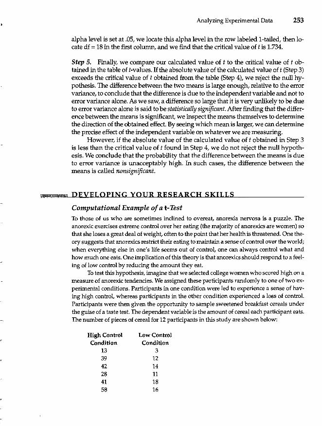
Analyzing Experimental Data 253

alpha level is set at .05, we locate this alpha level in the row labeled I-tailed, then lo­cate df = 18 in the first column, and we find that the critical value of t is 1.734.

Step 5. Finally, we compare our calculated value of t to the critical value of t ob­tained in the table of t-values. If the absolute value of the calculated value of t (Step 3) exceeds the critical value of t obtained from the table (Step 4), we reject the null hy­pothesis. The difference between the two means is large enough, relative to the error variance, to conclude that the difference is due to the independent variable and not to error variance alone. As we saw, a difference so large that it is very unlikely to be due to error variance alone is said to be statistically significant. After finding that the differ­ence between the means is significant, we inspect the means themselves to determine the direction of the obtained effect. By seeing which mean is larger, we can determine the precise effect of the independent variable on whatever we are measuring.

However, if the absolute value of the calculated value of t obtained in Step 3 is less than the critical value of t found in Step 4, we do not reject the null hypoth­esis. We conclude that the probability that the difference between the means is due to error variance is unacceptably high. In such cases, the difference between the means is called nonsignificant .

.. DEVELOPING YOUR RESEARCH SKILLS

Computational Example of at-Test To those of us who are sometimes inclined to overeat, anorexia nervosa is a puzzle. The anorexic exercises extreme control over her eating (the majority of anorexics are women) so that she loses a great deal of weight, often to the point that her health is threatened. One the­ory suggests that anorexics restrict their eating to maintain a sense of control over the world; when everything else in one's life seems out of control, one can always control what and how much one eats. One implication of this theory is that anorexics should respond to a feel­ing of low control by reducing the amount they eat.

To test this hypothesis, imagine that we selected college women who scored high on a measure of anorexic tendencies. We assigned these participants randomly to one of two ex­perimental conditions. Participants in one condition were led to experience a sense of hav­ing high control, whereas participants in the other condition experienced a loss of control. Participants were then given the opportunity to sample sweetened breakfast cereals under the guise of a taste test. The dependent variable is the amount of cereal each participant eats. The number of pieces of cereal for 12 participants in this study are shown below:

High Control Low Control Condition Condition

13 3 39 12 42 14 28 11 41 18 58 16

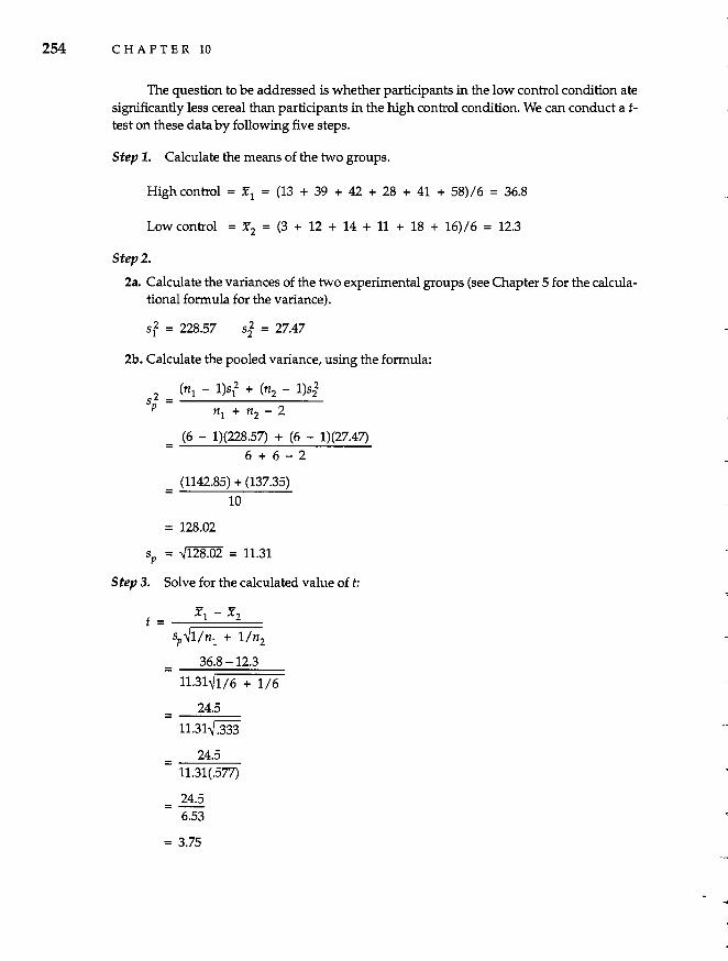
254 CHAPTER 10

The question to be addressed is whether participants in the low control condition ate significantly less cereal than participants in the high control condition. We can conduct a t­test on these data by following five steps.

Step 1. Calculate the means of the two groups.

High control = 1'1 = (13 + 39 + 42 + 28 + 41 + 58)/6 = 36.8

Low control = 1'2 = (3 + 12 + 14 + 11 + 18 + 16)/6 = 12.3

Step 2.

2a. Calculate the variances of the two experimental groups (see Chapter 5 for the calcula­tional formula for the variance).

Sf = 228.57 sf = 27.47

2b. Calculate the pooled variance, using the formula:

s2 = (n1 - l)sf + (n2 - l)sf p n1 +n2 -2

(6 - 1)(228.57) + (6 - 1)(27.47)

6 + 6 - 2

(1142.85) + (137.35)

10

= 128.02

sp = "128.02 = 11.31

Step 3. Solve for the calculated value of t:

t = 1'1 - 1'2

Sp ~1/nl + l/n2

36.8-12.3 = ::11:-:.3::-ht=,Jl=::/ 6:::==+=1=::/ 6=

24.5

11.31~.333

24.5 11.31(.577)

24.5 =--6.53

= 3.75

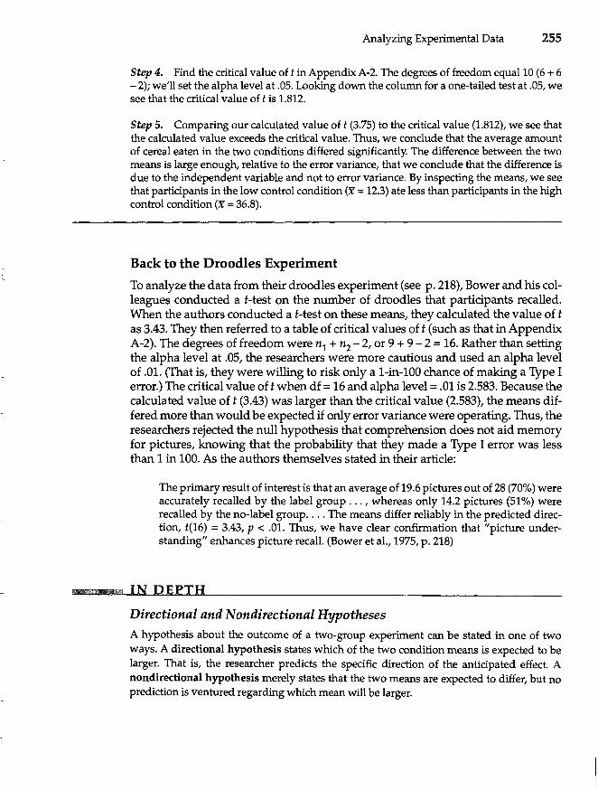
Analyzing Experimental Data 255

Step 4. Find the critical value of t in Appendix A-2. The degrees of freedom equal 10 (6 + 6 - 2); we'll set the alpha level at .05. Looking down the column for a one-tailed test at .05, we see that the critical value of t is 1.812.

Step 5. Comparing our calculated value of t (3.75) to the critical value (1.812), we see that the calculated value exceeds the critical value. Thus, we conclude that the average amount of cereal eaten in the two conditions differed significantly. The difference between the two means is large enough, relative to the error variance, that we conclude that the difference is due to the independent variable and not to error variance. By inspecting the means, we see that participants in the low control condition (X = 12.3) ate less than participants in the high control condition (X = 36.8).

Back to the Droodles Experiment

To analyze the data from their droodles experiment (see p. 218), Bower and his col­leagues conducted a t-test on the number of droodles that participants recalled. When the authors conducted a t-test on these means, they calculated the value of t as 3.43. They then referred to a table of critical values of t (such as that in Appendix A-2). The degrees of freedom were n1 + n2 - 2, or 9 + 9 - 2 = 16. Rather than setting the alpha level at .05, the researchers were more cautious and used an alpha level of .01. (That is, they were willing to risk only a l-in-l00 chance of making a Type I error.) The critical value of t when df = 16 and alpha level = .01 is 2.583. Because the calculated value of t (3.43) was larger than the critical value (2.583), the means dif­fered more than would be expected if only error variance were operating. Thus, the researchers rejected the null hypothesis that comprehension does not aid memory for pictures, knowing that the probability that they made a Type I error was less than 1 in 100. As the authors themselves stated in their article:

The primary result of interest is that an average of 19.6 pictures out of 28 (70%) were accurately recalled by the label group ... , whereas only 14.2 pictures (51 %) were recalled by the no-label group .... The means differ reliably in the predicted direc­tion, t(16) = 3.43, P < .01. Thus, we have clear confirmation that "picture under­standing" enhances picture recall. (Bower et al., 1975, p. 218)

time IN DEPTH

Directional and Nondirectional Hypotheses

A hypothesis about the outcome of a two-group experiment can be stated in one of two ways. A directional hypothesis states which of the two condition means is expected to be larger. That is, the researcher predicts the specific direction of the anticipated effect. A nondirectional hypothesis merely states that the two means are expected to differ, but no prediction is ventured regarding which mean will be larger.

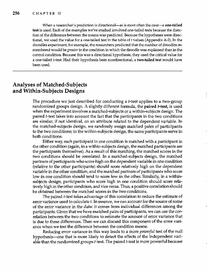
256 CHAPTER 10

When a researcher's prediction is directional-as is most often the case-a one-tailed test is used. Each of the examples we've studied involved one-tailed tests because the direc­tion of the difference between the means was predicted. Because the hypotheses were direc­tional, we used the value for a one-tailed test in the table of t values (Appendix A-2). In the droodles experiment, for example, the researchers predicted that the number of droodles re­membered would be greater in the condition in which the droodle was explained than in the control condition. Because this was a directional hypothesis, they used the critical value for a one-tailed t-test. Had their hypothesis been nondirectional, a two-tailed test would have been used.

Analyses of Matched-Subjects and Within-Subjects Designs

The procedure we just described for conducting a t-test applies to a two-group randomized groups design. A slightly different formula, the paired t-test, is used when the experiment involves a matched-subjects or a within-subjects design. The paired t-test takes into account the fact that the participants in the two conditions are similar, if not identical, on an attribute related to the dependent variable. In the matched-subjects design, we randomly assign matched pairs of participants to the two conditions; in the within-subjects design, the same participants serve in both conditions.

Either way, each participant in one condition is matched with a participant in the other condition (again, in a within-subjects design, the matched participants are the participants themselves). As a result of this matching, the matched scores in the two conditions should be correlated. In a matched-subjects design, the matched partners of participants who score high on the dependent variable in one condition (relative to the other participants) should score relatively high on the dependent variable in the other condition, and the matched partners of participants who score low in one condition should tend to score low in the other. Similarly, in a within­subjects design, participants who score high in one condition should score rela­tively high in the other condition, and vice versa. Thus, a positive correlation should be obtained between the matched scores in the two conditions.

The paired t-test takes advantage of this correlation to reduce the estimate of error variance used to calculate t. In essence, we can account for the source of some of the error variance in the data: it comes from individual differences among the participants. Given that we have matched pairs of participants, we can use the cor­relation between the two conditions to estimate the amount of error variance that is due to these differences. Then we can discard this component of the error vari­ance when we test the difference between the condition means.

Reducing error variance in this way leads to a more powerful test of the null hypothesi~ne that is more likely to detect the effects of the independent vari­able than the randomized groups t-test. The paired t-test is more powerful because

Analyzing Experimental Data 257

we have reduced the size of sp in the denominator of the formula for t; and as sp gets smaller, the calculated value of t gets larger. We will not go into the formula for the paired t-test here. However, a detailed explanation of this test can be found in most introductory statistics books.

!IMt CONTRIBUTORS TO BEHAVIORAL RESEARCH

Statistics in the Brewery: W. S. Gosset One might imagine that the important advances in research design and statistics came at the hands of statisticians slaving away in cluttered offices at prestigious universities. Indeed, many of those who prOvided the foundation for behavioral science, such as Wilhelm Wundt and Karl Pearson, were academicians. However, many methodological and statistical approaches were developed while solving real-world problems, notably in industry and agriculture.

A case in point involves the work of William Sealy Gosset (1876-1937), whose contri­butions to research included the t-test. With a background in chemistry and mathematics, Gosset was hired by Guinness Brewery in Dublin, Ireland, in 1899. Among his duties, Gos­set investigated how the quality of beer is affected by various raw materials (such as differ­ent strains of barley and hops) and by various methods of production (such as variations in brewing temperature). Thus, Gosset conducted experiments to study the effects of ingredi­ents and brewing procedures on the quality of beer, and became interested in developing better ways to analyze the data he collected.

During 1906-1907, Gosset spent a year in specialized study in London, where he stud­ied under Karl Pearson (whom we met in Chapter 6 when we discussed the Pearson corre­lation coefficient). During this time, Gosset worked on developing solutions to statistical problems he encountered at the brewery. In 1908, he published a paper based on this work that laid out the principles for the t-test. Interestingly, he published his work under the pen name Student, and to this day, this test is often referred to as Student's t.

Summary

1. The data from experiments are analyzed by determining whether the means of the experimental conditions differ. However, l!>ecause error variance can cause condition means to differ even when the independent variable has no effect, we must compare the difference between the condition means to how much we ex­pect the means to differ if the difference is due solely to error variance.

2. Researchers use inferential statistics to determine whether the observed dif­ferences between the means are greater than would be expected on the basis of error variance alone.

3. If the condition means differ more than expected based on the amount of error variance in the data, researchers reject the null hypothesis (which states that the independent variable does not have an effect) and conclude that the inde­pendent variable affected the dependent variable. If the means do not differ by

258 CHAPTER 10

more than error variance would predict, researchers fail to reject the null hy­pothesis and conclude that the independent variable does not have an effect.

4. When deciding to reject or fail to reject the null hypothesis, researchers may make one of two kinds of errors. A Type I error occurs when the researcher re­jects the null hypothesis when it is true (and, thus, erroneously concludes that the independent variable has an effect); a Type II error occurs when the researcher fails to reject the null hypothesis when it is false (and, thus, fails to detect a true effect of the independent variable).

5. Researchers can never know for certain whether a Type I or Type II error has occurred, but they can specify the probability that they have made each kind of error. The probability of a Type I error is called alpha; the probability of a Type II error is called beta.

6. To minimize the probability of making a Type II error, researchers try to design powerful studies. Power refers to the probability that a study will correctly re­ject the null hypothesis (and, thus, detect true effects of the independent vari­able). To ensure they have sufficient power, researchers often conduct a power analysis that tells them the optimal number of participants for their study.

7. Effect size indicates the strength of the independent variable's effect on the dependent variable. It is expressed as the proportion of the total variability in the dependent variable that is accounted for by the independent variable.

S. The t-test is used to analyze the difference between two means. A value for tis calculated by dividing the difference between the means by an estimate of how much the means would be expected to differ on the basis of error variance alone. This calculated value of t is then compared to a critical value of t. If the calculated value exceeds the critical value, the null hypothesis is rejected.

9. Hypotheses about the outcome of two-group experiments may be directional (predicting which of the two condition means will be larger) or nondirectional (predicting that the means will differ but not specifying which will be larger). Whether the hypothesis is directional or nondirectional has implications for whether the critical value of t used in the t-test is one- tailed or two-tailed.

10. The paired t-test is used when the experiment involves a matched-subjects or within-subjects design.

KEY TERMS

alpha level (p. 248) beta (p. 248) critical value (p. 252) directional hypothesis (p. 255) effect size (p. 250) experimental hypothesis

(p.246) failing to reject the null

hypothesis (p. 246)

inferential statistics (p.246)

nondirectional hypothesis (p.255)

null hypothesis (p. 246) one-tailed test (p. 256) paired t-test (p. 256) power (p. 248) power analysis (p. 249)

rejecting the null hypothesis (p.246)

standard error of the difference between two means (p. 251)

statistical significance (p. 248) t-test (p. 251) two-tailed test (p. 256) 1YPe I error (p. 248) Type II error (p. 248)

Analyzing Experimental Data 259

QUESTIONS FOR REVIEW

1. In analyzing the data from an experiment, why is it not sufficient simply to exam­ine the condition means to see whether they differ?

2. Assuming that all confounds were eliminated, the means of the conditions in an ex-periment may differ from one another for two reasons. What are they?

3. Why do researchers use inferential statistics?

4. Distinguish between the null hypothesis and the experimental hypothesis.

5. When analyzing data, why do researchers test the null hypothesis rather than the experimental hypothesis?

6. Explain the difference between rejecting and failing to reject the null hypothesis. In which case does a researcher conclude that the independent variable has an effect on the dependent variable?

7. Distinguish between a Type I and a Type II error.

8. Which type of error do researchers usually regard as more serious? Why?

9. Explain what it means if a researcher sets the alpha level for a statistical test at .05.

10. What does it mean if the difference between two means is statistically significant?

11. Do powerful studies minimize alpha or beta? Explain.

12. What information do researchers obtain from conducting a power analysis?

13. What would it mean if the effect size in an experiment was .25? .40? .OO?

14. Explain the rationale behind the t-test.

15. Write the formula for at-test.

16. Once researchers calculate a value for t, they compare that calculated value to a crit­ical value of t. What two pieces of information must be known in order to find the critical value of t in a table of critical values?

17. If the calculated value of t is less than the critical value, do you reject or fail to reject the null hypothesis? Explain.

18. If you reject the null hypothesis (and conclude that the independent variable has an effect), what's the likelihood that you have made a Type I error?

19. Distinguish between one-tailed and two-tailed t-tests.

20. Why must a different t-test be used for matched-subjects and within-subjects de­signs than for randomized groups designs?

21. What was W. S. Gosset's contribution to behavioral research?

QUESTIONS FOR DISCUSSION

1. If the results of a t-test lead you to reject the null hypothesis, what is the probability that you have made a Type II error?

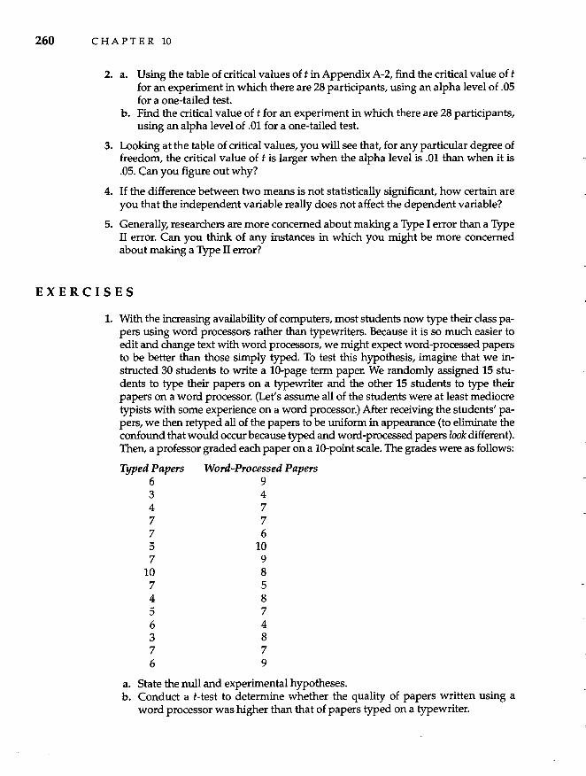
260 C HAP T E R 10

2. a. Using the table of critical values of t in Appendix A-2, find the critical value of t for an experiment in which there are 28 participants, using an alpha level of .05 for a one-tailed test.

b. Find the critical value of t for an experiment in which there are 28 participants, using an alpha level of .01 for a one-tailed test.

3. Looking at the table of critical values, you will see that, for any particular degree of freedom, the critical value of t is larger when the alpha level is .01 than when it is .05. Can you figure out why?

4. If the difference between two means is not statistically significant, how certain are you that the independent variable really does not affect the dependent variable?

5. Generally, researchers are more concerned about making a Type I error than a Type II error. Can you think of any instances in which you might be more concerned about making a Type II error?

EXERCISES

1. With the increasing availability of computers, most students now type their class pa­pers using word processors rather than typewriters. Because it is so much easier to edit and change text with word processors, we might expect word-processed papers to be better than those simply typed. To test this hypothesis, imagine that we in­structed 30 students to write a 1O-page term paper. We randomly assigned 15 stu­dents to type their papers on a typewriter and the other 15 students to type their papers on a word processor. (Let's assume all of the students were at least mediocre typists with some experience on a word processor.) After receiving the students' pa­pers, we then retyped all of the papers to be uniform in appearance (to eliminate the confound that would occur because typed and word-processed papers look different). Then, a professor graded each paper on a 10-point scale. The grades were as follows:

Typed Papers 6 3 4 7 7 5 7

10 7 4 5 6 3 7 6

Word-Processed Papers 9 4 7 7 6

10 9 8 5 8 7 4 8 7 9

a. State the null and experimental hypotheses. b. Conduct a t-test to determine whether the quality of papers written using a

word processor was higher than that of papers typed on a typewriter.

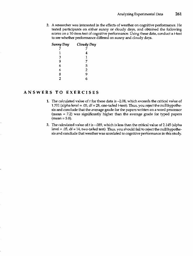
Analyzing Experimental Data 261

2. A researcher was interested in the effects of weather on cognitive performance. He tested participants on either sunny or cloudy days, and obtained the following scores on a 10-item test of cognitive performance. Using these data, conduct at-test to see whether performance differed on sunny and cloudy days.

Sunny Day Cloudy Day 7 7 1 4 3 1 9 7 6 5 6 2 8 9 2 6

ANSWERS TO EXERCISES

1. The calculated value of t for these data is -2.08, which exceeds the critical value of 1.701 (alpha level = .05, df = 28, one-tailed t-test). Thus, you reject the null hypothe­sis and conclude that the average grade for the papers written on a word processor (mean = 7.2) was significantly higher than the average grade for typed papers (mean = 5.8).

2. The calculated value of t is -.089, which is less than the critical value of 2.145 (alpha level = .05, df = 14, two-tailed test). Thus, you should fail to reject the null hypothe­sis and conclude that weather was unrelated to cognitive performance in this study.

CHAPTER

11 Analyzing Complex Designs

The Problem: Multiple Tests Inflate Type I Error The Rationale Behind ANOVA

Multivariate Analysis of Variance Experimental and Nonexperimental Uses of Inferential Statistics How ANOVA Works

Follow-Up Tests Computer Analyses

Between-Subjects and Within-Subjects ANOVAs

262

In Chapter 9, we discussed an experiment that investigated the effectiveness of various strategies for losing weight (Mahoney et aI., 1973). In this study, obese adults were randomly assigned to one of five conditions: self-reward for losing weight, self-punishment for failing to lose weight, self-reward for losing combined with self-punishment for not losing weight, self-monitoring of weight (but without rewarding or punishing oneself), and a control condition. At the end of the experi­ment, the researchers wanted to know whether some conditions were more effec­tive than others in helping participants lose weight.

Given the data shown in Table 11.1, how would you determine whether some of the weight-reduction strategies were more effective than others in helping participants lose weight? Clearly, the average weight loss was greatest in the self­reward condition than in the other conditions, but, as we've seen, we must conduct statistical tests to determine whether the differ~ces among the means are greater than we would expect based on the amount of error variance present in the data.

One possible way to analyze these data would be to conduct 10 t-tests, com­paring the mean of each experimental group to the mean of every other group: Group 1 versus Group 2, Group 1 versus Group 3, Group 1 versus Group 4, Group 1 versus Group 5, Group 2 versus Group 3, Group 2 versus Group 4, Group 2 ver­sus Group 5, Group 3 versus Group 4, Group 3 versus Group 5, and Group 4 versus Group 5. If you performed all 10 of these t-tests, you could tell which means dif­fered significantly from the others and determine whether the strategies differen­tially affected the amount of weight that participants lost.

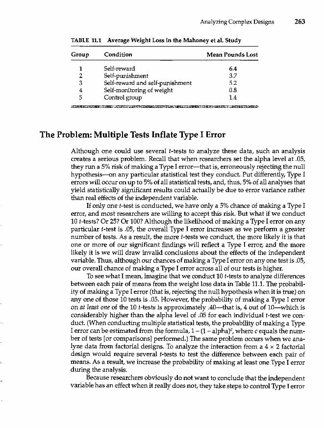
Analyzing Complex Designs 263

TABLE 11.1 Average Weight Loss in the Mahoney et al. Study

Group

1 2 3 4 5

Wh

Condition

Self-reward Self-punishment Self-reward and self-punishment Self-monitoring of weight Control group

1iIIi! §hi

Mean Pounds Lost

6.4 3.7 5.2 0.8 1.4

Mil!' r g kS

The Problem: Multiple Tests Inflate Type I Error

Although one could use several t-tests to analyze these data, such an analysis creates a serious problem. Recall that when researchers set the alpha level at .05, they run a 5% risk of making a Type I error-that is, erroneously rejecting the null hypothesis-on any particular statistical test they conduct. Put differently, Type I errors will occur on up to 5% of all statistical tests, and, thus, 5% of all analyses that yield statistically Significant results could actually be due to error variance rather than real effects of the independent variable.

If only one t-test is conducted, we have only a 5% chance of making a Type I error, and most researchers are willing to accept this risk. But what if we conduct 10 t-tests? Or 25? Or 100? Although the likelihood of making a Type I error on any particular t-test is .05, the overall Type I error increases as we perform a greater number of tests. As a result, the more t-tests we conduct, the more likely it is that one or more of our significant findings will reflect a Type I error, and the more likely it is we will draw invalid conclusions about the effects of the independent variable. Thus, although our chances of making a Type I error on anyone test is .05, our overall chance of making a Type I error across all of our tests is higher.

To see what I mean, imagine that we conduct 10 t-tests to analyze differences between each pair of means from the weight loss data in Table 11.1. The probabil­ity of making a Type I error (that is, rejecting the null hypothesis when it is true) on anyone of those 10 tests is .05. However, the probability of making a Type I error on at least one of the 10 t-tests is approximately .40-that is, 4 out of 10-which is considerably higher than the alpha level of .05 for each individual t-test we con­duct. (When conducting multiple statistical tests, the probability of making a Type I error can be estimated from the formula, 1- (1- alpha}C, where c equals the num­ber of tests [or comparisons] performed.) The same problem occurs when we ana­lyze data from factorial designs. To analyze the interaction from a 4 x 2 factorial design would require several t-tests to test the difference between each pair of means. As a result, we increase the probability of making at least one Type I error during the analysis.

Because researchers obviously do not want to conclude that the independent variable has an effect when it really does not, they take steps to control Type I error

264 CHAPTER 11

when they conduct many statistical analyses. The most straightforward way of pre­venting Type I error inflation when conducting many tests is to set a more stringent alpha level than the conventional .05 level. Researchers sometimes use the Bonfer­roni adjustment in which they divide their desired alpha level (such as .05) by the number of tests they plan to conduct. For example, if we wanted to conduct 10 t­tests to analyze all pairs of means in the weight-loss study described earlier (Table 11.1), we could use an alpha level of .005 rather than .05 for each t-test we ran. (We would use an alpha level of .005 because we divide our desired alpha level of .05 by the number of tests we will conduct; .05/10 = .005.) If we did so, the likelihood of making a Type I error on any particular t-test would be very low (.005), and the overall likelihood of making a Type I error across all 10 t-tests would not exceed our desired alpha level of .05.

Although this adjustment protects us against inflated Type I error when we conduct many tests, it has a drawback: As we make alpha more stringent and lower the probability of a Type I error, the probability of making a Type II error (and missing real effects of the independent variable) increases. By making alpha more stringent, we are requiring the condition means to differ from one another by a greater margin in order to declare the difference statistically significant. But if we require the means to be very different before we regard them as significantly dif­ferent, then smaller, but real differences between the means won't meet our crite­rion. As a result, our t-tests will miss certain effects that they would have detected if a more liberal alpha level of .05 was used for each test.

Researchers sometimes use the Bonferroni adjustment when they plan to con­duct only a few statistical tests but, for the reason just described, are reluctant to do so when the number of tests is large. Instead, researchers typically use a statistical procedure called analysis of variance when they want to test differences among many means. Analysis of variance--commonly called ANOVA-is a statistical proce­dure used to analyze data from designs that involve more than two conditions. ANOVA analyzes differences between all condition means in an experiment simul­taneously. Rather than testing the difference between each pair of means as at-test does, ANOVA determines whether any of a set of means differs from another using a single statistical test that holds the alpha level at .05 (or whatever level the re­searcher chooses) regardless of how many group means are involved in the test. For example, rather than conducting 10 t-tests among all pairs of five means (with the likelihood of a Type I error being about .40), ANOVA performs a single, simultane­ous test on all condition means with only a .05 chance of making a Type I error.

The Rationale Behind ANOVA

Imagine that we conduct an experiment in which we know the independent vari­able(s) have absolutely no effect. In such a case, we can estimate the amount of error variance in the data in one of two ways. Most obviously, we can calculate the error variance by looking at the variability among the participants within each of the conditions; all variance in the responses of participants in a single condition must be error variance. Alternatively, if we know for certain that the independent vari-

Analyzing Complex Designs 265

able has no effect, we can estimate the error variance in the data from the size of the differences between the condition means. We can do this because, if the indepen­dent variable has no effect (and there is no confounding), the only possible reason for the condition means to differ from one another is error variance. In other words, when the independent variable has no effect, the variability among condi­tion means and the variability within groups are both reflections of error variance.

. However, to the extent that the independent variable affects participants' re­sponses and creates differences between the experimental conditions, the variability among condition means should be larger than if only error variance is causing the means to differ. Thus, if we find that the variance between experimental conditions is markedly greater than the variance within the conditions, we have evidence that the independent variable is causing the difference (again assuming no confounds).

Analysis of variance is based on a statistic called the F-test, which is the ratio of the variance among conditions (between-groups variance) to the variance within conditions (within-groups, or error, variance). The larger the between-groups vari­ance relative to the within-groups variance, the larger the calculated value of F, and the more likely it is that the differences among the conditions means reflect true ef­fects of the independent variable rather than error variance. By testing this F-ratio, we can estimate the likelihood that the differences between the condition means are due to error variance.

We will devote most of the rest of this chapter to exploring how ANaVA works. The purpose here is not to show you how to conduct an ANaVA but rather to explain how ANaVA operates. In fact, the formulas used here are intended only to show you what an ANaVA does; researchers use other forms of these formu­las to actually compute an ANaVA. The computational formulas for ANaVA ap­pear in Appendix B.

How ANOVA Works

Recall that the total variance in a set of experimental data can be broken into two parts: systematic variance (which reflects differences among the experimental con­ditions) and unsystematic, or error, variance (which reflects differences among participants within the experimental conditions).

Total variance = systematic variance + error variance.

In a one-way design with a single independent variable, ANaVA breaks the total variance into these two components-systematic variance (presumably due to the independent variable) and error variance.

Total Sum of Squares

We learned in Chapter 2 that the sum of squares reflects the total amount of vari­ability in a set of data. We learned also that the total sum of squares is calculated by (1) subtracting the mean from each score, (2) squaring these differences, and

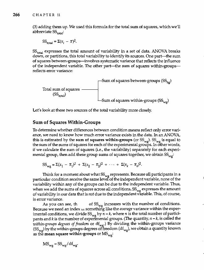
266 CHAPTER 11

(3) adding them up. We used this formula for the total sum of squares, which we'll abbreviate SStotal:

SStotal expresses the total amount of variability in a set of data. ANOVA breaks down, or partitions, this total variability to identify its sources. One part-the sum of squares between-groups-involves systematic variance that reflects the influence of the independent variable. The other part-the sum of squares within-groups­reflects error variance:

-{

Sum of squares between-groups (S~g)

Total sum of squares (SStotal)

Sum of squares within-groups (SSwg)

Let's look at these two sources of the total variability more closely.

Sum of Squares Within-Groups

To determine whether differences between condition means reflect only error vari­ance, we need to know how much error variance exists in the data. In an ANOVA, this is estimated by the sum of squares within-groups (or SSwg). SSwg is equal to the sum of the sums of squares for each of the experimental groups. In other words, if we calculate the sum of squares (Le., the variability) separately for each experi­mental group, then: add these group sums of squares together, we obtain SSwg:

SSwg = ~(x1 - %'1)2 + ~(x2 - 'f2)2 + ... + ~(xk - %'k)2.

Think for a moment about what SSw represents. Because all participants in a particular condition receive the same lever of the independent variable, none of the variability within any of the groups can be due to the independent variable. Thus, when we add the sums of squares across all conditions, SSwg expresses the amount of variability in our data that is not due to the independent variable. This, of course, is error variance.

As you can see, th of SSwg increases with the number of conditions. Because we need an index vI somethirig like the average variance within the exper­imental conditions, we divide SSwg by n - k, where n is the total number of partici­pants and k is the number of expenmental groups. (The quantity, n - k, is called the within-groups degrees of freedom or dfwg.) By dividing the within-groups variance (SSw ) by the within-groups degrees of treedom (dfwg)' we obtain a quantity known as th~ mean square within-groups or MSwg:

Analyzing Complex Designs 267

It should be clear that MSwg provides us with an estimate of the average within­groups, or error, variance. Later we will compare the amount of systematic variance in our data to MSwg'

Sum of Squares Between-Groups

Now that we've estimated the error variance from the variability within the groups, we must calculate the amount of systematic variance in the data-the variance that's due to the independent variable (assuming there are no confounds that would also create systematic variance). To estimate the systematic variance, ANOVA uses the sum of squares between-groups (sometimes called the sum of squares for treatment).

The calculation of the sum of squares between-groups (or S~g) is based on a simple rationale. If the independent variable has no effect, we will expect all of the group means to be roughly equal, aside from whatever differences are due to error variance. Because all of the means are the same, each condition mean would also be approximately equal to the mean of all the group means (the grand mean). However, if the independent variable is causing the means of some conditions to be larger or smaller than the means of others, the condition means not only will dif­fer among themselves but also will differ from the grand mean.

Thus, to calculate between-groups variance we first subtract the grand mean from each of the group means. Small differences indicate that the means don't dif­fer very much (and thus the independent variable has little, if any, effect). In con­trast, large differences between the condition means and the grand mean indicate large differences between the groups and suggest that the independent variable is causing the means to differ.

Thus, to obtain S~ , we (1) subtract the grand mean (GM) from the mean of each group, (2) square ~ese differences, (3) multiply each squared difference by the size of the group, then (4) sum across groups. This can be expressed by the fol­lowing formula:

S~g = ntCYl - GM)2 + n2(:f2 - GM)2 + ... + nk(:fk - GM)2.

We then divide S~g by the quantity k - 1, where k is the number of group means that went into the calculation of ~g' (The quantity k - 1 is called the between­groups degrees offreedom.) When S~g is diVIded by its degrees of freedom (k-1), the resulting number is called the mean square between-groups (or ~g)' which is our estimate of systematic or between-groups variance:

TheF-Test

We have seen how ANOVA breaks the total variance in participants' responses into components that reflect within-groups variance and between-groups variance. Be­cause error variance leads the means of the experimental conditions to differ slightly, we expect to find some systematic, between-groups variance even if the independent

268 CHAPTER 11

variables have no effect. Thus, we must test whether the between-groups variance is larger than we would expect based on the amount of within-groups (that is, error) variance in the data.

To do this, we conduct an F-test. To obtain the value of F, we calculate the ratio of between-groups variability to within-groups variability for each effect we are test­ing. If our study has only one independent variable, we simply divide ~g by MSwg:

If the independent variable has no effect, the numerator and denominator of the F­ratio are estimates of the same thing (the amount of error variance), and the value of F will be around 1.00. However, to the extent that the independent variable is caus­ing differences among the experimental conditions, systematic variance will be pro­duced and the numerator of F (which contains both systematic and error variance) will be larger than the denominator (which contains error variance alone).

The only question is how much larger the numerator needs to be than the de­nominator to conclude that the independent variable truly has an effect. We an­swer this question by locating a critical value of F, just as we did with the t-test. To find the critical value of F in Appendix A-3, we specify three things: (1) we set the alpha level (usually .05); (2) we calculate the degrees of freedom for the effect we are testing (dfb~); and (3) we calculate the degrees of freedom for the within-groups variance (dfwg)' (The calculations for degrees of freedom for various effects are shown in Appendix B.) With these numbers in hand, we can find the critical value of F in Appendix A-3. For example, if we set our alpha level at .05, and the between­groups degrees of freedom is 2 and the within-groups degrees of freedom is 30, the critical value of F is 3.32.

If the value of F we calculate for an effect exceeds the critical value of F ob­tained from the table, we conclude that at least one of the condition means differs from the others and, thus, that the independent variable has an effect. More for­mally, if the calculated value of F exceeds the critical value, we reject the null hy­pothesis and conclude that at least one of the condition means differs significantly from another. However, if the calculated value of F is less than the critical value, the differences among the group means are no greater than we would expect on the basis of error variance alone. Thus, we fail to reject our null hypothesis and con­clude that the independent variable does not have an effect.

In the experiment involving weight loss (Mahoney et a1., 1973), the calcu­lated value of F was 4.49. '. ~ critical value of F when dfb = 4 and dfw = 48 is 2.56. Given that the calculated value exceeded the critical vAlue, the au~ors rejected the null hypothesis and concluded that the five weight-loss strategies were differ­entially effective.

Extension of ANOVA to Factorial Designs

We have seen that, in a one-way ANOVA, we partition the total variability in a set of data into two components: between-groups (systematic) variance and within-groups (error) variance. Put differently, SStotal has two sources of variance: ~g and SSwg·

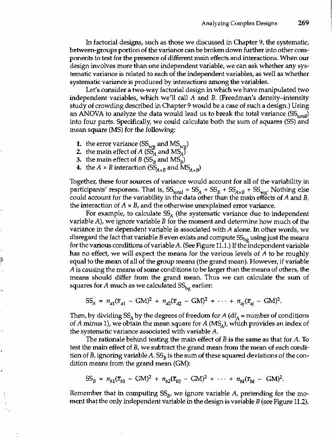
Analyzing Complex Designs 269

In factorial designs, such as those we discussed in Chapter 9, the systematic, between-groups portion of the variance can be broken down further into other com­ponents to test for the presence of different main effects and interactions. When our design involves more than one independent variable, we can ask whether any sys­tematic variance is related to each of the independent variables, as well as whether systematic variance is produced by interactions among the variables.

Let's consider a two-way factorial design in which we have manipulated two independent variables, which we'll call A and B. (Freedman's density-intensity study of crowding described in Chapter 9 would be a case of such a design.) Using an ANOVA to analyze the data would lead us to break the total variance (SStotal) into four parts. Specifically, we could calculate both the sum of squares (SS) and mean square (MS) for the following:

1. the error variance (SS~ and MSw~) 2. the main effect of A (S~ A and MS A)

3. the main effect of B (SSB and MSB) 4. the A x B interaction (SSAxB and MSAxB)

Together, these four sources of variance would account for all of the variability in participants' responses. That is, SStotal = SSA + SSB + SSAxB + SSwg. Nothing else could account for the variability in the data other than the main effects of A and B, the interaction of A x B, and the otherwise unexplained error variance.

For example, to calculate SSA (the systematic variance due to independent variable A), we ignore variable B for the moment and determine how much of the variance in the dependent variable is associated with A alone. In other words, we disregard the fact that variable B even exists and compute SSt,g using just the means for the various conditions of variable A. (See Figure 11.1.) H the independent variable has no effect, we will expect the means for the various levels of A to be roughly equal to the mean of all of the group means (the grand mean). However, if variable A is causing the means of some conditions to be larger than the means of others, the means should differ from the grand mean. Thus we can calculate the sum of squares for A much as we calculated S~g earlier:

SSA = na1(xa1 - GM)2 + na2(xa2 - GM)2 + ... + naj(xaj - GM)2.

Then, by dividing SSA by the degrees of freedom for A (dfA = number of conditions of A minus 1), we obtain the mean square for A (MSA), which provides an index of the systematic variance associated with variable A.

The rationale behind testing the main effect of B is the same as that for A. To test the main effect of B, we subtract the grand mean from the mean of each condi­tion of B, ignoring variable A. SSB is the sum of these squared deviations of the con­dition means from the grand mean (GM):

Remember that in computing SSB' we ignore variable A, pretending for the mo­ment that the only independent variable in the design is variable B (see Figure 11.2).

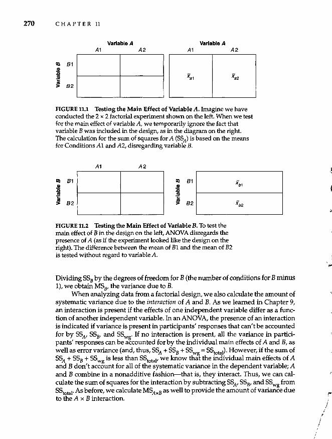
270 C HAP T E R 11

Variable A Variable A A1 A2 A1 A2

III 81 G)

:is III .;:

~ 82

FIGURE 11.1 Testing the Main Effect of Variable A. Imagine we have conducted the 2 x 2 factorial experiment shown on the left. When we test for the main effect of variable A, we temporarily ignore the fact that variable B was included in the design, as in the diagram on the right. The calculation for the sum of squares for A (SSA) is based on the means for Conditions Al and A2, disregarding variable B.

A1 A2

!XI 81 !XI 81 .!l G)

.a :is III .!! .;:

~ 82 ~ 82

FIGURE 11.2 Testing the Main Effect of Variable B. To test the main effect of B in the design on the left, ANOVA disregards the presence of A (as if the experiment looked like the design on the right). The difference between the mean of BI and the mean of B2 is tested without regard to variable A.

Xb1

Xb2

Dividing SSB by the degrees of freedom for B (the number of conditions for B minus 1), we obtain MSw the variance due to B.

When analyzing data from a factorial design, we also calculate the amount of systematic variance due to the interaction of A and B. As we learned in Chapter 9, an interaction is present if the effects of one independent variable differ as a func­tion of another independent variable. In an ANOVA, the presence of an interaction is indicated if variance is present in participants' responses that can't be accounted for by SSA' SSB' and SSwg. If no interaction is present, all the variance in partici­pants' responses can be accounted for by the individual main effects of A and B, as well as error variance (and, thus, SSA + SSB + SSwg = SStotal)' However, if the sum of SSA + SSB + SSwg is less than SStotal' we know that the individual main effects of A and B don't account for all of the systematic variance in the dependent variable; A and B combine in a nonadditive fashion-that is, they interact. Thus, we can cal­culate the sum of squares for the interaction by subtracting SSA' SSB' and SSwg from SStotal' As before, we calculate MSAxB as well to provide the amount of variance due to the A x B interaction.

/ !

I.~

.~

~

\ to'

/ ,. ,r

I 3 I I

I

Analyzing Complex Designs 271

In the case of a factorial design, we then calculate a value of F for each main effect and interaction we are testing. For example, in a 2 x 2 design, we calculate F for the main effect of A by dividing MSA by MSwg:

FA = MSA/MSwg·

We also calculate F for the main effect of B:

FB = MSB/MSwg·

To test the interaction, we calculate yet another value of F:

FAxB = MSAxB/MSwg·

Each of these calculated values of F is then compared to the critical value of F in a table such as that in Appendix B.

Note that the formulas used in the preceding explanation of ANOYA are in­tended to show conceptually how ANOYA works. When actually calculating an ANOYA, researchers use formulas that, although conceptually identical to those you have just seen, are easier to use. We are not using these calculational formulas in this chapter because they do not convey as clearly what the various components of ANOYA really reflect. The computational formulas, along with a numerical ex­ample, are presented in Appendix B.

Follow-Up Tests

When an F-test is statistically significant (that is, when the calculated value of F ex­ceeds the critical value), we know that at least one of the group means differs from one of the others. However, because the ANOYA tests all condition means simul­taneously, a significant F-test does not always tell us precisely which means differ: Perhaps all of the means differ from each other; maybe only one mean differs from the rest; or, some of the means may differ significantly from each other but not from other means.

The first step in interpreting the results of any experiment is to calculate the means for the significant effects. For example, if the main effect of A is found to be significant, we would calculate the means for the various conditions of A, ignoring variable B. If the main effect of B is significant, we would examine the means for the various conditions of B. If the interaction of A and B is significant, we would calculate the means for all combinations of A and B.

Main Effects

If an ANOYA reveals a significant effect for an independent variable that has only two levels, no further statistical tests are necessary. The significant F-test tells us that the two means differ significantly, and we can inspect the means to under­stand the direction and magnitude of the difference between them.

272 CHAPTER 11

However, if a significant main effect is obtained for an independent variable that has more than two levels, further tests are needed to interpret the finding. Sup­pose an ANaVA reveals a significant main effect that involves an independent variable that has three levels. The significant main effect indicates that a difference exists between at least two of the three condition means, but it does not indicate which means differ from which.

To identify which means differ significantly, researchers use follow-up tests, often called post hoc tests or multiple comparisons. Several statistical procedures have been developed for this purpose. Some of the more commonly used are the least significant difference (LSD) test, Tukey's test, Scheffe's test, and the Newman­Keu1s test. Although differing in specifics, each of these tests is used after a signif­icant F-test to determine precisely which condition means differ.

After obtaining a significant F-test in their study of weight loss, Mahoney and his colleagues (1973) used the Newman-Keuls test to determine which weight-loss strategies were more effective. Refer to the means in Table 11.1 as you read their de­scription of the resu1ts of this test: "Newman-Keuls comparisons of treatment means showed that the self-reward 5' s had lost significantly more pounds than either the self-mOnitoring (p < .025) or the control group (p < .025). The self-punishment group did not differ significantly from any other" (p. 406).

Follow-up tests are conducted only if the F-test is statistically significant. If the F-test in the ANOVA is not statistically significant, we must conclude that the independent variable has no effect (that is, we fail to reject the null hypothesis) and may not test differences between specific pairs of means.

Interactions

If an interaction is statistically significant, we know that the effects of one inde­pendent variable differ depending on the level of another independent variable. But again, we must inspect the condition means and conduct additional statistical tests to determine the precise nature of the interaction.

Specifically, when a significant interaction is obtained, we conduct tests of simple main effects. A simple main effect is the effect of one independent variable at a particu1ar level of another independent variable. It is, in essence, a main effect of the variable, but one that occurs under only one level of the other variable. If we obtained a significant A x B interaction, we cou1d examine four simple main ef­fects, which are shown in Figure 11.3:

1. The simple main effect of A at Bl. (Do the means of Conditions Al and A2 dif­fer for participants who received Condition Bl?) See Figure 11.3(a).

2. The simple main effect of A at B2 (Do the means of Conditions Al and A2 dif­fer for participants who received Condition B2?) See Figure 11.3(b).

3. The simple main effect of B at Al. (Do the means of Conditions Bl and B2 dif­fer for participants who received ConditionAl?) See Figure 11.3(c).

4. The simple main effect of B at A2. (Do the means of Conditions Bl and B2 dif­fer for participants who received ConditionA2?) See Figure 11.3(d).

....

/

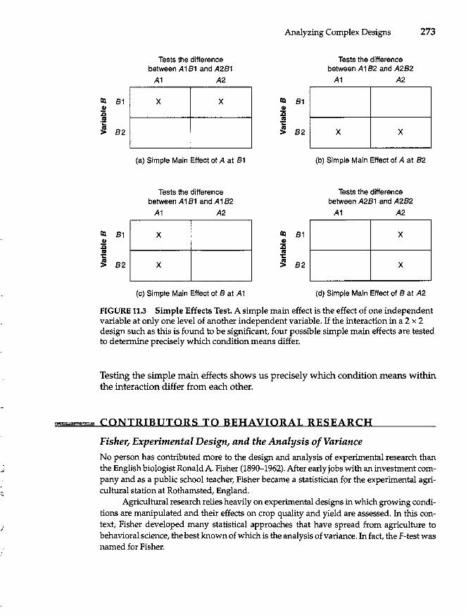
Analyzing Complex Designs 273

Tests the difference Tests the difference between A 1 81 and A281 between A182 and A282

A1 A2 A1 A2

IQ 81 X X IQ 81 ~ ~ ca -! 'i:

~ 82 ~ 82 X X

(a) Simple Main Effect of A at 81 (b) Simple Main Effect of A at 82

Tests the difference Tests the difference between A 1 81 and A 182 between A281 and A282

A1 A2 A1 A2

IQ 81 X IQ 81 X

~ .l!! .a .! ca

'i:

~ 82 X ~ 82 X

(c) Simple Main Effect of 8 at A1 (d) Simple Main Effect of 8 at A2

FIGURE 11.3 Simple Effects Test. A simple main effect is the effect of one independent variable at only one level of another independent variable. If the interaction in a 2 x 2 design such as this is found to be significant, four possible simple main effects are tested to determine precisely which condition means differ.

Testing the simple main effects shows us precisely which condition means within the interaction differ from each other.

!!!!IW!t¥'¥ti¥i CONTRIBUTORS TO BEHAVIORAL RESEARCH

Fisher, Experimental Design, and the Analysis of Variance

No person has contributed more to the design and analysis of experimental research than the English biologist Ronald A. Fisher (1890-1962). After early jobs with an investment com­pany and as a public school teacher, Fisher became a statistician f~r the experimental agri­cultural station at Rothamsted, England.

Agricultural research relies heavily on experimental designs in which growing condi­tions are manipulated and their effects on crop quality and yield are assessed. In this con­text, Fisher developed many statistical approaches that have spread from agriculture to behavioral science, the best known of which is the analysis of variance. In fact, the F-test was named for Fisher.

274 CHAPTER 11

In 1925, Fisher wrote one of the first books on statistical techniques, Statistical Methods for Research. Despite the fact that Fisher was a poor writer (someone once said that no stu­dents should try to read this book unless they had read it before), Statistical Methods became a classic in the field. Ten years later, Fisher published The Design of Experiments, a landmark in research design. These two books raised the level of sophistication in our understanding of research design and statistical analysis and paved the way for contemporary behavioral science (Kendall, 1970).

Between-Subjects and Within-Subjects ANOVAs

Each of the examples of ANOVA in this chapter involved between-subjects designs-experiments in which participants are randomly assigned to experimen­tal conditions (see Chapter 9). Although the rationale is the same, slightly different computational procedures are used for within-subjects and between-within (or mixed) designs in which each participant serves in more than one experimental condition. Just as we use a paired t-test to analyze data from a within-subjects two­group experiment, we use within-subjects ANOVA for multilevel and factorial within-subjects designs and use split-plot ANOVA for mixed (between-within) de­signs. Like the paired t-test, these variations of ANOVA capitalize on the fact that we have repeated measures on each participant to reduce the estimate of error variance, thereby providing a more powerful statistical test. Full details regarding these analyses take us beyond the scope of this book but may be found in most in­troductory statistics books.

Multivariate Analysis of Variance

We have discussed the two inferential statistics most often used to analyze differ­ences among means of a single dependent variable: the t-test (to test differences be­tween two conditions) and the analysis of variance (to test differences among more than two conditions). For reasons that will be clear in a moment, researchers some­times want to test differences between conditions on several dependent variables simultaneously. Because t-tests and ANOVAs cannot do this, researchers turn to multivariate analysis of variance. Whereas an analysis of variance tests differences among the means of two or more conditions on one dependent variable, a multi­variate analysis of variance, or MANOVA, tests differences between the means of two or more conditions on two or more dependent variables simultaneously.

A reasonable question to ask at this point is, Why would anyone want to test group differences on several dependent variables at the same time? Why not simply perform several ANOVAs-one on each dependent variable? Researchers turn to MANOVA rather than ANOVA for the following reasons.

I"

Analyzing Complex Designs 275

Conceptually Related Dependent Variables

One reason for using MANOVA arises when a researcher has measured several de­pendent variables, all of which tap into the same general construct. When several dependent variables measure different aspects of the same construct, the re­searcher may wish to analyze the variables as a set rather than individually.

Suppose you were interested in determining whether a marriage enrichment program improved married couples' satisfaction with their relationships. You con­ducted an experiment in which couples were randomly assigned to participate for two hours in either a structured marriage enrichment activity, an unstructured conversation on a topic of their own choosing, or no activity together. (You should recognize this as a randomized groups design with three conditions; see Chapter 9.) One month after the program, members of each couple were asked to rate their marital satisfaction on 10 dimensions involving satisfaction with finances, com­munication, ways of dealing with conflict, sexual relations, social life, recreation, and soon.

If you wanted to, you could analyze these data by conducting 10 ANOVAs­one on each dependent variable. However, because aU 10 dependent variables re­flect various aspects of general marital satisfaction, you might want to know whether the program affected satisfaction in general across all of the dependent measures. If this were your goal, you might use MANOVA to analyze your data. MANOVA combines the information from all 10 dependent variables into a new composite variable, then analyzes whether participants' scores on this new com­posite variable differ among the experimental groups.

Inflation of Type I Error

A second use of MANOVA is to control Type I error. As we saw earlier, the proba­bility of making a Type I error (rejecting the null hypothesis when it is true) in­creases with the number of statistical tests we perform. For this reason, we conduct one ANOVA rather than many t-tests when our experimental design involves more than two conditions (and, thus, more than two means). Type I error also becomes in­flated when we conduct t-tests or ANOVAs on many dependent variables. The more dependent variables we analyze in a study, the more likely we are to obtain signifi­cant differences that are due to Type I error rather than to the independent variable.

To use an extreme case, imagine we conduct a two-group study in which we measure 100 dependent variables, then test the difference between the two group means on each of these variables with 100 t-tests. You may be able to see that if we set our alpha level at .05, we could obtain significant t-tests on as many as five of our dependent variables even if our independent variable has no effect. Although few researchers use as many as 100 dependent variables in a single study, Type I error increases whenever we analyze more than one dependent variable.

Because MANOVA tests differences among the means of the groups across all dependent variables simultaneously, the overall alpha level is held at .05 (or what­ever level the researcher chooses) no matter how many dependent variables are

276 C HAP T E R 11

tested. Although most researchers don't worry about analyzing a few variables one by one, many use MANOVA to guard against Type I error whenever they analyze many dependent variables.

How MANOVA Works

MANOVA begins by creating a new composite variable that is a weighted sum of the original dependent variables. How this canonical variable is mathematically derived need not concern us here. The important thing is that the new canonical variable includes all of the variance in the set of original variables. Thus, it pro­vides us with a single index of our variable of interest (such as marital satisfaction).

In the second step of the MANOV A, a multivariate version of the F-test is per­formed to determine whether participants' scores on the canonical variable differ among the experimental conditions. If the multivariate F-test is significant, we con­clude that the experimental manipulation affected the set of dependent variables as a whole. For example, in our study of marriage enrichment, we would conclude that the marriage enrichment workshop created significant differences in the over­all satisfaction in the three experimental groups; we would then conduct addi­tional analyses to understand precisely how the groups differed. MANOVA has allowed us to analyze the dependent variables as a set rather than individually.

In cases in which researchers use MANOVA to reduce the chances of making a Type I error, obtaining a significant multivariate F-test then allows the researcher to conduct ANOVAs separately on each variable. Having been assured by the MANOVA that the groups differ significantly on something, we may then perform additional analyses without risking an increased chance of Type I error. However, if the MANOVA is not significant, examining the individual dependent variables using ANOVAs would run the risk of increasing Type I errors.

~ BEHAVIORAL RESEARCH CASE STUDY

Fear and Persuasion: An Example of MANOVA Since the 1950s, dozens of studies have investigated the effects of fear-inducing messages on persuasion. Put simply, when trying to persuade people to change undesirable behaviors (such as smoking, excessive suntanning, and having unprotected sexual intercourse), should one try to scare them with the negative consequences that may occur if they fail to change? Keller (1999) tested the hypothesis that the effects of fear-inducing messages on persuasion depend on the degree to which people already follow the recommendations ad­vocated in the message. In her study, Keller examined the effects of emphasizing mild ver­sus severe consequences on women's reactions to brochures that encouraged them to practice safe sex.

Before manipulating the independent variable, Keller assessed the degree to which the participants typically practiced safe sex, classifying them as either safe-sex adherents (those who always or almost always used a condom) or nonadherents (those who used con­doms rarely, if at all). In the study, 61 sexually active college women read a brochure about

I~

J

(

Analyzing Complex Designs 277

safe sex that either described relatively mild or relatively serious consequences of failing to practice safe sex. For example, the brochure in the mild consequences condition mentioned the possibility of herpes, yeast infections, and itchiness, whereas the brochure in the seri­ous consequences condition warned participants about AIDS-related cancers, meningitis, syphilis, dementia, and death. In both conditions, the brochures gave the same recommen­dations for practicing safe sex and reducing one's risk for contracting these diseases. After reading either the mild or severe consequences message, participants rated their reactions on seven dependent variables, including the likelihood that they would follow the recom­mendations in the brochure, the personal relevance of the brochure to them, the severity of the health consequences that were listed, and the degree to which participants thought they were able to follow the recommendations.

Because she measured several dependent variables, Keller conducted a multivariate analysis of variance. Given that this was a 2 (safe-sex adherents vs. nonadherents) by 2 (low vs. moderately serious consequences) factorial design, the MANOVA tested the main effect of ad­herent group, the main effect of consequence severity, and the group by severity interaction. Of primary importance to her hypotheses, the multivariate interaction was statistically significant. Having protected herself from inflated Type I error by using MANOVA (I guess we could say she practiced "safe stats"), Keller then conducted ANOV As separately on each dependent vari­able. (Had the MANOVAnot been statistically significant, she would not have done so.)

Results showed that participants who did not already practice safe sex (the nonadher­ents) were less convinced by messages that stressed moderately severe consequences than messages that stressed low severity consequences. Paradoxically, the safe-sex nonadherents rated the moderately severe consequences as less severe than the low severity consequences, and more strongly refuted the brochure's message when severe consequences were men­tioned. In contrast, participants who already practiced safe sex were more persuaded by the message that mentioned moderately severe rather than low severe consequences. These re­sults suggest that messages that try to persuade people to change unhealthy behaviors should not induce too high a level of fear if the target audience does not already comply with the message's recommendations.

Experimental and Nonexperimental Uses of Inferential Statistics

Most of the examples of t-tests, ANOVA, and MANOVA we have discussed in­volved data from true experimental designs in which the researcher randomly as­signed participants to conditions and manipulated one or more independent variables. At-test, ANOVA, or MANOVA was then used to test the differences among the means of the experimental conditions.

Although the t-test and analysis of variance were developed in the context of experimental research, they are also widely used to analyze data from nonexperi­mental studies. In such studies, participants are not randomly assigned to groups (as in a true experiment) but rather are categorized into naturally occurring groups.

278 C HAP T E R 11

Then, at-test, ANOVA, or MANOVAis used to analyze the differences among the means of these groups. For example, if we want to compare the average depression scores for a group of women and a group of men, we can use a t-test even though the study is not a true experiment.

As a case in point, Butler, Hokanson, and Flynn (1994) obtained a measure of depression for 73 participants on two different occasions five months apart. On the basis of these two depression scores, they categorized participants into one of five groups: (1) unremitted depression-participants who were depressed at both test­ing times, (2) remitted depression-participants who were depressed at Time 1 but not at Time 2, (3) new cases-participants who were not depressed at Time 1 but fell in the depressed range at Time 2, (4) nonrelapsers-participants who had once been depressed but were not depressed at both Time 1 and TIme 2, and (5) never depressed. The researchers then used MANOVA and ANOVA (as well as post hoc tests) to analyze whether these five groups differed in average self-esteem, depres­sion, emotional lability, and other measures. Even though this was a nonexperi­mental design and participants were classified into groups rather than randomly assigned, ANOVA and MANOVA were appropriate analyses.

Computer Analyses

In the early days of behavioral science, researchers conducted all of their statistical analyses by hand. Because analyses were time-consuming and cumbersome, re­searchers understandably relied primarily on relatively simple analytic tech­niques. The invention of the calculator (first mechanical, then electronic) was a great boon to researchers because it allowed them to perform mathematical opera­tions more quickly and with less error.

However, not until the widespread availability of computers and user­friendly statistical software did the modern age of statistical analysis begin. Analyses that once took many hours (or even days!) to conduct by hand could be performed on a computer in a few minutes. Furthermore, the spread of bigger and faster computers allowed researchers to conduct increasingly complex analyses and to test more sophisticated research hypotheses. Thus, over the past 25 years, we have seen a marked increase in the complexity of the analyses re­searchers commonly use. For example, prior to 1980, MANOVA-a complex and laborious analysis to perform by hand-was used only rarely; today, its use is quite common.

In the earliest days of the computer, computer programs had to be written from scratch for each new analysis. Researchers either had to be proficient at computer programming or have the resources to hire a programmer to write the programs for them. Gradually, however, statistical software packages were developed that any re­searcher could use by simply writing a handful of commands to inform the com­puter how their data were entered and which analyses to conduct. With the advent of menu and window interfaces, analyses became as easy as a few keystrokes on a computer keyboard or a few clicks of a computer mouse. Today, several software

r

Analyzing Complex Designs 279

packages exist that can perform most statistical analyses. (The most commonly used software statistical packages include SPSS, SAS, and BMDP.) Once researchers enter their data into the computer, name their variables, and indicate what analyses to per­form on which variables (either by writing a short set of commands or clicking on options on a computer screen), most analyses take only a few seconds.

Although computers have freed researchers from most hand calculations (oc­casionally, it is still faster to perform simple analyses by hand than to use the com­puter), researchers must understand when to use particular analyses, what requirements must be met for an analysis to be valid, and what the results a par­ticular analysis tell them about their data. Computers do not at all diminish the im­portance or necessity of understanding statistics.

Summary

1. When research designs involve more than two conditions (and, thus, more than two means), researchers analyze their data using ANOVA rather than t­tests because conducting many t-tests increases the chances that they will make a Type I error.

2. ANOVA partitions the total variability in participants' responses into between­groups variance (M~g) and within-groups variance (MSwg)' Then an F-test is conducted to determine whether the between-groups vanance exceeds what we would expect based on the amount of within-groups variance in the data. If it does, we reject the null hypothesis and conclude that at least one of the means differs from the others.

3. In a one-way design, a single F-test is conducted to test the effects of the lone independent variable. In a factorial design, an F-test is conducted to test each main effect and interaction.

4. For each effect being tested, the calculated value of F (the ratio of M~g/MSwg) is compared to a critical value of F. If the calculated value of F exceeds the crit­ical value, we know that at least one condition mean differs from the others. If the calculated value is less than the critical value, we fail to reject the null hypothesis and conclude that the condition means do not differ.

5. If the F-tests show that the main effects or interactions are statistically signif­icant, follow-up tests are often needed to determine the precise effect of the independent variable. Main effects of independent variables that involve more than two levels require post hoc tests, whereas interactions are decom­posed using simple effects tests.

6. Special varieties of ANOVA and MANOVA are used when data from within­subjects designs or mixed designs are being analyzed.

7. Multivariate analysis of variance (MANOVA) is used to test the differences among the means of two or more conditions on a set of dependent variables. MANOVA is used in two general cases: when the dependent variables all measure aspects of the same general construct (and, thus,lend themselves to analysis as a set), and when the researcher is concerned that performing

280 CHAPTER 11

separate analyses on several dependent variables will increase the possibility of making a Type I error.

S. In either case, MANOVA creates a new composite variable-a canonical variable-from the original dependent variables, then determines whether participants' scores on this canonical variable differ across conditions.

9. ANOVA and MANOVAmay be used to analyze data from both experimental and nonexperimental designs.

10. The computer revolution has greatly facilitated the use of complex statisti­cal analyses.

KEY TERMS

analysis of variance (ANOVA) mean square within-groups (MSwg) (p. 266)

simple main effect (p. 272) sum of squares (p. 265) sum of squares between-

(p.264) Bonferroni adjustment (p. 264) canonical variable (p. 276) follow-up tests (p. 272)

multiple comparisons (p.272)

multivariate analysis of variance (MANOVA) (p.274)

groups (S~g) (p. 267) sum of squares within-groups

(SSwg) (p. 266) F-test (p. 265) grand mean (p. 267) total sum of squares (SStotal)

(p.265) mean square between-groups (M~g) (p. 267)

post hoc tests (p. 272)

QUESTIONS FOR REVIEW

1. What's so bad about making a Type I error?

2. How does the Bonferroni adjustment control for Type I error when many statistical tests are conducted?

3. Why do researchers use ANOVA rather than t-tests to analyze data from experi­ments that have more than two groups?

4. If the independent variable has absolutely no effect on the dependent variable, will the means of the experimental conditions be the same? Why or why not?

5. An ANOVA for a one-way design partitions the total variance in a set of data into two components. What are they?

6. What kind of variance does the mean square within-groups (MSwg) reflect?

7. The sum of squares between-groups (S~g) reflects the degree to which the condi-tion means vary around the .

8. What is the name of the statistic used in an ANOVA?

9. If the independent variable has no effect, the calculated value of F will be around 1.00. Why?

I

Analyzing Complex Designs 281

10. In an experiment with two independent variables, an ANOVA partitions the total variance into four components. What are they?

11. MSwg appears in the denominator of every F-test. Why?

12. If the calculated value of F is found to be significant for the main effect of an inde­pendent variable with more than two levels, what tests does the researcher then conduct? Why are such tests not necessary if the independent variable has only two levels?

13. When are tests of simple main effects used, and what do researchers learn from them?

14. Who developed the rationale and computations for the analysis of variance?

15. Under what two circumstances would you use a multivariate analysis of variance?

16. Imagine that you conduct a study to test the average level of guilt experienced by Christians, Jews, Buddhists, Muslims, and Hindus. Could you use an ANOVA to analyze your data? Why or why not?

QUESTIONS FOR DISCUSSION

1. Go to the library and find a research article in a psychology journal that used analysis of variance. (This should not be difficult; ANOVA is perhaps the most commonly used analysis. If you have problems, try the journals Developmental Psy­chology, Journal of Personality and Social Psychology, and Journal of Experimental Psy­chology.) Read the article and see whether you understand the results of the ANOVAs that were conducted.

2. When researchers set their alpha level at .05, they reject the null hypothesis (and conclude that the independent variable has an effect) only if there is less than a 5% chance that the differences among the means are due to error variance. Does this mean that 5% of all results reported in the research literature are, in fact, Type I er­rors rather than real effects of the independent variables?

CHAPTER

12 Quasi-Experimental Designs

Pretest-PosHest Designs

Time Series Designs

Longitudinal Designs

Program Evaluation

Evaluating Quasi-Experimental Designs

282

To reduce the incidence of fatal traffic accidents, many states have passed laws re­quiring that passengers in automobiles wear seat belts. Proponents of such laws claim that wearing seat belts significantly decreases the likelihood that passengers will be killed or seriously injured in a traffic accident. Opponents of these laws argue that wearing seat belts does not decrease traffic fatalities. Instead, they say, it poses an increased risk because seat belts may trap passengers inside a burning car. Furthermore, they argue that such laws are useless because they are difficult to en­force and few people actually obey them anyway. Who is right? Do laws that re­quire people to wear seat belts actually reduce traffic fatalities?

This question seems simple enough until we consider the kind of research we would need to conduct to show that such laws actually cause a decrease in traffic fatalities. To answer such a question would require an experimental design such as those we discussed in Chapters 8 and 9. We would have to assign people randomly to either wearing or not wearing safety belts for a prolonged period of time, then measure the fatality rate for these two groups.

The problems of doing such a study should be obvious. First, we would find it very difficult to assign people randomly to wearing or not wearing seat belts and even more difficult to ensure that our participants actually followed our instruc­tions. Second, the incidence of serious traffic accidents is so low, relative to the number of drivers, that we would need a gigantic sample to obtain even a few se­rious accidents within a reasonable period of time. A third problem is an ethical one: Would we want to assign any people to not wearing seat belts, knowing that we might cause them to be killed or injured if they have an accident? I hope you can see that it would not be feasible to design a true experiment to determine whether seat belts are effective in reducing traffic injuries and fatalities.

Quasi-Experimental Designs 283

From the earliest days of psychology, behavioral researchers have shown a distinct preference for experimental designs over other approaches to doing re­search. In experiments we can manipulate one or more independent variables and carefully control other factors that might affect the outcome of the study, allowing us to draw relatively confident conclusions about whether the independent vari­ables cause changes in the dependent variables.

However, many real-world questions, such as whether seat-belt legislation re­duces traffic fatalities, can't be addressed within the narrow strictures of experimen­tation. Often, researchers do not have sufficient control over their participants to randomly assign them to experimental conditions. In other cases, they may be un­able or unwilling to manipulate the independent variable of interest. In such in­stances, researchers often use quasi-experimental designs. Unlike true experiments, quasi-experiments do not involve randomly assigning participants to conditions. In­stead, comparisons are made between people in groups that already exist (such as those who live in states with and without seat-belt laws) or within a single group of participants before and after some event has occurred (such as examining injuries be­fore and after a seat-belt law is passed).

Because such designs do not involve random assignment of participants to conditions, the researcher is not able to determine which participants will receive the various levels of the independent variable. In fact, in many studies the researcher does not manipulate the independent variable at all; researchers do not have the power to introduce legislation regarding seat-belt use, for example. In such cases, the term quasi-independent variable is sometimes used to indicate that the variable is not a true independent variable manipulated by the researcher but rather is an event that occurred for other reasons.

The strength of the experimental designs we examined in the preceding few chapters lies in their ability to demonstrate that the independent variables cause changes in the dependent variables. As we saw, experimental designs do this by eliminating alternative explanations for the findings that are obtained. Experimen­tal designs generally have high internal validity; researchers can conclude that the observed effects are due to the independent variables rather than to other, extrane­ous factors (see Chapter 8).

Generally speaking, quasi-experimental designs do not possess the same de­gree of internal validity as experimental designs. Because participants are not ran­domly assigned to conditions and the researcher may have no control over the independent variable, potential threats to internal validity are present in most quasi-experiments. Even so, a well-designed quasi-experiment that eliminates as many threats to internal validity as possible can provide strong circumstantial ev­idence about cause-and-effect relationships.

The quality of a quasi-experimental design depends on how many threats to internal validity it successfully eliminates. As we will see, quasi-experimental de­signs differ in the degree to which they control threats to internal validity. Needless to say, the designs that eliminate most of the threats to internal validity are prefer­able to those that eliminate only a few threats. In this chapter we will discuss several basic quasi-experimental designs. We will begin with the weakest, least preferable

284 CHAPTER 12

designs in terms of their ability to eliminate threats to internal validity, and then move to stronger quasi-experimental designs.

tf IN DEPTH

The Internal Validity Continuum Researchers draw a sharp distinction between experimental designs (in which the researcher controls both the assignment of participants to conditions and the independent variable) and quasi-experimental designs (in which the researcher lacks control over one or both of these aspects of the design). However, this distinction should not lead us to hastily conclude that experimental designs are unequivocally superior to quasi-experimental designs. Although this may be true in general, both experimental and quasi-experimental designs differ widely in terms of their internal validity. Indeed, some quasi-experiments are more internally valid than some true experiments.

A more useful way of conceptualizing research designs is along a continuum of low to high internal validity. Recall from Chapter 8 that internal validity refers to the degree to which a researcher draws accurate conclusions about the effects of an independent variable on participants' responses. At the low validity pole of the continuum are studies that lack the necessary controls to draw any meaningful conclusions about the effects of the inde­pendent variable whatsoever. As we move up the continuum, studies have increasingly tighter experimental control and hence higher internal validity. At the high validity pole of the continuum are studies in which exceptional design and tight control allow us to rule out every reasonable alternative explanation for the findings.

There is no point on this continuum at which we can unequivocally draw a line that sep­arates studies that are acceptable from the standpoint of internal validity from those that are unacceptable. Vniually all studies-whether experimental or quasi-experimental-possess some potential threats to internal validity. The issue in judging the quality of a study is whether the most serious threats have been eliminated, thereby allowing a reasonable degree of confidence in the conclusions we draw. As we will see, well-designed quasi-experiments can provide rather conclusive evidence regarding the effects of quasi-independent variables on behavior.

Pretest-Posttest Designs

As we said, researchers do not always have the power to assign participants to ex­perimental conditions. This is particularly true when the research is designed to examine the effects of an intervention on a group of people in the real world. For example, a junior high school may introduce a schoolwide program to educate stu­dents about the dangers of drug abuse, and the school board may want to know whether the program is effective in reducing drug use among the students. In this instance, random assignment is impossible because all students in the school were exposed to the program. If you were hired as a behavioral researcher to evaluate the effectiveness of the program, what kind of study would you design?

/

Quasi-Experimental Designs 285

How NOT to Do a Study: The One-Group Pretest-Posttest Design

One possibility would be to measure student drug use before the drug education program and again afterward to see whether drug use decreased. Such a design could be portrayed as

01 x 02

where 01 is a pretest measure of drug use, X is the introduction of the antidrug program (the quasi- independent variable), and 02 is the posttest measure of drug use one year later. (0 stands for observation.)

It should be apparent that this design, the one-group pretest-posttest de­sign, is a very poor research strategy because it fails to eliminate most threats to in­ternal validity. Many other things may have affected any change in drug use that we might observe other than the drug education program. If you observe a change in students' drug use between 01 and 02, how sure are you that the change was due to the program as opposed to some other factor?

Many other factors could have contributed to the change. For example, the students may have matured from the pretest to the posttest (maturation effects). In addition, events other than the program may have occurred between 01 and 02 (history effects); perhaps a popular rock musician died of an overdose, the princi­pal started searching students' lockers for drugs, or the local community started a citywide Just Say No to Drugs or DARE campaign. Another possibility is that the first measurement of drug use (01) may have started students thinking about drugs, resulting in lower use independently of the educational program (testing ef­fect). Extraneous factors such as these may have occurred at the same time as the antidrug education program and may have been responsible for decreased drug use. The one-group pretest-posttest design does not allow us to distinguish the ef­fects of the antidrug program from other possible influences.

In some studies, the internal validity of one-group pretest-posttest designs may also be threatened by regression to the mean-the tendency for extreme scores in a distribution to move, or regress, toward the mean of the distribution with repeated testing (Neale & Liebert, 1980). In many studies, participants are se­lected because they have extreme scores on some variable of interest. For example, we may want to examine the effects of a drug education program on students who are heavy drug users. Or, perhaps we are examining the effects of a remedial read­ing program on students who are poor readers. In cases such as these, a researcher may select participants who have extreme scores on a pretest (of drug use or read­ing ability, for example), expose them to the quasi-independent variable (the an­tidrug or reading program), then remeasure them to see whether their scores changed (drug use declined or reading scores improved, for example).

The difficulty with this approach is that when participants are selected be­cause they have extreme scores on the pretest, their scores may change from pretest to posttest because of the statistical artifact called regression to the mean. As we learned in Chapter 3, all scores contain measurement error that causes partici­pants' observed scores to differ from their true scores. Overall, measurement error

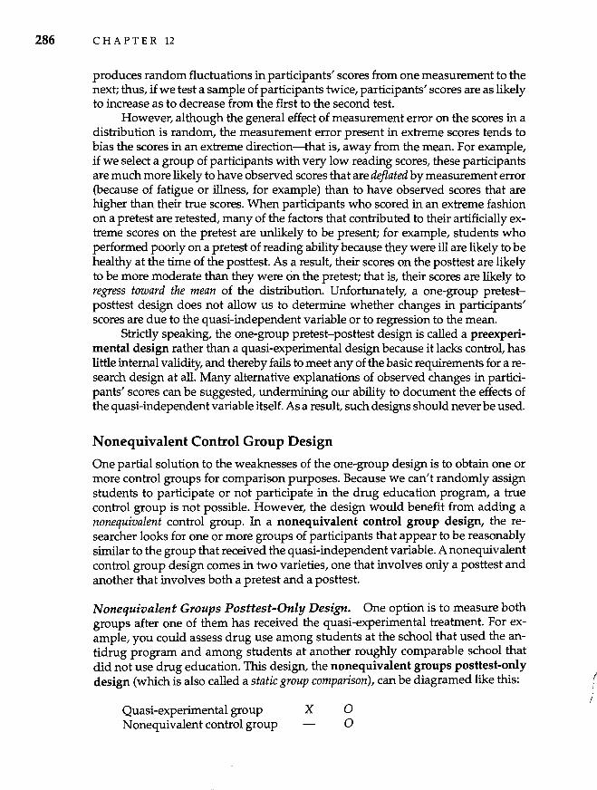
286 CHAPTER 12

produces random fluctuations in participants' scores from one measurement to the next; thus, if we test a sample of participants twice, participants' scores are as likely to increase as to decrease from the first to the second test.

However, although the general effect of measurement error on the scores in a distribution is random, the measurement error present in extreme scores tends to bias the scores in an extreme direction-that is, away from the mean. For example, if we select a group of participants with very low reading scores, these participants are much more likely to have observed scores that are deflated by measurement error (because of fatigue or illness, for example) than to have observed scores that are higher than their true scores. When participants who scored in an extreme fashion on a pretest are retested, many of the factors that contributed to their artificially ex­treme scores on the pretest are unlikely to be present; for example, students who performed poorly on a pretest of reading ability because they were ill are likely to be healthy at the time of the posttest. As a result, their scores on the posttest are likely to be more moderate than they were on the pretest; that is, their scores are likely to regress toward the mean of the distribution. Unfortunately, a one-group pretest­posttest design does not allow us to determine whether changes in participants' scores are due to the quasi-independent variable or to regression to the mean.

Strictly speaking, the one-group pretest-posttest design is called a preexperi­mental design rather than a quaSi-experimental design because it lacks control, has little internal validity, and thereby fails to meet any of the basic requirements for a re­search design at all. Many alternative explanations of observed changes in partici­pants' scores can be suggested, undermining our ability to document the effects of the quasi-independent variable itself. As a result, such designs should never be used.

Nonequivalent Control Group Design

One partial solution to the weaknesses of the one-group design is to obtain one or more control groups for comparison purposes. Because we can't randomly assign students to participate or not participate in the drug education program, a true control group is not possible. However, the design would benefit from adding a nonequivalent control group. In a nonequivalent control group design, the re­searcher looks for one or more groups of participants that appear to be reasonably similar to the group that received the quasi-independent variable. A nonequivalent control group design comes in two varieties, one that involves only a posttest and another that involves both a pretest and a posttest.

Nonequivalent Groups Posttest-Only Design. One option is to measure both groups after one of them has received the quasi-experimental treatment. For ex­ample, you could assess drug use among students at the school that used the an­tidrug program and among students at another roughly comparable school that did not use drug education. This design, the nonequivalent groups posttest-only design (which is also called a static group comparison), can be diagramed like this:

Quasi-experimental group Nonequivalent control group

x o o

I , /

Quasi-Experimental Designs 287

Unfortunately, this design also has many weaknesses. Perhaps the most trou­blesome is that we have no way of knowing whether the two groups were actually similar before the quasi-experimental group received the treatment. If the two groups differ at time 0, we don't know whether the difference was caused by variable X or whether the groups differed even before the quasi-experimental group received X (this involves biased assignment of participants to conditions or selection bias). Because we have no way of being sure that the groups were equivalent before par­ticipants received the quasi-independent variable, the nonequivalent control group posttest-only design is very weak in terms of internal validity and should rarely be used. However, as the following case study shows, such designs can sometimes provide convincing data.

~ BEHAVIORAL RESEARCH CASE STUDY

Nonequivalent Control Group Design: Perceived Responsibility and Well-Being Among the Aged Older people often decline in physical health and psychological functioning after they are placed in a nursing home. Langer and Rodin (1976) designed a study to test the hypothesis that a portion of this decline is due to the loss of control that older people feel when they move from their own homes to an institutional setting. The participants in their study were 91 people, ages 65 to 90, who lived in a Connecticut nursing home. In designing their study, Langer and Rodin were concerned about the possibility of experimental contamination. When participants in different conditions of a study interact with one another, the possibil­ity exists that they may talk about the study among themselves and that one experimental condition becomes "contaminated" by the other. To minimize the likelihood of contami­nation, the researchers decided not to randomly assign residents in the nursing home to the two experimental conditions. Rather, they randomly selected two floors in the facility, assigning residents of one floor to one condition and those on the other floor to the other condition. Residents on different floors did not interact much with one another, so this pro­cedure minimized contamination. However, the decision not to randomly assign partici­pants to conditions resulted in a quasi-experimental design-specifically, a nonequivalent control group design.

An administrator gave different talks to the residents on the two floors. One talk em­phasized the residents' responSibility for themselves and encouraged them to make their own decisions about their lives in the facility; the other emphasized the staff's responsibil­ity for the residents. Thus, one group was made to feel a high sense of responsibility and control, whereas the other group experienced lower responsibility and control. In both cases, the responsibilities and options stressed by the administrator were already available to all residents, so the groups differed chiefly in the degree to which their freedom, respon­sibility, and choice were explicitly stressed.

The residents were assessed on a number of measures a few weeks after hearing the talk. Compared with the other residents, those who heard the talk that emphasized their personal control and responsibility were more active and alert, happier, and more involved in activities within the nursing home. In addition, the nursing staff rated them as more in­terested, sociable, self-initiating, and vigorous than the other residents. In fact, follow-up

288 C HAP T E R 12

data collected 18 months later showed long-term psychological and physical effects of the intervention, including a lower mortality rate among participants in the high responsibility group (Rodin & Langer, 1977).

The implication is, of course, that giving residents greater choice and responsibility caused these positive changes. However, in considering these results, we must remember that this was a quasi-experimental design. Not only were participants not assigned ran­domly to conditions, but they lived on different floors of the facility. To some extent, partic­ipants in the two groups were cared for by different members of the nursing home staff and lived in different social groups. Perhaps the staff on one floor was more helpful than that on another floor, or social support among the residents was greater on one floor than another. Because of these differences, we cannot eliminate the possibility that the obtained differ­ences between the two groups were due to other variables that differed systematically be­tween the groups.

Most researchers do not view these alternative explanations to Langer and Rodin's find­ings as particularly plausible. (In fact, their study is highly regarded in the field.) We have no particular reason to suspect that the two floors of the nursing home differed in some way that led to the findings they obtained. Even so, the fact that this was a quasi-experiment should make us less confident of the findings than if a true experimental design had been used.

Nonequivalent Groups Pretest-Posttest Design. Some of the weaknesses of the nonequivalent control group design are eliminated by measuring the two groups twice, once before and once after the quasi-independent variable. The nonequiva­lent groups pretest-posttest design can be portrayed as follows:

Quasi-experimental group Nonequivalent control group

01 01

x 02 02

This design lets us see whether the two groups scored similarly on the de­pendent variable (for example, drug use) before the introduction of the treatment at point X. Even if the pretest scores at 01 aren't identical for the two groups, they provide us with baseline information that we can use to determine whether the groups changed from 01 to 02. If the scores change between the two testing times for the quasi-experimental group but not for the nonequivalent control group, we have somewhat more confidence that the change was due to the quasi-independent variable. For example, to evaluate the drug education program, you might obtain a nonequivalent control group from another school that does not have an antidrug program under way. If drug use changes from pretest to posttest for the quasi­experimental group but not for the nonequivalent control group, we might assume the program had an effect.

Even so, the nonequivalent groups pretest-posttest design does not eliminate all threats to internal validity. For example, a local history effect may occur. Some­thing may happen to one group that does not happen to the other (Cook & Camp­bell, 1979). Perhaps some event that occurred in the experimental school but not in

Quasi-Experimental Designs 289

the control school affected students' attitudes toward drugs-a popular athlete was kicked off the team for using drugs, for example. If this happens, what appears to be an effect of the antidrug program may actually be due to a local history effect. This confound is sometimes called a selection-by-history interaction because a "history" effect occurs in One group but not in the other.

In brief, although the nonequivalent groups design eliminates some threats to internal validity, it doesn't eliminate all of them. Even so, with proper controls and measures, this design can provide useful information about real-world problems.

BEHAVIORAL RESEARCH CASE STUDY

Nonequivalent Groups Pretest-Posttest Design: Self-Esteem and Organized Sports Children with high self-esteem generally fare better than those with low self-esteem; for ex­ample, they tend to be happier, less anxious, and generally better adjusted. In studies de­signed to identify the sources of high self-esteem in children, researchers have focused primarily on children's experiences in school and within their families. Smoll, Smith, Barnett, and Everett (1993) decided to extend this literature by studying how self-esteem may be af­fected by the adults who coach children's organized sports. Specifically, they were interested in whether coaches could be trained to treat their players in ways that bolster the players' self-esteem.

The researchers obtained the cooperation of 18 male head coaches of 152 boys who played Little League baseball in the Seattle area. Rather than randomly assigning coaches and their teams to conditions, the researchers decided to use the eight teams in one league as the quasi-experimental group and the 10 teams from two other leagues as the nonequiv­alent control group. Although the decision not to use random assignment resulted in a quasi­experimental design, the researchers concluded that this strategy was necessary to prevent information about the training program from being spread by coaches who were in the train­ing group to those who were not.

In looking for possible preexisting differences between the groups, the researchers found that the coaches who had been assigned to the two groups did not differ in average age, years of coaching experience, or socioeconomic level. Nor did the players in the two groups differ in mean age of the players (the average age was 11.4 years). Of course, the two groups may have differed systematically on some variable that the researchers did not ex­amine, but at least we have evidence that the coaches and players did not differ on major de­mographic variables before the study began.

Before the start of the season, a measure of self-esteem was administered to all of the players. Then, the eight coaches in the quasi-experimental group underwent a 21h hour training session designed to help them relate more effectively to young athletes. Among other things, coaches were taught how to use reinforcement and corrective instruction in­stead of punishment and punitive instruction when working with their players. The coaches in the nonequivalent control group did not participate in such a training session. Immedi­ately after the baseball season ended, players' self-esteem was assessed again.

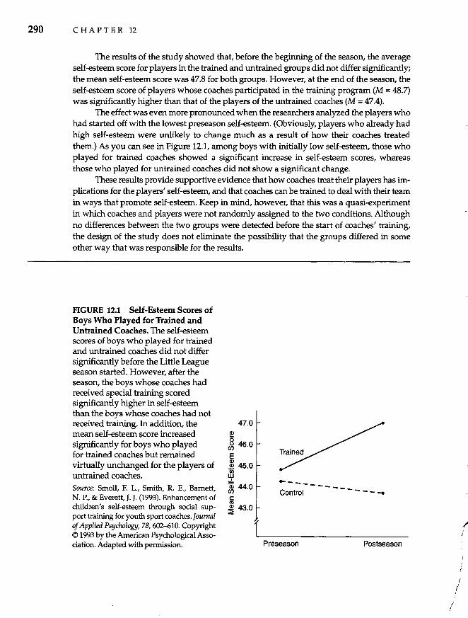
290 C HAP T E R 12

The results of the study showed that, before the beginning of the season, the average self-esteem score for players in the trained and untrained groups did not differ significantly; the mean self-esteem score was 47.8 for both groups. However, at the end of the season, the self-esteem score of players whose coaches participated in the training program (M = 48.7) was significantly higher than that of the players of the untrained coaches (M = 47.4).

The effect was even more pronounced when the researchers analyzed the players who had started off with the lowest preseason self-esteem. (ObViously, players who already had high self-esteem were unlikely to change much as a result of how their coaches treated them.) As you can see in Figure 12.1, among boys with initially low self-esteem, those who played for trained coaches showed a significant increase in self-esteem scores, whereas those who played for untrained coaches did not show a significant change.

These results provide supportive evidence that how coaches treat their players has im­plications for the players' self-esteem, and that coaches can be trained to deal with their team in ways that promote self-esteem. Keep in mind, however, that this was a quasi-experiment in which coaches and players were not randomly assigned to the two conditions. Although no differences between the two groups were detected before the start of coaches' training, the design of the study does not eliminate the possibility that the groups differed in some other way that was responsible for the results.

FIGURE 12.1 Self-Esteem Scores of Boys Who Played for Trained and Untrained Coaches. The self-esteem scores of boys who played for trained and untrained coaches did not differ significantly before the Little League season started. However, after the season, the boys whose coaches had received special training scored significantly higher in self-esteem than the boys whose coaches had not received training. In addition, the mean self-esteem score increased significantly for boys who played for trained coaches but remained virtually unchanged for the players of untrained coaches. Source: Smoil, F. 1., Smith, R. E., Barnett, N. P., & Everett, J. J. (1993). Enhancement of children's self-esteem through social sup­port training for youth sport coaches. Journal of Applied Psychology, 78, 602-610. Copyright © 1993 by the American Psychological Asso­ciation. Adapted with permission.

47.0

~

~ 46.0

E ~ 45.0 II)

w ~ 44.0 c: ttl ~ 43.0

.... _--­ -----Control - - - -

Preseason Postseason

. i

I

; .'

Quasi-Experimental Designs 291

Time Series Designs

Some of the weaknesses of the nonequivalent control group designs are further elim­inated by a set of procedures known as time series designs. Time series designs mea­sure the dependent variable on several occasions before and on several occasions after the quasi-independent variable occurs. By measuring the target behavior on several occasions, further threats to internal validity can be eliminated, as we'll see.

Simple Interrupted Time Series Design

The simple interrupted time series design involves taking several pretest mea­sures before introducing the independent (or quasi-independent) variable, then taking several posttest measures afterwards. This design can be diagramed as

01 02 03 04 x 05 06 07 08

As you can see, repeated measurements of the dependent variable have been inter­rupted by the occurrence of the quasi-independent variable (X). For example, we could measure drug use every three months for a year before the drug education program starts, then every three months for a year afterward. If the program had an effect on drug use, we should see a marked change between 04 and 05.

The rationale behind this design is that by taking multiple measurements both before and after the quasi-independent variable, we can examine the effects of the quasi-independent variable against the backdrop of other changes that may be occurring in the dependent variable. For example, using this design, we should be able to distinguish changes due to aging or maturation from changes due to the quasi-independent variable. If drug use is declining because of changing norms or because the participants are maturing, we should see gradual changes in drug use from one observation to the next, not just between the first four and the last four observations.

To see what I mean, compare the two graphs in Figure 12.2. Which of the graphs seems to show that the drug education program lowered drug use? In Fig­ure 12.2(a), drug use is lower after the program than before it, but it is unclear whether the decline is associated with the program or is part of a downward pattern that began before the initiation of the program. In Figure 12.2(b), on the other hand, the graph shows that a marked decrease in drug use occurred immediately after the program. Although we can't conclude for certain that the program was, in fact, re­sponsible for the change in drug use, the evidence is certainly stronger in 12.2(b) than in 12.2(a).

The central threat to internal validity with a simple interrupted time series design is contemporary history. We cannot rule out the possibility that the ob­served effects were due to another event that occurred at the same time as the quasi-independent variable. If a rock star died from drugs or an athlete was barred from the team at about the time that the drug education program began, we would

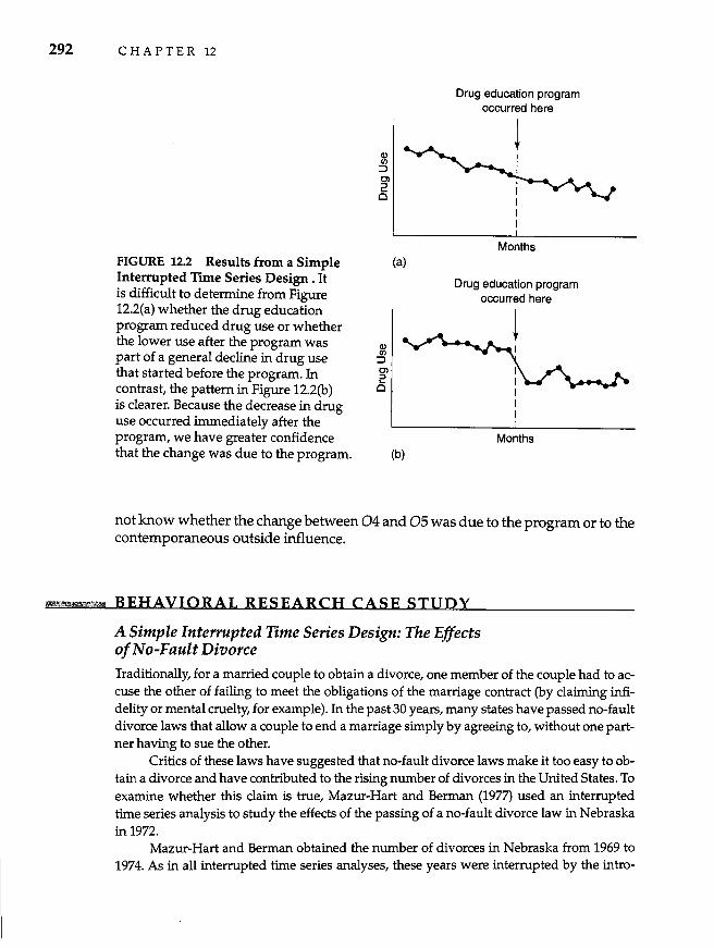
292 CHAPTER 12

Drug education program occurred here

Q) I/)

=> Cl 2 0

Months FIGURE 12.2 Results from a Simple (a) Interrupted Time Series Design. It Drug education program is difficult to determine from Figure occurred here 12.2(a) whether the drug education program reduced drug use or whether the lower use after the program was Q)

part of a general decline in drug use Ul =>

that started before the program. In Cl 2

contrast, the pattern in Figure 12.2(b) 0

is clearer. Because the decrease in drug use occurred immediately after the program, we have greater confidence Months that the change was due to the program. (b)

not know whether the change between 04 and 05 was due to the program or to the contemporaneous outside influence.

--!3¥!!!!M!!!I BEHAVIORAL RESEARCH CASE STUDY

A Simple Interrupted Time Series Design: The Effects o/No-Fault Divorce

Traditionally, for a married couple to obtain a divorce, one member of the couple had to ac­cuse the other of failing to meet the obligations of the marriage contract (by claiming infi­delity or mental cruelty, for example). In the past 30 years, many states have passed no-fault divorce laws that allow a couple to end a marriage simply by agreeing to, without one part­ner having to sue the other.

Critics of these laws have suggested that no-fault divorce laws make it too easy to ob­tain a divorce and have contributed to the rising number of divorces in the United States. To examine whether this claim is true, Mazur-Hart and Berman (1977) used an interrupted time series analysis to study the effects of the passing of a no-fault divorce law in Nebraska in 1972.

Mazur-Hart and Berman obtained the number of divorces in Nebraska from 1969 to 1974. As in all interrupted time series analyses, these years were interrupted by the intro-

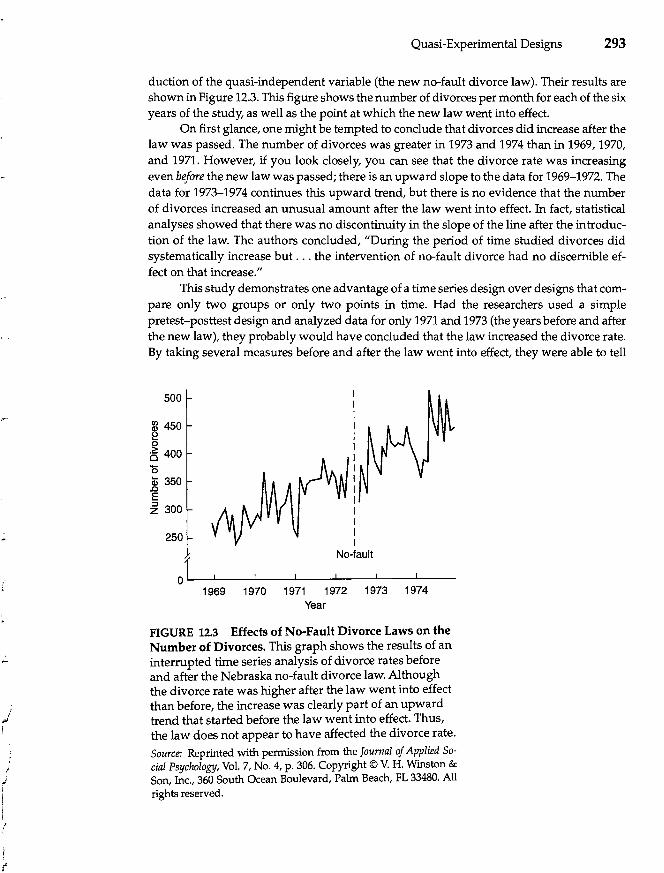
." i

,­"" I

.i I

~. I I I r ;

Quasi-Experimental Designs 293

duction of the quasi-independent variable (the new no-fault divorce law). Their results are shown in Figure 12.3. This figure shows the number of divorces per month for each of the six years of the study, as well as the point at which the new law went into effect.

On first glance, one might be tempted to conclude that divorces did increase after the law was passed. The number of divorces was greater in 1973 and 1974 than in 1969, 1970, and 1971. However, if you look closely, you can see that the divorce rate was increasing even before the new law was passed; there is an upward slope to the data for 1969-1972. The data for 1973-1974 continues this upward trend, but there is no evidence that the number of divorces increased an unusual amount after the law went into effect. In fact, statistical analyses showed that there was no discontinuity in the slope of the line after the introduc­tion of the law. The authors concluded, "During the period of time studied divorces did systematically increase but ... the intervention of no-fault divorce had no discernible ef­fect on that increase."

This study demonstrates one advantage of a time series design over designs that com­pare only two groups or only two points in time. Had the researchers used a simple pretest-posttest design and analyzed data for only 1971 and 1973 (the years before and after the new law), they probably would have concluded that the law increased the divorce rate. By taking several measures before and after the law went into effect, they were able to tell

500

~ 450 ~

~ 400 '0 Qj 350

.&l E ~ 300

250

No-fault

ol~~--~~--~~--~--1969 1970 1971 1972 1973 1974

Year

FIGURE 12.3 Effects of No-Fault Divorce Laws on the Number of Divorces. This graph shows the results of an interrupted time series analysis of divorce rates before and after the Nebraska no-fault divorce law. Although the divorce rate was higher after the law went into effect than before, the increase was clearly part of an upward trend that started before the law went into effect. Thus, the law does not appear to have affected the divorce rate.

Source: Reprinted with permission from the Journal of Applied So­cial Psychology, Vol. 7, No.4, p. 306. Copyright © V. H. Winston & Son, Inc., 360 South Ocean Boulevard, Palm Beach, FL 33480. All rights reserved.

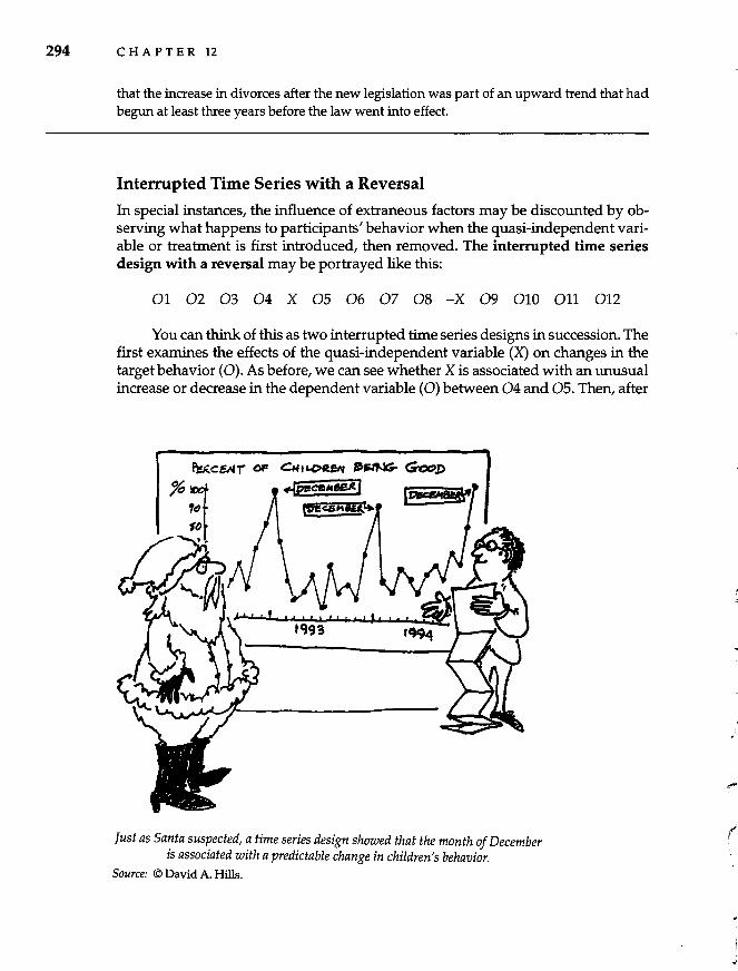
294 C HAP T E R 12

that the increase in divorces after the new legislation was part of an upward trend that had begun at least three years before the law went into effect.

Interrupted Time Series with a Reversal

In special instances, the influence of extraneous factors may be discounted by ob­serving what happens to participants' behavior when the quasi-independent vari­able or treatment is first introduced, then removed. The interrupted time series design with a reversal may be portrayed like this:

01 02 03 04 X 05 06 07 08 -X 09 010 011 012

You can think of this as two interrupted time series designs in succession. The first examines the effects of the quasi-independent variable (X) on changes in the target behavior (0). As before, we can see whether X is associated with an unusual increase or decrease in the dependent variable (0) between 04 and 05. Then, after

CH'&.D.~ ,,~ ~.P

+c:eMI£(] t!!<£iA+

Just as Santa suspected, a time series design showed that the month of December is associated with a predictable change in children's behavior.

Source: © David A. Hills.

1

I

!

i j

.-

Quasi-Experimental Designs 295

X has been in place for a while, we can remove it (at point -X) and observe what happens to O. Under some circumstances, we would expect the behavior to return to its pre-X level. If this occurs, we are more confident that X produced the ob­served changes. It would be unlikely that some external, historical influence oc­curred with X, then disappeared when X was removed. Of course, such an effect is logically possible, but in most instances it is unlikely.

To further increase our confidence that the quasi-independent variable, and not outside historical events, created the observed changes at X and -X, we could then reintroduce the independent variable, observe its effects, then remove it a sec­ond time. This is known as an interrupted time series design with multiple repli­cations and can be diagramed as follows:

01 02 03 X 04 05 06 -X 07 08 09 X 010 011 012 -X 013 014 015

Quasi-experimental designs where the variable of interest is introduced and then removed have three major limitations. The primary one is that researchers often do not have the power to remove the quasi-independent variable--to repeal seat-belt laws or no-fault divorce laws, for example. Second, the effects of some quasi-independent variables remain even after the variable itself is removed. For example, the effects of a community-wide program to reduce racial prejudice should linger even after the program itself is discontinued. Third, the removal of a quasi-independent variable may produce changes that are not due to the effects of the variable per se. For example, if we were interested in the effects of a new in­centive system on employee morale, removing work incentives might dampen morale because the employees would be angry about having the system removed (Cook & Campbell, 1979).

Control Group Interrupted Time Series Design

So far, we have discussed time series designs that measure a single group of par­ticipants before and after the quasi-independent variable. Adding comparison groups strengthens these designs by eliminating additional threats to internal va­lidity. By measuring more than one group on several occasions, only one of which receives the quasi-independent variable, we can minimize the plausibility of cer­tain alternative interpretations of the results. For example, we could perform an in­terrupted time series analysis on the group that received the quasi-independent variable and on a nonequivalent control group that did not receive the quasi­independent variable:

Quasi-experimental group: 01 02 03 04 X 05 06 07 08 Nonequivalent control group: 01 02 03 04 - 05 06 07 08

This design helps us rule out certain history effects. If both groups experience the same outside events but a change is observed only for the quasi-experimental group, we can be more certain (though not positive) that the change was due to X

296 C HAP T E R 12

rather than to an outside influence. Of course, local history effects are possible in which the experimental group experiences extraneous events that the nonequiva­lent control group does not.

Longitudinal Designs

Closely related to time series designs are longitudinal designs, but in the case of longitudinal designs, the quasi-independent variable is time itself. That is, nothing has occurred between one observation and the next other than the passage of time.

01 02 03 04 05

Longitudinal designs are used most frequently by developmental psychologists to study age-related changes in how people think, feel, and behave. For example, we might use a longitudinal design to study how the strategies that children use to re­member things change as they get older. To do so, we could follow a single group of children over a period of several years, testing their memory strategies when they were 4, 8, and 12 years old.

Typically, the goal of longitudinal research is to uncover developmental changes that occur as a function of age, but researchers must be alert for the possi­bility that something other than age-related development has produced the ob­served changes. Imagine, for example, that we are interested in how children's hand-eye coordination changes with age. We get a sample of 3-year-old children and study their hand-eye coordination at ages 3, 6,9, and 12, finding that hand-eye coordination increases markedly with age, particularly between ages 6 and 9. Is this change due to a natural developmental progression, or could something else have caused it? One possibility that comes to mind is that the effect was produced not by age-related changes but rather by playing sports. If participating in sports increases hand-eye coordination, older children would have better hand-eye coordination than younger kids because they have played more baseball, basketball, and soccer. Thus, changes across time observed in a longitudinal design do not necessarily re­flect a natural developmental sequence.

Longitudinal research can be very informative, but it has three drawbacks. First, researchers typically find it difficult to obtain samples of participants who agree to be studied again and again over a long period of time. (In fact, researchers themselves may have trouble mustering enough interest in the same topic over many years to maintain their own involvement in the study.) Second, even if they find such a sample, researchers often have trouble keeping track of the partici­pants, many of whom invariably move and, particularly if one is studying devel­opmental changes in old age, may even die. Third, repeatedly testing a sample over a period of years requires a great deal of time, effort, and money, and re­searchers often feel that their time is better spent doing several one-time studies rather than devoting their resources to a single longitudinal design.

Given these drawbacks, you may wonder why researchers use longitudinal de­signs instead of cross-sectional designs that compare groups of different ages at a

f

I ,

PM"e ...

,

I ...

Quasi-Experimental Designs 297

single point in time. For example, rather than tracking changes in memory strategies in one group of children over many years, why not test the memory strategies of different groups of 4, 8, and 12-year-olds? In fact, researchers do use cross-sectional designs to study age-related changes. However, cross-sectional designs have a shortcoming when studying development in that they cannot distinguish age­related changes from generational effects. Put simply, people of different ages dif­fer not only in age per se but also in the conditions under which their generation grew up. As a result, people who are of different ages today may differ in ways that have nothing to do with age per se. For example, a group of 70-year-olds who grew up during World War II and a group of 50-year-olds who grew up in the 1960s differ not only in age but also in the events experienced by members of their gen­eration. Thus, if we find a systematic difference between groups of 70- and 50-year­olds, we do not know whether the difference is developmental or generational because a cross-sectional design cannot separate these influences. By tracking a single group of participants as they age in a longitudinal design, generational ef­fects are eliminated because they all belong to the same generation.

A second advantage of longitudinal over cross-sectional designs for studying developmental change is that longitudinal designs allow the researcher to examine how individual participants change with age. A cross-sectional study that compares groups of different ages may reveal a significant difference between the groups even though only a small proportion of the participants differ between the groups. For example, cross-sectional studies show that, on average, older people have poorer memories than middle-aged people. However, such an effect could be ob­tained even if only a relatively small percent of the older people had impaired mem­ories and the rest were indistinguishable from the middle-aged participants; just a few forgetful participants could pull down the average memory score for the whole older group. As a result, we might be misled into concluding that memory gener­ally declines in old age. Yet, a longitudinal design that tracked participants from middle to old age would allow us to examine how individual participants changed, possibly revealing that memory decrements occurred in only a small number of the older participants.

Longitudinal designs can provide important information about the effects of time and aging on development. However, like all quasi-experimental designs, their results must be interpreted with caution, and researchers must carefully con­sider alternative explanations of the observed changes.

BEHAVIORAL RESEARCH CASE STUDY

Longitudinal Design: The Stability of Personality in Infancy and Childhood Lemery, Goldsmith, Klinnert, and Mrazek (1999) used a longitudinal design to examine the degree to which personality remains stable during infancy and early childhood. To obtain a sample of young infants who could be studied over time, the researchers recruited pregnant women who agreed to allow their children to be measured several times after birth. In this

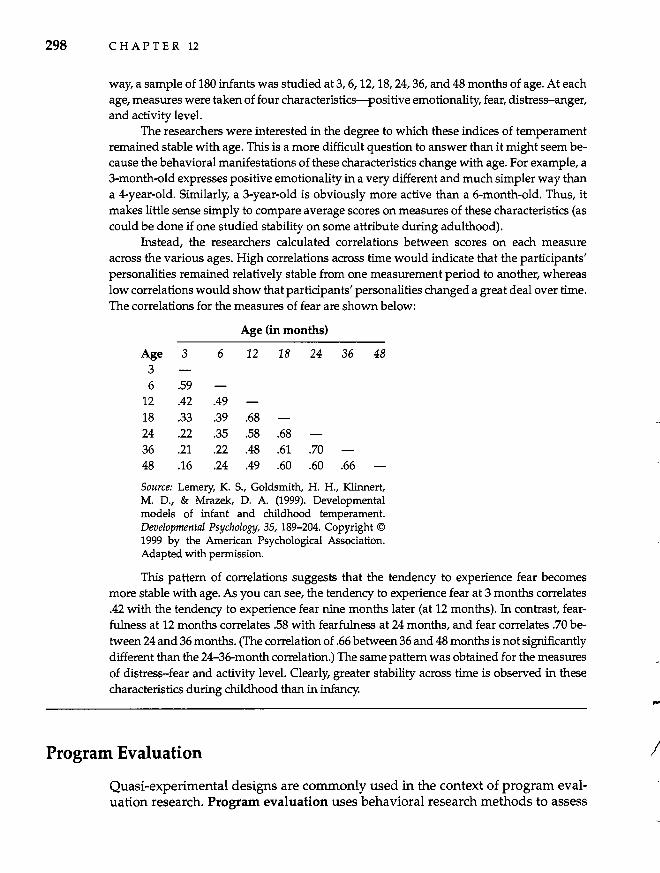
298 CHAPTER 12

way, a sample of 180 infants was studied at 3,6, 12, 18,24, 36, and 48 months of age. At each age, measures were taken of four characteristics-positive emotionality, fear, distress-anger, and activity level.

The researchers were interested in the degree to which these indices of temperament remained stable with age. This is a more difficult question to answer than it might seem be­cause the behavioral manifestations of these characteristics change with age. For example, a 3-month-old expresses positive emotionality in a very different and much simpler way than a 4-year-old. Similarly, a 3-year-old is obviously more active than a 6-month-old. Thus, it makes little sense simply to compare average scores on measures of these characteristics (as could be done if one studied stability on some attribute during adulthood).

Instead, the researchers calculated correlations between scores on each measure across the various ages. High correlations across time would indicate that the participants' personalities remained relatively stable from one measurement period to another, whereas low correlations would show that participants' personalities changed a great deal over time. The correlations for the measures of fear are shown below:

Age (in months)

Age 3 6 12 18 24 36 48 3 6 .59

12 .42 .49 18 .33 .39 .68 24 .22 .35 .58 .68 36 48

.21

.16 .22 .48 .61 .24 .49 .60

.70

.60 .66

SOUTce: Lemery, K. S., Goldsmith, H. H., Klinnert, M. D., & Mrazek, D. A. (1999). Developmental models of infant and childhood temperament. Developmental Psychology, 35, 189-204. Copyright © 1999 by the American Psychological Association. Adapted with permission.

This pattern of correlations suggests that the tendency to experience fear becomes more stable with age. As you can see, the tendency to experience fear at 3 months correlates .42 with the tendency to experience fear nine months later (at 12 months). In contrast, fear­fulness at 12 months correlates .58 with fearfulness at 24 months, and fear correlates .70 be­tween 24 and 36 months. (The correlation of .66 between 36 and 48 months is not significantly different than the 24-36-month correlation.) The same pattern was obtained for the measures of distress-fear and activity level. Clearly, greater stability across time is observed in these characteristics during childhood than in infancy.

Program Evaluation

Quasi-experimental designs are commonly used in the context of program eval­uation research. Program evaluation uses behavioral research methods to assess

,...

I

!

j .I

Quasi-Experimental Designs 299

the effects of interventions (or programs) designed to influence behavior. For ex­ample, a program may involve a new educational intervention designed to raise students' achievement test scores, a new law intended to increase seat-belt use, an incentive program designed to increase employee morale, a marketing campaign implemented to affect the public's image of a company, or a training program for Little League coaches. Because these kinds of programs are usually not under researchers' control, they must use quasi-experimental approaches to evaluate their effectiveness.

Although program evaluations often contribute to basic knowledge about human behavior, their primary goal is often to provide information to those who must make decisions about the target programs. Often, the primary audience for a program evaluation is not the scientific community (as is the case with basic re­search) but rather decision makers such as government administrators, legislators, school boards, and company executives. Such individuals need information about program effectiveness to determine whether program goals are being met, to de­cide whether to continue certain programs, to consider how programs might be improved, and to allocate money and other resources to programs.

In some instances, program evaluators are able to use true experimental de­signs to assess program effectiveness. Sometimes they are able to randomly assign people to one program or another and have control over the implementation of the program (which is, in essence, the independent variable). In educational settings, for example, new curricula and teaching methods are often tested using true ex­perimental designs. More commonly, however, program evaluators have little or no control over the programs they evaluate. When evaluating the effects of new legislation, such as the effects of no-fault divorce laws or seat-belt laws, researchers cannot use random assignment or control the independent variable. In industrial settings, researchers have little control over new policies regarding employees. Even so, companies often want to know whether new programs and policies re­duce absenteeism, increase morale, or bolster productivity. By necessity, then, pro­gram evaluation often involves quasi-experimental designs.

iN CONTRIBUTORS TO BEHAVIORAL RESEARCH

Donald Campbell and Quasi-Experimentation Few researchers have made as many ground-breaking methodological contributions to so­cial and behavioral science as Donald T. Campbell (1916-1996) who, among other things, popularized the use of quasi-experimental designs. Campbell's graduate education in psy­chology was interrupted by World War II when he left school to join the research unit of the Office of Strategic Services (055). At 055, he applied behavioral research methods to the study of wartime propaganda and attitudes, an experience that drew him to a lifelong in­terest in applied research. After the war (which included a stint in the navy), Campbell com­pleted his dissertation and obtained his Ph.D. Because many of his primary research interests-such as political attitudes, prejudice, and leadership-involved topics of real­world relevance, he became interested in applying traditional experimental designs to re­search settings in which full experimental control was not possible (Campbell, 1981). For

300 CHAPTER 12

example, he was interested in studying leadership processes in real military groups, which did not permit the strict control that was possible in laboratory experiments on leadership.

In the early 1960s, Campbell invited Julian Stanley to coauthor a brief guide to re­search designs that, for the first time, delved deeply into quasi-experimental research. Campbell and Stanley's (1966) Experimental and Quasi-Experimental Designs for Research has become a classic text for generations of behavioral researchers and is among the most cited works in the social and behavioral sciences. Later, Campbell was among the first to urge re­searchers to apply quasi-experimental designs to the evaluation of social and educational programs (Campbell, 1969, 1971). Throughout his illustrious career, Campbell made many other important contributions to measurement and methodology, including important work on validity (he was the first to make the distinction between internal and external va­lidity), unobtrusive measures, interviewing techniques, and the philosophy of science. In addition to his work on problems in behavioral measurement and research design, Camp­bell also published extensively on topics such as leadership, stereotyping, perception, atti­tudes, conformity, and cross-cultural psychology.

Evaluating Quasi-Experimental Designs

For many years, most behavioral scientists held a well-entrenched bias against quasi-experimental designs. For many, the tightly controlled experiment was the benchmark of behavioral research, and anything less than a true experiment was re­garded with suspicion. Most contemporary behavioral researchers tend not to share this bias against quasi-experimentation, recognizing that the limitations of quasi­experimental designs are compensated by a notable advantage. In particular, true experimentation that involves random assignment and researcher-manipulated in­dependent variables is limited in the questions it can address. Often we want to study the effects of certain variables on behavior but are unable or unwilling to conduct a true experiment that will allow unequivocal conclusions about causality. Faced with the limitations of the true experiment, we have a choice. We can aban­don the topic, leaving potentially important questions unanswered, or we can con­duct quasi-experimental research that provides us with tentative answers. Without quasi-experimental research, we would have no way of addressing many important questions. In many instances, we must be satisfied with making well-informed de­cisions on the basis of the best available evidence, while acknowledging that a cer­tain degree of uncertainty exists.

Threats to Internal Validity

One way to think about the usefulness of quasi-experimental research is to con­sider what is required to establish that a particular variable causes changes in be­havior. As we discussed earlier, to infer causality, we must be able to show that

1. the presumed causal variable preceded the effect in time,

(

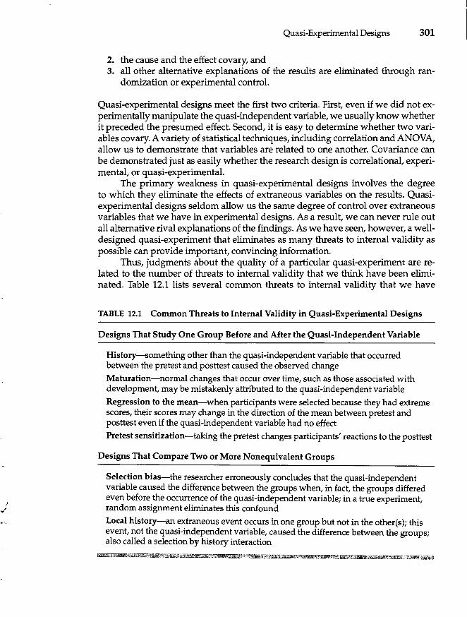
Quasi-Experimental Designs 301

2. the cause and the effect covary, and 3. all other alternative explanations of the results are eliminated through ran­

domization or experimental control.

Quasi-experimental designs meet the first two criteria. First, even if we did not ex­perimentally manipulate the quasi-independent variable, we usually know whether it preceded the presumed effect. Second, it is easy to determine whether two vari­ables covary. A variety of statistical techniques, including correlation and ANOVA, allow us to demonstrate that variables are related to one another. Covariance can be demonstrated just as easily whether the research design is correlational, experi­mental, or quasi-experimental.

The primary weakness in quasi-experimental designs involves the degree to which they eliminate the effects of extraneous variables on the results. Quasi­experimental designs seldom allow us the same degree of control over extraneous variables that we have in experimental designs. As a result, we can never rule out all alternative rival explanations of the findings. As we have seen, however, a well­deSigned quasi-experiment that eliminates as many threats to internal validity as possible can provide important, convincing information.

Thus, judgments about the quality of a particular quasi-experiment are re­lated to the number of threats to internal validity that we think have been elimi­nated. Table 12.1 lists several common threats to internal validity that we have

TABLE 12.1 Common Threats to Internal Validity in Quasi-Experimental Designs

Designs That Study One Group Before and After the Quasi-Independent Variable

History-something other than the quasi-independent variable that occurred between the pretest and posttest caused the observed change Maturation-normal changes that occur over time, such as those associated with development, may be mistakenly attributed to the quasi-independent variable

Regression to the mean-when participants were selected because they had extreme scores, their scores may change in the direction of the mean between pretest and posttest even if the quasi-independent variable had no effect

Pretest sensitization-taking the pretest changes participants' reactions to the posttest

Designs That Compare Two or More Nonequivalent Groups

Selection bias-the researcher erroneously concludes that the quasi-independent variable caused the difference between the groups when, in fact, the groups differed even before the occurrence of the quasi-independent variable; in a true experiment, random assignment eliminates this confound

Local history-an extraneous event occurs in one group but not in the other(s); this event, not the quasi-independent variable, caused the difference between the groups; also called a selection by history interaction

302 CHAPTER 12

mentioned in this chapter. Some of these threats arise when we look at the effect of a quasi-independent variable on changes in the behavior of a single group of par­ticipants; others occur when we compare one group of participants to another.

Increasing Confidence in Quasi-Experimental Results

Because they do not have enough control over the environment to structure the research setting precisely as they would like, researchers who use quasi­experimentation adopt a pragmatic approach to research-one that attempts to collect the most meaningful data under circumstances that are often less than ideal (Condray, 1986). The best quasi-experiments are those in which the researcher uses whatever procedures are available to devise a reasonable test of the research hypotheses. Thus, rather than adhering blindly to one particular design, quasi­experimentalists creatively "patch up" basic designs to provide the most meaning­ful and convincing data possible.

Thus, researchers often measure not only the effects of the quasi-independent variable on the outcome behavior but also assess the processes that are assumed to mediate their relationship. In many cases, simply showing that a particular quasi­independent variable was associated with changes in the dependent variable may not convince us that the quasi-independent variable itself caused the dependent variable to change. However, if the researcher can also demonstrate that the quasi­independent variable was associated with changes in processes assumed to medi­ate the change in the dependent variable, more confidence is warranted.

For example, rather than simply measuring students' drug use to evaluate the effects of a school's antidrug campaign, a researcher might also measure other vari­ables that should mediate changes in drug use, such as students' knowledge about and attitudes toward drugs. Unlike some extraneous events (such as searches of students' lockers by school authorities), the program should affect not only drug use but also knowledge and attitudes about drugs. Thus, if changes in knowledge and attitudes are observed at the experimental school (but not at a nonequivalent control school), the researcher has more confidence that the drug education pro­gram, and not other factors, produced the change.

By patching up basic quasi-experimental designs with additional quasi­independent variables, comparison groups, and dependent measures, researchers increase their confidence in the inferences they draw about the causal link between the quasi-independent and dependent variables. Such patched-up designs are inele­gant and may not conform to any formal design shown in research methods books, but they epitomize the way scientists can structure their collection of data to draw the most accurate conclusions possible (Condray, 1986). Researchers should never hesitate to invent creative strategies for analyzing whatever problem is at hand.

As I have mentioned previously, our confidence in the conclusions we draw from research comes not only from the fact that a particular experiment was tightly designed but also from seeing that the accumulated results of several different studies demonstrate the same general effect. Thus, rather than reaching conclu­sions on the basis of a single study, researchers often piece together many strands of information that were accumulated by a variety of methods, much the way Sher-

I •

/

Quasi-Experimental Designs 303

lock Holmes would piece together evidence in breaking a case (Condray, 1986). For example, although the results of a single quaSi-experimental investigation of a drug education program at 1 school may be open to criticism, demonstrating the effects of the program at 5 or 10 schools gives us considerable confidence in con­cluding that the program was effective.

Because our confidence about causal relationships increases as we integrate many diverse pieces of evidence, quasi-experimentation is enhanced by critical multiplism (Shadish, Cook, & Houts, 1986). The critical multiplist perspective ar­gues that researchers should critically consider many ways of obtaining evidence relevant to a particular hypothesis, then employ several different approaches. In quasi-experimental research, no single research approach can yield unequivocal conclusions. However, evidence from multiple approaches may converge to yield conclusions that are as concrete as those obtained in experimental research. Like a game of chess in which each piece has its strengths and weaknesses and in which no piece can win the game alone, quasi-experimentation requires the coordination of several different kinds of research strategies (Shadish et al., 1986). Although any sin­gle piece of evidence may be suspect, the accumulated results may be quite con­vincing. Therefore, do not fall into the trap of thinking that the data provided by quasi-experimental designs are worthless. Rather, simply interpret such data gen­erally with greater caution.

Summary

1. Many important research questions are not easily answered using true ex­perimental designs. Quasi-experimental designs are used when researchers cannot control the assignment of participants to conditions or cannot manip­ulate the independent variable. Instead, comparisons are made between people in groups that already exist or within one or more existing groups of participants before and after a quasi-independent variable has occurred.

2. The quality of a quasi-experimental design depends on its ability to minimize threats to internal validity.

3. One-group pretest-posttest designs possess little internal validity and should never be used.

4. In the nonequivalent control group designs, an experimental group that re­ceives the quasi-independent variable is compared with a nonequivalent comparison group that does not receive the quasi-independent variable. The effectiveness of this design depends on the degree to which the groups can be assumed to be equivalent and the degree to which local history effects can be discounted.

5. In time series designs, one or more groups are measured on several occasions both before and after the quasi-experimental variable is introduced.

6. Longitudinal designs examine changes in behavior over time, essentially treating time as the quasi-independent variable.

7. Although quasi-experimental designs do not allow the same degree of certainty about cause-and-effect relationships as an experiment does, a well-designed

304 CHAPTER 12

quasi-experiment can provide convincing circumstantial evidence regarding the effects of one variable on another.

KEY TERMS

contemporary history (p. 291) critical multiplism (p. 303) cross-sectional design (p. 296) experimental contamination

nonequivalent control group design (p. 286)

nonequivalent groups posttest­only design (p. 286)

nonequivalent groups pretest-posttest design (p.288)

quasi-experimental design (p.283)

quasi-independent variable (p.283)

(p.287) generational effects (p. 297) interrupted time series design

with a reversal (p. 294) interrupted time series design

with multiple replications (p.295)

one-group pretest-posttest design (p. 285)

preexperimental design (p.286)

regression to the mean (p. 285) selection bias (p. 287) selection-by-history

interaction (p. 289) simple interrupted time series

design (p. 291) time series design (p. 291)

local history effect (p. 288) longitudinal design (p. 296)

program evaluation (p. 298)

QUESTIONS FOR REVIEW

1. How do quasi-experimental designs differ from true experiments?

2. Under what circumstances would a researcher use a quasi-experimental rather than an experimental design?

3. Why should researchers never use the one-group pretest-posttest design?

4. What threats to internal validity are present when the nonequivalent control group posttest-only design is used? Which of these threats are eliminated by the pretest­posttest version of this design?

5. What is experimental contamination?

6. Does a nonequivalent groups pretest-posttest design eliminate local history as a potential explanation of the results? Explain.

7. Explain the rationale behind time series designs.

8. Describe the simple interrupted time series design.

9. Why is contemporary history a threat to internal validity in a simple interrupted time series design?

10. Discuss how the interrupted time series design with a reversal and the interrupted time series design with multiple replications improve on the simple interrupted time series design.

11. Distinguish between a longitudinal design and a cross-sectional design. -'

Quasi-Experimental Designs 305

12. When a longitudinal design reveals a change in behavior over time, why can we not conclude that the change is due to development?

13. What are generational effects, and why do they sometimes create a problem in cross-sectional designs?

14. What is program evaluation? Why do program evaluators rely heavily on quasi­experimental designs in their work?

15. What were some of Donald Campbell's contributions to behavioral research?

16. What three criteria must be met to establish that one variable causes changes in be­havior? Which of these criteria are met by quasi-experimental designs? Which of these criteria are not met, and why?

17. Why does quasi-experimentation sometimes require the use of "patched-up" designs?

18. Discuss the philosophy of critical multiplism as it applies to quasi-experimental research.

QUESTIONS FOR DISCUSSION

1. Although quasi-experimental designs are widely accepted in behavioral science, some researchers are troubled by the fact that the evidence provided by quasi­experiments is seldom as conclusive as that provided by true experiments. Imagine you are trying to convince a dubious experimentalist of the merits of quasi­experimental research. What arguments would you use to convince him or her of its value?

2. Imagine that your town or city has increased its nighttime police patrols to reduce crime. Design two quasi-experiments to determine whether this intervention has been effective, one that uses some variation of a nonequivalent control group de­sign and one that uses some variation of a time series design. For each design, dis­cuss the possible threats to internal validity, as well as the ways in which the design could be patched up to provide more conclusive evidence.

3. The Centers for Disease Control and Prevention released a report in 1998 that at­tributed part of the increase in youth smoking in the 1980s to the use of the cartoon character, Joe Camel, in cigarette advertising. Using annual data going back to 1965, the report showed that the number of people under the age of 18 who started smok­ing increased markedly in 1988, the same year that Joe Camel first appeared in to­bacco ads ("Daily Smoking by Teens Has Risen Sharply," 1998). a. What kind of a quasi-experimental design was used in this study? b. What potential threats to internal validity are present in this design? c. From these data, how confident are you that Joe Camel was responsible for in­

creases in youth smoking?

CHAPTER

13 Single-Case Research

Single-Case Experimental Designs Case Study Research

306

When I describe the results of a particular study to my students, they sometimes respond to the findings by pointing out exceptions. "That study can't be right," they object. "I have a friend (brother, aunt, roommate, or whomever) who does just the opposite." For example, if I tell my class that first-born children tend to be more achievement-oriented than later-born children, I can count on some student say­ing, "No way. I'm the third-born in my family, and I'm much more achievement­oriented than my older brothers." If I mention a study showing that anxiety causes people to prefer to be with other people, someone may retort, "But my roommate withdraws from people when she's anxious."

What such responses indicate is that many people do not understand the probabilistic nature of behavioral science. Our research uncovers generalities and trends, but we can nearly always find exceptions to the general pattern. Overall, achievement motivation declines slightly with birth order, but not every first-born child is more achievement-oriented than his or her younger siblings. Overall, people tend to seek out the company of other people when they are anxious or afraid, but some people prefer to be left alone when they are upset.

Behavioral science is not unique in this regard. Many of the principles and findings of all sciences are probabilities. For example, when medical researchers state that excessive exposure to the sun causes skin cancer, they do not mean that every person who suntans will get cancer. Rather, they mean that more people in a group of regular suntanners will get skin cancer than in an equivalent group of people who avoid the sun. Suntanning and skin cancer are related in a probabilis­tic fashion, but there will always be exceptions to the general finding. But these ex­ceptions do not violate the general finding that, overall, people who spend more time in the sun are more likely to get skin cancer than people who don't.

Although specific exceptions do not invalidate the findings of a particular study, these apparent contradictions between general findings and specific cases

,

) >

Single-Case Research 307

raise an important point for researchers to consider. Whenever we obtain a general finding based on a large number of participants, we must recognize that the effect we obtained is unlikely to be true of everybody in the world or even of every par­ticipant in the sample under study. We may find large differences between the av­erage responses of participants in various experimental conditions, for example, even if the independent variable affected the behavior of only some of our partici­pants. This point has led some to suggest that researchers should pay more atten­tion to the behavior of individual participants.

Since the earliest days of behavioral science, researchers have debated the merits of a nomothetic versus idiographic approach to understanding behavior. Most researchers view the scientific enterprise as an inherently nomothetic ap­proach, seeking to establish general principles and broad generalizations that apply across individuals. However, as we have seen, these general principles do not always apply to everyone. As a result, some researchers have argued that the nomothetic approach must be accompanied by an idiographic approach (see, for example, Allport, 1961). Idiographic research seeks to describe, analyze, and com­pare the behavior of individual participants. According to proponents of the idiogra­phic approach, behavioral scientists should focus not only on general trends-the behavior of the "average" participant-but also on the unique behaviors of specific individuals.

An emphasis on the study of single organisms has been championed by two quite different groups of behavioral researchers with different interests and orienta­tions. On one hand, some experimental psychologists interested in basic psycholog­ical processes have advocated the use of single-case (or single-subject) experimental designs. As we will see, these are designs in which researchers manipulate indepen­dent variables and exercise strong experimental control over extraneous variables, then analyze the behavior of individual participants rather than grouped data.

On the other hand, other researchers have advocated the use of case studies in which the behavior and personality of a single individual or group are described in detail. Unlike single-case experiments, case studies usually involve uncontrolled impressionistic descriptions rather than controlled experimentation. Case studies have been used most widely in clinical psychology, psychiatry, and other fields that specialize in the treatment of individual problems.

CONTRIBUTORS TO BEHAVIORAL RESEARCH

Single-Case Researchers Single-case research-whether Single-case experiments or case studies-has had a long and distinguished history in behavioral science. In fact, in the early days of behavioral science, it was common practice to study only one or a few participants. Only after the 1930s did re­searchers begin to rely on larger sample sizes, as most researchers do today (Boring, 1954; Robinson & Foster, 1979).

Many advances in behavioral science came from the study of single individuals in controlled experimental settings. Ebbinghaus, who began the scientific study of memory,

308 CHAPTER 13

conducted his studies on a single individual (himself). Stratton, an early researcher in per­ception, also used himself as a participant as he studied the effects of wearing glasses that reversed the world from left to right and top to bottom. (He soon learned to function quite normally in his reversed and inverted environment.) Many seminal ideas regarding condi­tioning were discovered and tested in single-case experiments; notably, both Pavlov and Skinner used single-case experimental designs. Many advances in psychophysiology, such as Sperry's (1975) work on split-brain patients, have come from the study of individuals un­dergoing brain surgery.

Case studies, often taken from clinical practice, have also contributed to the develop­ment of ideas in behavioral science. Kraepelin, who developed an early classification system of mental disorders that was the forerunner to the psychiatric system still used today, based his system on case studies (Garmezy, 1982). Most of the seminal ideas of Freud, Jung, Adler, and other early personality theorists were based on case studies. In developmental psychol­ogy, Piaget used case studies of children in developing his influential ideas about cognitive development. Case studies of groups have also been used by social psychologists, as in Fes­tinger's study of a group that expected the world to end.

Thus, although single-case research is less common than research that involves groups of participants, such studies have had a long and distinguished tradition in behavioral science.

Despite the fact that many noted behavioral researchers have used single­case approaches, single-case research has a mixed reputation in contemporary psy­chology. Some researchers insist that research involving the study of individuals is essential for the advancement of behavioral science, whereas other researchers see such approaches as having limited usefulness. In this chapter, we explore the ra­tionale behind these two varieties of single-case research, along with the advan­tages and limitations of each.

Single-Case Experimental Designs

In each of the experimental and quasi-experimental designs we have discussed so far, researchers assess the effects of variables on behavior by comparing the average responses of two or more groups of participants. In these designs, the unit of analy­sis is always grouped data. In fact, in analyzing the data obtained from these de­signs, information about the responses of individual participants is usually ignored.

Group designs, such as those we have been discussing, reflect the most com­mon approach to research in behavioral science. Most experiments and quasi­experiments conducted by behavioral scientists involve group designs. Even so, group designs have their critics, some as notable as the late B. F. Skinner, who offer an alternative approach to experimental research.

In the single-case experimental design, the unit of analysis is not the experi­mental group, as it is in group designs, but rather the individual participant. Often, more than one participant is studied (typically 3--8), but each participant's responses

, .... ,

/

Single-Case Research 309

are analyzed separately and the data from individual participants are rarely aver­aged. Because averages are not used, the data from single-participant experiments cannot be analyzed using inferential statistics such as t-tests and F-tests.

At first, the single-participant approach may strike you as an odd, if not inef­fective, way to conduct and analyze behavioral research. However, before you pass judgment, let's examine several criticisms of group experiments and how they may be resolved by using single-participant designs.

Criticisms of Group Designs and Analyses

Proponents of single-participant designs have suggested that group experimental designs fail to adequately handle three important research issues-error variance, generality, and reliability.

Error Variance. We saw earlier that all data contain error variance, which reflects the influence from unidentified factors that affect participants' responses in an un­systematic fashion. We also learned that researchers must minimize error variance because error variance masks the effects of the independent variable (see Chapter 8).

Group experimental deSigns, such as those we discussed in earlier chapters, provide two partial solutions to the problem of error variance. First, although the responses of any particular participant are contaminated by error variance in un­known ways, averaging the responses of several participants should provide a more accurate estimate of the typical effect of the independent variable. In essence, many idiosyncratic sources of error variance cancel each other out when we calcu­late a group mean. Presumably, then, the mean for a group of participants is a bet­ter estimate of the typical participant's response to the independent variable than the score of any particular participant.

Second, by using groups of participants we can estimate the amount of error variance in our data. This is what we did when we calculated the denominator of t-tests and F-tests (see Chapters 10 and 11). With this estimate, we can test whether the differences among the means of the groups are greater than we would expect if the differences were due only to error variance. Indeed, the purpose of using infer­ential statistics is to separate error variance from systematic variance to determine whether the differences among the group means are likely due to the independent variable or only to error variance.

Although group data provide these two benefits, proponents of single­participant designs criticize the way group designs and inferential statistics handle error variance. They argue that, first, much of the error variance in group data does not reflect variability in behavior per se but rather is created by the group design it­self, and second, researchers who use group designs accept the presence of error variance too blithely.

As we noted earlier, much of the error variance in a set of data is due to in­dividual differences among the participants. However, in one sense, this inter­participant variance is not the kind of variability that behavioral researchers are usually trying to understand and explain. Error variance resulting from individual

310 CHAPTER 13

differences among participants is an artificial creation of the fact that, in group de­signs, we pool the responses of many participants.

Single-participant researchers emphasize the importance of studying intra­participant variance-variability in an individual's behavior when he or she is in the same situation on different occasions. This is true behavioral variability that demands our attention. What we typically call error variance is, in one sense, partly a product of individual differences rather than real variations in a participant's behavior.

Because data are not aggregated across participants in single-participant re­search, individual differences do not contribute to error variance. Error variance in a single-participant design shows up when a particular participant responds dif­ferently under various administrations of the same experimental condition.

Most researchers who use group designs ignore the fact that their data con­tain a considerable amount of error variance. Ignoring error variance is, for single­participant researchers, tantamount to being content with sloppy experimental design and one's ignorance (Sidman, 1960). After all, error variance is the result of factors that have remained unidentified and uncontrolled by the researcher. Pro­ponents of single-participant designs maintain that, rather than accepting error variance, researchers should design studies in a way that allows them to seek out its causes and eliminate them. Through tighter and tighter experimental control, more and more intraparticipant error variance can be eliminated. And in the pro­cess, we can learn more and more about the factors that influence behavior.

Generality. In the eyes of researchers who use group designs, averaging across participants serves an important purpose. By pooling the scores of several partici­pants, the researcher minimizes the impact of the idiosyncratic responses of any particular participant. They hope that by doing so they can identify the general, overall effect of the independent variable, an effect that should generalize to most of the participants most of the time.

In contrast, single-participant researchers argue that the data from group de­signs do not permit us to identify the general effect of the independent variable as many researchers suppose. Rather than reflecting the typical effect of the indepen­dent variable on the average participant, results from group designs represent an average of many individuals' responses that may not accurately portray the re­sponse of any particular participant. Consider, for example, the finding that Amer­icans are having an average of 2.1 children. Although we all understand what this statistic tells us about childbearing in this country, personally, I don't know any family that has 2.1 kids.

Given that group averages may not represent any particular participant's re­sponse, attempts to generalize from overall group results may be misleading. Put differently, group means may have no counterpart in the behavior of individual participants (Sidman, 1960). This point is demonstrated in the accompanying box, "How Group Data Misled Us About Learning Curves."

In addition, exclusive reliance on group summary statistics may obscure the fact that the independent variable affected the behavior of some participants but had no effect (or even opposite effects) on other participants. Researchers who use

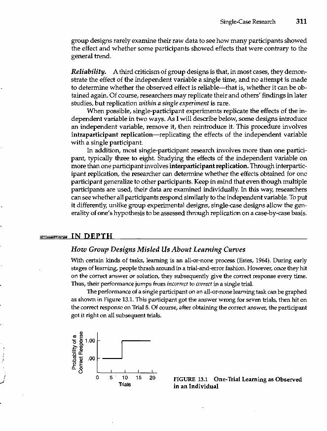
I

)

Single-Case Research 311

group designs rarely examine their raw data to see how many participants showed the effect and whether some participants showed effects that were contrary to the general trend.

Reliability. A third criticism of group designs is that, in most cases, they demon­strate the effect of the independent variable a single time, and no attempt is made to determine whether the observed effect is reliable-that is, whether it can be ob­tained again. Of course, researchers may replicate their and others' findings in later studies, but replication within a single experiment is rare.

When possible, single-participant experiments replicate the effects of the in­dependent variable in two ways. As I will describe below, some designs introduce an independent variable, remove it, then reintroduce it. This procedure involves intraparticipant replication-replicating the effects of the independent variable with a single participant.

In addition, most single-participant research involves more than one partici­pant, typically three to eight. Studying the effects of the independent variable on more than one participant involves interparticipant replication. Through interpartic­ipant replication, the researcher can determine whether the effects obtained for one participant generalize to other participants. Keep in mind that even though multiple participants are used, their data are examined individually. In this way, researchers can see whether all participants respond similarly to the independent variable. To put it differently, unlike group experimental designs, single-case designs allow the gen­erality of one's hypothesis to be assessed through replication on a case-by-case basis.

rim 1m IN DEPTH

How Group Designs Misled Us About Learning Curves

With certain kinds of tasks, learning is an all-or-none process (Estes, 1964). During early stages of learning, people thrash around in a trial-and-error fashion. However, once they hit on the correct answer or solution, they subsequently give the correct response every time. Thus, their performance jumps from incorrect to correct in a single trial.

The performance of a single participant on an all-or-none learning task can be graphed as shown in Figure 13.1. This participant got the answer wrong for seven trials, then hit on the correct response on Trial 8. Of course, after obtaining the correct answer, the participant got it right on all subsequent trials.

(I) as <IJ

'0 51.00 ~fE =(1) :0 a: 1l t5 .00 e ~ a. 0

()

o 5 10 15 20 Trials

FIGURE 13.1 One-Trial Learning as Observed in an Individual

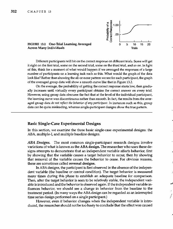
312 CHAPTER 13

FIGURE 13.2 One-Trial Learning Averaged Across Many Individuals

CI) as IIJ

'5 § 1.00 ~g. :a~ ~ ~ ,DO e ... a. 5

u o 5 10 15 20

Trials

Different participants will hit on the correct response on different trials. Some will get it right on the first trial, some on the second trial, some on the third trial, and so on. In light of this, think for a moment of what would happen if we averaged the responses of a large number of participants on a learning task such as this. What would the graph of the data look like? Rather than showing the all-or-none pattern we see for each participant, the graph of the averaged group data will show a smooth curve like that in Figure 13.2.

On the average, the probability of getting the correct response starts low, then gradu­ally increases until virtually every participant obtains the correct answer on every trial. However, using group data obscures the fact that at the level of the individual participant, the learning curve was discontinuous rather than smooth. In fact, the results from the aver­aged group data do not reflect the behavior of any participant. In instances such as this, group data can be quite misleading, whereas single-participant designs show the true pattern.

Basic Single-Case Experimental Designs

In this section, we examine the three basic single-case experimental designs: the ABA, multiple-I, and multiple baseline designs.

ABA Designs. The most common single-participant research designs involve variations of what is known as the ABA design. The researcher who uses these de­signs attempts to demonstrate that an independent variable affects behavior, first by showing that the variable causes a target behavior to occur, then by showing that removal of the variable causes the behavior to cease. For obvious reasons, these are sometimes called reversal designs.

In ABA designs, the participant is first observed in the absence of the indepen­dent variable (the baseline or control condition). The target behavior is measured many times during this phase to establish an adequate baseline for comparison. Then, after the target behavior is seen to be relatively stable, the independent vari­able is introduced and the behavior is observed again. If the independent variable in­fluences behavior, we should see a change in behavior from the baseline to the treatment period. (In many ways the ABA design can be regarded as an interrupted time series design performed on a single participant.)

However, even if behavior changes when the independent variable is intro­duced, the researcher should not be too hasty to conclude that the effect was caused

/

Single-Case Research 313

by the independent variable. Just as in the time series designs we discussed in Chapter 12, some other event occurring at the same time as the treatment could have produced the observed effect. To reduce this possibility, the independent vari­able is then withdrawn. If the independent variable is in fact maintaining the be­havior, the behavior may return to its baseline level. The researcher can further increase his or her confidence that the observed behavioral changes were due to the independent variable by replicating the study with other participants.

The design just described is an example of an ABA design, the Simplest single­participant design. In this design, A represents a baseline period in which the inde­pendent variable is not present, and B represents an experimental period. So, the ABA design involves a baseline period (A), followed by introduction of the inde­pendent variable (B), followed by the reversal period in which the independent variable is removed (A). Many variations and elaborations of the basic ABA design are possible. To increase our confidence that the changes in behavior were due to the independent variable, a researcher may decide to introduce the same level of the in­dependent variable a second time. This design would be labeled an ABAB design.

Deitz (1977) used an ABAB design to examine the effects of teacher reinforce­ment on the disruptive behavior of a student in a special education class. To reduce the frequency with which this student disrupted class by talking out loud, the teacher made a contract with the student, saying that she would spend 15 minutes with him after class (something he valued) if he talked aloud no more than 3 times during the class. Baseline data showed that, before the treatment program started, the student talked aloud between 30 and 40 times per day. The reinforcement pro­gram was then begun, and the rate of disruptive behavior dropped quickly to 10 outbursts, then to 3 or fewer (see Figure 13.3). When the reinforcement program was withdrawn, the number of outbursts increased, although not to their original level. Then, when it was reinstated, the student virtually stopped disrupting class. These data provide rather convincing evidence that the intervention was success­ful in modifying the student's behavior.

Logically, a researcher could reintroduce then remove a level of the indepen­dent variable again and again, as in an ABABABA or ABABABABA design. Each successive intraparticipant replication of the effect increases our confidence that the independent variable is causing the observed effects. In many instances, how­ever, the independent variable produces permanent changes in participants' behav­ior, changes that do not reverse when the independent variable is removed. When this happens, a single participant's data do not unequivocally show whether the initial change was due to the independent variable or to some extraneous variable that occurred at the same time. However, if the same pattern is obtained for other participants, we have considerable confidence that the observed effects were due to the independent variable.

Multiple-I Designs. ABA-type designs compare behavior in the absence of the independent variable (during A) with behavior in the presence of a nonzero level of an independent variable (during B). However, other Single-participant designs test differences among levels of an independent variable. Single-case experimental

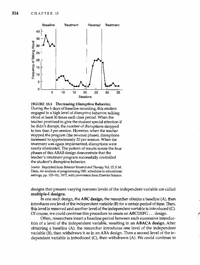
314 CHAPTER 13

Baseline Treatment Reversal Treatment

40

35 "0 :::J

~ 30 Ol .525 ..I<: iii E 20 0 >. g 15 CD :::J

110

5

0 5 10 15 20 25 30 35

Sessions

FIGURE 13.3 Decreasing Disruptive Behavior. During the 6 days of baseline recording, this student engaged in a high level of disruptive behavior, talking aloud at least 30 times each class period. When the teacher promised to give the student special attention if he didn't disrupt, the number of disruptions dropped to less than 3 per session. However, when the teacher stopped the program (the reversal phase), disruptions increased to approximately 20 per session. When the treatment was again implemented, disruptions were nearly eliminated. The pattern of results across the four phases of this ABAB design demonstrate that the teacher's treatment program successfully controlled the student's disruptive behavior. Source: Reprinted from Behavior Research and Therapy, Vol. 15, S. M. Dietz, An analysis of programming DRL schedules in educational settings, pp. 103-111, 1977, with permission from Elsevier Science.

designs that present varying nonzero levels of the independent variable are called multiple-I designs.

In one such design, the ABC design, the researcher obtains a baseline (A), then introduces one level of the independent variable (B) for a certain period of time. Then, this level is removed and another level of the independent variable is introduced (C). Of course, we could continue this procedure to create an ABCDEFG ... design.

Often, researchers insert a baseline period between each successive introduc­tion of a level of the independent variable, resulting in an ABACA design. After obtaining a baseline (A), the researcher introduces one level of the independent variable (B), then withdraws it as in an ABA design. Then a second level of the in­dependent variable is introduced (C), then withdrawn (A). We could continue to

Single-Case Research 315

manipulate the independent variable by introducing new levels of it, returning to baseline each time. Such designs are commonly used in research that investigates the effects of drugs on behavior. Participants are given different dosages of a drug, with baseline periods occurring between the successive dosages. In one such study, Dworkin, BirnIe, and Miyauchi (1989) tested the effects of cocaine on how rats react to punished and nonpunished responding. Over several days, four different dosages of cocaine were administered to five pairs of rats, with baseline sessions scheduled between each administration of the drug. While under the influence of the drug, one rat in each pair received punishment, whereas the other did not. (We'll return to the results of this experiment in a moment.)

Sometimes combinations of treatments are administered at each phase of the study. For example, Jones and Friman (1999) tested the separate and combined ef­fects of graduated exposure and reinforcement on a 14-year-old boy, Mike, who had been referred by his school principal because his class performance was severely disrupted by an insect phobia. Whenever he saw an insect in the classroom or his classmates teased him about bugs ("Mike, there's a bug under your chair"), Mike stopped working, pulled the hood of his jacket over his head, and started yelling. To begin, the researchers assessed Mike's ability to complete math problems under three baseline conditions-when he knew there were no bugs in the room, when the therapist told him there were bugs in the room (but he couldn't see any), and when three live crickets were released in the room. The baseline data showed that Mike could complete only about half as many problems when the crickets were loose than when the room was bug-free. After 10 baseline sessions, the therapists imple­mented a graduated exposure procedure in which Mike experienced a series of in­creasingly more difficult encounters with crickets until he could hold a cricket in each hand for 20 seconds. Interestingly, despite his increased courage with crickets, Mike's ability to complete math problems while insects were in the room did not improve during this phase. Then, as graduated exposure continued, the researchers also began to reward Mike with points for each correct math answer, points that he could trade for candy, toys, and other items. At that point, Mike's math performance with crickets loose in the room increased to the level he had shown initially when he knew no bugs were present. Then, a second baseline period was instituted for several sessions to see whether his math performance dropped. (It did, but only slightly.) When the combined treatment of graduated exposure and reinforcement was reinstituted, his math performance increased to an all-time high. The authors described this as a A-B-BC-A-BC design, where A was baseline, B was graduated ex­posure, and C was reinforcement.

Multiple Baseline Designs. As noted earlier, the effects of an independent vari­able do not always disappear when the variable is removed. For example, if a clin­ical psychologist teaches a client a new way to cope with stress, it is difficult to "unteach" it. When this is so, how can we be sure the obtained effects are due to the independent variable as opposed to some extraneous factor?

One way is to use a multiple baseline design. In a multiple baseline design, two or more behaviors are studied simultaneously. After obtaining baseline data on

316 CHAPTER 13

all behaviors, an independent variable is introduced that is hypothesized to affect only one of the behaviors. In this way, the selective effects of a variable on a specific behavior can be documented. By measuring several behaviors, the researcher can show that the independent variable caused the target behavior to change but did not affect other behaviors. If the effects of the independent variable can be shown to be specific to certain behaviors, the researcher has increased confidence that the obtained effects were, in fact, due to the independent variable.

Data from Single-Participant Designs

As we noted earlier, researchers who use single-participant designs resist analyz­ing their results in the forms of means, standard deviations, and other descriptive statistics based on group data. Furthermore, because they object to averaging data across participants, those who use such designs do not use statistics such as t-tests and F-tests to test whether the differences between experimental conditions are statistically significant.

The preferred method of presenting the data from single-participant designs is with graphs that show the results individually for each participant. Rather than testing the significance of the experimental effects, single-participant researchers employ graphic analysis (also known simply as visual inspection).

Put simply, the single-participant researcher judges whether the independent variable affected behavior by visually inspecting graphs of the data for individual participants. If the behavioral changes are pronounced enough to be discerned through a visual inspection of such graphs, the researcher concludes that the inde­pendent variable affected the participant's behavior. If the pattern is not clear enough to conclude that a behavioral change occurred, the researcher concludes that the independent variable did not have an effect.

Ideally, the researcher would like to obtain results like those shown in Fig­ure 13.4. As you can see in this ABA design, the behavior was relatively stable during the baseline period, changed quickly when the independent variable was introduced, then returned immediately to baseline when the independent variable was removed.

Unfortunately, the results are not always this clear-cut. Look, for example, at the data in Figure 13.5. During the baseline period, the participant'S responses were fluctuating somewhat. Thus, it is difficult to tell whether the independent variable caused a change in behavior during the treatment period, or whether the observed change was a random fluctuation such as those that occurred during baseline. (This is why single-participant researchers try to establish a stable base­line before introducing the independent variable.) Furthermore, when the inde­pendent variable was removed, the participant's behavior changed but did not return to the original baseline level. Did the independent variable cause changes in behavior? In the case of Figure 13.5, the answer to this question is uncertain.

Figure 13.6 shows the results from two participants in the study of the effects of cocaine on reactions to punishment described earlier (Dworkin et al., 1989). In the case of the Dworkin et al. study, graphic analysis revealed marked differences in -'

.!

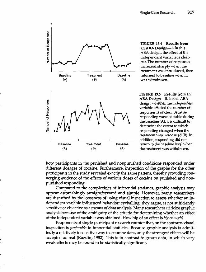
CIl CD CIl c: o a. CIl CD a: '5 CD ..c E :> z

:B CIl c: o a. :B a: '5 CD ..c E :> Z

Baseline (A)

Baseline (A)

Treatment (B)

Treatment (B)

Baseline (A)

Baseline (A)

Single-Case Research 317

FIGURE 13.4 Results from an ABA Design-I. In this ABA design, the effect of the independent variable is clear­cut. The number of responses increased sharply when the treatment was introduced, then returned to baseline when it was withdrawn.

FIGURE 13.5 Results from an ABA Design-II. In this ABA design, whether the independent variable affected the number of responses is unclear. Because responding was not stable during the baseline (A), it is difficult to determine the extent to which responding changed when the treatment was introduced (B). In addition, responding did not return to the baseline level when the treatment was withdrawn.

how participants in the punished and nonpunished conditions responded under different dosages of cocaine. Furthermore, inspection of the graphs for the other participants in the study revealed exactly the same pattern, thereby providing con­verging evidence of the effects of various doses of cocaine on punished and non­punished responding.

Compared to the complexities of inferential statistics, graphic analysis may appear astonishingly straightforward and simple. However, many researchers are disturbed by the looseness of using visual inspection to assess whether an in­dependent variable influenced behavior; eyeballing, they argue, is not sufficiently sensitive or objective as a means of data analysis. Many researchers criticize graphic analysis because of the ambiguity of the criteria for determining whether an effect of the independent variable was obtained. How big of an effect is big enough?

Proponents of single-participant research counter that, on the contrary, visual inspection is preferable to inferential statistics. Because graphic analysis is admit­tedlya relatively insensitive way to examine data, only the strongest effects will be accepted as real (Kazdin, 1982). This is in contrast to group data, in which very weak effects may be found to be statistically Significant.

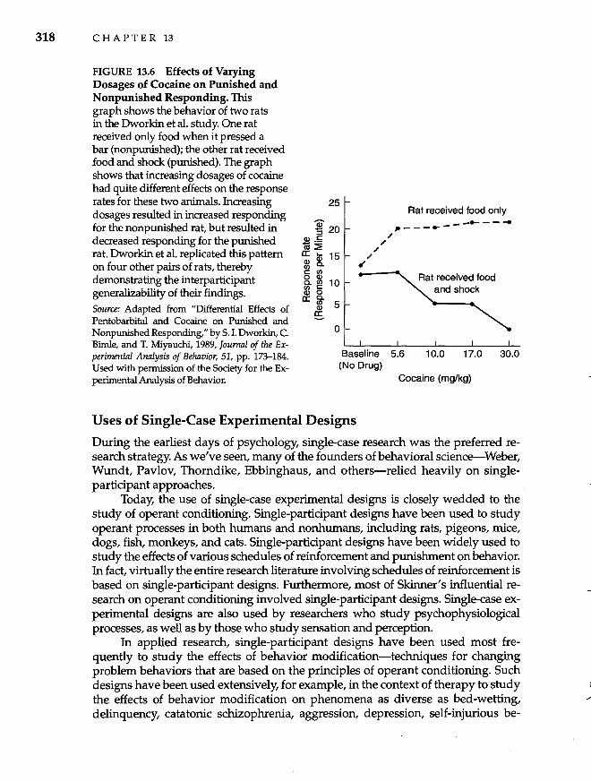
318 C HAP T E R 13

FIGURE 13.6 Effects of Varying Dosages of Cocaine on Punished and Nonpunished Responding. This graph shows the behavior of two rats in the Dworkin et al. study. One rat received only food when it pressed a bar (nonpunished); the other rat received food and shock (punished). The graph shows that increasing dosages of cocaine had quite different effects on the response rates for these two animals. Increasing dosages resulted in increased responding for the nonpunished rat, but resulted in decreased responding for the punished rat. Dworkin et aI. replicated this pattern on four other pairs of rats, thereby demonstrating the interparticipant generalizability of their findings. Source: Adapted from "Differential Effects of Pentobarbital and Cocaine on Punished and Nonpunished Responding," by S. 1. Dworkin, C. BirnIe, and T. Miyauchi, 1989, Journal of the Ex­perimental Analysis of Behavior, 51, pp. 173-184. Used with permission of the Society for the Ex­perimental Analysis of Behavior.

25

~ 20 CD .!: iii~

~ ~ 15 c: <J)

~ ~ 10 CD 0 a:g.

CD 5 1;.

o

,-

--

,­,­

,-

Rat received food only ---- .. --_ .... -- ....

Rat received food and shock

Baseline 5.6 (No Drug)

10.0 17.0 30.0

Cocaine (mg/kg)

Uses of Single-Case Experimental Designs

During the earliest days of psychology, single-case research was the preferred re­search strategy. As we've seen, many of the founders of behavioral science--Weber, Wundt, Pavlov, Thorndike, Ebbinghaus, and others-relied heavily on single­participant approaches.

Today, the use of single-case experimental designs is closely wedded to the study of operant conditioning. Single-participant designs have been used to study operant processes in both humans and nonhumans, including rats, pigeons, mice, dogs, fish, monkeys, and cats. Single-participant designs have been widely used to study the effects of various schedules of reinforcement and punishment on behavior. In fact, virtually the entire research literature involving schedules of reinforcement is based on single-participant designs. Furthermore, most of Skinner's influential re­search on operant conditioning involved single-participant designs. Single-case ex­perimental designs are also used by researchers who study psychophysiological processes, as well as by those who study sensation and perception.

In applied research, single-participant designs have been used most fre­quently to study the effects of behavior modification-techniques for changing problem behaviors that are based on the principles of operant conditioning. Such designs have been used extensively, for example, in the context of therapy to study the effects of behavior modification on phenomena as diverse as bed-wetting, delinquency, catatonic schizophrenia, aggression, depression, self-injurious be-

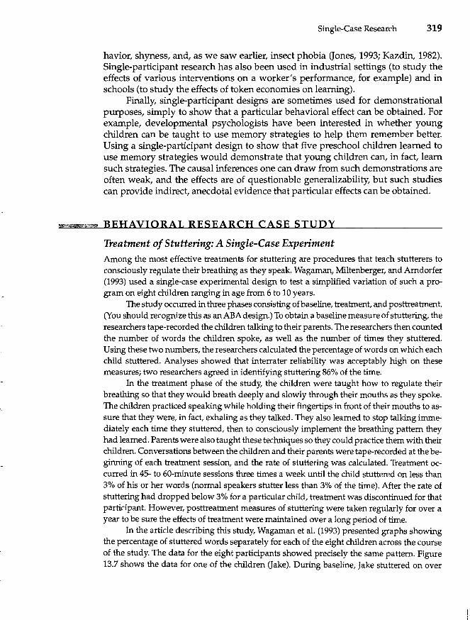
Single-Case Research 319

havior, shyness, and, as we saw earlier, insect phobia (Jones, 1993; Kazdin, 1982). Single-participant research has also been used in industrial settings (to Shldy the effects of various interventions on a worker's performance, for example) and in schools (to study the effects of token economies on learning).

Finally, single-participant designs are sometimes used for demonstrational purposes, simply to show that a particular behavioral effect can be obtained. For example, developmental psychologists have been interested in whether young children can be taught to use memory strategies to help them remember better. Using a single-participant design to show that five preschool children learned to use memory strategies would demonstrate that young children can, in fact, learn such strategies. The causal inferences one can draw from such demonstrations are often weak, and the effects are of questionable generalizability, but such studies can provide indirect, anecdotal evidence that particular effects can be obtained.

11M1MIWIi!Uap BEHAVIORAL RESEARCH CASE STUDY

Treatment of Stuttering: A Single-Case Experiment

Among the most effective treatments for stuttering are procedures that teach stutterers to consciously regulate their breathing as they speak. Wagaman, Miltenberger, and Arndorfer (1993) used a single-case experimental design to test a simplified variation of such a pro­gram on eight children ranging in age from 6 to 10 years.

The study occurred in three phases consisting of baseline, treatment, and posttreatment. (You should recognize this as an ABA design.) To obtain a baseline measure of stuttering, the researchers tape-recorded the children talking to their parents. The researchers then counted the number of words the children spoke, as well as the number of times they stuttered. Using these two numbers, the researchers calculated the percentage of words on which each child stuttered. Analyses showed that interrater reliability was acceptably high on these measures; two researchers agreed in identifying stuttering 86% of the time.

In the treatment phase of the study, the children were taught how to regulate their breathing so that they would breath deeply and slowly through their mouths as they spoke. The children practiced speaking while holding their fingertips in front of their mouths to as­sure that they were, in fact, exhaling as they talked. They also learned to stop talking imme­diately each time they stuttered, then to consciously implement the breathing pattern they had learned. Parents were also taught these techniques so they could practice them with their children. Conversations between the children and their parents were tape-recorded at the be­ginning of each treatment session, and the rate of stuttering was calculated. Treatment oc­curred in 45- to 60-minute sessions three times a week until the child stuttered on less than 3% of his or her words (normal speakers stutter less than 3% of the time). After the rate of stuttering had dropped below 3% for a particular child, treatment was discontinued for that participant. However, posttreatment measures of stuttering were taken regularly for over a year to be sure the effects of treatment were maintained over a long period of time.

In the article describing this study, Wagaman et al. (1993) presented graphs showing the percentage of stuttered words separately for each of the eight children across the course of the study. The data for the eight participants showed precisely the same pattern. Figure 13.7 shows the data for one of the children Gake). During baseline, Jake stuttered on over

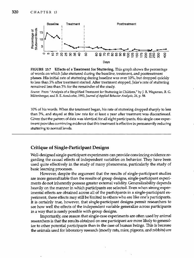
320 C HAP T E R 13

Baseline Treatment Posttreatment

01001001001001001001000 0 CD CD " " IX) IX) Ol Ol 0 C\I 10 " 0 C\I 10 0 0

,...,....,.... T"'" C\I (\IN (w) ~

Days

FIGURE 13.7 Effects of a Treatment for Stuttering. This graph shows the percentage of words on which Jake stuttered during the baseline, treatment, and posttreatment phases. His initial rate of stuttering during baseline was over 10%, but dropped quickly to less than 5% after treatment started. After treatment stopped, Jake's rate of stuttering remained less than 3% for the remainder of the study. Source: From "Analysis of a Simplified Treatment for Stuttering in Children," by J. R. Wagaman, R. G. Miltenberger, and R. E. Amdorfer, 1993, Journal of Applied Behavior Analysis, 26, p. 58.

10% of his words. When the treatment began, his rate of stuttering dropped sharply to less than 3%, and stayed at this low rate for at least a year after treatment was discontinued. Given that the pattern of data was identical for all eight participants, this single-case exper­iment provides convincing evidence that this treatment is effective in permanently reducing stuttering to normal levels.

Critique of Single-Participant Designs

Well-designed single-participant experiments can provide convincing evidence re­garding the causal effects of independent variables on behavior. They have been used quite effectively in the study of many phenomena, particularly the study of basic learning processes.

However, despite the argument that the results of single-participant studies are more generalizable than the results of group designs, single-participant experi­ments do not inherently possess greater external validity. Generalizability depends heavily on the manner in which participants are selected. Even when strong exper­imental effects are obtained across all of the participants in a single-participant ex­periment, these effects may still be limited to others who are like one's participants. It is certainly true, however, that single-participant designs permit researchers to see how well the effects of the independent variable generalize across participants in a way that is rarely possible with group designs.

Importantly, one reason that single-case experiments are often used by animal researchers is that the results obtained on one participant are more likely to general­ize to other potential participants than in the case of human beings. This is because the animals used for laboratory research (mostly rats, mice, pigeons, and rabbits) are

Single-Case Research 321

partially or fully inbred, thereby minimizing genetic variation. Furthermore, the par­ticipants used in a particular study are usually of the same age, have been raised in the same controlled environment, fed the same food, then tested under identical conditions. As a result, all possible participants are "clones or near-clones, both with respect to genetics and experiential history" (Denenberg, 1982, p. 21). Thus, unlike human research, in which the individual participants differ greatly (and in which one participant's response mayor may not resemble another's), the responses of only two or three nonhuman animals may be representative of many others.

One limitation of single-participant designs is that they are not well suited for studying interactions among variables. Although one could logically test a partici­pant under all possible combinations of the levels of two or more independent variables, such studies are often difficult to implement (see Kratochwill, 1978).

Finally, ethical issues sometimes arise when ABA designs are used to assess the effectiveness of clinical interventions. Is it ethical to withdraw a potentially helpful treatment from a troubled client to assure the researcher that the treatment was, in fact, effective? For example, we might be hesitant to withdraw the treat­ment that was introduced to reduce depression in a suicidal patient simply to con­vince ourselves that the treatment did, in fact, ameliorate the client's depression.

Case Study Research

We now tum our attention to a very different kind of single-case research-the case study. A case study is a detailed study of a single individual, group, or event. Within behavioral research, case studies have been most closely associated with clinical psychology, psychiatry, and other applied fields, where they are used to describe noteworthy cases of psychopathology or treatment. For example, a psycho­therapist may describe the case of a client who is a sociopath, or detail the therapist's efforts to use a particular treatment approach on a client who is afraid of thunder­storms. Similarly, psychobiographers have conducted psychological case studies of famous people, such as Jesus, Lincoln, and van Gogh (see Runyan, 1982).

Although case studies of individuals are most common, researchers some­times perform case studies of groups. For example, in his attempt to understand why groups sometimes make bad decisions, Janis (1982) conducted case studies of several political and military decision-making groups. Within educational research, studies are sometimes made of exemplary schools, with an eye toward understand­ing why these particular schools are so good (U.S. Department of Education, 1991). A great deal of social anthropology involves case studies of non-Western social groups, and ethologists have conducted case studies of troupes of baboons, chim­panzees, gorillas, and other nonhuman animals.

The data for case studies can come from a variety of sources, including ob­servation, interviews, questionnaires, news reports, and archival records (such as diaries, minutes of meetings, or school records). Typically, the researcher culls the available information together into a narrative description of the person, group, or event. In some instances, the researcher's subjective impressions are supplemented

322 C HAP T E R 13

by objective measures (such as measures of personality or behavior). The available information is then interpreted to explain how and why the individual or group under study behaved as it did, and conclusions, solutions, decisions, or recom­mendations are offered (Bromley, 1986).

Uses of the Case Study Method

Although used far less commonly by researchers than the other approaches we have examined, the case study method has at least four uses in behavioral research.

As a Source of Insights and Ideas. Perhaps the most important use of case stud­ies is as a source of ideas in the early stages of investigating a topic. (Doing an in­tensive case study was recommended as one approach to obtaining research ideas in Chapter 1.) Studying a few particular individuals in detail can provide a wealth of ideas for future investigation.

In fact, many seminal ideas in behavioral science emerged from intensive case studies of individuals or groups. For example, Freud's ideas emerged from his case studies of clients who came to him for therapy, and Piaget's ground-breaking work on cognitive development was based on the case studies he performed on his own children. Within social psychology, Janis' case studies of high-level decision-making groups paved the way for his theory of Groupthink, and Festinger's case study of a group who predicted the end of the world led to the theory of cognitive dissonance.

To Describe Rare Phenomena. Some behavioral phenomena occur so rarely that researchers are unlikely to obtain a large number of participants displaying the phenomenon for study. For example, if we were interested in the psychology of presidential assassins, we would be limited to case studies of the few people who have killed or tried to kill U.S. presidents (Weisz & Taylor, 1969). Similarly, studies of mass murderers require a case study approach. Luria (1987) used a case study approach to describe the life of a man who had nearly perfect memory-another rare phenomenon. Recently, Witelson, Kigar, and Harvey (1999) conducted an in­tensive case study of Einstein's brain. Although they found that Einstein's brain was no larger than average, one part of his parietal lobes was wider and uniquely structured when compared to those of 91 other individuals of normal intelligence. The literature in psychology and psychiatry contains many case studies of people with unusual psychological problems or abilities, such as multiple personalities, phobic reactions to dead birds, and "photographic memory."

Neuropsychologists, psychophysiologists, and neurologists sometimes conduct case studies of people who-because of unusual injuries, diseases, or surgeries-have sustained damage to their nervous systems. Although they would never purposefully damage people's brains or spinal cords, researchers sometimes take advantage of unusual opportunities to study the effects of brain trauma on personality and behavior.

Psychobiography. Psychobiography involves applying concepts and theories from psychology in an effort to understand the lives of famous people. Psychobi-

,\ ;

/

Single-Case Research 323

ographies have been written about many notable individuals, including Leonardo da Vmci (Freud's analysis of da Vmci is regarded as the first psychobiography), Mar­tin Luther, Mahatma Ghandi, Nathaniel Hawthorne, and Richard Nixon (McAdams, 1988). In some cases, the psychobiographer tries to explain the person's entire life, but in other instances, only specific aspects of the individual's behavior are studied. For example, Simonton (1998) used biographical and historical data to study the im­pact of stressful events on the mental and physical health of "Mad" King George ill between 1760 and 1811. His results showed that the king's health consistently deteri­orated following periods of increased stress after a nine-month delay.

Psychobiographies necessarily involve post hoc explanations, with no op­portunity to test one's hypotheses about why particular events occurred. Even so, biography has always involved speculations about psychological processes, usu­ally by writers who were not trained as psychologists. Even though interpretations of case study evidence are always open to debate, the systematic study of histori­cal figures from psychological perspectives adds a new dimension to biography and history.

Illustrative Anecdotes. Real, concrete examples often have more power than ab­stract statements of general principles. Researchers and teachers alike often use case studies to illustrate general principles to other researchers and to students. Although this use of case studies may seem of minor importance in behavioral science, we should remember that scientists must often convince others of the usefulness and importance of their findings. Supplementing "hard" empirical data with illustrative case studies may be valuable in this regard. Such case studies can never be offered as proof of a scientist's assertion, but they can be used to provide concrete, easy-to­remember examples of abstract concepts and processes.

Limitations of the Case Study Approach

Although the ca:se study approach has its uses, it also has noteworthy limitations as a scientific method.

Failure to Control Extraneous Variables. First, case studies are virtually use­less in providing evidence to test behavioral theories or psychological treatments. Because case studies deal with the informal observation of isolated events that occur in an uncontrolled fashion and without comparison information, researchers are unable to assess the viability of alternative explanations of their observations. No matter how plausible are the explanations offered for the individual's behavior or for the effectiveness of a given treatment, alternative explanations cannot be ruled out.

Too often, however, people use case studies as evidence for the accuracy of a particular explanation or for the effectiveness of a particular intervention. I re­cently heard on the radio that a particular member of Congress had spoken out against a proposal to tighten restrictions for the purchase of handguns. According to this member of Congress, such legislation was bound to be ineffective. His rea­soning was based on the case of Washington, D.C., a city that has relatively strict

324 C HAP T E R 13

handgun controls yet a very high murder rate. Clearly, he argued, the case of Wash­ington shows that gun controls do not reduce violent crime. Can you see the prob­lem with this argument?

His argument is based on case study evidence about a single city rather than on scientific data, and we have absolutely no way of knowing what the effect of handgun control is on the murder rate in Washington, D.C. Perhaps the murder rate would be even higher if there were no controls on the purchase of guns. For that matter, it's lOgically possible that the rate would be lower if there were gun control. The point is that, without relevant comparison information and control over other variables associated with murder (such as poverty and drug use), no conclusions about the effects of handgun control are possible from case study evidence.

Observer Biases. Most case studies rely on the observations of a single researcher. In behavioral science, the researcher is often the participant's psychotherapist. In light of this, we often have no way of determining the reliability or validity of the researcher's observations or interpretations. In addition, because the researcher­observer often has a stake in the outcome of the investigation (such as whether a therapeutic procedure works), we must worry about self-fulfilling prophecies and demand characteristics (see Chapter 8).

BEHAVIORAL RESEARCH CASE STUDY

A Case Study of a Case Study Case study approaches to research have been commonly used to describe particular cases of psychopathology or to document the effects of specific psychotherapeutic approaches. In many instances, case studies may be the only way to collect information about unusual phenomena.

Take, for example, the case of Jeffrey, a 28-year-old Israeli who developed posttraumatic stress disorder (PTSD) in the aftermath of a terrorist attack that left him seriously burned and disabled. PTSD is a prolonged psychological reaction to highly traumatic events, and is char­acterized by anxiety, irritability, withdrawal, insomnia, confusion, depression, and other signs of severe stress. Jeffrey's case was quite severe; he had stopped working, had isolated himself from family and friends, and had become depressed and withdrawn. In their case study ofJef­frey, Bar-Yoseph and Witztum (1992) first described Jeffrey's psychological and behavioral re­actions to the attack that nearly killed both his father and him 3 years earlier. They then presented their approach to helping Jeffrey overcome his problems through psychotherapy.

In the first phase of therapy, the primary goal was to establish a therapeutic relation­ship with Jeffrey. Because he was so depressed, withdrawn, and pessimistic about the prospect of getting better, the therapists proceeded slowly and carefully, focusing initially on only one of his problems (insomnia) rather than on all of them at once. Interestingly, because his symptoms did not emerge until a year after the attack (such a delay is common in PfSD), he continually refused to acknowledge that his problems were caused by the attack itself. After Jeffrey saw that he was improving, therapy entered a second phase. Week by week, the therapists encouraged Jeffrey to take up one activity that his physical injuries, depression, and apathy had led him to abandon after the attack. Thus, for the first time in 3 years, he

f )

I j

!

t J

Single-Case Research 325

began to mow the yard, go shopping, play soccer, and go to the hbrary. In the third phase of therapy, the therapists helped Jeffrey take yet another step toward psychological recovery­returning to full-time work. Although he had difficulty relating to his coworkers, he found he was again able to face the daily stresses of the working world. Even so, he continued to ago­nize over the fact that his life was not the way it had been before his problems began. As a re­sult, he viewed the positive changes that had occurred as a result of therapy as simply not good enough.

Along the way, Jeffrey continued to deny that the terrorist attack was the cause of his difficulties. For whatever reason, he found it too threatening to acknowledge that he was unable to cope with this particular misfortune. Believing that it was essential for Jeffrey to see the connection between the attack and his problems, the therapists tried a number of ap­proaches to show him the link. However, Jeffrey found such efforts too upsetting and in­sisted that the therapists stop. The therapists finally concluded that it was not in Jeffrey's best interests to force the issue further, and Jeffrey terminated treatment. Periodic follow­ups showed that, even 3 years later, Jeffrey had maintained the improvements he made dur­ing therapy, and he continued to get better.

After describing Jeffrey's case, Bar-Yoseph and Witztum (1992) discussed its implica­tions for understanding and treating PTSD. As we've seen, the conclusions that can be drawn from such studies are tenuous at best. Yet, a carefully documented case can provide other psychotherapists with novel approaches for their own practice, as well as generate hy­potheses to be investigated using controlled research strategies.

Summary

1. The principles and empirical findings of behavioral science are probabilistic in nature, describing the reactions of most individuals but recognizing that not everyone will fit the general pattern.

2. Single-case research comes in two basic varieties, single-case experimental designs and case studies, both of which can be traced to the earliest days of behavioral science.

3. Single-case experiments investigate the effects of independent variables on individual research participants. Unlike group designs, in which data are av­eraged across participants for analysis, each participant'S responses are ana­lyzed separately and the data from individual participants are not combined.

4. The most common single-participant designs, variations of the ABA design, involve a baseline period, followed by a period in which the independent variable is introduced. Then, the independent variable is withdrawn. More complex designs may involve several periods in which the independent vari­able is successively reintroduced, then withdrawn.

5. In multiple-I designs, several levels of the independent variable are adminis­tered in succession, often with a baseline period between each administration.

6. Multiple baseline designs allow researchers to document that the effects of the independent variable are specific to particular behaviors. Such designs

326 C HAP T E R 13

involve the simultaneous study of two or more behaviors, only one of which is hypothesized to be affected by the independent variable.

7. Because averages are not used, the data from single-participant experiments cannot be analyzed using inferential statistics. Rather, effects of the indepen­dent variable on behavior are detected through graphic analysis.

8. Single-case experiments are used most frequently to study the effects of basic learning processes and to study the effectiveness of behavior modification in treating behavioral and emotional problems.

9. A case study is a detailed, descriptive study of a single individual, group, or event. The case is described in detail, and conclusions, solutions, or recom­mendations are offered.

10. Case studies rarely allow a high degree of confidence in the researcher's in­terpretations of the data because extraneous variables are never controlled and the biases of the researcher may influence his or her observations and interpretations. Even so, case studies are useful in generating new ideas, studying rare phenomena, doing psychological studies of famous people (psychobiography), and serving as illustrative anecdotes.

KEY TERMS

ABA design (p. 312) ABACA design (p. 314) ABC design (p. 314) case study (p. 321) graphic analysis (p. 316) group design (p. 308) idiographic approach (p. 307) interparticipant replication

(p.311)

interparticipant variance (p.309)

intraparticipant replication (p.311)

intraparticipant variance (p.310)

multiple baseline design (p.315)

multiple-I design (p. 314)

QUESTIONS FOR REVIEW

narrative description (p.321)

nomothetic approach (p.307)

psychobiography (p. 322) reversal design (p. 312) single-case experimental

design (p. 308)

1. Distinguish between the nomothetic and idiographic approaches to behavioral science.

2. What criticisms do proponents of single-case experimental designs level against group designs?

3. Is the use of single-case studies a new approach to research in psychology? Explain.

4. Why do single-case researchers believe that the data from individual participants should not be combined, as when we compute a group mean?

5. What is the difference between interparticipant and intraparticipant variance? Which of these types of variance is more closely related to error variance in group

/ , ,

Single-Case Research 327

experimental designs? Which type is of primary interest to researchers who con­duct single-case experiments?

6. Researchers who use group designs replicate their findings by repeating the same (or a similar) experiment on other samples of participants. How do single-case re­searchers replicate their findings?

7. What is the rationale behind the ABA design?

8. Why is it essential for researchers to establish a stable baseline of behavior during the initial A phase of an ABA design?

9. Under what circumstances is an ABA design relatively useless as a way of testing the effects of an independent variable?

10. Can single-case experimental designs be used to test the effects of various levels of an independent variable (as in a one-way group design)? Explain.

11. How many levels of the independent variable are there in an ABACADA design?

12. What is a multiple baseline design, and when are such designs typically used?

13. How do researchers analyze the data from single-case experiments?

14. In what areas have single-case experiments been primarily used?

15. Discuss the advantages and disadvantages of single-case experimental designs, rel­ative to group designs.

16. What is a case study? Are case studies an example of descriptive, correlational, ex-perimental, or quasi-experimental research?

17. What are four primary reasons that behavioral researchers use case studies?

18. What is a psychobiography?

19. Why are behavioral scientists reluctant to trust case studies as a means of testing hypotheses?

QUESTIONS FOR DISCUSSION

1. Single-case experiments are controversial. Many researchers argue that they are the preferred method of experimental research, but others reject them as being of limited usefulness. Write a paragraph arguing in favor of single-case experiments. Then write a paragraph arguing against their usefulness.

2. How researchers feel about single-case experiments appears to stem, in part, from their personal areas of expertise. Single-case experimental designs lend themselves well to certain areas of investigation, whereas they are difficult, if not impossible, to implement in other areas. What do you see as some topics in behavioral science for which single-case designs might be most useful? What are some topics for which such designs would be difficult or impossible to use, and why? Are there topics for which group and single-case designs would be equally appropriate?

328 C HAP T E R 13

3. Locate a published experiment that used a group design, and redesign it, if possi­ble, using a single-case approach. Remember that many group designs do not con­vert easily to single-case experiments.

4. Locate a published experiment that used a single-case design (the Journal of Applied Behavior Analysis is a particularly good source of such studies). Redesign the exper­iment, if possible, as a group experimental design.

s. Conduct a psychobiography of someone you know well. Select a life choice the per­son has made (such as whom to date or marry, where to attend school, or what ca­reer to pursue), and gather as much information as possible to help to explain why the person made the choice he or she did. For example, you could delve into factors such as the person's background, previous experiences, personality, relationships, and situational pressures. (Don't rely too heavily on the reasons the person gives; people don't always know why they do things). When possible use concepts and theories you have learned in psychology. Write a brief report explaining the per­son's decision in light of these factors.

6. Having written the case study in Question 5, critically evaluate it. How certain are you that your observations and interpretations are valid? Can you generate alter­native, equally plausible explanations of the person's behavior?

j

i ;

CHAPTER

14 Ethical Issues in Behavioral Research

Approaches to Ethical Decisions

Basic Ethical Guidelines The Principle of Informed Consent Invasion of Privacy Coercion to Participate

Physical and Mental Stress

Deception in Research Confidentiality in Research

Common Courtesy Ethical Principles in Research with Animals

Scientific Misconduct

A Final Note

Imagine you are a student in an introductory psychology course. One of the course requirements is that you participate in research being conducted by faculty in the psychology department. When the list of available studies is posted, you sign up for a study titled "Decision Making." You report to a laboratory in the psy­chology building and are met by a researcher who tells you that the study in which you will participate involves how people make decisions. You will work with two other research participants on a set of problems, then complete questionnaires about your reactions to the task. The study sounds innocuous and mildly interest­ing, so you agree to participate.

You and the other two participants then work together on a set of difficult problems. As the three of you reach agreement on an answer to each problem, you give your group's answer to the researcher. After your group has answered all of the problems, the researcher says that, if you wish, he'll tell you how well your group performed on the problems. The three of you agree, so the researcher gives you a score sheet that shows that your group scored in the bottom 10% of all groups he has tested. Nine out of every 10 groups of participants performed better than your group! Not surprisingly, you're somewhat deflated by this feedback.

Then, to make things worse, one of the other participants offhandedly remarks to the researcher that the group's poor performance was mostly your fault. Now, you're not only depressed about the group's performance but embarrassed and angry as well. The researcher, clearly uneasy about the other participant's accusation, quickly escorts you to another room where you complete a questionnaire on which you give your reactions to the problem-solving task and the other two participants.

329

330 CHAPTER 14

When you finish the questionnaire, the researcher says, "Before you go, let me tell you more about the study you just completed. The study was not, as I told you earlier, about decision making. Rather, we are interested in how people re­spond when they are blamed for a group's failure by other members of the group." The researcher goes on to tell you that your group did not really perform poorly on the decision problems; in fact, he did not even score your group's solutions. You were assigned randomly to the failure condition of the experiment, so you were told your group had performed very poorly. Furthermore, the other two participants were not participants at all, but confederates-accomplices of the researcher-who were instructed to blame you for the group's failure.

This hypothetical experiment, which is similar to some studies in psychology, raises a number of ethical questions. For example, was it ethical

• for you to be required to participate in a study to fulfill a course requirement? • for the researcher to mislead you regarding the purpose of the study? (After

all, your agreement to participate in the experiment was based on false infor­mation about its purpose.)

• for you to be led to think that the other individuals were participants, when they were actually confederates?

• for the researcher to lie about your performance on the decision-making test, telling you that your group performed very poorly?

• for the confederate to appear to blame you for the group's failure, making you feel bad?

In brief, you were lied to and humiliated as part of a study in which you had little choice but to participate. As a participant who had participated in this study, how would you feel about how you were treated? As an outsider, how do you evaluate the ethics of this study? Should people be required to participate in research? Is it acceptable to mislead and deceive participants if necessary to obtain needed infor­mation? How much distress, psychological or physical, may researchers cause par­ticipants in a study?

Behavioral scientists have wrestled with ethical questions such as these for many years. In this chapter, we'll examine many of the ethical issues that behav­ioral researchers address each time they design and conduct a study.

Approaches to Ethical Decisions

Most ethical issues in research arise because behavioral scientists have two sets of obligations that sometimes conflict. On the one hand, the behavioral researcher's job is to provide information that enhances our understanding of behavioral pro­cesses and leads to the improvement of human or animal welfare. This obligation requires that scientists pursue research they believe will be useful in extending knowledge or solving problems. On the other hand, behavioral scientists also have an obligation to protect the rights and welfare of the human and nonhuman par-

I f

; t I

i )

/

Ethical Issues in Behavioral Research 331

ticipants that they study. When these two obligations coincide, few ethical issues arise. However, when the researcher's obligations to science and society conflict with obligations to protect the rights and welfare of research participants, the re­searcher faces an ethical dilemma.

The first step in understanding ethical issues in research is to recognize that well-meaning people may disagree-sometimes strongly-about the ethics of par­ticular research procedures. Not only do people disagree over specific research practices, but they often disagree over the fundamental ethical principles that should be used to make ethical decisions. Ethical conflicts often reach an impasse because of basic disagreements regarding how ethical decisions should be made and, indeed, whether they can be made at all.

People tend to adopt one of three general approaches to resolving ethical is­sues about research. These three approaches differ in terms of the criteria that people use to decide what is right and wrong (Schlenker & Forsyth, 1977). An in­dividual operating from a position of deontology maintains that ethics must be judged in light of a universal moral code. Certain actions are inherently unethical and should never be performed regardless of the circumstances. A researcher who operates from a deontological perspective might argue, for example, that lying is immoral in all situations regardless of the consequences, and thus that deception in research is always unethical.

In contrast, ethical skepticism asserts that concrete and inviolate moral codes such as those proclaimed by the deontologist cannot be formulated. Given the diversity of opinions regarding ethical issues and the absence of consensus re­garding ethical standards, skeptics resist those who claim to have an inside route to moral truth. Skepticism does not deny that ethical principles are important but rather insists that ethical rules are arbitrary and relative to culture and time. Ac­cording to ethical skepticism, ethical decisions must be a matter of the individual's conscience: One should do what one thinks is right and refrain from doing what one thinks is wrong. The final arbiter on ethical questions are individuals them­selves. Thus, a skeptic would claim that research ethics cannot be imposed from the outside but rather are a matter of the individual researcher's conscience.

The third approach to ethical decisions is utilitarian, one that maintains that judgments regarding the ethics of a particular action depend on the consequences of that action. An individual operating from a utilitarian perspective believes that the potential benefits of a particular action should be weighed against the potential costs. If the benefits are sufficiently large relative to the costs, the action is ethically permissible. Researchers who operate from this perspective base decisions regard­ing whether or not a particular research procedure is ethical on the benefits and costs associated with using the procedure. As we will discuss, the official guidelines for research enforced by the federal government and most professional organiza­tions, including the American Psychological Association, are essentially utilitarian.

People with different ethical ideologies often have a great deal of difficulty agreeing on which research procedures are permissible and which are not. As you can see, these debates involve not only the ethics of particular research practices, such as deception, but also disagreements about the fundamental principles that

332 CHAPTER 14

should guide ethical decisions. Thus, we should not be surprised that well-meaning people sometimes disagree about the acceptability of certain research methods.

IN DEPTH

What Is Your Ethical Ideology? To what extent do you agree or disagree with the following statements?

1. Weighing the potential benefits of research against its potential harm to participants could lead to sacrifiCing the participants' welfare and hence is wrong.

2. Scientific concerns sometimes justify potential harm to research participants. 3. If a researcher can foresee any type of harm, no matter how small, he or she should not

conduct the study. 4. What is ethical varies from one situation and society to the next. 5. Lying to participants about the nature of a study is always wrong, irrespective of the

type of study or the amount of information to be gained. 6. It is possible to develop codes of ethics that can be applied without exception to all

psychological research.

A deontologist would agree with statements 1, 3, 5, and 6, and disagree with state­ments 2 and 4. A skeptic would agree with statement 4 and disagree strongly with statements 5 and 6. How a skeptic would respond to statements 1, 2, and 3 would depend on his or her personal ethics. A utilitarian would agree with statements 2, 4, and 6, and disagree with statements 1, 3, and 5.

Source: From Schlenker and Forsyth, 1977. Reprinted with permission of Barry R. Schlenker and Aca­demic Press.

Basic Ethical Guidelines

Whatever their personal feelings about such matters, behavioral researchers are bound by two sets of ethical guidelines. The first involves principles formulated by professional organizations such as the American Psychological Association (APA). The AP A: s Ethical Principles of Psychologists and Code of Conduct (1992) sets forth ethical standards that psychologists must follow in all areas of professional life, including therapy, evaluation, teaching, and research. To help researchers make sound decisions regarding ethical issues, the APA has also published a set of guidelines for research that involves human participants, as well as regulations for the use and care of non­human animals in research. Also, the division of the APA for specialists in develop­mental psychology has set additional standards for research involving children.

Behavioral researchers are also bound by regulations set forth by the federal government, as well as by state and local laws. Concerned about the rights of re­search participants, the surgeon general of the United States issued a directive in 1966 that required certain kinds of research to be reviewed to ensure the welfare of

!

/

j I

I !

,I

Ethical Issues in Behavioral Research 333

human research participants. Since then, a series of federal directives have been is­sued to protect the rights and welfare of the humans and other animals who par­ticipate in research.

The official approach to research ethics in both the APA principles and federal regulations is essentially a utilitarian or pragmatic one. Rather than specifying a rigid set of do's and don'ts, these guidelines require that researchers weigh poten­tial benefits of the research against its potential costs and risks. Thus, in determin­ing whether to conduct a study, researchers must consider its likely benefits and costs. Weighing the pros and cons of a study is called a cost-benefit analysis.

Potential Benefits

Behavioral research has five potential benefits that should be considered when a cost-benefit analysis is conducted.

Basic Knowledge. The most obvious benefit of research is that it enhances our understanding of behavioral processes. Of course, studies differ in the degree to which they are expected to enhance knowledge. In a cost-benefit analysis, greater potential risks and costs are considered permissible when the contribution of the research is expected to be high.

Improvement of Research or Assessment Techniques. Some research is oon­ducted to improve the procedures that researchers use to measure and study be­havior. The benefit of such research is not to extend knowledge directly but rather to improve the research enterprise itself. Of course, such research has an indirect effect on knowledge by providing more reliable, valid, useful, or efficient research methods.

Practical Outcomes. Some studies provide practical benefits by directly im­proving the welfare of human beings or other animals. For example, research in clinical psychology may improve the quality of psychological assessment and treatment, studies of educational processes may enhance learning in schools, tests of experimental drugs may lead to improved drug therapy, and investigations of prejudice may reduce racial tensions.

Benefits for Researchers. Those who conduct research usually stand to gain from their research activities. First, research serves an important educational func­tion. Through conducting research, students gain firsthand knowledge about the research process and about the topic they are studying. Indeed, college and uni­versity students are often required to conduct research for class projects, senior research, master's theses, and doctoral dissertations. Experienced scientists also benefit from research. Not only does research fulfill an educational function for them as it does for students, but many researchers must conduct research to main­tain their jobs and advance in their careers.

Benefits for Research Participants. The people who participate in research may also benefit from their participation. Such benefits are most obvious in clinical

334 C HAP T E R 14

research in which participants receive experimental therapies that help them with a particular problem. Research participation also can serve an educational function as participants learn about behavioral science and its methods. Finally, some stud­ies may, in fact, be enjoyable to participants.

Potential Costs

Benefits such as these must be balanced against potential risks and costs of the re­search. Some of these costs are relatively minor. For example, research participants invest a certain amount of time and effort in a study; their time and effort should not be squandered on research that has limited value.

More serious are risks to participants' mental or physical welfare. Sometimes, in the course of a study, participants may suffer social discomfort, threats to their self-esteem, stress, boredom, anxiety, pain, or other aversive states. Participants may also suffer if the confidentiality of their data is compromised and others learn about their responses. Most serious are studies in which human and nonhuman an­imals are exposed to conditions that may threaten their health or lives. We'll return to these kinds of costs and how we protect participants against them in a moment.

In addition to risks and costs to the research participants, research has other kinds of costs as well. Conducting research costs money in terms of salaries, equip­ment, and supplies, and researchers must determine whether their research is jus­tified financially. In addition, some research practices may be detrimental to the profession or to society at large. For example, the use of deception may promote a climate of distrust toward behavioral research.

Balancing Benefits and Costs

. The issue facing the researcher, then, is whether the benefits expected from a par­ticular study are sufficient to warrant the expected costs. A study with only limited benefits warrants only minimal costs and risks, whereas a study that may make a potentially important contribution may permit greater costs.

Of course, researchers themselves may not be the most objective judges of the merits of a piece of research. For this reason, federal guidelines require that re­search be approved by an Institutional Review Board.

The Institutional Review Board

Many years ago, decisions regarding research ethics were left to the conscience of the individual investigator. However, after several cases in which the welfare of human and nonhuman participants was compromised (most of these cases were in medical rather than psychological research), the U.S. government ordered all re­search involving human participants to be reviewed by an Institutional Review Board ORB) at the investigator's institution. All institutions that receive federal funds (which includes virtually every college and university in the United States) must have an IRB that reviews research conducted with human participants.

To ensure maximum protection for participants, the members of an institu­tion's IRB must come from a variety of both scientific and nonscientific disciplines.

I I I

•

Ethical Issues in Behavioral Research 335

--- In addition, at least one member of the IRB must be a member of the community who is not associated with the institution in any way.

Researchers who use human participants must submit a written proposal to their institution's IRB for approval. This proposal describes the purpose of the re­search, the procedures that will be used, and the potential risks to research partici­pants. Although the IRB may exempt certain pieces of research from consideration by the board, most research involving human participants should be submitted for consideration. Research cannot be conducted without the prior approval of the in­stitution's IRB.

Six issues dominate the discussion of ethical issues in research that involves human participants (and, thus, the discussions of the IRB): lack of informed con­sent, invasion of privacy, coercion to participate, potential physical or mental harm, deception, and violation of confidentiality. In the following sections we will discuss each of these issues.

The Principle of Informed Consent

One of the primary ways of ensuring that participants' rights are protected is to ob­tain their informed consent prior to participating in a study. As its name implies, informed consent involves informing research participants of the nature of the study and obtaining their explicit agreement to participate. Obtaining informed consent ensures that researchers do not violate people's privacy and that prospec­tive research participants are given enough information about the nature of a study to make a reasoned decision about whether they want to participate.

Obtaining Informed Consent

The accepted general principal governing informed consent states:

Using language that is reasonably understandable to participants, psychologists in­form participants of the nature of the research; they inform participants that they are free to participate or to decline to participate or to withdraw from the research; they explain the foreseeable consequences of declining or withdrawing; they in­form participants of significant factors that may be expected to influence their will­ingness to participate (such as risks, discomforts, adverse effects, or limitations on confidentiality) ... ; and they explain other aspects about which the prospective participants inquire. (Ethical Principles, 1992, p. 1608)

Note that this principle does not require that the investigator divulge everything about the study. Rather, researchers are required to inform participants about fea­tures of the research that might influence their willingness to participate in it. Thus, researchers may withhold information about the hypotheses of the study, but they cannot fail to tell participants that they will experience pain or discomfort. When­ever researchers choose to be less than fully candid with a participant, they are ob­ligated to later inform the participant of all relevant details.

To document that informed consent was obtained, an informed consent form is typically used. This form provides the required information about the

336 CHAPTER 14

study and must be signed by the participant or by the participant's legally autho­rized representative (such as parents if the participants are children). In some cases, informed consent may be given orally but only if a witness is present to at­test that informed consent occurred.

Problems with Obtaining Informed Consent

Although few people would quarrel in principle with the notion that participants should be informed about a study and allowed to choose whether or not to partic­ipate, certain considerations may either make researchers hesitant to use informed consent or preclude informed consent altogether.

Compromising the Validity of the Study. The most common difficulty arises when fully informing participants about a study would compromise the validity of the data. People often act quite differently when they are under scrutiny than when they don't think they are being observed. Furthermore, divulging the nature of the study may sensitize participants to aspects of their behavior of which they normally are not aware. It would be fruitless, for example, for a researcher to tell participants, "This is a study of nonverbal behavior. During the next 5 minutes, researchers will be rating your expression, gestures, body position, and movement. Please act natu­rally." Thus, researchers sometimes wish to observe people without revealing to the participants that they are being observed, or at least without telling them what aspect of their behavior is being studied.

Participants Who Are Unable to Give Informed Consent. Certain classes of people are unable to give valid consent. Children, for example, are neither cogni­tively nor legally able to make such informed decisions. Similarly, individuals who are mentally retarded or who are out of touch with reality (such as psychotics) can­not be expected to give informed consent. When one's research calls for partici­pants who cannot provide valid consent, consent must be obtained from the parent or legal guardian of the participant.

Ludicrous Cases of Informed Consent. Some uses of informed consent would be ludicrous because obtaining participants' consent would impose a greater bur­den than not obtaining it. For a researcher who was counting the number of people riding in cars that passed a particular intersection, obtaining informed consent would be both impossible and unnecessary.

Federal guidelines permit certain, limited kinds of research to be conducted without obtaining informed consent if: (1) the research involves no more than min­imal risk to participants; (2) the waiver of informed consent will not adversely af­fect the rights and welfare of participants; and (3) the research could not feasibly be carried out if informed consent were required. For example, a researcher ob­serving patterns of seating on public buses would probably not be required to ob­tain participants' informed consent because the risk to participants is minimal, failure to obtain their consent would not adversely affect their welfare and rights,

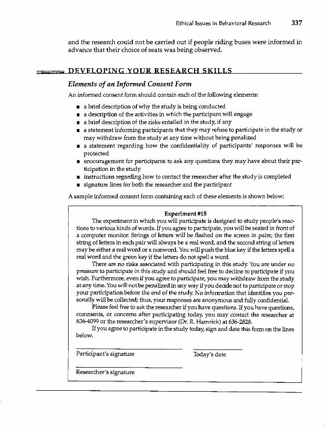
Ethical Issues in Behavioral Research 337

and the research could not be carried out if people riding buses were informed in advance that their choice of seats was being observed.

m:_W2"'i'P DEVELOPING YOUR RESEARCH SKILLS

Elements of an Informed Consent Form

An informed consent form should contain each of the following elements:

• a brief description of why the study is being conducted • a description of the activities in which the participant will engage • a brief description of the risks entailed in the study, if any • a statement informing participants that they may refuse to participate in the study or

may withdraw from the study at any time without being penalized • a statement regarding how the confidentiality of participants' responses will be

protected • encouragement for participants to ask any questions they may have about their par­

ticipation in the study • instructions regarding how to contact the researcher after the study is completed • signature lines for both the researcher and the participant

A sample informed consent form containing each of these elements is shown below:

Experiment #15 The experiment in which you will participate is designed to study people's reac­

tions to various kinds of words. If you agree to participate, you will be seated in front of a computer monitor. Strings of letters will be flashed on the screen in pairs; the first string of letters in each pair will always be a real word, and the second string of letters may be either a real word or a nonword. You will push the blue key if the letters spell a real word and the green key if the letters do not spell a word.

There are no risks associated with participating in this study. You are under no pressure to participate in this study and should feel free to decline to participate if you wish. Furthermore, even if you agree to participate, you may withdraw from the study at any time. You will not be penalized in any way if you decide not to participate or stop your participation before the end of the study. No information that identifies you per­sonally will be collected; thus, your responses are anonymous and fully confidential.

Please feel free to ask the researcher if you have questions. If you have questions, comments, or concerns after participating today, you may contact the researcher at 636-4099 or the researcher's supervisor (Dr. R. Hamrick) at 636-2828.

If you agree to participate in the study today, sign and date this form on the lines below.

Participant's signature Today's date

Researcher's signature

338 CHAPTER 14

Invasion of Privacy

The right to privacy is a person's right to decide "when, where, to whom, and to what extent his or her attitudes, beliefs, and behavior will be revealed" to other people (Singleton, Straits, Straits, & McAllister, 1988, p. 454). The APA ethical guide­lines do not offer explicit guidelines regarding invasion of privacy, noting only that "the ethical investigator will assume responsibility for undertaking a study involv­ing covert investigation in private situations only after very careful consideration and consultation" (American Psychological Association, 1992, p. 39). Thus, the cir­cumstances under which researchers may collect data without participants' knowl­edge is left to the investigator (and the investigator's IRB) to judge.

Most researchers believe that research involving the observation of people in public places (shopping or eating, for example) does not constitute invasion of pri­vacy. However, if people are to be observed under circumstances in which they rea­sonably expect privacy, invasion of privacy may be an issue.

• !!1ft! DEVELOPING YOUR RESEARCH SKILLS

You Be the Judge: What Constitutes Invasion of Privacy? In your opinion, which, if any, of these actual studies constitute an unethical invasion of privacy?

• Men using a public restroom are observed surreptitiously by a researcher hidden in a toi­let stall, who records the time they take to urinate (Middlemist, Knowles, & Matter, 1976).

• A researcher pretends to be a lookout for gay men having sex in a public restroom. On the basis of the men's car license plates, the researcher tracks down the participants through the Department of Motor Vehicles. Then, under the guise of another study, he interviews them in their homes (Humphreys, 1975).

• Researchers covertly film people who strip the parts from seemingly abandoned cars (Zimbardo, 1969).

• Participants waiting for an experiment are videotaped without their prior knowledge or consent. However, they are given the option of erasing the tapes if they do not want their tapes to be used for research purposes (Ickes, 1982).

• Researchers stage a shoplifting episode in a drug store, and shoppers' reactions are observed (Gelfand, Hartmann, Walder, & Page, 1973).

• Researchers hide under dormitory beds and eavesdrop on college students' conver­sations (Henle & Hubbell, 1938).

• Researchers embarrass participants by asking them to sing "Feelings" (Leary, Landel, & Patton, 1996).

• Researchers approach members of the other sex on a college campus and ask them to have sex (Clark & Hatfield, 1989).

What criteria did you use to decide which, if any, of these studies are acceptable to you?

Ethical Issues in Behavioral Research 339

Coercion to Participate

All ethical guidelines insist that potential participants must not be coerced into participating in research. Coercion to participate occurs when participants agree to participate because of real or implied pressure from some individual who has authority or influence over them. The most common example involves cases in which professors require that their students participate in research. Other exam­ples include employees in business and industry who are asked to participate in research by their employers, military personnel who are required to serve as par­ticipants, prisoners who are asked to "volunteer" for research, and clients who are asked by their therapists or physicians to provide data. What all of these classes of participants have in common is that they may believe, correctly or incorrectly, that refusing to participate will have negative consequences for them-a lower course grade, putting one's job in jeopardy, being reprimanded by one's superiors, or sim­ply displeasing an important person.

Researchers must respect an individual's freedom to decline to participate in research or to discontinue participation at any time. Furthermore, to assure that par­ticipants are not indirectly coerced by offering exceptionally high incentives, the guidelines state that{n!searchers cannot "offer excessive or inappropriate financial or other inducements to ~ain research participants, particularly when it might tend to coerce participation:1(Ethical Principles, 1992, Principle 6.14). Furthermore, "when research participation is a course requirement or opportunity for extra credit, the prospective participant is given the choice of equitable alternative activi­ties" (Ethical princiPles'r,1992, Principle 6.lld). Thus, when university and college students are required to ticipate in research, they must be given the option of ful­filling the requirement· an alternative fashion, such as by writing a paper that would require as much time and effort as serving as a research participant.

Physical and Mental Stress

Most behavioral research is innocuous, and the vast majority of participants are at no physical or psychological risk. However, because many important topics in be­havioral science involve how people or other animals respond to unpleasant phys­ical or psychological events, researchers sometimes design studies to investigate the effects of unpleasant events s\lch as stress, failure, fear, and pain. Researchers find it difficult to study such topics if they are prevented from exposing their par­ticipants to at least small amounts of physical or mental stress. But how much dis­comfort maya researcher inflict on participants?

At the extremes, most people tend to agree regarding the amount of discom­fort that is permissible. For example, most people agree that an experiment that leads participants to think they are dying is highly unethical. One study did just that by injecting participapts, without their knowledge, with a drug that caused them to stop breathing temporarily (Campbell, Sanderson, & Laverty, 1964). On the other hand, few people object to studies that involve only minimal risk. Minimal risk is

340 CHAPTER 14

"risk that is no greater in probability and severity than that ordinarily encountered in daily life or during the performance of routine physical or psychological exami­nations or tests" (OfficiaIIRB Guidebook, 1986).

Between these extremes, however, considerable controversy arises regarding the amount of physical and mental distress to be permitted in research. In large part, the final decision must be left to individual investigators and the IRB at their institutions. The decision is often based on a cost-benefit analysis of the research. Research procedures that cause stress or pain may be allowed only if the potential benefits of the research are extensive and only if the participant agrees to partici­pate after being fully informed of the possible risks.

Deception in Research

Perhaps no research practice has evoked as much controversy among behavioral researchers as deception. Forty years ago methodological deception was rare, but the use of deception increased dramatically during the 1960s (Christensen, 1988). Although some areas of behavioral research use deception rarely, if at all, it is com­mon in other areas (Adair, Dushenko, & Lindsay, 1985; Gross & Fleming, 1982).

Behavioral scientists use deception for a number of reasons. The most com­mon one is to prevent participants from learning the true purpose of a study so that their behavior will not be artificially affected. In addition to presenting partici­pants with a false purpose of the study, deception may involve:

• using an experimental confederate who poses as another participant or as an uninvolved bystander

• providing false feedback to participants • presenting two related studies as unrelated, • giving incorrect information regarding stimulus materials

In each instance, researchers use deception because they believe it is necessary for studying the topic of interest.

Objections to Deception

The objections that have been raised.r~arding the use of deception can be classi­fied roughly into two basic categorie~The most obvious objection is a strictly eth­ical one: Lying and deceit are immoral and reprehensible acts, even when they are used for good purposes such as research. Baumrind (1971) argued, for example, that "fundamental moral principles of reciprocity and justice are violated" when researchers use deception. She added that "scientific ends, however laudable they may be, do not themselves justify the use of means that in ordinary transactions would be regarded as reprehensible" (p. 890). This objection is obviously a deon-

10· one, based on the violation of moral rules. "" The secon 0 ,e on . en eception can be justified on the

. grounds that it leads to positive outcomes (the utilitarian perspective), it may lead to

Ethical Issues in Behavioral Research 341

undesirable consequences. For example, because of widespread deception, research participants may enter research studies already suspicious of what the researcher tells thexriJIn addition, participants who learn that they have been deceived may come to distrust behavioral scientists and the research process in general, under­mining the public's trust in psychology and related fields. Smith and Richardson (1983) found that people who participated in research that involved deception per­ceived psychologists as less trustworthy than those who participated in nondecep­tive research.

Although the first objection is a purely ethical one for which there is no ob­jective resolution, the second concern has been examined empirically. Several stud­ies have tested how research participants react when they learn they have been deceived by a researcher. In most studies that assessed reactions to deception, the vast majority of participants (usually over 90%) say they realize that deception is sometimes necessary for methodological reasons and report positive feelings about their participation in the study. Even Milgram (1963), who has been soundly criticized for his use of deception, found that less than 2% of his participants re­ported having negative feelings about their participation in his experiment on obe­dience. (See the box, "The Milgram Experiments" later in the chapter.)

Interestingly, researchers are typically more concerned about the dangers of deception than are research participants themselves (Fisher & Fryberg, 1994). Re­search participants do not seem to regard deception in research settings in the same way they view lying in everyday life. Instead, they view it as a necessary aspect of certain kinds of research (Smith & Richardson, 1983). As long as they are informed about details of the study afterward, participants generally do not mind being mis­led for good reasons (Christensen, 1988). In fact, research shows that, assuming they are properly debriefed, participants report more positive reactions to their participa­tion and higher ratings of a study's scientific value if the study includes deception (Coulter, 1986; Smith & Richardson, 1983; Straits, Wuebben, & Majka, 1972). Find­ings such as these should not be taken to suggest that deception is always an ac­ceptable practice. However, they do show that, when properly handled, deception per se need not have negative consequences for research participants.

Both APA and federal guidelines state that researchers should not use de­ception unless they have determined that the use of deception is justified by the research's possible scientific, educational, or applied value, and that the research could not be feasibly conducted without the use of deception. Importantly, re­searchers are never justified in deceiving participants about aspects of the study that might affect their willingness to participate. In the process of obtaining partic­ipants' informed consent, the researcher must accurately inform participants re­garding possible risks, discomfort, or unpleasant experiences.

Debriefing

Whenever deception is used, participants must be informed about the subterfuge "as early as it is feasible" (Ethical Principles, 1992, Principle 6.15c). Usually partici­pants are debriefed immediately after they participate, but occasionally researchers wait until the entire study is over and all of the data have been collected.

342 CHAPTER 14

A good debriefing accomplishes four goals. First, the debriefing clarifies the nature of the study for participants. Although the researcher may have withheld certain information at the beginning of the study, the participant should be more fully informed after it is over. This does not require that the researcher give a lec­ture regarding the area of research, only that the participant leave the study with a sense of what was being studied and how his or her participation contributed to knowledge in an area.

Occasionally, participants are angered or embarrassed when they find they were fooled by the researcher. Of course, the more smug a researcher is about the deception, the more likely the participant is to react negatively. Thus, researchers should be sure to explain the reasons for any deception that occurred, express their apologies for misleading the participant, and allow the participant to express his or her feelings about being deceived.

The second goal of debriefing is to remove any stress or other negative con­sequences that the study may have induced. For example, if participants were pro­vided with false feedback about their performance on a test, the deception should be explained. In cases in which participants have been led to perform embarrass­ing or socially undesirable actions, researchers must be sure that participants leave with no bad feelings about what they have done.

A third goal of the debriefing is for the researcher to obtain participants' re­actions to the study itself. Often, if carefully probed, participants will reveal that they didn't understand part of the instructions, were suspicious about aspects of the procedure, were disturbed by the study, or had heard about the study from other people. Such revelations may require modifications in the procedure.

The fourth goal of a debriefing is more intangible. Participants should leave the study feeling good about their participation. Researchers should convey their genuine appreciation for participants' time and cooperation, and give participants the sense that their participation was important.

Confidentiality in Research

The information obtained about research participants in the course of a study is confidential. Confidentiality means that the data that participants provide may be used only for purposes of the research and may not be divulged to others. When others have access to participants' data, their privacy is invaded and confidential­ity is violated.

Admittedly, in most behavioral research, participants would experience no adverse consequences if confidentiality were broken and others obtained access to their data. In some cases, however, the information collected during a study may be quite sensitive, and disclosure would undoubtedly have negative repercussions for the participant. For example, issues of confidentiality have been paramount among health psychologists who study persons who have tested positive for HIV or AIDS (Rosnow, Rotheram-Borus, Ceci, Blanck, & Koocher, 1993).

The easiest way to maintain confidentiality is to ensure that participants' re­sponses are anonymous. Confidentiality will not be a problem if the information

Ethical Issues in Behavioral Research 343

that is collected cannot be used to identify the participant. In many instances, how­ever, researchers need to know the identity of a research participant. For example, they may need to collate data collected in two different research sessions. To do so, they must know which participants' data are which.

Several practices are used to solve this problem. Sometimes participants are given codes to label their data that allow researchers to connect different parts of their data without divulging their identities. In cases in which the data are in no way potentially sensitive or embarrassing, names may be collected. In such cases, however, researchers should remove all information that might identify a partici­pant after the identifying information is no longer needed.

BEHAVIORAL RESEARCH CASE STUDY

The Milgram Experiments Perhaps no research has been the center of as much ethical debate as Stanley Milgram's (1963) studies of obedience to authority. Milgram was interested in factors that affect the de­gree to which people obey an authority figure's orders, even when those orders lead them to harm another person. To examine this question, he tested participants' reactions to an ex­perimenter who ordered them to harm another participant.

The Study Participants were recruited by mail to participate in a study of memory and learning. Upon arriving at a laboratory at Yale University, the participant met an experimenter and another participant who was participating in the same experimental session.

The experiment was described as a test of the effects of punishment on learning. Based on a drawing, one participant was assigned the role of teacher and the other participant was assigned the role of learner. The teacher watched as the leamer was strapped into a chair and fitted with an electrode on his wrist. The teacher was then taken to an adjoining room and seated in front of an imposing shock generator that would deliver electric shocks to the other participant. The shock generator had a row of 30 switches, each of which was marked with a voltage level, beginning with 15 volts and proceeding in IS-volt increments to 450 volts.

The experimenter told the teacher to read the learner a list of word pairs, such as blue-box and wild-duck. After reading the list, the teacher would test the leamer's memory by giving him the first word in each pair. The learner was then to give the second word in the pair. If the leamer remembered the word correctly, the teacher was to go to the next word on the list. However, if the learner answered incorrectly, the teacher was to deliver a shock by pressing one of the switches. The teacher was to start with the switch marked 15 volts, then increase the voltage one level each time the learner missed a word.

Once the study was under way, the learner began to make a number of errors. At first, the leamer didn't react to the shocks, but as the voltage increased, he began to object. When the learner received 120 volts, he Simply complained that the shocks were painful. As the voltage increased, he first asked and then demanded that the experimenter stop the study. However, the experimenter told the teacher that lithe experiment requires that you con­tinue." With increasingly strong shocks, the learner began to yell, then pound on the wall, and after 300 volts, scream in anguish. Most of the teachers were reluctant to continue, but the

344 CHAPTER 14

experimenter insisted that they follow through with the experimental procedure. After 330 volts, the learner stopped responding altogether; the teacher was left to imagine that the participant had fainted or, worse, died. Even then, the experimenter instructed the teacher to treat no response as a wrong answer and to deliver the next shock to the now silent learner.

As you probably know (or have guessed), the learner was in fact a confederate of the experimenter and received no shocks. The real participants, of course, thought they were ac­tually shocking another person. Yet 65% of the participants delivered all 30 shocks-up to 450 volts-even though the learner had protested, then fallen silent. This level of obedience was entirely unexpected and attests both to the power of authority figures to lead people to perform harmful actions and to the compliance of research participants.

The Ethical Issues Milgram's research sparked an intense debate on research ethics that continues today. Mil­gram's study involved virtually every ethical issue that can be raised.

• Participants were misled about the purpose of the study. • A confederate posed as another participant. • Participants were led to believe they were shocking another person, a behavior that,

both at the moment and in retrospect, may have been very disturbing to them. • Participants experienced considerable stress as the experiment continued: They sweated,

trembled, stuttered, swore, and laughed nervously as they delivered increasingly in­tense shocks.

• Participants' attempts to withdraw from the study were discouraged by the experi­menter's insistence that they continue.

What is your reaction to Milgram's experiment? Did Milgram violate basic ethical principles in this research?

Common Courtesy

A few years ago I conducted an informal survey of students who had participated in research as part of a course requirement in introductory psychology. In this sur­vey I asked what problems they had encountered in their participation. The vast majority of their responses did not involve violations of basic ethical principles involving coercion, harm, deception, or violation of confidentiality. Rather, their major complaints had to do with how they were treated as people during the course of the study. Their chief complaints were that: (1) the researcher failed to show up or was late; (2) the researcher was not adequately prepared; (3) the researcher was cold, abrupt, or downright rude; and (4) the researcher failed to show appreciation for the participant.

Aside from the formal guidelines, ethical research requires a large dose of common courtesy. The people who participate in research are contributing their

Ethical Issues in Behavioral Research 345

time and energy, often without compensation, to your research. They deserve the utmost in common courtesy.

Ethical Principles in Research with Animals

The APA Ethical Principles contain standards regarding the ethical treatment of an­imals, and the APA has published a more detailed discussion of these issues in Guidelines for Ethical Conduct in the Care and Use of Animals. These guidelines are no­ticeably less detailed than those involving human participants, but they are no less explicit regarding the importance of treating nonhuman animals in a humane and ethical fashion.

These guidelines stipulate that"gll research that uses nonhuman animals must be monitored closely by a erson who is ex erienced in the care and use of labora-ory aruma ,an a a veterinarian must be available for consu tation. Further-

"more, all personnel who are involved in animal research, including students, must be familiar with these guidelines and adequately trained regarding the use and care of animals. Thus, if you should become involved with such research, you are obligated to acquaint yourself with these guidelines and abide by them at all times.

The facilities in which laboratory animals are housed are closely regulated by the National Institutes of Health, as well as federal, state, and local laws. Obvi­ously, animals mu hous humane healthful conditions(The facil­ities should be inspected by a veterinarian at least twice a yea

Advocates of animal rights are most concerned, of course, about the experi­mental procedures to which the animals are subjected during research. APA guide­lines direct researchers to :"make reasonable efforts to minimize the discomfort, ~~~ i!!S:ss, and pain of animal participants," and require the investigator to jus' ___ p ___ e 0 all rocedures that mvolve moretflan momentary or slight pain to the §!!limal: " ctin animals to ain stress, or nvahon 1S used Q rnative rocedure is unavailable and the oal is 'usti 1e its

ro tiv a li value" (Ethical Principles, 1992, p. 1609, Standard 6.20). Procedures that involve more than minimal pain or distress require strong justification.

The APA regulations also provide guidelines for the use of surgical proce­dures, the study of animals in field settings, the use of animals for educational (as opposed to research) purposes, and the disposition of animals at the end of a study.

~ IN DEPTH

Behavioral Research and Animal Rights

During the 1980s, several animal rights organizations were formed to protest the use of ani­mals for research purposes. Some animal rights groups have simply pressured researchers to treat animals more humanely, whereas others have demanded that the practice of using ani­mals in research be stopped entirely. For example, People for the Ethical Treatment of Animals

346 CHAPTER 14

(PET A)-the largest animal rights organization in the world-opposes animal research of all kinds, arguing that animals should not be eaten, used for clothing, or experimented on. Al­though PETA does not endorse violence, members of certain other groups have resorted to terrorist tactics, burning or bombing labs, stealing or releasing lab animals, and ruining ex­periments. For example, in 1999, members of the Animal Liberation Front vandalized ani­mal research labs at the University of Michigan, causing $2 million worth of damage, destroying data, and abducting animals (Azar, 1999). (Ironically, the animals were released in a field near the university, and, unprepared to live outside a lab, many died before being rescued by researchers.)

Like most ethical issues in research, debates involving the use of animals in research arise because of the competing pressures to advance knowledge and improve welfare on the one hand and to protect animals on the other. Undoubtedly, animals have been occasionally mistreated, either by being housed under inhumane conditions or by being subjected to un­necessary pain or distress during the research itself. However, most psycholOgical research does not hurt the animals, and researchers who conduct research on animals argue that oc­casional abuses should not blind us to the value of behavioral research that uses animal par­ticipants. The vast majority of animal researchers treat their nonhuman participants with great care and concern.

On receiving the APA's Award for Distinguished Professional Contributions, Neal Miller (1985) chronicled in his address the significant contributions of animal research. In defending the use of animals in behavioral research, Miller noted that animal research has contributed to the rehabilitation of neuromuscular disorders, understanding and reducing stress and pain, developing drugs for the treatment of various animal problems, exploring processes involved in substance abuse, improving memory deficits in the elderly, increasing the survival rate for premature infants, and the development of behavioral approaches in psychotherapy. To this list of contributions from behavioral science, Joseph Murray, a 1990 winner of the Nobel Prize, adds the many advances in medicine that would have been im­possible without animal research, including vaccines (for polio, smallpox, and measles, for example), dialysis, organ transplants, chemotherapy, and insulin (Monroe, 1991). Even ani­mal welfare has been improved through research using animals; for example, dogs and cats today live longer and healthier lives than they once did because of research involving vac­cines and medicines for pets (Szymczyk, 1995).

To some animal rights activists, including the members of PETA, the benefits of the research are beside the point. They argue that, like people, nonhuman animals have certain moral rights. As a result, human beings have no right to subject nonhuman ani­mals to pain, stress, and sometimes death, or even to submit animals to any research against their will.

In an ideal world we would be able to solve problems of human suffering without using nonhuman animals in research. But in our less than perfect world, most behavioral re­searchers subscribe to the utilitarian view that the potential benefits of most animal research outweigh the potential costs. Several scientific organizations, including the American Associ­ation for the Advancement of Science and the American PsycholOgical Association, have en­dorsed the use of animals in research, teaching, and education while, of course, insisting that research animals be treated with utmost care and respect (" APA Endorses Resolution," 1990).

Ethical Issues in Behavioral Research 347

Scientific Misconduct

In addition to principles governing the treatment of human and animal partici­pants, behavioral researchers are bound by general ethical principles involving the conduct of scientific research. Such principles are not specific to behavioral re­search but apply to all scientists regardless of their discipline. Most scientific orga­nizations have set ethical standards for their members to guard against scientific misconduct.

The National Academy of Sciences identifies three major categories of scien­tific misconduct. The first category involves the most serious and blatant forms of scientific dishonesty, such as fabrication, falsification, and plagiarism. The APA Ethical Principles likewise addresses these issues, stating that researchers must not fabricate data or report false results. Furthermore, if they discover significant er­rors in their findings or analyses, researchers are obligated to take steps to correct such errors. Likewise, researchers do not plagiarize others' work, presenting "sub­stantial portions or elements of another's work or data as their own ... " (Ethical Principles, 1992, Standard 6.22).

A study of graduate students and faculty members in chemistry, civil engi­neering, microbiology, and sociology found that between 6% and 9% of the 4,000 respondents reported that they had direct knowledge of faculty members who had

Source: © 2000 by Sidney Harris ..

348 CHAPTER 14

plagiarized or falsified their data. (This statistic does not indicate that 6-9% of re­searchers plagiarize or falsify; a single instance of dishonesty may be known by several people.) Among the graduate students, between 10% and 20% (depending on the discipline) reported that their student peers had falsified data, and over 30% of the faculty reported knowledge of student plagiarism (Swazey, Anderson, & Lewis, 1993).

Although not rampant, such abuses are disturbingly common. Most behav­ioral scientists agree with former director of the National Science Foundation, Wal­ter Massey, who observed that "Few things are more damaging to the scientific enterprise than falsehoods-be they the result of error, self-deception, sloppiness, and haste, or, in the worst case, dishonesty"(Massey, 1992}. Because science relies so heavily on honesty and is so severely damaged by dishonesty, the penalties for sci­entific misconduct, whether by professional researchers or by students, are severe.

A second category of ethical abuses involves questionable research practices that, although not constituting scientific misconduct per se, are problematic. For ex­ample, researchers should take credit for work only in proportion to their true con­tribution to it. This issue sometimes arises when researchers must decide whom to include as authors on research articles or papers, and in what order to list them (au­thors are usually listed in descending order of their scientific or professional contri­butions to the project). Problems of "ownership" can occur in both directions: In some cases researchers have failed to properly acknowledge the contributions of other people whereas in other cases researchers have awarded authorship to people who didn't contribute substantially to the project (such as a boss, or a colleague who lent them a piece of equipment).

Other ethically questionable research practices include failing to report data inconsistent with one's own views and failing to make one's data available to other competent professionals who wish to verify the researcher's conclusions by re­analyzing the data. In the study described previously, for example, 15% of the respondents reported knowing researchers who did not present data that were in­consistent with their own previous research. Many opportunities for scientific mis­conduct arise when grant money is at stake; there have been instances in which researchers have sabotaged other researchers' grant applications in order to im­prove their friends' chances of obtaining grants, and cases in which researchers misused grant money for other purposes (Bell, 1992).

A third category of ethical problems in research involves unethical behavior that is not unique to scientific investigation, such as sexual harassment (of research assistants or research participants), abuse of power, discrimination, or failure to follow government regulations. Not surprisingly, such unethical behaviors occur in science as they do in all human endeavors (Swazey et al., 1993).

In many ways, the worst ethical violation of all is to conduct poorly designed research. A poorly designed study not only squanders scarce resources for research (such as money and participants' time) but, if somehow published, can slow the pace of scientific progress or, worse, lead us down the wrong roads. Although flaws creep into every researcher's studies, they have an ethical obligation to de­sign the best studies pOSSible under whatever circumstances they are operating.

Ethical Issues in Behavioral Research 349

w _ IN DEPTH

Should Scientists Consider the Ethical Implications of Controversial Findings? The scientific enterprise is often regarded as an objective search for the truth, or at least as a careful, systematic search for the most reasonable conclusions that can be drawn from cur­rent data. Thus, researchers should presumably state the facts as they see them, without con­cern for whether their conclusions are popular and without regard for how people might use the information they publish. But what should researchers do if publication of their findings might lead to people being harmed or might appear to condone unacceptable be­havior? And how should journal reviewers and editors react if they think publication of a well-designed investigation will have a negative impact? To suppress the publication of well-designed research would violate the fundamental tenets of scientific investigation, yet its publication may create undesirable effects, so an ethical dilemma arises.

A case in point involves an article that involved a meta-analysis of 59 previous stud­ies that examined the long-term effects of childhood sexual abuse among people who were currently enrolled in college (Rind, Tromovitch, & Bauserman, 1998). (You may recall from Chapter 2 that meta-analysis statistically summarizes and analyzes the results of several studies on the same topic.) Across the studies, students who reported being sexually abused as children were slightly less well adjusted than students who had not been abused, as we might expect. However, the meta-analysis revealed that this effect was due primarily to dif­ferences in the kinds of families in which the students grew up rather than to the sexual abuse itself. The article concluded that the effects of childhood sexual abuse on later adjust­ment are not as strong as people commonly believe. In fact, the authors suggested that re­searchers discard the term sexual abuse for a "value neutral" term such as adult-child sex.

The article was published in Psychological Bulletin, one of the most prestigious, rigor­ous, and demanding journals in behavioral science. It underwent the standard process of peer review in which other experts examined the quality of the study's methodology and conclusions, and recommended that it be published. However, upon publication, the article provoked great controversy because critics said that it condoned pedophilia. The outcry eventually reached the U.S. House of Representatives where a resolution was introduced condemning the article and, by association, the American Psychological Association, which publishes Psychological Bulletin. Under attack, the APA released a statement clarifying its po­sition against sexual abuse and promised to have the article's scientific quality reevaluated (Martin, 1999; McCarty, 1999).

Many behavioral scientists were dismayed that scientific findings were repudiated by members of Congress and others on the basis of the study's conclusions rather than the qual­ity of its methodology. (They were also troubled that APA buckled under political pressure and instituted an unprecedented reevaluation of the article.) What should the researchers have done? Lied about their results? Suppressed the publication of their unpopular find­ings? This particular case, perhaps more than any other in recent memory, highlights the ethical issues that may arise when behavioral research reaches controversial conclusions that may have implications for public policy. It also demonstrates that science does not occur in a vacuum but is influenced by social and political forces.

350 CHAPTER 14

A Final Note

The general consensus is that major kinds of ethical abuses, such as serious mistreat­ment of participants and outright data fabrication, are rare in behavioral science (Adler, 1991). However, the less serious kinds of ethical violations discussed in this chapter are disturbingly common. By and large, the guidelines discussed in this chapter provide only a framework for making ethical decisions about research prac­tices. Rather than specifying a universal code of do's and don'ts, they present the principles by which researchers should resolve ethical issues. No unequivocal crite­ria exist that researchers can use to decide how much stress is too much, when deception is and is not appropriate, or whether data may be collected without par­ticipants' knowledge in a particular study. As a result, knowledge of APA principles and federal regulations must be accompanied by a good dose of common sense.

Summary

1. Ethical issues must be considered whenever a study is designed. Usually the ethical issues are minor ones, but sometimes the fundamental conflict be­tween the scientific search for knowledge and the welfare of research partici­pants creates an ethical dilemma.

2. Researchers sometimes disagree not only regarding the ethicality of specific research practices but also regarding how ethical decisions should be made. Researchers operating from the deontological, skeptical, and utilitarian per­spectives use very different standards for judging the ethical acceptability of research procedures.

3. Professional organizations and the federal government have provided regu­lations for the protection of human and nonhuman participants.

4. Six issues must be considered when human participants are used in research: informed consent, invasion of privacy, coercion to participate, potential phys­ical or psychological harm, deception, and confidentiality. Although APA and federal guidelines provide general guidance regarding these issues, in the last analysis individual researchers must weigh the potential benefits of their re­search against its potential costs.

5. Federal regulations ~equire an Institutional Review Board (IRB) at an investi­gator's institution to approve research involving humans to protect research participants.

6. Professional and governmental regulations also govern the use and care of nonhuman animals in research.

7. Scientific misconduct involves behaviors that compromise the integrity of the scientific enterprise, including dishonesty (fabrication, falsification, and pla­giarism), questionable research practices, and otherwise unethical behavior (such as sexual harassment and misuse of power).

Ethical Issues in Behavioral Research 351

KEY TERMS

coercion to participate deontology (p. 331) invasion of privacy (p. 338) minimal risk (p. 339) scientific misconduct

(p.339) confidentiality (p. 342) cost-benefit analysis (p. 333) debriefing (p. 342) deception (p. 340)

ethical skepticism (p. 331) informed consent (p. 335) informed consent form (p. 335) Institutional Review Board

(IRB) (p. 334)

(p.347) utilitarian (p. 331)

QUESTIONS FOR REVIEW

1. Distinguish between deontology, skepticism, and utilitarianism as approaches to making decisions.

2. Which of these three ethical philosophies comes closest to the official ethical guide­lines expressed by federal regulatory agencies and the American Psychological As­sociation?

3. What factors should be considered when doing a cost-benefit analysis of a pro­posed study?

4. What is the purpose of the Institutional Review Board?

5. According to the principle of informed consent, what must participants be told be­fore soliciting their agreement to participate in a study?

6. When is it not necessary to obtain informed consent?

7. What must be done if a research participant is unable to give valid informed con­sent, as in the case of children or people who are very psychologically disturbed?

8. Why may researchers not offer potential participants large incentives (for example, a large amount of money) to participate in research?

9. In general, how much mental or physical risk is permissible in research?

10. Describe the concept of minimal risk.

11. Why do researchers use deception?

12. Why do some people object to the use of deception in research?

13. What four goals should a debriefing accomplish?

14. How do researchers maintain the confidentiality of participants' responses?

15. Describe the Milgram (1963) study and discuss the ethical issues it raised. ,

16. What are the basic ethical principles that animal researchers must follow?

[ 17. Discuss the pros and cons of using nonhuman animals in behavioral research.

18. What are some examples of scientific misconduct?

352 CHAPTER 14

QUESTIONS FOR DISCUSSION

1. How much distress or pain may researchers inflict on participants who freely agree to participate in a study after being fully informed about the pain or distress they will experience?

2. Milgram conducted his experiments on obedience in the days before all research was scrutinized by an Institutional Review Board. Imagine, however, that Milgram had submitted his research proposal to an IRB of which you were a member. What ethical issues would you raise as a member of the board? Would you have voted to approve Milgram's research? In thinking about this question, keep in mind that no one expected participants to obey the researcher as strongly as they did (see Schlenker & Forsyth, 1977).

3. To gain practice writing an informed consent form, write one for the Milgram study described in this chapter. Be sure to include all of the elements needed in an in­formed consent form.

4. Do you think that governmental agencies should exercise more or less control over behavioral research? Why?

CHAPTER

15 Scientific Writing

How Scientific Findings Are Disseminated

Elements of Good Scientific Writing

Avoiding Biased Language

Citing and Referencing Previous Research

Other Aspects of APA Style

Sample Manuscript

Parts of a Manuscript

As a system for advancing knowledge, science requires that investigators share their findings with the rest of the scientific community. Only if one's findings are made public can knowledge accumulate as researchers build on, extend, and refine one another's work. As we discussed in Chapter I, a defining characteristic of sci­ence is that, over the long haul, it is self-correcting; but self-correction can occur only if research findings are widely disseminated. To this end, informing others of the outcome of one's work is a critical part of the research process.

In this chapter we will examine how researchers distribute their work to other scientists, students, and the general public. Because the effective communi­cation of one's research nearly always involves writing, much of this chapter will be devoted to scientific writing. We will discuss criteria for good scientific writing and help you improve your own writing skills. We will also examine the guidelines that behavioral researchers use to prepare their research reports, a system of rules known as APA style. To begin, however, we'll take a look at the three main routes by which behavioral scientists disseminate their research to others.

How Scientific Findings Are Disseminated

Researchers disseminate the results of their investigations in three ways: journal publications, presentations at professional meetings, and personal contact.

353

354 C HAP T E R 15

Journal Publication

Journal publication is the primary route by which research findings are dissemi­nated to the scientific community. Scientific journals serve not only as a means of communication among researchers (most researchers subscribe to one or more jour­nals in their fields) but also as the basis for the permanent storage of research find­ings in library collections. Traditionally, journals were published only in printed form, but today entire journals are published in electronic media on CD-ROM and on the internet.

Before most journals will publish a research paper, it must undergo the pro­cess of peer review. In peer review, a paper is evaluated by other scientists who have expertise in the topic under investigation. Although various journals use slightly different systems of peer review, the general process is as follows.

1. The author submits copies of his or her paper to the editor of a relevant jour­nal. (The editor's name and address typically appear on the inside front cover of the journal.) Authors are permitted to submit a particular piece of work to only one journal at a time.

2. The editor (or an associate editor designated by the editor) then sends a copy of the paper to two or more peer reviewers who are known to be experts in the area of the paper. Each of the reviewers reads and evaluates the paper, addressing its conceptualization, methodology, analyses, interpretations, and contribution to the field. Each reviewer decides whether the paper, considered in its entirety, warrants publication in the journal.

3. The reviewers then send written reviews, typically a page or two in length, to the journal editor, along with their recommendations regarding whether the paper should be published.

4. Having received the reviewers' comments, suggestions, and recommenda­tions, the editor considers their input and reads the paper him- or herself. The edi­tor then makes one of four editorial decisions. First, he or she may decide to publish the paper as is. Editors rarely make this decision, however; even if the paper is ex­ceptional, the reviewers virtually always suggest ways in which it can be improved. Second, the editor may accept the paper for publication contingent on the author making certain revisions. Third, the editor may decide not to accept the paper for publication in the journal but will ask the authors to revise the paper in line with the reviewers' recommendations and to resubmit it for reconsideration. Editors make this decision when they think the paper has potential merit but see too many prob­lems to warrant publication of the original draft. The fourth decision an editor may make is to reject the paper, with no opportunity for the authors to resubmit the paper to that particular journal. However, once the manuscript is rejected by one journal, the author may revise and submit it for consideration at another journal.

The most common editorial decision is the fourth one-rejection. In the leading journals in behavioral science, between 70% and 90% of the submitted manuscripts are rejected for publication (Summary Report of Journal Operations, 1998, 1999). Even if

Scientific Writing 355

they are ultimately accepted for publication, most submitted papers undergo one or more rounds of reviews and revisions before they are published, so researchers must become accustomed to receiving critical feedback about their work. (The entire pro­cess, from submission to publication, usually takes a year or two.) Although no one likes having their work criticized or rejected, seasoned researchers realize that tight quality control is essential in science; critical feedback from reviewers and editors helps to assure that published articles meet minimum standards of scientific accept­ability. In addition, critical feedback may actually help the researcher by ensuring that his or her flawed studies and poorly written manuscripts are not published, thereby preventing even greater criticism and embarrassment in the long run.

Students are often surprised to learn that researchers are not paid for the articles they publish. Conducting and publishing research is part of many researchers' jobs at colleges and universities, hospitals, research institutes, and other research organi­zations. Thus, they are compensated for the research they conduct as part of their normal salaries and do not receive any extra pay when their articles are published.

Presentations at Professional Meetings

The second route by which scientific findings are distributed is through presenta­tions at professional meetings. Most behavioral researchers belong to one or more professional organizations, such as the American Psychological Association, the American Psychological Society, the American Educational Research Association, the Psychonomic Society, regional organizations (such as the Southeastern, Mid­western, and Western Psychological Associations), and a number of other groups that cater to specific areas of behavioral science (such as psychophysiology, law and psychology, social psychology, health psychology, developmental psychology, and so on). Most of these organizations hold annual meetings at which researchers present their latest work.

In most instances, researchers who wish to present their research submit a short proposal (usually 200-500 words) that is peer-reviewed by other researchers. The acceptance rate for professional meetings is much higher than that for journal publication; typically 50 to 80% of the submitted proposals are accepted for pre­sentation at the conference or convention.

Depending on the specific organization and on the researcher's preference, the presentation of a paper at a professional meeting can take one of two forms. One mode of presentation involves giving a talk to an audience. Typically, papers on re­lated topics are included in the same paper session, in which each speaker has 15 or 20 minutes to present his or her research and to answer questions from the audience.

A second mode of presentation is the poster session. In a poster session, re­searchers display summaries of their research on poster boards, providing the es­sential details of its background, methodology, results, and implications. The researchers then stand with their posters to provide details, answer questions, and discuss their work with interested persons. They also have copies of a longer research report on hand to distribute to interested parties. Many researchers pre­fer poster sessions over verbal presentations because more people typically attend

356 C HAP T E R 15

a particular poster session than a paper session (thus, the research gets wider expo­sure), and poster sessions allow more one-on-one interactions between researchers. Not only do poster sessions give the researchers who are presenting their stud­ies an opportunity to meet others who are interested in their topic, but they often serve as a social hour in which convention attendees gather to interact with one another.

Personal Contact

A great deal of communication among scientists occurs through informal channels, such as personal contact. After researchers have been actively involved in an area of investigation for a few years, they get to know others who are interested in the same topic. Not only do they talk with one another at professional meetings, sharing their latest ideas and findings, but they often send prepublication drafts of their latest pa­pers to these individuals and may even collaborate on research projects. Most re­searchers also stay in regular contact with one another through e-mail.

This network of researchers from around the world, which has been called the "hidden university," is an important channel of scientific communication that allows researchers to stay informed about the latest advances in their fields. Researchers who are linked to these informal networks often become aware of advances in their fields a year or more before those advances are published in sci­entific journals.

Peer Review, the Media, and the Internet As we have seen, the dissemination of research findings among members of the scientific community occurs primarily through journal publication, presentations at professional meetings, and personal contact. However, information about research is sometimes released in two additional ways-in the popular media and on the world wide web.

Researchers are sometimes interviewed about their work by reporters and writers. You have probably seen articles about behavioral research in newspapers and magazines, and heard stories about research, if not interviews with the researchers themselves, on tele­vision and radio. Although most scientists believe that researchers are obligated to share their findings with the public, the drawback of reporting research in the general media is that the audience who reads, hears, or sees the report has no way of judging the quality of the research or the accuracy of the interpretations. Researchers can talk about their research whether it meets minimum standards of scientific acceptability or passes the test of peer re­view. For this reason, researchers in some sciences, though not in psychology, are discour­aged from talking publicly about research that has not been peer-reviewed.

Furthermore, even if research has the scientific stamp of approval of peer review, pop­ular reports of research are notoriously inaccurate. News reporters and writers typically focus on the study's most interesting conclusion without addressing the qualifications and limitations of the study that one would find in a journal article.

Scientific Writing 357

The same problem of quality control arises when researchers post reports of their re­search on the world wide web. Because anyone can create a web site and post whatever they wish on it, we often have no way of knowing that research posted on the web was properly conducted, analyzed, and interpreted. (For this reason, many teachers do not allow students to use the web to locate previous research on a topic.) Sometimes, researchers post manuscripts after they have been peer-reviewed and accepted for publication, which is a different matter. As long as the research passed the critical process of peer-review, we have at least minimum assurance that other experts vieweq it as acceptable. However, if re­search posted on the web has not been peer-reviewed, you should be wary about using or citing it.

Elements of Good Scientific Writing

Good writing skills are essential for researchers. No matter how insightful, creative, or well designed particular studies may be, they are unlikely to have an impact on behavioral science if researchers do not convey their ideas and findings in a clear, accurate, and engaging manner. Unfortunately, good writing cannot be taught as easily as experimental design or the calculation of a correlation coefficient. It devel­ops only through conscious attention to the details of good writing, coupled with practice and feedback from others.

Although you will not suddenly learn to become an effective writer from the material in the next few pages, I hope that I can offer some suggestions that will help you develop your own writing skills. Specifically, this section will focus on the importance of organization, clarity, and conciseness, and offer you hints on how to achieve them.

Organization

The first prerequisite for clear writing is organization-the order in which one's ideas are expressed. The general organization of research reports in behavioral sci­ence is dictated by guidelines established by the American Psychological Associa­tion. Among other things, these guidelines stipulate the order in which sections of a paper must appear. In light of these guidelines (which we will examine in detail later in this chapter), you will have few problems with the general organization of a research paper.

Problems are more likely to arise in the organization of ideas within sections of the paper. If the order in which ideas are expressed is faulty, readers are likely to be­come confused. Someone once said that good writing is like a good road map; the writer should take the reader from point A to point B-from beginning to end­using the straightest possible route, without backtracking, without detours, and without getting the reader lost along the way. To do this, you must present your ideas in an orderly and logical progression. One thought should follow from and build on another in a manner that will be easily grasped by the reader.

358 C HAP T E R 15

Before you start writing, make a rough outline of the major points you wish to express. This doesn't necessarily need to be one of those detailed, multilevel outlines you learned to make in school; just a list of major points will usually suffice. Be sure the major points in your outline progress in an orderly fashion. Starting with an outline may alert you to the fact that your ideas do not flow coherently or that you need to add certain points to make them progress more smoothly.

As you write, be sure that the transitions between one idea and another are clear. If you move from one idea to another too abruptly, the reader may miss the connection between them and lose your train of thought. Pay particular attention to the transitions from one paragraph to another. Often, you'll need to write tran­sition sentences that explicitly lead the reader from one paragraph to the next.

Clarity

Perhaps the fundamental requirement of scientific writing is clarity. Unlike some forms of fiction in which vagueness enhances the reader's experience, the goal of scientific writing is to communicate information. It is essential, then, that the in­formation be conveyed in a clear, articulate, and unclouded manner.

This is a very difficult task, however. You don't have to read many articles published in scientific journals to know that not all scientific writers express them­selves clearly. Often, writers find it difficult to step outside themselves and imag­ine how a reader will interpret their words. Even so, clarity must be a writer's first and foremost goal.

Two primary factors contribute to the clarity of one's writing: sentence con­struction and word choice.

Sentence Construction. The best way to enhance the clarity of your writing is to pay close attention to how you construct your sentences; awkwardly constructed sentences distract and confuse the reader. First, state your ideas in the most explicit and straightforward manner possible. One way to do this is to avoid the passive voice. For example, compare the following sentences:

The participants were told by the experimenter to press the button when they were finished (passive voice).

The experimenter told the participants to press the button when they finished (active voice).

I think you can see that the second sentence, which is written in the active voice, is the better of the two.

Second, avoid overly complicated sentences. Be economical in the phrases you use. For example, the sentence, "There were several different participants who had not previously been told what their IQ scores were," is terribly convoluted. It can be streamlined to, "Several participants did not know their IQ scores." (In a mo­ment, I'll share with you one method I use for identifying awkwardly constructed sentences in my own writing.)

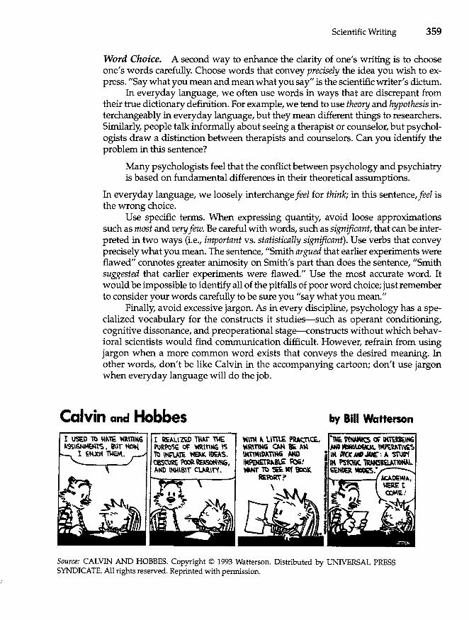
Scientific Writing 359

Word Choice. A second way to enhance the clarity of one's writing is to choose one's words carefully. Choose words that convey precisely the idea you wish to ex­press. "Say what you mean and mean what you say" is the scientific writer's dictum.

In everyday language, we often use words in ways that are discrepant from their true dictionary definition. For example, we tend to use theory and hypothesis in­terchangeably in everyday language, but they mean different things to researchers. Similarly, people talk informally about seeing a therapist or counselor, but psychol­ogists draw a distinction between therapists and counselors. Can you identify the problem in this sentence?

Many psychologists feel that the conflict between psychology and psychiatry is based on fundamental differences in their theoretical assumptions.

In everyday language, we loosely interchange feel for think; in this sentence, feel is the wrong choice.

Use specific terms. When expressing quantity, avoid loose approximations such as most and very few. Be careful with words, such as significant, that can be inter­preted in two ways (i.e., important vs. statistically significant). Use verbs that convey precisely what you mean. The sentence, "Smith argued that earlier experiments were flawed" connotes greater animosity on Smith's part than does the sentence, "Smith suggested that earlier experiments were flawed." Use the most accurate word. It would be impossible to identify all of the pitfalls of poor word choice; just remember to consider your words carefully to be sure you "say what you mean."

Finally, avoid excessive jargon. As in every discipline, psychology has a spe­cialized vocabulary for the constructs it studies-such as operant conditioning, cognitive dissonance, and preoperational stage-constructs without which behav­ioral scientists would find communication difficult. However, refrain from using jargon when a more common word exists that conveys the desired meaning. In other words, don't be like Calvin in the accompanying cartoon; don't use jargon when everyday language will do the job.

Calvin and Hobbes I REJ.LI no llIAT M:: P\JRI'O')E Of 'fIR.\nMG ,~ b IMFUlE ~ IOQS. C8St\1~ ~ ~''''. ~KO '","ISlr ClM.1T'f.

~\T1{ " 1ITTl£. PbalCE.. ~R'TU¥i C»l IE AM IMTI~IOft't\Wi AIm IM~~ra&! *"" 1b S M'f ~

RER)Rf? \

by Bill Watterson

Source: CALVIN AND HOBBES. Copyright © 1993 Watterson. Distributed by UNIVERSAL PRESS SYNDICATE. All rights reserved. Reprinted with permission.

360 C HAP T E R 15

Conciseness

A third important consideration in scientific writing is conciseness. Say what you are going to say as economically as possible. Like you, readers are busy people. Think how you feel when you must read a 26-page journal article that could have conveyed all of its points in only 15 pages. Have mercy on your readers! Concise­ness is also important for practical reasons. Scientific journals publish a limited number of pages each year, so papers that are unnecessarily long rob the field of badly needed journal space.

However, do not use conciseness as an excuse for skimpy writing. Research papers must contain all necessary information. Ideas must be fully developed, methods described in detail, results examined carefully, and so on. The advice to be concise should be interpreted as an admonition to include only the necessary in­formation and to express it as succinctly (yet clearly) as possible.

DEVELOPING YOUR RESEARCH SKILLS

What's Wrong with These Sentences?

Like all writers, scientists are expected to use words and grammar correctly to convey their ideas. Each of the sentences below contains one or more common writing or grammatical er­rors. Can you spot them?

1. Since this finding was first obtained on male participants, several researchers have questioned its generalizability.

Error: The preferred meaning of since is "between a particular past time and the pres­ent," and it should not be used as a synonym for because. In this example, the meaning of since is ambiguous--does it mean because or in the time since?

2. This phenomena has been widely studied.

Error: Phenomena is plural; the singular form is phenomenon.

3. While most researchers have found a direct relationship between incentives and per­formance, some studies have obtained a curvilinear relationship.

Error: While should be used to mean during the same time as. The proper word here is whereas or although.

4. Twenty females were used as participants.

Error: APA style specifies that female (and male) are generally to be used as adjectives, not as nouns. As such, they must modify a noun (female students, female employees, for example).

5. After assigning participants to conditions, participants in the experimental group completed the first questionnaire.

Error: The phrase after assigning participants to conditions is a dangling modifier that has no referent in the sentence. One possible remedy would be to write, "After the experi-

Scientific Writing 361

menter assigned participants to conditions, participants in the experimental group completed the first questionnaire."

6. The data was analyzed with at-test.

Error: Data is plural; datum is singular. Thus, the sentence should be, "The data were analyzed .... "

7. It is hypothesized that shy participants will participate less fully in the group discussion.

Error: As a pronoun, it must refer to some noun. In this sentence, it has no referent. The sentence could be rewritten in a number of ways, such as:

This study tested the hypothesis that ...

The hypothesis tested in this study was that ...

Based on previous research, one would expect that ...

8. When a person is in a manic state, they often have delusions of grandeur.

Error: Pronouns must agree in number with their corresponding nouns. In this case, person is singular but they is plural. The sentence could be written in one of two ways:

When people are in a manic state, they often have delusions of grandeur. (The noun and pronoun are both plural.)

When a person is in a manic state, he or she often has delusions of grandeur. (The noun and pronoun are both singular.)

Proofreading and Rewriting

Good writers are rewriters. Writers whose first draft is ready for public distribution are extremely rare, if they exist at all. Most researchers revise their papers many times before they allow anyone else to see them (unlike the students I've known who hand in their first draft!).

When you reread your own writing, do so with a critical eye. Have you in­cluded everything necessary to make your points effectively? Is the paper organized? Are ideas presented in a logical and orderly progression, and are the transitions be­tween them clear? Is the writing clear and concise? Have you used precise vocab­ulary throughout?

When you proofread your paper, read it aloud. I often imagine that I am a tele­vision newscaster and that my paper is the script of a documentary I am narrating. If you feel silly pretending to be a newscaster, just read your paper aloud slowly and listen to how it sounds. Reading a paper aloud is the best way I know to spot awkward constructions. Sentences that look fine on paper often sound stilted or convoluted when they are spoken.

Allow yourself enough time to write and revise your paper, then set it aside for a few days. After a period away from the paper, I am always able to see weak­nesses that I had missed earlier. Many researchers also seek feedback from col­leagues and students. They ask others to critique a polished draft of the paper.

362 C HAP T E R 15

Typically, other people will find areas of confusion, awkwardness, poor logic, and other problems. If you ask for others' feedback, be prepared to accept their criti­cisms and suggestions graciously. After all, that's what you asked them to give you! Whatever tactics you use, proofread and revise your writing not once but sev­eral times, until it reads smoothly from beginning to end.

Avoiding Biased Language

Gender-Neutral Language

Consider for a moment the following sentence: "The therapist who owns his own practice is as much a businessman as a psychologist." Many people regard such writing as unacceptable because it involves sexist language-language that rein­forces sexism by treating men and women differently. In the sentence above, the use of he and businessman seems to imply that all therapists are men.

In the 1970s, the American Psychological Association was one of several or­ganizations and publishers to adopt guidelines for the use of gender-neutral (or nonsexist) language. Using gender-neutral language is important for two reasons. First, careless use of gender-related language may promote sexism. For example, consider the sentence, "Fifty fraternity men and 50 sorority girls were recruited to serve in the study." The use of the nonparallel phrase men and girls reinforces stereotypes about and status differences between men and women. Second, sexist language can create ambiguity. For example, does the sentence, "Policemen expe­rience a great deal of job-related stress," refer only to policemen or to both male and female police officers?

The APA discusses many variations of sexist language and offers suggestions on how to use gender-neutral substitutes in your writing (Publication Manual, 1994, pp. 46-60). I'll discuss three common cases of sexist language.

Generic Pronouns. Historically, writers have used generic pronouns such as he, him, and his to refer to both men and women, as in the sentence, "Every citizen should exercise his right to vote." However, the use of generic masculine pronouns to refer to people of both sexes is problematic on two counts.

First, using masculine pronouns can create ambiguity and confusion. Con­sider the sentence, "After each participant completed his questionnaire, he was de­briefed." Are the participants described here both men and women, or men only? Second, many have argued that the use of generic masculine pronouns is inher­ently male centered and sexist (see Pearson, 1985). What is the possible justifica­tion, they ask, for using masculine pronouns to refer to both sexes?

Writers deal with gender-relevant pronouns in one of two ways. On one hand, phrases that include both he or she or his or her can be used: "After each par­ticipant completed his or her questionnaire, he or she was debriefed." However, the endless repetition of he or she in a paper can become tiresome. A second, pre­ferred way to avoid sexist language is to use plural nouns and pronouns; the plural

Scientific Writing 363

form of generic pronouns, such as they, them, and theirs are gender-free: "After par­ticipants completed their questionnaires, they were debriefed." Incidentally, APA style discourages use of the form he/she to refer to both sexes.

The Word Man. Similar problems arise when the word man and its variations (e.g., mankind, the average man, manpower, businessman, policeman, mailman) are used to refer to both men and women. Man-linked words not only foster confusion, but also maintain a system of language that has become outmoded. Modem awareness of and sensitivity to sexism forces us to ask ourselves why words such as policeman were traditionally used to refer to female police officers.

In most instances, gender-neutral words can be substituted for man-linked words. For example, terms such as police officer, letter carrier, chairperson, fire fighter, and supervisor are preferable to policeman, mailman, chairman, fireman, and foreman. Not only are such gender-neutral terms sometimes more descriptive than the man­linked version (the term fire fighter more clearly expresses the nature of the job than does fireman), but using gender-neutral language avoids the absurdity of reading about policemen who take time off from work each day to breast-feed their babies.

Nonequivalent Forms. Other instances of sexist language involve using words that are not equivalent for women and men. The earlier example involving "frater­nity men and sorority girls" is an example of this inequity. Furthermore, some words that seem structurally equivalent for men and women have different con­notations. For example, a person who mothered a child did something quite differ­ent from the person who fathered a child. If caretaking behavior is meant, gender-neutral words such as parenting or nurturing are preferred over mothering. Other words, such as coed, that do not have an equivalent form for the other gen­der (i.e., what is a male coed called?) should be avoided.

_INDEPTH

Sexist Language: Does It Really Matter?

Some writers object to being asked to use gender-neutral language. Some argue that so­called sexist language is really unnecessary because everyone knows that he refers to both men and women and that mankind includes everybody. Others point out that nonsexist lan­guage leads to awkwardly constructed sentences and distorts the English language.

At one level, the arguments for and against gender-neutral language are philosophi­cal or political: Should we write in ways that discourage sexism and promote egalitarian­ism? At another level, however, the debate regarding nonsexist language can be examined empirically. Several researchers have investigated the effects of sexist and nonsexist lan­guage on readers' comprehension.

Kidd (1971) examined the question of whether readers interpret the word man to refer to everyone as opponents of gender-neutral language maintain. In her study, participants read sentences that used the word man or a variation, then answered questions in which they identified the gender of the person referred to in each sentence. Although the word man

364 C HAP T E R 15

was used in the generic sense, participants interpreted it to refer specifically to men 86% of the time. If you want to demonstrate this effect on your own, ask 10 people to draw a cave­man and see how many opt to draw a cavewoman. People do not naturally assume that man refers to everybody (see also McConnell & Gavanski, 1994).

In another study, Stericker (1981) studied the effects of gender-relevant pronouns on students' attitudes toward jobs. Participants read descriptions of several jobs (such as lawyer, interior decorator, high school teacher). In these descriptions, Stericker experimen­tally manipulated the words he, he or she, or they in job descriptions. Her results showed that female participants were more interested in jobs when he or she was used in the description than when only he was used, but that male participants' preferences were unaffected by the pronouns being used. More recently, McConnell and Fazio (1996) showed that using man­suffix words (such as chairman of the board) led readers to draw different inferences about the person being described than did gender-neutral words (such as chair of the board).

In brief, studies have shown that using sexist or gender-neutral language does make a difference in the inferences readers draw (see Adams & Ware, 1989; McConnell & Fazio, 1996; Pearson, 1985). In the eyes of most readers, man, he, and other masculine pronouns are not generic, gender-neutral designations that refer to men and women equally.

Other Language Pitfalls

Avoid Labels. Writers should avoid labeling people when possible, and particu­larly when the label implies that the person is characterized in terms of a single defining attribute. For example, writing about "depressives" or "depressed people" seems to define the individuals solely in terms of their depression. To avoid the im­plication that a person as a whole is depressed (or disabled in some other way), APA style suggests using phrases that put people first, followed by a descriptive phrase about them. Thus, rather than writing about" depressed people," write about "people who are depressed." Similarly, "individuals with epilepsy" is preferred over "epileptics," "a person who has a disability" is preferred over "disabled person," "people with a mental illness" is preferred over "mentally ill people" (or, worse, "the mentally ill"), and so on.

Racial and Ethnic Identity. When describing people in terms of their racial or ethnic identity, writers must use the most accurate and specific terms, and should be sensitive to any biases that their terms contain. Preferences for nouns that refer to racial and ethnic groups change frequently, and writers should use the words that the groups in question prefer (assuming, of course, that they are accurate). The APAPublication Manual includes guidelines regarding the most appropriate desig­nations for various racial, ethnic, and cultural groups.

Parts of a Manuscript

In 1929, the American Psychological Association adopted a set of guidelines re­garding the preparation of research reports. This first set of guidelines, which was

Scientific Writing 365

only 7 pages long, was subsequently revised and expanded several times. The most recent edition of these guidelines-the Publication Manual of the American Psychological Association (4th edition)-was published in 1994 and runs more than 300 pages.

Most journals that publish behavioral research-not only in psychology but in other areas as well, such as education and communication-require that manu­scripts conform to APA style. In addition, most colleges and universities insist that students use APA style as they write theses and dissertations, and many professors ask that their students write class papers in APA style. Thus, a basic knowledge of APA style is an essential part of the behavioral researcher's toolbox.

The guidelines in the Publication Manual serve three purposes. First, many of the guidelines are intended to help authors write more effectively. Thus the man­ual includes discussions of grammar, clarity, word usage, punctuation, and so on. Second, some of the guidelines are designed to make published research articles uniform in certain respects. For example, the manual specifies the sections that every paper must include, the style of reference citations, and the composition of tables and figures. When writers conform to a single style, readers are spared from a variety of idiosyncratic styles that may distract them from the content of the paper itself. Third, some of the guidelines are designed to facilitate the conversion of manuscripts typed on word processors into printed journal articles. Certain style conventions assist the editors, proofreaders, and typesetters who prepare manuscripts for publication.

The APA Publication Manual specifies the parts that every research report must have, as well as the order in which they appear. Generally speaking, a re­search paper should have a minimum of seven sections:

• title page • abstract • introduction • method • results • discussion • references

In addition, papers may have sections for author notes, footnotes, tables, figures, and/ or appendixes, all of which appear at the end of the typed manuscript. Each of these sections is briefly discussed below.

Title Page

The title page of a research paper should include the title, the authors' names, the authors' affiliations, and a running head.

The title should state the central topic of the paper clearly yet concisely. As much as possible, it should mention the major variables under investigation. Titles of research reports are generally less than 15 words long. The title is centered near the top of the first page of the manuscript.

366 C HAP T E R 15

Good Titles

Effects of Caffeine on the Acoustic Startle Response

Parenting Styles and Children's Ability to Delay Gratification

Probability of Relapse After Recovery from an Episode of Depression

Poor Titles

A Study of Memory

Effects of Feedback, Anxiety, Cuing, and Gender on Semantic and Episodic

Memory Under Two Conditions of Threat: A Test of Competing Theories

In the examples of poor titles, the first is not sufficiently descriptive, and the phrase "A study of" is unnecessary. The second title is too long and involved.

Directly beneath the title are the author's name and affiliation. Most authors use their first name, middle initial, and last name. The affiliation identifies the in­stitution where the researcher is employed (or is a student).

At the top of the title page is the running head, an abbreviated form of the title. For example, the title "Effects of Social Exclusion on Dysphoric Emotions" could be reduced to "Effects of Exclusion." The running head is typed flush left at the top of the page in all uppercase letters. When an article is typeset for publica­tion, the running head appears at the top of every other page of the printed article.

Abstract

The second page of a manuscript consists of the abstract, a brief summary of the content of the paper. The abstract should describe, in 960 characters or less, the fol­lowing items:

• the problem under investigation • the participants used in the study • the research procedures • the findings • the conclusions or implications of the study

Because this is a great deal of information to convey in so few words, many re­searchers find it difficult to write an accurate and concise abstract that is coherent and readable. In some ways, the abstract is the single most important part of a jour­nal article because most readers decide whether to read an article on the basis of its abstract. Furthermore, the abstract is published in Psychological Abstracts and is re­trieved by computerized literature search services such as PsycInfo. Although the

I I I

Scientific Writing 367

abstract is usually the last part of a paper to be written, it is by no means the least important section.

Introduction

The body of a research report begins on page 3 of the manuscript. The title of the paper is repeated at the top of page 3, followed by the introduction itself. (The heading Introduction does not appear, however.)

The introduction describes for the reader the problem under investigation and presents a background context in which the problem can be understood. The author discusses aspects of the existing research literature that pertain to the study-not an exhaustive review of all research that has been conducted on the topic but rather a selective review of previous work that deals specifically with the topic under investigation.

When reviewing previous research, write in the past tense. Not only does it make sense to use past tense to write about research that has already been con­ducted ("Smith's findings showed the same pattern"), but writing in the present tense often leads to awkward sentences in which deceased persons seem to speak from the grave to make claims in the present ("Freud suggests that childhood mem­ories may be repressed"). Throughout the paper, but particularly in the introduc­tion, you will cite previous research conducted by others. We'll return later to how to cite previous studies using APA style.

After addressing the problem and presenting previous research, discuss the purpose and rationale of your research. Typically, this is done by stating explicit hypotheses that were examined in the study.

The introduction should proceed in an organized and orderly fashion. You are presenting, systematically and logically, the conceptual background that pro­vides a rationale for your particular study. In essence, you are building a case for why your study was conducted and what you expected to find. After writing the introduction, ask yourself:

• Did I adequately orient the reader to the purpose of the study and explain why it is important?

• Did I review the literature adequately, using appropriate, accurate, and com­plete citations?

• Did I deal with both theoretical and empirical issues relevant to the topic? • Did I clearly state the research question or hypothesis?

Method

The method section describes precisely how the study was conducted. A well-written method allows readers to judge the adequacy of the procedures that were used and provides a context for them to interpret the findings. A complete description of the method is essential so that readers may assess what a study does and does not demonstrate. The method section also allows other researchers to replicate the study

368 CHAPTER 15

if they wish. Thus, the method should describe, as precisely, concisely, and clearly as possible how the study was conducted.

The method section is typically subdivided into three sections, labeled Partic­ipants, Apparatus (or Materials), and Procedure. The participants and procedure sec­tions are nearly always included, but the apparatus or materials section is optional.

Participants. The participants section describes the participants and how they were selected. (As you will notice when you read older journal articles, until 1994, this section was labeled Subjects. Today, participants is the preferred term for the people or animals who were studied.) When human participants are used, re­searchers typically report the number, sex, and age of the participants, along with their general demographic characteristics. In many cases, the manner in which the participants were obtained is also described. When nonhuman animals are used, re­searchers report the number, genus, species, and strain, as well as their sex and age. Often, relevant information regarding the housing, nutrition, and other treatment of the animals is included as well.

Apparatus or Materials. If special equipment or materials were used in the study, they are described in a section labeled Apparatus or Materials. For example, sophisticated equipment for presenting stimuli or measuring responses should be described, as well as special instruments or inventories. This section is optional, however, and is included only when special apparatus or materials were used.

Procedure. The procedure section describes in a step-by-step fashion precisely how the study was conducted. Included here is information regarding experimen­tal manipulations, instructions to the participants, and all research procedures. The procedure must be presented in sufficient detail that another researcher could replicate the study in its essential details.

After writing the method section, ask yourself:

• Did I describe the method adequately and clearly, including all information that would be needed for another investigator to replicate the study?

• Did I fully identify the people or animals who participated? • Did I describe the apparatus and materials fully? • Did I report the research procedure fully in a step-by-step fashion?

Results

The results section reports the statistical analyses of the data collected in the study. Generally, writers begin by reporting the most important results, then work their way to secondary findings. Researchers are obligated to describe all relevant re­sults, even those that are contrary to their predictions. However, you should not feel compelled to include every piece of data obtained in the study. Most researchers collect and analyze more data than needed to make their points. However, you are not permitted to present only those data selected to support your hypothesis!

Scientific Writing 369

When reporting the results of statistical tests, such as t-tests or F-tests, include information about the kind of analysis that was conducted, the degrees of freedom for the test, the calculated value of the statistic, and an indication of its statistical sig­nificance or nonsignificance. If an experimental design was involved, also include the means and standard deviations for each condition. (Because it is difficult to type the conventional symbol for the mean, 'f, on many typewriters and word proces­sors, the symbol M is used for the mean.) The results of statistical analyses are typi­cally separated from the rest of the sentence by commas, as in the following sentence:

A trtest revealed that participants exposed to uncontrollable nOise made

more errors CM = 7.6) than participants who were exposed to controllable

noise <M = 4.3), Ji(39) = 4.77, 12 < .06.

Note that this sentence includes the name of the analysis, the condition means, the degrees of freedom (39), the calculated value of t (4.77), and the significance level of the test (.05).

When you need to report a large amount of data-many correlations or means, for example-consider putting some of the data in tables or in figures (graphs). APA style requires that tables and figures be appended to the end of the manuscript, with a reference to the table or figure at an appropriate place in the text. Tables and figures are often helpful in presenting data, but they should be used only when the results are too complex to describe in the text itself. Furthermore, avoid repeating the same data in both the text and in a table or figure. Remember to be economical.

The results should be reported as objectively as possible with minimal inter­pretation, elaboration, or discussion. The material included in the results section should involve what your data showed but not your interpretation of the data. After writing the results section, ask yourself:

• Did I clearly describe how the data were analyzed? • Did I include all results that bear on the original purpose of the study? • Did I include all necessary information when reporting statistical tests? • Did I describe the findings objectively, with minimal interpretation and dis­

cussion?

Discussion

Having described the results, you are free in the discussion to interpret, evaluate, and discuss your findings. As a first step, discuss the results in terms of the origi­nal purpose or hypothesis of the study. Most researchers begin the discussion with a statement of the central findings and how they relate tQ the hypotheses under in­vestigation. They then move on to discuss other findings in the study.

In your discussion, integrate your results with existing theory and previous findings, referencing others' work where appropriate. Note inconsistencies between your results and those of other researchers, and discuss alternative explanations of

370 CHAPTER 15

your findings, not just the one you prefer. Also mention qualifications and limita­tions of your study; however, do not feel compelled to dwell on every possible weak­ness or flaw in your research. All studies have shortcomings; it is usually sufficient simply to note yours in passing. After writing the discussion section, ask yourself:

• Did I state clearly what I believe are the major contributions of my research? • Did I integrate my findings with both theory and previous research, citing

others' work where appropriate? • Did I discuss alternative explanations or interpretations of my findings? • Did I note possible qualifications and limitations of my study?

Citing and Referencing Previous Research

Citations in the Text

Throughout the text of the paper, you will cite previous work that is relevant to your study. APA guidelines specify the form that such citations must take. If you are like most students, you may have learned to use footnotes to cite others' work. Rather than using footnotes, APA style uses the author-date system in which others' work is cited by inserting the last name of the author and the year of publication at the appropriate point in the text. The book you are reading uses the author-date system.

The author-date system allows you to cite a reference in one of two ways. The first way is to include the author's last name, followed by the date of publication in parentheses, as part of the sentence, as shown in the following examples:

Jones (1998) showed that participants ...

In a recent review of the literature, Jones (1998) concluded ...

This finding was replicated by Jones (1998).

If the work being cited has two authors, cite both names each time:

Jones and Williams (1998) showed ...

In a recent review of the literature, Jones and Williams (1998)

concluded ...

If the work has more than two authors but fewer than six, cite all authors the first time you use the reference. Then, if the reference is cited again, include only the first author, followed by et al. and the year:

Scientific Writing 371

Jones, Williams, Isner, Cutlip, and Bell (1998) showed that

participants. .. [first citation]

Jones et a.1. (1998) revealed. .. [subsequent citations]

The second way of citing references in the text is to place the authors' last names, along with the year of publication, within parentheses at the appropriate point:

Other studies have obtained simila.r results (Jones Be Smith, 1998).

If several works are cited in this fashion, alphabetize them by the last name of the first author and separate them by semicolons:

The effects of stress on decision making have been investigated in

several studies (Anderson, 1987; Cohen Be Bourne, 1978; Smith, Havert,

Be Menken, 1997; Willia.ms, 1990).

The Reference List

All references cited in the text must appear in a reference list that begins on a new page labeled References immediately after the discussion section. References are listed in alphabetical order by the first author's last name. The APA Publication Manual presents 77 variations of reference style, depending on whether the work being referenced is a book, journal article, newspaper article, dissertation, film, ab­stract on a CD-ROM, government report, or whatever. However, the vast majority of citations are four types of sources-journal articles, books, book chapters, and papers presented at professional meetings-so I'lllim.it my examples to these four types of references.

Journal article. The reference to a journal article includes the following items, in the order listed:

1. last name(s) and initials of author(s) 2. year of publication (in parentheses), followed by a period 3. title of the article, with only the first word of the title capitalized (with the ex­

ception of words that follow colons, which are also capitalized), followed by a period

4. name of the journal, followed by a comma (All important words in the title are capitalized, and the title is underlined; words underlined in a manuscript will be typeset in italic.)

5. volume number of the journal (underlined), followed by a comma 6. page numbers of the article, followed by a period

372 CHAPTER 15

Here are two examples of references to articles. Note that the first line of each ref­erence is indented.

Smith, M. B. (2000). The effects of research methods courses on

student depression. Journal of Cruelty to Students. 15. 67-78.

Smith, M. B., Jones, H. H., Be Long, 1. M. (1998). The relative

impact of !i-tests and E-tests on student mental health. American Journal

of Unfair Tea.ching. 7, 235-240.

Books. References to books include the following items, in the order listed:

1. last name(s) and initials of author(s) 2. year of publication (in parentheses), followed by a period 3. title of the book (only the first word of the title is capitalized, and the title is

underlined), followed by a period 4. city and state in which the book was published, followed by a colon 5. name of the publisher, period

Leary, M. R. (1995). Self-presentation: impression managemen!i

and in1iernerSOnal behavior. Boulder, CO: Westview Press.

Book Chapter. References to a book chapter in an edited volume include the fol­lowing, in the order listed:

1. last name(s) and initials of author(s) 2. year of publication (in parentheses), followed by a period 3. title of the chapter, followed by a period 4. the word "In," followed by the first initial(s) and last name(s) of the editor(s)

of the book, with "Eds." in parentheses, followed by a comma 5. title of the book (only the first word of the title is capitalized, and the title is

underlined) 6. page numbers of the chapter in parentheses, followed by a period 7. city and state in which the book was published (followed by a colon) 8. name of the publisher, period

Smith, K. L. (1992). Techniques for inducing statistical terror. In

J. Jones Be V. Smith (Eds.), A Tm!'pual for the sadistic teacher (pp. 45-67).

Baltimore: Neurosis Press.

Paper Presented at a Professional Meeting. References to a paper or poster that was presented at a professional meeting include the following, in the order listed:

Scientific Writing 373

1. last name(s) and initials of author(s) 2. year and month in which the paper was presented (in parentheses), followed

byacomma 3. title of the paper (underlined), followed by a period 4. phrase "Paper presented at the meeting of ... " followed by the name of the

organization, comma 5. city and state in which the meeting occurred, period

Wilson, H. K., &! Miller, F. M. (1988, April). Research methods.

existential philosophy. schizophrenia. and the fear of death. Paper

presented at the meeting of the Sooiety for Undergraduate Teaching,

Dallas, TX.

Other Aspects of APA Style

Optional Sections

In addition to the title page, abstract, introduction, method, results, discussion, and references, all of which are required in research reports, most research papers include one or more of the following sections.

Author Notes. Often, a page labeled Author Notes directly follows the references. In the author notes, the authors thank those who helped with the study, acknowl­edge grants and other financial support for the research, and give an address where they may be contacted for additional information or for copies of the paper. Although the author notes are inserted at the end of a typed manuscript, they typ­ically appear at the bottom of the first page of the published article.

Footnotes. In APA style, footnotes are rarely used. They are used to present ancillary information and are typed at the end of the paper. In the published ar­ticle, however, they appear at the bottom of the page on which the footnote su­perscript appears.

Tables and Figures. As noted earlier, tables and figures are often used to present results. A table is an arrangement of words or numbers in columns and rows; a fig­ure is any type of illustration, such as a graph, photograph, or drawing. The APA Publication Manual provides extensive instructions regarding how tables and figures should be prepared. In the typed manuscript they appear at the end of the paper, but in the published article they are inserted at the appropriate places in the text.

Appendixes. Appendixes are rarely included in published journal articles. Occa­sionally, however, authors wish to include detailed information in a manuscript

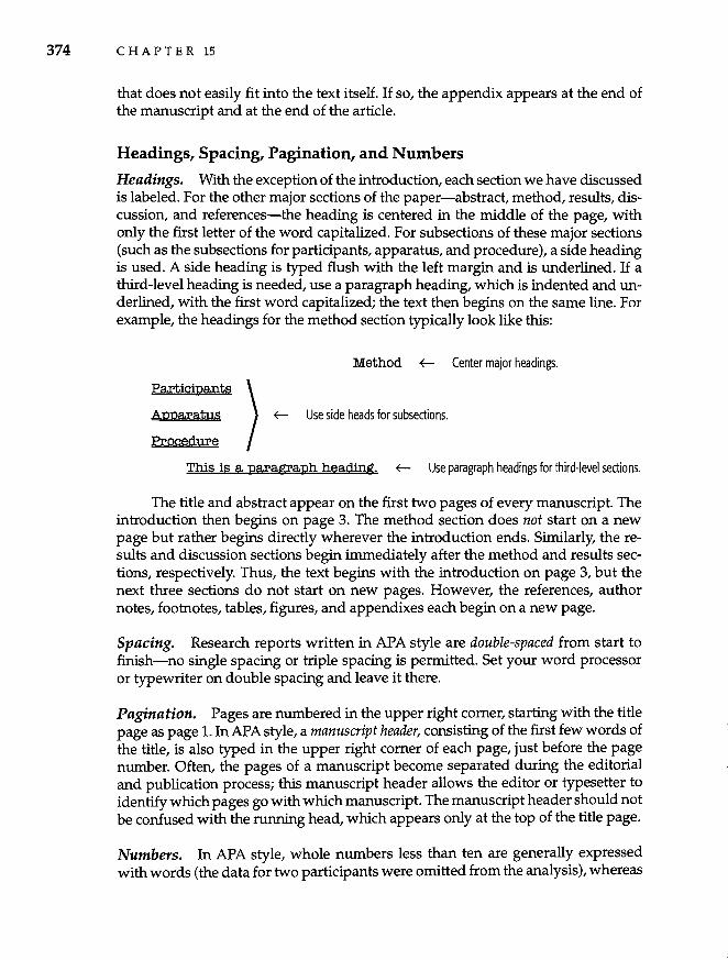
374 CHAPTER 15

that does not easily fit into the text itself. If so, the appendix appears at the end of the manuscript and at the end of the article.

Headings, Spacing, Pagination, and Numbers

Headings. With the exception of the introduction, each section we have discussed is labeled. For the other major sections of the paper-abstract, method, results, dis­cussion, and references-the heading is centered in the middle of the page, with only the first letter of the word capitalized. For subsections of these major sections (such as the subsections for participants, apparatus, and procedure), a side heading is used. A side heading is typed flush with the left margin and is underlined. If a third-level heading is needed, use a paragraph heading, which is indented and un­derlined, with the first word capitalized; the text then begins on the same line. For example, the headings for the method section typically look like this:

Method ~ Center major headings.

Participants )

ApParatus ~

Procedure

Use side heads for subsections.

This is a paragraph heading. ~ Use paragraph headings for third-level sections.

The title and abstract appear on the first two pages of every manuscript. The introduction then beginS on page 3. The method section does not start on a new page but rather begins directly wherever the introduction ends. Similarly, the re­sults and discussion sections begin immediately after the method and results sec­tions, respectively. Thus, the text begins with the introduction on page 3, but the next three sections do not start on new pages. However, the references, author notes, footnotes, tables, figures, and appendixes each begin on a new page.

Spacing. Research reports written in APA style are double-spaced from start to finish-no single spacing or triple spacing is permitted. Set your word processor or typewriter on double spacing and leave it there.

Pagination. Pages are numbered in the upper right comer, starting with the title page as page 1. In APA style, a manuscript header, consisting of the first few words of the title, is also typed in the upper right comer of each page, just before the page number. Often, the pages of a manuscript become separated during the editorial and publication process; this manuscript header allows the editor or typesetter to identify which pages go with which manuscript. The manuscript header should not be confused with the running head, which appears only at the top of the title page.

Numbers. In APA style, whole numbers less than ten are generally expressed with words (the data for two participants were omitted from the analysis), whereas

Scientific Writing 375

numbers 10 and above are expressed with numerals (Of the 20 participants who agreed to participate, 10 were women). However, numbers that begin a sentence must be expressed in words (Twenty rats served as participants). Furthermore, numbers that precede units of measurement should be expressed in numerals (the temperature was 8 degrees), as should numbers that represent time, dates, ages, and sample sizes (2 weeks; November 29,1954; 5-year-olds; n = 7).

mew he IN DEPTH

Who Deserves the Credit? As researchers prepare papers for publication or presentation they often face the poten­tially thorny question of who deserves to be listed as an author of the paper. Many people contribute to the success of a research project-the principle investigator (P.I.) who initi­ates and oversees the project, research assistants who help the P.I. design the study, other researchers not directly involved in the research who nonetheless offer suggestions, the clerical staff who types questionnaires and manuscripts, the individuals who collect the data, statistical consultants who help with analyses, technicians who maintain equipment and computers, and so on. Which of these individuals should be named as an author of the final paper?

According to the Publication Manual of the American Psychological Association (1994), au­thorship is reserved for those individuals who have made "substantial scientific contribu­tions" to a study (p. 294). Substantial scientific contributions include formulating the research problem and hypotheses, designing the study, conducting statistical analyses, interpreting results, and writing major parts of the research report-activities that require scientific knowledge about the project. Generally, supportive functions-such as maintaining equip­ment, writing computer programs, recruiting participants, typing materials, or Simply col­lecting data-do not by themselves constitute a "substantial scientific contribution" because they do not involve specialized knowledge about the research. However, individuals who contribute in these ways are often acknowledged in the author note that appears on the first page of the article.

The authors' names should be listed on the paper in order of decreasing contribution. Thus, the principal investigator-typically the faculty member or senior scientist who su­pervised the project-is listed first, followed by the other contributors. However, when an article is substantially based on a student's thesis or dissertation, the student is usually listed as first author. If two or more authors have had equal roles in the research, they some­times list their names in a randomly chosen order, then state that they contributed equally in the author's note.

The order in which authors are listed is based on the magnitude of the authors' sci­entific and professional contributions to the project and not on the sheer amount of time that each person devoted to the project. Thus, although P.I.'s may spend less time on the project than assistants who collect data, P.I.'s will likely be listed as first author because their contributions-<iesigning the study, conducting statistical analyses, and writing most of the manuscript-are more crucial to the scientific merit of the research.

376 C HAP T E R 15

To the new researcher, APA style is complex and confusing; indeed, veteran researchers are not familiar with every detail in the APA Publication Manual. Even so, the guidelines contained in this manual are designed to enhance effective com­munication among researchers, and behavioral researchers are expected to be fa­miliar with the basics of APA style. When preparing a manuscript for submission, researchers often refer to the Publication Manual when they are uncertain of how the manuscript should look.

Sample Manuscript

What follows is an example of a research report that has been prepared according to APA style.1 This is a manuscript that an author might submit for publication; the published article would, of course, look very different. I've annotated this manuscript to point out some of the basic guidelines that we have discussed in this chapter.

lThe sample manuscript was taken from "The Motivated Expression of Embarrassment Following a Self-Presentational Predicament" by Mark Leary, Journal of Personality, 64, 619-636, 1996. Reprinted by permission of the author and Blackwell Publishers.

The title page in­cludes five things: the manuscript header, the run­ning head, the manuscript title, the authors' names, and the authors' institu­tional affiliations. The first two or three words of the title (the manu­script header) should appear in the upper right­hand corner of every page, fol­lowed by the page number. (The title page is numbered as page 1.) The running head is an abbreviated title that will be printed at the tops of the pages of the pub­lished journal arti­cle. It should be no longer than 50 characters (count­ing letters, spaces, and punctuation) and appears near the upper left cor­ner on the title page. The title is followed by the authors' names and affiliations.

Social Blushing 1

Running head: BLUSHING AND FACE-SAVING

Social Blushing as a Face-Saving Display

Julie Landel Mark Leary

Wake Forest University

377

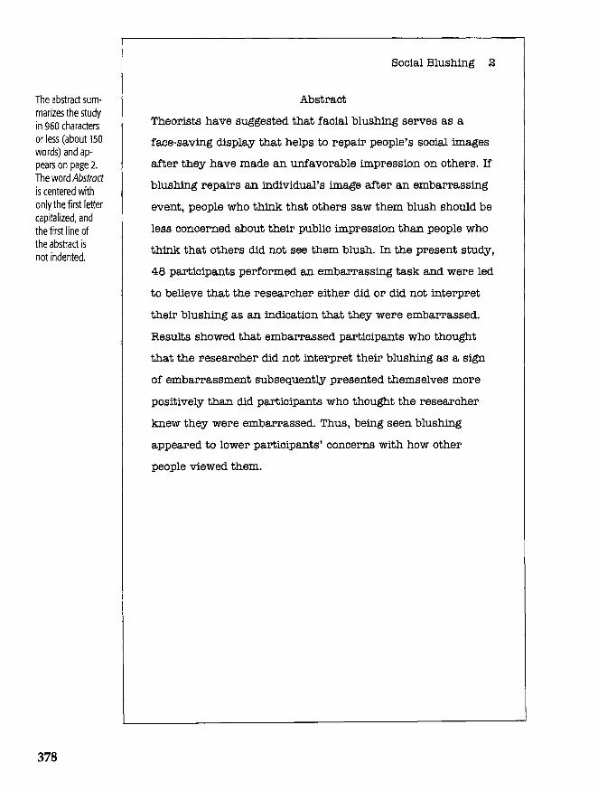
The abstract sum­marizes the study in 960 characters or less (about 150 words) and ap­pears on page 2. The word Abstract is centered with only the first letter capitalized, and the first line of the abstract is not indented.

378

Social Blushing 2

Abstract

Theorists have suggested that facial blushing serves as a

face-saving display that helps to repair people's social images

after they have made an unfavorable impression on others. If

blushing repairs an individual's image after an embarrassing

event, people who think that others saw them blush should be

less concerned about their public impression than people who

think that others did not see them blush. In the present study,

48 participants performed an embarrassing task and were led

to believe that the researcher either did or did not interpret

their blushing as an indication that they were embarrassed.

Results showed that embarrassed partiCipants who thought

that the researcher did not interpret their blushing as a sign

of embarrassment subsequently presented themselves more

positively than did participants who thought the researcher

knew they were embarrassed. Thus, being seen blushing

appeared to lower partiCipants' concerns with how other

people viewed them.

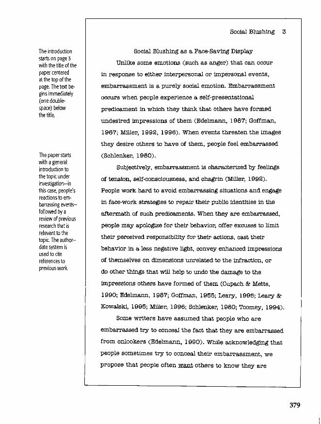
The introduction starts on page 3 with the title of the paper centered at the top of the page. The text be­gins immediately (one double­space) below the title.

The paper starts with a general introduction to the topic under investigation-in this case, people's reactions to em­barrassing events­followed bya review of previous research that is relevant to the topic. The author­date system is used to cite references to previous work.

Social Blushing 3

Social Blushing as a Face-Saving Display

Unlike some emotions (such as anger) that can occur

in response to either interpersonal or impersonal events,

embarrassment is a purely social emotion. Embarrassment

occurs when people experience a self-presentational

predicament in which they think that others have formed

undesired impressions of them (Edelmann, 1987; Goffman,

1967; Miller, 1992, 1996). When events threaten the i.m.ages

they desire others to have of them, people feel embarrassed

(Schlenker, 1980).

SuQjectively, embarrassment is characterized by feelings

of tension, self-consciousness, and chagrin (Miller, 1992).

People work hard to avoid embarrassing situations and engage

in face-work strategies to repair their public identities in the

aftermath of such predicaments. When they are embarrassed,

people may apologize for their behavior, offer excuses to limit

their perceived responsibility for their actions, cast their

behavior in a less negative light, convey enhanced impressions

of themselves on ctimensions unrelated to the infraction, or

do other things that will help to undo the damage to the

impressions others have formed of them (Cupach 8e Metts,

1990; Edelmann, 1987; Goffman, 1955;Lear,y, 1995;Lear,y8e

Kowalski, 1995; Miller, 1996; Schlenker, 1980; Toomey, 1994).

Some writers have assumed that people who are

embarrassed try to conceal the fact that they are embarrassed

from onlookers (Edelmann, 1990). While acknowledging that

people sometimes try to conceal their embarrassment, we

propose that people often lll:a.D.li others to know they are

379

When several references are given, they are alphabetized by the last name of the first author and separated by semicolons.

The last sentence of this paragraph includes a quota­tion. When quot­ing verbatim, the quote appears in quotation marks, with the page number of its source included in parentheses.

380

Social Blushing 4

embarrassed and sometimes behave in ways that convey

their embarrassment to others. They may verbalize their

chagrin (e.g., "Boy, do I feel stupid"; "Geez, this is

embarrassing") or convey it nonverbally through downcast

eyes, an embarrassed silly smile, or facial blushing

(Asendorpf, 1990; Edelmann, 1990; Miller Be Leary, 1992).

Rather than being a mere expression of their inner

feelings, the verbal and nonverbal behaviors that accompany

embarrassment ID.a8' reflect a motivation to convey

embarrassment to others. By publicly conveying their

embarrassment, people show others that they realize an image­

threatening predicament has occurred, express support for the

norms or rules they have violated, and implicitly indicate

that their inappropriate, foolish, or undesired behavior should

not be taken as a reflection of their personality, character,

or ability. Failing to appear embarrassed, in contrast, conveys

that the person is unaware of or unconcerned about the

embarrassing predicament and others' evaluations of him or

her (Semin Be Manstead, 1982). As Goffman (1967) noted, by

appearing embarrassed, a person "demonstrates that, while he

cannot present a sustainable and coherent self on this occasion,

he is at least disturbed by the fact and ID.a8' prove worthy at

another time" (p. Ill).

If verbal and nonverbal displays of embarrassment help to

repair one's social image, people whose embarrassment displays

go unnoticed by other people should take other steps to improve

their damaged social1mages. Thus, they should resort to

alternative self-presentational strategies to improve their public

image if others do not appear to recognize their embarrassment.

Two sentences in this paragraph c~e previous work by incorporating the authors' names into the sentence. The year of publi­cation follows their names in paren­theses.

The first sentence in this paragraph includes two refer­ences that were al­ready cited (in the previous para­graph). Because the Castelfranchi and Poggi article had only two au­thors, both of them are listed in the second c~tion below. However, the Leary, Britt, Cutlip, and Tem­pleton article had more than two au­thors, so the sec-0nd citation is listed as Leary et al.

SooiaJ. Blushing 5

Among light-skinned people, one response that often

signals embarrassment is faciaJ. blushing--a spontaneous

reddening or darkening of the face, neok, and ears (Leary,

Britt, Cutlip, Be Templeton, 1992). Several writers have

suggested that blushing diffuses threats to one's publio identity.

In an early discusSion of this theme, Burgess (1839) proposed

that blushing signals to others that the individual recognizes

that he or she has violated important moral rules (see also

Karoh, 1971; MaoCurdy, 1930). More recently, Castelfranohi

and Poggi (1990) suggested that "those who are blushing are

somehow saying that they know, care about, and fear others'

evaluation, and that they share those values deeply; they

also communicate their sorrow over any possible faults

or inadequacies on their part, thus performing an

acknowledgement, a confeSSion, and an apology .... " (p. 240).

Indirect evidence supports the idea that blushing

possesses face-saving or remedial qualities (Castelfranohi Be

Poggi, 1990; Leary et al., 1992). Blushing, like other signs of

embarrassment--such as downoast eyes and nervous grinning-­

seems to mitigate others' negative reactions to sooially

unacceptable behaviors (Semin Be Manstead, 1982). By

oonveying the individual's embarrassment about his or her

behavior, blushing reduces others' negative reactions to

ineptness, immorality, rudeness, and other sooially undesirable

actions. Thus, blushing should help to repair the damage

caused by self-presentationaJ. predicaments in much the same

way as does a verbal expression that makes one feel foolish

or embarrassed.

381

The final para­graph of the intro­duction states the objectives and predictions of the study.

The method section begins immediately following the end of the introduction, with the heading Method centered on the page. The subheadings Partic­ipants and Proce­dure appear as side headings, typed flush left and un­derlined. Because no specialized ma­terials or apparatus were used in this study, an appara­tus/materials sec­tion is not induded.

The number, sex, and age of the par­ticipants are given. Note that numbers 10 and larger are expressed in numerals.

382

Social Blushing 6

If this is true, a threat to one's public identity remains

unresolved if one's bluslting is not perceived by others or if the

flush is interpreted as something other than an indication of

embarrassment (such as physicaJ. exertion or alcohol

consumption). If, as we hypothesize, people want to be seen as

embarrassed because it improves their i.mage, individuals whose

blushes are not regarded as such by others should engage in

alternative face-work strategies to improve their damaged i.mage.

Thus, we predicted that individuals who convey an

undeSired social image should subsequently try to improve

their image to a greater extent if their blush does not

adequately convey their chagrin to others (because it is

interpreted as something other than an embarrassed blush).

SpecificaJ.ly, such individuals should try to convey more

positive impressions of themselves than individuals who have

either not been embarrassed or whose embarrassed blushes

have been perceived by others.

Method

ParticiPants

Participants were 24 male and 24 female undergraduate

students, ages 17 to 21, who participated in the study in

partial fulfillment of a course research requirement.

Experimental sessions were conducted by a female

researcher.

Procedure

Upon arriving at the lab, participants were told that the

study involved the relationship between physiologicaJ. processes

The procedure section does not necessarily have to be broken into subsections as it is here. However, using subsections sometimes helps the reader keep track of the differ­ent parts of the procedure. If sub­sections are used, they are labeled with paragraph headings. Para­graph headings are indented, underlined, and followed by a period, with only the first word of the heading capi­talized. The text then begins on the same line as the heading.

Social Blushing 7

and emotional experiences. In particular, participants were

led to believe that the researchers were interested in how the

relationship between physiological reactions and emotion

differs when people listen to music as compared to when they

perform music.

Thermistors were attached to the partiCipant's cheek

Gust below the zygomatic bone) and to the pad of the index

finger of the nondominant hand. The thermistor leads ran to a

bogus temperature monitor that, for the time being, was

visually obstructed by a clipboard.

Embarrassment induction. Participants were told that

they would first listen to a tape of a musical selection, then

sing the song while their physiological responses were

monitored. They were assured that the laboratory was

completely soundproof (which it was) so that no one,

including the researcher, would hear them as they sang. The

researcher gave the participant a sheet containing the lyrics

to the song, "Feelings" (Albert, 1975), started an instruction

tape, and left the room. The taped instructions reiterated that

participants should sit quietly as the song was played. Then,

when "Feelings" was played a second time, they were to sing

along with the music into a second tape recorder, imagining

that they were performing the song on stage.

After the participants sang the song, the researcher

reentered the chamber, stopped the recorder, and rewound the

tape. If the participant was in one of two embarrassment

conditions, the researcher remarked that she wanted to be

sure that the recorder had worked properly, then played a six

383

The procedure is described in enough detail that it can be replicated by an­other researcher.

384

Social Blushing 8

second portion of the participant's singing. As the tape pl.a3red,

the researcher did not look at the participant and did not

overtly react.

Blush interpretation m.a.nipulation. The researcher then

removed the clipboard from in front of the temperature

mOnitor, which had been preset to show that the participant's

face was warm. Motioning to the meter, the researcher

casually commented that the participant's face seemed to be

warm. Then, for participants in the blushing interpretation

condition, the researcher casually remarked that p1.a.ying the

tape must have caused the participant to blush. If the

participant was in the nonblW!bipg int;Em!reta.tion conditiop"

the researcher remarked that the increase in facial

temperature was a normal effect of the exertion of the facial

muscles involved in si.nging. For participants in the

nonemba.rra,ssed, control condition, the researcher did not

Pl.a3r the tape and made no reference to the temperature

monitor. In all conditions, the researcher refrained from

looking directly at the participant.

PeperuieP,t measures. The sensors were removed, and

the participant completed the experimental questionnaire.

However, before doing so, the researcher mentioned that she

would go over the participants' answers with them, thereby

making their ratings interpersonal and, thus, potentially

self-presentational.

The primary dependent measures involved a list of

10 evaluative, self-relevant adjectives (cheerful, egotistical,

The results section begins immediately after the method secton. The head­ing, Results, is centered. The re­sults section does not need to be broken into subsec­tions as it is here, but doing so often improves readabil­ity. Again, the sub­sections are labeled with side headings.

Abbreviations and acronyms (such as AN OVA) must be spelled out the first time they appear in a paper. Note that in describing the results of the F-test, the degrees of freedom, calculated value of E and probability level are included. Condition means are labeled M and included in parentheses.

Social Blushing 9

charming, appreciative, rude, friendly, arrogant, conceited,

honest, cruel) on which participants rated themselves on 12-

point scales C 1 = not at all; 12 = extremely). Because we were

concerned that the embarrassment manipulation might affect

participants' perceptions of the researcher differently across

conditions, thereby influencing the degree to which they

wanted to impress her, participants also rated the researcher

on three scales: competence, professionalism, and

pleasantness C 1 = not at all; 12 = extremely).

As a manipulation check, partiCipants were asked to

indicate whether they thought the researcher saw them

engage in several behaviors during the study. Embedded in

this list was "facial blushing" (l = not at all; 12 = extremely).

Participants were then debriefed, with the nature of the study

and the manipulations explained fully.

Results

Man.iJmla.tion Check

An analysis of variance CANOVA) performed on participants'

responses to the manipulation check revealed a significant

main effect of experimental condition, EC2, 43) = 4.29,

12 < .05. Tukey's test showed that partiCipants in the blushing­

interpretation condition CM = 8.1) thought the researcher had

seen them blushing significantly more than partiCipants in the

nonblushing-interpretation CM = 5.3) and control

CM = 6.6) conditions, 12 < .05, which did not differ

significantly from one another.

385

When available, information regarding the relia­bility of the measures (in this case, Cronbach's alpha) should be presented.

Again, all neces­sary statistical information is pro­vided. The figure is included at the end of the manu­scrip~ although it would appear here in the results in the published version of the article.

386

Social Blushing lO

Self-Presentations

Participants' self-ratings on the 10 adjectives were

coded such that high ratings reflected more positive self­

presentations. Because the lO items had acceptable interitem

reliability (Cronbach's alpha coefficient = .77), they were

summed to create a single measure of participants' self­

presentations to the researcher.

A 3 (condition) by 2 (sex) ANOVA performed on this

measure revealed only a significant main effect of condi-

tion, l(2, 42) = 3.28, 12 < .05. As can be seen in Figure 1,

participants' self-presentations were consistent with predictions.

Post hoc tests (Tokey's) showed that embarrassed participants

whose blushing was dismissed as an effect of the exertion

required of singing subsequently presented themselves

significantly more positively CM = 100.6) than embarrassed

participants whose blushing had been interpreted as a sign

of embarrassment CM = 93.6) or who had not been

embarrassed at all CM = 92.6), 12 < .05. The latter two

conditions did not differ Significantly, l(l,42) = .09,

12 > .05. Thus, embarrassed participants who thought the

researcher interpreted their blush as a sign of

embarrassment were no more self-enhancing than

nonembarrassed control participants.

One alternative explanation of these results is that the

experimental manipulation caused participants in some

conditions to feel more negatively toward the researcher,

thereby affecting their self-presentations. To determine whether

the effects were mediated by partiCipants' attitudes toward the

The discussion section begins immediately after the results section. It begins with a general statement of the study's major findings.

In this sentence, connections are drawn between the findings and other research.

Social Blushing 11

researcher, a multivariate analysis of variance was conducted

on the three ratmgs of the researcher. No effects approached

significance, 12 > .20.

Discussion

As predicted, embarrassed participants who believed

that the researcher did not perceive their blushes

subsequently presented themselves more positively than

embarrassed participants who thought the researcher had

seen them blush. When blushing did not serve to repair their

public images after an embarrassing event, participants

appeared to use other means to convey positive impressions

to the researcher. Participants whose blushes were

disregarded by the researcher appeared to compensate for

appearing silly on one dimension (i.e., singing) by

presenting themselves more positively on other, unrelated

dimensions. In contrast, participants who thought their

blushes were perceived as evidence of embarrassment did

not self-enhance relative to nonembarrassed participants

because their self-presentational predicament was largely

resolved by the blush itself. The compensatory tactic

shown by embarrassed participants whose blushes were

interpreted as a sign of exertion is simUar to that

demonstrated by Baumeister and Jones (1978). In their

study, participants who believed others had received

unflattering information about them subsequently presented

more positive impressions of themselves on dimensions

unrelated to the negative information.

387

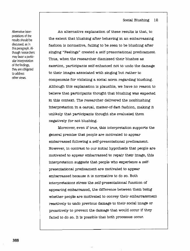
Alternative inter­pretations of the results should be discussed. as in this paragraph. Al­though researchers may favor a partic­ular interpretation of the findings. they are obligated to address other views.

388

Social Blushing 12

An alternative explanation of these results is that, to

the extent that blushing after behaving in an embarrassing

fashion is normative, failing to be seen to be blushing after

singing "Feelings" created a self-presentational predicament.

Thus, when the researcher dismissed their blushes as

exertion, participants self-enhanced not to undo the damage

to their images associated with singing but rather to

compensate for violating a social norm regarding blushing.

Although this explanation is plausible, we have no reason to

believe that participants thought that blushing was expected

in this context. The researcher delivered the nonblushing

interpretation in a casual, matter-of-fact fashion, making it

unlikely that partiCipants thought she evaluated them

negatively for not blushing.

Moreover, even if true, this interpretation supports the

general premise that people are motivated to appear

embarrassed following a self-presentational predicament.

However, in contrast to our initial hypothesis that people are

motivated to appear embarrassed to repair their image, this

interpretation suggests that people who experience a self­

presentational predicament are motivated to appear

embarrassed because it is normative to do so. Both

interpretations stress the self-presentational function of

appearing embarrassed, the difference between them being

whether people are motivated to convey their embarrassment

reactively to undo previous damage to their social image or

proactively to prevent the damage that would occur if they

failed to do so. It is possible that both processes occur.

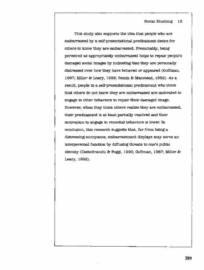
Social Blushing 13

This study also supports the idea that people who are

embarrassed by a self-presentational predicament desire for

others to know they are embarrassed. Presumably, being

perceived as appropriately embarrassed helps to repair people's

damaged social images by indicating that they are personally

distressed over how they have behaved or appeared (Goffman,

1967; Miller Be Leary, 1992; Semin Be Manstead, 1982). As a

result, people in a self-presentational predicament who think

that others do not know they are embarrassed are motivated to

engage in other behaviors to repair their damaged image.

However, when they think others realize they are embarrassed,

their predicament is at least partially resolved and their

motivation to engage in remedial behaviors is lower. In

conclusion, this research suggests that, far from being a

distressing annoyance, embarrassment displays may serve an

interpersonal function by diffusing threats to one's public

identity (Castelfranchi Be Poggi, 1990; Goffman, 1967; Miller Be

Leary, 1992).

389

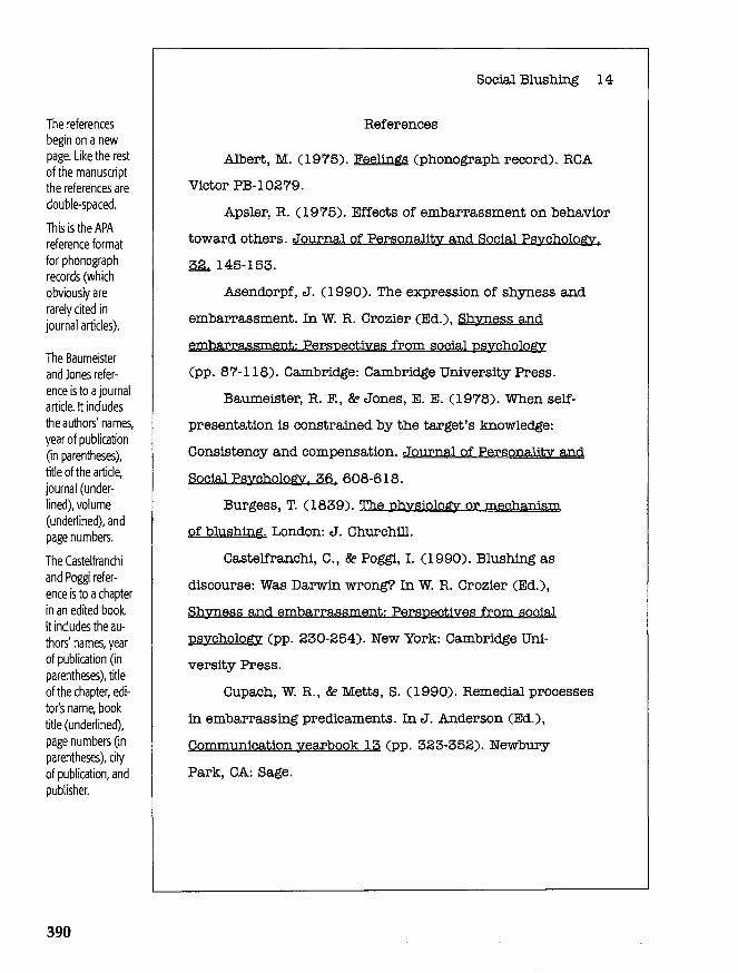
The references begin on a new page. Like the rest of the manuscript the references are double-spaced.

This is the APA reference format for phonograph records (which obviously are rarely cited in journal articles).

The Baumeister and Jones refer­ence is to a journal article. It includes the authors' names, year of publication (in parentheses), title of the article, journal (under­lined), volume (underlined), and page numbers.

The Castelfranchi and Poggi refer­ence is to a chapter in an edited book. It includes the au­thors' names, year of publication (in parentheses), title of the chapter, edi­tor's name, book title (underlined), page numbers (in parentheses), city of publication, and publisher.

390

Sooial Blushing 14

Referenoes

Albert, M. (1975). Feelings (phonograph reoord). RCA

Victor PB-I0279.

Apsler, R. (1975). Effects of embarrassment on behavior

toward others. Journal of Personality and Sooial Psychology,

.32.. 145-153.

Asendorpf, J. (1990). The expression of shyness and

embarrassment. In W. R. Crozier (Ed.), Shyness and

embarrassment: Perspectiyes from social psychology

(pp. 87-118). Cambridge: Cambridge University Press.

Baumeister, R. F., 8e Jones, E. E. (1978). When self­

presentation is oonstrained by the target's knowledge:

Consistenoy and oompensation. Journal of Personality and

Social Psychology, 36. 608-618.

Burgess, T. (1839). The physiology or mechanism

of blushi.ng. London: J. Churohill.

Castelfranohi, C., 8e Poggi, I. (1990). Blushing as

disoourse: Was Darwin wrong? In W. R. Crozier (Ed.),

Shyness and embarrassment: Perspectives from social

psychology (pp. 230-254). New York: Cambridge Uni­

versity Press.

Cupaoh, W. R., 8e Metts, S. (1990). Remedial prooesses

in embarrassing predioaments. In J. Anderson (Ed.),

Communication yearbook 13 (pp. 323-352). Newbury

Park, CA: Sage.

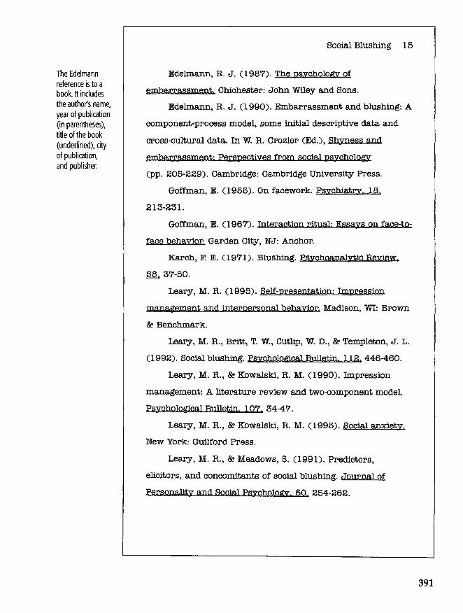
The Edelmann reference is to a book. It includes the author's name, year of publication (in parentheses), title of the book (underlined), city of publication, and publisher.

Social Blushing 15

Edelmann, R J. (1987). The psychology of

embarrassment. Chichester: John Wiley and Sons.

Edelmann, R J. (1990). Embarrassment and blushing: A

component-process model, some initial descriptive data and

cross-cultural data. In W. R Crozier (Ed.), Shyness and

embarrassment: Perspectives from social psychology

(pp. 205-229). Cambridge: Cambridge University Press.

Goffman, E. (1955). On facework. Psychiatry. 18,

213-231.

Goffman, E. (1967). Interaction ritual: Essays on face-to­

face behavior. Garden City, NJ: Anchor.

Karch, F. E. (1971). Blushing. Psychoanalytic Review .

.6..8... 37-50.

Leary, M. R (1995). Self-presentation: Impression

management and interpersonal behavior. Madison, WI: Brown

Be Benchmark.

Leary, M. R, Britt, T. W., Cutlip, W. D., Be Templeton, J. L.

(1992). Social blushing. Psychological Bulletin, 112, 446-460.

Leary, M. R., Be Kowalski, R M. (1990). Impression

management: A literature review and two-component model.

Psychological Bulletin, 107, 34-47.

Leary, M. R, Be Kowalski, R M. (1995). Social anxiety.

New York: Guilford Press.

Leary, M. R, Be Meadows, S. (1991). Predictors,

eliCitors, and concomitants of SOCial blushing. Journal of

Personality and SOCial Psychology, 60. 254-262.

391

392

Social Blushing 16

MacCurdy, J. T. (1930). The biological significance

of blushing and shame. British Journal of Psychology. 21.

174-182.

Miller, R S. (1992). The nature and severity of self­

reported embarrassing circumstances. PerSOnallkY and Social

Psychology Bulletin. 18. 190-198.

Miller, R S. (1996). Embarrassment: Poise and PerU in

eve:r:yda,y life. New York: Guilford.

Miller, R S., Be Leary, M. R. (1992). Social sources

and interactive functions of embarrassment: The case of

embarrassment. In M. S. Clark (Ed.), Emotion and social

behavior (pp. 202-221). Newbury Park, CA: Sage.

Schlenker, B. R (1980). Impression me.nagement: The

self-concept. social identity. and interpersonal relations.

Monterey, CA: Brooks/Cole.

Semin, G. R, Be Manstead, A. S. R (1982). The social

implications of embarrassment displays and restitution

behavior. European Journal of Social Psychology, 12,

367-377.

Toomey, S. T. (Ed.) (1994). The Me,llenge of facework.

Albany, NY: State University of New York Press.

The Authors' Notes give information regarding the authors' depart­mental affiliations, acknowledge the contributions of other people to the study, and pro­vide information for contacting the authors. An Authors' Notes page is typically not used for class papers, theses, or dissertations.

Social Blushing 17

Authors' Notes

Julie Landel, Department of Psychology; Mark Leary,

Department of Psychology, Wake Forest University.

We thank Katharine Patton for her comments on an

earlier version of this manuscript.

Correspondence concerning this article should be

addressed to: Mark R. Leary, Department of Psychology,

Wake Forest University, Winston-Salem, NC 27109. E-mail:

leary@wfu.edu.

393

Figures are at­tached to the end of the manuscript, with the captions for the figures provided on a separate page.

394

Social Blushing 18

Figure Caption

Figure 1. Positive self-presentations as a function of

embarrassment and observed blushing.

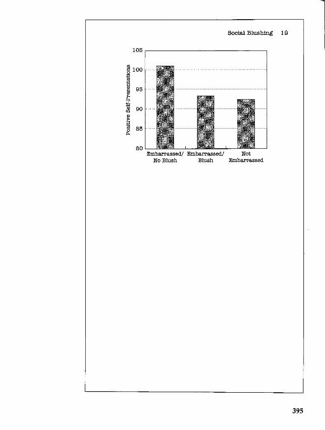
Social Blushing 19

105~----------------------------~

80 Embarrassed/ Embarrassed/ Not

No Blush Blush Embarrassed

395

396 C HAP T E R 15

KEY TERMS

abstract (p. 366) APA style (p. 365) author-date system (p. 370)

gender-neutral language (p.362)

paper session (p. 355)

peer review (p. 354) poster session (p. 355)

QUESTIONS FOR REVIEW

1. What are the three primary ways in which scientists share their work with the sci­entific community?

2. Why is peer review so important to science?

3. When an author submits a manuscript to a journal, what is the general process by which the decision whether or not to publish the paper is made?

4. Distinguish between a paper session and a poster session.

5. Why should we be cautious about reports of research that are published in the pop-ular media and posted on the world wide web?

6. What are the three central characteristics of good writing?

7. Why should authors avoid using gender-biased language?

8. List in order the major sections that all research papers must have.

9. What is the purpose of the introduction of a paper?

10. What information should be included in the method section of a paper? What sub­sections does the method section typically have?

11. When presenting the results of statistical analyses, what information should be presented?

12. Write each of the following references in APA style: a. a book written by Donelson R. Forsyth entitled Group Dynamics that was pub­

lished by Brooks/Cole Publications (based in Pacific Grove, CA) in 1990 b. a journal article entitled "Interpersonal Reactions to Displays of Depression and

Anxiety" that was published in the Journal of Social and Clinical Psychology in 1990; the authors were Michael B. Gurtman, Kathryn M. Martin, and Noelle M. Hintz­man, and the article appeared on pages 256 to 267 of Volume 9 of the journal

c. a chapter entitled "We always hurt the one we love" written by Rowland S. Miller, that appeared on pages 13-29 of an edited book entitled Aversive Inter­personal Behaviors; the book was edited by Robin M. Kowalski and published in 1997 by Plenum Press in New York City

d. a paper presented by Mark R. Leary at the meeting of the American Psycholog­ical Association that was held in Boston in August of 1999; the paper was titled "'The social and psychological importance of self-esteem"

Answers to Question 12 appear on page 398.

Scientific Writing 397

13. Find the violations of APA style in each of the following sentences:

a. Research suggests that attributions have an effect on relationship satiS­

faction over time (Wilson, 1987; Anderson and Camby, 1992).

b. Atkinson (1991) noted that "previous studies confounded diSease severity

with the cost of medical care. "

c. Wilson, Ebbet, and Demorest (1986) were unable to replicate the earlier

finding.

d. Carter and Steinmore (1994) manipulated the brightness of the stimuli

presented on the monitor screen. However, when analyzing their data,

Carter et aI. deleted all participants with reaction times greater than

1600 ms.

Answers to Question 13 appear on page 398.

398 C HAP T E R 15

ANSWERS TO QUESTION 12

a. Book Reference

Forsyth, D. R. (1990). Group dynAmics. Pacific Grove, CA:

Brooks/Cole.

b. Journal Reference

Gurtman, M. B., Martin, K. M., Be Hintzman, N. M. (1990). Inter­

personal reactions to displays of depression and anxiety. Journal of

Sooial and Clinioal Psychology, 9, 256-267.

c. Chapter Reference

Miller, R. S. (1997). We always hurt the ones we love. In R. M.

Kowalski (Ed.), Aversive interpersonal behaviors (pp. 13-29). New

York, NY: Plenum Press.

d. Paper Reference

Leary, M. R. (1999, August). The sooial and psychologioaJ. im,por­

ta.nce of self-esteem. Paper presented at the meeting of the American

Psyohologioal Assooiation, Boston, MA.

ANSWERS TO QUESTION 13

a. This sentence contains two violations of APA style: The "and" in "Anderson and Camby" should be an ampersand (&), and "Anderson & Camby" should precede "Wilson."

Researoh suggests that attributions have an effect on relationship satis­

faction over time (Anderson Be Camby, 1992; Wilson, 1987).

b. When quoting, the page number of the quotation must be given.

Atkinson (1991) noted that "previous studies confounded disease severity

with the cost of medical care" (p. 456).

c. This sentence is perfectly okay as it is. d. Because there are only two authors, both names should be given each time the

study is cited; use "et al." only when referencing sources that have more than two authors.

Carter and Steinmore (1994) manipulated the brightness of the stimuli

presented on the monitor screen. However, when analyzing their data,

Carter and Steinmore deleted all partiCipants with reaction times greater

than 1500 ms.

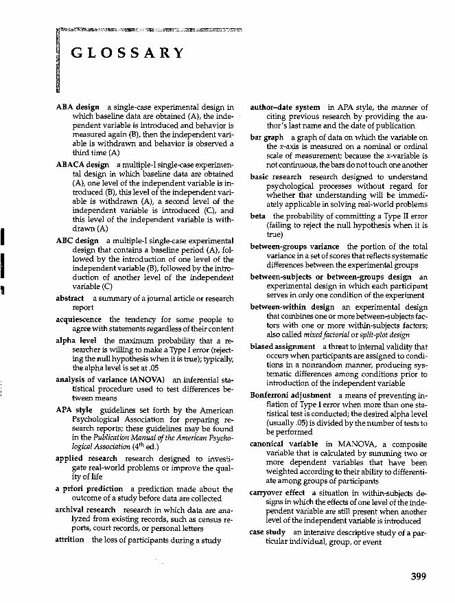
I I ,

GLOSSARY

ABA design a single-case experimental design in which baseline data are obtained (A), the inde­pendent variable is introduced and behavior is measured again (B), then the independent vari­able is withdrawn and behavior is observed a third time (A)

ABACA design a multiple-I single-case experimen­tal design in which baseline data are obtained (A), one level of the independent variable is in­troduced (B), this level of the independent vari­able is withdrawn (A), a second level of the independent variable is introduced (C), and this level of the independent variable is with­drawn (A)

ABC design a multiple-I single-case experimental design that contains a baseline period (A), fol­lowed by the introduction of one level of the independent variable (B), followed by the intro­duction of another level of the independent variable (C)

abstract a summary of a journal article or research report

acquiescence the tendency for some people to agree with statements regardless of their content

alpha level the maximum probability that a re­searcher is willing to make a Type I error (reject­ing the null hypothesis when it is true); typically, the alpha level is set at .05

analysis of variance (ANOVA) an inferential sta­tistical procedure used to test differences be­tween means

APA style guidelines set forth by the American Psychological Association for preparing re­search reports; these guidelines may be found in the Publication Manual of the American Psycho­logical Association (4th ed.)

applied research research designed to investi­gate real-world problems or improve the qual­ity of life

a priori prediction a prediction made about the outcome of a study before data are collected

archival research research in which data are ana­lyzed from existing records, such as census re­ports, court records, or personal letters

attrition the loss of participants during a study

author-date system in APA style, the manner of citing previous research by prOviding the au­thor's last name and the date of publication

bar graph a graph of data on which the variable on the x-axis is measured on a nominal or ordinal scale of measurement; because the x-variable is not continuous, the bars do not touch one another

basic research research designed to understand psychological processes without regard for whether that understanding will be immedi­ately applicable in solving real-world problems

beta the probability of committing a Type II error (failing to reject the null hypothesis when it is true)

between-groups variance the portion of the total variance in a set of scores that reflects systematic differences between the experimental groups

between-subjects or between-groups design an experimental design in which each participant serves in only one condition of the experiment

between-within design an experimental design that combines one or more between-subjects fac­tors with one or more within-subjects factors; also called mixed factorial or split-plot design

biased assignment a threat to internal validity that occurs when participants are assigned to condi­tions in a nonrandom manner, producing sys­tematic differences among conditions prior to introduction of the independent variable

Bonferroni adjustment a means of preventing in­flation of Type I error when more than one sta­tistical test is conducted; the desired alpha level (usually .05) is divided by the number of tests to be performed

canonical variable in MANOVA, a composite variable that is calculated by summing two or more dependent variables that have been weighted according to their ability to differenti­ate among groups of participants

carryover effect a situation in within-subjects de­signs in which the effects of one level of the inde­pendent variable are still present when another level of the independent variable is introduced

case study an intensive deSCriptive study of a par­ticular individual, group, or event

399

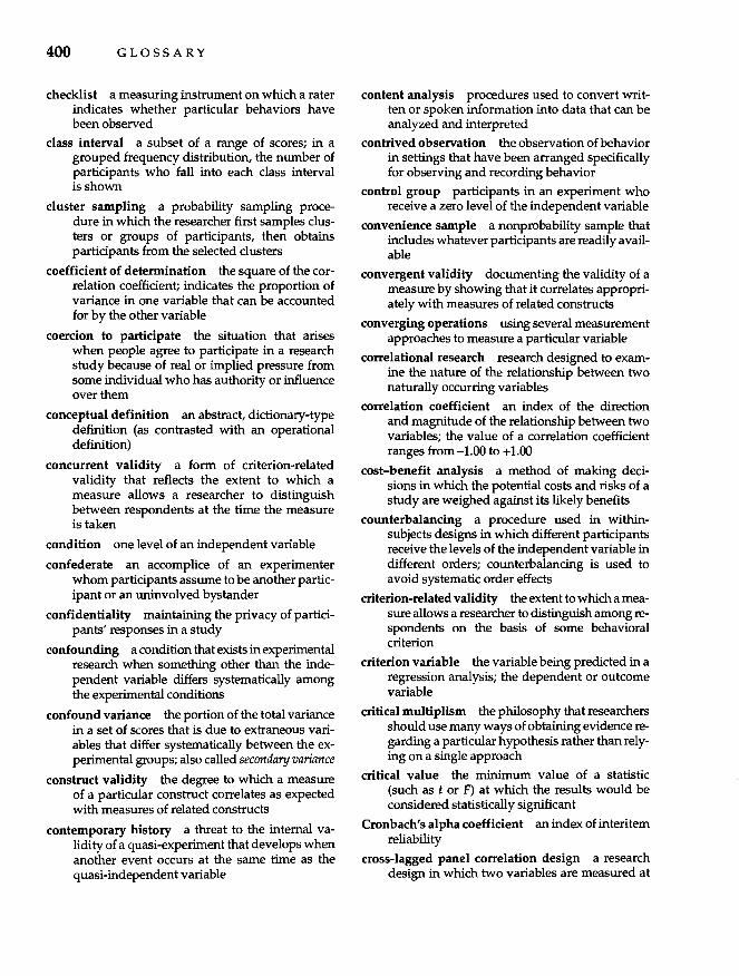
400 GLOSSARY

checklist a measuring instrument on which a rater indicates whether particular behaviors have been observed

class interval a subset of a range of scores; in a grouped frequency distribution, the number of participants who fall into each class interval is shown

cluster sampling a probability sampling proce­dure in which the researcher first samples clus­ters or groups of participants, then obtains participants from the selected clusters

coefficient of determination the square of the cor­relation coefficient; indicates the proportion of variance in one variable that can be accounted for by the other variable

coercion to participate the situation that arises when people agree to participate in a research study because of real or implied pressure from some individual who has authority or influence over them

conceptual definition an abstract, dictionary-type definition (as contrasted with an operational definition)

concurrent validity a form of criterion-related validity that reflects the extent to which a measure allows a researcher to distinguish between respondents at the time the measure is taken

condition one level of an independent variable

confederate an accomplice of an experimenter whom participants assume to be another partic­ipant or an uninvolved bystander

confidentiality maintaining the privacy of partici-pants' responses in a study

confounding a condition that exists in experimental research when something other than the inde­pendent variable differs systematically among the experimental conditions

confound variance the portion of the total variance in a set of scores that is due to extraneous vari­ables that differ systematically between the ex­perimental groups; also called secondary variance

construct validity the degree to which a measure of a particular construct correlates as expected with measures of related constructs

contemporary history a threat to the internal va­lidity of a quasi-experiment that develops when another event occurs at the same time as the quasi-independent variable

content analysis procedures used to convert writ­ten or spoken information into data that can be analyzed and interpreted

contrived observation the observation of behavior in settings that have been arranged specifically for observing and recording behavior

control group participants in an experiment who receive a zero level of the independent variable

convenience sample a nonprobability sample that includes whatever participants are readily avail­able

convergent validity documenting the validity of a measure by showing that it correlates appropri­ately with measures of related constructs

converging operations using several measurement approaches to measure a particular variable

correlational research research designed to exam­ine the nature of the relationship between two naturally occurring variables

correlation coefficient an index of the direction and magnitude of the relationship between two variables; the value of a correlation coefficient ranges from -1.00 to +1.00

cost-benefit analysis a method of making deci­sions in which the potential costs and risks of a study are weighed against its likely benefits

counterbalancing a procedure used in within­subjects designs in which different participants receive the levels of the independent variable in different orders; counterbalancing is used to avoid systematic order effects

criterion-related validity the extent to which a mea­sure allows a researcher to distinguish among re­spondents on the basis of some behavioral criterion

criterion variable the variable being predicted in a regression analysis; the dependent or outcome variable

critical multiplism the philosophy that researchers should use many ways of obtaining evidence re­garding a particular hypothesis rather than rely­ing on a single approach

critical value the minimum value of a statistic (such as t or F) at which the results would be considered statistically significant

Cronbach's alpha coefficient an index of interitem reliability

cross-lagged panel correlation design a research design in which two variables are measured at

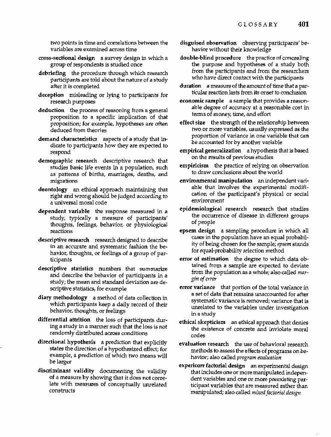
two points in time and correlations between the variables are examined across time

cross-sectional design a survey design in which a group of respondents is studied once

debriefing the procedure through which research participants are told about the nature of a study after it is completed

deception misleading or lying to participants for research purposes

deduction the process of reasoning from a general proposition to a specific implication of that proposition; for example, hypotheses are often deduced from theories

demand characteristics aspects of a study that in­dicate to participants how they are expected to respond

demographic research descriptive research that studies basic life events in a population, such as patterns of births, marriages, deaths, and migrations

deontology an ethical approach maintaining that right and wrong should be judged according to a universal moral code

dependent variable the response measured in a study, typically a measure of participants' thoughts, feelings, behavior, or physiological reactions

descriptive research research designed to describe in an accurate and systematic fashion the be­havior, thoughts, or feelings of a group of par­ticipants

descriptive statistics numbers that summarize and describe the behavior of participants in a study; the mean and standard deviation are de­scriptive statistics, for example

diary methodology a method of data collection in which participants keep a daily record of their behavior, thoughts, or feelings

differential attrition the loss of participants dur­ing a study in a manner such that the loss is not randomly distributed across conditions

directional hyp~the~is a prediction that explicitly states the direction of a hypothesized effect; for example, a prediction of which two means will be larger

discriminant validity documenting the validity of a measure by showing that it does not corre­late with measures of conceptually unrelated constructs

GLOSSARY 401

disguised observation observing participants' be­havior without their knowledge

double-blind procedure the practice of concealing the purpose and hypotheses of a study both from the participants and from the researchers who have direct contact with the participants

duration a measure of the amount of time that a par­ticular reaction lasts from its onset to conclusion

economic sample a sample that provides a reason­able degree of accuracy at a reasonable cost in terms of money, time, and effort

effect size the strength of the relationship between two or more variables, usually expressed as the proportion of variance in one variable that can be accounted for by another variable

empirical generalization a hypothesis that is based on the results of previous studies

empiricism the practice of relying on observation to draw conclusions about the world

environmental manipulation an independent vari­able that involves the experimental modifi­cation of the participant's physical or social environment

epidemiological research research that studies the occurrence of disease in different groups of people

epsem design a sampling procedure in which all cases in the population have an equal probabil­ity of being chosen for the sample; epsem stands for equal-probability selection method

error of estimation the degree to which data ob­tained from a sample are expected to deviate from the population as a whole; also called mar­gino/error

error variance that portion of the total variance in a set of data that remains unaccounted for after systematic variance is removed; variance that is unrelated to the variables under investigation in a study

ethical skepticism an ethical approach that denies the existence of concrete and inviolate moral codes

evaluation research the use of behavioral research methods to assess the effects of programs on be­havior; also called program evaluation

experico~ factorial design an experimental design that mcl~des one or more manipulated indepen­dent vanables and one or more preexisting par­ticipant variables that are measured rather than manipulated; also called mixed factorial design

402 GLOSSARY

experiment research in which the researcher as­signs participants to conditions and manipu­lates at least one independent variable

experimental contamination a situation that oc­curs when participants in one experimental con­dition are indirectly affected by the independent variable in another experimental condition be­cause they interacted with participants in the other condition

experimental control the practice of eliminating or holding constant extraneous variables that might affect the outcome of an experiment

experimental group participants in an experiment who receive a nonzero level of the independent variable

experimental hypothesis the hypothesis that the independent variable will have an effect on the dependent variable; equivalently, the hypothe­sis that the means of the various experimental conditions will differ from one another

experimental research research designed to test whether certain variables cause changes in be­havior, thoughts, or feelings; in an experiment, the researcher assigns participants to condi­tions and manipulates at least one independent variable

experimenter expectancy effect a situation in which a researcher's expectations about the outcome of a study influences participants' re­actions; also called Rosenthal effect

experimenter's dilemma the situation in which, generally speaking, the greater the internal va­lidity of an experiment, the lower its external validity, and vice versa

external validity the degree to which the results obtained in one study can be replicated or gen­eralized to other samples, research settings, and procedures

extreme groups procedure creating two groups of participants that have unusually low or unusu­ally high scores on a particular variable

face validity the extent to which a measurement procedure appears to measure what it is sup­posed to measure

factor (1) in experimental designs, an independent variable; (2) in factor analysis, the underlying dimension that is assumed to account for ob­served relationships among variables

factor analysis a class of multivariate statistical techniques that identifies the underlying dimen-

sions (factors) that account for the observed re­lationships among a set of measured variables

factorial design an experimental design in which two or more independent variables are manip­ulated

factor loading in factor analysis, the correlation between a variable and a factor

factor matrix a table that shows the results of a fac­tor analysis; in this matrix the rows are vari­ables and the columns are factors

failing to reject the null hypothesis concluding on the basis of statistical evidence that the null hypothesis is true-that the independent vari­able does not have an effect

falsifiability the requirement that a hypotheSiS must be capable of being falsified

field notes a researcher's narrative record of a par­ticipant's behavior

fit index in structural equations modeling, a statis­tic that indicates how well a hypothesized model fits the data

follow-up tests inferential statistics that are used after a significant F-test to determine which means differ from which; also called post hoc tests or multiple comparisons

frequency the number of participants who ob­tained a particular score

frequency distribution a table that shows the number of participants who obtained each pos­sible score on a measure

frequency polygon a form of line graph F-test an inferential statistical procedure used to

test for differences among condition means; the F-test is used in ANOVA

gender-neutral language language that treats men and women equally and does not perpetuate stereotypes about men and women

generational effects differences among people of various ages that are due to the different condi­tions under which each generation has grown up rather than age differences

grand mean the mean of all of the condition means in an experiment

graphical method presenting and summarizing data in pictorial form (e.g., graphs and pictures)

graphic analysis in single-case experimental re­search, the visual inspection of graphs of the data to determine whether the independent variable affected the participant's behavior

group design an experimental design in which several participants serve in each condition of the design, and the data are analyzed by exam­ining the average responses of participants in these conditions

grouped frequency distribution a table that indi­cates the number of participants who obtained each of a range of scores

hierarchical multiple regression a multiple re­gression analysis in which the researcher speci­fies the order that the predictor variables will be entered into the regression equation

histogram a form of bar graph in which the vari­able on the x-axis is on a continuous scale

history effects changes in participants' responses between pretest and posttest that are due to an outside, extraneous influence rather than to the independent variable

hypothesis a proposition that follows logically from a theory; also, a prediction regarding the outcome of a study

hypothetical construct an entity that cannot be di­rectly observed but that is inferred on the basis of observable evidence; intelligence, status, and anxiety are examples of hypothetical constructs

idiographic approach research that describes, ana­lyzes, and attempts to understand the behavior of individual participants; often contrasted with the nomothetic approach

independent variable in an experiment, the vari­able that is varied or manipulated by the re­searcher to assess its effects on participants' behavior

induction the process of reasoning from specific instances to a general proposition about those instances; for example, hypotheses are some­times induced from observed facts

inferential statistics mathematical analyses that allow researchers to draw conclusions regard­ing the reliability and generalizability of their data; t-tests and F-tests are inferential statistics, for example

informed consent the practice of informing partic­ipants regarding the nature of their participa­tion in a study and obtaining their written consent to participate

informed consent form a document that describes the nature of participants' participation in a study (including all possible risks) and pro-

GLOSSARY 403

vides an opportunity for participants to indi­cate in writing their willingness to participate

Institutional Review Board (IRB) a committee mandated by federal regulations that must evaluate the ethics of research conducted at in­stitutions that receive federal funding

instructional manipulation an independent vari­able that is varied through verbal information that is provided to participants

interaction the combined effect of two or more in­dependent variables such that the effect of one independent variable differs across the levels of the other independent variable(s)

interbehavior latency the time that elapses be­tween the occurrence of two behaviors

interitem reliability the consistency of respondents' responses on a set of conceptually related items; the degree to which a set of items that ostensibly measure the same construct are intercorrelated

internal validity the degree to which a researcher draws accurate conclusions about the effects of an independent variable

interparticipant replication in single-case experi­mental research, documenting the generalizabil­ity of an experimental effect by demonstrating the effect on other participants

interparticipant variance variability among the responses of the participants in a particular ex­perimental condition

interrater reliability the degree to which the obser­vations of two independent raters or observers agree; also called inter judge or interobserver relia­bility

interrupted time series design with a reversal a study in which (1) the dependent variable is measured several times; (2) the independent variable is introduced; (3) the dependent vari­able is measured several more times; (4) the in­dependent variable is then withdrawn; and (5) the dependent variable is again measured several times

interrupted time series design with multiple repli­cations a study in which (1) the dependent variable is measured several times; (2) the in­dependent variable is introduced; (3) the de­pendent variable is measured again; (4) the independent variable is withdrawn; (5) the de­pendent variable is measured; (6) the indepen­dent variable is introduced a second time; (7) more measures of the dependent variable

404 GLOSSARY

are taken; (8) the independent variable is once again withdrawn; and (9) the dependent vari­able is measured after the independent vari­able has been withdrawn for the second time

interval scale a measure on which equal distances between scores represent equal differences in the property being measured

interview a method of data collection in which re­spondents respond verbally to a researcher's questions

interview schedule the series of questions and accompanying response formats that guides an interviewer's line of questioning during an interview

intraparticipant replication in single-case ex­perimental research, the attempt to repeatedly demonstrate an experimental effect on a single participant by alternatively introducing and withdrawing the independent variable

intraparticipant variance variability among the re­sponses of a participant when tested more than once in a particular experimental condition

invasion of privacy violation of a research partici­pant's right to determine how, when, or where he or she will be studied

invasive manipulation an independent variable that directly alters the participant's body, such as surgical procedures or the administration of chemical substances

item-total correlation the correlation between re­spondents' scores on one item on a scale and the sum of their responses on the remaining items; an index of interitem reliability

knowledgeable informant someone who knows a participant well enough to report on his or her behavior

latency the amount of time that elapses between a particular event and a behavior

Latin square design an experimental design used to control for order effects in a within-subjects design

level one value of an independent variable

local history effect a threat to internal validity in which an extraneous event happens to one ex­perimental group that does not happen to the other groups

longitudinal design a study in which a single group of participants is studied over time

main effect the effect of a particular independent variable, ignoring the effects of other indepen­dent variables in the experiment

manipulation check a measure designed to deter­mine whether participants in an experiment perceived different levels of the independent variable differently

margin of error see error of estimation

matched random assignment a procedure for as­signing participants to experimental conditions in which participants are first matched into ho­mogeneous blocks, then participants within each block are assigned randomly to conditions

matched-subjects design an experimental design in which participants are matched into homo­geneous blocks, and participants in each block are randomly assigned to the experimental conditions

matched-subjects factorial design an experimen­tal design involving two or more independent variables in which participants are first matched into homogenous blocks and then, within each block, are randomly assigned to the experimen­tal conditions

maturation changes in participants' responses be­tween pretest and posttest that are due to the passage of time rather than to the independent variable; aging, fatigue, and hunger may pro­duce maturation effects, for example

mean the mathematical average of a set of scores; the sum of a set of scores divided by the number of scores

mean square between-groups an estimate of between-groups variance calculated by divid­ing the sum of squares between-groups by the between-groups degrees of freedom

mean square within-groups the average variance within experimental conditions; the sum of squares within-groups divided by the degrees of freedom within-groups

measurement error the deviation of a participant's observed score from his or her true score

measures of central tendency descriptive statistics that convey information about the average or typical score in a distribution; the mean, median, and mode are measures of central tendency

measures of strength of association descriptive statistics that convey information about the strength of the relationship between variables;

effect size, Pearson correlation, and multiple cor­relation are measures of strength of association

measures of variability descriptive statistics that convey information about the spread or vari­ability of a set of data; the range, variance, and standard deviation are measures of variability

median the score that falls at the 50th percentile; the middle score in a rank-ordered distribution

median-split procedure assigning participants to two groups depending on whether their scores on a particular variable fall above or below the median of that variable

meta-analysis a statistical procedure used to ana­lyze and integrate the results of many individ­ual studies on a single topic

methodological pluralism the practice of using many different research approaches to address a particular question

minimal risk risk to research participants that is no greater than they would be likely to en­counter in daily life or during routine physical or psychological examinations

mixed fadorial design (1) an experimental design that includes one or more between-subjects fac­tors and one or more within-subjects factors; also called between-within design; (2) also refers to an experimental design that includes both manipu­lated independent variables and measured par­ticipant variables; also called expericorr design

mode the most frequent score in a distribution

model an explanation of how a particular process occurs

moderator variable a variable that qualifies or mod­erates the effects of another variable on behavior

multiple baseline design a single-case experimen­tal design in which two or more behaviors are studied simultaneously

multiple comparisons inferental statistics that are used after a Significant F-test to determine which means differ from which; also called post hoc tests or follow-up tests

multiple correlation coefficient the correlation be­tween one variable and a set of other variables; often used in multiple regression to express the strength of the relationship between the out­come variable and the set of predictor variables

multiple-I design a single-case experimental de­sign in which levels of an independent variable are introduced one at a time

G LOSS A R Y 405

multiple regression analysis a statistical proce­dure by which an equation is derived that can predict one variable (the criterion or outcome variable) from a set of other variables (the pre­dictor variables)

multistage sampling a variation of cluster sam­pling in which large clusters of participants are sampled, followed by smaller clusters from within the larger clusters, followed by still smaller clusters, until participants are sampled from the small clusters

multivariate analysis of variance (MAN OVA) a statistical procedure that simultaneously tests differences among the means of two or more groups on two or more dependent variables

narrative description a descriptive summary of an individual's behavior, often with interpreta­tions and explanations, such as is generated in a case study

narrative record a full description of a partici­pant's behavior as it occurs

naturalistic observation observation of ongoing behavior as it occurs naturally with no intru­sion or intervention by the researcher

nay-saying the tendency for some participants to disagree with statements on questionnaires or in interviews regardless of the content

negative correlation an inverse relationship be­tween two variables such that participants with high scores on one variable tend to have low scores on the other variable, and vice versa

negatively skewed distribution a distribution in which there are more high scores than low scores

nominal scale a measure on which the numbers assigned to participants' characteristics are merely labels; participant sex is on a nominal scale, for example

nomothetic approach research that seeks to estab­lish general principles and broad generalizations; often contrasted with the idiographic approach

nondirectional hypothesis a prediction that does not express the direction of a hypothesized effect-for example, which of two means will be larger

nonequivalent control group design a quasi­experimental design in which the group of participants that receive the quasi-independent variable is compared to one or more groups of participants who do not receive the treatment

406 GLOSSARY

nonequivalent groups posHest-only design a quasi-experimental design in which two pre­existing groups are studied-one that has re­ceived the quasi-independent variable and one that has not

nonequivalent groups pretest-posHest design a quasi-experimental design in which two preex­isting groups are tested-one that has received the quasi-independent variable and one that has not; each group is tested twice-once before and once after one group receives the quasi­independent variable

nonprobability sample a sample selected in such a way that the likelihood of any member of the population being chosen for the sample cannot be determined

nonresponse problem the failure of individuals who are selected for a sample to agree to partic­ipate or answer all questions; nonresponse is a particular problem when probability samples are used in descriptive research

normal distribution a distribution of scores that rises to a rounded peak in the center with sym­metrical tails descending to the left and right of the center

null finding failing to obtain a statistically signifi­cant effect in a study

null hypothesis the hypothesis that the indepen­dent variable will not have an effect; equiva­lently, the hypothesis that the means of the various experimental conditions will not differ

numerical method presenting and summarizing data in numerical form (e.g., means, percent­ages, and other descriptive statistics)

observational measure a method of measuring be­havior by directly observing participants

one-group pretest-posHest design a preexperimen­tal design in which one group of participants is tested before and after a quasi-independent variable has occurred; because it fails to control for nearly all threats to internal validity, this de­sign should never be used

one-tailed test a statistic (such as t) used to test a directional hypothesis

one-way design an experimental design with a single independent variable

operational definition defining a construct by specifying precisely how it is measured or ma­nipulated in a particular study

operationism the philosophy that only operational definitions may be used in science

order effects an effect on behavior produced by the specific order in which levels of the inde­pendent variable are administered in a within­subjects design

ordinal scale a measure on which the numbers assigned to participants' responses reflect the rank order of participants from highest to lowest

outcome variable the variable being predicted in a multiple regression analysis; also called crite­rion or dependent variable

outlier an extreme score; typically scores that fall farther than ±3 standard deviations from the mean are considered outliers

paired t-test a t-test performed on a repeated mea­sures two-group design

panel survey design a study in which a single group of participants is studied over time; also called longitudinal survey design

paper session a session at a professional confer­ence in which researchers give oral presenta­tions about their studies

partial correlation the correlation between two variables with the influence of one or more other variables removed

participant observation a method of data collec­tion in which researchers engage in the same ac­tivities as the participants they are observing

Pearson correlation coefficient the most com­monly used measure of correlation

peer review the process by which experts evaluate research papers to judge their suitability for publication or presentation

perfect correlation a correlation of -1.00 or +1.00, indicating that two variables are so closely re­lated that one can be perfectly predicted from the other

phi coefficient a statistic that expresses the corre­lation between two dichotomous variables

physiological measure a measure of bodily activ­ity; in behavioral research, physiological mea­sures generally are used to assess processes within the nervous system

pilot test a preliminary study that examines the usefulness of manipulations or measures that later will be used in an experiment

placebo control group participants who receive an ineffective treatment; this is used to identify and control for placebo effects

placebo effect a physiological or psychological change that occurs as a result of the mere sug­gestion that the change will occur

point-biserial correlation the correlation between a dichotomous and a continuous variable

positive correlation a direct relationship between two variables such that participants with high scores on one variable tend also to have high scores on the other variable, whereas low scor­ers on one variable tend also to score low on the other

positively skewed distribution a distribution in which there are more low scores than high scores

poster session a session at a professional conference at which researchers display information about their studies on posters

post hoc explanation an explanation offered for a set of findings after the data are collected and analyzed

post hoc tests inferential statistics that are used after a Significant F-test to determine which means differ; also called follow-up tests or multi­ple comparisons

pOSHest-only design an experiment in which par­ticipants' responses are measured only once­after introduction of the independent variable

power the degree to which a research design is sensitive to the effects of the independent vari­able; powerful designs are able to detect effects of the independent variable more easily than less powerful designs

power analysis a statistic that conveys the power or sensitivity of a study; power analysis is often used to determine the number of participants needed to achieve a particular level of power

predictive validity a form of criterion-related va­lidity that reflects the extent to which a measure allows a researcher to distinguish between re­spondents at some time in the future

predictor variable in a regression analysis, a vari­able used to predict scores on the criterion or dependent variable

preexperlmental design a design that lacks the nec­essary controls to minimize threats to internal va­lidity; typically preexperimental designs do not involve adequate control or comparison groups

GLOSSARY 407

pretest-posUest design an experiment in which participants' responses are measured twice­once before and once after introduction of the independent variable

pretest sensitization the situation that occurs when completing a pretest affects participants' responses on the posttest

primary variance that portion of the total variance in a set of scores that is due to the independent variable; also called treatment variance

probability sample a sample selected in such a way that the likelihood of any individual in the population being selected can be specified

program evaluation the use of behavioral research methods to assess the effects of programs on be­havior; also called evaluation research

pseudoscience claims of knowledge that are couched in the trappings of science but that vio­late the central criteria of scientific investigation, such as systematic empiricism, public verifica­tion, and testability

psychobiography a biographical case study of an individual, with a focus on explaining the course of the person's life using psychological constructs and theories

psychometrics the field devoted to the study of psychological measurement; experts in this field are known as psychometricians

public verification the practice of conducting re­search in such a way that it can be observed, verified, and replicated by others

purposive sample a sample selected on the basis of the researcher's judgment regarding the "best" participants to select for research purposes

quasi-experimental design a research design in which the researcher cannot assign participants to conditions and/or manipulate the indepen­dent variable; instead, comparisons are made between groups that already exist or within a sin­gle group before and after a quasi-experimental treatment has occurred

quasi-experimental research research in which the researcher cannot assign participants to conditions or manipulate the independent variable

quasi-independent variable the independent vari­able in a quasi-experimental design; the de­signator quasi-independent is used when the variable is not manipulated by the researcher

408 GLOSSARY

questionnaire a method of data collection in which respondents provide written answers to written questions

quota sample a sample selected to include speci­fied proportions of certain kinds of participants

randomized groups design an experimental de­sign in which each participant serves in only one condition of the experiment; also called between-groups or between-subjects design

randomized groups factorial design an experi­mental design involving two or more indepen­dent variables in which each participant serves in only one condition of the experiment

range a measure of variability that is equal to the difference between the largest and smallest scores in a set of data

ratio scale a measure on which scores possess all of the characteristics of real numbers

raw data the original data collected on a sample of participants before it is summarized or analyzed

reaction time the time that elapses between a stimulus and a participant's response to that stimulus

reactivity the phenomenon that occurs when a participant's knowledge that he or she is being studied affects his or her responses

regression analysis a statistical procedure by which an equation is developed to predict scores on one variable based on scores from another variable

regression coefficient the slope of a regression line

regression constant the y-intercept in a regression equation; the value of y when x = 0

regression equation an equation from which one can predict scores on one variable from one or more other variables

regression to the mean the tendency for partici­pants who are selected on the basis of their ex­treme scores on some measure to obtain less extreme scores when they are retested

rejecting the null hypothesis concluding on the basis of statistical evidence that the null hy­pothesis is false

relative frequency the proportion of participants who obtained a particular score or fell in a par­ticular class interval

reliability the consistency or dependability of a measuring technique; reliability is inversely re­lated to measurement error

repeated measures design an experimental design in which each participant serves in more than one condition of the experiment; a within­subjects design

repeated measures factorial design an experimen­tal design involving two or more independent variables in which each participant serves in all conditions of the experiment

representative sample a sample from which one can draw accurate, unbiased estimates of the characteristics of a larger population

response format the manner in which respondents indicate their answers to questions

restricted range a set of data in which participants' scores are confined to a narrow range of the possible scores

reversal design a single-case experimental design in which the independent variable is introduced, then withdrawn

sample a subset of a population; the group of par­ticipants who are selected to participate in a re­search study

sampling the process by which a sample is chosen from a population to participate in research

sampling error the difference between scores ob­tained on a sample and the scores that would have been obtained if the entire population had been studied

sampling frame a list of the members of a popu­lation

scales of measurement properties of a measure that reflect the degree to which scores obtained on that measure reflect the characteristics of real numbers; typically, four scales of measurement are distinguished-nominal, ordinal, interval, and ratio

scatter plot a graphical representation of partici­pants' scores on two variables; the values of one variable are plotted on the x-axis and those of the other variable are plotted on the y-axis

scientific misconduct unethical behaviors involv­ing the conduct of scientific research, such as dishonesty, data fabrication, and plagiarism

secondary variance the variance in a set of scores that is due to systematic differences between the experimental groups that are not due to the in­dependent variable; also called confound variance

selection bias a threat to internal validity that arises when the experimental groups were not

equivalent before the manipulation of the inde­pendent or quasi-independent variable

selection-by-history interaction see local history effect

self-report measure a measure on which partici­pants provide information about themselves, on a questionnaire or in an interview, for example

simple frequency distribution a table that indi­cates the number of participants who obtained each score

simple interrupted time series design a quasi­experimental design in which participants are tested on many occasions-several before and several after the occurrence of the quasi-inde­pendent variable

simple main effect the effect of one independent variable at a particular level of another inde­pendent variable

simple random assignment placing participants in experimental conditions in such a way that every participant has an equal chance of being placed in any condition

simple random sample a sample selected in such a way that every possible sample of the desired size has the same chance of being selected from the population

simultaneous multiple regression a multiple re­gression analysis in which all of the predictors are entered into the regression equation in a sin­gle step; also called standard multiple regression

single-case experimental design an experimental design in which the unit of analysis is the indi­vidual participant rather than the experimental group; also called single-subject design

social desirability response bias the tendency for people to distort their responses in a manner that portrays them in a positive light

Spearman rank-order correlation a correlation co­efficient calculated on variables that are mea­sured on an ordinal scale

split-half reliability the correlation between re­spondents' scores on two halves of a single in­strument; an index of interitem reliability

split-plot factorial design a factorial design that combines one or more between-subjects factors with one or more within-subjects factors; also called mixed factorial design and between-within design

GLOSSARY 409

standard deviation a measure of variability that is equal to the square root of the variance

standard multiple regression see simultaneous multiple regression

statistical notation a system of symbols that repre­sents particular mathematical operations, vari­ables, and statistics; for example, in statistical notion, x stands for the mean, 1: means to add, and s2 is the variance

statistical significance a finding that is very un­likely to be due to error variance

stepwise multiple regression a multiple regres­sion analysis in which predictors enter the re­gression equation in order of their ability to predict unique variance in the outcome variable

strategy of strong inference designing a study in such a way that it tests competing predictions from two or more theories

stratified random sampling a sampling procedure in which the population is divided into strata, then participants are sampled randomly from each stratum

stratum a subset of a population that shares a cer­tain characteristic; for example, a population could be divided into the strata of men and women

structural equations modeling a statistical analy­sis that tests the viability of alternative causal explanations of variables that correlate with one another

subject variable a personal characteristic of re­search participants, such as age, gender, self­esteem, or extraversion

successive independent samples survey design a survey design in which different samples of par­ticipants are studied at different points in time

sum of squares the sum of the squared deviations between individual participants' scores and the mean; 1:(x - x)2

sum of squares between-groups the variance in a set of scores that is associated with the indepen­dent variable; the sum of the squared differ­ences between each condition mean and the grand mean

sum of squares within-groups the sum of the vari­ances of the scores within particular experimen­tal conditions

systematic variance the portion of the total vari­ance in a set of scores that is related in an orderly,

410 G LOS S A R Y

predictable fashion to the variables the researcher is investigating

table of random numbers a table containing numbers that occur in a random order that is often used to select random samples or to assign participants to experimental conditions in a random fashion; such a table appears in Appendix A-I

task completion time the amount of time it takes a research participant to complete a test, prob­lem, or other task

test bias the characteristic of a test that is not equally valid for different groups of people

test-retest reliability the consistency of respon­dents' scores on a measure across time

theory a set of propositions that attempt to specify the interrelationships among a set of constructs

time series design a class of quasi-experimental de­signs in which participants are tested on many occasions-several before and several after the occurrence of a quasi-independent variable

total mean square the variance of a set of data; the sum of squares divided by its degrees of freedom

total sum of squares the total variability in a set of data; calculated by subtracting the mean from each score, squaring the differences, and sum­mingthem

total variance the total sum of squares divided by the number of scores minus 1

treatment variance that portion of the total vari­ance in a set of scores that is due to the indepen­dent variable; also called primary variance

true score the hypothetical score that a participant would obtain if the attribute being measured could be measured without error

t-test an inferential statistic that tests the difference between two means

two-group experimental design an experiment with two conditions; the simplest possible experiment

two-tailed test a statistical test for a nondirectional hypothesis

Type I error erroneously rejecting the null hy­pothesis when it is true; concluding that an in­dependent variable had an effect when, in fact, it did not

Type II error erroneously failing to reject the null hypothesis when it is false; concluding that the independent variable did not have an effect when, in fact, it did

undisguised observation observing participants with their knowledge of being observed

unobtrusive measure a dependent variable that can be measured without affecting participants' responses

utilitarian an ethical approach maintaining that right and wrong should be judged in terms of the consequences of one's actions

validity the extent to which a measurement proce­dure actually measures what it is intended to measure

variability the degree to which scores in a set of data differ or vary from one another

variance a numerical index of the variability in a set of data

within-groups variance the variability among scores within a particular experimental condition

within-subjects design an experimental design in which each participant serves in more than one condition of the experiment; also called repeated measures design

z-score a statistic that expresses how much a par­ticular participant's score varies from the mean in terms of standard deviations; also called stan­dard score

APPENDIX A

Statistical Tables Appendix A-I Table of Random Numbers Appendix A-2 Critical Values of t Appendix A-3 Critical Values of F

411

412 APPENDIX A

APPENDIX A-l Table of Random Numbers

54 83 80 53 90 50 90 46 47 12 62 68 30 91 21 01 37 36 20 95 56 44 36 85 49 83 47 89 46 28 59 02 87 98 10 47 22 67 27 33 13 60 56 74 60 98 76 53 02 01 82 77 45 12 68 13 09 20 73 07 92 53 45 42 88 00 62 79 39 83 88 02 60 92 82 00 76 30 77 98 45 00 97 78 16 71 80 25 43 32 31 21 10 50 42 16 85 20 74 29 64 72 59 58 96 30 73 85 50 54 04 06 78 46 48 03 45 42 29 96 84 39 43 11 45 33 29 98 73 24 85 16 88 92 41 05 15 27 96 28 95 35 89 35 37 97 32 63 45 83 48 12 13 86 77 55 21 12 47 48 36 64 45 52 23 47 98 27 08 63 26 05 45 12 02 89 66 56 61 47 78 76 79 71 47 80 14 78 01 33 00 87 07 02 71 28 22 87 07 52 33 33 62 64 27 52 21 08 39 74 15 66 41 04 93 20 49 23 83 91 91 56 78 63 85 29 88 09 97 30 55 53 68 48 85 52 90 80 11 88 29 84 02 71 28 22 87 97 19 42 21 03 50 39 80 61 30 80 12 75 84 32 76 33 15 50 42 16 66 78 90 11 23 45 52 62 69 79 86 96 03 13 19 82 22 93 64 65 33 97 30 74 07 40 84 27 60 94 31 93 76 97 31 47 65 23 98 32 66 00 19 89 62 32 37 74 85 50 78 76 20 87 25 94 03 46 77 47 97 32 53 88 67 43 29 16 24 91 62 49 04 17 76 79 81 18 41 15 88 62 62 28 23 89 00 30 81 69 80 17 50 48 85 68 27 33 93 45 99 79 48 60 02 82 78 32 26 30 92 41 33 82 88 50 08 53 43 51 78 88 83 77 67 98 07 35 57 84 36 18 38 52 30 76 32 85 42 93 87 61 95 04 53 18 34 29 23 23 58 20 13 24 27 27 19 39 57 30 56 82 24 06 89 96 38 30 58 74 14 95 13 39 15 65 09 20 71 01 53 11 40 99 63 36 39 43 82 77 37 40 23 29 89 62 56 22 12 56 34 46 73 32 50 91 48 19 54 54 07 31 05 60 35 89 95 01 61 16 96 94 44 43 80 69 84 95 14 93 57 48 61 36 15 26 65 10 87 07 15 56 09 36 90 74 78 28 97 82 45 36 11 82 02 13 72 70 13 45 14 65 89 78 52 33 02 05 97 32 13 07 47 21 51 61 44 38 68 01 25 04 63 25 42 44 14 27 77 78 56 91 39 37 19 60 17 99 68 76 14 16 24 34 89 40 87 73 19 90 15 27 68 93 76 95 45 41 41 34 37 92 68 60 27 37 91 71 57 46 17 64 98 17 15 64 36 83 22 97 58 80 97 45 39 90 83 96 19 55 28 47 72 56 17 10 51 31 30 43 15 46 41 38 66 23 62 46 42 46 16 67 20 88 26 82 94 22 57 52 91 24 92 31 38 98 32 62 09 76 88 39 26 55 42 12 15 77 06 08 55 86 68 56 74 06 23 01 35 16 20 58 61 93 07 41 37 55 67 62 77 83 26 25 49 35 18 09 18 92 30 76 44 89 66 22 49 97 63 88 58 07 94 08 07 83 59 99 67 35 95 83 67 28 71 67 04 77 63 41 65 82 12 58 31 76 14 02 36 32 82 30 84 67 13 98 14 90 07 44 46 49 86 69 62 09 45 07 66 69 82 10 06 85 64 37 24 50 37 76 66 13 07 83 36 27 20 35 63 17 32 08 93 87 51 18 01 75 72 46 28 88 34 86 14 08 64 69 40 98 03 39 03 21 82 36 96 19 15 20 06 62 19 90 80 37 63 33 98 17 10 72 17 96 96 03 97 00 07 26 74 63 47 73 73 11 62 78 47 37 57 04 14 46 07 06 86 67 96 68 35 80 34 17 75 33 63 57 25 90 08 84 98 27 72 48 10 48 84 30 28 24 74 96 78 40 41 74 45 41 40 51 03 91 76 37 27 35 31 42 97 76 41 66 30 17 20 92 00 01 01 58 72 05 46 42 60 16 64 82 85 99 15 81 74 16 61 42 71 40 30 17 79 71 37 49 57 68 54 54 74 25 07 47 34 88 15 95 89 79 26 15 19 36 55 22 37 10

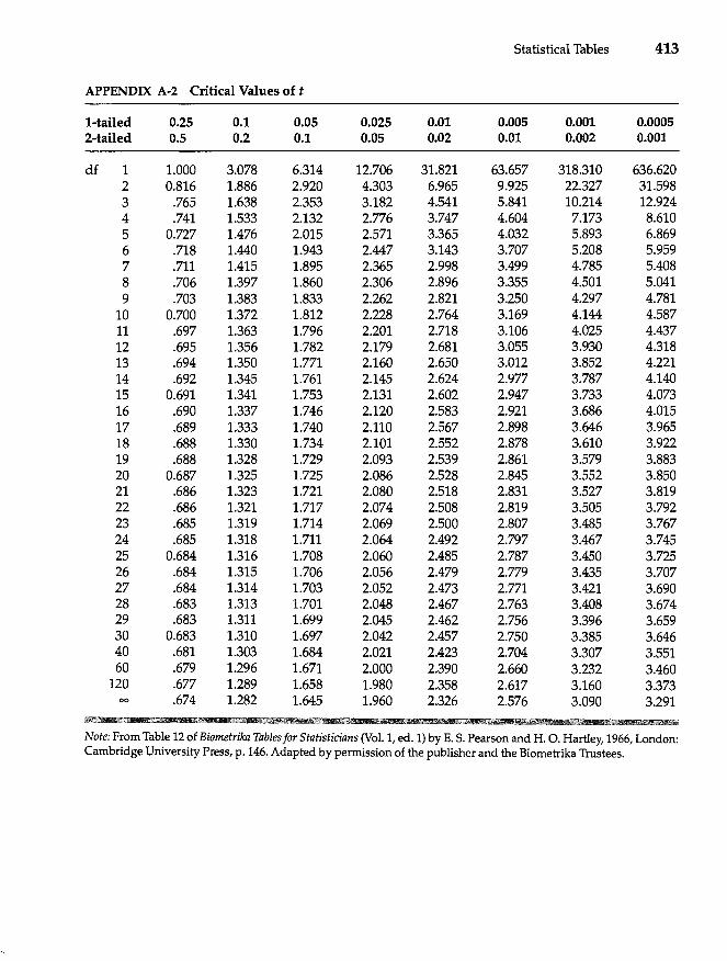
Statistical Tables 413

APPENDIX A-2 Critical Values of t

I-tailed 0.25 0.1 0.05 0.025 0.01 0.005 0.001 0.0005 2-tailed 0.5 0.2 0.1 0.05 0.02 0.01 0.002 0.001

df 1 1.000 3.078 6.314 12.706 31.821 63.657 318.310 636.620 2 0.816 1.886 2.920 4.303 6.965 9.925 22.327 31.598 3 .765 1.638 2.353 3.182 4.541 5.841 10.214 12.924 4 .741 1.533 2.132 2.776 3.747 4.604 7.173 8.610 5 0.727 1.476 2.015 2.571 3.365 4.032 5.893 6.869 6 .718 1.440 1.943 2.447 3.143 3.707 5.208 5.959 7 .711 1.415 1.895 2.365 2.998 3.499 4.785 5.408 8 .706 1.397 1.860 2.306 2.896 3.355 4.501 5.041 9 .703 1.383 1.833 2.262 2.821 3.250 4.297 4.781

10 0.700 1.372 1.812 2.228 2.764 3.169 4.144 4.587 11 .697 1.363 1.796 2.201 2.718 3.106 4.025 4.437 12 .695 1.356 1.782 2.179 2.681 3.055 3.930 4.318 13 .694 1.350 1.771 2.160 2.650 3.012 3.852 4.221 14 .692 1.345 1.761 2.145 2.624 2.977 3.787 4.140 15 0.691 1.341 1.753 2.131 2.602 2.947 3.733 4.073 16 .690 1.337 1.746 2.120 2.583 2.921 3.686 4.015 17 .689 1.333 1.740 2.110 2.567 2.898 3.646 3.965 18 .688 1.330 1.734 2.101 2.552 2.878 3.610 3.922 19 .688 1.328 1.729 2.093 2.539 2.861 3.579 3.883 20 0.687 1.325 1.725 2.086 2.528 2.845 3.552 3.850 21 .686 1.323 1.721 2.080 2.518 2.831 3.527 3.819 22 .686 1.321 1.717 2.074 2.508 2.819 3.505 3.792 23 .685 1.319 1.714 2.069 2.500 2.807 3.485 3.767 24 .685 1.318 1.711 2.064 2.492 2.797 3.467 3.745 25 0.684 1.316 1.708 2.060 2.485 2.787 3.450 3.725 26 .684 1.315 1.706 2.056 2.479 2.779 3.435 3.707 27 .684 1.314 1.703 2.052 2.473 2.771 3.421 3.690 28 .683 1.313 1.701 2.048 2.467 2.763 3.408 3.674 29 .683 1.311 1.699 2.045 2.462 2.756 3.396 3.659 30 0.683 1.310 1.697 2.042 2.457 2.750 3.385 3.646 40 .681 1.303 1.684 2.021 2.423 2.704 3.307 3.551 60 .679 1.296 1.671 2.000 2.390 2.660 3.232 3.460

120 .677 1.289 1.658 1.980 2.358 2.617 3.160 3.373 00 .674 1.282 1.645 1.960 2.326 2.576 3.090 3.291

IIIIIi

Note: From Table 12 of Biometrika Tables for Statisticians (Vol. 1, ed. 1) by E. S. Pearson and H. O. Hartley, 1966, London: Cambridge University Press, p. 146. Adapted by permission of the publisher and the Biometrika Trustees.

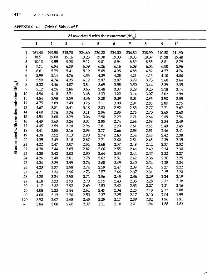
414 APPENDIX A

APPENDIX A-3 Critical Values of F

df associated with the numerator (dfbg)

1 2 3 4 5 6 7 8 9 10

1 161.40 199.50 215.70 224.60 230.20 234.00 236.80 238.90 240.50 241.90 2 18.51 19.00 19.16 19.25 19.30 19.33 19.35 19.37 19.38 19.40 3 10.13 9.55 9.28 9.12 9.01 8.94 8.89 8.85 8.81 8.79 4 7.71 6.94 6.59 6.39 6.26 6.16 6.09 6.04 6.00 5.96 5 6.61 5.79 5.41 5.19 5.05 4.95 4.88 4.82 4.77 4.74 6 5.99 5.14 4.76 4.53 4.39 4.28 4.21 4.15 4.10 4.06

.- 7 5.59 4.74 4.35 4.12 3.97 3.87 3.79 3.73 3.68 3.64

.J 8 5.32 4.46 4.07 3.84 3.69 3.58 3.50 3.44 3.39 3.35 '0 9 5.12 4.26 3.86 3.63 3.48 3.37 3.29 3.23 3.18 3.14 -.e 10 4.96 4.10 3.71 3.48 3.33 3.22 3.14 3.07 3.02 2.98 IU 11 4.84 3.98 3.59 3.36 3.20 3.09 3.01 2.95 2.90 2.85 .5 12 4.75 3.89 3.49 3.26 3.11 3.00 2.91 2.85 2.80 2.75 Ei Q 13 4.67 3.81 3.41 3.18 3.03 2.92 2.83 2.77 2.71 2.67 'I = QI 14 4.60 3.74 3.34 3.11 2.96 2.85 2.76 2.70 2.65 2.60 '0 QI 15 4.54 3.68 3.29 3.06 2.90 2.79 2.71 2.64 2.59 2.54

'j 0:5 16 4.49 3.63 3.24 3.01 2.85 2.74 2.66 2.59 2.54 2.49 0:5 17 4.45 3.59 3.20 2.96 2.81 2.70 2.61 2.55 2.49 2.45 .~

18 4.41 3.55 3.16 2.93 2.77 2.66 2.58 2.51 2.46 2.41 '0 .2! 19 4.38 3.52 3.13 2.90 2.74 2.63 2.54 2.48 2.42 2.38 IU 20 4.35 3.49 3.10 2.87 2.71 2.60 2.51 2.45 2.39 2.35 ... u Q 21 4.32 3.47 3.07 2.84 2.68 2.57 2.49 2.42 2.37 2.32 III III

22 4.30 3.44 3.05 2.82 2.66 2.55 2.46 2.40 2.34 2.30 IU .... 23 4.28 3.42 3.03 2.80 2.64 2.53 2.44 2.37 2.32 2.27 '0

24 4.26 3.40 3.01 2.78 2.62 2.51 2.42 2.36 2.30 2.25 25 4.24 3.39 2.99 2.76 2.60 2.49 2.40 2.34 2.28 2.24 26 4.23 3.37 2.98 2.74 2.59 2.47 2.39 2.32 2.27 2.22 27 4.21 3.35 2.96 2.73 2.57 2.46 2.37 2.31 2.25 2.20 28 4.20 3.34 2.95 2.71 2.56 2.45 2.36 2.29 2.24 2.19 29 4.18 3.33 2.93 2.70 2.55 2.43 2.35 2.28 2.22 2.18 30 4.17 3.32 2.92 2.69 2.53 2.42 2.33 2.27 2.21 2.16 40 4.08 3.23 2.84 2.61 2.45 2.34 2.25 2.18 2.12 2.08 60 4.00 3.15 2.76 2.53 2.37 2.25 2.17 2.10 2.04 1.99

120 3.92 3.07 2.68 2.45 2.29 2.17 2.09 2.02 1.96 1.91 00 3.84 3.00 2.60 2.37 2.21 2.10 2.01 1.94 1.88 1.83

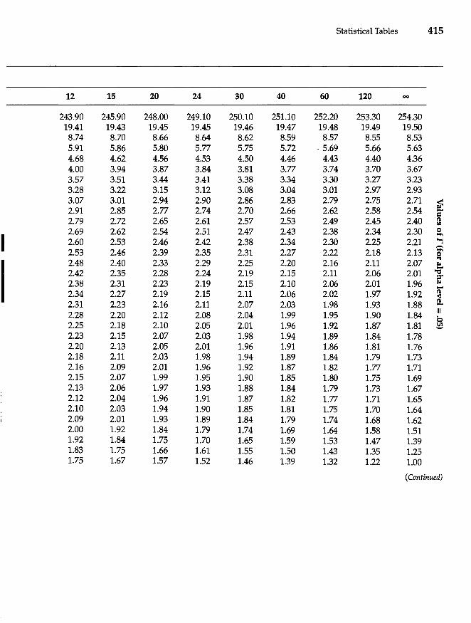
Statistical Tables 415

12 15 20 24 30 40 60 120 00

243.90 245.90 248.00 249.10 250.10 251.10 252.20 253.30 254.30 19.41 19.43 19.45 19.45 19.46 19.47 19.48 19.49 19.50 8.74 8.70 8.66 8.64 8.62 8.59 8.57 8.55 8.53 5.91 5.86 5.80 5.77 5.75 5.72 - 5.69 5.66 5.63 4.68 4.62 4.56 4.53 4.50 4.46 4.43 4.40 4.36 4.00 3.94 3.87 3.84 3.81 3.77 3.74 3.70 3.67 3.57 3.51 3.44 3.41 3.38 3.34 3.30 3.27 3.23 3.28 3.22 3.15 3.12 3.08 3.04 3.01 2.97 2.93 3.07 3.01 2.94 2.90 2.86 2.83 2.79 2.75 2.71 ~ 2.91 2.85 2.77 2.74 2.70 2.66 2.62 2.58 2.54 a' 2.79 2.72 2.65 2.61 2.57 2.53 2.49 2.45 2.40 ID

(I)

2.69 2.62 2.54 2.51 2.47 2.43 2.38 2.34 2.30 Q

I ....

2.60 2.53 2.46 2.42 2.38 2.34 2.30 2.25 2.21 "I'J .-2.53 2.46 2.39 2.35 2.31 2.27 2.22 2.18 2.13 ....

Q

2.11 2.07 "1

I 2.48 2.40 2.33 2.29 2.25 2.20 2.16 e. 2.42 2.35 2.28 2.24 2.19 2.15 2.11 2.06 2.01 ~

t:T 2.38 2.31 2.23 2.19 2.15 2.10 2.06 2.01 1.96 ~ -2.34 2.27 2.19 2.15 2.11 2.06 2.02 1.97 1.92 ID

~ 2.31 2.23 2.16 2.11 2.07 2.03 1.98 1.93 1.88 -2.28 2.20 2.12 2.08 2.04 1.99 1.95 1.90 1.84

II b

2.25 2.18 2.10 2.05 2.01 1.96 1.92 1.87 1.81 ~ 2.23 2.15 2.07 2.03 1.98 1.94 1.89 1.84 1.78 2.20 2.13 2.05 2.01 1.96 1.91 1.86 1.81 1.76 2.18 2.11 2.03 1.98 1.94 1.89 1.84 1.79 1.73 2.16 2.09 2.01 1.96 1.92 1.87 1.82 1.77 1.71 2.15 2.07 1.99 1.95 1.90 1.85 1.80 1.75 1.69 2.13 2.06 1.97 1.93 1.88 1.84 1.79 1.73 1.67 2.12 2.04 1.96 1.91 1.87 1.82 1.77 1.71 1.65 2.10 2.03 1.94 1.90 1.85 1.81 1.75 1.70 1.64 2.09 2.01 1.93 1.89 1.84 1.79 1.74 1.68 1.62 2.00 1.92 1.84 1.79 1.74 1.69 1.64 1.58 1.51 1.92 1.84 1.75 1.70 1.65 1.59 1.53 1.47 1.39 1.83 1.75 1.66 1.61 1.55 1.50 1.43 1.35 1.25 1.75 1.67 1.57 1.52 1.46 1.39 1.32 1.22 1.00

(Continued)

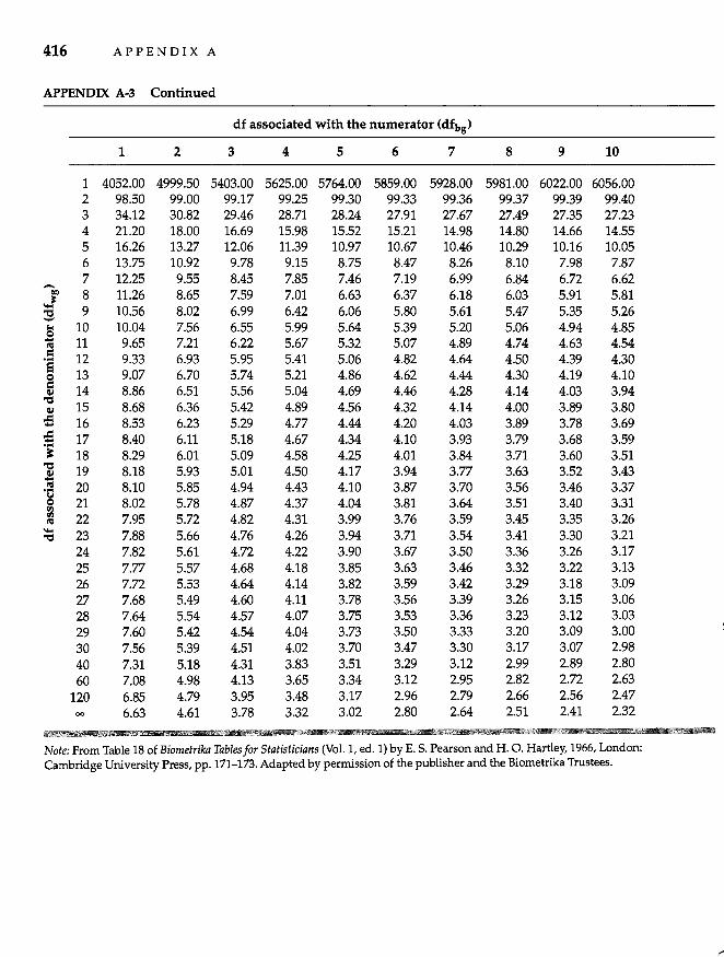
416 APPENDIX A

APPENDIX A-3 Continued

df associated with the numerator (dfbg)

1 2 3 4 5 6 7 8 9 10

1 4052.00 4999.50 5403.00 5625.00 5764.00 5859.00 5928.00 5981.00 6022.00 6056.00 2 98.50 99.00 99.17 99.25 99.30 99.33 99.36 99.37 99.39 99.40 3 34.12 30.82 29.46 28.71 28.24 27.91 27.67 27.49 27.35 27.23 4 21.20 18.00 16.69 15.98 15.52 15.21 14.98 14.80 14.66 14.55 5 16.26 13.27 12.06 11.39 10.97 10.67 10.46 10.29 10.16 10.05 6 13.75 10.92 9.78 9.15 8.75 8.47 8.26 8.10 7.98 7.87 7 12.25 9.55 8.45 7.85 7.46 7.19 6.99 6.84 6.72 6.62

--bI) 8 11.26 8.65 7.59 7.01 6.63 6.37 6.18 6.03 5.91 5.81 ..J

'tI 9 10.56 8.02 6.99 6.42 6.06 5.80 5.61 5.47 5.35 5.26 -'"' 10 10.04 7.56 6.55 5.99 5.64 5.39 5.20 5.06 4.94 4.85 ~ 11 9.65 7.21 6.22 5.67 5.32 5.07 4.89 4.74 4.63 4.54 = 12 9.33 6.93 5.95 5.41 5.06 4.82 4.64 4.50 4.39 4.30 .... a 13 9.07 6.70 5.74 5.21 4.86 4.62 4.44 4.30 4.19 4.10 5 14 8.86 6.51 5.56 5.04 4.69 4.46 4.28 4.14 4.03 3.94 'tI

15 8.68 6.36 5.42 4.89 4.56 4.32 4.14 4.00 3.89 3.80 GI

-= 16 8.53 6.23 5.29 4.77 4.44 4.20 4.03 3.89 3.78 3.69

-= 17 8.40 6.11 5.18 4.67 4.34 4.10 3.93 3.79 3.68 3.59 .~

18 8.29 6.01 5.09 4.58 4.25 4.01 3.84 3.71 3.60 3.51 'tI 19 8.18 5.93 5.01 4.50 4.17 3.94 3.77 3.63 3.52 3.43 GI "lU 20 8.10 5.85 4.94 4.43 4.10 3.87 3.70 3.56 3.46 3.37 .... {J

4.37 4.04 3.81 3.64 3.51 3.40 3.31 Q 21 8.02 5.78 4.87 <Il

~ 22 7.95 5.72 4.82 4.31 3.99 3.76 3.59 3.45 3.35 3.26 .....

23 7.88 5.66 4.76 4.26 3.94 3.71 3.54 3.41 3.30 3.21 'tI

24 7.82 5.61 4.72 4.22 3.90 3.67 3.50 3.36 3.26 3.17 25 7.77 5.57 4.68 4.18 3.85 3.63 3.46 3.32 3.22 3.13 26 7.72 5.53 4.64 4.14 3.82 3.59 3.42 3.29 3.18 3.09 27 7.68 5.49 4.60 4.11 3.78 3.56 3.39 3.26 3.15 3.06 28 7.64 5.54 4.57 4.07 3.75 3.53 3.36 3.23 3.12 3.03 29 7.60 5.42 4.54 4.04 3.73 3.50 3.33 3.20 3.09 3.00 30 7.56 5.39 4.51 4.02 3.70 3.47 3.30 3.17 3.07 2.98 40 7.31 5.18 4.31 3.83 3.51 3.29 3.12 2.99 2.89 2.80 60 7.08 4.98 4.13 3.65 3.34 3.12 2.95 2.82 2.72 2.63

120 6.85 4.79 3.95 3.48 3.17 2.96 2.79 2.66 2.56 2.47 00 6.63 4.61 3.78 3.32 3.02 2.80 2.64 2.51 2.41 2.32

ii i I ~ iii

Note: From Table 18 of Biometrika Tables for Statisticians (Vol. 1, ed. 1) by E. S. Pearson and H. O. Hartley, 1966, London: Cambridge University Press, pp. 171-173. Adapted by permission of the publisher and the Biometrika Trustees.

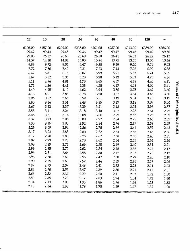
Statistical Tables 417

12 15 20 24 30 40 60 120 00

6106.00 6157.00 6209.00 6235.00 6261.00 6287.00 6313.00 6339.00 6366.00 99.42 99.43 99.45 99.46 99.47 99.47 99.48 99.49 99.50 27.05 26.87 26.69 26.60 26.50 26.41 26.32 26.22 26.13 14.37 14.20 14.02 13.93 13.84 13.75 13.65 13.56 13.46

9.89 9.72 9.55 9.47 9.38 9.29 9.20 9.11 9.02 7.72 7.56 7.40 7.31 7.23 7.14 7.06 6.97 6.88 6.47 6.31 6.16 6.07 5.99 5.91 5.82 5.74 5.65 5.67 5.52 5.36 5.28 5.20 5.12 5.03 4.95 4.86 5.11 4.96 4.81 4.73 4.65 4.57 4.48 4.40 4.31

~ 4.71 4.56 4.41 4.33 4.25 4.17 4.08 4.00 3.91 -c 4.40 4.25 4.10 4.02 3.94 3.86 3.78 3.69 3.60 tD

Ul

4.16 4.01 3.86 3.78 3.70 3.62 3.54 3.45 3.36 Q ..... 3.96 3.82 3.66 3.59 3.51 3.43 3.34 3.25 3.17 '"rj

3.80 3.66 3.51 3.43 3.35 3.27 3.18 3.09 3.00 g; 3.67 3.52 3.37 3.29 3.21 3.13 3.05 2.96 2.87

tot

e!. 3.55 3.41 3.26 3.18 3.10 3.02 2.93 2.84 2.75 '"d

l:T 3.46 3.31 3.16 3.08 3.00 2.92 2.83 2.75 2.65 I» -3.37 3.23 3.08 3.00 2.92 2.84 2.75 2.66 2.57 ~ 3.30 3.15 3.00 2.92 2.84 2.76 2.67 2.58 2.49 -3.23 3.09 2.94 2.86 2.78 2.69 2.61 2.52 2.42 II

b 3.17 3.03 2.88 2.80 2.72 2.64 2.55 2.46 2.36 '"'" -3.12 2.98 2.83 2.75 2.67 2.58 2.50 2.40 2.31 3.07 2.93 2.78 2.70 2.62 2.54 2.45 2.35 2.26 3.03 2.89 2.74 2.66 2.58 2.49 2.40 2.31 2.21 2.99 2.85 2.70 2.62 2.54 2.45 2.36 2.27 2.17 2.96 2.81 2.66 2.58 2.50 2.42 2.33 2.23 2.13 2.93 2.78 2.63 2.55 2.47 2.38 2.29 2.20 2.10 2.90 2.75 2.60 2.52 2.44 2.35 2.26 2.17 2.06 2.87 2.73 2.57 2.49 2.41 2.33 2.23 2.14 2.03 2.84 2.70 2.55 2.47 2.39 2.30 2.21 2.11 2.01 2.66 2.52 2.37 2.29 2.20 2.11 2.02 1.92 1.80 2.50 2.35 2.20 2.12 2.03 1.94 1.84 1.73 1.60 2.34 2.19 2.03 1.95 1.86 1.76 1.66 1.53 1.38 2.18 2.04 1.88 1.79 1.70 1.59 1.47 1.32 1.00

n i_

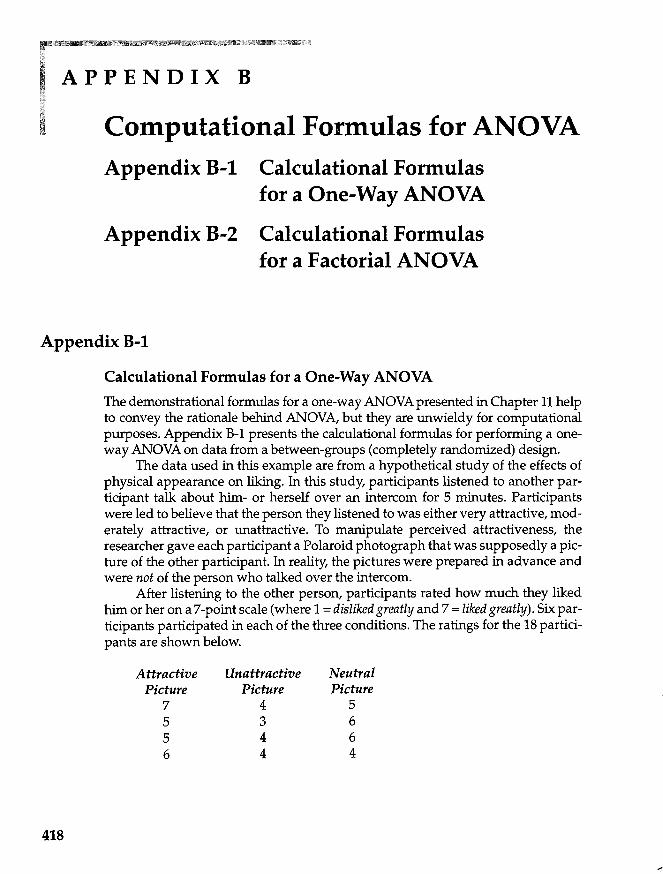
APPENDIX B

Computational Formulas for ANOVA Appendix B-1 Calculational Formulas

for a One-Way ANOVA

Appendix B-2 Calculational Formulas for a Factorial ANOVA

Appendix B-1

418

Calculational Formulas for a One-Way ANOVA

The demonstrational formulas for a one-way ANaVA presented in Chapter 11 help to convey the rationale behind ANOVA, but they are unwieldy for computational purposes. Appendix B-1 presents the calculational formulas for performing a one­way ANaVA on data from a between-groups (completely randomized) design.

The data used in this example are from a hypothetical study of the effects of physical appearance on liking. In this study, participants listened to another par­ticipant talk about him- or herself over an intercom for 5 minutes. Participants were led to believe that the person they listened to was either very attractive, mod­erately attractive, or unattractive. To manipulate perceived attractiveness, the researcher gave each participant a Polaroid photograph that was supposedly a pic­ture of the other participant. In reality, the pictures were prepared in advance and were not of the person who talked over the intercom.

After listening to the other person, participants rated how much they liked him or her on a 7-point scale (where 1 = disliked greatly and 7 = liked greatly). Six par­ticipants participated in each of the three conditions. The ratings for the 18 partici­pants are shown below.

Attractive Unattractive Neutral Picture Picture Picture

7 4 5 5 3 6 5 4 6 6 4 4

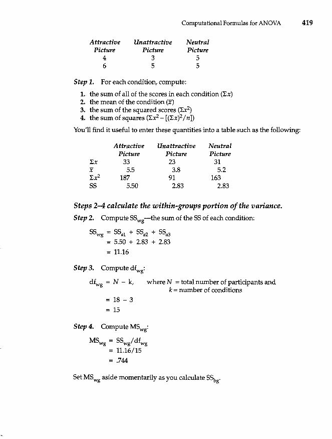
Computational Formulas for ANOVA 419

Attractive Picture

4 6

Unattractive Picture

3 5

Step 1. For each condition, compute:

Neutral Picture

5 5

1. the sum of all of the scores in each condition (l:x) 2. the mean of the condition (x) 3. the sum of the squared scores (l:,x2) 4. the sum ofsquares (l:x2- [(l:x)2/n))

You'll find it useful to enter these quantities into a table such as the following:

Attractive Unattractive Neutral Picture Picture Picture

l:x 33 23 31 x 5.5 3.8 5.2 l:x2 187 91 163 55 5.50 2.83 2.83

Steps 2-4 calculate the within-groups portion of the variance.

Step 2. Compute 55wg -the sum of the 55 of each condition:

5Swg = SSal + SSa2 + SSa3 = 5.50 + 2.83 + 2.83

= 11.16

Step 3. Compute dfwg:

dfwg=N-k,

= 18 - 3

= 15

where N = total number of participants and k = number of conditions

Step 4. Compute MSwg:

MSwg = 55wg/ dfwg = 11.16/15

= .744

5et MSwg aside momentarily as you calculate S~g.

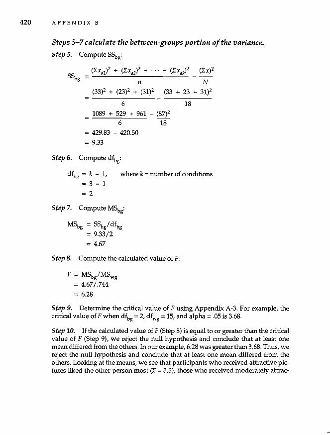
420 APPENDIX B

Steps 5-7 calculate the between-groups portion of the variance.

Step 5. Compute S%g:

(33)2 + (23)2 + (31)2 (33 + 23 + 31)2 =-------

6 18

= 1089 + 529 + 961 - (87)2 6 18

= 429.83 - 420.50

= 9.33

Step 6. Compute dfbg:

dfbg = k - 1,

= 3 - 1

= 2

where k = number of conditions

Step 7. Compute M%g:

M%g = S%gl dfbg = 9.33/2

= 4.67

Step 8. Compute the calculated value of F:

F = M%glMSwg = 4.671.744

= 6.28

Step 9. Determine the critical value of F using Appendix A-3. For example, the critical value of F when dfbg = 2, dfwg = 15, and alpha = .05 is 3.68.

Step 10. If the calculated value of F (Step 8) is equal to or greater than the critical value of F (Step 9), we reject the null hypothesis and conclude that at least one mean differed from the others. In our example, 6.28 was greater than 3.68. Thus, we reject the null hypothesis and conclude that at least one mean differed from the others. Looking at the means, we see that participants who received attractive pic­tures liked the other person most (x = 5.5), those who received moderately attrac-

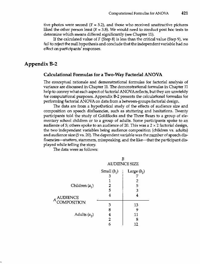
Computational Formulas for ANOVA 421

tive photos were second (x = 5.2), and those who received unattractive pictures liked the other person least (x = 3.8). We would need to conduct post hoc tests to determine which means differed significantly (see Chapter 11).

If the calculated value of F (Step 8) is less than the critical value (Step 9), we fail to reject the null hypothesis and conclude that the independent variable had no effect on participants' responses.

Appendix B-2

Calculational Formulas for a Two-Way Factorial ANOVA

The conceptual rationale and demonstrational formulas for factorial analysis of variance are discussed in Chapter 11. The demonstrational formulas in Chapter 11 help to convey what each aspect of factorial ANOVA reflects, but they are unwieldy for computational purposes. Appendix B-2 presents the calculational formulas for performing factorial ANOVA on data from a between-groups factorial design.

The data are from a hypothetical study of the effects of audience size and composition on speech disfluencies, such as stuttering and hesitations. Twenty participants told the study of Goldilocks and the Three Bears to a group of ele­mentary school children or to a group of adults. Some participants spoke to an audience of 5; others spoke to an audience of 20. This was a 2 x 2 factorial design, the two independent variables being audience composition (children vs. adults) and audience size (5 vs. 20). The dependent variable was the number of speech dis­fluencies-stutters, stammers, misspeaking, and the like-that the participant dis­played while telling the story.

The data were as follows:

AUDIENCE ACOMPOSmON

B AUDIENCE SIZE

Small (bI ) Large (b2)

3 7 1 2 2 5 5 3 4 4

3 8 4 2 6

13 9

11 8

12

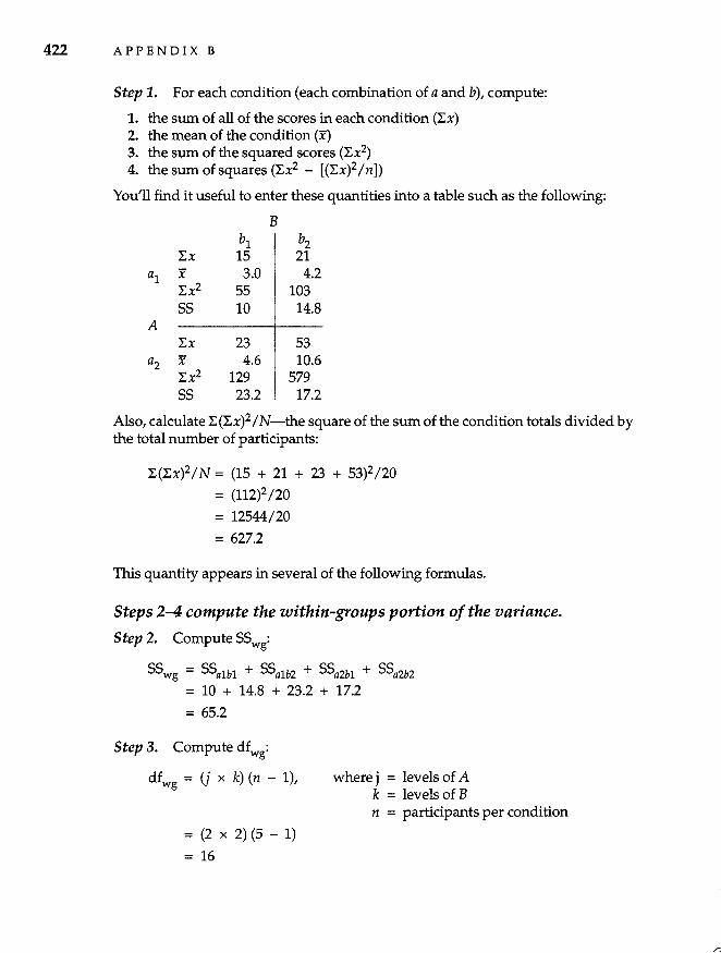
422 APPENDIX B

Step 1. For each condition (each combination of a and b), compute:

1. the sum of all of the scores in each condition (l:x) 2. the mean of the condition (x) 3. the sum of the squared scores (l:x2) 4. the sum of squares (l:x2 - [(l:x)2 / n])

You'll find it useful to enter these quantities into a table such as the following:

B bl b2

l:x 15 21 al X 3.0 4.2

l:x2 55 103 55 10 14.8

A l:x 23 53

a2 X 4.6 10.6 l:x2 129 579 55 23.2 17.2

Also, calculatel:(l:x)2 /N-the square of the sum of the condition totals divided by the total number of participants:

l:(l:x)2/N = (15 + 21 + 23 + 53)2/20

= (112)2/20

= 12544/20

= 627.2

This quantity appears in several of the following formulas.

Steps 2-4 compute the within-groups portion of the variance.

Step 2. Compute 55wg:

55wg = 55aIbI + 55aIb2 + 55a2bI + 55a2b2

= 10 + 14.8 + 23.2 + 17.2

= 65.2

Step 3. Compute dfwg:

dfwg = (j x k) (n - 1),

= (2 x 2) (5 - 1)

= 16

where j = levels of A k = levels of B n = participants per condition

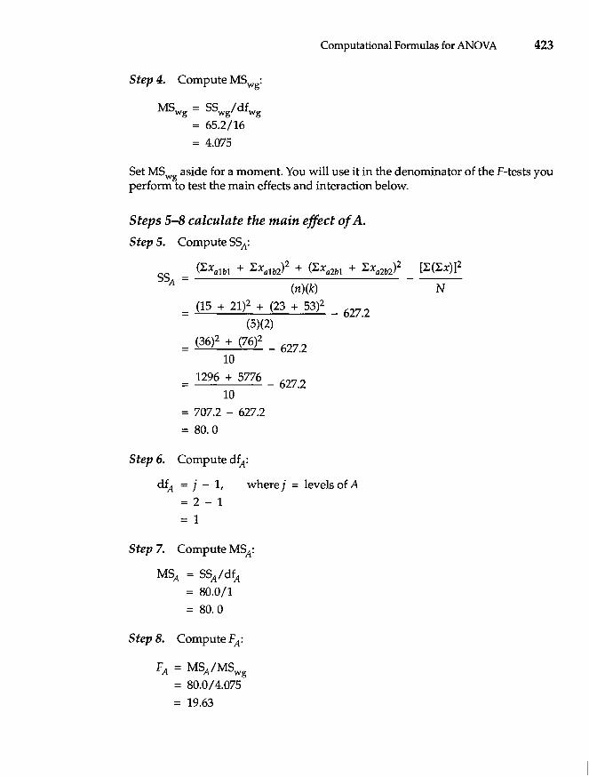
Computational Formulas for ANOVA 423

Step 4. Compute MSwg:

MSwg = SSwgl dfwg = 65.2/16

= 4.075

Set MSwg aside for a moment. You will use it in the denominator of the F-tests you perform to test the main effects and interaction below.

Steps 5-8 calculate the main effect of A.

Step 5. Compute SSA:

(LXa1b1 + LXa1b2)2 + (LXa2b1 + LXa2b2)2 SSA = --------------------------­

(n)(k)

(15 + 21)2 + (23 + 53)2 _ 627.2

(5)(2)

= (36)2 + (76)2 _ 627.2 10

= 1296 + 5776 _ 627.2 10

= 707.2 - 627.2

= 80.0

Step 6. Compute dfA:

dfA = j - I,

= 2 - 1

= 1

where j = levels of A

Step 7. Compute MSA:

MSA = SSAI dfA = 80.0/1

= 80.0

Step 8. Compute FA:

FA = MSAIMSwg = 80.0 I 4.075

= 19.63

[L(LX)]2

N

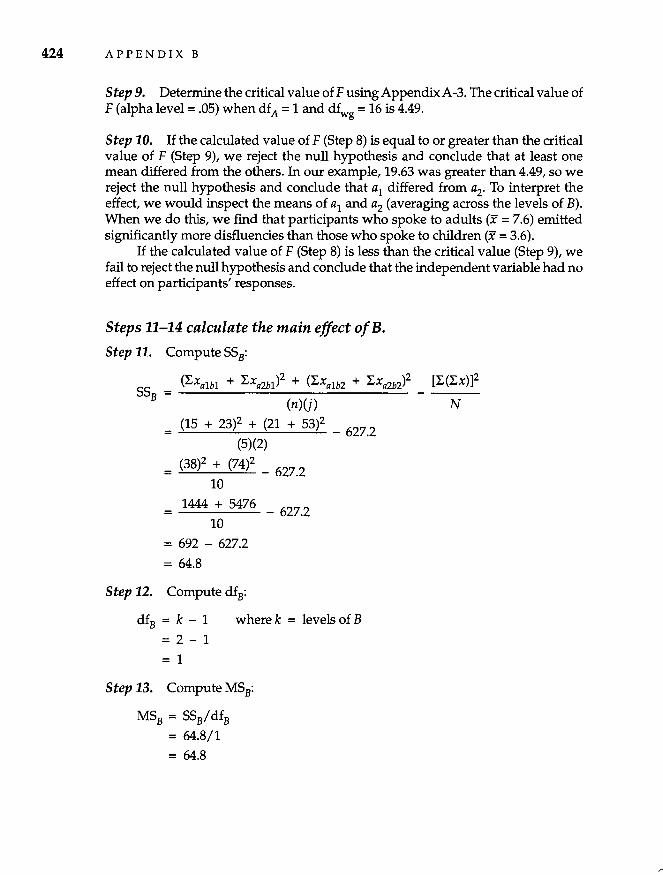
424 APPENDIX B

Step 9. Determine the critical value of F using Appendix A-3. The critical value of F (alpha level = .05) when dfA = 1 and dfwg = 16 is 4.49.

Step 10. If the calculated value of F (Step 8) is equal to or greater than the critical value of F (Step 9), we reject the null hypothesis and conclude that at least one mean differed from the others. In our example, 19.63 was greater than 4.49, so we reject the null hypothesis and conclude that al differed from a2. To interpret the effect, we would inspect the means of al and a2 (averaging across the levels of B). When we do this, we find that participants who spoke to adults (x = 7.6) emitted significantly more disfluencies than those who spoke to children (x = 3.6).

If the calculated value of F (Step 8) is less than the critical value (Step 9), we fail to reject the null hypothesis and conclude that the independent variable had no effect on participants' responses.

Steps 11-14 calculate the main effect ofB.

Step 11. Compute SSB:

(I:xalbl + I:xa2bl )2 + (I:xalb2 + I:xa2b2)2 SSB = --------~~-~~

(n)(j)

= (15 + 23)2 + (21 + 53)2 _ 627.2 (5)(2)

= (38)2 + (74)2 _ 627.2 10

= 1444 + 5476 _ 627.2 10

= 692 - 627.2

= 64.8

Step 12. Compute dfB:

dfB = k - 1 = 2 - 1

= 1

where k = levels of B

Step 13. Compute MSB:

MSB = SSB/ dfB

= 64.8/1

= 64.8

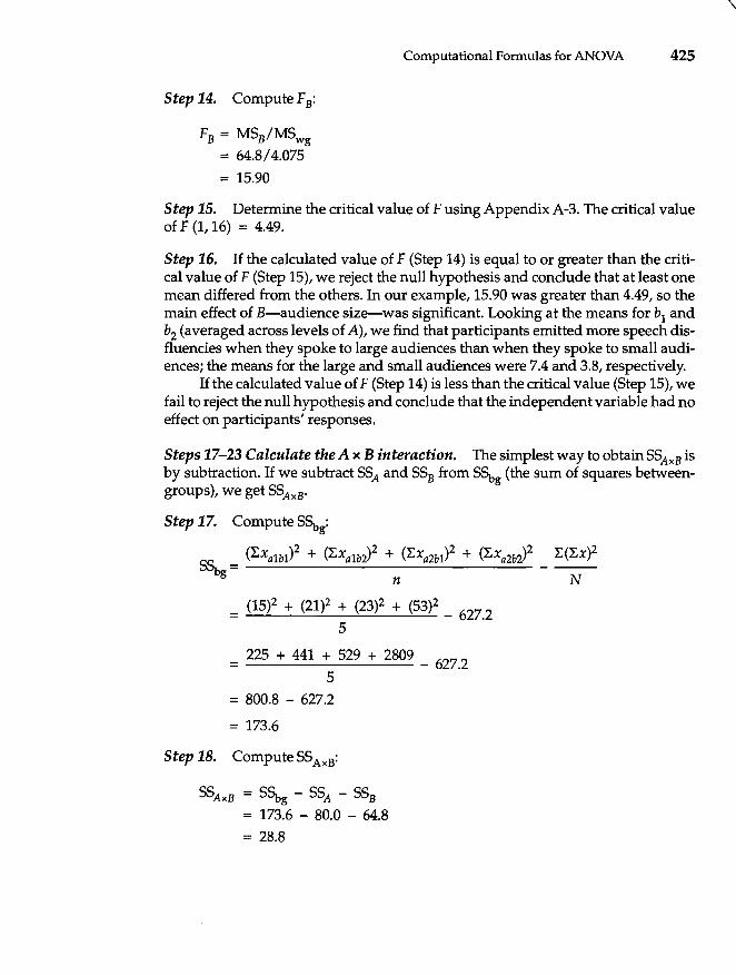
Step 14. Compute FB:

FB = MSB/MSwg = 64.8/4.075

= 15.90

Computational Formulas for ANOVA 425

Step 15. Determine the critical value of F using Appendix A-3. The critical value of F (1, 16) = 4.49.

Step 16. If the calculated value of F (Step 14) is equal to or greater than the criti­cal value of F (Step 15), we reject the null hypothesis and conclude that at least one mean differed from the others. In our example, 15.90 was greater than 4.49, so the main effect of B-audience size-was significant. Looking at the means for b1 and b2 (averaged across levels of A), we find that participants emitted more speech dis­fluencies when they spoke to large audiences than when they spoke to small audi­ences; the means for the large and small audiences were 7.4 and 3.8, respectively.

If the calculated value of F (Step 14) is less than the critical value (Step 15), we fail to reject the null hypothesis and conclude that the independent variable had no effect on participants' responses.

Steps 17-23 Calculate the A x B interaction. The simplest way to obtain SSAxB is by subtraction. If we subtract SSA and SSB from S~g (the sum of squares between­groups), we get SSAxB.

Step 17. Compute S~g:

(Lxalbl)2 + (Lxa1b2? + (Lxa2b1 )2 + (Lxa2b2? L(Lx)2 S~ = ---

g n N

= (15)2 + (21? + (23)2 + (53)2 _ 627.2 5

= 225 + 441 + 529 + 2809 _ 627.2 5

= 800.8 - 627.2

= 173.6

Step 18. Compute 55 AxB:

SSAxB = S~g - SSA - SSB = 173.6 - 80.0 - 64.8

= 28.8

\

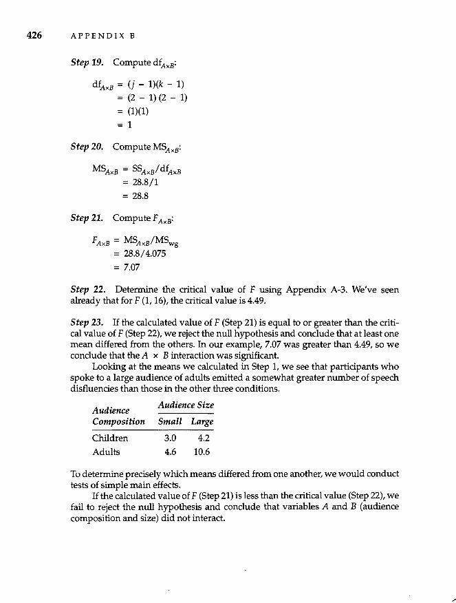
426 APPENDIX B

Step 19. Compute dfAxB:

dfAxB = (j - l)(k - 1)

= (2 - 1) (2 - 1)

= (1)(1)

= 1

Step 20. Compute MSAxB:

MSAxB = SSAxBldfAxB

= 28.8/1

= 28.8

Step 21. Compute FAxB:

FAxB = MSAxBIMSwg

= 28.8/4.075

= 7.07

Step 22. Determine the critical value of F using Appendix A-3. We've seen already that for F (1, 16), the critical value is 4.49.

Step 23. If the calculated value of F (Step 21) is equal to or greater than the criti­cal value of F (Step 22), we reject the null hypothesis and conclude that at least one mean differed from the others. In our example, 7.07 was greater than 4.49, so we conclude that the A x B interaction was significant.

Looking at the means we calculated in Step 1, we see that participants who spoke to a large audience of adults emitted a somewhat greater number of speech disfluencies than those in the other three conditions.

Audience Audience Size

Composition Small Large

Children 3.0 4.2

Adults 4.6 10.6

To determine precisely which means differed from one another, we would conduct tests of simple main effects.

If the calculated value of F (Step 21) is less than the critical value (Step 22), we fail to reject the null hypothesis and conclude that variables A and B (audience composition and size) did not interact.

REFERENCES

Adair, J. G., Dushenko, T. W., & Lindsay, R. C. L. (1985). Ethical regulations and their impact on research. American Psychologist, 40, 59-72.

Adams, K. L., & Ware, N. C. (1989). Sexism and the English language: The linguistic implications of being a woman. In J. Freeman (Ed.), Women: A feminist perspective (pp. 470-484). Mountain View, CA: Mayfield.

Adler, T. (1991, December). Outright fraud rare, but not poor science. APA Monitor, p. 11.

Agocha, V. B., & Cooper, M. L. (1999). Risk percep­tions and safer-sex intentions: Does a partner's physical attractiveness undermine the use of risk-relevant information? Personality and Social Psychology Bulletin, 25, 746-759.

Aiken, L. S., & West, S. G. (1991). Multiple regression: Testing and interpreting interactions. Newbury Park, CA: Sage.

Allport, G. W. (1961). Pattern and growth in personality. New York: Holt, Rinehart, and Winston.

American Psychological Association. (1985). Guide­lines for ethical conduct in the care and use of ani­mals. Washington, DC: Author.

American Psychological Association. (1992). Ethical principles in the conduct of research with human participants. Washington, DC: Author.

American Psychological Association. (1994). Publica­tion manual of the American Psychological Associa­tion (4th ed.). Washington, DC: Author.

Anderson, C. A (1989). Temperature and aggres­sion: Ubiquitous effects of heat on occurrence of human violence. Psychological Bulletin, 106, 74-96.

APAendorses resolution on the use of animals (1990, October-November). APA Science Agenda, p. 8.

Archer, D., Iritani, B., Kimes, D. D., & Barrios, M. (1983). Face-ism: Studies of sex differences in fa­cial prominence. Journal of Personality and Social Psychology, 45, 725-735.

Asendorpf, J. (1990). The expression of shyness and embarrassment. In W. R. Crozier (Ed.), Shyness and embarrassment (pp. 87-118). Cambridge: Cambridge University Press.

Ayala, F. J., & Black, B. (1993). Science and the courts. American Scientist, 81, 230-239.

Azar, B. (1999, July-August). Destructive lab attack sends a wake-up call. APA Monitor, p. 16.

Bales, R. F. (1970). Personality and interpersonal behav­ior. New York: Holt, Rinehart & Winston.

Baron, R. A, & Bell, P. A (1976). Aggression and heat: The influence of ambient temperature, negative affect, and a cooling drink on physical aggression. Journal of Personality and Social Psy­chology, 33, 245-255.

Bar-Yoseph, T. L., & Witztum, E. (1992). Using strate­gic psychotherapy: A case study of chronic PTSD after a terrorist attack. Journal of Contem­porary Psychotherapy, 22, 263-276.

Baumeister, R. F., Heatherton, T. F., & Tice, D. M. (1993). When ego threats lead to self-regulation failure: Negative consequences of high self­esteem. Journal of Personality and Social Psychol­ogy, 64, 141-156.

Baumeister, R. F., & Steinhilber, A (1984). Paradoxi­cal effects of supportive audiences on perfor­mance under pressure: The home disadvantage in sports championships. Journal of Personality and Social Psychology, 47, 85-93.

Baumrind, D. (1971). Principles of ethical conduct in the treatment of subjects: Reactions to the draft report of the committee on ethical standards in psychological research. American Psychologist, 26, 887-896.

Bell, C. R. (1962). Personality characteristics of vol­unteers for psychological studies. British Journal of Social and Clinical Psychology, 1,81-95.

Bell, R. (1992). Impure science: Fraud, compromise, and political influence in scientific research. New York: John Wiley & Sons.

Berelson, B. (1952). Content analysis in communication research. New York: The Free Press.

Bissonnette, V., Ickes, W., Bernstein, I., & Knowles, E. (1990). Personality moderating variables: A warning about statistical artifact and a compar­ison of analytic techniques. Journal of Personal­ity, 58, 567-587.

Boring, E. G. (1954). The nature and history of exper­imental control. American Journal of Psychology, 67,573-589.

Bower, G. H, Karlin, M. B., & Dueck, A (1975). Com­prehension and memory for pictures. Memory and Cognition, 3, 216-220.

Braginsky, B. M., Braginsky, D. D., & Ring, K. (1982). Methods of madness: The mental hospital as a last re­sort. Lanham, MD: University Press of America.

Bringmann, W. (1979, Sept/Oct). Wundt's lab: "humble ... but functioning" [Letter to the edi­tor]. APA Monitor, p. 13.

427

428 REFERENCES

Bromley, D. B. (1986). The case-study method in psy­chology and related disciplines. Chichester: John Wiley & Sons.

Brown, A. S. (1988). Encountering misspellings and spelling performance: Why wrong isn't right. Journal of Educational Psychology, 80, 488-494.

Bryan, J. H., & Test, M. A. (1967). Models and help­ing: Naturalistic studies in aiding behavior. Journal of Personality and Social Psychology, 6, 400-407.

Buchanan, C. M., Maccoby, E. E., & Dornbusch, S. M. (1996). Adolescents after divorce. Cambridge, MA: Harvard University Press.

Butler, A. c., Hokanson, J. E., & Flynn, H. A. (1994). A comparison of self-esteem lability and low trait self-esteem as vulnerability factors for de­pression. Journal of Personality and Social Psychol­ogy, 66, 166-177.

Cacioppo, J. T., & Tassinary, L. G. (1990). Psy­chophysiology and psychophysiological infer­ence. In J. T. Cacioppo & L. G. Tassinary (Eds.), Principles of psychophysiology: Physical, social, and inferential elements (pp. 3-33). New York: Cam­bridge University Press.

Campbell, D. T. (1969). Reforms as experiments. American Psychologist, 24, 409-429.

Campbell, D. T. (1971, September). Methods for the ex­perimenting society. Paper presented at the meet­ing of the American Psychological Association, Washington, DC.

Campbell, D. T. (1981). Comment: Another perspec­tive on a scholarly career. In M. Brewer & B. E. Collins (Eds.), Scientific inquiry and the social sci­ences (pp. 454-501). San Francisco: Jossey-Bass.

Campbell, D., Sanderson, R. E., & Laverty, S. G. (1964). Characteristics of a conditioned re­sponse in human subjects during extinction tri­als following a single traumatic conditioning trial. Journal of Abnormal and Social Psychology, 68,627-639.

Campbell, D. T., & Stanley, J. C. (1966). Experimental and quasi-experimental designs for research. Skokie, IL: Rand McNally.

Campbell, P. B. (1983). The impact of societal biases on research methods. In B. L. Richardson & J. WIrtenberg(Eds.), Sex role research (pp.197-214). New York: Praeger.

Cassandro, V. J. (1998). Explaining premature mor­tality across fields of creative endeavor. Journal of Personality, 66, 805-833.

Cheek, J. M. (1982). Aggregation, moderator vari­ables, and the validity of personality tests: A peer-rating study. Journal of Personality and So­cial Psychology, 43,1254-1269.

Chevalier-Skolnikoff, S., & Liska, J. (1993). Tool use by wild and captive elephants. Animal Behavior, 46, 209-219.

Christensen, L. (1988). Deception in psychological research: When is its use justified? Personality and Social Psychology Bulletin, 14, 664-675.

Cialdini, R. B., Vmcent, J. E., Lewis, S. K., Catalan, J., Wheeler, D., & Darby, B. L. (1975). Reciprocal concessions procedure for inducing compli­ance: The door-in-the-face technique. Journal of Personality and Social Psychology, 31, 206-215.

Clark, R. D., & Hatfield, E. (1989). Gender differ­ences in receptivity to sexual offers. Journal of Psychology and Human Sexuality, 2, 39-55.

Cochran, W. G., Mosteller, F., & Tukey, J. W. (1953). Statistical problems in the Kinsey report. Journal of the American Statistical Association, 48, 673-716.

Cohen, J. (1977). Statistical power analysis for the be­havioral sciences (Rev. ed.). New York: Academic Press.

Cohen, J. (1988). Statistical power analysis for the be­havioral sciences. Hillsdale, NJ: Lawrence Erl­baum Associates.

Cohen, J., & Cohen, P. (1983). Applied multiple regres­sion/correlation analysis for the behavioral sciences (2nd ed.). Hillsdale, NJ: Erlbaum.

Condray, D. S. (1986). Quasi-experimental analysis: A mixture of methods and judgment. In W. M. K. Trochim (Ed.), Advances in quasi-experimental de­sign and analysis (pp. 9-28). San Francisco: J ossey-Bass.

Cook, T. D., & Campbell, D. T. (1979). Quasi-experi­mentation. Boston: Houghton Mifflin.

Cooper, H. (1990). Meta-analysis and the integrative research review. In C. Hendrick & M. S. Clark (Eds.), Research methods in personality and social psychology (pp. 142-163). Newbury Park, CA: Sage.

Cordaro, L., & Ison, J. R. (1963). Psychology of the scientist: X. Observer bias in classical condition­ing of the planaria. Psychological Reports, 13, 787-789.

Coulter, X. (1986). Academic value of research par­ticipation by undergraduates. American Psychol­ogist, 41, 317.

Cowles, M. (1989). Statistics in psychology: An histori­cal perspective. Hillsdale, NJ: Erlbaum.

Cronbach, L. J. (1970). Essentials of psychological test­ing (3rd ed.). New York: Harper & Row.

Cronbach, L. J., & Meehl, P. E. (1955). Construct va­lidity in psychological tests. Psychological Bul­letin, 52, 281-302.

Daily smoking by teens has risen sharply. (1998, Oct. 9). Washington Post, p. A3.

Deitz, S. M. (1977). An analysis of programming DRL schedules in educational settings. Behav­iour Research and Therapy, 15, 103-11l.

Denenberg, V. H. (1982). Comparative psychology and single-subject research. In A. E. Kazdin & A. H. Tuma (Eds.), Single-case research designs (pp. 19-31). San Francisco: Jossey-Bass.

Dworkin, S. I., Bimle, c., & Miyauchi, T. (1989). Dif­ferential effects of pentobarbital and cocaine on punished and nonpunished responding. Jour­nal of the Experimental Analysis of Behavior, 51, 173-184.

Eagly, A. H., & Johnson, B. T. (1990). Gender and lead­ership style. Psychological Bulletin, 108, 233-256.

Eron, L. D., Huesmann, L. R., Lefkowitz, M. M., & Walder, L. O. (1972). Does television violence cause aggression? American Psychologist, 27, 253-263.

Estes, W. K. (1964). All-or-none processes in learning and retention. American Psychologist, 19, 16--25.

Ethical Principles of Psychologists and Code of Con­duct. (1992). American Psychologist, 47, 1597-1611.

Ferraro, F. R., Kellas, G., & Simpson, G. B. (1993). Failure to maintain equivalence of groups in cognitive research: Evidence from dual-task methodology. Bulletin of the Psychonomic Society, 31,301-303.

Festinger, L., Riecken, H. W., & Schachter, S. (1956). When prophecy Jails. Minneapolis: University of Minnesota Press.

Feyerabend, P. K. (1965). Problems of empiricism. In R. Colodny (Ed.), Beyond the edge of certainty. En­glewood Cliffs, NJ: Prentice-Hall.

Fiedler, F. E. (1967). A theory of leadership effectiveness. New York: McGraw- Hill.

Fisher, c., & Fryberg, D. (1994). College students weigh the costs and benefits of deceptive re­search. American Psychologist, 49, 417-427.

Frank, M. G., & Gilovich, T. (1988). The dark side of self- and social perception: Black uniforms and aggression in profeSSional sports. Journal of Per­sonality and Social Psychology, 54, 74-85.

Freedman, J. L. (1975). Crowding and behavior. San Francisco: W. H. Freeman.

Garmezy, N. (1982). The case for the single case in re­search. InA. E. Kazdin&A. H. Tuma (Eds.), Sin­gle-case research designs (pp. 5--17). San Francisco: Jossey-Bass.

Gelfand, D. M., Hartmann, D. P., Walder, P., & Page, B. (1973). Who reports shoplifters: A field­experimental study. Journal of Personality and Social Psychology, 25, 276--285.

Glass, G. V. (1976). Primary, secondary, and meta­analysis of research. Educational Researcher, 5, 3-8.

REFERENCES 429

Gottschalk, L. A., Uliana, R., & Gilbert, R. (1988). Presidential candidates and cognitive impair­ment measured from behavior in campaign de­bates. Public Administration Review, 48, 613-618.

Grady, K. E. (1981). Sex bias in research design. Psy­chology of Woman Quarterly, 5, 62~36.

Gross, A. E., & Fleming, I. (1982). Twenty years of de­ception in social psychology. Personality and So­cial Psychology Bulletin, 8, 402-408.

Hansel, C. E. M. (1980). ESP and parapsychology: A critical re-evaluation. Buffalo, NY: Prometheus Books.

Hempel, C. G. (1966). Philosophy of natural science. Englewood Cliffs, NJ: Prentice-Hall.

Henle, M., & Hubbell, M. B. (1938). "Egocentricity" in adult conversation. Journal of Social Psychol­ogy, 9, 227-234.

Hite, S. (1987). Women and love. New York: Alfred A. Knopf.

Hodges, E. V. E., & Perry, D. G. (1999). Personal and interpersonal antecedents and consequences of victimization by peers. Journal of Personality and Social Psychology, 76, 677-685.

Homer, J. R., & Gorman, J. (1988). Digging dinosaurs. New York: Workman.

Huck, S. W., & Sandler, H. M. (1979). Rival hypotheses: Alternative explanations of data-based conclusions. New York: Harper & Row.

Huff, D. (1954). How to lie with statistics. New York: W. W. Norton.

Humphreys, L. (1975). Tearoom trade: Impersonal sex in public places. Chicago: AIdine.

Hunt, M. (1974). Sexual behavior in the 1970s. Chicago: Playboy Press.

Hurlburt, R. T. (1998). Comprehending behavioral statis­tics (2nd ed.). Pacific Grove, CA: Brooks/Cole.

Hyde, J. S., Fennema, E., & Lamon, S. J. (1990). Gender differences in mathematics performance: A meta­analysis. Psychological Bulletin, 107, 139-155.

Ickes, W. (1982). A basic paradigm for the study of personality, roles, and social behavior. In W. Ickes & E. S. Knowles (Eds.), Personality, roles, and social behavior (pp. 305--341). New York: Springer-Verlag.

Ickes, W., Bissonnette, v., Garcia, S., & Stinson, L. L. (1990). Implementing and using the dyadic inter­action paradigm. In C. Hendrick & M. S. Dark (Eds.), Research methods in personality and social psychology (pp. 16--44). Newbury Park, CA: Sage.

Janis, I. L. (1982). Groupthink. Boston: Houghton Mifflin.

Jaynes, J. (1976). The origin of consciousness in the breakdown of the bicameral mind. Boston: Hough­ton Mifflin.

430 REFERENCES

Jones, E. E. (1993). Introduction to special section: Single-case research in psychotherapy. Journal of Consulting and Clinical Psychology, 61, 371-372.

Jones, K. M., & Friman, P. C. (1999). A case study of behavioral assessment and treatment of insect phobia. Journal of Applied Behavioral Analysis, 32, 95--98.

Jung, J. (1971). The experimenter's dilemma. New York: Harper & Row.

Kaplan, R M. (1982). Nader's raid on the testing in­dustry. American Psychologist, 37, 15--23.

Kazdin, A. E. (1982). Single-case research designs. New York: Oxford.

Keller, P. A. (1999). Converting the unconverted: The effect of inclination and opportunity to dis­count health-related fear appeals. Journal of Ap­plied Psychology, 84, 403-415.

Kendall, M. G. (1970). Ronald Aylmer Fisher, 1890-1962. In E. S. Pearson & M. G. Kendall (Eds.), Studies in the history of probability and sta­tistics (pp. 439-453). London: Charles Griffin.

Keppel, G. (1982). Design and analysis: A researcher's handbook. Englewood Cliffs, NJ: Prentice-Hall.

Kidd, V. (1971). A study of the images produced through the use of the male pronoun as the generic. Moments in Contemporary Rhetoric and Communication, 1,25--30.

Kinsey, A. C., Pomeroy, W. B., & Martin, c. E. (1948). Sexual behavior in the human male. Philadelphia: Saunders.

Kinsey, A. c., Pomeroy, W. B., Martin, C. E., & Geb­hard, P. H. (1953). Sexual behavior in the human fe­male. Philadelphia: Saunders.

Kirby, D. (1977). The methods and methodological problems of sex research. InJ. S. DeLora & c. A. B. Warren (Eds.), Understanding sexual interaction. Boston: Houghton Mifflin.

Kneip, R C., Delamater, A. M., Ismond, T., Milford, c., Salvia, L., & Schwartz, D. (1993). Self- and spouse ratings of anger and hostility as predic­tors of coronary heart disease. Health Psychol­ogy, 12, 301-307.

Kowalski, R M. (1995). Teaching moderated multiple regression for the analysis of mixed experimen­tal designs. Teaching of Psychology, 22,197-198.

Kramer, A. E, Coyne, J. T., & Strayer, D. L. (1993). Cognitive function at high altitude. Human Fac­tors, 35, 329-344.

Kratochwill, T. R (1978). Single subject research. New York: Academic Press.

Kuhn, T. S. (1962). The structure of scientific revolu­tions. Chicago: University of Chicago Press.

Langer, E. J., & Rodin, J. (1976). The effects of choice and enhanced personal responsibility for the

aged: A field experiment in an institutional set­ting. Journal of Personality and Social Psychology, 34,191-198.

Leary, M. R (1983). Social anxiousness: The con­struct and its measurement. Journal of Personal­ity Assessment, 47, 66-75.

Leary, M. R (1995). Self-presentation: Impression man­agement and interpersonal behavior. Boulder, CO: Westview Press.

Leary, M. R, & Kowalski, R M. (1993). The interac­tion anxiousness scale: Construct and criterion­related validity. Journal of Personality Assessment, 61,136-146.

Leary, M. R, Landel, J. L., & Patton, K. M. (1996). The motivated expression of embarrassment fol­lowing a self-presentational predicament. Jour­nal of Personality, 64, 619-636.

Leary, M. R, & Meadows, S. (1991). Predictors, elici­tors, and concomitants of social blushing. Jour­nal of Personality and Social Psychology, 60, 254-262.

Lemery, K. S., Goldsmith, H. H., Klinnert, M. D., & Mrazek, D. A. (1999). Developmental models of infant and childhood temperament. Develop­mental Psychology, 35, 189-204.

Levesque, R J. R (1993). The romantic experience of adolescents in satisfying love relationships. Journal of Youth and Adolescence, 22, 219-251.

Levin, I., & Stokes, J. P. (1986). An examination of the relation of individual difference variables to loneliness. Journal of Personality, 54, 717-733.

Lewinsohn, P. M., Hops, H., Roberts, R E., Seeley, J. R, & Andrews, J. A. (1993). Adolescent psy­chopathology: I. Prevalence and incidence of depression and other DSM-III-R disorders in high school students. Journal of Abnormal Psy­chology, 102, 133-144.

Luria, A. R (1987). The mind of a mnemonist. Cam­bridge, MA: Harvard University Press.

Mahoney, M. J., Moura, N. G. M., & Wade, T. C. (1973). Relative efficacy of self-reward, self­punishment, and self-monitoring techniques for weight loss. Journal of Consulting and Clinical Psychology, 40, 404-407.

Martin, S. (1999, July-August). APA defends stance against the sexual abuse of children. APA Moni­tor, p. 47.

Massey, W. (1992). National Science Foundation An­nual Report 1991. Washington, DC: National Sci­ence Foundation.

Maxwell, S. E., Camp, C. J., & Avery, R D. (1981). Measures of strength of association: A compara­tive examination. Journal of Applied Psychology, 66,525--534.

Maxwell, S. E., & Delaney, H. D. (1993). Bivariate me­dian splits and spurious statistical significance. Psychological Bulletin, 113, 181-190.

Mazur-Hart, S. F., & Berman, J. J. (1977). Changing from fault to no-fault divorce: An interrupted time series analysis. Journal of Applied Social Psy­chology, 7, 300-312.

McAdams, D. P. (1988). Biography, narrative, and lives: An introduction. Journal of Personality, 56, 2-18.

McCall, R (1988). Science and the press. American Psychologist, 43, 87-94.

McCarty, R (1999, July-August). Impact of research on public policy. APA Monitor, p. 20.

McClelland, D. c., Atkinson, J. w., Clark, R A., & Lowell, E. L. (1953). The achievement motive. New York: Appleton-Century-Crofts.

McConnell, A. R, & Fazio, R H. (1996). Women as men and people: Effects of gender-marked lan­guage. Personality and Social Psychology Bulletin, 22,1004-1013.

McConnell, A. R, & Gavanski, I. (1994, May). Women as men and people: Occupation title suffixes as primes. Paper presented at the 66th meeting of the Mid­western Psychological Association, Chicago.

McCrae, R R, & Costa, P. T., Jr. (1987). Validation of the five-factor model of personality across in­struments and observers. Journal of Personality and Social Psychology, 52, 81-90.

Middlemist, R D., Knowles, E. S., & Matter, C. F. (1976). Personal space invasion in the lavatory: Suggestive evidence for arousal. Journal of Per­sonality and Social Psychology, 35, 541-546.

Milgram, S. (1963). Behavioral study of obedience. Journal of Abnormal and Social Psychology, 67, 371-378.

Miller, N. E. (1985). The value of behavioral research on animals. American Psychologist, 40, 423-440.

Minium, E. (1978). Statistical reasoning in psychology and education (2nd ed.). New York: John Wiley & Sons.

Mischel, W. (1968). Personality and assessment. New York: Wiley.

Monroe, K. (1991, April 21). Nobel prize winner is convincing in defense of animal research. Win­ston-Salem Journal, p. A17.

Mook, D. G. (1983). In defense of external invalidity. American Psychologist, 38, 379-387.

Moscowitz, D. S. (1986). Comparison of self-reports, reports by knowledgeable informants, and be­havioral observation data. Journal of Personality, 54, 294-317.

National Institute of Mental Health. (1999, August). The numbers count: Mental illness in America.

REF ERE NeE 5 431

[On-line report). Available: www.nimh.nih.gov / publicat/numbers.cfm.

Neale, J. M., & Liebert, R M. (1980). Science and be­havior. Englewood Cliffs, NJ: Prentice-Hall.

Nisbett, R E., & Wilson, T. D. (1977). Telling more than we can know: Verbal reports on mental processes. Psychological Review, 84, 231-259.

Nunnally, J. C. (1978). Psychometric theory (2nd ed.). New York: McGraw-Hill.

Official IRB guidebook. (1986). The President's Commis­sion for the Study of Ethical Problems in Medi­cine and Biomedical and Behavioral Research. Washington, DC: Government Printing Office.

Orne, M. T., & Scheibe, K. E. (1964). The contribution of nondeprivation factors in the production of sensory deprivation effects: The psychology of the "panic button." Journal of Abnormal and So­cial Psychology, 68, 3-12.

Paulhus, D. L., Lysy, D. c., & Yik, M. S. M. (1998). Self-report measures of intelligence: Are they useful as proxy IQ tests? Journal of Personality, 66, 525-554.

Pearson, E. S., & Kendall, M. G. (1970). Studies in the history of statistics and probability. London: Griffin.

Pearson, J. C. (1985). Gender and communication. Dubuque, IA: Wm. C. Brown.

Pennebaker, J. W. (1990). Opening up: The healing power of confiding in others. New York: William Morrow.

Pennebaker, J. W., Kiecolt-Glaser, J. K., & Glaser, R (1988). Disclosure of traumas and immune function: Health implications for psychother­apy. Journal of Consulting and Clinical Psychology, 56, 239-245.

Piaget, J. (1951). Play, dreams, and imitation in child­hood (c. Gattegno & F. M. Hodgson, Trans.). New York: Norton.

Piliavin, I. M., Rodin, J., & Piliavin, J. A. (1969). Good Samaritanism: An underground phenomenon? Journal of Personality and Social Psychology, 13, 289-299.

Platt, J. R (1964). Strong inference. Science, 146, 347-353.

Popper, K. R (1959). The logic of scientific discovery. New York: Basic Books.

Powell, R (1962). Zen and reality. New York: Tap­linger Publishing.

Prussia, G. E., Kinicki, A. J., & Bracker, J. S. (1993). Psychological and behavioral consequences of job loss: A covariance structure analysis using Weiner's (1985) attribution model. Journal of Ap­plied Psychology, 78, 382-394.

Radner, D., & Radner, M. (1982). Science and unreason. Belmont, CA: Wadsworth.

432 REF ERE N C E S

Reardon, P., & Prescott, S. (1977). Sex as reported in a recent sample of psychological research. Psy­chology of Women Quarterly, 2, 57-61.

Reis, H. T., & Wheeler, L. (1991). Studying social in­teraction with the Rochester Interaction Record. In M. P. Zanna (Ed.), Advances in experimental social psychology (Vol. 24, pp. 270-318). San Diego: Academic Press.

Rind, B., Tromovitch, P., & Bauserman, R (1998). A meta-analytic examination of assumed proper­ties of child sexual abuse using college samples. Psychological Bulletin, 124, 22-53.

Robinson, J. P., Shaver, P. R, & Wrightsman, L. S. (1991). Measures of personality and social psycho­logical attitudes. San Diego: Academic Press.

Robinson, P. W., & Foster, D. F. (1979). Experimental psychology: A small-N approach. New York: Harper & Row.

Rodin, J., & Langer, E. J. (1977). Long-term effects of a control-relevant intervention with the institu­tionalized aged. Journal of Personality and Social Psychology, 35, 897-902.

Rosen, K. S., & Rothbaum, F. (1993). Quality of parental caregiving and security of attachment. Developmental Psychology, 29, 358-367.

Rosen, L. A, Booth, S. R, Bender, M. E., McGrath, M. L., Sorrell, S., & Drabman, R S. (1988). Ef­fects of sugar (sucrose) on children's behavior. Journal of Consulting and Clinical Psychology, 56, 583-589.

Rosenberg, A (1995). Philosophy of science (2nd ed.). Boulder, CO: Westview Press.

Rosengren, K. E. (1981). Advances in content analysis. Beverly Hills, CA: Sage.

Rosnow, R L., Rotheram-Borus, M. J., Ceci, S. J., Blanck, P. D., & Koocher, G. P. (1993). The insti­tutional review board as a mirror of scientific and ethical standards. American Psychologist, 48, 821-826.

Runyan, W. M. (1982). Life histories and psychobiogra­phy: Explorations in theory and method. New York: Oxford University Press.

Sales, S. M. (1973). Threat as a factor in authoritari­anism: An analysis of archival data. Journal of Personality and Social Psychology, 28, 44-57.

Sawyer, H. G. (1961). The meaning of numbers. Speech before the American Association of Advertising Agencies, as cited in E. J. Webb, D. T. Campbell, RD. Schwartz, & L. Sechrest, Unobtrusive mea­sures (1966). Skokie, IL: Rand McNally.

Scarr, S., Webber, P. L., Weinberg, R A, & Wittig, M. A (1981). Personality resemblance among adolescents and their parents in biologically re-

lated and adoptive families. Journal of Personal­ity and Social Psychology, 40, 885-898.

Schachter, S., & Singer, J. (1962). Cognitive, social, and physiological determinants of emotional state. Psychological Review, 65,379-399.

Scheier, M. F., & Carver, C. S. (1985). Dispositional optimism and physical well-being: The influ­ence of generalized outcome expectancies on health. Journal of Personality, 55, 169-210.

Schlenker, B. R, & Forsyth, D. R (1977). On the ethics of psychological research. Journal of Ex­perimental Social Psychology, 13, 369-396.

Schuman, H., & Kalton, G. (1985). Survey methods. In G. Lindzey & E. Aronson (Eds.), Handbook of social psychology (3rd ed., Vol. 1). New York: Random House.

Schwarz, N. (1999). Self-reports: How the questions shape the answers. American Psychologist, 54, 93-105.

Schwarz, N., Hippler, H. J., Deutsch, B., & Strack, F. (1985). Response categories: Effects on behav­ioral reports and comparative judgments. Pub­lic Opinion Quarterly, 49, 388-395.

Schwarz, N., Kniiuper, B., Hippler, H. J., Noelle­Neumann, E., & Clark, F. (1991). Rating scales: Numeric values may change the meaning of scale labels. Public Opinion Quarterly, 55, 570-582.

Sedikides, C. (1993). Assessment, enhancement, and verification determinants of the self-evaluation process. Journal of Personality and Social Psychol­ogy, 65, 317-338.

Shadish, W. R, Cook, T. D., & Houts, A C. (1986). Quasi-experimentation in a critical multiplist mode. In W. M. K. Trochim (Ed.), Advances in quasi-experimental design and analysis (pp. 29-46). San Francisco: Jossey-Bass.

Sidman, M. (1960). Tactics of scientific research. New York: Basic Books.

Simonton, D. K. (1988). Presidential style: Personal­ity, biography, and performance. Journal of Per­sonality and Social Psychology, 55, 928-936.

Simonton, D. K. (1998). Mad King George: The im­pact of personal and political stress on mental and physical health. Journal of Personality, 66, 443-466.

Singleton, R, Jr., Straits, B. c., Straits, M. M., & McAllister, R J. (1988). Approaches to social re­search. New York: Oxford University Press.

Smith, S. S., & Richardson, D. (1983). Amelioration of deception and harm in psychological research: The important role of debriefing. Journal of Per­sonality and Social Psychology, 44, 1075-1082.

Smoll, F. L., Smith, R E., Barnett, N. P., & Everett, J. J. (1993). Enhancement of children's self-esteem through social support training for youth sport coaches. Journal of Applied Psychology, 78, 602--610.

Sperry, R W. (1975). Lateral specialization in the sur­gically separated hemispheres. In B. Milner (Ed.), Hemispheric specialization and interaction. Cambridge: MIT Press.

Stanovich, K. E. (1996). How to think straight about psychology (5th ed.). Chicago: Scott, Foresman.

Steinberg, L., Fegley, S., & Dornbusch, S. M. (1993). Negative impact of part-time work on adoles­cent adjustment: Evidence from a longitudinal study. Developmental Psychology, 29, 171-180.

Stericker, A. (1981). Does this "he or she" business really make a difference? The effect of mascu­line pronouns as generics on job attitudes. Sex Roles, 7, 637--641.

Stigler, S. M. (1986). The history of statistics. Cam­bridge, MA: Belknap Press.

Stiles, W. B. (1978). Verbal response modes and di­mensions of interpersonal roles: A method of discourse analysis. Journal of Personality and So­cial Psychology, 36, 693-703.

Straits, B. c., Wuebben, P. L., & Majka, T. J. (1972). In­fluences on subjects' perceptions of experimen­tal research situation. Sociometry, 35, 499-518.

Summary report of journal operations, 1998. (1999). American Psychologist, 54, 715-716.

Swazey, J. P., Anderson, M.S., & Lewis, K. S. (1993). Ethical problems in academic research. Ameri­can Scientist, 81,542-553.

Szymczyk, J. (1995, August 14). Animals, vegetables, and minerals: I love animals and I can still work with them in a research laboratory. Newsweek, p.10.

Terkel, J., & Rosenblatt, J. S. (1968). Maternal behav­ior induced by maternal blood plasma injected into virgin rats. Journal of Comparative and Physi­ological Psychology, 65, 479-482.

TImms, M. W. H (1980). Treatment of chronic blush­ing by paradoxical intention. Behavioral Psy­chotherapy, 8, 59--61.

Underwood, B. J. (1957). Psychological research. New York: Appleton-Century-Crofts.

U.S. Department of Education. (1991). Effective com­pensatory education sourcebook (Vol. 5). Washing­ton, DC: Government Printing Office.

REFERENCES 433

U.S. Department of Health and Human Services. (1983). Code of federal regulations pertaining to the protection of human subjects. Washington, DC: Government Printing Office.

Viney, L. L. (1983). The assessment of psychological states through content analysis of verbal com­munications. Psychological Bulletin, 94, 542-563.

von Daniken, E. (1970). Chariots of the Gods? New York: Bantam.

Wagaman, J. R, Miltenberger, R G., & Arndorfer, R E. (1993). Analysis of a simplified treatment for stuttering in children. Journal of Applied Be­havior Analysis, 26, 53--61.

Walk, R D. (1969). Two types of depth discrimina­tion by the human infant with five inches of vi­sual depth. Psychonomic Society, 14, 251-255.

Watson, R I. (1978). The great psychologists (4th ed.). Philadelphia: J. B. Lippincott.

Weber, R P. (1990). Basic content analysis (2nd ed.). Newbury Park, CA: Sage.

Weick, K. E. (1968). Systematic observational meth­ods. In G. Lindzey & E. Aronson (Eds.), The handbook of social psychology (2nd ed., Vol. 2., pp. 357-451). Reading, MA: Addison-Wesley.

Weisz, A. E., & Taylor, R L. (1969). American Presi­dential assassinations. Diseases of the Nervous System, 30, 659--668.

What's the DIF? Helping to insure test question fair­ness. (1999, August). Research@ets.org [On-line re­port], pp. 1-3. Available: www.ets.org/research/ dif.html.

Wheeler, L., Reis, H, & Nezlek, J. (1983). Loneliness, social interaction, and sex roles. Journal of Per­sonality and Social Psychology, 45, 943-953.

Witelson, S. F., Kigar, D. L., & Harvey, T. (1999). The exceptional brain of Albert Einstein. The Lancet, 353,2149-2153.

Wundt, W. (1874). Principles of physiological psychol­ogy. Leipzig: Engelmann.

Zeskind, P. 5., Parker-Price, 5., & Barr, R G. (1993). Rhythmic organization of the sound of infant crying. Developmental Psychobiology, 26, 321-333.

Zimbardo, P. G. (1969). The human choice: individu­ating reason, and order versus deindividuation, impulse, and chaos. In W. J. Arnold & D. Levine (Eds.), Nebraska symposium on motivation, 1969. Lincoln, NE: University of Nebraska Press.

INDEX

ABA design, 312-313 ABC design, 314 Abstract, 366-367, 378 Acquiescence response style, 95-96 Alpha level, 248, 252, 255, 263-264, 268, 275 Analysis of variance (ANOVA), 263-278

factorial,268-271,421-426 follow-up tests and, 271-273 formulas for,418-426 invention of, 273-274 and MANOVA,274-276 nonexperimental uses of, 277-278 one-way, 418-421 rationale for, 263-265 two-way, 421-426 within-subjects, 274

Animal rights,345-346 APA style, 364-376 Appendix (of a research report), 373-374 Applied research, 5, 298-299, 318-319 A priori prediction, 16 Archival research, 97-98 Attrition, 202-203 Author-date system, 370-371 Author notes, 373, 393 Authorship credit, 375

Bargraph,122,124 Baseline, 188, 312-313, 316 Basic research, 4 Behavioral research

benefits of, 6-7, 333-334 costs of, 334 domains of, 25-27 founding of, 2-4 goals of, 4-6 strategies of, 23-25 value of, 6-7, 333-334 variability and, 34-37

Beta, 248 Between-groups design, 193 Between-groups variance, 197,267 Between-subjects design, 193

Between-within design, 228 Bias

acquiescence, 95-96 demand characteristics and, 205-206 experimenter, 205 nay-saying, 95-96 observer, 324 social deSirability, 95

Biased assignment, 202 Bonferroni adjustment, 264 Buddha, Gautama, 2

Campbell, Donald T., 299-300 Canonical variable, 276 Carryover effects, 196-197 Case study, 18,321-325 Causality, 152-153, 171 Census, 114 Central tendency, 125 Checklist, 83-84 Class interval, 120 Cluster sampling, 113-114 Coefficient of determination, 142-143 Coercion to participate, 339 Common sense, 10-11 Computer analyses, 278-279 Conceptual definition, 17 Concurrent validity, 68 Condition, 186, 191 Confederate, 187 Confidentiality, 342-343 Confounding, 200-208 Confound variance, 197-198 Construct, 66-67 Construct validity, 66-68 Contamination, 287 Contemporary history effect,291-292 Content analysis, 99-100 Contrived observation, 80 Control group, 188,208 Controversial findings, 349 Convenience sample, 117 Convergent validity, 67

435

436 INDEX

Converging operations, 55 Correlation

causality and, 152-153 and cross-lagged panel design, 171-172 graphs and, 139-141 invention of, 145-146 item-total, 62 as a measure of linear relationships,

140,163 multiple, 170 negative, 139 partial, 155-156 perfect, 139 positive, 138 regression analysis and, 163 reliability and, 60 variance and, 143 zero, 139

Correlational research, 23, 136-137 Correlation coefficient

coefficient of determination and, 142-143 defined, 138 formula for, 144 interpretation of, 138-139, 140 magnitude of, 138 multiple, 170 outliers and, 150-151 Pearson, 138, 143-146 reliability and, 60, 152 restricted range and, 148-150 sign of, 138-139 statistical significance of, 146-148

Cost-benefit analysis, 333-334 Counterbalancing, 194-196 Courtesy, 344-345 Criterion-related validity, 68-69 Criterion variable, 164 Critical multiplism, 303 Critical value

of F, 268,271,414-417 of T, 147-148 oft, 252-253,413

Cronbach's alpha coefficient, 62-63 Cross-lagged panel correlation design, 171-172 Cross-sectional survey design, 105

Debriefing, 341-342 Deception, 340-342 Deduction, 15

Degrees of freedom, 252, 268 Demand characteristics, 205-206 Demographic research, 107-108 Deontology, 331-332 Dependent variable, 24, 164, 190 Descriptive research, 23,104-109 Descriptive statistics, 119-131 Determination, coefficient of, 142-143 Deviation score, 39-40 Diary methodology, 92-93 Differential attrition, 202-203 Directional hypothesis, 255-256 Discriminant validity, 67 Discussion section (of a research report),

369-370,387 Disguised observation, 80-82 Disproof, 20-21 Door-in-the-face effect, 184 Double blind procedure, 206 Droodle, 218 Duration, measures of,84 Dyadic interaction paradigm, 82

Economic sample, 110-111 Edgeworth, Francis, 146 Effect size, 48, 250 Electroencephalogram (EEG), 85 Empirical generalization, 15 Empiricism, 8 Environmental manipulation, 187 Epidemiological research, 108 Epsem design, 111 Error of estimation, 109-111 Error variance, 43-45, 198-200,208-210,245-246,

250-251,256,266,309-310 Ethical skepticism, 331-332 Ethics

and animal participants, 345-346 approaches to, 330-334 and human participants, 335-345

Evaluation research, 5, 298-300 Expericorr factorial design, 235-239 Experiment24,185 Experimental contamination, 287 Experimental control, 197-210 Experimental design, 218-239,283-284,300-301 Experimental group, 188 Experimental hypothesis, 246 Experimental research, 24, 185-212

Experimenter expectancy effect, 205 Experimenter's dilemma, 211-212 External validity, 211 Extraneous variables, 153, 323 Extreme groups procedure, 237

Fabrication of data, 347-348 Face validity, 66 Factor

in experimental research, 224 in factor analysis, 176

Factor analysis, 175-179 Factorial design, 224--235 Factor loading, 177 Factor matrix, 176-177 Failure to reject the null hypothesis, 246-247 Falsifiability, requirement of, 10, 15-16 Field notes, 83 Figure, 373, 394 Fisher, Ronald A., 273-274 Fit index, 173 Fixed alternative response format, 90 Follow-up tests, 271-272 Frequency, 120 Frequency distribution, 120-121 Frequency histogram, 121-122 Frequency polygon, 121-122 F-test, 267-268, 271-273, 418-426 F values, table of, 414--417

Galton, Francis, 145 Gee-whiz graph, 123 Gender differences, 48-49 Gender neutral language, 362-364 Generalizability, 211-212, 310-311 Generational effects, 297 Gosset, William 5., 257 Grand mean, 267 Graphical methods, 120-125 Graphic analysis, 316 Graphing, of data, 121-125, 139,232-233,292,

316-317 Group design, 308-312 Grouped frequency distribution, 120-121

Headings (of a research report), 374 Hierarchical multiple regression, 168-170 Higher-order design, 227, 234--235 Histogram, 121-122

INDEX 437

History effect, 204, 291-292 Hypothesis, 14--15, 19-20 Hypothesis testing, 19-20,246-249 Hypothetical construct, 66-67

Idiographic approach, 307 Independentvariable,24,186-187,190 Individual differences, 208-209 Induction, 15 Inferential statistics, 37, 245-246, 277-278 (see also

F-test; t-test; MANOVA) Informed consent, 335-337 Institutional Review Board (IRB), 334--335 Instructional manipulation, 187 Intelligence testing, 53-54 Interaction, 231-234, 269-272, 321 Interbehavior latency, 84 Interitem reliability, 62-63 Internal validity, 200-208, 284, 300-301 Interparticipant replication, 311 Interparticipant variance, 309 Interrater reliability, 64, 85 Interrupted time series design, 291-296 Interval scale, 57 Interview, 93-94 Interview schedule, 93 Intraparticipant replication, 311 Intraparticipant variance, 310 Introduction (of a research report), 367, 379 Invasion of privacy, 338 Invasive manipulation, 187 Item-total correlation, 62

James, VVilliam, 3 Joumal,354

Knowledgeable informant, 81

Labels,364 Latency,84 Latent variable modeling, 173 Latin Square design, 195-196 Learning curve, 311-312 Level of an independent variable, 186 Linear regression analysis, 163-170 Linear relationship, 140, 163-164 Literary Digest, 109, 115-116 Local history effect, 288-289 Longitudinal design, 105-106,296-298

438 INDE X

Main effect, 230-231, 269-271 Manipulation check, 189 Margin of error, 110 Matched random assignment, 192 Matched-subjects design, 192,220, 228 Matched-subjects factorial design, 228 Maturation, 204 Mean, 39, 41, 125,244-245,251,255,267 Mean square between-groups, 267 Mean square for treatment, 267 Mean square within-groups, 266 Measuremen~36,54-57

Measurement error, 58-59, 210 Measures

of central tendency, 125-126 observational, 54, 78-85 physiological, 54, 85-86 self-report, 54, 85-96 of strength of association, 46-47 of variability, 126-127

Media, 356-357 Median, 126 Median split procedure, 237 Meta-analysis, 47-49 Method (of a research report}, 367-368, 382 Methodological pluralism, 21 Milgram, Stanley, 343 Miller, Neal, 346 Minimal risk, 339-340 Mixed factorial design, 228-229, 235-239 Mode, 126 Model, 14 Moderator variable, 239 Multiple baseline design, 315-316 Multiple comparisons, 272 Multiple correlation coefficient, 170 Multiple-I design, 313-315 Multiple regression analysis, 162-170,237 Multistage cluster sampling, 113 Multivariate analysis of variance (MANOVA),

274-277 Murray, Joseph, 346

Narrative description, 321-322 Narrative record, 83 Naturalistic observation, 78-79 Nay-saying response bias, 95 Negative correlation, 139 Negatively skewed distribution, 127-128

Nominal scale, 56 Nomothetic approach, 307 Nondirectional hypothesis, 255-256 Nonequivalent control group design, 286-290 Nonprobability sample, 116-117 Nonresponse problem, 115 Nonsexist language, 362-364 Normal distribution, 127, 129 Null finding, 22 Null hypothesis, 246-249 Numerical methods, 120

Observational methods, 78-85 Observational rating scale, 84 Observers, 64-65, 78-82, 85 One group pretest-posttest design, 285-286 One-tailed test, 256 One-way design, 219-224 Operational definition, 17 Operationalism, 17 Order effects, 194-195 Ordinal scale, 56 Outcome variable, 164 Outlier, 126, 131, 150-152

Paired t-test, 256-257 Panel survey design, 105-106 Paper session, 355 Partial correlation, 155-156 Participant observation, 79-80 Path analYSis, 173 Pearson, Karl, 146 Pearson correlation coefficient (see Correlation

coefficient) Peer review, 354 Perfect correlation, 139 Personal contact, 356 Phi coefficient, 157 Philosophy of science, 11-12 Physiological measure, 85-86 Pilot test, 189 Placebo control group, 208 Placebo effect, 206-208 Plagiarism, 347-348 Point biserial correlation, 157 Positive correlation, 138, 139 Positively skewed distribution, 127-128 Poster session, 355 Post hoc explanation, 16

Post hoc test, 272 Posttest-only design

experimental, 221-222 quasi-experimental, 286-287

Power, 194, 248-249, 256-257 Power analysis, 249 Prediction, 16, 163-164 Predictive validity, 68-69 Predictor variable, 164 Preexperimental design, 286 Presentation of a paper, 355-356 Pretest, 203, 222-223, 288-289 Pretest-posttest design

experimental, 221-223 quasi-experimental, 284-290

Pretest sensitization, 203, 223 Primary variance, 197 Probability sample, 111 Program evaluation, 5, 298-300 Proof, 19-20 Pseudoscience, 9 Psychobiography, 322-323 Psychology, defined, 2, 34 Psychometrics, 55 Publication (of a research article), 354-355 Public verification, 8 Purposive sample, 118

Quasi-experimental designs evaluating, 300-303 longitudinal designs, 296-298 pretest-posttest designs, 284-290 and program evaluation, 298-299 time series designs, 291-296

Quasi-experimental research, 25, 283 Quasi-independent variable, 283 Questionnaire, 86-93 Quota sample, 117-118

Racial and ethnic identity, 364 Random assignment, 191-193, 220, 228 Randomized groups design, 193,220,228 Random numbers table, 111-112,412 Random sampling, 111, 113 Range,38,126 Rating scales, 84 Ratio scale, 57 Raw data, 119 Reaction time, 84

INDEX 439

Reactivity, 80-81 References (in a research report), 370-373, 390 Regression

analysis,162-170 coefficient, 164 constant, 164 equation, 163 to the mean, 285-286

Rejecting the null hypothesis, 246-249, 253, 268 Relative frequency distribution, 120 Reliability

correlation and, 60, 152 defined,58 increasing,64-65 interitem, 62-63 interrater, 64 and measurement error, 58-59 of observational methods, 85 of the SAT, 69-70 split-half, 62 systematic variance and, 59-60 test-retest, 61-62 versus validity, 65

Repeated measures design, 193, 220, 228 Replication, 8-9,117,311 Representative sample, 109 Research report, writing of, 357-376 Response format, 88-91 Restricted range, 148-150 Results section (of a research report), 368, 385 Reversal design

quasi-experimental, 294-295 single-case experiment, 312

Rosenthal effect, 205

Sample, 109 (see also Sampling) Sampling

cluster, 113-114 convenience, 117 defined,109 multistage, 113 nonprobability, 116 probability,109-114 purposive, 118 quota, 117-118 representative, 109 simple random, 111 stratified random, 113

Sampling error, 109-110

440 INDEX

Sampling frame, 111 Scales of measurement, 56-57 Scatter plot, 139-141, 164 Science, 7-9, 11-12, 22 Scientific misconduct, 347-350 Scientific writing, 357-362 Secondary variance, 198 Selection bias, 287, 301 Selection-by-history interaction, 289 Self-report measure, 86-89 Significant effect, 248 Simple effects test, 272-273 Simple frequency distribution, 120-121 Simple interrupted time series design, 291-294 Simple main effect, 272-273 Simple random assignment, 191-192 Simple random sample, 111 Simultaneous multiple regression, 165-166 Single-case experimental design

analysis of, 316-318 critique of, 320-321 defined, 308-309 history of, 307-308 rationale for, 308-311 types of,312-317 uses of, 318-319

Single-case research, 306-325 Skepticffim, 331-332 Skewed distribution, 127-128 Skinner, B. F., 308, 318 Social desirability response bias, 95 Spearman rank-order correlation, 157 Specimen record (see Narrative record) Split-half reliability, 62 Split-plot factorial design, 228-229 Standard deviation, 127, 129-131 Standard error of the difference between two

means,251-252 Standard multiple regression, 165-166 Standard score, 131 Statistical notation, 41 Statistical significance

of a correlation coefficient, 146-148 defined, 248 of F, 268 oft, 253

Statistics, 37,243,245-256,277-278,309 Stepwffie multiple regression, 166-168

Stratified random sampling, 113 Stratum, 113 Strength of association, 46-47 Stress in research,339-340 Strong inference, 21 Structural equation models, 172-175 Subject variable, 189-190,235-239 Successive independent samples survey design,

105 Sum of squares

between-group, 267, 269 total, 40, 265 within-group, 266-267, 269

Survey research, 105-107 Systematic empiricism, 8 Systematic variance, 42-43, 59-60, 197-198

Table of random numbers, 111-112,412 Tables of results, 373 Task completion time, 84 Temporal measures, 84 Test bias, 71-72 Test-retest reliability, 61-62 Theory, 13-14, 15, 19-22 Time series design, 291-296 Title page (of a research report), 365-366 Total sum of squares, 40, 265 Treatment variance, 197-198 Triangulation (see Converging operations) True score, 58 t-test, 250-257 Two-group experimental design, 219 Two-tailed test, 256 Type I error, 247-248, 263-264, 275-276 Type II error, 247-249

Undffiguffied observation, 80-81 Unobtrusive measure, 81 Utilitarian approach to ethics, 331-334

Validity concurrent, 68 construct, 66-68 convergent, 67 and correlation, 67 criterion-related, 68 defined,65 discriminant, 67

external, 211-212 face, 66 ll1ternaL200-205, 211-212, 284,300-301 predictive, 68--69 of the SAT, 69-70, 72

Variability, 34, 126-127 (see also Variance) Variables

confotundll1g,200-201 dependent 24, 164, 190 ll1dependent,24, 186-187, 190 naanipuUating,186-187 naoderator, 239 sub1ect,189-190,235-239

Variance between-groups, 197,267 (see also Systenaatic

variance) confotund,197-198 and correlation, 143 defined, 37, 39-41

INDEX 441

error, 43-45 and error of estiDlation, 111 fornauUa for, 130 and standard deviation, 127 systenaatic, 42-43, 45-46 total, 42, 45 within-groups, 198, 266 (see also Error

variance) Voltunteer participants, 117

Within-groups variance, 198, 266 (see also Error variance)

Within-subjects design, 193-196,228 World wide web, 356-357 Writing, 357-364 Wtundt, WilhelD1, 3

z-score,130-131