Embed Size (px)
Citation preview

June 2014 Volume 07 No 03 ISSN 0974-5904
INTERNATIONAL JOURNAL OF EARTH SCIENCES AND ENGINEERING
Indexed in: Scopus Compendex and Geobase (products hosted on Engineering Village)
Elsevier, Amsterdam, Netherlands, Chemical Abstract Services-USA, Geo-Ref Information
Services-USA, List B of Scientific Journals in Poland, Directory of Research Journals
Scopus Journal Rating (SJR) 0.15 (2012); H-index: 2 (2012);
CSIR-NISCAIR, INDIA Impact Factor 0.042 (2011)
EARTH SCIENCE FOR EVERYONE
Published by
CAFET-INNOVA Technical Society
Hyderabad, INDIA
http://cafetinnova.org/

CAFET-INNOVA Technical Society
1-2-18/103, Mohini Mansion, Gagan Mahal Road, Domalguda
Hyderabad – 500 029, Andhra Pradesh, INDIA
Website: http://www.cafetinnova.org
Mobile: +91-7411311091
Registered by Government of Andhra Pradesh
Under the AP Societies Act., 2001 Regd. No.: 1575
The papers published in this journal have been peer reviewed by experts. The authors are solely
responsible for the content of the papers published in the journal.
Each volume, published in six bi-monthly issues, begins with February and ends with December
issue. Annual subscription is on the calendar year basis and begins with the February issue every
year.
Note: Limited copies of back issues are available.
Copyright © 2014 CAFET-INNOVA Technical Society
All rights reserved with CAFET-INNOVA Technical Society. No part of this journal should be
translated or reproduced in any form, Electronic, Mechanical, Photocopy, Recording or any
information storage and retrieval system without prior permission in writing, from CAFET-
INNOVA Technical Society.

INTERNATIONAL JOURNAL OF EARTH SCIENCES AND ENGINEERING
The International Journal of Earth Sciences and Engineering (IJEE) focus on Earth
sciences and Engineering with emphasis on earth sciences and engineering.
Applications of interdisciplinary topics such as engineering geology, geo-
instrumentation, geotechnical and geo-environmental engineering, mining engineering,
rock engineering, blasting engineering, petroleum engineering, off shore and marine
geo-technology, geothermal energy, resource engineering, water resources and
engineering, groundwater, geochemical engineering, environmental engineering,
atmospheric Sciences, Climate Change, and oceanography. Specific topics covered
include earth sciences and engineering applications, RS, GIS, GPS applications in earth
sciences and engineering, geo-hazards such as earthquakes, landslides, tsunami, debris
flows and subsidence, rock/soil improvements and development of models validations
using field, laboratory measurements.
Professors / Academicians / Engineers / Researchers / Students can send their papers
directly to: [email protected]
CONTACT:
For all editorial queries:
D. Venkat Reddy (Editor-in-Chief)
Professor, Department of Civil Engg.
NIT-Karnataka, Surathkal, INDIA
+91-9739536078
All other enquiries:
Hafeez Basha. R (Managing Editor)
+91-9866587053
Raju Aedla (Editor)
+91-7411311091

EDITORIAL COMMITTEE
D. Venkat Reddy
NITK, Surathkal, Karnataka, INDIA
EDITOR-IN-CHIEF
Trilok N. Singh
IIT-Bombay, Powai, INDIA
EXECUTIVE EDITOR
P. Ramachandra Reddy
Scientist G (Retd.), NGRI, INDIA
EXECUTIVE EDITOR
R. Pavanaguru
Professor (Retd.), OU, INDIA
EXECUTIVE EDITOR
Joanna Maria Dulinska Cracow University of Tech., Poland
EXECUTIVE EDITOR
Hafeez Basha R
CAFET-INNOVA Technical Society
MANAGING EDITOR
Raju Aedla
CAFET-INNOVA Technical Society
EDITOR
INTERNATIONAL EDITORIAL ADVISORY BOARD
Zhuping Sheng Texas A&M University System
USA
Choonam Sunwoo
Korea Inst. of Geo-Sci & Mineral
SOUTH KOREA
Hsin-Yu Shan National Chio Tung University
TAIWAN
Hyun Sik Yang Chonnam National Univ Gwangu
SOUTH KOREA
Krishna R. Reddy University of Illinois, Chicago
USA
L G Gwalani NiPlats Australia Limited
AUSTRALIA
Abdullah MS Al-Amri King Saud University, Riyadh
SAUDI ARABIA
Suzana Gueiros Dra Engenharia de Produção
BRAZIL
Shuichi TORII Kumamoto University, Kumamoto
JAPAN
Luigia Binda DIS, Politecnico di Milano, Milan
ITALY
Gonzalo M. Aiassa Cordoba Universidad Nacional
ARGENTINA
Nguyen Tan Phong Ho Chi Minh City University of
Technology, VIETNAM
Ganesh R. Joshi University of the Rykyus, Okinawa
JAPAN
Kyriakos G. Stathopoulos DOMI S.A. Consulting Engineers Athens,
GREECE
U Johnson Alengaram University of Malaya, Kuala Lumpur,
MALAYSIA
Robert Jankowski Gdansk University of Technology
POLAND
Paloma Pineda University of de Sevilla, Seville
SPAIN
Vahid Nourani Tabriz University
IRAN
Anil Cherian United Arab Emirates
DUBAI
P Hollis Watts WASM School of Mines
Curtin University, AUSTRALIA
Nicola Tarque Department of Engineering
Catholic University of Peru
S Neelamani Kuwait Institute for Scientific
Research, SAFAT, KUWAIT
Jaya naithani Université catholique de Louvain
Louvain-la-Neuve, BELGIUM
Mani Ram Saharan National Geotechnical Facility
DST, Dehradun, INDIA
Abdullah Saand Quaid-e-Awam University of Eng.
Sc. & Tech., Sindh, PAKISTAN
Subhasish Das IIT- Kharagpur, Kharagpur
West Bengal, INDIA
S Viswanathan IIT- Bombay, Powai, Mumbai
Maharashtra, INDIA
Katta Venkataramana NITK- Surathkal
Karnataka, INDIA
Ramana G V IIT– Delhi, Hauz Khas
New Delhi, INDIA
Usha Natesan Centre for Water Resources
Anna University, Chennai, INDIA
K U Maheshwar Rao IIT- Kharagpur, Kharagpur
West Bengal, INDIA
Kalachand Sain National Geophysical Research Institute,
Hyderabad, INDIA
G S Dwarakish NITK- Surathkal
Karnataka, INDIA
M K Nagaraj NITK- Surathkal
Karnataka, INDIA
R Sundaravadivelu IIT- Madras
Tamil Nadu, INDIA
S M Ramasamy Gandhigram Rural University
Tamil Nadu, INDIA
M R Madhav JNTU- Kukatpally, Hyderabad
Andhra Pradesh, INDIA
Chachadi A G Goa University, Taleigao Plateau
Goa, INDIA
R Bhima Rao IMMT, Bhubaneswar
Odissa, INDIA
Gholamreza Ghodrati Amiri Iran University of Sci. & Tech.
Narmak, Tehran, IRAN
C Natarajan NIT- Tiruchirapalli,
Tamil Nadu, INDIA
N Ganesan NIT- Calicut, Kerala
Kerala, INDIA
Shamsher B. Singh BITS- Pilani, Rajasthan
Rajasthan, INDIA
Pradeep Kumar R IIIT- Gachibowli, Hyderabad
Andhra Pradesh, INDIA
Vladimir e Vigdergauz ICEMR RAS, Moscow
RUSSIA

D P Tripathy National Institute of Technology
Rourkela, INDIA
E Saibaba Reddy JNTU- Kukatpally, Hyderabad
Andhra Pradesh, INDIA
Chowdhury Quamruzzaman Dhaka University
Dhaka, BANGLADESH
Parekh Anant kumar B Indian Institute of Tropical
Meteorology, Pune, INDIA
Datta Shivane Central Ground Water Board
Hyderabad, INDIA
Gopal Krishan National Institute of Hydrology
Roorkee, INDIA
Karra Ram Chandar NITK- Surathkal
Karnataka, INDIA
Prasoon Kumar Singh Indian School of Mines, Dhanbad
Jharkhand, INDIA
A G S Reddy Central Ground Water Board,
Pune, Maharashtra, INDIA
Rajendra Kumar Dubey Indian School of Mines, Dhanbad
Jharkhand, INDIA
Subhasis Sen Retired Scientist
CSIR-Nagpur, INDIA
M V Ramanamurthy Geological Survey of India
Bangalore, INDIA
A Nallapa Reddy
Chief Geologist (Retd.)
ONGC Ltd., INDIA
Bijay Singh Ranchi University, Ranchi
Jharkhand, INDIA
B R Raghavan Mangalore University, Mangalore
Karnataka, INDIA
C Sivapragasam Kalasalingam University,
Tamil Nadu, INDIA
Xiang Lian Zhou ShangHai JiaoTong University
ShangHai, CHINA
K. Bheemalingeswara Mekelle University
Mekelle, ETHIOPIA
Kripamoy Sarkar Assam University
Silchar, INDIA
Anand V. Shivapur SDM College of Engg. and Tech.
Karnataka, INDIA
S Suresh Babu Adhiyamaan college of Engineering
Tamil Nadu, INDIA
Nandipati Subba Rao Andhra University, Visakhapatnam
Andhra Pradesh, INDIA
M Suresh Gandhi University of Madras,
Tamil Nadu, INDIA
Debadatta Swain National Remote Sensing Centre
Hyderabad, INDIA
H K Sahoo Utkal University, Bhubaneswar
Odissa, INDIA
R N Tiwari Govt. P G Science College, Rewa
Madhya Pradesh, INDIA
B M Ravindra Dept. of Mines & Geology, Govt. of
Karnataka, Mangalore, INDIA
M V Ramana CSIR NIO
Goa, INDIA
N Rajeshwara Rao University of Madras
Tamil Nadu, INDIA
R Baskaran Tamil University, Thanjavur
Tamil Nadu, INDIA
Salih Muhammad Awadh College of Science
University of Baghdad, IRAQ
Sonali Pati Eastern Academy of Science and
Technology, Bhubaneswar, INDIA
Nuh Bilgin
Istanbul Technical University
Maslak, ISTANBUL
Naveed Ahmad University of Engg. & Technology,
Peshawar, PAKISTAN
Raj Reddy Kallu University of Nevada
1665 N Virginia St, RENO
Manish Kumar Tezpur University
Sonitpur, Assam, INDIA
Raju Sarkar
Delhi Technological University
Delhi, INDIA
Jaya Kumar Seelam National Institute of Oceanography Dona
Paula, Goa, INDIA
Safdar Ali Shirazi University of the Punjab,
Quaid-i-Azam Campus, PAKISTAN
C N V Satyanarayana Reddy Andhra University
Visakhapatnam, INDIA
S M Hussain University of Madras
Tamil Nadu, INDIA
Glenn T Thong Nagaland University
Meriema, Kohima, INDIA
T J Renuka Prasad Bangalore University
Karnataka, INDIA
Deva Pratap National Institute of Technology
Warangal, INDIA
Samir Kumar Bera Birbal sahni institute of palaeobotany,
Lucknow, INDIA
Mohammed Sharif Jamia University
New Delhi, INDIA
A M Vasumathi K.L.N. College of Inf. Tech.
Pottapalayam, Tamil Nadu, INDIA
Vladimir Vigdergauz ICEMR, Russian Academy of Sciences
Moscow, RUSSIA
C J Kumanan Bharathidasan University
Tamil Nadu, INDIA
B R Manjunatha Mangalore University
Karnataka, INDIA
Ranjith Pathegama Gamage Monash University, Clayton
AUSTRALIA
Ch. S. N. Murthy NITK- Surathkal
Karnataka, INDIA
K. Subramanian Coimbatore Institute of Technology
Tamil Nadu, INDIA


INDEX
Volume 07 June 2014 No.03
RESEARCH PAPERS
Study on Fresh and Hardened Properties of Concrete Incorporating Steel Slag as
Coarse Aggregate
By P S KOTHAI and R MALATHY
1024-1030
Geological Hazards in Deep Tunneling (A Case Study: Beheshtabad Water
Conveyance Tunnel)
By R. BAGHERPOUR and M.J. RAHIMDEL
1031-1040
Watershed Based Drainage Morphometric Analysis in A Part of Landslide Incidence
Areas of Coorg District, Karnataka State
By D.N. VINUTHA, S. RAMU, M.M. MUZAMIL and M.R. JANARDHANA
1041-1048
Impact of CO2 fertilization on growth and biomass in marine diatom Nitzschia sp
By RAJANANDHINI, K., P. SANTHANAM, S. JEYANTHI, A. SHENBAGA DEVI, S.
DINESH KUMAR AND B. BALAJI PRASATH
1049-1054
A Study on the Early UCC Strength of Stabilized Soil Admixed with Industrial
Waste Materials
By JIJO JAMES and P. KASINATHA PANDIAN
1055-1063
An analysis of earthquake information extraction based on GIS and RS
By ZUOWEI HUANG, WEI HUANG and ZOU YU
1064-1071
Flexural Behaviour of Stiffened Cold-Formed Steel Rectangular Hollow Sections
By PRABOWO SETIYAWAN, MOHD HANIM OSMAN, A. AZIZ SAIM, AHMAD
BAHARUDDIN ABD.RAHMAN and IMAN FARIDMEHR
1072-1081
Response and Reliability Analysis of pile foundation under Strong excitation
By YONGFENG XU, HAILONG WANG, LIQUN ZHANG and JIANLIN HU
1082-1088
Settlement algorithm research of pile foundation under load impact
By YONGFENG XU, LIQUN ZHANG, HAILONG WANG and MINFENG LI
1089-1095
Empirical Study on the Co-integration Relationship between Urban construction
land, Economic Growth and Urbanization Development of Jiangxi Province
By WEI LIU, YANG AN BAO and CHANG XIN XU
1096-1103
Discussion on Empirical Formula of Vertical Bearing Capacity of Single Press-in
Pipe Pile
By JIAFU YANG, YUZHENG LV, KUN LIU and ZHAOJUN CHU
1104-1109
Research and Experiment of Sticking Dust Isolation Curtain for Dust Reduction
By YANG XIUDONG and JIN LONGZHE
1110-1117
Predicting frost penetration of high-speed railway subgrade in seasonally frozen
regions based on empirical method
By ZHANG YU-ZHI, DU YAN-LIANG and SUN BAO-CHEN
1118-1126

Comprehensive Evaluation of the Development Quality of New-Type of
Urbanization of Jiangxi Province Based on Ecological Views
By WANG YONG XIANG
1127-1134
Simulation study of dense coherent tower sintering flue gas desulfurization system
By QIAN JIA, DONGHUI ZHANG, CUNYI SONG, ZHENSONG TONG and BAORUI
LIANG
1135-1140
Vehicle Information Compression and Transmission Methods Basis on Mixed Data
Types
By YANG JINGFENG, LI YONG, ZHANG NANFENG,HE JIARONG and XUE YUEJU
1141-1150
Numerical investigation on effect of pile tip shape on soil crushing behavior
By YANG WU
1151-1157
Estimation of Reservoir Capacity Using Remote Sensing Data – A Soft Classification
Approach
By JEYAKANTHAN V S
1158-1163
Experimental Investigation on RC and Retrofitted RC Column under Cyclic
Loading
By A.MURUGESAN AND G.S.THIRUGNANAM
1164-1170
An Experimental Study on Hybrid Fibre Reinforced Concrete
By NAZEER. M and GOURI MOHAN. L
1171-1177
Roof Failure Mechanism of Salt-solution Goaf in bedded salt deposits
By LIU JX, LIU YT, CHEN J, SHI XL, HOU JJ and CHEN XL
1178-1185
Effective Utilisation of Pond Ash as Fine Aggregate in Cement Concrete under
Flexure
By K.ARUMUGAM, R.ILANGOVAN and A.V.DEEPAN CHAKRAVARTHI
1186-1191
Variable Tap Parameter (α) Techniques for Sato based Blind Equalizer
By K SUTHENDRAN and T ARIVOLI
1192-1198
Inverse deduction of unsaturated soil parameters based on RBF neural network
model
By LIU J. X, W. LIU, Y. T. LIU and NI JUNJIE
1199-1204
Integral Action of Slab and Beam in Grid Floor Systems
By S. VIMALA and P. GOPALSAMY
1205-1209
Strength, Swelling and Durability Characteristics of Fly-Lime Stabilized Expansive
Soil-Ceramic Dust Mixes
By AKSHAYA KUMAR SABAT and BIDULA BOSE
1210-1215
Workability and Mechanical Performance of Concrete with copper slag
By M.VELUMANI and K.NIRMALKUMAR
1216-1222
Economic Comparison of Semi Continuous Mining System with Intermittent System
in Special Cycle Time
By ZHAODONG WANG
1223-1230
www.cafetinnova.org
Indexed in
Scopus Compendex and Geobase Elsevier, Chemical
Abstract Services-USA, Geo-Ref Information Services-USA,
List B of Scientific Journals, Poland,
Directory of Research Journals
ISSN 0974-5904, Volume 07, No. 03
June 2014, P.P. 1024-1030
#02070331 Copyright ©2014 CAFET-INNOVA TECHNICAL SOCIETY. All rights reserved.
Study on Fresh and Hardened Properties of Concrete Incorporating
Steel Slag as Coarse Aggregate
P S KOTHAI1 AND R MALATHY
2
1Department of Civil Engineering, Kongu Engineering College, Perundurai, Erode-638 052, Tamilnadu, India
2Department of Civil Engineering, Sona College of Technology, Salem-636 005, Tamilnadu, India
Email: [email protected], [email protected]
Abstract: Steel slag, a by-product of steel making, is produced during the separation of the molten steel from
impurities in steel-making furnaces. The slag occurs as a molten liquid melt and is a complex solution of silicates
and oxides that solidifies upon cooling. It is estimated that 115-180Mt of steel slag is poured out annually worldwide
and in addition to this previous accumulation of the material has created mountains of steel slag. In India, Steel slag
output is approximately 20% by mass, of the crude steel output. The slag in India is used mainly in the cement
manufacture and in other unorganized works, such as, landfills and railway ballast. In order to reduce the pollution
load on landfill for the disposal of steel slag at steel industries, it can be effectively utilized in construction as
aggregates in concrete. In this research work an attempt is made to utilize the steel slag as partial replacement
material for natural aggregates in concrete. Coarse aggregate in concrete is replaced by coarse slag in M20 grade
concrete. 10% to 100% replacement in 10% increment is made and fresh concrete properties such as slump
value,density and air content were determined. Hardened concrete properties such as compressive strength, split
tensile strength, flexural strength and modulus of elasticity of the concrete with steel slag were determined.
Optimum strength of the concrete is achieved at 30% replacement proportion of natural coarse aggregates by steel
slag.
Keywords: Concrete, Aggregates, Steel slag, Replacement, Strength, Durability.
1. Introduction
Steel slag, a by-product of steel making, is produced
during the separation of the molten steel from impurities
in steel-making furnaces. The slag occurs as a molten
liquid melt and is a complex solution of silicates and
oxides that solidifies upon cooling. Slags are named
based on the furnaces from which they are generated.
Shetty (1982) have reported that aggregates are the
important constituents in concrete. They give body to
the concrete, reduce shrinkage and effect economy. The
mere fact that the aggregates occupy 70-80 percent of
the volume of concrete, their impact on various
characteristics and properties of concrete is undoubtedly
considerable. NSA (1998) reported the results of the
risk assessments which demonstrate that BF (Blast
furnace), BOF (Basic Oxygen Furnace), and EAF
(Electric Arc Furnace) slags are safe for use in a broad
variety of applications and pose no significant risks to
human health or the environment. Maslehuddin et al
(2003) made a comparison study of steel slag and
crushed limestone aggregate. Their results showed that
the durability and physical properties of concrete with
steel slag aggregates was better than limestone
aggregates. Mindness et al (2003) states that aggregate
provide dimensional stability and wear resistance for
concrete. Not only do they provide strength and
durability to concrete, but they also influence the
mechanical and physical properties of concrete.
Aggregates act as a filler material and lower the cost of
concrete. Aggregates should be hard, strong, free from
undesirable impurities and chemically stable. They
should not interfere with the cement or any of the
materials incorporated into concrete. They should be
free from impurities and organic matters which may
affect the hydration process of cement. Mindness et al
(2003) identified a wide range of materials can be used
as an alternative to natural aggregates. When any new
material is used as a concrete aggregate, three major
considerations are relevant:(1) economy, (2)
compatibility with other materials and (3) concrete
properties. Shekarchi et al (2004) carried out tests
regarding the utilization of steel slag in concrete. The
results indicated that utilization of steel slag as
aggregate is advantageous when compared with normal
aggregate mixes. Zeghichi (2006) explained that when
the slag is allowed to cool slowly, it solidifies into a
grey, crystalline, stony material, know as air cooled, or
dense slag. This forms the material used as a concrete
aggregates, it is a real silico calcareous rock, similar to
the basalt, of angular aspect, rugous and of micro
1025 P S KOTHAI AND R MALATHY
International Journal of Earth Sciences and Engineering
ISSN 0974-5904, Vol. 07, No. 03, June, 2014, pp. 1024-1030
alveolar structure. Pajgade et al (2013) reported that the
steel slag must be allowed to undergo the weathering
process before using as an aggregate in construction
because of its expansive nature. This is done in order to
reduce the quantity of free lime to acceptable limits. The
steel slag is allowed to stand in stockpiles for a period
of at least 4 months and exposed to weather. Chinnaraju
et al (2013) discussed the effect of steel slag, a by-
product from steel industry as replacement for coarse
aggregate in concrete and eco sand, which is a
commercial by-product of cement manufacturing
process. Tests on compressive strength, flexural
strength, split tensile strength at 7days and 28days, and
water absorption at 28days were conducted on
specimens. It was concluded that replacing some
percentage of coarse aggregate with steel slag enhances
the strength.
2. Materials and Methods
Steel slag: Steel slag is obtained from the Basic Oxygen
Furnace of Agni Steels Private Limited, Ingur,
TamilNadu, India and its specific gravity in coarse form
is 3.1. The slag was collected from the open stocking
yard of the industry where the slag was exposed to
atmosphere over a period of more than 1.5years. The
chemical composition of steel slag is expressed in terms
of simple oxides calculated from elemental analysis
determined by Le-Chatlier Method (IS: 228, 1987).
Table 1. lists the chemical compounds present in steel
slag from a typical basic oxygen furnace and the
chemical composition satisfies ACI 233 R-03, 2003.
Table 2. Lists the physical and mechanical properties.
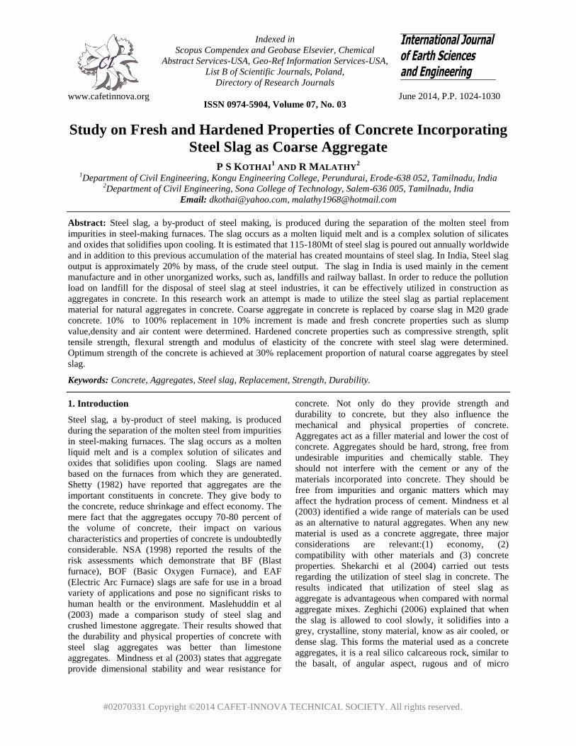
Sieve analysis of coarse aggregate and coarse slag was
conducted and found that there is no significant
variation in the particle size distribution of the coarse
aggregate and coarse slag. Particle size distribution
curve is given in Figure 1. Fraction of steel slag which
passes through 20mm size sieve and retained on
4.75mm size sieve is only used. Other materials used
are given below:
Cement: Ordinary Portland cement of 43 grade
conforming to IS: 8112 – 1989 and similar to ASTM
type III (C150 – 95) is used to find the effect of steel
slag in concrete without admixtures.
Fine aggregate: Natural river sand with fraction
passing through the 4.75mm sieve and retained on
600µm sieve is used. The specific gravity of fine
aggregate is 2.62, fineness modulus is 2.6 and density is
1654kg/m3.
Coarse aggregate: Crushed granite stone aggregates of
20mm maximum size (passes through 20mm size sieve
and retained on 4.75mm size sieve) having specific
gravity of 2.70, fineness modulus of 2.73 and density of
1590kg/m3 is used.
Water: Potable tap water available in the laboratory
with pH value of 7.0±1 and confirming to the
requirements of IS: 456 - 2000 was used for mixing
concrete and also for curing the specimens.
3. Experimental Methodology
The quantity of ingredients used in the M20 concrete
mix is given in Table 3. The reference mixture (CC)
was completely prepared with natural aggregates like
granite jelly and river sand, while the other mixtures
were prepared with the slag from steel plant. For the
entire test, the designed mix was taken with the w/c
ratio 0.5.
Table 4. gives the mix designation for various mixes of
concrete for coarse aggregate replacement with coarse
form of slag. Fresh concrete properties such as slump
value, density and air content were found out as per
IS: 1199 – 1959, ASTM C 231 specifications and
ASTM C 138 guidelines respectively. Hardened
concrete properties such as compressive strength, tensile
strength, flexural strength and modulus of elasticity
were determined as per IS: 516 –1959, IS: 5816-1970,
IS: 516-1959 and California test 522 (2000) procedure
respectively. Tests were conducted for all the
replacement proportions (10% to 100% in 10%
increment) of coarse aggregate by coarse slag for M20
grade concrete.
Figure 1. Particle size distribution curve
1026 Study on Fresh and Hardened Properties of Concrete Incorporating Steel Slag
as Coarse Aggregate
International Journal of Earth Sciences and Engineering
ISSN 0974-5904, Vol. 07, No. 03, June, 2014, pp. 1024-1030
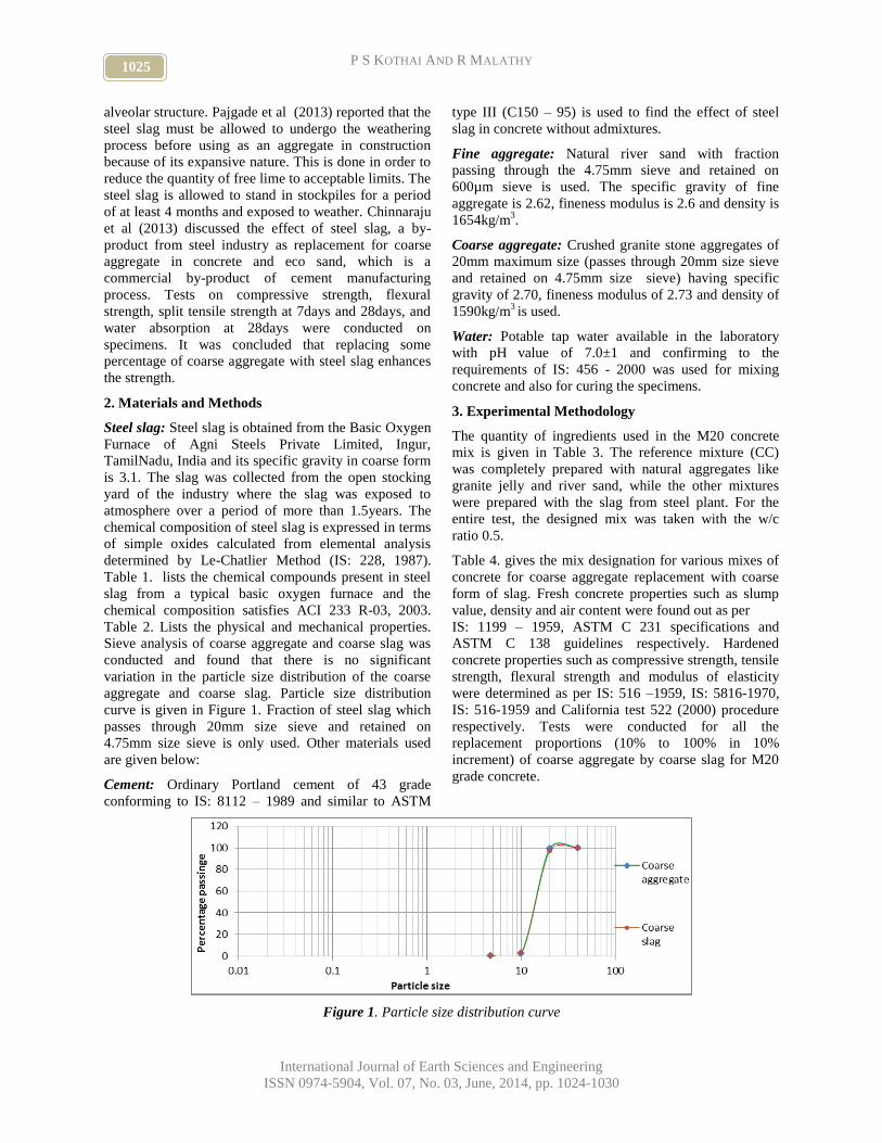
Table 1.Chemical composition of steel slag
Constituent Composition
(%)
Composition (%)
as per ACI 233
R-03
CaO 32.5 32 to 45
SiO2 34 32 to 42
Fe2O3 0.3 0.1 to 0.5
MgO 9 5 to 15
Al2O3 22 7 to 16
P2O5 0.56 --
SO3 0.7 --
Table 2. Properties of Steel slag
Test particlars Results
Specific gravity 3.10
Bulk
density(kg/m3)
1650
Aggregate impact
value
13.20
Aggregate crushing
value
26.70
Water absorption
(%)
0.79
Table 3. Mix Proportion
Cement
(kg/m3)
Fine
Aggregate
(kg/m3)
Coarse
aggregate
(kg/m3)
Water-
cement
ratio
372 592.29 1146.16 0.5
Table 4. Mix designation for various replacement
proportions
S.No
Mix Coarse
aggregate
%
Coarse
slag
%
Fine
aggregate
%
1. CC 100% - 100%
2. CS1 90% 10% 100%
3. CS2 80% 20% 100%
4. CS3 70% 30% 100%
5. CS4 60% 40% 100%
6. CS5 50% 50% 100%
7. CS6 40% 60% 100%
8. CS7 30% 70% 100%
9. CS8 20% 80% 100%
10. CS9 10% 90% 100%
11. CS10 - 100% 100%
4. Results and Discussion
Fresh concrete properties such as slump value, density
and air content of the various replacement proportions
are graphically represented in the following figures.
Figure 3. Slump value
Figure 4. Density
Figure 5.Air content
Slump value of conventional concrete is 100mm and
increase in the proportion of steel slag decreases the
workability of concrete. The density values of all the
replacement proportions were higher than conventional
1027 P S KOTHAI AND R MALATHY
International Journal of Earth Sciences and Engineering
ISSN 0974-5904, Vol. 07, No. 03, June, 2014, pp. 1024-1030
concrete density of 22.5kN/ m3. All the mixes show a
density value lies between 22.6kN/m3
to 22.85kN/m3.
Regarding air content value, mix CS1 shows an equal
percentage air content with conventional concrete and
all the other mixes show a decreased percentage of air
content when compared with the value of conventional
concrete which is 5.3%.
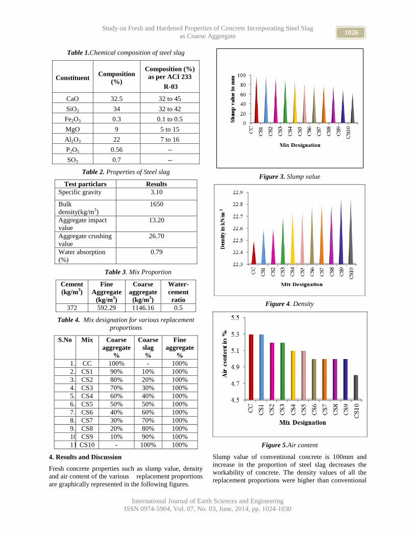
Results of the mechanical properties such as
Compressive strength, Split tensile strength, Flexural
strength and Modulus of Elasticity were graphically
represented in Figures 6, 7, 8 and 9.
Figure 6.Compressive strength
Figure 7.Split tensile strength
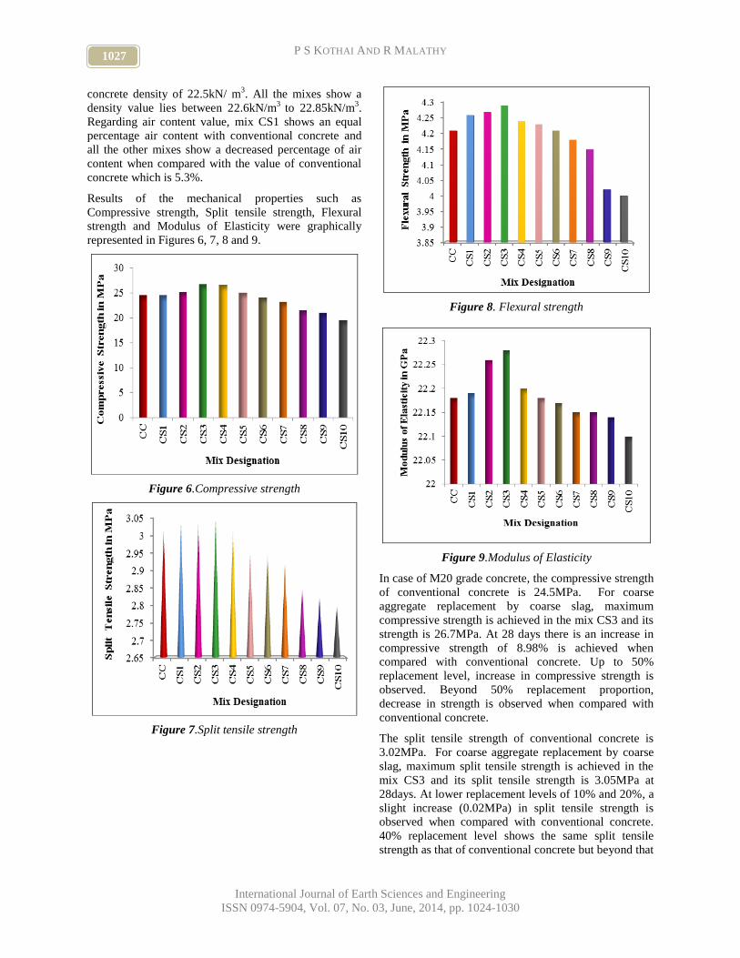
Figure 8. Flexural strength
Figure 9.Modulus of Elasticity
In case of M20 grade concrete, the compressive strength
of conventional concrete is 24.5MPa. For coarse
aggregate replacement by coarse slag, maximum
compressive strength is achieved in the mix CS3 and its
strength is 26.7MPa. At 28 days there is an increase in
compressive strength of 8.98% is achieved when
compared with conventional concrete. Up to 50%
replacement level, increase in compressive strength is
observed. Beyond 50% replacement proportion,
decrease in strength is observed when compared with
conventional concrete.
The split tensile strength of conventional concrete is
3.02MPa. For coarse aggregate replacement by coarse
slag, maximum split tensile strength is achieved in the
mix CS3 and its split tensile strength is 3.05MPa at
28days. At lower replacement levels of 10% and 20%, a
slight increase (0.02MPa) in split tensile strength is
observed when compared with conventional concrete.
40% replacement level shows the same split tensile
strength as that of conventional concrete but beyond that

1028 Study on Fresh and Hardened Properties of Concrete Incorporating Steel Slag
as Coarse Aggregate
International Journal of Earth Sciences and Engineering
ISSN 0974-5904, Vol. 07, No. 03, June, 2014, pp. 1024-1030
proportion split tensile strength decreases when
compared with that of conventional concrete.
For coarse aggregate replacement by coarse slag in M20
grade concrete, replacement proportions from 10% to
50% shows flexural strength value higher than that of
conventional concrete and an optimum strength is
observed in the mix CS3 at 28days. An increase of
0.08MPa is observed at 28days in the mix CS3 when
compared with conventional concrete. CS6 mix shows
strength similar to that of conventional concrete at 28
days. For replacement proportions beyond 60% the
flexural strength decreases when compared with
conventional concrete.
Up to 40% replacement level the value of modulus of
elasticity is higher than that of conventional concrete
and a maximum of 22.28GPa is observed in the mix
CS3 at 28 days curing. An increase of 0.45% is attained
in the same mix compared with conventional concrete.
Mix CS5 shows an equal value of modulus of elasticity
with conventional concrete. For replacement
proportions beyond 50% decrease in the value of
modulus of elasticity is observed when compared with
conventional concrete value.
Relationship between Compressive strength and
Flexural strength:
Figure10. Compressive strength Vs Flexural strength
The flexural strength and compressive strength test results
are plotted as a graph, and given in Figure 10. An analytical
equation for the relationship between these two was
derived from the test results as given below:
fr = 0.995√fck
Whereas for normal concrete as per IS 456 –2000, fr =
0.7√fck. It shows that the flexural strength increases in
concrete with steel slag aggregates.
Relationship between Compressive strength and
Modulus of Elasticity:

1029 P S KOTHAI AND R MALATHY
International Journal of Earth Sciences and Engineering
ISSN 0974-5904, Vol. 07, No. 03, June, 2014, pp. 1024-1030
Figure11. Compressive strength Vs Modulus of Elasticity
The modulus of elasticity and compressive strength test
results are plotted as a graph, and given in Figure 11. An
analytical equation for the relationship between these two
was derived from the test results as given below:
E = 5036.33√fck
whereas for normal concrete as per IS 456 – 2000, E =
5000√fck. It shows that the modulus of elasticity slightly
increases in concrete with steel slag aggregates.
5. Conclusions
From the experimental investigations on fresh concrete
properties, following conclusions were derived:
Concrete with steel slag aggregates in M20 grade
concrete, significantly reduces the workability of
concrete. More angularity and rough texture of the steel
slag aggregates affects the workability of the concrete.
It is suggested that the workability of steel slag
aggregate can be increased by use of plasticizers or air
entraining admixtures.
The density of steel slag aggregate concrete is higher
when compared with conventional concrete. The rough
texture and angular particles of steel slag aggregates
create better interlocking between the particles and the
cement paste which helps in improving the density of
concrete.
The air content in steel slag aggregate is comparatively
lower and hence workability was reduced. But increase
in air content affects the strength of the concrete.
Strength is the basic requirement in concrete and for
improving workability one can use plasticizers or air
entraining admixtures.
From the experimental investigations on hardened
concrete properties, following conclusions were
derived:
Replacing of 30% coarse aggregate by coarse slag in
M20 grade concrete has higher compressive strength,
split tensile strength, flexural strength and modulus of
elasticity values.
Up to 50% replacement the compressive strength is
observed to be more than that of conventional concrete.
40% replacement shows equal split tensile strength
value with conventional concrete but beyond 40%
replacement the split tensile strength decreases when
compared with conventional concrete.
Up to 50% replacement, flexural strength is higher than
conventional concrete. 60% replacement shows equal
value with conventional concrete and beyond that
proportion flexural strength decreases when compared
with conventional concrete.
Similar to that of flexural strength, when compared with
conventional concrete modulus of elasticity values also
increases up to 50%, equals at 60% and decreases
beyond that proportion.
For further improvement in strength water cement ratio
may be reduced by adding chemical admixtures like
plasticizers. Strength can also be improved by adding
mineral admixtures.
The relationship between the mechanical properties of
the concrete indicates that the strength of the steel slag

1030 Study on Fresh and Hardened Properties of Concrete Incorporating Steel Slag
as Coarse Aggregate
International Journal of Earth Sciences and Engineering
ISSN 0974-5904, Vol. 07, No. 03, June, 2014, pp. 1024-1030
aggregates concrete is comparatively higher than the
normal concrete strength specified by IS 456 – 2000.
Hence it is recommended that, steel slag aggregates can
be used as a replacement material for conventional
coarse aggregates in concrete in order to reduce the
exploitation of natural aggregates and to reduce the cost
of construction. Also industrial waste material
utilization in construction helps in reducing pollution
and achieving sustainability.
References
[1] Chinnaraju, K.., Ramkumar, VR., Lineesh, K.,
Nithya, S. and Sathish, V. 2013.Study on concrete
using steel slag as coarse aggregate replacement
and eco sand as fine aggregate replacement.
International Journal of Research in Engineering
and Advanced Technology. vol. 1, no.3, 1-6.
[2] Maslehuddin, M., Alfarabi Sharif, M., Shameem,
M., Ibrahim, M. and Barry, MS. 2003.Comparison
of Properties of Steel Slag and Crushed Limestone
Aggregates Concrete. Construction and Building
materials.Vol,17,105-112.
[3] Mindness, S., Young, J.F. and Darwin,D. 2003.
Concrete second edition. Pearson Education Inc.
[4] National Slag Association. 2003. Iron and Steel
making Slag Environmentally Responsible
Construction Aggregates. NSA Technical Bulletin.
[5] Pajgade,P.S. and Thakur.N.B. 2013. Utilisation of
Waste Product of Steel Industry. International
Journal of Engineering Research and Applications
(IJERA). Vol. 3, Issue 1, 2033-2041.
[6] Rustu S.Kalyoncu. 2001. Slag iron and Steel.US
Geological Survey Minerals Yearbook.
[7] Shekarchi, M., Soltani, M., Alizadeh, R., Chini ,
M., Ghods, P., Hoseini, M. and Montazer, Sh.
2004. Study of the mechanical properties of heavy
weight preplaced aggregate concrete using electric
arc furnace slag as aggregate. International
Conference on Concrete Engineering and
Technology, Malaysia.
[8] Shetty, M. S.1982. Concrete Technology Theory
and Practice. S.Chand and Company Ltd.
[9] Zeghichi, L. 2006. The effect of replacement of
naturals aggregates by Slag products on the
strength of concrete. Asian Journal of Civil
Engineering (Building and Housing). Vol. 7, 27-
35.
www.cafetinnova.org
Indexed in
Scopus Compendex and Geobase Elsevier, Chemical
Abstract Services-USA, Geo-Ref Information Services-USA,
List B of Scientific Journals, Poland,
Directory of Research Journals
ISSN 0974-5904, Volume 07, No. 03
June 2014, P.P.1031-1040
#02070332 Copyright ©2014 CAFET-INNOVA TECHNICAL SOCIETY. All rights reserved.
Geological Hazards in Deep Tunneling (A Case Study: Beheshtabad
Water Conveyance Tunnel)
R. BAGHERPOUR1 AND M. J. RAHIMDEL
2
1Department of Mining Engineering, Isfahan University of Technology, Isfahan 8415683111, Iran 2Department of Mining Engineering, Sahand University of Technology, Tabriz 513351996, Iran
Email: [email protected], [email protected]
Abstract: Knowledge of geology conditions and its hazards can play an important role in the selection of support
and suitable excavation method in underground structures. Water transport tunnel is one of the most important
structures with regard to the goal of excavation, special conditions and limitations considered in the design and
execution of them. Beheshtabad water Conveyance tunnel with 64930 meters length, 6 meters final diameter is the
largest water Conveyance tunnel in IRAN. Because of high over burden and weak rock in the most of tunnel path,
the probable geological hazards such as squeezing and rock burst must be studied. Squeezing stands for large time-
dependent convergence during tunnel excavation. This phenomenon occurs in weak rocks and deep conditions.
Besides, the height of overburden in some zone of the tunnel is about 1200 meters. The occurrence of this
phenomenon is always together with the instantaneous release of strain energy stored in the rock materials, causing
the harm to personal equipment and the collapse of underground structures. The existence of high thickness
overburden in some zones of this project indicates the high potential of rock burst hazard. In this research, the length
of the tunnel has been partitioned into sections using the interpreted geological, geophysical studies and borehole
data. After evaluating rock burst and squeezing potential with alternative analytical and experimental methods for
each section, the results of different methods are compared with each other. Results predict low to moderate
squeezing potential and moderate to high rock burst potential for some panels of the tunnel.
Keywords: Central plateau of Iran, geological hazards, rock burst, squeezing, Beheshtabad Water Conveyance
Tunnel.
1. Introduction:
Tunnels are one of the vital arteries that, because of a lot
of expenses spent for introduction of them and also
derangement of passing traffic as a result of perfect
demolition or serious damages, need the observation of
technical geotechnical considerations in design and
performance. Zayandehrud River is the only permanent
river in the Central Plateau of Iran. Water demand in
this area is constantly growing due to population
growth, key industries, withdrawal of ground water
tables and reduction of its quality. So, Beheshtabad
tunnel, by transporting 1070 millions of cube meters of
water per year to Iran central plateau, is considered in
order to eliminate the shortages in parts of drinking
water, industry and agriculture. This plan, consisting of
a dam with 184 meters height and water transport tunnel
with the length of about 65 km and 6 meters diameter, is
expected to be the longest water transport tunnel in
IRAN.
In this research, at the First, the tunnel was paneled
using the interpretation of geological, geophysical
studies and boreholes. Then, the squeezing and rock
burst potential was studied using empirical and
analytical methods for each panel. Finally, the results
were compared with each other.
1.1. Literature Review:
The Rock burst and squeezing are two main modes of
underground instability caused by overstressing of the
ground. Both modes are generally related to continuous
ground. Squeezing can occur both in massive (weak and
deformable) rocks and in highly jointed rock masses as
a result of overstressing. It is characterized by yielding
under the redistributed state of stress during and after
excavation [1]. The squeezing can be very large;
deformations as much as l7% of the tunnel diameter
have been reported in India [2]. According to the
unexpected geotechnical hazards during tunneling,
Singh et al., Goel et al., Jethwa et al., Hoek and Marinos
have studied the squeezing phenomenon for deep
tunnels in weak rocks and derived some criteria to
recognize it [2, 3, 4, 5, 6].
In most criteria, the overburden load plays an important
role in developing the squeezing conditions.
Furthermore, when an excavation for a deep

1032 Geological Hazards in Deep Tunneling (A Case Study: Beheshtabad Water
Conveyance Tunnel)
International Journal of Earth Sciences and Engineering
ISSN 0974-5904, Vol. 07, No. 03, June, 2014, pp. 1031-1040
underground tunnel or chamber is undertaken in a
strong and brittle rock, the change in stress results in
dynamic damage to the adjacent rock. This is referred to
as rockburst or break ways. Such rock bursts are a major
hazard for the safety of engineers and engineering
equipment, as well as affecting the shape/size of the
structure [7]. Hoek and Brown, Myrvang and Grimstad,
Hatcher, Haramy, Qiao and Tian, Wang and Park and
Amberg have been working to identify rock burst in
deep tunnels with brittle rocks [8, 9, 10, 11, 12, 13, 14].
2. Beheshtabad Water Conveyance Tunnel:
Beheshtabad Water Conveyance Tunnel, with about 65
kilometer length and 6 meter width, is one of the biggest
water supplying projects for transporting water to the
central plateau of Iran. This tunnel is located near Ardal
city with east north-west south direction. From the
entrance to 17 km of the tunnel, it is located in Zagros
zone and the output of it is in Sanandaj-Sirjan zone.
This tunnel is expected to transfer water to resolve
water deficiencies and shortcomings in industrial and
agriculture use in the central plateau of Iran, 1070 cubic
million meters annually [15].
Most important problems in path of this tunnel refers to
its cross to numerous fractures, resulting in many
problems and troubles during drilling and in the stages
of maintenance coverage of tunnel.
With regard to 19 boreholes in the tunnel path, tunnel
has been paneled to 16 sections. Engineering geological
properties for each panel are summarized in Table 1.
The rock engineering classification is shown in Table 2
[16].
Table1: Rock engineering geological characteristics for each tunnel section [16]
Secti
on Kilometer (m) Rock mass
Overburden
(m)
Density
(gr/cm3)
UCS
(MPa) RQD
I 5941-7800 Limestone with dolomite 600 2.530 65-75 95-100
II 7800-8116 Marl stone 781.58 2.968 20-40 95-100
III 8116-10790 Lime stone and Marl stone 1205.5 2.509 65-75 95-100
IV 10790-12129 Marl stone and conglomerate 340 2.488 70-90 95-100
V 12129-15492 Mud stone and conglomerate 294 2.450 30-45 95-100
VI 15492-17574 Weathered and altered andesitic 285 2.491 20-30 50-60
VII 17574-18013 Crushed limestone and Marly limestone 327 2.651 20-40 40-50
VIII 18013-20862 Marly and shale limestone 349 2.464 20-30 50-85
IX 20862-21730 Marl and Shale 477 2.733 25-35 85-90
X 21730-24174 Marl and Shale 621 2.646 20-40 85-90
XI 24174-29030 Alteration of massive limestone 654.45 2.646 40-50 75-85
XII 29030-31604 Shaly limestone 381 2.651 25-60 25-60
XIII 31604-34912 Melonitic limy sand stone with quarts
lenses 335.6 2.667 10-30 25-45
XIV 34912-37490 Melonitic limy sand stone with quarts
lenses 481 2.690 25-50 25-50
XV 37490-37892 Limestone and dolomite 571 2.690 50-80 90-100
Table2: Rock engineering classification of the studied tunnel [16]
Tunnel Section RMR Q
Value Rating Value Rating
I 54-55 Fair 1.65-2.67 Poor
II 60-64 Good 1.35-4 Poor
III 53-60 Fair 1.1-2 Poor
III 57-60 Fair 1.35-3 Poor
IV 50-71 Fair 2.4-13.3 Poor-Fair
V 56-61 Fair 2.3-9 Poor-Fair
VI 58-69 Good 3.92-9 Fair

1033 R. BAGHERPOUR AND M. J. RAHIMDEL
International Journal of Earth Sciences and Engineering
ISSN 0974-5904, Vol. 07, No. 03, June, 2014, pp. 1031-1040
VII 55-60 Fair 3.4-9 Poor-Fair
VIII 57-59 Fair 4.3-9 Fair
IX 19-21 Poor 0.006-0.015 Exceptionally Poor-
Extremely poor
X 23-28 Poor 0.006-0.02 Exceptionally Poor-
Extremely poor
XI 18-20 Poor 0.37-6 Fair
XII 50-64 Fair 2.1-6 Poor-Fair
XIII 50-57 Fair 0.95-2 Poor
XIV 49-59 Fair 1.1-3 Poor
XV 30-35 Poor 0.2-0.4 Poor
From Table 1, it can be seen that the classification
grading by Q system is lower than that by the RMR for
the same type rock. That is because Q system takes the
high stress field into consideration, and to some extent,
it causes rock mass instability.
Regarding researches in the studied area, stability
analysis and leakage quantity investigation have been
conducted. Rahimdel and et al. proposed the primary
support for tunnel section based on geology section and
rock masses of tunnel using RMR, Q and VNIMI
methods. The results based on VNIMI method are given
in Table 3 [17].
Table3: Primary support estimation for tunnel rock
masses
Rock Mass Primary Support
Limestone with dolomite,
marl stone, mud stone and
conglomerate
Using rock bolt or
shotcrete lining by 5 cm in
Thickness.
Crushed limestone and
marly limestone, Marly and
shale limestone and Shaly
limestone
Application of rock bolt
2.5 m in length with 1×1
distance together and
shotcrete lining by 5 cm or
more in Thickness with
mesh and rock bolt
Rafiee and et al. [15] used the Fuzzy Analytical
Hierarchy Process (FAHP) to support the estimation of
tunnel. In this study, regarding the numerical analysis
(finite difference program FLAC2D), six support
systems were considered as the decision alternative are
shown in Table 4 and support cost, factor of safety,
applicability, time, displacement and mechanization
were considered as the criteria. Calculations showed
that the alternative "E" should be selected as the
optimum support system to satisfy the goals and
objectives of Behashtabad Tunnel.
Table4: Explanation of Model Notations [15]
Support
system
(Alternative)
Explanation
A Supporting by shotcrete lining by 25 cm
in thickness together with IPE18
B Supporting by shotcrete lining by 30 cm
in thickness together with IPE16
C Supporting by shotcrete lining by 20 cm
in thickness together with wire mesh
D
This system is the combination of
shotcrete with steel fiber by 20 cm in
thickness
E
Application of rock bolt 3 m in length
with 1×1 distance together with shotcrete
lining by 10 cm in thickness
F
Application of rock bolt 3 m in length
with 2×2 distance together with shotcrete
lining by 20 cm in thickness
3. Squeezing:
The magnitude of tunnel convergence, the rate of
deformation and the extent of the yielding zone around
the tunnel depend on the geological and geotechnical
conditions, the in-situ state of stress relative to rock
mass strength, the groundwater flow and pore pressure,
and the rock mass properties [18]. Squeezing is,
therefore, synonymous with yielding and time-
dependence; its cost depends on the excavation and
support techniques adopted. If the support installation is
delayed, the rock mass moves into the tunnel and stress
redistribution take place around it. On the contrary, if
deformation is restrained, squeezing will lead to long-
term load build-up of rock support.
For the evaluation of the potential of squeezing,
empirical and semi-empirical methods have been
introduced via deferent researchers. These methods are
explained below.
3.1. Prediction of Squeezing:
3.1.1. Empirical approaches:
The empirical approaches are essentially based on
classification schemes. Two of these approaches are
1034 Geological Hazards in Deep Tunneling (A Case Study: Beheshtabad Water
Conveyance Tunnel)
International Journal of Earth Sciences and Engineering
ISSN 0974-5904, Vol. 07, No. 03, June, 2014, pp. 1031-1040
mentioned below in order to illustrate the uncertainty
still surrounding the subject, notwithstanding its
importance in tunneling practice.
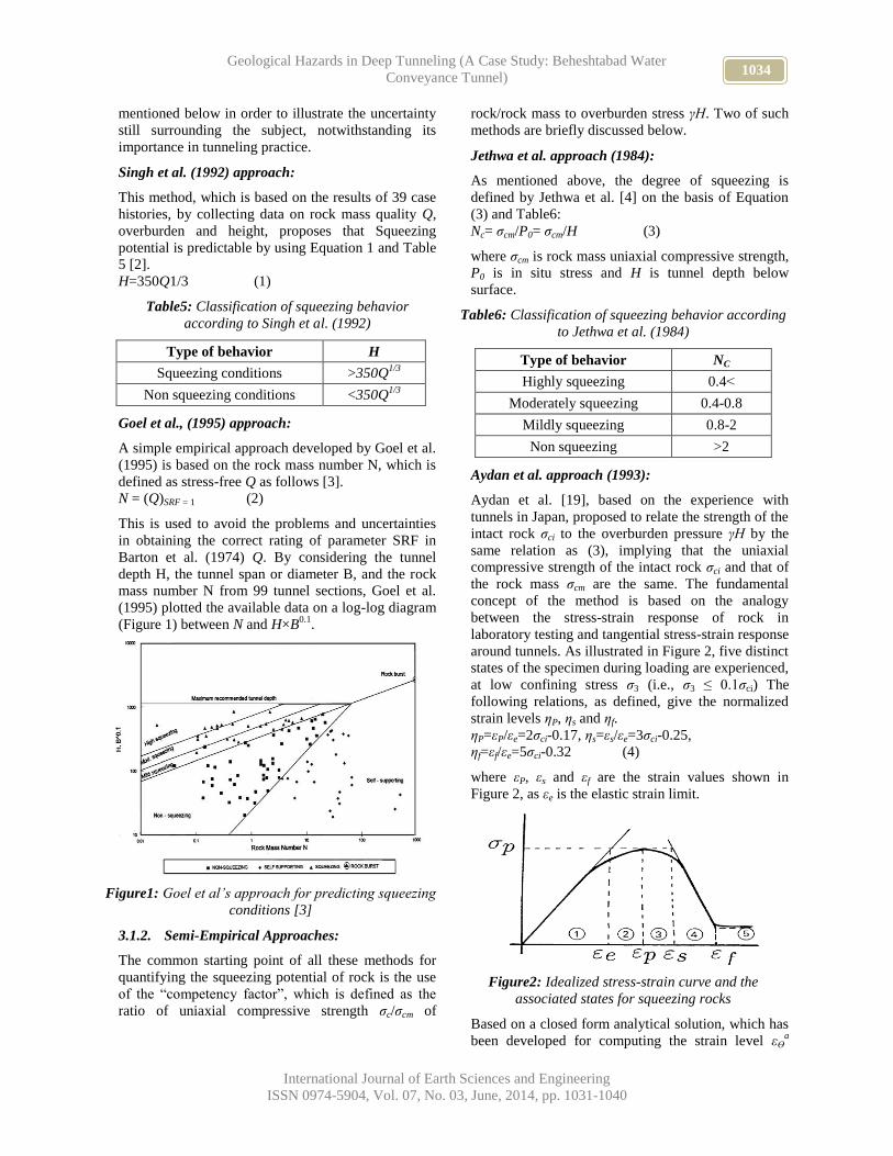
Singh et al. (1992) approach:
This method, which is based on the results of 39 case
histories, by collecting data on rock mass quality Q,
overburden and height, proposes that Squeezing
potential is predictable by using Equation 1 and Table
5 [2].
H=350Q1/3 (1)
Table5: Classification of squeezing behavior
according to Singh et al. (1992)
H Type of behavior
>350Q1/3
Squeezing conditions
<350Q1/3
Non squeezing conditions
Goel et al., (1995) approach:
A simple empirical approach developed by Goel et al.
(1995) is based on the rock mass number N, which is
defined as stress-free Q as follows [3].
N = (Q)SRF = 1 (2)
This is used to avoid the problems and uncertainties
in obtaining the correct rating of parameter SRF in
Barton et al. (1974) Q. By considering the tunnel
depth H, the tunnel span or diameter B, and the rock
mass number N from 99 tunnel sections, Goel et al.
(1995) plotted the available data on a log-log diagram
(Figure 1) between N and H×B0.1
.
Figure1: Goel et al’s approach for predicting squeezing
conditions [3]
3.1.2. Semi-Empirical Approaches:
The common starting point of all these methods for
quantifying the squeezing potential of rock is the use
of the “competency factor”, which is defined as the
ratio of uniaxial compressive strength σc/σcm of
rock/rock mass to overburden stress γH. Two of such
methods are briefly discussed below.
Jethwa et al. approach (1984):
As mentioned above, the degree of squeezing is
defined by Jethwa et al. [4] on the basis of Equation
(3) and Table6:
Nc= σcm/P0= σcm/H (3)
where σcm is rock mass uniaxial compressive strength,
P0 is in situ stress and H is tunnel depth below
surface.
Table6: Classification of squeezing behavior according
to Jethwa et al. (1984)
NC Type of behavior
0.4> Highly squeezing
0.4-0.8 Moderately squeezing
0.8-2 Mildly squeezing
>2 Non squeezing
Aydan et al. approach (1993):
Aydan et al. [19], based on the experience with
tunnels in Japan, proposed to relate the strength of the
intact rock σci to the overburden pressure γH by the
same relation as (3), implying that the uniaxial
compressive strength of the intact rock σci and that of
the rock mass σcm are the same. The fundamental
concept of the method is based on the analogy
between the stress-strain response of rock in
laboratory testing and tangential stress-strain response
around tunnels. As illustrated in Figure 2, five distinct
states of the specimen during loading are experienced,
at low confining stress σ3 (i.e., σ3 ≤ 0.1σci) The
following relations, as defined, give the normalized
strain levels ηP, ηs and ηf.
ηP=εP/εe=2σci-0.17, ηs=εs/εe=3σci-0.25,
ηf=εf/εe=5σci-0.32 (4)
where εP, εs and εf are the strain values shown in
Figure 2, as εe is the elastic strain limit.
Figure2: Idealized stress-strain curve and the
associated states for squeezing rocks
Based on a closed form analytical solution, which has
been developed for computing the strain level εϴa

1035 R. BAGHERPOUR AND M. J. RAHIMDEL
International Journal of Earth Sciences and Engineering
ISSN 0974-5904, Vol. 07, No. 03, June, 2014, pp. 1031-1040
around a circular tunnel in a hydrostatic stress field,
the five different degrees of squeezing are defined as
shown in Table 7. In this Table, εϴa is the tangential
strain around a circular tunnel in a hydrostatic stress
field [19], whereas εϴe is the elastic strain limit for the
rock mass.
Table7: Classification of squeezing behavior according
to Aydan et al. (1993)
Theoretical expression Squeezing degree
εϴa / εϴ
e ≤1 Non-squeezing
1≤ εϴa / εϴ
e ≤ ηP Light-squeezing
ηP ≤ εϴa / εϴ
e ≤ ηs Fair-squeezing
ηs ≤ εϴa / εϴ
e ≤ ηf Heavy-squeezing
εϴa / εϴ
e ≥ ηf Very heavy squeezing
3.1.3. Analytical-Theoretical Approaches:
Barla and International Society of Rock Mechanics
(ISRM) approaches:
The squeezing potential in these methods can be
expected in accordance with Table 8 by considering
the values of tangential stress (σϴ), uniaxial
compressive strength (σcm) and the maximum stress
(σ1).
Table8: Classification of squeezing behavior according
to Barla and ISRM approaches
Evaluation Method
Squeezing degree ISRM
(σθ/σcm)
Barla
(σcm/σ1)
<1 >1 Non-squeezing
1-2 1-0.4 Light-squeezing
2-4 0.4-0.2 Fair-squeezing
>4 0.2> Heavy-squeezing
3.2. Evaluation of squeezing potential in Beheshtabab
Water Conveyance Tunnel:
The results of assessing squeezing potential for the zone
of the tunnel in which there was the occurrence of this
phenomenon using different criteria have been shown in
Figure 3. To study the different criteria results, the
percentage of each category of the squeeze zones
studied was calculated as shown in Table 9. In average,
71, 20, 5 and 4 percent of total panels were in none,
light, moderate and heavy squeezing conditions,
respectively. So, most section of the tunnel was in none
squeezing potential.

1036 Geological Hazards in Deep Tunneling (A Case Study: Beheshtabad Water
Conveyance Tunnel)
International Journal of Earth Sciences and Engineering
ISSN 0974-5904, Vol. 07, No. 03, June, 2014, pp. 1031-1040
Figure3: The results of the squeezing potential using Singh (A), Goel (B), Jethwa (C), Aydan (D), Barla (E) and
ISRM (F) criteria.
Table9: The results of the squeezing potential in Beheshtabad Water Conveyance Tunnel
Percentage of tunnel sections in each squeezing condition Evaluation
criteria Non-squeezing Light-squeezing Fair-squeezing Heavy-
squeezing Very heavy-
squeezing
61 39 0 0 0 Singh
66 0 17 17 0 Goel
72 28 0 0 0 Jethwa
72 0 11 17 0 Aydan
78 22 0 0 0 Barla
72 28 0 0 0 ISRM
4. Rock Burst:
A rock burst is one of the most complicated dynamic
geological phenomena, with intricate mechanisms and
numerous affecting factors, which account for the
difficulty of predicting its characteristics. In the past
few years, many methods of forecasting rock bursts
have been proposed, including rock mechanics
assessment, stress detection and modern mathematical
theories.
The prevention of rock bursts is one of the key problems
in the construction of deep tunnels in which rock burst
prediction is a basic problem. In the construction of
underground engineering, it is of great importance for
the safety and the optimization of support measures to
make correct and timely predictions of the possibility,
as well as the scope and intensity of rock bursts in the
rock mass surrounding the ground to be excavated.
4.1. Rock Burst Prediction:
Regarding available and valid references,
comprehensive researches have carried out done in
classification and evaluation of rock burst phenomenon.
In most of them, Linear elastic criterion, Method of
Tensile Stress, Method of Brittleness coefficient and
Method of Stresses have been used for rock burst
prediction [7, 20, 21, 22, 23, 24, 25, 26, 27, 28, 29, 30,
31, 32, 33, 34].
Linear Elastic Criterion:
Linear elastic energy (LE) stored in rock before
reaching the peak strength can be defined by the
following equation.
2E
2cσEL (5)
Where E is unloading tangent elastic modulus of rock,
and σc is uniaxial compressive strength. Rock burst
potential is predictable by using Table 10.
Table10: Classification of Rock burst behavior
according to linear elastic criterion
50> 50-
100 100-150
150-
200 200< LE
(MPa)
Very
Low Low Moderate High
Very
High
Rock
bust
potential
Method of Tensile Stress:
Rock burst predictions using this method can be defined
by Equation (6). Rock burst potential is predictable by
using Table 11.
cσθσ
sT (6)
where σɵ: Tensile stress, σc: Uniaxial compressive
strength.
1037 R. BAGHERPOUR AND M. J. RAHIMDEL
International Journal of Earth Sciences and Engineering
ISSN 0974-5904, Vol. 07, No. 03, June, 2014, pp. 1031-1040
Table11: Classification of Rock burst behavior
according to the Method of Tensile Stress
0.3> 0.3-
0.5 0.5-0.7
0.7-
0.9 0.9< TS
Non-
Rock
Burst
Low Moderate High Very
High
Rock
bust
potential
Method of Brittleness Coefficient:
This method evalutes the tendency of rock burst through
the brittleness coefficient R of Rocks. This coefficient is
defined as the ratio of σc over σt (σc and σt are the
uniaxial compressive strength and the tensile strength of
the rock), i.e., β=σc/σt. In general, the grater β, the
higher the rock burst tendency (see Table 12).
Table12: Classification of Rock burst behavior
according to the method of brittleness coefficient
40< 40-26.7 26.7-14.5 14.5> Β
Non-
rock
burst
Low Moderate High
Rock
bust
potential
Method of Stresses:
Method of stresses combines the lithological character
of a rock mass (including tensile and compressive
strength) to judge the possibility that rock burst can take
place. This method introduces two factors of and β to
serve as criteria. and β are defined, respectively, as
the ratio of the rocks uniaxial compressive strength, σc,
over the major principle geostress, σ1, i.e., = σc/σ1 and
as the ratio of the rocks uniaxial tensile strength, σt, over
σ1, i.e., = σt/σ1. Because the index of the uniaxial
compressive can be determined easily, the value of is
generally used for a criterion having the following
Table.
Table13: Classification of Rock burst behavior
according to the Method of Stresses
10< 10-5 5-2.5 2.5>
Non- rock
burst Low Moderate High
Rock
bust
potential
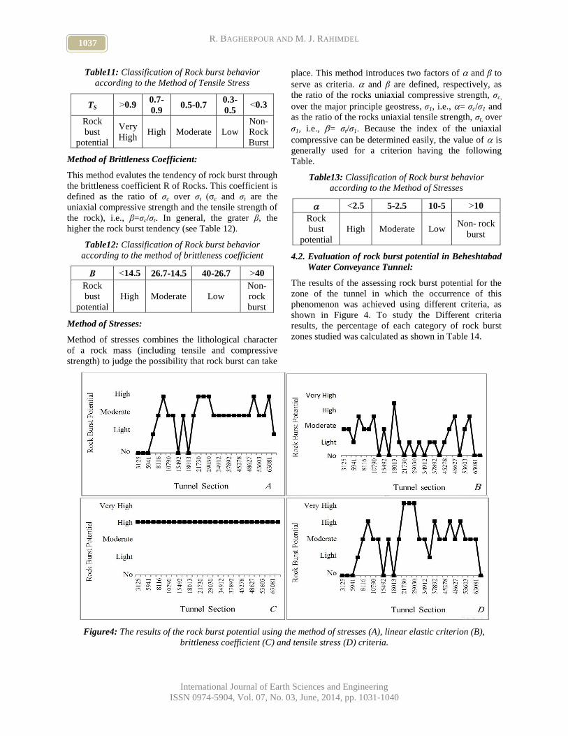
4.2. Evaluation of rock burst potential in Beheshtabad
Water Conveyance Tunnel:
The results of the assessing rock burst potential for the
zone of the tunnel in which the occurrence of this
phenomenon was achieved using different criteria, as
shown in Figure 4. To study the Different criteria
results, the percentage of each category of rock burst
zones studied was calculated as shown in Table 14.
Figure4: The results of the rock burst potential using the method of stresses (A), linear elastic criterion (B),
brittleness coefficient (C) and tensile stress (D) criteria.
1038 Geological Hazards in Deep Tunneling (A Case Study: Beheshtabad Water
Conveyance Tunnel)
International Journal of Earth Sciences and Engineering
ISSN 0974-5904, Vol. 07, No. 03, June, 2014, pp. 1031-1040
Table14: The results of the rock burst potential
Percentage of tunnel sections in each of rock burst conditions
Evaluation criteria Non-
rock burst Light- rock
burst Fair-
rock burst Heavy- rock
burst Very heavy-
rock burst
40 24 20 12 4 Linear elastic criterion
16 12 40 16 16 Tensile Stress
8 8 60 20 0 Stresses
0 0 0 100 0 Brittleness coefficient
Regarding Table 14, Linear elastic criterion predicts no
rock burst potential for more sections of the tunnel,
while Tensile Stress and Stresses methods assume the
major sections of tunnel to be in the fair rock burst
potential. According to brittleness coefficient, all tunnel
sections are unfortunately in heavy rock burst condition.
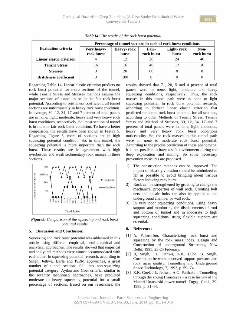
In average, 30, 12, 34, 17 and 7 percent of total panels
are in none, light, moderate, heavy and very heavy rock
burst conditions, respectively. So, most section of tunnel
is in none to fair rock burst condition. To have a better
comparison, the results have been shown in Figure 5.
Regarding Figure 5, more of sections are in high
squeezing potential condition. So, in this tunnel, the
squeezing potential is more important than the rock
burst. These results are in agreement with high
overburden and weak sedimentary rock masses in these
sections.
Figure5: Comparison of the squeezing and rock burst
potential results
5. Discussion and Conclusion:
Squeezing and rock burst potential was addressed in this
article using different empirical, semi-empirical and
analytical approaches. The results showed that empirical
and analytical methods were almost accommodated with
each other. In squeezing potential research, according to
Singh, Jethwa, Barla and ISRM approaches, a great
number of tunnel sections fell into non-squeezing
potential category. Aydan and Goel criteria, similar to
the recently mentioned approaches, have predicted
moderate to heavy squeezing potential for a small
percentage of sections. Based on our researches, the
results showed that 71, 20, 5 and 4 percent of total
panels were in none, light, moderate and heavy
squeezing conditions, respectively. Thus, the rock
masses in this tunnel path were in none to light
squeezing potential. In rock burst potential research,
according to forbear linear elastic criterion that
predicted moderate rock burst potential for all sections,
according to other Methods of Tensile Stress, Tensile
Stress and Method of Stresses, 30, 12, 34, 17 and 7
percent of total panels were in none, light, moderate,
heavy and very heavy rock burst conditions
noticeability. So, the rock masses in this tunnel path
were in none to moderate rock burst potential.
According to the precise prediction of these phenomena,
it is not possible to have a safe environment during the
deep exploration and mining. So some necessary
prevention measures are proposed.
1) The construction methods can be improved. The
impact of blasting vibration should be minimized as
far as possible to avoid bringing about various
factors inducing rock burst.
2) Rock can be strengthened by grouting to change the
mechanical properties of wall rock. Grouting bolt
nets and plastic bolts can also be applied to the
underground chamber or wall rock.
3) In very poor squeezing conditions, using heavy
support and monitoring the displacements of roof
and bottom of tunnel and in moderate to high
squeezing conditions, using flexible support are
essential.
6. Reference:
[1] A. Palmström, Characterizing rock burst and
squeezing by the rock mass index, Design and
Construction of underground Structures, New
Delhi, 1995, 23-25 February.
[2] B, Singh, J.L. Jethwa, A.K. Dube, B. Singh,
Correlation between observed support pressure and
rock mass quality, Tunnelling and Underground
Space Technology, 7, 1992, p. 59- 74.
[3] R.K. Goel, J.L. Jethwa, A.G. Paithakan, Tunnelling
through the young Himalayas – a case history of the
Maneri-Uttarkashi power tunnel. Engrg. Geol., 39,
1995, p. 31-44.
1039 R. BAGHERPOUR AND M. J. RAHIMDEL
International Journal of Earth Sciences and Engineering
ISSN 0974-5904, Vol. 07, No. 03, June, 2014, pp. 1031-1040
[4] J.L. Jethwa, B. Singh, Estimation of ultimate rock
pressure for tunnel linings under squeezing rock
conditions – a new approach. Design and
Performance of Underground Excavations, ISRM
Symposium, Cambridge, E.T. Brown and
J.A.Hudson eds., 1984, p. 231-238.
[5] E. Hoek, P. Marinos, Predicting Tunnel Squeezing
Problems in Weak Heterogeneous Rock Masses,
Tunnels and Tunneling International, 45 -51: part
one, 2000a, p. 33-36: Part 2.
[6] E. Hoek, P. Marinos, Predicting tunnel squeezing
problems in weak heterogeneous rock masses,
Tunnels and Tunnelling International Part two
(December), 2000b, p. 33–36.
[7] Q. Jiang, X.T. Feng, T.B. Xiang, G.S. Su, Rock
burst characteristics and numerical simulation
based on a new energy index: a case study of a
tunnel at 2500 m depth, Bulletin of Engineering
Geology and the Environment, 69, 2010, p. 381–
388.
[8] E. Hoek, E.T. Brown, Underground excavations in
rock, Institution of mining and metallurgy, London
1980, p. 527.
[9] A. Myrvang, E. Grimstad, Rock burst Problems in
Norwegian Highway Tunnels- Recent Case
Histories, Rock burst Prediction and Control. The
Institution of Mining and Metallurgy Oct., 1983, p.
133-139.
[10] R.D. Hatcher, Structural geology– principles,
concepts, and problems, Prentice Hall, Englewood
Cliffs, second edition, New Jersey, 1985.
[11] K.Y. Haramy, Underground strucures in rock bursts
zones – In: Underground structures, design and
instrumentation, Elsevier Science publishers B.V.,
Amsterdom, 1998.
[12] C.S. Qiao, Z.Y. Tian, Study of the possibility of
rockburst in Dong-gua-shan Copper Mine, Chinese
J. Rock Mech. Eng. Žexp. 17, 1998, p. 917-921.
[13] J.K. Wang, H.D. Park, Comprehensive Prediction
of Rock Burst Based on Analysis of Strain Energy
in Rock, Tunneling and Underground Space
Technology, 2001, p. 7-49.
[14] F. Amberg, Tunneling in high overburden with
reference to deep tunnels in Switzerland, Tunneling
and Underground Space Technology (19), 2004.
[15] R. Rafiee, M. Ataei, S.M.E. Jalali, The Optimum
Support Selection by Using Fuzzy Analytical
Hierarchy Prosess Method for Beheshtabad Water
Transporting Tunnel in Naien, Iranian Journal of
Fuzzy Systems, 10(6), 2013, p. 39-51.
[16] M. Hashemi, Rock mechanics reports, Water
Supply Project of the Central Plateau, Zayan-dehab
Consulting, 2007.
[17] M.J. Rahimdel, S. Mahdevari, R. Bagherpour,
Stability Assessments and Support Estimation of
Beheshtabad Water Transport Tunnel by VNIMI
Method, The 1st Asian and 9th Iranian Tunneling
Symposium, 2011.
[18] G. Barla, Tunnelling under Squeezing Rock
Conditions, 2002, p. 1-75.
[19] Ö. Aydan, T. Akagi, T. Kawamoto, The squeezing
potential of rock around tunnels: theory and
prediction, Journal of Rock Mechanics and Rock
Engineering, 26(4), 1993, p. l37-163.
[20] N.G.W. Cook, E. Hoek, J.P.G. Pretorius, W.D.
Ortlepp, M.D.G. Alamon, Rock mechanics applied
to the study of rock bursts, Journal of the South
African Institute of Mining and Metallurgy, 66,
1996, p. 435–528.
[21] U. Casten, Z. Fajklewicz, Induced gravity
anomalies and rockburst risk in coal mines – a case
history, Geophysical Prospecting, 41(1), 1993, p.
1–13.
[22] K. Shivakumar, M.V.M.S. Rao, C. Srinivasan, K.
Kusunose, Multifractal analysis of the spatial
distribution of area rock bursts at Kolar Gold
Mines, International Journal of Rock Mechanics &
Mining Sciences, 33(2), 1996, p.167–172.
[23] A.M. Linkov, Rockburst and the instability of rock
masses, International Journal of Rock Mechanics
and Mining Science, 33, 1996, p. 727–732.
[24] S.K. Sharan, A finite element perturbation method
for the prediction of Rock burst, Computers and
Structures, 85, 2004, p. 1304–1309.
[25] H.B. Zhao, Classification of rock burst using
support vector machine, Rock and Soil Mechanics
26(4), 2005, p. 642–644 (in Chinese).
[26] F.Q. Gong, X.B. Li, A distance discriminant
analysis method for prediction of possibility and
classification of rockburst and its application,
Chinese Journal of Rock Mechanics and
Engineering, 26(5), 2007, p. 1012–1018 (in
Chinese).
[27] W.C. Zhu, Z.H. Li, L. Zhu, C.A. Tang, Numerical
simulation on rock burst of underground opening
triggered by dynamic disturbance, Tunneling and
Underground Space Technology, 25, 2010, p. 587–
599.
[28] Y.C. Wang, Y.Q. Shang, H.Y. Sun, X.S. Yan,
Study of prediction of rock burst intensity based on
efficacy coefficient method, Rock and Soil
Mechanics, 31(2), 2010, p. 529–534 (in Chinese).
[29] J.L. Yang, X.B. Li, Z.L. Zhou, Y. Lin, A Fuzzy
assessment method of rock-burst prediction based
on rough set theory, Metal Mine, 6, 2010, p. 26–29
(in Chinese).
[30] J. Zhou, X.Z. Shi, L. Dong, H.Y. Hu, H.Y. Wang,
Fisher discriminant analysis model and its
application for prediction of classification of rock
burst in Deepburied Long Tunnel, Journal of Coal
Science and Engineering (China), 16 (2), 2010, p.
144–149.

1040 Geological Hazards in Deep Tunneling (A Case Study: Beheshtabad Water
Conveyance Tunnel)
International Journal of Earth Sciences and Engineering
ISSN 0974-5904, Vol. 07, No. 03, June, 2014, pp. 1031-1040
[31] H. Hu, D. Linming, L. Xuwei, Q. Qiuqiu, C.
Tongjun, G. Siyuan, Active velocity tomography
for assessing rock burst hazards in a kilometer deep
mine, Mining Science and Technology (China), 21,
2011, p. 673–676.
[32] C. Xuehua, L. Weiqing, Y. Xianyang, Analysis on
rock burst danger when fully mechanized caving
coal face passed fault with deep mining, Safety
Science, 50, 2012, p. 645–648.
[33] F. Jun, D. Linming, H. Hua, D. Taotao, Z. Shibin,
G. Bing, S. Xinglin, Directional hydraulic
fracturing to control hard-roof rock burst in coal
mines, International Journal of Mining Science and
Technology, 22, 2012, p. 177–181.
[34] N. Baisheng, L. Xiangchun, Mechanism research
on coal and gas outburst during vibration blasting,
Safety Science, 50, 2012, p. 741–744.

www.cafetinnova.org
Indexed in
Scopus Compendex and Geobase Elsevier, Chemical
Abstract Services-USA, Geo-Ref Information Services-USA,
List B of Scientific Journals, Poland,
Directory of Research Journals
ISSN 0974-5904, Volume 07, No. 03
June 2014, P.P.1041-1048
#02070333 Copyright ©2014 CAFET-INNOVA TECHNICAL SOCIETY. All rights reserved.
Watershed Based Drainage Morphometric Analysis in a Part of
Landslide Incidence Areas of Coorg District, Karnataka State
D N VINUTHA1, S RAMU
2, MOHAMMAD MUZAMIL AHMAD
3 AND M R JANARDHANA
1
1Department of Earth Science & Resource Management, Yuvaraja’s College, University of Mysore,
Mysore – 570005, Karnataka, India 2Department of Civil Engineering, KVG College of Engineering, Sullaya, Dakshina Kannada, India
3Department of Geology, University BDT College of Engineering, Davangere, Karnataka, India
Email: [email protected]
Abstract: Quantitative morphometric analysis of a watershed provides a description of the drainage system and
involves the quantification of the channel network and related parameters such as drainage area, gradient and relief.
These parameters in addition to the geology and the degree of weathering of rocks have a bearing on the occurrence
of landslides in the hilly terrains. The present study deals with the morphometric characteristics of the sub-
watersheds of Harangi watershed which is a part of Cauvery river mega basin in Coorg district of Karnataka State.
Morphometric characteristics comprising linear, areal and relief aspects of Harangi watershed which has been
subdivided into 10 sub-watersheds, were evaluated based on the Survey of India toposheets on 1:50000 scale,
orthorectified Landsat MSS and ETM imageries. Digital Elevation Model (DEM) was prepared by using ASTER
data and Geographical Information System (GIS) tool was used in the evaluation of linear, areal and relief aspects
and in the preparation of thematic maps. Landslide incidences are restricted to sub-watersheds 7 and 9 located in the
southwestern part of the Harangi basin. These sub-watersheds are located in highly weathered granitic gneiss region
with thick soil cover and are characterized by relatively low relief ratio and drainage density, stream frequency,
texture ratio, form factor, circulatory ratio and correlates well with the amount of vegetation and water absorption
capacity of the soil of the region.
Key words: Morphometry, Landslide, Harangi watershed, GIS, Western Ghat.
1. Introduction:
Morphometry is the measurement and mathematical
analysis of the configuration of the earth’s surface,
shape and dimension of its landforms (Clarke, 1966).
Morphometric analysis of a watershed provides a
quantitative description of the drainage system, which is
an important aspect of the characterization of
watersheds (Strahler, 1964).The close relationship
between hydrology and geomorphology play an
important role in the drainage morphometric analysis
(Horton, 1932). The influence of drainage morphometry
is very significant in understanding the landform
processes, soil physical properties and erosional
characteristics (Iqbal et al. 2012), which are all
fundamental features in the assessment of the possible
occurrence of landslides in any given area. Watershed is
taken as a basic unit in morphometric analysis as all the
hydrologic and geomorphic processes can be evaluated
within a finite area. Morphometric analysis can be
achieved through measurement of linear, areal and relief
aspects of the basin and slope contribution (Nag and
Chakraborty, 2003).
Harangi watershed region is witnessing a number of
landslides during and soon after heavy rain falls
disrupting normal life. The area is also known for
intense human activities related to plantation. The
region is hilly with varied geomorphologic features and
occurrence of landslides during monsoon season
warrants study of drainage morphometry vis-à-vis
landslide occurrences. However, the present authors
have restricted their studies to evaluate basin
morphometric characteristics encompassing relevant
linear, area and relief aspects of the Harangi watershed,
which is a part of Cauvery River in the SW part of
Karnataka state. The study serves as a platform to carry
out the natural hazard investigations in the region.
1.1. Study Area:
The study area lies in the Western Ghats encompassing
Coorg district and NW part is in South Kanara district.
The study area is bounded by latitudes 1406590.32 to
1372348.92 N and longitudes 610716.58 to 569484.17
East (UTM). It forms a part of Survey of India
toposheets 48P/10, P/11, P/14 and P/15 and covers an
area of about 664.76 Km2. The area under consideration

1042 Watershed Based Drainage Morphometric Analysis in a Part of Landslide Incidence
Areas of Coorg District, Karnataka State
International Journal of Earth Sciences and Engineering
ISSN 0974-5904, Vol. 07, No. 03, June, 2014, pp. 1041-1048
is known for picturesque hills and has a general
northwest-southeast trend. The location map of the
study area is depicted in Fig1. The geological
formations of the study area belong to the Archaean
metamorphic complex. The main rock types are
charnockites, granitic gneisses and dolerite dykes.
Major part of the study area is covered by granitic
gneisses (Fig. 2). The rocks are highly weathered and at
places, the soil cover extends to a depth of more than 12
m. The Coorg district is one of the major places that get
heavy rainfall in India. The river Harangi, a tributary of
the river Cauvery, originates in the Pushpagiri hills of
Western Ghats in Coorg district, Karnataka State. The
total length of the Harangi River is 50 km and the
southwest monsoon brings a lot of rains and is the
source of water in the catchment area. The present
landscape of the Coorg district under consideration is
viewed as the product of a series of interactions between
fluvial and denuded processes operating on underlying
geology that has been subjected to past vertical tectonics
(Vinutha et al., in press).
Fig1: Location map of the Harangi watershed
Fig2: Geological map of the Harangi watershed area
2. Methods of Investigation:
In the present study, an attempt has been made to study
the morphometric characteristics of Harangi basin. GIS
technique is employed for assessing various terrain and
morphometric parameters of the drainage basins and
watersheds, as they provide a flexible environment and
a powerful tool for the manipulation and analysis of
spatial information (Pankaj and Kumar, 2009). Drainage
map of the Coorg district as represented over the
topographical maps (scale 1:50,000), was acquired from
the Karnataka State Remote Sensing Centre (KSRSC),
Bangalore, in jpg format. Harangi river basin was
delineated in terms of surface – watershed area based on
topographic divides. The streams were georegistered to
the GIS using Universal Trans Mercator (UTM)
coordinates. Sub-watersheds numbering ten were
identified (Fig. 3). Determined watersheds were
imported into ArcView 3.2 and shape files were created
through manual digitizing. With all stream inventoried
and the Harangi watershed clearly defined and sub-

1043 D N VINUTHA, S RAMU, MOHAMMAD MUZAMIL AHMAD AND M R JANARDHANA
International Journal of Earth Sciences and Engineering
ISSN 0974-5904, Vol. 07, No. 03, June, 2014, pp. 1041-1048
watersheds demarcated, different morphometric
parameters were calculated for each of the sub-
watershed. Linear, areal and relief aspects of the basin
were computed in GIS environment by using ArcGIS
9.3 software. Ground truthing was carried out randomly
and the maps created in GIS environment were modified
as necessary. Linear, areal and relief parameters of the
watershed of the present study area were evaluated as
per the procedure detailed in Vittala et al, (2004). The
results of the analysis are shown in tables from 1 to 5.
Fig3: Drainage map of the Harangi watershed showing
sub-watershed boundary
3. Results and Discussion:
The morphometric analysis is carried out through the
evaluation of linear, areal and relief aspects of the basin.
The results of each of the parameters are presented and
discussed below.
3.1. Linear Aspects:
The linear aspects include the linear scale measurements
of the drainage networks and the dimensionless
numbers such as bifurcation ratio and stream length
ratio. The linear scale parameters analyzed in the
present study are stream order, stream length, mean
steam length, stream length ratio and bifurcation ratio
which have a direct relationship with the erodibility of a
region.
3.1.1. Stream Order (U):
Ordering of stream is the first stage of basin analysis
and stream ordering involves applying numerical
value to a streams position and size in the basin. In
the present study, ranking of streams has been carried
out according to Strahler (1964) stream ordering
system. The order wise stream numbers, area and
stream length of the 10 sub-watersheds evaluated in
GIS environment are presented in Table 2. Out of
these, sub-watershed 1is under III order, 4, 7, 8 and
10 are IV order whereas the remaining 2, 3, 5, 6 and 9
are V order. In Table 2 it is noticed that the maximum
frequency is in case of first order streams. It is also
observed that there is a decrease in stream frequency
as the stream order increases. Highest and lowest I
order streams are seen in 9th
and 4th
sub-watersheds
respectively. I and II order streams dominate in 9th
sub-watershed which incidentally has witnessed
landslides, moderate in 6th
and 3rd
sub-watersheds.
These sub-watersheds are occupied by hillocks.
Table2: Stream orders and Stream lengths of Harangi watersheds
Sl.
No.
Sub-water
shed name
Stream
Order
Stream Order (U) Stream Length (Lu) in km
I II III IV V I II III IV V
1 1 III 53.00 12.00 3.00 0.00 0.00 25.67 12.97 0.37 0.00 0.00
2 2 V 45.00 13.00 4.00 2.00 1.00 24.77 14.86 4.50 3.60 0.90
3 3 V 179.00 41.00 7.00 2.00 1.00 90.00 36.10 25.67 6.75 5.58
4 4 IV 41.00 9.00 2.00 1.00 0.00 20.36 5.48 4.86 1.35 0.00
5 5 V 124.00 29.00 6.00 2.00 1.00 51.98 18.00 8.10 5.40 4.50
6 6 V 248.00 47.00 13.00 2.00 1.00 124.40 38.70 18.90 6.39 6.30
7 7 IV 96.00 21.00 3.00 1.00 0.00 41.30 15.31 4.68 2.88 0.00
8 8 IV 126.00 25.00 7.00 1.00 0.00 61.71 18.00 4.95 4.50 0.00
9 9 V 406.00 89.00 25.00 6.00 1.00 145.94 38.01 24.32 8.20 7.10
10 10 IV 133.00 30.00 6.00 1.00 0.00 48.80 29.90 9.00 7.10 0.00
Total 1451.00 316.00 76.00 18.00 5.00 634.93 227.33 105.35 46.17 24.38
3.1.2. Stream Length (Lu):
The total length of individual stream segments of each
order is the stream length of that order. This has been
computed based on the law proposed by Horton
(1945) for all the sub-watersheds of the study area.
The stream length in each order increases
exponentially with increasing stream order. From
Table 2, it is clear that the overall drainage

1044 Watershed Based Drainage Morphometric Analysis in a Part of Landslide Incidence
Areas of Coorg District, Karnataka State
International Journal of Earth Sciences and Engineering
ISSN 0974-5904, Vol. 07, No. 03, June, 2014, pp. 1041-1048
development in the study area is more in sub-
watershed No. 9 which is covered with granitic
gneisses and is less in the watershed no 4. It reflects
the frequency of the drainage development is high in
areas which have witnessed landslides. Further, these
areas are highly dissected and over saturation in the
interfluves between the drainage lines may possibly
be the triggering factor for the inducement of
landslides. Generally, the total length of stream
segments is maximum in first order streams and
decreases as the stream order increases. In conformity
with the stream order maximum Lu is noticed in sub-
watershed No. 9 and minimum is seen in sub-
watershed No. 4.
3.1.3. Mean Stream Length (Lsm):
Mean stream length (Lsm) is characteristic property
related to the drainage network components and its
associated basin surface (Strahler, 1964); this has
been calculated by dividing the total stream length of
order (U) by the number of streams of segments in the
order. The mean stream length is presented in Table
3. It is seen that Lsm values exhibit variation from
0.12 - 9.00. The mean stream lengths of stream
increase with the increase of the stream order. But
some sub-watersheds shows opposite relation, higher
order stream has a small mean length. These sub-
watersheds show variable relative relief and
asymmetry in the degree of weathering.
3.1.4. Stream Length Ratio (RL):
The Stream Length Ratio (RL) is the ratio of the mean
length of the one order (Lu2) to the next lower order
(Lu1) of the stream segments. The RL values are
presented in Table 3. The stream length ratio between
the streams of different orders of the study area shows
a change in each sub-watershed. This change might
be attributed to variations in slope and topography
(Singh & Singh, 1997), indicating the late youth stage
of geomorphic development in the streams of the
study area.
Table3: Mean stream lengths and Stream length ratios of Harangi watershed
Sub -
Watershed
Name
Mean Stream Length (Lsm) in km Stream Length Ratio (RL)
Mean
Bifurcation
Ratio
I II III IV V II/I III/II IV/III V/IV VI/
V 2.81
1 0.48 1.08 0.12 0.00 0.00 0.51 0.03 0.00 0.00 0.00 2.68
2 0.55 1.14 1.13 1.80 0.90 0.60 0.30 0.80 0.25 0.00 3.93
3 0.50 0.88 3.67 3.38 5.58 0.40 0.71 0.26 0.83 0.00 3.69
4 0.50 0.61 2.43 1.35 0.00 0.27 0.89 0.28 0.00 0.00 3.53
5 0.42 0.62 1.35 2.70 4.50 0.35 0.45 0.67 0.83 0.00 4.35
6 0.50 0.82 1.45 3.20 6.30 0.31 0.49 0.34 0.99 0.00 4.86
7 0.43 0.73 1.56 2.88 0.00 0.37 0.31 0.62 0.00 0.00 5.20
8 0.49 0.72 0.71 4.50 0.00 0.29 0.28 0.91 0.00 0.00 4.57
9 0.36 0.43 0.97 1.37 7.10 0.26 0.64 0.34 0.87 0.00 5.14
10 0.37 1.00 1.50 7.10 9.00 0.61 0.30 0.79 0.00 0.00 2.81
3.1.5. Bifurcation Ratio (Rb):
Bifurcation ratio is the index of relief and dissection
(Horton, 1945) and is defined as the ratio of the
number of the stream segments of given order to the
number of segments of the next higher orders
(Schumn, 1956). Bifurcation ratio shows a small
range of variation for different regions or for different
environment except where the powerful geological
control dominates (Strahler, 1957). The higher values
of bifurcation ratio suggest that the area is tectonically
active and indicates structural control on the drainage
pattern. As per Horton (1945) bifurcation ratio having
a less value of about 2 to 3 is of flat region. When
geology is reasonably homogeneous throughout basin,
Rb values usually range from 3.0 to 5.0. High
variation in the bifurcation ratio of a watershed
indicates ruggedness topography. The mean Rb
values in the sub-watersheds of the study area (Table
4) range from 2.68 to 5.20. The study area is largely
covered with granitic gneisses (Fig. 2) and the mean
bifurcation value is by and large well within the
suggested limits of homogeneity of lithology. Further,
the Rb values of study area indicate that there is a
uniform decrease in Rb values of micro watershed 1,
2 and 4 from one order to the next order indicating
that the lower part of the sub-watershed of the basin is
relatively flat. Whereas in other sub-watersheds, the
Rb values are not same from one order to next order.
This irregularity is significant in watershed numbers 7

1045 D N VINUTHA, S RAMU, MOHAMMAD MUZAMIL AHMAD AND M R JANARDHANA
International Journal of Earth Sciences and Engineering
ISSN 0974-5904, Vol. 07, No. 03, June, 2014, pp. 1041-1048
and 9 and the ratio of the Rb of the lower orders is
variable suggesting that the streams are of highly
dissected drainage basins. In the study area, the
moderate values of Rb indicate a structural control in
the drainage pattern whereas the lower values indicate
that the sub-watersheds are less affected by structural
disturbances (Nag, 1998 & Chopra et al, 2005). This
is evident as the study area is characterized by
dendritic and sub-parallel drainage patterns (Fig. 3).
3.2. Relief Aspects:
Relief is the maximum elevation difference between the
highest and lowest points of a basin. Basin relief is an
important factor in understanding the denudational
characteristics of the basin (Sreedevi et al, 2009). The
relief measurements such as relief ratio (Rh) and total
relief have been carried out and the computed data are
presented in Table 5. The elevations of the maximum
and minimum points in the study area are 1620 m and
120 m above msl (Fig. 3) and hence the total relief of
the Harangi watershed is 1400 m. Most of the landslide
incidences have occurred at an elevation of 1200 m
above msl.
The maximum relief to horizontal distance along the
longest dimension of the basin parallel to the principal
drainage line is termed as relief ratio (Schumn, 1963).
Rh value has direct relationship between the relief and
channel gradient. The Rh value normally increases with
decreasing drainage area and size of the watersheds of a
given drainage basin (Gottaschalk, 1964). In the study
area, the values of relief ratio range from 0.03 – 0.14.
High to very high relief and slope are characterized by
high values of relief ratios. The Rh value of the sub-
watershed No. 9 is low suggesting low relative relief in
the area and as the soil cover is thick, facilitates high
infiltration of rain water.
Fig4: DEM map of Harangi Watershed
Table5: Relief aspects of Harangi watershed
Sl.
No.
Sub-
watershed
name
Basin
length (Lb)
(km)
Total
relief
(Mtrs)
Relief
ratio
(Rh)
1 1 8.00 260.00 0.03
2 2 6.70 380.00 0.06
3 3 20.30 480.00 0.02
4 4 11.05 200.00 0.02
5 5 20.85 400.00 0.02
6 6 16.18 680.00 0.04
7 7 12.33 400.00 0.03
8 8 14.42 680.00 0.05
9 9 22.18 420.00 0.02
10 10 41.70 360.00 0.01
3.3. Areal Aspects:
The morphometric parameters considered for the
present study to understand the areal aspects are sub-
watershed areas, perimeter, drainage density, stream
frequency, texture ratio, form factor, Circularity ratio,
elongation ratio and the length of the overland flow. The
computed values of these parameters are presented in
table 6 and discussed.
Table6: Areal aspects of sub-watersheds of Harangi watershed
Sl.
No
.
Su
b-w
ate
rsh
ed
na
me
Su
b-w
ate
rsh
ed
are
a
(km
2)
Per
imet
er(P
) (k
m)
Dra
ina
ge
den
sity
(D)
(km
-1)
Str
eam
Fre
qu
ency
(Fs)
Tex
ture
Ra
tio
(Rt)
Fo
rm F
act
or
(Ff)
Cir
cu
lari
ty R
ati
o
(Rc)
Elo
ng
ati
on
Ra
tio
(Re)
Len
gth
of
Ov
erla
nd
flo
w(L
g)
1 1 30.88 29.47 1.26 2.20 2.31 0.48 0.45 0.78 0.40
2 2 33.08 28.25 1.47 1.96 2.30 0.74 0.52 0.97 0.34
3 3 91.10 47.55 1.80 2.52 4.84 0.22 0.51 0.53 0.28

1046 Watershed Based Drainage Morphometric Analysis in a Part of Landslide Incidence
Areas of Coorg District, Karnataka State
International Journal of Earth Sciences and Engineering
ISSN 0974-5904, Vol. 07, No. 03, June, 2014, pp. 1041-1048
4 4 24.42 26.13 1.31 2.17 2.03 0.20 0.45 0.50 0.38
5 5 56.53 53.57 1.56 2.87 3.02 0.13 0.25 0.41 0.32
6 6 107.75 61.23 1.81 2.89 5.08 0.41 0.36 0.72 0.28
7 7 32.77 26.32 1.96 3.69 4.60 0.22 0.59 0.52 0.26
8 8 52.87 47.92 1.69 3.01 3.32 0.25 0.29 0.57 0.30
9 9 108.40 49.20 2.06 4.86 10.71 0.22 0.56 0.53 0.24
10 10 126.96 104.96 0.75 1.34 1.62 0.07 0.14 0.30 0.67
664.76
3.3.1. Watershed Area:
Harangi watershed covers an area of 664.76 sq. kms.
There are ten sub-watersheds in the study area
varying in their areal extent from 24.42 sq. kms. to
126.96 sq. kms. Sub-watershed No. 4 is the smallest
and sub-watershed No. 10 is the largest.
3.3.2. Drainage Density (Dd):
Drainage lines are numerous over impermeable areas
than permeable areas. Drainage density indicates the
closeness of spacing of channels and provides a
numerical measurement of the landscape dissection
and surface runoff potential. It is defined as the total
stream length per unit area in a region of the
watershed (Strahler et al, 1954). Density factor is
related to the interaction between climate and type of
rocks, relief, infiltration capacity, vegetation cover
and run-off intensity index. High Dd values are the
result of weak or impermeable sub-surface material,
sparse vegetation and mountainous relief. Low
density leads to coarse drainage texture signifying the
area of having permeable sub-soil material while high
drainage density leads to fine drainage texture. The
computed Dd values (Table 6) in the study area range
from 1.06 to 2.06 Km-1
reflecting high infiltration
capacity of the land/underlying rock and increased
transmissivity of the soil with thick vegetation. The
obtained data corroborates well with the field
condition of the study area.
3.3.3. Stream Frequency (Fs):
The total number of stream segments of all orders per
unit area is known as stream frequency (Horton,
1932). The Fs values of the sub-watersheds of the
study area are presented in Table 6. It is noted that
values of Fs vary from.1.34 - 4.86. It is also seen that
the drainage density values of the sub-watersheds
exhibits positive correlation with the stream
population with respect to increasing drainage
density. The Fs values of sub-watershed numbers 9
and 7 are relatively high (Table 6) in conformity with
the number of stream order and stream lengths.
3.3.4. Drainage Texture (Dt):
Drainage texture is the total number of stream
segment of all orders per perimeter of that area and
infiltration capacity is the single important factor
which influences drainage texture (Horton, 1945).
The amount and type of vegetation, precipitation,
infiltration capacity viz., absorption capacity of soil,
underlying lithology, and relief aspect of the terrain
influences the rate of surface run-off and affects the
drainage texture of an area. Based on the drainage
density five drainage textures have been classified
(Smith, 1950). The drainage density less than 2
indicates very coarse, between 2 and 4 is related to
coarse, between 4 and 6 is moderate, between 6 and 8
is fine and greater than 8 is very fine drainage texture.
The soft or weak rocks unprotected by vegetation
produce a fine texture, whereas massive and resistant
rocks cause coarse texture. The maximum value of
drainage texture ratio of the study area is 10.71 (Table
6) and is seen in the sub-watershed No. 9.
3.3.5. Form factor (Ff):
Form factor may be defined as the ratio of basin area
to square of basin length (Horton, 1932). The values
of form factor would always be greater than 0.78 for a
perfect circular basin. Smaller the value of form
factor, more elongated will be the basin. Rf values of
the study area are presented in Table 6. It is noted that
Ff values vary from 0.07 - 0.74. The value of Ff in
sub-watershed 2 suggest it is almost circular in shape
whereas Ff of remaining sub-watersheds lies well
below 0.78 suggesting elongated in shape and flow
for longer duration. Thus, there is more scope for
infiltration.
3.3.6. Circulatory Ratio (Rc):
The circulatory ratio is concerned with the length and
frequency of streams, geological structures, land
use/land cover, climate, relief and slope of the basin.
It is the ratio of the watershed area to the area of
circle having the same perimeter of the watershed. In
the study area, the Rc values range from 0.14 - 0.59
(Table 6). The Rc values of all the sub-watershed
suggest that the sub-watersheds are more or less
strongly elongated and comprise highly permeable
homogeneous geologic materials.
3.3.7. Elongation Ratio (Re):

1047 D N VINUTHA, S RAMU, MOHAMMAD MUZAMIL AHMAD AND M R JANARDHANA
International Journal of Earth Sciences and Engineering
ISSN 0974-5904, Vol. 07, No. 03, June, 2014, pp. 1041-1048
Elongation ratio is the ratio between the diameter of
the circle of the same area as the drainage basin and
the maximum length of the basin (Schumm, 1965).
The varying shapes of watershed can be classified
with the help of the index of elongation ratio i.e.,
circular (0.9 – 1.0), oval (0.8 – 0.9), less elongated
(0.7 – 0.8), elongated (0.5 – 0.7), and more elongated
(<0.5) (Pareta & Pareta, 2012). A circular basin is
more efficient in the discharge of run-off than an
elongated basin (Singh and Singh, 1997).
The elongation ratio values of the sub-watersheds of
the study area vary from 0.41 - 0.97 (Table 6). The
sub-watersheds 7 and 9 witnessing landslides have
elongation ratios 0.52 and 0.53 respectively
suggesting them to be elongated. Analysis of
elongation ratio (Re) indicates that these areas have
high infiltration capacity and low runoff.
3.3.8. Length of overland flow (Lg):
It is the length of water over the ground before it gets
concentrated into definite stream channels. This factor
basically relates inversely to the average slope of the
channel and is quit synonymous with the length of the
sheet flow to the large degree. The Lg value of the
study area shows variation from 0.24 to 0.67 kms
(Table 6). The values of Lg are relatively higher in1,
2, 4, 5 and 8 indicating low relief and lower values in
remaining sub-watersheds indicate relatively high
relief.
3.4. Conclusions:
The quantitative morphometric analysis at the sub basin
level enables to understand the nature of watersheds and
sub-watersheds, relationships among the different
aspects of the drainage patterns and their influence on
the vulnerability of the area for landslides. The study
was undertaken as a preliminary step to assess the role
of drainage development and its impact on the mass
movement in the Harangi watershed area. The
morphometric analysis of the drainage network of the
Harangi basin exhibits largely dendritic pattern and at
places sub-parallel pattern. The study area was divided
into 10 sub-basins on the basis of water divide and the
sub-basins were evaluated, both by conventional
methods and modern tools for their linear, relief and
areal parameters. The mean stream length of the river
was found ranging from 1.68 to 18.97 km among
different stream orders. The variation in stream length
ratio might be due to changes in slope and topography. I
and II order streams dominate in 9th
sub-watershed
which incidentally has witnessed more number of
landslides, moderate in 6th
and 3rd
sub-watersheds.
These sub-watersheds are occupied by hillocks. The
bifurcation ratio (Rb) of the lower orders is variable in
sub-watershed numbers 7 and 9 suggesting that the
streams are of variably dissected drainage basins. The
mean bifurcation ratio (Rbm) of the sub-watersheds No.
7 and 9 are 4.86 and 4.57 (Table 4) which indicates that
the geological structures are less disturbing the drainage
pattern.
The channel network morphometry indicates that the
basin and sub basins conforms Horton’s law of stream
number and stream lengths. The relief ratio Rh value of
the sub-watershed No. 9 known for incidences of
landslides is low suggesting low relative relief in the
area and as the soil cover is thick facilitates high
infiltration of rain water. All the sub-watersheds are
associated with low drainage density (Dd) reflecting
high infiltration capacity of the /underlying rock and
increased transmissivity of the soil with thick vegetation
while stream frequency is high in sub-watersheds 7 and
9 thus pointing at the streams of the first order are short
compared to other sub-watersheds. It is noted that Ff,
Rc and Re values show the elongative nature of the
basin suggesting flow for longer duration, low discharge
of runoff and highly permeable sub soil condition.
These factors in addition to human activity might have
induced the mass movement at places in the study
region.
4. Acknowledgement:
The first author wishes to thank the Karnataka State
Remote Sensing Centre, Bangalore for the soft copy of
the drainage map of the study area. Ms. Annapoorna H
and Mr. Abdul - Aleam Ahmed Ahmed Dihwa Al-
Qadhi are thanked for logistic support.
References:
[1] Chopra R, Raman Deep Dhiman and Sharma PK
(2005) Morphometric analysis of sub-watersheds in
Gurudaspur district, Punjab using Remote sensing
and GIS techniques, J Indian Soc of Remote
Sensing, 33(4): 531-539.
[2] Clarke JI (1966) Morphometry from maps, Essays
in geomorphology, 235-274.
[3] Gottschalk LC (1964) Reservoir Sedimentation in:
V.T. Chow (Ed.) Handbook of Applied Hydrology.
McGraw Hill Book Company, New York, Section
7-I.
[4] Kuldeep Pareta and Upasana Pareta (2012)
Quantitative Geomorphological Analysis of a
Watershed of Ravi River Basin, H.P. India, J
International Journal of Remote Sensing and GIS,
1: Issue 1,
[5] Horton RE (1932) Drainage basin characteristics,
Trans. Am. Geophys. Union 13.350-361.
[6] Horton RE (1945) Erosional development of
streams and their drainage basins Hydro physical
approach to quantitative morphology, Geol Soc
Am. Bull, 56: 275-370.
1048 Watershed Based Drainage Morphometric Analysis in a Part of Landslide Incidence
Areas of Coorg District, Karnataka State
International Journal of Earth Sciences and Engineering
ISSN 0974-5904, Vol. 07, No. 03, June, 2014, pp. 1041-1048
[7] Miller VC (1953) A Quantitative Geomorphic
Study of Drainage Basin Characteristics on the
Clinch Mountain Area, Virgina and Tennessee,
Proj. NR Tech Rep 3, Columbia University, 389-
402.
[8] Mohd Iqbal , Haroon Sajjad and Bhat FA (2012)
Morphometric analysis of Dudhganga catchment,
Kashmir valley, India using geographical
information system, J International Journal of
Current Research, 4: Issue 12, 410-416.
[9] Nag SK (1998) Morphometric analysis using
remote sensing techniques in the Chaka milli
watershed, Purulia district, West Bengal, J Indian
Soc Remote Sensing 26(1&2): 69-76.
[10] Nag SK and Chakraborty S (2003) Influences of
rock types and structures in the development of
drainage network in hard rock area, J Indian Soc
remote Sensing 31(1): 25-35.
[11] Pankaj A and Kumar P (2009) GIS-based
morphometric analysis of five major sub-
watersheds of Song River, Dehradun District,
Uttarkhand with special reference to landslide
incidences, J Indian Soc. Remote Sens, 37: 157 –
166.
[12] Schumn SA (1956) Evolution of drainage systems
and slopes in Badlands at Perth Amboy .New
Jersey, Geol Soc Am Bull 67: 597-646.
[13] Schumm SA (1963) Sinuosity of alluvial rivers on
the Great Plains, Bull. Geol. Soc. Amer. 74: 1089-
1100.
[14] Schumm SA and Lichty RW (1965) Time, Space,
and Casualty in geomorphology, J American
Journal of Science, 263: 110-119.
[15] Singh S and Singh MC (1997) Morphomertric
Analysis of Kanhar River Basin, National
Geographical Jour. of India, 43 (1): 31-43.
[16] Smith KG (1950) Standards for grading textures of
eritonal topography, Am Jour Sci 248: 655-668.
[17] Sreedevi PD, Owais S, Khan S.S and Ahmed S
(2009) Morphometric Analysis of a Watershed of
South India Using SRTM Data and GIS, J of the
Geological Society of India 73 (4): 543-552 .
[18] Strahler AN (1957) Quantitative analysis of
watershed geomorphology, Trans. Am Geophys
Union 38: 913-920.
[19] Strahler AN (1954) Quantitative slope, analysis,
Bull. Geol. Societ. Am. 67: 571-596.
[20] Strahler AN (1964) Quantitative geomorphology of
drainage basins and channel networks. In V. T.
Chow (Ed.), Handbook of Applied Hydrology. New
York: McGraw Hill. (pp. 4, 39-4, 76).
[21] Vinutha DN, Sridhara Raje Ars K & Janardhana
MR (2014), Landform studies & Geomorphological
mapping of a part of Coorg district, Karnataks state,
Communicated to International Journal of Geology,
Earth and Environmental science, (ISSN-2277-
2081) (In press).
[22] Vittala SS, Govindaiah S and Honne Gowda H
(2004), Morphometric analysis of sub-watersheds
in the Pawagada area of Tumkur district, South
India, using remote sensing and GIS techniques. J
Indian Soc of Remote Sensing 32(4):351–362.
www.cafetinnova.org
Indexed in
Scopus Compendex and Geobase Elsevier, Chemical
Abstract Services-USA, Geo-Ref Information Services-USA,
List B of Scientific Journals, Poland,
Directory of Research Journals
ISSN 0974-5904, Volume 07, No. 03
June 2014, P.P.1049-1054
#02070334 Copyright ©2014 CAFET-INNOVA TECHNICAL SOCIETY. All rights reserved.
Impact of CO2 Fertilization on Growth and Biomass in Marine
Diatom Nitzschia sp.
RAJANANDHINI K, P SANTHANAM, S JEYANTHI, A SHENBAGA DEVI, S DINESH KUMAR AND
B BALAJI PRASATH Department of Marine Science, Bharathidasan University, Tiruchirappalli, INDIA
Email: [email protected]
Abstract: Despite their microscopic size, marine phytoplankton is responsible for about half of the global primary
production and represents the basis of the marine food web. Microalgae are of particular interest because of their
rapid growth rates, tolerance to varying environmental conditions and can also fix greater amounts of CO2 per land
area than higher plants. Diatoms are the major photosynthesizing organisms contributing over 80% and serve as a
vital first link in the food chain. Nitzschia sp. is a unicellular diatom in the class Bacillariophyceae. Marine diatoms
are key players in the ocean carbon cycle they have been found to be capable of concentrating CO2 within the cell.
This experiment illustrates the importance of CO2 for the growth of the diatoms in sea water. Photosynthesis of
diatom Nitzschia sp. is likely to be simulated by increased availability of CO2 which has resulted in high growth and
biomass content in CO2 fertilized culture.
Keywords: Diatoms, Nitzschia sp., CO2 and Photosynthesis.
1. Introduction:
Carbon is the element of life. The oceans store much
more carbon than the atmosphere and the terrestrial
biosphere (plants and animals). The growth and
photosynthetic CO2 fixation of marine phytoplankton
were found to be enhanced by elevated levels of CO2
(Riebesell et al., 1993; Hein and Sand-Jensen, 1997).
Photosynthesis serves as a source of energy for
metabolism and growth for basically all forms of life on
Earth either in a direct or indirect way (Masojidek et al.,
2004). Photosynthesis is by far the largest component of
primary production (Littler et al., 1979; Heine, 1983;
Levitt and Bolton, 1990). Phytoplankton has been
recognized as an extremely important source of food for
larval forms of aquatic organisms, since they constitute
the microscopic plant life of the sea. They play an
important role in the biosynthesis of organic matter
(primary production) in the aquatic ecosystem which
directly or indirectly serves all the aquatic life as the
basic food.
Algae are photosynthetic, non-vascular plants
containing chlorophyll as a pigment (Vonshak and
Maske, 1982). Nearly half of the total photosynthesis
taking place on earth is associated with marine
phytoplankton (Camacho et al., 2003). Microalgae
promises to be a suitable energy resource because the
photoautotrophic mechanism that can convert
atmospheric carbon dioxide into biomass, fatty acid and
lipids (Spolaore et al., 2006, Chisti, 2007). Microalgae
are of particular interest because of their rapid growth
rates, tolerance to varying environmental conditions and
can also fix greater amounts of CO2 per land area than
higher plants (Brown, 1996).
Diatoms are unicellular, silica-forming autotrophic
organisms which can fix energy from the sun and thus
form the base of the food chain (Round et al., 1990).
Diatoms along with other micro algal species have been
found to be capable of concentrating CO2 (CO2
Concentrating Mechanisms, CCMs) within the cell
(Tortell et al., 1997; Badger et al., 1998; Raven and
Falkowski, 1999; Reinfelder et al., 2000; Giordano et
al., 2005), which usually involves an extra cellular
carbonic anhydrase (CA) that facilitates the conversion
of bicarbonate (HCO3ˉ) to CO2 (Nimer et al., 1999).
Marine diatoms are key players in the ocean carbon
cycle, accounting for atleast 40% of the marine primary
production (Nelson et al., 1995). Diatoms are important
marine photoautotrophic protists that account for up to
25% of the primary production on Earth (Falkowski and
Raven, 1997). Theoretically, photosynthesis and growth
of diatom species can be limited by the availability of
CO2 (Riebesell et al., 1993), and oceanic primary
production might be enhanced by increasing
atmospheric CO2 concentration (Hein and Sand-Jenson,
1997; Riebesell and Tortell, 2011; Schippers et al.,
2004).
Marine micro algae need carbon dioxide (CO2) in order
to grow. Like plants on land, they help to remove CO2
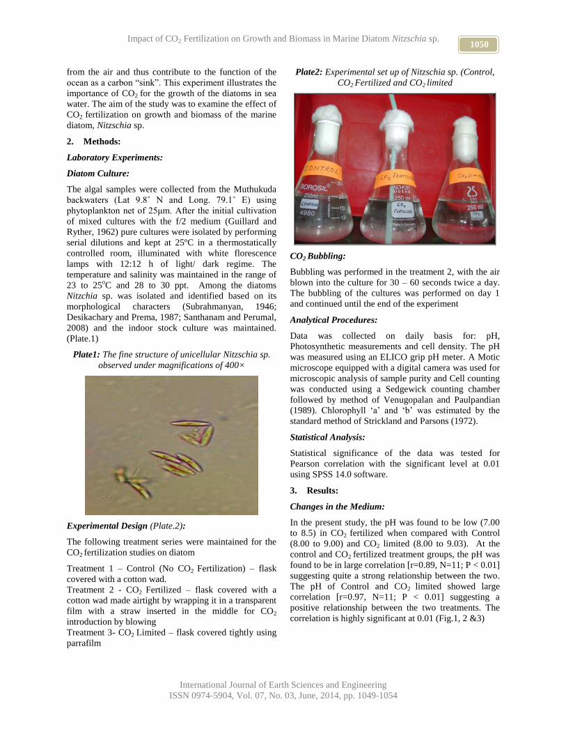
1050 Impact of CO2 Fertilization on Growth and Biomass in Marine Diatom Nitzschia sp.
International Journal of Earth Sciences and Engineering
ISSN 0974-5904, Vol. 07, No. 03, June, 2014, pp. 1049-1054
from the air and thus contribute to the function of the
ocean as a carbon “sink”. This experiment illustrates the
importance of CO2 for the growth of the diatoms in sea
water. The aim of the study was to examine the effect of
CO2 fertilization on growth and biomass of the marine
diatom, Nitzschia sp.
2. Methods:
Laboratory Experiments:
Diatom Culture:
The algal samples were collected from the Muthukuda
backwaters (Lat 9.8˚ N and Long. 79.1˚ E) using
phytoplankton net of 25μm. After the initial cultivation
of mixed cultures with the f/2 medium (Guillard and
Ryther, 1962) pure cultures were isolated by performing
serial dilutions and kept at 25ºC in a thermostatically
controlled room, illuminated with white florescence
lamps with 12:12 h of light/ dark regime. The
temperature and salinity was maintained in the range of
23 to 25oC and 28 to 30 ppt. Among the diatoms
Nitzchia sp. was isolated and identified based on its
morphological characters (Subrahmanyan, 1946;
Desikachary and Prema, 1987; Santhanam and Perumal,
2008) and the indoor stock culture was maintained.
(Plate.1)
Plate1: The fine structure of unicellular Nitzschia sp.
observed under magnifications of 400×
Experimental Design (Plate.2):
The following treatment series were maintained for the
CO2 fertilization studies on diatom
Treatment 1 – Control (No CO2 Fertilization) – flask
covered with a cotton wad.
Treatment 2 - CO2 Fertilized – flask covered with a
cotton wad made airtight by wrapping it in a transparent
film with a straw inserted in the middle for CO2
introduction by blowing
Treatment 3- CO2 Limited – flask covered tightly using
parrafilm
Plate2: Experimental set up of Nitzschia sp. (Control,
CO2 Fertilized and CO2 limited
CO2 Bubbling:
Bubbling was performed in the treatment 2, with the air
blown into the culture for 30 – 60 seconds twice a day.
The bubbling of the cultures was performed on day 1
and continued until the end of the experiment
Analytical Procedures:
Data was collected on daily basis for: pH,
Photosynthetic measurements and cell density. The pH
was measured using an ELICO grip pH meter. A Motic
microscope equipped with a digital camera was used for
microscopic analysis of sample purity and Cell counting
was conducted using a Sedgewick counting chamber
followed by method of Venugopalan and Paulpandian
(1989). Chlorophyll ‘a’ and ‘b’ was estimated by the
standard method of Strickland and Parsons (1972).
Statistical Analysis:
Statistical significance of the data was tested for
Pearson correlation with the significant level at 0.01
using SPSS 14.0 software.
3. Results:
Changes in the Medium:
In the present study, the pH was found to be low (7.00
to 8.5) in CO2 fertilized when compared with Control
(8.00 to 9.00) and CO2 limited (8.00 to 9.03). At the
control and CO2 fertilized treatment groups, the pH was
found to be in large correlation [r=0.89, N=11; P < 0.01]
suggesting quite a strong relationship between the two.
The pH of Control and CO2 limited showed large
correlation [r=0.97, N=11; P < 0.01] suggesting a
positive relationship between the two treatments. The
correlation is highly significant at 0.01 (Fig.1, 2 &3)

1051 RAJANANDHINI K, P SANTHANAM, S JEYANTHI, A SHENBAGA DEVI, S DINESH KUMAR
AND B BALAJI PRASATH
International Journal of Earth Sciences and Engineering
ISSN 0974-5904, Vol. 07, No. 03, June, 2014, pp. 1049-1054
Fig.1 Measurement of pH in marine diatom Nitzschia sp. culture
0
1
2
3
4
5
6
7
8
9
10
1 2 3 4 5 6 7 8 9 10 11
Days
pH
Control
Fertilised
Limited
Fig1: Measurement of pH in marine diatom Nitzchia sp.
culture
Fig2: Correlation between Control and CO2 fertilized
pH
Fig3: Correlation between Control and CO2 limited pH
Growth Study:
The overall range of cell growth of Nitzchia sp. in CO2
fertilized was found highest (86488 cells/ml) followed
by the CO2 limited (56927 cells/ml) and the control
(53704 cells/ml). The correlation between Control and
CO2 fertilized growth showed positive value [r=0.98,
N=11; P < 0.01] whereas the statistical values among
the cell density of Control and CO2 limited showed large
correlation [r=0.94, N=11; P < 0.01]. The correlation is
highly significant at 0.01 (Fig.4, 5&6)
Fig.4 Growth of marine diatom Nitzschia sp.
0
20000
40000
60000
80000
100000
120000
140000
160000
180000
1 2 3 4 5 6 7 8 9 10 11
Days
Cell
Den
sit
y (
cell
s/m
l)
Control
Fertilised
Limited
Fig5: Correlation between the growth of Nitzschia sp.
in Control and CO2 fertilized
Fig6: Correlation between the Nitzschia sp. growth in
Control and CO2 limited
Analysis of Chlorophyll Pigments:
The Nitzchia sp. biomass in terms of Chlorophyll ‘a’
concentration was observed in the average ranges of

1052 Impact of CO2 Fertilization on Growth and Biomass in Marine Diatom Nitzschia sp.
International Journal of Earth Sciences and Engineering
ISSN 0974-5904, Vol. 07, No. 03, June, 2014, pp. 1049-1054
0.05 mg/ml in Control, 0.07 mg/ml in CO2 fertilized and
0.06 mg/ml in CO2 limited. Similarly the Chlorophyll
‘b’ concentration was found to be in the average range
of 0.06 mg/ml in comparison with CO2 fertilized and
CO2 limited with the ranges of 0.07 mg/ml (Fig.7&8)
0
0.02
0.04
0.06
0.08
0.1
0.12
0.14
0.16
Co
ncen
trati
on
(m
g/m
l)
1 2 3 4 5 6 7 8 9 10 11
Days
Fig.7 Measurement of Chlorophyll ' a' in marine diatom
Nitzschia sp.
Control
Fertilised
Limited
0
0.05
0.1
0.15
0.2
0.25
Co
ncen
trati
on
(
mg
/ml)
1 2 3 4 5 6 7 8 9 10 11
Days
Fig. 8 Measurement of Chlorophyll 'b' in marine diatom
Nitzschia sp.
Control
Fertilised
Limited
4. Discussion:
This study showed that the primary producer Nitzschia
sp. used in this study increased their growth and
biomass when cultured in CO2 fertilized flask. It has
been reported that pH increases when algae grow
(Anderson, 2005). The pH of Nitzschia sp. cultivated
with the initial pH of 7.32 continued to increase and
reached up to 8.8. Meanwhile, the pH of control reached
a maximum of 9.27 and then started to decrease. This
shows that bicarbonate ions are the dominant inorganic
carbon species and have been reported to be utilized for
their growth. In the past, pH has not been considered to
be an important chemical parameter influencing biotic
processes in marine environments. However, a number
of studies have shown that pH and, in some cases,
inorganic carbon may be important in regulating the
growth rate and distribution of marine algae (Yoo 1991,
Hinga 1992, Riebesell et el., 1993). Therefore pH
mediated through [CO2] may be an important abiotic
factor affecting the ecology of marine phytoplankton.
Thus, atmospheric CO2 increase could potentially
promote phytoplankton productivity (Schippers et al.,
2004). He suggested that increased phytoplankton
productivity because of atmospheric CO2 elevation was
proportional to the increased atmospheric CO2, though it
was reported that unlike terrestrial plants, phytoplankton
would not show a significant response to the
atmospheric CO2 increase (Raven and Falkowski, 1999;
Tortell et al., 2000). Our results showed that biomass of
marine diatom increased in CO2 fertilized cultures in
response to the CO2 rise. Schippers et al., (2004)
predicted doubling of atmospheric CO2 could result in
an increase of the productivity of 10%-40% and Hein
and Sand-Jenson (1997) found 15-19% stimulation of
primary production in response to elevated CO2
concentration. The growth in CO2 limited cultures was
that the residual CO2 was still in the water and in the air
inside the flask. This was sufficient to trigger initial
growth of the algae but this could not be sustained
because of absence of CO2.
The growth curve of microalgae in Control is
characterized by an initial log phase and at about the 7th
day the growth enters the plateau stage. With an excess
of CO2 in CO2 fertilized cultures the plateau stage was
reached faster than with the control where CO2 was
available but not in excessive concentrations. In the
experiment limited enrichment of CO2 has enhanced the
photosynthetic activity showing a bright coloration in
the culture flask of CO2 fertilized with respect to the
other cultures. Morphological characteristics did not
affect the diatoms as they are highly tolerant to the wide
fluctuations of pH levels. Phytoplankters have different
affinities to CO2 and will use it in different ways.
Diatoms are highly tolerant to wide range of pH
fluctuations as their cell walls are made up of silica
frustules. As a result the diatoms grown in the acidified
cultures were capable of compensating the pH change
and they survived showing high productive results.
Some diatoms showed enhanced growth rate with
enriched CO2 and acidity (Riebesell et al., 1993;
Riebesell, 2004; Sobrino et al., 2008; Wu et al., 2010)
like the results have been observed with the presently
studied diatom Nitzschia sp.
Photosynthesis of diatoms is likely to be stimulated by
increased availability of CO2, lower pH might enhance
their respiration too (Wu et al., 2010), which would
down-regulate their contribution to the marine
biological CO2 pump. Different algal species or growth
conditions show differential preferences to CO2 or
HCO3− (Burkhardt et al., 2001; Nimer et al., 1997).
However, other studies show insignificant effects
(Boelen et al., 2011; Chen and Gao, 2003; Nielsen et
al., 2010, 2012; Tortell et al., 2002; Tortell and Morel,
2002) and even negative effects (Feng et al., 2009;
Low-DÉCarie et al., 2011; Torstensson et al., 2012) on
photosynthesis, growth or primary productivity in
diatoms or phytoplankton community.
1053 RAJANANDHINI K, P SANTHANAM, S JEYANTHI, A SHENBAGA DEVI, S DINESH KUMAR
AND B BALAJI PRASATH
International Journal of Earth Sciences and Engineering
ISSN 0974-5904, Vol. 07, No. 03, June, 2014, pp. 1049-1054
5. Conclusion:
It is understood that the CO2 is essential for the
photosynthesis of algae and terrestrial plants. This study
shows that photosynthetic activity has been triggered by
enrichment of CO2 .The potential for marine organisms
to adaptation for increasing CO2 and broader
implications for ocean ecosystems are not well known;
both more high priorities for future research.
6. Acknowledgements:
Authors are grateful to Head, Department of Marine
Science and authorities of Bharathidasan University,
Tiruchirappalli, for facilities provided. The Authors also
acknowledge to Dr. M. Anand, Assistant Professor,
Department of Marine Science and Coastal Studies,
Madurai Kamaraj University, Tamil Nadu, for his
valuable suggestions to carry out future studies with
different combination of atmospheric air viz., 100%
pure CO2 or CO2 + air mixture and the authors are also
thankful to Dr. D. Venkat Reddy, Editor-in-chief,
Professor of Geology, National Institute of Technology,
Karnataka for bringing out this paper into publishing.
References:
[1] Anderson, R.A (2005) Algal culturing techniques,
Elsevier Inc., San Diego, USA, pp.35-64.
[2] Badger, M.R., T.J. Andrews, S.M. Whitney, M.
Ludwig, D.C. Yellowlees, W. Leggat and G.D
Price (1998). The diversity and coevolution of
Rubisco, Plastids, Pyrenoids and Choloroplast-
based CO2-concentrating mechanisms in algae.
J.Bot.76: 1052-1071.
[3] Boelen, (2011). Neither elevated nor reduced CO2
affects the photo physiological performance of the
marine Antarctic diatom Chaetoceros brevis.
Journal of Experimental Marine Biology and
Ecology 406 (2011): 38–45.
[4] Brown, L.M. (1996). Uptake of Carbon Dioxide
from Flue Gas by Microalgae. Energy Conversion
Management, 37, 1363-1367.
[5] Burkhardt, S., Amoroso, G., Riebesell, U.,
Sultemeyer, D., (2001). CO2 and HCO3- uptake in
marine diatoms acclimated to different CO2,
concentrations. Limnology and Oceanography 46,
1378-1391.
[6] Camacho, R. F., Garcia, C. F., Fernandez, S. J. M.,
Chisti, Y., Molina, G. E. (2003). A mechanistic
model of photosynthesis in microalgae. Biotechnol
Bioeng. 81(4): 459-473.
[7] Chen X, Gao K (2003): Effect of CO2
concentrations on the activity of photosynthetic
CO2 fixation and extracellular carbonic anhydrase
in the marine diatom Skeletonema costatum. Chin
Sci Bull 48: 2616−2620.
[8] Chisti, Y, Biodiesel from microalgae, Biotech.
Adv., 2007, 25, 294-306.
[9] Desikachary, T.V., Prema, P., 1987. Diatoms from
the Bay of Bengal., In: Desikachary, T.V. (Ed.)
Atlas of Diatoms. Fascicles III and lV. TT Maps
and Publications Limited, Madras.
[10] Falkowski PG, Raven JA (1997) Aquatic
photosynthesis. Blackwell Science, Malden, MA.
[11] Feng, Y.Y., Hare, C.E., Leblanc, K., Rose, J.M.,
Zhang, Y.H., DiTuillio, G.R., Lee, P.A., Wilhelm,
S.W., Rowe, J.M., Sun, J., Nemeck, N., Gueguen,
C., Passow, U., Benner, I., Brown, C., Hutchins,
D.A., (2009). Effects of increased pCO2 and
temperature on the North Atlantic spring bloom. I.
The phytoplankton community and biogeochemical
response. Marine Ecology progress Series 388, 13-
25.
[12] Giordano, M., J. Beardall & J.A. Raven. (2005).
CO2 concentrating mechanisms in algae:
mechanisms, environmental modulation, and
evolution. Annu. Rev. Plant Biol. 56: 99-131.
[13] Guillard RRL, Ryther JH (1962). Studies of marine
planktonic diatoms. Can J Microbiol 8: 229-239.
[14] Hein, M., Sand-Jensen, K., (1997). CO2 increases
oceanic primary production. Nature 388, 527.
[15] Heine, J .N. 1983. Seasonal productivity of two red
algae in a Central California Kelp forest. J Phycol.,
19: 146-152.
[16] Hinga, R. 1992. Co-occurrence of dinoflagellate
blooms and high pH in marine enclosures. Mar.
Ecol. Prog. Ser. 86: 181-187, 1992.
[17] Levitt, GJ. And J.J. Bolton 1990. Seasonal primary
production of understory Rhodophyta in an
upwelling system. J. Phycol., 26: 214-220.
[18] Littler, M.M., S. N. Murray and K.E. Arnold 1979.
Seasonal variations in net photosynthesis
performance and cover of intertidal macrophytes.
Aquatic Bot., 7: 35-46.
[19] Low-DECarie, E., Fussmann, G.F., Bell, G.,
(2011). The effect of elevated CO2 on growth and
competition in experimental phytoplankton
communities. Global Change Biology 17, 2525-
2535.
[20] Masojidek, J., Koblizek, M., Torzillo, G. (2004).
Photosynthesis in microalgae. In: Handbook of
microalgal culture (Ed. Richmond A.) pp. 20-39.
Blackwell Publishing Company, 2121 State
Avenue, Ames, Iowa, USA.
[21] Nelson DM, Treguer, Brzezinski MA, Leynaert
A,Queginer (1995). Production and dissolution of
biogenic silica in the ocean: Revised global
estimates comparison with regional data and
relationship to biogenic sedimentation. Global
Biogeochem cycles 9: 359-372.
[22] Nimer, N.A., M.X. Ling,C. Brownlee and M.J.
Merrett (1999). Inorganic carbon limitation,

1054 Impact of CO2 Fertilization on Growth and Biomass in Marine Diatom Nitzschia sp.
International Journal of Earth Sciences and Engineering
ISSN 0974-5904, Vol. 07, No. 03, June, 2014, pp. 1049-1054
exofacial carbonic anhydrase activity and plasma
membrane redox activity in marine phytoplankton
species. J. Phycol.35: 1200-1205.
[23] Nimer, N.A., Iglesias-Rodriguez, M.D., Merrett,
M.J., (1997). Bicarbonate utilization by marine
phytoplankton species. Journal of Phycology 33,
625-631.
[24] Nielsen, L. T., Hallegraeff, G.M., Wright, S.W.,
Hansen, P.J., (2012). Effects of experimental
seawater acidification on an estuarine plankton
community. Aquatic Microbial Ecology 65, 271-
285.
[25] Nielsen, L.T., Jakobsen, H.H., Hansen, P.J., (2010).
High resilience of two coastal plankton
communities to twenty-first century seawater
acidification: evidence from microcosm studies.
Marine Biology Research 6, 542-555.
[26] Raven JA, Falkowski PG (1999). Oceanic sinks for
atmospheric CO2. Plant Cell Environ 22: 741–755.
[27] Riebesell, U., Tortell, P.D., (2011). Effects of ocean
acidification on pelagic organisms and ecosystems.
In: Gattuso, J.P., Hansson, L. (Eds.), Ocean
Acidification. Oxford University press, NewYork,
pp. 291-311.
[28] Riebesell, U., (2004). Effects of CO2 enrichment on
marine phytoplankton. Journal of Oceanography
60: 719–729.
[29] Riebesell,U., Wolf-Gladrow, D.A., Smetacek, V.,
(1993). Carbon dioxide limitation of marine
phytoplankton growth rates. Nature 361, 249-251.
[30] Reinfelder, J.R., Kraepiel, A.M.L., Morel, F.M.M.,
(2000). Unicellular C4 photosynthesis in a marine
diatom. Nature 407, 996-999.
[31] Round, F. E., R.M. Crawford & D.G. Mann.,
(1990). The Diatoms Biology and morphology of
the genera. Cambridge University press,
Cambridge: 747 pp.
[32] Santhanam, P and P. Perumal., (2008). Marine
plankton in Indian waters. Training Manual on GIS
and Marine Biodiversity (ed. John Milton), Loyola
College Pub., 1-12pp.
[33] Schippers, p., Lurling, M., Scheffer, M., (2004).
Increase of atmospheric CO2 promotes
phytoplankton productivity. Ecology Letters 7, 446-
451.
[34] Sobrino, C., M. L. Ward & P. J. Neale, (2008).
Acclimation to elevated carbon dioxide and
ultraviolet radiation in the diatom Thalassiosira
pseudonana: effects on growth, photosynthesis, and
spectral sensitivity of photo inhibition. Limnology
and Oceanography 53: 494–505.
[35] Spolaore. P, C. Joannis-Cassan, E. Duran A.
Isambert, commercial applications of microalgae, J.
Biosci. Bioeng., 2006,101, 87–96.
[36] Strickland, J.D.H., and T.R. Parsons. (1972). A
practical handbook of seawater analysis. Fish. Res.
Board Can. Bull. 167, 2nd ed. 310pp.
[37] Subrahmanyan, R. (1946). A systematic account of
the marine plankton diatoms of the Madras Coast.
Proc. Indian Acad. Sci., 24: 85-197.
[38] Torstensson, A., Chierici, M., Wulff, A., (2012).
The influence of increased temperature and carbon
dioxide levels on the benthic/sea ice diatom
Navicula directa. Polar Biology 35, 205-214.
[39] Tortell, P.D., Morel, F.M.M., (2002). Sources of
inorganic carbon for phytoplankton in the eastern
subtropical and equatorial Pacific Ocean.
Limnology and Oceanography 47, 1012-1012.
[40] Tortell, P.D., DiTullio, G.R., Sigman, D.M., Morel,
F.M.M., (2002). CO2 effects on taxonomic
composition and nutrient utilization in an equatorial
pacific phytoplankton assemblage. Marine Ecology
progress Series 236, 37-43.
[41] Tortell, P.D., J.R.Reinfelder and F.M.M. Morel,
(1997). Active uptake of bicarbonate by diatoms.
Nature 390: 243-244.
[42] Tortell PD, Rau GH, Morel FMM (2000). Inorganic
carbon acquisition in coastal Pacific phytoplankton
communities. Limnol Oceanogr; 485–1500.
[43] Venugopalan, V.K., and Paulpandian, A.L. (1989).
Methods in Hydrobiology. CAS in Marine biology,
Annamalai University, Parangipettai, India.
[44] Vonshak, A., Maske, H. (1982). Algae: growth
techniques and biomass production. In: Techniques
in bioproductivity and photosynthesis. (Ed.
Coombs, J., Hall, D.O.), p.66. Pergamon press Inc.,
Maxwell House, Fairview park, Elmsford, New
York, U.S.A.
[45] Wu, Y.P., Gao, K.S., Riebesell, U., (2010). CO2-
induced seawater acidification affects physiological
performance of the marine diatom Phaeodactylum
tricornutum. Biogeosciences 7, 2915-2923.
[46] Yoo, K I. (1991). Population dynamics of
dinoflagellate community in Masan Bay with a note
on the impact of environmental parameters. Mar.
Pollut Bull. 23: 185-188.

www.cafetinnova.org
Indexed in
Scopus Compendex and Geobase Elsevier, Chemical
Abstract Services-USA, Geo-Ref Information Services-USA,
List B of Scientific Journals, Poland,
Directory of Research Journals
ISSN 0974-5904, Volume 07, No. 03
June 2014, P.P.1055-1063
#02070335 Copyright ©2014 CAFET-INNOVA TECHNICAL SOCIETY. All rights reserved.
A Study on the Early UCC Strength of Stabilized Soil Admixed with
Industrial Waste Materials
JIJO JAMES AND P KASINATHA PANDIAN Department of Civil Engineering, Tagore Engineering College, Chennai – 127, Tamil Nadu, India
Email: [email protected], [email protected]
Abstract: The present study deals with the effect of additives on the early strength gain of soil stabilized with
conventional stabilizers like lime and cement. The development of UCC strength of stabilized soil admixed with
industrial wastes over a curing period of 2 hours, 3 days and 7 days was studied. The industrial wastes used in the
present work were ceramic dust and press mud obtained from pulverization of ceramic tiles from construction debris
and sugar industry respectively. Ceramic dust was used as admixture for cement stabilization and press mud was
used as admixture for lime stabilization of soil. The results of the study indicated that addition of press mud resulted
in increase in early strength when sufficient quantity of lime was available for reaction. The addition of ceramic dust
resulted in enhanced early strength in case of cement stabilization for all combinations studied but the maximum
strength gain was achieved for a specific percentage of cement and ceramic dust which can be considered as the
optimum dosage for the soil used in the study. The results of the study strengthen the fact established by earlier
studies that industrial wastes can be effectively used for soil stabilization purposes as additives to conventional
stabilizers.
Keywords: Cement Stabilization, Lime Stabilization, Press Mud, Ceramic Dust, Early strength.
Abbreviations:
UCC – Unconfined Compression
ICL – Initial Consumption of Lime
OLC – Optimum Lime Content
TRL – Transportation Research Laboratory
CBM – Cement Bound Material
RHA – Rice Husk Ash
Introduction:
In the present age, the only available land that man can
use for construction rarely suits for construction as most
of the so called good land has already been built upon.
As Civil Engineers, the onus has been thrust on us for
sustainable development of man conserving resources
for future generations as well. This has led to the
development of a branch of study called as Ground
Improvement Techniques for utilization of unusable
land. The basic principles of the ground improvement
have been acknowledged since mankind started
construction on and in the ground (ASCE, 1977).
Mitchell (1981) described a variety of ground
improvement technologies under six categories based on
principles. It is more appropriate to classify ground
improvement techniques under the following headings
viz. replacement, densification, consolidation /
dewatering, grouting, admixture stabilization, thermal
stabilization, reinforcement and miscellaneous methods
(Terashi and Juran, 2000).
With industrialization, another major problem that came
to the fore was pollution and solid waste production.
With rising turnover, industrial solid wastes produced
soon blew up to huge proportions. To cite an example,
the flyash production in India was 131.09 million tons
in the year 2010-11 (Central Electricity Authority,
2011). With research, one of the avenues for the
utilization of these waste materials came out to be their
use in soil improvement. The utilization of several
waste materials have improved over the years, the total
utilization of flyash produced in India stands at 73.13
million tons which is 55.79% of the total production in
the country (Central Electricity Authority, 2011). These
industrial by-products produce even better results when
combined with other materials like lime and cement that
have been used in soil improvement for long time
(Kavak et. al., Guleria and Dutta, 2011, Ramirez et. al.,
2012, Okonkwo et. al., 2012, Rahmat and Ismail, 2011).
Ordinary Portland cement is one of the most commonly
used stabilizers for soil stabilization. The addition of
cement to a material, in the present case soil, produces
hydrated calcium silicate and aluminate gels in the
presence of moisture, which crystallise and bond the
soil particles together. Most of the strength of a cement-
stabilised soil comes from the physical strength of the
matrix of hydrated cement (Al Rawas et. al., 2002).
Cement stabilized soils can be classified into three
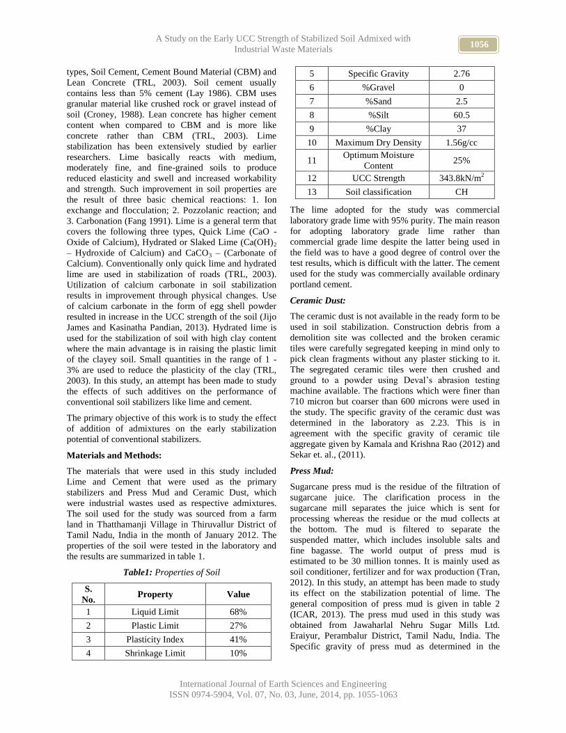
1056 A Study on the Early UCC Strength of Stabilized Soil Admixed with
Industrial Waste Materials
International Journal of Earth Sciences and Engineering
ISSN 0974-5904, Vol. 07, No. 03, June, 2014, pp. 1055-1063
types, Soil Cement, Cement Bound Material (CBM) and
Lean Concrete (TRL, 2003). Soil cement usually
contains less than 5% cement (Lay 1986). CBM uses
granular material like crushed rock or gravel instead of
soil (Croney, 1988). Lean concrete has higher cement
content when compared to CBM and is more like
concrete rather than CBM (TRL, 2003). Lime
stabilization has been extensively studied by earlier
researchers. Lime basically reacts with medium,
moderately fine, and fine-grained soils to produce
reduced elasticity and swell and increased workability
and strength. Such improvement in soil properties are
the result of three basic chemical reactions: 1. Ion
exchange and flocculation; 2. Pozzolanic reaction; and
3. Carbonation (Fang 1991). Lime is a general term that
covers the following three types, Quick Lime (CaO -
Oxide of Calcium), Hydrated or Slaked Lime (Ca(OH)2
– Hydroxide of Calcium) and CaCO3 – (Carbonate of
Calcium). Conventionally only quick lime and hydrated
lime are used in stabilization of roads (TRL, 2003).
Utilization of calcium carbonate in soil stabilization
results in improvement through physical changes. Use
of calcium carbonate in the form of egg shell powder
resulted in increase in the UCC strength of the soil (Jijo
James and Kasinatha Pandian, 2013). Hydrated lime is
used for the stabilization of soil with high clay content
where the main advantage is in raising the plastic limit
of the clayey soil. Small quantities in the range of 1 -
3% are used to reduce the plasticity of the clay (TRL,
2003). In this study, an attempt has been made to study
the effects of such additives on the performance of
conventional soil stabilizers like lime and cement.
The primary objective of this work is to study the effect
of addition of admixtures on the early stabilization
potential of conventional stabilizers.
Materials and Methods:
The materials that were used in this study included
Lime and Cement that were used as the primary
stabilizers and Press Mud and Ceramic Dust, which
were industrial wastes used as respective admixtures.
The soil used for the study was sourced from a farm
land in Thatthamanji Village in Thiruvallur District of
Tamil Nadu, India in the month of January 2012. The
properties of the soil were tested in the laboratory and
the results are summarized in table 1.
Table1: Properties of Soil
S.
No. Property Value
1 Liquid Limit 68%
2 Plastic Limit 27%
3 Plasticity Index 41%
4 Shrinkage Limit 10%
5 Specific Gravity 2.76
6 %Gravel 0
7 %Sand 2.5
8 %Silt 60.5
9 %Clay 37
10 Maximum Dry Density 1.56g/cc
11 Optimum Moisture
Content 25%
12 UCC Strength 343.8kN/m2
13 Soil classification CH
The lime adopted for the study was commercial
laboratory grade lime with 95% purity. The main reason
for adopting laboratory grade lime rather than
commercial grade lime despite the latter being used in
the field was to have a good degree of control over the
test results, which is difficult with the latter. The cement
used for the study was commercially available ordinary
portland cement.
Ceramic Dust:
The ceramic dust is not available in the ready form to be
used in soil stabilization. Construction debris from a
demolition site was collected and the broken ceramic
tiles were carefully segregated keeping in mind only to
pick clean fragments without any plaster sticking to it.
The segregated ceramic tiles were then crushed and
ground to a powder using Deval’s abrasion testing
machine available. The fractions which were finer than
710 micron but coarser than 600 microns were used in
the study. The specific gravity of the ceramic dust was
determined in the laboratory as 2.23. This is in
agreement with the specific gravity of ceramic tile
aggregate given by Kamala and Krishna Rao (2012) and
Sekar et. al., (2011).
Press Mud:
Sugarcane press mud is the residue of the filtration of
sugarcane juice. The clarification process in the
sugarcane mill separates the juice which is sent for
processing whereas the residue or the mud collects at
the bottom. The mud is filtered to separate the
suspended matter, which includes insoluble salts and
fine bagasse. The world output of press mud is
estimated to be 30 million tonnes. It is mainly used as
soil conditioner, fertilizer and for wax production (Tran,
2012). In this study, an attempt has been made to study
its effect on the stabilization potential of lime. The
general composition of press mud is given in table 2
(ICAR, 2013). The press mud used in this study was
obtained from Jawaharlal Nehru Sugar Mills Ltd.
Eraiyur, Perambalur District, Tamil Nadu, India. The
Specific gravity of press mud as determined in the
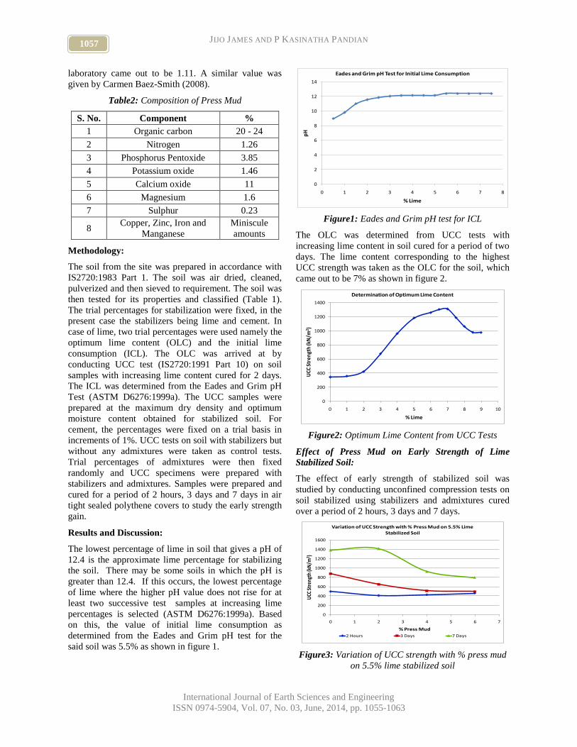
1057 JIJO JAMES AND P KASINATHA PANDIAN
International Journal of Earth Sciences and Engineering
ISSN 0974-5904, Vol. 07, No. 03, June, 2014, pp. 1055-1063
laboratory came out to be 1.11. A similar value was
given by Carmen Baez-Smith (2008).
Table2: Composition of Press Mud
S. No. Component %
1 Organic carbon 20 - 24
2 Nitrogen 1.26
3 Phosphorus Pentoxide 3.85
4 Potassium oxide 1.46
5 Calcium oxide 11
6 Magnesium 1.6
7 Sulphur 0.23
8 Copper, Zinc, Iron and
Manganese
Miniscule
amounts
Methodology:
The soil from the site was prepared in accordance with
IS2720:1983 Part 1. The soil was air dried, cleaned,
pulverized and then sieved to requirement. The soil was
then tested for its properties and classified (Table 1).
The trial percentages for stabilization were fixed, in the
present case the stabilizers being lime and cement. In
case of lime, two trial percentages were used namely the
optimum lime content (OLC) and the initial lime
consumption (ICL). The OLC was arrived at by
conducting UCC test (IS2720:1991 Part 10) on soil
samples with increasing lime content cured for 2 days.
The ICL was determined from the Eades and Grim pH
Test (ASTM D6276:1999a). The UCC samples were
prepared at the maximum dry density and optimum
moisture content obtained for stabilized soil. For
cement, the percentages were fixed on a trial basis in
increments of 1%. UCC tests on soil with stabilizers but
without any admixtures were taken as control tests.
Trial percentages of admixtures were then fixed
randomly and UCC specimens were prepared with
stabilizers and admixtures. Samples were prepared and
cured for a period of 2 hours, 3 days and 7 days in air
tight sealed polythene covers to study the early strength
gain.
Results and Discussion:
The lowest percentage of lime in soil that gives a pH of
12.4 is the approximate lime percentage for stabilizing
the soil. There may be some soils in which the pH is
greater than 12.4. If this occurs, the lowest percentage
of lime where the higher pH value does not rise for at
least two successive test samples at increasing lime
percentages is selected (ASTM D6276:1999a). Based
on this, the value of initial lime consumption as
determined from the Eades and Grim pH test for the
said soil was 5.5% as shown in figure 1.
0
2
4
6
8
10
12
14
0 1 2 3 4 5 6 7 8
pH
% Lime
Eades and Grim pH Test for Initial Lime Consumption
Figure1: Eades and Grim pH test for ICL
The OLC was determined from UCC tests with
increasing lime content in soil cured for a period of two
days. The lime content corresponding to the highest
UCC strength was taken as the OLC for the soil, which
came out to be 7% as shown in figure 2.
0
200
400
600
800
1000
1200
1400
0 1 2 3 4 5 6 7 8 9 10
UCC
Str
engt
h (k
N/m
2 )
% Lime
Determination of Optimum Lime Content
Figure2: Optimum Lime Content from UCC Tests
Effect of Press Mud on Early Strength of Lime
Stabilized Soil:
The effect of early strength of stabilized soil was
studied by conducting unconfined compression tests on
soil stabilized using stabilizers and admixtures cured
over a period of 2 hours, 3 days and 7 days.
0
200
400
600
800
1000
1200
1400
1600
0 1 2 3 4 5 6 7
UCC
Str
engt
h (k
N/m
2 )
% Press Mud
Variation of UCC Strength with % Press Mud on 5.5% Lime Stabilized Soil
2 Hours 3 Days 7 Days
Figure3: Variation of UCC strength with % press mud
on 5.5% lime stabilized soil
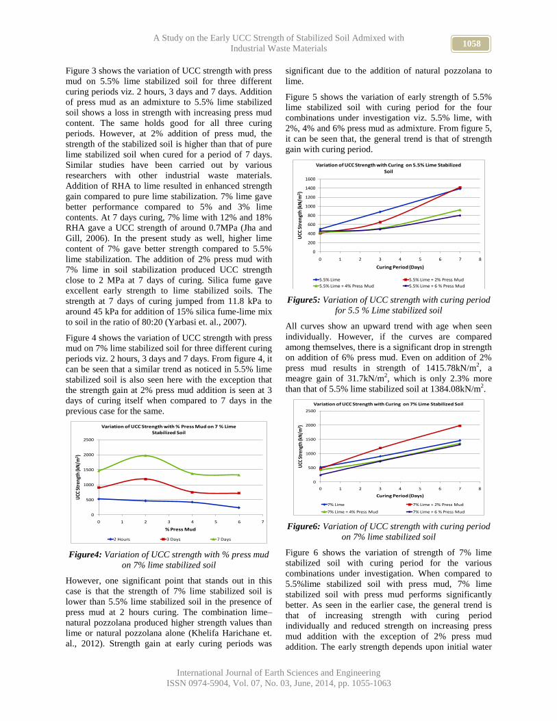
1058 A Study on the Early UCC Strength of Stabilized Soil Admixed with
Industrial Waste Materials
International Journal of Earth Sciences and Engineering
ISSN 0974-5904, Vol. 07, No. 03, June, 2014, pp. 1055-1063
Figure 3 shows the variation of UCC strength with press
mud on 5.5% lime stabilized soil for three different
curing periods viz. 2 hours, 3 days and 7 days. Addition
of press mud as an admixture to 5.5% lime stabilized
soil shows a loss in strength with increasing press mud
content. The same holds good for all three curing
periods. However, at 2% addition of press mud, the
strength of the stabilized soil is higher than that of pure
lime stabilized soil when cured for a period of 7 days.
Similar studies have been carried out by various
researchers with other industrial waste materials.
Addition of RHA to lime resulted in enhanced strength
gain compared to pure lime stabilization. 7% lime gave
better performance compared to 5% and 3% lime
contents. At 7 days curing, 7% lime with 12% and 18%
RHA gave a UCC strength of around 0.7MPa (Jha and
Gill, 2006). In the present study as well, higher lime
content of 7% gave better strength compared to 5.5%
lime stabilization. The addition of 2% press mud with
7% lime in soil stabilization produced UCC strength
close to 2 MPa at 7 days of curing. Silica fume gave
excellent early strength to lime stabilized soils. The
strength at 7 days of curing jumped from 11.8 kPa to
around 45 kPa for addition of 15% silica fume-lime mix
to soil in the ratio of 80:20 (Yarbasi et. al., 2007).
Figure 4 shows the variation of UCC strength with press
mud on 7% lime stabilized soil for three different curing
periods viz. 2 hours, 3 days and 7 days. From figure 4, it
can be seen that a similar trend as noticed in 5.5% lime
stabilized soil is also seen here with the exception that
the strength gain at 2% press mud addition is seen at 3
days of curing itself when compared to 7 days in the
previous case for the same.
0
500
1000
1500
2000
2500
0 1 2 3 4 5 6 7
UCC
Str
engt
h (k
N/m
2 )
% Press Mud
Variation of UCC Strength with % Press Mud on 7 % Lime Stabilized Soil
2 Hours 3 Days 7 Days
Figure4: Variation of UCC strength with % press mud
on 7% lime stabilized soil
However, one significant point that stands out in this
case is that the strength of 7% lime stabilized soil is
lower than 5.5% lime stabilized soil in the presence of
press mud at 2 hours curing. The combination lime–
natural pozzolana produced higher strength values than
lime or natural pozzolana alone (Khelifa Harichane et.
al., 2012). Strength gain at early curing periods was
significant due to the addition of natural pozzolana to
lime.
Figure 5 shows the variation of early strength of 5.5%
lime stabilized soil with curing period for the four
combinations under investigation viz. 5.5% lime, with
2%, 4% and 6% press mud as admixture. From figure 5,
it can be seen that, the general trend is that of strength
gain with curing period.
0
200
400
600
800
1000
1200
1400
1600
0 1 2 3 4 5 6 7 8
UCC
Str
engt
h (k
N/m
2 )
Curing Period (Days)
Variation of UCC Strength with Curing on 5.5% Lime Stabilized Soil
5.5% Lime 5.5% Lime + 2% Press Mud
5.5% Lime + 4% Press Mud 5.5% Lime + 6 % Press Mud
Figure5: Variation of UCC strength with curing period
for 5.5 % Lime stabilized soil
All curves show an upward trend with age when seen
individually. However, if the curves are compared
among themselves, there is a significant drop in strength
on addition of 6% press mud. Even on addition of 2%
press mud results in strength of 1415.78kN/m2, a
meagre gain of 31.7kN/m2, which is only 2.3% more
than that of 5.5% lime stabilized soil at 1384.08kN/m2.
0
500
1000
1500
2000
2500
0 1 2 3 4 5 6 7 8
UCC
Str
engt
h (k
N/m
2 )
Curing Period (Days)
Variation of UCC Strength with Curing on 7% Lime Stabilized Soil
7% Lime 7% Lime + 2% Press Mud
7% Lime + 4% Press Mud 7% Lime + 6 % Press Mud
Figure6: Variation of UCC strength with curing period
on 7% lime stabilized soil
Figure 6 shows the variation of strength of 7% lime
stabilized soil with curing period for the various
combinations under investigation. When compared to
5.5%lime stabilized soil with press mud, 7% lime
stabilized soil with press mud performs significantly
better. As seen in the earlier case, the general trend is
that of increasing strength with curing period
individually and reduced strength on increasing press
mud addition with the exception of 2% press mud
addition. The early strength depends upon initial water

1059 JIJO JAMES AND P KASINATHA PANDIAN
International Journal of Earth Sciences and Engineering
ISSN 0974-5904, Vol. 07, No. 03, June, 2014, pp. 1055-1063
content, stabilizer content and curing period (Wang Zhe
et. al., 2012). In the present work, all samples were
moulded with same water content and use admixtures
along with stabilizers. But still it is in agreement with
the report that strength increases with stabilizer content
as 7% lime performed better compared to 5.5% lime
stabilization. The curve for 2% press mud addition
significantly diverges from the other set of curves from
3 days of curing. The strength gain at 3 days curing for
2% press mud addition is 283.08kN/m2 which is 31.3%
more than the strength of 7% pure lime stabilized soil at
905.295kN/m2 for the same curing period. At 7 days of
curing, this gain increases to 509.24kN/m2, a 34.75%
increase over lime stabilized soil at 1465.16kN/m2.
Kavak et. al., (2011) reported addition of 3.33% Ground
Granulated Blast furnace Slag to 5% lime resulted in
better performance compared to 5% pure lime
stabilization. The presence of GGBS in lime
stabilization resulted in a strength gain of approximately
36% at 7 days of curing. Addition of waste cement dust
to lime gave better early strength of lime stabilized
black cotton soil when compared to pure lime
stabilization of the same. It resulted in a strength gain of
50% at 3 days curing and 25% gain at 7 days curing for
8% addition of waste cement dust-lime combination in
1:1 ratio. (Oza and Gundalia, 2013).
The reason behind the better performance of 7% lime
case, over 5.5% lime case may be due to the fact that
ICL lime content is used to raise the pH of the soil to
12.4 thereby producing favourable conditions for
stabilization but results in no extra lime available for the
actual stabilization. When 7% lime is added, there is
additional lime available beyond the initial consumption
of 5.5% for the pozzolanic reactions to take place
between soil and lime. For strength gains to occur, the
chemical reactions require a high pH (>12.4) to be
maintained, which is the ICL value (TRL, 2003). It is
well documented in literature that lime addition in
excess of ICL results in pozzolanic reactions leading to
strength gain (Nazrisar et. al., 2008, 2010). A possible
argument can be put forward to explain the poor
strength of 7% lime stabilized soil admixed with press
mud when compared to 5.5% lime stabilized soil
admixed with press mud at 2 hours curing. It may be
possible that the products of reaction between lime and
press mud may have poor rate of strength gain. In 5.5%
lime case, there isn’t enough lime available to react with
press mud beyond initial consumption, thereby resulting
in minimum interaction between lime and press mud.
Therefore early strength is better but gain is minimal. In
the 7% lime case, there is additional lime available
beyond initial consumption, which can lead to lime
press mud reaction products. This can explain poor
early strength but significant gain in strength with time.
However, the veracity of this argument can only be
confirmed upon detailed investigation. Chen and Lin
(2009) reported that for small quantities of sewage
sludge ash added to cement in soil stabilization, the
early strength gain was small but strength increased
with curing period due to continuation of pozzolanic
reactions. Similar trends are seen in the present study
with strength of 7% lime with press mud stabilized soil
having low strength at early age but gaining
significantly as curing increased.
Effect of Ceramic Dust on Early Strength of Cement
Stabilized Soil:
Usually, for soils with plasticity index greater than 20%,
cement stabilization will be only marginally effective
(TRL, 2003). The soil under study has a plasticity index
of 41% and hence plain cement stabilization may give
only marginal results. Hence, it was aimed to increase
the effectiveness of cement stabilization with
admixtures on such soils. Addition of inert filler,
resulting in greater bulk would aid the distribution
process so that the same amount of active cement would
be available throughout the material (TRL, 2003).
Hence, ceramic dust was used as an admixture
principally to add bulk. Particle size coarser than 600
microns but finer than 710 microns was used for the
study. This range was a balance that was necessitated to
provide bulk while reducing interference with
performance of index tests.
Soil cement consists of less than 5% cement (Lay,
1986). Several studies have been carried out with
additives to cement in soil stabilization. Rice husk ash
as an admixture to cement stabilization of soil resulted
in greater strength at 7 days of curing compared to plain
cement stabilization. It can be used to reduce the content
of cement used in stabilization due to the increased
strength achieved (Basha et. al., 2005). Increase in
ceramic dust content to expansive soil resulted in
increase in UCC strength of the soil up to 30% content
(Sabat, 2012). In the present work, ceramic dust was
used as an admixture rather than a stabilizer as done by
Sabat (2012).
0
500
1000
1500
2000
2500
3000
3500
4000
4500
5000
0 1 2 3 4 5 6 7 8 9
UCC
Str
engt
h (k
N/m
2 )
% Ceramic Dust
Variation of UCC Strength with % Ceramic Dust of 1% Cement Stabilized Soil
2 Hours 3 Days 7 Days
Figure7: Variation of UCC strength with % Ceramic
dust for 1% cement stabilized soil

1060 A Study on the Early UCC Strength of Stabilized Soil Admixed with
Industrial Waste Materials
International Journal of Earth Sciences and Engineering
ISSN 0974-5904, Vol. 07, No. 03, June, 2014, pp. 1055-1063
Cement stabilization was carried out by adopting trial
percentages starting from 1% to 4% in increments of
1%. Ceramic dust admixture was added in increments of
2% to the soil. The effect of addition of ceramic dust to
1% cement is shown in figure 7.
0
1000
2000
3000
4000
5000
6000
0 1 2 3 4 5 6 7 8 9
UCC
Str
engt
h (k
N/m
2 )
% Ceramic Dust
Variation of UCC Strength with % Ceramic Dust of 2% Cement Stabilized Soil
2 Hours 3 Days 7 Days
Figure8: Variation of UCC strength with % Ceramic
dust for 2% cement stabilized soil
From figures 7 to 10, it can be seen that the addition of
ceramic dust to cement resulted in the increase in the
early strength of the soil. It can be seen in all four cases
that the gain in strength is significant after three days of
curing. At lower cement content, viz. 1% and 2% there
is a dip in performance at 4% addition of ceramic dust
whereas at higher cement content, viz. 3% and 4%,
there is dip in performance at 6% addition of ceramic
dust at 7 days of curing. Egg shell ash admixed cement
stabilization of soil performed better than cement
stabilization after 7 and 14 days of curing. UCC
Strength at 6% and 8% cement content increased
considerably from (370KN/m2 and 471KN/m
2) for 7
days curing period and (432KN/m2 and 655KN/m
2) for
14 days curing period to (614KN/m2 and 687KN/m
2)
and (680KN/m2 and 988KN/m
2) respectively with
increase in eggshell ash content from 0% to 10%
(Okonkwo et. al., 2012). The strength of 2% cement
stabilized soil when admixed with 6% ceramic dust
resulted in the doubling of early strength for 7 day
curing period for the soil under study in the present
work.
0
1000
2000
3000
4000
5000
6000
0 1 2 3 4 5 6 7 8 9
UCC
Str
engt
h (k
N/m
2 )
% Ceramic Dust
Variation of UCC Strength with % Ceramic Dust of 3% Cement Stabilized Soil
2 Hours 3 Days 7 Days
Figure9: Variation of UCC strength with % Ceramic
dust for 3% cement stabilized soil
The initial strength gain between 2 hours and 3 days of
curing was poor across all four cement content cases.
But out of all combinations of cement, the greatest gain
in strength was observed for 2% cement with ceramic
dust as admixture. The average gain in strength between
3 days and 7 days across all combinations of ceramic
dust addition was 3351.92kN/m2 for 2% cement
stabilization which is a staggering 611% gain on the
average.
0
500
1000
1500
2000
2500
3000
3500
4000
4500
0 1 2 3 4 5 6 7 8 9
UC
C S
tre
ngt
h (k
N/m
2)
% Ceramic Dust
Variation of UCC Strength with % Ceramic Dust of 4% Cement Stabilized Soil
2 Hours 3 Days 7 Days
Figure10: Variation of UCC strength with % Ceramic
dust for 4% cement stabilized soil
In comparison, 1% cement with ceramic dust had a gain
of 168%, 3% cement with ceramic dust had a gain of
384% and 4% cement with ceramic dust had a gain in
strength of 322%. Addition of calcined paper sludge to
cement in soil stabilization produced similar strength to
that of cement stabilized soil at higher cement dosage at
7 days curing (Amaia Lisbona et. al., 2011). In this
study, addition of ceramic dust to cement has resulted in
significant gain in early strength of stabilized soil.
Hence, it can be inferred that for achieving a particular
strength of stabilized soil, the addition of ceramic dust
to cement can help in achieving the same strength at
lower cement content due to the contribution of ceramic
dust in strength gain.
Figures 11 to 14 show the gain in strength with curing
period for various levels of admixtures for cement
content varying from 1% to 4%. For 1% cement
content, addition of 8% ceramic dust resulted in a
strength gain of 2294.22kN/m2 when compared to pure
cement stabilization, which is a gain of 94%.
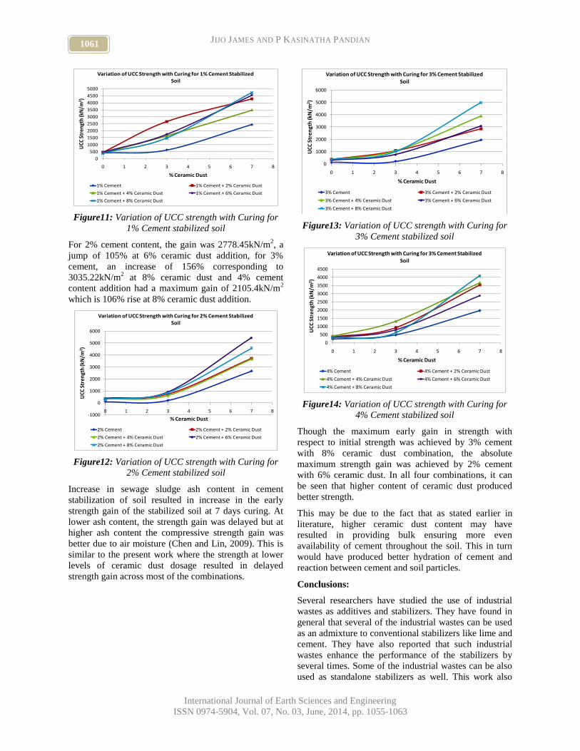
1061 JIJO JAMES AND P KASINATHA PANDIAN
International Journal of Earth Sciences and Engineering
ISSN 0974-5904, Vol. 07, No. 03, June, 2014, pp. 1055-1063
0
500
1000
1500
2000
2500
3000
3500
4000
4500
5000
0 1 2 3 4 5 6 7 8
UCC
Str
engt
h (k
N/m
2 )
% Ceramic Dust
Variation of UCC Strength with Curing for 1% Cement Stabilized Soil
1% Cement 1% Cement + 2% Ceramic Dust
1% Cement + 4% Ceramic Dust 1% Cement + 6% Ceramic Dust
1% Cement + 8% Ceramic Dust
Figure11: Variation of UCC strength with Curing for
1% Cement stabilized soil
For 2% cement content, the gain was 2778.45kN/m2, a
jump of 105% at 6% ceramic dust addition, for 3%
cement, an increase of 156% corresponding to
3035.22kN/m2 at 8% ceramic dust and 4% cement
content addition had a maximum gain of 2105.4kN/m2
which is 106% rise at 8% ceramic dust addition.
-1000
0
1000
2000
3000
4000
5000
6000
0 1 2 3 4 5 6 7 8
UCC
Str
engt
h (k
N/m
2 )
% Ceramic Dust
Variation of UCC Strength with Curing for 2% Cement Stabilized Soil
2% Cement 2% Cement + 2% Ceramic Dust
2% Cement + 4% Ceramic Dust 2% Cement + 6% Ceramic Dust
2% Cement + 8% Ceramic Dust
Figure12: Variation of UCC strength with Curing for
2% Cement stabilized soil
Increase in sewage sludge ash content in cement
stabilization of soil resulted in increase in the early
strength gain of the stabilized soil at 7 days curing. At
lower ash content, the strength gain was delayed but at
higher ash content the compressive strength gain was
better due to air moisture (Chen and Lin, 2009). This is
similar to the present work where the strength at lower
levels of ceramic dust dosage resulted in delayed
strength gain across most of the combinations.
0
1000
2000
3000
4000
5000
6000
0 1 2 3 4 5 6 7 8
UC
C S
tre
ngt
h (k
N/m
2 )
% Ceramic Dust
Variation of UCC Strength with Curing for 3% Cement Stabilized Soil
3% Cement 3% Cement + 2% Ceramic Dust
3% Cement + 4% Ceramic Dust 3% Cement + 6% Ceramic Dust
3% Cement + 8% Ceramic Dust
Figure13: Variation of UCC strength with Curing for
3% Cement stabilized soil
0
500
1000
1500
2000
2500
3000
3500
4000
4500
0 1 2 3 4 5 6 7 8
UC
C S
tre
ngt
h (k
N/m
2 )
% Ceramic Dust
Variation of UCC Strength with Curing for 3% Cement Stabilized Soil
4% Cement 4% Cement + 2% Ceramic Dust
4% Cement + 4% Ceramic Dust 4% Cement + 6% Ceramic Dust
4% Cement + 8% Ceramic Dust
Figure14: Variation of UCC strength with Curing for
4% Cement stabilized soil
Though the maximum early gain in strength with
respect to initial strength was achieved by 3% cement
with 8% ceramic dust combination, the absolute
maximum strength gain was achieved by 2% cement
with 6% ceramic dust. In all four combinations, it can
be seen that higher content of ceramic dust produced
better strength.
This may be due to the fact that as stated earlier in
literature, higher ceramic dust content may have
resulted in providing bulk ensuring more even
availability of cement throughout the soil. This in turn
would have produced better hydration of cement and
reaction between cement and soil particles.
Conclusions:
Several researchers have studied the use of industrial
wastes as additives and stabilizers. They have found in
general that several of the industrial wastes can be used
as an admixture to conventional stabilizers like lime and
cement. They have also reported that such industrial
wastes enhance the performance of the stabilizers by
several times. Some of the industrial wastes can be also
used as standalone stabilizers as well. This work also
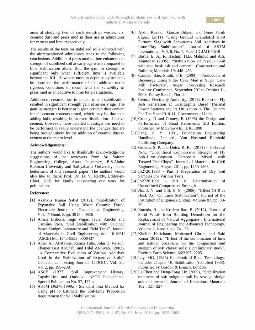
1062 A Study on the Early UCC Strength of Stabilized Soil Admixed with
Industrial Waste Materials
International Journal of Earth Sciences and Engineering
ISSN 0974-5904, Vol. 07, No. 03, June, 2014, pp. 1055-1063
aims at studying two of such industrial wastes, viz.
ceramic dust and press mud in their use as admixtures
for cement and lime respectively.
The results of the tests on stabilized soils admixed with
the aforementioned admixtures leads to the following
conclusions. Addition of press mud to lime enhances the
strength of stabilized soil at early age when compared to
lime stabilization alone. But, the gain in strength is
significant only when sufficient lime is available
beyond the ICL. However, more in-depth study needs to
be done on the performance of the additive under
rigorous conditions to recommend the suitability of
press mud as an additive to lime for all situations.
Addition of ceramic dust to cement in soil stabilization
resulted in significant strength gain at an early age. The
gain in strength is better at higher ceramic dust content
for all cement contents tested, which may be due to it
adding bulk, resulting in an even distribution of active
cement. However, more detailed investigations need to
be performed to really understand the changes that are
being brought about by the addition of ceramic dust to
cement at the micro level.
Acknowledgements:
The authors would like to thankfully acknowledge the
suggestions of the reviewers from Sri Sairam
Engineering College, Anna University, B.S.Abdur
Rahman University and Sathyabama University in the
betterment of this research paper. The authors would
also like to thank Prof. Dr. D. V. Reddy, Editor-in-
Chief, IJEE for kindly considering our work for
publication.
Reference:
[1] Akshaya Kumar Sabat (2012), “Stabilization of
Expansive Soil Using Waste Ceramic Dust”,
Electronic Journal of Geotechnical Engineering,
Vol. 17 Bund. Z pp. 3915 – 3926
[2] Amaia Lisbona, Iñigo Vegas, Javier Ainchil and
Carolina Ríos, “Soil Stabilization with Calcined
Paper Sludge: Laboratory and Field Tests”, Journal
of Materials in Civil Engineering, doi: 10.1061/
(ASCE) MT.1943-5533. 0000437
[3] Amer Ali Al-Rawas, Ramzi Taha, John D. Nelson,
Thamer Beit Al-Shab, and Hilal Al-Siyab, (2002),
“A Comparative Evaluation of Various Additives
Used in the Stabilization of Expansive Soils”,
Geotechnical Testing Journal, GTJODJ, Vol. 25,
No. 2, pp. 199–209.
[4] ASCE (1977) “Soil Improvement History,
Capabilities, and Outlook”. ASCE Geotechnical
Special Publication No. 57, 177 p.
[5] ASTM D6276:1999a - Standard Test Method for
Using pH to Estimate the Soil-Lime Proportion
Requirement for Soil Stabilization
[6] Aydin Kavak, Gamze Bilgen, and Omer Faruk
Capar, (2011) “Using Ground Granulated Blast
Furnace Slag with Seawateras Soil Additives in
Lime-Clay Stabilization”, Journal of ASTM
International, Vol. 8, No. 7, Paper ID JAI103648
[7] Basha, E. A., R. Hashim, H.B. Mahmud and A.S.
Muntohar (2005), “Stabilization of residual soil
with rice husk ash and cement”, Construction and
Building Materials 19: 448–453
[8] Carmen Baez-Smith, P.E. (2008), “Production of
Bioenergy Using Filter Cake Mud in Sugar Cane
Mill Factories”, Sugar Processing Research
Institute Conference, September 29th
to October 1st,
2008, Delray Beach, Florida.
[9] Central Electricity Authority, (2011), Report on Fly
Ash Generation at Coal/Lignite Based Thermal
Power Stations and Its Utilization in The Country
For The Year 2010-11, Government of India.
[10] Croney, D and Croney, P. (1998) the Design and
Performance of Road Pavements. 3rd Edition,
Published by McGraw-Hill, UK, 1998
[11] Fang, H. Y., 1991, Foundation Engineering
Handbook, 2nd ed., Van Nostrand Reinhold
Publishing Company.
[12] Guleria, S. P. and Dutta, R. K. (2011) - Technical
Note, “Unconfined Compressive Strength of Fly
Ash–Lime–Gypsum Composite Mixed with
Treated Tire Chips”, Journal of Materials in Civil
Engineering, August 2011, pp. 1255-1263
[13] IS2720:1983 - Part 1 Preparation of Dry Soil
Samples For Various Tests
[14] IS2720:1991 - Part 10 Determination of
Unconfined Compressive Strength
[15] Jha, J. N. and Gill, K. S. (2006), “Effect Of Rice
Husk Ash On Lime Stabilization”, Journal of the
Institution of Engineers (India), Volume 87, pp. 33-
39
[16] Kamala, R. and Krishna Rao, B. (2012), “Reuse of
Solid Waste from Building Demolition for the
Replacement of Natural Aggregates”, International
Journal of Engineering and Advanced Technology,
Volume 2, issue 1, pp. 74 - 76
[17] Khelifa Harichane, Mohamed Ghrici and Said
Kenai (2012), “Effect of the combination of lime
and natural pozzolana on the compaction and
strength of soft clayey soils: a preliminary study”,
Environ Earth Science, 66:2197–2205
[18] Lay, MG. (1986) Handbook of Road Technology.
Includes Chapter 10: Stabilisation (redrafted 1988).
Published by Gordon & Breach, London
[19] Li Chen and Deng-Fong Lin (2009), “Stabilization
treatment of soft subgrade soil by sewage sludge
ash and cement”, Journal of Hazardous Materials
162 : 321–327

1063 JIJO JAMES AND P KASINATHA PANDIAN
International Journal of Earth Sciences and Engineering
ISSN 0974-5904, Vol. 07, No. 03, June, 2014, pp. 1055-1063
[20] Mitchell, J.K. (1981) “State of the Art – Soil
Improvement”. Proceedings of the 10th ICSMFE.
Stockholm, Vol. 4, pp. 509-565.
[21] Mohamad Nidzam Rahmat and Norsalisma Ismail,
(2011), “Sustainable stabilisation of the Lower
Oxford Clay by non-traditional binder”, Applied
Clay Science 52 pp. 199–208
[22] Nasrizar, A.A., Muttharam, M. & Ilamparuthi, K.
(2008), “Effect of curing temperature on strength of
lime stabilized expansive soil”, Indian Geotechnical
Conference (IGC) 2008, Bangalore, Vol 2:28-30
[23] Nasrizar, A.A., Muttharam, M. & Ilamparuthi, K.
(2010), “Role of Lime Content on Soil-Lime
Reaction under Thermal Curing”, Indian
Geotechnical Conference – 2010, GEOtrendz, pp.
595 – 598
[24] Necmi Yarbası, Ekrem Kalkan, and Suat Akbulut
(2007), “Modification of the geotechnical
properties, as influenced by freeze–thaw, of
granular soils with waste additives”, Cold Regions
Science and Technology 48: 44–54
[25] Okonkwo, U. N, Odiong, I. C. and Akpabio, E. E.
(2012), “The Effects of Eggshell Ash on Strength
Properties of Cement-Stabilized Lateritic”,
International Journal of Sustainable Construction
Engineering & Technology (ISSN: 2180-3242) Vol
3, Issue 1, pp. 18 – 25
[26] Oza, J.B. and Gundaliya P.J. (2013), “Study of
black cotton soil characteristics with cement waste
dust and lime”, Procedia Engineering 51: 110 – 118
[27] Rafael Alavez-Ramirez, Pedro Montes-Garcia,
Jacobo Martinez-Reyes, Delia Cristina Altamirano-
Juarez, Yadira Gochi-Ponce, (2012), “The use of
sugarcane bagasse ash and lime to improve the
durability and mechanical properties of compacted
soil blocks”, Construction and Building Materials
34 pp. 296–305
[28] Sekar, T., Ganesan, N. and Nampoothiri, NVN.
(2011), “Studies on Strength Characteristics on
Utilization of Waste Materials as Coarse Aggregate
in Concrete”, International Journal of Engineering
Science and Technology, Volume 2, No. 7, pp.
5436 - 5440
[29] Sugarcane Breeding Centre, Indian Council of
Agricultural Research,
http://www.sugarcane.res.in/index.php/component/
content/article/15-faq/322-faq-organic-cultivation-
of-sugarcane, Last Retrieved on 28/11/2013
[30] Terashi M, and Juran I, (2000) Ground
improvement: State of the Art, GeoEng 2000,
Melbourne, Australia
[31] Tran G., 2012, Sugarcane Press Mud,
Feedipedia.org. A Programme by INRA, CIRAD,
AFZ and FAO.
http://www.feedipedia.org/node/563, Last
Retrieved on 28/11/2013
[32] Transportation Research Laboratory, UK, (2003),
“Literature Review Stabilised Sub-Bases for
Heavily Trafficked Roads”, PROJECT REPORT
ORIGIN PR/INT/202/00
[33] Wang Zhe, Xu Si-fa and Wang Guo-cai (2012),
“Study of Early Strength and Shrinkage Properties
of Cement or Lime Solidified Soil”, Energy
Procedia 16: 302 – 306.
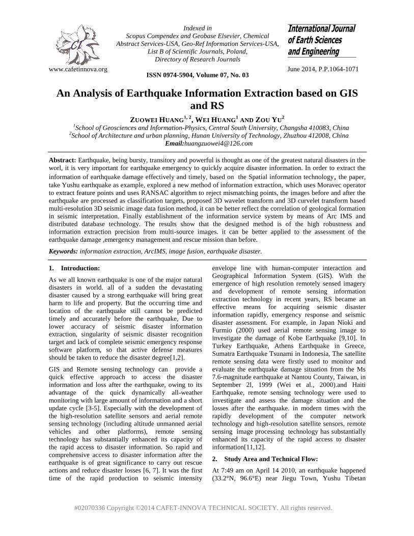
www.cafetinnova.org
Indexed in
Scopus Compendex and Geobase Elsevier, Chemical
Abstract Services-USA, Geo-Ref Information Services-USA,
List B of Scientific Journals, Poland,
Directory of Research Journals
ISSN 0974-5904, Volume 07, No. 03
June 2014, P.P.1064-1071
#02070336 Copyright ©2014 CAFET-INNOVA TECHNICAL SOCIETY. All rights reserved.
An Analysis of Earthquake Information Extraction based on GIS
and RS
ZUOWEI HUANG1, 2
, WEI HUANG1 AND ZOU YU
2
1School of Geosciences and Information-Physics, Central South University, Changsha 410083, China
2School of Architecture and urban planning, Hunan University of Technology, Zhuzhou 412008, China
Email:[email protected]
Abstract: Earthquake, being bursty, transitory and powerful is thought as one of the greatest natural disasters in the
worl, it is very important for earthquake emergency to quickly acquire disaster information. In order to extract the
information of earthquake damage effectively and timely, based on the Spatial information technology, the paper,
take Yushu earthquake as example, explored a new method of information extraction, which uses Moravec operator
to extract feature points and uses RANSAC algorithm to reject mismatching points, the images before and after the
earthquake are processed as classification targets, proposed 3D wavelet transform and 3D curvelet transform based
multi-resolution 3D seismic image data fusion method, it can be better reflect the correlation of geological formation
in seismic interpretation. Finally establishment of the information service system by means of Arc IMS and
distributed database technology. The results show that the designed method is of the high robustness and
information extraction precision from multi-source images. it can be better applied to the assessment of the
earthquake damage ,emergency management and rescue mission than before.
Keywords: information extraction, ArcIMS, image fusion, earthquake disaster.
1. Introduction:
As we all known earthquake is one of the major natural
disasters in world. all of a sudden the devastating
disaster caused by a strong earthquake will bring great
harm to life and property. But the occurring time and
location of the earthquake still cannot be predicted
timely and accurately before the earthquake, Due to
lower accuracy of seismic disaster information
extraction, singularity of seismic disaster recognition
target and lack of complete seismic emergency response
software platform, so that active defense measures
should be taken to reduce the disaster degree[1,2].
GIS and Remote sensing technology can provide a
quick effective approach to access the disaster
information and loss after the earthquake, owing to its
advantage of the quick dynamically all-weather
monitoring with large amount of information and a short
update cycle [3-5]. Especially with the development of
the high-resolution satellite sensors and aerial remote
sensing technology (including altitude unmanned aerial
vehicles and other platforms), remote sensing
technology has substantially enhanced its capacity of
the rapid access to disaster information. So rapid and
comprehensive access to disaster information after the
earthquake is of great significance to carry out rescue
actions and reduce disaster losses [6, 7]. It was the first
time of the rapid production to seismic intensity
envelope line with human-computer interaction and
Geographical Information System (GIS). With the
emergence of high resolution remotely sensed imagery
and development of remote sensing information
extraction technology in recent years, RS became an
effective means for acquiring seismic disaster
information rapidly, emergency response and seismic
disaster assessment. For example, in Japan Nioki and
Furmio (2000) used aerial remote sensing image to
investigate the damage of Kobe Earthquake [9,10]. In
Turkey Earthquake, Athens Earthquake in Greece,
Sumatra Earthquake Tsunami in Indonesia, The satellite
remote sensing data were firstly used to monitor and
evaluate the earthquake damage situation from the Ms
7.6-magnitude earthquake at Nantou County, Taiwan, in
September 2l, 1999 (Wei et al., 2000).and Haiti
Earthquake, remote sensing technology were used to
investigate and assess the damage situation and the
losses after the earthquake. in modern times with the
rapidly development of the computer network
technology and high-resolution satellite sensors, remote
sensing image processing technology has substantially
enhanced its capacity of the rapid access to disaster
information[11,12].
2. Study Area and Technical Flow:
At 7:49 am on April 14 2010, an earthquake happened
(33.2°N, 96.6°E) near Jiegu Town, Yushu Tibetan

1065 ZUOWEI HUANG, WEI HUANG AND ZOU YU
International Journal of Earth Sciences and Engineering
ISSN 0974-5904, Vol. 07, No. 03, June, 2014, pp. 1064-1071
Autonomous Prefecture, Qinghai Province, China.
According to the three elements of Yushu Earthquake
published by China Earthquake Administrator, Detailed
information for the adopted data is: SPOT-5 ortho-
image and “HJ1B-CCD” image data, 1:10000 scale
fundamental geographic data, field work data from State
Bureau of Surveying and Mapping and Ministry of Land
and Resources, population data, social economic data,
hydrological data, geological data, etc. Its focal depth
was 14 km below the ground surface. It killed more than
24000 people.
Based on these geographical spatial data, it establish
uniform data integration framework, so that we can
conduct data format conversion, the projection
transformation, geography association, remote sensing
image enhancement, establishing spatial index
relationship. In order to process remote sensing image
rapidly, shorten the data processing time, based on GIS
and RS the technical flow is constructed.
3. Method:
3.1. RS Image matching Approach Based on Improved
RANSAC Algorithm:
The basic idea of RANSAC is: during the processing of
parameter estimation, it differentiated treatment for all
possible input data, first design a judgment criterion
against the specific problem and use the judgment
criterion to rule out the data those are not consistent
with the estimated parameter in iteration way. Using
RANSAC algorithm to remove the abnormal pixels in
two image overlap, thus find out the best linear
regression with maximized data points to support the
linear transformation model parameter. through the
correct input data to estimate the parameters. It calls for
a certain confidence probability (p), error rate of data
(ε), meet the following relations between the minimum
sample number M an P (P > ε).
1 (1 (1 ) )m Mp (1)
Where the ε represents erroring rate of data, m
represents the matching point number of model
parameters.
In order to improve the ability of anti-interference in the
matching of image matching, a novel matching method
is put forward based on improved RANSAC algorithm
and SIFT. The basic matrix occupies a very important
position in the field of computer vision. Firstly it using
SIFT to extract invariant feature from images and pre-
matching. Secondly, the mismatching is wiped off by
improved RANSAC algorithm.
Given a pair of corresponding points m = [u, v, 1], m' =
[u', v', 1], it meet the following geometric constraints
relation: 0FmmT (2)
Where basic matrix
333231
232221
131211
FFF
FFF
FFF
F (3)
Based on Basic matrix F, for a pair of corresponding
matching points m and m', the Sampson distance is;
2
2
2
1
2
2
2
1 )'()'()()( MFMFFmFm
Fmmd
TT
T
(4)
The image matching process is as follows:
1) Input two images respectively (imag1 and image2),
Detect key points based on image1 and image2 and
get the set of matching points (mi↔m'i,i=1,2,...n),
then normalize the coordinate of points.
2) From the set of matching points, select eight
matching points at random, calculate its basic
matrix Fi based on RANSAC algorithm.
3) Based on the Sampson distance and t (the given
threshold value in advance), searching for all points
which meet the requirement (d<t) from the set of
matching point (mi↔m'i,i=1,2,...n), then view them
as inliers and record the number of inliers points
cater to the constrain of Fi.If the number of inliers
points is greater than the given threshold value,
then keep it, otherwise give up.
4) Repeat step (2) and (3) k times, record the number
of inliers points every time.
5) Selecting FL corresponding to the largest inliers,
taken it as the final inliers which also meet the
requirement of FL constrain. As for points which
cannot meet the requirement (d<t), then view them
as mismatching points and be wiped off.
3.2. 3D image fusion algorithm based on Wavelet
Transform:
Because the factors in the time direction to be more
considered in 3D seismic image fusion compared to the
2D seismic image fusion algorithm, so that the seismic
fusion image can be better reflect the correlation of
geological formation in seismic interpretation. How to
extract features in each 3D image, the main purpose is
preserves the main features. Because in the main texture
image of the earthquake, mainly including river, fault,
and some geological profile. These features in the high
frequency part, how to fusion effectively and get the
best effect of fusion, it resort to Wavelet Transform
,decomposition the 3D seismic image data in multi-scale
at first; Then using different fusion operator in low
frequency and high frequency respectively; finally, get
the 3D fusion image after reconstruction.
Specific decomposition for three-dimensional data
requires several steps, as follows: first of all, conduct
one-dimensional wavelet decomposition for each
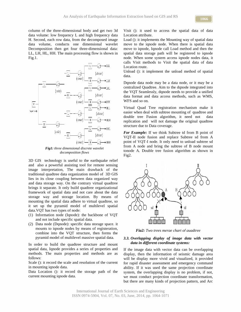
1066 An Analysis of Earthquake Information Extraction based on GIS and RS
International Journal of Earth Sciences and Engineering
ISSN 0974-5904, Vol. 07, No. 03, June, 2014, pp. 1064-1071
column of the three-dimensional body and get two 3d
data volume: low frequency L and high frequency data
H. Second, each row data, from the decomposed image
data volume, conducts one dimensional wavelet
Decomposition then get four three-dimensional data:
LL, LH, HL, HH. The main processing flow is shown in
Fig.1.
3D GIS technology is useful to the earthquake relief
and also a powerful assisting tool for remote sensing
image interpretation, The main drawback of the
traditional quadtree data organization model of 3D GIS
lies in its close coupling between data organized way
and data storage way. On the contrary virtual quadtree
brings it separate. It only build quadtree organizational
framework of spatial data and not care about the data
storage way and storage location. By means of
mounting the spatial data adhere to virtual quadtree, so
it set up the pyramid model of multilevel spatial
data.VQT has two types of node:
(1) Information node (Iqnode): the backbone of VQT
and not include specific spatial data.
(2) Data node (Dqnode): specific data storage space. it
mounts to iqnode nodes by means of registeration,
combine into the VQT structure, then forms the
pyramid model of multilevel massive spatial data.
In order to build the quadtree structure and mount
spatial data, Iqnode provides a series of properties and
methods. The main properties and methods are as
follows:
Scale (): it record the scale and resolution of the current
in mounting iqnode data.
Data Location (): it record the storage path of the
current mounting iqnode data.
Visit (): it used to access the spatial data of data
Location attribute.
Load (): it implements the Mounting way of spatial data
move to the iqnode node. When there is spatial data
move to iqnode, Iqnode call Load method and then the
spatial data storage path will be registered to iqnode
node. When some system access iqnode nodes data, it
calls Visit methods to Visit the spatial data of data
Location route.
Unload (): it implement the unload method of spatial
data.
Dqnode data node may be a data node, or it may be a
centralized Quadtree. Aim to the dqnode integrated into
the VQT Seamlessly, dqnode needs to provide a unified
data format and data access methods, such as WMS,
WFS and so on.
Virtual Quad Tree registration mechanism make it
easier when deal with subtree mounting of quadtree and
double tree Fusion algorithm, it need not data
replication and will not damage the original quadtree
structure due to Data coverage.
For Example: If we think Subtree td from B point of
VQT-II node fusion and replace Subtree sd from A
point of VQT-I node. It only need to unload subtree sd
from A node and bring the subtree of B node mount
tonode A. Double tree fusion algorithm as shown in
Fig2.
3.3. Overlapping display of image data with vector
data in different coordinate systems:
If the image data with vector data can be overlapping
display, then the information of seismic damage area
will be display more vivid and visualized, it provided
for rapid disaster assessment and emergency command
ability. If it was used the same projection coordinate
system, the overlapping display is no problem, if not,
we must conduct projection coordinate transformation,
but there are many kinds of projection pattern, and Arc
Fig2: Two trees merge chart of quadtree
Fig1: three dimensional discrete wavelet
decomposition flows

1067 ZUOWEI HUANG, WEI HUANG AND ZOU YU
International Journal of Earth Sciences and Engineering
ISSN 0974-5904, Vol. 07, No. 03, June, 2014, pp. 1064-1071
Map, image and vector overlapping display tools,
automatically loading the map projection to the pattern
of the first loaded after map converting, as there is
drawback of network delay, Arc IMS is not displayed in
accordance with the Arc Map, but the true projection of
the original map. To solve this problem, the image map
service and vector map service is relatively independent
of the application program, on the map window we
submitted two map services to the Arc IMS Application
Server at the same time, when displaying vector map
overlay on above of the image map, setting background
color of the vector map to transparent: Map Vector. Set
Background ("255.255.255"), you can see the lower
layer image, while computing the four corners
coordinate of the image map, and then transformed into
the the same coordinates of the vector coordinate
system, so that screen coordinates corresponding to
image coordinates and vector coordinates In this way, it
not only realize overlapping display of image data with
vector data at the web browser-side, but also ensure the
consistency of the coordinate system.
3.4. Network image processing technology based on
ION:
IDL, the product of RSI company ,based on Internet
scientific visualization development tools, has a lot of
analysis toolkit, map projection and software switch
package, adopting high speed graphic image processing
technology, which can quickly realize image processing
function and image classification function. ION Script
adopts CGI network realization mode, in general it is
comprised by ION Script and ION Java, and can be
used alone, also can combine to generate IDL
application in interactive environment. Take advantage
of HTML language and Java script language; it can be
easily developed network information service system.
Through Script interpreter in the ION server it will
convert ION script into HTML language, Script
application is a dynamic output HTML page, the
network image processing flow is shown in Fig.3.
4. Results and Analysis:
4.1. Analysis Platform and System Structure:
The selected platform must support large amount of
information releasing and well-stability aim to tackle
amounts of information duiring the time of information
analysis and processing. Considering the requirement of
earthquake damage assessment timeliness, the system
should possess database management, query function,
spatial analysis and the display function of spatial
characteristics. Web GIS platform: ArcIMS9.0; Servlet
engine: ServletExec5.0 ISAPI; Remote sensing image
processing: ENVI/IDL, database management platform:
Oracle9i; Web Server platform: IIS6.0; The spatial data
engine: ArcSDE9.0 for Oracle9i.according to the terrain
data, text data by means of simulation modeling
software. After the completion of conversion process,
and the successful implementation between all kinds of
heterogeneous systems, will measure the data through
GIS converted to create fire virtual environment
required for the format of the data, such as digital
elevation model data DEM, digital culture data DFD,
texture data TIFF or JPG format.
ION
interpreter
ION Script
document HTML
Database
IDL
Image
server
HTML
Client-
side
Server-side
Request
return
Fig3: Network image process flow of ION Script
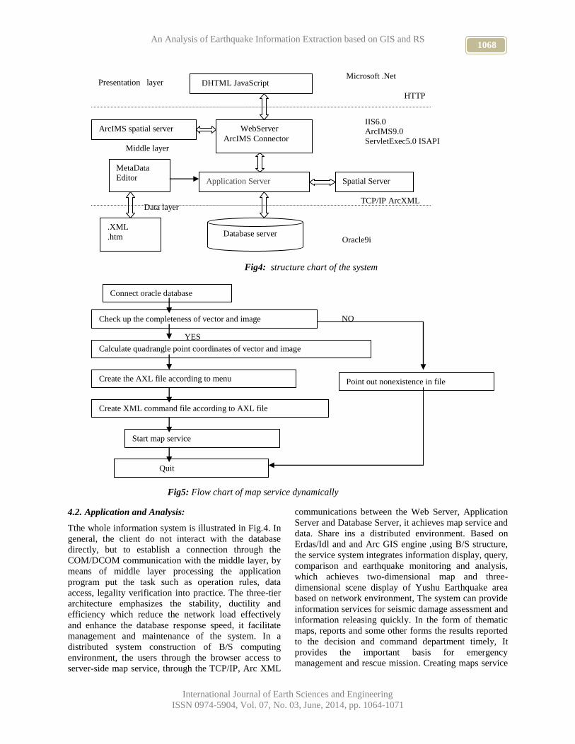
1068 An Analysis of Earthquake Information Extraction based on GIS and RS
International Journal of Earth Sciences and Engineering
ISSN 0974-5904, Vol. 07, No. 03, June, 2014, pp. 1064-1071
4.2. Application and Analysis:
Tthe whole information system is illustrated in Fig.4. In
general, the client do not interact with the database
directly, but to establish a connection through the
COM/DCOM communication with the middle layer, by
means of middle layer processing the application
program put the task such as operation rules, data
access, legality verification into practice. The three-tier
architecture emphasizes the stability, ductility and
efficiency which reduce the network load effectively
and enhance the database response speed, it facilitate
management and maintenance of the system. In a
distributed system construction of B/S computing
environment, the users through the browser access to
server-side map service, through the TCP/IP, Arc XML
communications between the Web Server, Application
Server and Database Server, it achieves map service and
data. Share ins a distributed environment. Based on
Erdas/Idl and and Arc GIS engine ,using B/S structure,
the service system integrates information display, query,
comparison and earthquake monitoring and analysis,
which achieves two-dimensional map and three-
dimensional scene display of Yushu Earthquake area
based on network environment, The system can provide
information services for seismic damage assessment and
information releasing quickly. In the form of thematic
maps, reports and some other forms the results reported
to the decision and command department timely, It
provides the important basis for emergency
management and rescue mission. Creating maps service
Connect oracle database
Check up the completeness of vector and image
Calculate quadrangle point coordinates of vector and image
Create the AXL file according to menu
Create XML command file according to AXL file
Start map service
Quit
Point out nonexistence in file
Fig5: Flow chart of map service dynamically
YES
NO
IIS6.0
ArcIMS9.0
ServletExec5.0 ISAPI
HTTP
TCP/IP ArcXML
DHTML JavaScript Presentation layer
Microsoft .Net
WebServer
ArcIMS Connector
ArcIMS spatial server
MetaData
Editor Application Server Spatial Server
Data layer
Database server Oracle9i
.XML
.htm
Fig4: structure chart of the system
Middle layer

1069 ZUOWEI HUANG, WEI HUANG AND ZOU YU
International Journal of Earth Sciences and Engineering
ISSN 0974-5904, Vol. 07, No. 03, June, 2014, pp. 1064-1071
automatically is one of the key step in order to realize
the seismic damage assessment rapidly and earthquake
damage information releasing in real-time, it can realize
the dynamic update of map service. To ensure the
stability of the system and data security this system
using C/S structure model. It adopted flow chart (Fig.5)
to realize create Web mapping service function
automatically. Using for manage the map service, Arc
IMS application server have a series of command. To
perform these commands, in general it should have
XML files of recorded Admin CMD command and
batch files or script file. And then adding commands of
start, stop, delete ArcIMS service of XML files, created
a command file, and then run the file. After create a new
map service chuanjian. XML documents, it can write
the file dynamically in the automatic service program,
then add the following command code: ServiceCMD = "
\ ProgramFiles \ ArcIMS \ Jre \ bin \ Java. Exe Com.
Esri. Aims. Admin. CMD. Exec http://webserver admin
file "and chuanjian. XML. Run the command, new map
service start.
The 3D interface after earthquake is shown in Fig.6.
When the user selects the real-time trajectory tracking,
firstly it select data communication protocol according
to the type of GPS(Fig.7), and then enter the trajectory
of import restrictions and time interval of data detection,
it can choose whether GE automatically path browser,
Finally, click on the "start" button, it can conduct
trajectory tracking in real time(Fig.8).
Based on current received data Policymakers can further
amend the right rescue course, and the corrected results
send to the rescue team in a GPS device, so as to realize
real-time interaction and save rescue time greatly.
The collapsed housing in Jiegu Town is shown in Fig.9.
In the western region of Victory Road, especially in the
southern section (Fig.9(a)), the damage was so serious
that almost all of the civil engineering structures
housing fell destroyed completely. Some of the brick
building was also collapsed .Many of the uncollapsed
ones suffered serious damage to the structure, which are
difficult to repair. For frame structure, the office
buildings for government and the services buildings
along the provincial and national highway were almost
in good condition(Fig.9(b). the collapse rate of the
housings on an alluvial fan in the west side of Jiegu
Town (Fig.9(c))reached up to 86%.
Fig8: Navigation aid route
Fig7: GPS module
Fig6: The 3D interface layout after
earthquake

1070 An Analysis of Earthquake Information Extraction based on GIS and RS
International Journal of Earth Sciences and Engineering
ISSN 0974-5904, Vol. 07, No. 03, June, 2014, pp. 1064-1071
There might be two reasons: (1) In that alluvial fan after
years of weathering, the surface was relatively flat and
solid, but the lower soil had been eroded, so that the
structure was not stable enough. (2)The region was near
the fault zone. Therefore, for the post-disaster
reconstruction and the future residential land, we should
keep away from the alluvial fan. the interpretation map
of seismic deformation can be obtained (Fig.10).From
the interpretation map, it can be found that the
earthquake caused different degrees of co-seismic
ground deformation between 32°48'N—33°20'N and
96°20'E—97°12'E.The surfface rupture zone from the
Longbao town in the northwest to the Jiegu town in the
southeast reached 70 km long. The overall trend was
119°.The nearer from the Yushu- Ganzi surface fault
zone, the greater the ground deformation. The
deformation gradient was larger in the northeast
direction and was relatively smaller in the southwest
direction.
5. Conclusion:
As one of the greatest natural disasters in the world,
earthquake is very important for emergency to quickly
acquire disaster information. In order to extract the
information of earthquake damage effectively and
timely, On the basis of the practical work in Yushu
Earthquake disaster situation monitoring, this paper puts
the emphasis on the methods and technical flow of
image processing in the application of monitoring and
assessment of earthquake disaster situation. The existing
problems are also analyzed. In modern times remote
sensing technology provides a quick effective approach
to access the disaster information and loss after the
earthquake, owing to its advantage of the quick
dynamically all-weather monitoring with large amount
of information and a short update cycle. It can not only
make full use of resources satellite images, can also
show much detailed image information related to the
earthquake, shorten the development cycle,
popularization of earthquake professional knowledge,
improve the work efficiency, for the ground at the same
time the emergency rescue mode innovation also has a
certain reference significance. It provides services
directly to the professional sectors for the earthquake
analysis and evaluation. This data are processed and
then are used in the information service system
construction to realize the interpretation, assessment and
service for the comprehensive disaster situation
information. The system plays an important role in
disaster relief actions.
References:
[1] Wei C J, Liu Y L, Wang S X, Zhang L F and
Huang X X. 2008. Investigation and assessment of
damage in earthquake Wenchuan Sichuan Quake
based on remote sensing. Journal of Remote
Sensing, 12(5): 673—682.
[2] Liu W G, Cui J T, Zhou L H. Subpixel registration
based on interpolation and extension phase
correlation [J]. Journal of Computer - aided Design
and Computer Graphics 2005, 17 (6): 1273 -1277.
[3] Sun J B, Liang F and Shen Z K.2008. InSAR
deformation observation and preliminary analysis
of the Ms 8 Wenchuan earthquake. Seismology and
Geology, 30(3): 787—795.
[4] Chen S R, Ma H J, Fan Y D, Xu F and Lian J.2008.
Road damage assessment from high resolution
satellite remote sensing imagery in Wenchuan
Fig10: Interpretation map of seismic ground
deformation
Fig9: collapsed housing in Jiegu Town
(a)Region of the south of Jiegu Town; (b) Building
of frame construction along the Provincial and
county roads; (c) Collapse of housing on the
alluvial fan structure housings collapsed
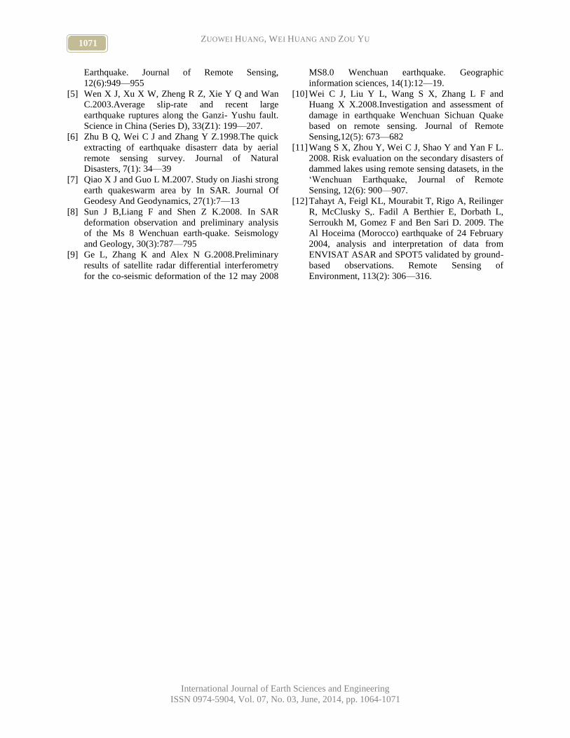
1071 ZUOWEI HUANG, WEI HUANG AND ZOU YU
International Journal of Earth Sciences and Engineering
ISSN 0974-5904, Vol. 07, No. 03, June, 2014, pp. 1064-1071
Earthquake. Journal of Remote Sensing,
12(6):949—955
[5] Wen X J, Xu X W, Zheng R Z, Xie Y Q and Wan
C.2003.Average slip-rate and recent large
earthquake ruptures along the Ganzi- Yushu fault.
Science in China (Series D), 33(Z1): 199—207.
[6] Zhu B Q, Wei C J and Zhang Y Z.1998.The quick
extracting of earthquake disasterr data by aerial
remote sensing survey. Journal of Natural
Disasters, 7(1): 34—39
[7] Qiao X J and Guo L M.2007. Study on Jiashi strong
earth quakeswarm area by In SAR. Journal Of
Geodesy And Geodynamics, 27(1):7—13
[8] Sun J B,Liang F and Shen Z K.2008. In SAR
deformation observation and preliminary analysis
of the Ms 8 Wenchuan earth-quake. Seismology
and Geology, 30(3):787—795
[9] Ge L, Zhang K and Alex N G.2008.Preliminary
results of satellite radar differential interferometry
for the co-seismic deformation of the 12 may 2008
MS8.0 Wenchuan earthquake. Geographic
information sciences, 14(1):12—19.
[10] Wei C J, Liu Y L, Wang S X, Zhang L F and
Huang X X.2008.Investigation and assessment of
damage in earthquake Wenchuan Sichuan Quake
based on remote sensing. Journal of Remote
Sensing,12(5): 673—682
[11] Wang S X, Zhou Y, Wei C J, Shao Y and Yan F L.
2008. Risk evaluation on the secondary disasters of
dammed lakes using remote sensing datasets, in the
‘Wenchuan Earthquake, Journal of Remote
Sensing, 12(6): 900—907.
[12] Tahayt A, Feigl KL, Mourabit T, Rigo A, Reilinger
R, McClusky S,. Fadil A Berthier E, Dorbath L,
Serroukh M, Gomez F and Ben Sari D. 2009. The
Al Hoceima (Morocco) earthquake of 24 February
2004, analysis and interpretation of data from
ENVISAT ASAR and SPOT5 validated by ground-
based observations. Remote Sensing of
Environment, 113(2): 306—316.
www.cafetinnova.org
Indexed in
Scopus Compendex and Geobase Elsevier, Chemical
Abstract Services-USA, Geo-Ref Information Services-USA,
List B of Scientific Journals, Poland,
Directory of Research Journals
ISSN 0974-5904, Volume 07, No. 03
June 2014, P.P.1072-1081
#02070337 Copyright ©2014 CAFET-INNOVA TECHNICAL SOCIETY. All rights reserved.
Flexural Behaviour of Stiffened Cold-Formed Steel Rectangular
Hollow Sections
PRABOWO SETIYAWAN1, MOHD HANIM OSMAN
2, A. AZIZ SAIM
2, AHMAD BAHARUDDIN
ABD.RAHMAN2 AND IMAN FARIDMEHR
2
1Dept. of Civil Engineering, Faculty of Engineering, Sultan Agung Islamic University, Semarang, Indonesia.
2Dept. of Structure and Material, Faculty of Civil Engineering, Universiti Teknologi Malaysia, 81310, Skudai,
Johor. Malaysia.
Email: [email protected]
Abstract: Full-scale cold-formed steel beams stiffened with splice plates have been experimentally studied to
investigate the strengthening effect to the section classification, flexural stiffness and moment capacity of the
sections. The study was done to investigate the increasing capacity of the section. The beams were hollow
rectangular section built up of C channel section and the strengthening of section was performed by adding the
thickness of the compression flange and web using splice hot-rolled steel plates connected using self-drilling screws.
The beam specimens were tested in bending under two point loads. The result was compared to the analytical study.
It was concluded that theoretically, the stiffened beam sections can be classified as plastic section especially for the
specimen with small screw spacing, assuming that a perfect composite action is achieved by the connection between
the cold-formed section and the stiffener plate. In addition, the strengthening has significantly increased the moment
capacity particularly to the beam stiffened with closest screw spacing.
Keywords: Cold-formed steel, section strengthening, rectangular hollow section, class of section, flexural stiffness,
moment capacity.
1. Introduction:
Recently, cold-formed steel C sections have begun to be
used as portal frame members in industrial building.
Combining two C sections to form either rectangular
hollow section or I section to increase the capacity of
the section is often performed. These combined sections
are remain slender, therefore, the methods to improve
the class of the section need to be considered. The
analytical study on behaviour of cold-formed steel
closed section as portal frame rafter had been carried-
out by Setiyawan et al. (2010). The results showed that
theoretically closed section rafter can achieve a longer
span compared to the open section. However, both the
sections failed in “combined bending and compression”
mode of failure. In preventing the combined bending
and compression mode of failure which causing the
section fail in buckling, adding the thickness of
compression elements of the section may be considered
as it significantly affected the section buckling resistant.
Strengthening method of steel sections is often applied
by constructing a compound/plated beam by welding
two equal plates to the flanges of the common beams.
This may increases the area of the sections so enlarging
the beam capacity (Joannides and Weller, 2002, Lam et.
al., 2004). The width of the stiffener plates may be
narrower or wider than the original flanges width. When
the capacity of the compound beams is not adequate to
withstand the applied load then a plate girder is
commonly used. Plate girder is a mostly typical built-up
section encountered in practical use. This section is
constructed by welding two flange plates and a web
plate to form a section. The commonly plate girder
sections found are I and box sections (Fig. 1).

1073 PRABOWO SETIYAWAN, MOHD HANIM OSMAN, A. AZIZ SAIM, AHMAD BAHARUDDIN
ABD.RAHMAN AND IMAN FARIDMEHR
International Journal of Earth Sciences and Engineering
ISSN 0974-5904, Vol. 07, No. 03, June, 2014, pp. 1072-1081
Figure 1: Typical stiffened sections (Joannides and Weller, 2002; Lam et al., 2004)
For cold-formed steel sections, the strengthening is
usually provided by attaching a stiffener at loading
points bolted to the web of channel sections. This is
intended to prevent local buckling as shown in Fig. 2
(Walker, 1975).
Figure 2: Stiffener plate of cold-formed steel C section
(Walker, 1975)
Methods of section strengthening on cold-formed steel
sections had been studied experimentally as well as
numerically by the previous researchers in order to
increase the capacity and observe the structural
behaviour (Salem et al., 2004; Serrette, 2004; Stone and
LaBoube, 2005; Young and Chen, 2008;. Xu et al.
2009). The methods was carried out by constructing
built-up sections or by attaching batten plate. Even
though the methods could increase the section capacity
of the cold-formed steel sections, however they cannot
prevent the local buckling as the section slenderness
especially for the compression elements was not
changed.
All the proposed methods of the section strengthening
however do not increase the class of the section as the
width to thickness ratio of the elements is still large.
Therefore, it is considered to strengthen the sections by
adding the compression element and web thicknesses.
This paper aims to investigate the increasing capacity of
the section when it is stiffened.
2. Research Methodology
2.1 Beam Specimens
The specimens used and the parameter details are
summarized in Table 1 and shown in Fig. 3.
Table 1: Types of beam specimen
No. Code of Specimens Thickness
(mm)
Number of Screw Rows Longitudinal Screw
Spacing (mm) Flange Web
1
2
3
CRBS-T1.5
CRBS-T1.9 CRBS-
T2.4
1.5
1.9
2.4
4
4
4
2
3
3
150
75
37.5
(b) Plate girder sections (a) Compound beams
Stiffener plate
P
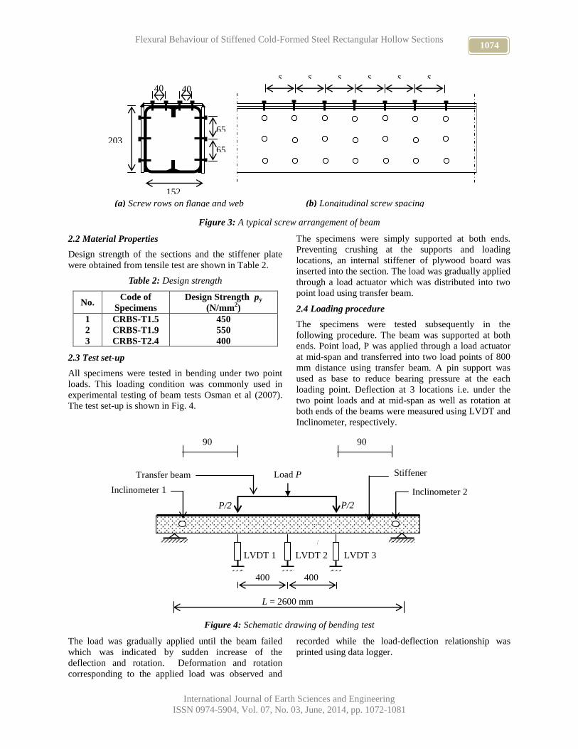
1074 Flexural Behaviour of Stiffened Cold-Formed Steel Rectangular Hollow Sections
International Journal of Earth Sciences and Engineering
ISSN 0974-5904, Vol. 07, No. 03, June, 2014, pp. 1072-1081
Figure 3: A typical screw arrangement of beam
2.2 Material Properties
Design strength of the sections and the stiffener plate
were obtained from tensile test are shown in Table 2.
Table 2: Design strength
No. Code of
Specimens
Design Strength py
(N/mm2)
1
2
3
CRBS-T1.5
CRBS-T1.9
CRBS-T2.4
450
550
400
2.3 Test set-up
All specimens were tested in bending under two point
loads. This loading condition was commonly used in
experimental testing of beam tests Osman et al (2007).
The test set-up is shown in Fig. 4.
The specimens were simply supported at both ends.
Preventing crushing at the supports and loading
locations, an internal stiffener of plywood board was
inserted into the section. The load was gradually applied
through a load actuator which was distributed into two
point load using transfer beam.
2.4 Loading procedure
The specimens were tested subsequently in the
following procedure. The beam was supported at both
ends. Point load, P was applied through a load actuator
at mid-span and transferred into two load points of 800
mm distance using transfer beam. A pin support was
used as base to reduce bearing pressure at the each
loading point. Deflection at 3 locations i.e. under the
two point loads and at mid-span as well as rotation at
both ends of the beams were measured using LVDT and
Inclinometer, respectively.
Figure 4: Schematic drawing of bending test
The load was gradually applied until the beam failed
which was indicated by sudden increase of the
deflection and rotation. Deformation and rotation
corresponding to the applied load was observed and
recorded while the load-deflection relationship was
printed using data logger.
90
0
P/2
Transfer beam
P/2
Load P
LVDT 1 LVDT 2 LVDT 3
Inclinometer 1 Inclinometer 2
400 400
L = 2600 mm
Stiffener
90
0
(a) Screw rows on flange and web (b) Longitudinal screw spacing
65
65
152
203
40 40
s s s s s s

1075 PRABOWO SETIYAWAN, MOHD HANIM OSMAN, A. AZIZ SAIM, AHMAD BAHARUDDIN
ABD.RAHMAN AND IMAN FARIDMEHR
International Journal of Earth Sciences and Engineering
ISSN 0974-5904, Vol. 07, No. 03, June, 2014, pp. 1072-1081
3. Results and Discussion
3.1 Moment-Rotation Curve
The result of the test, the moment-rotation diagrams, is
shown in Fig. 6 to Fig. 8. M’c and Mp are the
theoretical section capacities based on the Assumptions
A1, B1 and C1 (Setiyawan et.al. 2010). These
assumptions were taken in calculating the capacity of
the stiffened sections as it is not mentioned clearly in
the current design standard, BS 5950 Part 5:1998. The
assumptions are described as follows:
A1 : the thickness and dimensions of the stiffened
section is assumed equal to the thickness and
dimensions of the original section (t, B, D);
(ts = t l = B, D)
A2 : ts = t l = ax, ay
B1 : ts = tp l = B, D
B2 : ts = tp l = ax, ay
C1 : ts = t + tp l = B, D
C2 : ts = t + tp l = ax, ay
B B
D
t
ax
ax ay
B B
D
t
tp
D
B B
tp
ax
ay D
B B t
tp
D
B B
t
tp
ax
ay D
B B
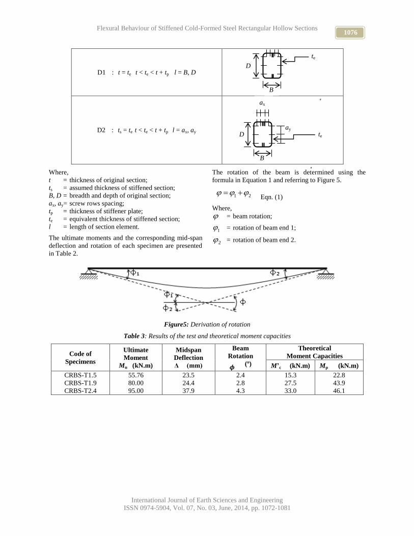
1076 Flexural Behaviour of Stiffened Cold-Formed Steel Rectangular Hollow Sections
International Journal of Earth Sciences and Engineering
ISSN 0974-5904, Vol. 07, No. 03, June, 2014, pp. 1072-1081
D1 : t = te t < te < t + tp l = B, D
D2 : ts = te t < te < t + tp l = ax, ay
Where,
t = thickness of original section;
ts = assumed thickness of stiffened section;
B, D = breadth and depth of original section;
ax, ay= screw rows spacing;
tp = thickness of stiffener plate;
te = equivalent thickness of stiffened section;
l = length of section element.
The ultimate moments and the corresponding mid-span
deflection and rotation of each specimen are presented
in Table 2.
The rotation of the beam is determined using the
formula in Equation 1 and referring to Figure 5.
1 2 Eqn. (1)
Where,
= beam rotation;
1 = rotation of beam end 1;
2 = rotation of beam end 2.
Figure5: Derivation of rotation
Table 3: Results of the test and theoretical moment capacities
Code of
Specimens
Ultimate
Moment
Mu (kN.m)
Midspan
Deflection
Δ (mm)
Beam
Rotation
𝝓 (º)
Theoretical
Moment Capacities
M’c (kN.m) Mp (kN.m)
CRBS-T1.5
CRBS-T1.9
CRBS-T2.4
55.76
80.00
95.00
23.5
24.4
37.9
2.4
2.8
4.3
15.3
27.5
33.0
22.8
43.9
46.1
te
D
B B
te
ax
ax ay
B B
D

1077 PRABOWO SETIYAWAN, MOHD HANIM OSMAN, A. AZIZ SAIM, AHMAD BAHARUDDIN
ABD.RAHMAN AND IMAN FARIDMEHR
International Journal of Earth Sciences and Engineering
ISSN 0974-5904, Vol. 07, No. 03, June, 2014, pp. 1072-1081
Figure 7: Moment-rotation curve of specimen CRBS-T1.9
M’c = 105(t = ts + tp)
Mp = 136 (t = ts + tp)
Mp = 43 (t = ts)
Mp = 79 (t = tp)
M = 80
Figure 6 Moment-rotation curve of specimen CRBS-T1.5
Mp = 92 (t = ts + tp)
M’c = 80(t = ts + tp)
Mp = 59 (t = tp)
Mp = 22 (t = ts)
M = 55
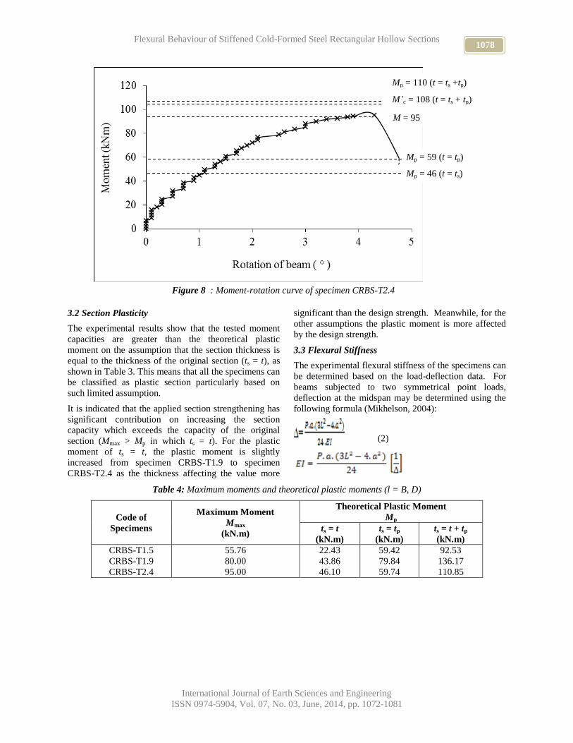
1078 Flexural Behaviour of Stiffened Cold-Formed Steel Rectangular Hollow Sections
International Journal of Earth Sciences and Engineering
ISSN 0974-5904, Vol. 07, No. 03, June, 2014, pp. 1072-1081
3.2 Section Plasticity
The experimental results show that the tested moment
capacities are greater than the theoretical plastic
moment on the assumption that the section thickness is
equal to the thickness of the original section (ts = t), as
shown in Table 3. This means that all the specimens can
be classified as plastic section particularly based on
such limited assumption.
It is indicated that the applied section strengthening has
significant contribution on increasing the section
capacity which exceeds the capacity of the original
section (Mmax > Mp in which ts = t). For the plastic
moment of ts = t, the plastic moment is slightly
increased from specimen CRBS-T1.9 to specimen
CRBS-T2.4 as the thickness affecting the value more
significant than the design strength. Meanwhile, for the
other assumptions the plastic moment is more affected
by the design strength.
3.3 Flexural Stiffness
The experimental flexural stiffness of the specimens can
be determined based on the load-deflection data. For
beams subjected to two symmetrical point loads,
deflection at the midspan may be determined using the
following formula (Mikhelson, 2004):
(2)
Table 4: Maximum moments and theoretical plastic moments (l = B, D)
Code of
Specimens
Maximum Moment
Mmax
(kN.m)
Theoretical Plastic Moment
Mp
ts = t
(kN.m)
ts = tp
(kN.m)
ts = t + tp
(kN.m)
CRBS-T1.5
CRBS-T1.9
CRBS-T2.4
55.76
80.00
95.00
22.43
43.86
46.10
59.42
79.84
59.74
92.53
136.17
110.85
Figure 8 : Moment-rotation curve of specimen CRBS-T2.4
Mp = 110 (t = ts +tp)
M = 95
Mp = 59 (t = tp)
Mp = 46 (t = ts)
M’c = 108 (t = ts + tp)

1079 PRABOWO SETIYAWAN, MOHD HANIM OSMAN, A. AZIZ SAIM, AHMAD BAHARUDDIN
ABD.RAHMAN AND IMAN FARIDMEHR
International Journal of Earth Sciences and Engineering
ISSN 0974-5904, Vol. 07, No. 03, June, 2014, pp. 1072-1081
Figure9: Determination of experimental flexural rigidity
Taken the value of P as equal to half of applied
maximum load on each beam, a = 900 mm, L = 2600
mm and E = 205,000 N/mm2, the flexural stiffness of
the specimens can be determined. The results are
compared to the theoretical values as shown in Table 4.
The theoretical values are calculated based on three
different assumptions as explained before.
It is shown that the theoretical flexural stiffness values
are closer to the experiment values if the thickness of
the stiffened section is assumed equal to the thickness of
the original section (t = ts). Comparing with the flexural
stiffness of the equivalent section, the experimental
values are equal to the same values on various
thicknesses as shown in Table 5.
The thickness of the equivalent sections is compared to
the total thickness of each stiffened section. Specimen
CRBS-T1.5 and T1.9 reach the theoretical flexural
stiffness similar to the experimental flexural stiffness
when the thickness is higher than the thickness of the
original section (ts > t). Meanwhile for specimen CRBS-
T2.4, the value is achieved when the thickness equals to
the thickness of the original section (ts = t).
It can be concluded that the strengthening applied to the
section does not significantly improve the flexural
stiffness of the beams as the value is equal to the
theoretical flexural stiffness for the thickness lower than
the total thickness of the stiffened sections.
Table 5: Experimental and theoretical flexural stiffness values
Code of
Specimens
Experimental
Flexural Stiffness, EI
(kN/mm2)
Theoretical
Flexural Stiffness, EI (kN.mm2)
(t = ts) (t = tp) (t = ts + tp)
CRBS-T1.5
CRBS-T1.9
CRBS-T2.4
3.6 x 10⁹
4.9 x 10⁹
5.3 x 10⁹
1.9 x 10⁸
2.5 x 10⁸
3.8 x 10⁸
4.8 x 10⁸
4.8 x 10⁸
5.0 x 10⁶
7.6 x 10⁸
8.2 x 10⁸
9.0 x 10⁸
Table 6: Equivalent thicknesses
Code of
Specimens
Section
Thickness
t
(mm)
Experimental
Flexural Stiffness,
EI
(mm4)
Stiffener
Thickness
tp
(mm)
Total
Thickness
(ts + tp)
(mm)
Equivalent
Thickness for
EIth = EIexp.
teq
(mm)
CRBS-T1.5
CRBS-T1.9
CRBS-T2.4
1.5
1.9
2.4
3.6 x 10⁹
4.9 x 10⁹
5.3 x 10⁹
3.0
3.0
3.0
4.5
4.9
5.4
2.3
3.0
2.4
3.4 Moment Capacity
The experimental moment capacities of the specimens
were determined by calculating the maximum moment.
In these tests, the maximum moment is equal to bending
moment, Mmax = 900 x P, where P is half of the
maximum P of the test result for each tested specimen.
The experimental moment capacity of the specimens is
then compared to the theoretical value as shown in
Table 6.
It is shown that the experimental moment capacity
exceed the theoretical values for Assumption A1 and B1
in which the thickness is assumed equal to the thickness
of the original section or the stiffener plate (Tables 7 (a)
and 7 (b)). In addition, the specimen CRBS-T2.4 is the
only specimen which the experimental moment capacity
a a
L
P P
Δ

1080 Flexural Behaviour of Stiffened Cold-Formed Steel Rectangular Hollow Sections
International Journal of Earth Sciences and Engineering
ISSN 0974-5904, Vol. 07, No. 03, June, 2014, pp. 1072-1081
exceeding the theoretical value on Assumption C1 in
which the thickness is assumed equal to the total
thickness of the original section and the stiffener plate
(Table 7 (c)), This means that the applied section
strengthening method is more effective than the other
specimens. Comparing to the moment capacity of the
equivalent section, the experimental moment capacity
values are equal to the values on various thicknesses as
shown in Table 8.
The equivalent thickness was compared to the total
thickness of each stiffened section as shown in Table 8.
t is obtained by trial and error on the calculation of
moment capacity until the value closed to the
experimental moment capacity (Assumption D1) is
derived.
It is indicated that the strengthening applied on the
specimen CRBS-T2.4 significantly improves the
moment capacity. The value is equivalent to the
theoretical moment capacity in which the thickness
larger than the total thickness of the original section and
stiffener plate. This does not occur on the specimens
CRBS-T1.5 and CRBS-T1.9.
Table 7: Experimental and theoretical moment capacities
Code of
Specimens
Experimental
Moment Capacity
(kN.m)
Theoretical Moment Capacity
ts = t
(kN.m)
ts = tp
(kN.m)
ts = t + tp
(kN.m)
CRBS-T1.5
CRBS-T1.9
CRBS-T2.4
55.76
80.00
95.00
15.29
27.55
33.00
49.19
57.81
44.64
80.25
105.41
87.82
Table 8: Moment capacities of experimental and equivalent sections
Code of Specimen Experimental Moment Capacity
(kN.m)
Theoretical Moment Capacity
(kN.m)
CRBS-T1.5
CRBS-T1.9
CRBS-T2.4
55.76
80.00
95.00
55.58 (teq = 3.3 mm)
80.90 (teq = 3.9 mm)
94.47 (teq = 5.8 mm)
Table 9: Ratios of equivalent to total thicknesses
Code of Specimens Section Thickness
(mm)
Total Thickness
(mm)
Equivalent Thickness
(mm)
CRBS-T1.5
CRBS-T1.9
CRBS-T2.4
1.5
1.9
2.4
4.5
4.9
5.4
3.3
3.9
5.8
4. Conclusion
Three specimens of full-scale cold-formed steel beams
stiffened with 3 mm plates have been tested. The
theoretical flexural stiffness and moment capacity had
been calculated and compared with the experimental
results.
The main conclusions of this investigation can be drawn
as follows:
i. The stiffening applied on cold-formed rectangular
hollow sections can improve the class of the
sections. Comparing to the thickness is assumed
equal to the thickness of the original section.
ii. The strengthening significantly increases the
flexural stiffness of the beams as the values are
higher than obtained theoretically for all the
assumptions.
iii. Moment capacity of the beams increases when the
longitudinal screw spacing decreases.
Generally, it is concluded that the strengthening applied
on cold-formed rectangular hollow sections can
improves the flexural behaviour of the sections.
5. Acknowledgements
The material required for the specimen fabrication was
generously donated by BlueScope Ltd. Financial
assistance was provided by Universiti Teknologi
Malaysia (UTM) and Sultan Agung Islamic University
(UNISSULA), Indonesia. The authors are grateful to Dr.
Joanna M. Dulinska for revising the article and also
acknowledge Dr D. Venkat Reddy, Editor- in -Chief -
International Journal of Earth Sciences & Engineering –
IJEE, for facilitating the publication process.
6. Reference:
[1] Beng, K. F. C. (1993). Building Design using Cold-
Formed Steel Sections: Work Examples to BS
5950: Part 5: 1987. Berkshire: The Steel
Construction Institute.

1081 PRABOWO SETIYAWAN, MOHD HANIM OSMAN, A. AZIZ SAIM, AHMAD BAHARUDDIN
ABD.RAHMAN AND IMAN FARIDMEHR
International Journal of Earth Sciences and Engineering
ISSN 0974-5904, Vol. 07, No. 03, June, 2014, pp. 1072-1081
[2] British Standards Institution (BSI). (1998). BS
5950: Structural Used of Steelwork in Building Part
5: Code of Practice for Design of Cold Formed
Section. London: The Steel Construction Institute.
[3] British Standards Institution (BSI). (2000). BS
5950: Structural Used of Steelwork in Building Part
1:2000: Code of Practice for Design in Simple and
Continuous Construction: Hot Rolled Section.
London: The Steel Construction Institute.
[4] International Textbook Company. (1975). Design
and Analysis of Cold-Formed Sections, edited by
A.C. Walker. London: International Textbook
Company.
[5] Joannides, F., Weller, A. (2002). Structural Steel
Design to BS 5950: Part 1. London: Thomas
Telford Publishing.
[6] Lam, D., Ang, T. C., Chiew, S. P. (2004).
Structural Steelwork Design to Limit State Theory
Third Edition. Oxford: Elsevier Butterworth-
Heinemann.
[7] Mikhelson, I. (2004). Structural Engineering
Formulas. New York: McGraw-Hill.
[8] Osman, M.H., Saim, A.A., Saleh, A.L. (2006).
Strength Test on Stainless Steel Purlins (Final
Report) for Yick Hoe Metal Industries Sdn Bhd.
Malaysia: CETU UTM Skudai.
[9] Osman, M.H., Saad, S., Saim, A.A., Keong, G.K.
(2007). Structural Performance of Composite Beam
with Trapezoid Web Steel Section. Malaysian
Journal of Civil Engineering 19 (2): 80 – 95.
[10] Serrette, R.L. (2004). Performance of Edge-Loaded
Cold-Formed Steel Built-Up Box Beams. Practice
Periodical on Structural Design and Construction,
ASCE. 9 (3): 170-174.
[11] Setiyawan, P. Osman, M. H. Saim, A. A. (2009).
Stiffening Of Cold-Formed Steel Section at Plastic
Hinge Formation. Monograf Persidangan
Kebangsaan Kejuruteraan Awam Kelima. USM,
Malaysia: 173-182.
[12] Setiyawan, P. Osman, M. H. Saim, A. A. (2010).
Stability of Cold-Formed Open and Closed Sections
Rafter in Portal Frame Design. Proceedings of the
Third International Graduate Conference on
Engineering, Science and Humanities. UTM,
Malaysia: 65
[13] Stone, T. A. and LaBoube, R. A. (2005). Behaviour
of Cold-Formed Steel Built-Up I-Sections. Thin-
Walled Structures. 43 (2005): 1805-1817.
[14] Sum, N. Z. (2006). Performance of Stainless Purlin
in Bending, These. Malaysia: Civil Engineering
Department UTM Skudai.
[15] Xu, L., Sultana, P., Zhou, X. (2009). Flexural
Strength of Cold-Formed Steel Built-Up Box
Sections. Thin-Walled Structures. 47 (2009): 807-
815.
[16] Young, B. and Chen, J. (2003). Design of Cold-
Formed Steels Built-Up Closed Sections with
Intermediate Stiffener. Journal of Structural
Engineering, ASCE. 134 (5): 727-737.
www.cafetinnova.org
Indexed in
Scopus Compendex and Geobase Elsevier, Chemical
Abstract Services-USA, Geo-Ref Information Services-USA,
List B of Scientific Journals, Poland,
Directory of Research Journals
ISSN 0974-5904, Volume 07, No. 03
June 2014, P.P.1082-1088
#02070338 Copyright ©2014 CAFET-INNOVA TECHNICAL SOCIETY. All rights reserved.
Response and Reliability Analysis of Pile Foundation under Strong
Excitation
YONGFENG XU, HAILONG WANG, LIQUN ZHANG AND JIANLIN HU Hebei Institute of Architecture and Civil Engineering Zhangjiakou City, Hebei Prov, China
Email: [email protected], [email protected], [email protected], [email protected]
Abstract: With the rapid development of high speed railway in china, more and more bridges or viaducts have been
constructed. Due to the vast area and complex terrain, many viaducts are needed in many cases. In addition, natural
condition is quite complex, so reliability of the viaducts is quite important to provide people’s safety. Usually, pile
foundation plays important role in keeping the good performance of viaducts. In order to improve the reliability of
giant pile group foundation, proper model has been used to simulate the response under strong excitation. For the
reason of uncertainty of natural condition, random process is used in the analysis. For a specified project, strong
excitation has been applied in the structure. In the calculation, equivalent method has been used to replace the
nonlinear load. The results show that biggest stress and bending moment is on the pile top and upper part of pile.
After paying attention to the design of pile, reliability can meet the demand of safety. Besides, the results also verify
the affectivity of the method.
Keywords: pile foundation, strong excitation, equivalent method, reliability.
1. Introduction:
With the rapid development of high speed railway in China, more and more bridges or land bridges have been constructed. Due to the vast area and complex terrain, many viaducts are needed in many cases. Take Shang hang high speed railway as the example, percentage of bridge and tunnel is up to 72.3%. In fact, percentage of bridge and tunnel in many other high speed railways is also more than 70%. This means a lot of viaducts with high reliability is needed. Due to the bridge is distributed in all of the country, complex natural condition in each place has to be taken into consideration, such as rain [1-3], wind [4-6], earthquake [7-11] and so on. Except natural condition, viaducts also influenced by other non-natural conditions, for example, train passing with different speed [12-16], heavy machinery, etc. Both the natural and non-natural conditions have to deeply study.
Pile foundation as supporting structure has been for thousands of years. But with the time developing, pile group has been used with the bridge becomes much larger. At the same time, pile with different work mechanism has its own classification, such as friction pile, supporting pile and so on.
Earthquake is a main cause to make bridge and pile failure. So, mechanism research of earthquake on bridge and pile is quite valuable. Due to the complexity of pile, we can’t apply correct load on the structure in the experiment. In fact, we can’t construct the same size of model as the same of actual size. So, simulation method is quite effective way to determine the parameters of the
structure. Simulation algorithm, with results of enough accuracy, is quite important to develop. Many studies have already been developed under different conditions [17-21]. At the same time, FEM method also has vast of research [22-25].
Due to the importance of pile, in this paper, response of
pile under strong excitation has been mainly studied.
We simulate the earthquake and study the response of
pile and pile group. Strong excitation is a random
process. The main contribution of the paper is the
proposition of an effective simulation method. The
remainder of the paper is organized as follows: random
excitation and reliability analysis method is described in
section 2. Parameters are listed in section 3. Analysis is
shown in section 4 and conclusion is in section 5.
2. Random excitation and reliability analysis
method:
2.1. Random vibration under strong excitation:
Assume that bedrock vibration is a random process,
)(txg is the bedrock acceleration time history with the
seismic risk analysis. The maximum of acceleration
value is 1.2 2/ sm , as shown in figure 1. If we take
)(txg as a sample function of random process, from
stochastic process theory, we can get:
TAEsgg x
Tx /]|)([|lim)( 2
(1)
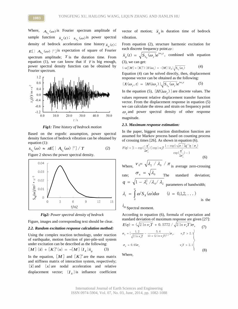
1083 YONGFENG XU, HAILONG WANG, LIQUN ZHANG AND JIANLIN HU
International Journal of Earth Sciences and Engineering
ISSN 0974-5904, Vol. 07, No. 03, June, 2014, pp. 1082-1088
Where, )(gxA
is Fourier spectrum amplitude of
sample function )(txg ; )(
gxs is power spectral
density of bedrock acceleration time history )(txg ;
]|)([| 2gxAE
is expectation of square of Fourier
spectrum amplitude; T is the duration time. From
equation (1), we can know that if T is big enough,
power spectral density function can be obtained by
Fourier spectrum.
Fig1: Time history of bedrock motion
Based on the ergodic assumption, power spectral
density function of bedrock vibration can be obtained by
equation (1):
TAEsgg xx /]|)([|)( 2 (2)
Figure 2 shows the power spectral density.
Fig2: Power spectral density of bedrock
Figure, images and corresponding text should be clear.
2.2. Random excitation response calculation method:
Using the complex reaction technology, under reaction
of earthquake, motion function of pier-pile-soil system
under excitation can be described as the following:
gX xIMxKxM }]{[}{][}]{[ * (3)
In the equation, ][M and *][K are the mass matrix
and stiffness matrix of interaction system, respectively;
}{x and }{x are nodal acceleration and relative
displacement vector; }{ XI is influence coefficient
vector of motion; gx is duration time of bedrock
vibration.
From equation (2), structure harmonic excitation for
each discrete frequency point : yi
jxg
j
geStx
)()( , combined with equation
(3), we can get:
)(}]{[}(){][][( *2jxXjj g
SIMiXKM (4)
Equation (4) can be solved directly, then, displacement
response vector can be obtained as the following: yi
jxjj
j
geSiHtX
)()}({},({ (5)
In the equation (5), )}({ jiH are discrete values. The
values represent relative displacement transfer function
vector. From the displacement response in equation (5)
we can calculate the stress and strain on frequency point
j and power spectral density of other response
magnitude.
2.3. Maximum response estimation:
In the paper, biggest reaction distribution function are
assumed for Markov process based on counting process
of crossing times [26]. As shown in equation (6).
1)2
exp(
)/2/exp(1exp{)]
2exp(1[)(
2
2
2.1
02
2
x
x
x
qTF
(6)
Where, // 020 is average zero-crossing
rate; 0 x The standard deviation;
2021 //1 q
parameters of bandwidth;
,...)2,1,0()(0
idSX
i
i
is the
thiSpectral moment.
According to equation (6), formula of expectation and
standard deviation of maximum response are given [27]:
xee TTE )ln2/5772.0ln2()( (7)
1.265.0
1.2,])ln2(13
4.5
ln2
2.1[
2.3
T
TTT
ex
ex
ee
(8)
Where,

1084 Response and Reliability Analysis of Pile Foundation under Strong Excitation
International Journal of Earth Sciences and Engineering
ISSN 0974-5904, Vol. 07, No. 03, June, 2014, pp. 1082-1088
69.0
69.0,)38.063.1(
0
045.0
q
e
e
(9)
2.4. Nonlinear dynamics of soil:
In the condition of strong excitation, nonlinear dynamic
performance of soil is studied by equivalent linear
method. In the equivalent linear iteration calculation,
equivalent shear strain of each soil element can be
determined by [28]:
0.22 eq (10)
Where, eqis the equivalent shear strain; is
standard deviation of random process of shear strain
response; 0, is zeroth order spectrum moment in
random process of shear strain response. With
equivalent shear strain, equivalent modulus and
equivalent damping ratio can be determined. Then
iterate the calculation till meet the accuracy
requirement.
2.5. Failure criterion of strength:
If mark yield shear of pile body yS as strength control
index, strength failure probability of pile foundation
under strong excitation is:
njmiSSPtP Yijf ,...,2,1,,...2,1},]{max[)( (11)
Where, ijS is shear response of pile
jat the depth i .
Using first-passage failure mechanism and maximum
overpassing yield shear events of pile body shear
response follows Poisson assumption. For stationary
random process with zero mean, probability of
maximum pile body shear force less than yield shear
can be described as:
)]2
exp(2
exp[)(2,
2
,
,
ijS
y
ijS
ijS
yij
STSSP
(12)
Where, ijS and ijS
are standard deviation of shear
process and derivative reaction process of pile j
at the
depth of i in group piles foundation respectively.
Accordingly, group pile foundation is in beyond
boundary for the first time, namely that first time failure
probability can be expressed as:
)(1, yijijf SSPP (13)
By equation (13) and biggest shear reaction process of
each pile at different depth in pile group, we can get
strength damage based failure probability, which can
evaluate the overall reliability of the foundation of pile
group.
3. Parameters:
T For a specified pile group structure, covering layer
with shear wave velocity m/s 500 < V , which has a
thickness of about 100 m, is composed of 10 kinds of
soil. Property of soil is shown in figure 1. Soil shear
wave velocity is tested in elastic wave velocity
experiment. And maximum shear modulus of soil is
determined by shear wave velocity. Figure 3 shows the
shear wave velocity profile. Relationship among ground
soil dynamic shear modulus ratio and damping ratio has
also been acquired by experimental method [29].
Ground soil is divided into 50 layers in the calculation
and thickness of each layer is smaller than 1/5
wavelength. Among of the all layers, maximum
thickness is 3.6 m and minimum thickness is 1.0m.
Considering the finite element boundary effect, set the
width of field soil layer is 5 times than that of the
foundation.
Table1: Gravities of soils
Soil layer Gravity/
3 mkN
Soil layer Gravity/
3 mkN
(1) silt 18.5 (6) fine sand 20.7
(2) fine sand 19.7 (7) coarse and 21.0
(3) silt 18.9 (8) medium sand 20.5
(4) silt 20.1 (9) gravel sand 22.4
(5) silt 20.5 (10) clay 21.3
elev
atio
n/m
soil shear velocities/m·s-1
Fig3: Section of soil shear velocities
Pile group is composed of 125 bored piles with diameter
of 2.5m and length of103m . Plane size of pier is
m113.5m 5.48 and thickness is m9 . Distance
between pier bottom and ground is m20 . Reinforced
concrete structure is simplified into equivalent mass

1085 YONGFENG XU, HAILONG WANG, LIQUN ZHANG AND JIANLIN HU
International Journal of Earth Sciences and Engineering
ISSN 0974-5904, Vol. 07, No. 03, June, 2014, pp. 1082-1088
effect on the pier. In the calculation, pile group is
simplified as equivalent 30 root piles. Pile body is
adopts beam element. Table 2 shows the main element
parameters of pile. Whole bridge pier structure is
simulated with block elements and mass of each block
elements iskg81038.3
. Moment of inertia is 2111056.5 mkg
Table2: Parameters of beam elements
Elasticity
modulus/
kPa107
Shear
modulus/
kPa107
Gravity/-3mkN
Cross-
sectional
area/
2m
Effective
shear
area
coefficient
Inertia
moment
/4m
3.21 1.62 24.4 4.9 0.9 1.92
4. Analyses:
Damage of foundation structure can cause damage of
upper bridge structure. This is one of main reasons to
lead to destroy. Base damage may be caused by damage
of foundation soil or inadequate strength of itself. Based
on characteristics excitation, bridge pile foundation and
foundation soil response are analyzed in detail. Figure 4
shows the system of pier - pile – soil. Pile is at depth of
83.0 m and distance between two piles is 3.375 m. In
the figure, #1 and
#29 are two side pile, and #15 pile
is in the middle. A ~ G represents x = 67.0, 85.0, 132.0,
177.0, 235.0, 301.0, 40.0 m in the soil profile.
Pier
x
A
B
C D E F G
y
Soil
29#
7# 1#
15#
11#
Fig4: Pier-pile group-soil system
4.1. Displacement Response:
Figure 5 shows the average reaction of largest
displacement of pile and soil. We can see that pile body
displacement reaction has relation with field soil
engineering properties and upper structure of bridge
pier. There are some remarkable characteristics: first,
due to large integral stiffness of pile group foundation,
and foundation soil assumed to transverse isotropy, pile
body displacement of side pile and middle pile are
almost uniformly; second, since the friction pile
foundation, pile end is in a state of freedom. During the
excitation, foundation of pile group may produce some
overall lateral movement. In the test, displacement of
pile end moves about 2.5 cm. In addition, due to the soft
soil layer from ground and depth of 37 m has weak
constraint to the pile body displacement and pull effect
of inertia of the upper structure of bridge pier, body
displacement distribution along the pile depth is in
triangular. From one end of the pile, displacement
increases gradually. Pile body displacement would get
the peak at about 30 m below the ground. At this time,
the displacement is 14.3 cm. Then, pile body
displacement decreases. Displacement of pile body at
the ground is about 7.2 cm and the displacement of pile
top is about 2.7 cm.
soil
soil
soil
15# pile
1# pile
Fig5: Pile displacement
soil
soil
soil
soil
soil
soil
soil
μx/m
H/m
Fig6: Displacement of soil
As shown in figure 6, for the foundation soil
displacement response, foundation soil away from the
base has a decreasing displacement with the increase of
depth. Displacement response at the surface is the
strongest. Displacement response of soil surrounding
foundation is close to pile displacement response at both
aspects of size and depth. As shown in figure 5. In
addition, Displacement response of the foundation soil
on both sides is related to the distance between soil and
foundation. This embodies the effect of pier-pile-soil
interaction on soil displacement reaction. If both sides
of the soil is divided into near field and far field, we can
know that pier-pile-soil interaction has significant effect
on displacement reaction of near field soil, and
displacement response of far field soil has almost close

1086 Response and Reliability Analysis of Pile Foundation under Strong Excitation
International Journal of Earth Sciences and Engineering
ISSN 0974-5904, Vol. 07, No. 03, June, 2014, pp. 1082-1088
to that of free field. Effects of interaction are quite
weak. It can be concluded that near field and far field
can be roughly divided with F section. Influence range
of interaction effect of pier-pile-soil on foundation soil
displacement is about 1.7 times of foundation width on
both sides.
4.2. The internal force response of pile foundation:
1# pile
7# pile
11# pile
15# pile
Fig7: Bending moment of pile
1# pile
7# pile
11# pile
15# pile
Fig8: Shear force response of pile shaft
Results analysis of pier - pile - soil system shows that
response of bending moment and sheer force of pile
above ground is very big. Maximum bending moment
is mkN101.15 4 , and maximum shear is
kN101.23 3 . This is because upper bridge piers have
huge inertia force to the basis under the strong
excitation. This may make the connection part between
upper structure of bridge pier and pile foundation is in a
range of plastic zone. Pile top would be probably
broken. Figures 7 and 8, shows the response of average
maximum bending moment and sheer force of pile body
underground. It can be seen from the figure, bending
moment and shear force response of pile body with 40m
depth are quite strong. Bending moment of side pile is
slightly larger than that of middle pile. Shear force
reaction of side pile is slightly bigger than that of
middle pile. Pile group effect has great influence on
shear response. In addition, we still can see the shear
force at depth of 5m is higher than that of side pile top.
We can conclude that when the pile is suffer great
excitation, pile top may be broken for the great force
and pile body also may be broken with the great force.
4.3. Reliability analysis of pile foundation:
In the paper, four yields shear stress are selected as
strength damage standard of pile foundation. The four
stress is kNSy 3000,2500,1500,1000 respectively. Figure
9 shows the reliability analysis results of side pile and
pile. We can see from the figure that side pile top and
pile body near the ground occurs with strength damage
under the low intensity level. This is due to the seismic
shear. With a relative high intensity of damage standard,
reliable probability is more than 99%. It basically
satisfies the reliability demand.
For middle pile, pile body stress is relatively small and
probability of failure is also small. But pile top and pile
body near ground are both the seismic vulnerability.
Overall, for large bridge seismic design of pile
foundation to meet the safety demand under the
condition of little excitation, and combined with
perspective of economy, pile top and upper part of pile
of pile group must take necessary measures into
consideration.
reliability
(a) Side pile
reliability
(b) Middle pile
Fig9: Reliability of pile in different places
It should be noted that strength damage standard of pile
foundation is arbitrary selected. In actual engineering,
strength damage standard of pile foundation should be
determined by experiment.
5. Conclusion:
1087 YONGFENG XU, HAILONG WANG, LIQUN ZHANG AND JIANLIN HU
International Journal of Earth Sciences and Engineering
ISSN 0974-5904, Vol. 07, No. 03, June, 2014, pp. 1082-1088
Due to the vast area and complex terrain and natural
condition, viaducts, with enough safety, are needed to
construct. Pile foundation is base of the bridge and
safety of it has great relationship with safety of viaduct.
For the reason of uncertainty of natural condition,
random excitation is used in the analysis and strong
excitation has been applied in the pile. In the
calculation, equivalent method has been used to replace
the nonlinear load.
In the result, we can obtain some useful conclusion. Due
to the inertia effect and weak constraint of soft soil on
pile body, under the condition of strong excitation,
maximum displacement appears at upper part of the pile
body and pile top displacement is smaller. If use pile
group, displacements of side pile and middle pile are
almost the same. Displacement reaction has close
relationship with distance between soil and foundation.
Under strong excitation, side pile would bear larger
bending moment and shear force.
Simulation method can use simple model instead of
complex model. It transfers the actual problem into
mathematical description of the problem. It can simulate
the actual situation by solving the mathematical model.
With the development of random function, model can
easily get realistic boundary conditions and get more
accurate result, which is close to the actual situation.
The simulation method and random function used in the
simulation of the pile foundation can get more accurate
results and reduce the design cost.
6. Reference:
[1] Xin Da-Bo, Wang Liang, Duan Zhong-Dong, Ou
Jin-Ping, Li Hui, Li Zhong - Hua. Static
characteristics of bridge deck sections of long-span
bridges under simultaneous actions of wind and
rain. Journal of Jilin University (Engineering and
Technology Edition), 41(SUPPL. 2): 174-179.
(2011)
[2] Gu Ming, Xu Shu - Zhuang. Effect of rain on
Flutter derivatives of bridge decks. Wind and
Structures, An International Journal, 11(3): 209-
220. (2008)
[3] Xin Dabo, Li Hui, Wang Liang, Ou Jinping.
Experimental study of rain effects on vortex
shedding of long Span bridge girders. Advances in
Structural Engineering, 15(10):1793-1799. (2012)
[4] Xin Dabo, Li Hui, Wang Liang, Ou Jinping.
Experimental study on static characteristics of the
bridge deck section under simultaneous actions of
wind and rain. Journal of Wind Engineering and
Industrial Aerodynamics, 107-108: 17-27. (2012)
[5] Denoël Vincent, Hortmanns Michael, Sedlacek
Gerhard. A semi-empirical method for the design of
bridge cables and bridge hangers in order to avoid
rain-wind induced vibrations. Stahlbau, 76(2):126-
130. (2007)
[6] Casas Joan R, Aparicio Angel C. Rain-wind-
induced cable vibrations in the Alamillo cable-
stayed bridge (Sevilla, Spain). Assessment and
remedial action. Structure and Infrastructure
Engineering, 6(5):549-556. (2010)
[7] Xia Xiushen, Chen Xingchong, Li Xiaoyang.
Analysis of bridge earthquake damage and
reasonable aseismic systems. Advanced Materials
Research, 433-440:4782-4787 (2012)
[8] Marshall Justin D, Coulston Paul J. Comparison of
bridge earthquake resisting system design in a
moderate seismic zone. Practice Periodical on
Structural Design and Construction, 18(2):83-91.
(2013)
[9] Kuribayashi Eiichi, Iwasaki Toshio. PROGRESS
REPORT OF RESEARCH WORKS IN BRIDGE
EARTHQUAKE ENGINEERING AT THE
PUBLIC WORKS RESEARCH INSTITUTE,
JAPAN. Turk Natl Comm on Earthquake Eng,
Ankara, 9:49-64. (1980)
[10] Feng X. Bridge earthquake protection with seismic
isolation. Technical Council on Lifeline Earthquake
Engineering Monograph, (16):267-275. (1999)
[11] Carden Lyle P. Itani Ahmad M., Buckle Ian G.
Composite action in steel girder bridge
superstructures subjected to transverse earthquake
loading, Transportation Research Record, (1814):
245-252. (2002)
[12] Xia Chao-Yi, Lei Jun-Qing, Zhang Nan. Coupled
vibration analysis for train and simply-supported
bridge system subjected to floating-ice collision.
Journal of Vibration and Shock, 31(13): 154-158.
(2012)
[13] Wang Shao-Qin, Xia He, Guo Wei-Wei, Du Xian-
Ting. Coupling vibration analysis of wind-train-
bridge system considering geometric nonlinearity
of bridge. Engineering Mechanics, 30(4):122-128.
(2013)
[14] Zhang Zhi-Chao, Zhang Ya-Hui, Lin Jia-Hao.
Influence of train speeds on random vibration of
train-bridge systems. Journal of the China Railway
Society, 33(4): 93-99. (2011)
[15] Zhu Yan, Li Xiaozhen. Stochastic space vibration
analysis of train-bridge time-varying system.
ICLEM 2010: Logistics for Sustained Economic
Development - Infrastructure, Information,
Integration - Proceedings of the 2010 International
Conference of Logistics Engineering and
Management, 387:1197-1204. (2010)
[16] Li Qi, Wu Dingjun, Li Jun. Train-bridge vibration
analysis of mix- marshalling freight trains'
traversing medium and small span bridges. Journal
of Tongji University, 35(2)171-175. (2007)

1088 Response and Reliability Analysis of Pile Foundation under Strong Excitation
International Journal of Earth Sciences and Engineering
ISSN 0974-5904, Vol. 07, No. 03, June, 2014, pp. 1082-1088
[17] Li Xiao-Peng, Duan Ze-Liang, Li Tao, Wen Bang-
Chun. Dynamic simulation of a vibratory pile
driving process. Journal of Vibration and Shock,
31(7): 24-26+38. (2012)
[18] Li Xiao-Peng, Zhao Guang-Hui, Ju Xing, Liang
Ya-Min. Dynamic simulation analysis of the
vibratory sinking pile system based on AMESim.
Journal of Northeastern University, 34(5): 683-686.
(2013)
[19] Liu Cheng-Wei. Han Xuan. Method and parameters
of numerical simulation on single pile. Chinese
Journal of Geotechnical Engineering, 32(SUPPL.
2): 204-207. (2010)
[20] Chen Ya-Dong, Wang Xu-Dong, Zai Jin-Min. Soil
displacement field visualization research in model
test of pile groups and numerical simulation.
Journal of Sichuan University (Engineering Science
Edition), 43(5):45-51. (2011)
[21] Zhang Qing-Song, Li Shu-Cai, Liu Song-Yu, Du
Guang-Yin. Study on test and numerical simulation
of soil disturbed around pile by dry jet mixing pile
construction. Rock and Soil Mechanics, 27(n
SUPPL.):127-130. (2006)
[22] Wang Wei-Dong, Li Yong-Hui, Wu Jiang-Bin.
Pile-soil interface shear model of super long bored
pile and its FEM simulation. Rock and Soil
Mechanics, 33(12):3818-3824+3832. (2012)
[23] Tan, S.A. Bui, T.Y. Interpretation of pile load test
failure using FEM simulation. Proceedings of the
6th European Conference on Numerical Methods in
Geotechnical Engineering - Numerical Methods in
Geotechnical Engineering, 607-611. (2006).
[24] Lu Qun, Yuan Jianbo, Li Huixia. 3D FEM
simulation and analysis of compacting effects on
underground pipeline by construction of single
jacked pile. ICPTT 2011: Sustainable Solutions for
Water, Sewer, Gas, and Oil Pipelines - Proceedings
of the International Conference on Pipelines and
Trenchless Technology 2011, 1429-1437. (2011)
[25] Lo Kuo- Feng, Ni Sheng-Huoo, Huang Yan-Hong,
Lehmann Lutz. Free field vibrations due to pile
driving using a coupled fem with SBFEM method.
Journal of Geoengineering, 7(2):69-73. (2012)
[26] Vanmarcke E H. Properties of spectral moments
with applications to random vibration. Journal of
Engineering Mechanics, ASCE, 98(EM2): 72-88.
(1972)
[27] Kiureghian A D. Structural response to stationary
excitation. Journal of Engineering Mechanics,
ASCE, 106(EM6): 875-884. (1980)
[28] CHEN Guo-xing, XIE Jun-fei, ZHANG Ke-xu. A
method of 2-D random response analysis of earth
dam earthquake performance. Earthquake
Engineering and Engineering Vibration, 14(3): 81-
90. (1994)
[29] YANG Wei-lin, CHEN Guo-xing, WANG Zhi-hua.
2D and 3D seismic response analyses of supergiant
bridge pier-group pile-soil interaction system on
deep overburden layers. Earthquake Engineering
and Engineering Vibration, 26(5): 172-183.
(2004).

www.cafetinnova.org
Indexed in
Scopus Compendex and Geobase Elsevier, Chemical
Abstract Services-USA, Geo-Ref Information Services-USA,
List B of Scientific Journals, Poland,
Directory of Research Journals
ISSN 0974-5904, Volume 07, No. 03
June 2014, P.P.1089-1095
#02070339 Copyright ©2014 CAFET-INNOVA TECHNICAL SOCIETY. All rights reserved.
Settlement algorithm research of pile foundation under load impact
YONGFENG XU, LIQUN ZHANG, HAILONG WANG AND MINFENG LI Hebei Institute of Architecture and Civil Engineering, Zhangjiakou City, Hebei Prov, China
Email: [email protected], [email protected], [email protected], [email protected]
Abstract: Bridge served as an important part of the infrastructure, is widely used in the design of highways and
high-speed railways. As bridges of large and complex, such as road and railway dual-use Bridge, bridge security
design is also extremely important. Pile is the base of bridge, and its stability and reliability must meet high
requirements. As one of the requirements, pile foundation settlement characteristics are very important. In order to
study characteristics of pile foundation settlement, a new algorithm of load-settlement curve, which is based on
dual-line load transfer function, has been developed. The method is then used to analyze the influence of
surroundings soil condition on the pile bearing capacity. According to instance validation, the method proposed in
this paper is effective and simple. This method can be used to promote in engineering practice.
Keywords: pile foundation, settlement, load impact, bearing capacity
1. Introduction:
Pile foundations, as the basis of common type, have
been widely used in high-rise buildings [1-4], high-
speed railways [5-7], highways [8-10], bridges [11-15],
special ports [16-17], large structures, and so on. In
order to meet the safety demand of buildings, ultimate
bearing capacity of pile has to be determined [18-22].
Under the working condition, deformation of the pile
would influence the settlement, so, we must understand
the deformation of the pile and settlement
characteristics under load impact [23-25].
In actual condition, pile load settlement is affected by
many factors [26], including pile length, material,
shape, and size. Besides, characteristics of interaction
between foundation soil and pile tip is also included.
Currently, common method used in the engineering to
determine the bearing capacity of pile is through static
load tests to get the relation between pile top load and
settlement [27-28]. The curve is named as p-s curve, as
shown in Figure 1. Static loading test result to determine
the bearing capacity of the pile is certainly reliable. But
it has to spend a lot of money and time, especially for
different sizes of piles under different soil conditions.
With the development of computers, analytical method
and finite element method have a great development.
Especially the finite element method, which can convert
complex practical problems to a series of simple
calculation models, has been widely applied in scientific
activities and engineering. However, too much
simplified conditions and Solver simpler make the finite
element method can’t get more accurate results. So, in
settlement problem of pile foundation, a number of
dedicated solutions have been developed, such as one-
way compression layer summation method, resonance
method and mechanical impedance method and so on.
One-way compression layer summation method is a
typical method of soil mechanics [29-30]. This method
is based on e-p curve obtained by confined compression
test, and amended by monitoring data in engineering
practice.
Pa
s
12
3
a
b
Pb Po
Fig.1: P-s curve
In the paper, a new settlement method based on double
lines hardening model is established to calculate the
relation between axial loading-settlement of piles. And
characteristics of pile-surrounding soil effects are taken
into account. Case analysis shows the availability of the
method and main contribution of this paper is
developing a new algorithm based on double broken
line model. The remainder of the paper is organized as
follows: analysis of pile settlement curve with axial load
is shown in section 2. Relationship between initial static
stiffness and ultimate bearing capacity is shown section
3. Analysis of test results is shown in section 4 and the
conclusion is shown in section 5.

1090 Settlement algorithm research of pile foundation under load impact
International Journal of Earth Sciences and Engineering
ISSN 0974-5904, Vol. 07, No. 03, June, 2014, pp. 1089-1095
l
o
P
Pl
PB
Pl
ul u
λ1
λ2
PB
ub u
k1
k2
(a) Pile (b) Soil surrounding pile (b) Pile Subsoil
Fig2: Framework of generalized multivariate system
2. Pile of the axial load settlement curve analytic
formula:
The mechanical model of pile and soil used as shown in
figure 2, which assumes that the cross section of pile is
homogeneous and elastic rods. Effect of pile and pile
subsoil is approximately expressed with double broken
line load transfer function. 1 and 2 are corresponding
shear stiffness coefficient of before and after pile
surround soil limit displacement lu . 1k and 2k are
corresponding compressive stiffness of before and after
pile surrounding soil elastic limit displacement. In
homogeneous foundation, when the pile top is bearing
axial stress, axial force and settlement of each section of
pile is decreasing with the increasing of depth.
Therefore, with the increasing of the pile top load, pile
soil is gradually into plastic hardening stage until
destruction from shallow to deep, gradually.
2.1. Pile surrounding soil at elastic stage
For illustration purposes, P and S are used to represent
pile top load and settlement, while BP and BS represent
reaction and sedimentation beard by pile bottom.
BP and BS are parameters in the formula below. When
the load is small, all of pile soil is in elastic state. The
displacement )(xu of pile section should satisfy the
following equation:
Blx
Blx
Su
Pdx
udEA
udx
udEA
|
|
012
2
(1)
Where, E and A are elastic modulus and sectional
area of respectively. If we mark EAbi / ,
1,2i . By equation (1), the ratio of pile top load and
settlement or pile stiffness can be calculated.
)()/(
)(/
11
111
lbthSPEAb
lbthEAbSPEAb
S
PK
BB
BB
(2)
For a given pile soil system, whether K in equation is
constant is determined by the relative size of lu and
bu . There are two conditions as the following:
(1) bl uu . In this condition, while luS0
and 1kS
P
B
B keeps constant, K is also a constant
of eoK . If we mark ji, as the following:
2,1,,)(
)(
1
1
ji
lbthkEAb
lbthEAbk
ji
ij
ij (3)
Then, we can describe eK as
EAbKe 111 (4)
eK is the slope of the s-axis at initial line segment on
the p-s curve.
(2) If bl uu . In this case, pile subsoil is possibly in
plastic hardening stage earlier than surrounding soil.
Let’s suppose 1crS to be the corresponding settlement
under the condition of bB uS . From equation (1),
we can get 1crS to be described as the following:
01
1
111 )]()([ bcr ulbsh
EAb
klbchS (5)
If 11 uScr , then subsoil pile will go into plastic state.
And under the condition of 10 crSS ,
Relationship of P-S is obviously a straight line segment
with slope of eK . But in lcr uSS 1 , the relation
becomes the following.
bulbshlbchkkEASbP )]()()[( 112121112 (6)
It means a straight line with slope of EAb112 and
point ),( 11111 crcr SEASb on the line. For a given pile

1091 YONGFENG XU, LIQUN ZHANG, HAILONG WANG AND MINFENG LI
International Journal of Earth Sciences and Engineering
ISSN 0974-5904, Vol. 07, No. 03, June, 2014, pp. 1089-1095
soil system, there generally are 21 kk ,
so 1112 . It means that if settlement of pile top is
greater than the 1crS , stiffness of the pile began to
decrease.
If lcr uS 1 , surrounding soil of pile would be in
plastic state earlier, relationship of P-S can be shown by
a line with slope of ek and with original point on the
line under the condition of luS 0 .
2.2. Part of surrounding soil into the plastic hardening
stage
When the settlement of pile top is greater than lu ,
continue to increase pile load will make soil from
shallow to deep gradually into the plastic state. Plastic
length 2l in the following figure 3 is used to illustrate
the algorithm of P-S curve of pile top. For mechanics
model shown in figure3, if first list two types of
differential equations of pile section, and then according
to continuous conditions of force and displacement on
the boundary surface, the solving process is very
complicate. In the paper, we drop the method, and
introduce a new kind of method. The new method can
be used to calculate the relationship between load
settlement and force of homogeneous cross section and
layered foundation
l
o
P
Pl
PB
x
C
l1l2
Elas
tic s
ectio
nPl
astic
sect
ion
B
Fig3: Shallow soil around pile into plastic hardening
state
First, use axial force cP and settlement cS to represent
influence of cross section under section C in figure 3.
Obviously, under the condition
of ll 20 , lc uS , as shown in figure 3, due
to BC section of pile soil in the elastic stage, equations
(4) and (5) the l is replaced by )( 2ll , then
corresponds cP to 2l can be calculated conveniently by
the above formula. Then, by figure 3, with differential
equation and boundary conditions of OC section as the
following:
clx
lx
ll
Su
Pcdx
duEA
uuudx
udEA
2
2
|
|
0)(212
2
And we can get pile top load and sedimentation value
when pile surrounding soil enters the plastic state.
lc
x
lcx
ulbshEAb
KlbchuS
ulbchklbshEAbdx
duEAP
)]1()()()1[(|
)]()()1[{|
22
2
220
222220
(7)
Where,
l
c
u
S ,
2
2
1
2
1 )(b
b
,
l
cc
u
PK . For
the reason that in condition of ll 20 , lc uS ,
so 1 .
2.3. All pile surrounding soil enters the plastic
hardening state
On this section, 3crSS , lB uS . In figure 3,
section C overlaps with pile bottom B . Obviously,
relationship between P-S of pile is still available to
determine with equation (7). But, some relative
parameters has to be changed as the
following: )1(l
B
u
Sa , ll 2 ,
l
Bc
u
PK .
Due to the calculation of BP has relationship with
relative size of BS and bu , we should give the explicit
expression of P - S relationship as the following two
conditions:
(1) lb uu . Because of bB uS , equation (7)
can be described as the following:
l
b
ulbchlbshEAb
ulbshlbchkkEASbP
])(*)([)1(
)](*)()[(
2222222
222221222
(8)
This means relationship of P-S is a line with slope of
EAb222 in condition of 3crSS .

1092 Settlement algorithm research of pile foundation under load impact
International Journal of Earth Sciences and Engineering
ISSN 0974-5904, Vol. 07, No. 03, June, 2014, pp. 1089-1095
(2) lb uu . When bBl uSu , BB SkP 1 .
We can get the sediment 4crS of pile under condition
of bB uS .
lbcr ulbchulbshEAb
klbchS ]1)()[1()]()([ 22
2
124
(9)
Then, we can also get the description of relationship
between P-S under condition of 43 crcr SSS as
the following:
lEAublbchlbshEASbP 2212212221 ])()()[1( (10)
So, we can see the relationship is a line with slope of
EAb221 . Obviously, when bB uS or 4crSS ,
relationship of P-S can follow equation (8). For a
special pile system, 2221 , so, stiffness is higher
when 43 crcr SSS than that of 4crSS .
At this point, as shown in figure 1 in this paper, the
mechanical model with a set of complete analytical
formulas is established for calculating the pile
settlement curve with axial load. If the pile
soil 02 , then the application must have some
changes.
l
c
lc
ulbEA
lKS
uKlP
)2
1(
)(
22
21
2
21
(11)
Then, in equation (8) and (10), EAb222 and
EAb221 would be instead by EAlk
k
/1 2
2
and
EAlk
k
/1 1
1
respectively.
It is easy to see from the derivation process and its
results described above, pile soil and pile elastic limit
displacement of the subsoil and relative size of pile's
axial load settlement curve shape can produce certain
effect. From calculation of 1crS , we can see only on the
condition
ofEAb
k
u
u
EAb
klbsh
b
l
1
12
1
11
21)
2()( ,
bottom soil of pile would enter plastic stage earlier than
surrounding soil.
3. Relationship between initial static stiffness and
ultimate bearing capacity
It is easy to see from (3) ~ (11) that axial load-
settlement curve is influenced by 9 parameters besides
parameter 2l . If the curve is drawn in coordinate system
ofl
S
EA
P , the curve would be a function of 6
dimensionless parameters described as the following:
lb11 , 21 / , luu ll / ,
EAlkk /11 , 21 / kk , luu bb /
From the physical and mechanical sense, 1 and 1k
reflect the ratio of pile shear stiffness coefficient and
pile subsoil compressive stiffness of pile on stiffness of
pile body. and represents the nonlinear level of
surrounding soil and subsoil of pile. So, load -
settlement curve is not only associated with the
nonlinear of soil, but also controlled by relative
characteristics between pile body and foundation soil.
3.1. Ultimate bearing capacity of pile
The ultimate bearing capacity of pile can be determined
by second inflection point on measured P-S curve.
Under this method, ultimate bearing capacity uP of
model shown in figure 2 is theoretically defined in two
conditions:
(1) Top load when pile surrounding soil in plastic stage
under condition of lb uu ;
(2) Top load when subsoil in the plastic stage under
condition of lb uu .
With the definition described above and equation (7),
dimensionless ultimate bearing capacity of pile can be
determined as the following:
lbbl
lbbluu
uuuchkshshu
uuchukkuchksh
EA
PP
)()1(
)()(
212222
2212222
(12)
Where 12 , 12 kk . From
equation (12) we can see know some important factors.
Firstly, ultimate bearing capacity of pile is not only
influenced by physics and elasticity parameters of pile
and soil, but also influenced by elastic displacement
limit and nonlinear parameters of soil. Secondly, when
took the ultimate bearing capacity as top load of pile,
degrees of intensity of soil and subsoil are different.
This is different from that we can see from theory.
When lb uu and 021 , equation (12)
can be described as the following:

1093 YONGFENG XU, LIQUN ZHANG, HAILONG WANG AND MINFENG LI
International Journal of Earth Sciences and Engineering
ISSN 0974-5904, Vol. 07, No. 03, June, 2014, pp. 1089-1095
lu ukP )( 221 (13)
So, only in this case, the ultimate bearing capacity of the
pile can be determined by side friction and reaction of
pile subsoil.
3.2 Relationship between initial static stiffness and
bearing capacity of pile
For model shown in figure 1, if used dimensionless
parameters and pile stiffness K , eK can be described
as the following:
1
111
111
*
*
thk
thk
K
KK e
e
(14)
So, we can see that eK is function of just
1 and1k .
eK increases nonlinearly with the increasing of 1k .
But when 21 10k ,
eK is almost not influenced
by1k . At the same time,
eK increases with 1
increases, and after about 5.21 ,1eK . This
means that, if the ratio of pile length to diameter is too
large or pile soil is hard, 1 may bigger than 2.5. Then,
all kinds of piles may have nearly the same initial static
stiffness. In fact, this is impossible. So, we can just
know that initial stiffness and ultimate bearing capacity
of pile would has no one to one correspondence
relationship when 5.21 .
For 5.21 , compared with equation (12) and (14),
we can find the quite complex relationship between
initial stiffness and ultimate bearing capacity of pile.
Therefore, with pile stiffness and correlation coefficient
to calculate bearing capacity is a kind of approximate or
experience method. As a special case, under the
conditions of lb uu and 0221 kk ,
analytic relations between pile bearing capacity and
initial stiffness can be derived as the following:
e
l
u Kth
uP )(
1
1
(15)
We can see that even in the simplest case, correlation
coefficient uR between pile bearing capacity and initial
static stiffness is also not a constant. It is also influenced
by pile size and elastic modulus. As shown in figure 4.
So, a conclusion can be acquired that correlation
coefficient is different under different size or strength
level of pile even if the properties of foundation soil are
exactly the same. This can be approved at the other side
that using stiffness to conclude ultimate bearing
capacity of the pile is difficult.
2
0 2 4 6
4
6
Fig.4: Coefficient eu KP of association for pure
friction pile
4. Analysis of test results
We would like to list some examples to verify the
affectivity of algorithm.
(1) Example 1
In this example, parameters of the pile are given:
mD 6.0 in diameter, ml 85.20 in length,
elastic modulus MPaE 4102.3 . Shear
modulus is about kPa41023.1 . Tested relationship
of P - S is described as solid lines in figure 6. It can be
approximately as a straight line at the beginning and the
end of load. According to the solid line and theoretical
formula available, we can obtain the result of
mkNk /1002.6 42 . Dotted lines in figure 5
represent the theoretical curve according to the model
proposed in the paper. Calculation parameters are
obtained by fitting the measured and selected data.
241 /1012.4 mkN 02
mmul 12.2
mkNk /1077.2 51
mmub 50.5 1
(2) Example 2
Pile soil is mainly clay. Pile bottom enters into strongly
weathered rock. Test pile has parameters
of cmcm 3535 , length ml 19 and elastic
modulus MPaE 4109.2 .
Based on the quick loading method, purpose of
engineering test is to determine the ultimate bearing
capacity of the pile. Solid line in figure 6 is the
measured P - S curve of pile, and dotted line is the
theoretical curve. Calculation parameters are described
as the following:

1094 Settlement algorithm research of pile foundation under load impact
International Journal of Earth Sciences and Engineering
ISSN 0974-5904, Vol. 07, No. 03, June, 2014, pp. 1089-1095
231 /100.3 mkN , 02
mmul 0.8
mkNk /103.2 51
mkNk /108.1 42 mmub 7.1
According to the definition method proposed in this
paper, the theoretical value of ultimate bearing capacity
of pile is 960kN
15000
5
10
15
3000 4500
P/kN
S/m
m
Test result
Simulation result
Fig.5: P-S curve of example 1
4000
5
10
15
800 1200
P/kN
S/m
m
Test result
Simulation result
Fig.6: P-S curve of example 2
5. Conclusion
Pile foundations is common type of basis and widely
used in various conditions. In order to meet the safety
demand of buildings, load – settlement relation has to be
determined. In the paper, we propose a method for the
determination. And, following conclusions are based
and limited to the extent of the data presented. The
method proposed in the paper has been verified by cases
and main conclusions are listed as the following:
(1) Based on the double lines hardening model, a set of
complete model is established to calculate the
relation between axial loading-settlement of piles.
The method can also easily calculate the load
settlement of piecewise homogeneous section.
(2) With the selected mechanical model, the
discriminant of pile subsoil prior to pile
surrounding soil into plastic state has been given.
Analysis shows that under axial load, pile
surrounding soil would enter plastic state earlier
than subsoil. Intensity level of the two kinds of soil
is different when the pile top is bearing ultimate
load.
(3) Analysis in the paper indicate that when the pile
soil system is in condition of value of 1 more than
2.5, there is almost no correlation between initial
stiffness and ultimate bearing capacity of pile;
when in the condition of value of 1 no more than
2.5, there would be some relation between them,
but its quantitative relation very complex. In
addition, friction pile is no exception. So, if we
calculate the ultimate bearing load with the pile
stiffness, we should give more attention.
5. Reference:
[1] Li Jun-Cai, Ji Guang-Qiang, Song Gui-Hua, Zhang
Qiong, Wang Zhi-Liang, Yan Xiao-Min. In-situ
measurement and analysis of sparse pile-raft
foundation of high-rise building. Rock and Soil
Mechanics, 30(4):1018-1022. (2009)
[2] Guo Zhong-Xian, Wang Zhan-Lei, Yang Zhi-Hong.
Field study of reactions of rigid pile composite
foundation for high-rise building. Rock and Soil
Mechanics, 30(1):163-168. (2009)
[3] Fan Cunxin, Chen Rong, Xue Songtao. Effect of
pile-soil-structure interaction on downwind
response of highrise building to wind-induced
vibration. Chinese Journal of Rock Mechanics and
Engineering, 23(12): 2078-2084. (2004)
[4] Huang Shaoming, Yue Jianyong, Liu Feng, Lu
Yunian. Comparative study on settlement bending
deflection of pile foundation mat of a certain super
high-rise building in Shanghai between
computation and observation. Journal of Building
Structures, 33(9):81-86. (2012)
[5] Ding Mingji. Numerical simulation on the post-
construction settlement of CFG pile-slab composite
foundation in high-speed railway. China Railway
Science, 29(3):1-6. (2008)
[6] Zeng Jun-Cheng, Zhang Ji-Wen, Tong Xiao-Dong,
Tu Yong-Ming. In-situ test of stress characteristics
of CFG pile composite foundation of high-speed
railway. Journal of the China Railway Society,
33(5):91-96. (2011)
[7] Zheng Gang, Jiang Yan, Han Jie, Liu Yuan-Feng.
Performance of cement-fly ash-gravel pile-
supported high-speed railway embankments over
soft marine clay. Marine Georesources and
Geotechnology, 29(2):145-161. (2011)

1095 YONGFENG XU, LIQUN ZHANG, HAILONG WANG AND MINFENG LI
International Journal of Earth Sciences and Engineering
ISSN 0974-5904, Vol. 07, No. 03, June, 2014, pp. 1089-1095
[8] Wang Cheng. Study of effective length of super-
long pile group in highway bridges. Rock and Soil
Mechanics, 31(5):1569-1573. (2010)
[9] Chakraborty Sanjoy, Montgomery Michael W.
Louisiana Highway 1 pile load test program.
Geotechnical Special Publication, 178:58-65.
(2008)
[10] Tomisawa K. Egawa T., Miura S. A study on the
design of Highway Bridge pile foundations in
volcanic ash ground. Advances in Transportation
Geotechnics II - Proceedings of the 2nd
International Conference on Transportation
Geotechnics, ICTG 2012, 635-642. (2012)
[11] Lin Cheng, Bennett Caroline R., Parsons Robert L.,
Han Jie. Analysis of bridge response considering
water-soil-pile-structure interaction under a scoured
condition. Geotechnical Special Publication, n 205
GSP, 73-80. (2010)
[12] Roling Matthew, Abdelsalam Sherif, Sritharan Sri,
Suleiman Muhannad. Load and resistance factor
design calibration for bridge pile foundations.
Transportation Research Record, (2204):233-241.
(2011)
[13] Mylonakis George, Nikolaou Aspasia, Gazetas
George. Soil-pile-bridge seismic interaction:
kinematic and inertial effects. Part I: soft soil.
Earthquake Engineering & Structural Dynamics,
26:337-359. (1997)
[14] Bergado D.T., Lorenzo G.A., Phien-Wej N., Lin
S.S., Voottipruex P. Compression mechanism of
DMM pile in subsiding soft ground under
embankment loading with application to bridge
approach embankment. Proceedings of the 16th
International Conference on Soil Mechanics and
Geotechnical Engineering: Geotechnology in
Harmony with the Global Environment, 3:1149-
1153. (2005)
[15] Xiao Y., Guo Y.R., Zhu P.S., Kunnath S., Martin
G.R. Networked pseudo dynamic testing of bridge
pier and precast pile foundation. Engineering
Structures, 38:32-41. (2012)
[16] Varun, Assimaki Dominic. Integrating soil-
structure interaction analyses of pile-supported
wharfs in seismic risk management of port systems.
Geotechnical Special Publication, (181). (2008)
[17] Lai Cheng, Jaradat Omar A., Weismair Max,
Arulmoli K. Seismic design criteria for pile-
supported wharves at the port of long beach.
TCLEE 2009: Lifeline Earthquake Engineering in a
Multihazard Environment, 357:86. (2009)
[18] Gao Xiao-Juan, Zhu Xiang-Rong. Forecasting
ultimate bearing capacity of single squeezed branch
pile by hyperbola method. Rock and Soil
Mechanics, 27(9):1596-1600. (2006)
[19] Zai Jin-Min, Lu Zhou, Huang Guang-Long.
Reliability analysis of design method of composite
pile foundation according to ultimate bearing
capacity of single pile. Rock and Soil Mechanics,
25(9):1483-1486. (2004)
[20] Liu Yong-Jian. Study of prediction method of
vertical ultimate bearing capacity of single pile
based on genetic algorithm and neural network.
Rock and Soil Mechanics, 25(1):59-63. (2004)
[21] Yao Zeliang, Jian Zhen, Bai Guoliang. Study and
application on computational methods for ultimate
bearing capacity of single pile. Key Engineering
Materials, 400-402:329-334. (2009)
[22] Yang Yuwen. Estimation of ultimate bearing
capacity of single pile with golden section. Chinese
Journal of Rock Mechanics and Engineering,
28(SUPPL. 2):3577-3584. (2009)
[23] Zhang Lei, Gao Guangyun, Gao Meng, Gu Baohe.
A method of determining the deformation modulus
of large diameter belled pile. Journal of Building
Structures, 31(SUPPL. 2): 285-291. (2010)
[24] She Yuexin, Chen Yadong, Wang Chengwu.
Bearing capacity and deformation behaviour of
branch pile. Applied Mechanics and Materials, 90-
93: (1355-1358). (2011)
[25] Qian Shuangbin, Zhang Lihua. Research of load-
bearing and deformation characteristics of long-
short pile composite foundation. Applied
Mechanics and Materials, 256-259(PART 1):592-
595. (2013)
[26] Stelzer D, Andersland O.B. Creep parameters for
pile settlement equations. Journal of Energy
Resources Technology, Transactions of the ASME,
111(4):258-263. (1989)
[27] Dong Tian-Wen, Liang Li. Solution of load-
settlement function of single screw pile under axial
pressure. Chinese Journal of Geotechnical
Engineering, 29(10):1483-1487. (2007)
[28] Zhang Zhan-Tao, Feng Zhi-Yan. Research on
bearing capacity and settlement property of
pressed-in pile in Xi'an loess area. Chinese Journal
of Rock Mechanics and Engineering, 24(14):2548-
2553. (2005)
[29] Cao Wen-Gui, Liu Hai-Tao, Zhang Yong-Jie. Study
on layer-wise summation method of settlement
computation for composite foundation with friable
material piles. Journal of Hydraulic Engineering,
41(8):984-990. (2010)
[30] Stolyarov V.G. Calculation of Bed Settlement by
the method of Layer-by-Layer Summation in
Accordance with Building Code 51-101-2004 and
the method of Integration. Soil Mechanics and
Foundation Engineering, 48(2):67-72. (2011).
www.cafetinnova.org
Indexed in
Scopus Compendex and Geobase Elsevier, Chemical
Abstract Services-USA, Geo-Ref Information Services-USA,
List B of Scientific Journals, Poland,
Directory of Research Journals
ISSN 0974-5904, Volume 07, No. 03
June 2014, P.P.1096-1103
#02070340 Copyright ©2014 CAFET-INNOVA TECHNICAL SOCIETY. All rights reserved.
Empirical Study on the Co-integration Relationship between Urban
Construction land, Economic Growth and Urbanization
Development of Jiangxi Province
WEI LIU1,2
, YANG AN BAO1 AND CHANG XIN XU
1
1Hohai University, School of Business, Nanjing, Jiangsu Province, CHINA
2East China Jiaotong University, School of Civil Engineer and Architecture, Nanchang, Jiangxi Province, CHINA
Email: [email protected]
Abstract: This paper studies the dynamic relationship among urban construction land, economic growth and
urbanization development of Jiangxi based on Statistical Yearbook 1997-2002. It applies the long-term and short-
term relationship to correlation analysis, co-integration test, Granger cause-and-effect test, impulse response and
variance decomposition of dynamic econometric analysis. Results show that (1) there is a co-integration relationship
in the long term among urban construction land, economic growth and urbanization development; (2) error
correction model suggests that the departure in the short term from the long-term urbanization development will be
adjusted to a equilibrium state by 7.8%; (3) impulse response function and variance decomposition show that urban
construction land is easily influenced by self-impact which is owing to the lagging behind; urban construction land
plays an important role in promoting the economic growth and land expansion accelerates the urbanization process.
Keywords: Urban construction land, economic growth, urbanization development, co-integration relationship.
1. Introduction:
As Jiangxi’s economy grows steadily and rapidly, the
urbanization is proceeding in depth with the proportion
increasing from 25.32% in 1997 to 47.51% in 2002 [1-2]
.
In the near future, Jiangxi will become a highly
urbanized region. The shifting of population from rural
areas to urban areas and the transformation of rural
areas into urban areas have brought about more urban-
utilized land and urban construction land. At the same
time, non-agricultural economic elements are gathered
in urban areas. They are the driven force of the
economic growth which further results in the increase of
the urbanization rate featured by more urban
construction land [2]
.
Current researches about urbanization and economic
growth mainly focus on the mechanisms or the
empirical studies of their relationships. Zhou Xiaogang
and Chen Dong (2008) conducted an empirical study of
relationship between urbanization rate and per capita
GDP of Jiangxi and found out the co-integration
relationship[2]
. Li Jinchang and Cheng Kaiming (2009)
adopted econometric methods and co-integration theory
of two variables to test the dynamic relationship
between economic growth and urbanization
development based on time sequence data [3]
. Gao Wei,
Min Jie and Zhang Anlu (2010) studied the dynamic
relationship among agricultural urban land, economic
growth and urbanization development [4]
.Research
group of Chinese economic growth and macroeconomic
stability did research on the relationship among
urbanization, industry efficiency and economic growth [5]
. Ba Shusong (2010) thought that urbanization could
generate a permanent effect on Chinese economic
growth and shift of mode by influencing aggregate
supply and demand [6]
.
Liu Aiying, Yao Lifen and Li Qingchen (2010) pointed
out the relationship between level of urbanization and
GDP by empirical study based on co-integration theory,
error correction model and Granger cause-and-effect
test. They also did comparative study on the relationship
between tertiary industry and level of urbanization.
Meng Junfeng (2013) based his study on vector
regression model, variance decomposition, impulse
response function and regression model as well as
urbanization rate and per capita GDP for Shaanxi
Province between 2000 and 2010. The study showed
that the long-term co-integration relationship between
urbanization and regional economic growth did exist
and that regional economic growth was more of the
driven force of urbanization than the vice versa [8]
.
As for researches about urban construction land, they
are mainly focused on the driven force and the
contribution to the economic growth under the method
of AHP and multiple linear regression model of
econometric analysis [9-13]
. Based on data from 1981 to
2007, Zhao Ke and Zhang Anlu (2011) adopted co-

1097 WEI LIU, YANG AN BAO AND CHANG XIN XU
International Journal of Earth Sciences and Engineering
ISSN 0974-5904, Vol. 07, No. 03, June, 2014, pp. 1096-1103
integration test, impulse response function and variance
decomposition to test and analyze the relationship
between urban construction land, economic growth and
urbanization development [14]
.
However, researches mentioned above did not integrate
urban construction land with economic growth and
urbanization development. This paper, based on
Statistical Yearbook 1997-2002, studies the long-term
and short-term relationship through co-integration test,
Granger cause-and-effect test, impulse response and
variance decomposition of dynamic econometric
analysis.
2. Theoretical framework, methodology and data
processing:
2.1. Theoretical framework:
The relationship among urban construction land,
economic growth and urbanization development is
complicated. According to Sims’ theory, if a group of
variables is simultaneous, they should be treated
equally. There should be no distinction of endogenous
from exogenous variables in advance [15]
. Therefore,
urban construction land, economic growth and
urbanization development are explainable variables.
Given the influence of hysteresis value on these
variables, the econometric model is described as:
1 1 1 1 1 1t t k t k t k t k t k t k tUCL UCL UCL GDP GDP UR UR
1 1 1 1 1 1t t k t k t k t k t k t k tGDP GDP GDP UCL UCL UR UR (1)
1 1 1 1 1 1t t k t k t k t k t k t k tUR UR UR UCL UCL GDP GDP
In expression (1),UCL , GDP ,UR stands for urban
construction land Urban construction land economic
growth and urbanization development;
、 、 、 、 、 、 、 、
are regression
coefficients of each variable; t t t 、 、 are random
disturbance terms of each equation respectively; and the
variables are not relevant to hysteresis values.
2.2. Methodology:
Traditional econometric method is based on economic
theory to describe the relationship between variables.
But such theory fails to provide an explanation for their
dynamic relationship. Endogenous variables may show
up at the left side of the equation or the right side, which
makes the estimation more complicated [16]
. VAR model
is good enough to solve this problem and easy to
operate.
2.3. Variables selection:
(1) Urban construction land (UCL ). Urban construction
land refers to land for housing, public facility, industry,
storage, transportation, road and square, municipal
public facilities, green land and special lands. With the
industrialization and urbanization process and under
strong economic growth, more and more agricultural
land will be transformed to urban construction land
which is the carrier of urban economy. Urban economy
is in the dominant place of the national economy. In this
paper, the area of urban construction land is the research
object. The unit is km2.
(2) Gross regional domestic product ( GDP ). GDP is
used to measure regional economic growth. National or
regional GDP refers to the total output of goods and
labor generated by a country or a region within a certain
period of time (one quarter or one year). It is regarded
as the best measurement of national or regional
economy. The unit is 100 million yuan.
(3) Urbanization (UR ). It is also called urbanization rate,
a quantity measurement of level of urbanization.
Usually, the urbanization rate is calculated by the
proportion of urban residents to total population. The
unit is %.
2.4. Data source and processing:
Data for UCL , GDP and UR are from Statistical
Yearbook of Jiangxi and the Statistical Yearbook of
China. Urban construction land of Jiangxi, GDP and
urbanization rate are shown in Table 1 and Figure 1.
Moreover, heteroscedasticity is eliminated to avoid its
influence and make research result more practical. Get
the natural logarithm of UCL , GDP and UR and apply
them to Eviews6.0 [16]
.
Table 1: Urban Construction Land of Jiangxi (UCL ), Gross Regional Domestic Product ( GDP ), Urbanization rate
(UR ) – Annual raw data
Year UCL (km2) GDP (100 million Yuan) UR (%)
1997 478 1605.77 25.32
1998 502 1719.87 26.05

1098 Empirical Study on the Co-integration Relationship between Urban Construction land,
Economic Growth and Urbanization Development of Jiangxi Province
International Journal of Earth Sciences and Engineering
ISSN 0974-5904, Vol. 07, No. 03, June, 2014, pp. 1096-1103
1999 529 1853.65 26.79
2000 559 2003.07 27.69
2001 580 2175.68 30.41
2002 602 2450.48 32.20
2003 624 2807.41 34.02
2004 647 3456.70 35.58
2005 671 4056.76 37.00
2006 759 4820.53 38.67
2007 825 5800.25 39.79
2008 848 6971.05 41.36
2009 888 7655.18 43.19
2010 966 9451.26 44.06
2011 986 11702.82 45.70
2012 1034 12948.88 47.51
Based on data from the Statistical Yearbook of Jiangxi and the Statistical Yearbook of China.①
0
4,000
8,000
12,000
16,000
98 00 02 04 06 08 10 12
GDP
400
600
800
1,000
1,200
98 00 02 04 06 08 10 12
UCL
25
30
35
40
45
50
98 00 02 04 06 08 10 12
UR
Figure1: Line Graphs of GDP-UCL-URI
3. Econometric analysis result:
3.1. Correlation analysis:
According to Table 1, carry out the correlation analysis
of urban construction land (UCL ), gross regional
domestic product ( GDP ) and urbanization rate(UR ) with
Eviews6.0. The results are shown in Table 2.
Table 2: Correlation Analysis
Correlation GDP UCL UR
GDP 1.000000
UCL 0.970392 1.000000
UR 0.928668 0.978630 1.000000
( , ) 0.970392r UCL GDP , ( , ) 0.928668r UR GDP ,
( , ) 0.978630r UR UCL
It can be concluded that UCL , GDP and UR have strong
correlation. The urban construction land, economic
growth and urbanization development are driven forces
of each other. Next, apply the three to stability test,
Johansen co-integration test, VEC error correction and
Granger cause-and-effect test.
3.2. Stability test:
This paper uses ADF and PP to test the stability of the
time sequence. Results show that lnUCL , ln GDP
and lnUR are unstable under 10% significant level. But
the first order difference sequences of lnd UCL ,
lnd GDP and lnd UR are stable. Thus, time sequences
of urban construction land, economic growth and
urbanization development are all first order single
whole sequence, namely, lnUCL - 1I
, ln GDP -
1Iand lnUR -
1I. Root test results are shown in
Table 3.
Table3: Root test results of variables
Variable ADF test PP test
t-statistic threshold Conclusion t-statistic threshold conclusion
lnUCL -2.203552 -3.342253(10%) unstable -1.879086 -3.324976(10%) unstable
lnd UCL -3.344689 -3.098896(5%) stable -3.625193 -3.098896(5%) stable

1099 WEI LIU, YANG AN BAO AND CHANG XIN XU
International Journal of Earth Sciences and Engineering
ISSN 0974-5904, Vol. 07, No. 03, June, 2014, pp. 1096-1103
ln GDP -2.536906 -3.342253(10%) unstable -2.392840 -3.342253(10%) unstable
lnd GDP -2.417891 -2.409889(5%) stable -2.304453 -2.298896(5%) stable
lnUR -1.329978 -3.342253(10%) unstable -1.096321 -3.324976(10%) unstable
lnd UR -2.809617 -2.690439(10%) stable -2.809617 -2.690439(10%) stable
3.3. Johansen co-integration test:
This paper uses Johansen co-integration test to see the
co-integration relationship among urban construction
land, economic growth and urbanization development.
The sequence selected has linear trend. But the co-
integration equation has only intercept. Table 4 shows
that the trace statistics and the Max-Eigen statistic are
below significant level of 5%, which means there is a
co-integration relationship.
Table 4: Johansen co-integration test results of variables
Hypothesized
No. of CE(s) Eigenvalue
Trace Statistic Max-Eigen Statistic
statistic 5%Critical
Value Prob.** Statistic
5%Critical
Value Prob.**
None * 0.952260 55.82577 29.79707 0.0000 42.58779 21.13162 0.0000
At most 1 0.596316 13.23798 15.49471 0.1064 12.69971 14.26460 0.0870
At most 2 0.037718 0.538268 3.841466 0.4632 0.538268 3.841466 0.4632
According to the test result, turn the co-integration
equation into a mathematical expression and make it
equal to VECM. There is:
- 0.0609* - 0.644* 1.161VECM LNUR LNGDP LNUCL (2)
Use ADP and PP to test the unit root of VECM. It is
found to be stable and thus gives testimony to the co-
integration relationship. Expression (2) shows the long-
term equilibrium relationship among urban construction
land, economic growth and urbanization development.
The urban construction land expands as the economy
grows and the level of urbanization rises. The elasticity
of urbanization development to economic growth is
0.0609, which means if the economy grows by 1%, the
urbanization rate will increase by 0.0609%. The
elasticity of urbanization development to economic
growth is 0.644, which means if the urban construction
land expands by 1%, the urbanization rate will increase
by 0.644%. And it is concluded that urbanization
development is mainly owing to the expansion of urban
construction land rather than the economic growth. It
indicates that the urbanization development of Jiangxi is
reliant on urban construction land. And urbanization
development is an unavoidable result of the expansion
of urban construction land and the economic growth [16]
.
3.4. Error correction model:
Co-integration relationship is a long-term stable
relationship between variables. VEC is introduced to
reflect the short-term relationship. VEC model is a VAR
model with co-integration restriction [16]
. The co-
integration relationship among three variables, namely,
lnUCL , ln GDP and lnUR , is expressed by VEC as:
int 1 - 4.472 * ln 2.729* ln 11.269Co Eq dnlGDP d UR d UR
The VEC model can be written as:
1 1
0.189 -0.142 1.147 0.549 0.082
0.196 int -0.629 0.419 -0.290 0.131
-0.078 0.166 -0.234 0.227 0.022
t t ty Co Eq y
;
ln
ln
ln
d GDP
Y d UCL
d UR
The overall test result of VEC model shows that the
simulation effect is good. The error correction positive
coefficient is -0.078, which fits the reversion correction
mechanism. The short-term result will be departure
from the long-term equilibrium and will be adjusted to
the equilibrium state by 7.8%. The error correction
positive coefficient of economic growth and urban
construction land is positive, which means as time goes
by, it requires more efforts to adjust to the equilibrium
state.
3.5. Granger causality test:
lnUCL , ln GDP and lnUR are time sequences and have
co-integration relationship. Based on Granger theory
and VEC model, the cause-and-effect relationship
among urban construction land, economic growth and
urbanization development of Jiangxi is shown in
Table5.

1100 Empirical Study on the Co-integration Relationship between Urban Construction land,
Economic Growth and Urbanization Development of Jiangxi Province
International Journal of Earth Sciences and Engineering
ISSN 0974-5904, Vol. 07, No. 03, June, 2014, pp. 1096-1103
Table 5: Granger causality test results based on VEC model
Null Hypothesis: Obs F-Statistic Prob.
LNGDP does not Granger Cause LNUR 14
0.21541 0.8102
LNUR does not Granger Cause LNGDP 8.68700 0.0079
LNUCL does not Granger Cause LNUR 14
0.33468 0.7241
LNUR does not Granger Cause LNUCL 1.39407 0.2969
LNUCL does not Granger Cause LNGDP 14
1.12442 0.3665
LNGDP does not Granger Cause LNUCL 4.27237 0.0496
From test results, it is clear that economic growth is the
Granger cause of urbanization development and urban
construction land is the Granger cause of economic
growth. The results are in line with the anticipation [16]
.
3.6. Impulse response function:
The impulse response function is used to measure the
influence of a standard deviation of the random
disturbance item on endogenous variables and the future
value [14]
. Table 2 shows the response of lnUCL , ln GDP
and lnUR to the standard deviation impact. The
horizontal axial stands for the lag period of the impact.
The vertical axial stands for the response degree of
dependent variable to explainable variables. The real
line is the impulse response function and the dotted line
stands for twice the positive or negative as the standard
deviation belt.
First consider the response of lnUCL to the standard
deviation impact of each variable. Figure 2 Line 1
shows a positive response of urban construction land to
ln GDP . It rises up between period 0-4, reaches the
maximum value at period 4 and decreases from period 4
to 10. It indicates that the economic growth has a
positive influence on urban construction land. The
response to self-standard deviation impact during the
lag period is also positive and reaches the maximum in
period 1 and reduces as a whole in latter periods. The
impact of lnUR to lnUCL is positive and continues to
increase.
Then, analyze the response of ln GDP to standard
deviation impact of each variable. Figure 2 Line 2
shows a positive response of ln GDP to self-standard
deviation impact during the lag period. But it is
downward generally. The response is positive with a
decrease first and an increase after that. It reaches the
minimum value at period 4, indicating that urban
construction land expansion has a great influence on the
economic growth. The response of lnUR to
ln GDP impact is positive and lasts for a long time under
a stable state since the second period. It suggests that
the urbanization development has a big influence on the
economic growth.
Next, analyze the impulse response function of lnUR
to standard deviation impact of each variable. Figure 2
Line 3 shows that the impact of lnUR has little
influence, though positive. It is a downward trend.
When lnUR suffers from lnUCL standard deviation
impact, the response is to increase first and maintains
stable from period 4 to 10. The impact of lnUCL to
lnUR is positive all the time. But the impact of lnUR
to itself shows a downward trend, though positive. It
becomes weaker with the maximum at period 1.
Generally speaking, the urban construction land
expansion, economic growth and urbanization
development have strong correlation. In particular, the
other two present a phase-after-phase relationship with
the economic growth. Economic growth will promote
the expansion of urban construction land and transform
agricultural land to urban construction land. However,
given that the land is the scare resource, the land area
will decrease as the economic grows and under
government control. Urbanization development will also
call for urban construction land.
The increase of urban construction land will also
increase the GDP. This is why local governments have
put efforts to increase the construction land in order to
stimulate the GDP growth. It is worthy of noticing that
government also controls the construction land
according to real situation. In recent years, many
countries have pursued urbanization development by
increasing the investment and input, which resulted in
the rapid growth of GDP. Besides, rural population
begins to dwell in urban areas. It will also promote the
urbanization development [14]
.

1101 WEI LIU, YANG AN BAO AND CHANG XIN XU
International Journal of Earth Sciences and Engineering
ISSN 0974-5904, Vol. 07, No. 03, June, 2014, pp. 1096-1103
-40
0
40
80
120
1 2 3 4 5 6 7 8 9 10
Percent LNUCL variance due to LNGDP
-40
0
40
80
120
1 2 3 4 5 6 7 8 9 10
Percent LNUCL variance due to LNUCL
-40
0
40
80
120
1 2 3 4 5 6 7 8 9 10
Percent LNUCL variance due to LNUR
-40
0
40
80
120
1 2 3 4 5 6 7 8 9 10
Percent LNGDP variance due to LNGDP
-40
0
40
80
120
1 2 3 4 5 6 7 8 9 10
Percent LNGDP variance due to LNUCL
-40
0
40
80
120
1 2 3 4 5 6 7 8 9 10
Percent LNGDP variance due to LNUR
-40
0
40
80
120
1 2 3 4 5 6 7 8 9 10
Percent LNUR variance due to LNGDP
-40
0
40
80
120
1 2 3 4 5 6 7 8 9 10
Percent LNUR variance due to LNUCL
-40
0
40
80
120
1 2 3 4 5 6 7 8 9 10
Percent LNUR variance due to LNUR
Variance Decomposition ± 2 S.E.
Figure 2: The responses of lnUCL , ln GDP and lnUR to corresponding standard deviations
3.7. Decomposition of Variance:
Variance decomposition is to evaluate the importance of
different structure impact by analyzing the contribution
degree of each structure impact to endogenous variables [12]
. Table 6, 7 and 8 are the results of variance
decomposition of urban construction land, economic
growth and urbanization decomposition.
Table 6 shows that the influence of ln GDP on lnUCL
grows fast in the previous 4 periods with an average
growth rate at 7% and the biggest contribution degree of
27.75%. However, the influence of lnUR on lnUCL is
the fastest in the previous 6 periods and becomes stable
at period 7 and 8 with only 26% and continues the fast
growth after that. The change of lnUCL is mainly due to
self-impact. Its contribution degree is as high as 58%.
Table 7 suggests that ln GDP is mainly influenced
by lnUCL . The contribution rate in the previous 6
periods grows very fast, from 28.79% to 41.63%. It
becomes stable after that, with the maximum
contribution rate of 52.98%. This indicates that urban
construction land is the most important factor to the
economic growth. The urbanization development is also
important as its biggest contribution degree is 40.67%.
Table 8 shows that lnUR is mainly influenced by
lnUCL . As construction land is more in urban areas,
many agricultural workers find jobs and settle in cities.
This may facilitate the urbanization process. The
contribution degree of the economic growth to the
urbanization is the largest in the second period and
drops down rapidly after that with the minimum value
of 1.31% at period 5. It doesn’t present a stable trend
within the predicted period [16]
.
Table 6: Variance decomposition results of urban construction land
Period S.E. LNGDP LNUCL LNUR
1 0.032093 0.000000 100.0000 0.000000
2 0.033841 5.935571 87.43660 6.627825
3 0.041851 19.75958 68.21250 12.02792
4 0.051755 27.74684 61.66603 10.58713
5 0.063839 22.06610 65.73274 12.20116
6 0.084157 17.77496 60.29260 21.93244
7 0.100443 18.35312 55.24070 26.40618
8 0.114052 15.17527 57.92360 26.90113
9 0.129123 11.90760 59.57147 28.52093
10 0.142173 10.64629 58.06309 31.29062

1102 Empirical Study on the Co-integration Relationship between Urban Construction land,
Economic Growth and Urbanization Development of Jiangxi Province
International Journal of Earth Sciences and Engineering
ISSN 0974-5904, Vol. 07, No. 03, June, 2014, pp. 1096-1103
Table 7: Variance decomposition results of economic growth
Period S.E. LNGDP LNUCL LNUR
1 0.015517 71.21130 28.78870 0.000000
2 0.024283 72.43622 27.28603 0.277746
3 0.028878 56.59993 22.35259 21.04748
4 0.030977 52.09657 15.67714 32.22629
5 0.034854 36.54180 27.48478 35.97342
6 0.039294 21.08367 41.62746 37.28886
7 0.041909 15.21326 44.38843 40.39830
8 0.046108 12.03310 47.29354 40.67336
9 0.052235 9.388398 51.28810 39.32351
10 0.055870 7.748685 52.98804 39.26328
Table 8: Variance decomposition results of urbanization development
Period S.E. LNGDP LNUCL LNUR
1 0.017965 2.169130 35.48921 62.34166
2 0.024629 3.201246 37.46880 59.32995
3 0.033451 2.085268 53.24939 44.66534
4 0.041809 2.001316 58.69138 39.30731
5 0.045731 1.676429 58.48093 39.84264
6 0.048274 1.504576 59.37822 39.11720
7 0.051012 1.457351 60.69081 37.85184
8 0.052813 1.359713 60.67422 37.96606
9 0.053876 1.364532 60.47869 38.15678
10 0.055003 1.309878 60.75556 37.93456
4. Main conclusion and policy suggestion:
4.1. Main conclusion:
Based on time sequence data of Jiangxi between 1997 to
2000, mainly conclusions are:
(1)There is a co-integration relationship or long-run
equilibrium relationship among urban construction land
lnUCL , economic growth ln GDP and urbanization
lnUR .
(2)Error correction model shows that the urbanization
development is a departure from the long-term
equilibrium in the short run and will be adjusted to the
equilibrium state by 7.8%.
(3)The impulse response function and variance
decomposition results show that urban construction land
is mainly influenced by self-impact and has much to do
with the lag value. Urban construction land plays an
important role to the economic growth and the
expansion of construction area will promote the
urbanization process.
4.2 Policy suggestion:
From the abovementioned analysis, it is concluded that
urban construction land is an unavoidable result of
economic growth and urbanization. In the near future,
the construction land will further expand. Much
agricultural land will become high-qualified cultivated
land that may threat the food security of Jiangxi
Province. Therefore, local government should strictly
comply with urban planning and land planning to
control urban growth and clear illegal construction land.
Currently, there is a large amount of illegal agricultural
construction land in the city periphery. The local
government should take an effective use of the land and
increase the intensive degree of land utilization. It
should also transform the economic growth mode from
the extensive mode of development to the one featuring
intensive, innovative and environment-friendly, so as to
stimulate the growth of Jiangxi in central China [2]
.
Note: ① Based on data from the Statistical Yearbook of
Jiangxi and the Statistical Yearbook of China (1997-
2012). ②This paper is sponsored by Graduate
Research and Innovation Project for Institutions of
Higher Learning in Jiangsu Province (2013B24214).

1103 WEI LIU, YANG AN BAO AND CHANG XIN XU
International Journal of Earth Sciences and Engineering
ISSN 0974-5904, Vol. 07, No. 03, June, 2014, pp. 1096-1103
References:
[1] China statistical yearbook newsroom, Statistical
Yearbook of Jiangxi (1997-2012), China Statistics
Press, 1997-2012.
[2] Zhou Xiaogang and Chen Dongyou, Economic
Growth and the Rise of Jiangxi (A Talk on Paper)
,Jiangxi Social Science, Volume No8. Issue No11.,
PP32-36., 2008.
[3] Li Jinchang and Cheng Kaiming, Dynamic
Econometric Analysis of China’s Urbanization and
Economic Growth, Journal f Finance and
Economics, Volume No32. Issue No9., PP19-
30.,2006.
[4] Gao Wei, He Jie and Zhang Anlu, Econometric
analysis of the dynamic relationship between the
circulation of farmland city, urbanization and
economic growth- a Case Study of Hubei Province
from 1980 to 2003, Resources Science, Volume No
32. Issue No39., PP 564-572., 2010.
[5] Research Group on China’s Economic Growth and
Macro Stability, Urbanization, industrial efficiency
and economic growth, Economic Research, Volume
No10., PP 4-21.,2009.
[6] Ba Shusong, Xing Yujing and Yang Xianling,
Impetus for rbanization and Economic growth: a
Long-term Perspective, Reform and Strategy,
Volume No26. Issue No2., PP 16- 19.,2010.
[7] Liu Aiying, Yao Lifen and Li Qingchen. Co-
integration Analysis on the Relation between
Urbanization and Economic Growth in China,
Journal of Anhui Agricultural Sciences, Volume
No39. Issue No14., PP 8710-8712.,2011.
[8] Meng Junfeng. Study on the relationship between
urbanization and Regional economic growth,
Northwest University, PP 5-50., 2013.
[9] Liu Rui, Zhu Daolin and Zhu Zhanqiang, Analysis
of the Driving Forces of Urban Sprawl in Dezhou
City Based on a Logistic Regression Model,
Resources Science, Volume No31.Issue No11., PP
1919-1926., 2009.
[10] Bao Liping and Wang Jinggang, motives of China’s
Urban Construction Land Expasion, China Land
Sciences, Volume No23. Issue No8., PP 68-
72.,2009.
[11] Chen Ligen, Chen Huiguang and Qu Futian,
Economic growth industrial structure adjustment
and urban construction land scale- a Case Study of
Maanshan City, Resources Science, Volume No26.
Issue No6., PP137-144., 2004.
[12] Jiang Hai, Xia Yanrong and Qu Futian,
Contribution of Urban Construction Land
Expansion to economic growth and Regional
differences, China Land Science, Volume No23.
Issue No8., PP4-8., 2009.
[13] Jiang Hai and Qu Futian, Contribution and
Response of Urban Construction Land Expansion
on Economic Growth at Different Development
Stages, China Population Resources and
Environment, Volume No19. Issue No1., PP70-
75.,2009.
[14] Zhao Ke and Zhang Anlu, An Econometric
Analysis of the Relationships Among Urban
Construction Land, Economic Development and
Level of Urbanization, China Population Resources
and Environment, Volume No21. Issue No1., PP 7-
12.,2011.
[15] [US]Damodar N.Gujarat, Basic Econometrics (the
Fourth Edition), China Renmin University Press,
PP 67-91., 2005.
[16] Li Yanyi, Liu Rong and Ding Weidai, Eviews
Statistical Analysis and Application (Revised) ,
Publishing House of Electronics Industry, PP 41-
188., 2013.
www.cafetinnova.org
Indexed in
Scopus Compendex and Geobase Elsevier, Chemical
Abstract Services-USA, Geo-Ref Information Services-USA,
List B of Scientific Journals, Poland,
Directory of Research Journals
ISSN 0974-5904, Volume 07, No. 03
June 2014, P.P.1104-1109
#02070341 Copyright ©2014 CAFET-INNOVA TECHNICAL SOCIETY. All rights reserved.
Discussion on Empirical Formula of Vertical Bearing Capacity of
Single Press-in Pipe Pile
YUZHENG LV1, JIAFU YANG
1, KUN LIU
1 AND ZHAOJUN CHU
2
1Beijing Canbao Institute of Architectural Design, Beijing, China
2Logistical Engineering University of PLA, Chongqing, China
Email: [email protected]
Abstract: The plugging effect and skin or tip compacting effect are produced because the soil at the bottom of
press-in pipe pile is compacted into the inside or outside of pipe pile and lower pipe pile bottom. They can affect the
vertical bearing capacity of single pipe pile, so the bearing mechanism of the press-in pipe pile is more complicated
than solid pile or closed pipe pile. The empirical formula of vertical bearing capacity of single pipe pile is obtained
in the current specifications in which only plugging effect is considered and the skin or tip compacting effect is not
considered. The effects on the vertical bearing capacity of single press-in pipe pile from the plugging effect and skin
or tip compacting effect are devoted in this paper. The outside skin friction resistance and tip resistance of the
empirical formula in the current specifications is revised and the empirical modified formula is established both
considering the plugging effect and skin or tip compacting effect.
Keywords: Press-in pipe pile; plugging effect; compacting effect; vertical bearing capacity.
1. Introduction:
With the advantages of good stability, high bearing
capacity and small settling volume, the pile foundation
is widely applied in high-rise buildings, super high-rise
building and long-span bridges engineering and is an
important base form of engineering constructions in our
country[1]. In recent years, the negative effects caused
by piling activities have attracted more and more social
attentions. The traditional construction methods of
piling (such as pile-driving method by hammer and pile
driving method by vibration) will produce noises,
vibration, pollution and spent clays and furthermore, the
applied mechanical equipments are cumbersome and
greatly rely on the people and lead to large limitation on
the field environment. With continuous improvement of
science and technology, the traditional construction
methods fail to meet the demands of development of
today’s society. Thus Japanese Giken Company put
“press-in” principle into practice and developed
pollution-free piling technology--- “press -in
construction method” [2]. The principle is to utilize the
pull-out resistance generated by several piles which
have been pressed into the ground (completed piles) as
the counter force and press the next pile into the ground
with static load at the top of press-in piles [3].
The press-in method will not cause significant ground
vibration and noises in the course of pile sinking. The
applied machines are convenient with high degree of
automation. The advantages in the aspects of
environmental protection property, economical
efficiency, speed ability and security are obvious
comparing with the traditional methods. The press-in
methods will play an important role in infrastructure
construction in our country [2-5]. But the construction
cost for pile foundation is relatively high and how to
reasonably determine the vertical bearing capacity of
single press-in pile has an important significance. In the
process of pile sinking, the press-in pipe pile will
produce compacting effect and plugging effect both of
which may impact vertical bearing capacity of single
pile of pile foundation. The bearing mechanism is more
complicated
[6-13]. As the static load test method,
dynamic testing method and in-situ testing method are
difficult and the costs are high and will waste time and
energy, the empirical formula method is a widely
applied determination method of bearing capacity of
pile foundation. The empirical formula of vertical
bearing capacity of single pipe pile in Technical Code
for Building Pile Foundations (JGJ94-2008) [14]
determined by empirical relations between index of
physical property of soils and bearing capacity
parameters of foundation only considers the impacts of
plugging effect and neglects compacting effect of pile
sides on the basis of JGJ94-94 [15], but both of them
fail to take the impacts of compacting effect of pile top
into consideration.
This article analyzes the impacts of compacting effect of
pile sides and pile top as well as plugging effect on the
vertical bearing capacity of press-in single pipe pile and
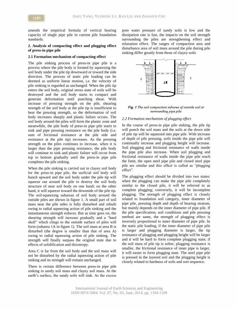
1105 JIAFU YANG, YUZHENG LV, KUN LIU AND ZHAOJUN CHU
International Journal of Earth Sciences and Engineering
ISSN 0974-5904, Vol. 07, No. 03, June, 2014, pp. 1104-1109
amends the empirical formula of vertical bearing
capacity of single pipe pile in current pile foundation
standards.
2. Analysis of compacting effect and plugging effect
of press-in pipe pile
2.1 Formation mechanism of compacting effect
The pile sinking process of press-in pipe pile is a
process where the pile body is formed by squeezing the
soil body under the pile tip downward or toward the side
direction. The process of static pile loading can be
deemed as uniform linear motion, i.e. the velocity of
pile sinking is regarded as unchanged. When the pile tip
enters the soil body, original stress state of soils will be
destroyed and the soil body starts to compact and
generate deformation until punching shear. With
increase of pressing strength on the pile, shearing
strength of the soil body at the pile tip is insufficient to
bear the pressing strength, so the deformation of soil
body increases sharply and plastic failure occurs. The
soil body around the piles will form the plastic zone and
meanwhile, the pile body of press-in pipe pile starts to
sink and pipe pressing resistance on the pile body (i.e.
sum of frictional resistance at the pile side and
resistance at the pile tip) increases. As the pressing
strength on the piles continues to increase, when it is
larger than the pipe pressing resistance, the pile body
will continue to sink and plastic failure will occur from
top to bottom gradually until the press-in pipe pile
completes the pile sinking.
When the pile sinking is carried out in clayey soil body
for the press-in pipe pile, the surficial soil body will
hunch upward and the soil body under the pile tip will
squeeze out around the pile to destroy the soil body
structure of near soil body on one hand; on the other
hand, it will squeeze toward the downside of the pile tip.
The soil-squeezing subareas of soil body around the
outside piles are shown in figure 1. A small part of soil
mass near the pile sides is fully disturbed and rebuilt
owing to radial squeezing action of pile sinking and the
instantaneous strength reduces. But as time goes on, the
shearing strength will increase gradually and a “hard
shell” which clings to the outside surface of piles will
form (subarea 1A in figure 1). The soil mass at area B is
disturbed (the degree is smaller than that of area A)
owing to radial squeezing action of pile sinking. The
strength will finally surpass the original state due to
effects of solidification and thixotropy.
Area C is far from the soil body and the soil mass will
not be disturbed by the radial squeezing action of pile
sinking and its strength will remain unchanged.
There is certain difference between press-in pipe pile
sinking in sandy soil mass and clayey soil mass. At the
earth’s surface, the sandy soils will sink. As the excess
pore water pressure of sandy soils is low and the
dissipation rate is fast, the impacts on the soil strength
surrounding the piles are strengthening effect and
relaxation effect. The ranges of compaction area and
disturbance area of soil mass around the pile during pile
sinking differ greatly from those of clayey soils
2.2 Formation mechanism of plugging effect
In the course of press-in pipe pile sinking, the pile tip
will punch the soil mass and the soils at the down side
of pile tip will be squeezed into pipe pile. With increase
of depth of pile pressing, soils inside the pipe pile will
continually increase and plugging height will increase.
Soil plugging and frictional resistance of walls inside
the pipe pile also increase. When soil plugging and
frictional resistance of walls inside the pipe pile reach
the limit, the open steel pipe pile and closed steel pipe
pile are similar and this effect is called as “plugging
effect”.
The plugging effect should be divided into two states:
when the plugging can make the pipe pile completely
similar to the closed pile, it will be referred to as
complete plugging; conversely, it will be incomplete
plugging. The strength of plugging effect is closely
related to foundation soil category, inner diameter of
pipe pile, pressing depth and depth of bearing stratum,
but mainly depends on the inner diameter of pipe pile. If
the pile specification, soil conditions and pile pressing
method are same, the strength of plugging effect is
inversely proportional to inner diameter of pipe pile. In
the static pile loading, if the inner diameter of pipe pile
is larger and plugging diameter is larger, the tip
resistance of plugging and plugging height will be larger
and it will be hard to form complete plugging state; if
the soil mass of pile tip is softer, plugging resistance is
smaller, the frictional resistance of inner pipe is larger,
it will easier to form plugging state. The steel pipe pile
is pressed in the layered soil and the plugging height is
closely related to hardness of soils and sort sequence.

1106
Discussion on Empirical Formula of Vertical Bearing Capacity of Single Press-in Pipe Pile
International Journal of Earth Sciences and Engineering
ISSN 0974-5904, Vol. 07, No. 03, June, 2014, pp. 1104-1109
3. Analysis of vertical bearing capacity of single
press-in pipe pile
3.1 Analysis of transfer process of vertical load of
press-in pipe pile
The ultimate bearing capacity of press-in pipe pile is
composed of frictional resistance of pile side and
resistance of pile tip. The vertical load on the tip will be
transferred to soils at surrounding pipe pile through
frictional resistance of pipe sides and gradually
transferred downward, leading to soil compaction of soil
mass at the bottom of pile tip, thus producing pile tip
resistance. The transfer process of vertical load of press-
in pipe pile is a process where the pile tip load is
undertaken by the frictional resistance at pile side and
pile tip resistance.
When the vertical load is gradually posed on the pile
tip, the upper pile body will produce compaction and
deformation and downward displacement relative to the
soils at the surrounding pile. The outside frictional
resistance will gradually play a role from top to bottom
and the pile load will be transferred to the soils around
the pile to reduce the pile load and pile compaction and
deformation with increase of depth. The outside
frictional resistance at original state of load imposing is
approximately linear to displacement. With increase of
vertical load of pile tip, the amount of compression and
relative displacement increase and the outside frictional
resistance at the bottom of pile will gradually play a
role. As the pile body and plugging form a whole and
there is no relative displacement, the inside frictional
resistance fails to play a role. When the outside
frictional resistance approaches the limit, the whole pile
body (including plugging) will sink with increase of
vertical load at pile tip and the relative replacement will
increase. The frictional resistance outside the pile plays
a role and the soils at the bottom of pile produced pile
tip resistance caused by compaction and react upon the
net area of pile tip. Meanwhile, the soils at the bottom
of pile squeeze into the pipe pile, causing relative
displacement between soil plug and inner wall of pipe
pile. The frictional force inside the pile plays a role
from top to bottom gradually. When the frictional
resistance outside the pile reaches the limit, the relative
displacement between pile and soil continues to
increase. Frictional resistance outside the pile remains
unchanged. The increment of vertical load at pile tip is
undertaken by pile tip resistance and frictional
resistance inside the pile. With increase of vertical load
at pile block, the frictional resistance inside the pile
gradually plays its role until reaching the limit and
remains unchanged. If the vertical load continues to
increase, the increment will be assumed by the pile tip
resistance until it reaches the limit or the soil body
deform and is not suitable for bearing the load. Then the
load borne by the pipe pile is the vertical ultimate
bearing capacity.
When the vertical load capacity acts upon the pile top,
the frictional resistance outside the pile and frictional
resistance inside the pile as well as pile tip resistance do
not play their roles simultaneously. Owing to soil plugs
inside the pile pipe, frictional resistance outside the pile
will reach the ultimate limit state before frictional
resistance inside the pile which reaches the limit state
prior to the pile tip resistance.
3.2 Impacts of plugging effect on vertical bearing
capacity of press-in pipe pile
Based on the analysis of formation mechanism of
compacting effect and plugging effect during press-in
pipe pile sinking, the soils at the press-in pipe pile tip
will move toward three directions: inwards the pipe pile,
outwards the pipe pile and downward the pipe tip.
The pipe tip soils squeezing into the pipe pile will form
soil plug, producing “plugging effect”. Without regard
to plugging effect and considering plugging effect, the
compositions of vertical bearing capacity of single
press-in pipe pile are shown in figure 2 (a) and (b).
(a) Without regard to
plugging effect
Fig. 1 The vertical bearing capacity of press-in
pipe pile
As shown in figure 2, no matter when the plugging
effect is considered or is not considered, the pile top
load is balanced by frictional resistance outside the
press-in pipe pile 1R , frictional resistance inside the
press-in pipe pile 2R and tip resistance of net area bpR ,
i.e. vertical bearing capacity of single press-in pipe
pile uR is composed of frictional resistance outside the
press-in pipe pile 1R , frictional resistance inside the
press-in pipe pile 2R and tip resistance of net area bpR .
However, there is significant difference between the
cases where frictional resistance inside the press-in pipe
pile is considered and not considered. When the
plugging effect is not considered, the frictional
1107 JIAFU YANG, YUZHENG LV, KUN LIU AND ZHAOJUN CHU
International Journal of Earth Sciences and Engineering
ISSN 0974-5904, Vol. 07, No. 03, June, 2014, pp. 1104-1109
resistance inside the press-in pipe pile is frictional
resistance from inner walls and soils inside the pipe pile
and plays its role with frictional resistance outside the
press-in pipe pile; when the plugging effect is taken into
consideration, the frictional resistance inside the press-
in pipe pile is frictional resistance from inner walls and
soil plug and plays its role when the frictional resistance
outside pipe pile approaches the limit.
When the plugging effect is not considered, the
calculation formula of vertical bearing capacity of
single press-in pipe pile is shown in formula (1):
paisiaisia
ppaisiaisia
bpu
qddlqdlqd
Aqlqulqu
RRRR
)(4
2
12
1
21
21
(1)
Therein: 1u and 2u peripheral length—peripheral length
outside the press-in pipe pile and peripheral length
inside the press-in pipe pile;
siaq —ultimate collateral resistance of soils at i
layer;
paq —ultimate tip resistance of bearing stratum;
pA —pile tip net area;
il —thickness of soils at i layer;
d、1d —outer diameter and inner diameter of
press-in pipe pile.
When the plugging effect is considered, the calculation
formula of vertical bearing capacity of single press-in
pipe pile is shown in formula (2):
pasaisia
ppasaisia
bpu
qddhqdlqd
Aqhqulqu
RRRR
)(4
2
12
1
21
21
(2)
Therein: saq —weighted collateral resistance of soil
plug;
h —height of soil plug
3.3 Impacts of compacting effect on vertical bearing
capacity of press-in pipe pile
When soils at pile tip squeeze outwards the pile,
compacting effect will occur. The soils surrounding the
pile will produce compaction displacement and become
denser and have more strength. The frictional resistance
outside the pile increases. When soils at pile tip squeeze
downward the pile tip, the pile tip compacting effect
will occur. The soils under the pile tip will produce
compaction displacement and become denser and
impose compacting effect on the foundation soils to
cause larger bearing capacity on the foundation. The
pile tip resistance will also increase. Therefore, when
calculating vertical bearing capacity of press-in pipe
pile, we should not only take plugging effect into
consideration, but also consider the compacting effect.
In order to consider the impacts of compacting effect
on vertical bearing capacity of single press-in pipe pile,
pile side compacting effect coefficient 1 and pipe tip
compacting effect coefficient 2 are introduced. The
frictional resistance outside the pile in formula (2) and
pile tip resistance are revised as shown in formula (3):
pasaisia
ppasaisia
bpu
qddhqdlqd
Aqhqulqu
RRRR
2
2
12
11
2211
21
)(4
(3)
There are multiple factors impacting height of soil
plug h , mainly including inner diameter of pipe pile,
characteristic value of pipe tip resistance, characteristic
value of soil plug and inner wall of pipe pile and depth
of pile tip in bearing stratum. According to analysis of
formation mechanism of plugging effect during press-in
pipe pile sinking, height of soil plug h is in direct
proportion to characteristic value of pipe tip resistance,
characteristic value of soil plug and inner wall of pipe
pile and depth of pile tip in bearing stratum and is
inversely proportional to characteristic value of
frictional resistance inside the soil plug. After referring
to related materials, the value of height of soil
plug h can be obtained as formula (4):
sa
pap
q
qdh
4
1 (4)
Therein: p —pile tip plugging effect coefficient and is
valued as 1 for closed-end pipe pile and is
valued according to formula (5) for open-
end pipe pile.
5,8.0
5,16.0
1
1
dh
dhd
h
b
bb
p
(5)
Therein: bh — the depth of pile tip in bearing stratum
Substitute formula (4) into formula (3) and the vertical
bearing capacity of single press-in pipe pile considering
plugging effect and compacting effect is shown in
formula (6):

1108
Discussion on Empirical Formula of Vertical Bearing Capacity of Single Press-in Pipe Pile
International Journal of Earth Sciences and Engineering
ISSN 0974-5904, Vol. 07, No. 03, June, 2014, pp. 1104-1109
pappaisia
sa
papsapaisia
pasaisiau
qd
qddlqd
q
qdqdqddlqd
qddhqdlqdR
4)(
4
4)(
4
)(4
2
12
2
12
1
112
2
12
1
2
2
12
11
(6)
After analysis of formula (6), the vertical bearing
capacity of single press-in pipe pile is made of three
contents: frictional resistance outside the press-in pipe
pile when the pile side compacting effect is considered;
tip resistance at pile tip net area when the pile tip
compacting effect is considered; tip resistance at pile tip
exposure area converted by frictional resistance inside
the press-in pipe pile when the plugging effect is
considered.
3.4 Comparison with empirical formula of vertical
bearing capacity of single concrete hollow pile in
Technical Code for Building Pile Foundations
Technical Code for Building Pile Foundations (JGJ94-
2008) stipulates that: when vertical bearing capacity of
single concrete hollow pile is determined by empirical
relation between physical property index of soils and
bearing capacity parameters, the calculation can be
carried out according to formula (7):
pappaisia
ppjpaisia
psu
qd
qddlqd
AAqlqu
RRR
44
)(2
121
2
1
(7)
Therein: u —peripheral length outside the press-in pipe
pile;
jA —pile tip net area of concrete hollow pile;
1pA —exposure area of concrete hollow pile.
Comparing formula (6) with formula (7), the calculation
of vertical bearing capacity of concrete hollow pile
according to formula (7) only considers impact of
plugging effect and neglects impact of compacting
effect.
In JGJ94-2008, empirical formula of vertical bearing
capacity of single concrete hollow pile is shown in
formula (8):
pappaisia
ppjpaisia
psu
qd
qddlqd
AAqlqu
RRR
44
)(2
121
21
1
(8)
Comparing formula (6) and (7) with formula (8), the
calculation of vertical bearing capacity of single
concrete hollow pile based on formula (8) considers
impact of pile side compacting effect but neglects
impact of pile tip compacting effect on the basis of
formula (7).
4. Conclusion
During press-in pipe line sinking, the soils at pile tip
will move toward three directions: one is inner side of
pipe pile, forming “plugging effect” and impacting the
frictional resistance inside the pile; the other one is
outside pile, forming “compacting effect” and impacting
frictional resistance outside the pile; the last one is at the
bottom of pile tip, forming “compacting effect” and
impacting pile tip resistance. Therefore, when
calculating vertical bearing capacity of single press-in
pipe pile, it is necessary to consider the impacts of
plugging effect and compacting effect. This article took
both plugging effect and compacting effect into
consideration and introduced pile side compacting effect
coefficient 1 , pile tip compacting effect coefficient 2
and pile tip plugging effect p into consideration and
empirical formula of vertical bearing capacity of
concrete single hollow pile in Technical Code for
Building Pile Foundations is revised.
The values of coefficients of 1 , 2 and p are
researched according to model test, field test, theoretical
analysis and numerical modeling. But there are multiple
reasons impacting plugging effect and compacting
effect in the course of pipe pile sinking, such as size of
outside and inside diameters of pile, depth of bearing
stratum, physical and chemical properties of bearing
stratum, pressing velocity, roughness of inner wall of
pile. It will be difficult to consider impacts of the
following factors dividually. So it has an important
practical significance to find a way to determine values
of 1 , 2 and p efficiently.
5. Reference:
[1] ZENG Guoxi, Feng Guodong et al. Pile Foundation
Engineering Manual [M]. Beijing: China Building
Industry Press, 1995.
[2] Akio Kitamura. Construction Revolution [M]
Japan: Giken Seisakusho Co., Ltd., 2006: 22-35.
[3] Yukihiro Ishihara. The Press-in Method: A
Construction Solution for Urban Development [J]
Chinese Journal of Underground Space and
Engineering, 2010, 6(2): 1707-1708. (In Chinese)
[4] Advantages of Press-in Method [EB/OL].
www.giken.net. cn/st/index.html, 2010-11-20
[5] Akio Kitamura. Silent Piling Technologies [M]
Japan: Giken Seisakusho Co., Ltd., 2008.
[6] CHU Zhaojun, LU Xin, DING Zhenzhou. Analysis
on Deformation of Soil at Surrounding Pile Due to
Press-in Piling in Layered Ground[J]. Journal of
1109 JIAFU YANG, YUZHENG LV, KUN LIU AND ZHAOJUN CHU
International Journal of Earth Sciences and Engineering
ISSN 0974-5904, Vol. 07, No. 03, June, 2014, pp. 1104-1109
logistical engineering university, 2012, 28(1): 16-
21. (In Chinese)
[7] Du Laibin. Brief Analysis of Plug Effect of PHC
Pipe Piles [J] Industrial Construction, 2005, 35
(Supplement): 590-594. (In Chinese)
[8] LIU Zengrong, DU Lihu. Analysis on Ultimate
Bearing Capacity of Single Pipe Pile of Open-end
Prestressed Concrete Pipe Pile [J] Concrete, 2012,
(3): 120-123. (In Chinese)
[9] LI Qi, LI Song, FEI Kang. Analysis on Soil
Plugging Effect of PHC Pipe Pile [J] Journal of
Water Resources and Architectural Engineering,
2009, 7(2): 45-47. (In Chinese)
[10] SHI Feng. Experimental Research on Load Transfer
Mechanism of Pretensioned High Strength Spun
Concrete Piles [J]. Chinese Journal of Geotechnical
Engineering, 2004, 26(1): 95 99. (In Chinese)
[11] FEI Kang, LIU Hanlong, GAO Yufeng, et al. Load
Transfer Mechanism for Field Pour Concrete Thin
Wall Cased Pile (PCC) [J]. Rock and Soil
Mechanics, 2004, 25(5): 764-768. (In Chinese)
[12] Luo Zhanyou, Tong Jianer, Gong Xiaonan. Study
on Compacting Effects of Jacked pile in the
Condition of Prebored Hole and Tubular Pile [J].
Ground Improvement, 2005, 16(1):3-8. (In
Chinese)
[13] PENG Jie, SHI Jianyong, HUANG Gang. Analysis
of Bearing Capacity of Pile Foundation in
Consideration of Compaction Effect [J] Journal of
Hehai University, 2002, 30(2): 105-108. (In
Chinese)
[14] JGJ94-2008, Technical Code for Building Pile
Foundations[S]. Beijing: China Building Industry
Press, 2008.
[15] JGJ94-94, Technical Code for Building Pile
Foundations[S]. Beijing: China Building Industry
Press, 1994.
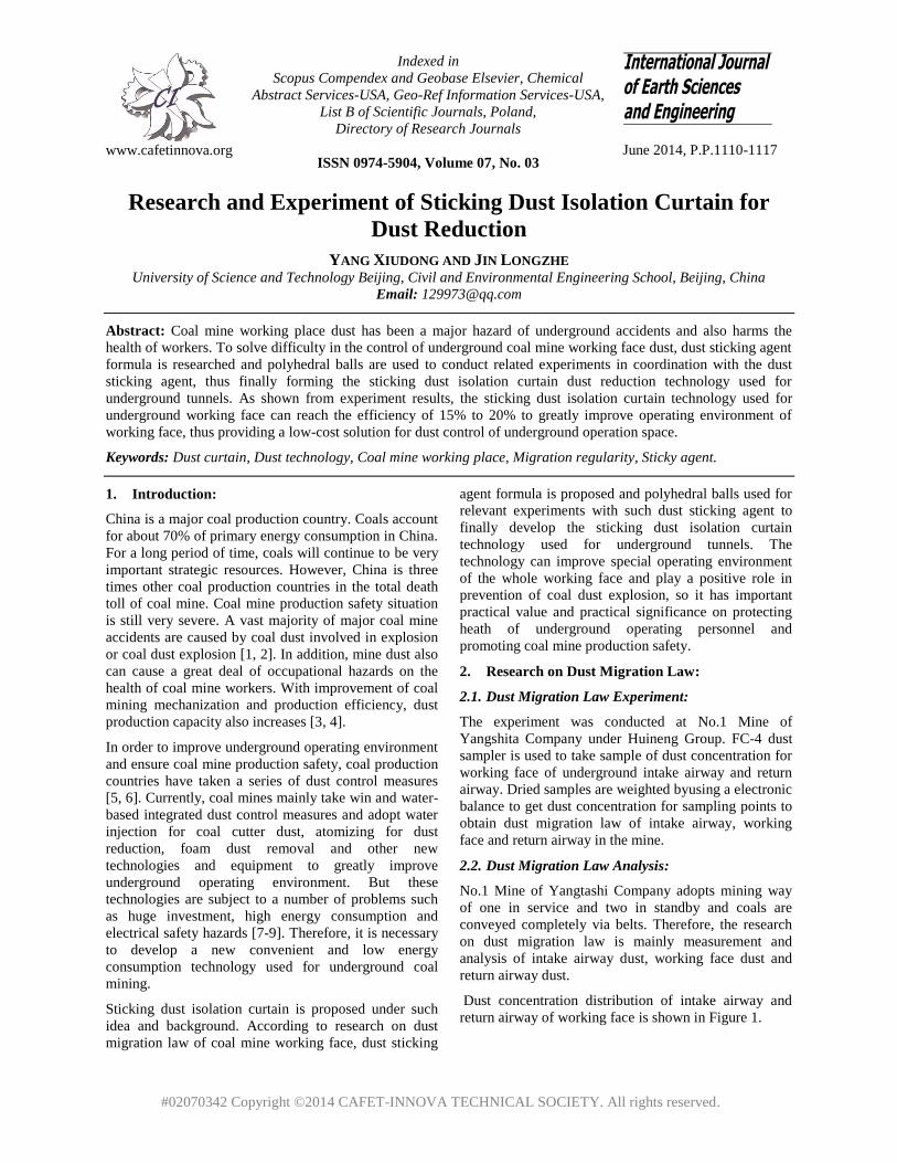
www.cafetinnova.org
Indexed in
Scopus Compendex and Geobase Elsevier, Chemical
Abstract Services-USA, Geo-Ref Information Services-USA,
List B of Scientific Journals, Poland,
Directory of Research Journals
ISSN 0974-5904, Volume 07, No. 03
June 2014, P.P.1110-1117
#02070342 Copyright ©2014 CAFET-INNOVA TECHNICAL SOCIETY. All rights reserved.
Research and Experiment of Sticking Dust Isolation Curtain for
Dust Reduction
YANG XIUDONG AND JIN LONGZHE University of Science and Technology Beijing, Civil and Environmental Engineering School, Beijing, China
Email: [email protected]
Abstract: Coal mine working place dust has been a major hazard of underground accidents and also harms the
health of workers. To solve difficulty in the control of underground coal mine working face dust, dust sticking agent
formula is researched and polyhedral balls are used to conduct related experiments in coordination with the dust
sticking agent, thus finally forming the sticking dust isolation curtain dust reduction technology used for
underground tunnels. As shown from experiment results, the sticking dust isolation curtain technology used for
underground working face can reach the efficiency of 15% to 20% to greatly improve operating environment of
working face, thus providing a low-cost solution for dust control of underground operation space.
Keywords: Dust curtain, Dust technology, Coal mine working place, Migration regularity, Sticky agent.
1. Introduction:
China is a major coal production country. Coals account
for about 70% of primary energy consumption in China.
For a long period of time, coals will continue to be very
important strategic resources. However, China is three
times other coal production countries in the total death
toll of coal mine. Coal mine production safety situation
is still very severe. A vast majority of major coal mine
accidents are caused by coal dust involved in explosion
or coal dust explosion [1, 2]. In addition, mine dust also
can cause a great deal of occupational hazards on the
health of coal mine workers. With improvement of coal
mining mechanization and production efficiency, dust
production capacity also increases [3, 4].
In order to improve underground operating environment
and ensure coal mine production safety, coal production
countries have taken a series of dust control measures
[5, 6]. Currently, coal mines mainly take win and water-
based integrated dust control measures and adopt water
injection for coal cutter dust, atomizing for dust
reduction, foam dust removal and other new
technologies and equipment to greatly improve
underground operating environment. But these
technologies are subject to a number of problems such
as huge investment, high energy consumption and
electrical safety hazards [7-9]. Therefore, it is necessary
to develop a new convenient and low energy
consumption technology used for underground coal
mining.
Sticking dust isolation curtain is proposed under such
idea and background. According to research on dust
migration law of coal mine working face, dust sticking
agent formula is proposed and polyhedral balls used for
relevant experiments with such dust sticking agent to
finally develop the sticking dust isolation curtain
technology used for underground tunnels. The
technology can improve special operating environment
of the whole working face and play a positive role in
prevention of coal dust explosion, so it has important
practical value and practical significance on protecting
heath of underground operating personnel and
promoting coal mine production safety.
2. Research on Dust Migration Law:
2.1. Dust Migration Law Experiment:
The experiment was conducted at No.1 Mine of
Yangshita Company under Huineng Group. FC-4 dust
sampler is used to take sample of dust concentration for
working face of underground intake airway and return
airway. Dried samples are weighted byusing a electronic
balance to get dust concentration for sampling points to
obtain dust migration law of intake airway, working
face and return airway in the mine.
2.2. Dust Migration Law Analysis:
No.1 Mine of Yangtashi Company adopts mining way
of one in service and two in standby and coals are
conveyed completely via belts. Therefore, the research
on dust migration law is mainly measurement and
analysis of intake airway dust, working face dust and
return airway dust.
Dust concentration distribution of intake airway and
return airway of working face is shown in Figure 1.
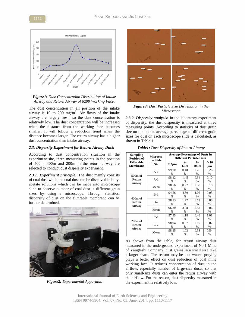
1111 YANG XIUDONG AND JIN LONGZHE
International Journal of Earth Sciences and Engineering
ISSN 0974-5904, Vol. 07, No. 03, June, 2014, pp. 1110-1117
Dust Migration Law Diagram
0
50
100
150
200
250
Air intake
200m
from
air intake
400m
from
air intake
600m
from
air intake
Coa
l cutter h
ead
Coa
l cutter w
orking
face
Coa
l cutter tail
500m
from
air ou
tlet
400m
from
air ou
tlet
300m
from
air ou
tlet
200m
from
air ou
tlet
Distance
Dust
concentr
ation(mg/m3)
```
Figure1: Dust Concentration Distribution of Intake
Airway and Return Airway of 6299 Working Face.
The dust concentration in all position of the intake
airway is 10 to 200 mg/m3. Air flows of the intake
airway are largely fresh, so the dust concentration is
relatively low. The dust concentration will be increased
when the distance from the working face becomes
smaller. It will follow a reduction trend when the
distance becomes larger. The return airway has a higher
dust concentration than intake airway.
2.3. Dispersity Experiment for Return Airway Dust:
According to dust concentration situation in the
experiment site, three measuring points in the position
of 500m, 400m and 200m in the return airway are
selected to conduct dust dispersity experiment.
2.3.1. Experiment principle: The dust mainly consists
of coal dust while the coal dust can be dissolved in butyl
acetate solutions which can be made into microscope
slide to observe number of coal dust in different grain
sizes by using a microscope. Through statistics,
dispersity of dust on the filterable membrane can be
further determined.
Figure2: Experimental Apparatus
Figure3: Dust Particle Size Distribution in the
Microscope
2.3.2. Dispersity analysis: In the laboratory experiment
of dispersity, the dust dispersity is measured at three
measuring points. According to statistics of dust grain
size on the photo, average percentage of different grain
sizes for dust on each microscope slide is calculated, as
shown in Table 1.
Table1: Dust Dispersity of Return Airway
Sampling
Position of
Filterable
Membrane
Microsco
pe Slide
No.
Average Percentage of Dusts in
Different Particle Sizes
<2μm 2-
6μm
6-
10μm
>10
μm
500m of
Return
Airway
A-1 99.00
%
0.48
%
0.25
%
0.26
%
A-2 98.12
% 1.45%
0.34%
0.10%
Mean 98.56
%
0.97
%
0.30
%
0.18
%
400m of Return
Airway
B-1 94.26
% 4.69%
1.02%
0.03%
B-2 98.33
%
1.47
%
0.12
%
0.08
%
Mean 96.30
% 3.08%
0.57%
0.06%
200m of
Return
Airway
C-1 97.35
%
1.18
%
0.46
%
1.01
%
C-2 98.94
% 0.87%
0.19%
0.07%
Mean 98.15
%
1.03
%
0.33
%
0.54
%
As shown from the table, for return airway dust
measured in the underground experiment of No.1 Mine
of Yangtashi Company, dust grains in a small size take
a larger share. The reason may be that water spraying
plays a better effect on dust reduction of coal mine
working face. It reduces concentration of dust in the
airflow, especially number of large-size dusts, so that
only small-size dusts can enter the return airway with
the airflow. For the reason, dust dispersity measured in
the experiment is relatively low.

1112 Research and Experiment of Sticking Dust Isolation Curtain for Dust Reduction
International Journal of Earth Sciences and Engineering
ISSN 0974-5904, Vol. 07, No. 03, June, 2014, pp. 1110-1117
3. Research on Main Formula of Sticking Agent:
Dust sticking agent is mainly made of surfactants. The
surfactant refers to the substance which has fixed
hydrophilic and lipophilic groups arranged directionally
on the solution surface to significantly reduce surface
tension [10, 11]. Therefore, surfactant solution can be
used to reduce water surface tension and generate
foaming effects. It can be made into dust sticking agent
and stunk on the dust isolation curtain to bond
underground dusts (mainly consisting of coal dust), thus
significantly reducing dusts.
According to actual needs and market availability of
surfactants, six kinds of common surfactants are
selected for research, including OP-10, triton X-100,
dodecylbenzene sulfonic acid (LAS), sodium dodecyl
benzene sulfonate, sodium lauryl sulfate and sodium
alcohol ether sulphate (AES).
3.1. Surfactant Wetting Experiment:
Wetting performance of surfactant solution on coal dust
is measured in the coal dust sedimentation experiment
mainly by sedimentation method specified in the
MT506 - 19965 Mine Dust Reduction Agent
Performance Measurement Method.
Wetting performance of surfactant solution on coal dust
is measured mainly in the coal dust sedimentation
experiment. If the coal dust sedimentation time is
shorter, wetting performance of coal dust in the
surfactant solution will be better; otherwise, wetting
performance of coal dust will be reduced.
Figure4: Coal Dust Sample Sedimentation
As shown from Figure 4, sedimentation time of coal
dust in the surfactant solution of 1% is measured. Its
statistics and analysis are shown in Figure 5.
Average sedimentation time of coal dust in surfactant solution of 1%
Aver
age
sedim
enta
tion tim
e /s
Sodium
alco
hol e
ther su
lpha
te (A
ES)
DOde
cyl b
enze
ne su
lfona
te
Sodium
dod
ecyl su
lfate
OP-
10
Triton
X-1
00
Dod
ecylbe
nzen
e sulfonic a
cid (L
AS)
Surfactant solution of 1%
Figure5: Sedimentation Experiment for Coal Dust in
Surfactant Solution of 1%
As shown from Figure 5, sedimentation time for coal
dust in surfactant solution of 1% follows the following
sequence: OP-10> sodium alcohol ether sulphate
(AES)> dodecylbenzene sulfonic acid (LAS)> dodecyl
benzene sulfonate> triton X-100> sodium dodecyl
sulfate. Therefore, triton X-100 and sodium dodecyl
sulfate can provide the better wetting performance.
3.2. Determination of Surfactant Surface Tension:
When dust suppressant can wet coal dusts, its surface
tension will be lower than water surface tension. Its
wetting performance will get better if the surface
tension is reduced. Surface tension for surfactant
solution of 0.1% is determined mainly by using BZY-
201 automatic surface tensiometer.
Determination results are shown in Figure 6.
As shown from Figure 6, all surfactant solutions of
0.1% have an ideal surface tension value of 20 to 40
mN•m-1, indicating surfactant solutions can wet coal
dusts to get the better dust suppression effect.
The experiment shows that, triton X-100, sodium lauryl
sulfate and sodium alcohol ether sulphate (AES) can be
taken as auxiliary materials for dust sticking agents to
provide a better effect; triton X-100 can provide the bets
effect, followed by OP-10, sodium dodecyl benzene
sulfonate and sodium alcohol ether sulphate (LAS).
Surface tension of surfactant solution of 0.1%
Surf
ace tensi
on m
N/m
Deion
ized
water
OP-
10
Dod
ecylbe
nzen
e sulfonic a
cid (L
AS)
Sodium
dod
ecyl su
lfate
Dod
ecyl ben
zene
sulfo
nate
Surfactant solution of 0.1%
sodium
alco
hol e
ther su
lpha
te (A
ES)
Trito
n X-100
Figure6: Determination of Surface Tension for
Surfactant Solution of 0.1%

1113 YANG XIUDONG AND JIN LONGZHE
International Journal of Earth Sciences and Engineering
ISSN 0974-5904, Vol. 07, No. 03, June, 2014, pp. 1110-1117
As shown from Figure 6, all surfactant solutions of
0.1% have an ideal surface tension value of 20 to 40
mN•m-1
, indicating surfactant solutions can wet coal
dusts to get the better dust suppression effect.
The experiment shows that, triton X-100, sodium lauryl
sulfate and sodium alcohol ether sulphate (AES) can be
taken as auxiliary materials for dust sticking agents to
provide a better effect; triton X-100 can provide the bets
effect, followed by OP-10, sodium dodecyl benzene
sulfonate and sodium alcohol ether sulphate (LAS).
4. Experimental Research on Field Dust Removal
Efficiency of Dust Isolation Curtain:
4.1. Field Experiment of Dust Isolation Curtain:
Dust control principle of the dust isolation curtain is that
dust particles are collected by effective collision
between dust particles and polyhedral ball blades and
dust sticking agent adsorption to reduce dusts. For this
reason, dust removal efficiency of the dust isolation
curtain may be associated with specific surface area of
polyhedral balls (size), curtain layer number and relative
position, dust sticking agent and other factors.
In order to study influencing factors of dust removal
efficiency for dust isolation curtain, a field experiment
of the dust isolation curtain is conducted in the return
airway of underground working face in the mine of
Yangshita Company. Polyhedral balls in two sizes are
selected for this experiment. The polyhedral ball in a
larger size is at the diameter of 50mm, specific surface
area of 236m2/m
3 and porosity of 85%; the polyhedral
ball in a smaller size is at the diameter of 38mm,
specific surface area of 300m2/m
3 and porosity of 90%,
as shown in the Figure 7.
Figure7: Scattered Small Polyhedral Balls
Polyhedral balls are collected with an engineering line
to form a dust isolation curtain. According to
measurement experiment of roadway at the sectional
dimension of 3.3m high and 5.2m wide, a small ball
curtain section needs about 120 small ball strings and
each string needs about 90 small balls; a large ball
curtain section needs about 80 large ball strings and
each string needs about 68 large balls, as shown in
Figure 8.
Figure8: Preliminarily Connected Curtain Strips of
Dust Isolation Curtain
Four sections are suspended in the experiment, of which
two are made of small balls and the other two made of
large balls. Balls are connected on the ground, packed in
sacks for loading and then transported to underground
return airway experiment position. It is required to hook
a section of curtain string by using a prefabricated
curved hook, lift it on the roadway roof anchor net and
then vertically hang it. No.1 large ball curtain, No.2
large ball curtain, No.1 small ball curtain and No.2 ball
curtain are hung successively along airflow direction at
the interval of 20m and wait for some time before
conducting the experiment. The dust isolation curtain
hung is shown in Figure 9.
Figure9: Dust Isolation Curtain Hung
After four dust isolation curtains are hung, successively
select sampling points along the airflow direction.
Sampling points are selected in a position 10m from the
large ball curtain in the upwind and downwind. Two
experimenters simultaneously start dust samplers to take
samples for 5min with a preset flow rate of 20L/min to
get the dust concentration before and after the dust runs
through a layer of large ball curtain, thus obtaining dust
removal efficiency for a layer of large ball curtain by
calculation. In such a way, the dust removal efficiency
can be calculated for curtains of one small ball layer,
two large ball layers, two small ball layers, one large
ball layer and one small ball layer, two large ball layers
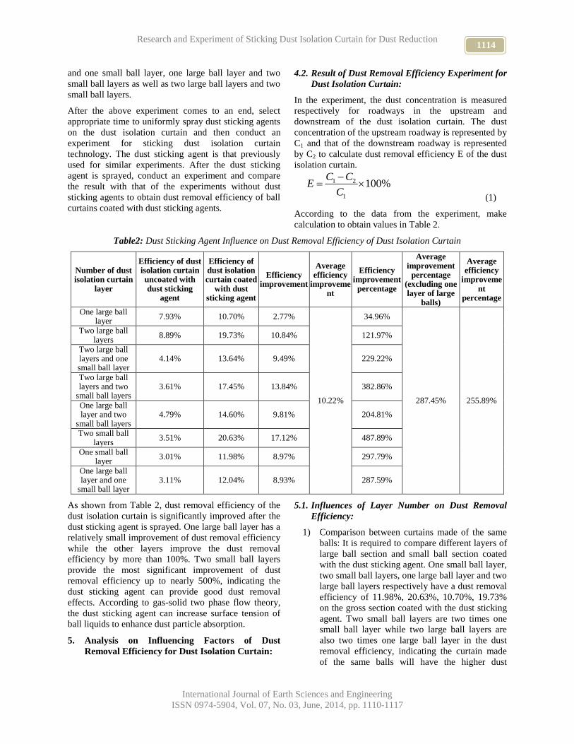
1114 Research and Experiment of Sticking Dust Isolation Curtain for Dust Reduction
International Journal of Earth Sciences and Engineering
ISSN 0974-5904, Vol. 07, No. 03, June, 2014, pp. 1110-1117
and one small ball layer, one large ball layer and two
small ball layers as well as two large ball layers and two
small ball layers.
After the above experiment comes to an end, select
appropriate time to uniformly spray dust sticking agents
on the dust isolation curtain and then conduct an
experiment for sticking dust isolation curtain
technology. The dust sticking agent is that previously
used for similar experiments. After the dust sticking
agent is sprayed, conduct an experiment and compare
the result with that of the experiments without dust
sticking agents to obtain dust removal efficiency of ball
curtains coated with dust sticking agents.
4.2. Result of Dust Removal Efficiency Experiment for
Dust Isolation Curtain:
In the experiment, the dust concentration is measured
respectively for roadways in the upstream and
downstream of the dust isolation curtain. The dust
concentration of the upstream roadway is represented by
C1 and that of the downstream roadway is represented
by C2 to calculate dust removal efficiency E of the dust
isolation curtain.
1 2
1
100%C C
EC
(1)
According to the data from the experiment, make
calculation to obtain values in Table 2.
Table2: Dust Sticking Agent Influence on Dust Removal Efficiency of Dust Isolation Curtain
Number of dust isolation curtain
layer
Efficiency of dust isolation curtain uncoated with dust sticking
agent
Efficiency of dust isolation curtain coated
with dust sticking agent
Efficiency improvement
Average efficiency
improvement
Efficiency improvement
percentage
Average improvement
percentage (excluding one layer of large
balls)
Average efficiency
improvement
percentage
One large ball layer
7.93% 10.70% 2.77%
10.22%
34.96%
287.45% 255.89%
Two large ball layers
8.89% 19.73% 10.84% 121.97%
Two large ball layers and one small ball layer
4.14% 13.64% 9.49% 229.22%
Two large ball layers and two
small ball layers 3.61% 17.45% 13.84% 382.86%
One large ball layer and two
small ball layers 4.79% 14.60% 9.81% 204.81%
Two small ball layers
3.51% 20.63% 17.12% 487.89%
One small ball layer
3.01% 11.98% 8.97% 297.79%
One large ball layer and one
small ball layer 3.11% 12.04% 8.93% 287.59%
As shown from Table 2, dust removal efficiency of the
dust isolation curtain is significantly improved after the
dust sticking agent is sprayed. One large ball layer has a
relatively small improvement of dust removal efficiency
while the other layers improve the dust removal
efficiency by more than 100%. Two small ball layers
provide the most significant improvement of dust
removal efficiency up to nearly 500%, indicating the
dust sticking agent can provide good dust removal
effects. According to gas-solid two phase flow theory,
the dust sticking agent can increase surface tension of
ball liquids to enhance dust particle absorption.
5. Analysis on Influencing Factors of Dust
Removal Efficiency for Dust Isolation Curtain:
5.1. Influences of Layer Number on Dust Removal
Efficiency:
1) Comparison between curtains made of the same
balls: It is required to compare different layers of
large ball section and small ball section coated
with the dust sticking agent. One small ball layer,
two small ball layers, one large ball layer and two
large ball layers respectively have a dust removal
efficiency of 11.98%, 20.63%, 10.70%, 19.73%
on the gross section coated with the dust sticking
agent. Two small ball layers are two times one
small ball layer while two large ball layers are
also two times one large ball layer in the dust
removal efficiency, indicating the curtain made
of the same balls will have the higher dust

1115 YANG XIUDONG AND JIN LONGZHE
International Journal of Earth Sciences and Engineering
ISSN 0974-5904, Vol. 07, No. 03, June, 2014, pp. 1110-1117
removal efficiency if its layers are more and the
efficiency is approximately proportional to the
number of layers.
2) Comparison between curtains made of different
balls: It is required to compare curtains made of
different balls in the dust removal efficiency on
the section coated with the dust sticking agent.
Two-layer curtain made of one small ball layer
and one large ball layer, three-layer curtain made
of two large ball layers and one small ball layer,
three-layer curtain made of two small ball layers
and one large ball layer and four-layer curtain
made of two large ball layers and small ball
layers respectively reach the dust removal
efficiency of 12.04%, 13.64%, 14.60% and
17.45% and the efficiency increases with the
number of layers.
Dust removal efficiency of the dust isolation curtain
increases with the number of layers, because more
layers can improve coal dust collection probability to
increase collisions between coal dust and balls.
5.2. Influences of Ball Size on Dust Removal
Efficiency:
Curtains made of different balls in the same layers are
compared in the dust removal efficiency as follows:
For one-layer curtains, large ball curtain and small ball
curtain respectively reach the dust removal efficiency of
10.70% and 11.98%, indicating the small ball curtain
can provide a better effect than the large ball curtain.
For two-layer curtains, large ball curtain, small ball
curtain and combined curtain respectively reach the dust
removal efficiency of 19.73%, 20.73% and 12.04%,
indicating the small ball curtain can provide a better
effect than the large ball curtain. For three-layer
combined curtains, the combined curtain made of two
large ball layers and one small ball layer and that made
of two small ball layers and one large ball layer
respectively reach the dust removal efficiency of
13.64% and 14.60%, indicating the combined curtain
provides the higher efficiency.
5.3. Change of Sticking Agent Dust Removal
Efficiency with Time:
The dust sticking agent can improve dust removal
efficiency of the dust isolation curtain, but it will be
reduced when absorbing coal dusts. Its dust removal
efficiency will decline with the time. For the reason,
dust sticking agents shall be timely added within a
certain time but frequent addition will cause cost
increase. Therefore, appropriate adding interval shall be
selected to reach the best level of cost and efficiency.
In this experiment, curtains hung for different days are
selected to calculate the dust removal efficiency in order
to study the change of dust removal effect with the time.
Dust reduction experiment is conducted for the curtain
made of two large ball layers, that made of one small
ball layer, that made of two small ball layers, that made
of two large ball layers and one small ball layer, that
made of two large ball layers and two small ball layers,
that made of one large ball layer and two small ball
layers and that made of one large ball layer and one
small ball layer just coated with the dust sticking agent
and those coated with the dust sticking agent for one
day. Its data is processed to calculate the dust removal
efficiency of curtains just coated with the dust sticking
agent and those coated with the dust sticking agent for
one day, as shown in Table 3.
It can be seen that, dust removal efficiency of dust
sticking agent coated curtains gradually declines with
the time. The dust removal efficiency of all curtains can
decline by more than 10% in one day. The curtain made
of two small ball layers provide the largest decline up to
nearly 50% while the curtain made of two large ball
layers and one small ball layer provide the smallest
decline of 10%.
Then, dust removal efficiency of curtains uncoated with
dust sticking agent and that of those just coated with
dust sticking agent are used to calculate the decline of
dust removal efficiency from coating to loss of dust
sticking agent effect. Calculation formula is shown as
follows:
Table3: Change of Dust Removal Effect of Dust Sticking Agent Coated Dust Isolation Curtain with Time
Number of dust isolation curtain layer
0 day One day
Dust reduction
effect decline
Average dust reduction effect
decline
Dust reduction effect decline percentage
Average dust reduction effect
decline percentage
Two large ball layers 12.99% 10.70% 2.29%
4.50%
17.63%
26.32%
Two large ball layers and one small ball layer
19.73% 11.95% 7.78% 39.44%
One large ball layer and one small ball layer
13.64% 12.27% 1.37% 10.02%
One large ball layer and two small ball layers
12.04% 10.13% 1.91% 15.87%
Two small ball layers 14.60% 10.19% 4.41% 30.21%
One large ball layer 20.63% 11.39% 9.24% 44.77%
1116 Research and Experiment of Sticking Dust Isolation Curtain for Dust Reduction
International Journal of Earth Sciences and Engineering
ISSN 0974-5904, Vol. 07, No. 03, June, 2014, pp. 1110-1117
1 2
1
( )100%
E E
E
(2)
Where, E1 is the dust removal efficiency of dust
isolation curtain just coated with dust sticking agent, E2
is the dust removal efficiency of dust isolation curtain
uncoated with dust sticking agent and ω is the decline of
the dust removal efficiency at loss of dust sticking agent
effect.
According to dust removal efficiency decline at loss of
dust sticking agent effect and that of curtains coated for
one day, effective period of dust sticking agent can be
calculated by the following formula:
1
D
(3)
Where, ω is dust removal efficiency decline at loss of
dust sticking agent effect and ω1 is that of curtains
coated with the dust sticking agent for one day.
Combined sticking dust isolation curtains have a
different effective period. The dust sticking agent can be
effective in the maximum time of seven days and
minimum time of one day, indicating effectiveness of
the dust sticking agent is unstable. The possible reason
is that the dust sticking agent is coated on each layer
and four layers are mutually independent in the
effectiveness of the dust sticking agent, but the
experiment adopts the method of mixed layer number
and measurement in groups for measurement of dust
removal efficiency. It causes a difference of effective
period between combined sticking dust isolation
curtains.
On the whole, average effective period of combined
sticking dust isolation curtains is 3.2 days. It can be
indicated that, dust isolation curtains coated with the
dust sticking agent can reach average effective period of
three days. After three days, dust isolation curtains need
to be cleaned and recoated with the dust sticking agent
to re-obtain high dust removal efficiency.
6. Conclusion:
Feasibility of sticking dust isolation curtain technology
is studied according to the research on migration law of
dusts from the upstream to the downstream of the
working face in No.1 Mine of Yangtashi Companny,
experimental determination of wetting and surface
tension for six kinds of surfactants and field experiment
for sticking dust isolation curtain technology. The
conclusion is reached as followed:
1) A shown from experiment research on six kinds of
surfactants including OP-10, triton X-100,
dodecylbenzene sulfonic acid (LAS), sodium
dodecyl benzene sulfonate, sodium lauryl sulfate
and sodium alcohol ether sulphate (AES), triton X-
100 and sodium lauryl sulfate can be taken as
auxiliary materials for dust sticking agents to
provide a better effect; triton X-100 can provide the
bets effect, followed by OP-10, sodium dodecyl
benzene sulfonate and sodium alcohol ether
sulphate (LAS).
2) According to field sampling measurement and
analysis, the dust concentration near the coal mine
working face in No.1 Mine of Yangtashi Company
is relatively low on the whole and it can be up to
200mg/m3. The dust concentration will be higher
when getting closer to the working face; it will
decline when getting away from the working face;
the return airway is higher than the intake airway in
the dust concentration.
3) According to field experiment of the dust sticking
agent, if no dust sticking agent is coated, small ball
curtains can provide relatively high dust removal
efficiency and the dust removal efficiency gradually
improves with increase of layers; if the dust
sticking agent is coated, small ball curtains are
higher than large ball curtains by 8.27% in the dust
removal efficiency.
4) According to analysis on the change of dust
removal effect with the time, coated dust sticking
agent can effectively improve the dust removal
efficiency and effective period of the dust sticking
agent can be up to three days. After three days, dust
isolation curtains need to be cleaned and recoated
with the dust sticking agent to re-obtain high dust
removal efficiency.
7. Reference:
[1] Dastidar Ashok, Amyotte Paul, Going John and
Chatrathi Kris, “Inerting of coal dust explosions in
laboratory-and intermediate-scale chambers”, Fuel,
vol. 80. no. 11., pp. 1593-1602., 2001.
[2] Sapko Michael J, Weiss Eric S, Cashdollar Kenneth
L, Zlochower Isaac A, “Experimental mine and
laboratory dust explosion research at NIOSH”,
Journal of Loss Prevention in the Process
Industries, vol. 13. no. 3., pp. 229-242., 2000.
[3] Page Steven J, Reed Randy, Listak Jeffrey M, “An
expanded model for predicting surface coal mine
drill respirable dust emissions”, International
Journal of Mining, Reclamation and Environment,
vol. 22. no. 3., pp. 210-221., 2008.
[4] Pollock D. E., J. D. Potts and G. J. Joy,
“Investigation into dust exposures and mining
practices in mines in the southern Appalachian
Region”, Mining Engineering, vol. 1. no. 2., pp. 44-
49., 2010.
[5] Belle Bharath K. and Du Plessis Jan, “Recent
advances in dust control technology on South
African underground coal mines”, Journal of the

1117 YANG XIUDONG AND JIN LONGZHE
International Journal of Earth Sciences and Engineering
ISSN 0974-5904, Vol. 07, No. 03, June, 2014, pp. 1110-1117
Mine Ventilation Society of South Africa, vol. 55.
no. 4., pp. 138-144., 2002.
[6] Ren Ting X, Brian Plush, Naj Aziz, “Dust Controls
and Monitoring Practices on Australian
Longwalls”, Procedia Engineering, vol. 26., pp.
1417-1429., 2011.
[7] Belle Bharath K, “Recent developments in the
control of respirable dust concentrations following
the 12m directive”, J Mine Vent Soc S Afr, vol. 56.
no. 3., pp. 85-90., 2003.
[8] Swanson J.-G, Agasty A, Langefeld O, “Wetting
the coal face for dust control in longwall mining at
high ventilation air speeds”, SME Annu. Meet.
Exhib., SME, Meet. Prepr, pp. 536-540., 2012.
[9] Kim J. and J. C. Tien, “Effect of operating
parameters of a liquid spray system on coal dust
suppression”, CIM bulletin, vol. 93. no. 1040., pp.
72-75., 2000.
[10] Dixon-Hardy, Darron William, Beyhan, Sunay,
Ediz I., Göktay and Erarslan Kaan, “The Use of Oil
Refinery Wastes as a Dust Suppression Surfactant
for Use in Mining”, Environmental Engineering
Science, vol. 25. no. 8., pp. 1189-1196., 2008.
[11] Jin_Longzhe, Jiang_Nannan, Chen_Shaojie,
“Experimental study on the impact of complex
surfactant in coal-water contact angle”, Progress in
Mine Safety Science and Engineering II, pp. 175-
177., 2014.

www.cafetinnova.org
Indexed in
Scopus Compendex and Geobase Elsevier, Chemical
Abstract Services-USA, Geo-Ref Information Services-USA,
List B of Scientific Journals, Poland,
Directory of Research Journals
ISSN 0974-5904, Volume 07, No. 03
June 2014, P.P.1118-1126
#02070343 Copyright ©2014 CAFET-INNOVA TECHNICAL SOCIETY. All rights reserved.
Predicting frost penetration of high-speed railway subgrade in
seasonally frozen regions based on empirical method
ZHANG YU-ZHI1,2
, DU YAN-LIANG1 AND SUN BAO-CHEN
1
1Structural Health Monitoring and Control Key Laboratory of Hebei Province, Shijiazhuang Tiedao University,
Shijiazhuang, China 2School of Mechanical and Electronic Control Engineering, Beijing Jiaotong University, Beijing, China
Email: [email protected]
Abstract: The frost penetration is important to choose the anti-freezing measures of the high-speed railway (HSR)
in seasonally frozen regions. However, at present, the effective prediction model is lacking. Based on the three-year
field temperature data captured in Harbin-Dalian HSR subgrade in China, we proposed to develop suitable empirical
formulas of the frost penetration depths with air and subgrade surface freezing indices. The steps toward its
development are detailed. Firstly, the frost penetration and surface temperature with time for further research could
be obtained from a temperature semi-empirical estimation formula continuous in time and space on the basis of
temperature monitoring data. And the air freezing index was also appropriately reduced through the comparison of
ratios between freezing and thawing indices during different freezing-thawing cycles. Secondly, correlations
between frost penetrations and freezing indices, including air and subgrade surface, were developed using empirical
methods. The surface n factors of different sections were presented and analyzed to identify the main influence
factors of frost penetration. Finally, prediction empirical formulas with a set of correction coefficients, which allows
conversion between the site-specific frost penetration and those associated with other conditions, were put forward.
The procedure and results provide reference for the design, construction and maintenance of similar engineering in
seasonally frozen regions.
Keywords: Frost penetration, Empirical method, freezing index, High-speed railway subgrade, seasonally frozen
region.
1. Introduction:
Frost penetration, reflecting the soil freezing capacity, is
the main basis of the anti-freezing measures for the
engineering experiencing frost problems in frozen
regions (Smith and Rager, 2002; Martel, 1988;
McCormick, 1990; Baïz et al., 2008). Besides, the frost
penetration in frozen regions directly influences the
engineering stability on it. The soil frost heaving and
thaw subsidence within frost penetration will cause the
irregularity of rail track; even influence the traffic
safety. (Baïz et al., 2008)
There are two kinds of models to predict frost
penetration, including theoretical and empirical models.
Theoretical models, incorporating meteorological
conditions and soil properties, can describe the physical
meaning. Yet the parameters included are rather
difficult to determine or complicated equations and
correlations are very hard to solve. (Smith and Rager,
2002; Martel, 1988; McCormick, 1990; Xu et al., 2010;
Xu et al., 2011a; Xu et al., 2011b) Since the empirical
model of frost penetration is generated in the form of
simple equations with the correction coefficients created
from the long-term historical records of frost effects, the
revised empirical formulas are usually used to predict
the frost penetration of the frozen regions engineering
(Baïz et al., 2008; McKeown et al., 1988; Shin E et al.,
2013; Bing et al., 1995; Khalili et al., 2007; Li and
Chen, 1992). In fact, the frost penetration depths of
these engineering vary from each other because the
different structure layers on it have largely changed the
soil thermal conduction. The new engineering structural
style in cold regions may produce the frost penetration
quite different from the predesigned.
Harbin-Dalian high-speed railway (HD HSR) is the first
HSR constructed in seasonally frozen regions in China
and the first HSR put into operation in the world.
Therefore, in the case of lacking plenty of monitoring
data, frost penetration prediction formulas for ordinary
railway were used at the design stage, relevant
theoretical research of the anti-freezing measures were
based on the former similar research, estimating the
frost penetration under supposed initial and boundary
conditions (Xu et al., 2010; Xu et al., 2011a; Xu et al.,
2011b). The soil layers being disturbed in construction
need certain time to form new balance thermal
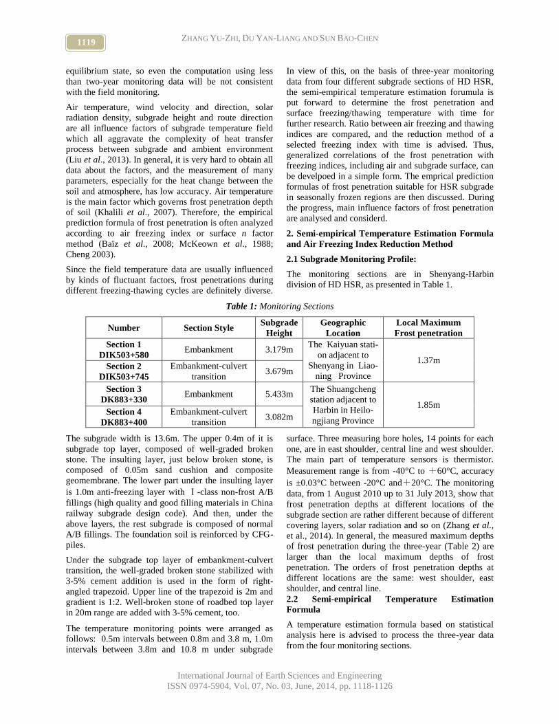
1119 ZHANG YU-ZHI, DU YAN-LIANG AND SUN BAO-CHEN
International Journal of Earth Sciences and Engineering
ISSN 0974-5904, Vol. 07, No. 03, June, 2014, pp. 1118-1126
equilibrium state, so even the computation using less
than two-year monitoring data will be not consistent
with the field monitoring.
Air temperature, wind velocity and direction, solar
radiation density, subgrade height and route direction
are all influence factors of subgrade temperature field
which all aggravate the complexity of heat transfer
process between subgrade and ambient environment
(Liu et al., 2013). In general, it is very hard to obtain all
data about the factors, and the measurement of many
parameters, especially for the heat change between the
soil and atmosphere, has low accuracy. Air temperature
is the main factor which governs frost penetration depth
of soil (Khalili et al., 2007). Therefore, the empirical
prediction formula of frost penetration is often analyzed
according to air freezing index or surface n factor
method (Baïz et al., 2008; McKeown et al., 1988;
Cheng 2003).
Since the field temperature data are usually influenced
by kinds of fluctuant factors, frost penetrations during
different freezing-thawing cycles are definitely diverse.
In view of this, on the basis of three-year monitoring
data from four different subgrade sections of HD HSR,
the semi-empirical temperature estimation forumula is
put forward to determine the frost penetration and
surface freezing/thawing temperature with time for
further research. Ratio between air freezing and thawing
indices are compared, and the reduction method of a
selected freezing index with time is advised. Thus,
generalized correlations of the frost penetration with
freezing indices, including air and subgrade surface, can
be develpoed in a simple form. The emprical prediction
formulas of frost penetration suitable for HSR subgrade
in seasonally frozen regions are then discussed. During
the progress, main influence factors of frost penetration
are analysed and considerd.
2. Semi-empirical Temperature Estimation Formula
and Air Freezing Index Reduction Method
2.1 Subgrade Monitoring Profile:
The monitoring sections are in Shenyang-Harbin
division of HD HSR, as presented in Table 1.
Table 1: Monitoring Sections
Number Section Style Subgrade
Height
Geographic
Location
Local Maximum
Frost penetration
Section 1
DIK503+580 Embankment 3.179m
The Kaiyuan stati-
on adjacent to
Shenyang in Liao-
ning Province
1.37m Section 2
DIK503+745
Embankment-culvert
transition 3.679m
Section 3
DK883+330 Embankment 5.433m
The Shuangcheng
station adjacent to
Harbin in Heilo-
ngjiang Province
1.85m Section 4
DK883+400
Embankment-culvert
transition 3.082m
The subgrade width is 13.6m. The upper 0.4m of it is
subgrade top layer, composed of well-graded broken
stone. The insulting layer, just below broken stone, is
composed of 0.05m sand cushion and composite
geomembrane. The lower part under the insulting layer
is 1.0m anti-freezing layer with Ⅰ-class non-frost A/B
fillings (high quality and good filling materials in China
railway subgrade design code). And then, under the
above layers, the rest subgrade is composed of normal
A/B fillings. The foundation soil is reinforced by CFG-
piles.
Under the subgrade top layer of embankment-culvert
transition, the well-graded broken stone stabilized with
3-5% cement addition is used in the form of right-
angled trapezoid. Upper line of the trapezoid is 2m and
gradient is 1:2. Well-broken stone of roadbed top layer
in 20m range are added with 3-5% cement, too.
The temperature monitoring points were arranged as
follows: 0.5m intervals between 0.8m and 3.8 m, 1.0m
intervals between 3.8m and 10.8 m under subgrade
surface. Three measuring bore holes, 14 points for each
one, are in east shoulder, central line and west shoulder.
The main part of temperature sensors is thermistor.
Measurement range is from -40°C to +60°C, accuracy
is ±0.03°C between -20°C and+20°C. The monitoring
data, from 1 August 2010 up to 31 July 2013, show that
frost penetration depths at different locations of the
subgrade section are rather different because of different
covering layers, solar radiation and so on (Zhang et al.,
et al., 2014). In general, the measured maximum depths
of frost penetration during the three-year (Table 2) are
larger than the local maximum depths of frost
penetration. The orders of frost penetration depths at
different locations are the same: west shoulder, east
shoulder, and central line.
2.2 Semi-empirical Temperature Estimation
Formula
A temperature estimation formula based on statistical
analysis here is advised to process the three-year data
from the four monitoring sections.

1120 Predicting frost penetration of high-speed railway subgrade in seasonally frozen regions
based on empirical method
International Journal of Earth Sciences and Engineering
ISSN 0974-5904, Vol. 07, No. 03, June, 2014, pp. 1118-1126
Considering the time phase difference, supposing the
ground is homogeneous soil with constant state, ,T z t
varying with the time t and the depth z , at a certain
subgrade section location in a specific area, can be
estimated as (Zhang et al., 2014; ANDERSLAND and
LADANYI, 2011):
2
, exp sinm s
u u
tT z t T A z z
a p p a p
(1)
where is the annual average temperature at depth z,
unit is degree centigrade, °C, As is the annual
temperature amplitude of subgrade surface, unit is °C, z
is the depth from the subgrade surface, unit is m, is
the average soil thermal diffusion coefficient ignoring
the earth interior heat flux, unit is m2/day, p is the
vibration period, 365 days,
is the initial phase angle ,
uz a p
is the time lag of the depth z from the
surface, t is the interval from the beginning date, unit is
day,
It is noticed that in the reference (Zhang et al., 2014;
ANDERSLAND and LADANYI, 2011) is adopted
uniformly using the average temperature of the
subgrade surface, which is suitable when the
temperature envelope is zero gradient type, but not
suitable when the temperature envelope is the positive
or negative type. So this paper adopted fitting functions
describing the average temperature with depth.
Original series were obained through averageing the
three-year monitoring annual average temperature and
temperature amplitude respectively. Then the functions
of annual average temperature and temperature
amplitude with depth can be fitted using least square
method. Through the initial value at depth 0.8m
comparasion with maximum value of the first cycle, the
initial phase angle could be determined. The thermal
diffusivity difference of broken stone and A/B fillings is
not considerd. The estimation formula could not only
eliminate the dispersibility of the field monitoring data,
but also provide a tool for temperature calculation
continuous in space and time. And then, supposed the
soil freezes at 0 °C, the frost penetration with time, a
series of [ , ] can be caculated from the
equations , 0T z t . The maximum depth of frost
penetration calculated (Table2) are very consistant with
the meastured results, whether the depths and the arrival
dates. The subgrade surface temperature with time could
be attained by the ,T z t at the depth z=0, then the
subgrade surface index could be computed.
Table 2: Measured and estimated maximum depths of frost penetration and arrival dates
Location
2010-2011 2011-2012 2012-2013 Estimated Model
Measure
d (m) Date
Measure
d (m) Date
Measure
d (m) Date
Estimate
d (m) Date
Section
1
East
shoulder 2.05 26 Feb 2.75 6 Mar 2.18 1 Mar 2.32 1 Mar
Central line 1.63 21 Feb 2.10 1 Mar 1.97 2 Mar 2.09 2 Mar
West
shoulder 2.50 26 Feb 2.80 1 Mar 2.80 1 Mar 2.80 5 Mar
Section
2
East
shoulder 2.10 21 Feb 2.78 6 Mar 2.30 1 Mar 2.56 1 Mar
Central line 1.55 6 Mar 2.10 6 Mar 2.25 6 Mar 2.25 5 Mar
West
shoulder 2.00 6 Mar 2.85 6 Mar 2.75 6 Mar 2.83 5 Mar
Section
3
East
shoulder 1.55 16 Mar 2.64 11 Mar 2.24 20 Mar 2.25 11 Mar
Central line 1.46 16 Mar 1.99 21 Mar 2.15 26 Mar 2.17 20 Mar
West
shoulder 2.02 16 Mar 2.94 1 Apr 2.45 1 Apr 2.85 20 Mar
Section
4
East
shoulder 2.65 16 Mar 2.70 16 Mar 2.80 16 Mar 3.06 22 Mar
Central line 1.35 21 Mar 2.20 16 Mar 2.20 25 Mar 2.43 22 Mar
West
shoulder 2.80 21 Mar 3.50 21 Mar 2.80 21 Mar 3.39 28 Mar
2.3 Air Freezing Index Reduction Method
Corresponding to the frost penetration with time
calculated from the above estimation model, the
freezing index with time should be determined from the
three-year air temperature data. Through comparing the
ratio between air freezing and thawing indices, the
reduction method of air freezing index is proposed.
The surface thawing and freezing indices and their ratio
are the important indicators of the subgrade thawing
subsidence and frost heaving in frozen regions (Cheng
mT
sA
deptht depthz

1121 ZHANG YU-ZHI, DU YAN-LIANG AND SUN BAO-CHEN
International Journal of Earth Sciences and Engineering
ISSN 0974-5904, Vol. 07, No. 03, June, 2014, pp. 1118-1126
et al., 2003). Referring to the ratio mentioned above, the
ratio between air freezing and thawing indices (FTR) is
obtained:
a f atr T T (2)
where a fT and atT are annual air freezing and
thawing indices, unit is degree-day centigrade, °C.days,
the sum of temperatures below and above 0°C in the
cold period using Norwegian method (Khalili A, 2007).
The FTR reflects the specific value between annual
cooling and heat quantity imported into the subgrade
and reveals the subgrade freezing capacity of one
freezing-thawing cycle to some extent. The ratios of the
three freezing and thawing cycles from 2010 to 2013 are
presented in Table 3. Generally, compared with
measured frost penetration (Table 2), the larger the FTR
is, the deeper the frost penetration is.
On account of the parameters of temperature estimation
formula obtained from the three-year monitoring data
using statistical analysis, the frost penetration depths
estimated are considered to correspond with the average
FTR respectively. In addition, to compare with the long
term meteorological statistical data, the FTR derived
from monthly average temperature (Cheng et al., 2003)
are presented in Table 4.
It is concluded: though there are some differences
between the two methods results, we can see that the
ratio between 2011-2012 FTR and the average FTR
(named as R) is almost most close to 1. Therefore,
subsequent calculation chooses the 2011-2012 freezing
indices as standards, which is reduced by the R’
calculated from the daily mean temperature. Compared
with 30 years statistic data, the computational results
should be accepted.
Table.3: FTR and R from the Air Daily Mean Temperature
Area Period Freezing
index(°C.days)
Thawing
index(°C.days) FTR R
Kai-yuan
2010-2011 -948.0 3684.5 0.2573 0.78
2011-2012 -1338.5 3866.5 0.3462 1.05
2012-2013 -1445.5 3780.0 0.3824 1.16
Shuang-
cheng
2010-2011 -1444.5 3485.0 0.4145 0.86
2011-2012 -1600.5 3560.0 0.4496 0.93
2012-2013 -2065.5 3543.0 0.5830 1.21
Table.4: FTR and R from the Air Monthly Average Temperature
Area Period
Maximum monthly
average
temperature
(°C)
Minimum monthly
average
temperature
(°C)
FTR
analytical
solution
R
Kai-
yuan
2010-2011 24.35 -14.98 0.4660 0.98
2011-2012 25.13 -15.63 0.4746 1.00
2012-2013 24.34 -15.35 0.4852 1.02
30 years
statistic data 23.80 -13.40 0.4058 0.85
Shuang-
cheng
2010-2011 23.89 -18.38 0.6623 0.99
2011-2012 24.68 -17.77 0.5969 0.89
2012-2013 24.08 -20.00 0.7470 1.12
30 years
statistic data 23.20 -18.10 0.6771 1.01
3 Correlations between Frost Penetration and
Freezing Indices, including Air and Subgrade
Surface
3.1 Correlation between Frost penetration and Air
Freezing Index
From a design point of view, the parameters of frost
penetration prediction formula developed should be as
less as possible, e.g., the correction coefficients and the
freezing index. The formula 0.5( )afz a T b is used,
where a fT , air freezing indices of 2012-2013, is
reduced as above, whose absolute value increases with
time gradually. The parameters a, b and test indicators
of fitting precision are presented in Table 5.

1122 Predicting frost penetration of high-speed railway subgrade in seasonally frozen regions
based on empirical method
International Journal of Earth Sciences and Engineering
ISSN 0974-5904, Vol. 07, No. 03, June, 2014, pp. 1118-1126
Table.5: Fitting Function Parameter and Test Indicator
Number Location Parameter
a b R-squared
Section 1
East shoulder 0.0811 0.210 0.998
Central line 0.0835 0.761 0.999
West shoulder 0.0832 0.061 0.998
Section 2
East shoulder 0.0844 0.282 0.998
Central line 0.0893 0.818 0.999
West shoulder 0.0871 0.154 0.998
Section 3
East shoulder 0.0796 1.032 0.999
Central line 0.0828 1.330 0.999
West shoulder 0.0868 0.834 0.999
Section 4
East shoulder 0.0971 1.027 0.998
Central line 0.0897 1.320 0.998
West shoulder 0.0996 0.861 0.996
a of different location in different areas varies within a
narrow range, between 0.08-0.10 basically, but b within
a rather large range. If the parameters are as less as
possible, supposing that b is a definite value in different
area, it would bring a large error.
Therefore, this paper selects a formula uniformly: 0.50.09( )afz T c . The parameters c and test
indicators are presented in Table 6. The frost
penetration depths and its fitting function with time are
presented in Figure 1(a) to (d).
Table.6: Fitting Function Parameter and Test Indicator
Number Location Parameter
c R-squared
Section 1
East shoulder 0.4062 0.986
Central line 0.9205 0.993
West shoulder 0.2100 0.992
Section 2
East shoulder 0.4049 0.993
Central line 0.8350 0.999
West shoulder 0.2170 0.997
Section 3
East shoulder 1.3490 0.983
Central line 1.5640 0.991
West shoulder 0.9403 0.997
Section 4
East shoulder 0.8142 0.992
Central line 1.3290 0.998
West shoulder 0.5760 0.987
The accuracy of this formula is relatively high, which
can describe the correlations of frost penetration and air
freezing index well. The parameters of two sections in
Kaiyuan are very close to each other. However, even the
two sections in Shuangcheng are adjacent; there is more
significant difference of the fitting function parameters.
The results may be due to the difference of embankment
height, subgrade fillings and statistical error, etc.

1123 ZHANG YU-ZHI, DU YAN-LIANG AND SUN BAO-CHEN
International Journal of Earth Sciences and Engineering
ISSN 0974-5904, Vol. 07, No. 03, June, 2014, pp. 1118-1126
0 200 400 600 800 1000 1200 14000.0
0.5
1.0
1.5
2.0
2.5
3.0
3.5
Air Freezing Index reduced/°C.daysF
rost
pen
etr
ati
on
/m
DEPTH1EO
DEPTH1EF
DEPTH1CO
DEPTH1CF
DEPTH1WO
DEPTH1WF
(a) Section 1
0 200 400 600 800 1000 1200 14000.0
0.5
1.0
1.5
2.0
2.5
3.0
3.5
Air Freezing Index reduced/°C.days
Fro
st P
en
etr
ati
on
/m
DEPTH2EO
DEPTH2EF
DEPTH2CO
DEPTH2CF
DEPTH2WO
DEPTH2WF
(b) Section 2
0 200 400 600 800 1000 1200 1400 1600 18000.0
0.5
1.0
1.5
2.0
2.5
3.0
3.5
Air Freezing Index reduced/°C.days
Fro
st
Pen
etr
ati
on
/m
DEPTH3EO
DEPTH3EF
DEPTH3CO
DEPTH3CF
DEPTH3WO
DEPTH3WF
(c) Section 3
0 200 400 600 800 1000 1200 1400 1600 18000.0
0.5
1.0
1.5
2.0
2.5
3.0
3.5
Air Freezing Index reduced/°C.days
Fro
st
Pen
etr
ati
on
/m
DEPTH4EO
DEPTH4EF
DEPTH4CO
DEPTH4CF
DEPTH4WO
DEPTH4WF
(d) Section 4
Figure 1: The depths of frost penetration obtained from
semi empirical formula and fitting function verse air
freezing index reduced
DEPTH: the frost penetration depth; 1-4:section1-4; E:
east shoulder, C: central line, W: west shoulder; O: frost
penetration obtained from semi empirical formula; F:
frost penetration obtained from fitting function.
3.2 Correlation between Frost penetration and
Subgrade Surface Freezing Index-surface n factor
method
A formula 0.5( )afsz T is used to describe the
correlation of frost penetration and subgrade surface
freezing index (McKeown et al., 1988). afsT Computed
from the temperature semi-empirical formula. The
parameters and test indicators are presented in
Table7.
Table.7: Fitting Function Parameters and Test Indicators
Number Location Parameter
R-squared
Section 1
East shoulder 0.0877 0.999
Central line 0.0886 0.998
West shoulder 0.0885 0.999
Section 2
East shoulder 0.0925 0.999
Central line 0.0934 0.998
West shoulder 0.0935 0.999
Section 3
East shoulder 0.0920 0.998
Central line 0.0913 0.995
West shoulder 0.0930 0.999
Section 4
East shoulder 0.0949 0.999
Central line 0.0914 0.996
West shoulder 0.0965 0.999

1124 Predicting frost penetration of high-speed railway subgrade in seasonally frozen regions
based on empirical method
International Journal of Earth Sciences and Engineering
ISSN 0974-5904, Vol. 07, No. 03, June, 2014, pp. 1118-1126
The parameters are rather close to each other, almost
around 0.09. The value is rather consistent with the
Canadian studies (McCormick, 1993), in which is
0.040 – 0.083 for grounds below cement pavements.
The n factor, that is the ratio between subgrade surface
freezing/thawing index and air freezing/thawing index
reduced, are presented as Table. 8
Table.8: n factor of sections
Number Location Factor
n+ n
- n
-/ n
+
Section 1
East shoulder 1.10 0.72 0.65
Central line 1.00 0.51 0.51
West shoulder 1.06 0.85 0.80
Section 2
East shoulder 1.08 0.67 0.62
Central line 0.99 0.53 0.53
West shoulder 1.03 0.79 0.77
Section 3
East shoulder 1.24 0.42 0.33
Central line 1.01 0.41 0.41
West shoulder 1.11 0.62 0.56
Section 4
East shoulder 1.05 0.65 0.62
Central line 0.83 0.50 0.61
West shoulder 0.94 0.75 0.80
n- : the freezing indices ratio between air and subgrade surface, n
+: the thawing indices ratio between air and
subgrade surface, n-/ n
+: the specific value of the two above ratios.
Several results can be summarized as follows:
1. The covering layers of different locations are
different, n- varies in a larger range than n
+. However, n
factors of different sections, including n+, n
- , n
-/ n
+,
show the similar rules. The orders of n+ from high to
low are: east shoulder, west shoulder, and central line.
But the orders of n- and n
-/ n
+ are: west shoulder, east
shoulder, and central line. n+, n
- , n
-/ n
+ could be
considered as the subgrade indicators of heat quantity,
cooling quantity and freezing capacity. The shoulders
are influenced by climate factors more serious than
central line, providing evidences for the frost
penetration depths differences at different locations of
one section.
2. n factors at the same locations of two sections in
Kaiyuan are very close. It is shown that the heat
quantity imported into and emitted from the subgrade is
very similar although the embankment heights and
fillings are little different. Two sections in Kaiyuan and
section 4 in shuangcheng have similar heights, n factors
are very similar too.
3. n factors of two sections in Shuangcheng are very
different. The n+ of section 3 are larger than section 4,
however, n- and n
-/ n
+ are smaller and the difference
between east and west shoulders is slightly bigger. The
results indicate that embankment which has a larger
height is conductive to thermal storage and frost
penetration depth decrease, but at the same time, may
make the transverse thermal difference more evident.
We can conclude that n factors are mainly related with
the embankment height and section locations in the case
of the same subgrade route direction and covering layer.
4. Predicting Frost penetration based on Empirical
Method
Based on the above, this paper attempts to put forward
the empirical frost penetration prediction formula with
correction coefficients for HSR subgrade in seasonally
frozen regions.
4.1 Empirical Formula according to Atmosphere
Freezing Index
The parameter a can be determined as 0.10
conservatively. Then considering the main influence
factors, the empirical formula for design frost
penetration is defined as:
0.5
0.10 f r dz T k k b (3)
Where kr: the correction coefficient of inherent
conditions, such as subgrade height and filling. In
general, the higher the height is, the larger the value will
be.
kd: the influence coefficient of route direction.
Generally, the sunny slope of east-west (EW) direction
1125 ZHANG YU-ZHI, DU YAN-LIANG AND SUN BAO-CHEN
International Journal of Earth Sciences and Engineering
ISSN 0974-5904, Vol. 07, No. 03, June, 2014, pp. 1118-1126
has the maximal value, and that of south-north (SN)
direction keeps the minimal value. For the shady slope,
the above rules are on the contrary (Li and Chen, 1992;
Liu, et al., 2013).
fT is the air freezing index on the basis of
meteorological data during a long-term, that is, at least
30 years.
b is a comprehensive coefficient of regional influence
factors which include Air temperature, topography,
geothermic, soil property and water, etc. The specific
areas, that the main influence factors are similar, could
be classified according to the criteria. Regional b series
could be obtained through statistical analysis of the field
monitoring data using the method in this paper.
According to the above data, b could be selected as 0.80
for Shuangcheng, 0.10 for Kaiyuan. In the case of
relative fixed subgrade conditions, b is mainly related
with regional climate.
4.2 Empirical Formula according to Subgrade
Surface Freezing Index-n Factor Method
The parameter is selected as 0.10 conservatively.
Then considering the main influence factors, the
empirical formula for maximum frost penetration is
defined as:
0.5
0.10 r d fz r r n T (4)
Where n: the freezing indices ratio between atmosphere
and subgrade surface.
fT is as same as above.
The variation trends of coefficients are contrary and
value range selected may be different.
rr: the correction coefficient of inherent conditions, such
as subgrade height and filling. In general, the higher the
height is, the smaller the value will be.
rd: the correction coefficient of route direction.
Generally, the sunny slope of EW direction has the
minimal value, and that of SN direction keeps the
maximal value. For the shady slope, the above rules are
on the contrary (Li and Chen, 1992; Liu, et al., 2013).
For the frost penetration of a certain subgrade location, z
can be corrected by the coefficients ks and kt. ks contain
influences of section form, gradient, solar exposure, etc.
In general, the value of shady slope is bigger. kt
represents the factor of distance from shoulder, the
larger the distance is, the smaller the value is.
5. Conclusions:
The frost penetration is an important basis of anti-
freezing measures in frozen regions. Correlations
between the frost penetration and air, subgrade surface
freezing indices are studied using empirical method, and
the computation steps for the prediction model are
detailed.
During the analysis process, some conclusions can be
obtained:
1. The FTR reflects the freezing capacity of a certain
cycle in a specific area to some extent. n factors,
including n+, n
- , n
-/ n
+ , could clearly show the rules of
cooling quantity, heat quantity and freezing capacity at
subgrade different locations of different areas. Main
influence factors of frost penetration can be discussed
through comparisons of FTR and n factors.
2. The main influence factors of frost penetration are:
air temperature, subgrade height and section transverse
location, etc. The larger the local freezing index and the
smaller the height are, the deeper the frost penetration
will be. The frost penetration of different section
locations are different, central line is smallest, then the
east shoulder, the west shoulder is largest.
3. The frost penetration is strongly related with air and
subgrade surface freezing indices. So the uniform
empirical formula could be attained to describe the
correlations between them. The influence factors can be
considered through the parameters and correction
coefficients of the formula, which can be determined
using the field monitoring data.
In practice, the modified empirical formula can be
useful for estimating the frost penetration at different
sites along the railway that have similar geotechnical
properties. What is more, the process and conclusions
about the frost penetration in this paper will provide
some references for the design and construction of
similar engineering, the maintenance and stability
analysis of HSR in seasonally frozen regions.
6. Acknowledgements:
This work was supported by the
National Key Technology R&D Program, the Ministry
of Science and Technology of the People's Republic of
China [Grant No: 2012BAG05B01]; and the National
Basic Research Program, the Ministry of Science and
Technology of the People's Republic of China [Grant
No: 2012CB723301].
2. Reference:
[1] ANDERSLAND O B, LADANYI B, 2011. Frozen
ground engineering. 2nd ed. Translated by Yang R,
Li Y., Beijing: China Architecture and Building
Press.
[2] Baïz S, Tighe S L, Haas CT, Mills B, Perchanok,
M, 2008. Development of frost and thaw depth
predictors for decision making about variable load
restrictions. Transportation Research Record:
Journal of the Transportation Research Board,
2053(1): 1-8.

1126 Predicting frost penetration of high-speed railway subgrade in seasonally frozen regions
based on empirical method
International Journal of Earth Sciences and Engineering
ISSN 0974-5904, Vol. 07, No. 03, June, 2014, pp. 1118-1126
[3] Bing WS, Zhou J, Wang XF, 1995. Calculation
methods research of road frost depth, Journal of
Harbin university of Architecture and Engineering,
28: 11-16.
[4] Cheng GD, Hao J, Wang KL, Wu QB, 2003.
Freezing and thawing index on the embankment in
permafrost regions. Journal of Glaciology and
Geocryology, 25: 603-607.
[5] Fischer C. J., Zubeck H, 2013. Comparison of
Theoretical Freezing Depths of Permeable and
Conventional Pavements. In ISCORD 2013@
sPlanning for Sustainable Cold Regions, 447-458.
ASCE.
[6] Khalili A., Rahimi H., Shariatmadari Z. A, 2007.
Validation of air freezing index (AFI), for
determination of frost penetration depth in typical
arid and semi-arid zones of Iran. DESERT
(BIABAN), 12:23-31.
[7] Li AG, Chen QH, 1992. Determination of frost
penetration in canal design, Water Resource and
Water Engineering, 3: 1-1.
[8] Liu ZY, Chen JB, Jin L, Zhang YJ, Lei C, 2013.
Roadbed temperature study based on earth-
atmosphere coupled system in permafrost regions
of the Qinghai-Tibet Plateau. Cold Regions Science
and Technology, 86: 167-176.
[9] Martel CJ, 1988. Predicting freezing design depth
of sludge-freezing beds. Journal of cold regions
engineering, 2: 145-156.
[10] McCormick G, 1990. Soil temperatures and
freezing indices at depth. Canadian Geotechnical
Journal, 27(6): 749-751.
[11] McCormick G, 1993. Frost penetration beneath
cleared pavements. Frost in Geotechnical
Engineering. Balkema, Rotterdam, 117-126.
[12] McKeown S., Clark J. I., Matheson D, 1988. Frost
penetration and thermal regime in dry gravel.
Journal of cold regions engineering, 2(3): 111-123.
[13] Shin E C, Park J J, Lee J S, 2013. An Analysis of
Frost Penetration Depth with Field Temperature
Data of Paved Road in Korea. In ISCORD 2013@
sPlanning for Sustainable Cold Regions, 367-378.
ASCE.
[14] Smith G M, Rager R E, 2002. Protective layer
design in landfill covers based on frost penetration.
Journal of geotechnical and geoenvironmental
engineering, 128(9): 794-799.
[15] Xu J, Niu FJ, Li AM, lin ZJ, 2010. Analysis of the
prevention effect of thermal-insulation method on
frost heave of railway subgrade in seasonal frozen
regions. Journal of the China Railway Society, 32:
124-31.
[16] Xu J, Niu FJ, Niu YH, lin ZJ, Xu ZY, 2011a. Study
on the temperature field of insulated subgrade with
frost resistant berm on seasonal frozen region,
Journal of the China Railway Society, 33: 84-90.
[17] Xu J, Niu FJ, Niu YH, Liu H, 2011b. Analysis on
the effect of replacing-soil method on inhibiting
frost heave of railway subgrade in seasonal frozen
soil region, China Railway Science, 32: 1-7.
[18] Zhang YZ, Du YL, Sun BC, 2014. Temperature
distribution research of high-speed railway roadbed
in seasonally frozen regions, Chinese Journal of
Rock Mechanics and Engineering, 33: 1286-1296.
www.cafetinnova.org
Indexed in
Scopus Compendex and Geobase Elsevier, Chemical
Abstract Services-USA, Geo-Ref Information Services-USA,
List B of Scientific Journals, Poland,
Directory of Research Journals
ISSN 0974-5904, Volume 07, No. 03
June 2014, P.P.1127-1134
#02070344 Copyright ©2014 CAFET-INNOVA TECHNICAL SOCIETY. All rights reserved.
Comprehensive Evaluation of the Development Quality of New-
Type of Urbanization of Jiangxi Province Based on Ecological Views
WANG YONG XIANG East China Jiaotong University, School of Civil Engineering and Architecture, Nanchang, Jiangxi Province, CHINA
Email:[email protected]
Abstract: New-type of urbanization is more than a shift of rural population to urban population. More importantly,
it sets up a direction to resource conservation, environment protection, science development and social harmony.
However, there are few efforts to evaluate the quality of new-type of urbanization. Based on previous researches,
this paper constructs a comprehensive evaluation system for evaluating the development quality of new-type of
urbanization and conducts a comprehensive evaluation through statistical methods such as cluster analysis and factor
analysis. Results show that following the scientific outlook on development and establishing the comprehensive
evaluation system with ecological ideas are significant to improve science and culture, enhance the quality of
ecological urbanization and protect our homeland. Under the system, more efforts will be made to beauty and enrich
Jiangxi.
Keywords: Ecology, Jiangxi Province, New-type of urbanization, Comprehensive evaluation.
1. Introduction:
The 18th
National Congress of the Communist Party of
China proposed to accelerate the pace of building new-
type of urbanization. Urbanization in the future will
become an important carrier of building a moderately
prosperous society as well as the driven force of
leveraging domestic demand. The rapid development of
urbanization is becoming a powerful engine for
economic growth and social development. "A resource-
conserving and environment-friendly society" is
scientific, economic, social and ecological civilization.
New-type of urbanization is an integration of urban and
rural areas, an interaction between production and city
and being economical, intensive, livable featuring
harmonious development. It aims at coordinated
development and mutual progress among large, middle-
sized cities and small cities and towns [1-9]
.
As a revolutionary base, big agricultural province and
tourism province, Jiangxi’s urbanization develops very
slowly. According to statistics reported in 2013 in
Jiangxi Province, by the end of 2012, the level of
urbanization in Jiangxi Province was 29.09% (see
Figure 1) [10]
; current and the next 20 years will be a
crucial period of rapid development of urbanization in
Jiangxi; Jiangxi’s urbanization will become the main
theme of economic and social development; new
urbanization has become a national development
strategy in central China.
However, there are still problems presenting in the
course of urbanization of Jiangxi. For example, the scale
of the city is small. The spatial distribution is far from
being reasonable. Some cities and towns fail to tailor to
their local situation. Urban planning is not reasonable.
Enclosure brings about a waste of land resources.
Infrastructures such as transportation, water and utility,
energy and communication are backward. Environment
deterioration has brought much pressure on the
development of Jiangxi. Therefore, it is necessary to
make the economic construction a center and reach a
balance between economic development, social
harmony and ecological protection [11]
.
Over the past 20 years, domestic scholars have achieved
fruitful results on the study of urbanization. But for a
long time, the proportion of urban population to total
population in the country is always used to measure the
urbanization level. Such method is the simplest one for
single indicator method. However, there are also many
disadvantages and limitations. In recent years, more and
more scholars began to focus on problems brought by
urban development and evaluate the quality of
urbanization from a multi-dimensional perspective
including population, economy, resources, environment
even the whole society rather than economic alone. Bai
Xianchun et al (2004) established an evaluation system,
determined the target value according to certain
standards and made a thorough study on coordination
development of urbanization based on econometric
model [12]
.
Research group of Fujian on City Investment (2005)
constructed the urbanization quality evaluation system
mainly from the core carrier and regional carrier of
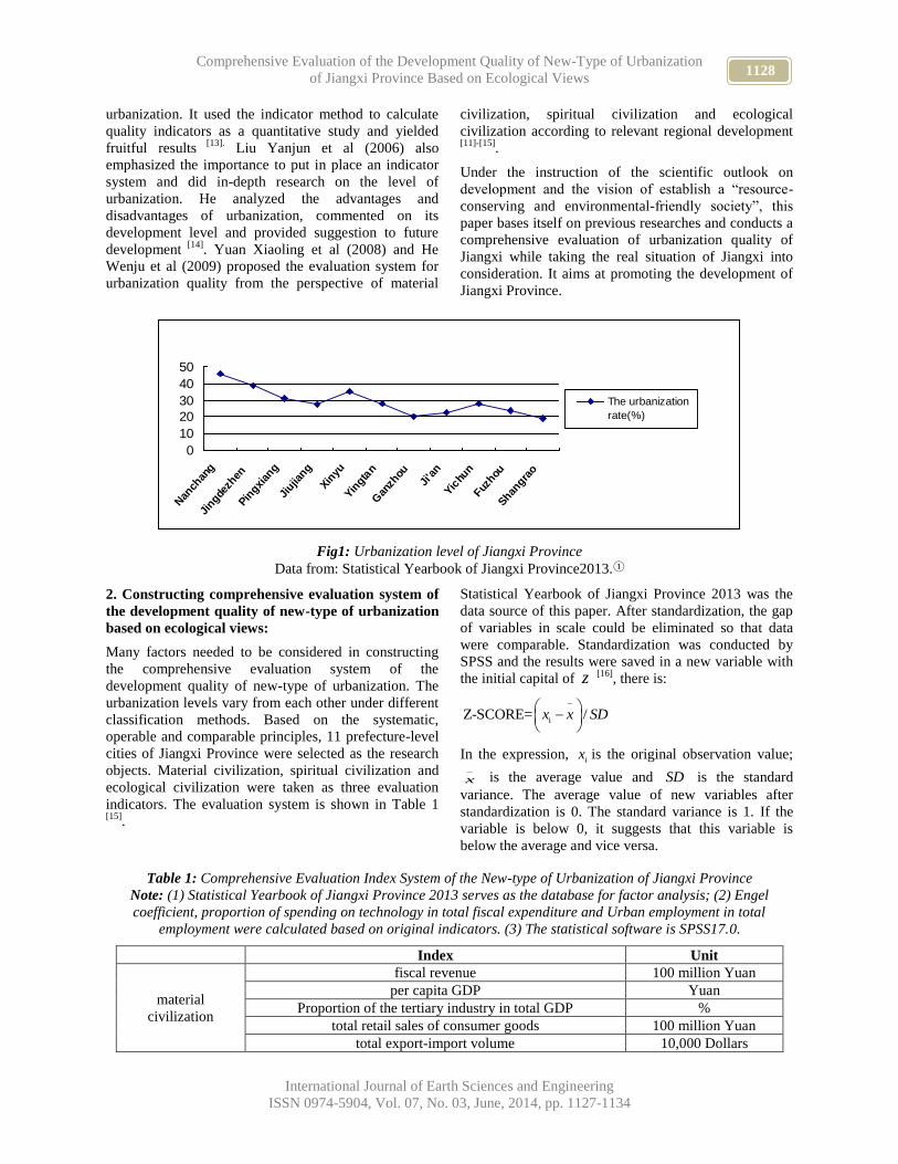
1128 Comprehensive Evaluation of the Development Quality of New-Type of Urbanization
of Jiangxi Province Based on Ecological Views
International Journal of Earth Sciences and Engineering
ISSN 0974-5904, Vol. 07, No. 03, June, 2014, pp. 1127-1134
urbanization. It used the indicator method to calculate
quality indicators as a quantitative study and yielded
fruitful results [13].
Liu Yanjun et al (2006) also
emphasized the importance to put in place an indicator
system and did in-depth research on the level of
urbanization. He analyzed the advantages and
disadvantages of urbanization, commented on its
development level and provided suggestion to future
development [14]
. Yuan Xiaoling et al (2008) and He
Wenju et al (2009) proposed the evaluation system for
urbanization quality from the perspective of material
civilization, spiritual civilization and ecological
civilization according to relevant regional development [11]-[15]
.
Under the instruction of the scientific outlook on
development and the vision of establish a “resource-
conserving and environmental-friendly society”, this
paper bases itself on previous researches and conducts a
comprehensive evaluation of urbanization quality of
Jiangxi while taking the real situation of Jiangxi into
consideration. It aims at promoting the development of
Jiangxi Province.
0
10
20
30
40
50
Nan
chan
gJi
ngdezh
enPin
gxian
gJi
ujiang
Xinyu
Yingta
nG
anzh
ou
Ji'a
nYic
hun
Fuzhou
Shangra
o
The urbanization
rate(%)
Fig1: Urbanization level of Jiangxi Province
Data from: Statistical Yearbook of Jiangxi Province2013.①
2. Constructing comprehensive evaluation system of
the development quality of new-type of urbanization
based on ecological views:
Many factors needed to be considered in constructing
the comprehensive evaluation system of the
development quality of new-type of urbanization. The
urbanization levels vary from each other under different
classification methods. Based on the systematic,
operable and comparable principles, 11 prefecture-level
cities of Jiangxi Province were selected as the research
objects. Material civilization, spiritual civilization and
ecological civilization were taken as three evaluation
indicators. The evaluation system is shown in Table 1 [15]
.
Statistical Yearbook of Jiangxi Province 2013 was the
data source of this paper. After standardization, the gap
of variables in scale could be eliminated so that data
were comparable. Standardization was conducted by
SPSS and the results were saved in a new variable with
the initial capital of z [16]
, there is:
iZ-SCORE= /x x SD
In the expression, ix is the original observation value;
x
is the average value and SD is the standard
variance. The average value of new variables after
standardization is 0. The standard variance is 1. If the
variable is below 0, it suggests that this variable is
below the average and vice versa.
Table 1: Comprehensive Evaluation Index System of the New-type of Urbanization of Jiangxi Province
Note: (1) Statistical Yearbook of Jiangxi Province 2013 serves as the database for factor analysis; (2) Engel
coefficient, proportion of spending on technology in total fiscal expenditure and Urban employment in total
employment were calculated based on original indicators. (3) The statistical software is SPSS17.0.
Index Unit
material
civilization
fiscal revenue 100 million Yuan
per capita GDP Yuan
Proportion of the tertiary industry in total GDP %
total retail sales of consumer goods 100 million Yuan
total export-import volume 10,000 Dollars
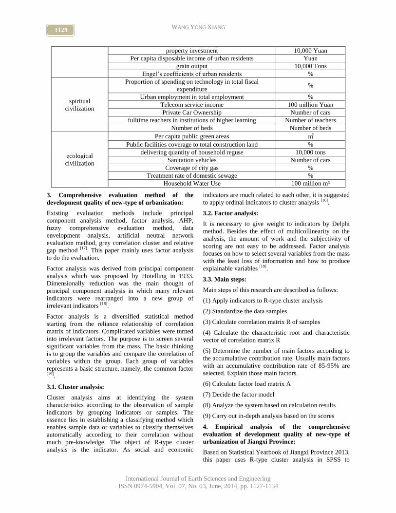
1129 WANG YONG XIANG
International Journal of Earth Sciences and Engineering
ISSN 0974-5904, Vol. 07, No. 03, June, 2014, pp. 1127-1134
property investment 10,000 Yuan
Per capita disposable income of urban residents Yuan
grain output 10,000 Tons
Engel’s coefficients of urban residents %
spiritual
civilization
Proportion of spending on technology in total fiscal
expenditure %
Urban employment in total employment %
Telecom service income 100 million Yuan
Private Car Ownership Number of cars
fulltime teachers in institutions of higher learning Number of teachers
Number of beds Number of beds
ecological
civilization
Per capita public green areas ㎡
Public facilities coverage to total construction land %
delivering quantity of household reguse 10,000 tons
Sanitation vehicles Number of cars
Coverage of city gas %
Treatment rate of domestic sewage %
Household Water Use 100 million m³
3. Comprehensive evaluation method of the
development quality of new-type of urbanization:
Existing evaluation methods include principal
component analysis method, factor analysis, AHP,
fuzzy comprehensive evaluation method, data
envelopment analysis, artificial neutral network
evaluation method, grey correlation cluster and relative
gap method [17]
. This paper mainly uses factor analysis
to do the evaluation.
Factor analysis was derived from principal component
analysis which was proposed by Hotelling in 1933.
Dimensionally reduction was the main thought of
principal component analysis in which many relevant
indicators were rearranged into a new group of
irrelevant indicators [18]
.
Factor analysis is a diversified statistical method
starting from the reliance relationship of correlation
matrix of indicators. Complicated variables were turned
into irrelevant factors. The purpose is to screen several
significant variables from the mass. The basic thinking
is to group the variables and compare the correlation of
variables within the group. Each group of variables
represents a basic structure, namely, the common factor [19]
.
3.1. Cluster analysis:
Cluster analysis aims at identifying the system
characteristics according to the observation of sample
indicators by grouping indicators or samples. The
essence lies in establishing a classifying method which
enables sample data or variables to classify themselves
automatically according to their correlation without
much pre-knowledge. The object of R-type cluster
analysis is the indicator. As social and economic
indicators are much related to each other, it is suggested
to apply ordinal indicators to cluster analysis [16]
.
3.2. Factor analysis:
It is necessary to give weight to indicators by Delphi
method. Besides the effect of multicollinearity on the
analysis, the amount of work and the subjectivity of
scoring are not easy to be addressed. Factor analysis
focuses on how to select several variables from the mass
with the least loss of information and how to produce
explainable variables [19]
.
3.3. Main steps:
Main steps of this research are described as follows:
(1) Apply indicators to R-type cluster analysis
(2) Standardize the data samples
(3) Calculate correlation matrix R of samples
(4) Calculate the characteristic root and characteristic
vector of correlation matrix R
(5) Determine the number of main factors according to
the accumulative contribution rate. Usually main factors
with an accumulative contribution rate of 85-95% are
selected. Explain those main factors.
(6) Calculate factor load matrix A
(7) Decide the factor model
(8) Analyze the system based on calculation results
(9) Carry out in-depth analysis based on the scores
4. Empirical analysis of the comprehensive
evaluation of development quality of new-type of
urbanization of Jiangxi Province:
Based on Statistical Yearbook of Jiangxi Province 2013,
this paper uses R-type cluster analysis in SPSS to

1130 Comprehensive Evaluation of the Development Quality of New-Type of Urbanization
of Jiangxi Province Based on Ecological Views
International Journal of Earth Sciences and Engineering
ISSN 0974-5904, Vol. 07, No. 03, June, 2014, pp. 1127-1134
cluster variables in which indicators of common
characteristics are put together and representative
indicator in each group is selected to reduce the number
of variables [19]
. Cluster analysis can reflect the
relationship between samples through the vertical bar
graph automatically produced by SPSS.
Subject 9 indicators of material civilization, the first
classification, in the comprehensive evaluation system
for development quality of new-type of urbanization of
Jiangxi. The first classification can have three sub-
categories, namely, Engel coefficient, proportion of the
tertiary industry in total GDP and the rest seven.
Correlation coefficient matrix of 7 indicators is shown
in Table 2.
Table 2: Correlation Coefficient Matrix
Zscore(fis
cal
revenue)
Zscore
(per
capita
GDP)
Zscore
(total retail
sales of
consumer
goods)
Zscore
(total
export-
import
volume)
Zscore
(property
investment
)
Zscore (Per
capita
disposable
income of
urban
residents)
Zscore
(grain
output)
Zscore(fiscal
revenue)
Pearson
Correlation 1 .048 .961
** .768
** .911
** .294 .463
Sig(2-tailed) .889 .000 .006 .000 .380 .152
N 11 11 11 11 11 11 11
Zscore (per
capita GDP)
Pearson
Correlation .048 1 .121 .370 .155 .845
** -.651
*
Sig(2-tailed) .889 .722 .263 .649 .001 .030
N 11 11 11 11 11 11 11
Zscore (total
retail sales of
consumer
goods)
Pearson
Correlation .961
** .121 1 .784
** .977
** .386 .353
Sig(2-tailed) .000 .722 .004 .000 .241 .287
N 11 11 11 11 11 11 11
Zscore (total
export-
import
volume)
Pearson
Correlation .768
** .370 .784
** 1 .772
** .478 .031
Sig(2-tailed) .006 .263 .004 .005 .137 .928
N 11 11 11 11 11 11 11
Zscore
(property
investment)
Pearson
Correlation .911
** .155 .977
** .772
** 1 .371 .311
Sig(2-tailed) .000 .649 .000 .005 .261 .352
N 11 11 11 11 11 11 11
Zscore (Per
capita
disposable
income of
urban
residents)
Pearson
Correlation .294 .845
** .386 .478 .371 1 -.482
Sig(2-tailed) .380 .001 .241 .137 .261 .133
N 11 11 11 11 11 11 11
Zscore (grain
output)
Pearson
Correlation .463 -.651
* .353 .031 .311 -.482 1
Sig(2-tailed) .152 .030 .287 .928 .352 .133
N 11 11 11 11 11 11 11
**. Correlation is significant at the 0.01 level (2 - tailed).
*. Correlation is significant at the 0.05level (2 - tailed).
Select a representative indicator in the third sub-category and calculate the average number of its correlation
coefficient (the square of correlation coefficient) with other indicators. There is:
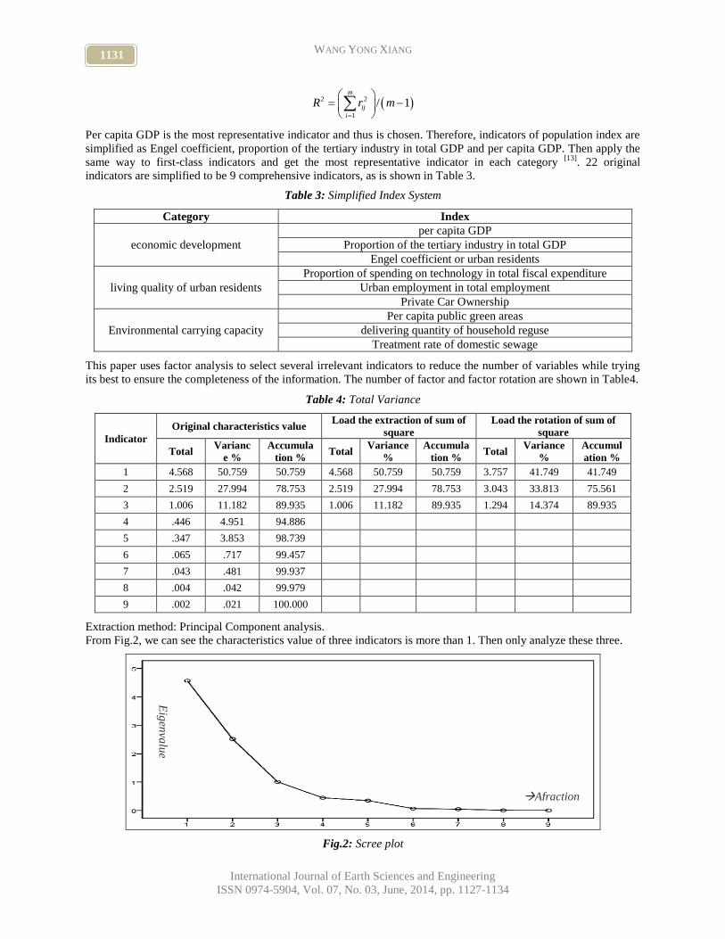
1131 WANG YONG XIANG
International Journal of Earth Sciences and Engineering
ISSN 0974-5904, Vol. 07, No. 03, June, 2014, pp. 1127-1134
2 2
1
/ 1m
ij
i
R r m
Per capita GDP is the most representative indicator and thus is chosen. Therefore, indicators of population index are
simplified as Engel coefficient, proportion of the tertiary industry in total GDP and per capita GDP. Then apply the
same way to first-class indicators and get the most representative indicator in each category [13]
. 22 original
indicators are simplified to be 9 comprehensive indicators, as is shown in Table 3.
Table 3: Simplified Index System
Category Index
economic development
per capita GDP
Proportion of the tertiary industry in total GDP
Engel coefficient or urban residents
living quality of urban residents
Proportion of spending on technology in total fiscal expenditure
Urban employment in total employment
Private Car Ownership
Environmental carrying capacity
Per capita public green areas
delivering quantity of household reguse
Treatment rate of domestic sewage
This paper uses factor analysis to select several irrelevant indicators to reduce the number of variables while trying
its best to ensure the completeness of the information. The number of factor and factor rotation are shown in Table4.
Table 4: Total Variance
Indicator
Original characteristics value Load the extraction of sum of
square
Load the rotation of sum of
square
Total Varianc
e %
Accumula
tion % Total
Variance
%
Accumula
tion % Total
Variance
%
Accumul
ation %
1 4.568 50.759 50.759 4.568 50.759 50.759 3.757 41.749 41.749
2 2.519 27.994 78.753 2.519 27.994 78.753 3.043 33.813 75.561
3 1.006 11.182 89.935 1.006 11.182 89.935 1.294 14.374 89.935
4 .446 4.951 94.886
5 .347 3.853 98.739
6 .065 .717 99.457
7 .043 .481 99.937
8 .004 .042 99.979
9 .002 .021 100.000
Extraction method: Principal Component analysis.
From Fig.2, we can see the characteristics value of three indicators is more than 1. Then only analyze these three.
Fig.2: Scree plot
Afraction
Eig
enva
lue

1132 Comprehensive Evaluation of the Development Quality of New-Type of Urbanization
of Jiangxi Province Based on Ecological Views
International Journal of Earth Sciences and Engineering
ISSN 0974-5904, Vol. 07, No. 03, June, 2014, pp. 1127-1134
Among contribution rate factor accumulative variance in Table 4, if three common factors extracted can describe
89.935 % of total variance of original variables, it indicates that 85% information is covered and these factors can
reflect most of the information. Then rotate the factor load matrix by varimax.
Table 5: Rotating Component Matrixa
Evaluation index ingredient
1 2 3
Zscore(per capita GDP) .894 .297 .216
Zscore (proportion of the tertiary industry in
total GDP) .139 .854 -.250
Zscore (Engel coefficient of urban residents) .649 .365 .407
Zscore (Proportion of spending on technology in
total fiscal expenditure) .349 .883 .185
Zscore (Urban employment in total employment) .894 .319 .202
Zscore (Private vehicle ownership) -.829 .485 -.158
Zscore (per capita green areas) .940 .121 -.120
Zscore (delivering quantity of household reguse) .033 .974 .009
Zscore (Treatment rate of domestic sewage) .155 -.105 .951
Extraction method: principal component analysis.
Rotation method: Orthogonal rotation method with
Kaiser standardization.
a. Rotation became convergence after 4 iterations.
For the first factor, per capita GDP, urban employment
in total employment and per capita green areas have
larger load. For the second factor, proportion of the
tertiary industry in total GDP, proportion of spending on
technology in total fiscal expenditure and delivering
quantity of household reguse have larger load. For the
third factor, Engel coefficient and treatment rate of
domestic sewage have larger load. Then, calculate the
coefficient of factor score function by regression
method and calculate the comprehensive score of three
factors.
COMPUTE score= 1 2 30.50759 * F + 0.27994 * F + 0.11182 * F
5. Conclusion:
Subject indicator value to linear system of equation,
rank in descending order and get the comprehensive
evaluation as Table 6 [10]
. The population urbanization
rate is also put into the Table for comparison.
Table 6: Comprehensive Evaluation of the development quality of new-type of urbanization of Jiangxi Province
City F1 F2 F3 F Ranking
Population
urbanization
rate
Rank by
urbanization
level
Nanchang 0.56268 2.66891 0.65429 1.11 1 46.13 1
Xinyu 1.82702 -0.17779 0.12013 0.89 2 34.83 3
Jingdezhen 1.29031 -0.44937 -1.65535 0.34 3 38.96 2
Pingxiang 0.50661 -0.33438 0.49066 0.22 4 31.13 4
Yingtan 0.4844 -1.02747 0.70866 0.04 5 28.2 5
Jiujiang -0.36713 0.10297 0.7656 -0.07 6 27.27 7
Ji’an -0.67359 -0.41021 0.53957 -0.4 7 22.45 9
Wuzhou -0.47306 -0.63646 -0.76393 -0.5 8 23.67 8
Yichun -0.86399 -0.53375 0.71764 -0.51 9 27.74 6
Shangrao -1.12524 0.01866 0.40607 -0.52 10 19.22 11
Ganzhou -1.168 0.77889 -1.98333 -0.60 11 20.41 10
Data from: Statistical Yearbook of Jiangxi
Province2013.①
From the result it is clear that:
1133 WANG YONG XIANG
International Journal of Earth Sciences and Engineering
ISSN 0974-5904, Vol. 07, No. 03, June, 2014, pp. 1127-1134
(1) In terms of comprehensive factor of new-type of
urbanization, Nanchang ranks the first. The rank of
urbanization quality is in line with the rank of
population urbanization rate. This has something to do
with its geographical advantage and policy
environment. But indicators such as per capita green
areas and treatment rate of domestic sewage still need
improvement.
(2)The rank of comprehensive factor of new-type of
urbanization of Xinyu, Jingdezhen, Pingxiang, Yingtan
and Jiujiang is in line with the rank of population
urbanization rate. But problems for each city in terms of
urbanization quality are different. Xinyu, Jingdezhen
and Pingxiang have some advantages in urbanization
quality. Efforts have been made on urban ecology in
recent years, making them green and civilized cities.
Urbanization quality in Jingdezhen and Pingxiang are
not satisfying and needs more efforts. Ji’an, Wuzhou,
Yichun, Shangrao and Ganzhou don’t stand out in
urbanization quality. Their indicators are relatively
weak and thus a comprehensive improvement is needed.
(3) The rank of comprehensive factor of Yichun is the
9th
, lagging behind Jiujiang (the 6th
). It only outperforms
Jiujiang in terms of population urbanization rate. This
indicates that it is not scientific to evaluate the
urbanization level simply by population urbanization
rate.
(4)If the urbanization level is evaluated by population
urbanization rate, Jingdezhen, Pingxiang, Yingtan and
Jiujiang are doing pretty well. But if evaluated by
urbanization quality, their ranks are much behind.
Jiangdezhen, Pingxiang and Yingtan are industrial cities
while Jiujiang is a tourist city. They have some
prevalences in urbanization development and are
suggested to take the opportunity of establishing a
“resource-conserving and environment-friendly” city to
upgrade traditional industries and put in place an
integrated and interactive industry clusters so as to
realize the effective use of resources and a positive
cycle of ecology. The urbanization quality will be
improved as a result.
(5)The score of urbanization quality of Nanchang and
Xinyu is higher than that of population urbanization
rate. These two cities have done a good job in
urbanization process. But their resources and
environment bearing capacity are not adapted to the
new-type of urbanization level.
Therefore, following the scientific outlook on
development and establishing the comprehensive
evaluation system with ecological ideas are significant
to improve science and culture, enhance the quality of
ecological urbanization and protect our common
homeland. Under the system, more efforts will be made
to beauty and enrich Jiangxi.
Notes: ① Based on data from the Statistical Yearbook
of Jiangxi Province 2013.
2. Reference:
[1] Luo Jianrong, Study on the Scientific Outlook on
development and Urbanization, Haitian Press, PP.
5-31, 2005.
[2] United Nations Human Habitat, The State of the
World's Cities Report 2001, Un-habitat, 2002.
[3] Urban Indicators Guidelines, United Nations
Human Settlements Programmer, Augest, 2004.
[4] Bloom DE, Canning D and Fink G, Urbanization
and the Wealth of Nation. Science, Volume 319.
Issue 1., PP772-775., 2008.
[5] USEAP, Pollution Prevention 1997-A National
Progerss Rpeort, EAP-742-R-97-000, 1997.
[6] USEAP, Innovation at the Environment protection
Agency, Decade of Progress, EPA 100-R-00-20,
2000.
[7] Segnstam L., Indicators of Environment and
Sustainable Development Theories and Pratical
Experience, Environmental Economics Series,
Paper No.98, The World Bank.2002.
[8] Williams O.O.David W., Natural resource and
environmental poli-cy trade-offs:a CGE analysis of
the regional impact of the Wetland Re-serve
Program. Land Use Policy, Volume19, PP231-241.,
2002.
[9] Young W.J., Lam D.C.L. and Ressel V., I,
Development of an environ-mental flows decision
support system. Environmental Modelling & Soft-
ware, Volume15., PP257-265., 2000.
[10] China Statistical Yearbook Newsroom, Statistical
Yearbook of Jiangxi Province2013, China
Statistical Publishing House, 2013.
[11] Yuan Xiaoling, Wang Xiao, He Weiwei and Chen
Yue, Comprehensive Evaluation of the quality of
Urbanization, Urban Development Research,
Volume2., PP38-45., 2008.
[12] Bai Xianchun, Ling Kang and Guo Cunzhi,
Synthesis Evaluation Of The Quality Of City
Development, China Population Resources and
Environment, Volume6., PP91-95., 2008.
[13] National Research Group, Fujian Team,
Constructing System of Quality Evaluation of
Urbanization of China and the Experimental
Analysis, Statistical Research, Volume7., PP15-19.,
2005.
[14] Liu Yanjun, Li Chenggu and Sun Di,Research On
Urbanization Integrated Level Of Urban Regional
Centers Evaluation--A Case Study On 15 Vice-
Provincial Cities Of China, Economic Geography,
Volume3., PP225-229., 2006.
[15] He Wenju, Deng Bosheng and Yang Zhimei,
Urbanization Quality from the two-oriented society

1134 Comprehensive Evaluation of the Development Quality of New-Type of Urbanization
of Jiangxi Province Based on Ecological Views
International Journal of Earth Sciences and Engineering
ISSN 0974-5904, Vol. 07, No. 03, June, 2014, pp. 1127-1134
perspective-a Case Study of Hunan Province,
Financial Theory and Practive, Volume30., PP118-
121., 2009.
[16] Yang Weizhong and Zhang Tian, SPSS Statistical
Analysis and Industry Applications (2nd
Edition),
Tsinghua University Press, PP75-190., 2013.
[17] Wang Hui and Chen Li, Multi-index
Comprehensive Evaluation Model and the Selection
of Weight Coefficient, Journal of Guangdong
College of Pharmacy, Volume5., PP33-36., 2007.
[18] Bai Huiqiang, The Application of Principal
Component Analysis in SPSS- An Example of the
Herbosa of Wenyu River, Sci-Tech Information
Development & Economy, Volume9., PP173-177.,
2009.
[19] Du Qiang and Jia Liyan, Mastering SPSS Statistical
Analysis, Posts and Telecom Press, PP248-305.,
2011.

www.cafetinnova.org
Indexed in
Scopus Compendex and Geobase Elsevier, Chemical
Abstract Services-USA, Geo-Ref Information Services-USA,
List B of Scientific Journals, Poland,
Directory of Research Journals
ISSN 0974-5904, Volume 07, No. 03
June 2014, P.P.1135-1140
#02070345 Copyright ©2014 CAFET-INNOVA TECHNICAL SOCIETY. All rights reserved.
Simulation study of dense coherent tower sintering flue gas
desulfurization system
QIAN JIA1, DONGHUI ZHANG
1,2, CUNYI SONG
1, ZHENSONG TONG
1 AND BAORUI LIANG
1
1School of Civil and Environmental Engineering, University of Science and Technology Beijing, 100083,
Beijing, China 2Beijing Guodian Longyuan Environmental Engineering Co., Ltd, Beijing, 100039
Email: [email protected]
Abstract: Using Fluent software, dense coherent tower simulation flue gas rectification system and delta wing plate
on the flue gas flow field and turbulence, circulating ash trajectory and the system pressure loss. The results showed
that: in the simulated conditions of flue gas rectification system optimum deflector arrangement of the C delta wing
plate can significantly increase the tower near the region of turbulent kinetic energy, multilayer delta wing panels
can increase the high-turbulence intensity region and mitigationits decay rate, the conditions to install the multi-
layer delta-wing boards, and more desirable. Dense coherent tower flue full access to all the cloth and the gas-solid
most of the particles involved in the inner loop, a small part into the dust collector, the system pressure drop of about
300 pa.
Keywords: Coherent tower; sintering flue gas; desulfurization; numerical simulation; flow field; turbulence;
particle trajectory; pressure loss.
1. Introduction:
Sintering flue gas with flow and low SO2 concentration,
high temperature and extremely unstable, leading to a
mature applied to other industrial flue gas
desulfurization technology cannot be directly applied to
the sintering flue gas desulfurization [1]
. The most
widely used industrial flue gas desulfurization limestone
gypsum wet FGD systems due to system complexity,
covers an area of great features, not suitable for steel
mills did not reserve enough space [2]
. Sintering flue gas
SO2 concentration in the lower features semidry
desulfurization technology feasibility. According to the
different characteristics of circulating fluidized semi-dry
FGD reactor can be divided into gas-solid flow
upstream bed (riser) and gas-solid and shed row bed [3]
.
The former has a high gas-solid slip velocity, the better
"three and one against" performance in industrial flue
gas desulfurization project in certain applications, such
as circulating fluidized bed (CFB Circulating Fluidized
Bed), due tosintering flue gas flow fluctuations to
enhance the flue gas velocity in the pipe is very
unstable, the collapse of the bed "phenomenon occurs
when the lower than the superficial gas velocity, which
severely restricted its stability [4]
. Gas-solid line and
shed bed plug-flow characteristics of its cis gravity
level, the minimum gas velocity, pressure loss, stable
running, on behalf of the technology is: rotating spray
drying method (SDA, Spray Dryer Absorber) method,
the drawback the flue gas turbulence intensity is low,
gas-solid slip velocity is low, and is not conducive to
the reaction [5]
.
Dense coherent tower flue gas desulfurization
technology (DFA-of FGD, Dense Flow Absorber Flue
Gas Desulphurization) is on the basis of gas-solid and
shed row bed to optimize the structure of the tower
body, the flue gas rectification system and chain
blender, adjust the flue gas flow field, and strengthen
the "three pass against" successfully applied to the
sintering flue gas desulfurization project [6]
. In this
paper, Fluent software simulation of the flue gas
rectification system and chain agitator on the gas flow
in the gray cycle track and the reaction zone turbulence
intensity, explore, and to seek a reasonable working
conditions, and provide a reference for the actual
project.
Fluent is a special simulation and numerical analysis for
flow and heat in the complex geometric region of the
exchange of fluent simulation software, using C
language development, the support of UNIX and
Windows and other platforms. Fluent provides a flexible
grid characteristics, can use the structured grid and
unstructured grid is convenient for various kinds of
complex regional division. For the two-dimensional
problem, can generate triangular element meshes and
quadrilateral element mesh; for the three-dimensional
problem, provide grid unit comprises a tetrahedron,
hexahedron, pyramid, wedge and hybrid grids. It is
widely applied in the field of aviation, automobile,

1136 Simulation study of dense coherent tower sintering flue gas desulfurization system
International Journal of Earth Sciences and Engineering
ISSN 0974-5904, Vol. 07, No. 03, June, 2014, pp. 1135-1140
machinery, electronics, power, water conservancy,
building design, material processing, processing
equipment, environmental protection, and shows good
applicability.
1 Research Contents and Methods
Dense coherent tower set flue gas rectifier system, the
upper part of the desulfurization tower and the tower
desulfurization reaction zone to install a chain blender.
A steel desulfurization tower geometry parameters and
run the basic parameters, such as shown in Table 1; In
this paper, flue gas rectifier system and the role of the
chain blender principle, to seek a reasonable layout and
operation mode, the study is divided into two aspects:
First, study three different types of flue gas rectification
system for gas flow in the study of the influence of the
chain agitator on the flue gas turbulence, and gas flow
in the last simulation and optimization of dense coherent
tower, circulating ash trajectory summary of the secret
coherent design and operation methods of the main
components of the tower law.
Table 1: mil coherent Taki this parameter
Table 1 Basic parameters of DFA
Parameters Value
Section size of the flue / (m) 3.2×3.2
Tower body size / (m) 8×5×18
Average flue gas flow rate /
(million Nm3 • h-1) 45
Entry SO2 concentration /
(mg • m-3) 1000~2000
Inlet flue gas temperature /
(℃) 100~160
Circulating ash concentration
/ (g • m-3) 400~800
Circulating ash moisture
content / (%) 3~5
Calcium sulfur ratio 0.9~1.6
Circulation ratio 20~100
1.1 flue gas rectifier systems research methods
Dense coherent tower flue gas rectification system of
gas flow in the main factors is the size, number and
location of the deflector. By adjustment of the spoiler
arrangement, with a smaller pressure loss tower
effective reaction zone flue gas flow evenly, to prevent
the deposition of circulating ash, and to prevent
"Karman vortex resonance in the following department
effect [7]
. A, B, C three deflector arrangement, for
example, the flue gas rectifier system simulation
studies, the relevant dimensions and the coordinates
shown in Figure 1, distribution of effect characterization
of flue gas through two methods: First, the simulated
flue gas flow lines, with intuitive qualitative flue gas
distribution uniformity; two quantitative comparison of
different height plane at different positions of the flue
gas flow rate in the Y plane and Z be 0 X different value
compared its speed, the difference between the smaller
flue gas distribution is more uniform.
Fig1 Geometric model of flue gas rectifier system
1.2 delta wing plate of research methods
The delta wing plate is one hassel within the
components installed in the effective reaction zone close
coherent tower desulfurization system, aims to raise the
tower two-phase flow turbulence intensity, the effective
reaction zone of gas-solid slip velocity to achieve the
purpose of improving the efficiency of the reaction, the
system does not produce too high pressure losses. Delta
wing plate analog array arranged in spiral blades, each
blade is at right angles to the edge 1m isosceles triangle,
its side of the axis of a right angle, tilt angle 60 °, each 8
leaves to form a helical blade, a layer of non-drivers
within the component layout from the dense tower at the
top of 5.5m, the second layer of delta-wing boards in the
first layer of the downstream 2 m at the third layer of

1137 QIAN JIA, DONGHUI ZHANG, CUNYI SONG, ZHENSONG TONG AND BAORUI LIANG
International Journal of Earth Sciences and Engineering
ISSN 0974-5904, Vol. 07, No. 03, June, 2014, pp. 1135-1140
the delta wing board layout in the first layer of the delta
wing plate downstream of 4m as shown in Figure 2.
This article first analog to install only the first layer of
the delta wing plate turbulent kinetic energy distribution
in the different sections of the dense coherent tower to
study the chain stirrer speed systems Y plane average
impact of the turbulence intensity, and then simulate the
multi-layer delta wing plate turbulent kinetic energy
indense coherent the distribution of the different
sections of the tower, of layers on a different system, the
Y plane average impact of the turbulence intensity.
Fig:2 geometry model of Delta wing plate
1.3CFD calculation
1.3.1 Meshing and model selection
Numerical simulation for the close coherence tower
with gas-solid flows using the Gambit software to
generate a dense coherent tower geometry, in order to
improve the stability and accuracy of the calculation,
the mesh in the numerical simulation of a hybrid grid
technology. Numerical simulation region in the
geometry of the rules, the use of six-side body structure
grid; in the irregular geometry of the region, using the
tetrahedral unstructured grid. Set in the value of the
number of simulated Chinese Communist 85140
computational grid, and 176 383 surface, 17 538 nodes.
Fluent software, gas standard k-ε turbulence model
closed the NS equations, based on Euler-Lagrange
method of Discrete Phase Model (DPM, Discrete Phase
Model) to calculate the particle phase orbit, the particle
size parameters based on the engineering of the actual
graythe sample size distribution data fitting, the median
diameter of 263μm, the distribution coefficient of 1.035,
the minimum size of 20μm, the maximum particle size
of 1000μm. Calculations using the coupled solver,
discrete format using the format of the second order
accuracy, pressure and velocity coupling the SIMPLE
algorithm.
1.3.2 The boundary conditions
Coherent dense tower reactor inlet velocity inlet
boundary condition, the speed to take the constant
value, the position before long-distance flue, it can be
regarded as fully developed pipe flow, for the entrance
of the turbulent kinetic energy dissipation rate, compiled
by Fortune Calculator for solving the estimation of
turbulence intensity and Reynolds number. In this
simulation, the speed at 18 m • s-1
, the turbulence
intensity to take 2.46%, the head diameter to take 3.2 m;
reactor outlet pressure outlet boundary conditions, the
reaction of the outlet and bag filter entrance connected
to the relative position static pressure fluctuations in the
-800 ~ -900 Pa, the numerical simulation value to -850
Pa; flue, reactor shell deflector and delta wing wall
boundary conditions for the restriction of fluid and solid
regions, which chain stirrer is set to slip wall around its
axis of rotation at a certain speed, and other wall
boundary using the default non-slip boundary
conditions.
2 Results Analysis
2.1 flue gas rectifier systems for flue gas distribution
Coherent dense tower flue gas rectification system
deflector arrangement under simulated flue gas stream
line in Figure 3; the tower at different heights plane flue
gas velocity distribution shown in Figure 4; different
tower cross-section of the turbulent kinetic energy
gradient, such asshown in Figure 5.
Fig3 Flue gasstreamlines on different arrangements of
baffle
Can be seen from Figure 3, in the role of the flue gas
rectification system, the flue gas are not found in the
fluidized bed easy backmixing [8], but the A, B, in the
emergence of a different position of the flue gas flow
deadarea, and C in the flue gas are more evenly
distributed and no obvious flow of the dead zone. Can
be seen from Figure 4, the deflector added to make the
flue gas flow rate, there was greater volatility in the
rectification of (Y = 6 plane) into the desulfurization
main reaction zone, A, B, in the flue gas flow are likely
to left low right trend, the minimum flow rate is less
than 1m / s, while the maximum flow rate has reached
more than 8.1m / s, C figure tower flue gas flow rate is
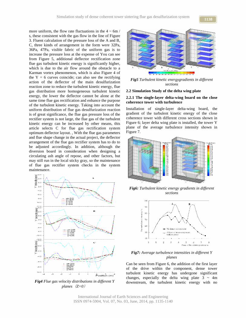
1138 Simulation study of dense coherent tower sintering flue gas desulfurization system
International Journal of Earth Sciences and Engineering
ISSN 0974-5904, Vol. 07, No. 03, June, 2014, pp. 1135-1140
more uniform, the flow rate fluctuations in the 4 ~ 6m /
s, these consistent with the gas flow in the line of Figure
3. Fluent calculation of the pressure loss of the A and B,
C, three kinds of arrangement in the form were 32Pa,
36Pa, 47Pa, visible fabric of the uniform gas is to
increase the pressure loss at the expense of You can see
from Figure 5, additional deflector rectification zone
flue gas turbulent kinetic energy is significantly higher,
which is due to the air flow around the obstacle to a
Karman vortex phenomenon, which is also Figure 4 of
the Y = 6 curves coincide; can also see the rectifying
action of the deflector of the main desulfurization
reaction zone to reduce the turbulent kinetic energy, flue
gas distribution more homogeneous turbulent kinetic
energy, the lower the deflector cannot be alone at the
same time flue gas rectification and enhance the purpose
of the turbulent kinetic energy. Taking into account the
uniform distribution of flue gas desulfurization reaction
is of great significance, the flue gas pressure loss of the
rectifier system is not large, the flue gas of the turbulent
kinetic energy can be increased by other means, this
article selects C for flue gas rectification system
optimum deflector layout. , With the flue gas parameters
and flue shape change in the actual project, the deflector
arrangement of the flue gas rectifier system has to do to
be adjusted accordingly. In addition, although the
diversion board in consideration when designing a
circulating ash angle of repose, and other factors, but
may still run in the local sticky gray, so the maintenance
of flue gas rectifier system checks in the system
maintenance.
Fig4 Flue gas velocity distributions in different Y
planes(Z=0)
Fig5 Turbulent kinetic energygradients in different
sections
2.2 Simulation Study of the delta wing plate
2.2.1 The single-layer delta-wing board on the close
coherence tower with turbulence
Installation of single-layer delta-wing board, the
gradient of the turbulent kinetic energy of the close
coherence tower with different cross sections shown in
Figure 6; layer delta wing plate is installed, the tower Y
plane of the average turbulence intensity shown in
Figure 7.
Fig6: Turbulent kinetic energy gradients in different
sections
Fig7: Average turbulence intensities in different Y
planes
Can be seen from Figure 6, the addition of the first layer
of the drive within the component, dense tower
turbulent kinetic energy has undergone significant
changes, especially the delta wing plate 3 ~ 4m
downstream, the turbulent kinetic energy with no

1139 QIAN JIA, DONGHUI ZHANG, CUNYI SONG, ZHENSONG TONG AND BAORUI LIANG
International Journal of Earth Sciences and Engineering
ISSN 0974-5904, Vol. 07, No. 03, June, 2014, pp. 1135-1140
additional components compared to increases of 2 to 3
times. Curve from Figure 7 we can see that the addition
of delta wing panels can not only change the
downstream turbulence intensity and its upstream flow
turbulence intensity. A turbulence intensity of the peak
area occurred in the area set the deflector, very
desulfurization cycle ash and flue gas mixing, and
turbulence intensity in the first layer of components
within the drive downstream 0.5m at a second the peak,
very conducive to the collision reaction of
desulfurization agent particles and SO2 from flue gas.
We can see from the figure, by adding a layer of delta
wing board, dense tower turbulent kinetic energy has
increased, but only extended to the downstream 3 ~ 4m
regional, and therefore we consider the addition of
multi-storey triangular wing.
2.2.2 multilayer delta wing plate of dense coherent
tower turbulence
Due to the limitations of the dense the Tata body size,
each delta wing plate cannot occupy the entire dense
phase the Tata body cross-section. Without layout of the
region of the delta wing plate, the flow pressure loss is
smaller, the flue gas flow from the middle, while the
short circuit flow phenomena, which is detrimental to
the dense tower of desulfurization. Set of two layers of
delta wing board, dense tower of smoke flow axial
velocity showed intermediate and high and low on both
sides of the distribution of additional multi-layer delta-
wing boards, and more conducive to the balanced flue
gas flow pressure loss. Layout of the first layer
downstream of the delta wing plate 2m, 4m and 6m at.
Close coherence of the different cross-section of the
tower mount multilayer delta wing plate, turbulent
kinetic energy gradient as shown in Figure 8 below; not
mounted delta wing panels and installation of single-
layer, four-story delta wing plate tower Y plane, the
average turbulence intensity in Figure9 shows.
Fig8: Turbulent kinetic energy gradients in different
sections
Fig9: Averageturbulence intensities in different Y
planes
Can be seen from Figure 8, after the addition of four-
layer delta-wing board, the new addition of a single set
of delta wing plate on the flue gas flow redistribution
and rectification, coupled with its own role to spin, the
dense phase tower internal effective reaction zone of
turbulent kinetic energy is further increased, the
downstream turbulent kinetic energy region and the
dense tower of export of high turbulent kinetic energy
region is connected into one. Can be seen from Figure 9,
after the addition of four-layer delta-wing boards, dense
tower of five high turbulence intensity peak, and four
other turbulence intensity peak occurred then ABCD
four-story-free drive component location; additional
four-story-free drive components, dense tower of
average turbulence intensity is increased to not add
components in case of a preset 3 to 4 times. Add a four-
layer delta-wing boards, dense towers of different
heights section of flue gas flow axial velocity gradient
is, we can see from Figure 10; additional four-story
delta wing panels, the tower flue gas flow improvement
in the flue gas flow is relatively uniform. Turbulence
intensity of the component after an additional four-story
drive within the region increased to 2.2 times the
original, gas-solid slip velocity significantly increased
the formation of a desulfurization reaction enabling the
effective reaction zone, the effective reaction zone The
pressure loss is about 80Pa, dense tower overall
pressure loss is less than 300Pa.
Figure 10: a high degree of cross-section on the flue
gas flow axial velocity
2.3 optimized dense coherent tower simulation study

1140 Simulation study of dense coherent tower sintering flue gas desulfurization system
International Journal of Earth Sciences and Engineering
ISSN 0974-5904, Vol. 07, No. 03, June, 2014, pp. 1135-1140
The optimized gas flow in the dense coherent within the
Tata line, recycling gray trace shown in Figure 11.
Fig11: Flue gas streamlines in DFA and trace line of
circulating ash
Can be seen from Figure 11, the optimized dense
coherent tower flue gas flow line and the gray loop can
be evenly distributed and full access to the delta wing
plate at the same time increase the flue gas turbulent
kinetic energy, there is no impact on mainstream smoke
the uniform distribution did not produce flue gas back
mixing on the desulfurization reaction is favorable.
Delta wing plate can to some extent, to change the
trajectory of circulating ash particles, the particle size
the greater the impact is more obvious. Semidry
desulfurization process a larger common problem is
when the cycle of gray humidification uneven, there
will be partial reunion, which led to the sticky wall and
even harden a serious threat to the stable operation of
the system. Another important role of the delta wing
plate is possible reunion cycle of gray broken to prevent
the sticky wall knot and other problems occur [9]
. Can
also see from the figure, most of the circulating ash will
be deposited into the ash bucket, a small part of the
small particle size of circulating ash to be flue to carry
out into the bag filter. Delta wing plate on the one hand
to strengthen the inner loop, the other hand, can
effectively reduce the load of the bag filter [10]
. Fluent
computing the entire dense coherent tower pressure loss
of about 300 pa flue gas rectifier system and two layers
of chain blender produce about 80 Pa and 180 Pa of
pressure loss. Visible even at the within component,
dense coherent tower smooth gravity flow, pressure loss
is still small.
3 Conclusions
Dense coherent tower flue gas rectifier systems in Table
1, conditions optimum deflector arrangement for C, flue
gas to be able to achieve uniform distribution of the
flow rate fluctuations within 4 to 6m / s, the pressure
loss of 47 Pa; delta wing board to increase the density of
coherent turbulent kinetic energy of the tower,
especially the effect on its nearby area, the turbulent
kinetic energy increases by 3-4 times; to enhance the
local turbulence intensity of the flue gas to a certain
extent, but to enhance the effect on the overall
turbulence intensity not obvious; mount multilayer delta
wing plate can increase the coverage area of high
turbulence intensity, and compared with the single-layer
turbulence intensity is not easy to attenuation.
Simulation results show that under optimal conditions:
uniform distribution of dense coherent tower of smoke
and gas-solid full access to the delta wing plate a
significant impact on the movement of large particles
circulating ash, most of the circulating ash particles
settlement involved in loop, only a small part of the
small particles of flue gas brought into the dust
collector, close coherence tower pressure loss of
approximately 300 pa.
4. Reference:
[1] Dang Y H, Qi Y H, Wang H F. Technology of flue
gas desulfurization, Journal of Iron and Steel
Research, 2010, 22(5): 1-6
[2] Feng L. Analysis of wet type desulphurization
method of sintering exhaust fume, Mining
Engineering, 2011, 9(3): 66-68
[3] Zhao Y Z, Cheng Y, Jin Y. CFD-DEM simulation
of clustering phenomena in riser and downer,
Journal of Chemical Industry and Engineering,
2007, 58(1): 44-53
[4] Zhou Y G, Peng J, Zhu X, et al. Hydrodynamics of
gas–solid flow in the circulating fluidized bed
reactor for dry flue gas desulfurization, Powder
Technology, 2011, 205(1-3): 208-216
[5] Wang F, Lu M. The study on spray dryer absorber
flue gas desulfurization for industrial boiler ,Fuel
and Energy Abstracts, 2002, 43 (4): 274
[6] Chang G Q, Song C Y, Wang L. A modeling and
experimental study of flue gas desulfurization in a
dense phase tower, Journal of Hazardous Materials,
2011, 189(1-2): 134-140
[7] Hou H C. Preliminary Analysis and Application on
karman Swirl, Journal of Qinghai Normal
University(Natural Science Edition), 2005, 3:23-25
[8] Wang J C, Wang X Y, Wang S D, et al. The
research on gas-solid flow in high particle flux CFB
riser, Boiler Technology, 2010, 41(1): 36-39
[9] Zheng X Y, Liu B Q. Mechanism research on
particle clustering and crushing in dense flue gas,
Electric Power Environmental Protection, 2006,
22(1): 55-57
[10] Zhu J L, Chen X J, Zhang T, et al. Computational
fluid dynamics simulation of hydrodynamics in an
internal-loop fluidized bed reactor with a funnel-
shaped internal, Acta Scientiae Circumstantiae,
2011, 31(6): 1212-1219.
www.cafetinnova.org
Indexed in
Scopus Compendex and Geobase Elsevier, Chemical
Abstract Services-USA, Geo-Ref Information Services-USA,
List B of Scientific Journals, Poland,
Directory of Research Journals
ISSN 0974-5904, Volume 07, No. 03
June 2014, P.P.1141-1150
#02070346 Copyright ©2014 CAFET-INNOVA TECHNICAL SOCIETY. All rights reserved.
Vehicle Information Compression and Transmission Methods Basis
on Mixed Data Types
YANG JINGFENG1,2,3
, LI YONG4**
, ZHANG NANFENG1,5
, HE JIARONG6 and XUE YUEJU
1*
1South China Agricultural University, Guangzhou, 510642, China
2Guangzhou Public Transport Data Management Center, Guangzhou, 510620, China
3Guangzhou Transport Information Control Center, Guangzhou, 510620, China
4Guangzhou Institute of Geography, Guangzhou, 510070, China
5Guangzhou Entry-exit Inspection and Quarantine, Guangzhou, 510623, China
6South China University of Technology, Guangzhou, 510641, China
Email: [email protected], [email protected], liyong@ gdas.ac.cn
Abstract: For the unbalanced coverage of mobile communication base station, data loss and incomplete data are
prone to emergence when a large amounts of real-time data transmission through 3G/GPRS network in the poor
communication environment of subregion, which is difficult to achieve large-scale farmland information collection
and transmission. Therefore, optimized Huffman coding compression algorithm for text-oriented information
(including location information) ,optimized iCAM06 compression algorithm for image, MPEG-4 compression
algorithm combined with DCT differential modulation algorithm for video are promoted in this paper. Through
corresponding compression method for vehicle information mixed data types of text, image, video respectively, this
paper designed data transmission strategies of different transmission priority and the data uniqueness checking
method at the same time. The whole process test results of data exchange and decompression show that, the data
compression algorithms can effectively realize data (text, image, and video) compression. The data sampling period
is relatively smaller and its adjacent data is closer, the higher compression rate can be obtained by corresponding
compression algorithms, and it can the basically ensure the decompression data without distortion. This will improve
the efficiency of information transmission of transportation, as well as to ensure the integrity of information, which
is of great significance to realization of transportation energy conservation.
Keywords: Vehicle Information; Data Compression; Priority Strategy Transmission Mode; Mixed Data Types.
1. Introduction:
The key operational vehicle information safety
supervision has been continuously strengthened along
with the national, provincial governments at all levels.
The standard terminal with satellite positioning function
were forcibly mounted on passenger bus, tourist charter,
dangerous goods vehicles, coaches, trucks, heavy
trucks, buses, taxis and so on. Some cities also require
passenger bus, tourist chartered buses, taxis and other
installation equipment using a video camera in order to
enhance information security regulatory standards.
Regardless the using of satellite positioning terminal or
video camera equipment, it must bear a lot of the cost of
wireless data transmission. If using new energy
vehicles, such as electric buses, hybrid buses, electric
taxis, etc., due to the need to upload more types of data
to the regulatory status of the platform, its wireless
transmission costs will rise at the same time. How to
meet the requirements of the competent authorities, and
saves the cost of wireless data transmission has become
an important problem to be solved at present industry.
The compressed data transmission is one of the
important ways to solve the problem, and it can ensure
the real-time and data quality of data transmission in the
city communication environment, many scholars have
conducted extensive research in this areas. Vehicle
information is now covered by the text, pictures, video
and other types of information. In order to improve data
transmission quality, many researchers have proposed a
variety of compression and transmission methods, for
example, Hashemian[1]、 Sharma[2]、 Shi[3]、
Meng[4] et al proposed for the Huffman coding
technology for wireless transmission of GPS, including
GPS coordinate, records and other text data
compression and transmission problems; Hu[5]、
Jou[6]、 Wang[7]、 Barr[8] et al put forward the LZW
compression algorithm which can be optimized by
establishing a method to quickly find a dictionary, and it
can greatly reduce the time of data compression to
achieve optimal compression, and improve transmission
efficiency; Wavelet compression[9] method for wireless
transmission of compressed gradually become a hot spot
1142 Vehicle Information Compression and Transmission Methods Basis on Mixed
Data Types
International Journal of Earth Sciences and Engineering
ISSN 0974-5904, Vol. 07, No. 03, June, 2014, pp. 1141-1150
in recent years. In terms of traffic information, based on
GML data compressions, Zhang[10] achieved a traffic
emergency data and realized a framework of urban
traffic emergency system architecture; Through random
matrices with restricted isometric conditions of the
original high-dimensional data onto a low dimensional
space, Li[11] realized the data fast and efficient
compression, and via a convex optimization algorithm
to complete the data decompression in traffic
information processing terminal after data transmission;
According to the characteristics of traffic data, Zhao[12]
using its research and comparative data compression
methods based on principal component analysis (PCA)
and independent component analysis (ICA) method,
respectively. Scholars' research results could furnish
some useful suggestions in the transmission terminal
data to a certain extent. However, the problem can not
be ignored is, because of the unbalanced nature of the
distribution of urban mobile communication base
stations, urban communication environment vary
greatly, the data transmission capacity is in greater
differences in different parts of the city, part of the
region exists communication blind area. The method
proposed by scholars rarely used in acquisition and
transmission terminal data on one hand, also rarely take
into consideration differences the problem in the larger
urban communication environment for real-time
transmission of data, that is, how to realize text,
pictures, video and other information integrated
transmission while coverage of communication base
station is uneven with large difference between the
communication environment in urban areas. In addition,
the large flow of data transmission needs to consume
more energy; low-power transmission[13] has important
significance to prolong the length of the various devices
work. Therefore, based on priority principle approach
for simple algorithms, short time-consuming,
minimizing overhead of data collection terminals and
the backend server, the vehicle operating data
information compression and transmission methods
based on priority strategies is proposed in this paper..
Data collection vehicle information compression and
transmission method can be achieving the optimized by
encryption, compression, transmission, reception,
decryption process, which is important to improve the
transmission efficiency of vehicle information to ensure
the integrity of information and transportation industry
to achieve energy saving.
2. Vehicle Information Compression and
Transmission Method
According to national standards, Ministry of
Transportation and the provincial technical standards
requirements, the current standard of vehicle
information including position, speed, altitude, license
plates, start/flameout, lights, driving status, drivers and
other types of text, plus photos and video that collected
through the data collection terminals. If the vehicles for
new energy vehicles, it needs to extending battery
status, temperature, and overall and the cell voltage,
current and other battery management information. The
data with different format, size, and type will be
uploaded via the data exchange and the wireless
communication module of the vehicle terminal.
The whole process from the point of view of data
transmission, namely, data collection, transmission,
reception, storage throughout the process point of view,
when compared to a large number of simultaneous
transmission vehicle terminal especially, the main
pressure is focused on how the backend server receives
a large number of short, transmission, integration of
data transmitted by the terminal.
The way to solve the problem of large amounts of data
transmission and access mainly includes three. First,
data optimization in vehicle terminal, extract the key
significance with application data, the remaining data is
temporarily stored in the terminal memory device.
Second, data are identified in the data receiving
platform to extract of critical data, but it must guarantee
the reliability of data transmission. The last, data are
compressed by vehicle terminal firstly, and
decompressed on the platform.
The compression-decompression method can ensure the
integrity of data transmission, but also can reduce the
data communication flow, which can save
communication costs, but its disadvantages are also very
obvious. Optimization transmission of terminal is with
less disadvantages, the main disadvantage is it requires
the performance processing each group of data
compression, which would lead to transmission time
delay. Real-time upload of vehicle information is
demanding on safety supervision, except pictures and
video information in the daily management which does
not affect the actual data application with reasonable
delaying. Moreover, with higher hardware configuration
of vehicle terminal at present, the capable of handling
large amounts of data vehicle terminal hardware
compression technology is promoted. Data collecting,
data compressing and transmitting could be performed
at the same time, which could not be simultaneously
affected.
2.1. Data Compression Algorithms
Due to the limitations of the vehicle terminal hardware
conditions, the applications for data transmission
compression by vehicle terminal were less in the past
for a long period of time in the practical. Images, video
and other data that takes up a lot of storage space are
usually collected in offline mode, namely, images, video
and other data in not considering the real-time
requirement when used by off-line way.
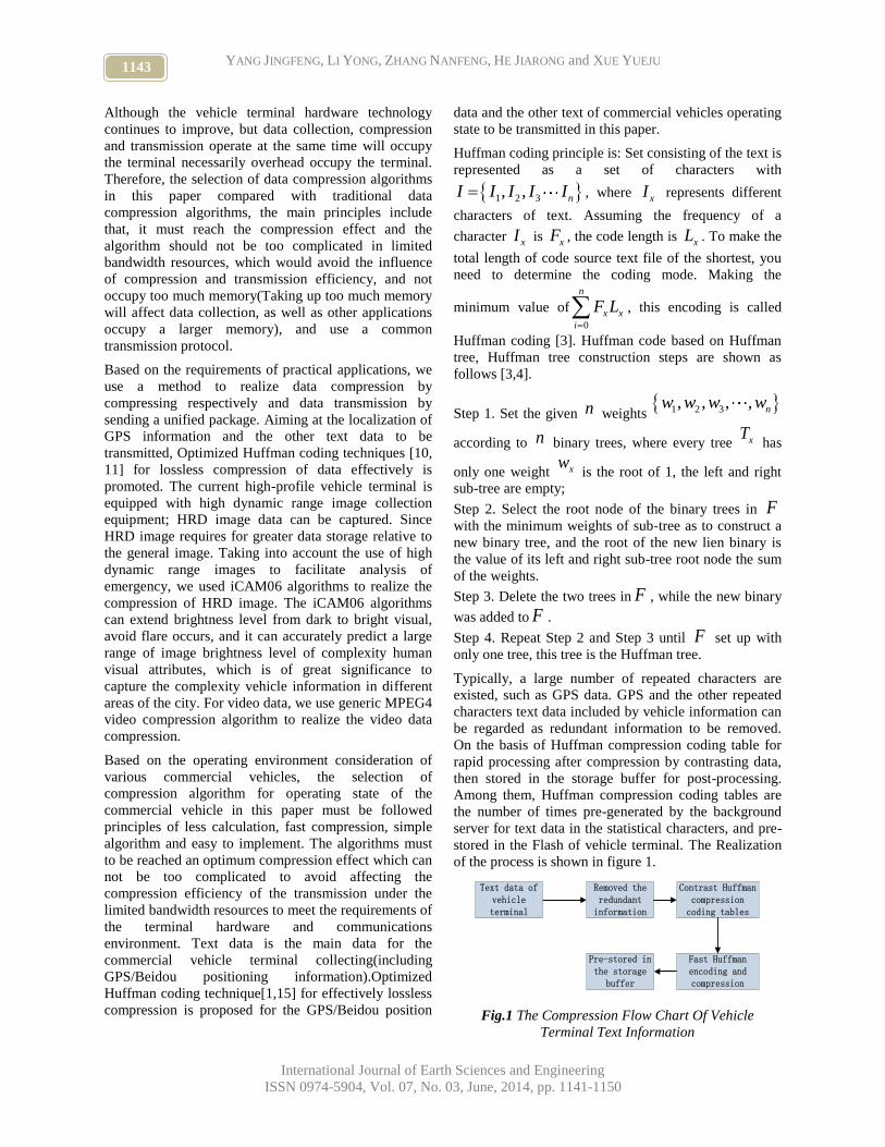
1143 YANG JINGFENG, LI YONG, ZHANG NANFENG, HE JIARONG and XUE YUEJU
International Journal of Earth Sciences and Engineering
ISSN 0974-5904, Vol. 07, No. 03, June, 2014, pp. 1141-1150
Although the vehicle terminal hardware technology
continues to improve, but data collection, compression
and transmission operate at the same time will occupy
the terminal necessarily overhead occupy the terminal.
Therefore, the selection of data compression algorithms
in this paper compared with traditional data
compression algorithms, the main principles include
that, it must reach the compression effect and the
algorithm should not be too complicated in limited
bandwidth resources, which would avoid the influence
of compression and transmission efficiency, and not
occupy too much memory(Taking up too much memory
will affect data collection, as well as other applications
occupy a larger memory), and use a common
transmission protocol.
Based on the requirements of practical applications, we
use a method to realize data compression by
compressing respectively and data transmission by
sending a unified package. Aiming at the localization of
GPS information and the other text data to be
transmitted, Optimized Huffman coding techniques [10,
11] for lossless compression of data effectively is
promoted. The current high-profile vehicle terminal is
equipped with high dynamic range image collection
equipment; HRD image data can be captured. Since
HRD image requires for greater data storage relative to
the general image. Taking into account the use of high
dynamic range images to facilitate analysis of
emergency, we used iCAM06 algorithms to realize the
compression of HRD image. The iCAM06 algorithms
can extend brightness level from dark to bright visual,
avoid flare occurs, and it can accurately predict a large
range of image brightness level of complexity human
visual attributes, which is of great significance to
capture the complexity vehicle information in different
areas of the city. For video data, we use generic MPEG4
video compression algorithm to realize the video data
compression.
Based on the operating environment consideration of
various commercial vehicles, the selection of
compression algorithm for operating state of the
commercial vehicle in this paper must be followed
principles of less calculation, fast compression, simple
algorithm and easy to implement. The algorithms must
to be reached an optimum compression effect which can
not be too complicated to avoid affecting the
compression efficiency of the transmission under the
limited bandwidth resources to meet the requirements of
the terminal hardware and communications
environment. Text data is the main data for the
commercial vehicle terminal collecting(including
GPS/Beidou positioning information).Optimized
Huffman coding technique[1,15] for effectively lossless
compression is proposed for the GPS/Beidou position
data and the other text of commercial vehicles operating
state to be transmitted in this paper.
Huffman coding principle is: Set consisting of the text is
represented as a set of characters with
1 2 3, , nI I I I I , where xI represents different
characters of text. Assuming the frequency of a
character xI is xF , the code length is xL . To make the
total length of code source text file of the shortest, you
need to determine the coding mode. Making the
minimum value of
0
n
x x
i
F L
, this encoding is called
Huffman coding [3]. Huffman code based on Huffman
tree, Huffman tree construction steps are shown as
follows [3,4].
Step 1. Set the given n weights 1 2 3, , , , nw w w w
according to n binary trees, where every tree xT has
only one weight xw is the root of 1, the left and right
sub-tree are empty;
Step 2. Select the root node of the binary trees in F
with the minimum weights of sub-tree as to construct a
new binary tree, and the root of the new lien binary is
the value of its left and right sub-tree root node the sum
of the weights.
Step 3. Delete the two trees in F , while the new binary
was added to F .
Step 4. Repeat Step 2 and Step 3 until F set up with
only one tree, this tree is the Huffman tree.
Typically, a large number of repeated characters are
existed, such as GPS data. GPS and the other repeated
characters text data included by vehicle information can
be regarded as redundant information to be removed.
On the basis of Huffman compression coding table for
rapid processing after compression by contrasting data,
then stored in the storage buffer for post-processing.
Among them, Huffman compression coding tables are
the number of times pre-generated by the background
server for text data in the statistical characters, and pre-
stored in the Flash of vehicle terminal. The Realization
of the process is shown in figure 1.
Removed the redundant
information
Contrast Huffman compression
coding tables
Fast Huffman encoding and compression
Pre-stored in the storage
buffer
Text data of vehicle terminal
Fig.1 The Compression Flow Chart Of Vehicle
Terminal Text Information

1144 Vehicle Information Compression and Transmission Methods Basis on Mixed
Data Types
International Journal of Earth Sciences and Engineering
ISSN 0974-5904, Vol. 07, No. 03, June, 2014, pp. 1141-1150
Huffman encoding is completely according to the
characters of probability to construct coding, there is no
error protection function. The algorithm needs to
calculate the source character of probability statistics
and obtains the probability distribution of the source
symbols. This process requires a large cache using the
hardware implementation of the algorithm. Generally, it
believes that the decoding is complexity, and it's not
conducive to the realization of hardware implementation
[15,16]. Huffman coding and arithmetic coding is a
typical probability model, many scholars proposed the
dictionary model for optimizing the original model, the
typical optimizing algorithms such as LZW algorithm
[4,15], etc.
For compression and decompression speed, LZW
algorithm is fast, and requires only one scan of the
compressed data to be compressed. The compression
ratio of the algorithm is very good for the continuous
input stream to be compressed with high rate repetition.
But the main drawback of this algorithm is the
adaptability is rather poor, and the compression rate is
less than Huffman algorithm. Moreover, the LZW
algorithm usually needs to combine with other
algorithms to reach the expected aim for some file with
very low complexity. For vehicle operation status data,
the data type apparently does not apply to LZW
algorithm.
Huffman coding method has certain limitation, such as
it need to scan flow of input symbols for two times, be
stored or transmitted by Huffman tree before the storage
or transmission of Huffman coding results. However,
the algorithm has high compression rate, simple and
practical, and all the coding has uniqueness while
decoding, very suitable for vehicle information data that
has high identification requirements. In order to
overcome the practical problem of cache, high
complexity caused by the Huffman coding, we
improved the structure of Huffman tree based on the
original. The main steps are as follows:
Step 1. Initialize the established binary Huffman tree,
one of the root node has a weight of 0;
Step 2. To encode without the new characters of newly
generated two nodes, the connection of the parent node
weights add 1, and another node, which is defined as
node weights of 0 nodes to define new weight of 0;
Step 3. The new characters have been encrypted through
search was coded character location, in the case of the
characters of the weight add 1 with coding and
compared with the original weight of the same node;
Step 4. Repeat Step 2 and Step 3 until all characters are
encoded.
The improved way of Huffman coding by weight set to
0, the original requires two symbols flow is simplified
to a scan. The algorithm only needs to scan a probability
of 1 characters, and it can only exchange the node
between the binary tree needs to node numbering, which
reduces the occupation of the cache, and the complexity
of the algorithm is decreased. Its deficiencies are mainly
embodied in the complete lost of coding error protection
function, and the data requirements are relatively high.
Popular image compression algorithm at present include
equalize histogram, local color adaptation algorithm,
tone compression method, adaptive algorithm, iCAM
algorithm, iCAM06 algorithm[17] et al. Through the
compression of base layer of large scale and layer
relatively complete reservation details, iCAM06
algorithm can obtain the histogram shape close to
original HDR images, and the distribution of different
pixel HDR image has good applicability, it is the best
performing algorithm [17]. This paper uses iCAM06
algorithm to compress the image information of vehicle
terminal in the driving process, and then realizes data
transmission.
ICAM06 algorithm converts the data into a XYZ signal,
using the edge preserving filter decomposes image into
a base layer (contains only large-scale change
information and detail layer) and detail layer (edge and
texture detail) to layered double filter processing
[18,19]. In view of the human visual system to the
characteristics of the local contrast is more sensitive
than the global contrast, the compression operation is
realize in high dynamic range scene and preserve local
details in the scene global dynamic range[18,19].
Layered double filtering processing algorithm is shown
as follows:
1( ) ( )
( )s p s p
p
J f p s g I I Ik s
Where, ( ) ( ) ( ), ( )p s
p
k s f p s g I I f p s
is
the Gaussian filtering function in the spatial domain,
( )p sg I I is the Gauss filter function intensity
domain, pI and sI are pixel intensity respectively,
represents the whole image.
Layered double filtering processing can adopt fuzzy
mathematics theory to deal with HRD images
effectively while keeping the edge sharpening in good
condition. Layered double filtering processing can also
prevent artificial halo phenomenon, and accurately
predict human visual properties in complex images
environment of a large range of brightness levels. This
proposed algorithm can better predict the color
appearance of complex wide range scene, and it's more
suitable for HDR image for cross-media copying [17,
18, 19].

1145 YANG JINGFENG, LI YONG, ZHANG NANFENG, HE JIARONG and XUE YUEJU
International Journal of Earth Sciences and Engineering
ISSN 0974-5904, Vol. 07, No. 03, June, 2014, pp. 1141-1150
The nonlinear compression effect of iCAM06 algorithm
is to realize the high dynamic range image gradual
compressing into a low dynamic range. Due to cut off
some color range by compression process, it may lead to
appear unrealistic rendering. The reason for this is, color
has been tonal mapping into general in the middle range
image, image color was scaling and tailored to coloring
is directly mapped to a specific profile. When the output
range compared to the input range greatly, the
specifically profile problem is especially obvious. In
this case, one specific performance is, if the image
scaling to smaller scale directly, many colors in the
output will become too dim to be observed, gradient
between colors can also be lost while the output
incompatible colors of the excess. Another specific
performance is, cutting operation is likely to cut off the
middle range of color, or to cut off a wide range of color
and to combine with the color of less zoom range.
The main method to solve this problem is to make the
color gamut in each direction being more uniform,
namely, to increase the brightness and improve
saturation. The specific approach is shown as follows.
Settings the average values of the image brightness
as avrJ . Setting the average brightness value for all
colors on the image with the sort brightness value
greater than 99%, denoted by 99J ; the average
brightness value for all colors on the image with the sort
brightness value less than or equal to 1%, denoted
by 01J . If 99 01
avr
J JK
J
( K is the proportional
coefficient, usually take 2K ), then continuing to
sorting statistics brightness value is greater than 98%
and less than or equal to 2% of average sort brightness
mean value, and remember to 98J and 02J respectively.
Calculating 98 02
avr
J J
J
, if 98 02
avr
J JK
J
, then further
calculating according to the extent of 1% recursive until
100i i
avr
J JK
J
, while iJ can be defined as the
maximum brightness value, and 100 iJ is the minimum
brightness value.
Cutting operation by iCAM06 algorithm will be done
after the maximum brightness value and minimum
brightness value has been got. Removing the color
beyond the range of the maximum and the minimum
limit, and scaling color between maximum brightness
and minimum brightness values, then the image
compression operations could be realized.
For the compression of video data, this paper uses
MPEG-4 video compression algorithm. Video image
can be divided into macro block by Mpeg-4 algorithm,
while DCT combined with differential modulation
methods for compression. The specific calculation of
MPEG-4 algorithm has the separable characteristics,
which can be fast compression at the same time and
provide compressed in different ways according to the
different object. That will not only provide a higher
compression ratio but also a better visual quality.
2.2. Data transmission method and Priority Strategy
Transmission Mode
The uploaded data of vehicle information according to
the file size of text data (including GPS positioning
data), image and video. According to the vehicle data
information for wireless transmission is of simple
structure, single function and small data redundancy
tolerance, all data would be uploaded by the
international standard NMEA-0183 GPS data
transmission as well as a variety of on-board GPS
monitoring terminal transmission protocol in this paper.
On the deployment of mobile base station, the
deployment of the city is not balanced, signal fade area
exist in the villages and overpass nearby due to various
reasons. Before the data is transmitted it usually
requires multiple handshaking to establish wireless
communication network, while communication is easy
to failure when handshaking. In expanding the data
acquisition range of the vehicle terminal, it needs to
transmit a large flow of vehicle information such as text,
pictures, video, and various exchanged sensor data,
which is easy to lose in the data transmission process. It
is difficult to ensure the integrity of the vehicle
information. Incomplete data may also be difficult to
parse while backend server receives the data, the
calculations pressure of background server for
completeness checking on the vehicle information will
also be increasing at the same time.
Based on the actual condition of vehicle information
and requirements, priority transmission principles and
requirements must be developed in the first time to meet
the different requirements of different transmission
situations. In the default setting or in this case of
receiving terminal without particular choice by users,
default the following principles for data transmission.
(1) Give priority to compress and transmit text data,
followed by the image, final the video in a better
wireless transmission or communications environment.
Make it a priority to compress and transmit the text data
such as GPS, temperature automatic collected or
exchanged by the receiving module or the sensor data
without manual input when receiving terminal did not
put forward the image, video transmission requirements,
then the manual input data, and the image, video etc.
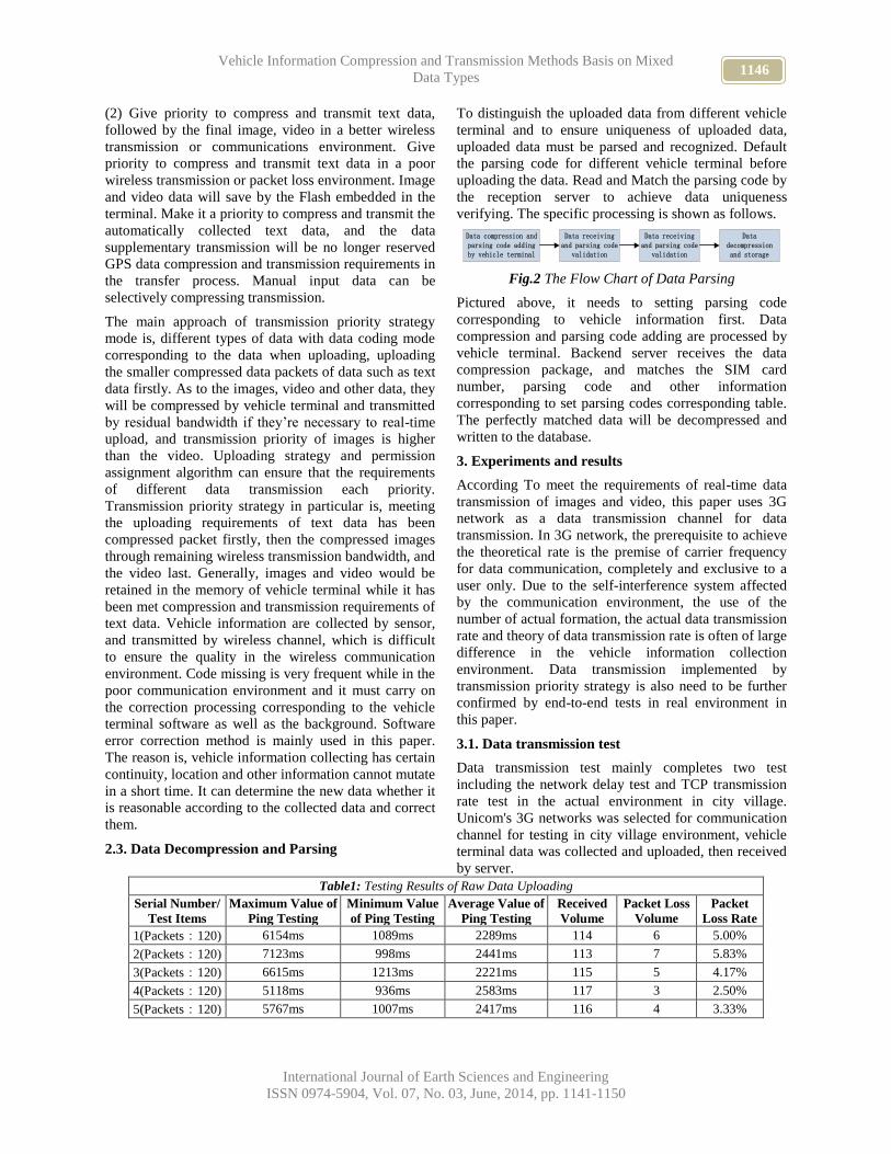
1146 Vehicle Information Compression and Transmission Methods Basis on Mixed
Data Types
International Journal of Earth Sciences and Engineering
ISSN 0974-5904, Vol. 07, No. 03, June, 2014, pp. 1141-1150
(2) Give priority to compress and transmit text data,
followed by the final image, video in a better wireless
transmission or communications environment. Give
priority to compress and transmit text data in a poor
wireless transmission or packet loss environment. Image
and video data will save by the Flash embedded in the
terminal. Make it a priority to compress and transmit the
automatically collected text data, and the data
supplementary transmission will be no longer reserved
GPS data compression and transmission requirements in
the transfer process. Manual input data can be
selectively compressing transmission.
The main approach of transmission priority strategy
mode is, different types of data with data coding mode
corresponding to the data when uploading, uploading
the smaller compressed data packets of data such as text
data firstly. As to the images, video and other data, they
will be compressed by vehicle terminal and transmitted
by residual bandwidth if they’re necessary to real-time
upload, and transmission priority of images is higher
than the video. Uploading strategy and permission
assignment algorithm can ensure that the requirements
of different data transmission each priority.
Transmission priority strategy in particular is, meeting
the uploading requirements of text data has been
compressed packet firstly, then the compressed images
through remaining wireless transmission bandwidth, and
the video last. Generally, images and video would be
retained in the memory of vehicle terminal while it has
been met compression and transmission requirements of
text data. Vehicle information are collected by sensor,
and transmitted by wireless channel, which is difficult
to ensure the quality in the wireless communication
environment. Code missing is very frequent while in the
poor communication environment and it must carry on
the correction processing corresponding to the vehicle
terminal software as well as the background. Software
error correction method is mainly used in this paper.
The reason is, vehicle information collecting has certain
continuity, location and other information cannot mutate
in a short time. It can determine the new data whether it
is reasonable according to the collected data and correct
them.
2.3. Data Decompression and Parsing
To distinguish the uploaded data from different vehicle
terminal and to ensure uniqueness of uploaded data,
uploaded data must be parsed and recognized. Default
the parsing code for different vehicle terminal before
uploading the data. Read and Match the parsing code by
the reception server to achieve data uniqueness
verifying. The specific processing is shown as follows.
Data compression and parsing code adding by vehicle terminal
Data receiving and parsing code
validation
Data receiving and parsing code
validation
Data decompression and storage
Fig.2 The Flow Chart of Data Parsing
Pictured above, it needs to setting parsing code
corresponding to vehicle information first. Data
compression and parsing code adding are processed by
vehicle terminal. Backend server receives the data
compression package, and matches the SIM card
number, parsing code and other information
corresponding to set parsing codes corresponding table.
The perfectly matched data will be decompressed and
written to the database.
3. Experiments and results
According To meet the requirements of real-time data
transmission of images and video, this paper uses 3G
network as a data transmission channel for data
transmission. In 3G network, the prerequisite to achieve
the theoretical rate is the premise of carrier frequency
for data communication, completely and exclusive to a
user only. Due to the self-interference system affected
by the communication environment, the use of the
number of actual formation, the actual data transmission
rate and theory of data transmission rate is often of large
difference in the vehicle information collection
environment. Data transmission implemented by
transmission priority strategy is also need to be further
confirmed by end-to-end tests in real environment in
this paper.
3.1. Data transmission test
Data transmission test mainly completes two test
including the network delay test and TCP transmission
rate test in the actual environment in city village.
Unicom's 3G networks was selected for communication
channel for testing in city village environment, vehicle
terminal data was collected and uploaded, then received
by server.
Table1: Testing Results of Raw Data Uploading
Serial Number/
Test Items
Maximum Value of
Ping Testing
Minimum Value
of Ping Testing
Average Value of
Ping Testing
Received
Volume
Packet Loss
Volume
Packet
Loss Rate
1(Packets:120) 6154ms 1089ms 2289ms 114 6 5.00%
2(Packets:120) 7123ms 998ms 2441ms 113 7 5.83%
3(Packets:120) 6615ms 1213ms 2221ms 115 5 4.17%
4(Packets:120) 5118ms 936ms 2583ms 117 3 2.50%
5(Packets:120) 5767ms 1007ms 2417ms 116 4 3.33%

1147 YANG JINGFENG, LI YONG, ZHANG NANFENG, HE JIARONG and XUE YUEJU
International Journal of Earth Sciences and Engineering
ISSN 0974-5904, Vol. 07, No. 03, June, 2014, pp. 1141-1150
Round trip time (RTT) is usually used as a measure of
3G network time delay. Low delay time is of extreme
importance in actual application. Lower delay is
advantageous for the uplink direction to improve
capacity and data throughput, and increase the coverage
of high bit rate, obtain higher transmission bit rate.
Typically, data transmission testing uses PING method,
namely by obtaining response time of sending and
receiving data packets to get connected server response
time. When sending upload packets in requesting, all the
serial number sequence will be added one firstly before
sending, the replying information will also be marked
the corresponding serial number. Then observe the Ping
packet response messages to detect the link for data
transmission delay calculation, such as packet loss,
grouping repetition and fault sequence etc.
The following table shows the data uploaded test results
in a village environment of a city. To be clear, several
uploaded tests were started at 10 in the morning, ICMP
packets for a total of 120 were send every time, the 3G
bandwidth rate of 70-120kbps (city 3G bandwidth rate
is about 700-900kbps), TCP transmission rate is close to
3G bandwidth rate.
The result of data packets uploaded test shows that, the
maximum delay time is 7123ms,the average delay time
of 2382ms, which meets the basic requirements in real
time data uploaded. 3G network takes the average
packet loss rate 4.17% of data uploading while the
network bandwidth is 70-120kbps. Relative to the
GPRS data transmission mode, 3G network has been
able to meet the requirement of actual application in the
setting of upload strategy and selecting transport
protocol, but also laid the foundation for the data
compression test environment. In addition, it appears
from the data uploading test results, village area of the
communication environment is relatively poor, data
compression and transmission will still be of importance
as well.
3.2. Data compression and decompression test
Based on the established vehicle terminal, 3G networks
and backend server system, setting default priority
transmission strategy, compression and transmission can
be started by the collected vehicle information, and the
results of comparing the uncompressed data
transmission with compressed data transmission can be
shown. The data compression testing is shown in Table
2. The main evaluation on the effect of data
compression is mainly based on the compression rate
and transmission time. Compression rate is one of the
most important indexes to measure the data
compression algorithm. Compression rate is a direct
measure of data reduction, the running time reflects the
complexity of the algorithm, and the combination of the
two indexes can be further estimated energy efficiency
of communication. Transmission error rate is the rate
between data length of accurately praised data
(compressed data containing the decompression
process) had not received by backend server and the
data length before compressing. Packet loss rate is the
ratio between the packet numbers of server has not been
received and data packets had been transmitted by
vehicle terminal.
Table2: Testing Result of Data Compression
Serial
Type
of
Data
Data
Collectio
n Cycle
Data
Length
Before
Compres
sion (kb)
Data
Length
After
Compres
sion (kb)
Compres
sion Rate
Transmis
sion Time
Before
Compres
sion(s)
Transmis
sion Time
After
Compres
sion (s)
Transmissi
on Error
Rate
Before
Compressi
on
Transmissi
on Error
Rate After
Compressi
on
Packet
Loss
Rate
Before
Compre
ssion
Packet
Loss
Rate
After
Compre
ssion
1 Text 30s 148 48 32.43% 0.45 0.14 2.21% 2.01% 4.39% 3.89%
2 Text 20s 2156 646 29.96% 6.76 2.02 2.47% 2.15% 4.12% 3.73%
3 Text 10s 5121 1473 28.76% 14.56 4.26 2.24% 2.07% 3.84% 3.22%
4 Text 5s 9892 2563 25.91% 29.28 7.09 2.29% 1.99% 3.67% 3.25%
5 Image 30min 6632 2236 33.72% 17.23 6.76 - - - -
6 Image 20min 13287 4029 30.32% 40.21 12.89 - - - -
7 Image 10min 24659 6321 25.63% 65.03 17.98 - - - -
8 Video 30min 28935 9356 32.33% 78.76 28.44 - - - -
9 Video 20min 53127 16549 31.15% 167.29 50.66 - - - -
10 Video 10min 112789 31080 27.56% 302.26 75.31 - - - -
Experiment result shows that, compressed transmission
effect was more notable. The transmission amount of
compressed data is reduced greatly, accounting for
about between the original amount of data of 1/4-1/3,
and the corresponding transmission time is shortened
into 1/4-1/3. In addition, it can be seen from the cycle of
data collection, data sampling period is relatively
smaller and its adjacent data is closer, all kinds of

1148 Vehicle Information Compression and Transmission Methods Basis on Mixed
Data Types
International Journal of Earth Sciences and Engineering
ISSN 0974-5904, Vol. 07, No. 03, June, 2014, pp. 1141-1150
algorithm could get a higher compression rate. In
particular, the correlation data has obtained the very
good compression rate, which greatly enhances the
communication efficiency of system, but also save the
cost of communication.
In order to further verify the results of data compression
algorithm, this paper compares the original data with the
parsed decompressed data. Through the data
exchanging, vehicle terminal could obtain the speed
sensor data. Exchange data through data compression
method based on the technology of Huffman coding for
data compression, and then the original data file and
compressed data files are transmitted to the backend
server through 3G network. After transmission, read the
received data file for decompression and inverse
quantization, and compare the difference between the
original data and data contrast reduction before and after
data compression.
To be clear, the speed testing data was selected for a
passenger bus driving data from 8:00 am to 16:00. An
average of 10 seconds data collection cycle was set in
the passenger bus vehicle terminal, and it generated for
a total of 2727 (theoretical value should be 2880,
because of various reasons in the process of data
collection, there are 153 errors, lost or not collected data
samples) speed data during the period. Before the data
compression, the original speed changing curve is
shown in Figure 3. In Figure 3, the horizontal represents
the speed of data collection time; the ordinate represents
speed value, where are the same as Figure 4. After the
data compression and transmission, the parsed speed
changing curve is shown in Figure 4. Figure 5 is the
speed value error rate comparison chart of before data
compression and after decompression. The horizontal
represents the speed of data collection time, the ordinate
represents the difference between the speed value before
compressed and the speed value after decompressed.
Fig.3 The Velocity Curve Before Data Compression
Figure 4 shows the decompressed and parsed data which
have been compressed, transmitted, parsed,
decompressed and warehoused to the backend server.
Fig.4 The Velocity Curve After Data Decompression
Fig.5 The Curve of Curve of Velocity Error Values
From the speed curve of the data before and after
compression, the speed error value curve can be seen,
the speed data consistent with original data basically
before compressed through the process of compression,
transmission, parsing, decompression, and data storage.
Coding, compression and other data processing
technology have met the basic requirements in actual
application. To accurately describe the data differences
between situation before and after the data compression
and transmission, this paper calculated the mean
variance to discriminate compression deviation after
transmission of the data. After calculation, the mean
square difference before and after data compression and
transmission is of only 0.2462, which is within a
reasonable range. The main reason for the deviation of
the data exists in data loss, data failing to parse and the
other reason during data transmission.
A total of 2727 data is to accurately have been parsed
during 2880 speed data transmitted by vehicle terminal,
the proportion of accurate transmission and parsing data
is up to 94.69%, which basically meet the requirements
of actual application. 153 errors, loss, and no sample
data contained the error data of 23, accounting for
0.80% of the total, loss of data 74, accounting for 2.57%
of the total loss rate, no sample data of 56 due to various
reasons did not collect, accounting for 1.94% of data
should be collected of the total. The availability testing
experiment results of compression and transmission
algorithm show that, the algorithm has high efficiency
and high transmission integrity.
4. Conclusions
Compression algorithm method is researched in this
paper to the vehicle information including text
information collection types (including position

1149 YANG JINGFENG, LI YONG, ZHANG NANFENG, HE JIARONG and XUE YUEJU
International Journal of Earth Sciences and Engineering
ISSN 0974-5904, Vol. 07, No. 03, June, 2014, pp. 1141-1150
information), image and video to compress the data by
using Huffman coding technology, iCAM06 algorithm,
MPEG-4 video respectively. On this basis, all kinds of
vehicle information is transmitted based on NMEA-
0183 various kinds of vehicle GPS monitoring
transmission protocol. Through the process of vehicle
information compression, transmission, decompression,
parsing and storage, the compression algorithms are
verified by speed data as an example. The algorithm
achieved great test results in the experiments, the
proportion of accurate data transmission and parse is up
to 94.69%, basically meet the requirements of data
uploading actual applications in different city region for
the urban public transport, passenger transport, taxi and
other industries. Meanwhile, the algorithm play an
important role for enhancing the efficiency of wireless
transmission applications and reducing the cost of data
transmission as well as the time, which has the practical
significance for the deployment of this base station, the
selection of communication mode and the other uses.
The data compression algorithms mentioned in this
paper provides a method with transmission reliability
and minimal distortion. It can provide reliable data
transmission method for different mobile base stations
coverage of the urban environment, which is important
to improve vehicle transmission efficiency of
information, ensure the integrity of information and the
realization of transport energy conservation.
5. Acknowledgements:
The research is supported by Science Program of
General Administration of Quality Supervision,
Inspection and Quarantine the People’s Republic of
China (2014IK183) and Guangdong Research Projects
Special Funds of Industry-Academy-Research
Cooperation (2012B091100345) and Guangzhou
Science and Technology Project (2014Y2-00044).
6. Reference:
[1] R. Hashemian. Condensed Table of Huffman
Coding, a New Approach to Efficient Decoding,
IEEE Transactions on Communications, Volume
No. 52, Issue No.1, 6-8, 2004.
[2] M. Sharma Compression Using Huffman Coding.
International Journal of Computer Science and
Network Security, Volume No. 10, Issue No.5,
133-141, 2010.
[3] P. Shi, M. Li, T. Yu. Design and Application of an
XML Date Compression Algorithm Based on
Huffman Coding. Journal of Beijing University of
Chemical Technology (Natural Science Edition),
Volume No. 40, Issue No.4, 120-124, 2013.
[4] F.Y. Meng. Research and Application of Huffman
Coding in Environmenta1 Protection Rea1
Monitoring System, Thesis of Degree of Master of
Ocean University of China,2010
[5] P. Hu, J.Z. Zhang. Study and Implementation for
Terminal Data Compression Technologies in
Remote Fault Diagnosis System. Computer
Engineering and Applications, Volume No. 48,
Issue No.4, 130-135, 2012.
[6] J.M. Jou, P.Y. Chen. A fast and efficient lossless
data-compression method. IEEE Transactions on
Communication, Volume No. 47, Issue No.9, 1278-
1283, 2006.
[7] Q. Wang, C. Qi, X.M. Luo. Modified LZW
algorithm and its parameters optimization. Journal
of Chongqing University of Posts and
Telecommunications, Volume No. 17, Issue No.3,
351-355, 2005.
[8] K.C. Barr, K. Asanovic. Energy-aware lossless data
compression. ACM Transactions on Computer
Systems, Volume No. 24, Issue No.3, 250–291,
2006.
[9] S.H.Yang, Y. Jia, S.W. Zhou. Virtual nodes-based
wavelet compression algorithm for wireless sensor
networks, Ruanjian Xuebao/Journal of Software,
Volume No. 24, Issue No.3, 557-563, 2013.
[10] H.Y.Zhang. Based on ArcGIS Server Urumuqi
Traffic Emergency System Data Compression
Technique Research, Thesis of Degree of Master of
Xinjiang University, 2011
[11] Q, Q. Li, Y. Zhou, Y. Yue. Compression method of
traffic flow data based on compressed sensing.
Journal of Traffic and Transportation Engineering,
Volume No. 12, Issue No.3, 113-120, 2012.
[12] Z.Q. Zhao, Y. Zhang, J.M. Hu. Comparative Study
of PCA and ICA Based Traffic Flow Compression.
Journal of Highway and Transportation Research
and Development, Volume No. 25, Issue No.11,
109-114, 2008.
[13] H.L. Xu, H. Zhang, Y. Shen. Environment
monitoring system for flowers in greenhouse using
low-power transmission. Transactions of the
Chinese Society of Agricultural Engineering
(Transactions of the CSAE), Volume No. 29, Issue
No.4, 237-244, 2013.
[14] X.J. Liu, X.L. Qiu, C.F. Sun. Design and
application of knowledge model and PDA-based
precision farming system. Transactions of the
CSAE, Volume No. 26, Issue No.1, 210-215, 2010.
[15] Q. Wang, C. Qi, X.M. Luo. Modified LZW
algorithm and its parameters optimization, Journal
of Chongqing University of Posts and
Telecommunications, Volume No. 3, Issue No.1,
85-91, 2009.
[16] X.M. He. Lossless data compression and
decompression software and hardware realization,
Thesis of Degree of Master of University of
Electronic Science and Technology of China, 2011.
[17] Z. Liu, D.D. Yand, M. Zhu. Comparison of HDR
Image Compression Algorithms, Imaging Science

1150 Vehicle Information Compression and Transmission Methods Basis on Mixed
Data Types
International Journal of Earth Sciences and Engineering
ISSN 0974-5904, Vol. 07, No. 03, June, 2014, pp. 1141-1150
and Photochemistry, Volume No. 29, Issue No.1,
32-44, 2011.
[18] J. Kuang, G.M. Johnson, M.D. Fairchild. iCAM06:
A Refined Image Appearance Model for HDR
Image Rendering, Journal of Visual
Communication and Image Representation, Volume
No. 18, Issue No.5, 406-414, 2007.
[19] F. Durand, J. Dorsey. Fast Bilateral Filtering for the
Display of High Dynamic Range Images, ACM
Transactions on Graphics, Volume No. 21, Issue
No.3, 257-266, 2007.
[20] A.N. Tang, C.C. Wu, L.H. Zheng. Wireless Data
Transmission Technology for Mobile Agriculture
Terminal, Transactions of the Chinese Society for
Agricultural Machinery, Volume No. 40, Specil
Issue, 244-247, 2009.
www.cafetinnova.org
Indexed in
Scopus Compendex and Geobase Elsevier, Chemical
Abstract Services-USA, Geo-Ref Information Services-USA,
List B of Scientific Journals, Poland,
Directory of Research Journals
ISSN 0974-5904, Volume 07, No. 03
June 2014, P.P.1151-1157
#02070347 Copyright ©2014 CAFET-INNOVA TECHNICAL SOCIETY. All rights reserved.
Numerical Investigation on Effect of Pile Tip Shape on Soil
Crushing Behaviour
YANG WU
Graduate School of Science and Engineering, Yamaguchi University, Ube 7558611, JAPAN
Email: [email protected]
Keywords: Pile, Particle crushing, Finite element method, Plastic work, Breakage factor.
1. Introduction:
The study of the mechanism for bearing capacity of pile
in sand is complicated by the rearrangement and
degradation of the sand structure under crushing. The
majority of the uncertainty is caused by a lack of
understanding of the physical mechanism that controls
the characteristics of deformation, strain and stress in
soil during pile loading. It was reported by Miura and
Yamamouchi (1977) that significant particle crushing
had been observed around pile tip region where
complicated stress existed. Accurate estimation of the
bearing capacity of pile penetrating into sand ground
relies on the reasonable consideration of strength
reduction of sand around pile tip owing to the particle
crushing. Well understanding of the crushing behaviour
of sand in surrounding of pile is beneficial to capture the
bearing mechanism of pile loading process.
Many previous studies on the relationship between the
crushing of soil and bearing capacity of pile in sand as
well as behaviour of sand surrounding pile tip have been
acquired. Simonini(1996) firstly correlated the breakage
factor Br with the constitutive model for sand. That
model had been employed to represent the mechanical
behaviour of the particle-crushing region around the pile
and to predict the development of the distribution of
breakage factor Br. Yasufuku and Hyde (1995) also
discussed the relationship between the bearing capacity
of pile and the load-displacement relationship in sand
considering the compressibility of sand. Zhang et al.
(2013) adopted a breakage mechanics model accounting
for the evolution of grain size distribution and combined
it with a new formula to simulate the end-bearing
capacity of pile penetrating into crushable soil. Until
now, all the numerical analysis focuses on the straight
pile penetrating into sand. In recent two decades, the
enlarged-base pile (underreamed pile) has gained
popularity in the economical aspect. Wu et al. (2013a),
Wu and Yamamoto (2014) implemented the numerical
analysis and confirmed the effect of pile tip shape on the
development of strain and stress contours around pile
tip. However, limited study has been conducted to
discuss the influence of pile tip shape on the crushing
behaviour of sand around pile.
The aim of this study is to predict the influence of pile
tip shape on evolution of breakage factor around pile
Abstract: Accurate estimation of the bearing capacity of pile penetrating into sand ground relies on the reasonable
consideration of strength reduction of sand around pile tip owing to the particle crushing. Crushing degree of sand is
dependent on not only its inherent features such as hardness, grain diameter size and relative density but also on the
pile tip shape which sand particles interact with. To investigate the influence of pile tip shape on the bearing capacity
of pile, model pile loading test with different pile tip shapes are performed under three surcharge pressure levels. To
understand the deformation of sand and its interactive behaviour with pile, finite element method incorporating the
mixed incremental method for the Updated Lagrangian method is employed to simulate the pile penetrating process.
The mechanical behaviour of sand in model ground and interactive region between sand and pile are represented by a
simple constitutive model for sand considering particle crushing and joint element, respectively. This study presents
a numerical study on the effect of pile tip shape on the deformation and crushing behaviour of sand in surrounding of
the pile. The predicted relationship between normalized bearing capacity and displacement shows good agreement
with the experimental measurements. Breakage factor is correlated with the plastic work based on plenty of
experimental data on granular materials and calculated for piles with different tip shapes respectively. The
distributions of plastic work and breakage factor around pile with variable convergent angle are displayed and
compared under different surcharge pressure levels. Numerical results demonstrate that degree of sand crushing
around pile decreases as the pile tip becomes sharper. Three sand elements, which are selected at different depths
beneath the pile tip, are predicted to exhibit distinctive crushing behaviour.

1152 Numerical Investigation on Effect of Pile Tip Shape on Soil Crushing Behaviour
International Journal of Earth Sciences and Engineering
ISSN 0974-5904, Vol. 07, No. 03, June, 2014, pp. 1151-1157
from the viewpoint of energy consumption. A mixed
incremental method for the UL method is used in the
finite element analysis combined with particle crushing
model to solve the large deformation problem. To better
simulate the interface behaviour, joint element,
simulating the soil-pile interaction, is employed in the
finite element analysis. The distribution of plastic work
and breakage factor are displayed for the model pile
with three different convergent angles respectively. The
predicted breakage factor plotted against the surcharge
pressure of the three elements beneath pile tip at
different depths under variable convergent angles and
surcharge pressures are also represented.
2. Description of model pile test with different pile
tip shapes:
Underreamed piles are usually made by enlarging the
diameter of pile base and hence provide greater bearing
capacity at a more economical cost than a straight-shaft
pile. Yamamoto et al. (2003) performed model pile
loading tests to understand the effect of pile tip shape on
the pile bearing mechanism. Three model piles adopted
in test owned the same shaft diameter as 30 mm and
enlarged-base diameter as 54 mm but differed with
convergent angle in Figure 1. In the model test, the
convergent angle between the axial line and base line
of base is defined to describe the shape of model pile
tip. The smaller the convergent angle is, the shaper the
tip of model pile becomes.
Model ground tank is filled with Toyoura sand, one kind
of uniform fine sand with mainly sub-angular particle
shape. The relative density of dry, dense, uniform sand
is approximately 90%.The mean grain size of Toyoura
sand is approximately 0.2 mm. Its maximum and
minimum densities are 1.332 g/cm3 and 1.646 g/cm
3,
respectively. The specific gravity of Toyoura sand is
2.65.
Model pile was driven into model ground tank by a
displacement-controlled method. The penetrating rate of
the model pile into the sand ground was 0.5 mm/min.
The maximum displacement of the model pile was
extended to a depth of 54 mm. Three surcharge pressure
levels, 200 kPa, 400 kPa and 600 kPa, was directly
applied to the upper surface of the model ground tank to
simulate actual soil stresses at different depths. Teflon
sheets were pasted to the interface between the model
ground tank and the Toyoura sand and between the
model pile and the Toyoura sand using silicon grease to
eliminate the effect of frictional force. The penetration
depth of the model pile and the load cell on the pile
head were recorded by a data logger and computer.
Figure 1: Model pile with different pile tip shape
(a) Model pile (b) Meshing
Figure 2: Outline of model pile test and meshing
It is very challenging work to simulate the pile loading
and penetrating process because it involves both
geometrical and material nonlinearities. More accurate
and reliable numerical solutions are obtained and
provide insight into the essence of the pile loading
problem by large deformation theory. The geometrical
nonlinearity has been solved by the mixed incremental
method for Updated Lagrangian (UL) method (Chen
and Mizuno (1990)) because that the stress and strain
integrations can be performed in a manner similar to
that used for the small deformation problem. The
material nonlinearity is solved by employing the
constitutive model considering particle crushing and
joint element. Pile is generally modeled as an
axisymmetric structure for analytical convenience. The
entire analysis area is the model ground tank, 300 mm
radially and 550 mm high, as shown in Figure 2 (a). The
surcharge pressures acting on the upper surface of the
model ground tank simulate the actual soil stress at
Different pile tip shape
90o 60o 30o
(mm)
300
550
(Joint element)
Toyoura
Sand
(Triangular
element)
Pile
3. Numerical preparation work:
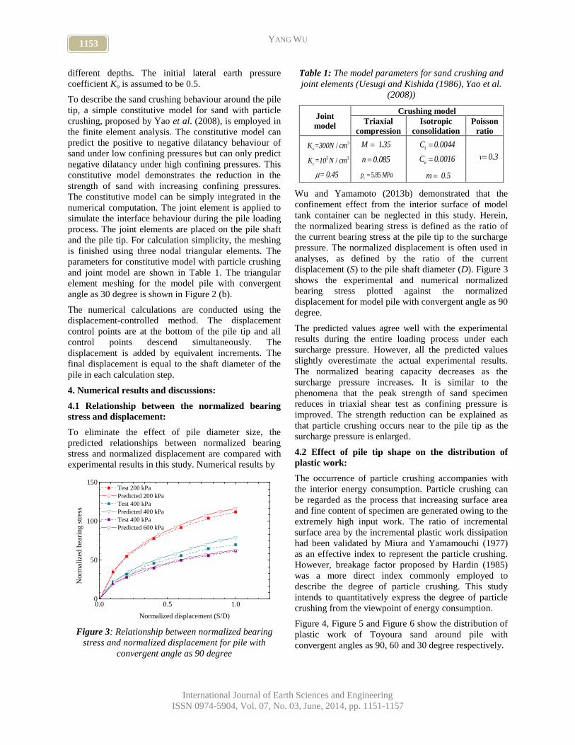
1153 YANG WU
International Journal of Earth Sciences and Engineering
ISSN 0974-5904, Vol. 07, No. 03, June, 2014, pp. 1151-1157
different depths. The initial lateral earth pressure
coefficient Ko is assumed to be 0.5.
To describe the sand crushing behaviour around the pile
tip, a simple constitutive model for sand with particle
crushing, proposed by Yao et al. (2008), is employed in
the finite element analysis. The constitutive model can
predict the positive to negative dilatancy behaviour of
sand under low confining pressures but can only predict
negative dilatancy under high confining pressures. This
constitutive model demonstrates the reduction in the
strength of sand with increasing confining pressures.
The constitutive model can be simply integrated in the
numerical computation. The joint element is applied to
simulate the interface behaviour during the pile loading
process. The joint elements are placed on the pile shaft
and the pile tip. For calculation simplicity, the meshing
is finished using three nodal triangular elements. The
parameters for constitutive model with particle crushing
and joint model are shown in Table 1. The triangular
element meshing for the model pile with convergent
angle as 30 degree is shown in Figure 2 (b).
The numerical calculations are conducted using the
displacement-controlled method. The displacement
control points are at the bottom of the pile tip and all
control points descend simultaneously. The
displacement is added by equivalent increments. The
final displacement is equal to the shaft diameter of the
pile in each calculation step.
4. Numerical results and discussions:
To eliminate the effect of pile diameter size, the
predicted relationships between normalized bearing
stress and normalized displacement are compared with
experimental results in this study. Numerical results by
0.0 0.5 1.00
50
100
150
No
rmal
ized
bea
rin
g s
tres
s
Normalized displacement (S/D)
Test 200 kPa
Predicted 200 kPa
Test 400 kPa
Predicted 400 kPa
Test 400 kPa
Predicted 600 kPa
Figure 3: Relationship between normalized bearing
stress and normalized displacement for pile with
convergent angle as 90 degree
Table 1: The model parameters for sand crushing and
joint elements (Uesugi and Kishida (1986), Yao et al.
(2008))
Joint
model
Crushing model
Triaxial
compression
Isotropic
consolidation
Poisson
ratio
Wu and Yamamoto (2013b) demonstrated that the
confinement effect from the interior surface of model
tank container can be neglected in this study. Herein,
the normalized bearing stress is defined as the ratio of
the current bearing stress at the pile tip to the surcharge
pressure. The normalized displacement is often used in
analyses, as defined by the ratio of the current
displacement (S) to the pile shaft diameter (D). Figure 3
shows the experimental and numerical normalized
bearing stress plotted against the normalized
displacement for model pile with convergent angle as 90
degree.
The predicted values agree well with the experimental
results during the entire loading process under each
surcharge pressure. However, all the predicted values
slightly overestimate the actual experimental results.
The normalized bearing capacity decreases as the
surcharge pressure increases. It is similar to the
phenomena that the peak strength of sand specimen
reduces in triaxial shear test as confining pressure is
improved. The strength reduction can be explained as
that particle crushing occurs near to the pile tip as the
surcharge pressure is enlarged.
4.2 Effect of pile tip shape on the distribution of
plastic work:
The occurrence of particle crushing accompanies with
the interior energy consumption. Particle crushing can
be regarded as the process that increasing surface area
and fine content of specimen are generated owing to the
extremely high input work. The ratio of incremental
surface area by the incremental plastic work dissipation
had been validated by Miura and Yamamouchi (1977)
as an effective index to represent the particle crushing.
However, breakage factor proposed by Hardin (1985)
was a more direct index commonly employed to
describe the degree of particle crushing. This study
intends to quantitatively express the degree of particle
crushing from the viewpoint of energy consumption.
Figure 4, Figure 5 and Figure 6 show the distribution of
plastic work of Toyoura sand around pile with
convergent angles as 90, 60 and 30 degree respectively.
3/sK =300N cm
5 3/cK =10 N cm
= 0.45
tC 0.0044
eC 0.0016
m 0.5
n 0.085
5.8 5cp MPa
M 1.35
v 0.3
4.1 Relationship between the normalized bearing
stress and displacement:

1154 Numerical Investigation on Effect of Pile Tip Shape on Soil Crushing Behaviour
International Journal of Earth Sciences and Engineering
ISSN 0974-5904, Vol. 07, No. 03, June, 2014, pp. 1151-1157
(a) 200 kPa (90 degree) (b) 600 kPa (90 degree)
Figure 4: Distribution of plastic work of sand around
pile with convergent angle as 90 degree
(a) 200 kPa (60 degree) (b) 600 kPa (60 degree)
Figure 5: Distribution of plastic work of sand around
pile with convergent angle as 60 degree
(a) 200 kPa (30 degree) (b) 600 kPa (30 degree)
Figure 6: Distribution of plastic work of sand around
pile with convergent angle as 30 degree
10-2
100
102
104
106
108
0.0
0.2
0.4
0.6
0.8
1.0
Bre
akag
e fa
cto
r
Plastic work Wp/kPa
Br=W
p
0.65/(W
p
0.65+550)
Figure 7: Relationship between breakage factor and
plastic work for Toyoura sand
(a) 200 kPa (90 degree) (b) 600 kPa (90 degree)
Figure 8: Contour of breakage factor Br of sand around
pile with convergent angle as 90 degree
(a) 200 kPa (60 degree) (b) 600 kPa (60 degree)
Figure 9: Contour of breakage factor Br of sand around
pile with convergent angle as 60 degree
(a) 200 kPa (30 degree) (b) 600 kPa (30 degree)
Figure 10: Contour of breakage factor Br of sand
around pile with convergent angle as 30 degree
(J/m3) (J/m3)
(J/m3) (J/m3)
0.10
0.05 0.05
0.10
0.15
0.05
0.10
0.15
0.05
0.15
0.10
0.05
0.10
0.05
0.10
(J/m3) (J/m3)

1155 YANG WU
International Journal of Earth Sciences and Engineering
ISSN 0974-5904, Vol. 07, No. 03, June, 2014, pp. 1151-1157
Predicted results represent that the distributed range of
high-value plastic work around pile significantly shrinks
as the convergent angle decreases. The high-value
plastic work concentrates at the corner point of the pile
tip and extends towards to the central line of model pile.
It is believed that the sand particle around that corner is
subjected to complicated stresses. To examine the
surcharge pressure effect on predicted result, a figure
includes two sub-titles (a) and (b) displaying the
distribution of plastic work for Toyoura sand when the
surcharge pressure are 200 kPa and 600 kPa. The
distributed range also expands in radial and vertical
direction with increasing surcharge pressure by
comparing (a) with (b) in each figure.
The experienced relationship between the breakage
factor and the plastic work is summarized by Hu et al.
(2011) from the experimental data on many kinds of
granular materials. The empirical equation for Toyoura
sand is shown in Figure 7. The breakage factor slightly
increases when plastic work is less than 102 J/m
3/kPa
and drastically increase as plastic work is over 103
J/m3/kPa. Crushing becomes sufficient once the plastic
work beyond 106 J/m3/kPa.
4.3 Effect of pile tip shape on the distribution of
breakage factor:
To investigate the effect of pile tip shape on the
crushing behaviour at different depths beneath the pile
tip, the breakage factor of the elements beneath the pile
tip at different depths are displayed and analyzed. Pile
tip bearing stress is estimated by the factor of the
sand layer beneath the pile tip. Yang (2006)
demonstrated that the influential zone beneath the pile
tip is approximately 2 and 3 times larger than the pile
diameter. Therefore, three elements at one and two
diameter length beneath pile tip are selected in Figure
11. Relationship between the breakage factor and
surcharge pressure for model pile with different
convergent angles as 90, 60 and 30 degree are shown in
Figure 11: Three elements beneath pile tip at different
depths
0 200 400 600 8000.076
0.080
0.084
0.088
0.092
0.096
0.100
Bre
akag
e fa
cto
r B
r
Surcharge pressure (kPa)
90 degree
60 degree
30 degree
(a) Breakage factor of element 1 beneath pile tip
0 200 400 600 8000.076
0.080
0.084
0.088
0.092
0.096
0.100
Bre
akag
e fa
ctor
Br
Surcharge pressure (kPa)
90 degree
60 degree
30 degree
(b) Breakage factor of element 2 beneath pile tip
0 200 400 600 8000.076
0.080
0.084
0.088
0.092
0.096
0.100
Bre
akag
e fa
cto
r B
r
Surcharge pressure (kPa)
90 degree
60 degree
30 degree
(c) Breakage factor of element 3 beneath pile tip
Figure 12: Crushing behaviour of sand beneath pile tip
at different depths for pile with three kinds of pile tip
shape
1 2
3
D
D
D
Figure 8, Figure 9 and Figure 10 display the breakage
factor contour of Toyoura sand around pile with
convergent angles as 90, 60 and 30 degree. The
crushing degree of Toyoura sand decreases as
convergent angle of pile becomes small. It is believed
that particles beneath flat base pile have less space to
move or rotate compared those beneath the pencil type
pile. The maximum breakage factor is 0.15 for pile with
convergent angle as 90 at surcharge pressure as 600 kPa
but it reduces to 0.10 for pile with convergent angle as
30. Similar to the distributed pattern of plastic work, the
high-value degree of particle crushing occurs at the at
the corner point of the pile tip. It displays the irregular
bulk shape. The distributed range of breakage factor
expands with increasing surcharge pressure.

1156 Numerical Investigation on Effect of Pile Tip Shape on Soil Crushing Behaviour
International Journal of Earth Sciences and Engineering
ISSN 0974-5904, Vol. 07, No. 03, June, 2014, pp. 1151-1157
Figure 12 (a), (b) and (c) respectively. Element 1 is on
the central line two diameter length beneath the pile tip.
Element 2 and 3 are two and one diameter length
beneath the corner point of pile tip in vertical direction.
It is represented that the predicted breakage factor
decreases as the convergent angle decreases. The
breakage factor reduces from 0.90 to 0.845 for element
1 as the convergent angle varies from 90 degree to 30
degree. Degree of particle crushing is affected by the
pile tip shape even the selected position changes. It is
also noticeable that breakage factor increase with the
increasing surcharge pressure. However, the increasing
tendency is less dependent on surcharge pressure level.
5. Conclusions:
To investigate the effect of pile tip shape on crushing
behaviour of sand around a pile, finite element analysis
has been presented that incorporates the mixed
incremental method for UL method and the
characteristics of particle crushing. The penetration of
model pile with three kinds of pile tip shape under
different surcharge pressures are analyzed respectively.
The distribution of breakage factor is predicted from the
viewpoint of energy consumption. The major findings
of the study are summarized below.
1. The predicted relationship between normalized
bearing stress and normalized displacement of model
piles agrees with the experimental results.
2. The distributed range of plastic work shrinks as the
convergent angle of pile becomes small. The high-value
plastic concentrates at the corner point of the pile tip
and extends towards to the central line of model pile.
The distributed range of plastic work also expands in
radial and vertical direction with increasing surcharge
pressure.
3. The distributed range of breakage factor deceases as
the convergent angle of pile decreases. The high-value
degree of particle crushing occurs at the at the corner
point of the pile tip. The distributed shape of breakage
factor displays the irregular bulk shape.
4. The breakage factor of three selected elements
beneath pile tip all show decreasing tendency as
convergent angle decreases. Degree of particle crushing
is affected by the pile tip shape even the selected
position changes. It is also noticeable that breakage
factor increase with the increasing surcharge pressure.
This study is the preliminary study of the crushing
degree of sand in surrounding of pile. This study can be
improved by some aspects. The particle crushing owing
to the contact between sand and pile should be further
discussed and more advanced interface element should
be employed in further study.
6. Acknowledgement:
This research is supported by the scholarship of the
Ministry of Education, Culture, Sports, Science and
Technology, Japan. The author expresses thanks to Prof.
Haruyuki YAMAMOTO in Hiroshima University for
his kind support. The editor-in-chief Prof. D. V. Reddy
and reviewers are especially thanked for their kind work
and constructive suggestions.
7. Reference:
[1] W. F. Chen and E. Mizuno (1990) “Nonlinear
analysis in soil mechanics: Theory and
Implementation”, Nertherlands, ELSEVIER, pp.
492-504.
[2] B. Hardin (1985) “Crushing of soil particles”,
Journal of Geotechnical Engineering, 111(10), pp.
1177-1192.
[3] W. Hu, Z. Y. Yin, C. Dano and P. Y. Hicher (2011)
“A constitutive model for granular materials
considering grain breakage”, Science China
Technological Sciences, 54(8), pp. 2188-2196.
[4] N. Miura and T. Yamamouchi (1977) “Effect of
particle-crushing on the shear characteristics of a
sand”, Proceeding of Japan Society of Civil
Engineering, 260, pp. 109-118. (In Japanese)
[5] P. Simonini (1996) “Analysis of behavior of sand
surrounding pile tips”, Journal of Geotechnical and
Geoenvironmental Engineering, 122(11), pp. 897-
905.
[6] M. Uesugi and H. Kishida (1986) “Influential
Factors of friction between Steel and Dry sands”,
Soils and Foundations, 26(2), pp. 33-46.
[7] Y. Wu, H. Yamamoto and Y. P. Yao (2013a)
“Numerical study on bearing behavior of pile
considering sand particle crushing”, Geomechanics
and Engineering, 5(3), pp. 241-261.
[8] Y. Wu and H. Yamamoto (2013b) “Numerical
analysis on effects of confinement and surcharge
pressure on the behaviour of sand surrounding
pile”, International Journal of Earth Sciences and
Engineering, 6(6), pp. 1472-1482.
[9] Y. Wu and H. Yamamoto (2014) “Numerical
Analysis of the Effect of Pile Tip Shape on Soil
Behavior around Pile”, Geotechnical Engineering
Journal of the SEAGS & AGSSEA, 45(2), pp.78-
89.
[10] H. Yamamoto, W. Li, K. Tominaga and H. Ogura
(2003) “Experiment study on effects of
overburdening pressures and end shapes for point
bearing capacities of pile”, Structure and
construction of proceeding of Japan Architecture,
49(B), pp. 157-162. (In Japanese)
[11] J. Yang (2006). “Influence zone for end bearing of
piles in sand”, Journal of Geotechnical and
Geoenvironmental Engineering-ASCE, 132(9), pp.
1229-1237.

1157 YANG WU
International Journal of Earth Sciences and Engineering
ISSN 0974-5904, Vol. 07, No. 03, June, 2014, pp. 1151-1157
[12] Y. P. Yao, H. Yamamoto and N. D. Wang (2008)
“Constitutive model considering sand crushing”,
Soils and Foundations, 48(4), pp. 603-608. N.
[13] N. Yasufuku and A. F. L. Hyde (1995) “Pile end-
bearing capacity in crushable sands”,
Geotechnique, 45(4), pp. 663-676.
[14] C. Zhang, G. D. Nguyen and I. Einav (2013) “The
end-bearing capacity of piles penetrating into
crushable soils”, Geotechnique, 63(5), pp. 341-354.
www.cafetinnova.org
Indexed in
Scopus Compendex and Geobase Elsevier, Chemical
Abstract Services-USA, Geo-Ref Information Services-USA,
List B of Scientific Journals, Poland,
Directory of Research Journals
ISSN 0974-5904, Volume 07, No. 03
June 2014, P.P.1158-1163
#02070348 Copyright ©2014 CAFET-INNOVA TECHNICAL SOCIETY. All rights reserved.
Estimation of Reservoir Capacity Using Remote Sensing Data – A
Soft Classification Approach
JEYAKANTHAN V S Deltaic Regional Centre, National Institute of Hydrology, Siddartha Nagar, Kakinada-533 003,
Andhra Pradesh, India
Email: [email protected]
Abstract: Sediments carried by the rivers are deposited in the reservoirs and cause several detrimental effects,
which include loss of storage capacity, upstream aggradations, effect on water quality and damage or impairment of
hydro-equipments. The deposition of sedimentation not only reduces the capacity but also the water-spread of the
reservoir. Satellite data has long been in use to estimate the water-spread area at different elevations of a reservoir,
which in turn can be used to quantify the capacity of the reservoir. This methodology to estimate the capacity of a
reservoir using remote sensing data involves hard or per-pixel based classification to delineate the water-spread area
at a particular elevation. One of the limitations of this approach is that the border pixels, representing soil class with
moisture, are classified entirely as water pixels, thereby giving inaccurate estimate of the water-spread area. To
estimate the water-spread area of Nagarjuna Sagar reservoir accurately, the sub-pixel or linear mixture model
(LMM) approach has been adopted in this study. The sub-pixel approach uses a linear mixture model of the spectra
to quantify the proportions of water and other classes present in each of the border pixels of the reservoir. IRS-1C
and 1D satellite image data (24m) of eight optimal dates ranging from minimum draw down level (MDDL) to full
reservoir level (FRL) were used to estimate the water-spread area of the reservoir. The extracted water-spread areas
using per-pixel and sub-pixel approaches were in turn used to quantify the capacity of the Nagarjuna Sagar
reservoir. The estimated capacity of the Nagarjuna Sagar reservoir using per-pixel and sub-pixel approaches was
8101.63 Mm3 and 8014.49 Mm3 respectively.
Keywords: Reservoir, Water-spread area, Capacity estimation, Per-pixel and Sub-pixel approaches.
Introduction:
Natural processes, such as erosion in the catchment
area, movement of sediment and its deposition in
various parts of the reservoir, require careful
consideration in the planning of major reservoir
projects. The silt that is deposited at different levels
reduces the storage capacity of the reservoir [1, 2].
Reduction in the storage capacity beyond a limit
prevents the reservoir from fulfilling the purpose for
which it is designed. Periodic capacity surveys of the
reservoir help to assess the rate of sedimentation and
reduction in storage capacity. Conventional techniques
for the estimation of the capacity of a reservoir, such as
hydrographic survey and inflow-outflow approaches,
are cumbersome, time consuming and expensive, and
they involve significant manpower. As an alternative to
conventional methods, the remote sensing technique
provides cost- and time-effective estimation of the live
capacity of a reservoir [3, 4]. Multi-date satellite remote
sensing data provide information on elevation contours,
in the form of water spread area, at different water
levels of a reservoir. The water spread area thus
interpreted from the satellite data is used as an input into
a simple volume estimation formula to calculate the
capacity of a reservoir. Such work has been reported by
[5] for the Malaprabha Reservoir in India, [6] for the
Poondi Reservoir in India, [7] for the Bargi Reservoir in
India and [4] for the Bhakra Reservoir in India
For quantification of the capacity of a reservoir, the only
thematic information that has to be extracted from the
satellite data is the water-spread area at different water
levels of the reservoir [8, 9]. The different approaches
such as maximum likelihood, minimum distance to
mean classification and band threshold method, to
delineate various thematic information from the remote
sensing digital data adopt the per-pixel based
methodology and assign a pixel to a single land cover
type [10, 11] whereas in reality, a single pixel may
contain more than one land cover (known as a mixed
pixel). Mixed pixels are common especially near the
boundaries of two or more discrete classes [12, 13]. The
boundary pixels of the water-spread area that are mixed
in nature, representing soil, vegetation class with
moisture are also classified as water pixels when a per-
pixel based approach is applied, thereby producing
inaccurate estimate of the water-spread area. To

1159 JEYAKANTHAN V S
International Journal of Earth Sciences and Engineering
ISSN 0974-5904, Vol. 07, No. 03, June, 2014, pp. 1158-1163
accurately compute the water-spread area to the
maximum possible extent, thereby reducing the error in
the estimation of capacity of a reservoir, a sub-pixel or
linear mixture model (LMM) approach has been chosen
for classifying the boundary pixels of water-spread area
from different water levels of Nagarjuna Sagar reservoir
located in Andhra Pradesh state of India.
Study Reservoir 1
Nagarjuna Sagar is one of the world's largest masonry
dam built across the river Krishna in Nagarjuna Sagar
town, Nalgonda District of Andhra Pradesh, India,
between 1955 and 1967. The capacity of Nagarjuna
Sagar reservoir at FRL (Full Reservoir Level) during
impoundment was 11,472 million cubic metres. The
dam is 490 ft (150 m) tall and 1.6 km long with 26 gates
which are 42 ft (13 m) wide and 45 ft (14 m) tall. The
geographic region pertains to the reservoir experiences
hot and dry summer throughout the year except during
the South-west monsoon season. The monsoon season is
from June to September and retreating monsoon or the
post monsoon season is during October to November.
The average rainfall in the district is 772 mm. 71% of
the annual rainfall is received during south-west
monsoon. The mean daily maximum temperature is
about 40o
C and the mean daily minimum is about 28o
C. The soils in and around the study reservoir mainly
comprise loamy sands, sandy loams and sandy clay
loams. In the areas of flat topography and alongside the
river Krishna and its tributaries comprises mainly of
black cotton soil.
Satellite Data Used
The image data used in this study were obtained by the
Indian Remote Sensing (IRS) satellites IRS-1C & 1D
(LISS-III sensor) which provides a spatial resolution of
24 m and spectral resolution in four different bands
(0.52-0.59, 0.62-0.68, 0.77-0.86, 1.55-1.70 μm). The
different dates of satellite data used and the respective
water level during the pass of the satellite over the
reservoir are given in Table 1. Reservoir water level
data and the hydrographic survey details have been
collected from the Nagarjuna sagar reservoir authority
responsible for the maintenance and operation of the
reservoir.
Table. 1 Details of satellite data used and the water
level during the pass of the satellite over the reservoir
Sl.No. Name of
the
Satellite
Date of
Satellite
Pass
Reservoir
Elevation
(m)
1. IRS-1C 23.10.2001 175.32
2. IRS-1D 12.12.2001 166.68
3. IRS-1D 24.12.2001 164.74
4. IRS-1D 25.02.2002 157.03
5. IRS-1D 14.09.2002 156.94
6. IRS-1D 11.05.2002 154.72
7. IRS-1D 27.11.2002 153.19
8. IRS-1D 22.12.2002 152.28
Methodology
The changes in water-spread could be accurately
estimated by analyzing the areal spread of the reservoir
at different elevations over a period of time using the
satellite image data [9,1]. Both the per-pixel and sub-
pixel or Linear Mixture Model (LMM) approaches have
been used in this study to extract the water-spread area
of the reservoir. Estimated water-spread areas were used
in a simple volume estimation formula to compute the
storage capacity of the reservoir. Estimation of water-
spread area and computation of capacity of the reservoir
using per-pixel and sub-pixel approaches are discussed
in the following sections.
Geo-Referencing Of Satellite Data
In the IRS-1C and 1D (LISS-III) satellite data the
reservoir water-spread area was free from clouds and
noise in all of the eight images used. The image scene of
23rd
October 2001 was geo-referenced with respect to
1:50,000 survey of India topographic maps. The geo-
referencing was done using ployconic projection and
nearest neighborhood re-sampling technique to create a
geo-referenced image of pixel size 24m x 24m.
Subsequently the other satellite images corresponding to
various water levels were also registered with the geo-
referenced image using the image to image registration
technique. In every image 20 to 25 ground control
points were used, which resulted in a root mean squared
error (RMSE) of 0.15 to 0.18 of a pixel.
3.2 Per-pixel based approach
The most widely used method for extracting
information on the surface cover from remotely sensed
data is image classification. Digital image classification
uses the spectral information represented by the digital
numbers in one or more spectral bands and attempts to
classify each individual pixel (per-pixel approach) based
on this spectral information. A number of commonly
used per-pixel based classifiers exist including the
maximum likelihood, the minimum distance to mean,
mahalanobis distance and the parallelipiped classifiers.
A detailed account of these and the other classifiers can
be found in [14, 15]. The objective of the per-pixel
based classifiers is to assign all pixels in the image to
particular classes or themes (e.g. water, forest, urban,
agriculture). The resulting classified image is comprised
of a mosaic of pixels, each of which belongs to a
particular theme and is essentially a thematic map of the
original image. The per-pixel based classification can be
divided into unsupervised and supervised classification.
The underlying requirement of supervised classification
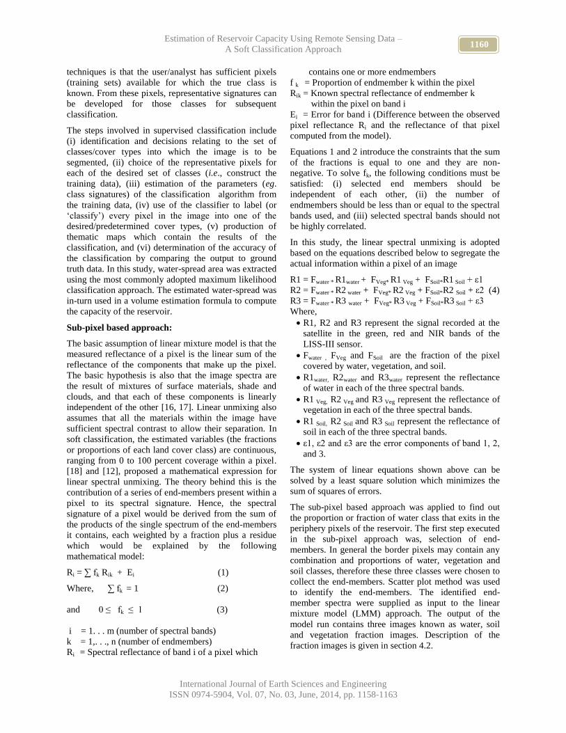
1160 Estimation of Reservoir Capacity Using Remote Sensing Data –
A Soft Classification Approach
International Journal of Earth Sciences and Engineering
ISSN 0974-5904, Vol. 07, No. 03, June, 2014, pp. 1158-1163
techniques is that the user/analyst has sufficient pixels
(training sets) available for which the true class is
known. From these pixels, representative signatures can
be developed for those classes for subsequent
classification.
The steps involved in supervised classification include
(i) identification and decisions relating to the set of
classes/cover types into which the image is to be
segmented, (ii) choice of the representative pixels for
each of the desired set of classes (i.e., construct the
training data), (iii) estimation of the parameters (eg.
class signatures) of the classification algorithm from
the training data, (iv) use of the classifier to label (or
‘classify’) every pixel in the image into one of the
desired/predetermined cover types, (v) production of
thematic maps which contain the results of the
classification, and (vi) determination of the accuracy of
the classification by comparing the output to ground
truth data. In this study, water-spread area was extracted
using the most commonly adopted maximum likelihood
classification approach. The estimated water-spread was
in-turn used in a volume estimation formula to compute
the capacity of the reservoir.
Sub-pixel based approach:
The basic assumption of linear mixture model is that the
measured reflectance of a pixel is the linear sum of the
reflectance of the components that make up the pixel.
The basic hypothesis is also that the image spectra are
the result of mixtures of surface materials, shade and
clouds, and that each of these components is linearly
independent of the other [16, 17]. Linear unmixing also
assumes that all the materials within the image have
sufficient spectral contrast to allow their separation. In
soft classification, the estimated variables (the fractions
or proportions of each land cover class) are continuous,
ranging from 0 to 100 percent coverage within a pixel.
[18] and [12], proposed a mathematical expression for
linear spectral unmixing. The theory behind this is the
contribution of a series of end-members present within a
pixel to its spectral signature. Hence, the spectral
signature of a pixel would be derived from the sum of
the products of the single spectrum of the end-members
it contains, each weighted by a fraction plus a residue
which would be explained by the following
mathematical model:
Ri = ∑ fk Rik + Ei (1)
Where, ∑ fk = 1 (2)
and 0 ≤ fk ≤ 1 (3)
i = 1. . . m (number of spectral bands)
k = 1,. . ., n (number of endmembers)
Ri = Spectral reflectance of band i of a pixel which
contains one or more endmembers
f k = Proportion of endmember k within the pixel
Rik = Known spectral reflectance of endmember k
within the pixel on band i
Ei = Error for band i (Difference between the observed
pixel reflectance Ri and the reflectance of that pixel
computed from the model).
Equations 1 and 2 introduce the constraints that the sum
of the fractions is equal to one and they are non-
negative. To solve fk, the following conditions must be
satisfied: (i) selected end members should be
independent of each other, (ii) the number of
endmembers should be less than or equal to the spectral
bands used, and (iii) selected spectral bands should not
be highly correlated.
In this study, the linear spectral unmixing is adopted
based on the equations described below to segregate the
actual information within a pixel of an image
R1 = Fwater * R1water + FVeg* R1 Veg + FSoil*R1 Soil + ε1
R2 = Fwater * R2 water + FVeg* R2 Veg + FSoil*R2 Soil + ε2 (4)
R3 = Fwater * R3 water + FVeg* R3 Veg + FSoil*R3 Soil + ε3
Where,
R1, R2 and R3 represent the signal recorded at the
satellite in the green, red and NIR bands of the
LISS-III sensor.
Fwater , FVeg and FSoil are the fraction of the pixel
covered by water, vegetation, and soil.
R1water, R2water and R3water represent the reflectance
of water in each of the three spectral bands.
R1 Veg, R2 Veg and R3 Veg represent the reflectance of
vegetation in each of the three spectral bands.
R1 Soil, R2 Soil and R3 Soil represent the reflectance of
soil in each of the three spectral bands.
ε1, ε2 and ε3 are the error components of band 1, 2,
and 3.
The system of linear equations shown above can be
solved by a least square solution which minimizes the
sum of squares of errors.
The sub-pixel based approach was applied to find out
the proportion or fraction of water class that exits in the
periphery pixels of the reservoir. The first step executed
in the sub-pixel approach was, selection of end-
members. In general the border pixels may contain any
combination and proportions of water, vegetation and
soil classes, therefore these three classes were chosen to
collect the end-members. Scatter plot method was used
to identify the end-members. The identified end-
member spectra were supplied as input to the linear
mixture model (LMM) approach. The output of the
model run contains three images known as water, soil
and vegetation fraction images. Description of the
fraction images is given in section 4.2.

1161 JEYAKANTHAN V S
International Journal of Earth Sciences and Engineering
ISSN 0974-5904, Vol. 07, No. 03, June, 2014, pp. 1158-1163
Computation of volume between successive water
Levels
Traditionally the reservoir volume between two
consecutive reservoir water levels, was computed using
the prismoidal formula, the Simpson formula and the
trapezoidal formulae [19]. Of these, the trapezoidal
formula has been most widely used for computation of
volume [20, 21]. The water-spread area estimated using
sub-pixel approach was used as an input in the volume
estimation formula to find out the, volume at different
water levels of the reservoir. In this study the volume
between two consecutive reservoir water levels was
computed using the following trapezoidal formula.
Trapezoidal Formula:
V = H/3 (A1+A2 + (√A1*A2)) (5)
Where V is the volume between two consecutive water
levels. A1 and A2 are the water-spread area at the
reservoir water level 1 and 2 respectively and H is the
difference between these two water levels.
Computation of storage capacity of the reservoir:
The volume computed between different water levels
(i.e from Minimum Draw Down Level to Full Reservoir
Level) was added up to calculate the cumulative or
storage capacity of the reservoir.
Results and discussion
Computation of reservoir capacity by per-pixel
approach
The supervised classification was performed by using
training sets generated for the different landcover
classes in and around the reservoirs. Since this exercise
involves the estimation of pixels that are occupied by
water, it is essential that the training set generation
should involve careful selection of water pixels. It may
note that the image subset of the study area contains
vegetation and soil as the primary land cover classes in
addition to the water class. Therefore only three
feature/landcover classes were considered to generate
training sets for the maximum likelihood classification.
Training sets were selected from the center of the
reservoir, periphery of the reservoir, from the
agricultural fields, shrubs in the peripheral areas and
from barren lands representing the soil class. The choice
of representative pixels (both number and type) was in
accordance with the suggestion of [14]. This procedure
was followed carefully for all the eight images
pertaining to the Nagarjuna Sagar reservoir. It may be
noted that three simple and spectrally distinct classes
namely water, soil and vegetation form the basic input
for the classification process. The extracted water
spread areas and the estimated capacity (8101.63 Mm3)
using per-pixel approach is given in Table 2.
Figure 1 (a) Feature space plot (NIR vs RED), (b) End-member spectra of Soil, Water and Vegetation (c) Fraction
images obtained by spectral un-mixing of image data of Nagarjunasagar Reservoir pertaining to the water level
175.32 m (Due to the recurring nature of the fraction images, only figures pertaining to the highest water level is
presented).

1162 Estimation of Reservoir Capacity Using Remote Sensing Data –
A Soft Classification Approach
International Journal of Earth Sciences and Engineering
ISSN 0974-5904, Vol. 07, No. 03, June, 2014, pp. 1158-1163
Table 2: Capacity estimation of Nagarjunasagar reservoir using the per-pixel and sub-pixel classification
approaches (2002)
Computation of reservoir capacity by sub-pixel
approach
The fraction images (Figure 1) generated using the sub-
pixel approach described in the methodology section
contain a wealth of information about the reservoir.
Each fraction image corresponds to a single land cover
only. For example, the pixels in the water fraction
image provide information only on the proportion or
amount of water it contains. Likewise the vegetation and
soil fraction image provide information on the
proportions of the respective classes only. However, in
this study the interest is only to know about, the amount
of water present in the border pixels of the reservoir.
The value of the pixels in the fraction image ranges
from 0 to 1. A pixel from the water fraction image
having a value of 0 indicates that there is no water at all
in that pixel, whereas a pixel having a value of 0.25
indicates that 25% of the area of the pixel is occupied by
water while a pixel value of 1 indicates that 100% of the
area of the pixel is occupied by water (i.e the pixel is
fully occupied by water). Therefore, for a pixel having a
value of 0.72, the area of water occupied by that pixel is
414.72 m2 (0.72 x 24m x 24m). The pixels representing
the reservoir border which have a minimum value of up
to 0.1 in the water fraction image (i.e a pixel contains a
minimum 10% of area of water) were isolated from the
water fraction image and the area covered by water in
these border pixels were estimated. The number of
pixels that contains 100% of water was also found out.
By summing up the area occupied by these two types of
pixels, the total water spread area, corresponding to a
particular water level of the reservoir was computed.
This exercise was carried out for all the eight images
used in this study. The water-spread area thus estimated
was again used as an input in the trapezoidal formula to
compute the storage capacity or cumulative capacity of
the Nagarjuna sagar reservoir using the sub-pixel
classification approach.
Here it is worth mentioning that, a pixel containing 71%
of water may be labelled as containing 100% of water
by the per-pixel approach. In such case the water-spread
area is over estimated. Conversely if the pixel contains
40% of water, then the entire pixel may not be
considered as a water pixel. Hence, the water-spread
area is under estimated. Such errors due to over
estimation or under estimation do not occur in the sub-
pixel approach. Thus, the sub-pixel approach reduces
the error imposed by the per-pixel approach. The
estimated cumulative capacity of Nagarjuna sagar
reservoir at the water level 175.32 m (Near FRL) using
the sub-pixel approach was 8014.49 Mm3. The capacity
estimated using per-pixel and sub-pixel approaches are
given in Table 2.
Conclusions
High spatial-resolution image data enables accurate
mapping of the terrain features. The use of high spatial
resolution satellite image data, however, is constrained
by factors such as cost and less area covered by the
sensor. Hence, in hydrological applications estimating
water-spread area may be difficult because a reservoir
may not be imaged in a single pass of the satellite and
atmospheric condition would be different from path to
path [22]. An alternative method to overcome such
constrains is the use of the sub-pixel based approach.
The simplest methodology for such an approach is
linear mixture modeling, which has been demonstrated
in this study to estimate the capacity of Nagarjuna sagar
reservoir in India. Though the sub-pixel approach found
to be a better alternative to per-pixel approach, there are
certain limitations such as the spatial location of the
fractions within a pixel is unknown. In addition the sub-
pixel classifier produces more accurate results only with
hyperspectral images. Hence, the use of hyperspectral
image data with higher spatial resolution would have
yielded better results.
Acknowledgement
Sl.
No
Date of
Satellite Pass
Reservoir
Elevation
above m.s.l
(m)
Waterspread
area - Perpixel
approach
(Mm2)
Waterspread
area - Subpixel
approach
(Mm2)
Cumulative
Volume -
Perpixel
approach
(Mm3)
Cumulative
Volume -
Subpixel
approach
(Mm3)
1. 23.10.2001 175.32 238.55 235.15 8101.63 8014.49 2. 12.12.2001 166.68 203.73 197.03 6192.96 6149.90 3. 24.12.2001 164.74 192.89 194.08 5808.28 5770.53 4. 25.02.2002 157.03 173.75 170.43 4395.53 4366.33 5. 14.09.2002 156.94 166.93 167.42 4380.20 4351.13 6. 11.05.2002 154.72 163.47 155.06 4013.46 3993.26 7. 27.11.2002 153.19 156.69 149.02 3768.56 3760.66 8. 22.12.2002 152.28 153.79 144.11 3627.29 3627.29

1163 JEYAKANTHAN V S
International Journal of Earth Sciences and Engineering
ISSN 0974-5904, Vol. 07, No. 03, June, 2014, pp. 1158-1163
The author thanks the Nagarjuna Sagar reservoir
authorities for providing the ground based data. The
author also thanks Director, NIH for giving permission
to publish the paper.
References
[1] Smith, L.C., and Pavelsky, T.M, “Remote sensing
of volumetric storage changes in lakes”, Earth
Surface Process and Landforms, Vol.34, pp.1353
– 1358, 2009.
[2] Sreenivasulu, V and Udayabaskar, P, “An
integrated approach for prioritization of reservoir
catchment using remote sensing and geographic
information system”, Geocarto International,
Vol.25, pp.149-168, 2010.
[3] Sabastin, M., Rao, P.P.N., Jayaraman. V., and
Chandrasekhar, M.G, “Reservoir storage loss
assessment and sedimentation modeling through
remote sensing techniques”, Proceedings of 6th
Inter. Symp. River sedimentation on Management
of Sediment – Philosophy, Aims and Techniques,
New Delhi, India, 1995
[4] Jain, S.K., Singh, P., and Seth, S.M, “Assessment
of sedimentation in Bhakra Reservoir in the
western Himalayan region using remotely sensed
data”, Hydrological Sciences Journal, Vol.47,
pp.203-212, 2002.
[5] Manavalan, P., Sathyanath, P., Sathyanarayn, M.,
and Raje Gowda, G. L, “Capacity evaluation of
the Malaprabha reservoir using digital analysis of
satellite data”. Tech. Report no. RC: BO: WR:
001:90, Regional Remote Sensing Service Centre,
Bangalore and Karnataka Engineering Research
Station, Krishnarajsagar, India, 1990.
[6] Jeyakanthan V.S, Sreenivasalu V, Rao Y.R.S.,
Ramasastri K.S, “Reservoir Capacity Estimation
Using Satellite Data”, International Symposium on
Photogrametry and Remote Sensing, Hyderabad,
2002.
[7] Goel, M.K., Jain, S.K., and Agarwal, P.K.,
“Assessment of sediment deposition rate in Bargi
Reservoir using digital image processing”,
Hydrological Sciences Journal, Vol.47(S),
pp.S81-S92, 2002.
[8] Morris, G.L., and Fan Jiahua, Reservoir
Sedimentation Handbook, (New York: McGraw-
Hill Book Co), 1998.
[9] Peng Dingzhi, Shenglian Guo., Pan Liu, Ting Liu,
“Reservoir storage curve estimation based on
remote sensing data”, Journal of Hydrologic
Engineering, Vol.11, pp.165-172, 2006.
[10] Jensen R.J., 1996. Introductory Digital Image
Processing : A remote sensing perspective, 2nd
edition, (London: Prentice Hall International
Ltd.,).
[11] Bastin, L. “Comparison of fuzzy c-means
classification, linear mixture modelling and MLC
probabilities as tools for unmixing coarse pixels”,
International Journal of Remote Sensing, Vol.18,
pp.3629-3648, 1997.
[12] Foody, G. M., and Cox, D. P., “Sub-pixel land
cover composition estimation using a linear
mixture model and fuzzy membership functions”,
International Journal of Remote Sensing, Vol.l5,
pp.619-631, 1994.
[13] Oleson, K. W., Sarlin, S., Garrison, J., Smith, S.,
Privette, L., and Emery, W., “Unmixing multiple
land cover type reflectance’s from coarse
resolution satellite data”, Remote Sensing of
Environment, Vol.54, pp.981-912, 1994.
[14] Mather, P. M., and Koch, M, “Extension of the
technique of Principal Component Analysis for
use in end-member selection”, pp. 346-353, 1997.
[15] Swain, P. H., and Davis, P. H., (Eds.), Remote
Sensing: The Quantitative Approach, New York,
NY: McGraw-Hill, 1978.
[16] Quarmby, N. A., Townsend, J.G.R., Settle.J.J.,
White, K. H., Milnes, M., Hindle, T. L., and
Silleos, N., “Linear mixture modelling applied to
A VHRR data for crop area estimation”,
International Journal of Remote Sensing, Vol.l3,
pp.415-425, 1992.
[17] Borel, C. C., and Gerstl, S. A. W., “Non-linear of
spectral unmixing models for vegetative and soil
surface”, Remote Sensing of Environment,
Vol.47,pp. 403-416, 1994.
[18] Settle, J.J., and Drake, N.A., “Linear mixing and
the estimation of ground cover proportions”,
International Journal of Remote Sensing, Vol.14,
pp.1159-1177, 1993.
[19] Patra, K.C., Hydrology and Water Resources
Engineering, (New Delhi: Narosa Publishing
House), 2001.
[20] Goel, M. K., and Jain, S. K., “Evaluation of
reservoir sedimentation using multi-temporal IRS-
1A LISS II data”, Asian Pacific Remote Sensing
& GIS Journal, Vol.8, pp.39-43, 1996.
[21] Rathore, D.S., Anju Choudhary, and Agarwal,
P.K., “Assessment of sedimentation in Harakud
Reservoir using digital remote sensing technique”,
Journal of the Indian Society of Remote Sensing,
Vol.34, pp.344-383, 2006.
[22] Hung, M.C., and Wu. Y.H., “Mapping and
visualizing the Great Salt Lake landscape
dynamics using multi-temporal satellite images-
1972-1996”, International Journal of Remote
Sensing, Vol.26, pp.1815-1834, 2005.

www.cafetinnova.org
Indexed in
Scopus Compendex and Geobase Elsevier, Chemical
Abstract Services-USA, Geo-Ref Information Services-USA,
List B of Scientific Journals, Poland,
Directory of Research Journals
ISSN 0974-5904, Volume 07, No. 03
June 2014, P.P.1164-1170
#02070349 Copyright ©2014 CAFET-INNOVA TECHNICAL SOCIETY. All rights reserved.
Experimental Investigation on RC and Retrofitted RC Column under
Cyclic Loading
A MURUGESAN1 AND G S THIRUGNANAM
2
1Department of Civil Engineering, Sona College of Technology, Salem-636005, Tamil Nadu, INDIA
2Department of Civil Engineering, Institute of Road and Transport Technology, Erode-638316, Tamil Nadu, INDIA
Email: [email protected], [email protected]
Abstract: Columns are important structural elements in a multi storey building it transmitting the entire loads to the
foundation. For the purpose of wind or earthquake engineering, columns may be designed to resist lateral forces. If
the columns are subjected to lateral load due to wind/ earthquake, the load carrying capacity of the member is
substantially reduced. Hence the load carrying capacity of the compression member has to be increased. There are
number of repairing techniques are available like external post tensioning, base isolators, supplementary dampers,
tuned mass dampers, active control system, Adhoc addition of structural support/reinforcement, connections
between buildings and their expansion additions and also retrofitting techniques. In this study, load carrying capacity
is increased by the way of retrofitting the columns. This experimental study aims in assessing the behavior of such
reinforced concrete columns with retrofitting technique, to investigate the ductile behavior and strength properties of
RC and retrofitted RC columns for the effective performance of the same during earthquakes. The RC column and
retrofitted RC column are designated as RCC and RRCC. The size of the column RCC and RRCC are 120 mm X
230 mm X 600 mm and designed for M30 mix concrete. This paper presents the seismic performance of the
reinforced concrete column designed for seismic loads as per IS 1893-2002 with and without retrofitting of FRP and
ductility recommendations are adopted as per IS 13920-1993. Specimen are cast with and without retrofitting and
tested under cyclic loading, simulating earthquake actions. The columns are examined in terms of load carrying
capacity, load deflection behavior, energy dissipation capacity, ductility factor and cracking characteristics. Based
on the test result important conclusions are drawn and the advantages of retrofitting with FRP wrapped reinforced
concrete column have been established.
Keywords: RC Column, RCC, Retrofitted RC Column, RRCC, Cyclic Loading, FRP.
1. Introduction:
Columns are skeletal structural elements, whose cross-
sectional shapes may be rectangular, square, circular, L-
shaped, etc. The size of the column section is dictated,
from a structural viewpoint, by its height and the loads
acting on it-which, in turn, depend on the type of floor
system, spacing of columns, number of storey, etc. The
column is generally designed to resist axial compression
combined with (biaxial) bending moments that are
induced by ‘frame action’ under gravity and lateral
loads.
When a column is subjected to an axial load within
elastic limits, just like any other composite section, the
stresses induced in steel and concrete are in proportion
to their modulli of elasticity, Es and Ec, respectively.
The failure of the tied column occurs suddenly with the
breaking down of concrete cylinder in a compression
test. In the present day, the seismic zones are altered in
India and the quantity of seismic force level has been
increased. It is harmful to the existing building
structures which needs to be strengthened and
retrofitting of existing concrete buildings are most
significance. Several investigators conveyed their
experimental and/or theoretical investigations on
structural elements such as concrete columns and beams
with fibre reinforced polymer composites in order to
carry their effectiveness. Some of the prominent works
are Saadatmanesh and Ehsani1, Naani
2 and
Neelamegam3 .The practical approach of FRP laminates
technically good and practically very effective and
efficient method of strengthening and upgrading
moment resisting RC frame members that are
structurally insufficient and impaired. The RC elements
such as beams, columns etc are in the FRP composite
materials are found special help with engineers and
applicators because of their many advantage. The main
objective of the study given herein was, to examine the
efficiency and effectiveness of FRP in columns.
Seismic deficiency of RC column:
Identification of detailing deficiencies is significant in
selection of mitigation strategies because acceptable
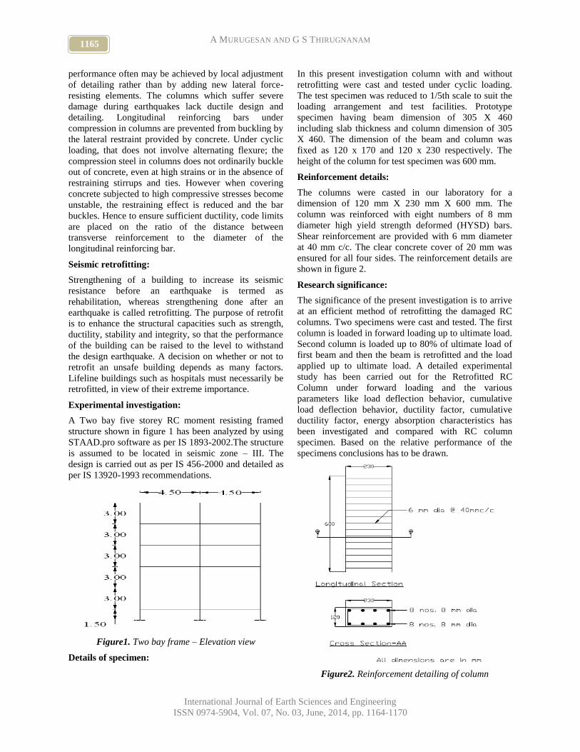
1165 A MURUGESAN AND G S THIRUGNANAM
International Journal of Earth Sciences and Engineering
ISSN 0974-5904, Vol. 07, No. 03, June, 2014, pp. 1164-1170
performance often may be achieved by local adjustment
of detailing rather than by adding new lateral force-
resisting elements. The columns which suffer severe
damage during earthquakes lack ductile design and
detailing. Longitudinal reinforcing bars under
compression in columns are prevented from buckling by
the lateral restraint provided by concrete. Under cyclic
loading, that does not involve alternating flexure; the
compression steel in columns does not ordinarily buckle
out of concrete, even at high strains or in the absence of
restraining stirrups and ties. However when covering
concrete subjected to high compressive stresses become
unstable, the restraining effect is reduced and the bar
buckles. Hence to ensure sufficient ductility, code limits
are placed on the ratio of the distance between
transverse reinforcement to the diameter of the
longitudinal reinforcing bar.
Seismic retrofitting:
Strengthening of a building to increase its seismic
resistance before an earthquake is termed as
rehabilitation, whereas strengthening done after an
earthquake is called retrofitting. The purpose of retrofit
is to enhance the structural capacities such as strength,
ductility, stability and integrity, so that the performance
of the building can be raised to the level to withstand
the design earthquake. A decision on whether or not to
retrofit an unsafe building depends as many factors.
Lifeline buildings such as hospitals must necessarily be
retrofitted, in view of their extreme importance.
Experimental investigation:
A Two bay five storey RC moment resisting framed
structure shown in figure 1 has been analyzed by using
STAAD.pro software as per IS 1893-2002.The structure
is assumed to be located in seismic zone – III. The
design is carried out as per IS 456-2000 and detailed as
per IS 13920-1993 recommendations.
Figure1. Two bay frame – Elevation view
Details of specimen:
In this present investigation column with and without
retrofitting were cast and tested under cyclic loading.
The test specimen was reduced to 1/5th scale to suit the
loading arrangement and test facilities. Prototype
specimen having beam dimension of 305 X 460
including slab thickness and column dimension of 305
X 460. The dimension of the beam and column was
fixed as 120 x 170 and 120 x 230 respectively. The
height of the column for test specimen was 600 mm.
Reinforcement details:
The columns were casted in our laboratory for a
dimension of 120 mm X 230 mm X 600 mm. The
column was reinforced with eight numbers of 8 mm
diameter high yield strength deformed (HYSD) bars.
Shear reinforcement are provided with 6 mm diameter
at 40 mm c/c. The clear concrete cover of 20 mm was
ensured for all four sides. The reinforcement details are
shown in figure 2.
Research significance:
The significance of the present investigation is to arrive
at an efficient method of retrofitting the damaged RC
columns. Two specimens were cast and tested. The first
column is loaded in forward loading up to ultimate load.
Second column is loaded up to 80% of ultimate load of
first beam and then the beam is retrofitted and the load
applied up to ultimate load. A detailed experimental
study has been carried out for the Retrofitted RC
Column under forward loading and the various
parameters like load deflection behavior, cumulative
load deflection behavior, ductility factor, cumulative
ductility factor, energy absorption characteristics has
been investigated and compared with RC column
specimen. Based on the relative performance of the
specimens conclusions has to be drawn.
Figure2. Reinforcement detailing of column
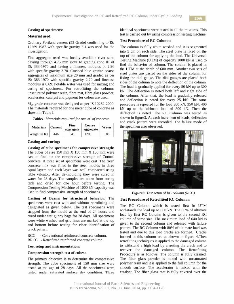
1166 Experimental Investigation on RC and Retrofitted RC Column under Cyclic Loading
International Journal of Earth Sciences and Engineering
ISSN 0974-5904, Vol. 07, No. 03, June, 2014, pp. 1164-1170
Casting of specimens:
Material used:
Ordinary Portland cement (53 Grade) confirming to IS:
12269-1987 with specific gravity 3.1 was used for the
investigation.
Fine aggregate used was locally available river sand
passing through 4.75 mm sieve to grading zone III of
IS: 383-1970 and having a fineness modulus of 2.96
with specific gravity 2.70. Crushed blue granite coarse
aggregates of maximum size 20 mm and graded as per
IS: 383-1970 with specific gravity 2.70 and fineness
modulus is 6.69. Potable water was used for mixing and
curing of specimens. For retrofitting the columns
unsaturated polymer resin, fibre mat, fibre glass powder,
accelerator, catalyst and pigment for colour are used.
M30 grade concrete was designed as per IS 10262-2009.
The materials required for one meter cube of concrete as
shown in Table I.
Table1. Materials required for one m3 of concrete
Materials Cement Fine
aggregate
Coarse
aggregate Water
Weight in Kg 446 541 1205 186
Casting and curing:
Casting of cube specimens for compressive strength:
The cubes of size 150 mm X 150 mm X 150 mm were
cast to find out the compressive strength of Control
concrete. A three set of specimens were cast .The fresh
concrete mix was filled in the steel moulds in three
equal layers and each layer was well compacted using
table vibrator. After de-moulding they were cured in
water for 28 days. The samples are taken from curing
tank and dried for one hour before testing. The
Compression Testing Machine of 1000 kN capacity was
used to find compressive strength of specimens.
Casting of Beams for structural behavior: The
specimens were cast with and without retrofitting and
designated as given below. The test specimens were
stripped from the mould at the end of 24 hours and
cured under wet gunny bags for 28 days. All specimens
were white washed and grid lines are marked at the top
and bottom before testing for clear identification of
crack pattern.
RCC - Conventional reinforced concrete column.
RRCC - Retrofitted reinforced concrete column.
Test setup and instrumentation:
Compression strength test of cubes:
The primary objective is to determine the compressive
strength. The cube specimens of 150 mm size were
tested at the age of 28 days. All the specimens were
tested under saturated surface dry condition. Three
identical specimens were tested in all the mixtures. This
test is carried out by using compression testing machine.
Test Procedure of RC Column:
The column is fully white washed and it is segmented
into 5 cm on each side. The steel plate is fixed on the
top of the column for applying the load. The Universal
Testing Machine (UTM) of capacity 1000 kN is used to
find the behavior of column. The column is placed in
the UTM at the depth of 600 mm. Another two sets of
steel plates are pasted on the sides of the column for
fixing the dial gauge. The dial gauges are placed both
sides of the column to note the deflection of the column.
The load is gradually applied for every 50 kN up to 300
kN. The deflection is noted both left and right side of
the column. After that, the load is gradually released
and deflection is noted for every 25 kN. The same
procedure is repeated for the load 300 kN, 350 kN, 400
kN up to the ultimate load of 800 kN. Then the
deflection is noted. The RC Column was tested as
shown in figure3. At each increment of loads, deflection
and crack pattern were recorded. The failure mode of
the specimen also observed.
Figure3. Test setup of RC column (RCC)
Test Procedure of Retrofitted RC Column:
The RC Column which is tested first in UTM
withstands the load up to 800 kN. The 80% of ultimate
load by first RC Column is given to the second RC
column of same size. The maximum load of 640 kN is
given to the second column and released with failure
pattern. The RC Column with 80% of ultimate load was
tested and due to this load cracks are formed. Cracks
formed in this column are as shown in figure 4.Then
retrofitting techniques is applied to the damaged column
to withstand a high load by arresting the crack and to
recover the damaged column. The Retrofitting
Procedure is as follows. The column is fully cleaned.
The fiber glass powder is mixed with unsaturated
polymer resin and it is applied to the full column for the
smooth surface. The accelerator is mixed with the
catalyst. The fiber glass mat is fully covered over the
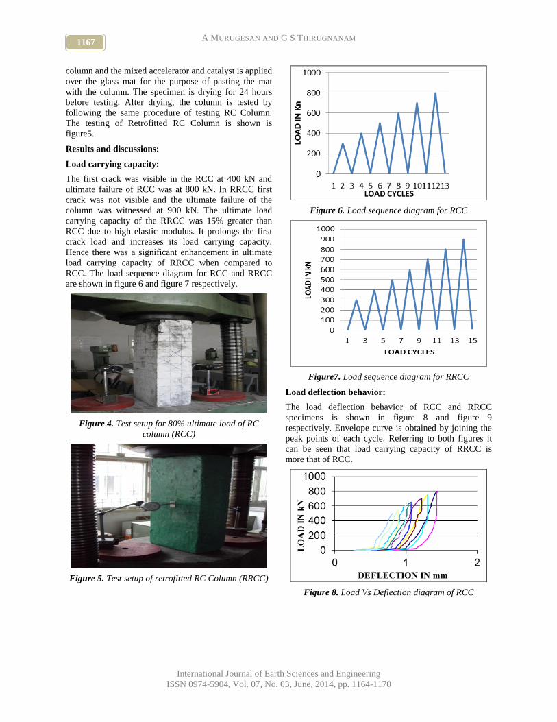
1167 A MURUGESAN AND G S THIRUGNANAM
International Journal of Earth Sciences and Engineering
ISSN 0974-5904, Vol. 07, No. 03, June, 2014, pp. 1164-1170
column and the mixed accelerator and catalyst is applied
over the glass mat for the purpose of pasting the mat
with the column. The specimen is drying for 24 hours
before testing. After drying, the column is tested by
following the same procedure of testing RC Column.
The testing of Retrofitted RC Column is shown is
figure5.
Results and discussions:
Load carrying capacity:
The first crack was visible in the RCC at 400 kN and
ultimate failure of RCC was at 800 kN. In RRCC first
crack was not visible and the ultimate failure of the
column was witnessed at 900 kN. The ultimate load
carrying capacity of the RRCC was 15% greater than
RCC due to high elastic modulus. It prolongs the first
crack load and increases its load carrying capacity.
Hence there was a significant enhancement in ultimate
load carrying capacity of RRCC when compared to
RCC. The load sequence diagram for RCC and RRCC
are shown in figure 6 and figure 7 respectively.
Figure 4. Test setup for 80% ultimate load of RC
column (RCC)
Figure 5. Test setup of retrofitted RC Column (RRCC)
Figure 6. Load sequence diagram for RCC
Figure7. Load sequence diagram for RRCC
Load deflection behavior:
The load deflection behavior of RCC and RRCC
specimens is shown in figure 8 and figure 9
respectively. Envelope curve is obtained by joining the
peak points of each cycle. Referring to both figures it
can be seen that load carrying capacity of RRCC is
more that of RCC.
Figure 8. Load Vs Deflection diagram of RCC
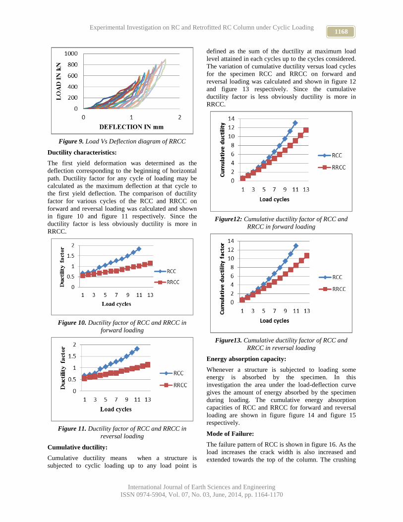
1168 Experimental Investigation on RC and Retrofitted RC Column under Cyclic Loading
International Journal of Earth Sciences and Engineering
ISSN 0974-5904, Vol. 07, No. 03, June, 2014, pp. 1164-1170
Figure 9. Load Vs Deflection diagram of RRCC
Ductility characteristics:
The first yield deformation was determined as the
deflection corresponding to the beginning of horizontal
path. Ductility factor for any cycle of loading may be
calculated as the maximum deflection at that cycle to
the first yield deflection. The comparison of ductility
factor for various cycles of the RCC and RRCC on
forward and reversal loading was calculated and shown
in figure 10 and figure 11 respectively. Since the
ductility factor is less obviously ductility is more in
RRCC.
Figure 10. Ductility factor of RCC and RRCC in
forward loading
Figure 11. Ductility factor of RCC and RRCC in
reversal loading
Cumulative ductility:
Cumulative ductility means when a structure is
subjected to cyclic loading up to any load point is
defined as the sum of the ductility at maximum load
level attained in each cycles up to the cycles considered.
The variation of cumulative ductility versus load cycles
for the specimen RCC and RRCC on forward and
reversal loading was calculated and shown in figure 12
and figure 13 respectively. Since the cumulative
ductility factor is less obviously ductility is more in
RRCC.
Figure12: Cumulative ductility factor of RCC and
RRCC in forward loading
Figure13. Cumulative ductility factor of RCC and
RRCC in reversal loading
Energy absorption capacity:
Whenever a structure is subjected to loading some
energy is absorbed by the specimen. In this
investigation the area under the load-deflection curve
gives the amount of energy absorbed by the specimen
during loading. The cumulative energy absorption
capacities of RCC and RRCC for forward and reversal
loading are shown in figure figure 14 and figure 15
respectively.
Mode of Failure:
The failure pattern of RCC is shown in figure 16. As the
load increases the crack width is also increased and
extended towards the top of the column. The crushing

1169 A MURUGESAN AND G S THIRUGNANAM
International Journal of Earth Sciences and Engineering
ISSN 0974-5904, Vol. 07, No. 03, June, 2014, pp. 1164-1170
and spalling of concrete is in the top of the column. The
mode of failure was brittle in nature.
The failure pattern of RRCC is shown in figure 17.The
brittle behavior as in RCC was not observed in the
RRCC. As the load increases, the crack was not visible
in the column. This is due to the presence of retrofitting
the column. If the column is retrofitted, the mode of
failure completely changes. The mode of failure
observed was ductile.
Figure 14. Energy absorption of RCC and RRCC in
forward loading
Figure 15. Energy absorption of RCC and RRCC in
reversal loading
Figure 16. Failure pattern of RCC
Figure 17: Failure pattern of RRCC
Conclusion:
Tests on columns subjected to cyclic loading were
carried out. The tested specimens with Indian standard
IS: 13920-1993 detailing shows which is essential for
load sequence, ductility factor, cumulative ductility
factor, and energy absorption factor. Also the test results
necessitate that the requirements of ductility factor,
energy absorption factor which are essentially needed
for earthquake resistant structure. Based on the
investigation, the following conclusions are drawn.
They are summarized below.
The test results have demonstrated that externally
bonded FRP sheets can effectively improve both
shear strength and ductility of column.
The first crack occurs at a load of 400 kN in RC
column but in a retrofitted RC column the crack
is not visible.
The ultimate load carrying capacity of retrofitted
RC column is 1.125 times more when compare to
RC column.
The deflection in RC column and retrofitted RC
column is nearly same in both forward and reversal
loading.
The cumulative ductility value of retrofitted RC
column is 15% more than that of RC column.
The energy absorption capacity of retrofitted RC
column is 15% more than that of RC column.
The use of FRP proved to be advantages over the
conventional one.
The test results exhibits ductility factor, cumulative
ductility factor and energy absorption capacity are
almost same for forward and reversal loading of
RCC and RRCC.
Acknowledgement:
Thanks to all staff members and Technical staff of
Institute of Road and Transport Technology and Sona
College of Technology for their constant support for this
Investigation. Technical support rendered by Prof.

1170 Experimental Investigation on RC and Retrofitted RC Column under Cyclic Loading
International Journal of Earth Sciences and Engineering
ISSN 0974-5904, Vol. 07, No. 03, June, 2014, pp. 1164-1170
K.Prasad Babu, Head, Department of Civil Engineering,
SCT is also highly acknowledged.
Reference:
[1] Saadatmanesh, H., and Eshani, M.R., “RC Beams
Strengthened with FRP Plats Part I: Experimental
Study”, ASCE Jl. of Struct.Engg., Vol.117. (ii), pp
3417-3433., 1991.
[2] Naani, A., “Concrete Repaired with Externally
Bonded FRP Reinforcement”, Conc. Intl., Vol. 17,
(6), pp 22-26, 1995,
[3] Neelemegam, M., “Use of Fibre Reinforced
Polymer Composites for Repair, Rehabilitation and
retrofitting of R.C.Structural Members-Indian
Perspectives” Proce. of Sixth Asian Symposium on
Polymers in Conc., Vol. 85-94, October, 2009.
[4] C.V.R.Murty, “Learning Earthquake Design and
Construction”, Indian Institute of Technology
Kanpur, Kanpur 208 016, India, 2003.
[5] S.R Umaa and Sudhir K.Jainb, “Seismic Design Of
Beam Column Joints In RC Moment Resisting
Frames”, Department of civil Engineering, IIT
Madras and Kanpur, India.
[6] G.S.Thirugnanam and P.Govindan, “Use of HFRC
in Hinged Zones of Continuous Beams”, IIRT
Erode, India.
[7] S.Pampanin, G.M.Calvi and M.Moratti
Dipartimento di Meccanica structturale, “Seismic
Behavior of RC Beam Column Joints Designed for
Gravity Loads”, Universita di Pavia, Italy.
[8] Pankaj agarwal and Manish Shrikhande
,“Earthquake Resistant Design of Structures”,
prentice hall of India provate limited, New Delhi-
110001, 2006,
[9] Manoj K. Joshi, C.V.R. Murty and M. P.
Jaisingh,”Cyclic Behavior Of Precast RC
Connection”
[10] IS 1893 (Part-I): 2002, Indian Standard Code:
Criteria for Earthquake Resistant Design of
Structures, Fifth Reversion, 2007, New Delhi.
[11] IS 13920: 1993, Indian Standard Code: Ductile
Detailing of Reinforced Concrete Structures
Subjected to Seismic Forces – Code of Practice,
Eighth Reversion, 2005, New Delhi.

www.cafetinnova.org
Indexed in
Scopus Compendex and Geobase Elsevier, Chemical
Abstract Services-USA, Geo-Ref Information Services-USA,
List B of Scientific Journals, Poland,
Directory of Research Journals
ISSN 0974-5904, Volume 07, No. 03
June 2014, P.P.1171-1177
#02070350 Copyright ©2014 CAFET-INNOVA TECHNICAL SOCIETY. All rights reserved.
An Experimental Study on Hybrid Fibre Reinforced Concrete
NAZEER M1 AND GOURI MOHAN L
2
1Department of Civil Engineering, TKM College of Engineering, Kollam–5, India
2Bishop Jerome Institute, Kollam–1, India
Email: [email protected]
Abstract: The low tensile strength and poor fracture toughness which are the prime drawbacks of conventional
concrete can be overcome by the addition of fibres to the matrix. The early development of fibre reinforced concrete
was using steel fibres in concrete. Later, combined use of metallic and synthetic fibres in concrete became popular
in the domain of fibre reinforced concrete. This new material is named as hybrid fibre reinforced concrete. In this
study, concrete containing hybrid fibres, combination of steel and polypropylene fibres, were investigated for their
compressive strength, splitting tensile and flexural properties, impact, toughness and residual strength. Concrete of
standard strength with steel fibres at 0.5, 1.0, 1.5, and 2.0percent of the total volume fraction and a fixed proportion
of polypropylene fibres of 0.2percent of the weight of cement is used for this study. The results are then analysed to
draw critical comments with respect to the improvements in the mechanical properties fibre reinforced concrete. The
results were then compared with test samples containing steel fibres only and conventional concrete. Even though
the compressive strength showed only a minor improvement; the flexural, impact, toughness and residual strength
was seen to be enhanced by the addition of the fibre combination rather than using mono fibre type.
Keywords: Fibre reinforced concrete, Hybrid fibre reinforced concrete, strength, Residual strength, Toughness,
Impact resistance.
1. Introduction:
Concrete is still the most widely used manufactured
construction material in the world even after the
invention of numerous building materials. This is
mainly due to its low cost and comparatively high
strength as compared to all other available construction
materials. The other advantages which promotes
concrete for wider application are water resistance, low
maintenance cost, ease in mouldability to required size
and shape, less energy input in manufacture and so on.
But the disadvantage with conventional concrete is its
low tensile strain capacity and poor fracture toughness.
This causes a major drawback in concrete which is
brittleness. Reinforcing concrete is the best way to
prevent the cracking of concrete subjected to tensile
stress.
The concept of reinforcing concrete with fibres to form
Fibre Reinforced Concrete (FRC) started since early
1940’s to impart ductility to conventional concrete. In
conventional concrete brittle failure occurs when the
structure is subjected to the peak tensile stress and
cannot withstand further load or deformation. The fibre
reinforced concrete structure also cracks at the same
peak tensile stress, but does not separate out and can
maintain the load to very large deformations.
It is well proved that the addition of short, discontinuous
fibres play an important role in the improvement of the
mechanical properties of concrete. It increases elastic
modulus, decreases brittleness; controls crack initiation
and its subsequent growth and propagation. In FRC,
fibres are very effective in arresting cracks at both
macro and micro levels. De-bonding and pulling out of
fibres require more energy absorption resulting in a
substantial increase in the toughness and fracture
resistance of the material to cyclic and dynamic loads.
But for an optimal response, different types of fibres
may be suitably combined to produce Hybrid Fibre
Reinforced Concrete (HFRC). The use of optimized
combinations of two or more types of fibres in the same
concrete mixture can produce a composite with better
engineering properties than that of individual fibres. In
well-designed hybrid composites, there is positive
interaction between the fibres and the resulting hybrid
performance exceeds the sum of individual fibre
performances and this phenomenon is often termed
“Synergy”. This includes combining fibres with
different shapes, dimensions, tensile strength and
young’s modulus to concrete matrices. It was seen that
hybrid fibre composites were not only stronger in
compression, but also depicted greater strength and
energy absorption capability in flexure.
The fibres, when used in a hybrid form, can result in
superior composite performance compared to their
individual fibre reinforced concretes [1]. A hybrid

1172 An Experimental Study on Hybrid Fibre Reinforced Concrete
International Journal of Earth Sciences and Engineering
ISSN 0974-5904, Vol. 07, No. 03, June, 2014, pp. 1171-1177
combination of steel and polypropylene fibres enhances
the resistance to both initiation and the fracture
behaviour of high performance hybrid fibre composites
[2]. The synergy effect in the hybrid fibres cementitious
system is reported in the literature by Qian and Stroeven
[3, 4].
The increased fibre availability makes it more efficient
in delaying the growth of micro cracks and thereby
improving the ultimate tensile capacity [5]. Replacing a
portion of the large diameters crimped fibres with
smaller diameter crimped fibres can significantly
enhance toughness [6]. Hybrid fibre reinforced high
strength concrete enhances the flexural toughness in
addition to the splitting tensile strength and modulus of
rupture [7].
It is seen from the experimental investigations done so
far that in order to produce hybrid composite, steel
fibres of different sizes were used in concrete with
dense packing and dimensional stability. This is not a
viable option as the steel fibres of lower aspect ratio are
even more costly. This option will naturally increase the
overall cost of making of Hybrid Fibre Reinforced
Concrete (HFRC) and hence is not a practical solution.
The authors identified that the better option is to replace
the small steel fibres with synthetic fibres. Among the
synthetic fibres, the polypropylene fibre is expected to
have a better synergistic behaviour with steel fibres and
is cheaper. In this context an experimental investigation
is planned to study the mechanical properties of HFRC
containing corrugated steel and polypropylene fibre and
also to compare the results with plain concrete and
SFRC.
2. Materials and methods:
In this study, control samples with no fibre content and
crimped steel fibre reinforced concrete (SFRC)
containing single type of fibre were also prepared from
the same mix.
2.1. Materials:
Ordinary Portland Cement (OPC) confirming to IS
12269-1989 [8] was used. The physical properties of
cement used are shown in Table 1.
Crushed natural stone of size 20mm and 10mm size was
used as coarse aggregate. The specific gravity of 20mm
fraction was found to be 2.69 and the fineness modulus
was found to be 7.07. The specific gravity of 10mm
fraction was found to be 2.82 and the fineness modulus
is 6.67. The 10mm and 20mm aggregates were well
graded in suitable proportion as per IS383-1970 [9] and
the ratio of 10mm to 20mm aggregate was obtained as
3:1.
River sand (<4.75mm) having fineness modulus 2.82,
specific gravity 2.68 conforming to Zone II grade as per
IS 383:1970 [9] was used as fine aggregate.
Table 1. Properties of Cement
Grade OPC 53 Grade
Specific gravity 3.13
Fineness 7percent
Initial setting time 159 minutes
Final setting time 247 minutes
Standard consistency 27percent
Polypropylene fibre used in the present study is ‘Recron
3S’ of Reliance Industries Limited. The properties of
the fibre are given in Table 2.
Table 2. Properties of Polypropylene Fibre
Specific gravity 0.91g/cm3
Constituents Virgin Polypropylene C3H6
Fibre Thickness 18 micron
Fibre Length 12 mm
Young’s modulus 5500-7000 MPa
Tensile strength 350 MPa
Melting Point 160°C
The steel fibre used in this study was round crimped
type having 0.45mm diameter and 25mm length from
STEWOLS INDIA (P) LTD. The aspect ratio of the
fibre was 55 and has a density of 7.2 g/cc.
Tap water suitable for drinking was used for mixing and
curing of concrete specimens.
The grade of concrete prepared for the experimental
study was M 25. The proportion used in the
investigation, after necessary adjustments made on the
trial mixes, is shown in Table 3. The cement content in
concrete was 367 kg/m3.
Table 3. Concrete Mix Proportion
Grade of
concrete
Mix proportion
C FA CA W
M25 1 1.13 2.623 0.41
2.2. Methods:
In this investigation, properties of concrete containing
hybrid fibres, with the combination of steel and
polypropylene fibres, were investigated. The
compressive strength, splitting tensile and flexural
properties, impact, toughness, and residual strength of
hybrid fibre reinforced concrete are determined.

1173 NAZEER M AND GOURI MOHAN L
International Journal of Earth Sciences and Engineering
ISSN 0974-5904, Vol. 07, No. 03, June, 2014, pp. 1171-1177
Concrete of standard strength containing steel fibres of
0.5, 1.0, 1.5, and 2.0percent by volume of concrete and
polypropylene fibres of 0.2percent by weight of cement
is used in this study. Depending on the fibre content and
fibre combination, the concrete mixes in the
investigation are designated as detailed in Table 4.
Table 4. Designation of concrete mixes
Mix
Designation
Steel Fibre,
percent
Polypropylene
Fibre, percent
SF0 0 0
SF5 0.5 0
SF10 1 0
SF15 1.5 0
SF20 2 0
SF5P 0.5 0.2
SF10P 1 0.2
SF15P 1.5 0.2
SF20P 2 0.2
Compressive strength of various mixes was determined
by conducting tests on 100mm cubes, 150mmΦx300mm
cylinders. Split tensile strength was determined by
testing 150mm diameter x 300mm height cylinders, and
flexural strength from 100mmx100mmx350mm prism
specimens [10, 11]. Impact resistance was determined
using 150mmdiameter x50mm thickness disc specimens
[12]. Flexural test for determining the toughness of FRC
specimens as per ASTM C 1018 [11] is used to establish
the load-deflection curve. The residual strength of FRC
prism specimens were determined by a method as
outlined in ASTM C1399-02 [13].
3. Results and discussions:
The workability of concrete is determined by measuring
the slump of concrete. The result is presented in Fig.1. It
is clear that, there exist a linear relationship between the
fibre content and slump of FRC. The inclusion of
Polypropylene fibres further decreases the workability
of concrete. However, the numerical value of this
reduction decreases with increase in steel fibre content.
It is observed that for SFRC mixes, the slump reduction
follow an equation in the form:
0 67.86 ................(1)vf fS S V
where Svf is the slump of concrete containing steel fibres
Vf, is the volume fraction of steel fibres and S0 is the
slump of corresponding control concrete.
y = -67.857x + 115
R2 = 0.9984
0
20
40
60
80
100
120
0 0.5 1 1.5 2Steel Fibre Volume, %
Slu
mp
, m
m
SFRC HFRC
Fig.1. Variation of Slump with Steel Fibre Content for
SFRC and HFRC
For each mix of control sample, SFRC and HFRC, three
cube specimens each of size 100mm were tested
according to the I.S specifications [14] at the age of 3, 7
and 28 days. The gain in compressive strength for
100mm cube was plotted on a column graph (Fig.2 and
3) to evaluate the increase in compressive strength with
age. The plotted values are the compressive strength at
age of 3 and 7days relative to the compressive strength
at the age of 28days. It was seen that for SFRC,
52percent of the 28days compressive strength was
attained at the age of 3daysand the compressive strength
attained at the age of 7day is about 63percent of the
28days strength.
0.52 0.52 0.52 0.52 0.540.62 0.63 0.63 0.63 0.64
1.00 1.00 1.00 1.00 1.00
0.00
0.20
0.40
0.60
0.80
1.00
1.20
1.40
SF0 SF5 SF10 SF15 SF20
Str
ength
Rela
tive t
o 2
8da
ys
stre
ngth
Mix Designation
3 7 28
Fig. 2. Compressive Strength of SFRC Mixes
A very similar trend is observed in the case of HFRC
specimens also (Fig. 3). For HFRC, about 53percent of
the 28day compressive strength was gained at the age of
3day; the compressive strength gain at the age of 7day is
about 64percent of the 28days strength. This clearly
indicates that the influence of fibre on compressive
strength is not significant for the type, content or
combination of the fibre used in this investigation.

1174 An Experimental Study on Hybrid Fibre Reinforced Concrete
International Journal of Earth Sciences and Engineering
ISSN 0974-5904, Vol. 07, No. 03, June, 2014, pp. 1171-1177
0.52 0.53 0.54 0.53 0.550.62 0.64 0.64 0.64 0.66
1.00 1.00 1.00 1.00 1.00
0.00
0.20
0.40
0.60
0.80
1.00
1.20
1.40
SF0 SF5P SF10P SF15P SF20P
Str
eng
th R
elat
ive
to 2
8d
ays
stre
ng
th
Mix Designation
3 7 28
Fig. 3. Compressive Strength of HFRC Mixes
The results of compressive strength at 28 days
determined from 100 mm cubes of SFRC and HFRC are
plotted against the steel fibre volume in the mix and
shown in Fig.4. It is clear that, the addition of steel
fibres to concrete improves the compressive strength up
to a steel fibre content of 1.5percent [15]. The increases
in compressive strength may be attributed to the
confinement offered by the fibres against lateral
expansion of the specimen. The compressive strength is
found to be decreasing with fibre content when the fibre
content is greater than 1.5 percent. The reduction in
strength is attributed to the reduction in the filling
ability in presence of high fibre content which in turn
reduces the compaction. The addition of polypropylene
fibre to SFRC causes an improvement in the
compressive strength for all SFRC mixes.
33
33.5
34
34.5
35
35.5
0 0.5 1 1.5 2 2.5
Co
mp
. S
tren
gth
, MP
a
Steel Fibre Volume, %
SFRC
HFRC
Fig.4. Variation of 28 Days Compressive Strength
determined using100 mm Cubes
Compressive strength test was also determined using
150mm diameter x 300mm height cylinders. The
cylinder compressive strength was found to increase
with increase in fibre content up to 1.5percent of steel
fibre and found to reduce when the fibre content is
greater than 1.5 percent. The variation of compressive
strength of cylinders against the steel fibre content was
plotted and shown in Fig. 5. It was observed that,
modification of steel fibre reinforced concrete with
polypropylene fibre enhances the compressive strength
of cylindrical specimens.
The flexural strength tests were conducted on beam
specimens of size 100mmx100mmx350mm as per
ASTM C1018 [11]. Flexural strength obtained for
SFRC was found to increase with increase in fibre
content. The increase in flexural strength was found to
be better in the case of HFRC when compared to SFRC
mixes. The increase in flexural strength may be
attributed to the effectiveness of the steel fibre in taking
up the tension developed in the beam specimens. The
synergistic response of the steel and polypropylene
fibres was found to give a better result. The flexural
strength increased from 8percent to 18percent in the
case of SFRC with varying fibre dosages. The increase
in flexural strength is found to range from 16percent for
mix with steel fibre volume of 0.5percent to 32percent
for mix with steel fibre volume of 2percent and
containing polypropylene fibre at a dosage of 0.2percent
of weight of cement.
19.5
20.0
20.5
21.0
21.5
22.0
0.0 0.5 1.0 1.5 2.0 2.5
Cy
lin
der
Co
mp
. Str
eng
th, M
Pa
Steel Fibre Volume, %
SFRC
HFRC
Fig.5. Variation of Cylinder Compressive Strength with
Steel Fibre Volume
The improvement in flexural strength of concrete by the
addition of steel fibre is almost linear with the steel fibre
content in the mix. The strength enhancement is
estimated to be about 0.52 MPa for every percentage of
steel fibre in the mix. Further, addition of polypropylene
fibre to SFRC mix causes enhancement in flexural
strength. The enhancement is proportional to the steel
fibre content in the mix (Fig. 6).
y = 0.52x + 5.24R² = 0.92
5
5.5
6
6.5
7
7.5
8
8.5
0 0.5 1 1.5 2 2.5
Mo
du
lus
of R
up
ture
, MP
a
Steel Fibre Volume, %
SFRC
HFRC
Fig. 6. Modulus of Rupture vs. Steel Fibre Volume

1175 NAZEER M AND GOURI MOHAN L
International Journal of Earth Sciences and Engineering
ISSN 0974-5904, Vol. 07, No. 03, June, 2014, pp. 1171-1177
The results of the split tensile strength test are as shown
in Fig.7. It was observed that the control samples
without fibre content exhibited a brittle failure whereas
the splitting tensile strength was seen to increase with
increase in fibre content.
0
1
2
3
4
5
6
0 0.5 1 1.5 2 2.5
Split
Tensile
Str
ength
, M
Pa
Steel Fibre Volume, %
SFRC
HFRC
Fig.7. Split Tensile Strength vs Steel Fibre Volume
The uniform distribution of steel fibres in the matrix
resulted in enhanced tensile strength of concrete and the
increase was in the range of 5 to 23percent for SFRC
containing steel fibres in the range of 0.5 to 2.0percent
by volume. Further, addition of polypropylene fibre to
these mixes causes an increase in tensile strength. This
increase is the range of 7 to 23percent. In the case of
split tensile failure, the fibre across the entire splitting
cross section is expected to be equally effective in
resisting the splitting of cylinder into two pieces.
Impact resistance is one of the important attributes of
FRC. Depending upon the impacting mechanism and
parameters, there are different tests to evaluate the
impact resistance of concrete. Among various test
procedures, the drop weight test or the repeated impact
test as per the ACI 544-2R-89 is the simplest one. The
impact resistance or number of blows of hammer
corresponding to first crack and ultimate failure of both
SFRC and HFRC is determined. The results obtained
from the experimental investigation are presented in
Fig.8 (Nc and Nf indicate respectively number of blows
required for first crack and failure of the specimen).
0
100
200
300
400
500
600
0 0.5 1 1.5 2 2.5
No
. o
f B
low
s
Steel Fibre Volume, %
Nc(SFRC)
Nf(SFRC)
Nc (HFRC)
Nf(HF RC)
Fig.8. Number of Blows vs. Steel Fibre Volume for
SFRC and HFRC
The test results indicate that the impact resistance of
concrete increases with addition of steel fibres. From
the results it can be clearly seen that in locations in the
structure requiring high impact resistance, SF20P mix
can be used .The hybrid fibre concrete is found to have
better first crack resistance. The ultimate strength is
found to increase by about 8 times for HFRC and about
5 times for SFRC. Thus, in locations where higher
impact resistance is required, HFRC can be used as an
alternative to SFRC.
Toughness is a measure of the energy absorption
capacity of a material and is used to characterize the
ability of the material to resist fracture when subjected
to static strains or to dynamic or impact loads. The
difficulties of conducting direct tension tests on FRC
prevent their use in evaluating toughness. Hence, the
simpler flexural test recommended by ASTM C 1018
[11] for determining the toughness of FRC specimens
are prepared and tested according to establish the load-
deflection response curve.
The total energy absorbed by the concrete prism
specimens tested for pure bending is used to assess the
toughness characteristics of fibre reinforced concrete.
The area under the load and deflection response of the
prism specimen is used to calculate the total energy
absorbed by the specimen. Trapezoidal rule is applied
for the calculation of the area.
The improvement in energy absorption capacity of
SFRC and HFRC specimens is plotted against the steel
fibre volume and is presented in Fig. 9. It is clear that
addition of 0.5percent steel fibre does not improve the
toughness of concrete. When the steel fibre volume is
greater than 1.5 percent, a tendency of decrease in the
toughness is observed. For 1.5percent steel fibre the
toughness value is improved by 65percent. Comparing
with the control mix, HFRC specimens also show a
similar trend.
0
10
20
30
40
50
60
70
80
0 0.5 1 1.5 2 2.5
Imp
rov
em
en
t in
En
erg
y A
bso
rpti
on
C
ap
ac
ity
, %
Steel Fibre Volume, %
SFRC HFRC
Fig.9. Improvement in Energy Absorption Capacity of
SFRC and HFRC Prisms with respect to the Control
Specimen

1176 An Experimental Study on Hybrid Fibre Reinforced Concrete
International Journal of Earth Sciences and Engineering
ISSN 0974-5904, Vol. 07, No. 03, June, 2014, pp. 1171-1177
As outlined in ASTM C1399 [13], the residual strength
of fibre reinforced concrete can be determined from a
prism flexure test. This load can be applied to the FRC
beam placed over a standard steel plate. Later, the load-
deflection test was performed on FRC beam without the
steel plate and the loads corresponding to 0.50, 0.75,
1.00 and 1.25mm deflections are determined. The
average of these loads multiplied with the factor L/bd2
gives the residual strength of the specimen. Table 5
shows the residual strength calculated for all SFRC and
HFRC specimens. The values reported in the Table 5
are the average from three tests.
The residual strength of control mix is not shown in the
table, as the failure was sudden and has not shown any
post-cracking behaviour. For SFRC specimens, the
residual strength increases with steel fibre volume.
Higher steel fibre content (above 1.5percent) adversely
affects the performance of concrete. Thus it may be
concluded that, the optimum steel fibre content for
improved post-crack behaviour of SFRC is between
1percent and 1.5percent. Also, the addition of
polypropylene fibre to SFRC is not found to influence
the post cracking behaviour except for SF5P.
Table 5. Residual Strength of SFRC and HFRC Prism
Specimens
Mix
Desig-
nation
Load, N
Residual
Strength,
MPa.
P0.50 P0.75 P1.00 P1.25 Pav
SF5 1300 2250 3400 4700 2912.5 0.87
SF10 1750 2800 4500 6000 3762.5 1.13
SF15 1800 3000 4200 5250 3562.5 1.07
SF20 1200 2000 2700 3750 2412.5 0.72
SF5P 1750 2750 4100 6000 3650 1.1
SF10P 1750 2700 3750 5000 3300 0.99
SF15P 1250 2250 3000 4500 2750 0.83
SF20P 1250 2000 3000 3750 2500 0.75
4. Conclusions:
Experimental investigations are carried out on SFRC
and HFRC using steel fibres and polypropylene fibres
on their physical properties of concrete. The various
physical properties examined are compressive strength,
tensile strength, impact strength, toughness and residual
strength. In light of the present investigation the
following conclusions are drawn.
[1] Addition of fibres to concrete causes reduction in
workability in terms of slump irrespective of the
type of fibre used. Addition of steel fibre causes
slump reduction at about 70mm for every
percentage of steel fibre for the concrete mix tested
in this study. Polypropylene fibre also causes slump
reduction when used in combination with steel
fibre. Hence use of a super plasticizing admixture
becomes a need for FRC.
[2] The rate of development of compressive strength
was not affected by the addition of fibres.
[3] The addition of steel fibre improves the flexural
strength of concrete depending on the steel fibre
volume. The enhancement is at the rate of 0.52
MPa for every percentage of steel fibre. The
enhancement in flexural strength due to addition of
polypropylene fibre is increasing with the steel
fibre content.
[4] Addition of fibre to concrete causes increase in split
tensile strength. The enhancement due to
polypropylene fibre addition is almost uniform.
[5] The impact resistance both up to first crack and
failure increases due to addition of polypropylene
fibre in SFRC.
[6] Addition of polypropylene fibre improves the
toughness of SFRC up to steel fibre volume of
1.5percent. Addition of 0.5percent steel fibre did
not cause improvement in toughness. In SFRC the
toughness decreases beyond 1.5percent of steel
fibre volume fraction.
Addition of steel fibre improves the residual strength of
FRC up to a dosage of 1.5percent of steel fibre.
Modification by addition of polypropylene fibre did not
improve the residual strength of SFRC.
2. Reference:
[1] W.Yao, J. Li and K. Wu. “Mechanical properties of
hybrid fiber-reinforced concrete at low fiber
volume fraction.” Cement and Concrete Research,
33(1), pp. 27-30., 2003.
[2] N. Banthia and N. Nandakumar. “Crack growth
resistance of hybrid fiber reinforced cement
composites.” Cement and Concrete Composites,
25(1), pp. 3-9., 2003.
[3] C.X. Qian and P. Stroeven. “Development of
hybrid polypropylene-steel fibre-reinforced
concrete.” Cement and Concrete Research. 30(1),
pp. 63-69., 2000.
[4] C.X. Qian and P. Stroeven. “Fracture properties of
concrete reinforced with steel-polypropylene hybrid
fibres.” Cement and Concrete Composites, 22(5),
pp. 343-351., 2000.
[5] A. Sivakumar and M. Santhanam. “Mechanical
properties of high-strength concrete reinforced with
metallic and non-metalic fibres.” Cement and
Concrete Composites. 29(8), pp. 603-608., 2007.
[6] N. Banthia and M. Sappakittipakorn. “Toughness
enhancement in steel fiber reinforced concrete
through fibre hybridization.” Cement and Concrete
Research, 37(9), pp. 1366-1372., 2007.
[7] A. Ravichandran, K. Suguna and P.N. Ragunath.
“Strength modelling of high-strength concrete with

1177 NAZEER M AND GOURI MOHAN L
International Journal of Earth Sciences and Engineering
ISSN 0974-5904, Vol. 07, No. 03, June, 2014, pp. 1171-1177
hybrid fibre reinforcement.” American Jl. of
Applied Sciences. 6(2), pp. 219-223., 2009.
[8] IS: 12269-1987- Specification for 53 Grade
Ordinary Portland Cement, Bureau of Indian
Standards, New Delhi, 2000.
[9] IS: 383–1970 - Specification for coarse and fine
aggregate from natural sources for concrete, Bureau
of Indian Standards, New Delhi.
[10] ASTM C 78-02- Standard test Method for Flexural
Strength of Concrete (Using simple beam with third
point loading).
[11] ASTM C 1018- 97- Standard test method for
Flexural Toughness and first crack strength of Fibre
Reinforced Concrete (using beam with third point
loading).
[12] ACI 544.2R – 89 – Measurement of properties of
Fibre Reinforced Concrete.
[13] ASTM C 1399- 02- Test method for obtaining
Average Residual- Strength of Fibre Reinforced
Concrete.
[14] IS: 516–1959 – Method of tests for strength of
concrete, Bureau of Indian Standards, New Delhi.
[15] Job Thomas and Anand Ramaswamy. “Mechanical
properties of steel fibre reinforced concrete”.
Journal of Materials in Civil Engineering. 19(5),
pp. 385–392. 2007.

www.cafetinnova.org
Indexed in
Scopus Compendex and Geobase Elsevier, Chemical
Abstract Services-USA, Geo-Ref Information Services-USA,
List B of Scientific Journals, Poland,
Directory of Research Journals
ISSN 0974-5904, Volume 07, No. 03
June 2014, P.P.1178-1185
#02070351 Copyright ©2014 CAFET-INNOVA TECHNICAL SOCIETY. All rights reserved.
Roof Failure Mechanism of Salt-solution Goaf in bedded salt
deposits
LIU JX1, 2
, LIU YT1, CHEN J
3, SHI XL
2, HOU JJ
4 AND CHEN XL
1
1School of Civil Engineering and Architecture, Southwest University of Science and Technology, Mianyang,
Sichuan, 621010, China; 2State key Laboratory of Rock and Soil Mechanics & Engineering, Institute of Rock and Soil Mechanics, Chinese
Academy of Sciences, Wuhan Hubei, 430071, China; 3College of Resources and Environment, Chongqing University, Chongqing, 404100, China;
4School of civil engineering and architecture, Hubei University of Technology, Wuhan, 430071, China
Email: [email protected]
Abstract: Serious disasters such as excessive subsidence, collapse, surface sink holes, might be induced by the roof
failure of the salt solution goafs in underground space. It is an urgent target to investigate the mechanical mechanism
of the roof failure subjected to vertical stress, longitudinal stress and brine buoyancy and injection pressure. By
implementation the theory of circular plate into study, the mechanical model of the circular roof is established. The
specific resolving solution based on Bessel function is obtained. Then, connected with the geology and mechanical
states of the roof, two main failure model and criteria are founded respectively for roof failure. In the end the roof
failure check process adopting the established models and criteria, as well as the improvement and promotion of the
method is presented. The mechanical models and failure criteria of this study provides significant references for
forecasting and controlling the roof failure and surface collapse in solution mining in salt deposits.
Keywords: Roof fracture, salt mine goaf, longitudinal stress mechanical model, failure criteria.
1. Introduction:
Salt mine, a significant source of large amount need in
industries and routine use, is generally exploited by way
of seawater evaporation (seashore regions), salt lake
exploitation and underground salt mine excavation [1].
In China, there are abundant salt mine in depth range of
10 ~ 4000 m, so approximate 90% of the salt mine is
exploited from underground salt mines. The main
contents of the salt mine are NaCl, KCl, NaSO4, and
some other soluble minerals. The rest insoluble
compositions are generally clay, anhydrite, mudstone,
organics, etc. The salt we mentioned in routine life
usually refers to sodium chloride (NaCl). Due to the
water-solution characteristics, much different with the
mental and coal exploitation, water-well-solution
method is used to fetch the salt. This method is carried
out by first drilling a well right through the destination
layer of salt rock, and then installing pipe systems.
Fresh water from internal casing is injected into the salt
mine; after solution, brine is driven out to the surface
from the annular space of the outer and internal pipes.
With the ongoing of the leaching, large cavern gradually
forms in deep underground, similar with the goafs of
coal or mental mine. The cavern is entirely filled with
compressive brine and sediment in the bottom.
All around the world, salt mine consists of two main
geological structures, dome salts and bedded rock salts.
The former is marine sedimentary and the latter is
lacustrine sedimentary [2]. In general, the dome salt is
characterized by content of NaCl, large thickness, few
nonsaline interbeds, so the salt exploitation in such
lithology is high efficient and easy roof controlling.
However, in China, mainly of the salt mines used for
salt products are bedded rock salts, which are composed
of thin salt layers and numerous insoluble interbeds
(usually, anhydrite, mudstone, argillaceous siltstone,
etc.)[2]. This complex conditions result in the insoluble
interbeds become the directly roof in or after
exploitation. Subjected to the comprehensive actions,
these roofs are easy to fracture and consequently induce
high pressure brine injects and erodes the upper strata,
even causes pipes damage and upper ground subsides.
In serious condition, the roof failure might further cause
collapse of the surface ground and brine eruption,
etc[3]. The impacts on the surface facilities will be very
threatening. Such as, as shown in Fig. 1, a sudden
surface collapse occurred in Russia above an abandoned
salt cavern [4]; and collapse occurred and formed
sinking lake on the ground surface above salt caverns, in
Dingyuan of Anhui Province, China [5]. The roof
failure has become the key factor for relative disasters,
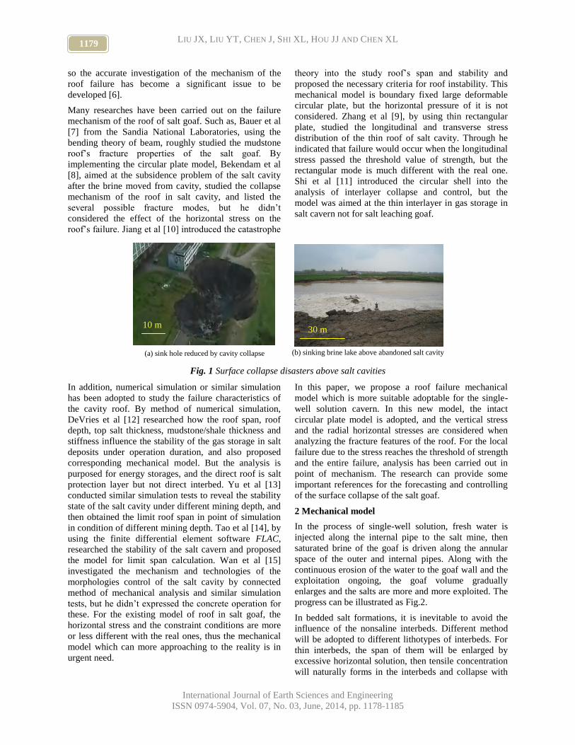
1179 LIU JX, LIU YT, CHEN J, SHI XL, HOU JJ AND CHEN XL
International Journal of Earth Sciences and Engineering
ISSN 0974-5904, Vol. 07, No. 03, June, 2014, pp. 1178-1185
so the accurate investigation of the mechanism of the
roof failure has become a significant issue to be
developed [6].
Many researches have been carried out on the failure
mechanism of the roof of salt goaf. Such as, Bauer et al
[7] from the Sandia National Laboratories, using the
bending theory of beam, roughly studied the mudstone
roof’s fracture properties of the salt goaf. By
implementing the circular plate model, Bekendam et al
[8], aimed at the subsidence problem of the salt cavity
after the brine moved from cavity, studied the collapse
mechanism of the roof in salt cavity, and listed the
several possible fracture modes, but he didn’t
considered the effect of the horizontal stress on the
roof’s failure. Jiang et al [10] introduced the catastrophe
theory into the study roof’s span and stability and
proposed the necessary criteria for roof instability. This
mechanical model is boundary fixed large deformable
circular plate, but the horizontal pressure of it is not
considered. Zhang et al [9], by using thin rectangular
plate, studied the longitudinal and transverse stress
distribution of the thin roof of salt cavity. Through he
indicated that failure would occur when the longitudinal
stress passed the threshold value of strength, but the
rectangular mode is much different with the real one.
Shi et al [11] introduced the circular shell into the
analysis of interlayer collapse and control, but the
model was aimed at the thin interlayer in gas storage in
salt cavern not for salt leaching goaf.
Fig. 1 Surface collapse disasters above salt cavities
In addition, numerical simulation or similar simulation
has been adopted to study the failure characteristics of
the cavity roof. By method of numerical simulation,
DeVries et al [12] researched how the roof span, roof
depth, top salt thickness, mudstone/shale thickness and
stiffness influence the stability of the gas storage in salt
deposits under operation duration, and also proposed
corresponding mechanical model. But the analysis is
purposed for energy storages, and the direct roof is salt
protection layer but not direct interbed. Yu et al [13]
conducted similar simulation tests to reveal the stability
state of the salt cavity under different mining depth, and
then obtained the limit roof span in point of simulation
in condition of different mining depth. Tao et al [14], by
using the finite differential element software FLAC,
researched the stability of the salt cavern and proposed
the model for limit span calculation. Wan et al [15]
investigated the mechanism and technologies of the
morphologies control of the salt cavity by connected
method of mechanical analysis and similar simulation
tests, but he didn’t expressed the concrete operation for
these. For the existing model of roof in salt goaf, the
horizontal stress and the constraint conditions are more
or less different with the real ones, thus the mechanical
model which can more approaching to the reality is in
urgent need.
In this paper, we propose a roof failure mechanical
model which is more suitable adoptable for the single-
well solution cavern. In this new model, the intact
circular plate model is adopted, and the vertical stress
and the radial horizontal stresses are considered when
analyzing the fracture features of the roof. For the local
failure due to the stress reaches the threshold of strength
and the entire failure, analysis has been carried out in
point of mechanism. The research can provide some
important references for the forecasting and controlling
of the surface collapse of the salt goaf.
2 Mechanical model
In the process of single-well solution, fresh water is
injected along the internal pipe to the salt mine, then
saturated brine of the goaf is driven along the annular
space of the outer and internal pipes. Along with the
continuous erosion of the water to the goaf wall and the
exploitation ongoing, the goaf volume gradually
enlarges and the salts are more and more exploited. The
progress can be illustrated as Fig.2.
In bedded salt formations, it is inevitable to avoid the
influence of the nonsaline interbeds. Different method
will be adopted to different lithotypes of interbeds. For
thin interbeds, the span of them will be enlarged by
excessive horizontal solution, then tensile concentration
will naturally forms in the interbeds and collapse with
10 m
(a) sink hole reduced by cavity collapse (b) sinking brine lake above abandoned salt cavity
30 m

1180 Roof Failure Mechanism of Salt-solution Goaf in bedded salt deposits
International Journal of Earth Sciences and Engineering
ISSN 0974-5904, Vol. 07, No. 03, June, 2014, pp. 1178-1185
fragments sinking to the bottom. Then the solution can
continue to the upper salt layer. However, for thin
interlayers, under the condition of solution properties
and safety need, ideal span of the interbeds is almost
impossible. The lower and upper salt layers are hard to
be connected by way of interbeds collapse. The
insoluble interbeds will appear on the top of the goaf
and become direct roof, as seen in Fig. 3.
The roof is subjected to several parts of forces, mainly
consisting of the following three parts:
(a)The first one is the horizontal stress, its direction
perpendicular to the roof boundary and inward to the
roof center, composed with the initial in situ stress and
the increment due to the excavation;
(b)The second part is the vertical stress, which is
downward perpendicular to the horizontal plane of the
roof, mainly inducing by the overlying strata rock mass;
Fig. 2 Diagrammatic sketch of the solution mining for
salt rock with single well
Fig. 3 schematic diagram of the stresses situation of the
roof
(c) The third part is the buoyancy of the brine, whose
direction is upward perpendicular to the down surface of
the roof.
In general, the cavern formed by water solution is
symmetry shape, can be regarded as a revolution body
along with a fixed axis. In addition, the well diameter is
often 10 ~ 30 mm, much smaller than the roof diameter
of 30 ~ 50 m, thus the roof can be rationally simplified
as intact circular plate. The established plate model of
the roof is illustrated in Fig. 4.
The lithology of the roof is assumed as homogenous,
and cylindrical coordinate is adopted for solution. The
center of the coordinate is located in the center of the
roof, r directs along with the radius direction from
center to outward; z-axis is downward perpendicular to
the middle plane of the roof.
The boundary of the roof is subjected to radially
distributed stress Fn. The rock salt is famous for its
rheology characteristics, so in the long-term of tectonic-
evolution, the in situ stresses perform hydrostatic
distribution. Ma et al [18] indicated that even in bedded
salt formations, if there is no obvious tectonic-activities,
the in-situ stress was almost hydrostatic state once the
depth is more than 400 m. Thus, in the following
analysis, the radial pressure Rh along the boundary
circumferential direction can be treated as evenly
distributed and its value is defined by the following
equation.
i
n
iiin hF
1
(1)
where, i is the factor of the horizontal stress of
stratum i, which is relative with the tectonic physics; hi
is the thickness of stratum I, rate m; i is the gravity
density of stratum I, rate kN/m3; n is the total number of
the upper strata; H is the depth of the roof, defined as
n
iihH
1 .
In vertical direction, the roof is subjected to evenly
distributed pressure of q, it is the differential part of the
vertical in-situ stress qv and the brine pressure brineq ,
that is:
n
ibrinebrineiibrinev HHhqqq
1
)( (2)
where, qv is the vertical in situ stress; qb is the brine
pressure; brine is the gravity density of the brine, hi is
defined as in Eq. (1); and is the mean density of the
overlying strata, defined as:
n
i
n
iiii hh
1 1
/ (3)
Horizontal
stress
Vertical stress
Buoyant stress
Goaf
Horizontal
stress

1181 LIU JX, LIU YT, CHEN J, SHI XL, HOU JJ AND CHEN XL
International Journal of Earth Sciences and Engineering
ISSN 0974-5904, Vol. 07, No. 03, June, 2014, pp. 1178-1185
r
¦ È
Fn
qn
Fn
qw
R
z
Fn
(a) Over-sight diagram (b) side-sight diagram
Fig. 4 Mechanical model of the circular roof of salt goaf
3 solution of the model
3.1 Deformation of the roof
For the edges simple supported sliding circular plate,
based on the stresses condition of the element in the
circular plate, Timoshenko deduced the differential
equation of the deflection of surface curvature when
subjected to horizontal longitudinal stress Fn and
vertical uniform stress q [17]:
2 2
2 2 2
d 1 d 1
d d 2
k qr
r r r R r D
(4)
Where φ is the gradient of the flexure plane; r is the
longitudinal coordinate variant; R is the radius of the
circular plate; q is the vertical stress acting on the
circular plate.
In Eq. (4), D is the flexural rigidity of the circular plate,
and its value is:
)1(12 2
3
EdD
(5)
Where E, and d are respectively the Young’s
modulus, Poisson’s ratio and thickness of the plate. k is
a parameter introduced for the convenience of solution,
its value is determined by:
D
RFk n
2
2 (6)
Eq. (4) belongs to Bessel function [18], and for the no-
hole circular plate, its general solution can be written as:
1 1 0
krC J
R
(7)
Where, J1 is a first-order Bessel function; C1 is a
parameter; and φ0 is a special solution of Eq. (4).
Generally, for the annular plate under boundary
conditions of GSS and GRS, as well as the uniform
distributed vertical stress q, the follow equation can be
used as one special solution of Eq.(4):
n
2
0 22 2
qrR qr
k D F
(8)
Thus, at this moment, the general solution of Eq.(4) can
be written as:
n
1 1
d
2 d
kr qrC J
R F r
(9)
Conducting integration on the both sides of Eq. (9), one
will obtain the expression of deflection:
n
2
1
0 24
C R kr qrJ C
k R F
(10)
Where J0 is the zero-order Bessel function; and C2 is
constant.
Boundary conditions:
When r=R, φ=0;
Subsequently, separately put the conditions r=R and
ω=0intothe expressions of φ Eqs.(7) and (10), then the
expressions of the constants C1 and C2 can be obtained
as:
3
1 2
12
qRC
k J k D
,
4 4
0
2 3 2
12 4
qR J k qRC
k J k D k D
Then put the expressions of constants C1and C2 into
Eqs. (7) and (10), one can obtain the expression of
curvature and deflection of the flexure plane:
3
1 1
2
12
krqR J R J k r
R
k J k D
(11)
Fn
w
z
q=qv-qbrine
r Fn
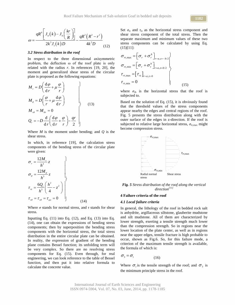
1182 Roof Failure Mechanism of Salt-solution Goaf in bedded salt deposits
International Journal of Earth Sciences and Engineering
ISSN 0974-5904, Vol. 07, No. 03, June, 2014, pp. 1178-1185
4
2 2 20 0
3 2
12 4
krqR J k J
qR R rR
k J k D k D
(12)
3.2 Stress distribution in the roof
In respect to the three dimensional axisymmetric
problem, the deflection ω of the roof plate is only
related with the radius r. In references [19, 20], the
moment and generalized shear stress of the circular
plate is proposed as the following equations:
d
d
d
d
0
d d
d d 2
r
r r
r
M Dr r
M Dr r
M M
qrQ D
r r r
(13)
Where M is the moment under bending; and Q is the
shear stress.
In which, in reference [19], the calculation stress
components of the bending stress of the circular plate
were given:
3
3
2
2
3
12
12
6
4
0
r
r
r
rz
r r z
Mz
h
Mz
h
Q hz
h
(14)
Where σ stands for normal stress, and τ stands for shear
stress.
Inputting Eq. (11) into Eq. (12), and Eq. (13) into Eq.
(14), one can obtain the expressions of bending stress
components; then by superposition the bending stress
components with the horizontal stress, the total stress
distribution in the entire circular plate can be obtained.
In reality, the expression of gradient of the bending
plane contains Bessel function; its unfolding term will
be very complex. So there are no resolving stress
components for Eq. (15). Even through, for real
engineering, we can look reference to the table of Bessel
function, and then put it into relative formula to
calculate the concrete value.
Set σrt and τrt as the horizontal stress component and
shear stress component of the total stress. Then the
separate maximum and minimum values of these two
stress components can be calculated by using Eq.
(15)[11]:
,max , /2
,min , /2
,max , 0
,min 0
h
rt r r r a z h
h
rt r r r a z h
rt rz r a z
rt
(15)
where σrh is the horizontal stress that the roof is
subjected to.
Based on the solution of Eq. (15), it is obviously found
that the threshold values of the stress components
appear nearby the edges and central regions of the roof.
Fig. 5 presents the stress distribution along with the
outer surface of the edges in z-direction. If the roof is
subjected to relative large horizontal stress, σrt,max might
become compression stress.
Fig. 5 Stress distribution of the roof along the vertical
direction[11]
4 Failure criteria of the roof
4.1 Local failure criteria
In general, the lithology of the roof in bedded rock salt
is anhydrite, argillaceous siltstone, glauberite mudstone
and silt mudstone. All of them are characterized by
lower strength, exerting a tensile strength much lower
than the compression strength. So in regions near the
lower location of the plate center, as well as in regions
near the upper edges, tensile fracture is high probable to
occur, shown as Fig.6. So, for this failure mode, a
criterion of the maximum tensile strength is available,
the formula of which is:
t 3 (16)
Where t is the tensile strength of the roof; and 3 is
the minimum principle stress in the roof.
Radial normal
stress
Shear stress
σrt,min
σrt,max
τrt,max
,max

1183 LIU JX, LIU YT, CHEN J, SHI XL, HOU JJ AND CHEN XL
International Journal of Earth Sciences and Engineering
ISSN 0974-5904, Vol. 07, No. 03, June, 2014, pp. 1178-1185
According to Eq. (16), one can find that the first
principle stress in the roof can determined as
max,3 rt . When the absolute value of max,rt
exceeds the tensile strength σt, local tensile failure in
the roof will happen, and then cause fracture and
collapse of the roof.
Fig. 6 Diagrammatic sketch of the partially failure of
the roof
4.2 Criteria of entire failure
During the salt exploitation process or after the
abandonment of the salt goaf, the creep of salt will
induce the stress increasing of the roof edges. Before the
stress exceeds the roof’s strength, large deformation of
the entire roof will perform induced by the horizontal
stress, and then cause large area of collapse of the roof.
This kind of failure is not caused by insufficient
strength but caused by insufficient stability, seen as
Fig.7.
Fig. 7 Diagrammatic sketch of the integral instability of
the roof
In reality, the goaf is subjected to both solution erosion
and creep shrinkage, the horizontal stress of the roof
edges is variable under different conditions. Thus for
the entire analysis of the roof stability, both the goaf
excavation and the rheology properties should be
comprehensive considered.
Based on Eq. (11), if J1(k)=0, the value of ω will be
infinitely great, which is incorrect for real conditions.
Assuming the zero-point of function J1 is
j1、j2、j3、…, and gradually become larger and larger
one by one. Then k = j1 can determine the minimum of
the horizontal force, that is:
n
2
1
2cr
DjF
R
(17)
According to the value table of Bessel function [18], we
can find the minimum of the root j1=3.832. Putting this
root value into Eq. (17), we can then get the value
expression of Fncr:
n 2
14.682cr
DF
R
(18)
In the above Eq. (18), Fn in fact is the uniform
distributed membrane stress of the circular plate edges.
If we set σr0 as the membrane stress evenly distributed
along with thickness, we can get[16]:
0
rn dF (19)
In conjunction with Eqs. (18) and (19), the threshold
value of the membrane stress σr0 in the edges of the
roof can be calculated[11]:
2
2
0 )(1
224.1)(
R
dEcrr
(20)
Where E is the Young’s modulus of the plate; μ is the
Poisson’s ratio of the roof; d is the mean thickness of
the roof; and R is the appearing radius of the roof.
For the mechanical parameters, such as E, μ, one can
obtained by method of laboratory tests; and for the
values of d and R, they can be valued by well-log
measurements of senor measurements.
However, the value that Eq. (20) gives is the theory
value of the threshold value, which is somewhat
different with the reality. Due to the uncertain
influences of sedimentary, in real engineering, the
lithologies, thickness, as well as mechanical strength
exists some certain of random. So for real application,
the Eq. (19) should be modified as following:
20 )(3.1)(R
dEcrr (21)
Where is modifying parameter, determined by the
specific petrophysical properties of the inerbeds. Its
value is lower than 1.0 and can be obtained according to
specific engineering. In Eq.(21), the Poisson’s ratio is
valued as 0.25.
From the above equation, it is found that the exposuring
span of the roof increases along with the solution
ongoing of the cavern. When the radius increases to
reach the above relationship, entire failure of the roof
will occur.
In addition, under different conditions of solution or
abandonment, the mechanical behaviors of the roof is
variable, thus the mechanical parameters should also be
modified. We recommend checking the softening
mechanism of the brine to the interbeds, thus the
mechanical behaviors versus time can be made, and
then rational modification can be conducted.
Brine
Roof
Brine
Roof

1184 Roof Failure Mechanism of Salt-solution Goaf in bedded salt deposits
International Journal of Earth Sciences and Engineering
ISSN 0974-5904, Vol. 07, No. 03, June, 2014, pp. 1178-1185
4.3 Other failure models
In reality, the failure models might not only the two
mentioned above. The analysis above approaches more
to the mechanism point. According to the previous
analysis, it is found the mineral components are another
important factor influencing the fracture properties. The
interbeds contain a certain soluble mineral, such as
NaCl, Na2SO4, and CaCl2. In cavern, the brine
concentration is different due to its density, in which the
top region has the lowest value, thus top solution is
most fast. The roof of interbed is inevitable influenced
by the unsaturated brine. There are two factors the brine
acts on the interbeds, the one is the high brine has
infiltration effect on the roof which will increase the
fracture of the interbed; the other is the solution effect,
which will destroy the matrix of the interbeds. So, in
this way, the failure model might be more complex that
analyzed above.
Above all, for the roof stability analysis, the available
process is proposed: first, the location and size of the
roof can be detected by Sonar measurement. Then, the
mechanical parameters, such as Young’s modulus E and
Poisson’s ratio μ, can be obtained by laboratory tests; if
the interbed contains soluble mineral compositions, the
immersion test should also be conducted to investigate
the softening performances. In end, the failure models
can be used to check whether the roof will collapse or
not.
5 For connected two-well solution mining
In addition, in real practice, the two-goaf system is
widely used. That is one goaf used for fresh water
injection and the other goaf is used for brine
withdrawing out. Due to the pressure state different
between the roofs of the two connected goafs, the
failure state may be different with each other. Generally
speaking, the goaf of brine withdrawing goaf has a
lower brine supporting pressure, thus collapse is higher
probable to occur.
Fig.8 connected two-well mining solution
For this connected goaf system, it is easy to establish
relative failure criteria for this kind of roof. What we
need do is only to change the brine pressure under the
roof, and then the criteria can be made.
6. Conclusions
In this paper, elastic theory of circular plate is
implemented to analyze the failure mechanism of the
roof in single well-solution salt cavern. The mechanical
model of sliding simple supported circular plate
subjected to vertical and horizontal stresses was
established. Elastic theory of circular intact plate was
used to fetch the resolving solution. According to the
solutions, mechanical analysis has been conducted on
the local failure and entire instability, and then
respective failure criteria of the two failure models have
been proposed. The investigation of the mineral solution
and brine softening has also been suggested. The
researches of this paper provide essential reference for
the roof failure mechanism and criteria, and also supply
important guidance for the surface subsidence
prediction and control of the salt cavern.
7. Reference:
[1] Wang Qingming. Rock salt deposit and
prospecting. Beijing, Chemical industry Press,
2007. (in Chinese)
[2] Kong Junfeng. Study on Subsidence above Salt
Cavern Underground Gas Storage and Related
Engineering Application[D]. Wuhan: University of
Chinese Academy of Sciences, 2012.
[3] Qiu Zhiyong. Mechanism analysis of surface
Goafs
Injection well Withdrawing well
Injection well
Withdrawing well

1185 LIU JX, LIU YT, CHEN J, SHI XL, HOU JJ AND CHEN XL
International Journal of Earth Sciences and Engineering
ISSN 0974-5904, Vol. 07, No. 03, June, 2014, pp. 1178-1185
collapse in the area of solution salt mining. Journal
of Safety Science and Technology, 2011, 12(7): 27-
31.
[4] Yang Chunhe, Jing Wenjun, JJK Daemen. Analysis
of major risks associated with hydrocarbon storage
caverns in bedded salt rock. Reliability Engineering
& System Safety, 2013, 113, pp94-111.
[5] Luo Xiaohui, Xi Zuping, Zhou Hong. Brief
Analysis on How to Prevent the Mined Ground
from Subsiding During Mining. China Well and
Rock Salt, 2011, 42, pp17-18.
[6] Luo Xiaohui, Xi Zuping, Zhou Hong. Brief analysis
on how to prevent the mined ground from subsiding
during mining[J]. China Well and Rock Salt,
2011,42(2), pp17-18
[7] Stephen Bauer, Brian Ehgartner, Bruce Levin,
James K. Linn. Waste Disposal in Horizontal
Solution Mined Caverns--Considerations of Site
Location, Cavern Stability, and Development
Considerations[C]// SMRI Fall Meeting, 1998.
[8] Roland Bekendam, Wim Paar. Induction of
Subsidence by Brine Removal[C] // SMRI Fall
Meeting, Austria, 2002.
[9] Jiang Deyi, Ren Song, Liu Xinrong, et al. Stability
analysis of rock salt cavern with catastrophe
theory[J]. Rock and Soil Mechanics, 2005, 26(7):
1099-1103.
[10] Zhang Peng, Lu Qingfeng, Zhang Wenguang, et al.
Stability analysis and control of rock salt cavern
roof[J]. China Well and Rock Salt, 2001, 42(2): 11-
14.
[11] Shi Xilin, Li Yinping, Yang Chunhe, Qu Dan’an,
Ma Hongling. Research on mechanical mechanism
of interlayer collapse in solution mining for salt
cavern gas storage. Rock and Soil Mechanics,
2009, 30(12), pp3615-3622.
[12] DeVries KL, Mellegard KD, Callahan GD,
Goodman WM.. Cavern roof stability for natural
gas storage in bedded salts. Final Report, National
Energy Technology Laboratory, United States
Department of Energy. Pittsburgh, Pennsylvania;
2005.
[13] Yu Hailong, Tan Xueshu, Xian Xuefu, et al. Model
test study on cavern stability of the rock salt[J].
Ground Pressure and Strata Control, 1995, 3(4):
156-159.
[14] Tao Lianjin, Jiang Deyi. Analysis on nonlinear
large deformation of saltrock cavity[J]. Journal of
Beijing Polytechnic University, 2001, 27(1): 64-67.
[15] Wan Yujin. Shape-controlling mechanism of gas
storage building in salt beds[J]. Natural Gas
Industry, 2004, 24(9): 130-132.
[16] MA Linjian, LIU Xinrong, MA Shu’na, et al.
Numerical analysis of in-situ ground stresses in
deep rock salt stratum containing mudstone
interlayers[J]. Journal of PLA University of Science
and Technology (Natural Science Edition), 2009,
10(6), pp604-609.
[17] Timoshenko S, Woinowsky KS. Theory of plates
and shells[M]. New York, USA: McQraw-Hill
Book Companty, 1959.
[18] Liang Kunmiao. Methods of Mathematical physics
[M]. Beijing: Higher Education Press, 2010. (in
Chinese)
[19] Liu Hongwen. Theory of plate and shell.
Hangzhou: Zhejiang University Press, 1987.
[20] Yu M. Double-shear strength theory. Beijing:
Science Press, 1998.

www.cafetinnova.org
Indexed in
Scopus Compendex and Geobase Elsevier, Chemical
Abstract Services-USA, Geo-Ref Information Services-USA,
List B of Scientific Journals, Poland,
Directory of Research Journals
ISSN 0974-5904, Volume 07, No. 03
June 2014, P.P.1186-1191
#02070352 Copyright ©2014 CAFET-INNOVA TECHNICAL SOCIETY. All rights reserved.
Effective Utilisation of Pond Ash as Fine Aggregate in Cement
Concrete under Flexure
K ARUMUGAM1, R ILANGOVAN
1 AND A V DEEPAN CHAKRAVARTHI
2
1Department of Civil Engineering, BIT Campus, Anna University, Triuchirappalli, India
2Department of Civil Engineering, Velammal College of Engineering and Technology, Madurai, India
Email: [email protected], [email protected], [email protected]
Abstract: With an increase of power consumption due to industrial development, the generation of coal ash has
been growing tremendously. Also environmental concern over its disposal has been raised. In order to examine the
usability of coal ash as an aggregate for concrete, the mechanical properties and durability of concrete using pond-
ash was analyzed in terms of pond ash content (10%,20%,30% wt %) as a part of fine aggregate. In this
experimental investigation, a mixes M25 grade was obtained by the proper proportion of pondash which gives
higher strength than the normal concrete. For that purpose we have tried with the replacement of pondash in
different percentage and compared the behavior with that of conventional concrete.
Keywords: Pond Ash, Electrostatic Precipitator, Wet Disposal, Fine Aggregate.
Introduction:
Use of waste and by products as concrete aggregate is of
great practical significance, because about 75% of
concrete comprises aggregate. There are various types of
waste materials that can be considered for usage as
aggregates. India’s power generation has undergone a
tremendous growth since independence. The production
of ash has also increased from 17.06million tones during
1900-91 to 68.82million tones in 1996-97and has
crossed 100million tones in year 2000. The ash needs to
be managed properly (or) otherwise it will cause land,
air and water pollution. Here there is serious concern
about utilizing it to the maximum extent. With the
increasing use of low grade coal of high ash content, the
current production of ash will be more then 100million
tones per year. Generally it is seen that the bottom is
around 20% of the total ash produced. Primarily, the fly
ash is disposed of using either dry or wet disposal
scheme. In dry disposal, the flyash is transported by
trucks, chute or conveyors to the site and disposed of by
constructing dry embankments. In wet disposal, the
flyash is transported as slurry through pipe and disposed
in large ponds (or) dykes. About 1000 million tons of
such ash referred to as pond ash, is available in India,
almost free of cost. Increase in demand and decrease in
the natural resources of fine aggregate for production of
concrete has resulted in the need of identifying new
sources of fine aggregate. This paper was possibility of
utilization of thermal power plant-Neyveli by-product-
pond ash as replacement to fine aggregate in concrete.
Fly ash collected through hoppers has been widely
accepted as a pozzolona and is being used by the
construction industry. Pond ash being coarser and less
pozzolonic is not being used. Recent reports indicate
that France leads the word by utilizing 50% of fly ash
followed by West Germany and U.K, while india
utilizes hardly 1% of the annual fly ash production of
nearly 100million tones.
Properties of Materials
It is deals with the study of the properties of various
materials like cement, fine aggregates, coarse
aggregates and water, which were used for casting
concrete specimens.
The various tests conducted to study the properties of
the above said materials are also discussed in this
chapter in detail.
The various materials used in this project are listed
below:
Cement – Birla Super 53 grade cement,
Fine aggregates – locally available sand, collected
from the Amravati river bed of Karur,
Coarse aggregates – locally available stones,
Water – ordinary portable drinking water.
Properties of Pond Ash
Table1: Physical Properties
Property Values Test method
Specific gravity 2.680 IS2386 – 1963
Bulk Density
(Kg/m3)
824 IS2386 – 1963
Absorption (%) Nil IS2386 – 1963
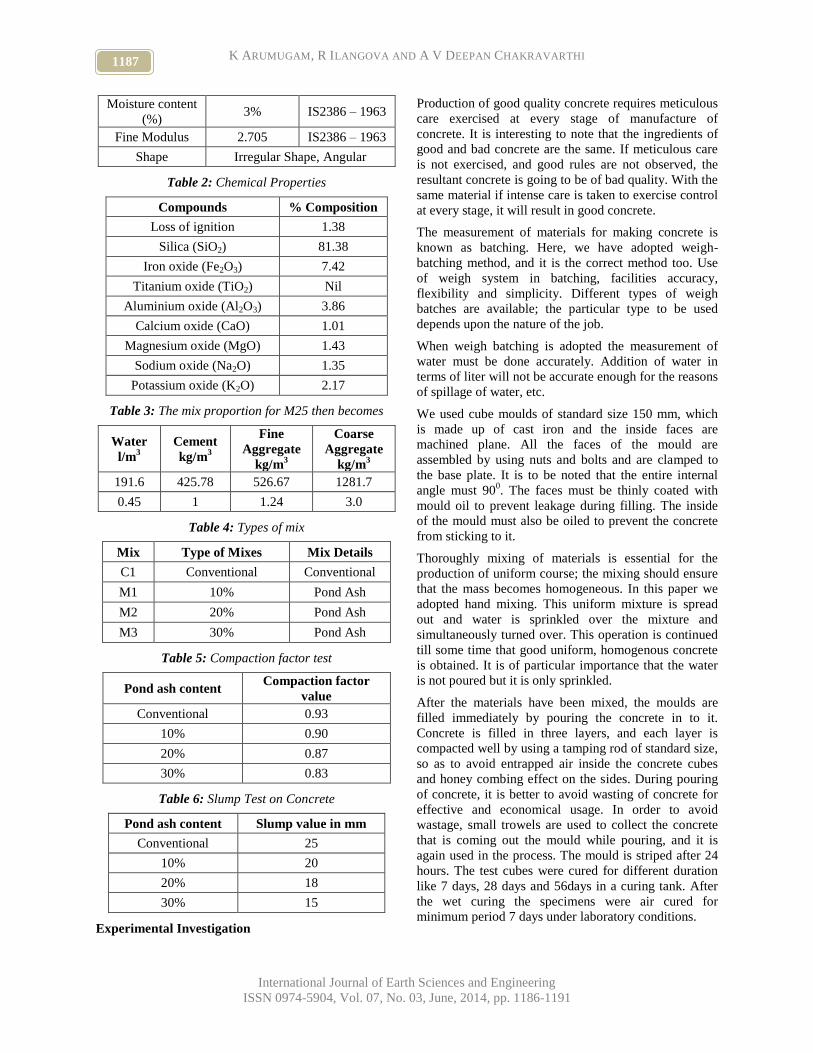
1187 K ARUMUGAM, R ILANGOVA AND A V DEEPAN CHAKRAVARTHI
International Journal of Earth Sciences and Engineering
ISSN 0974-5904, Vol. 07, No. 03, June, 2014, pp. 1186-1191
Moisture content
(%) 3% IS2386 – 1963
Fine Modulus 2.705 IS2386 – 1963
Shape Irregular Shape, Angular
Table 2: Chemical Properties
Compounds % Composition
Loss of ignition 1.38
Silica (SiO2) 81.38
Iron oxide (Fe2O3) 7.42
Titanium oxide (TiO2) Nil
Aluminium oxide (Al2O3) 3.86
Calcium oxide (CaO) 1.01
Magnesium oxide (MgO) 1.43
Sodium oxide (Na2O) 1.35
Potassium oxide (K2O) 2.17
Table 3: The mix proportion for M25 then becomes
Water
l/m3
Cement
kg/m3
Fine
Aggregate
kg/m3
Coarse
Aggregate
kg/m3
191.6 425.78 526.67 1281.7
0.45 1 1.24 3.0
Table 4: Types of mix
Mix Type of Mixes Mix Details
C1 Conventional Conventional
M1 10% Pond Ash
M2 20% Pond Ash
M3 30% Pond Ash
Table 5: Compaction factor test
Pond ash content Compaction factor
value
Conventional 0.93
10% 0.90
20% 0.87
30% 0.83
Table 6: Slump Test on Concrete
Pond ash content Slump value in mm
Conventional 25
10% 20
20% 18
30% 15
Experimental Investigation
Production of good quality concrete requires meticulous
care exercised at every stage of manufacture of
concrete. It is interesting to note that the ingredients of
good and bad concrete are the same. If meticulous care
is not exercised, and good rules are not observed, the
resultant concrete is going to be of bad quality. With the
same material if intense care is taken to exercise control
at every stage, it will result in good concrete.
The measurement of materials for making concrete is
known as batching. Here, we have adopted weigh-
batching method, and it is the correct method too. Use
of weigh system in batching, facilities accuracy,
flexibility and simplicity. Different types of weigh
batches are available; the particular type to be used
depends upon the nature of the job.
When weigh batching is adopted the measurement of
water must be done accurately. Addition of water in
terms of liter will not be accurate enough for the reasons
of spillage of water, etc.
We used cube moulds of standard size 150 mm, which
is made up of cast iron and the inside faces are
machined plane. All the faces of the mould are
assembled by using nuts and bolts and are clamped to
the base plate. It is to be noted that the entire internal
angle must 900. The faces must be thinly coated with
mould oil to prevent leakage during filling. The inside
of the mould must also be oiled to prevent the concrete
from sticking to it.
Thoroughly mixing of materials is essential for the
production of uniform course; the mixing should ensure
that the mass becomes homogeneous. In this paper we
adopted hand mixing. This uniform mixture is spread
out and water is sprinkled over the mixture and
simultaneously turned over. This operation is continued
till some time that good uniform, homogenous concrete
is obtained. It is of particular importance that the water
is not poured but it is only sprinkled.
After the materials have been mixed, the moulds are
filled immediately by pouring the concrete in to it.
Concrete is filled in three layers, and each layer is
compacted well by using a tamping rod of standard size,
so as to avoid entrapped air inside the concrete cubes
and honey combing effect on the sides. During pouring
of concrete, it is better to avoid wasting of concrete for
effective and economical usage. In order to avoid
wastage, small trowels are used to collect the concrete
that is coming out the mould while pouring, and it is
again used in the process. The mould is striped after 24
hours. The test cubes were cured for different duration
like 7 days, 28 days and 56days in a curing tank. After
the wet curing the specimens were air cured for
minimum period 7 days under laboratory conditions.

1188 Effective Utilisation of Pond Ash as Fine Aggregate in Cement Concrete under Flexure
International Journal of Earth Sciences and Engineering
ISSN 0974-5904, Vol. 07, No. 03, June, 2014, pp. 1186-1191
Name of
the test Size of mould
Number
of days
Compression
Test 150 x 150 x 150 mm 7 28 56
Split tensile
Strength
Ht - 300 & Dia - 150
mm 7 28 56
Flexural
Strength 100 x 100 x 500 mm 7 28 56
Methodology
The methodology adopted for experimental study has
fully been described the hardened properties of concrete
such as compressive Strength, Split tensile Strength and
Flexural Strength parameters of M25 grade concrete as
per relevant codes of practice, replacing cement by
Pond Ash partially in refer table 2.4. This experimental
study consisted of collection of different materials to be
used for the investigation, including Pond Ash sample
collection from Neyveli, characterization of materials,
designing the mix as per IS 10262-2009, mixing of
concrete, casting the specimen for various test
considered for the study, testing the specimens,
tabulation and analysis of data and finally discussion
followed by conclusions based on test results.
Collection of Sample and its preparation - Pond Ash
sample collected (Fig.4.1) from Neyveli was used for
the investigation, which partially contributes to Cement
content of the concrete mix.
Fig1: Pond Ash
Testing of Specimens
The concrete specimens are tested using a compression
testing apparatus. The specimen is rested over the
loading frame. Care should take that the specimen
should rest within the frame for effective load
application. Then the load is applied and the value of
the load for the first visible crack and the maximum
load is noted down to calculate the compressive strength
of the concrete, which is got by dividing the maximum
load attained by the area of contact.
Result Analysis
The mix design ratio for M25Grade Concrete was
derived as 0.45:1:1.24:3.0 (weight basis) respectively.
M25 grade concrete was cast by using cement of 53
grade of its specific gravity was 3.16. Sand conforming
to zone II was used its specific gravity was 2.648. The
coarse aggregate of 20mm size was used and its specific
gravity was 2.86. Then cubes, cylinders and prisms
were cast with concrete by using the moulds of size
150mm x 150mm x 150mm, 150mm x 300 mm and
100mm x 100mm x 500mm. After 24 hours the
specimens were removed from the mould and cured for
7 days, 28 days and 56days. After curing the specimens
were tested using compression testing machine and
flexure testing machine. Then the values are noted. The
above process was repeated for replacement of sand by
Pond ash. The above experimental results were
compared with ordinary concrete results.
Table 7: Compressive Strength of concrete for Different
mixes
MIX
7 Days
Strength
(N/mm2)
28 Days
Strength
(N/mm2)
56 Days
Strength
(N/mm2)
C1 16.2 26.35 28.47
M1 16.8 27.53 28.96
M2 17.7 28.23 29.54
M3 17.8 28.38 29.86
Fig 2: Compressive Strength with Different age
Fig 3: Compressive Strength Testing sample

1189 K ARUMUGAM, R ILANGOVA AND A V DEEPAN CHAKRAVARTHI
International Journal of Earth Sciences and Engineering
ISSN 0974-5904, Vol. 07, No. 03, June, 2014, pp. 1186-1191
Table 8: Split Tensile Strength of concrete for Different
mixes
MIX
7 Days
Strength
(N/mm2)
28 Days
Strength
(N/mm2)
56 Days
Strength
(N/mm2)
C1 2.04 2.88 2.95
M1 2.12 2.97 3.12
M2 2.2 3.12 3.21
M3 2.22 3.16 3.33
Fig 4: Split Tensile Strength with Different age
Fig 5: Split Strength Testing sample
Table 9: Flexural Strength of concrete for Different
mixes
MIX
7 Days
Strength
(N/mm2)
28 Days
Strength
(N/mm2)
56 Days
Strength
(N/mm2)
C1 3.38 3.98 4.15
M1 3.41 4.1 4.21
M2 3.49 4.18 4.32
M3 3.53 4.25 4.45
Fig 6: Flexural Strength with Different age
Fig 7: Flexural Strength Testing sample
Results Discussion
With the addition of pond ash there is reduction in
slump value of fresh concrete.
The unit weight of concrete gets reduced through
the addition of pond ash as replacement of fine
aggregate since it has lesser specific gravity than
fine aggregate.
The 7 days and 28 days strength shows that the
strength increases from standard concrete up to the
addition of 30% replacement of fine aggregate with
pond ash.
The compressive strength various from 29.86 N/mm2 to
28.47 N/mm2 for 56 days and 28.38 N/mm2 to 26.35
N/mm2 for 28 days and 17.8 N/mm2 to 16.2 N/mm2
for 7 days. This is the different range of replacement
of pond ash.
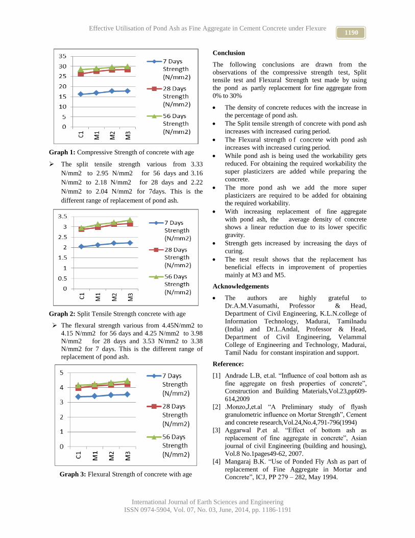
1190 Effective Utilisation of Pond Ash as Fine Aggregate in Cement Concrete under Flexure
International Journal of Earth Sciences and Engineering
ISSN 0974-5904, Vol. 07, No. 03, June, 2014, pp. 1186-1191
Graph 1: Compressive Strength of concrete with age
The split tensile strength various from 3.33
N/mm2 to 2.95 N/mm2 for 56 days and 3.16
N/mm2 to 2.18 N/mm2 for 28 days and 2.22
N/mm2 to 2.04 N/mm2 for 7days. This is the
different range of replacement of pond ash.
Graph 2: Split Tensile Strength concrete with age
The flexural strength various from 4.45N/mm2 to
4.15 N/mm2 for 56 days and 4.25 N/mm2 to 3.98
N/mm2 for 28 days and 3.53 N/mm2 to 3.38
N/mm2 for 7 days. This is the different range of
replacement of pond ash.
Graph 3: Flexural Strength of concrete with age
Conclusion
The following conclusions are drawn from the
observations of the compressive strength test, Split
tensile test and Flexural Strength test made by using
the pond as partly replacement for fine aggregate from
0% to 30%
The density of concrete reduces with the increase in
the percentage of pond ash.
The Split tensile strength of concrete with pond ash
increases with increased curing period.
The Flexural strength o f concrete with pond ash
increases with increased curing period.
While pond ash is being used the workability gets
reduced. For obtaining the required workability the
super plasticizers are added while preparing the
concrete.
The more pond ash we add the more super
plasticizers are required to be added for obtaining
the required workability.
With increasing replacement of fine aggregate
with pond ash, the average density of concrete
shows a linear reduction due to its lower specific
gravity.
Strength gets increased by increasing the days of
curing.
The test result shows that the replacement has
beneficial effects in improvement of properties
mainly at M3 and M5.
Acknowledgements
The authors are highly grateful to
Dr.A.M.Vasumathi, Professor & Head,
Department of Civil Engineering, K.L.N.college of
Information Technology, Madurai, Tamilnadu
(India) and Dr.L.Andal, Professor & Head,
Department of Civil Engineering, Velammal
College of Engineering and Technology, Madurai,
Tamil Nadu for constant inspiration and support.
Reference:
[1] Andrade L.B, et.al. “Influence of coal bottom ash as
fine aggregate on fresh properties of concrete”,
Construction and Building Materials,Vol.23,pp609-
614,2009
[2] .Monzo,J,et.al “A Preliminary study of flyash
granulometric influence on Mortar Strength”, Cement
and concrete research,Vol.24,No.4,791-796(1994)
[3] Aggarwal P.et al. “Effect of bottom ash as
replacement of fine aggregate in concrete”, Asian
journal of civil Engineering (building and housing),
Vol.8 No.1pages49-62, 2007.
[4] Mangaraj B.K. “Use of Ponded Fly Ash as part of
replacement of Fine Aggregate in Mortar and
Concrete”, ICJ, PP 279 – 282, May 1994.

1191 K ARUMUGAM, R ILANGOVA AND A V DEEPAN CHAKRAVARTHI
International Journal of Earth Sciences and Engineering
ISSN 0974-5904, Vol. 07, No. 03, June, 2014, pp. 1186-1191
[5] Ranganath R.V “A study on the charecterisation
and use of Ponded Fly Ash as Fine Aggregate in in
Mortar and Concrete” Ph.D Thesis, Report 1995,
IITD – Delhi,
[6] Ranganath R.V, et.al. “Influence of Size fraction of
ponded ash on its pozilanic activity” Cement
concrete Research, Vol.28, No.5, pp749-761, 1994.
[7] P. K. Kolay, D. N. Singh “Physical, chemical,
mineralogical, and thermal properties of cenospheres
from an ash lagoo” Cement and Concrete Research,
Issue 4, Volume 31, PP 539-542, April 2001,
[8] A.K.Mullick” Use of Industrial wastes for
sustainable cement and concrete constructions,”
The Indian concrete journal, Vol 81,No.12,16-
24(2007)
[9] Pranesh R.N. “Pond Ash in Cement Concrete –
Some studies on its feasibilities” Ph.D Thesis
Report 2008.VTU, Belgaum.
[10] Bharathi Ganesh “Pond Ash: An Alternative
Material as Fine Aggregate in Concrete for
Sustainable Construction” International Congress
on Advanced Materials, 2011.
[11] Leonards G. A. “Pulverized coal ash as structural
fill”, J. Geotech. Engng Div., ASCE, PP 517– 531,
1982.

www.cafetinnova.org
Indexed in
Scopus Compendex and Geobase Elsevier, Chemical
Abstract Services-USA, Geo-Ref Information Services-USA,
List B of Scientific Journals, Poland,
Directory of Research Journals
ISSN 0974-5904, Volume 07, No. 03
June 2014, P.P.1192-1198
#02070353 Copyright ©2014 CAFET-INNOVA TECHNICAL SOCIETY. All rights reserved.
Variable Tap Parameter (α) Techniques for Sato based Blind
Equalizer
K SUTHENDRAN1 AND T ARIVOLI
2
1Department of ECE, Kalasalingam Academy of Research and Education, Krishnankoil-626 126, India
2Department of ECE, Vickram College of Engineering, Enathi-630 561, India
Email: [email protected], [email protected]
Abstract: It is renowned that blind equalizers do not require training sequence to track the time varying
characteristics of the channel. But, it ends up in slow convergence to realize a selected Signal to Noise Ratio (SNR).
However, variable tap parameter (α) will speed up the convergence rate and also minimizes the mis adjustment for a
blind equalizer. In this work, two variable tap parameter techniques were used for Sato based blind equalizer
algorithm. Simulation results for Pulse Amplitude Modulated (PAM) signal show that the projected approach has a
higher convergence rate than the prevailing Sato algorithm with fastened α value.
Keywords: Blind Equalization, Convergence, Sato algorithm.
1. Introduction:
In the trendy data communication, plenty of effort has
been devoted to utilize the accessible channel
bandwidth with efficiency. Inter-Symbol Interference
(ISI) and Thermal noises are the two main factors,
which are limiting the performance of data transmission
systems. In essence, the ISI is generated by dispersion
within the transmit filter, the transmission medium, and
receive filter. In the band-limited (frequency selective)
time dispersive channel, the ISI is caused by multipath
propagation. The impact is that the modulated pulses are
spread in time into adjacent symbols, and it distorts the
transmitted signals inflicting data errors at the receiver.
Thermal noise is generated at the forepart of the
receiver. For bandwidth-limited channels, the ISI has
been recognized as the major drawback in high speed
data transmission over wireless channels. The
traditional band restricted filters fail to recover the
information once the received symbol contains ISI and
in-band noise. The Inter-Symbol Interference will be
removed by victimization equalization techniques.
Generally, the term equalization is used to describe any
signal process operation that minimizes the ISI [1]. An
equalizer within the receiver compensates for average
range of expected channel amplitude and delay
characteristics. Equalizer algorithm, equalizer structure
and the rate of modification of the multipath radio
channel are three main factors that affect the time
spread over that an equalizer converges. Two vital
problems in equalizer design and implementation are its
complexity and its training. For frequency selective
channel, the equalizer enhances the frequency
components with little amplitudes and attenuates the
sturdy frequencies within the received frequency
response and for a time-varying channel.
The mobile weakening channel could be a random and
time varying; equalizers should track the time varying
characteristics of the channel, and therefore referred to
as adaptive equalizers. Adaptive channel equalization is
an efficient tool in mitigating Inter-Symbol Interference
(ISI) caused by linear distortions in unknown channels
[2]. An adaptive filtering algorithmic program needs the
information regarding the “known” response so as to
estimate the error signal required for adaptive method.
In follow, the noted signals are often generated at the
receiver aspect in two ways. In first technique, the
transmitted training sequence is retrieved by the replica
of the known response that is stored within the receiver.
The synchronization should be done between
transmitted training sequence and better-known
response that is hold on within the receiver. With a
famed training sequence, the adaptive filtering
algorithmic program used to regulate the equalizer
coefficients, which correspond mathematically to
checking out the distinctive minimum quadratic error
performance surface. The second technique may be a
decision directed technique, in which, instead of the
known training sequence, a sequence of data symbols
are estimated from the equalizer can be used. This
estimated output could also be unreliable, so this may
not enable the tap weight coefficients to be optimized.
In general, the computation of error estimation is done
with the aid of the input vector and desired response,
and it is used to make the control over the adjustable
filter coefficients values. Depending on the filter
structure chosen, the adjustable coefficients may be in

1193 K SUTHENDRAN AND T ARIVOLI
International Journal of Earth Sciences and Engineering
ISSN 0974-5904, Vol. 07, No. 03, June, 2014, pp. 1192-1198
the form of tap weight reflection coefficients or rotation
parameters[2]. However, the elemental distinction
between the various applications of adaptive filtering
arises in the manner in which the required response is
extracted.
Training and tracking are the two general operational
modes of an adaptive equalizer. First, a better-known
training sequence -pseudorandom binary signal of fixed
length is sent by the transmitter. With this, the equalizer
at the receiver facet may adapt to a correct weight for
minimum bit error rate (BER) detection. Following this
training sequence, original data is sent and adaptive
equalizer utilizes the recursive algorithm to evaluate the
channel, and thus estimates the filter coefficients to
compensate the distortion created by multipath in the
channel. Equalizers require periodic training in order to
keep up effective ISI cancellation. In data
communication systems, user data is often segmented
into short time blocks or time slots. Time division
multiple access (TDMA) wireless systems are notably
well matched for equalizers. Due to time varying nature
of wireless channels, training signals should be sent
often and this occupies additional bandwidth. In several
applications better-known training sequence is needed
to adapt the equalizers by minimizing the mean square
error [MSE], however this being impractical and
expensive when long training sequence is necessary [3].
As an example, in step with 900MHz GSM standard, 26
bits out of each 148 bit frame are used as training
signals [4].
Recently, many researchers have aimed to enhance the
convergence rate and to reduce the steady state
estimation error based on variable step size algorithms
[5], [6], [7] and [8]. They have proposed totally
different criteria for the variable step size. R.Kwong and
E.W. Johnston in [5], regulate the variable step size
based on instantaneous squared predication error. In [7],
the variable step size is updated using the changes of
successive samples gradient. In [8], the authors have
projected a variable step size to reduce the squared error
at every step. Mayyas et al. in [6] have proposed a
variable step size algorithm that has quick convergence
at the early stages of adaptation. All these algorithms
are based on Least Mean square algorithm. In this
paper, a replacement variable step size algorithm is
proposed based on Sato’s blind algorithm.
2. Blind Algorithm:
Even though trained strategies have several
disadvantages, they are often adequate. The throughput
of the system drops due to the time slots occupied by
the training signal. Another disadvantage is that the
training signal is not forever known at the receiver, e.g.,
in a non cooperative (surveillance) surroundings.
Finally, the quicker time variable channel needs training
sequence more often to train the equalizer. This leads to
further reduction in the throughput of the system[9].
The Blind algorithms are ready to exploit characteristics
of the transmitted signals and do not need training
sequences. They are called so because they provide
equalizer convergence without burdening the transmitter
with training overhead. These trendy algorithms are
ready to acquire equalization through property restoral
techniques of the transmitted signal. In general, even
when the initial error rate is large, blind equalization
methodology directs the coefficient adaptation process
towards the optimal filter parameters. A Blind Equalizer
is ready to compensate amplitude and delay distortions
of communication channel victimization only the
channel output samples and the knowledge of the basic
statistical properties of the data symbols. The foremost
advantage of blind equalizers is that there is no training
sequence to calculate the tap weight coefficients;
therefore no bandwidth is wasted by its transmission.
Blind equalization is effective for a high-speed digital
radio, GPS, digital mobile communication systems,
multi-point networks, cable TV, and digital terrestrial
TV broadcasting [10], [11], [12] and [9].
The major downside is that the equalizer can generally
take an extended time to converge as compared to a
trained equalizer. The necessity for blind equalizers in
the field of information communications is greatly
mentioned by Godard [13], in the context of multipoint
networks. Blind joint equalization and carrier recovery
may find application in digital communication system
over multipath weakening channels. Moreover, it is
applied in extremely non-stationary digital mobile
communications, wherever it is impractical to use
training sequences. These techniques include algorithms
such as the Sato algorithm and Constant modulus
algorithm (CMA).
2.1. Sato’s Blind Algorithm:
Sato was the one who first introduced the concept of
blind equalization in 1975 for multilevel pulse
amplitude modulation, where there is no reference
sequence accessible and afterward Godard combined
Sato’s idea with a decision Directed (DD) algorithm and
obtains a brand new blind equalization scheme for
Quadrature Amplitude Modulation(QAM) data
transmission. Since blind equalization has attracted vital
scientific interest due to its potentials in terms of
overhead reduction and simplification of point to
multipoint communication. Sato proposed algorithm
which was designed only for real valued signal and
PAM [14]. However, its complex valued extension is
straightforward, which was derived by Godard. The cost
function proposed by Sato is given in (1),
)})(.{()( 2
kk
sato
ysignyEAJ (1)

1194 Variable Tap Parameter (α) Techniques for Sato based Blind Equalizer
International Journal of Earth Sciences and Engineering
ISSN 0974-5904, Vol. 07, No. 03, June, 2014, pp. 1192-1198
Where,
ky = output of the equalizer
0,1
0,1)( k
kk
y
yysign (2)
|)(|
)( 2
k
k
aE
aE
(3)
Sign denotes the usual signum function of a real scalar.
γ referred as scaling factor and ak denotes the input data
sequence.
Fig1: General block diagram for Blind equalizer
Fig. 1 shows the general block diagram of the Blind
Equalizer. It seems that Sato’s proposal appears to be
developed over Least Mean Square (LMS) algorithm,
which uses steepest decent criteria for convergence
method. Mathematically, differentiate any equation and
equate it to zero, then this offers the minimum; work it
to the steepest-descent criteria; it gives the tap weight
coefficient for the equalizer. So, differentiate (1) and
substitute it to the steepest-descent criteria and getting
(4) as shown below. The algorithm of Sato’s blind
equalization is based on (4), which is used for training
the output sequences[14].
)](.[.^
1
^
kkkkk ysignyrAA (4)
Where,
Ak = Weight used for training
α = Tap-adjusting coefficient
yk = Output sequence
rk = Input sequence
and
1.
k
i
ik xar (5)
Since this algorithm works under iteration basis, at
every iteration it tries to adapt its output sequence to the
self realized input sequence. Thus, it is also known as
self-learning equalizer. The convergence rate and
precision to output sequence are the two main design
considerations in Sato’s blind equalization. To get the
best result from Sato’s algorithm, the design
considerations should be optimized on the basis of its
parameters, in order that it will converge in no time with
a high precision output sequence. This can be more or
less guided by tap-adjusting coefficient ‘α’, because the
remaining parameters are not variable according to [15]
Fig2: The Sato based Blind equalizer with 5 taps
3. Proposed Algorithm:
In Sato’s blind equalization algorithm the initial value
of the tap parameter (α) is chosen between the minimum
and maximum values and these ranges of values are
finite to confirm the convergence and stability of the
algorithms. The fastened αmax is chosen with respect to
the stability condition of the algorithm, while αmin is
chosen to confirm desired steady-state performance
[16], [17] and [18]. In proposed approach the tap
parameter value starts with 0.0006 (optimum value
identified by Sato for PAM signal) to reconstruct the
very first symbol and this value is incremented by small
constant (s) for each iteration. The output distinction
between successive iterations is calculated and using
this value the iteration for reconstruction of very first
symbol is stopped. The updated tap parameter value is
chosen as beginning value for subsequent symbols. In
the reconstruction of the subsequent symbols α value is
decremented by small constant at each iteration and,
using this value the iteration is stopped. For first symbol
estimation, the specified SNR can be achieved by
changing the output difference value to stop the iteration
and for subsequent symbols estimation; by changing
αmin value the specified SNR output can be obtained.
The flowchart of the projected algorithm shown in fig.3
provides the detailed
nk
a
k
A
k
r
k Decision
Circuit
BlindEq
ualizer

1195 K SUTHENDRAN AND T ARIVOLI
International Journal of Earth Sciences and Engineering
ISSN 0974-5904, Vol. 07, No. 03, June, 2014, pp. 1192-1198
Fig3: Flow Chart for Proposed algorithm
4. Simulation Results:
The performance of the improved blind algorithm has
been studied for PAM symbols as done by Sato. The
PAM symbols, having ISI with five reflections with
relative amplitude (0.7, 0.6, 0.5, 0.3 and 0.1) as shown
in fig. 4 for symbol 3and Additive White Gaussian
Noise (AWGN) with 25dB SNR, are taken as the input
to the equalizer. The equalizer has been implemented by
a linear transversal filter with a five tap complex
circuitry as shown in fig.2.
Experiment1: Constant α (αconstant)
Small α value results minimum steady state error but
results in slow convergence. High α value will speed-up
the convergence however lead to maximum
misadjustment[16].The variable tap parameter value is
restricted to the range [αmin=0.0006, αmax=0.18] to
guarantee stability of the algorithm.
Fig.4. ISI model for Symbol 3
Experiment 2:α with Linear increment and decrement
(αlinear)
For the above mentioned input, the parameter value
chosen as 0.0006 and tap weights are initialized with
center tap (only center tap has one others are near zero)
[19] and [20]. The very first symbol is reconstructed by
using linear increment in α. i.e., α is incremented by
constant factor (s=0.02) for every iteration as
αk+1 = αk + s; where s=0.02
The output distinction between current iteration and
former iteration is calculated at in three completely
different sampling points and if all the three output
values are less than 0.001 (based on experimental
analysis, output distinction value 0.001 is chosen as
better value to stop the iteration) means that the iteration
for reconstruction of very first symbol is stopped. The
updated α =0.3006 is fixed as optimum or starting value
for subsequent symbol. In the reconstruction of the
following symbols the α is decremented by a the same
factor (say 0.02) at each iteration as
αk+1 = αk – s; where s=0.02
When α reaches 0.0006, the iteration is stopped. On trial
and error basis, for constant α input the optimum α
valueis 0.18. But in proposed approach it is found
0.3006 as αmax and with updated tap weights consequent
symbolsreconstructed with 30dB SNR in few iterations
with stability. While giving α as 0.3006 with center tap
initialization for experiment 1 means, it ends up in
misadjustment and subsequent symbols can’t be
reconstructed moreover.
Experiment 3:α with Nonlinear increment and
decrement (αnonlinear)
For an equivalent input, step size parameter value
chosen as 0.0006 and tap weights are initialized with
center tap. The very first symbol reconstructed by using
nonlinear increment of step size parameter value. That
is step size value calculated with the assistance of
iteration count as
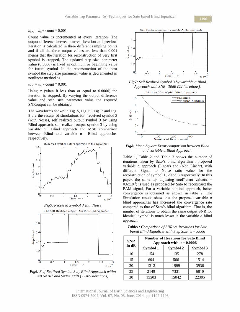
1196 Variable Tap Parameter (α) Techniques for Sato based Blind Equalizer
International Journal of Earth Sciences and Engineering
ISSN 0974-5904, Vol. 07, No. 03, June, 2014, pp. 1192-1198
αk+1 = αk + count * 0.001
Count value is incremented at every iteration. The
output difference between current iteration and previous
iteration is calculated in three different sampling points
and if all the three output values are less than 0.001
means that the iteration for reconstruction of very first
symbol is stopped. The updated step size parameter
value (0.3006) is fixed as optimum or beginning value
for future symbol. In the reconstruction of the next
symbol the step size parameter value is decremented in
nonlinear method as
αk+1 = αk - count * 0.001
Using α (when it less than or equal to 0.0006) the
iteration is stopped. By varying the output difference
value and step size parameter value the required
SNRoutput can be obtained.
The waveforms shown in Fig. 5, Fig. 6 , Fig. 7 and Fig.
8 are the results of simulations for received symbol 3
(with Noise), self realized output symbol 3 by using
Blind approach, self realized output symbol 3 by using
variable α Blind approach and MSE comparison
between Blind and variable α Blind approaches
respectively.
Fig5: Received Symbol 3 with Noise
Fig6: Self Realized Symbol 3 by Blind Approach withα
=0.6X10⁻³
and SNR=30dB (22305 iterations)
Fig7: Self Realized Symbol 3 by variable α Blind
Approach with SNR=30dB (22 iterations).
Fig8: Mean Square Error comparison between Blind
and variable α Blind Approach.
Table 1, Table 2 and Table 3 shows the number of
iterations taken by Sato’s blind algorithm , proposed
variable α approach (Linear) and (Non Linear), with
different Signal to Noise ratio value for the
reconstruction of symbol 1, 2 and 3 respectively. In this
paper, the same tap adjusting coefficient value(α =
0.6x10⁻³
) is used as proposed by Sato to reconstruct the
PAM signal. For a variable α blind approach, better
convergence is obtained as shown in table 2. The
Simulation results show that the proposed variable α
blind approaches has increased the convergence rate
compared to that of Sato’s blind algorithm. That is, the
number of iterations to obtain the same output SNR for
identical symbol is much lesser in the variable α blind
approach.
Table1: Comparison of SNR vs. Iterations for Sato
based Blind Equalizer with Step Size α = .0006
SNR
in dB
Number of Iterations for Sato Blind
Approach with α = 0.0006
Symbol 1 Symbol 2 Symbol 3
10 154 135 278
15 604 506 1514
20 1312 1999 3936
25 2149 7331 6810
30 15503 15042 22305
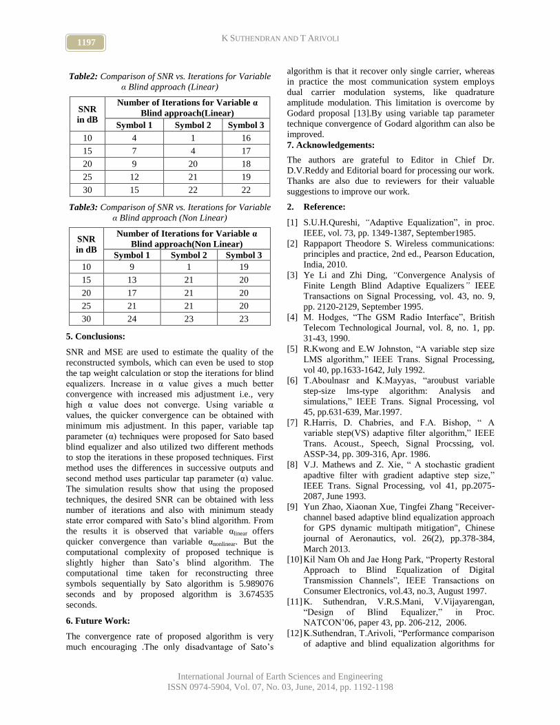
1197 K SUTHENDRAN AND T ARIVOLI
International Journal of Earth Sciences and Engineering
ISSN 0974-5904, Vol. 07, No. 03, June, 2014, pp. 1192-1198
Table2: Comparison of SNR vs. Iterations for Variable
α Blind approach (Linear)
SNR
in dB
Number of Iterations for Variable α
Blind approach(Linear)
Symbol 1 Symbol 2 Symbol 3
10 4 1 16
15 7 4 17
20 9 20 18
25 12 21 19
30 15 22 22
Table3: Comparison of SNR vs. Iterations for Variable
α Blind approach (Non Linear)
SNR
in dB
Number of Iterations for Variable α
Blind approach(Non Linear)
Symbol 1 Symbol 2 Symbol 3
10 9 1 19
15 13 21 20
20 17 21 20
25 21 21 20
30 24 23 23
5. Conclusions:
SNR and MSE are used to estimate the quality of the
reconstructed symbols, which can even be used to stop
the tap weight calculation or stop the iterations for blind
equalizers. Increase in α value gives a much better
convergence with increased mis adjustment i.e., very
high α value does not converge. Using variable α
values, the quicker convergence can be obtained with
minimum mis adjustment. In this paper, variable tap
parameter (α) techniques were proposed for Sato based
blind equalizer and also utilized two different methods
to stop the iterations in these proposed techniques. First
method uses the differences in successive outputs and
second method uses particular tap parameter (α) value.
The simulation results show that using the proposed
techniques, the desired SNR can be obtained with less
number of iterations and also with minimum steady
state error compared with Sato’s blind algorithm. From
the results it is observed that variable αlinear offers
quicker convergence than variable αnonlinear. But the
computational complexity of proposed technique is
slightly higher than Sato’s blind algorithm. The
computational time taken for reconstructing three
symbols sequentially by Sato algorithm is 5.989076
seconds and by proposed algorithm is 3.674535
seconds.
6. Future Work:
The convergence rate of proposed algorithm is very
much encouraging .The only disadvantage of Sato’s
algorithm is that it recover only single carrier, whereas
in practice the most communication system employs
dual carrier modulation systems, like quadrature
amplitude modulation. This limitation is overcome by
Godard proposal [13].By using variable tap parameter
technique convergence of Godard algorithm can also be
improved.
7. Acknowledgements:
The authors are grateful to Editor in Chief Dr.
D.V.Reddy and Editorial board for processing our work.
Thanks are also due to reviewers for their valuable
suggestions to improve our work.
2. Reference:
[1] S.U.H.Qureshi, “Adaptive Equalization”, in proc.
IEEE, vol. 73, pp. 1349-1387, September1985.
[2] Rappaport Theodore S. Wireless communications:
principles and practice, 2nd ed., Pearson Education,
India, 2010.
[3] Ye Li and Zhi Ding, “Convergence Analysis of
Finite Length Blind Adaptive Equalizers” IEEE
Transactions on Signal Processing, vol. 43, no. 9,
pp. 2120-2129, September 1995.
[4] M. Hodges, “The GSM Radio Interface”, British
Telecom Technological Journal, vol. 8, no. 1, pp.
31-43, 1990.
[5] R.Kwong and E.W Johnston, “A variable step size
LMS algorithm,” IEEE Trans. Signal Processing,
vol 40, pp.1633-1642, July 1992.
[6] T.Aboulnasr and K.Mayyas, “aroubust variable
step-size lms-type algorithm: Analysis and
simulations,” IEEE Trans. Signal Processing, vol
45, pp.631-639, Mar.1997.
[7] R.Harris, D. Chabries, and F.A. Bishop, “ A
variable step(VS) adaptive filter algorithm,” IEEE
Trans. Acoust., Speech, Signal Procssing, vol.
ASSP-34, pp. 309-316, Apr. 1986.
[8] V.J. Mathews and Z. Xie, “ A stochastic gradient
apadtive filter with gradient adaptive step size,”
IEEE Trans. Signal Processing, vol 41, pp.2075-
2087, June 1993.
[9] Yun Zhao, Xiaonan Xue, Tingfei Zhang "Receiver-
channel based adaptive blind equalization approach
for GPS dynamic multipath mitigation", Chinese
journal of Aeronautics, vol. 26(2), pp.378-384,
March 2013.
[10] Kil Nam Oh and Jae Hong Park, “Property Restoral
Approach to Blind Equalization of Digital
Transmission Channels”, IEEE Transactions on
Consumer Electronics, vol.43, no.3, August 1997.
[11] K. Suthendran, V.R.S.Mani, V.Vijayarengan,
“Design of Blind Equalizer,” in Proc.
NATCON’06, paper 43, pp. 206-212, 2006.
[12] K.Suthendran, T.Arivoli, “Performance comparison
of adaptive and blind equalization algorithms for
1198 Variable Tap Parameter (α) Techniques for Sato based Blind Equalizer
International Journal of Earth Sciences and Engineering
ISSN 0974-5904, Vol. 07, No. 03, June, 2014, pp. 1192-1198
wireless communication,” Bonfring International
journal of research in communication engineering,
vol 3, pp.1-6,March 2013.
[13] Dominique N. Godard, “Self-Recovering
Equalization and Carrier Tracking in Two
Dimensional Data Communication Systems”, IEEE
Transactions on Communications, vol.com-28,
No.11, pp. 1867-1875, 1980.
[14] Yoichi Sato, “A Method of Self-Recovering
Equalization for Multilevel Amplitude-Modulation
Systems”, IEEETransactions on Communications,
pp. 679-682, 1975.
[15] S. GuoYecai, He Longqing and Zhang Yanping,
“Design and Implementation of Adaptive Equalizer
Based on FPGA”, The Eighth International
Conferenceon Electronic Measurement and
Instruments (ICEMI,) pp. 790-794, 2007.
[16] Zhao Shengkui, Man Zhihong and KhooSuiyang,
“A Fast Variable Step-Size LMS Algorithm with
System Identification”, Second IEEE conference on
Industrial Electronics and Applications 2007, pp,
2340-2345, May 2007.
[17] Xue Wei, Yang Xiaoniu and Zhang Zhaoyang, “A
Variable step size Blind equalization algorithm for
QAM signals”, in Proc. IEEE ICMMT, pp.1801-
1804, 2010.
[18] Yuan Gao and XinyunQiu, “A new variable step
size CMA blind equalization algorithm”, 24th
IEEE
Chinese control and decision conference, pp.315-
317, 2012.
[19] David Smalley, “Equalization Concepts: A
Tutorial”, Application Report, Atlanta Regional
Technology Centre, SPRA140, October 1994.
[20] A. Benveniste and M. Goursat, "Blind equalizer."
IEEE Transactions on Communications, vol. COM-
32, pp.871-883, Aug. 1984.

www.cafetinnova.org
Indexed in
Scopus Compendex and Geobase Elsevier, Chemical
Abstract Services-USA, Geo-Ref Information Services-USA,
List B of Scientific Journals, Poland,
Directory of Research Journals
ISSN 0974-5904, Volume 07, No. 03
June 2014, P.P.1199-1204
#02070354 Copyright ©2014 CAFET-INNOVA TECHNICAL SOCIETY. All rights reserved.
Inverse Deduction of Unsaturated Soil Parameters Based on RBF
Neural Network Model
LIU J X1,2
, W LIU2, Y T LIU
1 AND NI JUNJIE
3
1School of Civil Engineering and Architecture, Southwest University of Science and Technology, Mianyang,
Sichuan, 621010, China 2State Key Laboratory of Geomechanics and Geotechnical Engineering, Institute of Rock and Soil Mechanics,
Chinese Academy of Sciences, Wuhan, 430071, China 3Administration of Coal Industry of Hechuan district of Chongqing, Chongqing, 631520, China
Email: [email protected]
Abstract: In order to calculate the seepage time of model test unsaturated parameters of red layers soil fillers with
different compaction states, finite element method (FEM) model of unsaturated water-gas two phase flows was
established and analyzed. The unsaturated parameters were inversely deducted based on radial basic function (RBF)
neural network model. The numerical simulation results for input targets along with different levels of parameters
for output were considered. By varying the compaction parameters and initial water saturation corresponding to real
experimental models, numerical simulations on seepage of real progress of model test were carried out. The results
indicated that the seepage time of the numerical simulations and the inverse model tests are exactly the same by
comparison, which shows that it is high feasible to inversely deduct unsaturated parameters by use of the RBF neural
network model.
Keywords: unsaturated soil, seepage time, RBF neural network model, numerical simulation, inverse deduction of
parameters.
1. Introduction:
With the high-speed development of massive
constructions in China, more and more engineering
projects face up to unsaturated soil, such as building
foundations, soil slopes and roads embankments and so
on. The accurate investigation of the physical and
mechanical characteristics of unsaturated soil is the
basic to guarantee the stability and safety of the
engineering. The determination of the soil-water
characteristic curve and permeability coefficients of the
unsaturated soil is the key issue to put the theory of
unsaturated soil into engineering application [1, 2]. To
determine these parameters, uniformly, the direct
method is used, that is, carrying on the humidification
or dehumidification and permeability experiments of the
unsaturated soil to chase relative parameters. However,
these operations occupy a long time to accomplish the
experiments, and it is also high cost of money and high
demand of equipment, resulting in many difficulties to
apply the theory of unsaturated soils to the practical
productions. Therefore, it has become an urgent and
necessary target to look for an alternative and available
method for the determination of these parameters.On the
other side, the artificial neural network is a typical non-
linear dynamic system, which is characterized with
good adaptability, self-organization, strong self-
learning, association, fault tolerance, and anti-
interference ability [3]. It is very convenient to establish
models to analyze the unknown complex system with
multiple causes. Compared with other neural network
models, the artificial neural network has many obvious
advantages, such as approximation ability, classification
ability and learning speed. In addition, it can avoid the
phenomenon of local minimum [4], so it is widely used
in back-analysis of geotechnical engineering [5]-[8].
2. RBF network structure
The structure of the Radial basis function (RBF)
network structure is shown in Figure 1, which is
composed of three layers of neurons. The first layer is
the input layer, the second layer is the radial base (RBF
layer), and the third layer is the output layer of linear
[9].
Nx
1x
2x
3x
The input layer The output layer RBF layer
1d
Md
2d
Fig.1 RBF network structure, i
x is the input information
and di is output information

1200 Inverse deduction of unsaturated soil parameters based on RBF neural network model
International Journal of Earth Sciences and Engineering
ISSN 0974-5904, Vol. 07, No. 03, June, 2014, pp. 1199-1204
It is assumed that the input neuron number is N, and
then RBF node layer neuron number is R, meanwhile,
the output node layer neuron number is M; the
connection weights between radial primary neurons j
and input layer neurons i is ji
w,
, and the weight vector
between the radial primary neurons j and the input layer
neurons is as following:
),...,(,2,1, Njjjj
wwww Rj ,...,3,2,1 (1)
Subsequently, the connection weight matrix between the
radial primary neurons and input layer neurons can be
expressed as:
1 1 2( , , )T
RW w w w (2)
1x
2x
3x
Nx
1,1 1,Nw w
w x
+
b
z y
Fig.2 RBF structure of the neurons
The radial basis, whose structure of neurons is shown in
Figure 2, and the radial basis function is used as the
activation function. The pure linear function is used as
the activation function of the linear output layer.
3 Inverse deductions of unsaturated parameters
3.1 Model production and design
Figure 3 illustrates the soil column infiltration test
equipment, which is 0.5 m in height, 0.1 m in diameter,
and with a constant head of 130.54 cm in the low part of
the specimen applied. The control of constant water
head is completed by the electronic valve and a water
level controller, and an electronic trigger is located on
the top of the specimen. When water seepage starts at
the top of the specimen, electronic trigger poles contact
water seepage, so that the electronic trigger can observe
short circuit. Subsequently, table automatically stops
and records water seepage time. The particles of all the
samples used for red clay soil were pulverized to be less
than 2 millimeter, according to the soil compaction test
in "Specification of Soil Test" (SL237-1999), the
maximum dry density is 1.855 g/cm3, and the optimum
moisture content is 12.81 %. According to "Handbook
for Design of Highway Subgrades", the permeability
test was carried out on the specimens’ compaction of 87
%, 90 %, 93 %, 95 % and 98 %, and each degree of
compaction (defined as the ratio of controlling dry
density to the maximum density) was carried out into
four groups for testing, according to different initial
water saturations. By series computation, the test results
were shown in Table 1.
Fig.3 Schematic diagram of test device
Table 1 Test results for the inverse deduction
No. name 87% 90% 93% 95% 98%
1 initial saturation 0.42 0.48 0.53 0.51 0.49
time/×104s 2.604 5.794 11.680 41.800 98.930
2 initial saturation 0.45 0.50 0.55 0.55 0.55
time/×104s 2.478 5.507 11.111 37.237 82.850
3 initial saturation 0.47 0.53 0.57 0.59 0.60
time/×104s 2.353 5.219 10.542 32.673 66.770
2 initial saturation 0.50 0.55 0.59 0.63 0.66
time/×104s 2.227 4.932 9.973 28.110 50.690
3.2 Finite element simulation
In order to obtain the trained samples, the course of soil
column test is analyzed by finite element analysis,
realizing by using the ANSYS simulation system. The
equation of unsaturated soil-water characteristic curve
and coefficient of permeability are suitable for model of
Van Genuchten et al. [10], whose expressions are shown
as follows:

1201 LIU J X., W LIU, Y T LIU AND NI JUNJIE
International Journal of Earth Sciences and Engineering
ISSN 0974-5904, Vol. 07, No. 03, June, 2014, pp. 1199-1204
0.5 1/ 2
0.5 1/ 2
1/ 1
0
( ) [1 (1 ( ) ) ]
(1 ( )) [1 ( ) ]
(( ) 1)
1
w w w w a a
s e e
g w w w a aws e e
g
w a a
c e
ww w re w
r
k k S S
k k S S
p p S
S SS
S
(3)
Where w is the water dynamic viscosity (pas); g is
the gas dynamic viscosity (pas), which is a known
value, so they can be obtained from the form manual; w
sk is the saturation of "1" water permeability
coefficient, and it can be obtained from conventional
permeability test; w
rS is the residual saturation, and it
can be determined by the conventional methods (see
reference [11] for more details). Therefore, the
unknown parameters are only 0p and a .
Table 2 is test parameters obtained from conventional
tests under different degrees of compaction.
Table 2 test parameters under different degrees of
compaction
name 87 % 90 % 93 % 95 % 98 %
porosityn
0.42 0.40 0.38 0.37 0.35
w
SK /ms-
1 6.79E-7
2.81E
-7
1.33
E-7
5.09
E-8
2.75E
-8
w
rS /% 3.33 4.04 4.60 4.88 6.05
It is considered that the parameters 0p is 40 kPa, 45
kPa, 50 kPa, 55 kPa and 60 kPa, a is 0.20, 0.24, 0.28,
0.32, 0.36 and 0.40, the total of 0p and a is up to 36,
which are formed to the orthogonal mode. In order to
obtain the different parameters of water seepage, the test
process was numerically simulated. Figure 5 shows the
grid of numerical model (10×100). The pressure head
h=1.3054 m is applied to the bottom of model. The top
is the seepage boundary, which keeps the top gas
pressure constant as zero, so as to allow the gas phase to
flow.
The calculation process ran under the condition of
circulating mode, and the condition is the average value
of the top node saturation, when the value is less than
0.99, the iterative algorithm of next period (20s) will be
conducted, or that the top node is degree of saturation,
the top of the water has seeped.
X/m
Y/m
0 0.05 0.10
0.1
0.2
0.3
0.4
0.5
Frame 001 16 Jan 2007 Flac2d Mesh to Tecplot Version 10
Fig.5 grid of numerical model
Table 3 is the water seepage time under different
degrees of compaction, different initial saturation and
different combination of the parameters from the
numerical simulation results.
Table 3 numerical water seepage time of combination of parameters under initial saturations corresponding of
different degrees of compaction
Compaction
coefficient 87% 90% 93% 95% 98%
Initial saturation 0.42 0.5 0.48 0.55 0.53 0.59 0.51 0.63 0.49 0.66
p0/Pa a time/×104s time /×104s time /×104s time /×104s time /×104s
40000 0.2 7.636 5.218 13.310 9.900 21.740 17.140 60.520 37.550 119.100 71.850
40000 0.24 4.735 3.662 9.039 7.295 15.640 13.030 42.420 29.330 80.310 55.110
40000 0.28 3.588 2.941 7.146 5.993 12.690 10.870 34.020 24.790 63.190 46.070
40000 0.32 2.985 2.518 6.064 5.189 10.930 9.486 29.110 21.810 53.520 40.350
40000 0.36 2.638 2.258 5.423 4.683 9.829 8.600 26.100 19.840 47.850 36.650
40000 0.4 2.456 2.122 5.089 4.430 9.271 8.200 24.570 18.900 44.930 34.900
45000 0.2 7.868 5.300 13.590 10.000 22.060 17.300 61.570 37.700 121.700 71.900

1202 Inverse deduction of unsaturated soil parameters based on RBF neural network model
International Journal of Earth Sciences and Engineering
ISSN 0974-5904, Vol. 07, No. 03, June, 2014, pp. 1199-1204
45000 0.24 4.747 3.640 9.011 7.230 15.530 12.900 42.230 29.000 80.180 55.100
45000 0.28 3.532 2.880 7.011 5.860 12.430 10.600 33.330 24.200 62.050 46.100
45000 0.32 2.901 2.440 5.879 5.030 10.590 9.190 28.200 21.100 51.990 40.400
45000 0.36 2.586 2.210 5.302 4.580 9.614 8.410 25.550 19.400 46.840 36.700
45000 0.4 2.419 2.090 5.025 4.380 9.129 8.040 24.210 18.700 44.290 34.900
50000 0.2 8.085 5.390 13.850 10.100 22.340 17.400 62.590 37.800 124.300 72.700
50000 0.24 4.766 3.630 8.996 7.180 15.440 12.800 42.050 28.600 80.050 53.900
50000 0.28 3.482 2.830 6.890 5.740 12.190 10.400 32.750 23.700 61.030 44.000
50000 0.32 2.858 2.390 5.786 4.930 10.390 8.970 27.730 20.600 51.290 38.300
50000 0.36 2.548 2.170 5.217 4.530 9.457 8.300 25.220 19.200 46.260 35.500
50000 0.4 2.385 2.070 4.954 4.290 9.014 7.970 23.990 18.500 43.850 34.100
55000 0.2 8.289 5.470 14.110 10.200 22.630 17.500 63.570 37.900 126.600 73.100
55000 0.24 4.781 3.610 8.975 7.130 15.370 12.700 41.910 28.400 79.990 53.500
55000 0.28 3.439 2.780 6.783 5.640 11.970 10.200 32.200 23.200 60.140 43.200
55000 0.32 2.833 2.370 5.730 4.870 10.290 8.890 27.440 20.400 50.780 37.900
55000 0.36 2.533 2.160 5.196 4.480 9.429 8.260 25.080 19.100 46.140 35.300
55000 0.4 2.351 2.040 4.875 4.240 8.957 7.870 23.550 18.400 43.340 33.900
60000 0.2 8.484 5.550 14.110 10.300 22.900 17.600 64.480 38.100 128.900 73.500
60000 0.24 4.797 3.600 8.980 7.090 15.300 12.600 41.800 28.100 79.900 53.000
60000 0.28 3.418 2.750 6.780 5.560 11.800 10.000 31.900 22.800 59.800 42.600
60000 0.32 2.818 2.350 5.730 4.830 10.200 8.810 27.300 20.200 50.500 37.600
60000 0.36 2.505 2.140 5.200 4.460 9.330 8.200 24.900 19.100 45.800 35.200
60000 0.4 2.316 2.010 4.880 4.210 8.830 7.840 23.500 18.300 42.600 33.400
65000 0.2 5.620 5.620 14.600 10.400 23.200 17.700 65.300 38.200 131.000 74.000
65000 0.24 3.590 3.590 8.960 7.050 15.200 12.500 41.700 27.800 79.900 52.600
65000 0.28 2.740 2.740 6.710 5.540 11.800 9.990 31.800 22.600 59.800 42.500
65000 0.32 2.340 2.340 5.690 4.810 10.200 8.800 27.300 20.200 50.600 37.600
65000 0.36 2.130 2.130 5.140 4.420 9.310 8.140 24.800 19.000 45.300 35.100
65000 0.4 1.990 1.990 4.760 4.170 8.730 7.790 23.100 18.000 41.900 33.200
3.3 Parameters inversion
The numerical simulations of different saturated water
seepage time were used as input vectors, and then the
corresponding parameters 0p and a were used as the
output vectors. The different seepage time of initially-
saturated water by tests (its saturation corresponds to the
saturation of numerical simulation) was regarded as the
test input vectors. All data was processed by waveform
normalization into (0, 1) according to Eq. 4.
min
max min
x xx
x x
(4)
The normalized input vectors and output vectors were
presented to RBF neural network model for training. In
next, the normalized testing datasets were used to
compute the output so that the model prediction
capability can be tested. The prediction results were
conducted by anti-normalization at the same time, and
then the predicted parameters of different degrees of
compaction can be obtained, as shown in Table 5.
Table 5 predictive values of parameters under different
degrees of compaction
parameter 87% 90% 93% 95% 98%
p0/kPa 42.82 47.79 53.53 59.38 63.88
a 0.356 0.319 0.288 0.241 0.218
In order to evaluate whether the inversion parameters
are correct or not, the seepage time of the initially-
saturated water corresponds to different compaction
through the corresponding numerical simulation (the
saturation is different from the saturation of different
inversion), compared with the corresponding actual
water seepage time, as specified in Table 6. In the
Table, compared with the actual test results, the

1203 LIU J X., W LIU, Y T LIU AND NI JUNJIE
International Journal of Earth Sciences and Engineering
ISSN 0974-5904, Vol. 07, No. 03, June, 2014, pp. 1199-1204
maximum error of the numerical simulation results
occurs in the 98% degree of compaction. When the
initial saturation is 0.55, its value is 1.819%. According
to Table 5, one can find that the error increases along
with the increment of the degree of compaction. Due to
the increase of the degree of compaction, the decrease
of the permeability coefficient resulted in the decrease
of the top exudation water, which consequently caused
the time of electronic trigger has certain errors with the
actual time at the same time. The increase of degree of
compaction leaded to the difficulty of sample
preparation, so that the samples are different, and this is
one of the main reasons, but overall speaking, the
inversion results and the actual results are basically
consistent.
Table 6 Numerical simulation results in contrast with actual values of water seepage times under different degrees
of compaction
Compaction
coefficient Initial saturation
Actual results
/×104s
Results of numerical
simulation/×104s
Percentage
difference %
87% 0.45 2.478 2.496 0.713
0.47 2.353 2.369 0.694
90% 0.50 5.507 5.547 0.726
0.53 5.219 5.257 0.728
93% 0.55 11.111 11.010 0.909
0.57 10.542 10.450 0.873
95% 0.55 37.237 36.813 1.137
0.59 32.673 32.327 1.061
98% 0.55 82.850 84.357 1.819
0.60 66.770 67.813 1.563
4. Conclusions
The water seepage time of the numerical simulation
results are set as the input targets, and different ranges
of parameters are considered as output targets, which
are trained by RBF neural network model. The model
test results are set as the test input variables, and RBF
neural network model was used to get the parameters
inversion.
In order to evaluate whether the inversion parameters
are invalid or not, the corresponding numerical
simulations were carried out on the seepage time of
initially-saturated water corresponding to different
compactions of soil. And compared with the
corresponding actual water seepage time, the maximum
error of the water seepage time is as low as 1.819%,
which shows that it is feasible enough to inversely
deduct the unsaturated parameters by RBF neural
network model.
5. Acknowledgement
This research work was partially funded by the National
Science Foundation of China (NSFC) (No. 41272297),
technology support project and international
cooperation project (No.2013GZ0071 and No.
2014HH0007) of Sichuan, China.
6. Reference:
[1] Qi Guoqing, Huang Runqiu. An universal
mathematical model of soil-water characteristic
curve, Vol.2 No.12, Journal of Engineering
Geology, pp. 182-186.
[2] Liu Haining, Jiang Tong, Liu Handong, Indirect
determination of permeability function equation of
unsaturated soils, Vol.11 No.25, Rock and Soil
Mechanics, pp. 1795-1799.
[3] Zhang Zhiguo. Study on Artificial Neural Networks
and their Applications in Geoscience[Ph. D.
Thesis][D], Changchun, Jilin University, 2006.
[4] Chen Guoxing, Li Fangming. Probabilistic
estimation of sand liquefaction based on neural
network model of radial basis function, Vol.3
No.28, Chinese Journal of Geotechnical
Engineering, pp.301-305.
[5] Wang Xuhua, Evaluation and Prediction of Slope
Stability Based on Engineering Fuzzy Set
Theory[Ph. D. Thesis][D], Dalian: Dalian
University of Technology, 2005.
[6] V. Genuchten, M. Th, A closed form equation for
predicting the hydraulic conductivity of unsaturated
soils, Vol.44, Soil Science Society of American
Journal, pp, 892-898.
[7] C. J. Miller, N. Yesiller, K. Yaldo, S. Merayyan,
Impact of soil type and compaction conditions on
soil water characteristic, Vol.9 No.128, Journal of
Geotechnical and Geoenvironmental Engineering,
pp.733-742.
[8] Ahmat Nor N L, S. Harun, Mohd Kassim AH.
Radial basis function modeling of hourly

1204 Inverse deduction of unsaturated soil parameters based on RBF neural network model
International Journal of Earth Sciences and Engineering
ISSN 0974-5904, Vol. 07, No. 03, June, 2014, pp. 1199-1204
streamflow hydrograph. Vol.1 No.12, Journal of
Hydrologic Engineering, pp.113-123.
[9] Yang Zhengrong, A novel radial basis function
neural network for discriminant analysis 2006(03).
DOI: 10. 1109 / TNN. 2006. 873282.
[10] Idri, A. Abran, S. Mbarki, An experiment on the
design of radial basis function neural networks for
software cost estimation, Vol.1 No.1, Information
and Communication Technologies, pp. 1621-1617.
[11] Wang Z L, Li Y C, Shen R F, Correction of soil
parameters in calculation of embankment
settlement using a BP network back-analysis
model, Vol.91, No.2-4, Engineering Geology, pp.
168-177.

www.cafetinnova.org
Indexed in
Scopus Compendex and Geobase Elsevier, Chemical
Abstract Services-USA, Geo-Ref Information Services-USA,
List B of Scientific Journals, Poland,
Directory of Research Journals
ISSN 0974-5904, Volume 07, No. 03
June 2014, P.P.1205-1209
#02070355 Copyright ©2014 CAFET-INNOVA TECHNICAL SOCIETY. All rights reserved.
Integral Action of Slab and Beam in Grid Floor Systems
S VIMALA1 AND P GOPALSAMY
2
1Department of civil engineering, PSNA College of Engineering and Technology, Dindigul, Tamil Nadu, India
2Department of civil engineering, Anna University, Madurai, Tamil Nadu, India
Email: [email protected]
Abstract: Engineers while designing the grid floor systems usually ignore the integral action of slab and grid beams
because of the complex behavior of these elements. In this paper the interaction between slab and beam is brought
into mathematical formulations. This interaction in (3m x 3m) grid system with fixed boundaries contributes to the
overall flexural strength of the systems by about 10 to 50% and it is dependent on the actions of width of floor to
beam width and depth of floor to beam heights. These aspects are clearly illustrated by means of graphical relations.
Suggestive ascriptions are ascribed to frame new code rules in the light of analytical studies presented in this paper
as Engineers usually underestimate the potential strength of grid floors by analyzing them as open grid systems.
Key words: Grid floor system, Slab and grid beam interaction, Joint force, Deflection.
1. Introduction:
Inhabitants of metropolitan cities particularly in
developing countries fostering modern culture are
invariably facing the problem of shortage in housing
because of the abundant influx of immigrants from
adjoining towns and villages. Nowadays, government
agencies like metropolitan development authorities in
developing countries are planning the mass housing
schemes to accommodate large number of people in the
limited available land- space, as ground cost might
corrode large portions of finance allocated for it. Mass
housing projects in dense inhabitations are envisaged to
have vertical expansion by providing storeyed
apartmental buildings.
While planning mass housing projects city and country
planning regulations stipulate the allocation of certain
portion of land public utilization by constructing
community halls, chapels, auditoria, marriage halls,
recreation halls etc. These buildings necessitate to have
unobstructed view and column free space inside the
building. This type of large span buildings could be
roofed by stressed skin structures, shells and grid floors.
Among these types of roofing grid floor systems are
having the unique advantages like flexibility to raise
further floors, creating aesthetically pleasing soffits,
cost reduction in construction and acquiring sites for
buildings.
An assemblage of beams spanning in different
directions with intersecting rigid joints, loads acting
perpendicular to the plane of the structure is known as
the interconnected grid system. When the beams
forming the grid lie in one and the same plane they are
called as flat grids. When the two sets of parallel beams
are lying in the one and the same plane; intersecting at
right angles, forming rigid joints at nodes, creating
rectangular meshes, then the resulting structure is called
as orthogonal grid system. Tiers of beams with rigid
intersecting joints form the layered grid systems.
In this paper a study on the effect of interaction forces
existing between slab and beam in 3 m x 3m square grid
system with fixed boundaries has been made.
2. Review of Literature:
Huber10
(1914) laid the base for the analysis of grids by
evolving plate bending differential equation to an
isotropic plate. Timoshenko25
(1940) realized the
mathematical similarity between plates and grid frames.
Guyon8 (1949) developed this concept of Timoshenko
to grids of zero torsional stiffness. Massonet15
(1950)
included the effect of torsion in his analysis. Ghosh5
(1958), Dutta and Som1 (1956) considered only the link
forces at the nodes ignoring rotations in the analysis
with the final results having appreciable variation from
those of exact methods.
Ewell-etal3 (1952), Reddy and Hendry
21 (1959) used the
moment distribution method to orthogonal grid frames,
facing the difficulty of solving too many simultaneous
equations.
Scordelis24
(1952) suggested a relaxation technique
obviating the need of solving simultaneous equations.
Reddy etal22
(1964), applied this procedure of Scordelis
to corner supported grids with the caption as
translational moment distribution. Ratnalikar and
Megre20
(1976) formulated a very slow convergent
Moment distribution process for Skew
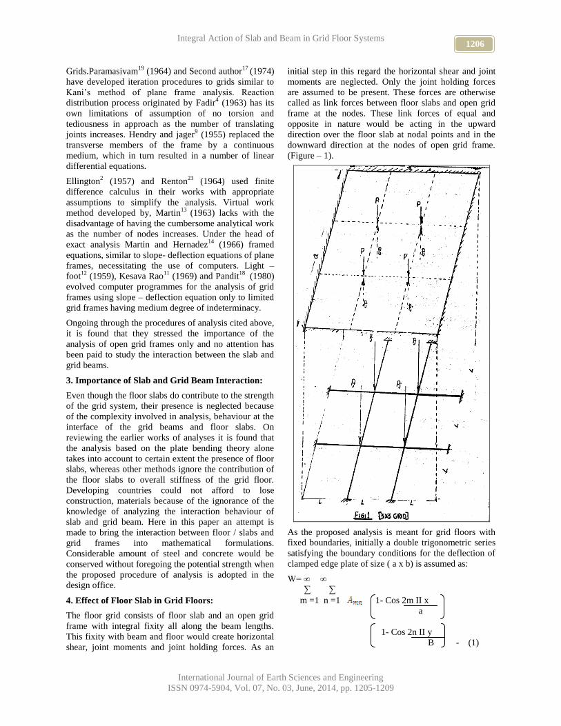
1206 Integral Action of Slab and Beam in Grid Floor Systems
International Journal of Earth Sciences and Engineering
ISSN 0974-5904, Vol. 07, No. 03, June, 2014, pp. 1205-1209
Grids.Paramasivam19
(1964) and Second author17
(1974)
have developed iteration procedures to grids similar to
Kani’s method of plane frame analysis. Reaction
distribution process originated by Fadir4 (1963) has its
own limitations of assumption of no torsion and
tediousness in approach as the number of translating
joints increases. Hendry and jager9 (1955) replaced the
transverse members of the frame by a continuous
medium, which in turn resulted in a number of linear
differential equations.
Ellington2 (1957) and Renton
23 (1964) used finite
difference calculus in their works with appropriate
assumptions to simplify the analysis. Virtual work
method developed by, Martin13
(1963) lacks with the
disadvantage of having the cumbersome analytical work
as the number of nodes increases. Under the head of
exact analysis Martin and Hernadez14
(1966) framed
equations, similar to slope- deflection equations of plane
frames, necessitating the use of computers. Light –
foot12
(1959), Kesava Rao11
(1969) and Pandit18
(1980)
evolved computer programmes for the analysis of grid
frames using slope – deflection equation only to limited
grid frames having medium degree of indeterminacy.
Ongoing through the procedures of analysis cited above,
it is found that they stressed the importance of the
analysis of open grid frames only and no attention has
been paid to study the interaction between the slab and
grid beams.
3. Importance of Slab and Grid Beam Interaction:
Even though the floor slabs do contribute to the strength
of the grid system, their presence is neglected because
of the complexity involved in analysis, behaviour at the
interface of the grid beams and floor slabs. On
reviewing the earlier works of analyses it is found that
the analysis based on the plate bending theory alone
takes into account to certain extent the presence of floor
slabs, whereas other methods ignore the contribution of
the floor slabs to overall stiffness of the grid floor.
Developing countries could not afford to lose
construction, materials because of the ignorance of the
knowledge of analyzing the interaction behaviour of
slab and grid beam. Here in this paper an attempt is
made to bring the interaction between floor / slabs and
grid frames into mathematical formulations.
Considerable amount of steel and concrete would be
conserved without foregoing the potential strength when
the proposed procedure of analysis is adopted in the
design office.
4. Effect of Floor Slab in Grid Floors:
The floor grid consists of floor slab and an open grid
frame with integral fixity all along the beam lengths.
This fixity with beam and floor would create horizontal
shear, joint moments and joint holding forces. As an
initial step in this regard the horizontal shear and joint
moments are neglected. Only the joint holding forces
are assumed to be present. These forces are otherwise
called as link forces between floor slabs and open grid
frame at the nodes. These link forces of equal and
opposite in nature would be acting in the upward
direction over the floor slab at nodal points and in the
downward direction at the nodes of open grid frame.
(Figure – 1).
As the proposed analysis is meant for grid floors with
fixed boundaries, initially a double trigonometric series
satisfying the boundary conditions for the deflection of
clamped edge plate of size ( a x b) is assumed as:
W= ∞ ∞
∑ ∑
m =1 n =1 1- Cos 2m II x
a
1- Cos 2n II y
B - (1)

1207 S VIMALA AND P GOPALSAMY
International Journal of Earth Sciences and Engineering
ISSN 0974-5904, Vol. 07, No. 03, June, 2014, pp. 1205-1209
The parameters are to be determined from the
conditions of minimum potential energy of the system.
Q = (U- W) - (2)
is a minimum with respect to these parameters.
Where U = ] dx dy
W = P w (x, y) (P – external load over the plate)
Substituting U and W for Q and using the condition
, the following expression is obtained.
- (3)
Where (x1, y1) defines the position of load ‘P’
D denotes the Torsional rigidity of the plate
D = E h3
12 (1 –µ2)
In this equation E, h & µ are the Young’s modulus,
Thickness of plate and Poisson’s ratio respectively. The
co-efficient of could be estimated using the
equation (3).
After substituting the co- efficient in Equation (1)
the deflection of the plate could be estimated.
5. Application to (3m x 3m) Square Grid Floor:
Maximum deflection in the floor slab of this (3mx3m)
grid with fixed boundaries could be treated as the case
of plated deflection for
Fixed edge conditions
Similarly the joint forces would cause upward
deflections of the plate due to joint
Force (Pj )
The net down ward deflection
of the plate = 6.76183x10⁻³ (P - Pj) a
2
Deflection of open grid in
The downward direction = 0.0763 Pj
As there is contact between the grid frame and the plate,
the resulting downward deflection of the plate and open
grid frame would be equal to each other.
Applying this Condition Pj = 0.07924 p
0 .07924+0.034(a/B)
α3
Where
α= Depth of beam / Plate thickness
B= Breadth of the grid beam.
Graphical relations (Figure-2) are obtained in
consideration of the variation in the ratios of floor width
to beam width and floor thickness to beam height. On
studying these relations, for beams with lower range of
the depth of beams (D/h ≤ 2) the interaction between
beam and slab is having its predominance to reduce the
deflection by about 50% when compared with the
corresponding open grid deflections. But very little
impact is observed in respect of interaction by about 10
percent in grids having higher values of beam depth
(D/h ≥ 7).
5.1 Illustration:
A grid floor of size 3m x3m is provided in a hall of size
15 m x 15 m with the following data. Calculate the
effect of floor slab in overall stiffness of the grid floor.
Data:
1208 Integral Action of Slab and Beam in Grid Floor Systems
International Journal of Earth Sciences and Engineering
ISSN 0974-5904, Vol. 07, No. 03, June, 2014, pp. 1205-1209
Floor slab thickness (h) = .15m
Depth of beam (D) = .60m
Rib width of beam (B) = .25m
Parameter α = 0.60 / 0.15 = 4.00
Joint holding force = 0.0792p
(0.07924 + (0.034(15/.25) )
43
= 0.710 p
Engineers usually assume the nodal load as ‘P’ for
regular design work as they are ignoring the joint forces.
Now in this illustration the nodal force has assumed a
value of “.710 p” by the proposed analysis. Thus the
floor slab reduces the overall deflection of grid frame by
about 29%.
6. Conclusion:
Here in this paper a rigorous mathematical analysis has
been presented to account for the integral action of floor
slabs and grid frame. This procedure could be extended
to grid floors of larger size, but the volume if
computational work would be enlarging as the size of
grid floor increases. In the graphical relations it is seen
that the maximum deflections are reducing by about 10
to 50% to (3m x 3m) grid. As deflection surface is one
of the viable methods through which the estimation of
moments and shears in the structure is possible, the true
moments and shears to grid floor would be reduced to a
greater extent, when the interaction between slab and
beam is taken into account. Code rules may be framed
to allow for the reduction in the design stress elements
after elaborate analytical study of various types of grids
on the lines illustrated in this paper. This in turn aids to
conserve construction materials like steel and concrete
to a greater extent.
7. Acknowledgements:
The authors are grateful to Editor in Chief
Dr.D.V.Reddy and Editorial board for processing our
work. Thanks are also due to reviewers Dr.P.Kathirvel
and Dr.V.G.Srisanthi for their valuable suggestions to
improve our work.
8. Reference:
[1] Dutta, A. and Som, P. – Analysis of Reinforced
Concrete Grid – The Indian concrete Journal –
December 1956- pp. 381 – 384.
[2] Ellington, J.P. and Mc Callian, H. – Moments and
Deflections in simply Supported Beam Grillages –
Aeronautical Quarterly – November 1957 – Vol.1–
pp. 360 – 365.
[3] Ewell, W.W. Okubo, S. & Abrams, J.I. –
Deflection in Grid Works and slabs – Trans. ASCE
–– 1952 – Vol.117 -pp. 869 – 890.
[4] Fadir, I. – Grid analysis by Reaction distributional
Method – Trans. ASCE – 1963– Vol.128 – pt.2 -
pp. 256-283.
[5] Ghosh, R.K. – Design of Simple Rectangular
Reinforced Concrete Grid – The Indian Concrete
Journal – June 1958 – pp.200 – 212.
[6] Gopalsamy, P. – Study on Interconnected Grid
systems- Thesis submitted to Madurai Kamaraj
university for Ph.D. degree – April 1985.
[7] Gopalsamy, P., Etal – Analysis of large span Grid
Floors for institutional Buildings – proceedings of
International symposium on school Buildings for
Afro Asian Countries – March 12-14 , 1986 –
CBRI- Roorkee, India - pp. 117 – 125.
[8] Guyon, Y. – Calculdes ponts Delles – Ann. Ponts
of Chausses– 1949 – Vol. 119 – pp. 553 – 612.
[9] Hendry, A.W. & Jager, L.G. – A General Method
for Analysis of Grid Frame Works – proc. Inst.
Civil Engineers (London- December (1955) – Vol.
4. pp. 937-971.
[10] Huber, M.T. – Die Ground Lagen Einer Rationellen
Berechnung Der Keru Z weise Bewhrten – Eisenbe
to r platten, zeitechrift Des 0 sterreichischen
ingenier U. Architekten – Vereiues– 1914 – vol.66
– no. 30.
[11] Kesava Rao – M.N. – Computer Analysis of grids –
Grillages and interconnected Girder systems – The
Indian concrete journal– January 1969- vol. 43 –
pp25 – 32.
[12] Light Foot, E. & Sanko, F – frame Works Resolved
by Generalized slope – Deflection – engineering –
January2 – 1959 – pp. 18- 20.
[13] Martin, J.B. – The Elastic Analysis of simple
Rectangular Grids by Virtual work method – The
structural engineer– June 1963 –– vol. 46 pp. 199 –
201.
[14] Martin, I. and Hernandex, J. – Orthogonal Grids
loaded Normal to their plane – proceedings of
ASCE. ST- January 1960 – pp.1- 12.
[15] Massonet, C. – Methods of calculations of Bridges
with Several Longitudinal Beams Taking into
Consideration Their Torsional resistance –
publication – International Association of bride and
structural Engineering– 1950 – vol. 10 – pp. 147 –
182.
[16] Megre, A.S. – Iteration method of Grids –
Institution of engineers (India) – July 1976 – Vol.
57– pp. 72 – 78.
[17] Meiyappan, Pl. and Gopalsamy , p. – A method of
Iteration to Grid Frames – National symposium on
Economy in construction- Madurai – March 1974 –
pp. A. 12-A. 19.
[18] Pandit, G.S. and Guptha, S.P. – Displacement
Approach to Irregular Grids – The Indian concrete
journal – September 1980 – pp. 238 – 244.

1209 S VIMALA AND P GOPALSAMY
International Journal of Earth Sciences and Engineering
ISSN 0974-5904, Vol. 07, No. 03, June, 2014, pp. 1205-1209
[19] Paramasivan, V. Dravid, P.S. and Ramesh, C.K. -
Grid Analysis by Rotation contribution Method-
The Indian concrete Journal – July 1967 – pp. 263 –
292.
[20] Retnalikar, M. and Megre, A.S. – Analysis of Skew
Grids by Moment distribution – proc. Institution of
Engineers (India)– September 1976 – vol. 57 – pp.
102 – 120.
[21] Reddy, D.V. and Hendry, A.W. – A Rapid moment
Torque Distribution method for grid Frame work
Analysis – Civil Engineering and Public works
Review – July / August 1959– vol. 54- no. 637 –
pp. 867 – 872.
[22] Reddy, D.V., Krithivasan and Vengatraman, T.S.-
Analysis of Corner Supported Grid Frame work by
translational Moment distributional – The Indian
Concrete journal – October 1964 – pp. 383 – 388.
[23] Renton, J.D. – A Finite Difference Analysis of
Flexural – Torsional Behaviour of Grillages – inst.
Journal of Mechanical Science– 1964-– vol. 6 - pp.
209 – 220.
[24] Scordelis, A.C. – discussion on deflection in Grid
frame works and slabs by Ewell – Etal – Trans.
ASCE– 1952 - vol.117 – pp. 892 – 897.
[25] Timoshenko, S. – Theory of plates and shells – Mc
– Graw hill book company – NewYork-1940.
www.cafetinnova.org
Indexed in
Scopus Compendex and Geobase Elsevier, Chemical
Abstract Services-USA, Geo-Ref Information Services-USA,
List B of Scientific Journals, Poland,
Directory of Research Journals
ISSN 0974-5904, Volume 07, No. 03
June 2014, P.P.1210-1215
#02070356 Copyright ©2014 CAFET-INNOVA TECHNICAL SOCIETY. All rights reserved.
Strength, Swelling and Durability Characteristics of Fly-Lime
Stabilized Expansive Soil-Ceramic Dust Mixes
AKSHAYA KUMAR SABAT AND BIDULA BOSE Department of Civil Engineering, Institute of Technical Education and Research, Siksha ‘O’ Anusandhan
University, Khandagiri Square, Bhubaneswar, OR, India
Email: [email protected], [email protected]
Abstract: Strength, swelling and durability are the three important characteristics to judge the efficiency of a
stabilized soil. Construction on expansive soil creates problems because of its alternate swell-shrink behavior and
low strength. Stabilization, using industrial wastes with binder, is one of the different methods to increase the
strength and reduce the swelling characteristics of the soil. However, seasonal climate change exposes the stabilized
soils to alternate wet-dry cycles, which affect these properties severely. Unconfined compressive strength, California
bearing ratio, swelling pressure and durability of expansive soil-ceramic dust mixes stabilized with an optimum
percentage of fly ash and lime have been discussed in this paper.
Keywords: strength, swelling, durability, expansive soil, fly ash, lime, ceramic dust.
1. Introduction:
Expansive soil also called as black cotton soil is a good
soil for farmers for growth of cotton crop but a bad soil
for civil engineers for construction. It expands
significantly when comes in contact with water and
shrinks when water squeezes out. This alternate swell-
shrink behavior of the soil damages lightly loaded
structures severely. Cracks of different shapes and
varying depths are found in pavements, buildings, canal
linings, retaining walls etc. These soils occupy more
than 20% of total soils of India and mostly found in the
states like, Karnataka, Uttarpradesh, Maharastra,
Andhrapradesh etc. Some prominent techniques to
counteract the damaging effect of this soil are,
prewetting, application of surcharge, sand cushion,
cohesive non swelling soil(CNS) cushion, under reamed
pile foundation,granular pile anchor, mechanical
stabilization, chemical stabilization, stabilization using
industrial wastes with or without a binder etc. Soil
stabilization may be defined as any process by which a
soil material is improved and made more stable,
resulting in improved bearing capacity, increase in soil
strength, and durability under adverse moisture and
stress conditions [1]. Three important characteristics to
assess the effectiveness of a stabilized soil are its
strength, swelling behaviour and durability. The
durability of a stabilized soil is assessed in the
laboratory by subjecting it to alternate wet-dry (W-D)
cycles simulating the worst field conditions.
Fly ash is an industrial by-product, produced by the
combustion of pulverized coal in thermal power plants
during production of electricity. Ceramic dust is another
industrial waste produced in ceramic industry, the
disposal of both the wastes creates a lot of
geoenvironmental problems. These two wastes can be
utilized in the stabilization of expansive soil along with
a binder like lime which, not only will save the
environment from their polluting effects, but also will
save a lot of valuable land, which could have been
utilized for their disposal. The positive effects of
stabilization of expansive soil using industrial wastes
with binders have been documented, very well in
literature. Some of the prominent wastes with binders
which have been successfully utilized for stabilization
of expansive soil are, rice husk ash-marble dust[2], rice
husk ash - lime [3], rice husk ash - cement[4,5], quarry
dust-lime[6],brick dust-lime[7],fly ash-lime[8],fly ash-
cement[9],granulated blast furnace slag-cement[10],red
mud -cement[11], bagasse ash - lime sludge[12],etc. To
the knowledge of the authors no investigation has been
reported so far, regarding the stabilization of expansive
soil using fly ash-lime and ceramic dust.
The objective of the present investigation is to study the
unconfined compressive strength at 0, 7 and 28 days of
curing, California bearing ratio, swelling pressure and
durability of fly ash -lime stabilized expansive soil-
ceramic dust mixes.
2. Materials and Methods:
The materials used and the methods adopted in the
experimental programme have been discussed below.
2.1 Materials
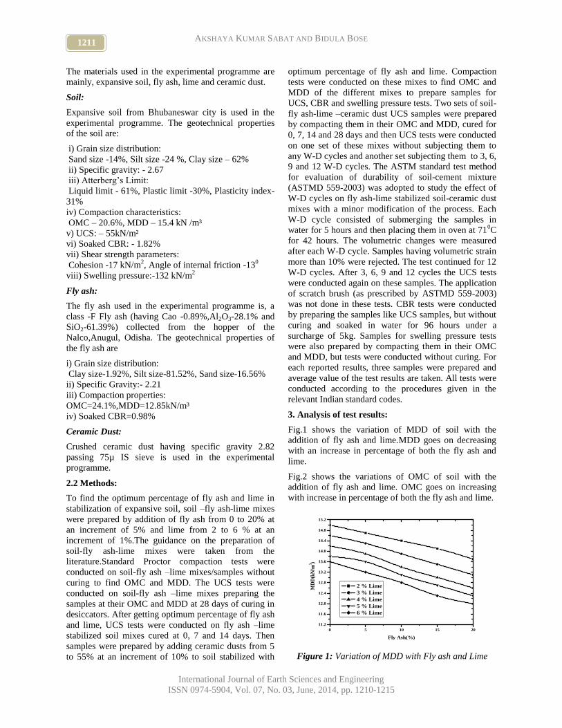
1211 AKSHAYA KUMAR SABAT AND BIDULA BOSE
International Journal of Earth Sciences and Engineering
ISSN 0974-5904, Vol. 07, No. 03, June, 2014, pp. 1210-1215
The materials used in the experimental programme are
mainly, expansive soil, fly ash, lime and ceramic dust.
Soil:
Expansive soil from Bhubaneswar city is used in the
experimental programme. The geotechnical properties
of the soil are:
i) Grain size distribution:
Sand size -14%, Silt size -24 %, Clay size – 62%
ii) Specific gravity: - 2.67
iii) Atterberg’s Limit:
Liquid limit - 61%, Plastic limit -30%, Plasticity index-
31%
iv) Compaction characteristics:
OMC – 20.6%, MDD – 15.4 kN /m³
v) UCS: – 55kN/m²
vi) Soaked CBR: - 1.82%
vii) Shear strength parameters:
Cohesion -17 kN/m2, Angle of internal friction -13
0
viii) Swelling pressure:-132 kN/m2
Fly ash:
The fly ash used in the experimental programme is, a
class -F Fly ash (having Cao -0.89%,Al2O3-28.1% and
SiO2-61.39%) collected from the hopper of the
Nalco,Anugul, Odisha. The geotechnical properties of
the fly ash are
i) Grain size distribution:
Clay size-1.92%, Silt size-81.52%, Sand size-16.56%
ii) Specific Gravity:- 2.21
iii) Compaction properties:
OMC=24.1%,MDD=12.85kN/m³
iv) Soaked CBR=0.98%
Ceramic Dust:
Crushed ceramic dust having specific gravity 2.82
passing 75µ IS sieve is used in the experimental
programme.
2.2 Methods:
To find the optimum percentage of fly ash and lime in
stabilization of expansive soil, soil –fly ash-lime mixes
were prepared by addition of fly ash from 0 to 20% at
an increment of 5% and lime from 2 to 6 % at an
increment of 1%.The guidance on the preparation of
soil-fly ash-lime mixes were taken from the
literature.Standard Proctor compaction tests were
conducted on soil-fly ash –lime mixes/samples without
curing to find OMC and MDD. The UCS tests were
conducted on soil-fly ash –lime mixes preparing the
samples at their OMC and MDD at 28 days of curing in
desiccators. After getting optimum percentage of fly ash
and lime, UCS tests were conducted on fly ash –lime
stabilized soil mixes cured at 0, 7 and 14 days. Then
samples were prepared by adding ceramic dusts from 5
to 55% at an increment of 10% to soil stabilized with
optimum percentage of fly ash and lime. Compaction
tests were conducted on these mixes to find OMC and
MDD of the different mixes to prepare samples for
UCS, CBR and swelling pressure tests. Two sets of soil-
fly ash-lime –ceramic dust UCS samples were prepared
by compacting them in their OMC and MDD, cured for
0, 7, 14 and 28 days and then UCS tests were conducted
on one set of these mixes without subjecting them to
any W-D cycles and another set subjecting them to 3, 6,
9 and 12 W-D cycles. The ASTM standard test method
for evaluation of durability of soil-cement mixture
(ASTMD 559-2003) was adopted to study the effect of
W-D cycles on fly ash-lime stabilized soil-ceramic dust
mixes with a minor modification of the process. Each
W-D cycle consisted of submerging the samples in
water for 5 hours and then placing them in oven at 710C
for 42 hours. The volumetric changes were measured
after each W-D cycle. Samples having volumetric strain
more than 10% were rejected. The test continued for 12
W-D cycles. After 3, 6, 9 and 12 cycles the UCS tests
were conducted again on these samples. The application
of scratch brush (as prescribed by ASTMD 559-2003)
was not done in these tests. CBR tests were conducted
by preparing the samples like UCS samples, but without
curing and soaked in water for 96 hours under a
surcharge of 5kg. Samples for swelling pressure tests
were also prepared by compacting them in their OMC
and MDD, but tests were conducted without curing. For
each reported results, three samples were prepared and
average value of the test results are taken. All tests were
conducted according to the procedures given in the
relevant Indian standard codes.
3. Analysis of test results:
Fig.1 shows the variation of MDD of soil with the
addition of fly ash and lime.MDD goes on decreasing
with an increase in percentage of both the fly ash and
lime.
Fig.2 shows the variations of OMC of soil with the
addition of fly ash and lime. OMC goes on increasing
with increase in percentage of both the fly ash and lime.
0 5 10 15 20
11.2
11.6
12.0
12.4
12.8
13.2
13.6
14.0
14.4
14.8
15.2
MD
D(k
N/m
3 )
Fly Ash(%)
2 % Lime
3 % Lime
4 % Lime
5 % Lime
6 % Lime
Figure 1: Variation of MDD with Fly ash and Lime

1212 Strength, Swelling and Durability Characteristics of Fly-Lime Stabilized Expansive
Soil-Ceramic Dust Mixes
International Journal of Earth Sciences and Engineering
ISSN 0974-5904, Vol. 07, No. 03, June, 2014, pp. 1210-1215
0 5 10 15 20
21
22
23
24
25
26
27
28
29
OM
C(%
)
Fly Ash (%)
2 % Lime
3 % Lime
4 % Lime
5 % Lime
6 % Lime
Figure 2: Variation of OMC with Fly ash and Lime
Fig. 3 shows the variations of UCS of soil with the
addition of fly ash and lime at 28 days of curing. UCS
increases with increase in percentage of both the fly ash
and lime up to a certain percentage of fly ash and lime,
thereafter it decreases. The UCS of soil increases to 352
kN/m2 from 55 kN/m
2 when the percentage of fly ash is
10% and lime is 5%. The strength increases due to
pozzolanic reaction between alumina and silica present
in fly ash and soil with calcium present in lime, the
strength decreases due to a carbonation reaction which
occurs due to availability of excess lime to react with
insufficient alumina and silica present in soil and fly
ash.
Fig.4 shows the variations of MDD of expansive soil
stabilized with an optimum percentage of fly ash and
lime with different percentage of ceramic dust. From the
figure it is observed that with increase in percentage
addition of ceramic dust the MDD goes on increasing.
Ceramic dust fills up the voids formed on soil-fly ash-
lime mix due to flocculation, when ceramic dust is
added to any soil-fly ash-lime mix it results in higher
density as the void space is filled with ceramic dust,
compared to that of soil –fly ash-lime mix where the
void space is empty.
Fig.5 shows the variation OMC of expansive soil
stabilized with an optimum percentage of fly ash and
lime, with different percentage of ceramic dust. From
the figure it is observed that with increase in the
percentage of addition of ceramic dust the OMC goes
on decreasing. Due to reduction in clay content of soil
the attraction of water molecules towards soil –fly ash-
lime –ceramic dust mixes decreases, hence OMC
decreases.
0 5 10 15 20
220
230
240
250
260
270
280
290
300
310
320
330
340
350
360
UC
S(k
N/m
2 )
Fly Ash (%)
2 % Lime
3 % Lime
4 % Lime
5 % Lime
6 % Lime
Figure 3: Variation of UCS (28 days Curing) with
Fly ash and Lime
0 5 10 15 20 25 30 35 40 45 50 55
0
3
6
9
12
15
18
MD
D(k
N/m
3 )
Ceramic dust(%)
Figure 4: Variation of MDD of Fly ash - Lime
stabilized soil with Ceramic dust(%)
0 5 10 15 20 25 30 35 40 45 50 55
0
5
10
15
20
25
30
OM
C(%
)
Ceramic dust(%)
Figure 5: Variation of OMC of Fly ash - Lime stabilized
soil with Ceramic dust(%).
Fig.6 shows the variations of UCS of soil stabilized with
optimum percentage of fly ash and lime, with different
percentage of ceramic dust, at different curing periods.
UCS of fly ash-lime stabilized soil increases with
increase in percentage addition of ceramic dust up to
35%, thereafter it decreases irrespective of the curing
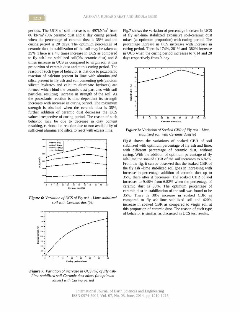
1213 AKSHAYA KUMAR SABAT AND BIDULA BOSE
International Journal of Earth Sciences and Engineering
ISSN 0974-5904, Vol. 07, No. 03, June, 2014, pp. 1210-1215
periods. The UCS of soil increases to 497kN/m2 from
86 kN/m2
(0% ceramic dust and 0 day curing period)
when the percentage of ceramic dust is 35% and the
curing period is 28 days. The optimum percentage of
ceramic dust in stabilization of the soil may be taken as
35% .There is a 4.8 times increase in UCS as compared
to fly ash-lime stabilized soil(0% ceramic dust) and 8
times increase in UCS as compared to virgin soil at this
proportion of ceramic dust and at this curing period. The
reason of such type of behavior is that due to pozzolanic
reaction of calcium present in lime with alumina and
silica present in fly ash and soil cementing gels(calcium
silicate hydrates and calcium aluminate hydrates) are
formed which bind the ceramic dust particles with soil
particles, resulting increase in strength of the soil. As
the pozzolanic reaction is time dependant its strength
increases with increase in curing period. The maximum
strength is obtained when the ceramic dust is 35%,
further addition of ceramic dust decreases the UCS
values irrespective of curing period. The reason of such
behavior may be due to decrease in clay content
resulting, carbonation reaction due to non availability of
sufficient alumina and silica to react with excess lime.
0 5 10 15 20 25 30 35 40 45 50 55
0
100
200
300
400
500
600
UC
S(k
N/m
2 )
Ceramic dust(%)
0 Day
7 Days
14 Days
28 Days
Figure 6: Variation of UCS of Fly ash - Lime stabilized
soil with Ceramic dust(%)
0 4 8 12 16 20 24 28
0
50
100
150
200
250
300
350
400
450
In
crea
se i
n U
CS
(%)
Curing period(days)
Figure 7: Variation of increase in UCS (%) of Fly ash-
Lime stabilized soil-Ceramic dust mixes (at optimum
values) with Curing period
Fig.7 shows the variation of percentage increase in UCS
of fly ash-lime stabilized expansive soil-ceramic dust
mixes (at optimum proportion) with curing period. The
percentage increase in UCS increases with increase in
curing period. There is 174%, 281% and 382% increase
in UCS when the curing period increases to 7,14 and 28
days respectively from 0 day.
0 5 10 15 20 25 30 35 40 45 50 55
0
1
2
3
4
5
6
7
8
9
10
Soa
ked
CB
R (
%)
Ceramic dust (%)
Figure 8: Variation of Soaked CBR of Fly ash - Lime
stabilized soil with Ceramic dust(%)
Fig.8 shows the variations of soaked CBR of soil
stabilized with optimum percentage of fly ash and lime,
with different percentage of ceramic dust, without
curing. With the addition of optimum percentage of fly
ash-lime the soaked CBR of the soil increases to 6.82%.
From the fig. it can be observed that the soaked CBR of
the fly ash –lime stabilized soil goes in increasing with
increase in percentage addition of ceramic dust up to
35%, there after it decreases. The soaked CBR of soil
increases to 9.46% from 6.82% when the percentage of
ceramic dust is 35%. The optimum percentage of
ceramic dust in stabilization of the soil was found to be
35%. There is 38% increase in soaked CBR as
compared to fly ash-lime stabilized soil and 420%
increase in soaked CBR as compared to virgin soil at
this proportion of ceramic dust. The reason of such type
of behavior is similar, as discussed in UCS test results.
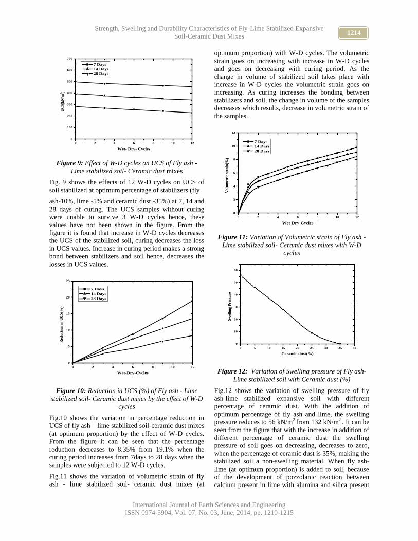
1214 Strength, Swelling and Durability Characteristics of Fly-Lime Stabilized Expansive
Soil-Ceramic Dust Mixes
International Journal of Earth Sciences and Engineering
ISSN 0974-5904, Vol. 07, No. 03, June, 2014, pp. 1210-1215
0 2 4 6 8 10 12
0
100
200
300
400
500
600
700
UC
S(k
N/m
2 )
Wet- Dry- Cycles
7 Days
14 Days
28 Days
Figure 9: Effect of W-D cycles on UCS of Fly ash -
Lime stabilized soil- Ceramic dust mixes
Fig. 9 shows the effects of 12 W-D cycles on UCS of
soil stabilized at optimum percentage of stabilizers (fly
ash-10%, lime -5% and ceramic dust -35%) at 7, 14 and
28 days of curing. The UCS samples without curing
were unable to survive 3 W-D cycles hence, these
values have not been shown in the figure. From the
figure it is found that increase in W-D cycles decreases
the UCS of the stabilized soil, curing decreases the loss
in UCS values. Increase in curing period makes a strong
bond between stabilizers and soil hence, decreases the
losses in UCS values.
0 2 4 6 8 10 12
0
5
10
15
20
25
Red
uct
ion
in U
CS
(%)
Wet-Dry-Cycles
7 Days
14 Days
28 Days
Figure 10: Reduction in UCS (%) of Fly ash - Lime
stabilized soil- Ceramic dust mixes by the effect of W-D
cycles
Fig.10 shows the variation in percentage reduction in
UCS of fly ash – lime stabilized soil-ceramic dust mixes
(at optimum proportion) by the effect of W-D cycles.
From the figure it can be seen that the percentage
reduction decreases to 8.35% from 19.1% when the
curing period increases from 7days to 28 days when the
samples were subjected to 12 W-D cycles.
Fig.11 shows the variation of volumetric strain of fly
ash - lime stabilized soil- ceramic dust mixes (at
optimum proportion) with W-D cycles. The volumetric
strain goes on increasing with increase in W-D cycles
and goes on decreasing with curing period. As the
change in volume of stabilized soil takes place with
increase in W-D cycles the volumetric strain goes on
increasing. As curing increases the bonding between
stabilizers and soil, the change in volume of the samples
decreases which results, decrease in volumetric strain of
the samples.
0 2 4 6 8 10 12
0
2
4
6
8
10
12
Vol
um
etri
c st
rain
(%)
Wet-Dry-Cycles
7 Days
14 Days
28 Days
Figure 11: Variation of Volumetric strain of Fly ash -
Lime stabilized soil- Ceramic dust mixes with W-D
cycles
0 5 10 15 20 25 30 35 40
0
10
20
30
40
50
60
Sw
elli
ng
Pre
ssu
re
Ceramic dust(%)
Figure 12: Variation of Swelling pressure of Fly ash-
Lime stabilized soil with Ceramic dust (%)
Fig.12 shows the variation of swelling pressure of fly
ash-lime stabilized expansive soil with different
percentage of ceramic dust. With the addition of
optimum percentage of fly ash and lime, the swelling
pressure reduces to 56 kN/m2
from 132 kN/m2 . It can be
seen from the figure that with the increase in addition of
different percentage of ceramic dust the swelling
pressure of soil goes on decreasing, decreases to zero,
when the percentage of ceramic dust is 35%, making the
stabilized soil a non-swelling material. When fly ash-
lime (at optimum proportion) is added to soil, because
of the development of pozzolanic reaction between
calcium present in lime with alumina and silica present

1215 AKSHAYA KUMAR SABAT AND BIDULA BOSE
International Journal of Earth Sciences and Engineering
ISSN 0974-5904, Vol. 07, No. 03, June, 2014, pp. 1210-1215
in fly ash and soil a strong cementing bond develops
between soil particles which prevents the swelling of
soil resulting, reduction in swelling pressure of
expansive soil. The swelling pressure of soil reduces
further by addition of ceramic dust. As the clay particles
are replaced by ceramic dust particles, the attraction of
the stabilized soil for water molecules decreases, hence
swelling pressure decreases. Another reason of such
phenomenon is, the development of strong inter-particle
bond between soil, fly ash-lime and ceramic dust
particles, which prevents swelling of the soil, hence
swelling pressure decreases.
4. Conclusion:
The following conclusions are drawn from this study.
The optimum percentages of fly ash, lime and
ceramic dust for stabilization of expansive soil are,
fly ash -10%, lime -5% and ceramic dust- 35%.
There is an eight times increase in UCS values of
the soil, stabilized at optimum percentages of fly
ash, lime and ceramic dust and cured for 28 days,
over virgin soil.
There is a 4.2 times increase in soaked CBR values
of the soil, stabilized at optimum percentages of fly
ash, lime and ceramic dust, over virgin soil.
At the optimum percentages of fly ash, lime and
ceramic dust the stabilized soil is a non-swelling
material having no swelling pressure.
An increase in the number of W-D cycles decreased
the UCS values and increased the volumetric strain
of soil stabilized at optimum percentages of fly ash,
lime and ceramic dust. Increase in curing period
decreases, the percentage loss of UCS and
volumetric strain of the stabilized soil.
The soil stabilized at optimum percentages of
stabilizers, with a minimum curing period of 7 days
was found to be durable, as the percentage loss in
strength is found to be below 20% after 12 W-D
cycles.
Acknowledgement:
The Authors gratefully acknowledge the reviewers and
the Editor in Chief of IJEE for their useful comments
and suggestions for improving the quality of this
manuscript.
2. Reference:
[1] M. Joel, and I.O. Agbedi, “Mechanical-Cement
stabilization of laterite for use as flexible pavement
material”, Journal of material in Civil Engineering,
Vol.23 (2), PP.146-152., 2011.
[2] A. K. Sabat, and R.P. Nanda, “Effect of marble dust
on strength and durability of rice husk ash
stabilised expansive soil”, International Journal of
Civil and Structural Engineering, Vol.1 (4) PP.939-
948., 2011.
[3] A. S. Muntohar and G. Hantoro, “Influence of rice
husk ash and lime on engineering properties of a
clayey subgrade”, Electronic Journal of
Geotechnical engineering, Vol.5., 2000.
[4] E.A.Basha, R.Hashim, and A.S.Muntohar, “Effect
of the cement-rice husk ash on the plasticity and
compaction of soil”, Electronic Journal of
Geotechnical engineering, Vol.8, Bundle A., 2003.
[5] A. N. Ramakrishna and A.V. Pradeep Kumar,
“Stabilisation of black cotton soil using rice husk
ash and cement’’, National conference on Civil
Engineering meeting the challenges of tomorrow -
2006, PP.215-220.,2006.
[6] A. K. Sabat, “A study on some geotechnical
properties of lime stabilised expansive soil –quarry
dust mixes”, International Journal of Emerging
trends in Engineering and Development,
Vol.1(2),PP.42-49.,2012.
[7] M. Abd EI-Aziz and M.A. Abo-Hashema,
“Measured effects on engineering properties of
clayey subgrade using lime-homra stabiliser”,
International Journal of Pavement Engineering,
Vol.14 (4)., PP.321-332.,2013.
[8] F. Zha, S. Liu, Y. Du, and K. Cui, “Behavior of
expansive soils stabilized with fly ash”, Natural
hazards, Vol.47 (3), PP.509-523., 2008.
[9] O.O.Amu, A.B.Fajobi and S.O. Afekhuai,
“Stabilizing potential of cement and fly ash mixture
on expansive clay soil”, Journal of Applied
Sciences, Vol.5 (9), PP.1669-1673., 2005.
[10] E. Cokca, V. Yazici, and V. Ozaydin, “Stabilisation
of expansive clays using granulated blast furnace
slag (GBFS) and GBFS-cement”, Geotechnical and
Geological Engineering, Vol.27 (4), PP.489-499.,
2009.
[11] E. Kalkan, “Utilization of red mud as a stabilization
material for the preparation of clay liners”,
Engineering Geology, Vol. 87(3-4), PP. 220-229.,
2006.
[12] A. K. Sabat, “Utilization of bagasse ash and lime
sludge for construction of flexible pavements in
expansive soil areas”, Electronic journal of
Geotechnical Engineering, Vol.17, Bund.
H.PP.1037-1046., 2012.
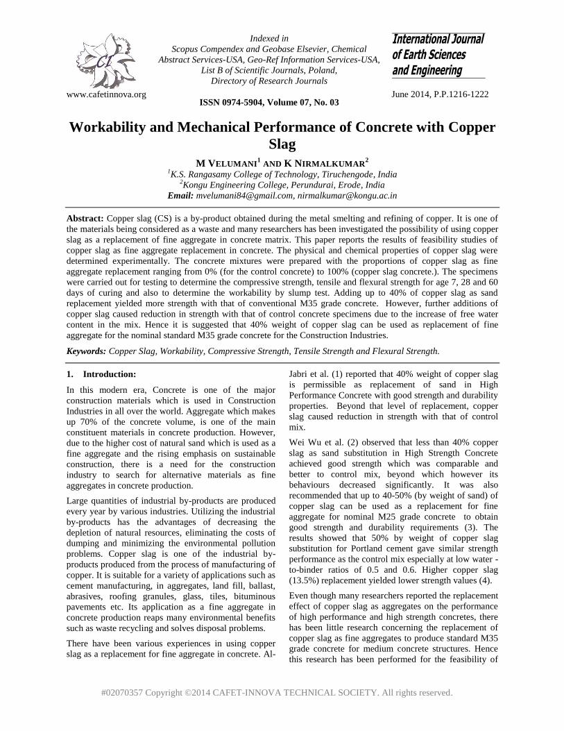
www.cafetinnova.org
Indexed in
Scopus Compendex and Geobase Elsevier, Chemical
Abstract Services-USA, Geo-Ref Information Services-USA,
List B of Scientific Journals, Poland,
Directory of Research Journals
ISSN 0974-5904, Volume 07, No. 03
June 2014, P.P.1216-1222
#02070357 Copyright ©2014 CAFET-INNOVA TECHNICAL SOCIETY. All rights reserved.
Workability and Mechanical Performance of Concrete with Copper
Slag
M VELUMANI1 AND K NIRMALKUMAR
2
1K.S. Rangasamy College of Technology, Tiruchengode, India
2Kongu Engineering College, Perundurai, Erode, India
Email: [email protected], [email protected]
Abstract: Copper slag (CS) is a by-product obtained during the metal smelting and refining of copper. It is one of
the materials being considered as a waste and many researchers has been investigated the possibility of using copper
slag as a replacement of fine aggregate in concrete matrix. This paper reports the results of feasibility studies of
copper slag as fine aggregate replacement in concrete. The physical and chemical properties of copper slag were
determined experimentally. The concrete mixtures were prepared with the proportions of copper slag as fine
aggregate replacement ranging from 0% (for the control concrete) to 100% (copper slag concrete.). The specimens
were carried out for testing to determine the compressive strength, tensile and flexural strength for age 7, 28 and 60
days of curing and also to determine the workability by slump test. Adding up to 40% of copper slag as sand
replacement yielded more strength with that of conventional M35 grade concrete. However, further additions of
copper slag caused reduction in strength with that of control concrete specimens due to the increase of free water
content in the mix. Hence it is suggested that 40% weight of copper slag can be used as replacement of fine
aggregate for the nominal standard M35 grade concrete for the Construction Industries.
Keywords: Copper Slag, Workability, Compressive Strength, Tensile Strength and Flexural Strength.
1. Introduction:
In this modern era, Concrete is one of the major
construction materials which is used in Construction
Industries in all over the world. Aggregate which makes
up 70% of the concrete volume, is one of the main
constituent materials in concrete production. However,
due to the higher cost of natural sand which is used as a
fine aggregate and the rising emphasis on sustainable
construction, there is a need for the construction
industry to search for alternative materials as fine
aggregates in concrete production.
Large quantities of industrial by-products are produced
every year by various industries. Utilizing the industrial
by-products has the advantages of decreasing the
depletion of natural resources, eliminating the costs of
dumping and minimizing the environmental pollution
problems. Copper slag is one of the industrial by-
products produced from the process of manufacturing of
copper. It is suitable for a variety of applications such as
cement manufacturing, in aggregates, land fill, ballast,
abrasives, roofing granules, glass, tiles, bituminous
pavements etc. Its application as a fine aggregate in
concrete production reaps many environmental benefits
such as waste recycling and solves disposal problems.
There have been various experiences in using copper
slag as a replacement for fine aggregate in concrete. Al-
Jabri et al. (1) reported that 40% weight of copper slag
is permissible as replacement of sand in High
Performance Concrete with good strength and durability
properties. Beyond that level of replacement, copper
slag caused reduction in strength with that of control
mix.
Wei Wu et al. (2) observed that less than 40% copper
slag as sand substitution in High Strength Concrete
achieved good strength which was comparable and
better to control mix, beyond which however its
behaviours decreased significantly. It was also
recommended that up to 40-50% (by weight of sand) of
copper slag can be used as a replacement for fine
aggregate for nominal M25 grade concrete to obtain
good strength and durability requirements (3). The
results showed that 50% by weight of copper slag
substitution for Portland cement gave similar strength
performance as the control mix especially at low water -
to-binder ratios of 0.5 and 0.6. Higher copper slag
(13.5%) replacement yielded lower strength values (4).
Even though many researchers reported the replacement
effect of copper slag as aggregates on the performance
of high performance and high strength concretes, there
has been little research concerning the replacement of
copper slag as fine aggregates to produce standard M35
grade concrete for medium concrete structures. Hence
this research has been performed for the feasibility of

1217 M.VELUMANI AND K.NIRMALKUMAR
International Journal of Earth Sciences and Engineering
ISSN 0974-5904, Vol. 07, No. 03, June, 2014, pp. 1216-1222
using copper slag as fine aggregate in M35 grade
concrete.
1.1 Literature Review:
There have been various experiences in using copper
slag as a replacement for fine aggregate in concrete. (5)
reported that Addition of up to 50% of copper slag as
sand replacement yielded comparable strength with that
of the control mix. However, further additions of copper
slag caused reduction in the strength due to an increase
of the free water content in the mix. Mixes with 80%
and 100% copper slag replacement gave the lowest
compressive strength value of approximately 80 MPa,
which is almost 16% lower than the strength of the
control mix. The results also demonstrated that the
surface water absorption decreased as copper slag
quantity increases up to 40% replacement; beyond that
level of replacement, the absorption rate increases
rapidly. Therefore, it is recommended that 40 wt% of
copper slag can used as replacement of sand in order to
obtain HPC with good strength and durability
properties.(2.Wei Wu, et.al) This study investigated the
mechanical properties of high strength concrete
incorporating copper slag as a fine aggregate and
concluded that less than 40% copper slag as sand
substitution can achieve a high strength concrete that
comparable or better to the control mix, beyond which
however its behaviors decreased significantly. The
workability and strength characteristics were assessed
through a series of tests on six different mixing
proportions at 20% incremental copper slag by weight
replacement of sand from 0% to 100%. (6) The results
demonstrated that surface water absorption decreased as
copper slag content increases up to 50% replacement.
Beyond that, the absorption rate increased rapidly and
the percentage volume of the permeable voids was
comparable to the control mixture. Therefore, it is
recommended that up to 40–50% (by weight of sand) of
copper slag can be used as a replacement for fine
aggregates in order to obtain a concrete with good
strength and durability requirements.(7.D.Brindha) For
this research work, M20 grade concrete was used and
tests were conducted for various proportions of copper
slag replacement with sand of 0 to 60%, cement of 0 to
20% in concrete. The obtained results were compared
with those of control concrete made with ordinary
Portland cement and sand. (1.S. Al-Jabri, et. al)This
research study was conducted to investigate the
performance of high strength concrete (HSC) made with
copper slag as a fine aggregate at constant workability
and to study the effect of superplasticizer addition on
the properties of HSC made with copper slag. Two
series of concrete mixtures were prepared with different
proportions of copper slag. The first series consisted of
six concrete mixtures prepared with different
proportions of copper slag at constant workability. The
water content was adjusted in each mixture in order to
achieve the same workability as that for the control
mixture. Even though many researchers reported the
replacement effect of copper slag as aggregates on the
performance of high performance and high strength
concretes, there has been little research concerning the
replacement of copper slag as fine aggregates to
produce standard M35 grade concrete for medium
concrete structures. Hence this research has been
performed for the feasibility of using copper slag as fine
aggregate in M35 grade concrete.
1.2 Research objectives:
The main objective of this research is to study the use of
copper slag as fine aggregate replacement in M35 grade
concrete. The following are the main objectives:
1. Determination of physical properties and chemical
compositions of copper slag.
2. Comparison of the results of the particle size
distribution of copper slag and sand (fine
aggregate).
3. Evaluating the compressive, tensile and flexural
strength of concrete specimens at different
proportions of copper slag admixed concrete and
M35 grade control concrete.
4. Also to determine the workability of copper slag
replacement concrete
1.3 Materials:
1.3.1 Cement:
The cement used in this study was Ordinary Portland
Cement (OPC) of 53 Grade with specific gravity of
3.15. This cement is one of the most widely used
cements in construction industry in India
1.3.2 Coarse and fine aggregates:
The coarse aggregate of 20 mm size with a specific
gravity of 2.65 was used in this study. The fine
aggregate is natural sand with a specific gravity of 2.64
and the fineness modulus of 2.95. The particle size
distribution was well-graded with over 60-80% of the
sand over the size range of 0.6 to 1.18mm. It is well
shown that the coarse and fine aggregates met the
specifications requirements as per the Indian Standard
codes.
1.3.3 Copper Slag (CS):
Copper slag is a by-product material obtained from the
process of manufacturing of copper. Copper slag used in
this work was brought from Sterlite Industries India
Limited (SIIL) Tuticorin, Tamil Nadu which produces a
huge amount of copper slag.
1.3.4 Water:
It is strictly adhered that the potable water is used for
making the concrete specimens because it plays a major

1218 Workability and Mechanical Performance of Concrete with copper slag
International Journal of Earth Sciences and Engineering
ISSN 0974-5904, Vol. 07, No. 03, June, 2014, pp. 1216-1222
role in water to cement ratio, consistency and slump
values of fresh concrete. Also the durability properties
get affected due to the use of the nature of the water
used. Hence most care had been taken for the water as
constituent in making the concrete specimens.
1.4 Physical properties and mechanical properties of
copper slag:
The physical and mechanical properties of the copper
slag are tabulated in Table1. Air cooled copper slag
was a black in colour and have glassy appearance. The
specific gravity of the copper slag was found as 4.00.
The bulk density of copper slag is 2.20 g/cm3. The
density varies from 3.16 to 3.87 g/cm3 which are higher
than that of conventional aggregate. Since the copper
slag used in this study is a granulated one and hence the
water absorption is somewhat higher (0.41%) than that
of conventional aggregate. The copper slag is made up
of regularly shaped, angular particles mostly between
4.75 mm and 2.36 mm in size.
The copper slag used in this study has a number of
favourable mechanical properties for aggregate use,
including good soundness characteristics, abrasion
resistance and good stability. It has high friction angle
due to sharp angular shape. However the slag tends to
be vitreous or glassy which adversely affects their
frictional properties, a problem arises if used in
pavement surfaces.
1.5 Chemical compositions of Copper Slag (CS):
Table 2 shows the chemical compositions present in the
waste copper slag and Ordinary Portland Cement.
In comparison with the chemical composition of natural
pozzolanas, the summation of three oxides (silica,
alumina and iron oxide) in copper slag is 93% which
exceeds nearly 28% of OPC. Hence it is recommended
that the copper slag is expected to have good potential
to produce high quality pozzolanas.
1.6 Sieve analysis of Copper slag and sand:
Gradation test was conducted on the samples of copper
slag and sand, and showed that both copper slag and
sand have comparable particle size distribution as
shown in Fig.1.
1.7 Experimental testing program:
1.7.1 Mix Design and preparation of copper slag
admixed concrete specimens:
Nine concrete mixtures with different proportions of
copper slag ranging from 0% (for the control mix) to
100% were considered as shown in Table 3.
1.7.2 Laboratory tests conducted for copper slag
admixed concrete:
The ingredients of concrete making materials were
weighed separately and mixed manually. The mixes
were compacted using vibrating table. The slump of the
fresh concrete was determined to ensure that it would be
within the design value and to study the effect of copper
slag replacement on the workability of concrete. The
specimens were remoulded after 24 hours, cured in
water and tested at room temperature for 7, 28 and 60
days.
To determine the unconfined compressive strength, nine
cubes (150mm x 150mm x 150mm) were casted for
each mix and water cement ratio, and three number of
samples were tested after 7, 28 and 60 days of curing.
Nine cylinders of 150mm diameter x 300mm long were
prepared for each mix to determine the split tensile
strength of concrete for 7, 28 and 60 days of curing.
Flexural strength (modulus of rupture) of the specimen
is determined for each mix by casting nine numbers of
prisms of 100mm x 100mm x 500mm tested after 7, 28
and 60 days of curing.
1.8 Results and Discussions:
1.8.1 Effect of copper slag replacement on the
workability of concrete:
The slump value of the concrete incorporating the
copper slag as fine aggregate increased when more
percentage of natural sand was replaced by the copper
slag as shown in Fig.2.The maximum slump value
obtained was 120mm at 40% copper slag replacement
compared to the slump value of 60 mm of control mix.
In general it can be concluded that the addition of
copper slag improves the workability of concrete mix. It
appears a much smoother surface than sand, which
reduces shear resistance in the concrete mix, thus
increasing its flowability. Water not absorbed by the
copper slag acts as lubricant between the solid particles,
reducing the inter-particle frictional force.
The effect of copper slag replacement as fine aggregates
on the workability of M35 grade concrete is presented
in Table 4.
1.8.2 Effect of copper slag replacement on the
compressive strength of concrete
The measured compressive strength value for 0 to 100%
a mix proportion was shown in Table 4. The
compressive strength values for concrete mixtures with
0 to 100% replacement of copper slag cured at 7, 28 and
60 days are plotted as shown in Fig.3.The test results
indicate that for the mixtures prepared up to 40% copper
slag replacement, the compressive strength of concrete
is comparable to the strength of the control mix with
100% sand. But for mixtures with 80% and 100%
copper slag the compressive strength decreased rapidly
below the strength of the control specimens. Hence the
40% copper slag content yielded the highest 60 days

1219 M.VELUMANI AND K.NIRMALKUMAR
International Journal of Earth Sciences and Engineering
ISSN 0974-5904, Vol. 07, No. 03, June, 2014, pp. 1216-1222
compressive strength of 62.32 N/mm2 compared with
42.13 N/mm2 for the control mix, when tested after 60
days where as the lowest compressive of 18.04 N/mm2
was obtained for Mix No.9 with 100% replacement.
This reduction in strength for concrete mixtures with
high copper slag contents is due to the increase in free
water content that results from the low water absorption
characteristics of copper slag in comparison with sand.
1.8.3 Effect of copper slag replacement on the split-
tensile strength of concrete:
The 7, 28 and 60 days tensile strength of M35grade
copper slag concrete is given in Table 5. Direct tensile
strength of concrete specimens cannot be determined
owing to difficulty in preparation of test specimen and
applying truly axial tensile load. Hence the specimen
was placed horizontally with its axis perpendicular to
the loading direction. The load is then applied and it is
calculated from the formula as given below:
Split tensile strength = 2P
LD where P=maximum load
at failure, L= length of cylindrical specimen in mm,
D=diameter of cylindrical specimen in mm.
The results show that the maximum tensile strength lies
at 40% replacement of copper slag in M35 grade
concrete at 7th
day (4.27 N/mm2), 28
th day (5.15
N/mm2) and 60day (5.83 N/mm2) Where the lowest
tensile strength of 2.67 N/mm2 was obtained for Mix
No.9 with 100% replacement. This reduction in strength
for concrete mixtures with high copper slag contents is
due to the increase in free water content that results
from the low water absorption characteristics of copper
slag in comparison with sand.
Fig.4 clearly represents that the copper slag admixed
concrete of M35 grade achieves 40% replacement of
copper slag is maximum compared with the other
proportions.
1.8.4 Effect of copper slag replacement on flexural
strength of concrete:
The flexural strength study is useful in the design of
pavement slabs and airfield runway as flexural tension
is critical in these cases. The results are affected by the
size of the specimens casting, curing and moisture
conditions, type manner of loading (three point or
central point loading) rate of loading etc,
The test was conducted for three points loading and the
strength is obtained according to the prescribed
standards. The 7, 28 and 60 days flexural strength
(modulus of rupture) values for copper slag concrete are
presented in Table 6.
The results showed that the 40% replacement of copper
slag yields optimum value than that of conventional
concrete at the age of 7th
day (3.81N/mm2), 28
thday
(7.89 N/mm
2) and 60 day (8.88 N/mm
2).Where the
lowest flexural strength of 1.12 N/mm2 was obtained for
Mix No.9 with 100% replacement. This reduction in
strength for concrete mixtures with high copper slag
contents is due to the increase in free water content that
results from the low water absorption characteristics of
copper slag in comparison with sand.
Fig.5 shows the typical flexural strength values of
copper slag concrete and conventional concrete. It is
clear that the presence of up to 40% copper slag as a
replacement for fine aggregate has resulted in increase
in the flexural strength.
1.9 Conclusions:
The following conclusions may be drawn from the
present study:
1. The workability of M35 grade copper slag concrete
increased rapidly with increase in copper slag
percentage of even up to 40% replacement for fine
aggregate.
2. Up to 40% increase of copper slag as sand
replacement yielded higher compressive strength
with that of control mix. Also up to
60%replacement of copper slag will be within the
desirable limit, beyond that there will be decrease
in compressive strength of concrete.
3. Similarly for 40% replacement of copper slag as
sand replacement, the tensile and flexural strengths
were also yielded higher strength than that of
control specimen and reduction in strength started
from 50% replacement. It was due to the lowest
surface water absorption beyond the addition of
40% replacement.
4. It is suggested that 40% weight of copper slag can
be used as replacement of sand in medium level
constructions where nominal concrete grades are
used.
5. Further research work is needed to explore the
effect of copper slag as fine aggregates combined
with other materials such as fly ash, crushed sand
stone powder, and Super plasticizers in other
superior concretes
2. Acknowledgement:
The author express their sincere thanks to the reviewer
Dr.S.Gopalakrishnan, Professor, EBETGroup of
Institution and Dr.N.Ramesh, Professor,
K.S.Rangasamy College of Technology, Tiruchengode
and editorial in-charge Dr.Reddy for their valuable
guidance in improving the paper.
3. Reference:
[1] Khalifa S.Al-Jabri, et.al. Copper slag as sand
replacement for high performance concrete. Cement
and Concrete composites 2009; 31:483-488.
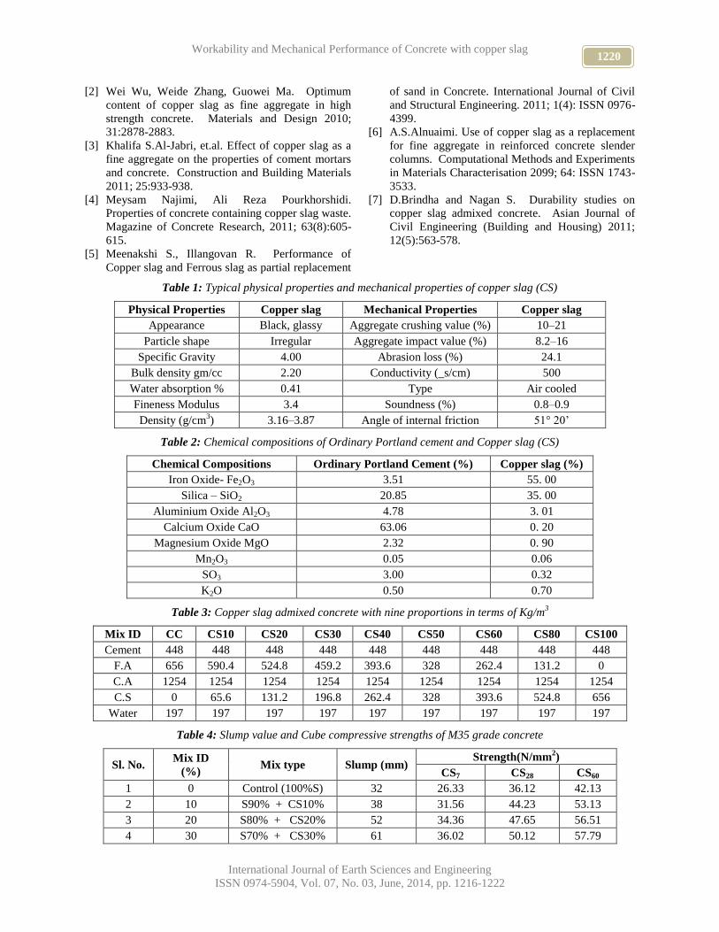
1220 Workability and Mechanical Performance of Concrete with copper slag
International Journal of Earth Sciences and Engineering
ISSN 0974-5904, Vol. 07, No. 03, June, 2014, pp. 1216-1222
[2] Wei Wu, Weide Zhang, Guowei Ma. Optimum
content of copper slag as fine aggregate in high
strength concrete. Materials and Design 2010;
31:2878-2883.
[3] Khalifa S.Al-Jabri, et.al. Effect of copper slag as a
fine aggregate on the properties of coment mortars
and concrete. Construction and Building Materials
2011; 25:933-938.
[4] Meysam Najimi, Ali Reza Pourkhorshidi.
Properties of concrete containing copper slag waste.
Magazine of Concrete Research, 2011; 63(8):605-
615.
[5] Meenakshi S., Illangovan R. Performance of
Copper slag and Ferrous slag as partial replacement
of sand in Concrete. International Journal of Civil
and Structural Engineering. 2011; 1(4): ISSN 0976-
4399.
[6] A.S.Alnuaimi. Use of copper slag as a replacement
for fine aggregate in reinforced concrete slender
columns. Computational Methods and Experiments
in Materials Characterisation 2099; 64: ISSN 1743-
3533.
[7] D.Brindha and Nagan S. Durability studies on
copper slag admixed concrete. Asian Journal of
Civil Engineering (Building and Housing) 2011;
12(5):563-578.
Table 1: Typical physical properties and mechanical properties of copper slag (CS)
Physical Properties Copper slag Mechanical Properties Copper slag
Appearance Black, glassy Aggregate crushing value (%) 10–21
Particle shape Irregular Aggregate impact value (%) 8.2–16
Specific Gravity 4.00 Abrasion loss (%) 24.1
Bulk density gm/cc 2.20 Conductivity (_s/cm) 500
Water absorption % 0.41 Type Air cooled
Fineness Modulus 3.4 Soundness (%) 0.8–0.9
Density (g/cm3) 3.16–3.87 Angle of internal friction 51° 20’
Table 2: Chemical compositions of Ordinary Portland cement and Copper slag (CS)
Chemical Compositions Ordinary Portland Cement (%) Copper slag (%)
Iron Oxide- Fe2O3 3.51 55. 00
Silica – SiO2 20.85 35. 00
Aluminium Oxide Al2O3 4.78 3. 01
Calcium Oxide CaO 63.06 0. 20
Magnesium Oxide MgO 2.32 0. 90
Mn2O3 0.05 0.06
SO3 3.00 0.32
K2O 0.50 0.70
Table 3: Copper slag admixed concrete with nine proportions in terms of Kg/m3
Mix ID CC CS10 CS20 CS30 CS40 CS50 CS60 CS80 CS100
Cement 448 448 448 448 448 448 448 448 448
F.A 656 590.4 524.8 459.2 393.6 328 262.4 131.2 0
C.A 1254 1254 1254 1254 1254 1254 1254 1254 1254
C.S 0 65.6 131.2 196.8 262.4 328 393.6 524.8 656
Water 197 197 197 197 197 197 197 197 197
Table 4: Slump value and Cube compressive strengths of M35 grade concrete
Sl. No. Mix ID
(%) Mix type Slump (mm)
Strength(N/mm2)
CS7 CS28 CS60
1 0 Control (100%S) 32 26.33 36.12 42.13
2 10 S90% + CS10% 38 31.56 44.23 53.13
3 20 S80% + CS20% 52 34.36 47.65 56.51
4 30 S70% + CS30% 61 36.02 50.12 57.79
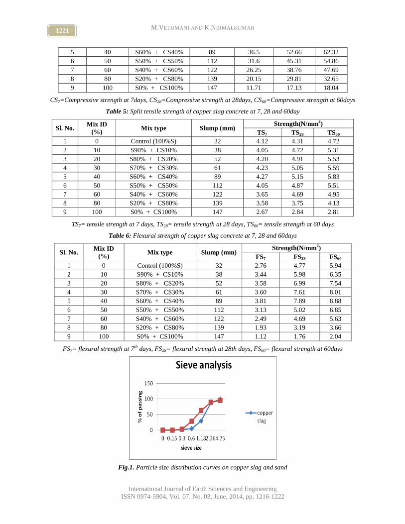
1221 M.VELUMANI AND K.NIRMALKUMAR
International Journal of Earth Sciences and Engineering
ISSN 0974-5904, Vol. 07, No. 03, June, 2014, pp. 1216-1222
5 40 S60% + CS40% 89 36.5 52.66 62.32
6 50 S50% + CS50% 112 31.6 45.31 54.86
7 60 S40% + CS60% 122 26.25 38.76 47.69
8 80 S20% + CS80% 139 20.15 29.81 32.65
9 100 S0% + CS100% 147 11.71 17.13 18.04
CS7=Compressive strength at 7days, CS28=Compressive strength at 28days, CS60=Compressive strength at 60days
Table 5: Split tensile strength of copper slag concrete at 7, 28 and 60day
Sl. No. Mix ID
(%) Mix type Slump (mm)
Strength(N/mm2)
TS7 TS28 TS60
1 0 Control (100%S) 32 4.12 4.31 4.72
2 10 S90% + CS10% 38 4.05 4.72 5.31
3 20 S80% + CS20% 52 4.20 4.91 5.53
4 30 S70% + CS30% 61 4.23 5.05 5.59
5 40 S60% + CS40% 89 4.27 5.15 5.83
6 50 S50% + CS50% 112 4.05 4.87 5.51
7 60 S40% + CS60% 122 3.65 4.69 4.95
8 80 S20% + CS80% 139 3.58 3.75 4.13
9 100 S0% + CS100% 147 2.67 2.84 2.81
TS7= tensile strength at 7 days, TS28= tensile strength at 28 days, TS60= tensile strength at 60 days
Table 6: Flexural strength of copper slag concrete at 7, 28 and 60days
Sl. No. Mix ID
(%) Mix type Slump (mm)
Strength(N/mm2)
FS7 FS28 FS60
1 0 Control (100%S) 32 2.76 4.77 5.94
2 10 S90% + CS10% 38 3.44 5.98 6.35
3 20 S80% + CS20% 52 3.58 6.99 7.54
4 30 S70% + CS30% 61 3.60 7.61 8.01
5 40 S60% + CS40% 89 3.81 7.89 8.88
6 50 S50% + CS50% 112 3.13 5.02 6.85
7 60 S40% + CS60% 122 2.49 4.69 5.63
8 80 S20% + CS80% 139 1.93 3.19 3.66
9 100 S0% + CS100% 147 1.12 1.76 2.04
FS7= flexural strength at 7th
days, FS28= flexural strength at 28th days, FS60= flexural strength at 60days
Fig.1. Particle size distribution curves on copper slag and sand

1222 Workability and Mechanical Performance of Concrete with copper slag
International Journal of Earth Sciences and Engineering
ISSN 0974-5904, Vol. 07, No. 03, June, 2014, pp. 1216-1222
Fig.2. Slump value for replacement of copper slag in
M35 grade concrete
Fig.3. Cube compressive strength of copper slag
concrete at 7, 28 and 60 days
Fig.4. Split-tensile strength of copper slag concrete at
7,28 and 60 days
Fig.5. Flexural strength of copperslag concrete at 7,28
and 60 days

www.cafetinnova.org
Indexed in
Scopus Compendex and Geobase Elsevier, Chemical
Abstract Services-USA, Geo-Ref Information Services-USA,
List B of Scientific Journals, Poland,
Directory of Research Journals
ISSN 0974-5904, Volume 07, No. 03
June 2014, P.P.1223-1230
#02070358 Copyright ©2014 CAFET-INNOVA TECHNICAL SOCIETY. All rights reserved.
Economic Comparison of Semi Continuous Mining System with
Intermittent System in Special Cycle Time
ZHAODONG WANG College of Mining Engineering,Liaoning Technical University ,Fuxin,123000,China
China Coal Technology & Engineering Group Corp ,Beijing 100013,China
Email: [email protected]
Abstract: Today, the mining process is dominated by large-scale mechanized mining with the coexistence of
various mining processes. With the continuity of mineral flow, open pit mining technology has three kinds of
processes: continuous, semi-continuous, and intermittent technology. Due to various factors involved in the mining
process system, optimization work is quite complex, and it is always an important research field in open pit mining.
Semi continuous mining technology is a comprehensive process based on the other two process. In the paper, we
give the transport distance under different mining process according to the recent level of open-pit mining
characteristics, and take minimum total cost in calculation period as the goal to establish the open pit mining process
optimization model. Calculation method of economic indicators of intermittent mining technology and semi
continuous process has been presented. And energy use of truck and belt conveyor has been compared. The semi
continuous technology combines the advantages of single bucket excavator, automobile and belt conveyor and can
be used in open pit mine to get high total benefit with low cost.
Keywords: open pit mining, semi continuous system, intermittent system, economic comparison.
1. Introduction:
With rapid and continuous development of the mining
industry, two or more production processes used in
open-pit mines are no longer uncommon. Integrated
production processes ensure the respective advantages
of each single production process under appropriate
circumstances with its wide range of adaptability. Its
high reliability and economic benefits are favored by
numerous open-pit mines [1]. Development of the open
mining process has been experienced from the initial
open-pit mining technology of simple human
exploitation to today's mechanized mass production. In
modern times, the mining process is dominated by
large-scale mechanized mining with the coexistence of
various mining processes. Open pit mining technology
has three kinds of processes: continuous, semi-
continuous, and intermittent with the continuity of
mineral flow.
(1) Intermittent continuous process. Intermittent
continuous technology is mainly in the manners of
shovel-truck technology. This process appears at an
early time and has wide application. Various research
focuses on the truck or other machinery dispatching [2-
6].
(2) Continuous mining process. Continuous mining
technology [7-11] originates from Germany. Typical
system is composed of bucket shovel, wheel conveyor
and dumping machine. It is originally from Germany
and greatly improves the production efficiency.
(3) Semi continuous process. Semi continuous process
[12-14] is based on the continuous production
technology and intermittent continuous mining
technology. It combines the advantages of continuous
and intermittent continuous processes. Some studies on
special application, such as crusher [15-16], reliability
[17-18].
Objects of the three kinds of process are processes from
mining to transport. In actual open pit mining, mining
sequence of ores or blocks requires responsible
attention. Perfect mining sequence will lead to higher
economic benefit. And the exploitation sequence with
the consideration of time and space [19-22] and random
distribution of mineral [23-24] is much easier to reduce
the cost of fixed investment and boost their total benefit.
In the paper, we mainly discussed the characteristics
and development status of semi continuous process.
Economic problems of the two processes have been
studied. With a certain open pit mine, economic
indicator of intermittent technology and semi
continuous process has been analyzed. Energy
efficiency of belt transportation and truck transportation
has been compared.
The main contributions of this paper is an investigation
on transport distance under different mining process
according to the recent level of open-pit mining

1224 Economic Comparison of Semi Continuous Mining System with Intermittent
System in Special Cycle Time
International Journal of Earth Sciences and Engineering
ISSN 0974-5904, Vol. 07, No. 03, June, 2014, pp. 1223-1230
characteristics, and take minimum total cost in the
calculation period as the goal to establish the open pit
mining process optimization model. The remainder of
the paper can be organized as the following: Section 2 is
the introduction of semi continuous technology in open
pit mining, including characteristics, application
conditions, and development. Calculation method of
transport distance of overburden is given in section 3.
Optimization model is described in section 4, including
objective and calculation method. Section 5 gives the
comparison results of semi continuous and intermittent
processes with a certain open pit mine. The conclusion
is given in section 6.
2. SEMI CONTINUOUS IN OPEN-PIT MINING
2.1. Characteristics of semi continuous in open-pit
mining
Semi continuous mining technology refers two kinds of
forms. One form includes three parts: the mining
process is intermittent; material transportation is by
truck with an intermittent manner from working face to
crush station; material transports continually after it
moving out of the crushing station. The other form is all
continuous transportation. The former one is combined
with the characteristics of high adaptability of shovel
truck technology, flexibility, and belt conveyor with
advantages of large climbing ability, high efficiency,
and low transportation cost. It is rapidly developed in
recent years, both technology and equipment. Two
kinds of semi continuous mining technology are widely
applied, and the technology is relatively mature. Both of
the two kinds are with less or without trucks and partly
or completely with the belt conveyor instead. This can
reduce the production cost and environmental pollution.
The advantages and disadvantages of semi continuous
mining technology are shown in table 1.
2.2. Conditions for application of semi continuous
mining technology
1) Geological conditions. Geological condition is the
fundamental condition to choose the semi continuous
mining technology, including coal, rock, soil thickness,
number, angle, lithology, geological structure and
mining depth complexity.
Mining system can use semi continuous mining
technology with single bucket-truck and semi portable
crusher station. Some nearly horizontal or gently
inclined seam, which has the advantages of simple
structure, small depth of pit, can use semi continuous
mining technology with single bucket and mobile
crusher.
The majority of open-pit stripping system is suitable for
semi continuous mining technology with single bucket
and mobile crusher in geological terms. But open pit
mine with complex mining condition is more suitable
for the semi continuous mining technology with single
bucket-truck + semi portable crusher station.
If the inner dump condition is poor, open pit mining
depth is larger, and stripping haul distance is far and
with the heavy car uphill, most stripped quantity should
be discharged. This would make the height of outer
dump area increasing. The truck would pass a long way
to dump. When uphill distance of heavy car is up to 2.8
km or above, semi continuous mining technology
should be used to get a higher benefit.
2) Climatic conditions. Freezing adhesive in equipment
is a not well resolved technical problem.
3) Equipment manufacturing conditions for semi
continuous technology. The key equipment of the semi
continuous technology is crushing machine, including
the semi mobile station and self-mobile crusher. This is
decive factors of mature of semi continuous technology.
Other equipment in semi continuous process system,
such as single bucket excavators, truck, belt conveyor,
dumping machine is mature and reliable.
Single bucket-truck + semi mobile crusher station
technology is mature. Semi mobile crushing station is
mature and various series of models are completed.
Single bucket and self-mobile crusher technology
crusher have existed but with no series of products.
Especially greater than 2500 ht / , mobile crusher has
just few application servers, and equipment in each link
matches unreasonable. Some key technologies are still
in the stage of research and development. For example:
overall structural design of self-mobile crusher itself,
operation stability, and single bucket excavator in the
working face with high efficiency, all these technologies
have not been fully tested in practice. So, single bucket
and self-mobile crusher have a low technology maturity,
and it is the main obstacle to effective decision-making.
Table1 Advantages and disadvantages of semi
continuous process
Content remarks
Adva
ntage
s
Low operating costs,
obvious advantages when
the material transport path
is uphill slope and
distance is long;
When
transportatio
n distance is
more than
2.8km, semi
continuous
technology
has obvious
economic
advantages
compared
with the
single
Less unit energy
consumption;
Low cost of spare parts
and repair maintenance;
Little constrain by fuel
shortage and less
environmental pollution;

1225 ZHAODONG WANG
International Journal of Earth Sciences and Engineering
ISSN 0974-5904, Vol. 07, No. 03, June, 2014, pp. 1223-1230
Less persons and low
labor intensity;
bucket truck
mining
technology.
disad
vanta
ges
Series production process
system, great fluctuations
in short-term production
capacity, buffer link;
Semi
continuous
mining
technology
is combined
process and
delivery
transportatio
n. It’s
mainly
manifested
in the
system
reliability
and initial
investment
Different levels of
freezing adhesive crusher
bin with the temperature
is below -10℃, clean
work is great, and low
production efficiency;
Higher initial investment,
but due to the long service
life, depreciation expense
is not high;
Cycle time of
manufacturing and
installation is long;
2.3. Development of semi continuous process
Semi continuous mining technology is developed based
on continuous mining technology and intermittent
mining technology. It has advantages of continuous
process and intermittent technology. It has strong
adaptability and can mine hard rock and freezing soft
rock mining in winter. It can give the continuous
operation on ore transportation, expand the scale of
production and reduce the cost of production.
At present, semi continuous mining technology mainly
has 2 forms: single bucket truck and semi mobile
crusher station and belt conveyor; single bucket and
self-mobile crusher and belt conveyor.
Semi continuous mining technology with single bucket
truck and semi mobile crusher station and belt conveyor
has been widely used. So far, hundreds of mines have
applied the mining technology. Maximum production
capacity of semi mobile crushing station has reached
14000 ht / . It feeds with the bucket capacity of 60 3m
of single bucket excavator and load of 365 t dump
truck. The semi continuous mining technology is fit for
mining field with irregular shape, thickness and
inclination of useful minerals, especially the concave
pit.
Semi continuous mining with single bucket and self-
mobile crusher is mining technology without fuel truck.
Its production capacity is generally 300 ~ 5000 ht / .
Due to the rapid development of large tonnage dump
truck, semi continuous mining technology with single
bucket truck and semi self-mobile crusher station and
belt conveyor. Production capacity of semi mobile
station improves especially faster. It greatly increases
production efficiency and reduces production cost soon.
In this stage, semi continuous mining technology with
single bucket and mobile crusher is gradually eliminated
due to the little improvement efficiency.
3. TRANSPORT DISTANCE OF OVERBURDEN
Under ideal conditions, material transport distance can
be calculated according to the loading position shown as
the following:
||,)()(max 22
i
zzyyxxS zx
zxzx
(1)
S is the transport distance, m ;
zx xx , are the X coordinates of unloading and loading
points;
zx yy , are Y coordinates of unloading and loading
points;
zx zz , are z coordinates of unloading and loading
points;
I is the climbing ability of transportation equipment,
% .
Compared to the calculation of transport distance with
equation (1) based on the loading and unloading
position, transport distance of overburden in open pit
mining is mainly due to the layout decisions of transport
system. As shown in Figure 1.
In order to shorten the haul distance of overburden,
shovel-truck process often adopts the manners of a
double row and inner dumping. At a specified mining
level, average transporting distance can be expressed as
the following:
)cotcot(cot2
4
cot2)cot(cot
4
cot2
c
cc
ck
HWL
HLHW
HLS (2)
Where, kS is the average haul distance, m ;
L is the bottom line length in the open pit mining, m ;
cH is the elevation difference between analysis level
height and bottom level height, m ;
is the slope angle of open-pit mine side, (°);
W is the bottom width of the open pit mining, m ;
is the slope angle of working side in open pit
mining, (°);
is the slope angle of dumping side in open pit
mining, (°)
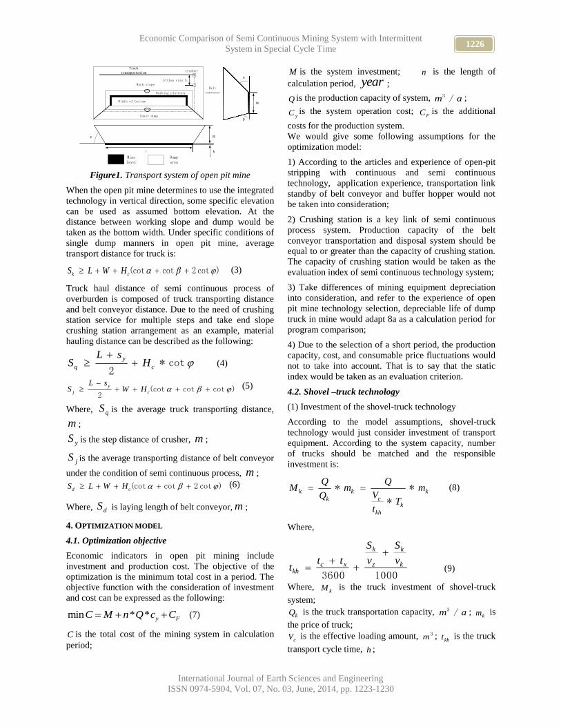
1226 Economic Comparison of Semi Continuous Mining System with Intermittent
System in Special Cycle Time
International Journal of Earth Sciences and Engineering
ISSN 0974-5904, Vol. 07, No. 03, June, 2014, pp. 1223-1230
Minelayer
Dumparea
Truck transportation
Truck transportation
Work slopeStep size SyStep size Sy
crushercrusher
Belt conveyerWorking platform
Width of bottom
Inner dump
ll
HH
h
φ H
α
W
β
Figure1. Transport system of open pit mine
When the open pit mine determines to use the integrated
technology in vertical direction, some specific elevation
can be used as assumed bottom elevation. At the
distance between working slope and dump would be
taken as the bottom width. Under specific conditions of
single dump manners in open pit mine, average
transport distance for truck is:
)cot2cot(cot ck HWLS (3)
Truck haul distance of semi continuous process of
overburden is composed of truck transporting distance
and belt conveyor distance. Due to the need of crushing
station service for multiple steps and take end slope
crushing station arrangement as an example, material
hauling distance can be described as the following:
cot*2
c
y
q HsL
S
(4)
)cotcot(cot2
c
y
j HWsL
S (5)
Where, qS is the average truck transporting distance,
m ;
yS is the step distance of crusher, m ;
jS is the average transporting distance of belt conveyor
under the condition of semi continuous process, m ;
)cot2cot(cot cd HWLS (6)
Where, dS is laying length of belt conveyor, m ;
4. OPTIMIZATION MODEL
4.1. Optimization objective
Economic indicators in open pit mining include
investment and production cost. The objective of the
optimization is the minimum total cost in a period. The
objective function with the consideration of investment
and cost can be expressed as the following:
min * * y FC M n Q c C (7)
C is the total cost of the mining system in calculation
period;
M is the system investment; n is the length of
calculation period, year ;
Q is the production capacity of system, am /3 ;
yC is the system operation cost; FC is the additional
costs for the production system.
We would give some following assumptions for the
optimization model:
1) According to the articles and experience of open-pit
stripping with continuous and semi continuous
technology, application experience, transportation link
standby of belt conveyor and buffer hopper would not
be taken into consideration;
2) Crushing station is a key link of semi continuous
process system. Production capacity of the belt
conveyor transportation and disposal system should be
equal to or greater than the capacity of crushing station.
The capacity of crushing station would be taken as the
evaluation index of semi continuous technology system;
3) Take differences of mining equipment depreciation
into consideration, and refer to the experience of open
pit mine technology selection, depreciable life of dump
truck in mine would adapt 8a as a calculation period for
program comparison;
4) Due to the selection of a short period, the production
capacity, cost, and consumable price fluctuations would
not to take into account. That is to say that the static
index would be taken as an evaluation criterion.
4.2. Shovel –truck technology
(1) Investment of the shovel-truck technology
According to the model assumptions, shovel-truck
technology would just consider investment of transport
equipment. According to the system capacity, number
of trucks should be matched and the responsible
investment is:
k
k
kh
c
k
k
k m
Tt
V
Qm
Q
QM *
*
* (8)
Where,
10003600k
k
z
k
xckh
v
S
v
S
ttt
(9)
Where, kM is the truck investment of shovel-truck
system;
kQ is the truck transportation capacity, am /3 ; km is
the price of truck;
cV is the effective loading amount, 3m ; kht is the truck
transport cycle time, h ;

1227 ZHAODONG WANG
International Journal of Earth Sciences and Engineering
ISSN 0974-5904, Vol. 07, No. 03, June, 2014, pp. 1223-1230
kT is the design operating time of truck in each year,
ah / ;
cT is the truck loading time, including actual loading
time, waiting time at the working platform, unloading
time, and so on, s ;
zv is the average running speed when truck is
overloading, hkm / ;
kv is the average running speed when truck is
unloading, hkm / .
(2) system operating expenses
According to the production experience of open-pit
mine, the system operating costs usually include
material costs, energy costs and personnel costs. Of the
three kinds of costs, personnel costs are relatively fixed.
Salary and welfare expenses of operators’ are especially
taken into consideration.
k
rtkkmkckrkkmkcky
Q
knScccSccc
**)(*)( (10)
Where, kc is unit cost of truck transportation;
kcc is the
material costs of truck transportation; knc is the energy
cost of truck transport; krc is the personnel expenses of
shovel-truck system; rn is the number of operators
matching for single equipment; rk is the annual salary
and welfare costs of operating staffs.
4.3. Semi continuous process
(1) System investment
According to the assumption of the model, semi
continuous technology investment including trucks,
crushing equipment, belt conveyor, conveying
equipment, dumping equipment etc. The truck
investment can be calculated by equation (8). The cycle
time of the operation can be corrected with the transport
distance as:
10003600k
q
z
q
xcsh
v
S
v
S
ttt
(11)
pddsqb MSmMMM * (12)
k
k
sh
c
k
q
q m
Tt
V
Qm
Q
QM *
*
* (13)
Where, sht is the transportation time of truck in semi
continuous process, h ;
bM is the investment of semi continuous system;
bm is the truck investment under semi continuous
process;
sM is the crushing equipment investment; dM is the
investment of belt conveyor;
pM is the investment of dumping and transfer
equipment in working surface;
qQ is the truck transportation capacity under semi
continuous technology, 3m ;
(2) System operating expenses
From Figure1 described before, fixed equipment in semi
continuous process system includes crushing equipment,
conveying equipment, belt conveyor, dumping face
conveyor, dumping machine and working platform.
Then, we can calculate the operation cost of semi
continuous process system as the following:
tbrjjnjcqknkcby ccSccSccc *)(*)( (14)
Where,
q
rrrrbr
Q
kn
Q
knc
**6 (15)
byc is the unit cost of operation under semi continuous
process; jcc is the material transport costs of belt
conveyor; jnc is the energy cost of belt conveyer;
brc is
the personnel costs in semi continuous process; tc is
other costs in semi continuous process, including other
link broken, dumping reproduced, etc.
(3) Additional costs
The additional cost considered mainly consists of three
parts:
1) Loosing blasting cost. Loosing blast cost index of
particle size of ore and rock and muck pile shape under
in semi continuous process conditions should consider
mining equipment efficiency, material crushing, and
belt conveyor transportation requirements, and the loose
blasting cost is generally higher;
2) The cost of crusher station equipment moving in
production process. This part of cost can be calculated
according to the moving distance of working slope and
step moving parameters of crusher station in one
calculation period.
3) Opportunity cost of semi continuous technology
investment. This is due to the increased investment
costs. In the model, we would use the investment loan
interest of higher part of semi continuous process to
intermittent process.
eMM
Q
C
S
vQcCCCc kb
y
y
spFJFYFPF *)(***8 (16)

1228 Economic Comparison of Semi Continuous Mining System with Intermittent
System in Special Cycle Time
International Journal of Earth Sciences and Engineering
ISSN 0974-5904, Vol. 07, No. 03, June, 2014, pp. 1223-1230
In the equation, FPc is the loosing blasting cost; FYc is
the additional costs of crusher moving; FJc is the
additional costs by additional investment; spcis the
loose blasting cost differences between semi continuous
process and shovel-truck process; v is the push
schedule of open pit mine, am / , Yc is the step cost of
crusher moving; e is the loan interest rate.
4.4. Solution
Based on the analysis above, if using semi continuous
process, cost of it must be less than that of an
intermittent process. Then,
kykkfbybb cQMCCcQMc *8*8 (17)
sp
y
Ykbbyky c
SQ
CvMM
Q
ecc
*
*)(*
8
812
(18)
Then, we can get the boundary conditions of application
of semi continuous technology.
5. APPLICATION
An open pit mining in northern part of China has been
used to verify the theory. The original approved
production capacity of 30 aMt / . The program would
use semi continuous technology with shovel, truck,
ground crushing station and belt semi continuous
process. The stripping is mainly using single bucket and
truck technology. The rock thickness is 32 m on
average and the approved capacity is 45 aMm /3 . Due
to the parameters of tested and experience, operation
forecast of the two process plan can be calculated. As
shown from table 2 to table 5.
The results show that, the upper step of open-pit with
semi continuous process for stripping is reasonable, and
the application can be further expanded.
Payload of truck and belt conveyor can be compared as
shown in table 6.
Table.2 Comparison of mining system on transporting
device
Item Intermittent
technology
Semi
continuous
technology
Truck transport
distance/ m 4323 1253
Truck speed with
load/ 1* hkm 30 25
Truck speed
without
load/ 1* hkm
40 32
Cycle time/ h 278 278
Transport
capacity/13 * aMm
0.45 0.21
Number of trucks 49 24
Length of
conveyer 5498
Transport distance
of conveyer 4245
Table.3 Comparison of mining system on investment
Item Intermittent
technology
Semi
continuous
technology
Truck
investment/ yuan 720 000 000 350 000 000
Investment of
conveyer/ yuan 0.00 124 350 000
Investment of other
equipment/ yuan 0.00 340 000 000
Total investment/ yuan 720 000 000 814 350 000
Table.4 Comparison of mining system on operation
Item Intermittent
technology
Semi
continuous
technology
Material
expenses/ yuan 1 027 500 000 881 320 000
Energy
expenses/ yuan 1 680 630 000 1 703 240 000
Personnel
expenses/ yuan 240 000 000 124 400 000
Total 2 948 130 000 2 708 960 000
Table.5 Comparison of mining system on additional
expenses
Item Intermittent
technology
Semi
continuous
technology
Step moving
expenses/yuan
211 320 000
Interest of
investment/yuan
63 240 000
Total 274 560 000
From table 6 we can see automobile transportation
energy consumption is about 60% for self-weight, and
only about 40% is used for the material carrier. The belt
conveyor transportation energy consumes 80% of the

1229 ZHAODONG WANG
International Journal of Earth Sciences and Engineering
ISSN 0974-5904, Vol. 07, No. 03, June, 2014, pp. 1223-1230
total to transport materials, and just about 20% for the
self-weight. Thus, in suitable conditions, belt conveyor
can be used instead of automobile transportation to save
a lot of energy consumption cost and production cost. It
is especially more obvious of the advantage in the long
distance transportation situation.
Table.6 Payload of the truck and belt conveyor
Item Truck
(154t)
Truck
(290t)
belt
conveyor
Load /t 154 290 605
Weight /t 101 211 140
Total weight of
load and unload /t
101*2+154
=356
211*2+290
=712
605+140=
645
Ratio of load and
total weight 1:2.31 1:2.46 1:1.2
Energy use rate of
load /% 43.2 40.7 81
According to the production experience of large open
pit mine, large truck fuel consumption can get
0.1~0.2 kmL/m3 , fuel costs is accounted for more than
50% of truck operating costs [25]. Therefore, sharp
fluctuations in oil prices will constitute a significant
impact on the shovel truck operation cost. Semi
continuous production process use belt conveyer instead
of trucks transport to increase the transportation
quantity and energy utilization rate. Due to the small
fluctuations in the power price, belt transportation cost
fluctuation is also small. This is good for the cost
accounting of mining and maintaining price stability.
When the semi continuous system is into production,
the cost of the process is low and the benefit would be
improved.
6. CONCLUSION
Due to various factors involved in the mining process
system, optimization work is quite complex, and it is
always an important research field in open pit mining.
Automobile transportation has the characteristics of
high flexibility and strong adaptability. But high self-
weight lead to high energy consumption, high tire
consumption, high repair costs, and high transportation
costs. Especially in the present stage, oil shortages and
rising prices, tire supply shortages and rising prices,
labor force rising prices, environmental protection
requirements to reduce carbon emissions and social
responsibility of corporate, the development of long
distance of truck transport are not conducive to the
mining with economic benefits and social benefits. So,
reduction of truck number is necessary.
In the paper, we give the transport distance under
different mining process according to the recent level of
open-pit mining characteristics, and take minimum total
cost in calculation period as the goal to establish the
open pit mining process optimization model.
Calculation method of economic indicators of
intermittent mining technology and semi continuous
process has been presented. And energy use of truck and
belt conveyor has been compared.
The semi continuous technology combines the
advantages of single bucket excavator, automobile and
belt conveyor. It has rapid development all over the
world, especially used in large scale open pit mine.
Semi continuous process used in open pit mine can get
high total benefit at low cost.
7. Reference:
[1] Wang Xifu, Zhang Daxian, Peng Shij. Engineering
Reliability Study on Combined Mining
Technology. Journal of Fuxin Mining Institute
(Natural Science), 16(1):28-31. (1997).
[2] Ma Ming, Li Hong-Jie, Lei He. 3D fracture
network and block analysis of the south end-slope
of Antaibao Coal Mine. Advances in Civil and
Industrial Engineering, 353-354: 1165-1170.
(2013).
[3] Blackwell G.H. Estimation of large open pit
haulage truck requirements, CIM Bulletin,
92(1028): 143-69. (1999).
[4] Hardy R.H. Selection criteria for loading and
hauling equipment – open pit mining
applications”, PhD thesis, Curtin University of
Technology, Sydney, 2: 558. (2007).
[5] Bastos Guilherme S., Souza Luiz E., Ramos Fabio
T., Ribeiro Carlos H. C. A single-dependent agent
approach for stochastic time-dependent truck
dispatching in open-pit mining. IEEE Conference
on Intelligent Transportation Systems,
Proceedings, ITSC, 1057-1062. (2011).
[6] Bastos Guilherme S. Decision making applied to
shift change in stochastic open-pit mining truck
dispatching?. IFAC Proceedings Volumes (IFAC-
Papers Online), 15(PART 1): 34-39. (2013).
[7] Ringleff Horst. MODERN OPEN-PIT MINING
TECHNOLOGY. Bulk Solids Handling, 5(1): 165-
166. (1985).
[8] Raaz Viktor, Mentges Bergbau Ulrich. Emissions
reduction by means of continuous open pit mining
technology. ThyssenKrupp techforum, 2: 54-59.
(2007).
[9] Benndorf Jörg. Application of efficient methods of
conditional simulation for optimising coal
blending strategies in large continuous open pit
mining operations. International Journal of Coal
Geology, 112:141-153. (2013).
[10] Schroeder D. Technical and economical aspects of
continuous mining with bucket wheel excavators.

1230 Economic Comparison of Semi Continuous Mining System with Intermittent
System in Special Cycle Time
International Journal of Earth Sciences and Engineering
ISSN 0974-5904, Vol. 07, No. 03, June, 2014, pp. 1223-1230
ZKG International, Edition B, 47(9): 513-518.
(1994).
[11] Glanz W., Weissflog J. CONTINUOUS
CONVEYING IN OPEN PIT MINES. Bulk Solids
Handling, 2(1): 81-89. (1982).
[12] Wang Hai-Jun, Li Ke-Min, Chen Shu-Zhao. Study
on application scope of stripping semi-continuous
system in internal dumping open pit mine. Journal
of Mining and Safety Engineering, 30(5): 761-765.
(2013).
[13] Jin-Long Sun, Chang-Sheng Ji, Shu-Zhao Chen. A
research on the optimization of layout depth of
semi-continuous technology crusher station in flat
dipping open pit mine. Journal of Convergence
Information Technology, 7(21): 44-52. (2012).
[14] Chen Shu-Zhao, Optimization and application
research on semi-continuous technology system
with mobile crusher in large open pit coal mines.
Journal of the China Coal Society, 37(3): 533-534.
(2012).
A. Kumar, H. Blumberg. A probabilistic model for a
repairable mining equipment inventory system and
procurement policy determination [J]. International
Journal of Surface Mining and Reclamation, (5):
117~121. (1991).
[15] K. Mukhopadhyay. Open pit system reliability [J].
Journal of Mines, Metals & Fuels, (8): 389~392.
(1988).
[16] CHE Zhao-xue, CAI Qing-xiang. Study on Semi-
Contiuous System for Loess Stripping in Surface
Mines of Heidaigou. Journal of China University
of Mining & Technology. 33(6): 673-677. (2004).
[17] M Cardu.C.Clcrici. An experimental research on
the commination law and work index concepts in
jaw crushers. 28th International Mineral
Processing Congress. (1993).
[18] Karparov K.N., Handley, M.F.. Engineering
application of thrust block analysis in slope
stability problems in open pit mines. Journal of the
Southern African Institute of Mining and
Metallurgy, 109(5): 309-327. (2009).
[19] Boland Natashia, Dumitrescu Irina, Froyland Gary,
Gleixner Ambros M.. LP-based disaggregation
approaches to solving the open pit mining
production scheduling problem with block
processing selectivity. Computers and Operations
Research, 36( ): 1064-1089. (2009).
[20] Chicoisne Renaud, Espinoza Daniel, Goycoolea
Marcos, Moreno Eduardo, Rubio Enrique. A new
algorithm for the open-pit mine production
scheduling problem. Operations Research, 60(3):
517-528. (2012).
[21] Yang Biao, Luo Zhou-Quan, Lu Guang, Lu Hao,
Wang Yi-Wei. Open pit mining limit dynamic
optimization based on economic time series
forecasting. Journal of the China Coal Society,
36(1): 29-33. (2011).
[22] Li Shouguo, Yang Chang, Lu Caiwu. Cut-off grade
optimization using stochastic programming in
open-pit mining. 6th International Conference on
Internet Computing for Science and Engineering,
ICICSE 2012, 66-69. (2012).
[23] Asad Mohammad Waqar Ali, Dimitrakopoulos
Roussos. A heuristic approach to stochastic cutoff
grade optimization for open pit mining complexes
with multiple processing streams. Resources
Policy, 38(4): 591-597. (2013).
[24] DENG Ming. The measures to reduce production
cost of Heidaigou open-pit coal mine. Opencast
Mining Technology, (3): 119-121. (2012).


