Integration of holomorphic Lie algebroids

arX

iv:0

803.

2031

v2 [

mat

h.D

G]

17

Mar

200

8

Integration of Holomorphic Lie Algebroids

Camille Laurent-Gengoux

Département de mathématiques

Université de Poitiers

86962 Futuroscope-Chasseneuil, France

[email protected]

Mathieu Stiénon ∗

E.T.H. Zürich

Departement Mathematik

8092 Zürich, Switzerland

[email protected]

Ping Xu †

Department of Mathematics

Penn State University

University Park, PA 16802, U.S.A.

[email protected]

Abstract

We prove that a holomorphic Lie algebroid is integrable if, and only if, its underlyingreal Lie algebroid is integrable. Thus the integrability criteria of Crainic-Fernandes (The-orem 4.1 in [6]) do also apply in the holomorphic context without any modification. As aconsequence we gave another proof of the theorem that a holomorphic Poisson manifoldis integrable if and only if its real part or imaginary part is integrable as a real Poissonmanifold [5, 20].

Contents

1 Introduction 2

2 Holomorphic Lie algebroids 4

2.1 Holomorphic Lie algebroids . . . . . . . . . . . . . . . . . . . . . . . . . . . . . 4

2.2 Tangent Lie algebroids . . . . . . . . . . . . . . . . . . . . . . . . . . . . . . . . 5

2.3 Equivalent definition of holomorphic Lie algebroids . . . . . . . . . . . . . . . . 7

2.4 Holomorphic Poisson manifolds . . . . . . . . . . . . . . . . . . . . . . . . . . . 9

∗Research supported by the European Union through the FP6 Marie Curie R.T.N. ENIGMA (Contractnumber MRTN-CT-2004-5652).

†Research partially supported by NSF grants DMS-0306665 and DMS-0605725 & NSA grant H98230-06-1-0047

1

http://arXiv.org/abs/0803.2031v2

mailto:[email protected]



3 Holomorphic Lie groupoids and holomorphic symplectic groupoids 10

3.1 Multiplicative (1,1)-tensors on Lie groupoids . . . . . . . . . . . . . . . . . . . 10

3.2 Nĳenhuis torsion of multiplicative (1,1)-tensors . . . . . . . . . . . . . . . . . . 11

3.3 Infinitesimal multiplicative (1,1)-tensors . . . . . . . . . . . . . . . . . . . . . . 14

3.4 Multiplicative Nĳenhuis tensors on Lie groupoids . . . . . . . . . . . . . . . . . 16

3.5 Holomorphic Lie groupoids . . . . . . . . . . . . . . . . . . . . . . . . . . . . . 17

3.6 Holomorphic symplectic groupoids . . . . . . . . . . . . . . . . . . . . . . . . . 19

3.7 Holomorphic extension of analytic Poisson structures . . . . . . . . . . . . . . . 23

1 Introduction

Since Lie’s third theorem fails for Lie algebroids, it has been a central theme of study in thetheory of Lie groupoids whether a given Lie algebroid is integrable. By an integrable Liealgebroid, we mean there exists an s-connected and s-simply connected Lie groupoid of whichit is the infinitesimal version. For real Lie algebroids, the integrability problem has beencompletely solved by Crainic-Fernandes [6] based on the work of Cattaneo-Felder on Poissonsigma models [4].

Recently, there has been increasing interest in holomorphic Lie algebroids and holomorphic Liegroupoids. It is a very natural question to find the integrability condition for holomorphic Liealgebroids. In [15], we systematically studied holomorphic Lie algebroids and their relationwith real Lie algebroids. In particular, we proved that associated to any holomorphic Liealgebroid A, there is a canonical real Lie algebroid AR such that the inclusion A → A∞

is a morphism of sheaves. Here A and A∞ denote, respectively, the sheaf of holomorphicsections and the sheaf of smooth sections of A. In other words, a holomorphic Lie algebroidcan be considered as a holomorphic vector bundle A → X whose underlying real vectorbundle is endowed with a Lie algebroid structure such that, for any open subset U ⊂ X,[A(U),A(U)] ⊂ A(U) and the restriction of the Lie bracket [·, ·] to A(U) is C-linear. It isthus natural to ask

Problem 1. Given a holomorphic Lie algebroid A with underlying real Lie alge-broid AR, what is the relation between the integrability of A and the integrabilityof AR?

To tackle this problem, we need an equivalent description of holomorphic Lie algebroids. Forthis purpose, we will view a holomorphic Lie algebroid as a real Lie algebroid structure ona holomorphic vector bundle A → X, whose almost complex structure JA : TA → TA isan infinitesimal multiplicative (1, 1)-tensor. By an infinitesimal multiplicative (1, 1)-tensor ona (real) Lie algebroid A, we mean a (1, 1)-tensor φA on A such that φA : TA → TA is anendomorphism of the tangent Lie algebroid TA→ TX.

On the level of Lie groupoids, if Γ X is an s-connected and s-simply connected Lie groupoidintegrating the real Lie algebroid A, then JA integrates to an automorphism JΓ : TΓ → TΓ of

2

the tangent groupoid TΓ TX such that J2Γ = − id. One can show that JΓ is fiberwise linear

with respect to the vector bundle structure TΓ → Γ. Hence it is a (1, 1)-tensor on Γ. Sucha (1, 1)-tensor is called multiplicative [5, 20]. All it remains to show is that JΓ is completelyintegrable, i.e. JΓ is a multiplicative Nĳenhuis tensor on Γ. The latter should presumablyfollow from the complete integrability of JA : TA→ TA. This motivates the following:

Problem 2. Establish a one-one correspondence between infinitesimal multiplica-tive Nĳenhuis tensors on A and multiplicative Nĳenhuis tensors on Γ.

To this end, we investigate multiplicative (1, 1)-tensors on Γ and their infinitesimal coun-terparts on A. In particular, we show that the infinitesimal of the Nĳenhuis torsion of amultiplicative (1, 1)-tensor on Γ is the Nĳenhuis torsion of its infinitesimal counterpart onA. We believe that our study of multiplicative (1, 1)-tensors on a Lie groupoid will be ofindependent interest.

Poisson manifolds are closely related to Lie algebroids. It is well known that associated toany Poisson manifold (X,π) there is a Lie algebroid (T ∗X)π, called the cotangent bundle Liealgebroid. If the Lie algebroid (T ∗X)π integrates to an s-connected and s-simply connectedLie groupoid Γ X, then Γ automatically admits a symplectic groupoid structure [17]. Inthis case, the Poisson structure (X,π) is said to be integrable. See [7] (also [4]) for the inte-grability conditions of a smooth Poisson manifold. The same situation applies to holomorphicPoisson structures as well, and one defines integrable holomorphic Poisson manifolds in asimilar fashion. As an application of our general theory, we prove that a holomorphic Poissonstructure (X,π), where π = πR + iπI , is integrable, if and only if (X,πR) and (X,πI) areintegrable real Poisson manifolds, recovering a theorem in [5] and [20], which was proved bydifferent methods.

The following notations are widely used in the sequel. For a manifold M , we use qM todenote the projection TM →M . And given a complex manifold X, TCX is shorthand for thecomplexified tangent bundle TX⊗C while T 1,0X (resp. T 0,1X) stands for the +i- (resp. −i-)eigenbundle of the almost complex structure. For a Lie algebroid A, the Nĳenhuis torsion[14, 13] of a bundle map φ : A → A over the identity is denoted Nφ, which is a section inΓ(∧2A∗ ⊗A) defined by

Nφ(V,W ) = [φV, φW ] − φ([φV,W ] + [V, φW ] − φ[V,W ]), ∀V,W ∈ Γ(A). (1)

When A is the Lie algebroid TX and φ : TX → TX is a (1, 1)-tensor, the Nĳenhuis torsionNφ is a (2, 1)-tensor on X.

While the paper was in writing, we learned that some similar results were also obtainedindependently by Cañez [2].

Acknowledgments We would like to thank Centre Émile Borel and Peking University fortheir hospitality while work on this project was being done. We also wish to thank RuiFernandes and Alan Weinstein for useful discussions and comments.

3

2 Holomorphic Lie algebroids

2.1 Holomorphic Lie algebroids

Holomorphic Lie algebroids were studied for various purposes in the literature. See [1, 9, 15,12, 21] and references cited there for details.

By definition, a holomorphic Lie algebroid is a holomorphic vector bundle A→ X, equippedwith a holomorphic bundle map A

ρ−→ TX, called the anchor map, and a structure of sheaf ofcomplex Lie algebras on A, such that

(a) the anchor map ρ induces a homomorphism of sheaves of complex Lie algebras from Ato ΘX ;

(b) and the Leibniz identity

[V, fW ] =(

ρ(V )f)

W + f [V,W ]

holds for all V,W ∈ A(U), f ∈ OX(U) and all open subsets U of X.

Here A is the sheaf of holomorphic sections ofA→ X and ΘX denotes the sheaf of holomorphicvector fields on X.

By forgetting the complex structure, a holomorphic vector bundle A → X becomes a real(smooth) vector bundle, and a holomorphic vector bundle map ρ : A → TX becomes a real(smooth) vector bundle map. Assume that A → X is a holomorphic vector bundle whoseunderlying real vector bundle is endowed with a Lie algebroid structure (A, ρ, [·, ·]) such that,for any open subset U ⊂ X,

(a) [A(U),A(U)] ⊂ A(U)

(b) and the restriction of the Lie bracket [·, ·] to A(U) is C-linear.

Then the restriction of [·, ·] and ρ from A∞ to A makes A into a holomorphic Lie algebroid,where A∞ denotes the sheaf of smooth sections of A→ X.

The following proposition states that any holomorphic Lie algebroid can be obtained out ofsuch a real Lie algebroid in a unique way.

Proposition 2.1 ([15]). Given a structure of holomorphic Lie algebroid on the holomorphic

vector bundle A → X with anchor map Aρ−→ TX, there exists a unique structure of real

smooth Lie algebroid on the vector bundle A → X with respect to the same anchor map ρsuch that the inclusion of sheaves A ⊂ A∞ is a morphism of sheaves of real Lie algebras.

By AR, we denote the underlying real Lie algebroid of a holomorphic Lie algebroid A. In thesequel, by saying that a real Lie algebroid is a holomorphic Lie algebroid, we mean that itis a holomorphic vector bundle and its Lie bracket on smooth sections restricts to a C-linearbracket on A(U), for all open subset U ⊂ X.

4

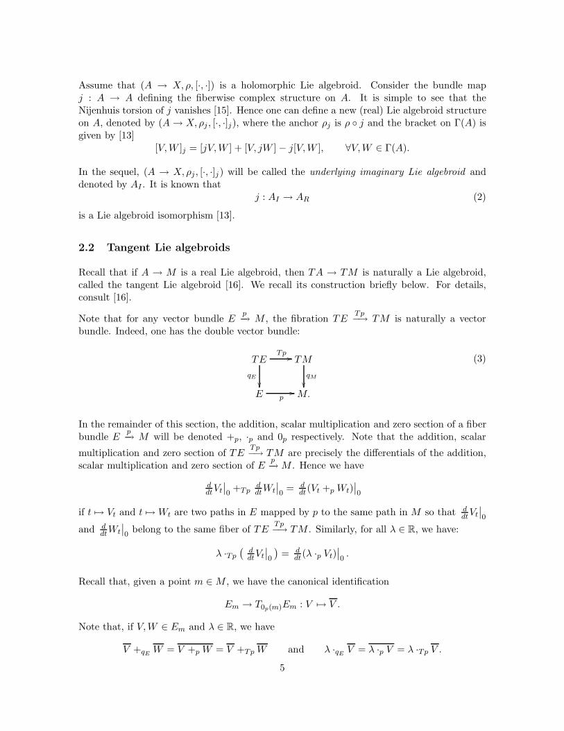
Assume that (A → X, ρ, [·, ·]) is a holomorphic Lie algebroid. Consider the bundle mapj : A → A defining the fiberwise complex structure on A. It is simple to see that theNĳenhuis torsion of j vanishes [15]. Hence one can define a new (real) Lie algebroid structureon A, denoted by (A → X, ρj , [·, ·]j), where the anchor ρj is ρ j and the bracket on Γ(A) isgiven by [13]

[V,W ]j = [jV,W ] + [V, jW ] − j[V,W ], ∀V,W ∈ Γ(A).

In the sequel, (A → X, ρj , [·, ·]j) will be called the underlying imaginary Lie algebroid anddenoted by AI . It is known that

j : AI → AR (2)

is a Lie algebroid isomorphism [13].

2.2 Tangent Lie algebroids

Recall that if A → M is a real Lie algebroid, then TA → TM is naturally a Lie algebroid,called the tangent Lie algebroid [16]. We recall its construction briefly below. For details,consult [16].

Note that for any vector bundle Ep−→ M , the fibration TE

Tp−→ TM is naturally a vectorbundle. Indeed, one has the double vector bundle:

TETp

//

qE

TM

qM

E p

// M.

(3)

In the remainder of this section, the addition, scalar multiplication and zero section of a fiberbundle E

p−→ M will be denoted +p, ·p and 0p respectively. Note that the addition, scalar

multiplication and zero section of TETp−→ TM are precisely the differentials of the addition,

scalar multiplication and zero section of Ep−→M . Hence we have

ddtVt

∣

∣

0+Tp

ddtWt

∣

∣

0= d

dt(Vt +p Wt)

∣

∣

0

if t 7→ Vt and t 7→Wt are two paths in E mapped by p to the same path in M so that ddtVt

∣

∣

0

and ddtWt

∣

∣

0belong to the same fiber of TE

Tp−→ TM . Similarly, for all λ ∈ R, we have:

λ ·Tp

(

ddtVt

∣

∣

0

)

= ddt

(λ ·p Vt)∣

∣

0.

Recall that, given a point m ∈M , we have the canonical identification

Em → T0p(m)Em : V 7→ V .

Note that, if V,W ∈ Em and λ ∈ R, we have

V +qEW = V +p W = V +Tp W and λ ·qE

V = λ ·p V = λ ·Tp V .

5

Obviously, if V is a section of Ep−→ M , then TV is a section of TE

Tp−→ TM . On the other

hand, the section V ∈ Γ(Ep−→M) induces another section SV of the same bundle TE

Tp−→ TMdefined by the relation

SV (v) = T0p(v) + V (m), where v ∈ TmM.

Note that, for all V,W ∈ Γ(E) and f ∈ C∞(M), we have

S(V +p W ) = SV +Tp SW and S(f ·p V ) = (f qM) ·Tp SV.

If E is a trivialized vector bundle M ×F −→M , a section is equivalent to a map V : M → F .Then SV is the section of Tp : TM × F × F −→ TM given by

TM → TM × F × F : vm 7→ (vm, 0, V (m)).

On the other hand, if V ∈ Γ(E), TV defines another section of Tp : TE → TM . Under thetrivialization p : M × F →M , TV is the section

TM → TM × F × F : vm 7→ (vm, V (m), vm(V )).

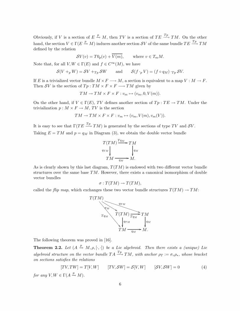
It is easy to see that Γ(TETp−→ TM) is generated by the sections of type TV and SV .

Taking E = TM and p = qM in Diagram (3), we obtain the double vector bundle

T (TM)TqM //

qTM

TM

qM

TM qM

// M.

As is clearly shown by this last diagram, T (TM) is endowed with two different vector bundlestructures over the same base TM . However, there exists a canonical isomorphism of doublevector bundles

σ : T (TM) → T (TM),

called the flip map, which exchanges these two vector bundle structures T (TM) → TM :

T (TM)qTM

**TTTTTTTTTTTTTTTTTTTT

TqM

99

99

99

99

99

99

99

99

9

σM%%KK

KKKKKKKK

T (TM)TqM

//

qTM

TM

qM

TM qM

// M.

The following theorem was proved in [16].

Theorem 2.2. Let (Ap−→ M,ρ, [·, ·]) be a Lie algebroid. Then there exists a (unique) Lie

algebroid structure on the vector bundle TATp−→ TM , with anchor ρT := σρ∗, whose bracket

on sections satisfies the relations

[TV, TW ] = T [V,W ] [TV,SW ] = S[V,W ] [SV,SW ] = 0 (4)

for any V,W ∈ Γ(Ap−→M).

6

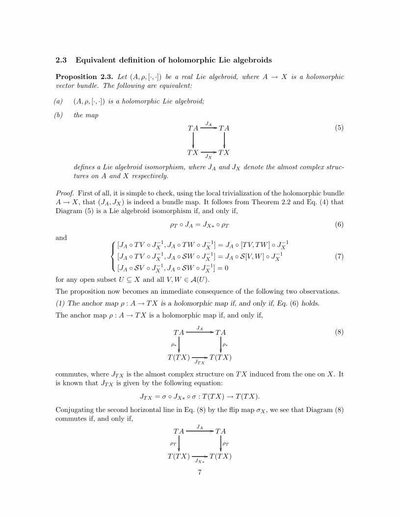
2.3 Equivalent definition of holomorphic Lie algebroids

Proposition 2.3. Let (A, ρ, [·, ·]) be a real Lie algebroid, where A → X is a holomorphicvector bundle. The following are equivalent:

(a) (A, ρ, [·, ·]) is a holomorphic Lie algebroid;

(b) the map

TA

JA // TA

TX

JX

// TX

(5)

defines a Lie algebroid isomorphism, where JA and JX denote the almost complex struc-tures on A and X respectively.

Proof. First of all, it is simple to check, using the local trivialization of the holomorphic bundleA→ X, that (JA, JX) is indeed a bundle map. It follows from Theorem 2.2 and Eq. (4) thatDiagram (5) is a Lie algebroid isomorphism if, and only if,

ρT JA = JX∗ ρT (6)

and

[JA TV J−1X , JA TW J−1

X ] = JA [TV, TW ] J−1X

[JA TV J−1X , JA SW J−1

X ] = JA S[V,W ] J−1X

[JA SV J−1X , JA SW J−1

X ] = 0

(7)

for any open subset U ⊆ X and all V,W ∈ A(U).

The proposition now becomes an immediate consequence of the following two observations.

(1) The anchor map ρ : A→ TX is a holomorphic map if, and only if, Eq. (6) holds.

The anchor map ρ : A→ TX is a holomorphic map if, and only if,

TAJA //

ρ∗

TA

ρ∗

T (TX)JTX

// T (TX)

(8)

commutes, where JTX is the almost complex structure on TX induced from the one on X. Itis known that JTX is given by the following equation:

JTX = σ JX∗ σ : T (TX) → T (TX).

Conjugating the second horizontal line in Eq. (8) by the flip map σX , we see that Diagram (8)commutes if, and only if,

TAJA //

ρT

TA

ρT

T (TX)

JX∗

// T (TX)

7

commutes, and the latter is precisely Eq. (6).

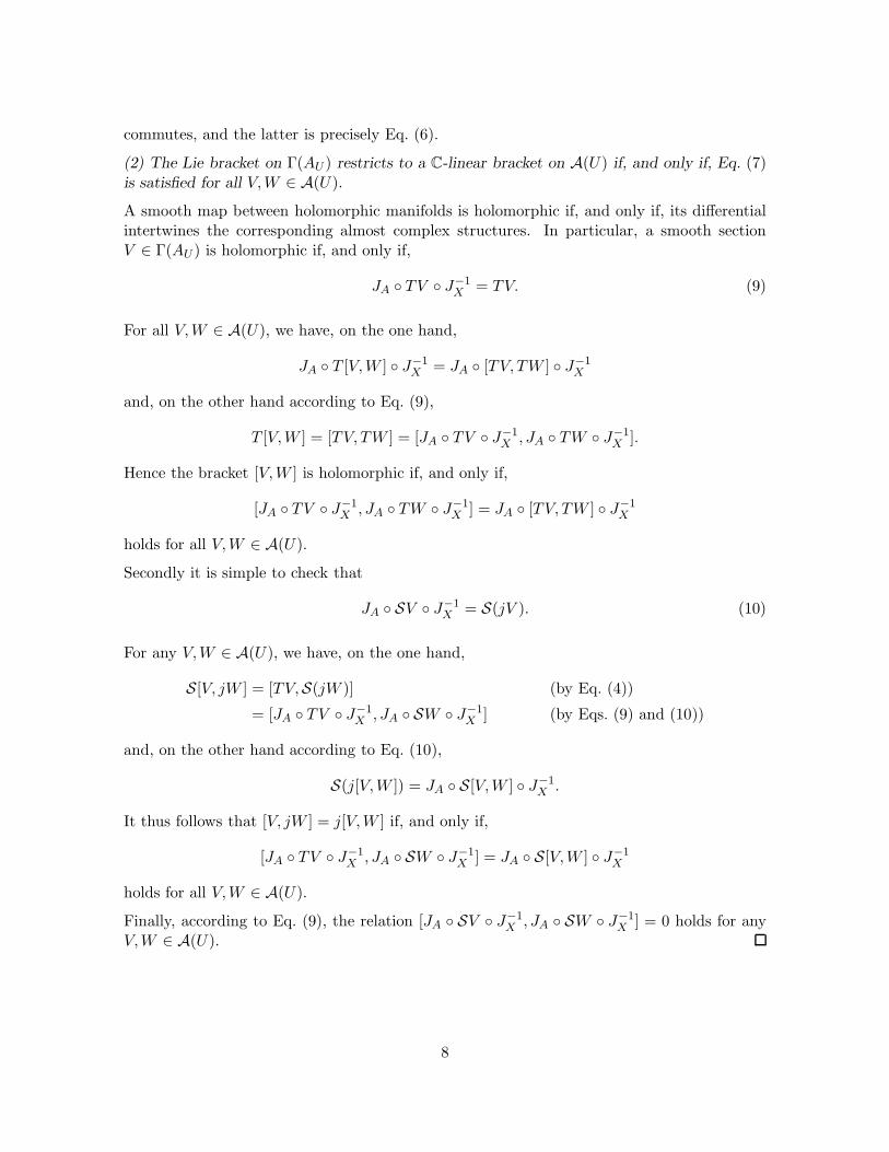
(2) The Lie bracket on Γ(AU ) restricts to a C-linear bracket on A(U) if, and only if, Eq. (7)is satisfied for all V,W ∈ A(U).

A smooth map between holomorphic manifolds is holomorphic if, and only if, its differentialintertwines the corresponding almost complex structures. In particular, a smooth sectionV ∈ Γ(AU ) is holomorphic if, and only if,

JA TV J−1X = TV. (9)

For all V,W ∈ A(U), we have, on the one hand,

JA T [V,W ] J−1X = JA [TV, TW ] J−1

X

and, on the other hand according to Eq. (9),

T [V,W ] = [TV, TW ] = [JA TV J−1X , JA TW J−1

X ].

Hence the bracket [V,W ] is holomorphic if, and only if,

[JA TV J−1X , JA TW J−1

X ] = JA [TV, TW ] J−1X

holds for all V,W ∈ A(U).

Secondly it is simple to check that

JA SV J−1X = S(jV ). (10)

For any V,W ∈ A(U), we have, on the one hand,

S[V, jW ] = [TV,S(jW )] (by Eq. (4))

= [JA TV J−1X , JA SW J−1

X ] (by Eqs. (9) and (10))

and, on the other hand according to Eq. (10),

S(j[V,W ]) = JA S[V,W ] J−1X .

It thus follows that [V, jW ] = j[V,W ] if, and only if,

[JA TV J−1X , JA SW J−1

X ] = JA S[V,W ] J−1X

holds for all V,W ∈ A(U).

Finally, according to Eq. (9), the relation [JA SV J−1X , JA SW J−1

X ] = 0 holds for anyV,W ∈ A(U).

8

2.4 Holomorphic Poisson manifolds

Definition 2.4. A holomorphic Poisson manifold is a complex manifold X equipped with aholomorphic bivector field π (i.e. π ∈ Γ(∧2T 1,0X) such that ∂π = 0), satisfying the equation[π, π] = 0.

Since ∧2TCX = ∧2TX ⊕ i ∧2 TX, for any π ∈ Γ(∧2TCX), we can write π = πR + iπI , whereπR and πI ∈ Γ(∧2TX) are (real) bivector fields on X. The following result was proved in [15].

Theorem 2.5 ([15]). Given a complex manifold X with associated almost complex structureJ , the following are equivalent:

(a) π = πR + iπI ∈ Γ(∧2T 1,0X) is a holomorphic Poisson bivector field;

(b) (πI , J) is a Poisson Nĳenhuis structure on X and π♯R = π♯

I J∗;

As a consequence, both πR and πI are Poisson tensors and they constitute a biHamiltoniansystem [14]. Both πR and πI define brackets ·, ·R and ·, ·I on C∞(M,R) in the standardway. These extend to C∞(M,C) by C-linearity. In a local chart (z1 = x1 + iy1, · · · , zn =xn + iyn) of complex coordinates of X, we indeed have

xi, xjR = 14ℜzi, zj, xi, xjI = 1

4ℑzi, zj,yi, yjR = −1

4ℜzi, zj, yi, yjI = −14ℑzi, zj,

xi, yjR = 14ℑzi, zj, xi, yjI = −1

4ℜzi, zj.

Here ℜ and ℑ denote the real and imaginary parts of a complex number.

Now we consider the cotangent bundle Lie algebroid of a holomorphic Poisson manifold andidentify its associated real and imaginary Lie algebroids. Assume that (X,π) is a holomorphicPoisson manifold, where π = πR + iπI ∈ Γ(∧2T 1,0X). Let A = (T ∗X)π be its correspondingholomorphic Lie algebroid, which can be defined in a similar way as in the smooth case. Tobe more precise, let Φ and Ψ, respectively, be the holomorphic bundle maps

Φ : TX → T 1,0X, Φ =1

2(1 − iJ)

andΨ : T ∗X → (T 1,0X)∗,Ψ = 1 − iJ∗,

where J is the almost complex structure on X. Define the anchor ρ : (T ∗X)π → TX to beρ = Φ−1 π# Ψ and the bracket

[α, β]π = Lραβ − Lρβα− d(ρα, β)

∀α, β ∈ Γ(T ∗X|U ) holomorphic. One easily sees that (T ∗X)π is a holomorphic Lie algebroid.Next proposition describes its real and imaginary Lie algebroids.

Proposition 2.6 ([15]). Let (X,π) be a holomorphic Poisson manifold, where π = πR+iπI ∈Γ(∧2T 1,0X). Then the underlying real and imaginary Lie algebroids of (T ∗X)π are isomorphicto (T ∗X)4πR

and (T ∗X)4πI, respectively.

9

3 Holomorphic Lie groupoids and holomorphic symplectic groupoids

3.1 Multiplicative (1,1)-tensors on Lie groupoids

Recall that a skew-symmetric (k, 1)-tensor on a smooth manifold M can be seen either as asection of the vector bundle ∧kT ∗M ⊗ TM → M , or as a bundle map ∧kTM → TM overthe identity on M . If Γ M is a Lie groupoid, then TΓ TM is naturally a Lie groupoid,called the tangent Lie groupoid [16]. Indeed for any k ≥ 1, this Lie groupoid structure extendsnaturally to a Lie groupoid ∧kTΓ ∧kTM , whose source, target, inverse and product mapsare given by ∧kTs, ∧kTt, ∧kT ι and ∧kTm, respectively. Here s, t, ι and m are the source,target, inverse and product maps of the groupoid Γ M .

Definition 3.1. A multiplicative (k, 1)-tensor φ on a Lie groupoid Γ M is a pair (φΓ, φM )of (k, 1)-tensors on Γ and M respectively such that

∧kTΓ

φΓ // TΓ

∧kTM

φM

// TM

is a Lie groupoid morphism.

Remark 3.2. It is simple to see that if (φΓ, φM ) is a multiplicative (k, 1)-tensor, φM iscompletely determined by φΓ, which is the restriction of φΓ to the unit space M . Hence weoften use φΓ to denote a multiplicative (k, 1)-tensor.

Proposition 3.3. If (φΓ, φM ) is a multiplicative (1, 1)-tensor on a Lie groupoid Γ M , then(NφΓ

,NφM) is a multiplicative (2, 1)-tensor on Γ.

The proof requires two lemmas. The first one, a general fact about Nĳenhuis tensors, is astraightforward consequence of Eq. (1). A (k, 1)-tensor φ on a manifold N is said to be tangentto a submanifold S ⊂ N if φ maps ∧kTS to TS. Any (k, 1)-tensor φ tangent to S induces byrestriction a (k, 1)-tensor on the submanifold S.

The following lemma can be easily verified.

Lemma 3.4. If S ⊂ N is a submanifold, and φ is (1, 1)-tensor tangent to S, then Nφ istangent to S. Moreover the restriction of Nφ to S is the Nĳenhuis tensor of the restriction ofφ to S.

The second lemma is a general fact regarding Lie groupoids, the proof of which is left to thereader. Recall that the graph of the multiplication of a given Lie groupoid Γ M is thesubmanifold ΛΓ

ΛΓ = (γ1, γ2, γ1γ2)|∀γ1, γ2 ∈ Γ s.t. t(γ1) = s(γ2)of Γ × Γ × Γ. Given a map Ψ : R→ R′, we denote by Ψ(3) the map

Ψ(3) : R×R×R→ R′ ×R′ ×R′ : (x, y, z) 7→(

Ψ(x),Ψ(y),Ψ(z))

.

10

Lemma 3.5.(a) The graphs of the multiplications of the Lie groupoids Γ M , TΓ TMand ∧2TΓ ∧2TM are related as follows

ΛTΓ = TΛΓ Λ∧2TΓ = ∧2TΛΓ.

(b) A smooth map Ψ from a Lie groupoid Γ M to another Lie groupoid Γ′ M ′ is a

groupoid homomorphism if, and only if, Ψ(3) maps ΛΓ to ΛΓ′.

Proof of Proposition 3.3. By Lemma 3.5(b), since the pair (φΓ, φM ) is a Lie groupoid homo-morphism, φ(3)

Γ : TΓ3 → TΓ3 maps ΛTΓ to itself. By Lemma 3.5(a), the latter is isomorphic

to TΛΓ. Hence φ(3)Γ is tangent to ΛΓ.

By Lemma 3.4, it follows that Nφ

(3)Γ

is also tangent to ΛΓ. A simple computation yields that

Nφ

(3)Γ

= N (3)φΓ.

Therefore N (3)φΓ

maps ∧2TΛΓ to TΛΓ. According to Lemma 3.5 again, this amounts to sayingthat (NφΓ

,NφM) is indeed a Lie groupoid homomorphism.

3.2 Nĳenhuis torsion of multiplicative (1,1)-tensors

Recall that, for any vector bundle Ep−→ M , one has the double vector bundle (3). Similarly,

one has the double vector bundle

∧2TETp

//

qE

∧2TM

qM

E p

// M.

(11)

In particular, when E is the tangent bundle TMp−→M , we have the double bundles

T (TM)Tp

//

qTM

TM

qM

TM p

// M

(12)

and

∧2T (TM)Tp

//

qTM

∧2TM

qM

TM p

// M.

(13)

11

There is an extension of the canonical flip map σ : T (TM) → T (TM), denoted by σ(1) inthis section, to T (∧2TM), which is defined as follows. Let µ ∈ Te1∧e2(∧2TM) be any tangentvector, where e1, e2 ∈ TmM . Write

µ = ddte1(t) ∧ e2(t)

∣

∣

0,

where e1(t), e2(t) ∈ Tm(t)M . Define

σ(2)(µ) = σ(1) ddte1(t)

∣

∣

∣

0∧ σ(1) d

dte2(t)

∣

∣

∣

0.

Then σ(2)(µ) is a vector in ∧2Tv(TM). Hence σ(2) maps Te1∧e2(∧2TM) to ∧2Tv(TM), wherev = (Tp)(e1 ∧ e2) ∈ TmM . Note that v changes according to e1 ∧ e2.

Lemma 3.6.(a) σ(1) is an isomorphism of double vector bundle (12), which interchangesthe horizontal and vertical bundle structures and induces the identities on the side bun-dles.

(b) σ(2) is an isomorphism from the double vector bundle

T (∧2TM)q∧2TM //

Tp

∧2TM

qM

TM p

// M

to the double vector bundle (13), which induces the identities on the side bundles.

Let φ : TM → TM be a (1, 1)-tensor on M . Then Tφ is a morphism of horizontal vector

bundle T (TM)Tp→ TM to itself over the identity. Define

Tφ = σ(1) Tφ (σ(1))−1.

From Lemma 3.6, it follows that Tφ is a morphism of vertical vector bundle qTM : T (TM) →TM to itself over the identity.

Similarly, if φ : ∧2TM → TM is a (2, 1)-tensor on M , then

Tφ = σ(1) Tφ (σ(2))−1

is a morphism from the vector bundle qTM : ∧2T (TM) → TM to the vector bundle qTM :T (TM) → TM over the identity.

Proposition 3.7. If φ is a (1, 1)-tensor (resp. (2, 1)-tensor) on a manifold M , then Tφ is a(1, 1)-tensor (resp. (2, 1)-tensor) on the manifold TM . Moreover, we have

NTφ = TNφ. (14)

12

Proof. It remains to prove Eq. (14). Note that for any section V of p : TM → M , TV is asection of Tp : T (TM) → TM , which is a tangent Lie algebroid. Let

TV = σ(1) TV.

Then TV is a section of the bundle qTM : T (TM) → TM , i.e. a vector field on TM .Considering p : TM → M as a Lie algebroid and Tp : T (TM) → TM as its tangent Liealgebroid, according to Eq. (4), we have [TV, TW ] = T [V,W ], where the left hand side of theequation refers to the Lie bracket of the tangent Lie algebroid T (TM) → TM . Hence

T[V,W ] = σ(1) T [V,W ] = σ(1) [TV, TW ] = [TV,TW ]. (15)

Here the bracket [TV,TW ] on the right hand side refers to the bracket on the vector fieldsX(TM), and the last equality follows from the definition of tangent Lie algebroid.

Now if φ is a (1, 1)-tensor on M , we have

(Tφ)(TV ) = σ(1) Tφ (σ(1))−1 σ(1) TV = σ(1) Tφ TV = σ(1) Tφ(V ) = T(φV ). (16)

Similarly, for any (2, 1)-tensor ψ on M and any sections V,W of TM →M , we have

(Tψ)(TV,TW ) = T(

ψ(V,W ))

. (17)

Using Eqs. (15) and (17), a simple computation leads to

NTφ(TV,TW ) = (TNφ)(TV,TW ).

On the other hand, using local coordinates, it is easy to see that for any u ∈ TM with u 6= 0and v ∈ Tu(TM), there always exists a section V of TM →M such that TV passes throughv at u. Since both NTφ and TNφ are (2, 1)-tensors on TM , it follows that they coincide at allpoints of TM except for the zero section of TM . Hence they must be equal at all points bycontinuity.

Now let Γ M be a Lie groupoid with Lie algebroid A. By definition A is identified withthe subbundle T s

MΓ of TΓ|M . In the sequel, we use this identification implicitly.

Let (φΓ, φM ) be a multiplicative (1, 1)-tensor on Γ. Then by Proposition 3.7, TφΓ is a (1, 1)-tensor on the manifold TΓ. Similarly if (ψΓ, ψM ) is a multiplicative (2, 1)-tensor on Γ, thenTψΓ is a (2, 1)-tensor on the manifold TΓ.

Lemma 3.8. Let (φΓ, φM ) and (ψΓ, ψM ) be a multiplicative (1, 1)-tensor and (2, 1)-tensor ona Lie groupoid Γ M , respectively. Then both TφΓ and TψΓ are tangent to the submanifoldT s

MΓ ⊂ TΓ. Hence they define a (1, 1)-tensor and (2, 1)-tensor on the submanifold T sMΓ of

TΓ.

Proof. By definition, TφΓ = σ(1)Tφ(σ(1))−1. It is well-known that σ(1) : T TsTMTΓ → T (T s

MΓ)is an isomorphism. Since φ : TΓ → TΓ is a groupoid morphism of the tangent groupoidTΓ TM , it follows that T Ts

TMTΓ is stable under Tφ. Hence it follows that T (T sMΓ) is stable

under Tφ. That is, TφΓ is tangent to the submanifold T sMΓ ⊂ TΓ.

Similarly, one proves that TψΓ is also tangent to T sMΓ.

13

Now we introduce

Definition 3.9. If (φΓ, φM ) (resp. (ψΓ, ψM )) is a multiplicative (1, 1)-tensor (resp. (2, 1)-tensor) on Γ, we define LieφΓ (resp. LieψΓ) to be the restriction of TφΓ (resp. TψΓ) to A(being identified with T s

MΓ and considered as a submanifold of TΓ).

The main result of this section is the following:

Theorem 3.10. Let Γ M be a Lie groupoid with Lie algebroid A. If φΓ is a multiplicative(1, 1)-tensor on Γ, then Lie(φΓ) is a (1, 1)-tensor on A (as a manifold), and Lie(NφΓ

) is a(2, 1)-tensor on A (as a manifold). Moreover we have

NLie(φΓ) = Lie(NφΓ). (18)

Proof. In Lemma 3.4, taking N = TΓ and S = T sMΓ, we obtain that NLieφΓ

= NTφΓ|T s

MΓ. The

latter is equal to TNφΓ|T s

MΓ according to Proposition 3.7, which is Lie(NφΓ

) by definition.

3.3 Infinitesimal multiplicative (1,1)-tensors

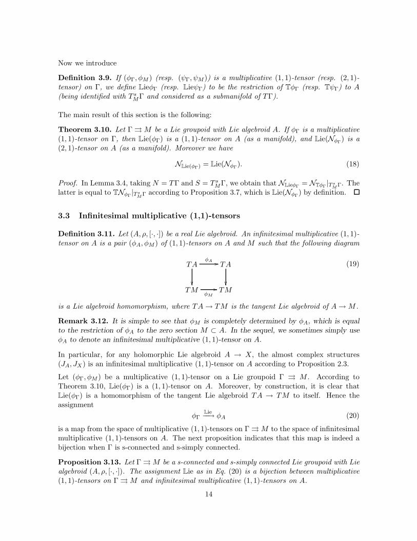
Definition 3.11. Let (A, ρ, [·, ·]) be a real Lie algebroid. An infinitesimal multiplicative (1, 1)-tensor on A is a pair (φA, φM ) of (1, 1)-tensors on A and M such that the following diagram

TAφA //

TA

TM

φM

// TM

(19)

is a Lie algebroid homomorphism, where TA→ TM is the tangent Lie algebroid of A→M .

Remark 3.12. It is simple to see that φM is completely determined by φA, which is equalto the restriction of φA to the zero section M ⊂ A. In the sequel, we sometimes simply useφA to denote an infinitesimal multiplicative (1, 1)-tensor on A.

In particular, for any holomorphic Lie algebroid A → X, the almost complex structures(JA, JX ) is an infinitesimal multiplicative (1, 1)-tensor on A according to Proposition 2.3.

Let (φΓ, φM ) be a multiplicative (1, 1)-tensor on a Lie groupoid Γ M . According toTheorem 3.10, Lie(φΓ) is a (1, 1)-tensor on A. Moreover, by construction, it is clear thatLie(φΓ) is a homomorphism of the tangent Lie algebroid TA → TM to itself. Hence theassignment

φΓLie−−→ φA (20)

is a map from the space of multiplicative (1, 1)-tensors on Γ M to the space of infinitesimalmultiplicative (1, 1)-tensors on A. The next proposition indicates that this map is indeed abĳection when Γ is s-connected and s-simply connected.

Proposition 3.13. Let Γ M be a s-connected and s-simply connected Lie groupoid with Liealgebroid (A, ρ, [·, ·]). The assignment Lie as in Eq. (20) is a bĳection between multiplicative(1, 1)-tensors on Γ M and infinitesimal multiplicative (1, 1)-tensors on A.

14

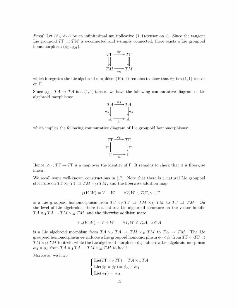
Proof. Let (φA, φM ) be an infinitesimal multiplicative (1, 1)-tensor on A. Since the tangentLie groupoid TΓ TM is s-connected and s-simply connected, there exists a Lie groupoidhomomorphism (φΓ, φM ):

TΓ

φΓ // TΓ

TM

φM

// TM

which integrates the Lie algebroid morphism (19). It remains to show that φΓ is a (1, 1)-tensoron Γ.

Since φA : TA → TA is a (1, 1)-tensor, we have the following commutative diagram of Liealgebroid morphisms:

TAφA //

qA

TA

qA

A

id// A

which implies the following commutative diagram of Lie groupoid homomorphisms:

TΓφΓ //

qΓ

TΓ

qΓ

Γ

id// Γ

Hence, φΓ : TΓ → TΓ is a map over the identity of Γ. It remains to check that it is fiberwiselinear.

We recall some well-known constructions in [17]. Note that there is a natural Lie groupoidstructure on TΓ ×Γ TΓ TM ×M TM , and the fiberwise addition map:

+Γ(V,W ) = V +W ∀V,W ∈ TγΓ, γ ∈ Γ

is a Lie groupoid homomorphism from TΓ ×Γ TΓ TM ×M TM to TΓ TM . Onthe level of Lie algebroids, there is a natural Lie algebroid structure on the vector bundleTA×A TA→ TM ×M TM , and the fiberwise addition map:

+A(V,W ) = V +W ∀V,W ∈ TaA, a ∈ A

is a Lie algebroid morphism from TA ×A TA → TM ×M TM to TA → TM . The Liegroupoid homomorphism φΓ induces a Lie groupoid homomorphism φΓ×φΓ from TΓ×ΓTΓ

TM×M TM to itself, while the Lie algebroid morphism φA induces a Lie algebroid morphismφA × φA from TA×A TA→ TM ×M TM to itself.

Moreover, we have

Lie(TΓ ×Γ TΓ) = TA×A TA

Lie(φΓ × φΓ) = φA × φA

Lie(+Γ) = +A

15

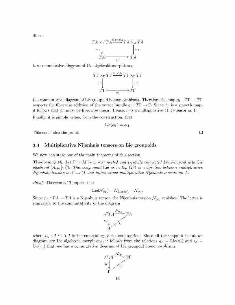
Since

TA×A TAφA×φA//

+A

TA×A TA

+A

TA

φA

// TA

is a commutative diagram of Lie algebroid morphisms,

TΓ ×Γ TΓφΓ×φΓ//

+Γ

TΓ ×Γ TΓ

+Γ

TΓ

φΓ

// TΓ

is a commutative diagram of Lie groupoid homomorphisms. Therefore the map φΓ : TΓ → TΓrespects the fiberwise addition of the vector bundle qΓ : TΓ → Γ. Since φΓ is a smooth map,it follows that φΓ must be fiberwise linear. Hence, it is a multiplicative (1, 1)-tensor on Γ.

Finally, it is simple to see, from the construction, that

Lie(φΓ) = φA.

This concludes the proof.

3.4 Multiplicative Nĳenhuis tensors on Lie groupoids

We now can state one of the main theorems of this section.

Theorem 3.14. Let Γ M be a s-connected and s-simply connected Lie groupoid with Liealgebroid (A, ρ, [·, ·]). The assignment Lie as in Eq. (20) is a bĳection between multiplicativeNĳenhuis tensors on Γ M and infinitesimal multiplicative Nĳenhuis tensors on A.

Proof. Theorem 3.10 implies that

Lie(NφΓ) = NLie(φΓ) = NφA

.

Since φA : TA→ TA is a Nĳenhuis tensor, the Nĳenhuis torsion NφAvanishes. The latter is

equivalent to the commutativity of the diagram

∧2TANφA //

qA

TA

A

ıA

;;wwwwwwwww

where ıA : A → TA is the embedding of the zero section. Since all the maps in the abovediagram are Lie algebroid morphisms, it follows from the relations qA = Lie(qΓ) and ıA =Lie(ıΓ) that one has a commutative diagram of Lie groupoid homomorphisms

∧2TΓNφΓ //

qΓ

TΓ

Γ

ıΓ

;;wwwwwwwww

16

where ıΓ : Γ → TΓ is the embedding to the zero section. Therefore the Nĳenhuis torsion NφΓ

vanishes. This completes the proof of the theorem.

3.5 Holomorphic Lie groupoids

Definition 3.15. : A holomorphic Lie groupoid is a (smooth) Lie groupoid Γ X, where bothΓ and X are complex manifolds and all the structure maps m, ǫ, ι, s and t are holomorphicmaps.

This definition requires a justification. The manifold

Γ2 = (γ1, γ2)|t(γ1) = s(γ2), γ1, γ2 ∈ Γ

admits a natural complex manifold structure since both the source and target maps areholomorphic surjective submersions. It thus makes sense to require the multiplication map tobe holomorphic.

The following result essentially follows from the definition and the Newlander-Nirenberg the-orem.

Proposition 3.16. The following assertions are equivalent:

(a) Γ X is a holomorphic Lie groupoid;

(b) Γ X is a real Lie groupoid, where Γ and X are almost complex manifolds withassociated almost complex structures JΓ and JX respectively such that (JΓ, JX) is amultiplicative Nĳenhuis tensor on Γ X.

A holomorphic Lie algebroid is said to be integrable if it is the Lie algebroid associated tosome holomorphic Lie groupoid.

The main theorem of this section is the following

Theorem 3.17. Assume that A→ X is a holomorphic Lie algebroid. Let Γ be a s-connectedand s-simply connected Lie groupoid integrating the underlying real Lie algebroid AR. ThenΓ admits a natural complex structure which makes it into a holomorphic Lie groupoid with itsholomorphic Lie algebroid being A→ X.

In other words, a holomorphic Lie algebroid A is integrable if, and only if, its underlying realLie algebroid AR is integrable. Similarly, a holomorphic Lie algebroid is integrable if, andonly if, its underlying imaginary Lie algebroid AI is integrable.

Proof. According to Proposition 2.3, the almost complex structure (JA, JX) is an infinitesimalmultiplicative Nĳenhuis tensor on A. By Theorem 3.14, it integrates to a multiplicativeNĳenhuis tensor (JΓ, JX) on Γ X. Since − idΓ : TΓ → TΓ is also a multiplicative (1, 1)-tensor and Lie(− idΓ) = − idA, it follows that J2

Γ = − idΓ and therefore JΓ is an almostcomplex structure on Γ. The conclusion thus follows from Proposition 3.16.

17

As a consequence, we can determine whether a holomorphic Lie algebroid is integrable byapplying the integrability criteria of Crainic-Fernandes: Theorem 4.1 in [6] to its underlyingreal Lie algebroid.

Remark 3.18. Note that, a complex structure on the Lie algebra of a real Lie group G ex-tends uniquely to an integrable complex Lie group structure on G. This is false for groupoids.The condition of s-connectedness and s-simply connectedness is indeed necessary. For in-stance, take a bundle of groups X × C X and consider it as a groupoid, where X is acomplex manifold and C is equipped with the additive group structure. Let L be a smoothnon-holomorphic function from X to the space of lattices in C (for instance X = C andf(x+ iy) = 1+ isin(x)) and consider the quotient groupoid (X×C)/L X. Clearly this is areal Lie groupoid integrating the underlying real Lie algebroid X × C → X with zero anchorand zero bracket. However the holomorphic structure on the Lie algebroid does not extendto a holomorphic groupoid structure on this quotient groupoid (X × C)/L X.

A holomorphic Lie algebroid may not be always integrable, as shown in the following

Example 3.19. Let X be a complex manifold and ω a holomorphic closed 2-form on X. ThenA : TX ⊕ (X × C) → X is naturally equipped with a holomorphic Lie algebroid structure,where the anchor is the projection onto the first component, and the Lie bracket is

[(X, f), (Y, g)] = ([X,Y ],X(g) − Y (f) + ω(X,Y )),

∀X,Y ∈ A(U), f, g ∈ OX(U). It is simple to see that its underlying real Lie algebroid AR isisomorphic to TX ⊕ (X × R

2) → X, where the Lie bracket is given by

[(X, f1, f2), (Y, g1, g2)] = ([X,Y ],X(g1) − Y (f1) + ω1(X,Y ),X(g2) − Y (f2) + ω2(X,Y )),

∀X,Y ∈ X(X) and f1, f2, g1, g2 ∈ C∞(R2,R), where ω1 and ω2 are the real and imaginaryparts of ω, respectively, i.e. ω = ω1 + iω2.

According to Example 3.7 in [6], the Lie algebroid TX ⊕ (X × R2) → X is integrable if and

only if the group of periods of (ω1, ω2):

(∫

γ

ω1,

∫

γ

ω2)| [γ] ∈ π2(M,x)

is a discrete subgroup of R2 (the argument in [6] is only presented for R-valued closed 2-forms,

but it clearly extends to R2-valued closed 2-forms).

Consider the complex manifold

N =

(z1, z2, z3) ∈ C3∣

∣z21 + z2

2 + z23 = 1

and the holomorphic 2-form on C3:

η =1

4π2

(

z1dz2 ∧ dz3 + z2dz3 ∧ dz1 + z3dz1 ∧ dz2)

.

It is clear that the pull back of η defines a holomorphic closed 2-form on N . By η1 and η2,we denote the real part and the imaginary part of η, respectively. Consider the submanifold

18

R3 of C

3 defined by R3 ∼= (z1, z2, z3)|y1 = y2 = y3 = 0. The intersection S of N with R

3 isa unit sphere:

S = N ∩ R3 =

(x1, x2, x3) ∈ R3∣

∣x21 + x2

2 + x23 = 1

The pull back of η1 to S is a real valued 2-form, which takes the same expression:

η1|S =1

4π2

(

x1dx2 ∧ dx3 + x2dx3 ∧ dx1 + x3dx1 ∧ dx2

)

.

It is clear that η1 is a volume form on the unit sphere:∫

Sη1 = 1. On the other hand, the pull

back of η2 to S vanishes.

Let X = N ×N , and ω =√

2 p∗1η+p∗2η, where p1, p2 stand for the projections on the first andsecond components. Then ω is a holomorphic closed 2-form on X. It is simple to see that thegroup of periods of (ω1, ω2) contains (1, 0) and (

√2, 0), and therefore is not discrete. Hence,

the corresponding holomorphic Lie algebroid A is not integrable.

We end this section with the following

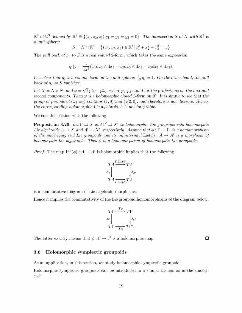
Proposition 3.20. Let Γ X and Γ′ X ′ be holomorphic Lie groupoids with holomorphic

Lie algebroids A→ X and A′ → X ′, respectively. Assume that φ : Γ → Γ′ is a homomorphismof the underlying real Lie groupoids and its infinitesimal Lie(φ) : A → A′ is a morphism ofholomorphic Lie algebroids. Then φ is a homomorphism of holomorphic Lie groupoids.

Proof. The map Lie(φ) : A→ A′ is holomorphic implies that the following

TAT Lie(φ)

//

JA

TA′

JA′

TA

T Lie(φ)// TA′

is a commutative diagram of Lie algebroid morphisms.

Hence it implies the commutativity of the Lie groupoid homomorphisms of the diagram below:

TΓTφ

//

JΓ

TΓ′

JΓ′

TΓ

Tφ// TΓ′.

The latter exactly means that φ : Γ → Γ′ is a holomorphic map.

3.6 Holomorphic symplectic groupoids

As an application, in this section, we study holomorphic symplectic groupoids.

Holomorphic symplectic groupoids can be introduced in a similar fashion as in the smoothcase.

19

Definition 3.21. A holomorphic symplectic groupoid is a holomorphic Lie groupoid Γ Xtogether with a holomorphic symplectic 2-form ω ∈ Ω2,0(Γ) such that the graph of multiplica-tion Λ ⊂ Γ × Γ × Γ is a Lagrangian submanifold, where Γ stands for the Γ equipped with theopposite symplectic structure.

As in the smooth case, this last condition is equivalent to ∂ω = 0 where ∂ : Ω2(Γ) → Ω2(Γ2)is the alternate sum of the pull back maps of the three face maps Γ2 → Γ. In this case, ω issaid to be multiplicative.

As in the smooth case, if Γ X is a holomorphic symplectic groupoid, then X is naturallya holomorphic Poisson manifold. More precisely, there exists a unique holomorphic Poissonstructure on X such that the source map s : Γ → X is a holomorphic Poisson map, while thetarget map is then an anti-Poisson map.

Given a holomorphic symplectic groupoid Γ X, its holomorphic Lie algebroid is isomorphicto the cotangent Lie algebroid (T ∗X)π → X, where π is the induced holomorphic Poissonstructure on X.

Conversely, a holomorphic Poisson manifold (X,π) is said to be integrable if it is the inducedholomorphic Poisson structure on the unit space of a holomorphic symplectic groupoid Γ X.We say that Γ X integrates the holomorphic Poisson structure (X,π).

The main theorem is the following:

Theorem 3.22. A holomorphic Poisson manifold is integrable if, and only if, either its realor its imaginary part is integrable as a real Poisson manifold.

More precisely, if (Γ X,ωR + iωI) is a holomorphic symplectic groupoid integrating theholomorphic Poisson structure (X,πR + iπI), then (Γ X, 4ωR) and (Γ X,−4ωI) aresymplectic groupoids integrating the real Poisson manifolds (X,πR) and (X,πI), respectively.

Conversely given a holomorphic Poisson manifold (X,π), where π = πR+iπI ∈ Γ(∧2T 1,0X), if(Γ X,ωR) is a s-connected and s-simply connected symplectic groupoid integrating (X,πR),then

(a) Γ X admits a holomorphic Lie groupoid structure. By JΓ : TΓ → TΓ we denote itsalmost complex structure;

(b) (Γ M,ωI), where ωI(·, ·) := ωR(JΓ·, ·), is a symplectic groupoid integrating (X,πI);

(c) (Γ X,ω), where ω := 14(ωR − iωI) , is a holomorphic symplectic groupoid integrating

(X,π).

This theorem can be derived from Theorem 5.2 in [20] or Theorem 3.4 in [5] via the equivalencerelation between holomorphic Poisson manifolds and Poisson Nĳenhuis structures establishedin Theorem 2.5. We, however, give a direct proof below, as an application of Theorem 3.22.We start with a simple fact of complex geometry.

Lemma 3.23. Let X be a complex manifold with almost complex structure J and αR ∈ Ω2(X)a two-form on the underlying real manifold. By αb

R we denote its induced bundle map αbR :

TX → T ∗X.

20

(a) If J∗ αbR = αb

R J , then α(·, ·) := α(·, ·) − iα(J ·, ·) is a (2, 0)-form on X.

(b) If, moreover, αbR : TX → T ∗X is a holomorphic map, then α is a holomorphic 2-form.

(c) Furthermore, dαR = 0 iff ∂α = 0.

Proof of Theorem 3.22. Assume that (Γ X,ωR+iωI) is a holomorphic symplectic groupoidintegrating the holomorphic Poisson structure (X,πR + iπI). Clearly, both (Γ X,ωR) and(Γ X,ωI) are symplectic groupoids. By ΠR and ΠI we denote the Poisson tensors corre-sponding to the symplectic two-forms ωR and ωI , respectively. Then the holomorphic Poissonbivector field corresponding to ω is 1

4(ΠR − iΠI). A Poisson map between two holomorphicPoisson manifolds is also a Poisson map between their real parts, and as well as between theirimaginary parts. As a consequence, we have 1

4s∗ΠR = πR and −14s∗ΠI = πI . It follows that

(Γ X, 4ωR) and (Γ X,−4ωI) are symplectic groupoids integrating, respectively, the realpart πR and the imaginary part πI of π.

Conversely, let (X,π), where π = πR + iπI ∈ Γ(∧2T 1,0X), be a holomorphic Poisson manifoldand (Γ X,ωR) a s-connected and s-simply connected symplectic groupoid integrating(X,πR). Hence the Lie algebroid of Γ X is isomorphic to (T ∗X)πR

. By Proposition 2.6,(T ∗X)πR

is the underlying real Lie algebroid of the holomorphic Lie algebroid (T ∗X) 14π.

According to Theorem 3.17, Γ X admits a multiplicative almost complex structure JΓ

which makes Γ into a holomorphic Lie groupoid.

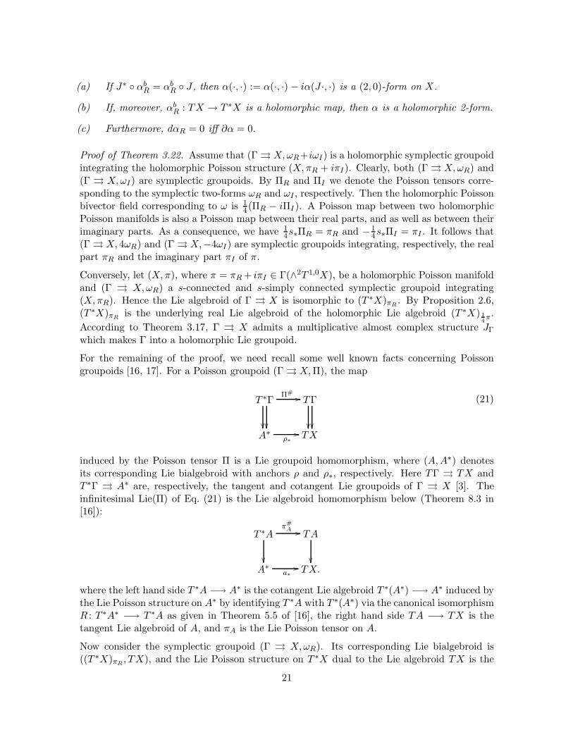
For the remaining of the proof, we need recall some well known facts concerning Poissongroupoids [16, 17]. For a Poisson groupoid (Γ X,Π), the map

T ∗Γ

Π#// TΓ

A∗

ρ∗// TX

(21)

induced by the Poisson tensor Π is a Lie groupoid homomorphism, where (A,A∗) denotesits corresponding Lie bialgebroid with anchors ρ and ρ∗, respectively. Here TΓ TX andT ∗Γ A∗ are, respectively, the tangent and cotangent Lie groupoids of Γ X [3]. Theinfinitesimal Lie(Π) of Eq. (21) is the Lie algebroid homomorphism below (Theorem 8.3 in[16]):

T ∗Aπ

#A //

TA

A∗

a∗

// TX.

where the left hand side T ∗A −→ A∗ is the cotangent Lie algebroid T ∗(A∗) −→ A∗ induced bythe Lie Poisson structure on A∗ by identifying T ∗A with T ∗(A∗) via the canonical isomorphismR : T ∗A∗ −→ T ∗A as given in Theorem 5.5 of [16], the right hand side TA −→ TX is thetangent Lie algebroid of A, and πA is the Lie Poisson tensor on A.

Now consider the symplectic groupoid (Γ X,ωR). Its corresponding Lie bialgebroid is((T ∗X)πR

, TX), and the Lie Poisson structure on T ∗X dual to the Lie algebroid TX is the

21

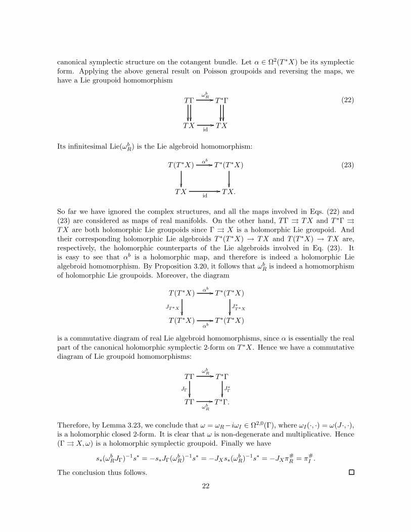
canonical symplectic structure on the cotangent bundle. Let α ∈ Ω2(T ∗X) be its symplecticform. Applying the above general result on Poisson groupoids and reversing the maps, wehave a Lie groupoid homomorphism

TΓ

ωbR // T ∗Γ

TX

id// TX

(22)

Its infinitesimal Lie(ωbR) is the Lie algebroid homomorphism:

T (T ∗X)αb

//

T ∗(T ∗X)

TX

id// TX.

(23)

So far we have ignored the complex structures, and all the maps involved in Eqs. (22) and(23) are considered as maps of real manifolds. On the other hand, TΓ TX and T ∗Γ

TX are both holomorphic Lie groupoids since Γ X is a holomorphic Lie groupoid. Andtheir corresponding holomorphic Lie algebroids T ∗(T ∗X) → TX and T (T ∗X) → TX are,respectively, the holomorphic counterparts of the Lie algebroids involved in Eq. (23). Itis easy to see that αb is a holomorphic map, and therefore is indeed a holomorphic Liealgebroid homomorphism. By Proposition 3.20, it follows that ωb

R is indeed a homomorphismof holomorphic Lie groupoids. Moreover, the diagram

T (T ∗X)αb

//

JT∗X

T ∗(T ∗X)

J∗T∗X

T (T ∗X)

αb

// T ∗(T ∗X)

is a commutative diagram of real Lie algebroid homomorphisms, since α is essentially the realpart of the canonical holomorphic symplectic 2-form on T ∗X. Hence we have a commutativediagram of Lie groupoid homomorphisms:

TΓωb

R //

JΓ

T ∗Γ

J∗Γ

TΓ

ωbR

// T ∗Γ.

Therefore, by Lemma 3.23, we conclude that ω = ωR− iωI ∈ Ω2,0(Γ), where ωI(·, ·) = ω(J ·, ·),is a holomorphic closed 2-form. It is clear that ω is non-degenerate and multiplicative. Hence(Γ X,ω) is a holomorphic symplectic groupoid. Finally we have

s∗(ωbRJΓ)−1s∗ = −s∗JΓ(ωb

R)−1s∗ = −JXs∗(ωbR)−1s∗ = −JXπ

#R = π#

I .

The conclusion thus follows.

22

Indeed the exact same proof as above leads to the following

Theorem 3.24. Let (X,π), where π = πR + iπI ∈ Γ(∧2T 1,0X), be a holomorphic Poissonmanifold. Assume that Γ X is a holomorphic Lie groupoid with almost complex structureJΓ, whose corresponding holomorphic Lie algebroid is (T ∗X)1

4π. Moreover, assume that there

exists a symplectic real 2-form ωR on the underlying real Lie groupoid such that (Γ X,ωR)is a symplectic groupoid integrating the real Poisson structure πR. Then ω = ωR − iωI ∈Ω2,0(Γ), where ωI(·, ·) = ω(J ·, ·), is a multiplicative holomorphic symplectic 2-form on Γ sothat (Γ X, 1

4ω) is a holomorphic symplectic groupoid integrating the holomorphic Poissonstructure π.

3.7 Holomorphic extension of analytic Poisson structures

To any analytic Poisson structure πreal on Rn, there associates a canonical holomorphic Pois-

son structure π on Cn, called its holomorphic extension, which can be defined as follows.

Assume that the Poisson brackets of πreal, on the canonical coordinates, are given by

xi, xj = φij(x1, . . . , xn),

where φij are, for all i, j = 1, . . . , n, real analytic functions on Rn. Then the Poisson brackets

of its holomorphic extension on Cn are given by

zi, zj = φij(z1, · · · , zn).

Then we have the following:

Theorem 3.25. If the holomorphic extension π of a real analytic Poisson structure πreal isintegrable, then πreal must be integrable.

Let πR and πI be the real part and the imaginary part of π. We advise the reader to keep inmind that πR is a smooth bivector field on C

n, and not to confuse it with πreal, which is asmooth bivector field on R

n.

Recall that a Poisson involution on a Poisson manifold P is a Poisson diffeomorphism Φ :P −→ P such that Φ2 = id.

Lemma 3.26. The complex conjugation map σ(z1, · · · , zn) = (z1, · · · , zn) is a Poisson invo-lution of (Cn, πR).

Proof. We write φij = fij + igij , where fij, gij ∈ C∞(Cn,R), and zk = xk + iyk, k = 1, · · · , n.One computes immediately that

πR = 14

∑ni,j=1 fij(z1, . . . , zn)( ∂

∂xi∧ ∂

∂xj− ∂

∂yi∧ ∂

∂yj)

+14

∑ni,j=1 gij(z1, . . . , zn)( ∂

∂xi∧ ∂

∂yj+ ∂

∂yi∧ ∂

∂xj).

By constructions, we have σ∗φij = φij . Thus it follows that ∀i, j = 1, · · · , n,

σ∗fij = fij , σ∗gij = −gij. (24)

23

On the other hand, it is obvious that

σ∗(∂

∂xj) =

∂

∂xj, σ∗(

∂

∂yj) = − ∂

∂yj(25)

The conclusion thus follows immediately.

Remark 3.27. Note that σ is an anti-Poisson map with respect to the imaginary part πI

of π.

It is well known that the stable locus of a Poisson involution carries a natural Poisson structure[11, 22]. More precisely, let Q be the stable locus of a Poisson involution Φ : P −→ P . Assumethat the Poisson tensor π on P is π =

∑

iXi ∧ Yi, where Xi and Yi are vector fields on P .Then the induced Poisson tensor πQ on Q is given by

πQ =∑

i

X+i ∧ Y +

i |Q, (26)

where X+i and Y +

i are vector fields on P defined by X+i = 1

2(Xi + Φ∗Xi) and Y +i = 1

2 (Yi +Φ∗Yi), respectively. The Poisson manifold (Q,πQ) is called a Dirac submanifold of (P, π)(which is also called a Lie-Dirac submanifold in [7]).

The following result was proved in [22] (see also [10, 7]).

Proposition 3.28. If Q is the stable locus of a Poisson involution on an integrable Poissonmanifold P , then Q is always an integrable Poisson manifold itself.

Lemma 3.29. Let π be the holomorphic extension on Cn of an analytic Poisson structure

πreal on Rn. The induced Poisson structure on the stable locus of the Poisson involution σ

on (Cn, πR) is isomorphic to (Rn, 14πreal).

Proof. Let Q be the stable locus of σ. Then Q = (z1, · · · , zn)|y1 = · · · = yn = 0 ∼= Rn. By

Eqs. (24) and (26), we have

(πR)Q =1

4

n∑

i,j=1

fij(z1, . . . , zn)|Q∂

∂xi∧ ∂

∂xj.

Since fij(z1, · · · , zn)|Q = φij(x1, · · · , xn), the right hand side is equal to 14πreal.

Proof of Theorem 3.25. It follows immediately from Theorem 3.22, Proposition 3.28 andLemma 3.29.

Example 3.30. Consider the holomorphic Poisson structure

π = ez21+z2

2+z23

2 z1∂

∂z2∧ ∂

∂z3+ c.p. (27)

on C3. It is clear that this is a holomorphic extension of the analytic Poisson structure:

πreal = ex21+x2

2+x23

2 x1∂

∂x2∧ ∂

∂x3+ c.p. (28)

on R3.

According to Example 3.3 in [8], the Poisson structure (28) is not integrable. By Theorem3.25, the holomorphic Poisson structure (27) on C

3 is not integrable either.

24

References

[1] M. N. Boyom, KV-cohomology of Koszul-Vinberg algebroids and Poisson manifolds,Internat. J. Math.16 (2005), no. 9, 1033–1061.

[2] S. Canez, Private communication.

[3] A. Coste, P. Dazord, and A. Weinstein, Groupoïdes symplectiques, Publications du Dé-partement de Mathématiques. Nouvelle Série. A, Vol. 2, Publ. Dép. Math. Nouvelle Sér.A, 87, Univ. Claude-Bernard, Lyon, 1987, pp. i–ii, 1–62.

[4] A. Cattaneo and G. Felder, Poisson sigma models and symplectic groupoids, Prog. Math.198 (2001) 61–93,

[5] M. Crainic, Generalized complex structures and Lie brackets arXiv:math/0412097

[6] M. Crainic and R.-L. Fernandes, Integrability of Lie brackets. Ann. of Math. (2) 157

(2003), 575–620.

[7] M. Crainic and R.-L. Fernandes, Integrability of Poisson brackets, J. Differential Geom-etry. 66 (2004), 71–137.

[8] M. Crainic and R.L. Fernandes, Lectures on integrability of Lie brackets,arXiv:0611259v1

[9] S. Evens, J.-H. Lu, and A. Weinstein, Transverse measures, the modular class, and acohomology pairing for Lie algebroids, Quart. J. Math. Oxford (2) 50 (1999), 417-436.arXiv:dg-ga/9610008v1

[10] R.L. Fernandes, A note on proper Poisson actions, arXiv:0503147.

[11] Fernandes, R., and Vanhaecke, P., Hyperelliptic Prym varieties and integrable systems,Commun. Math. Phys.221 (2001) 169-196.

[12] J. Huebschmann, Duality for Lie-Rinehart algebras and the modular class, J. ReineAngew. Math.510 (1999), 103–159.

[13] Y. Kosmann-Schwarzbach, The Lie bialgebroid of a Poisson-Nĳenhuis manifold. Lett.Math. Phys., 38(4):421–428, 1996.

[14] Y. Kosmann-Schwarzbach and F. Magri, Poisson-Nĳenhuis structures. Ann. Inst. H.Poincaré Phys. Théor., 53(1):35–81, 1990.

[15] C.-G. Laurent, M. Stienon, and P. Xu, Holomorphic Poisson manifolds and holomorphicLie algebroids, Preprint 2008.

[16] K. C. H. Mackenzie and P. Xu, Lie bialgebroids and Poisson groupoids. Duke Math. J.,73(2):415–452, 1994.

[17] K. C. H. Mackenzie and P. Xu, Integration of Lie bialgebroids. Topology, 39(3):445–467,2000.

25

[18] F. Magri and C. Morosi, On the reduction theory of the Nĳenhuis operators and itsapplications to Gelfand-Dikiı equations, Proceedings of the IUTAM-ISIMM symposiumon modern developments in analytical mechanics, Vol. II (Torino, 1982), 117, 1983,pp. 599–626.

[19] F. Magri and C. Morosi, Old and new results on recursion operators: an algebraic ap-proach to KP equation, Topics in soliton theory and exactly solvable nonlinear equations(Oberwolfach, 1986), World Sci. Publishing, Singapore, 1987, pp. 78–96.

[20] M. Stiénon and P. Xu, Poisson quasi-Nĳenhuis manifolds. Comm. Math. Phys. 27 (2007),709–725.

[21] A. Weinstein, The integration problem for complex Lie algebroids, From Geometry toQuantum Mechanics, in Honor of Hideki Omori, Y. Maeda, T. Ochiai, P. Michor, andA. Yoshioka, eds., Progress in Mathematics, Birkhäuser, New York (2007), 93-109.

[22] P. Xu, Dirac submanifolds and Poisson involutions, Ann. Scient. Ec. Norm. Sup. 36

(2003), 403–430.

26

Documents

Integration of holomorphic Lie algebroids