i

Integrated and Data-Driven

Transportation Infrastructure Management

through Consideration of

Life Cycle Costs and Environmental Impacts

By

ARASH SABOORI

DISSERTATION

Submitted in partial satisfaction of the requirements for the degree of

DOCTOR OF PHILOSOPHY

in

Civil and Environmental Engineering

in the

OFFICE OF GRADUATE STUDIES

of the

UNIVERSITY OF CALIFORNIA

DAVIS

Approved:

_______________________________ Professor John Harvey, Chair

_______________________________

Professor Alissa Kendall

_______________________________ Professor Miguel Jaller

Committee in Charge

2020

ProQuest Number:

All rights reserved

INFORMATION TO ALL USERSThe quality of this reproduction is dependent on the quality of the copy submitted.

In the unlikely event that the author did not send a complete manuscript and there are missing pages, these will be noted. Also, if material had to be removed,

a note will indicate the deletion.

Published by ProQuest LLC (

ProQuest

). Copyright of the Dissertation is held by the Author.

All Rights Reserved.This work is protected against unauthorized copying under Title 17, United States Code

Microform Edition © ProQuest LLC.

ProQuest LLC789 East Eisenhower Parkway

P.O. Box 1346Ann Arbor, MI 48106 - 1346

28023138

28023138

2020

ii

To My Dearest Wife & Best Friend in Life,

Aida For All Her Love, Patience,

Constructive Feedback, and Sacrifices

iii

ABSTRACT

The main goal of this dissertation was to develop frameworks, quantitative models, and databases needed

to support data-driven, informed, and integrated decision-making in managing the vast transportation

infrastructure in California. Such a management system was envisioned to consider both costs and

environmental impacts of management decisions, based on full life cycles of the infrastructure, and using

reliable, high quality data that well represent local conditions in terms of materials and energy sources,

production technologies, design methods, construction practices, and other critical parameters.

This PhD research consisted of three parts: 1) development of a comprehensive life cycle inventory (LCI)

database for implementation of life cycle assessment (LCA) methodology in transportation infrastructure

management in California. 2) Evaluation of current and potential sustainability actions at the state and

local government levels through the development of frameworks, models, and datasets needed for

objective and accurate quantification of the impacts of management decisions. 3) Assessment of recycling

practices available for pavements at their end of life to quantify changes in environmental impacts

compared to conventional methods, considering the effects of recycling through the use stage.

Through the first part of this research, the most comprehensive and up to date, as of 2019, life cycle

inventory database, the UCPRC LCI Database, was developed for accurate quantification of

transportation infrastructure management projects in the state of California. This database includes an

extensive list of all the energy sources, materials, mixes, transportation modes, and construction processes

used in the projects at state and local government levels.

In the UCPRC LCI Database, the electricity grid mix and other energy sources used in various life cycle

stages are modified to represent the state’s local conditions. Mix designs are defined based on

specifications enforced by Caltrans and also cover designs used by local governments. Construction

practices are closely simulated based on data collected from local contractors and experts in addition to

the collection of primary data from a few field projects. The LCI database developed and presented in this

chapter has been verified by a third party according to ISO recommendations.

In the second part of this research, multiple studies were also carried out to develop decision-making

frameworks, models, and tools for local governments and state agencies to assess their policies and

alternative decision choices in meeting their sustainability goals. The frameworks in each case laid the

roadmap in terms of what needs to be included in the study and what models are needed for quantifying

the environmental impacts. The UCPRC LCI Database was then utilized to develop the required models

in each case, which were then assembled in tools that can calculate life cycle costs and environmental

impacts of different alternatives.

The first project in part two compared urban street designs from a widely used complete street design

guide and conventional street designs. The comparison used LCA to consider the full life cycle

environmental impacts of conversion of several types of conventional streets to complete streets. The full

system impacts of complete streets on environmental impact indicators, considering materials,

iv

construction, and traffic changes, are driven by changes in reduction in VMT and changes in the operation

of the vehicles with regard to speed and drive cycle changes caused by congestion, if it occurs. An LCA

comparison of complete street implementation revealed the importance of considering speed and drive

cycle changes caused by congestion where it occurs.

The initial results indicate that application of the complete streets networks to streets where there is little

negative impact on vehicle drive cycles from speed change will have the most likelihood of causing

overall net reductions in environmental impacts. The results also indicate that there is a range of potential

VMT changes to which environmental impacts are more sensitive than they are to the effects of the

materials and construction stages, and that changes in vehicle speed have different effects on

environmental impacts depending on the context of their implementation, including the street type.

This second study in part two focused on comparing multiple pathways (scenarios) for Caltrans to

transition their fleet from vehicles with internal combustion engines burning fossil fuels to alternative

fleet vehicles (AFVs.) Four scenarios were considered based on AFV adoption rate including business as

usual (BAU), All-at-Once, a scenario based on the Department of General Services (DGS)

recommendations, and a Worst-Case scenario (do nothing, keep the current mix.) The project compared

the life cycle greenhouse gas (GHG) emissions, fuel consumption, and costs of vehicle purchase and

maintenance between 2018 and 2050.

The results showed a total life cycle costs of 2.4 billion dollars for the BAU case with 7.4 and 3.3 percent

increases versus BAU for the DGS and All-at-Once cases, and a 16.9 percent decrease for the Worst-Case

Scenario. Total GHG emissions during the analysis period of 2018 to 2050 reached close to 1.46 million

metric tonnes (MMT) of CO2e for the BAU case while the results for the DGS, All-at-Once show savings

of 2 and 9 percent in total GHG emissions versus BAU for the DGS and All-at-Once scenarios. The

Worst-Case Scenario results show that consequences of inaction in the adopting AFVs by Caltrans and

maintaining the current mix of vehicle technology and fuel will result in 54 percent increase in the GHG

footprint of their fleet between now and the year 2050.

The third chapter in part two focused on quantifying savings in greenhouse gases (GHG), energy, material

consumption, and costs that might be possible through increased use of recycled asphalt pavements

(RAP) in construction projects in California. The material production impacts of hot mix asphalt (HMA)

in Caltrans construction projects throughout the state during the entire analysis period of 33 years (2018

to 2050) results in close to 11.5 MMT of CO2e for the baseline scenario.

Increasing the RAP content in HMA from the baseline of the 11.5 percent can result in up to a 6 percent

of GHG savings with 30.5 percent RAP content during the 33-year analysis period, when using aromatic

BTX rejuvenating agents (RAs.) These reductions are equivalent to 0.7, 5.2, 6.2 percent reductions in

GHG emissions compared to the baseline. The potential saving can be as high as 9 percent when bio-

based RA is used.

The last segment of this research focused on end-of-life (EOL) of flexible pavements and developed the

required models for full life cycle comparison of alternatives. Cradle-to-laid impacts of conventional

v

alternatives and new in-place recycling options were first calculated followed by development of

performance prediction models that are needed to identify future performance during the use stage.

This first study in the last part was conducted to benchmark the cradle-to-laid environmental impacts of

several EOL treatments used in California for flexible pavements at their end of service life. The results

show that the material production stage is dominant in all impact categories for all treatments. The results

also show that the total amount of stabilizer added (which depends on percent stabilizer and the layer

thickness) has a significant impact on the total impacts. HMA overlay and HMA mill-and-fill have lower

impacts compared to all the full-depth reclamation (FDR)options with stabilizers across all impact

categories. Binder and stabilizer production caused more than 90 percent of the total impacts of the

material production across all cases.

The last study was focused on development of crack progression and roughness models for cold in-place

recycling (CIR) and FDR sections. Such models, which did not exist up to this point, allow a fair

comparison of EOL alternatives for flexible pavements by providing the means necessary for quantifying

the use stage impacts and including them in the analysis. As always, there is no EOL solution that fits all

cases, and the optimal decision is context sensitive. The selection of one treatment among all available

alternatives depends on circumstances (traffic levels, climate, and structural design), agency goals (only

considering costs or both costs and environmental impacts), project scope and analysis period (initial

costs and impacts versus full life cycle), and potential limitations (in terms of budget, available

technologies, and more).

vi

ACKNOWLEDGEMENT

This research was mainly funded by the California Department of Transportation, Division of Research

and Innovation. It was partly supported by a PhD grant from the U.S. Department of Transportation,

which was awarded by the National Center of Sustainable Transportation (NCST) at UC Davis Institute

of Transportation Studies.

I want to thank my advisor, Prof. John Harvey, for his continued support and insight throughout my PhD

years, without which I would not be able to finish this work. I am also grateful to my dissertation

committee members, Professor Alissa Kendall and Professor Miguel Jaller, for their support and guidance

on my dissertation. I would also like to thank Professor Boulanger and Professor Novan for serving as my

qualifying examination committee members. Great thanks go to Dr. Jeremy Lee, Dr. Ting Wang, and Dr.

Hui Li and my classmates, Dr. Yuan He, and Dr. Shawn Hung, for their help and support throughout my

PhD, especially in the first few quarters that I was adjusting to the new environment. I would also like to

thank all the UCPRC members that have helped and supported my research pursuits here.

I am incredibly grateful to my wife, Aida, for all her support and sacrifices. I would not be able to finish

this work without her continuous love and support. I am also in great debt to my parents and both my

brothers, Anooshiravan and Ashkan, for maintaining the magnificent support system that they have

provided me with throughout my life, especially during this chapter.

vii

TABLE OF CONTENTS

ABSTRACT ................................................................................................................................................. iii

ACKNOWLEDGEMENT ........................................................................................................................... vi

TABLE OF CONTENTS ............................................................................................................................ vii

LIST OF FIGURES .................................................................................................................................... xii

LIST OF TABLES .................................................................................................................................... xvii

ACRONYMS ............................................................................................................................................. xxi

CHAPTER 1. Introduction ........................................................................................................................ 1

CHAPTER 2. Background, Problem Statement, and Research Objectives .............................................. 4

2.1. Pavement LCA ............................................................................................................................... 7

2.1.1. Material Production................................................................................................................. 8

2.1.2. Construction, Maintenance, and Rehabilitation ...................................................................... 9

2.1.3. Use ........................................................................................................................................ 11

2.1.4. End-of-Life ........................................................................................................................... 13

2.1.5. The Issue of Allocation in LCA Studies ............................................................................... 15

2.1.6. Cost Effectiveness ................................................................................................................. 18

2.2. Implementation of Life Cycle Thinking in Local Roads Management in California .................. 18

2.3. Problem Statement and Gaps in the Knowledge .......................................................................... 20

2.4. Research Objectives ..................................................................................................................... 21

CHAPTER 3. Comprehensive Life Cycle Inventory for Transportation Infrastructure Projects, Calibrated to the Energy Mix, Technologies, and State-of-Practice in California.................................. 22

3.1. Introduction .................................................................................................................................. 22

3.2. Goal and Scope Assumptions Used to Develop Inventories ........................................................ 25

3.2.1. Goal and Scope of CARB/Caltrans Lawrence Berkeley National Laboratory Heat Island Study ............................................................................................................................................... 25

3.2.2. eLCAP ................................................................................................................................... 27

3.3. Allocation ..................................................................................................................................... 27

3.4. Life Cycle Impact Assessment ..................................................................................................... 28

3.5. Energy Sources ............................................................................................................................ 30

3.5.1. Electricity .............................................................................................................................. 30

3.5.4. Summary of Energy Sources ................................................................................................. 33

3.6. Material Production Stage for Conventional Materials ............................................................... 35

viii

3.6.1. Aggregate (Crushed) ............................................................................................................. 35

3.6.2. Aggregate (Natural) .............................................................................................................. 37

3.6.3. Bitumen ................................................................................................................................. 37

3.6.4. Bitumen Emulsion................................................................................................................. 40

3.6.5. Cement .................................................................................................................................. 41

3.6.6. Cement Admixtures .............................................................................................................. 48

3.6.7. Crumb Rubber Modifier ........................................................................................................ 48

3.6.8. Dowel and Tie Bar ................................................................................................................ 49

3.6.10. Paraffin (Wax)..................................................................................................................... 53

3.6.11. Quicklime ............................................................................................................................ 53

3.6.12. Reclaimed Asphalt Pavement (RAP) .................................................................................. 53

3.6.13. Styrene Butadiene Rubber (SBR) ....................................................................................... 54

3.6.14. Summary of the Material Production Impacts for Conventional Materials ........................ 55

3.7. Material Production Stage for Reflective Coatings ..................................................................... 55

3.8. Transportation Stage .................................................................................................................... 58

3.9. Mix Designs and Material Production Stage of Various Pavement Surface Treatments ............. 59

3.9.1. Bonded Concrete Overlay on Asphalt (BCOA) .................................................................... 60

3.9.2. Cape Seal .............................................................................................................................. 61

3.9.3. Cement Concrete ................................................................................................................... 61

3.9.4. Chip Seal ............................................................................................................................... 62

3.9.5. Fog Seal ................................................................................................................................ 62

3.9.6. Conventional Asphalt Concrete (Mill-and-Fill and Overlay-Only) ...................................... 62

3.9.7. Conventional Interlocking Concrete Pavement (Pavers) ...................................................... 64

3.9.8. Permeable Asphalt Concrete Pavement ................................................................................ 65

3.9.9. Permeable Portland Cement Concrete .................................................................................. 65

3.9.10. Reflective Coatings ............................................................................................................. 65

3.9.11. Rubberized Asphalt Concrete (Mill-and-Fill and Overlay-Only) ....................................... 66

3.9.12. Sand Seal ............................................................................................................................. 67

3.9.13. Slurry Seal ........................................................................................................................... 67

3.10. End-of-Life (EOL) Treatments: Cold In-Place Recycling and Full-Depth Recycling .............. 67

3.11. Construction Stage for Various Surface Treatments .................................................................. 67

3.12. Summary of Cradle-to-Gate Impacts (Material Production, Transportation, and Construction)

for Various Surface Treatments .......................................................................................................... 72

ix

3.13. Data Quality Requirements and Data Validation ....................................................................... 76

3.13.1. Data Quality Requirements ................................................................................................. 77

3.13.2. Data Validation ................................................................................................................... 78

3.14. Summary .................................................................................................................................... 85

CHAPTER 4. LCA Comparison of Urban Street Design Methodologies: Complete Streets versus Conventional Streets, with Sensitivity Analysis on Key Model Parameters .......................................... 87

4.1. Introduction .................................................................................................................................. 87

4.2. Goal and Scope ............................................................................................................................ 87

4.3. Assumptions and Modeling Approach ......................................................................................... 88

4.4. Data Sources and Data Quality .................................................................................................... 92

4.5. Study Limitations and Gaps ......................................................................................................... 92

4.6. Results and Discussion................................................................................................................. 93

4.7. Sensitivity Analysis and Conclusions .......................................................................................... 95

4.7.1. Change in VMT .................................................................................................................... 95

4.7.2. Changes in Traffic Speed ...................................................................................................... 99

4.8. Summary .................................................................................................................................... 103

CHAPTER 5. Assessment of Different Pathways for Adoption of Alternative Fuel Vehicles by Caltrans Fleet Services Considering Changes in GHG Emissions and Life Cycle Costs ................................... 105

5.1. Introduction ................................................................................................................................ 105

5.2. Background ................................................................................................................................ 106

5.2.1. Key Federal Statutes ........................................................................................................... 107

5.2.2. Major Initiatives in California ............................................................................................. 107

5.2.3. AFVs Acquired by Fleets Regulated under EPAct at National-Level ................................ 108

5.2.4. AFVs Acquired by State Agencies’ Fleet Services in California ....................................... 110

5.2.5. AFVs Currently Available in the Market ............................................................................ 111

5.3. Goal and Scope Definition ......................................................................................................... 112

5.4. Assumptions and Modeling Approach ....................................................................................... 113

5.4.1. Caltrans Fleet Statistics ....................................................................................................... 117

5.4.2. Annual Vehicle Miles Traveled (AVMT) ........................................................................... 121

5.4.3. Vehicle Fuel Efficiency ...................................................................................................... 121

5.4.4. Fuel Costs ............................................................................................................................ 125

5.4.5. Vehicle Costs ...................................................................................................................... 131

5.4.6. Fleet Replacement Schedule ............................................................................................... 133

5.4.7. Salvage Value ..................................................................................................................... 136

x

5.4.8. Life Cycle Environmental Impacts ..................................................................................... 136

5.5. Data Sources and Data Quality .................................................................................................. 148

5.6. Study Limitations and Gaps ....................................................................................................... 149

5.7. Results and Discussion............................................................................................................... 150

CHAPTER 6. Evaluation of Increased Use of Reclaimed Asphalt Pavement in Construction Projects Considering Costs and Environmental Impacts .................................................................................... 158

6.1. Introduction ................................................................................................................................ 158

6.2. Background ................................................................................................................................ 158

6.3. Goal and Scope Definition ......................................................................................................... 159

6.4. Assumptions and Modeling Approach ....................................................................................... 160

6.4.1. Material Consumption per Year .......................................................................................... 161

6.4.2. Mix Designs ........................................................................................................................ 162

6.4.3. LCA Calculations ................................................................................................................ 163

6.5. Data Sources and Data Quality .................................................................................................. 165

6.6. Study Limitations and Gaps ....................................................................................................... 165

6.7. Results and Discussion............................................................................................................... 168

6.7.1. GHG Emissions per Year .................................................................................................... 168

6.7.2. Cost Considerations ............................................................................................................ 168

6.7.3. RAP Cost Savings ............................................................................................................... 169

6.7.4. Discussion ........................................................................................................................... 171

6.8. The Issue of Allocation in LCA of Recycled Materials ............................................................. 172

CHAPTER 7. Cradle-to-Laid LCA Benchmarking and Comparison of Currently Available Alternatives for End of Life Treatment for Flexible Pavements in California .......................................................... 177

7.1. Introduction ................................................................................................................................ 177

7.2. Overview of In-Place Recycling of Flexible pavements ............................................................ 178

7.3. In-Place Recycling Technologies for Flexible Pavements ......................................................... 178

7.3.1. Construction Processes and Materials for Cold In-Place Recycling ................................... 179

7.3.2. Construction Processes and Materials for Full Depth Reclamation .................................... 182

7.4. Life Cycle Assessment Framework ........................................................................................... 183

7.4.1. Goal and Scope Definition .................................................................................................. 183

7.4.2. Life Cycle Inventory and Impact Assessment .................................................................... 188

7.4.3. Mix Designs for CIR and FDR Alternatives ....................................................................... 188

7.4.4. Transportation of Materials to Site ..................................................................................... 189

7.4.5. Construction Activities ....................................................................................................... 190

xi

7.4.6. End of Life .......................................................................................................................... 192

7.5. Final Results and Interpretation ................................................................................................. 192

7.6. Further Analysis on Transportation Distance ............................................................................ 197

7.7. Conclusions ................................................................................................................................ 198

CHAPTER 8. Performance Prediction Models for In-Place Recycling for Quantification of Use Stage Impacts .................................................................................................................................................. 200

8.2.2. Data Cleaning ...................................................................................................................... 204

8.3. Performance Modeling ............................................................................................................... 207

8.3.1. Cracking Models ................................................................................................................. 208

8.3.2. Roughness Models .............................................................................................................. 216

8.4. Conclusions ................................................................................................................................ 219

CHAPTER 9. Summary, Conclusions, and Recommended Future Work ............................................ 221

9.1. Introduction ................................................................................................................................ 221

9.2. Knowledge Gaps and Research Objectives................................................................................ 221

9.3. UCPRC LCI Database ............................................................................................................... 222

9.4. Complete Streets ........................................................................................................................ 222

9.5. Alternative Fuel Vehicles ........................................................................................................... 223

9.6. Increased Use of RAP in Construction Projects ........................................................................ 224

9.7. LCA Benchmarking of EOL Alternatives.................................................................................. 226

9.8. Performance Prediction Models ................................................................................................. 227

REFERENCES ......................................................................................................................................... 229

APPENDIX I. Review of Pavement LCA Models, Databases, and EOL Studies .................................... 240

APPENDIX II. Complete Streets LCA ..................................................................................................... 248

APPENDIX III. Increased Use of RAP .................................................................................................... 263

xii

LIST OF FIGURES

Figure 1.1: Research scope, main topics and projects covered under each topic ......................................... 2

Figure 2.1: General life cycle of a production system (Kendall, 2012.) ....................................................... 6

Figure 2.2: General life cycle assessment framework according to ISO (2006.) .......................................... 6

Figure 2.3: Life cycle stages of a pavement (Harvey et al., 2010.) .............................................................. 9

Figure 2.4: Flowchart for developing the construction stage LCI. ............................................................. 10

Figure 2.5: Flowchart for determining impacts of traffic delay caused by construction activities. ............ 11

Figure 2.6: GWP impact ranges for pavement life cycle components (Santero and Horvath, 2009.) ........ 12

Figure 2.7: EOL allocation rules potentially applicable for pavements (Van Dam et al., 2015.) ............... 17

Figure 2.8: Breakdown of public road ownership in California based on lane-miles (Caltrans, 2018a). ... 19

Figure 3.1: Scope of the pLCA tool............................................................................................................. 28

Figure 3.2: Scope of the eLCAP software. ................................................................................................. 29

Figure 3.3: Parameters used in the electricity model. ................................................................................. 31

Figure 3.4: The inputs and outputs of the electricity model. ...................................................................... 32

Figure 3.5: The model developed for the California electricity grid mix. .................................................. 32

Figure 3.6: Diesel combusted in industrial equipment................................................................................ 33

Figure 3.7: Inputs and outputs of diesel combusted in industrial equipment. ............................................. 34

Figure 3.8: Natural gas combusted in industrial equipment ....................................................................... 34

Figure 3.9: Inputs and outputs of the natural gas model. ............................................................................ 35

Figure 3.10: Model developed for crushed aggregate production. ............................................................. 36

Figure 3.11: Inputs and outputs of the crushed aggregate model. .............................................................. 37

Figure 3.12: The GaBi model developed for natural aggregate. ................................................................. 38

Figure 3.13: Inputs and outputs of the natural aggregate model. ................................................................ 39

Figure 3.14: GaBi model developed for bitumen........................................................................................ 39

Figure 3.15: Inputs and outputs of the bitumen model. .............................................................................. 40

Figure 3.16: The model developed for cement (general.) ........................................................................... 43

Figure 3.17: Inputs and outputs of the general model for cement that can be modified by a user. ............ 44

Figure 3.18: The model developed for cement production (precalciner method + CA electricity mix.) ... 44

Figure 3.19: Inputs and outputs of the precalciner method for production of portland cement. ................. 45

Figure 3.20: The model for cement production (preheater method + CA electricity mix.) ........................ 46

Figure 3.21: Inputs and outputs of the preheater method for production of portland cement..................... 47

Figure 3.22: The model developed for bitumen emulsion. ......................................................................... 48

Figure 3.23: Inputs and outputs of the bitumen emulsion model. ............................................................... 48

Figure 3.24: GaBi model developed for crumb rubber modifier (CRM.) ................................................... 49

Figure 3.25: Inputs and outputs for the grinding process of the CRM model............................................. 49

Figure 3.26: Inputs and outputs for the crushing process of the CRM model. ........................................... 49

Figure 3.27: Inputs and outputs for the pulverization process of the CRM model. .................................... 50

Figure 3.28: Model developed in GaBi for dowel and tie bar. ................................................................... 50

Figure 3.29: Inputs and outputs of the epoxy coating model taken from GaBi. ......................................... 51

Figure 3.30: Inputs and outputs for a 1.25 in dowel. .................................................................................. 51

Figure 3.31: Inputs and outputs for a 1.5 in dowel. .................................................................................... 52

xiii

Figure 3.32: Inputs and outputs for ¾ in tie bar. ......................................................................................... 52

Figure 3.33: The model developed for limestone. ...................................................................................... 52

Figure 3.34: Inputs and outputs of the limestone model. ............................................................................ 53

Figure 3.35: The model developed for HMA (the mix design can be modified) ........................................ 63

Figure 3.36: Inputs and outputs of the HMA model. .................................................................................. 64

Figure 3.37: The GaBi model developed for PCC. ..................................................................................... 65

Figure 3.38: Inputs and outputs of the PCC model. .................................................................................... 66

Figure 4.1: Cross section of a thoroughfare (Sacramento County, 2009.) .................................................. 90

Figure 4.2: LA-DG recommendation for thoroughfare as a complete street (City of LA, 2014) ............... 90

Figure 4.3: NACTO recommendation for thoroughfare from urban street design guide (NACTO, 2013)

pp. 13. ......................................................................................................................................................... 91

Figure 4.4: Breakdown of materials and construction (MAC) GWP of complete streets between their

conventional (Conv.) elements and complete street (CS) elements. ........................................................... 94

Figure 4.5: Histogram of changes in daily traffic after implementing road diets on conventional streets in

San Jose (Nixon et al., 2017.) ..................................................................................................................... 97

Figure 4.6: Difference in well-to-wheel and MAC GWP [kg CO2e] impacts (CS-Conv) during the

analysis period (30 years) for 32-ft minor residential only considering changes in VMT for well-to-wheel.

.................................................................................................................................................................... 98

figure 4.7: Difference in well-to-wheel and MAC GWP [kg CO2e] impacts (CS-CONV) during the

analysis period (30 years) for 96-ft thoroughfare only considering changes in VMT for well-to-wheel ... 98

Figure 4.8: Cumulative GHG emissions for 32-ft minor residential assuming only changes in VMT. ...... 99

Figure 4.9: Cumulative GHG emissions for 96-ft thoroughfare assuming only changes in VMT. ............ 99

Figure 4.10: Changes in MPG with speed based on US EPA’s MOVES data. ........................................ 101

Figure 4.11: Changes in tailpipe GHG emissions based on EMFAC model. ........................................... 101

Figure 4.12: Changes in tailpipe PM2.5 emissions based on EMFAC. .................................................... 102

Figure 4.13: Difference in well-to-wheel and MAC GWP [kg CO2e] impacts (CS-Conv) during the

analysis period (30 years) for 32-ft minor residential considering changes in both VMT and traffic speed

for well-to-wheel impacts. ........................................................................................................................ 102

Figure 4.14: Difference in well-to-wheel and MAC GWP [kg CO2e] impacts (CS-Conv) during the

analysis period (30 years) for 96-ft thoroughfare considering changes in both VMT and Traffic Speed for

well-to-wheel impacts. .............................................................................................................................. 103

Figure 4.15: Well-to-Wheel GHG emissions versus speed for a mix of 60% passenger cars and 40% light

duty trucks type 1. ..................................................................................................................................... 103

Figure 5.1:Breakdown of the national and statewide GHG emissions (MMT CO2e) by sector in the U.S.

and California in 2016 (EPA webpage on the U.S. GHG emissions, CARB webpage on CA GHG

emissions.) ................................................................................................................................................ 105

Figure 5.2: AFV acquisitions by regulated fleets per year by fuel type (top figure) and distribution of

AFV acquisitions per year by fuel type (bottom figure) ........................................................................... 109

Figure 5.3: Breakdown of AFV acquired by fleets regulated under EPAct between 1997-2017. ............ 110

Figure 5.4: Breakdown of state agencies fleet vehicles by fuel type in the year 2014. ............................ 111

Figure 5.5: Current model offerings for AFVs by vehicle category (AFDC webpage on AFVs.) ........... 111

Figure 5.6: Alternative fuel vehicles acquired by Caltrans since 2014 (Caltrans, 2018b) ........................ 113

Figure 5.7: Flowchart of model development used for this study. ............................................................ 116

xiv

Figure 5.8: Breakdown of each general category (sedans, vans, and trucks) into asset types in 2017

Caltrans fleet. ............................................................................................................................................ 119

Figure 5.9: Summary statistics of Caltrans fleet in 2017. ......................................................................... 120

Figure 5.10: Caltrans fleet age distribution. .............................................................................................. 120

Figure 5.11: Distribution of vehicles by vehicle miles traveled per day. .................................................. 121

Figure 5.12: Historical fuel efficiency values by vehicle category (EPA webpage on Fuel Economy

Trends and EIA webpage on AER2018) ................................................................................................... 122

Figure 5.13: MPG projections for selected vehicle fuel combinations, PUT: pickup truck, PC: passenger

car.) ........................................................................................................................................................... 123

Figure 5.14: Fuel efficiency in miles per gallon equivalent (MPGe) in the year 2018 by fuel and vehicle

category (bar charts on top) and the annual growth rate in MPGe (bottom bar charts.) ........................... 124

Figure 5.15: Historical prices of alternative fuels, dollar per gallon gasoline equivalent (GGE) (AFDC

webpage on Fuel Prices.) .......................................................................................................................... 125

Figure 5.16: Variation in fuel historical prices 2012-2017 (AFDC webpage on Fuel Prices.) ................. 126

Figure 5.17: Projection of future prices of fuels (EIA webpage on AEO2018.) ....................................... 126

Figure 5.18: Comparison of gasoline prices between California and the U.S. average. ........................... 128

Figure 5.19: Comparison of diesel prices between California and the U.S. average (EIA webpage on Price

of Petroleum and Other Liquids.) ............................................................................................................. 129

Figure 5.20: Comparison of electricity price in California versus the U.S. average, comparison of average

price of all sectors on top and transportation sector prices in the bottom (EIA webpage on the Electricity

Sector.) ...................................................................................................................................................... 130

Figure 5.21: Variation in electricity price ratio (California over the U.S. average) across different

economic sectors (EIA webpage on the Electricity Sector.) ..................................................................... 131

Figure 5.22: Natural gas price ratio (California over the U.S. average) by year (EIA webpage on Natural

Gas.) .......................................................................................................................................................... 131

Figure 5.23: Average annual growth rate in vehicle price (EIA webpage on Vehicle Price Projections in

AEO2018. ................................................................................................................................................. 133

Figure 5.24: Count of vehicles Caltrans acquired and disposed each year between 1997 to 2014 (DB2011-

14.) ............................................................................................................................................................ 134

Figure 5.25: Changes in Caltrans fleet count per year between 1997 to 2014 (DB2011-14.) .................. 134

Figure 5.26: The average age of vehicles disposed of by Caltrans, by vehicle type and fuel type (DB2011-

14.) ............................................................................................................................................................ 135

Figure 5.27: Comparison of components impacts across vehicle types, and breakdown of components

impacts. ..................................................................................................................................................... 140

Figure 5.28: Vehicle cycle GHG emissions in kg CO2e per vehicle lifetime (left) Breakdown of vehicle

cycle impacts by four main vehicle cycle items: fluids, batteries, ADR, and components (middle) Ranges

of the share of total vehicle cycle impacts for each main vehicle cycle item across all vehicle types (right)

.................................................................................................................................................................. 140

Figure 5.29: Annual percent change in vehicle weight and vehicle weight (lbs.) in 2018 and 2050 per

vehicle type (EIA webpage on New Vehicle Attributes in AEO 2018.) .................................................. 141

Figure 5.30: Average passenger vehicle weight by fuel type (EIA webpage on New Vehicle Attributes in

AEO 2018.) ............................................................................................................................................... 142

Figure 5.31: Percent increase in weight compared to conventional ICE vehicle (EIA webpage on New

Vehicle Attributes in AEO 2018.)............................................................................................................. 142

xv

Figure 5.32: WTP, PTW, and WTW for different feedstocks of selected vehicle fuel technologies. ...... 144

Figure 5.33: WTW and fuel cycle comparison of different light-duty vehicle types. .............................. 147

Figure 5.34: Comparison of life cycle cash flow across four scenarios. ................................................... 154

Figure 5.35: Comparison of GHG emissions across four scenarios: total GHG emissions, vehicle cycle

emissions, and emissions due to various fuel life cycle stages (WTP, PTW, and WTW.) ....................... 155

Figure 5.36: Comparison of total fuel consumption across all four cases. ............................................... 156

Figure 5.37: Comparison of WTW GHG emissions across cases. ........................................................... 157

Figure 6.1: Flowchart of model development used for this study. ............................................................ 161

Figure 6.2: Materials needed per year between 2018-2050 based on PaveM outputs. ............................. 162

Figure 6.3: GWP (kg CO2e) of material production stage for 1 kg of each of the mixes. ........................ 165

Figure 6.4. Breakdown of GWP between components across all mix designs considered in this study .. 166

Figure 6.5: Change in total GHG emissions between 2018-2050 compared to the baseline for the three

scenarios with higher RAP content. .......................................................................................................... 170

Figure 6.6: Percent change in GHG emissions compared to the baseline for mixes with higher RAP

content. ...................................................................................................................................................... 171

Figure 6.7: Ratio of GWP of 1 kg of HMA (using RAP over using virgin materials, under two allocation

methods.) ................................................................................................................................................... 176

Figure 7.1: CIR process: (a) construction (Van Dam et al., 2015); (b) CIR equipment (Wirtgen, 2012) 185

Figure 7.2: FDR process: (a) construction (Van Dam et al., 2015); (b) FDR equipment (Wirtgen, 2012.)

.................................................................................................................................................................. 186

Figure 7.3: FDR+FA construction process in the field (Jones et al., 2016.) ............................................. 187

Figure 7.4: Flowchart used for developing LCI and LCIA of the construction activities. ....................... 190

Figure 7.5: Comparison of total cradle to laid GHG and PED between all cases. .................................... 195

Figure 7.6: Comparison of GWP (kg CO2e) of treatments across cradle to laid life cycle stages. ........... 196

Figure 8.1: Application of performance models for a full life cycle comparative LCA between

alternatives. ............................................................................................................................................... 201

Figure 8.2: The framework to be used in the comparative LCA study between EOL treatments. ........... 202

Figure 8.3: Flowchart for conducting the data cleaning. .......................................................................... 205

Figure 8.4: Sample of the scatterplots and boxplots for time versus distress developed for each LOC to

evaluate reasonableness of roughness and cracking time histories (blue line indicating the application of a

new treatment, red line indicating an FDR or CIR treatment.) ................................................................. 206

Figure 8.5: Representation of one of the performance model tree branches. ............................................ 208

Figure 8.6: Survival curve for CIR sections (the legend refers to traffic levels) averaged across overlay

thickness and climate regions. .................................................................................................................. 210

Figure 8.7: Survival curve for FDR sections (the legend refers to traffic level) , averaged across overlay

thickness and climate regions. .................................................................................................................. 211

Figure 8.8: Crack initiation and progression models combined for CIR sections (A, B, C refer to low,

medium, and high traffic levels; Thin, Med, and Thick refer to surface thickness category.) .................. 214

Figure 8.9: Crack initiation and progression models combined for FDR sections (A, B, C refer to low,

medium, and high traffic levels.) .............................................................................................................. 215

Figure 8.10: Crack initiation and progression models combined for conventional “Thin Overlay” sections

(A, B, C refer to low, medium, and high traffic levels.) ........................................................................... 215

Figure 8.11: Crack initiation and progression models combined for conventional “Medium Overlay”

sections (A, B, C refer to low, medium, and high traffic levels.) ............................................................. 216

xvi

Figure 8.12: Crack initiation and progression models combined for conventional “Thick Overlay”

sections (A, B, C refer to low, medium, and high traffic levels.) ............................................................. 216

xvii

LIST OF TABLES

Table 2.1. Classification of environmental analysis tools based on the type and object of the study

(Finnveden and Moberg, 2005). Acronyms are defined in Table 2.2 ........................................................... 4

Table 2.2. Description of different environmental analysis tools ................................................................. 5

Table 2.3. Speed, acceleration, and fuel consumption in various traffic flow conditions for a Peugeot 406

sedan (Lepert and Brillet, 2009) ................................................................................................................. 11

Table 2.4. Inventory sources contributing to pavement life-cycle stages (FHWA, 2014) .......................... 14

Table 2.5. Maintained road miles and estimated annual vehicle miles of travel (AVMT) by jurisdiction

(Caltrans, 2018a) ......................................................................................................................................... 18

Table 3.1. The third-party review committee members .............................................................................. 23

Table 3.2. Energy sources and materials included in the UCPRC LCI database ....................................... 23

Table 3.3. Pavement composite surface materials and treatments, and transportation modes included in

the database ................................................................................................................................................. 24

Table 3.4. Parameters of interest in the cool pavement study ..................................................................... 26

Table 3.5. List of surface treatments considered in the cool pavements study ........................................... 26

Table 3.6. Possible allocation methods to be used for selected pavement materials in the database ......... 27

Table 3.7. TRACI 2.1 impact categories and selected inventory items to be used in the UCPRC eLCAP

software ....................................................................................................................................................... 30

Table 3.8. Electricity generation mix in CA (a) In year 2012 (CA Energy Almanac webpage) ............... 31

Table 3.9. Summary of selected LCI and LCIA results for energy sources (based on the 2012 CA

electricity grid mix) ..................................................................................................................................... 33

Table 3.10. (a) Aggregate—crushed production in plant, reproduction of table 10 of Marceau (2007) .... 35

Table 3.11. Aggregate—natural production in plant, reproduction of Table 9 of Marceau (2007) ............ 37

Table 3.12. Energy and material requirements for bitumen emulsion production in plant (one tonne of

residual bitumen), data from section 6.4 of the Eurobitume report (Eurobitume, 2012) ............................ 41

Table 3.13. Mineral stage composition of portland cement (type I/II & III) and Calcium Sulfo-aluminate

cement ......................................................................................................................................................... 42

Table 3.14. Modeling milling process of a 1 ln-km road to produce RAP ................................................. 53

Table 3.15. Transportation impacts of hauling 1 ln-km of RAP to the plant for further processing .......... 54

Table 3.16. Selected LCI and LCIA results for 1 kg of RAP, using the cut-off method for allocation ...... 54

Table 3.17. Selected LCI and LCIA results for 1 kg of RAP, using the 50/50 method for allocation ....... 54

Table 3.18. Summary of selected LCI and LCIA results for conventional materials (based on 2012 CA

electricity grid mix) ..................................................................................................................................... 56

Table 3.19. Summary of LCI and LCIA for conventional materials, energy sources, and transportation

(based on 2020 ca electricity grid mix) ....................................................................................................... 57

Table 3.20. Chemicals in each coating, mass breakdown, and LCI datasets used (GaBi, 2014) ................ 57

Table 3.21. Summary LCI and LCIA of reflective coatings ....................................................................... 58

Table 3.22. Summary of LCI and LCIA for major transportation modes (GaBi) ....................................... 59

Table 3.23. Pavement surface treatment alternatives considered ............................................................... 60

Table 3.24. Mix design for BCOA with three levels of SCM..................................................................... 61

Table 3.25. Mix designs for PCC items (mass per 1 m3 of mix) ................................................................. 61

xviii

Table 3.26. HMA with RAP mix design (percent by mass) ....................................................................... 63

Table 3.27. RHMA mix design ................................................................................................................... 66

Table 3.28. Typical in-place end of life recycling treatments in California ............................................... 67

Table 3.29. Construction process for different surface treatments (modeled based on Caltrans

specifications, consultation with local experts, and literature) ................................................................... 68

Table 3.30. Construction process for EOL treatments ................................................................................ 70

Table 3.31. Summary LCI and LCIA of treatments for default thicknesses and a functional unit of 1 ln-

km: 2012 grid mix ....................................................................................................................................... 72

Table 3.32. Summary LCI and LCIA of EOL treatments for a functional unit of 1 ln-km: 2012 grid mix 73

Table 3.33. Summary LCI and LCIA of treatments for 1 ln-km of treatment (with 2020 electricity grid

mix) ............................................................................................................................................................. 74

Table 3.34. Quality assessment methodology used for selected criteria ..................................................... 77

Table 3.35. (a) Data quality assessment of constituent materials and transportation modes ...................... 79

Table 3.36. Comparison of results for some of the database items with other sources .............................. 85

Table 3.37. Data sources for the main processes that were taken directly from GaBi................................ 85

Table 4.1. Conventional street dimensions (Sacramento County, 2009) .................................................... 89

Table 4.2. Street types in SAC-DG and their assumed equivalent categories in LA-DG ........................... 89

Table 4.3. Data sources and data quality assessment .................................................................................. 92

Table 4.4. Absolute values of various impacts categories for the two design options for the materials,

transportation, and construction (MAC) stages: conventional (Conv) and complete streets (CS) ............. 93

Table 4.5. Absolute change in MAC Impacts (impacts of CS-Option minus impacts of Conv.-Option) ... 94

Table 4.6. Percent change in MAC impacts (CS-Conv.)/Conv. ................................................................. 95

Table 4.7. Traffic assumptions made for traffic levels and speeds ............................................................. 96

Table 4.8. Well-to-wheel impacts of vehicle fuel combustion during the 30-year analysis period for

conventional design scenarios ..................................................................................................................... 96

Table 4.9. Conventional design speed limits and NACTO recommended values for different street types

.................................................................................................................................................................. 100

Table 5.1. Top 10 state agencies in California based on fleet size (out of 64 fleets reporting to DGS in the

year 2014. The total state vehicle count was 39,471) ............................................................................... 110

Table 5.2. Alternative fuel light-duty vehicle registration in the U.S. by 2018 (AFDC webpage on AFVs)

.................................................................................................................................................................. 112

Table 5.3. Two vehicle replacement schedules considered in this study .................................................. 114

Table 5.4. AFVs substitutes chosen for various vehicle types in Caltrans fleet ....................................... 114

Table 5.5. Vehicle categories and ............................................................................................................. 118

Table 5.6. Average annual vehicle miles traveled by vehicle category (DB2017) ................................... 121

Table 5.7. The average annual growth rate for vehicle fuel efficiency (EIA webpage on AER2018) ..... 123

Table 5.8. Price ratio of alternative fuels (California over U.S. averages) ............................................... 127

Table 5.9. Average purchase price by vehicle and fuel type (DB2011-14) .............................................. 132

Table 5.10. Number of vehicles acquired, minimum, average, and maximum purchase price by vehicle

type ............................................................................................................................................................ 132

Table 5.11. Average age and miles of Caltrans’ disposed vehicles, by vehicle type (DB2011-14) ......... 135

Table 5.12. Current DGS policy for fleet replacement (CA DGS webpage on Vehicle Replacement

Policy) ....................................................................................................................................................... 135

Table 5.13. Average service life by vehicle type ...................................................................................... 136

xix

Table 5.14. Weight comparison of trucks fuel tank: diesel vs. CNG (Reinhart, 2016) ............................ 138

Table 5.15. Vehicle cycle GHG emissions by fuel type (kg CO2e per kg of the vehicle) ........................ 138

Table 5.16. Final dataset used in the model for WTP, WTW, and vehicle cycle GHG impacts .............. 144

Table 5.17. Data sources used in this study and data quality assessment ................................................. 148

Table 5.18. Comparison of life cycle cost (in million dollars) across cases ............................................. 151

Table 5.19. Comparison of total GHG emissions between 2018 and 2050 (Tonnes of CO2e) and .......... 151

Table 5.20. Comparison of total vehicle on-board liquid fuel consumption ............................................. 151

Table 5.21. Breakdown of GHG emissions for cases with negative WTP ............................................... 152

Table 5.22. Abatement cost and potential for each case ........................................................................... 153

Table 6.1.The five scenarios considered for HMA for Caltrans projects across the entire network ........ 163

Table 6.2. Mix design component quantities by mass of mix for ............................................................. 163

Table 6.3. LCI of the items used in this study .......................................................................................... 163

Table 6.4. Environmental impacts of material production stage for 1 kg of each of the mixes................ 164

Table 6.5. Data sources and data quality assessment ................................................................................ 167

Table 6.6. Total changes in GHG emissions compared to the baseline for the analysis period (2018 to

2050) ......................................................................................................................................................... 168

Table 6.7. Annual tonnage of material, and costs ..................................................................................... 169

Table 6.8. Cost ($/ton) of virgin binder and aggregate ............................................................................. 169

Table 6.9. Cost savings for each mix ($ per tonne of HMA) .................................................................... 170

Table 6.10. Summary of abatement potential for increased RAP use in asphalt pavements in California172

Table 6.11. Factorial of cases considered for the main input parameters in evaluating the impact of

allocation methodology on RAP LCI........................................................................................................ 173

Table 6.12. LCI of background items used ............................................................................................... 174

Table 7.1. The EOL treatments considered in this study .......................................................................... 183

Table 7.2. Impact categories and inventories reported in this study ......................................................... 184

Table 7.3. HMA with RAP mix design ..................................................................................................... 189

Table 7.4. RHMA mix design ................................................................................................................... 189

Table 7.5. Summary of LCI and LCIA for the mixes used as the wearing course ................................... 189

Table 7.6. LCI and LCIA of transportation .............................................................................................. 190

Table 7.7. Construction details for each of the EOL treatments for 1 ln-km ............................................ 190

Table 7.8. Well-to-wheel impacts of burning 1 gallon of diesel in the equipment ................................... 191

Table 7.9. Summary of LCI and LCIA of the construction activities for 1 ln-km .................................... 191

Table 7.10. Cradle-to-laid impacts by life cycle stage for one application for each of the EOL treatments

for 1 ln-km ................................................................................................................................................ 193

Table 7.11. Percentage of the total impacts for each of the cradle to laid life cycle stages for each of the

EOL treatments ......................................................................................................................................... 197

Table 7.12. Increase in total cradle to laid impacts as the two-way transportation distance is increased

from 80 to 160 km..................................................................................................................................... 198

Table 7.13. Minimum two-way transport distance (miles) for in-place recycling and conventional

treatments to have the same cradle to laid initial treatment total impacts ................................................. 198

Table 8.1. General categorization of the data available in Caltrans’ PMS database ................................. 203

Table 8.2. Summary of the databases extracted for CIR and FDR from Caltrans’ PMS .......................... 204

Table 8.3. Distribution of observations across climate regions ................................................................ 204

Table 8.4. Summary of the data frames after data filtration ..................................................................... 205

xx

Table 8.5. Performance equations used for HMA models without CIR or FDR (Tseng, 2012) ............... 207

Table 8.6. Traffic categories considered for the performance tree ........................................................... 208

Table 8.7. HMA Surface thickness categories considered for the performance tree ................................ 208

Table 8.8. Survival analysis results for CIR sections (days to crack initiation) ....................................... 210

Table 8.9. Survival analysis results for FDR sections (days to crack initiation) ...................................... 211

Table 8.10. Descriptive statistics of final WPC model for CIR, with the confidence intervals (CI) and

significance level of the parameters .......................................................................................................... 213

Table 8.11. Descriptive statistics of final WPC model for FDR, with the confidence intervals (CI) and

significance level of the parameters .......................................................................................................... 214

Table 8.12. IRI performance model for CIR ............................................................................................. 217

Table 8.13. IRI performance model for FDR with no stabilization .......................................................... 218

Table 8.14. IRI performance model for FDR with foamed asphalt stabilization ...................................... 218

Table 8.15. Summary of IRI models for CIR and FDR sections .............................................................. 219

xxi

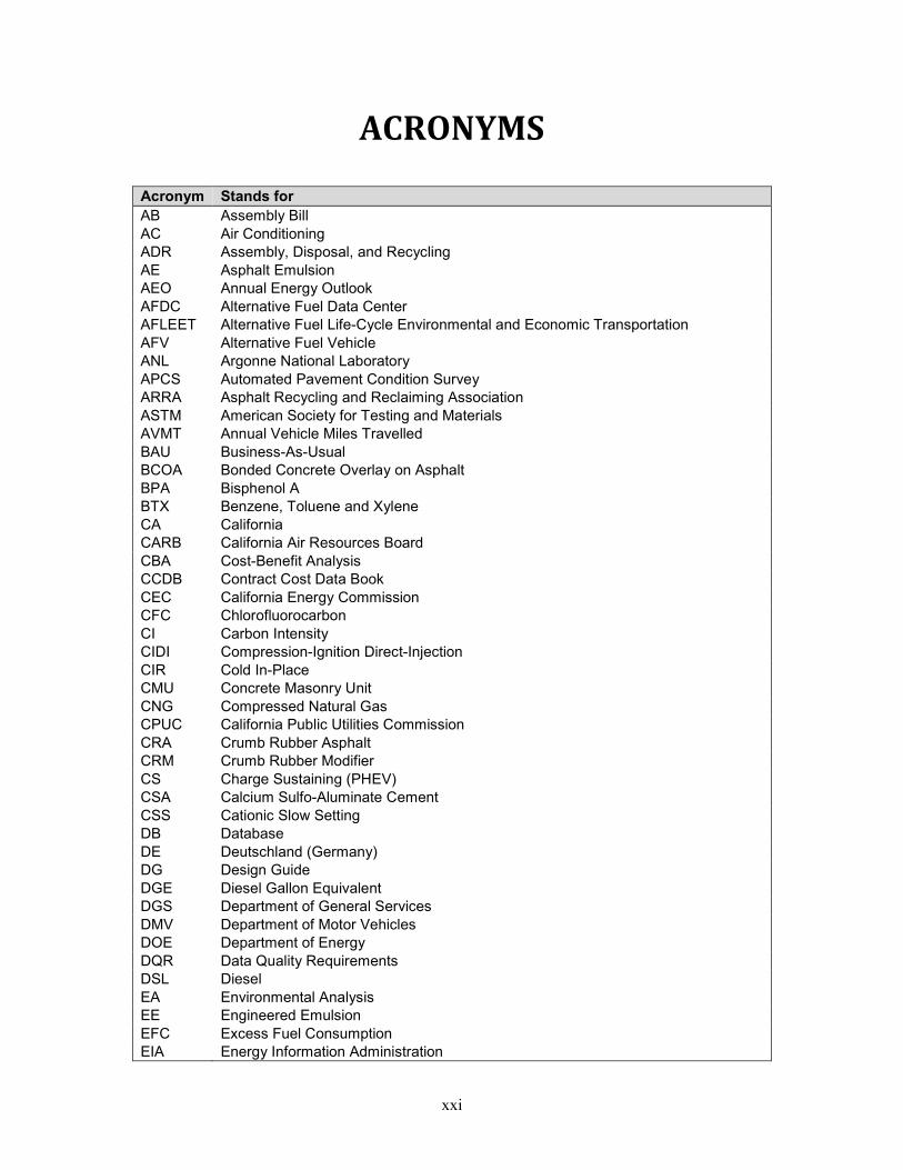
ACRONYMS

Acronym Stands for

AB Assembly Bill AC Air Conditioning ADR Assembly, Disposal, and Recycling AE Asphalt Emulsion AEO Annual Energy Outlook AFDC Alternative Fuel Data Center AFLEET Alternative Fuel Life-Cycle Environmental and Economic Transportation AFV Alternative Fuel Vehicle ANL Argonne National Laboratory APCS Automated Pavement Condition Survey ARRA Asphalt Recycling and Reclaiming Association ASTM American Society for Testing and Materials AVMT Annual Vehicle Miles Travelled BAU Business-As-Usual BCOA Bonded Concrete Overlay on Asphalt BPA Bisphenol A BTX Benzene, Toluene and Xylene CA California CARB California Air Resources Board CBA Cost-Benefit Analysis CCDB Contract Cost Data Book CEC California Energy Commission CFC Chlorofluorocarbon CI Carbon Intensity CIDI Compression-Ignition Direct-Injection CIR Cold In-Place CMU Concrete Masonry Unit CNG Compressed Natural Gas CPUC California Public Utilities Commission CRA Crumb Rubber Asphalt CRM Crumb Rubber Modifier CS Charge Sustaining (PHEV) CSA Calcium Sulfo-Aluminate Cement CSS Cationic Slow Setting DB Database DE Deutschland (Germany) DG Design Guide DGE Diesel Gallon Equivalent DGS Department of General Services DMV Department of Motor Vehicles DOE Department of Energy DQR Data Quality Requirements DSL Diesel EA Environmental Analysis EE Engineered Emulsion EFC Excess Fuel Consumption EIA Energy Information Administration

xxii

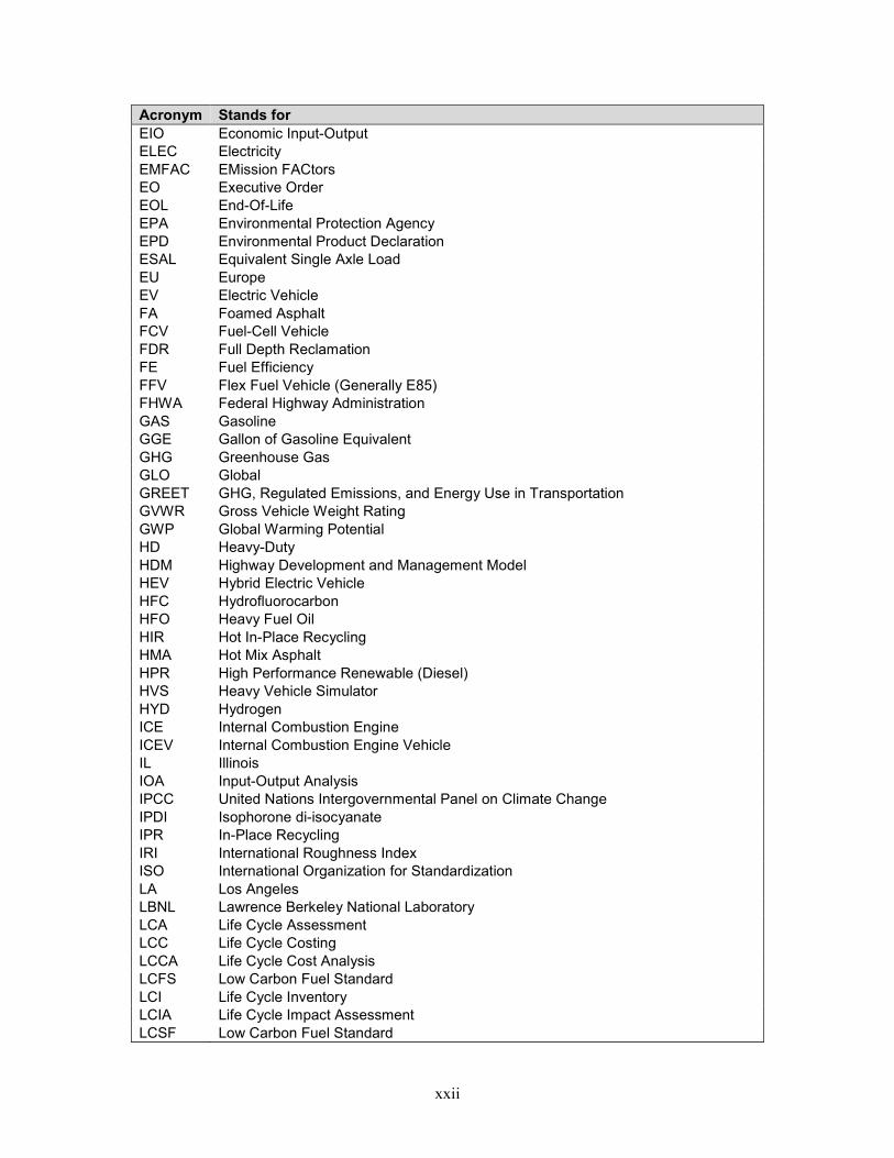
Acronym Stands for

EIO Economic Input-Output ELEC Electricity EMFAC EMission FACtors EO Executive Order EOL End-Of-Life EPA Environmental Protection Agency EPD Environmental Product Declaration ESAL Equivalent Single Axle Load EU Europe EV Electric Vehicle FA Foamed Asphalt FCV Fuel-Cell Vehicle FDR Full Depth Reclamation FE Fuel Efficiency FFV Flex Fuel Vehicle (Generally E85) FHWA Federal Highway Administration GAS Gasoline GGE Gallon of Gasoline Equivalent GHG Greenhouse Gas GLO Global GREET GHG, Regulated Emissions, and Energy Use in Transportation GVWR Gross Vehicle Weight Rating GWP Global Warming Potential HD Heavy-Duty HDM Highway Development and Management Model HEV Hybrid Electric Vehicle HFC Hydrofluorocarbon HFO Heavy Fuel Oil HIR Hot In-Place Recycling HMA Hot Mix Asphalt HPR High Performance Renewable (Diesel) HVS Heavy Vehicle Simulator HYD Hydrogen ICE Internal Combustion Engine ICEV Internal Combustion Engine Vehicle IL Illinois IOA Input-Output Analysis IPCC United Nations Intergovernmental Panel on Climate Change IPDI Isophorone di-isocyanate IPR In-Place Recycling IRI International Roughness Index ISO International Organization for Standardization LA Los Angeles LBNL Lawrence Berkeley National Laboratory LCA Life Cycle Assessment LCC Life Cycle Costing LCCA Life Cycle Cost Analysis LCFS Low Carbon Fuel Standard LCI Life Cycle Inventory LCIA Life Cycle Impact Assessment LCSF Low Carbon Fuel Standard

xxiii

Acronym Stands for

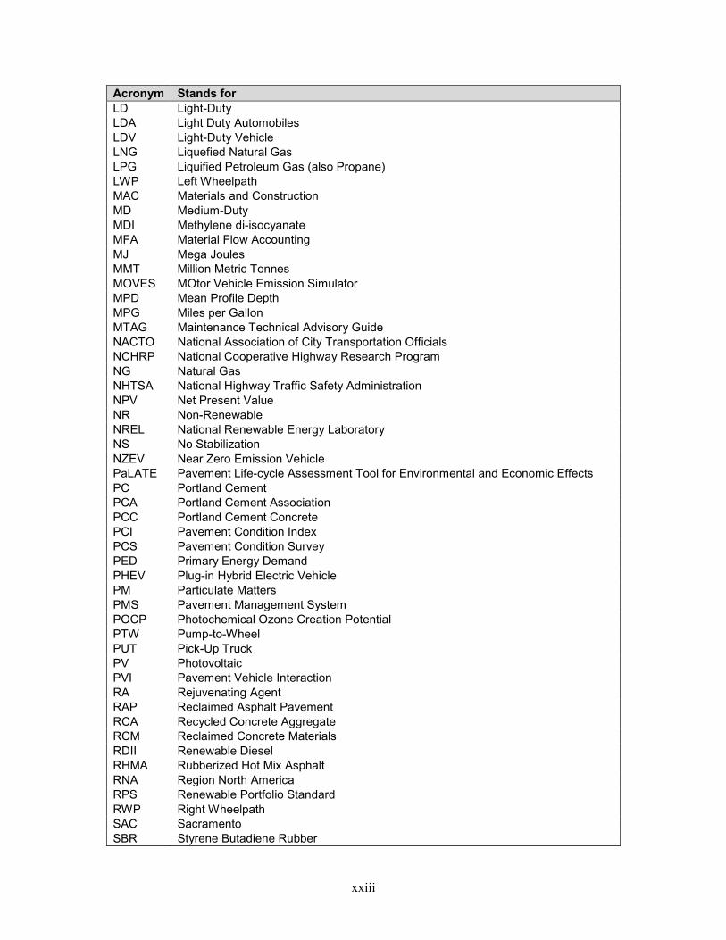
LD Light-Duty LDA Light Duty Automobiles LDV Light-Duty Vehicle LNG Liquefied Natural Gas LPG Liquified Petroleum Gas (also Propane) LWP Left Wheelpath MAC Materials and Construction MD Medium-Duty MDI Methylene di-isocyanate MFA Material Flow Accounting MJ Mega Joules MMT Million Metric Tonnes MOVES MOtor Vehicle Emission Simulator MPD Mean Profile Depth MPG Miles per Gallon MTAG Maintenance Technical Advisory Guide NACTO National Association of City Transportation Officials NCHRP National Cooperative Highway Research Program NG Natural Gas NHTSA National Highway Traffic Safety Administration NPV Net Present Value NR Non-Renewable NREL National Renewable Energy Laboratory NS No Stabilization NZEV Near Zero Emission Vehicle PaLATE Pavement Life-cycle Assessment Tool for Environmental and Economic Effects PC Portland Cement PCA Portland Cement Association PCC Portland Cement Concrete PCI Pavement Condition Index PCS Pavement Condition Survey PED Primary Energy Demand PHEV Plug-in Hybrid Electric Vehicle PM Particulate Matters PMS Pavement Management System POCP Photochemical Ozone Creation Potential PTW Pump-to-Wheel PUT Pick-Up Truck PV Photovoltaic PVI Pavement Vehicle Interaction RA Rejuvenating Agent RAP Reclaimed Asphalt Pavement RCA Recycled Concrete Aggregate RCM Reclaimed Concrete Materials RDII Renewable Diesel RHMA Rubberized Hot Mix Asphalt RNA Region North America RPS Renewable Portfolio Standard RWP Right Wheelpath SAC Sacramento SBR Styrene Butadiene Rubber

xxiv

Acronym Stands for

SCM Supplemental Cementitious Material SEA Strategic Environmental Assessment SEEA System of Economic and Environmental Accounting SFA Substance Flow Analysis SI Spark-Ignition SS Slow Setting STA Swedish Transportation Administration SUV Sport Utility Vehicle TAED Tetraacetyl ethylenediamine TMAH Tetramethyl-ammonium hydroxide TRACI Tool for Reduction and Assessment of Chemicals and other environmental Impacts UC University of California UCPRC University of California Pavement Research Center UP Unsaturated Polyester USEPA US Environmental Protection Agency USLCI US Life Cycle Inventory VIN Vehicle Identification Number VMT Vehicle Miles Traveled WMA Warm Mix Asphalt WPC Wheelpath Cracking WRF Weather Research and Forecasting WTP Well-to-Pump WTW Well-to-Wheels ZEV Zero Emission Vehicle

1

CHAPTER 1. Introduction

Sustainable development is a topic that the State of California is culturally dedicated to, historically a

pioneer in, and legally bound to strive for through state legislation and regulation, and other state and

local initiatives. The goal of sustainability legislation in California is to drastically reduce the state’s

environmental impacts and natural resource consumption while maintaining its economic excellence.

Sustainability considerations are pressing issues in all aspects of the state’s vast economic landscape. The

research presented in this dissertation is aimed at addressing some of the challenges that exist in

improving the transportation infrastructure management system. This research strives to achieve its

objectives by providing frameworks, models, and databases needed for incorporating objective and data-

driven lifecycle thinking into decision making at all levels: network level to project level for both state

agencies and local governments.

Figure 1.1 shows the scope of the research presented in this dissertation. There are three main categories:

1) development of a comprehensive life cycle inventory (LCI) database for implementation of life cycle

assessment (LCA) methodology in transportation infrastructure management in California. Such a

database should cover all the construction materials, transportation modes, construction activities used in

transportation projects in the state and should represent local conditions in terms of energy sources,

transport distance, mix design, and construction methodology. 2) Evaluation of current and potential

sustainability actions at the state and local government levels through the development of frameworks,

models, and datasets needed for objective and accurate quantification of the impacts of management

decisions. Several different abatement strategies are evaluated in detail. 3) Assessment of recycling

practices available for pavements at their end of life to quantify changes in environmental impacts

compared to conventional methods, considering the effects of recycling through the use stage. This

approach help avoid unintended consequences in cases where extra impacts during the use stage of new

options compared to conventional ones offset the improvements in the material production and

construction stages.

Following this introductory chapter, Chapter Two presents a review of the available information and

literature to identify the gaps in knowledge and the significance of the challenges that need to be

addressed in the field of sustainability of transportation infrastructure. This is followed by description of

the research objectives of this dissertation, and the tasks to address the challenges and achieve its

objectives.

The reliability of an LCA study is dependent on the quality and repeatability of the data used for

quantification of the impacts at each life cycle stage. Chapter Three presents all the assumptions and

modeling details for developing a comprehensive LCI database for transportation infrastructure

management in California. This chapter also includes a section on data quality assessment, which was

conducted under a third-party critical review process according to International Standards Organization

(ISO) standards. The LCI database presented in this chapter will be used in eLCAP, a web-based tool for

conducting LCA for decision-making at network and project levels in transportation infrastructure

management.

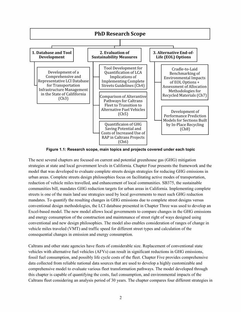
2

Figure 1.1: Research scope, main topics and projects covered under each topic

The next several chapters are focused on current and potential greenhouse gas (GHG) mitigation

strategies at state and local government levels in California. Chapter Four presents the framework and the

model that was developed to evaluate complete streets design strategies for reducing GHG emissions in

urban areas. Complete streets design philosophies focus on facilitating active modes of transportation,

reduction of vehicle miles travelled, and enhancement of local communities. SB375, the sustainable

communities bill, mandates GHG reduction targets for urban areas in California. Implementing complete

streets is one of the main land use strategies used by local governments to meet such GHG reduction

mandates. To quantify the resulting changes in GHG emissions due to complete street designs versus

conventional design methodologies, the LCI database presented in Chapter Three was used to develop an

Excel-based model. The new model allows local governments to compare changes in the GHG emissions

and energy consumption of the construction and maintenance of street right of ways designed using

conventional and new design philosophies. The model also enables consideration of ranges of change in

vehicle miles traveled (VMT) and traffic speed for different street types and calculation of the

consequential changes in emission and energy consumption.

Caltrans and other state agencies have fleets of considerable size. Replacement of conventional state

vehicles with alternative fuel vehicles (AFVs) can result in significant reductions in GHG emissions,

fossil fuel consumption, and possibly life cycle costs of the fleet. Chapter Five provides comprehensive

data collected from reliable national data sources that are used to develop a highly customizable and

comprehensive model to evaluate various fleet transformation pathways. The model developed through

this chapter is capable of quantifying the costs, fuel consumption, and environmental impacts of the

Caltrans fleet considering an analysis period of 30 years. The chapter compares four different strategies in

PhD Research Scope

1. Database and Tool Development

Development of a Comprehensive and

Representative LCI Database for Transportation

Infrastructure Management in the State of Calififornia

(Ch3)

2. Evaluation of Sustainability Measures

Tool Development for Quantification of LCA

Implications of Implementing Complete Streets Guidelines (Ch4)

Comparison of Alterantive Pathways for Caltrans Fleet to Transition to

Alternative Fuel Vehicles (Ch5)

Quantificaion of GHG Saving Potential and

Costs of Increased Use of RAP in Caltrans Projects

(Ch6)

3. Alternative End-of-Life (EOL) Options

Cradle-to-Laid Benchmarking of

Environmental Impacts of EOL Options +

Assessment of Allocation Methodologies for

Recycled Materials (Ch7)

Development of Performance Prediction Models for Sections Built

by In-Place Recycling (Ch8)

3

terms of the potential reduction in GHG emissions, changes in life cycle costs, and the average cost of

GHG abatement compared to the business as usual case.

In Chapter Six, the increased use of reclaimed asphalt pavement (RAP) in construction projects that are

annually handled by Caltrans is investigated. The goal of this chapter is to determine the potential

reduction in GHG emissions over a 30-year analysis period by assuming various levels of increase in

RAP content of asphalt mixtures in pavement projects in the whole state. Life cycle costs are also

included in the analysis, and the abatement cost is compared across different alternatives.

Use of recycled materials has always been encouraged and considered as a more sustainable approach

compared to conventional methods of using virgin materials and transferring old materials to landfills.

The last portion of this dissertation is focused on quantifying the actual impacts of various recycling

techniques currently available for pavements so that actual changes in impacts can be better understood.

This task is undertaken in Chapter Seven.

The performance during the use stage of sections built using recycled materials can be significantly

different from those sections built using conventional methods. Chapter Eight addresses this question by

developing predictive performance models for sections built using in-place recycled materials. The

models were developed by collecting data from Caltrans pavement management system and conducting

various statistical methods for analyzing empirical methods.

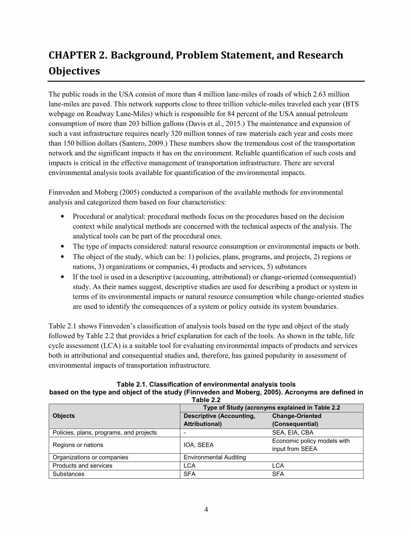
4

CHAPTER 2. Background, Problem Statement, and Research

Objectives

The public roads in the USA consist of more than 4 million lane-miles of roads of which 2.63 million

lane-miles are paved. This network supports close to three trillion vehicle-miles traveled each year (BTS

webpage on Roadway Lane-Miles) which is responsible for 84 percent of the USA annual petroleum

consumption of more than 203 billion gallons (Davis et al., 2015.) The maintenance and expansion of

such a vast infrastructure requires nearly 320 million tonnes of raw materials each year and costs more

than 150 billion dollars (Santero, 2009.) These numbers show the tremendous cost of the transportation

network and the significant impacts it has on the environment. Reliable quantification of such costs and

impacts is critical in the effective management of transportation infrastructure. There are several

environmental analysis tools available for quantification of the environmental impacts.

Finnveden and Moberg (2005) conducted a comparison of the available methods for environmental

analysis and categorized them based on four characteristics:

• Procedural or analytical: procedural methods focus on the procedures based on the decision

context while analytical methods are concerned with the technical aspects of the analysis. The

analytical tools can be part of the procedural ones.

• The type of impacts considered: natural resource consumption or environmental impacts or both.

• The object of the study, which can be: 1) policies, plans, programs, and projects, 2) regions or

nations, 3) organizations or companies, 4) products and services, 5) substances

• If the tool is used in a descriptive (accounting, attributional) or change-oriented (consequential)

study. As their names suggest, descriptive studies are used for describing a product or system in

terms of its environmental impacts or natural resource consumption while change-oriented studies

are used to identify the consequences of a system or policy outside its system boundaries.

Table 2.1 shows Finnveden’s classification of analysis tools based on the type and object of the study

followed by Table 2.2 that provides a brief explanation for each of the tools. As shown in the table, life

cycle assessment (LCA) is a suitable tool for evaluating environmental impacts of products and services

both in attributional and consequential studies and, therefore, has gained popularity in assessment of

environmental impacts of transportation infrastructure.

Table 2.1. Classification of environmental analysis tools

based on the type and object of the study (Finnveden and Moberg, 2005). Acronyms are defined in Table 2.2

Objects

Type of Study (acronyms explained in Table 2.2

Descriptive (Accounting,

Attributional)

Change-Oriented

(Consequential)

Policies, plans, programs, and projects - SEA, EIA, CBA

Regions or nations IOA, SEEA Economic policy models with input from SEEA

Organizations or companies Environmental Auditing

Products and services LCA LCA

Substances SFA SFA

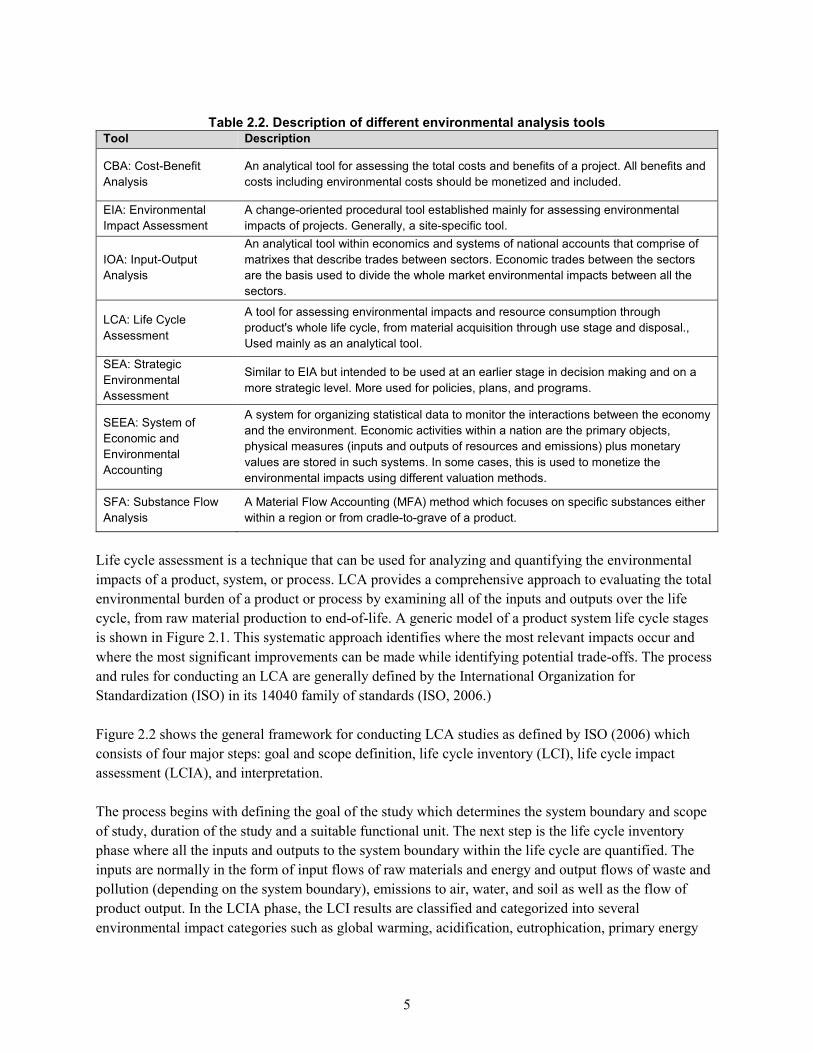
5

Table 2.2. Description of different environmental analysis tools

Tool Description

CBA: Cost-Benefit Analysis

An analytical tool for assessing the total costs and benefits of a project. All benefits and costs including environmental costs should be monetized and included.

EIA: Environmental Impact Assessment

A change-oriented procedural tool established mainly for assessing environmental impacts of projects. Generally, a site-specific tool.

IOA: Input-Output Analysis

An analytical tool within economics and systems of national accounts that comprise of matrixes that describe trades between sectors. Economic trades between the sectors are the basis used to divide the whole market environmental impacts between all the sectors.

LCA: Life Cycle Assessment

A tool for assessing environmental impacts and resource consumption through product's whole life cycle, from material acquisition through use stage and disposal., Used mainly as an analytical tool.

SEA: Strategic Environmental Assessment

Similar to EIA but intended to be used at an earlier stage in decision making and on a more strategic level. More used for policies, plans, and programs.

SEEA: System of Economic and Environmental Accounting

A system for organizing statistical data to monitor the interactions between the economy and the environment. Economic activities within a nation are the primary objects, physical measures (inputs and outputs of resources and emissions) plus monetary values are stored in such systems. In some cases, this is used to monetize the environmental impacts using different valuation methods.

SFA: Substance Flow Analysis

A Material Flow Accounting (MFA) method which focuses on specific substances either within a region or from cradle-to-grave of a product.

Life cycle assessment is a technique that can be used for analyzing and quantifying the environmental

impacts of a product, system, or process. LCA provides a comprehensive approach to evaluating the total

environmental burden of a product or process by examining all of the inputs and outputs over the life

cycle, from raw material production to end-of-life. A generic model of a product system life cycle stages

is shown in Figure 2.1. This systematic approach identifies where the most relevant impacts occur and

where the most significant improvements can be made while identifying potential trade-offs. The process

and rules for conducting an LCA are generally defined by the International Organization for

Standardization (ISO) in its 14040 family of standards (ISO, 2006.)

Figure 2.2 shows the general framework for conducting LCA studies as defined by ISO (2006) which

consists of four major steps: goal and scope definition, life cycle inventory (LCI), life cycle impact

assessment (LCIA), and interpretation.

The process begins with defining the goal of the study which determines the system boundary and scope

of study, duration of the study and a suitable functional unit. The next step is the life cycle inventory

phase where all the inputs and outputs to the system boundary within the life cycle are quantified. The

inputs are normally in the form of input flows of raw materials and energy and output flows of waste and

pollution (depending on the system boundary), emissions to air, water, and soil as well as the flow of

product output. In the LCIA phase, the LCI results are classified and categorized into several

environmental impact categories such as global warming, acidification, eutrophication, primary energy

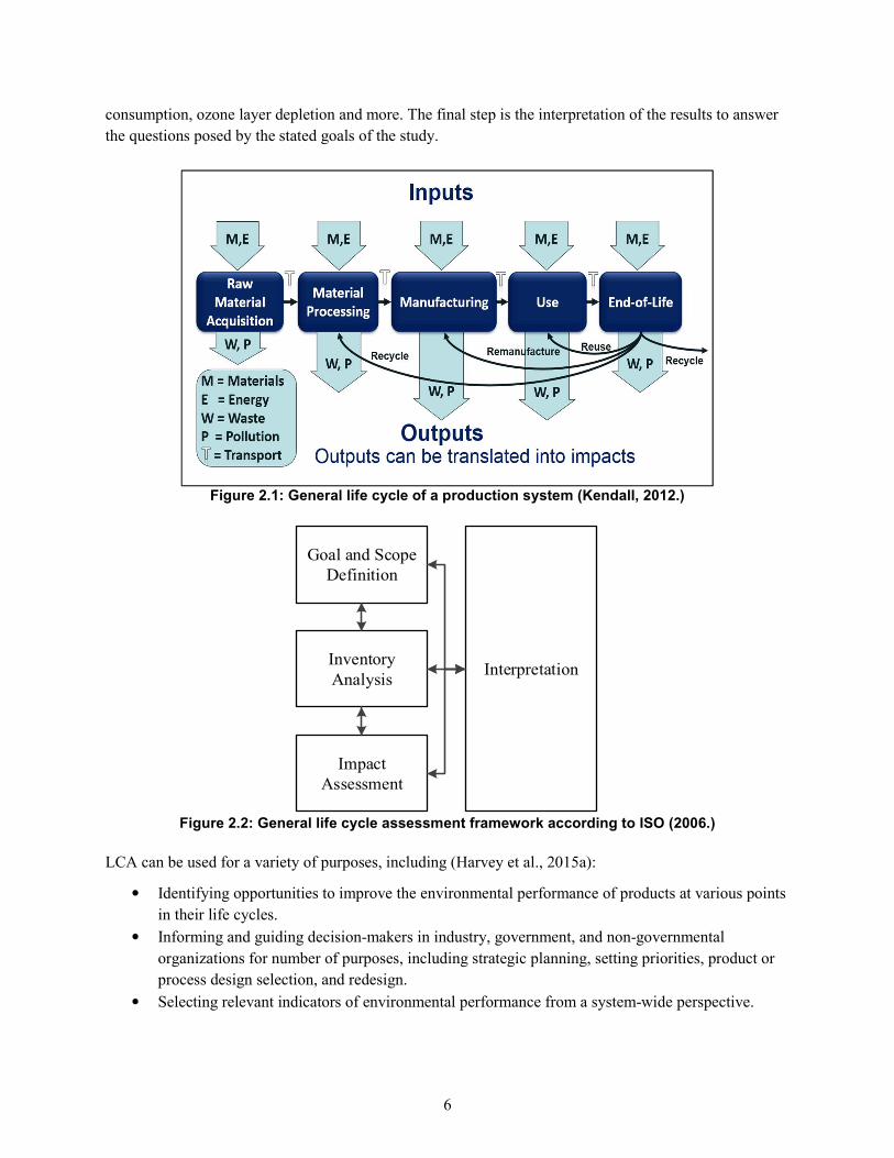
6

consumption, ozone layer depletion and more. The final step is the interpretation of the results to answer

the questions posed by the stated goals of the study.

Figure 2.1: General life cycle of a production system (Kendall, 2012.)

Goal and Scope Definition

Inventory Analysis

Impact Assessment

Interpretation

Figure 2.2: General life cycle assessment framework according to ISO (2006.)

LCA can be used for a variety of purposes, including (Harvey et al., 2015a):

• Identifying opportunities to improve the environmental performance of products at various points

in their life cycles.

• Informing and guiding decision-makers in industry, government, and non-governmental

organizations for number of purposes, including strategic planning, setting priorities, product or

process design selection, and redesign.

• Selecting relevant indicators of environmental performance from a system-wide perspective.

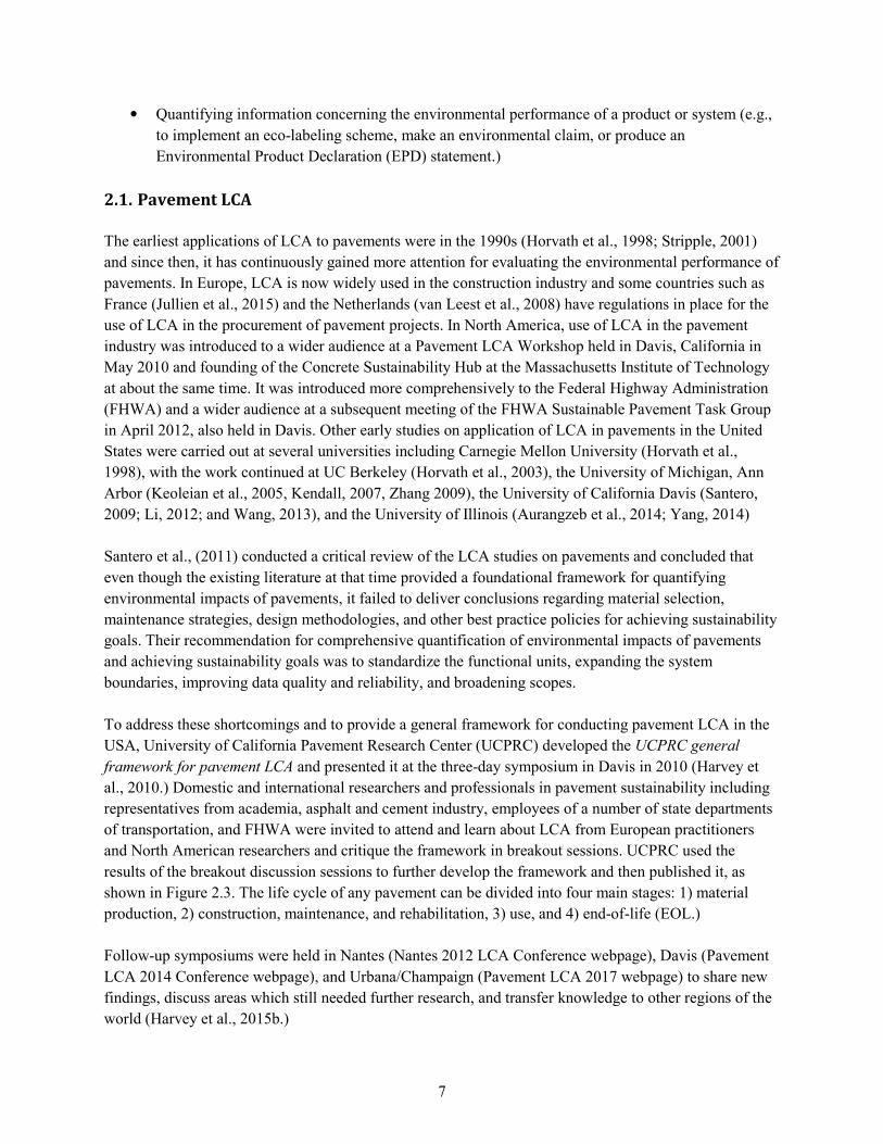
7

• Quantifying information concerning the environmental performance of a product or system (e.g.,

to implement an eco-labeling scheme, make an environmental claim, or produce an

Environmental Product Declaration (EPD) statement.)

2.1. Pavement LCA

The earliest applications of LCA to pavements were in the 1990s (Horvath et al., 1998; Stripple, 2001)

and since then, it has continuously gained more attention for evaluating the environmental performance of

pavements. In Europe, LCA is now widely used in the construction industry and some countries such as

France (Jullien et al., 2015) and the Netherlands (van Leest et al., 2008) have regulations in place for the

use of LCA in the procurement of pavement projects. In North America, use of LCA in the pavement

industry was introduced to a wider audience at a Pavement LCA Workshop held in Davis, California in

May 2010 and founding of the Concrete Sustainability Hub at the Massachusetts Institute of Technology

at about the same time. It was introduced more comprehensively to the Federal Highway Administration

(FHWA) and a wider audience at a subsequent meeting of the FHWA Sustainable Pavement Task Group

in April 2012, also held in Davis. Other early studies on application of LCA in pavements in the United

States were carried out at several universities including Carnegie Mellon University (Horvath et al.,

1998), with the work continued at UC Berkeley (Horvath et al., 2003), the University of Michigan, Ann

Arbor (Keoleian et al., 2005, Kendall, 2007, Zhang 2009), the University of California Davis (Santero,

2009; Li, 2012; and Wang, 2013), and the University of Illinois (Aurangzeb et al., 2014; Yang, 2014)

Santero et al., (2011) conducted a critical review of the LCA studies on pavements and concluded that

even though the existing literature at that time provided a foundational framework for quantifying

environmental impacts of pavements, it failed to deliver conclusions regarding material selection,

maintenance strategies, design methodologies, and other best practice policies for achieving sustainability

goals. Their recommendation for comprehensive quantification of environmental impacts of pavements

and achieving sustainability goals was to standardize the functional units, expanding the system

boundaries, improving data quality and reliability, and broadening scopes.

To address these shortcomings and to provide a general framework for conducting pavement LCA in the

USA, University of California Pavement Research Center (UCPRC) developed the UCPRC general

framework for pavement LCA and presented it at the three-day symposium in Davis in 2010 (Harvey et

al., 2010.) Domestic and international researchers and professionals in pavement sustainability including

representatives from academia, asphalt and cement industry, employees of a number of state departments

of transportation, and FHWA were invited to attend and learn about LCA from European practitioners

and North American researchers and critique the framework in breakout sessions. UCPRC used the

results of the breakout discussion sessions to further develop the framework and then published it, as

shown in Figure 2.3. The life cycle of any pavement can be divided into four main stages: 1) material

production, 2) construction, maintenance, and rehabilitation, 3) use, and 4) end-of-life (EOL.)

Follow-up symposiums were held in Nantes (Nantes 2012 LCA Conference webpage), Davis (Pavement

LCA 2014 Conference webpage), and Urbana/Champaign (Pavement LCA 2017 webpage) to share new

findings, discuss areas which still needed further research, and transfer knowledge to other regions of the

world (Harvey et al., 2015b.)

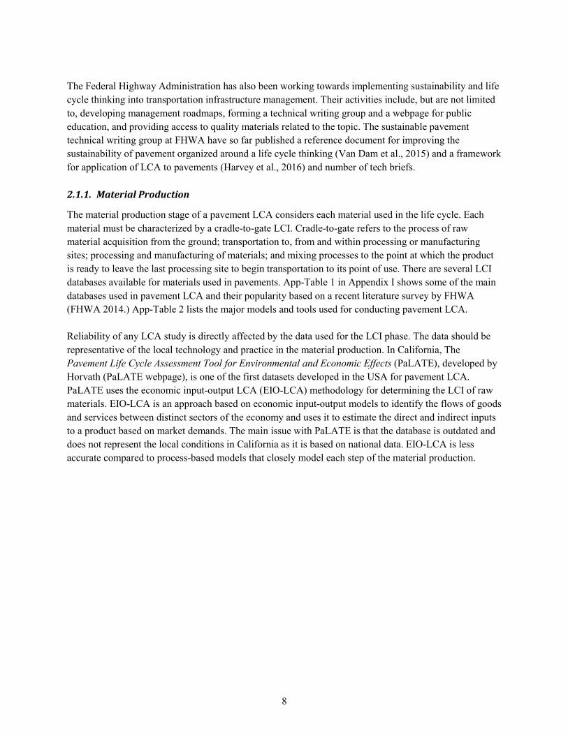
8

The Federal Highway Administration has also been working towards implementing sustainability and life

cycle thinking into transportation infrastructure management. Their activities include, but are not limited

to, developing management roadmaps, forming a technical writing group and a webpage for public

education, and providing access to quality materials related to the topic. The sustainable pavement

technical writing group at FHWA have so far published a reference document for improving the

sustainability of pavement organized around a life cycle thinking (Van Dam et al., 2015) and a framework

for application of LCA to pavements (Harvey et al., 2016) and number of tech briefs.

2.1.1. Material Production

The material production stage of a pavement LCA considers each material used in the life cycle. Each

material must be characterized by a cradle-to-gate LCI. Cradle-to-gate refers to the process of raw

material acquisition from the ground; transportation to, from and within processing or manufacturing

sites; processing and manufacturing of materials; and mixing processes to the point at which the product

is ready to leave the last processing site to begin transportation to its point of use. There are several LCI

databases available for materials used in pavements. App-Table 1 in Appendix I shows some of the main

databases used in pavement LCA and their popularity based on a recent literature survey by FHWA

(FHWA 2014.) App-Table 2 lists the major models and tools used for conducting pavement LCA.

Reliability of any LCA study is directly affected by the data used for the LCI phase. The data should be

representative of the local technology and practice in the material production. In California, The

Pavement Life Cycle Assessment Tool for Environmental and Economic Effects (PaLATE), developed by

Horvath (PaLATE webpage), is one of the first datasets developed in the USA for pavement LCA.

PaLATE uses the economic input-output LCA (EIO-LCA) methodology for determining the LCI of raw

materials. EIO-LCA is an approach based on economic input-output models to identify the flows of goods

and services between distinct sectors of the economy and uses it to estimate the direct and indirect inputs

to a product based on market demands. The main issue with PaLATE is that the database is outdated and

does not represent the local conditions in California as it is based on national data. EIO-LCA is less

accurate compared to process-based models that closely model each step of the material production.

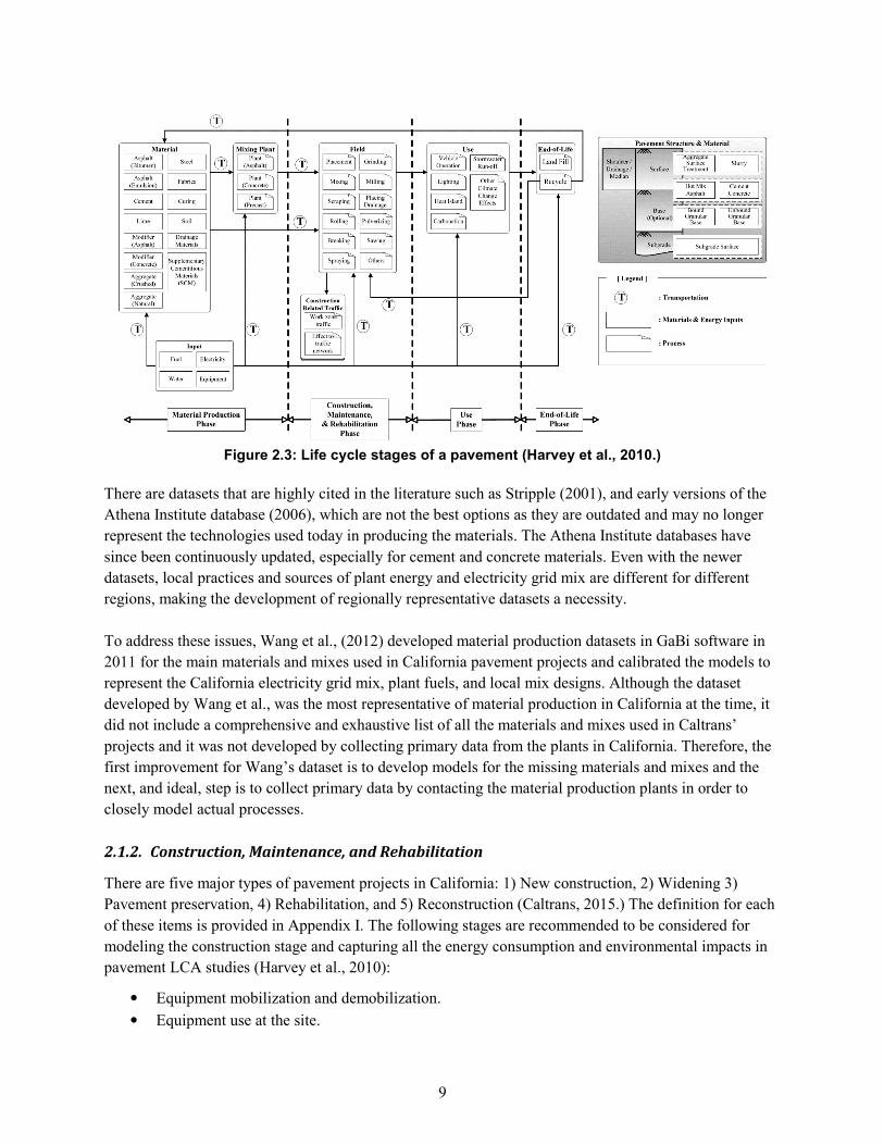
9

Figure 2.3: Life cycle stages of a pavement (Harvey et al., 2010.)

There are datasets that are highly cited in the literature such as Stripple (2001), and early versions of the

Athena Institute database (2006), which are not the best options as they are outdated and may no longer

represent the technologies used today in producing the materials. The Athena Institute databases have

since been continuously updated, especially for cement and concrete materials. Even with the newer

datasets, local practices and sources of plant energy and electricity grid mix are different for different

regions, making the development of regionally representative datasets a necessity.

To address these issues, Wang et al., (2012) developed material production datasets in GaBi software in

2011 for the main materials and mixes used in California pavement projects and calibrated the models to

represent the California electricity grid mix, plant fuels, and local mix designs. Although the dataset

developed by Wang et al., was the most representative of material production in California at the time, it

did not include a comprehensive and exhaustive list of all the materials and mixes used in Caltrans’

projects and it was not developed by collecting primary data from the plants in California. Therefore, the

first improvement for Wang’s dataset is to develop models for the missing materials and mixes and the

next, and ideal, step is to collect primary data by contacting the material production plants in order to

closely model actual processes.

2.1.2. Construction, Maintenance, and Rehabilitation

There are five major types of pavement projects in California: 1) New construction, 2) Widening 3)

Pavement preservation, 4) Rehabilitation, and 5) Reconstruction (Caltrans, 2015.) The definition for each

of these items is provided in Appendix I. The following stages are recommended to be considered for

modeling the construction stage and capturing all the energy consumption and environmental impacts in

pavement LCA studies (Harvey et al., 2010):

• Equipment mobilization and demobilization.

• Equipment use at the site.

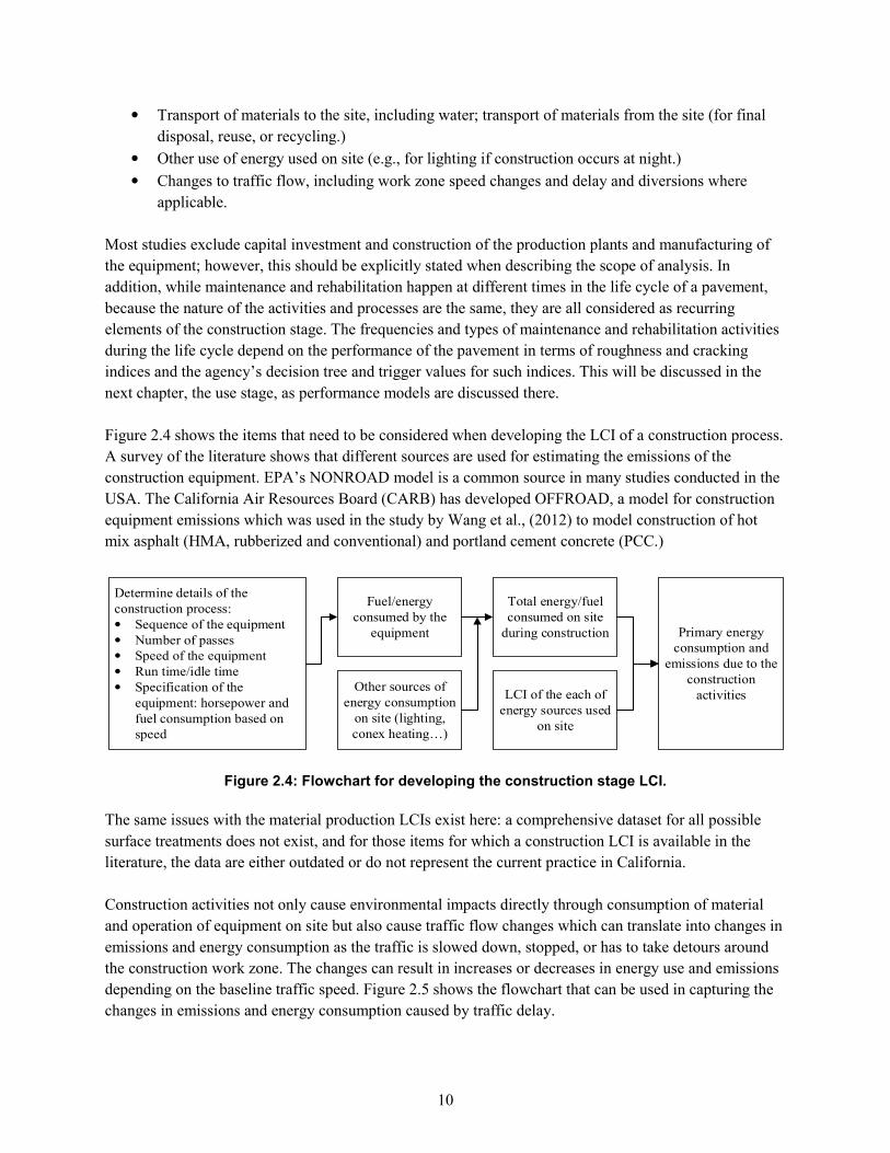
10

• Transport of materials to the site, including water; transport of materials from the site (for final

disposal, reuse, or recycling.)

• Other use of energy used on site (e.g., for lighting if construction occurs at night.)

• Changes to traffic flow, including work zone speed changes and delay and diversions where

applicable.

Most studies exclude capital investment and construction of the production plants and manufacturing of

the equipment; however, this should be explicitly stated when describing the scope of analysis. In

addition, while maintenance and rehabilitation happen at different times in the life cycle of a pavement,

because the nature of the activities and processes are the same, they are all considered as recurring

elements of the construction stage. The frequencies and types of maintenance and rehabilitation activities

during the life cycle depend on the performance of the pavement in terms of roughness and cracking

indices and the agency’s decision tree and trigger values for such indices. This will be discussed in the

next chapter, the use stage, as performance models are discussed there.

Figure 2.4 shows the items that need to be considered when developing the LCI of a construction process.

A survey of the literature shows that different sources are used for estimating the emissions of the

construction equipment. EPA’s NONROAD model is a common source in many studies conducted in the

USA. The California Air Resources Board (CARB) has developed OFFROAD, a model for construction

equipment emissions which was used in the study by Wang et al., (2012) to model construction of hot

mix asphalt (HMA, rubberized and conventional) and portland cement concrete (PCC.)

Determine details of the construction process:• Sequence of the equipment• Number of passes• Speed of the equipment• Run time/idle time• Specification of the

equipment: horsepower and fuel consumption based on speed

Other sources of energy consumption

on site (lighting, conex heating…)

Fuel/energy consumed by the

equipment

LCI of the each of energy sources used

on site

Total energy/fuel consumed on site

during construction Primary energy consumption and

emissions due to the construction

activities

Figure 2.4: Flowchart for developing the construction stage LCI.

The same issues with the material production LCIs exist here: a comprehensive dataset for all possible

surface treatments does not exist, and for those items for which a construction LCI is available in the

literature, the data are either outdated or do not represent the current practice in California.

Construction activities not only cause environmental impacts directly through consumption of material

and operation of equipment on site but also cause traffic flow changes which can translate into changes in

emissions and energy consumption as the traffic is slowed down, stopped, or has to take detours around

the construction work zone. The changes can result in increases or decreases in energy use and emissions

depending on the baseline traffic speed. Figure 2.5 shows the flowchart that can be used in capturing the

changes in emissions and energy consumption caused by traffic delay.

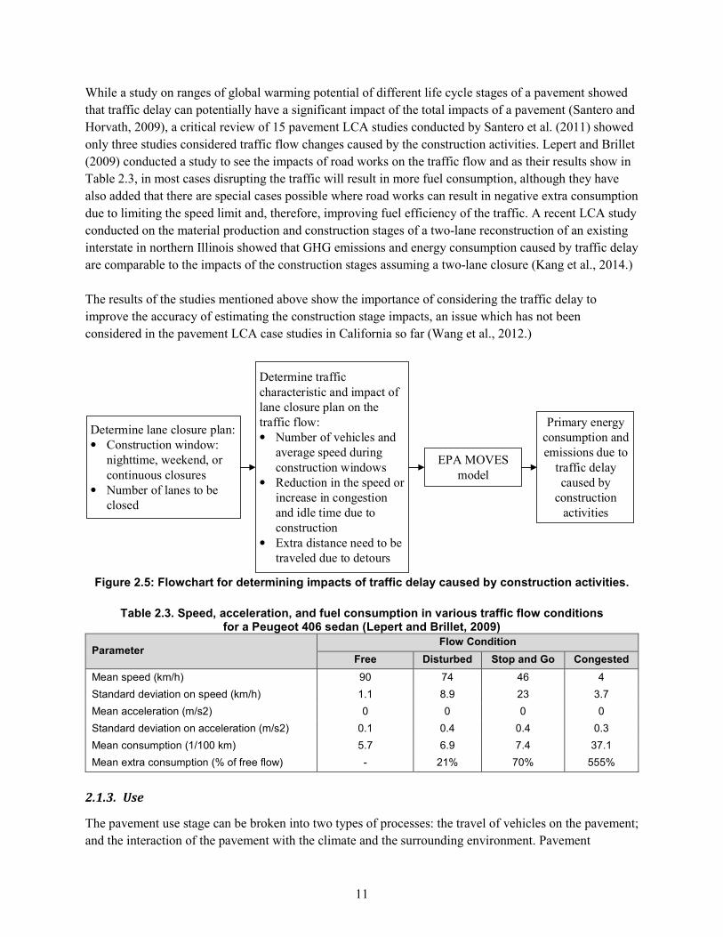
11

While a study on ranges of global warming potential of different life cycle stages of a pavement showed

that traffic delay can potentially have a significant impact of the total impacts of a pavement (Santero and

Horvath, 2009), a critical review of 15 pavement LCA studies conducted by Santero et al. (2011) showed

only three studies considered traffic flow changes caused by the construction activities. Lepert and Brillet

(2009) conducted a study to see the impacts of road works on the traffic flow and as their results show in

Table 2.3, in most cases disrupting the traffic will result in more fuel consumption, although they have

also added that there are special cases possible where road works can result in negative extra consumption

due to limiting the speed limit and, therefore, improving fuel efficiency of the traffic. A recent LCA study

conducted on the material production and construction stages of a two-lane reconstruction of an existing

interstate in northern Illinois showed that GHG emissions and energy consumption caused by traffic delay

are comparable to the impacts of the construction stages assuming a two-lane closure (Kang et al., 2014.)

The results of the studies mentioned above show the importance of considering the traffic delay to

improve the accuracy of estimating the construction stage impacts, an issue which has not been

considered in the pavement LCA case studies in California so far (Wang et al., 2012.)

Determine lane closure plan:• Construction window:

nighttime, weekend, or continuous closures

• Number of lanes to be closed

EPA MOVES model

Primary energy consumption and emissions due to

traffic delay caused by

construction activities

Determine traffic characteristic and impact of lane closure plan on the traffic flow:• Number of vehicles and

average speed during construction windows

• Reduction in the speed or increase in congestion and idle time due to construction

• Extra distance need to be traveled due to detours

Figure 2.5: Flowchart for determining impacts of traffic delay caused by construction activities.

Table 2.3. Speed, acceleration, and fuel consumption in various traffic flow conditions

for a Peugeot 406 sedan (Lepert and Brillet, 2009)

Parameter Flow Condition

Free Disturbed Stop and Go Congested

Mean speed (km/h) 90 74 46 4

Standard deviation on speed (km/h) 1.1 8.9 23 3.7

Mean acceleration (m/s2) 0 0 0 0

Standard deviation on acceleration (m/s2) 0.1 0.4 0.4 0.3

Mean consumption (1/100 km) 5.7 6.9 7.4 37.1

Mean extra consumption (% of free flow) - 21% 70% 555%

2.1.3. Use

The pavement use stage can be broken into two types of processes: the travel of vehicles on the pavement;

and the interaction of the pavement with the climate and the surrounding environment. Pavement

12

characteristics directly affect the use stage impacts through different mechanisms such as roughness,

surface texture and permeability, albedo, and more. Roughness, structural response under vehicle loads,

and macrotexture affect vehicle fuel economy, and can collectively be labeled as “pavement rolling

resistance” characteristics.

Figure 2.6, taken from Santero and Horvath (2009), shows the range of global warming potential for

different life cycle stages of pavements. The bottom five categories are related to the use stage, and as the

figure shows, impacts due to rolling resistance, which translate into fuel consumption in vehicles, are the

main source of impacts during the use stage; this is dependent on the traffic level of the section though

and might not be the case for low traffic volume roads.

Figure 2.6: GWP impact ranges for pavement life cycle components (Santero and Horvath, 2009.)

Performance prediction models are required to estimate progression of rolling resistance of the pavement

with time for determining vehicle fuel consumption during the use stage. Values of rolling resistance

coupled with pavement-vehicle interaction models are used to calculate the fuel consumption of the

vehicles. Models such as MOVES by EPA are then used to convert the fuel consumption into

environmental impacts.

Mean Profile Depth (MPD) and International Roughness Index (IRI), are the major parameters measuring

the effects of macrotexture and roughness, respectively, that contribute to the rolling resistance of flexible

pavements (Wang et al., 2012.) Pavement roughness, influenced by pavement surface wavelengths

between 0.5 and 50 m, is measured with IRI in units of in/mi or m/km and is defined as the ratio of the

vehicle’s accumulated vertical movement and the vehicle distance traveled during the measurement. MPD

13

is a measure of pavement macrotexture (unevenness with a wavelength between 0.5 mm to 50 mm) and

can be measured using the methodology described in ASTM E1845-15. Conversion of the IRI and MPD

into rolling resistance can be done through models such as HDM-4 developed by the International Road

Federation and calibrated to the USA conditions (Chatti and Zaabar, 2012.)

While there are multiple studies that have considered rolling resistance in the use stage such as (Yu and

Lu, 2012, Wang et al., 2012, and Zhang et al., 2010) and they have more or less used the same

methodology explained above in estimating fuel consumption but the main gaps in the knowledge are

lack of reliable roughness prediction models for different pavement surface treatments and for different

climatic regions and also an updated pavement-vehicle interaction model.

Another issue that should be considered in the use stage is the frequency of maintenance and

rehabilitation (M&R) activities. Frequency of M&R is typically determined using models for predicting

cracking initiation and progression with time. The performance models are used to estimate when the

cracking index will reach trigger values for doing maintenance and rehabilitation based on the agency’s

decision tree. For California, Tseng (2012) developed initial models for wheel-path crack initiation and

progression by collecting pavement condition survey (PCS) data and using survival models to determine

crack initiation and a mixed effect logit model to model crack progression. The shortcoming of the

models developed by Tseng is that they do not cover all the surface treatments conducted in pavement

projects in California, especially the ones related to the end-of-life stage of pavements such as CIR and

FDR. Tseng’s data also included the results of initial data mining of historic Caltrans pavement condition

surveys and as-built records, which have been substantially improved in the succeeding five years.

2.1.4. End-of-Life

There are three different options available at the end of a pavement service life:

• Removal of materials and disposal in landfills,

• Continued use (also referred to as reuse) in place as an underlying layer in its state at the end of

life of the pavement, or

• Pavement material recycling either:

o In-place: mainly for flexible pavements through partial depth methods of cold in-place

recycling (CIR) and hot in-place recycling (HIR), or full depth reclamation (FDR) of the

pavement (discussed below.) For rigid pavements, in large projects, on-site recycling unit

can be set up to process the old portland cement concrete by removing the steel

reinforcement and breaking the concrete to the desired gradation and specification. The

resulting material is called reclaimed concrete materials (RCM) and can be used as coarse

aggregate, base materials, or for embankment.

o At the recycling plant: used for both rigid and flexible pavements. Old asphalt concrete

and portland cement concrete are pulverized and moved to a central plant for further

processing. RCMs undergo the same processes as in an on-site recycling unit and have

the same applications. The resulting recycled flexible pavement materials at the plant,

called reclaimed asphalt pavement (RAP), can either be used directly as aggregate in base

layers or be mixed with hot mix asphalt to take advantage of the aged binder that still

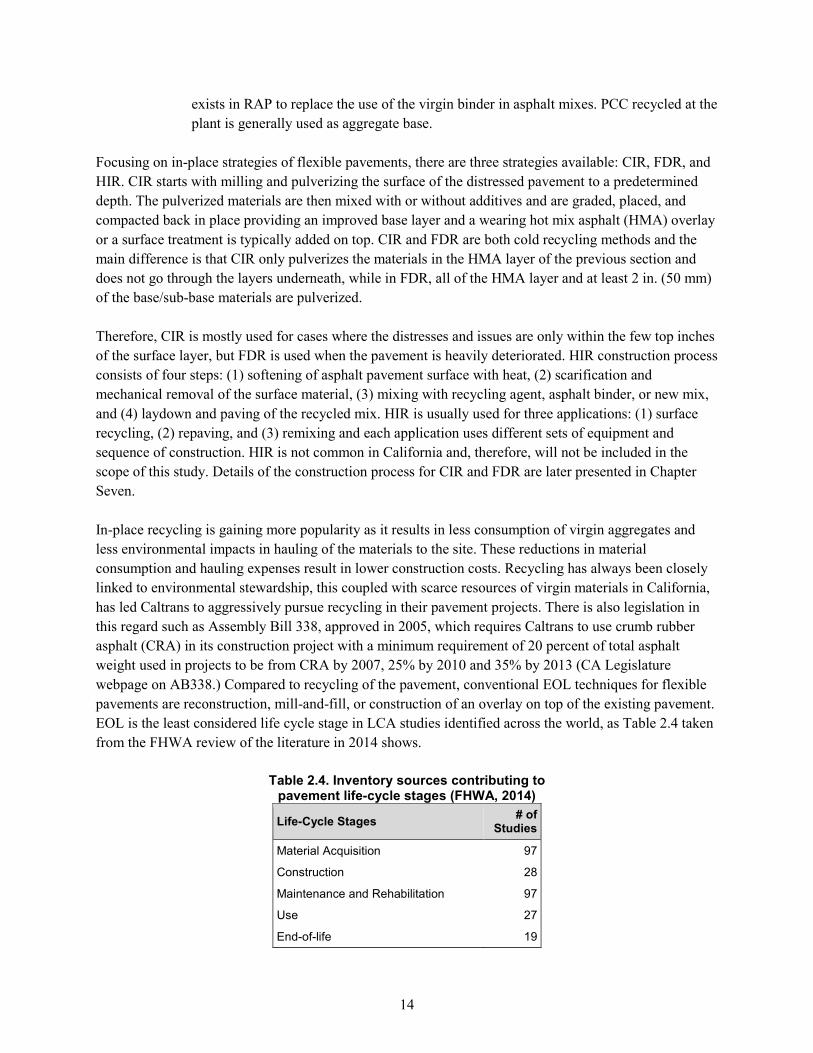
14

exists in RAP to replace the use of the virgin binder in asphalt mixes. PCC recycled at the

plant is generally used as aggregate base.

Focusing on in-place strategies of flexible pavements, there are three strategies available: CIR, FDR, and

HIR. CIR starts with milling and pulverizing the surface of the distressed pavement to a predetermined

depth. The pulverized materials are then mixed with or without additives and are graded, placed, and

compacted back in place providing an improved base layer and a wearing hot mix asphalt (HMA) overlay

or a surface treatment is typically added on top. CIR and FDR are both cold recycling methods and the

main difference is that CIR only pulverizes the materials in the HMA layer of the previous section and

does not go through the layers underneath, while in FDR, all of the HMA layer and at least 2 in. (50 mm)

of the base/sub-base materials are pulverized.

Therefore, CIR is mostly used for cases where the distresses and issues are only within the few top inches

of the surface layer, but FDR is used when the pavement is heavily deteriorated. HIR construction process

consists of four steps: (1) softening of asphalt pavement surface with heat, (2) scarification and

mechanical removal of the surface material, (3) mixing with recycling agent, asphalt binder, or new mix,

and (4) laydown and paving of the recycled mix. HIR is usually used for three applications: (1) surface

recycling, (2) repaving, and (3) remixing and each application uses different sets of equipment and

sequence of construction. HIR is not common in California and, therefore, will not be included in the

scope of this study. Details of the construction process for CIR and FDR are later presented in Chapter

Seven.

In-place recycling is gaining more popularity as it results in less consumption of virgin aggregates and

less environmental impacts in hauling of the materials to the site. These reductions in material

consumption and hauling expenses result in lower construction costs. Recycling has always been closely

linked to environmental stewardship, this coupled with scarce resources of virgin materials in California,

has led Caltrans to aggressively pursue recycling in their pavement projects. There is also legislation in

this regard such as Assembly Bill 338, approved in 2005, which requires Caltrans to use crumb rubber

asphalt (CRA) in its construction project with a minimum requirement of 20 percent of total asphalt

weight used in projects to be from CRA by 2007, 25% by 2010 and 35% by 2013 (CA Legislature

webpage on AB338.) Compared to recycling of the pavement, conventional EOL techniques for flexible

pavements are reconstruction, mill-and-fill, or construction of an overlay on top of the existing pavement.

EOL is the least considered life cycle stage in LCA studies identified across the world, as Table 2.4 taken

from the FHWA review of the literature in 2014 shows.

Table 2.4. Inventory sources contributing to

pavement life-cycle stages (FHWA, 2014)

Life-Cycle Stages # of

Studies

Material Acquisition 97

Construction 28

Maintenance and Rehabilitation 97

Use 27

End-of-life 19

15

A survey was conducted of recent LCA studies on EOL of pavements, and the summary is presented in

App-Table 3. Within these studies, there is no reliable data set that closely models the local practice in

California in terms of the construction activities, mix designs, and locally adjusted LCI for the materials

used in each EOL alternative. As the table shows, there are still questions and issues to address:

• Reliable and locally representative quantification of the impacts of the options available at EOL.

• Allocation of the impacts between the upstream and downstream projects when using recycled

materials (discussed below.)

• The performance of the sections built from recycled materials or built using in-place recycling

compared to the conventional techniques. This should be investigated from two perspectives:

o Surface roughness changes with time that directly affect vehicle fuel consumption.

o Section cracking performance that affects future maintenance and rehabilitation (M&R)

frequencies.

2.1.5. The Issue of Allocation in LCA Studies

ISO 14040 (2006) defines allocation as “partitioning the input or output flows of a process or a product

system between the product system under study and one or more other product systems.” Systems that

produce co-products, by-products, or recycled materials are areas of concern for allocation. Co-products

are two or more products that are produced in the same process, like the final products of a crude oil

refinery plant. A by-product is the result of a production process that is primarily focused on another

material, but the by-product can still be marketed and sold for value. What is left from a production

process that has no economic value and no use in other industries is called waste. In the case of a refinery

that processes crude oil and produces several refined products (co-products) how to allocate the total

emissions and environmental impacts of the oil extraction, transportation and refinery processes between

the co-products is an issue where they cannot be assigned exclusively to one product or another through

thermodynamic or mechanical decomposition of the processes. . As another example, fly ash is a waste of

coal combustion in power plants and can be used as a partial substitute for portland cement. Dividing the

impacts of coal combustion between the electricity generated by the plant (the main product) and the fly

ash (the waste) is an allocation issue.

Recycled materials are another area of concern. Recycling can be open-loop or closed-loop. In closed-

loop recycling, the material is recycled back into the original product system, such as the case for

aluminum cans or RAP back into HMA. In open-looped recycling, the material is recycled into other

product systems with a substantial change in the inherent properties. Another issue to consider is the

possible loss of quality during the recycling process and therefore the number of times recycling can be

repeated in the future. Quality degradation during the recycling process might be significant enough that it

would eventually lead to the disposal of the material as waste.

ISO 14040 recommends avoiding allocation, whenever possible, by: (1) Dividing the unit process into

sub-processes and collecting inputs and outputs related to each, or (2) Expanding the system boundaries

to include the additional functionalities related to the co-products. When the allocation is unavoidable,

ISO recommends partitioning the impacts based on the underlying physical relationships between them

such as mass proportions or energy content ratios. ISO also allows allocation based on economic value

16

where appropriate. However, these methods can yield significantly different results depending on the

physical property chosen for doing the allocation.

The issue of allocation is present in many aspects of pavement LCA studies such as environmental

impacts of asphalt binder as a co-product of an oil refinery, or supplemental cementitious materials

(SCMs) such as fly ash, slag cement, silica fume, and by-products of other industries. Another major area

of concern is recycled materials such as RAP and RCA. While allocation of co-products and by-products

in pavements have been considered by multiple studies (Sayagh, 2010; Huang, 2013; and Kang 2014),

best practice for allocation of recycled materials, either in-place or at plant is still an area of debate.

Recycling pavement materials, either in-place or at a plant, will displace the use of finite resources such

as virgin aggregates and sometimes virgin binders and therefore eliminate the impacts of producing virgin

materials. This avoidance of using virgin materials can result in reductions in environmental impacts that

should be allocated between the upstream project that provides the recycled materials and the downstream

project that uses it. There are also emissions and energy consumptions, referred here as environmental

burdens, for producing the recycled materials. These burdens for in-place recycling include pulverization,

processing, further addition of stabilizing agents and virgin aggregate to achieve specified gradations and

other specification limits for mix proportioning and properties. For plant recycling the burdens are caused

by: demolition, transportation to the plant, processing done at the plant, and transportation of the recycled

materials to the new construction site. The allocation of these environmental burdens between the

upstream and downstream projects is not straight forward. There can also be plant recycling of materials

produced at the plant but never transported to a construction site, for various reasons.

Allocation of recycled materials has been an area of discussion in all four international symposiums on

pavement LCA (Davis, CA 2010; Nantes, France 2012; Davis, CA 2014; and Urbana-Champaign, IL

2017) and three different approaches have been suggested (Harvey et al., 2010; Van Dam et al., 2015), as

explained in Figure 2.7:

• Cut-off method: benefits and burdens of recycling all goes to the downstream project (pavement 2

is responsible for R1, no reduction of environmental impacts allocated to pavement 1 for

producing recycled materials)

• 50/50 method: half the impacts to the second pavement and half to the first pavement

• Substitution method: The first pavement is given the full benefits (the impacts that are avoided by

substituting virgin materials in pavement 2)

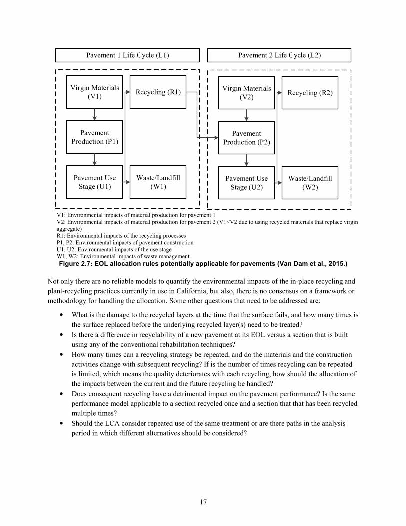
17

Virgin Materials (V1)

Pavement Production (P1)

Pavement Use Stage (U1)

Recycling (R1)

Waste/Landfill (W1)

Virgin Materials (V2)

Pavement Production (P2)

Pavement Use Stage (U2)

Recycling (R2)

Waste/Landfill (W2)

Pavement 1 Life Cycle (L1) Pavement 2 Life Cycle (L2)

V1: Environmental impacts of material production for pavement 1 V2: Environmental impacts of material production for pavement 2 (V1<V2 due to using recycled materials that replace virgin aggregate) R1: Environmental impacts of the recycling processes P1, P2: Environmental impacts of pavement construction U1, U2: Environmental impacts of the use stage W1, W2: Environmental impacts of waste management Figure 2.7: EOL allocation rules potentially applicable for pavements (Van Dam et al., 2015.)

Not only there are no reliable models to quantify the environmental impacts of the in-place recycling and

plant-recycling practices currently in use in California, but also, there is no consensus on a framework or

methodology for handling the allocation. Some other questions that need to be addressed are:

• What is the damage to the recycled layers at the time that the surface fails, and how many times is

the surface replaced before the underlying recycled layer(s) need to be treated?

• Is there a difference in recyclability of a new pavement at its EOL versus a section that is built

using any of the conventional rehabilitation techniques?

• How many times can a recycling strategy be repeated, and do the materials and the construction

activities change with subsequent recycling? If is the number of times recycling can be repeated

is limited, which means the quality deteriorates with each recycling, how should the allocation of

the impacts between the current and the future recycling be handled?

• Does consequent recycling have a detrimental impact on the pavement performance? Is the same

performance model applicable to a section recycled once and a section that that has been recycled

multiple times?

• Should the LCA consider repeated use of the same treatment or are there paths in the analysis

period in which different alternatives should be considered?

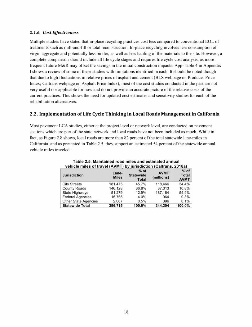
18

2.1.6. Cost Effectiveness

Multiple studies have stated that in-place recycling practices cost less compared to conventional EOL of

treatments such as mill-and-fill or total reconstruction. In-place recycling involves less consumption of

virgin aggregate and potentially less binder, as well as less hauling of the materials to the site. However, a

complete comparison should include all life cycle stages and requires life cycle cost analysis, as more

frequent future M&R may offset the savings in the initial construction impacts. App-Table 4 in Appendix

I shows a review of some of these studies with limitations identified in each. It should be noted though

that due to high fluctuations in relative prices of asphalt and cement (BLS webpage on Producer Price

Index; Caltrans webpage on Asphalt Price Index), most of the cost studies conducted in the past are not

very useful nor applicable for now and do not provide an accurate picture of the relative costs of the

current practices. This shows the need for updated cost estimates and sensitivity studies for each of the

rehabilitation alternatives.

2.2. Implementation of Life Cycle Thinking in Local Roads Management in California

Most pavement LCA studies, either at the project level or network level, are conducted on pavement

sections which are part of the state network and local roads have not been included as much. While in

fact, as Figure 2.8 shows, local roads are more than 82 percent of the total statewide lane-miles in

California, and as presented in Table 2.5, they support an estimated 54 percent of the statewide annual

vehicle miles traveled.

Table 2.5. Maintained road miles and estimated annual

vehicle miles of travel (AVMT) by jurisdiction (Caltrans, 2018a)

Jurisdiction Lane-Miles

% of Statewide

Total

AVMT (millions)

% of Total

AVMT

City Streets 181,475 45.7% 118,466 34.4% County Roads 146,128 36.8% 37,313 10.8% State Highways 51,279 12.9% 187,164 54.4% Federal Agencies 15,765 4.0% 964 0.3% Other State Agencies 2,067 0.5% 396 0.1% Statewide Total 396,715 100.0% 344,304 100.0%

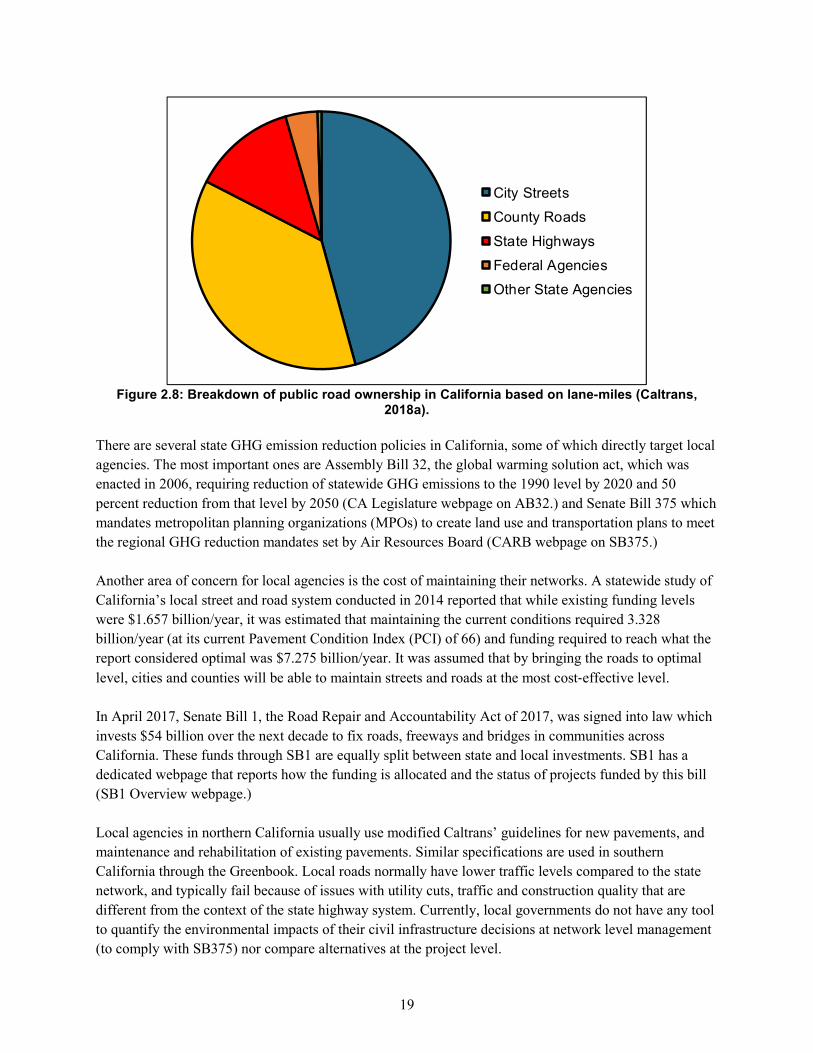
19

Figure 2.8: Breakdown of public road ownership in California based on lane-miles (Caltrans, 2018a).

There are several state GHG emission reduction policies in California, some of which directly target local

agencies. The most important ones are Assembly Bill 32, the global warming solution act, which was

enacted in 2006, requiring reduction of statewide GHG emissions to the 1990 level by 2020 and 50

percent reduction from that level by 2050 (CA Legislature webpage on AB32.) and Senate Bill 375 which

mandates metropolitan planning organizations (MPOs) to create land use and transportation plans to meet

the regional GHG reduction mandates set by Air Resources Board (CARB webpage on SB375.)

Another area of concern for local agencies is the cost of maintaining their networks. A statewide study of

California’s local street and road system conducted in 2014 reported that while existing funding levels

were $1.657 billion/year, it was estimated that maintaining the current conditions required 3.328

billion/year (at its current Pavement Condition Index (PCI) of 66) and funding required to reach what the

report considered optimal was $7.275 billion/year. It was assumed that by bringing the roads to optimal

level, cities and counties will be able to maintain streets and roads at the most cost‐effective level.

In April 2017, Senate Bill 1, the Road Repair and Accountability Act of 2017, was signed into law which

invests $54 billion over the next decade to fix roads, freeways and bridges in communities across

California. These funds through SB1 are equally split between state and local investments. SB1 has a

dedicated webpage that reports how the funding is allocated and the status of projects funded by this bill

(SB1 Overview webpage.)

Local agencies in northern California usually use modified Caltrans’ guidelines for new pavements, and

maintenance and rehabilitation of existing pavements. Similar specifications are used in southern

California through the Greenbook. Local roads normally have lower traffic levels compared to the state

network, and typically fail because of issues with utility cuts, traffic and construction quality that are

different from the context of the state highway system. Currently, local governments do not have any tool

to quantify the environmental impacts of their civil infrastructure decisions at network level management

(to comply with SB375) nor compare alternatives at the project level.

City Streets

County Roads

State Highways

Federal Agencies

Other State Agencies

20

What can help mitigate some of the challenges with the budget and reduce GHG emissions is to use

Caltrans’ type pavement structures where applicable, but to develop new designs for structures and M&R

that recognize the differences between the state and local networks and that potentially use less material,

cost less, and have less environmental impacts considering the whole life cycle of the option. This

requires new section designs, and estimates of the construction costs, service life, and GHG emissions in

each of the life cycle stages for them and to compare with conventional designs. There is no such model

available for local agencies at this point. Recent work at UCPRC (Jones et al., 2016) points towards the

potential of greater use of recycled materials, designs that are easier to maintain when utilities are present

and the potential benefits of more frequent preservation treatments as opposed to less frequent, but more

expensive rehabilitation treatments

2.3. Problem Statement and Gaps in the Knowledge

Based on the previous discussion presented in this proposal, the current gaps in the knowledge are:

• There are LCI datasets available for materials, surface treatments, and construction activities, but

these datasets generally: a) do not include a comprehensive list of all available options, b) are

outdated, and c) are not representative of the local conditions in terms of processes, mix designs,

and energy sources.

• Frameworks and models that can help local governments quantify the life cycle costs and

environmental impacts of their decisions in transportation infrastructure management do not exist

at this point. Such frameworks and data models are critical to help local governments evaluate

their strategies and decision making. Asset management through such frameworks and tools

would allow local governments and state agencies to find the most efficient solutions to meet

their goals at minimum cost. Such an approach would help managers avoid less optimal solutions

or even worse, cases where unintended consequences offset the whole benefits realized through a

novel approach.

• There are limited and unreliable data for quantifying the environmental impacts of EOL strategies

for flexible pavements; these strategies include conventional methods (such as reconstruction,

mill-and-fill, and overlays) and recycling strategies (either in-place or plant-recycling.)

• There are no reliable performance prediction models for pavements built from recycled materials.

Therefore, it is unclear whether such sections perform better, equally, or worse compared to

conventional strategies. If the performance is worse, it is possible that the potential savings in

environmental impacts due to recycling are offset by the need for more frequent maintenance and

rehabilitation in the future compared to conventional strategies.

• The surface roughness is going to affect vehicle fuel consumption during the use stage.

Roughness performance models for sections built using in-place recycling are also unknown at

this point.

• There is no consensus on the methodology on how to allocate the reduction in environmental

impacts due to recycling between the upstream project that is at its EOL and the downstream

project that is going to use the recycled materials.

21

2.4. Research Objectives

The main objectives of this research are to:

• Complete the LCI database for the materials and surface treatments used by Caltrans and local

governments on their pavement projects.

• Develop frameworks and models as a decision-making approach and tool for local and state

agencies, consisting of modules for LCA and Life Cycle Cost Analysis (LCCA.) The data to be

fed into the models will be taken from the UCPRC LCI database which is the deliverable of the

first objective in this list. The frameworks and tool will allow decision makers to quantify the

costs and environmental impacts of multiple alternatives during analysis period and within the

scope and system boundary set by the decision maker. The alternatives are a list of the

conventional treatments used by local agencies and new section designs that will be developed as

part of this project that are expected to use less materials and cost less in the initial construction

stage and over the life cycle. The cost estimates coupled with estimates of the service life of the

options and the future M&R frequencies will be used to compare the life cycle cost (LCC) of the

alternatives. LCC and LCA results can provide the decision maker with all the information

needed to select among available alternatives. The decision support approach and tool will be

mindful of the limitations of data, time, and expertise typically available to local government

agencies.

• Develop models to quantify the environmental impacts of EOL alternatives for flexible

pavements, using the practice in California as the case study.

• Investigate and recommend a methodology for handling allocation of the EOL impacts and

provide understanding on how it can affect the decision making in terms of selecting the

treatments based on their environmental impacts.

• Develop performance prediction models for recycled sections to understand how their roughness

and cracking change with time and therefore, allow fair comparison of recycling and conventional

methods throughout their life cycle.

22

CHAPTER 3. Comprehensive Life Cycle Inventory for

Transportation Infrastructure Projects, Calibrated to the

Energy Mix, Technologies, and State-of-Practice in California

3.1. Introduction

This chapter documents the details and assumptions used to develop the University of California

Pavement Research Center (UCPRC) life cycle inventory (LCI) database for quantifying the

environmental impacts of pavement projects in California, as well as some impacts from building heating,

cooling, and lighting. The UCPRC LCI database presented in this chapter is mostly the result of two LCA

studies by the UCPRC completed for the California Air Resources Board (CARB) and the California

Department of Transportation (Caltrans.) The goal and scope of each of those studies is defined in

Section 3.2.1. and Section 3.2.2. , respectively, in order to contextualize how they will use the LCI data

and to specify how the data will be applied within the scope of each study.

The data presented in this chapter are intended as background LCI data for those studies and do not

include foreground inventories for pavement designs, maintenance schedules, building designs, and

vehicle traffic levels and fuel consumption. Further, the data provided in this chapter do not include

background information for any use stage elements other than building energy consumption (e.g.,

pavement vehicle interaction [PVI], lighting, carbonation, albedo effects due to radiative forcing.)

Foreground data are “from the system of primary concern to the analyst” and background data “include

energy and materials that are delivered to the foreground system as aggregated data sets in which

individual plants and operations are not identified” (EPA webpage on LCA Glossary.)

These LCI have been incorporated into the LCA software called eLCAP (environmental Life Cycle

Assessment for Pavement.) These inventories will continue to be updated in the future as part of the

ongoing development of eLCAP and will be subjected to periodic outside critical review.

The models and inventories were either developed by the author or are modified versions of models

available in commercial software. In either case, the main goal in development of each LCI was to

represent the local conditions, technologies, and practices in terms of the electricity grid mix, material

production processes, plant energy sources, transportation modes, mix designs, construction

specifications (new construction, maintenance, and rehabilitation), and end-of-life practices used in

California. These inventories can also be used as a framework for creating regional LCI for other

locations around the world.

The main commercial source used in the development of these LCIs was the PE Profession Database

available in the software program GaBi (GaBi webpage). Other database sources were also used,

including ecoinvent (ecoinvent webpage) and the US Life Cycle Inventory (USLCI) which is hosted at the

NREL website (NREL webpage on USCLI.) The energy sources and materials for which LCIs were

developed and included in the UCPRC LCI database are listed in Table 3.2, and the composite materials

and transportation mode inventories are listed in Table 3.3. These LCIs combine the results of both

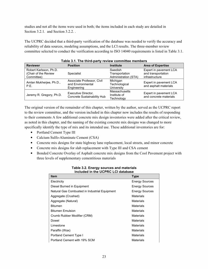
23

studies and not all the items were used in both; the items included in each study are detailed in

Section 3.2.1. and Section 3.2.2. .

The UCPRC decided that a third-party verification of the database was needed to verify the accuracy and

reliability of data sources, modeling assumptions, and the LCI results. The three-member review

committee selected to conduct the verification according to ISO 14040 requirements is listed in Table 3.1.

Table 3.1. The third-party review committee members

Reviewer Position Institute Area of Expertise

Robert Karlsson, Ph.D. (Chair of the Review Committee)

Specialist Swedish Transportation Administration (STA)

Expert in pavement LCA and transportation infrastructure

Amlan Mukherjee, Ph.D., P.E.

Associate Professor, Civil and Environmental Engineering

Michigan Technological University

Expert in pavement LCA and asphalt materials

Jeremy R. Gregory, Ph.D. Executive Director, Concrete Sustainability Hub

Massachusetts Institute of Technology

Expert in pavement LCA and concrete materials

The original version of the remainder of this chapter, written by the author, served as the UCPRC report

to the review committee, and the version included in this chapter now includes the results of responding

to their comments A few additional concrete mix design inventories were added after the critical review,

as noted in this chapter, and the naming of the existing concrete mix designs was changed to more

specifically identify the type of mix and its intended use. These additional inventories are for:

• Portland Cement Type III

• Calcium Sulfo-Aluminate Cement (CSA)

• Concrete mix designs for state highway lane replacement, local streets, and minor concrete

• Concrete mix designs for slab replacement with Type III and CSA cement

• Bonded Concrete Overlay of Asphalt concrete mix designs from the Cool Pavement project with

three levels of supplementary cementitious materials

Table 3.2. Energy sources and materials

included in the UCPRC LCI database

Item Type

Electricity Energy Sources

Diesel Burned in Equipment Energy Sources

Natural Gas Combusted in Industrial Equipment Energy Sources

Aggregate (Crushed) Materials

Aggregate (Natural) Materials

Bitumen Materials

Bitumen Emulsion Materials

Crumb Rubber Modifier (CRM) Materials

Dowel Materials

Limestone Materials

Paraffin (Wax) Materials

Portland Cement Type I Materials

Portland Cement with 19% SCM Materials

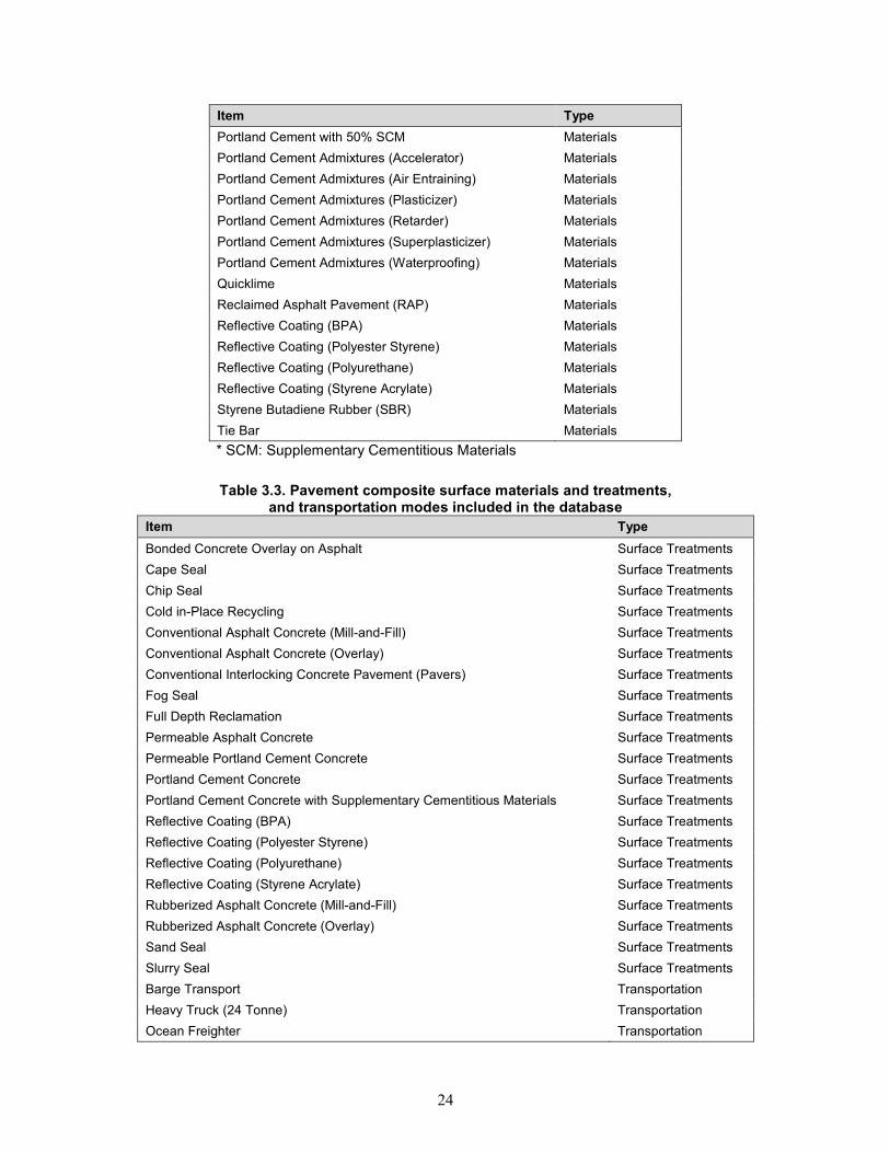
24

Item Type

Portland Cement with 50% SCM Materials

Portland Cement Admixtures (Accelerator) Materials

Portland Cement Admixtures (Air Entraining) Materials

Portland Cement Admixtures (Plasticizer) Materials

Portland Cement Admixtures (Retarder) Materials

Portland Cement Admixtures (Superplasticizer) Materials

Portland Cement Admixtures (Waterproofing) Materials

Quicklime Materials

Reclaimed Asphalt Pavement (RAP) Materials

Reflective Coating (BPA) Materials

Reflective Coating (Polyester Styrene) Materials

Reflective Coating (Polyurethane) Materials

Reflective Coating (Styrene Acrylate) Materials

Styrene Butadiene Rubber (SBR) Materials

Tie Bar Materials

* SCM: Supplementary Cementitious Materials

Table 3.3. Pavement composite surface materials and treatments,

and transportation modes included in the database

Item Type

Bonded Concrete Overlay on Asphalt Surface Treatments

Cape Seal Surface Treatments

Chip Seal Surface Treatments

Cold in-Place Recycling Surface Treatments

Conventional Asphalt Concrete (Mill-and-Fill) Surface Treatments

Conventional Asphalt Concrete (Overlay) Surface Treatments

Conventional Interlocking Concrete Pavement (Pavers) Surface Treatments

Fog Seal Surface Treatments

Full Depth Reclamation Surface Treatments

Permeable Asphalt Concrete Surface Treatments

Permeable Portland Cement Concrete Surface Treatments

Portland Cement Concrete Surface Treatments

Portland Cement Concrete with Supplementary Cementitious Materials Surface Treatments

Reflective Coating (BPA) Surface Treatments

Reflective Coating (Polyester Styrene) Surface Treatments

Reflective Coating (Polyurethane) Surface Treatments

Reflective Coating (Styrene Acrylate) Surface Treatments

Rubberized Asphalt Concrete (Mill-and-Fill) Surface Treatments

Rubberized Asphalt Concrete (Overlay) Surface Treatments

Sand Seal Surface Treatments

Slurry Seal Surface Treatments

Barge Transport Transportation

Heavy Truck (24 Tonne) Transportation

Ocean Freighter Transportation

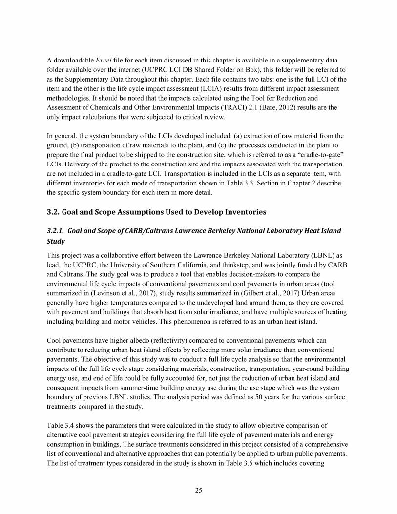
25

A downloadable Excel file for each item discussed in this chapter is available in a supplementary data

folder available over the internet (UCPRC LCI DB Shared Folder on Box), this folder will be referred to

as the Supplementary Data throughout this chapter. Each file contains two tabs: one is the full LCI of the

item and the other is the life cycle impact assessment (LCIA) results from different impact assessment

methodologies. It should be noted that the impacts calculated using the Tool for Reduction and

Assessment of Chemicals and Other Environmental Impacts (TRACI) 2.1 (Bare, 2012) results are the

only impact calculations that were subjected to critical review.

In general, the system boundary of the LCIs developed included: (a) extraction of raw material from the

ground, (b) transportation of raw materials to the plant, and (c) the processes conducted in the plant to

prepare the final product to be shipped to the construction site, which is referred to as a “cradle-to-gate”

LCIs. Delivery of the product to the construction site and the impacts associated with the transportation

are not included in a cradle-to-gate LCI. Transportation is included in the LCIs as a separate item, with

different inventories for each mode of transportation shown in Table 3.3. Section in Chapter 2 describe

the specific system boundary for each item in more detail.

3.2. Goal and Scope Assumptions Used to Develop Inventories

3.2.1. Goal and Scope of CARB/Caltrans Lawrence Berkeley National Laboratory Heat Island

Study

This project was a collaborative effort between the Lawrence Berkeley National Laboratory (LBNL) as

lead, the UCPRC, the University of Southern California, and thinkstep, and was jointly funded by CARB

and Caltrans. The study goal was to produce a tool that enables decision-makers to compare the

environmental life cycle impacts of conventional pavements and cool pavements in urban areas (tool

summarized in (Levinson et al., 2017), study results summarized in (Gilbert et al., 2017) Urban areas

generally have higher temperatures compared to the undeveloped land around them, as they are covered

with pavement and buildings that absorb heat from solar irradiance, and have multiple sources of heating

including building and motor vehicles. This phenomenon is referred to as an urban heat island.

Cool pavements have higher albedo (reflectivity) compared to conventional pavements which can

contribute to reducing urban heat island effects by reflecting more solar irradiance than conventional

pavements. The objective of this study was to conduct a full life cycle analysis so that the environmental

impacts of the full life cycle stage considering materials, construction, transportation, year-round building

energy use, and end of life could be fully accounted for, not just the reduction of urban heat island and

consequent impacts from summer-time building energy use during the use stage which was the system

boundary of previous LBNL studies. The analysis period was defined as 50 years for the various surface

treatments compared in the study.

Table 3.4 shows the parameters that were calculated in the study to allow objective comparison of

alternative cool pavement strategies considering the full life cycle of pavement materials and energy

consumption in buildings. The surface treatments considered in this project consisted of a comprehensive

list of conventional and alternative approaches that can potentially be applied to urban public pavements.

The list of treatment types considered in the study is shown in Table 3.5 which includes covering

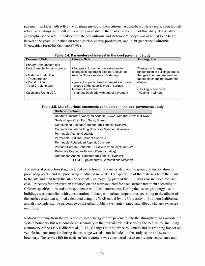
26

pavement surfaces with reflective coatings instead of conventional asphalt-based slurry seals, even though

reflective coatings were still not generally available in the market at the time of this study. The study’s

geographic scope was limited to the state of California and its temporal scope was assumed to be begin

between the years 2012 (then current electrical energy production) and 2020 (under the California

Renewables Portfolio Standard (RPS.)

Table 3.4. Parameters of interest in the cool pavement study

Pavement Side Climate Side Building Side

Energy Consumption and Environmental Impacts due to: - Material Production - Transportation - Construction -Total Cradle to Laid Calculated Using LCA

Changes in Urban temperature due to changes in pavement albedo. Calculated using a climate model considering: - percent of public roads changed each year - albedo of the specific type of surface treatment selected - changes in albedo with age of pavement

Changes in Energy consumption in buildings due to changes in urban temperature caused by changing pavement albedo - Cooling in summers - Heating in winters

Table 3.5. List of surface treatments considered in the cool pavements study

Surface Treatment

Bonded Concrete Overlay on Asphalt (BCOA) with three levels of SCM*

Seals (Cape, Chip, Fog, Sand, Slurry)

Conventional Asphalt Concrete, (mill and fill; overlay)

Conventional Interlocking Concrete Pavement (Pavers)

Permeable Asphalt Concrete

Permeable Portland Cement Concrete

Permeable Rubberized Asphalt Concrete

Portland Cement Concrete (PCC) with three levels of SCM

Reflective Coating (with four different coating)

Rubberized Asphalt Concrete (mill and fill; overlay) * SCM: Supplementary Cementitious Materials

The material production stage included extraction of raw materials from the ground, transportation to

processing plants, and the processing conducted in plants. Transportation of the materials from the plant

to the site and then from the site to the landfill or recycling plant at the EOL was also included for each

case. Processes for construction activities on site were modeled for each surface treatment according to

Caltrans specifications and correspondence with local contractors. During the use stage, energy use in

buildings was quantified with consideration of changes in urban temperatures according to the albedo of

the surface treatment applied calculated using the WRF model by the University of Southern California,

and also considering the percentage of the urban public pavements treated, and albedo changes expected

over time.

Radiative forcing from the reflection of solar energy off the pavement into the atmosphere was outside the

system boundary but was considered separately in the journal article describing the total study, including

a summary of the LCA (Gilbert et al., 2017.) Changes in the surface roughness and its resulting impact on

vehicle fuel consumption during the use stage was also not included in the study scope and system

boundary. The service life for each surface treatment was considered based on previous experience and

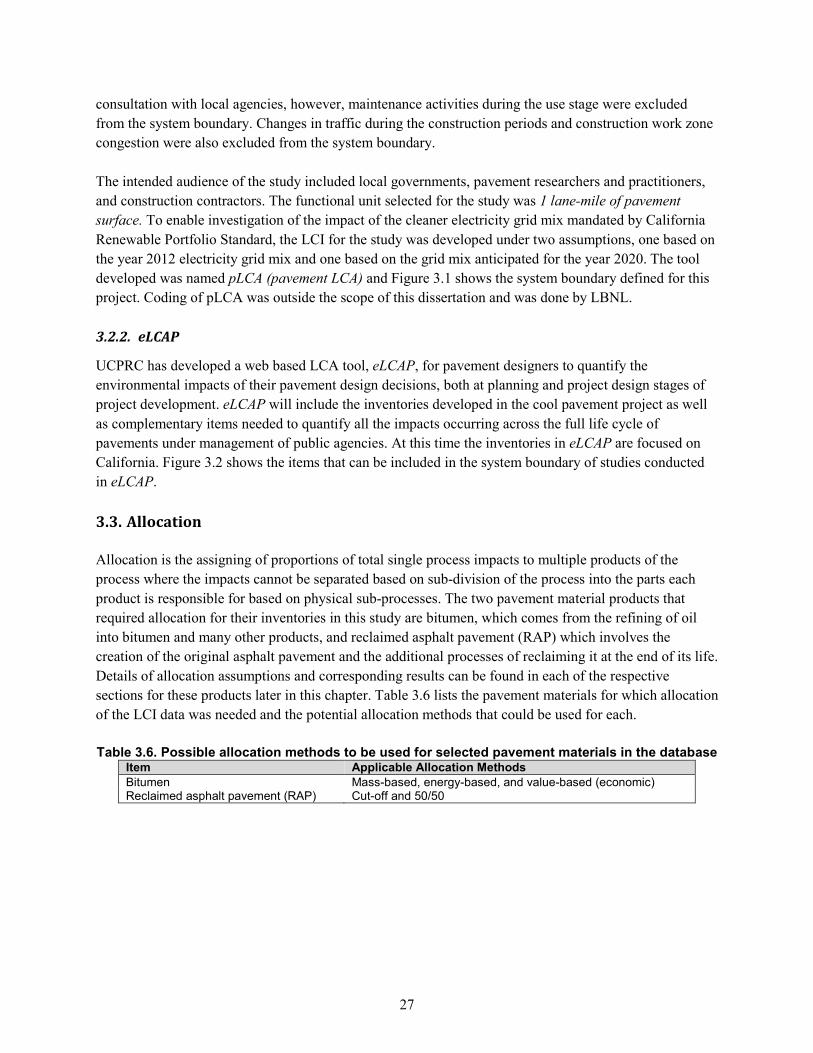
27

consultation with local agencies, however, maintenance activities during the use stage were excluded

from the system boundary. Changes in traffic during the construction periods and construction work zone

congestion were also excluded from the system boundary.

The intended audience of the study included local governments, pavement researchers and practitioners,

and construction contractors. The functional unit selected for the study was 1 lane-mile of pavement

surface. To enable investigation of the impact of the cleaner electricity grid mix mandated by California

Renewable Portfolio Standard, the LCI for the study was developed under two assumptions, one based on

the year 2012 electricity grid mix and one based on the grid mix anticipated for the year 2020. The tool

developed was named pLCA (pavement LCA) and Figure 3.1 shows the system boundary defined for this

project. Coding of pLCA was outside the scope of this dissertation and was done by LBNL.

3.2.2. eLCAP

UCPRC has developed a web based LCA tool, eLCAP, for pavement designers to quantify the

environmental impacts of their pavement design decisions, both at planning and project design stages of

project development. eLCAP will include the inventories developed in the cool pavement project as well

as complementary items needed to quantify all the impacts occurring across the full life cycle of

pavements under management of public agencies. At this time the inventories in eLCAP are focused on

California. Figure 3.2 shows the items that can be included in the system boundary of studies conducted

in eLCAP.

3.3. Allocation

Allocation is the assigning of proportions of total single process impacts to multiple products of the

process where the impacts cannot be separated based on sub-division of the process into the parts each

product is responsible for based on physical sub-processes. The two pavement material products that

required allocation for their inventories in this study are bitumen, which comes from the refining of oil

into bitumen and many other products, and reclaimed asphalt pavement (RAP) which involves the

creation of the original asphalt pavement and the additional processes of reclaiming it at the end of its life.

Details of allocation assumptions and corresponding results can be found in each of the respective

sections for these products later in this chapter. Table 3.6 lists the pavement materials for which allocation

of the LCI data was needed and the potential allocation methods that could be used for each.

Table 3.6. Possible allocation methods to be used for selected pavement materials in the database

Item Applicable Allocation Methods

Bitumen Mass-based, energy-based, and value-based (economic) Reclaimed asphalt pavement (RAP) Cut-off and 50/50

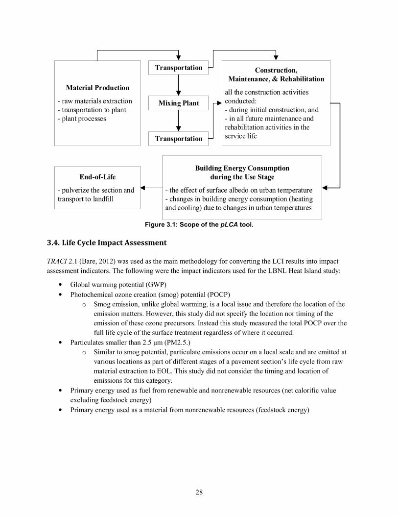
28

Material Production

- raw materials extraction - transportation to plant- plant processes

Mixing Plant

Transportation Construction,

Maintenance, & Rehabilitation

all the construction activities conducted:- during initial construction, and - in all future maintenance and rehabilitation activities in the service lifeTransportation

Building Energy Consumption

during the Use Stage

- the effect of surface albedo on urban temperature- changes in building energy consumption (heating and cooling) due to changes in urban temperatures

End-of-Life

- pulverize the section and transport to landfill

Figure 3.1: Scope of the pLCA tool.

3.4. Life Cycle Impact Assessment

TRACI 2.1 (Bare, 2012) was used as the main methodology for converting the LCI results into impact

assessment indicators. The following were the impact indicators used for the LBNL Heat Island study:

• Global warming potential (GWP)

• Photochemical ozone creation (smog) potential (POCP)

o Smog emission, unlike global warming, is a local issue and therefore the location of the

emission matters. However, this study did not specify the location nor timing of the

emission of these ozone precursors. Instead this study measured the total POCP over the

full life cycle of the surface treatment regardless of where it occurred.

• Particulates smaller than 2.5 μm (PM2.5.)

o Similar to smog potential, particulate emissions occur on a local scale and are emitted at

various locations as part of different stages of a pavement section’s life cycle from raw

material extraction to EOL. This study did not consider the timing and location of

emissions for this category.

• Primary energy used as fuel from renewable and nonrenewable resources (net calorific value

excluding feedstock energy)

• Primary energy used as a material from nonrenewable resources (feedstock energy)

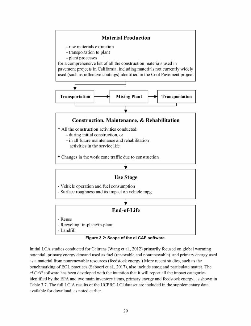
29

Material Production

- raw materials extraction - transportation to plant- plant processes

for a comprehensive list of all the construction materials used in pavement projects in California, including materials not currently widely used (such as reflective coatings) identified in the Cool Pavement project

Mixing PlantTransportation

Construction, Maintenance, & Rehabilitation

* All the construction activities conducted:- during initial construction, or - in all future maintenance and rehabilitation activities in the service life

* Changes in the work zone traffic due to construction

Transportation

Use Stage

- Vehicle operation and fuel consumption- Surface roughness and its impact on vehicle mpg

End-of-Life

- Reuse - Recycling: in-place/in-plant- Landfill

Figure 3.2: Scope of the eLCAP software.

Initial LCA studies conducted for Caltrans (Wang et al., 2012) primarily focused on global warming

potential, primary energy demand used as fuel (renewable and nonrenewable), and primary energy used

as a material from nonrenewable resources (feedstock energy.) More recent studies, such as the

benchmarking of EOL practices (Saboori et al., 2017), also include smog and particulate matter. The

eLCAP software has been developed with the intention that it will report all the impact categories

identified by the EPA and two main inventory items, primary energy and feedstock energy, as shown in

Table 3.7. The full LCIA results of the UCPRC LCI dataset are included in the supplementary data

available for download, as noted earlier.

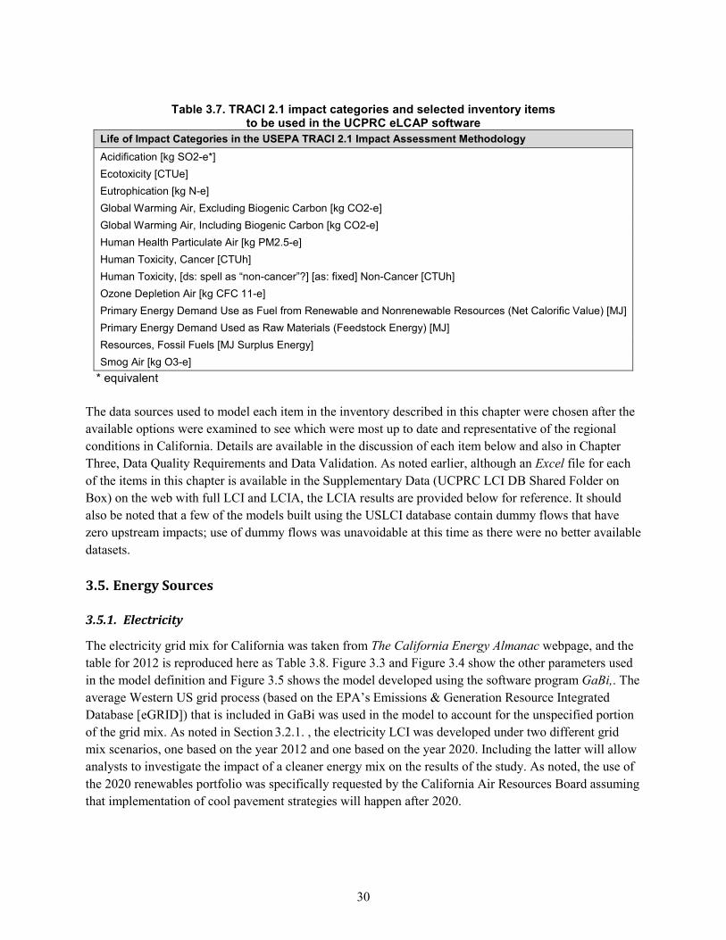
30

Table 3.7. TRACI 2.1 impact categories and selected inventory items

to be used in the UCPRC eLCAP software

Life of Impact Categories in the USEPA TRACI 2.1 Impact Assessment Methodology

Acidification [kg SO2-e*]

Ecotoxicity [CTUe]

Eutrophication [kg N-e]

Global Warming Air, Excluding Biogenic Carbon [kg CO2-e]

Global Warming Air, Including Biogenic Carbon [kg CO2-e]

Human Health Particulate Air [kg PM2.5-e]

Human Toxicity, Cancer [CTUh]

Human Toxicity, [ds: spell as “non-cancer”?] [as: fixed] Non-Cancer [CTUh]

Ozone Depletion Air [kg CFC 11-e]

Primary Energy Demand Use as Fuel from Renewable and Nonrenewable Resources (Net Calorific Value) [MJ]

Primary Energy Demand Used as Raw Materials (Feedstock Energy) [MJ]

Resources, Fossil Fuels [MJ Surplus Energy]

Smog Air [kg O3-e]

* equivalent

The data sources used to model each item in the inventory described in this chapter were chosen after the

available options were examined to see which were most up to date and representative of the regional

conditions in California. Details are available in the discussion of each item below and also in Chapter

Three, Data Quality Requirements and Data Validation. As noted earlier, although an Excel file for each

of the items in this chapter is available in the Supplementary Data (UCPRC LCI DB Shared Folder on

Box) on the web with full LCI and LCIA, the LCIA results are provided below for reference. It should

also be noted that a few of the models built using the USLCI database contain dummy flows that have

zero upstream impacts; use of dummy flows was unavoidable at this time as there were no better available

datasets.

3.5. Energy Sources

3.5.1. Electricity

The electricity grid mix for California was taken from The California Energy Almanac webpage, and the

table for 2012 is reproduced here as Table 3.8. Figure 3.3 and Figure 3.4 show the other parameters used

in the model definition and Figure 3.5 shows the model developed using the software program GaBi,. The

average Western US grid process (based on the EPA’s Emissions & Generation Resource Integrated

Database [eGRID]) that is included in GaBi was used in the model to account for the unspecified portion

of the grid mix. As noted in Section 3.2.1. , the electricity LCI was developed under two different grid

mix scenarios, one based on the year 2012 and one based on the year 2020. Including the latter will allow

analysts to investigate the impact of a cleaner energy mix on the results of the study. As noted, the use of

the 2020 renewables portfolio was specifically requested by the California Air Resources Board assuming

that implementation of cool pavement strategies will happen after 2020.

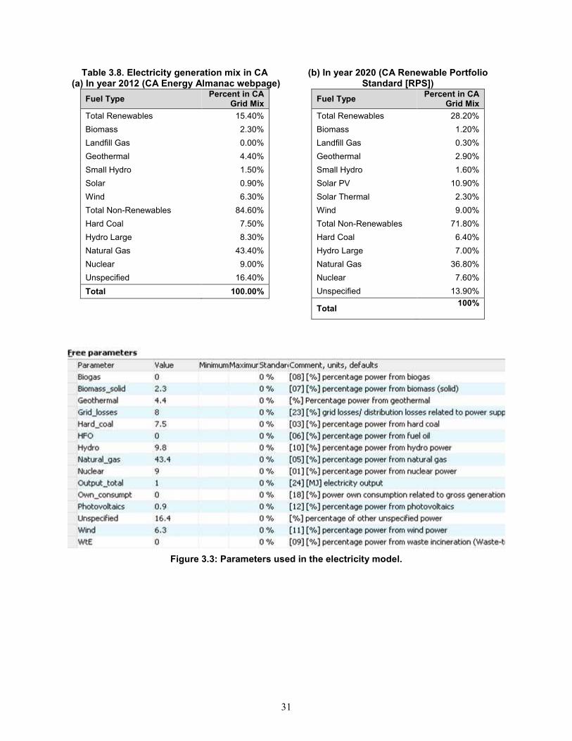
31

Table 3.8. Electricity generation mix in CA (a) In year 2012 (CA Energy Almanac webpage)

Fuel Type Percent in CA

Grid Mix

Total Renewables 15.40%

Biomass 2.30%

Landfill Gas 0.00%

Geothermal 4.40%

Small Hydro 1.50%

Solar 0.90%

Wind 6.30%

Total Non-Renewables 84.60%

Hard Coal 7.50%

Hydro Large 8.30%

Natural Gas 43.40%

Nuclear 9.00%

Unspecified 16.40%

Total 100.00%

(b) In year 2020 (CA Renewable Portfolio Standard [RPS])

Fuel Type Percent in CA

Grid Mix

Total Renewables 28.20%

Biomass 1.20%

Landfill Gas 0.30%

Geothermal 2.90%

Small Hydro 1.60%

Solar PV 10.90%

Solar Thermal 2.30%

Wind 9.00%

Total Non-Renewables 71.80%

Hard Coal 6.40%

Hydro Large 7.00%

Natural Gas 36.80%

Nuclear 7.60%

Unspecified 13.90%

Total 100%

Figure 3.3: Parameters used in the electricity model.

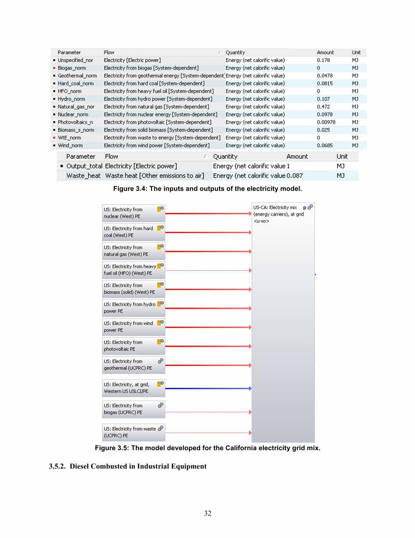
32

Figure 3.4: The inputs and outputs of the electricity model.

Figure 3.5: The model developed for the California electricity grid mix.

3.5.2. Diesel Combusted in Industrial Equipment

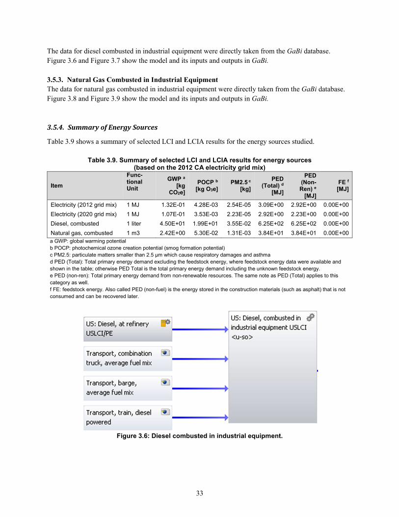
33

The data for diesel combusted in industrial equipment were directly taken from the GaBi database.

Figure 3.6 and Figure 3.7 show the model and its inputs and outputs in GaBi.

3.5.3. Natural Gas Combusted in Industrial Equipment

The data for natural gas combusted in industrial equipment were directly taken from the GaBi database.

Figure 3.8 and Figure 3.9 show the model and its inputs and outputs in GaBi.

3.5.4. Summary of Energy Sources

Table 3.9 shows a summary of selected LCI and LCIA results for the energy sources studied.

Table 3.9. Summary of selected LCI and LCIA results for energy sources

(based on the 2012 CA electricity grid mix)

Item

Func-tional Unit

GWP a [kg

CO2e]

POCP b [kg O3e]

PM2.5 c [kg]

PED (Total) d

[MJ]

PED (Non-Ren) e

[MJ]

FE f

[MJ]

Electricity (2012 grid mix) 1 MJ 1.32E-01 4.28E-03 2.54E-05 3.09E+00 2.92E+00 0.00E+00

Electricity (2020 grid mix) 1 MJ 1.07E-01 3.53E-03 2.23E-05 2.92E+00 2.23E+00 0.00E+00

Diesel, combusted 1 liter 4.50E+01 1.99E+01 3.55E-02 6.25E+02 6.25E+02 0.00E+00

Natural gas, combusted 1 m3 2.42E+00 5.30E-02 1.31E-03 3.84E+01 3.84E+01 0.00E+00 a GWP: global warming potential b POCP: photochemical ozone creation potential (smog formation potential) c PM2.5: particulate matters smaller than 2.5 μm which cause respiratory damages and asthma d PED (Total): Total primary energy demand excluding the feedstock energy, where feedstock energy data were available and shown in the table; otherwise PED Total is the total primary energy demand including the unknown feedstock energy. e PED (non-ren): Total primary energy demand from non-renewable resources. The same note as PED (Total) applies to this category as well. f FE: feedstock energy. Also called PED (non-fuel) is the energy stored in the construction materials (such as asphalt) that is not consumed and can be recovered later.

Figure 3.6: Diesel combusted in industrial equipment.

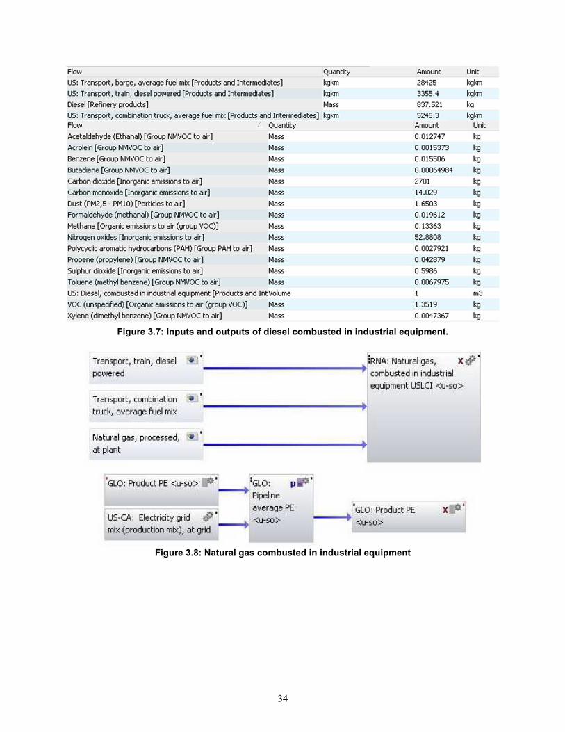
34

Figure 3.7: Inputs and outputs of diesel combusted in industrial equipment.

Figure 3.8: Natural gas combusted in industrial equipment

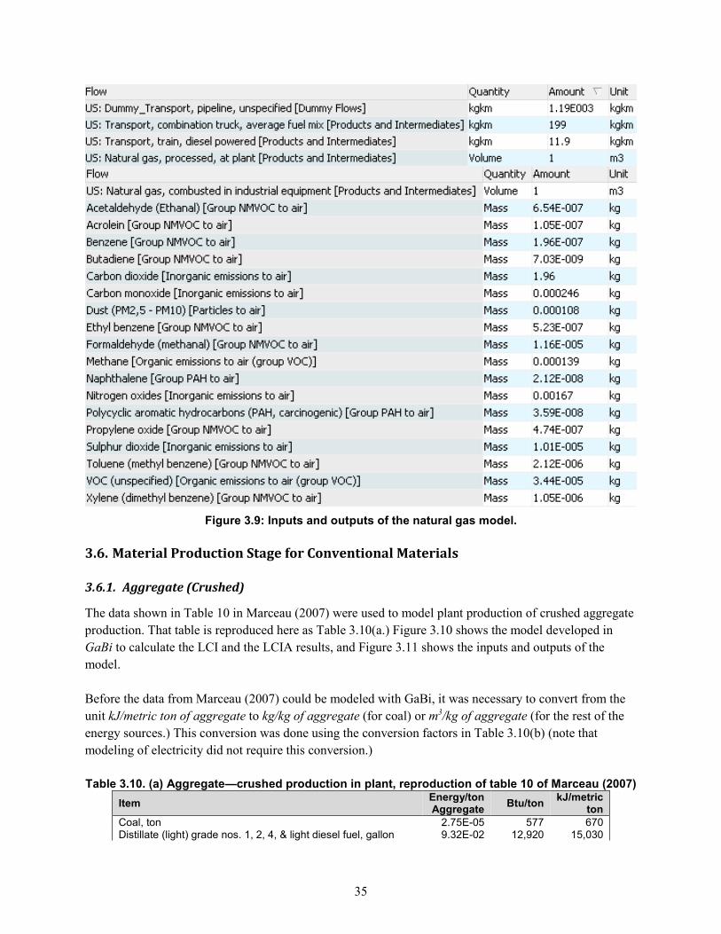
35

Figure 3.9: Inputs and outputs of the natural gas model.

3.6. Material Production Stage for Conventional Materials

3.6.1. Aggregate (Crushed)

The data shown in Table 10 in Marceau (2007) were used to model plant production of crushed aggregate

production. That table is reproduced here as Table 3.10(a.) Figure 3.10 shows the model developed in

GaBi to calculate the LCI and the LCIA results, and Figure 3.11 shows the inputs and outputs of the

model.

Before the data from Marceau (2007) could be modeled with GaBi, it was necessary to convert from the

unit kJ/metric ton of aggregate to kg/kg of aggregate (for coal) or m3/kg of aggregate (for the rest of the

energy sources.) This conversion was done using the conversion factors in Table 3.10(b) (note that

modeling of electricity did not require this conversion.)

Table 3.10. (a) Aggregate—crushed production in plant, reproduction of table 10 of Marceau (2007)

Item Energy/ton Aggregate

Btu/ton kJ/metric

ton Coal, ton 2.75E-05 577 670 Distillate (light) grade nos. 1, 2, 4, & light diesel fuel, gallon 9.32E-02 12,920 15,030

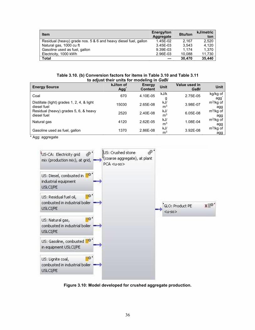
36

Item Energy/ton Aggregate

Btu/ton kJ/metric

ton Residual (heavy) grade nos. 5 & 6 and heavy diesel fuel, gallon 1.45E-02 2,167 2,520 Natural gas, 1000 cu ft 3.45E-03 3,543 4,120 Gasoline used as fuel, gallon 9.39E-03 1,174 1,370 Electricity, 1000 kWh 2.96E-03 10,088 11,730 Total — 30,470 35,440

Table 3.10. (b) Conversion factors for items in Table 3.10 and Table 3.11

to adjust their units for modeling in GaBi

Energy Source kJ/ton of

Agg* Energy

Content Unit

Value used in GaBi

Unit

Coal 670 4.10E-05 kJ/k

g 2.75E-05

kg/kg of agg*

Distillate (light) grades 1, 2, 4, & light diesel fuel

15030 2.65E-08 kJ/m3

3.98E-07 m3/kg of

agg Residual (heavy) grades 5, 6, & heavy diesel fuel

2520 2.40E-08 kJ/m3

6.05E-08 m3/kg of

agg

Natural gas 4120 2.62E-05 kJ/m3

1.08E-04 m3/kg of

agg

Gasoline used as fuel, gallon 1370 2.86E-08 kJ/m3

3.92E-08 m3/kg of

agg * Agg: aggregate

Figure 3.10: Model developed for crushed aggregate production.

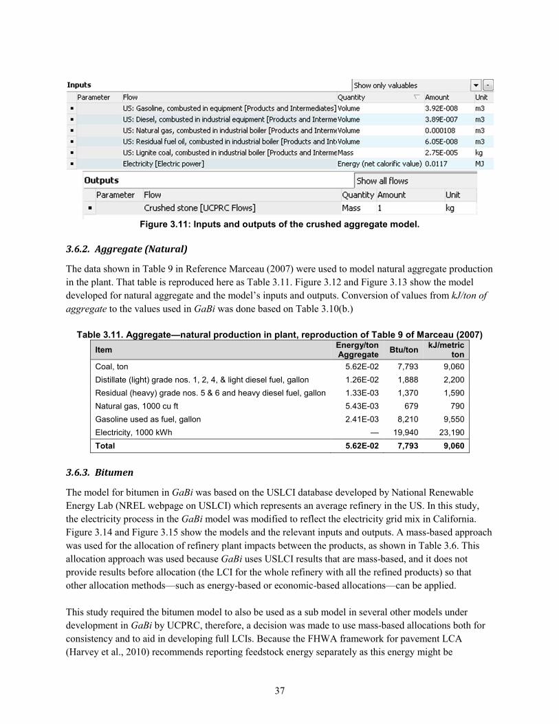
37

Figure 3.11: Inputs and outputs of the crushed aggregate model.

3.6.2. Aggregate (Natural)

The data shown in Table 9 in Reference Marceau (2007) were used to model natural aggregate production

in the plant. That table is reproduced here as Table 3.11. Figure 3.12 and Figure 3.13 show the model

developed for natural aggregate and the model’s inputs and outputs. Conversion of values from kJ/ton of

aggregate to the values used in GaBi was done based on Table 3.10(b.)

Table 3.11. Aggregate—natural production in plant, reproduction of Table 9 of Marceau (2007)

Item Energy/ton Aggregate

Btu/ton kJ/metric

ton

Coal, ton 5.62E-02 7,793 9,060

Distillate (light) grade nos. 1, 2, 4, & light diesel fuel, gallon 1.26E-02 1,888 2,200

Residual (heavy) grade nos. 5 & 6 and heavy diesel fuel, gallon 1.33E-03 1,370 1,590

Natural gas, 1000 cu ft 5.43E-03 679 790

Gasoline used as fuel, gallon 2.41E-03 8,210 9,550

Electricity, 1000 kWh — 19,940 23,190

Total 5.62E-02 7,793 9,060

3.6.3. Bitumen

The model for bitumen in GaBi was based on the USLCI database developed by National Renewable

Energy Lab (NREL webpage on USLCI) which represents an average refinery in the US. In this study,

the electricity process in the GaBi model was modified to reflect the electricity grid mix in California.

Figure 3.14 and Figure 3.15 show the models and the relevant inputs and outputs. A mass-based approach

was used for the allocation of refinery plant impacts between the products, as shown in Table 3.6. This

allocation approach was used because GaBi uses USLCI results that are mass-based, and it does not

provide results before allocation (the LCI for the whole refinery with all the refined products) so that

other allocation methods—such as energy-based or economic-based allocations—can be applied.

This study required the bitumen model to also be used as a sub model in several other models under

development in GaBi by UCPRC, therefore, a decision was made to use mass-based allocations both for

consistency and to aid in developing full LCIs. Because the FHWA framework for pavement LCA

(Harvey et al., 2010) recommends reporting feedstock energy separately as this energy might be

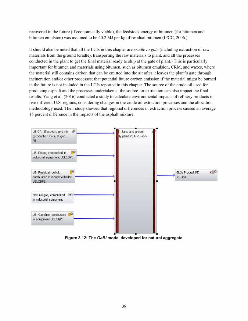
38

recovered in the future (if economically viable), the feedstock energy of bitumen (for bitumen and

bitumen emulsion) was assumed to be 40.2 MJ per kg of residual bitumen (IPCC, 2006.)

It should also be noted that all the LCIs in this chapter are cradle to gate (including extraction of raw

materials from the ground (cradle), transporting the raw materials to plant, and all the processes

conducted in the plant to get the final material ready to ship at the gate of plant.) This is particularly

important for bitumen and materials using bitumen, such as bitumen emulsion, CRM, and waxes, where

the material still contains carbon that can be emitted into the air after it leaves the plant’s gate through

incineration and/or other processes; that potential future carbon emission if the material might be burned

in the future is not included in the LCIs reported in this chapter. The source of the crude oil used for

producing asphalt and the processes undertaken at the source for extraction can also impact the final

results. Yang et al. (2016) conducted a study to calculate environmental impacts of refinery products in

five different U.S. regions, considering changes in the crude oil extraction processes and the allocation

methodology used. Their study showed that regional differences in extraction process caused an average

15 percent difference in the impacts of the asphalt mixture.

Figure 3.12: The GaBi model developed for natural aggregate.

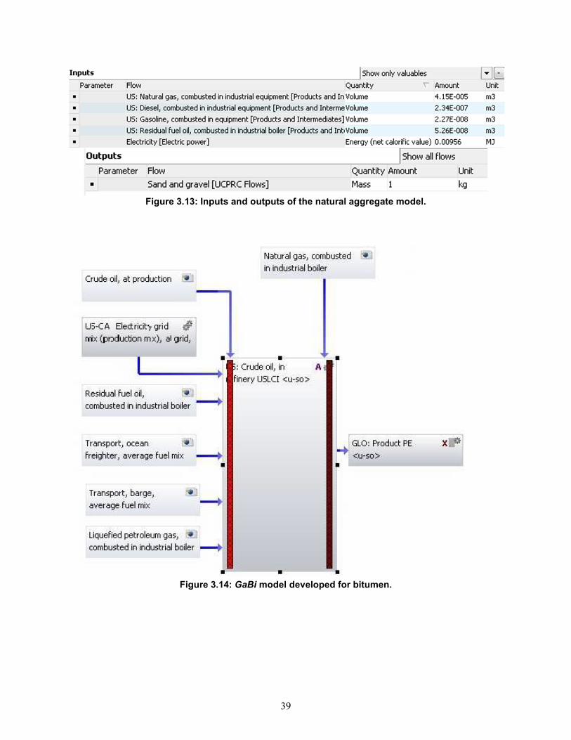
39

Figure 3.13: Inputs and outputs of the natural aggregate model.

Figure 3.14: GaBi model developed for bitumen.

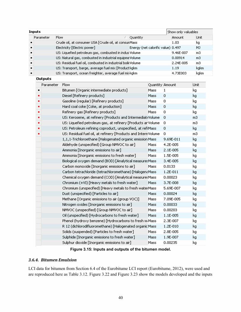
40

Figure 3.15: Inputs and outputs of the bitumen model.

3.6.4. Bitumen Emulsion

LCI data for bitumen from Section 6.4 of the Eurobitume LCI report (Eurobitume, 2012), were used and

are reproduced here as Table 3.12. Figure 3.22 and Figure 3.23 show the models developed and the inputs

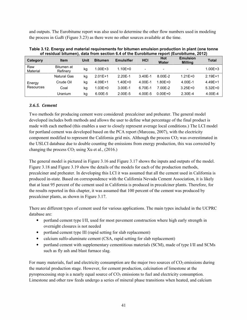
41

and outputs. The Eurobitume report was also used to determine the other flow numbers used in modeling

the process in GaBi (Figure 3.23) as there were no other sources available at the time.

Table 3.12. Energy and material requirements for bitumen emulsion production in plant (one tonne

of residual bitumen), data from section 6.4 of the Eurobitume report (Eurobitume, 2012)

Category Item Unit Bitumen Emulsifier HCl Hot

Water Emulsion

Milling Total

Raw Material

Bitumen at Refinery

kg 1.00E+3 1.10E+0 - - - 1.00E+3

Energy Resources

Natural Gas kg 2.01E+1 2.20E-1 3.40E-1 8.00E-2 1.21E+0 2.19E+1

Crude Oil kg 4.09E+1 1.40E+0 4.00E-1 1.80E+0 4.00E-1 4.49E+1

Coal kg 1.03E+0 3.00E-1 6.70E-1 7.00E-2 3.25E+0 5.32E+0

Uranium kg 6.00E-5 2.00E-5 4.00E-5 0.00E+0 2.30E-4 4.00E-4

3.6.5. Cement

Two methods for producing cement were considered: precalciner and preheater. The general model

developed includes both methods and allows the user to define what percentage of the final product is

made with each method (this enables a user to closely represent average local conditions.) The LCI model

for portland cement was developed based on the PCA report (Marceau, 2007), with the electricity

component modified to represent the California grid mix. Although the process CO2 was overestimated in

the USLCI database due to double counting the emissions from energy production, this was corrected by

changing the process CO2 using Xu et al., (2016.)

The general model is pictured in Figure 3.16 and Figure 3.17 shows the inputs and outputs of the model.

Figure 3.18 and Figure 3.19 show the details of the models for each of the production methods,

precalciner and preheater. In developing this LCI it was assumed that all the cement used in California is

produced in-state. Based on correspondence with the California Nevada Cement Association, it is likely

that at least 95 percent of the cement used in California is produced in precalciner plants. Therefore, for

the results reported in this chapter, it was assumed that 100 percent of the cement was produced by

precalciner plants, as shown in Figure 3.17.

There are different types of cement used for various applications. The main types included in the UCPRC

database are:

• portland cement type I/II, used for most pavement construction where high early strength in

overnight closures is not needed

• portland cement type III (rapid setting for slab replacement)

• calcium sulfo-aluminate cement (CSA, rapid setting for slab replacement)

• portland cement with supplementary cementitious materials (SCM), made of type I/II and SCMs

such as fly ash and blast furnace slag.

For many materials, fuel and electricity consumption are the major two sources of CO2 emissions during

the material production stage. However, for cement production, calcination of limestone at the

pyroprocessing step is a nearly equal source of CO2 emissions to fuel and electricity consumption.

Limestone and other raw feeds undergo a series of mineral phase transitions when heated, and calcium

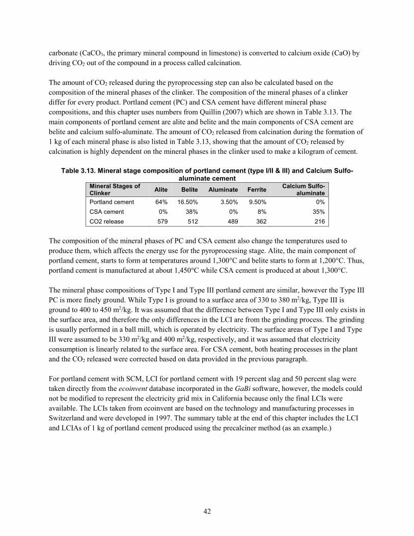
42

carbonate (CaCO3, the primary mineral compound in limestone) is converted to calcium oxide (CaO) by

driving CO2 out of the compound in a process called calcination.

The amount of CO2 released during the pyroprocessing step can also be calculated based on the

composition of the mineral phases of the clinker. The composition of the mineral phases of a clinker

differ for every product. Portland cement (PC) and CSA cement have different mineral phase

compositions, and this chapter uses numbers from Quillin (2007) which are shown in Table 3.13. The

main components of portland cement are alite and belite and the main components of CSA cement are

belite and calcium sulfo-aluminate. The amount of CO2 released from calcination during the formation of

1 kg of each mineral phase is also listed in Table 3.13, showing that the amount of CO2 released by

calcination is highly dependent on the mineral phases in the clinker used to make a kilogram of cement.

Table 3.13. Mineral stage composition of portland cement (type I/II & III) and Calcium Sulfo-

aluminate cement Mineral Stages of Clinker

Alite Belite Aluminate Ferrite Calcium Sulfo-

aluminate

Portland cement 64% 16.50% 3.50% 9.50% 0%

CSA cement 0% 38% 0% 8% 35%

CO2 release 579 512 489 362 216

The composition of the mineral phases of PC and CSA cement also change the temperatures used to

produce them, which affects the energy use for the pyroprocessing stage. Alite, the main component of

portland cement, starts to form at temperatures around 1,300°C and belite starts to form at 1,200°C. Thus,

portland cement is manufactured at about 1,450°C while CSA cement is produced at about 1,300°C.

The mineral phase compositions of Type I and Type III portland cement are similar, however the Type III

PC is more finely ground. While Type I is ground to a surface area of 330 to 380 m2/kg, Type III is

ground to 400 to 450 m2/kg. It was assumed that the difference between Type I and Type III only exists in

the surface area, and therefore the only differences in the LCI are from the grinding process. The grinding

is usually performed in a ball mill, which is operated by electricity. The surface areas of Type I and Type

III were assumed to be 330 m2/kg and 400 m2/kg, respectively, and it was assumed that electricity

consumption is linearly related to the surface area. For CSA cement, both heating processes in the plant

and the CO2 released were corrected based on data provided in the previous paragraph.

For portland cement with SCM, LCI for portland cement with 19 percent slag and 50 percent slag were

taken directly from the ecoinvent database incorporated in the GaBi software, however, the models could

not be modified to represent the electricity grid mix in California because only the final LCIs were

available. The LCIs taken from ecoinvent are based on the technology and manufacturing processes in

Switzerland and were developed in 1997. The summary table at the end of this chapter includes the LCI

and LCIAs of 1 kg of portland cement produced using the precalciner method (as an example.)

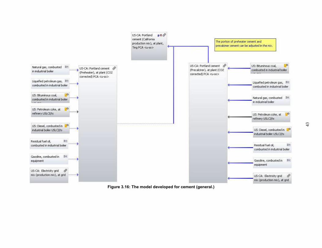
43

Figure 3.16: The model developed for cement (general.)

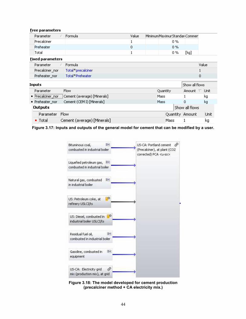
44

Figure 3.17: Inputs and outputs of the general model for cement that can be modified by a user.

Figure 3.18: The model developed for cement production (precalciner method + CA electricity mix.)

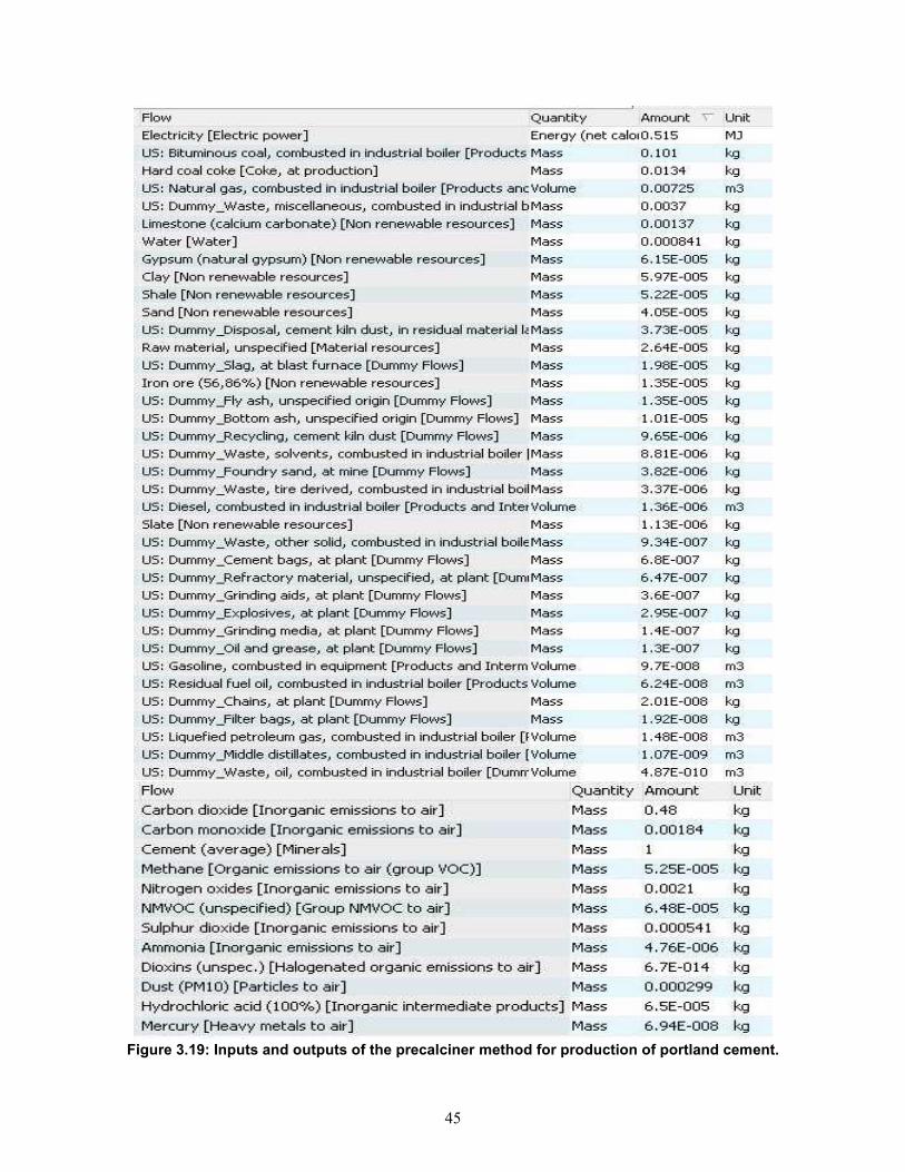
45

Figure 3.19: Inputs and outputs of the precalciner method for production of portland cement.

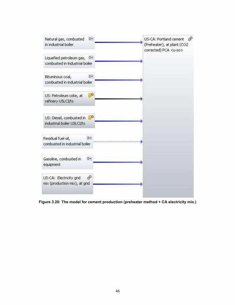
46

Figure 3.20: The model for cement production (preheater method + CA electricity mix.)

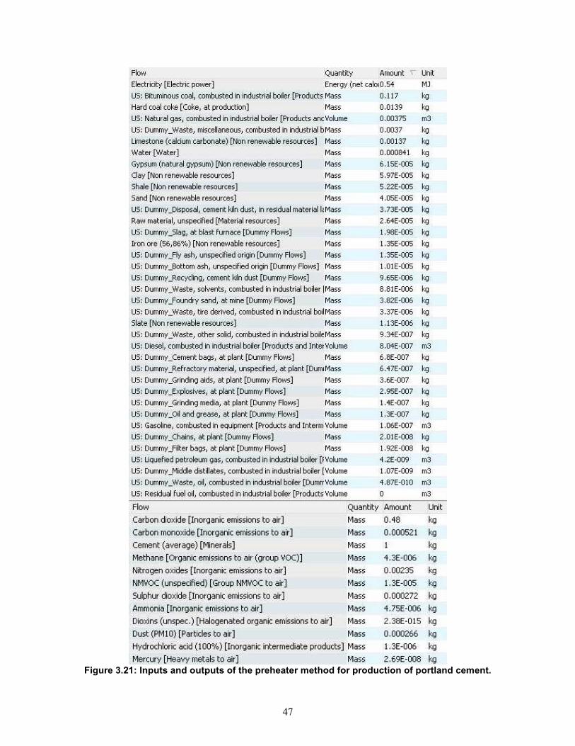
47

Figure 3.21: Inputs and outputs of the preheater method for production of portland cement.

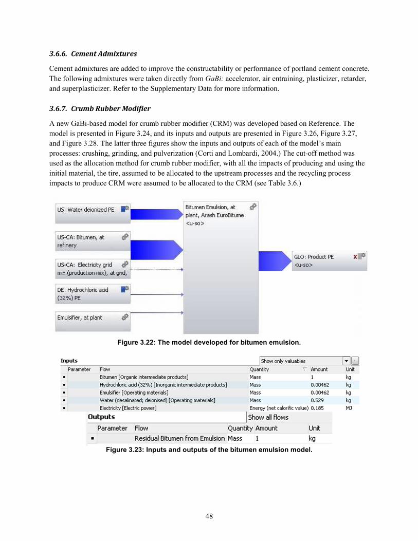
48

3.6.6. Cement Admixtures

Cement admixtures are added to improve the constructability or performance of portland cement concrete.

The following admixtures were taken directly from GaBi: accelerator, air entraining, plasticizer, retarder,

and superplasticizer. Refer to the Supplementary Data for more information.

3.6.7. Crumb Rubber Modifier

A new GaBi-based model for crumb rubber modifier (CRM) was developed based on Reference. The

model is presented in Figure 3.24, and its inputs and outputs are presented in Figure 3.26, Figure 3.27,

and Figure 3.28. The latter three figures show the inputs and outputs of each of the model’s main

processes: crushing, grinding, and pulverization (Corti and Lombardi, 2004.) The cut-off method was

used as the allocation method for crumb rubber modifier, with all the impacts of producing and using the

initial material, the tire, assumed to be allocated to the upstream processes and the recycling process

impacts to produce CRM were assumed to be allocated to the CRM (see Table 3.6.)

Figure 3.22: The model developed for bitumen emulsion.

Figure 3.23: Inputs and outputs of the bitumen emulsion model.

49

Figure 3.24: GaBi model developed for crumb rubber modifier (CRM.)

Figure 3.25: Inputs and outputs for the grinding process of the CRM model.

Figure 3.26: Inputs and outputs for the crushing process of the CRM model.

3.6.8. Dowel and Tie Bar

Dowel and tie bar models were developed in GaBi using the software’s predefined models for the

production of steel and the epoxy coating for covering the bars. The electricity used in the coating process

was not included because reliable data were unavailable and because the process energy was assumed to

be insignificant compared to energy consumption of the steel and epoxy production. Figure 3.28 shows

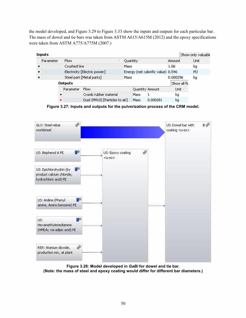
50

the model developed, and Figure 3.29 to Figure 3.33 show the inputs and outputs for each particular bar.

The mass of dowel and tie bars was taken from ASTM A615/A615M (2012) and the epoxy specifications

were taken from ASTM A775/A775M (2007.)

Figure 3.27: Inputs and outputs for the pulverization process of the CRM model.

Figure 3.28: Model developed in GaBi for dowel and tie bar. (Note: the mass of steel and epoxy coating would differ for different bar diameters.)

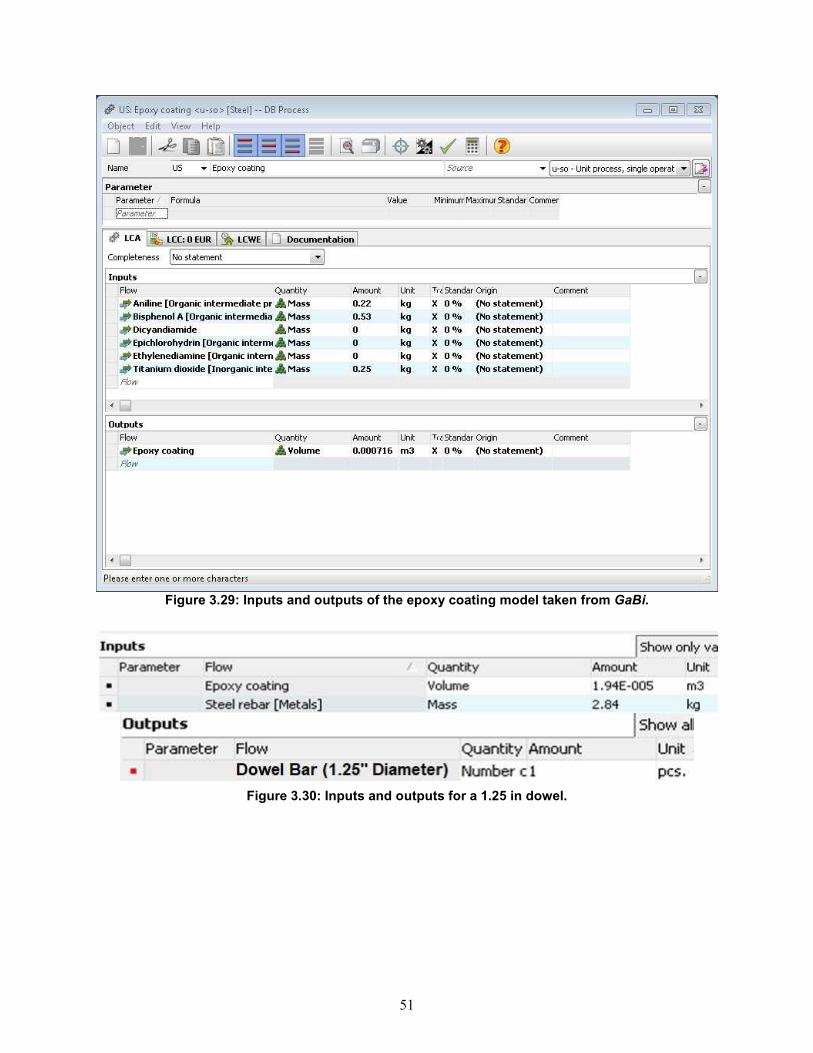
51

Figure 3.29: Inputs and outputs of the epoxy coating model taken from GaBi.

Figure 3.30: Inputs and outputs for a 1.25 in dowel.

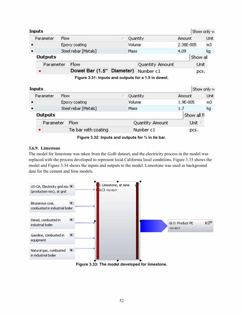
52

Figure 3.31: Inputs and outputs for a 1.5 in dowel.

Figure 3.32: Inputs and outputs for ¾ in tie bar.

3.6.9. Limestone

The model for limestone was taken from the GaBi dataset, and the electricity process in the model was

replaced with the process developed to represent local California local conditions. Figure 3.33 shows the

model and Figure 3.34 shows the inputs and outputs to the model. Limestone was used as background

data for the cement and lime models.

Figure 3.33: The model developed for limestone.

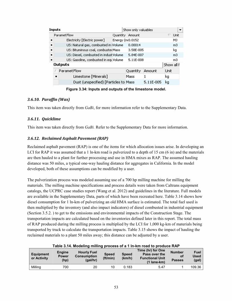
53

Figure 3.34: Inputs and outputs of the limestone model.

3.6.10. Paraffin (Wax)

This item was taken directly from GaBi, for more information refer to the Supplementary Data.

3.6.11. Quicklime

This item was taken directly from GaBi. Refer to the Supplementary Data for more information.

3.6.12. Reclaimed Asphalt Pavement (RAP)

Reclaimed asphalt pavement (RAP) is one of the items for which allocation issues arise. In developing an

LCI for RAP it was assumed that a 1 ln-km road is pulverized to a depth of 15 cm (6 in) and the materials

are then hauled to a plant for further processing and use in HMA mixes as RAP. The assumed hauling

distance was 50 miles, a typical one-way hauling distance for aggregates in California. In the model

developed, both of these assumptions can be modified by a user.

The pulverization process was modeled assuming use of a 700 hp milling machine for milling the

materials. The milling machine specifications and process details were taken from Caltrans equipment

catalogs, the UCPRC case studies report (Wang et al. 2012) and guidelines in the literature. Full models

are available in the Supplementary Data, parts of which have been recreated here. Table 3.14 shows how

diesel consumption for 1 ln-km of pulverizing an old HMA surface is estimated. The total fuel used is

then multiplied by the inventory (and also impact indicators) of diesel combusted in industrial equipment

(Section 3.5.2. ) to get to the emissions and environmental impacts of the Construction Stage. The

transportation impacts are calculated based on the inventories defined later in this report. The total mass

of RAP produced during the milling process is multiplied by the LCI for 1,000 kg-km of materials being

transported by truck to calculate the transportation impacts. Table 3.15 shows the impact of hauling the

reclaimed materials to a plant 50 miles away; this distance can be adjusted by a user.

Table 3.14. Modeling milling process of a 1 ln-km road to produce RAP

Equipment or Activity

Engine Power

(hp)

Hourly Fuel Consumption

(gal/hr)

Speed (ft/min)

Speed (km/h)

Time (hr) for One Pass over the

Functional Unit (1 lane-km)

Number of

Passes

Fuel Used (gal)

Milling 700 20 10 0.183 5.47 1 109.36

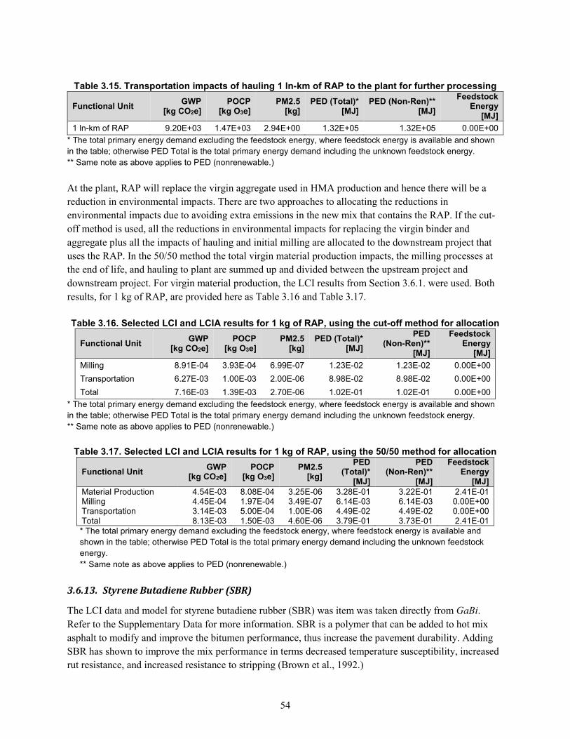
54

Table 3.15. Transportation impacts of hauling 1 ln-km of RAP to the plant for further processing

Functional Unit GWP

[kg CO2e] POCP

[kg O3e] PM2.5

[kg] PED (Total)*

[MJ] PED (Non-Ren)**

[MJ]

Feedstock Energy

[MJ]

1 ln-km of RAP 9.20E+03 1.47E+03 2.94E+00 1.32E+05 1.32E+05 0.00E+00

* The total primary energy demand excluding the feedstock energy, where feedstock energy is available and shown in the table; otherwise PED Total is the total primary energy demand including the unknown feedstock energy. ** Same note as above applies to PED (nonrenewable.)

At the plant, RAP will replace the virgin aggregate used in HMA production and hence there will be a

reduction in environmental impacts. There are two approaches to allocating the reductions in

environmental impacts due to avoiding extra emissions in the new mix that contains the RAP. If the cut-

off method is used, all the reductions in environmental impacts for replacing the virgin binder and

aggregate plus all the impacts of hauling and initial milling are allocated to the downstream project that

uses the RAP. In the 50/50 method the total virgin material production impacts, the milling processes at

the end of life, and hauling to plant are summed up and divided between the upstream project and

downstream project. For virgin material production, the LCI results from Section 3.6.1. were used. Both

results, for 1 kg of RAP, are provided here as Table 3.16 and Table 3.17.

Table 3.16. Selected LCI and LCIA results for 1 kg of RAP, using the cut-off method for allocation

Functional Unit GWP

[kg CO2e] POCP

[kg O3e] PM2.5

[kg] PED (Total)*

[MJ]

PED (Non-Ren)**

[MJ]

Feedstock Energy

[MJ]

Milling 8.91E-04 3.93E-04 6.99E-07 1.23E-02 1.23E-02 0.00E+00

Transportation 6.27E-03 1.00E-03 2.00E-06 8.98E-02 8.98E-02 0.00E+00

Total 7.16E-03 1.39E-03 2.70E-06 1.02E-01 1.02E-01 0.00E+00

* The total primary energy demand excluding the feedstock energy, where feedstock energy is available and shown in the table; otherwise PED Total is the total primary energy demand including the unknown feedstock energy. ** Same note as above applies to PED (nonrenewable.)

Table 3.17. Selected LCI and LCIA results for 1 kg of RAP, using the 50/50 method for allocation

Functional Unit GWP

[kg CO2e] POCP

[kg O3e] PM2.5

[kg]

PED (Total)*

[MJ]

PED (Non-Ren)**

[MJ]

Feedstock Energy

[MJ] Material Production 4.54E-03 8.08E-04 3.25E-06 3.28E-01 3.22E-01 2.41E-01 Milling 4.45E-04 1.97E-04 3.49E-07 6.14E-03 6.14E-03 0.00E+00 Transportation 3.14E-03 5.00E-04 1.00E-06 4.49E-02 4.49E-02 0.00E+00 Total 8.13E-03 1.50E-03 4.60E-06 3.79E-01 3.73E-01 2.41E-01 * The total primary energy demand excluding the feedstock energy, where feedstock energy is available and shown in the table; otherwise PED Total is the total primary energy demand including the unknown feedstock energy. ** Same note as above applies to PED (nonrenewable.)

3.6.13. Styrene Butadiene Rubber (SBR)

The LCI data and model for styrene butadiene rubber (SBR) was item was taken directly from GaBi.

Refer to the Supplementary Data for more information. SBR is a polymer that can be added to hot mix

asphalt to modify and improve the bitumen performance, thus increase the pavement durability. Adding

SBR has shown to improve the mix performance in terms decreased temperature susceptibility, increased

rut resistance, and increased resistance to stripping (Brown et al., 1992.)

55

3.6.14. Summary of the Material Production Impacts for Conventional Materials

Table 3.18 summarizes the selected LCI and LCIA results for the conventional materials included in the

database developed in this project. As noted in Section 3.2.1. , a decision was made to base an inventory

for LBNL Heat Island study on two electricity grid mixes since California is pursuing cleaner sources of

electricity through the Renewable Portfolio Standard (RPS.) One inventory was based on the year 2012

grid mix and the other was based on the projected California electricity grid mix in the year 2020.

Table 3.19 summarizes the selected LCI and LCIA results for the conventional materials included in the

database using the 2020 electricity grid mix. This table only contains the items that could have the

electricity process in their model changed.

3.7. Material Production Stage for Reflective Coatings

Four major types of reflective coatings were identified after conducting a literature review with

colleagues from Chinese universities who had worked extensively with them, Xuejuan Cao (from

(Chongqing Jiaotong University), Peilong Li (Xi’an International Studies University), Lijuan Zhang

(Shanghai Institute of Applied Physics), and Bo Pang (Beijing Jiaotong University.) Two of the groups

are epoxy or resin based and two are water based. Data on the chemical composition and mass breakdown

of an example of each type coating were extracted from the literature and sent to thinkstep, GaBi

software’s parent company. Using these data, the company developed models for each reflective coating

type and incorporated them into GaBi 6.3 and provided this study with the LCIs based on the GaBi 2014

database (GaBi, 2014.) However, thinkstep did not share the actual models with the UCPRC and

therefore, images of the model structure and unit processes cannot be shared.

Table 3.20 shows the chemicals in each of the four coating types, with the mass breakdown. Producing

this table required multiple resources (Cao et al., 2011; Cao et al., 2014; Feng et al., 2012; Santamouris et

al., 2011; Wang H. et al., 2012; Li et al., 2016) The table also shows the LCI dataset from GaBi (2014)

that were used to model each process. For most cases, matching LCI datasets were found and in cases

where matching datasets were not available, proxy datasets were utilized. The table also shows the region

where the LCI datasets were taken from since the production processes for a product can differ from

region to region, yielding different LCIs for the same product. US data were given preference.

The datasets developed in this project represent cradle-to-gate system boundary, meaning that all

upstream material and energy consumption and emissions and waste are included, from the extraction of

raw materials, to the transportation and processing in the plant. The LCIs also include an estimated

electricity use of 0.1 MJ/kg for mixing the various chemicals together; this accounts for less than

1 percent of the total primary energy demand of the coating.

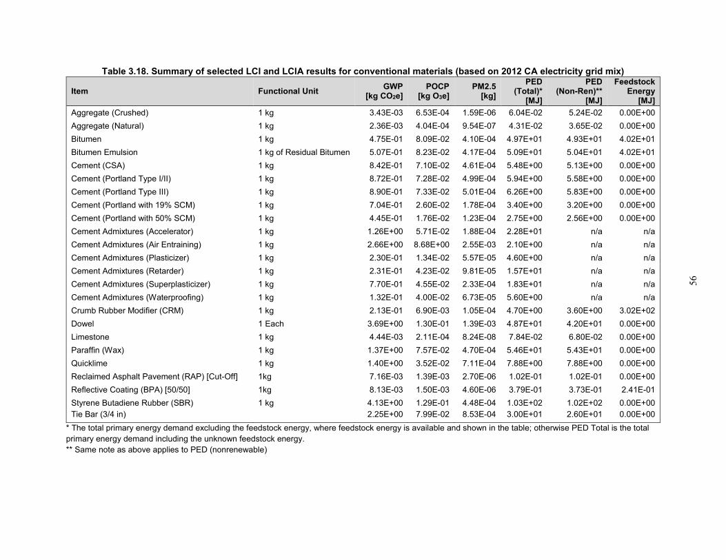
56

Table 3.18. Summary of selected LCI and LCIA results for conventional materials (based on 2012 CA electricity grid mix)

Item Functional Unit GWP

[kg CO2e] POCP

[kg O3e] PM2.5

[kg]

PED (Total)*

[MJ]

PED (Non-Ren)**

[MJ]

Feedstock Energy

[MJ]

Aggregate (Crushed) 1 kg 3.43E-03 6.53E-04 1.59E-06 6.04E-02 5.24E-02 0.00E+00

Aggregate (Natural) 1 kg 2.36E-03 4.04E-04 9.54E-07 4.31E-02 3.65E-02 0.00E+00

Bitumen 1 kg 4.75E-01 8.09E-02 4.10E-04 4.97E+01 4.93E+01 4.02E+01

Bitumen Emulsion 1 kg of Residual Bitumen 5.07E-01 8.23E-02 4.17E-04 5.09E+01 5.04E+01 4.02E+01

Cement (CSA) 1 kg 8.42E-01 7.10E-02 4.61E-04 5.48E+00 5.13E+00 0.00E+00

Cement (Portland Type I/II) 1 kg 8.72E-01 7.28E-02 4.99E-04 5.94E+00 5.58E+00 0.00E+00

Cement (Portland Type III) 1 kg 8.90E-01 7.33E-02 5.01E-04 6.26E+00 5.83E+00 0.00E+00

Cement (Portland with 19% SCM) 1 kg 7.04E-01 2.60E-02 1.78E-04 3.40E+00 3.20E+00 0.00E+00

Cement (Portland with 50% SCM) 1 kg 4.45E-01 1.76E-02 1.23E-04 2.75E+00 2.56E+00 0.00E+00

Cement Admixtures (Accelerator) 1 kg 1.26E+00 5.71E-02 1.88E-04 2.28E+01 n/a n/a

Cement Admixtures (Air Entraining) 1 kg 2.66E+00 8.68E+00 2.55E-03 2.10E+00 n/a n/a

Cement Admixtures (Plasticizer) 1 kg 2.30E-01 1.34E-02 5.57E-05 4.60E+00 n/a n/a

Cement Admixtures (Retarder) 1 kg 2.31E-01 4.23E-02 9.81E-05 1.57E+01 n/a n/a

Cement Admixtures (Superplasticizer) 1 kg 7.70E-01 4.55E-02 2.33E-04 1.83E+01 n/a n/a

Cement Admixtures (Waterproofing) 1 kg 1.32E-01 4.00E-02 6.73E-05 5.60E+00 n/a n/a

Crumb Rubber Modifier (CRM) 1 kg 2.13E-01 6.90E-03 1.05E-04 4.70E+00 3.60E+00 3.02E+02

Dowel 1 Each 3.69E+00 1.30E-01 1.39E-03 4.87E+01 4.20E+01 0.00E+00

Limestone 1 kg 4.44E-03 2.11E-04 8.24E-08 7.84E-02 6.80E-02 0.00E+00

Paraffin (Wax) 1 kg 1.37E+00 7.57E-02 4.70E-04 5.46E+01 5.43E+01 0.00E+00

Quicklime 1 kg 1.40E+00 3.52E-02 7.11E-04 7.88E+00 7.88E+00 0.00E+00

Reclaimed Asphalt Pavement (RAP) [Cut-Off] 1kg 7.16E-03 1.39E-03 2.70E-06 1.02E-01 1.02E-01 0.00E+00

Reflective Coating (BPA) [50/50] 1kg 8.13E-03 1.50E-03 4.60E-06 3.79E-01 3.73E-01 2.41E-01

Styrene Butadiene Rubber (SBR) 1 kg 4.13E+00 1.29E-01 4.48E-04 1.03E+02 1.02E+02 0.00E+00

Tie Bar (3/4 in) 2.25E+00 7.99E-02 8.53E-04 3.00E+01 2.60E+01 0.00E+00

* The total primary energy demand excluding the feedstock energy, where feedstock energy is available and shown in the table; otherwise PED Total is the total primary energy demand including the unknown feedstock energy. ** Same note as above applies to PED (nonrenewable)

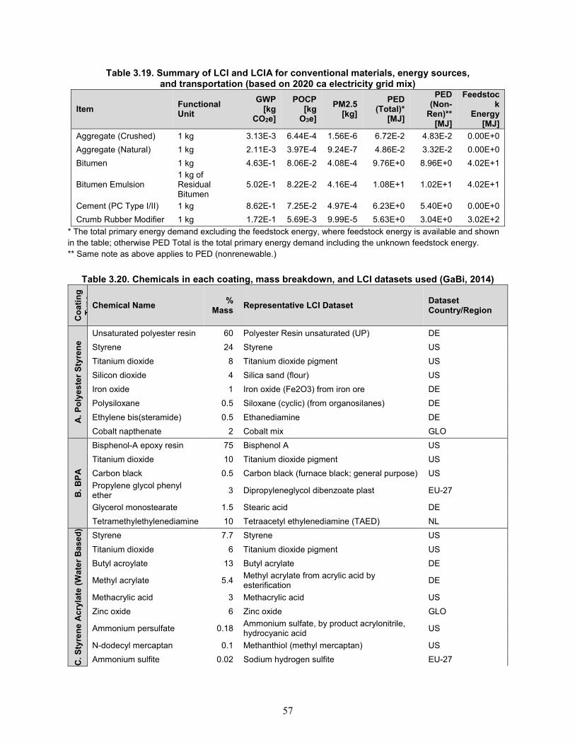
57

Table 3.19. Summary of LCI and LCIA for conventional materials, energy sources, and transportation (based on 2020 ca electricity grid mix)

Item Functional Unit

GWP [kg

CO2e]

POCP [kg

O3e]

PM2.5 [kg]

PED (Total)*

[MJ]

PED (Non-

Ren)** [MJ]

Feedstock

Energy [MJ]

Aggregate (Crushed) 1 kg 3.13E-3 6.44E-4 1.56E-6 6.72E-2 4.83E-2 0.00E+0

Aggregate (Natural) 1 kg 2.11E-3 3.97E-4 9.24E-7 4.86E-2 3.32E-2 0.00E+0

Bitumen 1 kg 4.63E-1 8.06E-2 4.08E-4 9.76E+0 8.96E+0 4.02E+1

Bitumen Emulsion 1 kg of Residual Bitumen

5.02E-1 8.22E-2 4.16E-4 1.08E+1 1.02E+1 4.02E+1

Cement (PC Type I/II) 1 kg 8.62E-1 7.25E-2 4.97E-4 6.23E+0 5.40E+0 0.00E+0

Crumb Rubber Modifier 1 kg 1.72E-1 5.69E-3 9.99E-5 5.63E+0 3.04E+0 3.02E+2

* The total primary energy demand excluding the feedstock energy, where feedstock energy is available and shown in the table; otherwise PED Total is the total primary energy demand including the unknown feedstock energy. ** Same note as above applies to PED (nonrenewable.)

Table 3.20. Chemicals in each coating, mass breakdown, and LCI datasets used (GaBi, 2014)

Co

ati

ng

T

yp

e

Chemical Name %

Mass Representative LCI Dataset

Dataset Country/Region

A.

Po

lye

ste

r S

tyre

ne

Unsaturated polyester resin 60 Polyester Resin unsaturated (UP) DE

Styrene 24 Styrene US

Titanium dioxide 8 Titanium dioxide pigment US

Silicon dioxide 4 Silica sand (flour) US

Iron oxide 1 Iron oxide (Fe2O3) from iron ore DE

Polysiloxane 0.5 Siloxane (cyclic) (from organosilanes) DE

Ethylene bis(steramide) 0.5 Ethanediamine DE

Cobalt napthenate 2 Cobalt mix GLO

B.

BP

A

Bisphenol-A epoxy resin 75 Bisphenol A US

Titanium dioxide 10 Titanium dioxide pigment US

Carbon black 0.5 Carbon black (furnace black; general purpose) US

Propylene glycol phenyl ether

3 Dipropyleneglycol dibenzoate plast EU-27

Glycerol monostearate 1.5 Stearic acid DE

Tetramethylethylenediamine 10 Tetraacetyl ethylenediamine (TAED) NL

C.

Sty

ren

e A

cry

late

(W

ate

r B

as

ed

)

Styrene 7.7 Styrene US

Titanium dioxide 6 Titanium dioxide pigment US

Butyl acroylate 13 Butyl acrylate DE

Methyl acrylate 5.4 Methyl acrylate from acrylic acid by esterification

DE

Methacrylic acid 3 Methacrylic acid US

Zinc oxide 6 Zinc oxide GLO

Ammonium persulfate 0.18 Ammonium sulfate, by product acrylonitrile, hydrocyanic acid

US

N-dodecyl mercaptan 0.1 Methanthiol (methyl mercaptan) US

Ammonium sulfite 0.02 Sodium hydrogen sulfite EU-27

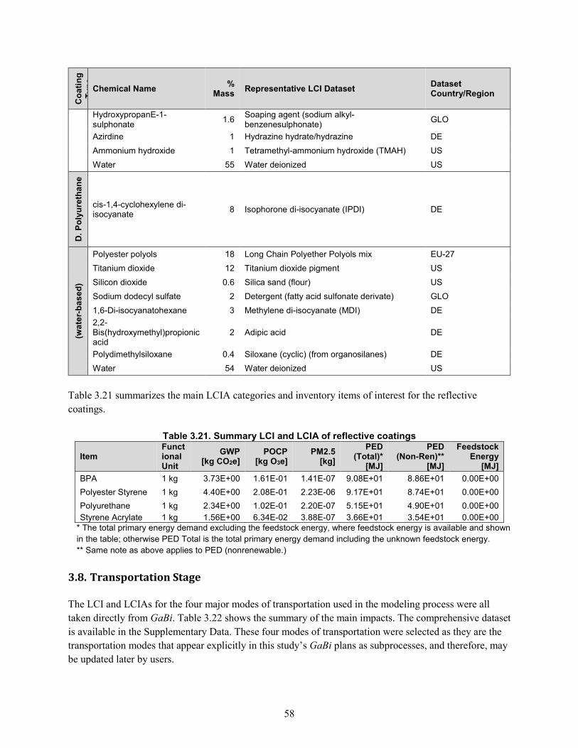
58

Co

ati

ng

T

yp

e

Chemical Name %

Mass Representative LCI Dataset

Dataset Country/Region

HydroxypropanE-1-sulphonate

1.6 Soaping agent (sodium alkyl-benzenesulphonate)

GLO

Azirdine 1 Hydrazine hydrate/hydrazine DE

Ammonium hydroxide 1 Tetramethyl-ammonium hydroxide (TMAH) US

Water 55 Water deionized US

D.

Po

lyu

reth

an

e

cis-1,4-cyclohexylene di-isocyanate

8 Isophorone di-isocyanate (IPDI) DE

(wa

ter-

ba

se

d)

Polyester polyols 18 Long Chain Polyether Polyols mix EU-27

Titanium dioxide 12 Titanium dioxide pigment US

Silicon dioxide 0.6 Silica sand (flour) US

Sodium dodecyl sulfate 2 Detergent (fatty acid sulfonate derivate) GLO

1,6-Di-isocyanatohexane 3 Methylene di-isocyanate (MDI) DE

2,2-Bis(hydroxymethyl)propionic acid

2 Adipic acid DE

Polydimethylsiloxane 0.4 Siloxane (cyclic) (from organosilanes) DE

Water 54 Water deionized US

Table 3.21 summarizes the main LCIA categories and inventory items of interest for the reflective

coatings.

Table 3.21. Summary LCI and LCIA of reflective coatings

Item Functional Unit

GWP [kg CO2e]

POCP [kg O3e]

PM2.5 [kg]

PED (Total)*

[MJ]

PED (Non-Ren)**

[MJ]

Feedstock Energy

[MJ]

BPA 1 kg 3.73E+00 1.61E-01 1.41E-07 9.08E+01 8.86E+01 0.00E+00

Polyester Styrene 1 kg 4.40E+00 2.08E-01 2.23E-06 9.17E+01 8.74E+01 0.00E+00

Polyurethane 1 kg 2.34E+00 1.02E-01 2.20E-07 5.15E+01 4.90E+01 0.00E+00

Styrene Acrylate 1 kg 1.56E+00 6.34E-02 3.88E-07 3.66E+01 3.54E+01 0.00E+00 * The total primary energy demand excluding the feedstock energy, where feedstock energy is available and shown in the table; otherwise PED Total is the total primary energy demand including the unknown feedstock energy. ** Same note as above applies to PED (nonrenewable.)

3.8. Transportation Stage

The LCI and LCIAs for the four major modes of transportation used in the modeling process were all

taken directly from GaBi. Table 3.22 shows the summary of the main impacts. The comprehensive dataset

is available in the Supplementary Data. These four modes of transportation were selected as they are the

transportation modes that appear explicitly in this study’s GaBi plans as subprocesses, and therefore, may

be updated later by users.

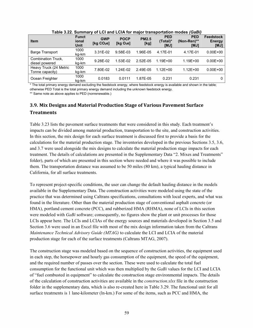
59

Table 3.22. Summary of LCI and LCIA for major transportation modes (GaBi)

Item Functional Unit

GWP [kg CO2e]

POCP [kg O3e]

PM2.5 [kg]

PED (Total)*

[MJ]

PED (Non-Ren)**

[MJ]

Feedstock Energy

[MJ]

Barge Transport 1000 kg-km

3.31E-02 9.58E-03 1.96E-05 4.17E-01 4.17E-01 0.00E+00

Combination Truck, diesel powered

1000 kg-km

9.28E-02 1.53E-02 2.52E-05 1.19E+00 1.19E+00 0.00E+00

Heavy Truck (24 Metric Tonne capacity)

1000 kg-km

7.80E-02 1.24E-02 2.49E-05 1.12E+00 1.12E+00 0.00E+00

Ocean Freighter 1000 kg-km

0.0183 0.0111 1.87E-05 0.231 0.231 0

* The total primary energy demand excluding the feedstock energy, where feedstock energy is available and shown in the table; otherwise PED Total is the total primary energy demand including the unknown feedstock energy. ** Same note as above applies to PED (nonrenewable.)

3.9. Mix Designs and Material Production Stage of Various Pavement Surface

Treatments

Table 3.23 lists the pavement surface treatments that were considered in this study. Each treatment’s

impacts can be divided among material production, transportation to the site, and construction activities.

In this section, the mix design for each surface treatment is discussed first to provide a basis for the

calculations for the material production stage. The inventories developed in the previous Sections 3.5, 3.6,

and 3.7 were used alongside the mix designs to calculate the material production stage impacts for each

treatment. The details of calculations are presented in the Supplementary Data “2. Mixes and Treatments”

folder), parts of which are presented in this section where needed and where it was possible to include

them. The transportation distance was assumed to be 50 miles (80 km), a typical hauling distance in

California, for all surface treatments.

To represent project-specific conditions, the user can change the default hauling distance in the models

available in the Supplementary Data. The construction activities were modeled using the state of the

practice that was determined using Caltrans specifications, consultations with local experts, and what was

found in the literature. Other than the material production stage of conventional asphalt concrete (or

HMA), portland cement concrete (PCC), and rubberized HMA (RHMA), none of LCIs in this section

were modeled with GaBi software; consequently, no figures show the plant or unit processes for those

LCIs appear here. The LCIs and LCIAs of the energy sources and materials developed in Section 3.5 and

Section 3.6 were used in an Excel file with most of the mix design information taken from the Caltrans

Maintenance Technical Advisory Guide (MTAG) to calculate the LCI and LCIA of the material

production stage for each of the surface treatments (Caltrans MTAG, 2007).

The construction stage was modeled based on the sequence of construction activities, the equipment used

in each step, the horsepower and hourly gas consumption of the equipment, the speed of the equipment,

and the required number of passes over the section. These were used to calculate the total fuel

consumption for the functional unit which was then multiplied by the GaBi values for the LCI and LCIA

of “fuel combusted in equipment” to calculate the construction stage environmental impacts. The details

of the calculation of construction activities are available in the construction.xlsx file in the construction

folder in the supplementary data, which is also re-created here in Table 3.29. The functional unit for all

surface treatments is 1 lane-kilometer (ln-km.) For some of the items, such as PCC and HMA, the

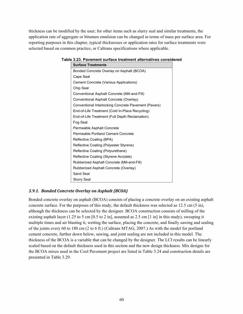
60

thickness can be modified by the user; for other items such as slurry seal and similar treatments, the

application rate of aggregate or bitumen emulsion can be changed in terms of mass per surface area. For

reporting purposes in this chapter, typical thicknesses or application rates for surface treatments were

selected based on common practice, or Caltrans specifications where applicable.

Table 3.23. Pavement surface treatment alternatives considered

Surface Treatments

Bonded Concrete Overlay on Asphalt (BCOA)

Cape Seal

Cement Concrete (Various Applications)

Chip Seal

Conventional Asphalt Concrete (Mill-and-Fill)

Conventional Asphalt Concrete (Overlay)

Conventional Interlocking Concrete Pavement (Pavers)

End-of-Life Treatment (Cold In-Place Recycling)

End-of-Life Treatment (Full Depth Reclamation)

Fog Seal

Permeable Asphalt Concrete

Permeable Portland Cement Concrete

Reflective Coating (BPA)

Reflective Coating (Polyester Styrene)

Reflective Coating (Polyurethane)

Reflective Coating (Styrene Acrylate)

Rubberized Asphalt Concrete (Mill-and-Fill)

Rubberized Asphalt Concrete (Overlay)

Sand Seal

Slurry Seal

3.9.1. Bonded Concrete Overlay on Asphalt (BCOA)

Bonded concrete overlay on asphalt (BCOA) consists of placing a concrete overlay on an existing asphalt

concrete surface. For the purposes of this study, the default thickness was selected as 12.5 cm (5 in),

although the thickness can be selected by the designer. BCOA construction consists of milling of the

existing asphalt layer (1.25 to 5 cm [0.5 to 2 in], assumed as 2.5 cm [1 in] in this study), sweeping it

multiple times and air blasting it, wetting the surface, placing the concrete, and finally sawing and sealing

of the joints every 60 to 180 cm (2 to 6 ft.) (Caltrans MTAG, 2007.) As with the model for portland

cement concrete, further down below, sawing, and joint sealing are not included in this model. The

thickness of the BCOA is a variable that can be changed by the designer. The LCI results can be linearly

scaled based on the default thickness used in this section and the new design thickness. Mix designs for

the BCOA mixes used in the Cool Pavement project are listed in Table 3.24 and construction details are

presented in Table 3.29.

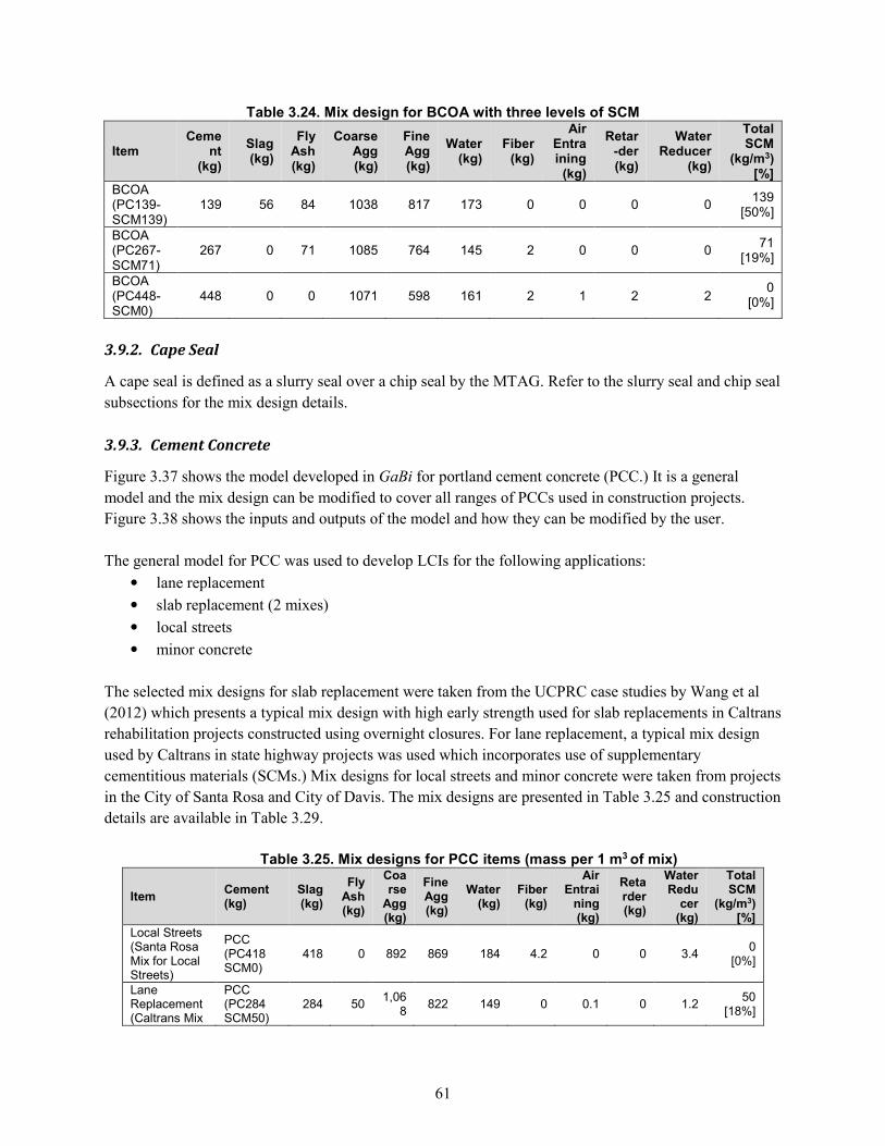
61

Table 3.24. Mix design for BCOA with three levels of SCM

Item Ceme

nt (kg)

Slag (kg)

Fly Ash (kg)

Coarse Agg (kg)

Fine Agg (kg)

Water (kg)

Fiber (kg)

Air Entraining

(kg)

Retar-der (kg)

Water Reducer

(kg)

Total SCM

(kg/m3) [%]

BCOA (PC139-SCM139)

139 56 84 1038 817 173 0 0 0 0 139

[50%]

BCOA (PC267-SCM71)

267 0 71 1085 764 145 2 0 0 0 71

[19%]

BCOA (PC448-SCM0)

448 0 0 1071 598 161 2 1 2 2 0

[0%]

3.9.2. Cape Seal

A cape seal is defined as a slurry seal over a chip seal by the MTAG. Refer to the slurry seal and chip seal

subsections for the mix design details.

3.9.3. Cement Concrete

Figure 3.37 shows the model developed in GaBi for portland cement concrete (PCC.) It is a general

model and the mix design can be modified to cover all ranges of PCCs used in construction projects.

Figure 3.38 shows the inputs and outputs of the model and how they can be modified by the user.

The general model for PCC was used to develop LCIs for the following applications:

• lane replacement

• slab replacement (2 mixes)

• local streets

• minor concrete

The selected mix designs for slab replacement were taken from the UCPRC case studies by Wang et al

(2012) which presents a typical mix design with high early strength used for slab replacements in Caltrans

rehabilitation projects constructed using overnight closures. For lane replacement, a typical mix design

used by Caltrans in state highway projects was used which incorporates use of supplementary

cementitious materials (SCMs.) Mix designs for local streets and minor concrete were taken from projects

in the City of Santa Rosa and City of Davis. The mix designs are presented in Table 3.25 and construction

details are available in Table 3.29.

Table 3.25. Mix designs for PCC items (mass per 1 m3 of mix)

Item Cement (kg)

Slag (kg)

Fly Ash (kg)

Coarse

Agg (kg)

Fine Agg (kg)

Water (kg)

Fiber (kg)

Air Entrai

ning (kg)

Retarder (kg)

Water Redu

cer (kg)

Total SCM

(kg/m3) [%]

Local Streets (Santa Rosa Mix for Local Streets)

PCC (PC418 SCM0)

418 0 892 869 184 4.2 0 0 3.4 0

[0%]

Lane Replacement (Caltrans Mix

PCC (PC284 SCM50)

284 50 1,06

8 822 149 0 0.1 0 1.2

50 [18%]

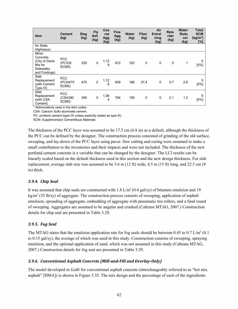
62

Item Cement (kg)

Slag (kg)

Fly Ash (kg)

Coarse

Agg (kg)

Fine Agg (kg)

Water (kg)

Fiber (kg)

Air Entrai

ning (kg)

Retarder (kg)

Water Redu

cer (kg)

Total SCM

(kg/m3) [%]

for State Highways) Minor Concrete (City of Davis Mix for Sidewalks and Footings)

PCC (PC335 SCM0)

335 0 1,12

9 812 163 0 0 0 1

0 [0%]

Slab Replacement (with Cement Type III)

PCC (PCIII475 SCM0)

475 0 1,12

8 609 166 37.4 0 0.7 2.6

0 [0%]

Slab Replacement (with CSA Cement)

PCC (CSA390 SCM0)

390 0 1,06

4 794 156 0 0 2.1 1.2

0 [0%]

* Abbreviations used in the item codes: CSA: Calcium Sulfo-aluminate cement PC: portland cement (type I/II unless explicitly stated as type III) SCM: Supplementary Cementitious Materials

The thickness of the PCC layer was assumed to be 17.5 cm (6.8 in) as a default, although the thickness of

the PCC can be defined by the designer. The construction process consisted of grinding of the old surface,

sweeping, and lay-down of the PCC layer using paver. Saw cutting and curing were assumed to make a

small contribution to the inventories and their impacts and were not included. The thickness of the new

portland cement concrete is a variable that can be changed by the designer. The LCI results can be

linearly scaled based on the default thickness used in this section and the new design thickness. For slab

replacement, average slab size was assumed to be 3.6 m (12 ft) wide, 4.5 m (15 ft) long, and 22.5 cm (9

in) thick.

3.9.4. Chip Seal

It was assumed that chip seals are constructed with 1.8 L/m2 (0.4 gal/sy) of bitumen emulsion and 19

kg/m2 (35 lb/sy) of aggregate. The construction process consists of sweeping, application of asphalt

emulsion, spreading of aggregate, embedding of aggregate with pneumatic tire rollers, and a final round

of sweeping. Aggregates are assumed to be angular and crushed (Caltrans MTAG, 2007.) Construction

details for chip seal are presented in Table 3.29.

3.9.5. Fog Seal

The MTAG states that the emulsion application rate for fog seals should be between 0.45 to 0.7 L/m2 (0.1

to 0.15 gal/sy), the average of which was used in this study. Construction consists of sweeping, spraying

emulsion, and the optional application of sand, which was not assumed in this study (Caltrans MTAG,

2007.) Construction details for fog seal are presented in Table 3.29.

3.9.6. Conventional Asphalt Concrete (Mill-and-Fill and Overlay-Only)

The model developed in GaBi for conventional asphalt concrete (interchangeably referred to as “hot mix

asphalt” [HMA]) is shown in Figure 3.35. The mix design and the percentage of each of the ingredients

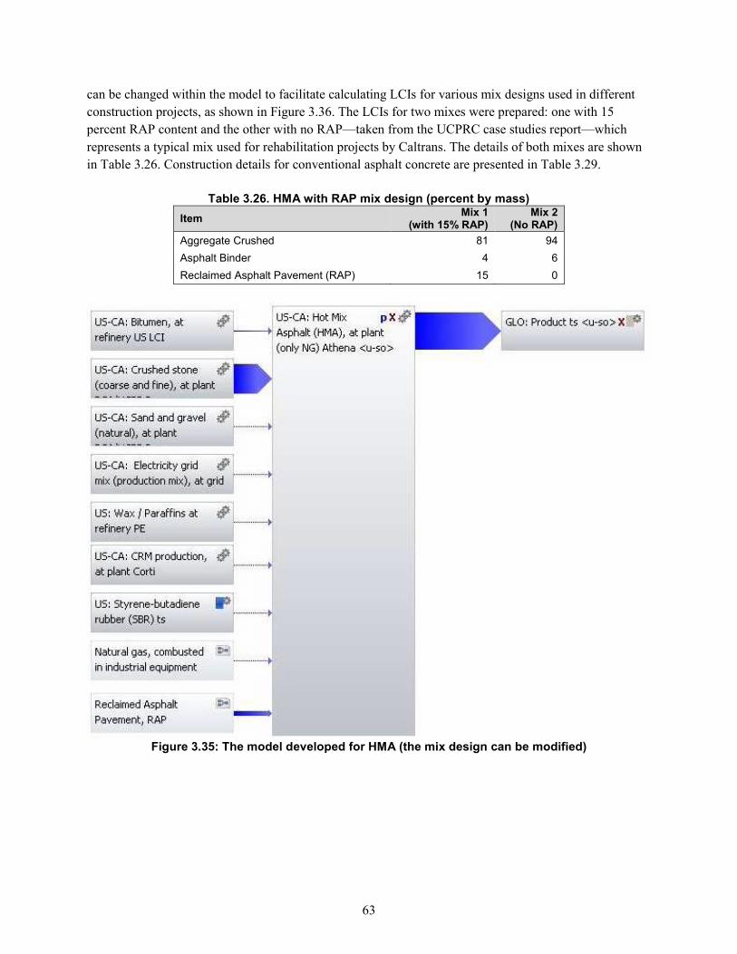
63

can be changed within the model to facilitate calculating LCIs for various mix designs used in different

construction projects, as shown in Figure 3.36. The LCIs for two mixes were prepared: one with 15

percent RAP content and the other with no RAP—taken from the UCPRC case studies report—which

represents a typical mix used for rehabilitation projects by Caltrans. The details of both mixes are shown

in Table 3.26. Construction details for conventional asphalt concrete are presented in Table 3.29.

Table 3.26. HMA with RAP mix design (percent by mass)

Item Mix 1

(with 15% RAP) Mix 2

(No RAP)

Aggregate Crushed 81 94

Asphalt Binder 4 6

Reclaimed Asphalt Pavement (RAP) 15 0

Figure 3.35: The model developed for HMA (the mix design can be modified)

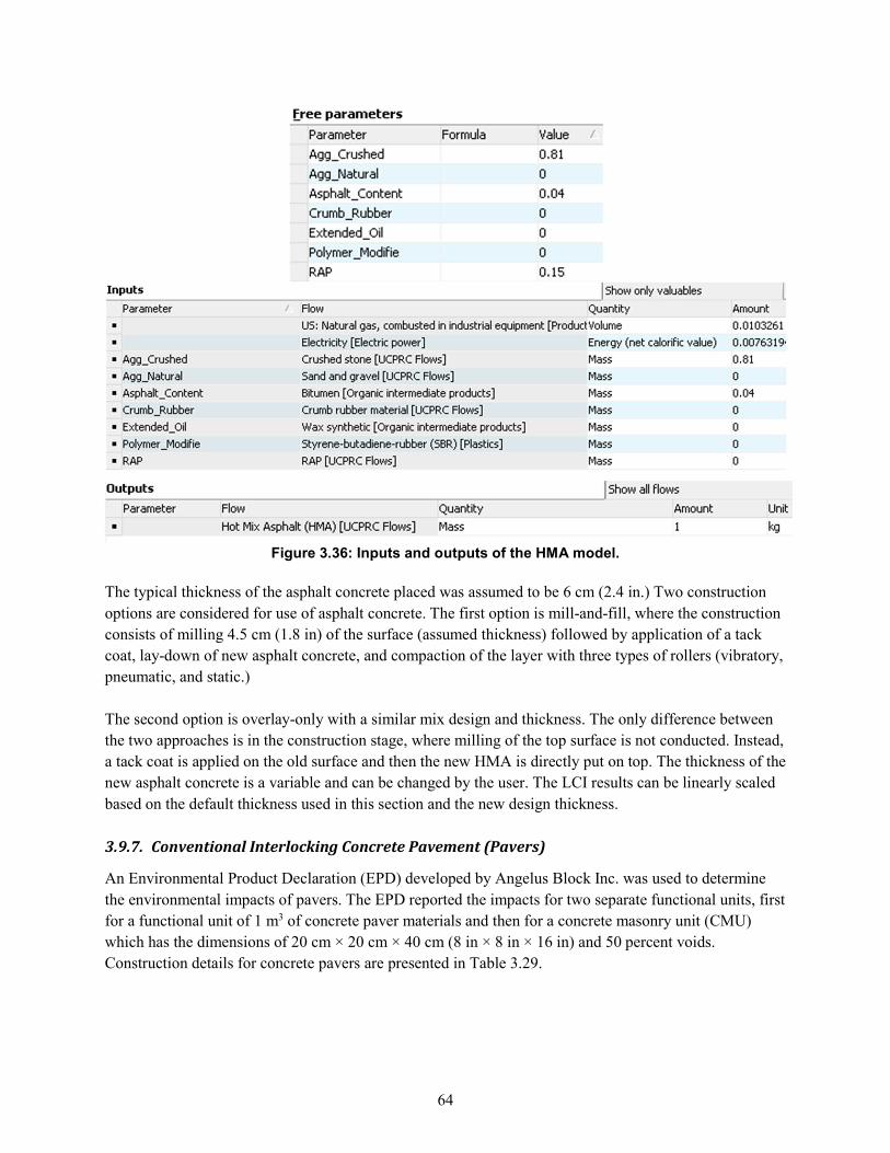
64

Figure 3.36: Inputs and outputs of the HMA model.

The typical thickness of the asphalt concrete placed was assumed to be 6 cm (2.4 in.) Two construction

options are considered for use of asphalt concrete. The first option is mill-and-fill, where the construction

consists of milling 4.5 cm (1.8 in) of the surface (assumed thickness) followed by application of a tack

coat, lay-down of new asphalt concrete, and compaction of the layer with three types of rollers (vibratory,

pneumatic, and static.)

The second option is overlay-only with a similar mix design and thickness. The only difference between

the two approaches is in the construction stage, where milling of the top surface is not conducted. Instead,

a tack coat is applied on the old surface and then the new HMA is directly put on top. The thickness of the

new asphalt concrete is a variable and can be changed by the user. The LCI results can be linearly scaled

based on the default thickness used in this section and the new design thickness.

3.9.7. Conventional Interlocking Concrete Pavement (Pavers)

An Environmental Product Declaration (EPD) developed by Angelus Block Inc. was used to determine

the environmental impacts of pavers. The EPD reported the impacts for two separate functional units, first

for a functional unit of 1 m3 of concrete paver materials and then for a concrete masonry unit (CMU)

which has the dimensions of 20 cm × 20 cm × 40 cm (8 in × 8 in × 16 in) and 50 percent voids.

Construction details for concrete pavers are presented in Table 3.29.

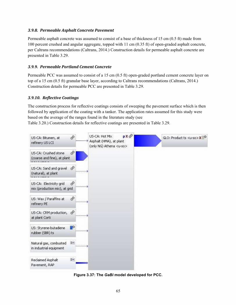
65

3.9.8. Permeable Asphalt Concrete Pavement

Permeable asphalt concrete was assumed to consist of a base of thickness of 15 cm (0.5 ft) made from

100 percent crushed and angular aggregate, topped with 11 cm (0.35 ft) of open-graded asphalt concrete,

per Caltrans recommendations (Caltrans, 2014.) Construction details for permeable asphalt concrete are

presented in Table 3.29.

3.9.9. Permeable Portland Cement Concrete

Permeable PCC was assumed to consist of a 15 cm (0.5 ft) open-graded portland cement concrete layer on

top of a 15 cm (0.5 ft) granular base layer, according to Caltrans recommendations (Caltrans, 2014.)

Construction details for permeable PCC are presented in Table 3.29.

3.9.10. Reflective Coatings

The construction process for reflective coatings consists of sweeping the pavement surface which is then

followed by application of the coating with a tanker. The application rates assumed for this study were

based on the average of the ranges found in the literature study (see

Table 3.20.) Construction details for reflective coatings are presented in Table 3.29.

Figure 3.37: The GaBi model developed for PCC.

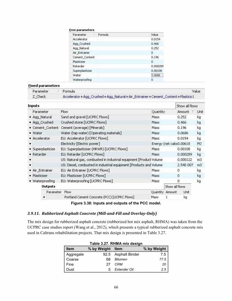
66

Figure 3.38: Inputs and outputs of the PCC model.

3.9.11. Rubberized Asphalt Concrete (Mill-and-Fill and Overlay-Only)

The mix design for rubberized asphalt concrete (rubberized hot mix asphalt, RHMA) was taken from the

UCPRC case studies report (Wang et al., 2012), which presents a typical rubberized asphalt concrete mix

used in Caltrans rehabilitation projects. That mix design is presented in Table 3.27.

Table 3.27. RHMA mix design

Item % by Weight Item % by Weight

Aggregate 92.5 Asphalt Binder 7.5 Coarse 68 Bitumen 77.5

Fine 27 CRM 20

Dust 5 Extender Oil 2.5

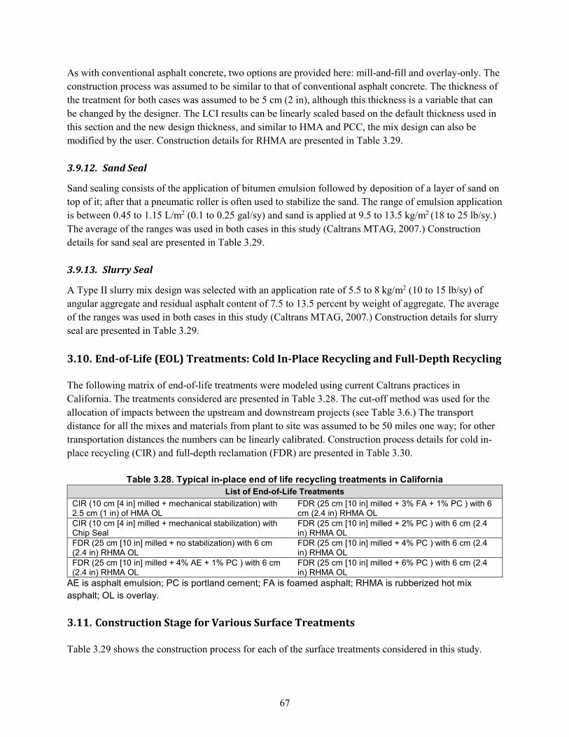
67

As with conventional asphalt concrete, two options are provided here: mill-and-fill and overlay-only. The

construction process was assumed to be similar to that of conventional asphalt concrete. The thickness of

the treatment for both cases was assumed to be 5 cm (2 in), although this thickness is a variable that can

be changed by the designer. The LCI results can be linearly scaled based on the default thickness used in

this section and the new design thickness, and similar to HMA and PCC, the mix design can also be

modified by the user. Construction details for RHMA are presented in Table 3.29.

3.9.12. Sand Seal

Sand sealing consists of the application of bitumen emulsion followed by deposition of a layer of sand on

top of it; after that a pneumatic roller is often used to stabilize the sand. The range of emulsion application

is between 0.45 to 1.15 L/m2 (0.1 to 0.25 gal/sy) and sand is applied at 9.5 to 13.5 kg/m2 (18 to 25 lb/sy.)

The average of the ranges was used in both cases in this study (Caltrans MTAG, 2007.) Construction

details for sand seal are presented in Table 3.29.

3.9.13. Slurry Seal

A Type II slurry mix design was selected with an application rate of 5.5 to 8 kg/m2 (10 to 15 lb/sy) of

angular aggregate and residual asphalt content of 7.5 to 13.5 percent by weight of aggregate. The average

of the ranges was used in both cases in this study (Caltrans MTAG, 2007.) Construction details for slurry

seal are presented in Table 3.29.

3.10. End-of-Life (EOL) Treatments: Cold In-Place Recycling and Full-Depth Recycling

The following matrix of end-of-life treatments were modeled using current Caltrans practices in

California. The treatments considered are presented in Table 3.28. The cut-off method was used for the

allocation of impacts between the upstream and downstream projects (see Table 3.6.) The transport

distance for all the mixes and materials from plant to site was assumed to be 50 miles one way; for other

transportation distances the numbers can be linearly calibrated. Construction process details for cold in-

place recycling (CIR) and full-depth reclamation (FDR) are presented in Table 3.30.

Table 3.28. Typical in-place end of life recycling treatments in California

List of End-of-Life Treatments

CIR (10 cm [4 in] milled + mechanical stabilization) with 2.5 cm (1 in) of HMA OL

FDR (25 cm [10 in] milled + 3% FA + 1% PC ) with 6 cm (2.4 in) RHMA OL

CIR (10 cm [4 in] milled + mechanical stabilization) with Chip Seal

FDR (25 cm [10 in] milled + 2% PC ) with 6 cm (2.4 in) RHMA OL

FDR (25 cm [10 in] milled + no stabilization) with 6 cm (2.4 in) RHMA OL

FDR (25 cm [10 in] milled + 4% PC ) with 6 cm (2.4 in) RHMA OL

FDR (25 cm [10 in] milled + 4% AE + 1% PC ) with 6 cm (2.4 in) RHMA OL

FDR (25 cm [10 in] milled + 6% PC ) with 6 cm (2.4 in) RHMA OL

AE is asphalt emulsion; PC is portland cement; FA is foamed asphalt; RHMA is rubberized hot mix

asphalt; OL is overlay.

3.11. Construction Stage for Various Surface Treatments

Table 3.29 shows the construction process for each of the surface treatments considered in this study.

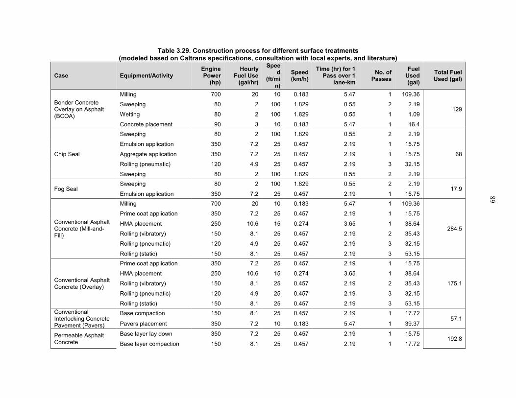
68

Table 3.29. Construction process for different surface treatments (modeled based on Caltrans specifications, consultation with local experts, and literature)

Case Equipment/Activity Engine Power

(hp)

Hourly Fuel Use

(gal/hr)

Speed

(ft/min)

Speed (km/h)

Time (hr) for 1 Pass over 1

lane-km

No. of Passes

Fuel Used (gal)

Total Fuel Used (gal)

Bonder Concrete Overlay on Asphalt (BCOA)

Milling 700 20 10 0.183 5.47 1 109.36

129 Sweeping 80 2 100 1.829 0.55 2 2.19

Wetting 80 2 100 1.829 0.55 1 1.09

Concrete placement 90 3 10 0.183 5.47 1 16.4

Chip Seal

Sweeping 80 2 100 1.829 0.55 2 2.19

68

Emulsion application 350 7.2 25 0.457 2.19 1 15.75

Aggregate application 350 7.2 25 0.457 2.19 1 15.75

Rolling (pneumatic) 120 4.9 25 0.457 2.19 3 32.15

Sweeping 80 2 100 1.829 0.55 2 2.19

Fog Seal Sweeping 80 2 100 1.829 0.55 2 2.19

17.9 Emulsion application 350 7.2 25 0.457 2.19 1 15.75

Conventional Asphalt Concrete (Mill-and-Fill)

Milling 700 20 10 0.183 5.47 1 109.36

284.5

Prime coat application 350 7.2 25 0.457 2.19 1 15.75

HMA placement 250 10.6 15 0.274 3.65 1 38.64

Rolling (vibratory) 150 8.1 25 0.457 2.19 2 35.43

Rolling (pneumatic) 120 4.9 25 0.457 2.19 3 32.15

Rolling (static) 150 8.1 25 0.457 2.19 3 53.15

Conventional Asphalt Concrete (Overlay)

Prime coat application 350 7.2 25 0.457 2.19 1 15.75

175.1

HMA placement 250 10.6 15 0.274 3.65 1 38.64

Rolling (vibratory) 150 8.1 25 0.457 2.19 2 35.43

Rolling (pneumatic) 120 4.9 25 0.457 2.19 3 32.15

Rolling (static) 150 8.1 25 0.457 2.19 3 53.15

Conventional Interlocking Concrete Pavement (Pavers)

Base compaction 150 8.1 25 0.457 2.19 1 17.72 57.1

Pavers placement 350 7.2 10 0.183 5.47 1 39.37

Permeable Asphalt Concrete

Base layer lay down 350 7.2 25 0.457 2.19 1 15.75 192.8

Base layer compaction 150 8.1 25 0.457 2.19 1 17.72

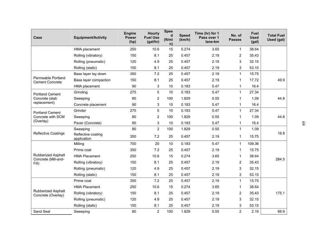
69

Case Equipment/Activity Engine Power

(hp)

Hourly Fuel Use

(gal/hr)

Speed

(ft/min)

Speed (km/h)

Time (hr) for 1 Pass over 1

lane-km

No. of Passes

Fuel Used (gal)

Total Fuel Used (gal)

HMA placement 250 10.6 15 0.274 3.65 1 38.64

Rolling (vibratory) 150 8.1 25 0.457 2.19 2 35.43

Rolling (pneumatic) 120 4.9 25 0.457 2.19 3 32.15

Rolling (static) 150 8.1 25 0.457 2.19 3 53.15

Permeable Portland Cement Concrete

Base layer lay down 350 7.2 25 0.457 2.19 1 15.75

49.9 Base layer compaction 150 8.1 25 0.457 2.19 1 17.72

HMA placement 90 3 10 0.183 5.47 1 16.4

Portland Cement Concrete (slab replacement)

Grinding 275 5 10 0.183 5.47 1 27.34

44.8 Sweeping 80 2 100 1.829 0.55 1 1.09

Concrete placement 90 3 10 0.183 5.47 1 16.4

Portland Cement Concrete with SCM (Overlay)

Grinder 275 5 10 0.183 5.47 1 27.34

44.8 Sweeping 80 2 100 1.829 0.55 1 1.09

Paver (Concrete) 90 3 10 0.183 5.47 1 16.4

Reflective Coatings Sweeping 80 2 100 1.829 0.55 1 1.09

16.8 Reflective coating application

350 7.2 25 0.457 2.19 1 15.75

Rubberized Asphalt Concrete (Mill-and-Fill)

Milling 700 20 10 0.183 5.47 1 109.36

284.5

Prime coat 350 7.2 25 0.457 2.19 1 15.75

HMA Placement 250 10.6 15 0.274 3.65 1 38.64

Rolling (vibratory) 150 8.1 25 0.457 2.19 2 35.43

Rolling (pneumatic) 120 4.9 25 0.457 2.19 3 32.15

Rolling (static) 150 8.1 25 0.457 2.19 3 53.15

Rubberized Asphalt Concrete (Overlay)

Prime coat 350 7.2 25 0.457 2.19 1 15.75

175.1

HMA Placement 250 10.6 15 0.274 3.65 1 38.64

Rolling (vibratory) 150 8.1 25 0.457 2.19 2 35.43

Rolling (pneumatic) 120 4.9 25 0.457 2.19 3 32.15

Rolling (static) 150 8.1 25 0.457 2.19 3 53.15

Sand Seal Sweeping 80 2 100 1.829 0.55 2 2.19 66.9

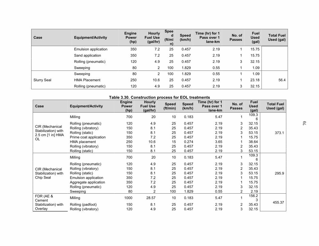
70

Case Equipment/Activity Engine Power

(hp)

Hourly Fuel Use

(gal/hr)

Speed

(ft/min)

Speed (km/h)

Time (hr) for 1 Pass over 1

lane-km

No. of Passes

Fuel Used (gal)

Total Fuel Used (gal)

Emulsion application 350 7.2 25 0.457 2.19 1 15.75

Sand application 350 7.2 25 0.457 2.19 1 15.75

Rolling (pneumatic) 120 4.9 25 0.457 2.19 3 32.15

Sweeping 80 2 100 1.829 0.55 1 1.09

Slurry Seal

Sweeping 80 2 100 1.829 0.55 1 1.09

56.4 HMA Placement 250 10.6 25 0.457 2.19 1 23.18

Rolling (pneumatic) 120 4.9 25 0.457 2.19 3 32.15

Table 3.30. Construction process for EOL treatments

Case Equipment/Activity Engine Power

(hp)

Hourly Fuel Use

(gal/hr)

Speed (ft/min)

Speed (km/h)

Time (hr) for 1 Pass over 1

lane-km

No. of Passes

Fuel Used (gal)

Total Fuel Used (gal)

CIR (Mechanical Stabilization) with 2.5 cm [1 in] HMA OL

Milling 700 20 10 0.183 5.47 1 109.3

6

373.1

Rolling (pneumatic) 120 4.9 25 0.457 2.19 3 32.15 Rolling (vibratory) 150 8.1 25 0.457 2.19 2 35.43 Rolling (static) 150 8.1 25 0.457 2.19 3 53.15 Prime coat application 350 7.2 25 0.457 2.19 1 15.75 HMA placement 250 10.6 15 0.274 3.65 1 38.64 Rolling (vibratory) 150 8.1 25 0.457 2.19 2 35.43 Rolling (static) 150 8.1 25 0.457 2.19 3 53.15

CIR (Mechanical Stabilization) with Chip Seal

Milling 700 20 10 0.183 5.47 1 109.3

6

295.9

Rolling (pneumatic) 120 4.9 25 0.457 2.19 3 32.15 Rolling (vibratory) 150 8.1 25 0.457 2.19 2 35.43 Rolling (static) 150 8.1 25 0.457 2.19 3 53.15 Emulsion application 350 7.2 25 0.457 2.19 1 15.75 Aggregate application 350 7.2 25 0.457 2.19 1 15.75 Rolling (pneumatic) 120 4.9 25 0.457 2.19 3 32.15 Sweeping 80 2 100 1.829 0.55 2 2.19

FDR (AE & Cement Stabilization) with Overlay

Milling 1000 28.57 10 0.183 5.47 1 156.2

3 455.37

Rolling (padfoot) 150 8.1 25 0.457 2.19 2 35.43 Rolling (vibratory) 120 4.9 25 0.457 2.19 3 32.15

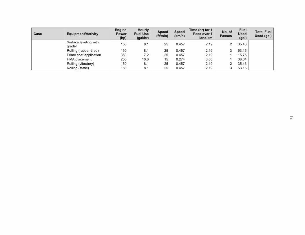
71

Case Equipment/Activity Engine Power

(hp)

Hourly Fuel Use

(gal/hr)

Speed (ft/min)

Speed (km/h)

Time (hr) for 1 Pass over 1

lane-km

No. of Passes

Fuel Used (gal)

Total Fuel Used (gal)

Surface leveling with grader

150 8.1 25 0.457 2.19 2 35.43

Rolling (rubber-tired) 150 8.1 25 0.457 2.19 3 53.15 Prime coat application 350 7.2 25 0.457 2.19 1 15.75 HMA placement 250 10.6 15 0.274 3.65 1 38.64 Rolling (vibratory) 150 8.1 25 0.457 2.19 2 35.43 Rolling (static) 150 8.1 25 0.457 2.19 3 53.15

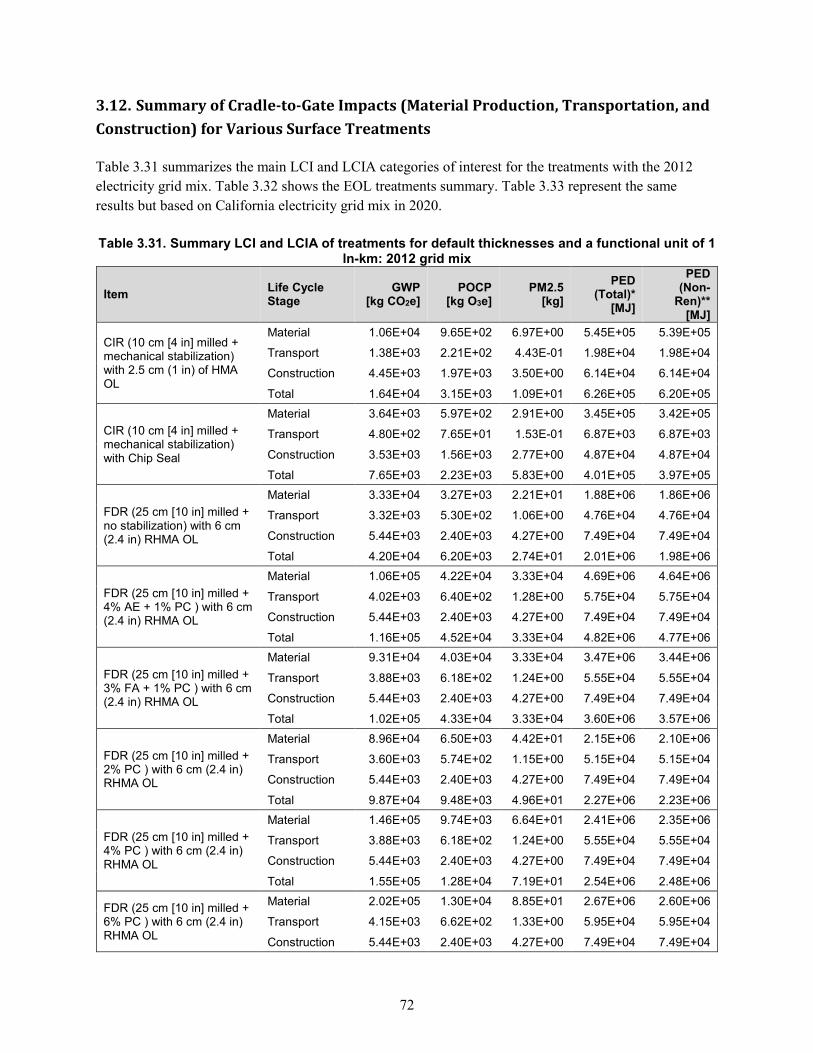
72

3.12. Summary of Cradle-to-Gate Impacts (Material Production, Transportation, and

Construction) for Various Surface Treatments

Table 3.31 summarizes the main LCI and LCIA categories of interest for the treatments with the 2012

electricity grid mix. Table 3.32 shows the EOL treatments summary. Table 3.33 represent the same

results but based on California electricity grid mix in 2020.

Table 3.31. Summary LCI and LCIA of treatments for default thicknesses and a functional unit of 1

ln-km: 2012 grid mix

Item Life Cycle Stage

GWP [kg CO2e]

POCP [kg O3e]

PM2.5 [kg]

PED (Total)*

[MJ]

PED (Non-

Ren)** [MJ]

CIR (10 cm [4 in] milled + mechanical stabilization) with 2.5 cm (1 in) of HMA OL

Material 1.06E+04 9.65E+02 6.97E+00 5.45E+05 5.39E+05

Transport 1.38E+03 2.21E+02 4.43E-01 1.98E+04 1.98E+04

Construction 4.45E+03 1.97E+03 3.50E+00 6.14E+04 6.14E+04

Total 1.64E+04 3.15E+03 1.09E+01 6.26E+05 6.20E+05

CIR (10 cm [4 in] milled + mechanical stabilization) with Chip Seal

Material 3.64E+03 5.97E+02 2.91E+00 3.45E+05 3.42E+05

Transport 4.80E+02 7.65E+01 1.53E-01 6.87E+03 6.87E+03

Construction 3.53E+03 1.56E+03 2.77E+00 4.87E+04 4.87E+04

Total 7.65E+03 2.23E+03 5.83E+00 4.01E+05 3.97E+05

FDR (25 cm [10 in] milled + no stabilization) with 6 cm (2.4 in) RHMA OL

Material 3.33E+04 3.27E+03 2.21E+01 1.88E+06 1.86E+06

Transport 3.32E+03 5.30E+02 1.06E+00 4.76E+04 4.76E+04

Construction 5.44E+03 2.40E+03 4.27E+00 7.49E+04 7.49E+04

Total 4.20E+04 6.20E+03 2.74E+01 2.01E+06 1.98E+06

FDR (25 cm [10 in] milled + 4% AE + 1% PC ) with 6 cm (2.4 in) RHMA OL

Material 1.06E+05 4.22E+04 3.33E+04 4.69E+06 4.64E+06

Transport 4.02E+03 6.40E+02 1.28E+00 5.75E+04 5.75E+04

Construction 5.44E+03 2.40E+03 4.27E+00 7.49E+04 7.49E+04

Total 1.16E+05 4.52E+04 3.33E+04 4.82E+06 4.77E+06

FDR (25 cm [10 in] milled + 3% FA + 1% PC ) with 6 cm (2.4 in) RHMA OL

Material 9.31E+04 4.03E+04 3.33E+04 3.47E+06 3.44E+06

Transport 3.88E+03 6.18E+02 1.24E+00 5.55E+04 5.55E+04

Construction 5.44E+03 2.40E+03 4.27E+00 7.49E+04 7.49E+04

Total 1.02E+05 4.33E+04 3.33E+04 3.60E+06 3.57E+06

FDR (25 cm [10 in] milled + 2% PC ) with 6 cm (2.4 in) RHMA OL

Material 8.96E+04 6.50E+03 4.42E+01 2.15E+06 2.10E+06

Transport 3.60E+03 5.74E+02 1.15E+00 5.15E+04 5.15E+04

Construction 5.44E+03 2.40E+03 4.27E+00 7.49E+04 7.49E+04

Total 9.87E+04 9.48E+03 4.96E+01 2.27E+06 2.23E+06

FDR (25 cm [10 in] milled + 4% PC ) with 6 cm (2.4 in) RHMA OL

Material 1.46E+05 9.74E+03 6.64E+01 2.41E+06 2.35E+06

Transport 3.88E+03 6.18E+02 1.24E+00 5.55E+04 5.55E+04

Construction 5.44E+03 2.40E+03 4.27E+00 7.49E+04 7.49E+04

Total 1.55E+05 1.28E+04 7.19E+01 2.54E+06 2.48E+06

FDR (25 cm [10 in] milled + 6% PC ) with 6 cm (2.4 in) RHMA OL

Material 2.02E+05 1.30E+04 8.85E+01 2.67E+06 2.60E+06

Transport 4.15E+03 6.62E+02 1.33E+00 5.95E+04 5.95E+04

Construction 5.44E+03 2.40E+03 4.27E+00 7.49E+04 7.49E+04

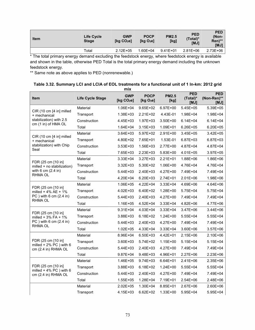
73

Item Life Cycle Stage

GWP [kg CO2e]

POCP [kg O3e]

PM2.5 [kg]

PED (Total)*

[MJ]

PED (Non-

Ren)** [MJ]

Total 2.12E+05 1.60E+04 9.41E+01 2.81E+06 2.73E+06

* The total primary energy demand excluding the feedstock energy, where feedstock energy is available

and shown in the table, otherwise PED Total is the total primary energy demand including the unknown feedstock energy. ** Same note as above applies to PED (nonrenewable.)

Table 3.32. Summary LCI and LCIA of EOL treatments for a functional unit of 1 ln-km: 2012 grid mix

Item Life Cycle Stage GWP

[kg CO2e] POCP

[kg O3e] PM2.5

[kg]

PED (Total)*

[MJ]

PED (Non-Ren)**

[MJ]

CIR (10 cm [4 in] milled + mechanical stabilization) with 2.5 cm (1 in) of HMA OL

Material 1.06E+04 9.65E+02 6.97E+00 5.45E+05 5.39E+05

Transport 1.38E+03 2.21E+02 4.43E-01 1.98E+04 1.98E+04

Construction 4.45E+03 1.97E+03 3.50E+00 6.14E+04 6.14E+04

Total 1.64E+04 3.15E+03 1.09E+01 6.26E+05 6.20E+05

CIR (10 cm [4 in] milled + mechanical stabilization) with Chip Seal

Material 3.64E+03 5.97E+02 2.91E+00 3.45E+05 3.42E+05

Transport 4.80E+02 7.65E+01 1.53E-01 6.87E+03 6.87E+03

Construction 3.53E+03 1.56E+03 2.77E+00 4.87E+04 4.87E+04

Total 7.65E+03 2.23E+03 5.83E+00 4.01E+05 3.97E+05

FDR (25 cm [10 in] milled + no stabilization) with 6 cm (2.4 in) RHMA OL

Material 3.33E+04 3.27E+03 2.21E+01 1.88E+06 1.86E+06

Transport 3.32E+03 5.30E+02 1.06E+00 4.76E+04 4.76E+04

Construction 5.44E+03 2.40E+03 4.27E+00 7.49E+04 7.49E+04

Total 4.20E+04 6.20E+03 2.74E+01 2.01E+06 1.98E+06

FDR (25 cm [10 in] milled + 4% AE + 1% PC ) with 6 cm (2.4 in) RHMA OL

Material 1.06E+05 4.22E+04 3.33E+04 4.69E+06 4.64E+06

Transport 4.02E+03 6.40E+02 1.28E+00 5.75E+04 5.75E+04

Construction 5.44E+03 2.40E+03 4.27E+00 7.49E+04 7.49E+04

Total 1.16E+05 4.52E+04 3.33E+04 4.82E+06 4.77E+06

FDR (25 cm [10 in] milled + 3% FA + 1% PC ) with 6 cm (2.4 in) RHMA OL

Material 9.31E+04 4.03E+04 3.33E+04 3.47E+06 3.44E+06

Transport 3.88E+03 6.18E+02 1.24E+00 5.55E+04 5.55E+04

Construction 5.44E+03 2.40E+03 4.27E+00 7.49E+04 7.49E+04

Total 1.02E+05 4.33E+04 3.33E+04 3.60E+06 3.57E+06

FDR (25 cm [10 in] milled + 2% PC ) with 6 cm (2.4 in) RHMA OL

Material 8.96E+04 6.50E+03 4.42E+01 2.15E+06 2.10E+06

Transport 3.60E+03 5.74E+02 1.15E+00 5.15E+04 5.15E+04

Construction 5.44E+03 2.40E+03 4.27E+00 7.49E+04 7.49E+04

Total 9.87E+04 9.48E+03 4.96E+01 2.27E+06 2.23E+06

FDR (25 cm [10 in] milled + 4% PC ) with 6 cm (2.4 in) RHMA OL

Material 1.46E+05 9.74E+03 6.64E+01 2.41E+06 2.35E+06

Transport 3.88E+03 6.18E+02 1.24E+00 5.55E+04 5.55E+04

Construction 5.44E+03 2.40E+03 4.27E+00 7.49E+04 7.49E+04

Total 1.55E+05 1.28E+04 7.19E+01 2.54E+06 2.48E+06

Material 2.02E+05 1.30E+04 8.85E+01 2.67E+06 2.60E+06

Transport 4.15E+03 6.62E+02 1.33E+00 5.95E+04 5.95E+04

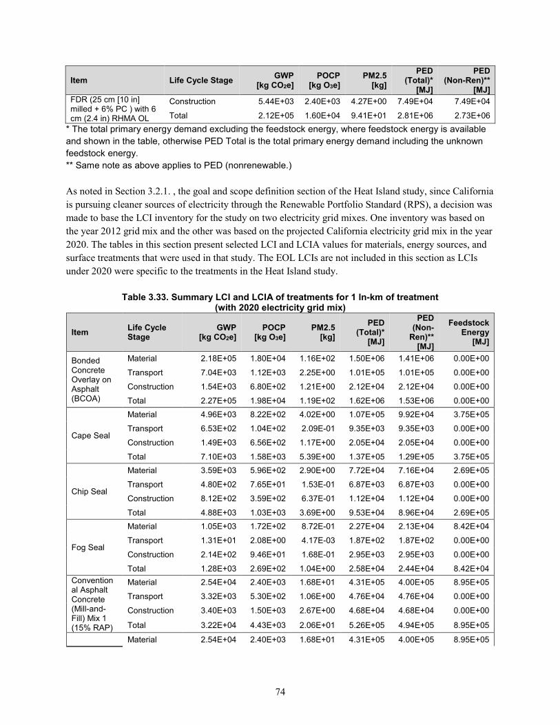
74

Item Life Cycle Stage GWP

[kg CO2e] POCP

[kg O3e] PM2.5

[kg]

PED (Total)*

[MJ]

PED (Non-Ren)**

[MJ] FDR (25 cm [10 in] milled + 6% PC ) with 6 cm (2.4 in) RHMA OL

Construction 5.44E+03 2.40E+03 4.27E+00 7.49E+04 7.49E+04

Total 2.12E+05 1.60E+04 9.41E+01 2.81E+06 2.73E+06

* The total primary energy demand excluding the feedstock energy, where feedstock energy is available and shown in the table, otherwise PED Total is the total primary energy demand including the unknown feedstock energy. ** Same note as above applies to PED (nonrenewable.)

As noted in Section 3.2.1. , the goal and scope definition section of the Heat Island study, since California

is pursuing cleaner sources of electricity through the Renewable Portfolio Standard (RPS), a decision was

made to base the LCI inventory for the study on two electricity grid mixes. One inventory was based on

the year 2012 grid mix and the other was based on the projected California electricity grid mix in the year

2020. The tables in this section present selected LCI and LCIA values for materials, energy sources, and

surface treatments that were used in that study. The EOL LCIs are not included in this section as LCIs

under 2020 were specific to the treatments in the Heat Island study.

Table 3.33. Summary LCI and LCIA of treatments for 1 ln-km of treatment

(with 2020 electricity grid mix)

Item Life Cycle Stage

GWP [kg CO2e]

POCP [kg O3e]

PM2.5 [kg]

PED (Total)*

[MJ]

PED (Non-

Ren)** [MJ]

Feedstock Energy

[MJ]

Bonded Concrete Overlay on Asphalt (BCOA)

Material 2.18E+05 1.80E+04 1.16E+02 1.50E+06 1.41E+06 0.00E+00

Transport 7.04E+03 1.12E+03 2.25E+00 1.01E+05 1.01E+05 0.00E+00

Construction 1.54E+03 6.80E+02 1.21E+00 2.12E+04 2.12E+04 0.00E+00

Total 2.27E+05 1.98E+04 1.19E+02 1.62E+06 1.53E+06 0.00E+00

Cape Seal

Material 4.96E+03 8.22E+02 4.02E+00 1.07E+05 9.92E+04 3.75E+05

Transport 6.53E+02 1.04E+02 2.09E-01 9.35E+03 9.35E+03 0.00E+00

Construction 1.49E+03 6.56E+02 1.17E+00 2.05E+04 2.05E+04 0.00E+00

Total 7.10E+03 1.58E+03 5.39E+00 1.37E+05 1.29E+05 3.75E+05

Chip Seal

Material 3.59E+03 5.96E+02 2.90E+00 7.72E+04 7.16E+04 2.69E+05

Transport 4.80E+02 7.65E+01 1.53E-01 6.87E+03 6.87E+03 0.00E+00

Construction 8.12E+02 3.59E+02 6.37E-01 1.12E+04 1.12E+04 0.00E+00

Total 4.88E+03 1.03E+03 3.69E+00 9.53E+04 8.96E+04 2.69E+05

Fog Seal

Material 1.05E+03 1.72E+02 8.72E-01 2.27E+04 2.13E+04 8.42E+04

Transport 1.31E+01 2.08E+00 4.17E-03 1.87E+02 1.87E+02 0.00E+00

Construction 2.14E+02 9.46E+01 1.68E-01 2.95E+03 2.95E+03 0.00E+00

Total 1.28E+03 2.69E+02 1.04E+00 2.58E+04 2.44E+04 8.42E+04

Conventional Asphalt Concrete (Mill-and-Fill) Mix 1 (15% RAP)

Material 2.54E+04 2.40E+03 1.68E+01 4.31E+05 4.00E+05 8.95E+05

Transport 3.32E+03 5.30E+02 1.06E+00 4.76E+04 4.76E+04 0.00E+00

Construction 3.40E+03 1.50E+03 2.67E+00 4.68E+04 4.68E+04 0.00E+00

Total 3.22E+04 4.43E+03 2.06E+01 5.26E+05 4.94E+05 8.95E+05

Material 2.54E+04 2.40E+03 1.68E+01 4.31E+05 4.00E+05 8.95E+05

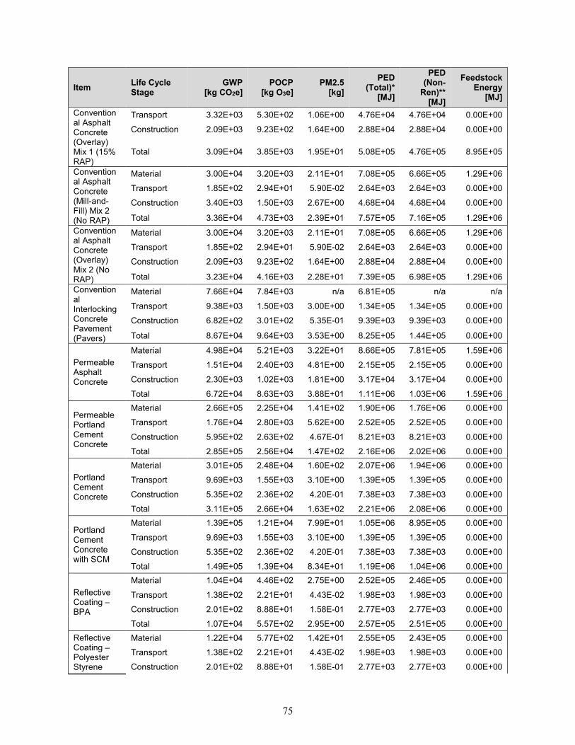
75

Item Life Cycle Stage

GWP [kg CO2e]

POCP [kg O3e]

PM2.5 [kg]

PED (Total)*

[MJ]

PED (Non-

Ren)** [MJ]

Feedstock Energy

[MJ]

Conventional Asphalt Concrete (Overlay) Mix 1 (15% RAP)

Transport 3.32E+03 5.30E+02 1.06E+00 4.76E+04 4.76E+04 0.00E+00

Construction 2.09E+03 9.23E+02 1.64E+00 2.88E+04 2.88E+04 0.00E+00

Total 3.09E+04 3.85E+03 1.95E+01 5.08E+05 4.76E+05 8.95E+05

Conventional Asphalt Concrete (Mill-and-Fill) Mix 2 (No RAP)

Material 3.00E+04 3.20E+03 2.11E+01 7.08E+05 6.66E+05 1.29E+06

Transport 1.85E+02 2.94E+01 5.90E-02 2.64E+03 2.64E+03 0.00E+00

Construction 3.40E+03 1.50E+03 2.67E+00 4.68E+04 4.68E+04 0.00E+00

Total 3.36E+04 4.73E+03 2.39E+01 7.57E+05 7.16E+05 1.29E+06

Conventional Asphalt Concrete (Overlay) Mix 2 (No RAP)

Material 3.00E+04 3.20E+03 2.11E+01 7.08E+05 6.66E+05 1.29E+06

Transport 1.85E+02 2.94E+01 5.90E-02 2.64E+03 2.64E+03 0.00E+00

Construction 2.09E+03 9.23E+02 1.64E+00 2.88E+04 2.88E+04 0.00E+00

Total 3.23E+04 4.16E+03 2.28E+01 7.39E+05 6.98E+05 1.29E+06

Conventional Interlocking Concrete Pavement (Pavers)

Material 7.66E+04 7.84E+03 n/a 6.81E+05 n/a n/a

Transport 9.38E+03 1.50E+03 3.00E+00 1.34E+05 1.34E+05 0.00E+00

Construction 6.82E+02 3.01E+02 5.35E-01 9.39E+03 9.39E+03 0.00E+00

Total 8.67E+04 9.64E+03 3.53E+00 8.25E+05 1.44E+05 0.00E+00

Permeable Asphalt Concrete

Material 4.98E+04 5.21E+03 3.22E+01 8.66E+05 7.81E+05 1.59E+06

Transport 1.51E+04 2.40E+03 4.81E+00 2.15E+05 2.15E+05 0.00E+00

Construction 2.30E+03 1.02E+03 1.81E+00 3.17E+04 3.17E+04 0.00E+00

Total 6.72E+04 8.63E+03 3.88E+01 1.11E+06 1.03E+06 1.59E+06

Permeable Portland Cement Concrete

Material 2.66E+05 2.25E+04 1.41E+02 1.90E+06 1.76E+06 0.00E+00

Transport 1.76E+04 2.80E+03 5.62E+00 2.52E+05 2.52E+05 0.00E+00

Construction 5.95E+02 2.63E+02 4.67E-01 8.21E+03 8.21E+03 0.00E+00

Total 2.85E+05 2.56E+04 1.47E+02 2.16E+06 2.02E+06 0.00E+00

Portland Cement Concrete

Material 3.01E+05 2.48E+04 1.60E+02 2.07E+06 1.94E+06 0.00E+00

Transport 9.69E+03 1.55E+03 3.10E+00 1.39E+05 1.39E+05 0.00E+00

Construction 5.35E+02 2.36E+02 4.20E-01 7.38E+03 7.38E+03 0.00E+00

Total 3.11E+05 2.66E+04 1.63E+02 2.21E+06 2.08E+06 0.00E+00

Portland Cement Concrete with SCM

Material 1.39E+05 1.21E+04 7.99E+01 1.05E+06 8.95E+05 0.00E+00

Transport 9.69E+03 1.55E+03 3.10E+00 1.39E+05 1.39E+05 0.00E+00

Construction 5.35E+02 2.36E+02 4.20E-01 7.38E+03 7.38E+03 0.00E+00

Total 1.49E+05 1.39E+04 8.34E+01 1.19E+06 1.04E+06 0.00E+00

Reflective Coating – BPA

Material 1.04E+04 4.46E+02 2.75E+00 2.52E+05 2.46E+05 0.00E+00

Transport 1.38E+02 2.21E+01 4.43E-02 1.98E+03 1.98E+03 0.00E+00

Construction 2.01E+02 8.88E+01 1.58E-01 2.77E+03 2.77E+03 0.00E+00

Total 1.07E+04 5.57E+02 2.95E+00 2.57E+05 2.51E+05 0.00E+00

Reflective Coating – Polyester Styrene

Material 1.22E+04 5.77E+02 1.42E+01 2.55E+05 2.43E+05 0.00E+00

Transport 1.38E+02 2.21E+01 4.43E-02 1.98E+03 1.98E+03 0.00E+00

Construction 2.01E+02 8.88E+01 1.58E-01 2.77E+03 2.77E+03 0.00E+00

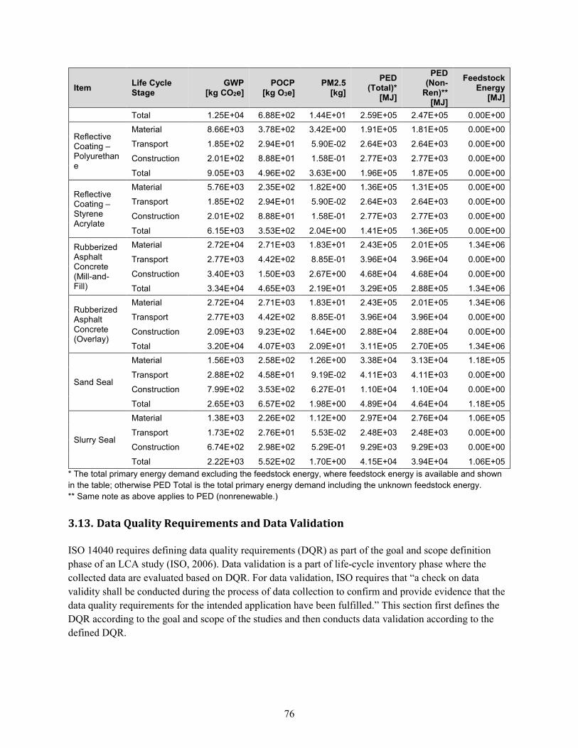
76

Item Life Cycle Stage

GWP [kg CO2e]

POCP [kg O3e]

PM2.5 [kg]

PED (Total)*

[MJ]

PED (Non-

Ren)** [MJ]

Feedstock Energy

[MJ]

Total 1.25E+04 6.88E+02 1.44E+01 2.59E+05 2.47E+05 0.00E+00

Reflective Coating – Polyurethane

Material 8.66E+03 3.78E+02 3.42E+00 1.91E+05 1.81E+05 0.00E+00

Transport 1.85E+02 2.94E+01 5.90E-02 2.64E+03 2.64E+03 0.00E+00

Construction 2.01E+02 8.88E+01 1.58E-01 2.77E+03 2.77E+03 0.00E+00

Total 9.05E+03 4.96E+02 3.63E+00 1.96E+05 1.87E+05 0.00E+00

Reflective Coating – Styrene Acrylate

Material 5.76E+03 2.35E+02 1.82E+00 1.36E+05 1.31E+05 0.00E+00

Transport 1.85E+02 2.94E+01 5.90E-02 2.64E+03 2.64E+03 0.00E+00

Construction 2.01E+02 8.88E+01 1.58E-01 2.77E+03 2.77E+03 0.00E+00

Total 6.15E+03 3.53E+02 2.04E+00 1.41E+05 1.36E+05 0.00E+00

Rubberized Asphalt Concrete (Mill-and-Fill)

Material 2.72E+04 2.71E+03 1.83E+01 2.43E+05 2.01E+05 1.34E+06

Transport 2.77E+03 4.42E+02 8.85E-01 3.96E+04 3.96E+04 0.00E+00

Construction 3.40E+03 1.50E+03 2.67E+00 4.68E+04 4.68E+04 0.00E+00

Total 3.34E+04 4.65E+03 2.19E+01 3.29E+05 2.88E+05 1.34E+06

Rubberized Asphalt Concrete (Overlay)

Material 2.72E+04 2.71E+03 1.83E+01 2.43E+05 2.01E+05 1.34E+06

Transport 2.77E+03 4.42E+02 8.85E-01 3.96E+04 3.96E+04 0.00E+00

Construction 2.09E+03 9.23E+02 1.64E+00 2.88E+04 2.88E+04 0.00E+00

Total 3.20E+04 4.07E+03 2.09E+01 3.11E+05 2.70E+05 1.34E+06

Sand Seal

Material 1.56E+03 2.58E+02 1.26E+00 3.38E+04 3.13E+04 1.18E+05

Transport 2.88E+02 4.58E+01 9.19E-02 4.11E+03 4.11E+03 0.00E+00

Construction 7.99E+02 3.53E+02 6.27E-01 1.10E+04 1.10E+04 0.00E+00

Total 2.65E+03 6.57E+02 1.98E+00 4.89E+04 4.64E+04 1.18E+05

Slurry Seal

Material 1.38E+03 2.26E+02 1.12E+00 2.97E+04 2.76E+04 1.06E+05

Transport 1.73E+02 2.76E+01 5.53E-02 2.48E+03 2.48E+03 0.00E+00

Construction 6.74E+02 2.98E+02 5.29E-01 9.29E+03 9.29E+03 0.00E+00

Total 2.22E+03 5.52E+02 1.70E+00 4.15E+04 3.94E+04 1.06E+05

* The total primary energy demand excluding the feedstock energy, where feedstock energy is available and shown in the table; otherwise PED Total is the total primary energy demand including the unknown feedstock energy. ** Same note as above applies to PED (nonrenewable.)

3.13. Data Quality Requirements and Data Validation

ISO 14040 requires defining data quality requirements (DQR) as part of the goal and scope definition

phase of an LCA study (ISO, 2006). Data validation is a part of life-cycle inventory phase where the

collected data are evaluated based on DQR. For data validation, ISO requires that “a check on data

validity shall be conducted during the process of data collection to confirm and provide evidence that the

data quality requirements for the intended application have been fulfilled.” This section first defines the

DQR according to the goal and scope of the studies and then conducts data validation according to the

defined DQR.

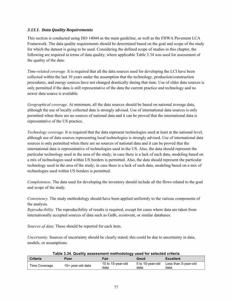
77

3.13.1. Data Quality Requirements

This section is conducted using ISO 14044 as the main guideline, as well as the FHWA Pavement LCA

Framework. The data quality requirements should be determined based on the goal and scope of the study

for which the dataset is going to be used. Considering the defined scope of studies in this chapter, the

following are required in terms of data quality; where applicable Table 3.34 was used for assessment of

the quality of the data:

Time-related coverage. It is required that all the data sources used for developing the LCI have been

collected within the last 10 years under the assumption that the technology, production/construction

procedures, and energy sources have not changed drastically during that time. Use of older data sources is

only permitted if the data is still representative of the data the current practice and technology and no

newer data source is available.

Geographical coverage. At minimum, all the data sources should be based on national average data,

although the use of locally collected data is strongly advised. Use of international data sources is only

permitted when there are no sources of national data and it can be proved that the international data is

representative of the US practice.

Technology coverage. It is required that the data represent technologies used at least at the national level,

although use of data sources representing local technologies is strongly advised. Use of international data

sources is only permitted when there are no sources of national data and it can be proved that the

international data is representative of technologies used in the US. Also, the data should represent the

particular technology used in the area of the study; in case there is a lack of such data, modeling based on

a mix of technologies used within US borders is permitted. Also, the data should represent the particular

technology used in the area of the study; in case there is a lack of such data, modeling based on a mix of

technologies used within US borders is permitted.

Completeness. The data used for developing the inventory should include all the flows related to the goal

and scope of the study.

Consistency. The study methodology should have been applied uniformly to the various components of

the analysis.

Reproducibility. The reproducibility of results is required, except for cases where data are taken from

internationally accepted sources of data such as GaBi, ecoinvent, or similar databases.

Sources of data. These should be reported for each item.

Uncertainty. Sources of uncertainty should be clearly stated; this could be due to uncertainty in data,

models, or assumptions.

Table 3.34. Quality assessment methodology used for selected criteria

Criteria Poor Fair Good Excellent

Time Coverage 15+ year-old data 10 to 15-year-old data

5 to 10-year-old data

Less than 5-year-old data

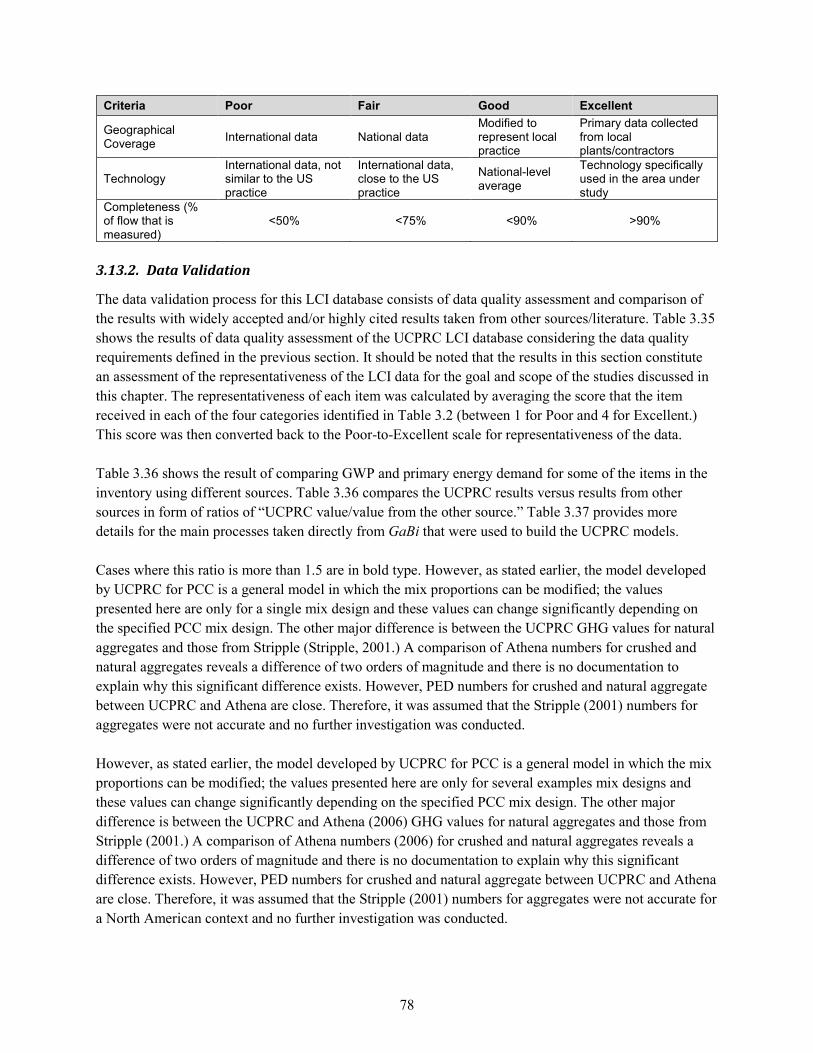
78

Criteria Poor Fair Good Excellent

Geographical Coverage

International data National data Modified to represent local practice

Primary data collected from local plants/contractors

Technology International data, not similar to the US practice

International data, close to the US practice

National-level average

Technology specifically used in the area under study

Completeness (% of flow that is measured)

<50% <75% <90% >90%

3.13.2. Data Validation

The data validation process for this LCI database consists of data quality assessment and comparison of

the results with widely accepted and/or highly cited results taken from other sources/literature. Table 3.35

shows the results of data quality assessment of the UCPRC LCI database considering the data quality

requirements defined in the previous section. It should be noted that the results in this section constitute

an assessment of the representativeness of the LCI data for the goal and scope of the studies discussed in

this chapter. The representativeness of each item was calculated by averaging the score that the item

received in each of the four categories identified in Table 3.2 (between 1 for Poor and 4 for Excellent.)

This score was then converted back to the Poor-to-Excellent scale for representativeness of the data.

Table 3.36 shows the result of comparing GWP and primary energy demand for some of the items in the

inventory using different sources. Table 3.36 compares the UCPRC results versus results from other

sources in form of ratios of “UCPRC value/value from the other source.” Table 3.37 provides more

details for the main processes taken directly from GaBi that were used to build the UCPRC models.

Cases where this ratio is more than 1.5 are in bold type. However, as stated earlier, the model developed

by UCPRC for PCC is a general model in which the mix proportions can be modified; the values

presented here are only for a single mix design and these values can change significantly depending on

the specified PCC mix design. The other major difference is between the UCPRC GHG values for natural

aggregates and those from Stripple (Stripple, 2001.) A comparison of Athena numbers for crushed and

natural aggregates reveals a difference of two orders of magnitude and there is no documentation to

explain why this significant difference exists. However, PED numbers for crushed and natural aggregate

between UCPRC and Athena are close. Therefore, it was assumed that the Stripple (2001) numbers for

aggregates were not accurate and no further investigation was conducted.

However, as stated earlier, the model developed by UCPRC for PCC is a general model in which the mix

proportions can be modified; the values presented here are only for several examples mix designs and

these values can change significantly depending on the specified PCC mix design. The other major

difference is between the UCPRC and Athena (2006) GHG values for natural aggregates and those from

Stripple (2001.) A comparison of Athena numbers (2006) for crushed and natural aggregates reveals a

difference of two orders of magnitude and there is no documentation to explain why this significant

difference exists. However, PED numbers for crushed and natural aggregate between UCPRC and Athena

are close. Therefore, it was assumed that the Stripple (2001) numbers for aggregates were not accurate for

a North American context and no further investigation was conducted.

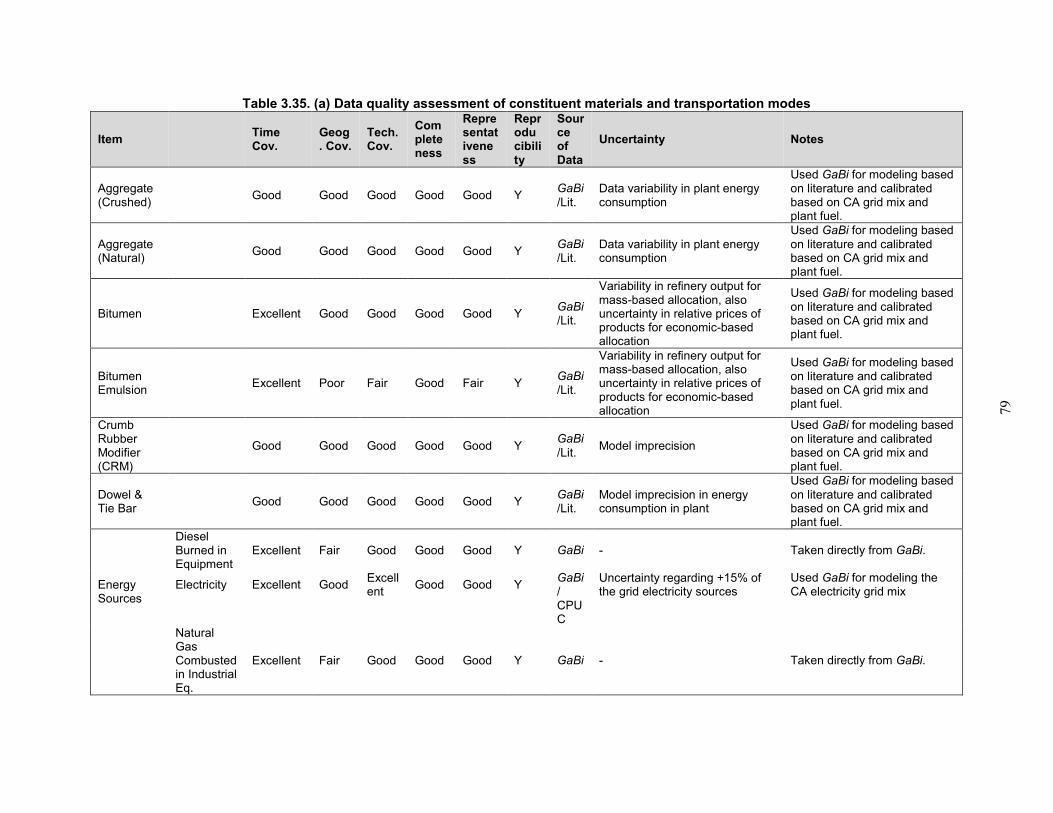
79

Table 3.35. (a) Data quality assessment of constituent materials and transportation modes

Item Time Cov.

Geog. Cov.

Tech. Cov.

Completeness

Representativeness

Reproducibility

Source of Data

Uncertainty Notes

Aggregate (Crushed)

Good Good Good Good Good Y GaBi

/Lit. Data variability in plant energy consumption

Used GaBi for modeling based on literature and calibrated based on CA grid mix and plant fuel.

Aggregate (Natural)

Good Good Good Good Good Y GaBi

/Lit. Data variability in plant energy consumption

Used GaBi for modeling based on literature and calibrated based on CA grid mix and plant fuel.

Bitumen Excellent Good Good Good Good Y GaBi

/Lit.

Variability in refinery output for mass-based allocation, also uncertainty in relative prices of products for economic-based allocation

Used GaBi for modeling based on literature and calibrated based on CA grid mix and plant fuel.

Bitumen Emulsion

Excellent Poor Fair Good Fair Y GaBi

/Lit.

Variability in refinery output for mass-based allocation, also uncertainty in relative prices of products for economic-based allocation

Used GaBi for modeling based on literature and calibrated based on CA grid mix and plant fuel.

Crumb Rubber Modifier (CRM)

Good Good Good Good Good Y GaBi

/Lit. Model imprecision

Used GaBi for modeling based on literature and calibrated based on CA grid mix and plant fuel.

Dowel & Tie Bar

Good Good Good Good Good Y GaBi

/Lit. Model imprecision in energy consumption in plant

Used GaBi for modeling based on literature and calibrated based on CA grid mix and plant fuel.

Energy Sources

Diesel Burned in Equipment

Excellent Fair Good Good Good Y GaBi - Taken directly from GaBi.

Electricity Excellent Good Excellent

Good Good Y GaBi

/ Uncertainty regarding +15% of the grid electricity sources

Used GaBi for modeling the CA electricity grid mix

CPUC

Natural Gas Combusted in Industrial Eq.

Excellent Fair Good Good Good Y GaBi - Taken directly from GaBi.

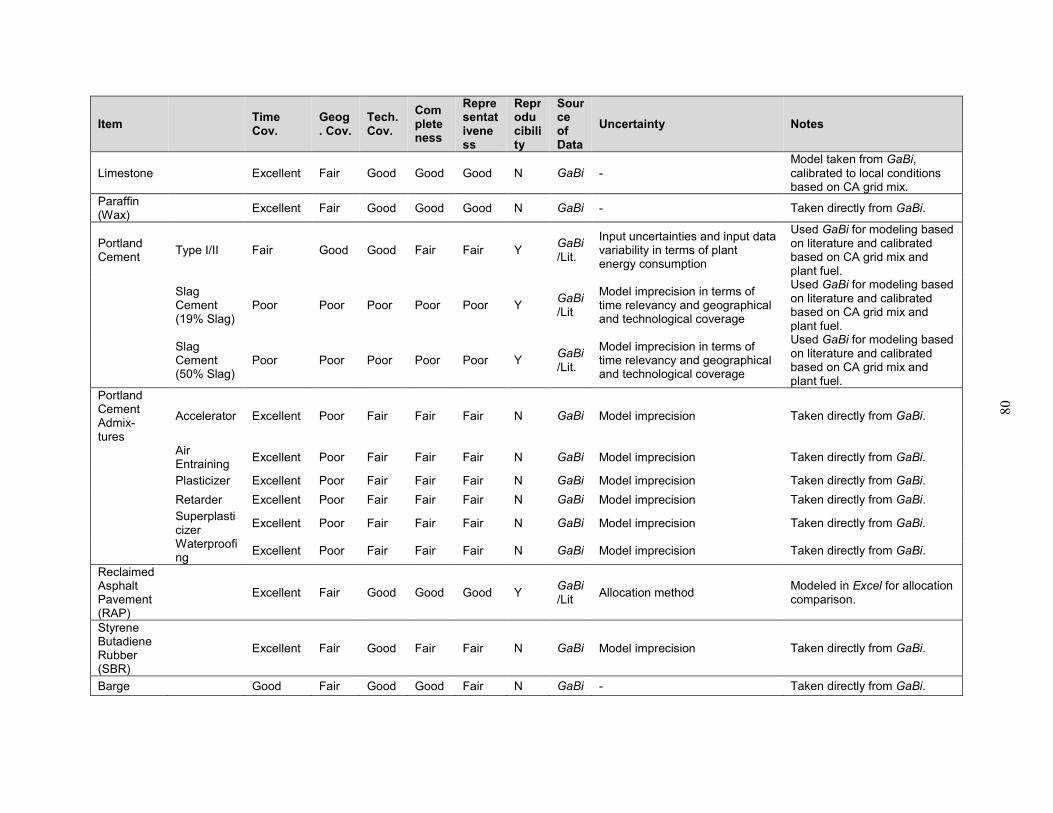
80

Item Time Cov.

Geog. Cov.

Tech. Cov.

Completeness

Representativeness

Reproducibility

Source of Data

Uncertainty Notes

Limestone Excellent Fair Good Good Good N GaBi - Model taken from GaBi, calibrated to local conditions based on CA grid mix.

Paraffin (Wax)

Excellent Fair Good Good Good N GaBi - Taken directly from GaBi.

Portland Cement

Type I/II Fair Good Good Fair Fair Y GaBi

/Lit.

Input uncertainties and input data variability in terms of plant energy consumption

Used GaBi for modeling based on literature and calibrated based on CA grid mix and plant fuel.

Slag Cement (19% Slag)

Poor Poor Poor Poor Poor Y GaBi

/Lit

Model imprecision in terms of time relevancy and geographical and technological coverage

Used GaBi for modeling based on literature and calibrated based on CA grid mix and plant fuel.

Slag Cement (50% Slag)

Poor Poor Poor Poor Poor Y GaBi

/Lit.

Model imprecision in terms of time relevancy and geographical and technological coverage

Used GaBi for modeling based on literature and calibrated based on CA grid mix and plant fuel.

Portland Cement Admix-tures

Accelerator Excellent Poor Fair Fair Fair N GaBi Model imprecision Taken directly from GaBi.

Air Entraining

Excellent Poor Fair Fair Fair N GaBi Model imprecision Taken directly from GaBi.

Plasticizer Excellent Poor Fair Fair Fair N GaBi Model imprecision Taken directly from GaBi.

Retarder Excellent Poor Fair Fair Fair N GaBi Model imprecision Taken directly from GaBi.

Superplasticizer

Excellent Poor Fair Fair Fair N GaBi Model imprecision Taken directly from GaBi.

Waterproofing

Excellent Poor Fair Fair Fair N GaBi Model imprecision Taken directly from GaBi.

Reclaimed Asphalt Pavement (RAP)

Excellent Fair Good Good Good Y GaBi

/Lit Allocation method

Modeled in Excel for allocation comparison.

Styrene Butadiene Rubber (SBR)

Excellent Fair Good Fair Fair N GaBi Model imprecision Taken directly from GaBi.

Barge Good Fair Good Good Fair N GaBi - Taken directly from GaBi.

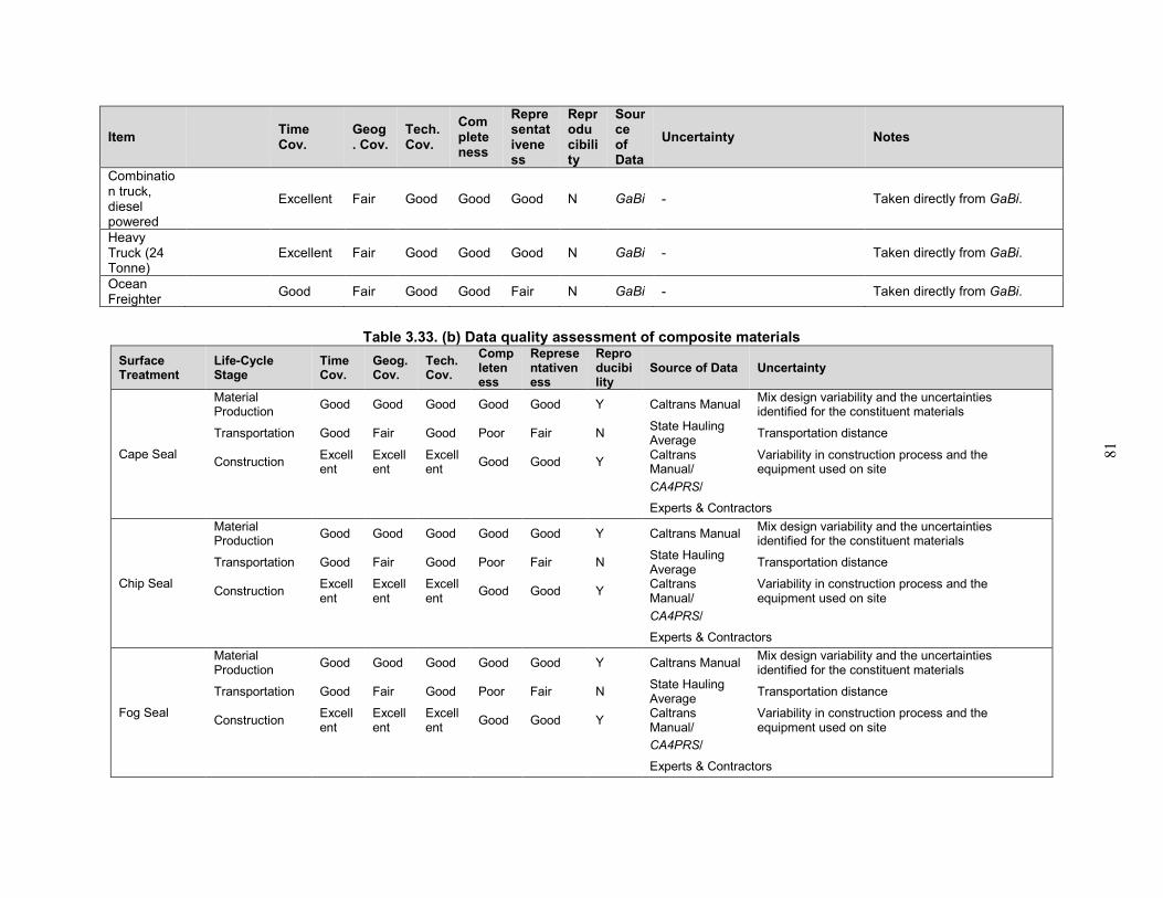
81

Item Time Cov.

Geog. Cov.

Tech. Cov.

Completeness

Representativeness

Reproducibility

Source of Data

Uncertainty Notes

Combination truck, diesel powered

Excellent Fair Good Good Good N GaBi - Taken directly from GaBi.

Heavy Truck (24 Tonne)

Excellent Fair Good Good Good N GaBi - Taken directly from GaBi.

Ocean Freighter

Good Fair Good Good Fair N GaBi - Taken directly from GaBi.

Table 3.33. (b) Data quality assessment of composite materials

Surface Treatment

Life-Cycle Stage

Time Cov.

Geog. Cov.

Tech. Cov.

Completeness

Representativeness

Reproducibility

Source of Data Uncertainty

Cape Seal

Material Production

Good Good Good Good Good Y Caltrans Manual Mix design variability and the uncertainties identified for the constituent materials

Transportation Good Fair Good Poor Fair N State Hauling Average

Transportation distance

Construction Excellent

Excellent

Excellent

Good Good Y Caltrans Manual/

Variability in construction process and the equipment used on site

CA4PRS/

Experts & Contractors

Chip Seal

Material Production

Good Good Good Good Good Y Caltrans Manual Mix design variability and the uncertainties identified for the constituent materials

Transportation Good Fair Good Poor Fair N State Hauling Average

Transportation distance

Construction Excellent

Excellent

Excellent

Good Good Y Caltrans Manual/

Variability in construction process and the equipment used on site

CA4PRS/

Experts & Contractors

Fog Seal

Material Production

Good Good Good Good Good Y Caltrans Manual Mix design variability and the uncertainties identified for the constituent materials

Transportation Good Fair Good Poor Fair N State Hauling Average

Transportation distance

Construction Excellent

Excellent

Excellent

Good Good Y Caltrans Manual/

Variability in construction process and the equipment used on site

CA4PRS/

Experts & Contractors

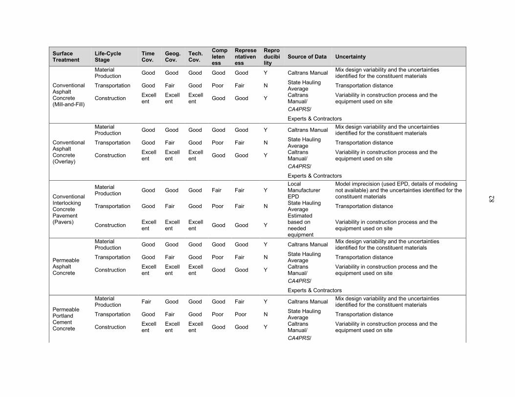
82

Surface Treatment

Life-Cycle Stage

Time Cov.

Geog. Cov.

Tech. Cov.

Completeness

Representativeness

Reproducibility

Source of Data Uncertainty

Conventional Asphalt Concrete (Mill-and-Fill)

Material Production

Good Good Good Good Good Y Caltrans Manual Mix design variability and the uncertainties identified for the constituent materials

Transportation Good Fair Good Poor Fair N State Hauling Average

Transportation distance

Construction Excellent

Excellent

Excellent

Good Good Y Caltrans Manual/

Variability in construction process and the equipment used on site

CA4PRS/

Experts & Contractors

Conventional Asphalt Concrete (Overlay)

Material Production

Good Good Good Good Good Y Caltrans Manual Mix design variability and the uncertainties identified for the constituent materials

Transportation Good Fair Good Poor Fair N State Hauling Average

Transportation distance

Construction Excellent

Excellent

Excellent

Good Good Y Caltrans Manual/

Variability in construction process and the equipment used on site

CA4PRS/

Experts & Contractors

Conventional Interlocking Concrete Pavement (Pavers)

Material Production

Good Good Good Fair Fair Y Local Manufacturer EPD

Model imprecision (used EPD, details of modeling not available) and the uncertainties identified for the constituent materials

Transportation Good Fair Good Poor Fair N State Hauling Average

Transportation distance

Construction Excellent

Excellent

Excellent

Good Good Y

Estimated based on needed equipment

Variability in construction process and the equipment used on site

Permeable Asphalt Concrete

Material Production

Good Good Good Good Good Y Caltrans Manual Mix design variability and the uncertainties identified for the constituent materials

Transportation Good Fair Good Poor Fair N State Hauling Average

Transportation distance

Construction Excellent

Excellent

Excellent

Good Good Y Caltrans Manual/

Variability in construction process and the equipment used on site

CA4PRS/

Experts & Contractors

Permeable Portland Cement Concrete

Material Production

Fair Good Good Good Fair Y Caltrans Manual Mix design variability and the uncertainties identified for the constituent materials

Transportation Good Fair Good Poor Poor N State Hauling Average

Transportation distance

Construction Excellent

Excellent

Excellent

Good Good Y Caltrans Manual/

Variability in construction process and the equipment used on site

CA4PRS/

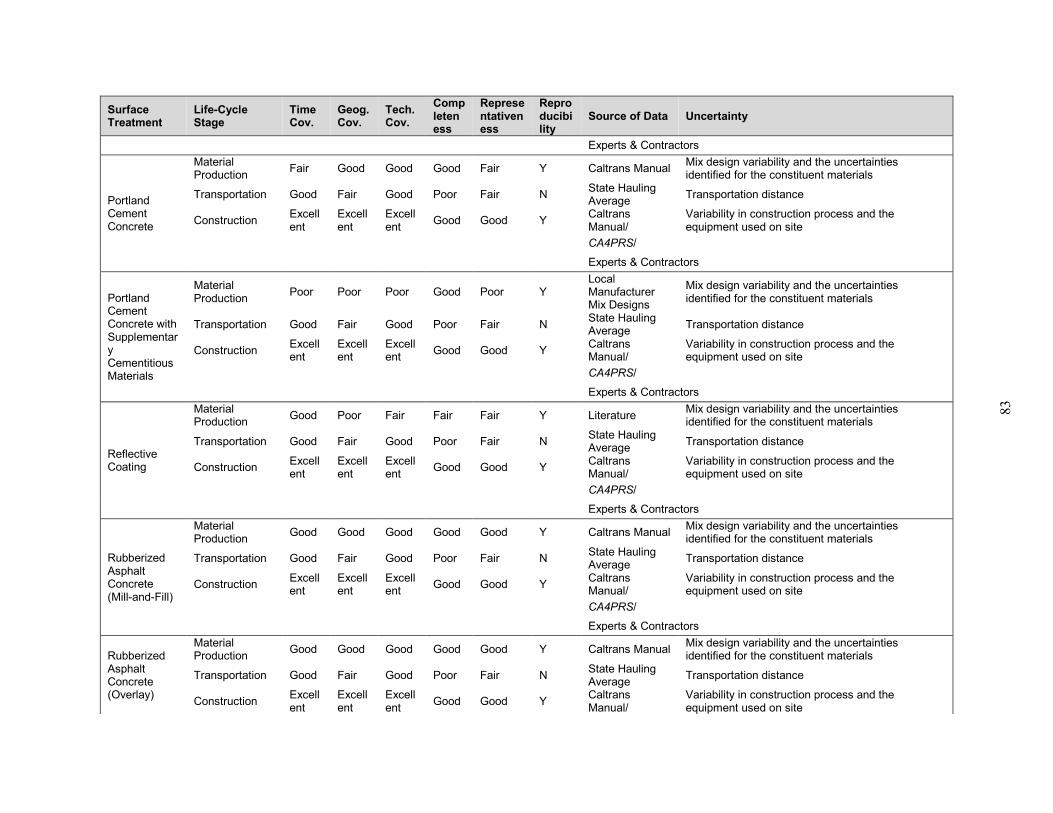
83

Surface Treatment

Life-Cycle Stage

Time Cov.

Geog. Cov.

Tech. Cov.

Completeness

Representativeness

Reproducibility

Source of Data Uncertainty

Experts & Contractors

Portland Cement Concrete

Material Production

Fair Good Good Good Fair Y Caltrans Manual Mix design variability and the uncertainties identified for the constituent materials

Transportation Good Fair Good Poor Fair N State Hauling Average

Transportation distance

Construction Excellent

Excellent

Excellent

Good Good Y Caltrans Manual/

Variability in construction process and the equipment used on site

CA4PRS/

Experts & Contractors

Portland Cement Concrete with Supplementary Cementitious Materials

Material Production

Poor Poor Poor Good Poor Y Local Manufacturer Mix Designs

Mix design variability and the uncertainties identified for the constituent materials

Transportation Good Fair Good Poor Fair N State Hauling Average

Transportation distance

Construction Excellent

Excellent

Excellent

Good Good Y Caltrans Manual/

Variability in construction process and the equipment used on site

CA4PRS/

Experts & Contractors

Reflective Coating

Material Production

Good Poor Fair Fair Fair Y Literature Mix design variability and the uncertainties identified for the constituent materials

Transportation Good Fair Good Poor Fair N State Hauling Average

Transportation distance

Construction Excellent

Excellent

Excellent

Good Good Y Caltrans Manual/

Variability in construction process and the equipment used on site

CA4PRS/

Experts & Contractors

Rubberized Asphalt Concrete (Mill-and-Fill)

Material Production

Good Good Good Good Good Y Caltrans Manual Mix design variability and the uncertainties identified for the constituent materials

Transportation Good Fair Good Poor Fair N State Hauling Average

Transportation distance

Construction Excellent

Excellent

Excellent

Good Good Y Caltrans Manual/

Variability in construction process and the equipment used on site

CA4PRS/

Experts & Contractors

Rubberized Asphalt Concrete (Overlay)

Material Production

Good Good Good Good Good Y Caltrans Manual Mix design variability and the uncertainties identified for the constituent materials

Transportation Good Fair Good Poor Fair N State Hauling Average

Transportation distance

Construction Excellent

Excellent

Excellent

Good Good Y Caltrans Manual/

Variability in construction process and the equipment used on site

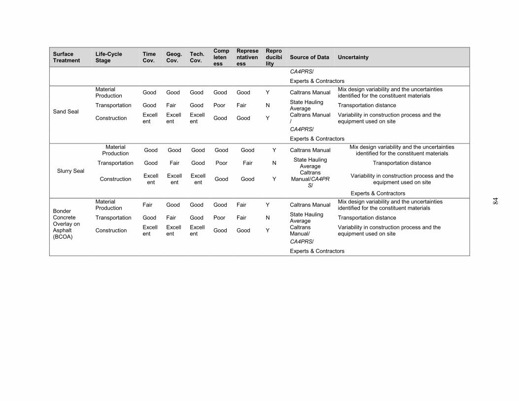
84

Surface Treatment

Life-Cycle Stage

Time Cov.

Geog. Cov.

Tech. Cov.

Completeness

Representativeness

Reproducibility

Source of Data Uncertainty

CA4PRS/

Experts & Contractors

Sand Seal

Material Production

Good Good Good Good Good Y Caltrans Manual Mix design variability and the uncertainties identified for the constituent materials

Transportation Good Fair Good Poor Fair N State Hauling Average

Transportation distance

Construction Excellent

Excellent

Excellent

Good Good Y Caltrans Manual/

Variability in construction process and the equipment used on site

CA4PRS/

Experts & Contractors

Slurry Seal

Material Production

Good Good Good Good Good Y Caltrans Manual Mix design variability and the uncertainties

identified for the constituent materials

Transportation Good Fair Good Poor Fair N State Hauling

Average Transportation distance

Construction Excell

ent Excell

ent Excell

ent Good Good Y

Caltrans Manual/CA4PR

S/

Variability in construction process and the equipment used on site

Experts & Contractors

Bonder Concrete Overlay on Asphalt (BCOA)

Material Production

Fair Good Good Good Fair Y Caltrans Manual Mix design variability and the uncertainties identified for the constituent materials

Transportation Good Fair Good Poor Fair N State Hauling Average

Transportation distance

Construction Excellent

Excellent

Excellent

Good Good Y Caltrans Manual/

Variability in construction process and the equipment used on site

CA4PRS/

Experts & Contractors

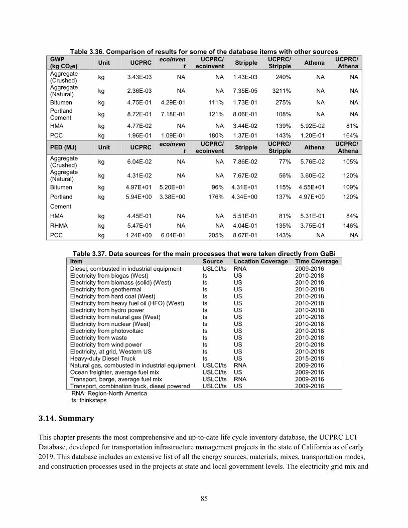
85

Table 3.36. Comparison of results for some of the database items with other sources GWP (kg CO2e)

Unit UCPRC ecoinven

t UCPRC/

ecoinvent Stripple

UCPRC/Stripple

Athena UCPRC/Athena

Aggregate (Crushed)

kg 3.43E-03 NA NA 1.43E-03 240% NA NA

Aggregate (Natural)

kg 2.36E-03 NA NA 7.35E-05 3211% NA NA

Bitumen kg 4.75E-01 4.29E-01 111% 1.73E-01 275% NA NA

Portland Cement

kg 8.72E-01 7.18E-01 121% 8.06E-01 108% NA NA

HMA kg 4.77E-02 NA NA 3.44E-02 139% 5.92E-02 81%

PCC kg 1.96E-01 1.09E-01 180% 1.37E-01 143% 1.20E-01 164%

PED (MJ) Unit UCPRC ecoinven

t

UCPRC/ ecoinvent

Stripple UCPRC/Stripple

Athena UCPRC/Athena

Aggregate (Crushed)

kg 6.04E-02 NA NA 7.86E-02 77% 5.76E-02 105%

Aggregate (Natural)

kg 4.31E-02 NA NA 7.67E-02 56% 3.60E-02 120%

Bitumen kg 4.97E+01 5.20E+01 96% 4.31E+01 115% 4.55E+01 109%

Portland kg 5.94E+00 3.38E+00 176% 4.34E+00 137% 4.97E+00 120%

Cement

HMA kg 4.45E-01 NA NA 5.51E-01 81% 5.31E-01 84%

RHMA kg 5.47E-01 NA NA 4.04E-01 135% 3.75E-01 146%

PCC kg 1.24E+00 6.04E-01 205% 8.67E-01 143% NA NA

Table 3.37. Data sources for the main processes that were taken directly from GaBi

Item Source Location Coverage Time Coverage

Diesel, combusted in industrial equipment USLCI/ts RNA 2009-2016 Electricity from biogas (West) ts US 2010-2018 Electricity from biomass (solid) (West) ts US 2010-2018 Electricity from geothermal ts US 2010-2018 Electricity from hard coal (West) ts US 2010-2018 Electricity from heavy fuel oil (HFO) (West) ts US 2010-2018 Electricity from hydro power ts US 2010-2018 Electricity from natural gas (West) ts US 2010-2018 Electricity from nuclear (West) ts US 2010-2018 Electricity from photovoltaic ts US 2010-2018 Electricity from waste ts US 2010-2018 Electricity from wind power ts US 2010-2018 Electricity, at grid, Western US ts US 2010-2018 Heavy-duty Diesel Truck ts US 2015-2018 Natural gas, combusted in industrial equipment USLCI/ts RNA 2009-2016 Ocean freighter, average fuel mix USLCI/ts US 2009-2016 Transport, barge, average fuel mix USLCI/ts RNA 2009-2016 Transport, combination truck, diesel powered USLCI/ts US 2009-2016 RNA: Region-North America ts: thinksteps

3.14. Summary

This chapter presents the most comprehensive and up-to-date life cycle inventory database, the UCPRC LCI

Database, developed for transportation infrastructure management projects in the state of California as of early

2019. This database includes an extensive list of all the energy sources, materials, mixes, transportation modes,

and construction processes used in the projects at state and local government levels. The electricity grid mix and

86

other energy sources used in various life cycle stages are modified to represent the state’s local conditions. Mix

designs are defined based on specifications enforced by Caltrans and also cover designs used by local

governments. Construction practices are closely simulated based on data collected from local contractors and

experts in addition to the collection of primary data collection from a few field projects. The LCI database

developed and presented in this chapter has been verified by a third party according to ISO recommendations.

This database was developed using the latest data from available databases, literature, and communications with

experts and contractors. The UCPRC LCI Database needs to be continually reviewed and get updated because of

the continuous improvements in material production technologies, construction practices, and energy sources

used for generating electricity and running the material plants. The revision and update process for the UCPRC

LCI Database should be repeated every few years using the latest available information. However, the most

critical measure that can be taken to improve the quality of the data is to collect primary data from local material

production plants and contractors.

87

CHAPTER 4. LCA Comparison of Urban Street Design

Methodologies: Complete Streets versus Conventional Streets, with

Sensitivity Analysis on Key Model Parameters

4.1. Introduction

Complete streets are considered solutions for transportation corridors to improve social, economic, and

environmental conditions of a neighborhood or community compared to conventional streets (Harvey et al.,

2018) and are meant to provide safe access for all users of all ages and abilities using all modes of transport

(Smart Growth America webpage on Implementing Complete Streets.) Besides improving safety and providing

access for all users, especially non-motorized transportation, other benefits of compete streets mentioned in the

literature are reduced costs and environmental burdens, and creation of more livable communities (Caltrans

2017.) Reduced environmental burdens are not the only purpose of complete streets but it is often mentioned in

the literature that complete streets are designed to encourage active modes of transport and there is often an

explicit or implicit assumption that they will therefore reduce vehicle miles travelled. However, there is no

environmental life cycle comparison of complete streets and conventional ones that takes into consideration the

possible changes in traffic patterns. This chapter addresses this gap in the knowledge.

4.2. Goal and Scope

The goal of this chapter is to quantify the environmental impacts of implementing complete streets (CS)

guidelines using the life cycle assessment methodology and compare with the impacts of streets designed under

conventional methods.

Six types of urban streets were benchmarked and compared under two design scenarios:

• A conventional design using Section Four of the Sacramento County Office of Engineering

Improvement Standard (Sacramento County, 2009), which is an example of a standard currently in use

for designing conventional streets, and

• A complete streets design using the Complete Streets Manual from the Department of Urban Planning

of the City of Los Angeles, (City of LA, 2014.)

The system boundary for each street type includes material production, transportation of raw materials from

extraction site to processing plant and from there to the construction site, and construction activities; this is

referred to as a cradle-to-laid LCA. Throughout this chapter, the LCA results for these stages of the life cycle

are referred to as MAC impacts (Material, transportation, And Construction.)

An analysis period of 30 years was selected for conducting the LCA and calculating payback periods for

offsetting the differences in environmental impacts due to complete streets designs compared with conventional

designs. The functional unit for all cases in this chapter is considered as one block, except where stated

otherwise.

88

Throughout this chapter, the Sacramento County Standard is referred to as SAC-DG (Sacramento Design

Guide), and the design option for each urban street type under SAC-DG is referred to as Conv-Option

(Conventional [Design] Option.) Similarly, the manual developed by the City of Los Angeles will be referred to

as LA-DG (LA Design Guide), and the design option for each street type under LA-DG is referred to as the CS-

Option (Complete Street [Design] Option.) All study details are covered in the “Assumptions and Modeling

Details” section, followed by results and discussion.

A sensitivity analysis was also conducted in which the assumed reductions in VMT for CS-Options were

evaluated for offsetting the extra MAC emissions of CS-Options compared to Conv-Options. The sensitivity

analysis considered a range of changes in vehicle miles traveled for the street type in question and the

surrounding network affected by the complete street. The change in vehicle miles traveled data was found in a

report from the City of San Jose, as were the following two cases of vehicle speed changes on the complete

street, which were also assumed to occur in the portion of traffic that moved to parallel routes in the surrounding

network:

• The typical conventional design maximum speed, and

• The design maximum speed recommended for complete streets by the National Association of City

Transportation Officials (NACTO)

The results of the LCA study and the limited sensitivity analysis in this chapter provide a quantitative

comparison of the environmental impacts of designing urban streets under conventional design guidelines versus

complete streets guidelines and includes sensitivity to different assumptions. However, it should be noted that

the scope of the LCA study in this chapter is limited to material production, transportation of materials to the

site, construction activities, and changes in vehicle miles traveled and vehicle speed, and their effects on

selected emissions from the production (well to pump) and combustion (pump to wheel) of vehicle fuel in the

use stage. The assessment does not include the end-of-life of the built infrastructure, or any other effects on

vehicles or the use of alternative modes of transportation in lieu of motorized vehicles.

All vehicles are assumed to burn gasoline and only passenger cars and light-duty trucks (SUVs) are considered,

which means that consideration of any heavier freight vehicles is excluded.

A limitation of many complete street designs is that they do not consider existing use of a conventional street for

freight vehicles (it can be said that they are “incomplete” in that sense.) Any changes in freight vehicle routes,

changes in speed and operation of freight vehicles, and changes to smaller freight vehicles that can operate on

complete streets and any other logistical changes are not considered in this sensitivity analysis.

In addition to those impacts already mentioned, complete streets can have other important impacts not

considered in the limited sensitivity analysis presented in this chapter. Additional case studies for field projects

can include consideration of expansion of the system boundaries for LCA, which were limited by the scope and

budget of this framework development project.

4.3. Assumptions and Modeling Approach

Six major urban street types identified in SAC-DG were chosen for this study and are listed in Table 4.1. The

goal of the LCAs in this section is to benchmark the selected environmental impacts, primary energy demand,

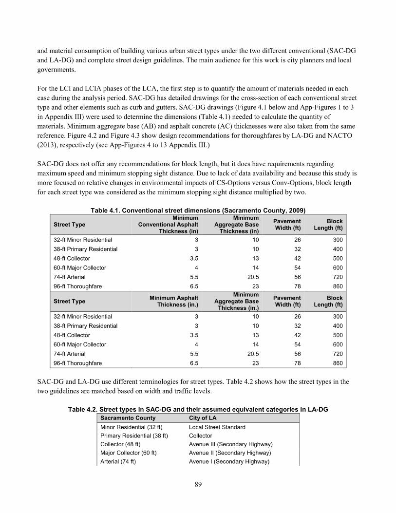
89

and material consumption of building various urban street types under the two different conventional (SAC-DG

and LA-DG) and complete street design guidelines. The main audience for this work is city planners and local

governments.

For the LCI and LCIA phases of the LCA, the first step is to quantify the amount of materials needed in each

case during the analysis period. SAC-DG has detailed drawings for the cross-section of each conventional street

type and other elements such as curb and gutters. SAC-DG drawings (Figure 4.1 below and App-Figures 1 to 3

in Appendix III) were used to determine the dimensions (Table 4.1) needed to calculate the quantity of

materials. Minimum aggregate base (AB) and asphalt concrete (AC) thicknesses were also taken from the same

reference. Figure 4.2 and Figure 4.3 show design recommendations for thoroughfares by LA-DG and NACTO

(2013), respectively (see App-Figures 4 to 13 Appendix III.)

SAC-DG does not offer any recommendations for block length, but it does have requirements regarding

maximum speed and minimum stopping sight distance. Due to lack of data availability and because this study is

more focused on relative changes in environmental impacts of CS-Options versus Conv-Options, block length

for each street type was considered as the minimum stopping sight distance multiplied by two.

Table 4.1. Conventional street dimensions (Sacramento County, 2009)

Street Type Minimum

Conventional Asphalt Thickness (in)

Minimum Aggregate Base

Thickness (in)

Pavement Width (ft)

Block Length (ft)

32-ft Minor Residential 3 10 26 300

38-ft Primary Residential 3 10 32 400

48-ft Collector 3.5 13 42 500

60-ft Major Collector 4 14 54 600

74-ft Arterial 5.5 20.5 56 720

96-ft Thoroughfare 6.5 23 78 860

Street Type Minimum Asphalt

Thickness (in.)

Minimum Aggregate Base

Thickness (in.)

Pavement Width (ft)

Block Length (ft)

32-ft Minor Residential 3 10 26 300

38-ft Primary Residential 3 10 32 400

48-ft Collector 3.5 13 42 500

60-ft Major Collector 4 14 54 600

74-ft Arterial 5.5 20.5 56 720

96-ft Thoroughfare 6.5 23 78 860

SAC-DG and LA-DG use different terminologies for street types. Table 4.2 shows how the street types in the

two guidelines are matched based on width and traffic levels.

Table 4.2. Street types in SAC-DG and their assumed equivalent categories in LA-DG

Sacramento County City of LA

Minor Residential (32 ft) Local Street Standard

Primary Residential (38 ft) Collector

Collector (48 ft) Avenue III (Secondary Highway)

Major Collector (60 ft) Avenue II (Secondary Highway)

Arterial (74 ft) Avenue I (Secondary Highway)

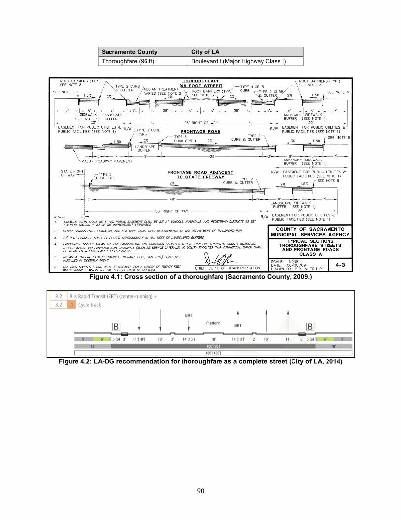
90

Sacramento County City of LA

Thoroughfare (96 ft) Boulevard I (Major Highway Class I)

Figure 4.1: Cross section of a thoroughfare (Sacramento County, 2009.)

Figure 4.2: LA-DG recommendation for thoroughfare as a complete street (City of LA, 2014)

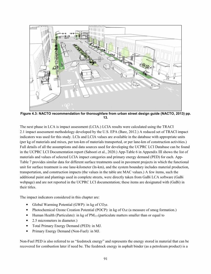
91

Figure 4.3: NACTO recommendation for thoroughfare from urban street design guide (NACTO, 2013) pp. 13.

The next phase in LCA is impact assessment (LCIA.) LCIA results were calculated using the TRACI

2.1 impact assessment methodology developed by the U.S. EPA (Bare, 2012.) A reduced set of TRACI impact

indicators was used for this study. LCIs and LCIA values are available in the database with appropriate units

(per kg of materials and mixes, per ton-km of materials transported, or per lane-km of construction activities.)

Full details of all the assumptions and data sources used for developing the UCPRC LCI Database can be found

in the UCPRC LCI Documentation report (Saboori et al., 2020.) App-Table 6 in Appendix III shows the list of

materials and values of selected LCIA impact categories and primary energy demand (PED) for each. App-

Table 7 provides similar data for different surface treatments used in pavement projects in which the functional

unit for surface treatment is one lane-kilometer (ln-km), and the system boundary includes material production,

transportation, and construction impacts (the values in the table are MAC values.) A few items, such the

additional paint and plantings used in complete streets, were directly taken from GaBi LCA software (GaBi

webpage) and are not reported in the UCPRC LCI documentation; these items are designated with (GaBi) in

their titles.

The impact indicators considered in this chapter are:

• Global Warming Potential (GWP): in kg of CO2e.

• Photochemical Ozone Creation Potential (POCP): in kg of O3e (a measure of smog formation.)

• Human Health (Particulate): in kg of PM2.5 (particulate matters smaller than or equal to

• 2.5 micrometers in diameter.)

• Total Primary Energy Demand (PED): in MJ.

• Primary Energy Demand (Non-Fuel): in MJ.

Non-Fuel PED is also referred to as “feedstock energy” and represents the energy stored in material that can be

recovered for combustion later if need be. The feedstock energy in asphalt binder (as a petroleum product) is a

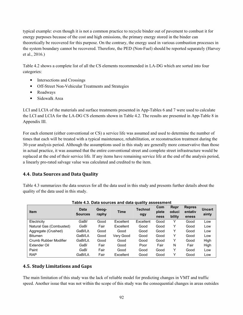
92

typical example: even though it is not a common practice to recycle binder out of pavement to combust it for

energy purposes because of the cost and high emissions, the primary energy stored in the binder can

theoretically be recovered for this purpose. On the contrary, the energy used in various combustion processes in

the system boundary cannot be recovered. Therefore, the PED (Non-Fuel) should be reported separately (Harvey

et al., 2016.)

Table 4.2 shows a complete list of all the CS elements recommended in LA-DG which are sorted into four

categories:

• Intersections and Crossings

• Off-Street Non-Vehicular Treatments and Strategies

• Roadways

• Sidewalk Area

LCI and LCIA of the materials and surface treatments presented in App-Tables 6 and 7 were used to calculate

the LCI and LCIA for the LA-DG CS elements shown in Table 4.2. The results are presented in App-Table 8 in

Appendix III.

For each element (either conventional or CS) a service life was assumed and used to determine the number of

times that each will be treated with a typical maintenance, rehabilitation, or reconstruction treatment during the

30-year analysis period. Although the assumptions used in this study are generally more conservative than those

in actual practice, it was assumed that the entire conventional street and complete street infrastructure would be

replaced at the end of their service life. If any items have remaining service life at the end of the analysis period,

a linearly pro-rated salvage value was calculated and credited to the item.

4.4. Data Sources and Data Quality

Table 4.3 summarizes the data sources for all the data used in this study and presents further details about the

quality of the data used in this study.

Table 4.3. Data sources and data quality assessment

Item Data

Sources

Geog-

raphy Time

Technol

ogy

Com

plete

ness

Repr

oduci

bility

Repres

entativ

eness

Uncert

ainty

Electricity GaBi/ Good Excellent Excellent Good Y Good Low Natural Gas (Combusted) GaBi Fair Excellent Good Good Y Good Low Aggregate (Crushed) GaBi/Lit. Good Good Good Good Y Good Low Bitumen GaBi/Lit. Good Very Good Good Good Y Good Low Crumb Rubber Modifier GaBi/Lit. Good Good Good Good Y Good High Extender Oil GaBi Fair Good Poor Fair N Fair High Paint GaBi Fair Good Good Good Y Good Low RAP GaBi/Lit. Fair Excellent Good Good Y Good Low

4.5. Study Limitations and Gaps

The main limitation of this study was the lack of reliable model for predicting changes in VMT and traffic

speed. Another issue that was not within the scope of this study was the consequential changes in areas outsides

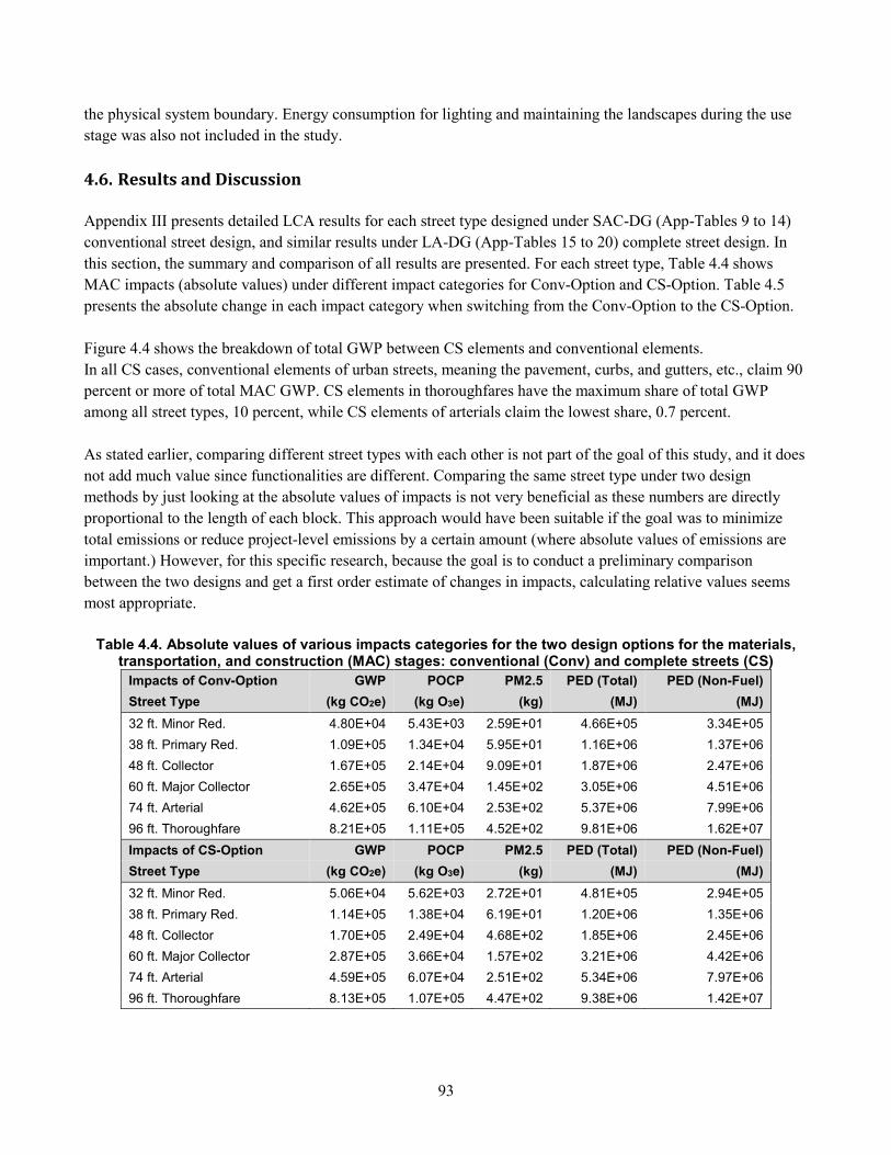
93

the physical system boundary. Energy consumption for lighting and maintaining the landscapes during the use

stage was also not included in the study.

4.6. Results and Discussion

Appendix III presents detailed LCA results for each street type designed under SAC-DG (App-Tables 9 to 14)

conventional street design, and similar results under LA-DG (App-Tables 15 to 20) complete street design. In

this section, the summary and comparison of all results are presented. For each street type, Table 4.4 shows

MAC impacts (absolute values) under different impact categories for Conv-Option and CS-Option. Table 4.5

presents the absolute change in each impact category when switching from the Conv-Option to the CS-Option.

Figure 4.4 shows the breakdown of total GWP between CS elements and conventional elements.

In all CS cases, conventional elements of urban streets, meaning the pavement, curbs, and gutters, etc., claim 90

percent or more of total MAC GWP. CS elements in thoroughfares have the maximum share of total GWP

among all street types, 10 percent, while CS elements of arterials claim the lowest share, 0.7 percent.

As stated earlier, comparing different street types with each other is not part of the goal of this study, and it does

not add much value since functionalities are different. Comparing the same street type under two design

methods by just looking at the absolute values of impacts is not very beneficial as these numbers are directly

proportional to the length of each block. This approach would have been suitable if the goal was to minimize

total emissions or reduce project-level emissions by a certain amount (where absolute values of emissions are

important.) However, for this specific research, because the goal is to conduct a preliminary comparison

between the two designs and get a first order estimate of changes in impacts, calculating relative values seems

most appropriate.

Table 4.4. Absolute values of various impacts categories for the two design options for the materials,

transportation, and construction (MAC) stages: conventional (Conv) and complete streets (CS)

Impacts of Conv-Option GWP POCP PM2.5 PED (Total) PED (Non-Fuel)

Street Type (kg CO2e) (kg O3e) (kg) (MJ) (MJ)

32 ft. Minor Red. 4.80E+04 5.43E+03 2.59E+01 4.66E+05 3.34E+05

38 ft. Primary Red. 1.09E+05 1.34E+04 5.95E+01 1.16E+06 1.37E+06

48 ft. Collector 1.67E+05 2.14E+04 9.09E+01 1.87E+06 2.47E+06

60 ft. Major Collector 2.65E+05 3.47E+04 1.45E+02 3.05E+06 4.51E+06

74 ft. Arterial 4.62E+05 6.10E+04 2.53E+02 5.37E+06 7.99E+06

96 ft. Thoroughfare 8.21E+05 1.11E+05 4.52E+02 9.81E+06 1.62E+07

Impacts of CS-Option GWP POCP PM2.5 PED (Total) PED (Non-Fuel)

Street Type (kg CO2e) (kg O3e) (kg) (MJ) (MJ)

32 ft. Minor Red. 5.06E+04 5.62E+03 2.72E+01 4.81E+05 2.94E+05

38 ft. Primary Red. 1.14E+05 1.38E+04 6.19E+01 1.20E+06 1.35E+06

48 ft. Collector 1.70E+05 2.49E+04 4.68E+02 1.85E+06 2.45E+06

60 ft. Major Collector 2.87E+05 3.66E+04 1.57E+02 3.21E+06 4.42E+06

74 ft. Arterial 4.59E+05 6.07E+04 2.51E+02 5.34E+06 7.97E+06

96 ft. Thoroughfare 8.13E+05 1.07E+05 4.47E+02 9.38E+06 1.42E+07

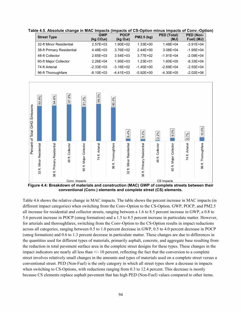
94

Table 4.5. Absolute change in MAC Impacts (impacts of CS-Option minus impacts of Conv.-Option)

Street Type GWP

(kg CO2e) POCP

(kg O3e) PM2.5 (kg)

PED (Total) (MJ)

PED (Non-Fuel) (MJ)

32-ft Minor Residential 2.57E+03 1.90E+02 1.33E+00 1.48E+04 -3.91E+04

38-ft Primary Residential 4.48E+03 3.76E+02 2.44E+00 3.08E+04 -1.95E+04

48-ft Collector 2.65E+03 3.54E+03 3.77E+02 -1.91E+04 -2.09E+04

60-ft Major Collector 2.26E+04 1.95E+03 1.23E+01 1.60E+05 -8.33E+04

74-ft Arterial -2.33E+03 -3.16E+02 -1.45E+00 -2.69E+04 -2.55E+04

96-ft Thoroughfare -8.10E+03 -4.41E+03 -5.92E+00 -4.30E+05 -2.02E+06

Figure 4.4: Breakdown of materials and construction (MAC) GWP of complete streets between their conventional (Conv.) elements and complete street (CS) elements.

Table 4.6 shows the relative change in MAC impacts. The table shows the percent increase in MAC impacts (in

different impact categories) when switching from the Conv-Option to the CS-Option. GWP, POCP, and PM2.5

all increase for residential and collector streets, ranging between a 1.6 to 8.5 percent increase in GWP, a 0.8 to

5.6 percent increase in POCP (smog formation) and a 1.5 to 8.5 percent increase in particulate matter. However,

for arterials and thoroughfares, switching from the Conv-Option to the CS-Option results in impact reductions

across all categories, ranging between 0.5 to 1.0 percent decrease in GWP, 0.5 to 4.0 percent decrease in POCP

(smog formation) and 0.6 to 1.3 percent decrease in particulate matter. These changes are due to differences in

the quantities used for different types of materials, primarily asphalt, concrete, and aggregate base resulting from

the reduction in total pavement surface area in the complete street designs for these types. These changes in the

impact indicators are nearly all less than +/- 10 percent, reflecting the fact that the conversion to a complete

street involves relatively small changes in the amounts and types of materials used on a complete street versus a

conventional street. PED (Non-Fuel) is the only category in which all street types show a decrease in impacts

when switching to CS-Options, with reductions ranging from 0.3 to 12.4 percent. This decrease is mostly

because CS elements replace asphalt pavement that has high PED (Non-Fuel) values compared to other items.

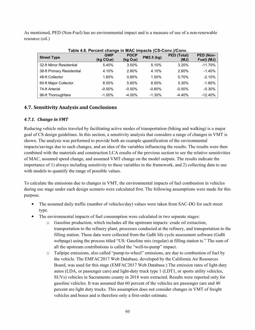
95

As mentioned, PED (Non-Fuel) has no environmental impact and is a measure of use of a non-renewable

resource (oil.)

Table 4.6. Percent change in MAC impacts (CS-Conv.)/Conv.

Street Type GWP

(kg CO2e) POCP

(kg O3e) PM2.5 (kg)

PED (Total) (MJ)

PED (Non-Fuel) (MJ)

32-ft Minor Residential 5.40% 3.50% 5.10% 3.20% -11.70%

38-ft Primary Residential 4.10% 2.80% 4.10% 2.60% -1.40%

48-ft Collector 1.60% 0.80% 1.50% 0.70% -2.10%

60-ft Major Collector 8.50% 5.60% 8.50% 5.30% -1.80%

74-ft Arterial -0.50% -0.50% -0.60% -0.50% -0.30%

96-ft Thoroughfare -1.00% -4.00% -1.30% -4.40% -12.40%

4.7. Sensitivity Analysis and Conclusions

4.7.1. Change in VMT

Reducing vehicle miles traveled by facilitating active modes of transportation (biking and walking) is a major

goal of CS design guidelines. In this section, a sensitivity analysis that considers a range of changes in VMT is

shown. The analysis was performed to provide both an example quantification of the environmental

impacts/savings due to such changes, and an idea of the variables influencing the results. The results were then

combined with the materials and construction LCA results of the previous section to see the relative sensitivities

of MAC, assumed speed change, and assumed VMT change on the model outputs. The results indicate the

importance of 1) always including sensitivity to these variables in the framework, and 2) collecting data to use

with models to quantify the range of possible values.

To calculate the emissions due to changes in VMT, the environmental impacts of fuel combustion in vehicles

during use stage under each design scenario were calculated first. The following assumptions were made for this

purpose.

• The assumed daily traffic (number of vehicles/day) values were taken from SAC-DG for each street

type.

• The environmental impacts of fuel consumption were calculated in two separate stages:

o Gasoline production, which includes all the upstream impacts: crude oil extraction,

transportation to the refinery plant, processes conducted at the refinery, and transportation to the

filling station. These data were collected from the GaBi life cycle assessment software (GaBi

webpage) using the process titled “US: Gasoline mix (regular) at filling station ts.” The sum of

all the upstream contributions is called the “well-to-pump” impact.

o Tailpipe emissions, also called “pump-to-wheel” emissions, are due to combustion of fuel by

the vehicle. The EMFAC2017 Web Database, developed by the California Air Resources

Board, was used for this stage (EMFAC2017 Web Database.) The emission rates of light-duty

autos (LDA, or passenger cars) and light-duty truck type 1 (LDT1, or sports utility vehicles,

SUVs) vehicles in Sacramento county in 2018 were extracted. Results were reported only for

gasoline vehicles. It was assumed that 60 percent of the vehicles are passenger cars and 40

percent are light duty trucks. This assumption does not consider changes in VMT of freight

vehicles and buses and is therefore only a first-order estimate.

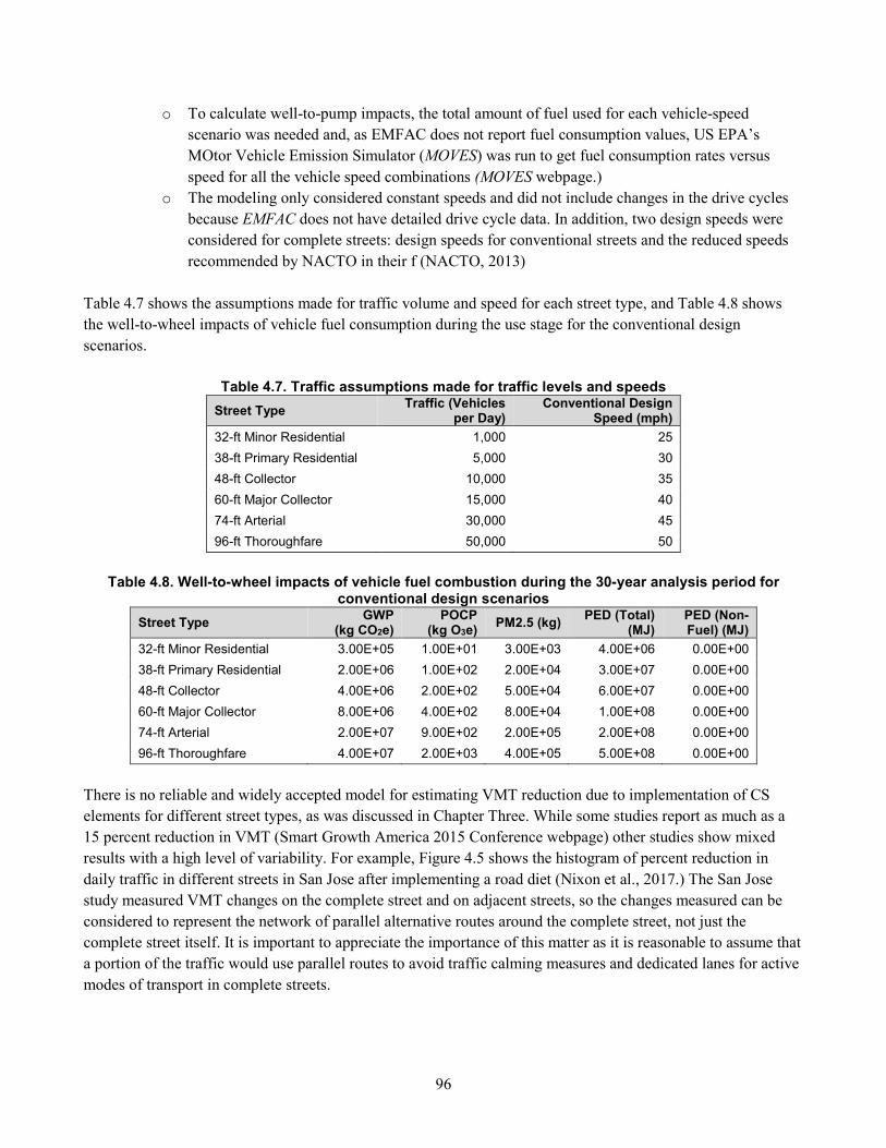
96

o To calculate well-to-pump impacts, the total amount of fuel used for each vehicle-speed

scenario was needed and, as EMFAC does not report fuel consumption values, US EPA’s

MOtor Vehicle Emission Simulator (MOVES) was run to get fuel consumption rates versus

speed for all the vehicle speed combinations (MOVES webpage.)

o The modeling only considered constant speeds and did not include changes in the drive cycles

because EMFAC does not have detailed drive cycle data. In addition, two design speeds were

considered for complete streets: design speeds for conventional streets and the reduced speeds

recommended by NACTO in their f (NACTO, 2013)

Table 4.7 shows the assumptions made for traffic volume and speed for each street type, and Table 4.8 shows

the well-to-wheel impacts of vehicle fuel consumption during the use stage for the conventional design

scenarios.

Table 4.7. Traffic assumptions made for traffic levels and speeds

Street Type Traffic (Vehicles

per Day) Conventional Design

Speed (mph)

32-ft Minor Residential 1,000 25

38-ft Primary Residential 5,000 30

48-ft Collector 10,000 35

60-ft Major Collector 15,000 40

74-ft Arterial 30,000 45

96-ft Thoroughfare 50,000 50

Table 4.8. Well-to-wheel impacts of vehicle fuel combustion during the 30-year analysis period for

conventional design scenarios

Street Type GWP

(kg CO2e) POCP

(kg O3e) PM2.5 (kg)

PED (Total) (MJ)

PED (Non-Fuel) (MJ)

32-ft Minor Residential 3.00E+05 1.00E+01 3.00E+03 4.00E+06 0.00E+00

38-ft Primary Residential 2.00E+06 1.00E+02 2.00E+04 3.00E+07 0.00E+00

48-ft Collector 4.00E+06 2.00E+02 5.00E+04 6.00E+07 0.00E+00

60-ft Major Collector 8.00E+06 4.00E+02 8.00E+04 1.00E+08 0.00E+00

74-ft Arterial 2.00E+07 9.00E+02 2.00E+05 2.00E+08 0.00E+00

96-ft Thoroughfare 4.00E+07 2.00E+03 4.00E+05 5.00E+08 0.00E+00

There is no reliable and widely accepted model for estimating VMT reduction due to implementation of CS

elements for different street types, as was discussed in Chapter Three. While some studies report as much as a

15 percent reduction in VMT (Smart Growth America 2015 Conference webpage) other studies show mixed

results with a high level of variability. For example, Figure 4.5 shows the histogram of percent reduction in

daily traffic in different streets in San Jose after implementing a road diet (Nixon et al., 2017.) The San Jose

study measured VMT changes on the complete street and on adjacent streets, so the changes measured can be

considered to represent the network of parallel alternative routes around the complete street, not just the

complete street itself. It is important to appreciate the importance of this matter as it is reasonable to assume that

a portion of the traffic would use parallel routes to avoid traffic calming measures and dedicated lanes for active

modes of transport in complete streets.

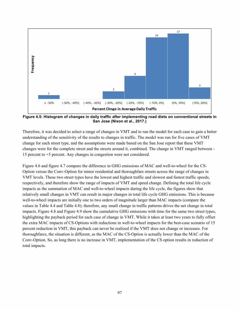
97

Figure 4.5: Histogram of changes in daily traffic after implementing road diets on conventional streets in San Jose (Nixon et al., 2017.)

Therefore, it was decided to select a range of changes in VMT and to run the model for each case to gain a better

understanding of the sensitivity of the results to changes in traffic. The model was run for five cases of VMT

change for each street type, and the assumptions were made based on the San Jose report that these VMT

changes were for the complete street and the streets around it, combined. The change in VMT ranged between -

15 percent to +5 percent. Any changes in congestion were not considered.

Figure 4.6 and figure 4.7 compare the difference in GHG emissions of MAC and well-to-wheel for the CS-

Option versus the Conv-Option for minor residential and thoroughfare streets across the range of changes in

VMT levels. These two street types have the lowest and highest traffic and slowest and fastest traffic speeds,

respectively, and therefore show the range of impacts of VMT and speed change. Defining the total life cycle

impacts as the summation of MAC and well-to-wheel impacts during the life cycle, the figures show that

relatively small changes in VMT can result in major changes in total life cycle GHG emissions. This is because

well-to-wheel impacts are initially one to two orders of magnitude larger than MAC impacts (compare the

values in Table 4.4 and Table 4.8); therefore, any small change in traffic patterns drives the net change in total

impacts. Figure 4.8 and Figure 4.9 show the cumulative GHG emissions with time for the same two street types,

highlighting the payback period for each case of change in VMT. While it takes at least two years to fully offset

the extra MAC impacts of CS-Options with reductions in well-to-wheel impacts for the best-case scenario of 15

percent reduction in VMT, this payback can never be realized if the VMT does not change or increases. For

thoroughfares, the situation is different, as the MAC of the CS-Option is actually lower than the MAC of the

Conv-Option. So, as long there is no increase in VMT, implementation of the CS option results in reduction of

total impacts.

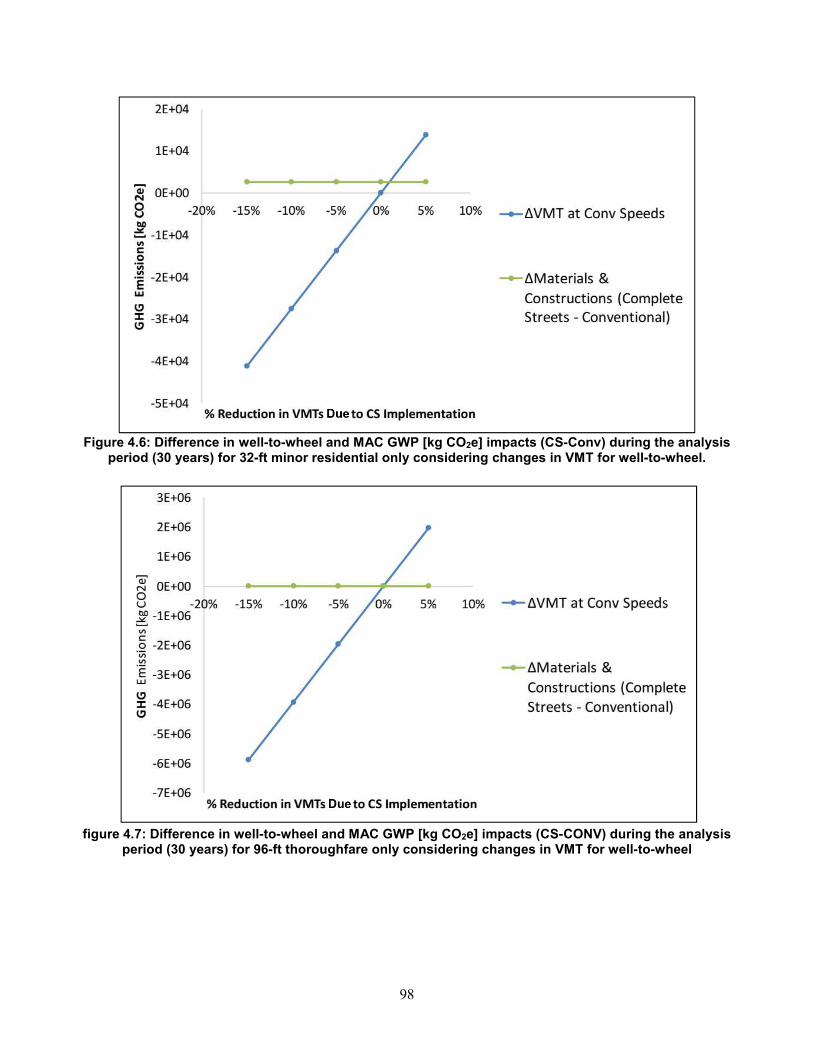
98

Figure 4.6: Difference in well-to-wheel and MAC GWP [kg CO2e] impacts (CS-Conv) during the analysis period (30 years) for 32-ft minor residential only considering changes in VMT for well-to-wheel.

figure 4.7: Difference in well-to-wheel and MAC GWP [kg CO2e] impacts (CS-CONV) during the analysis

period (30 years) for 96-ft thoroughfare only considering changes in VMT for well-to-wheel

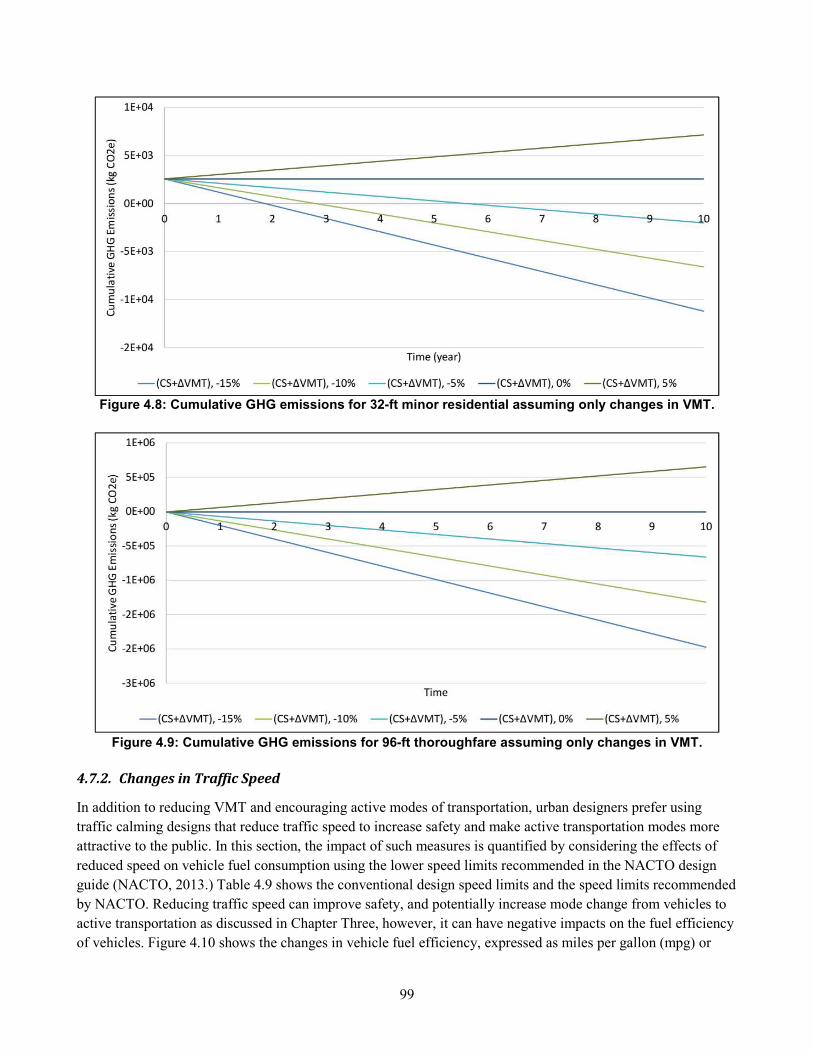
99

Figure 4.8: Cumulative GHG emissions for 32-ft minor residential assuming only changes in VMT.

Figure 4.9: Cumulative GHG emissions for 96-ft thoroughfare assuming only changes in VMT.

4.7.2. Changes in Traffic Speed

In addition to reducing VMT and encouraging active modes of transportation, urban designers prefer using

traffic calming designs that reduce traffic speed to increase safety and make active transportation modes more

attractive to the public. In this section, the impact of such measures is quantified by considering the effects of

reduced speed on vehicle fuel consumption using the lower speed limits recommended in the NACTO design

guide (NACTO, 2013.) Table 4.9 shows the conventional design speed limits and the speed limits recommended

by NACTO. Reducing traffic speed can improve safety, and potentially increase mode change from vehicles to

active transportation as discussed in Chapter Three, however, it can have negative impacts on the fuel efficiency

of vehicles. Figure 4.10 shows the changes in vehicle fuel efficiency, expressed as miles per gallon (mpg) or

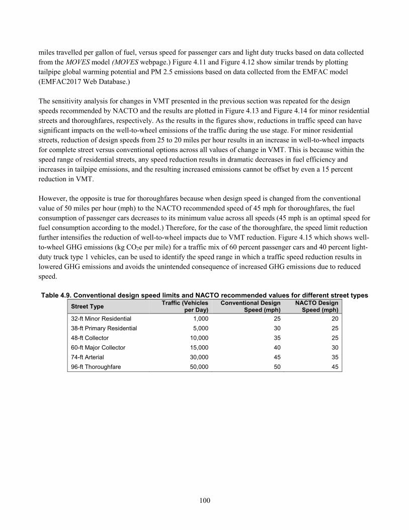
100

miles travelled per gallon of fuel, versus speed for passenger cars and light duty trucks based on data collected

from the MOVES model (MOVES webpage.) Figure 4.11 and Figure 4.12 show similar trends by plotting

tailpipe global warming potential and PM 2.5 emissions based on data collected from the EMFAC model

(EMFAC2017 Web Database.)

The sensitivity analysis for changes in VMT presented in the previous section was repeated for the design

speeds recommended by NACTO and the results are plotted in Figure 4.13 and Figure 4.14 for minor residential

streets and thoroughfares, respectively. As the results in the figures show, reductions in traffic speed can have

significant impacts on the well-to-wheel emissions of the traffic during the use stage. For minor residential

streets, reduction of design speeds from 25 to 20 miles per hour results in an increase in well-to-wheel impacts

for complete street versus conventional options across all values of change in VMT. This is because within the

speed range of residential streets, any speed reduction results in dramatic decreases in fuel efficiency and

increases in tailpipe emissions, and the resulting increased emissions cannot be offset by even a 15 percent

reduction in VMT.

However, the opposite is true for thoroughfares because when design speed is changed from the conventional

value of 50 miles per hour (mph) to the NACTO recommended speed of 45 mph for thoroughfares, the fuel

consumption of passenger cars decreases to its minimum value across all speeds (45 mph is an optimal speed for

fuel consumption according to the model.) Therefore, for the case of the thoroughfare, the speed limit reduction

further intensifies the reduction of well-to-wheel impacts due to VMT reduction. Figure 4.15 which shows well-

to-wheel GHG emissions (kg CO2e per mile) for a traffic mix of 60 percent passenger cars and 40 percent light-

duty truck type 1 vehicles, can be used to identify the speed range in which a traffic speed reduction results in

lowered GHG emissions and avoids the unintended consequence of increased GHG emissions due to reduced

speed.

Table 4.9. Conventional design speed limits and NACTO recommended values for different street types

Street Type Traffic (Vehicles

per Day) Conventional Design

Speed (mph) NACTO Design

Speed (mph)

32-ft Minor Residential 1,000 25 20

38-ft Primary Residential 5,000 30 25

48-ft Collector 10,000 35 25

60-ft Major Collector 15,000 40 30

74-ft Arterial 30,000 45 35

96-ft Thoroughfare 50,000 50 45

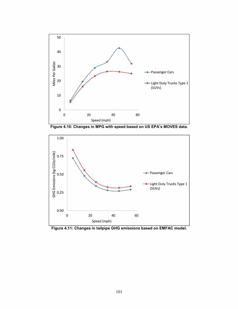
101

Figure 4.10: Changes in MPG with speed based on US EPA’s MOVES data.

Figure 4.11: Changes in tailpipe GHG emissions based on EMFAC model.

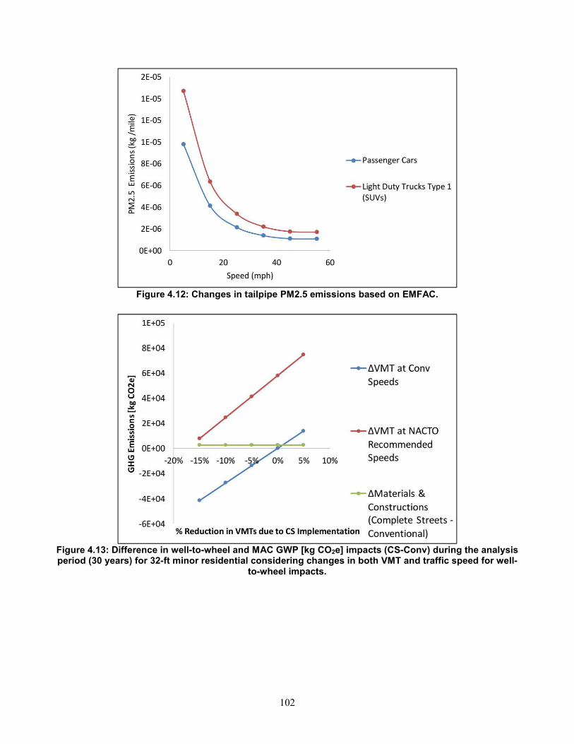
102

Figure 4.12: Changes in tailpipe PM2.5 emissions based on EMFAC.

Figure 4.13: Difference in well-to-wheel and MAC GWP [kg CO2e] impacts (CS-Conv) during the analysis period (30 years) for 32-ft minor residential considering changes in both VMT and traffic speed for well-

to-wheel impacts.

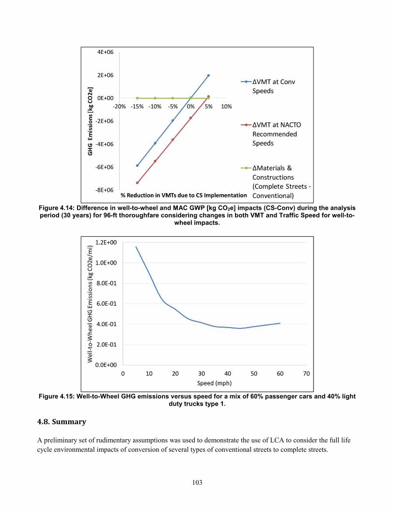
103

Figure 4.14: Difference in well-to-wheel and MAC GWP [kg CO2e] impacts (CS-Conv) during the analysis period (30 years) for 96-ft thoroughfare considering changes in both VMT and Traffic Speed for well-to-

wheel impacts.

Figure 4.15: Well-to-Wheel GHG emissions versus speed for a mix of 60% passenger cars and 40% light duty trucks type 1.

4.8. Summary

A preliminary set of rudimentary assumptions was used to demonstrate the use of LCA to consider the full life

cycle environmental impacts of conversion of several types of conventional streets to complete streets.

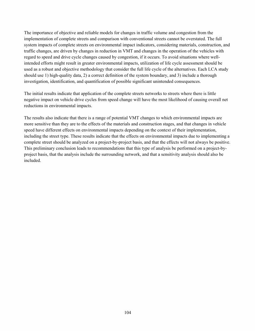
104

The importance of objective and reliable models for changes in traffic volume and congestion from the

implementation of complete streets and comparison with conventional streets cannot be overstated. The full

system impacts of complete streets on environmental impact indicators, considering materials, construction, and

traffic changes, are driven by changes in reduction in VMT and changes in the operation of the vehicles with

regard to speed and drive cycle changes caused by congestion, if it occurs. To avoid situations where well-

intended efforts might result in greater environmental impacts, utilization of life cycle assessment should be

used as a robust and objective methodology that consider the full life cycle of the alternatives. Each LCA study

should use 1) high-quality data, 2) a correct definition of the system boundary, and 3) include a thorough

investigation, identification, and quantification of possible significant unintended consequences.

The initial results indicate that application of the complete streets networks to streets where there is little

negative impact on vehicle drive cycles from speed change will have the most likelihood of causing overall net

reductions in environmental impacts.

The results also indicate that there is a range of potential VMT changes to which environmental impacts are

more sensitive than they are to the effects of the materials and construction stages, and that changes in vehicle

speed have different effects on environmental impacts depending on the context of their implementation,

including the street type. These results indicate that the effects on environmental impacts due to implementing a

complete street should be analyzed on a project-by-project basis, and that the effects will not always be positive.

This preliminary conclusion leads to recommendations that this type of analysis be performed on a project-by-

project basis, that the analysis include the surrounding network, and that a sensitivity analysis should also be

included.

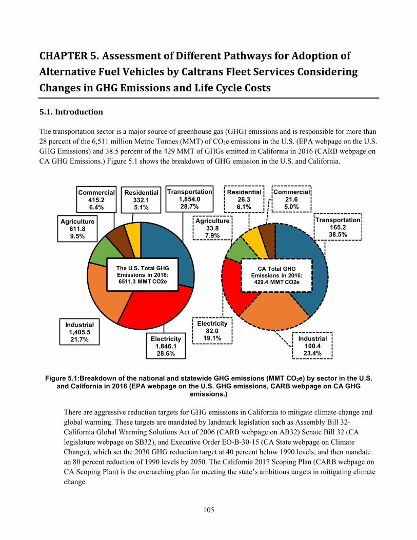
105

CHAPTER 5. Assessment of Different Pathways for Adoption of

Alternative Fuel Vehicles by Caltrans Fleet Services Considering

Changes in GHG Emissions and Life Cycle Costs

5.1. Introduction

The transportation sector is a major source of greenhouse gas (GHG) emissions and is responsible for more than

28 percent of the 6,511 million Metric Tonnes (MMT) of CO2e emissions in the U.S. (EPA webpage on the U.S.

GHG Emissions) and 38.5 percent of the 429 MMT of GHGs emitted in California in 2016 (CARB webpage on

CA GHG Emissions.) Figure 5.1 shows the breakdown of GHG emission in the U.S. and California.

Figure 5.1:Breakdown of the national and statewide GHG emissions (MMT CO2e) by sector in the U.S. and California in 2016 (EPA webpage on the U.S. GHG emissions, CARB webpage on CA GHG

emissions.)

There are aggressive reduction targets for GHG emissions in California to mitigate climate change and

global warming. These targets are mandated by landmark legislation such as Assembly Bill 32-

California Global Warming Solutions Act of 2006 (CARB webpage on AB32) Senate Bill 32 (CA

legislature webpage on SB32), and Executive Order EO-B-30-15 (CA State webpage on Climate

Change), which set the 2030 GHG reduction target at 40 percent below 1990 levels, and then mandate

an 80 percent reduction of 1990 levels by 2050. The California 2017 Scoping Plan (CARB webpage on

CA Scoping Plan) is the overarching plan for meeting the state’s ambitious targets in mitigating climate

change.

Transportation1,854.028.7%

Electricity1,846.128.6%

Industrial1,405.521.7%

Agriculture611.89.5%

Commercial415.26.4%

Residential332.15.1%

Transportation165.238.5%

Industrial100.423.4%

Electricity82.0

19.1%

Agriculture33.87.9%

Residential26.36.1%

Commercial21.65.0%

CA Total GHG Emissions in 2016: 429.4 MMT CO2e

The U.S. Total GHG Emissions in 2016: 6511.3 MMT CO2e

106

Multiple programs are aiming at reducing GHG emissions of the transportation sector in California. These

programs can be divided into three main categories: 1) land use, 2) cleaner fuels, 3) alternative vehicle

technologies.

The land use policies are aimed at reducing vehicle miles traveled (VMT) through various modified land use

planning and urban design philosophies, promotion of active modes of transport, public transit improvement

projects, provision of local shopping and service centers, reduction of urban sprawl and provision of incentives

and benefits for programs such as car-sharing, car-pooling, and more. SB375 is the main regulation for reducing

transportation GHG emissions through land use policies (CARB webpage on SB375.)

The Low Carbon Fuel Standard (LCFS) is the main program for transitioning to cleaner fuels that have lower

carbon footprints (CARB webpage on LCSF.) LCFS was initially approved in 2009 and is a market-based

instrument that sets targets for reductions in carbon intensity (CI) of fuel mix across the whole market. The CI is

calculated by conducting life cycle assessment (LCA) on each fuel pathway available in the market. Application

of LCA allows accounting of all the environmental impacts that occur during the full life cycle of a fuel

pathway, from raw material extraction from the ground to transportation to refinery plants, processes conducted

in the plant, transportation to the gas stations, and combustion in vehicles. CI is expressed in grams of CO2e

emitted per Megajoule of energy (gCO2e/MJ.)

New vehicles technologies are divided into zero emission vehicles (ZEV) and near-zero emission vehicles

(NZEV.) ZEVs and NZEVs are expected to play a major role in curbing GHG emissions from the transportation

sector by replacing the conventional internal combustion engine vehicles (ICEVs.) California 2016 ZEV Action

Plan (CA State webpage on ZEV Action Plan) mandates 1.5 million ZEVs and NZEVs, such as plug-in hybrid

electric vehicles (PHEVs), battery-electric vehicles (BEVs, also referred to as EVs), and hydrogen fuel cell

vehicles (FCVs), by 2025 and 4.2 million by 2030.

The State of California has begun two initiatives for state agencies to reduce the environmental impacts of their

fleet and buildings (Green CA webpage.) This chapter focuses on adoption of alternative fuel vehicles (AFVs)

for the Caltrans fleet. A brief background of AFVs is presented followed by a model to calculate life cycle costs,

fuel consumption, and GHG emissions of multiple pathways for transitioning Caltrans fleet to reduce GHG

emissions. The results of this chapter can be used to compare different pathways in terms of costs and

environmental impacts, identify the tradeoffs between options, and choose the most suitable approach to meet

the agency’s sustainability goals while controlling life cycle costs.

5.2. Background

The Energy Policy Act (EPAct) of 1992 (AFDC webpage on EPAct) defined alternative fuels and assigned the

United States Department of Energy (U.S. DOE) to develop a regulatory program for selected state fleets1 as

1 “State and alternative fuel provider fleets are considered covered fleets if they own, operate, lease, or otherwise control

50 or more non-excluded light-duty vehicles (less than or equal to 8,500 pounds) and if at least 20 of those vehicles are

used primarily within a single Metropolitan Statistical Area/Consolidated Metropolitan Statistical Area and are centrally

fueled or capable of being centrally fueled.” https://epact.energy.gov/

107

launching pads for advanced vehicles using alternative fuels. Energy Policy Act of 1992 considers the

followings as alternative fuels:

• Methanol, ethanol, and other alcohols

• Blends of 85 percent or more of alcohol with gasoline

• Natural gas and liquid fuels domestically produced from natural gas

• Liquefied petroleum gas (propane)

• Coal-derived liquid fuels

• Hydrogen

• Electricity

• Fuels (other than alcohol) derived from biological materials, including pure biodiesel (B100)

• P-Series2

5.2.1. Key Federal Statutes

Major federal statutes that established key transportation regulatory activities (DOE webpage on EPAct) are

listed below:

• Clean Air Act Amendments of 1990 which encouraged production and use of AFVs

• Energy Policy Act of 1992

• Energy Conservation Reauthorization Act of 1998 which allowed the fleets covered under EPAct to

include biodiesel blend use as credits towards compliance.

• Energy Policy Act of 2005 allowed covered fleets to reduce petroleum consumption instead of acquiring

alternative fuel vehicles.

• Energy Independence and Security Act of 2007 added certain electric drive vehicles and investments in

infrastructure, equipment, and emerging technologies to the list of items to gain credit for compliance.

5.2.2. Major Initiatives in California

Senate Bill 522, passed in 2003, adopted the recommendations from the California State Vehicle Fleet Fuel

Efficiency Report and required the collection of statewide fleet data and the publishing of annual public reports

about the fleet composition (CA Legislature webpage on SB522.)

Assembly Bill 236, passed in 2007, required increased use of alternative fuel vehicles to meet the following

targets: a 10 and 20 percent reduction or displacement of conventional vehicles by January 1, 2012, and January

1, 2020, respectively (CA Legislature webpage on AB236.)

Executive Order B-16-12, issued by Governor Brown in 2012, directed state fleets to increase the purchase of

ZEVs through the normal course of fleet replacement, requiring them to have at least 10 percent of light-duty

vehicle purchases from ZEVs by 2015. This target would increase to 25 percent by 2020 (CA State webpage on

EO-B1612)

2 “P-Series is a family of renewable, non-petroleum, liquid fuels that can substitute for gasoline. They are a blend of 25 or so

domestically produced ingredients. About 35 percent of P-Series comes from liquid by-products, known as "C5+" or "pentanes-plus",

which are left over when natural gas is processed for transport and marketing.”

108

Senate Bill 1275, Charge Ahead California Initiative, passed in 2014 established a state goal of one million

zero-emission and near-zero-emission vehicles in service by 2020 (CA Legislature webpage on SB1275.)

Executive Order (EO) B-30-15, issued by Governor Brown, directed “that all state agencies with jurisdiction

over sources of greenhouse gas emissions shall implement measures, pursuant to statutory authority, to achieve

reductions of greenhouse gas emissions to meet the 2030 and 2050” reductions targets of 40 percent and 80

percent below 1990 GHG emission levels, respectively.

The California State Administrative Manual set the ZEV purchasing policy for state agencies, which includes

the “ZEV and hybrid vehicle first” policy which requires departments to purchase light-duty following this

priority structure: (1) pure ZEVs, (2) PHEVs, and (3) hybrids. The policy also increased the ZEV purchasing

mandate annually by 5 percent so that it will be 50 percent by 2025 (CA DGS webpage on ZEV Purchasing

Policy.)

Section 3627 of the State Administrative Manual mandates the use of renewable diesel instead of conventional

diesel and biodiesel fuel for bulk transportation fuel purchases (CA DGS webpage on Fuel Purchasing Policy.)

Section 3620.1 of the Manual sets the vehicle fuel efficiency requirements, expressed in miles per gallon (mpg)

of fuel, for light-duty passenger vehicles to 38 and light-duty trucks, vans, and sport utility vehicles (SUVs) to

22.2 (CA DGS webpage on Fuel Efficiency Requirements.)

5.2.3. AFVs Acquired by Fleets Regulated under EPAct at National-Level

This section focuses on AFV acquisitions by covered fleets3 after the U.S. Congress passed the Energy Policy

Act in 1992. The goal is to observe adoption trends and popularity of different fuel types among fleet services.

The data were collected from the Alternative Fuel Data Center webpage maintained by the U.S. Department of

Energy (AFDC webpage on EPAct History.) The top graph in Figure 5.2 shows the number of AFVs acquired

by covered fleets between 1992 and 2017 and the bottom graph represents the distribution of AFVs by fuel type

in each year.

Compressed natural gas (CNG) and liquefied petroleum gas (LPG) vehicles were initially the popular choices

among fleet services between 1992 and 2000, as shown in Figure 5.2. However, gasoline mixed with ethanol up

to 85 percent (E85) started gaining traction from the second half of the 1990s, quickly reaching the first rank

among all fuel types. More than 90 percent of all AFVs acquired by covered fleets since 2005 are E85 vehicles.

Electric vehicles (EVs) adoption rates were highest between 1997 and 1999 with growth rates between 56 and

71 percent in the number of EVs acquired each year. During that time interval EVs were comprising 4 to 7.4

percent of all AFVs acquired each year. The two-digit growth rates quickly diminished to 3 to 8 percent range

until 2015 after which EVs have once again become a popular choice with growth rates of 10 to 11 percent in

annual acquisitions, making EVs the second most popular choice among all AFV options, after E85 vehicles.

3 “State and alternative fuel provider fleets are considered covered fleets if they own, operate, lease, or otherwise control

50 or more non-excluded light-duty vehicles (less than or equal to 8,500 pounds) and if at least 20 of those vehicles are

used primarily within a single Metropolitan Statistical Area/Consolidated Metropolitan Statistical Area and are centrally

fueled or capable of being centrally fueled.” –https://epact.energy.gov

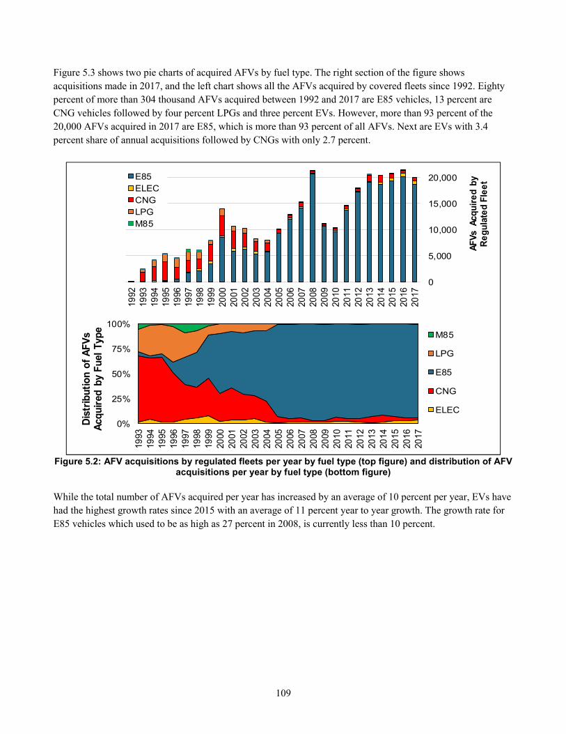
109

Figure 5.3 shows two pie charts of acquired AFVs by fuel type. The right section of the figure shows

acquisitions made in 2017, and the left chart shows all the AFVs acquired by covered fleets since 1992. Eighty

percent of more than 304 thousand AFVs acquired between 1992 and 2017 are E85 vehicles, 13 percent are

CNG vehicles followed by four percent LPGs and three percent EVs. However, more than 93 percent of the

20,000 AFVs acquired in 2017 are E85, which is more than 93 percent of all AFVs. Next are EVs with 3.4

percent share of annual acquisitions followed by CNGs with only 2.7 percent.

Figure 5.2: AFV acquisitions by regulated fleets per year by fuel type (top figure) and distribution of AFV acquisitions per year by fuel type (bottom figure)

While the total number of AFVs acquired per year has increased by an average of 10 percent per year, EVs have

had the highest growth rates since 2015 with an average of 11 percent year to year growth. The growth rate for

E85 vehicles which used to be as high as 27 percent in 2008, is currently less than 10 percent.

0

5,000

10,000

15,000

20,000

1992

1993

1994

1995

1996

1997

1998

1999

2000

2001

2002

2003

2004

2005

2006

2007

2008

2009

2010

2011

2012

2013

2014

2015

2016

2017

AF

Vs A

cq

uir

ed

by

Re

gu

late

d F

lee

t

E85

ELEC

CNG

LPG

M85

0%

25%

50%

75%

100%

1993

1994

1995

1996

1997

1998

1999

2000

2001

2002

2003

2004

2005

2006

2007

2008

2009

2010

2011

2012

2013

2014

2015

2016

2017

Dis

trib

uti

on

of

AF

Vs

Acq

uir

ed

by F

uel

Typ

e

M85

LPG

E85

CNG

ELEC

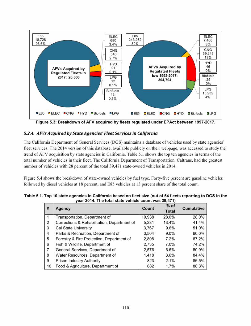
110

Figure 5.3: Breakdown of AFV acquired by fleets regulated under EPAct between 1997-2017.

5.2.4. AFVs Acquired by State Agencies’ Fleet Services in California

The California Department of General Services (DGS) maintains a database of vehicles used by state agencies’

fleet services. The 2014 version of this database, available publicly on their webpage, was accessed to study the

trend of AFV acquisition by state agencies in California. Table 5.1 shows the top ten agencies in terms of the

total number of vehicles in their fleet. The California Department of Transportation, Caltrans, had the greatest

number of vehicles with 28 percent of the total 39,471 state-owned vehicles in 2014.

Figure 5.4 shows the breakdown of state-owned vehicles by fuel type. Forty-five percent are gasoline vehicles

followed by diesel vehicles at 18 percent, and E85 vehicles at 13 percent share of the total count.

Table 5.1. Top 10 state agencies in California based on fleet size (out of 64 fleets reporting to DGS in the

year 2014. The total state vehicle count was 39,471)

# Agency Count % of

Total Cumulative

1 Transportation, Department of 10,938 28.0% 28.0% 2 Corrections & Rehabilitation, Department of 5,231 13.4% 41.4% 3 Cal State University 3,767 9.6% 51.0%

4 Parks & Recreation, Department of 3,504 9.0% 60.0% 5 Forestry & Fire Protection, Department of 2,808 7.2% 67.2% 6 Fish & Wildlife, Department of 2,735 7.0% 74.2% 7 General Services, Department of 2,576 6.6% 80.9% 8 Water Resources, Department of 1,418 3.6% 84.4%

9 Prison Industry Authority 823 2.1% 86.5% 10 Food & Agriculture, Department of 682 1.7% 88.3%

E8518,72893.6%

ELEC680

3.4%

CNG546

2.7%

HYD21

0.1%

Biofuels13

0.1%

LPG12

0.1%

E85 ELEC CNG HYD Biofuels LPG

AFVs Acquired by Regulated Fleets in

2017: 20,000

E85243,262

80%

ELEC7,406

3%

CNG39,24313%

HYD460%

Biofuels250%

LPG13,232

4%

E85 ELEC CNG HYD Biofuels LPG

AFVs Acquired by Regulated Fleets

b/w 1992-2017: 304,704

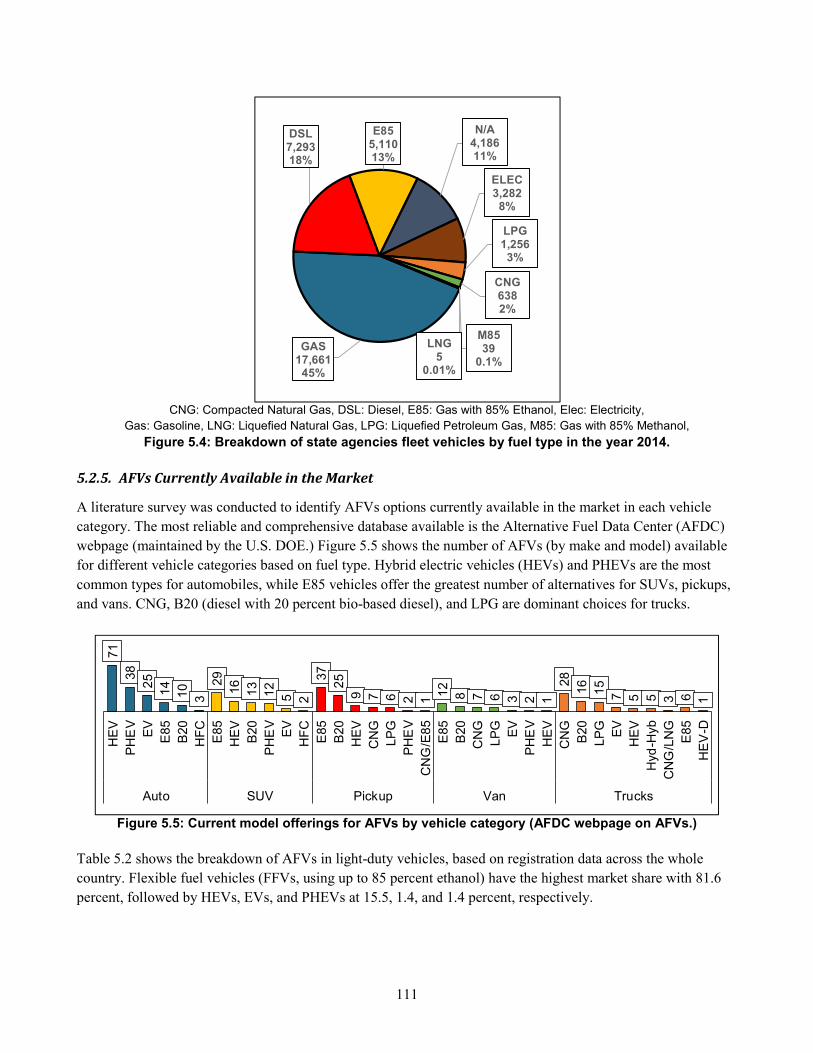
111

CNG: Compacted Natural Gas, DSL: Diesel, E85: Gas with 85% Ethanol, Elec: Electricity,

Gas: Gasoline, LNG: Liquefied Natural Gas, LPG: Liquefied Petroleum Gas, M85: Gas with 85% Methanol,

Figure 5.4: Breakdown of state agencies fleet vehicles by fuel type in the year 2014.

5.2.5. AFVs Currently Available in the Market

A literature survey was conducted to identify AFVs options currently available in the market in each vehicle

category. The most reliable and comprehensive database available is the Alternative Fuel Data Center (AFDC)

webpage (maintained by the U.S. DOE.) Figure 5.5 shows the number of AFVs (by make and model) available

for different vehicle categories based on fuel type. Hybrid electric vehicles (HEVs) and PHEVs are the most

common types for automobiles, while E85 vehicles offer the greatest number of alternatives for SUVs, pickups,

and vans. CNG, B20 (diesel with 20 percent bio-based diesel), and LPG are dominant choices for trucks.

Figure 5.5: Current model offerings for AFVs by vehicle category (AFDC webpage on AFVs.)

Table 5.2 shows the breakdown of AFVs in light-duty vehicles, based on registration data across the whole

country. Flexible fuel vehicles (FFVs, using up to 85 percent ethanol) have the highest market share with 81.6

percent, followed by HEVs, EVs, and PHEVs at 15.5, 1.4, and 1.4 percent, respectively.

GAS17,66145%

DSL7,29318%

E855,11013%

N/A4,18611%

ELEC3,2828%

LPG1,2563%

CNG6382%

M8539

0.1%

LNG5

0.01%

71

38

25

14

10

3

29

16

13

12

5 2

37

25

9 7 6 2 1

12

8 7 6 3 2 1

28

16

15

7 5 5 3 6 1

HE

V

PH

EV

EV

E85

B20

HF

C

E85

HE

V

B20

PH

EV

EV

HF

C

E85

B20

HE

V

CN

G

LP

G

PH

EV

CN

G/E

85

E85

B20

CN

G

LP

G

EV

PH

EV

HE

V

CN

G

B20

LP

G

EV

HE

V

Hyd

-Hyb

CN

G/L

NG

E85

HE

V-D

Auto SUV Pickup Van Trucks

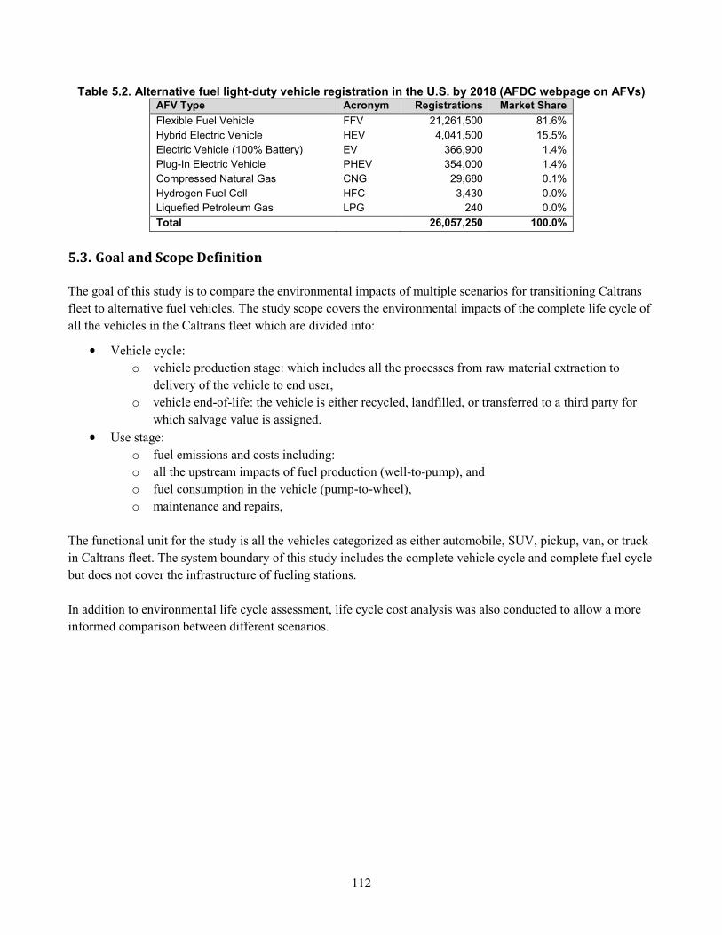
112

Table 5.2. Alternative fuel light-duty vehicle registration in the U.S. by 2018 (AFDC webpage on AFVs) AFV Type Acronym Registrations Market Share

Flexible Fuel Vehicle FFV 21,261,500 81.6%

Hybrid Electric Vehicle HEV 4,041,500 15.5%

Electric Vehicle (100% Battery) EV 366,900 1.4%

Plug-In Electric Vehicle PHEV 354,000 1.4%

Compressed Natural Gas CNG 29,680 0.1%

Hydrogen Fuel Cell HFC 3,430 0.0%

Liquefied Petroleum Gas LPG 240 0.0%

Total 26,057,250 100.0%

5.3. Goal and Scope Definition

The goal of this study is to compare the environmental impacts of multiple scenarios for transitioning Caltrans

fleet to alternative fuel vehicles. The study scope covers the environmental impacts of the complete life cycle of

all the vehicles in the Caltrans fleet which are divided into:

• Vehicle cycle:

o vehicle production stage: which includes all the processes from raw material extraction to

delivery of the vehicle to end user,

o vehicle end-of-life: the vehicle is either recycled, landfilled, or transferred to a third party for

which salvage value is assigned.

• Use stage:

o fuel emissions and costs including:

o all the upstream impacts of fuel production (well-to-pump), and

o fuel consumption in the vehicle (pump-to-wheel),

o maintenance and repairs,

The functional unit for the study is all the vehicles categorized as either automobile, SUV, pickup, van, or truck

in Caltrans fleet. The system boundary of this study includes the complete vehicle cycle and complete fuel cycle

but does not cover the infrastructure of fueling stations.

In addition to environmental life cycle assessment, life cycle cost analysis was also conducted to allow a more

informed comparison between different scenarios.

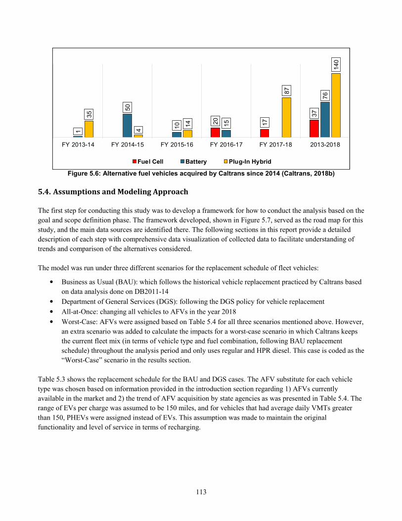
113

Figure 5.6: Alternative fuel vehicles acquired by Caltrans since 2014 (Caltrans, 2018b)

5.4. Assumptions and Modeling Approach

The first step for conducting this study was to develop a framework for how to conduct the analysis based on the

goal and scope definition phase. The framework developed, shown in Figure 5.7, served as the road map for this

study, and the main data sources are identified there. The following sections in this report provide a detailed

description of each step with comprehensive data visualization of collected data to facilitate understanding of

trends and comparison of the alternatives considered.

The model was run under three different scenarios for the replacement schedule of fleet vehicles:

• Business as Usual (BAU): which follows the historical vehicle replacement practiced by Caltrans based

on data analysis done on DB2011-14

• Department of General Services (DGS): following the DGS policy for vehicle replacement

• All-at-Once: changing all vehicles to AFVs in the year 2018

• Worst-Case: AFVs were assigned based on Table 5.4 for all three scenarios mentioned above. However,

an extra scenario was added to calculate the impacts for a worst-case scenario in which Caltrans keeps

the current fleet mix (in terms of vehicle type and fuel combination, following BAU replacement

schedule) throughout the analysis period and only uses regular and HPR diesel. This case is coded as the

“Worst-Case” scenario in the results section.

Table 5.3 shows the replacement schedule for the BAU and DGS cases. The AFV substitute for each vehicle

type was chosen based on information provided in the introduction section regarding 1) AFVs currently

available in the market and 2) the trend of AFV acquisition by state agencies as was presented in Table 5.4. The

range of EVs per charge was assumed to be 150 miles, and for vehicles that had average daily VMTs greater

than 150, PHEVs were assigned instead of EVs. This assumption was made to maintain the original

functionality and level of service in terms of recharging.

20

17

37

1

50

10 15

76

35

4

14

87

140

FY 2013-14 FY 2014-15 FY 2015-16 FY 2016-17 FY 2017-18 2013-2018

Fuel Cell Battery Plug-In Hybrid

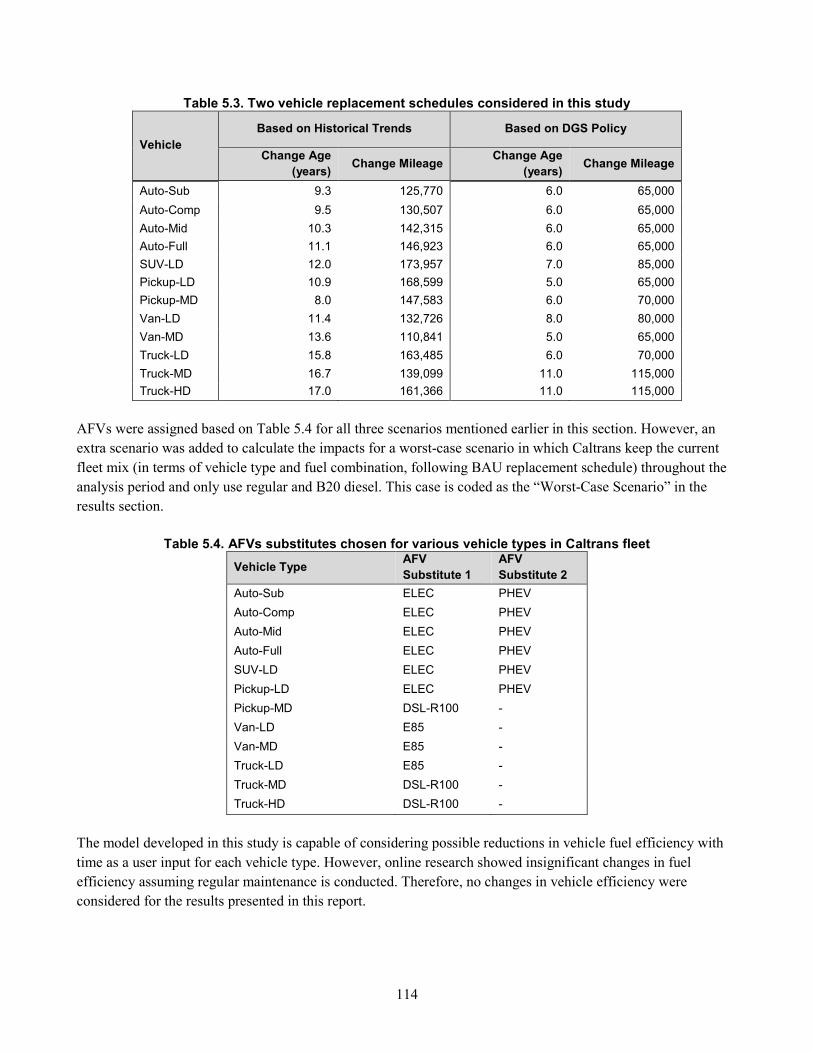
114

Table 5.3. Two vehicle replacement schedules considered in this study

Vehicle

Based on Historical Trends Based on DGS Policy

Change Age

(years) Change Mileage

Change Age

(years) Change Mileage

Auto-Sub 9.3 125,770 6.0 65,000

Auto-Comp 9.5 130,507 6.0 65,000

Auto-Mid 10.3 142,315 6.0 65,000

Auto-Full 11.1 146,923 6.0 65,000

SUV-LD 12.0 173,957 7.0 85,000

Pickup-LD 10.9 168,599 5.0 65,000

Pickup-MD 8.0 147,583 6.0 70,000

Van-LD 11.4 132,726 8.0 80,000

Van-MD 13.6 110,841 5.0 65,000

Truck-LD 15.8 163,485 6.0 70,000

Truck-MD 16.7 139,099 11.0 115,000

Truck-HD 17.0 161,366 11.0 115,000

AFVs were assigned based on Table 5.4 for all three scenarios mentioned earlier in this section. However, an

extra scenario was added to calculate the impacts for a worst-case scenario in which Caltrans keep the current

fleet mix (in terms of vehicle type and fuel combination, following BAU replacement schedule) throughout the

analysis period and only use regular and B20 diesel. This case is coded as the “Worst-Case Scenario” in the

results section.

Table 5.4. AFVs substitutes chosen for various vehicle types in Caltrans fleet

Vehicle Type AFV

Substitute 1

AFV

Substitute 2

Auto-Sub ELEC PHEV

Auto-Comp ELEC PHEV

Auto-Mid ELEC PHEV

Auto-Full ELEC PHEV

SUV-LD ELEC PHEV

Pickup-LD ELEC PHEV

Pickup-MD DSL-R100 -

Van-LD E85 -

Van-MD E85 -

Truck-LD E85 -

Truck-MD DSL-R100 -

Truck-HD DSL-R100 -

The model developed in this study is capable of considering possible reductions in vehicle fuel efficiency with

time as a user input for each vehicle type. However, online research showed insignificant changes in fuel

efficiency assuming regular maintenance is conducted. Therefore, no changes in vehicle efficiency were

considered for the results presented in this report.

115

Changes in vehicle miles traveled per year can also be incorporated in the model. Reduction in VMT is a

plausible situation as there are ongoing debates about setting tax rates based on VMT rather than gallons of fuel

purchased by consumers. The debates are mainly due to improvements in vehicle efficiency that has resulted in

shrinking revenues from state fuel taxes. The results presented in this report does not consider any changes in

the annual VMT of vehicles.

A discount rate of 4 percent was considered for life cycle cost calculations which can be modified by the user. It

should be noted that state vehicles are exempt from registration fees and taxes and fleet insurance is typically

handled through in-house insurance programs. However, the model has the capability of calculating these values

to provide an order of magnitude for comparison with other cost items.

The model allows the user to either use average annual vehicle miles traveled (AVMT) values (calculated based

on vehicle type) for all the 9,325 records in the model, or use actual AVMT based on 2017 data collected

through communication with DGS (missing and false data in actual AVMTs were replaced by average AVMT

of data records with similar vehicle type and model year in the data cleaning process.) The results presented in

this report are based on actual AVMT of the Caltrans fleet.

The salvage value for vehicles in service at the end of the analysis period for both vehicle costs and vehicle

cycle GHG emissions were calculated based on remaining useful life of each vehicle (explained in detail in

subsequent sections in this report.)

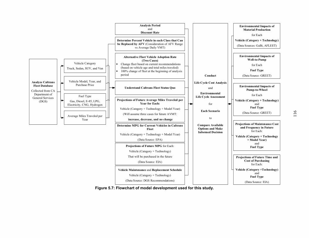
116

Analyze Caltrans

Fleet Database

Collected from CA Department of

General Services (DGS)

Vehicle Category

Truck, Sedan, SUV, and Van

Fuel Type

Gas, Diesel, E-85, LPG, Electricity, CNG, Hydrogen

Average Miles Traveled per Year

Vehicle Model, Year, and Purchase Price

Understand Caltrans Fleet Status Quo

Projections of Future Average Miles Traveled per

Year for Each:

Vehicle (Category + Technology + Model Year)

(Will assume three cases for future AVMT:

increase, decrease, and no change

Projections of Future MPG for Each:

Vehicle (Category + Technology)

That will be purchased in the future

(Data Source: EIA)

Determine MPG for Current Vehicles in Caltrans

Fleet

Vehicle (Category + Technology + Model Year)

(Data Source: EPA)

Vehicle Maintenance and Replacement Schedule

Vehicle (Category + Technology)

(Data Source: DGS Recommendations)

Analysis Period

andDiscount Rate

Conduct

Life Cycle Cost Analysis

and

Environmental

Life Cycle Assessment

for

Each Scenario

to

Compare Available

Options and Make

Informed Decision

Alternative Fleet Vehicle Adoption Rate

(Two Cases)

• Change fleet based on current recommendations (based on vehicle age and total miles traveled)

• 100% change of fleet at the beginning of analysis period

Environmental Impacts of

Material Production

for Each

Vehicle (Category + Technology)

(Data Sources: GaBi, AFLEET)

Environmental Impacts of

Well-to-Pump

for Each

Fuel Type

(Data Source: GREET)

Environmental Impacts of

Pump-to-Wheel

for Each

Vehicle (Category + Technology)

and Fuel Type

(Data Source: GREET)

Projections of Future Time and

Cost of Purchasing

for Each:

Vehicle (Category +Technology)

and Fuel Type

(Data Source: EIA)

Projections of Maintenance Cost

and Frequency in Future

for Each:

Vehicle (Category + Technology

+ Model Year)

and Fuel Type

Determine Percent Vehicle in each Class that Can

be Replaced by AFV (Consideration of AFV Range vs Average Daily VMT)

Figure 5.7: Flowchart of model development used for this study.

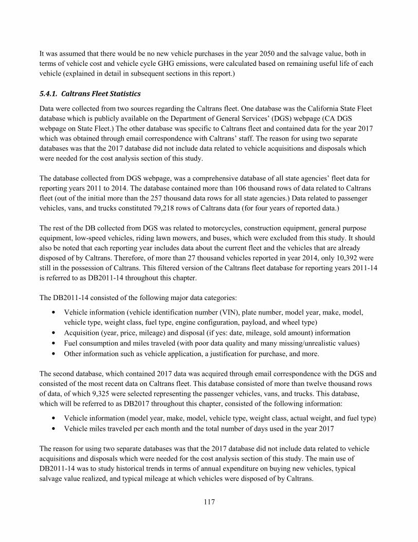
117

It was assumed that there would be no new vehicle purchases in the year 2050 and the salvage value, both in

terms of vehicle cost and vehicle cycle GHG emissions, were calculated based on remaining useful life of each

vehicle (explained in detail in subsequent sections in this report.)

5.4.1. Caltrans Fleet Statistics

Data were collected from two sources regarding the Caltrans fleet. One database was the California State Fleet

database which is publicly available on the Department of General Services’ (DGS) webpage (CA DGS

webpage on State Fleet.) The other database was specific to Caltrans fleet and contained data for the year 2017

which was obtained through email correspondence with Caltrans’ staff. The reason for using two separate

databases was that the 2017 database did not include data related to vehicle acquisitions and disposals which

were needed for the cost analysis section of this study.

The database collected from DGS webpage, was a comprehensive database of all state agencies’ fleet data for

reporting years 2011 to 2014. The database contained more than 106 thousand rows of data related to Caltrans

fleet (out of the initial more than the 257 thousand data rows for all state agencies.) Data related to passenger

vehicles, vans, and trucks constituted 79,218 rows of Caltrans data (for four years of reported data.)

The rest of the DB collected from DGS was related to motorcycles, construction equipment, general purpose

equipment, low-speed vehicles, riding lawn mowers, and buses, which were excluded from this study. It should

also be noted that each reporting year includes data about the current fleet and the vehicles that are already

disposed of by Caltrans. Therefore, of more than 27 thousand vehicles reported in year 2014, only 10,392 were

still in the possession of Caltrans. This filtered version of the Caltrans fleet database for reporting years 2011-14

is referred to as DB2011-14 throughout this chapter.

The DB2011-14 consisted of the following major data categories:

• Vehicle information (vehicle identification number (VIN), plate number, model year, make, model,

vehicle type, weight class, fuel type, engine configuration, payload, and wheel type)

• Acquisition (year, price, mileage) and disposal (if yes: date, mileage, sold amount) information

• Fuel consumption and miles traveled (with poor data quality and many missing/unrealistic values)

• Other information such as vehicle application, a justification for purchase, and more.

The second database, which contained 2017 data was acquired through email correspondence with the DGS and

consisted of the most recent data on Caltrans fleet. This database consisted of more than twelve thousand rows

of data, of which 9,325 were selected representing the passenger vehicles, vans, and trucks. This database,

which will be referred to as DB2017 throughout this chapter, consisted of the following information:

• Vehicle information (model year, make, model, vehicle type, weight class, actual weight, and fuel type)

• Vehicle miles traveled per each month and the total number of days used in the year 2017

The reason for using two separate databases was that the 2017 database did not include data related to vehicle

acquisitions and disposals which were needed for the cost analysis section of this study. The main use of

DB2011-14 was to study historical trends in terms of annual expenditure on buying new vehicles, typical

salvage value realized, and typical mileage at which vehicles were disposed of by Caltrans.

118

Caltrans fleet vehicles are divided into four major categories and 12 vehicle types, as shown in Table 5.5. There

are 9,325 vehicles in Caltrans fleet as of 2017.

Table 5.5. Vehicle categories and

types in Caltrans fleet Vehicle Category Vehicle Type

Passenger Car

Auto-Sub

Auto-Comp

Auto-Mid

Auto-Full

SUV-LD

Pickup Pickup-LD

Pickup-MD

Van Van-LD

Van-MD

Truck

Truck-LD

Truck-MD

Truck-HD

* L: Light, M: Medium, H: Heavy, D: Duty

Figure 5.8 shows the breakdown of Caltrans fleet by vehicle category and Figure 5.9 shows the fleet statistical

summary by graphing vehicle distribution by fuel type and gross weight category. Pickups constitute more than

43 percent of all Caltrans vehicles, followed by trucks and passenger cars with 36 and 15 percent shares,

respectively. Passenger cars collectively refer to subcompact, compact, midsize, full-size sedans, and SUVs in

this report. SUVs have the highest share of passenger cars followed by compact automobiles, with 37 and 34

percent, respectively.

Gasoline, diesel, and E85 are the top three ranking fuel types with 44.5, 29.8, and 15.6 percent share of all

vehicles, respectively. Most vehicles are in the “6,001-10,000” gross vehicle weight range (GVWR) with 37.4

percent share of the fleet followed by “6,000 and less” and “33,000 and more" category with 18.6 and 13.7

percent share, respectively.

Figure 5.10 shows the age distribution of Caltrans fleet. The average fleet age is 10.5 years (8.5 for passenger

cars, 9.8 for pickups, 11.9 for vans, and 11.8 for trucks.)

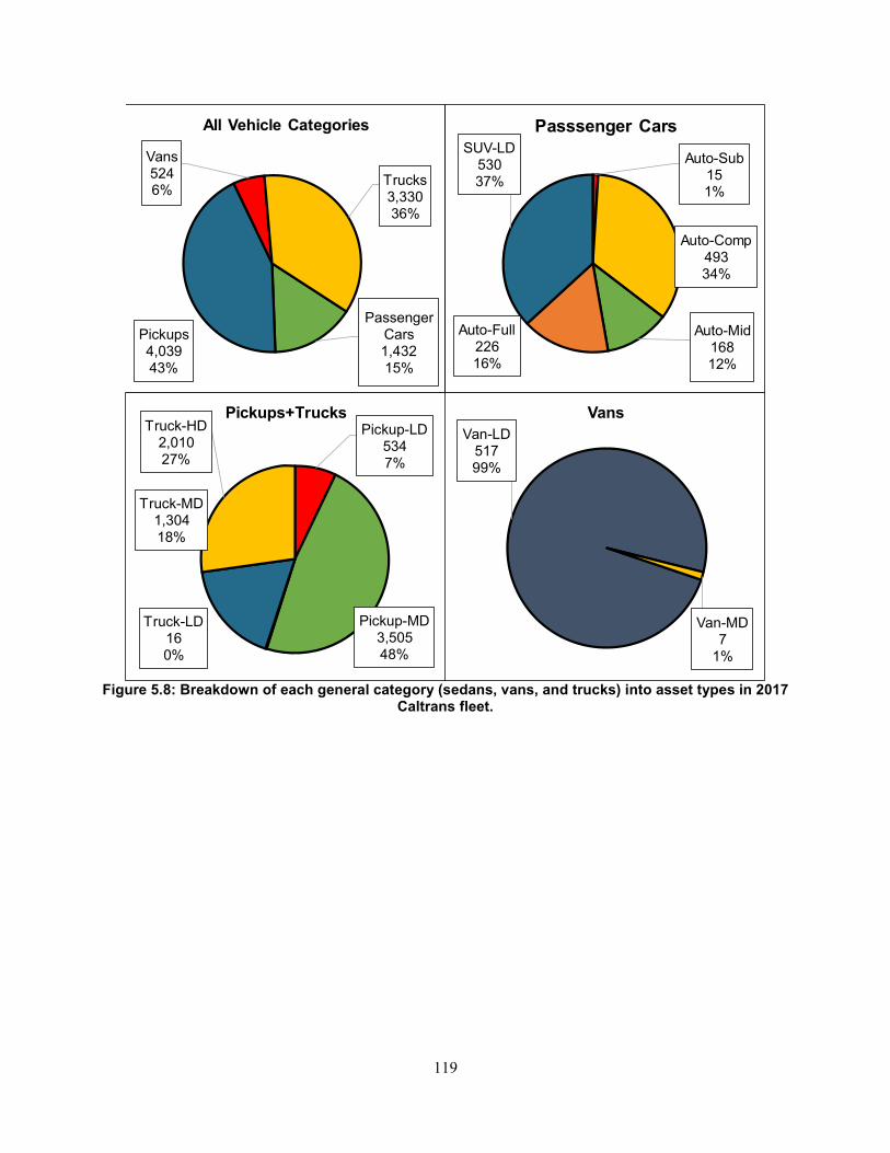
119

Figure 5.8: Breakdown of each general category (sedans, vans, and trucks) into asset types in 2017 Caltrans fleet.

Passenger Cars1,43215%

Pickups4,03943%

Vans5246%

Trucks3,33036%

All Vehicle Categories

Auto-Sub151%

Auto-Comp49334%

Auto-Mid16812%

Auto-Full22616%

SUV-LD53037%

Passsenger Cars

Van-LD51799%

Van-MD7

1%

VansPickup-LD

5347%

Pickup-MD3,50548%

Truck-LD160%

Truck-MD1,30418%

Truck-HD2,01027%

Pickups+Trucks

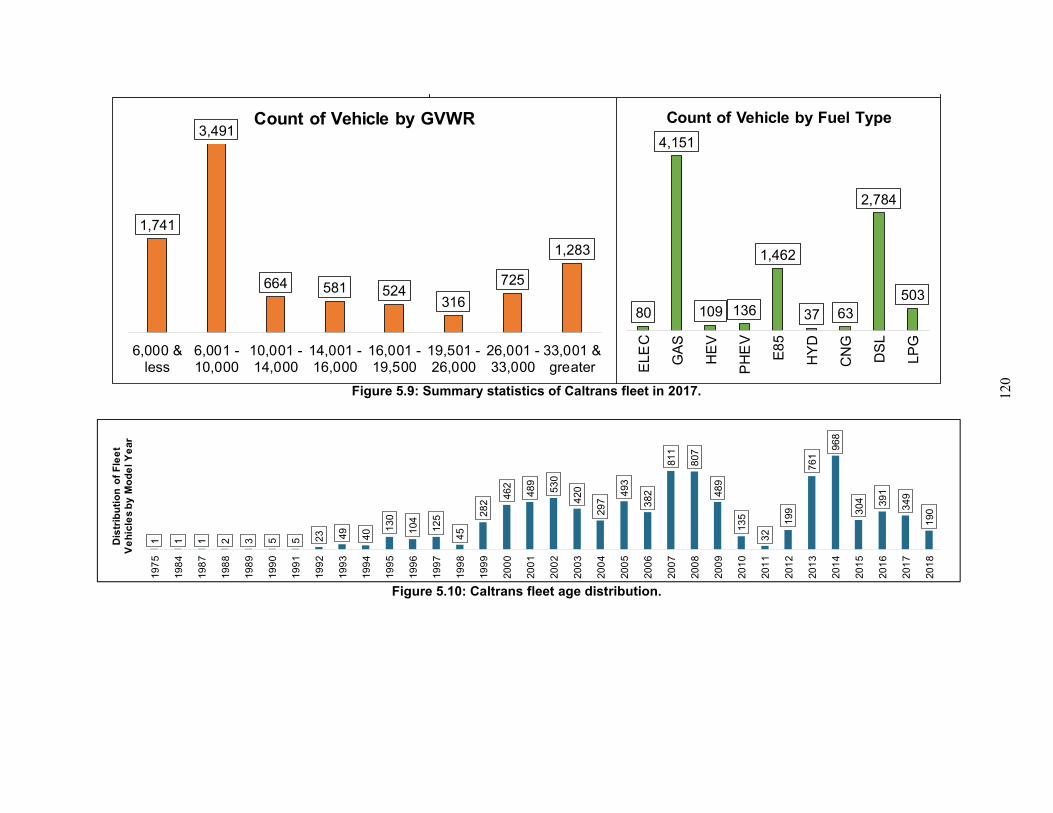
120

Figure 5.9: Summary statistics of Caltrans fleet in 2017.

Figure 5.10: Caltrans fleet age distribution.

1,741

3,491

664 581 524316

725

1,283

6,000 &less

6,001 -10,000

10,001 -14,000

14,001 -16,000

16,001 -19,500

19,501 -26,000

26,001 -33,000

33,001 &greater

Count of Vehicle by GVWR

80

4,151

109 136

1,462

37 63

2,784

503

ELE

C

GA

S

HE

V

PH

EV

E8

5

HY

D

CN

G

DS

L

LP

G

Count of Vehicle by Fuel Type

1 1 1 2 3 5 5 23 49

40 1

30

104

12

5

45

28

2

462

48

9

53

0

420

29

7

493

382

81

1

807

48

9

13

5

32

199

761

968

304 39

1

349

190

19

75

19

84

19

87

19

88

19

89

19

90

19

91

19

92

19

93

19

94

19

95

19

96

19

97

19

98

19

99

20

00

20

01

20

02

20

03

20

04

20

05

20

06

20

07

20

08

20

09

20

10

20

11

20

12

20

13

20

14

20

15

20

16

20

17

20

18

Dis

trib

uti

on

of

Fle

et

Ve

hic

les b

y M

od

el Y

ear

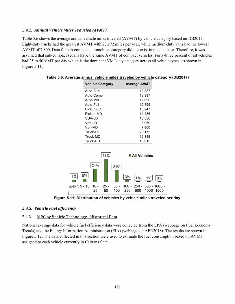
121

5.4.2. Annual Vehicle Miles Traveled (AVMT)

Table 5.6 shows the average annual vehicle miles traveled (AVMT) by vehicle category based on DB2017.

Light-duty trucks had the greatest AVMT with 23,172 miles per year, while medium-duty vans had the lowest

AVMT of 7,800. Data for sub-compact automobiles category did not exist in the database. Therefore, it was

assumed that sub-compact sedans have the same AVMT of compact vehicles. Forty-three percent of all vehicles

had 25 to 50 VMT per day which is the dominant VMT/day category across all vehicle types, as shown in

Figure 5.11.

Table 5.6. Average annual vehicle miles traveled by vehicle category (DB2017)

Vehicle Category Average AVMT

Auto-Sub 12,887 Auto-Comp 12,887 Auto-Mid 12,696 Auto-Full 12,899 Pickup-LD 13,247 Pickup-MD 14,436 SUV-LD 15,386 Van-LD 8,959 Van-MD 7,800 Truck-LD 23,172 Truck-MD 12,345 Truck-HD 13,015

Figure 5.11: Distribution of vehicles by vehicle miles traveled per day.

5.4.3. Vehicle Fuel Efficiency

5.4.3.1. MPG by Vehicle Technology - Historical Data

National average data for vehicle fuel efficiency data were collected from the EPA (webpage on Fuel Economy

Trends) and the Energy Information Administration (EIA) (webpage on AER2018). The results are shown in

Figure 5.12. The data collected in this section were used to estimate the fuel consumption based on AVMT

assigned to each vehicle currently in Caltrans fleet.

6.4

%

3% 5%

24%

43%

21%

3% 1% 1% 0%

upto 5 5 - 10 10 -25

25 -50

50 -100

100 -250

250 -500

500 -1000

1000 -1500

All Vehicles

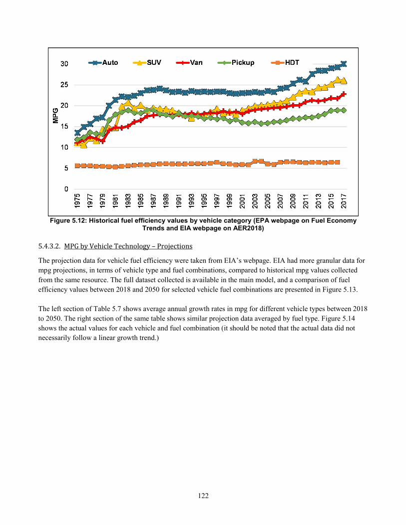
122

Figure 5.12: Historical fuel efficiency values by vehicle category (EPA webpage on Fuel Economy Trends and EIA webpage on AER2018)

5.4.3.2. MPG by Vehicle Technology – Projections

The projection data for vehicle fuel efficiency were taken from EIA’s webpage. EIA had more granular data for

mpg projections, in terms of vehicle type and fuel combinations, compared to historical mpg values collected

from the same resource. The full dataset collected is available in the main model, and a comparison of fuel

efficiency values between 2018 and 2050 for selected vehicle fuel combinations are presented in Figure 5.13.

The left section of Table 5.7 shows average annual growth rates in mpg for different vehicle types between 2018

to 2050. The right section of the same table shows similar projection data averaged by fuel type. Figure 5.14

shows the actual values for each vehicle and fuel combination (it should be noted that the actual data did not

necessarily follow a linear growth trend.)

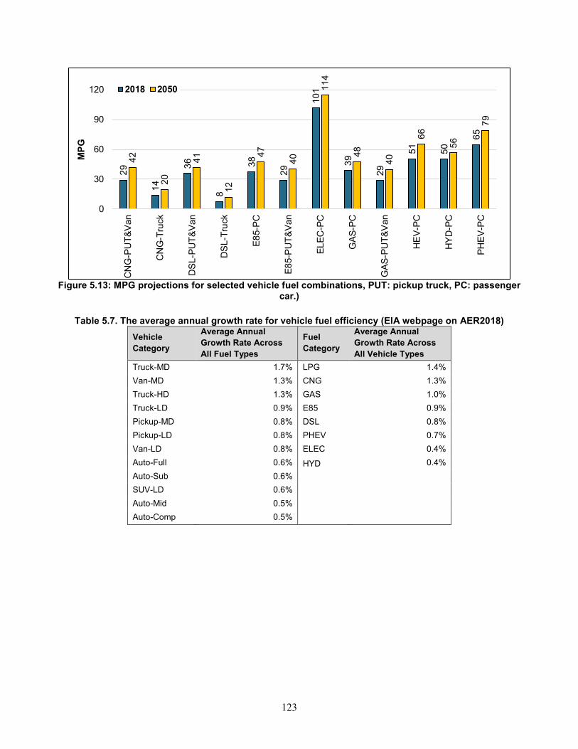
123

Figure 5.13: MPG projections for selected vehicle fuel combinations, PUT: pickup truck, PC: passenger car.)

Table 5.7. The average annual growth rate for vehicle fuel efficiency (EIA webpage on AER2018)

Vehicle

Category

Average Annual

Growth Rate Across

All Fuel Types

Fuel

Category

Average Annual

Growth Rate Across

All Vehicle Types

Truck-MD 1.7% LPG 1.4%

Van-MD 1.3% CNG 1.3%

Truck-HD 1.3% GAS 1.0%

Truck-LD 0.9% E85 0.9%

Pickup-MD 0.8% DSL 0.8%

Pickup-LD 0.8% PHEV 0.7%

Van-LD 0.8% ELEC 0.4%

Auto-Full 0.6% HYD 0.4%

Auto-Sub 0.6%

SUV-LD 0.6%

Auto-Mid 0.5%

Auto-Comp 0.5%

29

14

36

8

38

29

10

1

39

29

51

50

65

42

20

41

12

47

40

11

4

48

40

66

56

79

0

30

60

90

120

CN

G-P

UT

&V

an

CN

G-T

ruck

DS

L-P

UT

&V

an

DS

L-T

ruck

E8

5-P

C

E8

5-P

UT

&V

an

EL

EC

-PC

GA

S-P

C

GA

S-P

UT

&V

an

HE

V-P

C

HY

D-P

C

PH

EV

-PC

MP

G2018 2050

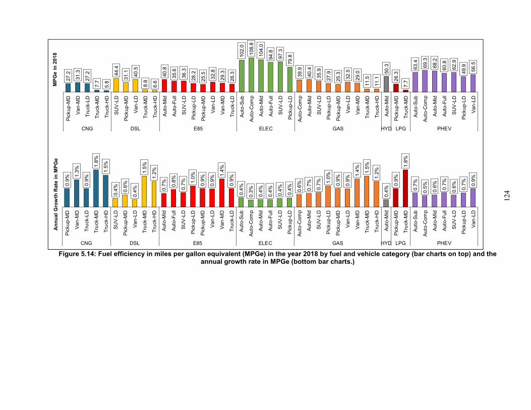
124

Figure 5.14: Fuel efficiency in miles per gallon equivalent (MPGe) in the year 2018 by fuel and vehicle category (bar charts on top) and the annual growth rate in MPGe (bottom bar charts.)

27

.2

31

.3

27

.2

7.7

5.8

44.4

31.1

40.5

8.8

6.6

40.8

35.6

36.3

28

.2

25.5

32.8

29.3

26.3

10

2.0

108.8

104.0

94.8

97.3

79.8

39

.9

40

.4

35.9

27

.9

25.3

32

.5

29.0

11.5

11.1

50

.3

26.3

7.7

63.4

69.3

68

.2

60.8

62.9

49.9

56.5

Pic

ku

p-M

D

Va

n-M

D

Tru

ck-L

D

Tru

ck-M

D

Tru

ck-H

D

SU

V-L

D

Pic

ku

p-M

D

Va

n-L

D

Tru

ck-M

D

Tru

ck-H

D

Auto

-Mid

Auto

-Fu

ll

SU

V-L

D

Pic

ku

p-L

D

Pic

ku

p-M

D

Va

n-L

D

Va

n-M

D

Tru

ck-L

D

Auto

-Sub

Au

to-C

om

p

Auto

-Mid

Auto

-Fu

ll

SU

V-L

D

Pic

ku

p-L

D

Au

to-C

om

p

Auto

-Mid

SU

V-L

D

Pic

ku

p-L

D

Pic

ku

p-M

D

Va

n-L

D

Va

n-M

D

Tru

ck-M

D

Tru

ck-H

D

Auto

-Mid

Pic

ku

p-M

D

Tru

ck-M

D

Auto

-Sub

Au

to-C

om

p

Auto

-Mid

Auto

-Fu

ll

SU

V-L

D

Pic

ku

p-L

D

Va

n-L

D

CNG DSL E85 ELEC GAS HYD LPG PHEV

MP

Ge

in

201

8

0.9

% 1.3

%

0.9

%

1.8

%

1.5

%

0.4

%

0.6

%

0.4

%

1.5

%

1.2

%

0.7

%

0.8

%

0.7

% 1.0

%

0.9

%

0.9

%

1.4

%

0.9

%

0.4

%

0.3

%

0.4

%

0.4

%

0.4

%

0.4

%

0.6

%

0.7

%

0.7

% 1.0

%

0.9

%

0.9

%

1.4

%

1.5

%

1.2

%

0.4

%

0.9

%

1.8

%

0.7

%

0.5

%

0.6

%

0.7

%

0.6

%

0.7

%

0.9

%

Pic

ku

p-M

D

Va

n-M

D

Tru

ck-L

D

Tru

ck-M

D

Tru

ck-H

D

SU

V-L

D

Pic

ku

p-M

D

Va

n-L

D

Tru

ck-M

D

Tru

ck-H

D

Auto

-Mid

Auto

-Fu

ll

SU

V-L

D

Pic

ku

p-L

D

Pic

ku

p-M

D

Va

n-L

D

Va

n-M

D

Tru

ck-L

D

Auto

-Sub

Au

to-C

om

p

Auto

-Mid

Auto

-Fu

ll

SU

V-L

D

Pic

ku

p-L

D

Au

to-C

om

p

Auto

-Mid

SU

V-L

D

Pic

ku

p-L

D

Pic

ku

p-M

D

Va

n-L

D

Va

n-M

D

Tru

ck-M

D

Tru

ck-H

D

Auto

-Mid

Pic

ku

p-M

D

Tru

ck-M

D

Auto

-Sub

Au

to-C

om

p

Auto

-Mid

Auto

-Fu

ll

SU

V-L

D

Pic

ku

p-L

D

Va

n-L

D

CNG DSL E85 ELEC GAS HYD LPG PHEV

An

nu

al

Gro

wth

Rate

in

MP

Ge

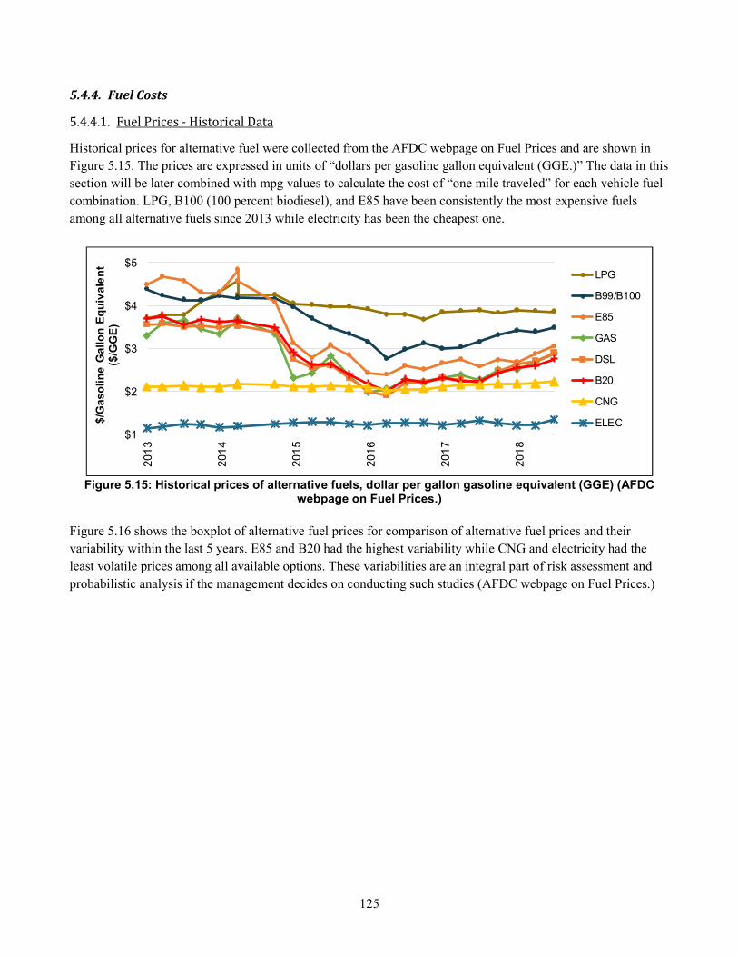
125

5.4.4. Fuel Costs

5.4.4.1. Fuel Prices - Historical Data

Historical prices for alternative fuel were collected from the AFDC webpage on Fuel Prices and are shown in

Figure 5.15. The prices are expressed in units of “dollars per gasoline gallon equivalent (GGE.)” The data in this

section will be later combined with mpg values to calculate the cost of “one mile traveled” for each vehicle fuel

combination. LPG, B100 (100 percent biodiesel), and E85 have been consistently the most expensive fuels

among all alternative fuels since 2013 while electricity has been the cheapest one.

Figure 5.15: Historical prices of alternative fuels, dollar per gallon gasoline equivalent (GGE) (AFDC webpage on Fuel Prices.)

Figure 5.16 shows the boxplot of alternative fuel prices for comparison of alternative fuel prices and their

variability within the last 5 years. E85 and B20 had the highest variability while CNG and electricity had the

least volatile prices among all available options. These variabilities are an integral part of risk assessment and

probabilistic analysis if the management decides on conducting such studies (AFDC webpage on Fuel Prices.)

$1

$2

$3

$4

$5

20

13

20

14

20

15

20

16

20

17

20

18

$/G

as

oli

ne

Ga

llo

n E

qu

iva

len

t ($

/GG

E)

LPG

B99/B100

E85

GAS

DSL

B20

CNG

ELEC

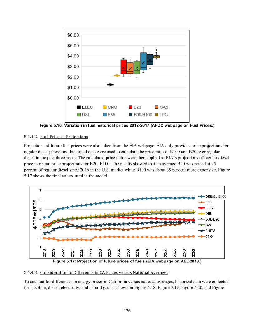
126

Figure 5.16: Variation in fuel historical prices 2012-2017 (AFDC webpage on Fuel Prices.)

5.4.4.2. Fuel Prices – Projections

Projections of future fuel prices were also taken from the EIA webpage. EIA only provides price projections for

regular diesel; therefore, historical data were used to calculate the price ratio of B100 and B20 over regular

diesel in the past three years. The calculated price ratios were then applied to EIA’s projections of regular diesel

price to obtain price projections for B20, B100. The results showed that on average B20 was priced at 95

percent of regular diesel since 2016 in the U.S. market while B100 was about 39 percent more expensive. Figure

5.17 shows the final values used in the model.

Figure 5.17: Projection of future prices of fuels (EIA webpage on AEO2018.)

5.4.4.3. Consideration of Difference in CA Prices versus National Averages

To account for differences in energy prices in California versus national averages, historical data were collected

for gasoline, diesel, electricity, and natural gas; as shown in Figure 5.18, Figure 5.19, Figure 5.20, and Figure

DSL-B100

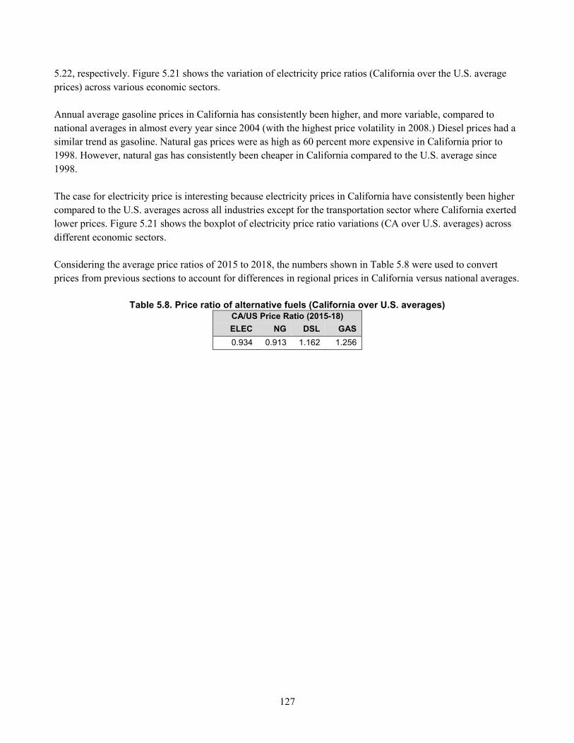
127

5.22, respectively. Figure 5.21 shows the variation of electricity price ratios (California over the U.S. average

prices) across various economic sectors.

Annual average gasoline prices in California has consistently been higher, and more variable, compared to

national averages in almost every year since 2004 (with the highest price volatility in 2008.) Diesel prices had a

similar trend as gasoline. Natural gas prices were as high as 60 percent more expensive in California prior to

1998. However, natural gas has consistently been cheaper in California compared to the U.S. average since

1998.

The case for electricity price is interesting because electricity prices in California have consistently been higher

compared to the U.S. averages across all industries except for the transportation sector where California exerted

lower prices. Figure 5.21 shows the boxplot of electricity price ratio variations (CA over U.S. averages) across

different economic sectors.

Considering the average price ratios of 2015 to 2018, the numbers shown in Table 5.8 were used to convert

prices from previous sections to account for differences in regional prices in California versus national averages.

Table 5.8. Price ratio of alternative fuels (California over U.S. averages)

CA/US Price Ratio (2015-18)

ELEC NG DSL GAS

0.934 0.913 1.162 1.256

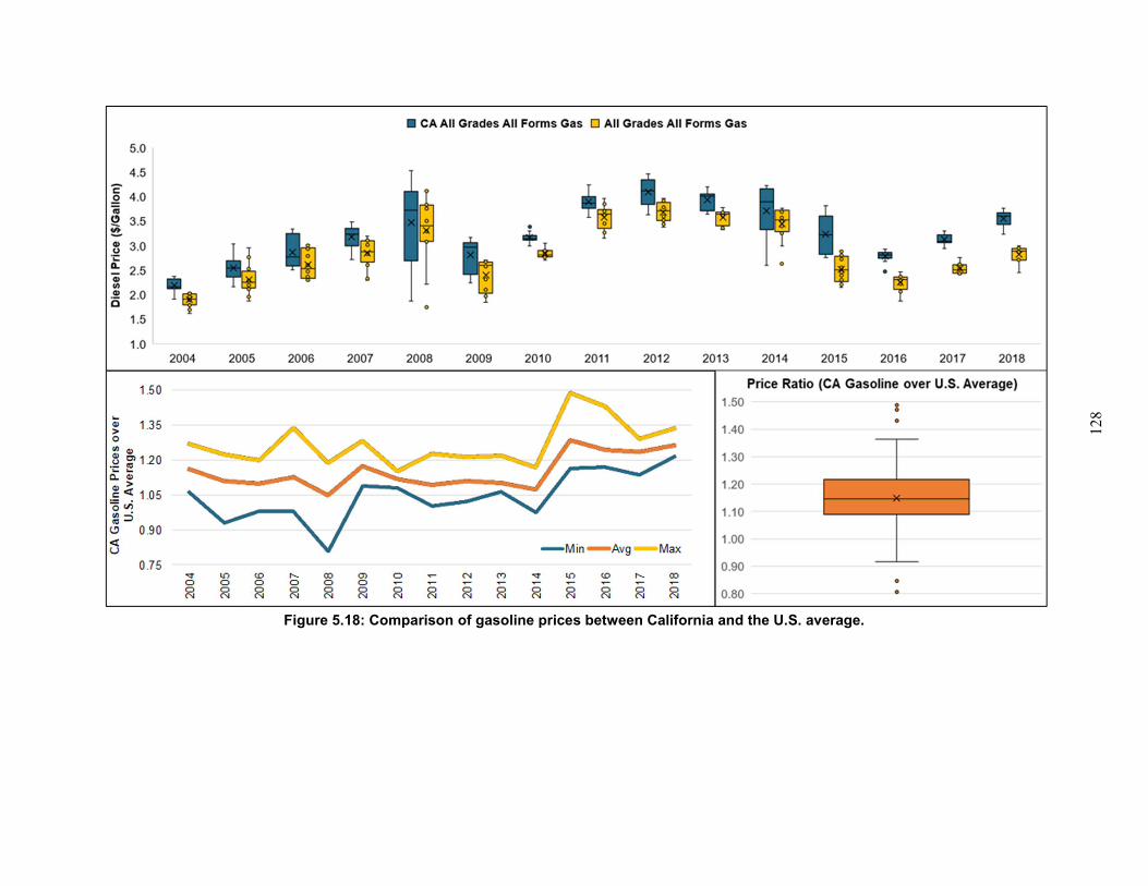
128

Figure 5.18: Comparison of gasoline prices between California and the U.S. average.

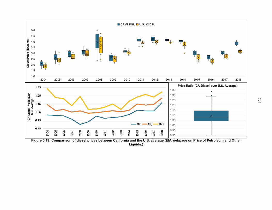
129

Figure 5.19: Comparison of diesel prices between California and the U.S. average (EIA webpage on Price of Petroleum and Other Liquids.)

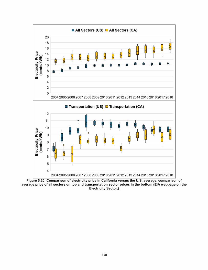
130

Figure 5.20: Comparison of electricity price in California versus the U.S. average, comparison of average price of all sectors on top and transportation sector prices in the bottom (EIA webpage on the

Electricity Sector.)

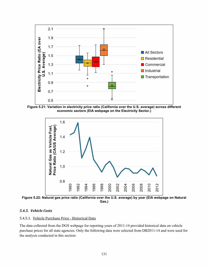
131

Figure 5.21: Variation in electricity price ratio (California over the U.S. average) across different economic sectors (EIA webpage on the Electricity Sector.)

Figure 5.22: Natural gas price ratio (California over the U.S. average) by year (EIA webpage on Natural Gas.)

5.4.5. Vehicle Costs

5.4.5.1. Vehicle Purchase Price - Historical Data

The data collected from the DGS webpage for reporting years of 2011-14 provided historical data on vehicle

purchase prices for all state agencies. Only the following data were selected from DB2011-14 and were used for

the analysis conducted in this section:

0.8

1.0

1.2

1.4

1.6

19

90

19

92

19

94

19

96

19

98

20

00

20

02

20

04

20

06

20

08

20

10

20

12

Na

tura

l G

as

as

Ve

hic

le F

ue

l,

Pri

ce

Ra

tio

(C

A/U

S A

ve

rag

e)

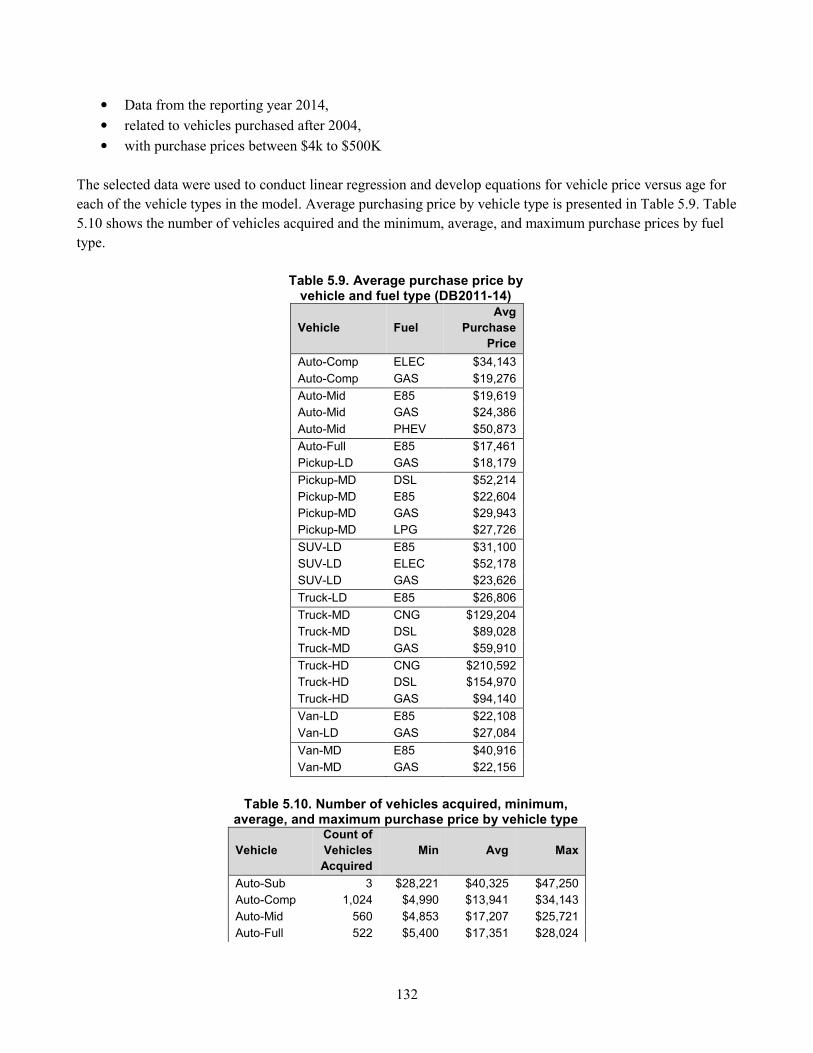
132

• Data from the reporting year 2014,

• related to vehicles purchased after 2004,

• with purchase prices between $4k to $500K

The selected data were used to conduct linear regression and develop equations for vehicle price versus age for

each of the vehicle types in the model. Average purchasing price by vehicle type is presented in Table 5.9. Table

5.10 shows the number of vehicles acquired and the minimum, average, and maximum purchase prices by fuel

type.

Table 5.9. Average purchase price by

vehicle and fuel type (DB2011-14)

Vehicle Fuel

Avg

Purchase

Price

Auto-Comp ELEC $34,143

Auto-Comp GAS $19,276

Auto-Mid E85 $19,619

Auto-Mid GAS $24,386

Auto-Mid PHEV $50,873

Auto-Full E85 $17,461

Pickup-LD GAS $18,179

Pickup-MD DSL $52,214

Pickup-MD E85 $22,604

Pickup-MD GAS $29,943

Pickup-MD LPG $27,726

SUV-LD E85 $31,100

SUV-LD ELEC $52,178

SUV-LD GAS $23,626

Truck-LD E85 $26,806

Truck-MD CNG $129,204

Truck-MD DSL $89,028

Truck-MD GAS $59,910

Truck-HD CNG $210,592

Truck-HD DSL $154,970

Truck-HD GAS $94,140

Van-LD E85 $22,108

Van-LD GAS $27,084

Van-MD E85 $40,916

Van-MD GAS $22,156

Table 5.10. Number of vehicles acquired, minimum,

average, and maximum purchase price by vehicle type

Vehicle

Count of

Vehicles

Acquired

Min Avg Max

Auto-Sub 3 $28,221 $40,325 $47,250

Auto-Comp 1,024 $4,990 $13,941 $34,143

Auto-Mid 560 $4,853 $17,207 $25,721

Auto-Full 522 $5,400 $17,351 $28,024

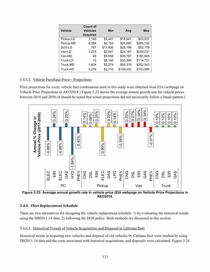
133

Vehicle

Count of

Vehicles

Acquired

Min Avg Max

Pickup-LD 1,140 $3,441 $15,647 $43,031

Pickup-MD 6,084 $2,152 $26,680 $285,132

SUV-LD 767 $11,936 $25,188 $52,178

Van-LD 1,279 $2,047 $24,187 $255,237

Van-MD 49 $5,556 $39,767 $187,845

Truck-LD 15 $8,140 $33,350 $114,731

Truck-MD 1,934 $2,274 $55,379 $252,543

Truck-HD 3,276 $2,710 $109,433 $743,095

5.4.5.2. Vehicle Purchase Price – Projections

Price projections for every vehicle fuel combination used in this study were obtained from EIA (webpage on

Vehicle Price Projections in AEO2018.) Figure 5.23 shows the average annual growth rate for vehicle prices

between 2018 and 2050 (it should be noted that actual projections did not necessarily follow a linear pattern.)

Figure 5.23: Average annual growth rate in vehicle price (EIA webpage on Vehicle Price Projections in AEO2018.

5.4.6. Fleet Replacement Schedule

There are two alternatives for designing the vehicle replacement schedule: 1) by evaluating the historical trends

using the DB2011-14 data, 2) following the DGS policy. Both methods are discussed in this section.

5.4.6.1. Historical Trends of Vehicle Acquisition and Disposal in Caltrans fleet

Historical trends in acquiring new vehicles and disposal of old vehicles by Caltrans fleet were studied by using

DB2011-14 data and the costs associated with historical acquisitions, and disposals were calculated. Figure 5.24

-0.8

8%

0.2

4%

-0.8

8%

0.2

5%

-1.8

4%

-0.4

0%

0.1

4%

0.0

8%

0.2

5%

-0.9

0%

0.2

5%

0.1

4%

-0.3

9%

0.2

3%

0.2

7%

0.3

4%

0.3

4%

-0.3

1%

0.1

0%

0.1

0%

0.1

0%

0.1

0%

ELE

C

E8

5

ELE

C

GA

S

HY

D

PH

EV

CN

G

DS

L

E8

5

ELE

C

GA

S

LP

G

PH

EV

CN

G

DS

L

E8

5

GA

S

PH

EV

CN

G

DS

L

E8

5

GA

S

PC Pickup Van Truck

An

nu

al

% C

ha

ng

e i

n

Ve

hic

le P

ric

e (

20

17

-20

50

)

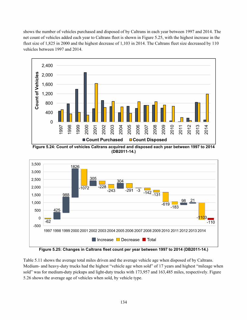
134

shows the number of vehicles purchased and disposed of by Caltrans in each year between 1997 and 2014. The

net count of vehicles added each year to Caltrans fleet is shown in Figure 5.25, with the highest increase in the

fleet size of 1,825 in 2000 and the highest decrease of 1,103 in 2014. The Caltrans fleet size decreased by 110

vehicles between 1997 and 2014.

Figure 5.24: Count of vehicles Caltrans acquired and disposed each year between 1997 to 2014 (DB2011-14.)

Figure 5.25: Changes in Caltrans fleet count per year between 1997 to 2014 (DB2011-14.)

Table 5.11 shows the average total miles driven and the average vehicle age when disposed of by Caltrans.

Medium- and heavy-duty trucks had the highest “vehicle age when sold” of 17 years and highest “mileage when

sold” was for medium-duty pickups and light-duty trucks with 173,957 and 163,485 miles, respectively. Figure

5.26 shows the average age of vehicles when sold, by vehicle type.

0

400

800

1,200

1,600

2,000

2,40019

97

19

98

19

99

20

00

20

01

20

02

20

03

20

04

20

05

20

06

20

07

20

08

20

09

20

10

20

11

20

12

20

13

20

14

Co

un

t o

f V

eh

icle

s

Count Purchased Count Disposed

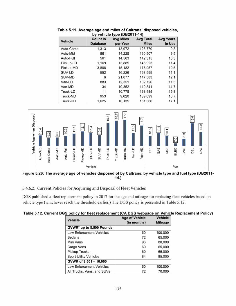
135

Table 5.11. Average age and miles of Caltrans’ disposed vehicles, by vehicle type (DB2011-14)

Vehicle Count in

Database

Avg Miles

per Year

Avg Total

Miles

Avg Years

in Use

Auto-Comp 1,313 13,972 125,770 9.3

Auto-Mid 861 14,225 130,507 9.5

Auto-Full 561 14,503 142,315 10.3

Pickup-LD 1,169 13,885 146,923 11.4

Pickup-MD 3,808 15,182 173,957 10.5

SUV-LD 552 16,226 168,599 11.1

SUV-MD 6 21,077 147,583 12.1

Van-LD 883 12,351 132,726 11.5

Van-MD 34 10,352 110,841 14.7

Truck-LD 11 10,778 163,485 15.8

Truck-MD 953 9,020 139,099 16.7

Truck-HD 1,625 10,135 161,366 17.1

Figure 5.26: The average age of vehicles disposed of by Caltrans, by vehicle type and fuel type (DB2011-14.)

5.4.6.2. Current Policies for Acquiring and Disposal of Fleet Vehicles

DGS published a fleet replacement policy in 2017 for the age and mileage for replacing fleet vehicles based on

vehicle type (whichever reach the threshold earlier.) The DGS policy is presented in Table 5.12.

Table 5.12. Current DGS policy for fleet replacement (CA DGS webpage on Vehicle Replacement Policy)

Vehicle Age of Vehicle

(in months)

Vehicle

Mileage

GVWR* up to 8,500 Pounds

Law Enforcement Vehicles 60 100,000

Sedans 72 65,000

Mini Vans 96 80,000

Cargo Vans 60 65,000

Pickup Trucks 60 65,000

Sport Utility Vehicles 84 85,000

GVWR of 8,501 – 16,000

Law Enforcement Vehicles 60 100,000

All Trucks, Vans, and SUVs 72 70,000

10

.4

9.3 9.5 1

0.3 11

.1 12

.1

11

.4

10

.5

15

.8 16

.7

17

.1

11

.5

14

.7

10

.3 11

.4

10

.1

7.0

8.9

15

.6

12

.0

Au

to-S

ub

Au

to-C

om

p

Au

to-M

id

Au

to-F

ull

Pic

kup-L

D

Pic

kup-M

D

SU

V-L

D

SU

V-M

D

Tru

ck-L

D

Tru

ck-M

D

Tru

ck-H

D

Va

n-L

D

Va

n-M

D

E8

5

GA

S

M85

EL

EC

CN

G

DS

L

LP

G

Vehicle Fuel

Ve

hic

le A

ge

wh

en

Dis

po

se

d

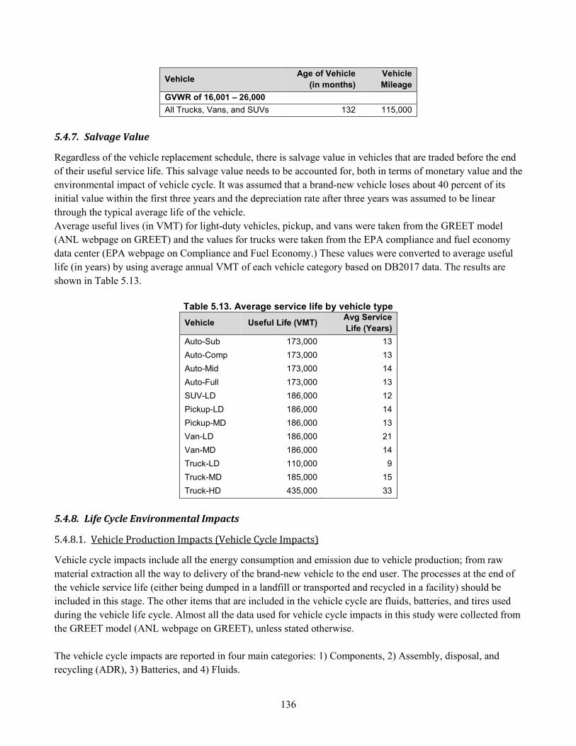
136

Vehicle Age of Vehicle

(in months)

Vehicle

Mileage

GVWR of 16,001 – 26,000

All Trucks, Vans, and SUVs 132 115,000

5.4.7. Salvage Value

Regardless of the vehicle replacement schedule, there is salvage value in vehicles that are traded before the end

of their useful service life. This salvage value needs to be accounted for, both in terms of monetary value and the

environmental impact of vehicle cycle. It was assumed that a brand-new vehicle loses about 40 percent of its

initial value within the first three years and the depreciation rate after three years was assumed to be linear

through the typical average life of the vehicle.

Average useful lives (in VMT) for light-duty vehicles, pickup, and vans were taken from the GREET model

(ANL webpage on GREET) and the values for trucks were taken from the EPA compliance and fuel economy

data center (EPA webpage on Compliance and Fuel Economy.) These values were converted to average useful

life (in years) by using average annual VMT of each vehicle category based on DB2017 data. The results are

shown in Table 5.13.

Table 5.13. Average service life by vehicle type

Vehicle Useful Life (VMT) Avg Service

Life (Years)

Auto-Sub 173,000 13

Auto-Comp 173,000 13

Auto-Mid 173,000 14

Auto-Full 173,000 13

SUV-LD 186,000 12

Pickup-LD 186,000 14

Pickup-MD 186,000 13

Van-LD 186,000 21

Van-MD 186,000 14

Truck-LD 110,000 9

Truck-MD 185,000 15

Truck-HD 435,000 33

5.4.8. Life Cycle Environmental Impacts

5.4.8.1. Vehicle Production Impacts (Vehicle Cycle Impacts)

Vehicle cycle impacts include all the energy consumption and emission due to vehicle production; from raw

material extraction all the way to delivery of the brand-new vehicle to the end user. The processes at the end of

the vehicle service life (either being dumped in a landfill or transported and recycled in a facility) should be

included in this stage. The other items that are included in the vehicle cycle are fluids, batteries, and tires used

during the vehicle life cycle. Almost all the data used for vehicle cycle impacts in this study were collected from

the GREET model (ANL webpage on GREET), unless stated otherwise.

The vehicle cycle impacts are reported in four main categories: 1) Components, 2) Assembly, disposal, and

recycling (ADR), 3) Batteries, and 4) Fluids.

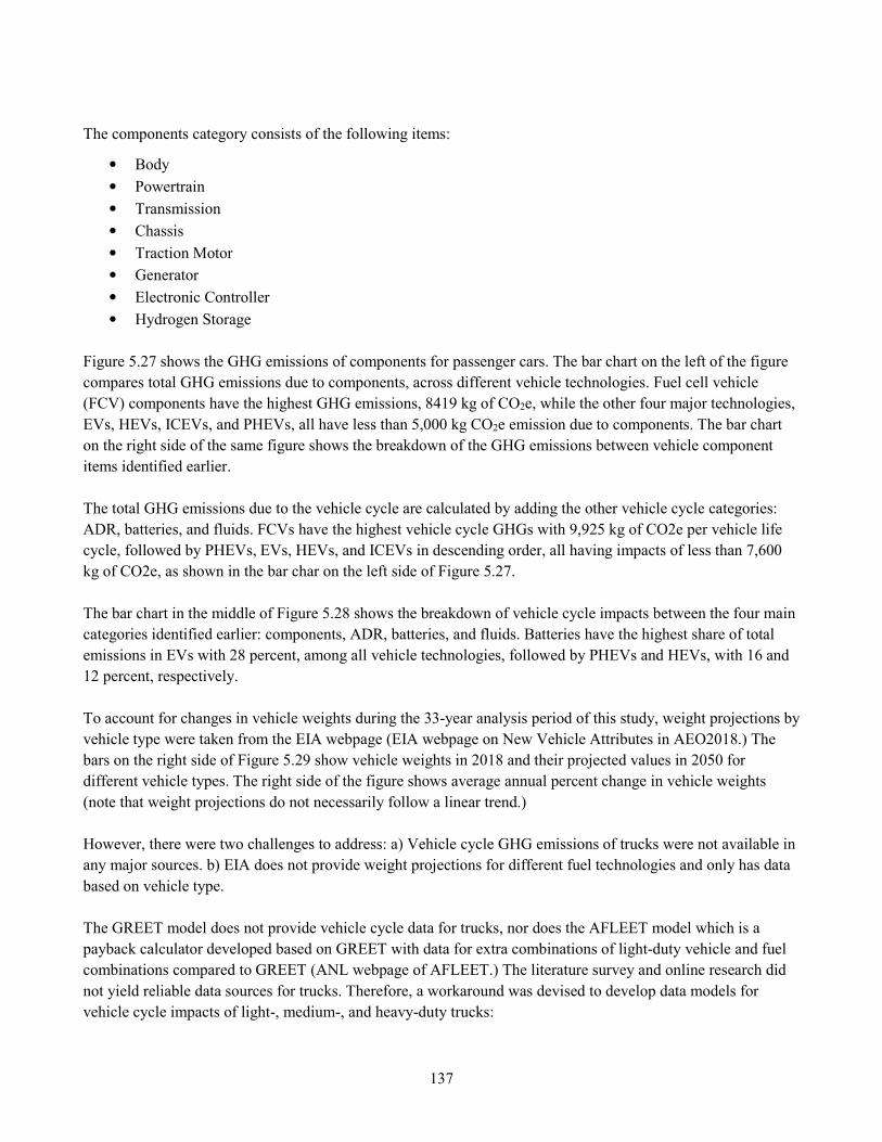
137

The components category consists of the following items:

• Body

• Powertrain

• Transmission

• Chassis

• Traction Motor

• Generator

• Electronic Controller

• Hydrogen Storage

Figure 5.27 shows the GHG emissions of components for passenger cars. The bar chart on the left of the figure

compares total GHG emissions due to components, across different vehicle technologies. Fuel cell vehicle

(FCV) components have the highest GHG emissions, 8419 kg of CO2e, while the other four major technologies,

EVs, HEVs, ICEVs, and PHEVs, all have less than 5,000 kg CO2e emission due to components. The bar chart

on the right side of the same figure shows the breakdown of the GHG emissions between vehicle component

items identified earlier.

The total GHG emissions due to the vehicle cycle are calculated by adding the other vehicle cycle categories:

ADR, batteries, and fluids. FCVs have the highest vehicle cycle GHGs with 9,925 kg of CO2e per vehicle life

cycle, followed by PHEVs, EVs, HEVs, and ICEVs in descending order, all having impacts of less than 7,600

kg of CO2e, as shown in the bar char on the left side of Figure 5.27.

The bar chart in the middle of Figure 5.28 shows the breakdown of vehicle cycle impacts between the four main

categories identified earlier: components, ADR, batteries, and fluids. Batteries have the highest share of total

emissions in EVs with 28 percent, among all vehicle technologies, followed by PHEVs and HEVs, with 16 and

12 percent, respectively.

To account for changes in vehicle weights during the 33-year analysis period of this study, weight projections by

vehicle type were taken from the EIA webpage (EIA webpage on New Vehicle Attributes in AEO2018.) The

bars on the right side of Figure 5.29 show vehicle weights in 2018 and their projected values in 2050 for

different vehicle types. The right side of the figure shows average annual percent change in vehicle weights

(note that weight projections do not necessarily follow a linear trend.)

However, there were two challenges to address: a) Vehicle cycle GHG emissions of trucks were not available in

any major sources. b) EIA does not provide weight projections for different fuel technologies and only has data

based on vehicle type.

The GREET model does not provide vehicle cycle data for trucks, nor does the AFLEET model which is a

payback calculator developed based on GREET with data for extra combinations of light-duty vehicle and fuel

combinations compared to GREET (ANL webpage of AFLEET.) The literature survey and online research did

not yield reliable data sources for trucks. Therefore, a workaround was devised to develop data models for

vehicle cycle impacts of light-, medium-, and heavy-duty trucks:

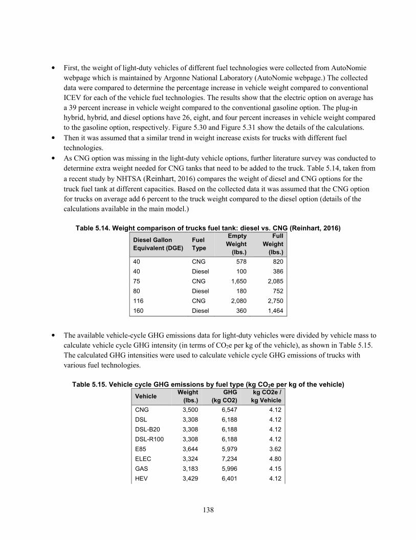
138

• First, the weight of light-duty vehicles of different fuel technologies were collected from AutoNomie

webpage which is maintained by Argonne National Laboratory (AutoNomie webpage.) The collected

data were compared to determine the percentage increase in vehicle weight compared to conventional

ICEV for each of the vehicle fuel technologies. The results show that the electric option on average has

a 39 percent increase in vehicle weight compared to the conventional gasoline option. The plug-in

hybrid, hybrid, and diesel options have 26, eight, and four percent increases in vehicle weight compared

to the gasoline option, respectively. Figure 5.30 and Figure 5.31 show the details of the calculations.

• Then it was assumed that a similar trend in weight increase exists for trucks with different fuel

technologies.

• As CNG option was missing in the light-duty vehicle options, further literature survey was conducted to

determine extra weight needed for CNG tanks that need to be added to the truck. Table 5.14, taken from

a recent study by NHTSA (Reinhart, 2016) compares the weight of diesel and CNG options for the

truck fuel tank at different capacities. Based on the collected data it was assumed that the CNG option

for trucks on average add 6 percent to the truck weight compared to the diesel option (details of the

calculations available in the main model.)

Table 5.14. Weight comparison of trucks fuel tank: diesel vs. CNG (Reinhart, 2016)

Diesel Gallon

Equivalent (DGE)

Fuel

Type

Empty

Weight

(lbs.)

Full

Weight

(lbs.)

40 CNG 578 820

40 Diesel 100 386

75 CNG 1,650 2,085

80 Diesel 180 752

116 CNG 2,080 2,750

160 Diesel 360 1,464

• The available vehicle-cycle GHG emissions data for light-duty vehicles were divided by vehicle mass to

calculate vehicle cycle GHG intensity (in terms of CO2e per kg of the vehicle), as shown in Table 5.15.

The calculated GHG intensities were used to calculate vehicle cycle GHG emissions of trucks with

various fuel technologies.

Table 5.15. Vehicle cycle GHG emissions by fuel type (kg CO2e per kg of the vehicle)

Vehicle Weight

(lbs.)

GHG

(kg CO2)

kg CO2e /

kg Vehicle

CNG 3,500 6,547 4.12

DSL 3,308 6,188 4.12

DSL-B20 3,308 6,188 4.12

DSL-R100 3,308 6,188 4.12

E85 3,644 5,979 3.62

ELEC 3,324 7,234 4.80

GAS 3,183 5,996 4.15

HEV 3,429 6,401 4.12

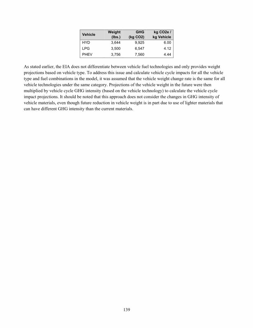
139

Vehicle Weight

(lbs.)

GHG

(kg CO2)

kg CO2e /

kg Vehicle

HYD 3,644 9,925 6.00

LPG 3,500 6,547 4.12

PHEV 3,756 7,560 4.44

As stated earlier, the EIA does not differentiate between vehicle fuel technologies and only provides weight

projections based on vehicle type. To address this issue and calculate vehicle cycle impacts for all the vehicle

type and fuel combinations in the model, it was assumed that the vehicle weight change rate is the same for all

vehicle technologies under the same category. Projections of the vehicle weight in the future were then

multiplied by vehicle cycle GHG intensity (based on the vehicle technology) to calculate the vehicle cycle

impact projections. It should be noted that this approach does not consider the changes in GHG intensity of

vehicle materials, even though future reduction in vehicle weight is in part due to use of lighter materials that

can have different GHG intensity than the current materials.

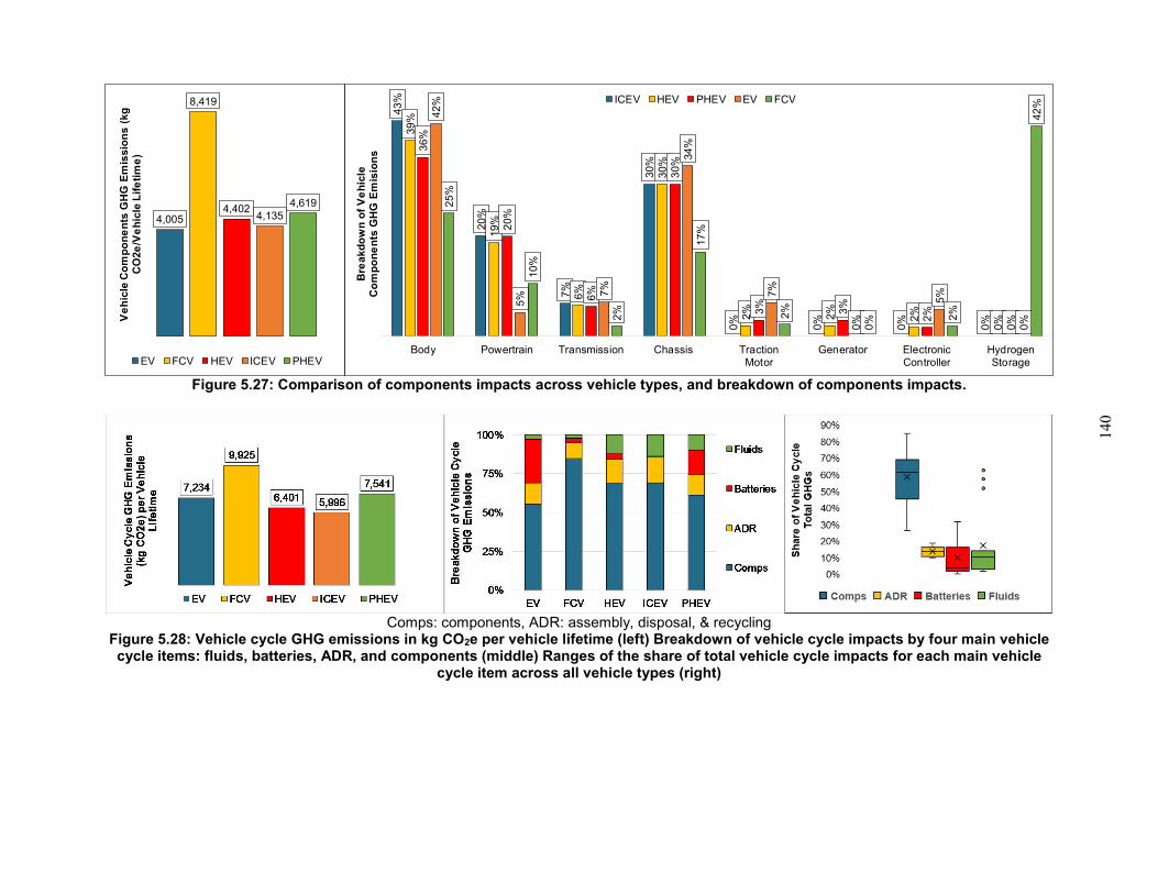
140

Figure 5.27: Comparison of components impacts across vehicle types, and breakdown of components impacts.

Comps: components, ADR: assembly, disposal, & recycling Figure 5.28: Vehicle cycle GHG emissions in kg CO2e per vehicle lifetime (left) Breakdown of vehicle cycle impacts by four main vehicle cycle items: fluids, batteries, ADR, and components (middle) Ranges of the share of total vehicle cycle impacts for each main vehicle

cycle item across all vehicle types (right)

4,005

8,419

4,4024,135

4,619

Ve

hic

le C

om

po

ne

nts

GH

G E

mis

sio

ns (

kg

C

O2e

/Ve

hic

le L

ife

tim

e)

EV FCV HEV ICEV PHEV

43

%

20%

7%

30%

0%

0%

0%

0%

39%

19%

6%

30%

2%

2%

2%

0%

36%

20%

6%

30%

3%

3%

2%

0%

42%

5% 7

%

34%

7%

0%

5%

0%

25

%

10%

2%

17%

2%

0% 2

%

42

%

Body Powertrain Transmission Chassis TractionMotor

Generator ElectronicController

HydrogenStorage

Bre

akd

ow

n o

f V

eh

icle

C

om

po

ne

nts

GH

G E

mis

ion

s

ICEV HEV PHEV EV FCV

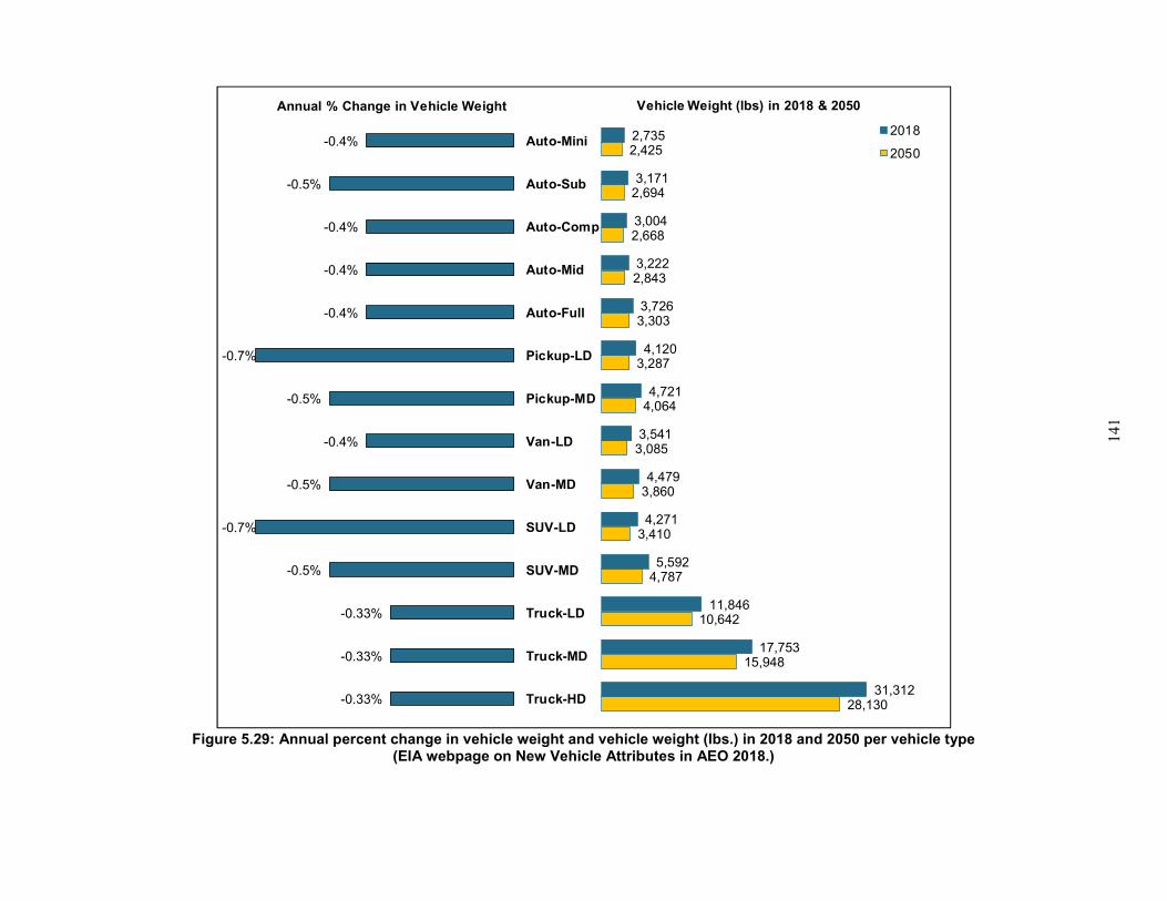
141

Figure 5.29: Annual percent change in vehicle weight and vehicle weight (lbs.) in 2018 and 2050 per vehicle type (EIA webpage on New Vehicle Attributes in AEO 2018.)

2,735

3,171

3,004

3,222

3,726

4,120

4,721

3,541

4,479

4,271

5,592

11,846

17,753

31,312

2,425

2,694

2,668

2,843

3,303

3,287

4,064

3,085

3,860

3,410

4,787

10,642

15,948

28,130

Vehicle Weight (lbs) in 2018 & 2050

2018

2050-0.4%

-0.5%

-0.4%

-0.4%

-0.4%

-0.7%

-0.5%

-0.4%

-0.5%

-0.7%

-0.5%

-0.33%

-0.33%

-0.33%

Auto-Mini

Auto-Sub

Auto-Comp

Auto-Mid

Auto-Full

Pickup-LD

Pickup-MD

Van-LD

Van-MD

SUV-LD

SUV-MD

Truck-LD

Truck-MD

Truck-HD

Annual % Change in Vehicle Weight

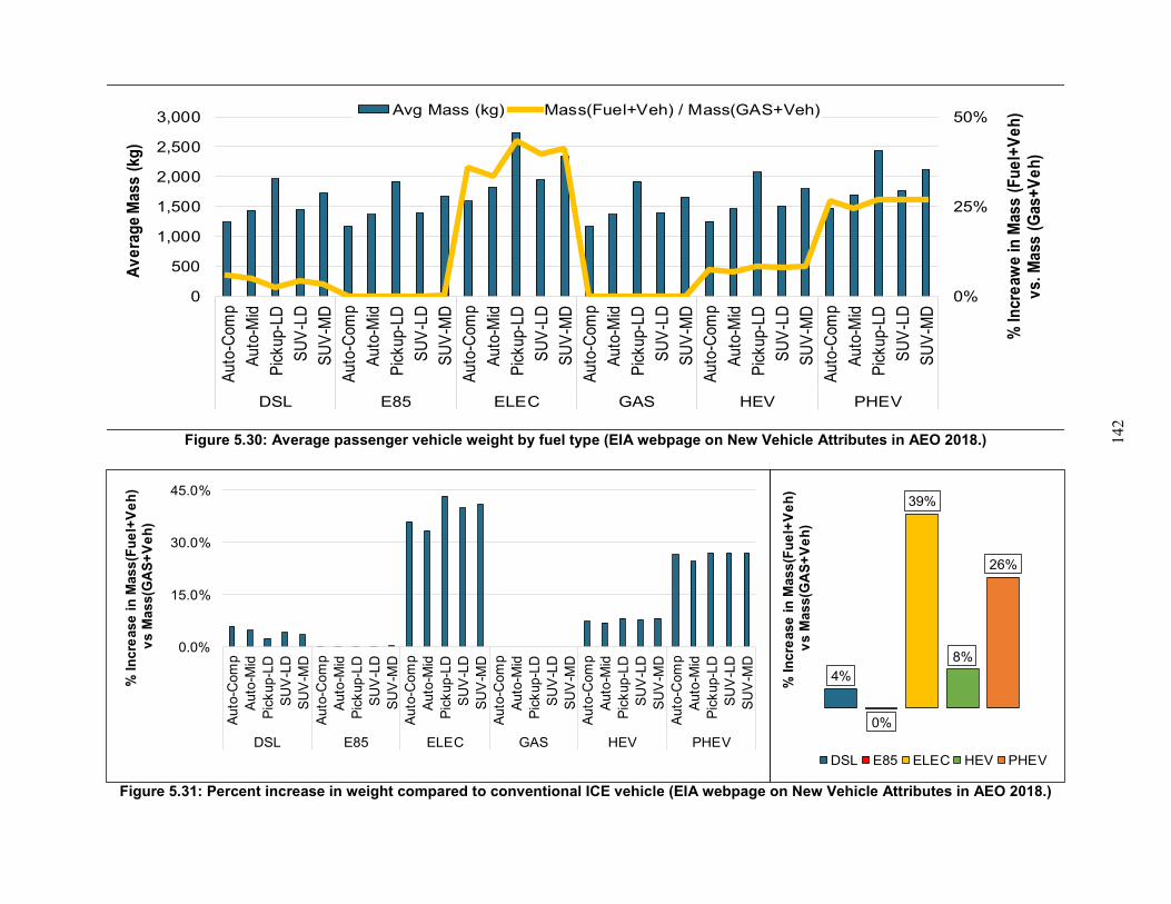
142

Figure 5.30: Average passenger vehicle weight by fuel type (EIA webpage on New Vehicle Attributes in AEO 2018.)

Figure 5.31: Percent increase in weight compared to conventional ICE vehicle (EIA webpage on New Vehicle Attributes in AEO 2018.)

0%

25%

50%

0

500

1,000

1,500

2,000

2,500

3,000

Aut

o-C

omp

Aut

o-M

id

Pic

kup-

LD

SU

V-L

D

SU

V-M

D

Aut

o-C

omp

Aut

o-M

id

Pic

kup-

LD

SU

V-L

D

SU

V-M

D

Aut

o-C

omp

Aut

o-M

id

Pic

kup-

LD

SU

V-L

D

SU

V-M

D

Aut

o-C

omp

Aut

o-M

id

Pic

kup-

LD

SU

V-L

D

SU

V-M

D

Aut

o-C

omp

Aut

o-M

id

Pic

kup-

LD

SU

V-L

D

SU

V-M

D

Aut

o-C

omp

Aut

o-M

id

Pic

kup-

LD

SU

V-L

D

SU

V-M

D

DSL E85 ELEC GAS HEV PHEV

% In

cre

awe

in M

ass

(Fu

el+

Ve

h)

vs.

Mas

s (G

as+

Ve

h)

Av

era

ge

Mas

s (k

g)

Avg Mass (kg) Mass(Fuel+Veh) / Mass(GAS+Veh)

0.0%

15.0%

30.0%

45.0%

Aut

o-C

omp

Aut

o-M

idP

ick

up-L

DS

UV

-LD

SU

V-M

DA

uto-

Com

pA

uto

-Mid

Pic

kup

-LD

SU

V-L

DS

UV

-MD

Aut

o-C

omp

Aut

o-M

idP

ick

up-L

DS

UV

-LD

SU

V-M

DA

uto-

Com

pA

uto

-Mid

Pic

kup

-LD

SU

V-L

DS

UV

-MD

Aut

o-C

omp

Aut

o-M

idP

ick

up-L

DS

UV

-LD

SU

V-M

DA

uto-

Com

pA

uto

-Mid

Pic

kup

-LD

SU

V-L

DS

UV

-MD

DSL E85 ELEC GAS HEV PHEV

% In

cre

ase

in

Mass

(Fu

el+

Ve

h)

vs M

ass(G

AS

+V

eh

)

4%

0%

39%

8%

26%

% In

cre

ase

in

Mass

(Fu

el+

Ve

h)

vs M

ass(G

AS

+V

eh

)

DSL E85 ELEC HEV PHEV

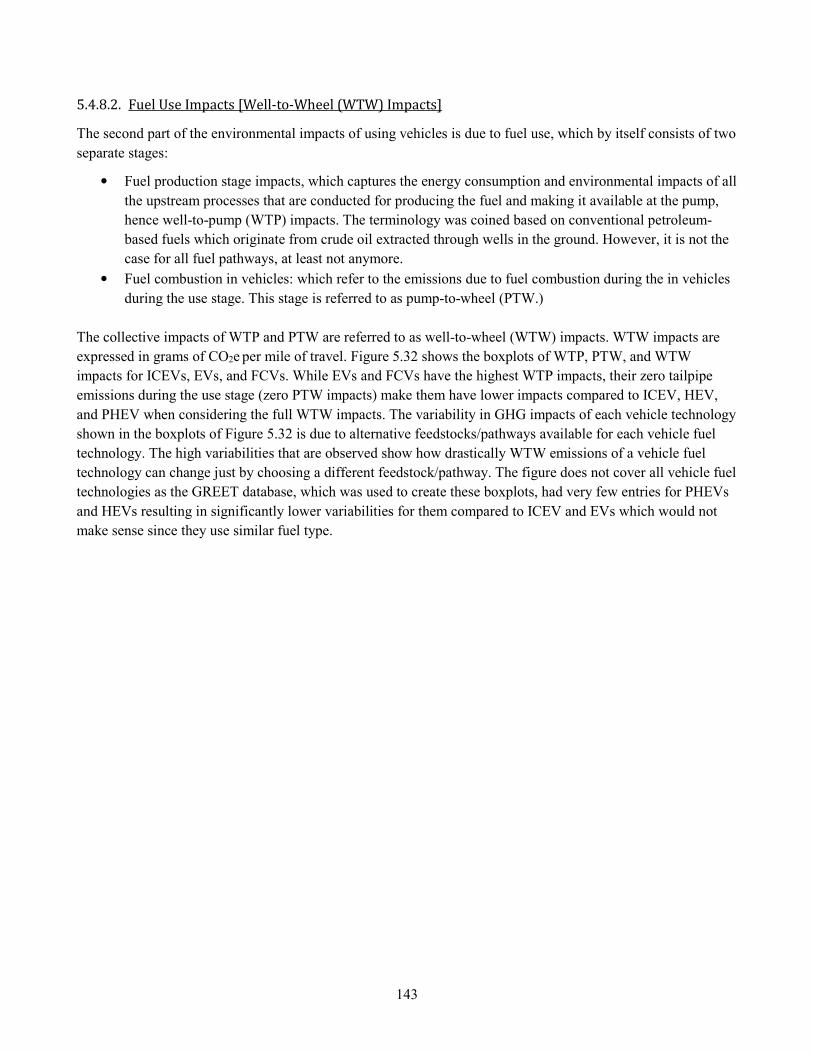
143

5.4.8.2. Fuel Use Impacts [Well-to-Wheel (WTW) Impacts]

The second part of the environmental impacts of using vehicles is due to fuel use, which by itself consists of two

separate stages:

• Fuel production stage impacts, which captures the energy consumption and environmental impacts of all

the upstream processes that are conducted for producing the fuel and making it available at the pump,

hence well-to-pump (WTP) impacts. The terminology was coined based on conventional petroleum-

based fuels which originate from crude oil extracted through wells in the ground. However, it is not the

case for all fuel pathways, at least not anymore.

• Fuel combustion in vehicles: which refer to the emissions due to fuel combustion during the in vehicles

during the use stage. This stage is referred to as pump-to-wheel (PTW.)

The collective impacts of WTP and PTW are referred to as well-to-wheel (WTW) impacts. WTW impacts are

expressed in grams of CO2e per mile of travel. Figure 5.32 shows the boxplots of WTP, PTW, and WTW

impacts for ICEVs, EVs, and FCVs. While EVs and FCVs have the highest WTP impacts, their zero tailpipe

emissions during the use stage (zero PTW impacts) make them have lower impacts compared to ICEV, HEV,

and PHEV when considering the full WTW impacts. The variability in GHG impacts of each vehicle technology

shown in the boxplots of Figure 5.32 is due to alternative feedstocks/pathways available for each vehicle fuel

technology. The high variabilities that are observed show how drastically WTW emissions of a vehicle fuel

technology can change just by choosing a different feedstock/pathway. The figure does not cover all vehicle fuel

technologies as the GREET database, which was used to create these boxplots, had very few entries for PHEVs

and HEVs resulting in significantly lower variabilities for them compared to ICEV and EVs which would not

make sense since they use similar fuel type.

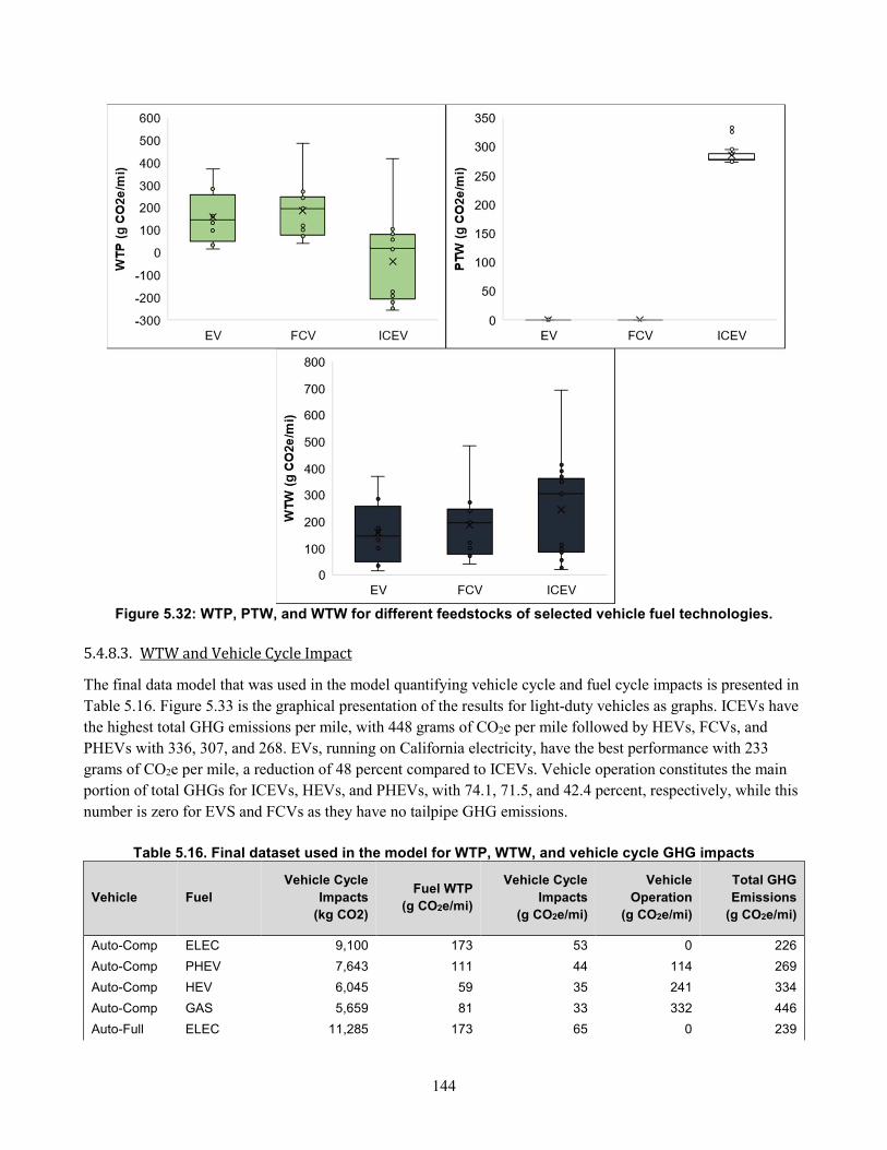
144

Figure 5.32: WTP, PTW, and WTW for different feedstocks of selected vehicle fuel technologies.

5.4.8.3. WTW and Vehicle Cycle Impact

The final data model that was used in the model quantifying vehicle cycle and fuel cycle impacts is presented in

Table 5.16. Figure 5.33 is the graphical presentation of the results for light-duty vehicles as graphs. ICEVs have

the highest total GHG emissions per mile, with 448 grams of CO2e per mile followed by HEVs, FCVs, and

PHEVs with 336, 307, and 268. EVs, running on California electricity, have the best performance with 233

grams of CO2e per mile, a reduction of 48 percent compared to ICEVs. Vehicle operation constitutes the main

portion of total GHGs for ICEVs, HEVs, and PHEVs, with 74.1, 71.5, and 42.4 percent, respectively, while this

number is zero for EVS and FCVs as they have no tailpipe GHG emissions.

Table 5.16. Final dataset used in the model for WTP, WTW, and vehicle cycle GHG impacts

Vehicle Fuel

Vehicle Cycle

Impacts

(kg CO2)

Fuel WTP

(g CO2e/mi)

Vehicle Cycle

Impacts

(g CO2e/mi)

Vehicle

Operation

(g CO2e/mi)

Total GHG

Emissions

(g CO2e/mi)

Auto-Comp ELEC 9,100 173 53 0 226

Auto-Comp PHEV 7,643 111 44 114 269

Auto-Comp HEV 6,045 59 35 241 334

Auto-Comp GAS 5,659 81 33 332 446

Auto-Full ELEC 11,285 173 65 0 239

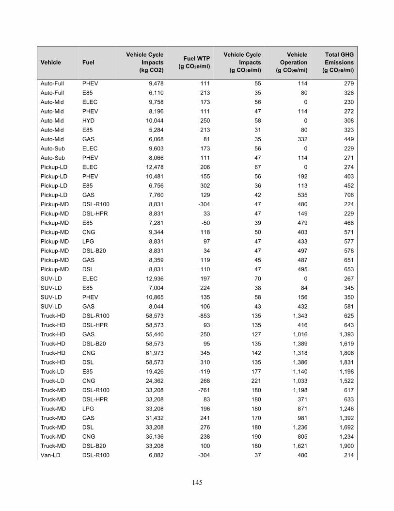
145

Vehicle Fuel

Vehicle Cycle

Impacts

(kg CO2)

Fuel WTP

(g CO2e/mi)

Vehicle Cycle

Impacts

(g CO2e/mi)

Vehicle

Operation

(g CO2e/mi)

Total GHG

Emissions

(g CO2e/mi)

Auto-Full PHEV 9,478 111 55 114 279

Auto-Full E85 6,110 213 35 80 328

Auto-Mid ELEC 9,758 173 56 0 230

Auto-Mid PHEV 8,196 111 47 114 272

Auto-Mid HYD 10,044 250 58 0 308

Auto-Mid E85 5,284 213 31 80 323

Auto-Mid GAS 6,068 81 35 332 449

Auto-Sub ELEC 9,603 173 56 0 229

Auto-Sub PHEV 8,066 111 47 114 271

Pickup-LD ELEC 12,478 206 67 0 274

Pickup-LD PHEV 10,481 155 56 192 403

Pickup-LD E85 6,756 302 36 113 452

Pickup-LD GAS 7,760 129 42 535 706

Pickup-MD DSL-R100 8,831 -304 47 480 224

Pickup-MD DSL-HPR 8,831 33 47 149 229

Pickup-MD E85 7,281 -50 39 479 468

Pickup-MD CNG 9,344 118 50 403 571

Pickup-MD LPG 8,831 97 47 433 577

Pickup-MD DSL-B20 8,831 34 47 497 578

Pickup-MD GAS 8,359 119 45 487 651

Pickup-MD DSL 8,831 110 47 495 653

SUV-LD ELEC 12,936 197 70 0 267

SUV-LD E85 7,004 224 38 84 345

SUV-LD PHEV 10,865 135 58 156 350

SUV-LD GAS 8,044 106 43 432 581

Truck-HD DSL-R100 58,573 -853 135 1,343 625

Truck-HD DSL-HPR 58,573 93 135 416 643

Truck-HD GAS 55,440 250 127 1,016 1,393

Truck-HD DSL-B20 58,573 95 135 1,389 1,619

Truck-HD CNG 61,973 345 142 1,318 1,806

Truck-HD DSL 58,573 310 135 1,386 1,831

Truck-LD E85 19,426 -119 177 1,140 1,198

Truck-LD CNG 24,362 268 221 1,033 1,522

Truck-MD DSL-R100 33,208 -761 180 1,198 617

Truck-MD DSL-HPR 33,208 83 180 371 633

Truck-MD LPG 33,208 196 180 871 1,246

Truck-MD GAS 31,432 241 170 981 1,392

Truck-MD DSL 33,208 276 180 1,236 1,692

Truck-MD CNG 35,136 238 190 805 1,234

Truck-MD DSL-B20 33,208 100 180 1,621 1,900

Van-LD DSL-R100 6,882 -304 37 480 214

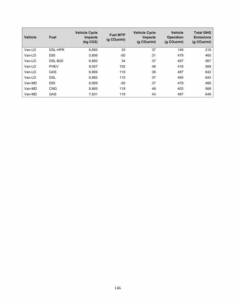
146

Vehicle Fuel

Vehicle Cycle

Impacts

(kg CO2)

Fuel WTP

(g CO2e/mi)

Vehicle Cycle

Impacts

(g CO2e/mi)

Vehicle

Operation

(g CO2e/mi)

Total GHG

Emissions

(g CO2e/mi)

Van-LD DSL-HPR 6,882 33 37 149 219

Van-LD E85 5,806 -50 31 479 460

Van-LD DSL-B20 6,882 34 37 497 567

Van-LD PHEV 9,007 102 48 418 569

Van-LD GAS 6,669 119 36 487 642

Van-LD DSL 6,882 110 37 495 643

Van-MD E85 6,909 -50 37 479 466

Van-MD CNG 8,865 118 48 403 568

Van-MD GAS 7,931 119 43 487 649

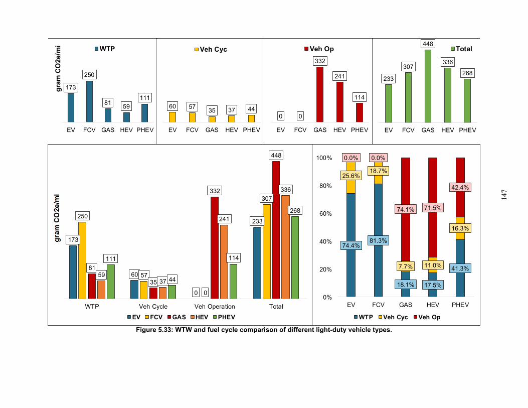
147

Figure 5.33: WTW and fuel cycle comparison of different light-duty vehicle types.

173

250

8159

111

EV FCV GAS HEV PHEV

gra

m C

O2

e/m

i

WTP

60 5735 37 44

EV FCV GAS HEV PHEV

Veh Cyc

0 0

332

241

114

EV FCV GAS HEV PHEV

Veh Op

233

307

448

336

268

EV FCV GAS HEV PHEV

Total

173

60

0

233250

57

0

307

81

35

332

448

5937

241

336

111

44

114

268

WTP Veh Cycle Veh Operation Total

GH

G E

mis

sio

ns (

g/m

ile

)

EV FCV GAS HEV PHEV

74.4%81.3%

18.1% 17.5%

41.3%

25.6%18.7%

7.7% 11.0%

16.3%

0.0% 0.0%

74.1% 71.5%

42.4%

0%

20%

40%

60%

80%

100%

EV FCV GAS HEV PHEV

WTP Veh Cyc Veh Op

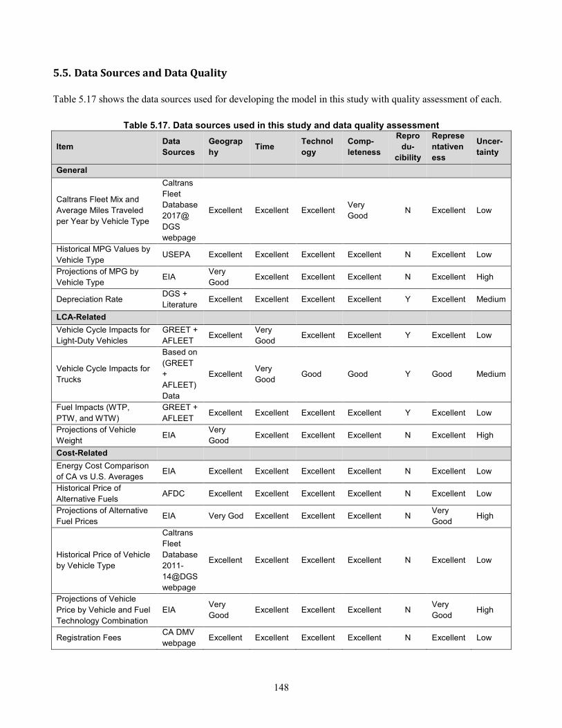
148

5.5. Data Sources and Data Quality

Table 5.17 shows the data sources used for developing the model in this study with quality assessment of each.

Table 5.17. Data sources used in this study and data quality assessment

Item Data

Sources

Geograp

hy Time

Technol

ogy

Comp-

leteness

Repro

du-

cibility

Represe

ntativen

ess

Uncer-

tainty

General

Caltrans Fleet Mix and Average Miles Traveled per Year by Vehicle Type

Caltrans Fleet Database 2017@

DGS webpage

Excellent Excellent Excellent Very Good

N Excellent Low

Historical MPG Values by Vehicle Type

USEPA Excellent Excellent Excellent Excellent N Excellent Low

Projections of MPG by Vehicle Type

EIA Very Good

Excellent Excellent Excellent N Excellent High

Depreciation Rate DGS + Literature

Excellent Excellent Excellent Excellent Y Excellent Medium

LCA-Related

Vehicle Cycle Impacts for Light-Duty Vehicles

GREET + AFLEET

Excellent Very Good

Excellent Excellent Y Excellent Low

Vehicle Cycle Impacts for Trucks

Based on

(GREET + AFLEET) Data

Excellent Very Good

Good Good Y Good Medium

Fuel Impacts (WTP,

PTW, and WTW)

GREET +

AFLEET Excellent Excellent Excellent Excellent Y Excellent Low

Projections of Vehicle Weight

EIA Very Good

Excellent Excellent Excellent N Excellent High

Cost-Related

Energy Cost Comparison of CA vs U.S. Averages

EIA Excellent Excellent Excellent Excellent N Excellent Low

Historical Price of Alternative Fuels

AFDC Excellent Excellent Excellent Excellent N Excellent Low

Projections of Alternative Fuel Prices

EIA Very God Excellent Excellent Excellent N Very Good

High

Historical Price of Vehicle by Vehicle Type

Caltrans Fleet

Database 2011-14@DGS webpage

Excellent Excellent Excellent Excellent N Excellent Low

Projections of Vehicle

Price by Vehicle and Fuel Technology Combination

EIA Very Good

Excellent Excellent Excellent N Very Good

High

Registration Fees CA DMV webpage

Excellent Excellent Excellent Excellent N Excellent Low

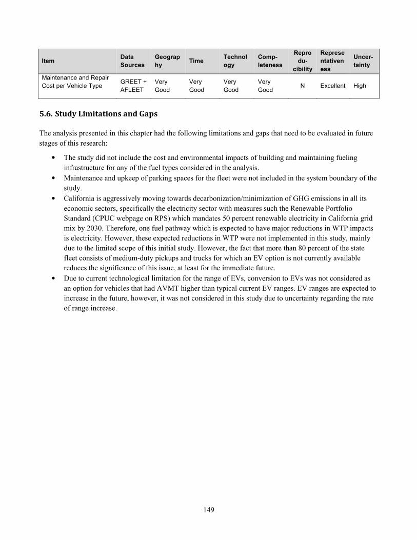
149

Item Data

Sources

Geograp

hy Time

Technol

ogy

Comp-

leteness

Repro

du-

cibility

Represe

ntativen

ess

Uncer-

tainty

Maintenance and Repair Cost per Vehicle Type

GREET +

AFLEET

Very

Good

Very

Good

Very

Good

Very

Good N Excellent High

5.6. Study Limitations and Gaps

The analysis presented in this chapter had the following limitations and gaps that need to be evaluated in future

stages of this research:

• The study did not include the cost and environmental impacts of building and maintaining fueling

infrastructure for any of the fuel types considered in the analysis.

• Maintenance and upkeep of parking spaces for the fleet were not included in the system boundary of the

study.

• California is aggressively moving towards decarbonization/minimization of GHG emissions in all its

economic sectors, specifically the electricity sector with measures such the Renewable Portfolio

Standard (CPUC webpage on RPS) which mandates 50 percent renewable electricity in California grid

mix by 2030. Therefore, one fuel pathway which is expected to have major reductions in WTP impacts

is electricity. However, these expected reductions in WTP were not implemented in this study, mainly

due to the limited scope of this initial study. However, the fact that more than 80 percent of the state

fleet consists of medium-duty pickups and trucks for which an EV option is not currently available

reduces the significance of this issue, at least for the immediate future.

• Due to current technological limitation for the range of EVs, conversion to EVs was not considered as

an option for vehicles that had AVMT higher than typical current EV ranges. EV ranges are expected to

increase in the future, however, it was not considered in this study due to uncertainty regarding the rate

of range increase.

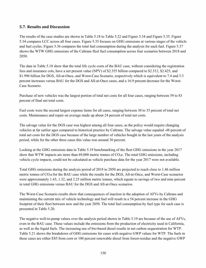
150

5.7. Results and Discussion

The results of the case studies are shown in Table 5.18 to Table 5.22 and Figure 5.34 and Figure 5.35. Figure

5.34 compares LCC across all four cases. Figure 5.35 focuses on GHG emissions at various stages of the vehicle

and fuel cycles. Figure 5.36 compares the total fuel consumption during the analysis for each fuel. Figure 5.37

shows the WTW GHG emissions of the Caltrans fleet fuel consumption across four scenarios between 2018 and

2050.

The data in Table 5.18 show that the total life cycle costs of the BAU case, without considering the registration

fees and insurance cots, have a net present value (NPV) of $2.355 billion compared to $2.512, $2.425, and

$1.996 billion for DGS, All-at-Once, and Worst-Case Scenario, respectively which is equivalent to 7.4 and 3.3

percent increases versus BAU for the DGS and All-at-Once cases, and a 16.9 percent decrease for the Worst-

Case Scenario.

Purchase of new vehicles was the largest portion of total net costs for all four cases, ranging between 59 to 83

percent of final net total costs.

Fuel costs were the second largest expense items for all cases, ranging between 30 to 35 percent of total net

costs. Maintenance and repair on average made up about 24 percent of total net costs.

The salvage value for the DGS case was highest among all four cases, as the policy would require changing

vehicles at far earlier ages compared to historical practice by Caltrans. The salvage value equaled -48 percent of

total net costs for the DGS case because of the large number of vehicles bought in the last years of the analysis

period, while for the other three cases this value was around 30 percent.

Looking at the GHG emissions data in Table 5.19 benchmarking of the fleet GHG emissions in the year 2017

show that WTW impacts are more than 69,000 metric tonnes of CO2e. The total GHG emissions, including

vehicle cycle impacts, could not be calculated as vehicle purchase data for the year 2017 were not available.

Total GHG emissions during the analysis period of 2018 to 2050 are projected to reach close to 1.46 million

metric tonnes of CO2e for the BAU case while the results for the DGS, All-at-Once, and Worst-Case scenarios

were approximately 1.43, 1.32, and 2.25 million metric tonnes, which equate to savings of two and nine percent

in total GHG emissions versus BAU for the DGS and All-at-Once scenarios.

The Worst-Case Scenario results show that consequences of inaction in the adoption of AFVs by Caltrans and

maintaining the current mix of vehicle technology and fuel will result in a 54 percent increase in the GHG

footprint of their fleet between now and the year 2050. The total fuel consumption by fuel type for each case is

presented in Table 5.20.

The negative well-to-pump values over the analysis period shown in Table 5.19 are because of the use of AFVs,

even in the BAU case. These values include the emissions from the production of electricity used in California,

as well as the liquid fuels. The increasing use of bio-based diesel results in net carbon sequestration for WTP.

Table 5.21 shows the breakdown of GHG emissions for cases with negative GWP values for WTP. The fuels in

these cases are either E85 from corn or 100 percent renewable diesel from forest-residue and the negative GWP

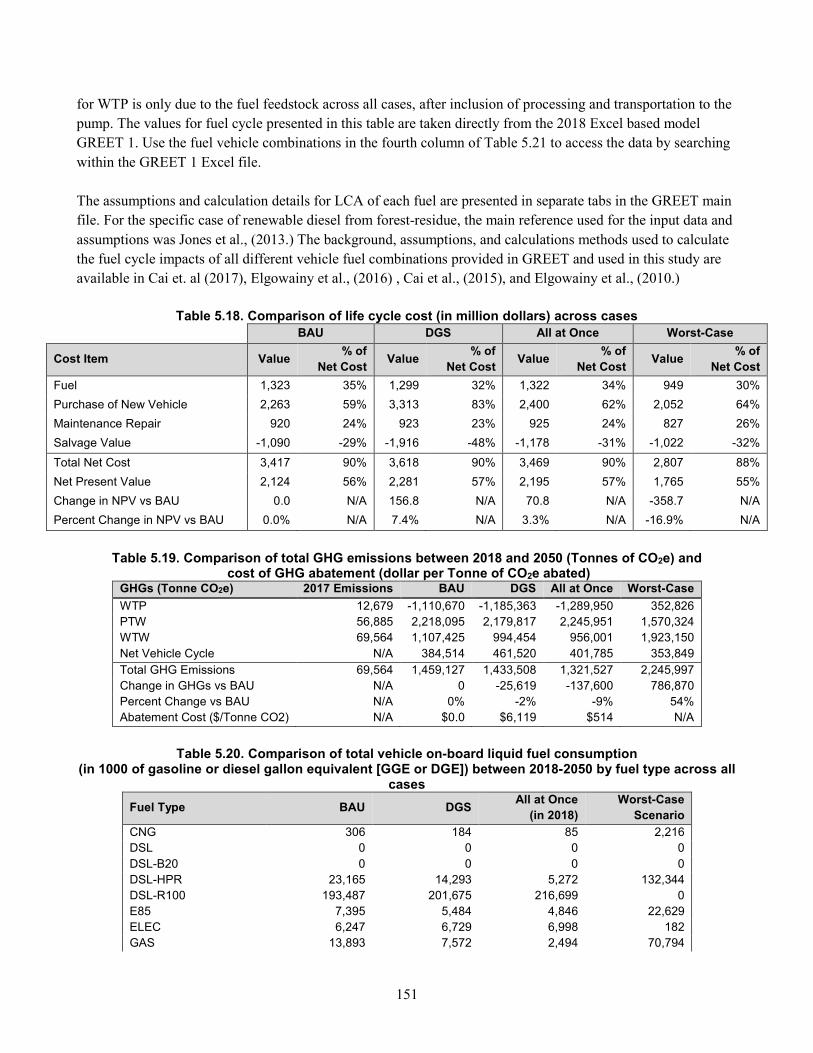
151

for WTP is only due to the fuel feedstock across all cases, after inclusion of processing and transportation to the

pump. The values for fuel cycle presented in this table are taken directly from the 2018 Excel based model

GREET 1. Use the fuel vehicle combinations in the fourth column of Table 5.21 to access the data by searching

within the GREET 1 Excel file.

The assumptions and calculation details for LCA of each fuel are presented in separate tabs in the GREET main

file. For the specific case of renewable diesel from forest-residue, the main reference used for the input data and

assumptions was Jones et al., (2013.) The background, assumptions, and calculations methods used to calculate

the fuel cycle impacts of all different vehicle fuel combinations provided in GREET and used in this study are

available in Cai et. al (2017), Elgowainy et al., (2016) , Cai et al., (2015), and Elgowainy et al., (2010.)

Table 5.18. Comparison of life cycle cost (in million dollars) across cases

BAU DGS All at Once Worst-Case

Cost Item Value % of

Net Cost Value

% of

Net Cost Value

% of

Net Cost Value

% of

Net Cost

Fuel 1,323 35% 1,299 32% 1,322 34% 949 30%

Purchase of New Vehicle 2,263 59% 3,313 83% 2,400 62% 2,052 64%

Maintenance Repair 920 24% 923 23% 925 24% 827 26%

Salvage Value -1,090 -29% -1,916 -48% -1,178 -31% -1,022 -32%

Total Net Cost 3,417 90% 3,618 90% 3,469 90% 2,807 88%

Net Present Value 2,124 56% 2,281 57% 2,195 57% 1,765 55%

Change in NPV vs BAU 0.0 N/A 156.8 N/A 70.8 N/A -358.7 N/A

Percent Change in NPV vs BAU 0.0% N/A 7.4% N/A 3.3% N/A -16.9% N/A

Table 5.19. Comparison of total GHG emissions between 2018 and 2050 (Tonnes of CO2e) and

cost of GHG abatement (dollar per Tonne of CO2e abated) GHGs (Tonne CO2e) 2017 Emissions BAU DGS All at Once Worst-Case

WTP 12,679 -1,110,670 -1,185,363 -1,289,950 352,826 PTW 56,885 2,218,095 2,179,817 2,245,951 1,570,324 WTW 69,564 1,107,425 994,454 956,001 1,923,150

Net Vehicle Cycle N/A 384,514 461,520 401,785 353,849

Total GHG Emissions 69,564 1,459,127 1,433,508 1,321,527 2,245,997 Change in GHGs vs BAU N/A 0 -25,619 -137,600 786,870 Percent Change vs BAU N/A 0% -2% -9% 54% Abatement Cost ($/Tonne CO2) N/A $0.0 $6,119 $514 N/A

Table 5.20. Comparison of total vehicle on-board liquid fuel consumption

(in 1000 of gasoline or diesel gallon equivalent [GGE or DGE]) between 2018-2050 by fuel type across all cases

Fuel Type BAU DGS All at Once

(in 2018)

Worst-Case

Scenario

CNG 306 184 85 2,216 DSL 0 0 0 0

DSL-B20 0 0 0 0 DSL-HPR 23,165 14,293 5,272 132,344 DSL-R100 193,487 201,675 216,699 0 E85 7,395 5,484 4,846 22,629 ELEC 6,247 6,729 6,998 182 GAS 13,893 7,572 2,494 70,794

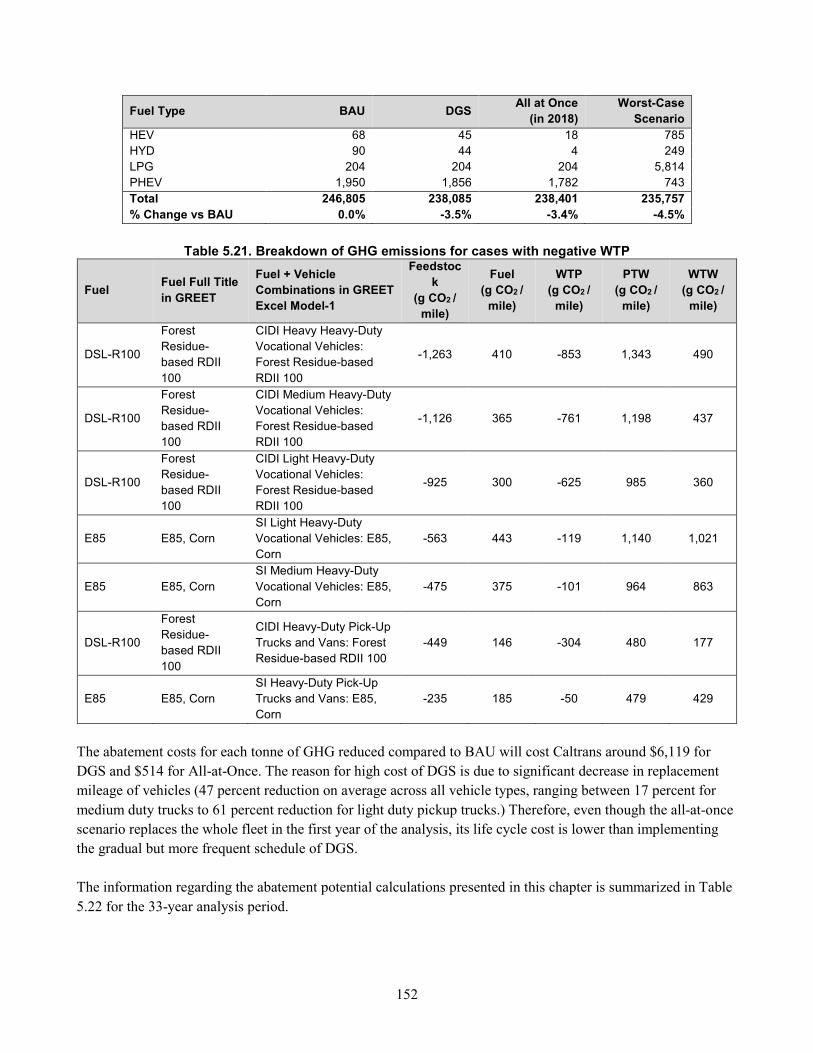
152

Fuel Type BAU DGS All at Once

(in 2018)

Worst-Case

Scenario

HEV 68 45 18 785 HYD 90 44 4 249 LPG 204 204 204 5,814 PHEV 1,950 1,856 1,782 743

Total 246,805 238,085 238,401 235,757

% Change vs BAU 0.0% -3.5% -3.4% -4.5%

Table 5.21. Breakdown of GHG emissions for cases with negative WTP

Fuel Fuel Full Title

in GREET

Fuel + Vehicle

Combinations in GREET

Excel Model-1

Feedstoc

k

(g CO2 /

mile)

Fuel

(g CO2 /

mile)

WTP

(g CO2 /

mile)

PTW

(g CO2 /

mile)

WTW

(g CO2 /

mile)

DSL-R100

Forest Residue-based RDII

100

CIDI Heavy Heavy-Duty Vocational Vehicles: Forest Residue-based

RDII 100

-1,263 410 -853 1,343 490

DSL-R100

Forest Residue-based RDII 100

CIDI Medium Heavy-Duty Vocational Vehicles: Forest Residue-based RDII 100

-1,126 365 -761 1,198 437

DSL-R100

Forest Residue-based RDII 100

CIDI Light Heavy-Duty Vocational Vehicles: Forest Residue-based RDII 100

-925 300 -625 985 360

E85 E85, Corn SI Light Heavy-Duty Vocational Vehicles: E85, Corn

-563 443 -119 1,140 1,021

E85 E85, Corn

SI Medium Heavy-Duty

Vocational Vehicles: E85, Corn

-475 375 -101 964 863

DSL-R100

Forest Residue-based RDII

100

CIDI Heavy-Duty Pick-Up Trucks and Vans: Forest Residue-based RDII 100

-449 146 -304 480 177

E85 E85, Corn SI Heavy-Duty Pick-Up Trucks and Vans: E85, Corn

-235 185 -50 479 429

The abatement costs for each tonne of GHG reduced compared to BAU will cost Caltrans around $6,119 for

DGS and $514 for All-at-Once. The reason for high cost of DGS is due to significant decrease in replacement

mileage of vehicles (47 percent reduction on average across all vehicle types, ranging between 17 percent for

medium duty trucks to 61 percent reduction for light duty pickup trucks.) Therefore, even though the all-at-once

scenario replaces the whole fleet in the first year of the analysis, its life cycle cost is lower than implementing

the gradual but more frequent schedule of DGS.

The information regarding the abatement potential calculations presented in this chapter is summarized in Table

5.22 for the 33-year analysis period.

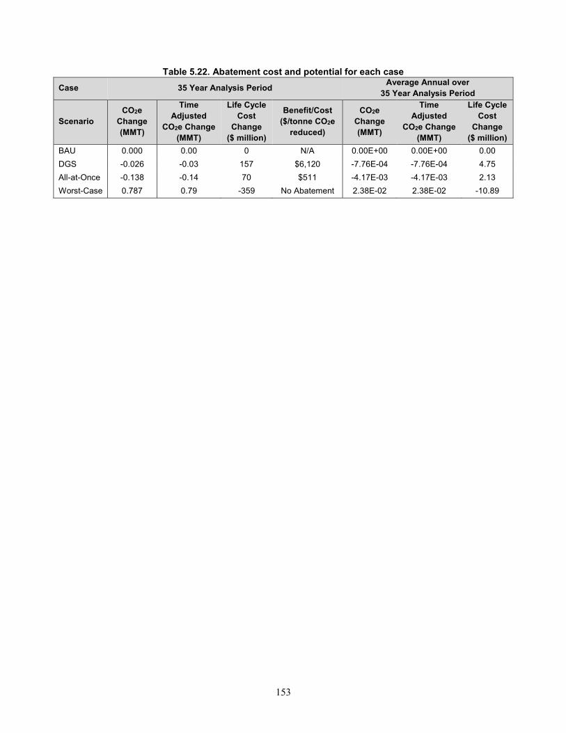
153

Table 5.22. Abatement cost and potential for each case

Case 35 Year Analysis Period Average Annual over

35 Year Analysis Period

Scenario

CO2e

Change

(MMT)

Time

Adjusted

CO2e Change

(MMT)

Life Cycle

Cost

Change

($ million)

Benefit/Cost

($/tonne CO2e

reduced)

CO2e

Change

(MMT)

Time

Adjusted

CO2e Change

(MMT)

Life Cycle

Cost

Change

($ million)

BAU 0.000 0.00 0 N/A 0.00E+00 0.00E+00 0.00

DGS -0.026 -0.03 157 $6,120 -7.76E-04 -7.76E-04 4.75

All-at-Once -0.138 -0.14 70 $511 -4.17E-03 -4.17E-03 2.13

Worst-Case 0.787 0.79 -359 No Abatement 2.38E-02 2.38E-02 -10.89

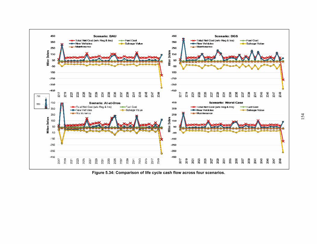
154

Figure 5.34: Comparison of life cycle cash flow across four scenarios.

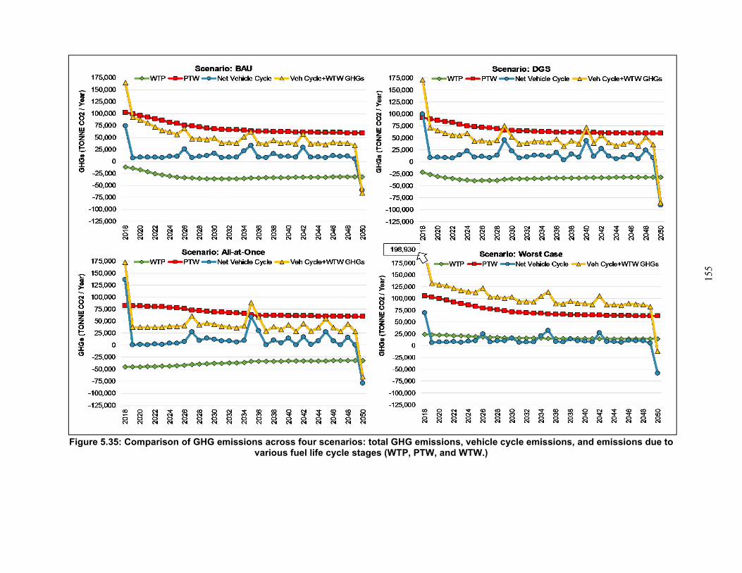
155

Figure 5.35: Comparison of GHG emissions across four scenarios: total GHG emissions, vehicle cycle emissions, and emissions due to various fuel life cycle stages (WTP, PTW, and WTW.)

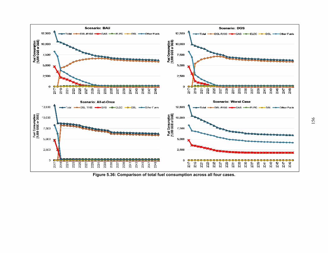
156

Figure 5.36: Comparison of total fuel consumption across all four cases.

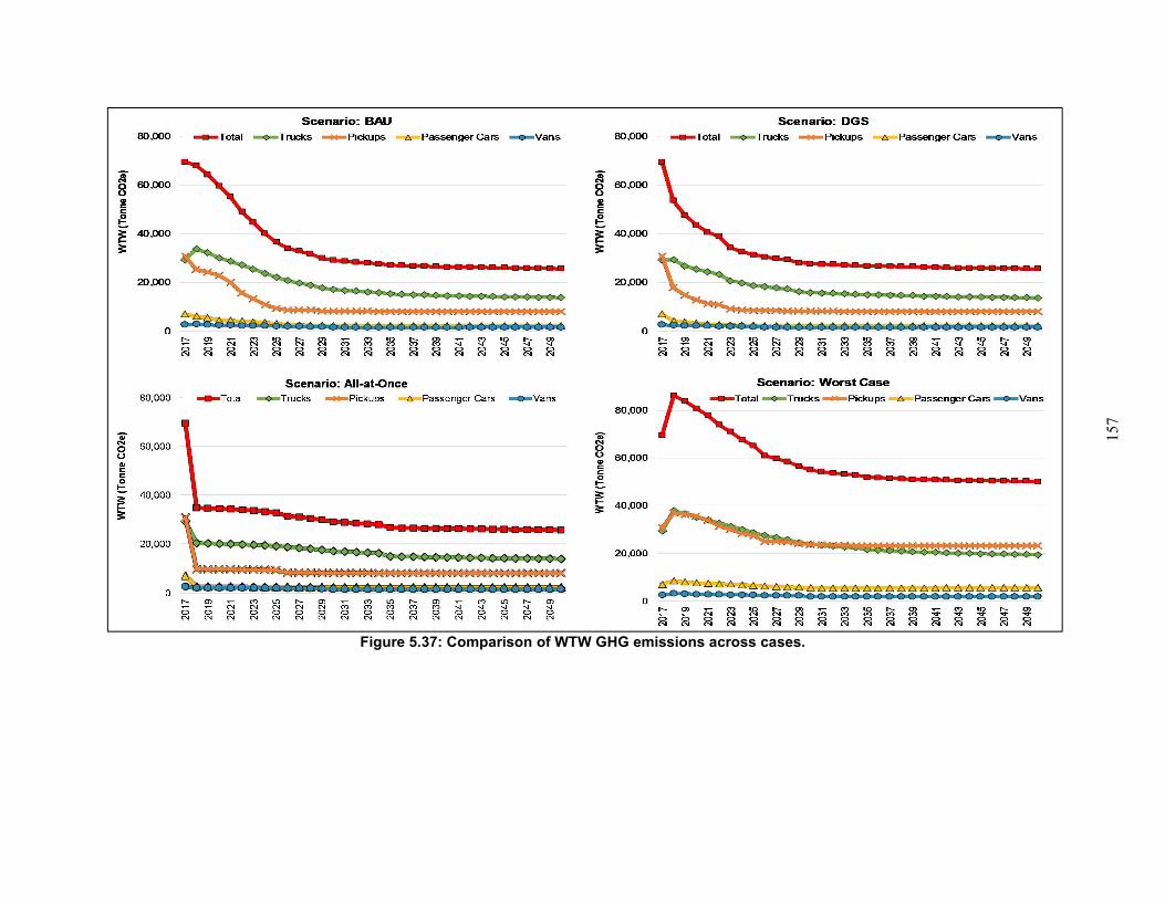
157

Figure 5.37: Comparison of WTW GHG emissions across cases.

158

CHAPTER 6. Evaluation of Increased Use of Reclaimed Asphalt

Pavement in Construction Projects Considering Costs and

Environmental Impacts

6.1. Introduction

Hot mix asphalt (HMA) is the surface type for approximately 75 percent of the state highway network and a

widely used structural material in a number of different pavement applications. Rubberized hot mix asphalt

(RHMA), which includes recycled used tires in the binder, is mandated for use for the surface layer of asphalt

pavements. Reclaimed asphalt pavement (RAP) is old HMA that is milled off of existing pavement and can be

used to partially replace virgin asphalt binder and aggregate in new HMA. RAP is not currently allowed in

RHMA because it reduces the cracking resistance of RHMA, which is a key factor in the current approach for

using RHMA as a surface material, and because the RAP binder displaces some of the waste tire rubber recycled

into RHMA. Caltrans must meet a legislative mandate for recycling waste tires in all kinds of hot mix asphalt.

Caltrans is currently developing technical approaches for increasing the percentage of RAP in HMA and

allowing some RAP in RHMA without reducing the performance of these materials. This chapter evaluates the

increased use of RAP in HMA compared with those from typical recent practice, without considering RHMA,

by calculating changes in environmental impacts and costs.

6.2. Background

Caltrans has allowed contractors to use up to 15 percent RAP (by weight) in HMA without any additional

engineering for a number of years (Caltrans, 2018c), which is considered as the baseline for this strategy in this

chapter. Up to 25 percent RAP was allowed in the past several years, however, the specifications called for a

very conservative approach to the engineering of the blended RAP/virgin binder and the use of expensive and

time consuming testing that also required the use of highly regulated solvents, all of which essentially

eliminated the use of more than 15 percent RAP. In 2018, the specifications were changed to allow up to 25

percent RAP without the need for the testing that was considered by industry to be onerous. Caltrans is working

on developing approaches to include approximately 40 percent RAP in HMA in the future, and to begin to use

up to 10 percent coarse RAP in RHMA. Coarse RAP consists of the larger particle sizes in the material and has

low binder content, with the result that this strategy would be to replace virgin aggregate with little or no

replacement of virgin binder. The use of RAP in RHMA was not considered in this study.

An important portion of Caltrans environmental impacts are due to projects awarded each year to contractors for

maintaining nearly 50,000 lane-miles of state highway pavement infrastructure in California. Additional

pavement infrastructure includes ramps, parking lots, turnouts, shoulders, rest areas, gore areas, drainage

facilities, dikes, and curbs. The purpose of this case study was to assess how much Caltrans can reduce the

environmental impacts due to the HMA materials used in these projects, specifically by increasing the amount

of RAP to replace virgin materials.

There are many different types of materials used in pavement projects; however, this chapter only focuses on the

increased use of recycled asphalt concrete in flexible pavements as a starting point. Similar evaluations should

159

also be conducted for other transportation infrastructure materials such as portland cement concrete, metals,

plastic polymers, and additives.

As noted, HMA and RHMA are used for the majority of the pavement surfaces in California (Caltrans 2015.)

The use of up to 15 percent RAP in asphalt is a mature and common practice across the nation. Asphalt surface

layers can be milled at the end of their service life and used as RAP in new construction or M and R activities by

blending it with virgin asphalt binder and aggregate to create new HMA, hence reducing virgin materials

(aggregate and binder) in the mix through replacement. The use of RAP provides cost savings to materials

producers. This is particularly true for the RAP binder which is much less expensive than virgin binder. The

replacement of part of the virgin binder in a new mix with aged asphalt binder left on RAP particles can be

allowed and obtain similar performance with a mix that has only virgin binder if the residual binder in RAP is

able to blend with the virgin binder in the new mix, and if the properties of blended binder are similar to those

the 100 percent virgin binder that would have been used otherwise.

RAP binder is stiffer and more brittle the specified virgin binder for a given climate region and application. The

properties of RAP binder vary considerably depending on the original properties it had before it was placed, the

amount of aging, and later processing. RAP piles at asphalt plants also have RAP from multiple locations. Even

if the RAP is milled from one location, it often has a mix of multiple asphalt layers placed over the years. RAP

should be processed to create greater uniformity before being used in new mixes. How to measure and engineer

the resultant properties of the blended binder, and also determine the degree of blending that occurs during

mixing, are the technological challenges to using higher percentages of RAP. Higher percentages of RAP often

require the use of a softer virgin binder for the portion of the total binder not replaced by the RAP binder and the

addition of softening additives, called rejuvenators, to facilitate blending of the aged and the virgin binders. It is

important that the mix containing the RAP have similar performance to a mix with virgin binder with respect to

fatigue and low-temperature cracking and rutting or else any cost and/or environmental benefits are in jeopardy.

6.3. Goal and Scope Definition

The goal of this study is to calculate how much reduction in GHG emissions can be achieved by increasing the

maximum RAP content in HMA mixes, going from 15, 25, 40, and 50 percent binder replacement, and scale

these calculations to the use of HMA on the state network in California. The scope of this study considers all the

impacts from materials extraction to transportation to plants, and all the processes conducted in the plant to

prepare the final mix. This is an example of an LCA with a cradle to gate scope. It was assumed that the

construction process and field performance of the mixes with higher RAP content is the same as the base

scenario. Therefore, the construction stage, use stage, and end-of-life were excluded from the scope of this

study. This assumption is not consistently valid and depends on the ability of the asphalt technology to adjust for

the RAP properties, which is considered in this study, but it is sufficiently valid for this first-order analysis.

The functional unit for this study is defined to be the California highway network. The analysis period

considered for this study is 33 years, from 2018 to 2050. Cost implications of these scenario changes were of

interest so that comparison with other reduction strategies would be possible.

160

6.4. Assumptions and Modeling Approach

The framework used for conducting this analysis is shown in Figure 6.1. A major part of the effort in this study

was spent on estimating the amount of materials used each year on the state highway network during the

analysis period. For this purpose, two options were considered:

• Material quantity estimates projected over the analysis period based on programmed work in the

Caltrans pavement management system (PaveM), or

• Projection of material quantities from historical data of construction projects published annually in the

Construction Cost Data Book.

PaveM is an asset management tool used for project prioritization, timing of future maintenance and

rehabilitation, and budget allocation. User inputs into PaveM include a multitude of decision-making factors

such as available budget, network characteristics (climate, traffic, dimensions), and agency decision trees that

trigger treatment based on current and predicted values of key performance indices such as cracking and surface

roughness for each segment in the network.

The output of PaveM is the type of treatment applied to each network segment, or “do nothing” for each year

during the analysis period within the defined budget limits. It also calculates the cost of each treatment applied.

The treatments for asphalt concrete are defined as thin, medium, and thick overlays, and provide an indication of

the thickness of the asphalt concrete treatment, which can be multiplied by the lane width and length of the

segment to get a volume. The volume can be converted to mass units typically used for asphalt materials, using

a typical density. The PaveM estimates will tend to be lower than the actual total amount of asphalt concrete

used by Caltrans because it only considers the lanes in the travelled way. It does not consider any paving on

shoulders, ramps, parking lots, gore areas, and other places where Caltrans uses this material.

The other approach would be to use the Contract Cost Data Book (Caltrans webpage on CCDB) which is

published annually by Caltrans. All the cost items of projects undertaken during the last fiscal year in Caltrans

projects are listed in the CCDB with the unit cost and the amount purchased across the year of each item,

regardless of where it was used. The CCDB can be used to estimate the amount of each material type used in

Caltrans projects in prior years and then use the historical data to project materials consumption in the future.

A PaveM run was conducted under the current default budgeting scenario which projected an expenditure of 267

million dollars in 2018 for asphalt paving materials. However, the data in the 2018 Construction Cost Data Book

(items 390132, 390135, 390136, 390137, 390401, 390402, 395020, and 395040) shows 545 million dollars in

the same year for the same items (Caltrans webpage on CCDB.) To address this discrepancy and calculate

material consumption in each year during the analysis period, the tonnages of materials from the CCDB 2018

were multiplied in all years after 2018 by the ratio of CCDB purchases in 2018 divided by the PaveM projected

purchases in 2018. This should account for the additional material used outside of the travelled way lanes. App-

Table 25 in Appendix V shows HMA and RHMA use in tonnes/year that was used in this study.

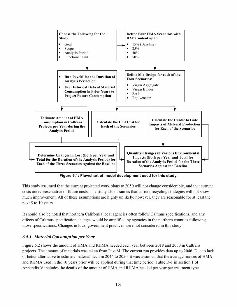
161

Define Four HMA Scenarios with

RAP Content up to:

• 15% (Baseline)• 25%• 40%• 50%

Define Mix Design for each of the

Four Scenarios:

• Virgin Aggregate• Virgin Binder • RAP • Rejuvenator

Calculate the Cradle to Gate

Impacts of Material Production

for Each of the Scenarios

Calculate the Unit Cost for

Each of the Scenarios

Estimate Amount of HMA

Consumption in Caltrans

Projects per Year during the

Analysis Period

Choose the Following for the

Study:

• Goal• Scope• Analysis Period • Functional Unit

• Run PaveM for the Duration of

Analysis Period, or

• Use Historical Data of Material

Consumption in Prior Years to

Project Future Consumption

Determine Changes in Cost (Both per Year and

Total for the Duration of the Analysis Period) for

Each of the Three Scenarios Against the Baseline

Quantify Changes in Various Environmental

Impacts (Both per Year and Total for

Duration of the Analysis Period for the Three

Scenarios Against the Baseline

Figure 6.1: Flowchart of model development used for this study.

This study assumed that the current projected work plans to 2050 will not change considerably, and that current

costs are representative of future costs. The study also assumes that current recycling strategies will not show

much improvement. All of these assumptions are highly unlikely; however, they are reasonable for at least the

next 5 to 10 years.

It should also be noted that northern California local agencies often follow Caltrans specifications, and any

effects of Caltrans specification changes would be amplified by agencies in the northern counties following

those specifications. Changes in local government practices were not considered in this study.

6.4.1. Material Consumption per Year

Figure 6.2 shows the amount of HMA and RHMA needed each year between 2018 and 2050 in Caltrans

projects. The amount of materials was taken from PaveM. The current run provides data up to 2046. Due to lack

of better alternative to estimate material need in 2046 to 2050, it was assumed that the average masses of HMA

and RHMA used in the 10 years prior will be applied during that time period. Table D-1 in section 1 of

Appendix V includes the details of the amount of HMA and RHMA needed per year per treatment type.

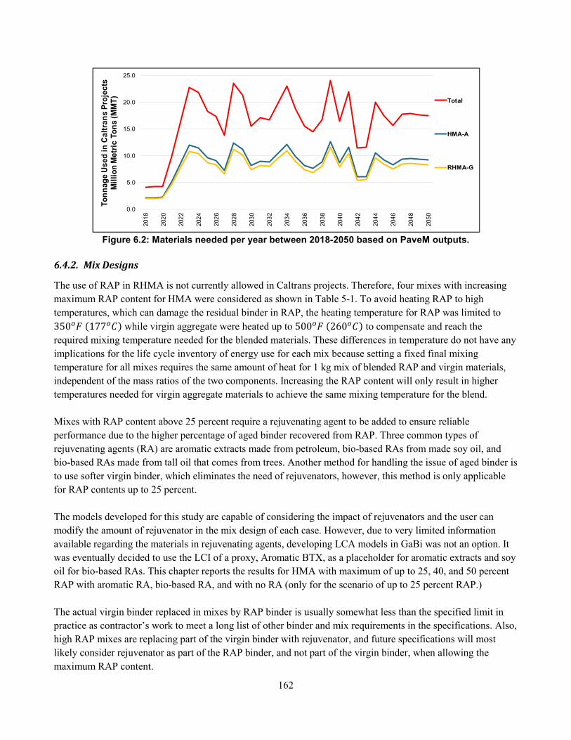
162

Figure 6.2: Materials needed per year between 2018-2050 based on PaveM outputs.

6.4.2. Mix Designs

The use of RAP in RHMA is not currently allowed in Caltrans projects. Therefore, four mixes with increasing

maximum RAP content for HMA were considered as shown in Table 5-1. To avoid heating RAP to high

temperatures, which can damage the residual binder in RAP, the heating temperature for RAP was limited to

350�� �177��� while virgin aggregate were heated up to 500�� �260��� to compensate and reach the

required mixing temperature needed for the blended materials. These differences in temperature do not have any

implications for the life cycle inventory of energy use for each mix because setting a fixed final mixing

temperature for all mixes requires the same amount of heat for 1 kg mix of blended RAP and virgin materials,

independent of the mass ratios of the two components. Increasing the RAP content will only result in higher

temperatures needed for virgin aggregate materials to achieve the same mixing temperature for the blend.

Mixes with RAP content above 25 percent require a rejuvenating agent to be added to ensure reliable

performance due to the higher percentage of aged binder recovered from RAP. Three common types of

rejuvenating agents (RA) are aromatic extracts made from petroleum, bio-based RAs from made soy oil, and

bio-based RAs made from tall oil that comes from trees. Another method for handling the issue of aged binder is

to use softer virgin binder, which eliminates the need of rejuvenators, however, this method is only applicable

for RAP contents up to 25 percent.

The models developed for this study are capable of considering the impact of rejuvenators and the user can

modify the amount of rejuvenator in the mix design of each case. However, due to very limited information

available regarding the materials in rejuvenating agents, developing LCA models in GaBi was not an option. It

was eventually decided to use the LCI of a proxy, Aromatic BTX, as a placeholder for aromatic extracts and soy

oil for bio-based RAs. This chapter reports the results for HMA with maximum of up to 25, 40, and 50 percent

RAP with aromatic RA, bio-based RA, and with no RA (only for the scenario of up to 25 percent RAP.)

The actual virgin binder replaced in mixes by RAP binder is usually somewhat less than the specified limit in

practice as contractor’s work to meet a long list of other binder and mix requirements in the specifications. Also,

high RAP mixes are replacing part of the virgin binder with rejuvenator, and future specifications will most

likely consider rejuvenator as part of the RAP binder, and not part of the virgin binder, when allowing the

maximum RAP content.

0.0

5.0

10.0

15.0

20.0

25.0

201

8

202

0

202

2

202

4

202

6

202

8

203

0

203

2

203

4

203

6

203

8

204

0

204

2

204

4

204

6

204

8

205

0

To

nn

ag

e U

se

d i

n C

alt

ran

s P

roje

cts

M

illi

on

Me

tric

To

ns

(M

MT

)

Total

HMA-A

RHMA-G

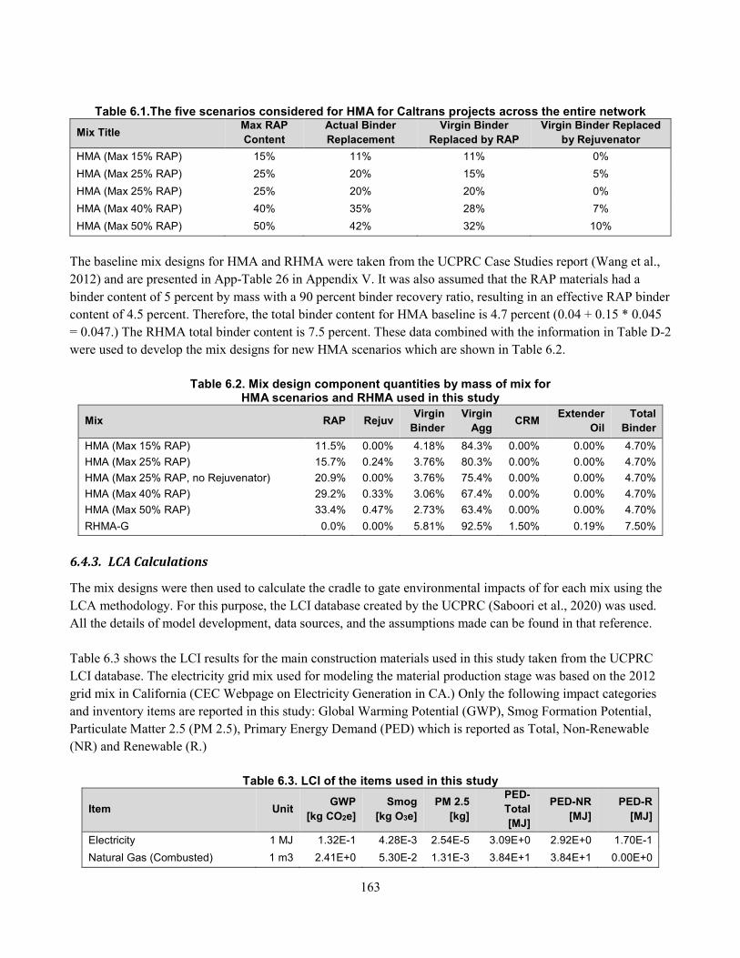
163

Table 6.1.The five scenarios considered for HMA for Caltrans projects across the entire network

Mix Title Max RAP

Content

Actual Binder

Replacement

Virgin Binder

Replaced by RAP

Virgin Binder Replaced

by Rejuvenator

HMA (Max 15% RAP) 15% 11% 11% 0%

HMA (Max 25% RAP) 25% 20% 15% 5%

HMA (Max 25% RAP) 25% 20% 20% 0%

HMA (Max 40% RAP) 40% 35% 28% 7%

HMA (Max 50% RAP) 50% 42% 32% 10%

The baseline mix designs for HMA and RHMA were taken from the UCPRC Case Studies report (Wang et al.,

2012) and are presented in App-Table 26 in Appendix V. It was also assumed that the RAP materials had a

binder content of 5 percent by mass with a 90 percent binder recovery ratio, resulting in an effective RAP binder

content of 4.5 percent. Therefore, the total binder content for HMA baseline is 4.7 percent (0.04 + 0.15 * 0.045

= 0.047.) The RHMA total binder content is 7.5 percent. These data combined with the information in Table D-2

were used to develop the mix designs for new HMA scenarios which are shown in Table 6.2.

Table 6.2. Mix design component quantities by mass of mix for

HMA scenarios and RHMA used in this study

Mix RAP Rejuv Virgin

Binder

Virgin

Agg CRM

Extender

Oil

Total

Binder

HMA (Max 15% RAP) 11.5% 0.00% 4.18% 84.3% 0.00% 0.00% 4.70%

HMA (Max 25% RAP) 15.7% 0.24% 3.76% 80.3% 0.00% 0.00% 4.70%

HMA (Max 25% RAP, no Rejuvenator) 20.9% 0.00% 3.76% 75.4% 0.00% 0.00% 4.70%

HMA (Max 40% RAP) 29.2% 0.33% 3.06% 67.4% 0.00% 0.00% 4.70%

HMA (Max 50% RAP) 33.4% 0.47% 2.73% 63.4% 0.00% 0.00% 4.70%

RHMA-G 0.0% 0.00% 5.81% 92.5% 1.50% 0.19% 7.50%

6.4.3. LCA Calculations

The mix designs were then used to calculate the cradle to gate environmental impacts of for each mix using the

LCA methodology. For this purpose, the LCI database created by the UCPRC (Saboori et al., 2020) was used.

All the details of model development, data sources, and the assumptions made can be found in that reference.

Table 6.3 shows the LCI results for the main construction materials used in this study taken from the UCPRC

LCI database. The electricity grid mix used for modeling the material production stage was based on the 2012

grid mix in California (CEC Webpage on Electricity Generation in CA.) Only the following impact categories

and inventory items are reported in this study: Global Warming Potential (GWP), Smog Formation Potential,

Particulate Matter 2.5 (PM 2.5), Primary Energy Demand (PED) which is reported as Total, Non-Renewable

(NR) and Renewable (R.)

Table 6.3. LCI of the items used in this study

Item Unit GWP

[kg CO2e]

Smog

[kg O3e]

PM 2.5

[kg]

PED-

Total

[MJ]

PED-NR

[MJ]

PED-R

[MJ]

Electricity 1 MJ 1.32E-1 4.28E-3 2.54E-5 3.09E+0 2.92E+0 1.70E-1

Natural Gas (Combusted) 1 m3 2.41E+0 5.30E-2 1.31E-3 3.84E+1 3.84E+1 0.00E+0

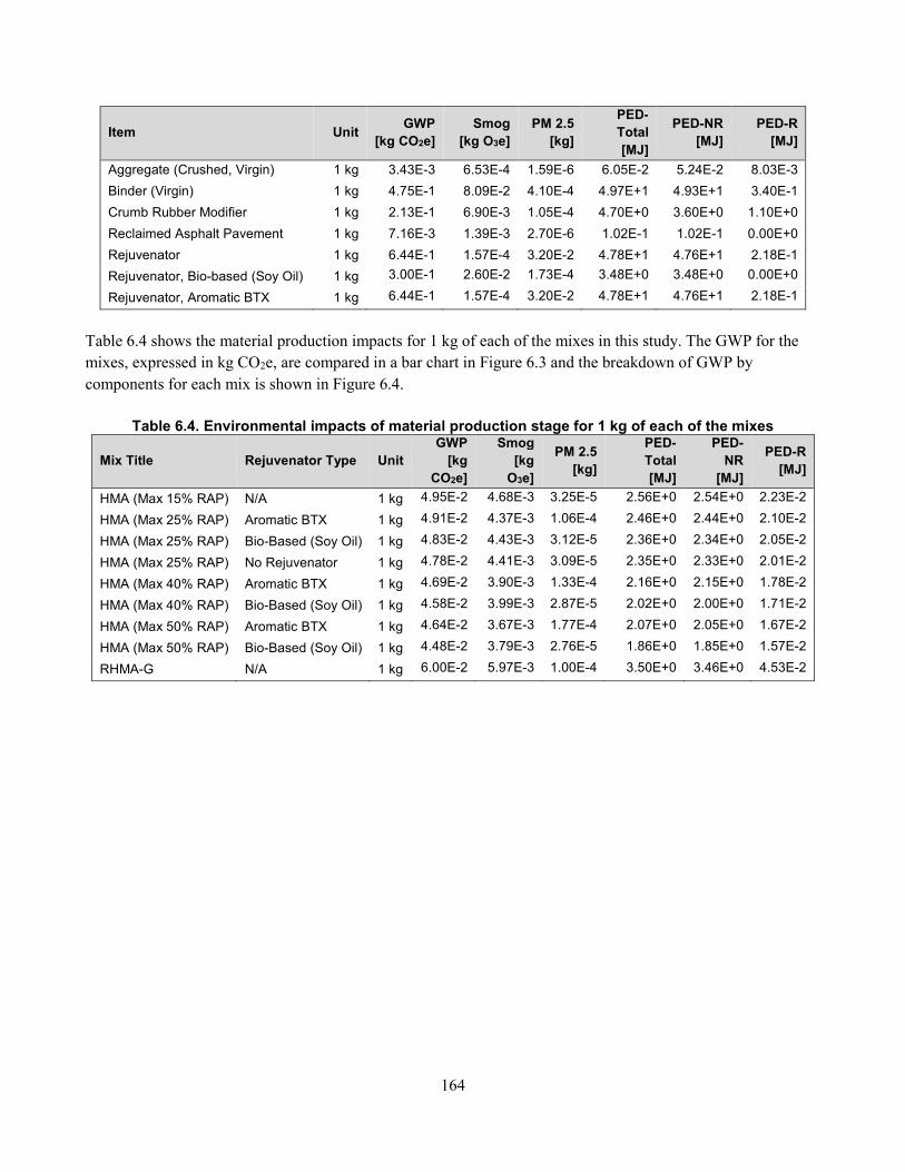
164

Item Unit GWP

[kg CO2e]

Smog

[kg O3e]

PM 2.5

[kg]

PED-

Total

[MJ]

PED-NR

[MJ]

PED-R

[MJ]

Aggregate (Crushed, Virgin) 1 kg 3.43E-3 6.53E-4 1.59E-6 6.05E-2 5.24E-2 8.03E-3

Binder (Virgin) 1 kg 4.75E-1 8.09E-2 4.10E-4 4.97E+1 4.93E+1 3.40E-1

Crumb Rubber Modifier 1 kg 2.13E-1 6.90E-3 1.05E-4 4.70E+0 3.60E+0 1.10E+0

Reclaimed Asphalt Pavement 1 kg 7.16E-3 1.39E-3 2.70E-6 1.02E-1 1.02E-1 0.00E+0

Rejuvenator 1 kg 6.44E-1 1.57E-4 3.20E-2 4.78E+1 4.76E+1 2.18E-1

Rejuvenator, Bio-based (Soy Oil) 1 kg 3.00E-1 2.60E-2 1.73E-4 3.48E+0 3.48E+0 0.00E+0

Rejuvenator, Aromatic BTX 1 kg 6.44E-1 1.57E-4 3.20E-2 4.78E+1 4.76E+1 2.18E-1

Table 6.4 shows the material production impacts for 1 kg of each of the mixes in this study. The GWP for the

mixes, expressed in kg CO2e, are compared in a bar chart in Figure 6.3 and the breakdown of GWP by

components for each mix is shown in Figure 6.4.

Table 6.4. Environmental impacts of material production stage for 1 kg of each of the mixes

Mix Title Rejuvenator Type Unit

GWP

[kg

CO2e]

Smog

[kg

O3e]

PM 2.5

[kg]

PED-

Total

[MJ]

PED-

NR

[MJ]

PED-R

[MJ]

HMA (Max 15% RAP) N/A 1 kg 4.95E-2 4.68E-3 3.25E-5 2.56E+0 2.54E+0 2.23E-2

HMA (Max 25% RAP) Aromatic BTX 1 kg 4.91E-2 4.37E-3 1.06E-4 2.46E+0 2.44E+0 2.10E-2

HMA (Max 25% RAP) Bio-Based (Soy Oil) 1 kg 4.83E-2 4.43E-3 3.12E-5 2.36E+0 2.34E+0 2.05E-2

HMA (Max 25% RAP) No Rejuvenator 1 kg 4.78E-2 4.41E-3 3.09E-5 2.35E+0 2.33E+0 2.01E-2

HMA (Max 40% RAP) Aromatic BTX 1 kg 4.69E-2 3.90E-3 1.33E-4 2.16E+0 2.15E+0 1.78E-2

HMA (Max 40% RAP) Bio-Based (Soy Oil) 1 kg 4.58E-2 3.99E-3 2.87E-5 2.02E+0 2.00E+0 1.71E-2

HMA (Max 50% RAP) Aromatic BTX 1 kg 4.64E-2 3.67E-3 1.77E-4 2.07E+0 2.05E+0 1.67E-2

HMA (Max 50% RAP) Bio-Based (Soy Oil) 1 kg 4.48E-2 3.79E-3 2.76E-5 1.86E+0 1.85E+0 1.57E-2

RHMA-G N/A 1 kg 6.00E-2 5.97E-3 1.00E-4 3.50E+0 3.46E+0 4.53E-2

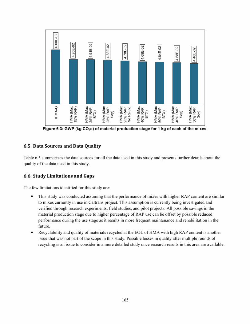
165

Figure 6.3: GWP (kg CO2e) of material production stage for 1 kg of each of the mixes.

6.5. Data Sources and Data Quality

Table 6.5 summarizes the data sources for all the data used in this study and presents further details about the

quality of the data used in this study.

6.6. Study Limitations and Gaps

The few limitations identified for this study are:

• This study was conducted assuming that the performance of mixes with higher RAP content are similar

to mixes currently in use in Caltrans project. This assumption is currently being investigated and

verified through research experiments, field studies, and pilot projects. All possible savings in the

material production stage due to higher percentage of RAP use can be offset by possible reduced

performance during the use stage as it results in more frequent maintenance and rehabilitation in the

future.

• Recyclability and quality of materials recycled at the EOL of HMA with high RAP content is another

issue that was not part of the scope in this study. Possible losses in quality after multiple rounds of

recycling is an issue to consider in a more detailed study once research results in this area are available.

6.0

0E

-02

4.9

5E

-02

4.9

1E

-02

4.8

3E

-02

4.7

8E

-02

4.6

9E

-02

4.6

4E

-02

4.5

8E

-02

4.4

8E

-02

RH

MA

-G

HM

A (

Ma

x15%

RA

P)

HM

A (

Ma

x25%

RA

P,

BT

X)

HM

A (

Ma

x25%

RA

P,

Soy)

HM

A (

Ma

x25%

RA

P,

No R

eju

v)

HM

A (

Ma

x40%

RA

P,

BT

X)

HM

A (

Ma

x50%

RA

P,

BT

X)

HM

A (

Ma

x40%

RA

P,

Soy)

HM

A (

Ma

x50%

RA

P,

Soy)

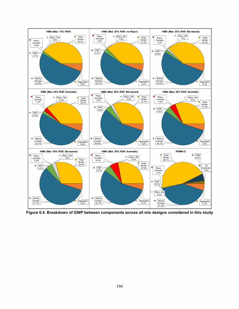
166

Figure 6.4. Breakdown of GWP between components across all mix designs considered in this study

Aggregate5.8%

Mixing Energy52.3%

RAP1.7%

Rejuv, Aromatic

0.0%

Rejuv, Bio0.0%

Virgin Binder40.2%

HMA (Max 15% RAP)

Aggregate5.4%

Mixing Energy54.1%

RAP3.1%

Rejuv, Aromatic

0.0%

Rejuv, Bio0.0%

Virgin Binder37.4%

HMA (Max 25% RAP, no Rejuv)

Aggregate5.7%

Mixing Energy53.5%

RAP2.3%

Rejuv, Aromatic

0.0%

Rejuv, Bio1.5% Virgin

Binder37.0%

HMA (Max 25% RAP, Bio-based)

Aggregate5.6%

Mixing Energy52.7%

RAP2.3%

Rejuv, Aromatic

3.1%

Rejuv, Bio0.0%

Virgin Binder36.4%

HMA (Max 25% RAP, Aromatic)

Aggregate5.0%

Mixing Energy56.5%

RAP4.6%

Rejuv, Aromatic

0.0%

Rejuv, Bio2.2%

Virgin Binder31.7%

HMA (Max 40% RAP, Bio-based)

Aggregate4.9%

Mixing Energy55.1%

RAP4.5%

Rejuv, Aromatic

4.5%

Rejuv, Bio0.0%

Virgin Binder31.0%

HMA (Max 40% RAP, Aromatic)

Aggregate4.9%

Mixing Energy57.7%

RAP5.3%

Rejuv, Aromatic

0.0%

Rejuv, Bio3.2%

Virgin Binder28.9%

HMA (Max 50% RAP, Bio-based)

Aggregate4.7%

Mixing Energy55.7%

RAP5.2%

Rejuv, Aromatic

6.5%

Rejuv, Bio0.0%

Virgin Binder27.9%

HMA (Max 50% RAP, Aromatic)

Aggregate5.3%

Mixing Energy41.3%

RAP0.0%

Rejuv, Aromatic

0.0%

Rejuv, Bio0.0%

Virgin Binder46.1%

CRM5.3%

Oil Extender

2.0%

RHMA-G

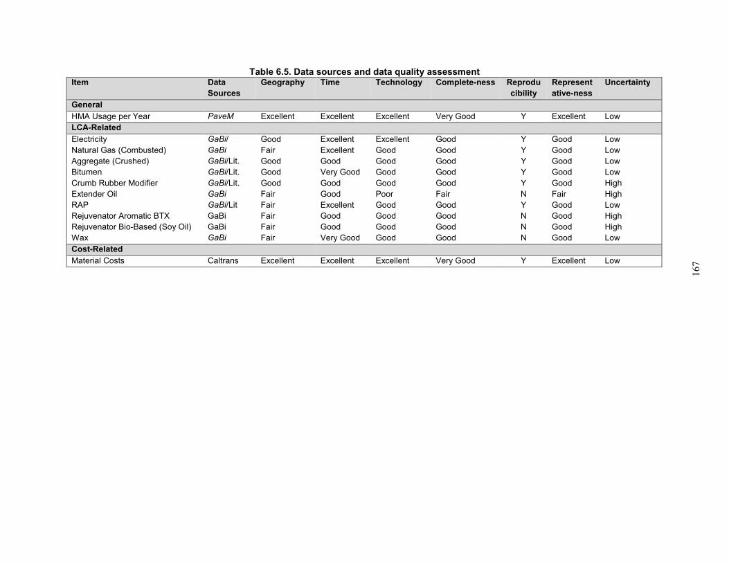
167

Table 6.5. Data sources and data quality assessment

Item Data

Sources

Geography Time Technology Complete-ness Reprodu

cibility

Represent

ative-ness

Uncertainty

General

HMA Usage per Year PaveM Excellent Excellent Excellent Very Good Y Excellent Low

LCA-Related

Electricity GaBi/ Good Excellent Excellent Good Y Good Low Natural Gas (Combusted) GaBi Fair Excellent Good Good Y Good Low Aggregate (Crushed) GaBi/Lit. Good Good Good Good Y Good Low Bitumen GaBi/Lit. Good Very Good Good Good Y Good Low Crumb Rubber Modifier GaBi/Lit. Good Good Good Good Y Good High Extender Oil GaBi Fair Good Poor Fair N Fair High RAP GaBi/Lit Fair Excellent Good Good Y Good Low Rejuvenator Aromatic BTX GaBi Fair Good Good Good N Good High Rejuvenator Bio-Based (Soy Oil) GaBi Fair Good Good Good N Good High Wax GaBi Fair Very Good Good Good N Good Low

Cost-Related

Material Costs Caltrans Excellent Excellent Excellent Very Good Y Excellent Low

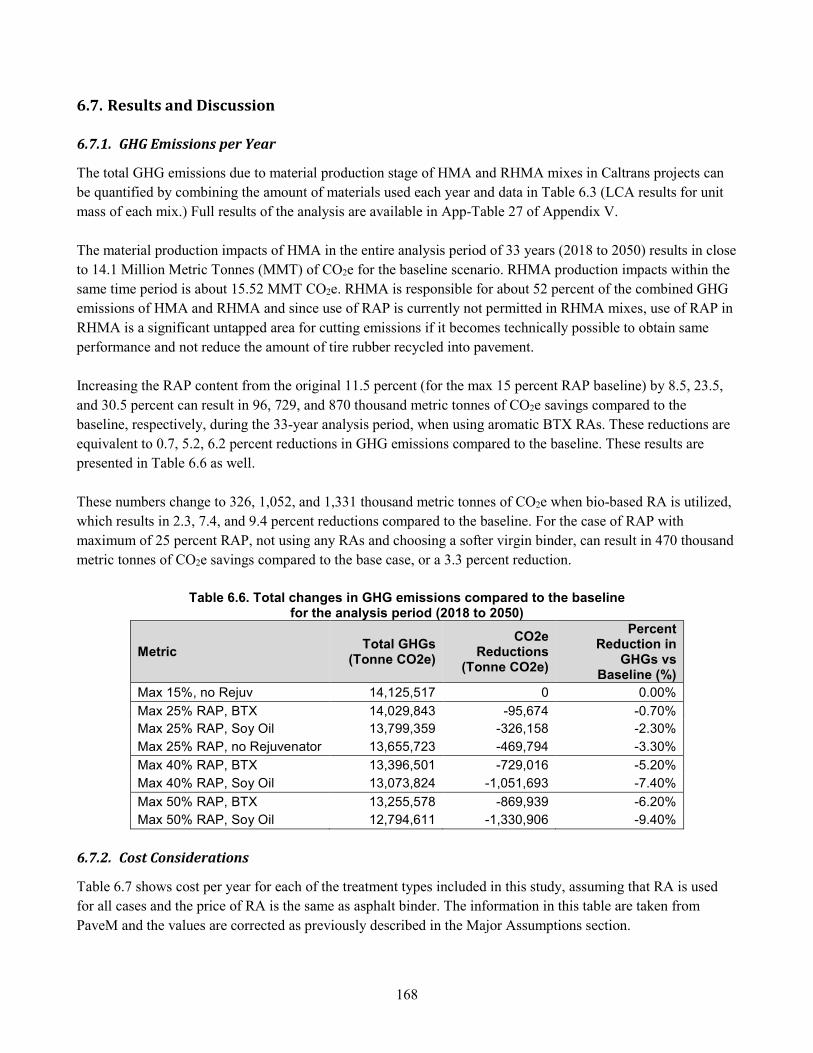
168

6.7. Results and Discussion

6.7.1. GHG Emissions per Year

The total GHG emissions due to material production stage of HMA and RHMA mixes in Caltrans projects can

be quantified by combining the amount of materials used each year and data in Table 6.3 (LCA results for unit

mass of each mix.) Full results of the analysis are available in App-Table 27 of Appendix V.

The material production impacts of HMA in the entire analysis period of 33 years (2018 to 2050) results in close

to 14.1 Million Metric Tonnes (MMT) of CO2e for the baseline scenario. RHMA production impacts within the

same time period is about 15.52 MMT CO2e. RHMA is responsible for about 52 percent of the combined GHG

emissions of HMA and RHMA and since use of RAP is currently not permitted in RHMA mixes, use of RAP in

RHMA is a significant untapped area for cutting emissions if it becomes technically possible to obtain same

performance and not reduce the amount of tire rubber recycled into pavement.

Increasing the RAP content from the original 11.5 percent (for the max 15 percent RAP baseline) by 8.5, 23.5,

and 30.5 percent can result in 96, 729, and 870 thousand metric tonnes of CO2e savings compared to the

baseline, respectively, during the 33-year analysis period, when using aromatic BTX RAs. These reductions are

equivalent to 0.7, 5.2, 6.2 percent reductions in GHG emissions compared to the baseline. These results are

presented in Table 6.6 as well.

These numbers change to 326, 1,052, and 1,331 thousand metric tonnes of CO2e when bio-based RA is utilized,

which results in 2.3, 7.4, and 9.4 percent reductions compared to the baseline. For the case of RAP with

maximum of 25 percent RAP, not using any RAs and choosing a softer virgin binder, can result in 470 thousand

metric tonnes of CO2e savings compared to the base case, or a 3.3 percent reduction.

Table 6.6. Total changes in GHG emissions compared to the baseline

for the analysis period (2018 to 2050)

Metric Total GHGs

(Tonne CO2e)

CO2e Reductions

(Tonne CO2e)

Percent Reduction in

GHGs vs Baseline (%)

Max 15%, no Rejuv 14,125,517 0 0.00%

Max 25% RAP, BTX 14,029,843 -95,674 -0.70%

Max 25% RAP, Soy Oil 13,799,359 -326,158 -2.30%

Max 25% RAP, no Rejuvenator 13,655,723 -469,794 -3.30%

Max 40% RAP, BTX 13,396,501 -729,016 -5.20%

Max 40% RAP, Soy Oil 13,073,824 -1,051,693 -7.40%

Max 50% RAP, BTX 13,255,578 -869,939 -6.20%

Max 50% RAP, Soy Oil 12,794,611 -1,330,906 -9.40%

6.7.2. Cost Considerations

Table 6.7 shows cost per year for each of the treatment types included in this study, assuming that RA is used

for all cases and the price of RA is the same as asphalt binder. The information in this table are taken from

PaveM and the values are corrected as previously described in the Major Assumptions section.

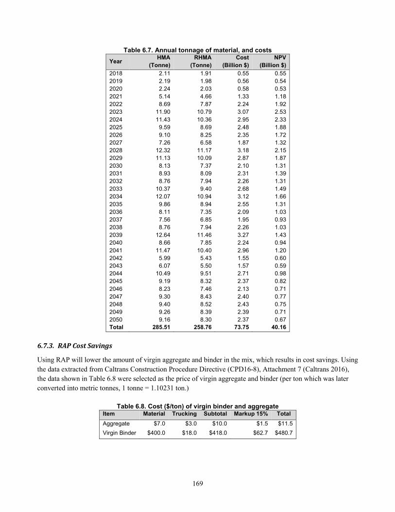
169

Table 6.7. Annual tonnage of material, and costs

Year HMA

(Tonne)

RHMA

(Tonne)

Cost

(Billion $)

NPV

(Billion $)

2018 2.11 1.91 0.55 0.55 2019 2.19 1.98 0.56 0.54 2020 2.24 2.03 0.58 0.53 2021 5.14 4.66 1.33 1.18 2022 8.69 7.87 2.24 1.92 2023 11.90 10.79 3.07 2.53

2024 11.43 10.36 2.95 2.33 2025 9.59 8.69 2.48 1.88 2026 9.10 8.25 2.35 1.72 2027 7.26 6.58 1.87 1.32 2028 12.32 11.17 3.18 2.15 2029 11.13 10.09 2.87 1.87

2030 8.13 7.37 2.10 1.31 2031 8.93 8.09 2.31 1.39 2032 8.76 7.94 2.26 1.31 2033 10.37 9.40 2.68 1.49 2034 12.07 10.94 3.12 1.66

2035 9.86 8.94 2.55 1.31 2036 8.11 7.35 2.09 1.03 2037 7.56 6.85 1.95 0.93 2038 8.76 7.94 2.26 1.03 2039 12.64 11.46 3.27 1.43 2040 8.66 7.85 2.24 0.94

2041 11.47 10.40 2.96 1.20 2042 5.99 5.43 1.55 0.60 2043 6.07 5.50 1.57 0.59 2044 10.49 9.51 2.71 0.98 2045 9.19 8.32 2.37 0.82

2046 8.23 7.46 2.13 0.71 2047 9.30 8.43 2.40 0.77 2048 9.40 8.52 2.43 0.75 2049 9.26 8.39 2.39 0.71 2050 9.16 8.30 2.37 0.67 Total 285.51 258.76 73.75 40.16

6.7.3. RAP Cost Savings

Using RAP will lower the amount of virgin aggregate and binder in the mix, which results in cost savings. Using

the data extracted from Caltrans Construction Procedure Directive (CPD16-8), Attachment 7 (Caltrans 2016),

the data shown in Table 6.8 were selected as the price of virgin aggregate and binder (per ton which was later

converted into metric tonnes, 1 tonne = 1.10231 ton.)

Table 6.8. Cost ($/ton) of virgin binder and aggregate

Item Material Trucking Subtotal Markup 15% Total

Aggregate $7.0 $3.0 $10.0 $1.5 $11.5

Virgin Binder $400.0 $18.0 $418.0 $62.7 $480.7

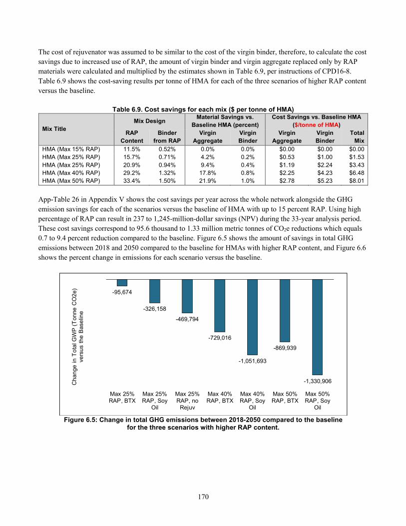
170

The cost of rejuvenator was assumed to be similar to the cost of the virgin binder, therefore, to calculate the cost

savings due to increased use of RAP, the amount of virgin binder and virgin aggregate replaced only by RAP

materials were calculated and multiplied by the estimates shown in Table 6.9, per instructions of CPD16-8.

Table 6.9 shows the cost-saving results per tonne of HMA for each of the three scenarios of higher RAP content

versus the baseline.

Table 6.9. Cost savings for each mix ($ per tonne of HMA)

Mix Title Mix Design

Material Savings vs.

Baseline HMA (percent)

Cost Savings vs. Baseline HMA

($/tonne of HMA)

RAP

Content

Binder

from RAP

Virgin

Aggregate

Virgin

Binder

Virgin

Aggregate

Virgin

Binder

Total

Mix

HMA (Max 15% RAP) 11.5% 0.52% 0.0% 0.0% $0.00 $0.00 $0.00 HMA (Max 25% RAP) 15.7% 0.71% 4.2% 0.2% $0.53 $1.00 $1.53

HMA (Max 25% RAP) 20.9% 0.94% 9.4% 0.4% $1.19 $2.24 $3.43 HMA (Max 40% RAP) 29.2% 1.32% 17.8% 0.8% $2.25 $4.23 $6.48 HMA (Max 50% RAP) 33.4% 1.50% 21.9% 1.0% $2.78 $5.23 $8.01

App-Table 26 in Appendix V shows the cost savings per year across the whole network alongside the GHG

emission savings for each of the scenarios versus the baseline of HMA with up to 15 percent RAP. Using high

percentage of RAP can result in 237 to 1,245-million-dollar savings (NPV) during the 33-year analysis period.

These cost savings correspond to 95.6 thousand to 1.33 million metric tonnes of CO2e reductions which equals

0.7 to 9.4 percent reduction compared to the baseline. Figure 6.5 shows the amount of savings in total GHG

emissions between 2018 and 2050 compared to the baseline for HMAs with higher RAP content, and Figure 6.6

shows the percent change in emissions for each scenario versus the baseline.

Figure 6.5: Change in total GHG emissions between 2018-2050 compared to the baseline for the three scenarios with higher RAP content.

-95,674

-326,158

-469,794

-729,016

-1,051,693

-869,939

-1,330,906

Max 25%RAP, BTX

Max 25%RAP, Soy

Oil

Max 25%RAP, no

Rejuv

Max 40%RAP, BTX

Max 40%RAP, Soy

Oil

Max 50%RAP, BTX

Max 50%RAP, Soy

Oil

Ch

an

ge

in T

ota

l GW

P (

Ton

ne

CO

2e)

vers

us

the

Base

line

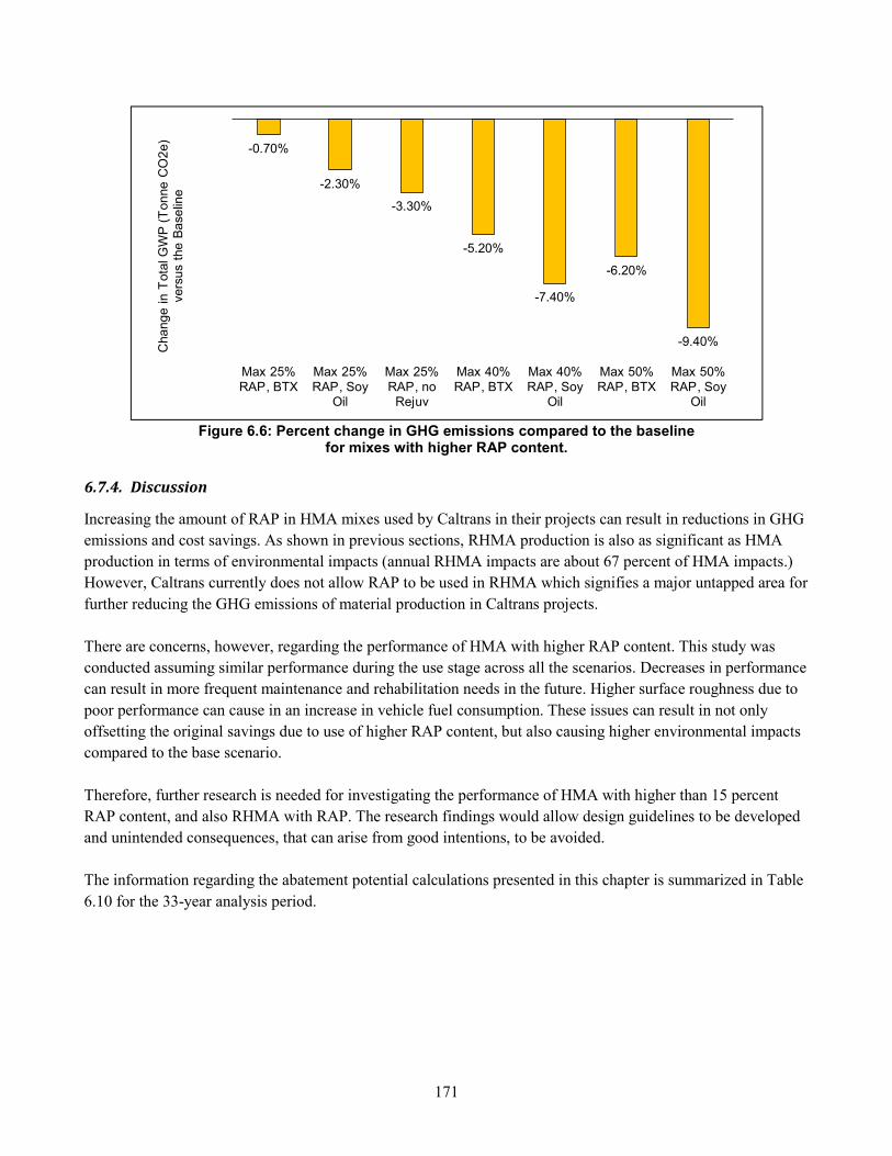
171

Figure 6.6: Percent change in GHG emissions compared to the baseline for mixes with higher RAP content.

6.7.4. Discussion

Increasing the amount of RAP in HMA mixes used by Caltrans in their projects can result in reductions in GHG

emissions and cost savings. As shown in previous sections, RHMA production is also as significant as HMA

production in terms of environmental impacts (annual RHMA impacts are about 67 percent of HMA impacts.)

However, Caltrans currently does not allow RAP to be used in RHMA which signifies a major untapped area for

further reducing the GHG emissions of material production in Caltrans projects.

There are concerns, however, regarding the performance of HMA with higher RAP content. This study was

conducted assuming similar performance during the use stage across all the scenarios. Decreases in performance

can result in more frequent maintenance and rehabilitation needs in the future. Higher surface roughness due to

poor performance can cause in an increase in vehicle fuel consumption. These issues can result in not only

offsetting the original savings due to use of higher RAP content, but also causing higher environmental impacts

compared to the base scenario.

Therefore, further research is needed for investigating the performance of HMA with higher than 15 percent

RAP content, and also RHMA with RAP. The research findings would allow design guidelines to be developed

and unintended consequences, that can arise from good intentions, to be avoided.

The information regarding the abatement potential calculations presented in this chapter is summarized in Table

6.10 for the 33-year analysis period.

-0.70%

-2.30%

-3.30%

-5.20%

-7.40%

-6.20%

-9.40%

Max 25%RAP, BTX

Max 25%RAP, Soy

Oil

Max 25%RAP, no

Rejuv

Max 40%RAP, BTX

Max 40%RAP, Soy

Oil

Max 50%RAP, BTX

Max 50%RAP, Soy

Oil

Cha

ng

e i

n T

ota

l GW

P (

Ton

ne

CO

2e)

vers

us

the B

ase

line

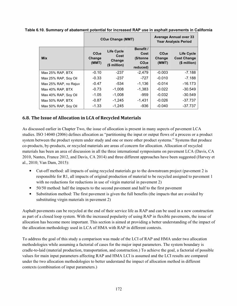
172

Table 6.10. Summary of abatement potential for increased RAP use in asphalt pavements in California

CO2e Change (MMT) Average Annual over 33

Year Analysis Period

Mix

CO2e

Change

(MMT)

Life Cycle

Cost

Change

($ million)

Benefit /

Cost

($/tonne

CO2e

reduced)

CO2e

Change

(MMT)

Life Cycle

Cost Change

($ million)

Max 25% RAP, BTX -0.10 -237 -2,479 -0.003 -7.188

Max 25% RAP, Soy Oil -0.33 -237 -727 -0.010 -7.188

Max 25% RAP, no Rejuv -0.47 -534 -1,136 -0.014 -16.173

Max 40% RAP, BTX -0.73 -1,008 -1,383 -0.022 -30.549

Max 40% RAP, Soy Oil -1.05 -1,008 -959 -0.032 -30.549

Max 50% RAP, BTX -0.87 -1,245 -1,431 -0.026 -37.737

Max 50% RAP, Soy Oil -1.33 -1,245 -936 -0.040 -37.737

6.8. The Issue of Allocation in LCA of Recycled Materials

As discussed earlier in Chapter Two, the issue of allocation is present in many aspects of pavement LCA

studies. ISO 14040 (2006) defines allocation as “partitioning the input or output flows of a process or a product

system between the product system under study and one or more other product systems.” Systems that produce

co-products, by-products, or recycled materials are areas of concern for allocation. Allocation of recycled

materials has been an area of discussion in all the three international symposiums on pavement LCA (Davis, CA

2010, Nantes, France 2012, and Davis, CA 2014) and three different approaches have been suggested (Harvey et

al., 2010; Van Dam, 2015):

• Cut-off method: all impacts of using recycled materials go to the downstream project (pavement 2 is

responsible for R1, all impacts of original production of material to be recycled assigned to pavement 1

with no reductions for reductions in use of virgin material in pavement 2)

• 50/50 method: half the impacts to the second pavement and half to the first pavement

• Substitution method: The first pavement is given the full benefits (the impacts that are avoided by

substituting virgin materials in pavement 2)

Asphalt pavements can be recycled at the end of their service life as RAP and can be used in a new construction

as part of a closed loop system. With the increased popularity of using RAP in flexible pavements, the issue of

allocation has become more important. This section is aimed at providing a better understanding of the impact of

the allocation methodology used in LCA of HMA with RAP in different contexts.

To address the goal of this study a comparison was made of the LCI of RAP and HMA under two allocation

methodologies while assuming a factorial of cases for the major input parameters. The system boundary is

cradle-to-laid (material production, transportation, and construction.) To achieve the goal, a factorial of possible

values for main input parameters affecting RAP and HMA LCI is assumed and the LCI results are compared

under the two allocation methodologies to better understand the impact of allocation method in different

contexts (combination of input parameters.)

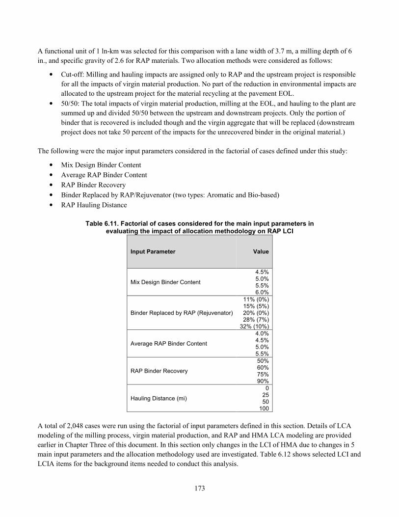
173

A functional unit of 1 ln-km was selected for this comparison with a lane width of 3.7 m, a milling depth of 6

in., and specific gravity of 2.6 for RAP materials. Two allocation methods were considered as follows:

• Cut-off: Milling and hauling impacts are assigned only to RAP and the upstream project is responsible

for all the impacts of virgin material production. No part of the reduction in environmental impacts are

allocated to the upstream project for the material recycling at the pavement EOL.

• 50/50: The total impacts of virgin material production, milling at the EOL, and hauling to the plant are

summed up and divided 50/50 between the upstream and downstream projects. Only the portion of

binder that is recovered is included though and the virgin aggregate that will be replaced (downstream

project does not take 50 percent of the impacts for the unrecovered binder in the original material.)

The following were the major input parameters considered in the factorial of cases defined under this study:

• Mix Design Binder Content

• Average RAP Binder Content

• RAP Binder Recovery

• Binder Replaced by RAP/Rejuvenator (two types: Aromatic and Bio-based)

• RAP Hauling Distance

Table 6.11. Factorial of cases considered for the main input parameters in

evaluating the impact of allocation methodology on RAP LCI

Input Parameter Value

Mix Design Binder Content

4.5% 5.0% 5.5% 6.0%

Binder Replaced by RAP (Rejuvenator)

11% (0%) 15% (5%) 20% (0%) 28% (7%)

32% (10%)

Average RAP Binder Content

4.0% 4.5% 5.0% 5.5%

RAP Binder Recovery

50% 60% 75% 90%

Hauling Distance (mi)

0 25 50

100

A total of 2,048 cases were run using the factorial of input parameters defined in this section. Details of LCA

modeling of the milling process, virgin material production, and RAP and HMA LCA modeling are provided

earlier in Chapter Three of this document. In this section only changes in the LCI of HMA due to changes in 5

main input parameters and the allocation methodology used are investigated. Table 6.12 shows selected LCI and

LCIA items for the background items needed to conduct this analysis.

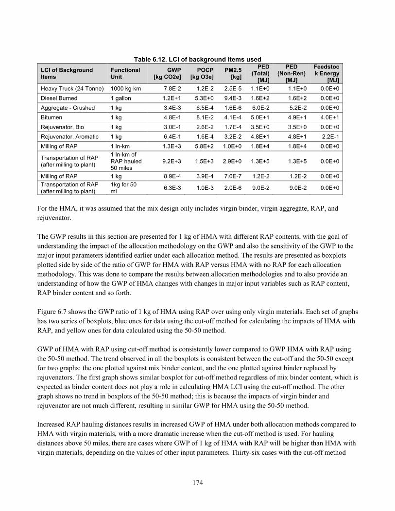
174

Table 6.12. LCI of background items used

LCI of Background Items

Functional Unit

GWP [kg CO2e]

POCP [kg O3e]

PM2.5 [kg]

PED (Total)

[MJ]

PED (Non-Ren)

[MJ]

Feedstock Energy

[MJ]

Heavy Truck (24 Tonne) 1000 kg-km 7.8E-2 1.2E-2 2.5E-5 1.1E+0 1.1E+0 0.0E+0

Diesel Burned 1 gallon 1.2E+1 5.3E+0 9.4E-3 1.6E+2 1.6E+2 0.0E+0

Aggregate - Crushed 1 kg 3.4E-3 6.5E-4 1.6E-6 6.0E-2 5.2E-2 0.0E+0

Bitumen 1 kg 4.8E-1 8.1E-2 4.1E-4 5.0E+1 4.9E+1 4.0E+1

Rejuvenator, Bio 1 kg 3.0E-1 2.6E-2 1.7E-4 3.5E+0 3.5E+0 0.0E+0

Rejuvenator, Aromatic 1 kg 6.4E-1 1.6E-4 3.2E-2 4.8E+1 4.8E+1 2.2E-1

Milling of RAP 1 ln-km 1.3E+3 5.8E+2 1.0E+0 1.8E+4 1.8E+4 0.0E+0

Transportation of RAP (after milling to plant)

1 ln-km of RAP hauled 50 miles

9.2E+3 1.5E+3 2.9E+0 1.3E+5 1.3E+5 0.0E+0

Milling of RAP 1 kg 8.9E-4 3.9E-4 7.0E-7 1.2E-2 1.2E-2 0.0E+0

Transportation of RAP (after milling to plant)

1kg for 50 mi

6.3E-3 1.0E-3 2.0E-6 9.0E-2 9.0E-2 0.0E+0

For the HMA, it was assumed that the mix design only includes virgin binder, virgin aggregate, RAP, and

rejuvenator.

The GWP results in this section are presented for 1 kg of HMA with different RAP contents, with the goal of

understanding the impact of the allocation methodology on the GWP and also the sensitivity of the GWP to the

major input parameters identified earlier under each allocation method. The results are presented as boxplots

plotted side by side of the ratio of GWP for HMA with RAP versus HMA with no RAP for each allocation

methodology. This was done to compare the results between allocation methodologies and to also provide an

understanding of how the GWP of HMA changes with changes in major input variables such as RAP content,

RAP binder content and so forth.

Figure 6.7 shows the GWP ratio of 1 kg of HMA using RAP over using only virgin materials. Each set of graphs

has two series of boxplots, blue ones for data using the cut-off method for calculating the impacts of HMA with

RAP, and yellow ones for data calculated using the 50-50 method.

GWP of HMA with RAP using cut-off method is consistently lower compared to GWP HMA with RAP using

the 50-50 method. The trend observed in all the boxplots is consistent between the cut-off and the 50-50 except

for two graphs: the one plotted against mix binder content, and the one plotted against binder replaced by

rejuvenators. The first graph shows similar boxplot for cut-off method regardless of mix binder content, which is

expected as binder content does not play a role in calculating HMA LCI using the cut-off method. The other

graph shows no trend in boxplots of the 50-50 method; this is because the impacts of virgin binder and

rejuvenator are not much different, resulting in similar GWP for HMA using the 50-50 method.

Increased RAP hauling distances results in increased GWP of HMA under both allocation methods compared to

HMA with virgin materials, with a more dramatic increase when the cut-off method is used. For hauling

distances above 50 miles, there are cases where GWP of 1 kg of HMA with RAP will be higher than HMA with

virgin materials, depending on the values of other input parameters. Thirty-six cases with the cut-off method

175

resulted in higher GWP for HMA with RAP versus HMA with virgin materials (GWP ratio of higher than one.)

The cases where the use of virgin materials results in less GWP compared to the use of RAP for the cut-off

method all have hauling distance of 100 miles with RAP binder recovery of 50 or 60 percent. The number of

these cases for the 50-50 method is 361 and for them, the following combinations of RAP binder recovery ratios

and hauling distance are observed: 75% + 100, 60% + 100, 50% + 100, 50% + 50, 50% + 25.

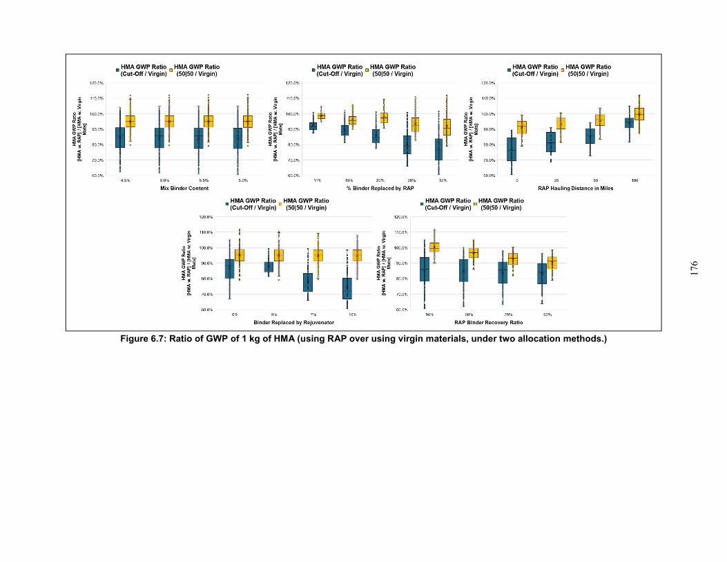
176

Figure 6.7: Ratio of GWP of 1 kg of HMA (using RAP over using virgin materials, under two allocation methods.)

177

CHAPTER 7. Cradle-to-Laid LCA Benchmarking and Comparison of

Currently Available Alternatives for End of Life Treatment for

Flexible Pavements in California

7.1. Introduction

Sustainability is an integral part of the Caltrans mission statement: “Provide a safe, sustainable, integrated, and

efficient transportation system to enhance California’s economy and livability” which has resulted in Caltrans

pursuing innovative materials and construction processes in their projects for many years. As pavements reach

their end-of-life (EOL), there are multiple options available and recycling has become increasingly popular due

to the general perception of recycling as a more sustainable alternative than other alternatives. This has also

been driven by cost considerations for virgin versus reclaimed asphalt binder, and virgin versus recycled

aggregate. Virgin aggregate has become scarcer in California near locations of greatest use which is another

contributing factor to the recent trends observed. It is widely believed that recycling will always lead to

significant environmental benefits, to the point that many pavement engineers exclusively associate the term

sustainability for pavements with recycling. Objective quantification of the environmental impacts of recycling

alternatives throughout their full life cycle is needed to have a better understanding of the performance of

different alternatives in terms of sustainability.

This chapter utilizes LCA methodology for benchmarking and comparison of the environmental impacts of the

current methods in practice for in-place recycling (IPR) or reclamation of flexible pavements at their EOL. The

methods considered in this study for in-place recycling are cold in-place (CIR) and full depth reclamation (FDR)

with different stabilizers and wearing courses on top of the recycled or reclaimed layer, and the primary current

practices of asphalt overlay and mill-and-fill (remove part of the asphalt and then overlay.)

In this chapter background information on in-place recycling methods for flexible pavements is presented

followed by the framework for conducting the “cradle-to-laid” LCA for each treatment. The framework is

described in detail including goal and scope definition, life cycle inventory development, impact assessment

methodology to use, followed by interpretation. The chapter is concluded with a summary of findings and

recommendations for the next stage of this study, which is development of performance models that are needed

for a full life cycle LCA comparison of alterative EOL options. Such an approach is needed for unbiased,

quantified, and objective decision-making which helps transportation planners avoid unintended consequences

and situations in which reducing emissions in construction stage results in such extra impacts during other life

cycle stages that the net result is worse than conventional options.

The main objectives of this chapter and the next are to:

• Develop models to quantify the environmental impacts of EOL alternatives for flexible pavements,

using the practice in California as the case study.

• Develop performance prediction models for sections built using in-place recycling techniques to

understand how their roughness and structural deterioration progress with time. These predictive models

for roughness and cracking are needed in the use stage to estimate fuel consumption in vehicles and

frequency of maintenance and rehabilitation based on cracking performance.

178

To achieve the project objectives, the following questions are addressed in this chapter:

• What are the environmental impacts of the EOL strategies for flexible pavements in California

considering only the material production, construction and EOL stages and without considering the use

stage performance?

• How much does each life cycle stage contribute to the total impacts (without considering the use stage)?

• How do current alternative EOL strategies for flexible pavements in California compare with each

other, in terms of cradle-to-laid impacts?

• How much does haul distance of materials contribute to the differences observed? What is the transport

distance for new materials (for FDR, CIR, and overlays) at which the different environmental impacts

are the same?

The following chapter on performance prediction models will address the following questions:

• How do sections built using IPR perform in the field? How quickly do cracks appear on the surface?

How does surface roughness vary with time under traffic?

• How do sections built using IPR and conventional strategies compare in terms field performance during

the use stage? Is the difference significant enough to warrant more frequent maintenance and

rehabilitation, resulting in more environmental impacts and costs?

7.2. Overview of In-Place Recycling of Flexible pavements

There are three different options available at the end of a flexible pavement’s service life, which can be applied

to either the entire pavement structure above the subgrade or layers within the structure:

• Removal of materials and disposal in landfills,

• Continued use (referred to here as reuse) in place as an underlying layer in its state at the end of life of

the pavement, or

• Pavement material recycling or reclamation either in place or at a recycling plant.

Recycling pavement materials (sometimes referred to as reclaiming depending on the technology), either in

place or at a plant from other projects and either full- or partial-depth, will displace use of virgin aggregates and

binders (particularly asphalt but others such as residual hydraulic cement as well) and therefore eliminate the

impacts of producing virgin materials. However, there are still emissions and energy consumption related to

demolition, processing, stabilization, and transportation of the recycled materials to an offsite processing plant

or transportation of stabilizing and additional virgin materials when recycling on site.

7.3. In-Place Recycling Technologies for Flexible Pavements

All in-place recycling technologies require that any drainage problems be addressed for the treatment to be

successful.

CIR is an in-place rehabilitation technique that is typically used when there is surface cracking, particularly top-

down cracking that has not proceeded all the way through the asphalt layers, and oxidation. It is not used for

heavily cracked pavement, pavement with deep moisture damage, or where the extensive cracks extend through

179

all asphalt layers. The CIR process includes milling the surface of the pavement, mixing the recycled material

with asphalt emulsion and often a small amount of cement, compacting it, and placing an asphalt overlay or a

chip seal as a wearing surface. The depth of asphalt pavement recycled with CIR is typically not less than 50

mm (2 in) or more than 100 mm (4 in) and there must be additional existing asphalt pavement below this depth

to support the milling machine, making CIR a partial-depth recycling process.

FDR is an in-place rehabilitation technique in which all the HMA layer and at least 0.17 ft (50 mm, 2 in) of the

base/sub-base materials are pulverized and an asphalt overlay, or a chip seal is placed as a wearing surface. FDR

is used where there is extensive cracking of the HMA, and the cracks extend through all the HMA layer. It is

also used where there is extensive delamination of the HMA layers and where there is extensive moisture

damage in the HMA. The pulverized materials are mixed with or without stabilizing agents and are graded,

placed, and compacted back in place providing an improved base layer before placing the wearing HMA overlay

or a surface treatment.

In some states, the term CIR includes all cold in-place recycling, including both partial-depth and full-depth. In

other states, such as California, the term CIR only refers to partial cold in-place recycling and the term CIR is

not applied to any FDR processes. In the remainder of this chapter, the term CIR is used to refer to partial-depth

recycling that is done in-place and leave some existing asphalt. FDR is used to refer to full-depth reclamation.

The benefits of in-place recycling, according to a study conducted by NCHRP in 2011, are as follows (Stroup-

Gardiner, 2011):

• Reduction in use of natural resources

• Elimination of materials generated for disposal or landfilling

• Reduction in fuel consumption primarily due to reduction in transportation of new materials

• Reduction in greenhouse gas

• Reduction in lane closure times

• Safety improvement by increasing friction, widening lanes, and eliminating overlay edge drop-off

• Reduction in costs of preservation, maintenance, and rehabilitation

• Improving base support with minimum overlay thickness

This section provides a review of the construction process and the materials used in each of the in-place

recycling techniques which serves as the basis of modeling the construction process in the next chapter for

estimating the environmental impacts.

7.3.1. Construction Processes and Materials for Cold In-Place Recycling

Figure 7.1 shows the construction process and the equipment used for a typical CIR project. The Asphalt

Recycling and Reclaiming Association (ARRA) recommends that the equipment used for CIR should be capable

of the following (ARRA, 2014):

• Milling of the existing roadway

• Sizing the resulting RAP

• Mixing the RAP with the stabilizer designated in the mix design, which are typically portland cement

and asphalt emulsion or foamed asphalt

180

• Meeting the required gradation and sizing with either the milling process or with additional sizing

equipment

• Producing a homogenous and uniformly coated mixture by mixing RAP and additives in the milling

machine or in an additional mixing chamber

• Placement and compaction according to the specifications

These requirements can be achieved through a set of equipment consisting of (not all the equipment may be

needed for every project):

• Pavement cold planer (milling machine) with a minimum 3.75 m (12.5 ft) cutter and a means for

controlling the depth of milling and the cross-slope or pulverization machine

• Crushing and sizing equipment

• Mixing and proportioning equipment

• Cement and asphalt emulsion or foamed asphalt storage and supply equipment

• Mixing and spreading equipment for dry cement

• Mixing and spreading equipment for corrective aggregate

• Paving equipment

• Water truck

• Broom truck

• Compaction equipment

• Fog sealing and sand spreading equipment

The construction process starts with roadway preparation in which the contractor should identify the location of

all utilities within the project site, clean and remove any dirt or obstacle, reference the profile and cross slope,

cold mill along cross walks and gutters to prepare for the final overlay, and correct all areas known to have soft

or yielding subgrades.

CIR construction is recommended to be allowed to proceed only when the RAP temperature is above 50°F

(10°C) and the previous overnight temperature was above 35°F (2°C.) A control strip with a minimum length of

1000 ft (300 m) should be constructed on the first day of the project to show that the construction process meets

the specifications. The optimal rates of stabilizer and the rolling pattern to achieve the optimum field density

should be identified from the control strip.

The existing pavement should be milled to the depth required by the plan or the specifications and the recycled

materials should be crushed and sized to the maximum particle size specified (ARRA, 2014.) The incorporation

of recycling additive or stabilizing agent can be in the form of applying mechanical, chemical, or bituminous

stabilizer or a combination of all. Mineral stabilization is defined as the addition of imported granular materials

to reach the desired characteristics in terms of gradation. Mechanical stabilization consists of compaction to

desired density, which improves stiffness, strength, rutting and fatigue properties, and decreases water

permeability. Chemical stabilization is achieved by adding one or a combination of portland cement, fly ash,

calcium chloride, magnesium chloride, and lime, with portland cement being the most commonly used chemical

stabilizer. These materials only stabilize if they create pozzolonic cementing action. Bituminous stabilization

consists of adding asphalt emulsion or foamed asphalt. Common practice in many states for partial-depth

recycling is to use a combination of bituminous stabilization with emulsions or more recently using foamed

181

asphalt and chemical stabilization. Mechanical stabilization in the form of compaction is used for all treatments,

and addition of imported granular materials is used if the existing in-place materials do not provide a

satisfactory gradation (Van Dam et al., 2015.) Cement or lime slurry may be directly added to the mixing

chamber or sprayer over the cutting teeth of the milling machine. If dry cement or corrective aggregate is

needed, it can be spread on the existing surface ahead of the milling operation (ARRA, 2014.) The CIR milling

and mixing process can be accomplished with a single-unit machine or a multi-unit train.

The placement of the recycled materials is conducted either with conventional asphalt pavers or cold mix

pavers, followed by compaction. The time between material placement and start of compaction is determined by

the contractor. Compaction (initial/breakdown, intermediate, and final compaction) is one of the main factors

affecting the future performance of the section. The type and number of compactors depend on many factors

such as the degree of compaction required, material properties of the pulverized mix, support capabilities of the

underlying layers, and the needed productivity. In general, the characteristics of the recycled mix determine the

type of roller needed and the thickness of the layer, and the required compaction dictates the weight, amplitude,

and frequency of the compactors. In any case, the contractor is responsible for determining the compaction plan

that meets the specified densities. The compaction should be monitored using nuclear density testing in

accordance with ASTM D2950, or the owner agency approved method (ARRA, 2014.)

For materials stabilized by chemical and bituminous materials, curing is a critical step and is needed to assure

that adequate strengths have been achieved for opening to traffic, prevent raveling, and facilitate placement of

the final wearing course. The curing rate depends on multiple factors, particularly if traditional asphalt

emulsions are used because the water that makes up 40 to 60 percent of the emulsion must be evaporated. The

factors affecting curing include the nature of the stabilization, temperature, humidity, moisture content of the

mix, compaction level, and drainage characteristics of the section and it is best to keep the traffic off the

pavement until sufficient curing has occurred to achieve adequate opening strengths.

For stabilization with traditional asphalt emulsions the curing period depends on the type and quality of the

agent, moisture content of the pulverized mix, mix level of compaction, aggregate characteristics, stabilizer

(cement or lime), and ambient conditions. The addition of cement along with asphalt emulsion helps provide

faster strength for earlier paving of the overlay and opening to traffic. ARRA (2014) states that for CIR a curing

period of at least 3 days and the moisture content of less than 3 percent should be required before proceeding to

secondary compaction or opening to traffic. ARRA recommends secondary compaction if the recycling agent is

emulsified asphalt with no chemical stabilizers added. If secondary compaction is planned, a separate rolling

pattern should be established during the control strip and the density of the recycled materials after secondary

compaction should be checked to verify compliance. ARRA suggests that secondary compaction be done with

pneumatic and double drum vibratory at temperatures above 80 °F (27 °C.) As materials are better understood

and contractors gain more experience, practice for local governments in many locations with light vehicles

moving at slow speeds is often to open within hours of construction, and to follow with re-compaction and

overlay several days later.

In the final step, a wearing course is usually laid on top. For low traffic roads, a single or double chip seal might

be enough but in sections with higher traffic levels, an HMA overlay is needed. The overlay thickness is

dependent on the specifics of the project, the agency’s policies, anticipated traffic, climate, economics,

stabilizing agent, and structural requirements. For HMA or Warm Mix Asphalt (WMA) overlays, ARRA

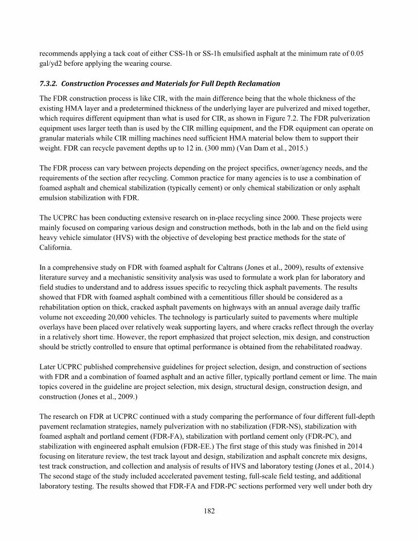
182

recommends applying a tack coat of either CSS-1h or SS-1h emulsified asphalt at the minimum rate of 0.05

gal/yd2 before applying the wearing course.

7.3.2. Construction Processes and Materials for Full Depth Reclamation

The FDR construction process is like CIR, with the main difference being that the whole thickness of the

existing HMA layer and a predetermined thickness of the underlying layer are pulverized and mixed together,

which requires different equipment than what is used for CIR, as shown in Figure 7.2. The FDR pulverization

equipment uses larger teeth than is used by the CIR milling equipment, and the FDR equipment can operate on

granular materials while CIR milling machines need sufficient HMA material below them to support their

weight. FDR can recycle pavement depths up to 12 in. (300 mm) (Van Dam et al., 2015.)

The FDR process can vary between projects depending on the project specifics, owner/agency needs, and the

requirements of the section after recycling. Common practice for many agencies is to use a combination of

foamed asphalt and chemical stabilization (typically cement) or only chemical stabilization or only asphalt

emulsion stabilization with FDR.

The UCPRC has been conducting extensive research on in-place recycling since 2000. These projects were

mainly focused on comparing various design and construction methods, both in the lab and on the field using

heavy vehicle simulator (HVS) with the objective of developing best practice methods for the state of

California.

In a comprehensive study on FDR with foamed asphalt for Caltrans (Jones et al., 2009), results of extensive

literature survey and a mechanistic sensitivity analysis was used to formulate a work plan for laboratory and

field studies to understand and to address issues specific to recycling thick asphalt pavements. The results

showed that FDR with foamed asphalt combined with a cementitious filler should be considered as a

rehabilitation option on thick, cracked asphalt pavements on highways with an annual average daily traffic

volume not exceeding 20,000 vehicles. The technology is particularly suited to pavements where multiple

overlays have been placed over relatively weak supporting layers, and where cracks reflect through the overlay

in a relatively short time. However, the report emphasized that project selection, mix design, and construction

should be strictly controlled to ensure that optimal performance is obtained from the rehabilitated roadway.

Later UCPRC published comprehensive guidelines for project selection, design, and construction of sections

with FDR and a combination of foamed asphalt and an active filler, typically portland cement or lime. The main

topics covered in the guideline are project selection, mix design, structural design, construction design, and

construction (Jones et al., 2009.)

The research on FDR at UCPRC continued with a study comparing the performance of four different full-depth

pavement reclamation strategies, namely pulverization with no stabilization (FDR-NS), stabilization with

foamed asphalt and portland cement (FDR-FA), stabilization with portland cement only (FDR-PC), and

stabilization with engineered asphalt emulsion (FDR-EE.) The first stage of this study was finished in 2014

focusing on literature review, the test track layout and design, stabilization and asphalt concrete mix designs,

test track construction, and collection and analysis of results of HVS and laboratory testing (Jones et al., 2014.)

The second stage of the study included accelerated pavement testing, full-scale field testing, and additional

laboratory testing. The results showed that FDR-FA and FDR-PC sections performed very well under both dry

183

and wet conditions. The FDR-NS sections tested performed acceptably. Due to problems associated with

construction, no conclusions could be drawn from the test results. Figure 7.3 shows the construction

methodology that was used in this study (Jones et al., 2016.)

7.4. Life Cycle Assessment Framework

This section summarizes the framework used for conducting LCA for each of the cases. First, the goal and scope

of the study is described and then the modeling effort for developing the life cycle inventory database is

explained in detail for each of the three life cycle stages. The models developed under this study and other LCA

efforts at UCPRC have undergone a 3rd party critical review according to the requirements of ISO 14040 (2006.)

The summary results for the LCI and LCIA for each stage are presented at the end of each section. The final

phase of LCA, the interpretation, is presented in the next chapter.

7.4.1. Goal and Scope Definition

The goal of this LCA study is to quantify the environmental impacts of the current EOL treatments in use for

flexible pavements through a benchmark study. The intended application is to provide an estimate of how

different alternatives perform in terms of the environmental impacts during material production, transportation,

construction, and the EOL of each section. As this range does not cover the full life cycle of the alternatives,

comparison between the LCA of treatments shall not be used as a basis for selecting between alternatives,

because without the performance models the number of maintenance and rehabilitation treatments needed for

each alternative during the use stage cannot be determined. For this stage of the study, attributional LCA was

conducted on a matrix of possible treatments for EOL of flexible pavements to identify the hot spots within the

cradle-to-laid period of each alternative. Table 7.1 shows the EOL treatments considered in this study.

Table 7.1. The EOL treatments considered in this study

Case # Description

Case 1 CIR (10 cm (0.33 ft) Milled + 1.5% FA + 1% PC) w. Chip Seal

Case 2 CIR (10 cm (0.33 ft) Milled + 3% FA + 2% PC) w. 2.5 cm (0.08 ft) of HMA OL

Case 3 FDR (25 cm (0.82 ft) Milled + Mech. Stab.) w. 6 cm (0.2 ft) RHMA OL

Case 4 FDR (25 cm (0.82 ft) Milled + 4% AE + 1% PC) w. 6 cm (0.2 ft) RHMA OL

Case 5 FDR (25 cm (0.82 ft) Milled + 3% FA + 1% PC) w. 6 cm (0.2 ft) RHMA OL

Case 6 FDR (25 cm (0.82 ft) Milled + 2% PC) w. 6 cm (0.2 ft) RHMA OL

Case 7 FDR (25 cm (0.82 ft) Milled + 4% PC) w. 6 cm (0.2 ft) RHMA OL

Case 8 FDR (25 cm (0.82 ft) Milled + 6% PC) w. 6 cm (0.2 ft) RHMA OL

Case 9 HMA Overlay (7.5cm (0.25 ft))

Case 10 HMA Mill & Fill (10 cm (0.33 ft)) AE: asphalt emulsion FA: foamed asphalt OL: overlay PC: portland cement RHMA: rubberized hot mix asphalt Stab.: stabilization

The location of use is limited to the state of California and the functional unit of the study is one ln-km of

pavement. The physical boundary only includes the main lanes and not the shoulders. As the system boundary

only includes material production and the construction stage, the analysis period is selected to be one year.

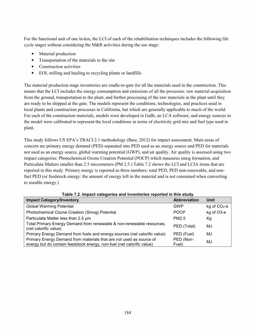
184

For the functional unit of one ln-km, the LCI of each of the rehabilitation techniques includes the following life

cycle stages without considering the M&R activities during the use stage:

• Material production

• Transportation of the materials to the site

• Construction activities

• EOL milling and hauling to recycling plants or landfills

The material production stage inventories are cradle-to-gate for all the materials used in the construction. This

means that the LCI includes the energy consumption and emissions of all the processes: raw material acquisition

from the ground, transportation to the plant, and further processing of the raw materials in the plant until they

are ready to be shipped at the gate. The models represent the conditions, technologies, and practices used in

local plants and construction processes in California, but which are generally applicable to much of the world.

For each of the construction materials, models were developed in GaBi, an LCA software, and energy sources in

the model were calibrated to represent the local conditions in terms of electricity grid mix and fuel type used in

plant.

This study follows US EPA’s TRACI 2.1 methodology (Bare, 2012) for impact assessment. Main areas of

concern are primary energy demand (PED) separated into PED used as an energy source and PED for materials

not used as an energy source, global warming potential (GWP), and air quality. Air quality is assessed using two

impact categories: Photochemical Ozone Creation Potential (POCP) which measures smog formation, and

Particulate Matters smaller than 2.5 micrometers (PM 2.5.) Table 7.2 shows the LCI and LCIA items that are

reported in this study. Primary energy is reported as three numbers: total PED, PED non-renewable, and non-

fuel PED (or feedstock energy: the amount of energy left in the material and is not consumed when converting

to useable energy.)

Table 7.2. Impact categories and inventories reported in this study

Impact Category/Inventory Abbreviation Unit

Global Warming Potential GWP kg of CO2-e

Photochemical Ozone Creation (Smog) Potential POCP kg of O3-e

Particulate Matter less than 2.5 µm PM2.5 Kg Total Primary Energy Demand from renewable & non-renewable resources, (net calorific value)

PED (Total) MJ

Primary Energy Demand from fuels and energy sources (net calorific value) PED (Fuel) MJ Primary Energy Demand from materials that are not used as source of energy but do contain feedstock energy, non-fuel (net calorific value)

PED (Non-Fuel)

MJ

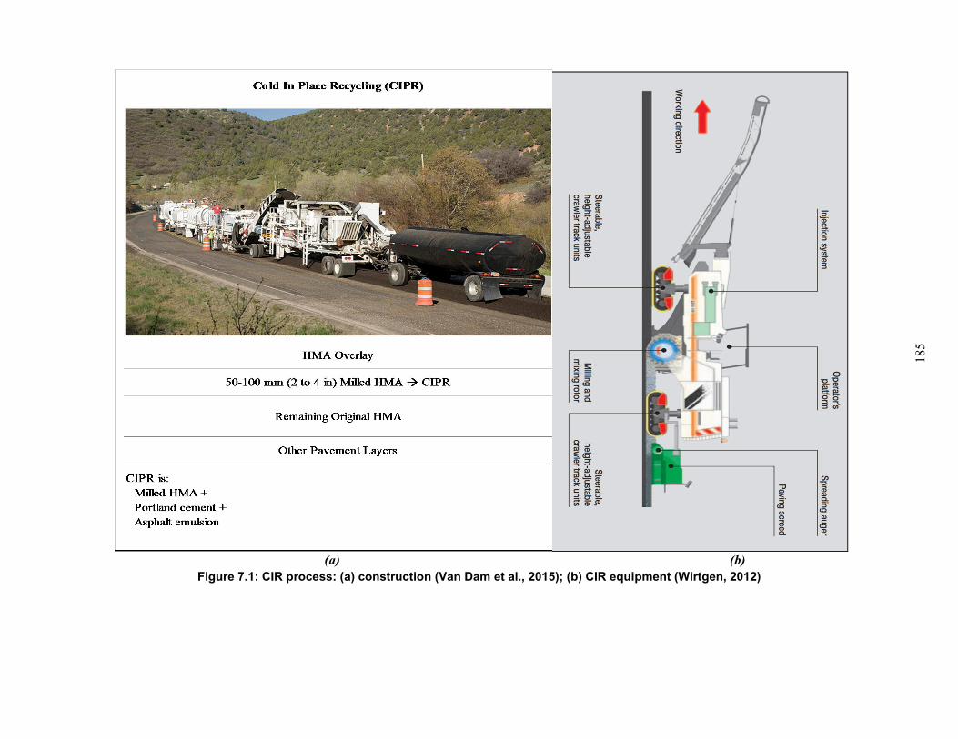
185

(a)

(b)

Figure 7.1: CIR process: (a) construction (Van Dam et al., 2015); (b) CIR equipment (Wirtgen, 2012)

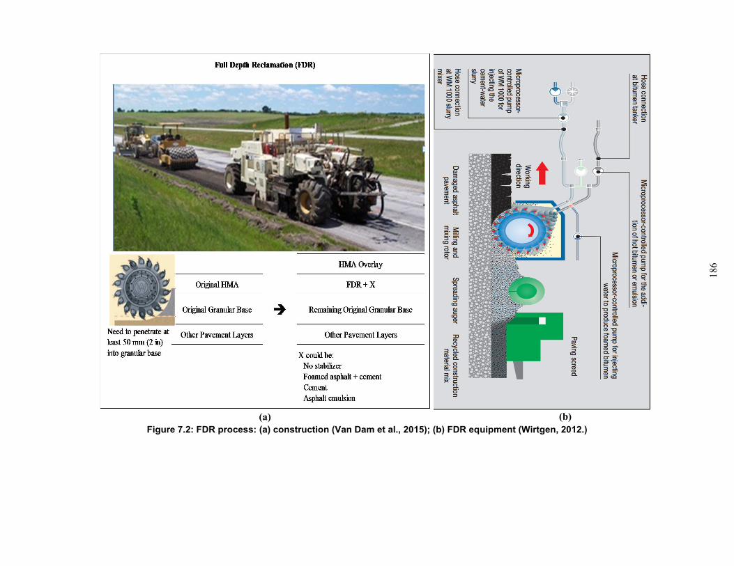
186

(a)

(b)

Figure 7.2: FDR process: (a) construction (Van Dam et al., 2015); (b) FDR equipment (Wirtgen, 2012.)

187

Figure 7.3: FDR+FA construction process in the field (Jones et al., 2016.) The process consists of: (1) Spreading cement on old asphalt surface; (2) Recycling train; (3) Uniform mix behind; (4) Padfoot roller compaction on uniform mix; (5) Steel wheel compaction showing tightly

bound surface; (6) Final compaction.

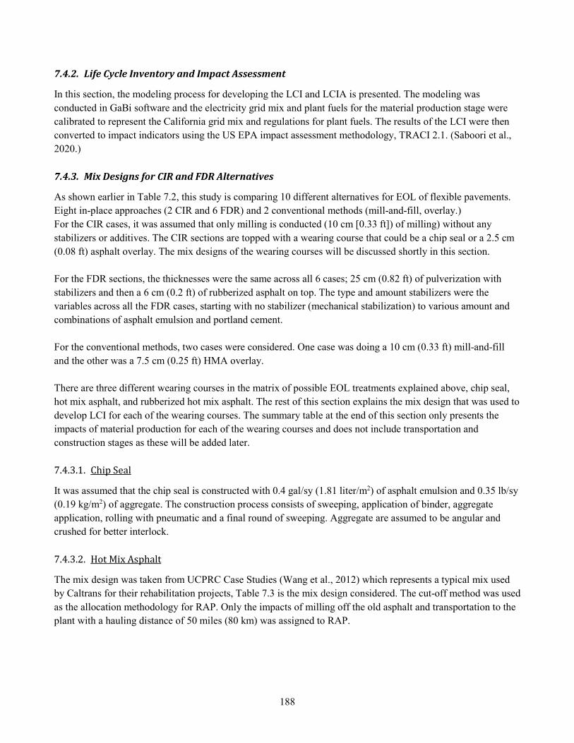
188

7.4.2. Life Cycle Inventory and Impact Assessment

In this section, the modeling process for developing the LCI and LCIA is presented. The modeling was

conducted in GaBi software and the electricity grid mix and plant fuels for the material production stage were

calibrated to represent the California grid mix and regulations for plant fuels. The results of the LCI were then

converted to impact indicators using the US EPA impact assessment methodology, TRACI 2.1. (Saboori et al.,

2020.)

7.4.3. Mix Designs for CIR and FDR Alternatives

As shown earlier in Table 7.2, this study is comparing 10 different alternatives for EOL of flexible pavements.

Eight in-place approaches (2 CIR and 6 FDR) and 2 conventional methods (mill-and-fill, overlay.)

For the CIR cases, it was assumed that only milling is conducted (10 cm [0.33 ft]) of milling) without any

stabilizers or additives. The CIR sections are topped with a wearing course that could be a chip seal or a 2.5 cm

(0.08 ft) asphalt overlay. The mix designs of the wearing courses will be discussed shortly in this section.

For the FDR sections, the thicknesses were the same across all 6 cases; 25 cm (0.82 ft) of pulverization with

stabilizers and then a 6 cm (0.2 ft) of rubberized asphalt on top. The type and amount stabilizers were the

variables across all the FDR cases, starting with no stabilizer (mechanical stabilization) to various amount and

combinations of asphalt emulsion and portland cement.

For the conventional methods, two cases were considered. One case was doing a 10 cm (0.33 ft) mill-and-fill

and the other was a 7.5 cm (0.25 ft) HMA overlay.

There are three different wearing courses in the matrix of possible EOL treatments explained above, chip seal,

hot mix asphalt, and rubberized hot mix asphalt. The rest of this section explains the mix design that was used to

develop LCI for each of the wearing courses. The summary table at the end of this section only presents the

impacts of material production for each of the wearing courses and does not include transportation and

construction stages as these will be added later.

7.4.3.1. Chip Seal

It was assumed that the chip seal is constructed with 0.4 gal/sy (1.81 liter/m2) of asphalt emulsion and 0.35 lb/sy

(0.19 kg/m2) of aggregate. The construction process consists of sweeping, application of binder, aggregate

application, rolling with pneumatic and a final round of sweeping. Aggregate are assumed to be angular and

crushed for better interlock.

7.4.3.2. Hot Mix Asphalt

The mix design was taken from UCPRC Case Studies (Wang et al., 2012) which represents a typical mix used

by Caltrans for their rehabilitation projects, Table 7.3 is the mix design considered. The cut-off method was used

as the allocation methodology for RAP. Only the impacts of milling off the old asphalt and transportation to the

plant with a hauling distance of 50 miles (80 km) was assigned to RAP.

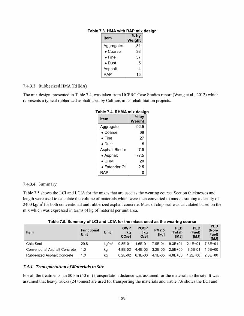
189

Table 7.3. HMA with RAP mix design

Item % by

Weight

Aggregate: 81

� Coarse 38

� Fine 57

� Dust 5

Asphalt 4

RAP 15

7.4.3.3. Rubberized HMA (RHMA)

The mix design, presented in Table 7.4, was taken from UCPRC Case Studies report (Wang et al., 2012) which

represents a typical rubberized asphalt used by Caltrans in its rehabilitation projects.

Table 7.4. RHMA mix design

Item % by

Weight

Aggregate 92.5

� Coarse 68

� Fine 27

� Dust 5

Asphalt Binder 7.5

� Asphalt 77.5

� CRM 20

� Extender Oil 2.5

RAP 0

7.4.3.4. Summary

Table 7.5 shows the LCI and LCIA for the mixes that are used as the wearing course. Section thicknesses and

length were used to calculate the volume of materials which were then converted to mass assuming a density of

2400 kg/m3 for both conventional and rubberized asphalt concrete. Mass of chip seal was calculated based on the

mix which was expressed in terms of kg of material per unit area.

Table 7.5. Summary of LCI and LCIA for the mixes used as the wearing course

Item Functional Unit

Unit GWP

[kg CO2e]

POCP [kg

O3e]

PM2.5 [kg]

PED (Total)

[MJ]

PED (Fuel)

[MJ]

PED (Non-Fuel) [MJ]

Chip Seal 20.8 kg/m2 9.8E-01 1.6E-01 7.9E-04 9.3E+01 2.1E+01 7.3E+01

Conventional Asphalt Concrete 1.0 kg 4.8E-02 4.4E-03 3.2E-05 2.5E+00 8.5E-01 1.6E+00

Rubberized Asphalt Concrete 1.0 kg 6.2E-02 6.1E-03 4.1E-05 4.0E+00 1.2E+00 2.8E+00

7.4.4. Transportation of Materials to Site

For all the treatments, an 80 km (50 mi) transportation distance was assumed for the materials to the site. It was

assumed that heavy trucks (24 tonnes) are used for transporting the materials and Table 7.6 shows the LCI and

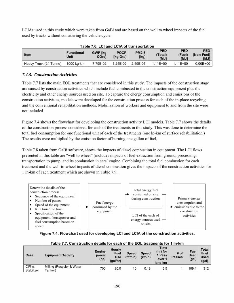
190

LCIAs used in this study which were taken from GaBi and are based on the well to wheel impacts of the fuel

used by trucks without considering the vehicle cycle.

Table 7.6. LCI and LCIA of transportation

Item Functional Unit

GWP [kg CO2e]

POCP [kg O3e]

PM2.5 [kg]

PED (Total)

[MJ]

PED (Fuel)

[MJ]

PED (Non-Fuel)

[MJ]

Heavy Truck (24 Tonne) 1000 kg-km 7.79E-02 1.24E-02 2.49E-05 1.11E+00 1.11E+00 0.00E+00

7.4.5. Construction Activities

Table 7.7 lists the main EOL treatments that are considered in this study. The impacts of the construction stage

are caused by construction activities which include fuel combusted in the construction equipment plus the

electricity and other energy sources used on site. To capture the energy consumption and emissions of the

construction activities, models were developed for the construction process for each of the in-place recycling

and the conventional rehabilitation methods. Mobilization of workers and equipment to and from the site were

not included.

Figure 7.4 shows the flowchart for developing the construction activity LCI models. Table 7.7 shows the details

of the construction process considered for each of the treatments in this study. This was done to determine the

total fuel consumption for one functional unit of each of the treatments (one ln-km of surface rehabilitation.)

The results were multiplied by the emission factor of burning one gallon of fuel,

Table 7.8 taken from GaBi software, shows the impacts of diesel combustion in equipment. The LCI flows

presented in this table are “well to wheel” (includes impacts of fuel extraction from ground, processing,

transportation to pump, and its combustion in cars’ engine. Combining the total fuel combustion for each

treatment and the well-to-wheel impacts of diesel combustion gives the impacts of the construction activities for

1 ln-km of each treatment which are shown in Table 7.9..

Determine details of the construction process:• Sequence of the equipment• Number of passes• Speed of the equipment• Run time/idle time• Specification of the

equipment: horsepower and fuel consumption based on speed

Fuel/energy consumed by the

equipmentLCI of the each of

energy sources used on site

Total energy/fuel consumed on site

during construction Primary energy consumption and

emissions due to the construction

activities

Figure 7.4: Flowchart used for developing LCI and LCIA of the construction activities.

Table 7.7. Construction details for each of the EOL treatments for 1 ln-km

Case Equipment/Activity Engine power

(hp)

Hourly Fuel Use

(gal/hr)

Speed (ft/min)

Speed (km/h)

Time (hr) for 1 Pass over 1

lane-km

# of Passes

Fuel Used (gal)

Total Fuel Used (gal)

CIR w. Stabilizer

Milling (Recycler & Water Tanker)

700 20.0 10 0.18 5.5 1 109.4 312

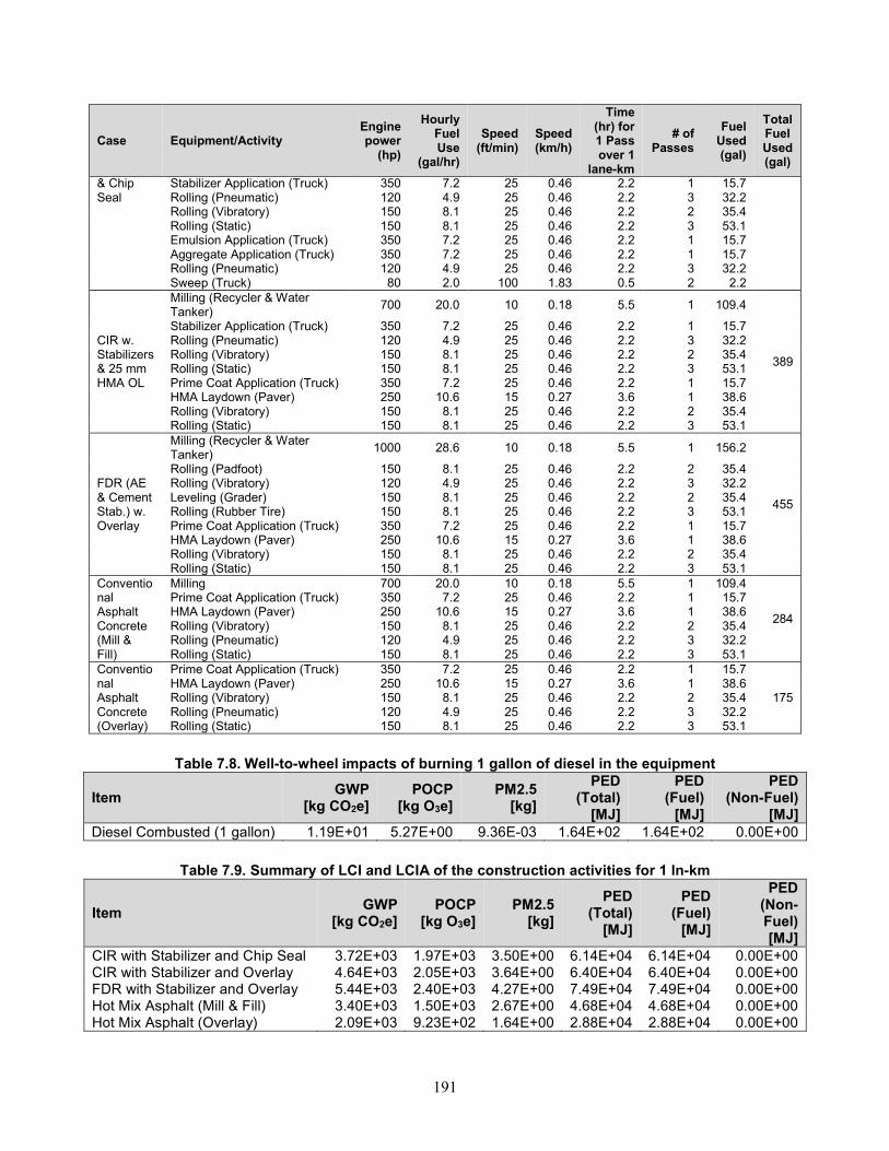
191

Case Equipment/Activity Engine power

(hp)

Hourly Fuel Use

(gal/hr)

Speed (ft/min)

Speed (km/h)

Time (hr) for 1 Pass over 1

lane-km

# of Passes

Fuel Used (gal)

Total Fuel Used (gal)

& Chip Seal

Stabilizer Application (Truck) 350 7.2 25 0.46 2.2 1 15.7 Rolling (Pneumatic) 120 4.9 25 0.46 2.2 3 32.2 Rolling (Vibratory) 150 8.1 25 0.46 2.2 2 35.4 Rolling (Static) 150 8.1 25 0.46 2.2 3 53.1 Emulsion Application (Truck) 350 7.2 25 0.46 2.2 1 15.7 Aggregate Application (Truck) 350 7.2 25 0.46 2.2 1 15.7 Rolling (Pneumatic) 120 4.9 25 0.46 2.2 3 32.2 Sweep (Truck) 80 2.0 100 1.83 0.5 2 2.2

CIR w. Stabilizers & 25 mm HMA OL

Milling (Recycler & Water Tanker)

700 20.0 10 0.18 5.5 1 109.4

389

Stabilizer Application (Truck) 350 7.2 25 0.46 2.2 1 15.7 Rolling (Pneumatic) 120 4.9 25 0.46 2.2 3 32.2 Rolling (Vibratory) 150 8.1 25 0.46 2.2 2 35.4 Rolling (Static) 150 8.1 25 0.46 2.2 3 53.1 Prime Coat Application (Truck) 350 7.2 25 0.46 2.2 1 15.7 HMA Laydown (Paver) 250 10.6 15 0.27 3.6 1 38.6 Rolling (Vibratory) 150 8.1 25 0.46 2.2 2 35.4 Rolling (Static) 150 8.1 25 0.46 2.2 3 53.1

FDR (AE & Cement Stab.) w. Overlay

Milling (Recycler & Water Tanker)

1000 28.6 10 0.18 5.5 1 156.2

455

Rolling (Padfoot) 150 8.1 25 0.46 2.2 2 35.4 Rolling (Vibratory) 120 4.9 25 0.46 2.2 3 32.2 Leveling (Grader) 150 8.1 25 0.46 2.2 2 35.4 Rolling (Rubber Tire) 150 8.1 25 0.46 2.2 3 53.1 Prime Coat Application (Truck) 350 7.2 25 0.46 2.2 1 15.7 HMA Laydown (Paver) 250 10.6 15 0.27 3.6 1 38.6 Rolling (Vibratory) 150 8.1 25 0.46 2.2 2 35.4 Rolling (Static) 150 8.1 25 0.46 2.2 3 53.1

Conventional Asphalt Concrete (Mill & Fill)

Milling 700 20.0 10 0.18 5.5 1 109.4

284

Prime Coat Application (Truck) 350 7.2 25 0.46 2.2 1 15.7 HMA Laydown (Paver) 250 10.6 15 0.27 3.6 1 38.6 Rolling (Vibratory) 150 8.1 25 0.46 2.2 2 35.4 Rolling (Pneumatic) 120 4.9 25 0.46 2.2 3 32.2 Rolling (Static) 150 8.1 25 0.46 2.2 3 53.1

Conventional Asphalt Concrete (Overlay)

Prime Coat Application (Truck) 350 7.2 25 0.46 2.2 1 15.7

175 HMA Laydown (Paver) 250 10.6 15 0.27 3.6 1 38.6 Rolling (Vibratory) 150 8.1 25 0.46 2.2 2 35.4 Rolling (Pneumatic) 120 4.9 25 0.46 2.2 3 32.2 Rolling (Static) 150 8.1 25 0.46 2.2 3 53.1

Table 7.8. Well-to-wheel impacts of burning 1 gallon of diesel in the equipment

Item GWP

[kg CO2e] POCP

[kg O3e] PM2.5

[kg]

PED (Total)

[MJ]

PED (Fuel)

[MJ]

PED (Non-Fuel)

[MJ] Diesel Combusted (1 gallon) 1.19E+01 5.27E+00 9.36E-03 1.64E+02 1.64E+02 0.00E+00

Table 7.9. Summary of LCI and LCIA of the construction activities for 1 ln-km

Item GWP

[kg CO2e] POCP

[kg O3e] PM2.5

[kg]

PED (Total)

[MJ]

PED (Fuel)

[MJ]

PED (Non-Fuel) [MJ]

CIR with Stabilizer and Chip Seal 3.72E+03 1.97E+03 3.50E+00 6.14E+04 6.14E+04 0.00E+00 CIR with Stabilizer and Overlay 4.64E+03 2.05E+03 3.64E+00 6.40E+04 6.40E+04 0.00E+00 FDR with Stabilizer and Overlay 5.44E+03 2.40E+03 4.27E+00 7.49E+04 7.49E+04 0.00E+00 Hot Mix Asphalt (Mill & Fill) 3.40E+03 1.50E+03 2.67E+00 4.68E+04 4.68E+04 0.00E+00 Hot Mix Asphalt (Overlay) 2.09E+03 9.23E+02 1.64E+00 2.88E+04 2.88E+04 0.00E+00

192

7.4.6. End of Life

For this study EOL was handled using available methods without considering repeated recycling and impacts on

quality. As mentioned earlier, questions remain regarding the number of times that aggregate can be recycled,

and the impact of multiple recycling on quality and field performance, these issues will be addressed in the next

stage of this research.

Regarding allocation, there are two common ways for handling it: the cut-off method where the virgin material

production impacts are assigned to the upstream project and the impacts of in-place recycling are applied to the

downstream project. The other method is the 50-50 method in which the total impacts (material production plus

EOL in-place recycling) are divided equally between the upstream and downstream projects. For this study the

cut-off method was selected assigning the impacts of milling the old asphalt, transportation to the plant, and any

further recycling activities to the RAP. It was also assumed that at the EOL of the downstream project, all the

overlay that was initially laid will be milled and then transported to a landfill or a recycling plant at similar

distances assumed for virgin materials. For reporting purposes, the EOL impacts were added to transportation

and construction impacts and were reported as part of them.

7.5. Final Results and Interpretation

In previous sections, environmental impacts of material production, transportation to site, construction, and EOL

were calculated for one application of each of the EOL treatments. In this section, the total impacts for each

treatment are provided and the share of different initial material production, transportation, and construction life

cycle stages in total impacts, excluding the use state, are discussed. Table 7.10 is the breakdown of the total

impacts for each treatment in detail based on life cycle stages included in this study. Table 7.11 shows the

percentage share of each initial material production, transportation, and construction life cycle stage in total

impacts. Bar charts of the results are also presented in Figure 7.5 and Figure 7.6.

The goal of this part of the project was to benchmark the cradle to laid environmental impacts of common EOL

treatments for flexible pavements at their end of service life in California considering only a single EOL. This

study cannot serve as a comparative study between treatments as the system boundary and scope of the study

does not include the use stage.

Considering total initial materials and construction impacts, as shown in Figure 7.5, CIR with 1.5 percent FA

and 1 percent portland cement has the lowest total impacts. All the FDR cases with stabilizer have higher total

impacts compared to the conventional options of mill-and-fill and HMA overlay. The results also show that the

total amount of stabilizer added (which depends on percent stabilizer and the layer thickness) has a significant

impact on the total impacts. The FDR option with highest cement content (6 percent) consistently had the

highest impacts in GWP, PM2.5, and PED (Fuel), while the FDR option with 4 percent asphalt emulsion and 1

percent portland cement had the highest impacts in POCP and PED categories. It must be kept in mind that there

is potential energy kept unused in asphalt that is not lost and can be recovered if need be, that is reported in the

table as PED (non-fuel), although the burning of RAP as an energy source is probably not cost-effective and has

a number of practical challenges.

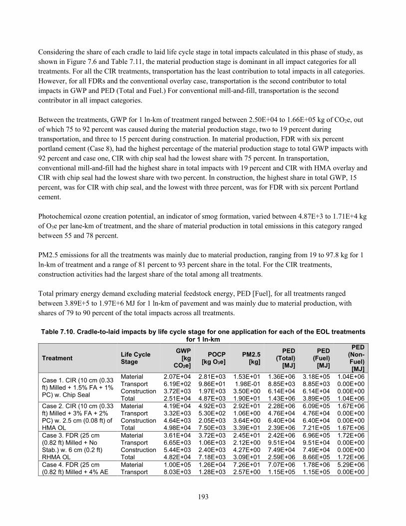
193

Considering the share of each cradle to laid life cycle stage in total impacts calculated in this phase of study, as

shown in Figure 7.6 and Table 7.11, the material production stage is dominant in all impact categories for all

treatments. For all the CIR treatments, transportation has the least contribution to total impacts in all categories.

However, for all FDRs and the conventional overlay case, transportation is the second contributor to total

impacts in GWP and PED (Total and Fuel.) For conventional mill-and-fill, transportation is the second

contributor in all impact categories.

Between the treatments, GWP for 1 ln-km of treatment ranged between 2.50E+04 to 1.66E+05 kg of CO2e, out

of which 75 to 92 percent was caused during the material production stage, two to 19 percent during

transportation, and three to 15 percent during construction. In material production, FDR with six percent

portland cement (Case 8), had the highest percentage of the material production stage to total GWP impacts with

92 percent and case one, CIR with chip seal had the lowest share with 75 percent. In transportation,

conventional mill-and-fill had the highest share in total impacts with 19 percent and CIR with HMA overlay and

CIR with chip seal had the lowest share with two percent. In construction, the highest share in total GWP, 15

percent, was for CIR with chip seal, and the lowest with three percent, was for FDR with six percent Portland

cement.

Photochemical ozone creation potential, an indicator of smog formation, varied between 4.87E+3 to 1.71E+4 kg

of O3e per lane-km of treatment, and the share of material production in total emissions in this category ranged

between 55 and 78 percent.

PM2.5 emissions for all the treatments was mainly due to material production, ranging from 19 to 97.8 kg for 1

ln-km of treatment and a range of 81 percent to 93 percent share in the total. For the CIR treatments,

construction activities had the largest share of the total among all treatments.

Total primary energy demand excluding material feedstock energy, PED [Fuel], for all treatments ranged

between 3.89E+5 to 1.97E+6 MJ for 1 ln-km of pavement and was mainly due to material production, with

shares of 79 to 90 percent of the total impacts across all treatments.

Table 7.10. Cradle-to-laid impacts by life cycle stage for one application for each of the EOL treatments

for 1 ln-km

Treatment Life Cycle Stage

GWP [kg

CO2e]

POCP [kg O3e]

PM2.5 [kg]

PED (Total)

[MJ]

PED (Fuel)

[MJ]

PED (Non-Fuel) [MJ]

Case 1. CIR (10 cm (0.33 ft) Milled + 1.5% FA + 1% PC) w. Chip Seal

Material 2.07E+04 2.81E+03 1.53E+01 1.36E+06 3.18E+05 1.04E+06 Transport 6.19E+02 9.86E+01 1.98E-01 8.85E+03 8.85E+03 0.00E+00 Construction 3.72E+03 1.97E+03 3.50E+00 6.14E+04 6.14E+04 0.00E+00 Total 2.51E+04 4.87E+03 1.90E+01 1.43E+06 3.89E+05 1.04E+06

Case 2. CIR (10 cm (0.33 ft) Milled + 3% FA + 2% PC) w. 2.5 cm (0.08 ft) of HMA OL

Material 4.19E+04 4.92E+03 2.92E+01 2.28E+06 6.09E+05 1.67E+06 Transport 3.32E+03 5.30E+02 1.06E+00 4.76E+04 4.76E+04 0.00E+00 Construction 4.64E+03 2.05E+03 3.64E+00 6.40E+04 6.40E+04 0.00E+00 Total 4.98E+04 7.50E+03 3.39E+01 2.39E+06 7.21E+05 1.67E+06

Case 3. FDR (25 cm (0.82 ft) Milled + No Stab.) w. 6 cm (0.2 ft) RHMA OL

Material 3.61E+04 3.72E+03 2.45E+01 2.42E+06 6.96E+05 1.72E+06 Transport 6.65E+03 1.06E+03 2.12E+00 9.51E+04 9.51E+04 0.00E+00 Construction 5.44E+03 2.40E+03 4.27E+00 7.49E+04 7.49E+04 0.00E+00 Total 4.82E+04 7.18E+03 3.09E+01 2.59E+06 8.66E+05 1.72E+06

Case 4. FDR (25 cm (0.82 ft) Milled + 4% AE

Material 1.00E+05 1.26E+04 7.26E+01 7.07E+06 1.78E+06 5.29E+06 Transport 8.03E+03 1.28E+03 2.57E+00 1.15E+05 1.15E+05 0.00E+00

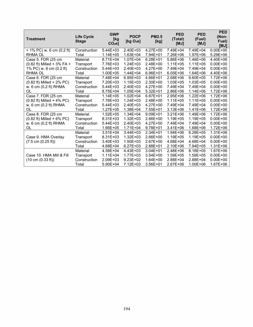
194

Treatment Life Cycle Stage

GWP [kg

CO2e]

POCP [kg O3e]

PM2.5 [kg]

PED (Total)

[MJ]

PED (Fuel)

[MJ]

PED (Non-Fuel) [MJ]

+ 1% PC) w. 6 cm (0.2 ft) RHMA OL

Construction 5.44E+03 2.40E+03 4.27E+00 7.49E+04 7.49E+04 0.00E+00 Total 1.14E+05 1.63E+04 7.94E+01 7.26E+06 1.97E+06 5.29E+06

Case 5. FDR (25 cm (0.82 ft) Milled + 3% FA + 1% PC) w. 6 cm (0.2 ft) RHMA OL

Material 8.71E+04 1.07E+04 6.28E+01 5.86E+06 1.46E+06 4.40E+06 Transport 7.76E+03 1.24E+03 2.48E+00 1.11E+05 1.11E+05 0.00E+00 Construction 5.44E+03 2.40E+03 4.27E+00 7.49E+04 7.49E+04 0.00E+00 Total 1.00E+05 1.44E+04 6.96E+01 6.05E+06 1.64E+06 4.40E+06

Case 6. FDR (25 cm (0.82 ft) Milled + 2% PC) w. 6 cm (0.2 ft) RHMA OL

Material 7.48E+04 6.95E+03 4.66E+01 2.68E+06 9.60E+05 1.72E+06 Transport 7.20E+03 1.15E+03 2.30E+00 1.03E+05 1.03E+05 0.00E+00 Construction 5.44E+03 2.40E+03 4.27E+00 7.49E+04 7.49E+04 0.00E+00 Total 8.75E+04 1.05E+04 5.32E+01 2.86E+06 1.14E+06 1.72E+06

Case 7. FDR (25 cm (0.82 ft) Milled + 4% PC) w. 6 cm (0.2 ft) RHMA OL

Material 1.14E+05 1.02E+04 6.87E+01 2.95E+06 1.22E+06 1.72E+06 Transport 7.76E+03 1.24E+03 2.48E+00 1.11E+05 1.11E+05 0.00E+00 Construction 5.44E+03 2.40E+03 4.27E+00 7.49E+04 7.49E+04 0.00E+00 Total 1.27E+05 1.38E+04 7.55E+01 3.13E+06 1.41E+06 1.72E+06

Case 8. FDR (25 cm (0.82 ft) Milled + 6% PC) w. 6 cm (0.2 ft) RHMA OL

Material 1.52E+05 1.34E+04 9.09E+01 3.21E+06 1.49E+06 1.72E+06 Transport 8.31E+03 1.32E+03 2.66E+00 1.19E+05 1.19E+05 0.00E+00 Construction 5.44E+03 2.40E+03 4.27E+00 7.49E+04 7.49E+04 0.00E+00 Total 1.66E+05 1.71E+04 9.78E+01 3.41E+06 1.68E+06 1.72E+06

Case 9. HMA Overlay (7.5 cm (0.25 ft))

Material 3.51E+04 3.44E+03 2.34E+01 1.94E+06 6.28E+05 1.31E+06 Transport 8.31E+03 1.32E+03 2.66E+00 1.19E+05 1.19E+05 0.00E+00 Construction 3.40E+03 1.50E+03 2.67E+00 4.68E+04 4.68E+04 0.00E+00 Total 4.68E+04 6.27E+03 2.88E+01 2.10E+06 7.94E+05 1.31E+06

Case 10. HMA Mill & Fill (10 cm (0.33 ft))

Material 4.58E+04 4.43E+03 3.04E+01 2.48E+06 8.16E+05 1.67E+06 Transport 1.11E+04 1.77E+03 3.54E+00 1.59E+05 1.59E+05 0.00E+00 Construction 2.09E+03 9.23E+02 1.64E+00 2.88E+04 2.88E+04 0.00E+00 Total 5.90E+04 7.12E+03 3.56E+01 2.67E+06 1.00E+06 1.67E+06

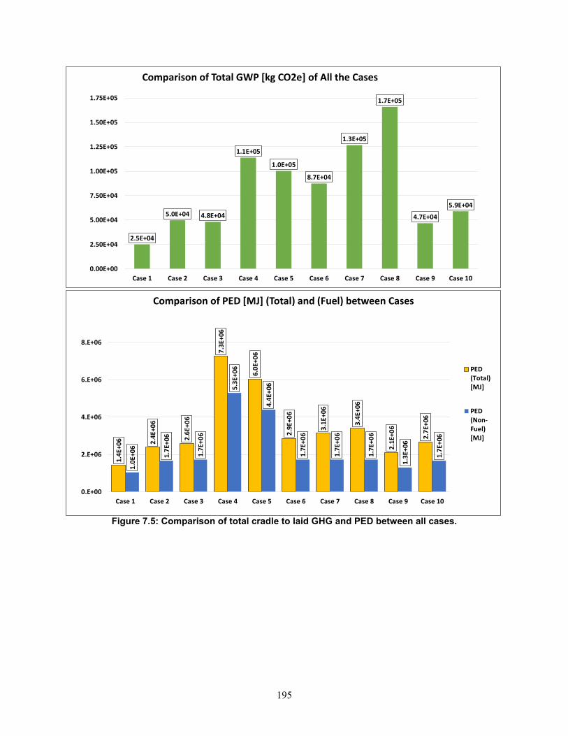
195

Figure 7.5: Comparison of total cradle to laid GHG and PED between all cases.

2.5E+04

5.0E+04 4.8E+04

1.1E+05

1.0E+05

8.7E+04

1.3E+05

1.7E+05

4.7E+04

5.9E+04

0.00E+00

2.50E+04

5.00E+04

7.50E+04

1.00E+05

1.25E+05

1.50E+05

1.75E+05

Case 1 Case 2 Case 3 Case 4 Case 5 Case 6 Case 7 Case 8 Case 9 Case 10

Comparison of Total GWP [kg CO2e] of All the Cases

1.4

E+

06 2.4

E+

06

2.6

E+

06

7.3

E+

06

6.0

E+

06

2.9

E+

06

3.1

E+

06

3.4

E+

06

2.1

E+

06

2.7

E+

06

1.0

E+

06

1.7

E+

06

1.7

E+

06

5.3

E+

06

4.4

E+

06

1.7

E+

06

1.7

E+

06

1.7

E+

06

1.3

E+

06

1.7

E+

06

0.E+00

2.E+06

4.E+06

6.E+06

8.E+06

Case 1 Case 2 Case 3 Case 4 Case 5 Case 6 Case 7 Case 8 Case 9 Case 10

Comparison of PED [MJ] (Total) and (Fuel) between Cases

PED

(Total)

[MJ]

PED

(Non-

Fuel)

[MJ]

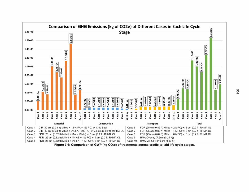
196

Case 1 CIR (10 cm (0.33 ft) Milled + 1.5% FA + 1% PC) w. Chip Seal Case 6 FDR (25 cm (0.82 ft) Milled + 2% PC) w. 6 cm (0.2 ft) RHMA OL Case 2 CIR (10 cm (0.33 ft) Milled + 3% FA + 2% PC) w. 2.5 cm (0.08 ft) of HMA OL Case 7 FDR (25 cm (0.82 ft) Milled + 4% PC) w. 6 cm (0.2 ft) RHMA OL Case 3 FDR (25 cm (0.82 ft) Milled + Mech. Stab.) w. 6 cm (0.2 ft) RHMA OL Case 8 FDR (25 cm (0.82 ft) Milled + 6% PC) w. 6 cm (0.2 ft) RHMA OL Case 4 FDR (25 cm (0.82 ft) Milled + 4% AE + 1% PC) w. 6 cm (0.2 ft) RHMA OL Case 9 HMA Overlay (7.5cm (0.25 ft)) Case 5 FDR (25 cm (0.82 ft) Milled + 3% FA + 1% PC) w. 6 cm (0.2 ft) RHMA OL Case 10 HMA Mill & Fill (10 cm (0.33 ft))

Figure 7.6: Comparison of GWP (kg CO2e) of treatments across cradle to laid life cycle stages.

2.1

E+

04

4.2

E+

04

3.6

E+

04

1.0

E+

05

8.7

E+

04

7.5

E+

04

1.1

E+

05

1.5

E+

05

3.5

E+

04

4.6

E+

04

3.7

E+

03

4.6

E+

03

5.4

E+

03

5.4

E+

03

5.4

E+

03

5.4

E+

03

5.4

E+

03

5.4

E+

03

3.4

E+

03

2.1

E+

03

6.2

E+

02

3.3

E+

03

6.6

E+

03

8.0

E+

03

7.8

E+

03

7.2

E+

03

7.8

E+

03

8.3

E+

03

8.3

E+

03

1.1

E+

04

2.5

E+

04

5.0

E+

04

4.8

E+

04

1.1

E+

05

1.0

E+

05

8.7

E+

04

1.3

E+

05

1.7

E+

05

4.7

E+

04

5.9

E+

04

0.0E+00

2.0E+04

4.0E+04

6.0E+04

8.0E+04

1.0E+05

1.2E+05

1.4E+05

1.6E+05

1.8E+05

Ca

se 1

Ca

se 2

Ca

se 3

Ca

se 4

Ca

se 5

Ca

se 6

Ca

se 7

Ca

se 8

Ca

se 9

Ca

se 1

0

Ca

se 1

Ca

se 2

Ca

se 3

Ca

se 4

Ca

se 5

Ca

se 6

Ca

se 7

Ca

se 8

Ca

se 9

Ca

se 1

0

Ca

se 1

Ca

se 2

Ca

se 3

Ca

se 4

Ca

se 5

Ca

se 6

Ca

se 7

Ca

se 8

Ca

se 9

Ca

se 1

0

Ca

se 1

Ca

se 2

Ca

se 3

Ca

se 4

Ca

se 5

Ca

se 6

Ca

se 7

Ca

se 8

Ca

se 9

Ca

se 1

0

Material Construction Transport Total

Comparison of GHG Emissions (kg of CO2e) of Different Cases in Each Life Cycle

Stage

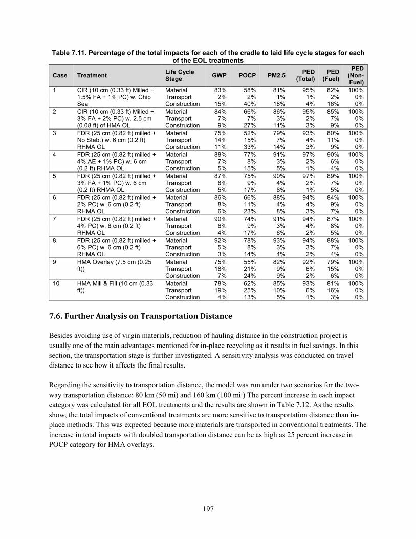
197

Table 7.11. Percentage of the total impacts for each of the cradle to laid life cycle stages for each of the EOL treatments

Case Treatment Life Cycle Stage

GWP POCP PM2.5 PED

(Total) PED

(Fuel)

PED (Non-Fuel)

1 CIR (10 cm (0.33 ft) Milled + 1.5% FA + 1% PC) w. Chip Seal

Material 83% 58% 81% 95% 82% 100% Transport 2% 2% 1% 1% 2% 0% Construction 15% 40% 18% 4% 16% 0% 2 CIR (10 cm (0.33 ft) Milled +

3% FA + 2% PC) w. 2.5 cm (0.08 ft) of HMA OL

Material 84% 66% 86% 95% 85% 100% Transport 7% 7% 3% 2% 7% 0% Construction 9% 27% 11% 3% 9% 0% 3 FDR (25 cm (0.82 ft) milled +

No Stab.) w. 6 cm (0.2 ft) RHMA OL

Material 75% 52% 79% 93% 80% 100% Transport 14% 15% 7% 4% 11% 0% Construction 11% 33% 14% 3% 9% 0% 4 FDR (25 cm (0.82 ft) milled +

4% AE + 1% PC) w. 6 cm (0.2 ft) RHMA OL

Material 88% 77% 91% 97% 90% 100% Transport 7% 8% 3% 2% 6% 0% Construction 5% 15% 5% 1% 4% 0% 5 FDR (25 cm (0.82 ft) milled +

3% FA + 1% PC) w. 6 cm (0.2 ft) RHMA OL

Material 87% 75% 90% 97% 89% 100% Transport 8% 9% 4% 2% 7% 0% Construction 5% 17% 6% 1% 5% 0% 6 FDR (25 cm (0.82 ft) milled +

2% PC) w. 6 cm (0.2 ft) RHMA OL

Material 86% 66% 88% 94% 84% 100% Transport 8% 11% 4% 4% 9% 0% Construction 6% 23% 8% 3% 7% 0% 7 FDR (25 cm (0.82 ft) milled +

4% PC) w. 6 cm (0.2 ft) RHMA OL

Material 90% 74% 91% 94% 87% 100% Transport 6% 9% 3% 4% 8% 0% Construction 4% 17% 6% 2% 5% 0% 8 FDR (25 cm (0.82 ft) milled +

6% PC) w. 6 cm (0.2 ft) RHMA OL

Material 92% 78% 93% 94% 88% 100% Transport 5% 8% 3% 3% 7% 0% Construction 3% 14% 4% 2% 4% 0% 9 HMA Overlay (7.5 cm (0.25

ft)) Material 75% 55% 82% 92% 79% 100%

Transport 18% 21% 9% 6% 15% 0% Construction 7% 24% 9% 2% 6% 0% 10 HMA Mill & Fill (10 cm (0.33

ft)) Material 78% 62% 85% 93% 81% 100%

Transport 19% 25% 10% 6% 16% 0% Construction 4% 13% 5% 1% 3% 0%

7.6. Further Analysis on Transportation Distance

Besides avoiding use of virgin materials, reduction of hauling distance in the construction project is

usually one of the main advantages mentioned for in-place recycling as it results in fuel savings. In this

section, the transportation stage is further investigated. A sensitivity analysis was conducted on travel

distance to see how it affects the final results.

Regarding the sensitivity to transportation distance, the model was run under two scenarios for the two-

way transportation distance: 80 km (50 mi) and 160 km (100 mi.) The percent increase in each impact

category was calculated for all EOL treatments and the results are shown in Table 7.12. As the results

show, the total impacts of conventional treatments are more sensitive to transportation distance than in-

place methods. This was expected because more materials are transported in conventional treatments. The

increase in total impacts with doubled transportation distance can be as high as 25 percent increase in

POCP category for HMA overlays.

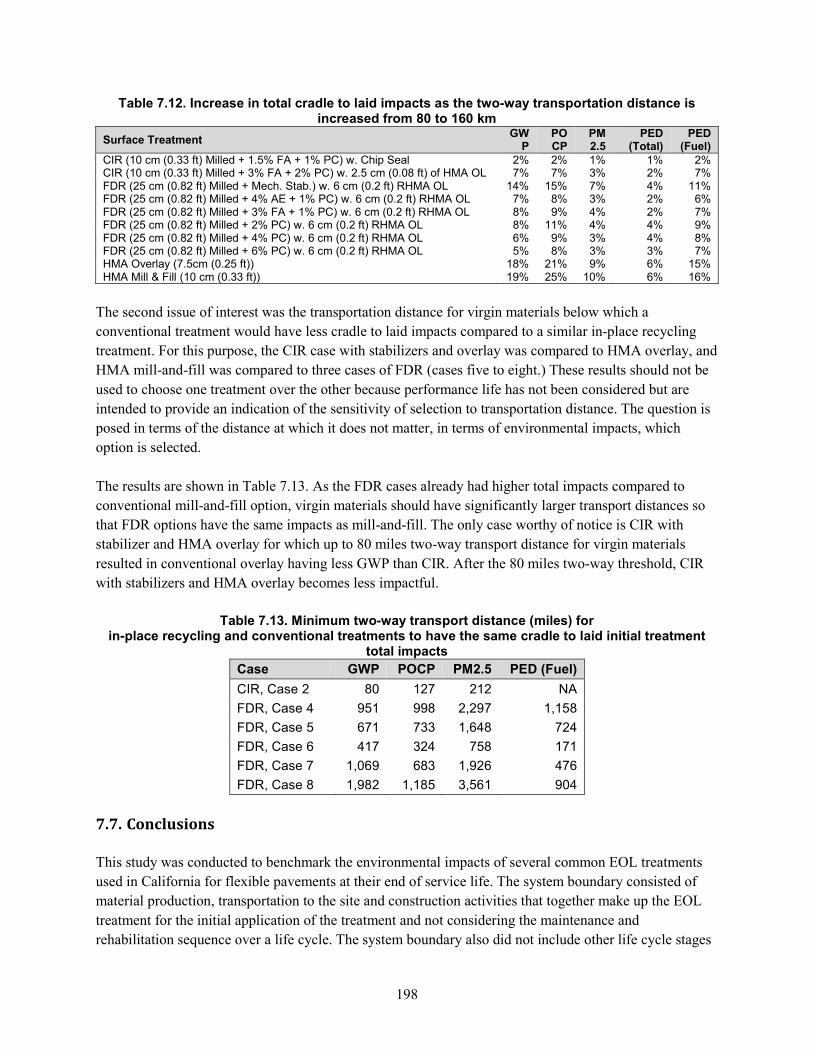
198

Table 7.12. Increase in total cradle to laid impacts as the two-way transportation distance is increased from 80 to 160 km

Surface Treatment GW

P POCP

PM 2.5

PED (Total)

PED (Fuel)

CIR (10 cm (0.33 ft) Milled + 1.5% FA + 1% PC) w. Chip Seal 2% 2% 1% 1% 2% CIR (10 cm (0.33 ft) Milled + 3% FA + 2% PC) w. 2.5 cm (0.08 ft) of HMA OL 7% 7% 3% 2% 7% FDR (25 cm (0.82 ft) Milled + Mech. Stab.) w. 6 cm (0.2 ft) RHMA OL 14% 15% 7% 4% 11% FDR (25 cm (0.82 ft) Milled + 4% AE + 1% PC) w. 6 cm (0.2 ft) RHMA OL 7% 8% 3% 2% 6% FDR (25 cm (0.82 ft) Milled + 3% FA + 1% PC) w. 6 cm (0.2 ft) RHMA OL 8% 9% 4% 2% 7% FDR (25 cm (0.82 ft) Milled + 2% PC) w. 6 cm (0.2 ft) RHMA OL 8% 11% 4% 4% 9% FDR (25 cm (0.82 ft) Milled + 4% PC) w. 6 cm (0.2 ft) RHMA OL 6% 9% 3% 4% 8% FDR (25 cm (0.82 ft) Milled + 6% PC) w. 6 cm (0.2 ft) RHMA OL 5% 8% 3% 3% 7% HMA Overlay (7.5cm (0.25 ft)) 18% 21% 9% 6% 15% HMA Mill & Fill (10 cm (0.33 ft)) 19% 25% 10% 6% 16%

The second issue of interest was the transportation distance for virgin materials below which a

conventional treatment would have less cradle to laid impacts compared to a similar in-place recycling

treatment. For this purpose, the CIR case with stabilizers and overlay was compared to HMA overlay, and

HMA mill-and-fill was compared to three cases of FDR (cases five to eight.) These results should not be

used to choose one treatment over the other because performance life has not been considered but are

intended to provide an indication of the sensitivity of selection to transportation distance. The question is

posed in terms of the distance at which it does not matter, in terms of environmental impacts, which

option is selected.

The results are shown in Table 7.13. As the FDR cases already had higher total impacts compared to

conventional mill-and-fill option, virgin materials should have significantly larger transport distances so

that FDR options have the same impacts as mill-and-fill. The only case worthy of notice is CIR with

stabilizer and HMA overlay for which up to 80 miles two-way transport distance for virgin materials

resulted in conventional overlay having less GWP than CIR. After the 80 miles two-way threshold, CIR

with stabilizers and HMA overlay becomes less impactful.

Table 7.13. Minimum two-way transport distance (miles) for

in-place recycling and conventional treatments to have the same cradle to laid initial treatment total impacts

Case GWP POCP PM2.5 PED (Fuel)

CIR, Case 2 80 127 212 NA

FDR, Case 4 951 998 2,297 1,158

FDR, Case 5 671 733 1,648 724

FDR, Case 6 417 324 758 171

FDR, Case 7 1,069 683 1,926 476

FDR, Case 8 1,982 1,185 3,561 904

7.7. Conclusions

This study was conducted to benchmark the environmental impacts of several common EOL treatments

used in California for flexible pavements at their end of service life. The system boundary consisted of

material production, transportation to the site and construction activities that together make up the EOL

treatment for the initial application of the treatment and not considering the maintenance and

rehabilitation sequence over a life cycle. The system boundary also did not include other life cycle stages

199

such as use stage, and traffic delays during construction activities. Twelve treatments were studied,

consisting of ten in-place recycling alternatives (CIR and FDR with different stabilization methods and

wearing courses on top) and two conventional treatments (HMA overlay and HMA mill-and-fill.) The

conclusions drawn from the results presented in this study are:

• There are large differences between the initial impacts of the treatments in each impact category

but as discussed earlier, due to limited scope of this stage and the fact that the system boundary

does not include all life cycle stages, comparison of the results shall not be used as basis for

decision making and selecting between alternatives.

• The material production stage is dominant in all impact categories for all treatments. The results

also show that the total amount of stabilizer added (which depends on percent stabilizer and the

layer thickness) has a significant impact on the total impacts.

• HMA overlay and HMA mill-and-fill have lower impacts compared to all the FDR options with

stabilizers across all impact categories.

• The FDR option with highest cement content (6 percent) consistently had the highest impacts in

GWP, PM2.5, and PED (Fuel), while the FDR option with 4 percent asphalt emulsion and 1

percent portland cement had the highest impacts in POCP and PED (Total and Non-Fuel.)

• Material production share in total impacts ranged between 75 to 92 percent for GWP, 52 to 78

percent for POCP, 79 to 93 for PM 2.5, 92 to 97 percent for PED (Total), and 79 to 90 percent for

PED (Fuel.) Binder and stabilizer production caused more than 90 percent of the total impacts of

the material production across all cases.

• Share of material transportation to site in total impacts ranged between two to 19 percent for

GWP, two to 25 percent for POCP, one to 10 percent for PM 2.5, one to six percent for PED

(Total), and two to 16 percent for PED (Fuel.)

• Construction activities impacts caused three to 15 percent of total impacts for GWP, 13 to 40

percent in POCP, four to 18 percent in PM 2.5, one to four percent of PED (Total), and three to

16 percent of PED (Fuel)

• Changing transportation distance has the most drastic effect on total impacts of conventional

treatments. This was already expected, as conventional treatments require the largest amount of

materials transported.

• Comparing the CIR with stabilizers and HMA overlay with the conventional treatment of an

HMA overlay shows that total GWP of the two options are close (5.0E+4 versus 4.7E+4,

respectively) with the conventional treatment performing slightly better. This remains true up to

transport distance of 80 miles (two-way) for the virgin materials, at which the impacts of both

two options become equal and after that distance the CIR outperforms the conventional treatment.

• Similar comparison of FDRs with conventional mill-and-fill resulted in very long transport

distances for virgin materials at which the impacts of the two treatments become equal. The

transport distances were all above 150 miles.

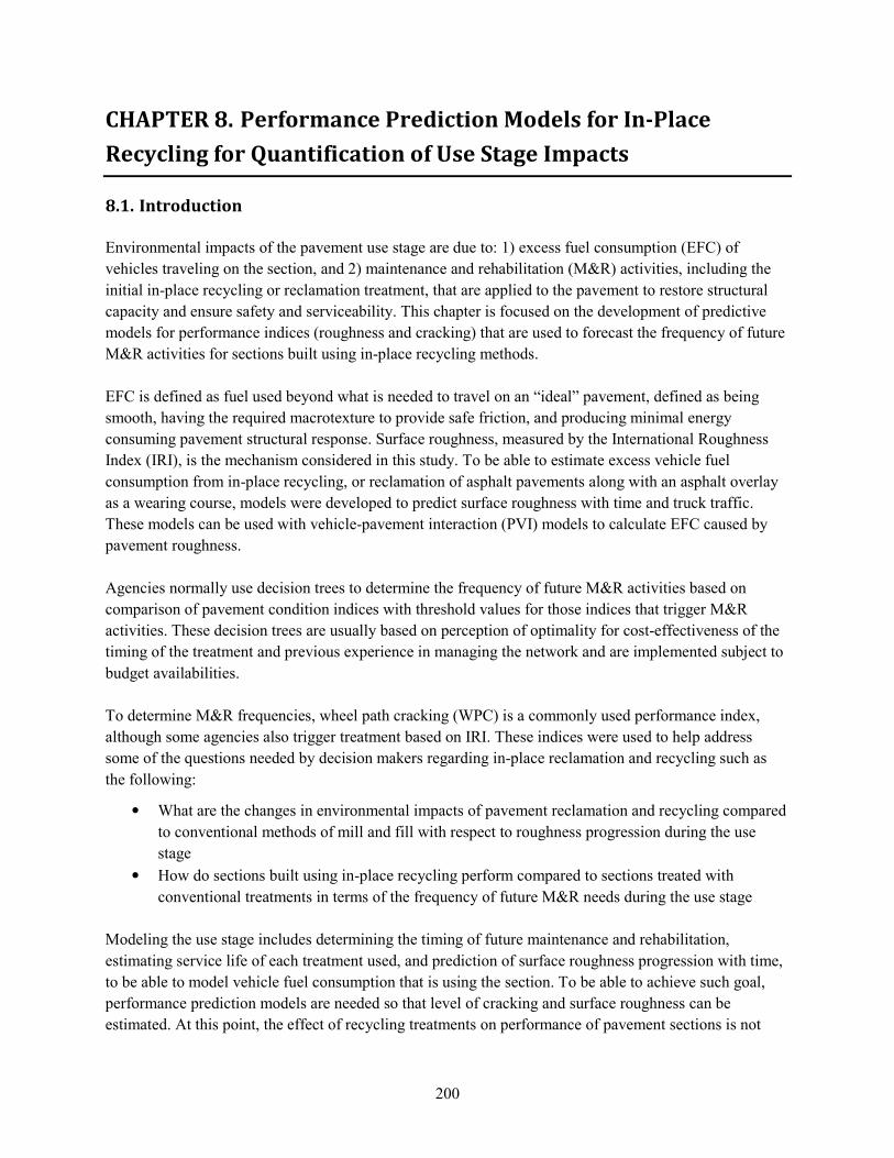
200

CHAPTER 8. Performance Prediction Models for In-Place

Recycling for Quantification of Use Stage Impacts

8.1. Introduction

Environmental impacts of the pavement use stage are due to: 1) excess fuel consumption (EFC) of

vehicles traveling on the section, and 2) maintenance and rehabilitation (M&R) activities, including the

initial in-place recycling or reclamation treatment, that are applied to the pavement to restore structural

capacity and ensure safety and serviceability. This chapter is focused on the development of predictive

models for performance indices (roughness and cracking) that are used to forecast the frequency of future

M&R activities for sections built using in-place recycling methods.

EFC is defined as fuel used beyond what is needed to travel on an “ideal” pavement, defined as being

smooth, having the required macrotexture to provide safe friction, and producing minimal energy

consuming pavement structural response. Surface roughness, measured by the International Roughness

Index (IRI), is the mechanism considered in this study. To be able to estimate excess vehicle fuel

consumption from in-place recycling, or reclamation of asphalt pavements along with an asphalt overlay

as a wearing course, models were developed to predict surface roughness with time and truck traffic.

These models can be used with vehicle-pavement interaction (PVI) models to calculate EFC caused by

pavement roughness.

Agencies normally use decision trees to determine the frequency of future M&R activities based on

comparison of pavement condition indices with threshold values for those indices that trigger M&R

activities. These decision trees are usually based on perception of optimality for cost-effectiveness of the

timing of the treatment and previous experience in managing the network and are implemented subject to

budget availabilities.

To determine M&R frequencies, wheel path cracking (WPC) is a commonly used performance index,

although some agencies also trigger treatment based on IRI. These indices were used to help address

some of the questions needed by decision makers regarding in-place reclamation and recycling such as

the following:

• What are the changes in environmental impacts of pavement reclamation and recycling compared

to conventional methods of mill and fill with respect to roughness progression during the use

stage

• How do sections built using in-place recycling perform compared to sections treated with

conventional treatments in terms of the frequency of future M&R needs during the use stage

Modeling the use stage includes determining the timing of future maintenance and rehabilitation,

estimating service life of each treatment used, and prediction of surface roughness progression with time,

to be able to model vehicle fuel consumption that is using the section. To be able to achieve such goal,

performance prediction models are needed so that level of cracking and surface roughness can be

estimated. At this point, the effect of recycling treatments on performance of pavement sections is not

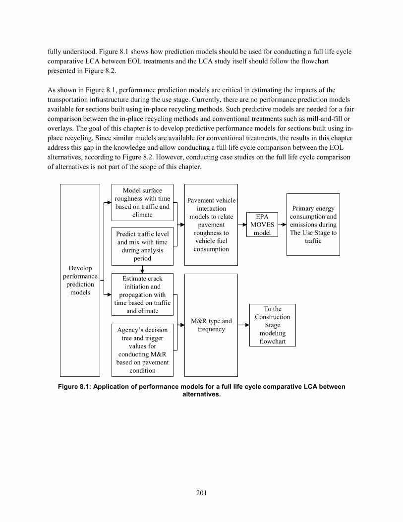
201

fully understood. Figure 8.1 shows how prediction models should be used for conducting a full life cycle

comparative LCA between EOL treatments and the LCA study itself should follow the flowchart

presented in Figure 8.2.

As shown in Figure 8.1, performance prediction models are critical in estimating the impacts of the

transportation infrastructure during the use stage. Currently, there are no performance prediction models

available for sections built using in-place recycling methods. Such predictive models are needed for a fair

comparison between the in-place recycling methods and conventional treatments such as mill-and-fill or

overlays. The goal of this chapter is to develop predictive performance models for sections built using in-

place recycling. Since similar models are available for conventional treatments, the results in this chapter

address this gap in the knowledge and allow conducting a full life cycle comparison between the EOL

alternatives, according to Figure 8.2. However, conducting case studies on the full life cycle comparison

of alternatives is not part of the scope of this chapter.

Develop performance

prediction models

EPA MOVES model

Primary energy consumption and emissions during The Use Stage to

trafficPredict traffic level and mix with time

during analysis period

Model surface roughness with time based on traffic and

climate

Estimate crack initiation and

propagation with time based on traffic

and climate

Pavement vehicle interaction

models to relate pavement

roughness to vehicle fuel consumption

Agency’s decision tree and trigger

values for conducting M&R

based on pavement condition

M&R type and frequency

To the Construction

Stage modeling flowchart

Figure 8.1: Application of performance models for a full life cycle comparative LCA between alternatives.

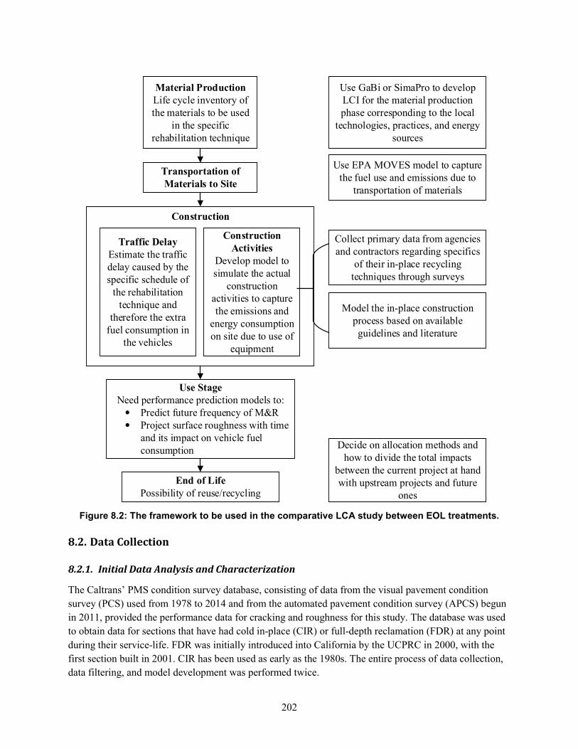
202

Collect primary data from agencies and contractors regarding specifics

of their in-place recycling techniques through surveys

Model the in-place construction process based on available guidelines and literature

Material Production

Life cycle inventory of the materials to be used

in the specific rehabilitation technique

Transportation of

Materials to Site

Construction

Activities

Develop model to simulate the actual

construction activities to capture the emissions and

energy consumption on site due to use of

equipment

Traffic Delay

Estimate the traffic delay caused by the specific schedule of

the rehabilitation technique and

therefore the extra fuel consumption in

the vehicles

Use Stage

Need performance prediction models to: • Predict future frequency of M&R • Project surface roughness with time

and its impact on vehicle fuel consumption

End of Life

Possibility of reuse/recycling

Use GaBi or SimaPro to develop LCI for the material production phase corresponding to the local

technologies, practices, and energy sources

Use EPA MOVES model to capture the fuel use and emissions due to

transportation of materials

Construction

Decide on allocation methods and how to divide the total impacts

between the current project at hand with upstream projects and future

ones

Figure 8.2: The framework to be used in the comparative LCA study between EOL treatments.

8.2. Data Collection

8.2.1. Initial Data Analysis and Characterization

The Caltrans’ PMS condition survey database, consisting of data from the visual pavement condition

survey (PCS) used from 1978 to 2014 and from the automated pavement condition survey (APCS) begun

in 2011, provided the performance data for cracking and roughness for this study. The database was used

to obtain data for sections that have had cold in-place (CIR) or full-depth reclamation (FDR) at any point

during their service-life. FDR was initially introduced into California by the UCPRC in 2000, with the

first section built in 2001. CIR has been used as early as the 1980s. The entire process of data collection,

data filtering, and model development was performed twice.

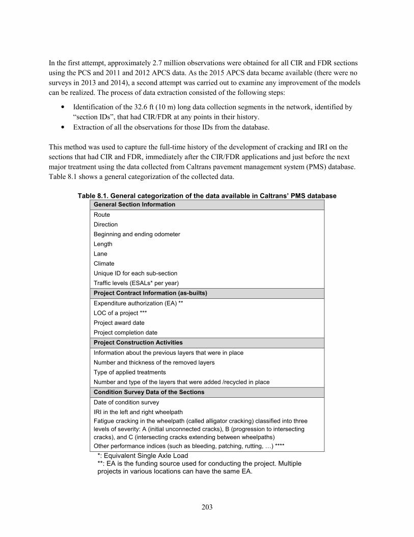
203

In the first attempt, approximately 2.7 million observations were obtained for all CIR and FDR sections

using the PCS and 2011 and 2012 APCS data. As the 2015 APCS data became available (there were no

surveys in 2013 and 2014), a second attempt was carried out to examine any improvement of the models

can be realized. The process of data extraction consisted of the following steps:

• Identification of the 32.6 ft (10 m) long data collection segments in the network, identified by

“section IDs”, that had CIR/FDR at any points in their history.

• Extraction of all the observations for those IDs from the database.

This method was used to capture the full-time history of the development of cracking and IRI on the

sections that had CIR and FDR, immediately after the CIR/FDR applications and just before the next

major treatment using the data collected from Caltrans pavement management system (PMS) database.

Table 8.1 shows a general categorization of the collected data.

Table 8.1. General categorization of the data available in Caltrans’ PMS database

General Section Information

Route

Direction

Beginning and ending odometer

Length

Lane

Climate

Unique ID for each sub-section

Traffic levels (ESALs* per year)

Project Contract Information (as-builts)

Expenditure authorization (EA) **

LOC of a project ***

Project award date

Project completion date

Project Construction Activities

Information about the previous layers that were in place

Number and thickness of the removed layers

Type of applied treatments

Number and type of the layers that were added /recycled in place

Condition Survey Data of the Sections

Date of condition survey

IRI in the left and right wheelpath

Fatigue cracking in the wheelpath (called alligator cracking) classified into three

levels of severity: A (initial unconnected cracks), B (progression to intersecting cracks), and C (intersecting cracks extending between wheelpaths)

Other performance indices (such as bleeding, patching, rutting, …) ****

*: Equivalent Single Axle Load **: EA is the funding source used for conducting the project. Multiple projects in various locations can have the same EA.

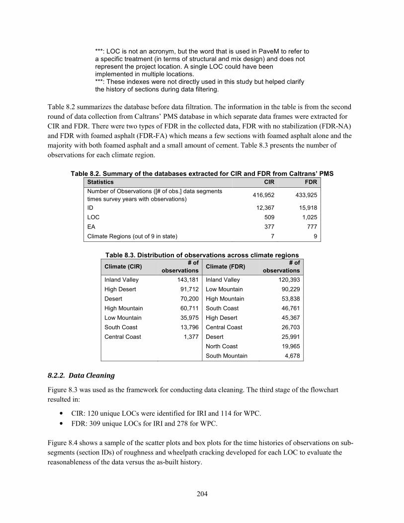
204

***: LOC is not an acronym, but the word that is used in PaveM to refer to a specific treatment (in terms of structural and mix design) and does not represent the project location. A single LOC could have been implemented in multiple locations. ***: These indexes were not directly used in this study but helped clarify the history of sections during data filtering.

Table 8.2 summarizes the database before data filtration. The information in the table is from the second

round of data collection from Caltrans’ PMS database in which separate data frames were extracted for

CIR and FDR. There were two types of FDR in the collected data, FDR with no stabilization (FDR-NA)

and FDR with foamed asphalt (FDR-FA) which means a few sections with foamed asphalt alone and the

majority with both foamed asphalt and a small amount of cement. Table 8.3 presents the number of

observations for each climate region.

Table 8.2. Summary of the databases extracted for CIR and FDR from Caltrans’ PMS

Statistics CIR FDR

Number of Observations ([# of obs.] data segments times survey years with observations)

416,952 433,925

ID 12,367 15,918

LOC 509 1,025

EA 377 777

Climate Regions (out of 9 in state) 7 9

Table 8.3. Distribution of observations across climate regions

Climate (CIR) # of

observations Climate (FDR)

# of

observations

Inland Valley 143,181 Inland Valley 120,393

High Desert 91,712 Low Mountain 90,229

Desert 70,200 High Mountain 53,838

High Mountain 60,711 South Coast 46,761

Low Mountain 35,975 High Desert 45,367

South Coast 13,796 Central Coast 26,703

Central Coast 1,377 Desert 25,991 North Coast 19,965 South Mountain 4,678

8.2.2. Data Cleaning

Figure 8.3 was used as the framework for conducting data cleaning. The third stage of the flowchart

resulted in:

• CIR: 120 unique LOCs were identified for IRI and 114 for WPC.

• FDR: 309 unique LOCs for IRI and 278 for WPC.

Figure 8.4 shows a sample of the scatter plots and box plots for the time histories of observations on sub-

segments (section IDs) of roughness and wheelpath cracking developed for each LOC to evaluate the

reasonableness of the data versus the as-built history.

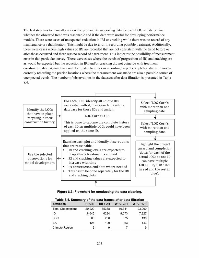
205

The last step was to manually review the plot and its supporting data for each LOC and determine

whether the observed trend was reasonable and if the data were useful for developing performance

models. There were cases of unexpected reduction in IRI or cracking while there was no record of any

maintenance or rehabilitation. This might be due to error in recording possible treatment. Additionally,

there were cases where high values of IRI are recorded that are not consistent with the trend before or

after those occurred and there was no record of a treatment. This indicates the possibility of measurement

error in that particular survey. There were cases where the trends of progression of IRI and cracking are

as would be expected but the reduction in IRI and/or cracking did not coincide with treatment

construction date. Again, this could be related to errors in recording project completion dates. Errors in

correctly recording the precise locations where the measurement was made are also a possible source of

unexpected trends. The number of observations in the datasets after data filtration is presented in Table

8.4.

Identify the LOCs

that have in-place

recycling in their

construction history.

Select “LOC_Corr”s

with more than one

sampling date.

Examine each plot and identify observations

that are reasonable:

• IRI and cracking levels are expected to

drop after a treatment is applied

• IRI and cracking values are expected to

increase with time

• Fix construction end date where needed

• This has to be done separately for the IRI

and cracking plots.

Use the selected

observations for

model development.

Select “LOC_Corr”s

with more than one

sampling date.

Highlight the project

award and completion

dates for each of the

actual LOCs as one ID

can have multiple

LOCs (CIR/FDR dates

in red and the rest in

blue).

For each LOCi, identify all unique IDs

associated with it, then search the whole

database for those IDs and assign:

LOC_Corr = LOCi

This is done to capture the complete history

of each ID, as multiple LOCs could have been

applied on the same ID.

Figure 8.3: Flowchart for conducting the data cleaning.

Table 8.4. Summary of the data frames after data filtration

Statistics IRI-CIR IRI-FDR WPC-CIR WPC-FDR

Total Observations 29,229 35368 19,311 23,090

ID 8,645 6284 8,073 7,827

LOC 83 206 75 130

EA 126 100 63 143

Climate Region 6 9 7 9

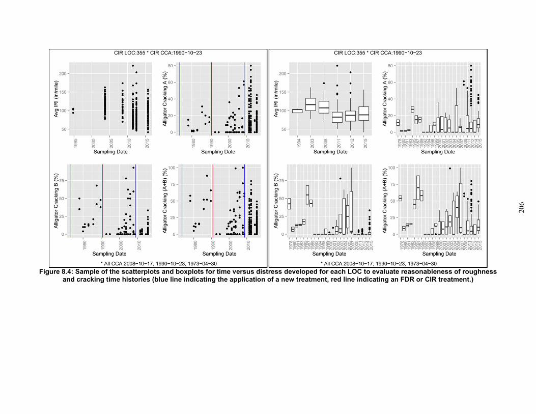
206

Figure 8.4: Sample of the scatterplots and boxplots for time versus distress developed for each LOC to evaluate reasonableness of roughness and cracking time histories (blue line indicating the application of a new treatment, red line indicating an FDR or CIR treatment.)

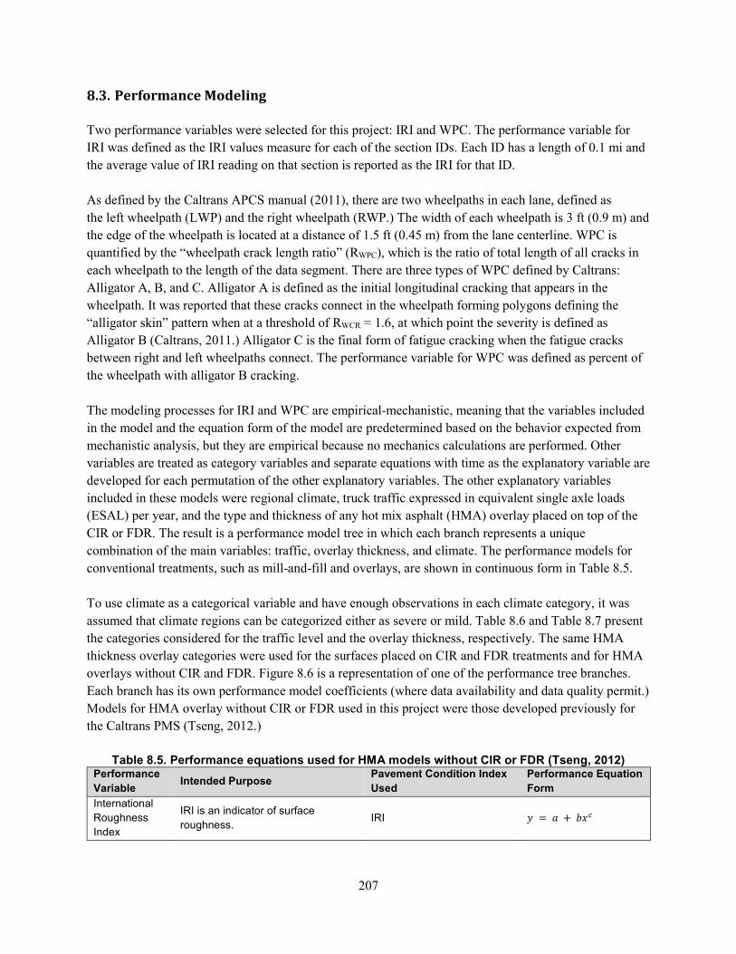
207

8.3. Performance Modeling

Two performance variables were selected for this project: IRI and WPC. The performance variable for

IRI was defined as the IRI values measure for each of the section IDs. Each ID has a length of 0.1 mi and

the average value of IRI reading on that section is reported as the IRI for that ID.

As defined by the Caltrans APCS manual (2011), there are two wheelpaths in each lane, defined as

the left wheelpath (LWP) and the right wheelpath (RWP.) The width of each wheelpath is 3 ft (0.9 m) and

the edge of the wheelpath is located at a distance of 1.5 ft (0.45 m) from the lane centerline. WPC is

quantified by the “wheelpath crack length ratio” (RWPC), which is the ratio of total length of all cracks in

each wheelpath to the length of the data segment. There are three types of WPC defined by Caltrans:

Alligator A, B, and C. Alligator A is defined as the initial longitudinal cracking that appears in the

wheelpath. It was reported that these cracks connect in the wheelpath forming polygons defining the

“alligator skin” pattern when at a threshold of RWCR = 1.6, at which point the severity is defined as

Alligator B (Caltrans, 2011.) Alligator C is the final form of fatigue cracking when the fatigue cracks

between right and left wheelpaths connect. The performance variable for WPC was defined as percent of

the wheelpath with alligator B cracking.

The modeling processes for IRI and WPC are empirical-mechanistic, meaning that the variables included

in the model and the equation form of the model are predetermined based on the behavior expected from

mechanistic analysis, but they are empirical because no mechanics calculations are performed. Other

variables are treated as category variables and separate equations with time as the explanatory variable are

developed for each permutation of the other explanatory variables. The other explanatory variables

included in these models were regional climate, truck traffic expressed in equivalent single axle loads

(ESAL) per year, and the type and thickness of any hot mix asphalt (HMA) overlay placed on top of the

CIR or FDR. The result is a performance model tree in which each branch represents a unique

combination of the main variables: traffic, overlay thickness, and climate. The performance models for

conventional treatments, such as mill-and-fill and overlays, are shown in continuous form in Table 8.5.

To use climate as a categorical variable and have enough observations in each climate category, it was

assumed that climate regions can be categorized either as severe or mild. Table 8.6 and Table 8.7 present

the categories considered for the traffic level and the overlay thickness, respectively. The same HMA

thickness overlay categories were used for the surfaces placed on CIR and FDR treatments and for HMA

overlays without CIR and FDR. Figure 8.6 is a representation of one of the performance tree branches.

Each branch has its own performance model coefficients (where data availability and data quality permit.)

Models for HMA overlay without CIR or FDR used in this project were those developed previously for

the Caltrans PMS (Tseng, 2012.)

Table 8.5. Performance equations used for HMA models without CIR or FDR (Tseng, 2012)

Performance

Variable Intended Purpose

Pavement Condition Index

Used

Performance Equation

Form

International Roughness Index

IRI is an indicator of surface roughness.

IRI � = � + ���

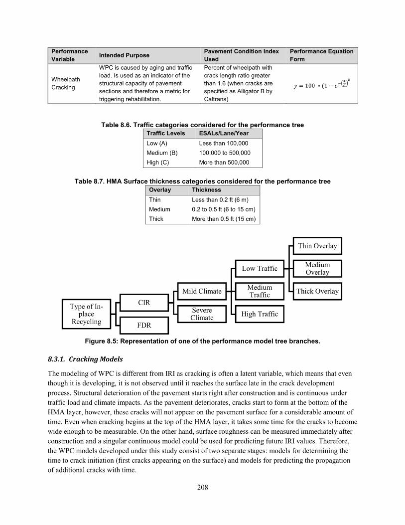
208

Performance

Variable Intended Purpose

Pavement Condition Index

Used

Performance Equation

Form

Wheelpath

Cracking

WPC is caused by aging and traffic load. Is used as an indicator of the structural capacity of pavement sections and therefore a metric for triggering rehabilitation.

Percent of wheelpath with crack length ratio greater than 1.6 (when cracks are specified as Alligator B by Caltrans)

� = 100 ∗ �1 − ������

�

Table 8.6. Traffic categories considered for the performance tree

Traffic Levels ESALs/Lane/Year

Low (A) Less than 100,000

Medium (B) 100,000 to 500,000

High (C) More than 500,000

Table 8.7. HMA Surface thickness categories considered for the performance tree

Overlay Thickness

Thin Less than 0.2 ft (6 m)

Medium 0.2 to 0.5 ft (6 to 15 cm)

Thick More than 0.5 ft (15 cm)

Figure 8.5: Representation of one of the performance model tree branches.

8.3.1. Cracking Models

The modeling of WPC is different from IRI as cracking is often a latent variable, which means that even

though it is developing, it is not observed until it reaches the surface late in the crack development

process. Structural deterioration of the pavement starts right after construction and is continuous under

traffic load and climate impacts. As the pavement deteriorates, cracks start to form at the bottom of the

HMA layer, however, these cracks will not appear on the pavement surface for a considerable amount of

time. Even when cracking begins at the top of the HMA layer, it takes some time for the cracks to become

wide enough to be measurable. On the other hand, surface roughness can be measured immediately after

construction and a singular continuous model could be used for predicting future IRI values. Therefore,

the WPC models developed under this study consist of two separate stages: models for determining the

time to crack initiation (first cracks appearing on the surface) and models for predicting the propagation

of additional cracks with time.

Type of In-place

Recycling

CIR

Mild Climate

Low Traffic

Thin Overlay

Medium Overlay

Thick OverlayMedium Traffic

High TrafficSevere Climate

FDR

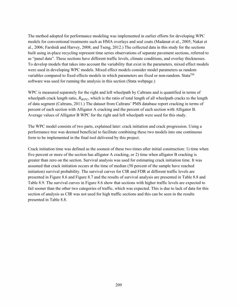
209

The method adopted for performance modeling was implemented in earlier efforts for developing WPC

models for conventional treatments such as HMA overlays and seal coats (Madanat et al., 2005; Nakat et

al., 2006; Farshidi and Harvey, 2008; and Tseng, 2012.) The collected data in this study for the sections

built using in-place recycling represent time series observations of separate pavement sections, referred to

as “panel data”. These sections have different traffic levels, climate conditions, and overlay thicknesses.

To develop models that takes into account the variability that exist in the parameters, mixed effect models

were used in developing WPC models. Mixed effect models consider model parameters as random

variables compared to fixed effects models in which parameters are fixed or non-random. StataTM

software was used for running the analysis in this section (Stata webpage.)

WPC is measured separately for the right and left wheelpath by Caltrans and is quantified in terms of

wheelpath crack length ratio, � !" , which is the ratio of total length of all wheelpath cracks to the length

of data segment (Caltrans, 2011.) The dataset from Caltrans’ PMS database report cracking in terms of

percent of each section with Alligator A cracking and the percent of each section with Alligator B.

Average values of Alligator B WPC for the right and left wheelpath were used for this study.

The WPC model consists of two parts, explained later: crack initiation and crack progression. Using a

performance tree was deemed beneficial to facilitate combining these two models into one continuous

form to be implemented in the final tool delivered by this project.

Crack initiation time was defined as the soonest of these two times after initial construction: 1) time when

five percent or more of the section has alligator A cracking, or 2) time when alligator B cracking is

greater than zero on the section. Survival analysis was used for estimating crack initiation time. It was

assumed that crack initiation occurs at the time of median (50 percent of the sample have reached

initiation) survival probability. The survival curves for CIR and FDR at different traffic levels are

presented in Figure 8.6 and Figure 8.7 and the results of survival analysis are presented in Table 8.8 and

Table 8.9. The survival curves in Figure 8.6 show that sections with higher traffic levels are expected to

fail sooner than the other two categories of traffic, which was expected. This is due to lack of data for this

section of analysis as CIR was not used for high traffic sections and this can be seen in the results

presented in Table 8.8.

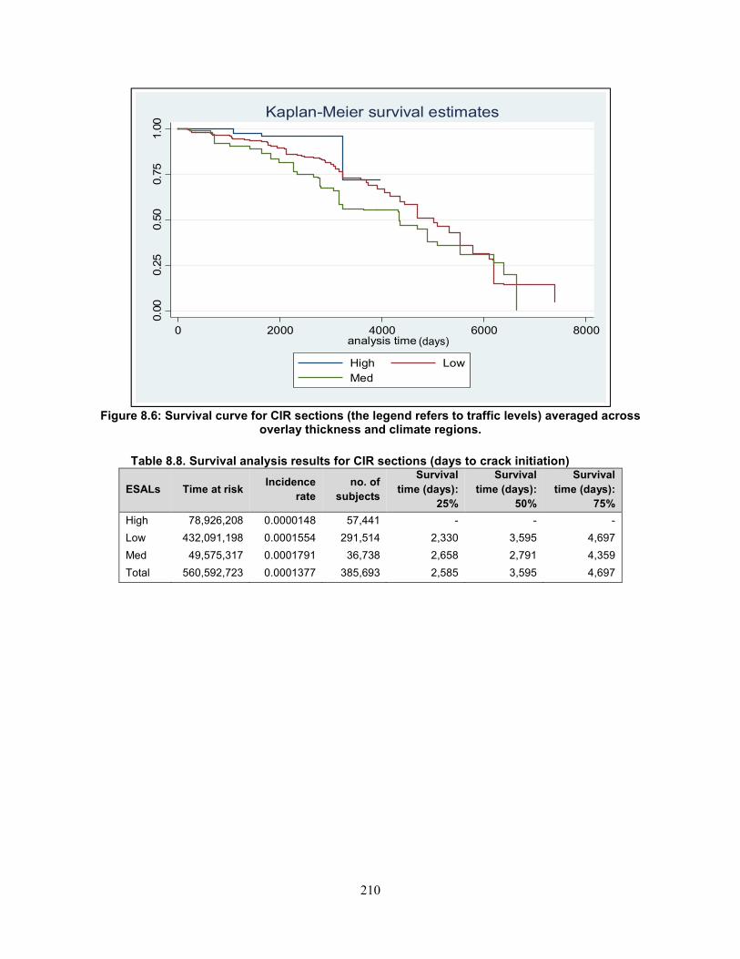
210

Figure 8.6: Survival curve for CIR sections (the legend refers to traffic levels) averaged across overlay thickness and climate regions.

Table 8.8. Survival analysis results for CIR sections (days to crack initiation)

ESALs Time at risk Incidence

rate

no. of

subjects

Survival

time (days):

25%

Survival

time (days):

50%

Survival

time (days):

75%

High 78,926,208 0.0000148 57,441 - - -

Low 432,091,198 0.0001554 291,514 2,330 3,595 4,697

Med 49,575,317 0.0001791 36,738 2,658 2,791 4,359

Total 560,592,723 0.0001377 385,693 2,585 3,595 4,697

0.0

00.2

50.5

00.7

51.0

0

0 2000 4000 6000 8000analysis time

High Low

Med

Kaplan-Meier survival estimates

(days)

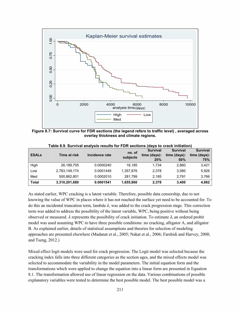
211

Figure 8.7: Survival curve for FDR sections (the legend refers to traffic level) , averaged across overlay thickness and climate regions.

Table 8.9. Survival analysis results for FDR sections (days to crack initiation)

ESALs Time at risk Incidence rate no. of

subjects

Survival

time (days):

25%

Survival

time (days):

50%

Survival

time (days):

75%

High 26,189,705 0.0000240 16,185 1,734 2,860 3,421

Low 2,783,149,174 0.0001449 1,357,876 2,378 3,580 5,926

Med 500,862,801 0.0002010 281,799 2,185 2,791 3,766

Total 3,310,201,680 0.0001541 1,655,860 2,378 3,400 4,862

As stated earlier, WPC cracking is a latent variable. Therefore, possible data censorship, due to not

knowing the value of WPC in places where it has not reached the surface yet need to be accounted for. To

do this an incidental truncation term, lambda $, was added to the crack progression stage. This correction

term was added to address the possibility of the latent variable, WPC, being positive without being

observed or measured. $ represents the possibility of crack initiation. To estimate $, an ordered probit

model was used assuming WPC to have three possible conditions: no cracking, alligator A, and alligator

B. As explained earlier, details of statistical assumptions and theories for selection of modeling

approaches are presented elsewhere (Madanat et al., 2005; Nakat et al., 2006; Farshidi and Harvey, 2008;

and Tseng, 2012.)

Mixed effect logit models were used for crack progression. The Logit model was selected because the

cracking index falls into three different categories as the section ages, and the mixed effects model was

selected to accommodate the variability in the model parameters. The initial equation form and the

transformations which were applied to change the equation into a linear form are presented in Equation

8.1. The transformation allowed use of linear regression on the data. Various combinations of possible

explanatory variables were tested to determine the best possible model. The best possible model was a

0.0

00.2

50.5

00.7

51.0

0

0 2000 4000 6000 8000 10000analysis time

High Low

Med

Kaplan-Meier survival estimates

(days)

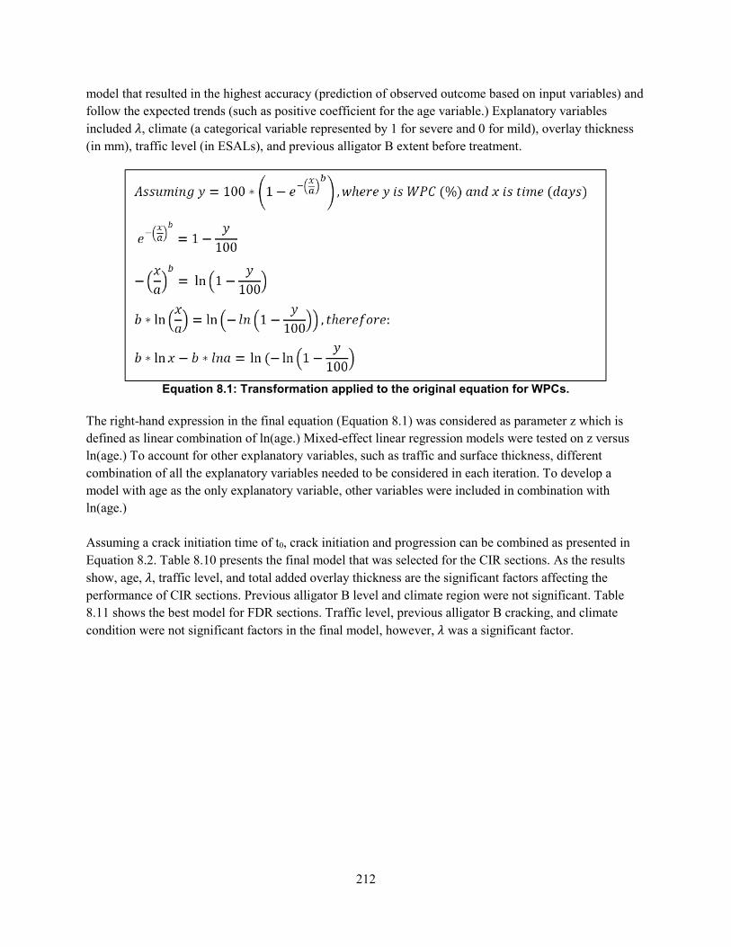
212

model that resulted in the highest accuracy (prediction of observed outcome based on input variables) and

follow the expected trends (such as positive coefficient for the age variable.) Explanatory variables

included $, climate (a categorical variable represented by 1 for severe and 0 for mild), overlay thickness

(in mm), traffic level (in ESALs), and previous alligator B extent before treatment.

Equation 8.1: Transformation applied to the original equation for WPCs.

The right-hand expression in the final equation (Equation 8.1) was considered as parameter z which is

defined as linear combination of ln(age.) Mixed-effect linear regression models were tested on z versus

ln(age.) To account for other explanatory variables, such as traffic and surface thickness, different

combination of all the explanatory variables needed to be considered in each iteration. To develop a

model with age as the only explanatory variable, other variables were included in combination with

ln(age.)

Assuming a crack initiation time of t0, crack initiation and progression can be combined as presented in

Equation 8.2. Table 8.10 presents the final model that was selected for the CIR sections. As the results

show, age, $, traffic level, and total added overlay thickness are the significant factors affecting the

performance of CIR sections. Previous alligator B level and climate region were not significant. Table

8.11 shows the best model for FDR sections. Traffic level, previous alligator B cracking, and climate

condition were not significant factors in the final model, however, $ was a significant factor.

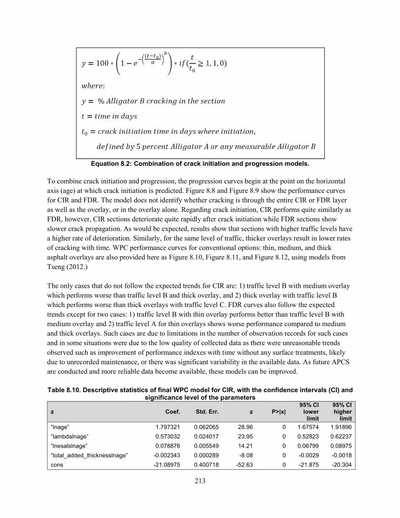
213

Equation 8.2: Combination of crack initiation and progression models.

To combine crack initiation and progression, the progression curves begin at the point on the horizontal

axis (age) at which crack initiation is predicted. Figure 8.8 and Figure 8.9 show the performance curves

for CIR and FDR. The model does not identify whether cracking is through the entire CIR or FDR layer

as well as the overlay, or in the overlay alone. Regarding crack initiation, CIR performs quite similarly as

FDR, however, CIR sections deteriorate quite rapidly after crack initiation while FDR sections show

slower crack propagation. As would be expected, results show that sections with higher traffic levels have

a higher rate of deterioration. Similarly, for the same level of traffic, thicker overlays result in lower rates

of cracking with time. WPC performance curves for conventional options: thin, medium, and thick

asphalt overlays are also provided here as Figure 8.10, Figure 8.11, and Figure 8.12, using models from

Tseng (2012.)

The only cases that do not follow the expected trends for CIR are: 1) traffic level B with medium overlay

which performs worse than traffic level B and thick overlay, and 2) thick overlay with traffic level B

which performs worse than thick overlays with traffic level C. FDR curves also follow the expected

trends except for two cases: 1) traffic level B with thin overlay performs better than traffic level B with

medium overlay and 2) traffic level A for thin overlays shows worse performance compared to medium

and thick overlays. Such cases are due to limitations in the number of observation records for such cases

and in some situations were due to the low quality of collected data as there were unreasonable trends

observed such as improvement of performance indexes with time without any surface treatments, likely

due to unrecorded maintenance, or there was significant variability in the available data. As future APCS

are conducted and more reliable data become available, these models can be improved.

Table 8.10. Descriptive statistics of final WPC model for CIR, with the confidence intervals (CI) and

significance level of the parameters

z Coef. Std. Err. z P>|x| 95% CI

lower limit

95% CI higher

limit

“lnage” 1.797321 0.062065 28.96 0 1.67574 1.91896

“lambdalnage” 0.573032 0.024017 23.95 0 0.52823 0.62237

“lnesalslnage” 0.078876 0.005549 14.21 0 0.06799 0.08975

“total_added_thicknesslnage” -0.002343 0.000289 -8.08 0 -0.0029 -0.0018

cons -21.08975 0.400718 -52.63 0 -21.875 -20.304

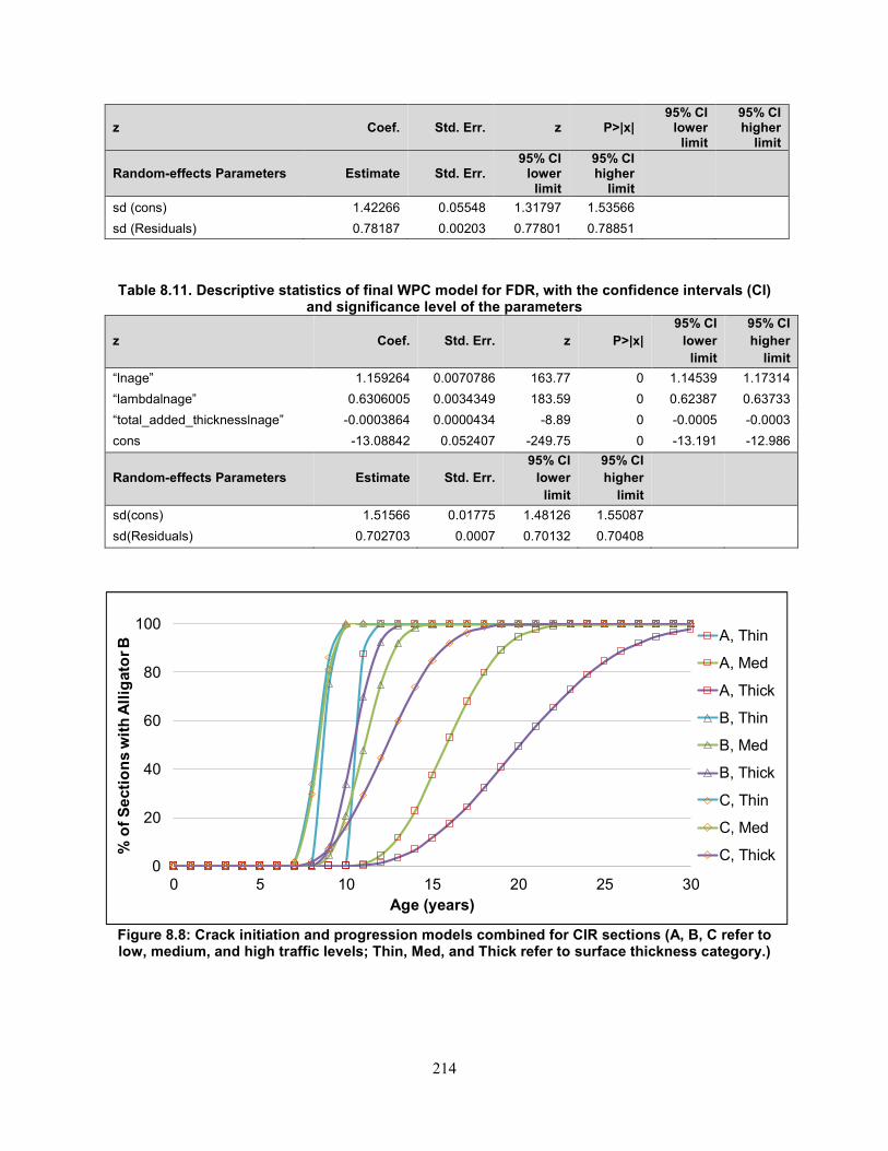
214

z Coef. Std. Err. z P>|x| 95% CI

lower limit

95% CI higher

limit

Random-effects Parameters Estimate Std. Err. 95% CI

lower limit

95% CI higher

limit

sd (cons) 1.42266 0.05548 1.31797 1.53566

sd (Residuals) 0.78187 0.00203 0.77801 0.78851

Table 8.11. Descriptive statistics of final WPC model for FDR, with the confidence intervals (CI)

and significance level of the parameters

z Coef. Std. Err. z P>|x|

95% CI

lower

limit

95% CI

higher

limit

“lnage” 1.159264 0.0070786 163.77 0 1.14539 1.17314

“lambdalnage” 0.6306005 0.0034349 183.59 0 0.62387 0.63733

“total_added_thicknesslnage” -0.0003864 0.0000434 -8.89 0 -0.0005 -0.0003

cons -13.08842 0.052407 -249.75 0 -13.191 -12.986

Random-effects Parameters Estimate Std. Err.

95% CI

lower

limit

95% CI

higher

limit

sd(cons) 1.51566 0.01775 1.48126 1.55087

sd(Residuals) 0.702703 0.0007 0.70132 0.70408

Figure 8.8: Crack initiation and progression models combined for CIR sections (A, B, C refer to low, medium, and high traffic levels; Thin, Med, and Thick refer to surface thickness category.)

0

20

40

60

80

100

0 5 10 15 20 25 30

% o

f S

ecti

on

s w

ith

All

igato

r B

Age (years)

A, Thin

A, Med

A, Thick

B, Thin

B, Med

B, Thick

C, Thin

C, Med

C, Thick

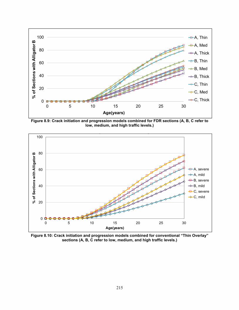
215

Figure 8.9: Crack initiation and progression models combined for FDR sections (A, B, C refer to low, medium, and high traffic levels.)

Figure 8.10: Crack initiation and progression models combined for conventional “Thin Overlay”

sections (A, B, C refer to low, medium, and high traffic levels.)

0

20

40

60

80

100

0 5 10 15 20 25 30

% o

f S

ecti

on

s w

ith

All

igato

r B

Age(years)

A, Thin

A, Med

A, Thick

B, Thin

B, Med

B, Thick

C, Thin

C, Med

C, Thick

0

20

40

60

80

100

0 5 10 15 20 25 30

% o

f S

ec

tio

ns

wit

h A

llig

ato

r B

Age(years)

Thin Overlay, Crack Initiation + Progression

A, severe

A, mild

B, severe

B, mild

C, severe

C, mild

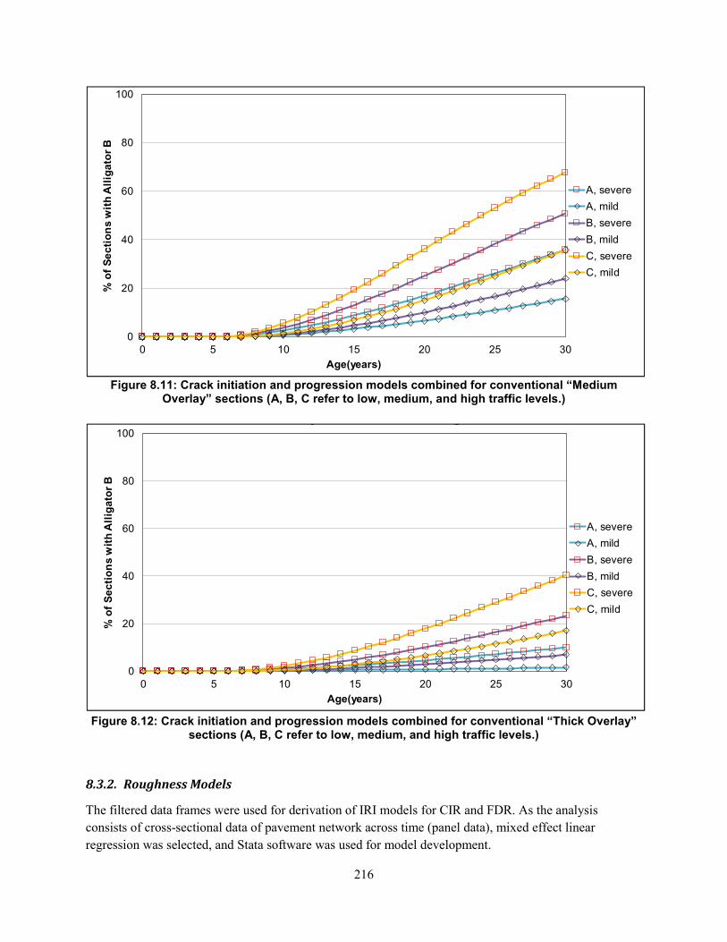
216

Figure 8.11: Crack initiation and progression models combined for conventional “Medium Overlay” sections (A, B, C refer to low, medium, and high traffic levels.)

Figure 8.12: Crack initiation and progression models combined for conventional “Thick Overlay”

sections (A, B, C refer to low, medium, and high traffic levels.)

8.3.2. Roughness Models

The filtered data frames were used for derivation of IRI models for CIR and FDR. As the analysis

consists of cross-sectional data of pavement network across time (panel data), mixed effect linear

regression was selected, and Stata software was used for model development.

0

20

40

60

80

100

0 5 10 15 20 25 30

% o

f S

ec

tio

ns

wit

h A

llig

ato

r B

Age(years)

A, severe

A, mild

B, severe

B, mild

C, severe

C, mild

0

20

40

60

80

100

0 5 10 15 20 25 30

% o

f S

ec

tio

ns

wit

h A

llig

ato

r B

Age(years)

Thick Overlay, Crack Initiation + Progression

A, severe

A, mild

B, severe

B, mild

C, severe

C, mild

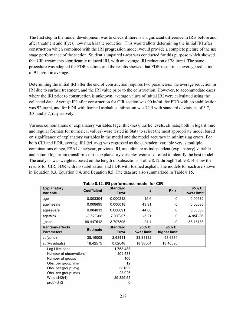
217

The first step in the model development was to check if there is a significant difference in IRIs before and

after treatment and if yes, how much is the reduction. This would allow determining the initial IRI after

construction which combined with the IRI progression model would provide a complete picture of the use

stage performance of the section. Student’s unpaired t-test was conducted for this purpose which showed

that CIR treatments significantly reduced IRI, with an average IRI reduction of 78 in/mi. The same

procedure was adopted for FDR sections and the results showed that FDR result in an average reduction

of 91 in/mi in average.

Determining the initial IRI after the end of construction requires two parameters: the average reduction in

IRI due to surface treatment, and the IRI value prior to the construction. However, to accommodate cases

where the IRI prior to construction is unknown, average values of initial IRI were calculated using the

collected data. Average IRI after construction for CIR section was 90 in/mi, for FDR with no stabilization

was 92 in/mi, and for FDR with foamed asphalt stabilization was 72.5 with standard deviations of 3.7,

3.3, and 5.7, respectively.

Various combinations of explanatory variables (age, thickness, traffic levels, climate; both in logarithmic

and regular formats for numerical values) were tested in Stata to select the most appropriate model based

on significance of explanatory variables in the model and the model accuracy in minimizing errors. For

both CIR and FDR, average IRI (iri_avg) was regressed as the dependent variable versus multiple

combinations of age, ESAL/lane/year, previous IRI, and climate as independent (explanatory) variables,

and natural logarithm transforms of the explanatory variables were also tested to identify the best model.

The analysis was weighted based on the length of subsections. Table 8.12 through Table 8.14 show the

results for CIR, FDR with no stabilization and FDR with foamed asphalt. The models for each are shown

in Equation 8.3, Equation 8.4, and Equation 8.5. The data are also summarized in Table 8.15.

Table 8.12. IRI performance model for CIR

Explanatory

Variable Coefficient

Standard

Error z P>|x|

95% CI

lower limit

age -0.003304 0.000212 -15.6 0 -0.00372

agelnesals 0.008695 0.000018 49.91 0 0.00086

agesevere 0.004013 0.000091 44.08 0 0.00383

agethick -3.52E-06 7.00E-07 -5.21 0 -4.85E-06

_cons 90.447512 3.707305 24.4 0 83.18133

Random-effects

Parameters Estimate

Standard

Error

95% CI

lower limit

95% CI

higher limit

sd(cons) 38.16008 2.63411 33.33132 43.6884

sd(Residuals) 18.42575 0.02048 18.38564 18.46595

Log Likelihood -1,753,438 Number of observations 404,588 Number of groups 106

Obs. per group: min 12 Obs. per group: avg 3816.9 Obs. per group: max 23,926 Wald chi2(4) 39,329.58 prob>chi2 = 0

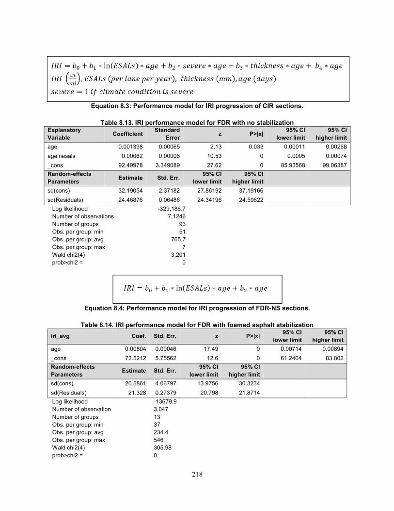
218

Equation 8.3: Performance model for IRI progression of CIR sections.

Table 8.13. IRI performance model for FDR with no stabilization

Explanatory

Variable Coefficient

Standard

Error z P>|x|

95% CI

lower limit

95% CI

higher limit

age 0.001398 0.00065 2.13 0.033 0.00011 0.00268

agelnesals 0.00062 0.00006 10.53 0 0.0005 0.00074

_cons 92.49978 3.349089 27.62 0 85.93568 99.06387

Random-effects

Parameters Estimate Std. Err.

95% CI

lower limit

95% CI

higher limit

sd(cons) 32.19054 2.37182 27.86192 37.19166

sd(Residuals) 24.46876 0.06486 24.34196 24.59622

Log likelihood -329,186.7 Number of observations 7,1246 Number of groups 93 Obs. per group: min 51 Obs. per group: avg 765.7

Obs. per group: max 7 Wald chi2(4) 3,201 prob>chi2 = 0

Equation 8.4: Performance model for IRI progression of FDR-NS sections.

Table 8.14. IRI performance model for FDR with foamed asphalt stabilization

iri_avg Coef. Std. Err. z P>|x| 95% CI

lower limit

95% CI

higher limit

age 0.00804 0.00046 17.49 0 0.00714 0.00894

_cons 72.5212 5.75562 12.6 0 61.2404 83.802

Random-effects

Parameters Estimate Std. Err.

95% CI

lower limit

95% CI

higher limit

sd(cons) 20.5861 4.06797 13.9756 30.3234

sd(Residuals) 21.328 0.27379 20.798 21.8714

Log likelihood -13679.9 Number of observation 3,047

Number of groups 13 Obs. per group: min 37 Obs. per group: avg 234.4 Obs. per group: max 546 Wald chi2(4) 305.98 prob>chi2 = 0

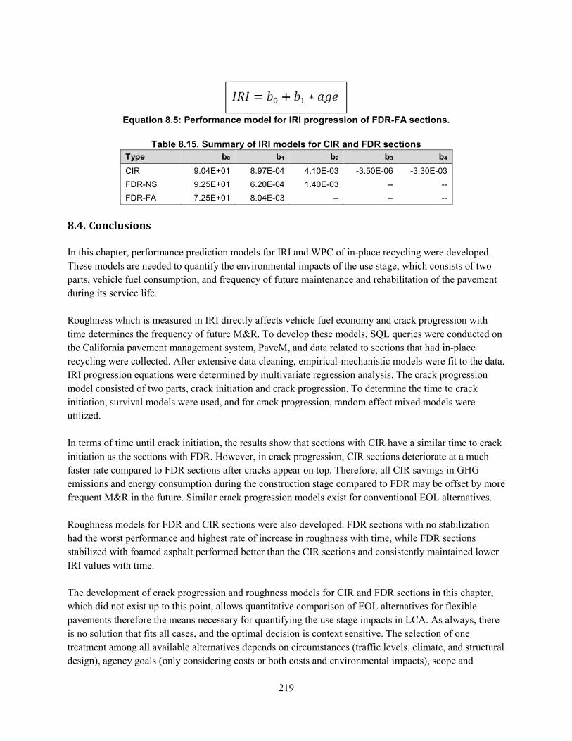
219

Equation 8.5: Performance model for IRI progression of FDR-FA sections.

Table 8.15. Summary of IRI models for CIR and FDR sections

Type b0 b1 b2 b3 b4

CIR 9.04E+01 8.97E-04 4.10E-03 -3.50E-06 -3.30E-03

FDR-NS 9.25E+01 6.20E-04 1.40E-03 -- --

FDR-FA 7.25E+01 8.04E-03 -- -- --

8.4. Conclusions

In this chapter, performance prediction models for IRI and WPC of in-place recycling were developed.

These models are needed to quantify the environmental impacts of the use stage, which consists of two

parts, vehicle fuel consumption, and frequency of future maintenance and rehabilitation of the pavement

during its service life.

Roughness which is measured in IRI directly affects vehicle fuel economy and crack progression with

time determines the frequency of future M&R. To develop these models, SQL queries were conducted on

the California pavement management system, PaveM, and data related to sections that had in-place

recycling were collected. After extensive data cleaning, empirical-mechanistic models were fit to the data.

IRI progression equations were determined by multivariate regression analysis. The crack progression

model consisted of two parts, crack initiation and crack progression. To determine the time to crack

initiation, survival models were used, and for crack progression, random effect mixed models were

utilized.

In terms of time until crack initiation, the results show that sections with CIR have a similar time to crack

initiation as the sections with FDR. However, in crack progression, CIR sections deteriorate at a much

faster rate compared to FDR sections after cracks appear on top. Therefore, all CIR savings in GHG

emissions and energy consumption during the construction stage compared to FDR may be offset by more

frequent M&R in the future. Similar crack progression models exist for conventional EOL alternatives.

Roughness models for FDR and CIR sections were also developed. FDR sections with no stabilization

had the worst performance and highest rate of increase in roughness with time, while FDR sections

stabilized with foamed asphalt performed better than the CIR sections and consistently maintained lower

IRI values with time.

The development of crack progression and roughness models for CIR and FDR sections in this chapter,

which did not exist up to this point, allows quantitative comparison of EOL alternatives for flexible

pavements therefore the means necessary for quantifying the use stage impacts in LCA. As always, there

is no solution that fits all cases, and the optimal decision is context sensitive. The selection of one

treatment among all available alternatives depends on circumstances (traffic levels, climate, and structural

design), agency goals (only considering costs or both costs and environmental impacts), scope and

220

analysis period considered for the project (initial costs and impacts versus full life cycle), and potential

limitations (in terms of budget, available technologies, and more.)

221

CHAPTER 9. Summary, Conclusions, and Recommended Future

Work

9.1. Introduction

The main goal of this dissertation was to develop frameworks, quantitative models, and databases needed

to support data-driven, informed, and integrated decision-making in managing the vast transportation

infrastructure in California. Such a management system was envisioned to consider both costs and

environmental impacts of management decisions, based on full life cycles of the infrastructure, and using

reliable, high quality data that well represent local conditions in terms of materials and energy sources,

production technologies, design methods, construction practices, and other critical parameters.

Various approaches were used in the studies included in this dissertation to be able to overcome

uncertainty in assumptions, parameters, and challenges in data (availability, quality, variability.)

9.2. Knowledge Gaps and Research Objectives

The major gaps in the knowledge identified at the beginning of this effort were:

• Integration of environmental impacts into the infrastructure management system requires a

reliable and representative life cycle inventories of different materials, surface treatments, and

construction activities used in the state of California. The available datasets generally did not

include a comprehensive list of all available options, were outdated, and were not representative

of the local conditions in terms of processes, mix designs, and energy sources.

• Frameworks and models needed by state and local governments quantify the life cycle costs and

environmental impacts of their decisions in transportation infrastructure management did not

cover some important areas of their operations. Without such frameworks and data models, state

and local governments could not properly evaluate all their strategies.

• There were limited and unreliable data for quantifying the environmental impacts of end-of-life

strategies for flexible pavements. Such models were needed to select among conventional and

novel approaches that are believed to more beneficial in terms of costs and environmental

impacts.

• There were no reliable performance prediction models for pavements built from recycled

materials. Therefore, it was unclear whether such sections perform better, equally, or worse

compared to conventional strategies. If the performance of recycled sections is worse, compared

to conventional methods, the potential savings in environmental impacts due to recycling may be

offset by the need for more frequent maintenance and rehabilitation in the future compared to

conventional strategies.

• A similar argument can be made regarding the surface roughness and how it would change with

time because roughness directly affects vehicle fuel consumption during the use stage. Roughness

performance models for sections built using in-place recycling were also not available.

• There was no consensus on how to allocate the environmental impacts and benefits of recycling

between the upstream and the downstream projects.

222

Therefore, the main objectives of this research were defined according to the gaps identified above, to

develop frameworks, models, and datasets needed to fill each gap.

9.3. UCPRC LCI Database

Through one of the research projects in this dissertation, the most comprehensive and up to date, as of

2019, life cycle inventory database, the UCPRC LCI Database, was developed for accurate quantification

of transportation infrastructure management projects in the state of California. This database includes an

extensive list of all the energy sources, materials, mixes, transportation modes, and construction processes

used in the projects at state and local government levels.

The electricity grid mix and other energy sources used in various life cycle stages are modified to

represent the state’s local conditions. Mix designs are defined based on specifications enforced by

Caltrans and also cover designs used by local governments. Construction practices are closely simulated

based on data collected from local contractors and experts in addition to the collection of primary data

collection from a few field projects. The LCI database developed and presented in this chapter has been

verified by a third party according to ISO recommendations.

The UCPRC LCI Database needs to be continually reviewed and periodically updated because of the

continuous improvements in material production technologies, construction practices, and energy sources

used for generating electricity and running the material plants, as well as improvements in data collection.

The revision and update process for the UCPRC LCI Database should be repeated every few years using

the latest available information. However, the most critical measure that can be taken to improve the

quality of the data is to collect primary data from local material production plants and contractors.

9.4. Complete Streets

This project demonstrated the use of LCA to consider the full life cycle environmental impacts of

conversion of several types of conventional streets to complete streets. The full system impacts of

complete streets on environmental impact indicators, considering materials, construction, and traffic

changes, are driven by changes in reduction in VMT and changes in the operation of the vehicles with

regard to speed and drive cycle changes caused by congestion, if it occurs. Therefore, the importance of

objective and reliable models for changes in traffic volume and congestion from the implementation of

complete streets and comparison with conventional streets cannot be overstated.

To avoid situations where well-intended efforts might result in greater environmental impacts, utilization

of life cycle assessment should be used as a robust and objective methodology that consider the full life

cycle of the alternatives. Each LCA study should use 1) high-quality data, 2) a correct definition of the

system boundary, and 3) include a thorough investigation, identification, and quantification of possible

significant unintended consequences.

223

The initial results indicate that application of the complete streets networks to streets where there is little

negative impact on vehicle drive cycles from speed change will have the most likelihood of causing

overall net reductions in environmental impacts.

The results also indicate that there is a range of potential VMT changes to which environmental impacts

are more sensitive than they are to the effects of the materials and construction stages, and that changes in

vehicle speed have different effects on environmental impacts depending on the context of their

implementation, including the street type.

The effects on environmental impacts due to implementing a complete street should be analyzed on a

project-by-project basis, and that the effects will not always be positive. This preliminary conclusion

leads to recommendations that this type of analysis be performed on a project-by-project basis, that the

analysis include the surrounding network, and that a sensitivity analysis should also be included.

The main limitation of this study was the lack of a reliable model for predicting changes in VMT and

traffic speed. Another issue that was not within the scope of this study was the consequential changes in

areas outsides the physical system boundary. Energy consumption for lighting and maintaining the

landscapes during the use stage was also not included in the study. Future works should focus on the

limitations identified above, specifically the lack of reliable models for changes in VMT and traffic speed.

9.5. Alternative Fuel Vehicles

This study was focused on comparing multiple pathways (scenarios) for Caltrans to transition their fleet

from vehicles with internal combustion engines burning fossil fuels to alternative fleet vehicles (AFVs.)

Four scenarios were considered based on AFV adoption rate including business as usual (BAU), all-at-

once, based on the Department of General Services (DGS) recommendations, and a worst-case scenario

(do nothing, keep the current mix.) The project compared the life cycle greenhouse gas (GHG) emissions,

fuel consumption, and costs of vehicle purchase and maintenance between 2018 to 2050.

The results showed a total life cycle costs of 2.4 billion dollars for the BAU case with 7.4 and 3.3 percent

increases versus BAU for the DGS and All-at-Once cases, and a 16.9 percent decrease for the Worst-Case

Scenario. Purchase of new vehicles was the largest portion of total net costs for all four cases, ranging

between 59 to 83 percent of final net total costs. Fuel costs were the second largest expense items for all

cases, ranging between 30 to 35 percent of total net costs. Maintenance and repair on average made up

about 24 percent of total net costs.

Total GHG emissions during the analysis period of 2018 to 2050 reached close to 1.46 million metric

tonnes of CO2e for the BAU case while the results for the DGS, All-at-Once show savings of 2 and 9

percent in total GHG emissions versus BAU for the DGS and All-at-Once scenarios. The Worst-Case

Scenario results show that consequences of inaction in the adopting AFVs by Caltrans and maintaining

the current mix of vehicle technology and fuel will result in 54 percent increase in the GHG footprint of

their fleet between now and the year 2050.

224

The study did not include the cost and environmental impacts of building and maintaining fueling

infrastructure for any of the fuel types considered in the analysis. Maintenance and upkeep of parking

spaces for the fleet were also not included in the system boundary of the study.

California is aggressively moving towards decarbonization/minimization of GHG emissions in all its

economic sectors, specifically the electricity sector with measures such the Renewable Portfolio Standard

(CPUC webpage on RPS) which mandates 50 percent renewable electricity in California grid mix by

2030. Therefore, one fuel pathway which is expected to have major reductions in WTP impacts is

electricity. However, these expected reductions in WTP were not implemented in this study, mainly due

to the limited scope of this initial study. However, the fact that more than 80 percent of the state fleet

consists of medium-duty pickups and trucks for which an EV option is not currently available reduces the

significance of this issue, at least for the immediate future.

Due to current technological limitation for the range of EVs, conversion to EVs was not considered as an

option for vehicles that had AVMT higher than typical current EV ranges. However, EV ranges are

expected to increase in the future but due to uncertainty regarding the rate of range increase, it was not

considered in this study.

Future work should consider more diverse portfolio of AFVs for different vehicle categories and also

include cleaner electricity grid that will power the electric vehicles.

9.6. Increased Use of RAP in Construction Projects

This chapter focused on quantifying savings in greenhouse gases (GHG), energy, material consumption,

and costs that might be possible through increased use of recycled asphalt pavements (RAP) in

construction projects in California. The material production impacts of hot mix asphalt (HMA) in

Caltrans construction projects throughout the state during the entire analysis period of 33 years (2018 to

2050) results in close to 11.5 Million Metric Tonnes (MMT) of CO2e for the baseline scenario. RHMA

production impacts within the same time period is about 15.2 MMT CO2e. RHMA is responsible for

about 44 percent of the combined GHG emissions of HMA and RHMA.

The use of RAP is currently not permitted in RHMA mixes, use of RAP in RHMA is a significant

untapped area for cutting emissions if it becomes technically possible to obtain same performance.

Increasing the RAP content in HMA from the baseline of the 11.5 percent can result in up to a 6 percent

of GHG savings with 30.5 percent RAP content during the 33-year analysis period, when using aromatic

BTX rejuvenating agents (RAs.) These reductions are equivalent to 0.7, 5.2, 6.2 percent reductions in

GHG emissions compared to the baseline. The potential saving can be as high as 9 percent when bio-

based RA is used.

Increasing RAP content in HMA can also result in cost savings of up to 9 percent reduction compared to

the baseline.

225

There are existing concerns, however, regarding the performance of HMA with higher RAP content. This

study was conducted assuming similar performance during the use stage across all the scenarios.

Decreases in performance can result in more frequent maintenance and rehabilitation needs in the future.

Higher surface roughness due to poor performance can cause in an increase in vehicle fuel consumption.

These issues can result in not only offsetting the original savings due to use of higher RAP content, but

also causing higher environmental impacts compared to the base scenario.

Therefore, further research is needed for investigating the performance of HMA with higher than 15

percent RAP content, and also RHMA with RAP. The research findings would allow design guidelines to

be developed and unintended consequences, that can arise from good intentions, to be avoided.

Allocating the environmental impacts of recycled materials between the upstream (which used the virgin

material and is the source of current recycled materials) and the downstream project (which uses the

recycled materials) is a pending challenge. There is currently no consensus on how to handle the issue of

allocation and tow common methodology currently in use are the 50-50 and the cut-off methods. In the

cut-off method, the impacts of virgin material production are assigned to the upstream project and the

downstream project is responsible for the recycling process impacts. In the 50-50 method, the total

impacts (virgin material production, the recycling process at the end of service life and possible hauling to

the treatment plant) are divided equally between the upstream and downstream project. To understand the

impact of the allocation methodology on the impacts of material production assigned to HMA with RAP,

the LCA of material production for the cases defined in the first part of this chapter was calculated using

both the 50-50 and the cut-off methods and the results were compared. The sensitivity of the results to the

hauling distances considered for the RAP materials was also investigated.

The results show that GWP of HMA with RAP using the cut-off method is consistently lower compared

to GWP HMA with RAP using the 50-50 method. Increased RAP hauling distances results in increased

GWP of HMA under both allocation methods compared to HMA with virgin materials, with a more

dramatic increase when the cut-off method is used. For hauling distances above 50 miles, there are cases

where GWP of 1 kg of HMA with RAP will be higher than HMA with virgin materials (depending on the

values of other input parameters.) The cases where the use of virgin materials results in less GWP

compared to the use of RAP for the cut-off method all have hauling distance of 100 miles with RAP

binder recovery of 50 or 60 percent. Binder recovery is the portion of the binder in the RAP that blends

with the virgin binder in the mix to create the final binder content. Binder recovery is increased for longer

and hotter mixing and silo storage times, and for RAP binders that are less aged. For the 50-50 method,

binder recovery ratios of 60 percent and above, with hauling distances of over 100 miles, resulted in

lower GWP for HMA with virgin materials compared to HMA with RAP. The binder recovery ratio

threshold that results in lower GWP for HMA with virgin materials compared to HMA with RAP

decreases with shorter hauling distances.

This section of the study was limited to comparison of allocation methodologies for EOL treatments. Due

to these limitations, no recommendation is made in terms of what allocation methodology should be

implemented in similar studies. Future studies should cover a more comprehensive system boundary and

consider more allocation methodologies.

226

9.7. LCA Benchmarking of EOL Alternatives

This study was conducted to benchmark the environmental impacts of several EOL treatments used in

California for flexible pavements at their end of service life. The system boundary consisted of material

production, transportation to the site and construction activities that together make up the EOL treatment.

The system boundary did not include other life cycle stages such as use stage, future maintenance and

rehabilitation, and traffic delays during construction activities. Ten treatments were studied, consisting of

eight in-place recycling alternatives (CIR and FDR with different stabilization methods and wearing

courses on top) and two conventional treatments (HMA overlay and HMA mill-and-fill.)

The results show that the material production stage is dominant in all impact categories for all treatments.

The results also show that the total amount of stabilizer added (which depends on percent stabilizer and

the layer thickness) has a significant impact on the total impacts. HMA overlay and HMA mill-and-fill,

have lower impacts compared to all the FDR options with stabilizers across all impact categories. Binder

and stabilizer production caused more than 90 percent of the total impacts of the material production

across all cases.

The study also examined the sensitivity of the results to the transportation distance of the virgin materials.

The results showed that changing the transportation distance has an important effect on total impacts of

conventional treatments. This was already expected, as conventional treatments require the largest amount

of materials transported.

Comparing the CIR with stabilizers and HMA overlay with the conventional treatment of an HMA

overlay shows that total GWP of the two options are close with the conventional treatment performing

slightly better. This remains true up to transport distance of 80 miles (two-way) for the virgin materials, at

which point the impacts of the two options become equal. For longer hauling distances the CIR

outperforms the conventional treatment.

Similar comparison of FDRs with conventional mill-and-fill resulted in very long transport distances for

virgin materials at which the impacts of the two treatments become equal. The transport distances were all

above 150 miles. At shorter hauling distances, conventional treatments had lower impacts.

There are large differences between the initial impacts of the treatments in each impact category but due

to limited scope of this stage and the fact that the system boundary does not include all life cycle stages,

comparison of the results shall not be used as basis for decision making and selecting between

alternatives. Such decision making requires a study that include the full life cycle of all the alternatives

considering the results of this chapter combined with the use stage impacts of each alternative when

calculated through models discussed in the next chapter. There are unsolved questions regarding the use

stage that need to be addressed:

• How does pavement surface roughness, which directly affects vehicle fuel consumption, change

with time under each treatment?

227

• What is the extension of life in terms of cracking, that determines future maintenance and

rehabilitation frequency and the section service life, differ between alternatives?

9.8. Performance Prediction Models

In this chapter, performance prediction models for IRI and WPC of in-place recycling were developed.

These models are needed to quantify the environmental impacts of the use stage, which consists of two

parts, vehicle fuel consumption, and frequency of future maintenance and rehabilitation of the pavement

during its service life.

Roughness which is measured in IRI directly affect vehicle mpg and crack progression with time

determines the frequency of future M&R. To develop these models, SQL queries were conducted on the

California pavement management system, PaveM, and data related to sections that had in-place recycling

were collected. After extensive data cleaning, mechanistic-empirical models were fit to the data. IRI

progression equations were determined by multivariate regression analysis. The crack progression model

consisted of two parts, crack initiation and crack progression. To determine the time to crack initiation,

survival models were used, and for crack progression, random effect mixed models were utilized.

In terms of time until crack initiation, the results show that sections with CIR have a similar time to crack

initiation as the sections with FDR. However, in crack progression, CIR sections deteriorate at a much

higher rate compared to FDR sections after cracks appear on top. Therefore, all CIR savings in GHG

emissions and energy consumption during the construction stage compared to FDR may be offset by more

frequent M&R in the future. Similar crack progression models exist for conventional EOL alternatives.

Roughness models for FDR and CIR sections were also developed. FDR sections with no stabilization

had the worst performance and highest rate of increase in roughness with time, while FDR sections

stabilized with foamed asphalt performed better than the CIR sections and consistently maintained lower

IRI values with time.

The development of crack progression and roughness models for CIR and FDR sections in this chapter,

which did not exist up to this point, allows a fair comparison of EOL alternatives for flexible pavements

by providing the means necessary for quantifying the use stage impacts and including them in the

analysis. As always, there is no solution that fits all cases, and the optimal decision is context sensitive.

The selection of one treatment among all available alternatives depends on circumstances (traffic levels,

climate, and structural design), agency goals (only considering costs or both costs and environmental

impacts), scope and analysis period considered for the project (initial costs and impacts versus full life

cycle), and potential limitations (in terms of budget, available technologies, and more.)

Some other thoughts, that are currently not included in the scope of this project but can be investigated

through lab/field tests and scenarios analysis, are:

• What is the damage level of the recycled layer when the surface layer fails?

• How many times can the surface be replaced before the underlying recycled layer needs to be

treated?

228

• Is there a difference in recyclability of a new pavement at its EOL versus a section that is built

using any of the conventional rehabilitation techniques?

• How many times can a recycling strategy be repeated on the same section? and do the

construction activities change with subsequent recycling?

• If the material quality changes with each subsequent recycling, how should the impacts be

allocated between the current and future recycling processes?

• Does consequent recycling have a detrimental impact on the pavement performance? Is the same

performance model applicable to a section recycled once and a section that that has been recycled

multiple times?

• Should the LCA consider repeated use of the same treatment or are there paths in the analysis

period in which different alternative should be considered?

229

REFERENCES

AFDC webpage on AFVs. https://afdc.energy.gov/vehicles/search/. Last accessed on 16 Apr 2020.

AFDC webpage on EPAct. https://afdc.energy.gov/files/pdfs/2527.pdf. Last accessed on 16 Apr 2020.

AFDC webpage on EPAct History.

https://afdc.energy.gov/files/u/data/data_source/10355/10355_epact_state_fp_vehicle_history.xlsx. Last

accessed in May 2019.

AFDC webpage on Fuel Prices. https://afdc.energy.gov/fuels/prices.html. Last accessed on 16 Apr 2020.

Alkins, A. E., Lane, B., and Kazmierowski, T. 2009. Sustainable Pavements: Environmental, Economic,

and Social Benefits of In-Situ Pavement Recycling. Transportation Research Record: Journal of the

Transportation Research Board, No. 2084(1). Washington, DC: Transportation Research Board of the

National Academies. pp 100-103.

ANL webpage on AFLEET. https://greet.es.anl.gov/afleet_tool. Last accessed on 16 Apr 2020.

ANL webpage on GREET. https://greet.es.anl.gov/. Last accessed on 16 Apr 2020.

ARRA. 2014. Recommended Construction Guidelines for Cold In-place Recycling (CIR) Using

Bituminous Recycling Agents. Annapolis, MD: Asphalt Recycling and Reclaiming Association.

ASTM 2007. Standard Specification for Epoxy-Coated Steel Reinforcing Bars. West Conshohocken,

PA: American Society for Testing and Materials International. (Standard A775/A775M).

ASTM 2012. Standard Specification for Deformed and Plain Carbon-Steel Bars for Concrete

Reinforcement. West Conshohocken, PA: American Society for Testing and Materials International.

(Standard A615/A615M).

Athena Institute. 2006. A Life Cycle Perspective on Concrete and Asphalt Roadways: Embodied

Primary Energy and Global Warming Potential. Ontario, Canada: Athena Institute.

Aurangzeb, Q., Al-Qadi, I. L. Ozer, H., and Yang, R. 2014. Hybrid Life Cycle Assessment for Asphalt

Mixtures with High RAP Content. Resources, Conservation and Recycling, Vol. 83. pp 77-86.

Autonomie webpage. https://www.autonomie.net/docs/Annex%202%20-

%20Vehicle%20Energy%20Consumption.xlsx. Last accessed on 16 Apr 2020.

Bare, J. 2012. Tool for the Reduction and Assessment of Chemical and Other Environmental

Impacts (TRACI). TRACI Version 2.1 User's Guide. Cincinnati, OH: Environmental Protection

Agency. (EPA/600/R-12/554 2012). Last accessed on 16 Apr 2020 at: https://www.epa.gov/chemical-

research/tool-reduction-and-assessment-chemicals-and-other-environmental-impacts-traci

Bemanian, S., Polish, P., and Maurer G. 2006. Cold In-Place Recycling and Full-Depth Reclamation

Projects by Nevada Department of Transportation: State of the Practice. Transportation Research

Record: Journal of the Transportation Research Board, No. 1949(1). Washington, DC:

Transportation Research Board of the National Academies. pp 54-71.

230

Birgisdóttir, H. 2005. Life Cycle Assessment Model for Road Construction and Use of Residues from

Waste Incineration. Ph.D. Dissertation. Copenhagen, Denmark: Technical University of Denmark.

BLS webpage on Producer Price Index. http://www.bls.gov/regions/mid-

atlantic/data/producerpriceindexconcrete_us_table.htm. Last accessed on 16 Apr 2020.

Brown, E. R., Parker, F., and Smith, M. R. 1992. Study of the Effectiveness of Styrene-Butadiene Rubber

Latex in Hot Mix Asphalt Mixes. Transportation Research Record: Journal of the Transportation

Research Board, No. 1342. Washington, DC: Transportation Research Board of the National Academies.

pp 85.

CA DGS webpage on Fuel Efficiency Requirements.

https://www.dgsapps.dgs.ca.gov/documents/sam/SamPrint/new/sam_master/sam_master_File/chap3600/3

620.1.pdf. Last accessed on 16 Apr 2020.

CA DGS webpage on Fuel Purchasing Policy.

https://www.documents.dgs.ca.gov/sam/SamPrint/new/sam_master/sam_master_file/chap3600/3627.pdf.

Last accessed on 16 Apr 2020.

CA DGS webpage on State Fleet. https://data.ca.gov/dataset/california-state-fleet. Last accessed in May

2020.

CA DGS webpage on Vehicle Replacement Policy.

https://www.documents.dgs.ca.gov/osp/sam/mmemos/MM17_05.pdf. Last accessed in May 2020.

CA DGS webpage on ZEV Purchasing Policy. http://sam.dgs.ca.gov/TOC/4100.aspx. Last accessed in

May 2020.

CA Legislature webpage on AB32.

http://leginfo.legislature.ca.gov/faces/billNavClient.xhtml?bill_id=201920200AB32. Last accessed on 16

Apr 2020.

CA Legislature webpage on AB338.

http://leginfo.legislature.ca.gov/faces/billTextClient.xhtml?bill_id=200520060AB338. Last accessed on

16 Apr 2020.

CA Legislature webpage on SB1275. http://www.leginfo.ca.gov/pub/13-14/bill/sen/sb_1251-

1300/sb_1275_bill_20140921_chaptered.pdf,. Last accessed on 16 Apr 2020.

CA Legislature webpage on SB32.

http://leginfo.legislature.ca.gov/faces/billPdf.xhtml?bill_id=201520160SB32&version=20150SB3288CH

P. Last accessed on 16 Apr 2020.

CA Legislature webpage on SB522.

https://leginfo.legislature.ca.gov/faces/billNavClient.xhtml?bill_id=200320040SB552. Last accessed on

16 Apr 2020.

CA Legislature webpage on AB236.

https://leginfo.legislature.ca.gov/faces/billNavClient.xhtml?bill_id=200720080AB236. Last accessed on

16 Apr 2020.

231

CA State webpage on Climate Change. https://www.climatechange.ca.gov/state/executive_orders.html.

Last accessed in May 2019.

CA State webpage on EO-B1612. https://www.gov.ca.gov/news.php?id=17472. Last accessed in May

2019.

CA State webpage on ZEV Action Plan. https://www.gov.ca.gov/wp-

content/uploads/2017/09/2016_ZEV_Action_Plan.pdf. Last accessed in May 2019.

Cai, H., Burnham, A., Wang, M., Hang, W., and Vyas A. 2015. The GREET Model Expansion for

Well-to-Wheels Analysis of Heavy-Duty Vehicles. Argonne, IL: Argonne National Lab. (No.

ANL/ESD-15/9). Last accessed on 17 Apr 2020 at: https://greet.es.anl.gov/publication-heavy-duty

Cai, H., Dunn, J., Pegallapati, A., Li, Q., Canter, C., Tan, E., and Biddy M. 2017. Supply Chain

Sustainability Analysis of Renewable Hydrocarbon Fuels via Indirect Liquefaction, Fast Pyrolysis,

and Hydrothermal Liquefaction: Update of the 2016 State-of-Technology Cases and Design Cases.

Argonne, IL: Argonne National Lab. (No. ANL-17/04)

Caltrans. 2011. Caltrans Automated Pavement Survey (APCS). Sacramento, CA: California

Department of Transportation.

Caltrans. 2014. Pervious Pavement Design Guide. Sacramento, CA: California Department of

Transportation.

Caltrans. 2015a. Highway Design Manual. Sacramento, CA: California Department of Transportation.

Caltrans. 2017. Complete Streets Implementation Action Plan 2.0. Sacramento, CA: California

Department of Transportation. Last accessed on 27 Nov 2017 at:

http://www.dot.ca.gov/hq/tpp/offices/ocp/docs/CSIAP2_rpt.pdf

Caltrans. 2018a. California Public Road Data 2017. Sacramento, CA: California Department of

Transportation.

Caltrans. 2018b. Caltrans Fact Booklet 2018. Sacramento, CA: California Department of

Transportation. Last accessed in March 2019 at: http://www.dot.ca.gov/drisi/library/cfb/2018-CFB.pdf

Caltrans. 2018c. Standard Specifications, Section 39-2.02B. Sacramento, CA: California Department of

Transportation. Last accessed in March 2019 at:

http://ppmoe.dot.ca.gov/hq/esc/oe/construction_contract_standards/std_specs/2018_StdSpecs/2018_StdSp

ecs.pdf

Caltrans MTAG. 2008. Maintenance Technical Advisory Guide (MTAG). Sacramento, CA: California

Department of Transportation.

Caltrans webpage on Asphalt Price Index. http://www.dot.ca.gov/hq/esc/oe/ac_index.html. Last accessed

in Jan 2016.

Caltrans webpage on CCDB 2018. http://ppmoe.dot.ca.gov/hq/esc/oe/awards/2018CCDB/2018ccdb.pdf.

Last accessed on 17 Apr 2020.

Cao, X., Tang, B., Zhu, H., Zhang, A., and Chen S. 2011. Cooling Principle Analyses and Performance

Evaluation of Heat-Reflective Coating for Asphalt Pavement. Journal of Materials in Civil Engineering

23 (7). pp 1067-1075.

232

Cao, X., Tang, B., Zhu, H., and Yuan Y. 2014. Preparation of Fluorinated Acrylate Heat Reflective

Coating for Pavement and Evaluation on Its Cooling Effect. TRB 93rd Annual Meeting Compendium

of Papers. Washington, DC: Transportation Research Board of the National Academies.

CARB webpage on AB32. https://www.arb.ca.gov/cc/ab32/ab32.htm. Last accessed on 16 Apr 2020.

CARB webpage on CA GHG Emissions. https://www.arb.ca.gov/cc/inventory/data/data.htm,. Last

accessed on 16 Apr 2020.

CARB webpage on CA Scoping Plan. https://www.arb.ca.gov/cc/scopingplan/scopingplan.htm. Last

accessed on 16 Apr 2020.

CARB webpage on LCSF. https://www.arb.ca.gov/fuels/lcfs/lcfs.htm. Last accessed on 16 Apr 2020.

CARB webpage on SB375. https://ww2.arb.ca.gov/our-work/topics/sustainable-communities. Last

accessed on 16 Apr 2020.

CEC webpage on Electricity Generation in CA. California Energy Commission, Sacramento, CA.

https://ww2.energy.ca.gov/almanac/electricity_data/total_system_power.html. Last accessed on 17 Apr

2020.

Chatti, K. and Zaabar I. 2012. Estimating the Effects of Pavement Condition on Vehicle Operating

Costs. Washington, DC: Transportation Research Board of the National Academies. (NCHRP Report

720).

City of LA. 2014. Complete Streets Manual. Los Angeles, CA: Department of City Planning. (CPC-

2013.910.GPA.SP.CA.MSC). Last accessed on 16 Apr 2020 at:

https://planning.lacity.org/odocument/c9596f05-0f3a-4ada-93aa-

e70bbde68b0b/Complete_Street_Design_Guide.pdf.

Corti, A. and Lombardi, L. 2004. End Life Tyres: Alternative Final Disposal Processes Compared By

LCA. Energy 29 (12). pp 2089-2108.

CPUC webpage on RPS. Renewable Portfolio Standard on CA Public Utility Commission webpage.

http://www.cpuc.ca.gov/rps_homepage/, 17Apr 2020

Cross, S. A., Chesner, W. H., Justus, H. G., and Kearney E. R. 2011. Life-Cycle Environmental Analysis

for Evaluation of Pavement Rehabilitation Options. Transportation Research Record: Journal of the

Transportation Research Board 2227(1). Washington, DC: Transportation Research Board of the

National Academies. pp: 43-52,

Davis, S. C., Diegel, S. W., and Boundy, R. G. 2015. Transportation Energy Data Book Edition 34

Oak Ridge, TN: Oak Ridge National Laboratory. (ORNL 6991).

DOE webpage on EPAct. https://epact.energy.gov/key-federal-statutes. Last accessed on 16 Apr 2020.

Eckmann, B., Delfosse, F., and Chevalier, E. 2012. Reducing Emissions and Consumption of Virgin

Aggregates Through Cold In-Place Recycling. Eurasphalt and Eurobitume Congress, 5th, 2012.

Istanbul, Turkey.

ecoinvent webpage. https://www.ecoinvent.org/database/database.html. Last accessed on 16 Apr 2020.

EIA webpage on AEO2018. https://www.eia.gov/outlooks/aeo/data/browser/#/?id=12-

AEO2018&cases=ref2018&sourcekey=0. Last accessed on 16 Apr 2020.

233

EIA webpage on AER2018. https://www.eia.gov/totalenergy/data/browser/?tbl=T01.08. Last accessed on

16 Apr 2020.

EIA webpage on Natural Gas. https://www.eia.gov/dnav/ng/ng_pri_sum_a_epg0_pdv_dmcf_a.htm. Last

accessed on 16 Apr 2020.

EIA webpage on New Vehicle Attributes in AEO 2018.

https://www.eia.gov/outlooks/aeo/data/browser/?id=52-

AEO2018&cases=ref2018&sourcekey=0#/?id=52-AEO2018&cases=ref2019&sourcekey=0. Last

accessed on 16 Apr 2020.

EIA webpage on Price of Petroleum and Other Liquids.

http://www.eia.gov/dnav/pet/pet_pri_gnd_a_epm0_pte_dpgal_m.htm. Last accessed on 16 Apr 2020.

EIA webpage on the Electricity Sector.

https://www.eia.gov/electricity/data/browser/#/topic/7?agg=0,1&geo=vvvvvvvvvvvvo&endsec=vg&freq

=M&start=200101&end=201412&ctype=linechart&ltype=pin&rtype=s&pin=&rse=0&maptype=0. Last

accessed on 16 Apr 2020.

EIA webpage on Vehicle Cost Projections. https://www.eia.gov/outlooks/aeo/data/browser/#/?id=114-

AEO2018andcases=ref2018andsourcekey=0. Last accessed on 16 Apr 2020.

Elgowainy, A., Han, J., Ward, J., Joseck, F., Gohlke, D., Lindauer, A., Ramsden T. 2016. Cradle-to-

Grave Life cycle Analysis of US Light Duty Vehicle-Fuel Pathways: A Greenhouse Gas Emissions

and Economic Assessment of Current (2015) and Future (2025-2030) Technologies. Argonne, IL:

Argonne National Lab. (No. ANL/ESD-16/7). Last accessed on 17 Apr 2020 at:

https://publications.anl.gov/anlpubs/2016/05/127895.pdf

Elgowainy, A., Han, J., Poch, L., Wang, M., Vyas, A., Mahalik, M., and Rousseau A. 2010. Well-To-

Wheels Analysis of Energy Use and Greenhouse Gas Emissions of Plug-In Hybrid Electric Vehicles. Argonne, IL: Argonne National Lab. (No. ANL/ESD/10-1). Last accessed on 17 Apr 2020 at:

https://afdc.energy.gov/files/pdfs/argonne_phev_evaluation_report.pdf

EMFAC2017 Web Database. Last accessed on 16 Apr 2020 at: https://www.arb.ca.gov/emfac/2017/

EPA webpage on Compliance and Fuel Economy. https://www.epa.gov/compliance-and-fuel-economy-

data. Last accessed on 16 Apr 2020.

EPA webpage on Fuel Economy Trends. https://www.epa.gov/fuel-economy-trends/highlights-co2-and-

fuel-economy-trends. Last accessed on 16 Apr 2020.

EPA webpage on LCA Glossary.

https://ofmpub.epa.gov/sor_internet/registry/termreg/searchandretrieve/glossariesandkeywordlists/search.

do?details=&glossaryName=Lifecycle%20Assessment%20Glossary. Last accessed on 16 Apr 2020.

EPA webpage on the U.S. GHG Emissions. https://www.epa.gov/ghgemissions/sources-greenhouse-gas-

emissions. Last accessed on 16 Apr 2020.

Eurobitume 2012. Life Cycle Inventory: Bitumen. Brussels, Belgium: Eurobitume. Last accessed on 16

Apr 2020 at: https://www.eurobitume.eu/fileadmin/pdf-downloads/LCI%20Report-Website-2ndEdition-

20120726.pdf

234

Farshidi, F. and Harvey, J. 2008. Evaluation of the Washington State Performance Model for Use by

Caltrans. Davis, CA: University of California Pavement Research Center. (Research Report UCPRC-

RR-2008-13).

FHWA 2014. Development of a Pavement Life Cycle Assessment (LCA) Framework: Synthesis and

Literature Review. Unpublished. Washington, DC: Federal Highway Administration.

Finnveden, G. and Moberg, Å. 2005. Environmental systems analysis tools–an overview. Journal of

cleaner production, 13(12). pp 1165-1173.

GaBi. 2014. Life Cycle Assessment Software, version 6.3. LCIs for Reflective Coating Materials.

Unpublished. San Francisco, CA: PE International. (PE Order Number PEA-11128).

GaBi webpage. http://www.GaBi-software.com/america/index/. Last accessed on 16 Apr 2020.

Gilbert, H. E., Rosado, P. J., Ban-Weiss, G., Harvey, J. T., Li, H., H. Mandel, B., Millstein, D., Mohegh,

A., Saboori, A., and Levinson, R. M. 2017. Energy and Environmental Consequences of a Cool Pavement

Campaign. Energy and Buildings 157. pp 53-77. Last accessed on 16 Apr 2020 at:

https://www.sciencedirect.com/science/article/pii/S0378778817309908?via%3Dihub

Green CA webpage. https://green.ca.gov/. Last accessed on 16 Apr 2020.

Harvey, J. T., Meijer, J., Ozer, H., Al-Qadi, I. L., Saboori, A., and, Kendall, A. 2016. Pavement Life

Cycle Assessment Framework. Washington, DC: U.S. Department of Transportation Federal Highway

Administration (FHWA-HIF-16-014).

Harvey, J., Kendall, A., Lee, I. S., Santero, N., Van Dam, T., and Wang T. 2010. Pavement Life Cycle

Assessment Workshop: Discussion Summary and Guidelines. Davis, CA: University of California.

(UCPRC-TM-2010-03). The conference webpage last accessed on 16 Apr 2020 at:

http://www.ucprc.ucdavis.edu/p-lca/

Harvey, J., Kendall, A., and Saboori, A. 2015a. The Role of Life Cycle Assessment in Reducing

Greenhouse Gas Emissions from Road Construction and Maintenance. Davis, CA: The National

Center for Sustainable Transportation, Institute of Transportation Studies, University of California.

Harvey, J., Jullièn, A., Steyn, W., Kendall, A., Jones, D., and Saboori, A. 2015b. Recommendations for

Application of the Results of the Pavement LCA 2014 Symposium to Southern Africa. Asphalt

Pavements for Southern Africa (CAPSA15), 11th, 2015. Sun City, South Africa. Last accessed in Apr

2020 at https://trid.trb.org/view.aspx?id=1404841.

Harvey, J. T., Kendall, A., Saboori, A., Ostovar, M., Butt, A. A., Hernandez, J., and Haynes, B. 2018.

Framework for Life Cycle Assessment of Complete Streets Projects. Davis, CA: National Center for

Sustainable Transportation, Institute of Transportation Studies, University of California.

Horvath, A. 2003. Life-Cycle Environmental and Economic Assessment of Using Recycled Materials

for Asphalt Pavements. University of California Transportation Center, Berkeley, CA.

Horvath, A. and Hendrickson, C. 1998. Comparison of Environmental Implications of Asphalt and Steel-

Reinforced Concrete Pavements. Transportation Research Record: Journal of the Transportation

Research Board 1626 (1). Washington, DC: Transportation Research Board of the National Academies.

pp: 105-113.

235

Huang, Y., Spray, A., and Parry, A. 2013. Sensitivity Analysis of Methodological Choices in Road

Pavement LCA. The International Journal of Life Cycle Assessment. Volume 18, Issue 1. Springer.

IPCC. 2006. IPCC Guidelines for National Greenhouse Gas Inventories. Kanagawa, Japan: Institute

for Global Environmental Strategies. Prepared by the National Greenhouse Gas Inventories Programme,

Eggleston H.S., Buendia L., Miwa K., Ngara T., and Tanabe K. (eds).

ISO. 2006. Environmental Management – Life Cycle Assessment – Principles and Framework.

Geneva, Switzerland: International Organization for Standardization. (ISO 14040).

Jones, D., Fu, P., and Harvey, J. T. 2009a. Full-Depth Pavement Reclamation with Foamed Asphalt in

California: Guidelines for Project Selection, Design, and Construction. Davis, CA: University of

California Pavement Research Center. (No. UCPRC-GL-2008-01).

Jones, D., Louw, S., and Wu, R. 2016. Full-Depth Recycling Study: Test Track Construction and

First-Level Analysis of Phase 1 and Phase 2 HVS Testing, Forensic Investigation, and Phase 1

Laboratory Testing. Davis, CA: University of California Pavement Research Center. ( No.

UCPRC-RR-2015-02).

Jones, D., Wu, R., and Louw, S. 2014. Full-Depth Recycling Study: Test Track Construction and

First Level Analysis Of Phase 1 HVS And Laboratory Testing. Davis, CA: University of California

Pavement Research Center. ( No. UCPRC-RR-2014-03).

Jones, S. B., Meyer, P. A., Snowden-Swan, L. J., Padmaperuma, A. B., Tan, E., Dutta, A., Jacobson, J.,

and Cafferty, K. 2013. Process Design and Economics for the Conversion of Lignocellulosic Biomass

To Hydrocarbon Fuels: Fast Pyrolysis and Hydrotreating Bio-Oil Pathway. Richland, WA: Pacific

Northwest National Lab. (No. PNNL-23053; NREL/TP-5100-61178.)

https://www.pnnl.gov/main/publications/external/technical_reports/PNNL-23053.pdf. Last accessed on

17 Apr 2020.

Jullien, A., Dauvergne, M., and Proust, C. 2015. Road LCA: The Dedicated ECORCE Tool and Database.

The International Journal of Life Cycle Assessment, 20(5). pp 655-670.

Kandhal, P. S. and Mallick, R. B. (1997). Pavement Recycling Guidelines for State and Local

Governments Participant's Reference Book. Washington, DC: Federal Highway Administration.

Kang, S., Yang, R., Ozer, H., and Al-Qadi, I. 2014. Life-Cycle Greenhouse Gases and Energy

Consumption for Material and Construction Phases of Pavement with Traffic Delay. Transportation

Research Record: Journal of the Transportation Research Board 2428 (1). Washington, D.C.:

Transportation Research Board of the National Academies. pp 27-34.

Kendall, A. 2007. Concrete Infrastructure Sustainability: Life Cycle Metrics, Materials Design, and

Optimized Distribution of Cement Production. PhD Dissertation, University of Michigan at Ann

Arbor.

Kendall, A. 2012. Life Cycle Assessment for Pavement: Introduction. Presentation in Minutes. Davis

CA: FHWA Sustainable Pavement Technical Working Group Meeting, April 25-26, 2012.

Keoleian, G., Kendall, A., Lepech, M., and Li, V. 2005. Guiding the Design and Application of New

Materials for Enhancing Sustainability Performance: Framework and Infrastructure Application. MRS

Proceedings, 895, 0895-G06-01. doi:10.1557/PROC-0895-G06-01

236

Lepert, P. and Brillet, F. 2009. The Overall Effects of Road Works on Global Warming Gas Emissions.

Transportation Research Part D; Vol (14). pp 576–84.

Levinson, R., Gilbert, H. E., Jin, L., Mandel, B., Millstein, D., Rosado, P. J., Harvey, J. T., Kendall, A.

M., Li, H., Saboori, A., Lea, J. Ban-Weiss, G., Mohegh, A., and Santero, N. 2017. Life-Cycle

Assessment and Co-Benefits of Cool Pavements. Sacramento, CA: California Air Resources Board.

Last accessed on 16 Apr 2020 at: https://www.arb.ca.gov/research/single-project.php?row_id=65149.

Levis, J. W., Barlaz, M. A., Tayebali, A., and Ranjithan S. R. 2012. Quantifying the Greenhouse Gas

Emission Reductions Associated with Recycling Hot Mix Asphalt. Road Materials and Pavement

Design 12(1). pp 57-77.

Li, H., Saboori, A., and Cao, X. 2016. Information synthesis and Preliminary Case Study for Life Cycle

Assessment of Reflective Coatings for Cool Pavements. International Journal of Transportation

Science and Technology, 5(1). pp 38-46.

Li, H. 2012. Evaluation of Cool PStrategies for Heat Island Mitigation. PhD Dissertation, Davis, CA:

University of California, Davis.

Liu, X., Cui Q., and Schwartz C. 2014. Performance Benchmark of Greenhouse Gas Emissions from

Asphalt Pavement in the United States. ICSI 2014@ Creating Infrastructure for a Sustainable World.

American Society of Civil Engineers.

Madanat, S., Nakat, Z., and Sathaye N. 2005. Development of Empirical-Mechanistic Pavement

Performance Models Using Data from the Washington State PMS Database. Davis, CA: University

of California Pavement Research Center. (Research Report UCPRC-RR-2005-05)

Marceau, M., Nisbet, M. A., Van Geem, M. G. 2007. Life Cycle Inventory of Portland Cement

Concrete. Skokie, IL: Portland Cement Association.

MOVES webpage. https://www.epa.gov/moves. Last accessed on 16 Apr 2020.

NACTO. 2013. Urban Street Design Guide. Island Press. Last accessed on 16 Apr 2020 at:

https://nacto.org/publication/urban-street-design-guide/

Nakat, Z., Madanat, S., Farshidi, F., and Harvey, J. 2006. Development of an Empirical-Mechanistic

Model of Overlay Crack Progression Using Data from the Washington State PMS Database. Davis,

CA: University of California Pavement Research Center. (Research Report UCPRC-RR-2006-15).

Nantes 2012 LCA Conference webpage. http://lca-construction2012.ifsttar.fr/. Last accessed on 16 Apr

2020.

Nixon, H., Agrawal, A. W., and Simons, C. 2017. Designing Road Diet Evaluations: Lessons Learned

from San Jose’s Lincoln Avenue Road Diet. San Jose, CA: Mineta Transportation Institute. (MTI

Report WP 12-14).

NREL webpage on USLCI. https://www.nrel.gov/lci/. Last accessed on 16 Apr 2020.

PaLATE webpage. http://faculty.ce.berkeley.edu/horvath/palate.html. Last accessed on 16 Apr 2020.

Pavement LCA 2014 Conference webpage. http://www.ucprc.ucdavis.edu/p-lca2014/Default.aspx. Last

accessed on 16 Apr 2020.

237

Pavement LCA 2017 Conference webpage. https://lcasymposium.ict.illinois.edu/. Last accessed on 16

Apr 2020.

Pereira, P. A. and Santos, L. P. 2006. Technical-Economical Evaluation of Pavement Recycling

Alternatives. Third Gulf Conference on Roads (TGCR06). Muscat, Oman.

Quillin, K. 2007. Calcium Sulfoaluminate Cements : Reduced CO2, Concrete Properties and

Applications. Bracknell, United Kingdom: IHS BRE Press.

Reinhart, T. E. 2016. Commercial Medium- and Heavy-Duty Truck Fuel Efficiency

Technology Study – Report #2. Washington, DC: National Highway Traffic Safety Administration.

(Report No. DOT HS 812 194).

Robinette, C. and Epps, J. 2010. Energy, Emissions, Material Conservation, and Prices Associated with

Construction, Rehabilitation, and Material Alternatives for Flexible Pavement. Transportation Research

Record: Journal of the Transportation Research Board, No. 2179. Washington, DC: Transportation

Research Board of the National Academies. pp. 10–22.

Saboori, A., Harvey, J., Butt, A. A., and Jones, D. 2017. Life Cycle Assessment and benchmarking of end

of life treatments of flexible pavements in California. Pavement Life-Cycle Assessment: Proceedings of

the Symposium on Life-Cycle Assessment of Pavements (Pavement LCA 2017). CRC Press. pp. 241-

250.

Saboori, A., Harvey, J., Li, H., Lea, J., Kendall, A., and Wang, T. 2020. Documentation of UCPRC

Life Cycle Inventory used in CARB/Caltrans LBNL Heat Island Project and other LCA Studies

Davis. CA: University of California Pavement Research Center.

Sacramento County. 2009. Improvement Standards, Section 4: Streets. Office of County

Engineering. Sacramento, CA: Sacramento County. Last accessed on 16 Apr 2020 at:

http://www.engineering.saccounty.net/Documents/Sect4StreetStds_Saccounty_%20Ver11_01_09.pdf

Santamouris, M., Synnefa, A., and Karlessi, T. 2011. Using Advanced Cool Materials in the Urban Built

Environment to Mitigate Heat Islands and Improve Thermal Comfort Conditions. Solar Energy 85 (12).

pp. 3085-3102.

Santero, N. J. 2009. Pavements and the Environment: A Life-Cycle Assessment Approach. PhD

Dissertation. Berkeley, CA: University of California, Berkeley.

Santero, N. J. 2011. Life-Cycle Assessment of Pavements. Part I: Critical Review. Resources,

Conservation and Recycling. Volume 55, Issues 9-10. Philadelphia, PA: Elsevier.

Santero, N. J., and Horvath, A. 2009. Global Warming Potential of Pavements. Environmental Research

Letters, 4(3), 034011.

Santos, J., Bryce, J., Flintsch, G., Ferreira, A., and Diefenderfer, B. 2014. A Life Cycle Assessment of In-

Place Recycling and Conventional Pavement Construction and Maintenance Practices. Structure and

Infrastructure Engineering 11(9). pp 1199-1217.

Sayagh, S., Ventura, A., Hoang, T., François, D., and Jullien, A. 2010. Sensitivity of the LCA Allocation

Procedure for BFS Recycled into Pavement Structures. Resources, Conservation and Recycling, 54(6).

pp 348-358.

238

SB1 Overview webpage. http://rebuildingca.ca.gov/overview.html. Last accessed on 16 Apr 2020.

Smart Growth America 2015 Conference in Baltimore webpage. https://www.newpartners.org/2015/. Last

accessed on 16 Apr 2020.

Smart Growth America webpage on Implementing Complete Streets.

https://www.smartgrowthamerica.org/app/legacy/documents/cs/factsheets/cs-networks.pdf. Last accessed

on 16 Apr 2020.

Stata webpage. https://www.stata.com/. Last accessed on 16 Apr 2020.

Stripple, H. 2001. Life Cycle Assessment of Road: A Pilot Study for Inventory Analysis. Rapport IVL

Swedish Environmental Research Institute. pp.1-96.

Stroup-Gardiner, M. 2011. Recycling and Reclamation of Asphalt Pavements Using In-Place

Methods. Washington DC: Transportation Research Board of the National Academies. (No. Project 20-

05 (Topic 40-13).

Synnefa, A., Santamouris, M., and Livada, I. 2006. A Study of the Thermal Performance of Reflective

Coatings for the Urban Environment. Solar Energy 80 (8). pp. 968-981.

Tseng, E. 2012. The Construction of Pavement Performance Models for Flexible Pavement

Wheelpath Cracking and IRI for the California Department of Transportation New Pavement

Management System. Master of Science Thesis. Davis, CA: University of California.

UCPRC LCI DB Shared Folder on Box. Last accessed on 16 Apr 2020 at:

https://ucdavis.box.com/s/va9w2mx6momdxq3dn3z4ym2lj5ucujdu

Van Dam, T.J., Harvey, J., Muench, S.T., Smith, K.D., Snyder, M.B., Al-Qadi, I.L., Ozer, H., Meijer, J.,

Ram, P., Roesler, J.R., and Kendall, A. 2015. Towards Sustainable Pavement Systems: A Reference

Document Washington, DC: Federal Highway Administration. (No. FHWA-HIF-15-002).

van Leest, A. J., van Hartskamp, S. B., and Meijer, J. P. 2008. Decision Support Model for Road

Pavements Based on Whole Life Costing, Life Cycle Assessment and Multi-Criteria Analysis. 9th

International Conference on Concrete Pavements.

Wang, H., Zhong, J., Feng, D., Meng, J., and Xie, N. 2012. Nanoparticles-modified Polymer-based Solar-

reflective Coating as a Cooling Overlay for Asphalt Pavement. International Journal of Smart and

Nano Materials 4 (2). pp. 102-111.

Wang, T., Lee, I. S., Kendall, A., Harvey, J., Lee, E. B., and Kim, C. 2012. Life Cycle Energy

Consumption and GHG Emission from Pavement Rehabilitation with Different Rolling Resistance.

Journal of Cleaner Production, 33. pp 86-96.

Wang, T. 2013. Reducing Greenhouse Gas Emissions and Energy Consumption Using Pavement

Maintenance and Rehabilitation: Refinement and Application of a Lifecycle Assessment Approach. PhD Dissertation. Davis, CA: University of California, Davis.

Wirtgen. 2012. Wirtgen Cold Recycling Technology. Wirtgen Company, Windhagen, Germany. Last

accessed on 17 Apr 2020 on http://media.wirtgen-

group.com/media/02_wirtgen/infomaterial_1/kaltrecycler/kaltrecycling_technologie/kaltrecycling_handb

uch/Cold_recycling_Manual_EN.pdf

239

Xu, X., Wildnauer, M., Gregory, J., and Kirchain, R. 2016. “Accounting for Variation in Life Cycle

Inventories: The Case of Portland Cement Production in the U.S.,” in Rewas 2016: Towards Materials

Resource Sustainability, eds. R.E. Kirchain, B. Blanpain, C. Meskers, E. Olivetti, D. Apelian, J.

Howarter, A. Kvithyld, B. Mishra, N. R. Neelameggham, J. Spangenberger (Hoboken, New Jersey: John

Wiley and Sons, 2016), 145-149. dx.doi.org/10.1002/9781119275039.ch21

Yang, R., Ozer, H., and Al-Qadi, I. L. 2016. Regional Upstream Life-Cycle Impacts of Petroleum

Products in the United States. Journal of Cleaner Production, 139. pp 1138-1149.

Yang, R. 2014. Development of A Pavement Life Cycle Assessment Tool Utilizing Regional Data and

Introducing an Asphalt Binder Model. Master of Science Thesis. Urbana/Champaign, IL: University of

Illinois at Urbana Champaign.

Yu, B. and Lu, Q. 2012. Life Cycle Assessment of Pavement: Methodology and Case Study.

Transportation Research Part D: Transport and Environment, 17(5). pp 380-388.

Zhang, H. 2009. Sustainable Pavement Asset Management Based on Life Cycle Models and

Optimization Methods. PhD Dissertation. Ann Arbor, MI: University of Michigan at Ann Arbor.

Zhang, H., Keoleian, G. A., Lepech M. D., and Kendall, A. 2010. Life-Cycle Optimization of Pavement

Overlay Systems. Journal of Infrastructure Systems, Vol. 16, No. 4. pp 310- 322.

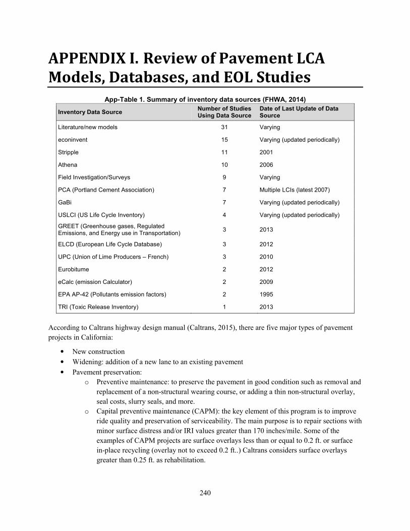
240

APPENDIX I. Review of Pavement LCA

Models, Databases, and EOL Studies

App-Table 1. Summary of inventory data sources (FHWA, 2014)

Inventory Data Source Number of Studies Using Data Source

Date of Last Update of Data Source

Literature/new models 31 Varying

econinvent 15 Varying (updated periodically)

Stripple 11 2001

Athena 10 2006

Field Investigation/Surveys 9 Varying

PCA (Portland Cement Association) 7 Multiple LCIs (latest 2007)

GaBi 7 Varying (updated periodically)

USLCI (US Life Cycle Inventory) 4 Varying (updated periodically)

GREET (Greenhouse gases, Regulated Emissions, and Energy use in Transportation)

3 2013

ELCD (European Life Cycle Database) 3 2012

UPC (Union of Lime Producers – French) 3 2010

Eurobitume 2 2012

eCalc (emission Calculator) 2 2009

EPA AP-42 (Pollutants emission factors) 2 1995

TRI (Toxic Release Inventory) 1 2013

According to Caltrans highway design manual (Caltrans, 2015), there are five major types of pavement

projects in California:

• New construction

• Widening: addition of a new lane to an existing pavement

• Pavement preservation:

o Preventive maintenance: to preserve the pavement in good condition such as removal and

replacement of a non-structural wearing course, or adding a thin non-structural overlay,

seal costs, slurry seals, and more.

o Capital preventive maintenance (CAPM): the key element of this program is to improve

ride quality and preservation of serviceability. The main purpose is to repair sections with

minor surface distress and/or IRI values greater than 170 inches/mile. Some of the

examples of CAPM projects are surface overlays less than or equal to 0.2 ft. or surface

in-place recycling (overlay not to exceed 0.2 ft..) Caltrans considers surface overlays

greater than 0.25 ft. as rehabilitation.

241

• Rehabilitation: major, non-routine work intended to return the roadway that exhibits major

structural distress to a good condition. Examples of roadway rehabilitation projects

include:

o Overlay

o Removal and replacement of the surface course

o Crack, seat, and overlay of rigid pavements regardless of overlay thickness

o Lane/shoulder replacements.

• Reconstruction: the replacement of the entire pavement section with a new structure.

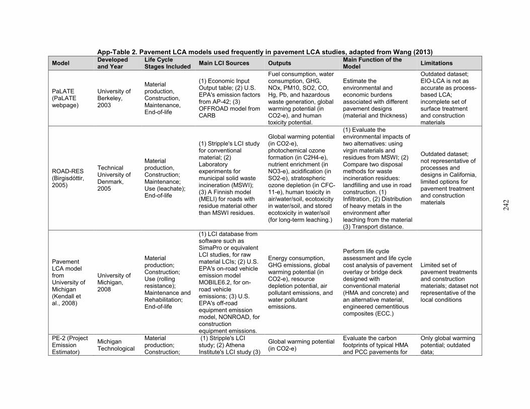
242

App-Table 2. Pavement LCA models used frequently in pavement LCA studies, adapted from Wang (2013)

Model Developed and Year

Life Cycle Stages Included

Main LCI Sources Outputs Main Function of the Model

Limitations

PaLATE (PaLATE webpage)

University of Berkeley, 2003

Material production, Construction, Maintenance, End-of-life

(1) Economic Input Output table; (2) U.S. EPA's emission factors from AP-42; (3) OFFROAD model from CARB

Fuel consumption, water consumption, GHG, NOx, PM10, SO2, CO, Hg, Pb, and hazardous waste generation, global warming potential (in CO2-e), and human toxicity potential.

Estimate the environmental and economic burdens associated with different pavement designs (material and thickness)

Outdated dataset; EIO-LCA is not as accurate as process-based LCA; incomplete set of surface treatment and construction materials

ROAD-RES (Birgisdóttir, 2005)

Technical University of Denmark, 2005

Material production, Construction; Maintenance; Use (leachate); End-of-life

(1) Stripple's LCI study for conventional material; (2) Laboratory experiments for municipal solid waste incineration (MSWI); (3) A Finnish model (MELI) for roads with residue material other than MSWI residues.

Global warming potential (in CO2-e), photochemical ozone formation (in C2H4-e), nutrient enrichment (in NO3-e), acidification (in SO2-e), stratospheric ozone depletion (in CFC- 11-e), human toxicity in air/water/soil, ecotoxicity in water/soil, and stored ecotoxicity in water/soil (for long-term leaching.)

(1) Evaluate the environmental impacts of two alternatives: using virgin materials and residues from MSWI; (2) Compare two disposal methods for waste incineration residues: landfilling and use in road construction. (1) Infiltration, (2) Distribution of heavy metals in the environment after leaching from the material (3) Transport distance.

Outdated dataset; not representative of processes and designs in California, limited options for pavement treatment and construction materials

Pavement LCA model from University of Michigan (Kendall et al., 2008)

University of Michigan, 2008

Material production; Construction; Use (rolling resistance); Maintenance and Rehabilitation; End-of-life

(1) LCI database from software such as SimaPro or equivalent LCI studies, for raw material LCIs; (2) U.S. EPA's on-road vehicle emission model MOBILE6.2, for on-road vehicle emissions; (3) U.S. EPA's off-road equipment emission model, NONROAD, for construction equipment emissions.

Energy consumption, GHG emissions, global warming potential (in CO2-e), resource depletion potential, air pollutant emissions, and water pollutant emissions.

Perform life cycle assessment and life cycle cost analysis of pavement overlay or bridge deck designed with conventional material (HMA and concrete) and an alternative material, engineered cementitious composites (ECC.)

Limited set of pavement treatments and construction materials; dataset not representative of the local conditions

PE-2 (Project Emission Estimator)

Michigan Technological

Material production; Construction;

(1) Stripple's LCI study; (2) Athena Institute's LCI study (3)

Global warming potential (in CO2-e)

Evaluate the carbon footprints of typical HMA and PCC pavements for

Only global warming potential; outdated data;

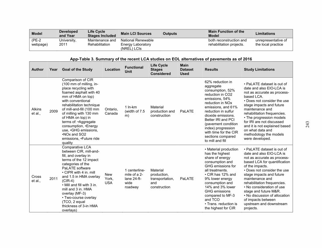
243

Model Developed and Year

Life Cycle Stages Included

Main LCI Sources Outputs Main Function of the Model

Limitations

(PE-2 webpage)

University, 2011

Maintenance and Rehabilitation

National Renewable Energy Laboratory (NREL) LCIs

both reconstruction and rehabilitation projects.

unrepresentative of the local practice

App-Table 3. Summary of the recent LCA studies on EOL alternatives of pavements as of 2016

Author Year Goal of the Study Location Functional Unit

Life Cycle Stages Considered

Main Dataset Used

Results Study Limitations

Alkins et al.,

2009

Comparison of CIR (100 mm of milling, in-place recycling with foamed asphalt with 40 mm of HMA on top) with conventional rehabilitation technique of mill-and-fill (100 mm of milling with 130 mm of HMA on top) in terms of: •Aggregate consumption, •Energy use, •GHG emissions, •NOx and SO2 emissions, •Future ride quality

Ontario, Canada

1 ln-km (width of 7.5 m)

Material production and construction

PaLATE

62% reduction in aggregate consumption, 52% reduction in CO2 emissions, 54% reduction in NOx emissions, and 61% reduction in sulfur dioxide emissions. Better IRI and PCI (pavement condition index) progression with time for the CIR sections compared to mill and fill

• PaLATE dataset is out of date and also EIO-LCA is not as accurate as process-based LCA. • Does not consider the use stage impacts and future maintenance and rehabilitation frequencies. • The progression models for IRI are not discussed and it is not explained based on what data and methodology the models were developed.

Cross et al.,

2011

Comparative LCA between CIR, mill-and-fill, and overlay in terms of the 12 impact categories of the PaLATE software • CIPR with 4 in. mill and 1.5 in HMA overlay (CIR-4) • Mill and fill with 3 in. mill and 3 in. HMA overlay (MF-3) • Two-course overlay (TCO, 2 equal thickness of 3-in HMA overlays)

New York, USA

1 centerline-mile of a 2-lane 24-ft-wide roadway

Material production, transportation, and construction

PaLATE

• Material production has the highest share of energy consumption and GHG emissions for all treatments. • CIR has 12% and 9% lower energy consumption and 14% and 3% lower GHG emissions compared to MF-3 and TCO • Trans. reduction is the highest for CIR

• PaLATE dataset is out of date and also EIO-LCA is not as accurate as process-based LCA for quantification of the impacts. • Does not consider the use stage impacts and future maintenance and rehabilitation frequencies. • No consideration of use stage and future M&R. • No discussion of allocation of impacts between upstream and downstream projects.

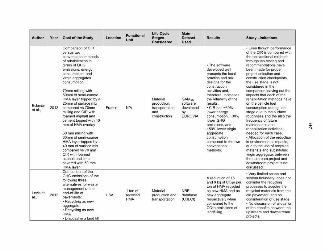
244

Author Year Goal of the Study Location Functional Unit

Life Cycle Stages Considered

Main Dataset Used

Results Study Limitations

Eckman et al.,

2012

Comparison of CIR versus two conventional methods of rehabilitation in terms of GHG emissions, energy consumption, and virgin aggregates consumption 70mm milling with 50mm of semi-coarse HMA layer topped by a 25mm of surface mix compared vs 70mm milling and CIR with foamed asphalt and cement topped with 40 mm of HMA overlay 60 mm milling with 60mm of semi-coarse HMA layer topped by 40 mm of surface mix compared vs 70 mm CIR with foamed asphalt and lime covered with 50 mm HMA layer

France N/A

Material production, transportation, and construction

GAÏABE

software developed by EUROVIA

• The software developed well presents the local practice and mix designs for the construction activities and, therefore, increases the reliability of the results. • CIR has ~30% lower energy consumption, ~30% lower GHG emissions, and ~50% lower virgin aggregate consumption compared to the two conventional methods.

• Even though performance of the CIR is compared with the conventional methods through lab testing and recommendations have been made for proper project selection and construction checkpoints, the use stage is not considered in the comparison leaving out the impacts that each of the rehabilitation methods have on the vehicle fuel consumption during use stage due to the surface roughness and the also the frequency of future maintenance and rehabilitation activities needed for each case. • Allocation of the reduction in environmental impacts, due to the use of recycled materials and substituting virgin aggregate, between the upstream project and downstream project is not discussed.

Levis et al.,

2012

Comparison of the GHG emissions of the following three alternatives for waste management at the end-of-life of pavements: • Recycling as new aggregate • Recycling as new HMA • Disposal in a land fill

USA 1 ton of recycled HMA

Material production and transportation

NREL database (USLCI)

A reduction of 16 and 9 kg of CO2e per ton of HMA recycled as new HMA and as new aggregate respectively when compared to the CO2e emissions of landfilling.

• Very limited scope and system boundary; does not consider the recycling processes to acquire the recycled materials from the old pavement, and no consideration of use stage. • No discussion of allocation of the benefits between the upstream and downstream projects.

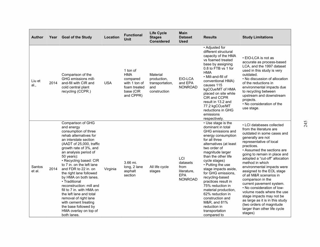
245

Author Year Goal of the Study Location Functional Unit

Life Cycle Stages Considered

Main Dataset Used

Results Study Limitations

Liu et al.,

2014

Comparison of the GHG emissions mill-and-fill with CIR and cold central plant recycling (CCPR.)

USA

1 ton of HMA compared with 1 ton of foam treated base (CIR and CPPR)

Material production, transportation, and construction

EIO-LCA and EPA NONROAD

• Adjusted for different structural capacity of the HMA vs foamed treated base by assigning 0.8 to FTB vs 1 for HMA • Mill-and-fill of conventional HMA) causes 115 kgCO2e/MT of HMA placed on site while CIR and CCPR result in 13.2 and 77.2 kgCO2e/MT reductions in GHG emissions respectively.

• EIO-LCA is not as accurate as process-based LCA, and the 1997 dataset used in this study is very outdated. • No discussion of allocation of the reductions in environmental impacts due to recycling between upstream and downstream projects. • No consideration of the use stage.

Santos et al.

2014

Comparison of GHG and energy consumption of three rehab alternatives for an interstate section (AADT of 25,000, traffic growth rate of 3%, and an analysis period of 50 years): • Recycling based: CIR to 7 in. on the left lane and FDR to 22 in. on the right lane followed by HMA on both lanes. • Traditional reconstruction: mill and fill to 7 in. with HMA on the left lane and total removal of right lane with cement treating the base followed by HMA overlay on top of both lanes.

Virginia

3.66 mi. long, 2 lane asphalt section

All life cycle stages

LCI datasets from literature, EPA NONROAD

• Use stage is the dominant in total GHG emissions and energy consumption for all three alternatives (at least two order of magnitude larger than the other life cycle stages) • Putting the use stage impacts aside, for GHG emissions, recycling-based practices result in 75% reduction in material production, 62% reduction in construction and M&R, and 81% reduction in transportation compared to

• LCI databases collected from the literature are outdated in some cases and generally are not representative of local practices. • Assumed the sections are going to remain in place and adopted a “cut‐off” allocation method in which environmental impacts were assigned to the EOL stage of all M&R scenarios in comparison in the current pavement system. • No consideration of low-volume roads where the use stage impacts may not be as large as it is in this study (two orders of magnitude larger than other life cycle stages)

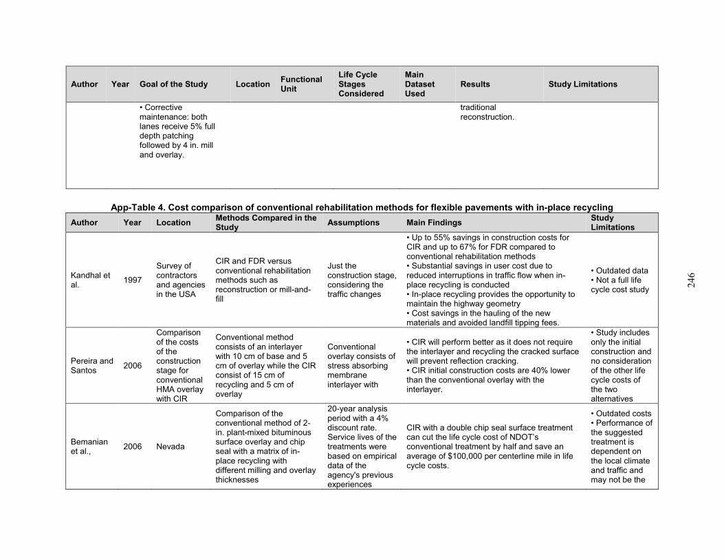
246

Author Year Goal of the Study Location Functional Unit

Life Cycle Stages Considered

Main Dataset Used

Results Study Limitations

• Corrective maintenance: both lanes receive 5% full depth patching followed by 4 in. mill and overlay.

traditional reconstruction.

App-Table 4. Cost comparison of conventional rehabilitation methods for flexible pavements with in-place recycling

Author Year Location Methods Compared in the Study

Assumptions Main Findings Study Limitations

Kandhal et al.

1997

Survey of contractors and agencies in the USA

CIR and FDR versus conventional rehabilitation methods such as reconstruction or mill-and-fill

Just the construction stage, considering the traffic changes

• Up to 55% savings in construction costs for CIR and up to 67% for FDR compared to conventional rehabilitation methods • Substantial savings in user cost due to reduced interruptions in traffic flow when in-place recycling is conducted • In-place recycling provides the opportunity to maintain the highway geometry • Cost savings in the hauling of the new materials and avoided landfill tipping fees.

• Outdated data • Not a full life cycle cost study

Pereira and Santos

2006

Comparison of the costs of the construction stage for conventional HMA overlay with CIR

Conventional method consists of an interlayer with 10 cm of base and 5 cm of overlay while the CIR consist of 15 cm of recycling and 5 cm of overlay

Conventional overlay consists of stress absorbing membrane interlayer with

• CIR will perform better as it does not require the interlayer and recycling the cracked surface will prevent reflection cracking. • CIR initial construction costs are 40% lower than the conventional overlay with the interlayer.

• Study includes only the initial construction and no consideration of the other life cycle costs of the two alternatives

Bemanian et al.,

2006 Nevada

Comparison of the conventional method of 2-in. plant-mixed bituminous surface overlay and chip seal with a matrix of in-place recycling with different milling and overlay thicknesses

20-year analysis period with a 4% discount rate. Service lives of the treatments were based on empirical data of the agency's previous experiences

CIR with a double chip seal surface treatment can cut the life cycle cost of NDOT’s conventional treatment by half and save an average of $100,000 per centerline mile in life cycle costs.

• Outdated costs • Performance of the suggested treatment is dependent on the local climate and traffic and may not be the

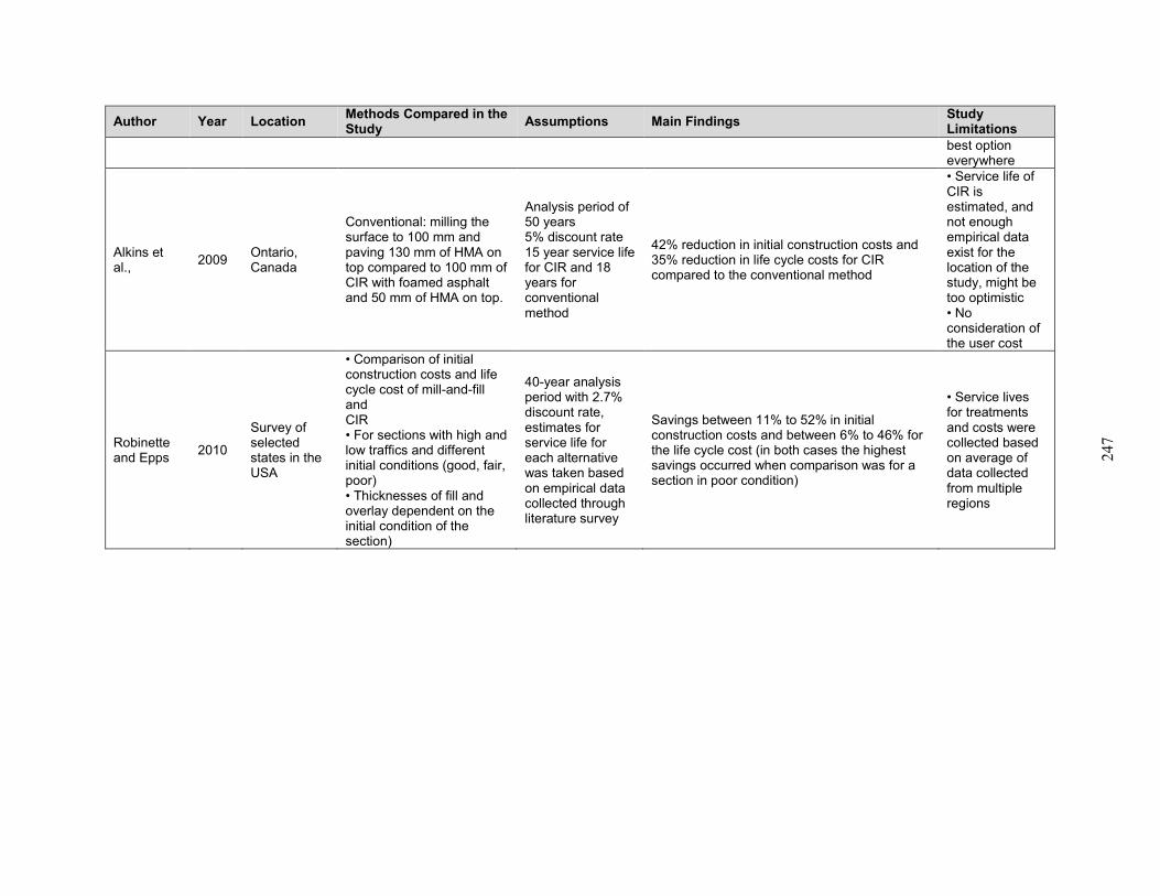
247

Author Year Location Methods Compared in the Study

Assumptions Main Findings Study Limitations

best option everywhere

Alkins et al.,

2009 Ontario, Canada

Conventional: milling the surface to 100 mm and paving 130 mm of HMA on top compared to 100 mm of CIR with foamed asphalt and 50 mm of HMA on top.

Analysis period of 50 years 5% discount rate 15 year service life for CIR and 18 years for conventional method

42% reduction in initial construction costs and 35% reduction in life cycle costs for CIR compared to the conventional method

• Service life of CIR is estimated, and not enough empirical data exist for the location of the study, might be too optimistic • No consideration of the user cost

Robinette and Epps

2010

Survey of selected states in the USA

• Comparison of initial construction costs and life cycle cost of mill-and-fill and CIR • For sections with high and low traffics and different initial conditions (good, fair, poor) • Thicknesses of fill and overlay dependent on the initial condition of the section)

40-year analysis period with 2.7% discount rate, estimates for service life for each alternative was taken based on empirical data collected through literature survey

Savings between 11% to 52% in initial construction costs and between 6% to 46% for the life cycle cost (in both cases the highest savings occurred when comparison was for a section in poor condition)

• Service lives for treatments and costs were collected based on average of data collected from multiple regions

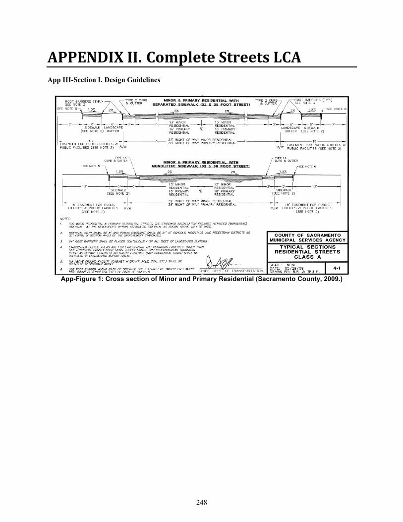
248

APPENDIX II. Complete Streets LCA

App III-Section I. Design Guidelines

App-Figure 1: Cross section of Minor and Primary Residential (Sacramento County, 2009.)

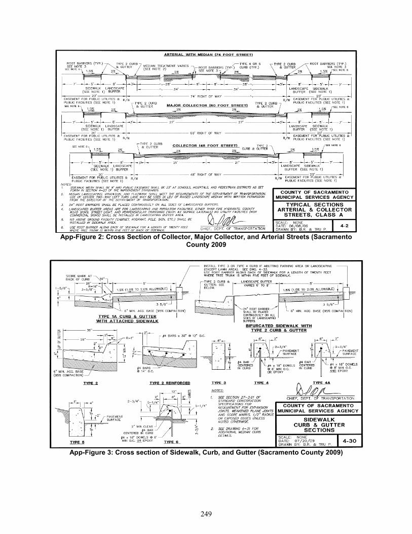
249

App-Figure 2: Cross Section of Collector, Major Collector, and Arterial Streets (Sacramento County 2009

App-Figure 3: Cross section of Sidewalk, Curb, and Gutter (Sacramento County 2009)

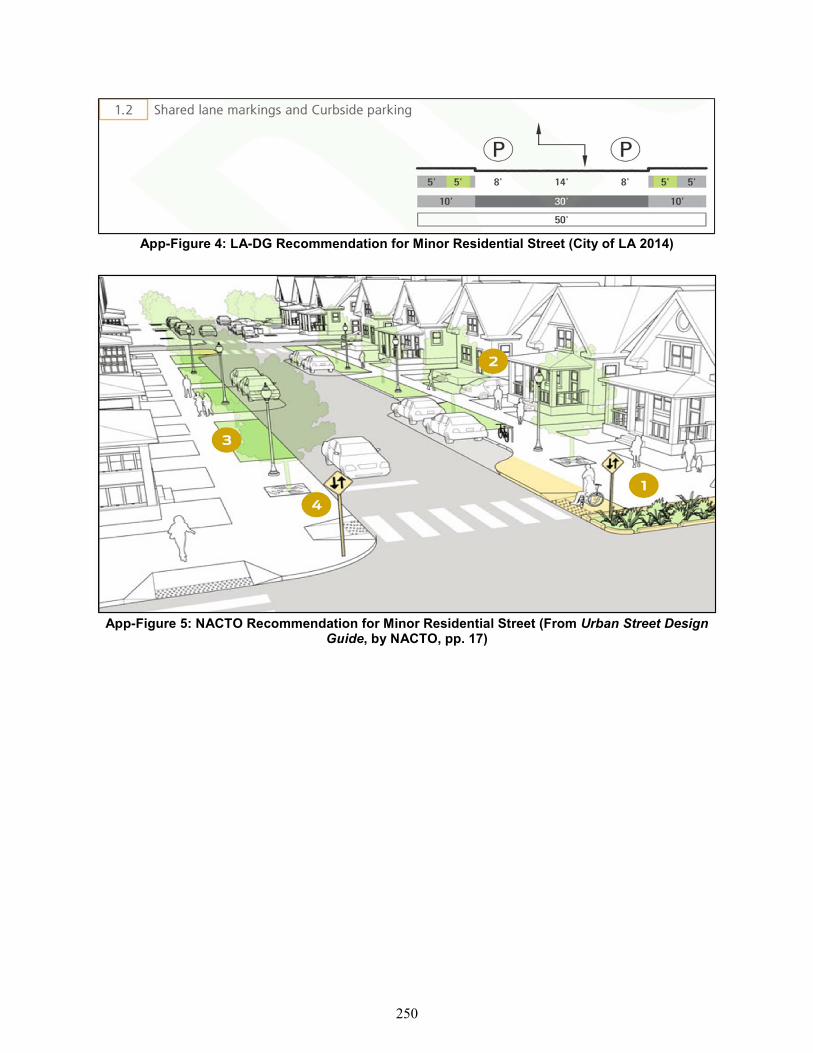
250

App-Figure 4: LA-DG Recommendation for Minor Residential Street (City of LA 2014)

App-Figure 5: NACTO Recommendation for Minor Residential Street (From Urban Street Design Guide, by NACTO, pp. 17)

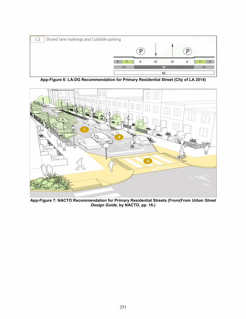
251

App-Figure 6: LA-DG Recommendation for Primary Residential Street (City of LA 2014)

App-Figure 7: NACTO Recommendation for Primary Residential Streets (From(From Urban Street Design Guide, by NACTO, pp. 16.)

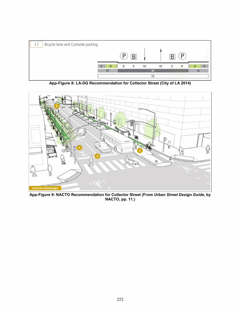
252

App-Figure 8: LA-DG Recommendation for Collector Street (City of LA 2014)

App-Figure 9: NACTO Recommendation for Collector Street (From Urban Street Design Guide, by NACTO, pp. 11.)

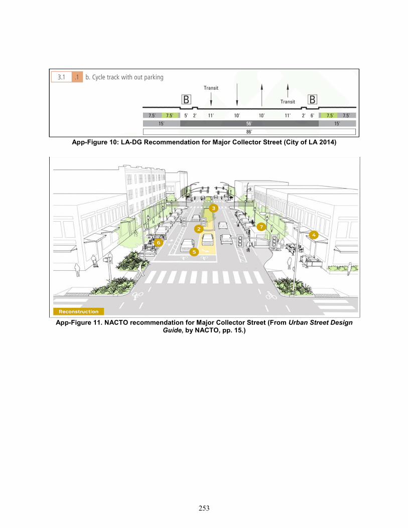
253

App-Figure 10: LA-DG Recommendation for Major Collector Street (City of LA 2014)

App-Figure 11. NACTO recommendation for Major Collector Street (From Urban Street Design Guide, by NACTO, pp. 15.)

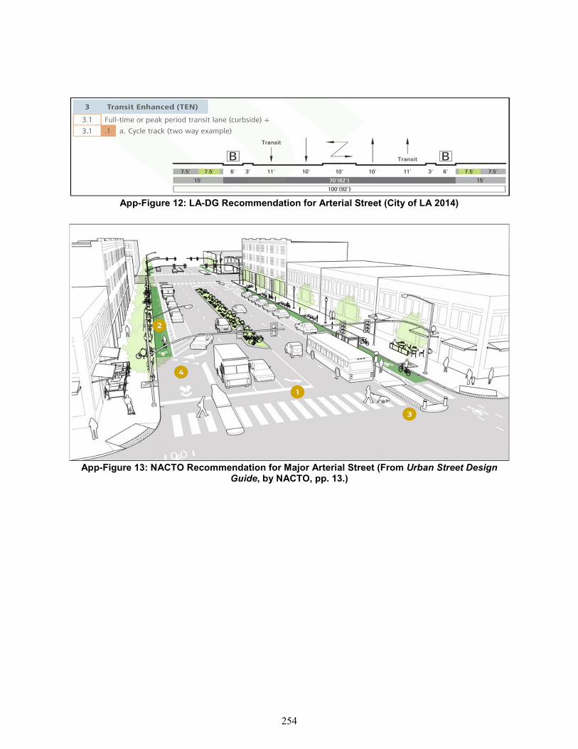
254

App-Figure 12: LA-DG Recommendation for Arterial Street (City of LA 2014)

App-Figure 13: NACTO Recommendation for Major Arterial Street (From Urban Street Design Guide, by NACTO, pp. 13.)

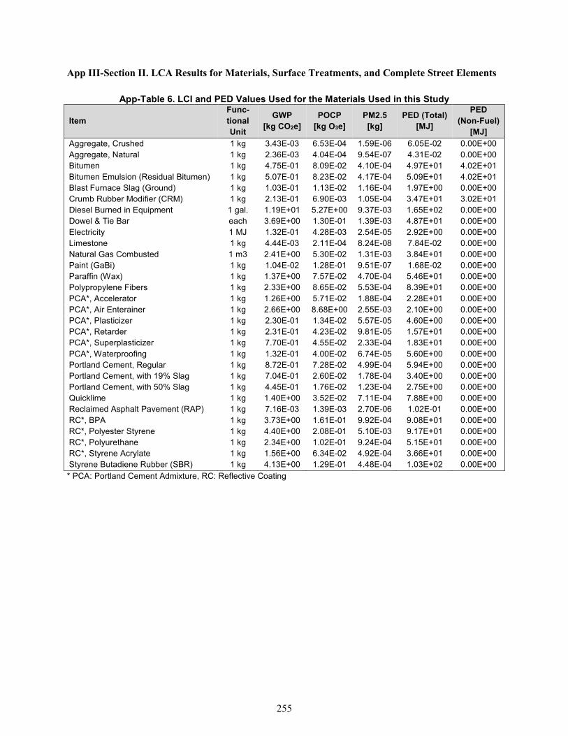
255

App III-Section II. LCA Results for Materials, Surface Treatments, and Complete Street Elements

App-Table 6. LCI and PED Values Used for the Materials Used in this Study

Item

Func-

tional

Unit

GWP

[kg CO2e]

POCP

[kg O3e]

PM2.5

[kg]

PED (Total)

[MJ]

PED

(Non-Fuel)

[MJ]

Aggregate, Crushed 1 kg 3.43E-03 6.53E-04 1.59E-06 6.05E-02 0.00E+00 Aggregate, Natural 1 kg 2.36E-03 4.04E-04 9.54E-07 4.31E-02 0.00E+00 Bitumen 1 kg 4.75E-01 8.09E-02 4.10E-04 4.97E+01 4.02E+01

Bitumen Emulsion (Residual Bitumen) 1 kg 5.07E-01 8.23E-02 4.17E-04 5.09E+01 4.02E+01 Blast Furnace Slag (Ground) 1 kg 1.03E-01 1.13E-02 1.16E-04 1.97E+00 0.00E+00 Crumb Rubber Modifier (CRM) 1 kg 2.13E-01 6.90E-03 1.05E-04 3.47E+01 3.02E+01 Diesel Burned in Equipment 1 gal. 1.19E+01 5.27E+00 9.37E-03 1.65E+02 0.00E+00 Dowel & Tie Bar each 3.69E+00 1.30E-01 1.39E-03 4.87E+01 0.00E+00

Electricity 1 MJ 1.32E-01 4.28E-03 2.54E-05 2.92E+00 0.00E+00 Limestone 1 kg 4.44E-03 2.11E-04 8.24E-08 7.84E-02 0.00E+00 Natural Gas Combusted 1 m3 2.41E+00 5.30E-02 1.31E-03 3.84E+01 0.00E+00 Paint (GaBi) 1 kg 1.04E-02 1.28E-01 9.51E-07 1.68E-02 0.00E+00 Paraffin (Wax) 1 kg 1.37E+00 7.57E-02 4.70E-04 5.46E+01 0.00E+00 Polypropylene Fibers 1 kg 2.33E+00 8.65E-02 5.53E-04 8.39E+01 0.00E+00

PCA*, Accelerator 1 kg 1.26E+00 5.71E-02 1.88E-04 2.28E+01 0.00E+00 PCA*, Air Enterainer 1 kg 2.66E+00 8.68E+00 2.55E-03 2.10E+00 0.00E+00 PCA*, Plasticizer 1 kg 2.30E-01 1.34E-02 5.57E-05 4.60E+00 0.00E+00 PCA*, Retarder 1 kg 2.31E-01 4.23E-02 9.81E-05 1.57E+01 0.00E+00 PCA*, Superplasticizer 1 kg 7.70E-01 4.55E-02 2.33E-04 1.83E+01 0.00E+00

PCA*, Waterproofing 1 kg 1.32E-01 4.00E-02 6.74E-05 5.60E+00 0.00E+00 Portland Cement, Regular 1 kg 8.72E-01 7.28E-02 4.99E-04 5.94E+00 0.00E+00 Portland Cement, with 19% Slag 1 kg 7.04E-01 2.60E-02 1.78E-04 3.40E+00 0.00E+00 Portland Cement, with 50% Slag 1 kg 4.45E-01 1.76E-02 1.23E-04 2.75E+00 0.00E+00 Quicklime 1 kg 1.40E+00 3.52E-02 7.11E-04 7.88E+00 0.00E+00 Reclaimed Asphalt Pavement (RAP) 1 kg 7.16E-03 1.39E-03 2.70E-06 1.02E-01 0.00E+00

RC*, BPA 1 kg 3.73E+00 1.61E-01 9.92E-04 9.08E+01 0.00E+00 RC*, Polyester Styrene 1 kg 4.40E+00 2.08E-01 5.10E-03 9.17E+01 0.00E+00 RC*, Polyurethane 1 kg 2.34E+00 1.02E-01 9.24E-04 5.15E+01 0.00E+00 RC*, Styrene Acrylate 1 kg 1.56E+00 6.34E-02 4.92E-04 3.66E+01 0.00E+00 Styrene Butadiene Rubber (SBR) 1 kg 4.13E+00 1.29E-01 4.48E-04 1.03E+02 0.00E+00

* PCA: Portland Cement Admixture, RC: Reflective Coating

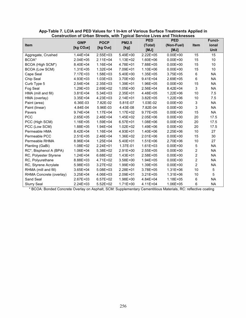
256

App-Table 7. LCIA and PED Values for 1 ln-km of Various Surface Treatments Applied in Construction of Urban Streets, with Typical Service Lives and Thicknesses

Item GWP

[kg CO2e]

POCP

[kg O3e]

PM2.5

[kg]

PED

(Total)

[MJ]

PED

(Non-Fuel)

[MJ]

Item

Funct-

ional

Unit

Aggregate, Crushed 1.44E+04 2.55E+03 5.49E+00 2.22E+05 0.00E+00 15 15 BCOA* 2.04E+05 2.11E+04 1.13E+02 1.60E+06 0.00E+00 15 10 BCOA (High SCM*) 8.40E+04 1.16E+04 4.78E+01 7.88E+05 0.00E+00 15 10 BCOA (Low SCM) 1.31E+05 1.32E+04 7.09E+01 1.10E+06 0.00E+00 15 10 Cape Seal 7.17E+03 1.58E+03 5.40E+00 1.35E+05 3.75E+05 6 NA Chip Seal 4.93E+03 1.03E+03 3.70E+00 9.41E+04 2.69E+05 6 NA

Curb Type 5 2.54E+04 2.35E+03 1.39E+01 1.96E+05 0.00E+00 15 NA Fog Seal 1.29E+03 2.69E+02 1.05E+00 2.56E+04 8.42E+04 3 NA HMA (mill and fill) 3.81E+04 5.34E+03 2.35E+01 4.48E+05 1.22E+06 10 7.5 HMA (overlay) 3.35E+04 4.23E+03 2.14E+01 3.82E+05 1.22E+06 10 7.5 Paint (area) 6.36E-03 7.82E-02 5.81E-07 1.03E-02 0.00E+00 3 NA

Paint (linear) 4.84E-04 5.96E-03 4.43E-08 7.82E-04 0.00E+00 3 NA Pavers 9.74E+04 1.17E+04 1.17E+02 9.77E+05 0.00E+00 15 NA PCC 2.65E+05 2.46E+04 1.45E+02 2.05E+06 0.00E+00 20 17.5 PCC (High SCM) 1.16E+05 1.59E+04 6.57E+01 1.08E+06 0.00E+00 20 17.5 PCC (Low SCM) 1.88E+05 1.94E+04 1.02E+02 1.49E+06 0.00E+00 20 17.5 Permeable HMA 8.42E+04 1.16E+04 4.93E+01 1.40E+06 2.25E+06 10 27

Permeable PCC 2.51E+05 2.46E+04 1.36E+02 2.01E+06 0.00E+00 15 30 Permeable RHMA 8.96E+04 1.25E+04 5.40E+01 1.51E+06 2.70E+06 10 27 Planting (GaBi) 1.08E+02 2.24E+01 1.37E-01 1.61E+03 0.00E+00 5 NA RC*, Bisphenol A (BPA) 1.06E+04 5.38E+02 2.91E+00 2.55E+05 0.00E+00 2 NA RC, Polyester Styrene 1.24E+04 6.68E+02 1.43E+01 2.58E+05 0.00E+00 2 NA RC, Polyurethane 8.88E+03 4.71E+02 3.58E+00 1.94E+05 0.00E+00 2 NA

RC, Styrene Acrylate 5.98E+03 3.27E+02 1.99E+00 1.39E+05 0.00E+00 2 NA RHMA (mill and fill) 3.65E+04 5.08E+03 2.28E+01 3.78E+05 1.31E+06 10 5 RHMA Concrete (overlay) 3.25E+04 4.06E+03 2.09E+01 3.21E+05 1.31E+06 10 5 Sand Seal 2.67E+03 6.57E+02 1.98E+00 4.84E+04 1.18E+05 6 NA Slurry Seal 2.24E+03 5.52E+02 1.71E+00 4.11E+04 1.06E+05 6 NA

* BCOA: Bonded Concrete Overlay on Asphalt, SCM: Supplementary Cementitious Materials, RC: reflective coating

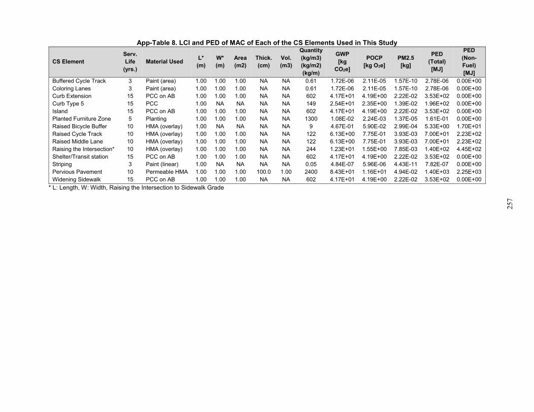
257

App-Table 8. LCI and PED of MAC of Each of the CS Elements Used in This Study

CS Element

Serv.

Life

(yrs.)

Material Used L*

(m)

W*

(m)

Area

(m2)

Thick.

(cm)

Vol.

(m3)

Quantity

(kg/m3)

(kg/m2)

(kg/m)

GWP

[kg

CO2e]

POCP

[kg O3e]

PM2.5

[kg]

PED

(Total)

[MJ]

PED

(Non-

Fuel)

[MJ]

Buffered Cycle Track 3 Paint (area) 1.00 1.00 1.00 NA NA 0.61 1.72E-06 2.11E-05 1.57E-10 2.78E-06 0.00E+00 Coloring Lanes 3 Paint (area) 1.00 1.00 1.00 NA NA 0.61 1.72E-06 2.11E-05 1.57E-10 2.78E-06 0.00E+00 Curb Extension 15 PCC on AB 1.00 1.00 1.00 NA NA 602 4.17E+01 4.19E+00 2.22E-02 3.53E+02 0.00E+00 Curb Type 5 15 PCC 1.00 NA NA NA NA 149 2.54E+01 2.35E+00 1.39E-02 1.96E+02 0.00E+00 Island 15 PCC on AB 1.00 1.00 1.00 NA NA 602 4.17E+01 4.19E+00 2.22E-02 3.53E+02 0.00E+00 Planted Furniture Zone 5 Planting 1.00 1.00 1.00 NA NA 1300 1.08E-02 2.24E-03 1.37E-05 1.61E-01 0.00E+00 Raised Bicycle Buffer 10 HMA (overlay) 1.00 NA NA NA NA 9 4.67E-01 5.90E-02 2.99E-04 5.33E+00 1.70E+01 Raised Cycle Track 10 HMA (overlay) 1.00 1.00 1.00 NA NA 122 6.13E+00 7.75E-01 3.93E-03 7.00E+01 2.23E+02 Raised Middle Lane 10 HMA (overlay) 1.00 1.00 1.00 NA NA 122 6.13E+00 7.75E-01 3.93E-03 7.00E+01 2.23E+02 Raising the Intersection* 10 HMA (overlay) 1.00 1.00 1.00 NA NA 244 1.23E+01 1.55E+00 7.85E-03 1.40E+02 4.45E+02 Shelter/Transit station 15 PCC on AB 1.00 1.00 1.00 NA NA 602 4.17E+01 4.19E+00 2.22E-02 3.53E+02 0.00E+00 Striping 3 Paint (linear) 1.00 NA NA NA NA 0.05 4.84E-07 5.96E-06 4.43E-11 7.82E-07 0.00E+00 Pervious Pavement 10 Permeable HMA 1.00 1.00 1.00 100.0 1.00 2400 8.43E+01 1.16E+01 4.94E-02 1.40E+03 2.25E+03 Widening Sidewalk 15 PCC on AB 1.00 1.00 1.00 NA NA 602 4.17E+01 4.19E+00 2.22E-02 3.53E+02 0.00E+00

* L: Length, W: Width, Raising the Intersection to Sidewalk Grade

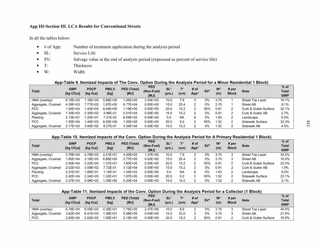
258

App III-Section III. LCA Results for Conventional Streets

In all the tables below:

• # of App: Number of treatment application during the analysis period

• SL: Service Life

• SV: Salvage value at the end of analysis period (expressed as percent of service life)

• T: Thickness

• W: Width

App-Table 9. Itemized Impacts of The Conv. Option During the Analysis Period for a Minor Residential 1 Block)

Total GWP

[kg CO2e] POCP

[kg O3e] PM2.5

[kg] PED (Total)

[MJ]

PED

(Non-Fuel)

[MJ]

SL*

(yrs.)

T*

(cm)

# of

App* SV*

W*

(m)

# per

Block Note

% of

Total

GWP

HMA (overlay) 9.18E+03 1.16E+03 5.88E+00 1.05E+05 3.34E+05 10.0 7.6 3 0% 3.70 1 Street Top Layer 19.1% Aggregate, Crushed 4.39E+03 7.77E+02 1.67E+00 6.77E+04 0.00E+00 15.0 25.4 2 0% 3.70 1 Street AB 9.1% PCC 1.54E+04 1.43E+03 8.44E+00 1.19E+05 0.00E+00 20.0 15.2 2 50% 0.91 2 Curb & Gutter Surface 32.1% Aggregate, Crushed 1.30E+03 2.30E+02 4.96E-01 2.01E+04 0.00E+00 15.0 15.2 2 0% 0.91 2 Curb & Gutter AB 2.7% Planting 2.13E+01 1.20E+01 7.31E-02 8.59E+02 0.00E+00 5.0 NA 6 0% 1.83 2 Landscape 0.0% PCC 1.55E+04 1.44E+03 8.50E+00 1.20E+05 0.00E+00 20.0 9.2 2 50% 1.52 2 Sidewalk Surface 32.3% Aggregate, Crushed 2.17E+03 3.84E+02 8.27E-01 3.34E+04 0.00E+00 15.0 15.2 2 0% 1.52 2 Sidewalk AB 4.5%

App-Table 10. Itemized Impacts of the Conv. Option During the Analysis Period for A Primary Residential 1 Block)

Total GWP

[kg CO2e] POCP

[kg O3e] PM2.5

[kg] PED (Total)

[MJ]

PED

(Non-Fuel)

[MJ]

SL*

(yrs.)

T*

(cm)

# of

App* SV*

W*

(m)

# per

Block Note

% of

Total

GWP

HMA (overlay) 3.76E+04 4.76E+03 2.41E+01 4.30E+05 1.37E+06 10.0 7.6 3 0% 3.70 3 Street Top Layer 34.5% Aggregate, Crushed 1.80E+04 3.19E+03 6.86E+00 2.77E+05 0.00E+00 15.0 25.4 2 0% 3.70 3 Street AB 16.5% PCC 2.40E+04 2.22E+03 1.31E+01 1.85E+05 0.00E+00 20.0 15.2 2 50% 0.91 2 Curb & Gutter Surface 22.0% Aggregate, Crushed 2.02E+03 3.59E+02 7.72E-01 3.12E+04 0.00E+00 15.0 15.2 2 0% 0.91 2 Curb & Gutter AB 1.9% Planting 3.31E+01 1.86E+01 1.14E-01 1.34E+03 0.00E+00 5.0 NA 6 0% 1.83 2 Landscape 0.0% PCC 2.42E+04 2.24E+03 1.32E+01 1.87E+05 0.00E+00 20.0 9.2 2 50% 1.52 2 Sidewalk Surface 22.1% Aggregate, Crushed 3.37E+03 5.98E+02 1.29E+00 5.20E+04 0.00E+00 15.0 15.2 2 0% 1.52 2 Sidewalk AB 3.1%

App-Table 11. Itemized Impacts of the Conv. Option During the Analysis Period for a Collector (1 Block)

Total GWP

[kg CO2e] POCP

[kg O3e] PM2.5

[kg] PED (Total)

[MJ]

PED

(Non-Fuel)

[MJ]

SL*

(yrs.)

T*

(cm)

# of

App* SV*

W*

(m)

# per

Block Note

% of

Total

GWP

HMA (overlay) 6.79E+04 8.59E+03 4.35E+01 7.76E+05 2.47E+06 10.0 8.9 3 0% 3.70 3 Street Top Layer 40.6% Aggregate, Crushed 3.62E+04 6.41E+03 1.38E+01 5.58E+05 0.00E+00 15.0 33.0 2 0% 3.70 3 Street AB 21.6% PCC 2.83E+04 2.62E+03 1.55E+01 2.18E+05 0.00E+00 20.0 15.2 2 50% 0.91 2 Curb & Gutter Surface 16.9%

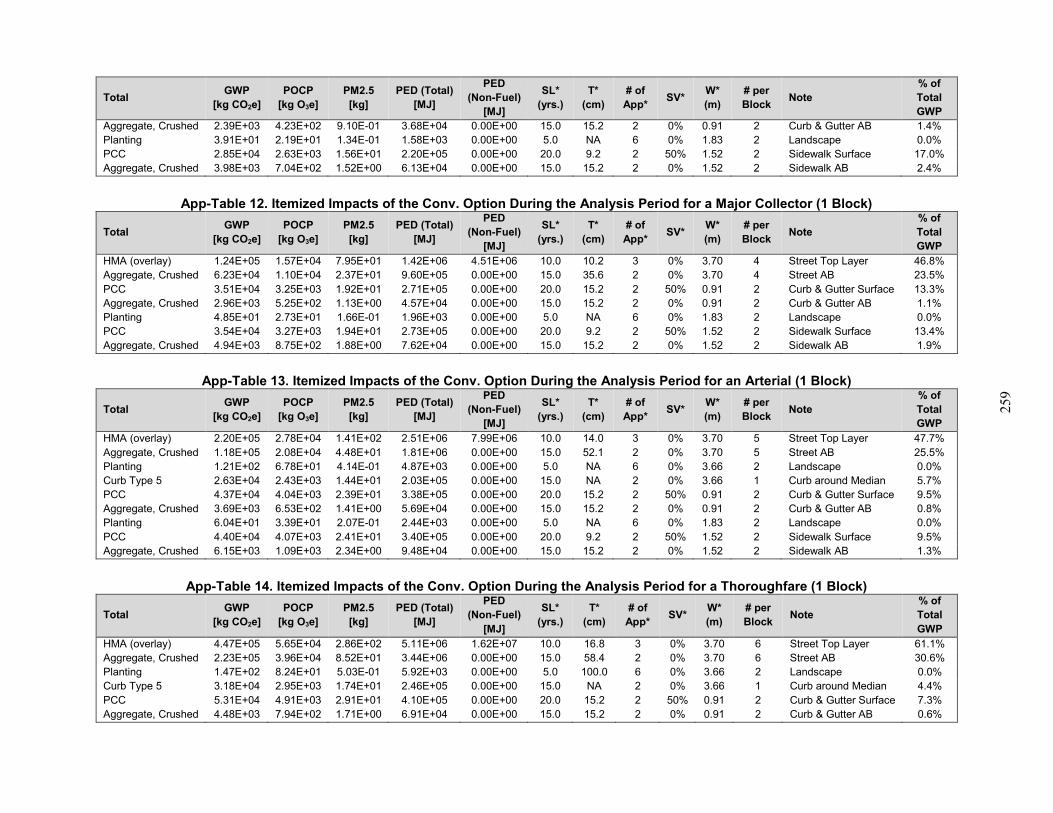
259

Total GWP

[kg CO2e] POCP

[kg O3e] PM2.5

[kg] PED (Total)

[MJ]

PED

(Non-Fuel)

[MJ]

SL*

(yrs.)

T*

(cm)

# of

App* SV*

W*

(m)

# per

Block Note

% of

Total

GWP

Aggregate, Crushed 2.39E+03 4.23E+02 9.10E-01 3.68E+04 0.00E+00 15.0 15.2 2 0% 0.91 2 Curb & Gutter AB 1.4% Planting 3.91E+01 2.19E+01 1.34E-01 1.58E+03 0.00E+00 5.0 NA 6 0% 1.83 2 Landscape 0.0% PCC 2.85E+04 2.63E+03 1.56E+01 2.20E+05 0.00E+00 20.0 9.2 2 50% 1.52 2 Sidewalk Surface 17.0% Aggregate, Crushed 3.98E+03 7.04E+02 1.52E+00 6.13E+04 0.00E+00 15.0 15.2 2 0% 1.52 2 Sidewalk AB 2.4%

App-Table 12. Itemized Impacts of the Conv. Option During the Analysis Period for a Major Collector (1 Block)

Total GWP

[kg CO2e] POCP

[kg O3e] PM2.5

[kg] PED (Total)

[MJ]

PED

(Non-Fuel)

[MJ]

SL*

(yrs.)

T*

(cm)

# of

App* SV*

W*

(m)

# per

Block Note

% of

Total

GWP

HMA (overlay) 1.24E+05 1.57E+04 7.95E+01 1.42E+06 4.51E+06 10.0 10.2 3 0% 3.70 4 Street Top Layer 46.8% Aggregate, Crushed 6.23E+04 1.10E+04 2.37E+01 9.60E+05 0.00E+00 15.0 35.6 2 0% 3.70 4 Street AB 23.5% PCC 3.51E+04 3.25E+03 1.92E+01 2.71E+05 0.00E+00 20.0 15.2 2 50% 0.91 2 Curb & Gutter Surface 13.3% Aggregate, Crushed 2.96E+03 5.25E+02 1.13E+00 4.57E+04 0.00E+00 15.0 15.2 2 0% 0.91 2 Curb & Gutter AB 1.1% Planting 4.85E+01 2.73E+01 1.66E-01 1.96E+03 0.00E+00 5.0 NA 6 0% 1.83 2 Landscape 0.0% PCC 3.54E+04 3.27E+03 1.94E+01 2.73E+05 0.00E+00 20.0 9.2 2 50% 1.52 2 Sidewalk Surface 13.4% Aggregate, Crushed 4.94E+03 8.75E+02 1.88E+00 7.62E+04 0.00E+00 15.0 15.2 2 0% 1.52 2 Sidewalk AB 1.9%

App-Table 13. Itemized Impacts of the Conv. Option During the Analysis Period for an Arterial (1 Block)

Total GWP

[kg CO2e] POCP

[kg O3e] PM2.5

[kg] PED (Total)

[MJ]

PED

(Non-Fuel)

[MJ]

SL*

(yrs.)

T*

(cm)

# of

App* SV*

W*

(m)

# per

Block Note

% of

Total

GWP

HMA (overlay) 2.20E+05 2.78E+04 1.41E+02 2.51E+06 7.99E+06 10.0 14.0 3 0% 3.70 5 Street Top Layer 47.7% Aggregate, Crushed 1.18E+05 2.08E+04 4.48E+01 1.81E+06 0.00E+00 15.0 52.1 2 0% 3.70 5 Street AB 25.5% Planting 1.21E+02 6.78E+01 4.14E-01 4.87E+03 0.00E+00 5.0 NA 6 0% 3.66 2 Landscape 0.0% Curb Type 5 2.63E+04 2.43E+03 1.44E+01 2.03E+05 0.00E+00 15.0 NA 2 0% 3.66 1 Curb around Median 5.7% PCC 4.37E+04 4.04E+03 2.39E+01 3.38E+05 0.00E+00 20.0 15.2 2 50% 0.91 2 Curb & Gutter Surface 9.5% Aggregate, Crushed 3.69E+03 6.53E+02 1.41E+00 5.69E+04 0.00E+00 15.0 15.2 2 0% 0.91 2 Curb & Gutter AB 0.8% Planting 6.04E+01 3.39E+01 2.07E-01 2.44E+03 0.00E+00 5.0 NA 6 0% 1.83 2 Landscape 0.0% PCC 4.40E+04 4.07E+03 2.41E+01 3.40E+05 0.00E+00 20.0 9.2 2 50% 1.52 2 Sidewalk Surface 9.5% Aggregate, Crushed 6.15E+03 1.09E+03 2.34E+00 9.48E+04 0.00E+00 15.0 15.2 2 0% 1.52 2 Sidewalk AB 1.3%

App-Table 14. Itemized Impacts of the Conv. Option During the Analysis Period for a Thoroughfare (1 Block)

Total GWP

[kg CO2e] POCP

[kg O3e] PM2.5

[kg] PED (Total)

[MJ]

PED

(Non-Fuel)

[MJ]

SL*

(yrs.)

T*

(cm)

# of

App* SV*

W*

(m)

# per

Block Note

% of

Total

GWP

HMA (overlay) 4.47E+05 5.65E+04 2.86E+02 5.11E+06 1.62E+07 10.0 16.8 3 0% 3.70 6 Street Top Layer 61.1% Aggregate, Crushed 2.23E+05 3.96E+04 8.52E+01 3.44E+06 0.00E+00 15.0 58.4 2 0% 3.70 6 Street AB 30.6% Planting 1.47E+02 8.24E+01 5.03E-01 5.92E+03 0.00E+00 5.0 100.0 6 0% 3.66 2 Landscape 0.0% Curb Type 5 3.18E+04 2.95E+03 1.74E+01 2.46E+05 0.00E+00 15.0 NA 2 0% 3.66 1 Curb around Median 4.4% PCC 5.31E+04 4.91E+03 2.91E+01 4.10E+05 0.00E+00 20.0 15.2 2 50% 0.91 2 Curb & Gutter Surface 7.3% Aggregate, Crushed 4.48E+03 7.94E+02 1.71E+00 6.91E+04 0.00E+00 15.0 15.2 2 0% 0.91 2 Curb & Gutter AB 0.6%

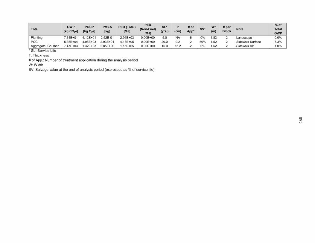
260

Total GWP

[kg CO2e] POCP

[kg O3e] PM2.5

[kg] PED (Total)

[MJ]

PED

(Non-Fuel)

[MJ]

SL*

(yrs.)

T*

(cm)

# of

App* SV*

W*

(m)

# per

Block Note

% of

Total

GWP

Planting 7.34E+01 4.12E+01 2.52E-01 2.96E+03 0.00E+00 5.0 NA 6 0% 1.83 2 Landscape 0.0% PCC 5.35E+04 4.95E+03 2.93E+01 4.13E+05 0.00E+00 20.0 9.2 2 50% 1.52 2 Sidewalk Surface 7.3% Aggregate, Crushed 7.47E+03 1.32E+03 2.85E+00 1.15E+05 0.00E+00 15.0 15.2 2 0% 1.52 2 Sidewalk AB 1.0%

* SL: Service Life T: Thickness # of App.: Number of treatment application during the analysis period W: Width SV: Salvage value at the end of analysis period (expressed as % of service life)

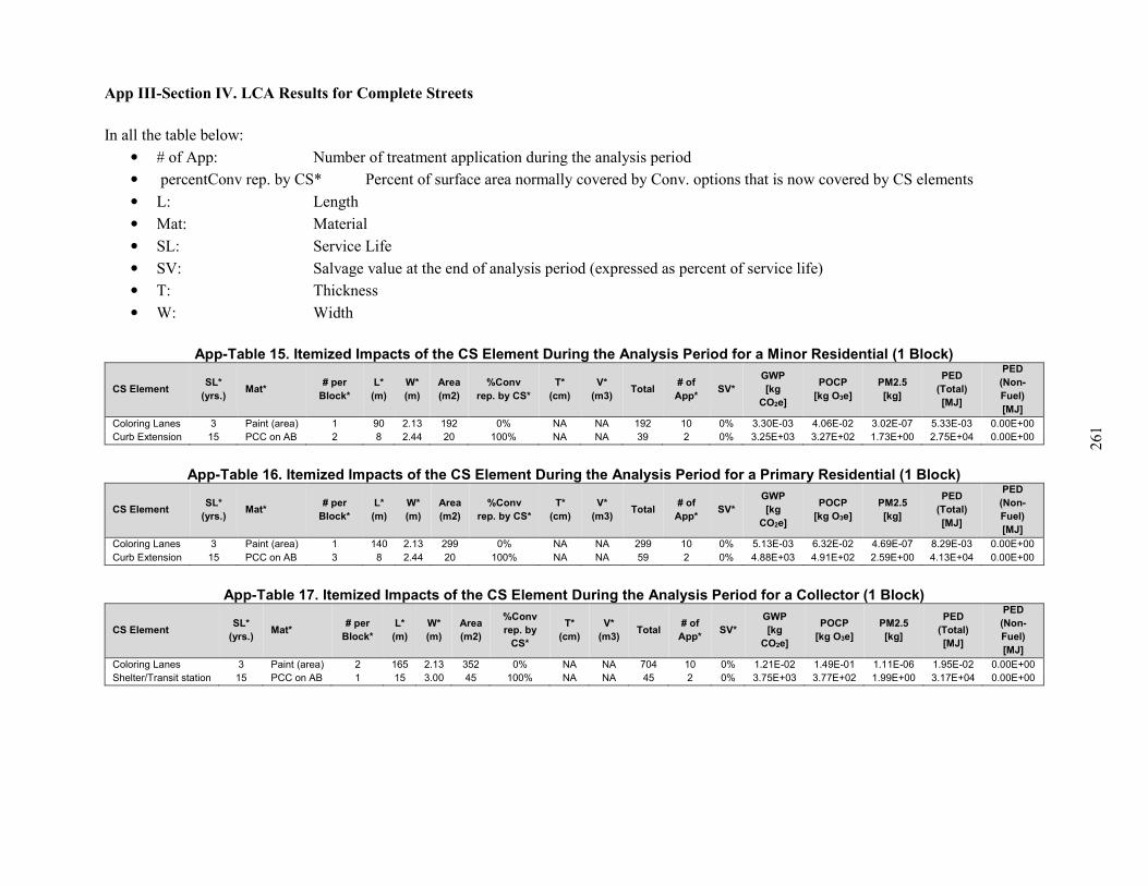
261

App III-Section IV. LCA Results for Complete Streets

In all the table below:

• # of App: Number of treatment application during the analysis period

• percentConv rep. by CS* Percent of surface area normally covered by Conv. options that is now covered by CS elements

• L: Length

• Mat: Material

• SL: Service Life

• SV: Salvage value at the end of analysis period (expressed as percent of service life)

• T: Thickness

• W: Width

App-Table 15. Itemized Impacts of the CS Element During the Analysis Period for a Minor Residential (1 Block)

CS Element SL*

(yrs.) Mat*

# per

Block*

L*

(m)

W*

(m)

Area

(m2)

%Conv

rep. by CS*

T*

(cm)

V*

(m3) Total

# of

App* SV*

GWP

[kg

CO2e]

POCP

[kg O3e]

PM2.5

[kg]

PED

(Total)

[MJ]

PED

(Non-

Fuel)

[MJ]

Coloring Lanes 3 Paint (area) 1 90 2.13 192 0% NA NA 192 10 0% 3.30E-03 4.06E-02 3.02E-07 5.33E-03 0.00E+00

Curb Extension 15 PCC on AB 2 8 2.44 20 100% NA NA 39 2 0% 3.25E+03 3.27E+02 1.73E+00 2.75E+04 0.00E+00

App-Table 16. Itemized Impacts of the CS Element During the Analysis Period for a Primary Residential (1 Block)

CS Element SL*

(yrs.) Mat*

# per

Block*

L*

(m)

W*

(m)

Area

(m2)

%Conv

rep. by CS*

T*

(cm)

V*

(m3) Total

# of

App* SV*

GWP

[kg

CO2e]

POCP

[kg O3e]

PM2.5

[kg]

PED

(Total)

[MJ]

PED

(Non-

Fuel)

[MJ]

Coloring Lanes 3 Paint (area) 1 140 2.13 299 0% NA NA 299 10 0% 5.13E-03 6.32E-02 4.69E-07 8.29E-03 0.00E+00

Curb Extension 15 PCC on AB 3 8 2.44 20 100% NA NA 59 2 0% 4.88E+03 4.91E+02 2.59E+00 4.13E+04 0.00E+00

App-Table 17. Itemized Impacts of the CS Element During the Analysis Period for a Collector (1 Block)

CS Element SL*

(yrs.) Mat*

# per

Block*

L*

(m)

W*

(m)

Area

(m2)

%Conv

rep. by

CS*

T*

(cm)

V*

(m3) Total

# of

App* SV*

GWP

[kg

CO2e]

POCP

[kg O3e]

PM2.5

[kg]

PED

(Total)

[MJ]

PED

(Non-

Fuel)

[MJ]

Coloring Lanes 3 Paint (area) 2 165 2.13 352 0% NA NA 704 10 0% 1.21E-02 1.49E-01 1.11E-06 1.95E-02 0.00E+00

Shelter/Transit station 15 PCC on AB 1 15 3.00 45 100% NA NA 45 2 0% 3.75E+03 3.77E+02 1.99E+00 3.17E+04 0.00E+00

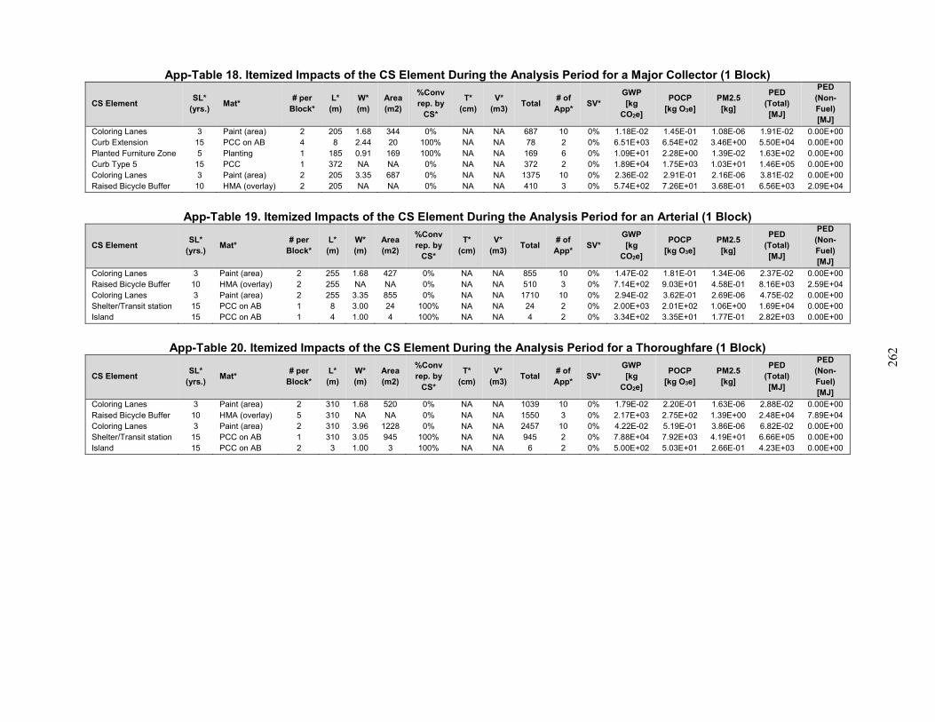
262

App-Table 18. Itemized Impacts of the CS Element During the Analysis Period for a Major Collector (1 Block)

CS Element SL*

(yrs.) Mat*

# per

Block*

L*

(m)

W*

(m)

Area

(m2)

%Conv

rep. by

CS*

T*

(cm)

V*

(m3) Total

# of

App* SV*

GWP

[kg

CO2e]

POCP

[kg O3e]

PM2.5

[kg]

PED

(Total)

[MJ]

PED

(Non-

Fuel)

[MJ]

Coloring Lanes 3 Paint (area) 2 205 1.68 344 0% NA NA 687 10 0% 1.18E-02 1.45E-01 1.08E-06 1.91E-02 0.00E+00

Curb Extension 15 PCC on AB 4 8 2.44 20 100% NA NA 78 2 0% 6.51E+03 6.54E+02 3.46E+00 5.50E+04 0.00E+00

Planted Furniture Zone 5 Planting 1 185 0.91 169 100% NA NA 169 6 0% 1.09E+01 2.28E+00 1.39E-02 1.63E+02 0.00E+00

Curb Type 5 15 PCC 1 372 NA NA 0% NA NA 372 2 0% 1.89E+04 1.75E+03 1.03E+01 1.46E+05 0.00E+00

Coloring Lanes 3 Paint (area) 2 205 3.35 687 0% NA NA 1375 10 0% 2.36E-02 2.91E-01 2.16E-06 3.81E-02 0.00E+00

Raised Bicycle Buffer 10 HMA (overlay) 2 205 NA NA 0% NA NA 410 3 0% 5.74E+02 7.26E+01 3.68E-01 6.56E+03 2.09E+04

App-Table 19. Itemized Impacts of the CS Element During the Analysis Period for an Arterial (1 Block)

CS Element SL*

(yrs.) Mat*

# per

Block*

L*

(m)

W*

(m)

Area

(m2)

%Conv

rep. by

CS*

T*

(cm)

V*

(m3) Total

# of

App* SV*

GWP

[kg

CO2e]

POCP

[kg O3e]

PM2.5

[kg]

PED

(Total)

[MJ]

PED

(Non-

Fuel)

[MJ]

Coloring Lanes 3 Paint (area) 2 255 1.68 427 0% NA NA 855 10 0% 1.47E-02 1.81E-01 1.34E-06 2.37E-02 0.00E+00

Raised Bicycle Buffer 10 HMA (overlay) 2 255 NA NA 0% NA NA 510 3 0% 7.14E+02 9.03E+01 4.58E-01 8.16E+03 2.59E+04

Coloring Lanes 3 Paint (area) 2 255 3.35 855 0% NA NA 1710 10 0% 2.94E-02 3.62E-01 2.69E-06 4.75E-02 0.00E+00

Shelter/Transit station 15 PCC on AB 1 8 3.00 24 100% NA NA 24 2 0% 2.00E+03 2.01E+02 1.06E+00 1.69E+04 0.00E+00

Island 15 PCC on AB 1 4 1.00 4 100% NA NA 4 2 0% 3.34E+02 3.35E+01 1.77E-01 2.82E+03 0.00E+00

App-Table 20. Itemized Impacts of the CS Element During the Analysis Period for a Thoroughfare (1 Block)

CS Element SL*

(yrs.) Mat*

# per

Block*

L*

(m)

W*

(m)

Area

(m2)

%Conv

rep. by

CS*

T*

(cm)

V*

(m3) Total

# of

App* SV*

GWP

[kg

CO2e]

POCP

[kg O3e]

PM2.5

[kg]

PED

(Total)

[MJ]

PED

(Non-

Fuel)

[MJ]

Coloring Lanes 3 Paint (area) 2 310 1.68 520 0% NA NA 1039 10 0% 1.79E-02 2.20E-01 1.63E-06 2.88E-02 0.00E+00

Raised Bicycle Buffer 10 HMA (overlay) 5 310 NA NA 0% NA NA 1550 3 0% 2.17E+03 2.75E+02 1.39E+00 2.48E+04 7.89E+04

Coloring Lanes 3 Paint (area) 2 310 3.96 1228 0% NA NA 2457 10 0% 4.22E-02 5.19E-01 3.86E-06 6.82E-02 0.00E+00

Shelter/Transit station 15 PCC on AB 1 310 3.05 945 100% NA NA 945 2 0% 7.88E+04 7.92E+03 4.19E+01 6.66E+05 0.00E+00

Island 15 PCC on AB 2 3 1.00 3 100% NA NA 6 2 0% 5.00E+02 5.03E+01 2.66E-01 4.23E+03 0.00E+00

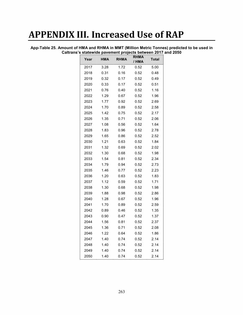
263

APPENDIX III. Increased Use of RAP

App-Table 25. Amount of HMA and RHMA in MMT (Million Metric Tonnes) predicted to be used in Caltrans’s statewide pavement projects between 2017 and 2050

Year HMA RHMA RHMA

/ HMA Total

2017 3.28 1.72 0.52 5.00

2018 0.31 0.16 0.52 0.48

2019 0.32 0.17 0.52 0.49

2020 0.33 0.17 0.52 0.51

2021 0.76 0.40 0.52 1.16

2022 1.29 0.67 0.52 1.96

2023 1.77 0.92 0.52 2.69

2024 1.70 0.89 0.52 2.58

2025 1.42 0.75 0.52 2.17

2026 1.35 0.71 0.52 2.06

2027 1.08 0.56 0.52 1.64

2028 1.83 0.96 0.52 2.78

2029 1.65 0.86 0.52 2.52

2030 1.21 0.63 0.52 1.84

2031 1.32 0.69 0.52 2.02

2032 1.30 0.68 0.52 1.98

2033 1.54 0.81 0.52 2.34

2034 1.79 0.94 0.52 2.73

2035 1.46 0.77 0.52 2.23

2036 1.20 0.63 0.52 1.83

2037 1.12 0.59 0.52 1.71

2038 1.30 0.68 0.52 1.98

2039 1.88 0.98 0.52 2.86

2040 1.28 0.67 0.52 1.96

2041 1.70 0.89 0.52 2.59

2042 0.89 0.46 0.52 1.35

2043 0.90 0.47 0.52 1.37

2044 1.56 0.81 0.52 2.37

2045 1.36 0.71 0.52 2.08

2046 1.22 0.64 0.52 1.86

2047 1.40 0.74 0.52 2.14

2048 1.40 0.74 0.52 2.14

2049 1.40 0.74 0.52 2.14

2050 1.40 0.74 0.52 2.14

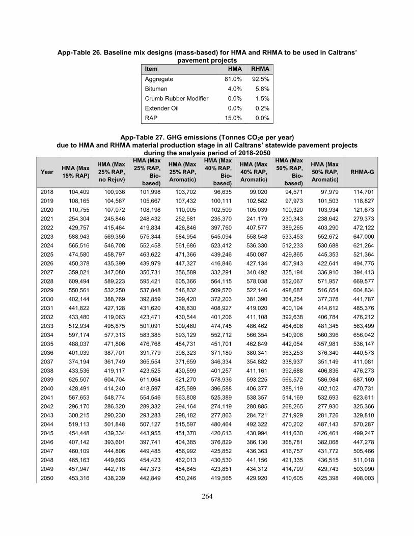
264

App-Table 26. Baseline mix designs (mass-based) for HMA and RHMA to be used in Caltrans’ pavement projects

Item HMA RHMA

Aggregate 81.0% 92.5%

Bitumen 4.0% 5.8%

Crumb Rubber Modifier 0.0% 1.5%

Extender Oil 0.0% 0.2%

RAP 15.0% 0.0%

App-Table 27. GHG emissions (Tonnes CO2e per year)

due to HMA and RHMA material production stage in all Caltrans’ statewide pavement projects during the analysis period of 2018-2050

Year HMA (Max

15% RAP)

HMA (Max

25% RAP,

no Rejuv)

HMA (Max

25% RAP,

Bio-

based)

HMA (Max

25% RAP,

Aromatic)

HMA (Max

40% RAP,

Bio-

based)

HMA (Max

40% RAP,

Aromatic)

HMA (Max

50% RAP,

Bio-

based)

HMA (Max

50% RAP,

Aromatic)

RHMA-G

2018 104,409 100,936 101,998 103,702 96,635 99,020 94,571 97,979 114,701

2019 108,165 104,567 105,667 107,432 100,111 102,582 97,973 101,503 118,827

2020 110,755 107,072 108,198 110,005 102,509 105,039 100,320 103,934 121,673

2021 254,304 245,846 248,432 252,581 235,370 241,179 230,343 238,642 279,373

2022 429,757 415,464 419,834 426,846 397,760 407,577 389,265 403,290 472,122

2023 588,943 569,356 575,344 584,954 545,094 558,548 533,453 552,672 647,000

2024 565,516 546,708 552,458 561,686 523,412 536,330 512,233 530,688 621,264

2025 474,580 458,797 463,622 471,366 439,246 450,087 429,865 445,353 521,364

2026 450,378 435,399 439,979 447,327 416,846 427,134 407,943 422,641 494,775

2027 359,021 347,080 350,731 356,589 332,291 340,492 325,194 336,910 394,413

2028 609,494 589,223 595,421 605,366 564,115 578,038 552,067 571,957 669,577

2029 550,561 532,250 537,848 546,832 509,570 522,146 498,687 516,654 604,834

2030 402,144 388,769 392,859 399,420 372,203 381,390 364,254 377,378 441,787

2031 441,822 427,128 431,620 438,830 408,927 419,020 400,194 414,612 485,376

2032 433,480 419,063 423,471 430,544 401,206 411,108 392,638 406,784 476,212

2033 512,934 495,875 501,091 509,460 474,745 486,462 464,606 481,345 563,499

2034 597,174 577,313 583,385 593,129 552,712 566,354 540,908 560,396 656,042

2035 488,037 471,806 476,768 484,731 451,701 462,849 442,054 457,981 536,147

2036 401,039 387,701 391,779 398,323 371,180 380,341 363,253 376,340 440,573

2037 374,194 361,749 365,554 371,659 346,334 354,882 338,937 351,149 411,081

2038 433,536 419,117 423,525 430,599 401,257 411,161 392,688 406,836 476,273

2039 625,507 604,704 611,064 621,270 578,936 593,225 566,572 586,984 687,169

2040 428,491 414,240 418,597 425,589 396,588 406,377 388,119 402,102 470,731

2041 567,653 548,774 554,546 563,808 525,389 538,357 514,169 532,693 623,611

2042 296,170 286,320 289,332 294,164 274,119 280,885 268,265 277,930 325,366

2043 300,215 290,230 293,283 298,182 277,863 284,721 271,929 281,726 329,810

2044 519,113 501,848 507,127 515,597 480,464 492,322 470,202 487,143 570,287

2045 454,448 439,334 443,955 451,370 420,613 430,994 411,630 426,461 499,247

2046 407,142 393,601 397,741 404,385 376,829 386,130 368,781 382,068 447,278

2047 460,109 444,806 449,485 456,992 425,852 436,363 416,757 431,772 505,466

2048 465,163 449,693 454,423 462,013 430,530 441,156 421,335 436,515 511,018

2049 457,947 442,716 447,373 454,845 423,851 434,312 414,799 429,743 503,090

2050 453,316 438,239 442,849 450,246 419,565 429,920 410,605 425,398 498,003

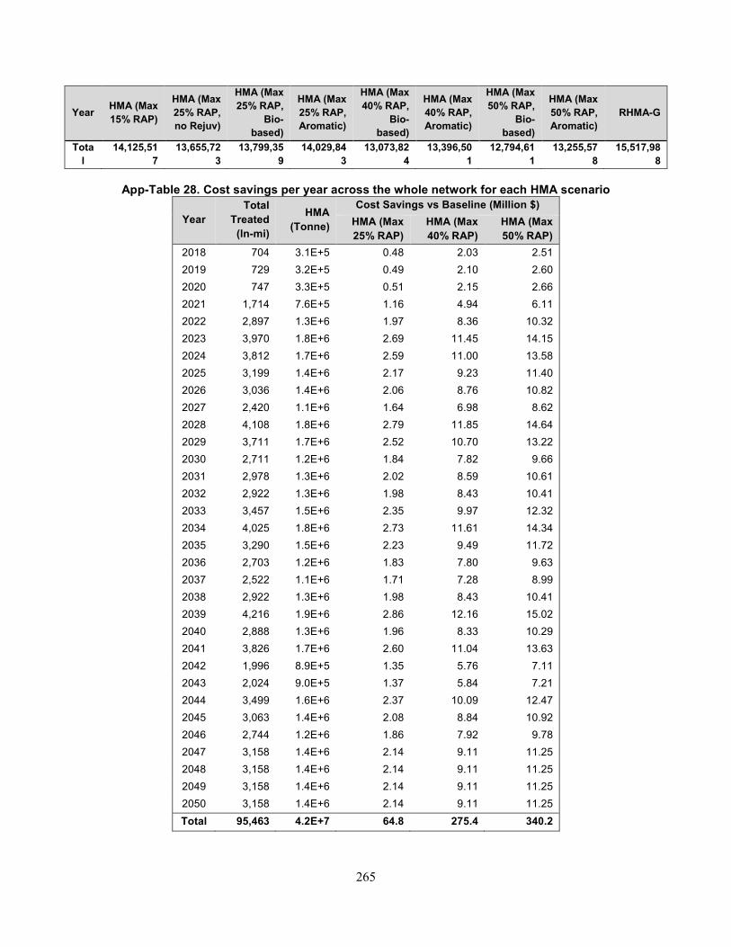
265

Year HMA (Max

15% RAP)

HMA (Max

25% RAP,

no Rejuv)

HMA (Max

25% RAP,

Bio-

based)

HMA (Max

25% RAP,

Aromatic)

HMA (Max

40% RAP,

Bio-

based)

HMA (Max

40% RAP,

Aromatic)

HMA (Max

50% RAP,

Bio-

based)

HMA (Max

50% RAP,

Aromatic)

RHMA-G

Tota

l

14,125,51

7

13,655,72

3

13,799,35

9

14,029,84

3

13,073,82

4

13,396,50

1

12,794,61

1

13,255,57

8

15,517,98

8

App-Table 28. Cost savings per year across the whole network for each HMA scenario

Year

Total

Treated

(ln-mi)

HMA

(Tonne)

Cost Savings vs Baseline (Million $)

HMA (Max

25% RAP)

HMA (Max

40% RAP)

HMA (Max

50% RAP)

2018 704 3.1E+5 0.48 2.03 2.51

2019 729 3.2E+5 0.49 2.10 2.60

2020 747 3.3E+5 0.51 2.15 2.66

2021 1,714 7.6E+5 1.16 4.94 6.11

2022 2,897 1.3E+6 1.97 8.36 10.32

2023 3,970 1.8E+6 2.69 11.45 14.15

2024 3,812 1.7E+6 2.59 11.00 13.58

2025 3,199 1.4E+6 2.17 9.23 11.40

2026 3,036 1.4E+6 2.06 8.76 10.82

2027 2,420 1.1E+6 1.64 6.98 8.62

2028 4,108 1.8E+6 2.79 11.85 14.64

2029 3,711 1.7E+6 2.52 10.70 13.22

2030 2,711 1.2E+6 1.84 7.82 9.66

2031 2,978 1.3E+6 2.02 8.59 10.61

2032 2,922 1.3E+6 1.98 8.43 10.41

2033 3,457 1.5E+6 2.35 9.97 12.32

2034 4,025 1.8E+6 2.73 11.61 14.34

2035 3,290 1.5E+6 2.23 9.49 11.72

2036 2,703 1.2E+6 1.83 7.80 9.63

2037 2,522 1.1E+6 1.71 7.28 8.99

2038 2,922 1.3E+6 1.98 8.43 10.41

2039 4,216 1.9E+6 2.86 12.16 15.02

2040 2,888 1.3E+6 1.96 8.33 10.29

2041 3,826 1.7E+6 2.60 11.04 13.63

2042 1,996 8.9E+5 1.35 5.76 7.11

2043 2,024 9.0E+5 1.37 5.84 7.21

2044 3,499 1.6E+6 2.37 10.09 12.47

2045 3,063 1.4E+6 2.08 8.84 10.92

2046 2,744 1.2E+6 1.86 7.92 9.78

2047 3,158 1.4E+6 2.14 9.11 11.25

2048 3,158 1.4E+6 2.14 9.11 11.25

2049 3,158 1.4E+6 2.14 9.11 11.25

2050 3,158 1.4E+6 2.14 9.11 11.25

Total 95,463 4.2E+7 64.8 275.4 340.2