Clemson UniversityTigerPrints

All Dissertations Dissertations

8-2009

Integer-valued time series and renewal processesYunwei CuiClemson University, ycui@clemson.edu

Follow this and additional works at: http://tigerprints.clemson.edu/all_dissertations

Part of the Statistics and Probability Commons

This Dissertation is brought to you for free and open access by the Dissertations at TigerPrints. It has been accepted for inclusion in All Dissertations byan authorized administrator of TigerPrints. For more information, please contact awesole@clemson.edu.

Recommended CitationCui, Yunwei, "Integer-valued time series and renewal processes" (2009). All Dissertations. Paper 401.

Integer-Valued Time Series and Renewal

Processes

A Dissertation

Presented to

the Graduate School of

Clemson University

In Partial Fulfillment

of the Requirements for the Degree

Doctor of Philosophy

Mathematical Sciences

by

Yunwei Cui

August 2009

Accepted by:

Dr. Robert B Lund, Committee Chair

Dr. Colin M Gallagher

Dr. Peter C Kiessler

Dr. Karunarathna B Kulasekera

Abstract

This research proposes a new but simple model for stationary time series of in-

teger counts. Previous work in the area has focused on mixture and thinning methods

and links to classical time series autoregressive moving-average difference equations;

in contrast, our methods use a renewal process to generate a correlated sequence of

Bernoulli trials. By superpositioning independent copies of such processes, stationary

series with binomial, Poisson, geometric, or any other discrete marginal distribution

can be readily constructed. The model class proposed is parsimonious, non-Markov,

and readily generates series with either short or long memory autocovariances. The

model can be fitted with linear prediction techniques for stationary series. Estima-

tion of process parameters based on conditional least squares methods is considered.

Asymptotic properties of the estimators are derived. The models sometimes have

an autoregressive moving-average structure and we consider the AR(1) count process

case in detail. Unlike previous methods based on mixture and thinning tactics, series

with negative autocorrelations can be produced.

ii

Dedication

To my family.

iii

Acknowledgments

I am grateful to my dissertation committee for providing tremendous help and

guidance during the process of completing this dissertation. My deep gratitude goes

to my dissertation committee chair, Dr. Robert Lund. Your knowledge and insights

in the area of time series modeling and analysis helped me choose this fruitful topic.

Your suggestions and encouragements guided me through the most difficult time of

this research when there seemed to be no progress ever made and the oral exam was

impending. Your office door is always open to me. No matter how busy you are, you

always can find time to meet me as long as you are on campus. Your directions and

insightful suggestions have significantly improved the quality of this work. Moreover,

Dr. Lund, you patiently helped me in writing and mentored me how to be a better

teacher and improve my teaching evaluation.

To Dr. Gallagher whose valuable comments have improved the overall qual-

ity of the research. Your teaching style and method greatly impressed me and will

definitely help me improve my class delivery on those subject which could be better

explained through examples.

To Dr. Kiessler whose classes first exposed me to Markov Chain and proba-

bility theory. I was inspired to take several advanced courses which contributed to

my decision to choose time series analysis and related field as the focus of my Ph.D

program. You are always willing to help me solve difficult probability problems. You

iv

also kindly pointed out the deficiencies in my presentation and encouraged to improve

my presentation skills.

To Dr. K.B. whose mathematical statistics courses are among the most im-

portant courses I ever took at Clemson. You keep high standards of your teaching.

Your advice is valuable to anyone who wants to be successful in his Ph.D. program.

v

Table of Contents

Title Page . . . . . . . . . . . . . . . . . . . . . . . . . . . . . . . . . . . i

Abstract . . . . . . . . . . . . . . . . . . . . . . . . . . . . . . . . . . . . ii

Dedication . . . . . . . . . . . . . . . . . . . . . . . . . . . . . . . . . . . iii

Acknowledgments . . . . . . . . . . . . . . . . . . . . . . . . . . . . . . iv

List of Tables . . . . . . . . . . . . . . . . . . . . . . . . . . . . . . . . . viii

List of Figures . . . . . . . . . . . . . . . . . . . . . . . . . . . . . . . . ix

1 Introduction . . . . . . . . . . . . . . . . . . . . . . . . . . . . . . . . 11.1 DARMA Models . . . . . . . . . . . . . . . . . . . . . . . . . . . . . 21.2 INARMA Models . . . . . . . . . . . . . . . . . . . . . . . . . . . . . 41.3 Regression Models . . . . . . . . . . . . . . . . . . . . . . . . . . . . 71.4 Hidden Markov Models . . . . . . . . . . . . . . . . . . . . . . . . . . 91.5 State-Space Models . . . . . . . . . . . . . . . . . . . . . . . . . . . 101.6 Outline of the Thesis . . . . . . . . . . . . . . . . . . . . . . . . . . . 13

2 A New Look at Time Series of Counts . . . . . . . . . . . . . . . . 142.1 The Renewal Process Building Block . . . . . . . . . . . . . . . . . . 162.2 General Results . . . . . . . . . . . . . . . . . . . . . . . . . . . . . . 172.3 The Classical Count Marginals . . . . . . . . . . . . . . . . . . . . . . 222.4 Fitting the Renewal Model . . . . . . . . . . . . . . . . . . . . . . . . 262.5 Comments . . . . . . . . . . . . . . . . . . . . . . . . . . . . . . . . . 282.6 Proofs . . . . . . . . . . . . . . . . . . . . . . . . . . . . . . . . . . . 29

3 Renewal AR(1) Count Series . . . . . . . . . . . . . . . . . . . . . . 343.1 AR(1) Count Series . . . . . . . . . . . . . . . . . . . . . . . . . . . . 353.2 Estimation . . . . . . . . . . . . . . . . . . . . . . . . . . . . . . . . . 383.3 Examples . . . . . . . . . . . . . . . . . . . . . . . . . . . . . . . . . 423.4 Proofs . . . . . . . . . . . . . . . . . . . . . . . . . . . . . . . . . . . 44

vi

Bibliography . . . . . . . . . . . . . . . . . . . . . . . . . . . . . . . . . 50

vii

List of Tables

3.1 Simulation results for h1,CLS and h2,CLS . . . . . . . . . . . . . . . . . 45

viii

List of Figures

2.1 A stationary series with binomial marginals . . . . . . . . . . . . . . 222.2 A stationary series with Poisson marginals and long memory . . . . . 242.3 A stationary series with geometric marginals . . . . . . . . . . . . . . 252.4 Fitted model to Key West data . . . . . . . . . . . . . . . . . . . . . 27

3.1 A stationary binomial AR(1) count series . . . . . . . . . . . . . . . . 43

ix

Chapter 1

Introduction

Integer-valued time series arise in many practical settings. Counts of objects

or occurrences of events taken sequentially in time have such structure; for examples,

consider the annual counts of hurricanes, the number of rainy days in successive weeks,

the number of patients treated each day in an emergency department, the number

of U.S. soldiers injured in Iraq in each month, or the daily counts of new swine flu

cases in Mexico. McKenzie [2003] and Fokianos and Kedem [2003] provide recent

overviews.

Count series are non-negative integers and are usually correlated over time.

They cannot be well approximated by continuous variables, especially when the counts

are relatively small (Brockwell and Davis, 2002, Chapter 8). Modeling and analyzing

count series remains one of the most challenging and undeveloped areas of time series

analysis. For example, developing a non-negative integer-valued time series with the

autocorrelation function ρ(h) = φh with 0 < φ < 1 is not easy.

Since the late 1970s, many authors have investigated ways to model count

series with a preset marginal distributions. Many of the results are based on classical

autoregressive moving-average (ARMA) methods. While mathematically innovative,

1

these models have some unresolved shortcomings. New models continue to emerge

as the area is still in its infancy (McKenzie, 2003). To acquaint the reader with this

area, we next review classical count models.

1.1 DARMA Models

The discrete autoregressive moving-average (DARMA) model (Jacobs and

Lewis, 1978a, 1978b, 1983) represents the first attempt to define a general stationary

series of counts. The simplest form of the model, the first order discrete autoregession

(DAR(1)) process (Jacobs and Lewis, 1978a, 1978b), is based on mixing copies of ran-

dom variables having the prescribed marginal distribution. The difference equation

governing a DAR(1) model is

Xt = VtXt−1 + (1 − Vt)At, t ≥ 1, (1.1)

where {Vt} is a sequence of independent and identically distributed Bernoulli ran-

dom variables with P (Vt = 1) = ζ ∈ (0, 1), and {At} is a sequence of independent

and identically distributed integer-valued random variables having the prescribed

marginal distribution (call this π). If X0 has distribution π, then it is easy to see that

{Xt} is stationary and has marginal distribution π. Moreover, the lag h autocorrela-

tion of {Xt} is ρ(h) = ζh for h ≥ 0. In fact, P (At = At−1) = ζ. Note that DAR(1)

autocorrelations must be non-negative since ζ ∈ (0, 1).

By introducing another random sequence {Zt} into (1.1), one can define the

DAR(p) model:

Xt = VtXt−Zt+ (1 − Vt)At, t ≥ 1,

where {At} and {Vt} are defined as before, and {Zt} are independent and identically

2

distributed random variables taking values in {1, 2, . . . , p}. Let φk = P (Zt = k). If

{X0, . . . , X−p+1} are independent and identically distributed with distribution π, then

{Xt} is stationary and also has marginal distribution π. Its autocorrelation function

satisfies the AR(p)-type Yule-Walker equation

ρX(k) = ζp∑

i=1

φiρX(k − i),

where ρX(k) = Corr(Xt, Xt+k) for k ≥ 0.

The DARMA(p, q) process is built with two component models:

Xt = VtYt−q + (1 − Vt)At−St, t ≥ 1;

Yt = UtYt−Zt+ (1 − Ut)At, t ≥ −q + 1,

where {At} and {Zt} are as above, {Ut} is a sequence of independent and identically

distributed Bernoulli random variables, and {St} are independent and identically

distributed random variables taking values in {1, 2, . . . , q}. If {Y−q, . . . , Y−q−p+1} are

independent and identically distributed with distribution π, then {Xt} for t > 1 is

stationary with marginal distribution π and has an ARMA(p, q) type autocorrelation

structure (Jacobs and Lewis, 1983) .

While the DAMA model generates integer-valued time series with any preset

distribution π, it is handicapped by the fact that for high correlations, the model

tends to generate series that have runs of constant values. This is not realistic in

practice since time series of counts usually exhibit variability over time. As a result,

DARMA models are rarely used in practice (MacDonald and Zucchini, 1997).

3

1.2 INARMA Models

Integer-valued autoregressive moving-average (INARMA) models were first

proposed independently by Mckenzie [1986] and Al-Osh and Alzaid [1987]. INARMA

models are based on the binomial thinning operator ◦ (Steutel and Van Harn, 1979),

which combines a non-negative integer valued random variable N and a probability

p via

p ◦ N =N∑

j=1

Bj.

Here, {Bj} is a sequence of independent Bernoulli random variables with success

probability p. Hence, p ◦N is the sum of N independent Bernoulli random variables,

each of which is unity with probability p.

The simplest model in the INARMA class is the integer-valued first order

autoregressive (INAR(1)) process {Xt} (McKenzie, 1985, 1988; Al-Osh and Alzaid,

1987). This model obeys an AR(1) difference equation with a thinning operator:

Xt = φ ◦ Xt−1 + Zt, 0 < φ < 1, (1.2)

where {Zt} is a sequence of independent and identically distributed count random

variables. It can be shown that the autocorrelation function of {Xt} at lag h is

ρ(h) = φh. But since φ must be positive in the above, only positively correlated

count series can be produced.

Different marginal distributions of Zt give rise to different marginal distribu-

tions of {Xt}. McKenzie [1986] [1988] used (1.2) to generate integer-valued count

series with Poisson, negative binomial, and geometric marginal distributions. To gen-

erate a stationary sequence {Xt} with a certain prescribed marginal distribution, one

can first derive the generating function of Zt through (1.2) and then invert this gen-

4

erating function to obtain the distribution of Zt. For example, to generate a series

{Xt} with Poisson marginals, {Zt} should be chosen to have a Poisson distribution

(McKenzie, 1986). It can be shown that if {Zt} is a sequence of independent and

identically distributed Poisson random variables with mean θ(1 − φ) (θ > 0) and

X0 is Poisson, mean θ, then {Xt} generated through (1.2) is stationary with Poisson

marginals, with mean θ and the AR(1) type autocorrelation structure ρ(h) = φh.

Not all marginal distributions can be constructed with (1.2). In fact, only

random variables with the so-called discrete self-decomposable distributions of Steutel

and Van Harn [1979] can be solutions to equation (1.2). One implication of this is

that stationary count series with binomial marginal distributions cannot be generated,

because the binomial distribution is not self-decomposable.

In (1.2), the thinning operation ◦ replaces scalar multiplication in the classical

AR(1) process. Extensions of the method to other ARMA models are possible. For

example, the Poisson INMA(q) process by McKenzie [1988] satisfies

Xt = Zt + θ1 ◦ Zt−1 + · · · + θq ◦ Zt−q, 0 < θi < 1, i = 1, . . . , q,

where {Zt} is a sequence of independent and identically distributed Poisson random

variables. Let θ = 1 +∑q

i=1 θi. If Zt has mean λ/θ and all thinning operations

are independently performed, then {Xt} generated by the above model has Poisson

marginals with mean λ and the classical moving-average (MA(q)) type autocorrelation

structure

ρ(0) =q−h∑

i=0

θiθi+h/θ, h = 1, . . . , q;

ρ(h) = 0, h > q.

5

Al-Osh and Alzaid [1990] and Du and Li [1991] proposed the INAR(p) process

Xt = φ1 ◦ Xt−1 + · · · + φp ◦ Xt−p + Zt, 0 < φi < 1, i = 1, . . . , p,

where {Zt} is a sequence of independent and identically distributed count random

variables. The marginal distributions of {Xt} are difficult to identify in the above

model. By Al-Osh and Alzaid’s assumption that given Xt, the thinned vector {φ1 ◦

Xt, . . . , φp◦Xt} has a multinomial distribution with parameters (φ1, . . . , φp, Xt), {Xt}

is stationary with an ARMA(p, p-1) autocorrelation structure. However, by the

assumption of Du and Li [1991] that the thinning operations {φ1◦Xt, . . . , φp◦Xt} are

performed independently, {Xt} is stationary with an AR(p) autocorrelation structure.

Most authors use Du and Li’s assumption [1991].

Gauthier and Latour [1994] extended the thinning operator ◦ to the generalized

thinning operation • defined

a • N =N∑

j=1

Xj, a > 0,

where N is a non-negative integer-valued random variable and {Xj} is a sequence of

independent and identically distributed non-negative integer-valued random variables

with mean a and finite variance. Gauthier and Latour [1994] and Latour [1997] [1998]

extended INAR(p) processes to the so-called generalized integer-valued autoregressive

(GINAR(p)) process by substituting • for ◦ in the INAR(p) model of Du and Li [1991].

Estimation methods for INARMA models have also been studied. Al-Osh and

Alzaid [1987] and Ronning and Jung [1992] investigate maximum likelihood methods

in the Poisson INAR(1) model. Al-Osh and Alzaid [1987] and Du and Li [1991]

studied conditional least squares estimation methods (Klimko and Nelson, 1978) in

6

the Poisson INAR(1) and INAR(p) models. Brannas [1994] proposed generalized

method of moments estimators for the Poisson INAR(1) model.

Applications of INARMA models are frequent; for example, the study of

epileptic seizure counts (Franke and Seligmann, 1993) and applications to economics

(Brannas and Hellstrom, 2001; Brannas and Shahiduzzaman, 2004; Bockenholt, 1999b;

Bockenholt, 2003; Rudholm, 2001; Freeland and McCabe, 2004).

1.3 Regression Models

Zeger [1988] proposed an important Poisson-based model to incorporate co-

variates (regressors) into the analysis of time series of counts. Given values for a

stationary series {ǫt}, {Yt} is assumed to be an independent sequence of counts with

Poisson distributions having the conditional moments

E(Yt|ǫt) = exp(D′tβ)ǫt and Var(Yt|ǫt) = exp(D′

tβ)ǫt,

where {Dt} is a p×1 vector of covariates and β is a p×1 vector of unknown coefficients

to be estimated. If {ǫt} has mean E(ǫt) = 1 and autocovariance Cov(ǫt, ǫt+h) =

σ2ρǫ(h), then {Yt} has

µt = E(Yt) = exp(D′tβ);

υt = Var(Yt) = µt + σ2µ2t ;

ρY (t, h) = Corr(Yt, Yt+h) =ρǫ(h)

[1 + (σ2µt)−1]12 [1 + (σ2µt+h)−1]

12

.

The correlations of {Yt} are determined by the latent process {ǫt}. In general, regres-

sion models for Poisson time series of counts are not stationary. A quasilikelihood

7

method was used to estimate parameters in this model.

Campbell [1994] extended Zeger’s work to higher orders of dependence and

studied the occurrences of sudden infant death syndrome. Brannas and Johansson

[1994] also studied the model, developing Poisson pseudomaximum likelihood estima-

tion methods.

Zeger and Qaqish [1988] also designed a model based on the assumption that

the past history of {Yt} affects Yt only through the values of Yt−1, . . . , Yt−q. In the

literature, this model is also called a Markov regression model. Let {Dt} be as before,

Ht be the history of the covariates and {Yt} through time t—say

Ht = {Dt, Dt−1, . . . , D0; Yt−1, Yt−2, . . . , Y0}.

Define µt = E(Yt|Ht) and Vt = Var(Yt|Ht). Conditional on Ht, the model assumes

log(µt) = D′tβ +

q∑

i=1

θi[ln(Y ∗t−i) − D′

t−iβ];

Vt = φµt, (1.3)

where Y ∗t−i = max(Yt−i, c), 0 < c < 1. An alternative model replaces Yt−i by Y ∗

t−i =

Yt−i + c, c > 0. Some transformation is necessary since log(Yt−i) is undefined when

Yt−i = 0, a possible value in the Poisson support set.

Quasilikelihood methods were originally used to estimate β. If additional as-

sumptions about the conditional distribution of Yt are available, likelihood estimation

can be conducted. Fahrmeir and Tutz [1994] applied the model to analyze the monthly

number of polio cases in the United States; Cameron and Leon [1993] used the model

to investigate the monthly number of strikes in the United States. But since the

transformation of Yt−i to Y ∗t−i is ad hoc and its impact on µt is hard to evaluate, the

8

model is not widely used today (MacDonald and Zucchini, 1997).

More generally, (1.3) has the form

h(µt) = D′tβ +

q∑

i=1

θifi(Ht);

Vt = g(µt)φ, (1.4)

where h(µt) is called a ‘link’ function and the fi(Ht)′s are functions based on the

process history. The model in (1.4) is very flexible. An autoregressive model of

order q (AR(q)) is obtained when {Yt} is Gaussian, h(µt) = µt, g(µt) = 1, and

fi(Ht) = Yt−i − D′t−iβ. Also, trend and seasonality can be added to the model by

incorporating a trend function of t and sine and cosine terms into h(µt) and fi(Ht).

Li [1991] proposed two methods of assessing the adequacy of the above model.

Li [1994] also extended Markov regression models by adding autoregressive and moving-

average terms. Albert [1994] used the model for magnetic resonance imaging. It is

important to note that Poisson marginal distributions are assumed in the above mod-

els. It may not be possible to construct explicit covariance structures and have any

marginal distributional type desired. In fact, this point is key in what follows.

1.4 Hidden Markov Models

In a hidden Markov model, a count series {Yt} is affected by the value of an un-

observable series {Ct}. It is assumed that Ct takes values in the set {1, 2, . . . ,m} and

evolves according to a strictly positive Markov chain with transitional and stationary

distributions

γij = P (Ct = j|Ct−1 = i) and δj = P (Ct = j), j = 1, 2, . . . ,m.

9

In the simplest case, a Poisson Markov model, it is assumed that conditional on Ct = j

and Dt (a p × 1 vector of covariates), that Yt has Poisson distribution with mean

µtj = exp(D′tβj),

where βj is a p × 1 vector of unknown coefficients to be estimated. Then Yt has the

conditional moments

E(Yt|Dt) =m∑

j=1

δjµtj;

E(Y 2t |Dt) =

m∑

j=1

δj(µtj + µ2tj);

E(YtYt+k|Dt) =m∑

i=1

m∑

j=1

δiγij(k)µtiµt+k,j,

where γij(k) = P (Ct+k = j|Ct = i). The parameters of the model, βj and γij, can

be estimated by maximum likelihood. MacDonald and Zucchini [1997] applied this

model to describe the daily number of epileptic seizures of a particular patient. More

details about this class of models can be found in MacDonald and Zucchini [1997].

1.5 State-Space Models

In the state-space model for a count series {Yt}, Yt is specified to have a certain

distribution based on a state variable Xt. The state variable Xt evolves stochastically

according to a particular distribution determined by Xt and Yt−1. Simple state-space

models are discussed in Brockwell and Davis [2002, Chapter 8]. For this model, Yt is

assumed to be Poisson with mean exp(Xt) with

P (Yt = k|Xt) =e−eXt ekXt

k!.

10

Moreover, Xt is assumed to obey a regression model with Gaussian noise

Xt = β′µt + Wt,

where µt is a p× 1 vector of covariates and β is a p× 1 vector of unknown coefficients

to be estimated. The noise term Wt is defined to be AR(1):

Wt = φWt−1 + Zt, {Zt} ∼ IID N(0, σ2).

Then, conditional on Xt, Xt+1 has a normal distribution with mean µ′t+1β + φ(Xt −

β′µt) and variance σ2. Estimation of θ = (β′, φ, σ2) can be conducted by maximum

likelihood techniques. Brockwell and Davis [2002] fit the model to the polio data of

Zeger [1988].

Several generalizations of basic state space models can be made. One approach

builds the model in a Bayesian framework. The most mathematically tractable model

is given by Harvey [1989]. In Harvey’s model, Yt, conditional on µt, has a Poisson

distribution with

P (Yt = k|µt) =e−µtµk

t

k!,

and µt (conditional on Yt−1) is taken to have a gamma distribution with density

f(µt|Yt−1) =bat

t xat−1e−btµt

Γ(at),

where at and bt is given by

at = ωat−1, bt = ωbt−1.

11

Then given the observation of Yt, the posterior distribution for µt is gamma with

density

f(µt|Yt) =baxa−1e−bµt

Γ(a), a = at + Yt, b = bt + 1.

The conditional distribution of Yt given Yt−1 is negative binomial with parameters at

and bt. Estimation of ω can be conducted with likelihood techniques. Harvey and

Fernandes [1989] used this model to analyze count series data on scores in soccer

games, fatalities of van drivers, and purse snatchings in Chicago. Johansson [1996]

applied this model to Swedish traffic accident fatalities.

So far, the five major model classes for count serries have been briefly intro-

duced. DARMA and INARMA are the two major types of models for stationary count

series. The remaining three model classes are generally not stationary as the obser-

vation at time t, Yt, is assumed to be affected by some latent processes that evolves

stochastically. The nuances of the later three model types lie with the assumptions

about the mechanisms that govern the latent processes and the conditional distribu-

tions of Yt. The simplest cases of these models are usually based on the assumption

of a linear relationship between the conditional mean of Yt and the latent process.

Complete overviews of models for integer-valued time series can be found in

McKenzie [2003], Chapter 7 of MacDonald and Zucchini [1997], and Chapter 1 of

Cameron and Trivedi [1998]. The literature for stationary time series models with

non-Gaussian marginals is by now vast. Besides count series, stationary series with ex-

ponential marginals (Lawrance and Lewis, 1977a, 1977b), gamma marginals (Al-Osh

and Alzaid, 1993), multinomial marginals (Bockenholt, 1999a), binomial marginals

(Weiβ, 2009), and conditional exponential family marginals (Benjamin et al., 2003)

exist.

12

1.6 Outline of the Thesis

The rest of this document proceeds as follows. In Chapter 2, a completely

new model for stationary count series will be introduced that is based upon renewal

processes. Here, we first introduce notation and review simple renewal processes.

Section 2.2 establishes some general time series properties of the model. Sections 2.3

considers how to construct binomial, Poisson, and geometric marginal distributions,

respectively. The last section contains proofs and technical derivations.

Chapter 3 studies renewal AR(1) count series. Section 3.1 establishes general

results about the AR(1) count process. Section 3.2 considers estimation issues, and

Section 3.3 gives examples and simulation results. Section 3.4 concludes with proofs

and technical details.

13

Chapter 2

A New Look at Time Series of

Counts

This chapter introduces a new model class to describe stationary integer count

time series. The model class is simple, parsimonious, non-Markov, and easily gener-

ates all classical discrete marginal distributions for counts such as binomial, Poisson,

and geometric. The model can readily produce either long or short memory series.

In Chapter 1, two types of general models for stationary count series were

presented. The discrete autoregressive moving-average (DARMA) model can gener-

ate a stationary integer-valued time series with any prescribed marginal distribution;

however, as noted by McKenzie [1985] [2003], these series tend to have sample paths

that are constant for long runs, a trait generally not seen in data. The integer-

valued autoregressive moving-average (INARMA) model uses a thinning operation in

a difference equation scheme that mimics autoregressive moving-average methods to

generate stationary integer-valued series that have negative binomial, geometric, and

Poisson marginal distributions. Unlike discrete autoregressive moving-average meth-

ods, thinning techniques cannot produce an arbitrary marginal count distribution.

14

However, the sample paths of thinned models seem to be more data-realistic than

those of discrete autoregressive moving-average models.

Here, we take a completely different approach to the problem. We regard the

marginal distribution as known and study methods that generate a stationary series

with the known marginal distribution. Our methods use a simple on/off renewal

process to generate a correlated sequence of Bernoulli trials. By superpositioning

independent copies of such processes, we will be able to construct series with any of

the classical count marginal distributions in an efficient manner. In fact, since a draw

from any discrete distribution can be constructed from a sequence of independent

coin tosses, the methods can generate discrete series with any specified marginal

distribution. By selecting the renewal lifetimes to have an infinite second moment,

long memory count series are obtained. Long memory count series cannot be produced

with non-unit root autoregressive moving-average difference equations and thinning

methods. By linking time series and renewal processes, several short proofs of classical

renewal results are obtained; these are pointed out in §2.2.

The only other paper linking count series to renewal processes seems to be

Blight [1989], who focuses on autoregressive moving-average structures of renewal

processes. It is also noted that Yule’s original formulation of autoregressive models

involved pea-shooters and point processes. An autoregressive moving-average slant is

not pursued here for two reasons. First, because our model’s parameters are limited

to those governing the renewal interarrival distribution, the class is naturally parsi-

monious and the parsimonizing effects of an autoregressive moving-average structure

are not needed. Second, as we show in §2.4 , our model can be fitted via general linear

prediction techniques for stationary series. Fokianos and Kedem [2003] discuss general

inference methods for time series of counts; again, an autoregressive moving-average

structure is not needed. This said, we state that some, but not all, of the series

15

constructed below indeed obey an autoregressive moving-average difference equation.

We prove that our renewal series are not Markov in general and demonstrate through

examples that their autocovariance structures can be intricate. For feel, sample paths

of several count series and their sample autocorrelations and partial autocorrelations

are provided.

2.1 The Renewal Process Building Block

This section establishes notation and the simple renewal process that we use

to build our model. Let fn = P (L = n) be the distribution of a random variable L

taking values in {1, 2, . . .} with f1 < 1. Later, L will also be called a lifetime. Let

L0, L1, L2, . . . be independent nonnegative integer-valued random variables with Li

distributed as L for all i ≥ 1; notice that we allow L0 to have a different distribution

than the rest of the Li’s. If L0 + L1 + · · · + Lk = n for some k ≥ 0, then a renewal

is said to have taken place at time n. If L0 ≡ 0, the process is called non-delayed;

otherwise, it is called delayed.

In the non-delayed situation, let un be the probability that a renewal occurs

at time n. Then un satisfies un =∑n

k=1 un−kfk for n ≥ 1 with u0 = 1. In the

delayed case, let wn be the probability of a renewal at time n. Conditioning on L0

gives w0 = b0 and wn =∑n

k=0 bkun−k for n ≥ 1, where bn = P (L0 = n) is the

distribution of the first lifetime. When L is non-lattice and L has finite mean, which

we henceforth assume, wn → E[L]−1 = µ−1 as n → ∞ (Feller, 1968, chapter XIII).

If bn = µ−1P (L > n) for n ≥ 0, the so-called first derived distribution of L, then the

delayed process is stationary in that wn ≡ µ−1 (Feller, 1968).

In a stationary renewal process, define Xt = 1 if a renewal occurs at time t;

16

otherwise, take Xt = 0. Then

P (X1,t = 1, X1,t+h = 0) = P (X1,t = 0, X1,t+h = 1) = µ−1(1 − uh);

P (X1,t = 0, X1,t+h = 0) = 1 − 2µ−1 + uhµ−1;

P (X1,t = 1, X1,t+h = 1) = µ−1uh, (2.1)

where uh is the non-delayed renewal probability at time h. Since E(Xt) = E(Xt+h) =

µ−1, we see that {Xt} is second-order stationary with

γ(h) = cov(Xt, Xt+h) = µ−1(uh − µ−1). (2.2)

2.2 General Results

The fact that γ(·) is a stationary autocovariance function has immediate im-

plications. For example, time series theory provides the following result.

Theorem 1. If E(L) < ∞, then the n × n renewal matrix Un with (i, j)th

entry (Un)i,j = u|i−j| is invertible for every n ≥ 1.

The proof of this and all subsequent results are in the §2.6.

A time series with autocovariance function γ(·) is said to have long memory

if∑∞

h=0 |γ(h)| = ∞ and short memory if the sum is finite. It is easy to generate long

memory series with this model. In fact, we offer the following result.

Theorem 2. If E(L) < ∞, then {Xt} has long memory if and only if E(L2) =

∞.

More can be said about the convergence speed of γ(h) to zero as h → ∞. By

(2.2), the convergence rate of γ(h) to zero is the same as the convergence rate of uh to

17

µ−1. The latter problem has been extensively studied (Pitman, 1974; Lindvall, 1992;

Hansen and Frenk, 1991; and Berenhaut and Lund 2001). For example, if E(Lr) < ∞

for some r ≥ 2, then it is known that nr−1(un − µ−1) → 0 as n → ∞. If L has a

finite generating function in that E(rL) < ∞ for some r > 1, then γ(h) decays to

zero geometrically in that |γ(h)| ≤ κs−h for some κ < ∞ and some s > 1, implying

a short memory autocovariance (Kendall, 1959).

In general, {Xt} will not be a Markov chain. The following result gives neces-

sary and sufficient conditions for {Xt} to be Markov.

Theorem 3. The series {Xt} is Markov if and only if L has a constant hazard

rate after lag 1; that is, hk = P (L = k | L ≥ k) is constant over k ≥ 2.

From independent copies of the above Bernoulli processes, we will easily be

able to construct time series with the classical count distributions. For a nonnegative

integer M ≥ 1, consider {Yt} defined by

Yt =M∑

i=1

Xi,t, n ≥ 0, (2.3)

where {Xi,t}Mi=1 are independent copies of {Xt}. Then {Yt} is stationary and Theorem

3 can be seen to apply without modification.

Theorem 4. The series {Yt} is Markov if and only if L has a constant hazard

rate after lag 1.

For notation, let α = 1− 2µ−1 + µ−1uh, β = µ−1(1− uh), and ν = µ−1uh. Use

(2.1) to get that Yt and Yt+h have the joint generating function

E[sYt

1 sYt+h

2 ] = {α + β(s1 + s2) + νs1s2}M , (2.4)

18

and probability distribution

P (Yt = i, Yt+h = j) =min(i,j)∑

ℓ=max(0,i+j−M)

M !αM+ℓ−i−jβi+j−2ℓνℓ

ℓ!(i − ℓ)!(j − ℓ)!(M + ℓ − i − j)!. (2.5)

This joint distribution has been called the bivariate binomial distribution (Kocher-

lakota and Kocherlakota, 1992). The conditional distribution of Yt+h given Yt = i

is

P (Yt+h = j|Yt = i) =min(i,j)∑

ℓ=max(0,i+j−M)

i

ℓ

M − i

j − ℓ

αM+ℓ−i−jβi+j−2ℓνℓµi(1−1/µ)i−M .

(2.6)

In general, it is not possible to write our model with the classical thinning

operator ◦ as defined in McKenzie [1986]. To see this on a superficial level, note that

a thinning based model cannot produce series with negative autocorrelations since all

thinning probabilities must be nonnegative. However, it is easy to have a negative lag

one autocorrelation in our model: simply choose a renewal lifetime where u1 < µ−1.

To explore the issue more deeply, consider the simple case where M = 1 and the

renewal process is non-delayed. Then Yt is either zero or one for each t. For a fixed

time t, let SN(t−1) be the time of the most recent renewal prior to time t. Then a

renewal happens at time t if and only if the item put in use at time SN(t−1) lasts

exactly t − SN(t−1) time units; this statement is conditional upon the event that this

item lasts more than t − 1 − SN(t−1) time units. Since YSN(t−1)= 1, we have

Yt = ht−SN(t−1)◦ 1 = ht−SN(t−1)

◦ YSN(t−1),

where hk is the hazard rate of L at index k. Because {t − SN(t−1)} is random with

time-varying dynamics, one cannot work the above equation into a difference scheme

19

of finite order with non-random coefficients. Introduction of M > 1 does not simplify

the issue.

This said, the model can be connected to the thinning operator in special

cases. For example, if L has a constant hazard rate after lag 1, then the process is

Markov by Theorem 4, and summing over all components gives

Yt = c1 ◦ Yt−1 + c2 ◦ (M − Yt−1),

where c1 = P (Xi,n = 1 | Xi,n−1 = 1) and c2 = P (Xi,n = 1 | Xi,n−1 = 0). Explicit

expressions of c1 and c2 are derived in §2.6. This yields the stationary binomial series

considered in McKenzie [1985]. Other generalities are possible when hk is constant

for k larger than some prescribed constant.

Likewise, few of our models obey autoregressive moving-average recursions.

For a case where a first order autoregressive structure does arise, suppose that L has

a constant hazard rate after lag 1. Then the lifetime probabilities can be expressed as

f1 = 1−f2/(1−r) and fn = f2rn−2 for n ≥ 2, where r < 1, and f1 < 1. From Theorem

4, we know that {Yt} is Markov. Hence, E(Yn | Yt−1, . . . , Y0) = E(Yt | Yt−1). Since the

joint distribution of (Yt, Yt−1) is bivariate binomial, Kocherlakota and Kocherlakota

[1992, page 62] gives

E(Yt|Yt−1) = Mµ−1(1 − φ) + φYt−1 (2.7)

where φ = (f1 − µ−1)/(1 − µ−1). Notice that φ ∈ (−1, 1) and note that φ can be

negative. Let Wt = Yt − E(Yt | Yt−1, . . . , Y0), and use the above to get

Yt −M

µ= φ

(

Yt−1 −M

µ

)

+ Wt.

20

Since {Wt} is a martingale difference with respect to {Yt}, {Wt} is white noise.

The general result, which we do not prove here, is that if L1 has a constant

hazard rate after lag k, then the model satisfies an autoregressive moving-average

difference equation with autoregressive order k and moving-average order k − 1.

The joint probability mass function of any n-tuple Y1, . . . , Yn, useful for likeli-

hood estimation, can be produced, but the complexity of the problem increases as a

function of 2n. This distribution is given explicitly in (2.5) when n = 2. The results

can be extended to higher orders inductively. For example, when n = 3, partition

the outcomes of the 2-dimensional components (Xi,1, Xi,2), i = 1, . . . ,M , into four

categories, which we denote by (1, 1), (1, 0), (0, 1), and (0, 0). The probability of each

outcome is easily computed from the renewal probabilities. For example, P (Xi,1 =

1, Xi,2 = 1) = f1/µ. We can also easily compute P (Xi,3 = 1|Xi,1 = i1, Xi,2 = i2) for

any i1, i2 ∈ {0, 1}. Now use these conditional probabilities along with the multinomial

distribution, akin to (2.5), to obtain the joint distribution of (Y1, Y2, Y3).

Hence, theoretically, one can calculate the joint distribution of any order;

practically, the computations become unwieldy for moderate n since the computation

at “level n” involves 2n categories to sum over. Later, this issue will lead us to

estimate parameters via general linear prediction methods for stationary series.

It will sometimes be advantageous to take M in (2.3) as random, independent

of {Xi,t} for all i. In this case, the covariance function simply becomes cov(Yt, Yt+h) =

E[M ]µ−1(uh − µ−1).

Next, we show how to use our model to generate stationary series with bino-

mial, Poisson, and geometric marginal distributions. We comment that it is easy to

simulate all renewal processes involved from independent and identically distributed

copies of L and its first derived lifetime L0. The simulation of discrete random vari-

ables having specified probability distributions is accomplished as in Ross [2006].

21

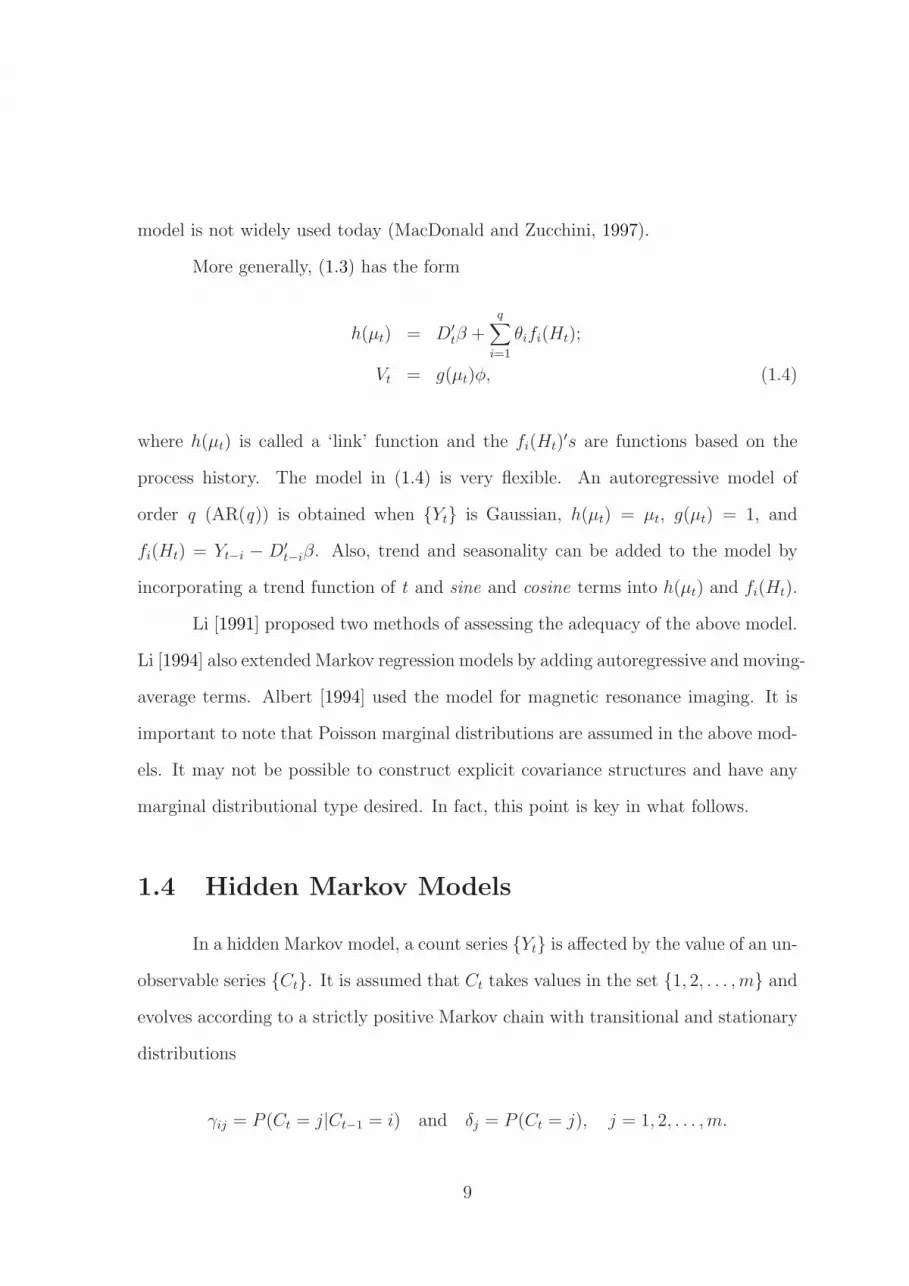
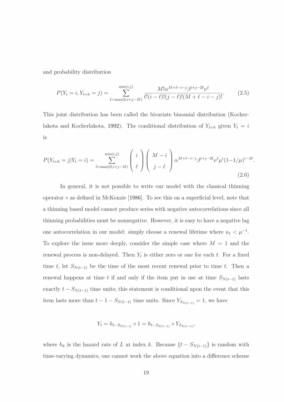
Binomial Count Series

Time of Observation

Coun

t

0 200 400 600 800 1000

01

23

45

0 10 20 30 40 50

0.00.2

0.40.6

0.81.0

Lag

Samp

le AC

F

Sample Autocorrelations

0 10 20 30 40 50

0.00.2

0.40.6

0.81.0

Lag

Sam

ple P

ACF

Sample Partial Autocorrelations

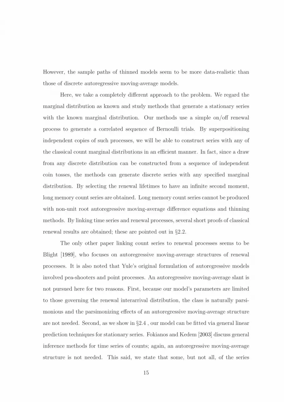
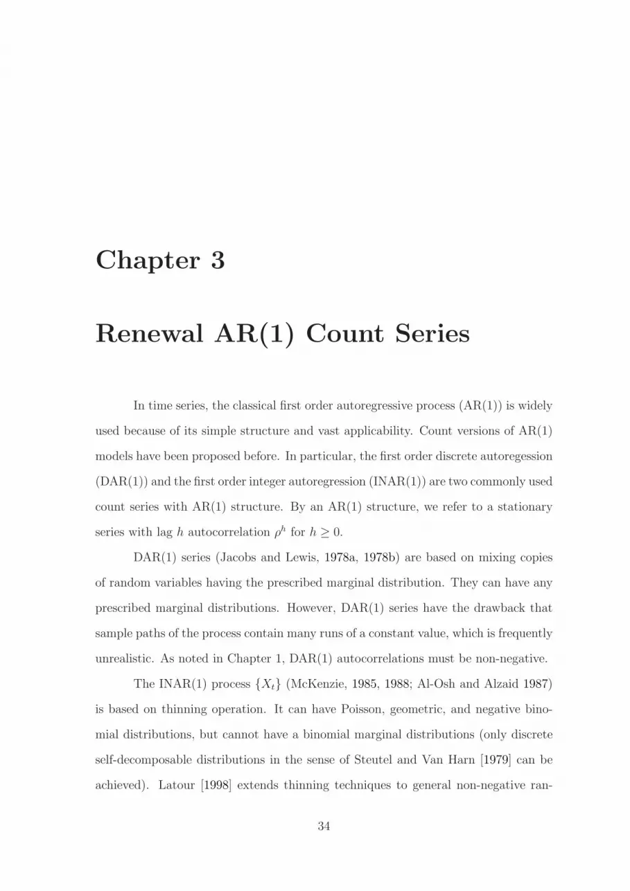
Figure 2.1: A Realization of a Stationary Series Having Binomial Marginals alongwith Sample Autocorrelations and Partial Autocorrelations.

2.3 The Classical Count Marginals

Stationary series with the classical count marginal distribution structures are

easily produced. When M is a unit point mass at M = m, Yt has a binomial distri-

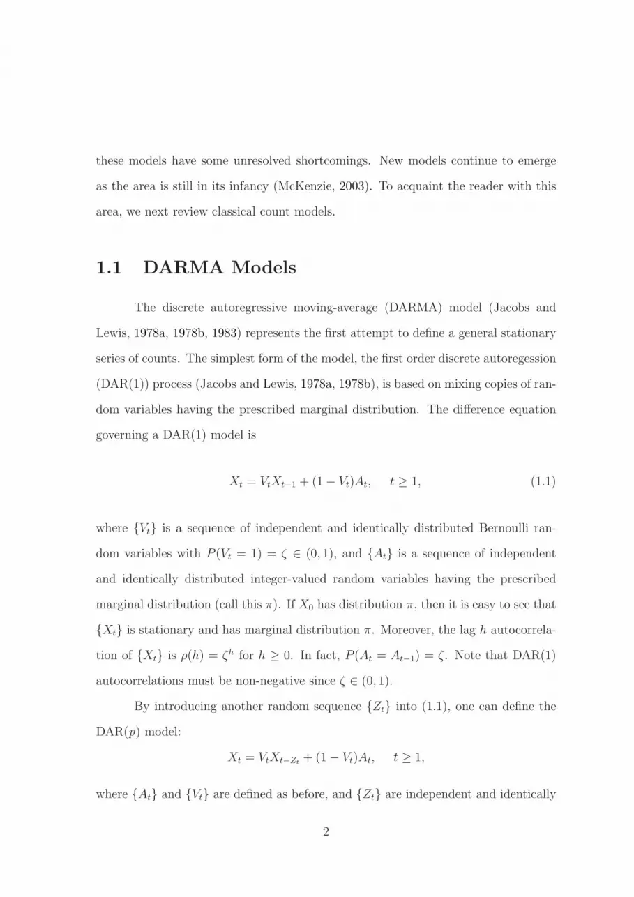
bution for each fixed n with m trials and success probability µ−1. Figure 2.1 shows

a sample path of 1000 observations sampled from a stationary series with a binomial

marginal distribution with m = 5 and success probability 1/2. The sample auto-

correlations and partial autocorrelations are also shown. The dashed lines are 95%

confidence bounds for white noise (pointwise). The renewal lifetime used here had

f1 = 3/4 and fn = (16)−1(3/4)n−2 for n ≥ 2. This lifetime has a constant hazard

rate past lag 1; hence, by Theorem 4, the series is Markov and, as discussed in the

last section, satisfies a first order autoregressive difference equation. Discrete autore-

gressive moving-average and other methods can generate the above series; we offer it

mainly as a baseline example.

22

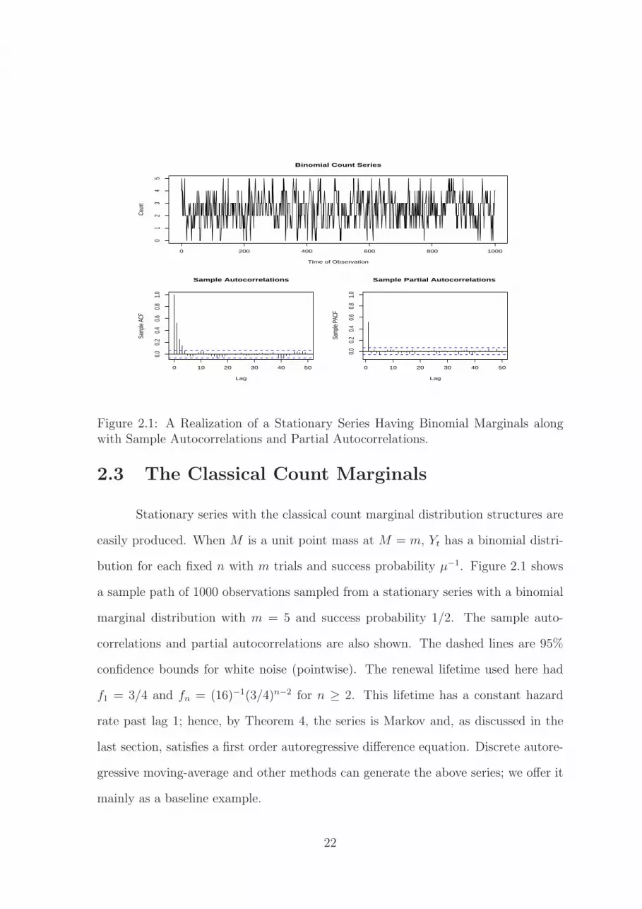
When M is Poisson with mean λ, a simple calculation will verify that Yt has

a Poisson distribution for each n with mean λ/µ. The joint probability generating

function of Yt and Yt+h is

E[sYt

1 sYt+h

2 ] = e−λ[1−{α+β(s1+s2)+νs1s2}], (2.8)

where α, β, and ν are as in the last section. From (2.8), it follows that (Yt, Yt+h)

has the bivariate Poisson distribution discussed in Holgate [1964] and Loukas et al.

[1986]:

P (Yt = i, Yt+h = j) =min(i,j)∑

ℓ=0

e−(2λ1−λ2) (λ1 − λ2)i+j−2ℓλℓ

2

ℓ!(i − ℓ)!(j − ℓ)!,

where λ1 = λ(β + ν), and λ2 = λν.

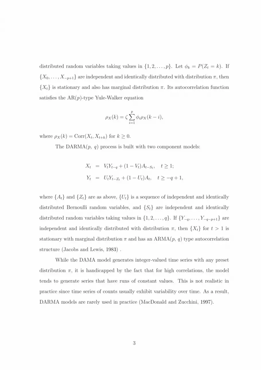
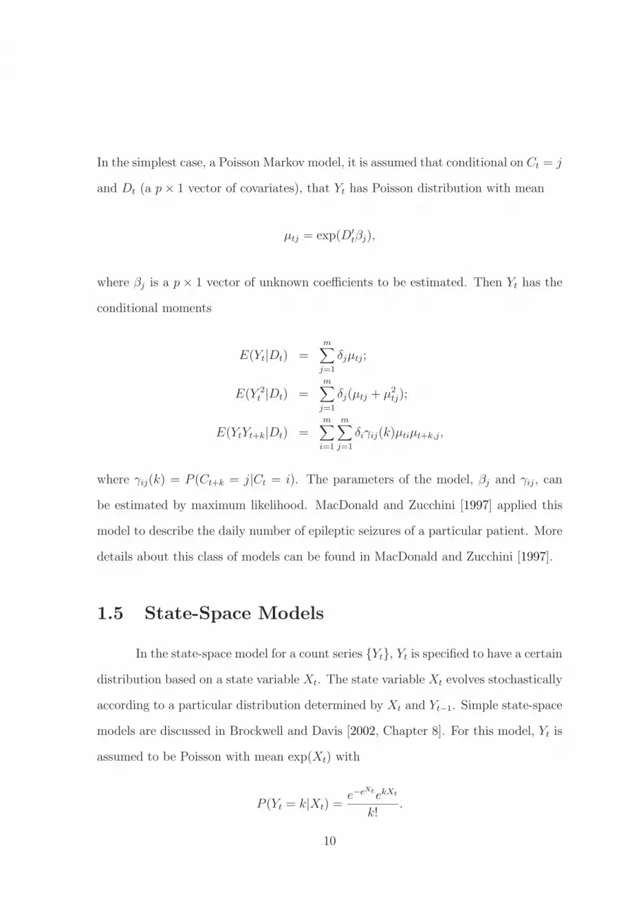
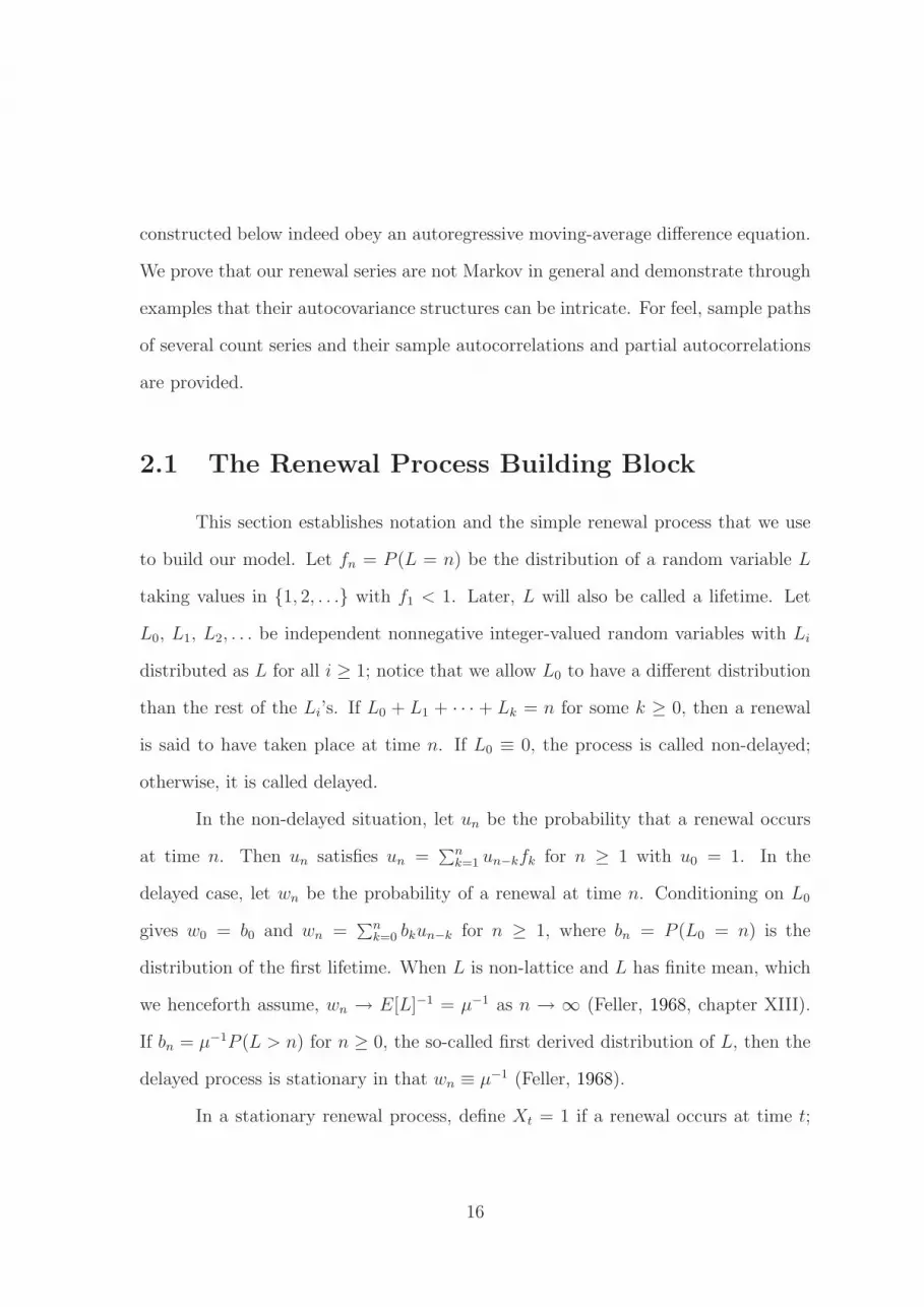
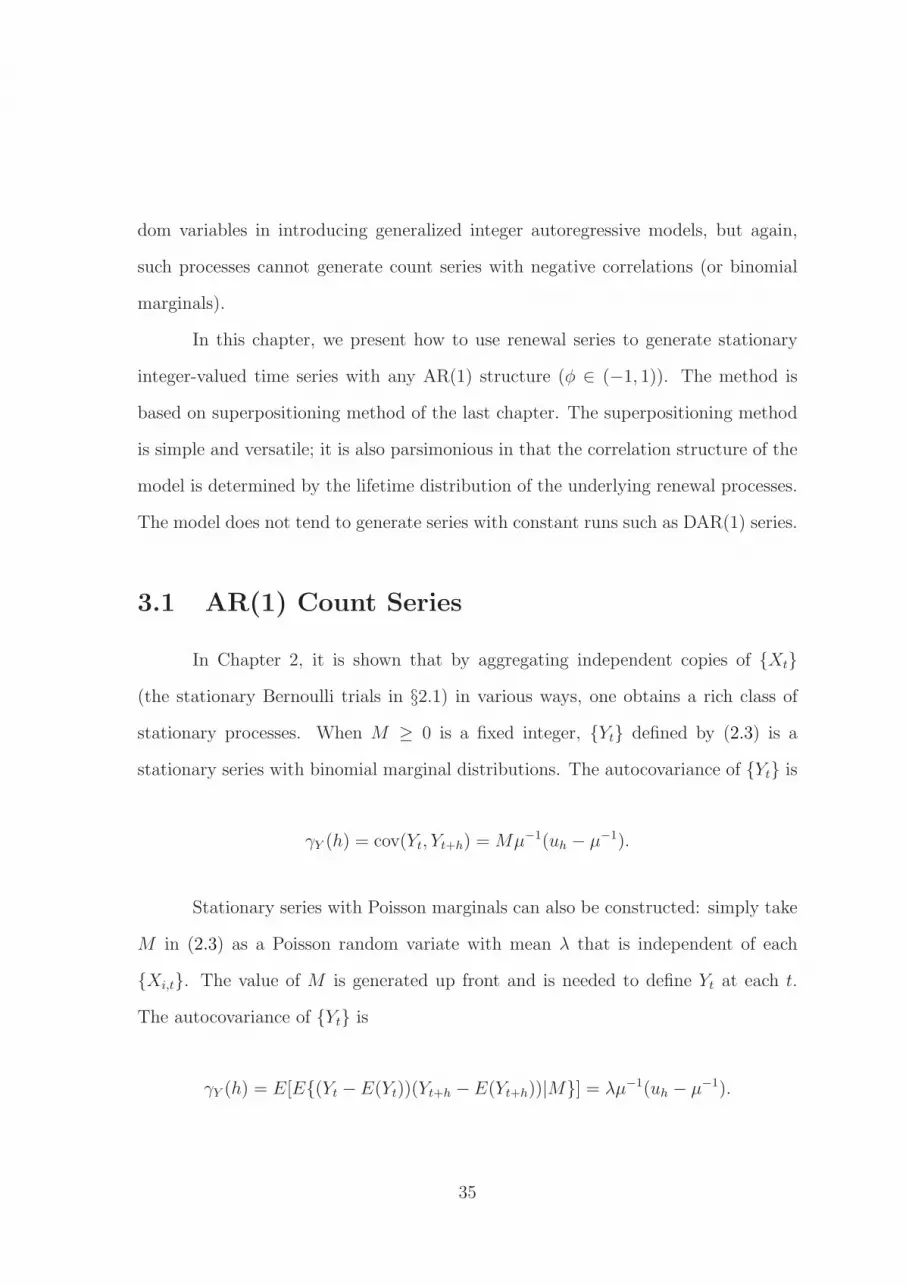
Figure 2.2 shows a sample path of 1000 points from a series with Poisson

marginal distributions with λ = 20. The renewal lifetime used here was Pareto: fn =

C/n2.5 for n ≥ 1, where C is a constant making the distribution’s probabilities sum to

unity. This lifetime has a finite mean but infinite second moment. By Theorem 2, the

series has long-memory, a trait that can be seen in the sample autocorrelations. We do

not know of other methods that can generate a long-memory Poisson count series with

such ease, although an unpublished technical report by A. M. M. Q. Quoreshi entitled

“A long memory count data time series model for financial application” attempts to

do this via fractional differencing.

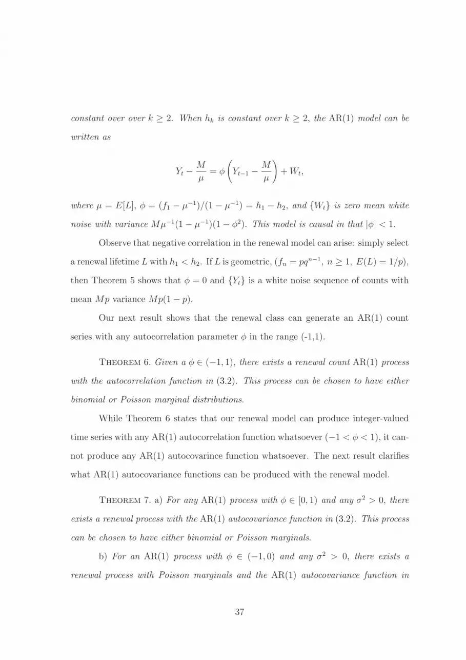
Stationary series with geometric marginals can also be constructed. Given

a collection {Xi,t} of independent and identically distributed copies of the renewal

processes in §2.1 , set Yt = inf{m ≥ 1 : Xm,t = 1}. Since P (Xi,t = 1) = µ−1 for all

i and t, Yt is the time of first success in independent Bernoulli trials having success

23

Poisson Count Series

Time of Observation

Coun

t

0 200 400 600 800 1000

68

1012

1416

18

0 10 20 30 40 50

0.00.2

0.40.6

0.81.0

Lag

Samp

le AC

F

Sample Autocorrelations

0 10 20 30 40 50

0.00.2

0.40.6

0.81.0

Lag

Sam

ple P

ACF

Sample Partial Autocorrelations

Figure 2.2: A Realization of a Long Memory Stationary Series Having PoissonMarginals along with Sample Autocorrelations and Partial Autocorrelations.

probability µ−1. Hence, Yt has a geometric distribution with success probability µ−1

for each t.

The autocovariance function of {Yt} is derived as follows. First, we will show

that E(YtYt+h) = (2 − uh)−1(2µ2 − µ). To do this, observe that the event {Yt =

k, Yt+h = j} with k > j happens precisely when Xi,t = Xi,t+h = 0 for each i satisfying

1 ≤ i < j, Xj,t = 0 and Xj,t+h = 1, and Xi,t = 0 for j + 1 ≤ i ≤ k − 1 and

Xk,t = 1. Using these and the independence of {Xi,t} in i gives P (Yt = k, Yt+h = j) =

αj−1β(µ − 1)k−j−1/µk−j for k > j, P (Yt = k, Yt+h = j) = αk−1β(µ − 1)j−k−1/µj−k

when k < j and P (Yt = k, Yt+h = j) = αk−1ν when k = j.

The above three probabilities now give

E[YtYt+h] =∞∑

k=1

∞∑

j=1

kjP (Yt = k, Yt+h = j) =2(2 − uh)

(1 − α)2− 1

1 − α. (2.9)

Using 1−α = (2− uh)µ−1 in (2.9) gives the aforementioned form of E[YnYn+h]. Now

24

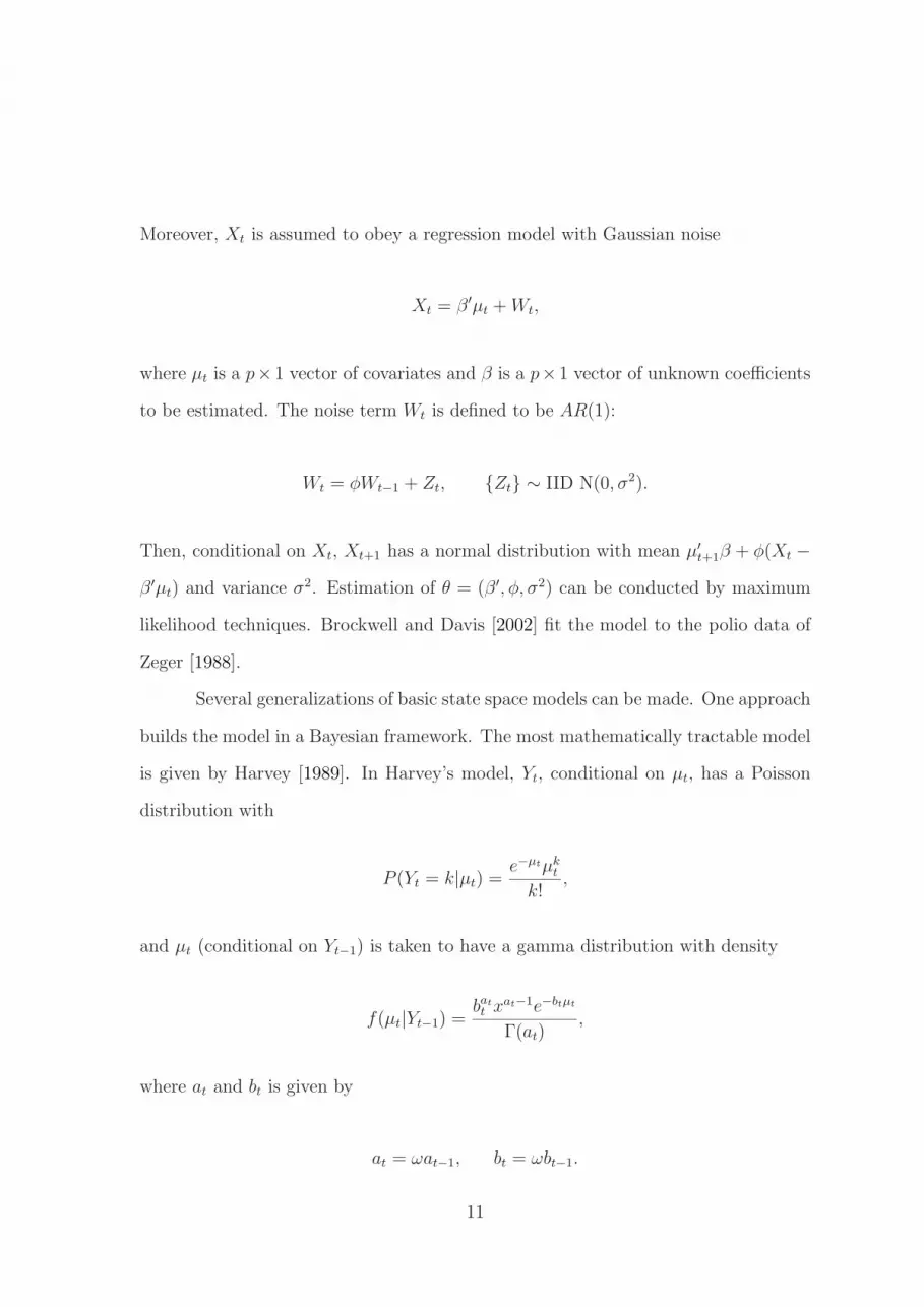
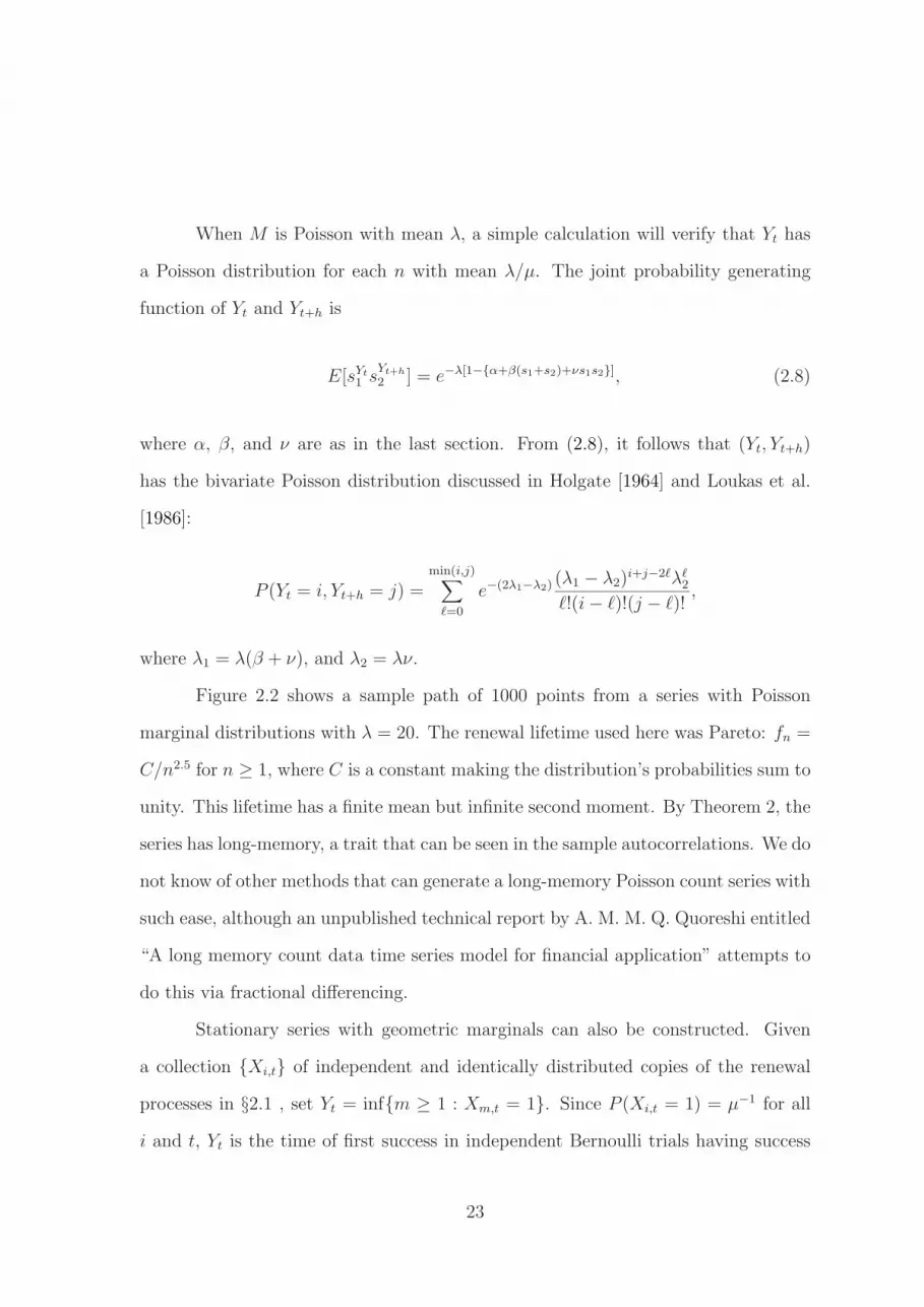
Geometric Count Series

Time of Observation

Coun

t

0 200 400 600 800 1000

24

68

1012

0 10 20 30 40 50

−0.4

0.00.4

0.8

Lag

Samp

le AC

F

Sample Autocorrelations

0 10 20 30 40 50

−0.4

0.00.4

0.8

Lag

Sam

ple P

ACF

Sample Partial Autocorrelations

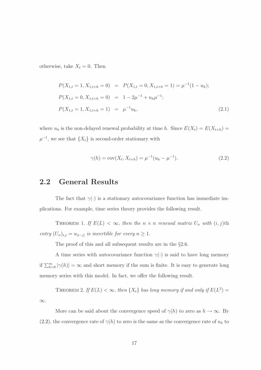
Figure 2.3: A Realization of a Stationary Series Having Geometric Marginals alongwith Sample Autocorrelations and Partial Autocorrelations.

apply E(Yt) = E(Yt+h) = µ to get Cov(Yt, Yt+h) = (µ2uh − µ)/(2 − uh) for h ≥ 0.

The joint probability generating function of Yt and Yt+h can be found as in

Marshall and Olkin [1985]:

E[sYt

1 sYt+h

2 ] =ν − (s1 + s2)τ − s1s2(β

2 − ατ)

{1 − (1 − 1/µ)s1}{1 − (1 − 1/µ)s2}(1 − αs1s2)s1s2,

where τ = µ−1(uh − µ−1), which is also called a bivariate geometric distribution.

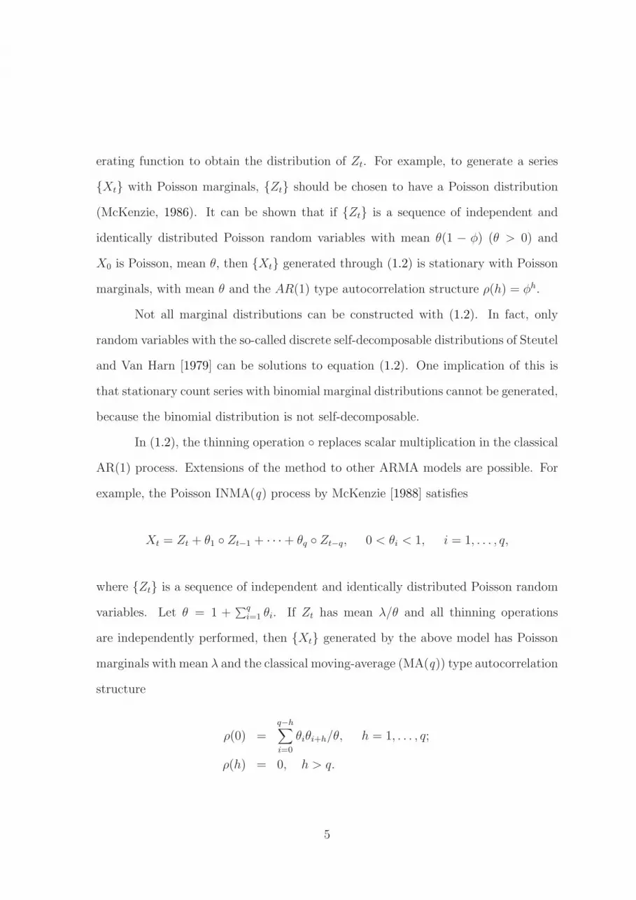
Figure 2.3 shows a sample path of 1000 points from a stationary series with

geometric marginal distributions. Here, the renewal lifetime used has f1 = 1/4 and

fn = (9/16)(1/4)n−2 for n ≥ 2. Observe that the lag one sample autocorrelations for

this process are negative; correlation structures with negative dependence have been

difficult to produce for some count model classes (McKenzie, 2003).

One can construct a stationary series from the above methods with any discrete

marginal distribution desired. To do this, let {Xi,t}∞t=0 be independent and identically

25

distributed stationary Bernoulli sequences for each i ≥ 1 and let f be a function

such that f(X1,t, X2,t, . . .) has the discrete marginal distribution in question. Such a

function exists since every discrete distribution can be generated from independent

and identically distributed coin tosses. In many cases, f requires only a finite number

of processes. Then Yt = f(X1,t, X2,t, . . .) is the desired stationary series. Of course,

one needs to derive the autocovariance function {Yt} for each different f .

2.4 Fitting the Renewal Model

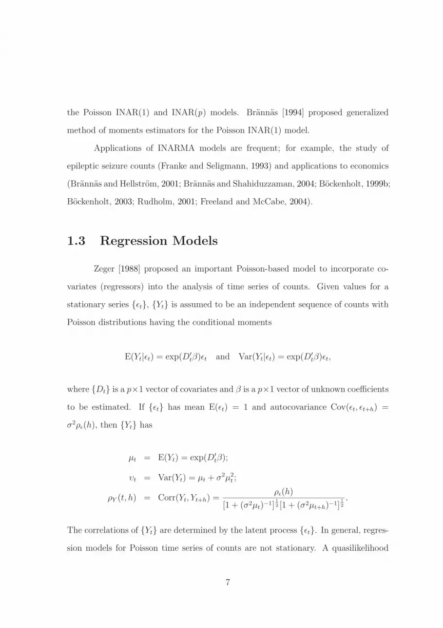
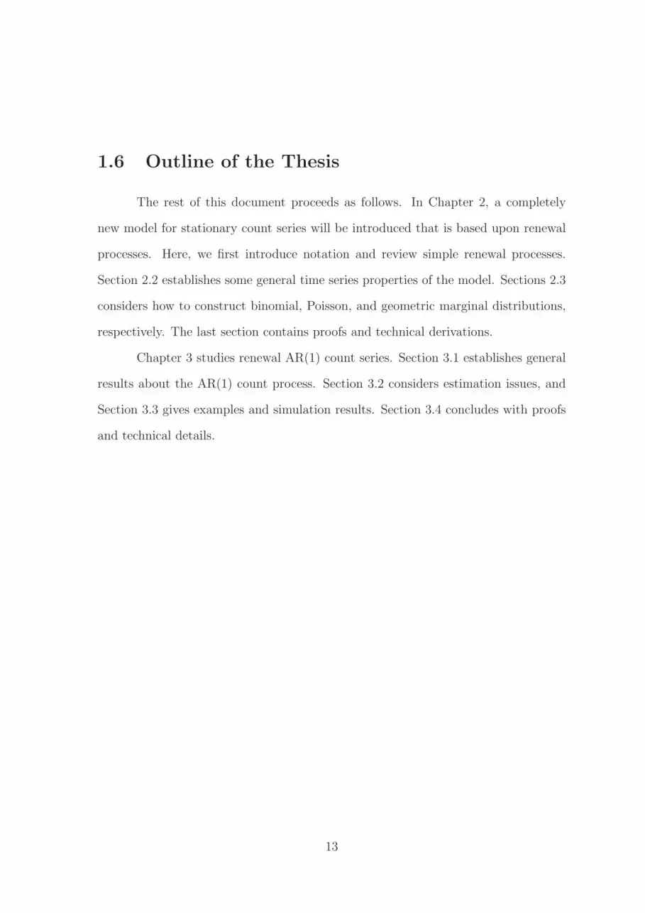
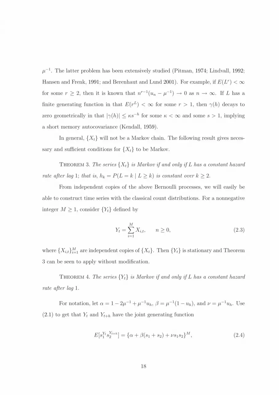
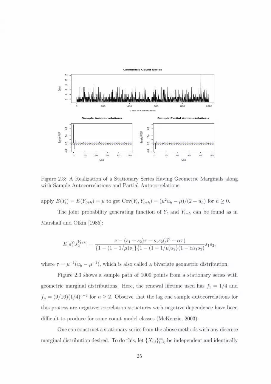
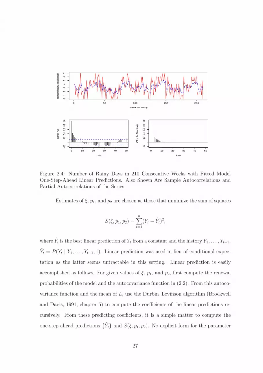
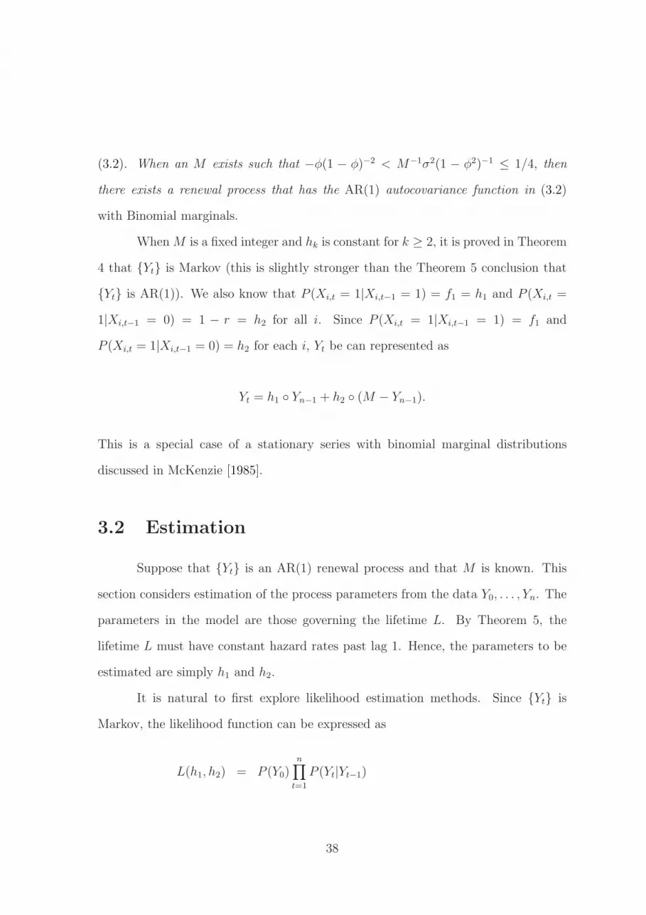
This section shows how to fit the renewal model to data. Figure 2.4 shows the

number of days in which non-zero rainfall was recorded at Key West, Florida in the

n = 210 week period spanning from January 2, 2005 — January 3, 2009, inclusive.

The sample autocorrelations of this data are displayed in the bottom graphic of

the figure and show that the data are correlated. It is natural to fit a model that

has binomial marginal distributions with M = 7 trials. To proceed further, one

must specify the renewal lifetime. We will work with the three-parameter mixture

geometric lifetime

P (L = k) = ξp1(1 − p1)k−1 + (1 − ξ)p2(1 − p2)

k−1, k ≥ 1

where ξ, p1, and p2 lie in [0,1]. When p1 = p2 (or ξ = 0 or ξ = 1) the model reduces

to a simple geometric lifetime, which has γ(h) = 0 for all h ≥ 1 and represents

uncorrelated data. One could try other discrete lifetime distributions or geometric

mixtures of three or more components, but the two component geometric mixture is

flexible and illustrates the general techniques. Also, Key West, a tropical locality,

was chosen for study because its rainfall is largely non-seasonal.

26

0 50 100 150 200

01

23

45

67

Week of Study

Numb

er of

Rain

y Day

s in W

eek

0 10 20 30 40 50

−0.2

0.20.4

0.60.8

1.0

Lag

Samp

le AC

F

0 10 20 30 40 50

−0.2

0.20.4

0.60.8

1.0

Lag

ACF

of the

Fitte

d Mod

el

Figure 2.4: Number of Rainy Days in 210 Consecutive Weeks with Fitted ModelOne-Step-Ahead Linear Predictions. Also Shown Are Sample Autocorrelations andPartial Autocorrelations of the Series.

Estimates of ξ, p1, and p2 are chosen as those that minimize the sum of squares

S(ξ, p1, p2) =n∑

t=1

(Yt − Yt)2,

where Yt is the best linear prediction of Yt from a constant and the history Y1, . . . , Yt−1:

Yt = P (Yt | Y1, . . . , Yt−1, 1). Linear prediction was used in lieu of conditional expec-

tation as the latter seems untractable in this setting. Linear prediction is easily

accomplished as follows. For given values of ξ, p1, and p2, first compute the renewal

probabilities of the model and the autocovariance function in (2.2). From this autoco-

variance function and the mean of L, use the Durbin–Levinson algorithm (Brockwell

and Davis, 1991, chapter 5) to compute the coefficients of the linear predictions re-

cursively. From these predicting coefficients, it is a simple matter to compute the

one-step-ahead predictions {Yt} and S(ξ, p1, p2). No explicit form for the parameter

27

estimates exist; however, values of ξ, p1 and p2 that minimize S(ξ, p1, p2) were found

with a gradient step and search algorithm.

Because S(ξ, p1, p2) = S(1 − ξ, p2, p1), the restriction ξ ∈ [0, 1/2] is imposed

for parameter identifiability. Following the sum of squares quasilikelihood theory in

Klimko and Nelson (1978) and the best linear prediction methods for stationary series

in Sørensen [2000], minimizers of the sum of squares can be shown to be asymptotically

normal. Moreover, estimates of the information matrix can be obtained from the

second derivative matrix of S evaluated at the estimated parameters; i.e., the inverse

of the so-called Hessian.

The estimated parameters of the model (the error margins listed are one stan-

dard error) are ξ = 0.1496 ± 0.0316, p1 = 0.1241 ± 0.0203, and p2 = 0.7764 ± 0.0288.

The one-step-ahead predictions are plotted in Figure 2.4 and seem to track the data

well. The sample autocorrelations of the fitted model are also plotted and reasonably

match those of the data for smaller lags, although some midrange dependence remains

unmodeled. From these estimators, a z-score for the hypothesis test that p1 = p2 is

z = 25.1856, which has a p-value of nearly zero; the same conclusion is obtained if

one tests a null hypothesis of ξ = 0 or ξ = 1. The mean of the fitted model is 3.0425,

while the sample mean is 3.0857. Overall, the model seems to fit the data roughly.

Future work will formalize the asymptotics of the fitting methods and incorporate

the possibility of periodic dynamics.

2.5 Comments

Nonstationary processes can also be produced with the renewal model. Such

a setup could also accommodate covariates. To do this, one can simply allow the

parameters in the model to vary with time or the covariates. For example, periodically

28

stationary series could be constructed with a periodic renewal process. A process with

binomial marginals that depend on a time-varying deterministic covariate ct at time

t could be obtained by allowing M and the renewal probabilities at time t to depend

on ct.

2.6 Proofs

Proof of Theorem 1. Let Γn be the n × n matrix with (i, j)th entry γ(|i − j|)

for 1 ≤ i, j ≤ n. Since uh → µ−1 as h → ∞, γ(h) → 0 as h → ∞. Applying

Proposition 5.1.1 in , Brockwell and Davis [1991] we infer that Γn is non-singular for

every n. Now let ~a be any nonzero n × 1 vector. Invertibility of Γn gives ~a′Γn~a > 0,

or equivalently, from (2.2), ~a′Un~a − µ−1~a′Jn~a > 0, where Jn denotes an n × n matrix

whose entries are all unity. Hence, ~a′Un~a > µ−1~a′Jn~a ≥ 0 and the result is proven.

Proof of Theorem 2. Equation (2.2) gives

∞∑

h=0

|γ(h)| =1

µ

∞∑

t=0

|P0(Xt = 1) − PS(Xt = 1)|, (2.10)

where P0(Xt = 1) denotes the probability of a renewal at time n in a non-delayed

renewal process and PS(Xt = 0) ≡ µ−1 is the stationary version of this probability;

i.e., L0 has the first derived distribution as discussed in §2.1. Given that E[L] < ∞,

Pitman [1974] shows that the sum in right hand side of (2.10) is finite if and only if

E[L0] < ∞. But since E[L0] = E[L2]/(2E[L]), the theorem follows.

29

Proof of Theorem 3. Recall that Xt is either zero or one for each n. If {Xt} is

Markov, then

P (Xt = 1 | Xt−1 = 0, Xt−2 = 0, . . . , Xt−k+1 = 0, Xt−k = 1) = P (Xt = 1 | Xt−1 = 0)

(2.11)

for all k ≥ 2. But the left hand side of (2.11) is

P (Xt = 1, Xt−1 = 0, . . . , Xt−k+1 = 0, Xt−k = 1)

P (Xt−1 = 0, . . . , Xt−k+1 = 0, Xt−k = 1)=

µ−1P (L = k)

µ−1P (L > k − 1)= hk,

where hk is the hazard rate of L at index k. The right hand side of (2.11) is seen to

be constant in t:

P (Xt = 1 | Xt−1 = 0) =P (Xt = 1) − P (Xt−1 = 1, Xt = 1)

P (Xt−1 = 0)=

µ−1P (L > 1)

1 − µ−1. (2.12)

Therefore, L must have constant hazard rates past lag 1 for {Xt} to be Markov.

Now suppose that L has a constant hazard rate past lag 1 and write fn =

f2rn−2 for n ≥ 2 and some r < 1. The hazard rate for L at lag k ≥ 2 is hk =

fk/(Σ∞ℓ=kfℓ) = 1 − r. To verify the Markov property, we need to show that

P (Xt = it | Xt−1 = it−1, Xt−2 = it−2, · · · , X0 = i0) = P (Xt = it | Xt−1 = it−1)

for every ik ∈ {0, 1} and all n ≥ 2. Because Xt is either zero or one for all t, we

need only consider the case where it = 1 (the case where it = 0 then follows by

complementation).

Our work proceeds by cases. If Xt−1 = 1 then

P (Xt = 1 | Xt−1 = 1, Xt−2 = it−2, · · · , X0 = i0) = P (Xt = 1 | Xt−1 = 1) = f1.

30

If Xt−1 = 0, there are two subcases. First, suppose that ik = 0 for 0 ≤ k ≤ t−1.

Then the lifetime L0 is in use at time t − 1 and

P (Xt = 1 | Xi = 0, 0 ≤ i ≤ n − 1) =P (L0 = t)

P (L0 ≥ t)= 1 − r,

where the fact that P (L0 = t) = µ−1P (L > t) for t ≥ 0 and ft = f2rt−2 for t ≥ 2

have been applied.

From (2.12), we have P (Xt = 1 | Xt−1 = 0) = (1 − f1)/(µ − 1). Using

E[L] = 1 + f2(1 − r)−2 and 1 − f1 = f2(1 − r)−1 gives P (Xt = 1 | Xt−1 = 0) = 1 − r,

which verifies the Markov property for this case.

Our second subcase entails the situation where ik = 1 for some k with 0 ≤

k ≤ t − 2. Let ℓ = max{k : ik = 1 and 0 ≤ k ≤ t − 1} be the maximum such index

and argue as above to finish our work:

P (Xt = 1 | Xt−1 = 0, . . . , Xℓ = 1, Xℓ−1 = iℓ−1, . . . , X0 = i0) =P (L = t − ℓ)

P (L ≥ t − ℓ)= 1 − r.

Proof of Theorem 4. Suppose that {Yt} is Markov. Then

P (Yt = M | Yt−1 = 0) = P (Yt = M | Yt−1 = 0, . . . , Y0 = M)

for all t ≥ 2. Applying the independence of the M component processes gives

ΠMi=1P (Xi,t = 1 | Xi,t−1 = 0) = ΠM

i=1P (Xi,t = 1 | Xi,t−1 = 0, . . . , Xi,0 = 1). (2.13)

We have selected special values for Yi to take on over 0 ≤ i ≤ t, extreme in that they

are either M or 0. Since the terms in the products in (2.13) are constant in i, we

31

infer that

P (X1,t = 1 | X1,t−1 = 0) = P (X1,t = 1 | X1,t−1 = 0, . . . , X1,0 = 1).

Now argue as in the proof of Theorem 3 to infer that L must have constant hazard

rates past lag 1.

Now suppose that L has constant hazard rates past lag 1. We need to show

that

P (Yt = j | Yt−1 = i, Yt−2, · · · , Y0) = P (Yt = j | Yt−1 = i). (2.14)

Conditional on the event Yt−1 = i and any values of Yt−2, . . . Y0, the ways in

which Yt = j can happen are enumerated as follows. If ℓ of the i component processes

{Xi,t} which are unity at time t − 1 are still unity at time n, then j − ℓ of the

component processes which were zero at time t − 1 must have transitioned unity to

make Yt = j. Summing over all possible ℓ and applying the Markov property of the

component processes provides

P (Yt = j | Yt−1 = i, Yn−2, · · · , Y0) =min(i,j)∑

ℓ=max(0,i+j−M)

(

i

ℓ

)(

M − i

j − ℓ

)

Jℓ, (2.15)

where Jℓ = f ℓ1(1 − f1)

i−ℓ(1 − r)j−ℓrM+ℓ−j−i. The expression for Jℓ is a simple multi-

nomial probability. In fact, the proof of Theorem 3 showed that

P (Xℓ,t = 1 | Xℓ,t−1 = 1, Xℓ,t−2 = it−2, . . . , Xℓ,0 = i0) = f1

P (Xℓ,t = 0 | Xℓ,t−1 = 1, Xℓ,t−2 = it−2, . . . , Xℓ,0 = i0) = 1 − f1

P (Xℓ,t = 1 | Xℓ,t−1 = 0, Xℓ,t−2 = it−2, . . . , Xℓ,0 = i0) = 1 − r

P (Xℓ,t = 0 | Xℓ,t−1 = 0, Xℓ,t−2 = it−2, · · · , Xℓ,0 = i0) = r.

32

for each of the component processes (1 ≤ ℓ ≤ M).

When h = 1, the Section §2.2 parameters can be evaluated as α = r(1− µ−1),

β = (1 − r)(1 − µ−1), and ν = µ−1f1. For the right side of (2.14), apply the above

results to the conditional distribution derived in (2.6) to obtain

P (Yt = j | Yt−1 = i) =min(i,j)∑

ℓ=max(0,i+j−M)

(

i

ℓ

)(

M − i

j − ℓ

)

Jℓ,

which completes our work.

33

Chapter 3

Renewal AR(1) Count Series

In time series, the classical first order autoregressive process (AR(1)) is widely

used because of its simple structure and vast applicability. Count versions of AR(1)

models have been proposed before. In particular, the first order discrete autoregession

(DAR(1)) and the first order integer autoregression (INAR(1)) are two commonly used

count series with AR(1) structure. By an AR(1) structure, we refer to a stationary

series with lag h autocorrelation ρh for h ≥ 0.

DAR(1) series (Jacobs and Lewis, 1978a, 1978b) are based on mixing copies

of random variables having the prescribed marginal distribution. They can have any

prescribed marginal distributions. However, DAR(1) series have the drawback that

sample paths of the process contain many runs of a constant value, which is frequently

unrealistic. As noted in Chapter 1, DAR(1) autocorrelations must be non-negative.

The INAR(1) process {Xt} (McKenzie, 1985, 1988; Al-Osh and Alzaid 1987)

is based on thinning operation. It can have Poisson, geometric, and negative bino-

mial distributions, but cannot have a binomial marginal distributions (only discrete

self-decomposable distributions in the sense of Steutel and Van Harn [1979] can be

achieved). Latour [1998] extends thinning techniques to general non-negative ran-

34

dom variables in introducing generalized integer autoregressive models, but again,

such processes cannot generate count series with negative correlations (or binomial

marginals).

In this chapter, we present how to use renewal series to generate stationary

integer-valued time series with any AR(1) structure (φ ∈ (−1, 1)). The method is

based on superpositioning method of the last chapter. The superpositioning method

is simple and versatile; it is also parsimonious in that the correlation structure of the

model is determined by the lifetime distribution of the underlying renewal processes.

The model does not tend to generate series with constant runs such as DAR(1) series.

3.1 AR(1) Count Series

In Chapter 2, it is shown that by aggregating independent copies of {Xt}

(the stationary Bernoulli trials in §2.1) in various ways, one obtains a rich class of

stationary processes. When M ≥ 0 is a fixed integer, {Yt} defined by (2.3) is a

stationary series with binomial marginal distributions. The autocovariance of {Yt} is

γY (h) = cov(Yt, Yt+h) = Mµ−1(uh − µ−1).

Stationary series with Poisson marginals can also be constructed: simply take

M in (2.3) as a Poisson random variate with mean λ that is independent of each

{Xi,t}. The value of M is generated up front and is needed to define Yt at each t.

The autocovariance of {Yt} is

γY (h) = E[E{(Yt − E(Yt))(Yt+h − E(Yt+h))|M}] = λµ−1(uh − µ−1).

35

We now relate the renewal model to AR(1) models. The classical stationary

and causal AR(1) process {Xt} with mean c satisfies the difference equation

Xt − c = φ(Xt−1 − c) + ǫt, (3.1)

where |φ| < 1 and {ǫt} is zero mean white noise with variance σ2. The autocovariance

and autocorrelation functions of the AR(1) model are

Cov(Xt, Xt+h) =σ2φh

1 − φ2and Corr(Xt, Xt+h) = φh, (3.2)

for h ≥ 0. While DAR(1) and INAR(1) models are capable of generating count

series with an AR(1) autocorrelation function with any φ > 0, they cannot generate

AR(1) count structures with φ < 0. Below, we show that our renewal class can easily

accommodate negative correlations.

Let hk = P (L = k|L ≥ k) be the hazard rate of the lifetime L at index k.

If a lifetime distribution has constant hazard rate after lag 1, then its probability

mass function has the form f2 = (1 − f1)(1 − r) and fn = f2rn−2 for n ≥ 2 for

some f1 = P (L = 1) and r ∈ (0, 1). Since h1 = P (L = 1|L ≥ 1) = f1 and

hk = P (L = k|L ≥ k) = fk/(Σ∞ℓ=kfℓ) = 1 − r the distribution of L is simply f1 = h1,

f2 = (1 − h1)h2, and fn = f2(1 − h2)n−2 for n ≥ 2. The mean of L is

µ = 1 +f2

(1 − r)2=

1 + h2 − h1

h2

. (3.3)

Our first result is the following. The proofs of all results in this section are

delegated to §3.5.

Theorem 5. {Yt} satisfies the AR(1) difference equation if and only if hk is

36

constant over over k ≥ 2. When hk is constant over k ≥ 2, the AR(1) model can be

written as

Yt −M

µ= φ

(

Yt−1 −M

µ

)

+ Wt,

where µ = E[L], φ = (f1 − µ−1)/(1 − µ−1) = h1 − h2, and {Wt} is zero mean white

noise with variance Mµ−1(1 − µ−1)(1 − φ2). This model is causal in that |φ| < 1.

Observe that negative correlation in the renewal model can arise: simply select

a renewal lifetime L with h1 < h2. If L is geometric, (fn = pqn−1, n ≥ 1, E(L) = 1/p),

then Theorem 5 shows that φ = 0 and {Yt} is a white noise sequence of counts with

mean Mp variance Mp(1 − p).

Our next result shows that the renewal class can generate an AR(1) count

series with any autocorrelation parameter φ in the range (-1,1).

Theorem 6. Given a φ ∈ (−1, 1), there exists a renewal count AR(1) process

with the autocorrelation function in (3.2). This process can be chosen to have either

binomial or Poisson marginal distributions.

While Theorem 6 states that our renewal model can produce integer-valued

time series with any AR(1) autocorrelation function whatsoever (−1 < φ < 1), it can-

not produce any AR(1) autocovarince function whatsoever. The next result clarifies

what AR(1) autocovariance functions can be produced with the renewal model.

Theorem 7. a) For any AR(1) process with φ ∈ [0, 1) and any σ2 > 0, there

exists a renewal process with the AR(1) autocovariance function in (3.2). This process

can be chosen to have either binomial or Poisson marginals.

b) For an AR(1) process with φ ∈ (−1, 0) and any σ2 > 0, there exists a

renewal process with Poisson marginals and the AR(1) autocovariance function in

37

(3.2). When an M exists such that −φ(1 − φ)−2 < M−1σ2(1 − φ2)−1 ≤ 1/4, then

there exists a renewal process that has the AR(1) autocovariance function in (3.2)

with Binomial marginals.

When M is a fixed integer and hk is constant for k ≥ 2, it is proved in Theorem

4 that {Yt} is Markov (this is slightly stronger than the Theorem 5 conclusion that

{Yt} is AR(1)). We also know that P (Xi,t = 1|Xi,t−1 = 1) = f1 = h1 and P (Xi,t =

1|Xi,t−1 = 0) = 1 − r = h2 for all i. Since P (Xi,t = 1|Xi,t−1 = 1) = f1 and

P (Xi,t = 1|Xi,t−1 = 0) = h2 for each i, Yt be can represented as

Yt = h1 ◦ Yn−1 + h2 ◦ (M − Yn−1).

This is a special case of a stationary series with binomial marginal distributions

discussed in McKenzie [1985].

3.2 Estimation

Suppose that {Yt} is an AR(1) renewal process and that M is known. This

section considers estimation of the process parameters from the data Y0, . . . , Yn. The

parameters in the model are those governing the lifetime L. By Theorem 5, the

lifetime L must have constant hazard rates past lag 1. Hence, the parameters to be

estimated are simply h1 and h2.

It is natural to first explore likelihood estimation methods. Since {Yt} is

Markov, the likelihood function can be expressed as

L(h1, h2) = P (Y0)n∏

t=1

P (Yt|Yt−1)

38

=

M

Y0

µ−Y0(1 − µ−1)M−Y0

n∏

t=1

P (Yt|Yt−1), (3.4)

where P (Yt|Yt−1) is calculated from (2.15) as

P (Yn = j|Yn−1 = i) =min(i,j)∑

ℓ=max(0,i+j−M)

(

i

ℓ

)(

M − i

j − ℓ

)

hℓ1(1 − h1)

i−ℓhj−ℓ2 (1 − h2)

M+ℓ−j−i.

This likelihood function is somewhat unwieldy: no simple closed-form expres-

sions for h1 and h2 that maximize the likelihood function are evident to us. Maxi-

mization of the likelihood appears to be a numerical task.

Since our AR(1) model is ergodic and stationary, the asymptotic properties

of conditional least squares estimators can be quantified (see Klimko and Nelson,

1978). We first consider the parameters φ and η = Mµ−1(1 − φ) as their asymptotic

properties can be easily quantified. A multivariate delta method with the relations

h1 = φ +η

M, h2 =

η

M(3.5)

will then identify the asymptotic distributions of the conditional least squares esti-

mates of h1 and h2.

Let g(φ, η) = E(Yt|Yt−1, · · · , Y0) = E(Yt|Yt−1). From (2.7), it is known that

g(φ, η) = φYt−1 + η. The conditional least squares estimators for φ and η, denoted by

φCLS and ηCLS, are minimizers of

Qn(φ, η) =n∑

t=0

(Yt − φYt−1 − η)2.

By solving the equations

39

∂Qn(φ, η)

∂φ= 0 and

∂Qn(φ, η)

∂η= 0,

the conditional least squares estimators are identified explicitly as

φCLS =

∑nt=1 YtYt−1 −

(

1n

∑nt=1 Yt

)

(∑n

t=1 Yt−1)∑n

t=1 Y 2t−1 −

(

1n

∑nt=1 Yt−1

)

(∑n

t=1 Yt−1); ηCLS =

1

n

(

n∑

t=1

Yt − φCLS

n∑

t=1

Yt−1

)

.

Since the conditions of Theorem 3.1 and 3.2 of Klimko and Nelson [1978] are satisfied,

φCLS and ηCLS are consistent and asymptotically normal with

φCLS

ηCLS

∼ AN2

φ

Mµ

(1 − φ)

, V −1WV −1

n

,

where V is the 2 × 2 matrix

V =

E[Y 2t−1] E[Yt−1]

E[Yt−1] 1

=

Mµ

(1 − 1µ) + M2

µ2Mµ

Mµ

1

,

and W is the 2 × 2 matrix

W =

E[(Yt − φYt−1 − Mµ

(1 − φ))2Y 2t−1] E[(Yt − φYt−1 − M

µ(1 − φ))2Yt−1]

E[(Yt − φYt−1 − Mµ

(1 − φ))2Yt−1] E[(Yt − φYt−1 − Mµ

(1 − φ))2]

.

Since (Yt, Yt−1)′ has a bivariate binomial distribution, the generating function of

(Yt, Yt−1)′ can be computed explicitly (see equation (2.4)). From this, one can calcu-

late all entires in W and identify the asymptotic information matrix C = V −1WV −1.

40

Specifically, tedious algebra identifies the entries of C as

C11 =(1 − φ)[−4φµ−1(1 − µ−1) + Mµ−1(1 + φ)(1 − µ−1) + φ]

Mµ−1(1 − µ−1);

C12 = C21 =(1 − φ)[Mµ−1(1 + φ) − M(1 + φ) − 2φµ−1(1 + φ) + φ]µ−1

1 − µ−1;

C22 =(1 − φ)[µ−2(1 + φ) − 2µ−1 − Mµ−2(1 + φ) + Mµ−1(1 + φ) + 1]Mµ−1

1 − µ−1.

The conditional least squares estimate of E[Yt] = M/µ is simply taken as

µY,CLS = ηCLS/(1− φCLS). A multivariate delta theorem (Brockwell and Davis, [1991],

Proposition 6.4.3) now gives

φCLS

µY,CLS

∼ AN2

φ

Mµ

, ACA′

n

,

where A is the 2 × 2 matrix

A =

1 0

Mµ(1−φ)

1(1−φ)

.

Let Σ = ACA′, then we have

Σ11 =(1 − φ)[−4φµ−1(1 − µ−1) + Mµ−1(1 + φ)(1 − µ−1) + φ]

Mµ−1(1 − µ−1);

Σ12 = Σ21 = φ(1 − 2µ−1);

Σ22 =Mµ−1(1 − µ−1)(1 + φ)

1 − φ.

Conditional least squares estimates of the hazard rates in (3.5) are obtained

by h1,CLS = φCLS + ηCLS/M and h2,CLS = ηCLS/M . Using a multivariate delta method

41

again gives

h1,CLS

h2,CLS

∼ AN2

h1

h2

, BCB′

n

, (3.6)

where B is the 2 × 2 matrix

B =

1 1M

0 1M

.

With ∆ = BCB′, then

∆11 =µ−1(1 − φ2)[M(1 − µ−1)2 − µ2] − (1 − φ)[φ(3µ−1 − 1) − µ−2(3φ + 1)]

Mµ−1;

∆12 = ∆21 =(1 − M)µ−1(1 − µ−1)(1 − φ2)

M;

∆22 =µ−2(1 − φ2)(−M + 1) + Mµ−1(1 − φ2) + (1 − φ)(1 − 2µ−1)

M(1 − µ−1).

3.3 Examples

This section considers several simulation issues, including how the parameter

estimators in the last section perform. We first address how to simulate a count series

with a given autocorrelation/autocovariance structure.

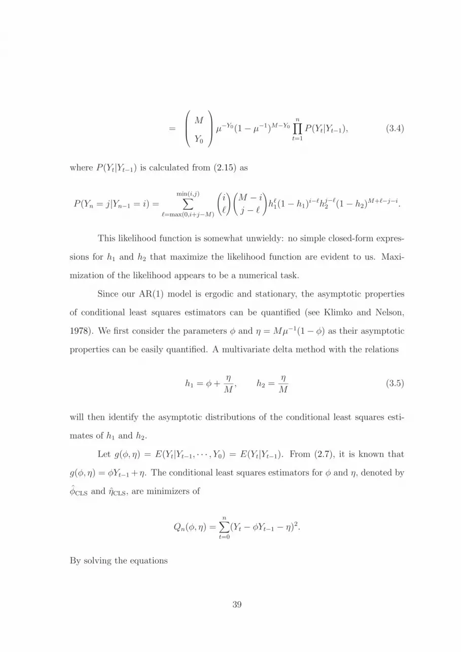
Example 1. a) Suppose we want to generate a stationary AR(1) count series

with binomial marginals that has the autocorrelation function ρ(h) = φh for h ≥ 0.

As in the proof of Theorem 6, pick any integer M ≥ 1. The two hazard rates

of L, h1 and h2, can be chosen as any numbers in (0, 1) that satisfy h1 − h2 = φ.

The renewal series generated by (2.3) with L having hazard rates h1 and hk = h2 for

k ≥ 2 has the given autocorrelation function.

b) Suppose we want to generate a stationary AR(1) count series with Poisson

42

Binomial renewal series with φ = 0.8

Time of Observation

Coun

t

0 100 200 300 400 500

24

68

10Binomial renewal series with φ = −0.6

Time of Observation

Coun

t

0 100 200 300 400 500

02

46

810

0 10 20 30 40 50

−1.0

−0.5

0.00.5

1.0

Lag

Samp

le AC

F

Sample Autocorrelations

0 10 20 30 40 50

−1.0

−0.5

0.00.5

1.0

Lag

Samp

le AC

F

Sample Autocorrelations

Figure 3.1: Top: A sample path of a stationary series with binomial marginals andρ(h) = φh for h ≥ 0, when a) φ = 0.8 and b) φ = −0.6. Bottom: Sample autocorre-lations of the series.

marginals and the autocovariance function γ(h) = σ2φh/(1−φ2) for h ≥ 0 and φ < 0.

By (3.16), it is possible to find a λ such that −φ(1−φ)−2 < λ−1(1−φ2)−1 < 1/4.

With such a λ, we then solve the second equation of (3.13) for µ−1. The parameters

in the lifetime distribution of L are now directly calculated from (3.12). The hazard

rates are h1 = φ − µ−1(φ − 1) and h2 = µ−1(1 − φ).

c) Suppose we want to generate a stationary AR(1) count series with binomial

marginals that has the autocovariance function γ(h) = (−4/5)h/(1−(4/5)2) for h ≥ 0.

This is an example that cannot be produced with our model class. To see this,

note that by (3.15) we would need to find and integer M ≥ 1 such that −φ(1−φ)−2 <

M−1(1 − φ2)−1 < 1/4 with φ = −4/5. However, no such M exists.

d) Suppose we want to generate a stationary AR(1) count series with binomial

marginals that has the autocovariance function γ(h) = (−1/5)h/(1−(1/5)2) for h ≥ 0.

This is an example with negative φ that we can handle. First, select M such

43

that −φ(1 − φ)−2 < M−1(1 − φ2)−1 < 1/4 with φ = −1/5. There are two choices:

M = 5 or M = 6. With M = 5, µ−11 = (12/5)(1+

√

1/6) and µ−12 = (12/5)(1−

√

1/6).

Direct calculation gives two possible distributions for L: f1 = 2/5 +√

6/10 and

fn = (3/10)(2/5−√

6/10)n−2 for n ≥ 2, or f1 = 2/5−√

6/10 and fn = (3/10)(2/5 +√

6/10)n−2 for n ≥ 2. Similar analyses hold with M = 6.

Example 2.

This example uses simulation to study the performance of the conditional least

squares estimators of h1 and h2. For each pair of h1 and h2 shown in Table 1, we

simulated binomial series of lengths n = 100, n = 500, and n = 1000 respectively.

Ten thousand simulations were performed in all cases. We have taken M = 10 in all

simulations. The variance of the white noise term in the AR(1) model is determined

by M , h1, and h2 (recall that h1 − h2 = φ). Each simulation run first generates a

sample series with the noted properties. Next, the estimates h1,CLS and h2,CLS are

computed. Reported are sample averages of the 10000 estimates h1,CLS and h2,CLS

and their sample standard deviation. Observe that the sample averages become closer

to their true values as n increases. Moreover, the sample standard deviations agree

with those listed in equation (3.6). In particular, when h1 = 0.9, h2 = 0.1 and

n = 1000, (3.6) gives [Var(h1,CLS)]12 ≈ 9.95 × 10−3, which is close to the sample

standard deviation of 1.015 × 10−2 listed in Table 1. Overall, the conditional least

squares estimates appear to work well.

3.4 Proofs

Proof of Theorem 5. Suppose that L has a constant hk over k ≥ 2. Letting

44

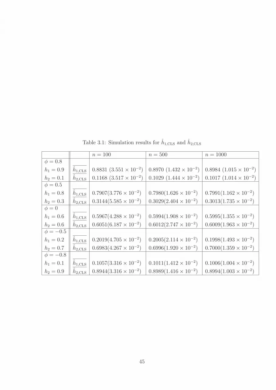
Table 3.1: Simulation results for h1,CLS and h2,CLS

n = 100 n = 500 n = 1000φ = 0.8

h1 = 0.9 h1,CLS 0.8831 (3.551 × 10−2) 0.8970 (1.432 × 10−2) 0.8984 (1.015 × 10−2)

h2 = 0.1 h2,CLS 0.1168 (3.517 × 10−2) 0.1029 (1.444 × 10−2) 0.1017 (1.014 × 10−2)φ = 0.5

h1 = 0.8 h1,CLS 0.7907(3.776 × 10−2) 0.7980(1.626 × 10−2) 0.7991(1.162 × 10−2)

h2 = 0.3 h2,CLS 0.3144(5.585 × 10−2) 0.3029(2.404 × 10−2) 0.3013(1.735 × 10−2)φ = 0

h1 = 0.6 h1,CLS 0.5967(4.288 × 10−2) 0.5994(1.908 × 10−2) 0.5995(1.355 × 10−2)

h2 = 0.6 h2,CLS 0.6051(6.187 × 10−2) 0.6012(2.747 × 10−2) 0.6009(1.963 × 10−2)φ = −0.5

h1 = 0.2 h1,CLS 0.2019(4.705 × 10−2) 0.2005(2.114 × 10−2) 0.1998(1.493 × 10−2)

h2 = 0.7 h2,CLS 0.6983(4.267 × 10−2) 0.6996(1.920 × 10−2) 0.7000(1.359 × 10−2)φ = −0.8

h1 = 0.1 h1,CLS 0.1057(3.316 × 10−2) 0.1011(1.412 × 10−2) 0.1006(1.004 × 10−2)

h2 = 0.9 h2,CLS 0.8944(3.316 × 10−2) 0.8989(1.416 × 10−2) 0.8994(1.003 × 10−2)

45

Wt = Yt − E(Yt|Yt−1 . . . , Y0), from (2.7) and §2.2 we know {Wt} is white noise and

Yt −M

µ= φ

(

Yt−1 −M

µ

)

+ Wt, (3.7)

with

φ =f1 − µ−1

1 − µ−1. (3.8)

Therefore, {Yt} satisfies an AR(1) difference equation.

By (3.3) and (3.8), φ = h1−h2. Since 0 < h1, h2 < 1, it is easy to see that −1 < φ < 1.

The variance of the white noise process {Wt} is seen to be

Var(Yt − φYt−1) = Cov(Yt , Yt) + φ2Cov(Yt−1, Yt−1) − 2φCov(Yt , Yt−1 )

= M1

µ(1 − 1

µ)(1 − φ2).

Now suppose that M is constant and that {Yt} satisfies the AR(1) difference

equation (3.1). Then {Yt} has the same autocovariance function as (3.2). Thus,

σ2φh

(1 − φ2)= Mµ−1(uh − µ−1), h ≥ 1,

σ2

(1 − φ2)= Mµ−1(1 − µ−1). (3.9)

Combining the two equations in (3.9) gives

uh = (1 − µ−1)φh + µ−1. (3.10)

Now take generating functions of both sides of (3.10) to get

U(s) = Σ∞n=0uns

n =µ − (µ + φ − 1)s

µ(1 − s)(1 − φs). (3.11)

46

The relationship between the generating function of the lifetime L — say F (s) =

E[SL] = Σ∞n=1fnsn — and U(s) is U (s) = (1−F (s))−1(Feller, 1968). Equation (3.11)

now gives

F (s) =1

1 −(

1 + φ−1µ

)

s

[(

φ − φ − 1

µ

)

s − φs2

]

.

Inverting this generating function, one gets, with r = 1 + µ−1(φ − 1),

f1 = φ − µ−1(φ − 1);

f2 = (1 − r)(r − φ);

fn = f2rn−2, ∀ n ≥ 2. (3.12)

Now suppose that M has a Poisson distribution and that {Yt} satisfies the AR(1)

difference equation (3.1). Then (3.9) holds with M replaced by λ:

σ2φh

(1 − φ2)= λµ−1(uh − µ−1), h ≥ 1,

σ2

(1 − φ2)= λµ−1(1 − µ−1). (3.13)

Arguing as above, it can be shown that L has a constant failure rate after lag 1. One

again obtains (3.12). This finished our work.

Proof of Theorem 6. Given the AR(1) autocorrelation function ρ(h) = τh for

h ≥ 0, −1 < τ < 1, pick any integer M ≥ 1 ( or λ > 0 for the Poisson marginals

) and any lifetime distribution L that has constant hazard rates after lag 1 with

τ = h1 − h2. Then as shown in the last proof, the series {Yt} generated from (2.3)

satisfies an AR(1) difference equation with φ = τ . Thus, {Yt} has the autocorrelation

function ρ(h) = τh for h ≥ 0.

47

Proof of Theorem 7. Arguing as in the proof of Theorem 5, if a renewal AR(1)

series has the autocovariance function γ(h) = σ2φh/(1−φ2) at lag h then (3.9) holds

for the case of binomial marginals and (3.13) holds for the case of Poisson marginals.

The distribution of L is given in (3.12). Hence, our work consists of identifying µ, and

showing that µ > 1 and the probabilities in (3.12) are legitimate lifetime probabilities.

This entails

µ > 1, if 0 < φ < 1 and

1 − φ < µ < 1 − φ−1, if − 1 < φ < 0. (3.14)

Using quadratic equations, it can be shown that any µ solving the second equation

in (3.9) or (3.13) will satisfy (3.14) if there exists an integer M such that

M−1σ2(1 − φ2)−1 ≤ 1/4, if 0 < φ < 1;

−φ(1 − φ)−2 < M−1σ2(1 − φ2)−1 ≤ 1/4, if − 1 < φ < 0 (3.15)

for the case of binomial marginals; or if there exists a real λ such that

λ−1σ2(1 − φ2)−1 ≤ 1/4, if 0 < φ < 1;

−φ(1 − φ)−2 < λ−1σ2(1 − φ2)−1 ≤ 1/4, if − 1 < φ < 0 (3.16)

for the case of Poisson marginals.

It is easy to show that −φ(1 − φ)−2 < 1/4 since −1 < φ < 1. So for the

Poisson case, a λ > 0 can be found that satisfies (3.16). Hence, one can always find

a renewal AR(1) series with Poisson marginals that has the autocovariance function

γ(h) = σ2φh/(1 − φ2) for any σ2 > 0 and φ ∈ (−1, 1). This proves part a).

48

For part b), if the AR(1) model has φ > 0, then an M satisfying (3.15) always

exists (take M as large as necessary in the first equation of (3.15)). When φ < 0,

a proper integer as required by (3.15) is not always available. For example, when

σ2(1 − φ2)−1 < −φ(1 − φ)−2, we cannot find an M ≥ 1 such that (3.15) is satisfied,

since M is at least one. That is, there is no renewal AR(1) series with binomial

marginals having the autocovariance function γ(h) = σ2φh/(1 − φ2).

Remark: For each feasible value of M or λ, there are two feasible roots in

step 2. The lifetime corresponding to these two roots are related: if one distribution

has f1, fn = f2rn−2 for n ≥ 2, then the other distribution has f1 = r, fn = f2f

n−21 for

n ≥ 2.

We now summarize how to generate a renewal process with the AR(1) auto-

covariance function γ(h) = σ2φh/(1 − φ2) for h ≥ 0.

1. For the binomial case, find an integer M ≥ 1 such that: if 0 < φ < 1, M−1σ2(1−

φ2)−1 ≤ 1/4; if −1 < φ < 0, −φ(1 − φ)−2 < M−1σ2(1 − φ2)−1 ≤ 1/4. For the

Poisson case, find a real λ > 0 such that: if 0 < φ < 1, λ−1σ2(1 − φ2)−1 ≤ 1/4;

if −1 < φ < 0, −φ(1 − φ)−2 < λ−1σ2(1 − φ2)−1 ≤ 1/4.

2. In the binomial case solve µ−1(1−µ−1) = M−1σ2(1−φ2)−1 for µ. In the Poisson

case, solve µ−1(1 − µ−1) = λ−1σ2(1 − φ2)−1 for µ.

3. The lifetime distribution parameters are then given by (3.12).

49

Bibliography

M. Al-Osh and A. Alzaid. First-order integer-valued autoregressive (INAR(1)) pro-cess. Journal of Time Series Analysis, 8:261–275, 1987.

M. Al-Osh and A. Alzaid. An integer-valued pth-order autoregressive (INAR(p))process. Journal of Applied Probability, 27:314–324, 1990.

M. Al-Osh and A. Alzaid. Some gamma processes based on the dirichlet-gammatransformation. Communications in Statistics - Stochastic Models, 9:123–143, 1993.

P. Albert. A Markov model for sequences of ordinal data from a relapsing-remittingdisease. Biometrics, 50:51–60, 1994.

M. Benjamin, R. Rigby, and D. Stasinopoulos. Generalized autoregressive movingaverage models. Journal of Applied Probability, 98:214–223, 2003.

K. Berenhaut and R. Lund. Geometric renewal convergence rates from hazard rates.Journal of Applied Probability, 38:180–194, 2001.

P. Blight. Time series formed from the superposition of discrete renewal processes.Journal of Applied Probability, 26:189–195, 1989.

U. Bockenholt. Autoregressive negative multinomial regression models. Journal of

the American Statistical Association, 94:757–765, 1999a.

U. Bockenholt. Mixed INAR(1) poisson regression models: analyzing heterogeneityand serial dependencies in longitudinal count data. Journal of Econometrics, 89:317–338, 1999b.

U. Bockenholt. Analysing state dependences in emotional experiences by dynamiccount data models. Journal of the Royal Statistical Society Series C, 52:213–226,2003.

K. Brannas. Estimation and testing in integer valued AR(1) models. Umea EconomicStudies, 355, 1994.

K. Brannas and J. Hellstrom. Generalized integer-valued autoregression. Econometric

Reviews, 20:425–443, 2001.

50

K. Brannas and P. Johansson. Time series count regression. Communication in

Statistics: Theory and Methods, 23:2907–2925, 1994.

K. Brannas and Q. Shahiduzzaman. Integer-valued moving average modelling of thenumber of transactions in stocks. Umea Economic Studies, 637, 2004.

P. Brockwell and R. Davis. Time Series: Theory and Methods, 2nd edition. Springer,New York, 1991.

P. Brockwell and R. Davis. Introduction to Time Series and Forecasting, 2nd edition.Springer, New York, 2002.

A. Cameron and L. Leon. Markov regression models for time series data. Presentedat Western Economic Association Meetings, Lake Tahoe, NV, 1993.

A. Cameron and P. Trivedi. Regression Analysis of Count Data. Cambridge UniversityPress, London, 1998.

M. Campbell. Time series regression for counts: an investigation into the relationshipbetween sudden infant death syndrome and environmental temperature. Journal

of the Royal Statistical Society Series A, 157:191–120, 1994.

J. Du and Y. Li. The integer valued autoregressive (INAR(p)) model. Journal of

Time Series Analysis, 12:129–142, 1991.

L. Fahrmeir and G. Tutz. Multivariate Statistical Modelling Based on Generalized

Linear Models. Springer-Verlag, New York, 1994.

W. Feller. An Introduction to Probability Theory and Its Applications, Volume I, 3rd

edition. Wiley, New York, 1968.

K. Fokianos and B. Kedem. Regression theory for categorical time series. Statistical

Science, 18:357–376, 2003.

J. Franke and T. Seligmann. Conditional maximum-likelihood estimates forINAR(1) processes and their applications to modelling epileptic seizure counts. InT. Edited by Rao, editor, Developments in Time Series, pages 310–330. Chapman& Hall, London, 1993.

R. Freeland and B. McCabe. Analysis of low count time series data by poissonautoregression. Journal of Time Series Analysis, 25:701–722, 2004.

G. Gauthier and A. Latour. Convergence forte des estimateurs des parametres d’unprocessus GENAR(p). Annales des Sciences Mathematiques du Quebec, 18:49–71,1994.

51

B. Hansen and J. Frenk. Some monotonicity properties of the delayed renewal func-tion. Journal of Applied Probability, 28:811–821, 1991.

A. Harvey. Forecasting, Structural Series Models and the Kalman Filter. CambridgeUniversity Press, Cambridge, 1989.

A. Harvey and C. Fernandes. Time series models for count or qualitative observations.Journal of Business and Economic Statistics, 7:407–417, 1989.

P. Holgate. Estimation for the bivariate poisson distribution. Biometrika, 51:241–245,1964.

P. Jacobs and P. Lewis. Discrete time series generated by mixtures I: correlationaland runs properties. Journal of the Royal Statistical Society Series B, 40:94–105,1978a.

P. Jacobs and P. Lewis. Discrete time series generated by mixtures II: asymptoticproperties. Journal of the Royal Statistical Society Series B, 40:222–228, 1978b.

P. Jacobs and P. Lewis. Stationary discrete autoregressive-moving average time seriesgenerated by mixtures. Journal of Time Series Analysis, 4:19–36, 1983.

P. Johansson. Speed limitation and motorway casualties: a time series count dataregression approach. Accident Analysis and Prevention, 28:73–87, 1996.

D. Kendall. Unitary dilations of Markov transition operators, and the correspondingintegral representations for transition-probability matrices. In U. Grenander, editor,Probability and Statistics, pages 139–161. John Wiley, New York, 1959.

L. Klimko and P. Nelson. On conditional least squares estimation for stochasticprocesses. Annals of Statistics, 6:629–642, 1978.

S. Kocherlakota and K. Kocherlakota. Bivariate Discrete Distributions. MarcelDekker, New York, 1992.

A. Latour. The multivariate GINAR(p) processes. Advances in Applied Probability,29:228–248, 1997.

A. Latour. Existence and stochastic structure of a non-negative integer-valued au-toregressive process. Journal of Time Series Analysis, 19:439–455, 1998.

A. Lawrance and P. Lewis. An exponential moving average sequence and point pro-cess, EMA(1). Journal of Applied Probability, 14:98–113, 1977a.

A. Lawrance and P. Lewis. The exponential autoregressive-moving averageEARMA(p, q) process. Journal of the Royal Statistical Society Series B, 42:150–161,1977b.

52

W. Li. Testing model adequacy for some Markov regression models for time series.Biometrika, 78:83–89, 1991.

W. Li. Time series models based on generalized linear models: some further results.Biometrics, 50:506–511, 1994.

T. Lindvall. Lectures on the Coupling Method. John Wiley & Sons, New York, 1992.

S. Loukas, C. Kemp, and H. Papageorgiou. Even point estimation for the bivariatepoisson distribution. Biometrika, 73:222–223, 1986.

I. MacDonald and W. Zucchini. Hidden Markov and Other Models for Discrete-Valued

Time Series. Chapman and Hall, London, 1997.

A. Marshall and I. Olkin. A family of bivariate distributions generated by the bivariatebernoulli distribution. Journal of the American Statistical Association, 80:332–338,1985.

E. McKenzie. Some simple models for discrete variate time series. Water Resources

Bulletin, 21:645–650, 1985.

E. McKenzie. Autoregressive-moving average processes with negative-binomial andgeometric marginal distributions. Advances in Applied Probability, 18:679–705,1986.

E. McKenzie. Some ARMA models for dependent sequences of poisson counts. Ad-

vances in Applied Probability, 20:822–835, 1988.

E. McKenzie. Discrete variate time series. In C. Rap. and D. Shanbhag, editors,Stochastic Processes: Modelling and Simulation, Handbook of Statistics, volume 21,pages 573–606. Elsevier Science B.V., North-Holland, Amsterdam, 2003.

J. Pitman. Uniform rate of convergence for Markov chain transition probabilities.Probability Theory and Related Fields, 29:193–227, 1974.

G. Ronning and R. Jung. Estimation of a first order autoregressive process withpoisson marginals for count data. In L. Fahrmeir, editor, Advances in GLIM and

Statistical Modelling. Springer-Verlag, New York, 1992.

S. Ross. Simulation, 4th edition. Academic Press, Boston, 2006.

N. Rudholm. Entry and the number of firms in the Swedish pharmaceuticals market.Review of Industrial Organization, 19:351–364, 2001.

M. Sørensen. Prediction-based estimating functions. Econometrics Journal, 3:123–137, 2000.

53

F. Steutel and K. V. Harn. Discrete analogues of self-decomposability and stability.Annals of Probability, 7:893–899, 1979.

C. Weiβ. A new class of autoregressive models for time series of binomial counts.Communications in Statistics, Theory and Methods, 38(447-460), 2009.

S. Zeger. A regression model for time series of counts. Biometrika, 75:621–629, 1988.

S. Zeger and B. Qaqish. Markov regression models for time series quasi-likelihoodapproach. Biometrics, 44:1019–1031, 1988.

54