Inner structure of La Fossa di Vulcano (Vulcano Island, southern

Tyrrhenian Sea, Italy) revealed by high-resolution electric resistivity

tomography coupled with self-potential, temperature, and CO2 diffuse

degassing measurements

A. Revil,1,2,3 A. Finizola,4,5 S. Piscitelli,6 E. Rizzo,6 T. Ricci,7 A. Crespy,8 B. Angeletti,8

M. Balasco,6 S. Barde Cabusson,9 L. Bennati,9,10 A. Boleve,3,11 S. Byrdina,9,12

N. Carzaniga,13 F. Di Gangi,4 J. Morin,5,14 A. Perrone,6 M. Rossi,12 E. Roulleau,15

and B. Suski16

Received 23 September 2007; revised 8 March 2008; accepted 2 April 2008; published 24 July 2008.

[1] La Fossa cone is an active stratovolcano located on Vulcano Island in the AeolianArchipelago (southern Italy). Its activity is characterized by explosive phreatic andphreatomagmatic eruptions producing wet and dry pyroclastic surges, pumice falldeposits, and highly viscous lava flows. Nine 2-D electrical resistivity tomograms (ERTs;electrode spacing 20 m, with a depth of investigation >200 m) were obtained to image theedifice. In addition, we also measured the self-potential, the CO2 flux from the soil, and thetemperature along these profiles at the same locations. These data provide complementaryinformation to interpret the ERT profiles. The ERT profiles allow us to identify the mainstructural boundaries (and their associated fluid circulations) defining the shallowarchitecture of the Fossa cone. The hydrothermal system is identified by very low values ofthe electrical resistivity (<20 W m). Its lateral extension is clearly limited by the craterboundaries, which are relatively resistive (>400Wm). Inside the crater it is possible to followthe plumbing system of the main fumarolic areas. On the flank of the edifice a thick layer oftuff is also marked by very low resistivity values (in the range 1–20 W m) because of itscomposition in clays and zeolites. The ashes and pyroclastic materials ejected during thenineteenth-century eruptions and partially covering the flank of the volcano correspond torelatively resistive materials (several hundreds to several thousands W m). We carried outlaboratory measurements of the electrical resistivity and the streaming potential couplingcoefficient of the main materials forming the volcanic edifice. A 2-D simulation of thegroundwater flow is performed over the edifice using a commercial finite element code. Inputparameters are the topography, the ERT cross section, and the value of the measuredstreaming current coupling coefficient. From this simulation we computed the self-potentialfield, and we found good agreement with the measured self-potential data by adjusting theboundary conditions for the flux of water. Inverse modeling shows that self-potential datacan be used to determine the pattern of groundwater flow and potentially to assess waterbudget at the scale of the volcanic edifice.

1Department of Geophysics, Colorado School of Mines, Golden,Colorado, USA.

2Universite Aix Marseille III, CNRS, Aix en Provence, France.3UMR5559, Equipe Volcan, University of Savoie, INSU, LGIT, CNRS,

Bourget du Lac, France.4Istituto Nazionale di Geofisica e Vulcanologia, Palermo, Italy.5Now at Laboratoire GeoSciences Reunion, UMR7154, UR, IPGP,

La Reunion, France.6Laboratory of Geophysics, IMAA, CNR, Tito Scalo, Italy.7INGV, Universita Roma Tre, Rome, Italy.8Universite Aix Marseille III, CNRS, Aix en Provence, France.

Copyright 2008 by the American Geophysical Union.0148-0227/08/2007JB005394$09.00

9Laboratoire Magma et Volcan, Universite Blaise Pascal, UMR6524,IRD, CNRS, Clermont-Ferrand, France.

10Now at Department of Earth and Atmospheric Sciences, PurdueUniversity, West Lafayette, Indiana, USA.

11Also at Savoie Technolac, Sobesol, Le Bourget du Lac, France.12IPGP, CNRS, Paris, France.13Department of Geology and Geosciences, Universita Milano-Bicocca,

Milan, Italy.14Pantheon-Sorbonne, Universite Paris 1, Paris, France.15GEOTOP-UQAM-McGill, Montreal, Quebec, Canada.16Institut de Geophysique, College Propedeutique, Universite de

Lausanne, Lausanne, Switzerland.

JOURNAL OF GEOPHYSICAL RESEARCH, VOL. 113, B07207, doi:10.1029/2007JB005394, 2008ClickHere

for

FullArticle

B07207 1 of 21

Citation: Revil, A., et al. (2008), Inner structure of La Fossa di Vulcano (Vulcano Island, southern Tyrrhenian Sea, Italy) revealed

by high-resolution electric resistivity tomography coupled with self-potential, temperature, and CO2 diffuse degassing measurements,

J. Geophys. Res., 113, B07207, doi:10.1029/2007JB005394.

1. Introduction

[2] Vulcano is a small volcanic island (3 � 7 km) locatedat the southernmost of the Aeolian Islands in the southernTyrrhenian Sea in Italy (38�240N, 14�580E). This island wasshaped during five main volcanic stages during the past120,000 years. The two overlapping calderas of the island,the 2.5-km-wide Caldera del Piano on the southeast and the3-km-wide Caldera della Fossa northwest of the island(Figure 1), were formed at about 98,000–77,000 and24,000–13,000 years ago, respectively. Volcanism hasmigrated to the north of the island over time. La Fossacone, which is the target of the present investigation,occupies the 3-km-wide Caldera della Fossa at the north-west end of the island. This edifice has been activethroughout the Holocene and constitutes the location ofmost of the historical eruptions of Vulcano island. In thevicinity of the Fossa cone, the Vulcanello edifice forms alow, roughly circular peninsula, on the northern tip ofVulcano (Figure 1). This area was formed as an islandbeginning in 183 BC and was connected to the Vulcanoisland in 1550 AD during its last eruption. The latesteruption from Vulcano consisted of explosive activity fromthe Fossa cone from 1888 to 1890 [e.g., Frazzetta et al.,1983, 1984].[3] There are two main reasons why we choose to

investigate La Fossa cone. The first reason is related tothe geohazards associated with the activity of the active LaFossa cone. The population of the island increases to nearly5,000 inhabitants during the summer from a few hundredsduring the winter. The main geohazards at Vulcano arerelated to sin-eruptive pyroclastic surges, bombs and blockfallout, phreatic explosions, gas hazard, debris flows, andlandslides of altered flanks and the subsequent formation oftsunamis. The second reason is related to the relativelymodest dimensions of this edifice and its strong hydrother-mal activity. The Fossa cone is therefore a perfect naturallaboratory to test the ability of geophysical methods toimage the substructure of an active volcano. In addition, weare interested to see how geophysical signals can be used tomonitor changes in its activity.[4] The use of deep DC electrical resistivity tomography

has recently gained in interest to map the substructure ofvolcanoes and active faults [e.g., Storz et al., 2000; Colellaet al., 2004; Diaferia et al., 2006; Finizola et al., 2006;Linde and Revil, 2007a]. However, electrical resistivitytomography alone is notoriously difficult to interpret un-equivocally. The main reason is that electrical resistivity ofvolcanic rocks depends on too much parameters includingthe water content, salinity, temperature, and cation exchangecapacity of the porous material [e.g., Waxman and Smits,1968; Revil et al., 2002, and references therein]. Therefore,it is essential to add additional information to electricalresistivity tomograms to improve their interpretation interms of geological and hydrogeological units [see Revilet al., 2004b; Finizola et al., 2006; Coppo et al., 2008].

[5] Self-potential signals correspond to the passive mea-surement of the distribution of the electrical potential at theground surface of Earth. Once filtered, these signalsevidenced polarization mechanisms at depth. One of themis related to groundwater flow and is known as the stream-ing potential. Gex [1992] and Di Fiore et al. [2004] haveperformed self-potential measurements at the island ofVulcano. However, while these works were very useful,only specific parts of the volcano were covered by theseinvestigations and self-potential signals were not interpretedquantitatively in terms of groundwater flow pattern.[6] In this paper, we interpret a set of new high-resolution

electrical resistivity tomograms crossing the Fossa cone ofVulcano Island. By high resolution, we mean that thespacing between the electrodes is only of 20 m. This allowsa resolution that is much higher than electromagneticmethods (e.g., TDEM) and classical large-scale resistivitysurveys without the use of a long cable (>1 km). To help theinterpretation of these tomograms, additional measurementsof temperature, self-potential, and CO2 flux from the soilwere carried out along the resistivity profiles at the samelocations than the electrodes used for the resistivity surveys.The temperature and CO2 flux reveal the position of thepermeable flow pathways of the hydrothermal system. Weshow that forward and inverse modeling of the self-potentialdata allow constraining the pattern of groundwater flow. Allthese measurements result in a unique data set, at akilometer scale, over an active volcano. This data set revealsfor the first time the inner substructure of La Fossa conestratovolcano, showing the main geological structure andthe extent of the hydrothermal system inside the edifice.

2. Geological Background

[7] Vulcano Island represents the southernmost portion ofa NW-SE elongated volcanic ridge that comprises sevenislands forming the Aeolian Archipelago (southern Italy).This archipelago is related to the subduction of the Africanplate underneath the European Plate [Keller, 1980; Ellam etal., 1989]. The ridge is affected by a regional, NW-SE to N-S striking fault system [Gasparini et al., 1982]. In ancienttimes, the Romans believed that Vulcano was the chimneyto the forge of the god Vulcan. The glow of eruptions wasthought to be from his forges and the island had grownbecause of his periodic clearing of cinders and ashes. Theearthquakes that either preceded or accompanied the explo-sions of ashes were considered to be due to Vulcan himselfmaking weapons for the other gods.[8] Nowadays, we know that the island has been shaped

during five distinct stages. These stages are Vulcano Pri-mordiale, Piano Caldera, Lentia Complex, La Fossa Calde-ra, and Vulcanello. The history of Vulcano begins with theformation of a stratovolcano. The collapse of this stratovol-cano produces the Piano caldera (see CP in Figure 1 andSantacroce et al. [2003]). Then, this caldera was partiallyfilled with pyroclastic deposits and lava flows. The strato-volcano and its caldera form the southern part of the island

B07207 REVIL ET AL.: STRUCTURE OF LA FOSSA DI VULCANO

2 of 21

B07207

of Vulcano. The Fossa cone grew within the Fossa caldera,which constitutes the northern part of the island (Figure 1).[9] The Fossa cone is a small stratovolcano with an

altitude of 391 m a.s.l. (meters above sea level; see Figures2 and 3). The diameter of its base is about 2 kilometers. TheFossa cone began to form 6,000 years ago [Dellino and LaVolpe, 1997; De Rosa et al., 2004]. Six volcanic succes-sions: Punte Nere, Palizzi, Caruggi, Forgia Vecchia, PietreCotte and Gran Cratere (post-1739), with different ventlocations and eruptive histories, shaped the edifice [Dellinoand La Volpe, 1997; De Rosa et al., 2004, De Astis et al.,2007]. Each succession follows the same evolution startingwith pyroclastic surges and ending with the emission ofhighly viscous lava flows. All the explosive and effusiveproducts of La Fossa cone have high potassium contentsand a chemical composition ranging from trachytic to themore evolved rhyolitic composition [Keller, 1980].[10] The last eruption of the Fossa cone occurred from

1888 to 1890. In the same century, Vulcano produced threeeruptions lasting more than one month (1822–1823, 1873,and 1886). The violence of the last eruption (1888–1890)was marked by the fall of volcanic bombs and blocks, about�1 m in diameter, at �1 km from the vent. Breadcrustbombs, distinctive of this style of eruption, were ejectedabout 500 m. These bombs are characterized by an aphyricglassy matrix of rhyolitic composition and xenoliths oftrachytic composition [De Fino et al., 1991]. Explosionswere intermittent and separated by quiet periods lasting afew minutes to a few days. Explosions varied in strength.Only the largest explosions, separated by longer quietperiods, could throw blocks and bombs. No domes or lavaflows were produced at the end of this eruption.[11] Nowadays, the peculiarity of La Fossa volcano is the

occurrence of thermal and seismic crisis. The last oneoccurred in 2004–2006 [Granieri et al., 2006; Aubert etal., 2008] and was characterized by strong increases of thetemperature of the fumaroles and an increase of the surfacearea covered by the fumarolic field (see below). Chemical

changes in the fumaroles and the occurrence of shallowseismic activity were indicative of an increase of the inputof magmatic fluids [Granieri et al., 2006]. However, duringsuch episodes, there was no evidence of magmatic rising.[12] There are three types of upper formations of the

Fossa cone: (1) The former is constituted of the Palizzipumice deposit, mainly scattered along the southern slopeof La Fossa cone and with a maximum thickness of 2 m atthe break in slope of the volcano [Frazzetta et al., 1983].The pumice fragments range in size from several centi-meters to about 30 cm, with a mean value of about10 cm. The glass matrix of the fragments has a trachyticcomposition. (2) The latter constituting the substratum isformed by a very impermeable fine-grained hydromag-matic tuff (Figure 2) and (3) the grey ashes from GranCratere that were deposited all over the edifice during the1888–1890 eruption.

3. Field Investigations

[13] In October 2005, May 2006, and October 2006, weperformed three geophysical surveys (electrical resistivity,self-potential, temperature, and soil CO2 flux) that wereorganized along nine profiles crossing the entire Fossa cone.The position of these profiles is shown on Figure 2. Notethat because we know nothing about the temporal variationof these, we did not try to provide a 3-D reconstruction ofthese data in the present work. We present in this section themethodology employed for the various measurements

3.1. Electrical Resistivity Profiles

[14] Because of their sensitivity to porosity, water satu-ration, and the presence of clays and zeolites minerals, DC-electrical resistivity and electromagnetic methods (e.g., timedomain electromagnetics) are efficient tools to image activevolcanoes [Fitterman et al., 1988; Zohdy and Bisdorf, 1990;Lenat et al., 2000]. DC-electrical resistivity measurementswere obtained along the nine profiles displayed in Figure 2.

Figure 1. Map of the Island of Vulcano (Italy). Abbreviations are as follows: PN, Punte Nere; Pa,Palizzi; FV, Forgia Vecchia; PC, Pietre Cotte; GC, Gran Cratere; V, Vulcanello, CF, Caldera della Fossa;and CP, Caldera del Piano.

B07207 REVIL ET AL.: STRUCTURE OF LA FOSSA DI VULCANO

3 of 21

B07207

The measurements were performed using a set of 64 brasselectrodes with a spacing of 20 m. We use a shielded cableof 1.26 km made of 8 segments of 160 m each. Two or threeroll-alongs of the electrodes were performed to completeeach profile. Contact between the electrodes and the groundwas improved by adding salty water at the base of eachelectrode to decrease the contact resistance between theground and the electrodes. We used the Wenner array for its

good signal-to-noise ratio. Reciprocity measurements (per-formed on one profile) show an uncertainty smaller than7%. Dipole-dipole measurements provide complementaryinformation with respect to the Wenner array. However,we did not perform such measurements because of timeconstraints.[15] The resistivity data were inverted with RES2DINV

[Loke and Barker, 1996], which uses the smoothness-

Figure 2. Position of the investigated area on the Fossa cone. Nine profiles (labeled from 1 to 9) havebeen performed crossing the Fossa edifice. The bright areas on the flanks of the volcano correspond to thehydromagmatic tuff discussed in the main text.

Figure 3. The Fossa cone observed from the south.

B07207 REVIL ET AL.: STRUCTURE OF LA FOSSA DI VULCANO

4 of 21

B07207

constrained method [Constable et al., 1987] to perform theinverse problem:

JTJþ aF� �

d ¼ JTg� aFr; ð1Þ

where F is a smoothing matrix, J is the Jacobian matrix ofpartial derivatives, r is a vector containing the logarithm ofthe model resistivity values, a is the damping factor, d is themodel perturbation vector, and g is the discrepancy vector.The discrepancy vector, g, contains the difference betweenthe calculated and measured apparent resistivity values. Themagnitude of this vector is given by a RMS (root-meansquared) value. The algorithm seeks to reduce this quantityin an attempt to find a better model after each iteration. Themodel perturbation vector, d, is the change in the modelresistivity values calculated using the above equation whichnormally results in an ‘‘improved’’ model. The uniquenessof the solution of the inverse problem is an issue here [see,e.g., Linde and Revil, 2007a]. This means that for the samedata set, there are several possible resistivity models that fitthe data equally well [e.g., Auken and Christiansen, 2004;

Binley and Kemna, 2005]. Additional information can behelpful to stabilize the inversion process. Starting from aninitial model, RES2DINV looks for an improved modelwith calculated apparent resistivity values closer to themeasured values. We used various initial models to test thestability of the inversion process. Starting the iterations witheither a uniform resistivity model or the apparent resistivitypseudosection did not alter the final result.[16] Topography was also included in the inversion

process. Topography was extracted from a very precisedigital elevation map (DEM of 1 � 1 m) of La Fossa coneprovided by Maria Marsella (see also Baldi et al. [2002]).North and east UTM coordinates were obtained from aportable GPS receiver. Four electrical resistivity tomogramsare displayed in Figures 4–7. Accounting for the complexgeometry of the volcano, a 3-D inversion of ERT would benecessary to define the complex structural heterogeneities ofthe Fossa edifice. However, we show below that 2-Dinversion of ERT provides an image that is consistent with

Figure 4. Temperature, self-potential, soil CO2 flux, andelectrical resistivity tomogram along profile 1. These datashow that the main activity is constrained inside the crater,which is characterized by self-potential, CO2, and tempera-ture anomalies. Note that the ground surface of the centralpart of the crater is cold.

Figure 5. Temperature, self-potential, soil CO2 flux, andelectrical resistivity tomogram along profile 3. Note that thebottom part of the crater is cold. On the northern flank of theedifice (the left side of the figure), a conductive area islaterally limited by two thermal anomalies. These anomaliesrepresent the boundary of the Forgia Vecchia crater whichlast eruption occurred in 1727.

B07207 REVIL ET AL.: STRUCTURE OF LA FOSSA DI VULCANO

5 of 21

B07207

the other data (self-potential, temperature, and CO2 flux) inorder to define the architecture of the volcano.

3.2. Temperature

[17] Thermal probes and a digital thermometer were usedto measure the temperature of the ground. Each temperaturemeasurement was done in four steps. First, we hammered asteel rod (2 cm in diameter) into the ground to a depth of30 ± 2 cm. Second, a thermal probe was inserted into thehole at the precise depth of 30 ± 1 cm by means of agraduated wooden stick. Third, the hole around the stickwas filled and compacted. Fourth, after 10 to 15 min (thisduration is required to achieve thermal equilibrium), atemperature reading is performed [see Finizola et al.,2002, 2003]. The duration to reach thermal equilibriumwas checked by looking at the time variation of thetemperature. We observed that the temperature stabilizedin less than 10 min.[18] The temperature profile provides an independent

way to see the extension of the hydrothermal body in thevicinity of the ground surface. The temperature was mea-sured with a sensitivity of 0.2�C. Owing to the maximumamplitude of diurnal variation at Vulcano at 30 cm depth

during the summer season (1.2�C), and owing to themaximum amplitude of seasonal variation, from 12.2 to27.2�C respectively in January and August [Lo Cascio andNavarra, 1997], a temperature above 30�C can be consid-ered as indicative of the underground geothermal system. Amap of the interpolated temperature is shown on Figure 8.[19] It is important to note that our CO2 flux, self-

potential, and temperature measurements were obtained atdifferent periods during the last 2004–2006 crisis, whichbegan in November 2004 [Granieri et al., 2006]. However,the amplitude the anomalies are not of primary importancebecause we will only use temperature anomalies as a way todetect qualitatively preferential fluid flow pathways in thehydrothermal system.

3.3. CO2 Diffuse Degassing

[20] The CO2 diffuse degassing measurements wereobtained with a spacing of 20 m (uncertainty <5%). Themethodology is described in details in the work of Chiodiniet al. [1996, 1998]. The accumulation chamber methodallows to measure quickly the CO2 fluxes from the soil ina wide interval from 0.2 to several hundreds g m�2 day�1.This method does not require corrections or assumptions onthe characteristics of the soil. The instrumentation consistsin an IR spectrometer, to measure CO2 fluxes from 0 to

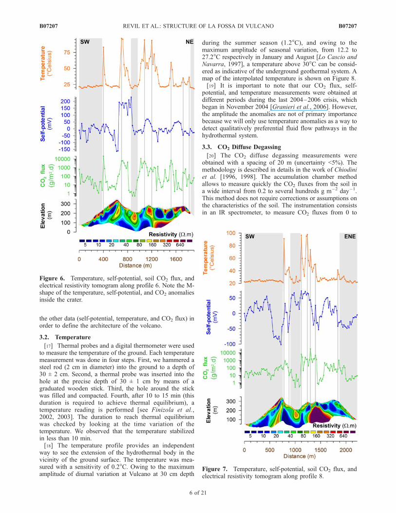
Figure 6. Temperature, self-potential, soil CO2 flux, andelectrical resistivity tomogram along profile 6. Note the M-shape of the temperature, self-potential, and CO2 anomaliesinside the crater.

Figure 7. Temperature, self-potential, soil CO2 flux, andelectrical resistivity tomogram along profile 8.

B07207 REVIL ET AL.: STRUCTURE OF LA FOSSA DI VULCANO

6 of 21

B07207

2000 mmol/mol (2% vol.), an accumulation chamber (typeA: dead volume 30 cm3), and a PDA to plot the CO2

concentration increase. The accumulation chamber is stoodon the ground so that the atmospheric air cannot penetrateinside. The gas permeating from the soil accumulates in thedead volume, thus the CO2 concentration increases; everysecond the gas is analyzed by the IR spectrometer andre-injected in the accumulation chamber so as not to depletethe CO2 concentration. The PDA software displays a curverepresenting the variation of the concentration of CO2 versustime. This rate is directly proportional to the flux of CO2

from the soil, expressed in g m�2 day�1 (the constant ofproportionality depends on the instrument dead volume andon the atmospheric pressure).[21] Carbon dioxide anomalies have their origin in mag-

ma degassing inside the volcanic system. The gas followsthe same preferential pathways as the hydrothermal fluids,providing information about the permeability distribution of

the edifice; high fluxes suggest permeable pathways fromthe hydrothermal system to the ground surface owing to thepresence of fractures.[22] A recent study by Granieri et al. [2006] shows that

in quiet periods, La Fossa crater area releases diffusivelyabout 200 ton day-1 of CO2 from a surface of 0.5 km2 whileduring crises the CO2 output may increase of one order ofmagnitude. These data suggest that a significant volume ofdegassing magma exists at depth and that during crises theincreasing of CO2 diffuse degassing is due to the opening ofnew fractures at shallow levels and the consequent increas-ing of the permeability of the soil. This could be due to theshallow seismicity or to a generalized increase of the porepressure in the volcanic system.

3.4. Self-Potential

[23] The self-potential (SP) method measures the distri-bution of the electric potential at the surface of Earth (and or

Figure 8. Map of the temperature at a depth of 30 cm superimposed on the DEM of La Fossa cone. Thewhite dots correspond to the location of the temperature measurements of the present study. The dotsinside the La Fossa crater correspond to the detailed temperature survey (at the same depth of 30 cm)reported by Aubert et al. [2008]. Note that the bottom of the crater is cold (<30�C). Thermal anomaliesare sometimes observed on the flanks of the volcano. In this case these anomalies are indicative of theboundaries of ancient craters.

B07207 REVIL ET AL.: STRUCTURE OF LA FOSSA DI VULCANO

7 of 21

B07207

in boreholes) with respect to a reference electrode [e.g.,Corwin and Hoover, 1979; Lenat, 2007]. Sources of self-potential fields include large-scale Earth currents due toionospheric activity, chemical potential gradients [Maineultet al., 2005, 2006], redox potentials [Linde and Revil,2007a], and electrokinetic conversion associated with fluidmovement through porous materials (the so-called stream-ing potential). In active volcanoes, the main source of self-potential anomalies is related to the flow of the groundwater[Massenet and Pham, 1985; Ishido et al., 1997; Bedrosianet al., 2007]. Self-potential is the only method that isdirectly sensitive to the pattern of groundwater flow andto changes in the seepage velocity [see Perrier et al., 1998;Kulessa et al., 2003a, 2003b; Rizzo et al., 2004; Suski et al.,2004, 2006; Hase et al., 2005; Titov et al., 2005; Jardani etal., 2006b, 2007; Wishart et al., 2006].[24] To perform the self-potential measurements, we used

a pair of nonpolarizing Cu/CuSO4 electrodes. The micro-porous nature of the end-contacts of these electrodes (madeof a low-permeability wood) avoids leakage of the CuSO4

solution during contact between with the ground. Wood isalso much more durable than the ceramics that is morecommonly used to make commercial electrodes. The dif-ference of electrical potential between the reference elec-trode (arbitrarily placed at the beginning of the profile)and the moving electrode was measured with a calibratedhigh impedance voltmeter (METRIX MX20, sensitivity of0.1 mV, input impedance of �100 MW). When interpret-ing self-potential data, we have to consider that the valueof the self-potential itself is meaningless. Only the gra-dient of the self-potential data (that is the electrical field)has a physical meaning.[25] Before and after each series of measurements, the

reference electrode and the roving electrode were put face-to-face to check that the difference of potential between thetwo electrodes was less than 2 mV (if this is not the case, thestatic value is removed to all the measurements). At eachstation, a small hole (�10 cm deep) was dug to improve theelectrical contact between the electrode and the ground. Foreach self-potential measurement, the value of the electricalresistance was also measured prior the self-potential mea-surement. Most of the time, the moisture in the soil wassufficiently high to insure low enough impedance contactbetween the scanning electrode and the ground. However, ifthe contact resistance was high (>1 MW), a small amount ofa saturated CuSO4 solution was placed at the bottom of thehole to decrease the contact resistance between the electrodeand the ground. We did not observe the type of driftreported by Corwin and Hoover [1979] associated withwatering the electrodes. The standard deviation on themeasurements is determined by performing twenty meas-urements few meters around the same station. At Vulcano, itis on the order of 12 mV in average. This relatively largestandard deviation is mainly due to the strong heterogeneityof the resistivity distribution near the surface of the ground.In the following, we will consider that the self-potentialmeasurement is a random process described by a Gaussiandistribution (as shown by Linde et al. [2007]) with astandard deviation of 12 mV.[26] To perform the self-potential measurements, a long

wire was used to connect the two electrodes to a MetrixMX20 voltmeter. The distance between two successive

measurement stations was 20 m. The total length of thewire was 400 m, and consequently, 20 measurements wererealized with the same reference. The advantage of thisprocedure was to avoid cumulative errors by changing thereference too often along the same profile. Every 400 m, anew reference station was established. As the profiles wereseveral kilometers long, several base stations were used tocover a profile. After the survey, the entire self-potentialprofile was reconstructed using the first reference station asthe unique reference for the entire profile.

4. Laboratory Measurements

[27] In this section, we report laboratory measurements ofthe electrical conductivity and streaming potential of acollection of 21 core samples from the edifices of La Fossadi Vulcano and Stromboli (a nearby volcano that is stronglyactive). Electrical conductivity measurements were per-formed on each sample in the frequency range from 20 Hzto 100 kHz, at room temperature (20 ± 2�C), using NaClsolutions with the following pore fluid conductivities sf =0.1 S m�1 and 0.5 S m�1(pH 7). The conductivity of thepore water sampled at the base of the volcano, in differentwells, is in the range 0.1 to 2.8 S m�1 and the pH is in therange 5.4 to 7.9 with a mean equal to 6.7 [Cortecci et al.,2001]. We believe that a water conductivity of 0.1 S m�1 isrepresentative of fresh (meteoric) waters while high con-ductivities are indicative of a mixture of fresh water andseawater and possibly hydrothermal fluids. The waterflowing along the slopes is locally affected by fumarolicfields is also enriched with the fumarolic acid condensatescoming from the pericrateric high-temperature fumarolesalong the fluid flow pathways highlighted by the resistivitytomograms and temperature anomalies.[28] We use a Waynekerr-6425 impedance meter for the

resistivity measurements. The samples were placed betweentwo stainless steel electrodes. Two circular pieces of brine-saturated filter paper were used to ensure good electricalcontacts between the sample and the electrodes. The jack-eted samples were first washed with demineralized waterand dried at 60�C for 2 days. The jacket was made of ahydrophobic adhesive. The samples were held under vacu-um prior to be saturated with a degassed brine at 0.1 S m�1

(see Revil et al. [2002] for a detailed version of theprocedure). Following the initial measurements, the salinityof the brine was then changed by placing the samples in a0.5 S m�1 electrolyte and by letting the brine diffuses to thesample through the two end-faces for 1 week (see Revil[1995] for tests of the effectiveness of this procedure). Theresults are reported in Table 1.[29] Electrical conductivity is sensitive to the water con-

tent, the mineralization of the pore water (salinity), thecation exchange capacity of the clay minerals (surfaceconductivity), and temperature [see Waxman and Smits,1968; Revil et al., 1998, 2002; Kalscheuer et al., 2007;Niwas et al., 2007; Jin et al., 2007; Tabbagh and Cosenza,2007; Shevnin et al., 2007]. In this paper, we assume asimple linear conductivity model,

s ¼ 1

Fsf þ ðF � 1Þss

� �; ð2Þ

B07207 REVIL ET AL.: STRUCTURE OF LA FOSSA DI VULCANO

8 of 21

B07207

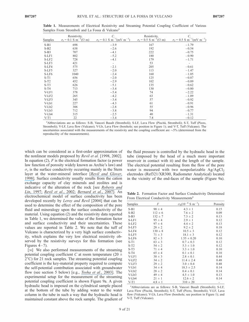
which can be considered as a first-order approximation ofthe nonlinear models proposed by Revil et al. [1998, 2002].In equation (2), F is the electrical formation factor (a powerlaw function of porosity widely known as Archie’s law) andss is the surface conductivity occurring mainly in the Sternlayer at the water-mineral interface [Revil and Glover,1998]. Surface conductivity usually results from the cationexchange capacity of clay minerals and zeolites and isindicative of the alteration of the rock [see Roberts andLin, 1997; Revil et al., 2002; Bernard et al., 2007]. Anelectrochemical model of surface conductivity has beendeveloped recently by Leroy and Revil [2004] that can beused to determine the effect of the composition of the porefluid and mineralogy upon the surface conductivity of thematerial. Using equation (2) and the resistivity data reportedin Table 1, we determined the value of the formation factorand surface conductivity and their uncertainties. Thesevalues are reported in Table 2. We note that the tuff ofVulcano is characterized by a very high surface conductiv-ity, which explains the very low electrical resistivity ob-served by the resistivity surveys for this formation (seeFigures 4–7).[30] We also performed measurements of the streaming

potential coupling coefficient C at room temperature (20 ±2�C) for 21 rock samples. The streaming potential couplingcoefficient is the key-material property required to computethe self-potential contribution associated with groundwaterflow (see section 5 below) [e.g., Tosha et al., 2003]. Theexperimental setup for the measurement of the streamingpotential coupling coefficient is shown Figure 9a. A givenhydraulic head is imposed on the cylindrical sample placedat the bottom of the tube by adding water to the watercolumn in the tube in such a way that the hydraulic head ismaintained constant above the rock sample. The gradient of

the fluid pressure is controlled by the hydraulic head in thetube (imposed by the head of a much more importantreservoir in contact with it) and the length of the sample.The electrical potential resulting from the flow of the porewater is measured with two nonpolarizable Ag/AgCl2electrodes (Ref321/XR300, Radiometer Analytical) locatedin the vicinity of the end-faces of the sample (Figure 9a).

Table 1. Measurements of Electrical Resistivity and Streaming Potential Coupling Coefficient of Various

Samples From Stromboli and La Fossa di Vulcanoa

SamplesResistivity,

sf = 0.1 S m�1(W m)C,

sf = 0.1 S m�1(mV m�1)Resistivity,

sf = 0.5 S m�1(W m)C,

sf = 0.5 S m�1(mV m�1)

S-B1 698 �3.9 167 �1.79S-B2 638 �2.6 192 �0.54S-B3 707 �4.1 222 �0.75S-LF1 802 �5.2 180 �0.90S-LF2 728 �4.1 179 �1.71S-LF3 421 - 53 -S-LF4 575 �2.1 205 �0.61S-LF5 327 �2.0 113 �1.47S-LF6 1040 �2.4 160 �1.05S-T1 656 �2.0 125 �0.87S-T2 452 �2.9 102 �0.89S-T3 626 �5.1 135 �0.62S-T4 713 �3.4 130 �0.80V-LF1 378 �5.4 74 �2.22V-LF2 265 �4.2 63 �1.09V-LF3 345 �3.4 57 �0.92V-Lb1 227 �4.3 61 �0.91V-Lb2 306 �2.8 55 �0.96V-Lb3 712 �3.8 94 �0.77V-Lb4 315 �2.5 40 �1.31V-T1 22 �3.4 7.8 �0.12aAbbreviations are as follows: S-B, Vancori Basalt (Stromboli); S-LF, Lava Flow (Piscita, Stromboli); S-T, Tuff (Pizzo,

Stromboli); V-LF, Lava flow (Vulcano); V-Lb, Lava Flow (borehole; see position in Figure 1); and V-T, Tuff (Vulcano). Theuncertainties associated with the measurements of the resistivity and the coupling coefficient are �5% (determined from thereproducility of the measurements).

Table 2. Formation Factor and Surface Conductivity Determined

From Electrical Conductivity Measurementsa

Samples F sS(10�4 S m�1) Porosity

S-B1 90 ± 4 4.3 ± 1 0.15S-B2 112 ± 6 7.6 ± 2 0.09S-B3 132 ± 7 7.3 ± 2 0.13S-LF1 95 ± 4 2.9 ± 1 0.12S-LF2 97 ± 4 4.4 ± 2 0.13S-LF3 28 ± 2 9.2 ± 2 0.18S-LF4 130 ± 8 10.5 ± 3 0.12S-LF5 71 ± 3 18.1 ± 3 0.12S-LF6 82 ± 3 1.55 ± 0.20 0.10S-T1 63 ± 3 0.7 ± 0.3 0.12S-T2 54 ± 2 5.3 ± 1.0 0.12S-T3 71 ± 4 3.3 ± 1.0 0.10S-T4 65 ± 4 0.1 ± 0.1 0.10V-LF1 38 ± 3 2.8 ± 0.1 0.44V-LF2 34 ± 2 11.4 ± 2.4 0.48V-LF3 29 ± 2 3.0 ± 0.4 0.48V-Lb1 34 ± 4 18.3 ± 2.5 0.14V-Lb2 28 ± 2 0.4 ± 0.1 0.14V-Lb3 49 ± 4 4.5 ± 1.0 0.13V-Lb4 21 ± 1 12.6 ± 2 0.14V-T1 4.8 ± 1 310 ± 20 -aAbbreviations are as follows: S-B, Vancori Basalt (Stromboli); S-LF,

Lava Flow (Piscita, Stromboli); S-T, Tuff (Pizzo, Stromboli); V-LF, Lavaflow (Vulcano); V-Lb, Lava Flow (borehole; see position in Figure 1); andV-T, Tuff (Vulcano).

B07207 REVIL ET AL.: STRUCTURE OF LA FOSSA DI VULCANO

9 of 21

B07207

The difference of the electrical potential measured betweenthe end-faces of the porous pack divided by the length of thesample is the streaming electrical field associated with theflow of the brine through the sample. The voltages aremeasured with a Metrix MX-20 voltmeter (internal imped-ance 100 MW, sensitivity 0.1 mV).[31] In the viscous-laminar flow regime (characterized by

low Reynolds numbers; see Boleve et al. [2007a]), thedifference of the electrical potential measured in the vicinityof the end-faces of the porous medium is proportional to theimposed hydraulic head H (Figures 10b and 10c) (this trendis nonlinear in the inertial-laminar flow regime). The slopeof the linear trend of streaming potential versus head is the

streaming potential coupling coefficient [e.g., Revil et al.,2004a; Boleve et al., 2007a, 2007b],

C ¼ @8

@H

� �j¼0

: ð3Þ

The values of the streaming potential coupling coefficientfor the different samples are reported in Table 1.[32] After completion of the electrical conductivity and

streaming potential measurements, we determined the po-rosity and matrix density from classical triple weightmeasurements. The samples were first washed with demin-eralized water for 1 week to let the salt diffusing out from

Figure 9. Examples of typical runs for five different volcanic rock samples. (a) Sketch of theexperimental setup used to measure the streaming potential coupling coefficient. The jacketed sample isplaced at the bottom of a Plexiglas tube. The record of the self-potentials during the flow of theelectrolyte through the sample is done with Ag/AgCl electrodes (‘‘Ref’’ is the reference electrode).The hydraulic heads are maintained constant at different levels with the help of the large reservoirand the valve. The electromotive force is recorded at these levels between the end-faces of the coresample with a high-impedance voltmeter. (b) Streaming potentials versus hydraulic heads using asolution at 0.1 S m�1 (this value is typical of the conductivity of the pore water flowing in theshallow aquifers of Vulcano). (c) Same with a solution at 0.5 S m�1. In both cases we observe linearrelationships. The streaming potential coupling coefficient is equal to the slope of these linear trends.The denomination of the samples is the same as in Tables 1 and 2.

B07207 REVIL ET AL.: STRUCTURE OF LA FOSSA DI VULCANO

10 of 21

B07207

the samples. Then the samples were dried at 60�C for 4 daysand their weights measured. Finally, the samples weresaturated with degassed water under vacuum and let standfor 2 additional days to allow complete saturation of theconnected porosity. Weight measurements of the saturatedsamples were carried out after that time. The saturatedsamples were weighted in air and water (buoyancy weight).Values of the porosity are reported in Table 2. A correlationbetween the formation factors and the connected porosities(not shown here) indicates that the formation factor is

related to the porosity by an Archie’s law F = f�m withm 2.0 ± 0.1.

5. Interpretation and Discussion

5.1. Uncertainty Associated With the Resistivity Data

[33] The analysis of the uncertainty associated with theinterpretation of the self-potential data in terms of ground-water flow will be discussed below in section 5.5. Wediscuss below the uncertainty associated with the resistivitydata, which show large RMS error (up to 25% at the fourthiteration). We performed a sensitivity analysis using profile

Figure 10. Sensitivity analysis of the resistivity data along profile 1. (a) We have used a simpleresistivity structure by trial and error that can reproduce the resistivity data. In the example shown herewe did not try to model the resistivity anomaly observed in the inversion of the data below the bottom ofthe crater (see Figure 11a). (b and c) The resistivity anomaly below of the bottom of the crater is notfound, even with 20% of white noise added to the data. Therefore it seems that this structure is not anartifact. The high RMS error found with this profile (25% at the fourth iteration) seems to be the result ofrandom noise existing in the data because of the low injected current.

B07207 REVIL ET AL.: STRUCTURE OF LA FOSSA DI VULCANO

11 of 21

B07207

1. We were especially interested by this profile to see if theresistive structure found at depth below the bottom part ofthe crater (see Figure 11a) was an artifact or not.[34] To perform the sensitivity analysis, we followed the

following steps (1) We used a simple resistivity distributionfor this profile (see Figure 10a); (2) we used the finiteelement code RESMOD to simulate the acquisition of thedata using the resistivity distribution and the known topog-raphy; (3) we contaminated these synthetic data withvarious levels of (white) noise; (4) we run RES2DINV onthese profiles to invert the synthetic apparent resistivitydata; and (5) we compare the inverted results with the inputresistivity data. The results are the following (see Figure10): (1) the resistive structure below the bottom of the crateris probably not an artifact because it cannot be reproducedwithout the presence of a resistive body at this location; (2)the deep resistive body on the flanks of the volcanoes have ahigher resistivity values than obtained from the resistivitytomograms (by using a trial and error approach, we obtaineda resistivity value of 4000 ± 1000 W m); (3) the high RMSerror is essentially due to the noise existing in the raw databecause of the relatively low current injected in the ground.However, adding white noise to the data does not change

the result of the inversion. It just changes the RMS value.Consequently, the inverse modeling is very robust to thepresence of such a noise.

5.2. Flanks

[35] Along the east-west direction (see profile 1 forexample), we observe a relatively simple architecture fromthe electrical resistivity tomogram. A resistive ash layer(100–1000 W m, 500 W m according to Figure 10) covers aconductive tuff layer (5 to 50 W m; see Figures 4 and 11). Atdepth, a highly and continuous resistive body is observed onboth sides of the volcano (Figures 4 and 11). We interpretthis body as corresponding to massive lava flow units withresistivity in the range 100 to 5000 W m (4000 W maccording to Figure 10). No thermal anomalies are observedat the ground surface along the flanks. The self-potentialsexhibit a classical W-shape [Ishido, 2004], which is tradi-tionally interpreted as the effect of the upwelling of hydro-thermal fluids in the central part of the edifice and thedownward flow of meteoritic groundwater along the flanksof the edifice [Michel and Zlotnicki, 1998; Revil et al.,2003]. This self-potential anomaly is quantitatively modeledin section 5.5.

Figure 11. (a) Architecture of the Fossa cone along the profile 1 (resistivity tomogram). Abbreviationsare as follows: Ah, ash; HS, hydrothermal system; C, conductive; and R, resistive. (b and d) Pictures ofthe Fossa cone from the west and east sides showing the position of the ashes relatively to the position ofthe hydromagmatic tuff (the line shows the position of the profile). (c) Picture taken inside the cratershowing the pyroclastic deposits.

B07207 REVIL ET AL.: STRUCTURE OF LA FOSSA DI VULCANO

12 of 21

B07207

[36] Profile 3 is nearly perpendicular to profile 1 (seeFigure 5). This profile shows a very complex pattern bycomparison with profile 1 and the existence of thermalanomalies. This complex pattern results from the evolutionof the volcano over time (see Figure 5). It crosses in thenorthern part of the profile, temperature anomalies related tothe crater boundaries of Forgia Vecchia. The first (and themost important) of the two Forgia Vecchia craters, ForgiaVecchia I, was formed during the 6th century B.C.[Giacomelli and Scandone, 2002]. The second crater, ForgiaVecchia II, was formed in 1727 A.D. [Frazzetta and LaVolpe, 1991], just before the extrusion of the Pietre Cotteobsidian lava flow that occurred in 1739 A.D. [De Fiore,1922].

5.3. Hydrothermal System

[37] Fumarolic activity indicates that the extension of thehydrothermal system is constrained by the boundary of themain crater, except for the area of Forgia Vecchia (seelocation Figure 1). The temperature map (Figure 8) showsthat the main structural morphological crater boundaries,identified by previous geological mapping, serve as prefer-ential fluid flow pathways for the upwelling of hot fluids.These structural boundaries are: (1) the southern crater rimof Caruggi cycles [De Astis et al., 2007] representing the ex-Commenda cycle; (2) the Fossa I crater rim located in theeastern part of the edifices; (3) different imbricated craterboundaries constituting the present-day cone of Vulcano

also called La Fossa cone or Gran Cratere (post-1739); and(4) a small temperature peak on Forgia Vecchia crater rim,in the northern part of the edifice. This shows that all thegeological crater boundaries, constituting the actual cone ofVulcano, act as preferential flowpaths for heated hydrother-mal fluids. The hydrothermal system is mainly containedinside the boundary of the craters including Forgia Vecchia.All the crater boundaries exhibit thermal anomalies(Figures 4–8). These boundaries are planes of mechanicalweakness along which cracks are periodically reopened bytectonic activity of the volcano during crises affecting LaFossa di Vulcano [see Granieri et al., 2006].[38] We have no idea about the nature of the resistive

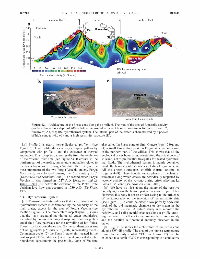
body lying below the bottom part of the crater (Figure 11a).However, this body if not an artifact owing to the influenceof the topography on the inversion of the resistivity data(see Figure 10). It could be either a low-porosity body (theneck of the old magmatic chamber) or dry steam in thehydrothermal system. A future study will monitor theresistivity and self-potential changes along a profile cross-ing the crater of La Fossa to see how stable is this anomalyand the positive self-potential anomaly observed in thecrater.[39] Figure 12 shows the architecture of the Fossa cone

along a SW-NE profile. The area of the highest-temperaturefumarolic activity (noted ‘‘F1’’ in Figure 12) can beextended to a depth of 200 m corresponding to a conductive

Figure 12. Architecture of the Fossa cone along the profile 6. The root of the area of fumarolic activitycan be extended to a depth of 200 m below the ground surface. Abbreviations are as follows: F1 and F2,fumaroles; Ah, ash; HS, hydrothermal system. The internal part of the crater is characterized by a pocketof high conductivity (C) and a high resistivity structure (R).

B07207 REVIL ET AL.: STRUCTURE OF LA FOSSA DI VULCANO

13 of 21

B07207

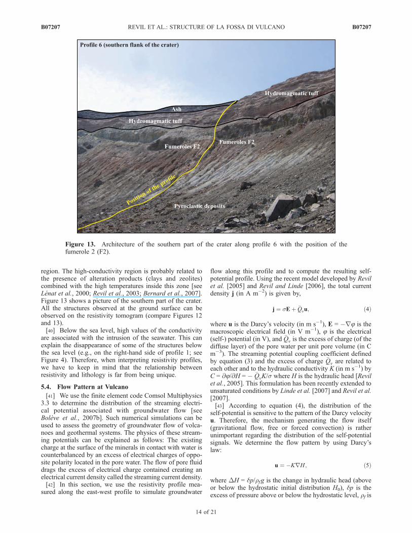
region. The high-conductivity region is probably related tothe presence of alteration products (clays and zeolites)combined with the high temperatures inside this zone [seeLenat et al., 2000; Revil et al., 2003; Bernard et al., 2007].Figure 13 shows a picture of the southern part of the crater.All the structures observed at the ground surface can beobserved on the resistivity tomogram (compare Figures 12and 13).[40] Below the sea level, high values of the conductivity

are associated with the intrusion of the seawater. This canexplain the disappearance of some of the structures belowthe sea level (e.g., on the right-hand side of profile 1; seeFigure 4). Therefore, when interpreting resistivity profiles,we have to keep in mind that the relationship betweenresistivity and lithology is far from being unique.

5.4. Flow Pattern at Vulcano

[41] We use the finite element code Comsol Multiphysics3.3 to determine the distribution of the streaming electri-cal potential associated with groundwater flow [seeBoleve et al., 2007b]. Such numerical simulations can beused to assess the geometry of groundwater flow of volca-noes and geothermal systems. The physics of these stream-ing potentials can be explained as follows: The existingcharge at the surface of the minerals in contact with water iscounterbalanced by an excess of electrical charges of oppo-site polarity located in the pore water. The flow of pore fluiddrags the excess of electrical charge contained creating anelectrical current density called the streaming current density.[42] In this section, we use the resistivity profile mea-

sured along the east-west profile to simulate groundwater

flow along this profile and to compute the resulting self-potential profile. Using the recent model developed by Revilet al. [2005] and Revil and Linde [2006], the total currentdensity j (in A m�2) is given by,

j ¼ sEþ �Qvu; ð4Þ

where u is the Darcy’s velocity (in m s�1), E = �r8 is themacroscopic electrical field (in V m�1), 8 is the electrical(self-) potential (in V), and �Qv is the excess of charge (of thediffuse layer) of the pore water per unit pore volume (in Cm�3). The streaming potential coupling coefficient definedby equation (3) and the excess of charge �Qv are related toeach other and to the hydraulic conductivity K (in m s�1) byC = @8/@H = � �QvK/s where H is the hydraulic head [Revilet al., 2005]. This formulation has been recently extended tounsaturated conditions by Linde et al. [2007] and Revil et al.[2007].[43] According to equation (4), the distribution of the

self-potential is sensitive to the pattern of the Darcy velocityu. Therefore, the mechanism generating the flow itself(gravitational flow, free or forced convection) is ratherunimportant regarding the distribution of the self-potentialsignals. We determine the flow pattern by using Darcy’slaw:

u ¼ �KrH ; ð5Þ

where DH = dp/rf g is the change in hydraulic head (aboveor below the hydrostatic initial distribution H0), dp is theexcess of pressure above or below the hydrostatic level, rf is

Figure 13. Architecture of the southern part of the crater along profile 6 with the position of thefumerole 2 (F2).

B07207 REVIL ET AL.: STRUCTURE OF LA FOSSA DI VULCANO

14 of 21

B07207

the pore fluid density (in kg m�3), and g is the accelerationof the gravity (in m s�2). The Darcy’s law is combined withthe continuity equation for the mass of the pore fluid togive:

S@H

@t¼ r � ðKrHÞ; ð6Þ

where t is time, s (in m�1) is the poroelastic storagecoefficient at saturation. The following computation isperformed for steady state conditions and therefore the flowis given by solving r(KrH) = 0. The flow can be imposedby using appropriate boundary conditions and conservationof pore water flux. Here, we impose the flux at theboundaries of the system.[44] The continuity equation, for the electrical charge is

r � j = 0. Combining this equation with equation (4) resultsin Poisson equation for the electrical potential with a sourceterm that depends only on the seepage velocity in theground:

r � ðsr8Þ ¼ =; ð7Þ

where = is the volumetric current source density (in A m�3)given by,

= ¼ �Qvr � uþr�Qv � u; ð8Þ

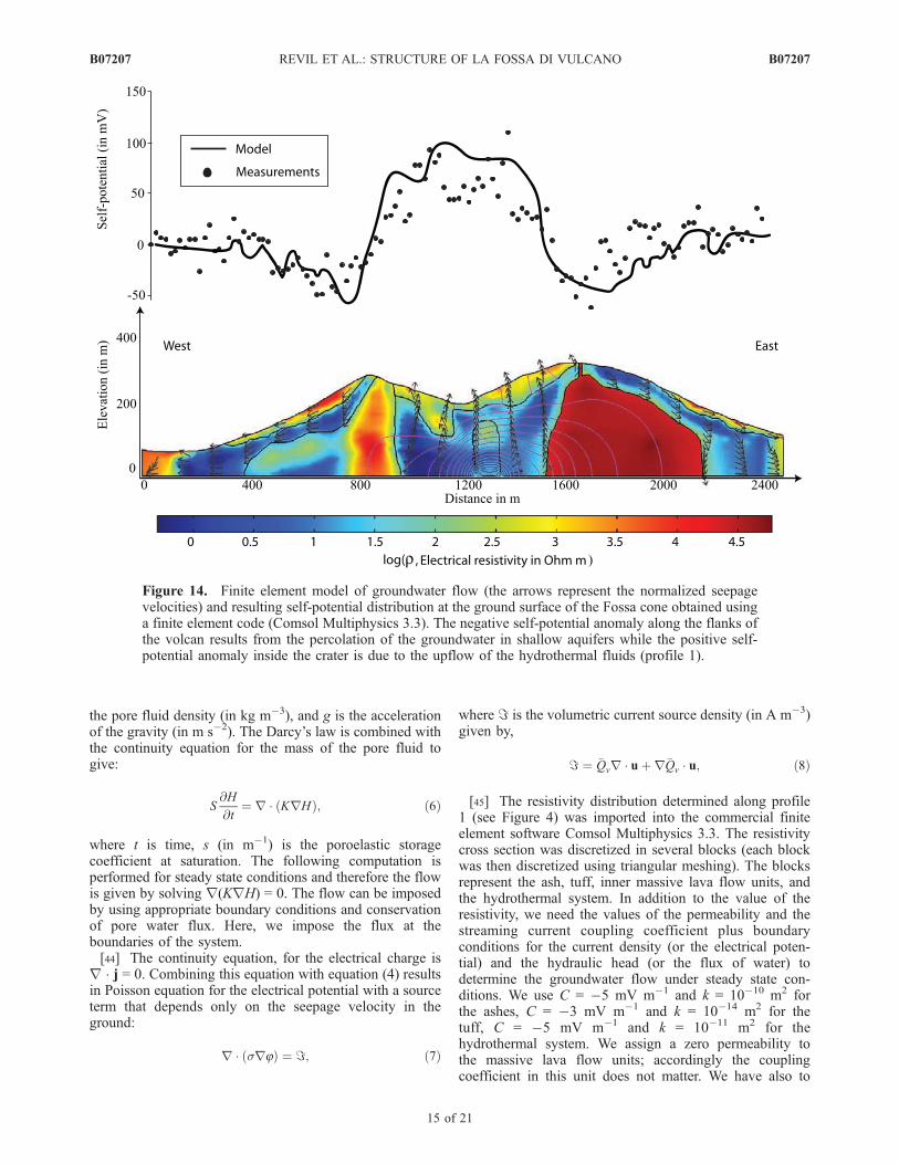
[45] The resistivity distribution determined along profile1 (see Figure 4) was imported into the commercial finiteelement software Comsol Multiphysics 3.3. The resistivitycross section was discretized in several blocks (each blockwas then discretized using triangular meshing). The blocksrepresent the ash, tuff, inner massive lava flow units, andthe hydrothermal system. In addition to the value of theresistivity, we need the values of the permeability and thestreaming current coupling coefficient plus boundaryconditions for the current density (or the electrical poten-tial) and the hydraulic head (or the flux of water) todetermine the groundwater flow under steady state con-ditions. We use C = �5 mV m�1 and k = 10�10 m2 forthe ashes, C = �3 mV m�1 and k = 10�14 m2 for thetuff, C = �5 mV m�1 and k = 10�11 m2 for thehydrothermal system. We assign a zero permeability tothe massive lava flow units; accordingly the couplingcoefficient in this unit does not matter. We have also to

Figure 14. Finite element model of groundwater flow (the arrows represent the normalized seepagevelocities) and resulting self-potential distribution at the ground surface of the Fossa cone obtained usinga finite element code (Comsol Multiphysics 3.3). The negative self-potential anomaly along the flanks ofthe volcan results from the percolation of the groundwater in shallow aquifers while the positive self-potential anomaly inside the crater is due to the upflow of the hydrothermal fluids (profile 1).

B07207 REVIL ET AL.: STRUCTURE OF LA FOSSA DI VULCANO

15 of 21

B07207

worry about the temperature dependence of the materialproperties because of the elevated field temperatures inthe volcanic edifice. However, the resistivity data aretaken directly from the ERT profiles so they include theeffect of the temperature. Revil et al. [2002] have shownthat the value of the streaming potential coupling coeffi-cient of volcaniclastic rocks is independent of the tem-perature so we do not have to worry about the directinfluence of the temperature upon the coupling coefficientused to perform the simulation in this study.[46] The simulated groundwater flow pattern is shown on

Figure 14. There is a downward flow inside the ashes andthe tuff materials along the flanks of the volcano while thereis an upward flow inside the boundary of the crater. Asshown from the CO2 data, there is no seal (very lowpermeability unit) inside the crater (except maybe at thebottom part of the crater). The upward flow of the hot porewater is responsible for pronounced evaporation of waterinside the crater boundaries. To check if this pattern ofgroundwater flow is compatible with the self-potential data,we determine the resulting self-potential distribution alongprofile 1. The simulated self-potential profile agrees quitewell with the measured self-potential profile (Figure 14). Inturn, this means that we could invert the measured self-potential data to determine the distribution of the Darcyvelocity of the water phase inside the edifice. This isperformed in the next section.

5.5. Inversion of Self-Potential Data

[47] The self-potential data are governed by a Poissonequation with a source term given by the divergence of thesource (streaming) current density. Inverting Poisson equa-tions is a well-established problem in the interpretation ofmagnetic and gravity data. Recently, various algorithmshave been proposed to invert self-potential data in termsof the divergence of the current density [Minsley et al.,2007], the three components of the current density itself[Jardani et al., 2007; Linde and Revil, 2007b], or theposition of the source [Jardani et al., 2006a].[48] In this paper, we follow the methodology proposed

recently by Jardani et al. [2007]. The relationship betweenthe electrical current density and the measured SP signalscan be written as,

8ðPÞ ¼ZW

KðP;MÞjsðMÞdV ; ð9Þ

where js is the source current density (in both saturated andunsaturated conditions) described in section 2 and K(P,M) isthe kernel connecting the SP data measured at a set ofnonpolarizing electrodes P (with respect to a referenceelectrode) and the source of current at point M in theconducting ground of support W. The components of thekernel correspond to the Green’s function of the problem.The kernel depends on the number of measurement stationsat the ground surface, the number of discretized elements inwhich the source current density is going to be determined,and the resistivity distribution of the medium. The inversionof the SP data follows a two-step process. The first step isthe inversion of the distribution of the current density js.The second step is the determination of u using thedistribution of js and assuming values for the excess charge

density and, eventually, an a prior distribution of the currentdensity determined by a prior model of groundwater flow.[49] We propose to determine the current density by

finding the minimum of the following objective function y ,

y ¼ Km� 8dð ÞTWd Km� 8dð Þ þ l2 m�m0ð ÞTWmk m�m0ð Þ;

ð10Þ

where l is the regularization parameter (0 < l < 1; seeTikhonov and Arsenin [1977]), K = (Kij

x , Kijz ) is a Nx2M

matrix corresponding to the kernel, which can be measuredby each component of a current density source m = (ji

x, jiz),

N is the number of self-potential stations and M is thenumber of discretized cells composing the ground, 2Mrepresents the number of elementary current sources toconsider (one horizontal component and one verticalcomponent per cell for a 2-D problem), m is the vector of2M model parameters (source current density), m0 is an aprior distribution of the source current density, Wd =diag{1/e1,. . .,1/eN} is a square diagonal weighting NxNmatrix (elements along the diagonal of this matrix are thereciprocal of the standard deviation ei of the data), and 8d isa vector of N elements corresponding to the self-potentialmeasurements at the surface of the volcano. In our analysis,we took a mean deviation standard of 12 mV by analyzingthe self-potential data along profile 1 (mean and standarddeviation). The standard deviation is mainly due toheterogeneity in the resistivity distribution just around theself-potential measurement stations.[50] The matrix Wk

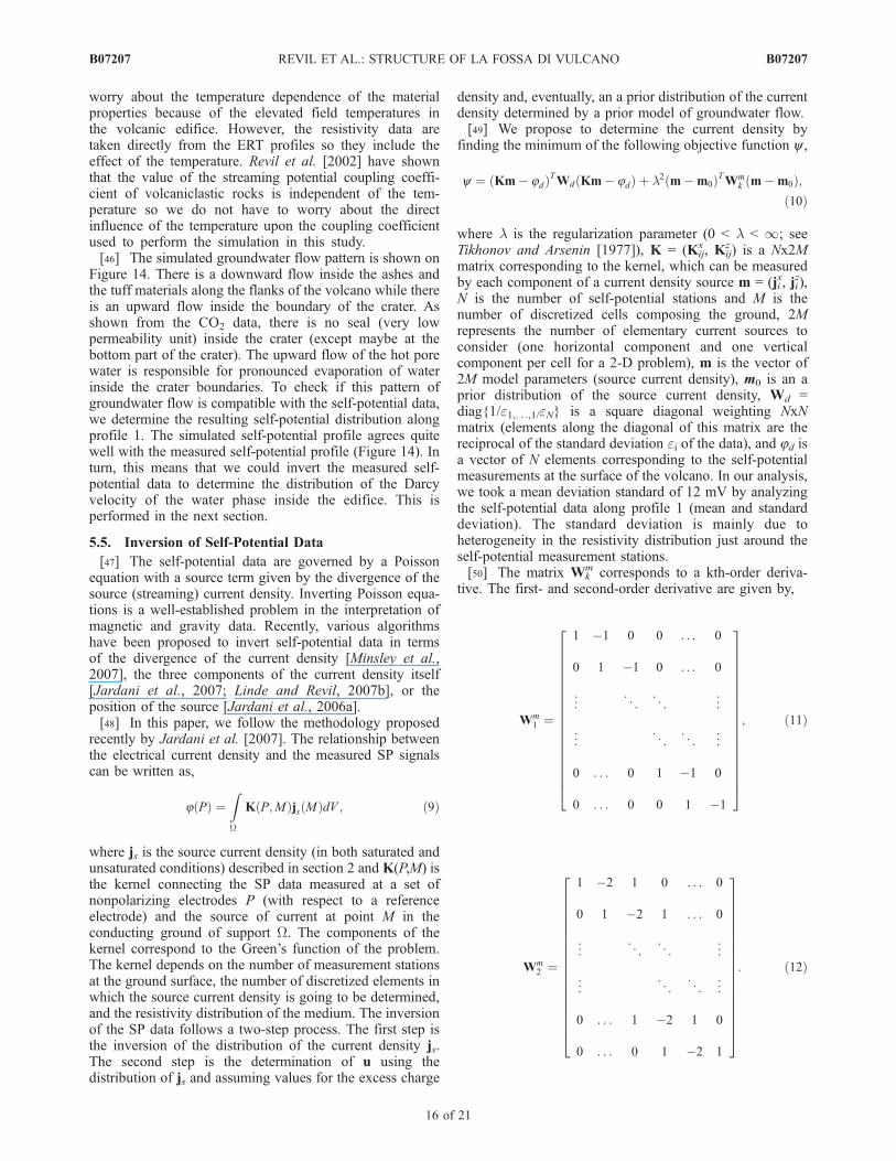
m corresponds to a kth-order deriva-tive. The first- and second-order derivative are given by,

Wm1 ¼

1 �1 0 0 . . . 0

0 1 �1 0 . . . 0

..

. . .. . .

. ...

..

. . .. . .

. ...

0 . . . 0 1 �1 0

0 . . . 0 0 1 �1

2666666666666666664

3777777777777777775

; ð11Þ

Wm2 ¼

1 �2 1 0 . . . 0

0 1 �2 1 . . . 0

..

. . .. . .

. ...

..

. . .. . .

. ...

0 . . . 1 �2 1 0

0 . . . 0 1 �2 1

2666666666666666664

3777777777777777775

: ð12Þ

B07207 REVIL ET AL.: STRUCTURE OF LA FOSSA DI VULCANO

16 of 21

B07207

To account for the depth sensitivity of the source, we use adepth weighting diagonal matrix S. If the medium has ahomogeneous resistivity distribution, it is defined from thedepth weighting function:

S ¼

1

zm1þ eð Þb0 . . . 0

0 1

zm2þ eð Þb. . . 0

..

. ... . .

. ...

0 0 . . . 1

zm2M þ eð Þb

266666666664

377777777775; ð13Þ

where the small value e is used to prevent the singularitywhen z is close to zero. The depth weighting (Nx3M) matrixis required to reduce the large sensitivity of the shallow cells[Li and Oldenburg, 1998; Boulanger and Chouteau, 2001;Chasseriau and Chouteau, 2003]. In the general case, thedepth weighting is given by [e.g., Spinelli, 1999],

S ¼ diag1

N

ffiffiffiffiffiffiffiffiffiffiffiffiffiffiffiffiffiffiffiXNj¼1

ðKijÞ2vuut

0@

1A: ð14Þ

[51] The solution of the problem is to find the unknownvectorm corresponding to the minimum of the cost functiongiven by @y /@m = 0. This minimum is given by [Hansen,1992]:

mw ¼ KTw WT

dWd

� �Kw þ l WT

mWm

� �� ��1KT

w WTdWd

� �8d

�þ l WT

mWm

� �m0

�: ð15Þ

where Kw = KS�1 The model vector is finally then given bym* = Smw. Because the model is linear with respect to thesource current density, the solution, in terms of streaming

current density, is obtained directly from equation (13).However, the solution of the inverse problem depends onthe value of the regularization parameter and the value ofthe a prior model m0. To determine the value of theregularization parameter, Hansen [1998] proposed to plotthe norm of the regularized smoothing solutions versus thenorm of the residuals of the data misfit function. Theresulting curve is hyperbolic and has therefore an L-shape.The determination of the regularization parameter, whichis chosen at the corner of the L-shape plot, is known asthe L-shape method. This is this method that we followbelow.[52] An alternative method is the cross-validation method

[Desbat and Girard, 1995]. The cross-validation methodallows choosing the best estimate of the regularizationparameter in terms of the overall error prediction of theself-potential data. The total error prediction E(l) is definedby,

EðlÞ ¼ 1

N

XNi¼1

8di � 8i*ðlÞ

� �2; ð16Þ

where 8id are the measured self-potential data and 8*i(l) are

the estimate of the self-potential data at each self-potentialstation for a choice of the regularization parameter l. Thebest choice of the regularization parameter is obtain to reachthe condition Min E(l).[53] The determine the resolution of the inverse problem,

we can introduce the resolution matrix of the self-potentialproblem. The forward model is given by �8 = Km where �8is the self-potential vector. The solution of the inverseproblem is given by m* = T�8 where T is the inversetransformation matrix. The resolution matrix R is definedby m* = Rm with R = KT [Menke, 1989]. The resolutionmatrix contains all the information related to the uncer-tainty of the solution m* for any cell of the investigatedsource volume.

Figure 15. Determination of the sources of current density in the system associated with the flow of thegroundwater. The ellipsoid corresponds to the deflation source volume observed by Gambino andGuglielmino [2008] for the period 1990–1996 inverting electro-optical and leveling measurements in anelastic homogeneous and isotropic half-space.

B07207 REVIL ET AL.: STRUCTURE OF LA FOSSA DI VULCANO

17 of 21

B07207

[54] The steps we follow to invert the self-potential dataon profile 1 are the following:[55] 1. We determine an a prior model of fluid flow using

the geometrical structure inferred from the electrical resis-tivity tomogram along this profile, a prior permeabilityvalue that we believe to be reasonable for the four typesof formations used to interpret the resistivity tomogram, andboundary conditions for the flow. The result is shown onFigure 14 and provides already a good fit of the self-potential data. Then we use this groundwater flow solutionto determine m0, the a prior distribution of the sourcecurrent density (Figure 15). This solution has not to bevery precise but physically meaningful to place a priorconstraints on the inversion of the self-potential data andto reduce the nonuniqueness of the solution.

[56] 2. The second step is the determination of the kernel.For each discretized cell, we consider a collection of Melementary source (in 2-D, there are 2M components of thecurrent density to retrieve) and N observation stations P.When computing the elements of K, one has to rememberthat the electrical potential is determined relatively to areference electrode. In our case, the reference electrode isplaced at the first station at the beginning of the profile). Bydefinition, the electrical potential at the reference is taken asequal to zero and this condition should be fulfilled for allthe elements of K by removing the potential computed atthis location from the self-potential distribution determinedover the field. By computing the kernel, we also take intoaccount the ground topography. In computing the kernel, wecan also to choose to restrain the solution to subvolumes ofthe volcanoes. In the present case, we consider that the very

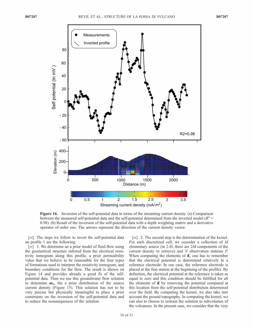
Figure 16. Inversion of the self-potential data in terms of the streaming current density. (a) Comparisonbetween the measured self-potential data and the self-potential determined from the inverted model (R2 =0.98). (b) Result of the inversion of the self-potential data with a depth weighting matrix and a derivativeoperator of order one. The arrows represent the direction of the current density vector.

B07207 REVIL ET AL.: STRUCTURE OF LA FOSSA DI VULCANO

18 of 21

B07207

resistive units are low-porosity units which can be consideras seals with a null permeability.[57] 3. The third step is the determination of the regular-

ization parameter using the L-shape method.[58] 4. The final problem is the determination of the best

fit solution using equation (15). The result of the inversionwith the use if an a prior model is shown in Figure 16.[59] We find that the source is mainly located below the

crater (sources along the flanks are very minor; seeFigure 16). Interestingly, the localization of the invertedsource current density is consistent with the position of thesource model inferred recently byGambino and Guglielmino[2008] for the subsidence of the Fossa edifice that occurredduring the period 1990–1996. During this period, electro-optical distance and leveling measurements were used byGambino and Guglielmino [2008] to infer a shallow prolateellipsoid responsible for the deformation of La Fossa Edifice.They explained the deformation as a transient migration ofhydrothermal fluids along this source model. Because thecurrent density evidences preferential fluid migration along aconduit, it is likely that deformation and self-potential datapoint out the same preferential fluid flow pathway below thecrater of La Fossa volcano.

6. Conclusion

[60] The inner structure of La Fossa di Vulcano (VulcanoIsland, southern Tyrrhenian Sea, Italy) is revealed by high-resolution electric resistivity tomography coupled with self-potential, temperature, and CO2 gas flux measurements.These measurements provide an idea of the architecture ofthe edifice including the geometry of the ash, tuff, lava flowunits, and the spatial organization of the hydrothermalsystem. Numerical modeling of the flow system along theeast-west profile shows the downward percolation of waterin the ash and tuff, and upward flow of groundwater insidethe crater that is required to explain the observed self-potential data measured along this profile.[61] Because of its relatively small size and importance

in terms of geohazards, La Fossa di Vulcano is a veryinteresting natural laboratory to see how various geophys-ical methods can be integrated to reveal the architecture ofa volcano and to monitor its thermohydromechanicalbehavior. In the near future, we plan to perform a three-dimensional joint inversion of electrical resistivity andgravity data. Such a joint inversion would probably be ableto identify structural discontinuities of the edifice and toestimate both density and resistivity values for each subunitusing a structural joint inversion approach [Gallardo andMeju, 2004] or sequential inversion approach with discretevalues for the resistivity and the mass density [e.g.,Krahenbuhl and Li, 2006]. The combination of varioussources of information (passive seismic data, self-potential,ground deformation, and variation of the gravity field) isprobably required to distinguish magmatic versus hydrother-mal phenomena and their implications in the assessment ofgeohazards.

[62] Acknowledgments. The INSU-CNRS, Instituto di Metodologieper l’Analisi Ambientale del CNR, the Laboratoire GeoSciences Reunion-IPGP, the CNR, the Istituto Nazionale di Geofisica e Vulcanologia, and theDipartimento per la Protezione Civile, through the DPC research program(V3.5 Vulcano, 2005–2007), are thanked for financial support. We also

thank Xavier Rassion and Etienne Wheris for their help in the field, withoutforgetting Peppe Sansone for his inimitable Sicilian recipes. We thank alsoA. Jardani for his help and Maria Marsella for facilitating the use ofVulcano DEM. This is IPGP contribution 2294. We thank the associateeditor, an anonymous referee, and David Fitterman for their very usefulcomments of our manuscript.

ReferencesAubert, M., S. Diliberto, A. Finizola, and Y. Chebli (2008), Double originof hydrothermal convective flux variations in the Fossa of Vulcano(Italy), Bull. Volcanol., doi:10.1007/s00445-007-0165-y, in press.

Auken, E., and A. V. Christiansen (2004), Layered and laterally constrained2D inversion of resistivity data, Geophysics, 69, 752–761.

Baldi, P., S. Bonvalot, P. Briole, M. Coltelli, K. Gwinner, M. Marsella,G. Puglisi, and D. Remy (2002), Validation and comparison of differenttechniques for the derivation of digital elevation models and volcanicmonitoring (Vulcano Island, Italy), Int. J. Remote Sens., 22, 4783–4800.

Bedrosian, P. A., M. J. Unsworth, and M. J. S. Johnston (2007), Hydro-thermal circulation at Mount St. Helens determined by self-potentialmeasurements, J. Volcan. Geotherm. Res., 160, 137–146.

Bernard, M.-L., M. Zamora, Y. Geraud, and G. Boudon (2007), Transportproperties of pyroclastic rocks from Montagne Pelee volcano (Martini-que, Lesser Antilles), J. Geophys. Res., 112, B05205, doi:10.1029/2006JB004385.

Binley, A., and A. Kemna (2005), DC resistivity and induced polarizationmethods, in Hydrogeophysics, edited by Y. Rubin and S. Hubbard, chap.5, pp. 129–156, Springer, New York.

Boleve, A., A. Crespy, A. Revil, F. Janod, and J. L. Mattiuzzo (2007a),Streaming potentials of granular media: Influence of the Dukhin andReynolds numbers, J. Geophys. Res., 112, B08204, doi:10.1029/2006JB004673.

Boleve, A., A. Revil, F. Janod, J. L. Mattiuzzo, and A. Jardani (2007b),Forward modeling and validation of a new formulation to compute self-potential signals associated with ground water flow, Hydrol. Earth Syst.Sci., 11(5), 1661–1671.

Boulanger, O., and M. Chouteau (2001), Constraints in 3-D gravity inver-sion, Geophys. Prospect., 49, 265–280.

Chasseriau, P., and M. Chouteau (2003), 3D gravity inversion using amodel of parameter covariance, J. Appl. Geophys., 52(1), 59–74.

Chiodini, G., F. Frondini, and B. Raco (1996), Diffuse emission of CO2

from the Fossa crater, Vulcano Island (Italy), Bull. Volcanol., 58, 41–50.Chiodini, G., R. Cioni, M. Guidi, L. Marini, and B. Raco (1998), Soil CO2

flux measurements in volcanic and geothermal areas, Appl. Geochem.,13, 543–552.

Colella, A., V. Lapenna, and E. Rizzo (2004), High-resolution imaging ofthe High Agri Valley basin (southern Italy) with electrical resistivitytomography, Tectonophysics, 386, 29–40.

Constable, S. C., R. L. Parker, and C. G. Constable (1987), Occam’s in-version—A practical algorithm for generating smooth models from elec-tromagnetic sounding data, Geophysics, 52, 289–300.

Coppo, N., P.-A. Schnegg, W. Heise, P. Falco, and R. Costa (2008), Multi-ple caldera collapses inferred from the shallow electrical resistivity sig-nature of the Las Canadas caldera, Tenerife, Canary Islands, J. Volcanol.Geotherm. Res., 170, 153–166.

Cortecci, G., E. Dinelli, L. Bolognesi, T. Boschetti, and G. Ferrara (2001),Chemical and isotopic compositions of water and dissolved sulfate fromshallow wells on Vulcano Island, Aeolian Archipelago, Italy, Geother-mics, 30, 69–91.

Corwin, R. F., and D. B. Hoover (1979), The self-potential method ingeothermal exploration, Geophysics, 44, 226–245.

De Astis, G., P. Dellino, L. La Volpe, F. Lucchi, and C. A. Tranne (2007),Geological Map of the Vulcano Island, scale 1:10000, edited by L. LaVolpe and G. De Astis, Ist. Nat. Geofis. Vulcanol., Napoli, Italy.

De Fino, M., L. La Volpe, and G. Piccarreta (1991), Role of magma mixingduring recent activity of La Fossa di Vulcano (Aeolian Islands, Italy),J. Volcanol. Geotherm. Res., 48, 385–398.

De Fiore, O. (1922), Vulcano (Isole Eolie), Riv. Vulcanol., suppl. III,393 pp., Fridlander Inst., Napoli, Italy.

Dellino, P., and L. La Volpe (1997), Stratigrafia, dinamiche eruttive edeposizionali, scenario eruttivo e valutazioni di pericolosita a La Fossadi Vulcano in CNR-GNV Progetto Vulcano 1993–1995, edited by L. LaVolpe et al., pp. 214–237, Felici Publ., Pisa, Italy.

De Rosa, R., N. Calanchi, P. F. Dellino, L. Francalanci, F. Lucchi, M. Rosi,P. L. Rossi, and C. A. Tranne (2004), 32nd International GeologicalCongress, Field Trip Guide Book–P42, vol. 5, Geology and Volcanism ofStromboli, Lipari, and Vulcano (Aeolian Islands), edited by L. Guerrieri,I. Rischia, and L. Serva, Agency for the Environ. Prot. and Tech. Serv.,Rome.

Desbat, L., and D. Girard (1995), The minimum reconstruction error choiceof regularization parameters: Some more efficient methods and their

B07207 REVIL ET AL.: STRUCTURE OF LA FOSSA DI VULCANO

19 of 21

B07207

application to deconvolution problems, SIAM J. Sci. Comput., 16(6),1387–1403.

Diaferia, I., M. Barchi, M. Loddo, D. Schiavone, and A. Siniscalchi (2006),Detailed imaging of tectonic structures by multiscale Earth resistivitytomographies: The Colfiorito normal faults (central Italy), Geophys.Res. Lett., 33, L09305, doi:10.1029/2006GL025828.

Di Fiore, B., P. Mauriello, and D. Patella (2004), On the localisation oflong-standing self-potential sources at Vulcano (Italy) by probability to-mography, Quadernidi Geofis., 35, 27–32.

Ellam, R. M., C. J. Hawkesworth, M. A. Menzies, and N. W. Rotgers(1989), The volcanism of southern Italy: Role of subduction and therelationship between potassic and sodic alkaline magmatism, J. Geophys.Res., 94, 4589–4601.

Finizola, A., S. Sortino, J.-F. Lenat, and M. Valenza (2002), Fluid circula-tion at Stromboli volcano (Aeolian Islands, Italy) from self-potential andCO2 surveys, J. Volcanol. Geotherm. Res., 116, 1–18.

Finizola, A., S. Sortino, J.-F. Lenat, M. Aubert, M. Ripepe, and M. Valenza(2003), The summit hydrothermal system of Stromboli. New insightsfrom self-potential, temperature, CO2 and fumarolic fluid measurements,Structural and monitoring implications, Bull. Volcanol., 65, 486–504,doi:10.1007/s00445-003-0276-z.

Finizola, A., A. Revil, E. Rizzo, S. Piscitelli, T. Ricci, J. Morin,B. Angeletti, L. Mocochain, and F. Sortino (2006), Hydrogeological in-sights at Stromboli volcano (Italy) from geoelectrical, temperature, andCO2 soil degassing investigations, Geophys. Res. Lett., 33, L17304,doi:10.1029/2006GL026842.

Fitterman, D. V., W. D. Stanley, and R. J. Bisdorf (1988), Electrical struc-ture of Newberry volcano, Oregon, J. Geophys. Res., 93, 10,119 –110,134.

Frazzetta, G., and L. La Volpe (1991), Volcanic history and maximumexpected eruption at ‘‘La Fossa di Vulcano’’ (Aeolian Islands, Italy), ActaVolcanol., 1, 107–113.

Frazzetta, G., L. La Volpe, and M. F. Sheridan (1983), Evolution of theFossa cone, Volcano, J. Volcanol. Geotherm. Res., 17, 329–360.

Frazzetta, G., P. Y. Gillot, L. La Volpe, and M. F. Sheridan (1984), Volcanichazards at Fossa of Volcano: Data from the last 6,000 years, Bull. Volca-nol., 47, 105–125.

Gallardo, L. A., and M. A. Meju (2004), Joint two-dimensional DC resis-tivity and seismic travel time inversion with cross-gradients constraints,J. Geophys. Res., 109, B03311, doi:10.1029/2003JB002716.

Gambino, S., and F. Guglielmino (2008), Ground deformation induced bygeothermal processes: A model for La Fossa crater (Vulcano Island,Italy), J. Geophys. Res., doi:10.1029/2007JB005016, in press.

Gasparini, C., G. Iannaccone, and R. Scarpa (1982), Seismotectonics of theCalabrian Arc, Tectonophysics, 84, 267–286.

Gex, P. (1992), Geophysical survey in the region of the crater of Vulcano,Italy (in French), Bull. Soc. Vaudoise Sci. Nat., 82(2), 157–172.

Giacomelli, L., and R. Scandone (2002), Vulcani e eruzioni, Pitagora Edi-trice, Boll. Della Soc. Geogr. Ital., vol. IX, pp. 478–480, La Soc. Geogr.Ital., Bologna, Italy.

Granieri, D., M. L. Carapezza, G. Chiodini, R. Avino, S. Caliro, M. Ranaldi,T. Ricci, and L. Tarchini (2006), Correlated increase in CO2 fumaroliccontent and diffuse emission from La Fossa crater (Vulcano, Italy): Evi-dence of volcanic unrest or increasing gas release from a stationary deepmagma body?, Geophys. Res. Lett., 33, L13316, doi:10.1029/2006GL026460.

Hansen, P. C. (1992), Analysis of discrete ill-posed problems by means ofthe L-curve, SIAM Rev., 34(4), 561–580.

Hansen, P. C. (1998), Rank-Deficient and Discrete Ill-Posed Problems:Numerical Aspects of Linear Inversion, 247 pp., SIAM, Philadelphia,Pa.

Hase, H., T. Hashimoto, S. Sakanaka, W. Kanda, and Y. Tanaka (2005),Hydrothermal system beneath Aso volcano as inferred from self-potentialmapping and resistivity structure, J. Volcanol. Geotherm. Res., 143, 259–277.

Ishido, T. (2004), Electrokinetic mechanism for the ‘‘W’’ -shaped self-po-tential profile on volcanoes, Geophys. Res. Lett., 31, L15616,doi:10.1029/2004GL020409.

Ishido, T., T. Kiruchi, N. Matsushima, Y. Yano, S. Nakao, M. Sugihara,T. Tosha, S. Takakura, and Y. Ogawa (1997), Repeated self-potentialprofiling of Izu-Oshima Volcano, Japan, J. Geomagn. Geoelectr., 49,1267–1278.

Jardani, A., A. Revil, F. Akoa, M. Schmutz, N. Florsch, and J. P. Dupont(2006a), Least squares inversion of self-potential (SP) data and applica-tion to the shallow flow of ground water in sinkholes, Geophys. Res.Lett., 33, L19306, doi:10.1029/2006GL027458.

Jardani, A., J. P. Dupont, and A. Revil (2006b), Self-potential signalsassociated with preferential groundwater flow pathways in sinkholes,J. Geophys. Res., 111, B09204, doi:10.1029/2005JB004231.

Jardani, A., A. Revil, A. Boleve, A. Crespy, J.-P. Dupont, W. Barrash, andB. Malama (2007), Tomography of the Darcy velocity from self-potentialmeasurements, Geophys. Res. Lett., 34, L24403, doi:10.1029/2007GL031907.

Jin, G., C. Torres-Verdin, S. Devarajan, E. Toumelin, and E. C. Thomas(2007), Pore-scale analysis of the Waxman-Smits shaly-sand conductivitymodel, Petrophysics, 48(2), 104–120.

Kalscheuer, T., M. Commer, S. L. Helwig, A. Hordt, and B. Tezkan (2007),Electromagnetic evidence for an ancient avalanche caldera rim on thesouth flank of Mount Merapi, Indonesia, J. Volcanol. Geotherm. Res.,162, 81–97.

Keller, J. (1980), The island of Vulcano, Soc. Ital. Min. Petr., 36, 368–413.Krahenbuhl, R. A., and Y. Li (2006), Inversion of gravity data using abinary formulation, Geophys. J. Int., 167, 543–556.

Kulessa, B., B. Hubbard, and G. H. Brown (2003a), Cross-coupled flowmodeling of coincident streaming and electrochemical potentials andapplication to subglacial self-potential data, J. Geophys. Res., 108(B8),2381, doi:10.1029/2001JB001167.

Kulessa, B., B. Hubbard, G. H. Brown, and J. Becker (2003b), Earth tideforcing of glacier drainage, Geophys. Res. Lett., 30(1), 1011,doi:10.1029/2002GL015303.

Lenat, J. F. (2007), Retrieving self-potential anomalies in a complex vol-canic environment: An SP/elevation gradient approach, Near SurfaceGeophys., 5(3), 161–170.

Lenat, J. F., D. Fitterman, D. B. Jackson, and P. Labazuy (2000), Geoelec-trical structure of the central zone of Piton de la Fournaise volcano (Re-union), Bull. Volcanol., 62, 75–89.

Leroy, P., and A. Revil (2004), A triple layer model of the surface electro-chemical properties of clay minerals, J. Colloid Interface Sci., 270, 371–380.

Li, Y., and D. W. Oldenburg (1998), 3-D inversion of gravity data, Geo-physics, 63, 109–119.

Linde, N., and A. Revil (2007a), Comment on ‘‘Electrical tomography ofLa Soufriere of Guadeloupe Volcano: Field experiments, 1D inversionand qualitative interpretation’’, by F. Nicollin et al., Earth Planet Sci.Lett., 258, 619–622, doi:10.1016/j.epsl.2006.02.020.

Linde, N., and A. Revil (2007b), Inverting self-potential data for redoxpotentials of contaminant plumes, Geophys. Res. Lett., 34, L14302,doi:10.1029/2007GL030084.

Linde, N., A. Revil, A. Boleve, C. Dages, J. Castermant, B. Suski, andM. Voltz (2007), Estimation of the water table throughout a catchmentusing self-potential and piezometric data in a Bayesian framework,J. Hydrol., 334, 88–98.

Lo Cascio, P., and E. Navarra (1997), Guida Naturalistica Alle Isole Eolie,112 pp., L’EPOS Publ., Palermo, Italy.

Loke, M. H., and R. D. Barker (1996), Rapid least-squares inversion ofapparent resistivity pseudosections by a quasi-Newton method, Geophys.Prospect., 44, 131–152.

Maineult, A., Y. Bernabe, and P. Ackerer (2005), Detection of advectedconcentration and pH fronts from self-potential measurements, J. Geo-phys. Res., 110, B11205, doi:10.1029/2005JB003824.

Maineult, A., Y. Bernabe, and P. Ackerer (2006), Detection of advected,reacting redox fronts from self-potential measurements, J. Contam. Hy-drol., 86, 32–52.

Massenet, F., and V. N. Pham (1985), Experimental and theoretical basis ofself-potential phenomena in volcanic areas with reference to results ob-tained on Mount Etna (Sicily), Earth Planet. Sci. Lett., 73, 415–429.

Menke, W. (1989), Geophysical Data Analysis: Discrete Inverse Theory,Int. Geophys. Ser., vol. 45, 289 pp., Academic Press, London.

Michel, S., and J. Zlotnicki (1998), Self-potential and magnetic survey-ing of La Fournaise volcano (Reunion island): Correlations with fault-ing, fluid circulation, and eruption, J. Geophys. Res., 103, 17,845–17,857.

Minsley, B. J., J. Sogade, and F. D. Morgan (2007), Three-dimensionalsource inversion of self-potential data, J. Geophys. Res., 112, B02202,doi:10.1029/2006JB004262.

Niwas, S., P. K. Gupta, and O. A. L. de Lima (2007), Nonlinear ElectricalConductivity Response of Shaly-Sand Reservoir, Curr. Sci., 92(5), 612–617.

Perrier, F., M. Trique, B. Lorne, J. P. Avouac, S. Hautot, and P. Tarits(1998), Electrical potential variations associated with yearly lake levelvariations, Geophys. Res. Lett., 25, 1955–1959.

Revil, A. (1995), Conductivite electrique et potentiel spontane dans lesmileux poreux: De la theorie a l’analyse des mesures en forage, Ph.D.thesis, Univ. Louis Pasteur, Strasbourg, France.

Revil, A., and P. W. J. Glover (1998), Nature of surface electrical conduc-tivity in natural sands, sandstones, and clays, Geophys. Res. Lett., 25,691–694.

Revil, A., and N. Linde (2006), Chemico-electromechanical coupling inmicroporous media, J. Colloid Interface Sci., 302, 682–694.

B07207 REVIL ET AL.: STRUCTURE OF LA FOSSA DI VULCANO

20 of 21

B07207

Revil, A., L. M. Cathles, S. Losh, and J. A. Nunn (1998), Electrical con-ductivity in shaly sands with geophysical applications, J. Geophys. Res.,103, 23,925–23,936.

Revil, A., D. Hermitte, E. Spangenberg, and J. J. Cocheme (2002), Elec-trical properties of zeolitized volcaniclastic materials, J. Geophys. Res.,107(B8), 2168, doi:10.1029/2001JB000599.

Revil, A., G. Saracco, and P. Labazuy (2003), The volcano-electric effect,J. Geophys. Res., 108(B5), 2251, doi:10.1029/2002JB001835.

Revil, A., V. Naudet, and J. D. Meunier (2004a), The hydroelectric problemof porous rocks: Inversion of the water table from self-potential data,Geophys. J. Int., 159, 435–444.

Revil, A., A. Finizola, F. Sortino, and M. Ripepe (2004b), Geophysicalinvestigations at Stromboli volcano, Italy. Implications for ground waterflow, Geophys. J. Int., 157, 426–440.

Revil, A., P. Leroy, and K. Titov (2005), Characterization of transportproperties of argillaceous sediments: Application to the Callovo-Oxfor-dian argilli te, J. Geophys. Res. , 110 , B06202, doi:10.1029/2004JB003442.

Revil, A., N. Linde, A. Cerepi, D. Jougnot, S. Matthai, and S. Finsterle(2007), Electrokinetic coupling in unsaturated porous media, J. ColloidInterface Sci., 313, 315–327, doi:10.1016/j.jcis.2007.03.037.

Rizzo, E., B. Suski, A. Revil, S. Straface, and S. Troisi (2004), Self-potentialsignals associated with pumping tests experiments, J. Geophys. Res., 109,B10203, doi:10.1029/2004JB003049.

Roberts, J. J., and W. Lin (1997), Electrical properties of partially saturatedTopopah Spring tuff: Water distribution as a function of saturation, WaterResour. Res., 33, 577–587.

Santacroce, R., R. Cristofolini, L. La Volpe, G. Orsi, and M. Rosi (2003),Italian active volcanoes, Episodes, 26(3), 227–234.

Shevnin, V., A. Mousatov, A. Ryjov, and O. Delgado-Rodriquez (2007),Estimation of clay content in soil based on resistivity modelling andlaboratory measurements, Geophys. Prospect., 55, 265–275.

Spinelli, L. (1999), Analyse Spatiale de l’Activite Electrique Cerebrale:Nouveaux Developpements (in French), Ph.D. thesis, 136 pp., Univ.Joseph Fourier-Grenoble I, Grenoble, France.

Storz, H., W. Storz, and F. Javobs (2000), Electrical resistivity tomographyto investigate geological structures of the earth’s upper crust, Geophys.Prospect., 48, 455–471.

Suski, B., E. Rizzo, and A. Revil (2004), A sandbox experiment of self-potential signals associated with a pumping-test, Vadose Zone J., 3,1193–1199.

Suski, B., A. Revil, K. Titov, P. Konosavsky, M. Voltz, C. Dages, andO. Huttel (2006), Monitoring of an infiltration experiment using theself-potential method, Water Resour. Res., 42, W08418, doi:10.1029/2005WR004840.

Tabbagh, A., and P. Cosenza (2007), Effect of microstructure on the elec-trical conductivity of clay-rich systems, Phys. Chem. Earth, 32(1–7),154–160.

Tikhonov, A. N., and V. Y. Arsenin (1977), Solutions of Ill-Posed Problems,John Wiley, New York.

Titov, K., A. Revil, P. Konasovsky, S. Straface, and S. Troisi (2005),Numerical modeling of self-potential signals associated with a pumpingtest experiment, Geophys. J. Int., 162, 641–650.

Tosha, T., N. Matsushima, and T. Ishido (2003), Zeta potential measured foran intact granite sample at temperatures to 200�C, Geophys. Res. Lett.,30(6), 1295, doi:10.1029/2002GL016608.

Waxman, M. H., and L. J. M. Smits (1968), Electrical conduction in oil-bearing sands, Soc. Pet. Eng. J., 8, 107–122.

Wishart, D. N., L. D. Slater, and A. E. Gates (2006), Self potential improvescharacterization of hydraulically-active fractures from azimuthal geoelec-trical measurements, Geophys. Res. Lett., 33, L17314, doi:10.1029/2006GL027092.

Zohdy, A. A. R., and R. J. Bisdorf (1990), Schlumberger soundings nearMedicine Lake, California, Geophysics, 55, 956–964.

�����������������������B. Angeletti and A. Crespy, Universite Aix Marseille III, CNRS,

Domaine de l’Arbois, F-13100 Aix en Provence, France.M. Balasco, A. Perrone, S. Piscitelli, and E. Rizzo, Laboratory of

Geophysics, IMAA, National Research Council, Cda S. Loja, Tito Scalo,PZ I-85050, Italy.S. Barde Cabusson and S. Byrdina, Laboratoire Magma et Volcan,

UMR6524, Universite Blaise Pascal, IRD, CNRS, 34 avenue Carnot, F-63000 Clermont-Ferrand, France.L. Bennati, Department of Earth and Atmospheric Sciences, Purdue

University, 550 Stadium Mall Drive, West Lafayette, IN 47906, USA.A. Boleve, Batiment Le Chablais, Domaine Universitaire, UMR5559,

Equipe Volcan, Universite de Savoie, INSU, LGIT, CNRS, F-73376 LeBourget-du-Lac CEDEX, France.N. Carzaniga, Department of Geology and Geosciences, Universita

Milano-Bicocca, Piazza della Scienza 4, I-20126 Milano, Italy.F. Di Gangi, Istituto Nazionale di Geofisica e Vulcanologia, Sezione di

Palermo, Via Ugo la Malfa 153, I-90146, Palermo, Italy.A. Finizola and J. Morin, Laboratoire GeoSciences Reunion, UMR7154,

UR, IPGP, 15 avenue Rene Cassin, BP 7151, F-97715, Saint Denis CEDEX9, La Reunion, France.A. Revil, Department of Geophysics, Colorado School of Mines, 1500

Illinois Street, Golden, CO 80401, USA. (arevil@mines.edu)T. Ricci, INGV, Universita Roma Tre, Sezione Roma 1, Via della Vasca

Navale 79, I-00146, Roma, Italy.M. Rossi, IPGP, CNRS, Place Jussieu, F-75252 Paris CEDEX 05, France.E. Roulleau, GEOTOP-UQAM-McGill, Universite du Quebec, CP 8888

Montreal, QC, H3C 3P8, Canada.B. Suski, Institut de Geophysique, College Propedeutique, Universite de

Lausanne, CH-1015 Lausanne, Switzerland.

B07207 REVIL ET AL.: STRUCTURE OF LA FOSSA DI VULCANO

21 of 21

B07207