Embed Size (px)
Citation preview

arX
iv:p
hysi
cs/0
4040
63v1
[ph
ysic
s.da
ta-a
n] 1
3 A
pr 2
004
Applied Probability Trust (2 February 2008)
INFORMATION AND COVARIANCE MATRICES FOR MULTI-
VARIATE BURR III AND LOGISTIC DISTRIBUTIONS
GHOLAMHOSSEIN YARI,∗ Iran University of Science and Technology
ALI MOHAMMAD-DJAFARI,∗∗ Laboratoire des Signaux et Systemes (Cnrs,Supelec,Ups)
Abstract
Main result of this paper is to derive the exact analytical expressions of
information and covariance matrices for multivariate Burr III and logistic
distributions. These distributions arise as tractable parametric models in
price and income distributions, reliability, economics, populations growth and
survival data. We showed that all the calculations can be obtained from one
main moment multi dimensional integral whose expression is obtained through
some particular change of variables. Indeed, we consider that this calculus
technique for improper integral has its own importance in applied probability
calculus.
Keywords: Gamma and Beta functions; Polygamma functions; Information and
Covariance matrices; Multivariate Burr III and Logistic models.
AMS 2000 Subject Classification: Primary 62E10
Secondary 60E05,62B10
∗ Postal address: Iran University of Science and Technology, Narmak, Tehran 16844, Iran.
email: [email protected]
∗∗ Postal address: Supelec, Plateau de Moulon, 3 rue Joliot-Curie, 91192 Gif-sur-Yvette, France.
email: [email protected]
1
2 Yari & Mohammad-Djafari
1. Introduction
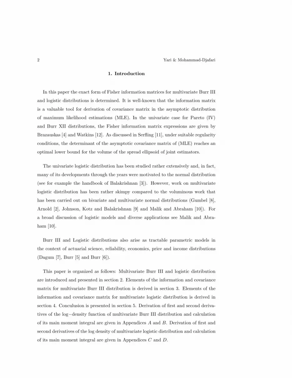
In this paper the exact form of Fisher information matrices for multivariate Burr III
and logistic distributions is determined. It is well-known that the information matrix
is a valuable tool for derivation of covariance matrix in the asymptotic distribution
of maximum likelihood estimations (MLE). In the univariate case for Pareto (IV)
and Burr XII distributions, the Fisher information matrix expressions are given by
Brazauskas [4] and Watkins [12]. As discussed in Serfling [11], under suitable regularity
conditions, the determinant of the asymptotic covariance matrix of (MLE) reaches an
optimal lower bound for the volume of the spread ellipsoid of joint estimators.
The univariate logistic distribution has been studied rather extensively and, in fact,
many of its developments through the years were motivated to the normal distribution
(see for example the handbook of Balakrishnan [3]). However, work on multivariate
logistic distribution has been rather skimpy compared to the voluminous work that
has been carried out on bivariate and multivariate normal distributions (Gumbel [8],
Arnold [2], Johnson, Kotz and Balakrishnan [9] and Malik and Abraham [10]). For
a broad discussion of logistic models and diverse applications see Malik and Abra-
ham [10].
Burr III and Logistic distributions also arise as tractable parametric models in
the context of actuarial science, reliability, economics, price and income distributions
(Dagum [7], Burr [5] and Burr [6]).
This paper is organized as follows: Multivariate Burr III and logistic distribution
are introduced and presented in section 2. Elements of the information and covariance
matrix for multivariate Burr III distribution is derived in section 3. Elements of the
information and covariance matrix for multivariate logistic distribution is derived in
section 4. Conculusion is presented in section 5. Derivation of first and second deriva-
tives of the log−density function of multivariate Burr III distribution and calculation
of its main moment integral are given in Appendices A and B. Derivation of first and
second derivatives of the log density of multivariate logistic distribution and calculation
of its main moment integral are given in Appendices C and D.

Information and Covariance Matrices 3
2. Multivariate Burr III and logistic distributions
The density function of the Burr III distribution is
fX(x) =αc(
x−µθ
)−(c+1)
θ(
1 + (x−µθ
)−c)α+1 , x > µ, (1)
where −∞ < µ < +∞ is the location parameter, θ > 0 is the scale parameter, c > 0 is
the shape parameter and α > 0 is the shape parameter which characterizes the tail of
the distribution.
The n-dimensional Burr III distribution is
fn(x) =
1 +n∑
j=1
(
xj − µj
θj
)
−cj
−(α+n)n∏
i=1
(α + i − 1)ci
θi
(
xi − µi
θi
)
−(ci+1)
, (2)
where x = [x1, · · · , xn], xi > µi, ci > 0, −∞ < µi < +∞ , α > 0, θi > 0 for
i = 1, · · · , n. One of the main properties of this distribution is that, the joint density
of any subset of the components of a multivariate Burr III random vector is again of
the form (2) [9].
The density of the logistic distribution is
fX(x) =α
θe−( x−µ
θ)(
1 + e−( x−µθ
))
−(α+1)
, x > µ, (3)
where −∞ < µ < +∞ is the location parameter, θ > 0 is the scale parameter and
α > 0 is the shape parameter.
The n-dimensional logistic distribution is
fn(x) =
1 +
n∑
j=1
e−
(
xj−µjθj
)
−(α+n)n∏
i=1
(α + i − 1)
θi
e−
(
xi−µiθi
)
, (4)
where x = [x1, · · · , xn], xi > µi, α > 0, −∞ < µi < +∞ and θi > 0 for i = 1, · · · , n.
The joint density of any subset of the components of a multivariate logistic random
vector is again of the form (4) [9].
3. Information Matrix for Multivariate Burr III
Suppose X is a random vector with the probability density function fΘ(.) where
Θ = (θ1, θ2, ..., θK). The information matrix I(Θ) is the K ×K matrix with elements
Iij(Θ) = −E
[
∂2ln fΘ(X)
∂θi∂θj
]
, i, j = 1, · · ·K. (5)

4 Yari & Mohammad-Djafari
For the multivariate Burr III, we have Θ = (µ1, · · · , µn, θ1, · · · , θn, c1, · · · , cn, α). In
order to make the multivariate Burr III distribution a regular family (in terms of
maximum likelihood estimation), we assume that vector µ is known and, without loss
of generality, equal to 0. In this case information matrix is (2n + 1)× (2n + 1). Thus,
further treatment is based on the following multivariate density function
fn(x) =
1 +
n∑
j=1
(
xj
θj
)
−cj
−(α+n)n∏
i=1
(α + i − 1)ci
θi
(
xi
θi
)
−(ci+1)
, xi > 0. (6)
The log-density function is:
ln fn(x) =
n∑
i=1
[ln(α + i − 1) − ln θi + ln ci] − (ci + 1) ln
(
xi
θi
)
− (α + n) ln
1 +n∑
j=1
(
xj
θj
)
−cj
. (7)
Since the information matrix I(Θ) is symmetric, it is enough to find elements Iij(Θ),
where 1 ≤ i ≤ j ≤ 2n + 1. The first and second partial derivatives of the above
expression are given in the Appendix A. In order to determine the information matrix
and score functions, we need to find expressions of the generic terms such as
E
ln
1 +
n∑
j=1
(
Xj
θj
)
−cj
and E
[
(
Xl
θl
)
−cl(
Xk
θk
)
−ck
]
and evaluation of the required orders partial derivatives of the last expectation at the
required points.
3.1. Main strategy to obtain expressions of the expectations
Derivation of these expressions are based on the following strategy: first, we derive
an analytical expression for the following integral
E
[
n∏
i=1
(
Xi
θi
)ri
]
=
∫ +∞
0
· · ·
∫ +∞
0
n∏
i=1
(
xi
θi
)ri
fn(x) dx, (8)
and then, we show that all the other expressions can easily be found from it. We
consider this derivation as one of the main contributions of this work. This derivation
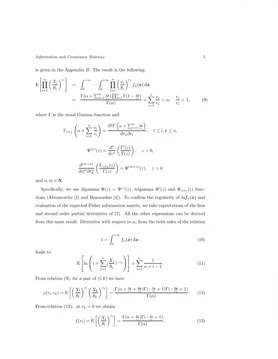
Information and Covariance Matrices 5
is given in the Appendix B. The result is the following:
E
[
n∏
i=1
(
Xi
θi
)ri
]
=
∫ +∞
0
· · ·
∫ +∞
0
n∏
i=1
(
xi
θi
)ri
fn(x) dx
=Γ(α +
∑ni=1
ri
ci)∏n
i=1 Γ(1 − ri
ci)
Γ(α)=
n∑
i=1
ri
ci
< α,ri
ci
< 1, (9)
where Γ is the usual Gamma function and
Γrlrk
(
α +
n∑
i=1
ri
ci
)
=∂2Γ
(
α +∑n
i=1ri
ci
)
∂rk∂rl
, 1 ≤ l, k ≤ n,
Ψ(n)(z) =dn
dzn
(
Γ′(z)
Γ(z)
)
, z > 0,
∂(m+n)
∂rml ∂rn
k
(
Γrlrk(z)
Γ(z)
)
= Ψ(m+n)(z), z > 0
and n, m ∈ NN.
Specifically, we use digamma Ψ(z) = Ψ(.)(z), trigamma Ψ′(z) and Ψrlrk(z) func-
tions (Abramowitz [1] and Brazauskas [4]). To confirm the regularity of lnfn(x) and
evaluation of the expected Fisher information matrix, we take expectations of the first
and second order partial derivatives of (7). All the other expressions can be derived
from this main result. Derivative with respect to α, from the both sides of the relation
1 =
∫ +∞
0
fn(x) dx, (10)
leads to
E
ln
1 +
n∑
j=1
(Xj
θj
)−cj
=
n∑
i=1
1
α + i − 1. (11)
From relation (9), for a pair of (l, k) we have
ϕ(rl, rk) = E
[(
Xl
θl
)rl(
Xk
θk
)rk]
=Γ(α + rl
cl+ ck
ck)Γ(− rl
cl+ 1)Γ(− rk
ck+ 1)
Γ(α). (12)
From relation (12), at rk = 0 we obtain
ξ(rl) = E
[(
Xl
θl
)rl]
=Γ(α + rl
cl)Γ(− rl
cl+ 1)
Γ(α). (13)

6 Yari & Mohammad-Djafari
Evaluating this expectation at rl = −cl, rl = −2cl and the relation (12) at (rl =
−cl, rk = −ck), we obtain
E
[
(
Xl
θl
)
−cl
]
=1
α − 1,
E
[
(
Xl
θl
)
−2cl
]
=2
(α − 1)(α − 2),
E
[
(
Xl
θl
)
−cl(
Xk
θk
)
−ck
]
=1
(α − 1)(α − 2).
Evaluating the required orders partial derivatives of (13) and (12) at the required
points, we have
E
[
ln
(
Xl
θl
)]
=[Ψ(α) − Γ′(1)]
cl
,
E
[
(
Xl
θl
)
−cl
ln
(
Xl
θl
)
]
=[Ψ(α − 1) − Γ′(2)]
cl(α − 1),
E
[
(
Xl
θl
)
−cl
ln2
(
Xl
θl
)
]
=
[
Ψ2(α − 1) + Ψ′(α − 1) − 2Ψ(α − 1)Γ′(2) + Γ′′(2)]
cl2(α − 1)
,
E
[
(
Xl
θl
)
−2cl
ln2
(
Xl
θl
)
]
=
[
2Ψ2(α − 2) + 2Ψ′(α − 2) − 2Ψ(α − 2)Γ′(3) + Γ′′(3)]
cl2(α − 1)(α − 2)
,
E
[
(
Xl
θl
)
−2cl
ln
(
Xl
θl
)
]
=[2Ψ(α − 2) − Γ′(3)]
cl(α − 1)(α − 2),
E
[
(
Xl
θl
)
−cl(
Xk
θk
)
−ck
ln
(
Xk
θk
)
]
=[Ψrl
(α − 2) − Γ′(2)]
ck(α − 1)(α − 2),
E
[
(
Xl
θl
)
−cl(
Xk
θk
)
−ck
ln
(
Xl
θl
)
ln
(
Xk
θk
)
]
=[−Γ′(2)(Ψrl
(α − 2) + Ψrk(α − 2))]
clck(α − 1)(α − 2)
+
[
(Γ′(2))2 + Ψrlrk(α − 2)
]
clck(α − 1)(α − 2).
From these equations with α replaced by (α + 1) and (α + 2) in (6), we can show
that
Information and Covariance Matrices 7
E
(Xl
θl)−cl
(
1 +∑n
j=1(Xj
θj)−cj
)
=α
α + nEα+1
[
(
Xl
θl
)
−cl
]
=1
α + n,
E
(Xl
θl)−2cl
(
1 +∑n
j=1(Xj
θj)−cj
)2
=
α(α + 1)
(α + n)(α + n + 1)Eα+2
[
(
Xl
θl
)
−2cl
]
=2
(α + n)(α + n + 1),
E
(Xl
θl)−cl ln2
(
Xl
θl
)
(
1 +∑n
j=1(Xj
θj)−cj
)
=
[
Ψ2(α) + Ψ′(α) − 2Ψ(α)Γ′(2) + Γ′′(2)]
cl2(α + n)
,
E
(Xl
θl)−cl ln
(
Xl
θl
)
(
1 +∑n
j=1(Xj
θj)−cj
)
=[Ψ(α) − Γ′(2)]
cl(α + n),
E
(Xl
θl)−2cl ln
(
Xl
θl
)
(
1 +∑n
j=1(Xj
θj)−cj
)2
=
[2Ψ(α) − Γ′(3)]
cl(α + n)(α + n + 1),
E
(Xl
θl)−2cl ln2
(
Xl
θl
)
(
1 +∑n
j=1(Xj
θj)−cj
)2
=
[
2Ψ2(α) + Γ′′(3) − 2Γ′(3)Ψ(α) + 2Ψ′(α)]
c2l (α + n)(α + n + 1)
,
E
(Xl
θl)−cl(Xk
θk)−ck ln
(
Xk
θk
)
(
1 +∑n
j=1(Xj
θj)−cj
)2
=
[Ψrk(α) − Γ′(2)]
ck(α + n)(α + n + 1),
E
(Xl
θl)−cl(Xk
θk)−ck ln
(
Xl
θl
)
ln(
Xk
θk
)
(
1 +∑n
j=1(Xj
θj)−cj
)2
=
[
Ψrlrk(α) − Γ′(2) (Ψrl
(α) + Ψrk(α)) + (Γ′(2))2
]
clck(α + n)(α + n + 1).
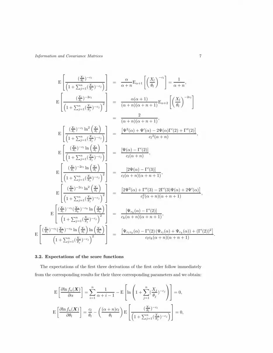
3.2. Expectations of the score functions
The expectations of the first three derivations of the first order follow immediately
from the corresponding results for their three corresponding parameters and we obtain:
E
[
∂ln fn(X)
∂α
]
=
n∑
i=1
1
α + i − 1− E
ln
1 +
n∑
j=1
(Xj
θj
)−cj
= 0,
E
[
∂ln fn(X)
∂θl
]
=cl
θl
−
(
(α + n)cl
θl
)
E
(Xl
θl)−cl
(
1 +∑n
j=1(Xj
θj)−cj
)
= 0,
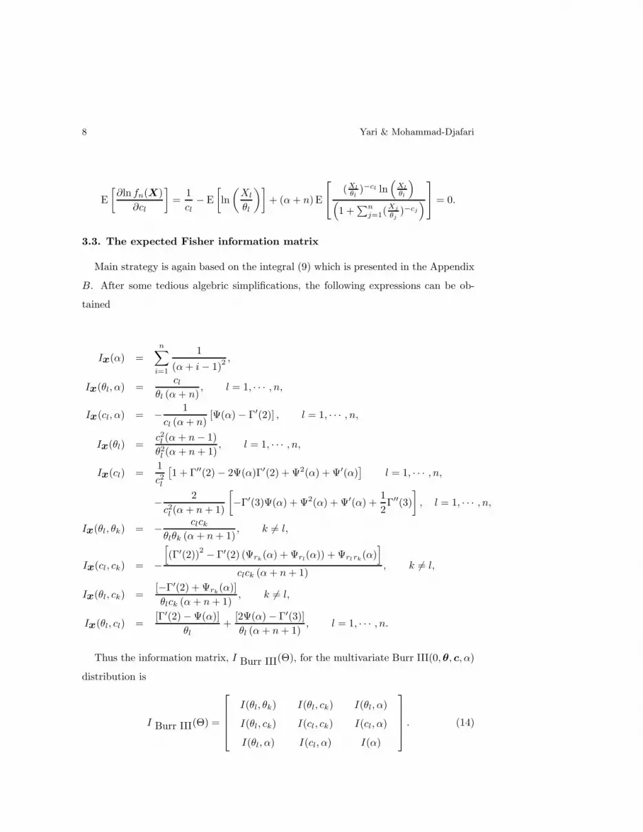
8 Yari & Mohammad-Djafari
E
[
∂ln fn(X)
∂cl
]
=1
cl
− E
[
ln
(
Xl
θl
)]
+ (α + n) E
(Xl
θl)−cl ln
(
Xl
θl
)
(
1 +∑n
j=1(Xj
θj)−cj
)
= 0.
3.3. The expected Fisher information matrix
Main strategy is again based on the integral (9) which is presented in the Appendix
B. After some tedious algebric simplifications, the following expressions can be ob-
tained
Ix(α) =
n∑
i=1
1
(α + i − 1)2 ,
Ix(θl, α) =cl
θl (α + n), l = 1, · · · , n,
Ix(cl, α) = −1
cl (α + n)[Ψ(α) − Γ′(2)] , l = 1, · · · , n,
Ix(θl) =c2l (α + n − 1)
θ2l (α + n + 1)
, l = 1, · · · , n,
Ix(cl) =1
c2l
[
1 + Γ′′(2) − 2Ψ(α)Γ′(2) + Ψ2(α) + Ψ′(α)]
l = 1, · · · , n,
−2
c2l (α + n + 1)
[
−Γ′(3)Ψ(α) + Ψ2(α) + Ψ′(α) +1
2Γ′′(3)
]
, l = 1, · · · , n,
Ix(θl, θk) = −clck
θlθk (α + n + 1), k 6= l,
Ix(cl, ck) = −
[
(Γ′(2))2− Γ′(2) (Ψrk
(α) + Ψrl(α)) + Ψrlrk
(α)]
clck (α + n + 1), k 6= l,
Ix(θl, ck) =[−Γ′(2) + Ψrk
(α)]
θlck (α + n + 1), k 6= l,
Ix(θl, cl) =[Γ′(2) − Ψ(α)]
θl
+[2Ψ(α) − Γ′(3)]
θl (α + n + 1), l = 1, · · · , n.
Thus the information matrix, I Burr III(Θ), for the multivariate Burr III(0, θ, c, α)
distribution is
I Burr III(Θ) =
I(θl, θk)
I(θl, ck)
I(θl, α)
I(θl, ck)
I(cl, ck)
I(cl, α)
I(θl, α)
I(cl, α)
I(α)
. (14)
Information and Covariance Matrices 9
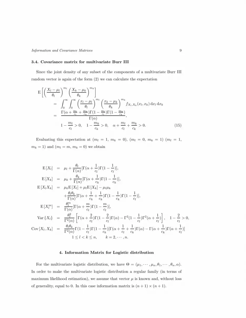
3.4. Covariance matrix for multivariate Burr III
Since the joint density of any subset of the components of a multivariate Burr III
random vector is again of the form (2) we can calculate the expectation
E
[(
Xl − µl
θl
)ml(
Xk − µk
θk
)mk]
=
∫
∞
0
∫
∞
0
(
xl − µl
θl
)ml(
xk − µk
θk
)mk
fXl,Xk(xl, xk) dxl dxk
=Γ(α + ml
cl+ mk
ck)Γ(1 − ml
cl)Γ(1 − mk
ck)
Γ(α),
1 −ml
cl
> 0, 1 −mk
ck
> 0, α +ml
cl
+mk
ck
> 0. (15)
Evaluating this expectation at (ml = 1, mk = 0), (ml = 0, mk = 1) (ml = 1,
mk = 1) and (ml = m, mk = 0) we obtain
E [Xl] = µl +θl
Γ(α)[Γ(α +
1
cl
)Γ(1 −1
cl
)],
E [Xk] = µk +θk
Γ(α)[Γ(α +
1
ck
)Γ(1 −1
ck
)],
E [XlXk] = µkE [Xl] + µlE [Xk] − µlµk
+θlθk
Γ(α)[Γ(α +
1
ck
+1
ck
)Γ(1 −1
ck
)Γ(1 −1
cl
)],
E [Xml ] =
θml
Γ(α)[Γ(α +
m
cl
)Γ(1 −m
cl
)],
Var {Xl} =θ2
l
Γ2(α)
[
Γ(α +2
cl
)Γ(1 −2
cl
)Γ(α) − Γ2(1 −1
cl
)Γ2(α +1
cl
)
]
, 1 −2
cl
> 0,
Cov [Xl, Xk] =θlθk
Γ2(α)Γ(1 −
1
cl
)Γ(1 −1
ck
)[Γ(α +1
cl
+1
ck
)Γ(α) − Γ(α +1
ck
)Γ(α +1
cl
)]
1 ≤ l < k ≤ n, k = 2, · · · , n.
4. Information Matrix for Logistic distribution
For the multivariate logistic distribution, we have Θ = (µ1, · · · , µn, θ1, · · · , θn, α).
In order to make the multivariate logistic distribution a regular family (in terms of
maximum likelihood estimation), we assume that vector µ is known and, without loss
of generality, equal to 0. In this case information matrix is (n + 1) × (n + 1).
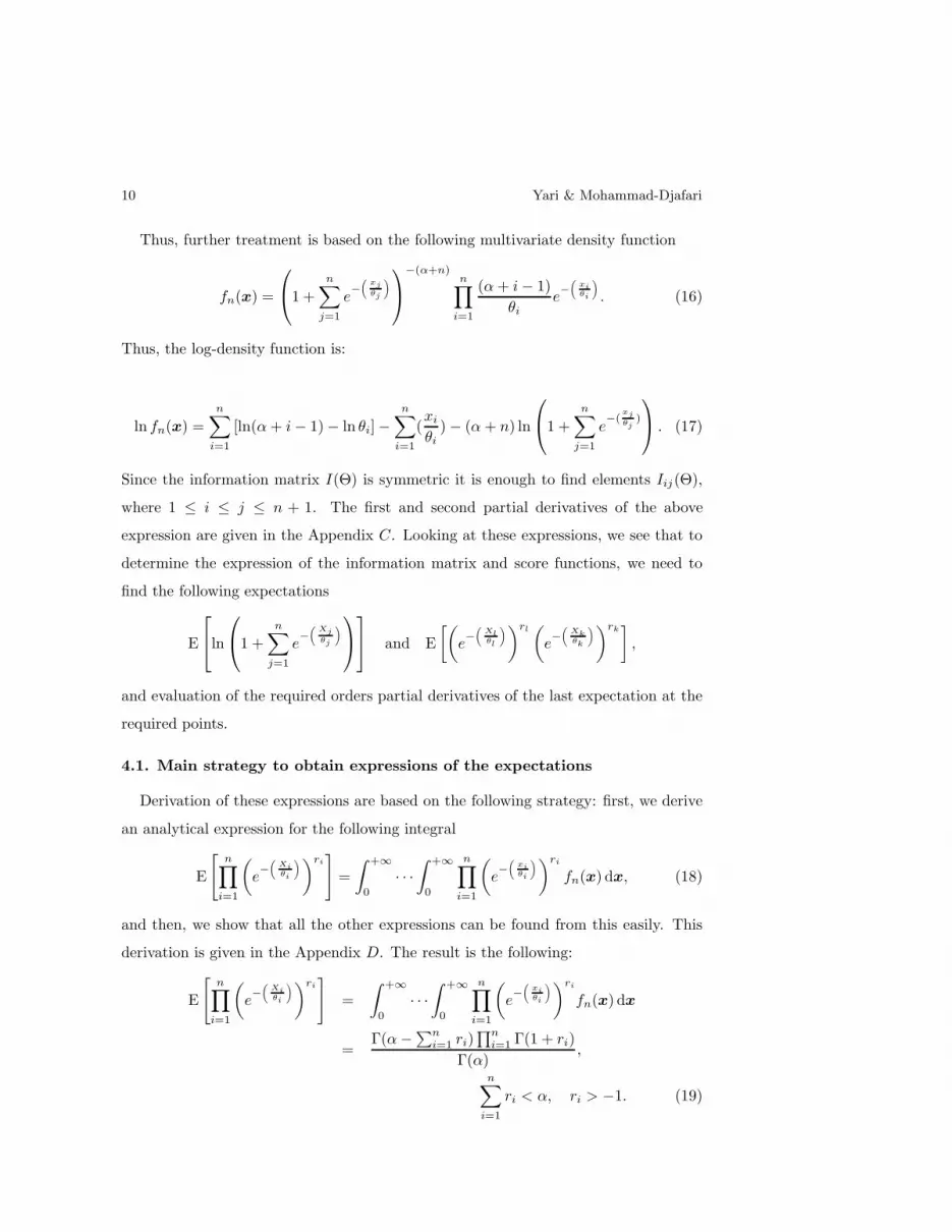
10 Yari & Mohammad-Djafari
Thus, further treatment is based on the following multivariate density function
fn(x) =
1 +
n∑
j=1
e−
(
xjθj
)
−(α+n)n∏
i=1
(α + i − 1)
θi
e−
(
xiθi
)
. (16)
Thus, the log-density function is:
ln fn(x) =
n∑
i=1
[ln(α + i − 1) − ln θi] −
n∑
i=1
(xi
θi
) − (α + n) ln
1 +
n∑
j=1
e−(
xjθj
)
. (17)
Since the information matrix I(Θ) is symmetric it is enough to find elements Iij(Θ),
where 1 ≤ i ≤ j ≤ n + 1. The first and second partial derivatives of the above
expression are given in the Appendix C. Looking at these expressions, we see that to
determine the expression of the information matrix and score functions, we need to
find the following expectations
E
ln
1 +n∑
j=1
e−
(
Xjθj
)
and E
[(
e−
(
Xlθl
))rl
(
e−
(
Xkθk
))rk
]
,
and evaluation of the required orders partial derivatives of the last expectation at the
required points.
4.1. Main strategy to obtain expressions of the expectations
Derivation of these expressions are based on the following strategy: first, we derive
an analytical expression for the following integral
E
[
n∏
i=1
(
e−
(
Xiθi
))ri
]
=
∫ +∞
0
· · ·
∫ +∞
0
n∏
i=1
(
e−
(
xiθi
))ri
fn(x) dx, (18)
and then, we show that all the other expressions can be found from this easily. This
derivation is given in the Appendix D. The result is the following:
E
[
n∏
i=1
(
e−
(
Xiθi
))ri
]
=
∫ +∞
0
· · ·
∫ +∞
0
n∏
i=1
(
e−
(
xiθi
))ri
fn(x) dx
=Γ(α −
∑ni=1 ri)
∏ni=1 Γ(1 + ri)
Γ(α),
n∑
i=1
ri < α, ri > −1. (19)
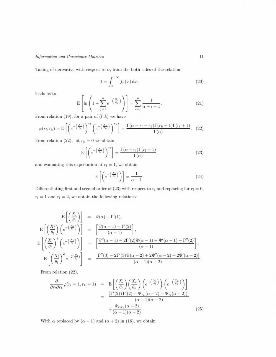
Information and Covariance Matrices 11
Taking of derivative with respect to α, from the both sides of the relation
1 =
∫ +∞
0
fn(x) dx, (20)
leads us to
E
ln
1 +n∑
j=1
e−
(
Xjθj
)
=n∑
i=1
1
α + i − 1. (21)
From relation (19), for a pair of (l, k) we have
ϕ(rl, rk) = E
[(
e−
(
Xlθl
))rl
(
e−
(
Xkθk
))rk
]
=Γ(α − rl − rk)Γ(rk + 1)Γ(rl + 1)
Γ(α). (22)
From relation (22), at rk = 0 we obtain
E
[(
e−
(
Xlθl
))rl]
=Γ(α − rl)Γ(rl + 1)
Γ(α), (23)
and evaluating this expectation at rl = 1, we obtain
E
[(
e−
(
Xlθl
))]
=1
α − 1. (24)
Differentiating first and second order of (23) with respect to rl and replacing for rl = 0,
rl = 1 and rl = 2, we obtain the following relations:
E
[(
Xl
θl
)]
= Ψ(α) − Γ′(1),
E
[(
Xl
θl
)(
e−
(
Xlθl
))]
=
[
Ψ(α − 1) − Γ′(2)
(α − 1)
]
,
E
[
(
Xl
θl
)2(
e−
(
Xlθl
))
]
=
[
Ψ2(α − 1) − 2Γ′(2)Ψ(α − 1) + Ψ′(α − 1) + Γ′′(2)
(α − 1)
]
,
E
[
(
Xl
θl
)2
e−2(
Xlθl
)
]
=
[
Γ′′(3) − 2Γ′(3)Ψ(α − 2) + 2Ψ2(α − 2) + 2Ψ′(α − 2)]
(α − 1)(α − 2).
From relation (22),
∂
∂rl∂rk
ϕ(rl = 1, rk = 1) = E
[(
Xl
θl
)(
Xk
θk
)(
e−
(
Xlθl
))(
e−
(
Xkθk
))]
=[Γ′(2) (Γ′(2) − Ψrk
(α − 2) − Ψrl(α − 2))]
(α − 1)(α − 2)
+Ψrlrk
(α − 2)
(α − 1)(α − 2). (25)
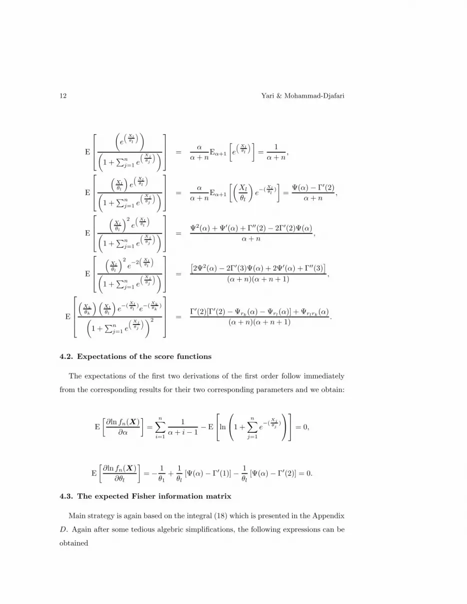
With α replaced by (α + 1) and (α + 2) in (16), we obtain
12 Yari & Mohammad-Djafari
E
(
e
(
Xlθl
))
(
1 +∑n
j=1 e
(
Xjθj
))
=α
α + nEα+1
[
e
(
Xlθl
)]
=1
α + n,
E
(
Xl
θl
)
e
(
Xlθl
)
(
1 +∑n
j=1 e
(
Xj
θj
))
=α
α + nEα+1
[(
Xl
θl
)
e−(
Xlθl
)
]
=Ψ(α) − Γ′(2)
α + n,
E
(
Xl
θl
)2
e
(
Xlθl
)
(
1 +∑n
j=1 e
(
Xjθj
))
=Ψ2(α) + Ψ′(α) + Γ′′(2) − 2Γ′(2)Ψ(α)
α + n,
E
(
Xl
θl
)2
e−2(
Xlθl
)
(
1 +∑n
j=1 e
(
Xjθj
))
=
[
2Ψ2(α) − 2Γ′(3)Ψ(α) + 2Ψ′(α) + Γ′′(3)]
(α + n)(α + n + 1),
E
(
Xk
θk
)(
Xl
θl
)
e−(
Xlθl
)e−(
Xkθk
)
(
1 +∑n
j=1 e
(
Xj
θj
))2
=Γ′(2)[Γ′(2) − Ψrk
(α) − Ψrl(α)] + Ψrlrk
(α)
(α + n)(α + n + 1).
4.2. Expectations of the score functions
The expectations of the first two derivations of the first order follow immediately
from the corresponding results for their two corresponding parameters and we obtain:
E
[
∂ln fn(X)
∂α
]
=
n∑
i=1
1
α + i − 1− E
ln
1 +
n∑
j=1
e−(
Xjθj
)
= 0,
E
[
∂ln fn(X)
∂θl
]
= −1
θ1+
1
θl
[Ψ(α) − Γ′(1)] −1
θl
[Ψ(α) − Γ′(2)] = 0.
4.3. The expected Fisher information matrix
Main strategy is again based on the integral (18) which is presented in the Appendix
D. Again after some tedious algebric simplifications, the following expressions can be
obtained

Information and Covariance Matrices 13
Ix(α) =
n∑
i=1
1
(α + i − 1)2 ,
Ix(θl, α) =1
θl (α + n)[Ψ(α) − Γ′(2)] , l = 1, · · · , n,
Ix(θl) =(α + n − 1)
θ2l (α + n + 1)
[
Ψ2(α) − 2Γ′(2)Ψ(α) + Γ′′(2) + Ψ′(α)]
+1
θ2l
− 2
[
Γ′(2) − Ψ(α)
θ2l (α + n + 1)
]
, l = 1, · · · , n,
Ix(θl, θk) = −
[
Γ′(2)[Γ′(2) − Ψrk(α) − Ψrl
(α)] + Ψrlrk(α)
θlθk(α + n + 1)
]
, k 6= l.
Thus the information matrix, IML(Θ), for the multivariate logistic (0, θ, α) distri-
bution is
IML(Θ) =
I(θl, θk)
I(θl, α)
I(θl, α)
I(α)
. (26)
4.4. Covariance matrix for multivariate Logistic
Since the joint density of any subset of the components of a multivariate logistic
random vector is again multivariate logistic distribution(4), we can use the relation
(22) with ∂∂rl∂rk
ϕ(rl = 0, rk = 0) and obtain
E [XlXk] = θlθk
[
(Γ′(1))2− Γ′(1) (Ψrk
(α) − Ψrl(α)) + Ψrlrk
(α)]
, k 6= l,
E [Xl] = θl [Ψ(α) − Γ′(1)] , l = 1, · · · , n,
E [Xk] = θk [Ψ(α) − Γ′(1)] , k = 1, · · · , n.
From second order derivative of relation (22), i.e., ∂2
∂r2
l
ϕ(rl = 0, rk = 0) we have
E[
X2l
]
= θ2l
[
(Γ′′(1)) − 2Γ′(1)Ψ(α) + Ψ2(α) + Ψ′(α)]
, l = 1, · · · , n,
Cov [Xl, Xk] = θlθk
[
−Γ′(1) (Ψrk(α) + Ψrl
(α) − 2Ψ(α)) + Ψrlrk(α) − Ψ2(α)
]
, k 6= l,
Var {Xl} = θ2l
[
Γ′′(1) − (Γ′(1))2 + Ψ′(α)]
, l = 1, · · · , n.
5. Conculusion
In this paper we obtained the exact forms of Fisher information and covariance
matrices for multivariate Burr III and multivariate logistic distributions. We showed

14 Yari & Mohammad-Djafari
that in both distributions, all of the expectations can be obtained from two main
moment multi dimensional integrals which have been considered and whose expression
is obtained through some particular change of variables. A short method of obtaining
some of the expectations as a function of α is used. To confirm the regularity of the
multivariate densities, we showed that the expectations of the score functions are equal
to 0.
Appendix A. Expressions of the derivatives
In this Appendix, we give in detail, the expressions for the first and second
derivatives of ln fn(x) , where, fn(x) is the multivariate Burr III density function
(6), which are needed for obtaining the expression of the information matrix:
∂ln fn(x)
∂α=
n∑
i=1
1
α + i − 1− ln
1 +
n∑
j=1
(xj
θj
)−cj
,
∂ln fn(x)
∂θl
=cl
θl
−(α + n)cl
θl
(xl
θl)−cl
(
1 +∑n
j=1(xj
θj)−cj
) , l = 1, · · · , n,
∂ln fn(x)
∂cl
=1
cl
− ln
(
xl
θl
)
+ (α + n)(xl
θl)−cl ln
(
xl
θl
)
(
1 +∑n
j=1(xj
θj)−cj
) , l = 1, · · · , n,
∂2ln fn(x)
∂θl∂α= −
cl
θl
(xl
θl)−cl
(
1 +∑n
j=1(xj
θj)−cj
) , l = 1, · · · , n,
∂2ln fn(x)
∂cl∂α=
(xl
θl)−cl ln
(
xl
θl
)
(
1 +∑n
j=1(xj
θj)−cj
) , l = 1, · · · , n,

Information and Covariance Matrices 15
∂2ln fn(x)
∂α2= −
n∑
i=1
1
(α + i − 1)2,
∂2ln fn(x)
∂θl2 = −
cl
θ2l
+(α + n)(1 − cl)cl
θ2l
(xl
θl)−cl
(
1 +∑n
j=1(xj
θj)−cj
)
+
(
(α + n)c2l
θ2l
)
(xl
θl)−2cl
(
1 +∑n
j=1(xj
θj)−cj
)2 , l = 1, · · · , n,
∂2ln fn(x)
∂cl2
= −1
c2l
− (α + n)(xl
θl)−cl ln2
(
xl
θl
)
(
1 +∑n
j=1(xj
θj)−cj
) + (α + n)(xl
θl)−2cl ln2
(
xl
θl
)
(
1 +∑n
j=1(xj
θj)−cj
)2 ,
∂2ln fn(x)
∂θk∂θl
=
(
(α + n)clck
θlθk
)
(xl
θl)−cl(xk
θk)−ck
(
1 +∑n
j=1(xj
θj)−cj
)2 , k 6= l,
∂2ln fn(x)
∂ck∂θl
= −
(
(α + n)cl
θl
) (xl
θl)−cl(xk
θk)−ck ln
(
xk
θk
)
(
1 +∑n
j=1(xj
θj)−cj
)2 , k 6= l,
∂2ln fn(x)
∂ck∂cl
= (α + n)(xl
θl)−cl(xk
θk)−ck ln
(
xk
θk
)
ln(
xl
θl
)
(
1 +∑n
j=1(xj
θj)−cj
)2 , k 6= l,
∂2ln fn(x)
∂cl∂θl
=1
θl
−
(
α + n
θl
)
(xl
θl)−cl
(
1 +∑n
j=1(xj
θj)−cj
)
+
(
(α + n)cl
θl
) (xl
θl)−cl ln
(
xl
θl
)
(
1 +∑n
j=1(xj
θj)−cj
)
−
(
(α + n)cl
θl
) (xl
θl)−2cl ln
(
xl
θl
)
(
1 +∑n
j=1(xj
θj)−cj
)2 l = 1, · · · , n.
Appendix B. Expression of the main integral
This Appendix gives one of the main results of this paper which is the derivation of
the expression of the following integral
E
[
n∏
i=1
(
Xi
θi
)ri
]
=
∫ +∞
0
· · ·
∫ +∞
0
n∏
i=1
(
xi
θi
)ri
fn(x) dx, (1)

16 Yari & Mohammad-Djafari
where, fn(x) is the multivariate Burr III density function (6). This derivation is done
in the following steps:
First consider the following one dimensional integral:
C1 =
∫ +∞
0
αc1
θ1
(
x1
θ1
)r1(
x1
θ1
)
−(c1+1)
1 +
n∑
j=1
(
xj
θj
)
−cj
−(α+n)
dx1
=
∫ +∞
0
αc1
θ1
(
x1
θ1
)r1(
x1
θ1
)
−(c1+1)
1 +n∑
j=2
(
xj
θj
)
−cj
−(α+n)
1 +
(
x1
θ1
)
−c1
1 +∑n
j=2
(
xj
θj
)
−cj
−(α+n)
dx1.
Note that, goings from first line to second line is just a factorizing and rewriting the
last term of the integrend. After many reflections on the links between Burr families
and Gamma and Beta functions, we found that the following change of variable
1 +
(
x1
θ1
)
−c1
1 +∑n
j=2
(
xj
θj
)
−cj
=
1
1 − t, 0 < t < 1, (2)
simplifies this integral and guides us to the following result
C1 =αΓ(1 − r1
c1
)Γ(α + n − 1 + r1
c1
)
Γ(α + n)
1 +
n∑
j=2
(
xj
θj
)
−cj
−(α+n)−r1+1
. (3)
Then we consider the following similar expression:
C2 =
∫ +∞
0
c2α(α + 1)Γ(1 − r1
c1
)Γ(α + n − 1 + r1
c1
)
θ2Γ(α + n)
(
x2
θ2
)r2(
x2
θ2
)
−(c2+1)
1 +n∑
j=2
(
xj
θj
)
−cj
−(α+n)−r1
c1+1
dx2,
=
∫ +∞
0
c2α(α + 1)Γ(1 − r1
c1
)Γ(α + n − 1 + r1
c1
)
θ2Γ(α + n)
(
x2
θ2
)r2(
x2
θ2
)
−(c2+1)
1 +
n∑
j=2
(
xj
θj
)
−cj
−(α+n)−r1
c1+1
1 +
(
x2
θ2
)
−c2
∑nj=2
(
xj
θj
)
−cj
−(α+n)−r1
c1+1
dx2,

Information and Covariance Matrices 17
and again using the following change of variable:
1 +
(
x2
θ2
)
−c2
1 +∑n
j=3
(
xj
θj
)
−cj
=
1
1 − t, (4)
we obtain:
C2 =α(α + 1)Γ(1 − r1
c1
)Γ(1 − r2
c2
)Γ(α + n − 2 + r1
c1
+ r1
c1
)
Γ(α + n)
1 +
n∑
j=3
(
xj
θj
)
−cj
−(α+n)−r1
c1−
r2
c2+2
. (5)
Continuing this method, finally, we obtain the general expression:
Cn = E
[
n∏
i=1
(
Xi
θi
)ri
]
=Γ(α +
∑ni=1
ri
ci)∏n
i=1 Γ(1 − ri
ci)
Γ(α),
n∑
i=1
ri
ci
< α, 1 −ri
ci
> 0. (6)
We may note that to simplify the lecture of the paper we did not give all the details
of these calculations.
Appendix C. Expressions of the derivatives
In this Appendix, we give in detail the expressions for the first and second derivatives
of ln fn(x), where, fn(x) is the multivariate logistic density function (16), which are
needed for obtaining the expression of the information matrix:

18 Yari & Mohammad-Djafari
∂ln fn(x)
∂α=
n∑
i=1
1
α + i − 1− ln
1 +n∑
j=1
e−(
xjθj
)
,
∂ln fn(x)
∂θl
= −1
θl
+xl
θ2l
−(α + n)
θl
(
xl
θl
)
e−(
xlθl
)
(
1 +∑n
j=1 e−(
xjθj
)) , l = 1, · · · , n,
∂2ln fn(x)
∂α2= −
n∑
i=1
1
(α + i − 1)2,
∂2ln fn(x)
∂θl∂α= −
(
xl
θl
)
e−(
xlθl
)
θl
(
1 +∑n
j=1 e−(
xj
θj)) , l = 1, · · · , n,
∂2ln fn(x)
∂θk∂θl
=(α + n)
θlθk
(xl
θl)(xk
θk)e
−(xlθl
)e−(
xkθk
)
(
1 +∑n
j=1 e−(
xjθj
))2 , k 6= l,
∂2ln fn(x)
∂θl2 =
1
θ2l
−2xl
θ3l
+2(α + n)
θ2l
(
xl
θl
)
e−(
xlθl
)
(
1 +∑n
j=1 e−(
xjθj
))
−(α + n)
θ2l
(
xl
θl
)2
e−(
xlθl
)
(
1 +∑n
j=1 e−(
xj
θj)) +
(α + n)
θ2l
(
xl
θl
)2
e−2(
xlθl
)
(
1 +∑n
j=1 e−(
xjθj
))2 ,
l = 1, · · · , n.
Appendix D. Expression of the main integral
This Appendix gives the second main result of this paper which is the derivation of
the expression of the following integral
E
[
n∏
i=1
(
e−
(
Xiθi
))ri
]
=
∫ +∞
0
· · ·
∫ +∞
0
n∏
i=1
(
e−
(
xiθi
))ri
fn(x) dx, (1)
where, fn(x) is the multivariate logistic density function (16). This derivation is done
in the following steps:

Information and Covariance Matrices 19
First consider the following one dimensional integral:
Cn =
∫ +∞
0
(α + n − 1)
θn
(
e−( xnθn
))rn
e−( xnθn
)
1 +n∑
j=1
e−(
xjθj
)
−(α+n)
dxn
=
∫ +∞
0
(α + n − 1)
θn
(
e−( xnθn
))rn
e−( xnθn
)
1 +
n−1∑
j=1
e−(
xjθj
)
−(α+n)
1 +e−( xn
θn)
1 +∑n−1
j=1 e−(
xj
θj)
−(α+n)
dxn. (2)
Note that, goings from first line to second line is just a factorizing and rewriting the
last term of the integrend. After looking for the links between logistic function and
Gamma and Beta functions, we found that the following change of variable
1 +e−( xn
θn)
1 +∑n−1
j=1 e−(
xjθj
)
=1
1 − t, 0 < t < 1, (3)
simplifies this integral and guides us to the following result
Cn =Γ(rn + 1)Γ(α + n − rn − 1)
Γ(α + n − 1)
1 +
n−1∑
j=1
e−(
xjθj
)
−(α+n)+rn+1
. (4)
Then we consider the following similar expression:
Cn−1 =Γ(rn + 1)Γ(α + n − rn − 1)
Γ(α + n − 1)
∫ +∞
0
(α + n − 2)
θn−1
(
e−(
xn−1
θn−1))rn−1
e−(
xn−1
θn−1)
1 +n−1∑
j=1
e−(
xjθj
)
−(α+n)+rn+1
dxn−1
=Γ(rn + 1)Γ(α + n − rn − 1)
Γ(α + n − 1)
∫ +∞
0
(α + n − 2)
θn−1
(
e−(
xn−1
θn−1))rn−1
e−(
xn−1
θn−1)
1 +
n−2∑
j=1
e−(
xjθj
)
−(α+n)+rn+1
1 +e−(
xn−1
θn−1)
1 +∑n−2
j=1 e−(
xjθj
)
−(α+n)+rn+1
dxn−1
(5)
and again using the following change of variable:
1 +e−(
xn−1
θn−1)
1 +∑n−2
j=1 e−(
xjθj
)
=1
1 − t,
20 Yari & Mohammad-Djafari
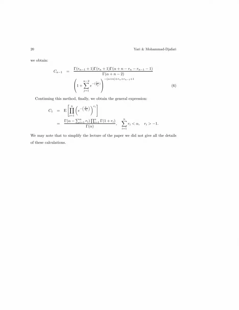
we obtain:
Cn−1 =Γ(rn−1 + 1)Γ(rn + 1)Γ(α + n − rn − rn−1 − 1)
Γ(α + n − 2)
1 +
n−2∑
j=1
e−(
xjθj
)
−(α+n)+rn+rn−1+1
(6)
Continuing this method, finally, we obtain the general expression:
C1 = E
[
n∏
i=1
(
e−
(
Xiθi
))ri
]
=Γ(α −
∑ni=1 ri)
∏ni=1 Γ(1 + ri)
Γ(α),
n∑
i=1
ri < α, ri > −1.
We may note that to simplify the lecture of the paper we did not give all the details
of these calculations.

Information and Covariance Matrices 21
References
[1] M. Abramowitz and I. A. Stegun, Handbook of Mathematical Functions. National
Bureau of Standards, Applied Mathematics Series (1972), no. 55.
[2] B. C. Arnold, Multivariate logistic distributions, New York: Marcel Dekker, 1992.
[3] N. Balakrishnan, Handbook of the logistic distribution, New York: Marcel Dekker,
1992.
[4] V. Brazauskas, Information matrix for Pareto (IV), Burr, and related distribu-
tions, Comm. Statist. Theory and Methods 32 (2003), no. 2, 315–325.
[5] I. W. Burr, Cumulative frequency functions, Ann. of Math. Statist.
[6] , A uesful approximation to the normal distribution function with applica-
tion for simulation, Technometrics.
[7] C. Dagum, A systematic approach to the generation of income distribution models,
Journal of Income Distribution 6 (1996), 105–326.
[8] E.J. Gumbel, Bivariate logistic distributions, Amarican Statistical Association 56
(1961), 335–349.
[9] N. L. Johnson, S. Kotz, and N. Balakrishnan, Continuous univariate distributions,
2nd edition, vol. 1, Wiley, New York, 1994.
[10] B. Malik, H.J.and Abraham, Multivariate logistic distributions, Annals of Statis-
tics 1 (1973), 588–590.
[11] R. J. Serfling, Approximation theorems of mathematical statistics, Wiley, New
York, 1980.
[12] A. J. Watkins, Fisher information for Burr XII distribution, RSS96.


