arX

iv:c

ond-

mat

/011

2025

v1 [

cond

-mat

.sta

t-m

ech]

3 D

ec 2

001

Infinitely many states and stochastic

symmetry in a Gaussian Potts-Hopfield model

A.C.D. van Enter and H.G. Schaap∗

February 1, 2008

1 Introduction

In this paper we study the mean-field Potts model with Hopfield-Mattisdisorder, in particular with Gaussianly distributed disorder. This model is ageneralization of the model studied in [BvEN]. It provides yet another exam-ple of a disordered model with infinitely many low-temperature pure states,such as is sometimes believed to be typical for spin-glasses [MPV]. In ourmodel, however, in contrast to [BvEN], instead of chaotic pairs we find thatthe chaotic size dependence is realized by chaotic q(q − 1)-tuples. For thenotion of chaotic size dependence, and the notion of chaotic pairs which wereintroduced by Newman and Stein we refer to [NS, NS2] and references men-tioned there. Compare also [BvEN] and [Nie]. For an extensive discussion ofthe Hopfield model, including some history and its relation with the theoryof neural networks, see [B, pag. 133 and further] or [BG]. A somewhat dif-ferent generalization of the Hopfield model to Potts spins can be found in [G].

We are concerned in particular with the infinite-volume limit behaviour ofthe Gibbs and ground state measures. The possible limit points are labeledas the minima of an appropriate mean-field (free) energy functional. Theseminima can be obtained as solutions of a suitable mean-field equation. Theseminima lie on the minimal-free-energy surface, which is a m(q− 1)-sphere in

∗Instute for Theoretical Physics, Rijksuniversiteit Groningen, NL-9747 AG Groningen,

The Netherlands; e-mail: A.C.D.van.Enter@phys.rug.nl, H.G.Schaap@phys.rug.nl

1

the (e1, · · · , eq)⊗m space. This space for q-state Potts spins and m patternsis formed by the m-fold product of the hyperplane spanned by the end pointsof the unit vectors eq, which are the possible values of the spins. But onlya limited area of the minimal free energy surface is accessible. Only thosevalues for which certain mean-field equations hold, are allowed. These equa-tions have the structure of fixed point equations. We derive them in chapter4. To obtain the Gibbs states we need to find the solutions of these equationson the minimal free energy surface.

The structure of the ground or Gibbs states for q = 2 and ξk Gaussian withm = 2 is known since a few years [BvEN]. Due to the Gaussian distributionwe have a nice symmetric structure: the ground states form a circle. Fora fixed configuration and a large finite volume the possible order-parametervalues become close to two diametrical points (which ones depend on thevolume of the system) on this circle. This paper treats the generalization ofthis structure to q-state Potts spins with q > 2. To have a concrete example,we concentrate on the case q = 3. It turns out that we again obtain a circlesymmetry but also a discrete symmetry, which generalizes the one for Isingspins. One gets instead of a single pair a triple of pairs (living on 3 separatecircles), where for each pair one has a similar structure as for the single pair

for q = 2. For q > 3 we get q(q−1)2

pairs and a similar higher-dimensionalstructure.

Our model displays quenched disorder. This means that we look at a fixed,particular realization of the patterns. It turns out that there is some kind ofself-averaging. The thermodynamic behaviour of the Hamiltonian is the samefor almost every realization. This is the case for the free energy and the as-sociated fixed point equations, as is familiar from many quenched disorderedmodels. However, this is not precisely true for the order parameters. Wewill see that they show a form of chaotic size dependence, i.e. the behaviourstrongly depends both on the chosen configuration and on the way one takesthe infinite-volume limit N → ∞ (that is, along which subsequence).

2 Notations and definitions

We start with some definitions. Consider the set ΛN = {1, · · · , N} ∈ N+.Let the single-spin space χ be a finite set and the N-spin configuration space

2

be χ⊗N . We denote a spin configuration by σ and its value at site i by σi.We will consider Potts spins, in the Wu representation [Wu]. The set χ⊗N isthen the N -fold tensor product of the set χ = {e1, · · · , eq}. The eσ are theprojection of the spinvectors eσ on the hypertetrahedron in Rq−1 spannedby the end points of eσ. For q = 3 we get for example for e1, e2 and e3 thevectors:

{(

10

)

,

(

−12

12

√3

)

,

(

−12

−12

√3

)}

.

The Hamiltonian of our model is defined as follows:

−βHN =β

N

m∑

k=1

N∑

i,j=1

ξki ξkj δ(σi, σj), with

δ(σi, σj) =1

q[1 + (q − 1)eσi · eσj ] ,

where ξki is the i-th component of the random N -component vector ξk. Forthe ξki ’s we choose i.i.d. N(0, 1) distributions. The vectors ξk = (ξk1 , · · · , ξkN),by analogy with the standard Hopfield model, are called patterns. If wecombine the above, we can rewrite the Hamiltonian HN as:

−βHN = βq − 1

qN

m∑

k=1

(

∑

ξki eσi

N

)2

+1

q − 1

(

∑

ξkiN

)2

.

So asymptotically

− βHN = NK

2

m∑

k=1

q2kN , (1)

with K = 2β

(

q − 1

q

)

and order parameters qkN =1

N

N∑

i=1

ξki eσi .

The last term is an irrelevant constant; in fact it approaches zero, due tothe strong law of large numbers. (The ξki ’s are i.i.d. N(0, 1) distributed soEξki = 0.) Note that any i.i.d. distribution with zero mean, finite varianceand symmetrically distributed around zero will give an analogous form ofHN , but we plan to consider only Gaussian distributions, for which we findthat a continous symmetry can be stochastically broken, just as in [BvEN].From now on we drop the subscript N to simplify the notation, when noconfusion can arise.

3

Furthermore we introduce two representations for the order parameters ~q.If we assume m = 2 then ~q = (~q1, ~q2) and the definitions are as follows: if weconsider the space Rq−1 spanned by the vectors e1, · · · , eq , the ~x-plane, wedefine ~q = (x1, · · · , x2(q−1)). It is often more convenient to look at the (higher-dimensional) (e1, · · · , eq)-space. In that case we take ~q = (a1, a2, a3, b1, b2, b3)for q = 3 and an equivalent equation for other values of q. For m 6= 2 thedefinitions are analogous.

3 Ground states

Now it is time to reveal the characteristics of the ground states for the Pottsmodel. First we discuss the simple behaviour for 1 pattern. Then the moreinteresting part: q > 2 and 2 patterns.

3.1 Ground states for 1 pattern

For one pattern ξ the Hamiltonian is of the following form:

−βH = NK

2~q21 =

β

N

N∑

i,j=1

ξiξjδ(σi, σj).

We easily see that the ground states are obtained by directing the spins withξi > 0 in one direction and the spins with ξi ≤ 0 in a different direction.If we have as the distribution for the ξi’s P (ξi = ±1) = 1

2, then the order

parameter is of the form: ~q1 = 12(eσi − eσj ), with 1 ≤ i, j ≤ q and i 6= j,

see also [vEHP]. So for q = 3 we have only 6 ground states. They form a

regular hexagon: (±34,∓

√3

4), ±(3

4,√

34

), (0,±√

32

). This regular hexagon withits interior is the convex set of possible order parameter values. It is easy tosee that for ξi N(0, 1)-distributed we get the same ground states except for

a scaling factor√

2/π multiplying the values of the order parameter values.

3.2 Ground states for 2 patterns

The Hamiltonian for 2 patterns (Gaussian i.i.d.) is:

−βHN =β

N

N∑

i,j=1

(ξiξj + ηiηj)δ(σi, σj) = NK

2(~q2

1 + ~q22).

4

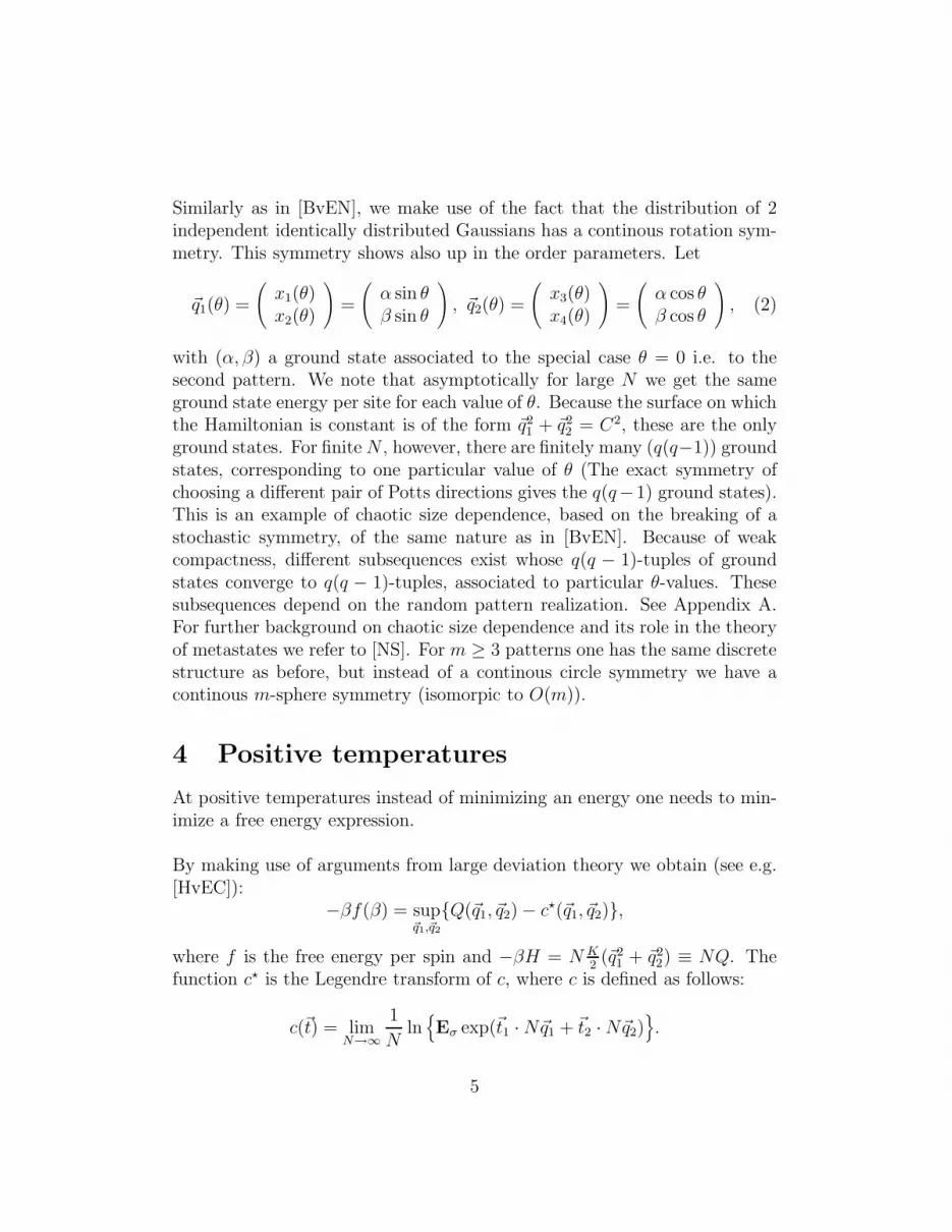
Similarly as in [BvEN], we make use of the fact that the distribution of 2independent identically distributed Gaussians has a continous rotation sym-metry. This symmetry shows also up in the order parameters. Let

~q1(θ) =

(

x1(θ)x2(θ)

)

=

(

α sin θβ sin θ

)

, ~q2(θ) =

(

x3(θ)x4(θ)

)

=

(

α cos θβ cos θ

)

, (2)

with (α, β) a ground state associated to the special case θ = 0 i.e. to thesecond pattern. We note that asymptotically for large N we get the sameground state energy per site for each value of θ. Because the surface on whichthe Hamiltonian is constant is of the form ~q2

1 + ~q22 = C2, these are the only

ground states. For finiteN , however, there are finitely many (q(q−1)) groundstates, corresponding to one particular value of θ (The exact symmetry ofchoosing a different pair of Potts directions gives the q(q−1) ground states).This is an example of chaotic size dependence, based on the breaking of astochastic symmetry, of the same nature as in [BvEN]. Because of weakcompactness, different subsequences exist whose q(q − 1)-tuples of groundstates converge to q(q − 1)-tuples, associated to particular θ-values. Thesesubsequences depend on the random pattern realization. See Appendix A.For further background on chaotic size dependence and its role in the theoryof metastates we refer to [NS]. For m ≥ 3 patterns one has the same discretestructure as before, but instead of a continous circle symmetry we have acontinous m-sphere symmetry (isomorpic to O(m)).

4 Positive temperatures

At positive temperatures instead of minimizing an energy one needs to min-imize a free energy expression.

By making use of arguments from large deviation theory we obtain (see e.g.[HvEC]):

−βf(β) = sup~q1,~q2

{Q(~q1, ~q2) − c⋆(~q1, ~q2)},

where f is the free energy per spin and −βH = N K2(~q2

1 + ~q22) ≡ NQ. The

function c⋆ is the Legendre transform of c, where c is defined as follows:

c(~t) = limN→∞

1

Nln{

Eσ exp(~t1 ·N~q1 + ~t2 ·N~q2)}

.

5

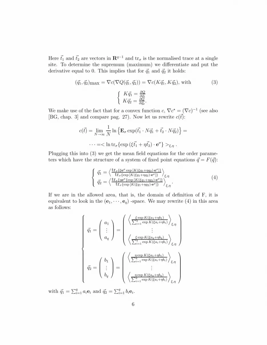
Here ~t1 and ~t2 are vectors in Rq−1 and trσ is the normalised trace at a singlesite. To determine the supremum (maximum) we differentiate and put thederivative equal to 0. This implies that for ~q1 and ~q2 it holds:

(~q1, ~q2)max = ∇c(∇Q(~q1, ~q2)) = ∇c(K~q1, K~q2), with (3)

{

K~q1 = ∂Q∂~q1

K~q2 = ∂Q∂~q2.

We make use of the fact that for a convex function c, ∇c⋆ = (∇c)−1 (see also[BG, chap. 3] and compare pag. 27). Now let us rewrite c(~t):

c(~t) = limN→∞

1

Nln{

Eσ exp(~t1 ·N~q1 + ~t2 ·N~q2)}

=

· · · =< ln trσ{exp (ξ~t1 + η~t2) · eσ} >ξ,η .

Plugging this into (3) we get the mean field equations for the order parame-ters which have the structure of a system of fixed point equations ~q = F (~q):

~q1 =⟨

trσ{ξeσ exp [K(ξq1+ηq2)·eσ ]}trσ{exp [K(ξq1+ηq2)·eσ ]}

⟩

ξ,η

~q2 =⟨

trσ{ηeσ{exp [K(ξq1+ηq2)·eσ ]}trσ{exp [K(ξq1+ηq2)·eσ ]}

⟩

ξ,η.

(4)

If we are in the allowed area, that is, the domain of definition of F, it isequivalent to look in the (e1, · · · , eq) -space. We may rewrite (4) in this areaas follows:

~q1 =

a1...aq

=

⟨

ξ expK(ξa1+ηb1)∑q

i=1expK(ξai+ηbi)

⟩

ξ,η...

⟨

ξ expK(ξaq+ηbq)∑q

i=1expK(ξai+ηbi)

⟩

ξ,η

~q2 =

b1...bq

=

⟨

η expK(ξa1+ηb1)∑q

i=1expK(ξai+ηbi)

⟩

ξ,η...

⟨

η expK(ξaq+ηbq)∑q

i=1expK(ξai+ηbi)

⟩

ξ,η

with ~q1 =∑qi=1 aiei and ~q2 =

∑qi=1 biei.

6

4.1 Ising spins

If we look at the behaviour for N → ∞, then due to the strong law of largenumbers 1

N

∑Ni=1 ξi = Eξ = 0. Each coordinate aj of vector ~q1 = (a1, a2)

is defined as 1N

∑Ni=1 ξiδ(σi, σj). This means that aj is the contribution of

the spins in the j-th direction to the sum 1N

∑Ni=1 ξi. Therefore: a1 + a2 =

1N

∑Ni=1 ξi = 0 a.e. This gives a necessary condition for the allowed area of

Ising spins:a1 = −a2 ∧ b1 = −b2. (5)

Furthermore for all Gibbs states the value of the energy is constant, therefore:

a21 + a2

2 + b21 + b22 =r⋆2

2. (6)

When we substitute (5) in equation (6) and project the result to the (x1, x2)-plane by the projection Π : e1 → 1, e2 → −1, we obtain the followingequation:

x21 + x2

2 = r⋆2.

Thus to get the radius of the circle of Gibbs states r⋆, just take the point~q1 = (a,−a), ~q2 = (0, 0). This corresponds to the point (2a, 0) in the (x1, x2)-plane, by the projection Π. Of course 2a = r⋆.

With this we calculate the equation for the first coordinate of ~q1 in the(e1, e2)-plane by substituting the corresponding fixed point equation:

a =1

2π

∫ ∫

ξexp βξa

exp βξa+ exp (−βξa) exp

(

−ξ2 + η2

2

)

dξdη =

1√2π

∫

ξexp βξa

exp βξa+ exp (−βξa) exp

(

−ξ2

2

)

dξ.

We replaced K by β, because for Ising spins K = 2β(2 − 1)/2 = β. Theequation for the second coordinate of ~q1 we calculate in the same way. Thevector ~q2 is simply (0, 0). Now project ~q1 and ~q2 to the (x1, x2)-plane. Thatis done by subtracting the second coordinate of the ~qi’s from the first one.We get the following equation for the radius r⋆:

r⋆ =1√2π

∫

ξ tanh

(

βξr⋆

2

)

exp

(

−ξ2

2

)

dξ. (7)

7

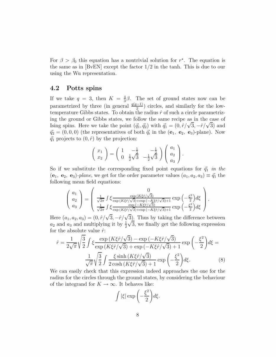
For β > β0 this equation has a nontrivial solution for r⋆. The equation isthe same as in [BvEN] except the factor 1/2 in the tanh. This is due to ourusing the Wu representation.

4.2 Potts spins

If we take q = 3, then K = 43β. The set of ground states now can be

parametrized by three (in general q(q−1)2

) circles, and similarly for the low-temperature Gibbs states. To obtain the radius r of such a circle parametriz-ing the ground or Gibbs states, we follow the same recipe as in the case ofIsing spins. Here we take the point (~q1, ~q2) with ~q1 = (0, r/

√3,−r/

√3) and

~q2 = (0, 0, 0) (the representatives of both ~qi in the (e1, e2, e3)-plane). Now~q1 projects to (0, r) by the projection:

(

x1

x2

)

=

(

1 −12

−12

0 12

√3 −1

2

√3

)

a1

a2

a3

.

So if we substitute the corresponding fixed point equations for ~q1 in the(e1, e2, e3)-plane, we get for the order parameter values (a1, a2, a3) ≡ ~q1 thefollowing mean field equations:

a1

a2

a3

=

01√2π

∫

ξ exp (Kξr/√

3)

exp (Kξr/√

3)+exp (−Kξr/√

3)+1exp

(

− ξ2

2

)

dξ

1√2π

∫

ξ exp (−Kξr/√

3)

exp (Kξr/√

3)+exp (−Kξr/√

3)+1exp

(

− ξ2

2

)

dξ

.

Here (a1, a2, a3) = (0, r/√

3,−r/√

3). Thus by taking the difference betweena2 and a3 and multiplying it by 1

2

√3, we finally get the following expression

for the absolute value r:

r =1

2√π

√

3

2

∫

ξexp (Kξr/

√3) − exp (−Kξr/

√3)

exp (Kξr/√

3) + exp (−Kξr/√

3) + 1exp

(

−ξ2

2

)

dξ =

1√π

√

3

2

∫

ξ sinh (Kξr/√

3)

2 cosh (Kξr/√

3) + 1exp

(

−ξ2

2

)

dξ. (8)

We can easily check that this expression indeed approaches the one for theradius for the circles through the ground states, by considering the behaviourof the integrand for K → ∞. It behaves like:

∫

|ξ| exp

(

−ξ2

2

)

dξ.

8

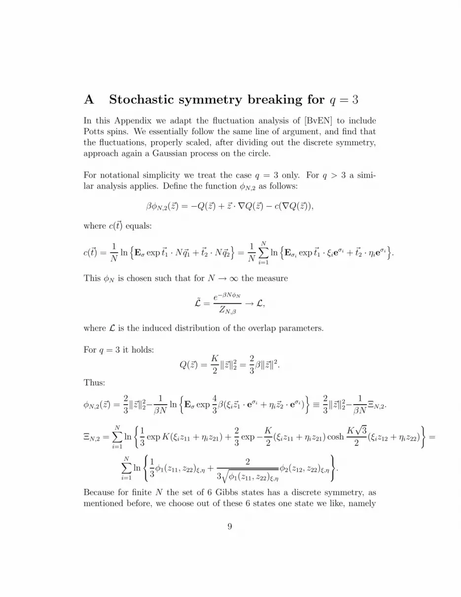
A Stochastic symmetry breaking for q = 3

In this Appendix we adapt the fluctuation analysis of [BvEN] to includePotts spins. We essentially follow the same line of argument, and find thatthe fluctuations, properly scaled, after dividing out the discrete symmetry,approach again a Gaussian process on the circle.

For notational simplicity we treat the case q = 3 only. For q > 3 a simi-lar analysis applies. Define the function φN,2 as follows:

βφN,2(~z) = −Q(~z) + ~z · ∇Q(~z) − c(∇Q(~z)),

where c(~t) equals:

c(~t) =1

Nln{

Eσ exp~t1 ·N~q1 + ~t2 ·N~q2}

=1

N

N∑

i=1

ln{

Eσiexp~t1 · ξieσi + ~t2 · ηieσi

}

.

This φN is chosen such that for N → ∞ the measure

L =e−βNφN

ZN,β→ L,

where L is the induced distribution of the overlap parameters.

For q = 3 it holds:

Q(~z) =K

2‖~z‖2

2 =2

3β‖~z‖2.

Thus:

φN,2(~z) =2

3‖~z‖2

2−1

βNln{

Eσ exp4

3β(ξi~z1 · eσi + ηi~z2 · eσi)

}

≡ 2

3‖~z‖2

2−1

βNΞN,2.

ΞN,2 =N∑

i=1

ln

{

1

3expK(ξiz11 + ηiz21) +

2

3exp−K

2(ξiz11 + ηiz21) cosh

K√

3

2(ξiz12 + ηiz22)

}

=

N∑

i=1

ln

1

3φ1(z11, z22)ξ,η +

2

3√

φ1(z11, z22)ξ,ηφ2(z12, z22)ξ,η

.

Because for finite N the set of 6 Gibbs states has a discrete symmetry, asmentioned before, we choose out of these 6 states one state we like, namely

9

the one of the form (0,±α sin θ, 0,±α cos θ). Note that the θ depends bothon N and on the realization of the random disorder variable. Then z11 =z21 = φ1 = 0. Inserting this and defining z12 = z1 and z22 = z2 we get for φ:

φ(z1, z2) =2

3‖(z1, z2)‖2

2 −1

βN

N∑

i=1

ln

{

1

3+

2

3cosh

2√3β(ξiz1 + ηiz2)

}

.

Putting (z1, z2) = 2√3(z1, z2) we obtain:

φ(z1, z2) =1

2‖(z1, z2)‖2

2 −1

βN

N∑

i=1

ln{

1

2+ cosh β(ξiz1 + ηiz2)

}

− 1

βNln

2

3.

¿From now on the last term will be ignored. So it is enough to prove nowthat with the 1

2term we get the desired chaotic pairs structure between the

patterns due to the quenched disorder for this class of ground states, oncewe divide out the appropriate discrete Potts permutation symmetry. Thusthe original model displays chaotic 6-tuples.

Therefore we only need to control the fluctuations of φ. Define

f ⋆N(~z)−Ef ⋆N (~z) ≡ 1

βN

N∑

i=1

ln {cosh β~z · (ξ, η)}− 1

βN

N∑

i=1

E ln {cosh β~z · (ξ, η)}.

(9)This is the fluctuation of the Ising case which we can estimate by [BvEN].Denote the corresponding φ function by φ⋆. We start with the followinglemma:

Lemma A.1

exp (−βNφ) ≤ exp (−βNφ⋆). (10)

Proof:

Because

exp (−βNφ) = exp (−βNEφ⋆) exp (−βN(φ− Eφ⋆),

we only have to estimate the quantity φ−Eφ⋆. Notice that also a lower boundis essential, because the quantity can become negative. First the estimatefrom above:

φ− Eφ⋆ =1

βN

N∑

i=1

ln{

1

2+ cosh β~z · (ξ, η)

}

− 1

βN

N∑

i=1

E ln {cosh β~z · (ξ, η)}.

10

Now use

ln{

1

2+ cosh β~z · (ξ, η)

}

= ln

{

1 +1

2 cosh β~z · (ξ, η)

}

+ln {cosh β~z · (ξ, η)} ≤

ln {cosh β~z · (ξ, η)} + ln3

2to get

φ−Eφ⋆ ≤ 1

βN

N∑

i=1

ln {cosh β~z · (ξ, η)}− 1

βN

N∑

i=1

E ln {cosh β~z · (ξ, η)}+1

βln

3

2=

f ⋆N(~z) −Ef ⋆N(~z) +1

βln

3

2. (11)

This is because cosh x ≥ 1 for all x ∈ R.

The lower bound is easy because:

1

βN

N∑

i=1

ln{

1

2+ cosh β~z · (ξ, η)

}

≥ 1

βN

N∑

i=1

ln {cosh β~z · (ξ, η)}.

This is due to the fact that the function lnα is monotonically increasing inα. Then it follows that:

φ− Eφ⋆ ≥ f ⋆N(~z) − Ef ⋆N(~z). (12)

Combine (11), (12) and use the fact that in the limit limN→∞ the constantterm 1

βln 3

2does not contribute to the expression exp {−βN(φ− Eφ⋆)} to

conclude the proof of lemma A.1.

Henceforth it is convenient to transform φ⋆ to polar coordinates. Definez = (r cos θ, r sin θ). Then (9) transforms to:

|f ⋆N(r, θ)| =

∣

∣

∣

∣

∣

1

βEψEζ ln cosh {βζr cosψ} − 1

βN

N∑

i=1

ln cosh {βrζi cos (θ − ψi)}∣

∣

∣

∣

∣

=

|Ef ⋆N(r, θ) − f ⋆N(r, θ)|.Here ζ, ψ denote the polar decomposition of the two-dimensional vector (ξ, η),i.e. ζ is distributed with density x exp−x2/2 on R+ and ψ uniformly on thecircle [0, 2π). See [BvEN, page 188]. This we see easily because:

ξz1+ηz2 = (ζ cosψ)(r cos θ)+(ζ sinψ)(r sin θ) = ζr(cos θ cosψ+sin θ sinψ) =

11

ζr cos (θ − ψ) and Eψ cos (θ − ψ) = Eψ cosψ.

With φ⋆ in this form, estimate (10) of lemma A.1 is not very useful, sincethe fluctuations of φ reach their minimum for a different radius (in r) ingeneral than the fluctuations of φ⋆ (in r⋆). Thus we need to transform φ⋆

such that the fluctuations of the transformed φ⋆ reach their minimum at thesame radius r as those of φ. This we achieve as follows. There is a uniformtransformation Π which translates all the points on the circle with radius r⋆

centered at the origin to the circle centered at the origin with radius r, theradius of φ. If we apply Π to φ⋆(r, θ) then we get φ⋆(r + r⋆ − r), the desiredtransformation of φ⋆(r, θ). Now we can prove the next lemma:

Lemma A.2 For every ǫ > 0 holds:

|f ⋆N(r, θ)| ≤ |f ⋆N(r + r⋆ − r, θ)| + ǫ. (13)

The constant r⋆ is the radius of the circle parametrizing the set of mean-fieldsolutions in the Ising case (q = 2). The constant r is the radius r in thePotts case q = 3 rescaled by the factor 2/

√3, thus r = (2/

√3)r.

Proof:

We use the following estimate, which is lemma 2.5 from [BvEN]:

|Ef ⋆N(r, θ) − f ⋆N (r, θ)| ≤ ǫ

2a.e. on every bounded set. (14)

Define:

O = {~z ∈ R2 : ‖~z‖ > r⋆ + δ}, O′ = {~z ∈ R2 : ‖~z‖ > r + δ}.

Set O ⊂ O′ because r ≤ r⋆. Check this by using (7) and (8) and the scaling-factor 2/

√3 for r. Decompose O′ as O ∪ O′ \ O. Because O′ \ O is a finite

set we can use estimate (14). With the already obtained estimate for O in[BvEN], (13) holds for all (r, θ) ∈ O′. Because of (14) is true for all finitesets, (13) holds for all (r, θ).

Note that in a neighbourhood of r it is equivalent to look in a neighbourhoodof r⋆. Now we are able to prove the following theorem:

12

Theorem A.1 Let L be the induced distribution of the overlap parametersand let m = m(θ) = (r cos θ, r sin θ), where θ ∈ [0, π) is a uniformly dis-tributed random variable. Then:

LN,β D→ 1

2δm(θ) +

1

2δ−m(θ) ≡ L∞,β[m].

Furthermore, the (induced) AW-metastate is the image of the uniform distri-bution of θ under the measure-valued map θ → L∞,β[m(θ)].

First we prove the following two lemmas:

Lemma A.3 For φN and ξi, ηi, with i ∈ N as defined above, there existstrictly positive constants W,W ′, l, l′ such that (r is the largest solution of(8))

∫

|‖~z‖−r|≥δN e−βNφN (~z)d~z

∫

|‖~z‖−r|<δN e−βNφN (~z)d~z

≤We−WN l

on a set of P-measure at least 1 −W ′e−K′N l′

, where δN = N− 1

10 .

Lemma A.4 Assume the hypotheses of lemma A.3. Let aN = N−1/25. Thenthere exist strictly positive constants K1, K2, C1, C2 such that on a set of P-measure at least 1 −K1e

−N1/25

the following bound holds,

∫

A′

Ne−βNφN (~z)d~z

∫

ANe−βNφN (~z)d~z

≤ C1e−N1/5

,

where

AN = {(r, θ) ∈ R+0 × [0, 2π)||r− r| < δN , gN(θ) − minθgN(θ) < aN}

A′N = {(r, θ) ∈ R+

0 × [0, 2π)||r− r| < δN , gN(θ) − minθgN(θ) ≥ aN}.

Here

gN(θ) =

√N

βEψEζ ln

{

1

2+ cosh βζr cosψ

}

− 1

β√N

N∑

i=1

ln{

1

2+ cosh {βrζi cos (θ − ψi)}

}

,

which is the polar coordinate form of the function gN(~z), which is defined as:

gN(~z) =1√N

N∑

i=1

{

ln{

1

2+ cosh β~z · (ξ, η)

}

−E ln{

1

2+ cosh β~z · (ξ, η)

}}

.

13

It is convenient to look at the following decomposition:

(φN − EφN)(~z) = β√N(gN(~z′) + hN (~z)), where

hN(~z) = gN(~z) − gN(~z′).

The variable ~z′ is the projection of ~z onto S1(r). Note that β√NgN =

φN − EφN ≡ fN . Define g⋆N and h⋆N in the same way but as decompositionof f ⋆N instead of fN .

Proof of lemma A.3:

Compare lemma 2.1 in [BvEN]. Define:

O = {~z ∈ R2 : ‖~z‖ > r⋆ + δ}, O′ = {~z ∈ R2 : ‖~z‖ > r + δ},

I = {~z ∈ R2 : ‖~z‖ ≤ r⋆ − δ}, I ′ = {~z ∈ R2 : ‖~z‖ ≤ r − δ}.Now we first estimate the numerator which we can also write as:

∫

|‖~z‖−r|≥δNe−βNφN (~z)d~z =

∫

O′∪I′

e−βNEφN (~z)e−βN(φN (~z)−EφN (~z)).

With lemma A.2 we have the following inequality:

sup~z∈O′

|f ⋆N(r, θ)| − ǫ ≤ sup~z∈O′

|f ⋆N(r + r⋆ − r, θ)| = sup~z∈O

|f ⋆N(r)|

P

[

sup(r,θ)∈O′

|f ⋆N(r, θ)| − ǫ ≥ C

2(r − r)2

]

≤ P

[

sup(r,θ)∈O

|f ⋆N(r, θ)| ≥ C

2(r − r⋆)2

]

.

(15)Lemma 2.4 of [BvEN] tells us that this event is of measure zero. Now we canestimate the integral.

First we estimate Eφ⋆N(~z). Because Eφ⋆N(~z) is a bounded function, in eachbounded interval one can always bound it from below by a function of thefollowing kind:

Eφ⋆N(~z) ≥ C(‖~z‖ − r)2 + Eφ⋆N(r), with C a positive bounded constant.

ThenEφ⋆N(~z + r⋆ − r) ≥ C(‖~z‖ − r⋆)2 + EφN(r⋆),

14

when we apply Π to this estimate. Now use estimate (15) with this constantC. Then it holds:∫

O′

e−βNEφN (~z)e−βN(φN (~z)−EφN (~z))dz ≤∫

Oe−βNEφ⋆

N (~z+r⋆−r)eβN |f⋆N (~z)|eǫβNd~z ≤

e−βN(Eφ⋆N (r⋆)−ǫ)

∫

Oe−βNC(r−r⋆)2eβN

C2

(r−r⋆)2dr = eβN(Eφ⋆N (r⋆)−ǫ)

∫

Oe−βN

C2

(r−r⋆)2dr ≤

· · · ≤ 2π2

βNCexp (−βN(Eφ⋆N(r⋆) − ǫ)) exp−βNC2

(

δ2

4

)

.

For further details see [BvEN]. The interior I gives a similar expression.Notice that the image of I under the transformation Π: r → r + r⋆ − r isI \ B(0, r⋆ − r). The ball B(0, r⋆ − r) is a finite set so we can integrateover I instead of I \ B(0, r⋆ − r) by (14). To estimate the denominator wejust replace r⋆ by r in the expressions of the proof of lemma 2.1 in [BvEN,pag.192,193]. Combining the estimates for the numerator and the denomi-nator gives the desired result.

Proof of lemma A.4:

¿From this moment we ignore the constants which enter by applying lemmaA.1, because they cancel out when we divide the numerator by the denomi-nator. For |hN | it holds:

|hN | ≤ |h⋆N | ≤ ǫ,

by lemma 2.6 of [BvEN]. Consider the following integral:

∫

θ:gN(θ)>aN +minθgN (θ)e−

√NgN (θ) ≤ 2πe−

√NminθgN (θ)e

√NaN .

Henceforth it is just a matter of plugging in to get the desired estimate onthe denominator. We refer to [BvEN] for the details. One gets a estimatefor the denominator in the same way. By dividing the two estimates lemmaA.4 is proven.

Proof of theorem A.1:

In the preceding paragraphs we have seen that the measures L concentrateon a circle at the places where the random function gN(θ) takes its minimum.Now it only remains to show that these sets degenerate to a single point, a.s.

15

in the limit N → ∞. If we have proven it for L, then we have proven it alsofor L, because limN→∞ L = L. With the help of [BvEN] this is very easy,because we can use Proposition 3.4 with the function

g(.) = ln{

cosh β.+1

2

}

.

This works because g is an aperiodic even function. And of course Proposition3.7 also holds for this g. These two propositions we use, tell us that theprocess ηN = gN(θ) − EgN(θ) converges to a strictly stationary Gaussianprocess, having a.s. continuously differentiable sample paths. And on anyinterval [s, s + t], t < π the function ηN has only one global minimum.Furthermore, if we define the sets:

LN = {θ ∈ [0, π) : ηN(θ) − minθ′ηN(θ′) ≤ ǫN},

with ǫN some sequence converging to zero, LND→ θ⋆. Then the remarks

below Proof of theorem 3 in [BvEN] conclude the proof.

This research was supported by the Samenwerkingsverband MathematischeFysica. A.v.E. thanks Christian Borgs for asking the question how the resultsof [BvEN] generalize to Potts spins.

References

[vEHP] A.C.D. van Enter, J.L. van Hemmen, and C. Pospiech, Mean-fieldtheory of random-site q-state Potts models, J. Phys. A 21, 791–801(1988).

[BvEN] A. Bovier A.C.D. van Enter, B. Niederhauser, Stochasticsymmetry-breaking in a Gaussian Hopfield model, J. Stat. Phys.95, 181–213 (1999).

[B] A. Bovier, Statistical mechanics of disordered systems, MaPhyStoLecture Notes 10, Aarhus (2001).

[BG] A. Bovier, V. Gayrard, Hopfield models as generalized randommean field models, in Mathematical Aspects of spin glasses andneural networks, Progress in Probability 41, Birkhauser, Boston,(1997).

16

[G] V. Gayrard, Thermodynamic limit of the q-state Potts-Hopfieldmodel with infinitely many patterns, J. Stat. Phys. 68, 977-1011(1992).

[HvEC] J.L. van Hemmen, A.C.D. van Enter, and J. Canisius, On a clas-sical spin glass model, Z. Phys. B - Condensed matter 50, 311-336(1983).

[MPV] M. Mezard, G. Parisi and M.‘A. Virasoro, Spin Glass Theory andBeyond, World scientific, (1987).

[Nie] B. Niederhauser, Mathematical Aspects of Hopfield Models, Disser-tation TU-Berlin, 2000.

[NS] C.M. Newman and D.L. Stein, Thermodynamic Chaos and thestructure of short-range spin glasses, in Mathematical Aspectsof spin glasses and neural networks, Progress in Probability 41,Birkhauser, Boston, (1997).

[NS2] C.M. Newman and D.L. Stein, The State(s) of Replica Symme-try Breaking: Mean Field Theories vs Short-Ranged Spin Glasses,formerly known as Replica Symmetry Breaking’s New Clothes, J.Stat.Phys. to appear, cond-mat/0105282 (2001).

[Wu] F.Y. Wu, The Potts-model, Rev. Mod. Phys. 54, 235 (1982).

17