Seediscussions,stats,andauthorprofilesforthispublicationat:https://www.researchgate.net/publication/274645007

InferenceofMarkovianPropertiesofMolecularSequencesfromNGSDataandApplicationstoComparativeGenomics

ARTICLEinBIOINFORMATICS·APRIL2015

ImpactFactor:4.98·DOI:10.1093/bioinformatics/btv395·Source:arXiv

CITATION

1

READS

89

6AUTHORS,INCLUDING:

JieRen

UniversityofSouthernCalifornia

6PUBLICATIONS64CITATIONS

SEEPROFILE

MinghuaDeng

PekingUniversity

87PUBLICATIONS2,358CITATIONS

SEEPROFILE

GesineReinert

UniversityofOxford

76PUBLICATIONS1,032CITATIONS

SEEPROFILE

FengzhuSun

UniversityofSouthernCalifornia

208PUBLICATIONS5,318CITATIONS

SEEPROFILE

Allin-textreferencesunderlinedinbluearelinkedtopublicationsonResearchGate,

lettingyouaccessandreadthemimmediately.

Availablefrom:JieRen

Retrievedon:03February2016

Inference of Markovian Properties of Molecular Sequences fromNGS Data and Applications to Comparative Genomics

Jie Ren1, Kai Song2, Minghua Deng2, Gesine Reinert3, Charles H. Cannon4,5 and Fengzhu Sun∗1,6,

1Molecular and Computational Biology Program, University of Southern California, Los Angeles, California, USA;2School of Mathematical Sciences, Peking University, Beijing, China;

3Department of Statistics, University of Oxford, 1 South Parks Road, Oxford OX1 3TG, UK;4Department of Biological Sciences, Texas Tech University, TX 79409-3131, USA;

5Xishuangbanna Tropical Botanic Garden, Chinese Academy of Sciences, Yunnan, China;6Centre for Computational Systems Biology, School of Mathematical Sciences, Fudan University, Shanghai, China.

Abstract

Next Generation Sequencing (NGS) technologies generate large amounts of short read data formany different organisms. The fact that NGS reads are generally short makes it challenging toassemble the reads and reconstruct the original genome sequence. For clustering genomes usingsuch NGS data, word-count based alignment-free sequence comparison is a promising approach, butfor this approach, the underlying expected word counts are essential.

A plausible model for this underlying distribution of word counts is given through modelling theDNA sequence as a Markov chain (MC). For single long sequences, efficient statistics are availableto estimate the order of MCs and the transition probability matrix for the sequences. As NGS data donot provide a single long sequence, inference methods on Markovian properties of sequences basedon single long sequences cannot be directly used for NGS short read data.

Here we derive a normal approximation for such word counts. We also show that the traditionalChi-square statistic has an approximate gamma distribution, using the Lander-Waterman model forphysical mapping. We propose several methods to estimate the order of the MC based on NGSreads and evaluate them using simulations. We illustrate the applications of our results by clusteringgenomic sequences of several vertebrate and tree species based on NGS reads using alignment-freesequence dissimilarity measures. We find that the estimated order of the MC has a considerable effecton the clustering results, and that the clustering results that use a MC of the estimated order give aplausible clustering of the species.

Our implementation of the statistics developed here is available as R package “NGS.MC” athttp://www-rcf.usc.edu/˜fsun/Programs/NGS-MC/NGS-MC.html.

Keywords: NGS; Alignment-free; Markov chain; Lander-Waterman model

1 Introduction

NGS technologies generate large amounts of overlapping short read data for many different organisms;for example a read is a subsequence of less than 400 bps for Illumina and 700 bps for 454 sequencingtechnologies, and can sometimes be much shorter. The fact that NGS reads are generally short makes itchallenging to reconstruct the original genome sequence.∗to whom correspondence should be addressed; fsun@usc.edu

1

arX

iv:1

504.

0095

9v1

[q-

bio.

GN

] 4

Apr

201

5

Recently several word-count based alignment-free sequence comparison methods have been appliedto infer the relationship among different species (Song et al., 2013; Yi and Jin, 2013) and metagenomicsamples (Behnam and Smith, 2014; Hurwitz et al., 2014; Jiang et al., 2012; Wang et al., 2014) basedon NGS reads without assembly. Our alignment-free sequence dissimilarity measures, d∗2 and dS2 (Songet al., 2014, 2013), and their variants (Behnam et al., 2013; Liu et al., 2011; Ren et al., 2013) have shownpromise. These methods require the knowledge about the approximate distribution of word counts in theunderlying sequences. While a model which assumes that all letters in the sequence are equally likelyis relatively straightforward to analyse, see Reinert et al. (2009), a Markov model for the underlyingsequences is more realistic.

Markov chains (MC) have been widely used to model molecular sequences (Almagor, 1983) withmany applications including the study of dependencies between the bases (Blaisdell, 1985), the enrich-ment and depletion of certain word patterns (Pevzner et al., 1989), prediction of occurrences of long wordpatterns from short patterns (Arnold et al., 1988; Hong, 1990), and the detection of signals in introns (Av-ery, 1987). Narlikar et al. (2013) studied the effect of the order of MCs on several biological problemsincluding phylogenetic analysis, assignment of sequence fragments to different genomes in metagnomicstudies, motif discovery, and functional classification of promoters. These applications showed the im-portance of accurate specification of the order of MCs. Reliable estimators for the order of the MC andthe transition probability matrix based on the sequence data are crucial.

Based on relatively long molecular sequences, for a general finite state MC sequence of letters froma finite alphabet A = {1, 2, · · · , L} of size L, Hoel (1954) showed, under the hypothesis that the longsequence follows a (k − 2)-th order MC, that twice the log-likelihood ratio of the probability of thesequence under a (k− 1)-th order MC versus that under the (k− 2)-th order MC model follows approx-imately a χ2-distribution with dfk = (L − 1)2Lk−2 degrees of freedom under general conditions. Healso approximated the log-likelihood ratio by the Pearson-type statistic

Sk =∑

w∈Ak

(Nw − Ew)2

Ew, (1)

which is also approximately χ2-distributed with the same degrees of freedom. Here, w = w1w2 · · ·wkdenotes a k-word formed of letters wi ∈ A, −w = w2 · · ·wk, w− = w1w2 · · ·wk−1, and −w− =

w2 · · ·wk−1; Nw denotes the count of the word w in the sequence, and Ew =N−wNw−N−w−

is the estimatedexpected count of w if the sequence is generated by a MC of order k−2. Here k ≥ 3; see also Avery andHenderson (1999) for a detailed study, Billingsley (1961a,b) for an an excellent exposition of statisticalissues related to MCs, as well as Ewens and Grant (2005); Reinert et al. (2000, 2005); Waterman (1995)for applications to sequence analysis.

The Chi-square statistic (1) and the log-likelihood ratio statistics can be used to test the order of a MC,using all k-words w ∈ Ak. When a particular order of MC is rejected, we can identify particular wordpatterns that are exceptional, through the approximate distribution of Nw. The approximate distributionsof Nw in long sequences is well understood, see for example Reinert et al. (2000, 2005); Waterman(1995). In particular, suppose that the sequence follows a stationary (k − 2)-th order MC and let

σ2w = Ew

(1− N−w

N−w−

)(1− Nw−

N−w−

).

ForZw =

Nw − Ew

σw, (2)

Theorem 6.4.2 in Reinert et al. (2005) gives that, as sequence length goes to infinity, for all real valuesx, P(Zw ≤ x) → Φ(x), where Φ denotes the cumulative distribution function of a standard normal

2

variable. We also say that Zw converges to the standard normal distribution N(0, 1) in distribution. Thisasymptotic result can then be used to find exceptional words in long sequences.

Given an NGS short read sample, it is tempting to use the test statistic Sk defined in (1) to test theorder of a MC by simply counting the number of the occurrences of words in short read data. However,as the short reads from NGS data are sampled randomly from the genome, some parts of the genomeare possibly not sampled and some parts are possibly sampled extensively. The sampling process intro-duces additional randomness to the statistic, and makes Sk deviate from its traditional χ2 -distribution.Similarly, the approximate distribution of Zw given in (2) will be different from the standard normaldistribution.

In this paper, we study these approximate distributions, both theoretically and by simulations. Firstwe extend the statistics Sk and Zw for a MC sequence to SRk and ZRw for the NGS read data. Our un-derlying model for the distribution of reads along the genome is the potentially inhomogeneous Lander-Waterman model for physical mapping (Lander and Waterman, 1988). We discover that for a set of shortreads sampled from a (k − 2)-th order MC sequence, the statistic SRk follows approximately a gammadistribution with shape parameter dfk/2 and scale parameter 2d, where d is a factor related to the distri-bution of the reads along the genome. We also show that, with the same factor d, the distribution of thesingle word statistic ZRw/

√d tends to the standard normal distribution. Based on the theoretical results,

we introduce an estimator for the order of the MC using NGS data. For practical purposes, we also givean estimator for the factor d when the underlying reads sampling distribution is unknown. To the best ofour knowledge, this is the first study of the Markovian properties of molecular sequences based on NGSread data.

To illustrate our theoretical results and our estimators, we first carry out a simulation study based ontransition probability matrices which are estimated from cis-regulatory module (CRM) DNA sequences,and insert repeats. We simulate different read lengths, numbers of reads, inhomogeneous sampling, aswell as sequencing errors, and we include a regime where the sampling rate depends on the GC content.If the GC bias is not very strong or the sequencing depth is not very low, then the simulation results agreewith our theoretical predictions despite the theoretical assumptions being slightly violated.

Next we apply our methods to cluster 28 vertebrate species using our alignment-free dissimilaritymeasures d∗2 and dS2 under different MC models which are estimated from NGS read samples. Theestimated orders based on NGS data without assembly are found to be consistent with those inferreddirectly from the long genome sequences. The clustering performs best when using MCs around theestimated order. Applying the same analysis to 13 tropical tree species whose genomes are unknown,based on their NGS read samples, the most plausible clustering is achieved when using a MC model oforder close to the one estimated from the NGS reads.

The paper is organized as follows. The “Methods” section contains the probabilistic models ofgenerating the MC sequence and sampling the short reads, as well as the theorem for the approximatedistributions of SRk and ZRw for NGS data. This theorem is used to derive our estimators for the orderof the MC and for the factor d. In the “Results” section, we first provide extensive simulation studiesincluding the comparison of the theoretical approximate distributions and the simulated results for SRkand ZRw, the effect of inhomogeneous sampling and sequencing errors, the efficiency of the estimatorof the factor d, and the evaluations of the methods for estimating the MC order. Second, we estimatethe orders of the MCs for 28 vertebrate species based on the simulated whole genome NGS samples.We then use our dissimilarity measures d∗2 and dS2 to cluster the NGS samples of the 28 species underdifferent MC orders to see the effect on the performance of the clustering. The applications show thatour new methods are effective for the inference of relationships among sequences based on NGS reads.Finally, we use our methods to study the relationships among 13 tree species whose complete genomicsequences as well as their phylogenetic relationships are unknown. Our clustering results are consistentwith the physical characteristics of the tree species. The paper concludes with some discussion of the

3

study.

2 Methods

2.1 Probabilistic modeling of a MC sequence and random sampling of the reads usingNGS

In NGS, a large number of reads are randomly sampled from the genome. Hence two random processesare involved in the generation of the short read data: the generation of the underlying genome sequenceand the random sampling of the reads.

We use an r-th order homogeneous ergodic MC to model the underlying genome sequence with eachletter taking values in a finite alphabet set A of size L. Since our study is based on genomic sequences,L = 4. As in Daley and Smith (2013); Lander and Waterman (1988); Simpson (2014); Zhai et al. (2012);Zhang et al. (2008), we assume that the genome is continuous and that the distribution of reads along thegenome follows a potentially inhomogeneous Poisson process with rate c(x) at position x. If c(x) = cfor all x, we refer to the sampling of the reads as homogeneous. We assume that all sampled reads havethe same length of β bps. A total of M reads are independently sampled from the genome of length Gbps.

We extend the statistics Sk and Zw in (1) and (2) to NGS short read data accordingly. Let NRw be

the number of occurrences of the k-word w in the short read data, where the superscript R refers to the“read” data, and define

SRk =∑

w∈Ak

(NR

w − ERw)2

ERw, (3)

ZRw =NR

w − ERwσRw

, (4)

where

ERw =NR−wN

Rw−

NR−w−

and (σRw)2 = ERw

(1−

NR−w

NR−w−

)(1−

NRw−

NR−w−

).

We have the following theorem on the approximate distributions of SRk and ZRw; the proof is given inthe Supplementary Materials. Note that for each read we discard the last k − 1 positions as they wouldlead to words of length less than k; the error made with this approximation is asymptotically negligiblewhen k is small relative to β.

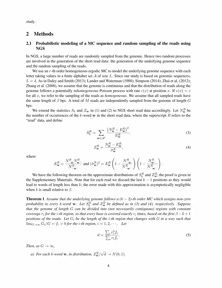
Theorem 1 Assume that the underlying genome follows a (k − 2)-th order MC which assigns non-zeroprobability to every k-word w. Let SRk and ZRw be defined as in (3) and (4), respectively. Supposethat the genome of length G can be divided into (not necessarily contiguous) regions with constantcoverage ri for the i-th region, so that every base is covered exactly ri times, based on the first β− k+ 1positions of the reads. Let Gi be the length of the i-th region that changes with G in a way such thatlimG→∞Gi/G = fi > 0 for the i-th region, i = 1, 2, · · · . Let

d =

∑i r

2i fi∑

i rifi. (5)

Then, as G→∞,

a) For each k-word w, in distribution, ZRw/√d→ N(0, 1).

4

b) The statistic SRk /d has an approximate χ2-distribution with dfk = (L− 1)2Lk−2 degrees of free-dom; equivalently, the statistic SRk has an approximate gamma distribution with shape parameterdfk/2 and scale parameter 2d.

If the M reads are sampled homogeneously along the genome with coverage c based on the first β−k+1 positions of the reads along the genome, i.e. c = M(β−k+1)

G−k+1 , the Lander-Waterman formula (Landerand Waterman, 1988) shows that the fraction of genome covered ri = i times is fi = exp(−c)ci/i!.Under this assumption, we obtain

d =

∑i i

2fi∑i ifi

=c2 + c

c= c+ 1.

The results in Theorem 1 continue to hold when taking d = c+ 1.In the Lander-Waterman model for physical mapping (Lander and Waterman, 1988), the factor c =

MβG is the coverage of the genome. Hence we refer to d from (5) as the effective coverage of the reads

along the genome based on the first β − k + 1 positions of each read.

2.2 Estimating the order of the MC based on NGS reads

Based on Theorem 1, we can estimate the order r of a MC sequence using NGS reads. First, we testthe null hypothesis that the sequence follows an independent identically distributed (i.i.d; MC order = 0)model. For a test at significance level α, if SR2 /d is higher than the 1− α quantile of the χ2-distributionwith df = (L − 1)2 degrees of freedom, the i.i.d hypothesis is rejected. If this null hypothesis isrejected, then here we propose an estimator for the order of a MC; it is an analog of a correspondingestablished estimator of MC orders based on long sequences that has been shown to be effective. In theSupplementary Materials we present four related estimators as well as estimators based on the AIC andBIC information criteria; the one presented here has the best performance in simulation studies.

We assume that the word length k ≥ 2 and that the assumptions of Theorem 1 are satisfied. Then,for k ≥ r + 2, SRk /d has approximately a χ2-distribution with (L − 1)2Lk−2 degrees of freedom. Ifk < r+ 2, then SRk /d will typically be larger than expected from this χ2-distribution. For k ≥ r+ 2, the

law of large numbers gives thatSRk+1

LSRk

→ 1 for G → ∞; if k < r + 2 then the ratio will be much largerthan 1 in the limit. Therefore we can estimate r as follows:

rSk= argmink

{SRk+1

SRk

}− 1. (6)

In general, we want the value of mink

{SRk+1

SRk

}to be very small, e.g, less than 0.01.

Using the law of large numbers it can be shown that under our assumptions this estimator is consis-tent, in the sense that rSk

tends to r in probability as G tends to infinity.

2.3 Estimating the effective coverage d

Often the effective coverage d is not known and we would like to estimate the effective coverage dusing NGS short read data. From Theorem 1, we can see that, under the general conditions stated inthe theorem, (ZRw)2/d follows a χ2-distribution with one degree of freedom. Since the median of theχ2-distribution with one degree of freedom is about 0.456, we can use the scaled median as a robustestimator for d;

d = median{(ZRw)2, w ∈ Ak}/0.456. (7)

5

When we assume that the underlying long sequence follows a MC of order at most m, we use(m+ 2)-words to estimate d using (7).

Note that for an i.i.d. model sequence, the set of 2-words would not yield meaningful results asthere are only 16 different 2-words and the median based on 16 numbers is generally not reliable. As anunderlying genome sequence following an r-th order MC can also be seen as an (r + 1)-th, (r + 2)-th,. . . , and higher order MC sequence, we can use k-words with relatively large k (≥ r+ 2) to estimate thefactor d, if the maximum order of a MC is unknown beforehand.

2.4 Simulation study

For the simulation study, we first generate MCs of different orders. For realistic parameter values, thetransition probability matrices of the MCs are based on real cis-regulatory module (CRM) DNA se-quences in mouse forebrain from Blow et al. (2010). We use CRM sequences here because CRMsequences are often used to study the effectiveness of alignment-free sequence dissimilarity measures(Goke et al., 2012; Ren et al., 2013; Song et al., 2014). To take into consideration that in real genomicsequences, many repeat regions are present, we insert repeats into the generated MCs. We simulate NGSdata by sampling a varying number of reads of different lengths from the MC, varying genome length aswell as coverage.

We include homogeneous and inhomogeneous sampling of the reads as well as sequencing errors.We also let the sampling rate of the reads depend on the GC content of the fragments based on data fromthe current sequencing technologies (Benjamini and Speed, 2012). We set the sequencing error rate at10%, which is relatively high compared to the true sequencing error rate in real sequencing in order toclearly distinguish among the estimators with regards to their robustness to sequencing errors. When asequencing error occurs at a position, the nucleotide base is changed to one of the other three nucleotideswith equal probability.

Once the NGS reads are generated, we calculate the statistics SRk and ZRw for each word w, the orderestimator rSk

and the estimator for effective coverage d based on (7); each procedure is repeated 1000times. In each repeat experiment, we let the order estimator choose the model from 1st, 2nd, · · · , 5thorder MCs; we estimate the effective coverage d by (7), using 3-tuples for a first order MC, and 4-tuplesfor a second order MC. The details are given in the Supplementary Materials.

2.5 Applications to the study of relationships among organisms

We test our methods on real and simulated NGS data from 28 vertebrate species whose complete genomicsequences are available and that are comprehensively studied in (Karolchik et al., 2008; Miller et al.,2007). We download the genomes of the 28 vertebrate species from UCSC Genome Browser, and thenuse MetaSim (Richter et al., 2008) to simulate reads from each of the 28 vertebrate species. In simulationsthe accuracy of the order estimation increases with read coverage. To reflect a worst-case scenario, weset the read coverage to be 1 as a lower bound for the performance although the current sequencingtechnology can generate data with very high read coverage. We set MetaSim to generate reads of length62bp under the error rate which is estimated by Illumina in our simulations.

To estimate the order of MC based on the NGS sample for each of the 28 species, we apply theorder estimator rSk

in (12); there is no sharp ratio transition found over k = 2, · · · , 14. Given that realgenomes consist of multiple types of regions (coding, non-coding and regulatory regions) and each typemay fit to different MC models, the result indicates that no suitable MC model can adequately fit allthe patterns in the genome. Instead, we fit the data with a MC model that can explain the majority (say80%) of the word patterns in the genome. Motivated by the normal approximation of a particular wordstatistic in Theorem 1, we study the fraction of k-words whose occurrences can be explained using the

6

statistic (ZRw)2/d by comparison to a χ2-distribution with one degree of freedom with type I error 0.01.We estimate the order of MC to be the smallest k − 2 under which more than 80% of k-words can beexplained by the (k − 2)-th order MC.

To cluster the organisms, we use the inferred MC models to estimate the expected number of oc-currences of word patterns and then study the relationships among the organisms using our dissimilaritymeasures d∗2 and dS2 . We briefly present their definitions below, please see Song et al. (2014, 2013) fordetails. Then we apply a similar approach to study the relationships among 13 tree species with NGSreads, for which neither the complete genome sequences nor their relationships are known. To estimatethe unknown effective coverage d using k-words by (7), we let k to be relatively large and use d as thevalue at which the estimated d stabilizes as k increases.

2.6 Alignment-free sequence comparison dissimilarity measures

Consider two sets of NGS reads from two genomes. We use superscripts (1) and (2) to denote the firstand the second read set, respectively. Suppose that M (i) reads of length β(i) are in the i-th data set.Since the reads can come from either the forward strand or the reverse strand of the genome in NGS,we supplement the observed reads by their complements and refer to the joint set of the reads and thecomplements as the read set.

Let N (i)w be the count of the word w in the i-th data set. We define EN (i)

w to be the expected numberof occurrences of word w based on either the i.i.d model or a Markov model, EN (i)

w = M (i)(β(i) −k + 1)(p

(i)w + p

(i)w ), where M (i)(β(i) − k + 1) is the total number of k-word in the i-th sample, w is the

complement of word w, and p(i)w is the probability of word w in the i-th genome under a specific model.

Then we define D∗2 and DS2 as follows,

D∗2 =∑

w∈Ak

N(1)w N

(2)w√

EN(1)w EN

(2)w

, and DS2 =

∑w∈Ak

N(1)w N

(2)w√(

N(1)w

)2+(N

(2)w

)2 ,where N (i)

w = N(i)w − EN (i)

w , i = 1, 2. Further, the dissimilarity measures d∗2 and dS2 , ranging from0 to 1, are defined as,

d∗2 =1

2

1− D∗2√ ∑w∈Ak

(N

(1)w

)2EN

(1)w

√ ∑w∈Ak

(N

(2)w

)2EN

(2)w

, and

dS2 =1

2

1− DS2√√√√ ∑

w∈Ak

(N

(1)w

)2√(N

(1)w

)2+(N

(2)w

)2√√√√ ∑

w∈Ak

(N

(2)w

)2√(N

(1)w

)2+(N

(2)w

)2

.

For comparison, we also use a simplistic dissimilarity measure based on the non-centered correlation

of the word frequencies defined as d2 = 12

1−

∑w∈Ak

N(1)w N

(2)w√ ∑

w∈Ak

(N

(1)w

)2√ ∑w∈Ak

(N

(2)w

)2 .

7

3 Results

3.1 Summary of simulation results

Due to page limitations, we summarize the simulation results here; details are given in the SupplementaryMaterials. Our extensive simulations show that the simulated mean, standard deviation and distributionsof SRk and ZRw are very close to their corresponding theoretical approximations given by Theorem 1.Both the effective coverage and the MC order can be estimated accurately under the parameter settingsof the current sequencing technologies.

3.2 The relationship among 28 vertebrate species

Table S4 shows the estimated orders of MCs for a group of 28 vertebrate species that are studied in(Karolchik et al., 2008; Miller et al., 2007) based on simulated NGS short reads. For each of the 28species, we compute the fraction of the k-words that have (ZRw)2/d within the 99% of a χ2-distributionwith one degree of freedom, for k = 8, 9, . . . , 14. Using 80% as a threshold, we estimate the order ofMC for each species to be the smallest k − 2 under which the fraction of words that can be explained bythe (k − 2)-th order MC is greater than the threshold.

Comparing our results with the results in Narlikar et al. (2013), where the order of MCs for a selectionof vertebrate genomes was estimated by AIC and BIC criteria using whole genome sequences, we findthat the estimated order based on NGS read data are almost the same as that estimated based on the wholegenome sequences in Narlikar et al. (2013). Our proposed methods of estimating the order of MC basedon short reads of NGS data achieve the same accuracy as that based on whole genome sequences.

For a given value of k, we compute d∗2 and dS2 using an r-th order MC, r = 0 (i.i.d model), . . . , (k−2)for each pair of species, yielding a 28 × 28 pairwise dissimilarity matrix under each MC model. Toevaluate the dissimilarity measures, we use the pairwise distance matrix obtained from Figure S1 inMiller et al. (2007) as the gold standard for the dissimilarity between each pair of the 28 species; thematrix is given as Table S5 in the Supplementary Materials. Note that the estimated orders of the 28species range from 7 to 11, and the average order is 10. To study the performance of the dissimilaritymeasures under different orders of MC, we choose k = 14 such that we can study the results under theMC model with orders up to 12.

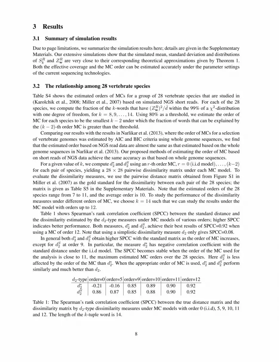
Table 1 shows Spearman’s rank correlation coefficient (SPCC) between the standard distance andthe dissimilarity estimated by the d2-type measures under MC models of various orders; higher SPCCindicates better performance. Both measures, d∗2 and dS2 , achieve their best results of SPCC=0.92 whenusing a MC of order 12. Note that using a simplistic dissimilarity measure d2 only gives SPCC=0.08.

In general both d∗2 and dS2 obtain higher SPCC with the standard matrix as the order of MC increases,except for dS2 at order 9. In particular, the measure d∗2 has negative correlation coefficient with thestandard distance under the i.i.d model. The SPCC becomes stable when the order of the MC used forthe analysis is close to 11, the maximum estimated MC orders over the 28 species. Here dS2 is lessaffected by the order of the MC than d∗2. When the appropriate order of MC is used, d∗2 and dS2 performsimilarly and much better than d2.

d2-type order=0 order=5 order=9 order=10 order=11 order=12d∗2 -0.21 -0.16 0.85 0.89 0.90 0.92dS2 0.86 0.87 0.85 0.88 0.90 0.92

Table 1: The Spearman’s rank correlation coefficient (SPCC) between the true distance matrix and thedissimilarity matrix by d2-type dissimilarity measures under MC models with order 0 (i.i.d), 5, 9, 10, 11and 12. The length of the k-tuple word is 14.

8

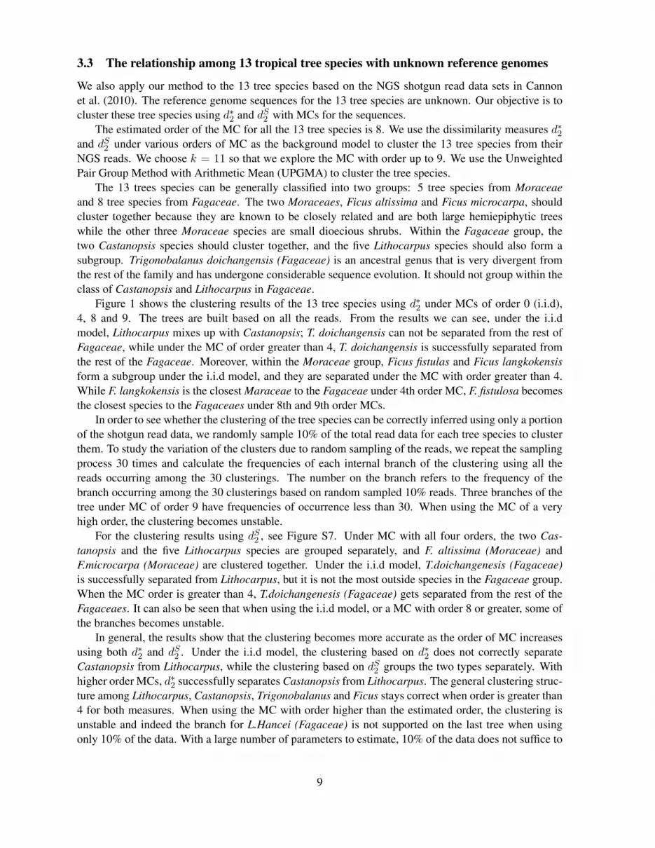
3.3 The relationship among 13 tropical tree species with unknown reference genomes

We also apply our method to the 13 tree species based on the NGS shotgun read data sets in Cannonet al. (2010). The reference genome sequences for the 13 tree species are unknown. Our objective is tocluster these tree species using d∗2 and dS2 with MCs for the sequences.

The estimated order of the MC for all the 13 tree species is 8. We use the dissimilarity measures d∗2and dS2 under various orders of MC as the background model to cluster the 13 tree species from theirNGS reads. We choose k = 11 so that we explore the MC with order up to 9. We use the UnweightedPair Group Method with Arithmetic Mean (UPGMA) to cluster the tree species.

The 13 trees species can be generally classified into two groups: 5 tree species from Moraceaeand 8 tree species from Fagaceae. The two Moraceaes, Ficus altissima and Ficus microcarpa, shouldcluster together because they are known to be closely related and are both large hemiepiphytic treeswhile the other three Moraceae species are small dioecious shrubs. Within the Fagaceae group, thetwo Castanopsis species should cluster together, and the five Lithocarpus species should also form asubgroup. Trigonobalanus doichangensis (Fagaceae) is an ancestral genus that is very divergent fromthe rest of the family and has undergone considerable sequence evolution. It should not group within theclass of Castanopsis and Lithocarpus in Fagaceae.

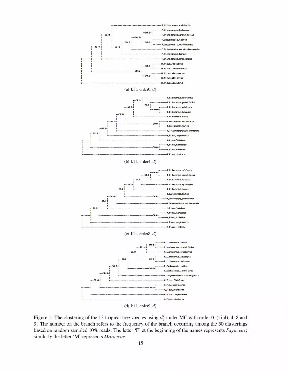
Figure 1 shows the clustering results of the 13 tree species using d∗2 under MCs of order 0 (i.i.d),4, 8 and 9. The trees are built based on all the reads. From the results we can see, under the i.i.dmodel, Lithocarpus mixes up with Castanopsis; T. doichangensis can not be separated from the rest ofFagaceae, while under the MC of order greater than 4, T. doichangensis is successfully separated fromthe rest of the Fagaceae. Moreover, within the Moraceae group, Ficus fistulas and Ficus langkokensisform a subgroup under the i.i.d model, and they are separated under the MC with order greater than 4.While F. langkokensis is the closest Maraceae to the Fagaceae under 4th order MC, F. fistulosa becomesthe closest species to the Fagaceaes under 8th and 9th order MCs.

In order to see whether the clustering of the tree species can be correctly inferred using only a portionof the shotgun read data, we randomly sample 10% of the total read data for each tree species to clusterthem. To study the variation of the clusters due to random sampling of the reads, we repeat the samplingprocess 30 times and calculate the frequencies of each internal branch of the clustering using all thereads occurring among the 30 clusterings. The number on the branch refers to the frequency of thebranch occurring among the 30 clusterings based on random sampled 10% reads. Three branches of thetree under MC of order 9 have frequencies of occurrence less than 30. When using the MC of a veryhigh order, the clustering becomes unstable.

For the clustering results using dS2 , see Figure S7. Under MC with all four orders, the two Cas-tanopsis and the five Lithocarpus species are grouped separately, and F. altissima (Moraceae) andF.microcarpa (Moraceae) are clustered together. Under the i.i.d model, T.doichangenesis (Fagaceae)is successfully separated from Lithocarpus, but it is not the most outside species in the Fagaceae group.When the MC order is greater than 4, T.doichangenesis (Fagaceae) gets separated from the rest of theFagaceaes. It can also be seen that when using the i.i.d model, or a MC with order 8 or greater, some ofthe branches becomes unstable.

In general, the results show that the clustering becomes more accurate as the order of MC increasesusing both d∗2 and dS2 . Under the i.i.d model, the clustering based on d∗2 does not correctly separateCastanopsis from Lithocarpus, while the clustering based on dS2 groups the two types separately. Withhigher order MCs, d∗2 successfully separates Castanopsis from Lithocarpus. The general clustering struc-ture among Lithocarpus, Castanopsis, Trigonobalanus and Ficus stays correct when order is greater than4 for both measures. When using the MC with order higher than the estimated order, the clustering isunstable and indeed the branch for L.Hancei (Fagaceae) is not supported on the last tree when usingonly 10% of the data. With a large number of parameters to estimate, 10% of the data does not suffice to

9

capture the information in the data. The best clustering is achieved under a MC of order 8 and 9.

4 Discussion

Next generation sequencing technologies provide large amount of data in the form of short reads. As-sembly of the millions of short reads to recover the long sequence is challenging, because the relativeshort length of the reads makes it difficult to resolve the repeat regions, not all regions may be cov-ered, and assembly is time consuming. While multiple sequence alignment may be prohibitive, we canuse word-count based dissimilarity measures to cluster the underlying species. These measures requirean underlying probability model for the sequences; Markov chains are a reasonable model for such se-quences. While transition probabilities can be estimated directly from count data, estimating the orderof a MC here is not straightforward.

Methods for estimating the order of a MC of a long sequence have been developed since the 1950s,but estimating the order of a MC directly from a set of short reads without assembly has not been studiedyet. In this paper, we develop two statistics SRk and ZRw and show that both SRk and ZRw have surprisinglysimple approximate distributions with only two parameters, one of them depending on the order ofthe original long MC sequence, and the other one depending on the distribution of the reads along thesequence. Intriguingly, one of these parameters is d = c + 1 under homogeneous sampling, where c isthe coverage of the reads along the genome based on the first β − k + 1 positions of each read.

Based on the property of SRk and ZRw, we develop an estimator for the order of a MC as well as anestimator for the parameter d based on NGS data. Extensive simulation studies are carried out to verifythe theorem and evaluate the estimator.

Finally, we apply the estimation methods to two NGS data sets. Since the real genome sequencesconsist of coding, non-coding and various regulatory regions, single standard MC models do not fit thedata well. Moreover, some enriched patterns, such as the motif sequences, are widespread throughoutthe genomes and violate the simple MC model for the whole genome sequence. Hence studying thefraction of k-words whose occurrences can be explained using the statistic (ZRw)2/d by comparison to aχ2

1 distribution is a more realistic way to determine the order of the MC for a real genome sequence. Theestimated orders are consistent with the orders estimated directly from the full genome sequences usingBIC methods.

Our primary motivation for this study is alignment-free genome comparison using NGS data. Further,we cluster the 28 species based on the NGS data using MC models with various orders. The results showthat the clustering performs best and gives stable results when using a MC model with order on andabove the estimated order. In addition, we apply the same analysis to 13 tropical tree species whosereference genomes are unknown; again the best clustering is achieved under a MC with the order withinthe estimated range.

When the sequence length is short or the sequencing depth is low, the numbers of occurrences ofsome k-words become small or even zero. Then the assumption of non-zero variance for all word countswhich underlies the gamma approximation for SRk no longer holds and the gamma approximation maynot work well. In such a situation an exact test for the order of MCs in the spirit of Besag and Mondal(2013) could be very helpful. In this paper we have only made a start on the Markov chain modellingof NGS data. An exhaustive study of errors in the data, in the form of power studies, could help tofurther understand the application range of our results. Finally, in this work we take the estimation of thetransition probabilities for granted, once the order of the MC is determined. While the estimation of thetransition probabilities of the MC model of a long sequence has been studied by Anderson and Goodman(1957) and Baum and Petrie (1966), it would be interesting to extend these methods to NGS data.

10

Acknowledgments

The authors would like to thank anonymous referees for helpful comments on this work and on previousrelated work. We thank Dr. Xiaohui Xie from UCI for explanation of the 28 vertebrate species. Theresearch is supported by National Natural Science Foundation of China (No.10871009, 10721403), andNational Key Basic Research Project of China (No.2009CB918503). FS is partially supported by USNIH P50 HG 002790 and NSF DMS-1043075 and OCE 1136818. GDR is partially supported by EPSRCEP/K032402/1.

Conflict of Interest: : None declared.

References

Almagor, H. (1983). A Markov analysis of DNA sequences. Journal of Theoretical Biology 104(4),633–645.

Anderson, T. W. and L. A. Goodman (1957). Statistical inference about Markov chains. The Annals ofMathematical Statistics 28(4), 89–110.

Arnold, J., A. J. Cuticchia, D. A. Newsome, W. W. Jennings, and R. Ivarie (1988). Mono-throughhexanucleotide composition of the sense strand of yeast DNA: a Markov chain analysis. NucleicAcids Research 16(14), 7145–7158.

Avery, P. J. (1987). The analysis of intron data and their use in the detection of short signals. Journal ofMolecular Evolution 26(4), 335–340.

Avery, P. J. and D. A. Henderson (1999). Fitting Markov chain models to discrete state series such asDNA sequences. Journal of the Royal Statistical Society: Series C (Applied Statistics) 48(1), 53–61.

Baum, L. E. and T. Petrie (1966). Statistical inference for probabilistic functions of finite state Markovchains. The Annals of Mathematical Statistics 37(6), 1554–1563.

Behnam, E. and A. D. Smith (2014). The amordad database engine for metagenomics. Bioinformat-ics 30(20), 2949–2955.

Behnam, E., M. S. Waterman, and A. D. Smith (2013). A geometric interpretation for local alignment-free sequence comparison. Journal of Computational Biology 20(7), 471–485.

Benjamini, Y. and T. Speed (2012). Summarizing and correcting the gc content bias in high-throughputsequencing. Nucleic Acids Research 40(10), e72.

Besag, J. and D. Mondal (2013). Exact goodness-of-fit tests for Markov chains. Biometrics 69(2),488–496.

Billingsley, P. (1961a). Statistical Inference for Markov Processes, Volume 2. University of ChicagoPress Chicago.

Billingsley, P. (1961b). Statistical methods in Markov chains. The Annals of Mathematical Statis-tics 32(1), 12–40.

Blaisdell, B. E. (1985). Markov chain analysis finds a significant influence of neighboring bases onthe occurrence of a base in eucaryotic nuclear DNA sequences both protein-coding and noncoding.Journal of Molecular Evolution 21(3), 278–288.

11

Blow, M. J., D. J. McCulley, Z. Li, T. Zhang, J. A. Akiyama, A. Holt, I. Plajzer-Frick, M. Shoukry,C. Wright, F. Chen, et al. (2010). Chip-seq identification of weakly conserved heart enhancers. NatureGenetics 42(9), 806–810.

Cannon, C. H., C. S. Kua, D. Zhang, and J. Harting (2010). Assembly free comparative genomicsof short-read sequence data discovers the needles in the haystack. Molecular Ecology 19(Suppl. 1),146–160.

Daley, T. and A. D. Smith (2013). Predicting the molecular complexity of sequencing libraries. NatureMethods 10(4), 325–327.

Ewens, W. J. and G. R. Grant (2005). Statistical methods in bioinformatics: an introduction. Springer.

Glenn, T. C. (2011). Field guide to next-generation DNA sequencers. Molecular Ecology Re-sources 11(5), 759–769.

Goke, J., M. H. Schulz, J. Lasserre, and M. Vingron (2012). Estimation of pairwise sequence similarityof mammalian enhancers with word neighbourhood counts. Bioinformatics 28(5), 656–663.

Hoel, P. G. (1954). A test for Markov chains. Biometrika 41(3/4), 430–433.

Hong, J. (1990). Prediction of oligonucleotide frequencies based upon dinucleotide frequencies obtainedfrom the nearest neighbor analysis. Nucleic Acids Research 18(6), 1625–1628.

Hurvich, C. M. and C. L. Tsai (1989). Regression and time series model selection in small samples.Biometrika 76(2), 297–307.

Hurwitz, B. L., A. H. Westveld, J. R. Brum, and M. B. Sullivan (2014). Modeling ecological drivers inmarine viral communities using comparative metagenomics and network analyses. Proceedings of theNational Academy of Sciences 111(29), 10714–10719.

Jiang, B., K. Song, J. Ren, M. Deng, F. Sun, and X. Zhang (2012). Comparison of metagenomic samplesusing sequence signatures. BMC Genomics 13(1), 730.

Karolchik, D., R. M. Kuhn, R. Baertsch, G. P. Barber, H. Clawson, M. Diekhans, B. Giardine, R. A.Harte, A. S. Hinrichs, F. Hsu, et al. (2008). The UCSC genome browser database: 2008 update.Nucleic Acids Research 36(suppl 1), D773–D779.

Katz, R. W. (1981). On some criteria for estimating the order of a Markov chain. Technometrics 23(3),243–249.

Lander, E. S. and M. S. Waterman (1988). Genomic mapping by fingerprinting random clones: a math-ematical analysis. Genomics 2(3), 231–239.

Liu, X., L. Wan, J. Li, G. Reinert, M. Waterman, and F. Sun (2011). New powerful statistics foralignment-free sequence comparison under a pattern transfer model. Journal of Theoretical Biol-ogy 284(1), 106–116.

Miller, W., K. Rosenbloom, R. Hardison, M. Hou, J. Taylor, B. Raney, R. Burhans, D. King, R. Baertsch,D. Blankenberg, et al. (2007). 28-way vertebrate alignment and conservation track in the UCSCgenome browser. Genome Research 17(12), 1797–1808.

Morvai, G. and B. Weiss (2005). Order estimation of Markov chains. Information Theory, IEEE Trans-actions on 51(4), 1496–1497.

12

Narlikar, L., N. Mehta, S. Galande, and M. Arjunwadkar (2013). One size does not fit all: On how markovmodel order dictates performance of genomic sequence analyses. Nucleic Acids Research 41(3), 1416–1424.

Peres, Y. and P. Shields (2005). Two new Markov order estimators. arXiv preprint math/0506080.

Pevzner, P. A., M. Y. Borodovsky, and A. A. Mironov (1989). Linguistics of nucleotide sequences i:the significance of deviations from mean statistical characteristics and prediction of the frequencies ofoccurrence of words. Journal of Biomolecular Structure and Dynamics 6(5), 1013–1026.

Reinert, G., D. Chew, F. Z. Sun, and M. S. Waterman (2009). Alignment-free sequence comparison (I):Statistics and power. Journal of Computational Biology 16(12), 1615–1634.

Reinert, G., S. Schbath, and M. Waterman (2000). Probabilistic and statistical properties of words: anoverview. Journal of Computational Biology 7(1-2), 1–46.

Reinert, G., S. Schbath, and M. S. Waterman (2005). Statistics on words with applications to biologicalsequences. Lothaire: Applied Combinatorics on Words, J. Berstel and D. Perrin, eds. 105, 251–328.

Ren, J., K. Song, F. Sun, M. Deng, and G. Reinert (2013). Multiple alignment-free sequence comparison.Bioinformatics 29(21), 2690–2698.

Richter, D., F. Ott, A. Auch, R. Schmid, and D. Huson (2008). MetaSim: a sequencing simulator forgenomics and metagenomics. PLoS One 3(10), e3373.

Simpson, J. T. (2014). Exploring genome characteristics and sequence quality without a reference.Bioinformatics 30(9), 1228–1235.

Song, K., J. Ren, G. Reinert, M. Deng, M. S. Waterman, and F. Sun (2014). New developments ofalignment-free sequence comparison: measures, statistics and next-generation sequencing. Briefingsin Bioinformatics 15(3), 343–353.

Song, K., J. Ren, Z. Zhai, X. Liu, M. Deng, and F. Sun (2013). Alignment-free sequence comparisonbased on next-generation sequencing reads. Journal of Computational Biology 20(2), 64–79.

Strelioff, C. C., J. P. Crutchfield, and A. W. Hubler (2007). Inferring markov chains: Bayesian estimation,model comparison, entropy rate, and out-of-class modeling. Physical Review E 76(1), 011106.

Tong, H. (1975). Determination of the order of a Markov chain by Akaike’s information criterion.Journal of Applied Probability 12, 488–497.

Wang, Y., L. Liu, L. Chen, T. Chen, and F. Sun (2014). Comparison of metatranscriptomic samples basedon k-tuple frequencies. PloS One 9(1), e84348.

Waterman, M. S. (1995). Introduction to Computational Biology: Maps, Sequences and Genomes.Chapman & Hall/CRC Interdisciplinary Statistics. Taylor & Francis.

Yi, H. and L. Jin (2013). Co-phylog: an assembly-free phylogenomic approach for closely relatedorganisms. Nucleic Acids Research 41(7), e75.

Zhai, Z., G. Reinert, K. Song, M. S. Waterman, Y. Luan, and F. Sun (2012). Normal and compoundpoisson approximations for pattern occurrences in ngs reads. Journal of Computational Biology 19(6),839–854.

13

Zhang, Z. D., J. Rozowsky, M. Snyder, J. Chang, and M. Gerstein (2008). Modeling chip sequencing insilico with applications. PLoS Computational Biology 4(8), e1000158.

Zhao, L. C., C. C. Y. Dorea, and C. R. Goncalves (2001). On determination of the order of a Markovchain. Statistical Inference for Stochastic Processes 4(3), 273–282.

14

(a) k11, order0, d∗2

(b) k11, order4, d∗2

(c) k11, order8, d∗2

(d) k11, order9, d∗2

Figure 1: The clustering of the 13 tropical tree species using d∗2 under MC with order 0 (i.i.d), 4, 8 and9. The number on the branch refers to the frequency of the branch occurring among the 30 clusteringsbased on random sampled 10% reads. The letter ‘F’ at the beginning of the names represents Fagaceae;similarly the letter ‘M’ represents Maraceae.

15

Supplementary Materials

A Proof of Theorem 1

Here we assume that the conditions of Theorem 1 prevail. In order to prove Theorem 1, we introducesome notations. Let Nw(i) denote the number of occurrences of w in the i-th region, i = 1, 2, · · · ;Ew(i) =

N−w(i)Nw− (i)

N−w− (i) be the estimated expected number of occurrences of w in the i-th region underthe (k − 2)-th order MC model; and Pw be the probability of w assuming that the MC starts from thestationary distribution. Similarly, let Nw, Ew, and σ2

w be the observed, expected, and variance of thenumber of occurrences of w along the long genome sequence. The same notations with superscript “R”indicate the corresponding quantities based on the short read data. We assume that k is small comparedto β, and hence the edge effects are small. Then we have the following lemma.

Lemma 1 a) For any k-word w, for any region i = 1, . . . , B, in distribution,

limG→∞

NRw(i)− ERw(i)

σRw= N

(0,

r2i fi∑j rjfj

). (8)

b) For any k-word w, in probability,

limG→∞

ERw −∑

iERw(i)√

ERw= 0. (9)

Proof of Lemma 1. To prove part a), note that under the null model that the MC is (k − 2)-th order,Theorem 6.4.2 in Reinert et al. (2005) gives that, as sequence length goes to infinity, in distribution,

Nw(i)− Ew(i)

σw(i)→ N(0, 1).

Here we use that the Markov chain assigns non-zero probability to every k-word w and hence the vari-ance σw would be non-zero. As NR

w(j) = rjNw(j) the corresponding result for NRw(j) follows; it

remains to identify the asymptotic variance. We have for any region i

limG→∞

Nw(i)

Gi= Pw, (10)

which does not depend on i as the MC is ergodic, and then we have approximately,

Ew(i) = GiP−wPw−

P−w−and

ERw =∑i

riEw(i) =∑i

riGiP−wPw−

P−w−, i = 1, 2, . . . , .

Thus

limG→∞

ERw(i)

ERw=

rifi∑j rjfj

;

limG→∞

1−NR−w(i)/NR

−w−(i)

1−NR−w/N

R−w−

= 1;

limG→∞

1−NRw−(i)/NR

−w−(i)

1−NRw−/N

R−w−

= 1.

16

From the above three equations, we have

limG→∞

σRw(i)

σRw=

√rifi∑j rjfj

.

Therefore

NRw(i)− ERw(i)

σRw=

(riNw(i)− riEw(i)

σRw(i)

)σRw(i)

σRw

→ N

(0,

r2i fi∑j rjfj

).

For Part b) of this lemma, note that

0 ≤ NRw −

B∑j=1

NRw(j) ≤ 2Mk

as the only differences in the counts occur due to not counting occurrences at the boundaries of theregions and there are M reads. As Nw ∼ PwG and as limG→∞

Mk√G→ 0, the second assertion follows.

�

From Lemma 1, we can easily show the first assertion in Theorem 1 by noting that

ZRw =NR

w − ERwσRw

=∑i

NRw(i)− ERw(i)

σRw+

∑iE

Rw(i)− ERwσRw

.

The last summand tends to 0 by (9). When Gi is large then the i-th term is close to a normal distribution

with mean 0 and variancer2j fj∑i rifi

. Since the dependence between the segments is weak, we can treat theterms in the first summand as independent. Part a) of Theorem 1 is proved.

Now we prove the part b) of Theorem 1. Suppose there are only two regions with coverage ri andregion length Gi, i = 1, 2. With (9), SRk has approximately the same distribution as

SR,∗k =∑w

(NR

w − ERw(1)− ERw(2))2

ERw

=∑w

(∑i

NRw(i)− ERw(i)√

ERw

)2

=∑w

(∑i

Nw(i)− Ew(i)√Ew(i)

√riERw(i)

ERw

)2

=∑w

(∑i

WiNw(i)− Ew(i)√

Ew(i)

)2

,

where

Wi =

√riERw(i)

ERw≈

√r2i fi∑j rjfj

, i = 1, 2.

17

Generally suppose that the reads come from B regions with each region having the same coverage.Let ri be the coverage and Gi be the genomic length of the i-th region. Using the same idea as above,we can approximate SRk by

SR,∗k =∑w

(B∑i=1

WiNw(i)− Ew(i)√

Ew(i)

)2

. (11)

Note that from Section 6.6.1 in Reinert et al. (2005), the vector

N(i) :=

(Nw(i)− Ew(i)√

Ew(i)

)w∈Ak

→ N(0,Σ2

Lk×Lk

),

in distribution, where Σ2Lk×Lk is the covariance matrix with rank dfk. Hence, in distribution,

∑w∈Ak

(Nw(i)− Ew(i)√

Ew(i)

)2

→ χ2(dfk),

where χ2(dfk) is a χ2 random variable with dfk = (L− 1)2Lk−2 degrees of freedom. On the other hand,

we can find a Lk × dfk matrix M such that Σ2Lk×Lk = MMT . Let M−1 be the pseudo-inverse of M ,

then we have

M−1N(i) =

Z1(i)...

Zdfk(i)

= Z(i)

such that approximately Z(i) ∼ N (0, Idfk). As N(i) = MZ(i) we obtain that

N(i)T · N(i) = Z(i)TMTMZ(i).

Since the left hand side has approximately a χ2 distribution with dfk degrees of freedom, the right handside should be in distribution close to Z(i)tZ(i). Thus approximately, MTM = Idfk×dfk . Also note thatM does not depends on i because the correlation structure of N(i) is the same across the regions underthe null model. Then (11) for SR,∗k can be written as

SR,∗k =

(B∑i=1

WiN(i)

)T ( B∑i=1

WiN(i)

)

=

(B∑i=1

WiZ(i)

)TMTM

(B∑i=1

WiZ(i)

)

=

(B∑i=1

WiZ(i)

)T ( B∑i=1

WiZ(i)

)

=

dfk∑k=1

(B∑i=1

WiZk(i)

)2

.

Since Zk(i) are all approximately i.i.d N (0, 1) random variables and∑B

i=1W2i ≈

∑Bi=1

r2i fi∑j rjfj

, weobtain that, in distribution,

Yk =B∑i=1

WiZk(i)→ N

(0,

B∑i=1

W 2i

)and

Yk√∑Bi=1W

2i

→ N (0, 1).

18

Hence

SRk =

(B∑i=1

W 2i

)dfk∑k=1

Yk√∑Bi=1W

2i

2

→

(∑Bi=1 r

2i fi∑B

j=1 rjfj

)χ2(dfk).�

B Methods

B.1 Estimating the order of a Markov chain based on Theorem 1

We assume that k ≥ 2 and that the assumptions of Theorem 1 are satisfied. Moreover we assume for nowthat d is known; in practice, the effective coverage d is replaced by the estimated value d. In addition toour estimator

rSk= argmink

{SRk+1

SRk

}− 1 (12)

we define four related estimators based on Theorem 1; they are all analogs of corresponding establishedestimators for the order of a Markov chain.

1. Instead of using SRk directly, we can calculate the p-value

pk = P(SRk ≥ sRk

)= P

(SRk /d ≥ sRk /d

)= P

(χ2dfk ≥ sRk /d

),

where sRk is the observed value of SRk based on the short read data. We expect pk to be small fork < r+ 2 while pk will not be that small for k ≥ r+ 2. Therefore, we expect log(pk+1)/ log(pk)to be the smallest when k = r + 1. Thus we can also estimate the order of a MC by

rpk = argmink

{log(pk+1)

log(pk)

}− 1. (13)

2. For a given significance level α, we check consecutively if pk+1 < α and stop when pk+1 ≥ α.We estimate r by

rh = argmink{pk+1 ≥ α} − 1, for a given significant level α. (14)

To avoid early stopping, we can also require that both pk and pk+1 are larger than α.

3. If k ≥ r + 2, then ZRw/√d is approximately standard normal N(0, 1) and thus (ZRw)2/d has

approximately a χ2-distribution with one degree of freedom. If k < r + 2, for some k-word w,(ZRw)2/d is generally larger than a χ2-distributed random variable with one degree of freedom.Therefore we would expect ZRmax(k) to be large when k < r + 2 and ZRmax(k) to be relativelysmall for k ≥ r+ 2. As ZRmax is the maximum value over Lk variables, we should divide ZRmax(k)by Lk. Therefore, we estimate the order of the MC r by

rZk= argmink

{ZRmax(k + 1)

ZRmax(k)

}− 1, (15)

where ZRmax(k) = maxw,|w|=k |ZRw|.

4. Extending the method by Morvai and Weiss (2005) and Peres and Shields (2005), for a set of shortreads and a (k − 1)-word v = v1 · · · vk−1, define

4k−1(v) = maxa∈A

∣∣∣∣∣NRva −

NR−vaN

Rv

NR−v

∣∣∣∣∣ ;19

then

4k = maxv∈Ak−1

{4k−1(v)} = maxw∈Ak

∣∣∣∣∣NRw −

NR−wN

Rw−

NR−w−

∣∣∣∣∣is the maximum difference between the number of occurrences of a k-word and its estimatedexpectation under the (k − 2)-th order MC. Our Peres-Shields-type estimator is

rPS(x) = argmaxk

{4k

4k+1

}− 1. (16)

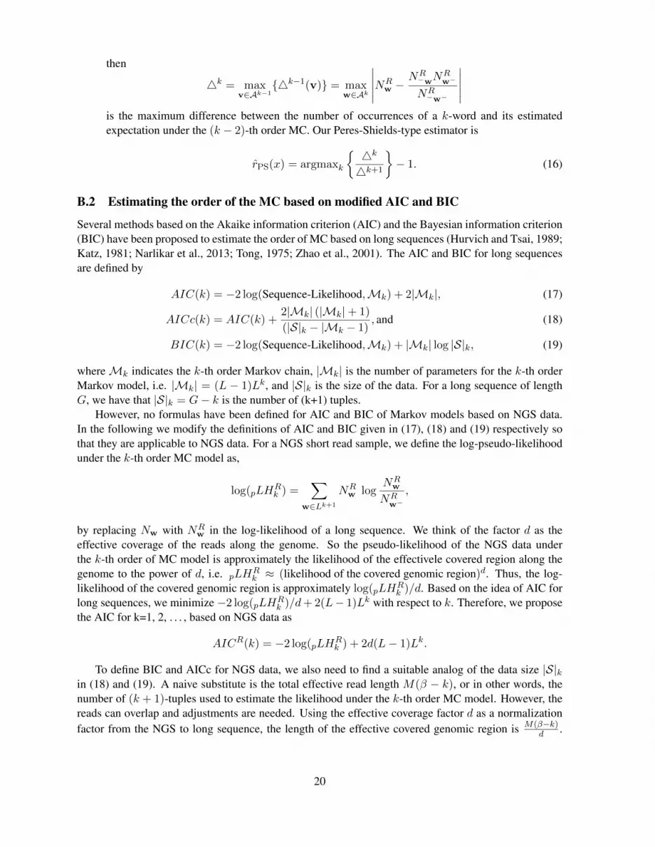
B.2 Estimating the order of the MC based on modified AIC and BIC

Several methods based on the Akaike information criterion (AIC) and the Bayesian information criterion(BIC) have been proposed to estimate the order of MC based on long sequences (Hurvich and Tsai, 1989;Katz, 1981; Narlikar et al., 2013; Tong, 1975; Zhao et al., 2001). The AIC and BIC for long sequencesare defined by

AIC(k) = −2 log(Sequence-Likelihood,Mk) + 2|Mk|, (17)

AICc(k) = AIC(k) +2|Mk| (|Mk|+ 1)

(|S|k − |Mk − 1), and (18)

BIC(k) = −2 log(Sequence-Likelihood,Mk) + |Mk| log |S|k, (19)

whereMk indicates the k-th order Markov chain, |Mk| is the number of parameters for the k-th orderMarkov model, i.e. |Mk| = (L − 1)Lk, and |S|k is the size of the data. For a long sequence of lengthG, we have that |S|k = G− k is the number of (k+1) tuples.

However, no formulas have been defined for AIC and BIC of Markov models based on NGS data.In the following we modify the definitions of AIC and BIC given in (17), (18) and (19) respectively sothat they are applicable to NGS data. For a NGS short read sample, we define the log-pseudo-likelihoodunder the k-th order MC model as,

log(pLHRk ) =

∑w∈Lk+1

NRw log

NRw

NRw−

,

by replacing Nw with NRw in the log-likelihood of a long sequence. We think of the factor d as the

effective coverage of the reads along the genome. So the pseudo-likelihood of the NGS data underthe k-th order of MC model is approximately the likelihood of the effectivele covered region along thegenome to the power of d, i.e. pLH

Rk ≈ (likelihood of the covered genomic region)d. Thus, the log-

likelihood of the covered genomic region is approximately log(pLHRk )/d. Based on the idea of AIC for

long sequences, we minimize −2 log(pLHRk )/d+ 2(L− 1)Lk with respect to k. Therefore, we propose

the AIC for k=1, 2, . . . , based on NGS data as

AICR(k) = −2 log(pLHRk ) + 2d(L− 1)Lk.

To define BIC and AICc for NGS data, we also need to find a suitable analog of the data size |S|kin (18) and (19). A naive substitute is the total effective read length M(β − k), or in other words, thenumber of (k + 1)-tuples used to estimate the likelihood under the k-th order MC model. However, thereads can overlap and adjustments are needed. Using the effective coverage factor d as a normalizationfactor from the NGS to long sequence, the length of the effective covered genomic region is M(β−k)

d .

20

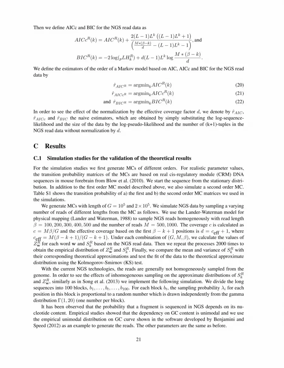
Then we define AICc and BIC for the NGS read data as

AICcR(k) = AICR(k) +2(L− 1)Lk

((L− 1)Lk + 1

)(M∗(β−k)

d − (L− 1)Lk − 1) , and

BICR(k) = −2 log(pLHRk ) + d(L− 1)Lk log

M ∗ (β − k)

d.

We define the estimators of the order of a Markov model based on AIC, AICc and BIC for the NGS readdata by

rAICR = argminkAICR(k) (20)

rAICcR = argminkAICcR(k) (21)

and rBICR = argminkBICR(k) (22)

In order to see the effect of the normalization by the effective coverage factor d, we denote by rAIC ,rAICc and rBIC the naive estimators, which are obtained by simply substituting the log-sequence-likelihood and the size of the data by the log-pseudo-likelihood and the number of (k+1)-tuples in theNGS read data without normalization by d.

C Results

C.1 Simulation studies for the validation of the theoretical results

For the simulation studies we first generate MCs of different orders. For realistic parameter values,the transition probability matrices of the MCs are based on real cis-regulatory module (CRM) DNAsequences in mouse forebrain from Blow et al. (2010). We start the sequence from the stationary distri-bution. In addition to the first order MC model described above, we also simulate a second order MC.Table S1 shows the transition probability of a) the first and b) the second order MC matrices we used inthe simulations.

We generate MCs with length ofG = 105 and 2×105. We simulate NGS data by sampling a varyingnumber of reads of different lengths from the MC as follows. We use the Lander-Waterman model forphysical mapping (Lander and Waterman, 1988) to sample NGS reads homogeneously with read lengthβ = 100, 200, 300, 400, 500 and the number of reads M = 500, 1000. The coverage c is calculated asc = Mβ/G and the effective coverage based on the first β − k + 1 positions is d = ceff + 1, whereceff = M(β − k + 1)/(G − k + 1). Under each combination of (G,M, β), we calculate the values ofZRw for each word w and SRk based on the NGS read data. Then we repeat the processes 2000 times toobtain the empirical distribution of ZRw and SRk . Finally, we compare the mean and variance of SRk withtheir corresponding theoretical approximations and test the fit of the data to the theoretical approximatedistribution using the Kolmogorov-Smirnov (KS) test.

With the current NGS technologies, the reads are generally not homogeneously sampled from thegenome. In order to see the effects of inhomogeneous sampling on the approximate distributions of SRkand ZRw, similarly as in Song et al. (2013) we implement the following simulation. We divide the longsequences into 100 blocks, b1, . . . , bt, . . . , b100. For each block bt, the sampling probability λi for eachposition in this block is proportional to a random number which is drawn independently from the gammadistribution Γ(1, 20) (one number per block).

It has been observed that the probability that a fragment is sequenced in NGS depends on its nu-cleotide content. Empirical studies showed that the dependency on GC content is unimodal and we usethe empirical unimodal distribution on GC curve shown in the software developed by Benjamini andSpeed (2012) as an example to generate the reads. The other parameters are the same as before.

21

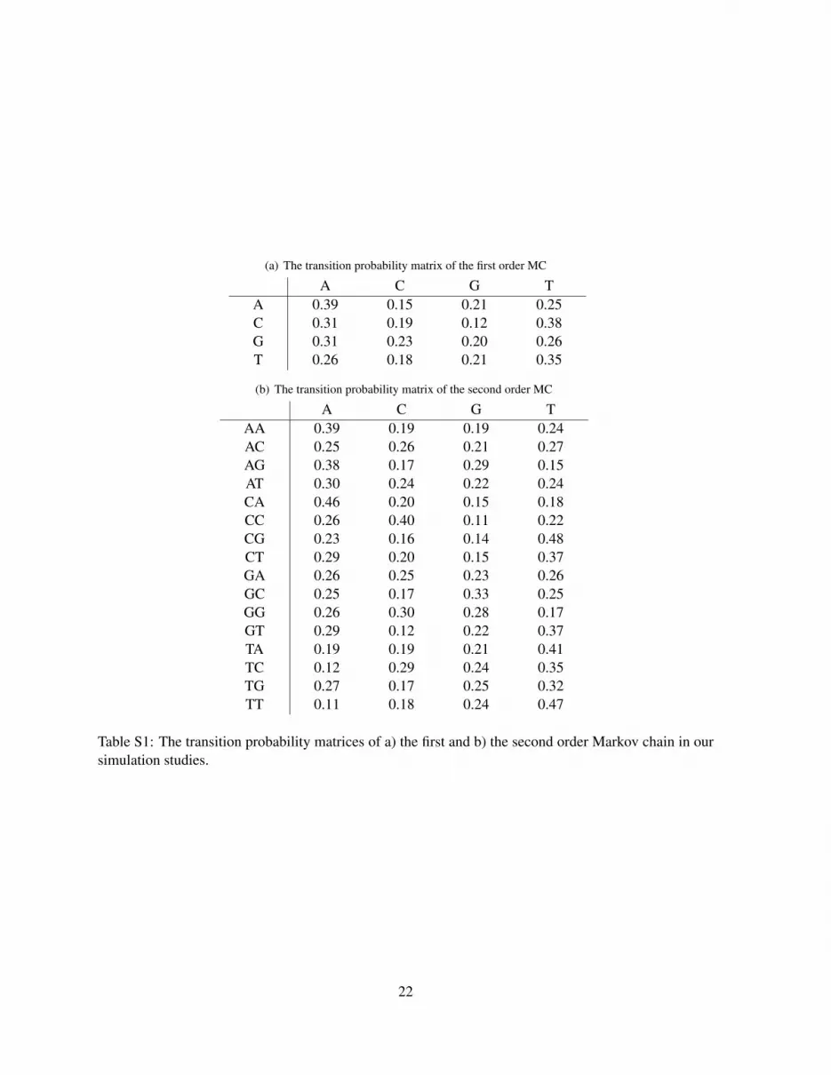
(a) The transition probability matrix of the first order MC

A C G TA 0.39 0.15 0.21 0.25C 0.31 0.19 0.12 0.38G 0.31 0.23 0.20 0.26T 0.26 0.18 0.21 0.35

(b) The transition probability matrix of the second order MC

A C G TAA 0.39 0.19 0.19 0.24AC 0.25 0.26 0.21 0.27AG 0.38 0.17 0.29 0.15AT 0.30 0.24 0.22 0.24CA 0.46 0.20 0.15 0.18CC 0.26 0.40 0.11 0.22CG 0.23 0.16 0.14 0.48CT 0.29 0.20 0.15 0.37GA 0.26 0.25 0.23 0.26GC 0.25 0.17 0.33 0.25GG 0.26 0.30 0.28 0.17GT 0.29 0.12 0.22 0.37TA 0.19 0.19 0.21 0.41TC 0.12 0.29 0.24 0.35TG 0.27 0.17 0.25 0.32TT 0.11 0.18 0.24 0.47

Table S1: The transition probability matrices of a) the first and b) the second order Markov chain in oursimulation studies.

22

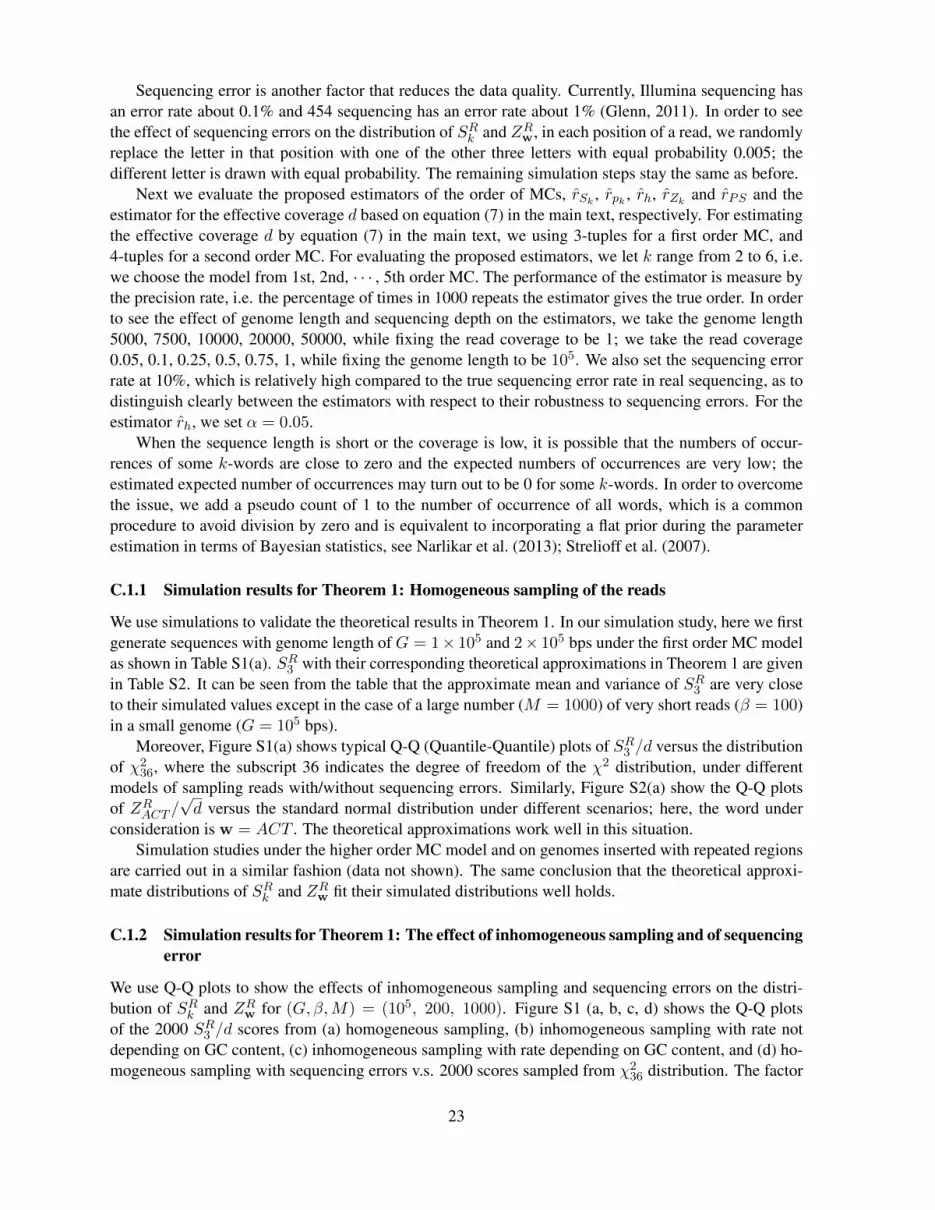
Sequencing error is another factor that reduces the data quality. Currently, Illumina sequencing hasan error rate about 0.1% and 454 sequencing has an error rate about 1% (Glenn, 2011). In order to seethe effect of sequencing errors on the distribution of SRk and ZRw, in each position of a read, we randomlyreplace the letter in that position with one of the other three letters with equal probability 0.005; thedifferent letter is drawn with equal probability. The remaining simulation steps stay the same as before.

Next we evaluate the proposed estimators of the order of MCs, rSk, rpk , rh, rZk

and rPS and theestimator for the effective coverage d based on equation (7) in the main text, respectively. For estimatingthe effective coverage d by equation (7) in the main text, we using 3-tuples for a first order MC, and4-tuples for a second order MC. For evaluating the proposed estimators, we let k range from 2 to 6, i.e.we choose the model from 1st, 2nd, · · · , 5th order MC. The performance of the estimator is measure bythe precision rate, i.e. the percentage of times in 1000 repeats the estimator gives the true order. In orderto see the effect of genome length and sequencing depth on the estimators, we take the genome length5000, 7500, 10000, 20000, 50000, while fixing the read coverage to be 1; we take the read coverage0.05, 0.1, 0.25, 0.5, 0.75, 1, while fixing the genome length to be 105. We also set the sequencing errorrate at 10%, which is relatively high compared to the true sequencing error rate in real sequencing, as todistinguish clearly between the estimators with respect to their robustness to sequencing errors. For theestimator rh, we set α = 0.05.

When the sequence length is short or the coverage is low, it is possible that the numbers of occur-rences of some k-words are close to zero and the expected numbers of occurrences are very low; theestimated expected number of occurrences may turn out to be 0 for some k-words. In order to overcomethe issue, we add a pseudo count of 1 to the number of occurrence of all words, which is a commonprocedure to avoid division by zero and is equivalent to incorporating a flat prior during the parameterestimation in terms of Bayesian statistics, see Narlikar et al. (2013); Strelioff et al. (2007).

C.1.1 Simulation results for Theorem 1: Homogeneous sampling of the reads

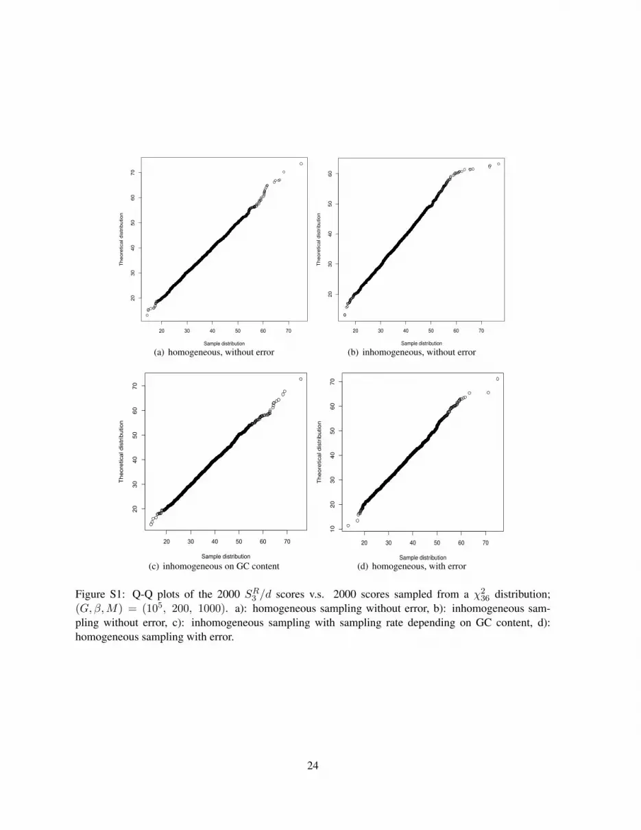
We use simulations to validate the theoretical results in Theorem 1. In our simulation study, here we firstgenerate sequences with genome length of G = 1× 105 and 2× 105 bps under the first order MC modelas shown in Table S1(a). SR3 with their corresponding theoretical approximations in Theorem 1 are givenin Table S2. It can be seen from the table that the approximate mean and variance of SR3 are very closeto their simulated values except in the case of a large number (M = 1000) of very short reads (β = 100)in a small genome (G = 105 bps).

Moreover, Figure S1(a) shows typical Q-Q (Quantile-Quantile) plots of SR3 /d versus the distributionof χ2

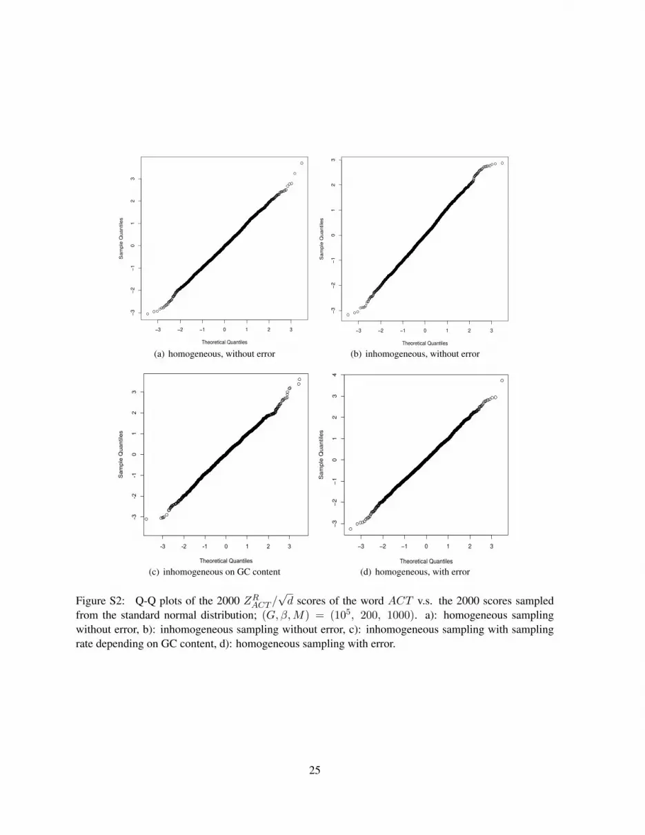
36, where the subscript 36 indicates the degree of freedom of the χ2 distribution, under differentmodels of sampling reads with/without sequencing errors. Similarly, Figure S2(a) show the Q-Q plotsof ZRACT /

√d versus the standard normal distribution under different scenarios; here, the word under

consideration is w = ACT . The theoretical approximations work well in this situation.Simulation studies under the higher order MC model and on genomes inserted with repeated regions

are carried out in a similar fashion (data not shown). The same conclusion that the theoretical approxi-mate distributions of SRk and ZRw fit their simulated distributions well holds.

C.1.2 Simulation results for Theorem 1: The effect of inhomogeneous sampling and of sequencingerror

We use Q-Q plots to show the effects of inhomogeneous sampling and sequencing errors on the distri-bution of SRk and ZRw for (G, β,M) = (105, 200, 1000). Figure S1 (a, b, c, d) shows the Q-Q plotsof the 2000 SR3 /d scores from (a) homogeneous sampling, (b) inhomogeneous sampling with rate notdepending on GC content, (c) inhomogeneous sampling with rate depending on GC content, and (d) ho-mogeneous sampling with sequencing errors v.s. 2000 scores sampled from χ2

36 distribution. The factor

23

20 30 40 50 60 70

2030

4050

6070

Homogeneous Sampling, without Error

Sample distribution

The

oret

ical

dis

trib

utio

n

(a) homogeneous, without error

20 30 40 50 60 7020

30

40

50

60

(b):Inhomogeneous Sampling, without Error

Sample distribution

Theore

tical dis

trib

ution

(b) inhomogeneous, without error

20 30 40 50 60 70

2030

4050

6070

inhomogeneous sampling based on GC content in fragments, without error

Sample distribution

The

oret

ical

dis

trib

utio

n

(c) inhomogeneous on GC content

20 30 40 50 60 70

10

20

30

40

50

60

70

(c):Homogeneous Sampling, with Error

Sample distribution

Th

eo

retica

l d

istr

ibu

tio

n

(d) homogeneous, with error

Figure S1: Q-Q plots of the 2000 SR3 /d scores v.s. 2000 scores sampled from a χ236 distribution;

(G, β,M) = (105, 200, 1000). a): homogeneous sampling without error, b): inhomogeneous sam-pling without error, c): inhomogeneous sampling with sampling rate depending on GC content, d):homogeneous sampling with error.

24

!3 !2 !1 0 1 2 3

!3

!2

!1

01

23

(a):Homogeneous Sampling, without Error

Theoretical Quantiles

Sam

ple

Quantile

s

(a) homogeneous, without error

!3 !2 !1 0 1 2 3!

3!

2!

10

12

3

(b):Inhomogeneous Sampling, without Error

Theoretical Quantiles

Sa

mp

le Q

ua

ntile

s

(b) inhomogeneous, without error

-3 -2 -1 0 1 2 3

-3-2

-10

12

3

inhomogeneous sampling based on GC content in fragments, without error

Theoretical Quantiles

Sam

ple

Qua

ntile

s

(c) inhomogeneous on GC content

!3 !2 !1 0 1 2 3

!3

!2

!1

01

23

4

(c):Homogeneous Sampling, with Error

Theoretical Quantiles

Sam

ple

Quantile

s

(d) homogeneous, with error

Figure S2: Q-Q plots of the 2000 ZRACT /√d scores of the word ACT v.s. the 2000 scores sampled

from the standard normal distribution; (G, β,M) = (105, 200, 1000). a): homogeneous samplingwithout error, b): inhomogeneous sampling without error, c): inhomogeneous sampling with samplingrate depending on GC content, d): homogeneous sampling with error.

25

(a) Genome length G = 1× 105

M = 500 M = 1000

β ˆmean mean var var p-value ˆmean mean var var p-value100 53.4 54.0 160.0 162.0 0.06 70.8 72.0 280.0 288.0 0.002200 71.6 72.0 277.4 288.0 0.99 106.9 108.0 660.5 648.0 0.15300 89.8 90.0 482.9 450.0 0.39 143.9 144.0 1139.5 1152.0 0.15400 107.6 108.0 655.0 648.0 0.84 179.8 180.0 1901.3 1800.0 0.20500 126.0 126.0 905.2 882.0 0.86 216.6 216.0 2675.3 2592.0 0.26

(b) Genome length G = 2× 105

M = 500 M = 1000

β ˆmean mean var var p-value ˆmean mean var var p-value100 44.6 45.0 110.9 112.5 0.12 53.7 54.0 142.7 162.0 0.61200 53.5 54.0 159.6 162.0 0.13 71.8 72.0 278.4 288.0 0.64300 62.7 63.0 222.5 220.5 0.95 89.0 90.0 440.1 450.0 0.41400 71.7 72.0 286.0 288.0 0.51 107.4 108.0 645.7 648.0 0.26500 80.9 81.0 357.5 364.5 0.69 124.7 126.0 821.3 882.0 0.99

Table S2: Comparison of mean and variance of SR3 with their corresponding theoretical approximationsunder a first order MC model and the fit of the data to the theoretical approximate distribution usingthe KS test. The simulation process was repeated 2000 times for each combination of (G,M, β). Thecolumns ˆmean and var are the simulated mean and variance; the columns mean and var are the theoreticalmean and variance.

d is ceff + 1 in homogeneous sampling; and d is calculated from the exact distribution of the sampledreads along the sequence in the inhomogeneous sampling situation. Figure S2 gives the Q-Q plots forZRACT /

√d, showing the effect of inhomogeneous sampling and sequencing error on the distribution of

ZRACT /√d. All Q-Q plots show a satisfactory fit, confirming that the theoretical results from Theorem 1

hold even when the assumptions are not necessarily satisfied.

C.1.3 Simulation results on estimating the order of MCs based on simulated NGS reads

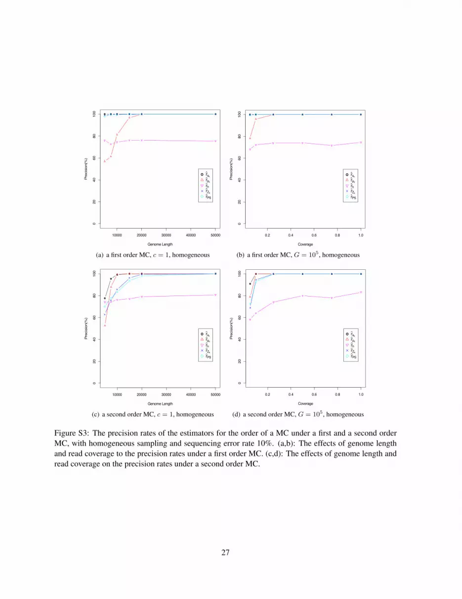
Figure S3 shows the effects of sequence length and read coverage on the precision of the estimators undera first and second order MCs, with homogeneous sampling and sequencing error rate 10%. It can be seenthat all the five estimators perform reasonably well. In particular, the precision rate of estimators rSk

,rpk , rZk

and rPS reach 100% when the genome length is larger than 20000 bps and the read coverageis greater than 0.2. The estimator rh performs slightly worse than the other four estimators. Since theestimator rh is based on hypothesis testing with a given significant level α, the precision rate is not ableto reach 100%. It is also possible that no k from 2 to 6 satisfies pk−1 < α and both pk and pk+1 arelarger than α such that the estimator rh fails to give an estimation. We observe that the precision of rhis sensitive to the accuracy of the estimation of the effective coverage d. In the simulation, if we take theunderlying true value of d in place of the estimated value of d in the computation, the precision rate ofrh goes up to above 90%.

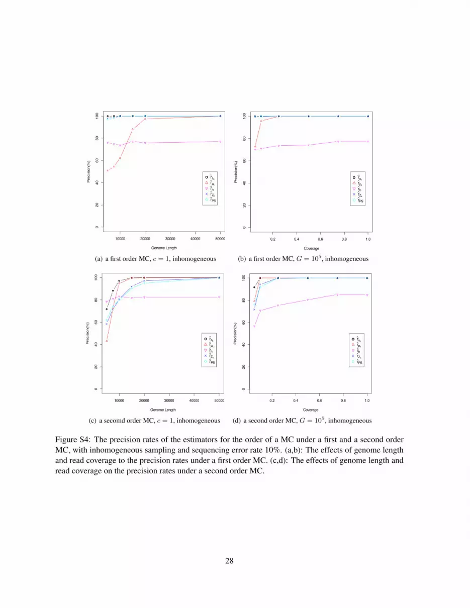
For inhomogeneous sampling, Figure S4 shows the effects of sequence length and read coverage onthe precision of the estimators. We can see that the precision rates under the inhomogeneous samplingstart at slightly lower values than those under the homogeneous case. As the genome length and the readcoverage increase, the estimators perform as well as they perform under the homogeneous sampling.

Figure S5 and S6 show the disappointing precision rates of the AIC and BIC based estimators of the

26

● ● ● ● ● ●

10000 20000 30000 40000 50000

020

4060

8010

0

Genome Length

Pre

cisi

on(%

)

● rsk

rpk

rhrZk

rPS

(c) MC1, Homogeneous Sampling, Coverage=1, Read Length=100

(a) a first order MC, c = 1, homogeneous

● ● ● ● ● ●

0.2 0.4 0.6 0.8 1.00

2040

6080

100

Coverage

Precision(%)

● rskrpkrhrZkrPS

(d) MC1, Homogeneous Sampling, Genome Length=1e+05, Read Length=100

(b) a first order MC, G = 105, homogeneous

●

●

●● ● ●

10000 20000 30000 40000 50000

020

4060

8010

0

Genome Length

Pre

cisi

on(%

)

● rsk

rpk

rhrZk

rPS

(c) MC2, Homogeneous Sampling, Coverage=1, Read Length=100

(c) a second order MC, c = 1, homogeneous

●

● ● ● ● ●

0.2 0.4 0.6 0.8 1.0

020

4060

80100

Coverage

Precision(%)

● rskrpkrhrZkrPS

(d) MC2, Homogeneous Sampling, Genome Length=1e+05, Read Length=100

(d) a second order MC, G = 105, homogeneous

Figure S3: The precision rates of the estimators for the order of a MC under a first and a second orderMC, with homogeneous sampling and sequencing error rate 10%. (a,b): The effects of genome lengthand read coverage to the precision rates under a first order MC. (c,d): The effects of genome length andread coverage on the precision rates under a second order MC.

27

● ● ● ● ● ●

10000 20000 30000 40000 50000

020

4060

8010

0

Genome Length

Pre

cisi

on(%

)

● rsk

rpk

rhrZk

rPS

(c) MC1, Inhomogeneous Sampling, Coverage=1, Read Length=100

(a) a first order MC, c = 1, inhomogeneous

● ● ● ● ● ●

0.2 0.4 0.6 0.8 1.00

2040

6080

100

Coverage

Precision(%)

● rskrpkrhrZkrPS

(d) MC1, Inhomogeneous Sampling, Genome Length=1e+05, Read Length=100

(b) a first order MC, G = 105, inhomogeneous

●

●

●

● ● ●

10000 20000 30000 40000 50000

020

4060

8010

0

Genome Length

Pre

cisi

on(%

)

● rsk

rpk

rhrZk

rPS

(c) MC2, Inhomogeneous Sampling, Coverage=1, Read Length=100

(c) a secomd order MC, c = 1, inhomogeneous

●

● ● ● ● ●

0.2 0.4 0.6 0.8 1.0

020

4060

80100

Coverage

Precision(%)

● rskrpkrhrZkrPS

(d) MC2, Inhomogeneous Sampling, Genome Length=1e+05, Read Length=100

(d) a second order MC, G = 105, inhomogeneous

Figure S4: The precision rates of the estimators for the order of a MC under a first and a second orderMC, with inhomogeneous sampling and sequencing error rate 10%. (a,b): The effects of genome lengthand read coverage to the precision rates under a first order MC. (c,d): The effects of genome length andread coverage on the precision rates under a second order MC.

28

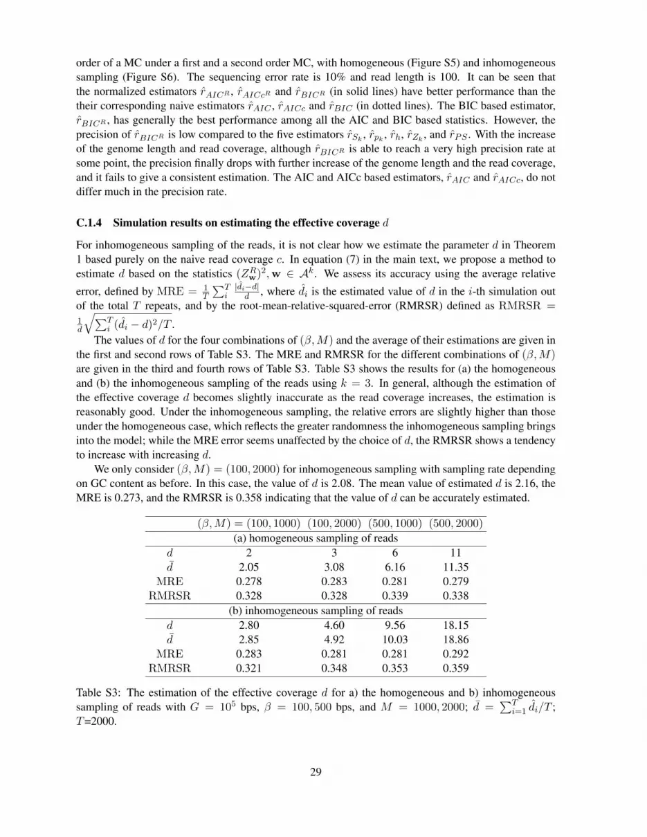
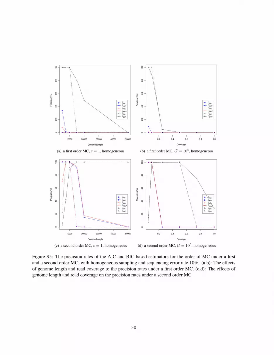
order of a MC under a first and a second order MC, with homogeneous (Figure S5) and inhomogeneoussampling (Figure S6). The sequencing error rate is 10% and read length is 100. It can be seen thatthe normalized estimators rAICR , rAICcR and rBICR (in solid lines) have better performance than thetheir corresponding naive estimators rAIC , rAICc and rBIC (in dotted lines). The BIC based estimator,rBICR , has generally the best performance among all the AIC and BIC based statistics. However, theprecision of rBICR is low compared to the five estimators rSk

, rpk , rh, rZk, and rPS . With the increase

of the genome length and read coverage, although rBICR is able to reach a very high precision rate atsome point, the precision finally drops with further increase of the genome length and the read coverage,and it fails to give a consistent estimation. The AIC and AICc based estimators, rAIC and rAICc, do notdiffer much in the precision rate.

C.1.4 Simulation results on estimating the effective coverage d

For inhomogeneous sampling of the reads, it is not clear how we estimate the parameter d in Theorem1 based purely on the naive read coverage c. In equation (7) in the main text, we propose a method toestimate d based on the statistics (ZRw)2,w ∈ Ak. We assess its accuracy using the average relative

error, defined by MRE = 1T

∑Ti|di−d|d , where di is the estimated value of d in the i-th simulation out

of the total T repeats, and by the root-mean-relative-squared-error (RMRSR) defined as RMRSR =1d

√∑Ti (di − d)2/T .

The values of d for the four combinations of (β,M) and the average of their estimations are given inthe first and second rows of Table S3. The MRE and RMRSR for the different combinations of (β,M)are given in the third and fourth rows of Table S3. Table S3 shows the results for (a) the homogeneousand (b) the inhomogeneous sampling of the reads using k = 3. In general, although the estimation ofthe effective coverage d becomes slightly inaccurate as the read coverage increases, the estimation isreasonably good. Under the inhomogeneous sampling, the relative errors are slightly higher than thoseunder the homogeneous case, which reflects the greater randomness the inhomogeneous sampling bringsinto the model; while the MRE error seems unaffected by the choice of d, the RMRSR shows a tendencyto increase with increasing d.

We only consider (β,M) = (100, 2000) for inhomogeneous sampling with sampling rate dependingon GC content as before. In this case, the value of d is 2.08. The mean value of estimated d is 2.16, theMRE is 0.273, and the RMRSR is 0.358 indicating that the value of d can be accurately estimated.

(β,M) = (100, 1000) (100, 2000) (500, 1000) (500, 2000)

(a) homogeneous sampling of readsd 2 3 6 11d 2.05 3.08 6.16 11.35

MRE 0.278 0.283 0.281 0.279RMRSR 0.328 0.328 0.339 0.338

(b) inhomogeneous sampling of readsd 2.80 4.60 9.56 18.15d 2.85 4.92 10.03 18.86

MRE 0.283 0.281 0.281 0.292RMRSR 0.321 0.348 0.353 0.359

Table S3: The estimation of the effective coverage d for a) the homogeneous and b) inhomogeneoussampling of reads with G = 105 bps, β = 100, 500 bps, and M = 1000, 2000; d =

∑Ti=1 di/T ;

T=2000.

29

● ● ● ● ● ●

10000 20000 30000 40000 50000

020

4060

8010

0

Genome Length

Pre

cisi

on(%

)

●

●● ● ● ●

●

●

rAICrAICR

rAICcrAICcR

rBICrBICR

(a) MC1, Homogeneous Sampling, Coverage=1, Read Length=100

(a) a first order MC, c = 1, homogeneous

● ● ● ● ● ●

0.2 0.4 0.6 0.8 1.00

2040

6080

100

Coverage

Precision(%)

●

● ● ● ● ●

●

●

rAICrAICRrAICcrAICcRrBICrBICR

(b) MC1, Homogeneous Sampling, Genome Length=1e+05, Read Length=100

(b) a first order MC, G = 105, homogeneous

● ● ●

● ● ●

10000 20000 30000 40000 50000

020

4060

8010

0

Genome Length

Pre

cisi

on(%

)

● ● ●

●

●

●

●

●

rAICrAICR

rAICcrAICcR

rBICrBICR

(c) MC2, Homogeneous Sampling, Coverage=1, Read Length=100

(c) a second order MC, c = 1, homogeneous

● ●

● ● ● ●

0.2 0.4 0.6 0.8 1.0

020

4060

80100

Coverage

Precision(%)

● ●

● ● ● ●

●

●

rAICrAICRrAICcrAICcRrBICrBICR

(d) MC2, Homogeneous Sampling, Genome Length=1e+05, Read Length=100

(d) a second order MC, G = 105, homogeneous

Figure S5: The precision rates of the AIC and BIC based estimators for the order of MC under a firstand a second order MC, with homogeneous sampling and sequencing error rate 10%. (a,b): The effectsof genome length and read coverage to the precision rates under a first order MC. (c,d): The effects ofgenome length and read coverage on the precision rates under a second order MC.

30

● ● ● ● ● ●

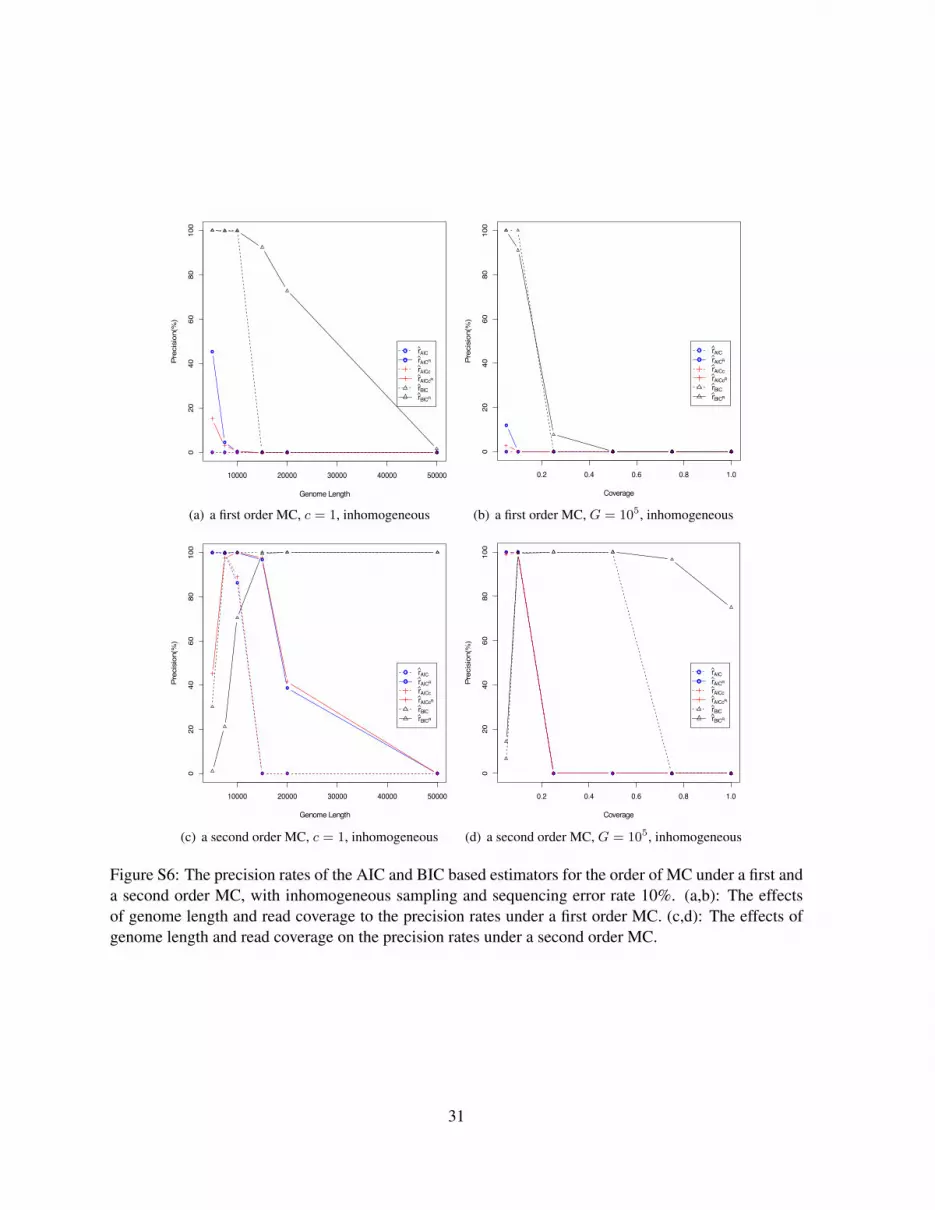
10000 20000 30000 40000 50000

020

4060

8010

0

Genome Length

Pre

cisi

on(%

)

●

●

● ● ● ●

●

●

rAICrAICR

rAICcrAICcR

rBICrBICR

(a) MC1, Inhomogeneous Sampling, Coverage=1, Read Length=100

(a) a first order MC, c = 1, inhomogeneous

● ● ● ● ● ●

0.2 0.4 0.6 0.8 1.00

2040

6080

100

Coverage

Precision(%)

●

● ● ● ● ●

●

●

rAICrAICRrAICcrAICcRrBICrBICR

(b) MC1, Inhomogeneous Sampling, Genome Length=1e+05, Read Length=100

(b) a first order MC, G = 105, inhomogeneous

● ●

●

● ● ●

10000 20000 30000 40000 50000

020

4060

8010

0

Genome Length

Pre

cisi

on(%

)

● ● ●

●

●

●

●

●

rAICrAICR

rAICcrAICcR

rBICrBICR

(c) MC2, Inhomogeneous Sampling, Coverage=1, Read Length=100

(c) a second order MC, c = 1, inhomogeneous

● ●

● ● ● ●

0.2 0.4 0.6 0.8 1.0

020

4060

80100

Coverage

Precision(%)

● ●

● ● ● ●

●

●

rAICrAICRrAICcrAICcRrBICrBICR

(d) MC2, Inhomogeneous Sampling, Genome Length=1e+05, Read Length=100

(d) a second order MC, G = 105, inhomogeneous

Figure S6: The precision rates of the AIC and BIC based estimators for the order of MC under a first anda second order MC, with inhomogeneous sampling and sequencing error rate 10%. (a,b): The effectsof genome length and read coverage to the precision rates under a first order MC. (c,d): The effects ofgenome length and read coverage on the precision rates under a second order MC.

31

C.2 The relationship among 28 vertebrate species

Table S4 shows the estimated orders of MC for the 28 genomes of vertebrate species based on their NGSsamples. For each of the 28 species, we compute the fraction of the k-tuple words that have (ZRw)2/dwithin the 99% of a χ2 distribution with one degree of freedom, for k = 8, 9, . . . , 14. Using 80% asa threshold, we estimate the orders of MC for each species to be the smallest k − 2 under which thefraction of words that can be explained by the (k − 2)-th order MC is greater than the threshold. Thelast two columns of Table S4 are the AIC-predicted optimal and BIC-predicted optimal orders obtainedin Narlikar et al. (2013).

We cluster the NGS datasets of the 28 species listed in the Table S4, using d∗2 and dS2 under MCmodels of varying order. Figure S1 in Miller et al. (2007) gives the phylogenetic tree of the 28 speciesbased on alignment methods, with branch lengths noted on it. We obtain the distance matrix of the 28species by computing pairwise disstance between each pair of the 28 species from the phylogenetic tree;the matrix is given as Table S5. We compare the dissimilarity matrices using d∗2 and dS2 under MC modelswith different order to the matrix Table S5 which we use as underlying truth.

C.3 The relationship among 13 tropical tree species with unknown reference genomes

We also apply our method to the 13 tree species (8 Fagaceae and 5 Moraceae) based on the NGS shotgunread data sets in Cannon et al. (2010). The reference genome sequences for the 13 tree species areunknown. Figure 1 in the main text shows the clustering results using d∗2 under MCs of order 0, 4, 8 and9. For the clustering results using dS2 , see Figure S7.

References

Almagor, H. (1983). A Markov analysis of DNA sequences. Journal of Theoretical Biology 104(4),633–645.

Anderson, T. W. and L. A. Goodman (1957). Statistical inference about Markov chains. The Annals ofMathematical Statistics 28(4), 89–110.

Arnold, J., A. J. Cuticchia, D. A. Newsome, W. W. Jennings, and R. Ivarie (1988). Mono-throughhexanucleotide composition of the sense strand of yeast DNA: a Markov chain analysis. NucleicAcids Research 16(14), 7145–7158.

Avery, P. J. (1987). The analysis of intron data and their use in the detection of short signals. Journal ofMolecular Evolution 26(4), 335–340.

Avery, P. J. and D. A. Henderson (1999). Fitting Markov chain models to discrete state series such asDNA sequences. Journal of the Royal Statistical Society: Series C (Applied Statistics) 48(1), 53–61.

Baum, L. E. and T. Petrie (1966). Statistical inference for probabilistic functions of finite state Markovchains. The Annals of Mathematical Statistics 37(6), 1554–1563.

Behnam, E. and A. D. Smith (2014). The amordad database engine for metagenomics. Bioinformat-ics 30(20), 2949–2955.

Behnam, E., M. S. Waterman, and A. D. Smith (2013). A geometric interpretation for local alignment-free sequence comparison. Journal of Computational Biology 20(7), 471–485.

Benjamini, Y. and T. Speed (2012). Summarizing and correcting the gc content bias in high-throughputsequencing. Nucleic Acids Research 40(10), e72.

32

Besag, J. and D. Mondal (2013). Exact goodness-of-fit tests for Markov chains. Biometrics 69(2),488–496.

Billingsley, P. (1961a). Statistical Inference for Markov Processes, Volume 2. University of ChicagoPress Chicago.

Billingsley, P. (1961b). Statistical methods in Markov chains. The Annals of Mathematical Statis-tics 32(1), 12–40.

Blaisdell, B. E. (1985). Markov chain analysis finds a significant influence of neighboring bases onthe occurrence of a base in eucaryotic nuclear DNA sequences both protein-coding and noncoding.Journal of Molecular Evolution 21(3), 278–288.

Blow, M. J., D. J. McCulley, Z. Li, T. Zhang, J. A. Akiyama, A. Holt, I. Plajzer-Frick, M. Shoukry,C. Wright, F. Chen, et al. (2010). Chip-seq identification of weakly conserved heart enhancers. NatureGenetics 42(9), 806–810.

Cannon, C. H., C. S. Kua, D. Zhang, and J. Harting (2010). Assembly free comparative genomicsof short-read sequence data discovers the needles in the haystack. Molecular Ecology 19(Suppl. 1),146–160.

Daley, T. and A. D. Smith (2013). Predicting the molecular complexity of sequencing libraries. NatureMethods 10(4), 325–327.

Ewens, W. J. and G. R. Grant (2005). Statistical methods in bioinformatics: an introduction. Springer.

Glenn, T. C. (2011). Field guide to next-generation DNA sequencers. Molecular Ecology Re-sources 11(5), 759–769.

Goke, J., M. H. Schulz, J. Lasserre, and M. Vingron (2012). Estimation of pairwise sequence similarityof mammalian enhancers with word neighbourhood counts. Bioinformatics 28(5), 656–663.

Hoel, P. G. (1954). A test for Markov chains. Biometrika 41(3/4), 430–433.

Hong, J. (1990). Prediction of oligonucleotide frequencies based upon dinucleotide frequencies obtainedfrom the nearest neighbor analysis. Nucleic Acids Research 18(6), 1625–1628.

Hurvich, C. M. and C. L. Tsai (1989). Regression and time series model selection in small samples.Biometrika 76(2), 297–307.

Hurwitz, B. L., A. H. Westveld, J. R. Brum, and M. B. Sullivan (2014). Modeling ecological drivers inmarine viral communities using comparative metagenomics and network analyses. Proceedings of theNational Academy of Sciences 111(29), 10714–10719.

Jiang, B., K. Song, J. Ren, M. Deng, F. Sun, and X. Zhang (2012). Comparison of metagenomic samplesusing sequence signatures. BMC Genomics 13(1), 730.

Karolchik, D., R. M. Kuhn, R. Baertsch, G. P. Barber, H. Clawson, M. Diekhans, B. Giardine, R. A.Harte, A. S. Hinrichs, F. Hsu, et al. (2008). The UCSC genome browser database: 2008 update.Nucleic Acids Research 36(suppl 1), D773–D779.

Katz, R. W. (1981). On some criteria for estimating the order of a Markov chain. Technometrics 23(3),243–249.

33

Lander, E. S. and M. S. Waterman (1988). Genomic mapping by fingerprinting random clones: a math-ematical analysis. Genomics 2(3), 231–239.

Liu, X., L. Wan, J. Li, G. Reinert, M. Waterman, and F. Sun (2011). New powerful statistics foralignment-free sequence comparison under a pattern transfer model. Journal of Theoretical Biol-ogy 284(1), 106–116.

Miller, W., K. Rosenbloom, R. Hardison, M. Hou, J. Taylor, B. Raney, R. Burhans, D. King, R. Baertsch,D. Blankenberg, et al. (2007). 28-way vertebrate alignment and conservation track in the UCSCgenome browser. Genome Research 17(12), 1797–1808.

Morvai, G. and B. Weiss (2005). Order estimation of Markov chains. Information Theory, IEEE Trans-actions on 51(4), 1496–1497.

Narlikar, L., N. Mehta, S. Galande, and M. Arjunwadkar (2013). One size does not fit all: On how markovmodel order dictates performance of genomic sequence analyses. Nucleic Acids Research 41(3), 1416–1424.

Peres, Y. and P. Shields (2005). Two new Markov order estimators. arXiv preprint math/0506080.

Pevzner, P. A., M. Y. Borodovsky, and A. A. Mironov (1989). Linguistics of nucleotide sequences i:the significance of deviations from mean statistical characteristics and prediction of the frequencies ofoccurrence of words. Journal of Biomolecular Structure and Dynamics 6(5), 1013–1026.

Reinert, G., D. Chew, F. Z. Sun, and M. S. Waterman (2009). Alignment-free sequence comparison (I):Statistics and power. Journal of Computational Biology 16(12), 1615–1634.

Reinert, G., S. Schbath, and M. Waterman (2000). Probabilistic and statistical properties of words: anoverview. Journal of Computational Biology 7(1-2), 1–46.

Reinert, G., S. Schbath, and M. S. Waterman (2005). Statistics on words with applications to biologicalsequences. Lothaire: Applied Combinatorics on Words, J. Berstel and D. Perrin, eds. 105, 251–328.

Ren, J., K. Song, F. Sun, M. Deng, and G. Reinert (2013). Multiple alignment-free sequence comparison.Bioinformatics 29(21), 2690–2698.

Richter, D., F. Ott, A. Auch, R. Schmid, and D. Huson (2008). MetaSim: a sequencing simulator forgenomics and metagenomics. PLoS One 3(10), e3373.

Simpson, J. T. (2014). Exploring genome characteristics and sequence quality without a reference.Bioinformatics 30(9), 1228–1235.

Song, K., J. Ren, G. Reinert, M. Deng, M. S. Waterman, and F. Sun (2014). New developments ofalignment-free sequence comparison: measures, statistics and next-generation sequencing. Briefingsin Bioinformatics 15(3), 343–353.

Song, K., J. Ren, Z. Zhai, X. Liu, M. Deng, and F. Sun (2013). Alignment-free sequence comparisonbased on next-generation sequencing reads. Journal of Computational Biology 20(2), 64–79.

Strelioff, C. C., J. P. Crutchfield, and A. W. Hubler (2007). Inferring markov chains: Bayesian estimation,model comparison, entropy rate, and out-of-class modeling. Physical Review E 76(1), 011106.

Tong, H. (1975). Determination of the order of a Markov chain by Akaike’s information criterion.Journal of Applied Probability 12, 488–497.

34

Wang, Y., L. Liu, L. Chen, T. Chen, and F. Sun (2014). Comparison of metatranscriptomic samples basedon k-tuple frequencies. PloS One 9(1), e84348.

Waterman, M. S. (1995). Introduction to Computational Biology: Maps, Sequences and Genomes.Chapman & Hall/CRC Interdisciplinary Statistics. Taylor & Francis.

Yi, H. and L. Jin (2013). Co-phylog: an assembly-free phylogenomic approach for closely relatedorganisms. Nucleic Acids Research 41(7), e75.

Zhai, Z., G. Reinert, K. Song, M. S. Waterman, Y. Luan, and F. Sun (2012). Normal and compoundpoisson approximations for pattern occurrences in ngs reads. Journal of Computational Biology 19(6),839–854.

Zhang, Z. D., J. Rozowsky, M. Snyder, J. Chang, and M. Gerstein (2008). Modeling chip sequencing insilico with applications. PLoS Computational Biology 4(8), e1000158.

Zhao, L. C., C. C. Y. Dorea, and C. R. Goncalves (2001). On determination of the order of a Markovchain. Statistical Inference for Stochastic Processes 4(3), 273–282.

35

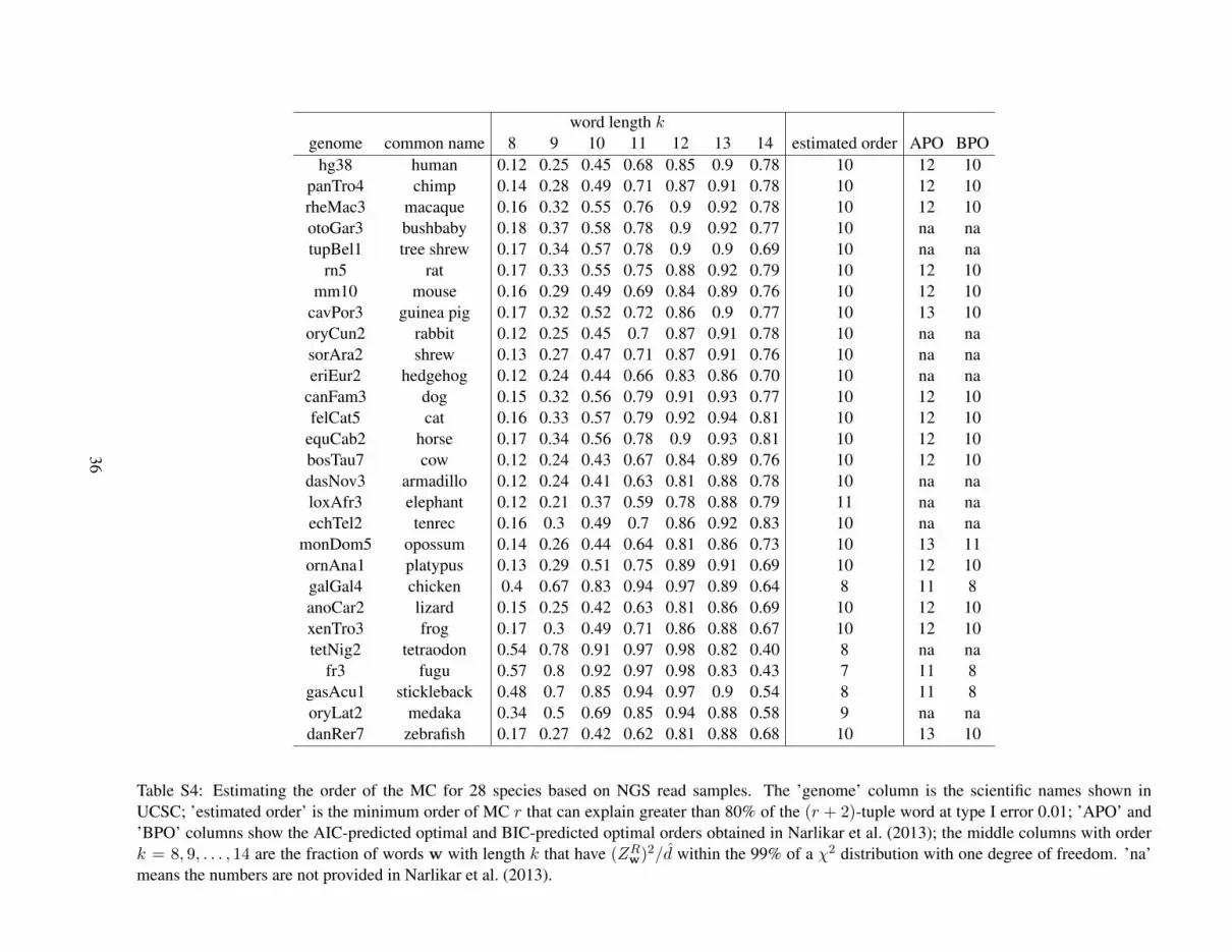
word length kgenome common name 8 9 10 11 12 13 14 estimated order APO BPO

hg38 human 0.12 0.25 0.45 0.68 0.85 0.9 0.78 10 12 10panTro4 chimp 0.14 0.28 0.49 0.71 0.87 0.91 0.78 10 12 10rheMac3 macaque 0.16 0.32 0.55 0.76 0.9 0.92 0.78 10 12 10otoGar3 bushbaby 0.18 0.37 0.58 0.78 0.9 0.92 0.77 10 na natupBel1 tree shrew 0.17 0.34 0.57 0.78 0.9 0.9 0.69 10 na na

rn5 rat 0.17 0.33 0.55 0.75 0.88 0.92 0.79 10 12 10mm10 mouse 0.16 0.29 0.49 0.69 0.84 0.89 0.76 10 12 10

cavPor3 guinea pig 0.17 0.32 0.52 0.72 0.86 0.9 0.77 10 13 10oryCun2 rabbit 0.12 0.25 0.45 0.7 0.87 0.91 0.78 10 na nasorAra2 shrew 0.13 0.27 0.47 0.71 0.87 0.91 0.76 10 na naeriEur2 hedgehog 0.12 0.24 0.44 0.66 0.83 0.86 0.70 10 na na

canFam3 dog 0.15 0.32 0.56 0.79 0.91 0.93 0.77 10 12 10felCat5 cat 0.16 0.33 0.57 0.79 0.92 0.94 0.81 10 12 10

equCab2 horse 0.17 0.34 0.56 0.78 0.9 0.93 0.81 10 12 10bosTau7 cow 0.12 0.24 0.43 0.67 0.84 0.89 0.76 10 12 10dasNov3 armadillo 0.12 0.24 0.41 0.63 0.81 0.88 0.78 10 na naloxAfr3 elephant 0.12 0.21 0.37 0.59 0.78 0.88 0.79 11 na naechTel2 tenrec 0.16 0.3 0.49 0.7 0.86 0.92 0.83 10 na na

monDom5 opossum 0.14 0.26 0.44 0.64 0.81 0.86 0.73 10 13 11ornAna1 platypus 0.13 0.29 0.51 0.75 0.89 0.91 0.69 10 12 10galGal4 chicken 0.4 0.67 0.83 0.94 0.97 0.89 0.64 8 11 8anoCar2 lizard 0.15 0.25 0.42 0.63 0.81 0.86 0.69 10 12 10xenTro3 frog 0.17 0.3 0.49 0.71 0.86 0.88 0.67 10 12 10tetNig2 tetraodon 0.54 0.78 0.91 0.97 0.98 0.82 0.40 8 na na

fr3 fugu 0.57 0.8 0.92 0.97 0.98 0.83 0.43 7 11 8gasAcu1 stickleback 0.48 0.7 0.85 0.94 0.97 0.9 0.54 8 11 8oryLat2 medaka 0.34 0.5 0.69 0.85 0.94 0.88 0.58 9 na nadanRer7 zebrafish 0.17 0.27 0.42 0.62 0.81 0.88 0.68 10 13 10

Table S4: Estimating the order of the MC for 28 species based on NGS read samples. The ’genome’ column is the scientific names shown inUCSC; ’estimated order’ is the minimum order of MC r that can explain greater than 80% of the (r + 2)-tuple word at type I error 0.01; ’APO’ and’BPO’ columns show the AIC-predicted optimal and BIC-predicted optimal orders obtained in Narlikar et al. (2013); the middle columns with orderk = 8, 9, . . . , 14 are the fraction of words w with length k that have (ZRw)2/d within the 99% of a χ2 distribution with one degree of freedom. ’na’means the numbers are not provided in Narlikar et al. (2013).

36

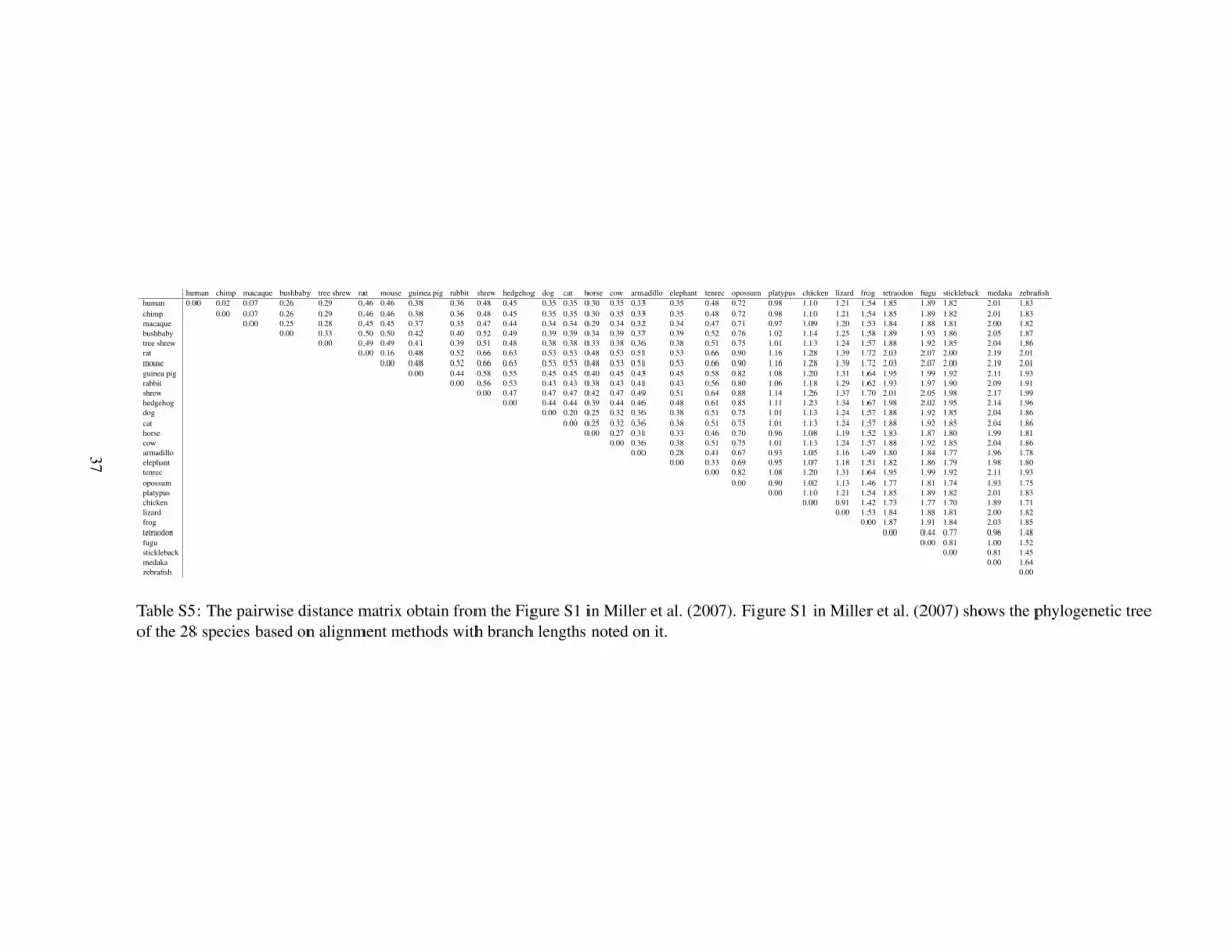
human chimp macaque bushbaby tree shrew rat mouse guinea pig rabbit shrew hedgehog dog cat horse cow armadillo elephant tenrec opossum platypus chicken lizard frog tetraodon fugu stickleback medaka zebrafishhuman 0.00 0.02 0.07 0.26 0.29 0.46 0.46 0.38 0.36 0.48 0.45 0.35 0.35 0.30 0.35 0.33 0.35 0.48 0.72 0.98 1.10 1.21 1.54 1.85 1.89 1.82 2.01 1.83chimp 0.00 0.07 0.26 0.29 0.46 0.46 0.38 0.36 0.48 0.45 0.35 0.35 0.30 0.35 0.33 0.35 0.48 0.72 0.98 1.10 1.21 1.54 1.85 1.89 1.82 2.01 1.83macaque 0.00 0.25 0.28 0.45 0.45 0.37 0.35 0.47 0.44 0.34 0.34 0.29 0.34 0.32 0.34 0.47 0.71 0.97 1.09 1.20 1.53 1.84 1.88 1.81 2.00 1.82bushbaby 0.00 0.33 0.50 0.50 0.42 0.40 0.52 0.49 0.39 0.39 0.34 0.39 0.37 0.39 0.52 0.76 1.02 1.14 1.25 1.58 1.89 1.93 1.86 2.05 1.87tree shrew 0.00 0.49 0.49 0.41 0.39 0.51 0.48 0.38 0.38 0.33 0.38 0.36 0.38 0.51 0.75 1.01 1.13 1.24 1.57 1.88 1.92 1.85 2.04 1.86rat 0.00 0.16 0.48 0.52 0.66 0.63 0.53 0.53 0.48 0.53 0.51 0.53 0.66 0.90 1.16 1.28 1.39 1.72 2.03 2.07 2.00 2.19 2.01mouse 0.00 0.48 0.52 0.66 0.63 0.53 0.53 0.48 0.53 0.51 0.53 0.66 0.90 1.16 1.28 1.39 1.72 2.03 2.07 2.00 2.19 2.01guinea pig 0.00 0.44 0.58 0.55 0.45 0.45 0.40 0.45 0.43 0.45 0.58 0.82 1.08 1.20 1.31 1.64 1.95 1.99 1.92 2.11 1.93rabbit 0.00 0.56 0.53 0.43 0.43 0.38 0.43 0.41 0.43 0.56 0.80 1.06 1.18 1.29 1.62 1.93 1.97 1.90 2.09 1.91shrew 0.00 0.47 0.47 0.47 0.42 0.47 0.49 0.51 0.64 0.88 1.14 1.26 1.37 1.70 2.01 2.05 1.98 2.17 1.99hedgehog 0.00 0.44 0.44 0.39 0.44 0.46 0.48 0.61 0.85 1.11 1.23 1.34 1.67 1.98 2.02 1.95 2.14 1.96dog 0.00 0.20 0.25 0.32 0.36 0.38 0.51 0.75 1.01 1.13 1.24 1.57 1.88 1.92 1.85 2.04 1.86cat 0.00 0.25 0.32 0.36 0.38 0.51 0.75 1.01 1.13 1.24 1.57 1.88 1.92 1.85 2.04 1.86horse 0.00 0.27 0.31 0.33 0.46 0.70 0.96 1.08 1.19 1.52 1.83 1.87 1.80 1.99 1.81cow 0.00 0.36 0.38 0.51 0.75 1.01 1.13 1.24 1.57 1.88 1.92 1.85 2.04 1.86armadillo 0.00 0.28 0.41 0.67 0.93 1.05 1.16 1.49 1.80 1.84 1.77 1.96 1.78elephant 0.00 0.33 0.69 0.95 1.07 1.18 1.51 1.82 1.86 1.79 1.98 1.80tenrec 0.00 0.82 1.08 1.20 1.31 1.64 1.95 1.99 1.92 2.11 1.93opossum 0.00 0.90 1.02 1.13 1.46 1.77 1.81 1.74 1.93 1.75platypus 0.00 1.10 1.21 1.54 1.85 1.89 1.82 2.01 1.83chicken 0.00 0.91 1.42 1.73 1.77 1.70 1.89 1.71lizard 0.00 1.53 1.84 1.88 1.81 2.00 1.82frog 0.00 1.87 1.91 1.84 2.03 1.85tetraodon 0.00 0.44 0.77 0.96 1.48fugu 0.00 0.81 1.00 1.52stickleback 0.00 0.81 1.45medaka 0.00 1.64zebrafish 0.00

Table S5: The pairwise distance matrix obtain from the Figure S1 in Miller et al. (2007). Figure S1 in Miller et al. (2007) shows the phylogenetic treeof the 28 species based on alignment methods with branch lengths noted on it.

37

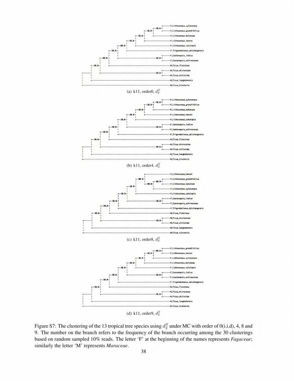
(a) k11, order0, dS2

(b) k11, order4, dS2

(c) k11, order8, dS2

(d) k11, order9, dS2

Figure S7: The clustering of the 13 tropical tree species using dS2 under MC with order of 0(i.i.d), 4, 8 and9. The number on the branch refers to the frequency of the branch occurring among the 30 clusteringsbased on random sampled 10% reads. The letter ‘F’ at the beginning of the names represents Fagaceae;similarly the letter ‘M’ represents Maraceae.

38