In situ validation of MERIS marine reflectance off the southwest Iberian Peninsula: assessment of vicarious adjustment and corrections for near-land adjacency

This article was downloaded by: [5.158.28.243]On: 14 March 2014, At: 04:09Publisher: Taylor & FrancisInforma Ltd Registered in England and Wales Registered Number: 1072954 Registeredoffice: Mortimer House, 37-41 Mortimer Street, London W1T 3JH, UK

International Journal of RemoteSensingPublication details, including instructions for authors andsubscription information:http://www.tandfonline.com/loi/tres20

In situ validation of MERIS marinereflectance off the southwest IberianPeninsula: assessment of vicariousadjustment and corrections for near-land adjacencySónia Cláudia Vitorino Cristinaab, Gerald Francis Moorec, PriscilaRaquel Fernandes Costa Goelaab, John David Icelyad & AliceNewtonae

a CIMA-FCT, University of Algarve, Faro, Portugalb Facultad de Ciencias del Mar y Ambientales, University of Cadiz,Puerto Real, Cadiz, Spainc Bio-Optika, Crofters, Gunnislake, UKd Sagremarisco Lda., Vila do Bispo, Portugale NILU-IMPEC, Kjeller, NorwayPublished online: 11 Mar 2014.

To cite this article: Sónia Cláudia Vitorino Cristina, Gerald Francis Moore, Priscila Raquel FernandesCosta Goela, John David Icely & Alice Newton (2014) In situ validation of MERIS marine reflectanceoff the southwest Iberian Peninsula: assessment of vicarious adjustment and corrections for near-land adjacency, International Journal of Remote Sensing, 35:6, 2347-2377

To link to this article: http://dx.doi.org/10.1080/01431161.2014.894657

PLEASE SCROLL DOWN FOR ARTICLE

Taylor & Francis makes every effort to ensure the accuracy of all the information (the“Content”) contained in the publications on our platform. Taylor & Francis, our agents,and our licensors make no representations or warranties whatsoever as to the accuracy,completeness, or suitability for any purpose of the Content. Versions of publishedTaylor & Francis and Routledge Open articles and Taylor & Francis and Routledge OpenSelect articles posted to institutional or subject repositories or any other third-partywebsite are without warranty from Taylor & Francis of any kind, either expressedor implied, including, but not limited to, warranties of merchantability, fitness for a

http://www.tandfonline.com/loi/tres20

http://dx.doi.org/10.1080/01431161.2014.894657

particular purpose, or non-infringement. Any opinions and views expressed in this articleare the opinions and views of the authors, and are not the views of or endorsed byTaylor & Francis. The accuracy of the Content should not be relied upon and should beindependently verified with primary sources of information. Taylor & Francis shall not beliable for any losses, actions, claims, proceedings, demands, costs, expenses, damages,and other liabilities whatsoever or howsoever caused arising directly or indirectly inconnection with, in relation to or arising out of the use of the Content.

This article may be used for research, teaching, and private study purposes. Anysubstantial or systematic reproduction, redistribution, reselling, loan, sub-licensing,systematic supply, or distribution in any form to anyone is expressly forbidden. Terms &Conditions of access and use can be found at http://www.tandfonline.com/page/terms-and-conditions

Taylor & Francis and Routledge Open articles are normally published under a CreativeCommons Attribution License http://creativecommons.org/licenses/by/3.0/. However,authors may opt to publish under a Creative Commons Attribution-Non-CommercialLicense http://creativecommons.org/licenses/by-nc/3.0/ Taylor & Francis and RoutledgeOpen Select articles are currently published under a license to publish, which is basedupon the Creative Commons Attribution-Non-Commercial No-Derivatives License, butallows for text and data mining of work. Authors also have the option of publishingan Open Select article under the Creative Commons Attribution License http://creativecommons.org/licenses/by/3.0/. It is essential that you check the license status of any given Open and OpenSelect article to confirm conditions of access and use.

Dow

nloa

ded

by [

5.15

8.28

.243

] at

04:

09 1

4 M

arch

201

4

http://www.tandfonline.com/page/terms-and-conditions

http://www.tandfonline.com/page/terms-and-conditions

http://creativecommons.org/licenses/by/3.0/.

http://creativecommons.org/licenses/by-nc/3.0/



In situ validation of MERIS marine reflectance off the southwestIberian Peninsula: assessment of vicarious adjustment and corrections

for near-land adjacency

Sónia Cláudia Vitorino Cristinaa,b*, Gerald Francis Moorec, Priscila Raquel FernandesCosta Goelaa,b, John David Icelya,d, and Alice Newtona,e

aCIMA-FCT, University of Algarve, Faro, Portugal; bFacultad de Ciencias del Mar y Ambientales,University of Cadiz, Puerto Real, Cadiz, Spain; cBio-Optika, Crofters, Gunnislake, UK;

dSagremarisco Lda., Vila do Bispo, Portugal; eNILU-IMPEC, Kjeller, Norway

(Received 8 June 2013; accepted 18 December 2013)

Water-leaving reflectance (ρw) data from the European Space Agency ocean coloursensor Medium Resolution Imaging Spectrometer (MERIS) was validated with in situρw between October 2008 and November 2011, off Sagres on the southwest coast of theIberian Peninsula. The study area is exceptional, since Stations A, B, and C at 2, 10, and18 km offshore are in optically deep waters at approximately 40, 100, and 160 m,respectively. These stations showed consistently similar bio-optical properties, character-istic of Case 1 waters, enabling the evaluation of adjacency effects independent of theusual co-varying inputs of coastal waters. Using the third reprocessing of MERIS withthe standard MEGS 8.1 processor, four different combinations of procedures were testedto improve the calibration between MERIS products and in situ data. These combina-tions included no vicarious adjustment (NoVIC), vicarious adjustment (VIC), and, formitigating the effects of land adjacency on MERIS ρw, the improved contrast betweenocean and land (ICOL) processor (version 2.7.4) and VIC + ICOL. Out of approximately130 potential matchups for each station, 38–77%, 74–86%, and 88–90% were achievedat Stations A, B, and C, respectively, depending on which of the four combinations wereused. Analyses of ρw comparing these various procedures, including statistics, scatterplots, histograms, and MERIS full-resolution images, showed that the VIC procedurecompared with NoVIC produced minimal changes to the calibration. For example, at theoceanic Station C, the regression slope was closer to unity at all wavelengths withNoVIC compared to VIC, whereas, with the exception of wavelengths 412 and 443 nm,the intercept, mean ratio (MR), absolute percentage difference (APD), and relativepercentage difference (RPD) were better with NoVIC. The differences for MR andAPD indicate that there was marginal improvement for these two bands with VIC, andan over-adjustment with RPD. ICOL also showed inconsistent results for improving theretrieval of the near-shore conditions, but under some conditions, such as ρw at wave-length 560 nm, the improvement was striking. VIC + ICOL showed results intermediatebetween those of VIC and ICOL implemented separately. In relation to other validationsites, the offshore Station C at Sagres had much in common with the Mediterranean deepwater, BOUSSOLE buoy, although the matchup statistics between MERIS ρw and in situρw were much better for Sagres than for BOUSSOLE. Strikingly, the matchup statisticsfor ρw at Sagres were very similar to those for the Acqua Alta Oceanographic Tower(AAOT), where the AAOT showed more scatter at 412 nm, probably because of theatmospheric correction where the aerosol optical thickness is higher at the AAOT.

*Corresponding author. Email: [email protected]

International Journal of Remote Sensing, 2014Vol. 35, No. 6, 2347–2377, http://dx.doi.org/10.1080/01431161.2014.894657

© 2014 The Author(s). Published by Taylor & Francis.This is an Open Access article. Non-commercial re-use, distribution, and reproduction in any medium, provided the originalwork is properly attributed, cited, and is not altered, transformed, or built upon in any way, is permitted. The moral rights of thenamed author(s) have been asserted.

Dow

nloa

ded

by [

5.15

8.28

.243

] at

04:

09 1

4 M

arch

201

4

Conversely, Sagres showed much greater scatter at 665 nm in the red as the values weregenerally close to the limits of detection owing to the clearer waters at Sagres comparedto the more turbid waters at the AAOT.

1. Introduction

It is essential to understand oceanic and coastal processes in an era of global change partlydriven by human activities (Newton and Icely 2008), and it is probable that only throughremote sensing of key drivers, such as wind conditions, sea surface temperature, andprimary production, that the necessary temporal and spatial data can be obtained toachieve this understanding. For example, remote sensing of ocean colour over the last30 years (Platt et al. 2008) has provided synoptic information on primary production(Behrenfeld et al. 2006; Field et al. 1998), detection of algal blooms (Ahn andShanmugam 2006; Carvalho et al. 2011), physical oceanography (McClain et al. 2002),fisheries biology (Santos 2000), sediment transport (Eleveld et al. 2008), and coastalmanagement (Banks et al. 2012; Platt and Sathyendranath 2008).

Considering the diversity of applications for remote-sensing data, it is important thatsatellite products are accurate and that they can be compared between different sensors.Combining internal calibration procedures for the satellite sensors with vicarious calibra-tion, based on in situ measurements, provides a useful approach for checking the accuracyof remote-sensing products (Morel 1998). This calibration is a continuous programmeduring the lifetime of a sensor for analysing field data together with instrument parametersto obtain values for the uncertainties of the derived satellite products (Antoine, d’Ortenzio,et al. 2008; McClain et al. 1992). In the specific case of ocean colour, this approach wasdeveloped by the Ocean Biology Processing Group (OPBG) for the National Aeronauticsand Space Administration (NASA), since the launch of the proof-of-concept Coastal ZoneScanner (CZCS) by NASA and their subsequent colour sensors including the Sea-viewingWide Field-of-view Sensor (SeaWiFS) and the Moderate Resolution Spectroradiometer(MODIS) (Bailey and Werdell 2006). Essentially, the integrated instrument and atmo-spheric correction system are adjusted to retrieve normalized water leaving radiances thatare in agreement with in situ measurements (Bailey and Werdell 2006; Antoine,d’Ortenzio, et al. 2008; Franz et al. 2007). These comparative measurements are subse-quently stored in databases such as the SeaWiFS Bio-optical Archive and Storage System(SeaBASS) (Hooker et al. 1994).

In the case of the Medium Resolution Imaging Spectrometer (MERIS), which is theocean colour sensor launched on the ENVISAT satellite by the European Space Agency(ESA), vicarious calibration was initially not considered necessary due to the rigorouscharacterization of the sensor before its launch, and the improvement of the on-boardcalibration systems compared to other missions (Antoine, d’Ortenzio, et al. 2008).However, this opinion has altered in recent years to the view that vicarious calibrationshould be used for MERIS (Kwiatkowska et al. 2008; McCulloch, Barker, and Zibordi2010; Zibordi, Mélin, and Berthon 2006).

The validation activities for these ocean colour sensors are based on long-termcalibration reference stations, which include the Marine Optical Bouy (MOBY;Broenkow, Clark, and Yarbrough 1996) off Hawaii in the Pacific Ocean, the AcquaAlta Oceanographic Tower (AAOT; Zibordi et al. 2002, Zibordi, Mélin, and Berthon2006; Zibordi et al. 2013) in the Adriatic Sea, and the Bouée pour l’acquisition de SériesOptiques à Long Terme (BOUSSOLE; Antoine, Guevel, et al. 2008) off Nice in theMediterranean. However, these reference stations have limited geographical coverage and

2348 S.C.V. Cristina et al.

Dow

nloa

ded

by [

5.15

8.28

.243

] at

04:

09 1

4 M

arch

201

4

there are regional differences for optical characteristics (Dowell and Platt 2009) through-out the oceans (Longhurst 1998, 2006). Therefore, it is important to have validationactivities covering other regions. Using MERIS as an example, there are additionalvalidation sites from the Baltic Sea (Kratzer, Brockmann, and Moore 2008), theSkagerrak (Sørensen, Aas, and Høkedal 2007), the North Sea (Petersen et al. 2008;Ruddick et al. 2008), and areas outside Europe, such as China (Cui et al. 2010).

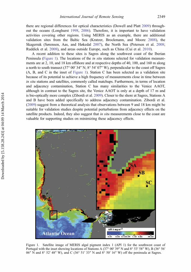
A recent addition to these sites is Sagres along the southwest coast of the IberianPeninsula (Figure 1). The locations of the in situ stations selected for validation measure-ments are at 2, 10, and 18 km offshore and at respective depths of 40, 100, and 160 m alonga north to south transect (37° 00′ 34″ N; 8° 54′ 07″W), perpendicular to the coast off Sagres(A, B, and C in the inset of Figure 1). Station C has been selected as a validation sitebecause of its potential to achieve a high frequency of measurements close in time betweenin situ stations and satellites, commonly called matchups. Furthermore, in terms of locationand adjacency contamination, Station C has many similarities to the Venice AAOT,although in contrast to the Sagres site, the Venice AAOT is only at a depth of 17 m andis bio-optically more complex (Zibordi et al. 2009). Closer to the shore at Sagres, Stations Aand B have been added specifically to address adjacency contamination. Zibordi et al.(2009) suggest from a theoretical analysis that observations between 9 and 18 km might besuitable for validation studies despite potential perturbations from adjacency effects on thesatellite products. Indeed, they also suggest that in situ measurements close to the coast arevaluable for supporting studies on minimizing these adjacency effects.

Figure 1. Satellite image of MERIS algal pigment index 1 (API 1) for the southwest coast ofPortugal with the inset showing locations of Stations A (37° 00′ 39″ N and 8° 53′ 58″ W), B (36° 56′06″ N and 8° 52′ 48″ W), and C (36° 51′ 33″ N and 8° 50′ 16″ W) off the peninsula at Sagres.

International Journal of Remote Sensing 2349

Dow

nloa

ded

by [

5.15

8.28

.243

] at

04:

09 1

4 M

arch

201

4

The validation work at Sagres is focused on the MERIS sensor, which had beenoperational since the launch of ENVISAT in 2002 (Rast, Bezy, and Bruzzi 1999) untilcontact was lost with the satellite in April 2012. This sensor provided spectral informationin 15 bands from 412 to 890 nm, with reduced spatial resolution (RR) at 1200 m and fullspatial resolution (FR) at 300 m. A preliminary validation of MERIS with in situ water-leaving reflectances (ρw) from Sagres was reported by Cristina et al. (2009), where five daysof matchups were achieved during the last six months of 2008. Their study concludes thatthere is a wide scatter in the data, especially at the blue wavelengths, and that the satellite-derived marine reflectance near the coast is underestimated due to error in the atmosphericcorrection caused by Rayleigh and aerosol scattering from the nearby land surface (Santer2010).

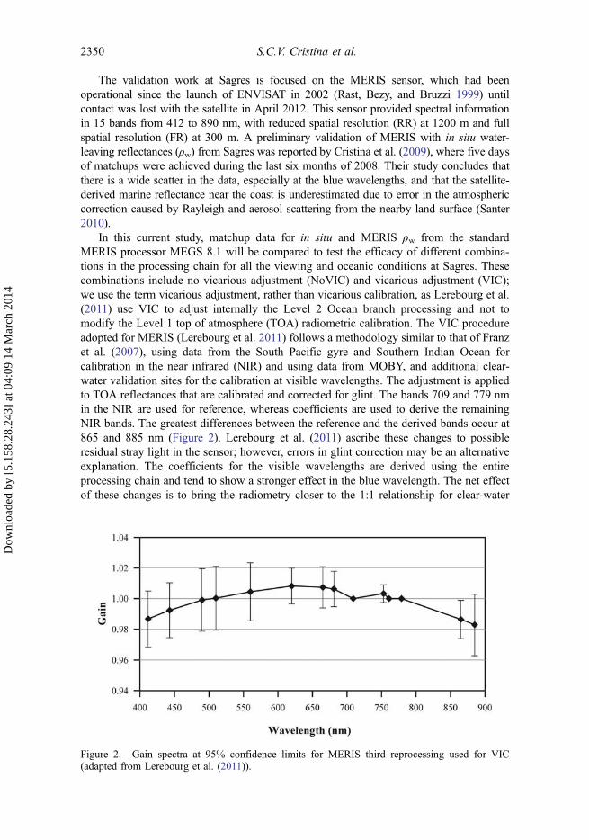
In this current study, matchup data for in situ and MERIS ρw from the standardMERIS processor MEGS 8.1 will be compared to test the efficacy of different combina-tions in the processing chain for all the viewing and oceanic conditions at Sagres. Thesecombinations include no vicarious adjustment (NoVIC) and vicarious adjustment (VIC);we use the term vicarious adjustment, rather than vicarious calibration, as Lerebourg et al.(2011) use VIC to adjust internally the Level 2 Ocean branch processing and not tomodify the Level 1 top of atmosphere (TOA) radiometric calibration. The VIC procedureadopted for MERIS (Lerebourg et al. 2011) follows a methodology similar to that of Franzet al. (2007), using data from the South Pacific gyre and Southern Indian Ocean forcalibration in the near infrared (NIR) and using data from MOBY, and additional clear-water validation sites for the calibration at visible wavelengths. The adjustment is appliedto TOA reflectances that are calibrated and corrected for glint. The bands 709 and 779 nmin the NIR are used for reference, whereas coefficients are used to derive the remainingNIR bands. The greatest differences between the reference and the derived bands occur at865 and 885 nm (Figure 2). Lerebourg et al. (2011) ascribe these changes to possibleresidual stray light in the sensor; however, errors in glint correction may be an alternativeexplanation. The coefficients for the visible wavelengths are derived using the entireprocessing chain and tend to show a stronger effect in the blue wavelength. The net effectof these changes is to bring the radiometry closer to the 1:1 relationship for clear-water

Figure 2. Gain spectra at 95% confidence limits for MERIS third reprocessing used for VIC(adapted from Lerebourg et al. (2011)).


Dow

nloa

ded

by [

5.15

8.28

.243

] at

04:

09 1

4 M

arch

201

4

sites (MQWG 2012). There are, however, concerns about the adjustment, since there areoffsets in the mean monthly remote-sensing reflectance (Rrs) ratios for MODIS andSeaWiFS (MQWG 2012), and because there is a reduction in valid matchups comparedto the second reprocessing (MQWG 2011). It is also important to note that most of thedifferences between these coefficients at different wavelengths are not statistically sig-nificant at the 95% confidence level (Figure 2).

An additional combination to the MERIS processing chain is the Improved Contrastbetween Ocean and Land (ICOL) processor, which has been implemented to correct foradjacency effects. These have been extensively studied by Santer and Schmechtig (2000),using 5S model calculations to demonstrate that the influence of adjacency is the strongestclose to shore but can still be significant up to 20 km offshore, depending on the relativecontributions of Rayleigh and aerosol scattering. Where Raleigh scattering dominates, theeffects are seen further offshore owing to the higher scale height of Rayleigh scatteringcompared to that of aerosol scattering. This effect should be corrected by ICOL (Santer2010; Santer and Zagolski 2009), which computes the TOA signal by removing the signalfrom the adjacent land pixels, thereby providing a product that can be used in oceancolour processors. Since VIC is also applied to the entire processing chain, and ICOLsubstantially changes the processing in near-shore waters, the effect of ICOL is tested inthis study both without vicarious adjustment (ICOL) and with vicarious adjustment(VIC + ICOL).

The development of good-quality remote-sensing products for monitoring thesewaters, particularly near the coast, would have important economic benefits for thisregion, where there is commercial fishing, a rapidly expanding aquaculture industry,and tourism based on cetacean and bird watching, recreational fishing, diving, and surfing(Loureiro, Newton, and Icely 2005, Loureiro et al. 2011).

2. Study area

2.1. General description

The coast at Sagres has a characteristic narrow continental shelf that descends rapidly todepths of over 1000 m at the continental slope. As the summer months are dominated bynortherly winds, an offshore Ekman transport drives an upwelling of relatively cool,nutrient-rich, subsurface waters along the west coast; after a prolonged period of northerlywinds, upwelled waters will circulate around Cape Saint Vincent at the southwestern tip ofthe Iberian Peninsula and flow eastwards along the southern shelf, including the Sagresarea (Loureiro, Newton, and Icely 2005; Relvas and Barton 2005; Relvas et al. 2007).These changes in water masses induce variations in the productivity and the bio-opticalproperties of the waters around Sagres. Although the subject of this article is radiometricreflectances, the bio-optical properties should be known for Sagres to facilitate theinterpretation of radiometric measurements.

2.2. Bio-optical properties

During the deployment of the radiometer, water samples were taken using a Niskin bottleat three depths (0 m, ½ Secchi depth, and 1 Secchi depth). The processing of thesesamples and subsequent chemical analysis are described in more detail in Cristina et al.(2010) and Goela et al. (2013). The water samples were essentially treated to obtain in situvalues for standard MERIS products including: algal pigment index 1 (API 1)


Dow

nloa

ded

by [

5.15

8.28

.243

] at

04:

09 1

4 M

arch

201

4

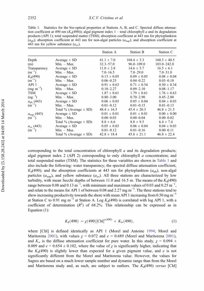
corresponding to the total concentration of chlorophyll a and its degradation products;algal pigment index 2 (API 2) corresponding to only chlorophyll a concentration; andtotal suspended matter (TSM). The statistics for these variables are shown in Table 1 andalso include the following: water transparency; the spectral diffuse attenuation coefficient,Kd(490); and the absorption coefficients at 443 nm for phytoplankton (aph), non-algalparticles (anap), and yellow substance (ays). All three stations are characterized by lowturbidity, with mean Secchi depths of between 11.0 and 16.5 m. The means of the Kd(490)range between 0.08 and 0.13 m−1, with minimum and maximum values of 0.03 and 0.25 m−1,and relate to the means for API 1 of between 0.08 and 2.27 mg m−3. The three stations tend toshow increasing productivity towards the shore withmeanAPI 1 increasing from 0.50mgm−3

at Station C to 0.91 mg m−3 at Station A. Log Kd(490) is correlated with log API 1, with acoefficient of determination (R2) of 68.2%. This relationship can be expressed as inEquation (1):

Kdð490Þ ¼ χð490Þ½Chl�eð490Þ þ Kwð490Þ; (1)

where [Chl] is defined identically as API 1 (Morel and Antoine 1994; Morel andMaritorena 2001), with values χ = 0.072 and e = 0.689 (Morel and Maritorena 2001),and Kw is the diffuse attenuation coefficient for pure water. In this study, χ = 0.094 ±0.009 and e = 0.654 ± 0.102, where the value of χ is significantly higher, indicating thatthe Kd(490) is slightly lower than expected for a given pigment value, and e is notsignificantly different from the Morel and Maritorena value. However, the values forSagres are based on a much lower sample number and dynamic range than from the Moreland Maritorena study and, as such, are subject to outliers. The Kd(490) versus [Chl]

Table 1. Statistics for the bio-optical properties at Stations A, B, and C. Spectral diffuse attenua-tion coefficient at 490 nm (Kd(490)); algal pigment index 1 – total chlorophyll a and its degradationproducts (API 1); total suspended matter (TSM); absorption coefficient at 443 nm for phytoplankton(aph); absorption coefficient at 443 nm for non-algal particles (anap); and absorption coefficient at443 nm for yellow substance (ays).

Station A Station B Station C

Depth Average ± SD 41.1 ± 7.0 104.4 ± 3.3 160.3 ± 40.5(m) Min. – Max. 32.3–57.0 96.0–109.0 103.0–242.0Transparency Average ± SD 11.0 ± 2.8 14.6 ± 5.7 16.5 ± 6.1(m−1) Min. – Max. 7.0–16.5 7.0–29.0 7.0–31.0Kd(490) Average ± SD 0.13 ± 0.05 0.09 ± 0.05 0.08 ± 0.04(m−1) Min. – Max. 0.06–0.25 0.04–0.22 0.03–0.18API 1 Average ± SD 0.91 ± 0.63 0.71 ± 0.54 0.50 ± 0.34(mg m−3) Min. – Max. 0.10–2.27 0.09–2.10 0.08–1.17TSM Average ± SD 1.87 ± 0.61 1.79 ± 0.61 1.76 ± 0.63(ug.–l) Min. – Max. 0.80–3.00 0.70–2.90 0.45–2.80aph (443) Average ± SD 0.06 ± 0.03 0.05 ± 0.04 0.04 ± 0.03(m−1) Min. – Max. 0.01–0.12 0.01–0.15 0.01–0.13

Total % (Average ± SD) 48.4 ± 16.5 45.4 ± 20.3 46.8 ± 21.5anap (443) Average ± SD 0.01 ± 0.01 0.01 ± 0.01 0.00 ± 0.00(m−1) Min. – Max. 0.00–0.03 0.00–0.04 0.00–0.02

Total % (Average ± SD) 8.8 ± 6.6 8.8 ± 9.5 6.4 ± 7.4ays (443) Average ± SD 0.05 ± 0.03 0.06 ± 0.04 0.04 ± 0.03(m−1) Min. – Max. 0.01–0.12 0.01–0.16 0.00–0.11

Total % (Average ± SD) 42.8 ± 18.4 45.8 ± 21.1 46.8 ± 22.4


Dow

nloa

ded

by [

5.15

8.28

.243

] at

04:

09 1

4 M

arch

201

4

relationship is comparable with the Gordon and Morel (1983) definition of Case 1 versusCase 2 waters.

The absorption coefficients at 443 nm for aph, anap, and ays are presented in Figure 3using the ternary diagrams classification proposed by Prieur and Sathyendranath (1981).In general, the properties at the three stations at Sagres are similar over an individualsampling campaign. Furthermore, the percentage differences between aph, anap, and aysare, respectively, 48, 9, and 43 for Station A and 47, 6, and 47 for Station C (Table 1),confirming that there are only limited differences between the coastal and offshorestations, and that these Case 1 waters are dominated by phytoplankton and yellowsubstances. The proportion of ays is comparable with that in the NOMAD database(Werdell and Bailey 2005), where the value is 42.2 ± 17.2.

3. Data and methods

The validation campaigns for this study at Sagres have taken into account the seven keyrecommendations by Bailey and Werdell (2006) for the validation of ocean coloursensors: (1) use a consistently processed in situ data set; (2) eliminate suspect in situdata (e.g. from optically shallow waters) from the validation set; (3) use a narrow timewindow for determining coincidence (i.e. no more than ±3 h) between in situ and satellitedata records; (4) use native resolution satellite products (i.e. avoid sub-sampled data); (5)use the mean of a 5 × 5 pixel box centred on the in situ location; (6) mask satellite pixelsappropriately on the Level 2 flags; and (7) use a homogeneity test to minimize the impactof geophysical variability in the 5 × 5 pixel box on the mean of satellite measurements.

The measurements for radiometric, atmospheric, and water variables in this studyare consistent with the protocols for the validation of MERIS products (Barker 2011see: http://hermes.acri.fr/mermaid/dataproto/CO-SCI-ARG-TN-0008_MERIS_Optical_Measurement_Protocols_Issue2_Aug2011.pdf, and Doerffer, 2002 see: https://earth.esa.int/workshops/mavt_2003/MAVT-2003_801_MERIS-protocols_issue1.3.5.pdf).

3.1. In situ radiometric data

In situ radiometric measurements were collected between October 2008 and November2011 from Stations A, B, and C. The radiometer used for these measurements was atethered attenuation coefficient chain sensor (TACCS) manufactured by Satlantic Inc.,Halifax, NS, Canada, comprising a floating buoy encasing a hyperspectral surface irra-diance sensor Es(λ) and a subsurface radiance sensor Lu(λ) located 0.62 m below thesurface, as well as a tethered attenuation chain (K-chain) supporting four subsurfaceirradiance sensors Ed(z) attached at nominal depths (z) of 2, 4, 8, and 16 m. Initially, Ed

(z) was measured only at 490 nm, but after an upgrade in 2010, Ed(z) was also measuredat 412, 560, and 665 nm. A compass with a pitch and roll sensor was also incorporated inthe TACCS during the upgrade of the sensors. The small size of the TACCS and theflexible attenuation chain allowed rapid deployment of the instrument from small boatsfor responsive sampling during campaigns for satellite matchups (Moore, Icely, andKratzer 2010).

The in situ measurements were timed to coincide with the MERIS overpass within±30 minutes at Station A and within ±1.5 hours at Stations B and C. At each site, theTACCS was deployed up to 20 m clear of the boat to avoid interference to the lightpattern from the shadow of the boat. After a period of acclimatization to the watertemperature, the instrument recorded five sets of data, each for 2 min, at a rate of


Dow

nloa

ded

by [

5.15

8.28

.243

] at

04:

09 1

4 M

arch

201

4

http://hermes.acri.fr/mermaid/dataproto/CO-SCI-ARG-TN-0008_MERIS_Optical_ Measurement_Protocols_Issue2_Aug2011.pdf

http://hermes.acri.fr/mermaid/dataproto/CO-SCI-ARG-TN-0008_MERIS_Optical_ Measurement_Protocols_Issue2_Aug2011.pdf

http://https://earth.esa.int/workshops/mavt_2003/MAVT-2003_801_MERIS-protocols_issue1.3.5.pdf

http://https://earth.esa.int/workshops/mavt_2003/MAVT-2003_801_MERIS-protocols_issue1.3.5.pdf

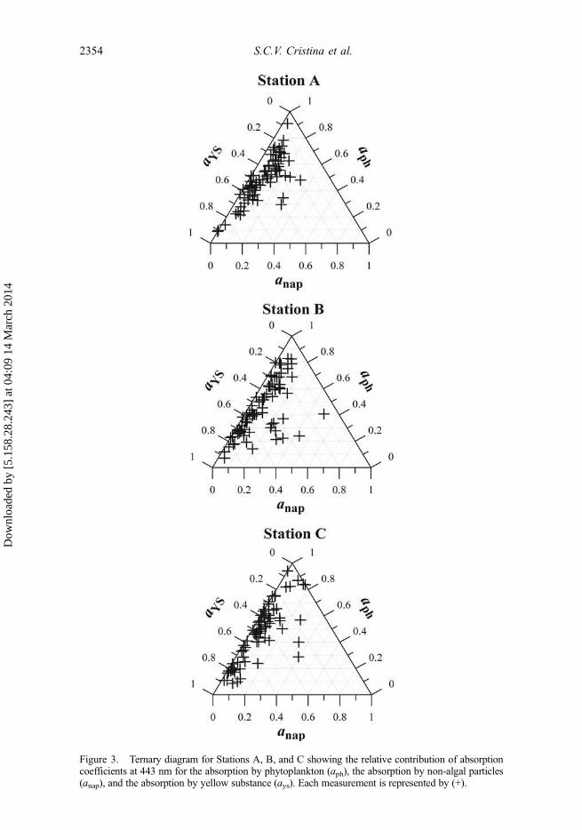
Figure 3. Ternary diagram for Stations A, B, and C showing the relative contribution of absorptioncoefficients at 443 nm for the absorption by phytoplankton (aph), the absorption by non-algal particles(anap), and the absorption by yellow substance (ays). Each measurement is represented by (+).


Dow

nloa

ded

by [

5.15

8.28

.243

] at

04:

09 1

4 M

arch

201

4

approximately one sample per second (depending on the integration time). The hyper-spectral sensors have shutters that provide dark readings at the same integration time asthe light readings, approximately every three seconds. These data were interpolated toprovide the dark offset for the spectra between wavelengths (λ) of 350 and 800 nm. Forthe Ed(z) sensors, dark readings were taken immediately post-deployment so that tem-perature effects were minimized.

The location and meteorological data at each sampling site were recorded continu-ously during the deployment of the radiometer with an Airmar PB150 ultrasonic weatherstation (Milford, NH, USA). At each station, the atmospheric conditions were alsorecorded with a MICROTOPS II sunphotometer (version 5.5; Solar Light CompanyInc., Glenside, PA, USA) to provide data on atmospheric pressure, water vapour, andaerosol optical thickness (AOT) at the wavelengths 380, 500, 870, 936, and 1020 nm.Activities related to water variables have been introduced in Section 2.2.

3.2. Processing in situ radiometric data

The raw data from each sensor were converted from binary to calibrated engineering unitsusing Satlantic SatCon software that could then be visually screened for stability overeach cast and rejected if there were excessive noise artefacts. Since the spectrographs hadslightly different spectral sampling points, the two hyper-spectral sensors were co-alignedby linear interpolation to a 1 nm grid. The data from the sensors of Es(λ), Lu(λ), and Ed(z)were corrected for the dark signal. The spectral diffuse attenuation coefficient Kd (m−1)from multi-depth Ed(z) at 412, 490, 560, and 665 nm was determined from the slope forthe natural log regression of the K-chain. Ed was obtained from the intercept at 412, 490,560, and 665 nm for measurements at each depth except for 2008 and 2009 data, whereonly data at 490 nm was available. For the 2010 and 2011 data, the Kd for the otherwavelengths was estimated by first determining Kd′(490) as in Equation (2):

Kd0ð490Þ ¼ Kdð490Þ � Kwð490Þ; (2)

where Kw(490) is taken from Morel and Antoine (1994).Second, Kd′ was determined at other wavelengths by converting the Kd′(490) obtained

from Equation (2) into the apparent chlorophyll using a simple inversion from Equation(3), again using the coefficients of Morel and Antoine (1994):

Kd0ðλ;ChlÞ ¼ χðλÞ ½Chl�eðλÞ: (3)

Kd(λ) was then estimated as in Equation (4):

KdðλÞ ¼ Kd0ðλÞ þ KwðλÞ; (4)

where the Kd spectra derived from the chlorophyll were normalized to Kd at 412, 490,560, and 665 nm, so that the final spectra were correct at the measured wavelengths.

The upwelling radiance Lu was extrapolated to just below the sea surface as inEquation (5):

Luð0�; λÞ ¼ LuðλÞe�0:62 KLðλÞ ; (5)


Dow

nloa

ded

by [

5.15

8.28

.243

] at

04:

09 1

4 M

arch

201

4

where Kd(λ) obtained from Equation (4) is assumed to approximate to KL(λ) in Equation(5). The assumption that Kd is a good estimate of KL has been tested using a simulateddataset calculated with Hydrolight (Mobley 1995) for both Case 1 and Case 2 waters. Forthese data, a realistic range of absorption (a) and scattering (b) is generated with anincreasing single scattering albedo ranging from that of pure water to 0.6. Kd is thencalculated at the K-chain depths from the simulated data using the log linear regression.KL is determined from the upwelling radiance at the depth of the radiance sensor, and thatjust below the surface. From these runs of the model, the mean value of the ratio betweenKd and KL was 1.005, but this has a scatter dependent on the single scattering albedo of±0.02. This additional uncertainty of 1–2% in the extrapolation of the measured radianceto the surface is accounted for in the error budget given in Table 2. The factor 0.62 is thedepth offset for the Lu(λ) sensor. From Lu(0

–,λ), the water leaving radiance Lw(λ) wasdetermined as in Equation (6):

LwðλÞ ¼ Luð0�; λÞ ð1� ρÞn2w

; (6)

where nw is the refractive index of seawater and ρ is the air sea surface reflectance frombelow, which depends on wind speed and view angle. The term ð1� ρÞ=n2w is the upwardradiance transmittance of the sea surface for normal incidence from below and isapproximately 0.54, with the exact values for nadir viewing in seawater taken fromTable 10-1 in Barker (2011).

The Es data between 2010 and 2011 were calculated by two methods depending onwhether the minimum pitch and roll during the sampling period was close to zero. If theminimum pitch and roll minimum were close to zero (<2°), then the Es value was taken atthe time when the TACCS was the closest to vertical. Where the minimum pitch and rollwas not close to vertical, then a correction was performed under the assumption that thediffuse solar irradiance was isotropic, and that the direct irradiance could be corrected bycalculating the angle with the cosine collector.

First, the ratio of direct to total irradiance (dt) was estimated from Equation (7):

dt ¼ Edir

Etot: (7)

Table 2. Summary of the uncertainty budget for water-leaving reflectance (ρw) determined for theTACCS at Station A (SA), Station B (SB), and Station C (SC) for wavelengths 443, 490, and560 nm.

443 nm 490 nm 560 nm

Uncertainty source SA SB SC SA SB SC SA SB SC

Absolute calibration of Lu(λ) 2.8 2.8 2.8 2.8 2.8 2.8 2.8 2.8 2.8Self-shading corrections 0.7 0.7 0.7 0.7 0.7 0.7 0.7 0.7 0.7Absolute calibration of Ed(λ) 3.1 3.1 3.1 3.1 3.1 3.1 3.1 3.1 3.1Bio-optical assumptions 2.2 2.2 2.2 1.2 1.2 1.2 2.0 2.0 2.0Geometrical effects 4.5 4.5 4.5 4.5 4.5 4.5 4.0 4.0 4.0Environmental perturbations 2.8 3.0 3.8 3.1 3.2 5.0 4.0 3.5 4.6Quadrature sum (%) 7.1 7.2 7.6 7.0 7.1 8.1 7.4 7.1 7.7


Dow

nloa

ded

by [

5.15

8.28

.243

] at

04:

09 1

4 M

arch

201

4

Second, the angle of the solar angle (θsun), and the apparent angle of the sun to theirradiance sensor (θsen), was calculated. The correction factor f for the direct irradiancewas from Equation (8):

f ¼ cosðθsenÞcosðθsunÞ : (8)

The final correction was estimated from Equation (9):

Es ¼ EsðobsÞð1 þ dt ðf � 1ÞÞ : (9)

There are limitations to this correction in that it applies to only small angles. Where theangle of tilt is large, the Fresnel reflectance of the ‘roughened’ sea surface becomessignificant when the buoy leans towards the anti-solar direction. For small angles, an errorof 2% was assumed, increasing to 4% at lower wavelengths where aerosol and Rayleighscattering dominated.

The self-shading correction for Lw(λ), derived from in-water radiometric measure-ments, was based on the model of Gordon and Ding (1992) and this correction followedthe ocean optics protocols for satellite ocean colour sensor validation (Mueller 2003). Thecorrection required the spectral absorption coefficient a(λ), which is approximated to Kd

(λ), and the quantity h, which is the ratio of diffuse to direct irradiance.The direct and diffuse irradiances were calculated following Bird and Riordan (1986)

and modified to use the extraterrestrial irradiances from Thuillier et al. (2003). The ozoneconcentration was extracted from the Total Ozone Mapping Spectrometer (availableonline on website http://ozoneaq.gsfc.nasa.gov/ozone_overhead_all_v8.md); water vapourconcentration and AOT were obtained from the MICROTOPS II (version 5.5) sunphot-ometer (Morys et al. 2001), although for the 2008 and 2009 data these parameters weretaken from the MERIS matchup pixel. The total irradiance was used as a check on the Es

(λ) derived from the normalization.Finally, all these measurements were used to estimate the water-leaving reflectance,

ρw(λ), from Equation (10). The radiometric data were determined at the MERIS wave-lengths using linear interpolation of the hyperspectral data. This was appropriate since thebandwidth of the Satlantic radiometer is between 10 and 12 nm.

ρw ¼ πLwðλÞEsðλÞ : (10)

3.3. Inter-comparison with other radiometric instruments

The uncertainties and the accuracy of the in situ radiometric data obtained by thePortuguese Satlantic TACCS were assessed during 2010 by inter-comparison with otherradiometers used by the MERIS Validation Team (MVT) supported by ESA. In February2010, there was a field inter-comparison and validation exercise at Sagres between thePortuguese hyperspectral and the Swedish Satlantic TACCS with filters set for MERISwavelengths. The details of this comparison are presented in Moore, Icely, and Kratzer(2010).


Dow

nloa

ded

by [

5.15

8.28

.243

] at

04:

09 1

4 M

arch

201

4

http://ozoneaq.gsfc.nasa.gov/ozone_overhead_all_v8.md

The second inter-comparison, under the title Assessment of In Situ RadiometricCapabilities for Coastal Water Remote Sensing Applications (ARC), was conceivedwithin the framework of the MVT. The ARC activities occurred during July 2010 witha phase of field measurements carried out at the AAOT in the north Adriatic Sea over fourdays characterized by favourable illumination and sea state conditions. The subsequentphase comprised an inter-calibration of the optical sensors deployed at the AAOT. Thisinter-calibration was achieved at the Joint Research Centre, Ispra Italy, through theabsolute radiometric calibration of the optical sensors using identical laboratory standardsand methods. These activities quantified differences among fundamental radiometricproducts derived from the deployment of three in-water and three above-water systems,with the Wire-Stabilized Profiling Environmental Radiometer (WiSPER) and thePortuguese and the Swedish TACCS comprising the in-water systems, and the SeaWiFSPhotometer Revision for Incident Surface Measurements (SeaPRISM) and Belgium andEstonian TriOS Optical Systems (TRIOS) comprising the above-water systems. Theresults from ARC 2010 are presented in Zibordi et al. (2012).

The uncertainties established during the inter-comparisons at Sagres and Venice forthe in situ radiometric data from the Portuguese TACCS were used to assess the uncer-tainties for ρw at 443, 490, and 560 nm for the three stations off Sagres. Table 2 showsvalues between 7 and 7.4% for Station A, between 7.1 and 7.2% for Station B, andbetween 7.6 and 8.1% for Station C.

3.4. Processing satellite data from MERIS

MERIS Level 1b images were processed to Level 2 with the Optical Data processor ofESA, version 8.1 (ODESA MEGS®; see earth.eo.esa.int/odesa/). Full resolution (FR)Level 2 data from MERIS, with a spatial resolution of 290 × 260 m, were obtainedwith the Basic ERS & ENVISAT (A)ATSR and MERIS Toolbox (BEAM version 4.9; seewww.brockmann-consult.de/cms/web/beam/). Based on the coordinates of the stationsfrom each field campaign at Sagres, 3 × 3 pixel matrices were extracted from theMERIS Level 2 products. A matrix was only compared with in situ data provided therewere five or more valid pixels. Using these procedures, it was possible to evaluate theperformance of the different combinations available from the MERIS processor: NoVIC,VIC, ICOL, and VIC + ICOL (see Section 1 for more details). Essentially, the Level 2procedure started with the NoVIC combination where the images were filtered forcontamination such as high glint, ice haze, and high solar zenith. These images couldthen be configured further by VIC, where a systematic bias to the spectral gains in theradiometric calibration and/or the TOA correction could be corrected by the coefficientsshown in Figure 2 (adapted from Table 3 in Lerebourg et al. 2011). MERIS Level 1bimages were also processed by ICOL version 2.7.4 with BEAM software version 4.9 andup to Level 2 with the ODESA MEGS® software. Santer (2010) presents the scientificbasis for ICOL (see Section 1).

3.5. Statistical methods for the matchup analysis

An analysis of the results from the matchups uses several statistical indicators to quantifythe agreement between satellite Level 2 products (yi) and in situ measurements (xi),including the mean ratio (MR) in Equation (11), the absolute percentage difference(APD) in Equation (12), the average of relative percentage difference (RPD) in


Dow

nloa

ded

by [

5.15

8.28

.243

] at

04:

09 1

4 M

arch

201

4

http://www.brockmann-consult.de/cms/web/beam/

Equation (13), and also the intercept, slope, and R2 from linear regressions. In thefollowing, i is the matchup index and N is the number of matchups:

MR ¼ 1

N

XNi¼1

yixi; (11)

APD ¼ 1

N

XNi¼1

yi � xij jxi

� �100 %; (12)

RPD ¼ 1

N

XNi¼1

yi � xixi

100 %: (13)

4. Results

4.1. Matchup analysis

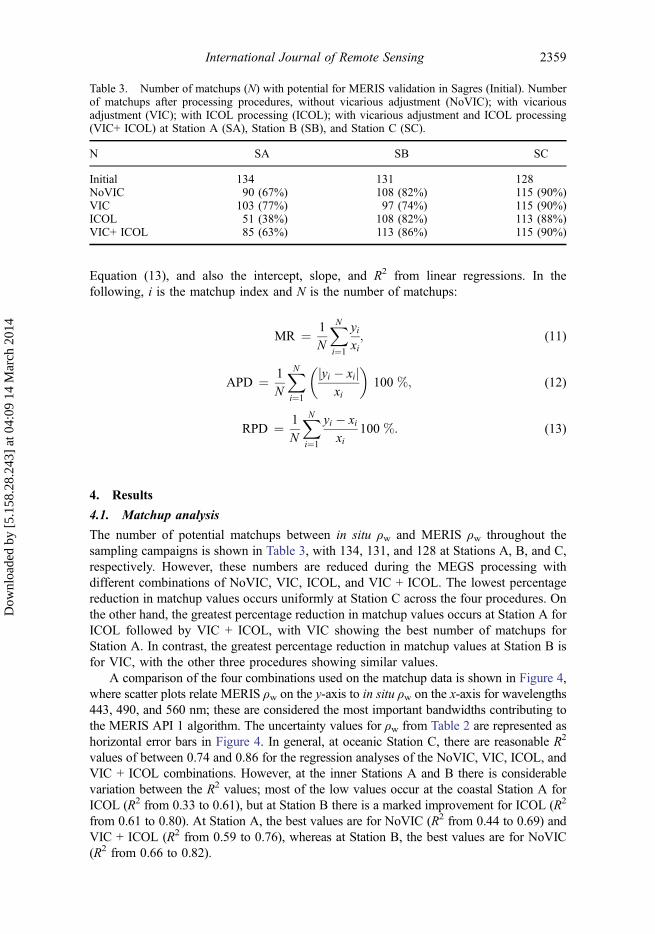
The number of potential matchups between in situ ρw and MERIS ρw throughout thesampling campaigns is shown in Table 3, with 134, 131, and 128 at Stations A, B, and C,respectively. However, these numbers are reduced during the MEGS processing withdifferent combinations of NoVIC, VIC, ICOL, and VIC + ICOL. The lowest percentagereduction in matchup values occurs uniformly at Station C across the four procedures. Onthe other hand, the greatest percentage reduction in matchup values occurs at Station A forICOL followed by VIC + ICOL, with VIC showing the best number of matchups forStation A. In contrast, the greatest percentage reduction in matchup values at Station B isfor VIC, with the other three procedures showing similar values.

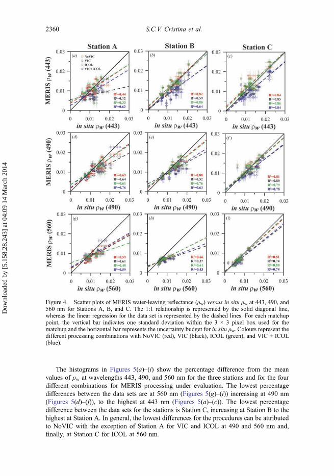
A comparison of the four combinations used on the matchup data is shown in Figure 4,where scatter plots relate MERIS ρw on the y-axis to in situ ρw on the x-axis for wavelengths443, 490, and 560 nm; these are considered the most important bandwidths contributing tothe MERIS API 1 algorithm. The uncertainty values for ρw from Table 2 are represented ashorizontal error bars in Figure 4. In general, at oceanic Station C, there are reasonable R2

values of between 0.74 and 0.86 for the regression analyses of the NoVIC, VIC, ICOL, andVIC + ICOL combinations. However, at the inner Stations A and B there is considerablevariation between the R2 values; most of the low values occur at the coastal Station A forICOL (R2 from 0.33 to 0.61), but at Station B there is a marked improvement for ICOL (R2

from 0.61 to 0.80). At Station A, the best values are for NoVIC (R2 from 0.44 to 0.69) andVIC + ICOL (R2 from 0.59 to 0.76), whereas at Station B, the best values are for NoVIC(R2 from 0.66 to 0.82).

Table 3. Number of matchups (N) with potential for MERIS validation in Sagres (Initial). Numberof matchups after processing procedures, without vicarious adjustment (NoVIC); with vicariousadjustment (VIC); with ICOL processing (ICOL); with vicarious adjustment and ICOL processing(VIC+ ICOL) at Station A (SA), Station B (SB), and Station C (SC).

N SA SB SC

Initial 134 131 128NoVIC 90 (67%) 108 (82%) 115 (90%)VIC 103 (77%) 97 (74%) 115 (90%)ICOL 51 (38%) 108 (82%) 113 (88%)VIC+ ICOL 85 (63%) 113 (86%) 115 (90%)


Dow

nloa

ded

by [

5.15

8.28

.243

] at

04:

09 1

4 M

arch

201

4

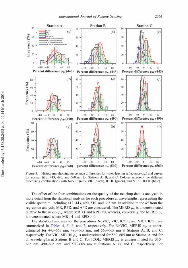
The histograms in Figures 5(a)–(i) show the percentage difference from the meanvalues of ρw at wavelengths 443, 490, and 560 nm for the three stations and for the fourdifferent combinations for MERIS processing under evaluation. The lowest percentagedifferences between the data sets are at 560 nm (Figures 5(g)–(i)) increasing at 490 nm(Figures 5(d)–(f)), to the highest at 443 nm (Figures 5(a)–(c)). The lowest percentagedifference between the data sets for the stations is Station C, increasing at Station B to thehighest at Station A. In general, the lowest differences for the procedures can be attributedto NoVIC with the exception of Station A for VIC and ICOL at 490 and 560 nm and,finally, at Station C for ICOL at 560 nm.

Figure 4. Scatter plots of MERIS water-leaving reflectance (ρw) versus in situ ρw at 443, 490, and560 nm for Stations A, B, and C. The 1:1 relationship is represented by the solid diagonal line,whereas the linear regression for the data set is represented by the dashed lines. For each matchuppoint, the vertical bar indicates one standard deviation within the 3 × 3 pixel box used for thematchup and the horizontal bar represents the uncertainty budget for in situ ρw. Colours represent thedifferent processing combinations with NoVIC (red), VIC (black), ICOL (green), and VIC + ICOL(blue).


Dow

nloa

ded

by [

5.15

8.28

.243

] at

04:

09 1

4 M

arch

201

4

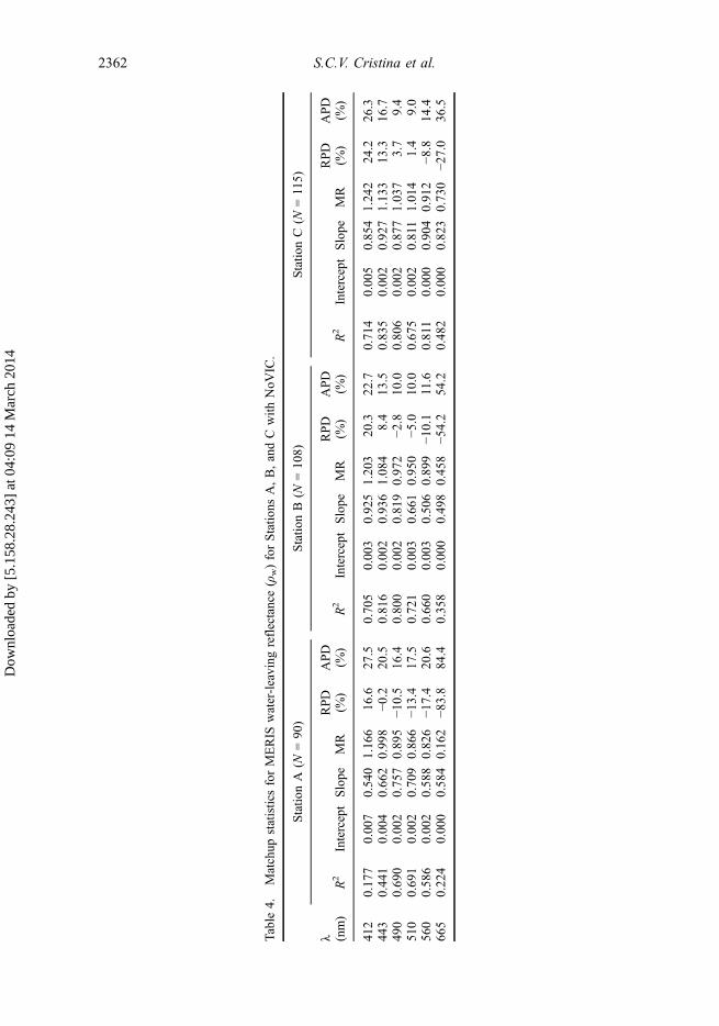
The effect of the four combinations on the quality of the matchup data is analysed inmore detail from the statistical analysis for each procedure at wavelengths representing thevisible spectrum, including 412, 443, 490, 510, and 665 nm. In addition to the R2 from theregression analysis, MR, RPD, and APD are considered. The MERIS ρw is underestimatedrelative to the in situ ρw, where MR <1 and RPD <0, whereas, conversely, the MERIS ρwis overestimated where MR >1 and RPD > 0.

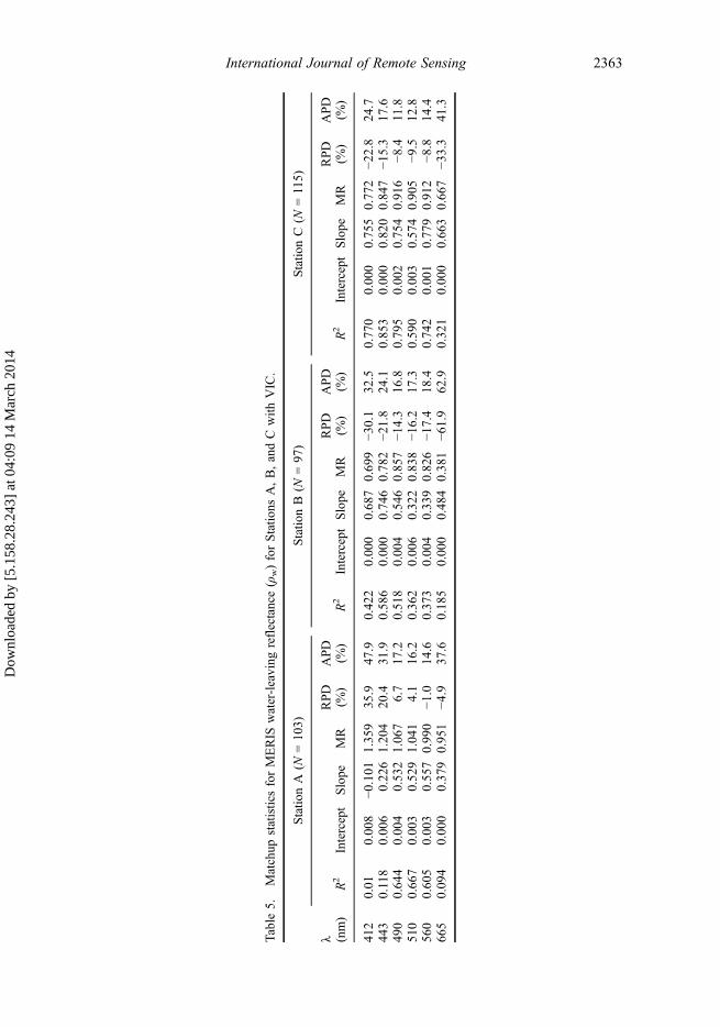
The statistical analyses for the procedures NoVIC, VIC, ICOL, and VIC+ ICOL aresummarized in Tables 4, 5, 6, and 7, respectively. For NoVIC, MERIS ρw is under-estimated for 443–665 nm, 490–665 nm, and 560–665 nm at Stations A, B, and C,respectively. For VIC, MERIS ρw is underestimated for 560–665 nm at Station A and forall wavelengths at Stations B and C. For ICOL, MERIS ρw is underestimated for 510–665 nm, 490–665 nm, and 560–665 nm at Stations A, B, and C, respectively. For

Figure 5. Histograms showing percentage differences for water-leaving reflectance (ρw) and curvesfor normal fit at 443, 490, and 560 nm for Stations A, B, and C. Colours represent the differentprocessing combinations with NoVIC (red), VIC (black), ICOL (green), and VIC + ICOL (blue).


Dow

nloa

ded

by [

5.15

8.28

.243

] at

04:

09 1

4 M

arch

201

4

Table

4.Matchup

statisticsforMERIS

water-leaving

reflectance(ρ

w)forStatio

nsA,B,andCwith

NoV

IC.

Statio

nA

(N=90

)Statio

nB(N

=10

8)Statio

nC(N

=115)

λ (nm)

R2

InterceptSlope

MR

RPD

(%)

APD

(%)

R2

InterceptSlope

MR

RPD

(%)

APD

(%)

R2

InterceptSlope

MR

RPD

(%)

APD

(%)

412

0.17

70.00

70.54

01.16

616

.627

.50.70

50.00

30.92

51.20

320

.322

.70.71

40.00

50.85

41.24

224

.226

.344

30.44

10.00

40.66

20.99

8−0.2

20.5

0.81

60.00

20.93

61.08

48.4

13.5

0.83

50.00

20.92

71.13

313

.316

.749

00.69

00.00

20.75

70.89

5−10

.516

.40.80

00.00

20.81

90.97

2−2.8

10.0

0.80

60.00

20.87

71.03

73.7

9.4

510

0.69

10.00

20.70

90.86

6−13

.417

.50.72

10.00

30.66

10.95

0−5.0

10.0

0.67

50.00

20.811

1.01

41.4

9.0

560

0.58

60.00

20.58

80.82

6−17

.420

.60.66

00.00

30.50

60.89

9−10

.111.6

0.811

0.00

00.90

40.91

2−8

.814

.466

50.22

40.00

00.58

40.16

2−83

.884

.40.35

80.00

00.49

80.45

8−54

.254

.20.48

20.00

00.82

30.73

0−27

.036

.5


Dow

nloa

ded

by [

5.15

8.28

.243

] at

04:

09 1

4 M

arch

201

4

Table

5.Matchup

statisticsforMERIS

water-leaving

reflectance(ρ

w)forStatio

nsA,B,andCwith

VIC.

Statio

nA

(N=10

3)Statio

nB(N

=97

)Statio

nC(N

=115)

λ (nm)

R2

Intercept

Slope

MR

RPD

(%)

APD

(%)

R2

InterceptSlope

MR

RPD

(%)

APD

(%)

R2

InterceptSlope

MR

RPD

(%)

APD

(%)

412

0.01

0.00

8−0.10

11.35

935

.947

.90.42

20.00

00.68

70.69

9−3

0.1

32.5

0.77

00.00

00.75

50.77

2−22

.824

.744

30.118

0.00

60.22

61.20

420

.431

.90.58

60.00

00.74

60.78

2−2

1.8

24.1

0.85

30.00

00.82

00.84

7−15

.317

.649

00.64

40.00

40.53

21.06

76.7

17.2

0.51

80.00

40.54

60.85

7−1

4.3

16.8

0.79

50.00

20.75

40.91

6−8

.411.8

510

0.66

70.00

30.52

91.04

14.1

16.2

0.36

20.00

60.32

20.83

8−1

6.2

17.3

0.59

00.00

30.57

40.90

5−9

.512

.856

00.60

50.00

30.55

70.99

0−1.0

14.6

0.37

30.00

40.33

90.82

6−1

7.4

18.4

0.74

20.00

10.77

90.91

2−8

.814

.466

50.09

40.00

00.37

90.95

1−4.9

37.6

0.18

50.00

00.48

40.38

1−6

1.9

62.9

0.32

10.00

00.66

30.66

7−33

.341

.3


Dow

nloa

ded

by [

5.15

8.28

.243

] at

04:

09 1

4 M

arch

201

4

Table

6.Matchup

statisticsforMERIS

water-leaving

reflectance(ρ

w)forStatio

nsA,B,andCwith

ICOL.

Statio

nA

(N=51

)Statio

nB(N

=10

8)Statio

nC(N

=113)

λ (nm)

R2

InterceptSlope

MR

RPD

(%)

APD

(%)

R2

InterceptSlope

MR

RPD

(%)

APD

(%)

R2

InterceptSlope

MR

RPD

(%)

APD

(%)

412

0.12

10.00

70.50

31.28

328

.331

.80.69

60.00

40.85

11.18

518

.520

.90.79

70.00

40.91

21.20

720

.723

.144

30.33

60.00

40.63

81.12

512

.518

.80.79

60.00

20.88

61.07

97.9

13.0

0.85

70.00

20.95

51.10

610

.614

.549

00.61

20.00

40.67

31.00

30.3

9.0

0.75

60.00

20.78

00.97

9–2

.110

.20.79

30.00

20.87

11.02

52.5

9.0

510

0.49

70.00

50.54

40.97

0–3

.010

.40.66

00.00

40.61

70.96

3–3

.710

.00.66

40.00

20.80

61.00

60.6

9.0

560

0.47

60.00

50.33

50.91

7–8

.313

.40.611

0.00

30.49

50.91

8–8

.211.3

0.79

80.00

00.92

60.66

6–3

3.4

11.6

665

0.21

60.00

10.30

00.75

8–2

4.2

29.1

0.37

20.00

00.49

80.64

5–3

5.5

38.4

0.48

30.00

00.85

50.75

4–2

4.6

35.0


Dow

nloa

ded

by [

5.15

8.28

.243

] at

04:

09 1

4 M

arch

201

4

Table

7.Matchup

statisticsforMERIS

water-leaving

reflectance(ρ

w)forStatio

nsA,B,andCwith

VIC

+ICOL.

Statio

nA

(N=85

)Statio

nB(N

=113)

Statio

nC(N

=115)

λ (nm)

R2

InterceptSlope

MR

RPD

(%)

APD

(%)

R2

InterceptSlope

MR

RPD

(%)

APD

(%)

R2

InterceptSlope

MR

RPD

(%)

APD

(%)

412

0.36

20.00

30.44

80.78

5–2

0.8

23.8

0.45

90.00

10.64

00.72

7–2

7.3

30.2

0.78

5–0

.001

0.81

30.73

4–2

6.6

28.1

443

0.62

00.00

20.611

0.86

4–1

3.0

18.4

0.64

00.00

10.72

40.80

9–1

9.1

23.2

0.84

40.00

00.85

70.81

9–1

8.1

19.9

490

0.75

70.00

20.74

40.92

6–6

.813

.60.63

10.00

30.63

80.87

6–1

2.4

15.1

0.77

90.00

10.78

30.90

2–9

.812

.651

00.70

60.00

20.711

0.92

7–6

.713

.00.52

30.00

40.45

90.86

1–1

3.9

15.4

0.56

70.00

30.60

40.89

8–1

0.2

12.9

560

0.59

30.00

30.58

50.91

8–7

.614

.20.43

30.00

30.38

90.85

0–1

5.0

15.9

0.73

80.00

10.81

60.90

7–9

.314

.766

50.13

40.00

10.23

60.82

1–1

7.0

24.0

0.24

70.00

00.54

40.57

1–4

2.9

44.6

0.32

80.00

00.71

50.69

6–3

0.4

38.2


Dow

nloa

ded

by [

5.15

8.28

.243

] at

04:

09 1

4 M

arch

201

4

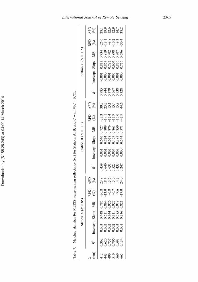
VIC + ICOL, MERIS ρw is underestimated for all the wavelengths for all three stations.Wavelengths not included in the above list are those where MERIS ρw is overestimated,which are generally in the blue bands (412–490 nm).

The quality of the R2, MR, RPD, and APD tends to be better at wavelengths 443, 490,and 510 nm and worse at 412 and 560 nm, with the worst wavelength at 665 nm for allfour procedures. There is also a trend towards improving statistical results from Station Ato Station C.

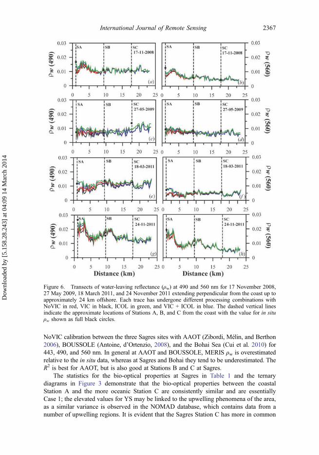
4.2. Comparisons of the effects of ICOL processing

Using all the matchup data it has been possible to trace the effect of ICOL on ρwreflectance from the coast to 24 km offshore incorporating all three of the validationstations. Figure 6 displays transects for ρw at 490 and 560 nm for the various combina-tions that are used for the matchup data and shows examples of the four ‘classes’ ofprofiles that could be identified along these transects. On 17 November 2008, the first‘class’ shows a peak between 3 and 8 km from the shore (Figures 6(a), (b)); on 27 May2009, the second ‘class’ shows no improvement near shore (Figures 6(c), (d)); on 18March 2011, the third ‘class’ shows a marked improvement near shore (Figures 6(e), (f));and finally on 24 November 2011, the fourth ‘class’ shows a dip between 3 and 8 km fromthe shore (Figures 6((g), (h)).

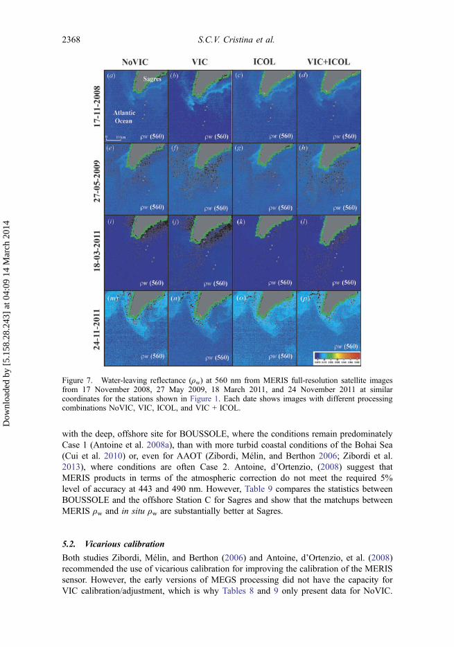
MERIS images from the same dates as the transects above are presented in Figure 7,showing the spatial distribution of ρw at 560 nm off Sagres for NoVIC, VIC, ICOL, andVIC + ICOL processing. Compared to NoVIC, there is a reduction in the number ofinvalid reflectances (black areas in the image) for all four dates after ICOL processing,particularly, on 18 March 2011. In contrast, the VIC processing shows little differencewith the NoVIC processing on 17 November 2008 and 24 November 2011, whereas it ismarkedly worse on 27 May 2009 and 18 March 2011. Finally, the combination ofVIC + ICOL does show some reduction in the number of invalid reflectances, but notas great as for ICOL on its own.

5. Discussion

5.1. General

The Sagres validation campaigns conform to the OPBG criteria, including the following:adherence to the MERIS protocols (Doerffer 2002) for the MERIS sensor; an objectiveprocedure for removing suspect data; a restriction of coincidence time between in situ andsatellite data records to 0.5 hour for the coastal Station A and up to 1.5 hour for the moreoffshore Stations B and C. This has resulted in between 272 and 315 matchups over theduration of the sampling campaigns between October 2008 and November 2011, depend-ing on which of the four combinations is used during the MERIS processing.Uncertainties of 8% can be ascribed to these values, based on the various inter-calibrationexercises carried out over the duration of the samplings campaigns (Moore, Icely, andKratzer 2010; Zibordi et al. 2012).

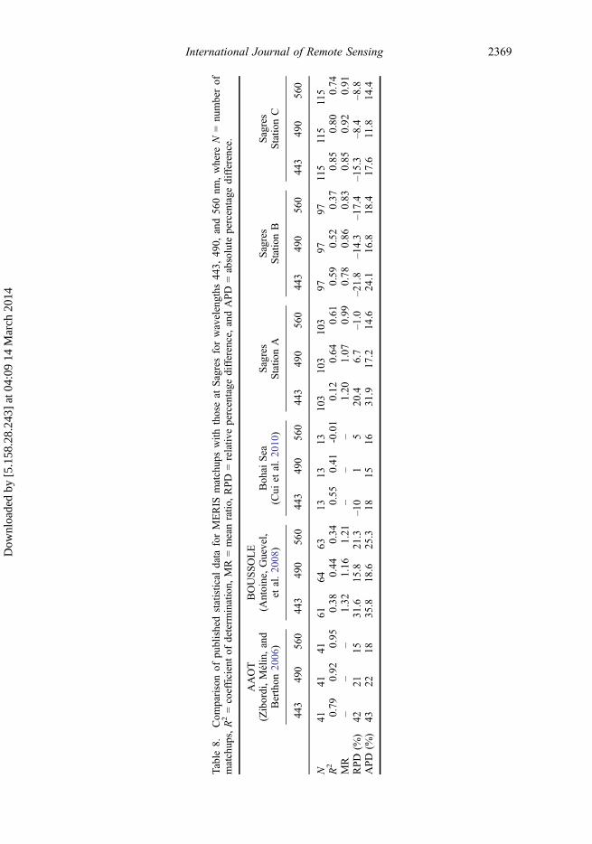
The statistical analysis of the validation data for the NoVIC, VIC, ICOL, andICOL + VIC procedures shows that the greatest statistical differences occur at the extremesof the visible spectra. This is to be expected as ρw at 412 nm is strongly dependent on theaccuracy of the atmospheric correction procedure (Antoine, d’Ortenzio, et al. 2008), and ρwat 665 nm has low values in Case 1 waters. Table 8 compares the statistical analysis for


Dow

nloa

ded

by [

5.15

8.28

.243

] at

04:

09 1

4 M

arch

201

4

NoVIC calibration between the three Sagres sites with AAOT (Zibordi, Mélin, and Berthon2006), BOUSSOLE (Antoine, d’Ortenzio, 2008), and the Bohai Sea (Cui et al. 2010) for443, 490, and 560 nm. In general at AAOT and BOUSSOLE, MERIS ρw is overestimatedrelative to the in situ data, whereas at Sagres and Bohai they tend to be underestimated. TheR2 is best for AAOT, but is also good at Stations B and C at Sagres.

The statistics for the bio-optical properties at Sagres in Table 1 and the ternarydiagrams in Figure 3 demonstrate that the bio-optical properties between the coastalStation A and the more oceanic Station C are consistently similar and are essentiallyCase 1; the elevated values for YS may be linked to the upwelling phenomena of the area,as a similar variance is observed in the NOMAD database, which contains data from anumber of upwelling regions. It is evident that the Sagres Station C has more in common

Figure 6. Transects of water-leaving reflectance (ρw) at 490 and 560 nm for 17 November 2008,27 May 2009, 18 March 2011, and 24 November 2011 extending perpendicular from the coast up toapproximately 24 km offshore. Each trace has undergone different processing combinations withNoVIC in red, VIC in black, ICOL in green, and VIC + ICOL in blue. The dashed vertical linesindicate the approximate locations of Stations A, B, and C from the coast with the value for in situρw shown as full black circles.


Dow

nloa

ded

by [

5.15

8.28

.243

] at

04:

09 1

4 M

arch

201

4

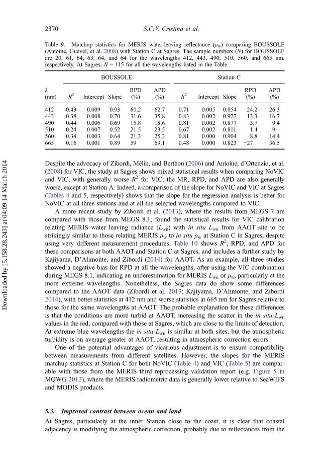
with the deep, offshore site for BOUSSOLE, where the conditions remain predominatelyCase 1 (Antoine et al. 2008a), than with more turbid coastal conditions of the Bohai Sea(Cui et al. 2010) or, even for AAOT (Zibordi, Mélin, and Berthon 2006; Zibordi et al.2013), where conditions are often Case 2. Antoine, d’Ortenzio, (2008) suggest thatMERIS products in terms of the atmospheric correction do not meet the required 5%level of accuracy at 443 and 490 nm. However, Table 9 compares the statistics betweenBOUSSOLE and the offshore Station C for Sagres and show that the matchups betweenMERIS ρw and in situ ρw are substantially better at Sagres.

5.2. Vicarious calibration

Both studies Zibordi, Mélin, and Berthon (2006) and Antoine, d’Ortenzio, et al. (2008)recommended the use of vicarious calibration for improving the calibration of the MERISsensor. However, the early versions of MEGS processing did not have the capacity forVIC calibration/adjustment, which is why Tables 8 and 9 only present data for NoVIC.

Figure 7. Water-leaving reflectance (ρw) at 560 nm from MERIS full-resolution satellite imagesfrom 17 November 2008, 27 May 2009, 18 March 2011, and 24 November 2011 at similarcoordinates for the stations shown in Figure 1. Each date shows images with different processingcombinations NoVIC, VIC, ICOL, and VIC + ICOL.


Dow

nloa

ded

by [

5.15

8.28

.243

] at

04:

09 1

4 M

arch

201

4

Table

8.Com

parisonof

publishedstatistical

data

forMERIS

matchup

swith

thoseat

Sagresforwavelengths

443,

490,

and56

0nm

,where

N=nu

mberof

matchup

s,R2=coefficientof

determ

ination,

MR=meanratio

,RPD

=relativ

epercentage

difference,andAPD

=absolute

percentage

difference.

AAOT

(Zibordi,Mélin,and

Berthon

2006

)

BOUSSOLE

(Antoine,Guevel,

etal.20

08)

Boh

aiSea

(Cui

etal.20

10)

Sagres

Statio

nA

Sagres

Statio

nB

Sagres

Statio

nC

443

490

560

443

490

560

443

490

560

443

490

560

443

490

560

443

490

560

N41

4141

6164

6313

1313

103

103

103

9797

97115

115

115

R2

0.79

0.92

0.95

0.38

0.44

0.34

0.55

0.41

-0.01

0.12

0.64

0.61

0.59

0.52

0.37

0.85

0.80

0.74

MR

––

–1.32

1.16

1.21

––

–1.20

1.07

0.99

0.78

0.86

0.83

0.85

0.92

0.91

RPD

(%)

4221

1531

.615

.821

.3–1

01

520

.46.7

–1.0

–21.8

–14.3

–17.4

–15.3

–8.4

–8.8

APD

(%)

4322

1835

.818

.625

.318

1516

31.9

17.2

14.6

24.1

16.8

18.4

17.6

11.8

14.4


Dow

nloa

ded

by [

5.15

8.28

.243

] at

04:

09 1

4 M

arch

201

4

Despite the advocacy of Zibordi, Mélin, and Berthon (2006) and Antoine, d’Ortenzio, et al.(2008) for VIC, the study at Sagres shows mixed statistical results when comparing NoVICand VIC, with generally worse R2 for VIC; the MR, RPD, and APD are also generallyworse, except at Station A. Indeed, a comparison of the slope for NoVIC and VIC at Sagres(Tables 4 and 5, respectively) shows that the slope for the regression analysis is better forNoVIC at all three stations and at all the selected wavelengths compared to VIC.

A more recent study by Zibordi et al. (2013), where the results from MEGS-7 arecompared with those from MEGS 8.1, found the statistical results for VIC calibrationrelating MERIS water leaving radiance (Lwn) with in situ Lwn from AAOT site to bestrikingly similar to those relating MERIS ρw to in situ ρw at Station C in Sagres, despiteusing very different measurement procedures. Table 10 shows R2, RPD, and APD forthese comparisons at both AAOT and Station C at Sagres, and includes a further study byKajiyama, D’Alimonte, and Zibordi (2014) for AAOT. As an example, all three studiesshowed a negative bias for RPD at all the wavelengths, after using the VIC combinationduring MEGS 8.1, indicating an underestimation for MERIS Lwn or ρw, particularly at themore extreme wavelengths. Nonetheless, the Sagres data do show some differencescompared to the AAOT data (Zibordi et al. 2013; Kajiyama, D’Alimonte, and Zibordi2014), with better statistics at 412 nm and worse statistics at 665 nm for Sagres relative tothose for the same wavelengths at AAOT. The probable explanation for these differencesis that the conditions are more turbid at AAOT, increasing the scatter in the in situ Lwnvalues in the red, compared with those at Sagres, which are close to the limits of detection.At extreme blue wavelengths the in situ Lwn is similar at both sites, but the atmosphericturbidity is on average greater at AAOT, resulting in atmospheric correction errors.

One of the potential advantages of vicarious adjustment is to ensure compatibilitybetween measurements from different satellites. However, the slopes for the MERISmatchup statistics at Station C for both NoVIC (Table 4) and VIC (Table 5) are compar-able with those from the MERIS third reprocessing validation report (e.g. Figure 5 inMQWG 2012), where the MERIS radiometric data is generally lower relative to SeaWIFSand MODIS products.

5.3. Improved contrast between ocean and land

At Sagres, particularly at the inner Station close to the coast, it is clear that coastaladjacency is modifying the atmospheric correction, probably due to reflectances from the

Table 9. Matchup statistics for MERIS water-leaving reflectance (ρw) comparing BOUSSOLE(Antoine, Guevel, et al. 2008) with Station C at Sagres. The sample numbers (N) for BOUSSOLEare 20, 61, 64, 63, 64, and 64 for the wavelengths 412, 443, 490, 510, 560, and 665 nm,respectively. At Sagres, N = 115 for all the wavelengths listed in the Table.

BOUSSOLE Station C

λ(nm) R2 Intercept Slope

RPD(%)

APD(%) R2 Intercept Slope

RPD(%)

APD(%)

412 0.43 0.009 0.93 60.2 62.7 0.71 0.005 0.854 24.2 26.3443 0.38 0.008 0.70 31.6 35.8 0.83 0.002 0.927 13.3 16.7490 0.44 0.006 0.69 15.8 18.6 0.81 0.002 0.877 3.7 9.4510 0.24 0.007 0.52 21.5 23.5 0.67 0.002 0.811 1.4 9560 0.34 0.003 0.64 21.3 25.3 0.81 0.000 0.904 −8.8 14.4665 0.16 0.001 0.89 59 69.1 0.48 0.000 0.823 −27 36.5


Dow

nloa

ded

by [

5.15

8.28

.243

] at

04:

09 1

4 M

arch

201

4

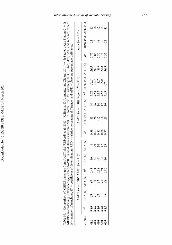
Table10

.Com

parisonof

MERIS

matchup

sfrom

AAOTsite(*Zibordi

etal.2

013;

†Kajiyam

a,D’A

limon

te,and

Zibordi

2014)with

SagresoceanStatio

nCwith

MERIS

water-leaving

reflectance(ρ

w)afterNoV

ICin

bold

italicsandafterVIC

inno

rmal

text

forwavelengths

413,

443,

490,

560,

and66

5nm

,where

N=nu

mberof

matchup

s,R2=coefficientof

determ

ination,

RPD

=relativ

epercentage

difference,andAPD

=absolute

percentage

difference.

AAOT(N

=16

0)*AAOT(N

=86

)*AAOT(N

=10

0)†Sagres(N

=115)

Sagres(N

=115)

λ(nm)

R2

RPD

(%)

APD

(%)

R2

RPD

(%)

APD

(%)

R2

RPD

(%)

APD

(%)

R2

RPD

(%)

APD

(%)

R2

RPD

(%)

APD

(%)

412

0.19

5569

0.43

–40

480.39

–43

440.71

24.2

26.3

0.77

–23

2544

30.46

1736

0.71

–23

290.67

–26

260.83

13.3

16.7

0.85

–15

1849

00.80

1117

0.88

–814

0.81

–12

140.81

3.7

9.4

0.80

–812

560

0.90

715

0.91

–212

0.88

–812

0.81

–8.8

14.4

0.74

–914

665

0.82

–444

0.80

–16

330.77

2836

0.48

–27

36.5

0.32

–23

41


Dow

nloa

ded

by [

5.15

8.28

.243

] at

04:

09 1

4 M

arch

201

4

vegetation cover over the land fluctuating with the seasonal changes during the year. Thussatellite-derived marine reflectance near the coast is underestimated due to errors in theatmospheric correction caused by Rayleigh and aerosol scattering from the nearby landsurface (Santer 2010). ICOL has been developed to improve these coastal adjacency errorsfor MERIS products (Santer and Schmechtig, 2000). On the basis of the striking uni-formity between the characteristics of the stations at Sagres, these coastal waters should beuseful for testing ICOL. Furthermore, the atmospheric conditions can be estimated fromthe local AERONET station, and the vegetation cover over the land fluctuates onlyrelatively slowly with the seasons. Nonetheless, the scatter plots in Figure 4 and thepoor statistical data for Station A (Tables 6, 7) suggest that the outcome of ICOLprocessing is inconsistent at Sagres, particularly close to the coast. However, Figure 7does show consistent improvement in the MERIS images for ρw at 560 nm after ICOLprocessing. Although most of the effects of ICOL occur within the initial 8 km offshore,there are certain conditions when the adjacency correction is affecting the offshore site at18 km. This can be inferred from the shift in slope towards the 1:1 from NoVIC (Table 4)to ICOL (Table 6) after changes in combination during MERIS processing. It is evidentthat ICOL needs to be studied in more detail at Sagres, but there are further considerationsthat might explain at least some of the observed differences.

(1) For the current research, combining ICOL with MEGS 8.1 has to be done offline.As MEGS 8.1 does not correct for adjacency, ICOL has been used to provideTOA reflectance at distinct wavelengths corrected for adjacency effects. However,the Rayleigh correction assumes that there is a specular rather than a Lambertiansurface adjacent to the viewed pixel and, therefore, there is an error for the Fresnelreflectance assumed by MEGS 8.1. This could explain those transects where thereare large peaks or dips in ρw over the range 3–8 km from the shore, consistentwith the Rayleigh scale height (e.g. Figures 6(a), (b), (g), and (h)).

(2) It could be argued that bottom effects may be affecting the results close to thecoast, but this is not the situation at Sagres where depths are substantially greaterthan 5 optical depths, even at the near-shore Station A (+40 m). It is possible thatsome differences are related to the changes in the bio-optical properties of thewater linked to upwelling events.

(3) Land reflectances may influence the atmospheric correction (AC) due to changesin vegetation cover during the seasons. As ICOL only performs a simple AC overland, the effect of vegetation is to produce changes in the spectral regions 680–740 nm (NIR), and there does seem to be more anomalous results from ICOLduring spring and autumn as opposed to summer.

Kratzer and Vinterhav (2010) tested the ICOL processor in combination with three otherprocessors for MERIS images of the Himmerfjärden Bay and the surrounding areas of thenorthwestern Baltic Sea; the satellite images corrected for adjacency present a signifi-cantly better fit with the in situ data. However, ICOL has also been tested at Lake Woods(an inland water between USA and Canada) and appears not to improve retrieval of waterconstituents (Binding et al. 2011).

Although the processing procedures for validation at Sagres have shown equivocalresults, it is evident that the data from the stations at Sagres could continue to prove usefulfor improving the processing procedures for MERIS products, and that this site would beuseful for any validation exercises for future ocean colour sensors such as the Ocean andLand Colour Instrument (OLCI) on Sentinel 3.


Dow

nloa

ded

by [

5.15

8.28

.243

] at

04:

09 1

4 M

arch

201

4

6. Conclusions

● Approximately 130 matchups between MERIS water-leaving reflectances (ρw) andin situ measurements have been obtained between 2008 and 2011 for each of threestations at Sagres (A, at 2 km; B, at 10 km; and C, at 18 km).

● These numbers are reduced during the MERIS third reprocessing proceduresdependent on the combinations of NoVIC, VIC, ICOL, and with ICOL + VIC:with approximately 20–60% for the inshore Station A; 20% for Station B; and 10%for the offshore Station C.

● The statistical comparison of the matchups between MERIS ρw and the in situ ρwshows a better coefficient of determination, and less uncertainty and bias, at thecentre of the visible spectra (490–560 nm) than at the extremes (412 and 665 nm).

● The oceanic Station C at Sagres is of particular interest because it has character-istics in common with both BOUSSOLE and AAOT validation sites. However,vicarious adjustment results in poorer statistics, with the regression slope beingcloser to unity at all wavelengths without vicarious adjustment. With the exceptionof the wavelengths 412 and 443 nm for R2, the intercepts MR, RPD, and APD arebetter without vicarious adjustment applied. The differences for MR and APDindicate that the vicarious adjustment results in a marginal improvement in thesetwo bands, whereas the RPD indicates that the vicarious is an over-adjustment.

● Overall, Station C, Sagres site, has achieved better matchup statistics for theMERIS sensor than BOUSSOLE (Table 9). The statistics for both NoVIC andVIC are similar to those for AAOT (Table 10). Differences can be attributed to themore turbid conditions at AAOT and low values for the red at Sagres.

● The ICOL processing shows mixed results with improvements to matchups occur-ring only for some campaigns.

● The uniformity between the bio-optical characteristics of the stations at Sagresindicate that validation data from Sagres is particularly useful for understanding theeffects of coastal adjacency on satellite ocean colour products.

AcknowledgementsWe would like to thank ESA and ACRI-ST for developing ODESA MEGS® (http://earth.eo.esa.int/odesa); Brockmann Consult for access to the MERIS Level 2 full-resolution satellite images; and toRicardo and Sara Magalhães for their boat support. We also thank Dr Samantha Lavender and twoanonymous referees for improvements to the text.

FundingThis work was funded by the European Space Agency for the ‘Technical Assistance for the Validationof MERIS Marine Products at Portuguese oceanic and coastal sites’ [21464/08/I-OL]; PhD grants fromFundação para a Ciência e a Tecnologia [SFRH/BD/78354/2011], [SFRH/BD/78356/2011]; supportedby the DEVOTES project (http://www.devotes-project.eu/) EC 7th Framework Programme [308392];and AQUA_USERS project EC 7th Framework Programme [607325].

Supplemental data and underlying research materialsThe underlying research materials for this article can be accessed at http://hermes.acri.fr/mermaid/home/home.php – MEris MAtchup In-situ Database (MERMAID).


Dow

nloa

ded

by [

5.15

8.28

.243

] at

04:

09 1

4 M

arch

201

4

http://earth.eo.esa.int/odesa

http://earth.eo.esa.int/odesa

http://www.devotes-project.eu/

http://hermes.acri.fr/mermaid/home/home.php

http://hermes.acri.fr/mermaid/home/home.php

ReferencesAhn, Y. H., and P. Shanmugam. 2006. “Detecting the Red Tide Algal Blooms from Satellite Ocean

Color Observations in Optically Complex Northeast-Asia Coastal Waters.” Remote Sensing ofEnvironment 103: 419–437. doi:10.1016/j.rse.2006.04.007.

Antoine, D., F. d’Ortenzio, S. B. Hooker, G. Bécu, B. Gentili, D. Tailliez, and A. J. Scott. 2008.“Assessment of Uncertainty in the Ocean Reflectance Determined by Three Satellite OceanColor Sensors (MERIS, SeaWiFS and MODIS-A) at an Offshore Site in the Mediterranean Sea(BOUSSOLE Project).” Journal of Geophysical Research 113: C07013. doi:10.1029/2007JC004472.

Antoine, D., P. Guevel, J.-F. Desté, G. Bécu, F. Louis, A. J. Scott, and P. Bardey. 2008. “The‘BOUSSOLE’ Buoy – A New Transparent-To-Swell Taut Mooring Dedicated to Marine Optics:Design, Tests and Performance at Sea.” Journal of Atmospheric and Oceanic Technology 25:968–989. doi:10.1175/2007JTECHO563.1.

Bailey, S. W., and P. J. Werdell. 2006. “A Multi-Sensor Approach for the On-Orbit Validation ofOcean Color Satellite Data Products.” Remote Sensing of Environment 102: 12–23. doi:10.1016/j.rse.2006.01.015.

Banks, A. C., P. Prunet, J. Chimot, P. Pina, J. Donnadille, E. Jeansou, M. Lux, G. Petihakis, G.Korres, G. Triantafyllou, C. Fontana, C. Estournel, C. Ulses, and L. Fernandez. 2012. “ASatellite Ocean Color Observation Operator System for Eutrophication Assessment in CoastalWaters.” Journal of Marine Systems 94: S2–S15. doi:10.1016/j.jmarsys.2011.11.001.

Barker, K. 2011. “MERIS Optical Measurements Protocols. Part A: In Situ Water ReflectanceMeasurements.” Revision 1.0, Document No.CO-SCI-ARG-TN-0008.

Behrenfeld, M. J., R. T. O’Malley, D. A. Siegel, C. R. McClain, J. L. Sarmiento, G. C. Feldman, A.J. Milligan, P. G. Falkowski, R. M. Letelier, and E. S. Boss. 2006. “Climate-Driven Trends inContemporary Ocean Productivity.” Nature 444: 752–755. doi:10.1038/nature05317.

Binding, C. E., T. A. Greenberg, J. H. Jerome, R. P. Bukata, and G. Letourneau. 2011. “AnAssessment of MERIS Algal Products during an Intense Bloom in Lake of the Woods.”Journal of Plankton Research 33: 793–806. doi:10.1093/plankt/fbq133.

Bird, R. E., and C. J. Riordan. 1986. “Simple Simple Solar Spectral Model for Direct and DiffuseIrradiance on Horizontal and Tilted Planes at the Earth’s Surface for Cloudless Atmospheres.”Journal of Climate and Applied Meteorology 25 (1): 87–97. doi:10.1175/1520-0450(1986)025<0087:SSSMFD>2.0.CO;2.

Broenkow, W. W., D. K. Clark, and M. A. Yarbrough. 1996. SeaWiFS Optical Buoy for the HawaiiTimes Series Experiment. Final Report NASA Contract RFPR-98012/272. Moss Landing, CA:Moss Landing Marine Laboratories Technical Publication 96-5.

Carvalho, G. A., P. J. Minnett, V. F. Banzon, W. Baringer, and C. A. Heil. 2011. “Long-TermEvaluation of Three Satellite Ocean Color Algorithms for Identifying Harmful Algal Blooms(Karenia brevis) along the West Coast of Florida: A Matchup Assessment.” Remote Sensing ofEnvironment 115: 1–18. doi:10.1016/j.rse.2010.07.007.

Cristina, S., P. Goela, J. Icely, A. Newton, and B. Fragoso. 2009. “Assessment of the OpticalProperties of the Ocean and Coastal Waters Using MERIS Satellite Products in Sagres Off theSouth West Coast of Portugal.” Journal of Coastal Research 56: 1479–1483.

Cristina, S., J. Icely, P. Goela, and A. Newton. 2010. “Validation of the MERIS Satellite Products inOceanic Waters Off Cape Sagres on the South-West Coast of Portugal.” Paper presented at theProceedings of the ESA Living Planet Symposium, SP-686, no. 107 European Space Agency,Bergen, June 28–July 2.

Cui, T., J. Zhang, S. Groom, L. Sun, T. Smyth, and S. Sathyendranath. 2010. “Validation of MERISOcean-Color Products in the Bohai Sea: A Case Study for Turbid Coastal Waters.” RemoteSensing of Environment 114: 2326–2336. doi:10.1016/j.rse.2010.05.009.

Doerffer, R. 2002. “Protocols for the Validation of MERIS Water Products.” European SpaceAgency Document No. PO-TN-MEL-GS-0043.

Dowell, M., and T. Platt, eds. 2009. Partition of the Ocean into Ecological Provinces: Role ofOcean-Colour Radiometry. Reports of the International Ocean-Colour Coordinating Group,No. 9. Dartmouth: Published by the International Ocean-Colour Coordinating Group.

Eleveld, M. A., R. Pasterkamp, H. J. van der Woerd, and J. D. Pietrzak. 2008. “Remotely SensedSeasonality in the Spatial Distribution of Sea-Surface Suspended Particulate Matter in theSouthern North Sea.” Estuarine, Coastal and Shelf Science 80: 103–113. doi:10.1016/j.ecss.2008.07.015.


Dow

nloa

ded

by [

5.15

8.28

.243

] at

04:

09 1

4 M

arch

201

4

Field, C. B., M. J. Behrenfeld, J. T. Randerson, and P. G. Falkowski. 1998. “Primary Production ofthe Biosphere: Integrating Terrestrial and Oceanic Components.” Science 281: 237–240.doi:10.1126/science.281.5374.237.

Franz, B. A., S. W. Bailey, P. J. Werdell, and C. R. McClain. 2007. “Sensor-Independent Approachto the Vicarious Calibration of Satellite Ocean Color Radiometry.” Applied Pptics 46: 5068–5082. doi:10.1364/AO.46.005068.

Goela, P. C., J. Icely, S. Cristina, A. Newton, G. Moore, and C. Cordeiro. 2013. “SpecificAbsorption Coefficient of Phytoplankton Off the Southwest Coast of the Iberian Peninsula: AContribution to Algorithm Development for Ocean Colour Remote Sensing.” Continental ShelfResearch 52: 119–132. doi:10.1016/j.csr.2012.11.009.

Gordon, H., and K. Ding. 1992. “Self-Shading of In-Water Optical Instruments.” Limnology andOceanography 37 (3): 491–500. doi:10.4319/lo.1992.37.3.0491.

Gordon, H. R., and A. Morel. 1983. “Remote Assessment of Ocean Color for Interpretation ofSatellite Visible Imagery.” In A Review, Lecture Notes on Coastal and Estuarine Studies, editedby R. T. Barber, N. K. Mooers, M. J. Bowman, and B. Zeitzschel. New York: Springer-Verlag.

Hooker, S. B., C. R. McClain, J. K. Firestone, T. L. Westphal, E.-N. Yeh, and Y. Ge. 1994. TheSeaWiFS Bio-Optical Archive and Storage System (SeaBASS): Part 1. NASA TechnicalMemorandum Vol. 104566. Greenbelt, MD: NASA Goddard Space Flight Center.

Kajiyama, T., D. D’Alimonte, and G. Zibordi. 2014. “Match-Up Analysis of MERIS RadiometricData in the Northern Adriatic Sea.” IEEE Geoscience and Remote Sensing Letters 11 (1): 19–23. doi:10.1109/LGRS.2013.2244844.

Kratzer, S., C. Brockmann, and G. Moore. 2008. “Using MERIS Full Resolution Data to MonitorCoastal Waters – A Case Study from Himmerfjärden, a Fjord-Like Bay in the NorthwesternBaltic Sea.” Remote Sensing of Environment 112: 2284–2300. doi:10.1016/j.rse.2007.10.006.

Kratzer, S., and C. Vinterhav. 2010. “Improvement of MERIS level 2 Products in Baltic Sea CoastalAreas by Applying the Improved Contrast between Ocean and Land Processor (ICOL) – DataAnalysis and Validation.” Oceanologia 52 (2): 211–236. doi:10.5697/oc.52-2.211.

Kwiatkowska, E. J., B. A. Franz, G. Meister, C. R. McClain, and X. Xiong. 2008. “CrossCalibration of Ocean-Color Bands from Moderate Resolution Imaging Spectroradiometer onTerra Platform.” Applied Optics 47: 6796–6810. doi:10.1364/AO.47.006796.

Lerebourg, C., C. Mazeran, J. P. Huot, and D. Antoine. 2011. “MERIS ATBD 2.24. VicariousAdjustment of the MERIS Ocean Colour Radiometry.” ACRI-ST. Ref.:MERIS ATBD 2.24Issue:1.0.

Longhurst, A. 1998. Ecological Geography of the Sea. San Diego, CA: Academic Press.Longhurst, A. 2006. Ecological Geography of the Sea. 2nd ed. San Diego, CA: Academic Press

Elsevier.Loureiro, S., A. Newton, and J. D. Icely. 2005. “Microplankton Composition, Production and

Upwelling Dynamics in Sagres (SW Portugal) during the Summer of 2001.” Scientia Marina69 (3): 323–341.

Loureiro, S., A. Reñé, E. Garcés, J. Camp, and D. Vaqué. 2011. “Harmful Algal Blooms (HABs),Dissolved Organic Matter (DOM), and Planktonic Microbial Community Dynamics at a Near-Shore and a Harbour Station Influenced by Upwelling (SW Iberian Peninsula).” Journal of SeaResearch 65 (4): 401–413. doi:10.1016/j.seares.2011.03.004

McClain, C. R., J. R. Christian, S. R. Signorini, M. R. Lewis, I. Asanuma, D. Turk, and C. Dupouy-Douchement. 2002. “Satellite Ocean-Color Observations of the Tropical Pacific Ocean.” DeepSea Research Part II: Topical Studies in Oceanography 49: 2533–2560. doi:10.1016/S0967-0645(02)00047-4

McClain, C. R., W. E. Esaias, W. Barnes, B. Guenther, D. Endres, S. Hooker, G. Mitchell, and R.Barnes. 1992. “SeaWiFS Calibration and Validation Plan.” In NASA Technical Memorandum104566, Vol. 3, edited by S. B. Hooker and E. R. Firestone. Greenbelt, MD: NASA GoddardSpace Flight Center.

McCulloch, M. E., K. L. Barker, and G. Zibordi. 2010. “Vicarious Adjustment of MERISReflectances Using an Inverse Technique.” Paper presented at the Proceedings of the ESALiving Planet Symposium, SP-686, Bergen, June 28–July 2.

Mobley, C. D. 1995. Hydrolight 3.0 Users Guide. SRIRI Project 5632. Menlo Park, CA: SRIInternational.


Dow

nloa

ded

by [

5.15

8.28

.243

] at

04:

09 1

4 M

arch

201

4

Moore, G. F., J. D. Icely, and S. Kratzer. 2010. “Field Inter-Comparison and Validation of In-WaterRadioamter and Sunphotometers for MERIS Validation.” Paper presented at the Proceedings ofthe ESA Living Planet Symposium, SP-686, Bergen, June 28–July 2.

Morel, A., ed. 1998. Minimum Requirements for an Operational Ocean-Colour Sensor for the OpenOcean. Reports of the International Ocean-Colour Coordinating Group, No. 1. IOCCG.Dartmouth: Published by the International Ocean-Colour Coordinating Group.

Morel, A., and D. Antoine. 1994. “Heating Rate within the Upper Ocean in Relation to its Bio-Optical State.” Journal of Physical Oceanography 24: 1652–1665. doi:10.1175/1520-0485(1994)024<1652:HRWTUO>2.0.CO;2.

Morel, A., and S. Maritorena. 2001. “Bio-Optical Properties of Oceanic Waters: A Reappraisal.”Journal of Geophysical Research 106: 7163–7180. doi:10.1029/2000JC000319.

Morys, M., F. M. Mims III, S. Hagerup, S. E. Anderson, A. Baker, J. Kia, and T. Walkup. 2001.“Design, Calibration and Performance of MICROTOPS II Handheld Ozone Monitor and SunPhotometer.” Journal of Geophysical Research Atmosphere 106 (D13): 14573–14582.doi:10.1029/2001JD900103.

MQWG. 2011. “MERIS 3rd Data Reprocessing – Software and ADF Updated.” Accessed July 15,2013. http://earth.eo.esa.int/pcs/envisat/meris/documentation/meris_3rd_reproc/MERIS_3rd_Reprocessing_Changes.pdf

MQWG. 2012. “MERIS 3rd Data Reprocessing: Validation Report.” Accessed July 15, 2013. http://earth.eo.esa.int/pcs/envisat/meris/documentation/meris_3rd_reproc/A879-NT-017-ACR_v1.0.pdf

Mueller, J. L. 2003. “In-Water Radiometric Profile Measurements and Data Analysis Protocols.” InOcean Optics Protocols for Satellite Ocean Color Sensor Validation, NASA TechnicalMemorandum – 2003-21621, Rev. 4, Vol. III., edited by J. L. Mueller, G. S. Fargion, and C.R. McClain, 7–19. Greenbelt, MD: NASA.

Newton, A., and J. Icely. 2008. “Land Ocean Interactions in the Coastal Zone, LOICZ: Lessonsfrom Banda Aceh, Atlantis, and Canute.” Estuarine, Coastal and Shelf Science 77: 181–184.doi:10.1016/j.ecss.2007.09.016.

Petersen, W., H. Wehde, H. Krasemann, F. Colijn, and F. Schroeder. 2008. “FerryBox and MERIS –Assessment of Coastal and Shelf Sea Ecosystems by Combining In-Situ and Remotely SensedData.” Estuarine, Coastal and Shelf Science 77: 296–307. doi:10.1016/j.ecss.2007.09.023

Platt, T., and S. Sathyendranath. 2008. “Ecological Indicators for the Pelagic Zone of the Oceanfrom Remote Sensing.” Remote Sensing of Environment 112: 3426–3436. doi:10.1016/j.rse.2007.10.016.

Platt, T., N. Hoepffner, V. Stuart, and C. Brown, eds. 2008. Why Ocean Colour? The SocietalBenefits of Ocean-Colour Technology. Reports of the International Ocean-Colour CoordinatingGroup, No. 7, IOCCG. Dartmouth: Published by the International Ocean-Colour CoordinatingGroup.

Prieur, L., and S. Sathyendranath. 1981. “An Optical Classification of Coastal and Oceanic WatersBased on the Specific Spectral Absorption Curves of Phytoplankton Pigments, DissolvedOrganic Matter, and Other Particulate Materials.” Limnology and Oceanography 26: 671–689.doi:10.4319/lo.1981.26.4.0671.

Rast, M., J. L. Bezy, and S. Bruzzi. 1999. “The ESA Medium Resolution Imaging SpectrometerMERIS- A Review of the Instrument and its Mission.” International Journal of Remote Sensing20: 1681–1702. doi:10.1080/014311699212416.

Relvas, P., and E. D. Barton. 2005. “A Separated Jet and Coastal Counterflow during UpwellingRelaxation Off Cape São Vicente (Iberian Peninsula).” Continental Shelf Research 25: 29–49.doi:10.1016/j.csr.2004.09.006.

Relvas, P., E. D. Barton, J. Dubert, P. B. Oliveira, Á. Peliz, J. C. B. da Silva, A. Santos, and P.Santos. 2007. “Physical Oceanography of the Western Iberia Ecosystem: Latest Views andChallenges.” Progress in Oceanography 74: 149–173. doi:10.1016/j.pocean.2007.04.021.

Ruddick, K., G. Lacroix, C. Lancelot, B. Nechad, Y. Park, S. Peters, and B. Van Mol. 2008. “OpticalRemote Sensing of North Sea.” In Remote Sensing of the European Seas, edited by V. Baraleand M. Gade, 79–90. Ispra: Springer.

Santer, R. 2010. “ICOL + ATBD.” Brockman Consult and University of Littoral, France, Version1.0, (D4).

Santer, R., and C. Schmechtig. 2000. “Adjacency Effects on Water Surfaces: Primary ScatteringApproximation and Sensitivity Study.” Applied Optics 39: 361–375. doi:10.1364/AO.39.000361.


Dow

nloa

ded

by [

5.15

8.28

.243

] at

04:

09 1

4 M

arch

201

4

http://earth.eo.esa.int/pcs/envisat/meris/documentation/meris_3rd_reproc/MERIS_3rd_Reprocessing_Changes.pdf

http://earth.eo.esa.int/pcs/envisat/meris/documentation/meris_3rd_reproc/MERIS_3rd_Reprocessing_Changes.pdf

http://earth.eo.esa.int/pcs/envisat/meris/documentation/meris_3rd_reproc/A879-NT-017-ACR_v1.0.pdf

http://earth.eo.esa.int/pcs/envisat/meris/documentation/meris_3rd_reproc/A879-NT-017-ACR_v1.0.pdf

Santer, R., and F. Zagolski. 2009. “ICOL Improve Contrast between Ocean and Land.” ATBD–MERIS level-1C. Revision 1, Report D6 (1), Univ. Littoral, France.

Santos, A. M. P. 2000. “Fisheries Oceanography Using Satellite and Airborne Remote SensingMethods: A Review.” Fisheries Research 49: 1–20. doi:10.1016/S0165-7836(00)00201-0.

Sørensen, K., E. Aas, and J. Høkedal. 2007. “Validation of MERIS Water Products and Bio‐OpticalRelationships in the Skagerrak.” International Journal of Remote Sensing 28: 555–568.doi:10.1080/01431160600815566.

Thuillier, G., M. Hersé, D. Labs, T. Foujols, W. Peeterman, D. Gillotay, P. C. Simon, and H.Mandel. 2003. “The Solar Spectral Irradiance from 200 to 2400 nm as Measured by theSOLSPEC Spectrometer from the ATLAS and EURECA Missions.” Solar Physics 214: 1–22.doi:10.1023/A:1024048429145.

Werdell, P. J., and S. W. Bailey. 2005. “An Improved In-Situ Bio-Optical Data Set for Ocean ColorAlgorithm Development and Satellite Data Product Validation.” Remote Sensing of Environment98 (1): 122–140. doi:10.1016/j.rse.2005.07.001.

Zibordi, G., J.-F. Berthon, J. P. Doyle, S. Grossi, D. van der Linde, C. Targa, and L. Alberotanza.2002. Coastal Atmosphere and Sea Time Series (CoASTS), Part 1: A Tower-Based Long-TermMeasurement Program. NASATechnical Memorandum 2002–206892, Vol. 19. Greenbelt, MD:NASA Goddard Space Flight Center.

Zibordi, G., J.-F. Berthon, F. Mélin, D. D’Alimonte, and S. Kaitala. 2009. “Validation of SatelliteOcean Color Primary Products at Optically Complex Coastal Sites: Northern Adriatic Sea,Northern Baltic Proper and Gulf of Finland.” Remote Sensing of Environment 113: 2574–2591.doi:10.1016/j.rse.2009.07.013.

Zibordi, G., F. Mélin, and J.-F. Berthon. 2006. “Comparison of SeaWiFS, MODIS and MERISRadiometric Products at a Coastal Site.” Geophysical Research Letters 33: L06617.doi:10.1029/2006GL025778.

Zibordi, G., F. Mélin, J.-F. Berthon, and E. Canuti. 2013. “Assessment of MERIS Ocean Color DataProducts for European Seas.” Ocean Science 9: 521–533. doi:10.5194/os-9-521-2013.

Zibordi, G., K. Ruddick, I. Ansko, G. Moore, S. Kratzer, J. Icely, and A. Reinart. 2012. “In SituDetermination of the Remote Sensing Reflectance: An Inter-Comparison.” Ocean Science 8:567–586. doi:10.5194/os-8-567-2012.


Dow

nloa

ded

by [

5.15

8.28

.243

] at

04:

09 1

4 M

arch

201

4

Documents

In situ validation of MERIS marine reflectance off the southwest Iberian Peninsula: assessment of vicarious adjustment and corrections for near-land adjacency