Improving the sensitivity of online controlled experiments by utilizing pre-experiment data

** To appear in WSDM 2013 **

Improving the Sensitivity of Online Controlled Experimentsby Utilizing Pre-Experiment Data

Alex Deng∗

MicrosoftOne Microsoft Way

Redmond, WA [email protected]

Ya Xu∗

Microsoft1020 Enterprise WaySunnyvale, CA 94089

[email protected]

Ron KohaviMicrosoft

One Microsoft WayRedmond, WA 98052

[email protected]

Toby WalkerMicrosoft

One Microsoft WayRedmond, WA 98052

[email protected]

ABSTRACT

Online controlled experiments are at the heart of makingdata-driven decisions at a diverse set of companies, includingAmazon, eBay, Facebook, Google, Microsoft, Yahoo, andZynga. Small differences in key metrics, on the order offractions of a percent, may have very significant businessimplications. At Bing it is not uncommon to see experimentsthat impact annual revenue by millions of dollars, even tensof millions of dollars, either positively or negatively. Withthousands of experiments being run annually, improving thesensitivity of experiments allows for more precise assessmentof value, or equivalently running the experiments on smallerpopulations (supporting more experiments) or for shorterdurations (improving the feedback cycle and agility). Wepropose an approach (CUPED) that utilizes data from thepre-experiment period to reduce metric variability and henceachieve better sensitivity. This technique is applicable to awide variety of key business metrics, and it is practical andeasy to implement. The results on Bing’s experimentationsystem are very successful: we can reduce variance by about50%, effectively achieving the same statistical power withonly half of the users, or half the duration.

Categories and Subject Descriptors

G.3 [ Probability and Statistics/Experiment Design]:controlled experiments, randomized experiments, A/B test-ing

General Terms

Measurement, Variance, Experimentation

∗Corresponding authors.

Permission to make digital or hard copies of all or part of this work forpersonal or classroom use is granted without fee provided that copies arenot made or distributed for profit or commercial advantage and that copiesbear this notice and the full citation on the first page. To copy otherwise, torepublish, to post on servers or to redistribute to lists, requires prior specificpermission and/or a fee.WSDM’13, February 4–8, 2013, Rome, Italy.Copyright 2013 ACM 978-1-4503-1869-3/13/02 ...$15.00.

Keywords

Controlled experiment, Variance, A/B testing, Search qual-ity evaluation, Pre-Experiment, Power, Sensitivity

1. INTRODUCTIONA controlled experiment is probably the oldest and the

most widely accepted methodology to establish a causal re-lationship (Mason et al. 1989; Box et al. 2005; Keppel et al.1992; Kohavi et al. 2009b; Manzi 2012). Now widely usedand re-discovered by many companies, it is referred to asa randomized experiment, an A/B test (Wikipedia), a splittest, a weblab (at Amazon), a live traffic experiment (atGoogle), a flight (at Microsoft), and a bucket test (at Ya-hoo!). This paper is focused on online controlled experi-ments, where experiments are conducted on live traffic tosupport data-driven decisions in online businesses, includ-ing e-business sites like Amazon and eBay, portal sites likeYahoo and MSN (Kohavi et al. 2009b), search engines likeMicrosoft Bing (Kohavi et al. 2012) and Google (Tang et al.2010b).

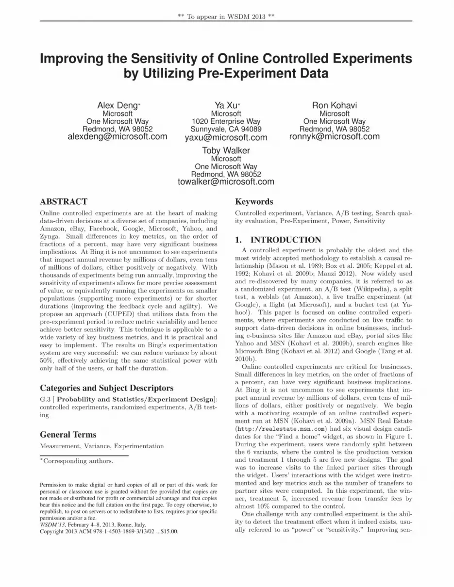
Online controlled experiments are critical for businesses.Small differences in key metrics, on the order of fractions ofa percent, can have very significant business implications.At Bing it is not uncommon to see experiments that im-pact annual revenue by millions of dollars, even tens of mil-lions of dollars, either positively or negatively. We beginwith a motivating example of an online controlled experi-ment run at MSN (Kohavi et al. 2009a). MSN Real Estate(http://realestate.msn.com) had six visual design candi-dates for the “Find a home” widget, as shown in Figure 1.During the experiment, users were randomly split betweenthe 6 variants, where the control is the production versionand treatment 1 through 5 are five new designs. The goalwas to increase visits to the linked partner sites throughthe widget. Users’ interactions with the widget were instru-mented and key metrics such as the number of transfers topartner sites were computed. In this experiment, the win-ner, treatment 5, increased revenue from transfer fees byalmost 10% compared to the control.

One challenge with any controlled experiment is the abil-ity to detect the treatment effect when it indeed exists, usu-ally referred to as “power” or “sensitivity.” Improving sen-


Figure 1: Widgets tested for MSN Real Estate.

sitivity is particularly important when running online ex-periments at large scale. A mature online experimentationplatform runs thousands of experiments a year (Kohavi et al.2012; Manzi 2012). The benefit of any increased sensitivityis therefore amplified by economies of scale. It might seemunnecessary to emphasize sensitivity for online experimentsbecause they tend to have very large sample sizes already(e.g. millions of users (comScore 2012)) and increasing sam-ple size is usually the most straightforward way to improvepower. In reality, even with a large amount of traffic, onlineexperiments cannot always reach enough statistical power.Google made it very clear that they are not satisfied withthe amount of traffic they have (Tang et al. 2010a, Slide6) even with over 10 billion searches per month (comScore2012). There are several reasons for this. First, the treat-ment effects we would like to detect tend to be very small.The sensitivity of controlled experiments is inversely propor-tional to the number of users squared, so whereas a smallsite may need 10,000 users to detect a 5% delta, detectinga 0.5% delta requires 100 times (10 squared) more users,or one million users. Even a 0.5% change in revenue peruser equates to millions of dollars for large online sites. Sec-ond, it is crucial to get results fast. One wants to launchgood features early, and more importantly, if the treatmentturns out to have a negative impact on users, we need tostop it as soon as possible. Third, there are many experi-ments that have low triggering rates; that is, only a smallfraction of the experiment’s users actually experience thetreatment feature. For example, in an experiment affectingonly recipe-related queries, the majority of the users will notsee the target feature because they didn’t search for recipesduring the experiment. In these cases, the effective samplesize can be small and statistical analysis can suffer from lowstatistical power. Finally, in a data-driven culture, there isalways demand to run more experiments to keep up with therate of innovation. A good online experimentation platformshould allow many experiments to run together. This also

requires that we make optimal use of large but still limitedtraffic.

One way to improve sensitivity is through variance reduc-tion. Kohavi et al. (2009b) provides examples where we canachieve a lower variance using a different evaluation metricor through filtering out users who are not impacted by thechange. Deng et al. (2011) shows how we can use page levelrandomization at the design stage to reduce variance of pagelevel metrics (Chapelle et al. 2012). However, these methodsare limited in their applicability to special cases and we wanta technique that is applicable to any metric as, in practice,businesses are likely to have a set of Key Performance Indi-cators (KPIs) that cannot be changed easily. Moreover, thetechnique should preferably not be based on any parametricmodel because model assumptions tend to be unreliable anda model that works for one metric does not necessarily workfor another.

In this paper, we propose a technique, called CUPED(Controlled-experiment Using Pre-Experiment Data), whichadjusts metrics using pre-experiment data for users in thecontrol and treatment to reduce metric variability.

The key contributions of our work include:• A theoretically sound and practical method to reduce

variances for online experiments using pre-experimentdata, which greatly increases experiment sensitivity.

• Extensions of approach to non-user metrics and par-tially missing pre-experiment data.

• Criteria for selecting the best covariates, including theempirical result that using the same metric from thepre-experiment typically gives the greatest variance re-duction.

• Validation of the results on real online experiments runat Bing, demonstrating a variance reduction of about50%, equivalent to doubling our traffic or halving thetime we need to run an experiment to get the samesensitivity.

• Practical guidance on choices important to successfulapplication of CUPED to real-world online experimen-tation, including factors like the best length to use forthe pre-experiment period and the use of multiple co-variates.

2. BACKGROUND AND RELATED WORK

2.1 Analyzing ExperimentsBecause of its wide applicability, we focus on the case

of the two-sample t-test (Student 1908; Wasserman 2003).This is the framework most commonly used in online exper-iment analysis. Suppose we are interested in some metricY (e.g. Queries per user). To apply the t-test, we assumethe observed values of the metric for users in the treatmentand control are independent realizations of random variablesY (t) and Y (c). The null hypothesis is that Y (t) and Y (c) havethe same mean and the alternative is that they do not. Thet-test is based on the t-statistic:

Y(t) − Y

(c)

√var

(Y

(t) − Y(c)

) , (1)

where ∆ = Y(t)−Y

(c)is an unbiased estimator for the shift

of the mean and the t-statistic is a normalized version of thatestimator. For online experiments, the sample sizes for both


control and treatment are at least in thousands, hence thenormality assumption on Y is usually unnecessary becauseof the Central Limit Theorem.

Because the samples are independent,

var(∆) = var(Y

(t) − Y(c)

)= var

(Y

(t))+ var

(Y

(c)).

In this framework, the key to variance reduction for the dif-ference in mean lies in reducing the variance of the meansthemselves. As we will see in Section 3, this connects ourproblem to techniques used in Monte Carlo sampling to im-prove estimation of a mean through variance reduction.

At a very high level, our proposal for variance reductionworks as follows. We conduct the experiment as usual butwhen analyzing the data, we compute an adjusted or cor-rected estimate of the delta. That adjusted estimate, ∆∗,incorporates pre-experiment information, such that

• ∆∗ is still an unbiased estimator for the shift in themeans (same as ∆), and

• ∆∗ has a smaller variance than ∆.Note that because of the reduced variance, the correspond-ing t-statistic would be larger for the same expected effectsize. We therefore achieved better sensitivity.

2.2 Linear ModelsWe begin with a short review of related work. Variance re-

duction has been a longstanding challenge for analyzing ran-domized experiments. The most popular parametric methodis based on linear modeling (Gelman and Hill 2006). A lin-ear model for an experiment assumes that the outcome isa linear combination of a treatment effect coupled with ad-ditional covariate terms. In particular, suppose Yi is theoutcome metric, Zi is the treatment assignment indicatorand Xi is a vector of covariates. The linear model assumesE(Yi|Zi,Xi) = θ0 + δZi + θ

TXi. Under the assumptionsof the model, linear regression (also called ANCOVA whencovariates are categorical variables) gives a consistent esti-mator for the average treatment effect and reduces variance.However, the linear model makes strong assumptions thatare usually not satisfied in practice, i.e., the conditional ex-pectation of the outcome metric is linear in the treatmentassignment and covariates. In addition, it also requires allresiduals to have a common variance.

2.3 Semi-Parametric ModelsTo overcome limitations of the linear model, researchers

have developed less restrictive models called semi-parametricmodels (Tsiatis 2006), for which Generalized EstimatingEquations (GEE) are used for fitting the model. Comparingstandard linear models with semi-parametric models, Yangand Tsiatis (2001) showed that linear model (ANCOVA) andGEE are asymptotically equivalent under the less restric-tive semi-parametric model and both give more efficient es-timates for the average treatment effect than the unadjustedt-test. Leon et al. (2003), Davidian et al. (2005) and Tsiatiset al. (2008) further refined the work using semi-parametricstatistical theory (Tsiatis 2006) and gave the analytical formof a class of estimators for the average treatment effect. Thisclass is complete in the sense that all possible RAL (regularand asymptotically linear) estimators for the average treat-ment effect are asymptotically equivalent to one in the class.The problem left is to find the estimator in the class withthe smallest variance and they provided general guidance.

In this paper, we look at the problem from a differentperspective. By connecting the variance reduction problemin randomized experiments to a similar problem in MonteCarlo simulation, we are able to derive a very powerful re-sult. Instead of diving into abstract Hilbert spaces and func-tional influence curves, our argument only involves elemen-tary probability. In particular, we propose to use the datafrom the pre-experiment period to reduce metric variability,which turns out to be very effective and practically applica-ble.

3. VARIANCE REDUCTIONVariance reduction is a common topic in Monte Carlo sam-

pling, where the goal is usually to estimate a parameter byrepeatedly simulating possible values from the underlyingdistribution. In Monte Carlo sampling significant efficiencygains can be had if we use sampling schemes that reduce thevariance by incorporating prior information. Unlike MonteCarlo simulations, in the world of online experiments, thepopulation is dynamic and data arrive gradually as the ex-periment progresses. We cannot design a sampling schemein advance and then collect data accordingly. However, wewill show that because we have pre-experiment data, we canadapt Monte Carlo variance techniques by applying them“retrospectively.”

The two Monte Carlo variance reduction techniques weconsider here are stratification and control variates. Foreach technique, we review the basic concepts and then showhow it can be adapted to the online experiment setting. Wedevote Section 3.3 to discussing the connections betweenthese two approaches and the implications in practice.

3.1 StratificationStratification is a common technique used in Monte Carlo

sampling to achieve variance reduction. In this section, weshow how it can be adapted to achieve the same goal in theworld of online experimentation.

3.1.1 Stratification in Simulation

The basic idea of stratification is to divide the samplingregion into strata, sample within each stratum separatelyand then combine results from individual strata together togive an overall estimate, which usually has a smaller variancethan the estimate without stratification.

Mathematically, we want to estimate E(Y ), the expectedvalue of Y , where Y is the variable of interest. The standardMonte Carlo approach is to first simulate n independentsamples Yi, i = 1, . . . , n, and then use the sample averageY as the estimator of E(Y ). Y is unbiased and var(Y ) =var(Y )/n.

Let’s consider a more strategic sampling scheme. Assumewe can divide the sampling region of Y into K subregions(strata) with wk the probability that Y falls into the kthstratum, k = 1, . . . ,K. If we fix the number of points sam-pled from the kth stratum to be nk = n · wk, we can definea stratified average to be

Ystrat =K∑

k=1

wkY k, (2)

where Y k is the average within the kth stratum.

The stratified average Ystrat and the standard average Yhave the same expected value but the former gives a smaller


variance when the means are different across the strata. Theintuition is that the variance of Y can be decomposed intothe within-strata variance and the between-strata variance,and the latter is removed through stratification. For ex-ample, the variance of children’s heights in general is large.However, if we stratify them by their age, we can get a muchsmaller variance within each age group. More formally,

var(Y ) =K∑

k=1

wk

nσ2k +

K∑

k=1

wk

n(µk − µ)2

≥K∑

k=1

wk

nσ2k = var(Ystrat)

where (µk, σ2k) denote the mean and variance for users in the

kth stratum. More detailed proof can be found in standardMonte Carlo books (e.g. Asmussen and Glynn (2008)). Agood stratification is the one that aligns well with the un-derlying clusters in the data. By explicitly identifying theseclusters as strata, we essentially remove the extra varianceintroduced by them.

3.1.2 Stratification in Online Experimentation

In the online world, because we collect data as they ar-rive over time, we are usually unable to sample from strataformed ahead of time. However, we can still utilize pre-experiment variables to construct strata after all the dataare collected (for theoretical justification see Asmussen andGlynn (2008, Page 153)). For example, if Yi is the numberof queries from a user i, a covariate Xi could be the browserthat the user used before the experiment started. The strat-ified average in (2) can then be computed by grouping Yaccording to the value of X,

Ystrat =

K∑

k=1

wkY k =

K∑

k=1

wk

1

nk

∑

i:Xi=k

Yi

.

Using superscripts to denote treatment and control groups,the stratified delta

∆strat = Y(t)strat − Y

(c)strat =

K∑

k=1

wk(Y(t)k − Y

(c)k )

enjoys the same variance reduction as the stratified averagein Eq. (2). It is important to note that by using only thepre-experiment information, the stratification variable X isindependent of the experiment effect. This ensures that thestratified delta is unbiased.

In practice, we don’t always know the appropriate weightswk to use. In the context of online experimentation, thesecan usually be computed from users not in the experiment.As we will see in Section 3.3, when we formulate the sameproblem in the form of control variates (Section 3.2), we nolonger need to estimate the weights.

3.2 Control VariatesWe showed how online experimentation can benefit from

the stratification technique widely used in the simulationliterature. In this section we show how another variance re-duction technique used in simulation, called control variates,can also be adopted in online experimentation. In Section3.2.1, we review control variates in its original form as avariance reduction technique for simulation. We then show

how the same idea can be applied in the context of onlineexperimentation in Section 3.2.2.

3.2.1 Control Variates in Simulation

The idea of variance reduction through control variatesstems from the following observation. Assume we can simu-late another random variable X in addition to Y with knownexpectation E(X). In other words, we have independentpairs of (Yi, Xi), i = 1, . . . , n. Define

Ycv = Y − θX + θEX, (3)

where θ is any constant. Ycv is an unbiased estimator of

E(Y ) since −θE(X) + θE(X) = 0. The variance of Ycv is

var(Ycv) = var(Y − θX) = var(Y − θX)/n

=1

n(var(Y ) + θ2var(X)− 2θcov(Y,X)).

Note that var(Ycv) is minimized when we choose

θ = cov(Y,X)/var(X) (4)

and with this optimal choice of θ, we have

var(Ycv) = var(Y )(1− ρ2), (5)

where ρ = cor(Y,X) is the correlation between Y and X.Compare (5) to the variance of Y , the variance is reduced bya factor of ρ2. The larger ρ, the better the variance reduc-tion. The single control variate case can be easily generalizedto include multiple variables.

It is interesting to point out the connection with linearregression. The optimal θ turns out to be the ordinary leastsquare (OLS) solution of regressing (centered) Y on (cen-tered) X, which gives variance

var(Ycv) = var(Y )(1−R2),

with R2 being the proportion of variance explained coeffi-cient from the linear regression. It is also possible to usenonlinear adjustment. i.e., instead of allowing only linearadjustment as in (3), we can minimize variance in a moregeneral functional space. Define

Ycv = Y − f(X) + E(f(X)), (6)

and then try to minimize the variance of (6). It can be shownthat the regression function E(Y |X) gives the optimal f(X).

3.2.2 Control Variates in Online Experimentation

Utilizing control variates to reduce variance is a very com-mon technique. The difficulty of applying it boils down tofinding a control variate X that is highly correlated with Yand at the same time has known E(X).

Although in general it is not easy to find control variate Xwith known E(X(t)) and E(X(c)), a key observation is that

E(X(t))−E(X(c)) = 0 in the pre-experiment period becausewe have not yet introduced any treatment effect. By usingonly information from before the launch of the experimentto construct the control variate, the randomization betweentreatment and control ensures that we have EX(t) = EX(c).

Given EX(t) − EX(c) = 0, it is easy to see the delta

∆cv = Y (t)cv − Y (c)

cv (7)

is an unbiased estimator of δ = E(∆). Notice how ∆cv does

not depend on the unknown E(X(t)) and E(X(c)) at all as


they cancel each other. With the optimal choice of θ fromEq (4), we have that ∆cv reduces variance by a factor of ρ2

compared to ∆, i.e.

var(∆cv) = var(∆)(1− ρ2).

To achieve a large correlation and hence better variance re-duction, an obvious approach is to choose X to be the sameas Y , which naturally leads to using the same variable dur-ing pre-experiment observation window as the control vari-ate. As we will see in the empirical results in Section 5, thisindeed turns out to be the most effective choice we foundfor control variates.

There is a slight subtlety that’s worth pointing out. Thepair (Y,X) may have different distributions in treatmentand control when there is an experiment effect. For ∆cv

to be unbiased, the same θ has to be used for both controland treatment. The simplest way to estimate it is from thepooled population of control and treatment. The impact onvariance reduction will likely be negligible. In the generalnonlinear control covariates case, we should use the same

functional form in both Y(t)cv and Y

(c)cv .

3.3 Connection between Stratification andControl Variates

We have discussed two techniques that both utilize co-variates to achieve variance reduction. The stratification ap-proach uses the covariates to construct strata while the cont-rol variates approach uses them as regression variables. Theformer uses discrete (or discretized) covariates, whereas con-trol variates seem more naturally to be continuous variables.It is, however, not surprising that these two approaches areclosely related. In fact, we can show that when the covariateX is categorical (say, with discrete values 1, . . . ,K) the twoapproaches produce identical estimates. Details are includedin Appendix A. The basic idea is to construct an indicatorvariable 1X=k for each stratum and use it as a control variatewith mean being the stratum weight wk. To this end, thecontrol variates technique is an extension of stratification,where both continuous and discrete covariates are applica-ble.

While these two techniques are well connected mathe-matically, they provide different insights into understandingwhy and how to achieve variance reduction. The stratifica-tion formulation has a nice analogy with mixture models,where each stratum is one component of the mixture model.Stratification is equivalent to separating samples accordingto their component memberships, effectively removing thebetween-component variance and achieving a reduced vari-ance. A better covariate is hence the one that can betterclassify the samples and align with their underlying struc-ture. On the other hand, the control variates formulationquantifies the amount of variance reduction as a function ofthe correlation between the covariates and the variable it-self. It is mathematically simpler and more elegant. Clearly,a better covariate should be the one with larger (absolute)correlation.

4. CUPED IN PRACTICEA simple yet effective way to implement CUPED is to

use the same variable from the pre-experiment period asthe covariate. Indeed, this is essentially what we have im-plemented in practice for Bing’s experimentation system.However, there are situations when this is not possible or

practical. For example, if we want to measure user reten-tion rate or conduct an experiment on new users, there areno pre-experiment data to work with. In fact, in most on-line experiments, we may not have pre-experiment informa-tion on all users. An additional challenge is how to usepre-experiment data for metrics whose analysis unit is nota user. This section is devoted to address practical chal-lenges like these using Bing’s experimentation system as acase study.

4.1 Selecting CovariatesThe choice of covariates is critical, as it directly deter-

mines the effectiveness of variance reduction. With the choiceof the right variables we can halve the variance but withthe wrong choice there is little reduction in variance. Tounderstand which pre-experiment variables worked best weevaluated a large number of possible pre-experiment vari-ables. Across a large class of metrics, our results consis-tently showed that using the same variable from the pre-experiment period as the covariate tends to give the bestvariance reduction. In addition, the lengths of the pre-experiment and the experiment periods also play a role.Given the same pre-experiment period, extending the lengthof the experiment does not necessarily improve the variancereduction rate. On the other hand, a longer pre-period tendsto give a higher reduction for the same experiment period.We discuss more details in the context of an empirical ex-ample in Section 5.

4.2 Handling Missing Pre-Experiment DataIn online sites, we might not have pre-experiment data

on all users in the experiment. This can occur becausesome users are visiting for the first time, or users simplydo not visit the site frequently enough to appear during thepre-experiment period. In addition, users are identified bycookies, which are unreliable and can “churn” (i.e. changedue to users clearing their cookies).

This poses a challenge for using the pre-experiment infor-mation to construct covariates. For users who are in theexperiment but not in the pre-experiment period, the corre-sponding covariates are not well-defined. One way to addressthis is to define another covariate that indicates whether ornot a user appeared in the pre-experiment period. With thisadditional binary covariate, we can set the missing covari-ate values to be any constant we like. Intuitively, this isequivalent to first splitting users into two strata: those thatappeared in the pre-experiment period and those that didnot. Note that for the stratum of users with pre-experimentdata, their pre-experiment covariates are well-defined so fur-ther variance reduction based on these covariates is possible.In addition, the stratification by presence in the pre-periodis a further source of variance reduction.

4.3 Beyond Pre-Experiment DataSo far we only considered reducing metrics variability based

on covariates constructed using the pre-experiment data.This is not only because using the same variable from thepre-period tends to give the best variance reduction, but alsobecause the pre-experiment information is guaranteed to beindependent of the experiment’s effect, which is crucial toavoid biased results.

It is probably easier to demonstrate this mathematicallywith the control variates formulation. In Eq. (7), the delta


∆cv is computed assuming E(X(t)) = E(X(c)). If there istruly a difference between control and treatment in terms ofX and this equality does not hold, ∆cv will be biased. Forexample, we know a faster page load-time usually leads tomore clicks on a search page (Kohavi et al. 2009b). If weuse the number of clicks as the covariate in an experimentthat improves page load-time, we will end up underestimat-ing the experiment impact on the load-time because part ofthe improvement is “adjusted away” by the covariate. SeeSection 5 for a real example of biased results caused by usinga covariate that violates the requirements described here.

However, this does not mean that covariates based on pre-experiment data are the only choice. All that is requiredis that the covariate X is not affected by the experiment’streatment. A natural extension is the class of covariates con-structed using information gathered at the first time a userappears in the experiment. For instance, the day-of-weeka user is first observed in the experiment is independent ofthe experiment itself. Such covariates can serve as an ad-ditional powerful source for variance reduction. To furtherextend this idea, covariates based on any information estab-lished before a user actually triggers the experiment featureare also valid. This can be particularly helpful if the featureto be evaluated has a low triggering rate.

4.4 Handling Non-User MetricsAs we mentioned in Section 1, in online experiments, users

(cookies) are the common randomization unit. In the discus-sion thus far, we have assumed that the analysis unit is also“user.” However, this is not always the case. For example,we may want to compute click-through-rate (CTR) as thetotal number of clicks divided by the total number of pages.The analysis unit here is a “page” instead of a “user.” Vari-ance estimation itself is harder when there is a mismatchbetween the analysis unit and the experiment unit. Themost common solution is to use the delta method to pro-duce correct estimate of variance that takes into account thecorrelation of pages from the same user (Deng et al. 2011;Tang et al. 2010b; Kohavi et al. 2009b). To achieve vari-ance reduction for these non-user level metrics, we need tocombine the delta method and our variance reduction tech-niques together. The details are provided in Appendix B.In fact, not only can the metric of interest (e.g. CTR) be atpage level, we can have page-level covariates as well. Thisopens the door to a larger class of covariates that are basedon features specific to a page that may be not specific to auser, e.g. time stamp on a page-view.

5. EMPIRICAL RESULTSIn this section, we share empirical results that show the ef-

fectiveness of CUPED for Microsoft Bing’s experimentationsystem. First we show how CUPED can greatly improve thesensitivity for a real experiment run at Bing. Next we lookdeeper into a 3-week A/A test, which is a controlled exper-iment where treatment is identical to control and hence thetreatment effect is known to be 0. Using an A/A experimentwe can examine important decisions that can have a largeimpact of the success of variance reduction for real-world on-line experimentation. Finally, we show how biased estimatesarise if we go past the user triggering into the experimentand choose a covariate inappropriately.

5.1 Slowdown Experiment in BingTo show the impact of CUPED in a real experiment we

examine an experiment that tested the relationship betweenpage load-time and user engagement on Bing. Delays, onthe order of hundreds of milliseconds, are known to hurtuser engagement (Kohavi et al. 2009b, Section 6.1.2). Inthis experiment, we deliberately delayed the server responseto Bing queries by 250 milliseconds. The experiment firstran for two weeks on a small fraction of Bing users, and weobserved an impact to click-through-rate (CTR) that wasborderline statistically significant, i.e., the p-value was justslightly below our threshold of 0.05. To confirm that thetreatment effect on this metric is real and not a false positive,a much larger experiment was run, which showed that thiswas indeed a real effect with a p-value of 2e-13.

We applied CUPED using CTR from the 2-week pre-period as the covariate. The result is impressive: the deltawas statistically significant from day 1! The top plot of Fig-ure 2 shows the p-values over time in log scale. The blackhorizontal line is the 0.05 significance bar. The vanilla t-test trends slowly down and by the time the experimentwas stopped in 2 weeks, it barely reached the threshold.When CUPED is applied, the entire p-value curve is belowthe bar. The bottom plot of Figure 2 compares the p-valuecurves when CUPED runs on only half the users. Even withhalf the users exposed to the experiment, CUPED results ina more sensitive test, allowing for more non-overlapping ex-periments to be run. While most experiments are not knownto be negative to the user experience a-priori, it has beenwell documented that most experiments are flat or nega-tive (Kohavi et al. 2009a; Manzi 2012), so being able to run

Figure 2: Slowdown experiment. Top: p-value. Bot-tom: p-value when using only half the users forCUPED.


experiments with the same statistical power on smaller pop-ulations of users is very important.

Applying CUPED to other experiments at Bing has re-sulted in similar increases to statistical power.

5.2 Factors Affecting CUPED EffectivenessIn this section we look at factors that can have a large

impact on the success of using CUPED in practice. Thedata we use here are from a 3-week A/A experiment.

5.2.1 Covariates

Figure 3 shows CUPED’s variance reduction rate for themetric queries-per-user. Two covariates are considered: (1)entry-day, which is a categorical variable indicating the firstday a user appears in the experiment and (2) queries-per-user in the 1-week pre-experiment period. Note that theentry-day is not pre-experiment data, but it satisfies thecondition required in Section 4.3 because the treatment hasno effect on when a user will come for the first time duringthe experiment.

Figure 3: Variance reduction for Queries/UU usingdifferent covariates.

Note that the full experiment ran for 3 weeks, but thereduction rate is evaluated and plotted as the experimentaccumulates data up until to the full 3 weeks. From theplot we can see that when only entry-day is used as thecovariate, the variance reduction rate increases as the ex-periment runs longer and stays at about 9% to 10% after 2weeks. On the other hand, using only the pre-experiment pe-riod queries-per-user, variance reduction rate can reach morethan 45%. When we combine the two covariates together,we only gain an extra 2% to 3% more reduction comparedto the pre-experiment queries-per-user alone. This suggeststhat the same metric computed in the pre-experiment pe-riod is a better single covariate. That is intuitive since thesame metric in the experiment and pre-experiment periodsshould naturally have high correlation. The fact that whencombining two covariates together the marginal variance re-duction is small means most correlation between entry-dayand queries-per-user can be “explained away” by the pre-experiment queries-per-user. More precisely, the partial cor-relation between entry-day and queries-per-user given pre-experiment queries-per-user is low.

5.2.2 Lengths of Experiment and Pre-Experiment

In addition to the effect of covariates, Figure 3 also pro-vides insights on the impact of the experiment length. An

interesting observation is that the variance reduction rate forthe pre-experiment covariate (green/triangle) is not mono-tonically increasing as the experiment duration increases. Itreaches the maximum at about 2 weeks and then starts toslowly decrease. To help understand the underlying reasonsfor this trend, we plot 4 variations of this curve with pre-period length varying from 3 days to 2 weeks. As shownin Figure 4, we see that a longer pre-period gives a highervariance reduction rate.

Figure 4: Impact of pre-experiment period length.

The trends in Figure 3 and 4 together reveal two conflict-ing factors that impact the effectiveness of CUPED.

• Correlation. The higher the correlation, the betterthe variance reduction. When we increase the pre-experiment period length or increase the experimentduration, the correlation increases for“cumulative”met-rics such as queries-per-user. This is because the longerthe period, the higher the signal-to-noise ratio.

• Coverage. Coverage is the percentage of users in theexperiment that also appeared in the pre-experimentperiod. Coverage is determined by:

– Experiment Duration. As the experiment dura-tion increases, coverage decreases. The reason isthat frequent visitors are seen early in the exper-iment and users seen later in the experiment areoften new or“churned”users. The result is that ascoverage decreases, the rate of variance reductiongoes down.

– Pre-period Duration. Increasing the pre-periodlength increases coverage because we have a bet-ter chance of matching an experiment user in thepre-period.

When pre-experiment period was chosen to be 2 weeks, thevariance reduction rate is about 50% for a large range ofexperiment durations.

5.2.3 Metric of Interest

Besides the choice of covariates and the lengths of ex-periment and pre-experiment, CUPED effectiveness variesfrom metric to metric, depending on the correlation betweenthe metric and its pre-experiment counterpart. We appliedCUPED on a few metrics, such as clicks-per-user and visits-per-user. CUPED performed well on all these metrics withsimilar variance reduction curves as in Figure 3. One no-table exception is revenue-per-user, where CUPED reducedthe variance by less than 5% due to the low correlation ofrevenue-per-user between the pre-experiment and the exper-iment periods. We also applied CUPED on a few page level


metrics (see the discussion in Section 4.4). Figure 5 showsthe reduction rate for click-through-rate (CTR), using 2-week pre-experiment CTR as the CUPED covariate. Figure6 plots the correlation curve between the two periods. Boththe variance reduction rate and the correlation are similarto those of queries-per-user.

Figure 5: Variance reduction rate for CTR.

Figure 6: Correlation between the metrics of inter-est and their covariates within the matched users.

5.3 Warning on Using Post-Triggering DataIn Section 4, we mentioned that to guarantee unbiased re-

sults, any covariate X has to satisfy the condition E(X(t)) =

E(X(c)). We illustrate this point in Figure 7. The data isfrom another Bing experiment, where queries-per-user in-creased statistically significantly. If we were to look fora metric with high correlation to queries-per-user, there isactually a much better candidate than the pre-experimentqueries-per-user: the “in-experiment” Distinct Queries-per-user (DQ-per-user). DQ is defined as query counts for auser after consecutive duplicated queries are removed. Asa result, DQ is extremely highly correlated with queries-per-user. Seemingly, DQ-per-user as covariate sounds likea good idea. However, Figure 7 shows that the CUPEDestimates ∆CUPED are negative and the confidence inter-vals are almost always below 0 (Note how narrow the confi-dence intervals are. DQ-per-user indeed reduced variance alot!). This suggests the queries-per-user difference betweenthe treatment and control is negative with 95% confidence, aresult that is directionally opposite of the known effect. Thecontradiction is only apparent because DQ-per-user does not

satisfy E(X(t)) = E(X(c)). In fact, since we know treatmenthas larger queries-per-user, it has larger DQ-per-user too.By (7), CUPED estimate ∆cv can be interpreted as the in-experiment delta for the metric of interest “corrected” bythe delta for the covariate. In this case the covariate deltais also positive, driving down the CUPED estimate below 0.This example illustrates the pitfall when extending CUPEDbeyond using pre-experiment (or pre-triggering) data.

Figure 7: Example where results are directionallyincorrect when covariates violate the pre-triggeringrequirement.

6. CONCLUSIONSIncreasing the sensitivity of online experiments allows for

more precise assessment of value, or equivalently running theexperiments on smaller populations (supporting more non-overlapping experiments) or for shorter durations (improv-ing the feedback cycle and agility). We introduced CUPED,a new technique for increasing the sensitivity of controlledexperiments by utilizing pre-experiment data. CUPED iscurrently live in Bing’s online experimentation system. Threeimportant recent experiments showed variance reductions of45%, 52% and 49% with one week of experiment and oneweek of pre-experiment data. This reassures that CUPEDcan indeed help us effectively achieve the same statisticalpower with about only half the users, or half the duration.

CUPED is widely applicable to organizations running on-line experimentation systems because of its simplicity, abil-ity to be added easily to existing systems, and its supportfor metrics commonly used in online businesses. Based onour experience applying CUPED at Bing, we can make thefollowing recommendations for others interested in applyingCUPED to their online experiments:

• Variance reduction works best for metrics where thedistribution varies significantly across the user pop-ulation. One common class of such metrics wherethe value is very different for light and heavy users.Queries-per-user is a paradigmatic example of such ametric.

• Using the metric measured in the pre-period as the co-variate typically provides the best variance reduction.

• Using a pre-experiment period of 1-2 weeks works wellfor variance reduction. Too short a period will leadto poor matching, whereas too long a period will re-duce correlation with the outcome metric during theexperiment period.

• Never use covariates that could be affected by thetreatment, as this could bias the results. We have


shown an example where directionally opposite con-clusions could results if this requirement is violated.

While CUPED significantly improves the sensitivity of on-line experiments, we would like to explore improvements:

• Optimized Covariate Selection. Extend CUPED to op-timize the selection of covariates, both for particularmetrics and for particular types of experiments (e.g., abackend experiment might use data center as a covari-ate). We also plan to study the theory and practice tooptimize selection of multiple covariates from a largelibrary of potential covariate variables.

• Incorporating Covariate Information into Assignment.Rather than adjusting the data after the experimentcompletes, if we can make randomization aware of co-variates we can potentially improve the sensitivity ofour experiments even more as well as allocating trafficmore efficiently to experiments.

7. ACKNOWLEDGMENTSWe wish to thank Sam Burkman, Leon Bottou, Thomas

Crook, Kaustav Das, Brian Frasca, Xin Fu, Mario Garzia,Li-wei He, Greg Linden, Roger Longbotham, Carlos GomezUribe, Zijian Zheng and many members of the Bing DataMining team.

References

Soren Asmussen and Peter Glynn. Stochastic Simulation.Springer-Verlag, 2008.

George E. P. Box, J. Stuart Hunter, and William G. Hunter.Statistics for experimenters: design, innovation, and dis-covery. Wiley, 2005.

Olivier Chapelle, Thorsten Joachims, Filip Radlinski, andYisong Yue. Large-scale validation and analysis of inter-leaved search evaluation. ACM Trans. Inf. Syst., 30(1):6:1–6:41, March 2012. ISSN 1046-8188.

comScore. comscore releases june 2012 u.s. search enginerankings, June 2012. http://www.comscore.com/Press_

Events/Press_Releases/2012/6/comScore_Releases_

June_2012_U.S._Search_Engine_Rankings.

M. Davidian, A.A. Tsiatis, and S. Leon. Semiparametricestimation of treatment effect in a pretest-posttest studywith missing data. Statistical Science, 20, 2005.

Shaojie Deng, Roger Longbotham, TobyWalker, and Ya Xu.Choice of the randomization unit in online controlled ex-periment. JSM proceedings, 2011.

Andrew Gelman and Jennifer Hill. Data analysis using re-gression and multilevel/hierarchical models. CambridgeUniversity Press, 2006.

Geoffrey Keppel, William H. Saufley, and Howard Toku-naga. Introduction to design and analysis: A Student’sHandbook. Worth Publishers, 1992.

Ron Kohavi, Thomas Crook, and Roger Longbotham.Online experimentation at Microsoft. Third Work-shop on Data Mining Case Studies and PracticePrize., 2009a. http://www.exp-platform.com/Pages/

expMicrosoft.aspx.

Ron Kohavi, Roger Longbotham, Dan Sommerfield, andRandal M. Henne. Controlled experiments on the web:survey and practical guide. Data Mining Knowledge Dis-covery, 18:140–181, 2009b. http://www.exp-platform.

com/Pages/hippo_long.aspx.

Ron Kohavi, Alex Deng, Brian Frasca, Roger Longbotham,Toby Walker, and Ya Xu. Trustworthy online controlledexperiments: Five puzzling outcomes explained. Pro-ceedings of the 18th Conference on Knowledge Discoveryand Data Mining, 2012. http://www.exp-platform.com/Pages/PuzzingOutcomesExplained.aspx.

S. Leon, A.A. Tsiatis, and M. Davidian. Semiparametricestimation of treatment effect in a pretest-posttest study.Biometrika, 59, 2003.

Jim Manzi. Uncontrolled: The Surprising Payoff of Trial-and-Error for Business, Politics, and Society. BasicBooks, 2012.

Robert L. Mason, Richard F. Gunst, and James L. Hess.Statistical design and analysis of experiments with appli-cations to engineering and science. Wiley, 1989.

Student. The probable error of a mean. Biometrika, 6:1–25,1908.

Diane Tang, Ashish Agarwal, Deirdre O’Brien, and MikeMeyer. Overlapping experiment infrastructure: More,better, faster experimentation (presentation). 2010a.URL http://research.google.com/archive/papers/

Overlapping_Experiment_Infrastructure_More_Be.

pdf.

Diane Tang, Ashish Agarwal, Deirdre O’Brien, and MikeMeyer. Overlapping experiment infrastructure: More,better, faster experimentation. Proceedings of the 16thConference on Knowledge Discovery and Data Mining,2010b.

Anastasios Tsiatis. Semiparametric Theory and MissingData. Springer-Verlag, 2006.

Anastasios A. Tsiatis, Marie Davidian, Min Zhang, and Xi-aomin Lu. Covariate adjustment for two-sample treatmentcomparisons in randomized clinical trials: A principled yetflexible approach. Statistics in Medicine, 27, 2008.

Larry Wasserman. All of Statistics: A Concise Course inStatistical Inference. Springer, 2003.

Wikipedia. A/b testing. http://en.wikipedia.org/wiki/

A/B_testing.

Li Yang and Anastasios A. Tsiatis. Efficiency study of es-timators for a treatment effect in a pretest-posttest trial.The American Statistician, 55, 2001.


APPENDIX

A. CONTROL VARIATES AS AN EXTEN-

SION OF STRATIFICATIONHere we show that when the covariates are categorical,

stratification and control variates produce identical results.For clarity and simplicity, we assume X is binary with

values 1 and 0. Let w = E(X). The two estimates are

Ystrat = wY 1 + (1− w)Y 0,

Ycv = Y − θX + θw,

where Y 1 denotes the average of Y in the {X = 1} stratum

and θ = cov(Y,X)/var(X) = Y 1 − Y 0. Plugging in the

expression for θ, we have

Ycv = Y − (Y 1 − Y 0)X + (Y 1 − Y 0)w

= (1−X)Y 0 + Y 0X + (Y 1 − Y 0)w

= wY 1 + (1− w)Y 0 = Ystrat,

where the second equality follows from the fact that Y =XY 1 + (1−X)Y 0.

To prove for the case with K > 2, we construct K − 1indicator variables as control variates. With the observationthat the coefficients θk = Y k−Y 0, the proof follows the samesteps as the binary case outlined above.

B. GENERALIZATION TO OTHER ANAL-

YSIS UNITAs we mentioned in Section 4, to achieve variance reduc-

tion for non-user level metrics, we need to incorporate deltamethod. The formulation we lay out in Section 3 makes iteasy to achieve this, as we will see below.

We use CTR as an example and derive for the controlvariates formulation since it’s more general.

Let n be the number of users (non-random). Denote Yi,j

the number of clicks on user i’s jth page-view during theexperiment and Xi,k the number of clicks on user i’s kthpage-view during the pre-experiment period. Let Ni andMi be the numbers of page-views from user i during theexperiment and pre-experiment respectively. The estimatefor CTR in Eq. (3) using Xi,j as the control variate becomes

Ycv =

∑i,j

Yi,j∑i,j

1− θ

∑i,k

Xi,k∑i,k

1+ θE(Xi,k)

=

∑iYi,+∑iNi

− θ

∑iXi,+∑iMi

+ θE(Xi,j),

where Yi,+ =∑

jYi,j is the total number of clicks from user

i. Similar notation applies to Xi,+.Following the same derivation as in Section 3.2.1, we know

var(Ycv) is minimized at

θ = cov

(∑iYi,+∑iNi

,

∑iXi,+∑iMi

)/var

(∑iXi,+∑iMi

)

.= cov

(Y

µN

− µY N

µ2N

− µY

µN

,X

µM

− µXM

µ2M

− µX

µM

)

/var

(X

µM

− µXM

µ2M

− µX

µM

)

= cov

(Y

µN

− µY N

µ2N

,X

µM

− µXM

µ2M

)/var

(X

µM

− µXM

µ2M

)

(8)

where the second equality follows from using Taylor ex-pansion to linearize the ratios and Y = 1

n

∑iYi,+ with

µY = E(Y ) (similarly for µX , µN and µM ).Because the user is the randomization unit and user level

observations are i.i.d., we have√n(Y ,N,X,M

)⇒ N(µ,Σ),

following a multivariate normal distribution with mean vec-tor µ and covariance matrix Σ easily estimated from thei.i.d. samples.

It is now straight forward to estimate θ in Eq. 8 using

θ = (βT1 Σβ2)/(β

T2 Σβ2),

where β1 = (1/µN ,−µY /µ2N , 0, 0)T and

β2 = (0, 0, 1/µM ,−µX/µ2M )T are the coefficients in Eq. 8.

Note that in the example above, both the metric of inter-est (CTR) and the covariate metric are at page-view level.We can easily see that the derivation works generally for var-ious combinations. The metric can be at user level while thecovariate can be at page-view level, etc. This opens door toa whole new class of covariates which are based on featuresspecific to a page not to a user. Finally, it is easy to see thatthe case with multiple control variates follow similarly.

Documents

Improving the sensitivity of online controlled experiments by utilizing pre-experiment data