Embed Size (px)
Citation preview

1
Improving the quality of demand forecasts through cross nested
logit: a stated choice case study of airport, airline and access mode
choice
Stephane Hess
Institute for Transport Studies
University of Leeds
Tim Ryley
Department of Civil and Building Engineering
Loughborough University
Lisa Davison
Department of Civil and Building Engineering
Loughborough University
Thomas Adler
Resources Systems Group Inc

2
ABSTRACT
Airport choice models have been used extensively in recent years to determine the transport
planning impacts of large metropolitan areas. However, these studies have typically focussed
solely on airports within a given metropolitan area, at a time when passengers are
increasingly willing to travel further to access airports. The present paper presents the
findings of a study that uses broader, regional data from the East Coast of the United States
collected through a stated choice based air travel survey. The study makes use of a Cross-
Nested Logit (CNL) structure that allows for the joint representation of inter-alternative
correlation along the three choice dimensions of airport, airline and access mode choice.
The analysis shows not only significant gains in model fit when moving to this more advanced
nesting structure, but the more appropriate cross-elasticity assumptions also lead to more
intuitively correct substitution patterns in forecasting examples.
INTRODUCTION
In recent times, and associated with the boom in low-cost airlines, consumers are increasingly
being offered flights from a large number of different airports, in many cases including
airports not traditionally associated with a metropolitan area. Airport regions could now be
considered to extend beyond a city region towards larger ‗mega‘ regions as people are willing
to travel further to access airports, generally in return for low cost flights. The longer surface
access journeys are typically to secondary airports from which the low-cost airlines operate.
As an example, survey evidence from Ryanair passengers at Charleroi airport in Belgium
shows that only 18% were residents of the local catchment area (Dennis, 2007). Evidence
from an East Midlands air travel survey (Ryley & Davison, 2008) demonstrates that many
individuals from this region had used the four largest London airports (Heathrow 67%,
Gatwick 63%, Luton 58% and Stansted 44%). This illustrates the willingness of individuals
to travel long distances in order to access airports, with all of the London airports being over
80 miles away from the survey area, in contrast to the proximity of the local East Midlands
airport.
In the U.S., the Federal Aviation Administration recently funded a major study
through the Airport Cooperative Research Program (ACRP) to review the issues associated
with high volumes of air traffic and the corresponding limitations in airport capacity in the
two ―coastal mega-regions.‖ That study included the compilation of data describing the major
passenger flows in the region and an examination of congestion levels at the major airports.
The study showed that the major airports in the east coast mega-region that includes the
major metropolitan areas of Boston, New York, Philadelphia, Baltimore and Washington
D.C. are all significantly congested at present and have limited options to increase capacity in
the future (Coogan & Adler, 2009). However, there are alternative airports in this region,
such as Stewart International Airport (north of New York City) that could serve future
growth, assuming that sufficient numbers of passengers are willing to travel to that airport
instead of the other larger airports in the region.
Given this trend, it is important to understand choices over larger regions. A large
number of airport choice studies have been conducted in recent years for large multi-airport
metropolitan areas such as San Francisco (Pels et al., 2001; Basar & Bhat, 2004; Hess &
Polak, 2006a), Greater London (Hess & Polak, 2006b) and Hong Kong (Loo, 2008). These
studies however ignore the possibility of travellers looking further afield in their choices of
departure airport. In contrast, the study presented here covers a larger region which involves

3
several metropolitan areas situated in close proximity, with significant scope for travellers
making use of outlying airports.
Another trend in recent years has been the growing use in studies of air travel
behaviour of more advanced model structures, allowing for a treatment of correlation
between alternatives (e.g. Pels et al., 2001; Hess & Polak, 2006a), choice set formation
(Basar & Bhat, 2004), and flexible deterministic (Hess et al., 2007) and random (Hess &
Polak, 2005a, 2005b) variations in sensitivities and hence behaviour across travellers.
Aside from the topical context of looking at choices in a much wider area, the present
paper falls into the group of papers looking in detail at the correlations between choices
sharing specific common traits, such as two flights departing from the same airport.
Traditionally, such work has dealt with the correlation along only a single dimension of
choice (generally airport) although some work has relied on multi-level Nested Logit (NL)
structures to accommodate the correlation along both the airport dimension and an additional
dimension of choice, for example airline (see for example Pels et al., 2001). However, as
recognised in the work of Hess & Polak (2006b), the multi-level NL model has important
shortcomings in this context, as the order of nesting means that the full correlation is only
accommodated along that dimension of choice which is nested at the highest level. In the face
of this severe limitation, the work by Hess & Polak (2006b) proposed the use of a Cross-
Nested Logit (CNL) structure that allows for a joint treatment of correlation along all
dimensions of choice without imposing any ordering. Despite the important gains in
performance and realism, the work by Hess & Polak (2006b) remains, to the authors‘
knowledge, the only application of the CNL structure in such a multi-dimensional choice
context.
In the present paper, we are again faced with a multi-dimensional choice process, with
travellers being offered a choice between alternatives made up of different airports, airlines
and access modes, making this study well suited for again deploying a CNL structure. The
additional contribution comes in the use of such a structure on stated choice (SC) data, which
is not hampered by the many issues of reliability often associated with revealed preference
(RP) data in an air travel behaviour context. Finally, as already highlighted above, we make
use of data looking at air travel behaviour in a much wider geographic area than has been the
case in past studies.
The remainder of this paper is organised as follows. We start with a description of the
data and the modelling methodology. This is followed by a description of the estimation
results, and a forecasting case study. Finally, we present the conclusions of the research.
SURVEY WORK
The data used in the present study comes from a recent air travel research project funded by
EPSRC1 called ‗INDICATOR: International and National Developments In Collaborations
relating to Air Travel and Operational Research‘. As part of this work, the East Coast US Air
Travel Survey (hereafter referred to as ECUSATS) was undertaken to examine airport travel
preferences, with a focus on airport choice, and how these vary across population segments.
ECUSATS follows a series of four bi-annual US internet-based air travel surveys undertaken
by Resource Systems Group Inc since 2000, where these have given rise to one of the largest
1 Engineering and Physical Sciences Research Council, a United Kingdom funding body

4
bodies of research on air travel behaviour (see, for example, Adler et al., 2005; Bhat et al.,
2006; Theis et al., 2006; Hess et al., 2007; Hess, 2007; Hess, 2008).
The geographic area for this study was the East Coast "mega-region" which extends
from Washington, DC to Boston, Massachusetts. In addition to the three major New York
airports (John F Kennedy Airport, LaGuardia Airport & Newark International Airport), this
region includes five major other airports (Ronald Reagan Washington National Airport,
Baltimore Washington International Airport, Washington Dulles International Airport,
Philadelphia International Airport and Boston Logan International Airport) and some regional
airports similar to those that serve New York City. Sampling from this larger region has
significantly reduced the boundary issue that would have arisen in a study focussing solely on
one metropolitan area, such as New York. For example, those who live on the southern end
of this region use Philadelphia International Airport as a major alternative, and Boston Logan
International Airport is an alternative for those on the north side of the region. Similarly, the
New York airports draw from a very wide region that encompasses much of the mega-region.
In common with a growing number of other stated choice studies in transport
research, the data was collected using an internet based stated choice survey. This is a cost
effective and efficient way to collect information from a range of individuals across a diverse
geographical area, while maintaining the benefits of other computer based surveys in terms of
allowing for scenarios to be customised to individual respondents. The sample of respondents
was obtained by making use of an internet panel which includes a broad socio-demographic
mix and allows quotas to be set to ensure that a more representative sample is achieved.
Allowing respondents to complete the survey in their own time increases response rates. The
requirement for respondents to have internet access is not seen as a disadvantage given that
over 79% of the total U.S. adult population has internet access and this proportion rises to
well over 90% for the demographic profile of air travellers (see Pew Research Center, 2010).
In addition, a very large and growing share of U.S. air travel is booked online, so that
respondents with air travel experience (i.e. those most suitable for the survey) are also likely
to be accustomed to using the internet.
The survey only makes use of panel members who have undertaken a domestic air
journey within the last twelve months, thus making the questionnaire more relevant to
respondents. Of the sample used in this study, 18 percent of respondents were aged under 30,
59 percent were aged between 30 and 50, 18 percent were aged between 50 and 60, and the
remaining respondents were aged over 60. The majority (76 percent) of respondents were
working, either in full-time employment (57 percent), part-time employment (10 percent), or
self-employed (9 percent). A large share (41 percent) of respondents were travelling on their
own or with a single other person (39 percent), and 86 percent of respondents stayed away for
a maximum of one week, with 33 percent of respondents staying away for three nights or
fewer. Business travellers accounted for 18 percent of the sample, with the majority of the
remainder relating to holiday travellers (38 percent) or travellers visiting friends or family (40
percent). A quarter of respondents had an annual income of under $50,000, while half of the
respondents had an annual income between $50,000 and $100,000.
The survey starts by collecting a large number of variables relating to the
respondent‘s previous flight, including departure and arrival airport, airline, access mode, etc.
Information on this base trip was used to generate a set of ten hypothetical choice situations
per respondent, for use in the stated choice survey. This customisation of the stated choice
scenarios to individual respondents‘ circumstances further increases relevance, and hence
5
arguably also response quality. The actual real world alternative was not included as one of
the options in the survey, as had been done in previous surveys in the same series. The use of
purely hypothetical alternatives, while still related to the recent choice, should ease problems
with non-trading (cf. Hess et al., 2010) as well as avoid issues with excessive reference point
formation (cf. Hess, 2008).
After providing information regarding their recent trip, respondents were asked to
select their three preferred airlines and their least preferred airline from a list of 35 airlines, as
illustrated in the first part of Figure 1. For each of these four airlines, respondents were then
asked to indicate their frequent flyer status in each of these airlines, where four levels were
available, namely no membership, and three grades of membership, hereafter referred to as
standard, silver and gold membership. Respondents were next asked to choose four preferred
airports from a selection of up to eight airports: four within 150 miles of their start / home
address, plus the previous airport used (which is likely to also be within 150 miles), plus the
option to specify up to three other additional airports. They then rank these airports, as
illustrated in the second part of Figure 1 for a given respondent.
The actual stated choice survey uses carefully designed choice experiments in which
the respondent is presented with two alternatives in each choice set, and asked which he or
she would most likely choose. Ten such scenarios were presented to each respondent. An
example choice situation is shown in Figure 2. As can be seen, respondents were not simply
asked to indicate a preference for either of the two flight options, but were at the same time
asked to indicate their preferred access mode for that specific flight, with six options, namely
bus, park & fly (P&F), kiss & fly (K&F, i.e. drop off by others), taxi, rail (where available),
and other, which primarily covers car sharing or car and public transport combinations, and
was rarely chosen. Here, it should be noted that the presentation of access mode choice in the
data was somewhat simplified, given that this was not the primary focus of the study. As an
example, travel time was not shown for car and bus, and no cost was shown for bus. This
simplistic specification clearly had implications for model specification, but a more detailed
treatment of the access time and cost components would have entailed additional questions to
respondents in relation to the current trip, along with a more complicated presentation of the
stated choice alternatives. While such a treatment is important in studies focussing in detail
on access mode (see e.g. Tam et al., 2010), this would have unnecessarily increased the
length of the survey, putting us at risk of respondent fatigue.
The factors that were used to describe the flight alternatives included:
Departure airport
Airline
Aircraft type
Arrival time
Number of connections
Airport to airport travel time (including connections)
On-time performance
Parking cost
Attributes of rail service
With the exception of ‗on-time performance‘, ‗parking cost‘ and ‗attributes of rail service‘,
all values in the stated choice experiment are proportional to the respondent‘s previous flight
and based on realistic options for that flight. As an example, flights with two connections
were only presented for journeys lasting at least four hours.

6
The actual values used for a given attribute and a given alternative in a given choice
scenario were obtained on the basis of an orthogonal design with ten attributes for two
alternatives (i.e. twenty attributes in the design), with attributes using between three and six
levels. Table 1 shows the specific levels used for each attribute, along with whether the actual
values were obtained in relation to the values for the current trip (i.e. shift or percentage
changes), or as absolute values. The airport and airline used for a given alternative were a
function of the value for the specific attribute from the design (with four possible levels each)
and the specific airports and airlines provided by the respondent in the questions shown in
Figure 1. For aircraft type, the design contained four different levels corresponding to
different aircraft type, but some types were only available for certain flight lengths, as shown
in Table 1. For arrival time, five different levels were used, corresponding to shifts in relation
to the preferred arrival time. Three different levels were used for connections, but flights with
two connections were only allowed on routes with a direct flight time of over four hours. For
flight time, four levels were used, corresponding to percentage variations around the current
reported flight time, where a similar approach was used for air fares, albeit with five levels.
The on-time performance, parking cost, and rail service attributes were not relative to current
values, and made use of between five and six levels.
After collecting responses on ten such hypothetical binary choice experiments, the survey
closes with the collection of data on air travel perceptions and attitudes, and background
socio-economic and transport information.
METHODOLOGY AND MODEL DEVELOPMENT
As already alluded to in earlier parts of the paper, the SC data collected in this project was
analysed with the help of discrete choice models belonging to the family of random utility
models. For a thorough introduction to such models, see Train (2003). This section of the
paper covers two main parts. We first discuss the specification of the utility function, which
was set to be identical for all models estimated. This is followed by a discussion of model
structure.
Utility specification
An extensive specification search was undertaken in the initial parts of the research effort.
This primarily included testing for the effects of all attributes included in the actual stated
choice survey. A number of observations were made early on:
Given the large number of airports and airlines, it was not practical to estimate
separate constants for each airport and airline (with the obvious normalisation), and
superior results were obtained by using a specification in which we work on the basis
of four airports and four airlines, corresponding to the set reported by each individual.
While this set varies across individuals, the meaning is identical, containing the three
highest ranking airlines along with the lowest ranking one. While necessary for
parsimony reasons, this simplification assumes that respondents derive the same
utility from their most preferred airport or airline, irrespective of which these are.
Efforts were made to include access time separately for different modes, but this had
to be imputed on the basis of distance, and the assumptions made in terms of travel
speed meant that, unsurprisingly, better performance was obtained when working with
distance.
7
Given the high correlation between distance and costs for car and bus travel, no
access cost could be included for these modes. For rail, access cost was explicitly
shown in the survey and could thus be used. However, travel time (relative to car)
could similarly not be included for rail, due to low variability, with the same applying
for frequency.
Low variability was also the reason for the inability to include parking cost in the
final specification
Significant effort also went into testing for any interactions with socio-demographic
characteristics, but no interactions that improved the model were found, so that a generic
specification was used for the present study. Efforts to incorporate distance interactions were
similarly unsuccessful. This was once again deemed acceptable in a context where the main
interest lies not in making detailed recommendations for policy makers or investigating
sensitivities in different population segments. Similarly, splitting the sample by journey
purpose is left as an avenue for future work. Finally, initial models also attempted to
incorporate airport and airline inertia, but these effects were found to be insignificant, which
is an interesting observation given the work by Hess & Polak (2006a), but could be put down
to differences between RP and SC contexts.
The final specification for the utility function is explained in

8
Table 2. A total of 34 parameters are included in this generic utility specification, but only a
selection of them will be applicable for any given alternative.
The first set of parameters to be estimated (δ) are constants that multiply an indicator
variable which is either equal to 0 or 1. As an illustration I airport rank 1 will only be equal to 1 if
the current alternative is for a flight departing from the highest ranked airport for that
respondent. Otherwise, the constant δairport rank 1 will not be included in the utility function for
that alternative. The set of constants contains the majority of parameters to be estimated for
this model, namely 27 out of 34. The first two groups include the constants to be estimated
for specific airport (δairport rank 1, δairport rank 2, δairport rank 3) and airline (δairline rank 1, δairline rank 2,
δairline rank 3) rankings, where the lowest ranked airport and airline are used as the base (i.e.
δairport rank 4 and δairline rank 4 are implicitly set to zero). This is followed by constants associated
with the three levels of frequent flier (FF) membership, where no membership is used as the
base. Next are constants for three aircraft types, namely regional jets, standard jets, and
widebody jets, where turboprop planes serve as the base. Given the likely additional bonus
effect associated with the airport closest to a passenger‘s ground origin (on top of standard
distance effects), two additional terms are estimated, namely δclosest of 4, which is estimated for
the airport that is the closest out of the four airports used in the choice sets for a given
respondent, and δclosest total, which is included in addition if this airport is also the one that is
closest overall to the passenger‘s ground origin2. Constants are then also associated with the
various access modes, where park & fly is used as the base, such that δp&f is implicitly set to
zero. This is followed by six inertia terms that capture the likely bonus effect for those
alternatives using the same access mode as that used by the respondent on his/her reported
trip. Here, another simplification was used by assuming that the access mode inertia is
identical across the four different airports for a respondent. Finally, separate terms are
associated with flights with a single connection and flights with two connections, where
direct flights are used as the base. With the exception of I closest of 4 and I closest total, only a single
indicator variable can be equal to 1 in each group, such that a maximum of nine constants are
included for any single alternative (out of 27), where this can be as low as one (access mode
inertia) if the base levels apply for all attributes for a given alternative (i.e. lowest ranked
airport and airline, turboprop, not closest airport, park & fly and a direct flight).
The remaining seven terms are marginal utility coefficients that multiply continuous
attributes, i.e. no longer indicator variables set to either zero or one. These seven coefficients
measure the impact of changes in access distance (miles), rail cost ($), flight time (min), early
(sde) and late (sdl) schedule delay (min)3, , on-time performance (%), and air fare ($). With
the exception of rail cost, where an additional multiplication by the rail indicator variable
applies, these coefficients are included for every alternative.
Model structure
2 The closest airport was not necessarily included in the set of four, hence why this additional term
can be estimated. 3 Schedule delay measures the difference between the preferred arrival time and scheduled arrival
time. This is thus different from unscheduled delay, which is captured in the on-time performance coefficient. The preferred arrival time is obtained from respondents during the initial parts of the survey, and the sde and sdl values are then computed using the scheduled arrival times for given flights shown in the stated choice scenarios.

9
For each respondent, there are four possible airports, four possible airlines, and six possible
access modes, leading to 96 different airport-airline-access mode combinations. With the
survey being based on binary choice sets, only a maximum of two airport-airline
combinations can be presented at any given time, though the added access mode dimension
turns this into a twelve alternatives. There is also the possibility that the two alternatives are
actually identical in terms of the airport, airline and access mode, but vary among some other
dimensions, such as for example air fare. This has implications in the specification of the
models as we will see now.
In the context of a choice of airline, airport and access mode, we would expect
heightened substitution between two alternatives sharing a given airport, or an airline, or an
access mode. In other words, if flights on airline A at airport A become unavailable, a
respondent will be more likely to switch to a different flight at the same airport, or a flight on
the same airline at a different airport, than to switch to a different airline and a different
airport. When estimating simple Multinomial Logit (MNL) models (cf. McFadden, 1974), we
do not allow for any correlations between the random part of the utility4. As a result, this
model cannot represent such substitution patterns, and there will be a proportional shift in
probability towards all alternatives if one alternative becomes unavailable or reduces in
attractiveness (e.g. due to increased cost).
The typical approach for dealing with such an issue is estimating a Nested Logit (NL)
model (cf. Daly and Zachary, 1978; McFadden, 1978; Williams, 1977)5. In this model, the
error terms still follow an extreme value distribution, as in the simple MNL model, but the
error terms of individual alternatives are no longer independently distributed. Any correlation
between the error terms (or unobserved utility components) will lead to heightened
substitution patterns between these two alternatives. Each alternative belongs to exactly one
nest in a NL model, where a nest groups together alternatives that are closer substitutes for
one another, and where single alternative nests are used for any alternatives whose error
terms are uncorrelated with those of any other alternatives. For each nest containing at least
two alternatives, we estimate an additional model parameter λ, where this parameter is
constrained between 0 and 1, with 1 reflecting an absence of correlation, and where the actual
level of correlation between the errors is given by 1- λ2, so that decreasing values of λ lead to
increased correlation6.
In the CNL model, we avoid the restriction of making the nests mutually exclusive, meaning
that an alternative can belong to multiple nests, leading to more flexible substitution patterns.
As an example, imagine the situation where we want to have correlation between alternatives
A and B, and between alternatives B and C, without correlation between alternatives A and
4 With Vi giving the modelled utility of alternative i out of J alternatives, the MNL probability of
choosing alternative i is given by . Here, Vi is a function of the attributes of alternative i
and estimated parameters which include the various constants and marginal utility coefficients listed above. 5 Here, we focus on the use of NL models for inter-alternative correlation, rather than NL models
applied for estimating models on mixed data sources (cf. Bradley & Daly, 1996; Wen, 2009). 6 In a two level NL model with M different nests, where defines the set of alternatives contained
in nest m, the probability of choosing alternative i (where i is contained in nest k) is given by
, with .

10
C. Such a scenario cannot be accommodated in a NL structure, as we would have to group
alternative B both with A and with C, thus also introducing correlation between A and C. In
the CNL structure, we would have two separate nests, grouping together A and B, and B and
C respectively. In a CNL model, an alternative is allowed to belong to more than one nest,
thus allowing for far greater flexibility in the specification of the correlation structure. As an
example, we can allow for situations in which we have correlation between alternatives A
and B, and between alternatives A and C, with no correlation between alternatives B and C.
The CNL model has its origins in the work of McFadden (1988), while the first use of the
term cross-nested logit is usually attributed to Vovsha (1997). Various alternative versions of
the CNL model have been proposed by Vovsha & Bekhor (1998), Ben-Akiva & Bierlaire
(1999) (further expanded by Bierlaire 2006), Papola (2004), and Wen & Koppelman (2001).
The differences between the models arise primarily in the specification of the allocation
parameters and the conditions associated with these parameters. The role of the allocation
parameters is to explain the membership of an alternative in the different nests of the model,
where these parameters are required given that we are no longer operating under the strict
single nest membership condition of the simple NL model7.
In the context of the present paper, we aim to allow for correlation along the three
dimensions of choice. For this purpose, each alternative is in these models specified as a
triplet of alternatives, made up of one airport, one airline, and one access mode. This gives
rise to the 96 combinations mentioned above8.
For the sake of further simplification (and readability), our graphical illustrations
make use of 12 separate alternatives, described by the following combinations taken from the
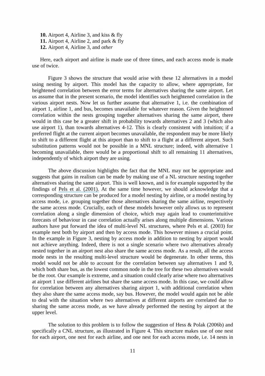
overall set of 96 combinations:
1. Airport 1, Airline 1, and bus
2. Airport 1, Airline 3, and taxi
3. Airport 1, Airline 1, and rail
4. Airport 2, Airline 4, and taxi
5. Airport 2, Airline 2, and kiss & fly
6. Airport 2, Airline 4, and park & fly
7. Airport 3, Airline 4, and rail
8. Airport 3, Airline 1, and other
9. Airport 3, Airline 2, and bus
7 In the present paper, the general specification also given in Train (2003) is used. Again using
different nests, with αjm describing the allocation of alternative j to nest m, we have that
. Here, the extra summation in comparison with the
NL formula ensures that each alternative can potentially belong to each nest. In the present specification, we have two conditions for the allocation parameters, namely , and
.
8 Given the possibility of the two alternatives presented in a single SC choice set being equivalent
along all three dimensions of choice, we in fact need to make use of two separate sets of 96 alternatives, giving rise to a final set of 192 alternatives. Of these, only two will clearly be available in any given choice set, with the availabilities (in the set of 192) being determined by the specific airports, airlines and access modes used for each of the two SC alternatives. The need to use two sets of 96 alternatives is simply a coding issue, and will be put to one side in the description of the nesting structures.
11
10. Airport 4, Airline 3, and kiss & fly
11. Airport 4, Airline 2, and park & fly
12. Airport 4, Airline 3, and other
Here, each airport and airline is made use of three times, and each access mode is made
use of twice.
Figure 3 shows the structure that would arise with these 12 alternatives in a model
using nesting by airport. This model has the capacity to allow, where appropriate, for
heightened correlation between the error terms for alternatives sharing the same airport. Let
us assume that in the present scenario, the model identifies such heightened correlation in the
various airport nests. Now let us further assume that alternative 1, i.e. the combination of
airport 1, airline 1, and bus, becomes unavailable for whatever reason. Given the heightened
correlation within the nests grouping together alternatives sharing the same airport, there
would in this case be a greater shift in probability towards alternatives 2 and 3 (which also
use airport 1), than towards alternatives 4-12. This is clearly consistent with intuition; if a
preferred flight at the current airport becomes unavailable, the respondent may be more likely
to shift to a different flight at this airport than to shift to a flight at a different airport. Such
substitution patterns would not be possible in a MNL structure; indeed, with alternative 1
becoming unavailable, there would be a proportional shift to all remaining 11 alternatives,
independently of which airport they are using.
The above discussion highlights the fact that the MNL may not be appropriate and
suggests that gains in realism can be made by making use of a NL structure nesting together
alternatives sharing the same airport. This is well known, and is for example supported by the
findings of Pels et al. (2001). At the same time however, we should acknowledge that a
corresponding structure can be produced for a model nesting by airline, or a model nesting by
access mode, i.e. grouping together those alternatives sharing the same airline, respectively
the same access mode. Crucially, each of these models however only allows us to represent
correlation along a single dimension of choice, which may again lead to counterintuitive
forecasts of behaviour in case correlation actually arises along multiple dimensions. Various
authors have put forward the idea of multi-level NL structures, where Pels et al. (2003) for
example nest both by airport and then by access mode. This however misses a crucial point.
In the example in Figure 3, nesting by access mode in addition to nesting by airport would
not achieve anything. Indeed, there is not a single scenario where two alternatives already
nested together in an airport nest also share the same access mode. As a result, all the access
mode nests in the resulting multi-level structure would be degenerate. In other terms, this
model would not be able to account for the correlation between say alternatives 1 and 9,
which both share bus, as the lowest common node in the tree for these two alternatives would
be the root. Our example is extreme, and a situation could clearly arise where two alternatives
at airport 1 use different airlines but share the same access mode. In this case, we could allow
for correlation between any alternatives sharing airport 1, with additional correlation when
they also share the same access mode, say bus. However, the model would again not be able
to deal with the situation where two alternatives at different airports are correlated due to
sharing the same access mode, as we have already performed the nesting by airport at the
upper level.
The solution to this problem is to follow the suggestion of Hess & Polak (2006b) and
specifically a CNL structure, as illustrated in Figure 4. This structure makes use of one nest
for each airport, one nest for each airline, and one nest for each access mode, i.e. 14 nests in

12
total. Each alternative in this model is still made up of an airport, and airline, and an access
mode, but now belongs to three nests, one airport nest, one airline nest, and one access mode
nest9. As an example, alternative 1 now falls into the first airport nest, the first airline nest,
and the bus nest. This alternative is correlated with alternative 8 along the bus dimension,
alternative 9 along the airline 1 dimension, alternative 3 along the airport 1 dimension, and
alternative 2 along both the airport 1 dimension and the airline 1 dimension. This discussion
highlights the clear advantages in flexibility. The model allows simultaneously for the
correlation along each of the three dimensions of choice, but in addition allows for even
higher correlation in case two alternatives share two of the three dimensions of choice.
Finally, with all the nesting being performed on the same level, no issues with ordering arise,
and unlike the multi-level NL model discussed above, this model still allows for correlation
between two alternatives that do not share the same airport but share the same access mode.
Another point needs to be addressed at this stage. We have specified a model structure
based on 96 alternatives, when the SC games are based on binary choice experiments. Here, it
is first worth noting that the added access mode dimension turns the two airport-airline
combinations presented in the SC into twelve different airport-airline-access-mode
alternatives. If the two airport-airline pairs are different, we then have twelve alternatives in a
given choice task, while otherwise, we have six. While we thus in each choice task already
allow for two alternatives to have the same access mode (one of the six options for alternative
A, and one of the six options for alternative B), this is only the case for the airport or airline
dimensions in those scenarios where both SC alternatives share the same airport or airline. So
the question arises as to how we can capture the correlation between alternatives sharing the
same airport or the same airline if these are not routinely presented jointly. The key to
understanding this comes in the structure of the NL and CNL models; these models allow for
an unobserved component in the utility function that is shared across such alternatives. As
long as sufficient cases arise in which they are presented jointly so as to allow for
identification, there is no need for this joint presentation to be universal. The number of cases
with equal airlines or equal airports was sufficiently high by design so as to allow for these
additional parameters to be identified.
Model estimation
All model estimation and forecasting work reported in this paper was carried out using
BIOGEME (Bierlaire, 2005), where the standard errors were corrected to account for the
repeated choice nature of the data used in the analysis by using the panel specification of the
sandwich estimator (cf. Daly & Hess, 2010).
MODELLING RESULTS
Five different models were estimated as part of this study. These included a simple MNL
model, three two-level NL models using nesting by airport, airline and access mode
respectively, and a CNL model. The results for these five models are summarised in
9 On a technical aside, the CNL specification works by allocating an alternative by different
proportions into different nests, collapsing back to a NL model when all allocation parameters are equal to 1, i.e. an alternative belongs into one nest. In the present context, the allocation parameters were all fixed to a value of 1/3, meaning that an alternative belongs to one airport, one airline, and one access mode nest. The estimation of actual values for the three non-zero allocation parameters for each alternative would have been very difficult due to the high number of parameters and would arguably not have provided any further benefits from an interpretation perspective.

13
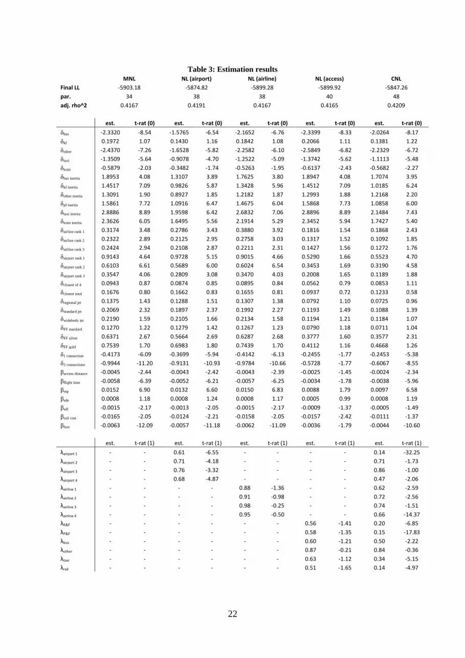
Table 3.
Looking first at the performance in terms of model fit, we can see that the move from
the MNL model to the NL model using nesting by airport is justified, giving a statistically
significant improvement in log-likelihood10
of 28.36 units, at the cost of four additional
parameters, namely the nesting parameters explaining the correlation in the different airport
nests. However, when looking at the remaining two NL structures, we observe improvements
in model fit compared to the MNL model by 3.91 units for NL (airline) and 3.26 units for NL
(access mode), which, at the cost of 4 respectively 6 additional parameters, are not
statistically significant beyond the 90% and 63% levels of confidence respectively. This
would suggest that allowing for correlation between alternatives sharing the same airport
provides gains in performance, while this is not the case for models allowing for correlation
between alternatives sharing the same airline or the same access mode. Most studies would
stop at this point, with the results suggesting significant correlation only along the airport
dimension. However, in the present analysis we go further by also estimating the CNL model
which allows for correlation along all three dimensions of choice at the same time. This
model not only offers a highly significant improvement in log-likelihood of 55.92 units when
compared to the MNL model (at the cost of 14 additional parameters), but similarly rejects all
three NL structures on the basis of χ2 tests at the highest level of confidence. This, in
conjunction with the later discussion on estimates, would suggest that there is in fact
correlation along all three dimensions of choice, but that in order to retrieve this correlation,
the analyst needs to specify a model that jointly allows for correlation along all dimensions of
choice. In other words, while the NL model nesting by airport is able to disentangle the
airport-specific correlation from the remaining error terms, this is not the case for the
remaining two NL structures, and a CNL model needs to be used.
Turning next to the actual estimates, and focussing on the MNL model, we can see
that, independently of the model structure, there is significant evidence of access mode
inertia, where interestingly, this is highest for taxi, rail and bus. Similarly, the positive
estimates for the various airport and airline constants, together with the decreasing size (with
the exception of δairline rank 2 and δairline rank 3, which are not significantly different from one
another) show that travellers‘ stated choices are consistent with their earlier rankings, with
their preferred airports and airlines being more likely to be chosen. The inclusion of these
terms could be criticised for endogeneity reasons, but does in this case allow us to produce
more reliable estimates of the remaining marginal utility coefficients, which are now less
affected by underlying preferences for specific airports or airlines. The estimates for δclosest of 4
and δclosest total are positive, suggesting an underlying preference for the closer airports,
independently of specific distance effects (see βaccess distance), but the estimates are not
significant at the usual levels of confidence. Issues with parameter significance also arise for
two out of the three aircraft type terms, though the actual values suggest an underlying
preference for larger aircraft, potentially due to perceived comfort advantages or the lower
risk of full flights.
Despite a few issues with parameter significance, affecting especially δFF standard, there
is also clear evidence to suggest that respondents are more likely to travel on an airline in
whose frequent flier programme they are a member, especially if they hold a silver or gold
membership. As expected, direct flights are seen as more appealing than connecting flights,
10
The sum of the logarithms of the modelled probabilities for the actual choices observed in the data.

14
where the use of separate terms for flights with one or two connections is justified by the fact
that the actual estimates reject a linearity assumption, with the value for δ2 connections being
more than twice the value for δ1 connection. Increases in access distance make an airport less
attractive. Increases in scheduled journey time have a negative effect, where this comes on
top of the effects of aircraft type and the number of connections. There are positive effects
associated with increases in on-time performance, and negative effects associated with late
schedule delay, i.e. flights that are scheduled to arrive later than the preferred arrival time.
The estimated effect associated with early schedule delay is positive, but is small and attains
only a low level of statistical significance. Finally, increases in rail cost and air fares have
negative impacts, with the former showing higher sensitivity than the latter. The move to the
four different nesting structures is accompanied by reductions in the significance of the
estimates. This is especially noticeable for the NL model using nesting by access mode,
where a large number of important parameters are no longer statistically significant.
We next turn our attention to the nesting parameters, which explain the correlation
between alternatives nested together, where these parameters, identified as λ, are constrained
to be between 0 and 1, with lower values for λ meaning higher correlation. The base value of
1 equates to an absence of correlation (as in a MNL model) and for this reason, the t-ratios
are calculated with respect to a base value of 1 rather than 0. In line with the findings on
model fit, we can see that all nesting parameters are significantly different from 1 in the
model using nesting by airport, showing correlation in all four airport nests, where this is
highest for those alternatives sharing the highest ranked airport, and those alternatives
sharing the lowest ranked airport. The model using nesting by airline shows low levels of
correlation which are only significant at low or very low levels of confidence. In the model
using nesting by access mode, several parameters attain moderate levels of statistical
significance, and do suggest the presence of some correlation for alternatives sharing the
same access mode. This is, as reported above, accompanied by problems with significance
level in the main utility parameters. Finally, in the CNL model, we obtain with four
exceptions (the nesting parameters for airport 2 and airport 3, significant at the 92% and 68%
level respectively, the airline 3 parameter, significant at the 87% level, and the one for other
access modes) highly significant estimates for all nesting parameters showing the presence of
high levels of correlation, and once again underlining the need for the CNL model in this
context, given the experiences with the NL structures.
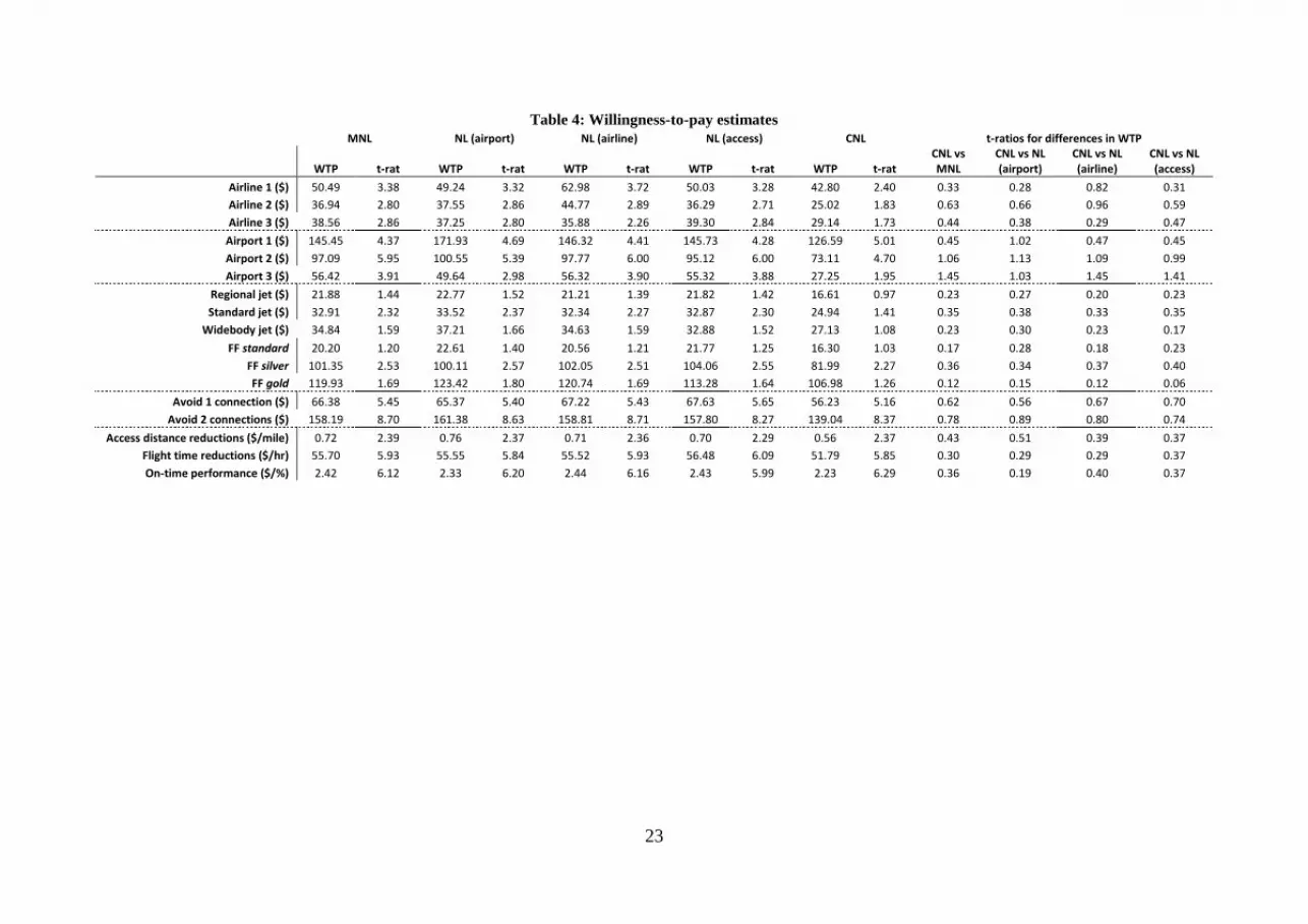
On the basis of the estimates from

15
Table 3, it is possible to calculate willingness-to-pay (WTP) measures for the various
components, and a selection of the most relevant ones is shown in Table 4, where in addition,
we report calculated t-ratios for these WTP measures (see e.g. Hess & Daly, 2009). The
actual WTP measures are simply obtained by the ratio between the relevant coefficient and
the air fare coefficient. For example, the WTP for avoiding travelling on an airline where the
respondent holds standard frequent flier membership is simply given by δFF standard/βfare.
Finally, given that our preferred model for this analysis is the CNL structure, we also
report t-ratios for differences between the WTP estimates in that model and the three
remaining models. The fact that none of these differences is significant at the usual levels of
confidence does in no way imply that the models are identical as reflected in the forecasting
analysis in the next section. In the study of the WTP indicators, it is important to recognise
the base lines, such that the airport WTP measures are for moving from the lowest ranked
airport to one of the three highest ranked airports, with a similar reasoning applying for the
airline indicators. For aircraft type, the base is a turboprop plane, with other baselines being
no membership for FF benefits, and direct flights. The actual values are largely consistent
with estimates in the various earlier studies referenced above, especially those making use of
the similar SP surveys in recent years.
FORECASTING ANALYSIS
As a final illustration of the differences between the various models estimated in this paper,
we now conduct two brief forecasting examples. Clearly, rescaling of the model outputs
would be required before undertaking any forecasting for the purposes of guiding policy
makers (cf. Louviere et al., 2000), but the aim of this example is purely illustrative.
Our first forecasting example makes use of a scenario where a single individual has
all 96 combinations of airport, airline and access mode available, and is observed to fly from
his/her preferred airport (airport 1), on his/her preferred airline (airline 1), and using kiss &
fly as the access mode. The aim of this example is to examine what would happen if this
alternative was to suddenly become unavailable. This example is not intended to be a realistic
representation of any actual condition, as the availability of an access mode is not likely to be
restricted for one airline at a given airport but available at that same airport for another
airline. However, the example is useful in illustrating the pattern of substitution that occurs
across the three choice dimensions.
The outputs are summarised in Table 5, which shows the changes in probabilities
resulting from the current alternative being made unavailable. To help understanding, Table 5
uses different shades for those cells relating to alternatives sharing no dimension with the
current alternative (i.e. different airport, airline and access mode), those cells relating to
alternatives sharing one dimension with the current alternative and those cells relating to
alternatives sharing two dimensions with the current alternative.
The effects of the IIA assumption on the MNL forecasts are immediately clear, with
proportional substitution towards all remaining alternatives, independent of the airport, airline
or access mode. In the NL model using nesting by airport, there is a greater shift towards
other alternatives at the same airport (airport 1), which is consistent with intuition. However,
the shift is the same for those alternatives sharing the same airport only, and those
alternatives sharing the same airport and the same access mode, where a greater shift would

16
be expected. Finally, alternatives that share the access mode or airline with the current
alternative, but use different airports, are treated in the same way as alternatives not sharing
any of the choice dimensions. The same issue arises in the NL models nesting by airline and
by access mode, with heightened substitution patterns only for those alternatives using airline
1 in the former, and those alternatives using K&F for the latter.
Finally, turning our attention to the CNL model, we can see that higher substitution
occurs for those alternatives that share the characteristics of the current alternative along two
dimensions (i.e. same airport and same airline; same airport and same access mode; same
airline and same access mode). This is followed by those alternatives that share only one
dimension of choice (i.e. same airport; same airline; same access mode). However, even here,
some differences arise, which are an effect of differences in nesting parameters, but possibly
also a result of different effects cancelling each other out or reinforcing one another. As an
example, the substitution is disproportionally high for three specific alternatives at airport 1,
namely the one using airline 1 and P&F, the one using airline 2 and K&F, and the one using
airline 3 and K&F. On the other hand, the substitution is unexpectedly low for those
alternatives using airline 4 at airport 1, where the pattern is the same as for alternatives not
sharing any choice dimensions. While these observations need further investigation, there is a
clear indication that the forecasting results from the CNL model are more intuitively correct
than those from the remaining three models.
Our second example uses a more realistic setting, where the respondent is now faced
with the situation where the option of getting someone to drive him/her to airport 1 is no
longer available, while it still exists for the three remaining airports.
The outputs of the forecasting example are summarised in Table 6, which shows the
changes in probabilities resulting from the three K&F alternatives being made unavailable at
airport 1. The effects of the IIA assumption on the MNL forecasts are once again clear. In the
NL model using nesting by airport and access mode, we see the expected greater shift
towards other options at airport 1 and towards the K&F alternatives at the three other airports
respectively. The NL model using nesting by airline is a special case as different airline
options are available at airport 1 and that these are all affected by K&F becoming
unavailable. However, given that the probability of the different K&F alternatives at airport 1
varied across airlines to begin with, the effect of K&F becoming unavailable clearly also
have a differential effect on the non K&F alternatives across the four different airlines.
However, as this model ignores the correlation along the airport and access mode dimensions,
the same pattern is repeated across all four airports, and also applies to the K&F alternatives
at the three remaining airports.
The above discussion has shown how each one of the three NL models shows a
departure from the MNL model by allowing for more realistic substitution patterns along a
single dimension of choice. Finally, turning our attention to the CNL model, we can see that
this model takes into account the correlations along all three dimensions of choice. As a
result, we obtain a far more diverse pattern of changes in probabilities, bringing together the
different effects observed for the three two-level NL models.
CONCLUSIONS
This paper has presented a discrete choice modelling analysis of air travel behaviour using
stated choice data collected in the East Coast area of the United States in 2008. In a departure

17
from much of the previous such work in this field, the work has looked at choice processes
involving airports in a much broader geographical area, reflecting the fact that passengers
increasingly travel to far outlying airports, often in return for cheap flights offered by low-
cost airlines.
Other than insights into willingness-to-pay patterns, the main contribution of this
papers comes in the use of advanced modelling techniques that allow us not only to explicitly
represent the three dimensional nature of the choice process, with passengers choosing an
airport, airline and access mode combination, but also to account for correlations along all
three dimensions of choice. In other words, any alternatives that share at least one dimension
of choice are closer substitutes for one another, where this increases further when alternatives
share multiple dimensions of choice. Here, the use of the CNL model offers significant gains
in model performance in estimation, and significantly more realistic substitution patterns in
forecasting. Importantly, the work also shows that the correlation along the airline and access
mode dimensions can only be adequately captured if additionally allowing for the correlation
along the airport dimension.
The CNL model has previously been used successfully in the analysis of a
corresponding three dimensional air passenger choice process using revealed preference (i.e.
real world) data (Hess & Polak, 2006b), and our findings in this paper, from what we believe
to be the first application of this type to stated choice data, reinforce the findings of this
earlier work, while also illustrating the applicability of this approach to stated choice data,
and air travel behaviour within a wider geographic area.
Several avenues for future work in air travel behaviour research can be identified.
These include a treatment of unobserved heterogeneity alongside the treatment of inter-
alternative correlation, the use of advanced nesting structures on joint RP/SP data, as well as
the incorporation of latent attitudes and perceptions which are bound to play a major role in
air travel choices.
ACKNOWLEDGEMENTS
The authors would like to thank the Engineering and Physical Sciences Research Council
(EPSRC) for the funding which enabled the survey work to be undertaken. ECUSATS was
commissioned and undertaken by Resources Systems Group Inc. The first acknowledges the
financial support of the Leverhulme Trust in the form of a Leverhulme Early Career
Fellowship. The authors are also grateful to Rhona Dallison and John Broussard for help with
data preparation.
REFERENCES
Adler, T., Falzarano, C. and Spitz, G. (2005), ―Modeling Service Trade-offs in Air Itinerary
Choices,‖ Transportation Research Record 1915, Transportation Research Board,
Washington D. C.

18
Basar, G. & Bhat, C. R. (2004), ‗A Parameterized Consideration Set model for airport choice:
an application to the San Francisco Bay area‘, Transportation Research Part B 38(10),
889–904.
Bhat, C., Adler, T. and Warburg, V. (2006), ―Modeling Demographic and Unobserved
Heterogeneity in Air Passengers‘ Sensitivity to Service Attributes in Itinerary Choice,‖
Transportation Research Record 1951, Transportation Research Board, Washington D.
C.
Ben-Akiva, M. & Bierlaire, M. (1999), Discrete choice methods and their applications to
short term travel decisions, in R. Hall, ed., ‗Handbook of Transportation Science‘,
Kluwer Academic Publishers, Dordrecht, The Netherlands, chapter 2, pp. 5–34.
Bierlaire, M., 2005. An introduction to BIOGEME Version 1.4. biogeme.ep.ch.
Bierlaire, M. (2006). A theoretical analysis of the cross-nested logit model. Annals of
Operations Research, Vol. 144, 287-300.
Bradley, M.A. & Daly, A.J. (1996), Estimation of Logit Choice Models Using Mixed Stated-
Preference and Revealed-Preference Information, in Travel Behaviour in an Era of
Change, Stopher, P. R. and Lee-Gosselin, M. (eds), chapter 9, pp. 209-231, Elsevier,
Oxford.
Coogan, M. and T. Adler (2009), ―Multimodal Approach to Aviation Capacity Planning in
Coastal Mega-Regions,‖ forthcoming Transportation Research Record, Transportation
Research Board, Washington D. C..
Daly, A.J. & Hess, S. (2010), Simple Approaches for Random Utility Modelling with Panel
Data, paper presented at the European Transport Conference, Glasgow, October 2010.
Daly, A. and S. Zachary (1978), Improved multiple choice models, in D.Hensher and
M.Dalvi, eds, ‗Determinants of Travel Choice‘, Saxon House, Sussex.
Dennis, N (2007) Stimulation or saturation? Perspectives on European low-cost airline
market and prospects for growth. Transportation Research Record, Volume 2007, pp 52-
59.
Hess, S. & Polak, J.W. (2005a), Accounting for random taste heterogeneity in airport-choice
modelling, Transportation Research Record, 1915, pp. 36-43.
Hess, S. & Polak J.W. (2005b), Mixed Logit modelling of airport choice in multi-airport
regions, Journal of Air Transport Management, 11(2), pp.59-68.
Hess, S. & Polak, J.W. (2006a), Airport, airline and access mode choice in the San Francisco
Bay area, Papers in Regional Science, 85(4), pp. 543-567.
Hess, S. & Polak, J.W. (2006b), Exploring the potential for cross-nesting structures in
airport-choice analysis: a case-study of the Greater London area, Transportation
Research Part E, 42, pp. 63-81.
Hess, S., Adler, T. & Polak, J.W. (2007), Modelling airport and airline choice behaviour with
the use of stated preference survey data, Transportation Research Part E, 43, pp. 221-
233.
Hess, S. (2007), Posterior analysis of random taste coefficients in air travel choice behaviour
modelling, Journal of Air Transport Management 13(4), pp. 203-212.
Hess, S. (2008), Treatment of reference alternatives in SC surveys for air travel choice
behaviour, Journal of Air Transport Management, 14(5), pp. 275-279
Hess, S. & Daly, A. (2009), Calculating errors for measures derived from choice modelling
estimates, paper presented at the 88th Annual Meeting of the Transportation Research
Board, Washington, D.C.
Hess, S., Rose, J.M. & Polak, J.W. (2010), Non-trading, lexicographic and inconsistent
behaviour in stated choice data, Transportation Research Part D, 15(7), pp. 405-417.

19
Loo B., (2008), ―Passengers‘ airport choice within multiairport regions (MARs): some
insights from a stated preference survey at Hong Kong International Airport‖, Journal of
Transport Geography, 16, 117-125.
Louviere, J.J., Hensher, D.A. and Swait, J.D. (2000), Stated Choice Methods—Analysis and
Application, Cambridge University Press, UK.
McFadden, D. (1974), Conditional logit analysis of qualitative choice behavior, in
P.Zarembka, ed., ‗Frontiers in Econometrics‘, Academic Press, New York, pp. 105–42.
McFadden, D. (1978), Modeling the choice of residential location, in A.Karlqvist,
L.Lundqvist, F.Snickars and J.Weibull, eds, ‗Spatial Interaction Theory and Planning
Models‘, North-Holland, Amsterdam, pp. 75–96.
Papola, A. (2004). Some developments on the Cross Nested Logit model. Transportation
Research Part B, 38, 833-851.
Pels, E., Nijkamp, P. & Rietveld, P. (2001), ‗Airport and airline choice in a multiairport
region: an empirical analysis for the San Francisco bay area‘, Regional Studies 35(1), 1–
9.
Pew Research Center (2010), Pew Internet and American Life Project, retrieved from
http://www.pewinternet.org/Static-Pages/Trend-Data/Whos-Online.aspx.
Pels, E., Nijkamp, P. & Rietveld, P. (2003), ‗Access to and competition between airports: a
case study for the San Francisco Bay area‘, Transportation Research Part A 37(1), 71–83.
Ryley, T. and Davison, L. (2008), ―UK air travel preferences: evidence from an East
Midlands household survey‖. Journal of Air Transport Management, 14(1), pp.43-46.
Tam, M.L., Lam, W.H.K. & Lo, H.P. (2010), Incorporating passenger perceived service
quality in airport ground access mode choice model, Transportmetrica, 6(1), pp. 3-17.
Theis, G., Ben-Akiva, M., Adler, T. and Clarke, J-P (2006), ―Risk Averseness Regarding
Short Connections in Airline Itinerary Choice,‖ Transportation Research Record 1951.
Train, K.E. (2003), Discrete choice methods with simulation, Cambridge University Press,
Cambridge, MA.
Vovsha, P. (1997), ‗Application of a Cross-Nested Logit model to mode choice in Tel Aviv,
Israel, Metropolitan Area‘, Transportation Research Record 1607, 6–15.
Vovsha, P. & Bekhor, S. (1998), ‗The Link-Nested Logit model of route choice: overcoming
the route overlapping problem‘, Transportation Research Record 1645, 133–142.
Wen, C.-H. & Koppelman, F. S. (2001), ‗The Generalized Nested Logit Model‘,
Transportation Research Part B: Methodological 35(7), 627–641.
Wen, C.-H. (2010), Alternative tree structures for estimating nested logit models with mixed
preference data, Transportmetrica, 6(4), pp. 291-309.
Williams, H. (1977), ‗On the formation of travel demand models and economic evaluation
measures of user benefits‘, Environment and Planning A 9, 285–344.

20
Table 1: Levels used in generation of choice scenarios
Attributes Number
of levels Reference point Details
Departure airport
4 Respondent ranking
1st
, 2nd
, 3rd
preferred and least preferred
Airline 4 Respondent ranking
1st
, 2nd
, 3rd
and 4th
preferred
Aircraft type 4 Available set based on flight length
Propeller (<2.5 hours), regional jet (<4 hours), standard jet (any trip), wide body(> 4 hours)
Arrival time (schedule delay early and late)
5 Respondent preferred time of arrival
2 hours earlier, 1 hour earlier, same as preferred, 1 hour later, 2 hours later
Number of connections
3 Available set based on nonstop flight length
0 , 1, or 2 connections (flights >4 hours)
Airport to airport travel time (including connections)
4 Respondent’s previous flight
85%, 100%, 115% and 130% previous flight
On-time performance
5 Generic 50%, 60%, 70%, 80%, 90% on time
Air fare 5 Respondent’s previous flight
50%, 75%, 100%, 125% and 150% of previous fare
Parking cost 4 Generic Ranging from $12-20 per day in the airport garage and from $7-10 per day on a remote lot with a 10 minutes shuttle ride.
Attributes of rail service
6 Generic Including ‘No direct rail service’, and then combination of fares of $20 or $40 for a round trip, with a 15 or 30 minute headways and taking either the same time as a car or 10 minutes less.

21
Table 2: Final utility specification
Coefficient Attribute Description δairport rank 1 I airport rank 1
Airport constants for three highest ranked airports, coefficients multiplied by
dummy variables for airport rank for given alternative (lowest ranked as base) δairport rank 2 I airport rank 2
δairport rank 3 I airport rank 3
δairline rank 1 I airline rank 1 Airline constants for three highest ranked airlines, coefficients multiplied by
dummy variables for airline rank for given alternative (lowest ranked as base) δairline rank 2 I airline rank 2
δairline rank 3 I airline rank 3
δFF standard I FF standard Frequent flier membership constants, coefficients multiplied by dummy variables
for membership level in airline for given alternative (no membership as base) δFF silver I FF silver
δFF gold I FF gold
δregional jet I regional jet Aircraft type constants, coefficients multiplied by dummy variables for aircraft
for given alternative (turboprop as base) δstandard jet I standard jet
δwidebody jet I widebody jet
δclosest of 4 I closest of 4 Local airport constants, coefficients multiplied by dummy variables indicating
whether airport for given alternative is closest out of four used, or closest overall δclosest total I closest total
δbus I bus
Access mode constants, coefficients multiplied by dummy variables for access
mode for given alternative (car as base)
δkf I kf
δtaxi I taxi
δrail I rail
δother I other
δbus inertia I bus inertia
Access mode inertia terms, coefficients multiplied by dummy variables
indicating whether access mode for given alternative is the same as the ―real
world‖ access mode
δpf inertia I pf inertia
δkf inertia I kf inertia
δtaxi inertia I taxi inertia
δrail inertia I rail inertia
δother inertia I other inertia
δ1 connection I 1 connection Coefficients for connections, multiplied by dummy variables for one or two
connections (direct flights as base) δ2 connections I 2 connections
βaccess distance xaccess distance Marginal utility coefficient for access distance
βrail cost xrail cost * I rail Marginal utility coefficient for rail cost, used for rail alternatives only
βflight time xflight time Marginal utility coefficient for flight time
βsde xsde Marginal utility coefficient for early and late schedule delay βsdl xsdl
βotp xotp Marginal utility coefficient for on-time performance
βfare xfare Marginal utility coefficient for fare
22
Table 3: Estimation results
MNL NL (airport) NL (airline) NL (access) CNL
Final LL -5903.18 -5874.82 -5899.28 -5899.92 -5847.26
par. 34 38 38 40 48
adj. rho^2 0.4167 0.4191 0.4167 0.4165 0.4209
est. t-rat (0) est. t-rat (0) est. t-rat (0) est. t-rat (0) est. t-rat (0)
δbus -2.3320 -8.54 -1.5765 -6.54 -2.1652 -6.76 -2.3399 -8.33 -2.0264 -8.17
δkf 0.1972 1.07 0.1430 1.16 0.1842 1.08 0.2066 1.11 0.1381 1.22
δother -2.4370 -7.26 -1.6528 -5.82 -2.2582 -6.10 -2.5849 -6.82 -2.2329 -6.72
δtaxi -1.3509 -5.64 -0.9078 -4.70 -1.2522 -5.09 -1.3742 -5.62 -1.1113 -5.48
δtrain -0.5879 -2.03 -0.3482 -1.74 -0.5263 -1.95 -0.6137 -2.43 -0.5682 -2.27
δbus inertia 1.8953 4.08 1.3107 3.89 1.7625 3.80 1.8947 4.08 1.7074 3.95
δkf inertia 1.4517 7.09 0.9826 5.87 1.3428 5.96 1.4512 7.09 1.0185 6.24
δother inertia 1.3091 1.90 0.8927 1.85 1.2182 1.87 1.2993 1.88 1.2168 2.20
δpf inertia 1.5861 7.72 1.0916 6.47 1.4675 6.04 1.5868 7.73 1.0858 6.00
δtaxi inertia 2.8886 8.89 1.9598 6.42 2.6832 7.06 2.8896 8.89 2.1484 7.43
δtrain inertia 2.3626 6.05 1.6495 5.56 2.1914 5.29 2.3452 5.94 1.7427 5.40
δairline rank 1 0.3174 3.48 0.2786 3.43 0.3880 3.92 0.1816 1.54 0.1868 2.43
δairline rank 2 0.2322 2.89 0.2125 2.95 0.2758 3.03 0.1317 1.52 0.1092 1.85
δairline rank 3 0.2424 2.94 0.2108 2.87 0.2211 2.31 0.1427 1.56 0.1272 1.76
δairport rank 1 0.9143 4.64 0.9728 5.15 0.9015 4.66 0.5290 1.66 0.5523 4.70
δairport rank 2 0.6103 6.61 0.5689 6.00 0.6024 6.54 0.3453 1.69 0.3190 4.58
δairport rank 3 0.3547 4.06 0.2809 3.08 0.3470 4.03 0.2008 1.65 0.1189 1.88
δclosest of 4 0.0943 0.87 0.0874 0.85 0.0895 0.84 0.0562 0.79 0.0853 1.11
δclosest total 0.1676 0.80 0.1662 0.83 0.1655 0.81 0.0937 0.72 0.1233 0.58
δregional jet 0.1375 1.43 0.1288 1.51 0.1307 1.38 0.0792 1.10 0.0725 0.96
δstandard jet 0.2069 2.32 0.1897 2.37 0.1992 2.27 0.1193 1.49 0.1088 1.39
δwidebody jet 0.2190 1.59 0.2105 1.66 0.2134 1.58 0.1194 1.21 0.1184 1.07
δFF standard 0.1270 1.22 0.1279 1.42 0.1267 1.23 0.0790 1.18 0.0711 1.04
δFF silver 0.6371 2.67 0.5664 2.69 0.6287 2.68 0.3777 1.60 0.3577 2.31
δFF gold 0.7539 1.70 0.6983 1.80 0.7439 1.70 0.4112 1.16 0.4668 1.26
δ1 connection -0.4173 -6.09 -0.3699 -5.94 -0.4142 -6.13 -0.2455 -1.77 -0.2453 -5.38
δ2 connections -0.9944 -11.20 -0.9131 -10.93 -0.9784 -10.66 -0.5728 -1.77 -0.6067 -8.55
βaccess distance -0.0045 -2.44 -0.0043 -2.42 -0.0043 -2.39 -0.0025 -1.45 -0.0024 -2.34
βflight time -0.0058 -6.39 -0.0052 -6.21 -0.0057 -6.25 -0.0034 -1.78 -0.0038 -5.96
βotp 0.0152 6.90 0.0132 6.60 0.0150 6.83 0.0088 1.79 0.0097 6.58
βsde 0.0008 1.18 0.0008 1.24 0.0008 1.17 0.0005 0.99 0.0008 1.19
βsdl -0.0015 -2.17 -0.0013 -2.05 -0.0015 -2.17 -0.0009 -1.37 -0.0005 -1.49
βrail cost -0.0165 -2.05 -0.0124 -2.21 -0.0158 -2.05 -0.0157 -2.42 -0.0111 -1.37
βfare -0.0063 -12.09 -0.0057 -11.18 -0.0062 -11.09 -0.0036 -1.79 -0.0044 -10.60
est. t-rat (1) est. t-rat (1) est. t-rat (1) est. t-rat (1) est. t-rat (1)
λairport 1 - - 0.61 -6.55 - - - - 0.14 -32.25
λairport 2 - - 0.71 -4.18 - - - - 0.71 -1.73
λairport 3 - - 0.76 -3.32 - - - - 0.86 -1.00
λairport 4 - - 0.68 -4.87 - - - - 0.47 -2.06
λairline 1 - - - - 0.88 -1.36 - - 0.62 -2.59
λairline 2 - - - - 0.91 -0.98 - - 0.72 -2.56
λairline 3 - - - - 0.98 -0.25 - - 0.74 -1.51
λairline 4 - - - - 0.95 -0.50 - - 0.66 -14.37
λK&F - - - - - - 0.56 -1.41 0.20 -6.85
λP&F - - - - - - 0.58 -1.35 0.15 -17.83
λbus - - - - - - 0.60 -1.21 0.50 -2.22
λother - - - - - - 0.87 -0.21 0.84 -0.36
λtaxi - - - - - - 0.63 -1.12 0.34 -5.15
λrail - - - - - - 0.51 -1.65 0.14 -4.97
23
Table 4: Willingness-to-pay estimates
MNL NL (airport) NL (airline) NL (access) CNL t-ratios for differences in WTP
WTP t-rat WTP t-rat WTP t-rat WTP t-rat WTP t-rat CNL vs MNL
CNL vs NL (airport)
CNL vs NL (airline)
CNL vs NL (access)
Airline 1 ($) 50.49 3.38 49.24 3.32 62.98 3.72 50.03 3.28 42.80 2.40 0.33 0.28 0.82 0.31
Airline 2 ($) 36.94 2.80 37.55 2.86 44.77 2.89 36.29 2.71 25.02 1.83 0.63 0.66 0.96 0.59
Airline 3 ($) 38.56 2.86 37.25 2.80 35.88 2.26 39.30 2.84 29.14 1.73 0.44 0.38 0.29 0.47
Airport 1 ($) 145.45 4.37 171.93 4.69 146.32 4.41 145.73 4.28 126.59 5.01 0.45 1.02 0.47 0.45
Airport 2 ($) 97.09 5.95 100.55 5.39 97.77 6.00 95.12 6.00 73.11 4.70 1.06 1.13 1.09 0.99
Airport 3 ($) 56.42 3.91 49.64 2.98 56.32 3.90 55.32 3.88 27.25 1.95 1.45 1.03 1.45 1.41
Regional jet ($) 21.88 1.44 22.77 1.52 21.21 1.39 21.82 1.42 16.61 0.97 0.23 0.27 0.20 0.23
Standard jet ($) 32.91 2.32 33.52 2.37 32.34 2.27 32.87 2.30 24.94 1.41 0.35 0.38 0.33 0.35
Widebody jet ($) 34.84 1.59 37.21 1.66 34.63 1.59 32.88 1.52 27.13 1.08 0.23 0.30 0.23 0.17
FF standard 20.20 1.20 22.61 1.40 20.56 1.21 21.77 1.25 16.30 1.03 0.17 0.28 0.18 0.23
FF silver 101.35 2.53 100.11 2.57 102.05 2.51 104.06 2.55 81.99 2.27 0.36 0.34 0.37 0.40
FF gold 119.93 1.69 123.42 1.80 120.74 1.69 113.28 1.64 106.98 1.26 0.12 0.15 0.12 0.06
Avoid 1 connection ($) 66.38 5.45 65.37 5.40 67.22 5.43 67.63 5.65 56.23 5.16 0.62 0.56 0.67 0.70
Avoid 2 connections ($) 158.19 8.70 161.38 8.63 158.81 8.71 157.80 8.27 139.04 8.37 0.78 0.89 0.80 0.74
Access distance reductions ($/mile) 0.72 2.39 0.76 2.37 0.71 2.36 0.70 2.29 0.56 2.37 0.43 0.51 0.39 0.37
Flight time reductions ($/hr) 55.70 5.93 55.55 5.84 55.52 5.93 56.48 6.09 51.79 5.85 0.30 0.29 0.29 0.37
On-time performance ($/%) 2.42 6.12 2.33 6.20 2.44 6.16 2.43 5.99 2.23 6.29 0.36 0.19 0.40 0.37

24
Table 5: First forecasting example (AP=airport, AL=airline)
MNL NL (airport) NL (airline)
Access mode Access mode Access mode
AP AL Bus P&F K&F Taxi Rail Other AP AL Bus P&F K&F Taxi Rail Other AP AL Bus P&F K&F Taxi Rail Other
1 1 19.7% 19.7% -100% 19.7% 19.7% 19.7% 1 1 29.2% 29.2% -100% 29.2% 29.2% 29.2% 1 1 23.1% 23.1% -100% 23.1% 23.1% 23.1%
1 2 19.7% 19.7% 19.7% 19.7% 19.7% 19.7% 1 2 29.2% 29.2% 29.2% 29.2% 29.2% 29.2% 1 2 18.1% 18.1% 18.1% 18.1% 18.1% 18.1%
1 3 19.7% 19.7% 19.7% 19.7% 19.7% 19.7% 1 3 29.2% 29.2% 29.2% 29.2% 29.2% 29.2% 1 3 18.1% 18.1% 18.1% 18.1% 18.1% 18.1%
1 4 19.7% 19.7% 19.7% 19.7% 19.7% 19.7% 1 4 29.2% 29.2% 29.2% 29.2% 29.2% 29.2% 1 4 18.1% 18.1% 18.1% 18.1% 18.1% 18.1%
2 1 19.7% 19.7% 19.7% 19.7% 19.7% 19.7% 2 1 13.6% 13.6% 13.6% 13.6% 13.6% 13.6% 2 1 23.1% 23.1% 23.1% 23.1% 23.1% 23.1%
2 2 19.7% 19.7% 19.7% 19.7% 19.7% 19.7% 2 2 13.6% 13.6% 13.6% 13.6% 13.6% 13.6% 2 2 18.1% 18.1% 18.1% 18.1% 18.1% 18.1%
2 3 19.7% 19.7% 19.7% 19.7% 19.7% 19.7% 2 3 13.6% 13.6% 13.6% 13.6% 13.6% 13.6% 2 3 18.1% 18.1% 18.1% 18.1% 18.1% 18.1%
2 4 19.7% 19.7% 19.7% 19.7% 19.7% 19.7% 2 4 13.6% 13.6% 13.6% 13.6% 13.6% 13.6% 2 4 18.1% 18.1% 18.1% 18.1% 18.1% 18.1%
3 1 19.7% 19.7% 19.7% 19.7% 19.7% 19.7% 3 1 13.6% 13.6% 13.6% 13.6% 13.6% 13.6% 3 1 23.1% 23.1% 23.1% 23.1% 23.1% 23.1%
3 2 19.7% 19.7% 19.7% 19.7% 19.7% 19.7% 3 2 13.6% 13.6% 13.6% 13.6% 13.6% 13.6% 3 2 18.1% 18.1% 18.1% 18.1% 18.1% 18.1%
3 3 19.7% 19.7% 19.7% 19.7% 19.7% 19.7% 3 3 13.6% 13.6% 13.6% 13.6% 13.6% 13.6% 3 3 18.1% 18.1% 18.1% 18.1% 18.1% 18.1%
3 4 19.7% 19.7% 19.7% 19.7% 19.7% 19.7% 3 4 13.6% 13.6% 13.6% 13.6% 13.6% 13.6% 3 4 18.1% 18.1% 18.1% 18.1% 18.1% 18.1%
4 1 19.7% 19.7% 19.7% 19.7% 19.7% 19.7% 4 1 13.6% 13.6% 13.6% 13.6% 13.6% 13.6% 4 1 23.1% 23.1% 23.1% 23.1% 23.1% 23.1%
4 2 19.7% 19.7% 19.7% 19.7% 19.7% 19.7% 4 2 13.6% 13.6% 13.6% 13.6% 13.6% 13.6% 4 2 18.1% 18.1% 18.1% 18.1% 18.1% 18.1%
4 3 19.7% 19.7% 19.7% 19.7% 19.7% 19.7% 4 3 13.6% 13.6% 13.6% 13.6% 13.6% 13.6% 4 3 18.1% 18.1% 18.1% 18.1% 18.1% 18.1%
4 4 19.7% 19.7% 19.7% 19.7% 19.7% 19.7% 4 4 13.6% 13.6% 13.6% 13.6% 13.6% 13.6% 4 4 18.1% 18.1% 18.1% 18.1% 18.1% 18.1%
NL (access) CNL
Access mode Access mode
AP AL Bus P&F K&F Taxi Rail Other AP AL Bus P&F K&F Taxi Rail Other
1 1 12% 12% -100% 12% 12% 12% 1 1 23.8% 48.9% -100% 14.7% 15.3% 12.8%
1 2 12% 12% 53.5% 12% 12% 12% 1 2 10.2% 11% 107.2% 10.1% 10.1% 10.1%
1 3 12% 12% 53.5% 12% 12% 12% 1 3 10.1% 10.4% 49.3% 10.1% 10.1% 10.1%
1 4 12% 12% 53.5% 12% 12% 12% 1 4 10.1% 10.1% 10.1% 10.1% 10.1% 10.1%
2 1 12% 12% 53.5% 12% 12% 12% 2 1 13.9% 14.7% 14.9% 13.9% 14.2% 10.9%
2 2 12% 12% 53.5% 12% 12% 12% 2 2 10.1% 10.1% 10.3% 10.1% 10.1% 10.1%
2 3 12% 12% 53.5% 12% 12% 12% 2 3 10.1% 10.1% 10.2% 10.1% 10.1% 10.1%
2 4 12% 12% 53.5% 12% 12% 12% 2 4 10.1% 10.1% 28.8% 10.1% 10.1% 10.1%
3 1 12% 12% 53.5% 12% 12% 12% 3 1 13% 13.9% 15.7% 12.5% 12.7% 10.9%
3 2 12% 12% 53.5% 12% 12% 12% 3 2 10.1% 10.1% 10.3% 10.1% 10.1% 10.1%
3 3 12% 12% 53.5% 12% 12% 12% 3 3 10.1% 10.1% 10.1% 10.1% 10.1% 10.1%
3 4 12% 12% 53.5% 12% 12% 12% 3 4 10.1% 10.1% 10.2% 10.1% 10.1% 10.1%
4 1 12% 12% 53.5% 12% 12% 12% 4 1 15.3% 16.6% 22% 17.5% 18.4% 11.6%
4 2 12% 12% 53.5% 12% 12% 12% 4 2 10.1% 10.1% 11.9% 10.1% 10.1% 10.1%
4 3 12% 12% 53.5% 12% 12% 12% 4 3 10.1% 10.1% 10.3% 10.1% 10.1% 10.1%
4 4 12% 12% 53.5% 12% 12% 12% 4 4 10.1% 10.1% 10.1% 10.1% 10.1% 10.1%
Alt. made unavailable No common dimension One common dimension Two common dimensions

25
Table 6: Second forecasting example (AP=airport, AL=airline)
MNL NL (airport) NL (airline)
Access mode Access mode Access mode
AP AL Bus P&F K&F Taxi Rail Other AP AL Bus P&F K&F Taxi Rail Other AP AL Bus P&F K&F Taxi Rail Other
1 1 31.9% 31.9% -100.0% 31.9% 31.9% 31.9% 1 1 39.8% 39.8% -100.0% 39.8% 39.8% 39.8% 1 1 35.4% 35.4% -100.0% 35.4% 35.4% 35.4%
1 2 31.9% 31.9% -100.0% 31.9% 31.9% 31.9% 1 2 39.8% 39.8% -100.0% 39.8% 39.8% 39.8% 1 2 33.3% 33.3% -100.0% 33.3% 33.3% 33.3%
1 3 31.9% 31.9% -100.0% 31.9% 31.9% 31.9% 1 3 39.8% 39.8% -100.0% 39.8% 39.8% 39.8% 1 3 30.9% 30.9% -100.0% 30.9% 30.9% 30.9%
1 4 31.9% 31.9% -100.0% 31.9% 31.9% 31.9% 1 4 39.8% 39.8% -100.0% 39.8% 39.8% 39.8% 1 4 30.0% 30.0% -100.0% 30.0% 30.0% 30.0%
2 1 31.9% 31.9% 31.9% 31.9% 31.9% 31.9% 2 1 18.0% 18.0% 18.0% 18.0% 18.0% 18.0% 2 1 35.4% 35.4% 35.4% 35.4% 35.4% 35.4%
2 2 31.9% 31.9% 31.9% 31.9% 31.9% 31.9% 2 2 18.0% 18.0% 18.0% 18.0% 18.0% 18.0% 2 2 33.3% 33.3% 33.3% 33.3% 33.3% 33.3%
2 3 31.9% 31.9% 31.9% 31.9% 31.9% 31.9% 2 3 18.0% 18.0% 18.0% 18.0% 18.0% 18.0% 2 3 30.9% 30.9% 30.9% 30.9% 30.9% 30.9%
2 4 31.9% 31.9% 31.9% 31.9% 31.9% 31.9% 2 4 18.0% 18.0% 18.0% 18.0% 18.0% 18.0% 2 4 30.0% 30.0% 30.0% 30.0% 30.0% 30.0%
3 1 31.9% 31.9% 31.9% 31.9% 31.9% 31.9% 3 1 18.0% 18.0% 18.0% 18.0% 18.0% 18.0% 3 1 35.4% 35.4% 35.4% 35.4% 35.4% 35.4%
3 2 31.9% 31.9% 31.9% 31.9% 31.9% 31.9% 3 2 18.0% 18.0% 18.0% 18.0% 18.0% 18.0% 3 2 33.3% 33.3% 33.3% 33.3% 33.3% 33.3%
3 3 31.9% 31.9% 31.9% 31.9% 31.9% 31.9% 3 3 18.0% 18.0% 18.0% 18.0% 18.0% 18.0% 3 3 30.9% 30.9% 30.9% 30.9% 30.9% 30.9%
3 4 31.9% 31.9% 31.9% 31.9% 31.9% 31.9% 3 4 18.0% 18.0% 18.0% 18.0% 18.0% 18.0% 3 4 30.0% 30.0% 30.0% 30.0% 30.0% 30.0%
4 1 31.9% 31.9% 31.9% 31.9% 31.9% 31.9% 4 1 18.0% 18.0% 18.0% 18.0% 18.0% 18.0% 4 1 35.4% 35.4% 35.4% 35.4% 35.4% 35.4%
4 2 31.9% 31.9% 31.9% 31.9% 31.9% 31.9% 4 2 18.0% 18.0% 18.0% 18.0% 18.0% 18.0% 4 2 33.3% 33.3% 33.3% 33.3% 33.3% 33.3%
4 3 31.9% 31.9% 31.9% 31.9% 31.9% 31.9% 4 3 18.0% 18.0% 18.0% 18.0% 18.0% 18.0% 4 3 30.9% 30.9% 30.9% 30.9% 30.9% 30.9%
4 4 31.9% 31.9% 31.9% 31.9% 31.9% 31.9% 4 4 18.0% 18.0% 18.0% 18.0% 18.0% 18.0% 4 4 30.0% 30.0% 30.0% 30.0% 30.0% 30.0%
NL (access) CNL
Access mode Access mode
AP AL Bus P&F K&F Taxi Rail Other AP AL Bus P&F K&F Taxi Rail Other
1 1 20.7% 20.7% -100.0% 20.7% 20.7% 20.7% 1 1 30.8% 57.7% -100.0% 21.0% 21.6% 19.0%
1 2 20.7% 20.7% -100.0% 20.7% 20.7% 20.7% 1 2 21.9% 26.1% -100.0% 22.4% 25.2% 18.6%
1 3 20.7% 20.7% -100.0% 20.7% 20.7% 20.7% 1 3 22.8% 26.1% -100.0% 23.8% 25.9% 19.1%
1 4 20.7% 20.7% -100.0% 20.7% 20.7% 20.7% 1 4 16.4% 16.5% -100.0% 16.5% 16.5% 16.2%
2 1 20.7% 20.7% 116.8% 20.7% 20.7% 20.7% 2 1 20.2% 21.1% 21.5% 20.2% 20.5% 17.0%
2 2 20.7% 20.7% 116.8% 20.7% 20.7% 20.7% 2 2 20.1% 20.6% 21.2% 20.5% 20.6% 17.8%
2 3 20.7% 20.7% 116.8% 20.7% 20.7% 20.7% 2 3 21.0% 21.4% 21.5% 21.5% 21.5% 18.2%
2 4 20.7% 20.7% 116.8% 20.7% 20.7% 20.7% 2 4 16.3% 16.3% 89.3% 16.3% 16.3% 16.2%
3 1 20.7% 20.7% 116.8% 20.7% 20.7% 20.7% 3 1 19.2% 20.2% 26.6% 18.7% 18.9% 17.0%
3 2 20.7% 20.7% 116.8% 20.7% 20.7% 20.7% 3 2 18.9% 19.3% 19.8% 18.7% 18.8% 17.3%
3 3 20.7% 20.7% 116.8% 20.7% 20.7% 20.7% 3 3 19.3% 19.6% 19.8% 19.2% 19.2% 17.6%
3 4 20.7% 20.7% 116.8% 20.7% 20.7% 20.7% 3 4 16.3% 16.3% 16.5% 16.3% 16.3% 16.2%
4 1 20.7% 20.7% 116.8% 20.7% 20.7% 20.7% 4 1 21.7% 23.1% 44.8% 24.0% 24.9% 17.7%
4 2 20.7% 20.7% 116.8% 20.7% 20.7% 20.7% 4 2 21.0% 21.6% 28.4% 22.7% 22.8% 18.2%
4 3 20.7% 20.7% 116.8% 20.7% 20.7% 20.7% 4 3 22.8% 23.4% 23.8% 24.4% 24.3% 18.6%
4 4 20.7% 20.7% 116.8% 20.7% 20.7% 20.7% 4 4 16.4% 16.5% 16.4% 16.5% 16.5% 16.2%
Alt. made unavailable No common dimension One common dimension Two common dimensions

26
Figure 1: Survey questions relating to personal airline and airport rankings

27
Figure 2: Example SC choice screen

28
Airport nest 1
Root
Trip option
Airport 1 Airline 1
Bus
Trip option
Airport 1 Airline 3
Taxi
Trip option
Airport 2 Airline 2 Kiss & fly
Trip option
Airport 2 Airline 4
Park & fly
Trip option
Airport 3 Airline 4
Rail
Trip option
Airport 3 Airline 1
Other
Trip option
Airport 4 Airline 3 Kiss & fly
Trip option
Airport 4 Airline 2
Park & fly
Trip option
Airport 3 Airline 2
Bus
Trip option
Airport 2 Airline 4
Taxi
Trip option
Airport 1 Airline 1
Rail
Airport nest 2
Airport nest 3
Airport nest 4
Trip option
Airport 4 Airline 3
Other
Figure 3: Structure for NL model using nesting by airport

29
Figure 4: Structure for CNL model


