Importance sampling in Bayesian networks using probability trees

Computational Statistics & Data Analysis 34 (2000) 387–413www.elsevier.com/locate/csda

Importance sampling in Bayesiannetworks using probability trees(

Antonio Salmer�ona ; ∗, Andr�es Canob, Seraf��n Moralb

aDepartment of Statistics and Applied Mathematics, University of Almer ��a, SpainbDepartment of Computer Science and Arti�cial Intelligence, University of Granada, Spain

Received 1 April 1999; received in revised form 1 October 1999; accepted 26 November 1999

Abstract

In this paper a new Monte-Carlo algorithm for the propagation of probabilities in Bayesian networksis proposed. This algorithm has two stages: in the �rst one an approximate propagation is carried outby means of a deletion sequence of the variables. In the second stage a sample is obtained usingas sampling distribution the calculations of the �rst step. The di�erent con�gurations of the sampleare weighted according to the importance sampling technique. We show how the use of probabilitytrees to store and to approximate probability potentials, and a careful selection of the deletion sequence,make this algorithm able to propagate over large networks with extreme probabilities. c© 2000 ElsevierScience B.V. All rights reserved.

Keywords: Bayesian networks; Simulation; Importance sampling; Probability trees; Approximate pre-computation

1. Introduction

It is known that exact probabilistic inference in Bayesian networks may be infeasi-ble in large networks (Cooper, 1990). This motivates the development of approximatealgorithms, most of them based on Monte Carlo simulation.

( This work has been supported by CICYT under projects TIC97-1135-C04-01 and TIC97-1135-C04-02.∗ Corresponding author.E-mail addresses: [email protected] (A. Salmer�on), [email protected] (A. Cano), [email protected](S. Moral).

0167-9473/00/$ - see front matter c© 2000 Elsevier Science B.V. All rights reserved.PII: S 0167-9473(99)00110-3

388 A. Salmer�on et al. / Computational Statistics & Data Analysis 34 (2000) 387–413

We can distinguish two groups of Monte Carlo algorithms: those based on Gibbssampling (Jensen et al., 1995; Pearl, 1987) and those based on importance sam-pling (Dagum and Luby, 1997; Fung and Chang, 1990; Henrion, 1988; Hern�andezet al., 1996,1998; Shachter and Peot, 1990). However, when dealing with verylarge networks with extreme probabilities, only the most sophisticated of them areable to provide accurate results, namely blocking Gibbs sampling (Jensen et al.,1995) and importance sampling based on approximate pre-computation (Hern�andezet al., 1996,1998). In both cases, the goal is to draw samples from a probabil-ity distribution that is di�cult to manage, in the sense that its size istoo big.Some importance sampling algorithms such as likelihood weighting (Fung and

Chang, 1990; Shachter and Peot, 1990) or backward simulation (Fung and Favero,1994) start simulating values for some variables of the graph without taking intoaccount the information stored in other parts of the graph. For example, likelihoodweighting starts simulating the root nodes, without considering how these values area�ected by the observations in other parts of the graph. Backward simulation triesto overcome this problem starting to simulate in the nodes observed, but again thisproblem appears when we continue obtaining values for the parents of the nodesobserved: the information in other parts of the graph is not taken into account. Inthe extreme case, when the values obtained are incompatible with the observationsor the ‘a priori’ probabilities then the con�guration obtains a weight of value 0 andhas to be discarded. An extension of likelihood weighting is the bounded-variancealgorithm, described in Dagum and Luby (1997). This method provides very goodapproximations in polynomial time for a wide class of networks: those without ex-treme probabilities. However, if extreme probabilities are present, the problem de-scribed above can arise. In fact, Dagum and Luby (1993) proved that the problemof approximating probabilities in Bayesian networks is NP-hard in the worst case.This motivates the study of heuristic procedures to make inferences in large networkswith extreme probabilities.A class of these heuristic procedures is composed by the importance sampling

algorithms based on approximate pre-computation. These methods perform �rst afast but non-exact propagation, following a node removal process (Zhang and Poole,1996). In this way, an approximate ‘a posteriori’ distribution is obtained. In a secondstage, a sample is drawn using the approximate distribution and the probabilities areestimated according to the importance sampling methodology. A similar idea can befound in consistency algorithms for propositional logic (Dechter and Rish, 1994),when a bounded directional resolution procedure is followed by a Davis–Putnambacktracking algorithm. The bounded directional resolution is as the approximateprobabilistic computation, and the Davis–Putnam backtracking uses the previous ap-proximate computations in the same way as the sample is obtained from the samplingdistribution.Known approximate pre-computation algorithms, proposed in Hern�andez et al.

(1996,1998), use probability tables (see Jensen, 1996) to represent the samplingdistributions. The main problem of the probability tables representation is that thesize of a table is proportional to the product of the number of possible values of

A. Salmer�on et al. / Computational Statistics & Data Analysis 34 (2000) 387–413 389

each of the variables for which the potential is de�ned, with independence of thepossible existence of regularities or repetitions.Under limited resources, it turns out necessary to �nd a method able to concentrate

more information in less space. To this end, two kinds of sparse representationshave been used in the context of Bayesian networks: rule bases (Poole, 1997a,b)and probability trees (Boutilier et al., 1996; Cano and Moral, 1997; Kozlov andKoller, 1997). They both try to use the regularities of the conditional distributions,i.e., context-speci�c independence (Boutilier et al., 1996) to simplify the network inorder to facilitate the inference procedures, as in Zhang and Poole (1996).The advantage of these methods over probability tables is more important when

we cannot a�ord to compute exact values and we have to approximate the poten-tials. Probability trees (rule bases too) have the possibility of approximating in anasymmetrical way, concentrating more resources (�ner discrimination) where theyare more necessary: higher values with more variability.In this paper we present a Monte Carlo algorithm based on pre-computation, in

which the approximation is based on the probability tree representation. Computa-tions are carried out directly over probability trees. The performance of the resultingalgorithm is compared with previous importance sampling based on pre-computationwith the probability tables representation, showing how the new methods reduce boththe error and computing time.We start o� establishing some notation and the concept of probability propagation

in Section 2. Approximate propagation by means of importance sampling techniqueis analyzed in Section 3, including a very simple motivating example. Probabilitytrees are studied in Section 4, including tree construction and operations necessaryto perform probability propagation using them. In Section 5 an importance samplingalgorithm using probability trees is proposed, pointing out the advantages of thisnew representation. Section 6 is devoted to describe the experimental tests carriedout for testing the algorithm proposed, and to discuss their results. The paper endswith conclusions in Section 7.

2. Notation and problem formulation

A Bayesian network is a directed acyclic graph where each node represents arandom variable, and the topology of the graph shows the independence relationsamong the variables, according to the d-separation criterion (Pearl, 1988). Given theindependences attached to the graph, the joint distribution is determined giving aprobability distribution for each node conditioned on its parents.Let A= {X1; : : : ; Xn} be the set of variables in the network. Assume each variable

Xi takes values on a �nite set Ui. For any set U , |U | stands for the number ofelements it contains. If I is a set of indices, we will write XI for the set {Xi | i∈ I}.N ={1; : : : ; n} will denote the set of indices of all the variables in the network; thus,XN = A. We will denote by UI the Cartesian product

∏i∈ I Ui. Given x∈UI and

J ⊆ I; xJ will denote the element of UJ obtained from x dropping the coordinatesnot in J .


A potential f de�ned on UI will be a mapping f :UI → R+0 , where R+0 is the set ofnon-negative real numbers. Probabilistic information (including ‘a priori’, conditionaland ‘a posteriori’ distributions) will always be represented by means of potentials,as in Lauritzen and Spiegelhalter (1988).If f is a potential de�ned on UI ; s(f) will denote the set of indices of the

variables for which f is de�ned (i.e. s(f) = I).The marginal of a potential f over a set of variables XJ with J ⊆ I is denoted by

f↓J . The conditional distribution of each variable Xi; i = 1; : : : ; n, given its parentsin the network, XF(i), is denoted by a potential pi(xi|xF(i)) where pi is de�ned overUi∪F(i).Then, the joint probability distribution for the n-dimensional random variable XN

can be expressed as

p(x) =∏i∈N

pi(xi|xF(i)) ∀x∈UN : (1)

An observation is the knowledge about the exact value Xi = ei of a variable. Theset of observations will be denoted by e, and called the evidence set. E will be theset of indices of the variables observed.Every observation, Xi = ei, is represented by means of a potential which is a

Dirac function de�ned on Ui as �i(xi; ei) = 1 if ei = xi; xi ∈Ui, and �i(xi; ei) = 0 ifei 6= xi.The goal of probability propagation is to calculate the ‘a posteriori’ probability

function p(x′k |e), for every x′k ∈Uk , where k ∈{1; : : : ; n}. This probability could beobtained from the joint distribution (1), but we assume that it is di�cult to managedue to its size, since we are interested in large networks and the number of valuesnecessary to specify the joint distribution grows exponentially in the number ofvariables in the network. Notice that p(x′k |e) is equal to p(x′k ; e)=p(e), and, sincep(e)=

∑x′k ∈Uk p(x

′k ; e), we can calculate the posterior probability if we compute the

value p(x′k ; e) for every x′k ∈Uk , normalizing afterwards. p(x′k ; e) can be expressed

in the following way:

p(x′k ; e) =∑x∈UNxE=exk=x

′k

∏i∈N

pi(xi|xF(i))

=∑x∈UN

( ∏i∈N

pi(xi|xF(i)))∏

j∈ E�j(xj; ej)

�k(xk ; x′k)

=∑x∈UN

g(x); (2)

where g(x)=(∏i∈N pi(xi|xF(i)))(

∏j∈ E �j(xj; ej))�k(xk ; x

′k) for all x∈UN and �k(xk ; x′k)

is equal to 1 if xk = x′k and 0 otherwise. One way of estimating the addition in (2)is the importance sampling technique.


3. Importance sampling in Bayesian networks

Importance sampling is well known as a variance reduction technique for esti-mating integrals by means of Monte Carlo methods (see, for instance, Rubinstein,1981). Here we study how to use it to estimate additions instead of integrals.The technique is based on a transformation of formula (2). We consider a proba-

bility function p∗ :UN → [0; 1], verifying that p∗(x)¿ 0 for every point x∈UN suchthat g(x)¿ 0. Then, we can write formula (2) as follows:

p(x′k ; e) =∑x∈UN ;g(x)¿0

g(x)p∗(x)

p∗(x) = E[g(X ∗)p∗(X ∗)

];

where X ∗ is a random variable with distribution p∗. Then,

�=g(X ∗)p∗(X ∗)

(3)

is an unbiased estimator of p(x′k ; e) with variance var(�)=E[�2]−[E�]2=(∑x∈UN g

2(x)=p∗(x))− p2(x′k ; e).Since the sample mean is an unbiased estimator of the expectation, we can estimate

p(x′k ; e) from a sample {x(j)}mj=1 for variable X ∗ as

1m

m∑j=1

g(x(j))p∗(x(j))

: (4)

Minimizing the variance of this sample mean is the same as minimizing the vari-ance of �. It can be shown that this minimum is equal to zero, and it can only beachieved if we sample with a distribution p∗(x)=g(x)=(

∑y∈UN g(y))=g(x)=p(x

′k ; e)

for all x∈UN .However, in general, we will not be able to use a sampling distribution proportional

to g(x), but at most a distribution close to it, in some sense.The drawback of this method, as formulated above, is that it is necessary to ap-

ply it separately to every value of variable Xk . And if we want to estimate the ‘aposteriori’ probability for a di�erent variable Xl, then we have to repeat the cal-culations obtaining a sample for each one of the possible values of variable Xl.If we want to calculate the ‘a posteriori’ probability for all the variables in thenetwork, then for each case of each variable, a sampling distribution has to becomputed and a sample drawn from it. This is the solution adopted in Cano etal. (1996). Dagum and Luby (1997) use a slightly di�erent method; they estimatep(x′k ; e) and p(e) with di�erent samples in order to obtain and approximation forp(x′k |e). However, this process may be too costly if the size of the network is largeenough.


Hern�andez et al. (1998) propose a variation over the former scheme that allowsto estimate the probabilities for all of the variables more quickly. The idea is toperform a simulation as if we wanted to estimate p(e). In this case,

p(e) =∑x∈UNxE=e

∏i∈N

pi(xi|xF(i))

=∑x∈UN

( ∏i∈N

pi(xi|xF(i)))∏

j∈ E�j(xj; ej)

= ∑

x∈UNf(x); (5)

with f(x) = (∏i∈N pi(xi|xF(i)))(

∏j∈ E �j(xj; ej)) for all x∈UN .

We can construct an estimator � for p(e) in the same way as we did before:

�=f(X ∗)p∗(X ∗)

; (6)

where f is as in Eq. (5).Using distribution p∗, we generate a sample x(i) ∈UN ; i = 1; : : : ; m. This single

sample is used to estimate all the probability values in the following way: for eachvalue x′k of variable Xk , we take all the con�gurations x

(j), j∈ J (x′k )⊆{1; : : : ; m} suchthat x(j)k = x

′k and estimate p(x

′k ; e) as

p(x′k ; e) =1m

∑j∈ J (x′k )

f(x(j))p∗(x(j))

=1m

m∑j=1

wj: (7)

Note that, in fact, what we are doing is to use an unbiased estimator, �x′k , ofp(x′k ; e), and each wj is a value for that estimator, which is de�ned as

�x′k =f(X ∗)�k(X ∗

k ; x′k)

p∗(X ∗); (8)

with X ∗ a random variable with distribution p∗, but in this case the sampling distri-bution, p∗, is constructed for estimating p(e) instead of p(x′k ; e). Therefore, we mustnot expect the minimum variance to be equal to zero, even in the case of choosingp∗ proportional to f. In fact, what we have when p∗ is proportional to f, is thatvar(�x′k ) = p(x

′k ; e)(p(e) − p(x′k ; e)), and therefore, taking into account Eq. (7) we

have var(p(x′k ; e)) = (1=m)p(x′k ; e)(p(e)− p(x′k ; e)).

However, sampling with a distribution proportional to f will not always be pos-sible (this is equivalent to know the conditional probabilities p(xk |e) which are thevalues we are estimating), and the best we will be able to do is to select p∗ closeto p(·|e).Once p∗ is selected, we can estimate p(x′k ; e), for each value x

′k of each variable

Xk; k ∈N − E, with the following algorithm:


Importance Sampling

1. For j := 1 to m (sample size)(a) Generate a con�guration x(j) ∈UN using p∗.(b) Calculate

wj :=(∏i∈N pi(x

(j)i |x(j)F(i))) · (

∏l∈ E �l(x

(j)l ; el))

p∗(x(j)): (9)

2. For each x′k ∈Uk , k ∈N − E, estimate p(x′k ; e) using formula (7).3. Normalize values p(x′k ; e) in order to obtain p(x

′k |e).

It can be shown that using the same sample obtained to estimate p(e), for estimatingevery p(x′k ; e), does not imply an important increment on the variances of the esti-mators, even in the case in which p∗ is not proportional to f. This is demonstratedin the following results.

Proposition 1. Let p(e) and p(x′k ; e); x′k ∈Uk be the sample mean estimators of

p(e) and p(x′k ; e); x′k ∈Uk respectively. Then; using the same sample of total size

m for computing both estimators; it holds that

∑x′k ∈Uk

var(p(x′k ; e)) = var(p(e)) +p2(e)−∑x′k ∈Uk p

2(x′k ; e)

m: (10)

Proof. Let � and �x′k be unbiased estimators of p(e) and p(x′k ; e) as de�ned in Eqs.

(6) and (8), respectively. Let Uk = {x′k1 ; : : : ; x′kn} be the set of all possible values ofvariable Xk . It is clear that � =

∑x′k ∈Uk �x′k and �x′ki · �x′kj = 0 if x

′ki 6= x′kj . In these

conditions,

E[�2] =E[(�x′k1 + · · ·+ �x′kn )2]

=∑x′k ∈Uk

E[�2x′k ] + 2∑

x′ki ;x′kj∈Uk

x′ki 6=x′kj

E[�x′ki · �x′kj ] =∑x′k ∈Uk

E[�2x′k ]:

Thus,

var(�) = E[�2]− [E�]2 = ∑

x′k ∈UkE[�2x′k ]

− p2(e): (11)

Since E[�x′k ] = p(x′k ; e), then var(�x′k ) = E[�

2x′k]− p2(x′k ; e). Substituting in formula

(11),

var(�) =∑x′k ∈Uk

(var(�x′k ) + p2(x′k ; e))− p2(e): (12)

Now, if we consider the sample mean estimators p(e) and p(x′k ; e), we have thatvar(p(e))=var(�)=m and var(p(x′k ; e))=var(�x′k )=m. This, together with formula (12)


implies that

∑x′k ∈Uk

var(p(x′k ; e)) = var(p(e)) +p2(e)−∑x′k ∈Uk p

2(x′k ; e)

m:

So, according to this proposition, for every �¿ 0, if we select m such that 1=m¡�,then we can assure that var(p(x′k ; e))¡var(p(e))+�. As a consequence, if we choosea sample producing a small variance in the estimation of p(e), then the same samplewill produce small variances for the estimations of every p(x′k ; e); x

′k ∈Uk .

In essence, we do not want to estimate p(x′k ; e) but the normalized value p(x′k |e)=

p(x′k ; e)=p(e). This is done by using p(x′k |e)= p(x′k ; e)=p(e). We do not know exact

results about the distribution or variance of this estimation. Geweke (1989) pro-vides asymptotic results showing that in the limit it has a normal distribution witha variance that in our case can be expressed as

�2 =E[(�k(Xk ; x′k)− p(x′k |e))2 · �]

m;

where Xk follows distribution p(·|e) and �k(Xk ; x′k) is equal to 1 if Xk = x′k and 0otherwise.When the weights are constant (p∗=p(:|e)) then this variance is exact and equal

to p(x′k |e)(1 − p(x′k |e))=m. This is a desirable variance, but problems occur whenwe have a large variance in the weights: most of them are small and a few of themvery high. Geweke (1989) de�nes the relative e�ciency of an estimator (RNE) asthe ratio of p(x′k |e)(1−p(x′k |e))=m (the variance obtained when p∗=p(:|e)) and thevariance of our estimator. Low values of the RNE indicate a poor behaviour of oursampling distribution.

3.1. Computing a sampling distribution

The performance of the simulation procedure described above depends on thesampling distribution. Known importance sampling algorithms, as those developed byCano et al. (1996); Fung and Chang (1990); Shachter and Peot (1990) and Dagumand Luby (1997) generate con�gurations simulating values for each non-observedvariable using its conditional distribution, and instantiating each observed variable inXE to the evidence e. This may lead to bad situations. This happens when most ofthe weights are low and a few of them are high. The following example illustratesthis situation.

Example 1. Assume a very simple Bayesian network with 2 variables X1 and X2.X1 is the father of variable X2. Each variable Xi can take two values {xi0 ; xi1}. Weassume the following initial probabilities:

p1(x10) = 1− �1; p1(x11) = �1;

p2(x20 |x10) = 1− �2; p2(x21 |x10) = �2;p2(x20 |x11) = 0; p2(x21 |x11) = 1;

where �0 and �1 are positive real numbers very close to zero.


The evidence set is e = {X2 = x21}. Then, the joint probabilities of con�gurationsand evidence are

p(x10 ; x20 ; e) = 0; p(x10 ; x21 ; e) = (1− �1)�2;p(x11 ; x20 ; e) = 0; p(x11 ; x21 ; e) = �1;

and the probability of the evidence is (1− �1)�2 + �1 = �1 + �2 − �1�2.Classical likelihood weighting simulation, works in the following way:

• It obtains a value for X1 according to its ‘a priori’ distribution p1. That is, weget x10 with probability 1− �1 and x11 with probability �1.

• The value of X2 is �xed to the observation X2 = x21 .• Con�guration (x1i ; x21) is weighted according to importance sampling (formula(9)), with the following values:

w(x10 ; x21) =(1− �1)�2(1− �1) = �2;

w(x11 ; x21) =�1�1= 1:

Observe that the weights are quite di�erent: one of them is 1 and the other oneis very close to 0. Furthermore, in most of the cases (with probability 1 − �1) wewill obtain a con�guration with low weight and in some very few cases we willobtain a con�guration of weight 1. This is an important problem in the estimation ofconditional probabilities. From an intuitive point of view, the situation is that mostof the con�gurations have very little importance in the estimation, and only few ofthem have a real importance.From a more formal point of view, when computing the conditional probabilities

for variable X1, the variance of the estimation of p(x11 ; e) for a sample of sizem is equal to var1 = �1(1 − �1)=m. This variance is much higher than when wegenerate the sample with probability proportional to p(:|e). In that case, the varianceis: var2 = �1�2(1 − �1)=m. The relative numerical e�ciency (RNE) of this samplingdistribution (Geweke, 1989) is var2=var1 = �2, which is very close to 0, indicating avery poor behaviour. 1

The situation is that when we start to simulate, the values obtained for variable X1according to its ‘a priori’ distribution are quite incompatible with the observation onX2. To solve this problem, Fung and Favero (1994) proposed the so called backwardsimulation, in which we start to simulate in the observations and then going backwardto the root nodes. In this case, the procedure is:• Fix the value of X2 to the observed value X2 = x21 .• From X2 obtain a value for its parent X1 by using the conditional probability ofX2 given X1 and the observed value. This implies that the sampling probabilitiesfor X1 are p∗(x10) = �2=(1 + �2) and p

∗(x11) = 1=(1 + �2).• The con�guration is weighted according to importance sampling: w(x10 ; x21) =(1− �1)(1 + �2) and w(x11 ; x21) = �1(1 + �2).

1 Note that we have used joint probabilities instead of conditional ones to compute the RNE. It can bechecked that the result is the same.


Again, we �nd the same situation: in most of the con�gurations (with probability1=(1 + �2)) we obtain the value x11 for variable X1, but in that case the weight isreally small if �1 is very close to 0.The problem now is that we start to simulate in the observations and they have a

high degree of inconsistency with the ‘a priori’ information about X1.In the example above, there are two parts of the graph which are contradictory,

which motivates that simulation will not work �ne when it starts in one part of thegraph without taking into account the information contained in other parts of thegraph. The result would be the obtainment of very small weights with a very highprobability. The solution to this problem could be to calculate the probability p(:|e)and then to simulate with this distribution. This is indeed feasible in the case of theabove very simple network involving only two variables, but in most of the casesit will be infeasible. Then, what we can do is to try to get an estimation of it ina reasonable time, so that when we simulate a value for a variable we use most ofthe information in the graph that we can a�ord.In this direction, the approximate pre-computation technique, introduced by

Hern�andez et al. (1996, 1998), consists of computing a sampling distribution gath-ering as much information as possible from all the information available. An exactsampling distribution (obtaining con�guration x with a probability equal to p(x|e))can be calculated locally by means of a probabilistic propagation algorithm, moreprecisely, we consider a variable elimination algorithm as in Zhang and Poole (1996).In the following, we brie y describe such procedure. More details can be found inHern�andez et al. (1998).Assume that H is the set of all the potentials involved in the calculation of f,

i.e. H = {pi | i = 1; : : : ; n} ∪ {�j(·; ej) | j∈E}. An elimination order � is consideredand variables are deleted according to such order: X�(1); : : : ; X�(n).The deletion of a variable X�(i) consists of combining all the functions in H which

are de�ned for that variable, marginalizing afterwards in order to remove X�(i) fromthe set of variables for which the combination is de�ned. The potential obtained isinserted in H . More precisely, the steps are as follows:• Let H�(i) = {hj ∈H |�(i)∈ s(hj)}.• Calculate h=∏hj ∈H�(i) hj and h

′ = h↓s(h)−�(i).• Transform H into H − H�(i) ∪ {h′}.Hern�andez et al. (1998) have shown that if h is the potential calculated when

deleting variable X�(i) and J = {�(i + 1); : : : ; �(n)} we have that, for every x∈UN ,p(x�(i)|xJ ; e)˙ h(x�(i); xJ∩s(h)); (13)

where symbol ˙ means “proportional to”.This provides a method to obtain a con�guration x with probability proportional to

p(x; e): we simulate values in the opposite deletion order: x�(n); x�(n−1); : : : ; x�(2); x�(1).To get a value x�(i) we use a sampling distribution p∗

�(i)(·|xJ ) = p(x�(i)|xJ ; e), whichis calculated using expression (13).This is the procedure to obtain an exact sampling distribution, i.e. p∗(x|e)=p(x|e).

In some cases, the computation of exact sampling functions h will not be possible.The di�culty is in the combination by multiplication of all the potentials in H�(i).


The resulting function h is de�ned for variables Xs(h), where s(h) =⋃hj ∈H�(i) s(hj),

and the number of values necessary to specify h is exponential in the number ofvariables for which it is de�ned.Hern�andez et al. (1998) propose to follow the same scheme as in exact

propagation, but when the computation of h′ is not feasible, they try to obtainan approximation. The approximation consists in not multiplying all the functionsbefore marginalizing, but considering some partition of H and then applying thecombination-marginalization steps to all the elements of the partition. Several crite-ria have been considered to determine the partition, but in general they are basedin not surpassing and upper limit for the size of a potential. A similar approximateapproach (the minibucket elimination) has been used in Dechter and Rish (1997) tocalculate the con�guration of maximum probability.Previous algorithms are based on the representation of probabilistic potentials by

means of probability tables. In this paper we propose probability trees (Boutilieret al., 1996) as a more convenient representation of potentials to obtain approxima-tions. Probability trees take advantage of context-speci�c independence to producemore e�cient representations of potentials. Cano and Moral (1997) have shown thecapabilities of probability trees to produce good approximations under limited re-sources. In this paper, we propose a new approximate method for deleting variables.This method is based on the use of probability trees instead of tables, and leadsto the de�nition of an e�cient algorithm for approximate probabilistic propagation.Probability trees have more power to represent potentials in a compact form. So, inthis way we can obtain better approximations using the same resources (space andtime) and, as a �nal consequence, a higher relative e�ciency value.One important aspect of the elimination procedure described here is the order in

which variables are removed. Depending on this order, potentials of di�erent sizesmay be obtained. This fact can be seen in the following example:

Example 2. Assume we have two potentials h1(X1; X4; X5) and h2(X1; X2; X3), and wewant to remove variables X1 and X2. If we remove �rst X1, we have to combine h1and h2, since both contain variable X1, obtaining a potential de�ned for the �vevariables X1; : : : ; X5. Then, we marginalize and obtain a new potential h′ de�ned forX2; X3; X4 and X5. Now we proceed to remove X2. To this end, we just have tomarginalize h′ obtaining a new potential h′′ de�ned for X3; X4 and X5. Observe thatthe biggest potential we have obtained is de�ned for �ve variables.If instead we remove �rst X2, we just have to marginalize h2 obtaining a new

potential h′ de�ned for variables X1 and X3. Now, in order to delete X1, we com-bine h1 and h′, obtaining a new potential h′′ de�ned for X1; X3; X4 and X5. Notethat, in this case, the biggest potential we have obtained is de�ned just for fourvariables.

It is convenient to �nd an elimination order producing small potentials, sincein this way we will obtain approximate potentials closer to the exact ones in theapproximation procedure described above, thus reducing the variability in the estima-tions.


In Hern�andez et al. (1998), the variables are deleted from leaves to roots, whichimplies that the simulation order is from roots to leaves, as it is in likelihood weight-ing (Fung and Chang, 1990) and bounded variance (Dagum and Luby, 1997).The problem of obtaining an optimal deletion sequence is the same as obtaining an

optimal triangulation of the moral graph associated with a Bayesian network. Goodheuristic algorithms for triangulating graphs have been developed by Cano and Moral(1995) and Kj�rul� (1992).The complexity of the resulting variable elimination algorithm will depend on

the size of intermediate potentials. Bad deletion sequences will give rise to big sizepotentials and therefore to the need of important approximation steps with the conse-quence of poor approximations of the sampling distribution p(·|e). A good deletionsequence may give rise to small potentials allowing an exact calculation of the sam-pling distribution p(·|e). Obtaining an optimal sequence is an NP-hard problem, butthere are good heuristics allowing to obtain good sequences in reasonable time.In this work we have considered the following heuristic: �rst of all remove vari-

ables that are contained in the domain of only one potential. If there are not suchvariables, then select one according to the minimum size heuristic (see Kj�rul�,1992), that is, one variable such that the size of the combination of all the potentialsfor which the variable is de�ned is the smallest.

4. Probability trees

A probability tree is a directed labeled tree, each of its inner nodes representinga variable and each of its leaf nodes representing a probability value. Each innernode will have as many outgoing arcs as possible values the variable it representshas. Each leaf of the tree contains a real number. We de�ne the size of a tree asthe number of leaves it has.A probability tree Tf on variables XI represents potential f :UI → R if for

each xI ∈UI the value f(xI) is the number stored in the leaf node that is obtainedstarting in the root node and selecting for each inner node labeled with Xi the childcorresponding to coordinate xi. We will denote by Tf(xI) the value f(xI).Each leaf of a tree T has associated a con�guration XJ = xJ where XJ are the

variables appearing in the path from the root node to the leaf, and xJ are the valuesof these variables corresponding to this path.Probability trees are appropriate tools for representing regularities in probability

potentials. Such regularities are characterized by the concept of context-speci�c in-dependence (see Boutilier et al., 1996).

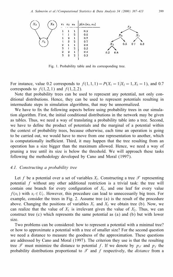
Example 3. Fig. 1 displays a network with variables X1; X2 and X3, each of themtaking two possible values, Xi = 1 or Xi = 2; i = 1; 2; 3. The table represents theconditional distribution P(X1|X2; X3). It can be seen that X1 and X3 are independentgiven context X2 = 2. This independence is re ected in the tree in the �gure: itcontains the same information as the table, but using �ve values instead of eight.The tree in Fig. 1 represents potential f(x1; x2; x3) = P(X1 = x1|X2 = x2; X3 = x3).


Fig. 1. Probability table and its corresponding tree.

For instance, value 0:2 corresponds to f(1; 1; 1) = P(X1 = 1|X2 = 1; X3 = 1), and 0:7corresponds to f(1; 2; 1) and f(1; 2; 2).Note that probability trees can be used to represent any potential, not only con-

ditional distributions. Hence, they can be used to represent potentials resulting inintermediate steps in simulation algorithms, that may be unnormalized.We have to �x the following aspects before using probability trees in our simula-

tion algorithm. First, the initial conditional distributions in the network may be givenas tables. Thus, we need a way of translating a probability table into a tree. Second,we have to de�ne the product of potentials and the marginal of a potential withinthe context of probability trees, because otherwise, each time an operation is goingto be carried out, we would have to move from one representation to another, whichis computationally ine�cient. Third, it may happen that the tree resulting from anoperation has a size bigger than the maximum allowed. Hence, we need a way ofpruning a tree until its size is below the threshold. We will approach these tasksfollowing the methodology developed by Cano and Moral (1997).

4.1. Constructing a probability tree

Let f be a potential over a set of variables XI . Constructing a tree T representingpotential f without any other additional restriction is a trivial task: the tree willcontain one branch for every con�guration of XI , and one leaf for every valuef(xI) with xI ∈UI . However, this procedure can lead to unnecessarily big trees. Forexample, consider the trees in Fig. 2. Assume tree (a) is the result of the procedureabove. Changing the positions of variables X1 and X2 we obtain tree (b). Now, wecan realize that the value of X1 is irrelevant given the value of X2. Thus, we canconstruct tree (c) which represents the same potential as (a) and (b) but with lowersize.Two problems can be considered: how to represent a potential with a minimal tree?

or how to approximate a potential with a tree of smaller size? For the second questionwe need a distance to measure the goodness of the approximation. These questionsare addressed by Cano and Moral (1997). The criterion they use is that the resultingtree T must minimize the distance to potential f. If we denote by pT and pf theprobability distributions proportional to T and f respectively, the distance from a


Fig. 2. Three trees containing the same information.

tree T to a potential f is measured by Kullback–Leibler’s divergence (Kullbackand Leibler, 1951):

D(f;T) =−∑xI ∈UI

pf(xI) logpf(xI)pT(xI)

: (14)

For the approximation, there are two subproblems, what is the structure (shape ofthe tree and variables on inner nodes) of the representation? and which are the num-bers on the tree leaves? The most di�cult problem is the �rst one. Given the struc-ture, the numbers minimizing the distance can be easily calculated using thefollowing result (Cano and Moral, 1997): given a tree structure the optimal approxi-mation of f can be obtained by putting in every leaf corresponding to con�gurationXJ = xJ the average of the values f(yI) with y∈UN and yJ = xJ .The methodology proposed in Cano and Moral (1997) to build a minimal proba-

bility tree is based on methods for inducing classi�cation rules from examples. Oneof these methods is Quinlan’s ID3 algorithm (Quinlan, 1986), that builds a decisiontree from a set of examples. A decision tree represents a sequential procedure fordeciding the class membership of a given instance of the attributes of the problem.That is, the leaves of the decision tree give us the class for a given instance of theattributes. ID3 builds a decision tree in a greedy way, by choosing a good test at-tribute to re�ne the actual structure. To determine which attribute should be the testattribute for a leaf node of the tree, the algorithm applies an information-theoreticmeasure Gain(Ai) over all the possible attributes Ai. This information measure givesan idea of the gain of information by partitioning a leaf node in the tree with anattribute.In the case of probability trees, Cano and Moral (1997) use the same algorithm, but

the information measure is di�erent, because each leaf in a decision tree representsa class, while in a probability tree, each leaf represents a probability value. Then,we need a measure particularly adapted to probabilities.The process of constructing a tree can be seen as follows. Assume T is the tree

we are constructing. A construction step requires to decide which branch to expandand which variable to place in the new node. This selection must be done in such away that the distance to the potential is minimized. If a leaf node in T correspondsto a con�guration XJ = xJ , we denote by T(XJ = xJ ; Xk) the tree obtained from Tby expanding the leaf de�ned by XJ = x with variable Xk . At each moment, both


the branch and the variable are selected in order to minimize the distance to f,that is,

D(T(XJ = xJ ; Xk); f) = min{D(T(XJ ′ = xJ ′ ; Xk′); f)}; (15)

where XJ ′ = xJ ′ is a leaf of T and k ′ ∈ I − J ′. The following proposition shows away of computing that minimum.

Proposition 2 (Cano and Moral, 1997). The pair (XJ = xJ ; Xk) minimizing expres-sion (15) is that one maximizing the measure of information

I(XJ = xJ ; Xk |f) = SXJ=xJ · (log|Uk | − log SXJ=xJ − E[Xk |XJ = xJ ]); (16)

where

SXJ=xJ =∑z∈UNzJ=xJ

f(zI);

E[Xk |XJ = xJ ] =−∑yk ∈Uk

f↓k(yk |XJ = xJ ) logf↓k(yk |XJ = xJ );

f↓k(yk |XJ = xJ ) =∑z∈UNzJ=xJzk=yk

f(zI):

The value of information I(XJ = xJ ; Xk |f) measures the distance from a tree T toa potential f before and after expanding the branch XJ = xJ with variable Xk . Theproposition above means that we must select branches leading to con�gurations withhigh probability, and variables with small entropy.With this, a procedure to construct an exact tree is to select nodes maximizing

function I . The procedure would �nish when, for every branch XJ = xJ , the valuesof f are uniform, that is, f(yI) = f(y′

I) for all yI ; y′I ∈UI such that yJ = y′

J = x.That is, the idea is to include nodes until no new information is provided by addingnew nodes.For constructing an approximate tree, Cano and Moral (1997) propose di�erent

alternatives. One of the alternatives consists of adding nodes until an exact repre-sentation is obtained or a maximum number of nodes is reached.The other alternative is to construct the entire tree and prune it afterwards. If

T is such tree, a pruning consists of selecting a node such that all its childrenare leaves and replacing it and its children by one node containing the average ofthe values of the leaf nodes being removed. We have two ways of performing apruning.The �rst way of pruning is to remove nodes while the maximum size is exceeded.

The selection of a node will be determined by that pair (XJ = xJ ; Xk) minimizing themeasure I(XJ = xJ ; Xk |f), that is, the pair minimizing the increment of the distanceto potential f.


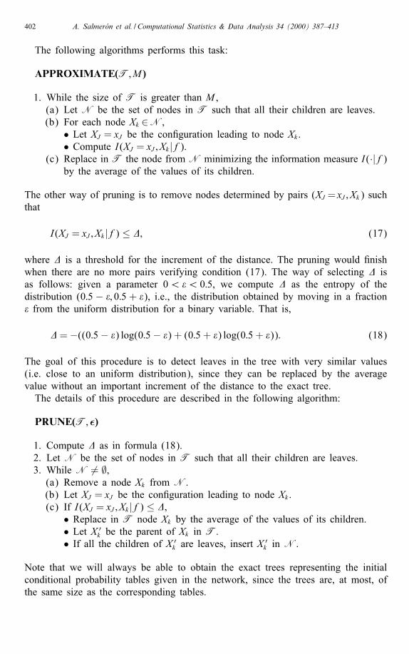
The following algorithms performs this task:

APPROXIMATE(T; M )

1. While the size of T is greater than M ,(a) Let N be the set of nodes in T such that all their children are leaves.(b) For each node Xk ∈N,

• Let XJ = xJ be the con�guration leading to node Xk .• Compute I(XJ = xJ ; Xk |f).

(c) Replace in T the node from N minimizing the information measure I(·|f)by the average of the values of its children.

The other way of pruning is to remove nodes determined by pairs (XJ = xJ ; Xk) suchthat

I(XJ = xJ ; Xk |f) ≤ �; (17)

where � is a threshold for the increment of the distance. The pruning would �nishwhen there are no more pairs verifying condition (17). The way of selecting � isas follows: given a parameter 0¡�¡ 0:5, we compute � as the entropy of thedistribution (0:5 − �; 0:5 + �), i.e., the distribution obtained by moving in a fraction� from the uniform distribution for a binary variable. That is,

�=−((0:5− �) log(0:5− �) + (0:5 + �) log(0:5 + �)): (18)

The goal of this procedure is to detect leaves in the tree with very similar values(i.e. close to an uniform distribution), since they can be replaced by the averagevalue without an important increment of the distance to the exact tree.The details of this procedure are described in the following algorithm:

PRUNE(T; �)

1. Compute � as in formula (18).2. Let N be the set of nodes in T such that all their children are leaves.3. While N 6= ∅,(a) Remove a node Xk from N.(b) Let XJ = xJ be the con�guration leading to node Xk .(c) If I(XJ = xJ ; Xk |f) ≤ �,

• Replace in T node Xk by the average of the values of its children.• Let X ′

k be the parent of Xk in T.• If all the children of X ′

k are leaves, insert X′k in N.

Note that we will always be able to obtain the exact trees representing the initialconditional probability tables given in the network, since the trees are, at most, ofthe same size as the corresponding tables.


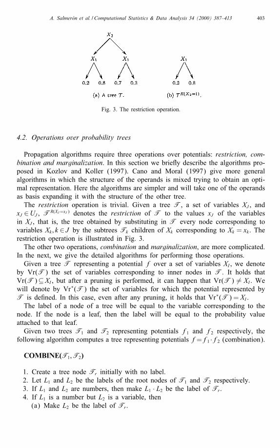
Fig. 3. The restriction operation.

4.2. Operations over probability trees

Propagation algorithms require three operations over potentials: restriction, com-bination and marginalization. In this section we brie y describe the algorithms pro-posed in Kozlov and Koller (1997). Cano and Moral (1997) give more generalalgorithms in which the structure of the operands is mixed trying to obtain an opti-mal representation. Here the algorithms are simpler and will take one of the operandsas basis expanding it with the structure of the other tree.The restriction operation is trivial. Given a tree T, a set of variables XJ , and

xJ ∈UJ , TR(XJ=xJ ) denotes the restriction of T to the values xJ of the variablesin XJ , that is, the tree obtained by substituting in T every node corresponding tovariables Xk; k ∈ J by the subtrees Tk children of Xk corresponding to Xk = xk . Therestriction operation is illustrated in Fig. 3.The other two operations, combination and marginalization, are more complicated.

In the next, we give the detailed algorithms for performing those operations.Given a tree T representing a potential f over a set of variables XI , we denote

by Vr(T) the set of variables corresponding to inner nodes in T. It holds thatVr(T)⊆XI , but after a pruning is performed, it can happen that Vr(T) 6= XI . Wewill denote by Vr∗(T) the set of variables for which the potential represented byT is de�ned. In this case, even after any pruning, it holds that Vr∗(T) = XI .The label of a node of a tree will be equal to the variable corresponding to the

node. If the node is a leaf, then the label will be equal to the probability valueattached to that leaf.Given two trees T1 and T2 representing potentials f1 and f2 respectively, the

following algorithm computes a tree representing potentials f=f1 ·f2 (combination).

COMBINE(T1;T2)

1. Create a tree node Tr initially with no label.2. Let L1 and L2 be the labels of the root nodes of T1 and T2 respectively.3. If L1 and L2 are numbers, then make L1 · L2 be the label of Tr .4. If L1 is a number but L2 is a variable, then(a) Make L2 be the label of Tr .


Fig. 4. Combination of two trees.

(b) For every tree T child of the root node of T2, make Th :=COMBINE(T1;T) be a child of Tr.

5. If L1 is a variable, assume that Xk is that variable.(a) Make Xk be the label of Tr.(b) For each xk ∈Uk ,

• Make Th:=COMBINE(TR(Xk=xk )1 ;TR(Xk=xk )

2 ) be a child of Tr.6. Return Tr.

We will denote the combination of trees by symbol ⊗. With this notation, the algo-rithm above returns a tree Tr =T1 ⊗T2.The combination process is illustrated in Fig. 4.Given a tree T representing a potential f de�ned over a set of variables XI , the

following algorithm computes a tree representing potential f↓(I−{i}), with i∈ I . Thatis, it removes variable Xi form T.

MARGINALIZE(T; Xi)

1. Let L be the label of the root node of T.2. If L is a number, create a node Tr with label L · |Ui|.3. Otherwise, let Xk be the variable corresponding to label L.(a) If Xk = Xi, then

i. Let T1; : : : ;Ts be the children of the root node of T.ii. Tr :=T1.iii. For i := 2 to s, Tr :=ADD(Tr, Ti).


Fig. 5. Addition of two trees.

(b) Otherwise,i. Create a node Tr with label Xk .ii. For each xk ∈UkA. Make Th :=MARGINALIZE(TR(Xk=xk ); Xi) be the next child of Tr.

4. Return Tr.

This algorithm uses procedure ADD(T1;T2), which computes the addition of T1

and T2. The procedure is as follows:

ADD(T1,T2)

1. Create a tree node Tr initially with no label.2. Let L1 and L2 be the labels of the root nodes of T1 and T2 respectively.3. If L1 and L2 are numbers, then make L1 + L2 be the label of Tr .4. If L1 is a number but L2 is a variable, then(a) Make L2 be the label of Tr .(b) For every child T of the root node of T2, make Th :=ADD(T1, T) be

a child of Tr.5. If L1 is a variable, assume that Xk is that variable.(a) Make Xk be the label of Tr.(b) For each xk ∈Uk ,

• Make Th :=ADD(TR(Xk=xk )1 ;TR(Xk=xk )

2 ) be a child of Tr .6. Return Tr.

The addition of two trees is illustrated in Fig. 5, where symbol ⊕ represents theaddition operation.


5. Importance sampling using probability trees

In this section we describe an importance sampling algorithm in which the po-tentials are represented by probability trees and the approximation is performed bypruning the tree.Assume we are carrying out a deletion algorithm and potentials are represented

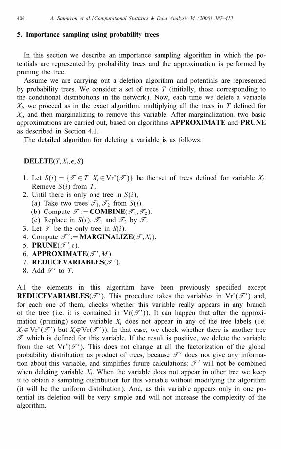
by probability trees. We consider a set of trees T (initially, those corresponding tothe conditional distributions in the network). Now, each time we delete a variableXi, we proceed as in the exact algorithm, multiplying all the trees in T de�ned forXi, and then marginalizing to remove this variable. After marginalization, two basicapproximations are carried out, based on algorithms APPROXIMATE and PRUNEas described in Section 4.1.The detailed algorithm for deleting a variable is as follows:

DELETE(T; Xi; �; S)

1. Let S(i) = {T∈T |Xi ∈Vr∗(T)} be the set of trees de�ned for variable Xi.Remove S(i) from T .

2. Until there is only one tree in S(i),(a) Take two trees T1;T2 from S(i).(b) Compute T :=COMBINE(T1;T2).(c) Replace in S(i), T1 and T2 by T.

3. Let T be the only tree in S(i).4. Compute T′ :=MARGINALIZE(T; Xi).5. PRUNE(T′; �).6. APPROXIMATE(T′; M).7. REDUCEVARIABLES(T′).8. Add T′ to T .

All the elements in this algorithm have been previously speci�ed exceptREDUCEVARIABLES(T′). This procedure takes the variables in Vr∗(T′) and,for each one of them, checks whether this variable really appears in any branchof the tree (i.e. it is contained in Vr(T′)). It can happen that after the approxi-mation (pruning) some variable Xi does not appear in any of the tree labels (i.e.Xi ∈Vr∗(T′) but Xi 6∈Vr(T′)). In that case, we check whether there is another treeT which is de�ned for this variable. If the result is positive, we delete the variablefrom the set Vr∗(T′). This does not change at all the factorization of the globalprobability distribution as product of trees, because T′ does not give any informa-tion about this variable, and simpli�es future calculations: T′ will not be combinedwhen deleting variable Xi. When the variable does not appear in other tree we keepit to obtain a sampling distribution for this variable without modifying the algorithm(it will be the uniform distribution). And, as this variable appears only in one po-tential its deletion will be very simple and will not increase the complexity of thealgorithm.


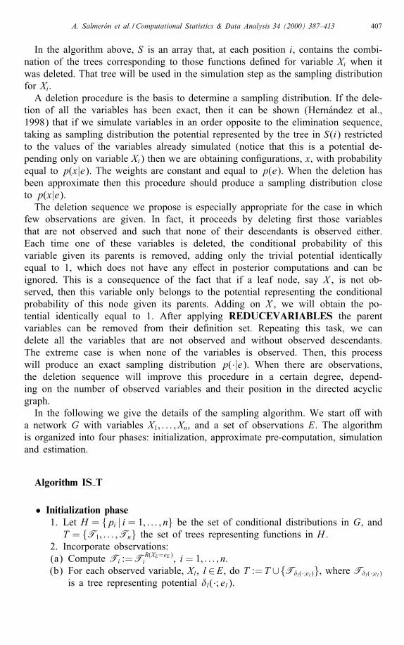
In the algorithm above, S is an array that, at each position i, contains the combi-nation of the trees corresponding to those functions de�ned for variable Xi when itwas deleted. That tree will be used in the simulation step as the sampling distributionfor Xi.A deletion procedure is the basis to determine a sampling distribution. If the dele-

tion of all the variables has been exact, then it can be shown (Hern�andez et al.,1998) that if we simulate variables in an order opposite to the elimination sequence,taking as sampling distribution the potential represented by the tree in S(i) restrictedto the values of the variables already simulated (notice that this is a potential de-pending only on variable Xi) then we are obtaining con�gurations, x, with probabilityequal to p(x|e). The weights are constant and equal to p(e). When the deletion hasbeen approximate then this procedure should produce a sampling distribution closeto p(x|e).The deletion sequence we propose is especially appropriate for the case in which

few observations are given. In fact, it proceeds by deleting �rst those variablesthat are not observed and such that none of their descendants is observed either.Each time one of these variables is deleted, the conditional probability of thisvariable given its parents is removed, adding only the trivial potential identicallyequal to 1, which does not have any e�ect in posterior computations and can beignored. This is a consequence of the fact that if a leaf node, say X , is not ob-served, then this variable only belongs to the potential representing the conditionalprobability of this node given its parents. Adding on X , we will obtain the po-tential identically equal to 1. After applying REDUCEVARIABLES the parentvariables can be removed from their de�nition set. Repeating this task, we candelete all the variables that are not observed and without observed descendants.The extreme case is when none of the variables is observed. Then, this processwill produce an exact sampling distribution p(·|e). When there are observations,the deletion sequence will improve this procedure in a certain degree, depend-ing on the number of observed variables and their position in the directed acyclicgraph.In the following we give the details of the sampling algorithm. We start o� with

a network G with variables X1; : : : ; Xn, and a set of observations E. The algorithmis organized into four phases: initialization, approximate pre-computation, simulationand estimation.

Algorithm IS T

• Initialization phase1. Let H = {pi | i = 1; : : : ; n} be the set of conditional distributions in G, andT = {T1; : : : ;Tn} the set of trees representing functions in H .

2. Incorporate observations:(a) Compute Ti :=TR(XE=eE)

i , i = 1; : : : ; n.(b) For each observed variable, Xl, l∈E, do T :=T ∪{T�l(·;el)}, where T�l(·;el)

is a tree representing potential �l(·; el).


• Collect phase (approximate pre-computation)3. Select an order � of variables in G, as described in Section 3.1.4. For i := 1 to n, DELETE(T; X�(i); �; S).

• Simulation phase5. For j := 1 to m (sample size),(a) wj := 1:0.(b) For i := n to 1,

(i) Simulate a value for X�(i), x( j)i , using p∗

i as sampling distribution, wherep∗i is the normalized potential corresponding to the tree Ti de�nedover variable X�(i) and obtained as Ti =TR(X�(i)=x0), where T is thetree stored in S(i), with �(i) = {�(i+1); : : : ; �(n)}, and x0 the currentcon�guration of variables already simulated (X�(i)).

(ii) Compute wj :=wj=p∗i (x

( j)i ).

(c) Compute

wj :=wj

(n∏i=1

pi(x(j)i |x(j)F(i))

)·(∏l∈ E

�l(x(j)l ; el)

):

• Estimation phase6. For each x′k ∈Uk , k ∈N − E,(a) Estimate p(x′k ; e) using formula (7).

7. Normalize values p(x′k ; e) to obtain p(x′k |e).

6. Experimental tests

Some experiments have been carried out to test the performance of the pro-posed algorithm. The experiments consisted of several propagations over a largenetwork, comparing the performance of four algorithms: likelihood weighting (Fungand Chang, 1990; Shachter and Peot, 1990), bounded variance algorithm (Dagumand Luby, 1997), importance sampling using probability tables (referenced as IS)as described in Hern�andez et al. (1998), and importance sampling using probabilitytrees (referenced as IS T).The network used is a subset of a pedigree one (Jensen et al., 1995), composed

by 441 variables. Each node has two parents (but the roots) and a maximum of 43children, and has three cases. The biggest initial conditional probability table has 27values, since each variable has three possible values. We have considered two typesof inferences over this network: in one case we have not considered observationsand in the other we have considered 166 observations.The reason to use this well-known kind of network in the experiments, is that

traditional simulation procedures fail to provide good estimations of the posteriorprobabilities. Extreme cases are the likelihood weighting method and the boundedvariance method: these methods do not even get any result, since all the con�gura-tions in the sample get a zero weight. This network has two features which maketraditional methods fall into troubles. In one hand, the presence of probabilities veryclose to zero due to the evidence, and, on the other hand, the high connectivity of


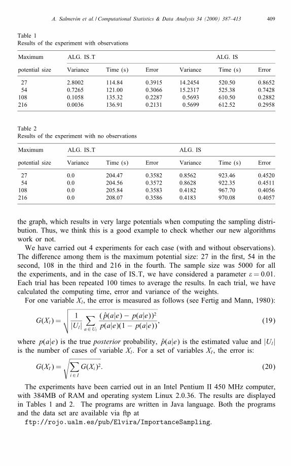
Table 1Results of the experiment with observations

Maximum ALG. IS T ALG. IS

potential size Variance Time (s) Error Variance Time (s) Error

27 2.8002 114.84 0.3915 14.2454 520.50 0.865254 0.7265 121.00 0.3066 15.2317 525.38 0.7428108 0.1058 135.32 0.2287 0.5693 610.50 0.2882216 0.0036 136.91 0.2131 0.5699 612.52 0.2958

Table 2Results of the experiment with no observations

Maximum ALG. IS T ALG. IS

potential size Variance Time (s) Error Variance Time (s) Error

27 0.0 204.47 0.3582 0.8562 923.46 0.452054 0.0 204.56 0.3572 0.8628 922.35 0.4511108 0.0 205.84 0.3583 0.4182 967.70 0.4056216 0.0 208.07 0.3586 0.4183 970.08 0.4057

the graph, which results in very large potentials when computing the sampling distri-bution. Thus, we think this is a good example to check whether our new algorithmswork or not.We have carried out 4 experiments for each case (with and without observations).

The di�erence among them is the maximum potential size: 27 in the �rst, 54 in thesecond, 108 in the third and 216 in the fourth. The sample size was 5000 for allthe experiments, and in the case of IS T, we have considered a parameter �= 0:01.Each trial has been repeated 100 times to average the results. In each trial, we havecalculated the computing time, error and variance of the weights.For one variable Xl, the error is measured as follows (see Fertig and Mann, 1980):

G(Xl) =

√√√√ 1|Ul|

∑a∈Ul

(p(a|e)− p(a|e))2p(a|e)(1− p(a|e)) ; (19)

where p(a|e) is the true posterior probability, p(a|e) is the estimated value and |Ul|is the number of cases of variable Xl. For a set of variables XI , the error is:

G(XI) =√∑

i∈ IG(Xi)2: (20)

The experiments have been carried out in an Intel Pentium II 450 MHz computer,with 384MB of RAM and operating system Linux 2.0.36. The results are displayedin Tables 1 and 2. The programs are written in Java language. Both the programsand the data set are available via ftp atftp://rojo.ualm.es/pub/Elvira/ImportanceSampling.


With regard to the obtained results, the following can be said:• Without observations our algorithm is really fast and optimal (the variance of theweights is equal to 0). The pre-computation is very fast: the deletion procedurewill select variables from leaves backward (variables belonging to only one po-tential). When deleting a variable, we sum in the conditional probability of thisvariable and then we obtain a potential equal to 1 in every case. In this wayan exact sampling distribution is obtained in a very short time. The simulationassociated to this exact sampling distributions is equivalent to the one carried outby the likelihood weighting and bounded variance algorithms, sharing all theiradvantages for the case of no observations.It is important to remark that in Jensen et al. (1995) the results of blocking Gibbssampling are reported for the case of no observations and this algorithm has aclearly superior behaviour in this case.

• In both cases, tables are much slower than probability trees and the results areworse. Specially in the case of no observations, the di�erences on time are verysigni�cative: tables do not have a procedure to approximate computations in sucha exible way as trees do.

• The IS T algorithm has a good behaviour even with very small trees (of size27). In practice, we will usually a�ord bigger trees, but we wanted to test thealgorithm in really hard conditions.

7. Conclusions

In this paper we have proposed an approximate propagation method able to dealwith large networks. In such networks, it is shown that using probability trees insteadof tables provides bene�ts, since trees allow to represent more e�ciently the mostimportant regions of a probability distribution, what leads to an improvement ofimportance sampling, as can be deduced from the experimental results.There were methods able to deal with very large networks, like blocking Gibbs

sampling, due to Jensen et al. (1995). However, there are cases in which ouralgorithm is superior to blocking Gibbs sampling, as in the experiment without obser-vations. Situations in which blocking Gibbs behaves better than IS T algorithm canexist, though we do not know them. But, in general, we think that it will be impos-sible to have a single algorithm better than all the other in every situation. The im-portance sampling based on approximate pre-computation provides a new paradigmto solve large problems, enlarging the set of cases that can be approximated andallowing future improvements. An example of a situation which can be solved withthis new algorithm arises in problems of Information Retrieval. Campos et al. (1998)provide a model for retrieving information in which they learn a polytree with therelationships between terms or keywords of a collection of documents. They usedit as a thesaurus, to expand queries adding new terms to them. Computation waseasy because of the polytree structure. Experiments showed that expanded queriesimproved the recuperation of documents using standard procedures (Smart). In thepaper, they propose to expand the terms graph with the document variables, creating


structures representing the relationships among them, in such a way that the com-plete graph could be used as a document recuperation system, by calculating themarginal probability of each document given the terms. The documents should beadded to the original network putting them as children of term variables. Our algo-rithm is specially appropriate for this task: documents are not observed and do nothave observed descendents; then it is possible to delete these variables following thedeletion procedure as was explained earlier for a network without observations. Allthe conditional probabilities are approximated by the constantly equal to 1 potential,which can be deleted afterwards. When we �nish deleting document variables, wehave an hypertree in which an exact deletion can be carried out in linear time. Thisfast procedure calculates exact sampling distributions and the quality of the sampleof our procedure will be optimal (all the weights are equal). This allows to solveclassical information retrieval problems with more than 10.000 variables. It is not atall clear how blocking Gibbs sampling would handle this kind of problems.An important point to remark is that some kind of pre-computation is always

necessary to solve large network problems by simulation, allowing to use as much aspossible information stored in other parts of the network when simulating a concretevariable. If we only use local information, we are sure to obtain a poor behaviourwhen con icting information is stored in di�erent parts of the graph. In the caseof Gibbs sampling algorithms, this is avoided by simulating values compatible withprevious instantiations of the variables in the graph. Our procedure presents a directway of doing it.One important feature of trees is their exibility, what makes the algorithm pro-

posed susceptible of being improved, for instance, using entropy criteria to selectthe trees that must be combined. The possibility of approximating uniform regionsin a distribution by an average value to free space for storing more of the mostinformative values, allow many modi�cations to the algorithm that were not possiblebefore.Other future alternative is to use di�erent samples to estimate each one of the

necessary joint probabilities p(x′k ; e) and p(e) as in Dagum and Luby (1997). Ifwe are interested in only a few conditional probabilities this may improve the �nalresults without an increasing of the computations, but experimental evaluations wouldbe necessary.About the future directions of research we want to point out the possibility of

improving the initial approximations by several iterations of the approximate stage.It has been shown in Kozlov and Koller (1997) that tree approximations can improveif we take into account information about all the potentials each time we calculatea tree approximation. This gives rise to an iterative propagation algorithm whichcan be organized in a join tree and such that the approximations in one part of thetree are improved by better approximations in another part. This methodology canimprove our initial approximations based only in a deletion procedure.Another interesting possibility of this algorithm is the determination of bad approx-

imate steps. If when we simulate a variable the normalization factor of the combinedtree is 0, then the �nal weight is 0, and this con�guration is �nally discarded. Theonly way in which this may happen is due to a previous approximate deletion of the


variable. If this zero normalization value is repeated very often for a given variable,then we can invest more e�ort (some additional computing time) in the approximatedeletion of this variable, trying to improve the quality of the approximation so that 0weights are avoided in the future. The same procedure can be applied to very smallvalues.

Acknowledgements

We want to thank Claus Skaaning Jensen for providing the network used in theexperiment.We are also very grateful to the anonymous referees for their valuable comments

and suggestions.

References

Boutilier, J., Friedman, N., Goldszmidt, M., Koller, D., 1996. Context-speci�c independence in Bayesiannetworks. In: Horvitz, E., Jensen, F. (Eds.) Proceedings of the 12th Conference on Uncertainty inArti�cial Intelligence. Morgan & Kau�man, San Francisco, CA, pp. 115–123.

Campos, L.M., de Fern�andez, J.M., Huete, J., 1998. Query expansion using Bayesian networks. In:Cooper, G.F., Moral, S. (Eds.) Proceedings of the 14th Conference on Uncertainty in Arti�cialIntelligence. Morgan & Kau�man, San Francisco, CA, pp. 53–60.

Cano, A., Moral, S., 1995. Heuristic algorithms for the triangulation of graphs. In: Bouchon-Meunier,B., Yager, R., Zadeh, L. (Eds.) Advances in Intelligent Computing. Springer, Berlin, pp. 98–107.

Cano, A., Moral, S., 1997. Propagaci�on exacta y aproximada con �arboles de probabilidad. In: Actasde la VII Conferencia de la Asociaci�on Espanola para la Inteligencia Arti�cial, pp. 635–644.

Cano, J., Hern�andez, L., Moral, S., 1996. Importance sampling algorithms for the propagation ofprobabilities in belief networks. Int. J. Approx. Reasoning 15, 77–92.

Cooper, G., 1990. The computational complexity of probabilistic inference using Bayesian beliefnetworks. Artif. Intell. 42, 393–405.

Dagum, P., Luby, M., 1993. Approximating probabilistic inference in Bayesian belief networks isNP-hard. Artif. Intell. 60, 141–153.

Dagum, P., Luby, M., 1997. An optimal approximation algorithm for Bayesian inference. Artif. Intell.93, 1–27.

Dechter, R., Rish, I., 1994. Directional resolution: The Davis–Putnam procedure, revisited. In: Doyle, J.,Sandewall, E., Torasso, P. (Eds.) Principles of Knowledge Representation and Reasoning (KR-94),pp. 134–145.

Dechter, R., Rish, I., 1997. A scheme for approximating probabilistic inference. In: Geiger, D., Shenoy,P. (Eds.) Proceedings of the 13th Conference on Uncertainty in Arti�cial Intelligence. Morgan &Kau�man, San Francisco, CA, pp. 132–141.

Fertig, K., Mann, N., 1980. An accurate approximation to the sampling distribution of the studentizedextreme-valued statistic. Technometrics 22, 83–90.

Fung, R., Chang, K., 1990. Weighting and integrating evidence for stochastic simulation in Bayesiannetworks. In: Henrion, M., Shachter, R., Kanal, L., Lemmer, J. (Eds.) Uncertainty in Arti�cialIntelligence, vol. 5. North-Holland, Amsterdam, pp. 209–220.

Fung, R., Favero, B.D., 1994. Backward simulation in Bayesian networks. In: de M�antaras, R.L., Poole,D. (Eds.) Proceedings of the 10th Conference on Uncertainty in Arti�cial Intelligence. Morgan &Kau�man, San Mateo, CA, pp. 227–234.

Geweke, J., 1989. Bayesian inference in econometric models using Monte Carlo integration.Econometrica 57, 1317–1339.


Henrion, M., 1988. Propagating uncertainty by logic sampling in Bayes’ networks. In: Lemmer,J., Kanal, L. (Eds.) Uncertainty in Arti�cial Intelligence, vol. 2. North-Holland, Amsterdam, pp.317–324.

Hern�andez, L., Moral, S., Salmer�on, A., 1996. Importance sampling algorithms for belief networksbased on approximate computation. Proceedings of the Sixth International Conference IPMU’96,vol. 2, Granada, Spain, pp. 859–864.

Hern�andez, L., Moral, S., Salmer�on, A., 1998. A Monte Carlo algorithm for probabilistic propagationin belief networks based on importance sampling and strati�ed simulation techniques. Internat.J. Approximate Reasoning 18, 53–91.

Jensen, C., Kong, A., Kj�rul�, U., 1995. Blocking gibbs sampling in very large probabilistic expertsystems. Internat. J. Human–Computer Studies 42, 647–666.

Jensen, F., 1996. An Introduction to Bayesian Networks. UCL Press, London.Kj�rul�, U., 1992. Optimal decomposition of probabilistic networks by simulated annealing. Statist.Comput. 2, 1–21.

Kozlov, D., Koller, D., 1997. Nonuniform dynamic discretization in hybrid networks. In: Geiger, D.,Shenoy, P. (Eds.) Proceedings of the 13th Conference on Uncertainty in Arti�cial Intelligence.Morgan & Kau�man, San Francisco, CA, pp. 302–313.

Kullback, S., Leibler, R., 1951. On information and su�ciency. Ann. Math. Statist. 22, 76–86.Lauritzen, S., Spiegelhalter, D., 1988. Local computations with probabilities on graphical structures andtheir application to expert systems. J. Roy. Statist. Soc. Ser. B 50, 157–224.

Pearl, J., 1987. Evidential reasoning using stochastic simulation of causal models. Artif. Intell. 32,247–257.

Pearl, J., 1988. Probabilistic Reasoning in Intelligent Systems. Morgan-Kau�man, San Mateo, CA.Poole, D., 1997a. Exploiting contextual independence and approximation in belief network inference.Technical Report, University of British Columbia.

Poole, D., 1997b. Probabilistic partial evaluation: exploiting rule structure in probabilistic inference.In: Proceedings of the 15th International Joint Conference on AI (IJCAI-97), pp. 1284–1291.

Quinlan, J., 1986. Induction of decision trees. Machine Learning 1, 81–106.Rubinstein, R., 1981. Simulation and the Monte Carlo Method. Wiley, New York.Shachter, R., Peot, M., 1990. Simulation approaches to general probabilistic inference on beliefnetworks. In: Henrion, M., Shachter, R., Kanal, L., Lemmer, J. (Eds.) Uncertainty in Arti�cialIntelligence, vol. 5. North-Holland, Amsterdam, pp. 221–231.

Zhang, N., Poole, D., 1996. Exploiting causal independence in Bayesian network inference. J. Artif.Intell. Res. 5, 301–328.

Documents

Importance sampling in Bayesian networks using probability trees