Implementing Local Intervals in CASL

Regivan H. N. Santiago, Anamaria M. Moreira 1

Departamento de Informatica e Matematica AplicadaUniversidade Federal do Rio Grande do Norte

Natal, Rio Grande do Norte, Brazil

Katiane R. Lopes2

Instituto Tocantinense Presidente Antonio CarlosAraguaına, Tocantins, Brazil

Abstract

This paper defines the basis for the implementation in CASL (Common Algebraic Specification Language) ofan interval library such that intervals behave as real numbers endowed with an error information. To achievethat, we redefine the notion of interval local set defined in [15] in such a way that it can be implemented inthe underlying logic of CASL. With these results, it is possible to manipulate intervals in CASL, as if theywere real numbers, with equational reasoning, and get an error estimation on the obtained results for free(from the width of the resulting interval). The paper describes the CASL definition of the interval libraryand presents a case study on a simple example requiring handling data with “tolerance” margin.

Keywords: Algebraic Specification Languages, Specification of Real numbers, Interval Arithmetics.

1 Introduction

The rigorous specification and development of systems where (continuous) numerical

data is manipulated is still an open problem, although some approaches to solve

it have already been proposed. Some of them include in the formal specification

language a version of the real numbers [13] and others, rational numbers [2]. Such

systems work with approximations and error information, and the chosen solution is

implemented through the use of libraries of data types and functions which specify

this data. The advantage of these approaches lies in the algebraic laws which are

the same as those for real (or rational) numbers. Therefore, it is enough to endow

any algebraic specification language with these libraries and apply equational logic

procedures to verify the system. However, these solutions lack the power to deal

1 Email: regivan,anamaria@dimap.ufrn.br2 Email: katianelopes@hotmail.com

Electronic Notes in Theoretical Computer Science 184 (2007) 133–149

1571-0661/$ – see front matter © 2007 Elsevier B.V. All rights reserved.

www.elsevier.com/locate/entcs

doi:10.1016/j.entcs.2007.03.019

with situations where the system computes with numbers which are essentially non-

representable (by rationals) — e.g. a simple system which calculates the circle area

S = π · r2, or systems where tolerance information is required. Furthermore, in

many cases, the treatment of error information is left to the implementation phase

and problems arise when specifiers or designers refine such specifications, since error

must be dealt with. Another approach, the one we tackle here, is to use an interval

representation for real numbers. This approach has the advantage of being able to

represent any real number and error information from the beginning, i.e., from the

specification. However, the price is the complete loss of theorems which are valid for

real number data, since (non-degenerate) intervals do not satisfy some important

algebraic properties of the real numbers.

In what follows we give a solution for this problem: intervals are seen as real

numbers with an error information and not just a set of real numbers. This means

that a real number (e.g. π) can be represented by any interval containing it (e.g.

[3, 4]). For that, there are two approaches: (1) interval arithmetic is changed to

behave as nearly as possible as real arithmetic [6]; or (2) we change the notion of

equality and the laws of algebra for intervals [14]. In this second approach, we

define an auxiliary equality called interval local equality to deal with intervals to

enable the verification of equational (only) properties. This work extends the ones

in [14,15], as it is now directly implementable in an algebraic specification language

(CASL), and rules for executing a limited local-equational reasoning with intervals

have been provided.

Then, we would like to apply these results to a formal specification language,

so that they can actually be used in a software development process. CASL [2] is

an algebraic specification language, already well known in academia, which presents

some characteristics that are essential to this work. Particularly, its strong and exis-

tential equalities, implementing respectively Scott’s simple equality and equivalence

[20], provide the necessary basis for a complete implementation of our approach.

The library of intervals is then built upon the basic rational library of CASL and

can be found in [5].

This work is then divided into the following sections: Section 2 introduces in-

terval arithmetic and shows that it does not constitute a field like real numbers;

Section 3 shows that intervals can be seen as information on real numbers and re-

lates consistency and equality; Section 4 introduces the theory of Scott’s simple

equality and Ω-sets, relating these concepts with CASL; Section 5 defines the the-

ory of local equality and local sets; Section 6 defines a boolean interval local set

which is implemented in CASL; Section 7 introduces some required axioms for the

specification and prove their soundness; Section 8 shows part of the specification

and puts the axioms to work; Section 9 provides a sample application and, finally,

Section 10 contains some final remarks.

R.H.N. Santiago et al. / Electronic Notes in Theoretical Computer Science 184 (2007) 133–149134

2 Interval Arithmetic

The idea of interval arithmetic was introduced by Moore [7,8] around the fifties, and

we call it here Moore arithmetic. Some other arithmetic proposals arose along

the time, but all of them work with the idea of correctness which is based on the

following implication

x ∈ [a, b] ⇒ f(x) ∈ F ([a, b])(1)

where x, f(x) ∈ , [a, b] is an interval, f is a real arithmetical function and F is

an interval arithmetic representation of f 3 . This idea of correctness states that, if

you compute with intervals, the desired result is always inside the obtained interval

result. Moreover, the maximum error is the width of this result interval. In other

words, if you use intervals to represent and compute real numbers the resulting error

is always described in the result interval F ([a, b]). From the specification viewpoint,

if you describe a system with intervals instead of punctual representations (e.g.

rational representations) the verification of any equational properties leads to an

immediate estimate of the involved error. In what follows we briefly introduce

Moore arithmetic.

2.1 Moore arithmetic

Moore interval arithmetic is based on the definition of intervals as given in Definition

2.1 and in interval equality as defined in Definition 2.2.

Definition 2.1 Given x1, x2 ∈ such that x1 ≤ x2, the set {x ∈ : x1 ≤ x ≤ x2}is called closed interval or here just interval and is denoted by X = [x1, x2].

Intervals of the form [x, x] are degenerate, where [x, x] is the interval counterpart

of a real number x ∈ . The set of all intervals is denoted by ( ). If x1 and x2

are restricted to rational numbers, , then, we define the set of all intervals with

rational endpoints, and denote it by ( ).

Although the theory presented here was first defined for ( ), ( ) is partic-

ularly important for this work because it can be “implemented” in an algebraic

specification language, and it inherits all the presented results.

Definition 2.2 [interval equality]

Equality on intervals is based on their set nature; i.e. two intervals are considered

indiscernibles if they are the same set. Therefore given A = [a1, a2] and B =

[b1, b2]

A = B ⇔ a1 = b1 ∧ a2 = b2(2)

Given A,B ∈ ( ), the operations of sum, subtraction, multiplication and divi-

sion are defined in Table 1, and obey the following property:

A ∗ B = {a ∗ b : a ∈ A ∧ b ∈ B}(3)

3 A full formalization of interval correctness and optimality can be found in [17,18,19].

R.H.N. Santiago et al. / Electronic Notes in Theoretical Computer Science 184 (2007) 133–149 135

Operation Definition OBS

A + B = [a1 + b1, a2 + b2]

A × B = [minK,maxK] K = {a1 × b1, a1 × b2, a2 × b1, a2 × b2}−A = [−a2,−a1]1

A= [

1

a2,

1

a1] 0 �∈ A

A − B = A + (−B)

A/B = A × ( 1B

) 0 �∈ B

Table 1Moore arithmetic for A = [a1, a2], B = [b1, b2] ∈ ( )

where ∗ ∈ {+,−,×, /} is one of the four arithmetical operations. Note that (3)

trivially satisfies the correctness property described above in (1) . For division,

Moore arithmetic establishes that 0 /∈ B. With those definitions, interval arithmetic

is defined by the application of real arithmetic to the endpoints of intervals, and is

trivially computational in the case of rational endpoints.

Example 2.3 [3, 4] + [1, 3] = [3 + 1, 4 + 3] = [4, 7], −[3, 4] = [−4,−3], etc.

2.2 Algebraic properties of Moore arithmetic

In Moore interval arithmetic we have that addition and multiplication are associative

and commutative and have an identity element, which is [0, 0] for addition and

[1, 1] for multiplication. However neither addition nor multiplication have inverse

operations. Indeed, A + (−A) �= [0, 0], for non-degenerate intervals. Instead, they

have pseudo-inverse operations where X − X ⊇ [0, 0] and X/X ⊇ [1, 1]. Finally,

the distribution of multiplication over addition is replaced by sub-distributivity:

A × (B + C) ⊆ A × B + A × C. This weakening of algebraic properties presents

serious consequences to our goal of real number representation, as shows Example

2.4.

Example 2.4 Suppose you would like to solve the equation X +[3, 4] = [1, 2]. Ap-

plying equational logic, you would derive at most X +[−1, 1] = [−3,−1] (according

to Moore Arithmetic) instead of X = [1, 2]− [3, 4] or X = [−3,−1]. In this example,

subtracting [3, 4] from both sides of the equation should have given us on the left

hand side X +[0, 0] which in turn would lead to X, by the fact that [0, 0] is identity

for +, but we only got [−1, 1] ⊇ [0, 0], because of the pseudo-inverse property. In

this paper we show a way to overcome this problem.

3 Moore Intervals as information on real numbers

The problems shown above come from the nature of the used equality for intervals,

where two intervals are considered equal if they are the same set. This section

R.H.N. Santiago et al. / Electronic Notes in Theoretical Computer Science 184 (2007) 133–149136

introduces another viewpoint, which allows the definition of a weaker notion of

interval equality, where two intervals are considered equal if they may represent some

common set of real numbers. This approach deals with intervals simultaneously as

an information on a real number and on the corresponding error. Within this

approach, the smaller the width of an interval, the better the information of the

represented real numbers, and the better the quality of the corresponding error.

The inclusion monotonicity property of Moore arithmetic [9], described bellow, is

the basis of this approach.

Inclusion monotonicity is a very important property of this arithmetic, since it

states that it preserves the quality of error; e.g. if A ⊆ C and B ⊆ D, i.e. if the

quality of error present in A is better than that of C and the same for B and D,

then A + B ⊆ C + D, i.e., the error of A + B is better than that of C + D.

This property of Moore arithmetic gives rise to the domain approach of interval

analysis [1,14]. In what follows we cite some of the definitions and propositions

which establish that.

Definition 3.1 Given A,B ∈ ( ), A � B if and only if B ⊆ A. Where A � B is

read “A is an information about B”.

Proposition 3.2 The partial order 〈 ( ),�〉 is a directed complete partial order

(dcpo) — see [14] —.

Therefore, considering degenerate intervals [a, a] as real numbers, this approach

considers the set ( ) as an information space, in the sense of Scott-Strachey [21],

on real numbers. There are many interesting consequences of that. One of them

is that this approach gives a foundation to usual interval algorithms in terms of

domain theory. Another consequence is that it extends the viewpoint of interval

from set to information, and this last viewpoint is where we start our approach.

3.1 Consistency and equality

One of the concepts in domain theory is that of consistency, formally:

Definition 3.3 Given a partial order 〈A,≤〉 and x, y ∈ A, x is consistent with y,

x � y, if there is z ∈ A such that x ≤ z and y ≤ z.

In other words, x and y are consistent information if they inform about the same

thing. In the case of intervals A,B ∈ ( ), A � B if and only if A∩B ∈ ( ). Table 2

establishes the relation between interval equality and consistency. You should note

that, although some algebraic properties of real numbers fail for intervals, they are

preserved in terms of consistency. Therefore, even if classical equational logic cannot

be applied to make intervals behave as real numbers with an error information, we

can develop a kind of equational logic for consistency which enables us to do that.

This logic and its application to CASL is what we present in this work.

R.H.N. Santiago et al. / Electronic Notes in Theoretical Computer Science 184 (2007) 133–149 137

Equality Consistency

x + (y + z) = (x + y) + z x + (y + z) � (x + y) + z

x + [0, 0] = x x + [0, 0] � x

x + y = y + x x + y � y + x

x − x ⊇ [0, 0] x − x � [0, 0]

x × (y × z) = (x × y) × z x × (y × z) � (x × y) × z

x × [1, 1] = x x × [1, 1] � x

x × y = y × x x × y � y × x

x/x ⊇ [1, 1] x/x � [1, 1]

x × (y + z) ⊆ (x × y) + (x × z) x × (y + z) � (x × y) + (x × z)

Table 2Equality vs. Consistency — x, y, z ∈ ( )

4 CASL and Scott equality

In this section we introduce the concept of simple equality and equivalence

introduced by Dana Scott [20] and the associated models called Ω-sets introduced

by Dana Scott and Michael Fourman [4]. We also relate to with the equalities in

CASL.

CASL [2,10] is a first order algebraic specification language proposed by ”The

Common Framework Initiative for algebraic specification and development” (COFI),

sponsored by IFIP WG1.3, aiming to establish a standard to the algebraic specifi-

cation area.

The central language resulting from this effort is CASL (Common Algebraic

Specification Language), from which sub-languages and extensions may be defined.

The ability to correctly deal with intervals representing real numbers and error

estimates can be seen as one extension to the core CASL language. However, the

features already present in the core language are enough to specify the solution

that we propose in this paper. So, our solution is implemented via the inclusion of

a CASL library with the definitions for intervals, local equality and other related

concepts. The basic features of CASL that allow us to do this are partiality and

the two equalities presented in the following.

Partiality in CASL is implemented with two equalities: strong, denoted by

x = y, and existential, denoted by xe= y. Existential equality formalizes the

following situation: “both x and y are defined and they are equal”

This kind of equality is suitable to express laws like associativity for semi-groups

(i.e. x + (y + z)e= (x + y) + z, where x + (y + z) and (x + y) + z are both terms

which are always defined). The second kind of equality (strong equality) enables

the terms to be undefined, and formalizes the following situation: “if x is defined

then y is defined and they are equal, and if y is defined then x is defined

R.H.N. Santiago et al. / Electronic Notes in Theoretical Computer Science 184 (2007) 133–149138

and they are equal”

Formally, strong equality can be expressed in terms of existential equality by

the following formula:

x = y ↔ [(def (x) → xe= y) ∧ (def (y) → y

e= x)(4)

In this meaning of equality, all undefined terms are equal. One example of a

theory which can be expressed by this second equality of CASL is category theory.

For example, the law of associativity for composition can be expressed as “x◦(y◦z) =

(x ◦ y) ◦ z”, where for non composable morphisms x, y and z we have the equality

for undefined terms x ◦ (y ◦ z) and (x ◦ y) ◦ z.

So, in CASL, equality has two meanings: one which requires definition (existence

of an interpretation) of both terms and other which allows them to be undefined.

The theory and models of these meanings for equality were formalized in [4,20],

where existential “e=” and strong equality “=”, in CASL, are named, respectively,

simple equality and equivalence.

The theory of simple (existential) equality is given by the following axiomatics:

(Axioms for simple equality)

(1) Refl: xe= x ↔ def (x);

(2) Symmetry: xe= y → y

e= x; and

(3) Transitivity: xe= y ∧ y

e= z → x

e= z.

The second meaning for CASL equality, called equivalence in Scott’s work, is

formalized by axiom (4) above which is equivalent to

x = y ↔ (def (x) ∨ def (y) → xe= y)(5)

In this work, following CASL conventions, we use the notation = for strong

equality and equivalence (Scott uses “≡” instead) ande= for existential and simple

equality (Scott uses “=”).

4.1 Models

The models for simple equality and, consequently, the sets designated by CASL

basic specifications are generalizations of usual sets. In what follows we present

such models, called Ω-sets. They are based on some classical algebraic notions such

as partial orders, lattices and Heyting algebras [4,12,11].

Complete Heyting algebras (cHa) can be viewed as algebraic structures and are

frequently used to interpret some logics like first order intuitionistic logic. They

are used for valuation of predicates (relations). In what follows, simple equality,

equivalence, and definability are interpreted as relations in which the codomain is

a cHa. The resulting models are called Ω-sets [4].

Definition 4.1 [Ω-sets]

Given a cHa Ω, an Ω-set is a mathematical structure of the form

R.H.N. Santiago et al. / Electronic Notes in Theoretical Computer Science 184 (2007) 133–149 139

⟨A, .

e= . : A × A → Ω

⟩such that 4 :

(1) Symmetry: xe= y = y

e= x ;

(2) Transitivity: xe= y ∧ y

e= z ≤ x

e= z .

On any Ω-set we can define the relations of definability and equivalence:

(1) refl: def (x) = xe= x ;

(2) equiv: x = y = def (x) ∨ def (y) ⇒ xe= y 5 .

Observe that Ω-sets generalize classical sets, for which the cHa is the well known

boolean algebra {0, 1}.As indicated in Section 3.1, we would like to use consistency as a kind of equiv-

alence relation which would enable us to manipulate intervals as if they were real

numbers. However, consistency is not a transitive relation on intervals. For ex-

ample, [1, 3] � [2, 5] and [2, 5] � [4, 6], but [1, 3] �� [4, 6]. Since simple equality is

transitive, it is not enough to formalize consistency. In what follows, we present

the notion of local equality and local sets, introduced in [16,15] to overcome this

problem. Local equality is not a primitive equality, it is an auxiliary relation (like

any other relation, e.g., ≤), defined using simple equality.

5 Local equality and local sets

Assuming simple equality (or in CASL terms existential equality) as primitive, local

equality is a relation which has a pre-condition on the transitive axiom. The idea is

to control the application of the transitive law in such a way that it is not required for

all triple of elements x, y, and z, but only for those where consistency is transitive.

Axiom 5.1 (Axioms for local equality) Assuming a first order language where

simple equality (existential equality in CASL) “e=” and definability “def” are defined,

and a partial binary operation symbol “�” which satisfies the following laws:

(1) Idempotency: x � x = x;

(2) Commutativity: x � y = y � x;

(3) Associativity:

x � (y � z) = (x � y) � z.

Local equality,lc=, is defined by the following axioms:

(1) Reflloc: xlc= x ↔ def (x) ;

(2) Symmetry: xlc= y → y

lc= x ; and

(3) Local Transitivity: def (x � z) → (xlc= y ∧ y

lc= z → x

lc= z).

4 The symbol .e= . means a function which interprets the predicate symbol “

e=”. The same is applied for

other predicate symbols.5 Therefore we can consider an Ω-set as a 4-tuple 〈A,

e= , def , = 〉.

R.H.N. Santiago et al. / Electronic Notes in Theoretical Computer Science 184 (2007) 133–149140

Relating Local and Simple equality.

Observe that if we assume the axioms of local equality and introduce the extra-

axiom: “∀x.∀y. def (x � y)”, the precondition of local equality is always true and

the law of transitivity can be freely applicable again.

Definition 5.2 [Local sets] A model for local equality is called local set and is

an Ω-set A endowed with a relation .lc= . : A × A → Ω and a partial function

� : A × A → A 6 , such that for all x, y, z ∈ A:

(1) x � x = x;

(2) x � y = y � x;

(3) x � (y � z) = (x � y) � z;

(4) xlc= x = def (x)

(5) xlc= y = y

lc= x

(6) def (x � z) ≤ ( xlc= y ∧ y

lc= z ⇒ x

lc= z )

Santiago [14,16,15] defines a cHa in such a way that consistency on intervals

becomes a simple equality. In those works, however, this cHa is not a boolean

algebra, and, therefore, those definitions cannot be directly specified in CASL. In

other words, a classical definition is required for the definability and simple equality

for intervals. Here we show that we can use the classical cHa {0, 1} as a valuation,

so that the implementation of local equality is immediately possible in CASL.

6 Interval boolean local set

The non-boolean local set found in [15], was extended to local algebras (local groups,

local rings, etc) by Bedregal and Santiago [3]. We now build a boolean version for

interval local equality based on a canonical extension of Ω-sets to local sets in the

following way:

Proposition 6.1 Given an Ω-set A endowed with a partial operation

� : A × A → A which is idempotent, commutative and associative, the function

.lc= . : A × A → Ω, defined by x

lc= y = def (x � y) defines a local set.

Proof. The proof is easy. The first three properties of a local set are exactly

the properties of idempotency, commutativity, and associativity of “�”. The last

three properties are proved as follows: (4) xlc= x = def (x � x) = def (x);

(5) xlc= y = def (x � y) = def (y � x) = y

lc= x ; (6) Since by definition

def (x � z) = xlc= z , then, trivially, local transitivity is satisfied. �

Particularly, for the boolean algebra {0, 1} we have:

6 It is trivial to note that a local set is a 6-tuple 〈A, .e= . , def , . = . , .

lc= . ,�〉, since it is an extension

of an Ω-set 〈A, .e= . , def , . = . 〉.

R.H.N. Santiago et al. / Electronic Notes in Theoretical Computer Science 184 (2007) 133–149 141

Proposition 6.2 Let Ω = {0, 1} be the canonical boolean algebra,“=” the usual

equality of Definition 2.2 and the function def : ( ) → Ω, where def([a, b]) = 1,

for all [a, b] ∈ ( ). Then, the structure, 〈 ( ), = : ( ) × ( ) → Ω〉, is an Ω-set.

Proof. Trivially, equality is symmetric and transitive. Moreover, since it is also

reflexive and for all A ∈ ( ), def(A) = 1, then (A = A) = 1 = def(A). �

Observe that, since def ([a, b]) = 1, for all [a, b] ∈ ( ), then existential “e=” and

strong “=” equalities coincide with usual interval equality. We use the usual symbol

of interval equality “=” to denote both of them.

Now, since 〈 ( ),=〉 is an Ω-set, it is enough to find an appropriate “�” in the

structure to canonically build a local equality “lc=” for intervals. Furthermore, to

serve our goal, this operation must capture consistency, in the sense that

“A � B if and only if Alc= B”(6)

The required operation is exactly interval intersection, denoted ∩ (overloading),

which is partial, commutative, associative, and idempotent. Therefore, the required

local set is defined as:

Definition 6.3 The canonical interval local set is the structure

〈 ( ),=, def,lc= ,∩〉 7 such that A

lc= B = def (A ∩ B). See Proposition

6.1.

Corollary 6.4 (Realization in CASL) Since CASL implements strong equality,

it is enough to add an interval specification with Moore arithmetics to its numbers

library and define directly local equality as:“ x lc y <=> def (x cap y)”. Where

“def” is primitive in CASL and “cap” is the intersection operation of the interval

library in CASL (For details see Lopes [5]).

Corollary 6.5 All consistency properties in Table 2, can now be expressed in terms

of local equality giving rise to a mathematical structure called local field. For if

A � B, then A ∩ B ∈ ( ) which is equivalent to Alc= B = 1. It means that this

structure may be expressed in CASL language enabling the specification of systems

with real numbers using intervals as if they were real numbers with an information

of error.

The above properties enable us to consider consistent intervals as equals; how-

ever, they are not enough to enable us to derive local equations from local equations

and carry on equational reasonning. In other words we need a kind of equational

logic for local equality. For that we still need a congruence law and some other

axioms. These laws must be introduced as axioms in the CASL Interval library.

Below we show that the property of correctness — see (1) — of interval arithmetics

guarantees the soundness of congruence axioms. Observe that, since CASL is a

first order language, general principles like congruence cannot be stated generally,

i.e. one axiom is required for each arithmetical symbol. The presentation for this

7 Since existential and strong equality coincide with usual interval equality, then interval local set can beviewed as a 5-tuple. Moreover, we do not differ the syntatic “def” from semantical “ def ”.

R.H.N. Santiago et al. / Electronic Notes in Theoretical Computer Science 184 (2007) 133–149142

theory would be simpler if this work were to be applied to higher-order languages,

such as, HASCASL [10], a higher-order extension of CASL.

7 Axioms for the CASL library

7.1 Congruence

In equational logic, congruence is a basic axiom, which states that for every opera-

tion symbol f in the specification:

x1 = y1 ∧ . . . ∧ xn = yn → f(x1, . . . , xn) = f(y1, . . . , yn)(7)

The instantiation and adaptation of this property for local equality and the four

arithmetical operations gives us the axioms below.

Congruence axioms

(i) xlc= y → −x

lc= −y (congr -k);

(ii) xlc= y ∧ (def 1

x∧ def 1

y) → 1

x

lc= 1

y(congr 1

k);

(iii) xlc= y ∧ w

lc= z → x + w

lc= y + z (congr +);

(iv) xlc= y ∧ w

lc= z → x × w

lc= y × z (congr ×).

Proposition 7.1 Congruence axioms (congr -k), (congr 1k), (congr +) and (congr

×) are sound.

Proof. By definition, if X,Y ∈ ( ), then Xlc= Y ↔ def (X ∩ Y ). Therefore,

Xlc= Y if and only if X ∩ Y ∈ ( ). Hence,

(1) If Xlc= Y , then X ∩ Y ∈ ( ) i.e. X ∩ Y = [a, b] ∈ ( ). By definition,

−X = {−x ∈ : x ∈ X}, −Y = {−y ∈ : y ∈ Y } and −X ∩ −Y = {−z ∈ :

−z ∈ −X ∧ −z ∈ −Y } = {−z ∈ : z ∈ X ∧ z ∈ Y } = {−z ∈ : z ∈ X ∩ Y }= {−z ∈ : z ∈ [a, b]} = −[a, b]; i.e. −X ∩ −Y ∈ ( ), and therefore −X

lc= −Y .

(2) Analogous to (congr -k).

(3) If Xlc= Y and W

lc= Z, then X ∩ Y = [a, b] ∈ ( ) and W

lc= Z = [c, d] ∈

( ),X+W = {x+w ∈ : x ∈ X∧w ∈ W} and Y +Z = {y+z ∈ : y ∈ Y ∧z ∈ Z}.Since X ∩ Y ∈ ( ) and W ∩ Z ∈ ( ) then there are k1 ∈ X ∩ Y and k2 ∈ W ∩ Z.

Trivially, k1 ∈ X, k1 ∈ Y , k2 ∈ W and k2 ∈ Z, and therefore k1 + k2 ∈ X + W

and k1 + k2 ∈ Y + Z; i.e. X + W ∩ Y + Z �= ∅. Since it is the non-empty

intersection of closed intervals, then X + W ∩ Y + Z ∈ ( ), which by definition

means X + Wlc= Y + Z.

(4) Analogous to (congr ×). �

More generally, we have:

Theorem 7.2 If F : ( ) → ( ) is a correct interval function which represents a

real function f : → , i.e, F has property (1), then it satisfies congruence for

local equality.

R.H.N. Santiago et al. / Electronic Notes in Theoretical Computer Science 184 (2007) 133–149 143

Proof. Suppose [a, b]lc= [c, d], then [a, b] ∩ [c, d] ∈ ( ). Since F is correct — see

(1) — then for all x ∈ [a, b] ∩ [c, d], f(x) ∈ F ([a, b]) and f(x) ∈ F ([c, d]), then

F ([a, b]) ∩ F ([c, d]) ∈ ( ), and hence F ([a, b])lc= F ([c, d]). �

7.2 �-introduction and monotonicity

The next axiom is responsible for the introduction of the definition of intersection in

the deductions. This axiom is very important, because without it it is not possible

to derive local equality.

(sup-intro) X � U ∧ Y � V ∧ U = V → def (X � Y ) ∧ X � V ∧ Y � U

This axiom defines the condition for the intersection existence and also generates

the information X � V and Y � U in the deduction; this is done for the case where

U and V are different terms but with the same meaning, enabling us to use this fact

when needed in deductions. This axiom is called �-introduction and its ASCII

abbreviation is “(sup-intro)”.

Proposition 7.3 Axiom �-introduction is sound.

Proof. Given X,U, Y, V ∈ ( ), suppose X � U, Y � V and U = V then X ∩ Y ⊇U . Therefore, X ∩ Y �= ∅ and hence X ∩ Y ∈ ( ) and def (X ∩ Y ) = 1. Since

U = V , Then X � V and Y � U . �

The next axioms express the monotonicity of Moore arithmetics. Observe that

“�” is the opposite order of inclusion order “⊆”. Therefore, inclusion monotonicity

of Moore arithmetic and the definition of “�” (section 3) are enough to prove their

soundness.

Monotonicity of arithmetics

(M +) X � Y ∧ W � Z → X + W � Y + Z.

(M ×) X � Y ∧ W � Z → X × W � Y × Z.

(M -) X � Y → −X � −Y .

(M invm) X � Y → 1X

� 1Y

; if 0 �∈ X or 0 �∈ Y .

8 Applying the axioms

The interval library for CASL is implemented in Lopes [5]. The library extends

“Basic/Numbers vs. 0.7” library, which contains a specification of rational numbers.

From this specification of rationals the Cartesian product called RatPair is built.

An element of RatPair has the form [ .. ]. The set of Moore intervals called

IntervalRat is a subset of RatPair, where for all [x..y] ∈ RatPair, x ≤ y. The

specification was developed and checked (syntax and statics semantics) with CATS

(CASL Tool Set) 8 .

8 See http://www.informatik.uni-bremen.de/cofi/Tools/CATS.html

R.H.N. Santiago et al. / Electronic Notes in Theoretical Computer Science 184 (2007) 133–149144

Below we show parts of this specification (omitting, e.g., the definition of some

operations, names of axioms):

library Interval version 0.7 from Basic/Numbers version 0.7 get Rat

spec RatPair = Ratthen %def

generated type RatPair ::= [__..__](proj1:Rat;proj2:Rat)

ops proj1__: RatPair -> Rat;proj2__: RatPair -> Rat;

vars a,b,c,d: Rat. [a..b]=[c..d] <=> a=c /\ b=d %(Interval_Equality)%

then %def ...

then %defsort IntervalRat = { a : RatPair . proj1(a) <= proj2(a)}

then %def

ops[1..1],[0..0] : IntervalRat;__+__ : IntervalRat * IntervalRat -> IntervalRat,

comm,assoc,unit [0..0];inva__: IntervalRat -> IntervalRat;__-__ : IntervalRat * IntervalRat -> IntervalRat;__*__ : IntervalRat * IntervalRat -> IntervalRat,

comm,assoc, unit [1..1];invm__ : IntervalRat ->? IntervalRat;__/__ : IntervalRat * IntervalRat -> IntervalRat;m__ : IntervalRat -> Rat; %(midpoint)%dist : IntervalRat * IntervalRat -> Rat; %(Distance)%width__ : IntervalRat -> Rat; %(width)%abs: IntervalRat -> Rat; %(absolute value)%__cap__: IntervalRat * IntervalRat ->? IntervalRat;

%(Intersection)%then

preds __include__:IntervalRat*IntervalRat;degen__:IntervalRat; %($x$ is degenerate)%__lc__:IntervalRat*IntervalRat; %(Local equality)%__inf__:IntervalRat*IntervalRat; %(Inform. Order)%

vars x, y, w, z:IntervalRat% Some definitions. def x % Every interval is defined. x include y <=> (proj1(x) >= proj1(y) /\

proj2(x) <= proj2(y)). degen(x) <=> proj1(x) = proj2(x). (x inf y) <=> (proj1(x)<= proj1(y)

/\ proj2(y) <= proj2(x))%Local equality axioms. (x lc x) <=> def x (%reflloc%)

. (x lc y) => (y lc x)

. def (x cap z) => ((x lc y) /\ (y lc z)=> (x lc z))%Local equality introduction. (x lc y) <=> def (x cap y) (%IntroLc01%). (x = y) => (x lc y) (%IntroLc02%)% Congruence. (x lc y) => (inva(x) lc inva(y)). ((x lc y) /\ (def (invm(x)) /\ def (invm(y))))

=> (invm(x) lc invm(y)). ((x lc y) /\ (w lc z)) => ((x + w) lc (y + z)). ((x lc y) /\ (w lc z)) => ((x * w) lc (y * z))

% defSup. ((x inf w) /\ (y inf z) /\ (w = z))

=> def(x cap y) /\ (x inf z) /\ (y inf w)%Monotonicity. ((x inf y) /\ (w inf z)) => (x + w) inf (y + z). ((x inf y) /\ (w inf z)) => (x * w) inf (y * z). (x inf y) => (inva(x) inf inva(y)). (x inf y) => (invm(x) inf invm(y))

then %implies

vars x, y, z, w:IntervalRat

%(Subdistributivity). x * (y + z) = (x * y) + (x * z) if degen(x). x * (y + z) include (x * y) + (x * z)% local field axioms. (x + (y + z)) lc ((x + y) + z). (x * (y * z)) lc ((x * y) * z). (x + y) lc (y + x). (x * y) lc (y * x). (x + inva(x)) lc w /\ w = [0..0]. (x * invm(x)) lc w /\ w = [1..1]. (x + w) lc x /\ w = [0..0]. (x * w) lc x /\ w = [1..1]. (x * (y + z)) lc ((x * y) + (x * z))% Algebraic properties of intervals. (x + (y + z)) = ((x + y) + z) (%Ass+%). (x * (y * z)) = ((x * y) * z) (%Comm+%). (x + y) = (y + x). (x * y) = (y * x). (x + w) = x /\ w = [0..0] (%id+%). (x * w) = x /\ w = [1..1]. (x + inva(x)) = w /\ (w = [0..0] if degen(x)) (%inv+%). (x * invm(x)) = w /\ (w = [1..1] if degen(x)). (x * (y + z)) = ((x * y) + (x * z))

if degen(x) /\ degen(y) /\ degen(z)end

Observe that in “% Local equality introduction” we introduced the axiom

“x = y ⇒ xlc= y” which is trivially sound.

In what follows we show the resolution of the equation π + x =√

2, making

the annotation of information error in [3, 4], [1, 2] and X. “pi” and “sqrt{2}” are

any degenerate intervals which respectively approximate π and√

2. This resolution

shows that the application of local equality on intervals enable us to algebraically

manipulate them as we do with real numbers.

In some points of the following deduction, we use the usual replacement of equals

by equals, since local equality is a binary predicate as any other. We abbreviate

usual replacement of equals by equals by (eq) (which is primitive in CASL). We

denote by (cong) the congruence for strong equality (which is also primitive in

CASL). We omit, as possible, the instantiation of axioms and modus ponens is

abbreviated by “MP”. Every occurrence of (refl) comes from the definability of

every interval. The axioms below were introduced in the text or were introduced in

R.H.N. Santiago et al. / Electronic Notes in Theoretical Computer Science 184 (2007) 133–149 145

the specification (and come from interval theory). We use “−x” instead of inva(x).

(8)

1. pi + x = sqrt{2} - Hypothesis2. X inf x - Hypothesis3. [3,4] inf pi - Hypothesis4. [1,2] inf sqrt{2} - Hypothesis5. [3,4] + X lc [1,2] - Hypothesis

6. [3,4] + X inf pi + x - (MP: M+,2,3)7. - [3,4] inf -pi - (MP: M-,3)8. pi = pi - Refl9. pi = pi => -pi = -pi - Congr. Rat

10. -pi = -pi - (MP: 8,9)11. -[3,4] = -[3,4] - Refl12.-[3,4] lc -[3,4] - (MP: 11, IntroLc02)

13. -[3,4] lc -[3,4] /\ [3,4] + X lc [1,2]- (Intro /\: 12, 5)

14. -[3,4] + ([3,4] + X) lc -[3,4] + [1,2]- (MP: 13, congr+)

15. (-[3,4] + [3,4]) + X lc -[3,4]+[1,2]- (eq: 14,Ass+)

16. X+((-[3,4])+[3,4]) lc -[3,4] + [1,2]-(eq: 15, Comm+)

17. X+([3,4]+(-[3,4])) lc -[3,4] + [1,2]-(eq: 16, Comm+)

18. -[3,4]+([3,4] + X ) inf -pi + (pi+ x)- (MP: 7,6,M+)

19. -pi + (pi + x) = -pi + sqrt{2}- (cong: 10,1)

20. (-pi + pi ) + x = -pi + sqrt{2} (eq: Ass+, 19)

21. (pi + (-pi)) + x = -pi + sqrt{2} (eq: Comm+, 20)

22. 0 + x = -pi + sqrt{2} - (eq: inv+, 21)

23. x + 0 = -pi + sqrt{2} - (eq: com+, 22)

24. x = -pi + sqrt{2} - (eq: id+, 23)

25. -[3,4] inf -pi /\ [1,2] inf sqrt{2}- (Intro /\: 7,4)

26. -[3,4]+[1,2] inf - pi + sqrt{2} - (MP: 25, M+)

27. X inf x /\ -[3,4]+[1,2] inf -pi + sqrt{2}- (Intro /\: 2,26)

28. X inf x /\ -[3,4]+[1,2] inf -pi + sqrt{2} /\x = -pi + sqrt{2} - (Intro /\: 27,24)

29. def(X cap -[3,4] + [1,2]) /\ X inf -pi + sqrt{2} /\-[3,4] + [1,2] inf x - (MP: sup-intro, 28)

30. def(X cap -[3,4] + [1,2]) - (Elim /\: 29)

31. X lc -[3,4] + [1,2] - (MP: 30, reflloc)

32. X lc [-4+1,-3+2] - Applying + and -

33. X lc [-3,-1] - integer library

9 A simple application

Some systems developed in engineerings require the treatment of data and tolerance,

i.e. those systems require the ability to deal with non-exact quantities with known

precision, and must be able to produce outputs which are numbers with known

precision. In what follows we present a simple system of this kind. It calculates the

value of a resistance Rp of two resistors R1 and R2 which are connected in parallel.

The well known formula for that is

Rp =1

1

R1+

1

R2

(9)

The values of resistance for those resistors are usualy known with a guaranteed

tolerance given by the manufacturer. For example, a resistor of 6.80 ohms with 10%

of tolerance, guarantees that the resistance’s value of the resistor varies between

6.80 ± 0.68, i.e. it lies between 6.80 − 0.68 = 6.12 and 6.80 + 0.68 = 7.48 Ohms —

or in other words the value of resistance belongs to the interval [6.12, 7.48].

Therefore, when we have a resistance of 6.80 Ohms with 10% of tolerance

conected with an other, in parallel, with 4.7 Ohms and 5% of tolerance, the com-

bination of resistance must vary between 2.58 Ohms and 2.97 Ohms. Since for

resistors R1 = 6.80 ± 0.68 and R2 = 4.70 ± 0.23, the result calculated by the en-

gineer belongs to interval [2.58, 2.97], for which the midpoint with the respective

tolerance is equal to 2.77 ± 0.20.

We mean that this kind of systems take into account data which are intervals,

and the corresponding algorithm which will implement the interval version of (9)

must implement operations that deal with intervals. Equation (9), designed for real

numbers, can be extended to Moore arithmetic (namely to the following interval

R.H.N. Santiago et al. / Electronic Notes in Theoretical Computer Science 184 (2007) 133–149146

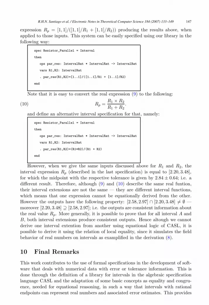
expression Rp = [1, 1]/([1, 1]/R1 + [1, 1]/R2)) producing the results above, when

applied to those inputs. This system can be easily specified using our library in the

following way:

spec Resistor_Parallel = Interval

then

ops par_res: IntervalRat * IntervalRat -> IntervalRat

vars R1,R2: IntervalRat

. par_res(R1,R2)=[1..1]/([1..1]/R1 + [1..1]/R2)

end

Note that it is easy to convert the real expression (9) to the following:

Rp =R1 × R2

R1 + R2.(10)

and define an alternative interval specification for that, namely:

spec Resistor_Parallel = Interval

then

ops par_res: IntervalRat * IntervalRat -> IntervalRat

vars R1,R2: IntervalRat

. par_res(R1,R2)=(R1*R2)/(R1 + R2)

end

However, when we give the same inputs discussed above for R1 and R2, the

interval expression Rp (described in the last specification) is equal to [2.20, 3.48],

for which the midpoint with the respective tolerance is given by 2.84 ± 0.64; i.e. a

different result. Therefore, although (9) and (10) describe the same real funtion,

their interval extensions are not the same — they are different interval functions,

which means that one expression cannot be equationally derived from the other.

However the outputs have the following property: [2.58, 2.97] ∩ [2.20, 3.48] �= ∅ —

moreover [2.20, 3.48] ⊇ [2.58, 2.97]; i.e. the outputs are consistent information about

the real value Rp. More generally, it is possible to prove that for all interval A and

B, both interval extensions produce consistent outputs. Hence altough we cannot

derive one interval extention from another using equational logic of CASL, it is

possible to derive it using the relation of local equality, since it simulates the field

behavior of real numbers on intervals as examplified in the derivation (8).

10 Final Remarks

This work contributes to the use of formal specifications in the development of soft-

ware that deals with numerical data with error or tolerance information. This is

done through the definition of a library for intervals in the algebraic specification

language CASL and the adaptation of some basic concepts as equality and congru-

ence, needed for equational reasoning, in such a way that intervals with rational

endpoints can represent real numbers and associated error estimates. This provides

R.H.N. Santiago et al. / Electronic Notes in Theoretical Computer Science 184 (2007) 133–149 147

in the specification level facilities for some already available programming languages

for interval computations, like Pascal-XSC and C-XSC.

The results in this paper extend those in [14,15] as follows:

(i) they are now directly implementable in an algebraic specification language

(CASL) with the definition and use of a boolean version of local sets, and

(ii) rules for executing a limited local-equational reasoning with intervals have

been provided. Of course, these results may also be applied to other algebraic

specification languages, provided partiality and both kinds of Scott equality,

as explained in Section 4, are available in the language.

Note that the approach here did not require an extension or any redefinition of

the CASL core, all the mathematical development was done for that, and the result

was the introduction of local equality as a simple relation symbol of a CASL theory.

There are still some limits to this solution. The first one comes from the first

order logic underlying CASL, leading to the need for multiple axioms for the more

general properties (e.g., congruence) needed (one axiom for each functional symbol

of a specification). This can be solved by the use of a higher order language or a

higher order extension of CASL. It may also be solved through the use of generic

modules, but both solutions are still future work.

Another problem lies in the implementation of a version of replacement of equals

by equals for local equality. Something like:

slc= t ∧ P (s) → P (t).(11)

However, taking s = [3, 5], t = [4, 6] and P (s) : “s < [6, 6]” 9 . Since “[3, 5]lc=

[4, 6]” and “P ([3, 5])” hold, then we would derive P ([4, 6]) : “[4, 6] < [6, 6]” which

does not hold. Therefore, (11) is not a valid principle. It happens because we are

working with information about objects instead of objects themselves, and therefore

properties of an information s are not necessarily properties of t. Observe that the

approach presented here deals with non-finitely representable objects (irrational

numbers) and can be extended to other domains. Therefore, a replacement law for

locally equal objects is a required subject of investigation if we want to increase

the automation of the verification process (derivation of local equations), e.g., by

rewriting systems.

Finally, we still do not know if there is a way to standardize the conversion of

specifications which describe interval functions to another which describe a local

equivalent expression which always return the optimal outputs. For example, we

still do not have a way to convert the second specification above into the first.

However, the answer seems to be in the deep study of the algebraic properties of

pseudo-inverses and sub-distributivity (fourth, eighth and ninth properties of Table

2). This is also a subject of future work.

9 [a, b] < [c, d] if and only if b < c (Moore [9] p. 10)

R.H.N. Santiago et al. / Electronic Notes in Theoretical Computer Science 184 (2007) 133–149148

References

[1] B. M. Acioly. Computational foundations of Interval mathematics. PhD thesis, Instituto deInformatica, Universidade Federal do Rio Grande do Sul, Dezembro 1991. in Portuguese.

[2] E. Astesiano and et all. Casl: The Common Algebraic Specification Language. Theoretical ComputerScience, 2(286):153–196, 2002.

[3] R. C. Bedregal, B. R. Bedregal, and R. H. N Santiago. Generalizing the real interval arithmetic.Tendencias em Matematica Aplicada e Computacional, 3(1):61–70, 2002.

[4] M. P. Fourman and D. S. Scott. Sheaves and logic. In Fourman M. P. and et all, editors, Applicationsof Sheaf Theory to Algebra, Analysis, and Topology, number 753 in Lecture Notes in Mathematics,pages 302–401. Springer-Verlag, 1979.

[5] K. R. Lopes. A linguagem de especificacao algebrica CASL e o tipo de dados intervalos. Master’s thesis,Programa de Pos-graduacao em Sistemas e Computacao. Departamento de Informatica e MatematicaAplicada (DIMAp), UFRN, Natal-RN-Brasil, 2004.

[6] S. M. Markov. On the extended interval arithmetic. Comptes Rendus de L’Academie Bulgare desSciences, 2(31):163–166, 1978.

[7] R. E. Moore. Interval Arithmetic and Automatic Error Analysis in Digital Computing. PhD thesis,Department of Mathematics, Stanford University, Stanford, California, Nov 1962. Published as AppliedMathematics and Statistics Laboratories Technical Report No. 25.

[8] R. E. Moore. Interval Analysis. Pretince Hall, New Jersey, 1966.

[9] R.E. Moore. Methods and Applications of Interval Analysis. SIAM, 1979.

[10] P. D. Mosses, editor. CASL Reference Manual.The Complete Documentation of the Common AlgebraicSpecification Language, volume 2960 of LNCS - Lecture Notes in Computer Science. Springer Verlag,2004.

[11] H. Rasiowa. An Algebraic Approach to Non-Classical Logics, volume 78 of Studies in Logic and TheFoundations of Mathematics. North-Holland Publishing Company, Amsterdam-London, 1974.

[12] H. Rasiowa and R. Sikorski. The Mathematics of Metamathematics, volume 41 of MonografieMatematyczne. Panstwowe Wydawnictwo Naukowe, 1963.

[13] M. Roggenbach. Specifying real numbers in Casl. In Lecture Notes in Computer Science 1827.Proceedings of 14th International Workshop on Algebraic Development Techniques — WADT’99, pages146–161, Bonas, France, 2000.

[14] R. H. N. Santiago. The Theory Interval Local Equations. PhD thesis, Universidade Federal dePernambuco, Recife, Pernambuco, Brazil, 1999.

[15] R. H. N. Santiago. Interval local equality. toward a model for real type. In Proceedings of theIV Workshop on Formal Methods, pages 54–59, Rio de Janeiro,RJ, 2001. Sociedade Brasileira deComputacao.

[16] R. H. N. Santiago and B. M. Acioly. Interval local equality. In Abstracts of 9th GAMM-IMACSInternational Symposium on Scientific Comouting, Computer Arithmetic and Validated Numerics —SCAN 2000/ International Conference on INterval Methods in Science and Engineering — INTERVAL2000, page 172, Karlsruhe-Germany, Sep 19 to Sep 22 2000. Karlsruhe Univesitat.

[17] R. H. N. Santiago, B.R.C. Bedregal, and B. M. Acioly. Interval representations. Tendencias emMatematica Aplicada e Computacional, 5(2):315–325, 2004.

[18] R.H.N. Santiago, B.R.C. Bedregal, and B.M. Acioly. Comparing continuity of interval functions basedon moore and scott topologies. Electronical Journal on Mathematics of Computation, 2(1):1–14, 2005.

[19] R.H.N. Santiago, B.R.C. Bedregal, and B.M. Acioly. Formal aspects of correctness and optimality ininterval computations. Formal Aspects of Computing, 18(2):231–243, 2006. Spring Verlag.

[20] D. S. Scott. Identity and existence in intuitionistic logic. In M.P. Fourman et al., editors, Lecture Notesin Mathematics 753, pages 660–696. Springer-Verlag, Durham, July 9-21 1977.

[21] J. Stoy. The Scott-Strachey Approach to Programing Language Theory. MIT Press, Massachusetts,1977.

R.H.N. Santiago et al. / Electronic Notes in Theoretical Computer Science 184 (2007) 133–149 149