Ignorance, Pervasive Uncertainty, and Household Finance∗

Yulei Luo†

The University of Hong KongJun Nie‡

Federal Reserve Bank of Kansas City

Haijun Wang§

Shanghai University of Finance and Economics

Forthcoming in Journal of Economic Theory

Abstract

This paper studies how the interaction between two types of uncertainty due to ignorance,

parameter and model uncertainty, affects strategic consumption-portfolio rules, precautionary

savings, and welfare. We incorporate these two types of uncertainty into a recursive utility

version of a canonical Merton (1971) model with uninsurable labor income and unknown in-

come growth, and derive analytical solutions and testable implications. We show that the in-

teraction between the two types of uncertainty plays a key role in determining the demand for

precautionary savings and risky assets. We derive formulas to evaluate both marginal and to-

tal welfare costs of ignorance-induced uncertainty and show they are significant for plausible

parameter values.

JEL Classification Numbers: C61, D81, E21.

Keywords: Ignorance, Unknown Income Growth, Pervasive Uncertainty, Strategic Asset

Allocation.

∗We thank Liang Dai, Ken Kasa, Junya Jiang, Tao Jin, Nan Li, Jianjun Miao, Tom Sargent, Neng Wang, Yu Xu,Jinqiang Yang, Yan Zeng, Tao Zha, and seminar and conference participants at Shanghai Jiao Tong University, ShanghaiUniversity of Finance and Economics, Tsinghua University, Sun Yat-Sen University, Central University of Finance andEconomics, Wuhan University, Zhejiang University, the China International Conference in Finance (CICF), AFR SummerInstitute of Economics and Finance, and the Shanghai Macroeconomics Workshop for helpful comments and discussionsrelated to this paper. Luo thanks the General Research Fund (GRF, No. HKU17500117 and HKU17500619) in HongKong for financial support. The views expressed here are the opinions of the authors only and do not necessarilyrepresent those of the Federal Reserve Bank of Kansas City or the Federal Reserve System. All remaining errors are ourresponsibility.

†Faculty of Business and Economics, University of Hong Kong, Hong Kong. Email address: yulei.luo@gmail.com.‡Research Department, Federal Reserve Bank of Kansas City, U.S.A. E-mail: jun.nie@kc.frb.org.§School of Mathematics and Shanghai Key Laboratory of Financial Information Technology, Shanghai University of

Finance and Economics, China. E-mail: whj@mail.shufe.edu.cn

1. Introduction

Most macroeconomic and financial models assume agents have a good understanding of the eco-

nomic models they use to make optimal decisions. However, there is plenty of evidence that

ordinary investors may be ignorant about certain aspects of the economic model, including the

structure of the model, the parameters, and the current state of the model economy that their deci-

sions are based on. For example, some households may not know the basics of risk diversification

when making financial decisions (van Rooija et al., 2011);1 some people may lack financial literacy,

meaning that they do not have the necessary skills and knowledge to make informed and effective

investment decisions (Lusardi and Mitchell, 2014); some investors may have incomplete informa-

tion about the investment opportunity set (Brennen, 1998); and some individuals may not have full

information about their own income growth (Guvenen, 2007). Such ignorance generates important

uncertainty for agents when they make economic and financial decisions.

Hansen and Sargent (2015) propose that using ignorance is a useful way to model different

types of uncertainty by specifying the details that the decision maker is ignorant about. They use

a simple Friedman one-equation tracking model to illustrate this idea. They mainly discussed two

types of ignorance: (i) the agent is ignorant about the conditional distribution of the state variable

in the next period and (ii) the agent is ignorant about the probability distribution of one key pa-

rameter (i.e., the response coefficient in their paper) in an otherwise fully trusted model. In other

words, the first type of ignorance represents model uncertainty (or MU) as the agent does not know

the distribution of shocks, while the second type of ignorance represents parameter uncertainty (or

PU) as the agent does not know model parameters. (When parameters are stochastic, we may also

view parameter uncertainty as state uncertainty.)2

Inspired by Hansen and Sargent (2015), we study how these two types of ignorance affect in-

tertemporal consumption-saving and asset allocation decisions —a core focus of modern macroe-

conomics and finance. Our central goal is to provide a unified framework to study how these two

types of ignorance (or the two types of uncertainty induced by ignorance: parameter uncertainty

and model uncertainty) interact with each other to affect the optimal consumption-saving-portfolio

decisions as well as the equilibrium asset returns. We derive analytical solutions to separate differ-

ent forces which determine consumption, precautionary saving, and asset allocation. In addition,

our framework also includes some other important factors such as incomplete markets, which are

proven to be important for determining consumption, saving, and asset allocations (Wang, 2003,

1Van Rooija et al. use the De Nederlandsche Bank (DNB) Household Survey data to study the relationship betweenfinancial literacy and stock market participation, and find that financial literacy affects financial decision-making: Thosewith low literacy are much less likely to invest in stocks.

2As the title of their paper suggests, Hansen and Sargent (2015) consider four types of ignorance. The first type isFriedman’s hypothesis in which the agent does not know the key parameter but knows its distribution. The last type iscalled “structured uncertainty,” which is less related to what we study in this paper. What we discuss here is related tothe first three types in their paper.

1

2009).

Specifically, we construct a continuous-time Merton (1971)-Wang (2009)-type model with unin-

surable labor income and unknown income growth in which investors have recursive utility and

face model uncertainty. We follow Hansen and Sargent (2007) to introduce model uncertainty by

incorporating the preference for robustness (RB). In robust control problems, agents are concerned

about the possibility that their true model is misspecified in a manner that is difficult to detect

statistically; consequently, they make their decisions as though the subjective distribution over

shocks was chosen by an evil agent to minimize their utility.3 In our model economy, investors not

only have incomplete information about income growth but are also concerned about the model

misspecification. Compared with the full-information rational expectations (FI-RE) case in which

income growth is known, parameter uncertainty due to unknown income growth creates an addi-

tional demand for robustness. In our recursive utility framework, we also disentangle two distinct

aspects of preferences: the agent’s elasticity of intertemporal substitution (EIS, attitudes towards

variation in consumption across time) and the coefficient of absolute risk aversion (CARA, atti-

tudes toward variation in consumption across states), which are shown to have different roles in

driving consumption-saving and portfolio choice decisions.4 As explained below, our model de-

livers not only rich theoretical results but also testable implications.

This paper has four main findings and contributions. First, we provide analytical solutions to

this rich framework with both types of uncertainty (PU and MU) to study strategic consumption-

portfolio rules in the presence of uninsurable labor income. Using the closed-forms solution, we

are able to inspect the exact mechanism through which these two types of induced uncertainty

interact and affect the demand for risky assets and precautionary saving.5 Specifically, we find

that the precautionary saving demand and the strategic asset allocation are mainly affected by the

effective coefficient of risk-uncertainty aversion (γ) that is determined by the interaction between

the CARA (γ), the EIS (ψ), and the degree of RB (ϑ) via the formula: γ = γ+ ϑ/ψ. This expression

clearly shows that both risk aversion and intertemporal substitution play roles in determining the

amount of precautionary savings and the optimal share invested in the risky asset, but without

model uncertainty, only risk aversion matters in determining these two demands.6

3There are three main ways to model ambiguity and robustness in the literature: the multiple priors model, thesmooth ambiguity model, and the robust control/filtering model (Hansen and Sargent 2007). In this paper, we followalong the lines of Hansen and Sargent to introduce robustness and model uncertainty into our model.

4Constant-relative-risk-aversion (CRRA) utility functions are more common in macroeconomics, mainly due tobalanced-growth requirements. CRRA utility would greatly complicate our analysis because the intertemporal con-sumption model with CRRA utility and stochastic labor income has no explicit solution and leads to non-linear con-sumption rules. See Cagetti et al. (2002) and Kasa and Lei (2018) for applications of RB in continuous-time models withCRRA utility.

5Hansen et al. (1999), Maenhout (2004), Ju and Miao (2012), Chen et al. (2014), and Luo and Young (2016) examinehow model uncertainty and ambiguity affect portfolio choices and/or asset prices.

6The interaction between the EIS and RB in the expression for γ is due to two facts: (i) the value function in ourbenchmark model is a function of the EIS and (ii) the RB parameter is normalized by the value function (so it convertsthe relative entropy to units of utility and makes it consistent with the units of the expected future value function

2

Second, we use our analytical results (as summarized by Proposition 2 in Section 4) to separate

different forces such as MU, PU, and the interaction between MU and PU in determining precau-

tionary saving and the demand for risky assets, which represent the two core parts of saving and

portfolio-choice decisions. We show that the share of precautionary saving due to MU and PU

together is very large at reasonable levels of model uncertainty. For example, when the degree of

model uncertainty (as measured by the detection error probability (DEP)) equals 0.2, MU and PU

together can account for about 80% of total precautionary saving for plausible parameter values.7

Out of this, about 46% comes from model uncertainty through the robust control channel and

54% comes from MU through robust filtering channel (or the interaction between PU and MU),

while PU itself slightly reduces precautionary saving. We theoretically prove and explain why PU

has such a negative impact on precautionary saving. In general, we show that the importance

of the interaction between MU and PU increases with the robustness parameter, highlighting the

importance of modeling the interaction between these two types of uncertainty when studying

consumption-saving-portfolio choice problems. To the best of our knowledge, our paper is the

first to provide a unified framework with analytical solutions to separate these different forces.

On the demand for risky assets, we show that its total demand decreases with the amount

of model uncertainty due to robustness, and can be decomposed into three components: (i) the

traditional speculation demand, (ii) the learning-induced hedging demand, and (iii) the income-

hedging demand. We find that the first and second components are determined by the robust

control and robust filtering channels respectively, while the third component is independent of

both channels. In addition, this decline is largely driven by the increase in the degree of robustness

through the robust control channel, though the relative importance of the robust filtering channel

increases with the degree of robustness.

Third, we quantitatively test the model implications on risky-asset holding using household-

level data . In particular, we conduct a calibration exercise to match the observed risky-asset hold-

ings by different educational groups in the data. The calibrated results suggest that less educated

households face more model uncertainty measured by the detection error probability, a commonly

used statistical tool to measure the amount of model uncertainty in the robustness literature.8 This

result is consistent with the recent empirical finding using survey data by Lusardi and Mitchell

(2014) which shows that highly educated people are usually more financial literate than low edu-

cated people. In addition, we show that the interaction between the two types of uncertainty is the

key to explain the data. In particular, if we shut down the model uncertainty channel, the model

with only parameter uncertainty cannot explain the observed patterns of asset holdings.

evaluated with the distorted model). See Section 3 for a detailed discussion on this issue.7DEP equal to 0.2 means that there is a probability of 0.2 that the reference model cannot be distinguished from the

distorted model based on a likelihood ratio test.8As we will explain later, a higher detection error probability means it is more difficult to distinguish the distorted

model from the approximating model, or, the agent faces less model uncertainty.

3

Fourth, we show that the welfare cost of ignorance in general equilibrium can be sizable.9 We

provide formulas to evaluate both the marginal and the total welfare costs due to the two types of

ignorance-induced uncertainties. Specifically, when ϑ = 2 (or DEP=0.25), a 10% increase in ϑ leads

to a welfare cost equivalent to about 2% percent reduction in initial consumption. In addition, this

welfare loss increases with the amount of parameter uncertainty. Furthermore, if we remove all

uncertainty in the model, the welfare gains could be as large as 23% of initial consumption.

The remainder of this paper is organized as follows. Section 2 provides a literature review.

Section 3 describes our model setup, introducing key elements step by step. Section 4 presents key

theoretical results. Section 5 presents quantitative results. Section 6 examines welfare implications

of ignorance. Section 7 concludes.

2. Literature Review

Our paper is related to two broad branches of literature, the first being the broad literature study-

ing consumption-saving and portfolio choices. Recent empirical studies on household portfolios

in the U.S. and major European countries have stimulated research in allowing for portfolio choice

between risky and risk-free financial assets when households receive labor income and have the

precautionary saving motive. The empirical research on household portfolios documents both

the increasing stock market participation rate in the U.S. and Europe and the importance of the

precautionary saving motive for portfolio choice (see Guiso et al., 2002). Some recent theoreti-

cal studies have also addressed the importance of parameter uncertainty or model uncertainty in

affecting agents’ optimal consumption and portfolio rules. For example, Brennen (1998) shows

that the uncertainty about the mean return on the risky asset has a significant effect on the port-

folio decision of a long-term investor. Maenhout (2004) explores how model uncertainty due to

a preference for robustness affects optimal portfolio choice and the equilibrium equity premium.

Wang (2009) finds that incomplete information about labor income growth can significantly affect

optimal consumption-saving and asset allocation.

Second, on the modeling strategy, our paper is related to a fast growing literature on modeling

induced uncertainty including both model uncertainty and parameter uncertainty. Besides Hansen

and Sargent (2015), this paper is also closely related to Gennotte (1986), Maenhout (2004), Garlappi

et al. (2007), Wang (2009), Collin-Dufresne et al. (2016), and Luo (2017). Maenhout (2004) explores

how model uncertainty due to a preference for robustness reduces the demand for the risky asset

and increases the equilibrium equity premium. Garlappi et al. (2007) examines how allowing

for the possibility of multiple priors about the estimated expected returns affects optimal asset

weights in a static mean-variance portfolio model. Wang (2009) studies the effects of incomplete

9In Section 6, we show that a unique general equilibrium under MU and PU can be constructed in the vein of Huggett(1993) and Wang (2003). (Wang (2003) constructs a general equilibrium under FI-RE in the same Bewley-Huggett typemodel economy with the CARA utility that we study.)

4

information about the mean income growth on a consumer’s consumption/saving and portfolio

choice in an incomplete-market economy. Collin-Dufresne et al. (2016) study general equilibrium

models with unknown parameters governing long-run growth and rare events, and show that

parameter learning can generate quantitatively significant macroeconomic risks that help explain

the existing asset pricing puzzles. Luo (2017) considers state uncertainty (uncertainty about the

value of total wealth) within an expected utility partial equilibrium model, and finds that state

uncertainty does not play an important role in determining strategic asset allocation unless the

investors face very tight information-processing constraints.

Many empirical and experimental studies have repeatedly supported that individual agents

are ambiguity averse (or have robustness preferences). For example, Ahn et al. (2014) use a rich

experiment data set to estimate a portfolio-choice model and found that about 40% of subjects

display either statistically significant pessimism or ambiguity aversion. Bhandari et al. (2017)

identify ambiguity shocks using survey data, and show that in the data, the ambiguity shocks are

an important source of variation in labor market variables.

However, our paper is also significantly different from the above papers. Unlike Maenhout

(2004), our paper explores how the interaction of model uncertainty and parameter uncertainty

affects the strategic consumption/saving-portfolio decisions in the presence of uninsurable labor

income and unknown income growth. The model presented in this paper can therefore be used to

study the relationship between the labor income risk and the stockholding behavior. Unlike Wang

(2009) and Collin-Dufresne et al. (2016), this paper considers more general concepts of ignorance

and induced uncertainty. We consider not only parameter uncertainty but also model uncertainty

due to robustness. Another key difference between our paper and Wang (2009) is that rather than

considering the discrete Markovian unknown income trend process as in Wang (2009), this paper

considers a continuous Gaussian unknown process that can be estimated using PSID data and

makes the general equilibrium analysis tractable. In addition, unlike Garlappi et al. (2007), this

paper focuses on incomplete information about the mean income growth, rather than incomplete

information about the risk premium, and studies how this type of incomplete information affects

the robust consumption and portfolio rules in an intertemporal setting. The key difference be-

tween this paper and Luo (2017) is that this paper focuses on examining parameter uncertainty

that is more difficult to learn than the state uncertainty discussed in Luo (2017), and examines how

it interacts with model uncertainty within a recursive utility general equilibrium framework in

which both types of uncertainty interact with intertemporal substitution and risk aversion.

3. The Model Setup

In this section, we lay out our continuous-time consumption-portfolio choice model with recur-

sive utility and two types of ignorance. To help explain the key structure of the model, we will

5

introduce each of the key elements one by one, starting with specifications of the labor income and

investment opportunity set, followed by the description of the information set, then the recursive

utility preference, and finally introducing the model uncertainty due to robustness.

As an overview, our model is a continuous-time recursive utility version of the Merton-type

model (1971) with uninsurable labor income and unknown income growth. Specifically, we gen-

eralize the Wang (2009) model in the following three aspects: (i) Rather than using the expected

utility specification, we adopt a recursive utility specification; (ii) to better explore the importance

of pervasive uncertainty due to ignorance in investors’ financial decision-making problem, we

not only consider parameter/state uncertainty due to unknown income growth, but also consider

model uncertainty due to a preference for robustness; and (iii) instead of adopting the discrete-

state Markovian income growth specification, here we consider a continuous-state Gaussian in-

come growth specification, which can be estimated using the PSID data and can help explore the

general equilibrium welfare implications of different types of ignorance. In summary, the typical

investor in our model economy has recursive utility and makes strategic consumption-saving-asset

allocation decisions with pervasive uncertainty. Finally, we assume that the investors can access

two financial assets: one risk-free asset and one risky asset, and also receive uninsurable labor

income.

3.1. Specifications of Labor Income and Investment Opportunity Set

Labor income (yt) is assumed to follow a continuous-time Ornstein-Uhlenbeck (OU) process:

dyt = (µt − ρyt) dt + σydBy,t, (1)

where σy is the unconditional volatility of the income change over an incremental unit of time,

the persistence coefficient ρ governs the speed of convergence or divergence from the steady state,

By,t is a standard Brownian motion defined on the complete probability space (Ω,Ft, P), and µt

is the unobservable income growth rate. Specifically, we assume that µt follows a mean-reverting

Ornstein-Uhlenbeck process:

dµt = λ (µ− µt) dt + σµdBµ,t, (2)

where Bµ,t is a standard Brownian motion defined over the complete probability space, λ and

µ are positive constants, and the correlation between dBy,t and dBµ,t is ρyµ ∈ [−1, 1]. (That is,

E[dBy,tdBµ,t

]= ρyµdt.) In other words, in this setting, both the income growth rate and actual

income are stochastic and risky. Since µt is unknown to investors, the investors need to estimate it

using their observations of the realized labor income. In the traditional signal extraction models,

the typical investor estimates the conditional distribution of the true income growth rate and then

represents the investor’s original optimizing problem as a Markovian one. If we assume that the

loss function in our model is the mean square error (MSE) due to incomplete information, then

6

given a Gaussian prior, finding the posterior distribution of the income growth rate becomes a

standard Kalman-Bucy filtering problem. However, given that we assume that households have

a preference for robustness, we might not only consider a robust control problem but also con-

sider a corresponding robust filtering problem. (We will discuss the robust filtering problem after

introducing model uncertainty due to robustness in Section 3.3.)

The agent can invest in both a risk-free asset with a constant interest rate r and a risky asset

(i.e., the market portfolio) with a risky return ret . The instantaneous return dre

t of the risky market

portfolio over dt is given by:

dret = (r + π) dt + σedBe,t, (3)

where π is the market risk premium, σe is the standard deviation of the market return, and Be,t is a

standard Brownian motion defined on (Ω,Ft, P) and is correlated with the Brownian motion, By,t.

Let ρye be the contemporaneous correlation between the labor income process and the return of the

risky asset. When ρye = 0, the labor income risk is purely idiosyncratic and is uncorrelated with

the risky market return; when ρye = 1, the labor income risk is perfectly correlated with the risky

market return. The consumer’s financial wealth evolution is given by

dwt = (rwt + yt − ct) dt + αt (πdt + σedBe,t) , (4)

where αt denotes the amount of wealth that the investor allocates to the market portfolio at time t.

3.2. Recursive Exponential Utility

In this paper, we assume that investors in our model economy have a recursive utility preference

of the Kreps-Porteus/Epstein-Zin type, and can disentangle the degree of risk aversion from the

elasticity of intertemporal substitution. Although the expected utility model has many attractive

features, it implies that the agent’s elasticity of intertemporal substitution is the reciprocal of the

coefficient of risk aversion. Conceptually, however, risk aversion and intertemporal substitution

capture two distinct aspects of the decision-making problem. Specifically, for every stochastic

consumption-portfolio stream, ct, αt∞t=0, the utility stream, V (Ut)∞

t=0, is recursively defined as

follows:

V (Ut) =(

1− e−β∆t)

V (ct) + e−β∆tV (CEt [Ut+∆t]) , (5)

where ∆t is time interval, β > 0 is the agent’s subjective discount rate, V (ct) = (−ψ) exp (−ct/ψ),

V (Ut) = (−ψ) exp (−Ut/ψ),

CEt [Ut+∆t] = G−1 (Et [G (Ut+∆t)]) ,

is the certainty equivalent of Ut+1 conditional on the period t information, and G (Ut+∆t) = − exp (−γUt+∆t) /γ.

In (5), ψ > 0 governs the elasticity of intertemporal substitution (EIS), while γ > 0 governs the

7

coefficient of absolute risk aversion (CARA).10 In other words, a high value of ψ corresponds to

a strong willingness to substitute consumption over time, and a high value of γ implies a high

degree of risk aversion. It is well-known that the CARA (or negative exponential) utility models

including our recursive exponential utility (REU) do not rule out negative consumption because

the marginal utility will not approach infinity as consumption converges to zero. We do not impose

a non-negativity consumption constraint explicitly in this paper because a closed-form solution to

the problem would not be available if that constraint were binding. Note that when ψ = 1/γ, the

functions V and G are the same and the recursive utility reduces to the standard time-separable

expected utility function used in Caballero (1990) and Wang (2003, 2009). In addition, ψ = 1/γ

also implies that the investor is indifferent about the time at which uncertainty is resolved.11

3.3. Incorporating Model Uncertainty Due to Robustness

As we mentioned above, the loss function in the model in which investors have a preference for

robustness might not still be the mean square error (MSE) due to incomplete information; con-

sequently, given a Gaussian prior, finding the posterior distribution of µt may not be a standard

Kalman-Bucy filtering problem. In other words, in the problem studied in this paper, robustness

may not only be applied to the control problem (robust control), but may also be applied to the

filtering problem (robust filtering). Hansen and Sargent (2007) argued that the simplest version

of robustness considers the question of how to make optimal decisions when the decision-maker

does not know the true probability model that generates the data. The main goal of introducing ro-

bustness is to design optimal policies that not only work well when the reference model governing

the evolution of the state variables is the true model, but also performs reasonably well when the

true economy is governed by the distorted model. In this paper, we follow Kasa (2006) and Hansen

and Sargent (2007, Chapter 17), and consider a situation in which the households pursue a robust

Kalman gain and faces the commitment on the part of the minimizing agent to previous distortions.

(Note that Hansen and Sargent (2007) also discussed robust filtering without commitment.) Specif-

ically, to solve this robust control and filtering problem, we adopt a two-stage procedure that can

decompose the original incomplete-information optimal problem into two sub-problems:12

1. Robust filtering problem. In the first stage, we assume that the investors solve a robust

filtering problem. The main idea of robust filtering is the same as the standard filtering

problem in which investors want to minimize the expected loss function determined by the

difference between the estimated state and the true state. The new feature is that in the10It is well known that the CARA utility specification is tractable for deriving the consumption function or optimal

consumption-portfolio rules in different settings. See Merton (1971), Caballero (1990), Calvet (2001), Wang (2003, 2009),Angeletos and Calvet (2006), and Luo (2017).

11Note that the investor prefers early resolution of uncertainty if γ > 1/ψ and prefers late resolution if γ < 1/ψ.12As in Wang (2004, 2009), the separation principle also applies to our robust filtering and control problem given the

CARA-Gaussian specification.

8

robust filtering problem, investors have a preference for robustness, which means they are

concerned that the state transition and observation equations are misspecified. Consequently,

the optimal Kalman gain is now affected by the preference for robustness.

2. Robust control problem. In the second stage, treating the perceived unobservable state as a

underlying state variable, the investors who are concerned about the model misspecification

solve the robust consumption-portfolio choice model. We then verify that the corresponding

value function leads to the same loss function we use in Stage 1.

It is worth noting that when the agent cannot observe µt perfectly, his optimization problem is

not recursive. However, adopting the above two-stage procedure helps convert the original non-

recursive optimization problem into a recursive formulation because the dynamics of the estimated

state contains the same information as the original non-recursive incomplete-information model.

3.3.1. Robust Filtering

Following Kasa (2006), and Hansen and Sargent (2007, Chapter 17), we first consider the filtering

problem. Specifically, we consider a situation in which the investor who is concerned about the

model pursues a robust Kalman gain. To obtain a robust Kalman filter gain, we first use relative

entropy to measure model uncertainty, and then use the Girsanov theorem to parameterize the

distorted model. Here, we use P and Q to denote the probability measures of the approximating

and distorted models, respectively.

Following the robust filtering literature, applying the change of measure from P to Q to the

state transition and observation equations, (2) and (1), yields the following distorted filtering

model:

dµt =[λ (µ− µt) + σµv1,t

]dt + σµdBµ,t, (6)

dyt =(µt − ρyt + σyv2,t

)dt + σydBy,t, (7)

where Bµ,t and By,t are Wiener processes that are related to the corresponding approximating pro-

cesses:

Bµ,t = Bµ,t −ˆ t

0v1,sds and By,t = By,t −

ˆ t

0v2,sds

and v1,t and v2,t are distortions to the conditional means of the two shocks, Bµ,t and By,t, respec-

tively. As shown in Pan and Basar (1996); Ugrinovskii and Petersen (2002); and Kasa (2006), a

robust filter can be characterized by the following dynamic zero-sum game:

Lt = infmj

supQ

lim sup

T→∞EQ [F]− ϑ−1H∞ (Q|P)

, (8)

9

subject to (6) and (7), where mj = Ej[µj]

is the conditional mean of µj, F ≡ T−1 ´ T0

(µj −mj

)2 dj is

the loss function, and H∞ is the relative entropy and is bounded from above:

H∞ (Q|P) = lim supT→∞

EQ

[1

2T

ˆ T

0

(v2

1,t + v22,t)

dj

]≤ η0, (9)

where η0 defines the set of models that the consumer is considering, and ϑ−1 is the Lagrange

multiplier on the relative entropy constraint, (9). In Appendix 8.2, we show that the loss function

due to incomplete information in our REU setting is (approximately) quadratic. Following the

literature, we use ϑ to measure the degree of robustness throughout the paper. As shown in Dai Pra

et al. (1996), the entropy constrained robust filtering problem, (8), is equivalent with the following

risk-sensitive filtering problem:13

1ϑ

log(ˆ

exp (ϑF (µ, m)) dP

)= sup

Q

ˆF (µ, m) dQ− ϑ−1H∞ (Q|P)

. (10)

The following proposition summarizes the results for this robust filtering problem:

Proposition 1. When ϑ ≥ σ2µ/(σ2

µ + λ2), there is a unique solution for the robust filtering problem, (10):

dmt = λ (µ−mt) dt + Kt [dyt − (mt − ρyt) dt] , (11)

dΣt

dt= −2λΣt + σ2

µ −(

1σ2

y− ϑ

)(η + Σt)

2 , (12)

where mt = Et [µt] and Σt = Et

[(µt −mt)

2]

is the conditional mean and variance of µt, respectively,

Kt = (η + Σt) /σ2y (13)

is the Kalman gain, and η = ρyµσyσµ,. In the steady state, the conditional variance converges to:

Σ∗ =−σ2

y λ + σ2y

√λ2 +

(1− ρ2

yµ

) (σ2

µ/σ2y

)− ϑ

(2λη + σ2

µ

)1− ϑσ2

y− η ≥ 0, (14)

where λ = λ + η/σ2y .

Proof. The right-hand side of (10) is an entropy constrained filtering problem in terms of the scaled

quadratic objective function F, while the left-hand side is a risk-sensitive filtering problem in terms

of the same function F, with risk-sensitivity parameter, ϑ. The solution of this risk-sensitive filter-

ing problem is just a special case of Pan and Basar (1996)’s Theorem 3.

13See Online Appendix A for a proof.

10

Using the expected mean mt, we can now rewrite the income process as:

dyt = (mt − ρyt) dt + σydBm,t, (15)

where dBm,t = dBy,t +(

µt−mtσy

)dt is the normalized unanticipated innovation of the income growth

process and a standard Brownian motion with respect to the investor’s filtration. Substituting it

into the estimated state updating equation yields:

dmt = λ (µ−mt) dt + σmdBm,t, (16)

where:

σm ≡ σyK =η + Σ∗

σy=−σyλ + σy

√λ2 +

(1− ρ2

yµ

) (σ2

µ/σ2y

)− ϑ

(2λη + σ2

µ

)1− ϑσ2

y(17)

is the diffusion coefficient (i.e., the instantaneous standard deviation of mt) and Σ∗ is given in (14).

It should be noted that the information structure generated by m0, Bm,s, s ∈ [0, t] is the same as

the one generated by ys, s ∈ [0, t]. It is worth noting that when ϑ = 0, the above robust filtering

problem reduces to the traditional optimal filtering problem in which:

Σ∗ = −σ2y λ + σ2

y

√√√√λ2 +

(1− ρ2

yµ

)σ2

µ

σ2y

and σm = −σyλ + σy

√√√√λ2 +

(1− ρ2

yµ

)σ2

µ

σ2y

. (18)

Note that when ρyµ = 1, the optimal filtering model reduces to the full-information model in which

µt is fully observable, Σ∗ = 0, and σm converges to σµ.14 As mentioned before, in this paper we

treat σµ > 0 as fundamental uncertainty, and treat the noise-to-signal ratio, σ2y /σ2

µ, as parameter

uncertainty. Given ρyµ, the learning mechanism is determined by the noise-to-signal ratio.

From (13), (14), and (17), it is straightforward to show that for different values of σy/σµ,

∂Σ∗

∂ϑ> 0,

∂σm

∂ϑ> 0, and

∂K∂ϑ

> 0.

That is, the steady state conditional variance (Σ∗), the diffusion coefficient (σm), and the robust

Kalman gain (K) are increasing with the preference for pursuing a robust Kalman filter. In Section

5, we will quantitatively examine the relative importance of robust control and filtering in deter-

14When ϑ = 0, it is straightforward to show that:

σm = σyλ + σy

√λ2 + 2λ

ρyµσµ

σy+

(σµ

σy

)2≤ σµ

when ρyµ ≤ 1. Throughout this paper, we rule out the possibility that σµ = 0 because the estimated value of thisparameter using the PSID is significantly positive.

11

mining precautionary savings and strategic asset allocation after using the US data to estimate the

joint y and µ process.

3.3.2. Robust Control

To introduce robust control into our model proposed above, we follow the continuous-time method-

ology proposed by Anderson et al. (2003) and adopted in Maenhout (2004) to assume that in-

vestors are concerned about the model misspecifications and take Equations (4), (15), and (16) as

the approximating model. The corresponding distorting model can thus be obtained by adding an

endogenous distortion υ (st) to the approximating model:

dst = (Λ + Σ · υt) dt + σ · dBt, (19)

where st =[

wt yt mt

]T, dst =

[dwt dyt dmt

]T, Λ =

[rwt + yt − ct + αtπ mt − ρyt λ (µ−mt)

]T,

υt =[

υ1,t υ2,t υ3,t

]T, dBt =

[dBe,t dBi,t

]T,15 σ =

αtσe 0

ρyeσy

√1− ρ2

yeσy

ρyeσm

√1− ρ2

yeσm

, and Σ ≡ σσT =

α2

t σ2e ρyeσyαtσe ρyeαtσeσm

ρyeσyαtσe σ2y σyσm

ρyeαtσeσm σyσm σ2m

.

Under RB, the HJB can thus be written as:

βV (Jt) = supct,αt

infυt

βV (ct) +DV (Jt) +

1ϑtH

, (20)

where

DV (Jt) = V ′ (Jt)((∂J)T · E [dst] + (∂J)T · Σ · υt −

γ

2

[(∂J)T · Σ · ∂J

]), (21)

where[

Jw Jy Jm

]T, the first two terms in (21) are the expected continuation payoff when the

state variable follows (19), i.e., the alternative model based on drift distortion υ (st),H =(υT

t · Σ · υt)

/2

is the relative entropy or the expected log likelihood ratio between the distorted model and the ap-

proximating model and measures the distance between the two models, and 1/ϑt is the weight on

the entropy penalty term.16 The last term, H/ϑt, in (20) quantifies the penalty due to RB. More

specifically, (∂J)T · Σ · υt is the adjustment to the expected continuation value when the state dy-

namics is governed by the distorted model with the mean distortion υt.

15To obtain independent Brownian motions, we apply a Cholesky decomposition to dBm,t: dBm,t = ρyedBe,t +√1− ρ2

yedBi,t, where Bi,t is a standard Brownian motion and independent of Be,t.16The last term in (22) is due to the investor’s preference for robustness. Note that the ϑt = 0 case corresponds to the

standard expected utility case. This robustness specification is called the multiplier (or penalty) robust control problem.

12

As shown in Anderson et al. (2003), the objective DV defined in (21) plays a crucial role in

introducing robustness. The investor accepts the approximating model as the best approximating

model, but is still concerned that it is misspecified. He or she therefore wants to consider a range

of models (i.e., the distorted model, (19)) surrounding the approximating model when computing

the continuation payoff. A preference for robustness is then achieved by having the agent guard

against the distorting model that is reasonably close to the approximating model.

The drift adjustment υ (st) is chosen to minimize the sum of (i) the expected continuation payoff

adjusted to reflect the additional drift component in (19) and (ii) an entropy penalty:

infυ

[V ′ (Jt) (∂J)T · Σ · υt +

1ϑtH]

, (22)

where ϑt is fixed and state-independent in Anderson et al. (2003); whereas it is state-dependent in

Maenhout (2004). The key reason for using a state-dependent counterpart ϑt in Maenhout (2004)

is to assure the homotheticity or scale invariance of the decision problem with the CRRA utility

function. In this paper, we also specify that ϑt is state-dependent (ϑ (st)) in the CARA-Gaussian

setting. The main reason for this specification is to guarantee homotheticity, which keeps robust-

ness from diminishing as the value of the total wealth increases.17 Solving first for the infimization

part of (22) yields υ∗t = −ϑtV ′ (Jt) ∂J, where ϑt = −ϑ/V (Jt) > 0 and ϑ is a constant (see Appendix

8.1 for the derivation).

Using a given detection error probability, we can easily calibrate the corresponding value of

ϑ that affects the optimal consumption-portfolio rules. Substituting for υ∗ in (20) leads to the

following HJB:

βV (Jt) = supct,αt

βV (ct) + V ′ (Jt)

((∂J)T · E [dst]−

12

γ[(∂J)T · Σ · ∂J

]), (23)

where γ = γ + ϑ/ψ.

It is worth noting that we can follow Munk and Sørensen (2010) and Wang et al. (2016) to con-

struct human wealth as the discount present value of the current and future labor incomes. Once

we define the total wealth of an investor as the sum of financial wealth and human wealth, we can

reduce the state space of our model to one dimension and write down the optimal investment and

consumption policies for a Merton problem (without labor income) as a function of total wealth.

Specifically, in our incomplete markets economy, there exists a unique stochastic discount factor ζt

17Note that the impact of robustness wears off if we assume that ϑt is constant. This is clear from the procedure ofsolving the robust HJB proposed. As argued in Maenhout (2004), here we can also define “1/V (Jt)” in the ϑt specifi-cation as a normalization factor that is introduced to convert the relative entropy to units of utility so that it is consistentwith the units of the expected future value function evaluated with the distorted model.

13

under the minimal martingale measure Qm satisfying:

dζt = −ζt

(rdt +

ρyeπ

σedBe,t

),

where ζ0 = 1. The human wealth under incomplete markets is then defined as follows:

h(yt, mt) = EPt

[ˆ ∞

t

ζs

ζtysds

∣∣∣∣F yt

]= E

Qm

t

[ˆ ∞

te−r(s−t)ysds

∣∣∣∣F yt

], (24)

where Qm is the risk-neutral probability measure with respect to P. Using (1) and (16), the expres-

sion of h(y, m) can thus be simplified as:

h(yt, mt) =yt

r + ρ+

mt

(r + ρ)(r + λ)+

1r(r + ρ)(r + λ)

λµ−

[(r + λ)σy + σm

] ρyeπ

σe

.

Using at = wt + ht to denote the total wealth, we have:

dat =

(rat + αtπ +

ρyeπσh

σe− ct

)dt + αtσedBe,t + σhdBm,t. (25)

where σh =(r+λ)σy+σm(r+ρ)(r+λ)

. This model can also be seen as a Merton problem, and delivers the same

solution as obtained in our original model. (See Online Appendix B for the derivation.)

4. Theoretical Results and Implications

This section delivers our theoretical results. We analytically solve the model and obtain the ro-

bustly strategic consumption-portfolio rules. Then we use the analytical solutions to separate the

contribution from the two types of ignorance-induced uncertainty, MU and PU, in determining the

key components in saving and portfolio-choice decisions. We finally explore how the induced un-

certainty interacts with the discount rate and the interest rate and affects consumption dynamics.

4.1. Inspecting the Robust Consumption-Saving-Portfolio Rules

The following proposition summarizes the solution and shows how different forces jointly deter-

mine the consumption and portfolio choices:

Proposition 2. Under robustness and unknown income trend, the decision rules for consumption and

portfolio choices, as well as the value function are given by:

(i) The optimal consumption rule is:

c∗t = r (wt + ht + lt) + Ψ + Π− Γ, (26)

where

14

ht =1

r+ρ

(yt +

µr −

πρyeσyrσe

)is the risk-adjusted human wealth;

lt =1

(r+ρ)(r+λ)

(mt − µ− πρyeσm

rσe

)is the perceived risk-adjusted income trend;

Ψ =(

β−rr

)ψ measures the effects of impatience on consumption and saving;

Π = π2

2rγσ2e

is the additional increase in the investor’s certainty equivalent wealth due to the presence of

the risky asset;

Γ ≡ 12

rγ(

1− ρ2ye

) [ σy

r + ρ+

σm

(r + ρ) (r + λ)

]2

(27)

is the investor’s precautionary saving demand, with γ ≡ γ + ϑ/ψ being the effective coefficient of absolute

risk-uncertainty aversion.

(ii) The optimal portfolio rule is:

α∗t = αs + αl + αy, (28)

where

αs =π

rγσ2e

(29)

is the standard speculation demand for the risky asset,

αl ≡ −ρyeσm

σe (r + ρ) (r + λ)(30)

is the learning-induced hedging demand,

αy = −ρyeσy

σe (r + ρ)(31)

is the labor income-hedging demand, and σm is given by (17).

(iii) The associated value function is

V (Jt) = (−ψ) exp((

α0 − rwt −r

r + ρyt −

r(r + ρ) (r + λ)

mt

)/ψ

), (32)

where

α0 =

(1− β

r

)ψ− ψ ln

(rβ

)− π2

2rγσ2e+

πρye

σe

[σy

(r + ρ)+

σm

(r + ρ) (r + λ)

]− λµ

(r + ρ) (r + λ)+

12

rγ(

1− ρ2ye

) [ σy

r + ρ+

σm

(r + ρ) (r + λ)

]2

. (33)

Proof. See Appendix A for the derivation.

We make several comments on this important proposition. First, the consumption rule (26)

illustrates how the optimal consumption is influenced by different forces in this rich framework.

15

In the standard permanent income model, the optimal consumption is given by the annuity value

of the lifetime wealth, r(wt + ht). Other terms on the right hand side of (26) show the influence

of the MU (via ϑ), PU (via K = σm/σy), incomplete market and their interactions on consumption.

Specifically, lt in the consumption policy function can be viewed as the investor’s risk-adjusted

certainty equivalent wealth due to the uncertainty about his income trend. Ψ captures the extra

saving due to impatience. When the interest rate r is endogenously determined, this term also

captures the effects of incomplete market on the equilibrium interest rate and savings. Π captures

the extra savings when there are risky assets in the economy. Γ captures the effect of precautionary

savings, which is jointly influenced by MU through ϑ and by PU through the Kalman gain, K. As

the Kalman gain is also affected by the robustness parameter ϑ, it is easy to see that the preference

for robustness (ϑ) affects the precautionary saving demand via two channels: (i) the direct channel

(the robust control channel) and (ii) the indirect channel (the robust filtering channel) via the robust

Kalman gain (K).18 In addition, both the correlation between the equity return and labor income

(ρye) and the correlation between labor income and the mean growth rate of labor income (ρyµ)

interact with the volatility of the noisy signal (σy) and the volatility of the perceived mean (σm),

and then affect the precautionary saving demand.

Second, our analytical solution allows us to conduct various decompositions to help under-

stand how PU and MU influence precautionary savings. For example, to fully explore how pa-

rameter uncertainty due to unknown income growth affects the precautionary saving demand, we

first shut down both the parameter uncertainty channel and the model uncertainty channel. In this

case, the investor has complete information about the parameter and has no concerns about model

specification, and the precautionary saving demand, Γ0, can be written as:19

Γ0 =12

rγ(

1− ρ2ye

) [ σy

r + ρ+

σµ

(r + ρ) (r + λ)

]2

. (34)

When we only shut down the model uncertainty channel, the precautionary saving demand, ΓPU,0,

can be written as:

ΓPU,0 =12

rγ(

1− ρ2ye

) [ σy

r + ρ+

σm,0

(r + ρ) (r + λ)

]2

, (35)

where σm,0 = −σyλ + σy

√λ2 +

(1−ρ2yµ)σ2

µ

σ2y

is the diffusion coefficient in dmt when ϑ = 0. We can

then define the amount of precautionary savings due to parameter uncertainty as:

ΓPU = ΓPU,0 − Γ0. (36)

Given the expressions of Γ and ΓPU,0, we define the amount of precautionary savings due to model

18In the next section, we will quantitatively show that the indirect channel has a significant impact on precautionarysaving and asset allocation and is comparable to the direct channel.

19Note that here when ρyµ = 1, σm = σµ.

16

uncertainty as:

ΓMU = Γ− ΓPU,0. (37)

We then define

ΓPU,MU = ΓPU + ΓMU = Γ− Γ0 (38)

as the additional demand for precautionary saving due to the interactions of model and parameter

uncertainty (i.e., the ignorance of the unknown parameter and model specification).

It is worth noting that we can decompose the precautionary saving demand due to robustness

and model uncertainty into: (i) the robust control component and (ii) the robust filtering component.

Here we can use the amount of the robust filtering component to measure the interaction between

parameter and model uncertainty. That is, the robust filtering part (denoted by ΓMU, f iltering) cap-

tures the joint effect of robustness and learning in determining precautionary saving. Specifically,

we decompose ΓMU as:

ΓMU = ΓMU,control + ΓMU, f iltering, (39)

where

ΓMU,control =12

r (γ− γ)(

1− ρ2ye

) [ σy

r + ρ+

σm,0

(r + ρ) (r + λ)

]2

(40)

measures the precautionary saving demand due to robust control. Note that here the robust control

component is mainly determined by the increase in the effective coefficient of risk-uncertainty

aversion from γ to γ, while the robust filtering component is mainly determined by the diffusion

coefficient, σm. In the next subsection, we will evaluate the relative importance of the additional

demand due to parameter and model uncertainty after estimating the yt and µt processes.

Third, expressions (28)-(30) clearly show how the interactions of parameter and model uncer-

tainty affect the learning-induced hedging demand for the risky asset (αl). As a reminder, from

(29) we see that the standard speculation demand for the risky asset (αs) only depends on the ro-

bust control channel and is irrelevant with the robust filtering part. In other words, this traditional

demand for the risky asset only relies on the control part. In contrast, (30) shows that the learning-

induced hedging demand (αl) only depends on the robust filtering channel and is independent of

the robust control channel. Note that we can view the robust filtering channel as the interaction be-

tween model and parameter uncertainty. In addition, (29) shows that the income-hedging demand

for the risky asset (αy) is independent of both parameter and model uncertainty.

Therefore, our analytical solutions allow us to exactly inspect the relative importance of the

three components in the total demand for the risky asset. Specifically, using (29) and (31), the rel-

ative importance of the learning-induced hedging demand to the traditional speculation demand

can be written as:

Ξls ≡|αl |αs

=rρyeσeγσm

π (r + ρ) (r + λ), (41)

17

which clearly shows that both the robust control (γ) and filtering (σm) channels affect Ξls. Further-

more, using (31) and (30), the relative importance of these channels (i.e., the robust-control channel

and the robust-filtering channel) in determining asset demands can be written as:

Ξly ≡|αl ||αy|

=σm

σy (r + λ)=

Kr + λ

, (42)

which shows that given r and λ, the relative importance of the learning-induced hedging demand

to the income hedging demand monotonically rises with the robust Kalman gain (K).

4.2. Effects on Expected Consumption Growth

Using the consumption and portfolio rules obtained above and the budget constraint, the dynam-

ics of consumption can be written as:

dc∗t = r

1

r + ρ(µt −mt) +

(r− β

r

)ψ +

12

rγ(

1− ρ2ye

) [ σy

r + ρ+

σm

(r + ρ) (r + λ)

]2

+π2

2rγσ2e

dt

+ r[

α∗σedBe,t +σy

r + ρdBy,t +

σm

(r + ρ) (r + λ)dBm,t

],

which means that the expected consumption growth is:

Et [dc∗t ]dt

= r

(r− β

r

)ψ +

12

rγ(

1− ρ2ye

) [ σy

r + ρ+

σm

(r + ρ) (r + λ)

]2

+π2

2rγσ2e

. (43)

From (43), we can infer some interesting implications of induced uncertainty for the consumption

dynamics. First, given our REU-OU specification, the consumption function obtained from our

model allows consumption and wealth to be negative. As argued in Weil (1993), there are several

ways to resolve this issue. One is to assume that the household’s discount rate (β) is less than the

market rate (r) (i.e., the household is more patient). Carroll (2001) argues that households with

β ≤ r will accumulate asset indefinitely, and in the limit, the income stream becomes irrelevant

as consumption comes to be financed increasingly out of capital income. Borrowing constraints

are unlikely to be of relevance for such households. This point is clear from (43) since expected

consumption growth is always positive if β ≤ r. In this case, the household is patient and will

manage to accumulate enough wealth to insure against income fluctuations. However, from a

general equilibrium perspective in sense of Huggett (1993) and Wang (2003), there exists a unique

general equilibrium in which the equilibrium interest rate r∗ < β. (See Online Appendix C for a

proof.) In this general equilibrium, (43) becomes:

Et [dc∗t ] = 0, (44)

18

which implies that equilibrium consumption is a martingale as predicted by the standard perma-

nent income model.

Another way to rule out negative consumption is to restrict the downward riskiness of the

income process such that consumption would not tend to zero or negative after a long sequence of

low income shock realizations. In addition, Weil (1993) also argued that we can impose a restriction

that the initial level of financial wealth (wt) is sufficiently large to guarantee the validity of the

optimal consumption rule. (If that a household has a high wealth level, then income uncertainty

should not matter much.)

It is relatively easier to argue that households have negative wealth since they are allowed to

have negative wealth. As is well-known in the literature, how much households would borrow

depends on the natural borrowing limit i.e. the present value of the lowest possible income the

household would receive from now on. (Of course, it is possible that the household might face a

stronger liquidity constraint than the natural borrowing limit, if access to credit markets is limited.)

It is also clear from (43) that the liquidity constraint problem is less severe in our model with both

parameter and model uncertainty because the additional demand for precautionary saving tilts

up consumption profiles and therefore leads to more wealth accumulation, which may reduce the

likelihood of being constrained in the future. In other words, the presence of pervasive uncertainty

relaxed the importance of liquidity constraints. As argued in Carroll (2001), the precautionary

saving demand interacts with the liquidity constraint because the inability to borrow when times

are bad provides an additional motive for accumulating assets when times are good, even for

impatient households whose discount rate is greater than the interest rate (i.e., β > r) in general

equilibrium. While it is clear that some households are liquidity constrained, and do not behave as

described in our paper, the models presented in this paper seem to account for important aspects

of reality that have not been explained by the existing consumption-asset allocation models.

5. Quantitative Results

In this section, we provide guidance on pinning down key PU and MU parameters. Then we use

the parameterized model to provide quantitative analysis to further help understand the theoreti-

cal analysis and test the model predictions. In addition, we also quantitatively evaluate the welfare

loss caused by PU and MU.

5.1. Estimation of PU Parameters

Our key PU parameters are associated with the unknown mean of the income process. To esti-

mate such an income process, we use household-level information in the Panel Study of Income

Dynamics (PSID) that contains both cross-sectional and longitudinal information about household

income as we need to identify key parameters. For details on the data, please see Online Appendix

19

D.

The income process we estimate is given as follows:

yt+1 = µt + ρyyt + ωyεt+1,

µt+1 = ρµµt + ωµεt+1,

where the mean of income µt is stochastic and follows an AR(1) process; εt+1 and εt+1 are the iid

standard normal innovations to the y and µ processes, respectively. The key parameters we want to

estimate are ρy, ρµ, ωy, and ωµ. We follow Blundell et al. (2008) to use both the cross-sectional and

time-dimensional variations in household incomes to identify the key parameters. The basic idea

is to derive cross-sectional variance and covariance cov(∆yt, ∆yt+j) (j = 0, 1, 2, ..., T)) and choose

parameters to match those empirical counterparts in the data.

The estimated values of the persistence coefficients, ρy and ρµ, are 0.196 and 0.959, respectively.

The estimated values of ωy and ωµ are 0.247 and 0.118, respectively. Following the literature, we

also normalize household income measures as ratios of the mean for that year. Using the estimates,

we can recover the corresponding parameter values used in our continuous-time model: ρ = 1.314,

λ = 0.034, σy = 0.422, σµ = 0.121, and ρyµ = 0.861.

Other parameters are taken from the literature. Following Campbell (2003), we set the param-

eter values for asset returns and volatility, and consumption as follows: π = 0.05, r = 0.025, and

σe = 0.16. The magnitude of the EIS (ψ) is a key issue in macroeconomics and asset pricing. For

example, Vissing-Jorgensen and Attanasio (2003) estimated the IES to be well in excess of one.

Campbell (2003), on the other hand, estimates its value to be well below one. Here we choose

ψ = 0.3, 0.5, and 0.8 for illustrative purposes.20

5.2. Calibration of the RB Parameter

To calibrate the robustness parameter (ϑ), the key parameter for MU in our model, we adopt the

calibration procedure outlined in Anderson et al. (2003). Specifically, we calibrate ϑ by using

the method of detection error probabilities (DEP) that is based on a statistical theory of model

selection. We can then infer what values of ϑ imply reasonable fears of model misspecification for

empirically-plausible approximating models. The model detection error probability denoted by q

is a measure of how far the distorted model can deviate from the approximating model without

being discarded; low values for this probability mean that agents are unwilling to discard many

models, implying that the cloud of models surrounding the approximating model is large. In this

case, it is easier for the investor to distinguish the two models. (See Online Appendix E for the

20Guvenen (2006) finds that stockholders have a higher EIS (around 1.0) than non-stockholders (around 0.1). Crumpet al. (2015) find that the EIS is precisely and robustly estimated to be around 0.8 in the general population using thenewly released FRBNY Survey of Consumer Expectations (SCE).

20

detailed calibration procedure.) Figure 1 illustrates how DEP (q) varies with the value of ϑ for

different values of ψ. We can see from the left upper panel of the figure that the stronger the

preference for robustness (higher ϑ), the less the value of q is, holding other parameters constant.

For example, when γ = 3 and ψ = 0.5, q = 26.7% when ϑ = 2, while q = 14.4% when ϑ = 4.

Both values of q are reasonable as argued in Anderson et al. (2003); Maenhout (2004); and Hansen

and Sargent (2007, Chapter 9). We set the value of ϑ to be in the range of [0, 4] in our subsequent

quantitative analysis. In addition, we can also see from this figure that given the same value of ϑ,

q increases with the value of ψ, and ψ has significant impact on the relationship between ϑ and q.

For example, holding other parameter values fixed, if ϑ = 4, q is about 14.4% when ψ = 0.5, while

it is about 5.6% when ψ = 0.3.

5.3. Quantitative Analysis

Using these existing, calibrated, and estimated parameter values, we can now examine how RB

affects the steady state conditional variance of the unobservable trend (Σ∗), the volatility of the

perceived trend (σm), and the robust Kalman gain (K) in the filtering problem. The upper panels

of Figure 2 shows how the conditional variance (Σ∗) and the volatility of the perceived trend (σm)

increases with ϑ for different values of the noise-to-signal ratio (σy/σµ).21 In addition, for given

values of ϑ, Σ∗ and σm increases with σy/σµ. Furthermore, the lower and left panel of Figure 2

shows that RB has a non-trivial impact on the Kalman gain (K) and increases the Kalman gain

in the filtering problem. The reason behind this result is that RB affects the Kalman gain via the

ϑσ2y term in (14) and the value of this term is not small given the estimated value of σy. This result

is also consistent with the results obtained in Kasa (2006) in a linear-quadratic problem.

Next, using the theoretical results obtained in the previous subsection, we can also quantita-

tively explore the importance of different mechanisms in determining precautionary saving. To

help understand the results, we present three main findings using Figure 3. First, the upper left

panel shows that the total contribution of model uncertainty and parameter uncertainty in precau-

tionary saving is increasing with the robustness parameter ϑ and is robust to different values of

the EIS parameter ψ. In particular, when ϑ = 2 and ψ = 0.3 (which corresponds to a DEP level

of 0.2), MU and PU together account for about 75% of total precautionary saving. Second, as the

upper right panel shows, all the precautionary saving is driven by MU and the interaction with

PU (corresponding to the ratio, ΓMU/ΓPU,MU , greater than 1), while the contribution of pure PU in

precautionary saving is slightly negative. This may seem a little surprising at the first glance, but

it turns out to be reasonable. In the absence of MU, the effect of PU on precautionary saving is

actually negative. This can be seen by comparing Γ0 and ΓPU,0 in (34) and (35): as σu > σm,0, we

have Γ0 > ΓPU,0. The economic intuition is that when the agent has enough information to tell the

21In the previous subsection, we estimate σy = 0.4218 and σµ = 0.1207, which means that the noise-to-signal ratio is3.52.

21

true size of the volatility of the growth mean (which is larger than the perceived volatility), he will

save more. Third, as the two middle panels show, as the degree of RB increases, the interaction

between MU and PU (the robust filtering channel), as captured by ΓMU, f iltering, plays a greater role

in creating precautionary saving, while the share of precautionary saving generated only by the

robust control channel (captured by ΓMU,control) declines. This decomposition highlights the impor-

tance of the interaction between MU and PU in driving up the demand for precautionary saving.

The two lower panels show the size of precautionary saving relative to the level without MU and

PU (i.e., Γ0). They show that the overall effect of MU and PU on precautionary saving increases

rapidly with the increase in the degree of robustness.

Figure 4 illustrates how the total amount of financial wealth invested in the risky asset (α) and

its three main components vary with the degree of RB given the estimated parameter values of the

income processes reported in Section 5.1. As the blue solid line shows, the total risky-asset holding

decreases with the degree of model uncertainty due to RB (ϑ). This decline is largely driven by the

decline in the traditional speculation demand (αs), which means more model uncertainty reduces

the demand for risky assets. In addition, as the black dashed line shows, the learning-induced

hedging demand (αl) becomes more negative as the degree of RB increases, which suggests that

higher model uncertainty also reduces risky-asset demand through the learning channel (or the

robust filtering channel). Indeed, as the upper middle panel in Figure 5 shows, the relative impor-

tance of the learning-induced hedging demand increases with the degree of RB, highlighting again

the importance of the interaction between MU and PU. In contrast, the income hedging demand

(αy) is a small negative number but independent of RB. As Figure 5 shows, these findings are very

robust to different parameter values. Overall, these two figures show that the three components in

the total demand for risky assets play different roles and vary differently with the degree of RB.

5.4. Testable Implications of Ignorance for Portfolio Choices

The theoretical and quantitative results in the previous sections suggest that more ignorance leads

to less holding of risky assets. As one testable implication, we show this is consistent with the

data. We test this prediction in two steps. First, there is evidence that highly educated people are

usually more financially literate (i.e., less ignorant). For example, Lusardi and Mitchell (2014) pro-

vide a recent survey testing participants’ command of financial principles and planning by using

their three-question poll about compounding, inflation, and risk. They find that people with more

education did better. In the U.S., for example, 44.3% of those with college degrees answered all

three questions correctly, compared with 31.3% of those with some college, 19.2% of those with

only a high school degree, and 12.6% of those with less than a high school degree. Among those

with post-graduate degrees, 63.8% got all answers right. Other countries showed similar results.

This suggests that people with higher education probably have better knowledge about the struc-

ture and parameters of the model, and are thus less ignorant about the model specification and

22

parameter uncertainty.

Second, we show that the education level is positively correlated with risky-asset holdings. To

do this, we use data from the Panel Study of Income Dynamics (PSID), which contains information

about individual households’ wealth, income, and stock holdings. In particular, we divide house-

holds into three groups by their educational level, and then examine their holdings of stocks, in

both absolute terms and relative terms. The details of the data set are explained in Online Ap-

pendix D. We report the number of households in each category in Table 1 and summarize the

main findings in Tables 2 and 3. Specifically, Table 2 shows that the amount of stock holdings in-

crease with the educational level, not only for the whole sample, but also by income groups.22 To

further control the effects of education on income that also influences the absolute level of stock-

holding, we report the relative stockholding, defined as the share of stockholding in households’

total wealth, in Table 3. In Table 3, when calculating households’ wealth, we consider two cases:

one includes home equities and one excludes home equities. It is clear from the table that the share

of wealth invested in stocks is positively correlated with the household’s educational level in both

cases. These findings can thus be consistent with our model’s predictions and highlight the impor-

tance of ignorance-induced uncertainty in explaining the data. Specifically, less well-educated in-

vestors probably face greater ignorance-induced uncertainty; consequently, they rationally choose

to invest less in the stock market even if the correlation between their labor income and equity

returns is the same as that for the well-educated investors.23

In the above argument, we have cited the evidence in the literature that highly educated people

are usually more financial literate or less ignorant. To further examine if our model is consistent

with this evidence, we conduct the following calibration exercise. Specifically, we use our model

to qualitatively infer the degree of model uncertainty for each educational group and examine

whether our model also supports the argument that highly educated people face less model uncer-

tainty or are less ignorant than low educated people. To implement this, we first fix the parameters

that are not related to ignorance and induced uncertainty at the same values as in the previous sub-

section: π = 0.05, r = 0.025, σe = 0.16, ρye = 0.35, ρ = 1.631, λ = 0.042, and ρyµ = 0.897. Second,

we use PSID data to separately estimate the key parameters for parameter uncertainty, i.e., σy/σµ.

The returned values for the low educational group (i.e., Less than High School), the middle edu-

cational group (i.e., High School and Some College), and the high educational group (i.e., College

and Above) are 5.90, 2.78, and 2.57 respectively.24 Finally, after fixing all other parameters, we use

22This is consistent with earlier work in the literature. For example, Tables 1 and 2 in Luo (2017) show a positiverelationship between the mean value of stockholding and the education level at all income and net worth levels usingthe Survey of Consumer Finances (SCF) data. Haliassos and Bertaut (1995) also find that the share invested in the stockmarket is substantially larger among those with at least a college degree compared to those with less than a high schooleducation at all income levels.

23As documented in Campbell (2006), there is some evidence that households understand their own limitations andconstraints, and avoid investment opportunities for which they feel unqualified.

24In this estimation exercise we apply a slightly stricter sample selection rule (by raising the threshold from 1% to 5%

23

the relative holding of risky assets to calibrate the parameter for model uncertainty, ϑ, for each

group. As we normalize the relative risky asset holding for the low educational group to be 1, we

also normalize the value of ϑ for the high educational group (which potentially faces less model

uncertainty) to be 0. So, this calibration exercise will tell us if the two lower educational groups do

have higher degrees of model uncertainty. The results are reported in Table 4.

There are two main findings in Table 4. First, our calibration results do suggest that more

educated households face less amount of model uncertainty. As the middle panel shows, the im-

plied DEP for the lowest educational group is 0.04, which is lower than the 0.16 for the middle

group, and further lower than the highest educational group. As a lower DEP means that it is

easier to distinguish the distorted model from the approximating model (or the distorted model is

more different from the approximating model in a statistical sense), our calibration results suggest

that households with less education face more model uncertainty. Second, as shown in the bot-

tom panel, the full-information rational expectation model (FI-RE) cannot explain the differences

in risky asset holding across different educational groups, suggesting that incorporating model

uncertainty and parameter uncertainty is important to explaining the data.

It is also worth noting that when we shut down the model uncertainty channel, parameter

uncertainty itself cannot explain the observed patterns of asset holdings. Holding other parameter

values fixed, the model without model uncertainty implies that the two ratios are 1.01 and 1.02,

respectively, which are well below the empirical counterparts.

6. The Welfare Costs of Ignorance

We have shown how the interactions of the two types of ignorance alter individual’s optimal con-

sumption and portfolio choices. The other important question is whether ignorance leads to sig-

nificant welfare loss. If so, how large could it be? In our model, compared to the FI-RE case, the

investor with incomplete information about income trend makes consumption and portfolio de-

cisions deviating from the first-best path. In other words, having more precise information about

income trends can improve the investor’s welfare. We measure the welfare cost of ignorance in

two ways: the marginal effects and the long-run effects. The basic idea is to measure the amount

of consumption or income an average investor is willing to give up to reduce such uncertainty due

to ignorance.

6.1. Local Welfare Effects

Rather than removing all uncertainty, in this subsection, we follow Barro (2009)’s local welfare

analysis and define a cost that measures the welfare benefits from reducing induced uncertainty

at the margin. This welfare analysis approach allows us to answer questions such as “how much

in removing income outliers) in order to make sure the solution for the low education group is an internal solution (i.e.,non-negative).

24

investors would pay to reduce partial uncertainty, such as 10% of parameter uncertainty, in order

to keep the level of lifetime utility unchanged.” In addition, the marginal analysis is useful because

most economic policies would not be designed to eliminate uncertainty entirely and thus calculat-

ing the potential benefits at the margin may be useful in itself. To examine the marginal effects of

induced uncertainty due to ignorance on welfare, we follow Barro (2009) to compute the marginal

welfare costs due to induced uncertainty at different degrees of robustness (ϑ). The basic idea of

this calculation is to use the value function (32) to calculate the effects of induced uncertainty on

the expected lifetime utility and compare them with those from proportionate changes in the initial

level of consumption.

Given the complexity of the value function, (32) and (33), we do the welfare analysis by consid-

ering a typical investor in a general equilibrium in which the two constant saving components, the

precautionary saving demand and the saving demand due to relative impatience, are exactly can-

celed out. Specifically, following Huggett (1993), Calvet (2001), and Wang (2003), we assume that

the economy is populated by a continuum of ex ante identical, but ex post heterogeneous agents,

of total mass normalized to one, with each agent solving the optimal consumption and savings

problem with parameter and model uncertainty proposed in the previous section. (See Online

Appendix C for the proof on the existence and uniqueness of the general equilibrium.)

The following proposition provides the result on the welfare costs of ignorance in general equi-

librium:

Proposition 3. The marginal welfare costs (mwc) due to model uncertainty for different degrees of param-

eter uncertainty measured by σy/σµ can be written as:

mwc (ϑ) ≡ − ∂V/∂ϑ

(∂V/∂c0) c0

=ψ

c0

2βψ2 (r∗ + ρ)2

σ2y r∗2

[1 + σm

(r∗+λ)σy

]2 + ψγ

1− 2r∗

r∗ + ρ−

2r∗ σmσy

(r∗ + λ)(

r∗ + λ + σmσy

)−1

, (45)

where r∗ is the equilibrium risk-free rate, ∂V/∂ϑ and ∂V/∂c0 are evaluated in general equilibrium for given

c0. We then use Ω = mwc (ϑ) · 0.1 · ϑ to measure how much initial consumption should be increased to

make the investor’s lifetime utility unchanged when there is 10% increase in ϑ.

Proof. Using the general equilibrium condition:25

12

r∗(

γ +ϑ

ψ

)σ2

y

(r∗ + ρ)2

[1 +

σm

(r∗ + λ) σy

]2

− ψ

(β

r∗− 1)= 0,

25See Online Appendix C for the derivation of this equilibrium condition.

25

where r∗ is the equilibrium interest rate, c0 = −ψ ln(

r∗β

)+ J0, and J0 = −α0− α1w0− α2y0− α3m0,

the value function, (32), can be rewritten as:

V0 = −βψ

r∗exp

(− 1

ψc0

),

where c0 is consumption at the initial period. The equilibrium interest rate, r∗, is determined by:

G =12

r∗γσ2

y

(r∗ + ρ)2

[1 +

σm

(r∗ + λ) σy

]2

− ψ

(β

r∗− 1)= 0.

We can then easily obtain that:

∂V0

∂c0=

β

r∗exp

(− c0

ψ

),

∂V0

∂ϑ=

∂V0

∂r∗∂r∗

∂ϑ

= − β

r∗exp

(− c0

ψ

)ψ

2βψ2(r∗+ρ)2

σ2y r∗2

[1+ σm

(r∗+λ)σy

]2

+ψγ

[1− 2r∗

r∗+ρ −2r∗ σm

σy

(r∗+λ)(

r∗+λ+ σmσy

)]−1

,

where we use the fact ∂r∗∂ϑ = − ∂G/∂ϑ

∂G/∂r∗ . Using these expressions, it is straightforward to compute

mwc (ϑ) = − ∂V0/∂ϑ(∂V0/∂c0)c0

.

The value of mwc (ϑ) provides the proportionate increase in initial consumption that compen-

sates, at the margin, for an increase in the degree of RB (i.e., an increase in model uncertainty)

for a given σy/σµ – in the sense of keeping the level of lifetime utility unchanged. To provide

some quantitative results, we use the same values as in the previous section: ψ = 0.5, σe = 0.16,

ρye = 0.35, ρ = 1.631, λ = 0.042, σy = 0.455, σµ = 0.121, and ρyµ = 0.897, and set set c0 = 0.4y.26

Figure 6 illustrate how the welfare costs due to ignorance (Ω) vary with ϑ for different values

of σy/σµ. It is clear from this figure that the welfare costs of ignorance are nontrivial for plau-

sible parameter values. For example, when γ = 3, ϑ = 2, σy/σµ = 3.5, we can calculate that

mwc (ϑ) = 0.1, which suggests that a 10% increase in ϑ (from 2 to 2.2, the corresponding reduc-

tion in DEP, p, from 0.245 to 0.229, is about 6.7%) requires an increase in initial consumption by

2% (i.e., Ω = mwc (ϑ) · 0.1 · ϑ = 2%) to make his lifetime utility unchanged. In other words, a

typical investor in our model economy would be willing to sacrifice 2% of his initial consumption

to reduce the degree of robustness by 10% (or the amount of model uncertainty, p, by about 6.7%).

In this case, if the investor’s initial consumption (c0) is $30, 000, he would pay $600 to remove the

26PSID has less information about durables expenditures. For nondurables, depending on whether we use before orafter tax income, the ratio of nondurables to gross income are 27% and 38%, respectively. As durables are about half ofnondurables, total consumption as a share of income would be 40% or 57%.

26

ignorance due to model uncertainty.

Furthermore, holding other parameter values unchanged, when the degree of parameter un-

certainty (σy/σµ) increases from 3.5 to 4, we can calculate that mwc (ϑ) = 0.112, which suggests

that a 10% increase in ϑ (from 2 to 2.2) requires an increase in initial consumption by 2.23% (i.e.,

Ω = mwc (ϑ) · 0.1 · ϑ = 2.23%) to make his lifetime utility unchanged. The above two numerical

examples show that a typical investor in our model economy would be willing to sacrifice more of

his initial consumption to reduce model uncertainty when facing more parameter uncertainty.

6.2. Total Welfare Costs due to Ignorance-Induced Uncertainty

In this section, we follow Lucas’ elimination-of-risk method (see Lucas 1987) to quantify the wel-

fare cost of ignorance in the general equilibrium. It is worth noting that in Lucas (1987), the welfare

cost of aggregate fluctuations is expressed in terms of percentage of consumption the representa-

tive agent in the endowment economy is willing to give up at all dates to switch to the deterministic

economy. However, such a welfare measure may not be very informative when the consumers

can choose optimal consumption–saving-portfolio plans because the marginal propensity of con-

sumption out of total wealth is now endogenous and affects consumption growth. Here we fol-

low Obstfeld (1994) and use (32) to assess the effects on attained welfare from large changes in

ignorance-induced uncertainty. Let c0 and r∗ be values that apply for our benchmark general equi-

librium model. Let c0 and r∗ be values that apply in an alternative situation that delivers the same

attained welfare. The following proposition summarizes the result about how ignorance affects

the welfare costs in general equilibrium:

Proposition 4. The welfare costs due to ignorance-induced uncertainty are given by:

∆ ≡ c0 − c0

c0=

ψ

c0ln(

r∗

r∗

), (46)

where r∗ and r∗ are the equilibrium interest rates in the our benchmark model and the alternative model,

respectively.

Proof. Using the value function, (32), we have

−βψ

r∗exp

(− 1

ψc0

)= −βψ

r∗exp

(− 1

ψc0

), (47)

which leads to (46).

To understand how the welfare cost varies with the degrees of parameter and model uncer-

27

tainty, we note that:

∂∆∂ϑ

=∂∆∂r∗

∂r∗

∂ϑ> 0,

∂∆∂(σy/σµ

) =∂∆∂r∗

∂r∗

∂(σy/σµ

) > 0;

for plausible values, so that higher ignorance-induced uncertainty leads to larger welfare costs.

To provide some quantitative results, we use the same parameter values as in the previous

subsection. Figure 7 illustrate how the welfare costs of parameter and model uncertainty due to

ignorance (∆) vary with ϑ for different values of σy/σµ. It is clear from this figure that the welfare

costs of ignorance are significant for plausible parameter values. For example, when γ = 3, ϑ = 2,

and σy/σµ = 3.5, we can calculate that ∆ = 22.6%. In other words, a typical investor in our model

economy would be willing to sacrifice 22.6% of his initial consumption in order to get rid of such

model uncertainty. It is worth noting that these values of welfare costs are not directly compa-

rable to those obtained in Lucas (1987) because our welfare calculations are based on removing

all induced uncertainty when individual households make optimal consumption-saving-portfolio

choices, while Lucas-type calculations are based on removing business cycles fluctuations in an

endowment representative agent economy.

Furthermore, holding other parameter values unchanged, when the degree of parameter un-

certainty (σy/σµ) increases from 3.5 to 4, we can calculate that ∆ = 25.1%, which suggests that

a typical investor facing more parameter uncertainty would be willing to sacrifice more of of his

initial consumption in order to get rid of such model uncertainty.

7. Conclusion

In this paper, we have studied how the interaction of two types of ignorance-induced uncertainty,

parameter and model uncertainty, affects strategic consumption-portfolio rules and precautionary

savings in a continuous-time recursive utility model with uninsurable labor income. Specifically,

we have explicitly solved the model to explore how the two types of ignorance-induced uncer-

tainty interact with intertemporal substitution, risk aversion, and the correlation between the risky

asset and labor income. We then showed that they have distinct impacts on households’ deci-

sions on consumption, precautionary savings, and strategic asset allocation, and can help make

the model fit the data on household portfolios well. Finally, our analysis implies that the welfare

gains from reducing the amount of induced uncertainty due to ignorance can be large.

28

8. Appendix

8.1. Solving the RB Model with Unknown Income Growth

In our benchmark model, we first guess that Jt = −α0− α1wt − α2yt − α3mt. The J function at time

t + ∆t can thus be written as:27

Jt+∆t ≡ J (wt+∆t, yt+∆t, mt+∆t) = −α0 − α1wt+∆t − α2yt+∆t − α3mt+∆t

≈ −α0 − [α1wt + α1 (rwt + yt − ct + αtπ)∆t + α1σeαt∆Be,t]

−[α2yt + α2 (mt − ρyt)∆t + α2ρyeσy∆Be,t + α2

√1− ρ2

yeσy∆Bi,t

]−[α3mt + α3λ (µ−mt)∆t + α3ρyeσm∆Be,t + α3

√1− ρ2

yeσm∆Bi,t

].

Using the above expression for Jt+∆t and assume that the time interval ∆t goes to infinitesimal dt,

we can compute the certainty equivalent of Jt+dt as follows:

exp (−γCEt) = Et [exp (−γJt+∆t)]

= exp(−γEt [−α1wt+dt − α2yt+dt − α3mt+dt] +

12

γ2 var t [−α1wt+dt − α2yt+dt − α3mt+dt] + γα0

)= exp

(γα0 − γ (∂J)T · (st + Et [dst]) +

γ2

2

[(∂J)T · Σ · ∂J

]dt)

= exp (−γJt) exp(−γ (∂J)T ·Et [dst] +

γ2

2

[(∂J)T · Σ · ∂J

]dt)

, (48)

where st =[

wt yt mt

]T, dst =

[dwt dyt dmt

]T, ∂J =

[Jw Jy Jm

]T, and

Σ =

α2

t σ2e ρyeσyαtσe ρyeαtσeσm

ρyeσyαtσe σ2y σyσm

ρyeαtσeσm σyσm σ2m

.

Solving this equation yields:

CEt [Jt+dt] = Jt +((∂J)T ·Et [dst]−

γ

2

[(∂J)T · Σ · ∂J

]dt)

. (49)

Substituting the expression of CEt into the HJB yields:

βV (Jt) = maxct,αt

minυt

βV (ct) +DV (st) +

12ϑt

(υT

t · Σ · υt

), (50)

27Here ∆Bt =√

∆tε and ε is a standard normal distributed variable.

29

where

DV (Jt) = V ′ (Jt)((∂J)T ·Et [dst] + υT

t · Σ · ∂J − γ

2

[(∂J)T · Σ · ∂J

]).

Solving first for the infimization part of the robust HJB equation yields:

υt = −ϑtV ′ (Jt) ∂J (51)

Substituting this optimal distortion into the robust HJB equation yields:

βV (Jt) = maxct,αt

βV (ct) + V ′ (Jt)

((∂J)T ·Et [dst]−

γ

2

[(∂J)T · Σ · ∂J

]− ϑt

2V ′ (Jt)

[(∂J)T · Σ · ∂J

]).

As in our benchmark model, we assume that ϑt = − ϑV(Jt)

. Given that V (Jt) = (−ψ) exp (−Jt/ψ) and

V ′ (Jt) = exp (−Jt/ψ), the HJB equation reduces to:

βV (Jt) = maxct,αt

βV (ct) + V ′ (Jt)

((∂J)T ·Et [dst]−

12

γ[(∂J)T · Σ · ∂J

]),

where γ = γ + ϑ/ψ. The FOCs are:

ct = −ψ ln(−α1

β

)+ (−α0 − α1wt − α2yt − α3mt) , (52)

and

αt = −π

γα1σ2e−

σeα2ρyeσy

α1σ2e−

σeα3ρyeσm

α1σ2e

. (53)

Substituting these expression back to the HJB yields:

(−α1 − β)ψ =

−α1

rwt + yt −

[−ψ ln

(− α1

β

)+ (−α0 − α1wt − α2yt − α3mt)

]+ αtπ

−α2 (mt − ρyt)− α3λ (µ−mt)

− 1

2 γ(

α21α2

t σ2e + α2

2σ2y + α2

3σ2m + 2α1σeαtα2ρyeσy + 2α1σeαtα3ρyeσm + 2α2α3σyσm

) .

Matching the coefficients, we obtain:

α1 = −r, α2 = − rr + ρ

, α3 = − r(r + ρ) (r + λ)

,

α0 =

(1− β

r

)ψ− ψ ln

(rβ

)− π2

2rγσ2e+

πρye

σe

[σy

(r + ρ)+

σm

(r + ρ) (r + λ)

]− λµ

(r + ρ) (r + λ)+

12

rγ(

1− ρ2ye

) [ σy

r + ρ+

σm

(r + ρ) (r + λ)

]2

.

Substituting these coefficients back to the FOCs, (52) and (53), yields the optimal consumption and

portfolio rules under parameter and model uncertainty in the main text. Substituting the value

30

function into υt = −ϑtV ′ (Jt) ∂J yields:

υt =ϑ

(−ψ) exp (−Jt/ψ)exp (−Jt/ψ)

[Jw Jy Jm

]T=

ϑ

ψ

[−α1 −α2 −α3

]T

= − ϑ

ψ

[r r

r+ρr

(r+ρ)(λ+r)

]T

where we use the fact that ∂J =[

Jw Jy Jm

]Tand Jt = −α0 − α1wt − α2yt − α3mt.

8.2. Deriving the Loss Function Due to Incomplete Information

Following Sims (Section 5, 2003), we first define the expected loss function due to incomplete

information as follows:

Lt = Et

[V (wt, yt, µt)−V (wt, yt, mt)

], (54)

where V (wt, yt, mt) is the value function obtained from our benchmark model and is given in (32),

and V (wt, yt, µt) is the corresponding value function when the income trend is observable, i.e.,

mt = µt. It is straightforward to show that:

Lt = Et

[V (wt, yt, µt)−V (wt, yt, mt)

]= V (wt, yt, mt)Et

[exp

(1ψ

((α0 − α0)−

r(r + ρ) (r + λ)

(µt −mt)

))− 1]

= V (wt, yt, mt)Et

[exp

(1ψ(α0 − α0)

)exp

(− r

ψ (r + ρ) (r + λ)(µt −mt)

)− 1]

' V (wt, yt, mt)Et

exp

(1ψ(α0 − α0)

)

1− rψ(r+ρ)(r+λ) (µt −mt)

+ 12

(r

ψ(r+ρ)(r+λ)

)2(µt −mt)

2

− 16

(r

ψ(r+ρ)(r+λ)

)3(µt −mt)

3

+ 124

(r

ψ(r+ρ)(r+λ)

)4(µt −mt)

4 + · · ·

− 1

where α0 is given by (33) and α0 is obtained by replacing σm in (33) by σµ. For Gaussian variables,

µt and mt, the higher-order moments (the third and fourth moments) of the loss function can be

written as:

− 16

(r

ψ (r + ρ) (r + λ)

)3

(µt −mt)3 +

124

(r

ψ (r + ρ) (r + λ)

)4

(µt −mt)4

=18

(r

ψ (r + ρ) (r + λ)

)4

Σ2,

31

where we use the facts that for Gaussian variables, we have:

Et

[(µt −mt)

j]=

σj (j− 1)!!, when j is even,

0, when j is odd.,

where mt = Et [µt] and σ is the standard deviation of µ. It is straightforward to calculate that the

ratio of the sum of the third and fourth moments to the second moment is:

ratio =

18

(r

ψ(r+ρ)(r+λ)

)4Σ2

12

(r

ψ(r+ρ)(r+λ)

)2Σ

=14

(r

ψ (r + ρ) (r + λ)

)2

Σ = 3.48× 10−3,

where we use the fact that Σ = 0.0451, ψ = 0.5, r = 0.02, ρ = 1.314, and λ = 0.034.28 Therefore,

minimizing Lt is equivalent to:

min12

V (wt, yt, mt) exp(

1ψ(α0 − α0)

)(r

ψ (r + ρ) (r + λ)

)2

Et

[(µt −mt)

2]

⇐⇒ min Et

[(µt −mt)

2]

,

i.e., the quadratic approximation is accurate and it is just the loss function we used in our robust

filtering problem proposed in Section 3.3.

References

[1] Ahn, David, Syngjoo Choi, Douglas Gale, and Shachar Kariv (2014), “Estimating Ambiguity

Aversion in a Portfolio Choice Experiment,” Quantitative Economics 5, 195-223.

[2] Anderson, Evan W., Lars Peter Hansen, and Thomas J. Sargent (2003), “A Quartet of Semi-

groups for Model Specification, Robustness, Prices of Risk, and Model Detection,” Journal

of the European Economic Association 1(1), 68-123.

[3] Angeletos, George-Marios and Laurent-Emmanuel Calvet (2006), “Idiosyncratic Production

Risk, Growth and the Business Cycle,” Journal of Monetary Economics 53(6), 1095-1115.

[4] Barro, Robert J. (2009), “Rare Disasters, Asset Prices, and Welfare Costs,” American Economic

Review 99(1), 243-264.

[5] Bhandari, Anmol, Jaroslav Borovicka, and Paul Ho (2017), “Identifying Ambiguity Shocks in

Business Cycle Models Using Survey Data,” Working Paper.

[6] Blundell, Richard, Luigi Pistaferri, and Ian Preston (2008), “Consumption Inequality and Par-

tial Insurance,” American Economic Review 98(5), 1887-1921.

[7] Brennan, Michael (1998), “The Role of Learning in Dynamic Portfolio Decisions,” European

28The conclusion is robust to the parameter values.

32

Finance Review 1, 295-306.

[8] Caballero, Ricardo (1990), “Consumption Puzzles and Precautionary Savings,” Journal of Mon-

etary Economics 25(1), 113-136.

[9] Cagetti, Marco, Lars Peter Hansen, Thomas J. Sargent, and Noah Williams (2002), “Robustness

and Pricing with Uncertain Growth,” Review of Financial Studies 15, 363-404.

[10] Calvet, Laurent E. (2001), “Incomplete Markets and Volatility,” Journal of Economic Theory 98(2)

295-338.

[11] Campbell, John Y. (2003) “Consumption-Based Asset Pricing.” In Handbook of the Economics of

Finance Vol. 1B, edited by George Constantinides, Milton Harris, and Rene Stulz, 803-887.

North-Holland Press.

[12] Campbell, John (2006), “Household Finance,” Journal of Finance LXI(4), 1553-1604.

[13] Campbell, John and Luis M. Viceira (2002), Strategic Asset Allocation: Portfolio Choice for Long-

Term Investors, Oxford University Press.

[14] Carroll, Christopher D. (2001), “A Theory of the Consumption Function, with and without

Liquidity Constraints,” Journal of Economic Perspectives 15(3), 23-45.

[15] Chen, Hui, Nengjiu Ju, Jianjun Miao (2014), “Dynamic Asset Allocation with Ambiguous

Return Predictability,” Review of Economic Dynamics 17(4), 799-823.

[16] Collin-Dufresne, Pierre, Michael Johannes, and Lars A. Lochstoer (2016), “Parameter Learning

in General Equilibrium: Asset Pricing Implications,” American Economic Review 106(3), 664-

98.

[17] Crump, Richard K., Stefano Eusepi, Andrea Tambalotti, and Giorgio Topa (2015), “Subjective

Intertemporal Substitution,” Federal Reserve Bank of New York Staff Reports, Number

734.

[18] Garlappi, Lorenzo, Raman Uppal, and Tan Wang (2007), “Portfolio Selection with Parameter

and Model Uncertainty: A Multi-Prior Approach,” Review of Financial Studies 20(1), 41-81.

[19] Dai Pra, Paolo, Lorenzo Meneghini, and Wolfgang J. Runggaldier (1996), “Connections be-

tween Stochastic Control and Dynamic Games,” Mathematics of Control, Signals and Systems

9(4), 303–326.

[20] Gennotte, Gerard (1986), “Optimal Portfolio Choice under Incomplete Information,” Journal

of Finance 41, 733–749.

[21] Guiso, Luigi, Michael Haliassos and Tullio Jappelli (2002), Household Portfolios, the MIT Press.

[22] Guvenen, Fatih (2006), “Reconciling Conflicting Evidence on the Elasticity of Intertemporal

Substitution: A Macroeconomic Perspective,” Journal of Monetary Economics 53(7), 1451-

1472.

33

[23] Guvenen, Fatih (2007), “Learning Your Earning: Are Labor Income Shocks Really Very Per-

sistent?,” American Economic Review 97(3), 687-712.

[24] Haliassos, Michael and Carol Bertaut (1995), “Why Do So Few Hold Stocks?” Economic Journal

105(432), pages 1110-29.

[25] Hansen, Lars Peter and Thomas J. Sargent (2005), “Robust Estimation and Control under

Commitment,” Journal of Economic Theory 124(9), 258-301.

[26] Hansen, Lars Peter and Thomas J. Sargent (2007), Robustness, Princeton University Press.

[27] Hansen, Lars Peter and Thomas J. Sargent (2015), “Four Types of Ignorance,” Journal of Mone-

tary Economics 69(C), 97-113.

[28] Hansen, Lars Peter, Thomas J. Sargent, and Thomas D. Tallarini, Jr. (1999), “Robust Permanent

Income and Pricing,” Review of Economic Studies 66(4), 873-907.

[29] Hansen, Lars Peter, Thomas J. Sargent, Gauhar Turmuhambetova, and Noah Williams (2006),

“Robust Control and Model Misspecification,” Journal of Economic Theory 128(1), 45-90.

[30] Huggett, Mark (1993), “The Risk-Free Rate in Heterogeneous-Agent Incomplete-Insurance

Economies,” Journal of Economic Dynamics and Control 17(5-6), 953-969.

[31] Ju, Nengjiu, and Jianjun Miao (2012), “Ambiguity, Learning, and Asset Returns,” Econometrica

80(2), 559–591.

[32] Kasa, Kenneth (2006), “Robustness and Information Processing,” Review of Economic Dynamics

9(1), 1-33.

[33] Kasa, Kenneth and Xiaowen Lei (2018), “Risk, Uncertainty, and the Dynamics of Inequality,”

Journal of Monetary Economics 94, 60-78.

[34] Lucas, Robert E. (1987), Models of Business Cycles, New York: Basil Blackwell.

[35] Luo, Yulei (2017), “Robustly Strategic Consumption-Portfolio Rules with Informational Fric-

tions,” Management Science 63(12), 4158–4174.

[36] Luo, Yulei and Eric R. Young (2016), “Induced Uncertainty, Market Price of Risk, and the

Dynamics of Consumption and Wealth,” Journal of Economic Theory 163, 1-41.

[37] Lusardi, Annamaria, and Olivia S. Mitchell (2014). “The Economic Importance of Financial

Literacy: Theory and Evidence,” Journal of Economic Literature 52(1), 5-44.

[38] Maenhout, Pascal (2004), “Robust Portfolio Rules and Asset Pricing,” Review of Financial Stud-

ies 17, 951–983.

[39] Merton, Robert C. (1971), “Optimum Consumption and Portfolio Rules in a Continuous-Time

Model,” Journal of Economic Theory 3(4), 373-413.

[40] Munk, Claus and Carsten Sørensen (2010), “Dynamic Asset Allocation with Stochastic Income

and Interest Rates, ” Journal of Financial Economics 96, 433-462.

34

[41] Obstfeld, Maurice (1994), “Risk-Taking, Global Diversification and Growth.” American Eco-

nomic Review 84, 1310-1329.

[42] Pan, Zigang and Tamer Basar (1996), “Model Simplification and Optimal Control of Stochas-

tic Singularly Perturbed Systems under Exponentiated Quadratic Cost,” SIAM Journal on

Control and Optimization 34(5), 1734-1766.

[43] Ugrinovskii, Valery A. and Ian R. Petersen (2002), “Robust Filtering of Stochastic Uncertain

Systems on an Infinite Time Horizon,” International Journal of Control 75(8), 614-626.

[44] van Rooij, Maarten and Rob Alessie (2011), “Financial Literacy and Stock Market Participa-

tion,” Journal of Financial Economics 102 (2), 449-472.

[45] Viceira, Luis (2001), “Optimal Portfolio Choice for Long-Horizon Investors with Non-tradable

Labor Income,” Journal of Finance 56(2), 433-470.

[46] Vissing-Jørgensen, Annette and Orazio P. Attanasio (2003), “Stock-Market Participation, In-

tertemporal Substitution, and Risk-Aversion,” American Economic Review 93(2), 383-391.

[47] Wang, Chong, Neng Wang, and Jinqiang Yang (2016), “Optimal Consumption and Savings

with Stochastic Income and Recursive Utility,” Journal of Economic Theory 165, 292-331.

[48] Wang, Neng (2003), “Caballero Meets Bewley: the Permanent-Income Hypothesis in General

Equilibrium,” American Economic Review 93(3), 927-936.

[49] Wang, Neng (2004), “Precautionary Saving and Partially Observed Income,” Journal of Mone-

tary Economics 51, 1645–1681.

[50] Wang, Neng (2009), “Optimal Consumption and Asset Allocation with Unknown Income

Growth,” Journal of Monetary Economics 56(4), 524-34.

[51] Weil, Philippe (1993), “Precautionary Savings and the Permanent Income Hypothesis,” Review

of Economic Studies 60(2), 367-383.

35

ϑ

0 0.5 1 1.5 2 2.5 3 3.5 4

DEP,

q

0

0.05

0.1

0.15

0.2

0.25

0.3

0.35

0.4

0.45

0.5

ψ=0.3ψ=0.5ψ=0.8

Figure 1. The Relationship between DEP (q) and RB (ϑ)

36

ϑ

0 1 2 3 4

Σ*

0

0.05

0.1

0.15

σy/σ

µ=3

σy/σ

µ=3.5

σy/σ

µ=4

ϑ

0 1 2 3 4

σm

0.1

0.2

0.3

0.4

ϑ

0 1 2 3 4

K

0.2

0.4

0.6

0.8

Figure 2. Effects of RB on the Robust Kalman Gain

0 1 2 3 4

0

0.5

1

PU,M

U/

=0.3=0.5=0.8

1 2 3 40

10

20

PU,M

U/0

1 2 3 41

1.5

2

MU

./PU

,MU

0 1 2 3 40

10

20

MU

./0

0 1 2 3 40

0.5

1

MU,

con

trol./

MU

0 1 2 3 40

0.5

1

MU,

filte

ring./

MU

Figure 3. Decomposition of Precautionary Saving Due to Different Forces

37

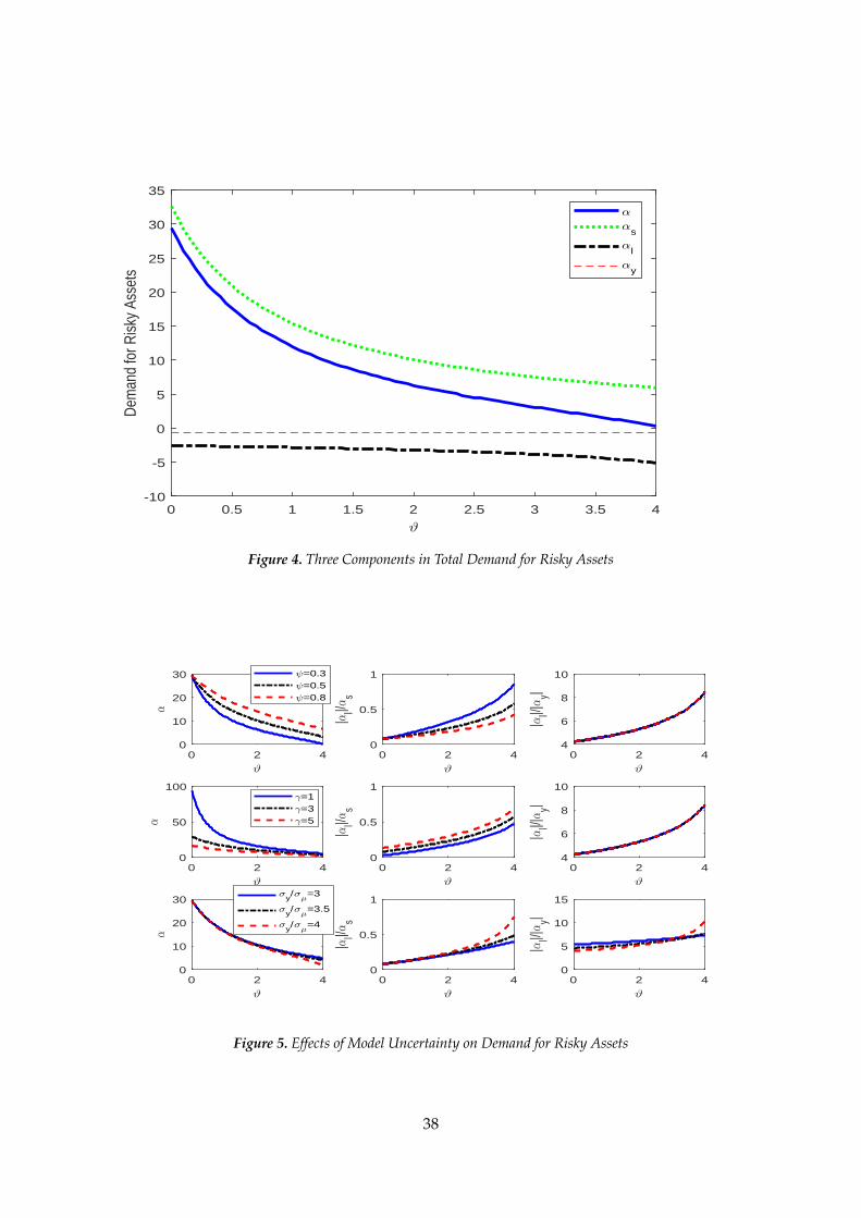
0 0.5 1 1.5 2 2.5 3 3.5 4-10

-5

0

5

10

15

20

25

30

35

Dem

and

for R

isky

Asse

ts

s

l

y

Figure 4. Three Components in Total Demand for Risky Assets

0 2 40

10

20

30 =0.3=0.5=0.8

0 2 40

0.5

1

|l|/

s

0 2 44

6

8

10

|l|/|

y|

0 2 40

50

100=1=3=5

0 2 40

0.5

1

|l|/

s

0 2 44

6

8

10

|l|/|

y|

0 2 40

10

20

30 y/ =3

y/ =3.5

y/ =4

0 2 40

0.5

1

|l|/

s

0 2 40

5

10

15

|l|/|

y|

Figure 5. Effects of Model Uncertainty on Demand for Risky Assets

38

ϑ

0 0.5 1 1.5 2 2.5 3 3.5

Ω

0

0.005

0.01

0.015

0.02

0.025

0.03

0.035

0.04

0.045

σy/σ

µ=3

σy/σ

µ=3.5

σy/σ

µ=4

Figure 6. The Marginal Welfare Costs of Ignorance

ϑ

1 1.5 2 2.5 3 3.5

∆

0.05

0.1

0.15

0.2

0.25

0.3

0.35

0.4

0.45

0.5

0.55

σy/σ

µ=3

σy/σ

µ=3.5

σy/σ

µ=4

Figure 7. The Total Welfare Costs of Ignorance

39

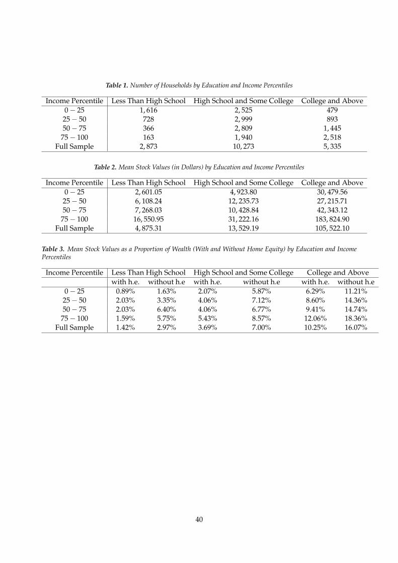
Table 1. Number of Households by Education and Income Percentiles

Income Percentile Less Than High School High School and Some College College and Above0− 25 1, 616 2, 525 47925− 50 728 2, 999 89350− 75 366 2, 809 1, 44575− 100 163 1, 940 2, 518

Full Sample 2, 873 10, 273 5, 335

Table 2. Mean Stock Values (in Dollars) by Education and Income Percentiles

Income Percentile Less Than High School High School and Some College College and Above0− 25 2, 601.05 4, 923.80 30, 479.5625− 50 6, 108.24 12, 235.73 27, 215.7150− 75 7, 268.03 10, 428.84 42, 343.1275− 100 16, 550.95 31, 222.16 183, 824.90

Full Sample 4, 875.31 13, 529.19 105, 522.10

Table 3. Mean Stock Values as a Proportion of Wealth (With and Without Home Equity) by Education and IncomePercentiles

Income Percentile Less Than High School High School and Some College College and Abovewith h.e. without h.e with h.e. without h.e with h.e. without h.e

0− 25 0.89% 1.63% 2.07% 5.87% 6.29% 11.21%25− 50 2.03% 3.35% 4.06% 7.12% 8.60% 14.36%50− 75 2.03% 6.40% 4.06% 6.77% 9.41% 14.74%75− 100 1.59% 5.75% 5.43% 8.57% 12.06% 18.36%

Full Sample 1.42% 2.97% 3.69% 7.00% 10.25% 16.07%

40

Table 4. Calibrating RB Parameter (ϑ) using Risky Asset Holdings (α)

≤ High School High School & Some College College & AboveDataRisky-Asset Holding, α (Data) 1 (normalized) 2.8 21.4PU Parameter, σy

σµ(Data) 5.90 2.78 2.57

Calibration ResultsMU Parameter, ϑ (Model) 5.5 4.0 0Corresponding DEP 0.04 0.16 0.50

Models’ Performanceα (Benchmark Model) 1 (normalized) 2.8 21.4α (FI-RE Model) 1 (normalized) 1 1

41