1SCIENTIFIC RepoRtS | 7: 7968 | DOI:10.1038/s41598-017-08532-7

www.nature.com/scientificreports

Identification of mega-environments and rice genotypes for general and specific adaptation to saline and alkaline stresses in IndiaS. L. Krishnamurthy1, P. C. Sharma1, D. K. Sharma1, K. T. Ravikiran1, Y. P. Singh2, V. K. Mishra2, D. Burman3, B. Maji3, S. Mandal3, S. K. Sarangi3, R. K. Gautam4, P. K. Singh4, K. K. Manohara5, B. C. Marandi6, G. Padmavathi7, P. B. Vanve8, K. D. Patil8, S. Thirumeni9, O. P. Verma10, A. H. Khan10, S. Tiwari11, S. Geetha12, M. Shakila12, R Gill13, V. K. Yadav14, S. K. B. Roy15, M. Prakash16, J. Bonifacio17, Abdelbagi Ismail 18, G. B. Gregorio17 & Rakesh Kumar Singh17

In the present study, a total of 53 promising salt-tolerant genotypes were tested across 18 salt-affected diverse locations for three years. An attempt was made to identify ideal test locations and mega-environments using GGE biplot analysis. The CSSRI sodic environment was the most discriminating location in individual years as well as over the years and could be used to screen out unstable and salt-sensitive genotypes. Genotypes CSR36, CSR-2K-219, and CSR-2K-262 were found ideal across years. Overall, Genotypes CSR-2K-219, CSR-2K-262, and CSR-2K-242 were found superior and stable among all genotypes with higher mean yields. Different sets of genotypes emerged as winners in saline soils but not in sodic soils; however, Genotype CSR-2K-262 was the only genotype that was best under both saline and alkaline environments over the years. The lack of repeatable associations among locations and repeatable mega-environment groupings indicated the complexity of soil salinity. Hence, a multi-location and multi-year evaluation is indispensable for evaluating the test sites as well as identifying genotypes with consistently specific and wider adaptation to particular agro-climatic zones. The genotypes identified in the present study could be used for commercial cultivation across edaphically challenged areas for sustainable production.

Soil salinity negatively affects agricultural production worldwide. More than 800 million hectares of land globally are salt-affected, including both saline and sodic soils, which represent more than 6% of the world’s total land area1. In India, 6.73 million ha are under salt-affected area2. Rice is considered salt-sensitive as it is not efficient in controlling the influx of Na+ through the roots, leading to a rapid accumulation of toxic concentrations in

1Central Soil Salinity Research Institute, Karnal, India. 2Central Soil Salinity Research Institute, Regional Research Station, Lucknow, India. 3Central Soil Salinity Research Institute, Regional Research Station, Canning Town, India. 4Central Island Agricultural Research Institute, Port Blair, A & N Islands, India. 5Central Coastal Agricultural Research Institute (CCARI), Ela, Goa, India. 6National Rice Research Institute (NRRI), Cuttack, Odisha, India. 7Indian Institute of Rice Research, Telengana, India. 8Dr. Balasaheb Sawant Konkan KrishiVidyapeeth, Khar Land, Panvel, India. 9Pandit Jawaharlal Nehru College of Agriculture and Research Institute, Karaikal, India. 10Narendra Deva University of Agriculture & Technology, Faizabad, Uttar Pradesh, India. 11Rajendra Agricultural University, Samastipur, India. 12Anbil Dharmalingam Agricultural College and Research Institute, Trichy, India. 13Punjab Agricultural University, Ludhiana, India. 14Chandra Shekhar Azad University of Agriculture & Technology, Kanpur, Uttar Pradesh, India. 15Centre for Strategic Studies, Salt Lake City, India. 16Annamalai University, Chidambaram, Tamil Nadu, India. 17Division of Plant Breeding, IRRI, Philippines. 18Crop and Environmental Sciences Division, IRRI, Philippines. Correspondence and requests for materials should be addressed to S.L.K. (email: krishnagene@gmail.com) or R.S. (email: r.k.singh@irri.org)

Received: 5 October 2016

Accepted: 14 July 2017

Published: xx xx xxxx

OPEN

www.nature.com/scientificreports/

2SCIENTIFIC RepoRtS | 7: 7968 | DOI:10.1038/s41598-017-08532-7

aboveground parts3–5. The problem of salinity has been addressed through better management practices and the introduction of salt-tolerant varieties in affected areas. These high-yielding stress-tolerant rice varieties are expected to provide a yield advantage of about 2 t ha−1 on these soils6. Thus, genetic improvement of salt toler-ance in rice appears to be economically feasible and a promising strategy for maintaining stable rice production globally7–9. Initial activities toward such efforts involve testing promising lines bred for salinity tolerance across various salt stress locations to assess their stability and to quantify the effect of genotype × environment (G × E) interactions on the growth and yield of these genotypes. But, studies on evaluating various rice genotypes across different salinity stress locations are quite meager and there is a need to understand the dynamics of cultivar behavior under various stress locations. Moreover, given the same level of salt stress across locations, ambient environmental differences might create variation in the performance of a single variety. Substantial area in India is affected by salt stress; hence, it is imperative to identify certain “hot spots” for evaluating genotypes for their actual value for salt tolerance. Because soil salinity is a much more dynamic state than alkalinity, site variations within saline soils over the years also affect trials considerably in such cases. Therefore, the present study seeks to identify superior cultivars for target regions over the years and to evaluate the possibility of subdividing the target regions into different environmental groups. By this, environments with similar interaction with genotypes can be merged, thus decreasing the cost of conducting field trials without compromising the repeatability of the trials. These objectives can be efficiently realized through the GGE biplot analysis technique.

The GGE biplot methodology consists of a set of biplots from which information regarding genotype and test environment evaluation can be interpreted. A biplot is a scatter plot that approximates and graphically displays a two-way table by both its row and column factors such that relationships among the row factors, relationships among the column factors, and the underlying interactions between row and column factors can be visualized simultaneously10, 11. The first application of biplots to agricultural data analysis for model selection was made on data from a performance trial of cotton genotypes12. This was followed by the application of biplots for the analysis of genotype by environment tables13–16. The biplot tool has become increasingly popular among plant breeders and other agricultural researchers since its use in cultivar evaluation and mega-environment analysis was established17. Biplots display both G (genotype main effects) and G × E (genotype × environment interaction) components, which are the two important sources of variation that are relevant to cultivar evaluation and have to be considered simultaneously for appropriate genotype and environment evaluation18–20. A “which-won-where” view of biplots can be used to demarcate distinct mega-environments to identify the best-performing geno-types in the corresponding environments21. The use of biplots has also been extended to visual analyses of other breeding-related data22, host by pathogen interactions23, diallel cross tables24, microarray data25, and QTL by environment interactions26. Significant improvement, modifications, and refinements took place in GGE biplot analysis leading to the evolution of different types of GGE biplots such as standard deviation (SD)-based, stand-ard error (SE)-based, and heritability adjusted (HA) biplots. Among these, HA-GGE biplots had been argued to be efficient in evaluating environments and genotypes from multi-location trials (MLTs)27. Biplot analysis has also been tried in rice for genotype and environment evaluation28, 29 and for line × tester data30, etc. But, GGE biplots have not been efficiently used for studies on the performance of genotypes across various salinity stress locations except by Sharifi (2012), who selected the best parents for salinity tolerance-contributing traits based on general combining ability (GCA) and specific combining ability (SCA) estimates depicted on a GGE biplot31. Hence, the current study was undertaken to appraise the effect of G × E interaction on the grain yield of 53 promising rice genotypes tested across 18 saline and alkaline stress locations for three consecutive years (2011 to 2013) and ana-lyzed for their value using the HA-GGE biplot technique (hereinafter in text will be denoted as GGE only). The main aim was to group various stress locations into distinct mega-environments so that locations with a similar effect on the genotypes could be discontinued for testing in the future and to identify the best locations for future testing, and to ascertain the stable and superior genotypes that could be used as varieties or suitable donors for a particular mega-environment or for wider adaptation across salt stress environments.

ResultsAnalysis of variance. Analysis of variance was done for the yield data from individual years (2011, 2012, and 2013) and three-year (2011–13) combinations (Tables 1 and 2). The results indicated that genotype, location, and genotype × location effects were significant in all three years (2011, 2012, and 2013) as well as in combined analysis for three years (2011–13). Additionally, the relative contribution of each source of variation to the total sum of squares was calculated for comparison.

Genotype by location (G × L) contributed the most (44.39%) to the total variation, closely followed by location (43.05%), during 2011. The effect of location remained highest (66.41% and 65.40%) in 2012 and 2013, respec-tively. Genotypes had greater interaction effects with locations or locations by year but the per se contribution was observed to be 7.35%, 6.62%, and 4.4% in 2011, 2012, and 2013, respectively, which was quite less comparatively. We noticed a profound effect of location (40.52%) in 2011–13. The main effects (G and Y) and genotype by year (G × Y) showed smaller effects than other sources of variation. Overall, the impact of different factors on yield can be ordered as Location (L) > Location × Year > Genotype × Location > Genotype × Location × Year > Year > Genotype > Genotype × Year. The different summary statistical parameters, mean, standard error, and standard deviation were estimated in different years (Supplementary Table 1).

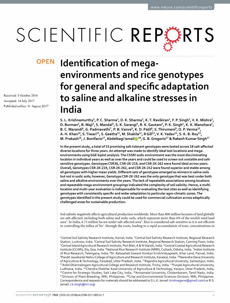
Evaluation of test environments. The biplot explained 51.7%, 44.6%, and 70.5% of the total variation of the environments in 2011, 2012, and 2013, respectively. GGE biplot showed two distinct clusters in 2011: one con-taining BSKKV, Kharland RS, Panvel (E10); CCARI, Goa (E4); and ADACRI, Trichy (E12), and the other contain-ing IIRR, Machilipatnam (E3); CSSRI, Karnal sodic environment (E7); NRRI, Cuttack (E2); and CSSRI, Karnal saline environment (E6) (Fig. 1a). The closest association was observed between the environments BSKKV, Kharland RS, Panvel (E10), and CCARI, Goa (E4). The location NDUAT, Faizabad (E9) showed negative or no

www.nature.com/scientificreports/

3SCIENTIFIC RepoRtS | 7: 7968 | DOI:10.1038/s41598-017-08532-7

correlation with most of the locations (except CIARI, Port Blair (E1) and PAJANCOA, Karaikal, Puducherry (E5)) and hence can be considered distinct. CSSRI, Karnal saline environment (E6) had the longest vector and hence was a highly discriminating location (Fig. 1a). But, its angle with the AEA is greater and hence less repre-sentative of other environments. The location ADACRI, Trichy (E12) was highly representative of other locations. Considering the above two qualities together, ADACRI, Trichy (E12) was the ideal location for testing genotypes for salt tolerance with its appreciable discriminating ability and representativeness (Supplementary Table 2). RAU, Pusa, Bihar (E11) showed the least discriminating ability and the locations NDUAT, Faizabad (E9) and CIARI, Port Blair (E1) were the least representative of other locations. There were three clusters of environments in 2012: CSSRI RRS, Canning Town (E13); IIRR, Machilipatnam (E3); and RAU, Pusa, Bihar (E11). Among these three, E13 and E3 were closely associated (Fig. 1b). The second cluster consisted of ADACRI, Trichy (E12); CSS, Kolkata (E14); and CIARI, Port Blair (E1), and the other contained the remaining environments. CSSRI Karnal sodic envi-ronment (E7) had the longest vector and hence was highly discriminating. The locations CSSRI RRS, Lucknow (E8); CSSRI Karnal sodic environment (E7); and NDUAT, Faizabad were highly representative environments (Fig. 1b). The remaining locations displayed medium to high discriminating power in 2012. Overall, the location CSSRI Karnal sodic environment (E7) can be considered ideal for evaluating genotypes. RAU, Pusa, Bihar (E11) was the least consistent (representative) location in 2012. GGE biplot showed four clusters in 2013 (Fig. 1c). The first cluster contained coastal locations such as CCARI, Goa (E4) and PAJANCOA, Karaikal, Puducherry (E5); the second contained mostly inland saline and alkaline locations – CSSRI, Karnal saline environment (E6); CSSRI, Karnal sodic environment (E7); CSSRI RRS, Lucknow (E8); NDUAT, Faizabad (E9); PAU, Ludhiana (17); and CSSRI, Nain Farm, Panipat (E18). Among these, CSSRI, Karnal saline environment (E6) was more associated with CSSRI, Nain Farm, Panipat (E18), and CSSRI RRS, Lucknow (E8) with NDUAT, Faizabad (E9). The third cluster contained RAU, Pusa, Bihar (E11); CIARI, Port Blair (E1); BSKKV, Kharland RS, Panvel (E10); and CSS, Kolkata (E14). Among these four locations, the first two and the last two were more closely associated.

Source

2011 Percent contribution to total SS

2012 Percent contribution to total SS

2013 Percent contribution to total SSdf MS df MS df MS

Genotype (G) 24 4251672** 7.35 29 5828938** 6.62 30 4089298** 4.4

Location (L) 11 54308145** 43.05 13 1.3E + 08** 66.41 16 1.13E + 08** 65.4

G × L 251 2454228** 44.39 362 1542148** 21.86 440 1393591** 22.1

Blocking 24 321024 0.56 28 604290.4 0.66 34 478228.4 0.6

Error 541 119245.2 781 145545 929 222628.7

Grand mean (kg ha−1) 1904.917 2385.858 2649.604

SE (kg ha−1) 345.319 381.5035 471.8354

LSD0.05 (kg ha−1) 565.1532 624.3732 772.2114

CV (%) 18.13 15.99 17.81

H (Vg/Vp) 0.42 0.74 0.66

Table 1. ANOVA and basic statistics in individual years (2011, 2012, and 2013). df = degrees of freedom; MS = mean square; SS = sum of squares; ** = significant at 1% level of probability.

Source

2011–13

Df MSPercent contribution to total SS

Genotype (G) 12 4876627** 1.64

Year (Y) 2 61830663** 3.46

Location (L) 17 85264239** 40.52

L × Y 23 36226572** 23.29

Block (L × Y) 86 353283.8** 0.85

G × Y 24 1929503** 1.29

G × L 200 2348058** 13.13

G × L × Y 273 1483738** 11.32

Error 1011 158898.4

Grand mean (kg ha−1) 2549.09

SE (kg ha−1) 398.62

LSD0.05 I (kg ha−1) 653.77

LSD0.05 II (kg ha−1) 856.99

CV (%) 15.64

H (Vg/Vp) 0.43

Table 2. ANOVA and basic statistics across three years (2011–13). Df = degrees of freedom; MS = mean square; SS = sum of squares; **− = Significant at 1% level of probability.

www.nature.com/scientificreports/

4SCIENTIFIC RepoRtS | 7: 7968 | DOI:10.1038/s41598-017-08532-7

The remaining environments were in the fourth and final cluster. CSSRI, Karnal sodic environment (E7) repeated the same performance as in 2012 as it had the longest vector, making it more discriminating than other environ-ments, and the environment NDUAT, Faizabad (E9) showed a smaller angle with the AEA and hence was a highly representative environment (Fig. 1c) in 2013.

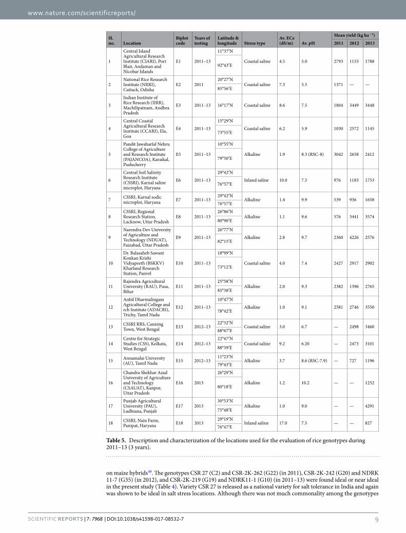
The discriminating ability, representativeness estimates, and desirability index of different locations were pooled and the mean values are presented in Table 3. The locations CSSRI, experimental farm, Nain (E18) and PAU, Ludhiana (E17) showed high discriminating power and come under the most desirable locations. But, these locations were included in the trial only in 2013 and are based on a single year’s values; hence, these could be downplayed for now. Besides these two locations, Karnal sodic environment (E7; 1.82) showed the highest discriminating ability, followed by Karnal saline environment (E6; 1.67), and carries the highest desirability index value based on three years of data. Desirability index is the overall manifestation of pooled performance based on the discriminatory power of a location and representativeness; therefore, it could be a better parameter to identify better locations for experimental setup. Other relatively desirable locations are CSSRI RRS, Lucknow (E8), NDUAT, Faizabad (E9), BSKKV, Kharland RS, Panvel (E10), and CCARI, Goa (E4). The location CSAUT, Kanpur had weak discriminating ability (E16; 0.24). The remaining locations possessed appreciable discrimi-nating ability, with values ranging from 0.58 (ADACRI, Trichy, E12) to 0.94 (BSKKV, Kharland RS, Panvel, E10, and CSSRI RRS, Lucknow, E8). Similar to discriminatory power, PAU, Ludhiana (E17) and CSSRI, experimental farm, Nain (E18) showed high representativeness but again based on a single year (2013) of data; however, CSSRI RRS, Lucknow (E8; 0.98) and saline and sodic/alkaline microplots in Karnal (E6 and E7) showed high repre-sentativeness compared with all locations (based on three years). Many environments did not appear as good

Figure 1. Association among the test environments and distance from the ideal genotype, based on the average environmental coordinate (AEC), considering stability and adaptability of rice genotypes evaluated across saline and alkaline environments for grain yield in (a) 2011, (b) 2012, and (c) 2013 growing seasons.

LocationDiscriminating power Mean ± SD

Representativeness Mean ± SD

Desirability index Mean ± SD

E1 0.77 ± 0.09 0.00 ± 0.63 0.10 ± 0.57

E2 0.73 ± 0.00 0.41 ± 0.00 0.15 ± 0.00

E3 0.70 ± 0.62 0.23 ± 0.39 0.14 ± 0.35

E4 1.03 ± 0.27 0.34 ± 1.08 0.50 ± 1.03

E5 0.89 ± 0.41 0.22 ± 0.89 0.34 ± 0.65

E6 1.67 ± 0.57 0.80 ± 0.25 1.35 ± 0.63

E7 1.82 ± 0.78 0.90 ± 0.14 1.67 ± 0.85

E8 0.94 ± 0.44 0.98 ± 0.02 0.94 ± 0.49

E9 1.01 ± 0.23 0.42 ± 1.00 0.61 ± 1.02

E10 0.94 ± 0.35 0.61 ± 0.59 0.75 ± 0.68

E11 0.63 ± 0.43 0.05 ± 0.86 0.01 ± 0.50

E12 0.58 ± 0.41 0.10 ± 1.01 0.34 ± 0.55

E13 0.84 ± 0.70 0.38 ± 0.43 0.04 ± 0.31

E14 0.84 ± 0.22 0.09 ± 0.10 0.22 ± 0.07

E15 0.49 ± 0.35 −0.03 ± 1.28 0.25 ± 0.57

E16 0.24 ± 0.00 −0.80 ± 0.00 −0.14 ± 0.00

E17 2.12 ± 0.00 1.00 ± 0.00 2.16 ± 0.00

E18 2.15 ± 0.00 0.94 ± 0.00 2.04 ± 0.00

Table 3. Standardized test location evaluation parameters.

www.nature.com/scientificreports/

5SCIENTIFIC RepoRtS | 7: 7968 | DOI:10.1038/s41598-017-08532-7

locations due to low desirability index (CIARI, Port Blair (E1), NRRI, Cuttack (E2), IIRR, Machilipatnam (E3), RAU, Pusa, Bihar (E11), CSSRI RRS, Canning Town (E13), and CSAUAT, Kanpur (E16)) and most of them were saline environments.

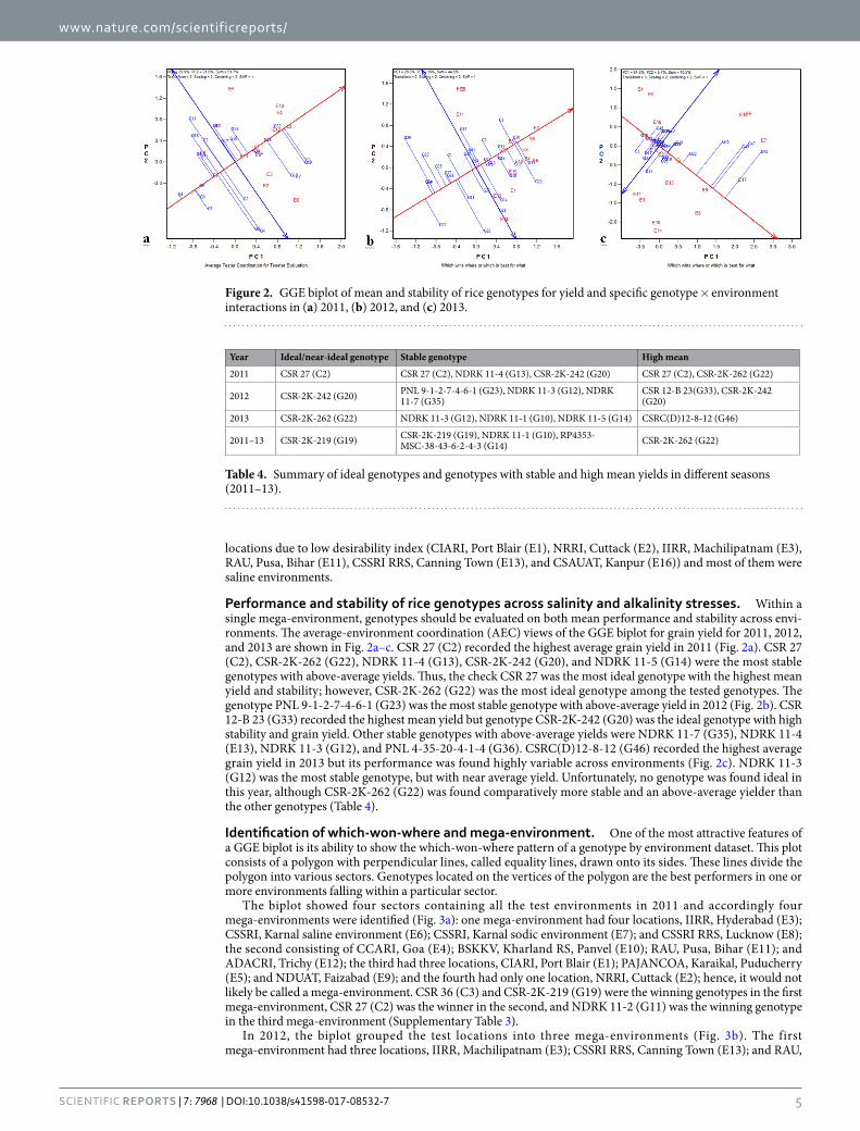
Performance and stability of rice genotypes across salinity and alkalinity stresses. Within a single mega-environment, genotypes should be evaluated on both mean performance and stability across envi-ronments. The average-environment coordination (AEC) views of the GGE biplot for grain yield for 2011, 2012, and 2013 are shown in Fig. 2a–c. CSR 27 (C2) recorded the highest average grain yield in 2011 (Fig. 2a). CSR 27 (C2), CSR-2K-262 (G22), NDRK 11-4 (G13), CSR-2K-242 (G20), and NDRK 11-5 (G14) were the most stable genotypes with above-average yields. Thus, the check CSR 27 was the most ideal genotype with the highest mean yield and stability; however, CSR-2K-262 (G22) was the most ideal genotype among the tested genotypes. The genotype PNL 9-1-2-7-4-6-1 (G23) was the most stable genotype with above-average yield in 2012 (Fig. 2b). CSR 12-B 23 (G33) recorded the highest mean yield but genotype CSR-2K-242 (G20) was the ideal genotype with high stability and grain yield. Other stable genotypes with above-average yields were NDRK 11-7 (G35), NDRK 11-4 (E13), NDRK 11-3 (G12), and PNL 4-35-20-4-1-4 (G36). CSRC(D)12-8-12 (G46) recorded the highest average grain yield in 2013 but its performance was found highly variable across environments (Fig. 2c). NDRK 11-3 (G12) was the most stable genotype, but with near average yield. Unfortunately, no genotype was found ideal in this year, although CSR-2K-262 (G22) was found comparatively more stable and an above-average yielder than the other genotypes (Table 4).

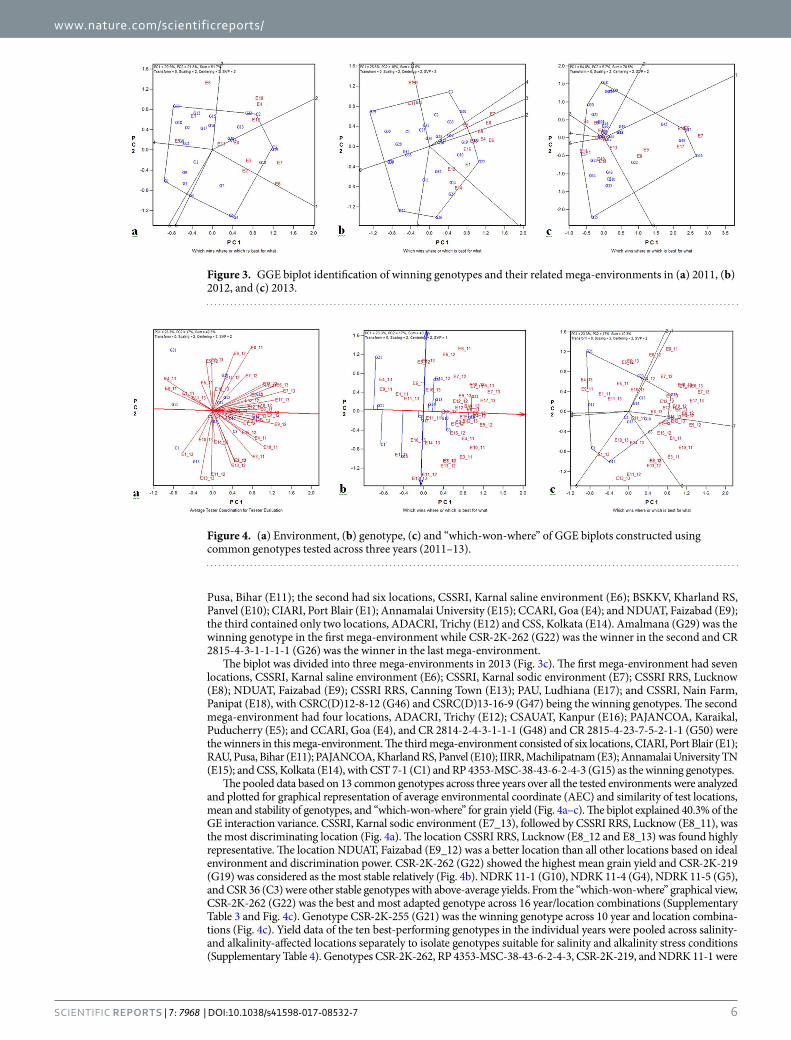
Identification of which-won-where and mega-environment. One of the most attractive features of a GGE biplot is its ability to show the which-won-where pattern of a genotype by environment dataset. This plot consists of a polygon with perpendicular lines, called equality lines, drawn onto its sides. These lines divide the polygon into various sectors. Genotypes located on the vertices of the polygon are the best performers in one or more environments falling within a particular sector.

The biplot showed four sectors containing all the test environments in 2011 and accordingly four mega-environments were identified (Fig. 3a): one mega-environment had four locations, IIRR, Hyderabad (E3); CSSRI, Karnal saline environment (E6); CSSRI, Karnal sodic environment (E7); and CSSRI RRS, Lucknow (E8); the second consisting of CCARI, Goa (E4); BSKKV, Kharland RS, Panvel (E10); RAU, Pusa, Bihar (E11); and ADACRI, Trichy (E12); the third had three locations, CIARI, Port Blair (E1); PAJANCOA, Karaikal, Puducherry (E5); and NDUAT, Faizabad (E9); and the fourth had only one location, NRRI, Cuttack (E2); hence, it would not likely be called a mega-environment. CSR 36 (C3) and CSR-2K-219 (G19) were the winning genotypes in the first mega-environment, CSR 27 (C2) was the winner in the second, and NDRK 11-2 (G11) was the winning genotype in the third mega-environment (Supplementary Table 3).

In 2012, the biplot grouped the test locations into three mega-environments (Fig.  3b). The first mega-environment had three locations, IIRR, Machilipatnam (E3); CSSRI RRS, Canning Town (E13); and RAU,

Figure 2. GGE biplot of mean and stability of rice genotypes for yield and specific genotype × environment interactions in (a) 2011, (b) 2012, and (c) 2013.

Year Ideal/near-ideal genotype Stable genotype High mean

2011 CSR 27 (C2) CSR 27 (C2), NDRK 11-4 (G13), CSR-2K-242 (G20) CSR 27 (C2), CSR-2K-262 (G22)

2012 CSR-2K-242 (G20) PNL 9-1-2-7-4-6-1 (G23), NDRK 11-3 (G12), NDRK 11-7 (G35)

CSR 12-B 23(G33), CSR-2K-242 (G20)

2013 CSR-2K-262 (G22) NDRK 11-3 (G12), NDRK 11-1 (G10), NDRK 11-5 (G14) CSRC(D)12-8-12 (G46)

2011–13 CSR-2K-219 (G19) CSR-2K-219 (G19), NDRK 11-1 (G10), RP4353-MSC-38-43-6-2-4-3 (G14) CSR-2K-262 (G22)

Table 4. Summary of ideal genotypes and genotypes with stable and high mean yields in different seasons (2011–13).

www.nature.com/scientificreports/

6SCIENTIFIC RepoRtS | 7: 7968 | DOI:10.1038/s41598-017-08532-7

Pusa, Bihar (E11); the second had six locations, CSSRI, Karnal saline environment (E6); BSKKV, Kharland RS, Panvel (E10); CIARI, Port Blair (E1); Annamalai University (E15); CCARI, Goa (E4); and NDUAT, Faizabad (E9); the third contained only two locations, ADACRI, Trichy (E12) and CSS, Kolkata (E14). Amalmana (G29) was the winning genotype in the first mega-environment while CSR-2K-262 (G22) was the winner in the second and CR 2815-4-3-1-1-1-1 (G26) was the winner in the last mega-environment.

The biplot was divided into three mega-environments in 2013 (Fig. 3c). The first mega-environment had seven locations, CSSRI, Karnal saline environment (E6); CSSRI, Karnal sodic environment (E7); CSSRI RRS, Lucknow (E8); NDUAT, Faizabad (E9); CSSRI RRS, Canning Town (E13); PAU, Ludhiana (E17); and CSSRI, Nain Farm, Panipat (E18), with CSRC(D)12-8-12 (G46) and CSRC(D)13-16-9 (G47) being the winning genotypes. The second mega-environment had four locations, ADACRI, Trichy (E12); CSAUAT, Kanpur (E16); PAJANCOA, Karaikal, Puducherry (E5); and CCARI, Goa (E4), and CR 2814-2-4-3-1-1-1 (G48) and CR 2815-4-23-7-5-2-1-1 (G50) were the winners in this mega-environment. The third mega-environment consisted of six locations, CIARI, Port Blair (E1); RAU, Pusa, Bihar (E11); PAJANCOA, Kharland RS, Panvel (E10); IIRR, Machilipatnam (E3); Annamalai University TN (E15); and CSS, Kolkata (E14), with CST 7-1 (C1) and RP 4353-MSC-38-43-6-2-4-3 (G15) as the winning genotypes.

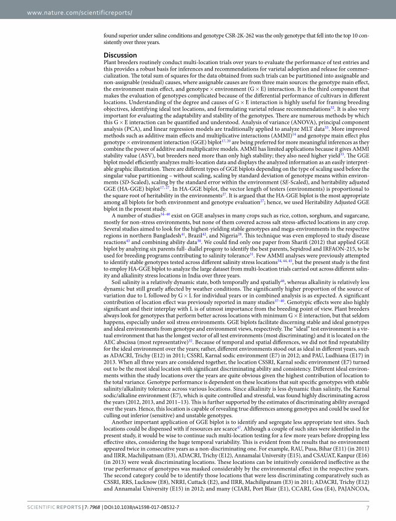
The pooled data based on 13 common genotypes across three years over all the tested environments were analyzed and plotted for graphical representation of average environmental coordinate (AEC) and similarity of test locations, mean and stability of genotypes, and “which-won-where” for grain yield (Fig. 4a–c). The biplot explained 40.3% of the GE interaction variance. CSSRI, Karnal sodic environment (E7_13), followed by CSSRI RRS, Lucknow (E8_11), was the most discriminating location (Fig. 4a). The location CSSRI RRS, Lucknow (E8_12 and E8_13) was found highly representative. The location NDUAT, Faizabad (E9_12) was a better location than all other locations based on ideal environment and discrimination power. CSR-2K-262 (G22) showed the highest mean grain yield and CSR-2K-219 (G19) was considered as the most stable relatively (Fig. 4b). NDRK 11-1 (G10), NDRK 11-4 (G4), NDRK 11-5 (G5), and CSR 36 (C3) were other stable genotypes with above-average yields. From the “which-won-where” graphical view, CSR-2K-262 (G22) was the best and most adapted genotype across 16 year/location combinations (Supplementary Table 3 and Fig. 4c). Genotype CSR-2K-255 (G21) was the winning genotype across 10 year and location combina-tions (Fig. 4c). Yield data of the ten best-performing genotypes in the individual years were pooled across salinity- and alkalinity-affected locations separately to isolate genotypes suitable for salinity and alkalinity stress conditions (Supplementary Table 4). Genotypes CSR-2K-262, RP 4353-MSC-38-43-6-2-4-3, CSR-2K-219, and NDRK 11-1 were

Figure 3. GGE biplot identification of winning genotypes and their related mega-environments in (a) 2011, (b) 2012, and (c) 2013.

Figure 4. (a) Environment, (b) genotype, (c) and “which-won-where” of GGE biplots constructed using common genotypes tested across three years (2011–13).

www.nature.com/scientificreports/

7SCIENTIFIC RepoRtS | 7: 7968 | DOI:10.1038/s41598-017-08532-7

found superior under saline conditions and genotype CSR-2K-262 was the only genotype that fell into the top 10 con-sistently over three years.

DiscussionPlant breeders routinely conduct multi-location trials over years to evaluate the performance of test entries and this provides a robust basis for inferences and recommendations for varietal adoption and release for commer-cialization. The total sum of squares for the data obtained from such trials can be partitioned into assignable and non-assignable (residual) causes, where assignable causes are from three main sources: the genotype main effect, the environment main effect, and genotype × environment (G × E) interaction. It is the third component that makes the evaluation of genotypes complicated because of the differential performance of cultivars in different locations. Understanding of the degree and causes of G × E interaction is highly useful for framing breeding objectives, identifying ideal test locations, and formulating varietal release recommendations32. It is also very important for evaluating the adaptability and stability of the genotypes. There are numerous methods by which this G × E interaction can be quantified and understood. Analysis of variance (ANOVA), principal component analysis (PCA), and linear regression models are traditionally applied to analyze MLT data33. More improved methods such as additive main effects and multiplicative interactions (AMMI)14 and genotype main effect plus genotype × environment interaction (GGE) biplot17, 20 are being preferred for more meaningful inferences as they combine the power of additive and multiplicative models. AMMI has limited applications because it gives AMMI stability value (ASV), but breeders need more than only high stability; they also need higher yield33. The GGE biplot model efficiently analyzes multi-location data and displays the analyzed information as an easily interpret-able graphic illustration. There are different types of GGE biplots depending on the type of scaling used before the singular value partitioning – without scaling, scaling by standard deviation of genotype means within environ-ments (SD-Scaled), scaling by the standard error within the environment (SE-Scaled), and heritability adjusted GGE (HA-GGE) biplot17, 27. In HA-GGE biplot, the vector length of testers (environments) is proportional to the square root of heritability in the environments27. It is argued that the HA-GGE biplot is the most appropriate among all biplots for both environment and genotype evaluation27; hence, we used Heritability Adjusted GGE biplot in the present study.

A number of studies34–40 exist on GGE analyses in many crops such as rice, cotton, sorghum, and sugarcane, mostly for non-stress environments, but none of them covered across salt stress-affected locations in any crop. Several studies aimed to look for the highest-yielding stable genotypes and mega-environments in the respective regions in northern Bangladesh41, Brazil42, and Nigeria28. This technique was even employed to study disease reactions43 and combining ability data30. We could find only one paper from Sharifi (2012) that applied GGE biplot by analyzing six parents full- diallel progeny to identify the best parents, Sepidrod and IRFAON-215, to be used for breeding programs contributing to salinity tolerance31. Few AMMI analyses were previously attempted to identify stable genotypes tested across different salinity stress locations34, 44, 45, but the present study is the first to employ HA-GGE biplot to analyze the large dataset from multi-location trials carried out across different salin-ity and alkalinity stress locations in India over three years.

Soil salinity is a relatively dynamic state, both temporally and spatially46, whereas alkalinity is relatively less dynamic but still greatly affected by weather conditions. The significantly higher proportion of the source of variation due to L followed by G × L for individual years or in combined analysis is as expected. A significant contribution of location effect was previously reported in many studies37–40. Genotypic effects were also highly significant and their interplay with L is of utmost importance from the breeding point of view. Plant breeders always look for genotypes that perform better across locations with minimum G × E interaction, but that seldom happens, especially under soil stress environments. GGE biplots facilitate discerning stable and ideal genotypes and ideal environments from genotype and environment views, respectively. The “ideal” test environment is a vir-tual environment that has the longest vector of all test environments (most discriminating) and it is located on the AEC abscissa (most representative)32. Because of temporal and spatial differences, we did not find repeatability for the ideal environment over the years; rather, different environments stood out as ideal in different years, such as ADACRI, Trichy (E12) in 2011; CSSRI, Karnal sodic environment (E7) in 2012; and PAU, Ludhiana (E17) in 2013. When all three years are considered together, the location CSSRI, Karnal sodic environment (E7) turned out to be the most ideal location with significant discriminating ability and consistency. Different ideal environ-ments within the study locations over the years are quite obvious given the highest contribution of location to the total variance. Genotype performance is dependent on these locations that suit specific genotypes with stable salinity/alkalinity tolerance across various locations. Since alkalinity is less dynamic than salinity, the Karnal sodic/alkaline environment (E7), which is quite controlled and stressful, was found highly discriminating across the years (2012, 2013, and 2011–13). This is further supported by the estimates of discriminating ability averaged over the years. Hence, this location is capable of revealing true differences among genotypes and could be used for culling out inferior (sensitive) and unstable genotypes.

Another important application of GGE biplot is to identify and segregate less appropriate test sites. Such locations could be dispensed with if resources are scarce47. Although a couple of such sites were identified in the present study, it would be wise to continue such multi-location testing for a few more years before dropping less effective sites, considering the huge temporal variability. This is evident from the results that no environment appeared twice in consecutive years as a non-discriminating one. For example, RAU, Pusa, Bihar (E11) (in 2011) and IIRR, Machilipatnam (E3), ADACRI, Trichy (E12), Annamalai University (E15), and CSAUAT, Kanpur (E16) (in 2013) were weak discriminating locations. These locations can be intuitively considered ineffective as the true performance of genotypes was masked considerably by the environmental effect in the respective years. The second category could be to identify those locations that were less discriminating comparatively such as CSSRI, RRS, Lucknow (E8), NRRI, Cuttack (E2), and IIRR, Machilipatnam (E3) in 2011; ADACRI, Trichy (E12) and Annamalai University (E15) in 2012; and many (CIARI, Port Blair (E1), CCARI, Goa (E4), PAJANCOA,

www.nature.com/scientificreports/

8SCIENTIFIC RepoRtS | 7: 7968 | DOI:10.1038/s41598-017-08532-7

Puducherry (E5), BSKKV, Kharland RS, Panvel (E10), RAU, Pusa, Bihar (E11), CSSRI, RRS, Canning Town (E13), and CSS, Kolkata (E14)) in 2013. Such variation for the discriminating ability of the locations over years suggests that decisions on continuing or dropping a location should be made only after series of tests over years, not based on two or three years of data, as a short period of information about locations could mislead the inferences27. Locations such as ADACRI, Trichy (E12), which was not highly discriminative but was representative in 2011, turned into a non-representative location with moderate discriminating ability in 2012. The same location in 2013 was neither discriminating nor representative. Contrary to this example, the CSSRI, Karnal saline microplots (E6) were non-representative of the ideal environment in 2011 but were less discriminative but more representative in 2012, but were found to be a near-to-representative and better discriminative environment.

This is also evident from the desirability index. One year of data showed the highest desirability for PAU, Ludhiana (E17) and CSSRI, Nain Farm (E18), but there is always risk in drawing inferences from one year of data. Desirability index based on three years clearly shows those environments as most desirable that have enough stress to segregate the tolerant and sensitive genotypes. CSSRI saline and alkaline microplots (E6 and E7) are the controlled facilities where there is minimal chance for any genotype to escape from stress. Moreover, saline environments are relatively more dynamic for the degree of stress; therefore, most of the saline sites had low or poor desirability index. Hence, one should not discontinue trials at certain locations based on a few years of data. Before making a decision about locations, especially under a dynamic state of soil conditions in salt-affected envi-ronments, we suggest considering about 5 years of data for decisions on omitting a trial site. Similar prioritization for targeting the most representative and discriminative locations has been done by other studies also17, 35, 39, 40, 48.

A genotype is considered ideal if it has high mean yield and is less variable across locations and seasons. Therefore, genotypes located closer to the virtual “ideal genotype” are more desirable. In the present study, dif-ferent genotypes were found ideal in different years. This is mainly because not all the genotypes over years were the same and some of the poor performers were dropped over years. The quality of the data over years could be considered quite reliable due to considerable CV (16–18%) and moderate to high broad-sense heritability (42–74%) over years (Table 1). The CV invariably is very high under stress environments where many of the gen-otypes could die during the course of evaluation; that’s why even very high CV is admissible for such experiments. Since every year the data comprised about 15 location results, the CV over the location on pooled analysis for individual years came down, which is quite obvious. Individual environmental data analysis from highly stressful sites such as CSSRI saline (E7) and alkaline (E8) microplots, where many of the entries could not survive or reach maturity, showed the CV to be very high as expected, and this is widely accepted in stress environments as long as reliable heritability estimates are obtained. The same was true with pooled analysis done over the years (Table 2). The dynamic state of salt stress over years further confounds the individual genotype performance. This is a bit different than in other studies21, 29 because of the high soil heterogeneity among locations as well as variation over the years. As breeders, we like to develop a highly adaptive genotype that is good over environments and years but, for the regional perspective, this is not practical in the long term just to avoid the buildup of virulent races that can devastate large areas such as the infamous devastation of maize crops in the United States in the late 1960s and early 1970s because of Bipolaris maydis race T (formerly known as Helminthosporium maydis) disease

Figure 5. Geographic location of sodic (black color) and saline (blue color) environments in India (modified from www.d-maps.com/carte.php?num_car=24853&lang=en).

www.nature.com/scientificreports/

9SCIENTIFIC RepoRtS | 7: 7968 | DOI:10.1038/s41598-017-08532-7

on maize hybrids49. The genotypes CSR 27 (C2) and CSR-2K-262 (G22) (in 2011), CSR-2K-242 (G20) and NDRK 11-7 (G35) (in 2012), and CSR-2K-219 (G19) and NDRK11-1 (G10) (in 2011–13) were found ideal or near ideal in the present study (Table 4). Variety CSR 27 is released as a national variety for salt tolerance in India and again was shown to be ideal in salt stress locations. Although there was not much commonality among the genotypes

Sl. no. Location

Biplot code

Years of testing

Latitude & longitude Stress type

Av. ECe (dS/m) Av. pH

Mean yield (kg ha−1)

2011 2012 2013

1

Central Island Agricultural Research Institute (CIARI), Port Blair, Andaman and Nicobar Islands

E1 2011–13

11°37′N

Coastal saline 4.5 5.0 2793 1153 178892°43′E

2National Rice Research Institute (NRRI), Cuttack, Odisha

E2 201120°27′N

Coastal saline 7.3 5.5 1371 — —85°56′E

3Indian Institute of Rice Research (IIRR), Machilipatnam, Andhra Pradesh

E3 2011–13 16°17′N Coastal saline 8.6 7.5 1804 3449 3448

4Central Coastal Agricultural Research Institute (CCARI), Ela, Goa

E4 2011–1315°29′N

Coastal saline 6.2 5.9 1030 2572 114573°55′E

5

Pandit Jawaharlal Nehru College of Agriculture and Research Institute (PAJANCOA), Karaikal, Puducherry

E5 2011–13

10°55′N

Alkaline 1.9 8.3 (RSC-8) 3042 2658 241279°50′E

6Central Soil Salinity Research Institute (CSSRI), Karnal saline microplot, Haryana

E6 2011–1329°42′N

Inland saline 10.0 7.5 976 1183 175376°57′E

7 CSSRI, Karnal sodic microplot, Haryana E7 2011–13

29°42′NAlkaline 1.4 9.9 539 936 1658

76°57′E

8CSSRI, Regional Research Station, Lucknow, Uttar Pradesh

E8 2011–1326°86′N

Alkaline 1.1 9.6 576 3441 357480°90′E

9Narendra Dev University of Agriculture and Technology (NDUAT), Faizabad, Uttar Pradesh

E9 2011–1326°77′N

Alkaline 2.8 9.7 2360 4226 257682°15′E

10

Dr. Balasaheb Sawant Konkan Krishi Vidyapeeth (BSKKV) Kharland Research Station, Panvel

E10 2011–13

18°99′N

Coastal saline 4.0 7.4 2427 2917 290273°12′E

11Rajendra Agricultural University (RAU), Pusa, Bihar

E11 2011–1325°58′N

Alkaline 2.0 9.3 2382 1396 276585°38′E

12Anbil Dharmalingam Agricultural College and rch Institute (ADACRI), Trichy, Tamil Nadu

E12 2011–1310°47′N

Alkaline 1.0 9.1 2581 2746 355078°42′E

13 CSSRI RRS, Canning Town, West Bengal E13 2012–13

22°32′NCoastal saline 3.0 6.7 — 2498 3460

88°67′E

14Centre for Strategic Studies (CSS), Kolkata, West Bengal

E14 2012–1322°47′N

Coastal saline 9.2 6.20 — 2473 310188°39′E

15 Annamalai University (AU), Tamil Nadu E15 2012–13

11°23′NAlkaline 3.7 8.6 (RSC-7.9) — 727 1196

79°43′E

16

Chandra Shekhar Azad University of Agriculture and Technology (CSAUAT), Kanpur, Uttar Pradesh

E16 2013

26°29′N

Alkaline 1.2 10.2 — — 125280°18′E

17Punjab Agricultural University (PAU), Ludhiana, Punjab

E17 201330°53′N

Alkaline 1.0 9.0 — — 429175°48′E

18 CSSRI, Nain Farm, Panipat, Haryana E18 2013

29°19′NInland saline 17.0 7.5 — — 827

76°47′E

Table 5. Description and characterization of the locations used for the evaluation of rice genotypes during 2011–13 (3 years).

www.nature.com/scientificreports/

1 0SCIENTIFIC RepoRtS | 7: 7968 | DOI:10.1038/s41598-017-08532-7

Code Genotype ParentageYears of testing

G1 RAU-1428-13-7 Sita/Type-3 2011G2 RAU-1-16-48 EMS mutant of Rasi 2011G3 CR 2218-64-1-327-4-1 Savitri/Patnai-1 2011G4 CR 2218-207-3-1-1 Savitri/Patnai-1 2011G5 CR 2461-1-122-2-1 Gayatri/IET14652 2011G6 CR 2462-1-154-1-1 Gayatri/Patnai-1 2011G7 CR 2219-44-2 Savitri/Rahaspunjar 2011G8 CARI Dhan 2 Milyang 55 2011G9 CARI Dhan 5 Somaclonal variant of Pokkali 2011G10 NDRK 11-1 Savita/Annada 2011–13

G11 NDRK 11-2 Selection from traditional landrace Gujarat-70 2011–13

G12 NDRK 11-3 Selection from traditional landrace Amghaur 2011–13

G13 NDRK 11-4 Azucena/IR64 2011–13G14 NDRK 11-5 BWO 267-3 2011–13G15 RP 4353-MSC-38-43-6-2-4-3 IET9993/N52 2011–13G16 RP 4631-146-19-1-1-2-3 CSR3/Kasturi 2011G17 PNL 9-1-2-7-4-6-1 PNL 1/PNL 3 2011G18 PNL 1-1-1-6-7-1 IR64/PAK Basmati 2011G19 CSR-2K-219 Jaya/CSR 23 2011–13G20 CSR-2K-242 IR5711-3B-7-B-9-1-8/NDRK 5032 2011–13G21 CSR-2K-255 O. perennis/CSR 21 2011–13G22 CSR-2K-262 IR72/CSR 23 2011–13G23 PNL 9-1-2-7-4-6-1 PNL 1/PNL 3 2012G24 PNL 1-1-1-6-7-1-1 IR64/PAK Basmati 2012G25 CR 2815-4-3-1-1-1-1 Annapurna/FL478 2012G26 CR 2815-4-23-8-5-4-2-1 Annapurna/FL478 2012G27 CR 2815-4-26-1-S-3-1-1 Annapurna/FL478 2012G28 CARI Dhan 4 Somaclonal variant of Pokkali 2012G29 Amal-Mana Pankaj/SR 26B 2012G30 CSRC(D)7-0-4 SR 26B/Pankaj 2012G31 CSR 12-B 18 CSR 23/CSR 27 2012G32 CSR 12-B 19 CSR 23/CSR 27 2012G33 CSR 12-B 23 CSR 23/CSR 27 2012–13G34 NDRK 11-6 IRRI introduction 507 (EC 541934) 2012–13

G35NDRK 11-7

IR10206-29-2-1/Kuatikputih 2012–13(IR65199-4B-10-1-2)

G36 PNL 4-35-20-4-1-4 IR64/PNL 2 2012–13G37 CR 2218-41-2-1-1-S-B-1 Savitri/Patnai 2012G38 CR 2840-1-3-3B-S-B IR64/FL496 2012G39 CR 2839-1-S-13-1-5-B-1 Swarna/FL496 2012G40 NDRK 11-8 BW 267-3 2013G41 NDRK 11-14 CSRC(s)-2-1-7/N. Usar 3//N. Usar 3 2013G42 NDRK 11-17 Sarjoo 52/N. Usar 3 2013G43 KR 09003 Mutant of Improved white ponni 2013G44 KR 09009 Mutant of Improved white ponni 2013G45 CSRC(D)2-17-5 Pankaj/NC 678 2013G46 CSRC(D)12-8-12 Pankaj/Najani 2013G47 CSRC(D)13-16-9 Pankaj/Gavir Saru 2013G48 CR 2814-2-4-3-1-1-1 Naveen/FL478 2013G49 CR 2218-64-1-327-4-1 Savitri/Patnai 2013G50 CR 2815-4-23-7-5-2-1-1 Annapurna/FL478 2013G51 CSR 11-121 CSR 11/MI48 2013G52 CSR 27-192 CSR 27/MI48 2013G53 CSR 10-M2-27 CSR 10/IR20//IR26 2013C1 CST 7-1 Coastal saline check 2011–13C2 CSR 27 Inland saline check 2011–13C3 CSR 36 Alkaline check 2011–13LC Local check Locally adapted variety 2011–13

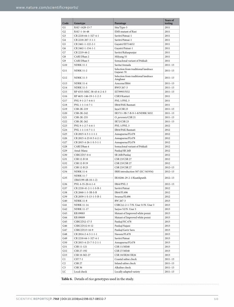
Table 6. Details of rice genotypes used in the study.

www.nature.com/scientificreports/

1 1SCIENTIFIC RepoRtS | 7: 7968 | DOI:10.1038/s41598-017-08532-7

identified as stable or near ideal, the data suggest that CSR-2K-219 (G19), CSR-2K-242 (G20), and CSR-2K-262 (G22) appeared again and again as stable, ideal, or top yielders in different environments and also over years. This implies that these genotypes seem to be most promising despite the high soil heterogeneity prevailing at the salt-affected test locations. Indeed, salt stress could be such a dynamic state in which the degree of stress experi-enced by a genotype can vary every day depending upon the soil moisture, temperature, and relative humidity of the microclimate50, 51. The environments used in the current study represent saline and alkaline soils (different because of the chemical composition of salts) and also coastal and inland salinity (different because of the vicinity of the seacoast and mode of salinization). Hence, the genotypes as given in Table 4 could be considered suitable for such soils. When three years of data were considered together, CSR-2K-219 (G19) and CSR-2K-262 (G22) were found promising over years (2011–13). Breeders need not only stable varieties; these should also have higher yields to make them attractive to farmers for adoption. It is important to consider here that the checks continue to outperform test genotypes in many instances. CSR 27 (C2) was the ideal genotype in 2011 and CSR 36 (C3) in 2011–12 (combined analysis of 2011 and 2012, not shown). These two were the winning genotypes in two mega-environments in 2011 as well. Considering these results, CSR-2K-219 and CSR-2K-262 are the most suita-ble genotypes for the majority of the salt stress locations, followed by CSR-2K-242. These genotypes were superior among all others with higher mean yields and stability; thus, they could be nominated for the formal release pro-cess and commercialization. A number of studies, although not exactly on GGE, looked for stable rice genotypes across salt stress locations and nominated the most stable and highest-yielding genotypes in the national varietal testing process for release34, 44, 48, 52.

As mentioned earlier, salinity and alkalinity (or sodicity) are two different kinds of salt stress although both exert stress due to high Na+ concentration. Na+ is in soil solution as soluble salt in saline soils but the same Na+ is adhered on clay micelles through a colloidal complex in alkaline soils5. In this study, genotype performances were compared across salinity- and alkalinity-affected locations separately. Many genotypes that respond well under salinity are also tolerant of alkalinity. This could be quite common but not a rule of thumb5, 50, 51. Some genotypes performed well under salinity but not under alkalinity and vice-versa and some performed well under both stresses. This implies that the genotypes showed specific adaptation to saline and alkaline conditions by vir-tue of different combinations of mechanisms/genes governing their tolerance53–55. The top ten genotypes in each year were separated and the genotypes that were consistently high yielding across three years were shortlisted. Genotypes CSR-2K-262, RP 4353-MSC-38-43-6-2-4-3, CSR-2K-219, and NDRK 11-1 were found to be consist-ently superior under saline conditions and, interestingly, CSR-2K-262 was the only genotype that fell into the top ten in three years consistently under alkaline/sodic conditions also. Thus, CSR-2K-262 could be considered as suitable for both saline and sodic conditions and could be considered as one of the best findings. Based on results over years, in 2016, CSR-2K-262 was released as rice variety CSR46 for the salt-affected areas of provinces of Uttar Pradesh in India.

Dividing a target region into meaningful sub-regions is the only way to make use of any repeatable genotype by location interactions in plant breeding. Using a maize (Zea mays L.) multi-environment trial (MET) dataset, Gauch and Zobel (1997) presented a “which-won-where” methodology for identifying mega-environments21. Data from multiple years are needed for such groupings. Attempts to group test locations into mega-environments using multi-seasonal data were previously reported in different crops, for example, in spring wheat56, cotton57, sugarcane40, and rice47. As of today, there are no reports on grouping rice-growing salt stress-affected locations of India into different zones. This is highly essential for deploying zone-specific rice genotypes for the management of salt-affected soil in India. “Which-won-where” plots constructed in the present study grouped the locations used for testing each year into different mega-environments: three mega-environments in 2011, three in 2012, and three in 2013 were identified. But, the grouping did not correspond with the geographic location or stress type (salinity and alkalinity) prevalent at the locations. However, a higher degree of stress (E6, E7, E11, and E12) always found space in one or another sub-group while some of the environments with less stress during the growing season (E2 and E17) could not find space in the mega-groups. Some of the non-repeatability of the “which-won-where” pattern could be because new locations and new genotypes were added every year from 2012 and 2013 and this has been reported earlier56 (details were given in Materials and Methods). This might have caused yearly fluctuations in genotypic and environmental scores, thereby disturbing the “which-won-where” pattern. As pointed out by Gauch and Zobel (1997), if the which-win-where pattern is used as the sole crite-rion, the identified mega-environments would vary substantially when genotypes are changed or deleted from the data21. Second, each of the locations used in this study may be distinct and cannot be grouped with any other location. This is supported by the lack of repeatable associations among environments. Third, the biplot itself couldn’t capture all of the complex G × E variation and hence the patterns may not be sufficiently clear. A repeatable which-won-where pattern over years is a necessary and sufficient condition for mega-environment delineation58. Moreover, this should be based on data in which the same set of genotypes was tested in the same set of test environments across multiple years33, which may be facilitated in most of the cases. Also, repeatable associations between locations cannot be relied upon and may not be grouped into different mega-environments due to the dynamic nature of soil salinity, which varies spatially as well as temporally20, 22. It is possible to obtain repeatable inferences if we use the same locations and genotypes for testing across years to the extent possible. But, that could be through an academic study but not forward-looking breeding processes, which always try to omit inferior genotypes and add more to test performance. However, if the mega-environment patterns are repeatable, breeders can go ahead with focused breeding efforts and rely more on such mega-environments for better inferences.

ConclusionsThe location CSSRI sodic environment was the most discriminating one and could be used for decisions on geno-types to retain for further testing and release. Overall, the most promising genotypes (CSR-2K-219, CSR-2K-262,

www.nature.com/scientificreports/

1 2SCIENTIFIC RepoRtS | 7: 7968 | DOI:10.1038/s41598-017-08532-7

and CSR-2K-242) with high mean yield and stability could be used for commercial cultivation across salt-affected soils. The lack of repeatable associations among the locations and repeatable mega-environment groupings sug-gests the complexity of the abiotic stress soil salinity. This warrants multi-location testing for about five years under salt-affected environments to group locations into distinct mega-environments before deciding about the real value of the location to discriminate and be representative for the target stress. The present study high-lights the fact that which-won-where plots could be used to identify the winners but not as the sole criterion for mega-environment grouping. For the time being, continuity of the testing locations for a few more years and improving the efficiency of the less discriminating sites could be a better option for strengthening the results obtained so far. Salinity and alkalinity are two different kinds of stress and they exert stress on plants differently. Genotypes CSR-2K-262, RP 4353-MSC-38-43-6-2-4-3, CSR-2K-219, and NDRK 11-1 were identified as the most promising genotypes under saline soils consistently over years but CSR-2K-262 was the only genotype that was most promising and consistent under alkaline/sodic conditions over three years of testing consistently; hence, it could be suggested for both saline and alkaline conditions. Location-specific ambient conditions contribute to the success of a cultivar; hence, multi-location testing is one of the best ways for identifying genotypes with specific adaptation to a particular agro-climatic zone.

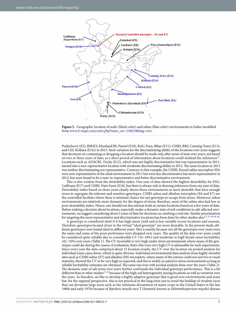
MethodsPlant materials and testing locations. The experiment was conducted across 18 locations that com-prised nine saline and nine alkaline environments that adequately represent the diverse salt stress conditions in India (Fig. 5). The soils in coastal saline locations varied from sandy loam to clay loam, with ECe (electrical conductivity of saturation extract) of 3.0–17.0 dS m−1 and pH of 5.0–7.5 (measured as pH1:2, meaning that the pH has a mix of 1 part soil and 2 parts distilled water; hereinafter referred to as pH). Similarly, soils in alkaline locations varied from sandy loam to clay loam, with ECe of 1.0–3.7 dS m−1 and pH of 8.3–10.2 (Table 5). Salinity and alkalinity were measured before transplanting and at the time of transplanting, flowering, and maturity. The testing sites were increased each year after the first year of testing with 12, 14, and 18 locations in 2011, 2012, and 2013, respectively. All the experiments were conducted in the wet season.

A total of 53 genotypes were tested during 2011 to 2013 across the selected locations with three national checks, CST 7-1 (coastal saline), CSR 27 (inland saline), and CSR 36 (alkaline). In the first year (2011), 22 salt-tolerant genotypes were evaluated across 12 salt stress locations. Among these, the 10 best genotypes were promoted to the next year of testing (2012). In 2012, 17 new genotypes along with the previous year’s 10 prom-ising genotypes were tested across 14 salt stress locations. Among these 17, the top four genotypes were selected and promoted to the next year. In 2013, the 10 best genotypes from 2011 and 4 genotypes from 2012 were assessed across 17 stress locations along with 14 new entries. The experiment was severely damaged due to high salt stress along with submergence at NRRI, Cuttack (E2). Sowing was done at different sites from the last week of May to the first week of June. The trials were laid out in a randomized complete block design with three replications. The genotypes tested in each year were different as inferior genotypes were discarded and new breeding lines were added every year. A total of 22, 27, and 28 genotypes were tested in 2011, 2012, and 2013, respectively. The details of these genotypes with their pedigrees appear in Table 6. At each site, data on days to 50% flowering, plant height, panicle length, number of filled grains/panicle, 1000-grain weight, and grain yield were recorded. Grain yield was determined from the whole plot and expressed in t/ha.

Statistical analysis. Since the locations and genotypes were different between years of testing, analysis was done separately for each year. Additionally, the genotypes common over three years were used for pooled analysis to evaluate their performance over different year and location combinations. Codes were used for loca-tions (Table 1) and genotypes (Table 2) in the individual years 2011, 2012, and 2013. GGE biplot software was used for the option of heritability adjusted GGE (HA-GGE) biplot analysis27. The biplots were generated using scaling (2), centering (2), and SVP (2) GGE biplot software. We constructed biplots using those principal com-ponents that were having information ratio (IR) > 1. Yield data from a multi-location trial consist of three com-ponents: a genotype main effect (G), an environmental component (E), and an interaction term of genotype and environment (GE). But, for the identification of superior cultivars, only G and GE are of utmost importance. A GGE biplot is first constructed by centering the G × E two-way table by environmental means and subjecting the environment-centered data matrix to singular value decomposition (SVD), which yields three component matri-ces: the SV matrix, the genotype eigenvector matrix, and the environment eigenvector matrix.

The general model for GGE biplots is as follows:

∑µ

λ α γ ε=−

= +=

py

S (1)ij

ij j

j k

t

k ik jk ij1

Here, the GGE biplot used is heritability adjusted (HA) and hence the scaling factor Sj becomes SD/ H . The cosine of angle (αjj’) between two environments is measured as genetic correlation between them10, 11, 16

α=′ ′r cos (2)g jj jj( )

The genetic gain (G) observed in target environment j’ through indirect selection in test environment j is given by ref. 26

σ= ′ ′G i h r( ) (3)j j g jj g j( ) ( )

www.nature.com/scientificreports/

13SCIENTIFIC RepoRtS | 7: 7968 | DOI:10.1038/s41598-017-08532-7

The discriminating ability of a location is judged by the length of its vector. Further, desirability index of the locations across years were calculated as product of representativeness and discriminating ability estimates. The projection of a genotype from the average tester (AT) axis is used to decide the stability of the genotype. The “which-won-where” option was used to identify which genotype was the winner in a given set of environments and to categorize mega-environments. The biplots were interpreted as described by Yan17.

References 1. FAO. Extent of salt affected soils. www.fao.org/soils-portal/soil-management/management-of-someproblem-soils/salt-affected-

soils/more-information-on-saltaffected-soils/en/ [last accessed 3 December 2014]. 2. Mondal, A. K., Sharma, R. C. & Singh, G. B. Assessment of salt affected soils in India using GIS. Geocarto Int. 24(6), 437–456 (2009). 3. Yeo, A. R., Yeo, M. E., Flowers, S. A. & Flowers, T. G. Screening of rice (Oryza sativa L.) genotypes for physiological characters

contributing to salinity resistance, and their relationship to overall performance. Theor. Appl. Genet. 79, 377–383 (1990). 4. Roshandel, P. & Flowers, T. The ionic effects of NaCl on physiology and gene expression in rice genotypes differing in salt tolerance.

Plant Soil 315, 135–147 (2009). 5. Singh, R. K. & Flowers, T. J. Physiology and molecular biology of the effects of salinity on rice. In: Handbook of Plant and Crop

Stress, Pessarakli, M. (Ed.), 3rd edn., CRC Press, Taylor & Francis Group, Boca Raton, FL, USA, pp. 899–939 (2011). 6. Ponnamperuma, F. N. Evaluation and improvement of lands for wetland rice production. In: Senadhira, D. (Ed.), Rice and problem

soils in South and Southeast Asia. IRRI Discussion Paper Series No. 4, International Rice Research Institute, Manila, Philippines (1994).

7. Ali, S. et al. Stress indices and selectable traits in SALTOL QTL introgressed rice genotypes for reproductive stage tolerance to sodicity and salinity stresses. Field Crops Res. 154, 65–73 (2013).

8. Krishnamurthy, S. L., Sharma, S. K., Gautam, R. K. & Kumar, V. Path and association analysis and stress indices for salinity tolerance traits in promising rice (Oryza sativa L.) genotypes. Cereal Res. Commun. 42(3), 474–483 (2014).

9. Krishnamurthy, S. L., Gautam, R. K., Sharma, P. C. & Sharma, D. K. Effect of different salt stresses on agro-morphological traits and utilization of salt stress indices for reproductive stage salt tolerance in rice. Field Crops Res., doi:10.1016/j.fcr.2016.02.018 (2016).

10. Gabriel, K. R. The biplot graphic display of matrices with application to principal component analysis. Biometrika 58, 453–467 (1971).

11. Yan, W. & Tinker, N. A. Biplot analysis of multi-environment trial data: Principles and applications. Can. J. Plant Sci. 86, 623–645 (2006).

12. Bradu, D. & Gabriel, K. R. The biplot as a diagnostic tool for models of two-way tables. Technometrics 20, 47–68 (1978). 13. Kempton, R. A. The use of biplots in interpreting variety by environment interactions. J. Agric. Sci. 103, 123–135 (1984). 14. Gauch, H. G. AMMI analysis of yield trials. In: Kang M.S., Gauch H.G. (Eds) Genotype-by-environment interaction. CRC Press,

Boca Raton, F. L. pp. 1–40 (1992). 15. Cooper, M. & DeLacy, I. H. Relationships among analytic methods used to study genotypic variation and genotype-by-environment

interaction in plant breeding multi-environment experiments. Theor. Appl. Genet. 88, 561–572 (1994). 16. Kroonenberg, P. M. Introduction to biplots for G × E tables. Department of Mathematics, Research Report 51. University of

Queensland, Australia (1995). 17. Yan, W., Hunt, L. A., Sheng, Q. & Szlavnics, Z. Cultivar evaluation and mega-environment investigation based on GGE biplot. Crop

Sci. 40, 597–605 (2000). 18. Kang, M. S. A rank-sum method for selecting high-yielding stable corn genotypes. Cereal Res. Commun. 16, 113–115 (1988). 19. Kang, M. S. Simultaneous selection for yield and stability in crop performance trials: Consequences for growers. Agron. J. 85,

754–757 (1993). 20. Yan, W. & Kang, M. S. GGE biplot analysis: A graphical tool for breeders, geneticists, and agronomists. CRC Press, Boca Raton, FL

(2003). 21. Gauch, H. G. & Zobel, R. W. Identifying mega-environments and targeting genotypes. Crop Sci. 37, 311–326 (1997). 22. Yan, W. & Rajcan, I. Biplot evaluation of test sites and trait relations of soybean in Ontario. Crop Sci. 42, 11–20 (2002). 23. Yan, W. & Falk, D. E. Biplot analysis of host-by-pathogen interaction. Plant Dis. 86, 1396–1401 (2002). 24. Yan, W. & Hunt, L. A. Biplot analysis of diallel data. Crop Sci. 42, 21–30 (2002). 25. Pittelkow, Y. E. & Wilson, S. R. The GE-biplot for microarray data. Proc. Virtual Conf. Genomics Bioinformatics 2, 8–11 (2003). 26. Yan, W., Tinker, N. A. & Falk, D. QTL identification, mega-environment classification, and strategy development for marker-based

selection using biplots. J. Crop Improve. 14, 299–324 (2005). 27. Yan, W. & Holland, J. B. A heritability-adjusted GGE biplot for test environment evaluation. Euphytica 171, 355–369 (2010). 28. Nassir, A. L. Genotype × environment analysis of some yield components of upland rice (Oryza sativa L.) under two ecologies in

Nigeria. Int. J. Plant Breed. Genet. 7(2), 105–114, doi:10.3923/ijpbg.2013 (2013). 29. Ogunbayo, S. A. et al. Comparative performance of forty-eight genotypes in diverse environments using the AMMI and GGE biplot

analyses. Int. J. Plant Breed. Genet. 8(3), 139–152 (2014). 30. Fotokian, M. H. & Agahi, K. Biplot analysis of genotype by environment for cooking quality in hybrid rice: A tool for line × tester

data. Rice Sci. 21(5), 282–287 (2014). 31. Sharifi, P. Graphic analysis of salinity tolerance traits of rice (Oryza sativa L.) using biplot method. Cereal Res. Commun. 40(3),

342–350 (2012). 32. Yan, W. & Hunt, L. A. Interpretation of genotype × environment interaction for winter wheat yield in Ontario. Crop Sci. 41, 19–25

(2001). 33. Zobel, R. W., Wright, M. J. & Gauch, H. G. Statistical analysis of a yield trial. Agron J. 80, 388–393 (1998). 34. Krishnamurthy, S. L. et al. Analysis of stability and G × E interaction of rice genotypes across saline and alkaline environments in

India. Cereal Res. Commun., doi:10.1556/0806.43.2015.055 (2015b). 35. Mohammadi, R. & Amri, A. Genotype × environment interaction and genetic improvement for yield and yield stability of rainfed

durum wheat in Iran. Euphytica 192, 227–249 (2013). 36. Samonte, S. O. P. B., Wilson, L. T., McClung, A. M. & Medley, J. C. Targeting Cultivars onto Rice Growing Environments Using

AMMI and SREG GGE Biplot Analyses. Crop Sci., doi:10.2135/cropsci2004.0627 (2004). 37. Rakshit, S. et al. GGE biplot analysis to evaluate genotype, environment and their interactions in sorghum multi-location data.

Euphytica 185, 465–479, doi:10.1007/s10681-012-0648-6 (2012). 38. Ullah, H. et al. Selecting high yielding and stable mungbean [Vigna radiata (L.) Wilczek] genotypes using GGE biplot techniques.

Can. J. Plant Sci. 92(5), 951–960 (2012). 39. Nai-yin, X., Michel, F., Guo-wei, Z., Jian, L. & Zhi-guo, Z. The application of GGE biplot analysis for evaluating test locations and

mega-environment investigation of cotton regional trials. J. Integr. Agric. 13(9), 1921–1933 (2014). 40. Luo, J. et al. Biplot evaluation of test environments and identification of mega-environment for sugarcane cultivars in China. Sci. Rep.

5, 15505, doi:10.1038/srep15505 (2015). 41. Akter, A. et al. GGE biplot analysis for yield stability in multi-environment trials of promising hybrid rice (Oryza sativa L.).

Bangladesh Rice J. 19(1), 1–8 (2015).

www.nature.com/scientificreports/

1 4SCIENTIFIC RepoRtS | 7: 7968 | DOI:10.1038/s41598-017-08532-7

42. Balestre, M., B dos Santos, V., Soares, A. A. & Souza Reis, M. Stability and adaptability of upland rice genotypes. Crop Breed. Appl. Biotechnol. 10, 357–363 (2010).

43. Tabien, R. E., Samonte, S. O. P. B., Abalos, M. C. & Gabriel, R. C. S. GGE biplot analysis of performance in farmers’ fields, disease reaction and grain quality of bacterial leaf blight-resistant rice genotypes. Philipp. J. Crop Sci. 33(1), 3–19 (2008).

44. Anandan, A., Eswaran, R., Sabesan, T. & Prakash, M. Additive main effects and multiplicative interactions analysis of yield performances in rice genotypes under coastal saline environments. Adv. Biol. Res. 3(1–2), 43–47 (2009).

45. Krishnamurthy, S. L. et al. Yield stability of rice lines for salt tolerance using additive main effects and multiplicative interaction analysis - AMMI. J. Soil Salin. Water Qual. 7(2), 98–106 (2015).

46. Tack, J. et al. High vapor pressure deficit drives salt-stress induced rice yield losses in India. Global Change Biol. 21, 1668–1678 (2015).

47. Yan, W., Fregeau-Reid, J. A., Martin, R. A., Pageau, D. & Mitechell Fetch, J. W. How many test locations and replications are needed in crop variety trials in a target region? Euphytica 202, 361–372 (2015).

48. Krishnamurthy, S. L. et al. G × E interaction and stability analysis for salinity and sodicity tolerance in rice at reproductive stage. J. Soil Salin. Water Qual. 8(2), 162–172 (2016b).

49. Levings, C. S. Texas cytoplasm of Maize: Cytoplasmic male sterility and disease susceptibility. Sci. 250, 942–947 (1990). 50. Wassmann, R. et al. Climate change affecting rice production: The physiological and agronomic basis for possible adaptation

strategies. Adv. Agron. 101, 59–102 (2009). 51. Singh, R. K., Redoña, E. D. & Refuerzo, L. Varietal improvement for abiotic stress tolerance in crop plants: Special reference to

salinity in rice. In: Abiotic Stress Adaptation in Plants: Physiological, Molecular and Genomic Foundation. Pareek, A., Sopory, S. K., Bohnert, H. J. & Govindjee (Eds), Springer, Dordrecht, Netherlands, pp. 387‒415 (2010).

52. Islam, M. R. et al. Assessment of adaptability of recently released salt tolerant rice varieties in coastal regions of South Bangladesh. Field Crops Res. 190, 34–43 (2016).

53. Jagadish, S. V. K. et al. Genetic advances in adapting rice to a rapidly changing climate. J. Agron. Crop Sci. 198(5), 360–373, doi:10.1111/j.1439-037X.2012.00525.x (2012).

54. Tiwari, S. et al. Mapping QTLs for salt tolerance in rice (Oryza sativa L.) by bulked segregant analysis of recombinant inbred lines using 50K SNP chip. PLoS ONE 11(4), e0153610 (2016).

55. Kumar, V. et al. Genome-wide association mapping of salinity tolerance in rice (Oryza sativa). DNA Res. 1–13, doi:10.1093/dnares/dsu046 (2015).

56. Navabi, A., Yang, R. C., Helm, J. & Spaner, D. M. Can spring wheat-growing mega-environments in the northern Great Plains be dissected for representative locations or niche-adapted genotypes? Crop Sci. 46, 1107–1116 (2006).

57. Blanche, S. B. & Myers, G. O. Identifying discriminating locations for cultivar selection in Louisiana. Crop Sci 46, 946–949 (2006). 58. Yan, W., Kang, M. S., Ma, B. L., Woods, S. & Cornelius, P. L. GGE biplot vs. AMMI analysis of genotype-by-environment data. Crop

Sci. 47, 643–655 (2007).

AcknowledgementsThe authors sincerely thank the Bill & Melinda Gates Foundation for funding support under the STRASA project (IRRI-ICAR collaborative project), the directors of all the partner institutes for encouragement, and Bill Hardy for technical editing of the manuscript.

Author ContributionsConceived the design: R.K.S., G.B.G., and A.I.; performed the experiments: S.L.K., K.T.R., Y.P.S., V.K.M., D.B., B.M., S.M., S.K.S., R.K.G., P.K.S., K.K.M., B.C.M., G.P., P.B.V., K.D.P., S. Th, O.P.V., A.H.K., S. Ti, S.G., M.S., R.G., V.K.Y., S.K.B.R., and M.P.; analyzed the data: J.B., S.L.K., K.T.R., and R.K.S.; wrote the manuscript: S.L.K. and K.T.R.; made revisions: R.K.S., A.I., P.C.S., and D.K.S.; approved the final version of the paper.

Additional InformationSupplementary information accompanies this paper at doi:10.1038/s41598-017-08532-7Competing Interests: The authors declare that they have no competing interests.Publisher's note: Springer Nature remains neutral with regard to jurisdictional claims in published maps and institutional affiliations.

Open Access This article is licensed under a Creative Commons Attribution 4.0 International License, which permits use, sharing, adaptation, distribution and reproduction in any medium or

format, as long as you give appropriate credit to the original author(s) and the source, provide a link to the Cre-ative Commons license, and indicate if changes were made. The images or other third party material in this article are included in the article’s Creative Commons license, unless indicated otherwise in a credit line to the material. If material is not included in the article’s Creative Commons license and your intended use is not per-mitted by statutory regulation or exceeds the permitted use, you will need to obtain permission directly from the copyright holder. To view a copy of this license, visit http://creativecommons.org/licenses/by/4.0/. © The Author(s) 2017