Embed Size (px)
Citation preview
sustainability
Article
Hydrostatic Pressure Wheel for Regulation of Open ChannelNetworks and for the Energy Supply of Isolated Sites
Ludovic Cassan 1,* , Guilhem Dellinger 2, Pascal Maussion 3 and Nicolas Dellinger 2
�����������������
Citation: Cassan, L.; Dellinger, G.;
Maussion, P.; Dellinger, N.
Hydrostatic Pressure Wheel for
Regulation of Open Channel
Networks and for the Energy Supply
of Isolated Sites. Sustainability 2021,
13, 9532. https://doi.org/10.3390/
su13179532
Academic Editors: Mosè Rossi,
Massimiliano Renzi, David Štefan
and Sebastian Muntean
Received: 6 July 2021
Accepted: 18 August 2021
Published: 24 August 2021
Publisher’s Note: MDPI stays neutral
with regard to jurisdictional claims in
published maps and institutional affil-
iations.
Copyright: © 2021 by the authors.
Licensee MDPI, Basel, Switzerland.
This article is an open access article
distributed under the terms and
conditions of the Creative Commons
Attribution (CC BY) license (https://
creativecommons.org/licenses/by/
4.0/).
1 Institut de Mécanique des Fluides, Toulouse INP, Université de Toulouse, Allée du Professeur Camille Soula,31400 Toulouse, France
2 Laboratoire des Sciences de l’Ingénieur, de l’Informatique et de l’Imagerie (ICUBE), ENGEES,67000 Strasbourg, France; [email protected] (G.D.); [email protected] (N.D.)
3 LAPLACE, Toulouse INP, Université de Toulouse, 2 Rue Camichel, 31071 Toulouse, France;[email protected]
* Correspondence: [email protected]
Abstract: The Hydrostatic Pressure Wheel is an innovative solution to regulate flow discharges andwaters heights in open channel networks. Indeed, they can maintain a water depth while producingenergy for supplying sensors and a regulation system. To prove the feasibility of this solution,a complete model of water depth–discharge–rotational speed relationship has been elaborated. Thelatter takes into account the different energy losses present in the turbine. Experimental measurementsachieved in IMFT laboratory allowed to calibrate the coefficients of head losses relevant for a largerange of operating conditions. Once the model had been validated, an extrapolation to a real caseshowed the possibility of maintaining upstream water level but also of being able to produce sufficientenergy for supplying in energy isolated sites. The solution thus makes it possible to satisfy primaryenergy needs while respecting the principles of frugal innovation: simplicity, robustness, reducedenvironmental impact.
Keywords: renewable energy; water wheel; low tech; frugal innovation; experimental model;theoretical model
1. Introduction
Irrigation systems have a lot of weir structures in order to change the water elevation,water velocities, etc. These “small” drops represent a non-negligible hydroelectric poten-tial [1]. Nevertheless, the role of the turbine in this study is a little bit different. Its functionis not only to produce electricity but also to serve as a water level controller. Indeed, theregulation of water height and flow discharge in irrigation systems is also crucial to savethe water resources and, as mentioned before, requires many regulation systems (sluicegates, spillways, weirs, etc). The fact is that these systems can be very isolated and thereforedifficult to power, especially in remote areas. To overcome this problem, a turbine couldregulate the water level automatically by adjusting its rotational speed. Part of the energysupplied by the turbine would then be used to power the sensors and the control systemneeded for this regulation and data transmission. Moreover, in the context of isolated areas,the rest of the energy provided by the turbine could also be used for supplying the localelectricity grid. Indeed, the water wheels are also a good example of the low-tech conceptfor energy supply [2]. Therefore, we will also discuss the power performance in the contextof isolated communities in developing countries in line with the frugal innovation concept.Although equipping a low head in a large river may involve some environmental issues,power generation with low-head coupled with solar energy and storage devices is fullyrelevant if no other source is available (isolated zone).
As noted above, irrigation systems are constructed with weirs that can be exploited.Typically, these structures have head differences between 0.5 and 3 m and have a low
Sustainability 2021, 13, 9532. https://doi.org/10.3390/su13179532 https://www.mdpi.com/journal/sustainability
Sustainability 2021, 13, 9532 2 of 18
flow rate. Turbines suitable for this kind of hydraulic sites are the Kaplan turbine,the Archimedean Screw Turbine (AST) and the various types of water wheels [3]. It is alsopossible to add the Very Low Head (VLH) turbine to this list. For obvious economicaland ecological reasons, the turbine chosen must be inexpensive, robust, fish-friendly andprovide the sediment continuity. The Kaplan and VLH turbine reach a better hydraulicefficiency than the other two, but they require complex control elements and are muchmore expensive [4]. The AST turbine has almost the same efficiency as a well-designedwater wheel but is slightly more expensive and much more complex to build. Finally, thechoice was made to consider water wheels.
By combining the different types of water wheels, they are able to exploit water headfrom 0.5 to 12 m [5]. The three main types of water wheels are the overshot wheels, thebreastshot wheels and the undershot wheels. It is also possible to speak about stream waterwheels but they are designed to exploit the flow velocity and not the head difference [6].For the overshot wheels, the water enters from above and the wheel is rotated by thewater weight. These turbines are used for heads between 2.5 and 12 m and can reachefficiencies of about 80% [4,7]. In the case of the breastshot wheels, the water enters atapproximately the same height than the turbine’s rotation axis. This type of wheel worksfor head differences between 1.5 and 4 m and can achieve efficiencies between 60% and70% [8–11]. The last main type of water wheel is the undershot wheel. In this case, theflow enters below the axis of rotation. This type of turbine is adapted for very low headdifferences between 0.5 and 2.5 m and can reaches efficiencies of 80% [12,13]. Regardingthe head differences in the context of irrigation systems, undershot wheels seem to bethe most suitable. Specifically, the Hydrostatic Pressure Wheel (HPW) developed by [14]is chosen in order to achieve the objectives presented above. The wheel is composed ofradial blades and is driven to rotate by the hydrostatic pressure exerted by the flow onthe blades. In addition, this turbine is chosen because it presents a very simple design,is robust, inexpensive and fish-friendly [14].
As a reminder of the general context, the stated objectives are to replace the regulationstructures of irrigation system that require manual operation and maintenance with aturbine. The latter will adjust the water level automatically by changing its rotationalspeed and, at the same time, will produce some energy for local consumption. In order toproperly design the system according to the site characteristics, a theoretical model thatlinks hydraulic conditions, geometrical parameters and turbine performance is required.Currently, there is only one theoretical model, proposed by [14]. However, this model isnot able to predict directly the water level upstream to the wheel and the flow dischargethrough it. In irrigation systems, due to the modulation of water demand, it is essentialto control water levels and flows throughout the network. Therefore, to control theseparameters with water wheels, an improved model is needed and is presented in this article.
The paper is structured as follows. In Section 2, a new theoretical model is establishedbased on the [14] model. Special attention is paid to the consideration of various energylosses (gap leakage, drag forces, etc.) as they are very significant. The experimental setupinstalled in the IMFT hydraulic laboratory and used for providing experimental data onthe HPW turbine is presented in Section 3. After calibrating the loss models with theexperimental results, the ability of the theoretical model to accurately reproduce the wheelperformance, the upstream water levels and the flow discharges absorbing by the wheelare discussed in Section 4. Finally, a discussion about the possibilities to use these turbinesfor the electrification of an isolated village in a low-tech context is analyzed in Section 5.
2. Operating Principle and Theoretical Models2.1. Operating Principle
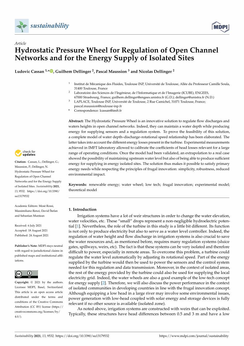
As shown in Figure 1, the HPW developed in [14] consists of a wheel made up ofradial blades longer than the inlet water height. This turbine converts the potential energyof a fluid into mechanical energy thanks to rotation induced by the fluid pressure exertedon its blades. This mechanical energy can then be transformed into electrical energy thanks
Sustainability 2021, 13, 9532 3 of 18
to a generator. This last transformation will not be discussed here although it is a crucialpoint for power generation [14]. The mechanical power supplied by the wheel is given by:
P = Phyd η = ρgQ∆Hη (1)
where Phyd is the available hydraulic power, ρ is the density of water, Q is the flow rate,g is the acceleration of gravity, ∆H is the hydraulic head difference and η—the hydraulicefficiency of the turbine. The efficiency depends on the different losses present in theturbine which are mainly due to the flow leakages and the drag forces. The latter presentwhen the blades enter into the flow and when they leave it. Thus, minimizing these lossesis a key issue in order to increase the turbine performance.
Figure 1. 3D view of a HPW turbine.
To use the wheel effectively as a regulation and energy production system, it isnecessary to determine the influence of the wheel on the upstream water level and topredict its energy recovery performance. For this purpose, a theoretical model is establishedin the following part. The latter is able to determine the upstream water level and theperformance of the turbine according to the geometrical parameters of the wheel and theflow conditions.
2.2. Theoretical Model
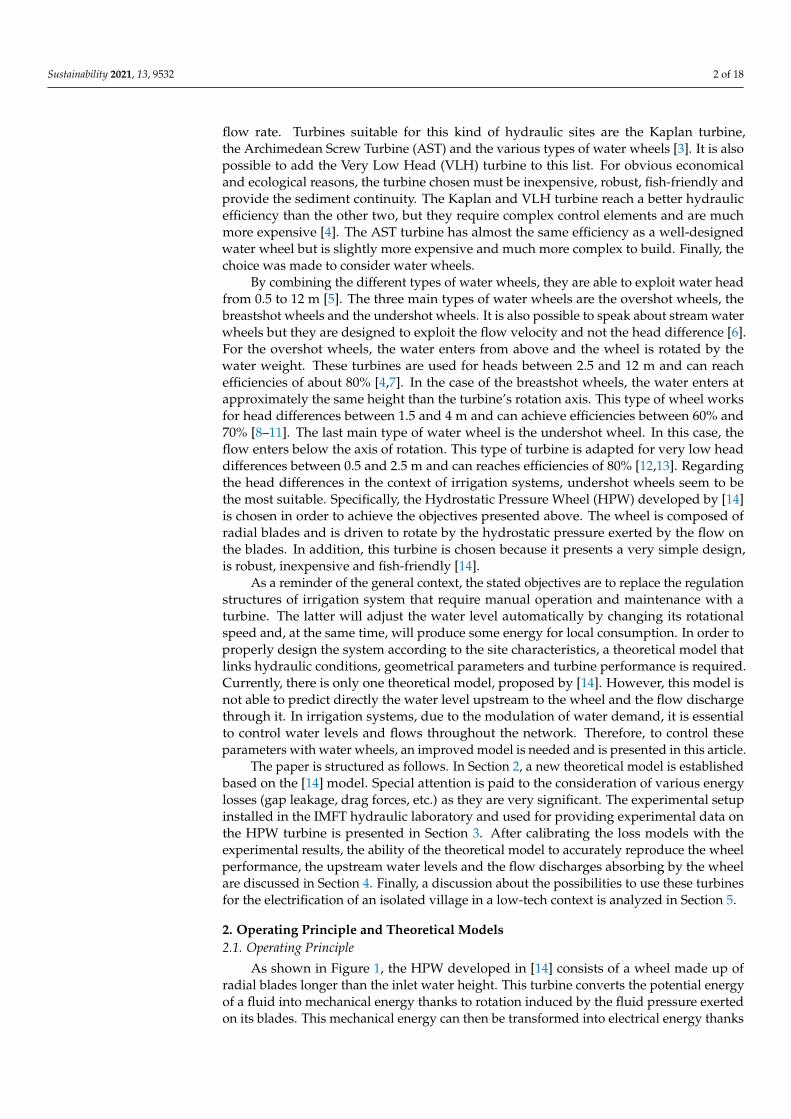
As presented in Figure 2, the HPW turbine has radial blades longer than the inletwater level. This is why this type of wheel is dedicated to very low heads between 0.3 and1 m [14]. The main geometrical parameters of this turbine are the radius of the wheel r, thewidth L and the number of blades N. These parameters are shown in Figure 2. It should benoted that each blade is defined by a plane that contains the axis of rotation. The mechanicalpower is obtained by the displacement of a vertical blade submitted to a force inducedby the flow pressure more important on the upstream face than on the downstream side.The model is derived by considering force balance on a blade. Compared to the previousstudy [14], the theory is rewritten here with a global efficiency formula η incorporatingleakages and turbulence disturbance. The theory presented here will help upscale thewheel in a real scale application. Furthermore, as discussed earlier, an integrated formulafor mechanical power as a function of upstream water depth and rotational speed is neededto develop efficient control of water level. To establish the model, a vertical blade with afinite radius r and a width L is considered. The water level upstream to the blade is equalto d1 and the downstream one is equal to d2. The distance between the blade and the bed isdenoted dl (Figure 2).
The total flow rate Q can be decomposed in two parts:
Q = Qw + Ql (2)
with Qw being the flow through the surface bounded by the height d1 and the width L thatactually contributes to wheel rotation, and Ql representing the flow leakage that appears
Sustainability 2021, 13, 9532 4 of 18
around the wheel. It may be noted that to optimize the wheel performance, it is necessaryto limit the value of Ql .
dl
d2
d1
ω
r L
wlat
r
V1V2
B
Side View Front View
z
xy
Figure 2. Schematic view of the HPW machine.
The flow leakage Ql can be decomposed in two leakages. The first one is Ql,1, whichoccurs between the blades and the bottom and, the second one—Ql,2, which occurs betweenthe wheel and the two side walls. Both leakages can be determined by using the Torricelliequation and are a function of the head difference (d1 − d2), the wheel width L and the gapsbetween the wheel and the canal. To determine the first leakage Ql,1 occurring between theblades and the bottom, the gap dl is not used directly. Instead, an equivalent opening wrepresenting the surface opening for flow under the wheel is introduced. This value hasto be calibrated for each wheel geometry for the following reasons. Firstly, unlike sluicegate, the discharge formula is written here without considering the vertical contractionof the flow stream. Indeed, it is difficult to measure and evaluate accurately this valueknowing that it evolves with the submergence d2/d1 [15,16]. Secondly, the wheel cannotbe modeled like an orifice because the blades are moving and then the opening dependson the radial position of the wheel. Therefore w represents an averaged value of the spacebetween blade and bed during a rotation. Eventually, to determine the leakage Ql,2, thegap wlat between the wheel an the sidewall is used. As a consequence, the portion of thedischarge Ql that was not flowing into the wheel can by expressed as:
Ql =√
2g(d1 − d2)wL + 2√
2g(d1 − d2)d1wlat (3)
The water flowing into the wheel Qw can be determined by assuming that when ablade is in the vertical position in the fluid, the water and the blade have the same velocitylocally. The submerged length of the blade is equal to d1, as represented in the Figure 2.The averaged velocity of the flow va is then given by the integration of the horizontalcomponent of the velocity of the submerged part of the blade:
va =1d1
∫ r−d1
rzωdz = ωr
(1 − 1
2r/d1
)(4)
The flow Qw is then equal to:
Qw = Ld1va = Ld1ωr(
1 − 12r/d1
)(5)
Sustainability 2021, 13, 9532 5 of 18
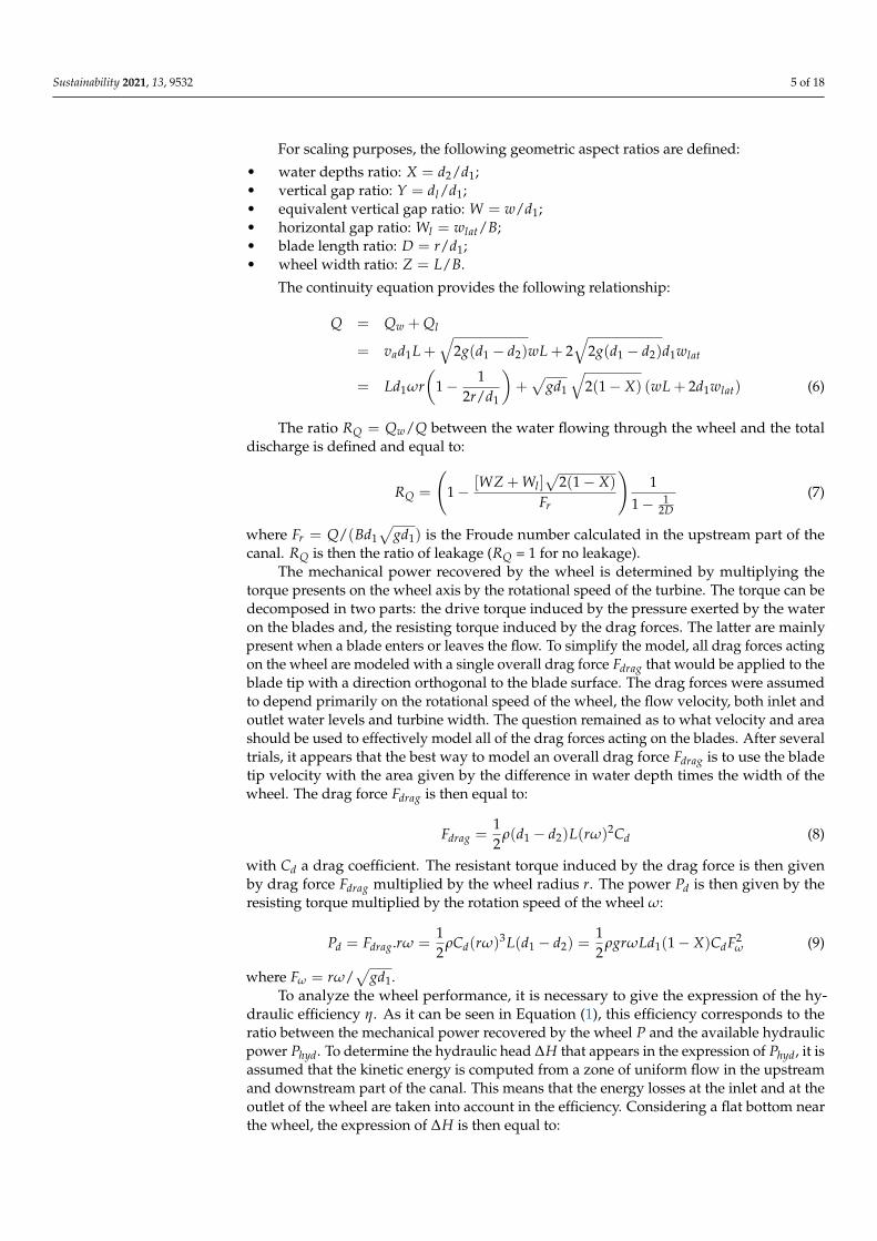
For scaling purposes, the following geometric aspect ratios are defined:
• water depths ratio: X = d2/d1;• vertical gap ratio: Y = dl/d1;• equivalent vertical gap ratio: W = w/d1;• horizontal gap ratio: Wl = wlat/B;• blade length ratio: D = r/d1;• wheel width ratio: Z = L/B.
The continuity equation provides the following relationship:
Q = Qw + Ql
= vad1L +√
2g(d1 − d2)wL + 2√
2g(d1 − d2)d1wlat
= Ld1ωr(
1 − 12r/d1
)+√
gd1
√2(1 − X) (wL + 2d1wlat) (6)
The ratio RQ = Qw/Q between the water flowing through the wheel and the totaldischarge is defined and equal to:
RQ =
(1 − [WZ + Wl ]
√2(1 − X)
Fr
)1
1 − 12D
(7)
where Fr = Q/(Bd1√
gd1) is the Froude number calculated in the upstream part of thecanal. RQ is then the ratio of leakage (RQ = 1 for no leakage).
The mechanical power recovered by the wheel is determined by multiplying thetorque presents on the wheel axis by the rotational speed of the turbine. The torque can bedecomposed in two parts: the drive torque induced by the pressure exerted by the wateron the blades and, the resisting torque induced by the drag forces. The latter are mainlypresent when a blade enters or leaves the flow. To simplify the model, all drag forces actingon the wheel are modeled with a single overall drag force Fdrag that would be applied to theblade tip with a direction orthogonal to the blade surface. The drag forces were assumedto depend primarily on the rotational speed of the wheel, the flow velocity, both inlet andoutlet water levels and turbine width. The question remained as to what velocity and areashould be used to effectively model all of the drag forces acting on the blades. After severaltrials, it appears that the best way to model an overall drag force Fdrag is to use the bladetip velocity with the area given by the difference in water depth times the width of thewheel. The drag force Fdrag is then equal to:
Fdrag =12
ρ(d1 − d2)L(rω)2Cd (8)
with Cd a drag coefficient. The resistant torque induced by the drag force is then givenby drag force Fdrag multiplied by the wheel radius r. The power Pd is then given by theresisting torque multiplied by the rotation speed of the wheel ω:
Pd = Fdrag.rω =12
ρCd(rω)3L(d1 − d2) =12
ρgrωLd1(1 − X)CdF2ω (9)
where Fω = rω/√
gd1.To analyze the wheel performance, it is necessary to give the expression of the hy-
draulic efficiency η. As it can be seen in Equation (1), this efficiency corresponds to theratio between the mechanical power recovered by the wheel P and the available hydraulicpower Phyd. To determine the hydraulic head ∆H that appears in the expression of Phyd, it isassumed that the kinetic energy is computed from a zone of uniform flow in the upstreamand downstream part of the canal. This means that the energy losses at the inlet and at theoutlet of the wheel are taken into account in the efficiency. Considering a flat bottom nearthe wheel, the expression of ∆H is then equal to:
Sustainability 2021, 13, 9532 6 of 18
∆H = d1 − d2 +Q2
2gB2
(1
(d1 + dl)2 − 1(d2 + dl)2
)(10)
The mechanical power P provided by the wheel corresponds to the available hydraulicpower calculated with the flow Qw minus the drag loss Pd:
P = ρgQw∆H − Pd =12
ρgQd1
((1 + X)− 1
3D
(1 + X2 + X
)− CdF2
ω
)(1 − X)RQ (11)
Finally, combining the Equations (7), (9) and (10); the wheel efficiency η is equal to:
η =12(1 + X)− 1
3D(1 + X2 + X
)− CdF2
ω
1 − 12 F2
r1+X+2Y
(1+Y)2(X+Y)2
RQ (12)
Except the drag term, the Equation (12) is similar to the formula proposed by [14].Here all corrections are given in the same equation which provides a better view of thedimensionless significant numbers. These independent numbers are X, Y, Z, Cd, D, Fr, ω.The number RQ, Fω and η can be deduced from others. For a given rotational speed ω,the Froude number provides the relationship between flow rate and water depth. Thecoefficient Cd is considered constant for a given wheel shape even though a Reynoldsdependence could be expected. This analysis tends to prove that a Froude similarity couldbe applied for the wheel design.
3. Experimental Setup
Experimental data are necessary to calibrate and validate the theoretical model estab-lished previously. In addition, experimental measurements are needed to investigate theperformance of the HPW turbine experimentally. An experimental setup was thereforeinstalled in the hydraulic laboratory of the Toulouse Institute of Fluid Mechanics (IMFT).This device allows to test the efficiency and the mechanical behavior of the turbine fordifferent geometrical and hydraulic parameters. The wheel geometries considered in thisstudy are as simple as possible in order to obtain low-cost and low-maintenance turbines.These characteristics are essential in a context of isolated sites where it is difficult to replacea broken component with a new one. Moreover, plane blades seem to be more suitablefor controlling the flow through the wheel even at low speeds by stopping it completelyif necessary. The blades are attached to the side disks. They are slightly shorter than theradius which allows the air and water pressures to be balanced between the blades.
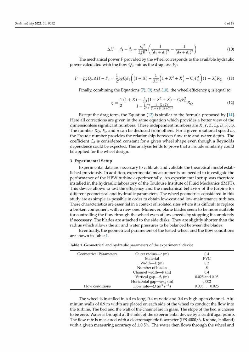
Eventually, the geometrical parameters of the tested wheel and the flow conditionsare shown in Table 1.
Table 1. Geometrical and hydraulic parameters of the experimental device.
Geometrical Parameters Outer radius—r (m) 0.4Material PVC
Width—L (m) 0.2Number of blades 8
Channel width—B (m) 0.4Vertical gap—dl (m) 0.025 and 0.05
Horizontal gap—wlat (m) 0.002Flow conditions Flow rate—Q (m3 s−1) 0.005 . . . 0.025
The wheel is installed in a 4 m long, 0.4 m wide and 0.4 m high open channel. Alu-minum walls of 0.9 m width are placed on each side of the wheel to conduct the flow intothe turbine. The bed and the wall of the channel are in glass. The slope of the bed is chosento be zero. Water is brought at the inlet of the experimental device by a centrifugal pump.The flow rate is measured with a electromagnetic flowmeter (IFS 4000/6, Krohne, Holland)with a given measuring accuracy of ±0.5%. The water then flows through the wheel and
Sustainability 2021, 13, 9532 7 of 18
leads to its rotation. The water then exits at the outlet. All water levels are measuredwith dial gauges. The torque provided by the wheel Ch is balanced by an overall braketorque, which consists of two terms: a friction term C f induced by the friction in the device(rotational guidance) and a brake torque Cb induced and controlled by a Prony brake. Themotion equation is defined as follows:
Jdω
dt= Ch − C f − Cb (13)
with J—the inertia of the rotating parts. A torque meter is coupled directly in line, betweenthe wheel axis (accuracy of 1 mN m) and the Prony brake. This latter provides the value ofCb; in steady state the equation above becomes:
Cb = Ch − C f (14)
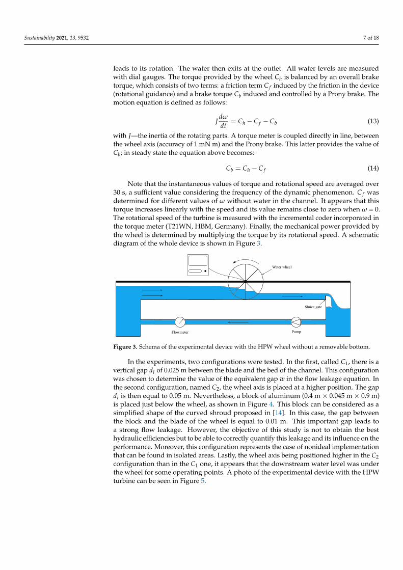
Note that the instantaneous values of torque and rotational speed are averaged over30 s, a sufficient value considering the frequency of the dynamic phenomenon. C f wasdetermined for different values of ω without water in the channel. It appears that thistorque increases linearly with the speed and its value remains close to zero when ω = 0.The rotational speed of the turbine is measured with the incremental coder incorporated inthe torque meter (T21WN, HBM, Germany). Finally, the mechanical power provided bythe wheel is determined by multiplying the torque by its rotational speed. A schematicdiagram of the whole device is shown in Figure 3.
Flowmeter Pump
Sluice gate
Water wheel
Figure 3. Schema of the experimental device with the HPW wheel without a removable bottom.
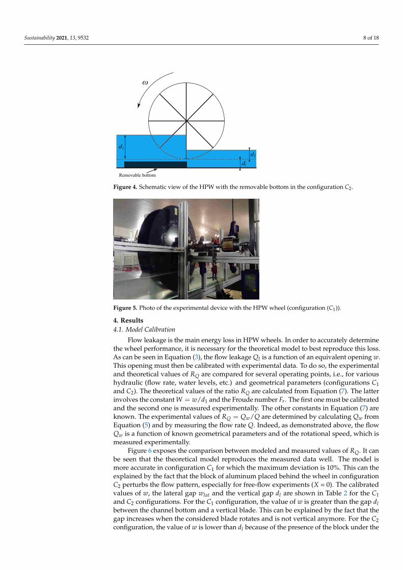
In the experiments, two configurations were tested. In the first, called C1, there is avertical gap dl of 0.025 m between the blade and the bed of the channel. This configurationwas chosen to determine the value of the equivalent gap w in the flow leakage equation. Inthe second configuration, named C2, the wheel axis is placed at a higher position. The gapdl is then equal to 0.05 m. Nevertheless, a block of aluminum (0.4 m × 0.045 m × 0.9 m)is placed just below the wheel, as shown in Figure 4. This block can be considered as asimplified shape of the curved shroud proposed in [14]. In this case, the gap betweenthe block and the blade of the wheel is equal to 0.01 m. This important gap leads toa strong flow leakage. However, the objective of this study is not to obtain the besthydraulic efficiencies but to be able to correctly quantify this leakage and its influence on theperformance. Moreover, this configuration represents the case of nonideal implementationthat can be found in isolated areas. Lastly, the wheel axis being positioned higher in the C2configuration than in the C1 one, it appears that the downstream water level was underthe wheel for some operating points. A photo of the experimental device with the HPWturbine can be seen in Figure 5.
Sustainability 2021, 13, 9532 8 of 18
dl
d2
d1
ω
Removable bottom
Figure 4. Schematic view of the HPW with the removable bottom in the configuration C2.
Figure 5. Photo of the experimental device with the HPW wheel (configuration (C1)).
4. Results4.1. Model Calibration
Flow leakage is the main energy loss in HPW wheels. In order to accurately determinethe wheel performance, it is necessary for the theoretical model to best reproduce this loss.As can be seen in Equation (3), the flow leakage Ql is a function of an equivalent opening w.This opening must then be calibrated with experimental data. To do so, the experimentaland theoretical values of RQ are compared for several operating points, i.e., for varioushydraulic (flow rate, water levels, etc.) and geometrical parameters (configurations C1and C2). The theoretical values of the ratio RQ are calculated from Equation (7). The latterinvolves the constant W = w/d1 and the Froude number Fr. The first one must be calibratedand the second one is measured experimentally. The other constants in Equation (7) areknown. The experimental values of RQ = Qw/Q are determined by calculating Qw fromEquation (5) and by measuring the flow rate Q. Indeed, as demonstrated above, the flowQw is a function of known geometrical parameters and of the rotational speed, which ismeasured experimentally.
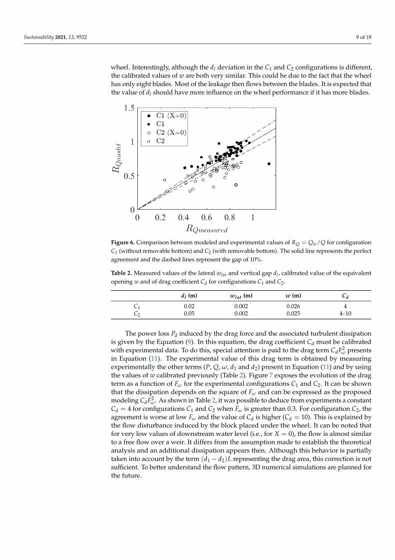
Figure 6 exposes the comparison between modeled and measured values of RQ. It canbe seen that the theoretical model reproduces the measured data well. The model ismore accurate in configuration C1 for which the maximum deviation is 10%. This can theexplained by the fact that the block of aluminum placed behind the wheel in configurationC2 perturbs the flow pattern, especially for free-flow experiments (X = 0). The calibratedvalues of w, the lateral gap wlat and the vertical gap dl are shown in Table 2 for the C1and C2 configurations. For the C1 configuration, the value of w is greater than the gap dlbetween the channel bottom and a vertical blade. This can be explained by the fact that thegap increases when the considered blade rotates and is not vertical anymore. For the C2configuration, the value of w is lower than dl because of the presence of the block under the
Sustainability 2021, 13, 9532 9 of 18
wheel. Interestingly, although the dl deviation in the C1 and C2 configurations is different,the calibrated values of w are both very similar. This could be due to the fact that the wheelhas only eight blades. Most of the leakage then flows between the blades. It is expected thatthe value of dl should have more influence on the wheel performance if it has more blades.
Figure 6. Comparison between modeled and experimental values of RQ = Qw/Q for configurationC1 (without removable bottom) and C2 (with removable bottom). The solid line represents the perfectagreement and the dashed lines represent the gap of 10%.
Table 2. Measured values of the lateral wlat and vertical gap dl , calibrated value of the equivalentopening w and of drag coefficient Cd for configurations C1 and C2.
dl (m) wlat (m) w (m) Cd
C1 0.02 0.002 0.026 4C2 0.05 0.002 0.025 4–10
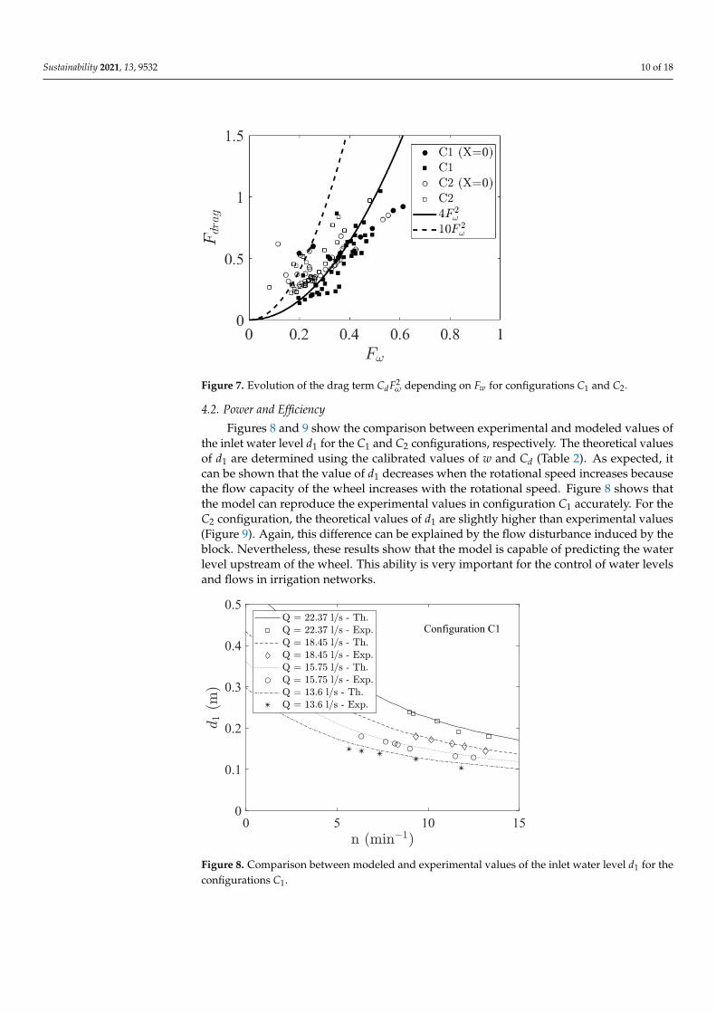
The power loss Pd induced by the drag force and the associated turbulent dissipationis given by the Equation (9). In this equation, the drag coefficient Cd must be calibratedwith experimental data. To do this, special attention is paid to the drag term CdF2
ω presentsin Equation (11). The experimental value of this drag term is obtained by measuringexperimentally the other terms (P, Q, ω, d1 and d2) present in Equation (11) and by usingthe values of w calibrated previously (Table 2). Figure 7 exposes the evolution of the dragterm as a function of Fω for the experimental configurations C1 and C2. It can be shownthat the dissipation depends on the square of Fω and can be expressed as the proposedmodeling CdF2
ω . As shown in Table 2, it was possible to deduce from experiments a constantCd = 4 for configurations C1 and C2 when Fω is greater than 0.3. For configuration C2, theagreement is worse at low Fω and the value of Cd is higher (Cd = 10). This is explained bythe flow disturbance induced by the block placed under the wheel. It can be noted thatfor very low values of downstream water level (i.e., for X = 0), the flow is almost similarto a free flow over a weir. It differs from the assumption made to establish the theoreticalanalysis and an additional dissipation appears then. Although this behavior is partiallytaken into account by the term (d1 − d2)L representing the drag area, this correction is notsufficient. To better understand the flow pattern, 3D numerical simulations are planned forthe future.
Sustainability 2021, 13, 9532 10 of 18
Figure 7. Evolution of the drag term CdF2ω depending on Fw for configurations C1 and C2.
4.2. Power and Efficiency
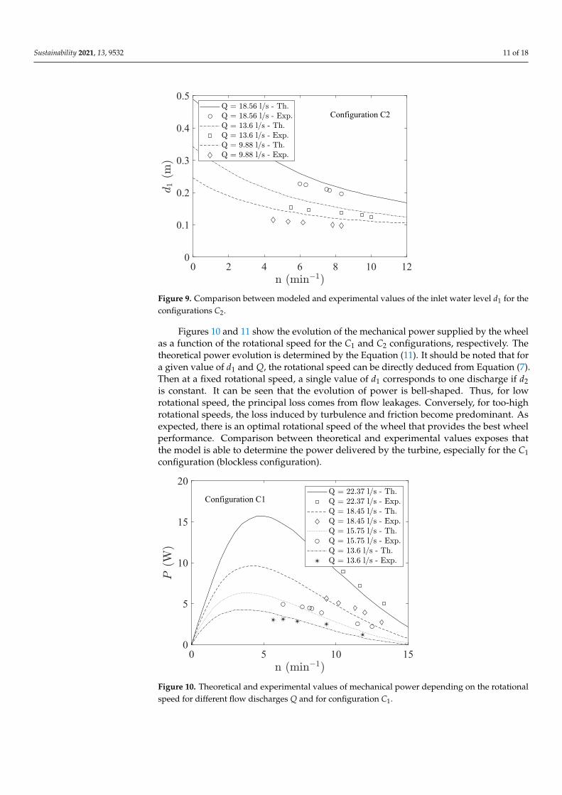
Figures 8 and 9 show the comparison between experimental and modeled values ofthe inlet water level d1 for the C1 and C2 configurations, respectively. The theoretical valuesof d1 are determined using the calibrated values of w and Cd (Table 2). As expected, itcan be shown that the value of d1 decreases when the rotational speed increases becausethe flow capacity of the wheel increases with the rotational speed. Figure 8 shows thatthe model can reproduce the experimental values in configuration C1 accurately. For theC2 configuration, the theoretical values of d1 are slightly higher than experimental values(Figure 9). Again, this difference can be explained by the flow disturbance induced by theblock. Nevertheless, these results show that the model is capable of predicting the waterlevel upstream of the wheel. This ability is very important for the control of water levelsand flows in irrigation networks.
0 5 10 150
0.1
0.2
0.3
0.4
0.5
Configuration C1
Figure 8. Comparison between modeled and experimental values of the inlet water level d1 for theconfigurations C1.
Sustainability 2021, 13, 9532 11 of 18
0 2 4 6 8 10 120
0.1
0.2
0.3
0.4
0.5
Configuration C2
Figure 9. Comparison between modeled and experimental values of the inlet water level d1 for theconfigurations C2.
Figures 10 and 11 show the evolution of the mechanical power supplied by the wheelas a function of the rotational speed for the C1 and C2 configurations, respectively. Thetheoretical power evolution is determined by the Equation (11). It should be noted that fora given value of d1 and Q, the rotational speed can be directly deduced from Equation (7).Then at a fixed rotational speed, a single value of d1 corresponds to one discharge if d2is constant. It can be seen that the evolution of power is bell-shaped. Thus, for lowrotational speed, the principal loss comes from flow leakages. Conversely, for too-highrotational speeds, the loss induced by turbulence and friction become predominant. Asexpected, there is an optimal rotational speed of the wheel that provides the best wheelperformance. Comparison between theoretical and experimental values exposes thatthe model is able to determine the power delivered by the turbine, especially for the C1configuration (blockless configuration).
0 5 10 150
5
10
15
20
Configuration C1
Figure 10. Theoretical and experimental values of mechanical power depending on the rotationalspeed for different flow discharges Q and for configuration C1.
Sustainability 2021, 13, 9532 12 of 18
0 2 4 6 8 10 120
5
10
15
20
Configuration C2
Figure 11. Theoretical and experimental values of mechanical power depending on the rotationalspeed for different flow discharges Q and for configuration C2.
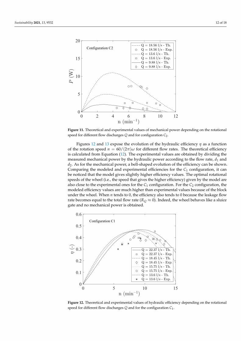
Figures 12 and 13 expose the evolution of the hydraulic efficiency η as a functionof the rotation speed n = 60/(2π)ω for different flow rates. The theoretical efficiencyis calculated from Equation (12). The experimental values are obtained by dividing themeasured mechanical power by the hydraulic power according to the flow rate, d1 andd2. As for the mechanical power, a bell-shaped evolution of the efficiency can be shown.Comparing the modeled and experimental efficiencies for the C1 configuration, it canbe noticed that the model gives slightly higher efficiency values. The optimal rotationalspeeds of the wheel (i.e., the speed that gives the higher efficiency) given by the model arealso close to the experimental ones for the C1 configuration. For the C2 configuration, themodeled efficiency values are much higher than experimental values because of the blockunder the wheel. When n tends to 0, the efficiency also tends to 0 because the leakage flowrate becomes equal to the total flow rate (RQ ≈ 0). Indeed, the wheel behaves like a sluicegate and no mechanical power is obtained.
0 5 10 150
0.1
0.2
0.3
0.4
0.5
0.6
Configuration C1
Figure 12. Theoretical and experimental values of hydraulic efficiency depending on the rotationalspeed for different flow discharges Q and for the configuration C1.
Sustainability 2021, 13, 9532 13 of 18
0 2 4 6 8 10 120
0.1
0.2
0.3
0.4
0.5
0.6
Configuration C2
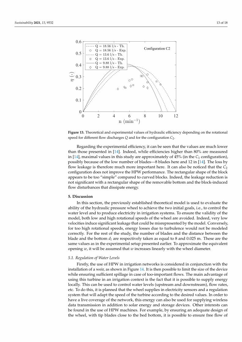
Figure 13. Theoretical and experimental values of hydraulic efficiency depending on the rotationalspeed for different flow discharges Q and for the configuration C2.
Regarding the experimental efficiency, it can be seen that the values are much lowerthan those presented in [14]. Indeed, while efficiencies higher than 80% are measuredin [14], maximal values in this study are approximately of 45% (in the C1 configuration),possibly because of the low number of blades—8 blades here and 12 in [14]. The loss byflow leakage is therefore much more important here. It can also be noticed that the C2configuration does not improve the HPW performance. The rectangular shape of the blockappears to be too “simple” compared to curved blocks. Indeed, the leakage reduction isnot significant with a rectangular shape of the removable bottom and the block-inducedflow disturbances that dissipate energy.
5. Discussion
In this section, the previously established theoretical model is used to evaluate theability of the hydraulic pressure wheel to achieve the two initial goals, i.e., to control thewater level and to produce electricity in irrigation systems. To ensure the validity of themodel, both low and high rotational speeds of the wheel are avoided. Indeed, very lowvelocities induce significant leakage that could be misrepresented by the model. Conversely,for too high rotational speeds, energy losses due to turbulence would not be modeledcorrectly. For the rest of the study, the number of blades and the distance between theblade and the bottom dl are respectively taken as equal to 8 and 0.025 m. These are thesame values as in the experimental setup presented earlier. To approximate the equivalentopening w, it will be assumed that w increases linearly with the wheel diameter.
5.1. Regulation of Water Levels
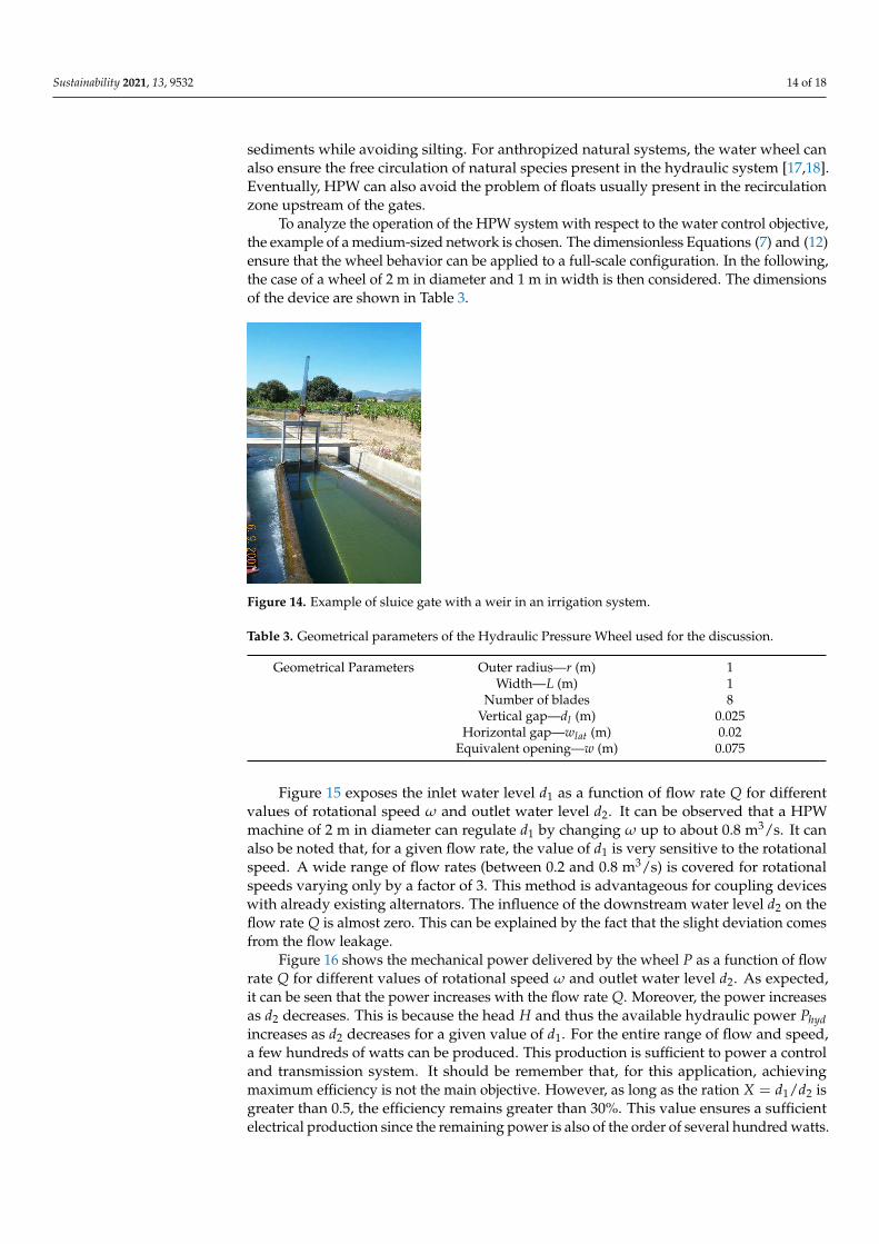
Firstly, the use of HPW in irrigation networks is considered in conjunction with theinstallation of a weir, as shown in Figure 14. It is then possible to limit the size of the devicewhile ensuring sufficient spillage in case of too-important flows. The main advantage ofusing this turbine in an irrigation context is the fact that it is possible to supply energylocally. This can be used to control water levels (upstream and downstream), flow rates,etc. To do this, it is planned that the wheel supplies in electricity sensors and a regulationsystem that will adapt the speed of the turbine according to the desired values. In order tohave a live coverage of the network, this energy can also be used for supplying wirelessdata transmission in addition to solar energy and storage devices. Other interests canbe found in the use of HPW machines. For example, by ensuring an adequate design ofthe wheel, with tip blades close to the bed bottom, it is possible to ensure free flow of
Sustainability 2021, 13, 9532 14 of 18
sediments while avoiding silting. For anthropized natural systems, the water wheel canalso ensure the free circulation of natural species present in the hydraulic system [17,18].Eventually, HPW can also avoid the problem of floats usually present in the recirculationzone upstream of the gates.
To analyze the operation of the HPW system with respect to the water control objective,the example of a medium-sized network is chosen. The dimensionless Equations (7) and (12)ensure that the wheel behavior can be applied to a full-scale configuration. In the following,the case of a wheel of 2 m in diameter and 1 m in width is then considered. The dimensionsof the device are shown in Table 3.
Figure 14. Example of sluice gate with a weir in an irrigation system.
Table 3. Geometrical parameters of the Hydraulic Pressure Wheel used for the discussion.
Geometrical Parameters Outer radius—r (m) 1Width—L (m) 1
Number of blades 8Vertical gap—dl (m) 0.025
Horizontal gap—wlat (m) 0.02Equivalent opening—w (m) 0.075
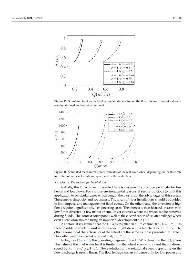
Figure 15 exposes the inlet water level d1 as a function of flow rate Q for differentvalues of rotational speed ω and outlet water level d2. It can be observed that a HPWmachine of 2 m in diameter can regulate d1 by changing ω up to about 0.8 m3/s. It canalso be noted that, for a given flow rate, the value of d1 is very sensitive to the rotationalspeed. A wide range of flow rates (between 0.2 and 0.8 m3/s) is covered for rotationalspeeds varying only by a factor of 3. This method is advantageous for coupling deviceswith already existing alternators. The influence of the downstream water level d2 on theflow rate Q is almost zero. This can be explained by the fact that the slight deviation comesfrom the flow leakage.
Figure 16 shows the mechanical power delivered by the wheel P as a function of flowrate Q for different values of rotational speed ω and outlet water level d2. As expected,it can be seen that the power increases with the flow rate Q. Moreover, the power increasesas d2 decreases. This is because the head H and thus the available hydraulic power Phydincreases as d2 decreases for a given value of d1. For the entire range of flow and speed,a few hundreds of watts can be produced. This production is sufficient to power a controland transmission system. It should be remember that, for this application, achievingmaximum efficiency is not the main objective. However, as long as the ration X = d1/d2 isgreater than 0.5, the efficiency remains greater than 30%. This value ensures a sufficientelectrical production since the remaining power is also of the order of several hundred watts.
Sustainability 2021, 13, 9532 15 of 18
Figure 15. Simulated inlet water level estimated depending on the flow rate for different values ofrotational speed and outlet water level.
Figure 16. Simulated mechanical power estimates of the real-scale wheel depending on the flow ratefor different values of rotational speed and outlet water level.
5.2. Electric Production for Isolated Site
Initially, the HPW wheel presented here is designed to produce electricity for lowheads and low flows. For various environmental reasons, it seems judicious to limit thisapplication to particular cases which benefit the most from the advantages of this system.These are its simplicity and robustness. Thus, run-of-river installations should be avoidedto limit impacts and management of flood events. On the other hand, the diversion of highflows requires significant civil engineering costs. The interest is then focused on cases withlow flows diverted (a few m3/s) or small river courses where the wheel can be removedduring floods. This context corresponds well to the electrification of isolated villages whereeven a few kilowatts can bring an important development aid [19].
As before, it is assumed that the HPW is installed in a 1 m channel (i.e., L = 1 m). It isthen possible to work by unit width as one might do with a hill chart for a turbine. Theother geometrical characteristics of the wheel are the same as those presented in Table 3.The outlet water level is taken equal to d2 = 0.7 m.
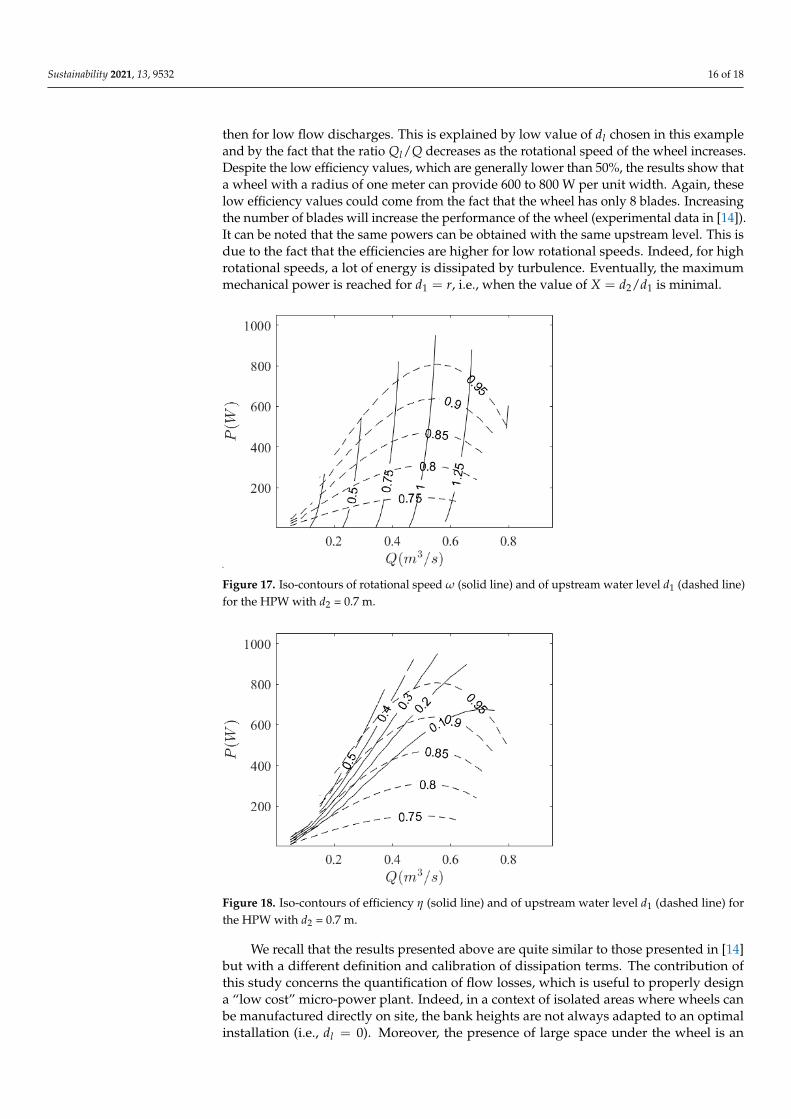
In Figures 17 and 18, the operating diagram of the HPW is drawn in the P, Q plans.The value of the inlet water level is limited by the wheel size (d1 < r) and the rotationalspeed by Fω = rω/
√gd1 < 1. The evolution of the rotational speed depending on the
flow discharge is nearly linear. The flow leakage has an influence only for low power and
Sustainability 2021, 13, 9532 16 of 18
then for low flow discharges. This is explained by low value of dl chosen in this exampleand by the fact that the ratio Ql/Q decreases as the rotational speed of the wheel increases.Despite the low efficiency values, which are generally lower than 50%, the results show thata wheel with a radius of one meter can provide 600 to 800 W per unit width. Again, theselow efficiency values could come from the fact that the wheel has only 8 blades. Increasingthe number of blades will increase the performance of the wheel (experimental data in [14]).It can be noted that the same powers can be obtained with the same upstream level. This isdue to the fact that the efficiencies are higher for low rotational speeds. Indeed, for highrotational speeds, a lot of energy is dissipated by turbulence. Eventually, the maximummechanical power is reached for d1 = r, i.e., when the value of X = d2/d1 is minimal.
Figure 17. Iso-contours of rotational speed ω (solid line) and of upstream water level d1 (dashed line)for the HPW with d2 = 0.7 m.
Figure 18. Iso-contours of efficiency η (solid line) and of upstream water level d1 (dashed line) forthe HPW with d2 = 0.7 m.
We recall that the results presented above are quite similar to those presented in [14]but with a different definition and calibration of dissipation terms. The contribution ofthis study concerns the quantification of flow losses, which is useful to properly designa “low cost” micro-power plant. Indeed, in a context of isolated areas where wheels canbe manufactured directly on site, the bank heights are not always adapted to an optimalinstallation (i.e., dl = 0). Moreover, the presence of large space under the wheel is an
Sustainability 2021, 13, 9532 17 of 18
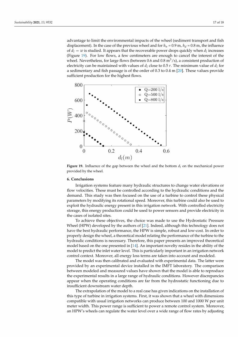
advantage to limit the environmental impacts of the wheel (sediment transport and fishdisplacement). In the case of the previous wheel and for hu = 0.9 m, hd = 0.8 m, the influenceof dl = w is studied. It appears that the recoverable power drops quickly when dl increases(Figure 19). For low flows, a few centimeters are enough to cancel the interest of thewheel. Nevertheless, for large flows (between 0.6 and 0.8 m3/s), a consistent production ofelectricity can be maintained with values of dl close to 0.5 r. The minimum value of dl fora sedimentary and fish passage is of the order of 0.3 to 0.4 m [20]. These values providesufficient production for the highest flows.
Figure 19. Influence of the gap between the wheel and the bottom dl on the mechanical powerprovided by the wheel.
6. Conclusions
Irrigation systems feature many hydraulic structures to change water elevations orflow velocities. These must be controlled according to the hydraulic conditions and thedemand. This study was then focused on the use of a turbine to control these physicalparameters by modifying its rotational speed. Moreover, this turbine could also be used toexploit the hydraulic energy present in this irrigation network. With controlled electricitystorage, this energy production could be used to power sensors and provide electricity inthe cases of isolated sites.
To achieve these objectives, the choice was made to use the Hydrostatic PressureWheel (HPW) developed by the authors of [21]. Indeed, although this technology does nothave the best hydraulic performance, the HPW is simple, robust and low-cost. In order toproperly design the wheel, a theoretical model relating the performance of the turbine to thehydraulic conditions is necessary. Therefore, this paper presents an improved theoreticalmodel based on the one presented in [14]. An important novelty resides in the ability of themodel to predict the inlet water level. This is particularly important in an irrigation networkcontrol context. Moreover, all energy loss terms are taken into account and modeled.
The model was then calibrated and evaluated with experimental data. The latter wereprovided by an experimental device installed in the IMFT laboratory. The comparisonbetween modeled and measured values have shown that the model is able to reproducethe experimental results in a large range of hydraulic conditions. However discrepanciesappear when the operating conditions are far from the hydrostatic functioning due toinsufficient downstream water depth.
The extrapolation of the model to a real case has given indications on the installation ofthis type of turbine in irrigation systems. First, it was shown that a wheel with dimensionscompatible with usual irrigation networks can produce between 100 and 1000 W per unitmeter width. This power range is sufficient to power a remote control system. Moreover,an HPW’s wheels can regulate the water level over a wide range of flow rates by adjusting
Sustainability 2021, 13, 9532 18 of 18
its rotation speed. Eventually, electricity production with a HPW can be significant evenif there are high flow leakages due to implementation difficulties. Nevertheless, themechanical power can drop quickly when the gap between the wheel and the bottomis too large. The turbine then no longer works with hydrostatic forces but recovers thekinetic energy.
Author Contributions: Conceptualization: L.C.; experimentations: L.C.; analysis: L.C., G.D., P.M.and N.D.; original draft preparation: L.C. and G.D.; review and editing: L.C., G.D., P.M. and N.D.;supervision: L.C. All authors have read and agreed to the published version of the manuscript.
Funding: This research received no external funding.
Informed Consent Statement: Not applicable.
Data Availability Statement: Not applicable.
Conflicts of Interest: The authors declare no conflict of interest.
References1. Butera, I.; Balestra, R. Estimation of the hydropower potential of irrigation networks. Renew. Sustain. Energy Rev. 2015, 48, 140–151.
[CrossRef]2. Kim, B.; Azzaro-Pantel, C.; Pietrzak-David, M.; Maussion, P. Life cycle assessment for a solar energy system based on reuse
components for developing countries. J. Clean. Prod. 2019, 208, 1459–1468. [CrossRef]3. Williamson, S.J.; Stark, B.H.; Booker, J.D. Low head pico hydro turbine selection using a multi-criteria analysis. Renew. Energy
2014, 61, 43–50. [CrossRef]4. Quaranta, E.; Revelli, R. Gravity water wheels as a micro hydropower energy source: A review based on historic data, design
methods, efficiencies and modern optimizations. Renew. Sustain. Energy Rev. 2018, 97, 414–427. [CrossRef]5. Müller, G.; Kauppert, K. Performance characteristics of water wheels. J. Hydraul. Res. 2004, 42, 451–460. [CrossRef]6. Quaranta, E. Stream water wheels as renewable energy supply in flowing water: Theoretical considerations, performance
assessment and design recommendations. Energy Sustain. Dev. 2018, 45, 96–109. [CrossRef]7. Quaranta, E.; Revelli, R. Output power and power losses estimation for an overshot water wheel. Renew. Energy 2015, 83, 979–987.
[CrossRef]8. Quaranta, E.; Revelli, R. Performance characteristics, power losses and mechanical power estimation for a breastshot water wheel.
Energy 2015, 87, 315–325. [CrossRef]9. Quaranta, E.; Revelli, R. Optimization of breastshot water wheels performance using different inflow configurations. Renew.
Energy 2016, 97, 243–251. [CrossRef]10. Quaranta, E.; Revelli, R. Hydraulic Behavior and Performance of Breastshot Water Wheels for Different Numbers of Blades.
J. Hydraul. Res. 2017, 143, 04016072. [CrossRef]11. Vidali, C.; Fontan, S.; Quaranta, E.; Cavagnero, P.; Revelli, R. Experimental and dimensional analysis of a breastshot water wheel.
J. Hydraul. Res. 2016, 54, 473–479. [CrossRef]12. Quaranta, E.; Revelli, R. CFD simulations to optimize the blades design of water wheels. Drink. Water Eng. Sci. Discuss.
2017,10, 27-32. [CrossRef]13. Quaranta, E.; Müller, G. Sagebien and Zuppinger water wheels for very low head hydropower applications. J. Hydraul. Res. 2018,
56, 526–536. [CrossRef]14. Senior, J.; Saenger, N.; Müller, G. New hydropower converters for very low-head differences. J. Hydraul. Res. 2010, 48, 703–714.
[CrossRef]15. Belaud, G.; Cassan, L.; Baume, J.P. Calculation of Contraction Coefficient under Sluice Gates and Application to Discharge
Measurement. J. Hydraul. Eng. 2009, 135, 1086–1091. [CrossRef]16. Belaud, G.; Cassan, L.; Baume, J.P. Contraction and Correction Coefficients for Energy-Momentum Balance under Sluice Gates.
In Proceedings of the World Environmental and Water Resources Congress 2012, Albuquerque, NM, USA, 20–24 May 2012.[CrossRef]
17. Guiot, L.; Cassan, L.; Belaud, G. Modeling the Hydromechanical Solution for Maintaining Fish Migration Continuity at CoastalStructures. J. Irrig. Drain. Eng. 2020, 146, 04020036. [CrossRef]
18. Guiot, L.; Cassan, L.; Dorchies, D.; Sagnes, P.; Belaud, G. Hydraulic management of coastal freshwater marsh to conciliate localwater needs and fish passage. J. Ecohydraul. 2020, in press. [CrossRef]
19. UNCTAD. The Least Developed Countries Report 2017: Transformational Energy Access; United Nations Conference on Trade andDevelopment: Geneva, Switzerland, 2017.
20. Baudoin, J.M.; Burgun, V.; Chanseau, M.; Larinier, M.; Ovidio, M.; Sremski, W.; Steinbach, P.; Voegtle, B. The ICE Protocol forEcological Continuity—Assessing the Passage of Obstacles by Fish: Concepts, Design and Application; Onema: Vincennes, France, 2014.
21. Müller, G.; Kauppert, K. Old watermills—Britain’s new source of energy? Civ. Eng. 2002, 150, 178–186. [CrossRef]


