Hydraulic resistance determination in marsh wetlands

Water Resources Management14: 285–309, 2000.© 2000Kluwer Academic Publishers. Printed in the Netherlands.

285

Hydraulic Resistance Determination in MarshWetlands

VASSILIOS A. TSIHRINTZIS1∗ and EDGAR E. MADIEDO2

1 Laboratory of Ecological Engineering and Technology, Department of EnvironmentalEngineering, Democritus University of Thrace, Xanthi 67100, Greece2 Formerly, Graduate Student, Department of Civil and Environmental Engineering, FloridaInternational University, Miami, FL 33199, U.S.A.(∗ author for correspondence, e-mail: [email protected], [email protected])

(Received: 18 January 2000; revised: 9 August 2000)

Abstract. Restoration of degraded and creation of constructed wetlands require proper hydraulicdesign. Of particular importance is the accurate determination of flow resistance factors and theproper use of resistance equations, something essential for computing basic hydraulic parameters,such as depth and velocity, and for modeling the hydrodynamics of the system. In this study, selectedprevious theoretical, laboratory and field studies on wetlands and vegetated-channel hydraulics arereviewed, and existing data from these studies are extracted and compiled in a common database.Resistance determining parameters are discussed, and results are summarized and presented, aimingat obtaining laws governing the flow, and deriving values for frictional factors under various flowscenarios. Graphs of Darcy-Weisbachf or Manning’sn versus appropriate hydraulic parametersare presented. A modifiedn-VRgraph is also presented, appropriate for marsh preliminary hydraulicanalyses and design. These graphs also indicate missing information and can guide in future research.

Key words: Chèzy equation, Darcy-Weisbach equation, hydraulic resistance, Manning’s equation,marsh, retardance curves, roughness, vegetation, wetland

1. Introduction

In recent years, interest on wetlands has come to scene due to the multiple functionsthey provide and their vital part in the balance of the global ecosystem (Mitsch andGosselink, 1986; Buenoet al., 1995; Tsihrintzis, 1999). Several wetland restorationprojects have been undertaken (e.g., Tsihrintziset al., 1995a, 1996, 1998), as wellas constructed wetland creation projects for wastewater and stormwater treatment(e.g., Hammer, 1989; Moshiri, 1993; Reedet al., 1995; Kadlec and Knight, 1996;Tsihrintziset al., 1995b; Economopoulou and Tsihrintzis, 1999, 2000a). Thus, theneed has emerged for accurate estimation of wetland hydraulic parameters, andtherefore, it is important the proper formulation of resistance to flow in wetlands(Economopoulou and Tsihrintzis, 2000b).

In this article, several previous studies on flow through vegetation (i.e., grassor wetlands) have been searched and are summarized and presented. The em-phasis was on marsh type of vegetation (i.e., emergent herbaceous vegetation),

286 V. A. TSIHRINTZIS AND E. E. MADIEDO

with applications in constructed wetlands hydraulics or tidal marsh modeling. Flowconditions covered the laminar, transitional and turbulent states. Most previousstudies have expressed hydraulic resistance in various ways and in terms of variousparameters. This study attempts to compile existing data in a common database,and express hydraulic resistance with commonly used parameters and equations.Indeed, experimental data from these studies have been extracted and used to com-pute values for the Darcy-Weisbach frictional factorf , the Manning’s roughnessfactor n, the flow Reynolds numberRe (defined using the hydraulic radius), thehydraulic radiusR (or the flow depthy) and the parameterVR (i.e., the productof the mean velocity and the hydraulic radius). Compiled data are presented ingraphs:f vs Re, n vs VR and n vs R (or y, since in most wetlands, the flowdepth and the hydraulic radius are nearly equal because the depth is shallow andthe flow is wide). These graphs do not contain enough data to cover all conditions,indicating needs for future research. However, as shown in examples, they can beused in preliminary design.

2. Review and theoretical background

Numerous studies have been undertaken in the past on resistance to flow in openchannels (lined or natural), including channels with alluvial and gravel beds andvegetated channels. Several publications summarize theory and present design aids(e.g., Chow, 1959; Simons and Sentürk, 1992; Yen, 1992). The three traditionalformulas, used for flow resistance computation in open channels are the Darcy-Weisbach, Chèzy and Manning equations, which respectively read:

V =√

8g

f

√RS (a) V = C√RS (b) V = 1

nR2/3S1/2 (c) (1)

whereV is the mean flow velocity (m s−1); R is the hydraulic radius of the crosssection (m);S is the slope of the energy grade line (m m−1); g is the gravity accel-eration (m s−2); f is the Darcy-Weisbach frictional factor;C is Chèzy’s resistancefactor (m1/2 s−1); andn is the Manning’s resistance coefficient (s m−1/3).

The three resistance coefficientsf , C andn generally depend on the Reynoldsnumber and the boundary relative roughness and, to some extent, on the shape ofthe channel (Chow, 1959). However, in practice, onlyf is expressed in terms of theReynolds number (e.g., Chow, 1959) for any flow state (i.e., laminar, transitional,and turbulent).C andn, although they have also been expressed as functions of theRe (e.g., Henderson, 1966), usually are taken from tables as constants (obviouslyassuming fully developed turbulent flow), depending mostly on the channel wallmaterial, condition and geometry (Cowan, 1956; Chow, 1959; Barnes, 1967; Arce-ment and Schneider, 1989; Yen, 1992). However, in the laminar and transitionalflows, the Manning’s and Chèzy’s equations are valid only ifn andC are recog-nized as also dependent on the Reynolds number. Furthermore, a channel does not

HYDRAULIC RESISTANCE DETERMINATION IN MARSH WETLANDS 287

have a constant resistance coefficient under all occasions and conditions. Actually,satisfactory characterization in terms of frictional factors have been achieved forthe case of steady, uniform, sediment-free flows in channels of impervious rigidboundaries, with densely distributed, nearly homogeneous roughness on the wetperimeter (Chow, 1959; Coyle, 1975; Simons and Sentürk, 1992; Guillen, 1996).In other cases of open channel flow, limited research has been conducted, tryingto describe the variation of flow resistance in the presence of various roughnesselements on the boundary of the channel, such as resistance to flow in alluvialchannels or in gravel and mountain channels.

Previous studies have also covered vegetated (grassed) channels and flood-plains, with emphasis on the establishment of relations containing similar para-meters to those used in lined or alluvial channels (Chow, 1959). However, whenvegetation is present in a channel, turbulence intensity increases, causing additionalloss of energy and retardance of flow. Traditionally, resistance to flow in grassedchannels has also been described by use of Manning’s equation, withn depend-ing on a retardance factor, which is a function of the vegetation characteristics(i.e., height, thickness, density, etc.), and the previously mentioned parameterVR(Chow, 1959; Coyle, 1975; Kouwen and Li, 1980; French, 1985).

Flow in wetlands has a list of specific and unique characteristics which makeit different from flow in open channels. Excellent descriptions of these character-istics have been presented by Kadlec (1990), among others. Among them are thefollowing: (1) slopes are mild; (2) flows generally do not reach turbulent condition,but rather remain in the laminar or transitional states, controlled by vegetationresistance; (3) density and type of vegetation are different from grassed channels;(4) areas are intermittently flooded; (5) depending on the water level, there maybe channeling, i.e., concentrated flows in deeper portions of the wetland only;(6) depths are shallow and the bed topography is highly variable (there may existhummocks and depressions, for example, a±0.3 m bed fluctuation around themean bed level may be common in some freshwater marshes, something quite im-portant if one considers that usual depths vary between 0.1 and 0.5 m); (7) the ratioof flow depth to vegetation height is quite smaller than that in grassed channels,being of the order of 1.0 for submerged vegetation and quite lower than 1.0 foremergent vegetation; (8) due to the vegetation presence in the wetland, the velocityis variable from point to point, both in magnitude and in direction, thus leadingto a highly variable in space roughness; and (9) there are several wetland types.Mitsch and Gosselink (1986) describe about 15 different types in the U.S.A. only,therefore, generalization in terms of hydrology and flow behavior is difficult orimpossible. For example, in constructed wetlands common Reynolds numbers mayrange between 1 and 1000 (Kadlec, 1990) and in tidal marshes between 5000 and60 000 (Roig, 1994), or in constructed wetlands the vegetation is always emergentand in tidal marshes it changes from totally out of water to emergent to submerged,depending on the tide (Tsihrintziset al., 1996).


The resistance to flow in wetlands depends on various mechanisms, a resultof the interaction of flow with the channel walls and the vegetation stems andcanopy. The most important resistance mechanisms are the following (Roig, 1994):(1) form drag (due to the hydrostatic pressure difference upstream and downstreamof a stem, as a result of flow passing around the stem); (2) skin or surface drag(from shear stress from solid surfaces in contact with the flow, such as channelbed and walls and vegetation surface); (3) wave drag (due to deformation of thefree surface of water when the stems penetrate it); (4) energy losses due to fluidviscosity and turbulence.

In many instances, flow in wetlands is in the laminar or transitional states, whichlimits the use of the Manning’s formula. Adjustments to the formula have beenproposed in order to be used (Horton, 1938; Turner and Chanmeesri, 1984; Scar-latos and Tisdale, 1989; Kadlec, 1990, and others). For example, Kadlec (1990)proposed the use of the Manning’s equation in combination with the expression forlaminar flow to account for the energy grade line slope in the channel:

S = 3v

gy2V + n2

R4/3V 2 (2)

where v is the kinematic viscosity (m2 s−1) and y is the flow depth (m). Al-ternatively, Kadlec (1990) proposed the following general empirical equation fordescribing wetland flow:

Q

W= q = KyβSαf (3)

whereQ is the flow rate (m3 s−1); W is the flow width (m);q is the discharge perunit width (m3 s−1 m−1);K is a resistance coefficient, which depends on the veget-ation density and bed litter; andα andβ are exponents. There are specific valuesfor K, α andβ recommended for use in constructed wetlands (based on Kadlec’sdata from Houghton Lake Wetland):α = 1.0,β = 3.0, andK = 1× 107/86 400 s−1

m−1 for dense vegetation andK = 5× 107/86 400 s−1 m−1 for sparse vegetation. Ingeneral,α varies from 0.5 (turbulent flow) to 1.0 (laminar flow),β varies from 1.67(turbulent flow) to 3.0 (laminar flow), andK must be determined for each exponentchosen by a regression analysis on field data collected (discharge and flow depth)for a specific site.

Although Equation (3) may give a more accurate physical description of wet-land flow, its application requires values for parametersK, α andβ, which makesits use site-specific; for this reason use of Manning’s equation is still widespread.Actually, Equation (3) reduces to Manning’s equation forα = 1/2, β = 5/3 andK = 1/n. However, when Manning’s equation is used,n should be consideredvariable with flow depth, as a result of vertical vegetation density variation. Kadlecand Knight (1996) have summarized existing data on Manning’sn values in variouswetland types and present them in a graph relatingn to flow depth. Then values


on this graph range over nearly three orders of magnitude, because data have beencollected under various conditions and from various wetland types. Kadlec andKnight (1996) have also drawn on this graph two speculative lines, applying tosparse and dense emergent marsh vegetation. Similarly, Reedet al. (1995) suggestthe use of Manning’s formula in constructed wetland design, with a variablen

given by the equation:n = γ /y1/2, whereγ is a constant, which for most marsheswith emergent vegetation assumes values from 1 to 4 m1/6s. A discussion on theuse of this type of equations forn is presented by Economopoulou and Tsihrintzis(2000b).

3. Methods and materials

3.1. BACKGROUND STUDIES

Representative studies on hydraulic resistance of vegetation are those by Hsieh(1962), Petryk and Bosmajian (1975), Pasche and Rouvé (1985), Shih and Rahi(1982), Kutija and Hong (1996), Naotet al. (1996), and Darby and Thorne (1996).These studies, which helped develop an understanding of the flow through vegeta-tion and draw qualitative conclusions, are summarized in Table I.

3.2. STUDIES USED IN DATA EXTRACTION AND ANALYSIS

Table II presents studies containing quantitative data used to prepare the databaseand the analyses for this study. Detailed experimental conditions for these studiesare presented in Tables III and IV. These studies covered various conditions, suchas submerged wetland vegetation (Chiew and Tan, 1992; Chen, 1976), emergentwetland vegetation (Chen, 1976; Turner and Chanmeesri, 1984; Kadlec, 1990;Roig, 1994; Fathi-Maghadam and Kouwen, 1997; Wuet al., 1999), flexible ve-getation (Turner and Chanmeesri, 1984; Kadlec, 1990; Hall and Freeman, 1994;Fathi-Maghadam and Kouwen, 1997), and rigid stems (Roig, 1994). For all thesestudies the section of the channel was rectangular.

Measured hydraulic parameters and data from these studies were extracted andre-analyzed to derive Darcy-Weisbachf and Manning’sn values, using Equa-tion (1), and produce graphs relatingf andn with flow parameters (i.e.,Re, VR,andR or y). Data from other studies (e.g., Cox, 1942; Palmer, 1945; Cox andPalmer, 1948; Ree, 1941, 1949; Ree and Palmer, 1949; Coyle, 1975; Kouwen andLi, 1980; Kouwen, 1988), conducted mainly on grasses, were also reviewed tolook at resistance behavior. Most of these studies have been used to derive or testthe vegetation retardance curves for grassed-channel design (Chow, 1959; French,1985). Therefore, these data were not re-analyzed but the retardance curves areutilized directly.

290V.A

.TS

IHR

INT

ZIS

AN

DE

.E.M

AD

IED

O

Table I. Summary of studies with qualitative data reviewed

HY

DR

AU

LIC

RE

SIS

TAN

CE

DE

TE

RM

INA

TIO

NIN

MA

RS

HW

ET

LA

ND

S291

Table II. Summary of studies with quantitative data used

292V.A

.TS

IHR

INT

ZIS

AN

DE

.E.M

AD

IED

O

Table III. Summary of experimental conditions for studies used in analyses – Vegetation parameters

HY

DR

AU

LIC

RE

SIS

TAN

CE

DE

TE

RM

INA

TIO

NIN

MA

RS

HW

ET

LA

ND

S293

Table IV. Summary of experimental conditions for studies used in analyses – Hydraulic parameters

Study Experimental Hydraulic parameter

conditions Friction Depthy Mean Froude number Reynolds Parameter Darcy- Manning’s

slope velocityV Fr = number VR Weisbach n

S (m) (m s−1) V/(gy)1/2 Re = VR/v (m2 s−1) f (s m−1/3)

Kadlec S = 0.00001 0.00001 0.05–0.30 0.00003–0.00054 0.00004–0.00031 1–134 0.000001–0.000161 50855–816 15.5–2.6

(1990) S = 0.0001 0.00010 0.05–0.30 0.00021–0.00287 0.00030–0.00167 9–718 0.000011–0.000861 8805–286 6.4–1.6

S = 0.001 0.00100 0.05–0.30 0.00111–0.01157 0.00159–0.00675 46–2894 0.000056–0.003472 3178–176 3.9–1.2

S = 0.01 0.01000 0.05–0.30 0.00344–0.03981 0.00492–0.02321 144–9954 0.000172–0.011944 3307–149 3.9–1.1

Chen S = 0.001 0.001 0.027–0.088 0.00895–0.09576 0.017–0.103 200–7000 0.00024–0.00840 26.3–0.75 0.317–0.065

(1976) S = 0.005 0.005 0.022–0.055 0.01072–0.06522 0.023–0.089 200–3000 0.00024–0.00360 76.4–5.1 0.524–0.157

S = 0.035 0.035 0.023–0.039 0.02119–0.06196 0.045–0.101 400–2000 0.00048–0.00240 138.6–27.7 0.707–0.346

S = 0.087 0.087 0.012–0.047 0.00803–0.12647 0.023–0.185 80–5000 0.00010–0.00600 1266.0–20.3 1.921–0.306

S = 0.164 0.164 0.012–0.037 0.01001–0.09662 0.029–0.160 100–3000 0.00012–0.00360 1541.0–51.4 2.120–0.468

S = 0.316 0.316 0.016–0.035 0.02241–0.10403 0.056–0.179 300–3000 0.00036–0.00360 793.0–79.3 1.597–0.574

S = 0.555 0.555 0.013–0.023 0.01823–0.05329 0.051–0.113 200–1000 0.00024–0.00120 1727.0–345.4 2.280–1.115

Wu et al. S = 0.00383 0.00383 0.008–0.041 0.00235–0.01206 0.008–0.019 16–412 0.00002–0.00046 434.3–84.7 1.052–0.610

(1990) S = 0.00533 0.00533 0.013–0.046 0.00451–0.01596 0.013–0.024 49–612 0.00006–0.00068 267.2–75.5 0.895–0.587

S = 0.01025 0.01025 0.007–0.051 0.00337–0.02454 0.013–0.035 20–1043 0.00002–0.00115 496.3–68.1 1.100–0.567

S = 0.0273 0.0273 0.012–0.051 0.00942–0.04005 0.027–0.057 94–1702 0.00011–0.00188 289.5–68.1 0.919–0.567

S = 0.041 0.041 0.008–0.047 0.0077–0.04523 0.027–0.067 51–1772 0.00006–0.00197 434.3–73.9 1.052–0.583

Chiew and Low density 0.14 0.007–0.0199 0.0700–0.1598 0.267–0.362 377–2147 0.00045–0.00258 14.12–6.47 0.186–0.149

Tan (1992) High density 0.14 0.0103–0.0238 0.0699–0.1202 0.220–0.249 535–1862 0.00064–0.00223 19.88–13.03 0.235–0.219

Hall and Low density 0.00066– 0.340–0.489 0.025–0.110 0.014–0.050 4518–24693 0.005–0.030 17.88–8.86 0.37–0.27

Freeman (1994) 0.00507

High density 0.00221– 0.366–0.527 0.025–0.110 0.013–0.048 4735–25709 0.006–0.031 63.01–28.79 0.7 –0.49

0.01583

294V.A

.TS

IHR

INT

ZIS

AN

DE

.E.M

AD

IED

O

Table IV. (continued)

Study Experimental Hydraulic parameter

conditions Friction Depthy Mean Froude number Reynolds Parameter Darcy- Manning’s

slope velocityV Fr = number VR Weisbach n

S (m) (m s−1) V/(gy)1/2 Re = VR/v (m2 s−1) f (s m−1/3)

Fathi- Pine and 0.004– 0.06–0.30 0.10–0.90 0.058–1.173 5000–225000 0.005–0.135 0.384–2.0925 0.0438–0.1336

Maghadam and cedar tree 0.00700

Kouwen (1997) models

Turner and Section A 0.0020 0.01–0.10 0.02535–0.04942 0.081–0.050 203–3963 0.00025–0.00494 2.443–6.425 0.082–0.195

Chanmeesri Section B 0.0020 0.01–0.10 0.04217–0.06839 0.135–0.069 338–5484 0.00042–0.00684 0.883–3.356 0.049–0.141

(1984) Section D 0.0025 0.01–0.10 0.04518–0.07852 0.144–0.079 362–6297 0.00045–0.00785 0.961–3.182 0.051–0.137

Section G 0.0027 0.01–0.10 0.02844–0.06222 0.091–0.063 228–4990 0.00028–0.00622 2.620–5.473 0.085–0.180

Section E 0.0028 0.01–0.10 0.05149–0.11527 0.164–0.116 413–9244 0.00051–0.01153 0.829–1.654 0.048–0.099

Section H 0.0028 0.01–0.10 0.05335–0.09487 0.170–0.096 428–7608 0.00053–0.00949 0.772–2.442 0.046–0.120

S = 0.0017 0.0017 0.01–0.10 0.02377–0.03768 0.076–0.038 191–3022 0.00024–0.00377 2.361–9.398 0.081–0.236

S = 0.0021 0.0021 0.01–0.10 0.02536–0.04019 0.081–0.041 203–3223 0.00025–0.00402 2.563–10.203 0.084–0.246

S = 0.0034 0.0034 0.01–0.10 0.02821–0.04682 0.090–0.047 226–3755 0.00028–0.00468 3.352–12.171 0.096–0.268

S = 0.0050 0.0050 0.01–0.10 0.03302–0.05738 0.105–0.058 265–4601 0.00033–0.00574 3.599–11.919 0.099–0.266

S = 0.0067 0.0067 0.01–0.10 0.03811–0.07262 0.122–0.073 306–5823 0.00038–0.00726 3.621–9.972 0.100–0.243

S = 0.0084 0.0084 0.01–0.10 0.04190–0.08360 0.134–0.084 336–6704 0.00042–0.00836 3.755–9.432 0.102–0.236

S = 0.01000 0.0100 0.01–0.10 0.04589–0.09156 0.147–0.092 368–7343 0.00046–0.00916 3.727–9.361 0.101–0.235

Roig (1994) s/d = 4 0.00128–0.06836 0.061–0.424 0.03987–0.24317 0.032–0.163 3763–28541 0.00376–0.02854 2.849–12.328 0.139–0.279

s/d = 6 0.00013–0.04107 0.055–0.348 0.05261–0.30273 0.045–0.257 4589–29291 0.00459–0.02929 0.322–4.293 0.043–0.165

s/d = 8 0.00120–0.03132 0.056–0.336 0.09144–0.36021 0.071–0.317 6812–32962 0.00681–0.03296 0.716–2.138 0.057–0.117

s/d = 12 0.00053–0.02459 0.048–0.305 0.13106–0.43190 0.109–0.381 8646–36860 0.00865–0.03686 0.160–0.883 0.029–0.072

s/d = 4 nu 0.00252–0.03847 0.057–0.318 0.10132–0.34083 0.088–0.266 7077–32922 0.00708–0.03292 1.240–2.568 0.075–0.125

s/d = 6 nu 0.00215–0.05377 0.061–0.376 0.05938–0.26408 0.049–0.185 4516–28786 0.00452–0.02879 2.471–7.033 0.128–0.206


4. Results and discussion

4.1. GENERAL OBSERVATIONS

The reviewed studies and data in Tables I and II allowed making several generalobservations on flow in wetlands and through vegetation, which are presented here.Generally, the influence of vegetation (particularly flexible vegetation) on flowresistance is difficult and complex to model. This is due to transport processes,turbulence, drag forces, roughness and velocities around the stems and through thefoliage, mechanisms that are not well understood.

It can be stated that:

(1) flow in wetlands is controlled by the vegetation drag;(2) because the vegetation density varies vertically in most wetland systems, the

roughness and velocity pattern are highly variable with depth. An increase invegetation density (as measured with vegetation density parameters, such asthe ratio of separation of stems to diameter of stems and/or the number of stemsper unit surface area) results in an increase in flow resistance. With respectto the arrangement of the vegetation, relatively lower values of resistance areobtained, when less frontal area of vegetation is directly exposed to the flow(e.g., square arrangement vs staggered arrangement);

(3) the flexural properties of the vegetation, (i.e., rigid vs flexible vegetation) greatlyaffect flow properties. Stiffness is defined by the module of elasticityE ofthe specific stem material and the moment of inertiaI of the stem section,parameters which measure the stem’s ability to resist bending due to flowforces;

(4) the degree of submergence (i.e., submerged vs emergent vegetation). For sub-merged vegetation, the resistance generally has the highest values at low velo-cities and shallow flow depths, but as the velocity or flow depth increase, theeffects of vegetation on the resistance shows an appreciable decrease. On theother hand, in the case of emergent vegetation some studies have reported thatthe resistance to flow initially decreases with increasing depth up to the point ofsubmergence and then it increases with increasing depth to a maximum value,which occurs slightly above the point of submergence (e.g., Wuet al., 1999).Other studies have reported that, for emergent vegetation, resistance only in-creases with increasingRe (e.g., Turner and Chanmeesri, 1984; Roig, 1994) tothe point of submergence. It definitely seems that the vegetation configuration(i.e., stem, branches and leaves) and the variation of the vegetation densityand frontal area with depth, are important factors in this behavior. Finally, inthe case of wetland flows, where a combination of submerged and emergentvegetation may exist, and in some cases even floating species (i.e., periphyton)may exist, the overall resistance is a combination of both effects;

(5) for an increase in either vegetation density or drag coefficients or stem diameteror flexural modulusEI, a decrease in the velocity is expected. However, when


the velocity increases and flow moves from the laminar state to the transitionaland turbulent states, the drag coefficientCd does not significantly affect thegeneral resistance coefficient, due to the fact that theCd value tends to aconstant;

(6) when the flow is within the laminar or transitional states, the use of the Man-ning’s equation may not be adequate for the analysis and hydraulic character-ization of the flow, unlessn is expressed as function ofRe andy;

(7) there is not available enough amount of data to derive a general definition orequation for flow resistance through wetlands. The predictions and approxim-ations derived from the comparison with each of the studies presented here,should be checked and adjusted to the specific characteristics of the site inquestion.

To summarize, for each situation, representative parameters describing vegetationresistance are the: flexural module (EI), drag coefficient, height, diameter, anddensity of vegetation (or separation between stems). It has to be noticed that in wet-lands, vegetation densities often exceed by large the observed densities in vegetatedopen channels or overland area flows, and also that marsh wetland vegetation isemergent.

4.2. OBSERVATIONS FROM DATA ANALYSIS OF THE STUDIES USED

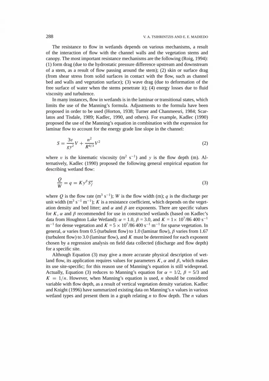
Results of the re-analyses of the data are presented in Figures 1 to 3. Figure 1presents the Darcy-Weisbachf vs the Reynolds numberRe, and Figures 2 and 3the Manning’sn vs the parameterVRand the hydraulic radiusR (or flow depthy),respectively.

First observation is that the data cover a wide range of Reynolds numbers(between about 1 and 250 000). Most of the data are in the transitional state, sincein flow through vegetation the standard open channel flow values ofRe for goingfrom laminar to transitional and to turbulent flow are generally not valid. Kadlec(1990) presents a graph that defines state of flow in wetlands, showing that thetransition from one state of flow to the other depends on vegetation characteristics(i.e., stem diameter, density and vertical variation), velocity and depth of flow. Ageneral range for the transitional state may be forRe values between 100 and10 000 (when open channel flow is considered). If stem drag is considered (whichmay be more appropriate), the transitional state may range fromRe as low as 20 to1000 up toRe greater than 100 000 (depending on stem diameter). Based on this,the data examined here are mostly in the transitional state, with few of them in thelaminar and some of them in the turbulent states.

Figure 1 also contains the open channel flowf − Re relations for laminar flow(f = 24/Re) and for smooth turbulent flow (Blasius equation:f = 0.223/Re0.25

and Prandlt-von Karman equation: 2log(Re·f 0.5) + 0.4 = f −0.5). The resistancevalues for vegetation are several orders of magnitude higher than those for open

HY

DR

AU

LIC

RE

SIS

TAN

CE

DE

TE

RM

INA

TIO

NIN

MA

RS

HW

ET

LA

ND

S297

Figure 1. f -Re graph for the compiled data.

298V.A

.TS

IHR

INT

ZIS

AN

DE

.E.M

AD

IED

O

Figure 2. n-VRgraph for the compiled data.

HY

DR

AU

LIC

RE

SIS

TAN

CE

DE

TE

RM

INA

TIO

NIN

MA

RS

HW

ET

LA

ND

S299

Figure 3. n-R graph for the compiled data.


channel flow. In addition, in Figure 2, the five retardance curves, used in grassedchannel design, are also shown for comparison (R.C. – A to E).

The following conclusions can be drawn from each specific study: Kadlec’s(1990) data for emergent marsh vegetation (sedges) offer the highest resistancevalues, laying mostly in the laminar and transitional states. Figures 1 to 3 showthatf decreases with increasing Reynolds number orn decreases with increasingVRparameter orR. Based on the data,f decreases withRe to about the –0.8 to–0.9 power, which is nearly parallel to the lawf = 24/Re for laminar open channelflow, butf values are 3 to 4 orders of magnitude higher. Furthermore, for a givenvalue of theRe, resistance factors increase with increasing slope. Similar trendsare observed on Chen’s (1976) data for grassed slopes, which also mostly coverthe laminar state (except maybe for his steeper slope). Again,f decreases withReto about the –1.0 power and increases with increasing slope. However,f valuesfor grass are quite lower than those for marsh vegetation (by more than an order ofmagnitude).

Wu et al. (1999) presented results for both emergent and submerged vegetation.Only the emergent vegetation data are used here. The simulated vegetation theyused in their experiments was stiffer and denser than most natural grasses, as alsoshown in Figures 1 to 3. The resistance again is shown to increase with slope. Thedependence off on Re in these experiments is to about the –0.5 power. Chiewand Tan (1992) study was similar to Chen’s (1996) but used a different grass. Theresistance factor values are lower, even for the high density experiment implyingoverall sparser vegetation. In this case, the Darcy-Weisbachf is related to theRe tothe –0.34 and –0.39 powers for the low and high density experiments, respectively,values which are in the range of theRe exponents for the study by Wuet al. (1999).However, thef values are about one order of magnitude lower.

The study by Hall and Freeman (1994) covered turbulent conditions (but notfully developed turbulence), with resistance decreasing with increasingRe. Twostem densities were used, approximately 400 and 800 stems m−2. The first densityprobably reflects a developing wetland condition, and the second a nearly de-veloped wetland (a mature wetland is estimated at about 1000 to 1500 stems m−2).Thef values were found to depend on the –0.46 and –0.41 powers ofRe, for thehigh and low vegetation densities, respectively. The Fathi-Maghadam and Kouwen(1997) study also covers turbulent flow conditions. Real vegetation samples (pineand cedar trees) with stems and canopy were used. Resistance factors were foundto increase with increasing flow depth, because more and more vegetation areaobstructed the flow. For depths greater than 0.06 m (stem height),f was foundto decrease withRe to about the –0.5 to –0.8 power. Compared to the previouslymentioned studies, and particularly the one by Hall and Freeman (1994), the res-istance factors for these experiments seem lower than those for marsh vegetation.However, these data compare well to retardance curves B to D for grass channels.

The study by Turner and Chanmeesri (1984), ranged mostly in the transitionalstate and employed flexible emergent vegetation. The computed values of the fric-


tional resistance factorsf andn increase with increasing Reynolds number (Fig-ures 1 to 3). This is a trend that was also observed in other studies on emergentgrasses (e.g., Palmer, 1945), as well as in rough open channel flow in the trans-itional state. The graphs also reveal the effect of slope on flow resistance. Indeed,the curves labeled TC–S =. . . present experimental results for a given vegetationdensity and for various slopes. The data do not show any trend with respect toresistance dependence on slope. For a given slope, however, vegetation densitysignificantly affects resistance. Indeed, the data labeled TC-Section A throughH are for similar slopes but for different vegetation densities and arrangements(Table III). Based on the results, it seems that the vegetation parameters that signi-ficantly affect resistance are the number of stems per unit bed surface area andthe separation ratios/d (distance between stems divided by diameter). Finally,resistance values for wheat seem to be quite lower than those for marsh wetlands.

Similar results were observed in the study by Roig (1994). The results show thatthe flow resistance decreases as the value for the parameters/d increases, i.e., largerdistance between stems (or lower vegetation density) result in less resistance. Addi-tionally, the general tendency is an increase in thef value with increasing Reynoldsnumber, but as the flow depth reaches or exceeds the stem height, the flow resist-ance starts decreasing with increasingRe. This is more obvious for experimentswith non-uniform stem height where some stems were totally submerged.

Figures 1 to 3 can be useful primarily in three cases: (1) In an analysis of a spe-cific flow through a given vegetation, if a similarity can be established with someof the studies or with characteristics intermediate between two or more of them;in this case, an estimation of the frictional resistance factor,f or n, can be madegraphically from one of the three types of graphs. The value obtained this way,although not exact, may give enough degree of accuracy for preliminary analyses.(2) New curves can be added by comparison to Figures 1 and 2, that would apply tomarsh wetlands. This procedure is described in the following section and the use ofthe graphs in two design examples. (3) In guiding future research or in the designof experiments for specific wetland sites; depending on the purpose of the research,these curves can help in giving basic range of values for hydraulic parameters tobe tested, and in the analysis of results to predict expected tendencies.

4.3. PROPOSED DESIGN GRAPHS FOR MARSH WETLANDS

Figures 1 and 2 are modified here to become useful design aids for marsh wetlands.They are presented again as Figures 4 and 5 (f vsRe andn vs VR). In these newgraphs, the data by Kadlec (1990) and Hall and Freeman (1994) have been main-tained. The data by Chen (1976), Chiew and Tan (1992), Wuet al. (1999), Turnerand Chanmeesri (1984) and Roig (1994) have been excluded because the emphasisof this article is on marsh wetlands and the vegetation types and densities, and flowconditions for these studies were different, resulting in overall lower resistancevalues.

302V.A

.TS

IHR

INT

ZIS

AN

DE

.E.M

AD

IED

O

Figure 4. f -Re proposed design graph for marsh wetlands.

HY

DR

AU

LIC

RE

SIS

TAN

CE

DE

TE

RM

INA

TIO

NIN

MA

RS

HW

ET

LA

ND

S303

Figure 5. n-VRproposed design graph for marsh wetlands.


Hall and Freeman (1994) present a graph showing a nearly linear increase inManning’snwith vegetation density. This graph was extrapolated to compute Man-ning’s n values for vegetation densities of 1000 stems m−2 and 1500 stems m−2.The respective increase ofn was about 25 and 75%, compared ton for vegetationdensity of 800 stems m−2. Respectivef values were also computed and found toincrease by about 56 and 306% overf values for the 800 stems m−2 vegetationdensity. New curves have been added and are shown in Figures 4 and 5. The curvesfor vegetation densities of 1500 stems m−2 lay at approximately the extension ofKadlec’s (1990) data for slope 0.01.

As mentioned, the resistance data by Fathi-Maghadam and Kouwen (1997) inFigures 1 to 3 seem to be about an order or magnitude lower than expected valuesfor marsh wetlands. And of course this is expected since these authors dealt withfloodplain bush and brush vegetation, which is flexible but not as dense. However,these data are useful here because they show trends. The data for the highest depth(submerged canopy), for both pine and cedar, match nicely retardance curve B (Fig-ure 2). Therefore, the trend of retardance curve B shows continuation of the databy Fathi-Maghadam and Kouwen (1997) for higherRe values. Furthermore, thiscurve lays at about the extention of Hall and Freeman (1994) data for vegetationdensity of 400 stems m−2, implying that this curve can be used in marsh wetlands,representing sparse vegetation. Thus, in Figure 5, retardance curve B is plottedto be used for low density marsh vegetation (e.g., a newly planted constructedwetland). Furthermore, retardance curve A is plotted and also four other curveswhich have resulted by increasing retardance curve A values by 32, 66, 132 and340%. These percentages resulted by moving up retardance curve A and matchingit with Hall and Freeman’s (1994) measured and extrapolated curves (except forthe uppermost curve which is speculative and reflects a condition of very densevegetation and significant bed litter). Therefore, retardance curve A itself seems tocorrespond to a marsh vegetation density of about 600 stems m−2, while the threefollowing curves to vegetation densities 800, 1000 and 1500 stems m−2, and theuppermost curve to a very dense marsh vegetation condition with significant bedlitter. It has to be noticed here that retardance curve A has been derived for fairly tallgrass, i.e., 0.75–0.90 m (Chow, 1959), which, although not as stiff and dense, mayotherwise have similarities with sparse emergent herbaceous marsh vegetation.f

values were also computed and plotted vsRe in Figure 4 (using a conservativeslope of 0.01 and an assumed kinematic viscosity of 1.2×10−6 m2 s−1).

Figures 4 and 5 seem to be complete for marsh-type vegetation, covering theentire range of Reynolds numbers and both sparse and dense conditions. Of coursemost curves, particularly for highRe, have been derived by comparison and, there-fore, they have to be used with caution and only in preliminary studies. One shouldalso have the following in mind: originally, the retardance curves have been de-veloped for slopes steeper than 1%. Based on data presented by Kouwen and Li(1980),n values for flatter slopes (e.g., 0.0005) may be about half of those forsteeper slopes, whereas, a tenfold increase in vegetation stiffness may result in


about a doubling of then value. Therefore, the two effects, i.e., flatter slope in awetland and stiffer vegetation compared to grass, seem to balance out, implyingthat the retardance curves, if adjusted for vegetation density as described, can beused with caution in wetland preliminary design. It has to also be noticed that, tothe best knowledge of this writer, there are no studies on marshes covering this areaof Re, which may be important when designing marsh channels for certain uses,e.g., flood control, where flow rate is high and flow may be in the turbulent state(see following example).

Figures 4 and 5 also contain four speculative curves, presented by Kadlec andKnight (1996), and applying to constructed marsh wetlands (i.e., depths 0.1 to1.0 m, and mostly laminar and transitional flow). These curves are for both sparseand dense vegetation and for friction slopesS = 0.0001 and 0.01. The four curvesagree well with the data and proposed curves in Figures 4 and 5. Actually, it canbe seen that Kadlec’s (1990) and Hall and Freeman’s (1994) data are for sparsevegetation. For dense vegetation, values have to be between Kadlec and Knight’s(1996) two dense-vegetation curves and our proposed curves (i.e., R.C. – A× 2.32to R.C. – A× 4.40).

5. Use of the data: design examples

5.1. A CONSTRUCTED WETLAND FOR WASTEWATER TREATMENT

Problem: Wastewater will be treated in a free-water surface constructed wetland.The flow rate is estimated at 2500 m3 day−1. Pollutant removal requirements havedetermined a minimum hydraulic residence time of 5 days. The available length is1000 m, with a longitudinal slope of 0.0001. The vegetation species to be used isbulrush. Determine the required width and flow depth 3 months and a few yearsafter the planting.

Solution: To achieve the required residence time of 5 days, the mean flow velocityshould not exceed:V = (1000 m)/(5 d) = 0.002315 m s−1. Based on the given flowrateQ = 2500 m3 day−1 = 0.02894 m3 s−1, the required flow area will beA =12.5 m2.

First the problem is solved for time 3 months after the planting, when the ve-getation will be sparse. To determine the resistance coefficient, Figure 5 and thefollowing trial-and-error procedure will be used:

1. Assume a Manning’sn value of 2 s m−1/3. From Figure 5 and Kadlec’s (1990)line for S = 0.0001, one getsVR= 0.00023 m2 s−1 (alternatively, Kadlec andKnight’s (1996) line for sparse vegetation andS = 0.0001 can be used, which,however, gives slightly lowern values).

2. Using this value for parameterVRand the required velocityV , one can get thevalue ofR = 0.0994 m.


3. This value ofR is used in Manning’s equation to calculate a new value forparameterVR: VR= (R5/3 S1/2)/n = 0.000107 m2 s−1. This value is comparedto theVRvalue of the first step. If different, a new value ofn is assumed andthe iterative procedure is repeated from the first step until convergence.

This procedure leads to the following results for this problem:n = 1.55 s m−1/3,R = 0.216 m, andVR= 0.0005 m2 s−1. The problem is now solved for time a fewyears after planting, when the wetland will be nearly fully grown (assume densevegetation). Figure 5 (Kadlec and Knight’s (1996) curve for dense vegetation andslopeS = 0.0001) will be used and the previously described iterative procedure.The results are the following:n = 2.55 s m−1/3, R = 0.518 m, andVR= 0.0012 m2

s−1. The widthW of the wetland will be calculated based on the long-term con-dition:W = A/y≈A/R = 12.5/0.518 = 24.1 m. For the 3-month condition, and tomaintain the required velocity (and residence time), the depth will be maintainedat 0.518 m by downstream control.

5.2. A RIPARIAN CORRIDOR FOR STORMWATER TREATMENT AND

CONVEYANCE

Problem:Drainage of a certain urban development site was proposed to be donethrough a riparian corridor which was designed for a triple function: treatment ofrunoff from frequent storms, safe conveyance of the 100-yr storm runoff with an es-timated peak flowQ = 10 m3 s−1, and freshwater wetland habitat development forwildlife. The riparian corridor would contain mainly cattails. The site conditionsimpose a maximum depthy = 1 m. The cross section will be trapezoidal with a sideslope ofz = 5:1 (horizontal to vertical). The longitudinal slope will beS = 0.01. Thechannel will be regularly maintained (i.e., vegetation will be partially harvested) toavoid development of very dense vegetation. Design the channel section.

Solution:The bottom width of the trapezoidal section is not known, therefore, thesolution will proceed by assuming a value for it and following a trial-and-errorprocedure. Let’s assumeW = 30 m. Then, for the trapezoidal section withz =5 andy = 1 m, the flow area is:A = (W + zy)y = 35 m2. Then, for the givendischarge, the velocity is:V = Q/A = 10/35 = 0.2857 m s−1. To continue, a valuefor n is assumed and the three-step procedure described in the previous example isfollowed, which, after some iterations, results in:n = 0.33 s m−1/3,R = 0.84 m, andVR= 0.23 m2 s−1 (using curve labeled R.C. – A× 2.32 in Figure 5). The value ofthe hydraulic radiusR should be tested now for the assumed value of bottom widthW . Based on geometry, for the given section:R = (W + 5)/(W + 10.2) = 35/40.2 =0.87 m6= 0.84 m. Therefore, one needs to assume a new value forW . Actually, thevalue that makesR = 0.84 m, which isW = 22.3 m, is assumed. Based on this,A =27.3 m2 andV = 0.3663 m s−1. A new trial and error procedure is then undertakento find Manning’sn value. The new and final results are:n = 0.25 s m−1/3, R =


0.84 m, andVR= 0.308 m2 s−1. It should be noted that the resulting section is wide(W»y), therefore, data developed for rectangular sections (Figures 4 and 5) can beused.

6. Conclusions

For flow through vegetation, the frictional factorsf andn decrease with increasingReynolds number or parameterVR. Compared to vegetated channel flow, the valuesobtained for the resistance coefficients are quite higher, obviously because of thesmall ratio of depth to vegetation height, and also the higher density of marshvegetation. The factorf ranges from 0.1 to 1000 in most studies presented, and upto 50 000 in the study by Kadlec (1990) for laminar flow. Similarly, Manning’sn

ranges from about 0.02 to 1 for most studies and up to about 15 in the study byKadlec (1990). Based on comparison with data for grassed channels and wetlandvegetation, retardance curves are proposed for turbulent marsh flow. These curvesare to be used with caution and in marsh preliminary design only. From the com-piled studies, areas can also be identified where additional field or laboratory dataare needed.

References

Arcement, G. J. and Schneider, V. R.: 1989, Guide for Selecting Manning’s Roughness Coeffi-cients for Natural Channels and Flood Plains.U.S. Geological Survey, Water-Supply Paper2339, prepared in cooperation with the Federal Highway Administration, U.S. Department ofTransportation, U.S.A.

Barnes, H. H.: 1967, Roughness Characteristics of National Channels,U.S. Geological Survey, WaterSupply Paper 1849, U.S.A.

Bueno, J. A., Tsihrintzis, V. A. and Alvarez, L.: 1995, South Florida greenways: A conceptual frame-work for the ecological reconnectivity of the region,Landscape and Urban Planning, Elsevier,33, 247–266.

Chen, C.-L.: 1976, Flow resistance in broad shallow grassed channels,Journal of the HydraulicsDivision, ASCE,102(HY3), 307–322.

Chiew, Y. and Tan, S.: 1992, Frictional resistance of overland flow on tropical turfed slope.Journalof Hydraulic Engineering, ASCE,118(1), 92–97.

Chow, V. T.: 1959,Open-Channel Hydraulics, McGraw-Hill Inc., New York, U.S.A.Cowan, W. L.: 1956, Estimating hydraulic roughness coefficient,Agricultural Engineering37(7),

473–475.Cox, M. B.: 1942, Tests on Vegetated Waterways,Oklakoma Agricultural Experimental Station,

Technical Bulletin, T-15, U.S.A.Cox, M. B. and Palmer, V. J.: 1948, Results of Tests on Vegetated Water Waterways, and Method

of Field Application,Oklahoma Agricultural Experiment Station, in cooperation with the SoilConservation Service, U.S. Department of Agriculture, Miscellaneous publication No. MP-12,U.S.A., pp. 5–43.

Coyle, J. J.: 1975, Grassed Waterways and Outlets,Engineering Field Manual, U.S. Department ofAgriculture, Soil Conservation Service, Washington D.C., U.S.A., pp. 7.1–7.43.

Darby, S. E. and Thorne, C. R.: 1996, Predicting stage-discharge curves in channels with bankvegetation,Journal of Hydraulic Engineering, ASCE,122(10), 583–586.


Economopoulou, M. A. and Tsihrintzis, V. A.: 1999, Technical analysis for the use of selectednatural systems for wastewater treatment in Greece,Proceedings of the International ScientificConference HELECO ’99, Technical Chamber of Greece, Thessaloniki, Greece, June 3–6, Vol. I,pp. 21–29 (in Greek).

Economopoulou, M. A. and Tsihrintzis, V. A.: 2000a, Graphical design and analysis of constructedwetlands treating municipal wastewater (submitted).

Economopoulou, M. A. and Tsihrintzis, V. A.: 2000b, Hydraulic design of constructed wetlands,Proceedings of the 8th National Conference of the Hellenic Hydrotechnical Society, April 19–22,Athens, Greece, pp. 235–242 (in Greek).

Fathi-Maghadam, F. and Kouwen, N.: 1997, Nonrigid, nonsubmerged, vegetative roughness onfloodplains,Journal of Hydraulic Engineering, ASCE,123(1), 51–57.

French, R. H.: 1985,Open Channel Hydraulics, McGraw Hill, New York, U.S.A.Guillen, D.: 1996, Determination of Roughness Coefficients for Streams in West-Central Florida,

US Geological Survey, in cooperation with the Southwest Florida Water Management District.Report 96–226, pp. 1–93.

Hall, B. R. and Freeman, G. E.: 1994, Study of hydraulic roughness in wetland vegetation takes newlook at Manning’sn, The Wetlands Research Program Bulletin, US Army Corps of Engineers,Waterways Experiment Station, 4(1), 1–4.

Hammer, D. A. (ed.): 1989,Constructed Wetlands for Wastewater Treatment, Municipal, Industrial,Agricultural, Lewis Publishers, Boca Raton, Florida, U.S.A.

Henderson, F. M.: 1966,Open Channel Flow, Macmillan Publishing Co., Inc. New York, U.S.A.Horton, R. H.: 1938, The interpretation and application of runoff plat experiments with reference to

soil erosion problems,Proceedings, Soil Science Society of America,3, 340–349.Hsieh, T.: 1962, The Resistance of Piers on High Velocity Flow, Master Thesis, State University of

Iowa, pp. 1–50.Kadlec, R. H.: 1990, Overland flow in wetlands: Vegetation resistance,Journal of Hydraulic

Engineering, ASCE,116(5), 691–706.Kadlec, H. R. and Knight, R. L.: 1996,Treatment Wetlands, Lewis Publishers, Boca Raton, U.S.A.Kouwen, N.: 1988, Field estimation of the biomechanical properties of grass,Journal of Hydraulic

Research, 26(5), 559–568.Kouwen, N. and Li, R.-M.: 1980, Biomechanics of vegetative channel linings,Journal of the

Hydraulics Division, ASCE,106(HY6), 1085–1103.Kutija, V. and Hong, H.: 1996, A numerical model for assessing the additional resistance to flow

introduced by flexible vegetation,Journal of Hydraulic Research34(1), 99–114.MacVicar, T. K.: 1985, A Wet Season Field Test of Experimental Water Deliveries to Northeast

Shark River Slough.South Florida Water Management District, Tech. Pub. 85–3, West PalmBeach, Florida, U.S.A.

Mitsch, W. J. and Gosselink, J. G.: 1986,Wetlands, Van Nostrand-Reinhold, New York, U.S.A.Moshiri, G. A. (ed.): 1993,Constructed Wetlands for Water Quality Improvement, Lewis Publishers,

Boca Raton, Florida, U.S.A.Naot, D., Nezu, I. and Nakagawa, H.: 1996, Hydrodynamic behavior of partly vegetated open

channels,Journal of Hydraulic Engineering, ASCE,122(11), 625–633.Palmer, V. J.: 1945, A method for designing vegetated waterways,Agricultural Engineering26(12),

516–520.Pasche, E. and Rouvé, G.: 1985, Overbank flow with vegetatively roughened flood plains,Journal of

Hydraulic Engineering, ASCE,111(9), 1262–1278.Petryk, S. and Bosmajian, G.: 1975, Analysis of flow through vegetation,Journal of the Hydraulics

Division, ASCE,101(HY7), 871–884.Ree, W. O.: 1941, Hydraulic tests of Kudzu as a conservation channel lining,Agricultural

Engineering22(1), 27–29.


Ree, W. O.: 1949, Hydraulic characteristics of vegetation for vegetated waterways,AgriculturalEngineering30(4), 184–187 and 189.

Ree, W. O. and Palmer, V. J.: 1949, Flow of Water in Channels Protected by Vegetative Lining,U.S.Soil Conservation Service, Technical Bulletin, No. 967, U.S.A.

Reed, S. C., Crites, R. W. and Middlebrooks, E. J.: 1995,Natural Systems for Waste Managementand Treatment, 2nd ed., McGraw-Hill, Inc., New York, U.S.A.

Roig, L. C.: 1994,Hydrodynamic Modeling of Flows in Tidal Wetlands, Ph.D. Thesis, University ofCalifornia, Davis.

Scarlatos, P. D. and Tisdale, T. S.: 1989, Simulation of wetland flow dynamics,Water: Laws andManagement, AWRA, 9A15–23.

Shih, S. F. and Rahi, G. S.: 1982, Seasonal variation of Manning’s roughness coefficient in asubtropical marsh,Transactions of ASAE25, 116–120.

Simons, D. B. and Sentürk, F.: 1992,Sediment Transport Technology. Water and Sediment Dynamics,Water Resources Publications, Littleton, Colorado, U.S.A.

Tsihrintzis, V. A.: 1999, Protection of wetlands from development impacts,Proceedings of the Inter-national Conference ECOSUD 99 – Ecosystems and Sustainable Development, Wessex Instituteof Technology, May 3-1-June 2, Lemnos, Greece, pp. 273–282.

Tsihrintzis, V. A., Vasarhelyi, G. M. and Lipa, J.: 1995a, Hydrodynamic and constituent trans-port modeling of coastal wetlands, Gordon and Beach Publishing Co.,Journal of MarineEnvironmental Engineering1(4), 295–314.

Tsihrintzis, V. A., Vasarhelyi, G. M. and Lipa, J.: 1995b, Multiobjective approaches in freshwaterwetland restoration and design,Water International, IWRA, 20(2), 98–105.

Tsihrintzis, V. A., Vasarhelyi, G. M. and Lipa, J.: 1996, Ballona Wetland: A multi-objective saltmarsh restoration plan,Water, Maritime and Energy, ICE,118(2), 131–144.

Tsihrintzis, V. A., John D. L. and Tremblay P. J.: 1998, Hydrodynamic modeling of wetlands forflood detention,Water Resources Management, EWRA,12(4), 251–269.

Turner, A. K. and Chanmeesri, N.: 1984, Shallow flow of water through non-submerged vegetation,Agricultural Water Management, Elsevier Science Publishers,8, 375–385.

Wu, F.-C., Shen, H. W. and Chou, Y.-J.: 1999, Variation of roughness coefficients for unsubmergedand submerged vegetation,Journal of Hydraulic Engineering, ASCE,125(9), 934–942.

Yen, B. C.: 1992, ‘Hydraulic Resistance in Open Channels’, in B. C. Yen (ed.),Channel Flow Res-istance: Centennial of Manning’s Formula Water Resources Publications, Littleton, Colorado,U.S.A., pp. 1–135.

Documents

Hydraulic resistance determination in marsh wetlands