Hydra@Hull - University of Hull

THE UNIVERSITY OF HULL

The impact of the extent of Activity-Based Costing use and the extent of

ISO 9000 implementation on organisational performance

being a Thesis submitted for the Degree of

Doctor of Philosophy

in the University of Hull

By:

Witchulada Vetchagool

MBA (Financial Accounting), Kasetsart University, Thailand

BBA (Accounting), Khon Kaen University, Thailand

October 2016

II

ACKNOWLEDGEMENTS

I would like to take this opportunity to express my appreciation and sincere gratitude

to the many people who have supported me throughout the development of this

thesis. I wish firstly to thank my respected supervisor, Dr Marcjanna Augustyn, for

her generous support, dedication and encouragement at every stage of the thesis. I

am very grateful to her for the patience she has shown throughout my study. I also

thank my second supervisor, Dr Sumona Mukhuty for her useful suggestions and her

valuable help.

I would like to express my appreciation to Faculty of Business Administration and

Accountancy, Khon Kaen University, who provided me with the scholarship to

pursue my Ph.D. study. My special thanks also go to my colleagues, friends, and all

the staff at the Business School, University of Hull, for their support and

encouragement.

I would like to thank to my father, Mr Wimol Vetchagool and my mother, Mrs

Petlum Vetchagool for their unconditional love and support during my study. Thanks

to Wittawat, Wipavee, and Dr Chayakom for always helping me to get through the

hardest moments. Finally, I would like to acknowledge all the respondents in this

survey who kindly responded to the questionnaire. Without them, the thesis would

never have been completed.

III

ABSTRACT

Activity-based costing (ABC) is one of the most-researched management accounting

areas that can improve organisational performance (OP). However, the studies on

ABC and its impact on OP were still deficient and contradictory. Furthermore, ABC

might be the most advantageous approaches used concurrently with ISO 9000. This

study aims to investigate the impact of the extent of ABC use and the extent of ISO

9000 implementation on OP in order to identify the role of ABC and ISO 9000 in

improving OP, and, in addition, to assess the combined effects of ABC and ISO

9000 on OP. Two conceptual models were developed to illustrate the relationships

between variables.

There were 601 usable questionnaires (19.36 percent) received; 191 organisations

that adopted both ABC and ISO 9000 compared to 410 organisations that adopted

only ISO 9000. Three data analysis techniques were employed: exploratory factor

analysis (EFA), confirmatory factor analysis (CFA), and structural equation

modelling (SEM). EFA and CFA results provide evidence that the extent of ABC

use (CA: cost analysis, CS: cost strategy, CE: cost evaluation), the extent of ISO

9000 implementation (MP: management principle, CP: Cooperation principle) and

organisational performance (OPP: operational performance, FP: financial

performance) are multidimensional.

SEM results indicate the extent of ABC use directly improves OPP and subsequently

indirectly improves FP through OPP. On the other hand, the extent of ISO 9000

implementation of organisations that adopted only ISO 9000 improves neither OPP

nor FP. However, the management principle (MP) of organisations that adopted both

ABC and ISO 9000 can directly improve both OPP and FP, and subsequently

indirectly improve FP through OPP. The result implies a potential synergy effect of

ABC and ISO 9000, which extends the body of knowledge of management

accounting and quality management research.

IV

Table of Contents

ACKNOWLEDGEMENTS ........................................................................................ II

ABSTRACT ............................................................................................................... III

Table of Contents ....................................................................................................... IV

List of Tables............................................................................................................ VII

List of Figures .......................................................................................................... VII

List of abbreviation .............................................................................................. XVIII

Chapter 1: Introduction ................................................................................................ 1

1.1 Research problem ............................................................................................... 1

1.2 The aims, the objectives and the research hypotheses ....................................... 6

1.3 Research structure .............................................................................................. 7

1.4 Research contribution ....................................................................................... 10

Chapter 2: Literature Review ..................................................................................... 12

2.1 Management accounting (MA) and organisational performance improvement

................................................................................................................................ 12

2.2 The impact of the extent of activity-based costing use on organisational

performance ............................................................................................................ 27

2.3 The impact of the extent of ISO 9000 implementation on organisational

performance ............................................................................................................ 37

2.4 The combined impact of activity-based costing and ISO 9000 on

organisational performance .................................................................................... 46

2.5 Factors moderating the impact of activity-based costing and ISO 9000 on

organisational performance .................................................................................... 51

2.6 Conceptual models ........................................................................................... 56

2.7 Summary .......................................................................................................... 58

Chapter 3: Research Methodology ............................................................................. 59

3.1 The research design .......................................................................................... 59

3.2 Questionnaire design ........................................................................................ 69

V

3.3 Data Analysis ................................................................................................... 91

3.4 Summary ........................................................................................................ 119

Chapter 4: Research Results..................................................................................... 122

4.1 Preliminary analysis ....................................................................................... 122

4.2 Descriptive analysis ........................................................................................ 131

4.3 Results of exploratory factor analysis (EFA) ................................................. 142

4.4 Results of confirmatory factor analysis (CFA) .............................................. 161

4.4.1 Results of testing the dimensionality ....................................................... 161

4.4.2 Results of testing the validity and reliability ........................................... 182

4.5 Results of structural equation modelling (SEM) ............................................ 191

4.5.1 Results of Model 1: The extent of ABC use and organisational

performance model (191 cases of organisations that adopted both ABC and ISO

9000) ................................................................................................................. 191

4.5.2 Results of Model 2: The extent of ISO 9000 implementation and

organisational performance (191 cases of organisations that adopted both ABC

and ISO 9000) ................................................................................................... 201


organisational performance (410 cases of organisations adopting only ISO 9000)

.......................................................................................................................... 211


organisational performance model (601 cases of all respondents) ................... 220

4.6 The results of multi-group analysis ................................................................ 229

Chapter 5: Discussion of Findings ........................................................................... 261

5.1 The factorial structure of the extent of ABC use, the extent of ISO 9000

implementation, and organisational performance ................................................ 261

5.2 The impact of the extent of ABC use on organisational performance ........... 266


performance .......................................................................................................... 268

VI

5.4 The significant differences between organisations that adopted both ABC and

ISO 9000 and organisations that adopted only ISO 9000 .................................... 271

5.5 The moderating impacts of the initiatives on organisational performance. ... 273

Chapter 6: Conclusion, Limitations and Recommendations .................................... 281

6.1 Conclusion ...................................................................................................... 281

6.2 Research contributions ................................................................................... 286

6.3 Limitations and recommendations for further research ................................. 289

References ................................................................................................................ 297

Appendices ............................................................................................................... 315

Appendix A: The questionnaire ........................................................................... 315

Appendix B: Levene's Test for Equality of Variances ......................................... 321

Appendix C: Outliers test ..................................................................................... 325

Appendix D: Histogram for testing normality ..................................................... 337

Appendix E: Linearity tested by statistic ............................................................. 348

Appendix F: Scatter plots of testing linearity ....................................................... 381

Appendix G: Scatter plots of testing homoscedasticity ........................................ 385

Appendix H: Respondents’ profile ....................................................................... 389

VII

List of Tables

Table 2.1: Perspective of four main performance measurements .............................. 15

Table 2.2: The ABC literature in terms of impact/influence, relationship/association,

and significant differences ......................................................................................... 34

Table 2.3: The ISO 9000 literature in terms of impact/influence,

relationship/association, and significant differences.................................................. 43

Table 2.4: Previous studies in the association and the impact of ABC complementary

with other initiatives (FP)........................................................................................... 49

Table 2.5: Previous studies in the association and the impact of ABC complementary

with other initiatives (OPP) ........................................................................................ 50

Table 3.1: The measures used in evaluating the association and the impact of ABC

and ISO 9000 ............................................................................................................. 78

Table 3.2: Overall response rate................................................................................. 90

Table 3.3: Identifying significant factor loadings based on sample size ................. 103

Table 3.4: Absolute fit indices ................................................................................. 115

Table 3.5: Incremental fit indices............................................................................. 115

Table 3.6: Parsimony fit indices............................................................................... 115

Table 4.1: Conclusion sample size of each moderating variable ............................. 124

Table 4.2 Pearson’s correlation coefficient (Model 1)............................................. 127

Table 4.3: Pearson’s correlation coefficient (Model 2) ........................................... 128



Table 4.6: Respondents’ position ............................................................................. 131

VIII

Table 4.7: Descriptive analysis of demographic data .............................................. 132

Table 4.8: The number of ABC-adopting organisations .......................................... 132

Table 4.9: Type of business ..................................................................................... 133

Table 4.10: Number of employees ........................................................................... 134

Table 4.11: Classifying size of firm by the total annual revenues of organisations 134

Table 4.12: Descriptive analysis of demographic data ............................................ 135

Table 4.13: Descriptive statistics (Model 1) ............................................................ 138




Table 4.17: KMO and Bartlett’s Test of nine indicators (Model 1)......................... 142

Table 4.18: Total variance explained of nine indicators (Model 1) ......................... 143

Table 4.19: Rotated factor matrix of nine indicators (Model 1) .............................. 143

Table 4.20: Descriptive statistics and reliability analysis of independent constructs

(Model 1) .................................................................................................................. 144

Table 4.21: KMO and Bartlett’s test of eight indicators (Model 2) ......................... 145

Table 4.22: Total variance explained of eight indicators (Model 2) ........................ 145

Table 4.23: Rotated factor matrix of eight indicators (Model 2) ............................. 146

Table 4.24: Descriptive statistics and reliability analysis of independent construct

(Model 2) .................................................................................................................. 147

Table 4.25: KMO and Bartlett’s Test of eight indicators (Model 3) ....................... 147

Table 4.26: Total variances explained of eight indicators (Model 3) ...................... 148

IX



(Model 3) .................................................................................................................. 149

Table 4.29: KMO and Bartlett’s Test of eight indicators (Model 4) ....................... 149

Table 4.30: Total variances explained of eight indicators (Model 4) ...................... 150



(Model 4) .................................................................................................................. 151

Table 4.33: KMO and Bartlett’s test of seven indicators (Model 1) ........................ 152

Table 4.34: Total variances explained of seven indicators (Model 1) ..................... 152

Table 4.35: Total variances explained of seven indicators (adapted Model 1) ........ 152

Table 4.36: Rotated factor matrix of seven indicators (Model 1) ............................ 153

Table 4.37: Descriptive statistics and reliability analysis (Model 1) ....................... 154

Table 4.38: KMO and Bartlett’s Test (Model 2)...................................................... 154









X




Table 4.50: Model Fit Summary of ABC (Models I and II) .................................... 163

Table 4.51: Model Fit Summary of ISO (Models I and II) ...................................... 166

Table 4.52: Model Fit Summary of ISO (Models I and II) ...................................... 168

Table 4.53: Model fit summary of ISO (Models I and II) ....................................... 171

Table 4.54: Model fit summary of OP (Models I and II) ......................................... 173

Table 4.55: Model fit summary of OP (Models I and II) ......................................... 175

Table 4.56: Model Fit Summary of OP (Models I, II and III) ................................. 178

Table 4.57: Model Fit Summary of OP (Models I and II) ....................................... 180

Table 4.58: Selected AMOS output relating to independent construct (Model 1) ... 182

Table 4.59: Selected AMOS output relating to the independent construct (Model 2)

.................................................................................................................................. 183


.................................................................................................................................. 184


.................................................................................................................................. 185

Table 4.62: Selected AMOS output relating to dependent construct (Model 1) ...... 186

Table 4.63: Selected AMOS output relating to the dependent construct (Model 2) 187



Table 4.66: Parameter summary of Model 1 ............................................................ 193

XI

Table 4.67: Output of assessment of normality ....................................................... 194

Table 4.68: Model fit summary of Model 1 ............................................................. 195

Table 4.69: Selected AMOS Output (Model 1) ....................................................... 196

Table 4.70: EVCI, BIC and AIC values (Model 1).................................................. 198

Table 4.71: Bootstrap results (Model 1) .................................................................. 198

Table 4.72: Hypothesised relationships (Model 1) .................................................. 200

Table 4.73: Direct, indirect and total impact (Model 1) .......................................... 200

Table 4.74: Parameter Summary of Model 2 ........................................................... 203


Table 4.76: Model fit summary (Model 2)............................................................... 205






Table 4.82: Parameter Summary (Model 3) ............................................................. 213






XII



Table 4.90: Parameter summary (Model 4) ............................................................. 222








Table 4.98: Goodness-of-fit measures of the two models ....................................... 230

Table 4.99: Baseline comparisons of the two models .............................................. 230

Table 4.100: Standardised regression weights and p-values (Model 2 and 3) ......... 232

Table 4.101: Goodness-of-fit statistics for tests of multiple group invariance (Model

2 and 3) ..................................................................................................................... 233

Table 4.102: GOF measures of unconstrained and two models (type of business) . 235



Table 4.105: GOF statistics for tests of multiple group invariance (Type of business)

.................................................................................................................................. 238



.................................................................................................................................. 240

XIII

Table 4.108: GOF measures of unconstrained and two models (size of business) .. 241



Table 4.111: GOF statistics for tests of multiple group invariance (Size of business)

.................................................................................................................................. 244



.................................................................................................................................. 246

Table 4.114: GOF measures of unconstrained and two models (age of ABC) ........ 247

Table 4.115: Standardised regression weights and p-values (age of ABC) ............. 248

Table 4.116: GOF statistics for tests of multiple group invariance: The extent of

ABC use on organisational performance (Age of ABC) ......................................... 249

Table 4.117: GOF measures of unconstrained and two models (age of ABC) ........ 250

Table 4.118: GOF measures of unconstrained and two models (age of ISO).......... 251




Table 4.122: GOF measures of unconstrained and two models (frequency use of

ABC) ........................................................................................................................ 255

Table 4.123: GOF statistics for tests of multiple group invariance (frequency use of

ABC) ........................................................................................................................ 256


ABC) ........................................................................................................................ 257

Table 4.125: Hypothesised relationships of four models ......................................... 260

XIV

Table 5.1: The current study findings in relation to the previous studies (ABC and FP)

.................................................................................................................................. 275

Table 5.2: The current study findings in relation to the previous studies (ABC and

OPP) ......................................................................................................................... 276

Table 5.3: The current study findings in relation to the previous studies (ABC, OPP,

and FP) ..................................................................................................................... 277

Table 5.4: The current study findings in relation to the previous studies (ISO 9000

and FP) ..................................................................................................................... 278

Table 5.5: The current study findings in relation to the previous studies (ISO 9000

and OPP) .................................................................................................................. 279

Table 5.6: The current study findings in relation to the previous studies (ISO 9000,

OPP, and FP) ............................................................................................................ 280

Table 6.1: Summary of all hypotheses (direct impact on FP and OPP, and indirect

impact on FP) ........................................................................................................... 291

Table 6.2: Summary of all hypotheses (moderating factor: type of business) ......... 292

Table 6.3: Summary of all hypotheses (moderating factor: size of business) ......... 293

Table 6.4 Summary of all hypotheses (moderating factor: age of ABC)................. 294

Table 6.5: Summary of all hypotheses (moderating factor: age of ISO 9000) ........ 295

Table 6.6: Summary of all hypotheses (moderating factor: frequency use of ABC)

.................................................................................................................................. 296

XV

List of Figures

Figure 1.1: The processes of ISO 9000 and ABC ........................................................ 3

Figure 1.2: The research process diagram.................................................................... 9

Figure 2.1: The theoretical foundations of performance improvement theory .......... 20

Figure 2.2: Simple system model ............................................................................... 22

Figure 2.3: Activity-based costing process ................................................................ 23

Figure 2.4: The ISO 9000 process ............................................................................. 23

Figure 2.5: A diagram representation of fit as moderation ........................................ 27

Figure 2.6: The impact of the extent of ABC use on organisational performance .... 37

Figure 2.7: The impact of the extent of ISO 9000 implementation on organisational

performance................................................................................................................ 46

Figure 2.8: The impact of the extent of ABC use on organisational performance

(Model 1) .................................................................................................................... 56

Figure 2.9: The impact of the extent of ISO 9000 implementation on organisational

performance (Model 2) .............................................................................................. 57

Figure 3.1: The research onion................................................................................... 60

Figure 3.2: The process of deduction ......................................................................... 63

Figure 3.3: Methodological choice ............................................................................ 65

Figure 3.4: The research process onion...................................................................... 68

Figure 3.5: Types of questionnaire............................................................................. 69

Figure 3.6: Reflective measurement model (effect model) and formative

measurement model (causal model) ........................................................................... 74

Figure 3.7: The questions and scales measuring the extent of ABC use construct .... 81

XVI

Figure 3.8: Bivariate scatterplots under conditions of homoscedasticity and

heteroscedasticity ....................................................................................................... 96

Figure 3.9: The positive correlation, negative correlation and no correlation ........... 97

Figure 3.10: Multiple group dialogue box ............................................................... 118

Figure 3.11: The analysis process diagram (1) ........................................................ 120

Figure 3.12: The analysis process diagram (2) ........................................................ 121

Figure 4.1: Overall response rates ............................................................................ 122

Figure 4.2: Missing values ....................................................................................... 125

Figure 4.3: Models I and II of the extent of ABC use (Model 1) ............................ 162

Figure 4.4: Model II: First-order factor model (Model 1) ....................................... 164

Figure 4.5: Models I and II of the extent of ISO 9000 implementation (Model 2) . 165





Figure 4.10: Model II: First-order factor model (Model 4) ..................................... 171

Figure 4.11: Models I and II of OP (Model 1) ......................................................... 172

Figure 4.12: Model II: First-order factor model of OP (Model 1) ........................... 174




Figure 4.16: Model III: First-order factor model of OP (Model 3) .......................... 179

XVII



Figure 4.19: SEM of Model 1 .................................................................................. 191

Figure 4.20: The relationship between the extent of ABC use and OP (Model 1) .. 192

Figure 4.21: Selected AMOS output for Model 1: Model summary ....................... 193


Figure 4.23: The relationship between the extent of ISO 9000 implementation and

OP (Model 2) ........................................................................................................... 202

Figure 4.24: Selected AMOS Output for Model 2: Model Summary ...................... 203



OP (Model 3) ........................................................................................................... 212

Figure 4.27: Selected AMOS output for Model 3: Model summary ....................... 212



OP (Model 4) ........................................................................................................... 221

Figure 4.30: Selected AMOS Output for Model 4: Model Summary ...................... 221

XVIII

List of abbreviation

Activity-based costing (ABC)

Adjusted goodness-of-fit statistic (AGFI)

Akaike information criterion (AIC)

Asymptotic distribution free (ADF)

Average variance extracted (AVE)

Bayesian information criterion (BIC)

Chief Executive Officer (CEO)

Common method variance (CMV)

Comparative fit index (CFI)

Confirmatory factor analysis (CFA)

Construct reliability (CR)

Corrected item-total correlation (CITC)

Covariance structures analysis (COVS)

Expected cross validation index (ECVI)

Exploratory factor analysis (EFA)

Financial performance (FP)

General systems theory (GST)

Generalised least squares (GLS)

Goodness-of-fit statistic (GFI)

International Organization for Standardization (ISO)

Maximum likelihood estimation (ML)

Normed fit index (NFI)

Operational performance (OPP)

Organisational performance (OP)

Return on assets (ROA)

Root mean square error of approximation (RMSEA)

Root mean square residual (RMR)

Standardised root mean square residual (SRMR)

Structural equation modeling (SEM)

Tucker-Lewis index (TLI)

Unweighted least squares (ULS)

Weighted least squares (WLS)

1

Chapter 1: Introduction

Introduction

This thesis addresses the contributions of Activity-based costing (ABC) and ISO

9000 to organisational performance. This chapter provides an overview of the

research, which is presented in four sections. Section 1.1 introduces the research

problem of the study. The aims, the objectives and the research hypotheses are

identified in Section 1.2. The research structure is outlined in Section 1.3. The last

section discusses the research contribution.

1.1 Research problem

Management accounting provides information in relation to managing organisational

resources for managers (Langfield-Smith et al., 2009). It helps managers plan,

evaluate and control activities (Proctor, 2002). Moreover, it contributes to improving

organisational performance through process improvement and cost management

techniques (Langfield-Smith et al., 2009). Phadoongsitthi (2003) pointed out that

management accounting practices form an organisation’s infrastructure, adding value

by enabling and facilitating the effective use of scarce resources.

Activity-based costing (ABC) has enjoyed a high profile in management accounting

research worldwide over the last 25 years (Jankala & Silvola, 2012). Improving

organisational performance is a positive role for ABC, as illustrated in the literature

(Askarany & Yazdifar, 2012). Topics in the area of ABC research include “the

diffusion levels of ABC in various countries, the reasons for adopting ABC, the

problems associated with ABC and critical success factors relating to its successful

implementation” (Sartorius et al., 2007: 2). Elhamma (2015) has indicated that most

of the research on ABC have been conducted by using a contingency theory

approach. Researcher have focused on the relationship between ABC adoption and

several contingency factors such as strategy, firm size, organisational structure,

structure of changes. However, the studies related to the impact of ABC on

performance are still insufficient. Maiga and Jacobs (2008) point out that the link

between ABC and its impact is still questionable.

2

Previous studies have investigated the association (Ittner et al., 2002; Cagwin &

Ortiz, 2005; Hardan & Shatnawi, 2013) and the impact (Banker et al., 2008) of ABC

on performance. Some studies have most frequently measured ABC using a category

scale (a 0–1 variable), namely ABC-adopter and non-ABC adopter; or in a

continuum of ABC adoption levels by applying only one indicator (Jankala &

Silvola, 2012); or in three dimensions of ABC implementation (Zaman, 2009).

Banker et al. (2008) suggested that employing a more granular scale to measure

ABC might give greater insight into the association between ABC and performance.

In this study, in contrast, ABC is measured as a theoretical construct, which cannot

be observed directly, rather than as a single observed variable. However, few studies

have measured ABC in term of a construct (Cagwin & Bouwman, 2002; Maiga &

Jacobs, 2008). At present, little is known about measuring ABC in term of a

construct and, in particular, there is an absence of clarity regarding the dimensional

structure of ABC, and its impact on performance.

The current study will fill this gap by empirically investigating the impact of ABC

on organisational performance in terms of the extent of ABC use for a range of

purposes. As Malmi and Granlund (2009: 598) pointed out, “the goodness of any

Management Accounting practice depends on the objective of users of the MA as

well as the organisational and social context in which the MA practice takes place”.

In some literature, ABC was found to show no association with financial

performance, particularly return on assets (ROA), profitability and return on

investment (ROI) (Cagwin & Bouwman, 2002; Ittner et al., 2002; Cagwin & Ortiz,

2005; Maiga & Jacobs, 2008). However, interestingly, Cagwin and Bouwman (2002)

found that ABC had a positive relationship with ROI improvement, but only when

ABC was employed concurrently with alternative initiatives, such as just-in-time,

theory of constraints, computer integrated manufacturing, value chain analysis,

business process reengineering, flexible manufacturing systems, and total quality

management . The reason for this finding is that as “ABC often provides more and

better information about processes, ABC may be most beneficial if other initiatives

are employed concurrently” (Cagwin & Bouwman, 2002: 10). Banker et al. (2008)

indicated that employing ABC by itself did not lead to performance improvement.

As a result, Cagwin and Bouwman (2002) and Jankala and Silvola (2012)

3

recommended that further research was needed to investigate which combinations of

initiatives provide a positive effect when used concurrently with ABC.

Previous studies have attempted to link ABC and other initiatives such as technology

integration, supply chain management (Cagwin & Ortiz, 2005), balance scorecard

(Maiga & Jacobs, 2003), total quality management (Cagwin & Barker, 2006) and

just-in-time (Huson & Nanda, 1995; Kaynak, 1996). However, the establishment of a

relationship between ABC and technology integration, supply chain management,

and balance scorecard and organisational performance showed only a weak

significance (P<0.10). Some other initiatives, namely total quality management and

just-in-time, have difficulty in specifying the exact implementation claimed and

identifying the practice adoption date (Sharma, 2005). It may not be reliable to use

public announcements because organisations seldom announce the beginning of

using the total quality management system (Easton & Jarrell, 1998).

This study responds to the call for additional research using ABC in order to

discover which combinations of initiatives provide a positive effect when used

concurrently with ABC. Focusing on organisational performance improvement, ISO

9000 is one of the most popular and enduring programmes (Gershon, 2010) which

organisations can employ to improve performance through process improvement

(ISO 9004, 2009). ISO 9000 identifies eight principles to “be used by top

management as they lead their organisations and improve performance” (Oakland,

2003: 209). ISO 9000 and ABC are relatively similar in their particular emphasis on

managing activities and their documentation (Larson & Kerr, 2002). Many processes

considered for the accomplishment of ISO 9000 certification are also necessary

when employing ABC, as Larson and Kerr (2007) concluded in Figure 1.1.

Figure 1.1: The processes of ISO 9000 and ABC

Source: Larson and Kerr (2007: 203)

4

ISO 9001 is based on a process-orientation approach of managing organisational

activities (Yu et al., 2012). The general requirement is to determine the activities

needed and the sequence and interaction of these in relation to the processes being

performed. Documents are required for ISO 9001 certification, “including records,

determined by the organisation to be necessary to ensure the effective planning,

operation and control of its processes” (ISO 9001, 2008: 2). The next step is an

action that contributes to performance such as management responsibility, resource

management, and product realisation. The ISO 9001 (2008) indicated that

performance measurement in the quality management system was related to

customer satisfaction, internal audit, monitoring, processes and product

measurement. In order to continually improve quality, corrective action is

appropriate in response to the nonconformities encountered and also preventive

action is taken in response to the effects of potential problems (ISO 9001, 2008).

In the ABC process, Horngren et al. (2008: 150) illustrated that ABC “first

accumulates indirect resource costs for each of the activities of the area being costed,

and then assigns the costs of each activity to the products, services or other cost

objects that require that activity”. “Activity-based costing also causes managers to

look closely at the relationships among resources, activities, and cost objects,

especially analysing the unit’s production process” (Horngren et al., 2008: 151). A

process map is recommended in order to capture the interrelationship among cost

objects, activities and resources (Horngren et al., 2008). In summary, ABC begins

with conducting a process map, followed by a two-stage allocation process.

As discussed above when looking at the similarity of ABC and ISO 9000 processes,

it is possible that both ABC and ISO 9000 are complementary (Larson & Kerr,

2007). Grieco and Pilachowski (1995) and Hilton et al. (2000) also supported the

idea that there are benefits to combining ABC and ISO 9000. Documentation of an

organisation’s process for ISO 9000 certification can be relatively straightforward

compared to the activity list of ABC. Both ISO 9000 and ABC support the process

view of management, that is, a horizontal orientation of business management. This

relationship can be explained by general systems theory (GST), in which an

organisation is considered as a system and each process is viewed as a sub-system.

The benefits derived from the use of ABC and ISO 9000 depend on the extent to

which they become incorporated into the organisation sub-systems. They are both

5

expected to be beneficial in processing activities and subsequently contributing to

performance improvement. However, few studies have previously been conducted

into ABC and ISO 9000 complementarity and their impact on performance (Grieco

& Pilachowski, 1995).

Only two recent scholarly articles have focused on ABC and ISO 9000 (Larson &

Kerr, 2002; Larson & Kerr, 2007). Surprisingly, Larson and Kerr (2002) found

ABC-only organisations outperformed organisations that adopted both ABC and ISO

9000; also, ISO 9000-only organisations showed better performance than

organisations that adopted both ABC and ISO 9000. In follow-up research based on

interviews, Larson and Kerr (2007) suggested there was evidence of the potential for

complementary use of ABC and ISO 9000, but there was evidence that both actually

competed for scarce funding and organisational attention hence performance fell.

The finding of Larson and Kerr (2002)’s survey above, might be due to limitations

such as measuring ABC and ISO 9000 in a category scale (a 0–1 variable), and also

measuring organisational performance using only non-financial performance

indicators. This study attempts to address these limitations by operationalising ABC

and ISO 9000 in term of a construct. In addition, it measures organisational

performance in terms of a construct concerning both non-financial and financial

performance measures. In particular, organisational performance has been measured

by performance indicators which were previously used in the ABC and ISO 9000

literature. These indicators include sales, return on assets (ROA), cost, quality,

delivery reliability, process efficiency, and process effectiveness. Thus, this research

contends that, it is possible that if organisations adopted both ABC and ISO 9000,

they could achieve greater organisational performance than organisations adopting

only one of them, due to a likely synergy effect in relation to the general systems

theory (GST), in particular, process and output.

Turning to ISO 9000, the principles of ISO 9000 are broadly accepted as necessary

for effective quality management (Munting & Cruywagen, 2008). These principles

could lead to organisational performance improvement (ISO 9004, 2009). Earlier

studies focused on the requirements for implementing ISO 9001, and the association

between ISO 9000 and performance. Little is known about measuring ISO 9000 in

terms of a construct. In particular, there is a relative absence of studies of ISO 9000

6

in the context of principles and the impact of ISO 9000 on organisational

performance. Further, the findings concerning ISO 9000 and performance that do

exist are contradictory (Naveh & Marcus, 2005; Feng et al., 2008; Jang & Lin, 2008;

Psomas et al., 2013; Fatima, 2014).

There is an absence of clarity relating to the dimensional structure of the extent of

ABC use, the extent of ISO 9000 implementation, and organisational performance

(in relation to the ABC and ISO 9000 literature). Then, this study tests the

dimensionality of these three constructs. Finally, regarding previous studies and

contingency theory, the current study also tests the moderating impacts on

organisational performance.

In this study, the target population is organisations that adopted ABC and ISO 9000.

ABC provides the guideline in calculating product/service costing based on their

main activities whilst ISO 9001, dictates the requirements for a quality management

system. Therefore, it is possible for any organisation to adopt both ABC and ISO

9000 or either of them in the similar way. All Thai ISO 9001-registered

organisations, including organisations that adopted ABC and ISO 9000, were

selected in this study as a sample representing the population.

1.2 The aims, the objectives and the research hypotheses

The study aims to test the impact of the extent of ABC use on organisational

performance, and in addition, to the impact of the extent of ISO 9000

implementation on organisational performance. It also aims to test the significant

differences between organisations that adopted both ABC and ISO 9000, and

organisations that adopted only ISO 9000, in order to discover whether there is a

synergy effect between ABC and ISO 9000 in relation to the explanation of general

systems theory (GST). The moderating impacts of these techniques on organisational

performance are also studied.

Prior to conducting the study, previous research into the relationship and the impact

of ABC and ISO 9000 on organisational performance has been critically reviewed.

Furthermore, conceptual models for the study based on previous empirical studies

and relevant theories have been developed. According to these main aims, the

research can be separated into seven objectives, as follows:

7

1. To test the dimensionality of the extent of ABC use, the extent of ISO 9000

implementation, and organisational performance.

2. To test both direct and indirect impacts of the extent of ABC use on organisational

performance of organisations that adopted both ABC and ISO 9000.

3. To test both direct and indirect impacts of the extent of ISO 9000 implementation

on organisational performance of organisations that adopted both ABC and ISO

9000.


on organisational performance of organisation that adopted only ISO 9000.


on organisational performance of all organisations studied.

6. To test whether there are significant differences between organisations that

adopted both ABC and ISO 9000 and organisations that adopted only ISO 9000.

7. To test the moderating impacts of the extent of ABC use and the extent of ISO

9000 implementation on organisational performance.

According to these objectives, the main hypotheses address: the extent to which

ABC use has a direct/indirect impact on organisational performance; the extent to

which ISO 9000 implementation has a direct/indirect impact on organisational

performance; whether there are significant differences between organisations that

adopted both ABC and ISO 9000 and organisations that adopted only ISO 9000; and

the strength of the impact of the extent of ABC use/ISO 9000 implementation on

organisational performance depending on the type of business, size of business, age

of ABC, age of ISO 9000 and frequency of ABC use. All the hypotheses were

explored by conducting surveys and employing structural equation modelling (SEM).

1.3 Research structure

The thesis is organised into six chapters in relation to the research process as shown

diagrammatically in Figure 1.2. Chapter 1 is the introduction, which includes the

research problem of this study. It also describes the research aims, objectives, and

main hypotheses. The research structure and contribution of this study to knowledge

8

are also discussed. The literature review (Chapter 2) covers management accounting,

ABC, quality management, ISO 9000, and organisational performance improvement

and the impact of the extent of ABC use and the impact of the extent of ISO 9000

implementation on organisational performance. The combined impacts of ABC and

ISO 9000 are also critically discussed. This chapter points out the factors moderating

organisational performance, followed by the appropriate conceptual models based on

earlier studies. It concludes with the development of hypotheses that relate to the

research objectives and are linked to the research methodology in the next chapter.

Chapter 3 discusses the research methodology used in this study. It contains research

philosophy, research approach, methodological choice, research strategy, time

horizons, and collection methods. Questionnaire design, target population,

operationalisation of study constructs and data analysis techniques are also

discussed.

Chapter 4 reports the research results, such as preliminary analysis of response rate

and sample size, tests of non-response bias, and screening data (missing data,

normality, linearity, outliers, multicollinearity, and homoscedasticity). Descriptive

analysis includes demographic data and organisation characteristics including central

tendency, dispersion and distribution of scores. In addition, it shows the results of

EFA, CFA, SEM, and multi group analysis, respectively. All hypotheses are also

tested and discussed in this chapter.

Chapter 5 discusses the research results including comparison with the findings of

previous studies. It starts with the factorial structure of the extent of ABC use, the

extent of ISO 9000 implementation, and organisational performance through EFA

and CFA. The impact of the extent of ABC use, the extent of ISO 9000

implementation on organisational performance as well as differences between

organisations that adopted both ABC and ISO 9000, and organisations that adopted

only ISO 9000, are also discussed. Additionally, this chapter shows the results of the

moderating impacts of the extent of ABC use and the extent of ISO 9000

implementation on organisational performance.

Chapter 6 presents the conclusion of the whole thesis. It includes the research

contribution, research limitations and implications for future study.

Figure 1.2: The research process diagram

Formulate and clarify the research topic

(Chapter 1)

Critically review the literature

(Chapter 2)

Decide on research approach and choose research strategy

(Chapter 3)

Produce a questionnaire and choose data analysis techniques

(Chapter 3)

Analyse the quantitative data

(Chapter 4)

Discuss the findings and write the conclusion including the limitation and recommendation

(Chapter 5 and 6)

Collect primary data using a questionnaire

(Chapter 3)

9

10

1.4 Research contribution

The current study contributes to the body of knowledge concerning the development

of performance improvement theory by investigating the impact of the extent of

ABC use and the impact of the extent of ISO 9000 implementation on organisational

performance. Furthermore, the study tests the difference between organisations that

adopted both ABC and ISO 9000 and organisations that adopted only ISO 9000 in

order to discover whether there is a synergy effect between ABC and ISO 9000 in

relation to the explanation of general systems theory (GST). The moderating impact

of various variables is also studied with regard to contingency theory and previous

studies. The three levels of the main contribution are discussed as follows.

1.4.1 Theoretical level

ABC, viewed as the theory of cost accounting (Malmi & Granlund, 2009), has been

questioned regarding its potential to generate performance improvement. There is an

absence of research examining the impact of the extent of ABC use on organisational

performance: in particular, measuring ABC in terms of a construct rather than a

binary approach (adopting/ non-adopting) approach. Rather than focusing on ABC

only, ISO 9000 system is considered as having a process orientation approach to

managing organisational activities. In the ISO 9000 literature, there is an absence of

studies examining its impact on organisational performance, especially an absence of

studies measuring ISO 9000 in terms of a construct consisting of the principles

mentioned in ISO 9004 (2009).

The findings of this study provide evidence that improves the understanding of the

roles of ABC and ISO 9000 in management accounting and quality management

research. In other words, the results advance our knowledge of the causal

relationship between the extent of ABC use, the extent of ISO 9000 implementation,

and organisational performance. That is, it examines a synergy effect between ABC

and ISO 9000 by comparing the significant differences between organisations that

adopted both ABC and ISO 9000 and organisations that adopted only ISO 9000. No

previous study examines the impact of both ABC and ISO 9000 on organisational

performance.

11

Moreover, there were no studies testing the dimensionality of the extent of ABC use,

or the extent of ISO 9000 implementation, as to whether it is unidimensional or

multidimensional. If it is considered as a multidimensional construct, this study

reveals the purposes of using ABC and the principles of implementing ISO 9000 that

can help to improve organisational performance.

1.4.2 Methodological level

This study employs three main techniques: namely, EFA - exploratory factor

analysis; CFA - confirmatory factor analysis; and SEM - structural equation

modelling. These techniques are employed in covariance structural analysis to test

the dimensionality and the causal relationship between the extent of ABC use, the

extent of ISO 9000 implementation, and organisational performance. In addition,

multi-group analysis is employed with the objective of discovering a synergy effect

of ABC and ISO 9000 as well as testing the moderating impact of five contingent

factors. The use of SEM is relatively rare in management accounting research; the

use of this technique in this research is a further methodological contribution.

1.4.3 Practical level

The findings provide an understanding of how the extent of ABC use and the extent

of ISO 9000 implementation may improve organisational performance, and in

particular, may motivate organisations extensively using ABC and implementing

ISO 9000 principles to achieve greater organisational performance improvement.

Further if ABC and/or ISO 9000 are revealed as multidimensional then this research

will demonstrate which dimension will have the most significant effect on

organisational performance. Moreover, the findings could be beneficial for an

organisation engaged in the decision to adopt ABC or ISO 9000 individually or

combined in term of potential to improve organisational performance as a strategy in

running their business.

12

Chapter 2: Literature Review

Introduction

The objective of this chapter is to discuss critically the literature regarding the

impact of the extent of ABC use and the extent of ISO 9000 implementation on

organisational performance in order to develop the hypotheses and eventually

propose the appropriate conceptual models. These conceptual models, based on

earlier studies, relate to the research objectives, and are linked to the research

methods as discussed in the next chapter. The first section concerns management

accounting and organisational performance improvement, including relevant

theories, followed by the impact of the extent of ABC use on organisational

performance and the impact of the extent of ISO 9000 implementation on

organisational performance (see Sections 2.2 and 2.3). Section 2.4 discusses the

combined impact of ABC and ISO 9000 on organisational performance. Factors

moderating the impact of ABC and ISO 9000 on organisational performance are

presented in Section 2.5, followed by the conceptual models in the last section.

2.1 Management accounting (MA) and organisational performance

improvement

Management accounting (MA) is defined as “processes and techniques that are

focused on the effective use of organisational resources to support managers in their

task of enhancing both customer value and shareholder value” (Langfield-Smith et

al., 2009: 6). It is relevant as it can provide important information to managers from

employees who direct and control the organisation’s operation (Seal et al., 2015).

Moreover, it is particularly crucial to use MA information at the chief executive

officers (CEOs) level, as CEOs have the greatest capacity to affect their

organisation’s behaviour and therefore performance (Vandenbosch & Higgins, 1996;

Tripsas & Gavetti, 2000). They perceive and interpret information and then take

action regarding this information (Daft & Weick, 1984; Hambrick & Mason, 1984).

Accordingly, management accounting (MA) provides information to support the

development and evaluation of organisational strategies concerning the business

direction and implementation of initiatives. Therefore, “management accounting may

contribute to activities that seek to improve the organisation’s performance in terms

13

of quality, delivery, time, flexibility, innovation and cost, through modern process

improvement and cost management techniques” (Langfield-Smith et al., 2009: 27).

In other words, management accounting is associated with an organisation’s

performance. Previous studies suggest relation between management accounting

techniques and organisational performance, however, some of these studies produced

mixed results (see Section 2.2).

Given the above discussion, organisational performance improvement is considered

a central topic in management accounting research for the following reasons:

(1) Management accounting may increase organisational performance via process

improvement and cost management. However, successful management accounting

alone cannot necessarily ensure organisational performance improvement. Therefore,

studying the implications of management accounting, particularly the improvement

of organisational performance, is a highly relevant issue in management accounting

research (Langfield-Smith et al., 2009).

(2) Management accounting is generally concerned with information and managing

resources. This raises the question whether or not an organisation’s information

usage and resource management will lead to benefits such as performance

improvement. In order to answer this question or evaluate the role of management

accounting, examining organisational performance is central to understanding the

management accounting role and the implications.

Van Tiem et al. (2012: 5) indicated performance improvement (PI) is “the science

and art of improving people, process, performance, organisations, and ultimately

society”. In other words, performance improvement is systems process that relates

organisation, objectives, and strategies with the workforce responsible for achieving

those goals (Van Tiem et al., 2012). As this study focuses on performance

improvement (the output in system theory), it needs to specify and define


Organisational performance is a very broad topic. Neely (2007: 126) reviewed a

variety of dictionary definitions of performance, and described that performance is:

“1) measurable by either a number or an expression that allows

communication; 2) to accomplish something with specific intention; 3)

14

the result of an action; 4) the ability to accomplish or the potential for

creating a result; 5) a comparison of a result with some benchmark or

reference selected or imposed – either internationally or externally; 6) a

surprising result compared to expectations; 7) acting out, in psychology;

8) a show in the performance arts; 9) a judgment by comparison”

The literature on organisational performance of management accounting does not

provide an exact meaning for organisational performance but expresses the measures

used to evaluate organisational performance. In this study, the definition of

“organisational performance” has been determined in two parts: first is the meaning

of “organisational”, and the latter is “performance”. The definition of

“organisational” is viewed as “relating to an organisation”, while “performance” is

defined as the outcome of an action. Consequently, this study defines

“organisational performance” as the outcomes of an organisation’s action. For

instance, when an organisation performs well in controlling costs in relation to

product/service contribution, it may suppose that reduction in costs has occurred, and

consequently that financial performance has also improved.

Neely (2007) described four different perspectives on performance measurement

consisting of accounting and finance, marketing, operations management, and supply

chain management, as displayed in Table 2.1. Table 2.1 indicates the measures

which are normally used in measuring the four different perspectives. Rather than

measuring intangible assets within a financial framework, several articles

recommend integrating nonfinancial indicators into the measurement (Kaplan, 2010).

For example, financial measures are aggregate and provide effective feedback on

gaining an appreciation of overall performance improvement.

15

Table 2.1: Perspective of four main performance measurements

Perspective Measures

1. Accounting and Finance Cash flow planning

Profitability

Gross profit margin

ROE

ROA

Operating profit margin

Asset

EPS

Net profit margin

Residual income

2. Marketing Marketing return on investment

Marketing activity

Customer satisfaction

Customer loyalty

3. Operations management Quality

Dependability

Speed

Flexibility

Cost

4. Supply chain management Prove dysfunctional

Customer and supplier profitability report

Source: Summarised from Neely (2007)

So management accounting has implications, particularly in organisational

performance improvement to focus on process improvement and cost management.

Business is the set of activities that combine processes to create products and

services for customers (Dooley, 2007). In terms of process improvement, prior to

improving the process, it is necessary to realise the current situation and consider any

weak stages in the processes (Dooner et al., 2001). Cost management systems

concentrate on the identification and eradication of non-value-added activities

(Langfield-Smith et al., 2009). Drury (2005) reiterated that cost management focuses

on cost reduction and continuous improvement. Therefore, it can be implied that cost

management includes the actions that are taken by managers to reduce costs.

Activity based costing (ABC) has been a high-profile management accounting

technique worldwide over the last 25 years (Jankala & Silvola, 2012). Pike et al.

(2011: 65) states “ABC has been applied in a wide variety of commercial

manufacturing businesses, public utilities, wholesale and retail organisations and a

range of service firms”. “The benefits of ABC system and its impacts on companies’

16

performance have motivated numerous empirical studies on ABC systems and it is

considered as one of the most-researched management accounting areas in developed

countries” (Fei & Isa, 2010: 144). The term ABM or ABCM (activity-based cost

management) is used to describe the cost management applications of ABC (Drury,

2005).

ABC began with the work of Robin Cooper and Robert Kaplan as a substitution for

traditional cost methods (Cooper & Kaplan, 1999; Maelah & Ibrahim, 2006). It is

designed to address the problems with traditional costing by identifying cost drivers.

Designation of cost drivers allows an organisation to gain better quality information

in order to understand the behaviour of an activity and specify the root causes of

overhead costs (Maelah & Ibrahim, 2006; Tseng & Lai, 2007). ABC, therefore,

concentrates on exact information about the “true cost” of products, services,

processes, activities and customers. In other words, an ABC system focuses on

activities involved in production of a product/service and the consumption of those

activities (Mansor et al., 2012). It provides a detailed mechanism that assists

managers in understanding how the organisation’s activities affect costs. During

ABC analysis, organisations gain a deeper understanding of their business processes,

cost behaviour (Drury, 2005), and cost structure (Mansor et al., 2012).

Understanding the costs of each activity is useful; an organisation can identify

activity as either valued-added or non-value-added (Drury, 2005). The non-value

added activity may possibly be eliminated; this is an opportunity for cost reduction.

Additionally, “ABC can help identify the drivers of quality problems by highlighting

the quality-related non-value-added activities, which can therefore facilitate quality

improvement” (Maiga & Jacobs, 2008: 535). Ittner (1999) referred to Cooper et al.

(1992) and indicated that some organisations ranked all activities in the ABC system

based on customer value. This was a useful supplement as it focused on improving

and eliminating the low customer value activities. This implies that the ABC concept

can be used to identify non-value-added activities and quality improvement

opportunities along the value chain. In addition, due to the customer’s preference to

purchase the product or/and service of the lowest price as well as having satisfactory

quality, this is also a chance for organisations to increase sales, and consequently

increase profitability.

17

In the past two decades, ABC literature has featured ABC from different

perspectives (Mansor et al., 2012). The research topics contain “the diffusion levels

of ABC in various countries, the reasons for adopting ABC, the problems associated

with ABC and critical success factors relating to its successful implementation”

(Sartorius et al., 2007: 2). However, Elhamma (2015: 5) stated that in the ABC

literature “the studies on its performance are still insufficient”. Banker et al. (2008:

2) also supported the view that “a more rigorous approach is needed to measure the

impact of ABC” on performance.

Within this stream of literature, Cagwin and Bouwman (2000) found ABC

demonstrated a positive relationship with ROI improvement when ABC was

employed concurrently with other initiatives, because “ABC often provides more

and better information about processes, ABC may be most beneficial if other

initiatives are employed concurrently” (Cagwin & Bouwman, 2000: 10). The

researchers recommended further research was needed to investigate which

combinations of initiatives provide a positive effect when used with ABC. In

addition, Banker et al. (2008) asserted ABC alone may not transform a firm into a

world-class competitor but information from ABC can help a firm make strategic

decisions (Gupta & Galloway, 2003). Jankala and Silvola (2012: 518) recommended

studying ABC with “some other management practices such as balanced scorecard,

just-in-time production, enterprise resource planning systems, for example” as the

package.

Hence, ABC might be the most advantageous in organisational improvement if other

initiatives are used concurrently. It is therefore a valuable system when supporting

other systems by considering activities and cost drivers as follows:

(1) Highlighting the valuable activities and the non-value activities (Innes &

Mitchell, 1995). These non-value activities could be eliminated for cost reduction

(Anderson & Young, 1999).

(2) Providing more accurate information for making decisions on processes which

require improvements (Gupta & Galloway, 2003): for example, quality improvement

opportunities (Ittner, 1999), and effective operations decision-making processes

(Gupta & Galloway, 2003).

18

(3) Examining all activities that are truly relevant to production and determining

what portion and value of each resource is consumed (Gupta & Galloway, 2003).

In this study, ISO 9000 is addressed when used concurrently with ABC, that is, they

may act in combination to provide a synergy effect to enhance organisational

performance, for the following reasons:

(1) ABC and ISO 9000 are similar in their emphasis on documenting and managing

activities (Larson & Kerr, 2002). Many processes considered in the achievement of

ISO 9000 registration are also necessary to implement ABC (Larson & Kerr, 2007).

Grieco and Pilachowski (1995) and Hilton et al. (2000) also supported the idea that

there are benefits to combining ABC and ISO 9000. Both require documentation of

the organisation’s processes; however, ISO 9000 certification may be relatively

straightforward when compared to the activity list of an ABC system.

(2) “Activity-based costing causes managers to look closely at the relationships

among resources, activities, and cost objects, especially analysing the unit’s

production processes” (Horngren et al., 2008: 151). Similarly, ISO 9001 is based on

a process orientation approach to managing organisational activities (Yu et al.,

2012). Within an ISO 9001 framework, and with ABC activities organisations can be

considered as chains in interlinked processes along a firm’s value chain.

It is noticeable that both ABC and ISO 9000 support the process management,

horizontal orientation of business management. They both take a process view;

though, in breaking down the processing activities, ABC might require greater detail.

(3) ISO 9000 is part of a process improvement programme (Gershon, 2010). ISO is

related to total quality management (TQM). “With TQM, the quality movement

began, and the notion of continuous improvement entered the consciousness of

management” (Gershon, 2010: 62). TQM was established using the 14 points of

Deming. “Deming and Juran had contributed to building Japan’s success in the

1950s and 1960s and it was appropriate that they should set down their ideas for how

organisations could achieve success” (Oakland, 2003: 18). TQM aims “to provide a

quality product to customers, which will, in turn, increase productivity and lower

cost” (Besterfield et al., 1995: 3)

19

Just as the quality management system (QMS) actively works to improve business

performance, ISO 9000 also provides a sound basis for QMS (Munro-Faure et al.,

1993). Eight principles in ISO 9000 were indicated to “be used by top management

as they lead their organisations and improve performance” (Oakland, 2003: 209).

Furthermore, ISO 9001 “promotes the adoption of a process approach when

developing, implementing and improving the effectiveness of a quality management

system, to enhance customer satisfaction by meeting customer requirements.” (ISO

9001, 2008: V). “Certification programs will always be important and ISO is a very

helpful one with regard to quality” (Gershon, 2010: 67).

This study believes that using ABC as process improvement and cost management,

while also implementing ISO 9000 certification as process improvement, can lead to

the performance improvement of organisations. The ABC research recommends that

adopting ABC helps organisations in their decision-making to accomplish

organisational performance improvement (Cooper & Kaplan, 1999). “The

information elicited through ABC is stated to be especially beneficial to firms facing

diminishing financial performance” (Jankala & Silvola, 2012: 501). Similarly, ISO

9000 provides the direction for systematic and continual improvement in overall

organisational performance (ISO 9004, 2009). Both initiatives seem to be powerful

systems increasing organisational performance. ISO 9000 provides important

information about all processes in conducting products and services which help ABC

in specifying the set of activities and allocation of costs.

As an initial step in the research of any empirical phenomenon, a theoretical

foundation for the study is important. Various theories support the idea that ISO

9000 and ABC are complementary. Performance improvement (PI), is wider than an

individual group of theoretical practices. In other words, performance improvement

is wider than covered by any single theory.

Swanson (1999: 9) described the theory of improvement as deriving from three

theoretical fields: “economic theory, psychological theory and systems theory”. The

researcher proposed “the theoretical foundations of performance improvement

theory” (Swanson, 1999: 12), as shown in Figure 2.1.

20

Figure 2.1: The theoretical foundations of performance improvement theory

Source: Swanson (1999: 12)

Three specific economic theory perspectives are applicable to performance

improvement - “scarce resource theory, sustainable resource theory, and human

capital theory” (Swanson, 1999: 12). While “gestalt psychology, behavioral

psychology, and cognitive psychology” (Swanson, 1999: 14) are proposed as the

most appropriate psychological theory perspectives for performance improvement.

Finally, three particular system theory views are suggested as suitable: namely,

“general systems theory, chaos theory and futures theory” (Swanson, 1999: 16).

Additionally, ethics is considered as a vital support for the body of knowledge for

performance improvement (Swanson, 1999).

This study will employ scarce resource theory, general systems theory and

contingency theory with the objective of the explanation of the relationship between

ABC, ISO 9000, and organisational performance.

Scarce resource theory

Scarce resource theory suggests that there is only a limited number of available

resources, such as money, time, workers, machines, factories, and raw materials, etc.

Therefore, choices have to be made by selecting the best alternative to gain the most

advantage with limited resources (Swanson, 1999).

As this study focuses on management accounting and quality management,

particularly the ABC and the ISO 9000 system, if an organisation has adopted ABC,

it is possible that ABC was selected as the best decision support system concerning

21

organisational performance. Similarly, if ISO 9000 was implemented in some

organisations, it can imply that ISO 9000 is beneficial in supporting organisation

management. Thus, scarce resource theory supports the individual impact of ABC

and ISO 9000 on performance in that applying ABC and ISO 9000 an organisation

could gain additional performance. In other words, it is possible that management

adopted either an ABC or ISO 9000 initiative because they believed ABC and ISO

9000 can improve organisational performance.

Cagwin and Ortiz (2005) referred to previous studies and concluded that researchers

frequently recommended using ABC and other system initiatives that supplement

each other instead of necessarily existing separately. As a result, they support each

other, improve the effectiveness of each and together raise performance to a greater

level. ISO 9000 certification is considered for use with ABC in this case due to the

ISO 9000’s process-orientation approach. All activities in organisations can be

viewed as chains of interconnected processes (Yu et al., 2012). Regarding scarce

resource theory, an organisation will adopt both ABC and ISO 9000 if they are

viewed as effective complementary initiatives that increase organisational

performance with given resource constraints.

General systems theory

In 1940, the concept of general systems theory (GST) was introduced, encouraged by

Ludwig von Bertanlanffy, but it was not widely known until the 1960s. Bertalanffy

(1968) defined a system as the complicated set of interacting components. In GST, a

fundamental theory is its concentration on interactions: in other words, the

fundamental systems-interactive paradigm consists of organisational analysis

characteristics – that is, the continual stages of input, process, and output that

illustrate the concept of openness/closeness. The core of general systems theory is

concerned with inputs, processes, outputs, and feedback (Swanson, 1999), as

presented in Figure 2.2. In addition, it indicates that there are systems, subsystems,

and that all these systems are open systems. Swanson (1999: 6) points out “General

systems theory helps professionals from being drawn into espoused performance

theories that have little substance”.

22

Figure 2.2: Simple system model

Source: adapted from Bertalanffy (1968)

The output of a system can be presented in terms of goods/services. In particular,

Swanson (1999: 5) indicated that “the actual fulfilment of the goods or services

requirement is thought of in terms of units of performance. These goods or services

units of performance are usually measured in terms of quantity, time, and quality”.

This study mainly focuses on processes and outputs. “The output from a process is

that which is transferred to somewhere or to someone - the customer” (Oakland,

2003: 12). ABC and ISO 9000 are both concerned with the process approach, as

shown in Figures 2.3 and 2.4. Cohen (2002: 14) explained that ABC is “widely seen

to provide a better understanding of what processes were being performed and how

these processes react to different inputs and variables…when problems did occur the

users had the necessary data at their fingertips to simulate trade-offs that could

quickly highlight potential corrective action”. Similarly, in terms of ISO 9000, “for

an organisation to function effectively, it has to determine and manage numerous

linked activities. An activity or set of activities using resources, and managed in

order to enable the transformation of inputs into outputs, can be considered as a

process. Often the output from one process directly forms the input to the next” (ISO

9001, 2008: V).

An organisation is viewed as a system; each activity is a sub-system. ABC and ISO

9000 relate to process and the appropriate sequence of these processes in the system.

In order to improve performance, the organisation needs to ensure that each process

is effective. The benefits of ABC and ISO 9000 depend on the extent to which they

become incorporated sub-systems. They are expected to be beneficial in processing

23

activities as a “synergy effect” (discussed next) and subsequently contribute to

performance improvement.

Figure 2.3: Activity-based costing process

Source: Drury (2015: 260)

Figure 2.4: The ISO 9000 process

Source: ISO 9001 (2008: VI)

Synergy effect

Synergy effect is explained as “the combined return of the whole is greater than the

sum of the returns from the individual parts” (Knoll, 2008: 14). “When

complementary activities are undertaken, they must all be done together to achieve

maximum effect” (Milgrom & Roberts, 1992: 118). Hence, it is possible that the

organisational performance improvement occurs when both ABC and ISO 9000 are

24

adopted; it is greater than the performance of the organisations that adopted only ISO

9000 or ABC.

The process approach is highlighted in both ABC and ISO 9000. ISO 9000 promotes

the development of formal internal processes for continuous quality improvement. It

provides both general information and specific procedures in producing products/

services. It underlines the important need of considering the value-added processes

(ISO 9001, 2008). Similarly, the ABC concept aims to allocate resource costs to

products based on activity consumption (Van Tiem et al., 2012). ABCM emphasises

non-value-added activity and value-added activity. The ISO 9000 procedure helps

ABC increase the degrees of information and accuracy in calculating product/service

costs. Thus, ABC and ISO 9000 are complementary in relation to the following

steps:

(1) In the first step of ABC, overhead costs will be categorised into cost pools, such

as orders, machine set-up, packaging, and inspection. Although ISO 9000 processes

do not provide directly the cost amount of each cost pool, ISO 9000 documentation

concerns an activity and set of activities related to resources. This information can be

used when considering the appropriate cost pools.

(2) The next step of ABC is to find out the specific activities performed by product/

services in order to identify cost drivers or structural determinants of the

organisation’s activities. ISO 9000 provides details of the necessary components of a

formal quality assurance system, such as activities or a set of activities.

(3) These activities can be grouped into specific categories, such as administration,

manufacturing, and maintenance. The next step is classifying the activities into

value-added activity and non-value-added activity. Rather than being based on only

an accounting classification, the ISO 9000 concept helps highlight the interaction of

cost drivers, increasing the understanding of cause and effect activities, rather than

being based on only an accounting classification.

Similarly, the steps of ISO 9000 include determining the major activities linked to

manage the quality of the activities before processing inputs into outputs. It assists

ABC in determining the activities in relation to product/service by providing the

consumption of each product/service, or customer requirement. In the meantime,

25

ABC helps identify the non-value-added activities, leading to improvement in the

ISO 9000 procedure, and consequently decreases costs because of the elimination of

non-value-added activities and improvement of organisational efficiency.

(4) In calculating product/service costs, activity rate equals cost pools divided by

cost drivers. It thus provides details relating the cost of each activity, then the

calculating product/ service costs by using the activity rate of each activity and the

number of units which the product/service consumed. In this process, the units of

product/service which each activity consumed likely came from ISO 9000

documentation.

In general systems theory (GST), the system is viewed as either closed or open: “An

open system recognises the dynamic interaction of a system with its environment”

(Robbins & Barnwell, 2002: 11). This environment might include government,

financial institutions, labour force, and supplier etc. (Robbins & Barnwell, 2002).

However, in this study, environment variables are assumed to be equal under the

ceteris paribus assumption, discussed next.

Ceteris Paribus

Ceteris paribus means that other things stay the same or other things are held

constant or equal. “The ceteris paribus condition in economic theory assumes that

the world outside the environment described by the theoretical model does not

change, so that it has no impact on the economic phenomena under review” (Bierens

& Swanson, 2000: 223).

In general systems theory (GST), this study mainly focuses on processes

(independent variables: ABC and ISO 9000) and output (dependent variables).

However, most economic variables are usually affected by more than one cause, but

models often depend on an assumption of independent variables. According to the

ceteris paribus tautology, this study intends to hold constant these factors other than

ABC and ISO 9000, so the effect of ABC and ISO 9000 on organisational

performance is in isolation, assuming other factors constant such as law regulation,

inflation rate, and other initiatives.

26

Contingency theory

Contingency theory (CT) has contributed importantly to different research areas,

such as management accounting (Sofiah Md & Langfield-Smith, 2005; Al-Omiri &

Drury, 2007) and operations management (Jayaram et al., 2010; Zhang et al., 2012;

Ashidirad et al., 2013).

Contingency theory indicates any operations system and organisational management

are unequally effective in all environments and contexts (Drazin & Van de Ven,

1985). This means a particular context could contribute to a particular system more

than in other contexts. “One of the most important concepts in this theory is fit”

(Donaldson, 2001: 313). Venkatraman (1989) introduced the operationalisation of

“fit” within the contingency theory by focusing on six perspectives: namely, fit as

moderation, matching, mediation, profile deviation, gestalts, and covariation. The

two most frequently used variants are the moderation approach and the mediation

approach in the strategy management accounting system literature (Gerdin & Greve,

2004).

The first stream of fit is “fit as moderation”. The moderator is determined as “a

qualitative or quantitative variable that affects the direction and/or strength of the

relation between an independent and dependent or criterion variable” (Baron &

Kenny, 1986: 1174). As shown in Figure 2.5, “in a formal representation Z is a

moderator if the relationship between two (or more) variables, say X and Y, is a

function of the level of Z” (Venkatraman, 1989: 425). The fit between the

independent variable and the moderating variable is the primary determinant of the

dependent variable.

Contingency factors

The current study views “fit” as moderation. It is believed that not all organisations

received the same organisational performance from using ABC or implementing ISO

9000 or both; rather, it depends on various variables which might affect the strength

of the relation between ABC, ISO 9000, and organisational performance.

Based on the literature, the moderator variables including type of business, size of

business, age of ABC, age of ISO 9000 and frequency of ABC use are used as

27

potential significant influential factors. Greater detail as well as the rationale behind

the choice of these moderators, is discussed in Section 2.5.

Figure 2.5: A diagram representation of fit as moderation

Source: Venkatraman (1989: 425)

In summary, this study employs scarce resource theory, general systems theory, and

contingency theory as explanations of the relationship between ABC, ISO 9000 and

organisational performance in relation to moderating variables. In addition, these

relevant theories were used to interpret the results in this study. Synergy effect is

applied as the explanation of the combined effect of ABC and ISO 9000, particularly

in the process approach. While the ceteris paribus tautology implies the impact of

ABC and ISO 9000 on organisational performance are isolated.

2.2 The impact of the extent of activity-based costing use on organisational

performance

Activity-based costing (ABC) was developed early 1980s, followed by various

publications (Kaplan & Johnson, 1987). It began with the work of Robin Cooper and

Robert Kaplan as a substitution for traditional cost methods (Cooper & Kaplan,

1999; Maelah & Ibrahim, 2006). ABC is defined by CIMA official terminology

(CIMA, 2008) as “An approach to the costing and monitoring of activities which

involves tracing resource consumption and costing final outputs. Resources are

assigned to activities, and activities to cost objects based on consumption estimates.

The latter utilise cost drivers to attach activity costs to outputs”.

Traditional costing captures the same cost per unit without consideration of change

in both size, set-up times and economy of scale (Vercio & Shoemaker, 2007). The

traditional approach may distort product and service costs. Traditional costing looks

28

at what was spent, while ABC focuses on resources consumed in terms of activities

(Rasiah, 2011).

ABC is designed to address the problems with traditional costing by identifying cost

drivers. At the heart of ABC is the cost accumulation model (Hicks, 1992), Drury

(2015) illustrated a two-stage allocation process for ABC. The first stage concerns

the allocation of original indirect resources costs to activity cost pools, such as

activity cost centres 1, 2, and 3. The second stage is relevant to the allocation of

activity costs to the products, services and customers. A cost driver will be chosen

for each activity centre. Horngren et al. (2008: 154) concluded “the cost objects in

the first stage are activities, and the cost objects in the second stage are the

products”. Designation of cost drivers allows an organisation to gain better quality

information in order to understand the cost behaviour of an activity and specify the

root causes of the overhead costs (Maelah & Ibrahim, 2006; Tseng & Lai, 2007).

ABC, therefore, concentrates on more exact information about the “true cost” of

products, services, processes, activities and customers. During ABC analysis,

organisations gain a deep understanding of their business processes and cost

behaviour. Management then applies this insight to improve decision-making at the

operating and strategic levels; this is known as activity-based management (ABM).

Simply put, ABM is ABC in action (CIMA, 2008).

“ABC may be thought of as a theory of cost accounting if we consider

that following certain cost assignment procedures accounting produces

more useful information for managerial decision-making. Improved

decision-making is assumed to lead to better performance. Hence, the

theory of ABC, or more broadly, the theory of cost accounting explains

how cost accounting should be done, and why, to ensure better

performance” (Malmi & Granlund, 2009: 607)

However, Malmi and Granlund (2009) considered ABC is not a theory but a tool: “It

might be better to refer to the theory of cost accounting, or theory of product costing,

instead of the theory of ABC” (Malmi & Granlund, 2009: 607).

Drury and Tayles (2005) described the themes of research studied in the ABC

literature. Their explanation of the development of ABC and first concerned the

theory, followed by the features and applications of ABC and the extent of ABC use.

29

Other issue referred to the function of ABC and using a contingency approach,

investigating the antecedents of ABC employment and non-ABC employment, and

the organisational factors effecting achievement and failure of ABC systems. The

final theme was testing the relationship between adopting ABC and financial


Related to the final stream, Kennedy and Affleck-Graves (2001), revealed that

organisations that adopted ABC accomplish higher abnormal returns than

organisations that did not adopt ABC at approximately 27 percent. Ittner et al. (2002)

reported that ABC had a positive association with quality levels and cycle time.

Banker et al. (2008) also found an impact of ABC on costs and time improvement.

However, these studies focused on the usage of ABC versus non-usage of ABC (a 0-

1 variable). This might not adequately explain the ability of ABC to influence

performance since ABC can be used for various different purposes. As Swenson

(1995: 8) reported, “the applications of ABC techniques were quite varied, and the

participants represented a wide variety of industries, yet each firm appeared to

benefit from at least one dimension of its ABC system”. This suggests organisations

can receive benefit from using ABC for either one particular purpose or more than

one purpose.

Swenson (1995) described the ABC applications by all firms in his sample as

product costing, pricing decisions, customer profitability, sourcing decision,

performance measurement, cost reduction, product design, and process

improvement. Likewise, Krumwiede (1998) indicated the purposes of using ABC as

product costing, cost reduction, pricing decisions, budgeting, outsourcing decisions,

performance measurement, and others. Innes et al. (2000) and Cotton et al. (2003)

defined ABC applications as cost reduction, performance measurement,

product/service pricing, cost modelling, budgeting, output decision, customer

profitability analysis, stock valuation, new product/service design, and other

applications. Cagwin and Bouwman (2002) defined purposes of using ABC as

including product costing, outsourcing decisions, pricing decisions, budgeting,

product mix decisions, determining customer profitability, cost management, as an

off-line analytic tool, and performance measurement. So a number of researchers

used very similar categories.

30

Cagwin and Bouwman (2002) found that organisations tended to employ ABC for

various purposes with statistical significance. Cost reduction and product costing

showed the highest levels of employment, whereas outsourcing decisions showed the

least use. The findings supported the idea that there were different degrees of using

ABC for specific purposes among organisations. This might have an effect on

whether ABC impacts on organisational performance or not. Therefore, it would be

interesting to investigate the extent of ABC use in different contexts and consisting

of different purposes. Interestingly, it leads to particular questions, such as: for

which purposes do organisations mainly employ ABC? Is ABC employed for a wide

range of different purposes? In addition, does ABC use for different purposes impact

performance?

Maiga and Jacobs (2008: 539-540) referred to Cagwin and Bouwman (2002) and

concluded that “one would expect the benefits received from an innovation, such as

ABC, to depend on the extent to which it becomes incorporated into an

organisational sub-system”. Thus it is possible that using ABC for more purposes

might yield higher performance improvement than others.

In previous studies Maiga and Jacobs (2008) pointed out that the extent of ABC use

was defined as the breadth of use. Jankala and Silvola (2012) defined the extent of

ABC use as frequency of use. In contrast to Maiga and Jacobs (2008), Jankala and

Silvola (2012), in this research, the definition of “The extent of ABC use” is

determined into two parts: first is the meaning of “the extent of”, and the latter is

“ABC use”. “The extent of” is generally defined as “the degree of something”, while

the Cambridge Dictionary defines “use” as “a purpose for which something is used”.

Consequently, “The extent of ABC use” is defined as “the degrees which ABC is

used”.

Previous studies have examined the relationship/association between ABC (in

different contexts) and organisational performance (in different measures) as

follows:

Cagwin and Bouwman (2002) indicated that there was no direct relationship between

ABC and return on investment (ROI) with p-value of 0.348 (P>0.05). On the other

hand, there was a positive relationship between ABC and the improvement of return

on investment (ROI) once ABC was employed concurrently with alternative

31

initiatives. They qualified this finding as applicable when used in complex and

diverse firms, where implemented in environments, where costs were particularly

crucial, and where there were limited numbers of intra-company transactions. This

provides evidence that there was no relationship between using ABC alone and ROI.

On the contrary, results showed the impact of ABC complementary with other

initiatives (TQM, JIT, BPR, CIM, JIT, FMS, TOC and VCA, complexity and

diversity) was significant at 0.05 (more details are discussed in Section 2.4).

Ittner et al. (2002) examined the association between ABC and performance by

focusing on extensive use (1=yes and 0=no) rather than a continuum of ABC use

levels. They found ABC use had no significant relationship with return on assets

(ROA). On one hand, the results showed that ABC use demonstrated positive impact

on time improvement at a highly significant level (P<0.001). ABC use was also

positively associated with quality levels at weak significance (P<0.10), whereas

ABC use was not positively associated with cost reduction. However, cost reduction

was indirectly associated with ABC use via quality and cycle time (P<0.001).

Cagwin and Ortiz (2005) studied whether a context-specific benefit was received

from using ABC with the initiatives, such as technology integration (TI) and supply

chain management (SCM). ABC was measured by a single survey item. Multiple

regression results showed an insignificant association between ABC and financial

performance (proxied by ROA). However, the impact of ABC complementary with

SCM was significant (P<0.05), and also with TI at a weak significance (P<0.10).

Maiga and Jacobs (2008) investigated whether the extent of ABC use contributes

direct profitability improvement or indirectly through plant operational performance.

In this case, the extent of ABC use was operationalised as consisting of design

manufacturing, manufacturing engineering, product management, and plantwide.

They found that extent of ABC use had significant association with the improvement

of quality (P<0.001), the improvement of cycle time (P<0.001), and the

improvement of cost (P<0.05). Conversely, the extent of ABC use had no significant

association with profitability (consisting of market share, turnover on assets, return

on sales and ROA). However, extent of ABC use was indirectly related with

profitability via operational performance measures (improvement of quality,

improvement of cycle-time, and improvement of cost). In addition, the extent of

32

ABC use was indirectly related with the improvement of cost via improvement of

quality and improvement of cycle-time.

Jankala and Silvola (2012) examined the relationship between the extent of ABC use

and financial performance (namely sales and ROI) in small firms. The results

showed that the extent of ABC use had a positive relationship with subsequent sales

improvement over the two following years (P<0.10). On the one side, results showed

an insignificant relationship between the extent of ABC use and return on investment

(ROI). However, the extent of ABC use had a positive indirect relationship with

return on investment (ROI) via sales growth over two following years (P<0.001).

Jankala and Silvola (2012: 515) concluded that “more extensive ABC use has a

positive lag in sales growth that also impacts positively on ROI”.

Hardan and Shatnawi (2013) examined the relationship between ABC and

performance in Jordan. The results were based on a questionnaire survey and

structured interviews. This research found that there was a significant positive

relationship between employing ABC and the reduction in expenses of telecom

organisations, which subsequently led to profitability improvement.

Subsequently, concerns with ABC literature about the impact of ABC and

performance are as follows.

Banker et al. (2008) studied the effect of ABC on world-class manufacturing

practices (WCM) and performance (cost, quality and time). The researchers

indicated ABC had no direct impact on overall plant performance but was significant

on individual measures such as cost (P<0.05) and time (P<0.10). Results showed the

impact of ABC, complementary with WCM, was not significant (greater detail is

discussed in Section 2.4). On the other hand, ABC had an indirect impact on plant

performance via world-class manufacturing (WCM) practices (P<0.01). In addition,

ABC had a significantly indirect impact on return on assets (ROA) via WCM. This

study recommended that organisations could reap significant advantages by adopting

ABC with other advanced manufacturing practices (such as JIT, TQM, pull system,

competitive benchmarking, continuous process improvement, and self-directed

teams).

33

Zaman (2009) investigated the impact of using ABC on overall organisational

performance based on survey strategy. All respondents were ABC-organisations.

The independent variables were strategic cost allocation method, increased

efficiency and increased effectiveness, whereas overall performance was the

dependent variable. The regression findings were significantly positive at 5 percent

significance. ABC use (strategic cost allocation method, increased efficiency,

increased effectiveness) impacted on increased overall performance. The multiple

correlation coefficient value of 0.924 implied that there was a strong relationship

between the predicted values of the dependent variable and the observed variables.

It appears that little emphasis is devoted to investigating the impact of ABC on

organisational performance, especially in the context of the degrees to which ABC is

used. All relevant studies are summarised in Table 2.2 below, by classifying

impact/influence, relationship/association, and significant difference studies,

respectively.

Table 2.2: The ABC literature in terms of impact/influence, relationship/association, and significant differences

Note: D: direct impact/association, I: indirect impact/association, ND: no direct impact/association, NI: no indirect impact/association

S: sales ROA: return on assets (ROA) ROI: Return on investment HPR: Holding Period Returns CAR: Cumulative Abnormal Returns ROS: Return on Sales TOA:

Turnover on Assets P: Profitability MS: Market Share C: Cost E: Efficiency EF: Effectiveness Q: Product/service quality T: Time improvement

Authors

(impact/influence) Classifying group

Financial Performance Marketing

Performance

Operational Performance

S ROA ROI HPR CAR ROS TOA P MS C E EF Q T

Banker et al. (2008) -Using or not I D/I ND/I D/I

Zaman (2009) -Using ABC D D D

Authors

(relationship/association) Classifying group

Cagwin and Bouwman

(2002)

-Using (Breadth of ABC use, Depth of

ABC use, Integration in evaluation systems,

Time since implementation.)

-Not using ABC

ND

Ittner et al. (2002) -Using or not ND ND/I D D

Cagwin and Ortiz (2005) -Using or not ND

Maiga and Jacobs (2008) -Using (Breadth of ABC use)

-Not using ABC

ND/I ND/I ND/I ND/I D/I D D

Jankala and Silvola (2012) -Using (Frequent use)

-Not using ABC

D ND/I

Hardan and Shatnawi (2013) -Using ABC D

Authors

(significant difference) Classifying group

Kennedy and Affleck-Graves

(2001) Using or not

/ /

2 4 2 1 1 1 1 1 1 3 1 1 3 3

34

35

To sum up, previous studies studied both the relationship and impact of the extent of

ABC use and organisational performance in different contexts such as measuring

ABC and organisational performance differently, employing methodology

differently, etc., the finding were as follows.

In financial performance, Zaman (2009) found ABC impacted on overall revenues.

In addition, Jankala and Silvola (2012) indicated that the extent of ABC use was

positively related with subsequent performance (sales growth over two immediate

years). Hardan and Shatnawi (2013) reported the association between ABC and

profitability. Recently, Maiga (2014) found that ABC adoption was related to

profitability by employing econometric analysis.

On the other hand, Cagwin and Bouwman (2002) concentrated on the financial

performance results of ABC in relation to use with the initiatives. They reported that

there was no evidence indicating the direct association of ABC and return on

investment (ROI). However, ABC had a positive relationship with improvement in

ROI when ABC was used various other initiatives.

Ittner et al. (2002) and Cagwin and Ortiz (2005) examined the association between

ABC and return on assets (ROA). They reported that there was no significant

association. Moreover, Maiga and Jacobs (2008) indicated that the extent of ABC

use had no significant positive relationship with profitability. Similarity, Jankala and

Silvola (2012) indicated no positive direct association between the extent of ABC

use and return on investment (ROI).

Based on the studies above, there was both the association (Ittner et al., 2002;

Cagwin & Ortiz, 2005; Hardan & Shatnawi, 2013; Maiga, 2014) and the impact

(Banker et al., 2008) of ABC on performance by measuring ABC in category scale (a

0–1 variable), namely ABC-adopter and non-ABC adopter, in a continuum of ABC

adoption levels by applying only one indicator (Jankala & Silvola, 2012) in the three

dimensions of ABC implementation (Zaman, 2009). A few studies measured ABC in

term of a construct, such as Cagwin and Bouwman (2002), Maiga and Jacobs (2008),

and Zaman (2009). There was no study investigating ABC in terms of the degrees

which ABC is used (the extent of ABC use).

36

According to the mixed results mentioned above about the association and impact

between ABC and financial performance, this issue needs further examination.

Hence, this current study proposes the following hypothesis:

H1: The extent of ABC use has positive impact on financial performance

In term of operational performance, the ABC literature highlights three potential

aspects of operational advantages, such as lower costs (Anderson & Young, 1999),

improving quality, and time (Bescos & Charaf, 2013). Ittner et al. (2002) found ABC

use had a positive relationship with quality and cycle time. Maiga and Jacobs (2008)

found that extent of ABC use was significantly related with improvement of quality,

cycle time and cost. Similarly, Maiga (2014) found that ABC adoption was related to

quality, cycle time and cost. In addition, Banker et al. (2008) indicated a direct

impact of ABC on costs and time. Apart from three potential types of operational

benefits, Zaman (2009) found that ABC could lead to increased efficiency and

effectiveness.

On the other hand, there was no association between operational performance,

particularly costs and ABC, according to Ittner et al. (2002). Moreover, Banker et al.

(2008) revealed that there was no impact of ABC on quality. The findings however

were still inconclusive; thus, it needs further investigation. Therefore, the following

hypothesis is suggested.

H2: The extent of ABC use has positive impact on operational performance.

There was only one previous study which found operational performance, such as

cost, quality, and time, mediated between ABC and financial performance (Maiga &

Jacobs, 2008). Apart from operational performance, Banker et al. (2008) reported

that there was an indirect association between ABC and return on assets (ROA)

through world-class manufacturing (WCM).

It is possible that ABC will impact on financial performance as mediation, through

operational performance. Previous research has shown that ABC had a direct

relationship and impact on operational performance, as per the studies of Ittner et al.

(2002), Zaman (2009), Banker et al. (2008), and Maiga and Jacobs (2008), and ABC

also had direct relationship and impact on financial performance as shown in the

studies of Zaman (2009), Jankala and Silvola (2012), and Hardan and Shatnawi

37

(2013). It is possible that ABC may affect financial performance through operational

performance. In short, it is appropriate to test the indirect impact of ABC on

financial performance. Therefore, this study examines the following hypothesis.

H3: The extent of ABC use has positive impact on financial performance via

operational performance.

In summary, hypotheses H1-H3 are depicted below in Figure 2.6



performance

The ISO 9000 family deals with several aspects of quality management and includes

some of ISO’s best-recognised certifications. It was established by the International

Organisation for Standardization, based in Geneva, Switzerland, and was launched in

1987 (Abraham et al., 2000). The standards provide guidance and tools for

organisations that desire to assure that their products/services consistently satisfy the

requirements of customers as well as maintaining consistent improvement of the

quality (ISO 9000, 2015).

There are many separate standards or guidelines in the ISO 9000 series: for example,

ISO 9000 concerns the basic concepts and language. ISO 9001 includes the basic

requirements to achieve a quality management system (QMS). An organisation has

to fulfil these requirements to demonstrate the ability to provide consistent products/

services enhancing customer satisfaction, meeting regulatory requirements, and

38

applicable statutory regulations. ISO 9001 is used for ISO 9000

certification/registration. It has been organised in a user-friendly format with terms

that are easily recognised by all business sectors (ISO, 2009).

ISO 9004:2009 “provides guidance to support the achievement of sustained success

for any organisation in a complex, demanding, and ever-changing environment, by a

quality management approach” (ISO 9004, 2009: E). This standard addresses both

the requirements and expectations of all related parties. It also provides the direction

for both systematic and continual improvement in organisational performance (ISO

9004, 2009). Based on ISO 9004, it can be concluded that following these principles

can lead to organisational performance improvement.

Principle 1: Customer focus means that “organisations depend on their customers

and therefore should understand current and future customer needs, should meet

customer requirements and strive to exceed customer expectations” (ISO 9004,

2009: 38).

Principle 2: Leadership means that “leaders establish unity of purpose and direction

of the organisation. They should create and maintain the internal environment in

which people can become fully involved in achieving the organisation's objectives”

(ISO 9004, 2009: 39).

Principle 3: Involvement of people means that “people at all levels are the essence of

an organisation and their full involvement enables their abilities to be used for the

organisation's benefit” (ISO 9004, 2009: 39).

Principle 4: Process approach means that “a desired result is achieved more

efficiently when activities and related resources are managed as a process” (ISO

9004, 2009: 40).

Principle 5: System approach to management means that “identifying, understanding

and managing interrelated processes as a system contributes to the organisation's

effectiveness and efficiency in achieving its objectives” (ISO 9004, 2009: 40).

Principle 6: Continual improvement means that “continual improvement of the

organisation's overall performance should be a permanent objective of the

organisation” (ISO 9004, 2009: 41).

39

Principle 7: Factual approach to decision-making means that “effective decisions are

based on the analysis of data and information” (ISO 9004, 2009: 41).

Principle 8: A mutually beneficial supplier relationship means that “an organisation

and its suppliers are interdependent and a mutually beneficial relationship enhances

the ability of both to create value” (ISO 9004, 2009: 42).

Recently, ISO 9001:2015 replaced previous editions (ISO 9001:2008). It introduces

significant changes and was published in September 2015. All organisations that use

ISO 9001 are recommended to transition to ISO 9001:2015. “ISO 9001:2008

certifications will not be valid after three years from publication of ISO 9001:2015”

(IAF ID 9, 2015: 6). In other words, ISO 9001:2008 will not be eligible in 2019.

ISO 9001:2015 reduces the earlier existing eight principles to seven quality

management principles. The fifth principle of the eight quality principles, “System

approach to management”, no longer exists. The terms of some principles have been

changed: for example, the term “Involvement of People” has been changed to

“Engagement of People”. “Continual Improvement” has been changed to

“Improvement”. “Factual approach to decision making” has been changed to

“Evidence-based Decision Making”. Finally, the term “Mutually beneficial

supplier relationships” has been changed to “Relationship Management”. However,

during data collection for the study in 2014, the standard was based on eight quality

management principles, as mentioned above. Therefore, eight principles are studied

in this current research.

Most previous empirical studies have focused on the requirements of implementing

ISO 9001. However, “ISO 9001 certified organisations can implement the standard

in very different ways” (Lee et al., 2009: 647). Lee et al. (2009) examined

performance consequences (overall performance and behavioural performance) and

contextual factors that were related with different ISO 9000:2000 principles. They

found that organisations with differently implemented ISO 9000 had significantly

different performance consequences (customer satisfaction, internal administration

efficiency, the improvement of the quality cost, and the employee turnover rate).

Therefore, it will be interesting to investigate ISO 9000 in the context of

implementing eight principles, as (ISO 9004, 2009) mentioned.

40

The definition of “The extent of ISO 9000 implementation” has been determined into

two parts: first is the meaning of “the extent of”, and the latter is “ISO 9000

implementation”. The definition of “extent” is generally accepted as “the degree of

something”, whereas “implementation” is defined as “the act of putting something

into effect”. To sum up, “the extent of ISO 9000 implementation” is defined as “the

degree of putting ISO 9000 into effect”. The extent of ISO 9000 implementation

operationalisation is discussed later in Chapter 3 (See section 3.2.2.2).

Previous studies have investigated the association/ relationship between ISO 9000

(in different contexts) and organisational performance (in different measures), as

follows.

Naveh and Marcus (2005) tested hypotheses by applying hierarchical linear models

(HLM). The study found two phases in employing ISO 9000: namely, 1) installation

(external coordination and integration); and 2) usage (in daily practice and as a

catalyst for change). The performance was explained in two dimensions (operational

performance and business performance), which were tested against the measurement

model by CFA. The researchers indicated that using ISO 9000 was positively

associated with operating performance (lower defect rates, reduced cost of quality,

higher productivity, on-time delivery, and customer satisfaction) and was positively

associated with business performance (growth in sales and gross profit margins

improvement). The indirect relationship between the usage and business

performance was not fully supported, because cost of goods sold had an insignificant

relationship. In addition, the result showed the high-usage ISO-9000-registered-

organisations exceeded non-ISO-9000 registered-organisations in ROA.

Feng et al. (2008) developed an ISO 9000 relationship model in order to examine the

association between ISO 9000 certification and organisational performance. The

researchers focused on approaches for implementing ISO 9001: namely, planning for

ISO 9000, organisational commitment, and implementing procedures. The results

showed that the three approaches were strongly associated with operational

performance (cost reduction, improvement of quality, increase of productivity,

improvement of internal procedures, increase of customer satisfaction, improvement

in employee morale) but demonstrated a weak positive association with business

performance (increase of market share, improvement of corporate image,

41

improvement of competitive advantage, increase of access to global markets,

increase of profits).

Prajogo et al. (2012) tested the relationship among different aspects of ISO 9000

implementation, operational performance, and supply chain management practices.

The study employed structural equation modelling (SEM) in order to test the

research model and the hypotheses. The results showed there were three different

aspects of ISO 9000 - 1) basic, 2) advanced, and 3) supportive implementation - and

three aspects of supply chain management practices (internal processes, supplier

relationships, and customer relationships). The research found that supplier and

internal process management both had a positive association with operational

performance, whereas customer process management had no significant association

with operational performance (on time delivery, cost effectiveness, product

innovation, or product performance).

Fatima (2014) studied the association between ISO 9000 and financial performance

(gross profit, sales, net profit before tax, and net profit after tax) of ISO-registered

organisations in Pakistan. The results concluded that ISO 9000 certification had an

association with financial performance of medium firms and large firms, whereas

there was no evidence of an association between ISO 9000 certification and the

financial performance of small firms. Therefore, it could not indicate that ISO 9000

certification always leads to financial performance improvement in Pakistani

organisations.

In the context of past impact studies of ISO 9000 on performance findings were

interpreted as follows.

Jang and Lin (2008) concluded that depth of ISO 9000 implementation had a direct

impact on operational performance (as measured by improvement of internal

procedures, increase of productivity, cost reductions, improvement of employees’

morale). It also indirectly influenced marketing performance (as measured by

improvement of on time delivery, improvement of customer satisfaction, and

improvement of perceived quality) and business performance (increased

profitability) via operational performance. These results suggest a positive impact

exists between ISO 9000 implementation and organisational performance.

42

Psomas et al. (2013) found that the three ISO 9000 objectives - namely, customer

satisfaction focus, continuous improvement, and prevention of nonconformities -

impacted on the product/service quality dimension (product/service quality,

consistent and reliable products/services, product/service conformance to

specifications), and the operational performance dimension (company efficiency,

company productivity, process effectiveness). However, the financial performance

(net profit, company financial results, profitability, cash flow from operations, sales

growth) was not directly influenced by ISO 9000.

It appears that little emphasis has been placed on investigating the impact of ISO

9000 on organisational performance, especially in the context of the principles as

ISO 9004:2009 mentioned. All relevant studies are summarised in Table 2.3 below,

by classifying by impact/influence, relationship/association, and significant

differences, respectively.

Table 2.3: The ISO 9000 literature in terms of impact/influence, relationship/association, and significant differences

Authors

(impact/influence

)

Classifyin

g group

Financial Per. Marketing Per. Operational Per.

CF

R P CF S

RO

A SP

G

P

NP

B

NP

A

C

S

M

S

C

I

G

M

C

L

IA

E

C

Q C

E

T

O

E

P

R

E

F Q

C

R

C

O

I

D

E

M

L

D

C

A

P

I

P

P T

Jang and Lin

(2008)

Depth of

implement

ation

I I I

D D ND

/I D D

ND

/I

Psomas et al.

(2013) Objectives

ND

/I

ND

/I

ND

/I

ND

/I

ND

/I

D D D D D D

Authors

(relationship/asso

ciation)

Classifyin

g group


CF

R P CF S

RO

A SP

G

P

NP

B

NP

A

C

S

M

S

C

I

G

M

C

L

IA

E

C

Q C

E

T

O

E

P

R

E

F Q

C

R

C

O

I

D

E

M

L

D

C

A

P

I

P

P T

Naveh and Marcus

(2005) Usages D/I

ND

/I

D

/I D

D N D D D

Feng et al. (2008) Approache

s D D D D D

D D D D D D

Prajogo et al.

(2012) Aspects

I I I I

Fatima (2014) N/A D D D D

Authors

difference

Classifyin

g group


CF

R P CF S

RO

A SP

G

P

NP

B

NP

A

C

S

M

S

C

I

G

M

C

L

IA

E

C

Q C

E

T

O

E

P

R

E

F Q

C

R

C

O

I

D

E

M

L

D

C

A

P

I

P

P T

Lee et al. (2009) Principles / / / /

Psomas and

Kafetzopoulos

(2014)

-Adopted

-Non-

adopted

/ / / /

/ / / / / / /

Naveh and Marcus

(2005) Usages /

Total 1 3 2 4 1 1 2 3 1 5 2 1 1 1 1 1 5 1 2 5 2 4 2 2 2 2 1 1 1 1 3

Note: D: direct impact/association, I: indirect impact/association, ND: no direct impact/association, NI: no indirect impact/association

CFR: Company financial results P: profitability CF: Cash flow from operations S: Sales ROA: return on assets (ROA) SP: long-run stock price performance (buy-and-hold abnormal return) GP: gross profit NPB: net profit before tax NPA: net

profit after tax CS: customer satisfaction MS: market share CI: corporate image GM: increased access to global markets CL: customer loyalty IAE: internal administration efficiency CQ: reduced cost of quality C: cost ET: the employee turnover

rate OE: organisational efficiency PR: productivity EF: process effectiveness Q: product/service quality CR: consistent and reliable products/services CO: product/service conformance to specifications ID: improved internal procedures EM:

improved employees’ morale LD: lower defect rates CA: competitive advantage PI: product innovation PP: product performance T: time improvement

43

44

In summary, previous studies (see Table 2.3) found either the relationship or impact

of the extent of ISO 9000 implementation and organisational performance in

different contexts, as follows.

In financial performance, Naveh and Marcus (2005) indicated that using ISO 9000

was positively associated with financial performance, particularly in sales, and profit

margin. Feng et al. (2008) also found the relationship between ISO 9000 and

organisations’ profits. Similarly, the findings of Fatima (2014) reported that there

was a direct relation between ISO 9000 certification and financial performance

(gross profit, sales, net profit before tax and net profit after tax) of medium

organisations and large organisations.

However, Naveh and Marcus (2005) reported no direct association between ISO

9000 and financial performance, particularly in the long-run stock price. Moreover,

Psomas et al. (2013) indicated that ISO 9001 had no significant direct impact on

financial performance, namely, net profit, company financial results, profitability,

cash flow from operations, and sales growth.

It is noted that some previous studies supported as association/relationship between

using ISO 9000 and financial performance, whereas others not. Adopting ISO 9000

might act as a sign of high-quality products and services, leading to charging a

higher price or attracting clients, and consequently an increase in revenue. Regarding

the econometric model, Starke et al. (2012) found ISO 9000 was associated with

increased sales revenues, decreased cost of goods sold, and increased asset-turnover

ratios. According to mixed findings, this needs further investigation to understand

the association between variables, in addition it is noted that most previous studies

treated simply measuring ISO 9000 as a dichotomous variable (a 0–1 variable).

Further, there was no study investigating ISO 9000 as measured in the context of the

extent of ISO 9000 implementation. Hence, the following hypothesis is suggested.

H4: The extent of ISO 9000 implementation has positive impact on financial

performance.

In the process management model, ISO 9000 might assist organisations in cutting

down production costs and thereby allowing development time for new products

(Dimara et al., 2004) as well as enhancing internal process efficiency (Santos &

45

Escanciano, 2002). Cost reduction, quality improvement, customer cost reduction,

internal improvement, and greater involvement of employees were found as

important motivations for obtaining the certification (Anderson et al., 1999). Starke

et al. (2012: 982) indicated “the main reason for adopting the ISO 9000 standards is

to improve organisational performance through a more efficient use of resources and

processes in order to generate better quality products and services”. This is

consistent with the concept of quality management, as all procedures assure that

quality is assessed and the corrective steps carried out if necessary. In short, it seems

the role of ISO 9000 relates to operational performance improvement.

In previous studies, Naveh and Marcus (2005) and Feng et al. (2008) confirmed that

using ISO 9000 was positively associated with operational performance. Moreover,

in the impact analysis, Jang and Lin (2008) and Psomas et al. (2013) indicated that

ISO 9000 had a significant direct impact on operational performance. However, not

all indicators measuring operational performance were statically significant: for

example, Naveh and Marcus (2005) found ISO 9000 had no positive relationship to

operational performance, particularly costs of goods sold. Jang and Lin (2008)

revealed that ISO 9000 had no significant direct effect on operational performance,

especially in terms of improved delivery time and quality. These show contradictory

results.

It is noticeable that there was no study investigating ISO 9000 as measured by the

context of the extent of ISO 9000 implementation. Hence, the current study proposed

the following hypothesis.

H5: The extent of ISO 9000 implementation has positive impact on operational

performance.

In terms of a non-directional hypothesis, Naveh and Marcus (2005) found ISO 9000

had an indirect relationship with financial performance (sales, profit margin and

long-run stock) via operational performance. Furthermore, Psomas et al. (2013)

indicated that ISO 9000 indirectly impacted financial performance (net profit,

profitability, cash flow from operations, company financial results, and sales growth)

via operational performance. Similarly, Jang and Lin (2008) found the indirect

impact of ISO 9000 on financial performance, particular increased profitability

through operational performance.

46

Based on previous studies, it is possible that ISO 9000 impacts on financial

performance through operational performance. Consequently, this study examines

the following hypothesis.

H6: The extent of ISO 9000 implementation has positive impact on financial

performance via operational performance.

In summary, hypotheses H4-H6 are depicted below in Figure 2.7

Figure 2.7: The impact of the extent of ISO 9000 implementation on

organisational performance

2.4 The combined impact of activity-based costing and ISO 9000 on


In light of previous related studies which are related to this study, there was a need

for further tests using ABC to find whether the degrees of using of ABC is related to

the use of some other management practices (Cagwin & Bouwman, 2002). Banker et

al. (2008) indicated that adoption of ABC only might not increase performance.

Cagwin and Bouwman (2002) found no positive relationship between ABC and

return on investment (ROI) improvement, but there was a significant relationship

when using ABC with other initiatives such as TQM, business process reengineering

(BPR), computer-integrated manufacturing (CIM), JIT, flexible manufacturing

systems (FMS), theory of constraints (TOC), and value chain analysis (VCA). It

implies that the positive synergies were achieved from concurrent use of other

initiatives together with ABC. Results revealed organisations that disclosed financial

47

performance improvement were those organisations that employed ABC alongside

the other initiatives.

Other research found the association of ABC complementary with technology

integration (TI) and supply chain management (SCM) had a beneficial effect on

ROA (Cagwin & Ortiz, 2005). Maiga and Jacobs (2003) reported the association of

using ABC complementary with balance scorecard (BSC), had a positive impact on

performance variables of product quality, margin on sales, and customer satisfaction.

On the other hand, Banker et al. (2008) indicated that using ABC with world class

manufacturing did not provide evidence of a beneficial impact on costs, quality, and

time.

All relevant studies above are summarised in Table 2.4 (FP) - 2.5 (OPP), classifying

the association and the impact of using ABC with other initiatives on financial

performance and operational performance.

With reference of the study of ISO 9000 in isolation, Han et al. (2007) indicated that

ISO 9000 could not assure a firm’s business performance improvement or customer

satisfaction by itself. In the literature, there were only two scholarly articles that have

focused on ISO 9000 and ABC (Larson & Kerr, 2002; Larson & Kerr, 2007).

However, the result of these two examinations were inconclusive.

Larson and Kerr (2002) found that ISO and ABC were not complementary in their

impact upon performance (performance constructs included customer service,

efficiency, flexibility, on-time delivery, and productivity). In addition, their findings

reported that there was statistically significant differences between performances of

organisations that adopted only ABC and organisations that adopted both ABC and

ISO 9000 (P<0.05). Similarly, there was a statistically significant link between

performance of organisations that adopted only ISO 9000 and organisations that

adopted both ABC and ISO 9000. Their research disclosed that ABC-only

organisations outperformed organisations that adopted both ABC and ISO 9000; ISO

9000-only organisations had better performances than organisations that adopted

both, ABC and ISO 9000.

Interestingly, in subsequent research Larson and Kerr (2007) reported the potential

for complementary employment of ABC and ISO 9000 for: 1) providing better

48

understanding of costs to serve particular customers; 2) customer service

improvement; 3) helping maintain margin objectives; 4) order accuracy; and 5) cycle

times improvement. However, they pointed out that was evidence that ABC and ISO

9000 projects may compete for scarce funding and managerial attention.

Larson and Kerr (2002) pointed out a number of limitations to their work. First, the

measure of complementarity was indirect: it was based on the judgement of a single

respondent; further organisations may be using both tools without any thought of

exploiting their complementary nature. In the second article based on a case study

and interview, they drew attention to the fact that their case study was not

generalisable and an overall dearth of case study in the area. As the results from the

two articles are still unclear and have limitations, further investigation is appropriate

for understanding the possible complementarity between ISO 9000 and ABC.

The possible synergy between ABC and ISO 9000 can be explained by general

systems theory (GST), as discussed in Section 2.1. ABC and ISO 9000 are

considered as process improvement and cost management techniques, thus

enhancing performance. Scarce resource theory underpins the decision-making of an

organisation. When ABC and ISO 9000 are complementary, investing in both of

them may lead to the better outcome. However, companies may not realise the

complementarity or have the resources to invest in both systems.

In addition, if ABC and ISO 9000 impact on both financial performance and

operational performance (as proposed in hypotheses H1-H6). It is logical to assume

that organisations that have adopted both ABC and ISO 9000 could get better

performance than organisations that adopted only ISO 9000.

Because of this, it is possible that organisations that adopted both ABC and ISO

9000 have positive impact on financial performance and operational performance

differently from organisations that adopted only ISO 9000. The following hypothesis

is proposed.

H7: There are significant differences in performance between organisations that

adopted both ABC and ISO 9000 and organisations that adopted only ISO 9000.

Table 2.4: Previous studies in the association and the impact of ABC complementary with other initiatives (FP)

The positive

association and impact

Using with other initiatives findings from Previous Studies Responses and Methods

Rejected Null Hypothesis (H null) Fail to reject H null

ABC X other initiative -

--> FP

Note: Financial

performance (FP)

(1) TQM, JIT, BPR, CIM, JIT, FMS,

TOC and VCA

(2) Complexity and diversity

Cagwin and Bouwman (2002)

ABC X (1), ROI, path = 0.10 (P= 0.003 <0.05)

ABC X (2), ROI, path = 0.12 (P= 0.012 <0.05)

204 members of Institute of Internal

auditors (IIA) in U.S.

Using Structural Equation

Modelling (Lisrel)

(1) Technology integration (TI)

(2) Supply chain management (SCM)

Cagwin and Ortiz (2005)

ABC X (1), ROA, beta = 0.014 (P= 0.020 <0.10)

ABC X (2), ROA, beta = 0.009 (P= 0.059 <0.10)

305 firms in the motor carrier

industry

Using multiple regression analysis

(1) BSC-customer perspective

(2) BSC-internal process perspective

(3) BSC-learning growth perspective

(4) BSC-financial perspective

Maiga and Jacobs (2003)

ABC X (1), Margin on sales, beta = 0.14 (P<0.10) ABC X (2), Margin on sales, beta = -0.03 (P>0.10)

ABC X (3), Margin on sales, beta = 0.19 (P<0.10)

ABC X (4), Margin on sales, beta = 0.19 (P<0.10)

83 US companies

Using regression analysis

49

Table 2.5: Previous studies in the association and the impact of ABC complementary with other initiatives (OPP)

The positive

association and impact

Using with other initiatives findings from Previous Studies Responses and Methods

Rejected Null Hypothesis (H null) Fail to reject H null

ABC X other initiative -

--> OPP

Note: Operational

performance (OPP)

World-class manufacturing

(WCM)

Banker et al. (2008)

ABC X WCM

Costs (beta = -0.04, P= 0.48 > 0.10) Quality (beta = -0.02, P= 0.57 > 0. 10)

Time (beta = -0.03, P= 0.39 > 0. 10)

1250 manufacturing plants

across the US.

Using ordinary least squares

(OLS) regressions

(1) BSC-customer perspective

(2) BSC-internal process

perspective

(3) BSC-learning growth

perspective

(4) BSC-financial perspective


ABC X (1), product quality, beta = 0.22 (P<0.10) ABC X (2), product quality, beta = 0.25 (P<0.05)

ABC X (3), product quality, beta = 0.18 (P<0.10)

ABC X (4), product quality, beta = 0.21 (P<0.10)

83 US companies

Using regression analysis

50

51

2.5 Factors moderating the impact of activity-based costing and ISO 9000 on


In discussion of the impact of independent variable on dependent variable, it is

appropriate to consider the significance of moderating factors. Moderator is defined

as “a qualitative or quantitative variable that affects the direction and/or strength of

the relation between an independent and dependent or criterion variable” (Baron &

Kenny, 1986: 1174). Based on the literature and contingency theory, some factors

may moderate the impact of the extent of ABC use and the extent of ISO 9000

implementation on organisational performance (OP), as follows.

2.5.1 Factors moderating the impact of the extent of ABC use on organisational

performance

These moderating variables include type of business, size of business, age of ABC,

age of ISO 9000, and frequency of ABC use.

Type of business

ABC has its origins in manufacturing organisations (Clarke & Mullins, 2001; Al-

Omiri & Drury, 2007) however, empirical studies also showed that ABC has been

implemented by non-manufacturing organisations. Innes and Mitchell (1995)

indicated that ABC has been used by both manufacturing and non-manufacturing in

the same manner, even it was first intended for development in a manufacturing

context. Cagwin and Bouwman (2002: 12) described that “ABC research suggests

that the efficacy of initiatives may fundamentally differ between manufacturing and

service companies” (Rotch, 1990; Cooper, 1988, 1989). Thus, it is possible that the

strength of the impact of the extent of ABC use on organisational performance

depends on the types of business. And therefore, the following hypotheses are

proposed.

H8: The strength of the impact of the extent of ABC use on financial performance

depends on type of business.

H9: The strength of the impact of the extent of ABC use on operational performance

depends on type of business.

52

Size of business

In the literature, small organisations have not implemented ABC because they face

the substantial costs of development and implementation (Kim LaScola et al., 2003).

Innes and Mitchell (1995) reported that an obviously significant higher rate of

adoption of ABC was evident in the larger organisations surveyed. However, Kim

LaScola et al. (2003) found that a small manufacturing organisation with modest

resources could undertake some ABC implementation. However, “Larger

organisations have relatively greater access to resources to experiment with the

introduction of more sophisticated accounting systems” (Al-Omiri & Drury, 2007:

407). It could therefore be reasonably assumed that ABC implementation in small

organisations differ from larger organisation, subsequently; the different sizes of

businesses might influence the strength of the impact of the extent of ABC use on

organisational performance. The following hypotheses are therefore proposed.


depends on size of business.

H11: The strength of the impact of the extent of ABC use on operational

performance depends on size of business.

Age of initiative

Kennedy and Affleck-Graves (2001) found that the superior performance of

organisations adopting ABC did not occur immediately; it took at least one or two

years for performance improvement become apparent. This implies that the length of

time using ABC might influence to organisational performance. Jankala and Silvola

(2012: 517) concluded that “the effects of ABC may not be visible in financial

performance immediately after adoption, and it may take even several years before

any improvements in financial performance are achieved”. Maiga and Jacobs (2008)

also suggested further performance studies comparing subsamples in relation to

length of ABC use.

With respect to ABC, an organisation can gain knowledge of ABC method through

implementing it. Thus, greater experience may generate gains in organisational

performance. This study proposes that the age of ABC moderates the strength of the

53

impact of the extent of ABC use on performance and the following hypotheses are

proposed.


depends on the age of the ABC.


performance depends on the age of the ABC.

Age of ISO 9000 is also considered as a moderating variable when examining the

impact of ABC on organisational performance (greater details is provided in Section

2.5.2).


depends on the age of the ISO 9000.


performance depends on the age of the ISO 9000.

Frequency of use of ABC

Jankala and Silvola (2012) indicated that more extensive ABC use has a positive

impact and lag in sales growth that also impacts positively on ROI. Their research

classified the extent of ABC use by using a five-point scale with the range from “not

used at all” (scored 1) up to “used systematically as a part of normal routines”

(scored 5). Therefore, it is possible that the strength of the impact of the extent of

ABC use on organisational performance might depend on the frequency of ABC use.

The following hypotheses are proposed.


depends on the frequency of ABC use.


performance depends on the frequency of ABC use.

54

2.5.2 Factors moderating the impact of the extent of ISO 9000 implementation

on organisational performance

Type of business

There are fundamental differences between manufacturing and service organisations

(Glautier & Underdown, 1997). Martínez-Costa and Martínez-Lorente (2007) tested

the impact of ISO 9000 on organisational performance, indicating that some

organisations acheived better performance after certification depending on the way

of application and the specific company circumstances. They suggested that “the

differences amongst different industries and amongst other company characteristics

in relation to the benefits of ISO application could be interesting to analyse”

(Martínez-Costa & Martínez-Lorente, 2007: 497). Therefore, it is possible that the

strength of the impact of the extent of ISO 9000 implementation on organisational

performance depends on the type of business as a moderating variable. The

following hypotheses are therefore proposed.

H18: The strength of the impact of the extent of ISO 9000 implementation on

financial performance depends on the type of business.


operational performance depends on the type of business.

Size of business

Previous research found that large and medium organisations had higher operational

and business performance improvement than small organisations (Feng et al., 2008).

Also, Fatima (2014) found that there was significant differences between ISO 9000

implementation and financial performance of medium-sized and large-sized firms

compared to small firms. Ismyrlis and Moschidis (2015) also reported that

companies with more than 250 employees achieved better performance than those

with less than 250 employees. Based on the above, this study presumes that the

strength of the impact of the extent of ISO 9000 implementation on organisational

performance might depend on size of business as a moderating variable. The

following hypotheses are proposed.

55


financial performance depends on size of business.


operational performance depends on size of business.

Age of initiative

With respect to ISO 9000 certification, firms can gain knowledge of quality

improvement, international standard and international markets through implementing

this certification. Thus, experience with ISO 9000 certification seems to help firms

increase quality, fulfil customer needs, and achieve competitiveness (Anderson et al.,

1999; Docking & Dowen, 1999; Santos & Escanciano, 2002). Haversjo (2000) found

ISO 9000 affected sales growth when organisations adopted ISO 9000 for more than

three years. Ismyrlis and Moschidis (2015) also confirmed that the more years that a

company achieved ISO 9001 certification resulted in better performance. Therefore,

it is possible to assume that the strength of the impact of the extent of ISO 9000

implementation on organisational performance might depend on the age of the ISO

9000 as a moderating variable. The following hypotheses are proposed.


financial performance depends on age of ISO 9000 certification.


operational performance depends on age of ISO 9000 certification.

Apart from these three moderating variables as discussed above, age of ABC and

frequency of ABC use are also considered as moderator variables in relation to the

impact of the extent of ISO 9000 implementation on organisational performance;

therefore, these hypotheses are suggested.


financial performance depends on the age of the ABC system.


operational performance depends on the age of the ABC system.

56


financial performance depends on frequency of ABC use.


operational performance depends on frequency of ABC use.

2.6 Conceptual models

A conceptual model is a diagram that includes constructs based on relevant theories

and logic to present visually all hypotheses that will be examined (Hair et al., 2007).

There are two models in this study. They are developed with regard to the theories

and previous studies discussed above in order to overview this study. The first model

represents the relationship between the extent of ABC use and organisational

performance including moderating variables (See Figure 2.8). The second model

shows the relationship between the extent of ISO 9000 implementation and

organisational performance including moderating variables (See Figure 2.9).


(Model 1)

In Figure 2.8, the first model consists of three constructs: the extent of ABC use,

operational performance, and financial performance presenting the relationship with

the three main paths (A-C). Path A depicts the direct impact between the extent of

ABC use and financial performance. Path B illustrates the direct impact between the

extent of ABC use and operational performance. Path C presents the indirect impact

57

between the extent of ABC use and financial performance through operational

performance. Additionally, type of business, size of business, and age of ABC, age

of ISO 9000 and frequency of ABC use are considered factors moderating the

strength of these relationships (see Section 2.5). The hypotheses are proposed (see

Section 2.2) in order to examine whether the extent of ABC use impacts on financial

performance and operational performance.

Figure 2.9: The impact of the extent of ISO 9000 implementation on

organisational performance (Model 2)

In Figure 2.9, the second model consists of three constructs: the extent of ISO 9000

implementation, operational performance, and financial performance presenting the

relationship with the three main paths (A-C). Path A depicts the direct impact

between the extent of ISO 9000 implementation and financial performance. Path B

illustrates the direct impact between the extent of ISO 9000 implementation and

operational performance. Path C presents the indirect impact between the extent of

ISO 9000 implementation and financial performance through operational

performance. Additionally, type of business, size of business, and age of ABC, age

of ISO 9000 and frequency of ABC use are considered as factors moderating the

strength of these relationships (see Section 2.5). The hypotheses are proposed (See

Section 2.3) in order to examine whether the extent of ISO 9000 implementation

impact on financial performance and operational performance.

58

2.7 Summary

This chapter started with critical discussion about management accounting and

organisational performance improvement including the relevant theories. It specified

the definition of the extent of ABC use, the extent of ISO 9000 implementation, and

organisational performance. The previous studies concerning ABC, ISO 9000 and

organisational performance have been reviewed in order to assess the role of ABC

and ISO 9000 in generating an understanding of the causal relationship between

ABC, ISO 9000 and organisational performance.

In the literature, there is an absence of clarity concerning: 1) the dimensionality of

the extent of ABC use, the extent of ISO 9000 implementation, and organisational

performance; 2) the direct impact on organisational performance of the extent of

ABC use as measured by nine purposes of ABC use (see Chapter 3) and the extent of

ISO 9000 implementation as measured by eight principles (see Chapter 3); and 3) a

synergy effect of ABC use and ISO 9000 implementation on organisational

performance all of these items measured in terms of a construct. Two conceptual

models illustrated the relationship between the extent of ABC use, the extent of ISO

9000 implementation, financial performance, operational performance, and

moderating variables.

59

Chapter 3: Research Methodology

Introduction

This chapter is organised into four sections. Section 3.1 briefly outlines the

rudimentary concepts of research design, which subsequently directs the appropriate

choice of research design, including research philosophy, research approach,

methodological choice, research strategy, time horizon, and techniques and

procedures. Questionnaire design, target population, and operationalisation of study

constructs are discussed in Section 3.2. Section 3.2 also discusses pre-test

questionnaire, pilot studies, ethical and validity issues, and reliability. Section 3.3

explains data analysis techniques including preliminary analysis, descriptive

analysis, factor analysis, structural equation modelling (SEM), and multiple group

analysis.

Methodology is primarily concerned with conducting research. It implies the route

the researcher needs to take to achieve these objectives: namely, knowledge, insight,

design, solution, and intervention (Jonker & Pennink, 2010). McBurney and White

(2004: 81) stated that “the method section is the heart of the paper”. Research

methods are procedures as ways or tools of addressing research problems (Ghauri &

Grønhaug, 2010).

3.1 The research design

“Research design is the blueprint for fulfilling objectives and answering questions.

Selecting a design may be complicated by the availability of a large variety of

methods, techniques, procedures, protocols, and sampling plans” (Cooper &

Schindler, 1998: 132). It is a plan for collecting and analysing data in order to

answer questions or problems the researcher has posted. In other words, research

design presents the framework for data collection and data analysis.

Saunders et al. (2012) introduced the research process onion as presented in Figure

3.1. Its six layers contain research philosophy, research approach, methodological

choice, research strategy, time horizon, and techniques and procedures, and is

discussed next.

60

Figure 3.1: The research onion

Source: Saunders et al. (2012: 128)

3.1.1 Research philosophy

Before choosing research methods, it is crucial to understand what research

philosophy is. Research philosophy is dependent on the way a researcher thinks

about the development of knowledge (Saunders et al., 2009). In addition, the critical

understanding of philosophical issues is very important to help a researcher identify

and elucidate the research design (Easterby-Smith et al., 2004). Research

philosophies are the belief systems or the worldviews of the researcher (Punch,

1998). That is, the adopted philosophy could be imagined as the assumptions about

the direction in which the researcher views the world. Saunders et al. (2012: 128)

also supported Johnson and Clark’s (2006) description that “the important issue is

not so much whether our research should be philosophically informed, but how well

we are able to reflect upon our philosophical choices and defend them in relation to

the alternatives we could have adopted”.

Two paths concerning research philosophy are: 1) ontology, and 2) epistemology.

Ontology is concerned with the nature of reality, leading to questions about the way

the world operates (Saunders et al., 2012). Objectivism and subjectivism are two

aspects of ontology. “Objectivism is an ontological position that implies that social

phenomena confront us as external facts beyond our reach or influence” (Bryman &

61

Bell, 2015: 32). Conversely, “subjectivism asserts that social phenomena are created

from the perceptions and consequent actions of social actors” (Saunders et al., 2012:

132). It is often referred to as constructionism.

Epistemology is related to what constitutes acceptable knowledge in a research area

(Saunders et al., 2012). They assert that two basic compelling research philosophies

are, 1) positivism, which depends on existing theories; and 2) interpretivism, which

gathers information to establish a new theory. Saunders et al. (2012: 134) suggested,

“if your research reflects the philosophy of positivism then you will probably adopt

the philosophical stance of a natural scientist. You will prefer collecting data about

an observable reality and search for regularities and causal relationships in your data

to create law-like generalisations like those produced by scientists”. Positivism can

be called a quantitative paradigm or scientific approach (Sekaran, 2000; Collis &

Hussey, 2003). On the other hand, interpretivism is also known as social

constructionism, which belongs to the qualitative paradigm (Collis & Hussey, 2003).

Saunders et al. (2012: 137) explained that “interpretivism advocates that it is

necessary for the researcher to understand differences between humans in our role as

social actors”. Researchers in this paradigm perceive social reality as a complexity of

human minds; they always attempt to examine the viewpoints of human beings who

are involved with or relevant to the phenomena in their study (Burrell & Morgan,

1979).

Axiology (a branch of philosophy) investigates judgments about value. It is the

social enquiry, in particular, with which researchers are concerned (Saunders et al.,

2012). In summary, the research philosophy comprises assumptions about the global

perspectives of the researcher (Walliman, 2006). They answer and question as: what

is the relationship between the researcher and that which is studied (epistemology);

what is the viewpoint of the nature of reality (ontology); what is the function of its

values (axiology); and how is the study procedure produced, through an inductive or

deductive approach (methodology) (Creswell & Clask, 2007; Saunders et al., 2007).

This current study employs positivism, for the following reasons:

1) The study intends to examine the impact of ABC and ISO 9000 on organisational

performance. Based on the prior literature, the results are contradictory and there is a

need for further investigation. Furthermore, this study also adopts the theories

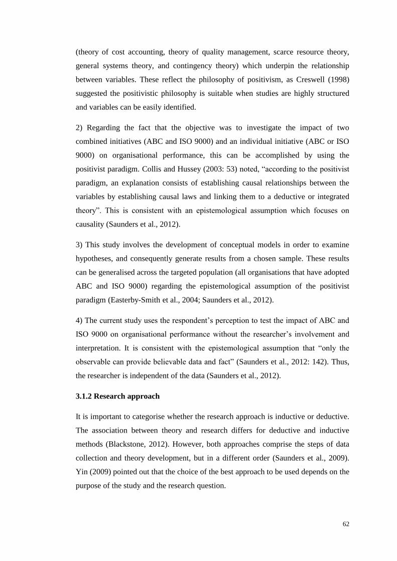
62

(theory of cost accounting, theory of quality management, scarce resource theory,

general systems theory, and contingency theory) which underpin the relationship

between variables. These reflect the philosophy of positivism, as Creswell (1998)

suggested the positivistic philosophy is suitable when studies are highly structured

and variables can be easily identified.

2) Regarding the fact that the objective was to investigate the impact of two

combined initiatives (ABC and ISO 9000) and an individual initiative (ABC or ISO

9000) on organisational performance, this can be accomplished by using the

positivist paradigm. Collis and Hussey (2003: 53) noted, “according to the positivist

paradigm, an explanation consists of establishing causal relationships between the

variables by establishing causal laws and linking them to a deductive or integrated

theory”. This is consistent with an epistemological assumption which focuses on

causality (Saunders et al., 2012).

3) This study involves the development of conceptual models in order to examine

hypotheses, and consequently generate results from a chosen sample. These results

can be generalised across the targeted population (all organisations that have adopted

ABC and ISO 9000) regarding the epistemological assumption of the positivist

paradigm (Easterby-Smith et al., 2004; Saunders et al., 2012).

4) The current study uses the respondent’s perception to test the impact of ABC and

ISO 9000 on organisational performance without the researcher’s involvement and

interpretation. It is consistent with the epistemological assumption that “only the

observable can provide believable data and fact” (Saunders et al., 2012: 142). Thus,

the researcher is independent of the data (Saunders et al., 2012).

3.1.2 Research approach

It is important to categorise whether the research approach is inductive or deductive.

The association between theory and research differs for deductive and inductive

methods (Blackstone, 2012). However, both approaches comprise the steps of data

collection and theory development, but in a different order (Saunders et al., 2009).

Yin (2009) pointed out that the choice of the best approach to be used depends on the

purpose of the study and the research question.

63

Bryman and Bell (2015) stated that the association between theory and research can

be commonly viewed in a deductive approach. In other words, “it involves the

development of a theory that is then subjected to a rigorous test through a series of

propositions” (Saunders et al., 2012: 145). The important characteristics of the

deductive approach are the finding of causal relationships between variables, the

collection of quantitative data, controls to allow the testing of hypotheses, then a

highly structured methodology for replication, operationalisation, reductionism and

generalization (Saunders et al., 2003). Bryman (2012) clarified the process of

deduction as shown in Figure 3.2. The deduction process begins with theory and

hypothesis, followed by data collection and findings. Hypotheses can be confirmed

or rejected, or theory revised. “The researcher, on the basis of what is known about a

particular domain and of theoretical considerations in relation to that domain,

deduces a hypothesis that must then be subjected to empirical scrutiny” (Bryman,

2012: 24). The implication can be examined and on the basic of the findings, the

initial theory or hypothesis can be confirmed or rejected (Burns & Burns, 2008).

Figure 3.2: The process of deduction

Source: Bryman (2012: 24)

Conversely, the inductive approach focuses on obtaining an insight into the meaning

of events, the collection of qualitative data and a more flexible structure to allow

changes of research emphasis (Saunders et al., 2003). Thus the conclusions based on

empirical observations are drawn and used as a basis for producing new theories.

Theory is the consequence of research when working from an inductive stance

(Bryman, 2012). Sekaran and Bougie (2010) pointed out that both deductive and

inductive approaches can be used in qualitative and quantitative research; however, it

64

should be noted that the inductive approach is regularly used in qualitative and

exploratory researches while the deductive approach is more often used in

quantitative and causal studies.

Saunders et al. (2012) also introduced a new approach called the abductive approach

form. “Instead of moving from theory to data (as in deduction) or data to theory (as

in induction) an abductive approach moves back and forth, in effect combining

deduction and induction” (Saunders et al., 2012: 147). Thus, the researcher can mix

both deductive and inductive approaches within the same piece of study.

In conclusion, following the three forms of reasoning as Saunders et al. (2012)

proposed, the deductive approach begins with theory and develops research from

academic literature. The researcher in this approach designs a research strategy to

examine theory. On the other hand, the researcher in an inductive approach starts by

gathering data to explore a phenomenon and generates theory. Lastly, in the

abductive approach, the researcher collects data to research a phenomenon and

builds a new theory or modifies existing theory, then subsequently examines it

through additional data collection.

Deduction is chosen, as the approach of this study as it aims to discover the impact

of ABC and ISO 9000 on organisational performance using relevant theories drawn

from literature (Bryman & Bell, 2015).

3.1.3 Methodological choice

The previous two sections discussed research philosophy and research approach,

which subsequently influence the selection of methodological choice in this section

and the next two layers of the research onion. The methodological choice, firstly, is

related to following a mono method (quantitative or qualitative) or multiple methods.

It needs to consider the research question through a philosophical lens, the way in

which philosophical assumptions will inform the methodological choice. Saunders et

al. (2012) indicated that a quantitative study is frequently employed, as a data

collection technique, in order to supply operating numerical data. In contrast,

qualitative study is normally used as a synonym for an interview, or for a data

analysis procedure, namely, categorising for operating on non-numerical data.

65

Figure 3.3: Methodological choice


Mono method (quantitative or qualitative method)

“Conducting research on the basis of a quantitative method or methodology has a

long tradition. This tradition can be traced back historically to natural science”

(Jonker & Pennink, 2010: 65). It is based on the postulation that knowledge about

reality can only be obtained independent of the researcher”. Saunders et al. (2012:

162) stated, “quantitative research is generally associated with positivism, especially

when used with predetermined and highly structured data collection techniques”. It is

normally related to a deductive approach by focusing on the testing of theory. The

data is analysed by a range of statistic techniques. Experimental and survey research

strategies are principally related to quantitative research (Saunders et al., 2012).

Qualitative research is “research in which the researcher makes an attempt to

understand a specific organisational reality and occurring phenomena from the

perspective of those involved” (Jonker & Pennink, 2010: 77). Saunders et al. (2012)

indicated that qualitative research is concerned with an interpretive philosophy, as

researchers are required to make sense of the subjective and socially constructed

meanings depicted about the phenomenon being researched. Several strategies are

related to qualitative research: namely, action research, grounded theory, case study,

ethnography, and narrative research.

Given the above discussion, a mono method quantitative approach is selected in this

study as Saunders et al. (2012) stated that in general, quantitative research related to

66

positivism, particularly when employed with highly structured data collection

techniques is appropriate.

Multiple methods

The philosophy of realism, often leads to a multiple methods research design

(Saunders et al., 2012). Inductive and deductive approaches can apply multiple

methods. As shown in Figure 3.3, multiple methods can be separated into two forms:

multimethod and mixed methods. Multimethod is divided between multimethod

quantitative study (researchers may use a questionnaire and structured observation

analysing data with quantitative procedures) and multimethod qualitative study

(researcher may choose in-depth interviews and diary accounts analysing data with

qualitative processes). On the other hand, mixed methods research can combine both

quantitative and qualitative research.

The multiple method has not been chosen as the quantitative research fits the

objectives of this current study. In other words, the proposed hypotheses can be

examined based on quantitative data alone.

3.1.4 Research strategy

“A strategy is a plan of action to achieve a goal” (Saunders et al., 2012: 173).

Research strategies must be consistent with the research philosophy and research

approach. These strategies provide a general plan to address research questions

(Saunders et al., 2003). Either a deductive approach, inductive approach or both of

them can use a variety of research strategies, such as experiments, surveys, case

studies, grounded theory, ethnography, and action research. Saunders et al. (2012)

suggested the choice of the research strategy will therefore be dependent upon your

research question(s) and objectives. Research strategy is depicted in the research

process onion as the fifth layer.

The research strategy for this current research is a survey based on questionnaires

which is usually associated with deduction. A questionnaire approach is a popular

method because of the benefits of a highly economical process and ease of

comparison. Miller et al. (2010) explained the advantage of this survey strategy is

that researchers can generalise the results from a chosen sample to a larger

population when the research is conducted well. It is commonly used in business and

67

management research for answering questions such as what, where, who, how many,

and how much (Zikmund, 2000; Saunders et al., 2012). In addition, this survey

strategy is generally perceived as authoritative. However, the limitation of using

surveys is an inability to demonstrate causation between variables as only

associations can be identified (Miller et al., 2010).

3.1.5 Time horizons

Studies can have varying time horizons, They can be cross-sectional and longitudinal

(Saunders et al., 2003). A cross-sectional study is defined by Cooper and Schindler

(1998: 132) as when “studies are carried out once and represent a snapshot of one

point in time”. In contrast, longitudinal studies are applied over an extended period

(Cooper & Schindler, 1998). In a cross-sectional study, the data is collected at a

single point in time; most surveys belong to this category. David and Sutton (2011:

209) indicated, “in cross-sectional design the exploration of relationships and

associations between variables needs to be carefully thought through. With cross-

sectional design there is no pre-test/post-test measure to compare, as the data is

collected at one point in time”. To address this problem, an extensive literature

review and prior experience are required (David & Sutton, 2011).

The purpose of a longitudinal survey is to examine continuity of results and notice

the action of changing something that occurs over time (Zikmund, 2000). Even

though “the main strength of longitudinal research is its capacity to study change and

development” (Saunders et al., 2012: 190), longitudinal studies are not frequently

employed by individual researchers because this technique is more expensive and

time-consuming (David & Sutton, 2011).

Regarding the constraints of time (Cooper & Schindler, 1998), this study adopts a

cross-sectional survey because it aims to research the impact of ABC and ISO 9000

on organisational performance at one point in time. To sum up, the chosen

approaches of research philosophy, research approach, methodological choice,

research strategy and time horizons are presented with bold font in Figure 3.4.

68

Figure 3.4: The research process onion

* Bold font indicates approaches chosen in this study

Source: Adapted from Saunders et al. (2012: 128)

3.1.6 Techniques and procedures

There are two basic sources of data: primary and secondary data. Primary data is

“data gathered and assembled specifically for the research project in hand” while

secondary data is, “data that have been previously collected for some project other

than the one at hand” (Zikmund, 2000: 58). In order to achieve the objectives of the

current research, primary data is needed.

There are many data collection methods related to a survey strategy, such as

questionnaires, observation and interviews. However, the questionnaire is widely

used as the data collection method in a survey strategy (Saunders et al., 2003). As

shown in Figure 3.5, a questionnaire is separated into two types: 1) self-

administered, which contains on-line questionnaires, postal questionnaires, and

delivery and collection questionnaires; whereas, 2) interviewer administered

questionnaires include telephone questionnaires and structured interviews (Saunders

et al., 2003).

69

Figure 3.5: Types of questionnaire


In this study, the self-administered postal questionnaire is selected to test the

hypotheses. This method helps this researcher to conduct a large scale survey at a

relatively low cost; as Cooper and Schindler (1998) noted, “mail surveys typically

cost less than personal interviews”. Additionally, the benefit of saving time is

considered as an advantage. It is convenient for respondents to answer questions

when they are free. “This method requires the questionnaire to be highly structured,

with questions being predominantly closed-ended” (Remenyi et al., 1998: 156).

However, mail surveys are not inexpensive as they include follow-up mailing,

additional postage, and printing additional questionnaires (Zikmund, 2000).

However, a disadvantage of self-administered postal questionnaires is that this

method cannot guarantee that the right person has answered the questionnaire, there

is greater risk of missing data or not collecting additional data and it is difficult to

ask a lot of questions (Bryman & Bell, 2007). In this current study, such problems

are addressed by writing a good covering letter, follow-up letters, stamped return

envelopes, and an appropriate length of questionnaire (Sekaran, 2000).

3.2 Questionnaire design

“A questionnaire is a prepared set of questions (measures) used by respondents or

interviewers to record answers (data)” (Hair et al., 2007: 257). Sekaran and Bougie

(2010: 197) defined a questionnaire as “a preformulated written set of questions to

which respondent record their answers, usually within rather closely defined

alternatives”. Generally speaking, a questionnaire contains the questions and scales

to generate the data: “The final outcome of a well-constructed questionnaire is

reliable and valid data if the related phases of the research are executed well” (Hair

et al., 2007: 257).

70

This section discusses the relevance of the process in designing a questionnaire and

the relevant issues concerning the questionnaire design in this case. The

questionnaire was developed between January and November 2014, and involved

study of the literature, a pre-test stage, ethical issue stage, pre-contact stage and a

pilot study in order to ensure the final version of a questionnaire was not

misunderstood and was of manageable length.

Hair et al. (2007) recommended five steps for the questionnaire design process, as

per the following sections:

3.2.1 Initial considerations (including sampling),

3.2.2 Clarification of concepts (including operationalisation of study constructs),

3.2.3 Determine question types,

3.2.4 Pre-test the questionnaire,

3.2.5 Administer the questionnaire

3.2.1 Initial considerations

At the beginning of developing a questionnaire, this current study has clearly

identified what is being researched and what is aimed from this study. One of the

critical early undertakings in a questionnaire is developing the questions: When the

preliminary list of questions are incorporated in a questionnaire, they should be

evaluated from the respondent’s perspective (Hair et al., 2007). It needs potential

respondents to answer using the self-completion approach. Hair et al. (2007)

suggested that researchers must decide whether respondents will answer a particular

question, and whether they will respond accurately. Respondents may refuse to reply

to sensitive questions or questions that seem an invasion of their privacy.

Sampling

The target population

A target population is “the total collection of elements about which we wish make

some inferences” (Cooper & Schindler, 1998: 215). Accordingly, this study aims to

investigate the impact of ABC and ISO 9000 on organisational performance; thus,

71

the target population is all the organisations that adopted ABC and ISO 9000 in

Thailand. “The basic idea of sampling is that by selecting some of elements in a

population, we may draw conclusions about the entire population” (Cooper &

Schindler, 1998: 215). Cooper and Schindler (1998) also indicated that there are

massive advantages for using a sample rather than census, such as cost of taking

cencus and the speed of contribution.

All Thai ISO-9001-registered organisations are supposed to have a similar quality

management system. In addition, Thai ISO-9001-registerd organisations that adopted

ABC are assumed to employ similar processes for calculation of product/service

costs. Therefore, all Thai ISO-9001-registered organisations were selected in this

study as a sample representing the whole population. Consequently, the results of

this current study can be generalised to the target population of Thai companies.

As discussed in Chapter 2, ABC is optional; this study cannot specify the number of

organisations adopting ABC. Recently, there was a study of Intakhan (2014), which

found 95 organisations had adopted ABC out of 174 ISO-9001-registered

organisations in Thailand (from 900 sample ISO 9001-registered organisations). In

order to increase the number of respondents and avoid receiving a low response rate,

all ISO-9001-registered organisations in Thailand were selected for this current study

(3,105 Thai ISO-9001-registered organisations; updated in December 2014). These

organisations are considered the sample size (see Appendix H).

Regarding a general organisational structure, managers are divided into three groups:

supervisory or first-line management, middle management, and senior or top

management (Buchanan & Huczynski, 2004). The formal structure refers to the way

tasks are administered and the authority of individuals. An organisation chart of a

firm indicates both middle managers and first-line managers who have responsibility

for reporting their work to top management (Dick and Ellis, 2005). Quality managers

normally have responsibility for ISO 9000 whereas the accounting manager is

usually responsible for ABC. Both of them commonly are the same level of

management as middle managers, depending on the size of organisation (Dick and

Ellis, 2005). Therefore, the top manager generally has authority to direct activities of

lower level managers and use their information. In other words, the top manager or

CEO is the highest-ranking executive in an organisation and whose main

72

responsibilities include developing and implementing high-level strategies, making

major corporate decisions, and managing the overall operations and resources of a

firm.

Because of these reasons, the CEOs or staff members in a similar position, who have

the ability and knowledge to answer the questionnaire, are targeted respondents. In

order to ensure a questionnaire is directed to the right person, the cover letter

describing the aim of this current study is attached in an envelope. Additionally, the

pre-contact stage was administered before sending a questionnaire (discussed later in

Section 3.2.5).

3.2.2 Clarification of concepts

“In designing the content, structure and appearance of a questionnaire a number of

aspects need to be taken into account” (Hair et al., 2007: 264). The constructs that

are to be measured must be clearly defined. Also, classification and outcome

information, type and wording of questions, questionnaire sequence, and general

layout must be considered (Hair et al., 2007).

Operationalisation of study constructs

Operationalising the concepts is the technique to reduce abstract notions of

observable behaviour and characteristics in a tangible way (Sekaran & Bougie,

2010). It looks at “the behaviour dimensions, facets, or properties denoted by the

concept” (Sekaran & Bougie, 2010: 127). Sekaran and Bougie (2010) indicated that

four steps are needed in operationalisation:

1) Tautology of construct

2) Considering the content of the measure

3) Indicating a response format

4) Assessing the validity and reliability of measurement (also discussed in Section

3.3.3.2)

The three main constructs need to be clarified in operationalisation of constructs are,

as follows.

73

The extent of ABC use construct operationalisation

The definition of “the extent of ABC use” has been discussed in Chapter 2 (see

Section 2.1.1). It is defined as “the degree which ABC is used”. After the construct

was defined, the next step in the process of measuring abstract constructs is finding

out whether there are any existing measures of the construct in the literature

(Sekaran & Bougie, 2010).

In previous studies Maiga and Jacobs (2008) measured the extent of ABC by four

variables - namely, design engineering, manufacturing engineering, product

management, and plant-wide while Jankala and Silvola (2012) measured the extent

of ABC by one variable only. In contrast to these previous studies, this study

particularly focuses on the “purposes” of using ABC because others focused on the

purposes (or objectives) of adopting ABC (see Section 2.2).

Cagwin and Bouwman (2002) described the purposes of using ABC as consisting of

product costing, cost management, pricing decisions, product mix decisions,

determining customer profitability, budgeting, an off-line analytic tool, outsourcing

decisions, and performance measurement. These nine indicators were used to

measure the APPLIC construct in their research. The current study follows the use of

ABC for specific purposes, as Cagwin and Bouwman (2002) indicated, because

using an existing variable could enhance levels of reliability and validity of

measurement. Additionally, the same indicator enables greater comparison across

earlier evaluation studies. In summary, the construct “the extent of ABC use”

consists of nine indicators.

Briefly put, the measurement model can be reflective or formative (Bollen &

Lennox, 1991; Edwards & Bagozzi, 2000). The reflective measurement model

represents the fact that the latent construct is considered as the cause and the measure

of its reflective indicator. In the sense of domain sampling, reflective indicators can

be interchanged. Therefore, deleting one specific indicator will not affect the sense

of content (Nunnally & Bernstein, 1994). In contrast, in a formative measurement

model, the indicators cause the latent construct. Elimination of relevant indicators

will reduce the scale validity in the case (Coltman et al., 2008). In a reflective scale,

all indicators are expected to correlate and each indicator is assumed to share a

common basis. Thus, increasing the value of the construct will translate into an

74

enhancement in the value for all indicators (Sekaran & Bougie, 2010). Most

research supposed the relation between latent construct and observed variables is

reflective: “The reflective view dominates the psychological and management

sciences; however, the formative view is common in economics and sociology”

(Coltman et al., 2008: 1).

Figure 3.6: Reflective measurement model (effect model) and formative

measurement model (causal model)

Source: Coltman et al. (2008: 7)

As displayed in Figure 3.6, a formative construct is a summation of the indicators

(Diamantopoulos & Winklhofer, 2001). The only variance (error) is the random

variance at the construct level (Law & Wong, 1999). Thus, the error term is related

to the construct as a whole and not with each indicator. In addition, “cause indicators

are exogenous, their variances and covariances are not explained by a formative

measurement” (Hancock & Mueller, 2006: 47). Hancock and Mueller (2006)

indicated that a construct would be just a linear combination of its indicators, “in this

sense it would be similar to a principal component in exploratory factor analysis or a

predicted criterion score in multiple regression” (Hancock & Mueller, 2006: 46).

Conversely, with a reflective construct, the individual indicator is individually

related to the construct. The error terms are reflected individually for each indicator

because the covariance of individual indicators is shared with other indicators, and

the random variance for individual indicators is treated as an error for an indicator

(Law & Wong, 1999).

This study focuses on the degree to which ABC is used by organisations. It is

possible that when the degrees of using ABC increase, all indicators consequently

75

increase. In other words, if an organisation uses a significant degree of ABC, ABC

should be consistently used for various purposes (indicators). Then, eliminating any

indicators should not change the conceptual domain of the construct. At the same

time, it is not appropriate to consider the construct as formative, as removing an

indicator would modify the definition of the construct. Based upon the above

reasoning, this current study views the extent of ABC use as reflective construct.

The extent of ISO 9000 implementation construct operationalisation

In this study, the definition of “The extent of ISO 9000 implementation” construct

has been previously determined in Chapter 2 (Section 2.1.1) as “the degree of

putting ISO 9000 into effect”. As discussed in Section 2.3, ISO 9004 is not intended

for certification, and ISO-9001-registered organisations might implement the eight

quality management principles (as ISO 9004 mentioned) differently. Therefore, it

would be appropriate to investigate the extent of ISO 9000 implementation in terms

of the different principles. There has been no study that operationalised the construct

in terms of “the extent of ISO 9000 implementation”, Kuncoro (2013) used these

quality management principles as indicators to measure a ISO 9000 construct:

namely, “the ISO quality management principles” construct as a formative construct.

In contrast, this study uses quality management principles to measure a construct

called “the extent of ISO 9000 implementation” as a reflective construct.

As mentioned earlier, the eight principles are not the requirements for implementing

ISO 9001. The organisation does not need to employ all of them. It depends on the

degree to which ISO 9000 is put into effect. When the extent of the ISO 9000

implementation construct changes, all principles (indicators) are supposed to change

in a comparable way. For this reflective model, the principle (indicator) is

interchangeable because a change in the extent of ISO 9000 implementation

constructs causes changes in all of the indicators. Therefore, deleting one specific

indicator will not affect the sense of content. Based upon these reasons, this current

study views the extent of ISO 9000 implementation as a reflective construct.

76

Organisational performance construct operationalisation

“Organisational performance” has been defined in Chapter 2 as “the outcomes of

an organisation’s action” (see Section 2.1). Neely (2007) suggested four dimensions

in measuring organisational performance: namely, accounting and finance,

marketing, operational management, and supply chain management. However,

regarding the literature on ABC, ISO 9000 and performance, two dimensions

(accounting and finance, and operational management) were frequently used to

measure organisational performance. Table 3.1 presents the comprehensive

indicators used in previous studies of both ABC and ISO 9000, which can be

explained from two perspectives: firstly, accounting and finance, in particular, sales

and return on assets; and secondly, operation management, in particular, cost,

quality, time improvement, organisational efficiency and process effectiveness.

Consequently, seven indicators are selected to measure organisational performance.

Organisational efficiency has been changed to process efficiency because both ABC

and ISO 9000 are associated with a process approach and activities (Kaplan &

Anderson, 2004; ISO 9001, 2008).

In the ISO 9000 literature, time delivery was frequently used in measuring

performance (Jang & Lin, 2008; Prajogo et al., 2012), whereas Naveh and Marcus

(2005) measured on-time delivery. Improving time is also often cited as one of the

ABC benefits (Charaf & Bescos, 2014). In the ABC literature, Ittner et al. (2002) and

Banker et al. (2008) indicated that the time indicator consists of manufacturing cycle

time and customer lead time. On the other hand, Maiga and Jacobs (2008) defined

time as consisting of new production time, manufacturing lead time, delivery

reliability, and customer responsiveness. In this study, time improvement

particularly focuses on delivery reliability due to its relevance to both ABC and ISO

9000 measures. In addition, it also seems to be a sensible measure to use delivery

reliability indicator for both manufacturing and non-manufacturing.

77

Operational performance construct operationalisation

Five out of seven indicators are considered as operational performance measures:

namely, reduced total costs, product/service quality, delivery reliability, process

efficiency, and process effectiveness. This study defines operational performance as

the “the outcomes of an organisation relating to an organisation’s process”. It is

considered as a reflective construct because these five indicators are caused by an

operational performance construct and correlated highly with each other (see section

4.1.3.4). Therefore, when operational performance changes, all indicators are

supposed to change in a comparative way.

Financial performance construct operationalisation

The remaining two indicators are considered as financial performance: namely, sales,

and return on assets (ROA). This study defines financial performance as “the

outcomes of an organisation relating to its financial situation”. It is considered a

reflective construct because these two indicators are caused by financial performance

constructs and are correlated highly with each other (see section 4.1.3.4). Then,

when financial performance changes, all indicators are supposed to change in a

comparative way.

78

Table 3.1: The measures used in evaluating the association and the impact of

ABC and ISO 9000

Indicators/variable ISO ABC Authors

1. Accounting and Finance

Net profit/increased profitability /

/

Jang and Lin (2008), Feng et al. (2008), Psomas et al. (2013)

Hardan and Shatnawi (2013)

Company financial results / Psomas et al. (2013)

Cash flow from operations / Psomas et al. (2013)

Sales growth /

/

Psomas et al. (2013), Naveh and Marcus (2005), Fatima (2014),

Psomas and Kafetzopoulos (2014)

Zaman (2009), Jankala and Silvola (2012)

Return on assets (ROA) /

/

Naveh and Marcus (2005)

Banker et al. (2008), Ittner et al. (2002), Cagwin and Ortiz (2005),


Long-run stock price performance / Naveh and Marcus (2005)

Gross profit / Naveh and Marcus (2005), Fatima (2014)

Net profit before tax / Psomas et al. (2013) Fatima (2014)

Net profit after tax / Fatima (2014)

Return on investment / Cagwin and Bouwman (2000), Jankala and Silvola (2012)

Holding period returns / Kennedy and Affleck-Graves (2001)

Cumulative abnormal returns / Kennedy and Affleck-Graves (2001)

Return on sales / Maiga and Jacobs (2008)

Turnover on assets / Maiga and Jacobs (2008)

3. Operations management

The improvement of internal

administration efficiency

/ Lee et al. (2009)

Reduced cost of quality / Naveh and Marcus (2005)

The improvement of the cost /

/

Jang and Lin (2008), Naveh and Marcus (2005), Feng et al. (2008),

Lee et al. (2009), Prajogo et al. (2012)

Ittner et al. (2002), Banker et al. (2008), Maiga and Jacobs (2008)

The low employee turnover rate Lee et al. (2009)

Efficiency /

/

Psomas et al. (2013), Psomas and Kafetzopoulos (2014)

Zaman (2009)

Company productivity / Jang and Lin (2008), Psomas et al. (2013), Naveh and Marcus (2005),

Feng et al. (2008)

Effectiveness /

/

Psomas et al. (2013), Psomas and Kafetzopoulos (2014)

Zaman (2009)

Product/service quality /

/

Jang and Lin (2008), Psomas et al. (2013), Feng et al. (2008), Psomas

and Kafetzopoulos (2014)


Consistent and reliable

products/services

/ Psomas et al. (2013)

Product/service conformance to

specifications

/ Psomas et al. (2013)

Improved internal procedures / Jang and Lin (2008), Feng et al. (2008)

Improved employees’ morale / Jang and Lin (2008), Feng et al. (2008)

Lower defect rates / Naveh and Marcus (2005)

Improved competitive advantage / Feng et al. (2008)

Product innovation / Prajogo et al. (2012)

Product performance / Prajogo et al. (2012)

Time improvement /

/

Jang and Lin (2008), Naveh and Marcus (2005), Prajogo et al. (2012)


79

Types of scales

“A scale is a tool or mechanism by which individuals are distinguished as to how

they differ from one another on the variables of interest to our study” (Sekaran &

Bougie, 2010: 141). Zikmund (2003: 296) defined a scale as “a continuous spectrum

or series of categories”. Scaling aims to represent quantitatively an item’s, an event’s

or a person’s place on the spectrum (Zikmund, 2003). Four types of scales are

described as follows.

Firstly, nominal scale is “one that allows the researcher to assign subjects to certain

categories or groups” (Sekaran & Bougie, 2010: 141). It is the simplest type of scale

(Zikmund, 2003). There are only two groups, such as male or female, yes or no.

Secondly, ordinal scale “not only categorizes the variables in such a way as to denote

differences among the various categories, it also rank-orders the categories in some

meaningful way” (Sekaran & Bougie, 2010: 142). This scale provides information

on how participants discern them by rank-ordering them. Thirdly, interval scales

“allow us to perform certain arithmetical operations on the data collected from the

respondents” (Sekaran & Bougie, 2010: 143). This can measure the distance on the

scale between two points. Zikmund (2003) also pointed out that interval scales

indicate order and measure order or distance in units of equal intervals. “It is a more

powerful scale than nominal and ordinal scales and has for its measure of central

tendency the arithmetic mean. Its measures of the dispersion are range, the standard

deviation, and variance” (Sekaran & Bougie, 2010: 144-145). Finally, ratio scale

“not only measures the magnitude of the differences between points on the scale but

also taps the proportions in the differences” (Sekaran & Bougie, 2010: 145).

A previous study of Cagwin and Bouwman (2002), (in an APPLIC construct

equivalent to the extent of ABC use construct in this study), operationalised their

survey items by asking whether ABC is consistently used for the following nine

purposes by using a five-point Likert scale (1=strongly disagree, 2=disagree, 3=no

opinion, 4=agree, and 5=strongly agree). Based on the literature, Likert scales are

normally treated as ordinal scales (Bertram, 2006). For data collection, Likert

surveys are speedy, efficient and inexpensive methods. However, “as a general rule,

mean and standard deviation are invalid parameters for descriptive statistics

whenever data are on ordinal scales” (Allen & Seaman, 2007: 64-65). Ordinal scale

80

fails to measure the space between each choice, which cannot necessarily be

equidistant.

Many researchers aim to treat Likert scales as continuous variables when the range

of values is relatively large and when the gap among values are equivalent (Larsen &

Marx, 1981; Kerlinger, 1992). Allen and Seaman (2007) indicated that in some

circumstances Likert scales might be used with an interval procedure. The interval

should be an attribute of data, not of labels, and a “scale item should be at five and

preferably seven categories” (Allen & Seaman, 2007: 65). For instance, using a

continuous line or track bar in measuring the pain measurement (worst ever to best

ever) can yield a continuous interval measure (Allen & Seaman, 2007).

This study initially created a 10-point scale without a label for each value, only for

extreme values: namely, strongly disagree and strongly agree (each point shows

approximately 10%, the maximum at 100%). However, after the pre-test study, five

of seven colleagues suggested using the scale with a less than 10-point scale due to it

being too much and difficult to discriminate between the 10 different options. This

study decided to use the scale from 1 to 7 as a continuous scale with markers in

equality of each point as showed in Figure 3.7. In addition, in the pilot study, ten

organisations had no problem with this scale. Based on the pilot study, the scale

establishes the quality of magnitude of differences in scales point. For instance,

respondents circled the number 4, 5, 6, and 7 for the item 5.1a, 5.1b, 5.1c, and 5.1d,

respectively (See Figure 3.7). They indicated that the extent of ABC use for product

costing (5.1a) for cost management (5.1b) was the same as the extent of ABC use for

pricing decisions (5.1c) over product mix decision (5.1d). That was, the magnitude

of difference represented by space between points 4 and 5 on the scale was the same

as the magnitude of difference represented by space between points 6 and 7, or

between any other two points. As such, this scale was viewed as a continuous scale,

which is more powerful than the nominal and ordinal scales. This scale was applied

when measuring the respondent’s view toward the object of interest, such as the

extent of ABC use, the extent of ISO 9000 implementation, operational performance,

and financial performance.

The category scale, is applied to ask demographic questions, on areas such as

manufacturing or non-manufacturing in Section C (see Appendix A). Additionally,

81

multiple choice is appropriately used when there are multiple alternatives for

respondents: for example, respondents are asked for their positions, namely, Chief

Executive Officer (CEO), Managing Director, and Other (specify: ___), as shown in

Section D (see Appendix A).

Figure 3.7: The questions and scales measuring the extent of ABC use construct

One question is used in measuring one indicator in order to minimise questionnaire

size and avoid a low response rate. Saunders et al. (2012) indicated using a shorter

questionnaire increased response rates. In addition, respondents may not respond to a

question which is too difficult or too long as Sekaran and Bougie (2010: 202). The

questions 5.1a - 5.1i showed the exact name of each indicator. Definitions of the

relevant term are presented in the glossary on the last page of the questionnaire (see

Appendix A). It is assumed that respondents understand the definitions of each

indicator as these indicators are general terms and used as the purpose of ABC in

organisations. None of the organisations (in the pilot study) confused the definition

of nine purposes.

For the extent of the ISO 9000 implementation construct, Kuncoro (2013) used a

five-point Likert scale for measuring a construct and included three or four questions

for measuring each principle. Unlike this previous study, this study uses one

question in measuring each principle as an interval scale.

In the operational performance construct, five indicators have been discussed in

previous studies, as follows.

82

First, the reduced total cost indicator is previously measured by both ordinal scales

and ratio scales. In ABC studies, Zaman (2009) also used a five-point Likert type

scale. Ittner et al. (2002) measured cost by asking respondents to specify the changes

in manufacturing costs while Maiga and Jacobs (2008) used a seven-point Likert

scale to measure cost improvement (four variables account for cost improvement).

Banker et al. (2008) asked respondents about the change in manufacturing costs in

the last five years by providing multiple choices: namely, “1 = Increased more than

20%, 2 = increased 11–20%, 3 = increased 1–10%, 4 = no change, 5 = decreased 1–

10%, 6 = decreased 11–20%, and 7 = decreased more than 20%” (Banker et al.,

2008: 12). In the ISO 9000 literature, the studies of Jang and Lin (2008), Naveh and

Marcus (2005), Feng et al. (2008), Lee et al. (2009), and Prajogo et al. (2012)

applied a five-point Likert scale with “1” specifying “strongly disagree” and “5”

specifying “strongly agree” to measure the reduced cost variable.

In the product/service quality measure, ABC literature, Ittner et al. (2002) asked

respondents to specify the amount of 1) finished product first pass quality yield in

percentage terms and 2) scrap and rework costs as a percentage of sales. Banker et

al. (2008) asked about the change in plant first-pass quality yield in the last five

years by providing multiple choices namely “1 = declined more than 20%, 2 =

declined 1–20%, 3 = stayed the same, 4 = improved 1–20%, 5 = improved more than

20%” (Banker et al., 2008: 12). Conversely, Maiga and Jacobs (2008) used a seven-

point Likert scale measuring quality improvement (three variables account for cost

improvement). In the ISO 9000 literature, Jang and Lin (2008) and Feng et al. (2008)

applied a five-point Likert scale, whereas Psomas et al. (2013) used a seven-point

Likert scale where 1 represented “strongly disagree” and 7 represented “strongly

agree”.

Discussing time improvement in previous studies of ABC, Ittner et al. (2002: 715)

asked respondents to specify “manufacturing cycle time from start of production to

completion of product in hours and standard lead-time from order entry to shipment

in days”. Banker et al. (2008: 9) asked about “the change in manufacturing cycle

time and the change in lead-time during the last five years” by providing multiple

choices. On the other hand, Maiga and Jacobs (2008) used a seven-point Likert scale

measuring time improvement (four variables account for time improvement -

namely, manufacturing lead time, new product introduction time, customer

83

responsiveness, and delivery reliability/dependability). In the ISO 9000 literature,

particularly on time delivery, was measured by applying a five-point Likert scale

with “1” indicating “strongly disagree” and “5” indicating “strongly agree” (Naveh

& Marcus, 2005; Jang & Lin, 2008; Prajogo et al., 2012).

For efficiency, Psomas et al. (2013) used a seven-point Likert scale where 1

represented “strongly disagree” and 7 represented “strongly agree” to measure a

particular company efficiency whereas Zaman (2009) used a five-point Likert type

scale to measure effectiveness. Similarly, for the effectiveness measure, Psomas et al.

(2013) used a seven-point Likert scale (1 represented strongly disagree and 7

represented strongly agree) in measuring particular process effectiveness whereas

Zaman (2009) used a five-point Likert type scale measuring effectiveness.

In the financial performance construct, two indicators have been discussed as

follows.

Psomas et al. (2013) used a seven-point Likert scale where 1 represented “strongly

disagree” and 7 represented “strongly agree” to measure sales, whereas Naveh and

Marcus (2005) measured sales by using a five-point Likert scale with “1” indicating

“strongly disagree” and “5” indicating “strongly agree”. In the ABC literature,

Zaman (2009) also used a five-point Likert type scale while Jankala and Silvola

(2012) collected annual sales from the two-year period, after the survey, from

statutory financial information

In ISO 9000 literature, return on assets (ROA) is measured by using a five-point

Likert scale (Naveh & Marcus, 2005). As in previous studies of ABC, Ittner et al.

(2002) asked respondents to specify ROA. Conversely, Maiga and Jacobs (2008)

used a seven-point Likert scale measuring ROA.

Unlike the previous studies, this study uses one question in measuring each

performance indicator (sales, return on assets, reduced total cost, product/ service

quality, delivery reliability, process efficiency, and process effectiveness) as an

interval scale (see Appendix A).

84

3.2.3 Determine question types, format and sequence

There are two forms used in questionnaires: closed and open-ended questions. In the

closed questions, the researcher specifies the answer alternatives, whereas open

questions allow respondents to provide answers in their own way (Saunders et al.,

2016). However, open questions may not motivate busy participants to provide

answers. So, this study decides to use closed questions which are relatively

convenient for collecting data and which are also normally easy to analyse (Collis &

Hussey, 2003). Respondents can also compare responses that have been

predetermined (Saunders et al., 2016). In addition, it is more appropriate to a

positivist, deductive approach (Zikmund, 2003; Saunders et al., 2012).

After considering the type of question, the next step is creating the questionnaire

structure. Hair et al. (2007: 266) showed that “the structure follows a three-part

sequence of questionnaire sections. The questions in the initial section are referred to

as opening questions. The middle section has questions directed specifically at the

topics addressed by the research objectives. The final section includes the

classification questions that help the researcher to better understand the results”. The

classification questions are shown at the end of questionnaire, such as age and

income, as “there is simply an effort to increase response and reduce error” (Hair et

al., 2007: 271). The questionnaire contains relevant questions about ISO 9000 in the

first part as all respondents are ISO-9001-registered organisations. Questions

regarding the organisation’s characteristics and personal details (demography) are

placed in the last two sections of the questionnaire.

Collis and Hussey (2003: 125) referred to Kerlinger (1986), suggesting that “good

research questions for a positivistic study should express a relationship between

variables, be stated in unambiguous terms in question form, and imply the possibility

of empirical testing”. Hair et al. (2007) recommended that questions should use

simple words, brief sentences, avoiding ambiguity, leading questions, and double-

barrelled questions. Ideally, a question should “be no longer than 20 words,

excluding possible answers” (Saunders et al., 2016: 452). In addition, questions

should be asked in logical order. In other words, early questions should be general

and the latter be more specific for minimizing position bias.

85

Reliability and validity issues

Bryman and Bell (2007: 162) explained, “reliability is fundamentally concerned with

issues of consistency of measures”. It has different meanings from validity. “When a

measure has low reliability, some of the differences in scores between people which

it produces are spurious differences, not real differences” (Punch, 1998: 100). The

careful construction and piloting of the questions and using the existing questions

from reputable surveys can improve the reliability (David & Sutton, 2004).

In summary, reliability and stability of the questionnaire mean that if this study is

done again by the same researcher in different times and places or other researchers

similar results with occur. In this study, the questions are predominantly drawn from

earlier research (see sections 2.2-2.4).

Cronbach’s alpha

Establishing measurement reliability is crucial in applied and theoretical research as

reliability constitutes an important primary step for assuring construct validity

(Iacobucci & Duhachek, 2003). This study employs Cronbach alpha in order to test

internal consistency (reliability). It is defined as follows.

Where p is the number of items in the scale, σ is the variance of the ith item, i = 1,

2, .… p and σT2 is the variance of the entire test, hence, it is the summation of the

item variances and covariances, as

It is noted that a high value for Cronbach’s alpha shows good internal consistency of

the items in the scale; however, it does not imply that there is scale

unidimensionality (Gliem & Gliem, 2003). Alpha value can be high despite low item

intercorrelations and multidimesionality (Panayides, 2013). In other words, a

coefficient alpha is appropriate to test internal consistency (reliability), but not a

suitable technique to test dimensionality.

86

SPSS software is used in the current study for examining Cronbach alpha. Its value

is generally accepted at a minimum criterion level of 0.60 (Nunnally, 1978).

However, for exploratory studies, alpha ranges from 0.50 to 0.60 are considered

adequate (Nunnally, 1978). SPSS outputs also show the corrected item-total

correlation (CITC) and the value that Cronbach's alpha would be if that particular

item was deleted from the scale. The Corrected Item-Total Correlation (CITC) is the

correlation of the item designated with the summated score for all other items (Gliem

& Gliem, 2003). These values should be at least 0.40 (Nunnally & Bernstein, 1994).

An Alpha score is helpful in that it can demonstrate whether an improvement can be

made by dropping an item from a construct. In the pilot study, ten questionnaires

were sent to respondents in Thailand, overall they showed 0.71, which met the cut

off value of 0.60 (Nunnally, 1978).

“Validity refers to the extent to which a test measures what we actually wish to

measure” (Cooper & Schindler, 1998: 166). The objective of measurement is to

measure whatever we propose, which is complicated and difficult to understand

(Zikmund, 2000). As Sekaran and Bougie (2010) expressed, validly can be separated

into three groups; namely, content validity, criterion-related validity, and construct

validity. Zikmund (2000: 282) illustrates that “face validity or content validity refers

to the subjective agreement among professionals that the scale logically appears to

reflect accurately what it purports to measure”.

The questionnaire was first revised by the supervisors and also a professional

lecturer at Hull University, then seven colleagues, three PhD academic researchers

who had graduated from the UK, and academics from Khon Kaen University and

Kasetsart University in Thailand. Moreover, the questionnaire was piloted with ten

ISO-9001-registered organisations in Thailand. These steps ensure that the measures

employed by the researcher actually measure what this study is supposed to measure,

thus achieving content validity.

Construct validity is established by the degree to which the measure confirms a

network of related hypotheses generated from a theory based on the concepts.

Establishing construct validity occurs during the statistical analysis of the data. In

construct validity, the empirical evidence is consistent with the theoretical logic of

the concepts. In its simplest form, if the measure behaves the way it is supposed to,

87

in a pattern of intercorrelation with a variety of other variables, there is evidence for

construct validity (Zikmund, 2000). Construct validity is the most normally cited

validity assessment in social science fields (Cooper & Schindler, 1998; Punch,

1998). It is relevant to how the measurement conforms to theoretical expectations

(Cooper & Schindler, 1998; Punch, 1998). The construct validity is also described

with confirmatory factor analysis (CFA) in section 3.3.3.2.

The positivist approach taken in this research implies that validity was ensured

through content and construct validity. The research was taken from previous studies

and their theoretical concepts. Moreover, the questionnaire was sent to experts such

as CEOs, who form the target population, and other researchers in the field as part of

the pilot study. Therefore, since selection of the primary measurement items was

based on extensive review of theories and the literature, it was considered to have

content validity. The researcher tried to increase validity and reliability during data

analysis by using only completed questionnaires in order to present accurate and

reliable results. Thus, any returned questionnaires with missing data were excluded

from data analysis.

3.2.4 Pre-test the questionnaire

The processes of pre-test and pilot study have been employed to ensure that the

questionnaire is validated and reliable. A draft questionnaire was then subjected to

pre-test study by seven colleagues. Additionally, the questionnaire was revised by

supervisors and also a professional lecturer at the University of Hull. After that, the

questionnaire continued onto the process of translation into a Thai version, discussed

next.

As the targeted population is in Thailand, the questionnaire needed to be translated

into the Thai language. Saunders et al. (2012) referred to Usunnier (1998) and

summarised both the advantages and disadvantages of the four techniques for

translating a questionnaire as consisting of direct translation, back-translation,

parallel translation, and mixed techniques. The study employed a mixed technique.

This technique provides the best match between source and target questionnaires.

The questionnaire was first checked for grammar and translated into Thai by a

professional translator. After that, the questionnaire with the Thai version has been

translated back into English by another professional translator and three PhD

88

academic researchers who graduated from the UK to ensure the accuracy of

translation. Additionally, it was tested again by an academic from Khon Kaen

University and an academic from Kasetsart University in Thailand. Subsequently,

the Thai version of the questionnaire continued on to pilot testing.

The first phase of the pilot study began with an in-depth interview of top

management: namely, two CEOs, a manager, a quality manager and an accounting

manager (two organisations which adopted both ABC and ISO 9000, whereas three

organisations which adopted only ISO 9000). The final phase of the pilot study was

conducted (five organisations) to test the research process of drop and collect by the

researcher (in November 2014).

3.2.5 Administration of the questionnaire

This step involved ethical issues, the pre-contact phase, and collecting data, as

follows.

Ethical issue

“The goal of ethics in research is to ensure that no one is harmed or suffers adverse

consequences from research activities” (Cooper & Schindler, 1998: 108).

Researchers cannot ignore ethical issues because they are directly related to the

integrity of a piece of work, including any disciplines that they involve. It is crucial

to consider the way a researcher within social sciences more generally has dealt with

ethical research issues (Bryman & Bell, 2007). This study follows the ethical

procedures for research documented in the Hull University Business School

(HUBS): “The School’s ethical procedures for research are designed to establish a

research ethics system which provides guidance, advice and monitors this important

issue” (HUBS, 2011). HUBS (2011) suggested a flowchart of document in order to

depict what the researcher needs to be aware of regarding ethical obligations. Before

sending the pro forma (copy of proposal) and an informed consent letter to the ethics

committee for approval, they need to be approved and signed by supervisors and the

researcher. Diener and Crandall (1978) described that four main areas should be

considered: harm to participant, lack of informed consent, invasion of privacy, and

deception. Subsequently, this pro forma and the informed consent letter were sent to

89

the HUBS research ethics committee to approve in mid-November 2014. Finally, the

research ethics committee approved them at the end of November 2014.

Pre-contact

As mentioned in section 3.1.6, there are some disadvantages to self-administered

postal questionnaires. These are addressed here. Firstly, the disadvantage of self-

administered postal questionnaire was indicated by Bryman and Bell (2007), who

said this method cannot ever be sure that the right person has answered the

questionnaire. This can be addressed by describing in the cover letter and pre-contact

as Hair et al. (2007) suggested via preliminary contact such as letter, email or phone.

In this study, before the survey was operated, phone calls to all ISO-9001-registered

organisations were undertaken during September 2014 and October 2014. This step

was conducted in order to verify the names and addresses of the organisation, ask for

permission to send a questionnaire, and indicate the most appropriate person to

respond to the questionnaire. However, only 320 organisations out of 3,105

registered organisations gave the names of the possible respondents and their

position. Some organisations refused to provide the name but they allowed the

researcher to send the questionnaire addressed to the respondent’s position.

The covering letter (see Appendix A) described the aim of the survey, and it

accompanied the questionnaire (Saunders et al., 2012). In this study, the content of

the letter, included the letterhead, what the research is about, why it is useful,

confidentiality, a token reward for participation, and contact details for queries. The

name of a respondent was specified in some organisations from the pre-contact, as

mentioned above. Saunders et al. (2012: 446) also referred to the research of Dillman

(2009) and others that states “the covering letter will affect the response”.

Also, the critical disadvantage of self-administered postal questionnaires is the low

response rate (Cooper & Schindler, 1998). Saunders et al. (2012) suggested

strategies for raising postal questionnaire response rates. This study adopted an

incentive strategy by providing an opportunity to enter the prize draw of £150 as a

monetary incentive aimed at maximising the response rate. The current questionnaire

is not too long, which may also increase the response rate to very high. In addition,

the pre-paid return envelope is attached and a handwritten signature appeared in the

90

covering letter. Pre-contact and follow up are also administered. These strategies are

considered as effective methods to enhance the response rate.

Collecting data

Organisations listed among the Thai ISO 9000 register were chosen as the sample

frame for this research (see section 3.2.1). There are 3,105 companies across

different industries, both manufacturing and non-manufacturing organisations. As

previously mentioned, the questionnaire including the cover letter, the approval letter

and the prepaid envelope was posted to the Chief Executive Officer, Managing

Director or other names (staff in the same position) at 3,105 Thai-ISO-9000

registered firms in the beginning of December 2014. The respondent was given three

weeks to return the questionnaires; in total, 189 returned questionnaires were

received by December 2014. Two-hundred and seventy-four questionnaires were

returned in January 2015 after a reminder letter and further phone call. Finally, a

total of 619 questionnaires (or 19.94 per cent) were by 28 February 2015 after two

reminder letters and two calls. However, 18 of the 619 returned questionnaires were

judged as not valid for the analysis mainly due to missing data. Hence, 601 (or 19.36

percent) were considered usable and were included in the final data analysis. The

respondents consist of 601 ISO 9000 organisations; 191 organisations that adopted

both ABC and ISO 9000, and 410 organisations that adopted only ISO 9000. There

are more than 20 categories (see Appendix H) following the International Standard

Industrial Classification of All Economic Activities (ISIC). However, this study

widely specifies the type of business as consisting of two types: manufacturing and

non-manufacturing.

Table 3.2: Overall response rate

Returned

Period

Returned

questionnaires

Uncompleted

questionnaires

Usable

questionnaires

December 2014 189 9 180

January 2015 274 3 271

February 2015 156 6 150

TOTAL 619 18 601

91

3.3 Data Analysis

There are five subsections of data analysis techniques in this study, as follows.

3.3.1 Preliminary analysis

3.3.2 Descriptive analysis

3.3.3 Factor analysis

3.3.3.1 Exploratory factor analysis (EFA)

3.3.3.2 Confirmatory factor analysis (CFA)

3.3.4 Structural equation modelling (SEM)

3.3.5 Multi-group analysis

Each subsection is discussed in following sections.

3.3.1 Preliminary analysis

Preliminary and descriptive analysis was carried out in order to summarise the data

in a meaningful way, such as explaining the basic features of the sample, patterns of

data, and testing assumptions underlying the selected statistical methods. This

section includes response rate, sample size, tests for non-response bias, screening

data (deals with outliers, missing data, normality, linearity, homoscedasticity, and

multicollinearity), general characteristics of participators, and descriptive statistics

for research variables (central tendency, dispersion, and distribution of score).

3.3.1.1 Response rate and sample size

To test the adequacy of sample size, most of the published sample size

recommendations were simplified rules based on experts’ experience, such as the

absolute numbers. For example, Comrey and Lee (1992) indicated that a sample size

of 50 is very poor, 100 is poor, 200 is fair, 300 is good, 500 is very good, and above

1,000 is excellent. A sub sampling study of Costello and Osborne (2005b) indicated

that for a sample size as small as 26 cases (2:1), only 10% of the samples recovered

the correct factor structure, whereas 70 percent in the largest (20:1 or 260 cases)

92

produced correct results. Additionally, Hair et al. (2006) suggested a sample size of

between 100 to 150 would obtain stable maximum likelihood estimation results.

On the one hand, some authors focused on the number of cases per variable (rules of

thumb); Nunnally and Bernstein (1994), for instance, suggested 10 cases for each

variable to be factor analysed, whereas Hair et al. (2007) recommended five cases

for each item as the minimum absolute sample size. However, Brown (2006: 142)

indicated that “rules of thumb are very crude and usually do not generalize to the

researcher’s data set and model. Thus, sample size requirements should be evaluated

in the context of particular data set and model at hand”.

Marsh and Bailey (1991) recommended calculating sample size by the ratio (r) of

indicators to latent variables (p/k). Meanwhile, Boomsma (1982) indicated that if r =

12 requires a sample size of at least 50, if r = 4, it requires a sample size of at least

100; if r = 3, it requires at least 200 sample, and for r = 2, it requires a sample size of

at least 400. In multi-group analysis, this study considers the 1-Sample Z-test

method with regards to an online sample size calculator (Statistical Solution, 2016)

which uses the 1-Sample Z-test method.

This study considers the adequacy of sample size by following absolute numbers

(Hair et al., 2006), rules of thumb (Nunnally & Bernstein, 1994), ratio (r) of p/k

(Marsh & Bailey, 1991),and the 1-Sample Z-test method in order to obtain stable

factor analysis and SEM solutions.

3.3.1.2 The tests of non-response bias

In this current study, despite the satisfactory response rate, non-response bias is

possible. Hussey and Hussey (1997) indicated that non-response bias occurs when

not all the questionnaires are returned and not all the questions in the questionnaires

have been completed. It is claimed that non-response bias is a major problem with

data collection methods using mailed questionnaire (Mangione, 1995; Chongruksut,

2002) as research findings may be incorrectly reported if respondents' answers differ

from those of non-respondents (Mangione, 1995). Armstrong and Overton (1977)

described that there are three methods of estimating non-response bias: namely, 1)

comparison with known values for population; 2) subjective estimates; and 3)

extrapolation. In the first method, if the known values come from a different source

93

instrument, then differences may occur. The second method has a problem in the

uncertainty about the use of subjective estimates. Thus, extrapolation method is the

more appropriate method to test non-response bias in this study. Measuring the non-

response bias is based on the presumption that the late response may be a surrogate

of non-respondents (Wallace and Mellor, 1988). The validity of the early and the late

responses was evaluated using Levene’s test, which is applied to test homogeneity of

variance. If it is not significant (p-value > 0.05), this means that no statistically

significant differences in the mean scores between early and late respondents (see

section 4.1.2).

3.3.1.3 Screening data

Tabachnick and Fidell (2014: 63) suggested “before choosing a technique, you

should determine the fit between your data and some very basic assumptions

underlying most of the multivariate statistics”. Each technique is discussed as

follows.

Missing data

“Missing data is one of the most pervasive problems in data analysis” (Tabachnick &

Fidell, 2007: 62). Hair et al. (2010: 36) defined missing data as “information not

available for a subject (or case) about which other information is available”. Missing

data may occur due to errors in data entry or on the part of the respondents (Hair et

al., 1998). Tabachnick and Fidell (2007) indicate that the number of missing data is

less important than the pattern of missing data. In other words, the seriousness is

dependent on the pattern of missing data. The patterns of missing data are classified

into three levels: namely, missing completely at random (MCAR), missing at

random (MAR), and missing not at random (MNAR).

Tabachnick and Fidell (2007) illustrated that if the data set is large and a few random

points are missing (say, 5% or less) the problem is less serious. Hair et al. (2010: 48)

also recommended that “variables with as little as 15 percent missing data are

candidates for the deletion, but higher levels of missing data (20-30 percent) can

often be remedied”. On the other hand, if a number of data are missing from small to

moderate data, the problem is more serious. In this study, if missing data are more

than 5%, deleting data is chosen in order to address the problem (see section 4.1.3.1).

94

Outliers

“Outliers are observations with a unique combination of characteristics identifiable

as distinctly different from the other observations” (Hair et al., 2010: 64).

Tabachnick and Fidell (2007: 72) also described that “an outlier is a case with such

an extreme value on one variable (a univariate outlier) or such a strange combination

of scores on two or more variables (multivariate outlier) that it distorts the statistics”.

Moore et al. (2012: 18) suggested that “you should search for an explanation for any

outliers. Sometimes outliers point to errors made in recording the data. In other

cases, the outlying observation may be equipment failure or other unusual

circumstances”.

The presence of an outlier has four reasons: the first is procedure error, namely

errors in data collection, recording, or entry; second is failure to identify missing-

value codes; third is that the outlier is not a member of the study population; and

finally there is the case with more extreme values than a normal distribution. In order

to identify the outliers, box plots are used in this study as they are “simpler and

literally box in observations that are around the median” (Tabachnick & Fidell,

2007: 74). This means that extreme values are cases that fall far away from the box.

After outliers are identified, the researcher needs to discover why the cases are

extreme and make a decision for dealing with them (see section 4.1.3.2).

Normality

Hair et al. (2010: 36) defined normality as the “degree to which the distribution of

the sample data corresponds to a normal distribution”. “Screening continuous

variables for normality is an important early step in almost every multivariate

analysis, in particular when inference is a goal” (Tabachnick & Fidell, 2007: 79).

Regression presumes that variables are normally distributed. Variables with non-

normal distribution (skewness or kurtosis) can distort associations and significance

tests. Testing for normality may be undertaken in either graphical (such as

histogram and normal probability plot) or statistical methods, namely Kolmogorov-

Smirnov and Shapiro-Wilk test (Tabachnick & Fidell, 2007; Hair et al., 2010).

Amos also reports the output of assessment of normality in terms of critical ratio

(C.R.) of skew and kurtosis. Kline (2005) indicated that values of skew index

95

exceeding 3.00 seem to be extreme skew, whereas the values from 8.00 to over 20.0

are considered extreme kurtosis.

In order to test normality, a histogram has been employed in this study because the

process location is clearly identifiable (see section 4.1.3.3) as well as considering the

C.R. of skew and kurtosis from SEM results (see Section 4.5).

Multivariate normality

The assumption of multivariate normality is the underlying assumption of most

multivariate analysis and statistical tests. It assumes that all variables and all

combinations of the variables are a normal distribution. “Screening continuous

variables for normality is an important early step in almost every multivariate

analysis, particular when inference is a goal” (Tabachnick & Fidell, 2007: 79).

In SEM, it regularly assumes that the multivariate distribution is a normal

distribution (Kline, 2005). “In applied research, multivariate normality is examined

using Mardia’s normalized multivariate kurtosis value” (Khine, 2013: 11). Mardia’s

coefficient is computed based on the formula p (p+2) where p is the number of

observed variables in the model (Raykov & Marcoulides, 2006). “If the Mardia’s

coefficient is lower than the value obtained from the above formula, then the data is

deemed as multivariate normal” (Khine, 2013: 11). The Mardia’s coefficient can be

also found in most SEM software such as AMOS.

In addition, Byrne (2010) referred to Bentler (2005) suggesting that in practice, the

z-statistic of values above 5 are indicative of non-normal distribution. This study

tests multivariate normality based on either Mardia’s coefficient or z-statistic

through AMOS results (see section 4.5).

Linearity

Hair et al. (2010: 35) explained, “linearity is used to express the concept that the

model possesses the properties of additivity and homogeneity”. “The assumption of

linearity is that there is a straight-line relationship between variables” (Tabachnick &

Fidell, 2014: 117). Linearity can be examined by bivariate scatterplots. If both

variables display linearity, the scatter plot is oval-shaped. Conversely, nonlinearity

shows as non-oval in scatterplot (Tabachnick & Fidell, 2014). However, using

96

bivariate scatterplots may be burdensome if there are numerous variables

(Tabachnick & Fidell, 2014).

In this study, there are numerous variables; thus, testing deviation from linearity is

firstly examined. If the significant value of deviation from linearity is above 0.05,

then the relationship between the variables is linear. On the other hand, if there is

significant value deviation from linearity below 0.05; it needs further examination by

bivariate scatterplots (see section 4.1.3.3).

Homoscedasticity

Hair et al. (2010: 35) described homoscedasticity as “when the variance of errors

term appears constant over a range of predictor variables, the data are said to be

homoscedastic”. On the other hand, “when the error terms have increasing or

modulating variance, the data are said to be heteroscedastic” (Hair et al., 2010: 35).

“Homoscedasticity is related to the assumption of normality when the assumption of

multivariate normality is met, the relationships between variables are

homoscedastic” (Tabachnick & Fidell, 2014: 119). Homoscedasticity can be tested

by graphical tests of equal variance dispersion and statistic tests (Hair et al., 2010).

In a statistic test, the Levene test is commonly used in assessing the equality of

variance (Hair et al., 2010). In contrast, in the graphical test, “the bivariate

scatterplots between two variables are of roughly the same width all over with some

bulging toward the middle” (Tabachnick & Fidell, 2014: 119), as illustrated in

Figure 3.8. Two metric variables are best tested graphically. Cones or diamonds

shapes are noticed when there is departure from an equal dispersion. This study tests

homoscedasticity by determining scatterplots (see section 4.1.3.3).

Figure 3.8: Bivariate scatterplots under conditions of homoscedasticity and

heteroscedasticity

Source: Tabachnick and Fidell (2014: 119)

97

Multicollinearity

Multicollinearity is a problem with a correlation matrix that occurs when variables

have excessively high correlation (Tabachnick & Fidell, 2007). Kline (2005: 56)

pointed out “multicollinearity can occur because what appear to be separate variables

actually measure the same thing”. Inspecting a correlation matrix is one of methods

to assessing multicollinearity. A correlation matrix with values greater than 0.90 is

considered as involving multicollinearity (Kline, 2005). Other statistics are tolerance

and variance inflation factor (VIF). Tolerance comes from 1- R2 indicating the

proportion of total standardised variance that is unique. Variance inflation factor

(VIF) equals 1/ (1- R2), the ratio of the total standardised variance. Hair et al. (2010:

204) indicated “a common cut-off threshold is a tolerance value of 0.10, which

corresponds to a VIF value of 10”. The values of tolerance less than 0.1 and VIFs

exceeding 10 are signs of serious multicollinearity (Hair et al., 2010).

In this study, multicollinearity is examined by using Pearson’s correlation coefficient

(see section 4.1.3.4) because it is easy to interpret from considering the direction of

the correlation. Pearson’s correlation coefficient measures the strength of a linear

relationship between two variables. Its values range from +1 to -1. In Figure 3.9, a

value of 0 means that two variables have no association, a value exceeds 0 indicating

a positive association, and a value below 0 indicating a negative association (Kline,

2005).

Figure 3.9: The positive correlation, negative correlation and no correlation

Source: https://statistics.laerd.com

98

3.3.2 Descriptive statistics

Descriptive statistics are examined to report the basic characteristics of the data in

this research. These descriptive statistics contain central tendency, dispersion, and

distribution of score (see section 4.2). Randolph and Myers (2013) stated that one of

the most common ways of analysing and describing data is to compute measures of

central tendency.

Central tendency

Central tendency is defined as “an estimation of the centre of a distribution of

values” (Faulkner & Faulkner, 2009: 157). Three major types of estimates of central

tendency are usually used including mean, median, and mode.

In central tendency, mean is the most frequently used measure (Mann, 2013) for

finding the accurate average of data. The mean is the summation of all the values

divided by the number of values.

Mean = Sum of all values / Number of values

“The median is the value in the middle of a distribution after all of the values have

been ranked in order from smallest to largest” (Randolph & Myers, 2013: 11). Mann

(2013: 91) illustrated the calculation of median consisting of two steps: firstly, “rank

the data set in increasing order”, followed by “find the middle term. The value of this

term is the median”. In other words, the median is the formal version of the midpoint

regarding a specific rule (Moore et al., 2012).

“The mode is simply the value or attribute that occurs most frequently in a

distribution of values” (Randolph & Myers, 2013: 13).

Dispersion

Dispersion relates to the spread of the values around the central tendency. The range

and the standard deviation commonly measure dispersion. The range equals the

highest value minus the lowest value. “The Standard Deviation (S.D.) measures

spread by looking at how far the observations are from their mean” (Moore et al.,

2012: 39). Researchers frequently use the S.D. method when measuring the

dispersion of a set of data to show how the data is spread around.

99

Distribution of score

Distribution of score is related to the skewness and kurtosis (Tabachnick & Fidell,

2014). Hair et al. (2010: 36) defined “skewness as measure of the symmetry of a

distribution, in most instances the comparison is made to a normal distribution”.

Kurtosis is defined as a “measure of the peakedness or flatness of a distribution when

compared with a normal distribution” (Hair et al., 2010: 35). A distribution is

symmetric if it appears the same between left and right from the centre point. Data

with high kurtosis tends to have a sharp peak and heavy tails. Conversely, data with

low kurtosis tends to have a flat top (Tabachnick & Fidell, 2014). In normal

distribution, skewness and kurtosis values tend to be zero. Thus, the further the

values are far from 0, the more likely it is that the data might not distribute normally.

3.3.3 Factor analysis

This study applies factor analysis (in terms of exploratory factor analysis and

confirmatory factor analysis) in order to test the dimensional structure of the extent

of ABC use, the extent of ISO 9000 implementation, and organisational

performance.

Factor analysis (FA) refers to “an interdependent technique whose primary purpose

is to define the underlying structure among the variables in the analysis” (Hair et al.,

2006: 104). One type of factor analysis is exploratory factor analysis (EFA),

indicated as “orderly simplification of interrelated measures”. It is assumed that each

common factor affects every manifest variable (observed variables) and common

factors are either uncorrelated or all correlated. EFA is grounded on a data-driven

approach without the constraints of a number of factors. Confirmatory factor analysis

(CFA), on the other hand, is theory-driven. It is used to test the hypothesis with

regard to the underlying structure of data.

Factor analysis is applied in this study in order to establish underlying dimensions

between variables and constructs. Regarding theory, factor analysis allows this

current study to confirm or refine theory (Tabachnick & Fidell, 2007; Williams et al.,

2012). Looking at the extent of ABC use, Cagwin and Bouwman (2002) considered

nine purposes for the unidimensional construct without testing dimensionality. In

100

terms of the extent of ISO 9000 implementation, most previous studies indicated the

construct as a single construct without testing the dimensionality.

The organisational performance literature indicated organisational performance as

multidimensional. However, based on both ABC and ISO 9000 literature, no study

has tested the dimensionality of the organisational performance construct. Because

of this, this study conducts EFA in order to explore the factorial structure of

organisational performance, as Courtney (2013: 1) suggested that EFA is

“particularly appropriate for scale development where little theoretical basis exists

for specifying the number and patterns of common factors”. CFA is also employed

in this study to confirm the results of EFA, and to ascertain the respective

dimensions regarding theories and literature. This is an important step to extract a

number of factors as this decision directly affects the findings and subsequent theory

development. In other words, it is making a decision as to how many factors

(constructs) to retain when applying EFA and CFA before testing the effect of

initiatives (the extent of ABC use or/and the extent of ISO 9000 implementation) on

a performance construct. Indirect effect might occur in the case of considering

organisational performance as more than one factor. Similarly, if the extent of ABC

use and the extent of ISO 9000 implementation are multidimensional, different

dimensions might impact on organisational performance differently.

3.3.3.1 Exploratory factor analysis (EFA)

There are important issues that need to be considered in employing EFA: namely,

sample size, factorability of R, the inter-correlation, missing data, outliers, linearity,

normality, multicollinearity and homoscedasticity. Most issues (except factorability

of R and the inter-correlation) have been discussed in section 3.3.1.

The strength of the relationships and linear relationship can be measured by

considering the correlation matrix. It is generally expected to have correlation

coefficients greater than 0.30 (Tabachnick & Fidell, 2007). However, using

correlation coefficients still have some limitations as it does not indicate the practical

meaning of factors’ significance as the values are restricted from 0 to 1. Therefore,

instead of considering only correlation coefficients, the factorability of R, a complex

measure is recommended for evaluating the strength of the relationships and

suggesting the factorability of variables.

101

There are two statistical methods employed to test the factorability of R: 1) Bartlett’s

test of sphericity; and 2) the Kaiser-Meyer-Olkin (KMO). The guidelines for both

are: Bartlett’s test of sphericity should be statically significant (p-value ≤ 0.05),

whereas a KMO index value of 0.80 or over is meritorious, 0.70 or over is middling,

0.60 or over is mediocre, and below 0.50 is not acceptable (Hair et al., 2006). Based

on Kaiser’s criterion or eigenvalue rule, only factors with an eigenvalue of 1.0 or

above can be retained for further investigation (Pallant, 2007). Furthermore, the level

of cumulative percentage of the total variance of 60 is considered as satisfactory in

social sciences (Hair et al., 2006). However, 50 percent of the variance explained is

the minimally acceptable level (Beavers et al., 2013).

If the data met all the assumptions, this means factor analysis is the appropriate

method to apply. Brown (2006: 20) stated that “other procedural aspects of EFA

include 1) selection of a specific method to estimate the factor model; 2) selection of

the appropriate number of factors; 3) in the case of models that have more than one

factor, selection of technique to rotate the initial factor matrix to foster the

interpretability of the solution; 4) if desired, selection of the method to compute

factor scores”.

Factor extraction

There are many methods that can be used to estimate the common factor model, such

as maximum likelihood (ML), unweighted least squares, image factoring, principal

axis factoring (PAF), generalised least squares, and alpha factoring (Brown, 2006;

Hair et al., 2010; Williams et al., 2012). Brown (2006) indicated that ML and PAF

are the most commonly used factor extraction methods. Fabrigar et al. (1999)

explained that if data are relatively normally distributed, ML is the most appropriate

option because “it allows for the computation of a wide range of indexes of the

goodness of fit of the model and permits statistical significance testing of factor

loadings and correlations among factors and the computation of confidence

intervals.” (Costello & Osborne, 2005a: 2). On the other hand, if multivariate

normality is seriously violated, they recommend employing PAF (Fabrigar et al.,

1999).

102

In this study, ML has been selected to be employed as it can indicate underlying

factors that reflect what the variables share in common and how the data of the

current study is normally distributed (Hair et al., 2006).

Factor rotation

Once the appropriate number of factors is considered, the extracted factors are

related. Rotation maximises high-item loadings whilst minimising low-item

loadings, thus developing a more explainable and simplified result (Brown, 2006).

Orthogonal technique and oblique technique are two common rotation techniques

(Hair et al., 2010). Orthogonal method includes varimax, quartimax, and equamax,

whereas oblique method contains direct oblimin, quartimin, and promax. The

orthogonal method produces factors that are uncorrelated, while the oblique method

allows the factors to relate (Hair et al., 2010). Researchers in the social science area

expecting some correlation among factors due to behaviour being seldom partitioned

into packaged units that function separately (Costello & Osborne, 2005b).

In fact, there is no broadly favoured method of oblique rotation since all methods

tend to produce similar results (Fabrigar et al., 1999). In other words, although there

are many alternatives for executing the steps of EFA, the differences between them

are insignificant, so it doesn’t really matter which methods the researcher selects

(Costello & Osborne, 2005a). Finally, this study employs the most commonly used

orthogonal approach, particularly varimax, as an appropriate method when the

theoretical hypotheses concern unrelated dimensions.

Factor interpretation

A factor loading shows the relationship between the variables and their factor. Hair

et al. (2010) assessed the loadings regarding practical significance; factor loadings in

the range of ±0.30-0.40 are acceptable as a minimum requirement, ±0.50 or above

are of practical significance, and exceeding 0.70 shows a well-defined structure and

the goal of any factor analysis. However, factor loadings should be assessed at

stricter levels. Hair et al. (2010) also recommended considering factor loadings with

different sample sizes by employing a power level of 80 percent, a 0.05 significant

level and the proposed inflation of standard errors. The sample size needed for

significance is displayed in Table 3.3. In this study, the sample sizes of four models

103

range from 191 to 601, then the current study uses 0.40 as the cut-point value as the

minimum level, as Hair et al. (2010) suggested.

In summary, EFA is a data-driven approach. No specifications are indicated

regarding the number of factors or the pattern of association between factors and

their indicators (Brown, 2006). Therefore, seven indicators are examined in EFA in

order to consider the number of factors and the pattern of indicator-factor loadings

(see section 4.4.1). This study determines the number of factors to retain in EFA by

considering only factors with an eigenvalue (Kaiser’s criterion) of 1.0 or above

(Pallant, 2007) and factor loadings more than 0.40 (Hair et al., 2010).

Table 3.3: Identifying significant factor loadings based on sample size

Factor Loading Sample size needed for significance

0.30 350

0.35 250

0.40 200

0.45 150

0.50 120

0.55 100

0.60 85

0.65 70

0.70 60

0.75 50

Source: Hair et al. (2010: 117)

EFA by nature is exploratory without inferential statistics. It is employed as the most

appropriate for exploring the data. However, it is not used to test hypotheses or

theories (Costello & Osborne, 2005a). Costello and Osborne (2005a) also cautioned

researchers against leaping to conclusions regarding exploratory analyses.

Confirmatory factor analysis (CFA) is recommended in that it allows researchers to

test hypotheses through inferential techniques, providing more substantive analytical

options. Because of this, CFA is proposed as a more sophisticated technique for

testing the dimensional structure of measures in this study (Byrne, 2010).

3.3.3.2 Confirmatory factor analysis (CFA)

CFA is applied to this study for two main objectives: namely, testing the

dimensionality of constructs, and testing validity and reliability of the measurements

104

(Hair et al., 2006). There are five steps for testing CFA using similar processes as for

when examining SEM (see section 3.3.4).

3.3.3.2.1 Testing the dimensional structure of the measurement

In order to test the dimensionality of the measure, alternative models are established

in this study as follows: I) all indicators can be tested with only one construct (one

factor model); II) all the factors are allowed to be freely related (first-order factors

model); and III) all factors may be correlated as a higher order factor model (Byrne,

2010).

Kline (2005: 199) illustrated that “in order for a CFA model with a second-order

factor to be identified, there must be at least three first-order factors. Also each first-

order factor should have at least two indicators”. However, “given the specification

of only three first-order factors, the higher order structure will be just-identified”

(Byrne, 2010: 132), and lead to an identification problem (Byrne, 2010). Therefore,

only first two models (I and II) are examined in the study to find out the dimensional

structure of the extent of ABC use, the extent of ISO 9000 implementation, and

organisational performance (see section 4.4.1).

3.3.3.2.2 Testing the validity and reliability of the measurement

CFA is also employed to assess convergent validity and discriminant validity (Hair

et al., 2006), as follows.

Convergent validity

Hair et al. (2010: 709) indicated, “that the items are indicators of a specific construct

should converge or share a high proportion of variance in common”. In cases of high

convergent validity, the minimum of all factor loadings should be 0.5 or above and

ideally 0.7 or higher (Hair et al., 2010). Additionally, average variance extracted

(AVE) and construct reliability (CR) should be satisfied.

AVE is computed as a summation of standardised factor loadings extracted by a

number of items per construct (Hair et al., 2010). AVE should exceed the value of

0.5 or above to indicate adequate convergent validity (Hair et al., 2010).

105

AVE = Sum of standardised factor loading

Number of items per construct

CR is computed as the squared sum of factor loadings divided by squared sum of

factor loadings and sum of standard errors. Diamantopoulos and Siguaw (2000)

suggested that CR should exceed 0.60. However, Nunnally (1978) suggested the

generally accepted minimum criterion level of 0.50 (see Section 4.4.2).

CR = the squared sum of factor loadings

(Squared sum of factor loadings + sum of standard errors)

Discriminant validity

There are two types of discriminant validity coefficients. The first includes the

correlations between measures of different traits that are provided by the same

measurement method. The second type includes correlations between measures of

different traits that are obtained using different methods of measurement (Raykov,

2011). In order to assess discriminant validity, Hair et al. (2006) suggested

comparison between the variance extracted estimate (or average AVE) and the

squared correlation estimate by CFA. If average AVE exceeds the squared

correlation estimate, it means there is evidence of discriminant validity (see Section

4.4.2).

3.3.3.2.3 Common method variance (bias)

The common method variance (CMV) biases might have potential effects on

research results (Podasakoff et al., 2003). Then, it is crucial to understand their

sources and how to control or minimise CMV. CMV may be a concern when using

self-report questionnaires collecting data at the same time from the same respondents

(Chang et al., 2010). “Self-report data can build false correlations if the respondents

have a propensity to provide consistent answers to survey questions that are

otherwise not related” (Chang et al., 2010: 178). Therefore, common methods can

cause systematic measurement errors and the actual relationship among theoretical

factors (Podasakoff et al., 2003; Chang et al., 2010).

Many statistical remedies are used to detect and control any possible CMV. A post

hoc Harman one-factor analysis is often employed in order to check whether

106

variance in the data can be largely assigned to a single factor (Chang et al., 2010).

However, Podasakoff et al. (2003) indicated that a post hoc Harman one-factor

analysis is insensitive as there is no given guideline for an acceptable percentage of

explained variance of a single-factor model. Therefore, comparing the model fit of

two models with CFA is an alternative way to support the result of a post hoc

Harman one-factor analysis. Consequently, this study examines a post hoc Harman

one-factor analysis of four models by EFA, followed by comparing model fit of the

first model and the second model. Two steps are tested for detecting and controlling

CMV (see Section 4.4.2).

3.3.4 Structural equation modelling (SEM)

Byrne (2010: 3) defined structural equation modelling (SEM) as “a statistical

methodology that takes a confirmatory approach to the analysis of a structural theory

bearing on some phenomenon”. Similarly, SEM is defined by Raykov and

Marcoulides (2006: 1) as “a statistical methodology used by social, behavioural, and

educational scientists as well as biologists, economists, marketing, and medical

researchers”. “Structural equation modelling also referred to as causal modelling,

causal analysis, simultaneous equation modelling, analysis of covariance structures,

path analysis, or confirmatory factor analysis” (Tabachnick & Fidell, 2007: 676).

“Today, structural equation modelling (SEM) has become a popular and important

way of analysing data” (Ghauri & Grønhaug, 2010: 194). In terms of SEM, it

expresses “two important aspects of the procedure: (a) that the causal processes

under study are represented by a series of structural (i.e., regression) equations, and

(b) that these structural equations can be modelled pictorially to enable a clearer

conceptualisation of the theory under study” (Byrne, 2010: 3). SEM presents

measurement error whereas traditional regression analysis ignores measurement

errors (Raykov & Marcoulides, 2006). Additionally, SEM uses both observed and

latent variable, while regression analysis examines only observed variables (Byrne,

2010).

SEM has been used in this study because firstly, SEM allows this current study to

examine both direct and indirect effects (Raykov & Marcoulides, 2006). Secondly,

multi-group analysis in SEM allows this study to test the significant differences

between organisations that adopted both ABC and ISO 9000 and organisations that

107

adopted only ISO 9000. In addition, this study can test the moderating impacts on


Generally, there are two sub models for SEM: a measurement model and a structural

model. The measurement model relates to manifest variables and construct variables,

whereas structural model identifies an association among construct variables (Byrne,

2010). In other words, the measurement model illustrates the connections between

the latent variables and their observed variables whereas the structural describes the

causal connections among latent variables (Blunch, 2008).

“Latent variable is a central concept in SEM. Latent variables are measures of hidden

or unobserved phenomena and theoretical constructs. In social work, latent variables

represent complex social and psychological phenomena, such as attitudes, social

relationships, or emotions, which are best measured with multiple observed items”

(Bowen & Guo, 2012: 1-2). “As latent variables cannot be measured directly, they

are measured by indicators (observed variables), usually questions in a questionnaire

or some sort of test” (Blunch, 2008: 5).

Rectangles are used to represent observed variables, which may be either indicators

of latent variables in the measurement model or independent or dependent variables

in the structural model. Ellipses indicating latent variables, independent and

dependent variables as well as errors of prediction in the structural model and errors

of measurement in the measurement model. Arrows are used to illustrate association

and are of two sorts. Straight arrows point in one direction and indicate direction of

prediction, from predictor to outcome (Tabachnick & Fidell, 2007; Byrne, 2010).

Individual programs

Kline (2005) indicated eight different SEM computer programs. “They include

Amos, the CALIS procedure of SAS/STAT, EQS, LISREL, Mplus, Mx Graph, the

RAMONA module of SYSTAT, and the SEOATH module of STATISTICA”

(Kline, 2005: 79). The choice of software is dependent on the objective of the SEM

analysis and the computing skills of the user (Khine, 2013).

108

AMOS

AMOS is “actually an acronym for analysis of moment structures or in other words,

the analysis of mean and covariance structures” (Byrne, 2010: 17). AMOS is “the

Microsoft Windows interface, the program allows you to choose from two

completely different methods of model specification” (Byrne, 2001: 15).

Byrne (2010: 17) noted “the choice of which Amos method to use is purely arbitrary

and bears solely on how comfortable you feel in working within either a graphical

interface or a more traditional programming interface”. This study applies AMOS

due to it being accessible and provided by the University of Hull.

3.3.4.1 The steps of SEM approach

In structural equation modelling literature, five steps are mentioned for testing SEM

models: 1) model specification, 2) identification, 3) estimation, 4) evaluation, and 5)

modification (Schumacker & Lomax, 2004; Kline, 2005; Blunch, 2008; Byrne,

2010; Hair et al., 2010; Kline, 2013; Tabachnick & Fidell, 2014).

It is noted that the first two steps have been involved in operationalising constructs

as discussed in section 3.2.2 and also indicated in the two previous sections (See

section 3.3.2 and 3.3.3)

3.3.4.1.1 Model specification

In this step, a model is stated. “Model specification involves determining every

relationship and parameter in the model that is of interest to the researcher”

(Schumacker & Lomax, 2004: 62). In other words, the model is specified by

hypothesised relationships representing parameters’ paths. These relationships can

be determined as fixed, free or constrained. Fixed parameters are fixed at zero or

one. If a parameter is fixed at zero, this means no relationship between variables and

it does not need a path (straight arrows). Free parameters are estimated from the

observed data and are assumed by the researcher to be non-zero. Constrained

parameters are specified to be equal to a certain value (e.g. 1.0) or equal to another

parameter in the model that needs to be estimated.

Kline (2005) indicated that three types of parameters needed to be specified:

directional effects, variances, and covariances. Directional effects explain the

109

association between the observed indicators and latent variables, called factor

loadings, and relationships between latent variables and other latent variables (called

path coefficients). Tabachnick and Fidell (2014) defined directional effects as

regression coefficients. “Regression represents the influence of one or more

variables on another” (Byrne, 2010). Conversely, covariances are non-directional

associations among independent latent variables. Variances are then estimated for

indicator error (Kline, 2005).

3.3.4.1.2 Model identification

Blunch (2008) indicated two rules for obtaining identification. Firstly, the three-

indicator rule meant that “a confirmatory factor model is identified, if 1) every factor

has at least three indicators, 2) no manifest variable is indicator for more than one

factor, and 3) the error terms are not correlated” (Blunch, 2008: 129). In the latter,

the two-indicator rule has conditions consisting of: 1) every factor has at least two

indicators, 2) no manifest variable is indicator for more than one factor, 3) the error

terms are not correlated, and 4) the covariance matrix for the latent variables does

not contain zeros” (Blunch, 2008: 129). Tabachnick and Fidell (2014: 765) also

supported the idea that “if there are only two indicators for a factor, the model may

be identified; if there are no correlated errors, each indicator loads on only one

factor, and none of the variances or covariances among factors is equal to zero”.

The degrees of freedom in SEM are “equal to the amount of unique information in

the sample variance/covariance matrix (variance and covariances) minus the number

of parameters in the model to be estimated (regression coeficients and variance and

covariances of independent variables)” (Tabachnick & Fidell, 2014: 750). The

following formula, [p(p+1)]/2, where p represents the number of observed variables,

is used to compute the number of variances and covariances (Tabachnick & Fidell,

2014).

Schumacker and Lomax (2010) described that there are three identification types:

just-identified, over-identified and under-identified. When the degree of freedom is

zero, the model is just-identified. “A model is over-identified when there is more

than one way of estimating a parameter (or parameters)” (Schumacker & Lomax,

2004: 64). On the other hand, the last type of identification shows negative degree of

freedom, and then the parameter estimation is not possible (Kline, 2013). Kline

110

(2013) suggested that before continuing to model estimation, the issues relating to

sample size (see section 3.3.1.1) and data screening (see section 3.3.1.3) have to be

considered.

3.3.4.1.3 Model estimation

“In estimation, the goal is to produce Σ (θ) (estimated model-implied covariance

matrix) that resembles S (estimated sample covariance matrix) of the observed

indicators, with the residual matrix (S – Σ (θ)) being as little as possible. When S -

Σ(θ) = 0, then χ2 becomes zero, and a perfect model is obtained for the data” (Khine,

2013: 11). There are various estimation techniques: namely, maximum likelihood

estimation (MLE), unweighted least squares (ULS), generalised least squares (GLS),

weighted least squares (WLS), and asymptotic distribution free (ADF) methods


This study uses maximum likelihood (ML). Nachtigall et al. (2003: 7) stated that

“the most common type of estimating parameters and computing model fit is the

maximum likelihood method (ML) requiring multivariate, normally distributed

continuous variables”. Furthermore, MLE “is currently the most frequently used

estimation method in SEM” (Tabachnick & Fidell, 2014: 770). Raykov and

Marcoulides (2006: 30) also supported the idea that “ML method can also be

employed with minor deviations from normality”.

3.3.4.1.4 Model evaluation

“Once the parameter estimates are obtained for a specified SEM model, they should

determine how well the data fit the model” (Schumacker & Lomax, 2004: 69).

Schumacker and Lomax (2004: 69) indicated two ways to think about model fit: 1)

considering “some global-type omnibus test of the fit of the entire model”; and 2)

examining “the fit of individual parameters of the model” (Schumacker & Lomax,

2004: 70). In the parameter estimates, Byrne (2010: 67) stated that “examples of

parameters exhibiting unreasonable estimates are correlations > 1.00, negative

variances, and covariance or correlation matrices that are not positive definite”.

First, the SEM literature reported various statistical indices of overall model fit. It

should be noted that each fit index has a few problems (Kline, 2005). Kline (2005)

described basic limitations of all fit indexes in SEM as: 1) values of fit indices

111

present only the overall fit of the model, not each part of the model. This means that

even when the overall fit of the model appears a perfect fit, some parts might be a

poor fit; 2) no single index indicates a gold standard for all models, so models should

be assessed based on more than one index; 3) fit indices did not mean that the results

are theoretically meaningful; and 4) value of fit indexes indicates sufficient fit but

does not mean the model has high power. Finally, the sampling distributions of

several fit indexes applied in SEM are unknown (except RMSEA).

Second, there are three main features of individual parameters for consideration.

Firstly, “whether a free parameter is significantly different from zero (critical value

exceeds 1.96 for a two-tailed test at the 0.05 level)”. Secondly, “whether the sign of

the parameter agrees with what is expected from the theoretical model”. Lastly,

“parameter estimates should be within an expected range of values” (Schumacker &

Lomax, 2004: 70). This section discusses the various goodness-of-fit indices

available in SEM software.

Schumacker and Lomax (2004: 81) stated, “finding a statistically significant

theoretical model that also has practical and substantive meaning is the primary goal

of using structural equation modeling to test theories”. There are three types of

model fit criteria as Schumacker and Lomax (2004) illustrated. The first is the non-

statistical significance of chi-square and root-mean-square error of approximation

(RMSEA). Next is the statistical significance of individual parameter estimates for

the paths in the model. Last is the magnitude and the direction of parameter

estimates.

Absolute fit indices

“Absolute fit indices are a direct measure of how well the model specified by the

researcher reproduces the observed data” (Hair et al., 2010). The most commonly

applied are chi-square (χ2), goodness-of-fit statistic (GFI), the root mean square error

of approximation (RMSEA), and the root mean square residual (RMR) (Schumacker

& Lomax, 2004; Hair et al., 2010). “These criteria are based on differences between

the observed (Original, S) and model-implied (reproduced, Σ) variance-covariance

matrices” (Schumacker & Lomax, 2010: 85).

112

Chi-square (χ2)

Chi-square, also known as the generalised likelihood ratio (Byrne, 2010), shows the

differences between observed and implied covariance matrices. The value close to

zero means there is a small difference between the expected and observed covariance

matrices (Schumacker & Lomax, 2004). In addition, when the p-value ≤ 0.05 the

chi-square is close to zero. In other words “a nonsignificant χ2 value indicates that

the two matrices are similar, indicating that the implied theoretical model

significantly reproduces the sample variance-covariance relationships in the matrix”

(Schumacker & Lomax, 2004: 100).

However, this fit statistic is likely to be implausible regarding the size of

correlations. For instance, higher correlations contribute to bigger values of chi-

square. Additionally, chi-square is affected by sample size, particular in the larger

size and non-normal distribution. Both can lead to rejection of the model (Kline,

2005). Due to the restrictiveness of chi-square, it is seldom that a chi-square only is

used in applied research (Brown, 2006).

As mentioned, using only a single statistical significance cannot identify a correct

model; thus, researchers normally employ several criteria when considering and

evaluating model fit (Schweizer et al., 2003; Schumacker & Lomax, 2004; Hair et

al., 2010): for example, the comparative fit index (CFI), the root mean square error

of approximation (RMSEA), and the comparative fit index (CFI). This broad range

of fit indices is applied in the study to evaluate the measurement models and the

structural models.

Goodness-of-fit statistic (GFI)

GFI was produced by Jöreskog and Sorbom as an optional to the χ2 test (Tabachnick

& Fidell, 2014). It is based on “the ratio of the sum of the squared differences

between the observed and reproduced matrices to the observed variances, thus

allowing for scale” (Schumacker & Lomax, 2004: 101). Values for GFI range from

0.00 to 1.00. Hair et al. (2010) indicated the cut-off point of 0.90.

113

The root mean square error of approximation (RMSEA)

RMSEA indicates the amount of unexplained variance: “RMSEA estimates the

amount of error of approximation per model degree of freedom and takes sample

size into account” (Kline, 2005: 139). “It has become regarded as one of the most

informative fit indices” (Diamantopoulos & Siguaw, 2000: 85). The values range

from 0 to 1, a smaller RMSEA value implying a better model fit. An RMSEA value

between 0.08 and 0.10 presents a mediocre fit and under 0.08 indicates a good fit

(MacCallum et al., 1996).

The root mean square residual (RMR)

RMR represents “the average residual value derived from the fitting of the variance-

covariance matrix for the hypothesised model to the variance-covariance matrix of

the sample data” (Byrne, 2001: 82). The values range from 0 to 1.00, an RMR value

below 0.05 is viewed as a well-fitting model (Byrne, 2001). However, values less

than 0.08 are considered as acceptable (Hooper et al., 2008).

Incremental fit indices

“Incremental fit indices differ from absolute fit indices in that they assess how well

the estimated model fits relative to some alternative baseline model” (Hair et al.,

2010: 668). Schumacker and Lomax (2004) called the criteria a model comparison.

“They typically compare a proposed model with a null model” (Schumacker &

Lomax, 2004: 103).

Normed fit index (NFI)

Hair et al. (2010: 668) indicated that NFI is “one of original incremental fit indices”.

“This statistic assesses the model by comparing the χ2 value of the model to the χ2

of the null model. Values for this statistic range between 0 and 1 with Bentler and

Bonnet (1980) recommending values greater than 0.90 indicating a good fit”

(Hooper et al., 2008: 55).

Comparative fit index (CFI)

The comparative fit index (CFI) is an improvement on the NFI (Hair et al., 2010).

Values for CFI range from 0.00 to 1.00 (Schumacker & Lomax, 2004): the values

114

closer to 1.0 indicating a good model fit (Brown, 2006). CFI values exceeding 0.95

imply the good-fitting model (Tabachnick & Fidell, 2007). Hair et al. (2010: 669)

stated, “CFI values above 0.90 are usually associated with a model that fits well”.

Tucker-Lewis index (TLI)

The Tucker-Lewis index or Bentler-Bonnet NNFI (non-normed fit index) is used for

comparing the proposed model to the null model (Kline, 2005). “The measure can be

used to compare alternative models or to compare a proposed model against a null

model” (Schumacker & Lomax, 2010: 88). “TLI is not normed and thus its values

can fall below 0 or above 1. Typically though, models with good fit have values that

approach 1, and a model with a higher value of 0.90 suggests a better fit than a

model with lower value” (Hair et al., 2010: 668).

Parsimony fit indices

The parsimony fit index “is improved either by better fit or by a simpler model”

(Hair et al., 2010: 669). “Parsimony refers to the number of estimated parameters

required to achieve a specific level of fit” (Schumacker & Lomax, 2004: 104). This

includes the adjusted goodness-of-fit statistic (AGFI) and normed chi-square (NC).

The adjusted goodness-of-fit statistic (AGFI)

GFI was adjusted as AGFI, the values are “typically lower than GFI values in

proportion to model complexity” (Hair et al., 2010: 669). AGFI ranges between 0

and 1. The value of 0.85 is considered as acceptable (Hair et al., 2006) and above

0.90 considered as well-fitting model (Hooper et al., 2008).

Normed chi-square (NC; Chi-square /df)

This index is considered as reducing the sensitivity of chi-square. The small ratio

value (chi-square/df ) of 2 indicates a good fit, and of between 2 and 3 indicates an

acceptable fit (Schweizer et al., 2003). Generally, “chi-square /df ratios on the order

of 3:1 or less are associated with better-fitting models, except in circumstances with

larger samples (greater than 750) or other extenuating circumstances, such as a high

degree of model complexity” (Hair et al., 2010: 668). Hooper et al. (2008: 54)

concluded that “Although there is no consensus regarding an acceptable ratio for this

115

statistic, recommendations range from as high as 5.0 (Wheaton et al, 1977) to as low

as 2.0 (Tabachnick & Fidell, 2007)”.

As discussed above, the chosen indices of the three types of model fit in this study

are shown in Tables 3.4-3.6.

Table 3.4: Absolute fit indices

Measures Recommendation

GFI Above 0.90 (Hair et al., 2010)

RMSEA Below 0.08 (MacCallum et al., 1996)

RMR Below 0.08 (Hooper et al., 2008)

Table 3.5: Incremental fit indices


NFI Above 0.90 (Hooper et al., 2008)

CFI Above 0.90 (Bentler, 1992)

TLI Above 0.90 (Hair et al., 2010)

Table 3.6: Parsimony fit indices


AGFI Above 0.85 (Hair et al., 2006)

Chi-square /df Below 5.00 (Wheaton et al., 1977)

3.3.4.1.5 Model modification

Schumacker and Lomax (2010: 173) indicated that “a final step in structural equation

modelling is to consider changes to a specified model that has poor model-fit indices,

that is model modification”. Tabachnick and Fidell (2014: 776) stated that “there are

at least two reasons for modifying a SEM model: to improve fit and to test

hypotheses”. “The modification of a specified model with the aim of improving fit

has been termed a specification search. Accordingly, a specification search is

conducted with the intent to detect and correct specification errors in a proposed

model” (Raykov & Marcoulides, 2006: 49). In this process, “a researcher either adds

116

or removes parameters to improve the fit. Additionally, parameters could be changed

from fixed to free or from free to fix” (Khine, 2013: 16).

Model validation

Firstly, a model is satisfied with the final best-fitting model. Next, there is model

validation by replication. In other words, the model should be tested by using

different samples. Regarding limited resources, this study could not replicate the

model with different data. However, the current study data was already tested in

different groups: namely, organisations with ABC and ISO 9000; organisations with

only ISO 9000; and organisations with different types of firm, sizes, time using ABC

or ISO 9000, and frequency of using ABC.

In addition, this study applies two techniques in order to provide evidence of model

validity. The first is three indices: namely, expected cross validation index (ECVI),

Bayesian information criterion (BIC), and Akaike information criterion (AIC). The

model with the lowest values of ECVI, BIC, and AIC is considered as the most

stable in the population.

The latter is Bootstrap; it treats a random sample of data as a substitute for the

population and re-samples in order to create sample bootstrap estimates and standard

error (Schumacker & Lomax, 2010). It needs to compare the results and the bias

between bootstrap and ML. Indifferent results or small differences are required to

determine model validation. In this study, bootstrap is operated at 1000 bootstrap

samples with 95-percentile confidence interval (see Section 4.5).

Testing hypotheses

Path models are the logical extension of multiple regression models (Schumacker &

Lomax, 2010). The individual path in a structural model represents a particular

hypothesis. Null hypothesis indicates there is no relationship between constructs.

This null hypothesis can be rejected when p-value ≤ 0.05. The current study

considers p-value ≤ 0.05 as an acceptable significance level, p-value ≤ 0.01 is

viewed as strong significance level, and p-value ≤ 0.001 is viewed as a highly

significant level.

117

3.3.5 Multi group analysis

The previous section discussed the analysis based on a single sample. This section

focuses on an application that analyses more than one sample. The research

objectives are: to examine the differences between two groups of organisations that

adopted both ABC and ISO 9000 and organisations that adopted only ISO 9000; and

to test the moderating impacts (type of business, size of business, age of initiatives

and frequency of ABC use) of ABC and ISO 9000 on organisational performance.

Baron and Kenny (1986) recommended using multi-group analysis to model

moderating variables effects in a structural model context. Sauer and Dick (1993:

636) stated that “tests of discrete (categorical) moderator variable effects can be

performed by utilizing the moderator to divide the sample into groups and

performing a chi-square test of the significance of the difference between designated

structural parameters across groups”

AMOS can provide evidence of multiple group equivalence regarding the covariance

structures analysis (COVS). The initial step examines the null hypothesis (H null), Σ1

= Σ2 where Σ1 is the population variance-covariance matrix of organisations that

adopted ABC and ISO 9000 and Σ2 is the population variance-covariance matrix of

organisation adopted ISO 9000. In types of business, Σ1 = Σ2 where Σ1 is the

population variance-covariance matrix of manufacturing and Σ2 is the population

variance-covariance matrix of non-manufacturing. If H null cannot be rejected, then

two groups are viewed to have equivalent covariance structures; therefore, tests for

invariance are not required (Byrne, 2010). Similarly, for size of business, null

hypothesis (H null), Σ1 = Σ2 where Σ1 is the population variance-covariance matrix of

small and medium organisations and Σ2 is the population variance-covariance matrix

of large organisations.

Age of ABC and age of ISO 9000 are classified into two groups: adopted ABC or

implemented ISO 9000 for less than average number of years; and adopted ABC or

implemented ISO 9000 greater than or equal to the average number of years. Lastly,

frequency of ABC use is classified by average frequency use, null hypothesis (H null),

Σ1 = Σ2 where Σ1 is below average frequency use of ABC, Σ2 is the population

variance-covariance matrix of above or equal to average frequency use of ABC.

118

Before testing hypotheses, it is important to examine the model fit, as parameters are

estimated for interested groups at the same time. This multi-group analysis provides

a set of fit statistics for overall model fit (Byrne, 2004). If they meet the model fit, it

then proceeds to the hypothesis test.

Figure 3.10: Multiple group dialogue box

With the automated multiple-group approach, five models are generated as depicted

in the multiple group dialogue box (see Figure 3.10). Unconstrained (no equality

constraints) is compared with other models with particular parameters equally

constraint (presented into five models). Model A generates a model with

measurement weights that are constant across the groups. Model B’s measurement

weights and structural weight (the regression weight for predicting financial

performance construct, operational performance construct and paths from each

indicator to an independent construct) are constant across the groups. With Model C,

the measurement weights, structural weight, and structural covariances (factor

variances and covariances) are constant across the groups. With Model D,

measurement weights, structural weight, structural covariances and structural

residuals (the variance of constructs) are constant across the groups. Lastly, Model E

has all its parameters (measurement weights, structural weight, structural

covariances, structural residuals and measurement residual) constant across the

groups. However, the objective of the current study was to examine the significant

difference in path coefficients; therefore, only measurement weights (Model A) and

structural weights (Model B) are compared to the unconstrained model in order to

find out which parameters contribute to these noninvariant results.

This χ2 difference and ΔCFI value are used to determine difference across the

groups. χ2 difference value (between a configural model and Model A or Model B)

119

is significant when p-value ≤ 0.05. It means one or more of factor loadings or

structural paths are not identifying equivalently across the groups (Byrne, 2010). In

addition, if the ΔCFI value (a configural model and Model A or Model B) yields a

different value of less than -0.01, it is the evidence of non-invariance (Cheung &

Rensvold, 2002).

3.4 Summary

This chapter briefly explains the methodology or procedures to address research

problems in order to achieve research objectives. The chapter started with the

research design, which is a plan for collecting and analysing data. This can be

accomplished by employing a positivist paradigm. The deductive approach is

chosen, as it is the most common perspective for the relationship between theory and

the study. Quantitative data is collected to examine hypotheses and interpret results.

The research strategy is a survey based on a questionnaire. The questionnaire design

is discussed including the target population, operationalisation of constructs,

question types, pre-test study, and the questionnaire. The chapter considers the

reliability and validity of variables. Data analysis techniques are explained including

preliminary analysis, descriptive analysis, EFA, CFA, and SEM. Figures 3.11 and

3.12 show the analysis process in relation to research results referring to the section

numbers in Chapter 4.

Figure 3.11: The analysis process diagram (1)

4.1 Preliminary analysis 4.1.1 Response rate and sample size

4.1.2 The test for non-response bias 4.1.3 Screening data

4.2 Descriptive analysis 4.1.1 Demographic data

4.1.2 Organisation characteristics 4.1.3 Descriptive statistics

4.3 Results of EFA

4.3.1 Results of EFA of independent construct 4.3.2 Results of EFA of dependent construct

4.4 Results of CFA

(A measurement model)

4.4.1.1 Results of CFA of independent construct

4.4.1.2 Results of CFA of dependent construct

4.4.1 Testing the

dimensionality

4.4.2 Testing the validity

and reliability

SEM

Factor Analysis

12

0

Figure 3.12: The analysis process diagram (2)

SEM

4.5 Results of a single model

(A structural model)

4.5.1

Results of

Model 1

4.6 Results of Multi-group analysis

4.5.2

Results of

Model 2

4.5.3

Results of

Model 3

4.5.4

Results of

Model 4

4.6.1 Testing the significant

differences (Model 2 as

compared with Model 3)

4.6.2 Testing the moderating

impact

4.6.2.1

Type of

business

4.6.2.2

Size of

business

4.6.2.3

Age of

ABC

4.6.2.4

Age of

ISO 9000

4.6.2.5

Frequency

use of ABC

12

1

122

Chapter 4: Research Results

Introduction

This chapter reports the results of the study. The data collected by questionnaires are

analysed following the procedures discussed in Section 3.3. The first section of this

chapter starts with preliminary analysis: namely, response rate and sample size, test

of non-response bias, and screening data (missing data, outliers, normality,

multicollinearity, linearity, and homoscedasticity). Descriptive analysis is presented

in Section 4.2, including demographic data and organisation characteristics including

central tendency, dispersion, and distribution of score. Sections 4.3 and 4.4 report the

results of exploratory factor analysis (EFA) and confirmatory factor analysis (CFA),

respectively. The results of structural equation modelling (SEM) are shown in

Section 4.5, and the results of multi-group analysis are presented in the last section.

4.1 Preliminary analysis

4.1.1 Response rate and sample size

Response rate

For the results from data collection (see Appendix H), 619 returned questionnaires

out of 3,105 ISO-9001-registered organisations were received (or 19.94 percent), and

601 (or 19.36 percent) were considered as completed questionnaires, as shown in

Figure 4.1.

Figure 4.1: Overall response rates

123

Adequacy of sample size

All organisations can be classified into two groups: 1) organisations that adopted

both ABC and ISO 9000 (191 cases); and 2) organisations that adopted only ISO

9000 (410 cases). The data from the first group examines the impact of the extent of

ABC use on organisational performance (Model 1: 191 cases), and also investigates

the impact of the extent of ISO 9000 implementation on organisational performance

(Model 2: 191 cases). Additionally, the study employs the data from the second

group to test the impact of the extent of ISO 9000 implementation on organisational

performance (Model 3: 410 cases). Finally, Model 4 combines data from both

groups, examining the extent of ISO 9000 implementation overall (601 cases).

In Model 1 (ABC firms) with 18 indicators, the sample size (191) exceeds the

required sample size of 180 cases that Nunnally and Bernstein (1994) recommended

and is adequate (100-150 cases) (Hair et al., 2006) to obtain stable maximum

likelihood estimation results. In addition, regarding the three constructs and 18

indicators in Model 1, the ratio (r) is 6 (18/3), which suggests this study sample size

(191) is acceptable as per Marsh and Bailey (1991).

Models 2, 3, and 4 (ISO results) with 16 variables show sample sizes (191, 410, and

601 cases) exceeding the required sample size (160) as per Nunnally and Bernstein

(1994) and Hair et al. (2006). The ratio (r) is 5.33 (16/3) which means this study

sample size (191, 410, and 601 cases) is acceptable as per Marsh and Bailey (1991).

According to the online sample size calculator (Statistical Solution, 2016), which

uses the 1-Sample Z-test method, the known mean values of the four models are

4.89, 5.09, 4.83, and 4.91, whereas the expected mean value of all models is 4. The

known standard deviation values are 1.12, 1.01, 1.14, and 1.13, respectively. With

alpha 0.05 and power 0.80, the required sample sizes of the four models are 13, 8,

15, and 13 respectively. The actual sample sizes (see Table 4.1) exceed these

required sample sizes. Therefore, the study considers all the moderating variables as

adequate for using multi-group analysis because they met the minimum requirement

of the 1-Sample Z-test method.

124

Table 4.1: Conclusion sample size of each moderating variable

Moderating variables ABC--->OP ISO--->OP ISO --->OP ISO --->OP

(Adopted

ABC&ISO)

(Adopted

ABC&ISO)

(Adopted only

ISO)

(the whole

sample)

Type Manu 152 152 176 328

Non-Manu 39 39 234 273

Size Small and Med 145 145 345 494

Large 46 46 65 107

Age of

ABC

Less than Aver. 99 99 N/A N/A

Above & Equal Aver. 92 92 N/A N/A

Age of

ISO

Less than Aver. 106 106 253 356

Above & Equal Aver. 85 85 157 245

Frequency of

ABC use

Less than Aver. 66 66 N/A N/A

Above & Equal Aver. 125 125 N/A N/A

4.1.2 The test for non-response bias

Regarding the test for non-response bias, all variables are chosen and tested: namely,

the extent of ABC use, the extent of ISO 9000 implementation, and organisational

performance indicators.

As discussed in Section 3.3.1.2, Levene’s test is used to measure the homogeneity of

variance. As shown in Appendix B, it is not significant (P>0.05). This means that

there are no statistically significant differences in the mean scores between early and

late respondents. In other words, the answers of early and late respondents are not

different. Therefore, non-response bias is not considered a problem in this current

study.

4.1.3 Screening data

This sector deals with data screening: namely, missing data, outliers, normality,

linearity, homoscedasticity, and multicollinearity. These tasks must be accomplished

prior to the main data analysis. All are discussed in the subsections, as follows.

4.1.3.1 Missing data

There are 18 uncompleted questionnaires. In other words, the missing values are

2.91 percent (18 out of 619). Deleting cases is one procedure for handing missing

125

data and cause of action is adopted because missing data accounts for more than 5%


Figure 4.2: Missing values

4.1.3.2 Outliers

Regarding the box plots shown in Appendices C1-C4 for Models 1, 2, 3 and 4,

respectively, the outliers in the study are unique in their combinations of values

across variables. In other words, these outliers are expected to occur as the

questionnaire allows respondents to specify the number of years the organisation has

implemented ISO 9001, the number of years the organisation has used ABC, the

number of employees, the total revenues, et cetera. On the other hand, for questions

2, 3, 5, and 6, the respondents were asked to select the values for 1-to-7-point-scale

questions. All of the values are occur within the normal range of values, as indicated.

Furthermore, there were no errors (data entry) or failure to specify missing-value.

Because of this, all resultant outliers remain in the analysis.

4.1.3.3 Normality, linearity, and homoscedasticity

Normality is checked using the histograms shown in Appendices D1-D4 for Models

1, 2, 3 and 4, respectively. The shapes of the distribution are inspected for normality.

Similarly, the results of skewness and kurtosis as shown in Tables 4.13-4.16

indicated that the data did not seriously depart from the normality assumption.

Therefore, it can be concluded that the data comes from a normal distribution.

Further results of multivariate normality are presented in section 4.5 (results of

SEM).

Results presented in Appendices E1-E4 for Models 1, 2, 3 and 4, respectively, show

that pairs of variables have insignificant deviation from linearity (P>0.05), and are

18

601

Uncompletedquestionnaires

Usablequestionnaires

126

therefore considered linear. However, in Model 1 (see Appendix E1), there are four

pairs showing significant deviation from linearity (P<0.05, non-linear). Models 2, 3,

and 4 depicted two, three and four pairs (see Appendix E2-E4), respectively, with

significant deviation from linearity (P<0.05, non-linear).

It is noted that only 13 out of 231 pairs have significant deviation from linearity

(P<0.05, non-linear); therefore, these pairs are further tested in scatterplot as

displayed in Appendices F1-F4. Scatterplots showed that these variables are

normally distributed in an oval. Consequently, it can be concluded that all the pairs

possess the quality of linearity.

Homoscedasticity was examined by scatterplot, as displayed in Appendices G1-G4.

The results displayed in an oval, which means the relationships between variables

are homoscedastic (constancy of the variance).

4.1.3.4 Multicollinearity

Multicollinearity is examined using Pearson’s correlation coefficient (R2). As

depicted in Tables 4.2- 4.5, the values of correlation coefficients that are less than

0.90 should demonstrate that no problem exists with multicollinearity (Kline, 2005).

In Model 1, the values of R2 range from 0.047 to 0.695. The values of R2 of Model 2

are between 0.030 and 0.579. In Model 3 and 4, the values of R2 range from 0.002 to

0.837, and from 0.050 to 0.702, respectively.

Table 4.2 Pearson’s correlation coefficient (Model 1)

ABC-X1 ABC-X2 ABC-X3 ABC-X4 ABC-X5 ABC-X6 ABC-X7 ABC-X8 ABC-X9 ABC-Y1 ABC-Y2 ABC-Y3 ABC-Y4 ABC-Y5 ABC-Y6 ABC-Y7

ABC-X1 1.000

ABC-X2 .614 1.000

ABC-X3 .304 .301 1.000

ABC-X4 .330 .402 .598 1.000

ABC-X5 .332 .376 .695 .506 1.000

ABC-X6 .277 .299 .344 .295 .309 1.000

ABC-X7 .349 .337 .309 .491 .345 .358 1.000

ABC-X8 .270 .273 .712 .537 .560 .389 .330 1.000

ABC-X9 .327 .359 .375 .348 .356 .626 .337 .326 1.000

ABC-Y1 .340 .364 .307 .338 .372 .258 .384 .220 .325 1.000

ABC-Y2 .238 .281 .305 .262 .398 .198 .436 .281 .263 .649 1.000

ABC-Y3 .256 .341 .342 .462 .358 .308 .470 .267 .369 .551 .438 1.000

ABC-Y4 .322 .263 .331 .430 .313 .237 .445 .339 .283 .527 .474 .637 1.000

ABC-Y5 .165 .284 .202 .243 .198 .143 .106 .203 .259 .346 .240 .463 .291 1.000

ABC-Y6 .285 .303 .213 .331 .252 .047 .332 .272 .159 .289 .272 .298 .317 .390 1.000

ABC-Y7 .256 .284 .197 .162 .278 .190 .349 .143 .281 .461 .359 .434 .409 .319 .238 1.000

Note ** significant at the 0.01, * significant at the 0.05

12

7

Table 4.3: Pearson’s correlation coefficient (Model 2)

ISO-X1 ISO-X2 ISO-X3 ISO-X4 ISO-X5 ISO-X6 ISO-X7 ISO-X8 ISO-Y1 ISO-Y2 ISO-Y3 ISO-Y4 ISO-Y5 ISO-Y6 ISO-Y7

ISO-X1 1.000

ISO-X2 .299 1.000

ISO-X3 .314 .456 1.000

ISO-X4 .579 .243 .264 1.000

ISO-X5 .469 .279 .413 .353 1.000

ISO-X6 .458 .332 .296 .433 .516 1.000

ISO-X7 .490 .297 .291 .325 .410 .542 1.000

ISO-X8 .428 .422 .569 .418 .369 .394 .467 1.000

ISO-Y1 .282 .158 .171 .321 .214 .125 .163 .210 1.000

ISO-Y2 .284 .279 .268 .304 .327 .378 .370 .321 .515 1.000

ISO-Y3 .169 .251 .129 .173 .200 .307 .095 .139 .333 .173 1.000

ISO-Y4 .159 .131 .030 .098 .156 .199 .109 .168 .218 .248 .393 1.000

ISO-Y5 .208 .212 .124 .204 .249 .235 .134 .214 .318 .260 .366 .419 1.000

ISO-Y6 .236 .172 .154 .341 .221 .237 .083 .252 .367 .295 .328 .246 .474 1.000

ISO-Y7 .144 .232 .041 .142 .171 .192 .147 .127 .210 .128 .370 .278 .477 .328 1.000


12

8



ISO-X1 1.000

ISO-X2 .329 1.000

ISO-X3 .414 .548 1.000

ISO-X4 .527 .352 .510 1.000

ISO-X5 .407 .278 .349 .492 1.000

ISO-X6 .471 .354 .511 .837 .515 1.000

ISO-X7 .390 .252 .336 .525 .430 .518 1.000

ISO-X8 .360 .477 .731 .361 .381 .430 .264 1.000

ISO-Y1 .109 .082 .153 .054 .070 .128 .079 .180 1.000

ISO-Y2 .073 .092 .111 .093 .042 .103 .107 .097 .373 1.000

ISO-Y3 .109 .165 .158 .201 .095 .155 .197 .118 .096 .150 1.000

ISO-Y4 .049 .127 .067 .113 .104 .096 .103 .079 .109 .167 .779 1.000

ISO-Y5 .157 .203 .193 .198 .106 .159 .141 .195 .189 .211 .788 .773 1.000

ISO-Y6 .112 .002 .128 .060 .061 .080 .027 .148 .024 .011 .259 .182 .264 1.000

ISO-Y7 .057 .110 .069 .093 .040 .075 .038 .080 .102 .126 .476 .565 .639 .055 1.000


12

9



ISO-X1 1.000

ISO-X2 .341 1.000

ISO-X3 .399 .528 1.000

ISO-X4 .587 .339 .441 1.000

ISO-X5 .466 .298 .380 .492 1.000

ISO-X6 .479 .357 .450 .698 .526 1.000

ISO-X7 .420 .272 .328 .458 .429 .530 1.000

ISO-X8 .327 .442 .664 .323 .340 .400 .318 1.000

ISO-Y1 .112 .088 .143 .091 .078 .110 .095 .199 1.000

ISO-Y2 .147 .152 .163 .174 .136 .197 .192 .155 .402 1.000

ISO-Y3 .113 .182 .148 .176 .113 .191 .167 .123 .156 .154 1.000

ISO-Y4 .123 .146 .074 .156 .152 .143 .116 .084 .114 .197 .681 1.000

ISO-Y5 .203 .219 .188 .232 .169 .193 .147 .181 .200 .230 .690 .702 1.000

ISO-Y6 .169 .057 .145 .166 .124 .135 .050 .161 .097 .090 .271 .212 .321 1.000

ISO-Y7 .086 .146 .065 .112 .081 .114 .073 .090 .128 .129 .449 .491 .598 .124 1.000


13

0

131

4.2 Descriptive analysis

4.2.1 Demographic data

Demographic data were contained in the last section of questionnaire. It included the

respondents’ positions, the length of time in the organisation, the length of time in

their present position, the length of time involved in ISO 9000, and the length of

time involved in ABC, as analysed below.

4.2.1.1 Respondent position

In this study, respondents’ positions include Chief Executive Officer (CEO),

Managing Director, and others. More than half of the respondents (71.7 percent) are

within the other category. This means respondents in this study are not only Chief

Executive Officers (CEO) and Managing Directors, but also people in similar status

as a Chief Executive Officer (CEO) or Managing Director who have the ability and

knowledge to answer the questionnaire. In the returned questionnaires, other

positions included General Manager, Senior Manager, Accounting and Finance

Manager, Project Manager, Production Manager and Quality Manager. As shown in

Table 4.6, the remaining 28.3 percent came from top management teams, consisting

of Chief Executive Officer (9.3%) and Managing Director (19%).

Table 4.6: Respondents’ position

Position Frequency Percent Valid Percent Cumulative Percent

Chief Executive Officer 56 9.3 9.3 9.3

Managing Director 114 19.0 19.0 28.3

Other, specify..... 431 71.7 71.7 100.0

Total 601 100.0 100.0

4.2.1.2 Length of time in the organisation, in their present position, involved in

ISO 9000, and involved in ABC

Table 4.7 shows the average number of years for which the respondents have worked

in the current organisation. The number of years ranged from 2 years to 17 years

with an average of 8 years.

132

Table 4.7: Descriptive analysis of demographic data

N Minimum Maximum Mean Std. Deviation

The length in organisation 601 2 17 8 2.79

The length in the present position 601 2 15 7 3.14

Years of involvement in ISO 9001 601 2 15 6 2.37

Years of involvement in ABC 191 2 12 7 2.14

The analyses of the number of years respondents have occupied their current position

are presented in Table 4.7; years in the current position range from 2 years to 15

years (average 7 years).

Table 4.7 presents the different number of years of involvement in ISO 9001

certification. Respondents have been involved in ISO 9001 certification for a range

of between 2 years and 15 years. The average number of years involved in ISO 9001

certification is 6 years.

Four hundred respondents have not been involved in ABC, whereas 201 respondents

have been involved (even if their organisations have not adopted ABC). In other

words, ABC has been implemented by 191 organisations, whereas 10 additional

respondents had experience in ABC.

Table 4.8 shows 191 respondents (31.8 percent) whose companies adopted both

ABC and ISO 9000, while 68.2 percent have not adopted ABC (410 cases).

Additionally, the majority of ABC-adopting organisations are in manufacturing (152

cases, 79.6 percent). The remaining 39 organisations (20.4 percent) come from non-

manufacturing. ABC-adopting organisations have been involved in ABC from 2 to

12 years with an average of 7 years (see Table 4.7).

Table 4.8: The number of ABC-adopting organisations

Frequency Percent Valid Percent Cumulative Percent

ABC 191 31.8 31.8 31.8

Non-ABC 410 68.2 68.2 100.0

Total 601 100.0 100.0

133

4.2.2 Organisation characteristics

Organisation characteristics were contained in section C of the questionnaire. This

contains type of business, number of employees (full-time equivalent), and the total

annual revenues of the organisation.

4.2.2.1 Type of business

Even though all ISO-9000-registered organisations are classified by the International

Standard Industrial Classification of All Economic Activities (ISIC) (Thai Industrial

Standard Institue, 2014), as shown in Appendix H, in this study, the classification of

all types can be divided traditionally into two types; namely, manufacturing and non-

manufacturing. As illustrated in Table 4.9, the highest number of responses comes

from manufacturing (54.6 percent), while the remaining 45.4 percent is non-

manufacturing.

Table 4.9: Type of business


Manufacturing 328 54.6 54.6 54.6

Non-Manufacturing 273 45.4 45.4 100.0

Total 601 100.0 100.0

4.2.2.2 Number of employees (full-time equivalent)

With regard to the size of Thai firms, the measure regulated by the Ministry of

Industry of Thailand (http://www.sme.go.th/Pages/Define.aspx) is that firms

consisting of less than 50 employees are considered small, while those composed of

50 to 200 employees are medium-size firms. Thai firms with more than 200

employees are determined as large firms.

Table 4.10 showed that 22.1 percent of the 601 participating firms had less than 50

employees. These firms are considered small. The majority of respondent firms are

medium size (60.1 percent), whereas there are 107 large firms included (17.8

percent).

134

Table 4.10: Number of employees


Less than 50 133 22.1 22.1 22.1

50-200 361 60.1 60.1 82.2

More than 200 107 17.8 17.8 100

Total 601 100.0 100.0

4.2.2.3 Total annual revenues of the organisation

The size of the organisation has been measured by both the number of employees

and the annual revenues. The respondents were also asked to indicate these annual

revenues. The revenue department of Thailand identifies the size of organisations by

the annual revenues: companies with revenues less than 30 million baht are classified

as small and medium enterprises (SME) (http://www.rd.go.th/publish/38056.0.html).

Therefore, in this study, organisation revenues ranged from less than 30 million baht,

meaning they were classified as small and medium firms (SME). Organisations with

revenues more than or equal to 30 million baht are categorised in the large group. In

the survey, all revenues were specified, ranging from 0.20 million baht to 52,000

million baht with an average at 766.60 million baht. As demonstrated in Table 4.11,

the highest number of responses came from large organisations (86.7 percent), while

the remaining 13.3 percent were small and medium organisations.

Table 4.11: Classifying size of firm by the total annual revenues of organisations


Less than 30 million baht (SME) 80 13.3 13.3 13.3

More than or equal to 30 million baht 521 86.7 86.7 100

Total 601 100.0 100.0

4.2.2.4 Descriptive statistics for moderating variables

Age of ISO 9001, age of ABC, and frequency of ABC use variables are presented in

Table 4.12. The years their organisations have implemented ISO 9001 range from 2

years to 12 years with the average number of years of implementing ISO 9001

certification at 6 years. Organisations have used ABC for a range from 3 years to 10

135

years, with the average number of years ABC being 6 years. The scale of frequency

of ABC use ranged from 1 to 7 with average of frequency of use of 5.

Table 4.12: Descriptive analysis of demographic data

N Minimum Maximum Mean Std. Deviation

Age of ISO 9001 601 2 12 6 2.18

Age of ABC 191 3 10 6 1.67

Frequency use of ABC 191 2 7 5 1.10

4.2.3 Descriptive statistics

The independent constructs and dependent construct related to Models 1, 2, 3, and 4

are described next.

In Model 1, as shown in Table 4.13, variables ABC-X1 to ABC-X9 measuring the

extent of ABC use showed mean values with a range of between 4.39 and 5.26,

whereas the mean values of organisational performance are between 4.40 and 5.57.

The standard error of mean values is between 0.066 and 0.094, which explains how

exactly the mean of the sample estimates the population mean. Small values (0.066-

0.094), indicate more precise estimates of the population mean. The median values

of all variables (ABC-X1 to ABC-X9 and ABC-Y1 to ABC-Y7) are 4, 5 and 6 and

mode variables are also between 4 and 6. Standard deviation (S.D.) values of all

variables are between 0.909 and 1.298, which measures the dispersion. In this model,

S.D. results indicated that the data demonstrated normal distribution. This is also

supported by the results of the histogram shapes, as shown in Appendices D1-D4.

Furthermore, variance values are between 0.826 and 1.685, which also indicates a

spread-out distribution with low concentration.

Most skewness values (except variables ABC-X4, ABC-Y3, ABC-Y4, and ABC-

Y6) are negative and close to zero (between -0.040 and -0.416), presenting a very

slight skew to the right hand side. In addition, all the kurtosis values are negative

(except variables ABC-X1) and relatively close to zero (between -0.213 and -0.887)

which depicts very slight flat shape and of no concern. The standard error of

skewness and the standard error of kurtosis are 0.176 and 0.350 respectively; they

are roughly close to zero, showing small deviation of the underlying distribution of

136

the sample from a symmetric distribution. This is also supported with a histogram

for testing normality (see section 4.1.3.3) as all data are reasonably normally

distributed and critical ratio (CR) values are in the SEM results (see section 4.5.1).

Model 2, as presented in Table 4.14, ISO-X1 to ISO-X8 variables measuring the

extent of ISO 9000 implementation showed mean values with a range between 4.72

and 5.46, whereas the mean values of organisational performance are between 4.86

and 5.34. The standard error of mean values explains how precisely the mean of the

sample estimates the population mean. Small values between 0.067 and

0.091indicate more precise estimates of the population mean. The median values of

all variables (ISO-X1 to ISO 9000-X8 and ISO-Y1 to ISO-Y7) are 5-6 as well as the

mode variables, which are also 5-6. Standard deviation (S.D.) values are between

0.923 and 0.1254, which reflects the dispersion. The results indicated that the data

are normal distribution. Furthermore, variance values are between 0.853 and 1.572,

which indicate a spread-out distribution with low concentration.

All skewness values are negative (except variables ISO-Y3 and ISO-Y5) and close to

zero (between -0.018 and -0.388), presenting a very slight skew to the right hand

side. In addition, most the kurtosis values (except variables ISO-Y3) are negative

and relatively close to zero (between -0.079 and -0.714), which presents a very slight

flat shape and of no concern. The standard error of skewness and the standard error

of kurtosis are 0.176 and 0.350, respectively; they are roughly close to zero, showing

small deviation of the underlying distribution of the sample from a symmetric

distribution. This is also supported in the histogram for testing normality (see section

4.1.4.3) and critical ratio (CR) values are in the SEM results (see section 4.5.2).

Model 3 (see Table 4.15), ISO-X1 to ISO-X8 measuring the extent of ISO 9000

implementation, showed mean values with a range between 4.33 and 5.12, whereas

the mean values of organisational performance are between 4.53 and 5.29. The

standard error of mean values, which explains how exactly the mean of the sample is

estimated, has the population mean showing the small values (between 0.048 and

0.065) indicate more precise estimates of the population mean. The median values of

all variables (ISO-X1 to ISO-X8 and ISO-Y1 to ISO-Y7) are 4-5 while the mode

variables, which are 4-6. Standard deviation (S.D.) values are between 0.968 and

1.323, which measured the dispersion to indicate that the data are normally

137

distributed. Furthermore, variance values are between 0.936 and 1.750, which

indicates a spread-out distribution with low concentration.

Most skewness values (except variables ISO-X4, ISO-X5 and ISO-Y5) are negative

and close to zero (between -0.016 and -0.358), presenting a very slight skew to the

right hand side. In addition, all the kurtosis values are negative and relatively close to

zero (between -0.189 and -0.824), which depicts a very slightly flat shape and of no

concern. The standard error of skewness and the standard error of kurtosis are 0.121

and 0.240, respectively; they are roughly close to zero showing small deviation in

the underlying distribution of the sample from a symmetrical distribution. This is

also supported in the histogram for testing normality (see section 4.1.3.3) and critical

ratio (CR) values are in the SEM results (see section 4.5.3).

Model 4, as shown in Table 4.16, the mean values of ISO-X1 to ISO-X8 showed

mean values with a range between 4.64 and 5.07, whereas the mean values of

organisational performance are between 4.81 and 5.21. The standard error of mean

values is between 0.039 and 0.051, indicating more precise estimates of the

population mean. The median values of all variables (ISO-X1 to ISO-X8 and ISO-

Y1 to ISO-Y7) are 5 and the mode variables are 5 and 6. Standard deviation (S.D.)

values are between 0.965 and 1.250, which indicates that the data are in normal

distribution. Similarly, variance values are between 0.932 and 1.550, which presents

small values in a spread-out distribution with low concentration.

Most skewness values (except variables ISO-X4 and ISO-Y5) are negative and close

to zero (between -0.067 and -0.348), presenting a very slight skew to the right hand

side. In addition, all the kurtosis values are negative and relatively close to zero

(between -0.113 and -0.727), which depicts a very slightly flat shape and of no

concern. The standard error of skewness and the standard error of kurtosis are 0.100

and 0.199, respectively; they are roughly close to zero showing a small deviation in

the underlying distribution of the sample from a symmetrical distribution. This is

also supported in the histogram for testing normality (see section 4.1.3.3) and critical

ratio (CR) values in SEM results (see section 4.5.4).

Table 4.13: Descriptive statistics (Model 1)

ABC-X1 ABC-X2 ABC-X3 ABC-X4 ABC-X5 ABC-X6 ABC-X7 ABC-X8 ABC-X9 ABC-Y1 ABC-Y2 ABC-Y3 ABC-Y4 ABC-Y5 ABC-Y6 ABC-Y7

N Valid

191 191 191 191 191 191 191 191 191 191 191 191 191 191 191 191

Missing 0 0 0 0 0 0 0 0 0 0 0 0 0 0 0 0

Mean 5.26 5.08 4.63 4.39 4.98 5.02 5.10 4.67 4.74 5.56 5.57 4.60 4.63 4.86 4.98 4.40

Std. Error of Mean .066 .073 .083 .086 .085 .088 .074 .094 .082 .075 .068 .085 .085 .076 .068 .085

Median 5.00 5.00 5.00 4.00 5.00 5.00 5.00 5.00 5.00 6.00 6.00 5.00 5.00 5.00 5.00 4.00

Mode 5 5 5 4 5 5 5 4 5 6 6 4 4 5 5 5

Std. Deviation .909 1.010 1.153 1.182 1.181 1.214 1.026 1.298 1.130 1.039 .937 1.179 1.180 1.047 .934 1.174

Variance .826 1.020 1.330 1.398 1.394 1.473 1.052 1.685 1.276 1.079 .878 1.389 1.393 1.097 .873 1.379

Skewness -.416 -.190 -.297 .144 -.299 -.040 -.064 -.154 -.211 -.290 -.324 .145 .058 -.085 .198 -.179

Std. Error of Skewness .176 .176 .176 .176 .176 .176 .176 .176 .176 .176 .176 .176 .176 .176 .176 .176

Kurtosis .281 -.441 -.249 -.349 -.213 -.664 -.623 -.619 -.273 -.655 -.277 -.828 -.565 -.346 -.654 -.887

Std. Error of Kurtosis .350 .350 .350 .350 .350 .350 .350 .350 .350 .350 .350 .350 .350 .350 .350 .350

Range 5 4 5 5 5 5 4 5 5 4 4 5 5 5 4 5

Minimum 2 3 2 2 2 2 3 2 2 3 3 2 2 2 3 2

Maximum 7 7 7 7 7 7 7 7 7 7 7 7 7 7 7 7

Sum 1005 970 884 839 952 959 975 892 906 1062 1064 878 884 929 951 841

Note: Product costing (ABC-X1), cost management (ABC-X2), pricing decisions (ABC-X3), product mix decisions (ABC-X4), determine customer profitability (ABC-X5),

budgeting (ABC-X6), as an off-line analytic tool (ABC-X7), outsourcing decisions (ABC-X8), performance measurement (ABC-X9), sales (ABC-Y1), ROA (ABC -Y2),

total reduced costs (ABC -Y3), product/service quality (ABC -Y4), delivery reliability (ABC -Y5), process efficiency (ABC -Y6), and process effectiveness (ABC -Y7)

13

8



N Valid

191 191 191 191 191 191 191 191 191 191 191 191 191 191 191

Missing 0 0 0 0 0 0 0 0 0 0 0 0 0 0 0

Mean 5.46 5.26 4.92 5.18 5.31 5.19 4.72 4.85 5.05 5.30 5.00 5.34 4.88 5.19 4.86

Std. Error of Mean .073 .071 .080 .084 .070 .082 .091 .089 .068 .067 .067 .072 .068 .074 .074

Median 6.00 5.00 5.00 5.00 5.00 5.00 5.00 5.00 5.00 5.00 5.00 5.00 5.00 5.00 5.00

Mode 6 5 5 6 5 6 5 5 5 5 5 5 5 5 5

Std. Deviation 1.009 .976 1.102 1.156 .971 1.131 1.254 1.231 .942 .924 .923 1.001 .933 1.024 1.017

Variance 1.018 .952 1.214 1.337 .943 1.280 1.572 1.515 .887 .855 .853 1.003 .871 1.048 1.034

Skewness -.342 -.238 -.381 -.353 -.388 -.311 -.179 -.299 -.018 -.076 .000 -.078 .075 -.059 .095

Std. Error of Skewness .176 .176 .176 .176 .176 .176 .176 .176 .176 .176 .176 .176 .176 .176 .176

Kurtosis -.508 -.135 -.357 -.504 -.079 -.390 -.599 -.490 -.569 -.146 .314 -.688 -.354 -.714 -.262

Std. Error of Kurtosis .350 .350 .350 .350 .350 .350 .350 .350 .350 .350 .350 .350 .350 .350 .350

Range 4 5 5 5 4 5 5 5 4 4 5 4 4 4 5

Minimum 3 2 2 2 3 2 2 2 3 3 2 3 3 3 2

Maximum 7 7 7 7 7 7 7 7 7 7 7 7 7 7 7

Sum 1043 1005 939 989 1015 991 901 927 964 1013 955 1019 933 991 929

Note: Customer focus (ISO-X1), leadership (ISO-X2), involvement of people (ISO-X3), process approach (ISO-X4), system approach to management (ISO-X5), continual

improvement (ISO-X6), factual approach to decision-making (ISO-X7) and mutually beneficial supplier relationships (ISO-X8), sales (ISO-Y1), ROA (ISO-Y2), total costs

(ISO-Y3), product/service quality (ISO-Y4), delivery reliability (ISO-Y5), process efficiency (ISO-Y6), and process effectiveness (ISO-Y7)

13

9



N Valid 410 410 410 410 410 410 410 410 410 410 410 410 410 410 410

Missing 0 0 0 0 0 0 0 0 0 0 0 0 0 0 0

Mean 4.68 4.98 4.65 4.33 4.75 4.88 4.51 5.12 5.29 5.14 5.03 4.91 4.53 4.88 4.78

Std. Error of Mean .057 .054 .057 .055 .054 .053 .061 .061 .048 .049 .060 .062 .061 .065 .057

Median 5.00 5.00 5.00 4.00 5.00 5.00 5.00 5.00 5.00 5.00 5.00 5.00 4.00 5.00 5.00

Mode 5 5 5 4 4 5 5 5 6 5 5 5 4 5 5

Std. Deviation 1.160 1.092 1.161 1.110 1.096 1.068 1.244 1.244 .968 .996 1.209 1.253 1.239 1.323 1.144

Variance 1.347 1.193 1.348 1.233 1.202 1.140 1.546 1.548 .936 .992 1.461 1.569 1.536 1.750 1.310

Skewness -.030 -.346 -.134 .221 .069 -.092 -.019 -.358 -.273 -.317 -.158 -.016 .120 -.163 -.177


Kurtosis -.555 -.189 -.669 -.320 -.790 -.610 -.649 -.625 -.475 -.287 -.542 -.824 -.666 -.713 -.527


Range 5 5 5 5 5 5 5 5 4 5 5 5 5 6 5

Minimum 2 2 2 2 2 2 2 2 3 2 2 2 2 1 2

Maximum 7 7 7 7 7 7 7 7 7 7 7 7 7 7 7

Sum 1920 2042 1906 1774 1946 2002 1849 2099 2170 2108 2064 2013 1856 2000 1961




14

0



N Valid

601 601 601 601 601 601 601 601 601 601 601 601 601 601 601

Missing 0 0 0 0 0 0 0 0 0 0 0 0 0 0 0

Mean 4.93 5.07 4.73 4.60 4.93 4.98 4.58 5.03 5.21 5.19 5.02 5.04 4.64 4.98 4.81

Std. Error of Mean .048 .043 .047 .049 .044 .045 .051 .051 .039 .040 .046 .049 .047 .051 .045

Median 5.00 5.00 5.00 5.00 5.00 5.00 5.00 5.00 5.00 5.00 5.00 5.00 5.00 5.00 5.00

Mode 5 5 5 5 5 5 5 5 6 5 5 5 5 5 5

Std. Deviation 1.171 1.064 1.148 1.192 1.090 1.097 1.250 1.245 .965 .976 1.125 1.194 1.162 1.243 1.105

Variance 1.372 1.132 1.319 1.421 1.188 1.203 1.561 1.550 .932 .953 1.266 1.426 1.351 1.546 1.222

Skewness -.170 -.348 -.215 .082 -.102 -.143 -.067 -.331 -.184 -.265 -.123 -.116 .015 -.217 -.121


Kurtosis -.589 -.113 -.612 -.615 -.727 -.568 -.653 -.591 -.550 -.205 -.306 -.718 -.529 -.572 -.427


Range 5 5 5 5 5 5 5 5 4 5 5 5 5 6 5

Minimum 2 2 2 2 2 2 2 2 3 2 2 2 2 1 2

Maximum 7 7 7 7 7 7 7 7 7 7 7 7 7 7 7

Sum 2963 3047 2845 2763 2961 2993 2750 3026 3134 3121 3019 3032 2789 2991 2890




14

1

142

4.3 Results of exploratory factor analysis (EFA)

The study aims to test the dimensionality of the extent of ABC use, the extent of ISO

9000 implementation, and organisational performance. Therefore, EFA is conducted

in order to explore the factorial structure of all relevant items. All indicators are first

tested by EFA. The set of variables is tested for reliability by Cronbach’s alpha (see

sections 4.3.1 and 4.3.2). The results of CFA are reported in section 4.4.1. These

results are presented in the following constructs: independent constructs, and

dependent constructs. Testing validity and reliability such as convergent validity and

discriminate validity by CFA are shown in section 4.4.2, including testing for

common method variance (bias).

4.3.1 Results of EFA of the independent constructs (the extent of ABC use and

the extent of ISO 9000 implementation)

Model 1

The strength of the inter-correlations among the nine indicators in measuring the

extent of the ABC use construct that has been presented in Table 4.2 (see section

4.1.3.4); most pairs have correlation coefficients of more than 0.30. Some values are

smaller than 0.30 (between 0.270 and 0.299), however this is not enough to conclude

that factor analysis is not feasible. This needs to consider Bartlett’s test of sphericity

and the Kaiser-Meyer-Olkin (KMO) statistic, as shown in Table 4.17. Bartlett’s test

of sphericity is significant (p-value < 0.05) with the KMO index at 0.821, this is

considered as meritorious. The data also met all requirements of sample size, missing

data, outlier, linearity, normality, multicollinearity and homoscedasticity as reported

in section 4.1. As a result, nine indicators have been tested with EFA as they met all

the assumptions for EFA.

Table 4.17: KMO and Bartlett’s Test of nine indicators (Model 1)

Kaiser-Meyer-Olkin Measure of Sampling Adequacy. .821

Bartlett's Test of Sphericity Approx. Chi-Square 714.405

Df 36

Sig. .000

143

Regarding Kaiser’s criterion or eigenvalue rule (1 or more than 1), there are three

factors with an eigenvalue of 1 or greater (see Table 4.18). The cumulative

percentage of variance (criterion) is more than the 60 percent which is declared as

satisfactory in the social sciences (Hair et al., 2006).

Table 4.18: Total variance explained of nine indicators (Model 1)

Factor Eigenvalues

Percentage of variance Accumulative percentage

1 4.207 46.749 46.749

2 1.204 13.375 60.125

3 1.005 11.169 71.294

4 .747

5 .464

6 .454

7 .379

8 .313

9 .227

The results of rotation method (orthogonal, particularly varimax) as shown in Table

4.19, reveal factor loadings ranging from 0.363 to 0.973. Conceptually interpreted,

factor 1 (the first construct) can explain 0.897, 0.595, 0.695, and 0.727 of the

variance associated with the responses in indicators 3, 4, 5 and 8, respectively. On

the other hand, factor 2 can explain 0.691, 0.789 and 0.363 of the variance associated

with the responses in indicators 1, 2 and 7, respectively. The third factor can explain

0.973 and 0.552 of the variance associated with the responses in indicators 6 and 9,

respectively.

Table 4.19: Rotated factor matrix of nine indicators (Model 1)

Indicator Factor

1 2 3

ABC-X1 .192 .691 .147

ABC-X2 .181 .789 .157

ABC-X3 .897 .142 .167

ABC-X4 .595 .345 .143

ABC-X5 .695 .276 .148

ABC-X6 .179 .144 .973

ABC-X7 .279 .363 .262

ABC-X8 .727 .131 .246

ABC-X9 .263 .290 .552

144

Regarding the use of a value of 0.40 as a minimum level of satisfaction (Hair et al.,

2010), indicator 7 with the value of 0.363 is removed from the construct. In

summary, EFA suggests the dimensionality of “the extent of ABC use construct” as

consisting of three constructs (factors). Each construct has been arranged by

subsequent indicators. Indicators 1 and 2 are grouped in the first construct (factor 1);

indicators 3, 4, 5 and 8 are incorporated in factor 2, and indicators 6 and 9 are

categorised in the third factor. Factor 1 is related to analysis of cost by employing

ABC, so it was named cost analysis. Factor 2 is relevant to strategy, so it was called

cost strategy. Factor 3 is concerned with evaluation; therefore, it was named as cost

evaluation.

Table 4.20 reports mean, standard deviation (S.D.), the corrected item-total

correlation (CITC), and Cronbach's alpha. CITC values ranged from 0.61 to 0.81

which exceeds the value of 0.40 a satisfactory level (Nunnally & Bernstein, 1994).

Reliability scores of the overall three constructs are 0.76, 0.86, and 0.77, which are

more than the 0.60 recommended by Nunnally (1978). Regarding the results in the

last column, removal of any indicator would result in a lower Cronbach's alpha or

equivalent value. Therefore, all indicators are kept for further investigation.

Table 4.20: Descriptive statistics and reliability analysis of independent

constructs (Model 1)

Factors and variables Descriptive

statistic

Reliability

Mean S.D. CITC Cronbach’ s alpha

Cost analysis 0.76

Product costing (ABC-X1) 5.26 0.909 0.61 n/a

Cost management (ABC-X2) 5.08 1.010 0.61 n/a

Cost strategy 0.86

Pricing decisions (ABC-X3) 4.63 1.153 0.81 0.77

Product mix decisions (ABC-X4) 4.39 1.182 0.62 0.85

Determine customer profitability (ABC-X5) 4.98 1.181 0.68 0.83

Outsourcing decisions (ABC-X8) 4.67 1.298 0.70 0.82

Cost evaluation 0.77

Budgeting (ABC-X6) 5.02 1.214 0.63 n/a

Performance measurement (ABC-X9) 4.17 1.130 0.63 n/a

145

Model 2

The strength of the inter-correlations among the eight indicators in measuring the

extent of the ISO 9000 implementation construct has been presented in Table 4.3

(see section 4.1.3.4); most pairs have correlation coefficients of more than 0.30.

Although some values are smaller than 0.30 (between 0.243 and 0.299), this is not

enough to conclude that factor analysis is not feasible, as mentioned earlier. In Table

4.21, Bartlett’s test of sphericity is significant (P<0.05) with a KMO index of 0.829,

which is considered as meritorious. All indicators also met requirements of EFA

such as sample size, missing data, outlier, linearity, normality, multicollinearity, and

homoscedasticity (see Section 4.1). Thus, eight indicators have been input into EFA.

Table 4.21: KMO and Bartlett’s test of eight indicators (Model 2)


Bartlett's Test of Sphericity

Approx. Chi-Square 513.411

Df 28

Sig. .000

Regarding the Kaiser’s criterion or eigenvalue rule (1 or more than 1), there are two

factors with an eigenvalue of 1 or above (see Table 4.22). Cumulative percentage of

variance (criterion) is more than the 60 percent which is determined as satisfactory

in the social sciences (Hair et al., 2006).

Table 4.22: Total variance explained of eight indicators (Model 2)

Factor Eigenvalues


1 3.800 47.502 47.502

2 1.044 13.045 60.547

3 .747

4 .648

5 .605

6 .475

7 .357

8 .323

The results of the rotation method in Table 4.23 show values of factor loadings

ranging from 0.415 to 0.704 which are above the value of 0.40 as a minimum level

146

of satisfaction (Hair et al., 2010). Conceptually interpreted, factor 1 (the first

construct) can explain that 0.704, 0.610, 0.545, 0.683 and 0.647 of the variance are

associated with the responses in indicators 1, 4, 5, 6 and 7, respectively. On the other

hand, factor 2 can explain 0.415, 0.989 and 0.508 of the variance associated with the

responses in indicators 2, 3 and 8, respectively.

Factor 1 is related to operational management for employing ISO 9000, so it was

named management principle. Factor 2 is relevant to operational cooperation, so it

was called cooperation principle.

Table 4.23: Rotated factor matrix of eight indicators (Model 2)

Indicator Factor

1 2

ISO-X1 .704 .218

ISO-X2 .323 .415

ISO-X3 .140 .989

ISO-X4 .610 .180

ISO-X5 .545 .340

ISO-X6 .683 .202

ISO-X7 .647 .203

ISO-X8 .475 .508

In Table 4.24, the values of the corrected item-total correlation (CITC) range from

0.50 to 0.66, which are above the value at 0.40 a satisfactory level (Nunnally &

Bernstein, 1994). The reliability scores of the two constructs overall are 0.80 and

0.74, which are more than the 0.60 needed, as recommended by Nunnally (1978).

Regarding the results in the last column, removal of any indicator would result in a

lower Cronbach's alpha or equivalent value. Therefore, all indicators are retained for

further investigation.

147


construct (Model 2)

Factors and variables Descriptive statistic Reliability


Management principle 0.80

customer focus (ISO-X1) 5.46 1.009 0.66 0.75

process approach (ISO-X4) 5.18 1.156 0.53 0.78

system approach to management (ISO-X5) 5.31 .971 0.56 0.78

continual improvement (ISO-X6) 5.19 1.131 0.64 0.75

factual approach to decision making (ISO-

X7)

4.72 1.254 0.57 0.78

Cooperation principle 0.74

leadership (ISO-X2) 5.26 .976 0.50 0.72

involvement of people (ISO-X3) 4.92 1.102 0.61 0.58

supplier relationships (ISO-X8) 4.85 1.231 0.59 0.62

Model 3


extent of ISO 9000 implementation construct has been presented in Table 4.4 (see

section 4.1.3.4); most pairs have correlation coefficients of more than 0.30, whereas

some values are smaller than 0.30 (between 0.252 and 0.278). In Table 4.25,

Bartlett’s test of sphericity is significant (p-value < 0.05) with a KMO index of

0.826, which is considered meritorious. These indicators also met all the

assumptions for EFA and as a result, eight indicators have been entered into EFA.

Table 4.25: KMO and Bartlett’s Test of eight indicators (Model 3)




df 28

Sig. .000

Regarding Kaiser’s criterion or eigenvalue rule (1 or more than 1), there are two

factors with an eigenvalue of 1 or above (see Table 4.26). Cumulative percentage of

variance (criterion) is more than the 60 percent considered as satisfactory in the

social sciences (Hair et al., 2006).

148

Table 4.26: Total variances explained of eight indicators (Model 3)

Factor Eigenvalues


1 4.129 51.612 51.612

2 1.147 14.340 65.951

3 .616

4 .606

5 .579

6 .526

7 .248

8 .149

The results of the rotation method are shown in Table 4.27, values of factor loadings

range from 0.493 to 0.909, which exceed the value of 0.40 regarded as a minimum

level of satisfaction (Hair et al., 2010). Conceptually interpreted, factor 1 (the first

construct) can explain 0.493, 0.909, 0.495, 0.846 and 0.546 of the variance

associated with the responses in indicators 1, 4, 5, 6 and 7, respectively. On the other

hand, factor 2 can explain 0.548, 0.799 and 0.824 of the variance associated with the

responses in indicators 2, 3 and 8, respectively. As mentioned earlier in Model 2, the

first factor was named management principle, whereas Factor 2 was called

cooperation principle.


Indicator Factor

1 2

ISO-X1 .493 .315

ISO-X2 .250 .548

ISO-X3 .349 .799

ISO-X4 .909 .226

ISO-X5 .495 .285

ISO-X6 .846 .286

ISO-X7 .546 .193

ISO-X8 .207 .824


0.55 to 0.77, which are above the value of 0.40 as considered satisfactory (Nunnally

& Bernstein, 1994). The reliability scores of the two constructs are 0.84 and 0.81

which are more than 0.60, as recommended by Nunnally (1978). Regarding the

149

results in the last column, removal of any indicators would result in a lower

Cronbach's alpha or equivalent value. Therefore, all indicators are kept in further

investigation.


construct (Model 3)

Factors and variables

Descriptive

statistic Reliability





system approach to management (ISO-X5) 4.75 1.096 0.57 0.82


factual approach to decision making (ISO-

X7) 4.51 1.244 0.58 0.82


leadership (ISO-X2) 4.98 1.092 0.55 0.74



Model 4


extent of ISO 9000 implementation construct has been presented in Table 4.5 (see

Section 4.1.3.4); most pairs have correlation coefficients of more than 0.30, while

some values are smaller than 0.30 (between 0.272 and 0.298). In Table 4.29,

Bartlett’s test of sphericity is significant (P<0.05) with KMO index of 0.854, which

is considered as meritorious. All indicators also met requirements of sample size,

missing data, outlier, linearity, normality, multicollinearity and homoscedasticity, as

reported in Section 4.1. As a result, eight indicators have been input into EFA.

Table 4.29: KMO and Bartlett’s Test of eight indicators (Model 4)




Df 28

Sig. .000

150

Regarding with Kaiser’s criterion or eigenvalue rule (1 or more than 1), there are two

factors with an eigenvalue of 1 or above (see Table 4.30). The cumulative percentage

of variance (criterion) shows 64.330 which is more than 60 percent suggested as

satisfactory in the social sciences (Hair et al., 2006).

Table 4.30: Total variances explained of eight indicators (Model 4)

Factor Eigenvalues


1 4.031 50.381 50.381

2 1.116 13.949 64.330

3 .631

4 .577

5 .546

6 .516

7 .324

8 .259

The results of the rotation method are shown in Table 4.31, values of factor loadings

range from 0.540 to 0.819 which exceeds the value of 0.40 as the minimum level of

satisfaction (Hair et al., 2010). Conceptually interpreted, factor 1 (the first construct)

can explain 0.610, 0.803, 0.578, 0.770 and 0.566 of the variance associated with the

responses in indicators 1, 4, 5, 6 and 7, respectively. On the other hand, factor 2 can

explain 0.540, 0.819 and 0.728 of the variance associated with the responses in

indicators 2, 3 and 8, respectively. As mentioned before, the first factor was named

management principle; whereas Factor 2 was called cooperation principle.


Indicator Factor

1 2

ISO-X1 .610 .270

ISO-X2 .273 .540

ISO-X3 .294 .819

ISO-X4 .803 .231

ISO-X5 .578 .268

ISO-X6 .770 .280

ISO-X7 .566 .221

ISO-X8 .227 .728

151


0.53 to 0.72, which are above the value of 0.40 suggested as satisfactory level

(Nunnally & Bernstein, 1994). The reliability scores of these two constructs are 0.84

and 0.78, which is more than the 0.60 as recommended by Nunnally (1978).


lower Cronbach's alpha or equivalent value. Therefore, all indicators are kept in for



construct (Model 4)

Factors and variables Descriptive

statistic

Reliability





system approach to management (ISO-X5) 4.93 1.090 0.59 0.82


factual approach to decision making (ISO-X7) 4.58 1.250 0.57 0.83


Leadership (ISO-X2) 5.07 1.064 0.53 0.70



4.3.2 Results of EFA of the dependent construct (organisational performance)

Model 1

The strength of the inter-correlations among the seven indicators in measuring the

organisational performance construct has been presented in Table 4.2 (see section

4.1.3.4); most pairs have correlation coefficients of more than 0.30. Although some

values are smaller than 0.30 (between 0.238 and 0.298), Bartlett’s test of sphericity

is significant (p-value < 0.05) with KMO index of 0.822, as shown in Table 4.33,

which is considered as meritorious. These indicators also met requirements of

sample size, missing data, outlier, linearity, normality, multicollinearity and

homoscedasticity (see section 4.1). As a result, seven indicators have been further

tested with EFA.

152

Table 4.33: KMO and Bartlett’s test of seven indicators (Model 1)




Df 21

Sig. .000

Regarding Kaiser’s criterion or eigenvalue rule (1 or more than 1), there is only one

factor with an eigenvalue of 3.452 (see Table 4.34). The cumulative percentage of

variance (criterion) is less than 60 per cent, thought satisfactory in social sciences

(Hair et al., 2006). Then, considering factor 2 which shows an eigenvalue of 0.958,

which is close to 1, Ledesma and Valero-Mora (2007) indicated that using 1.00 as an

eigenvalue rule might lead to arbitrary decisions. Then, applying an eigenvalue rule

of 0.958 (close to 1) is considered as reasonable and the second factor in this model

is shown in Table 4.35.

Table 4.34: Total variances explained of seven indicators (Model 1)

Factor Eigenvalues


1 3.452 49.311 49.311

2 .958

3 .715

4 .636

5 .592

6 .337

7 .311

Table 4.35 shows two factors with a cumulative percentage of variance (criterion)

exceeds the 60 percent considered satisfactory in the social sciences (Hair et al.,

2006).

Table 4.35: Total variances explained of seven indicators (adapted Model 1)

Factor Eigenvalues


1 3.452 49.311 49.311

2 .958 13.688 62.999

3 .715

4 .636

5 .592

6 .337

7 .311

153

With the results of the rotation method as shown in Table 4.36, values of factor

loadings range from 0.337 to 0.808. Conceptually interpreted, factor 1 (the first

construct) can explain 0.808, 0609, 0504, 0.337, and 0.417 of the variance associated

with the responses in indicators 3, 4, 5, 6 and 7, respectively. In addition, factor 2

can explain 0.752 and 0.725 of the variance associated with the responses in

indicators 1 and 2, respectively. However, this study uses the value of 0.40 as a

minimum level of satisfaction, as Hair et al. (2010) suggested. Therefore, indicator 6

with the value of 0.337 is removed from the construct. In summary, EFA suggests a

dimensionality of the “organisational performance construct” as consisting of two

constructs (factors). Each construct has been arranged by subsequent indicators.

Indicators 1 and 2 are grouped in the first construct (factor 1), whereas indicators 3,

4, 5, and 7 are incorporated into factor 2. Factor 1 was named as financial

performance based on the literature, while factor 2 was called operational

performance.

Table 4.36: Rotated factor matrix of seven indicators (Model 1)

Indicator Factor

1 2

ABC-Y1 .254 .752

ABC-Y2 .405 .725

ABC-Y3 .808 .308

ABC-Y4 .609 .407

ABC-Y5 .504 .174

ABC-Y6 .337 .231

ABC-Y7 .417 .371


0.44 to 0.68, which exceeds the value at 0.40 suggested as a satisfactory level

(Nunnally & Bernstein, 1994). The reliability scores of the two constructs are 0.78

and 0.75, which are more than the 0.60, as recommended by Nunnally (1978).


lower Cronbach's alpha or equivalent value. Therefore, all indicators are kept in for


154

Table 4.37: Descriptive statistics and reliability analysis (Model 1)



Financial performance 0.78

Sales(ABC-Y1) 5.56 1.039 0.65 n/a

Return on assets (ABC-Y2) 5.57 0.937 0.65 n/a

Operational performance 0.75

Total costs (ABC-Y3) 4.60 1.179 0.68 0.61

Product/service quality (ABC-Y4) 4.63 1.180 0.58 0.67

Delivery reliability (ABC-Y5) 4.86 1.047 0.44 0.74

Process effectiveness (ABC-Y7) 4.40 1.174 0.48 0.73

Model 2


organisational performance construct has been presented in Table 4.3 (see section

4.1.3.4); some pairs have correlation coefficients of more than 0.30. On the other

hand, some have values below 0.30 (between 0.128 and 0.295). However, it is not

enough to conclude that factor analysis is not feasible. This needs to consider

Bartlett’s test of sphericity and the Kaiser-Meyer-Olkin (KMO), as shown in Table

4.38. Bartlett’s test of sphericity is significant (p-value < 0.05) with KMO index of

0.773, which is considered middling. As a result, seven indicators have been entered

into with EFA because they met all the requirements.

Table 4.38: KMO and Bartlett’s Test (Model 2)




Df 21

Sig. .000

With Kaiser’s criterion or eigenvalue rule (1 or more than 1), there are two factors

with an eigenvalue of 1 or above (see Table 4.39). The cumulative percentage of

variance (criterion) is close to the traditional 60 percent and is more than the 50

percent satisfactory level (Beavers et al., 2013).

155


Factor Eigenvalues


1 2.945 42.074 42.074

2 1.115 15.922 57.997

3 .792

4 .672

5 .614

6 .451

7 .411

In Table 4.40, values of factor loadings range from 0.501 to 0.839, which exceed the

value of 0.40 seen as the minimum level of satisfaction (Hair et al., 2010).

Conceptually interpreted, factor 1 (the first construct) can explain 0.501, 0.508,

0.743, 0.510, and 0.608 of the variance associated with the responses in indicators 3,

4, 5, 6, and 7, respectively. In addition, factor 2 can explain 0.839 and 0.570 of the

variance associated with the responses in indicators 1 and 2, respectively. In Model

1, process efficiency (indicator 6) was removed from the construct. Therefore, this

indicator needs to be deleted from Model 2 because of the consistency required when

comparing the four models. In summary, EFA suggests dimensionality of

organisational performance construct as two constructs (factors): operational

performance (consisting of four indicators), and financial performance (consisting of

two indicators).


Indicator Factor

1 2

ISO-Y1 .206 .839

ISO-Y2 .184 .570

ISO-Y3 .501 .252

ISO-Y4 .508 .156

ISO-Y5 .743 .198

ISO-Y6 .510 .318

ISO-Y7 .608 .091


0.46 to 0.56, which exceed the value at 0.40 seen as a satisfactory level (Nunnally &

Bernstein, 1994). The reliability scores of the two constructs are 0.68 and 0.71,

156

which are more than 0.60 as recommended by Nunnally (1978). Regarding the

results in the last column, removal of any indicator would result in a lower

Cronbach's alpha or equivalent value. Therefore, all indicators are kept in for further

investigation.





Sales(ISO-Y1) 5.05 0.942 0.52 n/a

Return on assets (ISO-Y2) 5.30 0.924 0.52 n/a


Total costs (ISO-Y3) 5.00 .923 0.49 0.66

Product/service quality (ISO-Y4) 5.34 1.001 0.46 0.67

Delivery reliability (ISO-Y5) 4.88 .933 0.56 0.61

Process effectiveness (ISO-Y7) 4.86 1.017 0.48 0.66

Model 3


organisational performance construct has been presented in Table 4.4 (see Section

4.1.3.4); some pairs have correlation coefficients of more than 0.30, whereas some

have values below 0.30 (between 0.011 and 0.278). Bartlett’s test of sphericity is

significant (p-value < 0.05) with KMO index at 0.778, as shown in Table 4.42, which

is considered as middling. As a result, seven indicators have been further tested with

EFA because they met all the requirements for EFA.





Df 21

Sig. .000

With Kaiser’s criterion or eigenvalue rule (1 or more than 1), there are two factors

with an eigenvalue of 1 or above (see Table 4.43). The cumulative percentage of

157

variance is more than 60 percent seen as satisfactory in the social sciences (Hair et

al., 2006).


Factor Eigenvalues


1 3.191 45.584 45.584

2 1.293 18.472 64.056

3 .965

4 .629

5 .527

6 .221

7 .174

In Table 4.44, values of factor loadings range from 0.262 to 0.890. Conceptually

interpreted, factor 1 (the first construct) can explain 0.867, 0.860, 0.890, 0.262, and

0.626 of the variance associated with the responses in indicators 3, 4, 5, 6, and 7,

respectively. On the other hand, factor 2 can explain 0.707 and 0.514 of the variance

associated with the responses in indicators 1 and 2, respectively. This study uses the

value of 0.40 as a minimum level of satisfaction, as Hair et al. (2010) suggested.

Thus, indicator 6 with the value of 0.262 is removed from the construct. In summary,

EFA suggests the dimensionality of organisational performance construct as two

constructs (factors). They are named as operational performance and financial

performance.


Indicator Factor

1 2

ISO-Y1 .038 .707

ISO-Y2 .117 .514

ISO-Y3 .867 .082

ISO-Y4 .860 .104

ISO-Y5 .890 .220

ISO-Y6 .262 .008

ISO-Y7 .626 .142


0.47 to 0.85, which exceed the value of 0.40 seen a the satisfactory level (Nunnally

& Bernstein, 1994). The reliability score of the overall operational performance

158

construct is 0.89, which is more than the 0.60 as recommended by Nunnally (1978).

On the other hand, the reliability score of the overall financial performance construct

is 0.55, which is less than the value at 0.60. However, for exploratory studies, alphas

ranging from 0.50 to 0.60 are considered adequate (Nunnally, 1978). Thus, two

variables adequately measure financial performance. Regarding the results in the last

column, removal of any indicator would result in a lower Cronbach's alpha or

equivalent value. Therefore, all indicators are kept in for further investigation.





Sales(ISO-Y1) 5.29 0.968 0.47 n/a

Return on assets (ISO-Y2) 5.14 0.996 0.47 n/a


Total costs (ISO-Y3) 5.03 1.209 0.78 0.85


Delivery reliability (ISO-Y5) 4.53 1.239 0.85 0.82


Model 4


organisational performance construct has been presented in Table 4.5 (see Section

4.1.3.4); some pairs have correlation coefficients of more than 0.30. On the other

hand, some have values below 0.30 (between 0.090 and 0.271). Bartlett’s test of

sphericity is significant (p-value < 0.05) with KMO index at 0.787 as shown in Table

4.46, which is considered middling. As a result, seven indicators have been further

tested with EFA because they met all assumptions of EFA.





Df 21

Sig. .000

159

With Kaiser’s criterion or eigenvalue rule, there are two factors with an eigenvalue

of 1.266 or above (see Table 4.47). The cumulative percentage of variance is more

than 60 percent seen as satisfactory in the social sciences (Hair et al., 2006).


Factor Eigenvalues


1 3.074 43.916 43.916

2 1.266 18.084 62.000

3 .913

4 .615

5 .568

6 .308

7 .257

The findings are consistent with the results of rotation method. In Table 4.48, values

of factor loadings range from 0.307 to 0.868. Conceptually interpreted, factor 1 (the

first construct) can explain 0.782, 0.807, 0.868, 0.307, and 0.618 of the variance

associated with the responses in indicators 3, 4, 5, 6, and 7, respectively. On the

other hand, factor 2 can explain 0.859 and 0.457 of the variance associated with the

responses in indicators 1 and 2 respectively. This study uses the value of 0.40 as

minimum level of satisfaction (Hair et al., 2010). Then, indicator 6 with the value of

0.307 is removed from the construct. Finally, EFA suggests dimensionality of the

organisational performance construct as two constructs (factors). They are named as

operational performance and financial performance.


Indicator Factor

1 2

ISO-Y1 .053 .859

ISO-Y2 .163 .457

ISO-Y3 .782 .125

ISO-Y4 .807 .086

ISO-Y5 .868 .181

ISO-Y6 .307 .097

ISO-Y7 .618 .108

160


0.40 to 0.80 which exceeds the value at 0.40 seen as a satisfactory level (Nunnally &

Bernstein, 1994). The reliability score of the overall operational performance

construct is 0.86, which is more than 0.60 as recommended by Nunnally (1978). On

the other hand, the reliability score of the overall financial performance construct is

0.59, which is less than the value at 0.60. However, for exploratory studies alphas

ranging from 0.50 to 0.60 are considered adequate (Nunnally, 1978). Thus, two

variables adequately measure financial performance.





Sales (ISO-Y1) 5.21 .965 0.40 n/a

Return on assets (ISO-Y2) 5.19 .976 0.40 n/a


Total costs (ISO-Y3) 5.02 1.125 0.71 0.82


Delivery reliability (ISO-Y5) 4.64 1.162 0.80 0.78


In summary, EFA and Cronbach’s alpha suggest the appropriate number of three

factors in the extent of ABC use construct and two factors in the extent of ISO 9000

implementation construct. In the dependent construct, EFA suggests two factors of

organisational performance. The results indicate that the independent and dependent

constructs can be explained as multidimensional constructs. They are further tested

by CFA, in the next section.

161

4.4 Results of confirmatory factor analysis (CFA)

This study aims to test the dimensionality of the extent of ABC use, the extent of

ISO 9000 implementation, and organisational performance. It conducts CFA in order

to test the dimensionality of constructs testing validity and reliability of the

measurements as follows:

4.4.1 Results of testing the dimensionality

4.4.1.1 Results of testing the dimensionality of independent constructs (the

extent of ABC use, the extent of ISO 9000 implementation)

Each model has been tested by CFA by following five steps: 1) model specification,

2) identification, 3) estimation, 4) evaluation, and 5) modification.

Model 1

Step 1 Model specification

With the extent of ABC use, two alternative models (see Figure 4.3) are specified in

order to test the dimensionality of the measures, namely

I. One factor model, all indicators might be employed to measure only one factor.

II. First-order factor model using, EFA results to specify three factors and the pattern

of indicator-factor loading.

162

Figure 4.3: Models I and II of the extent of ABC use (Model 1)

Note: Product costing (ABC-X1), cost management (ABC-X2), pricing decisions (ABC-X3), product mix

decisions (ABC-X4), determine customer profitability (ABC-X5), budgeting (ABC-X6), outsourcing decisions

(ABC-X8), performance measurement (ABC-X9)

Step 2 Model identification

Model I contains a construct with eight indicators. As shown in Figure 4.3 with eight

observed variables, the number of variances and co-variances of the observed

variables is [8(8+1)]/2 = 36. With 16 parameters (7+9) specified for estimation

(number of weights + number of variances), the degree of freedom is 36-16= 20

presenting the model over-identified.

Model II consists of three constructs. As shown in Figure 4.3 with eight observed

variables, the number of variances and co-variances of the observed variables is

[8(8+1)]/2 = 36. With 19 parameters (5+3+11) specified for estimation (number of

weights + number of covariance + number of variances), the degree of freedom is

36-19= 17 presenting the model over-identified.

Step 3-5 Model estimation, evaluation, and modification

In model estimation, the data for the model is entered into the AMOS program by

employing Maximum Likelihood (ML) estimation. Schumacker and Lomax (2010)

concluded two ways to think about model fit: first is model-fit criteria, second is the

individual parameters of the model.

163

Model I yielded a χ2 value of 157.635, with 20 degrees of freedom and a probability

of 0.000 (p < 0.05), thereby indicating that the fit of the data to the hypothesised

model is not entirely sufficient (Byrne, 2010). On the other hand, Model II reported

χ2 value of 24.188 and with a probability of 0.114 (p > 0.05), thereby indicating that

the fit of the data to the hypothesised model is entirely sufficient (Byrne, 2010). In

addition, the outputs of goodness-of-fit (GOF) indices of each model are presented in

Table 4.50. It provides evidence that the Model II outputs of GOF are better than the

same outputs of GOF in Model I. The GOF measures indicate that the Model II GOF

fits the data well: GFI=0.969, RMSEA=0.047, RMR=0.046, NFI=0.963, CFI=0.989,

TLI=0.981, AGFI=0.935, chi-square/df=1.423.

Table 4.50: Model Fit Summary of ABC (Models I and II)

Measures Recommended I II

Chi-square 157.635 24.188

P-value 0.000 0.114

Goodness-of fit statistic (GFI) Above 0.90 (Hair et al., 2010) 0.828 0.969

The root mean square error of

approximation (RMSEA)

Below 0.08 (MacCallum et al., 1996)

0.190 0.047

The root mean square residual (RMR) Below 0.08 (Hooper et al., 2008) 0.124 0.046

Normed fit index (NFI) Above 0.90 (Hooper et al., 2008) 0.759 0.963

Comparative fit index (CFI) Above 0.90 (Bentler, 1992) 0.780 0.989

Tucker-Lewis Index (TLI) Above 0.90 (Hair et al., 2010) 0.692 0.981

The adjusted goodness-of-fit statistic

(AGFI)

Above 0.85 (Hair et al., 2006)

0.691 0.935

Chi-square /df Below 5.00 (Wheaton et al., 1977) 7.882 1.423

Considering the individual parameters of Model II (see Figure 4.4), the path

coefficient from each construct to the observed variables are significant and the

standardised regression weights (factor loadings) are above the cut off value of 0.50,

supporting the validity and reliability of the variables. All variances show nonzero

(p<0.05). There is no negative variance and no standardised parameter estimate

greater than 1. With statistical evidence, the extent of ABC use can be considered in

this study as a multidimensional construct in order to determine which constructs

measure the use of ABC impact on the organisation performance.

164

Figure 4.4: Model II: First-order factor model (Model 1)

Model 2


In the extent of ISO 9000 implementation, two alternative models are specified in

order to test the dimensionality of measures: namely,

I) One factor model, all indicators might be employed to measure only one factor;

II) First-order factor model, using EFA results to specify two factors and the pattern


165

Figure 4.5: Models I and II of the extent of ISO 9000 implementation (Model 2)

Note: Customer focus (ISO-X1), leadership (ISO-X2), involvement of people (ISO-X3), process approach (ISO-

X4), system approach to management (ISO-X5), continual improvement (ISO-X6), factual approach to decision

making (ISO-X7) and mutually beneficial supplier relationships (ISO-X8)


Model I contains a construct with eight indicators. As shown in Figure 4.5 with eight

observed variables, the number of variances and covariances of the observed


(number of weights + number of variances), the degree of freedom is 36-15= 21,

presenting the model as over-identified.

Model II consists of two constructs. As shown in Figure 4.5 with eight observed

variables, [8(8+1)]/2 = 36. With 17 parameters (6+1+10) specified for estimation

(number of weights + number of covariance + number of variances), the degree of

freedom is 36-17= 19 presenting the model over-identified.


The data for this model are entered into the AMOS program by using ML estimation.

Model-fit criteria and the individual parameters have been considered in this model.

Model I, yielded a χ2 value of 88.080, with 21 degrees of freedom and a probability


model is not entirely sufficient (Byrne, 2010). Model II reports χ2 value of 48.386

with a probability of 0.000 (p < 0.05). However, with the limitations of χ2 on sample

size and its basis on the central χ2 distribution (Byrne, 2010), developing goodness-

166

of-fit indices takes a more practical approach to the evaluation process. The outputs

of goodness-of-fit (GOF) indices of each model are presented in Table 4.51. With

the results of three sets of goodness-of-fit statistics: absolute fit indices, incremental

fit indices, and parsimony fit indices. The Model II GOF is better than the same GOF

in Model I. The GOF measures show that the Model II GOF fits the data well:

GFI=0.944, RMSEA=0.090, RMR=0.057, NFI=0.907, CFI=0.941, TLI=0.913,

AGFI=0.893, chi-square/df=2.547.

Table 4.51: Model Fit Summary of ISO (Models I and II)


Chi-square 88.080 48.386

P-value 0.000 0.000




Below 0.08 (MacCallum et al.,

1996), however below 0.10

presents a mediocre fit

0.134 0.090




Tucker-Lewis Index (TLI) Above 0.90 (Hair et al., 2010) 0.807 0.913


(AGFI) Above 0.85 (Hair et al., 2006) 0.814 0.893


Considering the individual parameters of Model II (See Figure 4.6), the path

coefficient from each construct to the observed variables are significant and the

standardised regression weights (factor loadings) above the value of 0.50 supporting

the validity and reliability of the variables. All variances show nonzero (p<0.05).

There is no negative variance and no standardised parameter estimate greater than

the value of 1.

With the statistical evidence, the extent of ISO 9000 implementation can be

considered in this study as a multidimensional construct in order to determine which

constructs measuring ISO 9000 implementation influence the organisational

performance.

167


Model 3


In Model 3, two alternative models are specified in order to test dimensionality of

measures; I) one factor model, and II) First-order factor model.



X4), system approach to management (ISO-X5), continual improvement (ISO-X6), factual approach to decision


168


It is noted that Model 2 and Model 3 have the same indicators, which are explained

by the same constructs. Then, both Model I and II of Model 3 have the same number

of the degree of freedom as Model 2 which present the model over-identified.


The data for the model was entered into the AMOS program by using ML

estimation. Model-fit criteria and the individual parameters are discussed.



model is not entirely sufficient (Byrne, 2010). Model II reports χ2 value of 72.933

with a probability of 0.000 (p < 0.05). However, with the limitations of χ2 namely

sample size and its basis on the central χ2 distribution (Byrne, 2010), developing

goodness-of-fits indices takes a more practical approach to the evaluation process.

The outputs of goodness-of-fit (GOF) indices of each model are presented in Table

4.52. With the provided results of three sets of GOF statistics: absolute fit indices,

incremental fit indices, and parsimony fit indices. Model II GOF is better than the

same GOF in Model I. The goodness of fit measures indicate that the Model II GOF

fits the data well: GFI=0.956, RMSEA=0.083, RMR=0.061, NFI=0.954, CFI=0.966,

TLI=0.950, AGFI=0.917, Chi-square/df=3.839.

Table 4.52: Model Fit Summary of ISO (Models I and II)


Chi-square 355.282 72.933

P-value 0.000 0.000





1996) 0.202 0.073




Tucker-Lewis index (TLI) Above 0.90 (Hair et al., 2010) 0.702 0.950




169


coefficients are significant and above the cut off value of 0.5. All variances show

nonzero (p<0.05). No negative variance and no standardised parameter estimate

greater than the value of 1. With statistical evidence, the extent of ISO 9000

implementation can be considered in this study as a multidimensional construct.


Model 4


In Model 4 (similar to Model 2 and 3), two alternative models are specified in order

to test dimensionality of measures as shown in Figure 4.9.

170



X4), system approach to management (ISO-X5), continual improvement (ISO-X6), factual approach to decision-



It is noted that Models 2, 3 and 4 have the same indicators, which are explained in

the same construct. Therefore, both Models I and II of Model 4 have the same

number of degree of freedom as Model 2 and 3, which present the model over-

identified.

Steps 3-5 Model estimation, evaluation, and modification

The data for the model were entered into the AMOS program using ML estimation.



model is not entirely sufficient (Byrne, 2010). Model II reports a χ2 value of 68.084

with a probability of 0.000 (p < 0.05). However, the limitations of χ2 (namely

sample size and its basis on central χ2 distribution) (Byrne, 2010), then developing

goodness-of-fit (GOF) indices takes a more practical approach to the evaluation

process. The GOF indices of each model are presented in Table 4.53, resulting in

three sets: absolute fit indices, incremental fit indices, and parsimony fit indices. The

Model II GOF is better than the same GOF in Model I. GOF measures show that the

Model II GOF fits the data well: GFI=0.974, RMSEA=0.066, RMR=0.041,

NFI=0.965, CFI=0.974, TLI=0.962, AGFI=0.950, chi-square/df=3.583.

171

Table 4.53: Model fit summary of ISO (Models I and II)


Chi-square 336.175 68.084

P-value 0.000 0.000





1996) 0.162 0.066







Chi-square/df Below 5.00 (Wheaton et al., 1977) 16.809 3.583


coefficient from each construct to the observed variables is significant and the

standardised regression weights (factor loadings) of more than 0.50 support the

validity and reliability of the variables. All variances show nonzero (p<0.05): no

negative variance and no standardised parameter estimate greater than the value of 1.

With statistical evidence, the extent of ISO 9000 implementation can be considered

and employed in this study as a multidimensional construct.


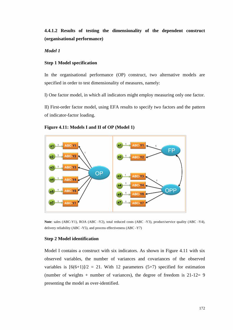
172

4.4.1.2 Results of testing the dimensionality of the dependent construct

(organisational performance)

Model 1


In the organisational performance (OP) construct, two alternative models are

specified in order to test dimensionality of measures, namely:

I) One factor model, in which all indicators might employ measuring only one factor.

II) First-order factor model, using EFA results to specify two factors and the pattern


Figure 4.11: Models I and II of OP (Model 1)

Note: sales (ABC-Y1), ROA (ABC -Y2), total reduced costs (ABC -Y3), product/service quality (ABC -Y4),

delivery reliability (ABC -Y5), and process effectiveness (ABC -Y7)


Model I contains a construct with six indicators. As shown in Figure 4.11 with six

observed variables, the number of variances and covariances of the observed


(number of weights + number of variances), the degree of freedom is 21-12= 9

presenting the model as over-identified.

173

Model II consists of two constructs, as shown in Figure 4.11 with six observed

variables, [6(6+1)]/2 = 21. With 13 parameters (4+1+8) specified for estimation

(number of weights + number of covariance + number of variances), the degree of

freedom is 21-13= 8, presenting the model as over-identified.


Model I yielded a χ2 value of 39.913, with 9 degrees of freedom and a probability of

0.000 (p < 0.05), thereby indicating that the fit of the data to the hypothesised model

is not entirely sufficient (Byrne, 2010). On the other hand, Model II reports a χ2

value of 14.136 and with a probability of 0.078 (p > 0.05), thereby indicating that the

fit of the data to the hypothesised model is entirely sufficient (Byrne, 2010). The

output of goodness-of-fit (GOF) indices of each Model is presented in Table 4.54. It

provides evidence that the Model II GOF is better than the same GOF in Model I.

GOF measures indicate the Model II GOF fits the data well: GFI=0.976,

RMSEA=0.064, RMR=0.040, NFI=0.965, CFI=0.984, TLI=0.971, AGFI=0.937,

chi-square/df=1.767.

Table 4.54: Model fit summary of OP (Models I and II)


Chi-square 39.913 14.136

P-value 0.000 0.078





1996) 0.134 0.064






(AGFI)

Above 0.85 (Hair et al., 2006)

0.843 0.937



coefficient from each construct to the observed variables is significant and the

standardised regression weights (factor loadings) of more than the value of 0.50

174

support the validity and reliability of the variables. All variances show nonzero

(p<0.05); no negative variance and no standardised parameter estimate is greater

than the value of 1. With statistical evidence, the organisational performance

construct can be considered in this study as a multidimensional construct.

Figure 4.12: Model II: First-order factor model of OP (Model 1)

Model 2


In Model 2, two alternative models are specified in order to test dimensionality of

measures, the same as Model 1, as shown in Figure 4.13.


Note: sales (ISO-Y1), ROA (ISO-Y2), total costs (ISO-Y3), product/service quality (ISO-Y4), delivery

reliability (ISO-Y5), and process effectiveness (ISO-Y7)

175


It is noted that Models 1 and 2 have the same indicators in measuring the same

constructs. Therefore, both Models I and II of Model 2 have the same numbers of the

degree of freedom as Model 1, which present as an over-identified model.


The data for the model were entered into the AMOS program using ML estimation.

Model I yielded a χ2 value of 51.208, with 9 degrees of freedom and a probability of

0.000 (p < 0.05), thereby indicating that the fit of the data to the hypothesised model

is also not entirely sufficient (Byrne, 2010). Model II reports a χ2 value of 15.486

with a probability of 0.05 (≤ 0.05), thereby indicating that the fit of the data to the

hypothesised model is also not entirely sufficient (Byrne, 2010). However, the

output of goodness-of-fit (GOF) indices (see Table 4.55) provides evidence that the

Model II GOF is better than the same GOF in Model I. Overall the GOF measures

indicate that the Model II GOF fits the data at an acceptable level: GFI=0.975,

RMSEA=0.070, RMR=0.036, NFI=0.935, CFI=0.966, TLI=0.937, AGFI=0.935,

chi-square/df=1.936.

Table 4.55: Model fit summary of OP (Models I and II)


Chi-square 51.208 15.486

P-value 0.000 0.050




Below 0.08 (MacCallum et al., 1996) 0.157 0.070






(AGFI)

Above 0.85 (Hair et al., 2006) 0.817 0.935

Chi-square/df Below 5.00 (Wheaton et al., 1977) 5.690 1.936

176

Considering the individual parameters of the model (see Figure 4.14), the path

coefficients are significant and the standardised regression weights more than the

value of 0.50 which supports the validity and reliability of the variables. All

variances show nonzero (p<0.05). There is no negative variance and no standardised

parameter estimate greater than 1. With statistical evidence, the organisational

performance construct can be considered in this study as a multidimensional

construct.


Model 3


In the organisational performance (OP) construct, two alternative models (I and II)

are specified in order to test dimensionality of measures, as shown in Figure 4.15.

177


Note: sales (ISO-Y1), ROA (ISO-Y2), total costs (ISO-Y3), product/ service quality (ISO-Y4), delivery



It is noted that all four models have the same indicators, which are explained by the

same constructs. Therefore, both Model I and II have the same number of the

degrees of freedom, which presents an over-identified model.



of 0.000 (p<0.05), thereby indicating that the fit of the data to the hypothesised

model is not entirely sufficient (Byrne, 2010). Similarly, Model II reports a χ2 value

of 50.400 with a probability of 0.000 (p<0.05). However, the limitations of χ2

(Byrne, 2010) mean it needs to consider goodness-of-fit (GOF) indices. The GOF

indices are presented in Table 4.56. It provides evidence that the Model II GOF is

better than the same GOF in I. GOF measures indicate that the Model II GOF fits the

data at an acceptable level (except RMSEA and Chi-square/df): GFI=0.962,

RMR=0.037, NFI=0.957, CFI=0.963, TLI=0.931, AGFI=0.901. Regarding the

values of RMSEA and chi-square/df not being satisfactory, further modification was

required to improve the key model fit statistics.

178

Table 4.56: Model Fit Summary of OP (Models I, II and III)

Measures Recommended I II III

Chi-square 104.390 50.400 26.835

P-value 0.000 0.000 0.000

Goodness-of fit statistic (GFI) Above 0.90 (Hair et al., 2010) 0.924 0.962 0.979




1996) 0.161 0.114 0.083

The root mean square residual

(RMR)

Below 0.08 (Hooper et al., 2008) 0.080 0.037 0.030

Normed fit index (NFI) Above 0.90 (Hooper et al., 2008) 0.911 0.957 0.977

Comparative fit index (CFI) Above 0.90 (Bentler, 1992) 0.918 0.963 0.983

Tucker-Lewis index (TLI) Above 0.90 (Hair et al., 2010) 0.863 0.931 0.963

The adjusted goodness-of-fit

statistic (AGFI)

Above 0.85 (Hair et al., 2006) 0.822 0.901 0.937

Chi-square /df Below 5.00 (Wheaton et al., 1977) 11.599 6.300 3.834

Considering the modification indices, this study decided to add an additional

parameter by selecting the highest value of the modification index, which would

reduce the χ2 value. Within indicators in the same construct, the covariance between

measurement errors of indicators 5 and 7 is suggested (Kline, 2013). Consequently,

the χ2 value has decreased from 50.4 to 26.835 (a probability of 0.00) indicating the

fit of the data to the hypothesised model is not entirely sufficient. However, all other

GOF indices are satisfactory (see Model III).

In Figure 4.16, the path coefficients are significant and the standardised regression

weights more than the value of 0.50 which supports the validity and reliability of the

variables. All variances show nonzero (p<0.05). There is no negative variance and

no standardised parameter estimate greater than 1. With statistical evidence, the

organisational performance construct can be considered in this study as a

multidimensional construct.

179

Figure 4.16: Model III: First-order factor model of OP (Model 3)

Model 4


In the organisational performance construct, two alternative models (I and II) are

specified in order to test the dimensionality of measures, as shown in Figure 4.17.


Note: sales (ISO-Y1), ROA (ISO-Y2), total costs (ISO-Y3), product/service quality (ISO-Y4), delivery



It is noted that all four models have the same indicators, which are explained by the

same constructs. Then, both Models I and II of Model 4 have the same number of the

degree of freedom as Models 1, 2, and 3, which presents the model as over-

identified.

180


The data for the model are entered into the AMOS program using ML estimation.



model is not entirely sufficient (Byrne, 2010). Model II reports a χ2 value of 34.467

with a probability of 0.000 (p < 0.05). However, the limitations of χ2 (Byrne, 2010)

mean that developing goodness-of-fits indices takes a more practical approach to the

evaluation process. The output of the goodness-of-fit (GOF) indices (Table 4.57)

provides evidence that the Model II GOF is better than the same GOF in Model I.

GOF measures indicate that the Model II GOF fits the data at an acceptable level:

GFI=0.981, RMSEA=0.074, RMR=0.028, NFI=0.974, CFI=0.98, TLI=0.962,

AGFI=0.950, chi-square/df=4.308

Table 4.57: Model Fit Summary of OP (Models I and II)


Chi-square 123.336 34.467

P-value 0.000 0.000





1996) 0.146 0.074








Considering the individual parameters of the model (see Figure 4.18), the path

coefficients are significant and the standardised regression weights of more than the

value of 0.50 support the validity and reliability of the variables. All variances show

nonzero (p<0.05) with no negative variance and no standardised parameter estimate

greater than the value of 1. With statistical evidence, the organisational performance

can be considered in this study as a multidimensional construct.

181


The statistical results of CFA support EFA and Cronbach’s alpha results and indicate

both independent and dependent constructs are multidimensional. The next step is to

evaluate the measurement model by testing the validity and reliability.

182

4.4.2 Results of testing the validity and reliability

4.4.2.1 Results of testing the validity and reliability of the independent construct

(the extent of ABC use and the extent of ISO 9000 implementation)

Model 1

As shown in Table 4.58, none of the factor loadings (FL) of the eight observed

variables is less than 0.50 (range from 0.752-0.897), as Hair et al. (2010) suggested.

Thus, it can be concluded that all observed variables converge on each latent

construct. Additionally, in CA, CS and CE constructs, the average variance extracted

(AVE) values show 0.78, 0.78 and 0.79 respectively, which exceed the value of 0.50

and which represents a good overall amount of variance in the observed variables

accounting for the three constructs (Hair et al., 2010). The construct reliability (CR)

values of CA, CS and CE constructs are 0.78, 0.81 and 0.71, each exceeding 0.60,

which provides evidence that indicators measuring each construct have an overall

good reliability (Diamantopoulos & Siguaw, 2000).

Table 4.58: Selected AMOS output relating to independent construct (Model 1)

Construct U.Est FL SE CR Er E.Est SE CR

Cost Analysis (CA)

Product costing 1 0.757 e1 0.351 0.073 4.789

Cost management 1.192 0.811 0.181 6.585 e2 0.347 0.097 3.557

Cost Strategy (CS)

Pricing decisions 1 0.897 e3 0.259 0.055 4.700

Product mix decisions 0.779 0.681 0.075 10.435 e4 0.746 0.086 8.679

Determine customer profitability 0.871 0.763 0.071 12.212 e5 0.58 0.073 7.961

Outsourcing decisions 0.979 0.780 0.078 12.594 e8 0.657 0.085 7.728

Cost evaluation (CE)

Budgeting 1 0.752 e6 0.391 0.115 3.402

Performance measurement 1.03 0.832 0.144 7.149 e7 0.636 0.121 5.275

Note: U.Est: unstandardised regression estimates; FL: factor loading; SE: standard error; CR: critical

ratio; Er: Error; E.Est: error variance estimates

In discriminant validity, this study compares the average variance-extracted (AVE)

value and the square of correlation estimates between a pair of constructs (CA, CS,

and CE). The first pair, CA and CE, have average variance extracted (AVE) values

183

= 0.78, exceeding the square of correlation estimates = 0.24. The second pair, CA

and CS, have average variance extracted (AVE) values = 0.79, also exceeding the

square of correlation estimates = 0.28. Similarly, the last pair, CS and CE, have

average variance extracted (AVE) values = 0.79, exceeding the square of correlation

estimates = 0.26. These provide evidence to support discriminant validity.

Model 2




construct. Additionally, in MP and CP constructs, the average variance extracted

(AVE) values show 0.68 and 0.69 respectively which exceed the value of 0.50,

which represents a good overall amount of variance in the observed variables

accounting for the three constructs (Hair et al., 2010). The construct reliability (CR)

values of MP and CP constructs are 0.78, and 0.71, exceeding 0.60 and providing

evidence that indicators measuring each construct have an overall good reliability

(Diamantopoulos & Siguaw, 2000).

Table 4.59: Selected AMOS output relating to the independent construct

(Model 2)


Management principle (MP)

customer focus 1 .733 e1 .469 .063 7.458

process approach .980 .627 .126 7.794 e4 .807 .095 8.478

system approach to management .856 .652 .106 8.087 e5 .539 .065 8.295

continual improvement 1.087 .710 .124 8.743 e6 .631 .082 7.740

factual approach to decision making 1.136 .670 .137 8.295 e7 .862 .106 8.145

Cooperation principle (CP)

Leadership 1 .574 e2 .635 .075 8.501

involvement of people 1.388 .705 6.724 .206 e3 .607 .086 7.086

supplier relationships 1.762 .802 6.978 .252 e8 .539 .106 5.102


ratio; Er: error; E.Est: error variance estimates

184


value and the square of correlation estimates between a pair of constructs (MP and

CP). As a result, average variance extracted (AVE) values = 0.69, exceeding the

square of correlation estimates = 0.52, which provide evidence of discriminant

validity.

Model 3


variables is less than 0.50 (range from 0.571-0.930) as Hair et al. (2010) suggested.

Therefore, it can be concluded that all observed variables converge on each latent


(AVE) values show 0.71 and 0.77 respectively which exceed the value of 0.50,

representing a good overall amount of variance in the observed variables accounting

for the three constructs (Hair et al., 2010). The construct reliability (CR) values of

MP and CP constructs are 0.80 and 0.78, exceeding 0.60, which provides evidence

that indicators that measure each construct have an overall good reliability



(Model 3)



customer focus 1 .571 e1 .905 .066 13.691

process approach 1.528 .913 .120 12.690 e4 .205 .029 7.048

system approach to management .949 .574 .099 9.545 e5 .804 .059 13.683


factual approach to decision making 1.102 .587 .113 9.711 e7 1.010 .074 13.637


Leadership 1 .597 e2 .766 .058 13.220

involvement of people 1.656 .930 .133 12.433 e3 .182 .052 3.521

supplier relationships 1.497 .784 .123 12.148 e8 .594 .059 10.062



185





validity.

Model 4





(AVE) values show 0.71 and 0.75 respectively, exceeding the value of 0.50, which

represents a good overall amount of variance in the observed variables accounting

for the three constructs (Hair et al., 2010). The construct reliability (CR) values of

MP and CP constructs are 0.80 and 0.75, exceeding 0.60, which provides evidence

that indicators that measure each construct have an overall good reliability



(Model 4)



customer focus 1 .668 e1 .758 .050 15.202

process approach 1.247 .819 .075 16.735 e4 .467 .039 11.837

system approach to management 0.898 .645 .065 13.808 e5 .693 .045 15.458


factual approach to decision making .981 .615 .074 13.237 e7 .970 .062 15.738


Leadership 1 .608 e2 .712 .046 15.348

involvement of people 1.557 .878 .108 14.358 e3 .303 .047 6.499

supplier relationships 1.441 .749 .104 13.901 e8 .680 .055 12.363



186





validity.

4.4.2.2 Results of testing the validity and reliability of the dependent construct

(organisational performance)

Model 1

As shown in Table 4.62, none of the factor loadings (FL) of the six observed



construct. Additionally, in FP and OPP constructs, the average variance extracted

(AVE) values show 0.81 and 0.66 respectively, exceeding the value of 0.50, which


for the two constructs (Hair et al., 2010). The construct reliability (CR) values of FP

and OPP constructs are 0.81 and 0.71, exceeding 0.60, which provides evidence that

indicators that measure each construct have an overall good reliability


Table 4.62: Selected AMOS output relating to dependent construct (Model 1)



Sales 1 .891 e1 .222 .077 2.899

ROA 0.737 .728 .081 9.058 e2 .410 .058 7.087


Total costs 1 .823 e3 .446 .079 5.625

P/S quality 0.914 .751 .092 9.971 e4 .603 .084 7.146

Delivery Reliability 0.538 .498 .083 6.510 e5 .820 .090 9.122

Process Effectiveness 0.687 .567 .092 7.474 e7 .930 .105 8.843

Note: P/S: product/service; U.Est: unstandardised regression estimates; FL: factor loading; SE:

standard error; CR: critical ratio; Er: error; E.Est: error variance estimates

187





validity.

Model 2

As shown in Table 4.63, none of the factor loadings of the six observed variables is

less than 0.50 (range from 0.571-0.825), as Hair et al. (2010) suggested. Thus, it can

be concluded that all observed variables converge on each latent construct.

Additionally, in the FP and OPP constructs, the average variance extracted (AVE)

values show 0.72 and 0.62 respectively, exceeding the value of 0.50, which


for the two constructs (Hair et al., 2010). The construct reliability (CR) values of the

FP and OPP constructs are 0.72 and 0.73, exceeding 0.60, which provide evidence

that indicators that measure these two constructs have an overall good reliability


Table 4.63: Selected AMOS output relating to the dependent construct (Model

2)



Sales 1 .825 e1 .281 .132 2.131

ROA .742 .624 .170 4.355 e2 .519 .089 5.847


Total costs 1 .593 e3 .550 .070 7.854

P/S quality 1.044 .571 .185 5.633 e4 .673 .083 8.068


Process Effectiveness 1.106 .595 .191 5.784 e7 .664 .085 7.828





188



validity.

Model 3

As shown in Table 4.64, none of the factor loadings (FL) of the six observed



construct. Additionally, the average variance extracted (AVE) values of the FP and

OPP constructs are 0.62 and 0.81, exceeding the value of 0.5, which represents a

good overall amount of variance in the observed variables accounting for the two

constructs (Hair et al., 2010). In addition, the construct reliability (CR) value of the

OPP construct is 0.85, above 0.60, which provides evidence that indicators that

measure the OPP construct have an overall good reliability (Diamantopoulos &

Siguaw, 2000). In the FP construct, CR is 0.59, which is close to 0.60, the minimum

acceptable level. Therefore, it can be concluded than the two indicators that measure

FP have an overall acceptable level.


3)



Sales 1 .528 e1 .673 .101 6.663

ROA 1.376 .706 .477 2.886 e2 .496 .173 2.873


Total costs 1 .886 e3 .312 .035 8.895

P/S quality 1.023 .875 .043 23.652 e4 .366 .039 9.501


Process Effectiveness .628 .588 .050 12.641 e7 .855 .064 13.263





189


square of correlation estimates = 0.08, which provides evidence of discriminant

validity.

Model 4

As shown in Table 4.65, none of the factor loadings of the six observed variables is

less than 0.50 (range from 0.557-0.882), as Hair et al. (2010) suggested. Therefore, it

can be concluded that all observed variables converge on each latent construct.

Additionally, the average variance extracted (AVE) values of the FP and OPP

constructs are 0.64 and 0.78, exceeding the value of 0.5, which represents a good

overall amount of variance in the observed variables accounting for two constructs

(Hair et al., 2010). The construct reliability (CR) values of the FP and OPP

constructs are 0.62 and 0.83, exceeding 0.60, which provides evidence that indicators

measuring these two constructs have an overall good reliability (Diamantopoulos &

Siguaw, 2000).


4)



Sales 1 .577 e1 .620 .077 8.071

ROA 1.218 .696 .271 4.490 e2 .491 .105 4.683


Total costs 1 .791 e3 .473 .036 13.289

P/S quality 1.089 .812 .052 20.870 e4 .485 .039 12.582


Process Effectiveness .784 .631 .050 15.587 e7 .733 .046 15.812







validity

190

Testing common method variance (CMV) of the independent construct and

dependent construct

In the independent construct of the four models, all selected variables are entered

into the SPSS program for EFA. In addition, the number of factors extracted is

restricted to 1 without the rotation method. The Harman’s single factor results

include only one factor that emerged to explain 41, 40, 43, and 43 percent of the

variance in Models 1, 2, 3, and 4 respectively, which implies CMV is not a major

concern. Similarly, with the dependent construct of the four models, according to the

Harman’s single factor results, only one factor emerged to explain 45, 31, 46, and 42

percent of the variance in Models 1, 2, 3, and 4, respectively, which implies CMV is

not a major concern.

In addition, in order to support the Harman’s single factor results above, each model

compares the model fit between two models (Model I and II). The first model (I) and

second model (II) are presented in Section 4.4.1. It shows the second model (II) of

all Models (1-4) fits the data better than the first model (I) of all Models (1-4),

indicating that CMV is not responsible for the relationship among the variables.

191

4.5 Results of structural equation modelling (SEM)

4.5.1 Results of Model 1: The extent of ABC use and organisational

performance model (191 cases of organisations that adopted both ABC and ISO

9000)

This study aims to investigate the causal relationship between the extent of ABC use

and organisational performance. From the EFA and CFA results, the extent of ABC

use can be explained as a multidimensional construct including three factors: cost

analysis, cost strategy and cost evaluation. Likewise organisational performance can

be divided into two constructs (operational performance and financial performance)

as a multidimensional construct. The three-factor CFA model of independent

structure is presented on the left in Figure 4.19, whereas the two dependent

constructs are on the right. It is noted that all indicators, error terms associated with

indicators, and all double-headed arrows indicating correlations among the

independent and dependent factors have been excluded from the figure, though they

are contained in the model before the program will operate the analysis, presented

later in this section.

Figure 4.19: SEM of Model 1

The steps of structural equation modelling (SEM)

The model has been tested with SEM by the following five steps: 1) model

specification, 2) identification, 3) estimation, 4) evaluation, and 5) modification.

192

Model specification

Model specification was first developed as illustrated earlier in Chapter 2, based on

previous studies and relevant theories (see section 2.6). Regarding the EFA and CFA

results, the extent of ABC use construct is explained using the three-factor CFA

model as a multidimensional construct (see sections 4.3.1 and 4.4.1.1). Similarly,

organisational performance is considered a multidimensional construct (two-factor

CFA model) with regard to EFA and CFA results (see sections 4.3.2 and 4.4.1.2).

As shown in Figure 4.20, Model 1 consists of five constructs. Each construct has

been tested for validity of the indicator variables (see section 4.4.2). These five

constructs are measured by using indicators (see section 3.2.2) which constitute the

measurement model section. Each indicator has its related error term.

Figure 4.20: The relationship between the extent of ABC use and OP (Model 1)

Model identification

The next step of SEM is model identification. This is needed to compute the degrees

of freedom. The degrees of freedom are equal to the number of elements in a

correlation matrix minus the number of parameters in the model to be estimated. As

shown in Figure 4.20 with eight observed variables (the extent of ABC use

193

construct), four observed variables (operational performance construct) and two

observed variables (financial performance construct), the number of observed

(measured) variables = 8+4+2= 14. Then, the number of elements in a correlation

matrix = [14(14+1)]/2 = 105 follows before the number of parameters in the model is

estimated = 38 (16 regression weights, 13 covariances and 19 variances). Thereby

the degree of freedom is 105-38 = 67, indicating it is over-identified. It means that

there is more than one way to estimate the parameters.

Figure 4.21: Selected AMOS output for Model 1: Model summary

Table 4.66: Parameter summary of Model 1

Weights Covariances Variances Means Intercepts Total

Fixed 21 0 0 0 0 21

Labelled 0 0 0 0 0 0

Unlabelled 16 3 19 0 0 38

Total 37 3 19 0 0 59

Before proceeding to model estimation, the requirements of SEM should be

considered. Sample size, multicollinearity, and missing data have been discussed

earlier (see section 4.1) and have met the conditions for SEM. Multivariate normality

is discussed next.


The normality of each variable has been tested earlier in the chapter, indicating that

data comes from a normal distribution (see section 4.1.3.3). The AMOS output also

194

confirms the normality with CR of skew and kurtosis less than 3 (See Table 4.67). In

particular multivariate normality, Byrne (2010) suggested that in practice, values

more than 5.00 are suggestive of data that are a non-normal distribution. In this

model, the z-statistic of 4.684 (less than 5.00) is indicative of normality in the

sample. In addition, the Mardia’s coefficient (14.348) is less than the value obtained

from the formula p(p+2) = 14(14+2) supporting the fact that the data is deemed as

multivariate normal (Khine, 2013). Therefore, it can confirm that there is a

multivariate normal distribution which met the conditions of the Maximum

Likelihood (ML) estimation method in further analysis.

Table 4.67: Output of assessment of normality

Variable min max skew CR kurtosis CR

ABC_X6 2.000 7.000 -.040 -.226 -.678 -1.914

ABC_X9 2.000 7.000 -.209 -1.181 -.297 -.838

ABC_X3 2.000 7.000 -.294 -1.660 -.274 -.772

ABC_X4 2.000 7.000 .142 .804 -.371 -1.046

ABC_X5 2.000 7.000 -.296 -1.673 -.239 -.674

ABC_X8 2.000 7.000 -.153 -.861 -.634 -1.789

ABC_X2 3.000 7.000 -.188 -1.062 -.461 -1.301

ABC_X1 2.000 7.000 -.412 -2.327 .243 .685

ABC_Y1 3.000 7.000 -.288 -1.625 -.669 -1.887

ABC_Y2 3.000 7.000 -.321 -1.812 -.301 -.850

ABC_Y7 2.000 7.000 -.177 -.999 -.895 -2.526

ABC_Y5 2.000 7.000 -.084 -.476 -.368 -1.039

ABC_Y4 2.000 7.000 .057 .324 -.581 -1.640

ABC_Y3 2.000 7.000 .144 .814 -.838 -2.364

Multivariate

14.348 4.684

Model estimation

In this step, the data for the model are entered into Amos program by using ML

estimation technique as discussed in Chapter 3 (See Section 3.3.4.1.3).

Model evaluation

As depicted in Figure 4.21, the model yielded a χ2 value of 99.772, with 67 degrees

of freedom and a probability of 0.006 (p < 0.05), thereby indicating that the fit of the

data to the hypothesised model is not entirely sufficient (Byrne, 2010). However, as

mentioned earlier given the limitations of χ2 (see Section 3.3.4.1.4) developing other

195

goodness-of-fit (GOF) indices takes a more practical approach to the evaluation

process.

The outputs of GOF indices are presented in Table 4.68. GFI = 0.932 which is more

than 0.90 and considered as an acceptable value (Hair et al., 2010). Thus, it can be

concluded that the hypothesised model fits the sample fairly well. RMSEA value is

0.051 which is below 0.08 are indicated as reasonable errors of approximation in the

population (MacCallum et al., 1996). RMR shows 0.059 which below 0.08, are

indicating an acceptable level of fit (Hooper et al., 2008).

In incremental fit indices, a NFI value of 0.916 exceeds 0.90 (Hooper et al., 2008).

The CFI (0.970) indicates that the model fits the data well in the terms that the

hypothesised model adequately explains the sample data (Bentler, 1992; Byrne,

2010). TLI yields values of 0.960 which fits the data well (Hair et al., 2010) . The

next set of fit statistics is model parsimony, the AGFI value of 0.893 is adequate as it

is more than 0.85 as (Hair et al., 2006). Chi-square shows 1.489 (below 5) being

indicative of a good fit (Wheaton et al., 1977).

Table 4.68: Model fit summary of Model 1

Measures Recommended Output

Goodness-of fit statistic (GFI) Above 0.90 (Hair et al., 2010) 0.932

The root mean square error of approximation

(RMSEA)


1996)

0.051

The root mean square residual (RMR) Below 0.08 (Hooper et al., 2008) 0.059

Normed Fit Index (NFI) Above 0.90 (Hooper et al., 2008) 0.916

Comparative Fit Index (CFI) Above 0.90 (Bentler, 1992) 0.970

Tucker-Lewis Index (TLI) Above 0.90 (Hair et al., 2010) 0.960

The adjusted goodness-of-fit statistic (AGFI) Above 0.85 (Hair et al., 2006) 0.893

Chi-square /df Below 5.00 (Wheaton et al., 1977) 1.489

Both the unstandardised and standardised regression weights are shown in Table

4.69. “Standardised parameter estimates are transformations of unstandardised

estimates that remove scaling and can be used for informal comparisons of

parameters throughout the model” (Suhr, 2010: 2). This study interprets the outputs

of standardised estimates because it is typically used for interpretation (Hox &

196

Bechger, 2001). However, it considers unstandardised parameters for variance and

covariance because the SEM output provides only unstandardised variances and

covariances.

In reviewing the structural parameter estimates for Model 1, it is highlighted that

three parameters that are not significant (P>0.05), these parameters represent the

regression paths from cost analysis to financial performance (P =0.153), from cost

strategy to financial performance (P =0.837), and cost evaluation to financial

performance (P =0.822). Other regression paths and factor loadings are significant

and no standardised parameter estimate greater than the value of 1. In addition, all

variances and covariances show nonzero (p<0.05) and no negative variances.

Squared multiple correlation (R2) for the endogenous variables are as follows:

operational performance (0.38) and financial performance (0.63). With the given

information (Table 4.68 and 4.69), the Model 1 fits the data well due to the

goodness-of-fits (GOF) indices and individual parameters met the requirements.

Table 4.69: Selected AMOS Output (Model 1)

Unstd. Std. S.E. C.R. P

Regression weights

OPP <--- CA .353 .248 .151 2.344 .019

OPP <--- CS .263 .277 .094 2.802 .005

OPP <--- CE .245 .226 .117 2.102 .036

FP <--- CA .186 .137 .130 1.428 .153

FP <--- CS .017 .019 .081 .206 .837

FP <--- CE -.022 -.022 .100 -.225 .822

FP <--- OPP .681 .716 .101 6.752 ***

ABC_Y3 <--- OPP 1.000 .824

ABC_Y4 <--- OPP .911 .750 .089 10.278 ***

ABC_Y5 <--- OPP .541 .502 .081 6.643 ***

ABC_Y2 <--- FP .739 .729 .079 9.387 ***

ABC_Y1 <--- FP 1.000 .889

ABC_X8 <--- CS .982 .776 .079 12.484 ***

ABC_X5 <--- CS .883 .767 .072 12.286 ***

ABC_X4 <--- CS .795 .690 .075 10.603 ***

ABC_X3 <--- CS 1.000 .890

ABC_X9 <--- CE 1.072 .849 .144 7.465 ***

ABC_X6 <--- CE 1.000 .737

ABC_X1 <--- CA 1.000 .750

ABC_X2 <--- CA 1.212 .818 .165 7.326 ***

ABC_Y7 <--- OPP .684 .566 .090 7.569 ***

Variances

CS 1.047 .141 7.439 ***

197


CE .797 .162 4.914 ***

CA .463 .093 4.949 ***

Var1 .581 .104 5.594 ***

Var2 .317 .081 3.932 ***

e12 .443 .075 5.873 ***

e13 .607 .082 7.397 ***

e14 .817 .089 9.158 ***

e15 .933 .105 8.919 ***

e11 .409 .056 7.263 ***

e10 .224 .072 3.094 .002

e1 .359 .066 5.444 ***

e2 .336 .087 3.841 ***

e8 .666 .085 7.795 ***

e5 .570 .072 7.912 ***

e4 .728 .084 8.617 ***

e3 .275 .055 5.018 ***

e9 .355 .111 3.189 .001

e6 .669 .114 5.848 ***

Covariances

CS <--> CA .343 .073 4.706 ***

CE <--> CA .310 .072 4.305 ***

CS <--> CE .486 .099 4.926 ***

Note: Unstd: unstandardised regression estimates, Std: standardised regression estimates (factor loadings), SE: standard error,

CR: Critical Ratio, P: probability, product costing (ABC-X1), cost management (ABC-X2), pricing decisions (ABC-X3),

product mix decisions (ABC-X4), determine customer profitability (ABC-X5), budgeting (ABC-X6), as an off-line analytic

tool (ABC-X7), outsourcing decisions (ABC-X8), performance measurement (ABC-X9), sales (ABC-Y1), ROA (ABC -Y2),

total reduced costs (ABC -Y3), product/service quality (ABC -Y4), delivery reliability (ABC -Y5), process effectiveness (ABC

-Y7), CA: cost analysis, CS: cost strategy, CE: cost evaluation OPP: operational performance, FP: financial performance

Model modification and validation

As discussed in Section 3.3.4.1.5, Table 4.70 shows the values of EVCI, BIC and

AIC. It can be seen that the default model (hypothesised model) has the smallest

values of these three indexes which it is the most stable in the population

(Schumacker & Lomax, 2010). In addition, it can be seen that the results from ML

(See Table 4.69) and from bootstrap (See Table 4.71) are similar. The values of bias

provide evidence that the difference between ML results and bootstrap is very small

which is indicative of being stable estimates of the whole population.

198

Table 4.70: EVCI, BIC and AIC values (Model 1)

Models ECVI BIC AIC

Default model .925 299.358 175.772

Saturated model 1.105 551.489 210.000

Independence model 6.427 1266.754 1221.222

Table 4.71: Bootstrap results (Model 1)

Parameter Estimate SE Bias P

OPP <--- CA .248 .133 .002 .042

OPP <--- CS .277 .109 -.003 .015

OPP <--- CE .226 .117 .001 .047

FP <--- CA .137 .094 .001 .130

FP <--- CS .019 .098 -.002 .858

FP <--- CE -.022 .113 .002 .867

FP <--- OPP .716 .103 .004 .002

ABC_Y3 <--- OPP .824 .039 .001 .002

ABC_Y4 <--- OPP .750 .049 .002 .002

ABC_Y5 <--- OPP .502 .069 .000 .002

ABC_Y2 <--- FP .729 .064 .005 .002

ABC_Y1 <--- FP .889 .044 .000 .002

ABC_X8 <--- CS .776 .037 .000 .002

ABC_X5 <--- CS .767 .035 -.001 .002

ABC_X4 <--- CS .690 .054 .001 .002

ABC_X3 <--- CS .890 .036 -.001 .002

ABC_X9 <--- CE .849 .068 .000 .002

ABC_X6 <--- CE .737 .058 -.001 .002

ABC_X1 <--- CA .750 .058 -.001 .002

ABC_X2 <--- CA .818 .056 .001 .002

ABC_Y7 <--- OPP .566 .060 -.002 .002

Hypothesis testing (Model 1)

It is hypothesised that the extent of ABC use positively impacts on financial and

operational performance as indicated in H1 and H2 respectively. However, as results

of EFA and CFA found the extent of ABC use and organisational performance are

multidimensional, the hypotheses have been modified as follows:

Hypothesis 1a: Cost analysis (CA) has a positive impact on FP

Hypothesis 1b: Cost strategy (CS) has a positive impact on FP

Hypothesis 1c: Cost evaluation (CE) has a positive impact on FP

199

Hypothesis 2a: Cost analysis (CA) has a positive impact on OPP

Hypothesis 2b: Cost strategy (CS) has a positive impact on OPP

Hypothesis 2c: Cost evaluation (CE) has a positive impact on OPP

Path coefficients and related p-value are used to examine the impact of CA, CS, and

CE on OPP and FP. As presented in Table 4.72, the results reveal only three out of

six constructs have a direct positive direct impact on FP and OPP. The path

coefficients between CA, CS, CE and OPP are 0.25 (P≤ 0.05), 0.28 (P≤ 0.01), and

0.23 (P≤ 0.05). These acceptable significant path coefficients provide evidence to

reject the Null hypothesis and indicate that the extent of ABC use has a positive

direct impact on operational performance.

On the other hand, the path coefficients between CA, CS, CE and FP are not

significant. These indicate that there is no evidence to indicate the positive impact of

the extent of ABC use on financial performance.

It is also hypothesised that the extent of ABC use indirectly impacts on financial

performance (FP) through operational performance (OPP) as indicated in H3.

However, as discussed above in the results of EFA and CFA the hypothesis has been

modified as follows:

Hypothesis 3a: Cost analysis (CA) has an indirect impact on FP through OPP

Hypothesis 3b: Cost strategy (CS) has an indirect impact on FP through OPP

Hypothesis 3c: Cost evaluation (CE) has an indirect impact on FP through OPP

As presented in Table 4.73, the results report that CA, CS, and CE have impact on

FP though OPP. Relating to CA and FP, this indirect impact increases the

standardised coefficient from 0.14 to 0.32. Similarly, in CS and FP, this indirect

impact increases the standardised coefficient from 0.02 to 0.22. Additionally, as CE

has a very small negative direct impact on FP, this indirect impact increases the

standardised coefficient from -0.02 to 0.14. With this evidence, this study rejects the

Null hypothesis and indicates that the extent of ABC use has an indirect impact on

financial performance through operational performance.

Table 4.72: Hypothesised relationships (Model 1)

Hypothesised Relationships Standardised

estimate

S.E.

C.R.

P-value Null

hypothesis

interpretation

H1 FP <--- the extent of ABC use

FP <--- CA

FP <--- CS

FP <--- CE

0.14

0.02

-0.02

0.097

0.060

0.074

1.420

0.206

-0.225

0.156

0.837

0.822

Fail to Rej.

Fail to Rej.

Fail to Rej.

The positive effect of CA on FP is not found at p-value 0.05

The positive effect of CS on FP is not found at p-value 0.05

The positive effect of CE on FP is not found at p-value 0.05

H2 OPP <--- the extent of ABC use

OPP <--- CA

OPP <--- CS

OPP <--- CE

0.25

0.28

0.23

0.151

0.094

0.117

2.344

2.802

2.102

0.019*

0.005**

0.036*

Reject

Reject

Reject

CA has a positive direct impact on OPP at p-value 0.05

CS has a positive direct impact on OPP at p-value 0.05

CE has a positive direct impact on OPP at p-value 0.05

Table 4.73: Direct, indirect and total impact (Model 1)

Dependent construct Independent construct Direct impact Indirect impact (H3) Total impact

FP

(R2=0.63)

CA 0.14 0.18* 0.32

CS 0.02 0.20** 0.22

CE -0.02 0.16* 0.14

Note: *** significant at the 0.001, ** significant at the 0.01, *significant at the 0.05

20

0

201


organisational performance (191 cases of organisations that adopted both ABC

and ISO 9000)

This study aims to examine the causal relationship between the extent of ISO 9000

implementation and organisational performance. From the EFA and CFA results, the

extent of ISO 9000 implementation can be explained as a multidimensional construct

including two factors: management principle and cooperation principle. As well as

organisational performance, which can be explained by two constructs (operational

performance and financial performance) as a multidimensional construct. A two-

factor CFA model of independent structure is presented on the left in Figure 4.22

whereas on the right of the figure shows the two dependent constructs.



Model specification

Model specification is first developed as illustrated earlier in Chapter 2 based on

previous studies and relevant theories (see Section 2.6). Regarding with EFA and

CFA results, the extent of ISO 9000 implementation construct is explained by two-

factor CFA model as a multidimensional construct (see Section 4.3.1 and 4.4.1.1).

Similarly, organisational performance is considered as a multidimensional construct

202

(two-factor CFA model) with regard to EFA and CFA results (see Section 4.3.2 and

4.4.1.2).

As shown in Figure 4.23, Model 2 consists of four constructs. Each construct has

been tested for validity of the indicator variables (see Section 4.4.2). These five

constructs are measured by using indicators (see Section 3.2.2) which constitute the


Figure 4.23: The relationship between the extent of ISO 9000 implementation

and OP (Model 2)


The next step of SEM is model identification. As shown in Figure 4.23 with eight

observed variables (the extent of ISO 9000 implementation construct), four observed

variables (operational performance construct) and two observed variables (financial

performance construct), the number of observed (measured) variables = 8+4+2= 14.

Then the number of elements in a correlation matrix = [14(14+1)]/2 = 105. The

number of parameters in the model to be estimated = 34 (15 regression weights, 1

203

covariances and 18 variances), thereby the degrees of freedom is 105-34 = 71

indicating it is over-identified.

Figure 4.24: Selected AMOS Output for Model 2: Model Summary

Table 4.74: Parameter Summary of Model 2


Fixed 20 0 0 0 0 20



Total 35 1 18 0 0 54

This model met the assumptions of SEM namely sample size, multivariate normality,

multicollinearity and missing data (See Section 4.1). Multivariate normality is

discussed next.


Normality of each variable has been tested in the previous chapter indicating the data

come from a normal distribution (See Section 4.1). The AMOS output also confirms

the normality with a CR of skew and kurtosis of less than 3 (See Table 4.75).

Concerning multivariate normality in particular, Byrne (2010) suggested that, in

practice, values above 5.00 are suggestive of data that are non-normally distributed.

In this model, the z-statistic of 4.687 (less than 5.00) is indicative of normality in the

sample. In addition, the Mardia’s coefficient (14.357) is less than the value obtained

from the formula p(p+2) = 14(14+2), supporting the idea that the data are deemed as

204

multivariate normal (Khine, 2013). Therefore, it can be confirmed that this is a

multivariate normal distribution.



ISO_X8 2.000 7.000 -.296 -1.673 -.508 -1.433

ISO_X1 3.000 7.000 -.339 -1.915 -.526 -1.484

ISO_X4 2.000 7.000 -.351 -1.979 -.522 -1.473

ISO_X5 3.000 7.000 -.385 -2.171 -.108 -.305

ISO_X6 2.000 7.000 -.309 -1.743 -.411 -1.159

ISO_X7 2.000 7.000 -.177 -1.001 -.615 -1.734

ISO_X2 2.000 7.000 -.236 -1.330 -.163 -.459

ISO_X3 2.000 7.000 -.378 -2.135 -.379 -1.069

ISO_Y1 3.000 7.000 -.018 -.102 -.585 -1.651

ISO_Y2 3.000 7.000 -.075 -.425 -.173 -.489

ISO_Y7 2.000 7.000 .094 .530 -.287 -.809

ISO_Y5 3.000 7.000 .074 .420 -.376 -1.062

ISO_Y4 3.000 7.000 -.077 -.437 -.701 -1.979

ISO_Y3 2.000 7.000 .000 .000 .275 .776

Multivariate

14.357 4.687

Model estimation

In this step, the data for the model are entered into the Amos program by ML

estimation. The results are reported in the next step.

Model evaluation

As shown in Figure 4.24, it yielded a χ2 value of 130.213, with 71 degrees of

freedom and a probability of less than 0.000 (p < 0.05), thereby indicating that the fit

of the data to the hypothesised model is not entirely sufficient (Byrne, 2010).

However, given the limitations of χ2 (see Section 3.3.4.1.4), developing other

goodness-of-fit (GOF) indices takes a more comprehensive approach to the

evaluation process.

The outputs of GOF indices are presented in Table 4.76. With a GFI = 0.918, which

is more than 0.90 which is considered as an acceptable value (Hair et al., 2010).

Therefore, it can be concluded that the hypothesised model fits the sample fairly

well. RMSEA shows 0.066, which is below 0.08 indicates reasonable errors of

205

approximation in the population (MacCallum et al., 1996). The RMR value of 0.057

is below 0.08, indicating an acceptable level of fit (Hooper et al., 2008).

In incremental fit indices, a NFI value of 0.891 would seem to be an adequate fitting

model as it is relatively close to 0.90 (Hooper et al., 2008). The CFI (0.924)

identified that the model fits the data well in that the hypothesised model adequately

explained the sample data (Bentler, 1992; Byrne, 2010). The TLI yields a value of

0.903, which is more than 0.90, as (Hair et al., 2010) suggested. The next set of fit

statistics is model parsimony. An AGFI value of 0.879 is an adequate fitting model

as it exceeds 0.85, as Hair et al. (2006) indicated. Chi-square/df shows 1.834, which

is below 5 and therefore indicative of good fit (Wheaton et al., 1977).

Table 4.76: Model fit summary (Model 2)




(RMSEA)


1996)

0.066


Normed fit index (NFI) Above 0.90 (Hooper et al., 2008) 0.891

Comparative fit index (CFI) Above 0.90 (Bentler, 1992) 0.924

Tucker-Lewis index (TLI) Above 0.90 (Hair et al., 2010) 0.903


Chi-square/df Below 5.00 (Wheaton et al., 1977) 1.834

Table 4.77, in reviewing the structural parameter estimates for Model 2, highlights

the two parameters that are not significant at a 95% confidence level (P>0.05); these

parameters represent the paths from cooperation principle to operational

performance (P = 0.741), and from cooperation principle to financial performance P

= 0.454). Other regression paths and factor loadings are significant and no

standardised parameter estimate is greater than 1. In addition, all variances and

covariances show nonzero (p<0.05) with no negative variances. Squared multiple

correlation (R2) for the endogenous variables are as follows: operational performance

(0.18) and financial performance (0.42). With the given information (Tables 4.76

and 4.77), Model 2 fits the data well as the goodness-of-fit (GOF) indices and

individual parameters met the requirements.

206



Regression weights

OOP <--- MP .279 .379 .123 2.275 .023

OOP <--- CP .051 .054 .154 .331 .741

FP <--- MP .308 .365 .138 2.238 .025

FP <--- CP .124 .114 .165 .749 .454

FP <--- OOP .352 .307 .129 2.717 .007

ISO_Y3 <--- OOP 1.000 .584

ISO_Y4 <--- OOP 1.066 .574 .190 5.623 ***

ISO_Y5 <--- OOP 1.256 .726 .201 6.254 ***

ISO_Y2 <--- FP 1.179 .787 .199 5.930 ***

ISO_Y1 <--- FP 1.000 .655

ISO_Y7 <--- OOP 1.124 .596 .195 5.756 ***

ISO_X3 <--- CP 1.368 .704 .201 6.795 ***

ISO_X2 <--- CP 1.000 .581

ISO_X7 <--- MP 1.140 .666 .138 8.274 ***

ISO_X6 <--- MP 1.103 .714 .125 8.823 ***

ISO_X5 <--- MP .871 .656 .107 8.166 ***

ISO_X4 <--- MP .997 .631 .127 7.870 ***

ISO_X1 <--- MP 1.000 .726

ISO_X8 <--- CP 1.735 .799 .245 7.080 ***

Variances

MP .533 .099 5.372 ***

CP .319 .081 3.919 ***

Var1 .238 .065 3.666 ***

Var2 .221 .059 3.726 ***

e12 .559 .070 7.970 ***

e13 .669 .083 8.065 ***

e14 .410 .069 5.931 ***

e15 .663 .085 7.849 ***

e11 .324 .086 3.783 ***

e10 .504 .077 6.558 ***

e3 .610 .085 7.163 ***

e2 .628 .074 8.471 ***

e7 .871 .105 8.274 ***

e6 .624 .080 7.814 ***

e5 .534 .064 8.347 ***

e4 .800 .094 8.524 ***

e1 .480 .062 7.679 ***

e8 .546 .104 5.240 ***

Covariances

MP <--> CP .299 .059 5.117 ***


CR: Critical Ratio, P: probability, customer focus (ISO-X1), leadership (ISO-X2), involvement of people (ISO-X3), process

approach (ISO-X4), system approach to management (ISO-X5), continual improvement (ISO-X6), factual approach to

decision-making (ISO-X7) and mutually beneficial supplier relationships (ISO-X8), sales (ISO-Y1), ROA (ISO-Y2), total costs

(ISO-Y3), product/service quality (ISO-Y4), delivery reliability (ISO-Y5), and process effectiveness (ISO-Y7)

207


Table 4.78 shows the values of EVCI, BIC and AIC. It can be seen that the default

model (hypothesised model) has the smallest values of these three indices, being the

most stable in the population (Schumacker & Lomax, 2010). In addition, it can be

seen that the results from ML (See Table 4.77) and from bootstrap (see Table 4.79)

are similar. The values of bias provide evidence that the difference between ML

results and bootstrap is very small, which suggests stability of the estimates of the

whole population.


Models ECVI BIC AIC

Default model 1.043 308.790 198.213

Saturated model 1.105 551.489 210.000




OOP <--- MP .379 .175 .009 .024

OOP <--- CP .054 .162 -.008 .809

FP <--- MP .365 .190 -.007 .042

FP <--- CP .114 .164 -.010 .500

FP <--- OOP .307 .165 .008 .023

ISO_Y3 <--- OOP .584 .074 .005 .002

ISO_Y4 <--- OOP .574 .076 .001 .002

ISO_Y5 <--- OOP .726 .068 -.004 .002

ISO_Y2 <--- FP .787 .128 .003 .002

ISO_Y1 <--- FP .655 .107 .001 .002

ISO_Y7 <--- OOP .596 .074 -.004 .002

ISO_X3 <--- CP .704 .054 .002 .002

ISO_X2 <--- CP .581 .068 .002 .002

ISO_X7 <--- MP .666 .056 .001 .002

ISO_X6 <--- MP .714 .061 -.001 .002

ISO_X5 <--- MP .656 .054 .003 .002

ISO_X4 <--- MP .631 .058 -.005 .002

ISO_X1 <--- MP .726 .052 -.002 .002

ISO_X8 <--- CP .799 .049 -.001 .002

208


It is hypothesised that the extent of ISO 9000 implementation positively impacts on

financial and operational performance, as indicated in H4 and H5, respectively.

However, as the results of the EFA and CFA found the extent of ISO 9000

implementation and organisational performance are multidimensional, the

hypotheses have been modified as follows:

Hypothesis 4a: Management principle (MP) has a positive impact on FP

Hypothesis 4b: Cooperation principle (CP) has a positive impact on FP

Hypothesis 5a: Management principle (MP) has a positive impact on OPP

Hypothesis 5b: Cooperation principle (CP) has a positive impact on OPP

Path coefficients and related p-values are used to examine the impact of MP and CP

on OPP and FP. This study considers that p-value < 0.05 is considered an acceptable

significance level. As presented in Table 4.80, the results reveal only two out of four

constructs have a direct positive direct impact on FP and OPP. The path coefficient

between MP and FP is 0.37 and the path coefficient between MP and OPP is 0.38.

These results give evidence to reject a Null hypothesis and indicate that management

principle (MP) has a positive direct impact on both financial performance (FP) and

operational performance (OPP). On the other hand, the path coefficients between CP

and FP and OPP are not significant. These indicate that there is no evidence to

indicate the positive impact of CP on FP and CP on OPP.

It is also hypothesised that the extent of ISO 9000 implementation (MP and CP)

indirectly impacts on financial performance (FP), as indicated in H6. However, as

discussed above in the results of EFA and CFA, the hypotheses have been modified

as follows:

Hypothesis 6a: Management principle (MP) has an indirect impact on FP through

OPP

Hypothesis 6b: Cooperation principle (CP) has an indirect impact on FP through

OPP

209

In Table 4.81, the result of indirect impact between MP and FP is significant,

whereas the indirect impact of CP and FP is insignificant at a 0.05 level. With the

evidence provided, this study rejects the Null hypothesis and indicates the impact of

mediation between management principle (MP) on financial performance through

operational performance, but fails to reject the Null hypothesis indicating no indirect

impact of cooperation principle (CP) on financial performance via operational

performance.


Hypothesised Relationships Standardised

Estimate

S.E.

C.R.

P-value Null

hypothesis

Interpretation

H4 FP <--- the extent of ISO 9000

FP <--- MP

FP <--- CP

0.37

0.11

0.138

0.165

2.238

0.749

0.025*

0.454

Reject

Fail to Reject

MP has a positive direct impact on FP at p-value 0.05

The positive effect of CP on FP is not found at p-value 0.05

H5 OPP <--- the extent of ISO 9000

OPP <--- MP

OPP <--- CP

0.38

0.05

0.123

0.154

2.275

0.331

0.023*

0.741

Reject

Fail to Reject

MP has a positive direct impact on OPP at p-value 0.05




FP

(R2=0.42)

MP 0.37* 0.12 * 0.49

CP 0.11 0.02 0.13


21

0

211


organisational performance (410 cases of organisations adopting only ISO 9000)

This model examines the causal relationship between the extent of ISO 9000

implementation and organisational performance of organisations that adopted only

ISO 9000. EFA and CFA results provide evidence that the extent of ISO 9000

implementation can be explained as a multidimensional construct including two

factors as well as organisational performance, as depicted in Figure 4.25.



Model specification


been tested for validity of the indicator variables (see section 4.4.2). These four

constructs are measured by using indicators (see section 3.2.2), which constitute the



As shown in Figure 4.26 with eight observed variables (the extent of ISO 9000

implementation construct), four observed variables (operational performance

construct) and two observed variables (financial performance construct), the number

of observed (measured) variables = 8+4+2= 14. Therefore, the number of elements

in a correlation matrix = [14(14+1)]/2 = 105. The number of parameters in the model

to be estimated = 35 (15 regression weights, 2 covariances and 18 variances),

212

thereby the number of degrees of freedom is 105-35 = 70, indicating it is over-

identified.


and OP (Model 3)

Figure 4.27: Selected AMOS output for Model 3: Model summary

213

Table 4.82: Parameter Summary (Model 3)


Fixed 20 0 0 0 0 20



Total 35 2 18 0 0 55

In this model, all assumptions met SEM requirements, such as sample size,

multicollinearity, and missing data. Multivariate normality is discussed next.


The normality of each variable has been tested as in the previous chapter, indicating

the data come from a normal distribution (see section 4.1) as well as the result from

AMOS’s output in Table 4.83. For multivariate normality in particular, the z-statistic

of 11.501 (more than 5.00), as shown in Table 4.83, might not be suggestive of

normality in the sample (Byrne, 2010). However, the Mardia’s coefficient (24.043)

is less than the value obtained from the formula p(p+2) = 14(14+2), supporting the

idea the data are deemed as multivariate normal (Khine, 2013). Therefore, it is

confirmed that there is a multivariate normal distribution of the data, which can

employ the maximum likelihood (ML) estimation method in further analysis.


Variable min max skew CR Kurtosis CR

ISO_X8 2.000 7.000 -.357 -2.949 -.632 -2.614

ISO_X1 2.000 7.000 -.030 -.246 -.563 -2.325

ISO_X4 2.000 7.000 .221 1.823 -.331 -1.368

ISO_X5 2.000 7.000 .068 .565 -.795 -3.286

ISO_X6 2.000 7.000 -.092 -.757 -.617 -2.550

ISO_X7 2.000 7.000 -.018 -.153 -.656 -2.712

ISO_X2 2.000 7.000 -.345 -2.850 -.201 -.832

ISO_X3 2.000 7.000 -.133 -1.102 -.676 -2.792

ISO_Y1 3.000 7.000 -.272 -2.245 -.483 -1.998

ISO_Y2 2.000 7.000 -.316 -2.608 -.298 -1.232

ISO_Y7 2.000 7.000 -.176 -1.458 -.535 -2.213

ISO_Y5 2.000 7.000 .120 .991 -.673 -2.781

ISO_Y4 2.000 7.000 -.016 -.134 -.828 -3.423

ISO_Y3 2.000 7.000 -.157 -1.298 -.550 -2.274

Multivariate

24.043 11.501

214

Model estimation

In this step, the data for the model are entered into the AMOS program by using ML

estimation.

Model evaluation

As depicted in Figure 4.27, the evaluation yielded a χ2 value of 163.017, with 70

degrees of freedom and a probability of less than 0.000 (p < 0.05), thereby

suggesting that the fit of the data to the hypothesised model is not entirely adequate

(Byrne, 2010). However, as per the limitations of χ2 (see section 3.3.4.1.4), the other

goodness-of-fit (GOF) indices need to be considered.

The outputs of GOF indices are presented in Table 4.84. GFI = 0.945 which is more

than 0.90, which is considered an acceptable value (Hair et al., 2010). RMSEA is

0.057, which is below 0.08 and indicates a reasonable error of approximation in the

population (MacCallum et al., 1996). RMR shows 0.053, which is below 0.08 and is

an acceptable level of fit (Hooper et al., 2008). In incremental fit indices, a NFI

value of 0.943 exceeds 0.90, the value Hooper et al. (2008) suggested. The CFI

(0.966) indicates that the model fits the data well in the sense that the hypothesised

model adequately explained the sample data (Bentler, 1992; Byrne, 2010). TLI =

0.956, which fits the data well (Hair et al., 2010). The next set of fit statistics is

model parsimony. An AGFI value of 0.917 suggest an adequate fitting model with a

value more than 0.85 (Hair et al., 2006). Chi-square/df shows 2.329 (below 5), which

is indicative of a good fit (Wheaton et al., 1977).

215





(RMSEA)


1996)

0.057







Both the unstandardised and standardised factor loadings are shown in Table 4.85. In

considering the structural parameter estimates for Model 3, it is highlighted that four

parameters are not significant at a 95% confidence level (P >0.05); these parameters

represent the paths from management principle to operational performance (P

=0.056), from cooperation principle to operational performance (P =0.151),

management principle to financial performance (P =0.904), and cooperation

principle to financial performance (P =0.053). Other regression paths and factor

loadings are significant and no standardised parameter estimate is greater than 1. In

addition, all variances and covariances show nonzero (p <0.05) and no negative

variances. Squared multiple correlation (R2) for the endogenous variables are as

follows: operational performance (0.05) and financial performance (0.12). With the

information given (Tables 4.84 and 4.85), the Model 3 fits the data well as the

goodness-of-fit (GOF) indices and individual parameters met the requirements.



Regression weights

OOP <--- MP .221 .137 .116 1.912 .056

OOP <--- CP .170 .104 .118 1.437 .151

FP <--- MP .010 .011 .080 0.121 .904

FP <--- CP .166 .188 .086 1.934 .053

FP <--- OOP .135 .251 .043 3.164 .002

ISO_Y3 <--- OOP 1.000 .888

ISO_Y4 <--- OOP 1.018 .872 .043 23.583 ***

216


ISO_Y5 <--- OOP 1.028 .890 .042 24.226 ***

ISO_Y2 <--- FP 1.078 .625 .295 3.661 ***

ISO_Y1 <--- FP 1.000 .597

ISO_Y7 <--- OOP .626 .587 .050 12.609 ***

ISO_X3 <--- CP 1.642 .926 .131 12.518 ***

ISO_X2 <--- CP 1.000 .599

ISO_X7 <--- MP 1.103 .588 .113 9.724 ***

ISO_X6 <--- MP 1.456 .905 .115 12.664 ***

ISO_X5 <--- MP .948 .574 .099 9.549 ***

ISO_X4 <--- MP 1.528 .913 .120 12.702 ***

ISO_X1 <--- MP 1.000 .572

ISO_X8 <--- CP 1.496 .787 .123 12.201 ***

Variances

MP .439 .072 6.094 ***

CP .428 .068 6.321 ***

Var1 1.095 .099 11.057 ***

Var2 .293 .092 3.197 .001

e12 .309 .035 8.848 ***

e13 .376 .039 9.694 ***

e14 .320 .037 8.734 ***

e15 .857 .065 13.265 ***

e11 .603 .113 5.344 ***

e10 .601 .099 6.053 ***

e3 .192 .051 3.785 ***

e2 .762 .058 13.199 ***

e7 1.009 .074 13.635 ***

e6 .207 .027 7.598 ***

e5 .804 .059 13.684 ***

e4 .204 .029 7.037 ***

e1 .904 .066 13.691 ***

e8 .587 .059 10.030 ***

Covariances

MP <--> CP .265 .038 6.933 ***

e14 <--> e15 .166 .037 4.522 ***






217



model (hypothesised model) has the smallest values of these three indices and is the

most stable in the population (Schumacker & Lomax, 2010). In addition, it can be

seen that the results from ML (see Table 4.85) and from bootstrap (see Table 4.87)

are similar. The values of bias provide evidence that the difference between ML

results and bootstrap is very small, which indicates that they are stable estimates of

the whole population.


Models ECVI BIC AIC

Default model .488 373.583 210.000

Saturated model .513 631.697 233.017




OOP <--- MP .137 .070 -.002 .051

OOP <--- CP .104 .074 -.001 .152

FP <--- MP .011 .103 -.003 .942

FP <--- CP .188 .106 -.002 .090

FP <--- OOP .251 .080 -.012 .007

ISO_Y3 <--- OOP .888 .019 .000 .002

ISO_Y4 <--- OOP .872 .023 .001 .002

ISO_Y5 <--- OOP .890 .020 -.001 .002

ISO_Y2 <--- FP .625 .137 .000 .002

ISO_Y1 <--- FP .597 .153 .022 .002

ISO_Y7 <--- OOP .587 .044 -.001 .002

ISO_X3 <--- CP .926 .021 .000 .002

ISO_X2 <--- CP .599 .053 -.001 .002

ISO_X7 <--- MP .588 .045 -.002 .002

ISO_X6 <--- MP .905 .017 .000 .002

ISO_X5 <--- MP .574 .048 .002 .002

ISO_X4 <--- MP .913 .014 -.001 .002

ISO_X1 <--- MP .572 .041 .000 .002

ISO_X8 <--- CP .787 .032 .000 .002

218



financial and operational performance, as indicated in H7 and H8 respectively.

However, as the results of EFA and CFA found the extent of ISO 9000

implementation and organisational performance are multidimensional, then the

hypotheses have been modified, as follows:





Path coefficients and related p-value are used to examine the impact of MP and CP

on OPP and FP. As presented in Table 4.88, the results reveal no independent

construct (MP and CP) has a direct positive impact on FP and OPP. Therefore, this

study fails to reject the Null hypotheses because there is no evidence to indicate the

positive impact of MP and CP on FP and OPP at a 0.05 significant level.

It is also hypothesised that the extent of ISO 9000 implementation (MP and CP)

indirectly impacts on financial performance (FP) through operational performance

(OPP), as indicated in H9. However, as discussed in the results of EFA and CFA, the

hypothesis has been modified as follows:


OPP


OPP

As presented in Table 4.89, the results report that the indirect impacts of both MP

and CP on FP through OPP are not significant. With the evidence provided, this

study fails to reject the Null hypotheses because there is no evidence to indicate the

positive impact of MP and CP on FP though OPP


Hypothesised relationships Standardised

estimate

S.E.

C.R.

P-

value

Null

hypothesis

Interpretation

H7 FP <--- the extent of ISO 9000

FP <--- MP

FP <--- CP

0.01

0.19

0.080

0.086

0.121

1.934

0.904

0.053

Fail to Reject

Fail to Reject

The positive effect of MP on FP is not found at p-value 0.05


H8 OPP <--- the extent of ISO 9000

OPP <--- MP

OPP <--- CP

0.14

0.10

0.116

0.118

1.912

1.437

0.056

0.151

Fail to Reject

Fail to Reject

The positive effect of MP on OPP is not found at p-value 0.05

The positive effect of CP on OPP is not found at p-value 0.05



FP

(R2=0.12)

MP 0.01 0.03 0.04

CP 0.19 0.03 0.22


21

9

220


organisational performance model (601 cases of all respondents)

This model investigates the causal relationship between the extent of ISO 9000

implementation and organisational performance of all organisations studied. EFA

and CFA results provide evidence of the extent to which ISO 9000 implementation

can be explained as a multidimensional construct as well as organisational

performance; which can be explained by two constructs, as shown in Figure 4.28.



Model specification


been tested for validity of the indicator variables (see section 4.4.2). These four

constructs are measured by using indicators (see section 3.2.2), which constitute the



As presented in Figure 4.29 with eight observed variables (the extent of ISO 9000

implementation construct), four observed variables (operational performance

construct), and two observed variables (financial performance construct), the number

of observed (measured) variables = 8+4+2= 14. Then, the number of elements in a

correlation matrix = [14(14+1)]/2 = 105, and the number of parameters in the model

to be estimated = 34 (15 regression weights, 1 covariances and 18 variances),

221

thereby the number of degrees of freedom is 105-34 = 71, indicating it is over-

identified.


and OP (Model 4)

Figure 4.30: Selected AMOS Output for Model 4: Model Summary

222

Table 4.90: Parameter summary (Model 4)


Fixed 20 0 0 0 0 20



Total 35 1 18 0 0 54

In this model, all assumptions met SEM requirements such as sample size,

multicollinearity, and missing data. Multivariate normality is discussed next.


The normality of each variable has been tested in the previous chapter indicating the

data come from a normal distribution (see section 4.1) as well as the AMOS’s results

in Table 4.90. For multivariate normality in particular, as shown in Table 4.91, the z-

statistic of 10.279 (more than 5.00) might not be suggestive of normality in the

sample (Byrne, 2010). However, the Mardia’s coefficient (17.749) is less than the

value obtained from the formula p(p+2) = 14(14+2), supporting the idea the data are

deemed as multivariate normal (Khine, 2013). Therefore, it can be confirmed that

there is a multivariate normal distribution of the data, which is appropriate to apply

the maximum likelihood (ML) estimation method in further analysis.



ISO_X8 2.000 7.000 -.331 -3.308 -.596 -2.982

ISO_X1 2.000 7.000 -.169 -1.696 -.594 -2.971

ISO_X4 2.000 7.000 .082 .819 -.620 -3.101

ISO_X5 2.000 7.000 -.102 -1.021 -.731 -3.659

ISO_X6 2.000 7.000 -.143 -1.427 -.573 -2.870

ISO_X7 2.000 7.000 -.067 -.673 -.658 -3.292

ISO_X2 2.000 7.000 -.347 -3.474 -.122 -.611

ISO_X3 2.000 7.000 -.214 -2.144 -.617 -3.088

ISO_Y1 3.000 7.000 -.184 -1.838 -.556 -2.782

ISO_Y2 2.000 7.000 -.264 -2.645 -.213 -1.066

ISO_Y7 2.000 7.000 -.121 -1.212 -.434 -2.171

ISO_Y5 2.000 7.000 .014 .145 -.535 -2.677

ISO_Y4 2.000 7.000 -.116 -1.160 -.722 -3.613

ISO_Y3 2.000 7.000 -.123 -1.232 -.314 -1.571

Multivariate

17.749 10.279

223

Model estimation

The data for the model are entered into the AMOS program by using ML estimation.

Model evaluation

The model-fit criteria, as presented in Figure 4.30, yielded a χ2 value of 165.829,

with 71 degrees of freedom and a probability of less than 0.000 (p < 0.05), thereby

indicating that the fit of the data to the hypothesised model is not entirely sufficient

(Byrne, 2010). However, because of the limitations of χ2 (see Section 3.3.4.1.4), the

goodness-of-fit (GOF) indices must be considered.

The outputs of GOF indices are presented in Table 4.92. GFI = 0.963, above 0.90, is

considered as an acceptable value (Hair et al., 2010). An RMSEA is 0.047, which is

below 0.08 and indicates a reasonable error of approximation in the population

(MacCallum et al., 1996). RMR shows 0.041, which is below 0.08 and indicates an

acceptable level of fit (Hooper et al., 2008). In incremental fit indices, a NFI value

of 0.951 exceeds 0.90 as Hooper et al. (2008) suggested. The CFI (0.971) indicates

that the model fits the data well in the sense that the hypothesised model adequately

explains the sample data (Bentler, 1992; Byrne, 2010). TLI = 0.963 which fits the

data well, as (Hair et al., 2010) suggested. The next set of fit statistics is model

parsimony. An AGFI value of 0.945 is an adequate fitting model as it is more than

0.85, the number Hair et al. (2006) indicated. Chi-square shows 2.336 (below 5),

which is indicative of good fit (Wheaton et al., 1977).





(RMSEA)


1996)

0.047







224

Both the unstandardised and standardised factor loadings are shown in Table 4.93. In

reviewing the structural parameter estimates for Model 4, it is highlighted that there

are three parameters that are not significant at a 95% confidence level (P>0.05);

these parameters represent the paths from cooperation principle to operational

performance (P =0.218), from management principle to financial performance (P

=0.128), and from cooperation principle to financial performance (P=0.053).

Other regression paths and factor loadings are significant and no standardised

parameter estimate exists greater than the value of 1. In addition, all variances and

covariances show nonzero (p<0.05) and no negative variances. Squared multiple

correlation (R2) for the endogenous variables are as follows: operational performance

(0.08) and financial performance (0.17). With the information given (Tables 4.92

and 4.93), the Model 4 fits the data well as the goodness-of-fit (GOF) indices and

individual parameters met the requirements.



Regression weights

OPP <--- MP .247 .217 .075 3.284 .001

OPP <--- CP .111 .081 .090 1.233 .218

FP <--- MP .085 .123 .056 1.523 .128

FP <--- CP .132 .158 .068 1.932 .053

FP <--- OPP .166 .271 .040 4.111 ***

ISO_Y3 <--- OPP 1.000 .790

ISO_Y4 <--- OPP 1.086 .808 .052 20.790 ***

ISO_Y5 <--- OPP 1.158 .886 .052 22.435 ***

ISO_Y2 <--- FP 1.279 .713 .231 5.544 ***

ISO_Y1 <--- FP 1.000 .563

ISO_Y7 <--- OPP .784 .631 .050 15.581 ***

ISO_X3 <--- CP 1.540 .872 .107 14.457 ***

ISO_X2 <--- CP 1.000 .611

ISO_X7 <--- MP .982 .616 .074 13.274 ***

ISO_X6 <--- MP 1.149 .821 .068 16.788 ***

ISO_X5 <--- MP .897 .645 .065 13.819 ***

ISO_X4 <--- MP 1.246 .819 .074 16.764 ***

ISO_X1 <--- MP 1.000 .669

ISO_X8 <--- CP 1.440 .752 .103 13.978 ***

Variances

MP .612 .070 8.743 ***

CP .422 .055 7.644 ***

225


Var1 .729 .066 10.966 ***

Var2 .244 .053 4.609 ***

e12 .475 .036 13.369 ***

e13 .494 .039 12.768 ***

e14 .290 .033 8.861 ***

e15 .734 .046 15.839 ***

e11 .468 .089 5.256 ***

e10 .635 .064 9.999 ***

e3 .315 .046 6.865 ***

e2 .707 .046 15.310 ***

e7 .968 .061 15.744 ***

e6 .392 .033 11.836 ***

e5 .693 .045 15.480 ***

e4 .467 .039 11.904 ***

e1 .757 .050 15.221 ***

e8 .672 .055 12.305 ***

Covariances

MP <--> CP .326 .037 8.861 ***








model (hypothesised model) has the smallest values of these three indexes and it is

the most stable in the population (Schumacker & Lomax, 2010). In addition, it can

be seen that the results from ML (see Table 4.93) and from bootstrap (see Table

4.95) are similar. The values of bias provide evidence that the difference between

ML results and bootstrap is very small, which indicates they are stable estimates of

the whole population.

226


Models ECVI BIC AIC

Default model .350 383.381 210.000

Saturated model .390 671.852 233.829




OOP <--- MP .217 .063 .000 .003

OOP <--- CP .081 .065 -.001 .218

FP <--- MP .123 .090 -.004 .186

FP <--- CP .158 .090 .004 .070

FP <--- OOP .271 .062 -.001 .002

ISO_Y3 <--- OOP .790 .023 -.001 .002

ISO_Y4 <--- OOP .808 .027 .000 .002

ISO_Y5 <--- OOP .886 .019 .000 .002

ISO_Y2 <--- FP .713 .082 .002 .002

ISO_Y1 <--- FP .563 .071 .004 .002

ISO_Y7 <--- OOP .631 .036 -.001 .002

ISO_X3 <--- CP .872 .022 .000 .002

ISO_X2 <--- CP .611 .042 -.003 .002

ISO_X7 <--- MP .616 .032 .000 .002

ISO_X6 <--- MP .821 .021 .002 .002

ISO_X5 <--- MP .645 .035 -.001 .002

ISO_X4 <--- MP .819 .021 .000 .002

ISO_X1 <--- MP .669 .032 -.001 .002

ISO_X8 <--- CP .752 .026 .001 .002



financial and operational performance, as indicated in H10 and H11, respectively.

However, as the results of EFA and CFA found the extent of ISO 9000

implementation and organisational performance to be multidimensional, the

hypotheses have been modified, as follows:



227



Path coefficients and related p-value are used to examine the impact of MP and CP

on OPP and FP. As presented in Table 4.96, the results reveal no independent

construct (both MP and CP) has a direct positive impact on FP (P > 0.05). Therefore,

this study fails to reject the Null hypotheses (10a, 10b) as there is no evidence to

indicate the positive impact of MP and CP on FP.

On the other hand, the path coefficient between MP and OPP is highly significant (p-

value ≤ 0.001). With significant p-value, the Null hypothesis (11a) is rejected and it

can be implied that MP has a positive impact on OPP. However, this study fails to

reject all the Null hypotheses (11b) as there is no evidence to indicate the positive

impact of CP on OPP.

It is also hypothesised that the extent of ISO 9000 implementation indirectly impacts

on financial performance (FP) through operational performance (OPP), as indicated

in H12. However, as discussed in the results of EFA and CFA, the hypothesis has

been modified as follows:


OPP


OPP

As presented in Table 4.97, the results report that MP has an indirect impact on FP

though OPP (p-value ≤ 0.001). In terms of MP and FP, this indirect impact increases

the standardised coefficient from 0.12 to 0.18. On the other hand, the indirect impact

of CP on FP through OPP is insignificant. With the information provided, this study

rejects the Null hypothesis 12a and indicates that MP has an indirect impact on FP

though OPP. Conversely, it fails to reject the Null hypothesis 12b, because there is

no evidence to indicate the positive impact of CP on FP though OPP.


Hypothesised relationships Standardised

estimate

S.E.

C.R.

P-value Null

hypothesis

Interpretation

H

10

FP <--- the extent of ISO 9000

FP <--- MP

FP <--- CP

0.12

0.16

0.056

0.068

1.523

1.932

0.128

0.053

Fail to Reject

Fail to Reject



H

11

OPP <--- the extent of ISO 9000

OPP <--- MP

OPP <--- CP

0.22

0.08

0.075

0.090

3.284

1.233

0.001***

0.218

Reject

Fail to Reject

MP has a positive direct impact on OPP at p-value 0.05

The positive effect of CP on OPP is not found at p-value 0.05



FP

(R2=0.18)

MP 0.12 0.06*** 0.18

CP 0.16 0.02 0.18


22

8

229

4.6 The results of multi-group analysis

The study investigates whether there are significant differences in the organisational

performance of organisations that adopted both ABC and ISO (Model 2) as

compared with organisations that adopted only ISO 9001 (Model 3) in order to

determine whether there is a synergy impact on financial performance and

operational performance. Multi-group analysis has been employed in order to

discover whether any paths are equivalent across the two models (see section 4.6.1)

In addition, some factors might moderate the impact of the extent of ABC use and

the extent of ISO 9000 implementation on organisational performance such as type

of business, size of business, age of ABC, age of ISO 9000, and frequency of ABC

use. Therefore, the moderating variables effects have been tested using multi-group

analysis in order to find out which moderating variable moderate the impact on

financial performance and operational performance as Baron and Kenny (1986)

suggested (see section 4.6.2).

4.6.1 Testing the significant differences in Model 2 as compared with Model 3

The impact on organisational performance (OP) might differ depending on the

employment of ABC and ISO 9000. Two groups are specified: the first comprises

organisations that employed both ABC and ISO 9000 (Model 2); and the latter

comprises organisations that employed only ISO 9000 (Model 3). This study tests for

the equivalence of a causal structure involving the impact of the extent of ISO 9000

implementation on financial performance (FP) and operational performance (OPP)

across Model 2 and Model 3. The total sample of Model 2 is 191 cases and Model 3

includes 410 cases. Null hypothesis (H Null), Σ1 = Σ2 where Σ1 is the population

variance-covariance matrix of Model 2 and Σ2 is the population variance-covariance

matrix of Model 3.

Before testing the hypothesis, the model fit needs to be examined (Byrne, 2004).

Tables 4.98 and 4.99 show the configural models with the χ2 value = 316.680, CFI

0.951 and CMIN/DF = 2.230, representing a good fit across the two groups. With the

automated multi-group approach, Models A and B are generated. In Table 4.98, the

Δχ2 value between Model B and the unconstrained model yields a difference of

230

49.055 with 15 degrees of freedom. The value of the χ2 difference is significant (P <

0.05). It means one or more path coefficients are equivalent across the two models.

In addition, on Table 4.99, the ΔCFI value between Model B and the unconstrained

model yields a difference of -0.01, which is equal to the cut off value of -0.01, as

evidence of non-invariance (Cheung & Rensvold, 2002). Regarding the results, this

study tests further in the next step, as shown in Table 4.101.

Table 4.98: Goodness-of-fit measures of the two models

Model NPAR CMIN DF P CMIN/DF

Unconstrained (configural model) 68 316.680 142 .000 2.230

Measurement weights (Model A) 58 343.528 152 .000 2.260

Structural weights (Model B) 53 365.735 157 .000 2.330

Table 4.99: Baseline comparisons of the two models

Model NFI RFI IFI TLI CFI

Unconstrained (configural model) .915 .891 .951 .937 .951

Measurement weights (Model A) .908 .890 .947 .936 .946

Structural weights (Model B) .902 .887 .942 .932 .941

In Table 4.101, in the measurement model, the Δχ2 value between Model A1 and the

unconstrained model yields a difference of 26.848 with 10 degrees of freedom. The

value of χ2 difference is significant (P < 0.05). This means one or more factor

loadings of the four constructs (MP, CP, OPP and FP) is not identifying equivalently

across the two models. As a result, only the MP construct is constrained equally, as

shown in Model A2. The Δχ2 value between Model A2 and the unconstrained model

yields a difference of 14.759 with 4 degrees of freedom. The value of χ2 difference

is significant (P < 0.05). Then, each indicator measuring MP is tested by

constraining it equally, as shown in Models A3, A4, A5, and A6. Only Model A3 is

significant with a Δ χ2 value of 8.918 (P < 0.05), which indicates that factor loading

ISO-X4 (process approach) is operating somewhat differently in measurement for

organisations that adopted both ISO and ABC, and organisations that adopted only

ISO 9000. In Model A7, only the CP construct is constrained equally. The value of

231

χ2 difference of 6.170 (P > 0.05) is not significant. Similarly, as with Model A8, the

OPP and FP constructs are constrained equally. The Δχ2 difference of 5.988 (P >

0.05) is not significant. These results identify equivalently across the two groups of

all factors of the CP, OPP, and FP constructs.

In the structural model (Model B), all factor loadings from each construct to its

indicators (except ISO-X4) are constrained equally. Model B1 constrains the paths

from MP to OPP and CP to OPP, a Δ χ2 value of 19.828 (P < 0.05), which is

statistically significant. It indicates that one or more path coefficients are not

equivalent across the two models. Similarly Models B2 and B3, results indicate that

the paths from MP to OPP and CP to OPP across the two models operate differently.

Similarly, in Model B4, all factor loadings (except ISO-X4) and the paths from MP

to FP and CP to FP are constrained equally, a Δ χ2 value of 38.266 (P < 0.05), which

is statistically significant. It means one or more path coefficients are not equivalent

across the two models. With the results of Models B5 and B6, the paths from MP to

FP and CP to FP across the two models operate differently.

In the current study, it is hypothesised that there are significant differences between

Models 2 and 3, as presented in hypothesis 13.

H13: there are significant differences between organisations that adopted both ABC

and ISO 9000 (Model 2) and organisations with only ISO 9000 (Model 3).

With the statistical evidence, this study rejects the Null hypothesis and indicates that

there are significant differences between the two models. All the different points are

included in Table 4.100. Firstly, the factor loading of ISO-X4 on MP of Model 2

(0.63) is less than that of Model 3 (0.91). Secondly, in Model 2, MP has direct

impact on both FP and OPP, whereas there is no significant direct impact of either

MP or CP on either FP or OPP at 0.05 level in Model 3. However, in Model 3, CP

has direct impact on FP at 0.10 level, while no relationship exists in Model 2.

Overall, at a significance level of 0.05, in organisations (in Model 2) that adopted

both ABC and ISO 9000, MP has a direct impact on FP and OPP, whereas there was

no evidence to indicate that in organisations which adopted only ISO 9000 (in Model

3) MP and CP have any direct impact on either FP or OPP.

232

Table 4.100: Standardised regression weights and p-values (Model 2 and 3)

The relationships Model 2 Model 3

Std. estimate p-value Std. estimate p-value

MP ---> ISO-X4 0.63 0.000*** 0.91 0.000***

MP ---> FP 0.37 0.025* 0.01 0.904

CP ---> FP 0.11 0.454 0.19 0.053

MP ---> OPP 0.38 0.023* 0.14 0.056

CP ---> OPP 0.05 0.741 0.10 0.151

Note: *** It is significant at the 0.001, ** at the 0.01, *at the 0.05

Table 4.101: Goodness-of-fit statistics for tests of multiple group invariance (Model 2 and 3)

Model description

Comparative

model

χ2 df Δ χ2 Δdf P-Value CFI ΔCFI

Unconstrained (Configural model: Co model) - 316.680 142 - - - 0.951 -

Model A; Measurement model

Model A1; All factor loadings constrained equally A1 versus Co model 343.528 152 26.848 10 0.003** 0.946 0.005

Model A2; Factor loadings for only MP constrained equally A2 versus Co model 331.439 146 14.759 4 0.005** 0.948 0.003

Model A3; Factor loading of ISO-X4 constrained equally A3 versus Co model 325.598 143 8.918 1 0.003** 0.949 0.002

Model A4; Factor loading of ISO-X5 constrained equally A4 versus Co model 316.958 143 0.278 1 0.598 0.951 0.000



Model A7; Factor loadings for only CP constrained equally A7 versus Co model 322.850 144 6.17 2 0.056 0.950 0.001

Model A8; Factor loadings for only OPP and FP constrained equally A8 versus Co model 322.668 146 5.988 4 0.200 0.950 0.001

Model B; Structural model

Model B1; factor loadings (except ISO-X4) and paths from MP and CP to OPP constrained equally B1 versus Co model 336.503 153 19.828 11 0.048* 0.948 0.003

Model B2; factor loadings (except ISO-X4) and path from MP to OPP constrained equally B2 versus Co model 336.501 152 19.821 10 0.031* 0.948 0.003

Model B3; factor loadings (except ISO-X4) and path from CP to OPP constrained equally B3 versus Co model 336.017 152 19.337 10 0.036* 0.948 0.003

Model B4; factor loadings (except ISO-X4) and path from MP and CP to FP constrained equally B4 versus Co model 354.946 154 38.266 12 0.000*** 0.943 0.008

Model B5; factor loadings (except ISO-X4) and path from MP to FP constrained equally B5 versus Co model 339.016 152 22.336 10 0.013* 0.947 0.004

Model B6; factor loadings (except ISO-X4) and path from CP to FP constrained equally B6 versus Co model 335.430 152 18.750 10 0.044* 0.948 0.003


23

3

234

4.6.2 Testing factors moderating the impact of an independent construct on a

dependent construct

The last objective of the study was to test the moderating impacts of contingent

factors on the impact of the extent of ABC use and the extent of ISO 9000

implementation on organisational performance. Multiple-group analysis was applied

in order to find out which moderating variable moderates the direct impact on FP and

OPP.

Based on contingency theory and previous studies, the strength of the impact on

organisational performance might depend on moderating variables such as type of

business, size of business, age of ABC, age of ISO 9000, and frequency of ABC use,

as follows.

4.6.2.1 Type of business

This current study proposes the hypotheses that the strength of the impact of the

extent of ABC use and the extent of ISO 9000 implementation on organisational

performance depends on the type for business.

Model 1

The impact of the extent of ABC use on organisational performance might differ

depending on the type of business. The two groups are manufacturing (n=152) and

non-manufacturing (n=39). Table 4.102 shows the configural model with the χ2

value = 183.858, CFI = 0.955 and CMIN/DF = 1.372 representing a good fit across

the two groups.

In Table 4.102, the Δχ2 value between Model A and the unconstrained model yields

a difference of 16.687 with 9 degrees of freedom. The value of χ2 difference is not

significant (P>0.05). The ΔCFI value between Model A and the unconstrained model

provides a difference of 0.007, which is more than the cut off value of -0.01 as

evidence of invariance (Cheung & Rensvold, 2002). It means that all factor loadings

are equivalent across the two groups.

Similarly, the Δχ2 value between Model B and the unconstrained model yields a

difference of 19.30 with 16 degrees of freedom. The value of χ2 difference is not

significant (P>0.05). The ΔCFI value between Model B and the unconstrained model

235

provides a difference of 0.003 which is more than the cut off value of -0.01 and

evidence of invariance (Cheung & Rensvold, 2002). It means that all path

coefficients are equivalent across the two groups.

Table 4.102: GOF measures of unconstrained and two models (type of business)

Model NPAR CMIN DF P CMIN/DF CFI

Unconstrained (configural model) 76 183.858 134 .003 1.372 .955

Measurement weights (Model A) 67 200.545 143 .001 1.402 .948

Structural weights (Model B) 60 203.158 150 .003 1.354 .952

Provided with these results, all factor loadings and path coefficients are equivalent

across two groups. This current study fails to reject the Null hypothesis and indicates

that the extent of ABC use impacts equally on financial performance and operational

performance across manufacturing and non-manufacturing.

Model 2

The impact of the extent of ISO 9000 implementation on organisational performance

might differ depending on type of business. The two groups are manufacturing

(n=152) and non-manufacturing (n=39). Table 4.103 shows the configural model

with the χ2 value = 216.825, CFI = 0.907 and CMIN/DF = 1.527, representing a

good fit across two groups.



significant (P> 0.05). The ΔCFI value between Model A and the unconstrained

model provides a difference of 0.002, which is more than the cut off value of -0.01

and therefore evidence of invariance (Cheung & Rensvold, 2002). It means that all

factor loadings are equivalent across the two groups.





236








Provided with these results, all factor loadings and path coefficients are equivalent

across the two groups. This current study fails to reject the Null hypothesis and

indicates that the extent of ISO 9000 implementation impacts equally on financial

performance and operational performance across manufacturing and non-

manufacturing of organisations that adopted both ABC and ISO 9000.

Model 3

In this model, two groups are manufacturing (n=176) and non-manufacturing

(n=234). Table 4.104 shows the configural model with the χ2 value = 250.420, CFI =

0.961 and CMIN/DF = 1.789 representing a good fit across the two groups.






Table 4.105, in the measurement model, the Δχ2 value between Model A1 and the


value of χ2 difference is significant (P<0.05). This means one or more factor

loadings of the four constructs (MP, CP, OPP and FP) are not identifying

equivalently across the two groups. The Δχ2 value between Model A3 and the


237

value of the χ2 difference is significant (P<0.05). Then, each indicator in measuring

CP is tested by constraining it as shown in Model A4, and A5. Both Models A4 and

A5 are significant with a Δ χ2 value of 5.247 and 11.788 (P<0.05), which indicates

that factor loading ISO-X3 and ISO-X8 are operating somewhat differently in

measurement of the construct in manufacturing and in non-manufacturing

organisations.

On the other hand, in the structural model, computation of the Δχ2 value of Model

B1 is not statistically significant (P>0.05). It means that all path coefficients are

equivalent across the two groups. Then, this study fails to reject the Null hypotheses

and indicates that the extent of ISO 9000 implementation impacts equally on

financial performance (FP) and operational performance (OPP) across manufacturing

and non-manufacturing organisations that adopted only ISO 9000.


Model description Comparative model χ2 Df Δ χ2 Δdf P-Value CFI ΔCFI

Unconstrained model (Configural model: Co model) - 250.420 140 - - - 0.961 -


Model A1; All factor loadings constrained equally A1 versus Co model 271.149 150 20.729 10 0.023* 0.957 0.004

Model A2; Factor loadings of MP, OPP and FP constrained equally A2 versus Co model 259.351 148 8.931 8 0.348 0.961 0.000

Model A3; Factor loadings of CP constrained equally A3 versus Co model 262.303 142 11.883 2 0.003** 0.958 0.003

Model A4; Factor loading of ISO-X3 constrained equally A4 versus Co model 255.677 141 5.247 1 0.022* 0.960 0.001



Model B1; factor loadings (except ISO-X3 and X8) and paths from MP

and CP to OPP and FP constrained equally B1 versus Co model 272.170 153 21.75 13 0.059 0.958 0.003


23

8

239

Model 4

Two groups are manufacturing (n=328) and non-manufacturing (n=273). Table

4.106 shows the configural model with the χ2 value = 264.852, CFI = 0.964 and

CMIN/DF = 1.865 representing a good fit across two groups.



Unconstrained 68 264.852 142 .000 1.865 .964



In Table 4.107, the measurement model, the Δχ2 value between Model A1 and the



loadings of four constructs (MP, CP, OPP and FP) are not identifying equivalently

across the two groups. As a result, only the CP construct is constrained equally as

shown in Model A3. The Δχ2 value between Model A3 and the unconstrained model

yields a difference of 13.161 with 2 degrees of freedom. The value of χ2 difference

is significant (P<0.05). Therefore, each indicator in measuring CP is tested by

constraining it equally as shown in Models A4 and A5. Both Models A4 and A5 are

significant with a Δ χ2 value of 6.208 and 13.158 (P<0.05), which indicate that factor

loading ISO-X3 and ISO-X8 are operating somewhat differently in measurement of

constructs of manufacturing and non-manufacturing.

On the other hand, in the structural model, computation of the Δχ2 value of Model

B1 is not statistically significant (P>0.05). It means that all path coefficients are

equivalent across the two groups. So, this study fails to reject the Null hypotheses

and indicates that the extent of ISO 9000 implementation impacts equally on

financial performance (FP) and operational performance (OPP) across manufacturing

and non-manufacturing groups of all organisations studied.


Model description

Comparative model χ2 Df Δ χ2 Δdf P-Value CFI ΔCFI




Model A2; Factor loadings of only MP constrained equally A2 versus Co model 267.687 146 2.835 4 0.586 0.964 0.000

Model A3; Factor loadings of only CP constrained equally A3 versus Co model 278.013 144 13.161 2 0.001*** 0.961 0.003

Model A4; Factor loadings of ISO-X3 constrained equally A4 versus Co model 271.060 143 6.208 1 0.013* 0.962 0.002

Model A5; Factor loadings of ISO-X8 constrained equally A5 versus Co model 278.010 143 13.158 1 0.000*** 0.960 0.004

Model A6; Factor loadings of OPP and FP constrained equally A6 versus Co model 268.182 146 3.33 4 0.504 0.964 0.000


Model B1; factor loadings (except ISO-X3 and X8) and paths from MP



24

0

241

4.6.2.2 Size of business

This current study proposes hypotheses that the strength of the impact of the extent

of ABC use and the extent of ISO 9000 implementation on organisational

performance depends on the size of the business.

Model 1


depending on the size of the business. Two groups are small and medium

organisations (n=145) and large organisations (n=46). Table 4.108 shows the

configural model with the χ2 value = 184.276, CFI = 0.955 and CMIN/DF = 1.375

representing a good fit across two groups.




provides a difference of 0.005, which is more than the value of -0.01 highlighted as









Table 4.108: GOF measures of unconstrained and two models (size of business)





Provided with this result, all factor loadings and path coefficients are equivalent

across the two groups. This current study fails to reject the Null hypotheses and

242

indicates that the extent of ABC use impacts equally on financial performance and

operational performance across small and medium organisations and large

organisations.

Model 2


might differ depending on size of business. The two groups are small and medium

organisations (n=145) and large organisations (n=46). Table 4.109 shows the

configural model with the χ2 value = 202.355, CFI = 0.923 and CMIN/DF = 1.425

representing a good fit across two groups.


















Provided with this result, all factor loadings and path coefficients are equivalent

across the two groups. This current study fails to reject the Null hypotheses and

indicates that the extent of ISO 9000 implementation use impacts equally on

financial performance and operational performance across small and medium

243

organisations and large organisations of organisations that adopted both ABC and

ISO 9000.

Model 3

The two groups are small and medium organisations (n=345) and large organisations

(n=65). Table 4.110 shows the configural model with the χ2 value = 238.486, CFI =

0.965 and CMIN/DF = 1.703 representing a good fit across two groups.










across the two groups. As a result, OPP and FP constructs are significant as shown in

Models A3 and A6, respectively. The Δχ2 value between Model A3 and the


value of χ2 difference is significant (P<0.05). Then, each indicator in measuring OPP

is tested by constraining it equally, as shown in Models A4 and A5. Only A5 is

significant with a Δ χ2 value of 7.438 (P<0.05), which indicates that factor loading

ISO-Y7 is operating somewhat differently in the measurement of the construct of

size of business. In addition, Model A6 provides evidence that ISO-Y2 in measuring

FP is not operating equivalently across the two groups. On the other hand, in the

structural model, computation of the Δχ2 value of Model B1 is not significant (P >

0.05). It means that all path coefficients are equivalent across the two groups.

Regarding the results, this study fails to reject Null hypotheses and indicates that the

extent of ISO 9000 implementation use impacts equally on financial performance

(FP) and operational performance (OPP) across small and medium organisations and

large organisations among organisations that adopted only ISO 9000.


Model description

Comparative model χ2 df Δ χ2 Δdf P-Value CFI ΔCFI




Model A2; Factor loadings of MP and CP constrained equally A2 versus Co model 243.530 146 5.044 6 0.538 0.965 0.000

Model A3; Factor loadings of OPP constrained equally A3 versus Co model 250.863 143 12.377 3 0.006** 0.962 0.003

Model A4; Factor loadings of ISO-Y4 and Y5 constrained equally A4 versus Co model 238.739 142 0.253 2 0.881 0.966 0.001

Model A5; Factor loadings of ISO-Y7 constrained equally A5 versus Co model 245.924 141 7.438 1 0.006* 0.963 0.002

Model A6; Factor loadings of FP constrained equally A6 versus Co model 243.487 141 5.001 1 0.025* 0.964 0.001


Model B1; factor loadings (except ISO-X7 and Y2) and paths from MP


Note: ***significant at the 0.001, ** significant at the 0.01, *significant at the 0.05

24

4

245

Model 4

In this model, the two groups are small and medium organisations (n=494) and large

organisations (n=107). Table 4.112 shows the configural model with the χ2 value =

230.558, CFI = 0.973 and CMIN/DF = 1.624 representing a good fit across two

groups.










across the two groups.

In the measurement model, computation of the Δχ2 values of Models A2-A11

provide evidence that factor loadings of ISO-X5 (P<0.05), ISO-X6 (P<0.05), ISO-

X7 (P<0.05), and ISO-Y7 (P<0.001) are not operating equivalently across the two

groups. On the other hand, in the structural model, computation of the Δχ2 value of

Model B1 is not statistically significant (P>0.05). It means that all path coefficients


Therefore, this study fails to reject the Null hypotheses, and indicates that the extent

of ISO 9000 implementation use impacts equally on financial performance (FP) and

operational performance (OPP) across small and medium organisations and large

organisations of all organisations studied.


Model description





Model A2; Factor loadings of only MP constrained equally A2 versus Co model 241.279 146 10.721 4 0.030* 0.971 0.002





Model A7; Factor loadings of only CP constrained equally A7 versus Co model 230.653 144 0.095 2 0.954 0.974 0.001

Model A8; Factor loadings of only OPP constrained equally A8 versus Co model 244.689 145 14.131 3 0.003** 0.970 0.003

Model A9; Factor loading of ISO-Y7 constrained equally A9 versus Co model 241.819 143 11.261 1 0.001** 0.970 0.003

Model A10; Factor loadings of ISO-Y4 and Y5 constrained equally A10 versus Co model 230.767 144 0.209 2 0.901 0.974 0.001

Model A11; Factor loadings of only FP constrained equally A11 versus Co model 233.214 143 2.656 1 0.103 0.973 0.000


Model B1; factor loadings (except ISO-X5, X6, X7 and Y7) and paths

from MP and CP to OPP constrained equally B1 versus Co model 243.845 153 13.287 2 0.275 0.973 0.000


24

6

247

4.6.2.3 Age of ABC

Model 1


depending on the age of ABC (classified by average years of using ABC= 5.81).

Two groups include organisations that adopted ABC for fewer than average years (n

= 99), and organisations that adopted ABC greater or equal to average years (n = 92).

Table 4.114 shows the configural model with the χ2 value = 171.521, CFI = 0.961

and CMIN/DF = 1.280 representing a good fit across two groups.

Table 4.114, in the measurement model, the Δχ2 value between Model A and the


value of χ2 difference is not significant (P>0.05). This means all factor loadings of

four constructs (MP, CP, OPP and FP) are equivalent across the two groups. On the

other hand, in the structural model, the Δχ2 value between Model B and the


value of χ2 difference is significant (P<0.05). It means one or more coefficient paths

are not equivalent across the two groups. This study proceeds with further

examination, as shown in Table 4.116.

Table 4.114: GOF measures of unconstrained and two models (age of ABC)





In Table 4.116, Model B1 is compared with unconstrained model, χ2 difference

value is significant (P<0.05). In addition, Models B2 and B3 are significant

(P<0.05). It means the paths from CA to OPP and CS to OPP across the two groups

operate differently. Therefore, this study rejects the Null hypothesis and indicates the

strength of the impact of CA and CS on operational performance depends on the age

of ABC. On the other hand, Model B4 and B5 are not significant (P>0.05) as the

evidence of invariance.

248

Apart from the impact of CA and CS on OPP, this study found no evidence

indicating the strength of the impact of CE on operational performance in the context

of the age of the ABC. In addition, no evidence indicates the age of ABC moderates

the impact of the extent of use of ABC on financial performance.

In summary, Table 4.115 showed for organisations that adopted ABC for greater

than or equal to the average number of years, ABC has a much stronger positive

impact on OPP (path coefficients =0.442+0.339) than organisations that adopted

ABC for less than the average number of years (path coefficients =0.487).

Table 4.115: Standardised regression weights and p-values (age of ABC)

The relationships Less than Average Above Average

Std. estimate p-value Std. estimate p-value

CA ---> FP 0.014 0.924 0.271 0.059

CS ---> FP -0.087 0.583 0.086 0.469

CE ---> FP -0.005 0.973 -0.081 0.564

CA ---> OPP 0.063 0.673 0.442 0.003**

CS ---> OPP 0.487 0.001*** -0.041 0.767

CE ---> OPP 0.105 0.499 0.339 0.028*


Table 4.116: GOF statistics for tests of multiple group invariance: The extent of ABC use on organisational performance (Age of ABC)

Model description

Comparative

model

χ2 df Δ χ2 Δdf P-Value CFI ΔCFI



Model A1: All factor loadings constrained equally A1 versus Co model 188.151 143 16.630 9 0.055 0.953 0.008


Model B1; factor loadings and paths from CA, CS and CE to OPP

constrained equally B1 versus Co model 198.838 146 27.317 12 0.007** 0.945 0.016

Model B2; factor loadings and path from CA to OPP constrained equally B2 versus Co model 191.359 144 19.838 10 0.031* 0.951 0.010

Model B3; factor loadings and path from CS to OPP constrained equally B3 versus Co model 197.675 144 26.154 10 0.004** 0.944 0.017

Model B4; factor loadings and path from CE to OPP constrained equally B4 versus Co model 188.944 144 17.423 10 0.066 0.953 0.008

Model B5; factor loadings and paths from CE to OPP, CA, CS and CE to

FP, and OPP to FP constrained equal Model B5 versus Co model 194.395 148 22.874 14 0.062 0.952 0.009


24

9

250

Model 2


of organisations adopting both ABC and ISO 9000 might differ depending on the age

of the ABC (classified by average years of using ABC). The two groups include one

using ABC less-than-average years (n=99) and one using ABC for a greater or equal

number of years to average years (n=92) are considered, as mentioned in Model 1.


and CMIN/DF = 1.498, representing a good fit across two groups.




provides a difference of 0.008, which was more than the cut off value of -0.01

demonstrates evidence of invariance (Cheung & Rensvold, 2002). It means that all

factor loadings are equivalent across the two groups.




provides a difference of 0.009, which is more than the cut off value of -0.01,

highlighted as evidence of invariance (Cheung & Rensvold, 2002). It means that all

path coefficients are equivalent across the two groups.

Table 4.117: GOF measures of unconstrained and two models (age of ABC)


Unconstrained (Configural model) 68 212.647 142 .000 1.498 .905



Hence, this study fails to reject the Null hypotheses and indicates that the extent of

ISO 9000 implementation impacts equally on financial performance and operational

performance of organisations implementing ABC despite differences in the years of

maturity of the ABC system.

251

4.6.2.4 Age of ISO 9000

Model 1


depending on the age of the ISO 9000 (classified by average number of years

implementing ISO 9000=6.18). The two groups are organisations that adopted ISO

9000 less than the average number of years (n = 106) and organisations that adopted

ISO 9000 for a greater or equal number of years than the average (n = 85). Table






provides a difference of 0.001, which is more than the value of -0.01, highlighted as








coefficients are equivalent across the two groups

Table 4.118: GOF measures of unconstrained and two models (age of ISO)





Regarding the result, this study fails to reject the Null hypotheses and indicates that

the impact of the extent of ABC use impacts equally on financial performance and

operational performance across organisations that implemented ISO 9000 for fewer

252

than the average number of years and organisations that implemented ISO 9000 for

more than or equal to the number to the average.

Model 2


of an organisation that adopted both ABC and ISO 9000 might differ depending on

the age of the ISO 9000 (classified into two groups: implemented ISO 9000 for

fewer than the average years, and greater or equal to average years). Table 4.119

shows the configural model with the χ2 value = 216.192, CFI = 0.907 and CMIN/DF

= 1.522 representing a good fit across two groups.


















Hence, this study fails to reject the Null hypotheses and indicates that the extent of

ISO 9000 implementation impacts equally on financial performance and operational

253

performance across organisations that adopted ISO 9000 for fewer than the average

and organisations that adopted ISO 9000 for more or equal years.

Model 3

The two samples are organisations which adopted ISO 9000 for fewer than the

average years (n = 253) and greater or equal to average years (n = 157). Table 4.120

shows the configural model with the χ2 value = 256.681, CFI = 0.958 and CMIN/DF

= 1.833 representing a good fit across two groups.










provides a difference of 0.003, which is more than the cut off value of -0.01,

highlighted as evidence of invariance (Cheung & Rensvold, 2002). It means that all

path coefficients are equivalent across the two groups.







the extent of ISO 9000 implementation impacts equally on financial performance

and operational performance across organisations that implemented ISO 9000 less

than the average years and organisations that implemented ISO 9000 greater or equal

to the average years.

254

Model 4

The two samples are organisations that adopted ISO 9000 fewer than the average

numbers years ago (n = 359) or greater or equal to average years (n = 242). Table






















and operational performance across organisations that implemented ISO 9000 for

fewer years than the average and organisations that implemented ISO 9000 for more

years or equal to the average.

255

4.6.2.5 Frequency of ABC use

Model 1


depending on the frequency of ABC use (classified by average of frequency use =

4.85). The two groups include organisations that frequently adopted ABC less often

than average (n = 66) and organisations that frequently adopted ABC more often or

equally often as the average (n = 125). Table 4.122 shows the configural model with

the χ2 value = 172.835, CFI = 0.946 and CMIN/DF = 1.290 representing a good fit

across two groups.


ABC)








loadings of the five constructs (CA, CS, CE, OPP and FP) is not identifying

equivalently across the two groups. Models A1-A6 provide evidence that factor

loadings of ABC-X4 (P<0.05), and ABC-X8 (P<0.05) are not equivalent across the

two groups. On the other hand, in the structural model, computation of the Δχ2 value

of Model B1 is not significant (P>0.05). It means that all path coefficients are

equivalent across the two groups.

Therefore, this study fails to reject the Null hypotheses and indicates that the extent

of ABC use impacts equally on financial performance (FP) and operational

performance (OPP) across organisations that adopted ABC less frequently than the

average and organisations that adopted ABC equally or more often than the average.

Table 4.123: GOF statistics for tests of multiple group invariance (frequency use of ABC)

Model description





Model A2; Factor loadings of OPP and FP constrained equally A2 versus Co model 173.329 138 0.494 4 0.974 0.951 0.005

Model A3; Factor loadings of CA and CE constrained equally A3 versus Co model 178.602 136 5.767 2 0.056 0.940 0.006

Model A4; Factor loadings of ABC-X4 constrained equally A4 versus Co model 185.078 135 12.243 1 0.000*** 0.930 0.016

Model A5; Factor loadings of ABC-X5 constrained equally A5 versus Co model 174.472 135 1.637 1 0.201 0.945 0.001

Model A6; Factor loadings of ABC-X8 constrained equally A6 versus Co model 179.617 135 6.782 1 0.009** 0.938 0.008


Model B1; factor loadings (except ABC-X4 and X8) and paths from

CA, CS and CE to OPP and FP constrained equally B1 versus Co model 191.451 148 18.616 14 0.180 0.939 0.007


25

6

257

Model 2


might differ depending on the frequency of ABC use. The two groups include

organisations that adopted ABC less frequently than average (n = 66), and

organisations that adopted ABC more or equally frequently than average (n = 125).


and CMIN/DF = 1.496 representing a good fit across two groups.




provides a difference of 0.000, which is more than the value of -0.01, highlighting




difference 21.16 with 15 degrees of freedom. The value of χ2 difference is not






ABC)







and operational performance across organisations that used ABC less frequently than

average and organisations that used ABC more or equally frequent to average years.

258

4.7 Summary

The chapter reports preliminary analysis results namely sample size, response rate,

test of non-response bias and screening data (missing data, outliers, normality,

multicollinearity, linearity, and homoscedasticity). It provides the evidence that all

necessary conditions for conducting multivariate analysis, namely EFA, CFA and

SEM, are met. Descriptive analysis is also presented. EFA is employed for

identifying the number and pattern of constructs. A set of variables is tested for

reliability by Cronbach’s alpha. CFA is also employed to confirm the results of EFA

and ascertain the respective dimensions. The results provide evidence that the extent

of ABC use, the extent of ISO 9000 implementation, and organisational performance

are multidimensional.

The extent of ABC use is composed of three factors: namely, cost analysis (CA),

cost strategy (CS), and cost evaluation (CE). The extent of ISO 9000 implementation

is composed of two constructs: namely, management principle (MP), and

cooperation principle (CP). Organisational performance is composed of two

constructs: namely, operational performance (OPP), and financial performance (FP).

Then, the mediation analysis occurs because there are two dimensions of


Model 1 and Model 2 use the data from the same respondents (organisations-group

1) that adopted both ABC and ISO 9000. Model 1 examines the impact of CA, CS,

and CE on both FP and OPP, whereas Model 2 investigates the impact of MP and CP

on FP and OPP. As concluded in Table 4.125, the results of the SEM provide

evidence that CA (0.25, P<0.05), CS (0.28, P<0.01), and CE (0.23, P<0.05) have

positive direct impact on OPP. In addition, they have indirect impact on FP through

OPP (CA =0.18, P<0.05, CA =0.20, P<0.01, and CA =0.16, P<0.05, respectively).

However, there is no evidence that these three constructs have direct impact on FP.

In Model 2, MP has a positive impact on both FP (0.37, P<0.05) and OPP (0.38,

P<0.05), whereas CP does not have any impact on either FP or OPP. In addition,

there is evidence of indirect impact of MP on FP through OPP (0.12, P<0.05).

In contrast to Models 1 and 2, Model 3 employs the data from organisations-group 2

that adopted only ISO 9000. The findings are contradictory with Model 2. There is

no evidence that MP and CP has a positive impact on FP and OPP.

259

Overall, Model 4 combines the impact of the extent of ISO 9000 implementation on

OP from data of respondent groups 1 and 2. In other words, this model includes

organisations that adopted both ABC and ISO 9000 (Model 2), and organisations

that adopted only ISO 9000 (Model 3). Table 4.125 reports that MP has a positive

impact on OPP (0.22, P<0.001) and it consequently impacts indirectly on FP via

OPP (0.06, P<0.001). Conversely, there is no evidence that CP has a positive impact

on both FP and OPP.

In addition, the results from multi-group analysis reveal that there are statically

significant differences between organisations that adopted both ABC and ISO 9000

(Model 2) and organisations with only ISO 9000 (Model 3), namely: 1) factor

loading from MP to ISO-X4, 2) the direct impact of MP and CP on FP, and 3) the

direct impact of MP and CP on OPP. It implies organisations that adopted both ABC

and ISO 9000 have a much stronger positive impact on OP than those only adopting

ISO 9000.

Multi-group analysis also provides evidence that only the age of ABC moderates the

impact of the extent of ABC use on OPP, whereas others (type of business, size of

business, age of ABC, age of ISO 9000, and frequency of use of ABC) do not. It

implies that in organisations that used ABC for longer than average ABC has a much

stronger impact on OPP than those that adopted ABC less.

Table 4.125: Hypothesised relationships of four models

Model Hypotheses Direct impact on FP Direct impact on OPP Indirect impact on FP via OPP

Path Path coefficient and

P-value


P-value


P-value

1 H1a, H2a, H3a CA --> FP (0.14, P=0.156) CA --> OPP (0.25, P=0.019*) CA --> OPP--> FP 0.18*

H1b, H2b, H3b CS --> FP (0.02, P=0.837) CS --> OPP (0.28, P=0.005**) CS --> OPP--> FP 0.20**

H1c, H2c, H3c CE --> FP (-0.02, P=0.822) CE --> OPP (0.23, P=0.036*) CE --> OPP--> FP 0.16*

2 H4a, H5a, H6a MP --> FP (0.37, P=0.025*) MP --> OPP (0.38, P=0.023*) MP --> OPP--> FP 0.12*

H4b, H5b, H6b CP --> FP (0.11, P=0.454) CP --> OPP (0.05, P=0.741) CP --> OPP--> FP 0.02

3 H7a, H8a, H9a MP --> FP (0.01, P=0.904) MP --> OPP (0.14, P=0.056) MP --> OPP--> FP 0.03

H7b, H8b, H9b CP --> FP (0.19, P=0.053w) CP --> OPP (0.10, P=0.151) CP --> OPP--> FP 0.03

4 H10a, H11a, H12a MP --> FP (0.12, P=0.128) MP --> OPP (0.22, P=0.001***) MP --> OPP--> FP 0.06***

H10b, H11b, H12b CP --> FP (0.16, P=0.053) CP --> OPP (0.08, P=0.218) CP --> OPP--> FP 0.02


26

0

261

Chapter 5: Discussion of Findings

Introduction

This chapter discusses the current study results in comparison with results of

previous studies and relevant theories. These research results are interpreted in

relation to the following objectives. Firstly, the study objective was to discover the

factorial structure of the extent of ABC use, the extent of ISO 9000 implementation,

and organisational performance. Secondly, it examined the impact of the extent of

ABC use on organisational performance as well as the impact of the extent of ISO

9000 implementation on organisational performance. Lastly, it investigated the

difference in organisational performance between organisations that adopted both

ABC and ISO 9000, and organisations that adopted only ISO 9000. The moderating

impacts of ABC and ISO 9000 on organisational performance were also studied.

5.1 The factorial structure of the extent of ABC use, the extent of ISO 9000

implementation, and organisational performance

The current study operationalised the three constructs (the extent of ABC use, the

extent of ISO 9000 implementation, and organisational performance) by identifying

the valid and reliable indicators that were previously applied in the literature of ABC

and ISO 9000. The study further considers whether these constructs are

unidimensional or multidimensional, as follows.

The extent of ABC use

The results from EFA and CFA provide evidence that the extent of ABC use is

multidimensional. It is composed of three constructs: namely, cost analysis (CA),

cost strategy (CS), and cost evaluation (CE). One of the nine indicators has been

removed from this study because of the EFA results. In addition to testing

dimensionality by CFA, this study also compares the goodness-of-fit (GOF) indices

results between the one factor model (Model I) and the first-order factors model

(Model II). The results indicate that the first-order factors model fits data better than

the one factor model. It provides evidence that the extent of ABC use is a

multidimensional construct.

262

Cronbach’s alpha and the corrected item-total correlation (CITC) give evidence of

internal reliability. In addition, CFA provides evidence of convergent validity and

discriminant validity. In each construct, all factor loadings are higher than 0.50, the

average variance extracted (AVE) is greater than 0.50, construct reliability (CR)

exceeds 0.60, all of which show the convergent validity. Furthermore, average AVE

exceeds the squared correlation estimate, which provides evidence of discriminant

validity. A post hoc Harman one factor analysis and comparing model fit of the one

factor model and the first-order factors model were employed for detecting common

method variance (CMV). The results show that CMV biases do not affect this

research result.

Regarding statistical evidence, the extent of ABC use is multidimensional. The result

is not surprising as the applications of ABC techniques were relatively varied

(Swenson, 1995). The differences among the three factors are distinct and are related

to the analysis, strategy, and evaluation of ABC. However, this finding contradicts

previous assumptions, such as those of Maiga and Jacobs (2008), who assumed the

extent of ABC use as a unidimensional construct consisting of four indicators:

namely, design manufacturing, manufacturing engineering, product management,

and plantwide, without providing evidence. Similarly, this study employed the same

nine indicators in measuring the extent of ABC use as Cagwin and Bouwman

(2002). Cagwin and Bouwman (2002) applied nine indicators in terms of the

“application construct” and assumed this construct was a unidimensional construct

without testing dimensionality.

Further, it is noted that some studies investigated the association and impact of ABC

and performance by measuring ABC in a category scale (1, 0), namely, ABC-adopter

and non-ABC adopter, such as the studies of Ittner et al. (2002), Cagwin and Ortiz

(2005), Banker et al. (2008), and Hardan and Shatnawi (2013). ABC was also

measured on a continuum of ABC adoption levels by applying only one indicator,

namely, frequency of ABC use (Jankala & Silvola, 2012). However, few studies

measured ABC in terms of a construct but without testing dimensionality (Cagwin &

Bouwman, 2002; Maiga & Jacobs, 2008). Based only on EFA results, Zaman (2009)

found ABC was composed of three dimensions (strategic cost allocation method,

increased efficiency, and increased effectiveness). At present, few have measured

263

ABC in terms of a construct, and in particular, there is an absence of clarity

concerning testing the dimensional structure of ABC.

This is the first study that examines the dimensionality and produces

multidimensional results of the extent of an ABC use construct in the context of the

nine purposes of using ABC, by employing EFA and further by CFA, and by testing

the goodness-of-fit (GOF) indices of the two models (Models I and II). The result

confirms three dimensions of the extent of ABC use. Specifying this construct as

unidimensional would impact the research results and may produce contradictory

results due to measuring the extent of ABC use in different dimensions. Specifically,

this study confirms the dimensionality of the extent of ABC use in relation to the

purposes of using ABC.

The extent of ISO 9000 implementation

The results of EFA and CFA provide evidence that the extent of ISO 9000

implementation is multidimensional. It is composed of two dimensions: namely,

management principle (MP), and cooperation principle (CP). This study also

compares the goodness-of-fit (GOF) indices results between the one factor model

(Model I) and the first-order factors model (Model II). The results indicate that the

first-order factors model fits data better than the one factor model. It provides

evidence that the extent of ISO 9000 implementation is a multidimensional

construct. The result is not surprising as ISO 9004 provides a wider focus on quality

management in terms of different principles. The first factor (MP) seems related to

activities in operations management, while the latter (CP) is related to cooperation

(with humans), such as communicating and sharing information.

The Cronbach’s alpha, CITC and CFA results provide evidence of internal

reliability, convergent validity and discriminant validity. Each construct shows factor

loadings exceed 0.50; AVE and CR surpass 0.50 and 0.60, respectively, which give

evidence of convergent validity. Additionally, the average AVE exceeds the squared

correlation estimate, which provides evidence of discriminant validity. A post hoc

Harman one factor analysis result and the GOF indices results of two models

indicate that CMV biases do not affect these research results.

264

The result of the current study is consistent with the study of Elshaer and Augustyn

(2016), indicating the quality management (QM) construct was a multi-dimensional

construct composed of six practices, based on EFA and CFA results. These practices

were embedded within ISO 9000 principles, the EFQM Excellence Model and

Baldrige framework for performance excellence. Conversely, regarding EFA and

CFA results, Jang and Lin (2008) indicated the level/ extent of ISO 9000

implementation was unidimensional, consisting of eight indicators namely

identification of quality aspects, defining standards procedures, documentation,

training, top management support, employee involvement, periodic auditing, and

corrective action.

To the best of the researcher’s knowledge, this is the first study that examines the

dimensionality of the extent of ISO 9000 implementation (with regard to eight

principles as ISO 9004: 2009), by employing EFA and further by CFA, by testing

the goodness-of-fit (GOF) indices of the two models (Model I and II). The result

identifies two dimensions of the extent of ISO 9000 implementation. Specifying this

construct as the unidimensional construct would affect research results and may

produce contradictory results due to measuring the extent of ISO 9000

implementation in different dimensions. Specifically, this study confirms the

dimensionality of the extent of ISO 9000 implementation in relation to the quality

management principles.

Organisational performance

The organisational performance construct is reported as a multidimensional

construct. Organisational performance is composed of two dimensions: namely,

financial performance (FP) and operational performance (OPP). As mentioned for

the previous two constructs, Cronbach’s alpha, CITC and CFA provide the evidence

of internal reliability, convergent validity and discriminant validity. CMV biases do

not affect research results. The result is consistent with expectation, as this study

assumed organisational performance as consisting of financial performance and

operational performance, as Neely (2007) suggested. Multidimensional systems of

performance measurement were proposed because of the limitations of single

indicator measure (Rogers & Wright, 1998).

265

In relation to association studies, in the ABC literature, some researchers such as

Cagwin and Bouwman (2002), Cagwin and Ortiz (2005), and Jankala and Silvola

(2012) used only a single indicator in measuring organisational performance. On the

other hand, in terms of a construct in relation to association studies, Maiga and

Jacobs (2008) applied market share (MS), return on sales (ROS), turnover on assets

(TOA), and return on assets (ROA) in order to measure a performance construct.

However, this was without testing the dimensionality. Ittner et al. (2002) assumed

performance was composed of three dimensions: cost, quality, and time, but without

evidence of statistical testing. In the impact studies, Zaman (2009) asserted the

overall performance was unidimensional based on EFA results only. Conversely,

Banker et al. (2008) assumed the performance was multidimensional but without

testing the dimensionality.

In relation to association studies, in the ISO 9000 literature, some researchers such as

Naveh and Marcus (2005) indicated that performance was multidimensional

(operating performance and business performance) based on CFA results only.

Similarly, Feng et al. (2008) indicated that performance was multidimensional with

regard to EFA results only. Fatima (2014) indicated business performance consists

of different variables without statistical evidence. In the impact studies, Psomas et al.

(2013) organised the performance into three dimensions, such as financial

performance, operational performance, and product/service quality, using EFA only.

Jang and Lin (2008) viewed performance as divided into four dimensions (namely,

operational performance, market performance, market share, and business

performance) by testing each single dimension of performance.


dimensionality of seven performance indicators drawn from the prior ABC and ISO

9000 literature, by employing EFA and further CFA, and by testing the goodness-of-

fits (GOF) indices of the two models (Model I and II). Identifying organisational

performance in different dimensions could lead to different results and different

implications for management accounting practice, in particular ABC, and quality

management practice and ISO 9000. This study provides evidence of two

dimensions of organisational performance in relation to the potential implication of

ABC and ISO 9000.

266

5.2 The impact of the extent of ABC use on organisational performance

Model I was employed to test the impact of the extent of ABC use and organisational

performance. As discussed in section 5.1, the extent of ABC use was composed of

three constructs: namely, cost analysis (CA), cost strategy (CS), and cost evaluation

(CE). In addition, organisational performance had two dimensions: namely, financial

performance (FP) and operational performance (OPP). Therefore, this study

examines the direct impact of the extent of ABC use on FP and OPP and the indirect

impact on FP of three dimensions (CA, CS, and CE).

SEM results provide evidence of the extent of ABC use (CA, CS, and CE) impact on

operational performance (OPP). The empirical analysis shows all the purposes of

using ABC, such as cost analysis (CA), cost strategy (CS), and cost evaluation (CE),

could contribute to improving operational performance, especially in cost strategy

(CS), which has the strongest significant impact on OPP (0.28, P<0.01) relative to

other factors.

It is noted that in the association studies, Ittner et al. (2002) found that ABC was

associated with improvement of quality and time. Similarly, Maiga and Jacobs

(2008) indicated the extent of ABC use had a significant positive relationship with

cost, quality and time. This current study extends the association analysis to the

impact analysis and provides evidence of direct impact on OPP. The result (the direct

impact of ABC on OPP) is consistent with the study of Banker et al. (2008), which

found ABC had a positive impact on operational performance such as cost and time.

However, there is no evidence that the extent of ABC use has a direct impact on FP

(P>0.05). This result is similar to association studies; ABC was found to have no

association with financial performance, such as return on assets (ROA), return on

investment (ROI), and profitability (Cagwin & Bouwman, 2002; Ittner et al., 2002;

Cagwin & Ortiz, 2005; Maiga & Jacobs, 2008). This is in contrast with the impact

study of Zaman (2009), which found that ABC’s impact on overall performance

consisted of creating more value for the customer, and improving overall revenue,

profitability, and financial return indicators. The different results might be because

Zaman (2009) employed a different data analysis technique and a different sample

from the current study.

267

Besides the direct impact results of the extent of ABC use on FP and OPP, this

current study found an indirect impact of the extent of ABC use on FP through OPP.

The study of Maiga and Jacobs (2008) also indicated the extent of ABC use had a

positive indirect association on FP through OPP: namely, cost improvement, quality

improvement, and cycle-time improvement. The current result corroborates the

association study of Maiga and Jacobs (2008). It is noted that CS has the strongest

significant indirect impact on FP, relative to other factors (CA and CE).

In summary, the extent of ABC use impacted organisational performance,

particularly operational performance (OPP) as expected; and, it impacted indirectly

on financial performance (FP) through operational performance (OPP). Within cost

accounting theory, ABC is viewed as a process improvement and part of cost

management. During ABC analysis, organisations gain a deeper understanding of

their business processes, cost behaviour (Drury, 2005), and cost structure (Mansor et

al., 2012). The result shows the ability of ABC at a theoretical level to improve

organisational performance, as Langfield-Smith et al. (2009) mentioned,

management accounting may improve the organisation’s performance through

process improvement and cost management. Moreover, the result is consistent with

the general systems theory (GST), which explains a basic thinking model of inputs,

processes, outputs, and a feedback loop (Bertalanffy, 1968) in the context of scarce

resource theory (Swanson, 1999). The outputs of a system are presented in the form

of goods or services, which are normally measured in quantity, time, and quality

feature measures (Swanson, 1999). Thus, when the organisation is viewed as a

system, and each activity a sub-system, ABC focuses on cost-related activities,

which allows the evaluation of whether those activities add value or not (Maiga &

Jacobs, 2008). The benefit of ABC is dependent on the extent to which it becomes

incorporated into a sub-system (Cagwin & Bouwman, 2002). Hence, ABC is

expected to be beneficial in processing activities and subsequently contribute to



impact of the extent of ABC use (as a multidimensional construct) on both financial

performance and operational performance by using cost accounting theory, general

systems theory (GST), and scarce resources theory to explain of the impact of the

extent of ABC use on organisational performance. This study also advances our

268

understanding of the association between ABC and performance and provides

evidence that cost analysis (CA), cost strategy (CS), and cost evaluation (CE) can

improve operational performance (OPP) and subsequently improve financial

performance (FP) through OPP.


performance

As discussed in section 5.1, the impact of the extent of ISO 9000 implementation on

organisational performance was investigated by the three different models (different

sample groups): namely, Models 2, 3, and 4. Model 2 investigated the impact of the

extent of ISO 9000 implementation on the performance of organisations that adopted

both ABC and ISO 9000, whereas Model 3 examines the impact of the extent of ISO

9000 implementation on organisations that adopted only ISO 9000. The significant

differences between Model 2 and Model 3 are also discussed in the next section

regarding the multi-group analysis results. Lastly, Model 4 tested the impact of the

extent of ISO 9000 implementation of all the organisations studied.

In section 5.1, the extent of ISO 9000 implementation was composed of two

dimensions (namely, management principle (MP) and cooperation principle (CP))

and organisational performance was composed of two dimensions (namely, financial

performance (FP) and operational performance (OPP)). Therefore, this study

examines the direct impact on FP and OPP and indirect impact on FP of the two

dimensions.

With Model 4 (all organisations studied), the empirical evidence indicates that

management principle (MP) has a direct impact on OPP (0.22, P≤ 0.001), which is

consistent with the result of organisations that adopted both ABC and ISO 9000

(Model 2). Conversely, there is no evidence that management principle (MP) has a

direct impact on OPP in organisations that adopted only ISO 9000 implementation

(Model 3). The result also shows evidence that cooperation principle (CP) does not

have a significant impact on OPP among any of all three models. The contradictory

results among the three models might be due to different sample groups and sample

sizes in relation to a synergy effect.

269

The result (the direct impact of ISO 9000 on OPP) is consistent with previous

studies, namely Jang and Lin (2008), which reported that the depth of ISO 9000

implementation had an impact on operational performance. Similarly, Psomas et al.

(2013) found operational performance was directly affected by ISO 9001. This result

also advances our understanding in the association studies of Naveh and Marcus

(2005) and Feng et al. (2008), which found ISO 9000 had a positive association with

operational performance.

In terms of financial performance (the direct impact of ISO 9000 on FP), there was

no evidence indicating the extent of ISO 9000 implementation impacting on the FP

of organisations that adopted only ISO 9000 implementation (Model 3) and all

organisations studied (Model 4). It contrasts with the result of organisations that

adopted both ABC and ISO 9000 (Model 2), which found a direct impact of

management principle (MP) on FP. The contradictory results among the three

models might be due to different sample groups particularly the synergy effect. That

is, ABC and ISO 9000 might be viewed as having a complementary or a synergy

effect on organisational performance. As expected, “many organisations have found

the pursuit of performance can best be achieved by implementing ABC systems”

(Maiga & Jacobs, 2003: 285). For example, Kennedy and Affleck-Graves (2001)

reported that ABC organisations achieve around 27% higher abnormal return than

non-ABC organisations.

The result (the direct impact of ISO 9000 on FP) advances our understanding of the

association studies of Naveh and Marcus (2005), Feng et al. (2008) and Fatima

(2014) and indicates that management principle (MP) has a direct impact on FP.

However, this result contrasts with the study of Psomas et al. (2013), which

employed multiple linear regression. The different results might be due to

employing different data analysis techniques.

Furthermore, this study also found that management principle (MP) has an indirect

impact on FP through OPP in all organisations studied (Model 4) and the

organisations that adopted ABC and ISO 9000 (Model 2). However, there is no

evidence of indirect impact on FP within organisations that adopted only ISO 9000

implementation (Model 3). The contradictory results among three models might be

due to different sample groups. The indirect impact of ISO 9000 on FP through OPP

270

is also significant. This result is consistent with the studies of Jang and Lin (2008)

and Psomas et al. (2013). It corroborates the association study of Naveh and Marcus

(2005) which found an indirect association between ISO 9000 and FP through OPP

are also significant.

Turning to the direct impact of ISO 9000 on OPP, the comparative analysis of the

path coefficients indicates that the extent of ISO 9000 implementation of

organisations that adopted ABC and ISO 9000 had a much stronger impact on OPP

(0.38, P≤ 0.05) than all organisations studied (0.22, P≤ 0.001) but at the lower-

significance level. Similarly, in the indirect impact on FP through OPP, the extent of

ISO 9000 implementation of organisations that adopted ABC and ISO 9000 has a

much stronger indirect impact on FP (0.12, P≤ 0.05) than all organisations studied

(0.06, P≤ 0.001).

In terms of ISO 9000, quality management theory is viewed as a process

improvement (Gershon, 2010). It provides a sound basis for a quality management

system (QMS) and could lead to improving performance (Munro-Faure et al., 1993).

Even though both management principle (MP) and cooperation principle (CP)

provide the direction for systematic and continual improvement leading to

performance improvement as ISO 9004:2009 mentioned, this study found only

management principle (MP) impacted on organisational performance. This might be

due to MP including principles that directly relate to activities in operations

management. ISO 9000 at a theoretical level has potential to improve the activities

(sub-systems). So, ISO 9000 will benefit the company and improve performance

depending on the extent to which it becomes an incorporated sub-system. The

potential transformation of input to output leads to a more valuable set of results.

The result of this current study is consistent with the explanation of general systems

theory (GST). In contrast, cooperation principle (CP) did not have a powerful direct

impact on either OPP or FP among all three models. One explanation is that

cooperation with people who work an organisation and suppliers might not relate

directly to the transformation of input to output. Consequently, it is insufficient to

improve the organisation’s activities (sub-system) and performance. It can be

concluded that organisations that implemented ISO 9000, particularly in the context

CP, may not improve OPP or FP.

271


impact of the extent of ISO 9000 implementation (as a multidimensional construct)

on both financial performance and operational performance by using quality

management theory, general systems theory (GST), and scarce resource theory to

explain the impact of the extent of ISO 9000 implementation on organisational

performance. This study advances our understanding of the association between ISO

9000 and performance and provides evidence that management principles (MP) can

improve both financial performance (FP) and operational performance (OPP),

particularly in organisations that have adopted both ABC and ISO 9000.

5.4 The significant differences between organisations that adopted both ABC

and ISO 9000 and organisations that adopted only ISO 9000

In order to test the significant differences between organisations that adopted both

ABC and ISO 9000 and organisations that adopted only ISO 9000, organisations that

adopted both ABC and ISO 9000 (Model 2) are compared with organisations that

adopted only ISO 9000 (Model 3). These two models are subjected to multi-group

analysis in SEM. The multi-group analysis aims to find out whether the two groups

are different at a statically significant level and, which factor loadings or path

coefficients are subject of significant difference. Moreover, it provides evidence if

there is a synergy effect between ABC and ISO 9000 on organisational performance.

The χ2 difference value and the ΔCFI value provide evidence that the null

hypothesis of invariance across the two models (Model 2 and 3) of interest is

rejected. It means there are one or more paths that are not identifying equivalently

across the two models. As a result, multi-group analysis reveals that there are

statistically significant differences between organisations that adopted both ABC and

ISO 9000 (Model 2) and organisations that adopted only ISO 9000 (Model 3).

Firstly, management principles (MP) of organisations that adopted both ABC and

ISO 9000 have direct impact on FP and OPP; subsequently, they have an indirect

impact on FP through OPP. Conversely, there is no evidence that the extent of ISO

9000 implementation of organisations that adopted only ISO 9000 has any impact on

FP and OPP (P>0.05). Secondly, Cooperation principles (CP) have a direct impact

on financial performance improvement in Model 3 but with a weak significance

272

(path coefficient=0.19, P=0.053<0.10) while no relationship exists within

organisations that adopted both ABC and ISO 9000 (Model 2).

With the information given, the extent of ISO 9000 implementation of organisations

that extensively use ABC and ISO 9000 has a much stronger positive impact on

organisational performance than organisations that adopted only ISO 9000. It implies

that employing ABC complementarily with ISO 9000 can generate greater financial

performance and operational performance. In other words, adopting only ISO 9000

might not be a sufficient contribution to organisational performance improvement.

The current result is consistent with expectations because all indicators in measuring

organisational performance were previously used in both the ABC and ISO 9000

literature; therefore, organisations that adopted both ABC and ISO 9000 should gain

better organisational performance than organisations that adopted only ISO 9000.

ABC and ISO 9000 support the process management, horizontal orientation of

activities in operations management. As with general system theory (GST), the

organisation is viewed as a system and all activities are sub-systems. Hence, ABC

and ISO 9000 are assumed to improve an organisation’s processes, with the potential

of the ABC and ISO 9000 on a theoretical level, subsequently contributing to the

organisation’s improvement. The multi-group analysis result produces strong

evidence that adopting both ABC and ISO 9000 creates a much stronger positive

impact on organisational performance than adopting only ISO 9000.

This current result contrasts markedly with the study of Larson and Kerr (2002),

which found ISO-9000-only organisations displayed better performance than

organisations that adopted both ABC and ISO 9000. This previous study (Larson &

Kerr, 2002) concluded that ABC and ISO 9000 were not complementary on

performance (as measured by customer service, efficiency, flexibility, on-time

delivery, and productivity). The contradictory results may be due to Larson and Kerr

(2002) measuring ABC and ISO 9000 with a category scale (ABC- adopter, ISO

9000-adopter, non-adopter), whereas this study employed a multidimensional

construct and measured the extent of ABC use and the extent of ISO 9000

implementation, in other words, greater sophistication. Furthermore, Larson and

Kerr (2002) applied different data analysis techniques and a different sample from

this current study.

273

Besides ISO 9000, previous studies found a synergy between ABC and other

initiatives such as TQM, business process reengineering (BPR), computer-integrated

manufacturing (CIM), JIT, flexible manufacturing systems (FMS), theory of

constraints (TOC), value chain analysis (VCA), balance scorecard (BSC),

technology integration (TI), and supply chain management (SCM) (Cagwin &

Bouwman, 2002; Maiga & Jacobs, 2003; Cagwin & Ortiz, 2005). However, in an

impact study, Banker et al. (2008) found no evidence of a synergy impact between

ABC and world-class manufacturing (WCM). To the best of the researcher’s

knowledge, this study is the first study that examines the synergy effect of ABC and

ISO 9000 by employing multi-group analysis in SEM. The results provide strong

evidence of a synergy effect of ABC and ISO 9000.

5.5 The moderating impacts of the initiatives on organisational performance.

As discussed in Chapter 2, and regarding contingency theory, previous studies

indicated that some factors could moderate the impact of the extent of ABC use, and

the extent of ISO 9000 implementation on organisational performance, such as type

of business, size of business, age of ABC, age of ISO 9000, and frequency of use of

ABC. Multi-group analysis was employed to find out which moderating variables

moderate the direct impact on FP and OPP.

From the statistical results, there is no evidence that the moderating variables

moderate the impact of independent constructs on organisational performance

(except age of ABC). As reported in section 4.6.2, this result is surprising; it

contrasts with contingency theory and previous expectation. This might be due to the

type of business, both non-manufacturing and manufacturing organisations, that have

adopted ABC and ISO 9000 in a similar way, even given that ABC and ISO 9000

were first introduced into manufacturing. Additionally, classifying organisations into

only two groups might not be sufficient, so distributing organisations into different

industries (more than two groups) might be considered. Similarly, in size of

business, it is possible that small and medium organisations have similar operational

management systems and sufficient resources to adopt ABC and ISO 9000, the same

as the large organisations.

274

Regarding age of ISO 9000, there is no evidence indicating age of ISO 9000

moderates the impact of the extent of ABC use and the extent of ISO 9000

implementation on organisational performance. This result is not expected, as

increasing experience with ISO 9000 seems to help organisations increase quality,

fulfil customer needs, and achieve competitiveness (Anderson et al., 1999; Docking

& Dowen, 1999; Santos & Escanciano, 2002). However, it might be because this

study classified the age of ISO into two groups (adopted ISO 9000 less than average

and adopted ISO 9000 greater or equal to average). Identifying the age of ISO 9000

by using the average years might not be sufficient.

In terms of the frequency of ABC use, the result is not in line with experience. This

might be due to this study classifying the frequency use of ABC into two groups

(frequently used ABC less than average, and frequently used ABC greater or equal to

average). It might be insufficient to identify frequency of ABC use by using the

average. In addition, even though each sample size is statistically adequate, some

samples are small. It might affect the results of these moderating variables.

Only age of ABC was found to moderate the impact of the extent of ABC use on

organisational performance, particularly in operational performance. With the multi-

group analysis results, it implies that organisations that used ABC for more than the

average years have a much stronger impact on OPP than organisations that adopted

ABC for less time. The result is not surprising, as Kennedy and Affleck-Graves

(2001) found that the superior performance of organisations adopting ABC did not

occur immediately. More experiences in using ABC overtime seems to gain more

organisational performance improvement.

In summary, only the age of ABC moderated the strength of the impact of the extent

of ABC use on organisational performance. It implies that not all organisations that

adopted ABC can gain the same organisational performance boost regarding the

length of using ABC. This result is consistent with the explanation of contingency

theory (Venkatraman, 1989), ie various environmental variables affecting the results

between independent variable and dependent variable.

A comprehensive summary of the current findings and their relationship to previous

studies concerning ABC, ISO and OP are shown in Tables 5.1 to 5.6 which follow.

Table 5.1: The current study findings in relation to the previous studies (ABC and FP)

Association The findings of this current study The findings from the association studies Responses and Methods

Rejected H null Accepted H null Rejected H null Accepted H null

ABC --> FP Cagwin and Bouwman (2002)

FB-ROI (path coefficient = 0.05, P> 0.10)

204 members of Institute of Internal auditors

(IIA) in U.S.

Using Structural Equation Modeling (Lisrel)

Jankala and Silvola (2012)

FB-Sales (path coefficient = 0.137, P <0.10)

1,000 small Finish firms.

Using Structural Equation Modeling (Amos)

Ittner et al. (2002)

FB- ROA (beta coefficient = -1.263, P> 0.10)

2,789 US manufacturing plants

Using ordinary least squares (OLS)


FB-Profitability (path coefficient = 0.05, P> 0.10)

Note: Profitability includes MS, ROS, TOA and ROA

691 manufacturing plants across the US.

Using Structural Equation Modeling

Cagwin and Ortiz (2005)

FB-ROA (beta coefficient = 0.004, P> 0.10)

305 firms in the motor carrier industry

Using multiple regression analysis

Hardan and Shatnawi (2013)

financial performance (P<0.001)

27 firms in the telecom industry in Jordan

(Quantitative and Qualitative approaches)

Using t-test analysis

impact The findings of this current study The findings from the impact study Responses and Methods


ABC --> FP (CA, 0.14, P> 0.05)

(CS, 0.02, P>0.05)

(CE, -0.02, P> 0.05)

Zaman (2009)

FB-overall performance (P<0.05)

Note: overall performance includes create

more value for customer, improved overall

revenue, profitability, and financial return.

82 respondents through 17 organisations

Using regression model by SPSS

Note: H null: Null Hypothesis, in this study if P<0.05, then the null hypothesis is rejected.

27

5

Table 5.2: The current study findings in relation to the previous studies (ABC and OPP)



ABC --> OPP Ittner et al. (2002)

OPP-quality level (beta coefficient = 0.70, P <0.10)

OPP-cycle time (beta coefficient = 2.018, P < 0.01)

2,789 manufacturing plants across the US.


regressions


OPP-cost improvement (path coefficient = 0.171, P = P <0.05)

OPP-quality improvement (path coefficient = 0.205, P = P < 0.001)

OPP-cycle-time improvement (path coefficient = 0.190, P < 0.001)



Impact The findings of this current study The findings from the impact studies Responses and Methods

Rejected H null Rejected H null Rejected H null Accepted H null

ABC --> OPP (CA, 0.25, P<0.05)

(CS, 0.28, P<0.01)

(CE, 0.23, P<0.05)

Banker et al. (2008)

OPP-costs (beta coefficient = 0.22 = P <0.05)

OPP-time (beta coefficient = 0.11 = P <0.10)



regressions

Note: H null: Null Hypothesis, in this study, if P<0.05, then the null hypothesis is rejected.

27

6

Table 5.3: The current study findings in relation to the previous studies (ABC, OPP, and FP)

Association The findings of this current study The findings from the association study Responses and Methods


Mediation = OPP

ABC --> OPP--> FP


Mediation = cost improvement

FP-Profitability (P <0.05)

Mediation = quality improvement


Mediation = cycle-time improvement


Note: Profitability construct consists of MS, ROS, TOA and ROA



Impact The findings of this current study The findings from the impact study Responses and Methods


ABC --> OPP--> FP

(CA, 0.18, P<0.05)

(CS, 0.20, P<0.01)

(CE, 0.16, P<0.05)


27

7

Table 5.4: The current study findings in relation to the previous studies (ISO 9000 and FP)



ISO 9000 --> FP Naveh and Marcus (2005)

FP (P<0.05)

Note: FP consists of sales and profit margin

1,150 respondents in 924 organisations

Using hierarchical linear models (HLM)

Feng et al. (2008)

ISO-Factor 1: FP (beta coefficient = 0.13, P<0.05)



Note: FP consists of market share, corporate image,

competitive advantage, access to global market and profit

613 companies in Australia and New

Zealand

Using multiple regressions

Fatima (2014)

FP-sales (P<0.001)

FP-gross profit (P<0.01)

FP-Net profit before tax (NPBT) (P<0.05)

FP- Net profit after tax (NPAT) (P<0.05)

95 companies in Karachi Stock Exchange

(KSE)

Using paired t-test procedure for normal

distribution and Wilcoxon Signed Rank

(WSR) test for abnormal distribution

Impact The findings of this current study The findings from the impact study Responses and Methods


ISO 9000 --> FP Model 2

(MP, 0.37, P<0.05)

Model 2

(CP, 0.11, P>0.05)

Model 3

(MP, 0.01, P>0.05)

(CP, 0.19, P>0.05)

Model 4

(MP, 0.12, P>0.05)

(CP, 0.16, P>0.05)

Psomas et al. (2013)

FP (P>0.05)

Note: FP consists of net profit,

company, financial results,

profitability, cash flow from

operations, and sales growth

100 Greek service companies Using

Multiple linear regression


27

8

Table 5.5: The current study findings in relation to the previous studies (ISO 9000 and OPP)



ISO 9000 --> OPP Naveh and Marcus (2005)

OPP (P<0.05)

Note: OPP consists of lower defect rates, lower defect rates,

reduced cost of quality, higher productivity, and on time delivery



Feng et al. (2008)

ISO-Factor 1: OPP (beta coefficient = 0.27, P<0.05)



Note: OPP consists of cost reduction, increased productivity,

quality improvement, improved internal procedures, improved

employee morale, improved competitive advantage

613 companies in Australia and New

Zealand

Using multiple regressions



ISO 9000 --> OPP Model 2

(MP, 0.38, P<0.05)

Model 4

(MP, 0.22, P<0.001)

Model 2

(CP, 0.05, P>0.05)

Model 3

(MP, 0.14, P>0.05)

(CP, 0.10, P>0.05)

Model 4

(CP, 0.08, P>0.05)

Jang and Lin (2008)

OPP (path coefficient = 0.25, P<0.05)

Note: OPP consists of increased productivity, cost reductions,

improved internal procedures, improved employees’ morale

441 companies in Taiwan



OPP (beta coefficient = 0.55, P<0.05)

Note: OPP consists of company efficiency, company

productivity, process effectiveness,

100 Greek service companies Using



27

9

Table 5.6: The current study findings in relation to the previous studies (ISO 9000, OPP, and FP)

Association The findings of this current study The findings from the association study Responses and Methods


Mediation = OPP

ISO 9000 --> OPP--> FP

Naveh and Marcus (2005)

Mediation = operational performance (OPP)

FP (P<0.05)

Note: FP consists of sales and profit margin





ISO 9000 --> OPP--> FP

Model 2

(MP, 0.12, P<0.05)

Model D

(MP, 0.06, P<0.001)

Model 2

(CP, 0.02, P>0.05)

Model 3

(MP, 0.03, P>0.05)

(CP, 0.03, P>0.05)

Model 4

(CP= 0.02, P>0.05)

Jang and Lin (2008)


FP-increased profitability

(path coefficient = 0.09, P<0.05)

441 companies in Taiwan




FP (P<0.001)

Note: FP consists of net profit, company, financial

results, profitability, cash flow from operations, and

sales growth

100 Greek service companies



28

0

281

Chapter 6: Conclusion, Limitations and Recommendations

Introduction

The findings of this thesis reports the impact of the extent of ABC use and the extent

of ISO 9000 implementation on organisational performance. The dimensional

structure of the extent of ABC use, the extent of ISO 9000 implementation, and

organisational performance were tested first. It also tested any differential impact

between organisations that adopted both ABC and ISO 9000, and organisations that

adopted only ISO 9000. All results have been compared with previous studies to

improve the understanding of the relationship among ABC, ISO 9000 and


The chapter provides a conclusion of all findings in relation to the study aims,

objectives and hypotheses, as illustrated in section 6.1. The research contribution is

presented in section 6.2, followed by the limitations and recommendations for

further research in the last section.

6.1 Conclusion

The study aimed to investigate the impact of the extent of ABC use and the extent of

ISO 9000 implementation on organisational performance. ABC, one of the most-

studied management accounting fields in developed countries (Fei & Isa, 2010), is

viewed as a theory of cost accounting (Malmi & Granlund, 2009). It is illustrative of

an approach to aspects of management accounting that potentially improves

organisational operation (Cooper & Kaplan, 1992). Even though improving

organisational performance seems to be a positive role for ABC as illustrated in the

literature (Askarany & Yazdifar, 2012), the studies on ABC and its impacts on

organisational performance were still insufficient (Elhamma, 2015) and

contradictory.

Many of the previous studies investigated the association (Ittner et al., 2002; Cagwin

& Ortiz, 2005; Hardan & Shatnawi, 2013) and the impact (Banker et al., 2008) of

ABC and organisational performance by measuring ABC in a category scale (a 0–1

variable), namely ABC-adopter and non-ABC adopter; or in a continuum of ABC

adoption levels by applying only one indicator (Jankala & Silvola, 2012): or in the

282

three dimensions of ABC implementation (Zaman, 2009). Banker et al. (2008)

suggested that employing a more granular scale in measuring the extent of ABC

implementation might give a greater insight into the causal relationship between

ABC and performance. A feature of this research is that ABC is measured as a

theoretical construct, which cannot be observed directly, rather than as a single

observed variable. However, few studies such as Cagwin and Bouwman (2002) and

Maiga and Jacobs (2008) measured ABC in terms of a construct. At present, little is

known about measuring ABC in term of a construct, and related to this in particular,

there is an absence of clarity concerning the dimensional structure of ABC.

From a management accounting perspective, ABC might improve performance when

it is used concurrently with other initiatives (Cagwin & Bouwman, 2002; Jankala &

Silvola, 2012) as ABC adoption by itself might not be as effective in improving

performance (Banker et al., 2008). Some previous studies found a synergy effect of

ABC and other initiatives on performance (Cagwin & Bouwman, 2002; Maiga &

Jacobs, 2003; Cagwin & Ortiz, 2005), whereas others found no evidence indicating a

complementarity in adoption (Larson & Kerr, 2002; Banker et al., 2008). A case has

been made for a synergy effect of ABC and ISO 9000 processes in relation to the

general system theory (GST), it is possible that both ABC and ISO 9000 are

complementary (see section 2.4).

The principles of ISO 9000 are broadly accepted as necessary to effective quality

management (Munting & Cruywagen, 2008). These principles could lead to

organisational performance improvement (ISO 9004, 2009). Previous studies have

focused on the requirements of implementing ISO 9001 and the association between

ISO 9000 and performance. Little is known about measuring the ISO 9000 in terms

of a construct; in particular, there is an absence of studying ISO 9000 in the context

of ISO principles and the impact of this on organisational performance.

In order to achieve the objectives of this study, it commenced by extensively

reviewing the literature in order to clarify the definition of the extent of ABC use, the

extent of ISO 9000 implementation, and organisational performance (operational

performance and financial performance). The extent of ABC use is defined as the

degree to which ABC is used. The extent of ISO 9000 implementation is defined as

the degree of putting ISO 9000 into effect. This study defines operational

283

performance as the outcomes of an organisation relating to the organisation’s

processes. Financial performance is defined as the outcomes of an organisation

relating to its financial situation.

In contrast to prior studies that have focused on the association and the impact of

only ABC on organisational performance (Ittner et al., 2002; Maiga & Jacobs, 2008;

Zaman, 2009; Jankala & Silvola, 2012; Hardan & Shatnawi, 2013). This study

examines the impact of ABC in terms of the extent of ABC use on organisational

performance, and the impact of the extent of ISO 9000 implementation on

organisational performance in the absence of ABC. It also tests the significant

differences between organisations that have adopted both ABC and ISO 9000, and

organisations that adopted only ISO 9000.

The conceptual models were presented in Chapter 2 (see section 2.6) based on

reviews of the literature and relevant theories: namely, general system theory (GST),

scarce resources theory, and contingency theory. The synergy effect concept and the

ceteris paribus tautology are also used to underpin the models in the study. These

models depict the interrelation between the extent of ABC use, the extent of ISO

9000 implementation, and operational performance (OPP) and financial performance

(FP), including various moderating variables (type of business, size of business, age

of ABC, age of ISO 9000, and frequency of ABC use). They also guide the

hypotheses that are tested in this study. The main hypotheses were: that the extent of

ABC use/the extent of ISO 9000 implementation has a direct impact on FP and OPP;

the extent of ABC use/the extent of ISO 9000 implementation has an indirect impact

on FP through OPP; and the strength of the impact of the extent of ABC use/the

extent of ISO 9000 implementation on FP and OPP depends on moderating

variables.

In Chapter 3 (research methodology), the questionnaire design is discussed. In this

study, all Thai ISO-9001-registered organisations were selected as a sample

representation for the whole population. Three constructs (the extent of ABC use, the

extent of ISO 9000 implementation, and organisational performance) are

operationalised by critically reviewing the previous studies in order to find valid

measures for them. Firstly, the extent of ABC use was measured by nine purposes

(indicators). Secondly, the extent of ISO 9000 implementation was measured by

284

eight principles (indicators). Lastly, organisational performance was measured by

seven indicators, which were previously applied in the ABC and ISO 9000 literature.

A continuous scale of 1-7 was employed to measure the three constructs based on the

results of a pre-test and pilot study.

601 (or 19.36 percent) out of 3,105 ISO-9001-registered organisations satisfactorily

completed the questionnaire. All organisations were classified into two groups:

organisations that adopted both ABC and ISO 9000 (191 cases), and organisations

that adopted only ISO 9000 (410 cases). The first group was used to examine the

impact of the extent of ABC use on organisational performance (Model 1), and

investigate the impact of the extent of ISO 9000 implementation on organisational

performance (Model 2). On the other hand, Model 3 employed data of the second

group to test the impact of the extent of ISO 9000 implementation on organisational

performance. Finally, Model 4 examines the impact of the extent of ISO 9000

implementation on organisational performance of all organisations studied.

The results of the screening the data (namely: sample size, missing data, outliers,

normality, multicollinearity, linearity, and homoscedasticity) provided evidence that

all the important conditions for employing EFA, CFA, and SEM, were met. The

EFA result suggested that the extent of ABC use, the extent of ISO 9000

implementation, and organisational performance are multidimensional. Each

construct met the internal consistency requirements based on Cronbach’s alpha and

the corrected item-total correlation (CITC) results. In the CFA process, two models

were specified: I) a one factor model with all indicators; and II) the first-order factors

model. The CFA result provided evidence that the first-order factors model (Model

II) fits the data better than a one-factor model (Model I), which affirms that these

three constructs are multidimensional as EFA previously suggested. CFA also gave

evidence of convergent validity and discriminant validity.

The extent of ABC use is composed of three dimensions: namely, cost analysis

(CA), cost strategy (CS), and cost evaluation (CE). The extent of ISO 9000

implementation is composed of two dimensions: namely, management principle

(MP), and cooperation principle (CP). Similarly, organisational performance is

composed of two dimensions: namely, operational performance (OPP) and financial

performance (FP). According to the different sample groups (Models 1, 2, 3, and 4)

285

and results of factor analysis, the proposed hypotheses (in Chapter 2) are modified as

shown in Tables 6.1-6.6. These tables also provide a complete summary of the

findings of the thesis in the context of the hypotheses developed.

SEM first tested the impact of the extent of ABC use on organisational performance

(Model 1). The results indicate that cost analysis (CA), cost strategy (CS), and cost

evaluation (CE) directly improve operational performance (OPP), which is consistent

with the study of Banker et al. (2008), which also found ABC had a positive impact

on OPP improvement. The results also advance our understanding in the positive

association between ABC and OPP in supporting the findings of Ittner et al. (2002)

and Maiga and Jacobs (2008). However, the results show cost analysis (CA), cost

strategy (CS), and cost evaluation (CE) does not directly improve financial

performance (FP), but indirectly improves FP through OPP.

Three different models (Models 2, 3, and 4) further tested the impact of the extent of

ISO 9000 implementation on organisational performance. The result of organisations

that adopted both ABC and ISO 9000 (Model 2) indicates that management principle

(MP) directly improves both operational performance (OPP) and financial

performance (FP). In addition, MP indirectly improves FP through OPP. The result

(direct impact on OPP) is consistent with Jang and Lin (2008) and Psomas et al.

(2013). This result also advances our understanding of the association between ISO

9000 and OPP in supporting the findings of Naveh and Marcus (2005) and Feng et

al. (2008). The result (the MP direct impact on FP) corroborates our understanding

of the positive association between ISO 9000 and FP of Naveh and Marcus (2005),

Feng et al. (2008) and Fatima (2014).

In Model 3, related to organisations that adopted only ISO 9000, there was no

evidence of the direct or indirect impact on financial performance (FP) or operational

performance (OPP). In contrast, for all the organisations studied (Model 4), the

results show that management principle (MP) directly improves operational

performance (OPP), in addition to indirectly improving FP through OPP. It is noted

that cooperation principle (CP) is not shown to improve organisational performance

among the three models (2, 3, and 4). It implies that CP would be ineffective in

improving organisational performance.

286

The multi-group analysis result shows that the extent of ISO 9000 implementation of

organisations that adopted both ABC and ISO 9000 has a much stronger impact on

organisational performance than organisations that adopted only ISO 9000. It implies

that there was complementarity or a synergy effect of ABC and ISO 9000. This

result contradicts the finding of Larson and Kerr (2002), who found that ISO-9000

only organisations had better performances than organisations that adopted both

ABC and ISO 9000. The multi-group analysis results also indicated the age of ABC

moderates the impact of the extent of ABC use on organisational performance. There

were no other statistically significant moderating impacts and this is at variance with

expectations dictated by contingency theory and previous studies. This might be due

to the limitation of sample sizes in testing multi-group analysis in this research etc

(see sections 5.5 and 6.3).

6.2 Research contributions

This study contributes to the body of knowledge in relation to the development of

performance improvement theory by investigating the impact of the extent of ABC

use and the extent of ISO 9000 implementation on organisational performance.

Additionally, it demonstrates a synergy effect between ABC and ISO 9000 in

relation to general systems theory (GST) by demonstrating significant difference in

impact between organisations that adopted both ABC and ISO 9000, and

organisations that adopted only ISO 9000. Moderating impacts on organisational

performance are also examined related to several contingency factors.

The contribution can be analysed into three levels: theoretical, methodological and

empirical level, as follows.

6.2.1 Theoretical level

The study contributes to a theory of cost accounting and a theory of quality

management. In ABC, little was known about measuring ABC in terms of a

construct, and in particular, there was a lack of studies examining the impact of the

extent of ABC use on organisational performance, especially an absence of clarity

concerning the dimensional structure of ABC and organisational performance. This

study provides evidence for management accounting research that advances our

knowledge of the causal relationship between the extent of ABC use and

287

organisational performance, as shown in the proposed model. The SEM result

provides evidence to improve our understanding of the direct and indirect

relationships between the extent of ABC use and financial performance.

Consequently, similar studies can use these models in further research.

Regarding ISO 9000, most studies investigated the relationship between ISO 9000

and performance by focusing on the requirements of implementing ISO 9001. Little

was known about measuring the ISO 9000 in term of ISO 9000 principles (ISO

9004, 2009) and as a construct, and in particular there was a lack of studies

examining the impact of the extent of ISO 9000 implementation on organisational

performance, especially an absence of clarity concerning the dimensional structure

of ISO 9000 and organisational performance. This study provides evidence for

quality management research by improving our knowledge of the causal relationship

between the extent of ISO 9000 implementation and organisational performance, as

shown in the proposed model. The SEM result provides evidence to improve our

understanding of the direct and indirect relationships between the extent of ISO 9000

implementation and financial performance. Finally, the model presented here can be

employed in similar studies in further research.

The multi-group analysis provides evidence that the extent of ISO 9000

implementation in organisations that adopted both ABC and ISO 9000 have a much

stronger impact on organisational performance than organisations that adopted only

ISO 9000. It implies a potential synergy effect between ABC and ISO 9000, which

extends the body of knowledge for two different streams: management accounting

research, and quality management research. In the light of a new complementary

adoption of ABC and ISO 9000, this study is cross-disciplinary, which few previous

studies have attempted. Thus, the results of this study contribute to the development

of performance improvement theory.

6.2.2 Methodological level

As the first objective of this study was to test the dimensionality of the extent of

ABC use, the extent of ISO 9000 implementation, and organisational performance.

The study employed EFA and CFA in order to test the dimensional construct. This is

the first study that examined the dimensionality of the extent of ABC use construct

in terms of purposes, the extent of ISO 9000 implementation in terms of the

288

principles, and organisational performance by employing EFA and further CFA, by

testing the goodness-of-fit (GOF) indices of the two models (Model I and II).

The key contribution at the methodological level is the use of Cronbach’s alpha,

CITC, EFA, and CFA, testing the dimensional nature of the constructs employed, in

addition to testing the hypotheses using SEM. SEM provides greater credibility to

the findings, especially in the large sample size because it deals with a system of

simultaneous regression equations and manages measurement error. It is also flexible

for analysing complex relationships among multiple variables in order to test both

direct effects and indirect effects. The study also validated the models by using the

bootstrap technique, by considering the Cross validation index (ECVI), Bayesian

information criterion (BIC) and Akaike information criterion (AIC). Thus, the

models can be replicated in subsequent research.

Most previous studies in the management accounting literature and quality

management literature commonly used the regression analysis technique. However,

with regard to measurement error, regression analysis technique will tend to

underestimate the findings. Therefore, in the light of encouragement to adopt more

sophisticated techniques, SEM, especially in covariance structural analysis, might be

recommended in management accounting and quality management researches as an

alternative and improved manner in which to explain relationships.

To the best of the researcher’s knowledge, this study employed multi-group analysis

for the first time in testing the significant differences between two groups

(organisations that adopted both ABC and ISO 9000, and organisation that adopted

only ISO 9000) in order to determine a synergy effect between ABC and ISO 9000.

In addition to examining moderating impacts on the relationship between ABC and

ISO 9000 and organisational performance, which no previous studies in ABC and

ISO 9000 research has employed before.

6.2.3 Practical level

The results of the study provide evidence that the extent of ABC use in terms of cost

analysis (CA), cost strategy (CS), and cost evaluation (CE) can positively impact

operational performance, subsequently leading to financial performance

improvement. It may help an organisation in considering more extensive use of ABC

289

for cost analysis (CA), cost strategy (CS), and cost evaluation (CE). The findings

show the extensive use of ABC for various purposes has the benefit in improving

both operational and financial performance.

In ISO 9000, conversely, there is no evidence indicating the extent of ISO 9000

implementation (MP: management principle, and CP: cooperation principle) impacts

on organisational performance in organisations that adopted only ISO 9000.

However, for organisations that adopted both ABC and ISO 9000, this study

provides evidence that management principle (MP) can directly improve both

operational performance and financial performance.

These results raise two important questions for organisations concerning the ISO

9000 implementation. Firstly, if an organisation adopted only ISO 9000 without

using ABC, it might not be sufficient in improving organisational performance. ABC

highlights value-adding and non-value-adding activities, which motivate and justify

the need for ISO 9000 practice. Likewise, ISO 9000 elaborates in much more detail

about each process in product/service activities, which helps ABC to specify cost

drivers. Hence, a better outcome may come from implementing the two cross-

disciplinary practices. Secondly, the cooperation principle (CP) does not appear to

improve organisational performance in this study. It is possible that this principle

might offer benefit in other aspects, but improving organisational is not detected. It

is possible that future research could give greater attention to this variable and

develop more appropriate and robust construct.

In summary, the study findings may motivate organisations concerning extensively

using ABC and implementing ISO 9000 principles to achieve organisational

performance improvement as the optional strategy in running the business.

6.3 Limitations and recommendations for further research

This study examined the impact of the extent of ABC use and the extent of ISO 9000

implementation on organisational performance. However, the effect of other

variables (apart from ABC and ISO 9000) might impact on performance, such as

inflation rate, government policy, and other organisational initiatives/ practices.

Typically, the research adopted the ceteris paribus assumption that all other things

remain the same, except those under immediate consideration. The effect of these

290

independent constructs on dependent constructs was assumed in isolation. Hence,

further study may consider other factors that influence organisational performance.

The survey used perceptual measures to assess the impact of the extent of ABC use

and the extent of ISO 9000 implementation on financial performance (FP). In future

research, measuring financial performance by using actual published financial data

would be helpful and complementary to the results shown here. The research focused

on all ISO 9000 registered companies in Thailand. Although the principles of ISO

9000 are international, extending these results to all ISO 9000 registered companies

should be undertaken with care.

One limitation is sample size of each group in testing the moderating impacts. Even

though sample size was adequate in testing multi-group analysis, some samples were

small, further study is suggested to employ an even larger sample. Additionally, a

quantitative approach was employed in this current study for investigating causal

relationships. Further research may as a step towards advancing in-depth

understanding, be undertaken by conducting case studies or interview. Finally,

because of time limitation, this study was conducted using a cross-sectional method.

Future studies could consider the use of longitudinal data, as it would be valuable

over time to demonstrate a continued causal relationship between the extent of ABC

use, the extent of ISO 9000 implementation, and organisational performance.

Notwithstanding the limitations mentioned above, the research represented a

significant study of organisational performance in the context of ABC and ISO 9000.

Further, it used sophisticated techniques to identify constructs related to these items

and incorporate them in a SEM analysis, which revealed significant findings, which

have theoretical, methodological, and practical contributions.

Table 6.1: Summary of all hypotheses (direct impact on FP and OPP, and indirect impact on FP)

Model Direct impact on FP Direct impact on OPP Indirect impact on FP through OPP

Alternative Hypothesis (Halt) Results Alternative Hypothesis (Halt) Results Alternative Hypothesis (Halt) Results

1 H1a:CA has positive impact on FP

H1b:CS has positive impact on FP

H1c:CE has positive impact on FP

Fail to Reject H Null



H2a:CA has positive impact on OPP

H2b:CS has positive impact on OPP

H2c:CE has positive impact on OPP

Rejected H Null

Rejected H Null

Rejected H Null

H3a:CA has positive impact on FP through OPP

H3b:CS has positive impact on FP through OPP

H3c:CE has positive impact on FP through OPP

Rejected H Null

Rejected H Null

Rejected H Null

2 H4a:MP has positive impact on FP

H4b:CP has positive impact on FP

Rejected H Null


H5a:MP has positive impact on OPP

H5b:CP has positive impact on OPP

Rejected H Null


H6a:MP has positive impact on FP through OPP

H6b:CP has positive impact on FP through OPP

Rejected H Null




















Rejected H Null




Rejected H Null


Note: FP: Financial Performance, OPP: Operational performance, CA: Cost analysis, CS: Cost strategy, CE: Cost evaluation, MP: Management principle, CP: Cooperation

principle. In this study, if P < 0.05, then the Null hypothesis (H Null) is rejected.

Hypothesis 13 is not included in the Table. It is hypothesized that there are significant differences between organisations that adopted both ABC and ISO 9000 (Model 2) and

organisations that adopted only ISO 9000 (Model 3)

29

1

Table 6.2: Summary of all hypotheses (moderating factor: type of business)

Model Direct impact on FP Direct impact on OPP

Alternative Hypothesis (Halt) Results Alternative Hypothesis (Halt) Results

1 H14a:The strength of the impact of CA on FP depends on type of business

H14b:The strength of the impact of CS on FP depends on type of business

H14a:The strength of the impact of CE on FP depends on type of business




H15a:The strength of the impact of CA on OPP depends on type of business

H15b:The strength of the impact of CS on OPP depends on type of business

H15a:The strength of the impact of CE on OPP depends on type of business




2 H16a:The strength of the impact of MP on FP depends on type of business

H16b:The strength of the impact of CP on FP depends on type of business



H17a:The strength of the impact of MP on OPP depends on type of business

H17b:The strength of the impact of CP on OPP depends on type of business





















29

2

Table 6.3: Summary of all hypotheses (moderating factor: size of business)



1 H22a:The strength of the impact of CA on FP depends on size of business

H22b:The strength of the impact of CS on FP depends on size of business

H22a:The strength of the impact of CE on FP depends on size of business




H23a:The strength of the impact of CA on OPP depends on size of business

H23b:The strength of the impact of CS on OPP depends on size of business

H23a:The strength of the impact of CE on OPP depends on size of business




2 H24a:The strength of the impact of MP on FP depends on size of business

H24b:The strength of the impact of CP on FP depends on size of business



H25a:The strength of the impact of MP on OPP depends on size of business

H25b:The strength of the impact of CP on OPP depends on size of business





















29

3

Table 6.4 Summary of all hypotheses (moderating factor: age of ABC)



1 H30a:The strength of the impact of CA on FP depends on age of ABC

H30b:The strength of the impact of CS on FP depends on age of ABC

H30a:The strength of the impact of CE on FP depends on age of ABC




H31a:The strength of the impact of CA on OPP depends on age of ABC

H31b:The strength of the impact of CS on OPP depends on age of ABC

H31a:The strength of the impact of CE on OPP depends on age of ABC

Rejected H Null

Rejected H Null


2 H32a:The strength of the impact of MP on FP depends on age of ABC

H32b:The strength of the impact of CP on FP depends on age of ABC



H33a:The strength of the impact of MP on OPP depends on age of ABC

H33b:The strength of the impact of CP on OPP depends on age of ABC



3 N/A N/A

4 N/A N/A



29

4

Table 6.5: Summary of all hypotheses (moderating factor: age of ISO 9000)



1 H34a:The strength of the impact of CA on FP depends on age of ISO 9000

H34b:The strength of the impact of CS on FP depends on age of ISO 9000

H34a:The strength of the impact of CE on FP depends on age of ISO 9000




H35a:The strength of the impact of CA on OPP depends on age of ISO 9000

H35b:The strength of the impact of CS on OPP depends on age of ISO 9000

H35a:The strength of the impact of CE on OPP depends on age of ISO 9000




2 H36a:The strength of the impact of MP on FP depends on age of ISO 9000

H36b:The strength of the impact of CP on FP depends on age of ISO 9000



H37a:The strength of the impact of MP on OPP depends on age of ISO 9000

H37b:The strength of the impact of CP on OPP depends on age of ISO 9000




















principle. In current study, if P < 0.05, then the Null hypothesis (H Null) is rejected.

29

5

Table 6.6: Summary of all hypotheses (moderating factor: frequency use of ABC)



1 H42a:The strength of the impact of CA on FP depends on the frequency use of

ABC

H42b:The strength of the impact of CS on FP depends on the frequency use of

ABC

H43a:The strength of the impact of CE on FP depends on the frequency use of

ABC

Fail to Reject H

Null

Fail to Reject H

Null

Fail to Reject H

Null

H43a:The strength of the impact of CA on OPP depends on frequency use of

ABC

H43b:The strength of the impact of CS on OPP depends on frequency use of

ABC

H43a:The strength of the impact of CE on OPP depends on frequency use of

ABC

Fail to Reject H

Null

Fail to Reject H

Null

Fail to Reject H

Null

2 H44a:The strength of the impact of MP on FP depends on the frequency use of

ABC

H44b:The strength of the impact of CP on FP depends on the frequency use of

ABC

Fail to Reject H

Null

Fail to Reject H

Null

H45a:The strength of the impact of MP on OPP depends on frequency use of

ABC

H45b:The strength of the impact of CP on OPP depends on frequency use of

ABC

Fail to Reject H

Null

Fail to Reject H

Null

3 N/A N/A

4 N/A N/A



29

6

297

References

Abraham, M., Crawford, J., Carter, D. & Mazotta, F. (2000) Management decisions

for effective ISO 9000 accreditation. Management Decision, 38(3), 182-193.

Al-Omiri, M. & Drury, C. (2007) A survey of factors influencing the choice of

product costing systems in UK organizations. Management Accounting Research,

18(4), 399.

Allen, I. E. & Seaman, C. A. (2007) Likert Scales and Data Analyses. Quality

Progress, 40(7), 64-65.

Anderson, S. W., Daly, J. D. & Johnson, M. F. (1999) Why firms seek ISO 9000

certification; regulatory compliance or compettitive advantage? Production and

Operations Management, 8(1), 28-43.

Anderson, S. W. & Young, S. M. (1999) The impact of contextual and process

factors on the evaluation of activity-based costing systems. Accounting,

Organizations and Society, 24(7), 525-559.

Armstrong, J. S. & Overton, T. S. (1977) Estimating nonresponse bias in mail

surveys. JMR, Journal of Marketing Research, 14(3), 396.

Ashidirad, M., Soltani, E. & Syed, J. (2013) Strategic Alignment Between

Competitive Strategy and Dynamic Capability: Conceptual Framework and

Hypothesis Development. . Strategic Change, 22(3-4), 213-224.

Askarany, D. & Yazdifar, H. (2012) An investigation into the mixed reported

adoption rates for ABC: Evidence from Australia, NewZealand and the UK. Int.

J.ProductionEconomics, 135, 430-439.

Banker, R. D., Bardhan, I. R. & Chen, T.-Y. (2008) The role of manufacturing

practices in mediating the impact of activity-based costing on plant performance.

Accounting, Organizations and Society, 33(1).

Baron, R. M. & Kenny, D. A. (1986) The moderator-mediator variable distinction in

social psychological research: conceptual, strategic, and statistical considerations. J

Pers Soc Psychol, 51(6), 1173-82.

Beavers, A. S., Lounsbury, J. W. R., Jennifer K., Huck, S. W., Skolits, G. J. &

Esquivel, S. L. (2013) Practical Considerations for Using Exploratory Factor

Analysis in Educational Research. Practical Assessment, Research & Evaluation,

18(6).

298

Bentler, P. M. (1992) On the Fit of Models to Covariances and Methodology to the

Bulletin. Psychological Bulletin, 112(3), 400.

Bertalanffy, L. v. (1968) General system theory : foundations, development,

applications. Rev. ed. ed. New York :: Braziller.

Bertram, D. (2006) Likert scales Available online:

http://poincare.matf.bg.ac.rs/~kristina/topic-dane-likert.pdf

Bescos, P.-L. & Charaf, K. (2013) The adoption of ABC and improvement of

performance: the case of the central bank of Morocco, Cost Management. 27, 4,

Jul/Aug

Jul/Aug 2013 2013, 27-38.

Besterfield, D. H., Besterfield, C. M., Besterfield, G. H. & Besterfield, M. S. (1995)

Total quality management. Englewood Cliffs, N.J. :: Prentice Hall.

Bierens, H. J. & Swanson, N. R. (2000) The econometric consequences of the ceteris

paribus conditon in economic theory. Journal of Econometrics, 95(2), 223-253.

Blackstone, A. (2012) Principles of Sociological Inquiry: Qualitative and

Quantitative Methods.

Blunch, N. J. (2008) Introduction to structural equation modelling using SPSS and

AMOS. London :: SAGE.

Bollen, K. & Lennox, R. (1991) Conventional Wisdom on Measurement - a

Structural Equation Perspective. Psychological Bulletin, 110(2), 305-314.

Bowen, N. K. & Guo, S. (2012) Structural equation modeling. Oxford ;: Oxford

University Press.

Brown, T. A. (2006) Confirmatory factor analysis for applied research. London ::

Guilford Press.

Bryman, A. (2012) Social research methods, 4th edition. Oxford ; New York:

Oxford University Press.

Bryman, A. & Bell, E. (2007) Business research methods, 2nd edition. Oxford ;:

Oxford University Press.

Bryman, A. & Bell, E. (2015) Business research methods. 4th edition. ed.

http://poincare.matf.bg.ac.rs/~kristina/topic-dane-likert.pdf

299

Buchanan, D. A. & Huczynski, A. (2004) Organizational behaviour : an

introductory text, 5th edition. Harlow, England ; New York: FT/Prentice Hall.

Burns, R. B. & Burns, R. A. (2008) Business research methods and statistics using

SPSS.SAGE Publications Ltd.

Burrell, G. & Morgan, G. (1979) Sociological Paradigms and Organizational

Analysis.Heinemann.

Byrne, B. M. (2001) Structural equation modeling with AMOS : basic concepts,

applications, and programming. Mahwah, N.J.: Lawrence Erlbaum Associates.

Byrne, B. M. (2004) Testing for Multigroup Invariance Using AMOS Graphics: A

Road Less Traveled, Structural Equation Modeling. A Multidisciplinary Journal,

11(2).

Byrne, B. M. (2010) Structural equation modeling with AMOS : basic concepts,

applications, and programming. 2nd ed. ed. New York ;: Routledge.

Cagwin, D. & Barker, K. J. (2006) Activity-Based Costing, Total Quality

Management and Business Process Reengineering: Their separate and concurrent

association with improvement in financial performance. Academy of Accounting and

Financial Studies Journal, 10(1), 49-77.

Cagwin, D. & Bouwman, M. J. (2000) The Association Between Activity-Based

Costing and Improvement in Financial Performance. Management Accounting

Research, 13(1), 1-39.

Cagwin, D. & Bouwman, M. J. (2002) The Association Between Activity-Based

Costing and Improvement in Financial Performance. Management Accounting

Research, 13(1), 1-39.

Cagwin, D. & Ortiz, D. (2005) The Context-Specific Benefit of Use of Activity-

Based Costing with Supply Chain Management and Technology Integration

Academy of Accounting and Financial Studies Journal, 9(2).

Chang, S.-j., Van Witteloostuijn, A. & Eden, L. (2010) From the Editors: Common

method variance in international business research. Journal of International Business

Studies, 41(2), 178-184.

Charaf, K. & Bescos, P.-L. (2014) Activity-Based costing in Morocco, Cost

Management. 28, 3, May/Jun 2014 2014, 14-21.

300

Cheung, G. W. & Rensvold, R. B. (2002) Evaluating goodness-of-fit indexes for

testing measurement invariance. Structural Equation Modeling: A Multidisciplinary

Journal, 9, 233–255. Structural Equation Modeling: A Multidisciplinary Journal,

9(2).

Chongruksut, W. (2002) The adoption of activity-based costing In Thailanddoctoral

thesis. School of Accounting and Finance, Faculty of Business and Law, Victoria

University.

CIMA (2008) Activity Based Costing. Available online:

http://www.cimaglobal.com/Documents/ImportedDocuments/cid_tg_activity_based_

costing_nov08.pdf.pdf.

Clarke, P. & Mullins, T. (2001) Activity based costing in the non-manufacturing

sector in Ireland: A preliminary investigation. Irish Journal of Management, 22(2),

1-18.

Cohen, E. B. (2002) Challenges of information technology education in the 21st

century. Hershey, Pa. :: Idea Group :.

Collis, J. & Hussey, R. (2003) Business research : a practical guide for

undergraduate and postgraduate students, 2nd edition. Houndmills, Basingstoke,

Hampshire ; New York: Palgrave Macmillan.

Coltman, T., Devinney, T. M., Midgley, D. F. & Venaik, S. (2008) Formative versus

reflective measurement models: Two applications of formative measurement.

Available online: http://works.bepress.com/tcoltman/6.

Comrey, A. L. & Lee, H. B. (1992) A first course in factor analysis

Erlbaum.Hillsdale, NJ:Erlbaum.

Cooper, D. R. & Schindler, P. S. (1998) Business research methods, 6th edition.

Boston: Irwin/McGraw-Hill.

Cooper, R. & Kaplan, R. S. (1992) Activity-Based Systems: Measuring the Costs of

Resource Usage. Accounting Horizons, 6(3), 1.

Cooper, R. & Kaplan, R. S. (1999) The Design of Cost Management System. New

Jersey, U.S: Prentice Hall.

http://www.cimaglobal.com/Documents/ImportedDocuments/cid_tg_activity_based_costing_nov08.pdf.pdf

http://www.cimaglobal.com/Documents/ImportedDocuments/cid_tg_activity_based_costing_nov08.pdf.pdf

http://works.bepress.com/tcoltman/6

301

Costello, A. B. & Osborne, J. W. (2005a) Exploratory Factor Analysis: Four

recommendations for getting the most from your analysis. . Practical Assessment,

Research, and Evaluation, 10(7), 1-9.

Costello, A. B. & Osborne, J. W. (2005b) Exploratory Factor

Analysis: Four recommendations for getting the most from your analysis. . Practical

Assessment, Research, and Evaluation, 10(7), 1-9.

Cotton, W. D. J., Jackman, S. M. & Brown, R. A. (2003) Note on a New Zealand

replication of the Innes et al. UK activity-based costing survey. Management

Accounting Research, 14(1), 67-72.

Courtney, M. G. R. (2013) Determining the Number of Factors to Retain in EFA:

Using the SPSS R-Menu v2.0 to Make More Judicious Estimations. Practical

Assessment, Research & Evaluation, 18(8).

Creswell, J. & Clask, V. (2007) Designing and Conducting Mixed Methods

Research.Sage. CA: Thousand Oaks.

Creswell, J. W. (1998) Qualitative inquiry and research design: Choosing among

five designs. Thousand Oaks, CA: Sage.

Daft, R. L. & Weick, K. E. (1984) Toward a model of organizations as Interpretation

systems. Academy of Management. The Academy of Management Review (pre-

1986), 9(000002), 284.

David, M. & Sutton, C. D. (2004) Social research : the basics. London ; Thousand

Oaks: SAGE Publications.

David, M. & Sutton, C. D. (2011) Social research : an introduction, 2nd edition.

London: SAGE.

Diamantopoulos, A. & Siguaw, J. A. (2000) Introducing Lisrel : a guide for the

uninitiated. London :: Sage.

Diamantopoulos, A. & Winklhofer, H. M. (2001) Index construction with formative

indicators: An alternative to scale development. Journal of Marketing Research,

38(2), 269-277.

Diener, E. & Crandall, R. (1978) Ethics in social and behavioral research. Chicago:

University of Chicago Press.

302

Dimara, E., Skuras, D., Tsekouras, K. & Goutsos, S. (2004) Strategic orientation and

financial performance of firms implementing ISO 9000. The International Journal of

Quality & Reliability Management, 21(1), 72-89.

Docking, D. S. & Dowen, R. J. (1999) Market interpretation of ISO 9000

registration. The Journal of Financial Research, 22(2), 147-160.

Donaldson, L. (2001) The contingency theory of organizations. Thousand Oaks,

Calif. ;: SAGE.

Dooley, B. (2007) Using Activity Based Costing techniques to drive supply chain

process improvement and business profitability Supply Chain Europe, 16(2), 32-35.

Dooner, M., Ellis, T. & Swift, K. (2001) A technique for revealing and agreeing an

agenda for process improvement. Journal of Materials Processing Technology,

118(1–3), 216-218.

Drazin, R. & Van de Ven, A. H. (1985) Alternative Forms of Fit in Contingency

Theory. Administrative Science Quarterly, 30(4), 514.

Drury, C. (2005) Management accounting for business. 3rd ed. ed. London ::

Thomson.

Drury, C. (2015) Management and cost accounting. 9th ed. ed. Andover :: Cengage

Learning.

Drury, C. & Tayles, M. (2005) Explicating the design of overhead absorption

procedures in UK organizations. The British Accounting Review, 37(1), 47-84.

Easterby-Smith, M., Thorpe, R. & Jackson, P. (2004) Management research, 3rd

edition. Los Angeles ; London: SAGE.

Easton, G. S. & Jarrell, S. J. (1998) The effects of total quality management on

corporate performance: an empirical investigation. Journal of Business, 71(2), 253-

307.

Edwards, J. R. & Bagozzi, R. P. (2000) On the nature and direction of relationships

between constructs and measures. Psychological Methods, 5(2), 155-174.

Elhamma, A. (2015) ABC and performance: the case of large Moroccan firms Cost

Management. 29, 4, Jul/Aug 2015 2015, 5-11.

303

Elshaer, I. A. & Augustyn, M. M. (2016) Testing the dimensionality of the quality

management construct. Total Quality Management & Business Excellence, 27(3-4),

353-367.

Fabrigar, L. R., Wegener, D. T., MacCallum, R. C. & Strahan, E. J. (1999)

Evaluating the use of exploratory factor analysis in psychological research.

Psychological Methods, 4(3), 272-299.

Fatima, M. (2014) Impact of ISO 9000 on Business Performance in Pakistan:

Implications for Quality in Developing Countries. The Quality Management Journal,

21(1), 16-24.

Faulkner, C. A. & Faulkner, S. S. (2009) Research methods for social workers: A

practice-based approach. Chicago, IL: Lyceum Books, Inc

Fei, Z. Y. & Isa, C. R. (2010) Factors Influencing Activity-Based Costing Success:

A Research Framework. International Journal of Trade, Economics and Finance,

1(2), 144.

Feng, M., Terziovski, M. & Samson, D. (2008) Relationship of ISO 9001:2000

quality system certification with operational and business performance. Journal of

Manufacturing Technology Management, 19(1), 22-37.

Gerdin, J. & Greve, J. (2004) Forms of contingency fit in management accounting

research - a critical review. Accounting, Organizations and Society, 29(3,4), 303-

326.

Gershon, M. (2010) Choosing Which Process Improvement Methodology to

Implement. The Journal of Applied Business and Economics, 10(5), 61-69.

Ghauri, P. N. & Grønhaug, K. (2010) Research methods in business studies, 4th

edition. New York: Financial Times Prentice Hall.

Glautier, M. W. E. & Underdown, B. (1997) Accounting theory and practice. 6th ed.

ed. London :: Financial Times.

Gliem, J. A. & Gliem, R. R. (2003) Calculating, interpreting, and reporting

Cronbach's Alpha reliability coefficient for likert-type scales, Midwest Research to

Practice Conference in Adult, Continuing, and Community Education. Ohio, USA,

82-88.

Grieco, P. L. & Pilachowski, M. (1995) Activity Based Costing: The Key to World

Class Performance. West Palm Beach, FL: PT Publications.

304

Gupta, M. & Galloway, K. (2003) Activity-based costing/management and its

implications for operations management. Technovation, 23(2), 131-138.

Hair, J., Black, W., Babin, B., Anderson, R. & Tatham, R. (2006) Multivariate data

analysis. 6th ed. ed. Upper Saddle River, N.J. :: Pearson Prentice Hall.

Hair, J. F., Anderson, R. E., Tatham, R. L. & Black, W. C. (1998) Multivariate Data

Analysis 5th ed edition.New Jersey: Prentice-Hall International.

Hair, J. F., Black, W. C., Babin, B. J. & Anderson, R. E. (2010) Multivariate data

analysis : a global perspective. 7th ed. ed. Upper Saddle River, N.J. ;: Pearson

Education.

Hair, J. F., Money, A. H., Samouel, P. & Page, M. (2007) Research methods for

business. Chichester :: John Wiley.

Hambrick, D. C. & Mason, P. A. (1984) Upper Echelons: The organization as a

reflection of its top managers. Academy of Management. The Academy of

Management Review (pre-1986), 9(000002), 193.

Han, S. B., Chen, S. K. & Ebrahimpour, M. (2007) The impact of ISO 9000 on TQM

and business performance. Journal of Business and Economic Studies, Vol. 13 No. 2,

pp. 1-23., 13(2), 1-23.

Hancock, G. R. & Mueller, R. O. (2006) Structural equation modeling : a second

course. Greenwich, Conn.: IAP.

Hardan, A. S. & Shatnawi, T. M. (2013) Impact of Applying the ABC on Improving

the Financial Performance in Telecom Companies. International Journal of Business

and Management, 8(12).

Haversjo, T. (2000) The financial effects of ISO 9000 registration for Danish

companies. Managerial Auditing Journal, 15(1/2), 47-52.

Hicks, D. T. (1992) Activity-based costing for small and mid-sized businesses : an

implementation guide. New York :: Wiley.

Hilton, R. W., Maher, M. W. & Selto, F. (2000) Cost Management : Strategies for

Business Decisions.McGraw-Hill Companies.

Hooper, D., Coughlan, J. & Mullen, M. (2008) Structural Equation Modelling:

Guidelines for Determining Model Fit. . Electronic Journal of Business Research

Methods, 6(1), 53-60.

305

Horngren, C. T., Sundem, G. L., Stratton, W., Burgstahler, D. & Schatzberg, J.

(2008) Introduction to management accounting. 14th international edition ed. Upper

Saddle River, NJ. :: Prentice Hall.

Hox, J. J. & Bechger, T. M. (2001) An introduction to structural equation modeling.

Family Science Review, 11, 354-373.

Huson, M. & Nanda, D. (1995) The impact of just-In-time manufacturing on firm

performance. Journal of Operations Management, 5-14.

Hussey, J. & Hussey, R. (1997) Business research : a practical guide for

undergraduate and postgraduate students. Basingstoke :: Macmillan Business.

Iacobucci, D. & Duhachek, A. (2003) Advancing Alpha: Measuring Reliability With

Confidence. JOURNAL OF CONSUMER PSYCHOLOGY, 13(4), 478-787.

Innes, J., Falconer, M. & Sinclair, D. (2000) Activity-based costing in the U.K.'s

largest companies: A comparison of 1994 and 1999 survey results. Management

Accounting Research, 11(3), 349-362.

Innes, J. & Mitchell, F. (1995) A survey of activity-based costing in the U.K.'s

largest companies. Management Accounting Research, 6(2), 137-153.

Intakhan, P. (2014) Direct & Indirect Effects of Top Management Support on ABC

Implementation Success: Evidence from ISO 9000 Certified Companies in Thailand

International Conference on Accounting Studies 2014, ICAS 2014. Kuala Lumpur,

Malaysia, 18-19 August 2014. 458-470.

Ismyrlis, V. & Moschidis, O. (2015) The effects of ISO 9001 certification on the

performance of Greek companies. TQM Journal, 27(1), 150.

ISO 9000 (2015) The International Organization for Standardization. Available

online: http://www.iso.org/iso/home/standards/management-standards/iso_9000.htm.


online: http://www.iso.org/iso/catalogue_detail?csnumber=46486.


online: http://www.iso.org/iso/catalogue_detail?csnumber=41014.

Ittner, C. D. (1999) Activity-based costing concepts for quality improvement.

European Management Journal, 17(5), 492-500.

http://www.iso.org/iso/home/standards/management-standards/iso_9000.htm

http://www.iso.org/iso/catalogue_detail?csnumber=46486

http://www.iso.org/iso/catalogue_detail?csnumber=41014

306

Ittner, C. D., Lanen, W. N. & Larcker, D. F. (2002) The association between

activity-based costing and manufacturing performance. Journal of Accounting

Research, 40(3), 711-726.

Jang, W.-Y. & Lin, C.-I. (2008) An integrated framework for ISO 9000 motivation,

depth of ISO implementation and firm performance. Journal of Manufacturing

Technology Management 19(2), 194-216.

Jankala, S. & Silvola, H. (2012) Lagging Effects of the Use of Activity-Based

Costing on the Financial Performance of Small Firms. Journal of Small Business

Management, 50(3), 498.

Jayaram, J., Ahire, S. L. & Dreyfus, P. (2010) Contingency relationships of firm

size, TQM duration, unionization, and industry context on TQM implementation - A

focus on total effects. Journal of Operations Management, 28(4), 345.

Jonker, J. & Pennink, B. (2010) The essence of research methodology a concise

guide for master and PhD students in management science. Berlin ;: Springer.

Kaplan, R. S. (2010) Conceptual Foundations of the Balanced Scorecard. St. Louis:

Federal Reserve Bank of St Louis.

Kaplan, R. S. & Anderson, S. R. (2004) Time-driven activity-based costing. Harvard

Business Review, 82(11), 131.

Kaplan, R. S. & Johnson, H. T. (1987) Relevance Lost: the rise and fall of

management accounting. Boston: Harvard Business School Press.

Kaynak, H. (1996) The Relationship between Just-in-Time Purchasing and Total

Quality Management and Their Effects on the Performance of Firms Operating in the

U.S.: An Empirical Investigation, [Lecture].unpublished.

Kennedy, T. & Affleck-Graves (2001) The impact of activity-based costing

techniques on firm performance. Journal of Management Accounting, 13, 19-45.

Kerlinger, F. N. (1992) Foundations of behavioral research. New York: Harcourt

Brace College Publishers.

Khine, M. S. (2013) Structural equation modeling in educational research : concepts

and applications. Rotterdam :: Sense Publishers.

Kim LaScola, N., Nachtmann, H., Roztocki, N., Rona Colosimo, W. & Bidanda, B.

(2003) Implementing activity-based costing systems in small manufacturing firms: A

field study. Engineering Management Journal, 15(1), 3-10.

307

Kline, R. B. (2005) Principles and practice of structural equation modeling. 2nd ed.

ed. New York :: Guilford Press.

Kline, R. B. (2013) Exploratory and confirmatory factor analysis. , in

Schatsschneider, Y. P. C. (ed), Applied quantitative analysis in the social sciences

New York: Routledge, 171-207). New York: Routledge.

Knoll, S. (2008) Cross-business synergies a typology of cross-business synergies and

a mid-range theory of continuous growth synergy realization. In: Müller-Stewens, G.

(ed.) 1st ed. ed. Wiesbaden :: Betriebswirtschaftlicher Verlag Dr. Th. Gabler.

Krumwiede, K. R. (1998) The Implementation Stages of Activity-Based Costing and

the Impact of Contextual and Organizational Factors. Journal of Management

Accounting Research 10, 239-237.

Kuncoro, A. (2013) Employing Quality Management Principles to Improve the

Performance of Educational Systems: An Empirical Study of the Effect of ISO 9001

Standard on Teachers and Administrators Performance in the Indonesian Vocational

Education System. Ph.D. Doctoral Dissertation University of Central Florida,

Florida. Available online: http://purl.fcla.edu/fcla/etd/CFE0005019.

Langfield-Smith, K., Thorne, H. & Hilton, W. R. (2009) Management Accounting :

Information for Managing and Creating Value. Australia: McGraw-Hill Education -

Europe.

Larsen, R. J. & Marx, M. L. (1981) An introduction to mathematical statistics and its

applications.Prentice-Hall.

Larson, P. D. & Kerr, S. G. (2002) ISO and ABC: Complements or Competitors. The

international Journal of Logistics Management, 13(2).

Larson, P. D. & Kerr, S. G. (2007) Integration of process management tools to

support TQM Implementation: ISO 9000 and Activity-based costing. Total quality

management, 18, 201-207.

Law, K. S. & Wong, C. S. (1999) Multidimensional constructs in structural equation

analysis: An illustration using the job perception and job satisfaction constructs.

Journal of Management, 25(2), 143-160.

Ledesma, R. D. & Valero-Mora, P. (2007) Determining the Number of Factors to

Retain in EFA: an easy-to-use computer program for carrying out Parallel Analysis.

Practical Assessment, Research & Evaluation, 12(2).

http://purl.fcla.edu/fcla/etd/CFE0005019

308

Lee, P., K. C, To, W. M. & Yu, B. T. W. (2009) The implementation and

performance outcomes of ISO 9000 in service organizations. The International

Journal of Quality & Reliability Management, 26(7), 646-662.

MacCallum, R. C., Browne, M. W. & Sugawara, H., M. (1996) Power Analysis and

Determination of Sample Size for Covariance Structure Modeling. Psychological

Methods, 1(2), 130-149.

Maelah, R. & Ibrahim, D. N. (2006) Activity-Based Costing (ABC) Adoption among

Manufacturing Organizations: The Case of Malaysia. International Journal of

Business and Society, 7.

Maiga, A. S. (2014) Assessing self-selection and endogeneity issues in the relation

between activity-based costing and performance. Advances in Accounting, 30(2),

251-262.

Maiga, A. S. & Jacobs, F. A. (2003) Balanced scorecard, activity-based costing and

company performance: An empirical analysis. Journal of Managerial Issues, 15(3),

283-301.

Maiga, A. S. & Jacobs, F. A. (2008) Extent of ABC Use and Its Consequences.

Contemporary Accounting Research, 25(2), 7.

Malmi, T. & Granlund, M. (2009) In Search of Management Accounting Theory.

European Accounting Review, 18(3), 597-620.

Mangione, T. W. (1995) Mail surveys : improving the quality. Thousand Oaks,

Calif. :: Sage Publications.

Mann, P. S. (2013) Introductory Statistics, 8. edition. Chichester: Wiley.

Mansor, N. N. A., Tayles, M. & Pike, R. (2012) Information Usefulness and Usage

in Business Decision-Making: An Activity-Based Costing (ABC) Perspective.

International Journal of Management, 29(1), 19-32.

Marsh, H. W. & Bailey, M. (1991) Confirmatory factor analysis of multitrait-

multimethod data: A comparison of alternative models. Applied Psychological

Measurement, 15, 47-70.

Martínez-Costa, M. & Martínez-Lorente, Á. R. (2007) A triple analysis of ISO 9000

effects on company performance. International Journal of Productivity and

Performance Management, 56(5/6), 484-499.

309

McBurney, D. & White, T. L. (2004) Research methods, 6th edition. Australia ;

Belmont, CA: Thomson/Wadsworth.

Milgrom, P. & Roberts, J. (1992) Economics, organization and management. In:

Roberts, J. (ed.). London :: Prentice-Hall International.

Miller, P. G., Strang, J. & Miller, P. M. (2010) Addiction Research Methods

(Addiction Press) A John Wiley & Sons, Ltd., Publication. Available online:

http://www.imd.inder.cu/adjuntos/article/340/Addiction%20Research%20Methods.p

df.

Moore, D. S., McCabe, G. P. & Craig, B. A. (2012) Introduction to the practice of

statistics. 7th ed. ed. New York :: W.H. Freeman.

Munro-Faure, L., Munro-Faure, M. & Bones, E. (1993) Achieving quality standards;

a step-by-step guide to BS5750/ISO9000. London :: Pitman.

Munting, P. & Cruywagen, H. (2008) Quality management in South African

architectural practices. Available online:

http://repository.up.ac.za/bitstream/handle/2263/5582/Munting_Quality(2008).pdf?s

equence=1.

Nachtigall, C., Kroehne, U., Funke, F. & Steyer, R. (2003) Pros and cons of

structural equation modeling. Methods of Psychological Research, 8(2), 1-22.

Naveh, E. & Marcus, A. (2005) Achieving competitive advantage through

implementing a replicable management standard: Installing and using ISO 9000.

Journal of Operations Management, 24(1), 1-26.

Neely, A. D. (2007) Business Performance Measurement: Unifying Theory and

Integrating Practice. Cambridge University Press, Cambridge.

Nunnally, J. C. (1978) Psychometric theory New York: McGraw-Hill. .

Nunnally, J. C. & Bernstein, I. H. (1994) Psychometric theory, 3rd edition. New

York: McGraw-Hill.

Oakland, J. S. (2003) Total quality management text with cases. 3rd ed. ed.

Amsterdam ;: Butterworth-Heinemann.

Pallant, J. (2007) SPSS survival manual : a step by step guide to data analysis using

SPSS for Windows. 3rd ed. ed. Maidenhead :: Open University Press.

http://www.imd.inder.cu/adjuntos/article/340/Addiction%20Research%20Methods.pdf

http://www.imd.inder.cu/adjuntos/article/340/Addiction%20Research%20Methods.pdf

http://repository.up.ac.za/bitstream/handle/2263/5582/Munting_Quality(2008).pdf?sequence=1

http://repository.up.ac.za/bitstream/handle/2263/5582/Munting_Quality(2008).pdf?sequence=1

310

Panayides, P. (2013) Coefficient alpha: interpret with caution. Europe’s Journal of

Psychology, 9(4), 687-696.

Phadoongsitthi, M. (2003) The role of managerial accounting in emerging

economies: An empirical study of Thailand. 3112505 Ph.D. University of Maryland,

College Park, 2003. Available online:

http://search.proquest.com/docview/305324935?accountid=11528.

Pike, R. H., Tayles, M. E. & Nur Naha Abu, M. (2011) Activity-based costing user

satisfaction and type of system. The British Accounting Review, 43(1), 65-72.

Podasakoff, P. M., MacKenzie, S. B., Lee, J.-Y. & Podsakoff, N. P. (2003) Common

method biases in behavioral research: A critical review of the literature and

recommended remedies. Journal of Applied Psychology, 88(5), 879-903.

Prajogo, D., Huo, B. & Han, Z. (2012) The effects of different aspects of ISO 9000

implementation on key supply chain management practices and operational

performance. Supply Chain Management, 17(3), 306-322.

Proctor, R. (2002) Managerial accounting for business decisions. Harlow :: Pearson

Education.

Psomas, E. & Kafetzopoulos, D. (2014) Performance measures of ISO 9001 certified

and non-certified manufacturing companies. Benchmarking, 21(5), 756.

Psomas, E. L., Pantouvakis, A. & Kafetzopoulos, D. P. (2013) The impact of ISO

9001 effectiveness on the performance of service companies. Managing Service

Quality, 23(2), 149-164.

Punch, K. (1998) Introduction to social research : quantitative and qualitative

approaches. London ; Thousand Oaks, Calif.: SAGE Publications.

Randolph, K. A. & Myers, L. L. (2013) Basic statistics in multivariate analysis.

Oxford ;: Oxford University Press.

Rasiah, D. (2011) Why Activity Based Costing (ABC) is still tagging behind the

traditional costing in Malaysia? Journal of Applied Finance and Banking, 1(1), 83-

106.

Raykov, T. (2011) Evaluation of Convergent and Discriminant Validity with

Multitrait-Multimethod Correlations. British Journal of Mathematical and Statistical

Psychology, 64(1), 38-52.

http://search.proquest.com/docview/305324935?accountid=11528

311

Raykov, T. & Marcoulides, G. A. (2006) A first course in structural equation

modeling. 2nd ed. ed. Mahwah, N.J. :: Lawrence Erlbaum Associates.

Remenyi, D., Williams, B., Money, A. & Swartz, E. (1998) Doing research in

business and management : an introduction to process and method. London :: Sage.

Robbins, S. P. & Barnwell, N. (2002) Organisation theory : concepts and cases. 4th

ed. ed. Frenchs Forest, N.S.W. :: Prentice Hall.

Rogers, E. W. & Wright, P. M. (1998) Measuring organizational performance in

strategic human resource management: Problems, prospects, and performance

information markets. Human Resource Management Review, 8(3), 311-331.

Santos, L. & Escanciano, C. (2002) Benefits of the ISO 9000: 1994 system: Some

considerations to reinforce competitive advantage. The International Journal of

Quality & Reliability Management, 19(2/3), 321-344.

Sartorius, K., Eitzen, C. & Kamala, P. (2007) The design and implementation of

Activity Based Costing (ABC): a South African survey. Meditari Accountancy

Research, 15(2), 1-21.

Sauer, P. L. & Dick, A. (1993) Using Moderator Variables in Structural Equation

Models. Advances in Consumer Research. Leigh McAlister and Michael L.

Rothschild, Provo, UT : Association for Consumer Research, 20, 636-640.

Saunders, M., Lewis, P. & Thornhill, A. (2003) Research methods for business

students, 3rd edition. Harlow, England ; New York: Prentice Hall.

Saunders, M., Lewis, P. & Thornhill, A. (2007) Research Methods for Business

Students, 4thed edition.London: Prentice Hall.


students, 5th edition. New York: Prentice Hall.


students, 6th edition. Harlow, England ; New York: Pearson.


students. Seventh edition. ed.

Schumacker, R. E. & Lomax, R. G. (2004) A beginner's guide to structural equation

modeling. 2nd ed. ed. Mahwah, N.J. :: Erlbaum.

312

Schumacker, R. E. & Lomax, R. G. (2010) A beginner's guide to structural equation

modeling, 3. edition. New York, N.Y.: Routledge.

Schweizer, K., Moosbrugger, H. & Schermelleh-Engel, K. (2003) Models for

hierarchical structures in differential psychology. Methods of Psychological

Research, 8(2), 159-180.

Seal, W., Rohde, C., Garrison, H. R. & Noreen, W. E. (2015) Management

accounting. 5th ed. ed. Maidenhead :: McGraw-Hill Education.

Sekaran, U. (2000) Research methods for business : a skill-building approach, 3rd

edition. New York: J. Wiley.

Sekaran, U. & Bougie, R. (2010) Research methods for business : a skill-building

approach, 5th edition. Chichester: Wiley.

Sharma, D. S. (2005) The association between ISO 9000 certification and financial

performance. The International Journal of Accounting, 40(2), 151-172.

Sofiah Md, A. & Langfield-Smith, K. (2005) The effect of service process type,

business strategy and life cycle strategy on bureaucratic MCS in service

organizations. Management Accounting Research, 16(4), 399-421.

Starke, F., Eunni, R. V., Nuno Manoel Martins Dias, F. & Claudio Felisoni de, A.

(2012) Impact of ISO 9000 certification on firm performance: evidence from Brazil.

Management Research Review, 35(10), 974-997.

Statistical Solution (2016) Power and Sample size Calculator. Available online:

http://www.statisticalsolutions.net/pssZtest_calc.php.

Suhr, D. (2010) The basics of structural equation modeling. Available online:

http://www.lexjansen.com/wuss/2006/tutorials/TUT-Suhr.pdf.

Swanson, R. A. (1999) The foundation of performance improvement and

implications for practice. In R. Torraco (ED). The theory and practice of

performance improvement. Berrett-Koehler:San Francisco. pp. 1-25.Berrett-

Koehler:San Francisco.

Swenson, D. (1995) The benefits of activity-based cost management to the

manufacturing industry. Journal of Management Accounting Research, 7, 167.

Tabachnick, B. G. & Fidell, L. S. (2007) Using multivariate statistics, 5th edition.

Boston: Pearson/Allyn & Bacon.

http://www.statisticalsolutions.net/pssZtest_calc.php

http://www.lexjansen.com/wuss/2006/tutorials/TUT-Suhr.pdf

313

Tabachnick, B. G. & Fidell, L. S. (2014) Using multivariate statistics. In: Fidell, L.

S. (ed.) 6th ed. ed. Harlow :: Pearson.

Thai Industrial Standard Institue (2014) List of certified companies in Thailand: ISO

9000. Created online: http://app.tisi.go.th/syscer/9000_t.html.

Tripsas, M. & Gavetti, G. (2000) Capabilities, cognition, and inertia: Evidence from

digital imaging. Strategic Management Journal, 21(10/11), 1147-1161.

Tseng, L. & Lai, C. (2007) ABC Joint products decision with multiple resource

constraints. Journal of American Academy of Business, 11(1), 237-243.

Van Tiem, D. M., Moseley, J. L. & Dessinger, J. C. (2012) Fundamentals of

performance improvement optimizing results through people, process, and

organizations ; interventions, performance support tools, case studies. 3rd ed. ed. San

Francisco, Calif. :: Pfeiffer.

Vandenbosch, B. & Higgins, C. (1996) Information acquisition and mental models:

An investigation into the relationship between behavior and learning. Information

Systems Research, 7(2), 198.

Venkatraman, N. (1989) The Concept of Fit in Strategy Research: Toward Verbal

and Statistical Correspondence. The Academy of Management Review, 14(3), 423-

444.

Vercio, A. & Shoemaker, B. (2007) ABCs of Batch Processing. Journal of

Accountancy, volume 204 issue 2 (1 August 2007), page 40, 204(2), 40.

Walliman, N. (2006) Social Research Methods., 1st ed edition.Thousand Oaks, CA:

Sage.

Wheaton, B., Muthen, B., Alwin, D. F. & Summers, G. (1977) Assessing Reliability

and Stability in Panel Models. Sociological Methodology, 8(1), 84-136.

Williams, B., Brown, T. & Andrys, O. (2012) Exploratory factor analysis: a five-step

guide for novices. Australasian Journal of Paramedicine, 8(3), 1-13.

Yin, R. K. (2009) Case study research : design and methods, 4th edition. Los

Angeles, Calif.: Sage Publications.

Yu, B. T. W., To, W. M. & Lee, P. K. (2012) Quality management framework for

public management decision making. Management Decision, 50(3), 420-438.

http://app.tisi.go.th/syscer/9000_t.html

314

Zaman, M. (2009) The impact of activity based costing on firm performance.

International review of business research paper, 5, 200-208.

Zhang, D., Linderman, K. & Schroeder, R. G. (2012) The moderating role of

contextual factors on quality management practices. Journal of Operations

Management, 30(1–2), 12-23.

Zikmund, W. G. (2000) Business research methods, 6th edition. Fort Worth, TX:

Dryden Press.

Zikmund, W. G. (2003) Business research methods, 7th edition. Mason, OH:

Thomson/South-Western.

315

Appendices

Appendix A: The questionnaire

The questionnaire for the

STUDY OF ISO 9000 and ACTIVITY-BASED COSTING in Thailand

Thank you for taking your time to complete this questionnaire. I am a doctoral student at University

of Hull, in the UK, pursuing a degree entitled “The Impact of ISO 9000 and Activity-Based Costing

on Organisational Performance”. The purpose of this study is to examine “The Impact of ISO 9000

and Activity-Based Costing on Organisational Performance”. This investigation is required

understanding “The Impact of ISO 9000 certification and Activity-Based Costing” as both a separate

initiative and combined initiatives.

If you would like to participate in the prize draw of £150 and receive a summary report of the study

results, please provide your information in the space below or enclose a business card. I will be

delighted to provide you with this information. Additionally, if you have any concerns or questions

related to this survey, please contact my supervisor, Dr Marcjanna Augustyn, Hull University

Business School, The University of Hull, Scarborough Campus, Filey Road, Scarborough, YO11 3AZ,

United Kingdom, email: [email protected]. All responses to this survey will be kept

confidential and secure. The results will be used only for academic purposes with no specific

individuals or firms identified. Please return the completed questionnaire using the self-addressed

envelope enclosed within ten days.

Name…………………………………………..........................................................................................

Position …………………………………………….................................................................................

Organisation Name…………………………………………………………………………...................

Address…………………………………………………………………………………………………..

Telephone No……………………………….......................................................................................... ...

Witchulada Vetchagool Home Address in Thailand:

Lecturer in Khon Kaen University 15/1-9 Soi Paholyothin 30

Ph.D. student in Accounting Paholyothin Road, Chatuchak,

University of Hull, U.K. Bangkok, Thailand 10900

E-mail: [email protected] Tel: +66970628259

mailto:[email protected]

316

Questionnaire our reference.........

The Impact of ISO 9000 and Activity-Based Costing on Organisational Performance

Before answering a question that contains a reference number (1-18), please read the definition of

the relevant term in glossary on page 5.

Section A: ISO 9000 Certification

1. How many years has the organisation had ISO 9001 certification1? Please indicate the number of

years.

o …………………….. year(s)

2. Please indicate the extent to which you agree or disagree with the following statements about the

implementation of ISO 9000 principles in your organisation by circling a number on the scale from

1 representing “strongly disagree” to 7 representing “strongly agree”.

Our organisation fully implements ISO

9000 principles (as defined in 9004:2009)

of :

Strongly disagree Strongly agree

2.1 Customer focus2

2.2 Leadership3

2.3 Involvement of people4

2.4 Process approach5

2.5 System approach to management6

2.6 Continual improvement7

2.7 Factual approach to decision making8

2.8 Mutually beneficial supplier relationship9

1 2 3 4 5 6 7

1 2 3 4 5 6 7

1 2 3 4 5 6 7

1 2 3 4 5 6 7

1 2 3 4 5 6 7

1 2 3 4 5 6 7

1 2 3 4 5 6 7

1 2 3 4 5 6 7


organisational performance of your organisation by circling a number on the scale from 1

representing “strongly disagree” to 7 representing “strongly agree”.

I believe that since obtaining the ISO 9001

certification..........


3.1 our sales12 have increased

3.2 our ROA13 has increased

3.3 our total costs14 have decreased

3.4 our product/service quality15 has improved

3.5 our delivery reliability16 has improved

3.6 our process efficiency17 has improved

3.7 our process effectiveness18 has improved

1 2 3 4 5 6 7

1 2 3 4 5 6 7

1 2 3 4 5 6 7

1 2 3 4 5 6 7

1 2 3 4 5 6 7

1 2 3 4 5 6 7

1 2 3 4 5 6 7

317

Section B: Activity-Based Costing (ABC)11

4. Has your organisation adopted Activity-Based Costing (ABC)?

o Yes (Please go to question 5,6, 7 and section C,D)

o No (Please skip to section C, D)


extent of ABC use in your organisation by circling a number on the scale from 1 representing

“strongly disagree” to 7 representing “strongly agree”.

The extent of ABC use


5.1 ABC is consistently used for the following

purposes:

a. Product10 costing

b. Cost management

c. Pricing decisions

d. Product10 mix decisions

e. Determine customer profitability

f. Budgeting

g. As an off-line analytic tool

h. Outsourcing decisions

i. Performance measurement

5.2 ABC is used systematically as a part of our

normal routines

1 2 3 4 5 6 7

1 2 3 4 5 6 7

1 2 3 4 5 6 7

1 2 3 4 5 6 7

1 2 3 4 5 6 7

1 2 3 4 5 6 7

1 2 3 4 5 6 7

1 2 3 4 5 6 7

1 2 3 4 5 6 7

1 2 3 4 5 6 7


organisational performance of your organisation by circling a number on the scale from 1

representing “strongly disagree” to 7 representing “strongly agree”.

I believe that since obtaining Activity-Based

Costing..........


6.1 our sales12 have increased

6.2 our ROA13 has increased

6.3 our total costs14 have decreased

6.4 our product/service quality15 has improved

6.5 our delivery reliability16 has improved

6.6 our process efficiency17 has improved

6.7 our process effectiveness18 has improved

1 2 3 4 5 6 7

1 2 3 4 5 6 7

1 2 3 4 5 6 7

1 2 3 4 5 6 7

1 2 3 4 5 6 7

1 2 3 4 5 6 7

1 2 3 4 5 6 7

7. How many years has the organisation used ABC? Please indicate the number of years.

o …………………….. year(s)

318

Section C: Organisation Characteristics

8. Please classify your organisation’s main activity according to the following type of business

(Please choose only one answer).

o Manufacturing

o Non-Manufacturing

9. Please indicate the number of employees (full-time equivalent) in your organisation.

o …………………….. employees(s)

10. Please indicate the annual revenues of your organisation.

o …………………….. baht(s)

Section D: Demography

11. Please select your position in your organisation:

o Chief Executive Officer

o Managing Director

o Others, please specify…………………………

12. How long have you worked in this organisation? Please indicate the number of years.

o …………………….. year(s)

13. How long have you been in this position? (As you selected in question 11) Please indicate the

number of years.

o …………………….. year(s)

14. How long have you been involved in ISO 9001? Please indicate the number of years.

o …………………….. year(s)

15. How long have you been involved in Activity-Based costing? Please indicate the number of

years. (Based on your own experience even if your organisation has not adopted ABC)

o …………………….. year(s)

Thank you for your time and for sharing experiences

319

Glossary-ISO 9000 Certification

1ISO 9000 (ISO) is the internationally recognized standard for the quality management of businesses.

It is applied to the processes that create and control the products, services and organisation supplies.

Additionally, it prescribes systematic control of activities to ensure that the needs and expectations of

customers are met. ISO 9001 is designed and intended to apply virtually to any product made by any

process anywhere in the world.

2Customer focus Organisations depend on their customers and therefore should understand current

and future customer needs, meet customer requirements and strive to exceed customer expectations.

3Leadership Leaders establish unity of purpose and direction of the organisation. They should create

and maintain the internal environment in which people can become fully involved in achieving the

organisation's objectives.

4Involvement of people People at all levels are the essence of an organisation and their full

involvement enables their abilities to be used for the organisation's benefit.

5Process approach A desired result is achieved more efficiently when activities and related resources

are managed as a process

6System approach to management Identifying, understanding and managing interrelated processes

as a system contributes to the organisation's effectiveness and efficiency in achieving its objectives.

7Continual improvement Continual improvement of the organisation's overall performance should

be a permanent objective of the organisation.

8Factual approach to decision making Effective decisions are based on the analysis of data and

information.

9Mutually beneficial supplier relationship An organisation and its suppliers are interdependent and

a mutually beneficial relationship enhances the ability of both to create value.

10Product is a) product intended for, or required by, a customer, b) any intended output resulting from

the product realization processes. Wherever the term “product” occurs, it can also mean “service”.

Glossary-Activity-Based Costing

11Activity-Based Costing (ABC) is an information system that maintains and processes data on an

organisation’s activities and products/services. ABC identifies the activities performed, traces cost to

these activities and then traces the cost of activities to products/services according to the activities

consumed.

320

Glossary-Organisational Performance

12Sales main income received from selling goods or services

13Return on assets (ROA) net income before corporate tax divided by total assets.

14Total costs include all four categories of costs: 1) direct material costs (materials that are directly

traceable to the goods or services being produced), 2) direct labour costs (the labours that are directly

traceable to the goods or service being produced), 3) overhead costs (all production costs other than

direct materials and direct labour) and 4) period costs (all costs that are not product costs/service costs,

for example, advertising costs, office supplies costs, research and development costs and CEOs’

salaries).

15Product/service quality is the degree to which a set of inherent characteristics fulfils requirements.

Requirement is need or expectation that is stated, generally implied.

16Delivery reliability is the ability to deliver consistently on the promised due date.

17Process efficiency is the maximum possible output has been achieved with the smallest possible

resources used.

18Process effectiveness is the extent to which planned activities are realized and planned results

achieved.

Appendix B: Levene's Test for Equality of Variances

Independent Samples Test

Levene's Test for

Equality of Variances

t-test for Equality of Means

F Sig. t df Sig. (2-

tailed)

Mean

Difference

Std. Error

Difference

95% Confidence Interval of

the Difference

Lower Upper

ISO-X1 Equal variances assumed .536 .467 -.374 58 .710 -.067 .178 -.424 .290

Equal variances not assumed -.374 57.773 .710 -.067 .178 -.424 .290

ISO-X2 Equal variances assumed .338 .563 -.687 58 .495 -.167 .243 -.652 .319


ISO-X3 Equal variances assumed .088 .767 .889 58 .378 .167 .187 -.209 .542

Equal variances not assumed .889 57.998 .378 .167 .187 -.209 .542

ISO-X4 Equal variances assumed .015 .904 .628 58 .532 .100 .159 -.219 .419


ISO-X5 Equal variances assumed 2.173 .146 -.226 58 .822 -.033 .148 -.329 .262


ISO-X6 Equal variances assumed .605 .440 .000 58 1.000 .000 .197 -.393 .393

Equal variances not assumed .000 51.439 1.000 .000 .197 -.394 .394

ISO-X7 Equal variances assumed .596 .443 1.147 58 .256 .233 .204 -.174 .641

Equal variances not assumed 1.147 56.772 .256 .233 .204 -.174 .641

ISO-X8 Equal variances assumed .065 .799 1.105 58 .274 .267 .241 -.216 .750


Note: Significant level is less than 0.05

32

1

(Appendix B)


Levene's Test for




tailed)

Mean

Difference

Std. Error

Difference


the Difference

Lower Upper

ISO-Y1 Equal variances assumed .663 .419 -.475 58 .637 -.133 .281 -.696 .429


ISO-Y2 Equal variances assumed .114 .737 1.284 58 .204 .300 .234 -.168 .768


ISO-Y3 Equal variances assumed .099 .754 2.986 58 .004 .833 .279 .275 1.392

Equal variances not assumed 2.986 56.804 .004 .833 .279 .274 1.392

ISO-Y4 Equal variances assumed 1.442 .235 .430 58 .669 .133 .310 -.488 .754


ISO-Y5 Equal variances assumed 3.102 .083 -.894 58 .375 -.267 .298 -.863 .330


ISO-Y6 Equal variances assumed .331 .567 1.266 58 .211 .333 .263 -.194 .860


ISO-Y7 Equal variances assumed .309 .581 .294 58 .770 .067 .227 -.388 .521



32

2

(Appendix B)


Levene's Test for




tailed)

Mean

Difference

Std. Error

Difference


the Difference

Lower Upper

ABC-X1 Equal variances assumed .286 .600 .422 18 .678 .162 .383 -.643 .966


ABC-X2 Equal variances assumed .323 .577 1.262 18 .223 .525 .416 -.349 1.400

Equal variances not assumed 1.262 17.196 .224 .525 .416 -.352 1.403

ABC-X3 Equal variances assumed 1.474 .240 .112 18 .912 .030 .271 -.539 .600


ABC-X4 Equal variances assumed .613 .444 .573 18 .574 .273 .476 -.727 1.273

Equal variances not assumed .579 17.771 .570 .273 .471 -.718 1.263

ABC-X5 Equal variances assumed .044 .837 -.094 18 .926 -.051 .537 -1.180 1.079

Equal variances not assumed -.094 17.158 .926 -.051 .538 -1.185 1.084



ABC-X7 Equal variances assumed .002 .962 .501 18 .623 .222 .444 -.710 1.155


ABC-X8 Equal variances assumed .241 .629 -.521 18 .609 -.323 .620 -1.626 .980

Equal variances not assumed -.520 17.087 .610 -.323 .622 -1.634 .988

ABC–X9 Equal variances assumed .479 .498 -.352 18 .729 -.111 .316 -.775 .552





32

3

(Appendix B)


Levene's Test for



F Sig. t df Sig. (2-tailed) Mean

Difference

Std. Error

Difference

95% Confidence Interval

of the Difference

Lower Upper

ABC-Y1 Equal variances assumed .295 .594 .068 18 .946 .040 .592 -1.203 1.283

Equal variances not assumed .068 16.334 .947 .040 .598 -1.226 1.307

ABC-Y2 Equal variances assumed .298 .592 -.116 18 .909 -.061 .521 -1.155 1.034


ABC-Y3 Equal variances assumed .536 .474 .420 18 .679 .141 .337 -.566 .849




ABC-Y5 Equal variances assumed .003 .956 .787 18 .442 .333 .424 -.557 1.224







32

4

Appendix C: Outliers test

Appendix C-1: Outliers (Model 1)

32

5

(Appendix C-1)

32

6

(Appendix C-1)

32

7


32

8

(Appendix C-2)

32

9

(Appendix C-2)

33

0


33

1

(Appendix C-3)

33

2

(Appendix C-3)

33

3


33

4

(Appendix C-4)

33

5

(Appendix C-4)

33

6

Appendix D: Histogram for testing normality

Appendix D-1: Histogram (Model 1)

33

7

(Appendix D-1)

33

8

(Appendix D-1)

33

9


34

0

(Appendix D-2)

34

1


34

2

(Appendix D-3)

34

3

(Appendix D-3)

34

4


34

5

(Appendix D-4)

34

6

(Appendix D-4)

34

7

Appendix E: Linearity tested by statistic

Appendix E-1: Linearity checked by statistic (Model 1)

ANOVA Table

Mean Square F Sig.

ABC-Y1 * ABC-X1 Between Groups Deviation from Linearity 1.524 1.609 .174

Within Groups .947


Within Groups .826


Within Groups 1.295

ABC-Y4 * ABC-X1 Between Groups Deviation from Linearity .997 .791 .532

Within Groups 1.261


Within Groups 1.082


Within Groups .808


Within Groups 1.295

34

8

(Appendix E-1)

ANOVA Table

Mean Square F Sig.


Within Groups .936


Within Groups .821


Within Groups 1.212


Within Groups 1.299


Within Groups .999


Within Groups .804


Within Groups 1.281

34

9

(Appendix E-1)

ANOVA Table

Mean Square F Sig.


Within Groups .998


Within Groups .807


Within Groups 1.247


Within Groups 1.258


Within Groups 1.056


Within Groups .840


Within Groups 1.306

35

0

(Appendix E-1)

ANOVA Table

Mean Square F Sig.


Within Groups .969

Total


Within Groups .814

Total


Within Groups 1.094

Total


Within Groups 1.150

Total


Within Groups .995

Total


Within Groups .757

Total


Within Groups 1.320

Total

35

1

(Appendix E-1)

ANOVA Table

Mean Square F Sig.


Within Groups .926


Within Groups .746


Within Groups 1.231


Within Groups 1.257


Within Groups 1.048


Within Groups .793


Within Groups 1.274

35

2

(Appendix E-1)

ANOVA Table

Mean Square F Sig.


Within Groups .989


Within Groups .816

ABC-Y3 * ABC-X6 Between Groups Deviation from Linearity 1.097 .865 .486

Within Groups 1.268


Within Groups 1.328


Within Groups 1.052


Within Groups .890


Within Groups 1.304

35

3

(Appendix E-1)

ANOVA Table

Mean Square F Sig.


Within Groups .918


Within Groups .722


Within Groups 1.089


Within Groups 1.118


Within Groups 1.097


Within Groups .788


Within Groups 1.221

35

4

(Appendix E-1)

ANOVA Table

Mean Square F Sig.


Within Groups 1.046


Within Groups .829


Within Groups 1.308


Within Groups 1.247


Within Groups 1.064


Within Groups .818


Within Groups 1.354

35

5

(Appendix E-1)

ANOVA Table

Mean Square F Sig.


Within Groups .984


Within Groups .826


Within Groups 1.204


Within Groups 1.285


Within Groups 1.046


Within Groups .849


Within Groups 1.272

35

6


ANOVA Table

Mean Square F Sig.

ISO-Y1 * ISO–X1 Between Groups Deviation from Linearity .212 .256 .857

Within Groups .831

ISO-Y2 * ISO-X1 Between Groups Deviation from Linearity .507 .639 .591

Within Groups .795


Within Groups .836

ISO-Y4 * ISO-X1 Between Groups Deviation from Linearity 1.789 1.845 .140

Within Groups .970

ISO-Y5 * ISO-X1 Between Groups Deviation from Linearity .984 1.177 .320

Within Groups .835


Within Groups .999


Within Groups 1.023

35

7

(Appendix E-2)

ANOVA Table

Mean Square F Sig.

ISO-Y1 * ISO–X2 Between Groups Deviation from Linearity 1.143 1.324 .263

Within Groups .864


Within Groups .780


Within Groups .809


Within Groups .987


Within Groups .847


Within Groups 1.031


Within Groups .998

35

8

(Appendix E-2)

ANOVA Table

Mean Square F Sig.


Within Groups .870


Within Groups .789


Within Groups .841


Within Groups 1.004


Within Groups .845


Within Groups 1.008


Within Groups 1.042

35

9

(Appendix E-2)

ANOVA Table

Mean Square F Sig.


Within Groups .785


Within Groups .779


Within Groups .834


Within Groups 1.003


Within Groups .831


Within Groups .916


Within Groups 1.037

36

0

(Appendix E-2)

ANOVA Table

Mean Square F Sig.


Within Groups .860


Within Groups .773


Within Groups .820


Within Groups .975


Within Groups .821


Within Groups 1.017


Within Groups 1.010

36

1

(Appendix E-2)

ANOVA Table

Mean Square F Sig.


Within Groups .870


Within Groups .743


Within Groups .760


Within Groups .964


Within Groups .816


Within Groups .934


Within Groups .964

36

2

(Appendix E-2)

ANOVA Table

Mean Square F Sig.

ISO-Y1 * ISO–X7 Between Groups Deviation from Linearity .923 1.065 .375

Within Groups .867


Within Groups .748


Within Groups .848


Within Groups .974


Within Groups .845


Within Groups 1.049


Within Groups 1.016

36

3

(Appendix E-2)

ANOVA Table

Mean Square F Sig.


Within Groups .862


Within Groups .775


Within Groups .845


Within Groups .976


Within Groups .851


Within Groups .991


Within Groups 1.001

36

4


ANOVA Table

Mean Square F Sig.

ISO-Y1 * ISO–X1 Between Groups Deviation from Linearity .954 1.029 .392

Within Groups .927


Within Groups .993


Within Groups 1.423


Within Groups 1.552


Within Groups 1.481

ISO-Y6 * ISO-X1 Between Groups Deviation from Linearity 1.073 .617 .651

Within Groups 1.739


Within Groups 1.318

36

5

(Appendix E-3)

ANOVA Table

Mean Square F Sig.


Within Groups .924


Within Groups .985


Within Groups 1.428


Within Groups 1.545


Within Groups 1.478


Within Groups 1.757


Within Groups 1.306

36

6

(Appendix E-3)

ANOVA Table

Mean Square F Sig.


Within Groups .924


Within Groups .980


Within Groups 1.423


Within Groups 1.559


Within Groups 1.492


Within Groups 1.724


Within Groups 1.294

36

7

(Appendix E-3)

ANOVA Table

Mean Square F Sig.


Within Groups .937


Within Groups .984


Within Groups 1.398


Within Groups 1.563


Within Groups 1.473


Within Groups 1.757


Within Groups 1.311

36

8

(Appendix E-3)

ANOVA Table

Mean Square F Sig.


Within Groups .941


Within Groups .997


Within Groups 1.453


Within Groups 1.546


Within Groups 1.517


Within Groups 1.749


Within Groups 1.308

36

9

(Appendix E-3)

ANOVA Table

Mean Square F Sig.


Within Groups .920

ISO-Y2 * ISO-X6 Between Groups Deviation from Linearity .007 .007 1.000

Within Groups .994


Within Groups 1.428


Within Groups 1.566


Within Groups 1.497


Within Groups 1.722


Within Groups 1.301

37

0

(Appendix E-3)

ANOVA Table

Mean Square F Sig.


Within Groups .940


Within Groups .985


Within Groups 1.417


Within Groups 1.567


Within Groups 1.511


Within Groups 1.747


Within Groups 1.317

37

1

(Appendix E-3)

ANOVA Table

Mean Square F Sig.


Within Groups .891


Within Groups .989


Within Groups 1.441


Within Groups 1.535


Within Groups 1.488


Within Groups 1.698


Within Groups 1.296

37

2


ANOVA Table

Mean Square F Sig.


Within Groups .918


Within Groups .931


Within Groups 1.235


Within Groups 1.389


Within Groups 1.283


Within Groups 1.509


Within Groups 1.219

37

3

(Appendix E-4)

ANOVA Table

Mean Square F Sig.


Within Groups .927


Within Groups .928


Within Groups 1.225


Within Groups 1.393


Within Groups 1.287


Within Groups 1.542


Within Groups 1.200

37

4

(Appendix E-4)

ANOVA Table

Mean Square F Sig.


Within Groups .918


Within Groups .934


Within Groups 1.241


Within Groups 1.417


Within Groups 1.310


Within Groups 1.510


Within Groups 1.216

37

5

(Appendix E-4)

ANOVA Table

Mean Square F Sig.


Within Groups .929


Within Groups .925


Within Groups 1.223


Within Groups 1.395


Within Groups 1.270


Within Groups 1.508


Within Groups 1.215

37

6

(Appendix E-4)

ANOVA Table

Mean Square F Sig.


Within Groups .930


Within Groups .942


Within Groups 1.255


Within Groups 1.385


Within Groups 1.309


Within Groups 1.528


Within Groups 1.216

37

7

(Appendix E-4)

ANOVA Table

Mean Square F Sig.


Within Groups .926


Within Groups .922


Within Groups 1.217


Within Groups 1.407


Within Groups 1.298


Within Groups 1.505


Within Groups 1.212

37

8

(Appendix E-4)

ANOVA Table

Mean Square F Sig.


Within Groups .929


Within Groups .919


Within Groups 1.241


Within Groups 1.415


Within Groups 1.323


Within Groups 1.546


Within Groups 1.225

37

9

(Appendix E-4)

ANOVA Table

Mean Square F Sig.


Within Groups .897


Within Groups .935


Within Groups 1.243


Within Groups 1.420


Within Groups 1.313


Within Groups 1.500


Within Groups 1.209

38

0

Appendix F: Scatter plots of testing linearity

Appendix F-1: Scatter plots of testing linearity (Model 1)

Y5, X4

Y6, X4

Y6, X5

Y2, X6

38

1


Y6, X6

Y7, X6

38

2


Y3, X1

Y1, X8

Y4, X8

38

3


Y3, X1

Y4, X1

Y5, X1

Y6, X6

38

4

Appendix G: Scatter plots of testing homoscedasticity

Appendix G-1: Scatter plots of testing homoscedasticity (Model 1)

X1, Y1

X2, Y2

X3, Y3

X4, Y4

X5, Y5

X6, Y6

38

5


X1, Y1

X2, Y2

X3, Y3

X4, Y4

X5, Y5

X6, Y6

38

6


X1, Y1

X2, Y2

X3, Y3

X4, Y4

X5, Y5

X6, Y6

38

7


Y1, X1

Y2,X2

Y3,X3

Y4,X4

Y5,X5

Y6,X6

38

8

389

Appendix H: Respondents’ profile

ISIC Industrial Classification Total Coding R N U %

Begins Ends

1 Agriculture, Hunting and Forestry 61 0001 0061 2 0 2 0.33

14 Other mining and quarrying 7 - - -

151 Production, processing and preservation

of meat, fish, fruit, vegetables, oils and

fats

50 0069 0118 8 2 6

1.00

152 Dairy products 11 0119 0129 - - -

153 Grain mill products, starches and

prepared animal feeds

67 0130 0196 13 1 12

2.00

154 Other food products 56 0197 0252 11 0 11 1.83

155 Beverages 17 0253 0269 4 0 4 0.67

16 Tobacco products 3 0270 0272 - - -

17 Textiles 29 0273 0301 5 0 5 0.83

19 Leather/footwear 2 0302 0303 - - -

20 Wood products 11 0304 0314 - - -

21 Paper & paper products 43 0315 0357 25 1 24 3.99

22 Publishing/printing 16 0358 0373 2 0 2 0.33

232 Petroleum products 45 0374 0418 4 0 4 0.67

241 Basic chemicals 132 0419 0550 13 0 13 2.16

242 Other chemical products 157 0551 0707 27 1 26 4.33

243 Man-made fibres 2 0708 0709 - - -

251 Rubber products 60 0710 0769 11 0 11 1.83

252 Plastic products 143 0770 0912 29 1 28 4.66

261 Glass & glass products 24 0913 0936 4 0 4 0.67

2691-3 Ceramic/clay products 19 0937 0955 2 0 2 0.33

2694-5 Cement/concrete 111 0956 1066 13 0 13 2.16

2696-9 Cutting, shaping and finishing of stone 4 1067 1070 0 0 0 0.00

271 Basic iron/steel 53 1071 1123 10 0 10 1.66

272 Precious/non-ferrous metals 15 1124 1138 - - -

73 Casting of metals 15 1139 1153 - - -

28 Metal products 305 1154 1458 88 3 85 14.14

29 Machinery and equipment 117 1459 1575 22 0 22 3.66

30 Office/accounting/computing machinery 43 1576 1618 8 0 8 1.33

31 Electrical machinery 197 1619 1815 72 1 71 11.81

32 Radio, TV, communication equipment 31 1816 1846 11 0 11 1.83

3311 Medical appliances 7 1847 1853 1 0 1 0.17

3312 Instruments and appliance for

measuring

23 1854 1876 6 0 6

1.00

34/35 Motor vehicles/transport equipment 67 1877 1943 18 1 17 2.83

3610 Furniture 10 1944 1953 1 0 1 0.17

3691 Jewellery 5 1954 1958 - - -

3693 Sports goods 1 1959 1959 - - -

3694 Games/toys 6 1960 1965 1 0 1 0.17

390

(Appendix H)

ISIC Industrial Classification Total Coding R N U %

Begin

s

Ends

3699 Other manufacturing 6 1966 1971 2 0 2 0.33

37 Recycling 14 1972 1985 - - -

401 Production of electricity 19 1986 2004 - - -

402 Manufacture of gas 25 2005 2029 3 0 3 0.50

41 Collection, purification and

distribution of Water

37 2030 2066 6 0 6

1.00

45 Construction 105 2067 2171 34 1 33 5.49

502 Maintenance and repair of motor

vehicles

69 2172 2240 11 0 11

1.83

505 Retail sale of automotive fuel 1 2241 2241 - - -

51/52 Wholesale/retail trade 351 2242 2592 78 2 76 12.65

551 Hotels & accommodation 1 2593 2593 - - -

60-63 Transport & supporting activities 148 2594 2741 19 2 17 2.83

642 Telecommunications 10 2742 2751 2 0 2 0.33

66 Insurance 32 2752 2783 2 0 2 0.33

70 Real estate activities 15 2784 2798 3 0 3 0.50

71 Renting of Machinery and

equipment

5 2799 2803 - - -

72 Computer & related activities 121 2804 2924 31 2 29 4.83

7412 Accounting, book-keeping and

audited activities, tax consultancy

1 2925 2925 - - -

7414 Business &management consultancy 8 2926 2933 2 0 2 0.33

7421 Architectural/engineering/technical

consultancy

59 2934 2992 4 0 4

0.67

7422 Technical testing & analysis 5 2993 2997 - - -

7491 Labour recruitment 3 2998 3000 - - -

7492/

7499

Investigation/security and other

services

10 3001 3010 1 0 1

0.17

7493 Cleaning 3 3011 3013 1 0 1 0.17

7495 Packaging 1 3014 3014 - - -

75 Public administration 22 3015 3036 - - -

80 Education 16 3037 3052 4 0 4 0.67

8511 Hospital 13 3053 3065 - - -

8519 Other human health activities 15 3066 3080 - - -

90 Sanitation and similar activities 23 3081 3103 5 0 5 0.83

91 Activities of membership

Organisation N.E.C

2 3104 3105 - - -

Total 3,105 619 18 601 100

Note: R indicates the total number of returned questionnaires

N indicates the number of non-usable or uncompleted questionnaires

U indicates the number of usable questionnaires