Hybridizing and Coalescing Load Value Predictors

Martin Burtscher∗ Benjamin G. Zorn Department of Computer Science Microsoft Research University of Colorado 1 Microsoft Way Boulder, CO 80309-0430 Redmond, WA 98052-6399 burtsche@cs.colorado.edu zorn@microsoft.com

∗ now at Cornell University

Abstract Most well -performing load value predictors are hy-

brids that combine multiple predictors into one. Such hy-brids are often large. To reduce their size and to improve their performance, this paper presents two storage reduc-tion techniques as well as a detailed analysis of the inter-action between a hybrid’s components. We found that state sharing and simple value compression can shrink the size of a predictor by a factor of two without compro-mising the performance. Our component analysis re-vealed that combining well -performing predictors does not always yield a good hybrid, whereas sometimes a poor predictor can make an excellent complement to an-other predictor in a hybrid.

Performance evaluations using a cycle-accurate simu-lator running SPECint95 show that hybridizing can im-prove non-hybrids by thirty to fifty percent over a wide range of sizes. With fifteen kilobytes of state, our coa-lesced-hybrid yields a harmonic mean speedup of twelve and fifteen percent with a re-fetch and a re-execute mis-prediction recovery mechanism, respectively, which is higher than the speedup of other predictors we evaluate, some of which are six times larger.

1. Introduction

Load instructions read data from memory rather than from the processor’s fast register file. Because the mem-ory hierarchy occasionally incurs long latencies, loads can take many cycles to execute, which slows down program execution. If the performance gap between CPUs and memory continues to widen, the load latency will become even longer. Unfortunately, load instructions are not only among the slowest but also among the most frequently executed instructions in current high-performance micro-processors. Hence, improving their execution speed can significantly boost the overall CPU performance.

Load instructions often fetch predictable sequences of values [12]. For instance, about half of all the load in-structions in the SPECint95 benchmark suite retrieve the same value that they did the previous time they were exe-cuted. Such behavior, which has been demonstrated ex-plicitly on a number of architectures, is referred to as value locality [8, 12].

To exploit as much of the existing load value locality as possible, hybrid predictors have been proposed that combine several different predictors into one. A selector determines the best component for each prediction. Un-fortunately, such hybrid predictors can be large [18, 25].

We devised two storage reduction techniques that de-crease the amount of state required by the well -performing last n value [5] and stride predictors by a fac-tor of two or more. We achieve this saving by letting the stride component reuse information already stored in the last n value component, making the former completely storage-less. In addition, it is possible to shrink the last n value component by sharing as many as 75% of the bits between the n values in each predictor line, i.e., by storing the values in a compressed format. Both techniques result in a significant decrease in predictor size with only a neg-ligible impact on the performance.

The hybrid load value predictor we designed incorpo-rates such a storage-less stride and a reduced-storage last three value predictor as well as a register value predictor [24], which is also storage-less. This coalesced-hybrid, as we call it , is not only small but also highly effective. With only fifteen kilobytes of state, it yields a speedup that surpasses the speedup of other, up to six times larger, predictors we considered both with a re-fetch and a re-execute misprediction recovery mechanism. Among pre-dictors of similar size, the coalesced-hybrid outperforms the other predictors by fifteen to fifty percent. Section 5.1 provides more results.

A detailed study of our hybrid’s three main compo-nents (Section 5.2) reveals that they exploit distinct kinds

of load value locality and thus contribute independently to the overall performance. This observation, which has also been made by Wang and Franklin [25] and others, indi-cates that predictors can be combined effectively to ex-ploit a larger fraction of the existing load value locality. Building hybrid predictors may therefore be worthwhile in spite of their greater complexity. Our study further shows that not all predictors make good components for a hybrid and, more surprisingly, that some predictors with a poor individual performance make a more valuable addi-tion to a hybrid than other predictors with a good individ-ual performance. Hence, detailed analyses are necessary to identify components that complement each other well .

The remainder of this paper is organized as follows: Section 2 introduces related work. Section 3 describes the storage reduction techniques and the architecture of our coalesced-hybrid load value predictor. Section 4 explains the evaluation methods. Section 5 presents the results. Section 6 concludes the paper with a summary.

2. Related Work

Background: To date, several categories of load value locality have been observed, including last value (se-quences of identical values: e.g., 2, 2, 2, 2) [8, 12], stride (sequences of values with a constant offset between them: e.g., 1, 3, 5, 7, 9) [8, 19], last n value (repetitions within the last n values, e.g., 1, 2, 1, 2, 1, 2) [5, 11, 25], and fi-nite context predictabilit y (reoccurring arbitrary se-quences of values: e.g., 1, 7, 3, ..., 1, 7, 3) [19]. Last value predictabilit y is the simplest and most prominent kind of load value locality. Pure stride predictabilit y (with a non-zero offset), on the other hand, occurs only infrequently. Last n value and finite context predictabilit y have considerable potential but the latter is hard to exploit in small predictors. At least twenty percent of the dy-namically executed load instructions cannot be predicted using any of the above mentioned schemes.

Like branch mispredictions, incorrect load value pre-dictions necessitate a recovery process and thus incur a cycle penalty. Consequently, a load value predictor can actually slow down a processor instead of speeding it up if the percentage of incorrect predictions is so large that more cycles are added than saved. It is therefore impor-tant not to attempt a prediction if the prediction is likely to be incorrect. This is why almost all l oad value predic-tors are equipped with a confidence estimator (CE). A prediction is only made if the estimated confidence that the prediction will be correct is high. There are two main approaches to confidence estimation in the current value prediction literature: saturating counters [12] and predic-tion outcome histories [3, 4, 6]. Both approaches have close counterparts in the branch prediction literature be-cause confidence estimators are similar in design to

branch predictors. Saturating counters can count up and down between

two boundaries, say zero and fifteen. If the counter has reached fifteen, counting up will not change its value. Likewise, counting down from zero leaves the counter at zero. The bimodal [13] confidence estimator uses such counters to record how many predictable values have been seen in the recent past. The higher the count, the higher the confidence that the next load will be predict-able since predictable load instructions do not frequently become unpredictable and vice-versa.

The SAg [26] confidence estimator represents an alter-native approach. It works based on keeping a small his-tory of the most recent prediction outcomes (success or failure) [22]. Such histories consist of a short bit-pattern in which every bit indicates whether the corresponding load value was predictable or not. For instance, the left-most bit may record whether the most recent load value was predictable, the next bit keeps the same information about the second most recent load value, etc. Every pos-sible history pattern has a saturating counter associated with it to record the number of correct predictions that followed the corresponding history pattern in the recent past, thus assigning a confidence to each pattern.

Predicting a load value allows the CPU to start proc-essing the dependent instructions without having to wait for the memory access to complete. Speculative execu-tion is required to continue executing with a predicted value before the prediction outcome is known [20]. Be-cause branch prediction requires a similar mechanism, most modern microprocessors already contain the neces-sary hardware to perform this kind of speculation.

Unfortunately, branch misprediction recovery hard-ware causes all the instructions that follow a misspecu-lated instruction to be purged and re-fetched. This is a very costly operation and makes a high prediction accu-racy paramount. Unlike branches, which invalidate the entire execution path when mispredicted, mispredicted loads only invalidate the instructions that depend on the loaded value. In fact, even the dependent instructions per se are correct, they just need to be re-executed with the correct input value(s) [11]. A better recovery mechanism for load misspeculation therefore only re-executes the in-structions that depend on the mispredicted load value. Such a recovery policy is less susceptible to mispredic-tions but may be hard to implement.

Techniques: Several research groups [5, 11, 25] have investigated last n value predictabilit y and noted its poten-tial. In this paper we show how the size of such a predic-tor can be reduced twofold by sharing the most significant bits among the n values. We found that up to 75% of the bits can be shared between the n values in each predictor line essentially without loss of performance.

Tullsen and Seng [24] present a register value predic-tor (Reg) that is storage-less except for its confidence es-

timator. It predicts that a load will fetch a value that is al-ready in the target register of the load instruction before the load is executed. Since the predictor uses the CPU’s register file as a source for values, it does not require any value storage in the predictor. This paper includes a per-formance analysis of a register value predictor showing that it complements other predictors exceptionally well i n a hybrid load value predictor. We further demonstrate how a stride predictor can also be made storage-less in combination with a last two value predictor.

Other Predictors: Lipasti et al. [12] designed a last value (LV) predictor with a bimodal confidence estimator. In prior work [2, 3] we show that the SAg confidence es-timator is able to improve the performance of most pre-dictors. We therefore also use SAg confidence estimators in our coalesced-hybrid predictor.

Sazeides and Smith [19] introduce the stride 2-delta (St2d) and the finite context method (FCM) predictor. The former maintains two strides instead of one. The stride used for making predictions is only updated if a new stride has been seen at least twice in a row, which re-duces the number of mispredictions [8]. A stride 2-delta predictor is included in our performance comparison in Section 5.1. Finite context method predictors retain short sequences of fetched load values. During a prediction they try to find the current sequence in their “database” and, if found, use the next value from the stored sequence to make a prediction.

Hybrids: Our performance comparison also includes a hybrid between a finite context method and a stride 2-delta predictor (St2d+FCM), as proposed by Rychlik et al. [18]. Their hybrid does not include any state reduction techniques. In a later technical report, Rychlik et al. augmented their predictor with a popular last value pre-dictor and studied updating only one component at a time to increase the predictor’s capacity [17].

Wang and Franklin designed a predictor that makes predictions based on the last four distinct values (LD4V) [25]. Their predictor uses a two-level access-pattern-based bimodal confidence estimator (acBim). In previous work, we show that it may not be necessary to store dis-tinct values and propose a predictor that retains the last four values (L4V) independent of whether they are dis-tinct or not [5]. In this paper we show that the size of such a predictor can be reduced significantly by storing compressed values.

Wang and Franklin further propose a hybrid predictor that combines a last four distinct value predictor with a stride predictor (LD4V+St). In Section 5.1, we compare our predictor with both of Wang and Franklin’s. In their hybrid, the stride component shares its base value with the last four distinct value component [25].

Pinuel et al. present a hybrid between a last value, a stride, and a finite context method predictor [15] (LV+St+FCM) in which the stride component also ob-

tains its base value from the last value component. In ad-dition, the FCM component shares a value field with the last value component.

We now show that not only the base value but also the offset (or stride) required by the stride predictor can be shared with a last n value predictor, thus making the stride predictor completely storage-less. Furthermore, we are also able to reduce the size of the last n value predictor by sharing bits among the n values.

3. Design of the Coalesced-Hybrid Predictor

Our predictor started out as a simple last value predic-tor with a SAg confidence estimator [3]. The first part of Figure 3.1 (denoted as Tag SAg LV) shows an excerpt of four lines from such a predictor with eight-bit partial tags and ten-bit prediction outcome histories (the associated saturating counters are not shown). It predicts that a load instruction will fetch the same value that it did the previ-ous time it was executed, but the predicted value is only used if the partial tag matches and the confidence associ-ated with the history in the selected predictor line is above a preset threshold.

Tag SAg LV (last value predictor)

tag hist last value8 10 64

Tag SAg L4V (last four value predictor)

tag hist last value hist8 10 64 10

Tag SAg L4pV (last four partial value predictor)

tag hist last value hist 2nd pval hist 3rd pval hist8 10 64 10 16 10 16 10

4th pval16

64 …second last value

Figure 3.1: Architecture excerpts of three stages in the evolution of the coalesced-hybrid load value predictor. Only the tag and the first two of the L4V predictor’s four components are shown.

In a previous publication [5], we show that even for moderate predictor sizes it is beneficial to reduce the height of a last value predictor in order to make it wider (yielding, for example, a last four value predictor that is one forth as tall ). Doing so increases the performance of the predictor without significantly changing the overall predictor size. The size does increase a littl e due to the duplication of the second level of the SAg confidence es-timator. The middle part of Figure 3.1 shows one line of a partially tagged SAg last four value predictor (Tag SAg L4V). The predictor basically consists of four independ-ent “ last value” components that share the partial tags. Whichever of the four components reports the highest

confidence is selected to make the next prediction. In case of a tie the component with the youngest value is se-lected [5]. Using the already present confidence informa-tion to guide the selection process eliminates the need for additional storage of selector related information [16, 18].

We have already shown the last four value predictor to perform well [5]. Now we improve this predictor further. The enhancements described in the remainder of this sec-tion are novel contributions of this paper.

First, we realized that the most significant bits of the four values within each predictor line are almost always identical. Hence, it suff ices to store them only once in-stead of four times. Surprisingly, as many as 48 bits (or three quarters of all the bits) can be shared virtually with-out degrading the performance of the predictor. The last four partial value predictor (Tag SAg L4pV in Figure 3.1) stores the full 64 bits of the most recently loaded (last) value but retains only the sixteen least significant bits of the three remaining values in each line. This reduces the predictor’s size by about a factor of two. As a conse-quence, the predictor is able to store twice as many values as its predecessor of the same size, which improves the performance, in particular with small predictors.

We then noticed that a last two value or wider predic-tor includes a “ free” stride predictor. Stride predictors re-tain the last value and the difference (offset) between the last and the second to last value. The predicted value is the last value plus the offset. Our last four (partial) value predictor already retains the last value, and the stride can be computed on-the-fly out of the second to last value and the last value. The predicted value evaluates to two times the last value minus the second last value. The necessary subtraction can be performed in parallel with the access to the second level of the confidence estimator since the two operations are independent. Except for the extra confi-dence estimator, the stride predictor is storage-less in combination with a last n value predictor (for n ≥ 2).

Because the fourth component of the L4pV predictor hardly contributes to the overall performance (Section 5.5), we decided to leave it out and to add two additional confidence estimators, one of which is used for the stor-age-less stride predictor. We found Tullsen and Seng’s register value predictor [24] to be an ideal candidate for the second confidence estimator since their predictor is also storage-less and only requires a confidence estimator.

We then added one more enhancement to the predictor. Bekerman et al. [1] and, independently, by Calder et al. [6] found that infrequently executed loads that alias with frequently executed loads evict useful predictor entries often enough to degrade the performance. According to their suggestion, we added a bit to the partial tags (which we termed b-tags) to indicate whether the last access to a given predictor line resulted in a tag miss. This bit makes it possible to prevent a predictor line from being updated after a first tag miss. Only allowing updates after at least

two consecutive misses effectively prevents infrequently executed loads from being able to pollute the predictor.

Figure 3.2 shows the architecture of the resulting coa-lesced-hybrid load value predictor with its storage-less stride, storage-less register, and reduced-storage last three partial value components (St+Reg+L3pV).

Every line of the predictor includes a nine-bit partial b-tag. A predictor line can only be updated after at least two consecutive tag misses, and predictions are only made if the partial tag matches. The five identical SAg confidence estimators each consist of an array of ten-bit histories “hist” to record which of the last ten seen load values were predictable and an array of three or four-bit saturating counters to “measure” how frequently each possible history-pattern has recently been followed by a predictable load value [2, 3]. Predictions are only made if the current history has a high enough count associated with it. The first confidence estimator forms the stride predictor (St) whose only other element is the adder since it shares values with the L3pV component. The second confidence estimator belongs to the register value compo-nent (Reg), which uses values from the CPU’s register file for making predictions. The remaining three confidence estimators, the 64-bit field and the two twenty-bit partial value fields form the last three partial value (L3pV) com-ponent. We increased the size of the partial values from sixteen to twenty bits so that the predictor can accommo-date programs that are larger than our benchmark suite. The predictor can be pipelined over two stages similar to the way we pipelined the last four value predictor [5].

PC …yyxxx..xx00

btag 2nd pval 3rd pval9 64

· · · ·· · · · 1024 lines· · · ·

4 4 4 4 4match adder

· · · 1024 cntrs · ·· · · · ·

register val

concatenate and select value

yes/no predict predicted valuematch & >=threshold

last valuehist

···

hist

·

hist

valid and maximum confidence

hist

···

hist

···

1010 10 10

···

··

2010 20

Figure 3.2: The architecture of our B-Tag SAg St+Reg+L3pV ”coalesced-hybrid” load value predictor.

The five sub-components operate independently and perform five confidence estimations and five value pre-dictions in parallel. The value of the component reporting the highest confidence is used for making a prediction, but only if the confidence is above the preset threshold. In other words, the component that is the most likely to be correct is selected to make the prediction. To break ties, the sub-components are prioritized from left to right, that is, the stride component has the highest priority, the regis-ter component has a medium priority, and the last three

value component has the lowest priority. Within the last three value component, the more recent values have a higher priority [5]. Changing the prioritization order among the three main components has virtually no effect on the speedup [2]. We use St+Reg+L3pV for no particu-lar reason. The only minute performance difference we could detect is that prioritizing the L3pV component over the Reg component seems to be slightly disadvantageous.

When the predictor is updated, each component again makes a value prediction whose result is compared with the true load value. The confidence estimators are then updated based on the outcome of this comparison, i.e., the counters are incremented or decremented and a new bit is shifted into the history field. At the same time, the values within the L3pV component are passed on to the next “older” sub-component and the true load value is copied into the 64-bit last value field.

4. Evaluation Methods

4.1 Benchmarks

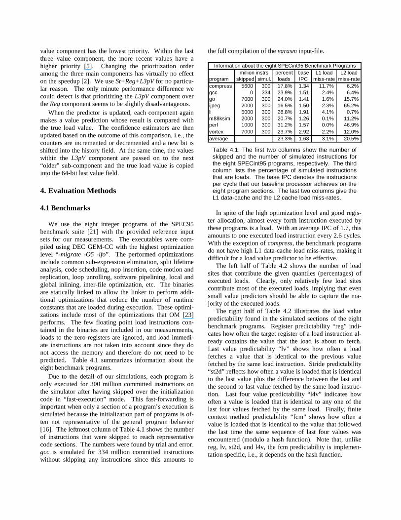
We use the eight integer programs of the SPEC95 benchmark suite [21] with the provided reference input sets for our measurements. The executables were com-piled using DEC GEM-CC with the highest optimization level “ -migrate -O5 -ifo” . The performed optimizations include common sub-expression elimination, split li fetime analysis, code scheduling, nop insertion, code motion and replication, loop unrolli ng, software pipelining, local and global inlining, inter-file optimization, etc. The binaries are statically linked to allow the linker to perform addi-tional optimizations that reduce the number of runtime constants that are loaded during execution. These optimi-zations include most of the optimizations that OM [23] performs. The few floating point load instructions con-tained in the binaries are included in our measurements, loads to the zero-registers are ignored, and load immedi-ate instructions are not taken into account since they do not access the memory and therefore do not need to be predicted. Table 4.1 summarizes information about the eight benchmark programs.

Due to the detail of our simulations, each program is only executed for 300 milli on committed instructions on the simulator after having skipped over the initialization code in “ fast-execution” mode. This fast-forwarding is important when only a section of a program’s execution is simulated because the initialization part of programs is of-ten not representative of the general program behavior [16]. The leftmost column of Table 4.1 shows the number of instructions that were skipped to reach representative code sections. The numbers were found by trial and error. gcc is simulated for 334 milli on committed instructions without skipping any instructions since this amounts to

the full compilation of the varasm input-file.

percent base L1 load L2 loadprogram skipped simul. loads IPC miss-rate miss-ratecompress 5600 300 17.8% 1.34 11.7% 6.2% gcc 0 334 23.9% 1.51 2.4% 6.4% go 7000 300 24.0% 1.41 1.6% 15.7% ijpeg 2000 300 16.5% 1.50 2.3% 65.2% li 5000 300 28.8% 1.91 4.1% 0.7% m88ksim 2000 300 20.7% 1.26 0.1% 11.2% perl 1000 300 31.2% 1.57 0.0% 46.9% vortex 7000 300 23.7% 2.92 2.2% 12.0% average 23.3% 1.68 3.1% 20.5%

million instrsInformation about the eight SPECint95 Benchmark Programs

Table 4.1: The first two columns show the number of skipped and the number of simulated instructions for the eight SPECint95 programs, respectively. The third column lists the percentage of simulated instructions that are loads. The base IPC denotes the instructions per cycle that our baseline processor achieves on the eight program sections. The last two columns give the L1 data-cache and the L2 cache load miss-rates.

In spite of the high optimization level and good regis-ter allocation, almost every forth instruction executed by these programs is a load. With an average IPC of 1.7, this amounts to one executed load instruction every 2.6 cycles. With the exception of compress, the benchmark programs do not have high L1 data-cache load miss-rates, making it diff icult for a load value predictor to be effective.

The left half of Table 4.2 shows the number of load sites that contribute the given quantiles (percentages) of executed loads. Clearly, only relatively few load sites contribute most of the executed loads, implying that even small value predictors should be able to capture the ma-jority of the executed loads.

The right half of Table 4.2 ill ustrates the load value predictabilit y found in the simulated sections of the eight benchmark programs. Register predictabilit y “ reg” indi-cates how often the target register of a load instruction al-ready contains the value that the load is about to fetch. Last value predictabilit y “ lv” shows how often a load fetches a value that is identical to the previous value fetched by the same load instruction. Stride predictabilit y “st2d” reflects how often a value is loaded that is identical to the last value plus the difference between the last and the second to last value fetched by the same load instruc-tion. Last four value predictabilit y “ l4v” indicates how often a value is loaded that is identical to any one of the last four values fetched by the same load. Finally, finite context method predictability “ fcm” shows how often a value is loaded that is identical to the value that followed the last time the same sequence of last four values was encountered (modulo a hash function). Note that, unlike reg, lv, st2d, and l4v, the fcm predictabilit y is implemen-tation specific, i.e., it depends on the hash function.

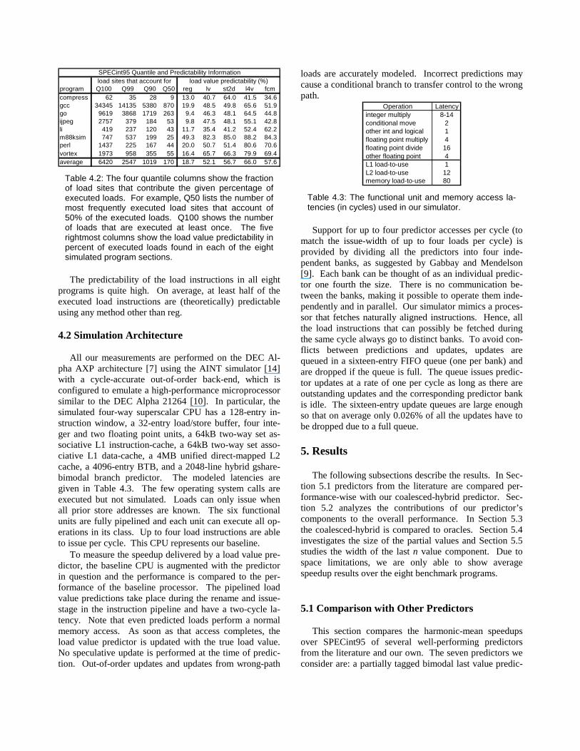
load sites that account forprogram Q100 Q99 Q90 Q50 reg lv st2d l4v fcmcompress 62 35 28 9 13.0 40.7 64.0 41.5 34.6 gcc 34345 14135 5380 870 19.9 48.5 49.8 65.6 51.9 go 9619 3868 1719 263 9.4 46.3 48.1 64.5 44.8 ijpeg 2757 379 184 53 9.8 47.5 48.1 55.1 42.8 li 419 237 120 43 11.7 35.4 41.2 52.4 62.2 m88ksim 747 537 199 25 49.3 82.3 85.0 88.2 84.3 perl 1437 225 167 44 20.0 50.7 51.4 80.6 70.6 vortex 1973 958 355 55 16.4 65.7 66.3 79.9 69.4 average 6420 2547 1019 170 18.7 52.1 56.7 66.0 57.6

load value predictability (%)SPECint95 Quantile and Predictability Information

Table 4.2: The four quantile columns show the fraction of load sites that contribute the given percentage of executed loads. For example, Q50 lists the number of most frequently executed load sites that account of 50% of the executed loads. Q100 shows the number of loads that are executed at least once. The five rightmost columns show the load value predictability in percent of executed loads found in each of the eight simulated program sections.

The predictabilit y of the load instructions in all eight programs is quite high. On average, at least half of the executed load instructions are (theoretically) predictable using any method other than reg.

4.2 Simulation Architecture

All our measurements are performed on the DEC Al-pha AXP architecture [7] using the AINT simulator [14] with a cycle-accurate out-of-order back-end, which is configured to emulate a high-performance microprocessor similar to the DEC Alpha 21264 [10]. In particular, the simulated four-way superscalar CPU has a 128-entry in-struction window, a 32-entry load/store buffer, four inte-ger and two floating point units, a 64kB two-way set as-sociative L1 instruction-cache, a 64kB two-way set asso-ciative L1 data-cache, a 4MB unified direct-mapped L2 cache, a 4096-entry BTB, and a 2048-line hybrid gshare-bimodal branch predictor. The modeled latencies are given in Table 4.3. The few operating system calls are executed but not simulated. Loads can only issue when all prior store addresses are known. The six functional units are fully pipelined and each unit can execute all op-erations in its class. Up to four load instructions are able to issue per cycle. This CPU represents our baseline.

To measure the speedup delivered by a load value pre-dictor, the baseline CPU is augmented with the predictor in question and the performance is compared to the per-formance of the baseline processor. The pipelined load value predictions take place during the rename and issue-stage in the instruction pipeline and have a two-cycle la-tency. Note that even predicted loads perform a normal memory access. As soon as that access completes, the load value predictor is updated with the true load value. No speculative update is performed at the time of predic-tion. Out-of-order updates and updates from wrong-path

loads are accurately modeled. Incorrect predictions may cause a conditional branch to transfer control to the wrong path.

Operation Latency integer multiply 8-14 conditional move 2 other int and logical 1 floating point multiply 4 floating point divide 16 other floating point 4 L1 load-to-use 1 L2 load-to-use 12 memory load-to-use 80

Table 4.3: The functional unit and memory access la-tencies (in cycles) used in our simulator.

Support for up to four predictor accesses per cycle (to match the issue-width of up to four loads per cycle) is provided by dividing all the predictors into four inde-pendent banks, as suggested by Gabbay and Mendelson [9]. Each bank can be thought of as an individual predic-tor one fourth the size. There is no communication be-tween the banks, making it possible to operate them inde-pendently and in parallel. Our simulator mimics a proces-sor that fetches naturally aligned instructions. Hence, all the load instructions that can possibly be fetched during the same cycle always go to distinct banks. To avoid con-flicts between predictions and updates, updates are queued in a sixteen-entry FIFO queue (one per bank) and are dropped if the queue is full . The queue issues predic-tor updates at a rate of one per cycle as long as there are outstanding updates and the corresponding predictor bank is idle. The sixteen-entry update queues are large enough so that on average only 0.026% of all the updates have to be dropped due to a full queue.

5. Results

The following subsections describe the results. In Sec-tion 5.1 predictors from the literature are compared per-formance-wise with our coalesced-hybrid predictor. Sec-tion 5.2 analyzes the contributions of our predictor’s components to the overall performance. In Section 5.3 the coalesced-hybrid is compared to oracles. Section 5.4 investigates the size of the partial values and Section 5.5 studies the width of the last n value component. Due to space limitations, we are only able to show average speedup results over the eight benchmark programs.

5.1 Comparison with Other Predictors

This section compares the harmonic-mean speedups over SPECint95 of several well -performing predictors from the literature and our own. The seven predictors we consider are: a partially tagged bimodal last value predic-

tor (LV) [12], a partially tagged bimodal stride 2-delta predictor (St2d) [19], a partially tagged last distinct four value predictor (LD4V) [25] with an access-pattern-based bimodal confidence estimator, a hybrid between a LD4V and a stride predictor (LD4V+St) [25], a partially tagged SAg last four value predictor (L4V) [5], our coalesced-hybrid (St+Reg+L3pV), and a partially tagged bimodal hybrid of a stride 2-delta and a finite context method pre-dictor (St2d+FCM) [18]. The performance of the individ-ual components of our hybrid is discussed in the next sec-tion.

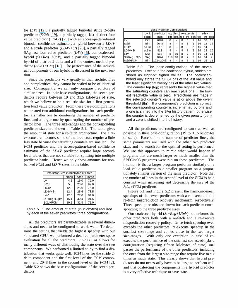
Since the predictors vary greatly in their architectures and complexities, they cannot be scaled to be of identical size. Consequently, we can only compare predictors of similar sizes. In their base configurations, the seven pre-dictors require between 19 and 31.5 kilobytes of state, which we believe to be a realistic size for a first genera-tion load value predictor. From these base-configurations we created two additional configurations for each predic-tor, a smaller one by quartering the number of predictor lines and a larger one by quadrupling the number of pre-dictor lines. The three size-ranges and the corresponding predictor sizes are shown in Table 5.1. The table gives the amount of state for a re-fetch architecture. For a re-execute architecture, some of the predictors require a littl e less state because the saturating counters are smaller. The FCM predictor and the access-pattern-based confidence estimator of the LD4V predictor require large second-level tables that are not suitable for splitti ng into multiple predictor banks. Hence we only show amounts for non-banked FCM and LD4V sizes in the table.

small base largeLV 4.8 19.0 76.0 St2d 5.8 23.0 92.0 LD4V 12.3 25.0 76.0 LD4V+St 12.4 25.6 78.5 L4V 12.8 27.0 84.0 St+Reg+L3pV 15.1 30.4 91.5 St2d+FCM 19.9 31.5 78.0

Predictor-Size in Kilobytes of State

Table 5.1: The amount of state (in kilobytes) required by each of the seven predictors’ three configurations.

All the predictors are parametrizable in several dimen-sions and need to be configured to work well . To deter-mine the setting that yields the highest speedup with our simulated CPU, we performed a detailed parameter space evaluation for all the predictors. St2d+FCM allows for many different ways of distributing the state over the two components. We performed a limited study to find a dis-tribution that works quite well: 1024 lines for the stride 2-delta component and the first level of the FCM compo-nent, and 2048 lines in the second level of the FCM [2]. Table 5.2 shows the base-configurations of the seven pre-dictors.

conf. predictor tag histestim. lines bits bits top thr pen top thr pen

LV Bim 2048 8 - 8 5 1 16 10 15St2d Bim 2048 8 - 8 5 1 16 12 12LD4V acBim 512 8 - 8 3 2 16 14 9LD4V+St acBim 512 8 - 8 7 2 16 13 10L4V SAg 512 8 10 8 7 4 16 14 11St+Reg+L3pV SAg 1024 1+8 10 8 7 2 16 14 9St2d+FCM Bim 1024/2048 8 - 8 5 1 16 15 11

re-fetchre-executeBase Predictor Configurations

Table 5.2: The base-configurations of the seven predictors. Except in the coalesced-hybrid, strides are stored as eight-bit signed values. The coalesced-hybrid only stores the full 64 bits of the last value and the least significant twenty bits of the other two values. The counter top (top) represents the highest value that the saturating counters can reach plus one. The low-est reachable value is zero. Predictions are made if the selected counter’s value is at or above the given threshold (thr). If a component’s prediction is correct, the corresponding counter is incremented by one and a one is shifted into the SAg history pattern, otherwise the counter is decremented by the given penalty (pen) and a zero is shifted into the history.

All the predictors are configured to work as well as possible in their base-configuration (19 to 31.5 kilobytes of state). Except for the number of predictor lines, the same parameters are used with the other two predictor sizes and no search for the optimal setting is performed. We use this approach to mimic what would happen if programs that are much larger or much smaller than the SPECint95 programs were run on these predictors. The intuition is that a larger program performs similarly on a load value predictor to a smaller program on a propor-tionately smaller version of the same predictor. Note that the number of lines in the second level of the FCM is held constant when increasing and decreasing the size of the St2d+FCM predictor.

Figure 5.1 and Figure 5.2 present the harmonic-mean speedups of the seven predictors with a re-execute and a re-fetch misprediction recovery mechanism, respectively. Three speedup results are shown for each predictor corre-sponding to the three predictor sizes.

Our coalesced-hybrid (St+Reg+L3pV) outperforms the other predictors both with a re-fetch and a re-execute misprediction recovery policy. Its re-fetch speedup even exceeds the other predictors’ re-execute speedup in the smallest size-range and comes close in the two larger size-ranges. With only one exception in case of re-execute, the performance of the smallest coalesced-hybrid configuration (requiring fifteen kilobytes of state) sur-passes the performance of the other predictors, including the ones from the largest size-range that require five to six times as much state. This clearly shows that hybrid pre-dictors do not necessarily have to be large to perform well and that coalescing the components in a hybrid predictor is a very effective technique to save state.

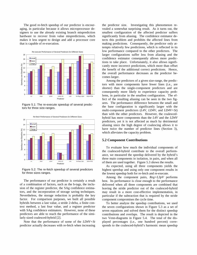
The good re-fetch speedup of our predictor is encour-aging, in particular because it allows microprocessor de-signers to use the already existing branch misprediction hardware to recover from value mispredictions, which makes it less urgent to design and add a processor core that is capable of re-execution.

Re-execute Performance of Several Predictors for Different Sizes

0

2

4

6

8

10

12

14

16

18

LV St2d LD4V LD4V+St L4V St+Reg+L3pV St2d+FCM

Predictor

Spe

edup

ove

r B

asel

ine

(%)

small

base

large

Figure 5.1: The re-execute speedup of several predic-tors for three size-ranges.

Re-fetch Performance of Several Predictors for Different Sizes

0

2

4

6

8

10

12

14

16

LV St2d LD4V LD4V+St L4V St+Reg+L3pV St2d+FCM

Predictor

Spe

edup

ove

r B

asel

ine

(%)

small

base

large

Figure 5.2: The re-fetch speedup of several predictors for three sizes ranges.

The performance of our predictor is certainly a result of a combination of factors, such as the b-tags, the inclu-sion of the register predictor, the SAg confidence estima-tors, and the incorporation of storage saving techniques. Nevertheless, the storage reduction is probably the key factor. For comparison purposes, we built all possible hybrids between a last value, a stride 2-delta, a finite con-text method, a last four value, and a register predictor with SAg confidence estimators. However, none of these predictors are able to reach the performance of the simi-larly sized coalesced-hybrid [2].

Note that the performance of some of the LD4V+St predictor actually decreases with re-fetch when increasing

the predictor size. Investigating this phenomenon re-vealed a somewhat surprising result. As it turns out, the smallest configuration of the affected predictor suffers significantly from aliasing. The confidence estimator de-tects this problem and prohibits the affected lines from making predictions. Consequently, the predictor only at-tempts relatively few predictions, which is reflected in its low performance compared to the other predictors. The larger configurations suffer less from aliasing and the confidence estimator consequently allows more predic-tions to take place. Unfortunately, it also allows signifi-cantly more incorrect predictions, which more than offset the benefit of the additional correct predictions. Hence, the overall performance decreases as the predictor be-comes larger.

Among the predictors of a given size-range, the predic-tors with more components have fewer lines (i.e., are shorter) than the single-component predictors and are consequently more likely to experience capacity prob-lems, in particular in the smallest configuration. The ef-fect of the resulting aliasing can be seen in the two fig-ures. The performance difference between the small and the base configuration is significantly larger with the multi -component predictors (L4V, LD4V, and LD4V+St) than with the other predictors. However, the coalesced-hybrid has more components than the L4V and the LD4V predictors, yet it is not affected as much by detrimental aliasing since the high degree of coalescing allows it to have twice the number of predictor lines (Section 3), which alleviates the capacity problem.

5.2 Component Contributions

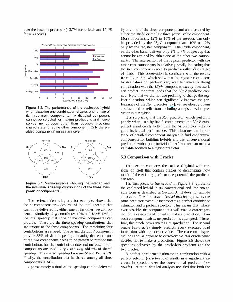
To evaluate how much the individual components of the coalesced-hybrid contribute to the overall perform-ance, we measured the speedup delivered by the hybrid’s three main components in isolation, in pairs, and when all of them are used together. Figure 5.3 shows the results.

As expected, using all three components yields the highest speedup and using only one component results in the lowest speedup both for re-fetch and re-execute.

Among the component pairs, Reg+L3pV performs best. Its performance is close enough to the performance delivered when all three components are combined that leaving the stride predictor out of the coalesced-hybrid may result in a more cost-effective implementation, in particular if the subtraction that is required by the stride component compromises the cycle time.

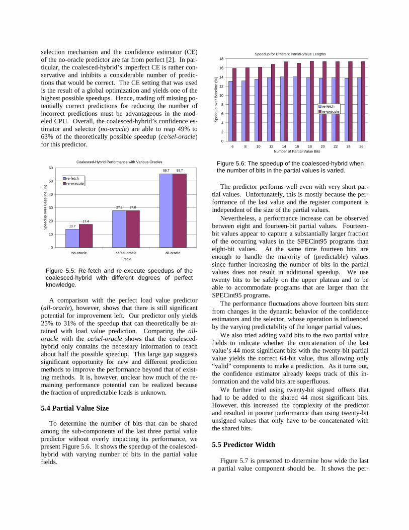
To better analyze the speedup contributions, we used the seven configurations shown in Figure 5.3 as a set of seven equations and solved them for the distinct speedup contributions and overlaps. The result is depicted in the two Venn-diagrams in Figure 5.4. The total of the dis-played percentages (i.e., one hundred percent) corre-sponds to the coalesced-hybrid’s harmonic mean speedup

over the baseline processor (13.7% for re-fetch and 17.4% for re-execute).

Predictor Performance after Disabling some Components

0 2 4 6 8 10 12 14 16 18

St+Reg+L3pV

St+Reg

St+L3pV

Reg+L3pV

St

Reg

L3pV

Con

figur

atio

n

Speedup over Baseline (%)

re-executere-fetch

Figure 5.3: The performance of the coalesced-hybrid when disabling any combination of zero, one, or two of its three main components. A disabled component cannot be selected for making predictions and hence serves no purpose other than possibly providing shared state for some other component. Only the en-abled components’ names are given.

St Reg St Reg

33% 6% 33% 3%

3%

34%

2% 10%

15%

L3pV

re-fetch re-execute

1%7% 12%

29%

L3pV

12%

Figure 5.4: Venn-diagrams showing the overlap and the individual speedup contributions of the three main predictor components.

The re-fetch Venn-diagram, for example, shows that the St component provides 2% of the total speedup that cannot be delivered by either one of the other two compo-nents. Similarly, Reg contributes 10% and L3pV 12% to the total speedup that none of the other components can provide. These are the three speedup contributions that are unique to the three components. The remaining four contributions are shared. The St and the L3pV component provide 33% of shared speedup, meaning that either one of the two components needs to be present to provide this contribution, but the contribution does not increase if both components are used. L3pV and Reg add 6% of shared speedup. The shared speedup between St and Reg is 3%. Finally, the contribution that is shared among all three components is 34%.

Approximately a third of the speedup can be delivered

by any one of the three components and another third by either the stride or the last three partial value component. More importantly, 12% to 15% of the speedup can only be provided by the L3pV component and 10% to 12% only by the register component. The stride component, on the other hand, delivers only 2% to 7% of speedup that cannot be attained by either one of the other two compo-nents. The intersection of the register predictor with the other two components is relatively small , indicating that the Reg component is able to predict a rather distinct set of loads. This observation is consistent with the results from Figure 5.3, which show that the register component by itself does not perform very well but makes a strong combination with the L3pV component exactly because it can predict important loads that the L3pV predictor can-not. Note that we did not use profili ng to change the reg-ister allocation, which can significantly improve the per-formance of the Reg predictor [24], yet we already obtain a substantial benefit from including a register value pre-dictor in our hybrid.

It is surprising that the Reg predictor, which performs poorly when used by itself, complements the L3pV com-ponent significantly better than the St predictor with its good individual performance. This ill ustrates the impor-tance of detailed component analyses to find cooperative components for building hybrids and that unconventional predictors with a poor individual performance can make a valuable addition to a hybrid predictor.

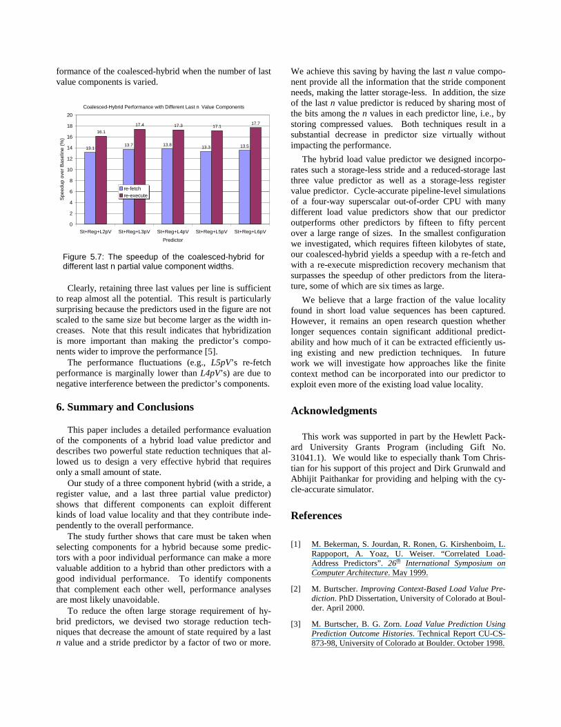
5.3 Comparison with Oracles

This section compares the coalesced-hybrid with ver-sions of itself that contain oracles to demonstrate how much of the existing performance potential the predictor can reap.

The first predictor (no-oracle) in Figure 5.5 represents the coalesced-hybrid in its conventional and implement-able form as described in Section 3. It does not include an oracle. The first oracle (ce/sel-oracle) represents the same predictor except it incorporates a perfect confidence estimator and a perfect selector. This means that, when-ever possible, the component that will make a correct pre-diction is selected and forced to make a prediction. If no such component exists, no prediction is attempted. There-fore, this oracle never makes a misprediction. The second oracle (all -oracle) simply predicts every executed load instruction with the correct value. There are no mispre-dictions and, as opposed to ce/sel-oracle, this oracle never decides not to make a prediction. Figure 5.5 shows the speedups delivered by the oracle-less predictor and the two oracles.

A perfect confidence estimator in combination with a perfect selector (ce/sel-oracle) results in a significant in-crease in speedup over the conventional predictor (no-oracle). A more detailed analysis revealed that both the

selection mechanism and the confidence estimator (CE) of the no-oracle predictor are far from perfect [2]. In par-ticular, the coalesced-hybrid’s imperfect CE is rather con-servative and inhibits a considerable number of predic-tions that would be correct. The CE setting that was used is the result of a global optimization and yields one of the highest possible speedups. Hence, trading off missing po-tentially correct predictions for reducing the number of incorrect predictions must be advantageous in the mod-eled CPU. Overall , the coalesced-hybrid’s confidence es-timator and selector (no-oracle) are able to reap 49% to 63% of the theoretically possible speedup (ce/sel-oracle) for this predictor.

Coalesced-Hybrid Performance with Various Oracles

13.7

27.8

55.7

17.4

27.8

55.7

0

10

20

30

40

50

60

no-oracle ce/sel-oracle all-oracle

Oracle

Spe

edup

ove

r B

asel

ine

(%)

re-fetchre-execute

Figure 5.5: Re-fetch and re-execute speedups of the coalesced-hybrid with different degrees of perfect knowledge.

A comparison with the perfect load value predictor (all -oracle), however, shows that there is still significant potential for improvement left. Our predictor only yields 25% to 31% of the speedup that can theoretically be at-tained with load value prediction. Comparing the all -oracle with the ce/sel-oracle shows that the coalesced-hybrid only contains the necessary information to reach about half the possible speedup. This large gap suggests significant opportunity for new and different prediction methods to improve the performance beyond that of exist-ing methods. It is, however, unclear how much of the re-maining performance potential can be realized because the fraction of unpredictable loads is unknown.

5.4 Partial Value Size

To determine the number of bits that can be shared among the sub-components of the last three partial value predictor without overly impacting its performance, we present Figure 5.6. It shows the speedup of the coalesced-hybrid with varying number of bits in the partial value fields.

Speedup for Different Partial-Value Lengths

0

2

4

6

8

10

12

14

16

18

6 8 10 12 14 16 18 20 22 24 26Number of Partial-Value Bits

Spe

edup

ove

r B

asel

ine

(%)

re-fetchre-execute

Figure 5.6: The speedup of the coalesced-hybrid when the number of bits in the partial values is varied.

The predictor performs well even with very short par-tial values. Unfortunately, this is mostly because the per-formance of the last value and the register component is independent of the size of the partial values.

Nevertheless, a performance increase can be observed between eight and fourteen-bit partial values. Fourteen-bit values appear to capture a substantially larger fraction of the occurring values in the SPECint95 programs than eight-bit values. At the same time fourteen bits are enough to handle the majority of (predictable) values since further increasing the number of bits in the partial values does not result in additional speedup. We use twenty bits to be safely on the upper plateau and to be able to accommodate programs that are larger than the SPECint95 programs.

The performance fluctuations above fourteen bits stem from changes in the dynamic behavior of the confidence estimators and the selector, whose operation is influenced by the varying predictabilit y of the longer partial values.

We also tried adding valid bits to the two partial value fields to indicate whether the concatenation of the last value’s 44 most significant bits with the twenty-bit partial value yields the correct 64-bit value, thus allowing only “valid” components to make a prediction. As it turns out, the confidence estimator already keeps track of this in-formation and the valid bits are superfluous.

We further tried using twenty-bit signed offsets that had to be added to the shared 44 most significant bits. However, this increased the complexity of the predictor and resulted in poorer performance than using twenty-bit unsigned values that only have to be concatenated with the shared bits.

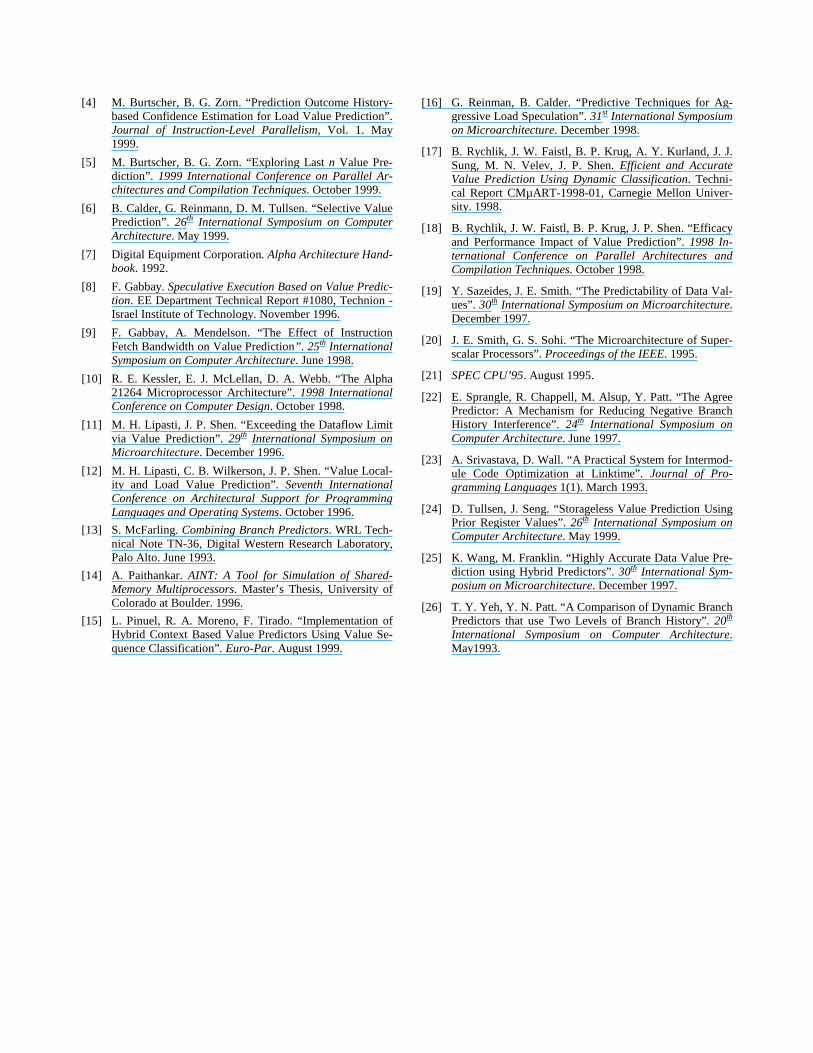
5.5 Predictor Width

Figure 5.7 is presented to determine how wide the last n partial value component should be. It shows the per-

formance of the coalesced-hybrid when the number of last value components is varied.

Coalesced-Hybrid Performance with Different Last n Value Components

13.113.7 13.8 13.3 13.5

16.1

17.4 17.3 17.117.7

0

2

4

6

8

10

12

14

16

18

20

St+Reg+L2pV St+Reg+L3pV St+Reg+L4pV St+Reg+L5pV St+Reg+L6pV

Predictor

Spe

edup

ove

r B

asel

ine

(%)

re-fetchre-execute

Figure 5.7: The speedup of the coalesced-hybrid for different last n partial value component widths.

Clearly, retaining three last values per line is suff icient to reap almost all the potential. This result is particularly surprising because the predictors used in the figure are not scaled to the same size but become larger as the width in-creases. Note that this result indicates that hybridization is more important than making the predictor’s compo-nents wider to improve the performance [5].

The performance fluctuations (e.g., L5pV’s re-fetch performance is marginally lower than L4pV’s) are due to negative interference between the predictor’s components.

6. Summary and Conclusions

This paper includes a detailed performance evaluation of the components of a hybrid load value predictor and describes two powerful state reduction techniques that al-lowed us to design a very effective hybrid that requires only a small amount of state.

Our study of a three component hybrid (with a stride, a register value, and a last three partial value predictor) shows that different components can exploit different kinds of load value locality and that they contribute inde-pendently to the overall performance.

The study further shows that care must be taken when selecting components for a hybrid because some predic-tors with a poor individual performance can make a more valuable addition to a hybrid than other predictors with a good individual performance. To identify components that complement each other well , performance analyses are most likely unavoidable.

To reduce the often large storage requirement of hy-brid predictors, we devised two storage reduction tech-niques that decrease the amount of state required by a last n value and a stride predictor by a factor of two or more.

We achieve this saving by having the last n value compo-nent provide all the information that the stride component needs, making the latter storage-less. In addition, the size of the last n value predictor is reduced by sharing most of the bits among the n values in each predictor line, i.e., by storing compressed values. Both techniques result in a substantial decrease in predictor size virtually without impacting the performance.

The hybrid load value predictor we designed incorpo-rates such a storage-less stride and a reduced-storage last three value predictor as well as a storage-less register value predictor. Cycle-accurate pipeline-level simulations of a four-way superscalar out-of-order CPU with many different load value predictors show that our predictor outperforms other predictors by fifteen to fifty percent over a large range of sizes. In the smallest configuration we investigated, which requires fifteen kilobytes of state, our coalesced-hybrid yields a speedup with a re-fetch and with a re-execute misprediction recovery mechanism that surpasses the speedup of other predictors from the litera-ture, some of which are six times as large.

We believe that a large fraction of the value locality found in short load value sequences has been captured. However, it remains an open research question whether longer sequences contain significant additional predict-abilit y and how much of it can be extracted eff iciently us-ing existing and new prediction techniques. In future work we will i nvestigate how approaches like the finite context method can be incorporated into our predictor to exploit even more of the existing load value locality.

Acknowledgments

This work was supported in part by the Hewlett Pack-ard University Grants Program (including Gift No. 31041.1). We would like to especially thank Tom Chris-tian for his support of this project and Dirk Grunwald and Abhijit Paithankar for providing and helping with the cy-cle-accurate simulator.

References

[1] M. Bekerman, S. Jourdan, R. Ronen, G. Kirshenboim, L. Rappoport, A. Yoaz, U. Weiser. “Correlated Load-Address Predictors” . 26th International Symposium on Computer Architecture. May 1999.

[2] M. Burtscher. Improving Context-Based Load Value Pre-diction. PhD Dissertation, University of Colorado at Boul-der. April 2000.

[3] M. Burtscher, B. G. Zorn. Load Value Prediction Using Prediction Outcome Histories. Technical Report CU-CS-873-98, University of Colorado at Boulder. October 1998.

[4] M. Burtscher, B. G. Zorn. “Prediction Outcome History-based Confidence Estimation for Load Value Prediction” . Journal of Instruction-Level Parallelism, Vol. 1. May 1999.

[5] M. Burtscher, B. G. Zorn. “Exploring Last n Value Pre-diction” . 1999 International Conference on Parallel Ar-chitectures and Compilation Techniques. October 1999.

[6] B. Calder, G. Reinmann, D. M. Tullsen. “Selective Value Prediction” . 26th International Symposium on Computer Architecture. May 1999.

[7] Digital Equipment Corporation. Alpha Architecture Hand-book. 1992.

[8] F. Gabbay. Speculative Execution Based on Value Predic-tion. EE Department Technical Report #1080, Technion - Israel Institute of Technology. November 1996.

[9] F. Gabbay, A. Mendelson. “The Effect of Instruction Fetch Bandwidth on Value Prediction” . 25th International Symposium on Computer Architecture. June 1998.

[10] R. E. Kessler, E. J. McLellan, D. A. Webb. “The Alpha 21264 Microprocessor Architecture”. 1998 International Conference on Computer Design. October 1998.

[11] M. H. Lipasti, J. P. Shen. “Exceeding the Dataflow Limit via Value Prediction” . 29th International Symposium on Microarchitecture. December 1996.

[12] M. H. Lipasti, C. B. Wilkerson, J. P. Shen. “Value Local-ity and Load Value Prediction” . Seventh International Conference on Architectural Support for Programming Languages and Operating Systems. October 1996.

[13] S. McFarling. Combining Branch Predictors. WRL Tech-nical Note TN-36, Digital Western Research Laboratory, Palo Alto. June 1993.

[14] A. Paithankar. AINT: A Tool for Simulation of Shared-Memory Multiprocessors. Master’s Thesis, University of Colorado at Boulder. 1996.

[15] L. Pinuel, R. A. Moreno, F. Tirado. “ Implementation of Hybrid Context Based Value Predictors Using Value Se-quence Classification” . Euro-Par. August 1999.

[16] G. Reinman, B. Calder. “Predictive Techniques for Ag-gressive Load Speculation” . 31st International Symposium on Microarchitecture. December 1998.

[17] B. Rychlik, J. W. Faistl, B. P. Krug, A. Y. Kurland, J. J. Sung, M. N. Velev, J. P. Shen. Efficient and Accurate Value Prediction Using Dynamic Classification. Techni-cal Report CMµART-1998-01, Carnegie Mellon Univer-sity. 1998.

[18] B. Rychlik, J. W. Faistl, B. P. Krug, J. P. Shen. “Eff icacy and Performance Impact of Value Prediction” . 1998 In-ternational Conference on Parallel Architectures and Compilation Techniques. October 1998.

[19] Y. Sazeides, J. E. Smith. “The Predictabil ity of Data Val-ues” . 30th International Symposium on Microarchitecture. December 1997.

[20] J. E. Smith, G. S. Sohi. “The Microarchitecture of Super-scalar Processors” . Proceedings of the IEEE. 1995.

[21] SPEC CPU’95. August 1995.

[22] E. Sprangle, R. Chappell , M. Alsup, Y. Patt. “The Agree Predictor: A Mechanism for Reducing Negative Branch History Interference”. 24th International Symposium on Computer Architecture. June 1997.

[23] A. Srivastava, D. Wall . “A Practical System for Intermod-ule Code Optimization at Linktime”. Journal of Pro-gramming Languages 1(1). March 1993.

[24] D. Tullsen, J. Seng. “Storageless Value Prediction Using Prior Register Values” . 26th International Symposium on Computer Architecture. May 1999.

[25] K. Wang, M. Franklin. “Highly Accurate Data Value Pre-diction using Hybrid Predictors” . 30th International Sym-posium on Microarchitecture. December 1997.

[26] T. Y. Yeh, Y. N. Patt. “A Comparison of Dynamic Branch Predictors that use Two Levels of Branch History” . 20th International Symposium on Computer Architecture. May1993.