Hybrid Computer Implementation of ADI Procedure - OnePetro

SOCIEZ’YOF PETROLEUMENGINEERS OF AIME6200 North Central Expressway ;&:m ~p~ ~AGa

Dallas, Texas 75206Wwu

THIS IS A PREPRINT --- SUBJECT TO CORRECTION

Hybrid Computer Implementation of AD I Procedure

By

Kenneth A. Bishop, Don W. Green, Member AIME, U. of Kansasand David T. Buzzelli, The Dow Chemical Co.

@ Copyright 1969American Institute of Mining, Metallurgical, and Petroleum Engineers, Inc.

This paper was prepared for the ~~~n Annual Fall IYIeetirigof the Society of Petroleum Erugineers. n .. ..

of AIME, to be held in Denver, Colo., Sept. 28-Ott. 1, 1969, Permissionto copy is restrictedto anabstractof not more than 300 words. Illustrationsmay not be copied. The abstract should containconspicuousacknowledgmentof where and by whom the paper is pres;nted. Publicationelsewhereafterpublicationin the JOURNAL OF PETROLEUMTECHNOLOGYor the SOCIETYOF PETROLEUMENGINEERS JCXJRI’JALisusually granted upon request to the Editor of the appropriatejournalprovided agreementto giveproper credit is made.

Discussionof this paper is invited. Three copies of any discussion should be sent to theSociety of Petroleum Engineersoffice. Such discussionmay be presented at the above meeting and,with the paper, may be consideredfor publication in one of the two SPE magazines.

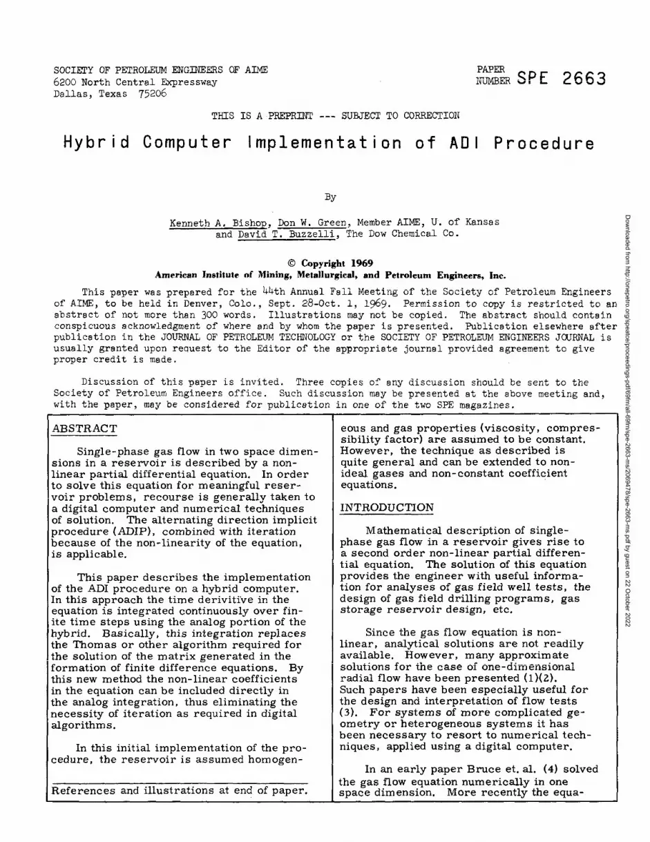
ABSTRACT eous and gas properties (viscosity, compres-sibility factor) are assumed tobe constant.

Single-phase gas flow in two space dimen- However, the technique as describedissions in a reservoir is describedby anon- quite general and canbe extended tenon-linear partial differential equation. In order ideal gases and non-constant coefficientto solve this equation for meaningful reser- equations.~roir ~rob~emsj recQIJrse is generally taken toa digital computer and numerical techniques INTRODUCTIONof solution. The alternating direction implicitprocedure (ADIP), combined with iteration Mathematical description of single-because of the non-linearity of the equation, phase gas flow in a reservoir gives risetois applicable. a second order non-linear partial differen-

tial equation. The solution of this equationThis paper describes the implementation provides the engineer with useful informa-

of the ADI procedure on a hybrid computer. tion for analyses of gasfield well tests, theIn this approach the time derivative in the design of gas field drilling programs, gasequation is integrated continuously over fin- storage reservoir design, etc.ite time steps using the analog portion of thehybrid. Basically, this integration repiaces m,— - AL --- ma. , ~“.,q+;nm ;C mn’n_

~ln~~ LIle gdb lLufi U+UC4LJW. .= ..VH

the Thomas or other algorithm required for linear, analytical solutions are not readilythe solution of the matrix generated in the available. However, many approximateformation of finite difference equations. By soiutions for the case of one-dimensionalthis new method the non-linear coefficients radial flow have been presented (l)(2).in the equation canbe included directly in Such papers have been especially useful forthe analog integration, thus eliminating the the design and interpretation of flow testsnecessity of iteration as required in digital (3). For systems of more complicated ge-algorithms. ometry or heterogeneous systems it has

been necessary to resort to numerical tech-In this initial implementation of the pro- niques, applied using a digital computer.

cedure, the reservoir is assumed homogen-In an early paper Bruce et. al. (4) solved

References and illustrations at end of paper.the gas flow equation numericallyin onespace dimension. More recently the equa-

Dow

nloaded from http://onepetro.org/speatce/proceedings-pdf/69fm

/all-69fm/spe-2663-m

s/2069478/spe-2663-ms.pdf by guest on 22 O

ctober 2022

2 HYBRID COMPUTER IMPLEMENTATION OF ADI PROCEDURE SPE 266?

tion has been solved in two space dimen-sions by Henderson et. al. (5)(6) throughapplication of the alternating direction im -plicit and alternating direction iterative pro-cedures as proposed by Peaceman and Rach -ford (7) and Douglas, Peaceman and Rach-ford (8). Henderson et. al. applied theirsolution to the development and operation ofgas storage reservoirs (6) and to the anal-ysis of gas fields (5). The equation hasbeen solved in three space dimensions,through application of an alternating direc-tion iterative procedure, by Casebolt (9).

Examples of the application of analogand hybrid computers to the solution of par-tial cliff erential equations may be foundeasily in the literature although most ofthem consider one space dimension andtime. Notable because of the treatment of

.. -:---- --- T7-- I..- Iinymuitipie space dimensluus ar= A+JW= \J VI,

who describes the use of special purposeanalogs and Howe et. al. (1 1) and Valentine(1 2), who describe the use of electronicdifferential analyzer (general purpose)computers for solving field problems.

Several authors have employed hybridmachines in the solution of partial differ-ential equations. Little (13) and Handler(14) have used Monte Carlo techniques forone and two dimensional problems. Vich -nevetsky (15)(16) has employed a serialtechnique for sharing a lim it ed amount ofanalog hardware.

Bishop et. al. (17) previously haveapplied the alternating direction implicitprocedure on a hybrid computer to solvethe differential equation describing two-dimensional, single-phase flow of a slightlycompressible fluid. The technique wasshown to be valid and potentially to offersome advantages in computing speed overthe digital approach. Subsequent to thefirst presentation, the hybrid program hasbeen run for several different time steps,grid, and source term sizes and found tobehave in a very satisfactory manner.

PURPOSE AND SCOPE

The purpose of this paper is to showhybrid computer implementation of theADI procedure for solution of the two-dimensional, single-phase, gas flow equa-tion. In the work discussed, gas compres-srDiiity and viscosity -were $aSsiinied tG beconstant with pressure but the technique isnot subject to this restriction. The basicalgorithm wiii be descrilled and resultsfrom sample calculations will be shown.For purposes of checking the hybrid re-sults, they will be compared to calculations

made using a digital computer algorithm inwhich an ADI (iterative) procedure has beenapplied.

TWO-DIMENSIONAL, GAS FLOW EQUATION

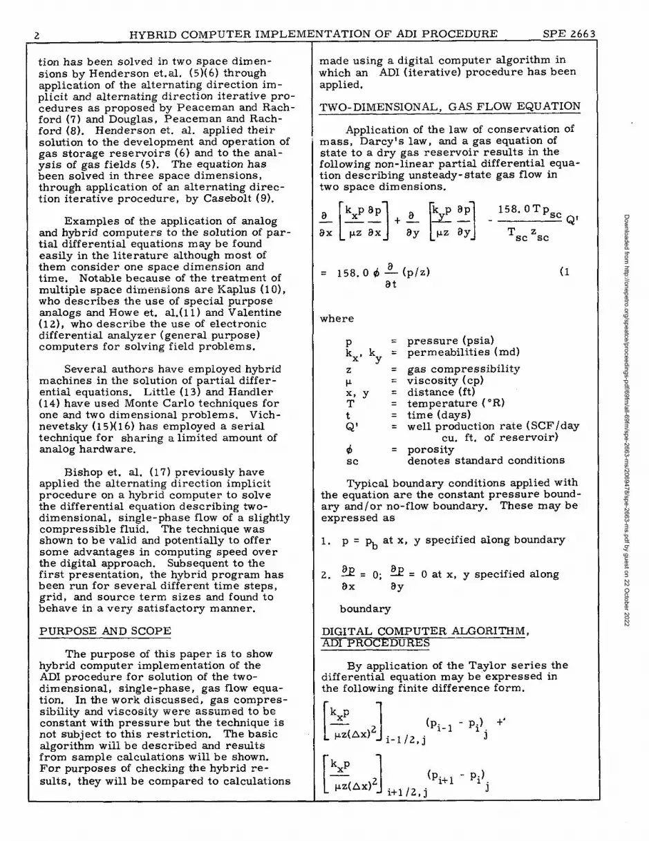
Application of the law of conservation ofmass, Darcy’s law, and a gas equation ofstate to a dry gas reservoir results in thefollowing non-linear partial differential equa-tion describing unsteady- state gas flow intwo space dimensions.

aX L ~Z axJ ay LPZ ayj Tsc Zsc

= 158.0 ~ A (p/Z) (1at

where

= pressure (psia):x, kv = permeabilities (red)

.z =

P=XSY=T=t =Q’ =

4=Sc

gas compressibilityviscosity (cp)distance (ft)temperature ( “R)time (days)well production rate ( SCF /day

cu. ft. of reservoir)porositydenotes standard conditions

Typical boundary conditions applied withthe equation are the constant pressure bound-ary and /or no-flow boundary. These may beexpressed as

1. p = ~ at x, y specified along boundary

2. s ecified alongl&’= O; EJ?=Oatx, y pax ay

boundary

DIGITAL COMPUTER ALGORITHM,ADI PROCEDURES

By application of the Taylor series thedifferential equation may be expressed inthe following finite difference form.

r~p -1

1- 1x(pi_~ - pi) “

WZ(AX)2 i-l ,2, j J

I I1%( AX)2J i+l ,2,~pi+i - ‘i)j

Dow




ctober 2022

PE 2663 KENNETH A. BISHOP, DON W GREEN. DAVID T- BUZZELLI 3

+- [1Y ‘Pj-~ - Pj)pz(Ay)2 i,i-1,2 i

-“

[1+.5Y!‘Pj+~ - Pj)pz(Ay)2 i, j+ ~,2 i

158.0 T p~cQij

TzSc Sc AxAy

dr= 158.0=

1(p/’z)k+l - {p/z)k] 1>1\Lj

At

where unit thickness of the reservoir hasbeen assumed and where the superscript kdenotes time level. Qij is the well produc-

tion rate in SCF /day for a well located at thei, j node. Available digital solution tech-niques differ essentially in the selection ofthe time indices which have been left unspec-ified in the terms on the left-hand side inEquation (2).

The set of difference equations (2) maybe solved by an explicit numerical scheme,however, the maximum timestep size isrestricted by stability considerations. Hen-derson et. al. solved these equations byapplication of the alternating direction im -plicit procedure (5). In their solution, thecoefficient terms were evaluated at the endof the previous time step (time k). Forsome cases, the errors (as indicated bymaterial balance calculations) becomelarge using this procedure and the tech-nique is not acceptable.

The alternating direction iterative pro-cedure is a valid technique for solving thisequation (6). The approach is implementedby adding an iteration parameter term tothe difference equations. The equations arethen iterated upon in two steps, being solvedfirst with the x direction derivitive termswritten implicitly and therl ‘with the y direc -tion terms written implicitly. Coefficientterms are evaluated at the end of the pre-vious y direction iteration. After comple-ting the two parts of the calculation, the co-efficient terms are updated and the proced-ure repeated. In this manner the equationsare iterated upon until a completely implicitsolution is obtained.

Casebolt (9) developed a computer pro-gram to solve the difference equations ineither two or three space dimension? by.—-,..application of an AU (Iterative) procedure.This algorithm is described in the appendix

---——— .,— ——.-— —. ———

and was applied in the present work as ameans of checking the hybrid computer al-gorithm that follows.

HYBRID COMPUTER COMPUTATIONALALGORITH M

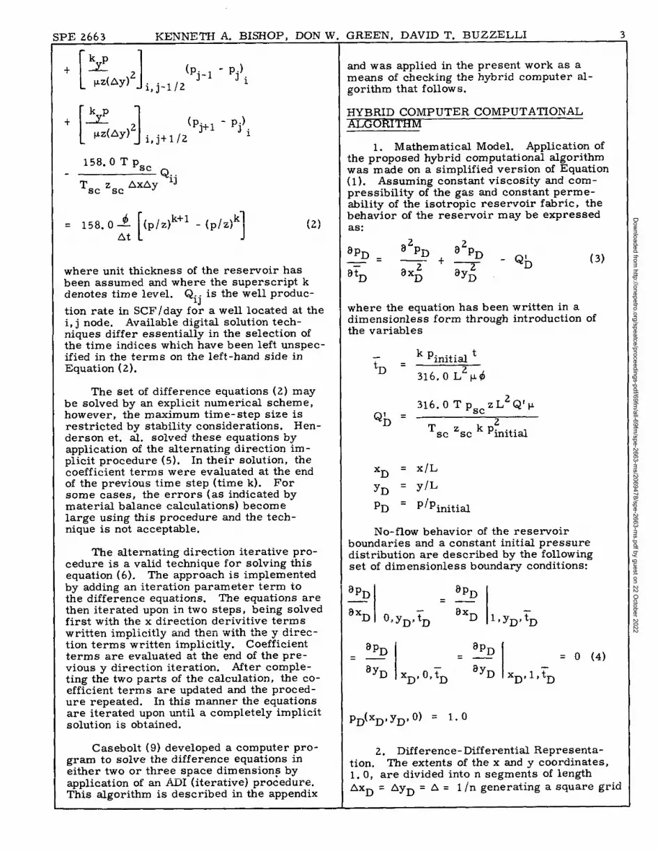
1. Mathematical Model. Application ofthe proposed hybrid computational algorithmwas made on a simplified version of Equation(l). Assuming constant viscosity and com-pressibility of the gas and constant perme-ability of the isotropic reservoir fabric, thebehavior of the reservoir may be expressedas:

apD .a2pD 82pD—+— . Q~ (3)

aTD ax; ay~

where the equation has been written in adim ensionless form through int reduction ofthe variables

k Pinitid tTD =

316,0 L2t.L~

316.0 T pScz L2Qf PQ~ =

T k p~nitiaSc ‘Sc

‘D= x/L

YD = y/L

pD = P/Piniti~

No-flow behavior of the reservoirboundaries and a constant initial pressuredistribution are described by the followingset of dimensionless boundary conditions:

apD” apD “=

a‘D o,yD, ID axD l,yD, tD

aPD apJJ=— =—

I

= o (4)

a‘D XD, O,TD ayD XD, l,tD

PD(XDYYD>0) ‘ 1.0

2. Difference-DifferentialRepresenta-tion. The extents of the x and y coordinates,1.0, are divided inton segments of lengthAxD =AyD=A= 1 /n generating a square grid

Dow




ctober 2022

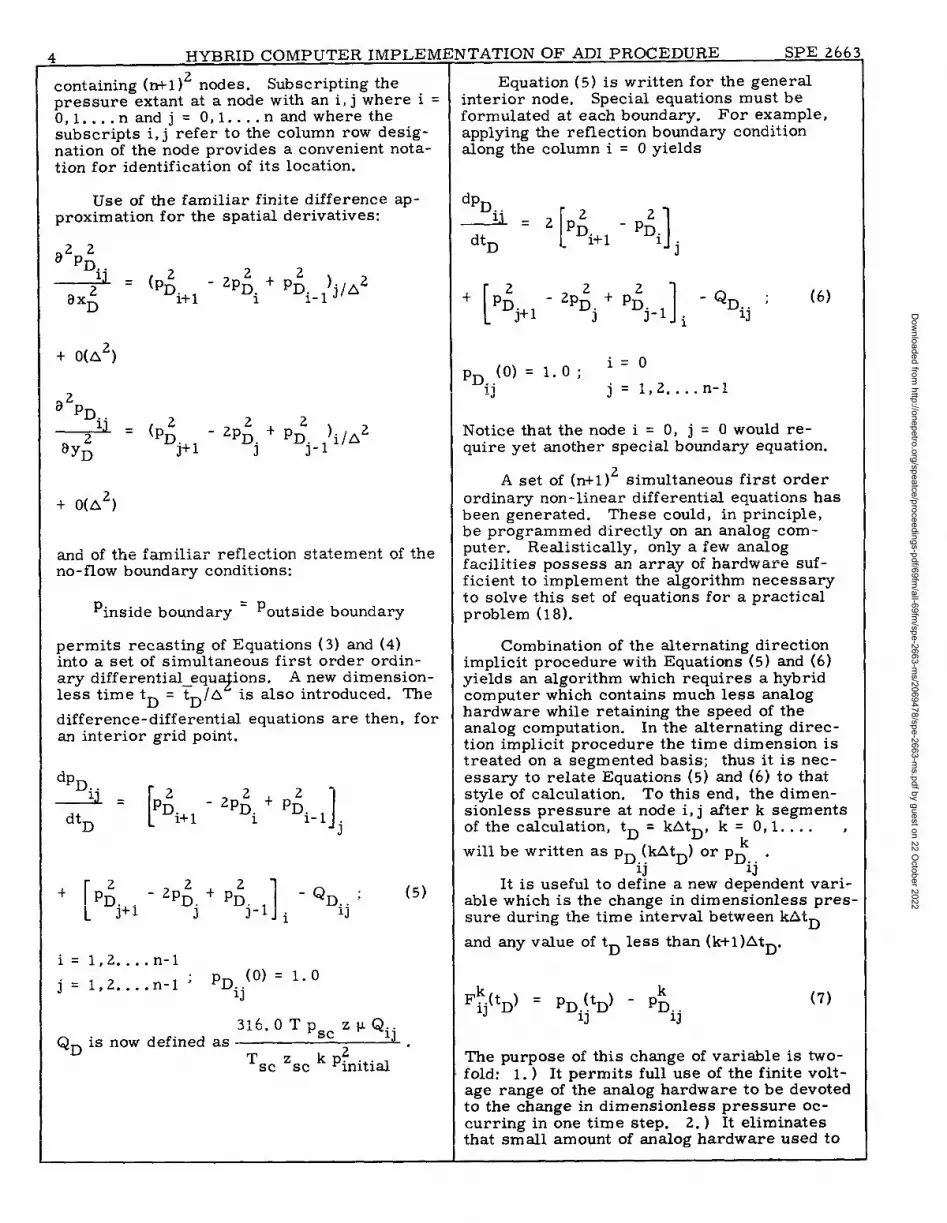
containing (n+l )2 nodes. Subscripting thepressure extant at a node with an i, j where i =0,1 . . . . nandj = 0,1 . . ..nand where thesubscripts i, j refer to the column row desig-nation of the node provides a convenient nota-tion for identification of its location.

Use of the familiar finite difference ap-proximation for the spatial derivatives:

D&p;J . (p; - 2P; + P; ).,A2

ax; i+ 1 i i_l JL/

+ 0(A2)

a2pD..+ . (p: - 2p; + ‘;j-~i/A2ayD j+ 1 j

+ 0(A2)

P. = poutside boundaryreside bound ary

permits recasting of Equations (3) and (4)into a set of simultaneous first order ordin-ary differential_equ~ions. A new dimension-less time tD = tD/A is also introduced. The

difference-differential equations are then, foran interior grid point.

@D

[

Ji=p; - 2p; + p;dtD i+ 1 i i-1 1j

+ (P: - 2p; + p;1 -QD ; (5)L ‘j+i j j-idi ~j

i=l,2 . . .. n-lpD (o) = 1.0

j= 1,2 . . ..n-l. ij

316.0 T n ~pQ..Fsc

QD is now defined ELS ~lJ

.

Sc k P~nitial‘Sc

Equation (5) is written for the generalinterior node. Special equations must beformulated at each boundary. For example,applying the reflection boundary conditionalong the column i = O yields

dPD

[

>= 2P;- P;.

dtD i+ 1 1lj+

[P; - 2p; + p; 1 -QD ; (6)

j+ 1 j j-1 i ij

pJJ(0)=l.o; i=oii-d j=l, Z.. .. n-l

Notice that the node i = O, j = O would re-quire yet another special boundary equation.

A set of (n+l )2 simultaneous first orderordinary non-linear differential equations hasbeen generated. These could, in principle,be programmed directly on an analog com -puter. Realistically, only a few analogfacilities possess an array of hardware suf-ficient to implement the algorithm necessaryto solve this set of equations for a practicalproblem (18).

Combination of the alternating directionimplicit procedure with Equations (5) and (6)yields an algorithm which requires a hybridcomputer which contains much less analoghardware while retaining the speed of theanalog computation. In the alternating direc-tion implicit procedure the time dimension istreated on a segmented basis; thus it is nec-essary to relate Equations (5) and (6j to thatstyle of calculation. To this end, the dimen-sionless pressure at node i, j after k segmentsof the calculation, tD = kAtD, k = O, 1. . . . ,

,-will be written as pD (kAtD) or pDK .

ii iiIt is useful to define a new depkndent vari-

able which is the change in dimensionless pres-sure during the time intervai between kAtD

and any value of tD less than (k+l )AtD.

F~(tD) = pD (tD) - p:ij ij

(7)

The purpose of this change of variable is two-fold: 1. ) It permits full use of the finite volt-age range of the analog hardware to be devotedto the change in dimensionless pressure oc-curring in one time step. 2. ) It eliminatesthat small amount of analog hardware used to

Dow




ctober 2022

;PE 2663 KENNETH A. BISHOP, DON W ------ - . . ..- - ------- . -

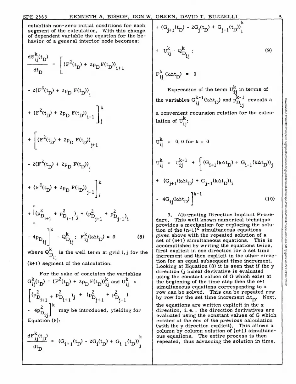
establish non- zero initial conditions for eachsegment of the calculation. With this changeof dependent variable the equation for the be-havior of a general interior node becomes:

dF&D)

dtD(F’2(tD)+ 2pDF(tD))i+ ~

- 2( F2(tD) + 2pD F(tD))i

+ (F2(tD) + 2pD F(tD))i-k

j

r

(F2(tD) + 2PD F(tD))1 j+ ~L

- 2(F2(tD) + 2pD F(tD))j

+ (F2(tD) + 2PD ‘@D))j-l

r

k

i

I+(I& + ‘il_l)j + ‘p: +‘~i+l “ j+ 1 j_l)i1

k

- 4pD - Q: ; F:(kAtD) =0ij ij

(8)

where Q~o. is the well term at grid i, j for the

(k+l ) seg~Jent of the calculation.

For the sake of concision the variables

Gfj(tD) = (F2(tD) + 2PD F(tD))fj and Uk. =lJ

[(P:i+l

2+ pD )j+ (p; +P; )

i+ 1 j+l j_l. lk

- 4p;1

may be introduced, yielding forij

Equati& (8):

dFf.(tD)= (G i+ ~(tD) - 2Gi(tD) + Gi_ ~(tD))k

dtn j

til%JLl!ilN, LJf’lv lJJ “l’. B u LZmLLl

+ (Gj+l(tD) - 2Gj(tD) + Gj_l(tD));

(9)

F; (kAtD) = O

Expression of the term U~i in terms of

the variables G‘k- 1

~- l(kAtD) and pn reveals a-. .lJ

a convenient recursion relation for the calcu-

lation of U;:-J

Uk = O. Ofork=Oij

Uk = Uk-’ +[

(Gi+l(kAtD) + Gi ~- (kAtD))jij ij

~ (Gj+l(kAtD) + Gj - ~(kAtD))i

1

k-1- 4Gij(kAtD) (lo)

3. Alternating Direction Implicit Proce-dure. This well known numerical technique

?3provides a mec anism for replacing the solu-tion of the (n+l ) simultaneous eqUatiOnSgiven above with the repeated solution of aset of (n+l ) simultaneous equations. This isaccomplished by writing the equations twice,first explicit in one direction for a set timeincrement and then explicit in the other direc-tion for an equal subsequent time increment.Looking at Equation (8) it is seen that if the ydirection (j index) derivative is evaluatedusing the constant values of G which exist atthe beginning of the time step then the n+lsimultaneous equations corresponding to arow can be solved. This can be repeated rowby row for the set time increment At=. Next,

the equations are written explicit in the xdirection, i. e. , the direction derivatives areevaluated using the constant values of G whichexisted at the end of the previous calculation(with the y direction explicit). This allows acolumn by column solution of (n+l ) simultane-ous equations. The entire process is thenrepeated, thus advancing the soiution in time.

Dow




ctober 2022

i6 HYBRID COMPUTER IMPLEMENTATION OF ADI PROCEDURE SPE 266:

Application of the ADI technique to Equa-tion (5) written in the form of Equation (9)results in the following set of equations for acalculation which is implicit in the x directionand explicit in the y direction (calculation ofthe jth row, general interior node).

dF~.(tD)

[ 1k

= Gi+l(tD) - 2G~tD) + Gi-l(tD)dtD j

+Uk. -Q&,;lJ i~

(11)

F;j(kAtD) = O

U~j for the interior node is defined by Equa-

tion (10) for k = 0,2,4 . . . . , (even). Again----- .-special boundary equations must be writtento satisfy the boundary conditions.

It should also be noted that ~.heterms

(Gi+l (tD) - 2Gj(tD) + Gj _ ~(tD))~ which

ap~ear in the ADI repre~entation of Equation(9) are each zero by definition; thereforethe explicit nature of the y-dire tion behavior

2is completely contained in the U.. term.lj

Similarly, application of the techniqueon the subsequent time increment where thex direction is handled explicitly and the ydirection implicitly (calculation of the ithCdii~J~J) giVe S:

,k,. , r lkw=

[

Gj+l(tD) - 2Gj(tD) + Gj-l(tD)dtD

1 i

ij-Q~ ;+ Ukij

(12)

Ffj (kAtD) = O

where again U~j is defined from Equation (1 O)

withk = 1,3,5,7... , (odd).

It should be noted that Equations (11) and,(l Z) are identical fr~ml time step to time stepdiffering only in the particular values of

U~j and Q~-. . Specifically, these equations11

are identical (with the exception of the Uk. and

Q: ) to those which arise from the analysis ofij

a one dimensional treatment of the problemwhich is familiar to most analog computerorient ed engineers.

4. Hybrid Computer Implementation.While a more efficient use of time is possible,a conceptually straight-forward impl em ent a-tion of the algorithm is one in which the com -mutational responsibilities are serial and areassigned as follows:

I

H

HI

Iv

Digital Computer Responsibility:computation, storage, and appropri-

ate disposition of the Uk.kand pDlJ ij

together with executive responsibilityfor analog mode control.Analog Computer Responsibility:

computation of the Fk.(t ) andq DGk.(t ) together with generation ofq Dpossible overload interrupts.Digital Logic (Analog ComPuter)Responsibility execution of wellintroduction together with controlof the analog computation period.Interface Responsibility: analog to

digital conversion of F!.(kAtD) and

digital to analog conversion of Uk:

and p: , together with transmisl~ionij

of analog mode and interrupt com -mands.

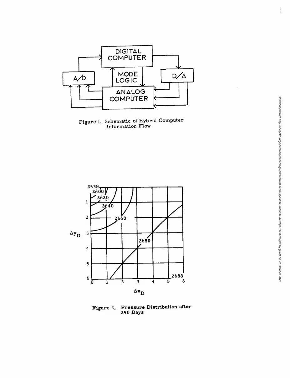
These responsibilities are indicated schemat-ically in Figure 1 and are presented schem at-. . .icaily m APPerJCiiX B.

EXAMPLE APPLICATION OF THE‘TECITNIQUM ‘——

The hybrid algorithm was implement edon an example problem for which the follow-ing conditions were specified. The reservoirwas assumed in plan view to be square inshape with a single well in the center prociuc -ing at a constant rate. The sides ‘of the res-ervoir were 1800 feet in length with a thicknessof 1.0 feet and flow was in the horizontal di-rection only (two dimensional). Initial reser-voir pressure was 4000 psia with the bound-aries taken to be no-flow boundaries.

In implementation of the solution, onlyone-quarter of the system was treated makinguse of symmetry. For this quadrant the wellwas located on one corner and the symmetrybmmdaries adjacent to the well were specifiedas no-flow boundaries.

Dow




ctober 2022

PE 2663 KENNETH A. BISHOP, DON W. GREEN, DAVID T. BUZZELLI 1’(

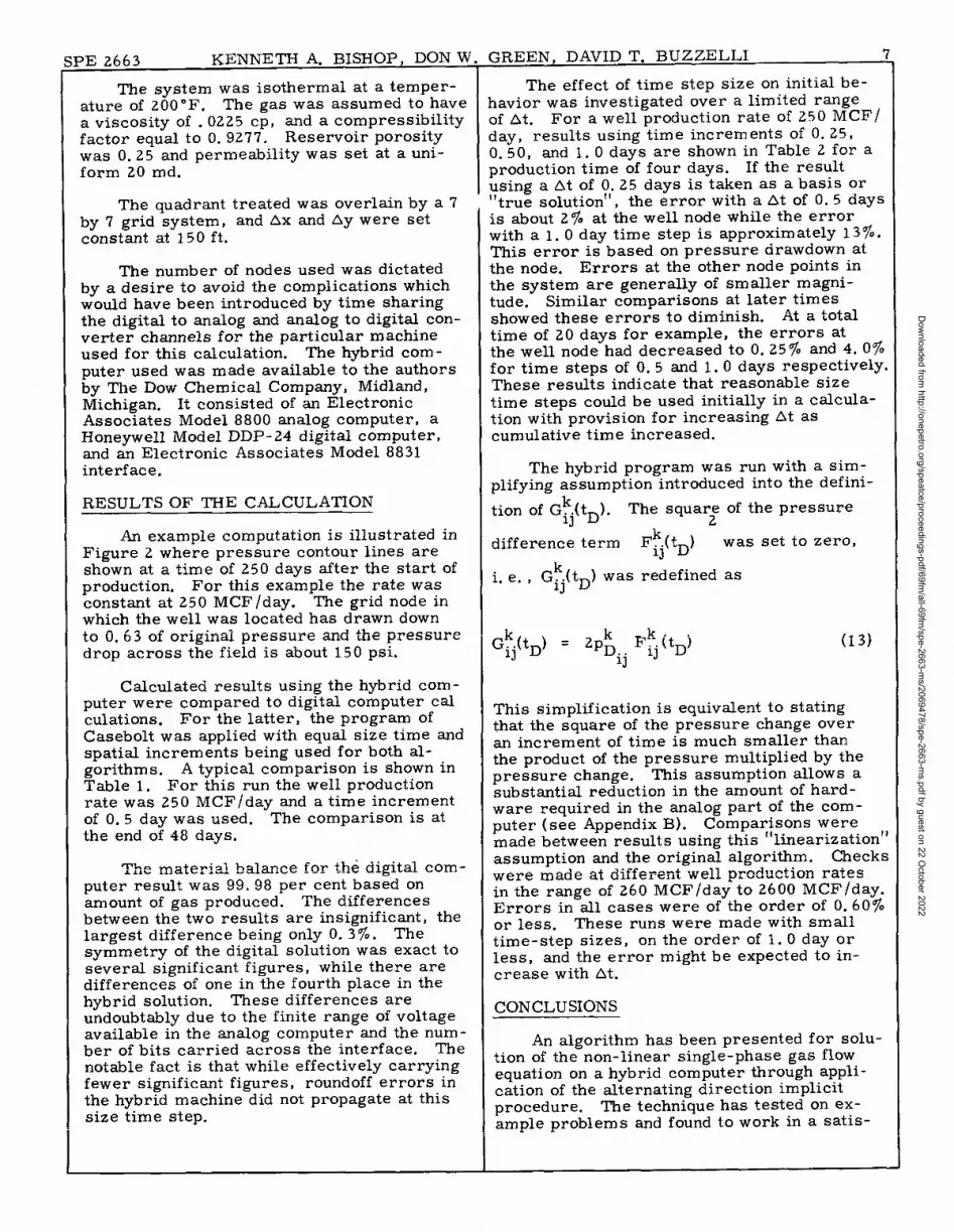
The system was isothermal at a temper-ature of 200° F. The gas was assumed to havea viscosity of . 0225 cp, and a compressibilityfactor equal to O. 9277. Reservoir porositywas O. 25 and permeability was set at a uni-form 20 md.

IThe quadrant treated was overlain by a 7

by 7 grid system, and Ax and Ay were setconstant at 150 ft.

The number of nodes used was dictatedby a desire to avoid the complications whichwould have been introduced by time sharingthe digital to analog and analog to digital con-vert er channels for the particular machineused for this calculation. The hybrid com -puter used was made available to the authorsby The Dow Chemical Company, Midland,Michigan. It consisted of an ElectronicAssociates Model 8800 analog computer, aHoneywell Model DDP-24 digital computer,and an Electronic Associates Model 8831interface.

RESULTS OF THE CALCULATION

An example computation is illustrated inFigure 2 where pressure contour lines areshown at a time of 250 days after the start ofproduction. For this example the rate wasconstant at 250 MCF /day. The grid node inwhich the well was located has drawn downto 0. 63 of original press-ure aiid the press’uredrop across the field is about 150 psi.

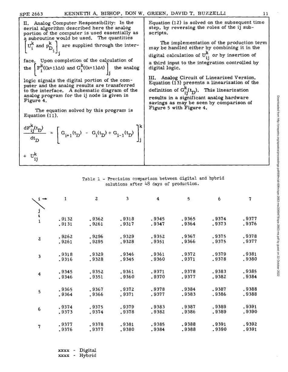
Calculated results using the hybrid com -puter were compared to digital computer calculations. For the latter, the program ofCasebolt was applied with equal size time andspatial increments being used for both al-gorithms. A typical comparison is shown inTable 1. For this run the well productionrate was 250 MCF/day and a time incrementof O. 5 day was used. The comparison is atthe end of 48 days.

The m.+~pi~l halanfie fnr ~h~ d~gital cOm -L.lla.G. AU.“.... -.. w- ---puter result was 99.98 per cent based onamount of gas produced. The differencesbetween the two results are insignificant, thelargest difference being only O. 3%. Thesymmetry of the digital solution was exact toseveral significant figures, while there aredifferences of one in the fourth place in thehybrid solution. These differences areundoubtable due to the finite range of voltageavailable in the analog computer and the num -ber of bits carried across the interface. Thenotable fact is that while effectively carryingfewer significant figures, roundoff errors inthe hybrid machine did not propagate at thissize time step.

The effect of time step size on initial be-havior was investigated over a limited rangeof At. For a well production rate of 250 MCF/day, results using time increments of O. 25,0.50, and 1.0 days are shown in Table 2 for aproduction time of four days. If the resultusing a At of O. 25 days is taken as a basis or“true solution”, the error with a At of O. 5 daysis about 270 at the well node while the errorwith a 1.0 day time step is approximately 137’..This error is based on pressure drawdown atthe node. Errors at the other node points inthe system are generally of smaller magni-tude. Similar comparisons at later timesshowed these errors to diminish. At a totaltime of 20 days for example, the errors atthe well node had decreased to O. 25% and 4.07.for time steps of O. 5 and 1.0 days respectively.These results indicate that reasonable sizetime steps could be used initially in a calcula-tion with provision for increasing At ascumulative time increased.

The hybrid program was run with a sim-plifying assumption introduced into the defini-

tion of Gk.(t ). The squar: of the pressureq D

difference term F~j(tD) was set to zero,

i.e., G~j(tD)Was redefined as

G;j(tD) . 2P: +j(tD)ij

This simplification is equivalent to statingthat the square of the pressure change overan increment of time is much smaller thanthe product of the pressure multiplied by thepressure change. This assumption allows asubstantial reduction in the amount of hard-ware required in the analog part of the com -puter (see Appendix B). Comparisons weremade between results using this “linearization”assumption and the original algorithm. Checks

-. J:cc-...,.-+ ...all mwnA,l,-.+innP2+PCwere made aL U~~~C~-G,,Lw=.. ~Lvu-uQ..... -----in the range of 260 MCF/day to 2600 MCF/day.Errors in all cases were of the order of O. 60%or less. These runs were made with smalltime-step sizes, on the order of 1.0 day orless, and the error might be expected to in-crease with At.

CONCLUSIONS

An algorithm has been presented for solu-tion of the non-linear single-phase gas flowequation on a hybrid computer through appli-cation of the alternating direction implicitprocedure. The technique has tested on ex-ample problems and found to work in a satis -

Dow




ctober 2022

; HYBRID COMPUTER IMPLEMI

factory manner as atested by comparisons tocalculations made using accepted digital- com -put er methods of solution.

The analo~ portion of a hybrid computercarries fewer ‘significant places” in a calcu-lation than do most digital machines. How-ever, in the problem presented, round-offerror did not grow.

A simplification to the basic algorithmwas presented which consisted of neglectinga non-linear term in the difference equation(the square of the pressure difference). Theerror introduced by this simplification wasnegligible for the cases studied.

NOMENCLATURE

F

G

kLPQ’

:

tu

xY7_.

g+’

4

P

dimensionless pressure differencevariable, Equation (7)

dimensionless pressure differencevariable, Equation (8)

permeability, mdlength of reservoir side, ft.pressure, psiawell production rate, SCF/day ft3

of reservoirwell production rate, SCF /daytemperature, “Rtime, daysdimensionless pressure variable,

Equation (8)distance, ftdistance, ftcompressibility factor,

dimensionlessconstants, Equation (A- 1)dimensionless x, y increment,

Ax/L, Ay/Lporosity, dimensionlessviscosity, cp

Subscripts

b = boundary value of variableD = dimensionless variablei = grid iocation index,initial = initial conditionj = grid location index,Sc = standard conditionsY = y directionx = x direction

Superscript

k = time indexs = iteration number

ACKNOWLEDGEMENT

eGtarnrl

row

The authors wish to acknowledge thesupport provided by The Dow Chemical Com-pany, Midland, Michigan, the University of

TATION OF ADI PROCEDURE SPE 2663

:ansas Computation Center, and Mr. Joseph:asebolt (Master of Science Thesis),

3EFERENCES

1.

2.

3.

4.

5.

6.

7.

8.

9.

10.

Aronofsky, J. S. and Jenkins, R. ,“A Simplified Analysis of UnsteadyRadial Gas Flow, ” Trans. A. I. M. E. ,201 (1954) 149.

Miller, C. C. , Dyes, A. B. , and Hutch-inson, C. A. Jr. , “The Estimation ofPermeability and Reservoir Pressuresfrom Bottom Hole Pressure BuildupCharacteristics, ” Trans. A. 1. M. E. ,189 (1950) 91.

Al Hussainy, R. and Ramey, H. J. Jr. ,and Crawford, P. B. , “me Fl~~ of RealGases Through Porous Media, Trans.A.LM. E. , 237 (1966) 624.

Bruce, G. H. , Peaceman, D. W. andRachford, H. H. Jr, , “Calculations ofUnstead~- State Gas F1OW Through PorousMedia, ‘ Trans. A. I. M. E. , 198 (1953)79.

Henderson, J. H. , Dempsey, J. R. andNelson, A. D. , “Practical Application

cm n:—.-.la-.l F.T,, tic. wical Mod~~01 ELlW-O-DMHCUDLWLJ=-L. . u... -. .-— .. --—for Gas Reservoir Studies, ” Journal ofPet. Tech. , 19 (September 1967 ) 1127.—

Henderson, J. H. , Dempsey, J. R. andTyler, J. C. , “Use of Numerical Reser-voir Models in t-he Development arxi,Op-eration of Gas Storage Reservoirs,SPE 2009, Presented at Symposium onNumerical Simulation of Reservoir Per-formance, Dallas, Texas, (April 1968).

Peaceman, D. W. and Rachford, H. N. ,“ The Num erica,l Solution of Parabolicand Elliptic Differential Equations, “Journal of Industrial & Applied Math, 311955).

—

Douglas, J. Jr. , Peaceman, D. W. , andRachford, H. H. Jrs. , “A Method forCalculating Multi- D~~ensional Immis-cible Displacement, Trans. A. 1. M. E. ,216 (1959) 297.

Casebolt, J. E. , “A Procedure for theNumerical Solution of the Equation De-scribing Three Dim ensional Unsteady-State Flow in Gas Reservoirs, “ M. S.Thesis, University of Kansas, Lawrence,Kansas, (1967).

Karplus, W. J. , Analog Simulations:Solution of Field Problems, lVlcGraw -Hill, New Y ork, (1958).

Dow




ctober 2022

PE 2663 KENNETH A. BISHOP, DON W

’11.

12.

13.

14.

15.

16.

17.

18.

Howe, R. M. and Haneman, V. S. , “TheSolution of Partial Differential Equationsby Difference Methods Using ;he Elec-tronic Differential AnalYser~ Proceed-ings IRE, (1953) 1497-1508,

Valentine, R. , “The Solution of Reser-voir Engineering Problems on t~,e Gen-eral Purpose Analog Computer,Electronic Associates, Inc. , Princeton,= - .--....+<~= flan+a~ B.ennrt No, 149,LOmpULaL~VIJu* .. ..-. .-r -- .(November 1959).

Little, W. D. , “Hybrid Computer Solu-tion of Partial Differential Equations byMonte Carlo Method s,” Proc. FJCC,AFIPS, 29 (November 1966) 181-190,

Handler, H. , “High Speed Monte CarloTechnique for Hybrid Computer S#utionof Partial Differential Equations,Ph. D. Dissertation, Electrical Engineering Department, University of Arizona,(1967).

Vichnevetsky, Robert, “ A New StableComputing Method for the Serial HybridComputer Integr~~ion of Partial Differ-ential Equations, 1968 Spring JointComputer Conference, AFIPS, Vol. 32,Thompson Book Co. , (1968).

Vichnevetsky, Robert, “Application ofHybrid Computers LWLILGAJ1.e=.-..”.. V..- -- L- 41-- 1.-+ ti-~+<mmnfPartial Differential Equations of theFirst and Second Orders, ” IFIP Con-gress 68, Edinburgh, Scotland, (August5-10, 1968).

Bishop, K. A. , Green, D. W. andBuzzelli, D. T. , “Hybrid ComputerImplement ation of the Alternating Direc-tion Implicit Procedure for the Solutionof Two Dimensional Parabolic PartialDifferential Equations, ” Presented at64th National Meeting, A. L Ch. E. ,New Orleans, Louisiana, (March 16-20,1969).

Bishop, K. A. , iiSolution of P artiai Dif-ferential Euuations Using a General Pur-pose Analog Computer, ‘r Computer Ap-plications in the Earth Sciences: Col-loquium on Simulation, Clomlputer Con-tribution No. 22, State Geological Survey(Kansas) (1968).

APPENDIX A

Digital Computer Algorithm

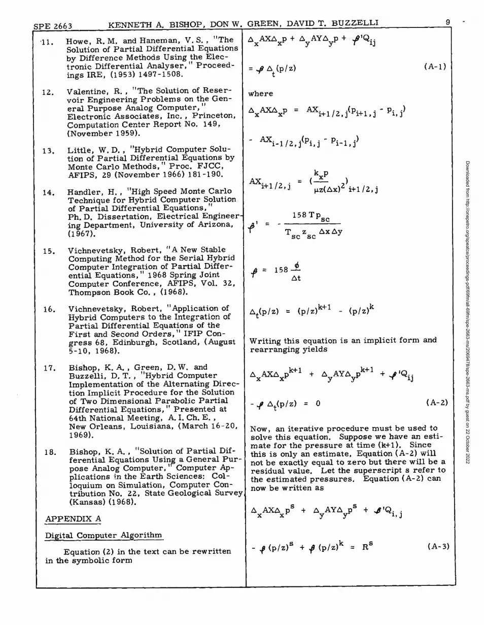
Equation (2) in the text can be rewrittenin the symbolic form

GREEN , DAVID T. BUZZELLI s

AxaAxp + AYA~AYP + #’Qij

= # At(P/Z) (A-1)

where

Ax-xp = ~i+l/2, j(pi+l, j - pi, j)

-Ax i-1/2, j(pi,j - ‘i-l,j)

kxpAx.1+1/2, j = (— )

pz(Ax)2 i+l /2, j

158 Tpsc

# = - Tsczsc AxAy

At(p/z) = (p/Z)k+l- (p/Z)k

Writing this equation is an implicit form andrearranging yields

Ax AXAxp ‘+1 + AyAYAyp k+ 1 +~IQ..q

- +? At(p/z) = O (A-2)

Now, an iterative procedure must be used tosolve this equation. Suppose we have an esti-mate for the pressure at time (k+l ). Sincethis is only an estimate, Equation (A-2) ‘willnot be exactly equal to zero but there will be aresidual value. Let the superscript s refer tothe estimated pressures. Equation (A- 2) cannow ‘be Written as

AxAXAxps + AyAYAyps -t ~ ‘Q.l,j

- # (p/z)s + ~ (p/z)k = Rs (A-3)

.D

ownloaded from

http://onepetro.org/speatce/proceedings-pdf/69fm/all-69fm

/spe-2663-ms/2069478/spe-2663-m

s.pdf by guest on 22 October 2022

o HYBRID COMPUTER IMPLEM’

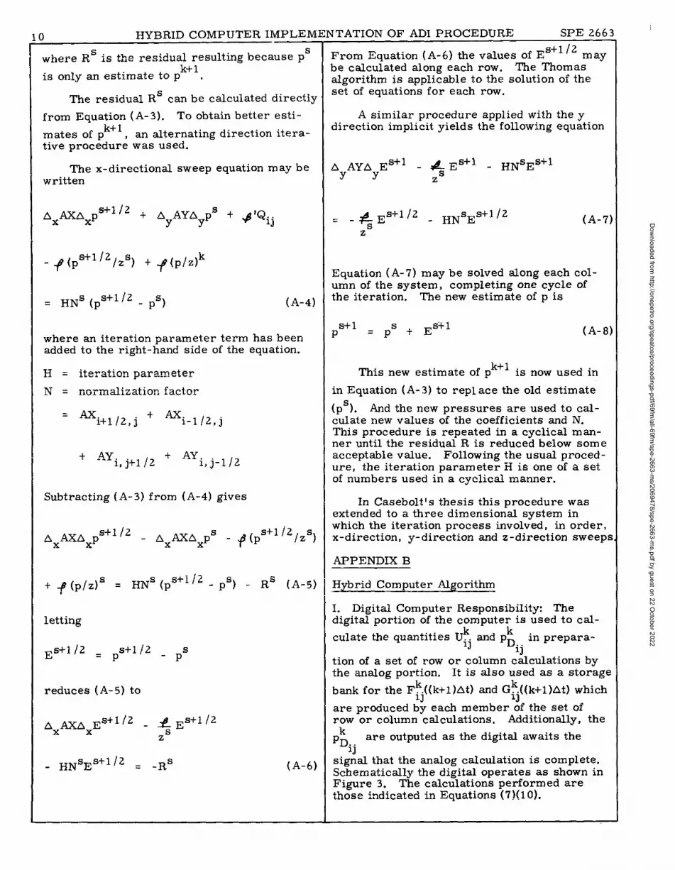
, s s:. 4ka -n +~121 vpsu]ting because pWnere R 1= L1lGLSS.”1.-. . .k+1

is only an estimate to p .

The residual Rs can be calculated directly

from Equation (A- 3). To obtain better esti-k+ 1mates of p an alternating direction itera-

tive procedur~ was used.

The x-directional sweep equation may bewritten

AxAXAxps+l ~’ + AyAYAyps + #Qij

-#(p‘+1121ZS) + f9

= HNS (p’+’ /2 - ps)

plz)k

(A-4)

where an iteration parameter term has beenadded to the right-hand side of the equation.

~= 4+ov3+inn narameter.I,v. L&. . . . . y-. ---- ----

N = Rorm,dizatior, factcM-

=Ax -+ Ax.i+l/2, j l-1/2, j

+ AY. + AY.1, J+l /2 l, j-i/2

Subtracting (A- 3) from (A-4) gives

AxAXAxp S+l /2 - AxAxAxps - ~ (p ‘+1’2/zs)

+ + (p/z)s = HIVs(ps+~~~-ps) _ Rs (A-5)

letting

Es+l /2 = ps+l/2- Ps

reduces (A-5) to

A AXA Es+l/2 - ~ ES+112x x z

- HNsEs+l/2 . -Rs (A-6)

tTATION OF ADI PROCEDURE SPE 2663—

From Equation (A- 6) the values of ES+ll’ maybe calculated along each row. ‘The ‘Tlnomasalgorithm is applicable to the solution of theset of equations for each row.

A similar procedure applied with the ydirection implicit yields the following equation

AYAYAYES+l - #$ ES+l - HNSES+lz

(A-7]

Equation (A- 7) may be solved along each col-umn of the system, completing one cycle ofthe iteration. The new estimate of p is

s+ 1P

s+ 1=PS+E (A-8)

This new estimate of pk+l is now used in

in Equation (A-3) to replace the old estimate

(ps). And the new pressures are used to cal-culate new values of the coefficients and N.This procedure is repeated in a cyclical man-ner until the residual R is reduced below someacceptable value. Following the usual proced -ure, the iteration parameter ‘H is one of a setof numbers used in a cyclical manner.

In Casebolt !s thesis this procedure wasextended to a three dimensional system inwhich the iteration process involved, in order,x-direction, y-direction and z-direction sweeps

APPENDIX B

Hvbrid Comnuter Akorithm

I. Digital Computer Responsibility: Thedigital portion of the computer is used to cal-

culate the quantities U!. and p:q in prepara-ii

tion of a set of row or column c~culations bythe analog portion. It is also used as a storage

bank for the F~i((k+l )At) and G~((k+l )At) which

are produced b~ each member ~f the set ofrow or column calculations. Additionally, the

P: are outputed as the digital awaits the:<‘J

signal that the analog calculation is complete.Schem aticslly the digital operates as shown inFigure 3. The calculations perform ed arethese indicated in Equations (7)(1 O).

Dow




ctober 2022

PE 2663 KENNETH A. BISHOP, DON W. GREEN, DAVID T. BUZZELLI 11

II. Analog Computer Responsibility: In theserial algorithm described here the analogportion of the computer is used essentially as~ subroutine would be used. The quantities

Equation (12 ) is solved on the subsequent timestep, by reversing the roles of the ij sub-scripts.

The implementation of the production termmay be handled either by combining it in the

digital calculation of Uk. or by insertion of

a third input to the int el~ration cent rolled bydigital logic.

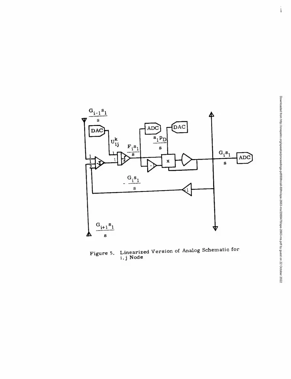
HI. Analog Circuit of Linearized Version.~y~auicm 11?) mresent.s a linearization of thew“.. +. .s ,A-, ~-------

definition of Gk.( t ). This linearizationq Dresults in a significant analog hardwaresavings as may be seen by comparison ofFigure 5 with Figure 4.

Iu: and p: I are supplied through the inter-

face. Upon completion of the calylation of

[the F~((k+l )At)- and G~((k+l )At)

1the analog

iL -IJ

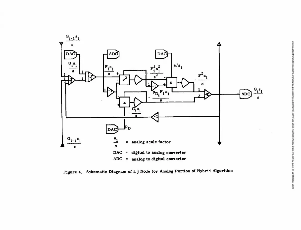
la.&nJUSAG S@lXik the rli_@t~~ portion of the com -puter and the analog results are transferredto the interface. A schematic diagram of theanalog program for the ij node is given inFigure 4.

The equation solved by this program isEquation (11 ).

dF;.(tD) =

[ 1k

Gi+l (tD) - Gi(tD) + Gi-l(tD)dtD j

L

Table 1 - Precision comparisonbetween digital and hybridsolutionsafter 48 days of production.

2 3 4 51

.9132

. 9131

.9262

.9261

.9318

.9316

, 9345.9346

.9365

.9364

.9374

.9373

.9377

.9376

6i-

\341

2

3

4

5

6

7

7

.9377

.9376

.9378

.9377

.9381

.9380

.9385

.9384

.9388

.9388

.9391

.9390

.9392

.9391

.9362

. 9261.9318.9317

.9345

.9347.9365.9364

.9374

.9373

.9375

.9375.9296.9295

.9329

.9328.9352.9351

.9367

.9366

.9361

.9360.9372.9371

.9379

.9378.9329.9328

.9346

.9345

.9352

.9351.9361.9360

.9371

.9370.9378.9377

.9383

.9382

.9367

.9366.9372, 9371

.9378

.9377.9384.9383

.9387

.9386

.9375

.9374.9379.9378

.9383

.9382.9387.9386

.9389

.9389

.9378

.9377.9381.9380

.9385

.9384.9388.9388

.9391

.9390

Xxxx - Digit alXxxx - Hybrid

Dow




ctober 2022

Table 2 - Calculateddimensionlesspressures for time stepsof 0.25, 0.50, and 1.0 days total time = 4.0 days

Q,= 250 MCF/day.

\~+

\

1

i: .97311 .9736

.9766

3

.9906

.9907

.9897

7

.9961

.9960

.9961

.9906 .9932 .99643 .9906 ● 9932 00~A. u“”.

.9898 .9934 .9965

.9960 .9964 .99737 .9961 .9964 .9974

.9962 .9964 ,9974

xxxx At = 0.25 DayXXXX At = O. 50 DayXXXX At = 1.00 Day

Dow




ctober 2022

f

DIGITALt >

Figure I. Schematic of Hybrid ComputerInform ation Flow

AY~

1/ 2 40

A

3

2680

5 )

I6 2688

01 2 3456

AxD

Figure 2. Pressure Distribution after250 Days

Dow




ctober 2022

I

N

T

E

R

F

A

c

E

r1 I

Transfer I

--is-J

-cloutput

P;i.

1 ‘+“ = “+1

~Wnm=f*-& ~tore ~m=a Rml.s !**. .------- - ---- — ..-. w.“- ------) F:((k+l )At) & G:((k+ 1)At)

of i&j

k= k+lI

Figure 3. Flow Chart for Digital Portion ofHybrid AlgOrithm

Dow




ctober 2022

G.l-lsl

UislFisl

s1l_ T s+

- x’-.

-—

Isx

1°Gisl

-—

IYDACPD

Gi+lsl ‘1— = analog scale factors s

DAC = digital to analog converter

ADC = analog to digital converter

Figure 4. Schamatic Diagram of i, j Node for Analog Portion of Hybrid Algorithm

Dow




ctober 2022

I

G.l-lsls

3DAC

I

U:j‘lpD

Fisl — s

I

1_-

S

G i+lsl

s

Figure 5. Linearizedi}j Node

Version of Analog Schematic for

Dow




ctober 2022

Documents

Hybrid Computer Implementation of ADI Procedure - OnePetro