1

HOW INTEGRATED IS THE WORLD ECONOMY?*

Harry P. Bowen†, Haris Munandar

‡ and Jean-Marie Viaene

§

March 4, 2010

Abstract

This paper develops a methodology to measure the degree of economic integration between nations that are members of an integrated area. We show that a fully integrated economic area (IEA) is characterized by three properties regarding the distribution of member shares of total IEA output and total IEA stocks of physical and human capital. We then show that the expected distribution of member shares within a fully IEA is a harmonic series, with the share distribution depending only on the number of IEA members. This property is then used to develop a composite indicator of the degree of economic integration within an IEA that indicates the distance between the theoretical and actual distribution of shares: the closer is the actual distribution to the expected distribution, the greater the degree of integration. We empirically compute our degree of integration index for US states, and alternative regional trading agreements (e.g., EU countries, MERCOSUR, Bangkok Agreement, etc.) and a World comprising 64 countries.

JEL Classification: E13, F15, F21, F22, O57

Keywords: Distribution of production, economic convergence, factor

mobility, economic integration.

* We thank Richard Paap and seminar participants at Erasmus, Leuven, Michigan and the Tinbergen

Institute for helpful comments and suggestions. We also thank Julia Swart for her very able research

assistance. Portions of the paper were written while J.-M. Viaene was visiting the Department of

Economics of the University of Michigan, whose hospitality and financial support are gratefully

acknowledged. † McColl School of Business, Queens University of Charlotte, 1900 Selwyn Avenue, Charlotte, NC

28274; e-mail: bowenh@queens.edu. ‡ Central Bank of Indonesia and University of Indonesia, Jl. M.H. Thamrin No. 2, Jakarta 10350,

Indonesia; e-mail: hmunandar@bi.go.id. § (Corresponding author) Erasmus University Rotterdam, Tinbergen Institute and CESifo, P.O. Box

1738, 3000 DR Rotterdam, The Netherlands; e-mail: viaene@few.eur.nl.

peer

-006

0163

4, v

ersi

on 1

- 20

Jun

201

1Author manuscript, published in "Review of World Economics 146, 3 (2010) 389-414"

DOI : 10.1007/s10290-010-0061-y

2

1. Introduction

The past decade has witnessed a surge of negotiating activity around regional

trade agreements (RTAs) as numerous subsets of countries have sought deeper

integration among themselves. The WTO expects close to 400 RTAs to be

implemented by 2010.1 To date, the most notable examples of RTAs include NAFTA

(United States, Canada and Mexico), the accession of 12 additional countries into the

European Union (EU), and MERCOSUR. However, there are several ongoing efforts

to initiate or renew agreements among a variety of nations (e.g., Free Trade for the

Americas, ASEAN). On average, each trading nation is currently a member of six

preferential agreements. However, the typical developed country of the Northern

hemisphere is on average a member of thirteen agreements (World Bank, 2005).

Geographically, free trade initiatives are unevenly distributed across various parts of

the world. Regional economic integration has come late to East Asia, but its pace has

accelerated since the creation of the WTO.

The present “spaghetti bowl” of preferential treatments is a complex web of

treaties and rules whose prospects for a reallocation of global production are

fundamental, but not yet fully understood (Bhagwati, 2002). The potential for greater

mobility of productive factors within any given integrated area is increasingly

powerful, not only because cross-border factor flows are becoming more important,2

but also because the international trade literature has long recognized that cross-

border factor flows and trade in goods and services can be substitutes (Mundell, 1957)

or complements (Markusen, 1983). Hence, reduced barriers to the movement of

goods and of productive factors within a RTA would be expected to affect the final

1 See the WTO website for an update of existing and planned free trade initiatives.

2 The importance of factor mobility in many parts of the world is evidenced by the growing importance

in many nations‟ balance of payments of remittances from abroad (e.g., International Monetary Fund,

2004). Capital flows in the form of foreign direct investment continue to be important among

industrialized countries and they are increasingly also being directed toward developing countries.

peer

-006

0163

4, v

ersi

on 1

- 20

Jun

201

1

3

distribution of production across RTA members. Since integration is

multidimensional, the measurement of its intensity is a challenging issue of

considerable importance. This paper is an attempt at developing such a methodology.

Quantification of the degree of economic integration within an integrated area

generates fresh insights into a number of critical questions. First, it is important to

evaluate integration efforts of major existing RTAs and to observe how these evolve

through time. Second, it allows for a comparison of the degree of economic

integration across different RTAs since the coverage and depth of preferential

treatments vary from one agreement to the other. For example, some RTAs involve

only traditional tariff-cutting policies while others include rules on e.g. services,

competition, investment and migration, and further institutional arrangements like the

European Monetary Union to adopt a single currency. The economic union of the

United States is perhaps the most sophisticated form of integration, with member

states unifying all economic and socio-economic policies. As a rule, it is believed in

policy circles that the degree of integration increases with the intensity of policy

harmonization. Finally, assessing the degree of economic integration for the world as

a whole serves to quantify the effects of globalization. On the one hand, most WTO

liberalization initiatives that emerged from the Uruguay Round went into force only in

the mid-1990s. On the other hand, the architecture of an RTA is discriminatory since

member countries seek to eliminate trade barriers among themselves but maintain

those on imports from non-member countries, with numerous rules of origin also

usually imposed to prevent the free movement of goods even within a RTA.

Several empirical studies estimate the extent of economic integration by

openness, often measured by the ratio of trade to GDP. Greenaway et al. (2001)

extend these proxies to construct the so-called index of extended intra-industry trade

peer

-006

0163

4, v

ersi

on 1

- 20

Jun

201

1

4

that can distinguish between penetration of a market due to increased imports versus

increased production by domestic affiliates of foreign companies. However, a trade

measure is a narrow indicator of the changes brought about by a RTA, and for this

reason broader measures of globalization have also been estimated. For example,

Andersen and Herbertsson (2003) use factor analysis to combine several variables

believed to be indicators of globalization into a single indicator. Riezman et al. (2005,

2006) use applied general equilibrium techniques to compute alternative metrics of

the distance between free trade, autarky and observed (restricted) trade equilibria. Our

point of departure relative to this literature is that we seek to measure the degree of

integration within a given RTA. In addition, we consider forms of integration that are

deeper than “globalization” in that the latter is considered a liberalization process that

leads to “a reduction in the barriers - whether technological or legislative - to

economic exchanges between nations” (Ethier, 2002). Our analysis expands on this to

include also economic and socio-economic policy coordination.

Our indicator of the degree of integration measures the distance between

observed values (shares) of output and factor stocks across RTA members and the

values (shares) expected theoretically to emerge within a fully integrated economic

area (IEA), the latter being an integrated area in which goods and factors are freely

mobile and policies are harmonized. The theoretical foundation of our indicator uses

the cross-country equalization of factor marginal products as the force driving the

allocation of resources across IEA members, and we combine this with the latest

developments regarding the increasingly observed empirical regularity of Zipf‟s law

in economic data (e.g., Gabaix, 2008). Our framework yields three related theoretical

predictions. The first is that factor mobility among members of an IEA implies that

each member‟s share of total IEA output will equal its shares of the total IEA stock of

peer

-006

0163

4, v

ersi

on 1

- 20

Jun

201

1

5

each productive factor (i.e., its shares of total IEA physical and human capital). We

call this theoretical outcome the “equal-share” relationship. The second prediction is

that the distribution of output and productive factors across IEA members is expected

to exhibit Zipf‟s law;3 this law establishes a specific relationship among member

shares of output and productive factors, namely, that the e.g. output share of the

largest member is two times that of the second largest member, three times that of the

third largest member, etc. Of course, the question arises as to why Zipf‟s law will

occur. In the literature, a central mechanism for the emergence of Zipf‟s law is

random growth of shares, and similarly our explanation builds on the random nature

of output and factor shares that arises from policy harmonization within an IEA. In

this setting, we apply the results of Gabaix (1999) to infer that if IEA member shares

evolve as geometric Brownian motion with a lower bound, then the limiting

distribution of these shares will exhibit Zipf‟s law. Thirdly, if Zipf‟s law holds, we

show that the expected distribution of shares within an IEA is a harmonic series,

where the shares of this series depend only on the number of IEA members. This

allows us to derive, for an IEA of fixed size, the expected distribution of shares across

IEA members. The closer the actual distribution of shares is from this expected

distribution the greater the degree of integration within the given IEA. Our measure of

the degree of economic integration reflects therefore the distance between expected

and actual distributions.

Given the potential importance of our metrics for future integration policies,

we empirically compute our measures of integration for the 50 US states and the

District of Columbia (hereafter called the 51 US states) and for different RTAs (e.g.,

3 Other recent theoretical and empirical contributions show Zipf‟s law to be an empirical regularity in

international trade. For example, Hinloopen and van Marrewijk (2006) find that the Balassa index of

comparative advantage obeys to the rank-size rule, and very often to Zipf‟s law. Also, the size

distribution of exporters analyzed in Helpman et al. (2004) conforms roughly to Zipf‟s law.

peer

-006

0163

4, v

ersi

on 1

- 20

Jun

201

1

6

EU countries, Andean Community, MERCOSUR, Latin American Integration

Association, and Bangkok Agreement) and a “world” comprising 64 countries.4 The

data generally cover the period from 1965 to 2000.

The remainder of the paper is as follows. Section 2 derives the theoretical

properties of a fully integrated economic area with respect to the distribution of output

and factors across IEA members and the expectation that member shares of IEA

output and factors will evolve randomly. Section 3 discusses the implications of this

randomness for the long-run distribution of output and factors across IEA members

and the expectation that member shares will conform to a rank-share distribution that

exhibits Zipf‟s law. Section 4 computes the theoretical shares and describes the data

used to measure actual shares of our economic groups. Section 5 provides a weak test

of the equal-share relationship. Section 6 defines our integration measures and

computes these measures for alternative economic groups. Section 7 summarizes and

discusses the consequences of our findings. An Appendix discusses data methods and

sources.

2. Equality of Output and Factor Shares

We consider an economy (or economic unit) that produces a single good by

means of a constant return to scale production function:

(1) ( , )t t tY F K H

where Yt is the level of output, Kt is the level of physical capital stock and Ht is the

level of human capital stock, all at time t. To facilitate interpretation we assume the

production function takes the Constant Elasticity of Substitution (CES) form:

(2) 1/

(1 )t t tY K H

4 This is the scenario dreamed of by ideological organizations like the Global Awareness Society

International (GASI): “Globalization has made possible what was once merely a vision: the peoples of

our world united under the roof of one Global Village”. See the GASI website, originally cited in

Rodrik (1997).

peer

-006

0163

4, v

ersi

on 1

- 20

Jun

201

1

7

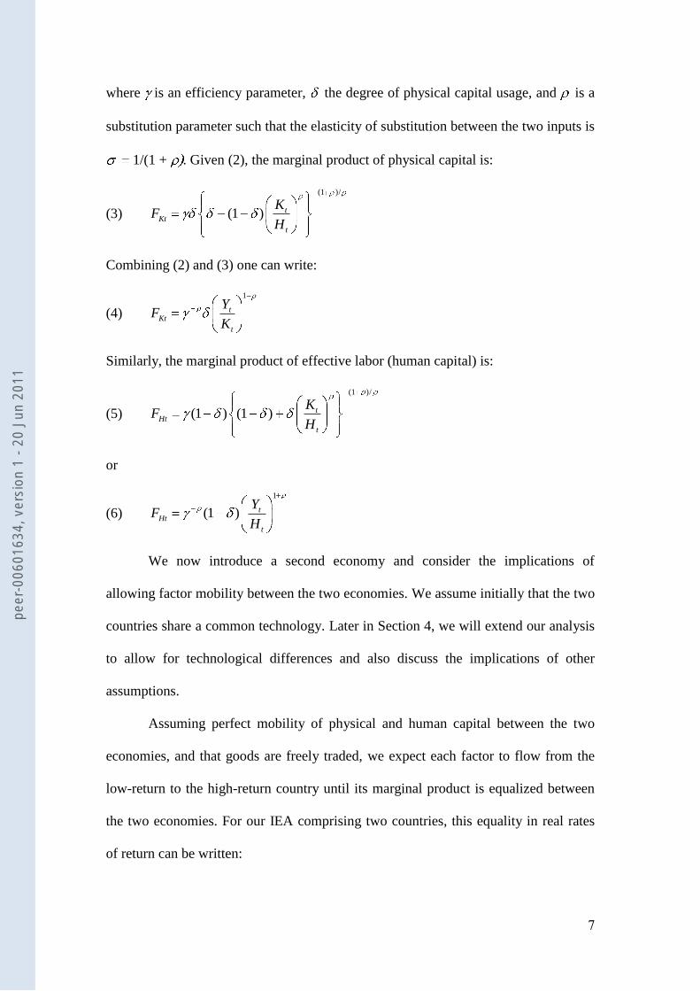
where is an efficiency parameter, the degree of physical capital usage, and is a

substitution parameter such that the elasticity of substitution between the two inputs is

1/(1 + . Given (2), the marginal product of physical capital is:

(3)

(1 )/

(1 ) tKt

t

KF

H

Combining (2) and (3) one can write:

(4)

1

tKt

t

YF

K

Similarly, the marginal product of effective labor (human capital) is:

(5)

(1 )/

(1 ) (1 ) tHt

t

KF

H

or

(6)

1

(1 ) tHt

t

YF

H

We now introduce a second economy and consider the implications of

allowing factor mobility between the two economies. We assume initially that the two

countries share a common technology. Later in Section 4, we will extend our analysis

to allow for technological differences and also discuss the implications of other

assumptions.

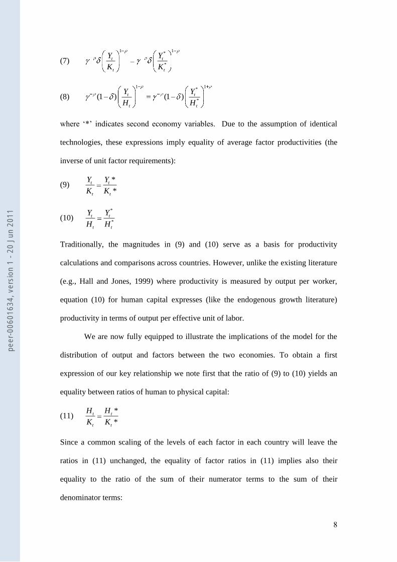
Assuming perfect mobility of physical and human capital between the two

economies, and that goods are freely traded, we expect each factor to flow from the

low-return to the high-return country until its marginal product is equalized between

the two economies. For our IEA comprising two countries, this equality in real rates

of return can be written:

peer

-006

0163

4, v

ersi

on 1

- 20

Jun

201

1

8

(7)

1 1*

*

t t

t t

Y Y

K K

(8)

1 1*

*(1 ) (1 )t t

t t

Y Y

H H

where „*‟ indicates second economy variables. Due to the assumption of identical

technologies, these expressions imply equality of average factor productivities (the

inverse of unit factor requirements):

(9) *

*

t t

t t

Y Y

K K

(10) *

*

t t

t t

Y Y

H H

Traditionally, the magnitudes in (9) and (10) serve as a basis for productivity

calculations and comparisons across countries. However, unlike the existing literature

(e.g., Hall and Jones, 1999) where productivity is measured by output per worker,

equation (10) for human capital expresses (like the endogenous growth literature)

productivity in terms of output per effective unit of labor.

We are now fully equipped to illustrate the implications of the model for the

distribution of output and factors between the two economies. To obtain a first

expression of our key relationship we note first that the ratio of (9) to (10) yields an

equality between ratios of human to physical capital:

(11) *

*

t t

t t

H H

K K

Since a common scaling of the levels of each factor in each country will leave the

ratios in (11) unchanged, the equality of factor ratios in (11) implies also their

equality to the ratio of the sum of their numerator terms to the sum of their

denominator terms:

peer

-006

0163

4, v

ersi

on 1

- 20

Jun

201

1

9

(12) * *

* *

t t t t

t t t t

H H H H

K K K K

Similarly, the equality of ratios in (9) implies:

(13) * *

* *

t t t t

t t t t

Y Y Y Y

K K K K

Together, expressions (12) and (13) imply the following set of equalities:

(14) * * *

t t t

t t t t t t

H Y K

H H Y Y K K

Relationship (14) indicates the distribution of factors and economic activity between

the two economies of our IEA. Specifically, when technologies are identical and there

are no barriers to factor mobility, each economy‟s shares of total IEA output, physical

capital and human capital will be identical. We hereafter call (14) the equal-share

relationship.5

Relationship (14) extends easily to an IEA with l = 1,..., N members.

Specifically, if all members have the same technology and there is perfect mobility of

physical and human capital among members then the equalization of factor rates of

return implies:

(15)

1 1 1

nt nt nt

N N N

lt lt ltl l l

H Y K

H Y K n = 1, …, N

or SnHt = SnYt = SnKt in compact form, where Snjt represents member n’s share of the

total IEA amount of variable j (j = Y, K, or H) at date t.

The equal-share relationship (15) has implications regarding the relative

economic performance of IEA members. For example, consider a reallocation of

physical capital among IEA members that leaves the total IEA stock of capital

5 Our framework also relates to the broad topic of output convergence since, if the equal-share

relationship holds, it is clear that the two economies will have the same output per efficiency unit of

labor. This implication is the essence of the productivity convergence hypothesis (Barro and Sala-i-

Martin, 2004), here interpreted in terms of efficiency units of labor and not per capita.

peer

-006

0163

4, v

ersi

on 1

- 20

Jun

201

1

10

unchanged. From (15), any country that gains physical capital will experience an

increase in the return to human capital and hence will accumulate human capital

either on its own, or through an inflow of human capital from those IEA members

whose physical capital was reduced. An IEA member that gains physical and human

capital will subsequently increase its output, and hence also its share of total IEA

output, to re-establish the equality of its output and factor shares as in (15). By the

same reasoning, an inflow of foreign direct investment into one IEA member will

increase that member‟s share of total IEA physical capital and its return to human

capital, ultimately raising the country‟s shares of both total IEA human capital and

total IEA output.

In addition to insights regarding the effects of factor accumulation on the

distribution of output among IEA members, equation (15) offers a key insight on the

effects of pursuing coordinated versus independent policies within an IEA. To

understand this, assume that IEA member n increases its human capital by a factor .

It then follows from (15) that, as described above, this member‟s shares of total IEA

physical capital and total IEA output will also increase. In contrast, if all IEA

members increase their human capital by the common factor then all shares would

remain the same. This suggests that the more harmonized (coordinated) are the

economic policies of IEA members the more likely are member shares to be stable

over time with, in the extreme, full harmonization implying that members‟ shares are

constant over time. In this case, any change over time in members‟ shares would

arise only from random events such as innovation, resource discovery, natural

disasters, civil unrest, etc. Since randomness of members‟ shares is more likely the

greater the extent of economic and socio-economic integration among members, such

randomness is more likely if members do not run independent monetary or exchange

peer

-006

0163

4, v

ersi

on 1

- 20

Jun

201

1

11

rate policies, fiscal policies are constrained by institutions, education systems are

harmonized, and successful local industrial policies are rapidly imitated. Accepting

that changes in output and factor shares in a fully integrated economy will occur

randomly, the question then arises as to the implications of this randomness for the

long run distribution of economic activity across IEA members. This is the subject of

the next section.

3. Long Run Distribution of Activity

Our interest in the long-run distribution of activity within a fully integrated

economic area is that it can serve as the benchmark for measuring of the extent of

integration within a given IEA. Toward this end, we adapt the specification and

results of Gabaix (1999) to our setting to derive the implications of random shares for

the long-run distribution of economic activity within an IEA. Specifically, Gabaix

shows (his Proposition 1) that if the city shares of a nation‟s population evolve

randomly as geometric Brownian motion with an infinitesimal lower bound then the

steady state distribution of these shares will be a rank-size distribution that exhibits

the property known as Zipf‟s law. This law implies the existence of a relationship

between the values of a given variable (share) and the rank number of these values.

This means, for example, that the population share of a nation‟s secondary largest city

will be one-half the population share of its largest (first ranked) city.

Translating Gabaix‟s (1999) result to our framework requires the assumption

that the evolution of an IEA member‟s output and factor shares can be approximated

by geometric Brownian motion with a lower bound. Formally, this assumes that the

growth over time in the shares of member n is captured by the following dynamic

process:

peer

-006

0163

4, v

ersi

on 1

- 20

Jun

201

1

12

(16) njt

t

njt

dSdt dB

S

In this expression, Snjt > min( )njtS is member n‟s share of variable j (j = Y, K, H)

where min( )njtS is the lower bound, Bt is a Wiener process,6 is a drift parameter, and

is the standard deviation of the distribution of shares. As in Gabaix, the distribution

of the growth rates of shares is assumed to be common to all IEA members; this

translates to assuming that the values of and are common to all IEA members.

The specification of Brownian motion in (16) is only one of many ways to model

random dynamics, but it has the property of being parsimonious in terms of number of

parameters. The assumption of a lower bound on shares seems realistic in our context

since important income transfers are institutionalized to prevent

states/regions/countries from vanishing: relief programs are in place in case of

disasters like a tsunami; the EU maintains a social fund and a regional fund.7

Accepting the above characterization for random shares, Gabaix‟s (1999)

result allow us to conclude that the long-run distributions of IEA members‟ output

and factor shares will exhibit Zip‟s law. In our context, Zip‟s law implies the

following relationship between the share values Snjt for a particular variable j (j = Y,

K, H) and their rank number across IEA members:

(17) 1( )njt jt njtS R , n = 1,…, N; j = Y, K, H.

6 The term dBt is the increment of the process. It is defined in continuous time as dBt = t(dt)

1/2, where

t is a stochastic term with zero mean and unit standard deviation, implying E[dBt] = 0 and Var(dBt) =

dt. In discrete time, one needs to approximate the increment dBt. A possibility is to assume one or more

shocks for each of the 365 calendar days of a year (dt = 1/365), in which case dBt is the running sum

over all discrete increments (“shocks”). The drift is expected to be zero since the sum over n of the

output and factor shares must be one. The standard deviation can be estimated using past and current

observations. 7 Technically, the assumption of a lower bound on the output and factors shares is needed to obtain a

power law distribution since, otherwise, the distribution of shares would be lognormal.

peer

-006

0163

4, v

ersi

on 1

- 20

Jun

201

1

13

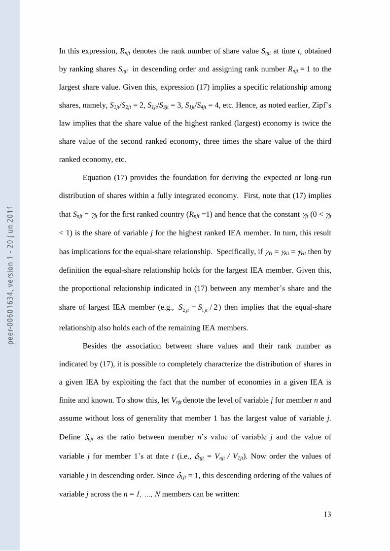
In this expression, Rnjt denotes the rank number of share value Snjt at time t, obtained

by ranking shares Snjt in descending order and assigning rank number Rnjt = 1 to the

largest share value. Given this, expression (17) implies a specific relationship among

shares, namely, S1jt/S2jt = 2, S1jt/S3jt = 3, S1jt/S4jt = 4, etc. Hence, as noted earlier, Zipf‟s

law implies that the share value of the highest ranked (largest) economy is twice the

share value of the second ranked economy, three times the share value of the third

ranked economy, etc.

Equation (17) provides the foundation for deriving the expected or long-run

distribution of shares within a fully integrated economy. First, note that (17) implies

that Snjt = jt for the first ranked country (Rnjt =1) and hence that the constant jt (0 < jt

< 1) is the share of variable j for the highest ranked IEA member. In turn, this result

has implications for the equal-share relationship. Specifically, if Yt = Kt = Ht then by

definition the equal-share relationship holds for the largest IEA member. Given this,

the proportional relationship indicated in (17) between any member‟s share and the

share of largest IEA member (e.g., 2 1 / 2jt jtS S ) then implies that the equal-share

relationship also holds each of the remaining IEA members.

Besides the association between share values and their rank number as

indicated by (17), it is possible to completely characterize the distribution of shares in

a given IEA by exploiting the fact that the number of economies in a given IEA is

finite and known. To show this, let Vnjt denote the level of variable j for member n and

assume without loss of generality that member 1 has the largest value of variable j.

Define njt as the ratio between member n‟s value of variable j and the value of

variable j for member 1‟s at date t (i.e., njt = Vnjt / V1jt). Now order the values of

variable j in descending order. Since 1jt = 1, this descending ordering of the values of

variable j across the n = 1, …, N members can be written:

peer

-006

0163

4, v

ersi

on 1

- 20

Jun

201

1

14

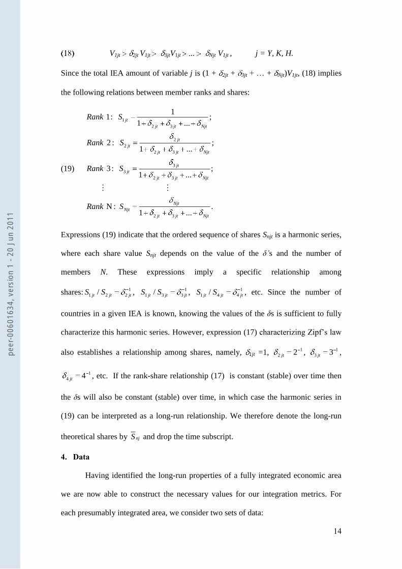
V1jt 2jt V1jt 3jtV1jt .. Njt V1jt , j = Y, K, H.

Since the total IEA amount of variable j is (1 + 2jt + 3jt + … + Njt)V1jt, (18) implies

the following relations between member ranks and shares:

(19)

1

2 3

2

2

2 3

3

3

2 3

2 3

1 1: ;

1 ...

2 : ;1 ...

3 : ;1 ...

N : .1 ...

jt

jt jt Njt

jt

jt

jt jt Njt

jt

jt

jt jt Njt

Njt

Njt

jt jt Njt

Rank S

Rank S

Rank S

Rank S

Expressions (19) indicate that the ordered sequence of shares Snjt is a harmonic series,

where each share value Snjt depends on the value of the δ’s and the number of

members N. These expressions imply a specific relationship among

shares:1

1 2 2/jt jt jtS S , 1

1 3 3/jt jt jtS S , 1

1 4 4/jt jt jtS S , etc. Since the number of

countries in a given IEA is known, knowing the values of the δs is sufficient to fully

characterize this harmonic series. However, expression (17) characterizing Zipf‟s law

also establishes a relationship among shares, namely, jt =1, 1

2 2jt , 1

3 3jt ,

1

4 4jt , etc. If the rank-share relationship (17) is constant (stable) over time then

the δs will also be constant (stable) over time, in which case the harmonic series in

(19) can be interpreted as a long-run relationship. We therefore denote the long-run

theoretical shares by njS and drop the time subscript.

4. Data

Having identified the long-run properties of a fully integrated economic area

we are now able to construct the necessary values for our integration metrics. For

each presumably integrated area, we consider two sets of data:

peer

-006

0163

4, v

ersi

on 1

- 20

Jun

201

1

15

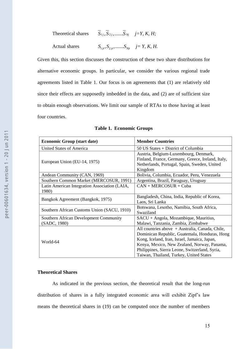
Theoretical shares 1 2, ,.......j j NjS S S j=Y, K, H;

Actual shares 1 2, ,.......jt jt NjtS S S j= Y, K, H.

Given this, this section discusses the construction of these two share distributions for

alternative economic groups. In particular, we consider the various regional trade

agreements listed in Table 1. Our focus is on agreements that (1) are relatively old

since their effects are supposedly imbedded in the data, and (2) are of sufficient size

to obtain enough observations. We limit our sample of RTAs to those having at least

four countries.

Table 1. Economic Groups

Economic Group (start date) Member Countries

United States of America 50 US States + District of Columbia

European Union (EU-14, 1975)

Austria, Belgium-Luxembourg, Denmark,

Finland, France, Germany, Greece, Ireland, Italy,

Netherlands, Portugal, Spain, Sweden, United

Kingdom

Andean Community (CAN, 1969) Bolivia, Columbia, Ecuador, Peru, Venezuela

Southern Common Market (MERCOSUR, 1991) Argentina, Brazil, Paraguay, Uruguay

Latin American Integration Association (LAIA,

1980)

CAN + MERCOSUR + Cuba

Bangkok Agreement (Bangkok, 1975) Bangladesh, China, India, Republic of Korea,

Laos, Sri Lanka

Southern African Customs Union (SACU, 1910) Botswana, Lesotho, Namibia, South Africa,

Swaziland

Southern African Development Community

(SADC, 1980)

SACU + Angola, Mozambique, Mauritius,

Malawi, Tanzania, Zambia, Zimbabwe

World-64

All countries above + Australia, Canada, Chile,

Dominican Republic, Guatemala, Honduras, Hong

Kong, Iceland, Iran, Israel, Jamaica, Japan,

Kenya, Mexico, New Zealand, Norway, Panama,

Philippines, Sierra Leone, Switzerland, Syria,

Taiwan, Thailand, Turkey, United States

Theoretical Shares

As indicated in the previous section, the theoretical result that the long-run

distribution of shares in a fully integrated economic area will exhibit Zipf‟s law

means the theoretical shares in (19) can be computed once the number of members

peer

-006

0163

4, v

ersi

on 1

- 20

Jun

201

1

16

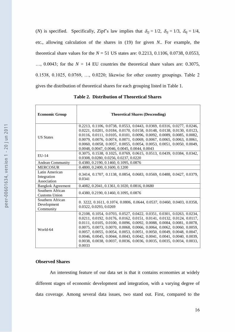
(N) is specified. Specifically, Zipf‟s law implies that 2j = 1/2, 3j = 1/3, 4j = 1/4,

etc., allowing calculation of the shares in (19) for given N.. For example, the

theoretical share values for the N = 51 US states are: 0.2213, 0.1106, 0.0738, 0.0553,

…, 0.0043; for the N = 14 EU countries the theoretical share values are: 0.3075,

0.1538, 0.1025, 0.0769, …, 0.0220; likewise for other country groupings. Table 2

gives the distribution of theoretical shares for each grouping listed in Table 1.

Table 2. Distribution of Theoretical Shares

Economic Group Theoretical Shares (Descending)

US States

0.2213, 0.1106, 0.0738, 0.0553, 0.0443, 0.0369, 0.0316, 0.0277, 0.0246,

0.0221, 0.0201, 0.0184, 0.0170, 0.0158, 0.0148, 0.0138, 0.0130, 0.0123,

0.0116, 0.0111, 0.0105, 0.0101, 0.0096, 0.0092, 0.0089, 0.0085, 0.0082,

0.0079, 0.0076, 0.0074, 0.0071, 0.0069, 0.0067, 0.0065, 0.0063, 0.0061,

0.0060, 0.0058, 0.0057, 0.0055, 0.0054, 0.0053, 0.0051, 0.0050, 0.0049,

0.0048, 0.0047, 0.0046, 0.0045, 0.0044, 0.0043

EU-14 0.3075, 0.1538, 0.1025, 0.0769, 0.0615, 0.0513, 0.0439, 0.0384, 0.0342,

0.0308, 0.0280, 0.0256, 0.0237, 0.0220

Andean Community 0.4380, 0.2190, 0.1460, 0.1095, 0.0876

MERCOSUR 0.4800, 0.2400, 0.1600, 0.1200

Latin American

Integration

Association

0.3414, 0.1707, 0.1138, 0.0854, 0.0683, 0.0569, 0.0488, 0.0427, 0.0379,

0.0341

Bangkok Agreement 0.4082, 0.2041, 0.1361, 0.1020, 0.0816, 0.0680

Southern African

Customs Union 0.4380, 0.2190, 0.1460, 0.1095, 0.0876

Southern African

Development

Community

0. 3222, 0.1611, 0.1074, 0.0806, 0.0644, 0.0537, 0.0460, 0.0403, 0.0358,

0.0322, 0.0293, 0.0269

World-64

0.2108, 0.1054, 0.0703, 0.0527, 0.0422, 0.0351, 0.0301, 0.0263, 0.0234,

0.0211, 0.0192, 0.0176, 0.0162, 0.0151, 0.0141, 0.0132, 0.0124, 0.0117,

0.0111, 0.0105, 0.0100, 0.0096, 0.0092, 0.0088, 0.0084, 0.0081, 0.0078,

0.0075, 0.0073, 0.0070, 0.0068, 0.0066, 0.0064, 0.0062, 0.0060, 0.0059,

0.0057, 0.0055, 0.0054, 0.0053, 0.0051, 0.0050, 0.0049, 0.0048, 0.0047,

0.0046, 0.0045, 0.0044, 0.0043, 0.0042, 0.0041, 0.0041, 0.0040, 0.0039,

0.0038, 0.0038, 0.0037, 0.0036, 0.0036, 0.0035, 0.0035, 0.0034, 0.0033,

0.0033

Observed Shares

An interesting feature of our data set is that it contains economies at widely

different stages of economic development and integration, with a varying degree of

data coverage. Among several data issues, two stand out. First, compared to the

peer

-006

0163

4, v

ersi

on 1

- 20

Jun

201

1

17

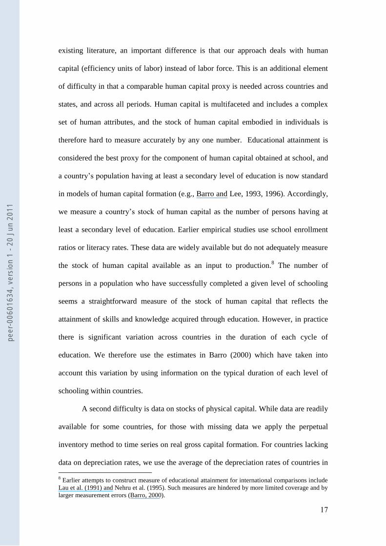
existing literature, an important difference is that our approach deals with human

capital (efficiency units of labor) instead of labor force. This is an additional element

of difficulty in that a comparable human capital proxy is needed across countries and

states, and across all periods. Human capital is multifaceted and includes a complex

set of human attributes, and the stock of human capital embodied in individuals is

therefore hard to measure accurately by any one number. Educational attainment is

considered the best proxy for the component of human capital obtained at school, and

a country‟s population having at least a secondary level of education is now standard

in models of human capital formation (e.g., Barro and Lee, 1993, 1996). Accordingly,

we measure a country‟s stock of human capital as the number of persons having at

least a secondary level of education. Earlier empirical studies use school enrollment

ratios or literacy rates. These data are widely available but do not adequately measure

the stock of human capital available as an input to production.8 The number of

persons in a population who have successfully completed a given level of schooling

seems a straightforward measure of the stock of human capital that reflects the

attainment of skills and knowledge acquired through education. However, in practice

there is significant variation across countries in the duration of each cycle of

education. We therefore use the estimates in Barro (2000) which have taken into

account this variation by using information on the typical duration of each level of

schooling within countries.

A second difficulty is data on stocks of physical capital. While data are readily

available for some countries, for those with missing data we apply the perpetual

inventory method to time series on real gross capital formation. For countries lacking

data on depreciation rates, we use the average of the depreciation rates of countries in

8 Earlier attempts to construct measure of educational attainment for international comparisons include

Lau et al. (1991) and Nehru et al. (1995). Such measures are hindered by more limited coverage and by

larger measurement errors (Barro, 2000).

peer

-006

0163

4, v

ersi

on 1

- 20

Jun

201

1

18

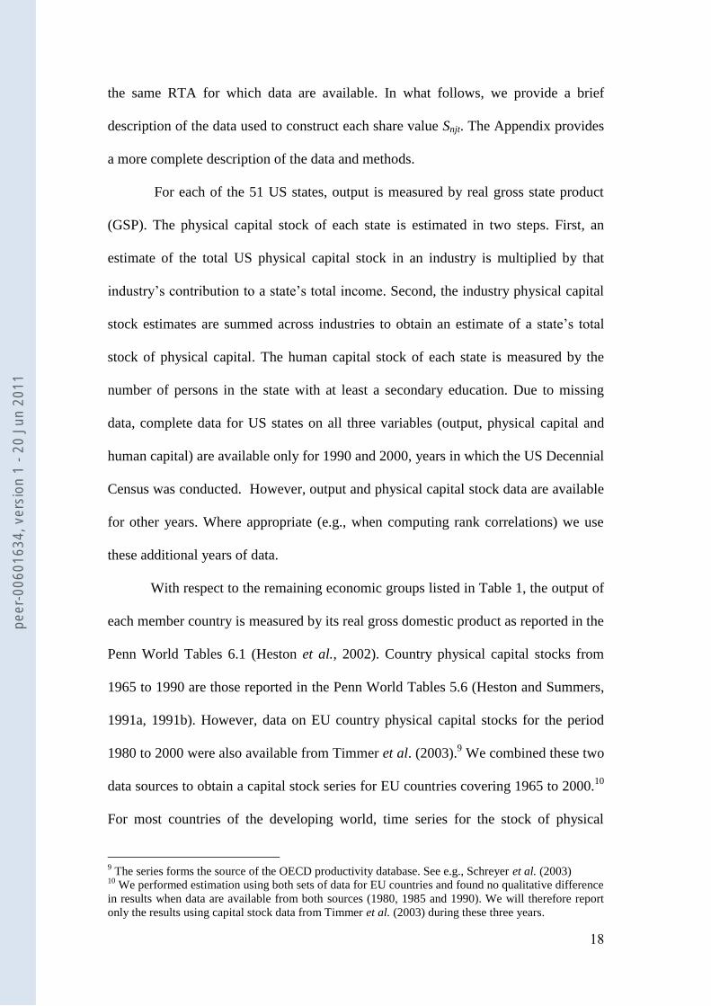
the same RTA for which data are available. In what follows, we provide a brief

description of the data used to construct each share value Snjt. The Appendix provides

a more complete description of the data and methods.

For each of the 51 US states, output is measured by real gross state product

(GSP). The physical capital stock of each state is estimated in two steps. First, an

estimate of the total US physical capital stock in an industry is multiplied by that

industry‟s contribution to a state‟s total income. Second, the industry physical capital

stock estimates are summed across industries to obtain an estimate of a state‟s total

stock of physical capital. The human capital stock of each state is measured by the

number of persons in the state with at least a secondary education. Due to missing

data, complete data for US states on all three variables (output, physical capital and

human capital) are available only for 1990 and 2000, years in which the US Decennial

Census was conducted. However, output and physical capital stock data are available

for other years. Where appropriate (e.g., when computing rank correlations) we use

these additional years of data.

With respect to the remaining economic groups listed in Table 1, the output of

each member country is measured by its real gross domestic product as reported in the

Penn World Tables 6.1 (Heston et al., 2002). Country physical capital stocks from

1965 to 1990 are those reported in the Penn World Tables 5.6 (Heston and Summers,

1991a, 1991b). However, data on EU country physical capital stocks for the period

1980 to 2000 were also available from Timmer et al. (2003).9 We combined these two

data sources to obtain a capital stock series for EU countries covering 1965 to 2000.10

For most countries of the developing world, time series for the stock of physical

9 The series forms the source of the OECD productivity database. See e.g., Schreyer et al. (2003)

10 We performed estimation using both sets of data for EU countries and found no qualitative difference

in results when data are available from both sources (1980, 1985 and 1990). We will therefore report

only the results using capital stock data from Timmer et al. (2003) during these three years.

peer

-006

0163

4, v

ersi

on 1

- 20

Jun

201

1

19

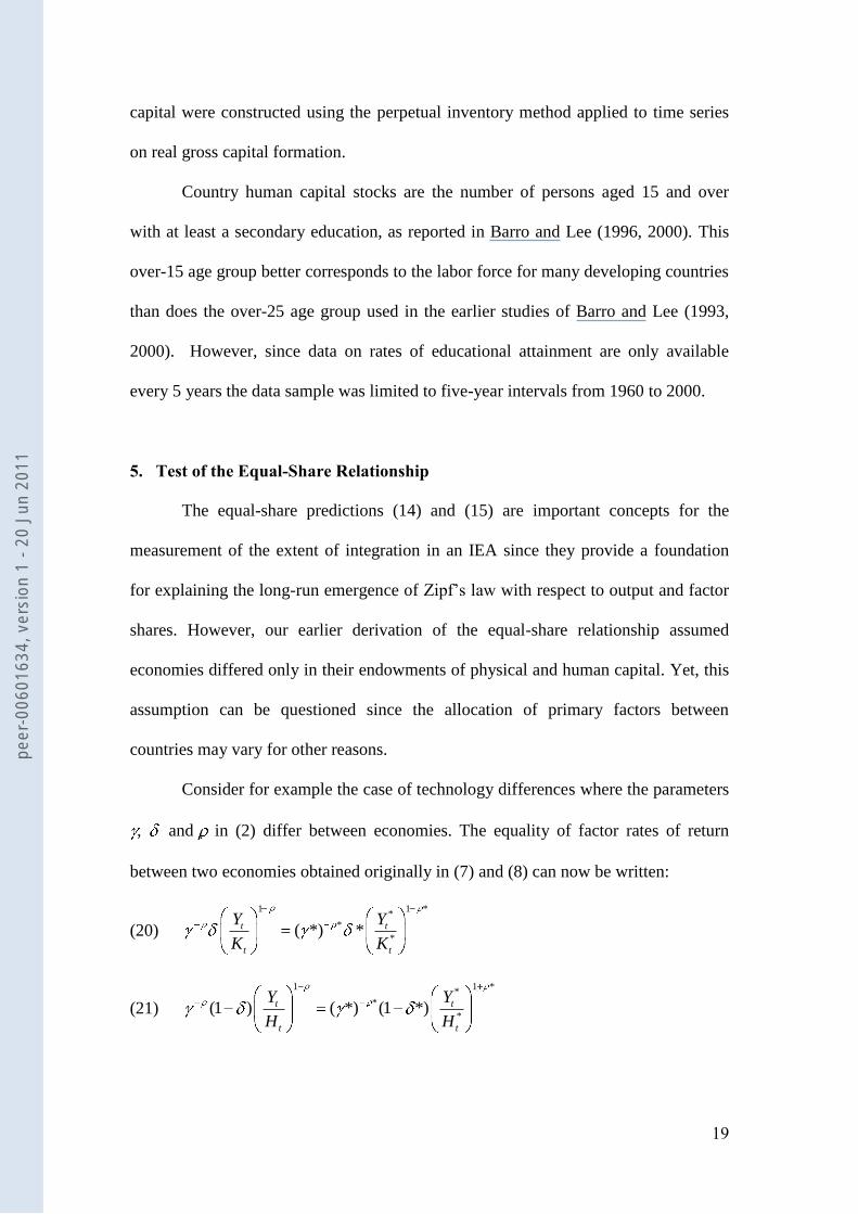
capital were constructed using the perpetual inventory method applied to time series

on real gross capital formation.

Country human capital stocks are the number of persons aged 15 and over

with at least a secondary education, as reported in Barro and Lee (1996, 2000). This

over-15 age group better corresponds to the labor force for many developing countries

than does the over-25 age group used in the earlier studies of Barro and Lee (1993,

2000). However, since data on rates of educational attainment are only available

every 5 years the data sample was limited to five-year intervals from 1960 to 2000.

5. Test of the Equal-Share Relationship

The equal-share predictions (14) and (15) are important concepts for the

measurement of the extent of integration in an IEA since they provide a foundation

for explaining the long-run emergence of Zipf‟s law with respect to output and factor

shares. However, our earlier derivation of the equal-share relationship assumed

economies differed only in their endowments of physical and human capital. Yet, this

assumption can be questioned since the allocation of primary factors between

countries may vary for other reasons.

Consider for example the case of technology differences where the parameters

, and in (2) differ between economies. The equality of factor rates of return

between two economies obtained originally in (7) and (8) can now be written:

(20)

1 1 **

*

*( *) *t t

t t

Y Y

K K

(21)

1 1 **

*

*(1 ) ( *) (1 *)t t

t t

Y Y

H H

peer

-006

0163

4, v

ersi

on 1

- 20

Jun

201

1

20

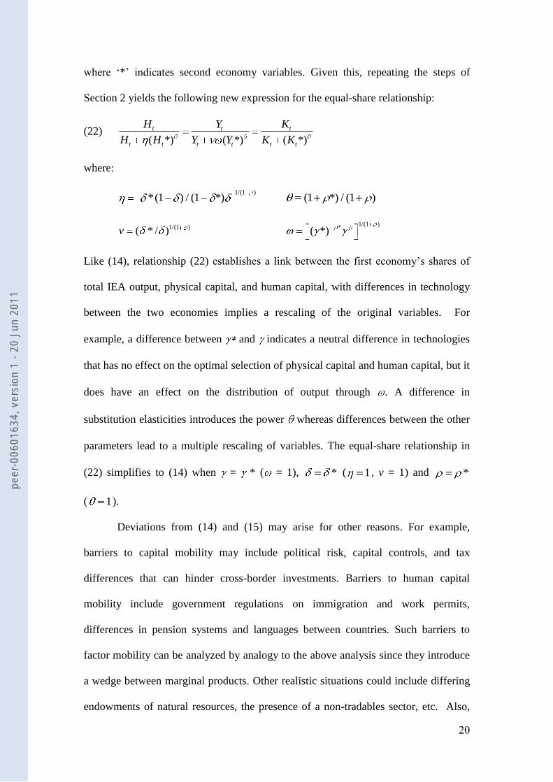
where „*‟ indicates second economy variables. Given this, repeating the steps of

Section 2 yields the following new expression for the equal-share relationship:

(22) ( *) ( *) ( *)

t t t

t t t t t t

H Y K

H H Y Y K K

where:

1/(1 )

*(1 ) / (1 *) (1 *) / (1 )

1/(1 )( * / )v 1/(1 )

*( *)

Like (14), relationship (22) establishes a link between the first economy‟s shares of

total IEA output, physical capital, and human capital, with differences in technology

between the two economies implies a rescaling of the original variables. For

example, a difference between and indicates a neutral difference in technologies

that has no effect on the optimal selection of physical capital and human capital, but it

does have an effect on the distribution of output through . A difference in

substitution elasticities introduces the power whereas differences between the other

parameters lead to a multiple rescaling of variables. The equal-share relationship in

(22) simplifies to (14) when = * ( = 1), * ( 1 , v = 1) and *

( 1).

Deviations from (14) and (15) may arise for other reasons. For example,

barriers to capital mobility may include political risk, capital controls, and tax

differences that can hinder cross-border investments. Barriers to human capital

mobility include government regulations on immigration and work permits,

differences in pension systems and languages between countries. Such barriers to

factor mobility can be analyzed by analogy to the above analysis since they introduce

a wedge between marginal products. Other realistic situations could include differing

endowments of natural resources, the presence of a non-tradables sector, etc. Also,

peer

-006

0163

4, v

ersi

on 1

- 20

Jun

201

1

21

the adding-up constraint of shares within each group may imply a non-linear

relationship among them. Given this, whether (14) and (15) are too simple to capture

a complex world is a matter of empirical verification, that is, the equal-share

prediction may not hold exactly but may hold in a statistical sense.

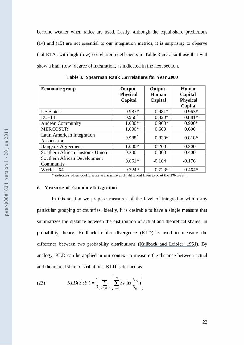
To provide an indication of the potential empirical validity of the equal-share

relationship, we can examine for a “weak” form of this relationship, namely, that

there will be conformity between (pair-wise) rankings of the output and factor shares

across members of an economic group. Table 3 provides evidence of this weaker

proposition by reporting Spearman rank correlation coefficients for pair-wise rankings

of the shares across our nine economic groups using year 2000 data. All rank

correlations are positive except for SADC, and are significant in 18 of the 27 cases.

High correlations are obtained for US States, Andean Community, EU-14 and LAIA,

indicating conformity between (pair-wise) rankings. The correlation coefficients in

the first column equal unity for three of the RTAs, indicating a perfect monotone

relationship between output and physical capital shares. The rank correlations

involving human capital are generally lower, showing less support for the equal-share

relationship. This might reflect that human capital as a primary factor is of less

importance in countries with unused resources and an ill-functioning labor market.

Despite exceptions, these results provide support for a “weak” form of the

equal-share relationship. This finding may reflect that the equalization of marginal

returns between countries is not used in absolute form but is instead transformed into

ratios. For example, the ratio of (9) to (10) yields the ratio of human to physical

capital in (11) and, using the properties of identities of ratios, we were able to derive

(14). Hence, wedges between marginal products like tariffs and transport costs, which

are ignored in our theoretical model but are present in the data, tend to cancel or

peer

-006

0163

4, v

ersi

on 1

- 20

Jun

201

1

22

become weaker when ratios are used. Lastly, although the equal-share predictions

(14) and (15) are not essential to our integration metrics, it is surprising to observe

that RTAs with high (low) correlation coefficients in Table 3 are also those that will

show a high (low) degree of integration, as indicated in the next section.

Table 3. Spearman Rank Correlations for Year 2000

* indicates when coefficients are significantly different from zero at the 1% level.

6. Measures of Economic Integration

In this section we propose measures of the level of integration within any

particular grouping of countries. Ideally, it is desirable to have a single measure that

summarizes the distance between the distribution of actual and theoretical shares. In

probability theory, Kullback-Leibler divergence (KLD) is used to measure the

difference between two probability distributions (Kullback and Leibler, 1951). By

analogy, KLD can be applied in our context to measure the distance between actual

and theoretical share distributions. KLD is defined as:

(23) , , 1

1( : ) ln( )

3

Nnj

njt

j Y K H n njt

SKLD S S S

S

Economic group Output-

Physical

Capital

Output-

Human

Capital

Human

Capital-

Physical

Capital

US States 0.987*

0.981*

0.963*

EU–14 0.956*

0.820*

0.881*

Andean Community 1.000*

0.900*

0.900*

MERCOSUR 1.000*

0.600

0.600

Latin American Integration

Association 0.988

* 0.830*

0.818*

Bangkok Agreement 1.000*

0.200 0.200

Southern African Customs Union 0.200 0.000 0.400

Southern African Development

Community 0.661*

-0.164 -0.176

World – 64 0.724*

0.723*

0.464*

peer

-006

0163

4, v

ersi

on 1

- 20

Jun

201

1

23

In this formula, Snjt

is the observed share value at time t whereas njS is the

time-independent theoretical share. Values of KLD range between zero and infinity. It

is zero (complete integration) when the shares are pair-wise equal, i.e., nj njtS S at

date t for all n and j. Otherwise, observed deviations indicate how far a group of

economies is from full integration. One drawback of the index in (23) is that it is not

symmetric, in the sense that a deviation between an actual and theoretical share can be

negative or positive. This means that a zero value of KLD could arise either because

the distance between the shares is zero, or because the shares are equidistant around a

common mean. For this reason, the following symmetric version of Kullback-Leibler

divergence (SKLD) is often preferred:

(24) , , 1

1( : ) ( ) ln( )

3

Nnj

njt njt

j Y K H n njt

SSKLD S S S S

S

The values of the SKLD will be higher than those of KLD because all deviations

between actual and theoretical shares in the SKLD index are measured positively.

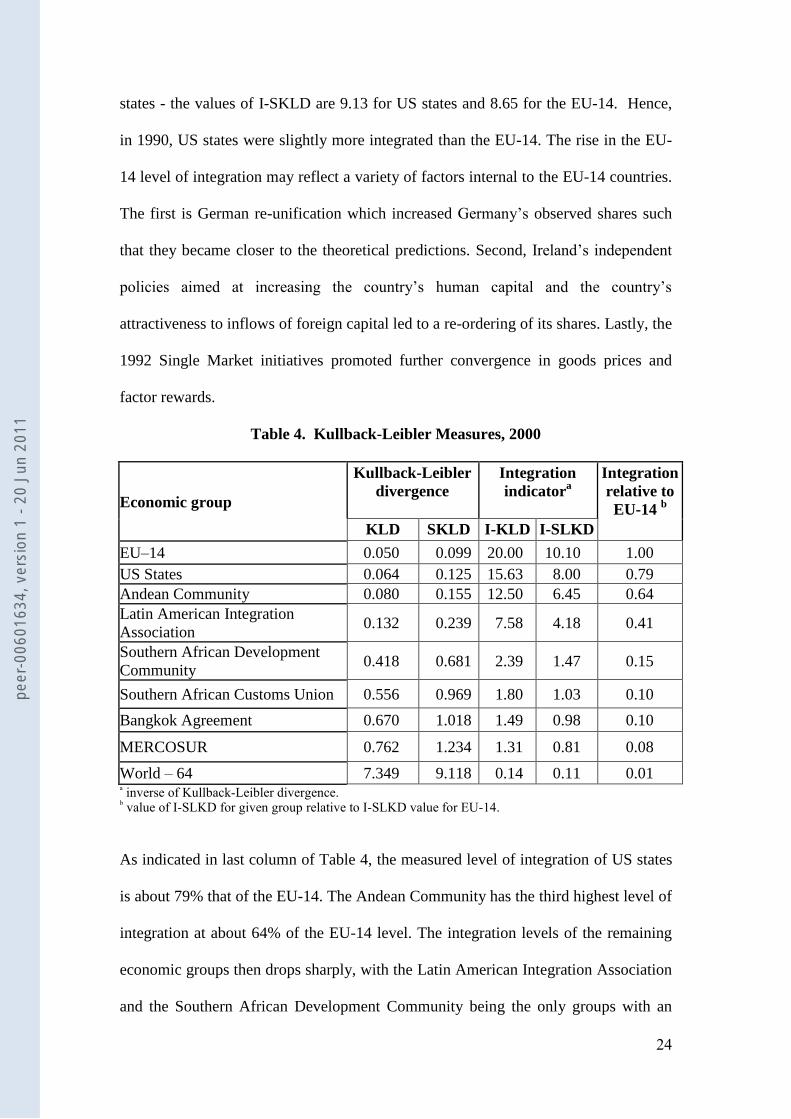
Table 4 presents the computed integration indicators (23) and (24) for US states and

our economic groupings listed in Table 1 using data for the year 2000. As our

measures (23) and (24) indicate the extent of divergence, we also invert their values to

obtain an indicator of the extent of integration rather than extent of divergence; the

inverted values of KLD and SKLD are denoted I-KLD and I-SLKD. The last column

of Table 4 lists the value of I-SLKD for each economic group as a percentage of the

value of I-SLKD obtained for the EU-14. The economic groups are listed in

descending order from most to least integrated on the basis of our measures.

As Table 4 indicates, the EU-14 has the highest level of integration in year

2000. This result is surprising, in that we expected US states to show the highest level

of integration. For 1990 - the other year that human capital data are available for US

peer

-006

0163

4, v

ersi

on 1

- 20

Jun

201

1

24

states - the values of I-SKLD are 9.13 for US states and 8.65 for the EU-14. Hence,

in 1990, US states were slightly more integrated than the EU-14. The rise in the EU-

14 level of integration may reflect a variety of factors internal to the EU-14 countries.

The first is German re-unification which increased Germany‟s observed shares such

that they became closer to the theoretical predictions. Second, Ireland‟s independent

policies aimed at increasing the country‟s human capital and the country‟s

attractiveness to inflows of foreign capital led to a re-ordering of its shares. Lastly, the

1992 Single Market initiatives promoted further convergence in goods prices and

factor rewards.

Table 4. Kullback-Leibler Measures, 2000

Economic group

Kullback-Leibler

divergence

Integration

indicatora

Integration

relative to

EU-14 b

KLD SKLD I-KLD I-SLKD

EU–14 0.050 0.099 20.00 10.10 1.00

US States 0.064 0.125 15.63 8.00 0.79

Andean Community 0.080 0.155 12.50 6.45 0.64

Latin American Integration

Association 0.132 0.239 7.58 4.18 0.41

Southern African Development

Community 0.418 0.681 2.39 1.47 0.15

Southern African Customs Union 0.556 0.969 1.80 1.03 0.10

Bangkok Agreement 0.670 1.018 1.49 0.98 0.10

MERCOSUR 0.762 1.234 1.31 0.81 0.08

World – 64 7.349 9.118 0.14 0.11 0.01 a inverse of Kullback-Leibler divergence.

b value of I-SLKD for given group relative to I-SLKD value for EU-14.

As indicated in last column of Table 4, the measured level of integration of US states

is about 79% that of the EU-14. The Andean Community has the third highest level of

integration at about 64% of the EU-14 level. The integration levels of the remaining

economic groups then drops sharply, with the Latin American Integration Association

and the Southern African Development Community being the only groups with an

peer

-006

0163

4, v

ersi

on 1

- 20

Jun

201

1

25

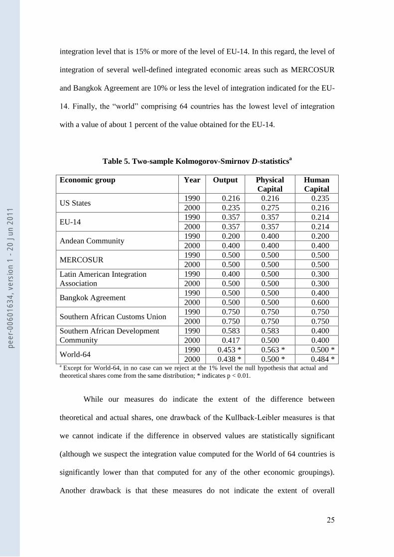
integration level that is 15% or more of the level of EU-14. In this regard, the level of

integration of several well-defined integrated economic areas such as MERCOSUR

and Bangkok Agreement are 10% or less the level of integration indicated for the EU-

14. Finally, the “world” comprising 64 countries has the lowest level of integration

with a value of about 1 percent of the value obtained for the EU-14.

Table 5. Two-sample Kolmogorov-Smirnov D-statisticsa

Economic group Year Output Physical

Capital

Human

Capital

US States 1990 0.216 0.216 0.235

2000 0.235 0.275 0.216

EU-14 1990 0.357 0.357 0.214

2000 0.357 0.357 0.214

Andean Community 1990 0.200 0.400 0.200

2000 0.400 0.400 0.400

MERCOSUR 1990 0.500 0.500 0.500

2000 0.500 0.500 0.500

Latin American Integration

Association

1990 0.400 0.500 0.300

2000 0.500 0.500 0.300

Bangkok Agreement 1990 0.500 0.500 0.400

2000 0.500 0.500 0.600

Southern African Customs Union 1990 0.750 0.750 0.750

2000 0.750 0.750 0.750

Southern African Development

Community

1990 0.583 0.583 0.400

2000 0.417 0.500 0.400

World-64 1990 0.453 * 0.563 * 0.500 *

2000 0.438 * 0.500 * 0.484 * a

Except for World-64, in no case can we reject at the 1% level the null hypothesis that actual and

theoretical shares come from the same distribution; * indicates p < 0.01.

While our measures do indicate the extent of the difference between

theoretical and actual shares, one drawback of the Kullback-Leibler measures is that

we cannot indicate if the difference in observed values are statistically significant

(although we suspect the integration value computed for the World of 64 countries is

significantly lower than that computed for any of the other economic groupings).

Another drawback is that these measures do not indicate the extent of overall

peer

-006

0163

4, v

ersi

on 1

- 20

Jun

201

1

26

conformity of the distributions of actual and theoretical shares, that is, whether the

actual and theoretical shares come from the same distribution. To address this issue,

Table 5 reports values of the non-parametric two-sample Kolmogorov-Smirnov (KS)

D-statistic which tests, for each economic grouping, whether the actual and theoretical

shares come from the same distribution.

The KS test is a “goodness of fit” test whose D-statistic measures the maximal

distance between two cumulative frequency distributions. In this test, the null

hypothesis is that both sets of shares come from a common distribution against the

alternative hypothesis that they do not. As the results in Table 5 indicate, we can

reject the null hypothesis that actual and theoretical shares arise from the same

distribution only for “World-64”. This finding suggests that only relatively small

values of our integration measures are indicative of limited integration within a given

economic area.11

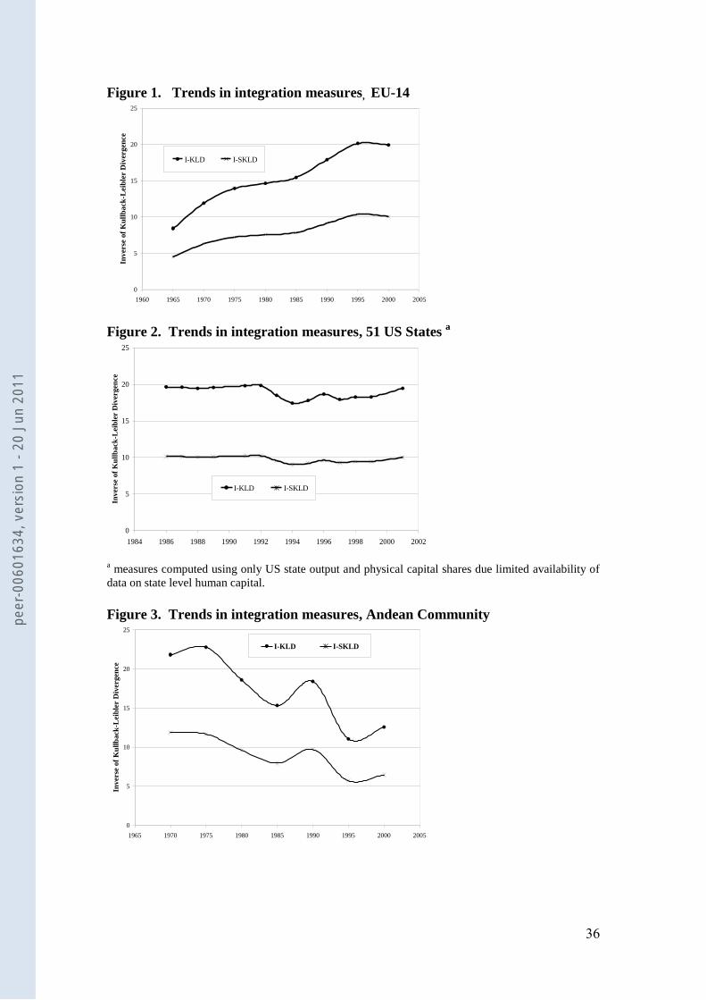
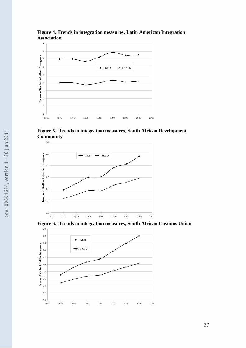
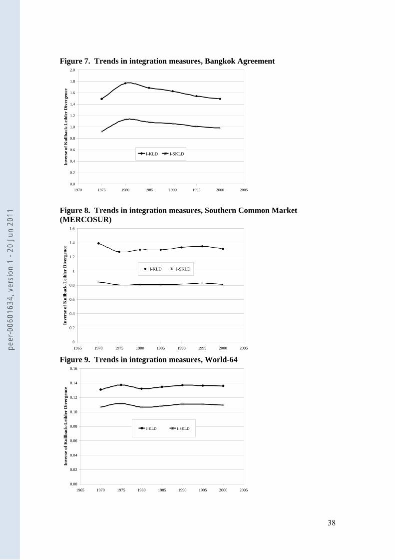
Figures 1 to 9 show the values of our integration measures I-KLD and I-

SKLD for each economic group at different points in time in order to visualize the

trend in integration in different regions of the world. Figures 1, 5 and 6 indicate

that the EU-14 and Africa RTAs evidence the most substantial increases in

integration over time. In contrast, Figure 2 shows the level of integration among US

states remained relatively constant over time, notwithstanding some movement

toward less integration in the 1990s as US states gained greater fiscal autonomy

implying less fiscal coordination. Figure 3 indicates that the relatively high level of

integration of the Andean Community indicated in Table 4 masks a marked decline

in its level of integration over time. Similarly, Figure 7 indicates a general decline

11

While popular, the Kolmogorov-Smirnov statistic is known to have low power, meaning that it more

often accepts the null hypothesis when it is false. However, it is possible to compute “delta-corrected”

KS statistics to assess if our results reflect the low power of the standard K-S statistic (e.g., Khamis,

2000).

peer

-006

0163

4, v

ersi

on 1

- 20

Jun

201

1

27

in the level of integration among Bangkok Agreement countries. Finally, Figure 9

indicates that the level of integration of our “world” of 64 countries increased only

slightly over time. This finding is perhaps surprising, given the common perception

that the processes of globalization have meant freer movement of goods and factors

among countries. Yet, this results is perhaps less surprising than at first glance,

since our theoretical requirements for complete integration include the complete

harmonization of economic as well as social policies.

[Insert Figures 1 to 9 about here]

7. Conclusion

This paper derived a set of specific relationships expected to arise between

economies that are members of a fully integrated economic area (IEA). In this regard,

a key relationship expected to hold for any IEA member is the equal-share

relationship that links a member‟s shares of total IEA output and factors supplies.

Given the equal-share relationship, it was then demonstrated that complete

harmonization of economic and social policies across IEA members implied that IEA

members output and factor shares would be expected to evolve randomly. The

randomness of output and factor share was then shown to imply that the distribution

of each share across IEA members would exhibit Zipf‟s Law. This result allowed us

to develop a method for computing, for any IEA with a fixed number of members, the

theoretically expected values of each IEA member‟s output and factor shares. These

theoretical share values were then used along with actual observed share values to

derive a measure of the level of integration within any economic group.

For the year 2000, the values of our integration measures indicated that the

group comprised of 14 “core” EU countries had the highest level of integration. US

states had the next highest level integration, measured to be about 79% of the

peer

-006

0163

4, v

ersi

on 1

- 20

Jun

201

1

28

integration level of the EU group. The Andean Community ranked third in terms of

its level of integration, measured to be about 64% of the integration level of the EU

country group. The remaining country groups all evidenced substantially lower levels

of integration, with values of our integration measures that were at most 41% of the

value obtained for the EU group. The least integrated group was a “world” comprising

64 countries, with a level of integration value only 1% the level exhibited by the EU

group. A surprising finding was that the measured level integration of our “world”

increased only slightly over time. Finally, formal statistical tests for the conformity

between the theoretical and actual distribution of shares indicated that, except of the

world of 64 countries, in no case could the hypothesis of non-integration be rejected.

Apart of offering, for the first time, a numerical indication of the degree of

integration, perhaps a key contribution of our analysis is to suggest that greater factor

mobility and reduced barriers to the flow of goods between countries can be expected

to lead to the emergence of the equal-share relationship. The latter, when coupled

with harmonized economic and social policies, offers new insights into the

distribution of economic activity in an integrated economic area and the relative

growth performance of its members. peer

-006

0163

4, v

ersi

on 1

- 20

Jun

201

1

29

References

Andersen, T.M., Herbertsson, T.T., 2003, “Measuring Globalization,” Institute of

Economic Studies, Working Paper W03:03.

Barro, R.J., 1999, “Determinants of Democracy,” Journal of Political Economy 107,

S158-S183.

Barro, R.J., Lee, J.W., 1993, “International Comparisons of Educational Attainment,”

Journal of Monetary Economics 32, 363-394.

Barro, R.J., Lee, J.W., 1996, “International Measures of Schooling Years and

Schooling Quality,” American Economic Review 86, 218-223.

Barro, R.J., Lee, J.W., 2000, “International Data on Educational Attainment: Updates

and Implications,” Center for International Development Working Paper 42

(Cambridge, M.A : Harvard University).

Barro, R.J., Sala-i-Martin, X., 2004, Economic Growth (Cambridge, M.A.: MIT

Press).

Bhagwati, J.N., 2002, Free Trade Today (Princeton: Princeton University Press).

Easterly, W., Levine, R., 1998, “Africa‟s Growth Tragedy: Policies and Ethnic

Divisions,” Quarterly Journal of Economics 112, 1203-1250.

Ethier, W.J., 2002,” Globalization, Globalization,” Tinbergen Institute Discussion

Paper TI 2002-088/2.

Gabaix, X., 1999, “Zipf‟s Law for Cities: An Explanation,” Quarterly Journal of

Economics 114(4), 739-767.

Gabaix, X., 2008, “Power Laws in Economics and Finance,” NBER Working Paper

14299.

Garofalo, G., Yamarik, S., 2002, “Regional Convergence: Evidence from a New

State-by-State Capital Stock Series,” Review of Economics and Statistics 82,

316-323.

Greenaway, D., Lloyd, P., Milner, C., 2001, “New Concepts and Measures of the

Globalization of Production,” Economics Letters 73, 57-63.

Hall, R.E., Jones, C.I., 1999, “Why Do Some Countries Produce So Much More

Output Per Worker Than Others?” Quarterly Journal of Economics 114, 83-116.

Helpman, E., Melitz, M.J., Yeaple, S.R., 2004, “Export versus FDI with

Heterogeneous Firms,” American Economic Review 94, 300-316.

peer

-006

0163

4, v

ersi

on 1

- 20

Jun

201

1

30

Heston, A., Summers, R., 1991a, “The Penn World Table (Mark 5): An Expanded Set

of International Comparisons, 1950-1988,” Quarterly Journal of Economics

106, 327-368.

Heston, A., Summers, R. 1991b, Penn World Table Version 5.6, Center for

International Comparisons at the University of Pennsylvania.

Heston, A., Summers, R., Aten, B., 2002, Penn World Table Version 6.1, Center for

International Comparisons at the University of Pennsylvania.

Hinloopen, J., van Marrewijk, C., 2006, “Comparative Advantage, the Rank-Size

Rule, and Zipf‟s Law,” Tinbergen Institute Discussion Paper 06-100/1.

International Monetary Fund, 2004, International Financial Statistics, (Washington

DC: International Monetary Fund).

Khamis, H. J., 2000, The two-stage δ-corrected Kolmogorov-Smirnov test. Journal of

Applied Statistics, 27(4): 439 – 450.

Kullback, S., Leibler, R.A., 1951,”On Information and Sufficiency,” Annals of

Mathematical Statistics 22, 79-86.

Lau, L., Jamison, D., and Louat, F. (1991), “Education and Productivity in

Developing Countries: an Aggregate Production Function Approach,” Report

no. WPS 612, The World Bank, March.

Markusen, J.R., 1983,”Factor Movements and Commodity Trade as Complements,”

Journal of International Economics 14, 341-356.

Mundell, R., 1957, “International Trade and Factor Mobility,” American Economic

Review 47, 321-335.

Munnell, A., 1990, “Why Has Productivity Growth Declined? Productivity and Public

Investment,” New England Economic Review, 407-438.

Nehru, V., Swanson, E., and Dubey, A. (1995), “A New Data Base on Human Capital

Stock: Sources, Methodology, and Results,” Journal of Development

Economics, 46, 379-401.

Rajan, R.G., Zingales, L., 1998, “Financial Dependence and Growth,” American

Economic Review 88, 559-586.

Ramey, G., Ramey, V.A., 1995, “Cross-country Evidence on the Link between

Volatility and Growth,” American Economic Review 85, 1138-1151.

Riezman, R., Whalley, J., Zhang, S., 2005, “Metrics Capturing the Degree to Which

Individual Economies are Globalized,” CESifo Working Paper No. 1450.

peer

-006

0163

4, v

ersi

on 1

- 20

Jun

201

1

31

Riezman, R., Whalley, J., Zhang, S., 2006, “Distance Measures between Free Trade

and Autarky for the World Economy,” CESifo Working Paper.

Rodrik, D., 1997, Has Globalization Gone Too Far?, (Washington DC: Institute for

International Economics).

Schreyer, P., Bignon, P.-E, Dupont, J., 2003, “OECD Capital Services Estimates:

Methodology and a First Set of Results,” OECD Statistics Working Paper,

2003/6.

Timmer, M.P., Ypma, G., van Ark, B., 2003, “IT in the European Union: Driving

Productivity Divergence?” GGDC Research Memorandum GD-67, University

of Groningen.

US Bureau of Economic Analysis, 2002, Fixed Assets and Consumer Durable Goods

for 1925-2001.

World Bank, 2005, Global Economic Prospects: Trade, Regionalism and

Development (Washington, DC: The World Bank).

peer

-006

0163

4, v

ersi

on 1

- 20

Jun

201

1

32

Appendix: Data Methods and Sources

US States

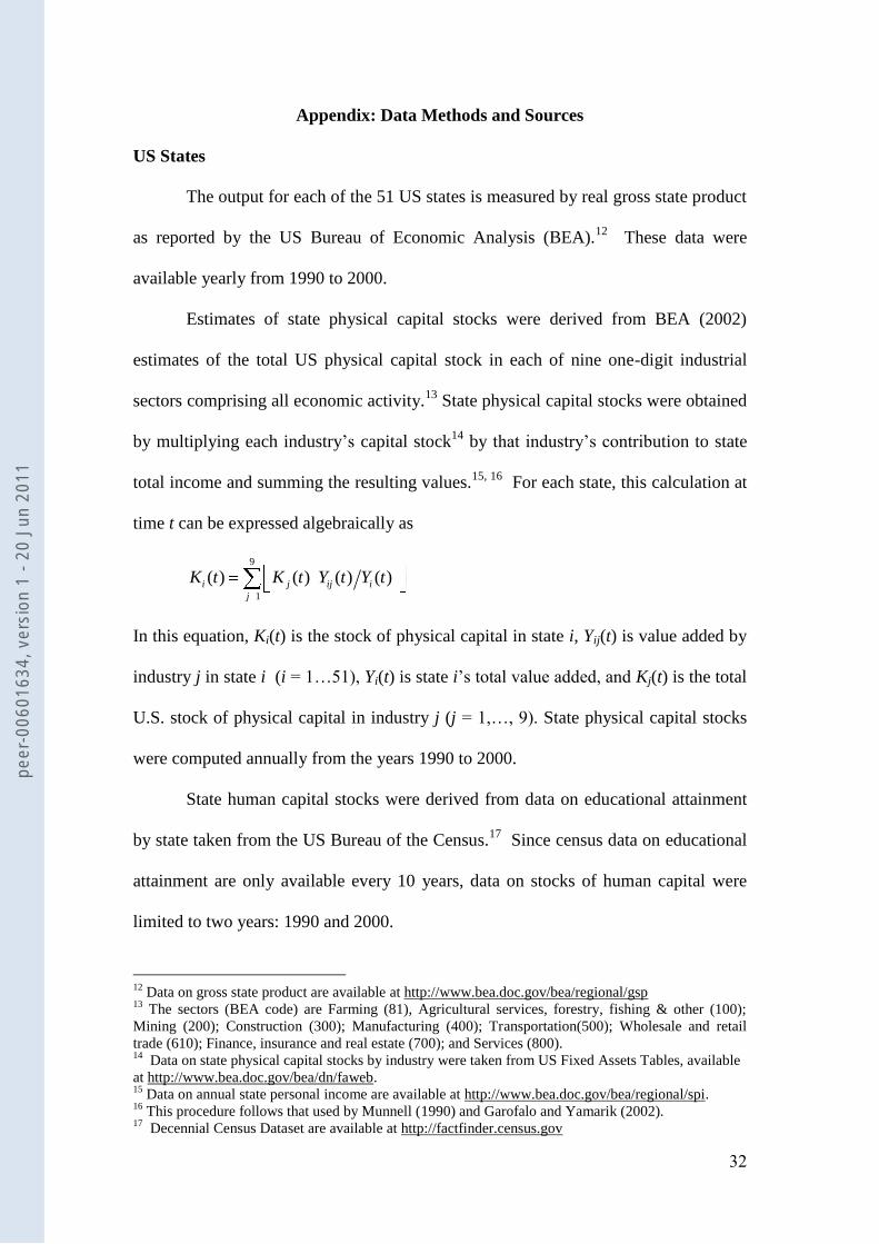
The output for each of the 51 US states is measured by real gross state product

as reported by the US Bureau of Economic Analysis (BEA).12

These data were

available yearly from 1990 to 2000.

Estimates of state physical capital stocks were derived from BEA (2002)

estimates of the total US physical capital stock in each of nine one-digit industrial

sectors comprising all economic activity.13

State physical capital stocks were obtained

by multiplying each industry‟s capital stock14

by that industry‟s contribution to state

total income and summing the resulting values.15, 16

For each state, this calculation at

time t can be expressed algebraically as

9

1

( ) ( ) ( ) ( )i j ij i

j

K t K t Y t Y t

In this equation, Ki(t) is the stock of physical capital in state i, Yij(t) is value added by

industry j in state i (i = 1…51), Yi(t) is state i‟s total value added, and Kj(t) is the total

U.S. stock of physical capital in industry j (j = 1,…, 9). State physical capital stocks

were computed annually from the years 1990 to 2000.

State human capital stocks were derived from data on educational attainment

by state taken from the US Bureau of the Census.17

Since census data on educational

attainment are only available every 10 years, data on stocks of human capital were

limited to two years: 1990 and 2000.

12

Data on gross state product are available at http://www.bea.doc.gov/bea/regional/gsp 13

The sectors (BEA code) are Farming (81), Agricultural services, forestry, fishing & other (100);

Mining (200); Construction (300); Manufacturing (400); Transportation(500); Wholesale and retail

trade (610); Finance, insurance and real estate (700); and Services (800). 14

Data on state physical capital stocks by industry were taken from US Fixed Assets Tables, available

at http://www.bea.doc.gov/bea/dn/faweb. 15

Data on annual state personal income are available at http://www.bea.doc.gov/bea/regional/spi. 16

This procedure follows that used by Munnell (1990) and Garofalo and Yamarik (2002). 17

Decennial Census Dataset are available at http://factfinder.census.gov

peer

-006

0163

4, v

ersi

on 1

- 20

Jun

201

1

33

EU Countries (EU-14)

Total output of each country is measured by real gross domestic product

(GDP) computed as the product of real GDP per capita (base year = 1996) and

population. Per capita GDP and population data were taken from Penn World Tables

6.1 (Heston, Summers and Aten, 2002).18

These data on output cover the period 1960

to 2000.

Data on physical capital stocks were derived from Penn World Tables 5.6

(Heston and Summers, 1991a; 1991b) which reports four data series for each country:

1) population, 2) physical capital stock per worker, 3) real GDP per capita and 4) real

GDP per worker.19

Country physical capital stocks were constructed as the product of

the first three series divided by the last series. Data cover the period 1965-1990. The

capital stock series for each EU country was updated to 2000 using data from Timmer

et al. (2003).20

Each country‟s stock of human capital stock was measured by multiplying the

percentage of its population aged 15 and over with at least a secondary level of

education by the country‟s total population. Data on rate of educational attainment by

country were taken from Barro and Lee (2000).21

Data on rate of educational

attainment were only available every 5 years, limiting data sample to five-year

intervals from 1960 to 2000.

Other Regions (Andean Community, MERCOSUR, LAIA, Bangkok, SACU,

SADC)

Output

18

Penn World Tables 6.1 is available at http://datacentre2.chass.utoronto.ca/pwt 19

Penn World Tables 5.6 is available at http://datacentre2.chass.utoronto.ca/pwt56 20

This physical capital database is available at http://www.ggdc.net/dseries/growth-accounting.shtml 21

Others studies that have used the Barro-Lee data include, for example, Rajan and Zingales (1998),

Ramey and Ramey (1995), Barro (1999), Easterly and Levine (1998), Hall and Jones (1999).

peer

-006

0163

4, v

ersi

on 1

- 20

Jun

201

1

34

Total output of each country is measured by real gross domestic product

(GDP) computed as the product of real GDP per capita (base year = 1996) and

population. Per capita GDP and population data were taken from Penn World Tables

6.1 (PWT 6.1) (Heston, Summers and Aten, 2002).22

These data cover the period

1960 to 2000. Missing values for Botswana, Cuba, Laos, Namibia and Swaziland

were obtained from Penn World Table 6.2. Missing values for Angola in PWT 6.1

and PWT 6.2 for years 1997-2000 were computed from the World Development

Indicators (WDI) database by applying the WDI growth rates of real GDP to the

existing real GDP data in PWT 6.1.

Physical Capital

Country physical capital stocks were computed in three steps. First, for

country n, real investment in each year was computed using the following formula:

* * /100nt nt nt ntI rgdpl k pop

Deta on the investment share of real GDP ( ntk ), real gross domestic product per capita

( ntrgdpl ) and total population ( ntpop ) were taken from PWT 6.1. Second,

depreciation rates were obtained from PWT 5.6 for the latest year available, 1992, and

for the following variables: 15% for producer durables; 3.5% for nonresidential

construction; 3.5% for other construction; 3.5% for residential construction; 24% for

transportation equipment. An overall depreciation rate was then computed as the

weighted average of the above depreciation rates with weights being the share of each

type of investment in the total. This was done for Malawi, Mauritius, Zambia,

Zimbabwe, Bolivia, Colombia, Ecuador, Venezuela and India. For countries with

lacking data on depreciation rates, the average of the depreciation rates of countries in

the same trade agreement were used instead., The depreciation rate for Angola,

22

Penn World Tables 6.1 is available at http://datacentre2.chass.utoronto.ca/pwt

peer

-006

0163

4, v

ersi

on 1

- 20

Jun

201

1

35

Botswana, Lesotho, Mozambique, Namibia, South Africa, Swaziland and Tanzania is

the average of the depreciation rates of Malawi, Mauritius, Zambia and Zimbabwe;

the depreciation rate for Argentina, Brazil, Paraguay, Peru, Uruguay and Cuba is the

average of the depreciation rates of Bolivia, Colombia, Ecuador and Venezuela; the

depreciation rate for Bangladesh, China, Laos, Sri Lanka and Korea Republic is the

depreciation rate for India.

Given data on real investment and the rate of deprecation for each county, the

stock of physical capital at time t was constructed using the perpetual inventory

method:

1 *(1 )nt nt nt ntK K I

where Knt is stock of physical capital of country n at time (t – 1), nt its depreciation

rate, and its assumed that Kn0 = In0.

For Angola, Botswana, Cuba, Laos, Namibia and Swaziland PWT 6.2 was

used to obtain any missing values after conversion to base year 1996. Remaining

missing values for Angola from 1997 to 2000 were obtained using United Nations

data on Gross Capital Formation (base year = 1990) converted into 1996 values.

Human Capital

Each country‟s stock of human capital is measured as the product of its

population aged 15 and over and the percent of its population aged 15 and over with a

secondary level of education. This measure of human capital stock does not account

for differences in the quality of schooling across countries.23

23

Recent work has sought to improve on international measures of human capital. International test

scores of students at primary and secondary levels provide useful information on the quality of

education. The International Adult Literacy Survey is a very promising attempt to measure directly the

skills of workforce for international comparisons. However, these measures are at present restricted by

a limited sample that consists mostly of OECD countries (Barro and Lee, 2000).

peer

-006

0163

4, v

ersi

on 1

- 20

Jun

201

1

36

Figure 1. Trends in integration measures, EU-14

0

5

10

15

20

25

1960 1965 1970 1975 1980 1985 1990 1995 2000 2005

Inv

erse

of

Ku

llb

ack

-Leib

ler D

iverg

en

ce

I-KLD I-SKLD

Figure 2. Trends in integration measures, 51 US States

a

0

5

10

15

20

25

1984 1986 1988 1990 1992 1994 1996 1998 2000 2002

Inv

erse

of

Ku

llb

ack

-Leib

ler D

iverg

en

ce

I-KLD I-SKLD

a measures computed using only US state output and physical capital shares due limited availability of

data on state level human capital.

Figure 3. Trends in integration measures, Andean Community

0

5

10

15

20

25

1965 1970 1975 1980 1985 1990 1995 2000 2005

Inv

erse

of

Ku

llb

ack

-Leib

ler D

iverg

en

ce

I-KLD I-SKLD

peer

-006

0163

4, v

ersi

on 1

- 20

Jun

201

1

37

Figure 4. Trends in integration measures, Latin American Integration

Association

0

1

2

3

4

5

6

7

8

9

1965 1970 1975 1980 1985 1990 1995 2000 2005

Inv

erse

of

Ku

llb

ack

-Leib

ler D

iverg

en

ce

I-KLD I-SKLD

Figure 5. Trends in integration measures, South African Development

Community

0.0

0.5

1.0

1.5

2.0

2.5

3.0

1965 1970 1975 1980 1985 1990 1995 2000 2005

Inver

se o

f K

ull

back

-Lei

ble

r D

iver

gen

ce

I-KLD I-SKLD

Figure 6. Trends in integration measures, South African Customs Union

0.0

0.2

0.4

0.6

0.8

1.0

1.2

1.4

1.6

1.8

2.0

1965 1970 1975 1980 1985 1990 1995 2000 2005

Inv

erse

of

Ku

llb

ack

-Lei

ble

r D

iver

gen

ce

I-KLD

I-SKLD

peer

-006

0163

4, v

ersi

on 1

- 20

Jun

201

1

38

Figure 7. Trends in integration measures, Bangkok Agreement

0.0

0.2

0.4

0.6

0.8

1.0

1.2

1.4

1.6

1.8

2.0

1970 1975 1980 1985 1990 1995 2000 2005

Inv

erse

of

Ku

llb

ack

-Lei

ble

r D

iver

gen

ce

I-KLD I-SKLD

Figure 8. Trends in integration measures, Southern Common Market

(MERCOSUR)

0

0.2

0.4

0.6

0.8

1

1.2

1.4

1.6

1965 1970 1975 1980 1985 1990 1995 2000 2005

Inver

se o

f K

ull

back

-Lei

ble

r D

iver

gen

ce

I-KLD I-SKLD

Figure 9. Trends in integration measures, World-64

0.00

0.02

0.04

0.06

0.08

0.10

0.12

0.14

0.16

1965 1970 1975 1980 1985 1990 1995 2000 2005

Inv

erse

of

Ku

llb

ack

-Lei

ble

r D

iver

gen

ce

I-KLD I-SKLD

peer

-006

0163

4, v

ersi

on 1

- 20

Jun

201

1