How do private equity fees vary across public pensions?∗

Juliane Begenau† Emil Siriwardane‡

March 2020

Abstract

We document large variation in net-of-fee performance across public pension funds invest-ing in the same private equity fund. In aggregate, these differences imply that the pensions inour sample would have earned $45 billion more – equivalent to $8.50 more per $100 invested– had they each received the best observed terms in their respective funds. There are also largepension-effects in the sense that some pensions systematically pay more fees than others wheninvesting in the same fund. With better terms, the 95th percentile pension would have earned$14.91 more per $100 invested compared to $1.12 for the 5th percentile pension. Attributeslike commitment size, overall size, relationships, and governance account for a modest amountof the pension effects, meaning similar pensions consistently pay different fees.

∗We are grateful to Jonathan Berk, Ted Berk, John Campbell, Peter DeMarzo, Mark Egan, Debbie Gregory, PaulGompers, Daniel Green, Robin Greenwood, Victoria Ivashina, Josh Lerner, Hanno Lustig, Monika Piazzesi, JoshRauh, Claudia Robles-Garcia, Amit Seru, Andrei Shleifer, Per Stromberg, Boris Vallee, and Luis Viceira, as wellas seminar participants at Harvard, the University of Washington, Stanford, and the Swedish House of Finance fortheir comments and discussions. Josh Coval, Chris Malloy, and Adi Sunderam in particular have given us invaluablefeedback at various stages of this project. Sid Beaumaster, Francesca Guiso, and Rick Kaser provided excellentresearch assistance. We are also indebted to Maeve McHugh and Michael Smyth at Preqin for their help compilingthe dataset for our analysis. First draft is from November 2019.†Begenau: Stanford GSB and NBER and CEPR. E-mail: begenau@stanford.edu‡Siriwardane: Harvard Business School. E-mail: esiriwardane@hbs.edu.

1 Introduction

Over the last twenty years, state and local defined-benefit pensions have increasingly shifted capital

out of traditional asset classes like fixed income and into private-market investment vehicles like

private equity and venture capital (Ivashina and Lerner, 2018). This shift has been accompanied

by an intense public policy debate over the fees charged by the general partners (GPs) of private-

market funds. In response, pensions in states like California, Pennsylvania, and New Jersey have

conducted lengthy internal audits of the fees they pay in private equity. While investment costs in

private markets are generally known to be large (Gompers and Lerner, 2010; Metrick and Yasuda,

2010; Phalippou et al., 2018), there is almost no systematic evidence on how they are determined,

mainly because fees are privately negotiated, rarely observed, and often not even recorded.1

In this paper, we shed some light on the costs public pensions face when investing in private

markets using detailed pension-level portfolio data from 1990 to 2018. We overcome the inherent

data opacity issues by comparing the net-of-fee cash flows received by different pensions invested

in the same private-market fund. Our definition of fees encompasses management fees, perfor-

mance fees, or any other costs that are borne by investors. Under plausible assumptions on the

structure of private-market funds that we discuss below, we can infer whether pensions investing

in the same fund pay different fees by measuring whether they earn different net-of-fee returns. In

other words, we use within-fund variation in net-of-fee returns to assess the degree to which fee

structures vary across investors in the same fund.

We start by developing a simple ex-post measure of within-fund fee dispersion that reflects how

much each pension could have potentially gained had it paid the lowest fees in the fund. Impor-

tantly, we do not observe all investors (i.e., the limited partners or LPs) in a given fund, meaning

true fee dispersion and hence potential gains would be larger if other unobserved investors (e.g.,

private endowments or family offices) pay lower fees than U.S. public pensions. We then aggregate

1Indeed, CalPERS – the largest U.S. public pension fund with over $350 billion in assets – recently came underscrutiny when it admitted that it did not fully track all of the fees it had paid to the private equity firms in which itinvests. CalPERS eventually disclosed that it paid about 700 basis points in annual all-in-costs for its private equityportfolio, which is orders of magnitude larger than the cost of passive investments in public equities.

1

potential gains over our entire sample, which covers roughly $500 billion of investments made by

200 U.S. pension funds into 2,600 private-market funds. According to our estimates, public pen-

sions would have earned nearly $45 billion more on their investments – equivalent to $8.50 more

per $100 invested – had each pension received the best ex-post fee contract in its respective funds.

This can be naturally interpreted as capital that was redistributed to fund managers or other un-

observed investors.2 We also find that aggregate potential gains due to within-fund fee dispersion

have been relatively stable through time, though they do vary across sub-asset classes. In tradi-

tional buyout private equity, potential gains due to fee dispersion are $10.90 per $100 invested

whereas in venture capital they are $5.00.

We then document the existence of large pension effects, meaning some pensions consistently

earn higher net-of-fee returns compared to others when investing in the same fund. Formally,

in a simple fixed-effects model, an F-test consistently rejects the null hypothesis of no pension

effects. The standard deviation of pension effects on investment performance is over 500 basis

points, highlighting the large impact that fees can have on pension-level investment returns. As an

alternative way to quantify how differences in fees translate to performance, we compute potential

gains from within-fund fee dispersion at the pension level. The 5th percentile fund could have

earned $1.12 more per $100 invested in private markets with different contract terms, whereas the

95th percentile pension could have earned $14.91.

The pattern of strong pension effects indicates that some pensions have systematically paid

higher fees than other pensions in their respective funds over the course of our sample. We argue

that this empirical finding is due to ex-ante differences in willingness to pay for the same fund.

There are several natural economic reasons to expect that pensions may differ in their willingness

to pay. For example, if some investors are better informed about GP skill than others, then those

investors may require fee breaks because their capital commitment will send a positive signal to

less informed investors. We explore several different mechanisms that might generate pension ef-

fects by mapping relative within-fund performance to pension characteristics like size, the capital

2Our potential gain estimate assumes that funds generate enough surplus to support this alternative fee schedule.In Section 3.4.2, we argue why this is plausible and provide an alternative estimate that is guaranteed to be feasible.

2

share in the fund, or experience as measured by number of investments in private-market investing.

We find evidence that larger pensions (overall AUM) with stronger ties to the GP of a fund tend

to outperform other investors in the fund. These results are consistent with the idea that securing

capital from these pensions creates value for GPs, possibly through positive signaling effects, and

some of this value flows to these pensions through lower fees. Pensions that have more mem-

ber representation on their boards also appear to pay lower fees, perhaps because more member

representation lowers agency frictions at public pensions (Andonov et al., 2018).

More importantly though, the aforementioned pension characteristics account for only a mod-

est amount of the total pension effects that we find in the data. Using our baseline fixed-effects

model, we still find strong statistical evidence of pension effects even after controlling for several

pension attributes (e.g., commitment size or experience in private markets). Strikingly, the distri-

bution of pension effects is virtually identically whether we control for observable characteristics

or not. In addition, controlling for pension characteristics does little to change which pension funds

stand to gain the most and how much they would gain if they paid similar fees as the best perform-

ing investors in our sample. This suggests that two seemingly similar pensions choose different

fee structures when investing in the same fund.

We then explore a possible mechanism through which fee structures vary in practice. Private-

market cost structures typically feature a fixed annual management fee and a performance-based

fee (carry). While we cannot observe the fee schedule for any investor-fund pair, we argue that

it is possible to use our data to infer the average within-fund range of carry rates. Intuitively,

within-fund differences in carry across investors should be easier to detect for more profitable

funds. We indeed find a strong relationship between fund performance and the range of net-of-fee

returns within a fund: after controlling for age, within-fund return dispersion is insensitive to fund

performance for unprofitable funds and is linearly increasing in performance for profitable funds.

Our estimates suggest that carry rates differ by around 10-20 percentage points across investors in

the average fund. Thus, carry appears to be an important dimension of how overall fees vary across

investors.

3

In the last part of the paper, we evaluate several explanations for our findings. Perhaps the

simplest is that observed within-fund variation in net-of-fee returns is not driven by fees, but is in-

stead due to measurement error or bespoke investment structures that may exist for some investors

in a fund (e.g., co-investment). To assess the possibility of measurement error, we directly filed

Freedom of Information Act (FOIA) requests for a subsample of pensions in our data and found

virtually no measurement error in this audit. Moreover, measurement error should bias us against

finding strong pension effects, yet we confirm that they are still present when measuring returns

using only realized cash flows.3 We also perform several quality checks of the data and argue that

any bias from returns on bespoke structures like co-investment are likely to be minimal. In addi-

tion, we find similar amounts of within-fund return variation in a sample where these structures

are known to be rarely employed. Fees therefore appear to be the primary source of within-fund

return variation on which our analysis is based.4

Investors in the same fund may rationally agree to pay different fees because they differ in their

information about manager skill, meaning they have heterogenous expectations about the gross

return of the fund. A profit-maximizing GP would then optimally elicit these expectational dif-

ferences and charge different fees accordingly, perhaps by offering a menu of fees. For rational

beliefs to drive our results, some pensions must have rationally chosen fee structures that led to

consistently higher costs over several private equity cycles. As discussed above, a related expla-

nation for fee dispersion is that GPs offer fee breaks to more informed investors in order to attract

less informed investors into the fund. This logic extends to the case when there are LP-GP specific

synergies. However, while size and relationships do correlate with lower fees, the fact that there

are large pension effects after controlling for such characteristics means that they do not fully ac-

count for any informational edges, signaling effects, or LP-GP synergies that might cause fees to

vary within funds.5

3See Figure 1 and its discussion in Section 3.1.1 for concrete examples of the time paths of net-of-fee returns fordifferent investors within the same fund.

4See Section 3.4 and Section 5 for an extensive discussion of these issues.5An analogous argument applies to differences in preferences. Fee dispersion could also arise if the marginal cost

of a GP partnering with some pensions is higher than for others. Still, given that we control for several attributes andU.S. public pensions have relatively homogenous reporting requirements, the pension effects that we document seem

4

Another potential interpretation of our findings is that optimization frictions lead some pensions

to consistently pay more fees than others even when investing in the same fund. Optimization

frictions might arise from biased beliefs about gross fund returns, a failure to fully internalize the

cost structure of private market investments, poor negotiation skill, or agency frictions. These

frictions are inherently difficult to identify empirically, though we do have suggestive evidence in

this direction: less than 5% of pension investors in our sample have any mention of performance

fees or carry on their annual report, despite the fact that we find differences in carry to be an

important component of price dispersion. Moreover, there is some evidence that frictions in labor

markets and political considerations distort public pension investment decisions (Dyck et al., 2018;

Andonov et al., 2018). Overall, it is hard to imagine that optimization frictions of this kind play no

role in explaining why pensions with similar characteristics – and therefore those that in principle

should have similar outside options when bargaining, similar preferences, and information – appear

to systematically pay different fees when investing in the same private-market fund.

Related Literature There is an active public policy debate about the extent to which investing

in private markets enhances the welfare of public pension beneficiaries, who are typically teach-

ers, police, firefighters, and other public servants. A fundamental issue in this debate is how any

value that is created by these investment vehicles gets split between investors and investment man-

agement firms. This is ultimately a question of how fees are determined and whether GPs price

discriminate.6 One way that we contribute to this debate relates to measurement, as the specific

contracts between GPs and investors are essentially unobservable. Thus, we view our approach to

estimating within-fund differences in fees as a first step in understanding how fees are determined

for pensions when they invest in private markets. Our finding of large pension effects implies price

dispersion in this setting has important distributional implications for pensions as well.

The fact that pensions systematically pay different fees when investing in the same fund may

unlikely to be explained by differences in marginal costs across investors.6There is a closely related debate on the value proposition of private markets. Several studies find that private equity

outperforms public equities (Harris et al., 2014; Robinson and Sensoy, 2016; Kaplan and Schoar, 2005), whereas othersargue that risk-adjusted returns are zero or negative (Sorensen et al., 2014; Gupta and Van Nieuwerburgh, 2019).

5

not be surprising to many, as price dispersion – often a result of price discrimination – is among

the first concepts taught in introductory microeconomics courses. Price dispersion is a ubiquitous

phenomena, occurring in automobile sales, airline tickets, mortgage markets and the mutual fund

industry (e.g., Knetter, 1989; Goldberg, 1996; Allen et al., 2019; Hortaçsu and Syverson, 2004).

In the context of private markets, co-investment and other special purposes vehicles have emerged

in the last few years as an imperfect way for the general partners of private market funds to differ-

entiate among their investors (Lerner, Mao, Schoar, and Zhang, 2018; Fang, Ivashina, and Lerner,

2015; Braun, Jenkinson, and Schemmerl, 2019). These investment arrangements offer select in-

vestors exposure to a different asset mix than the so-called main fund, typically at a reduced cost.

Relative to prior work on these alternative fund structures, we argue that price dispersion also oc-

curs more directly through fee contracts in the main fund. The observation that some pensions

consistently receive better terms is also consistent with Lerner et al. (2018), who show that GPs

offer certain special purposes vehicles only to a select set of investors.

What is perhaps more surprising is that differences in willingness to pay across pensions ap-

pear systematic and largely unexplained by easily-observable pension characteristics.7 This fact is

somewhat puzzling, as one might expect that rationally behaving pensions with similar attributes

(e.g., size or experience) should should in principle have similar information, expertise, and bar-

gaining power. In turn, they should pay similar same fees when investing in the same fund. While

it is difficult to unequivocally prove that pensions are not fully optimizing, the notion that they

fail to do so on behalf of their beneficiaries is consistent with prior research on agency and labor

market frictions at public pensions (Andonov et al., 2017, 2018; Dyck et al., 2018).

Our results also inform theories of fee determination for investors in the same fund. In the

benchmark model of Berk and Green (2004), within-fund fee dispersion is nonexistent because

investors are assumed to be homogenous in every dimension. In Bernstein and Winter (2012), con-

tracts may vary across investors if some create positive externalities for the fund, perhaps through

signaling effects. Our evidence suggests that these externalities must be mostly unrelated to size

7Because pensions with similar attributes are likely to have comparable marginal costs from the perspective of GPs,it seems natural to attribute the price dispersion that we observe to cross-pension differences in willingness to pay.

6

and several other pension characteristics in order to explain outcomes in private markets.

The paper is organized as follows. In Section 2, we provide background about the data and

present a simple accounting framework through which we interpret our results. Section 3 docu-

ments how large potential gains from within-fund fee dispersion are in aggregate. We also discuss

other potential sources for within-fund variation in net-of-fee returns and conduct several robust-

ness tests to ensure that fees are the primary source of this variation. In Section 4, we show that

some pensions systematically, that is across funds, pay higher fees than others when investing in

the same fund and measure the extent to which these pension effects can be explained by observ-

ables. Section 5 evaluates several interpretations for our results and concludes. Additional details

and results are available in an online appendix.

2 Data and Empirical Framework

2.1 Institutional details

The focus of this study is public pension investment into private market vehicles, namely private

equity (PE). A typical PE fund has two types of investors, the general partner (GP) and the limited

partners (LP). The GP is responsible for investing the fund’s total pool of capital and usually

contributes about 1 to 5% of their own capital in a fund. Thus, the bulk of the fund’s capital comes

from LPs, who are entities like pensions, endowments, and family offices. Most funds have a

lifespan of ten to fifteen years with a specific start and end date.

The standard life cycle of a PE fund has four stages. Stage 1 is the fundraising stage, which

can take 2+ years. Stage 2 is the investment stage, or the stage where deals are sourced and closed,

which takes 2-5+ years. Stage 3 involves managing and improving the companies in the portfolio,

which takes between 3-7+ years. Last, stage 4 is the exit stage at which the assets in the portfolio

are sold. Once an LP has committed capital to the fund during the first stage, the capital gets drawn,

i.e. employed by the GP, during the second and third stage. Finally, LPs receive distributions when

the GP liquidates the fund’s assets.

7

As a part of the limited partnership agreement between LPs and a GP, the GP receives a fee for

managing and deploying the fund’s capital on behalf of the LPs. The usual fee contract in private

market vehicles revolves around two main components: a management fee and a performance

fee, the latter of which is also known as carried interest. The standard contract has an annual

management fee of 1.25% to 2% on the LP’s committed capital and a 15-30% performance fee.

The performance fee is typically only charged after the fund has achieved a “preferred” return or

hurdle rate of at least 5-8%. After that, during the "the catch up period," the GP gets any positive

distributions until it realizes its carried interest (15-30%) on the cumulative distributions up to this

point. Any dollar distributions thereafter are split according to the agreed upon carried interest

arrangement. The limited partnership agreement between the LP and the GP often has several

other provisions (e.g., portfolio company cost-sharing) that determine the total cost born by LPs,

though management and carry are generally the two building blocks of fees.

2.2 Empirical Framework

We structure our empirical analysis around a general set of accounting identities that relates gross

and net-of-fee returns for each investor p in fund f . Let γp f t denote the cumulative gross return at

time t for investor p in fund f . We further decompose γp f t into a fund-wide and investor-specific

component:

γp f t = g f t + εp f t

where g f t is the cumulative gross return on fund f at time t that is common to all investors. εp f t is

any component of investor p’s gross return that is not shared by other investors. In practice, εp f t

might reflect co-investment arrangements or specific restrictions that investor p puts on fund f in

terms of its investment mandate (e.g., ESG).8

Next, define cp f t as the cumulative cost at time t that pension p must pay to the GP of fund f .

We will define specific elements of the cost structure in later sections, but for now it is useful to

8Some investors might have specific investment restrictions. For example, -they might not want to invest in anytobacco related companies. The -GP then offers the LP the fund without the non-conforming part.

8

think of it as encompassing any contractual feature of the limited partnership agreement that puts

a wedge between investor p’s gross return and its net-of-fee return. Thus, we define investor p’s

cumulative net-of-fee return return at time t as follows:

rp f t = γp f t− cp f t

= g f t + εp f t− cp f t

Our identifying assumption for most of the analysis in the paper is that εp f t ≈ 0 for all of

the pensions that we observe in fund f . This is not to say that εp f t is truly zero, but rather that

the net-of-fee returns that we observe are not primarily driven by deviations of investor p’s gross

performance from that of the other investors. This assumption would be violated if, for instance,

cash flows from co-investment are bundled with our data on net-of-fee returns. We discuss when

the assumption that εp f t ≈ 0 is more or less likely to hold extensively in Section 3.4.3.

Under the assumption that εp f t ≈ 0, the net-of-fee return for investor p is

rp f t = g f t− cp f t

Furthermore, if we define σ f (·) as the standard deviation operator across investors in fund f , then

within-fund variation in net-of-fee returns at any given point in time is driven by variation in costs

across investors:

σ f (rp f t) = σ f (cp f t)

In other words, assuming that all investors that we observe have the same before-cost exposure

to fund f , then any variation in net-of-fee returns across investors must be driven by variation in

the costs borne by investors in fund f . For this reason, we refer to within-fund return dispersion

and within-fund fee (or cost) dispersion interchangeably. In a broad sense, the goal of the paper

is to measure the extent of within-fund fee variation and understand its underlying sources. The

simple accounting framework laid out above implies that we can do so by studying the net-of-fee

9

performance of different investors in the same fund at a given point in time. After we document

variation in rp f t across investors, we then analyze how standard contractual features in private

markets may give rise to different cp f t .

2.3 Data Description

We obtain data from Preqin, a data provider that specializes in alternative assets markets. Preqin’s

data on private market investments is sourced primarily from legally-required annual reports, Free-

dom of Information Acts (FOIA) requests, and direct contact with investors. The data covers funds

from vintage year 1990 onward and contains cash-flow data on LP-level investment into individual

funds. The vast majority of investors in our data are U.S. public pension funds (83%) and UK pub-

lic pension funds (7%). Other investor types in our dataset include public university endowments,

government agencies, insurance companies, foundations, and private sector pensions. Throughout

the paper, we only use data on U.S. public pensions. The unit of observation is investor-fund-date.

We observe the amount of committed capital by the investor in the fund, the amount of capital that

has been “called” from the investor (i.e., actual contribution amounts), and the amount of capi-

tal that has been distributed back to the investor by the fund. These variables are all reported in

cumulative terms, and importantly, are reported net of all fees, including both management and

performance fees. We also observe the net asset value of each investor’s current investments in

the fund. For a given investor in a fund, the net asset value reflects the market value of invest-

ments that have not been liquidated yet. Together, the contributions, distributions, and remaining

net asset values allow us to calculate standard industry variables such as the internal rate of return

(which pensions also directly report) as well as the total return multiple on invested capital, defined

formally as:

rp f t ≡Market Valuep f t +Cumulative Distributionp f t

Invested Capitalp f t.

In practice, this measure of returns is frequently referred to as TVPI – it is simply the total return

received by p from investing in fund f , unadjusted for the timing of cash flows.

10

The fact that Preqin sources its data primarily through public pensions may cause selection bias

in the types of private-market funds that we observe. For example, public pensions may not have

access to the same set of private-market funds in which endowments invest. While selection of this

kind might bias estimates of, say, private equity returns as an asset class, it should not influence our

analysis of within-fund variation in returns across public pensions. Nonetheless, because our study

is based primarily on within-fund variation in returns, we have taken several steps to ensure the

quality of the Preqin data. Perhaps most importantly, we filed direct FOIA requests for data from a

subset of pensions in the Preqin sample. Reassuringly, in the vast majority of cases, the return data

from our direct FOIA requests perfectly matches the data in Preqin. The online appendix contains

much more detail on the results of this audit.

The online appendix also reports several additional quality checks that we perform on the

Preqin data, though we highlight the main ones here. We drop any observations where the vintage

of the fund is missing, the fund vintage is before 1990, or the data to compute TVPI is not available.

To be conservative we drop co-investments from the data, as co-investments have a different fee

and investment structure than a standard fund. We discuss the issue of co-investment and how it

might impact our results later in Section 4.4. To avoid any potential accounting issues with younger

funds, we also drop observations where the year of the report date is less than one year after the

fund’s reported close. Given our focus is on U.S. public pensions, we only include observations

from U.S. based investors where TVPI is computed in dollars.9

We further eliminate all observations within a fund-quarter where the range of TVPI across

investors is implausibly large. Our determination of whether a within-fund-quarter TVPI range is

implausibly large is based on two standard contractual features of fees in private markets. Building

on the accounting framework from Section 2.2, we approximate the cumulative costs borne by

9Most U.S. institutions report cash flows in dollars, even if the fund that they are invested in is denominated inanother currency. There are a few UK and Canadian institutions that report the cash flows of a subset of their funds indollars. We could potentially expand our investor universe if we allow non-dollar denominated cash flows and convertthem into dollars, though this would require additional assumptions on the appropriate timing of exchange rates.

11

investor p in fund f at time t as:

cp f t ≈ mp f × t +κp f ×max(g f t−1,0) (1)

where mp f is the annual management fee paid by investor p to fund f and κp f is the carry rate. As

discussed in Section 2.1, management fees and carry (or profit-sharing) are the two building blocks

of fees in private markets. Management fees are paid as a fixed percentage of assets and carry is

paid only when fund f is profitable, the latter of which is reflected in the second term above.10

With this approximate cost structure in the background, we assume that the maximum range of

carry rates within a given fund is crangef and the maximum range in management is mrange

f . At each

point in time, we then define the maximum allowable range of TVPI as

Allowable Range of TV PI f t = mrangef × t + crange

f ×max[TV PImax

f t −1,0]

(2)

where TV PImaxf t is the maximum observed TVPI in the fund as of time t. Our bounds on allowable

TVPI range are motivated by Equation (1). Specifically, we set the bounds assuming that one

investor gets the lowest combination of management and carry and another investor gets the highest

combination. Because we do not observe the gross-of-fee return for fund f in our data, we proxy

for it using the maximum observed TVPI. Under these assumptions, it is straightforward to show

that the range of TPVI within a fund at each point in time is defined as in Equation (2). Despite its

limitations, we prefer this economically-driven approach to data screening compared to dropping

fund-quarters where the range of TVPI exceeds a fixed threshold. This is because older and more

profitable funds should naturally have wider ranges of TVPI than younger, less profitable ones.

When implementing our filtering procedure, we set mrangef = 0.03 and crange

f = 0.3. We also drop

fund-quarter tuples where the within-fund range of DVPI, defined as the cumulative distributions

divided by invested capital, exceeds the allowable range. Overall, this procedure drops about 7% of

10In practice, the way that carry is charged to investors is more complicated than our simple model. For example, itis common that carry is only charged after returns clear a preferred hurdle rate.

12

distinct fund-quarters in the data, leaving us with a total of just over 300,000 pension-fund-quarter

observations. Henceforth, we refer to this as the master sample.

Given that our eventual focus will be on within-fund return dispersion, we also create what

we call the core sample by condensing the master sample as follows. First, we eliminate from the

complete dataset any fund-quarter that does not have at least two investors, as this is a necessary

requirement to compute within-fund dispersion. Then, for each fund, we choose the quarter with

the largest number of investors reporting returns, breaking ties with the latest date. We break ties

by taking the latest possible report date because it allows for any differences in management and

carry within the fund to play out over the longest possible horizon. By construction, the core

sample is unique at the investor-fund (p, f ) level.

2.4 Summary Statistics

Table 1 presents summary statistics for the core sample. There are 231 unique pension funds

investing in 2,535 different funds in the core sample. There are 916 general parters (GPs), implying

that the average GP has about 3 different funds. Of the 2,535 funds in the core sample, 42% are

private equity, 23% are venture capital, 21% are real estate, 11% are private debt, and the remaining

are either infrastructure or multi-strategy.

The median fund in the core sample is 7 years old and has 3 different investors. The median

investment size is about 30 million dollars, which accounts for about 3 percent of the median fund.

The median overall size of the pensions in our data is just under of 10 billion, though we see some

extremely large funds that have over 300 billion in assets. Our net-of-fee return measure TVPI

shows that the median multiple on invested capital is about 1.3, meaning that investors get about

$1.3 for each $1 invested.11

11It is important to note that TVPI does not account for differences in investment horizon across fund (e.g., olderversus newer funds), meaning some of cross-fund variation in TVPI is driven these age differences. In our analysisin Sections 3 and 4 we control for age differences. In addition, the maximum within-fund range of 1.12 occurred ina 1990s vintage fund whose total return on capital was around 8. Thus, for a fund of that age and profitability, evensmall differences in contract terms across investors can generate large differences in ex-post performance.

13

3 How large is within-fund dispersion performance?

We begin by measuring within-fund dispersion in net-of-fee returns and assessing how large this

dispersion is in aggregate. As our baseline measure of dispersion, we compute how much better

off investors would have been had they each earned the best net-of-fee return in their respective

funds. We document that the largest potential investor gains are in private equity funds and the

smallest potential gains are in venture capital funds. In aggregate, U.S. public pension funds in our

sample would have $8.50 more per $100 dollar invested if they had received the best returns in the

funds in which they invest. Based on the observed investment amounts, this amounts to roughly

$45 billion dollars of surplus that is either redistributed to other investors or the general partners

of private-market vehicles. After presenting our baseline results, we develop a lower bound on the

redistribution that occurs due to within-fund performance dispersion and explore the robustness of

our potential gain estimates.

3.1 Measuring fee dispersion

3.1.1 Illustrative Example

Because we do not observe the actual contract terms between LPs and GPs (pensions and invest-

ment management firms), we instead use ex-post dispersion in net-of-fee returns to detect differ-

ences in fees. As discussed in our motivating framework from Section 2.2, this is a reasonable

approach under the assumption that investors in the same fund have the same gross return. Intu-

itively, if two investors in the same fund have the same return before costs, then any difference in

their net-of-fee return must arise because they face different costs.

When operationalizing this logic in the data, we use TVPI as our main measure of returns. We

prefer this simple measure of returns over internal rates of return (IRRs) because the latter is easier

to manipulate. For instance, a recent paper by Andonov et al. (2018) that also uses data from

Preqin finds that some pensions selectively omit intermediate cash flows when returns are poor,

which makes computing accurate IRRs more challenging. And, in our inspection of the data, the

14

self-reported IRRs often have other issues; for example, it is often the case that reported IRRs are

not annualized during the early years of a fund’s life, but are annualized in later years. Compared

to IRRs, TVPIs are simpler and harder to distort. Of course, comparing TVPIs across investors or

a subset of investors in the same fund implicitly assumes that cash flows occur at the same time for

that subset. This seems more plausible in the context of private-market investment because of the

typical fund structure. With that said, we do our best to explicitly account for the timing of cash

flows in our subsequent analysis.

Figure 1 highlights the intuition of our approach using actual data. Panel A of the the figure

shows how TVPI evolves for one of the funds in our data. Our data-sharing agreement with Preqin

prevents us from revealing the identity of the fund, so for this example we will refer to it as “Fund

I”. There are over 20 different investors in Fund I, though for readability we only show TVPIs

for three investors, who we will call investors A, B, and C. These three investors have had very

different experiences in Fund I. Fifteen years from the fund’s close data, Investor A has earned

$2.45 per dollar invested, B has earned $2.59, and C has earned $2.82. In other words, despite

investing in the same fund, Investor C has outperformed A by 37 percentage points over the life

of the fund. Moreover, at each point in time, Investor C’s TVPI in Fund I has always exceeded

that of A’s. The patterns naturally imply that C has a fee contract that dominates A in Fund I. We

also show the evolution of DVPI for this fund, which is the ratio of cash distributions over invested

capital. DVPI does not depend on fund-value reporting standards across pensions or differing fund

value estimates. It is simply the ratio of the cumulative cash flow received to the cumulative cash

invested. It is clear that investors who outperform in TVPI terms also do so in terms of DVPI.

The preceding example focused on a relatively high–performing fund (e.g., the lowest TVPI is

well above 2). In Panel B of Figure 1, we show how TVPI and DVPI evolve for a lower-performing

fund in our data (“Fund II”). Fund II has 11 different investors and we focus on two (Investors X

and Y ) for the plot to again make it easier to read. After 11 years in Fund II, Investor X has earned

$1.43 for each dollar invested whereas Investor Y has earned $1.72. So Y has outperformed X

by 29 percentage points. For the first 18 quarters after close, both investors had nearly identical

15

TVPIs. After that, Y consistently outperformed X throughout the lifetime of the fund. Thus,

Investor Y appears to have gotten a better fee contract in Fund II than Investor X .12 As in the

previous example, the same investor that does well in terms of TVPI also does well in terms of

DVPI, the latter of which reflects actual cash distributions. Overall, these examples illustrate how

we use dispersion in within-fund performance to learn about within-fund differences in costs across

investors.

3.1.2 Potential Gains due to Fee Dispersion

Building on the preceding logic, within each fund f we define investor p’s potential gain at time t,

denoted sp f t , as:

sp f t = rmaxf t − rp f t (3)

where rmaxf t is the maximum TVPI earned by investors in fund f at time t. Intuitively, this is the

incremental return that investor p would have earned in fund f if it had received the best return in

the fund. For example, suppose that after 10 years pension fund A earned a TVPI of 1.5 in fund f .

Further suppose that this is the maximum observed TVPI for the fund. If pension fund B earned a

TVPI of 1.4 over the same horizon, then pension fund B’s potential gain in fund f would be 0.1.

Next, we convert the net-of-fee return gains to dollars by multiplying it by the amount that pension

p invested in fund f . Let ap f t be the amount that p invested in fund f as of time t. Then,

dp f t = ap f t× sp f t (4)

is pension p’s potential dollar gain at time t under the counterfactual. Continuing with our previous

example, if pension fund B invested $10 million in fund f , then its potential dollar gain would be

$1 million. This metric implicitly assumes that each fund f generates enough surplus to support

this counterfactual fee schedule. We discuss the plausibility of this assumption, as well as other

counterfactual exercises in Section 3.4.12In the online appendix, we show that there are similar patterns for both funds when looking at DVPI, which

measures returns only using distributed cash flows.

16

Comparison Group for Computing Potential Gains To compute the gain measures sp f t and

dp f t in the data, we need to be precise about the reference group that we use to compute rmaxf t . In

several of our robustness checks, we will consider different ways of defining the reference group.

In all cases, we will consider only investors in the same fund f with returns occurring in the same

quarter t. In certain cases, we will require further that returns for the comparison group occur in

the same month, which we will refer to as return-month restrictions.

Because it is most natural to compare investors who receive distributions from fund f on the

same schedule, in our most stringent tests we will additionally only compare investors who com-

mitted capital to fund f at the same time. A limitation of our data is that we do not have well-

populated information on the round of fundraising in which investor p committed to fund f . We

instead build a proxy using the quarter of the first observed return for investor p in fund f in our

data, which we denote by ip. Then, when computing our gain measures, we only compare in-

vestors in fund f at time t who also have the same ip. We call this an initial-quarter restriction on

the comparison group. Similarly, initial-month restrictions on the comparison group require that

the month of the first observed return be the same across investors in the comparison group.

3.2 Estimates across vintage-year and asset class

We now provide a sense for the magnitude of potential gains due to within-fund fee dispersion and

show how they vary through time and by asset class. For this particular analysis, we use the core

sample. As a reminder, for each fund f , the core sample keeps the quarter t where the most number

investors report returns, breaking ties with the last observed date. Using the core sample, we then

compute potential dollar gains dp f for each investor p in each of their funds f . Here, we suppress

time dependencies because the core sample is unique at the investor-fund level.

More formally, let Fv denote the set of funds (and investors in those funds) for vintage year v.

Then, the potential gains due to fee differences within funds from vintage year v are given by:

Gv =∑p, f∈Fv dp f

∑p, f∈Fv ap f.

17

where dp f is defined in Equation 4 and ap f is the amount that p has invested in fund f . When

computing potential gains for this subsection, we compare the last observed return of investors in

the same fund, conditional on returns occurring in the same quarter. Furthermore, we require that

funds be at least 5 years old (i.e., the observed return is at least 5 years after the fund vintage)

to ensure that differences in both management and carry have adequate time to impact net-of-fee

returns.

Panel A of Figure 2 shows that potential gains typically range between 5% and 12% of dollars

invested. The bars corresponding to the left axis plot Gv for each vintage year in our sample. The

maroon line in Figure 2 Panel A corresponds to the right axis and shows the number of investor-

manager pairs in each vintage year. Unsurprisingly, our underlying sample is less populated for

funds in the 1990s, though as risen steadily over time. The peak number of investor-manager pairs

occurred in 2006 and 2007 during the pre-crisis boom in private equity. In terms of potential gains,

one might expect that within-fund fee differences would trend down through time as the private

equity industry matured and investors became more comfortable with the nuances of fund-raising

and fee negotiation. However, there are no obvious temporal patterns that immediately stand out

from the graph, suggesting that differences in within-fund fees – and hence differences in ex-post

performance – have not systematically changed through time.

Within private markets, there are several sub-asset classes like private equity, venture capital,

real estate, etc. We can develop a sense of how large fee differences are across these sub-asset

classes by computing potential gains within each one. Specifically, let Fy denote the set of fund-

investor pairs where the fund is in asset class y. Similar to our other aggregation techniques, we

define potential gains in asset class y as:

Gy =∑p, f∈Fy dp f

∑p, f∈Fy ap f.

Panel B of Figure 2 shows plots our estimate of Gy by asset class. The figure reveals fairly large

differences across the sub-asset classes in terms of within-fund fee dispersion. In private equity,

18

within-fund fee dispersion is large enough that investors would have $10.90 more per $100 invested

had they all received the best ex-post fee in their respective funds. Again, best in this context is

defined relative to the other investors that we see in our data. Infrastructure, real estate, and private

debt all display relatively similar patterns in terms of the size of within-fund fee dispersion, with

gains ranging from $7.50-7.90 per $100 invested. Interestingly, potential gains due to within-fund

fee differences are the smallest for venture capital and multi-strategy funds.13 For venture capital

funds, which make up over 20% of our data, potential gains are $5.00 per $100 invested, less than

half of what they are in private equity. In other words, investors in venture capital funds are much

more likely to receive similar terms than when investing in private equity.

3.3 Aggregate Estimates for U.S. Pension Funds

Next, we consider how within-fund fee differences have impacted the performance of U.S. pension

funds. To aggregate across pensions and funds, we simply sum the dollar shortfall and scale it by

the total amount invested in our dataset:

GA =∑p, f dp f

∑p, f ap f

where the summations are only over U.S. pensions. GA measures how much better off pensions

would be if they received the best return in each of the funds in which they invested. Put differently,

GA captures how much extra surplus U.S. pensions would have captured had they been given the

best (ex-post) fee terms in each of their funds.14

Table 2 presents estimates of GA under different restrictions on how we compare investors when

computing their potential gains (see Section 3.1.2). In column (1), we consider only funds whose

status is liquidated and whose age is at least 10 years.15 Furthermore, when comparing returns

13There are only two multi-strategy funds in the sample for this analysis.14In this context, the best fee terms for fund f are defined based on the other investors that we observe in fund f ,

including LPs that are not U.S. pensions. Because this is certainly not the full set of investors in the fund, our measureof potential gain is therefore likely to understate the true potential gains.

15For a given fund-quarter, we define age as the year of the report date minus the year of the fund’s vintage.

19

across investors in the same fund, we impose initial-month and month-return restrictions. That is,

we require that the investors in the comparison group meet the following criteria: (i) the first month

that we observe a return in fund f must be the same across investors; and (ii) the return date that we

use to compute return dispersion must be in the same month (as opposed to the same quarter). As

previously discussed, these two restrictions are designed to ensure that we only compare investors

who invested in fund f at the same time and received cash flows from f on the same schedule.

To see more concretely how these restrictions work in practice, suppose that we observe three

different investors p = A,B,C in fund f . Further suppose that the first observation date for both

A and B occurs in October 2005 and the first observation date for investor C occurs in November

2005. In this case, we would discard information on C and look for the last observation after 2015

for both A and B, such that the month of the observation is the same. When two such observations

exist, we then compute potential gains as described above. If not, then no information from fund

f would be included in our aggregation analysis.16

Returning to column (1), we estimate 4.70% in potential gains when focusing on liquidated

funds with an age of at least 10 years, along with initial-month and return-month restrictions on in-

vestors. In column (2), we obtain a similar estimate of 4.57% when we relax the month-restrictions

and instead compute within-fund gains by comparing investors whose first and last return quarter

is the same. In both columns, the total number of investor-fund pairs is always less than 600. Given

there are thousands of investor-fund observations in our core sample, the potential gain estimates

in those columns is unlikely to be representative.

In columns (3)-(5) we broaden the subset of investor-funds over which we compute GA by con-

sidering all funds, not just those that have been liquidated. In all three computations, we impose

both initial-month and return-month restrictions. Considering funds that have not yet been liqui-

dated expands our sample substantially, as now we aggregate over at least 2,089 funds and 103

investors, depending on the specification. The difference between columns (3) through (5) is the

16As we explore below, we could require that the first observed return for the pensions that we compare occurs inthe same quarter. In this case, then we would include pension C in our return dispersion, provided that A, B, and Chave at least one return that occurs in the same quarter after 2015.

20

age restriction that we put on the funds that we consider. Column (3) is more conservative along

this dimension, as we only aggregate using data where the fund is at least 10 years old. The age

restrictions in columns (4) and (5) are 8 and 4, respectively. In all cases, the estimated GA rises

sharply, ranging from 6.8 to 8.5%.

Columns (6)-(8) mirrors the analysis in columns (3)-(5), though instead imposes initial-quarter

and return-quarter restrictions when computing within-fund potential gains. This is arguably the

most natural way to compare investors in the same fund because it is typical for fund distributions

to occur on a quarterly basis; thus, any within-quarter differences in pension reporting are more

likely due to differences in reporting practices as opposed to the actual timing of cash flows. The

estimates from these columns range from 6.8% to 8.4%, which is similar to columns (3)-(5). Thus,

month-restrictions versus quarter-restrictions do not appear to materially impact our results.

Columns (9) through (11) present another set of estimates of aggregate potential gains GA. In

these columns, when computing potential gains, we only require that investors be in the same fund

and that their returns occur in the same quarter (plus the usual age restrictions). The potential gain

estimates are the largest in this setup, ranging from 8.9% to 10.3%. Compared to the previous

estimates, our approach in columns (9) through (11) does not put restrictions on whether investors’

first observed return occurs in the same month or quarter. A valid concern here is that we may be

comparing investors who do not invest at the same time and thus the timing of their cash flows is

unlikely to be economically comparable. On the other hand, just because two pensions do not start

reporting returns to Preqin at the same time does not mean that they did not invest at the same time.

Overall, when considering a broad sample of funds (e.g., not only liquidated funds), the average

estimate of GA is 8.5%. In other words, the public pensions in our sample could have captured

$8.50 more in surplus for every $100 invested had they each received the best fee in their respective

funds. In dollar terms, potential gains in our sample are nearly $45 billion. More broadly, Ivashina

and Lerner (2018) report that public pensions have shifted over $1 trillion into private market

vehicles over the last decade or so. Assuming that our estimates of potential gains apply to this

larger sample, then public pensions could have captured nearly $85 billion of extra surplus had

21

they received the same fee contract as other investors in their funds.

It is important to reiterate that our estimate of potential gains is based on an ex-post measure

of cost. One way to think about it in ex-ante terms is as follows. Consider a fund that is ten years

old, has a gross TVPI of 1.7, and has only two pension investors, A and B. Further suppose that

pension A pays an annual management fee of 1.5% and a carry rate of 15%, whereas B pays a 2%

management fee and a carry rate of 20%. In this case, A’s net-of-fee TVPI after 10 years will be

1.445 (= 1.7 - 0.015×10 - 0.15×0.7) and B’s net-of-fee TVPI will be 1.36, both of which are near

the average TVPI in our data. Thus, the ex-post difference between investor A and B’s net-of-fee

return is 0.085, which also corresponds to our estimate of aggregate potential gains.

3.4 Robustness

3.4.1 Alternative Return Measures

DVPI Our analysis thus far has used TVPI to measure returns and hence within-fund fee disper-

sion. A potential concern is that pension funds differ in their reports of the fund’s market value.

The fee dispersion we observe may therefore just be due to different reporting standards across

pension funds. To address this concern, we use another common measure of returns in private

equity called the distributed value to paid-in capital ratio (DVPI). DVPI is the amount of cumula-

tive distributions received by investor p in fund f divided by their cumulative amount of invested

capital in the fund. DVPI is thus immune to differences in fund-value reporting standards across

pension funds.

As discussed in Section 3.1.1, Figure 1 shows examples of TVPI and DVPI time paths for

different investors in the same fund. For these examples, the performance ranking of investors is

consistent across both measures.

Quantitatively, aggregate fee dispersion is significant regardless of whether we use TVPI or

DVPI as return measure. The second row of Table 2 shows that our measurement of potential

gains are largely unaffected by market values: our aggregate potential gain measure still exhibits

significant fee dispersion when we use DVPI dispersion to measure fee dispersion. For complete-

22

ness, we repeat the preceding analysis using DVPI as a return measure and reassuringly find that

within-fund dispersion in performance – as captured by potential gains – are also fairly large.

IRR The internal rate of return (IRR) is another metric that is commonly used in practice to

evaluate performance. As discussed in Section 3.1.1, we prefer TVPI to IRR for several reasons

(e.g., IRRs are easier to manipulate). For robustness, in the online appendix we recompute potential

gains for U.S. pensions using IRRs instead of TVPIs. That is, for each fund f , we define investor

p’s potential IRR gain as the difference between the maximum observed IRR in the fund and

pension p’s IRR. We then aggregate over all investors and funds by weighting potential IRR gains

by the size of the investment by p in f . In aggregate, we find that U.S. public pensions would have

earned 1.65% more in annual IRR had each received the best terms in their respective funds.17

3.4.2 Lower Bound on Redistribution from Fee Dispersion

Our counterfactual gain calculation in Section 3.3 makes the following assumption on the size

of the surplus of the fund. We assume the fund returned enough surplus such that all pensions

invested with this fund could have received the same net-of-fee return per dollar invested as the

best performing public pension fund in the fund. This is a plausible assumption because we do

not observe all LPs in a given fund, particularly institutions like endowments, sovereign wealth

funds, or private pensions. Prior research has found that public pensions underperform these other

institutions when selecting private equity GPs (Lerner et al., 2007), so it seems reasonable to think

they also do so when investing in the same private-market fund.

With that said, for robustness we consider an alternative measure of fee dispersion that makes

no assumptions on the unobserved surplus of a given fund. Specifically, we calculate for each

pension fund the excess TVPI multiple over the worst performing pension fund:

ep f t = rp f t− rminf t ,

17This estimate is based on a combination of hand-reported IRRs by investors in our dataset and manually computedIRRs based on the reported cash flows. See the online appendix for more details.

23

where rminf t is the minimum observed return in fund f at time t. The dollar amount of excess is:

dep f t = ap f t× ep f t .

The dollar amount dep f t is how many more dollars pension fund p received over the pension fund

with the worst performance, i.e., highest fee schedule, in the same fund. Critically, this excess

gain measure of fee dispersion is budget-feasible because we only consider actual distributions

made by the fund to its pension investors. Using the core sample, we calculate the value-weighted

average excess gain over the worst performing fund as Ep =∑ f∈Fp de

p f∑ f∈Fp ap f

. This denotes the average

redistribution of investment gains on private equity funds across public pension funds. The second

row of Table 2 presents the results for Ep for different cuts of the core sample. For liquidated

funds, the excess gain over the worst performing pension fund is around 2.3%, though in the

broader sample it is as high as 4.3%. Assuming that we observe the worst performing investor,

these numbers represent a lower bound of excess gains some pensions leave on the table because

we only consider redistribution among the pensions that we observe in a given fund.18

3.4.3 Does within-fund dispersion in returns reflect differences in fees?

A natural concern could be that our findings are not driven by differences in fees but by specific

investor-fund arrangements such as co-investments or investor fund restrictions. Returning to our

accounting framework from Section 2.2, the cumulative net-of-fee return of investor p in fund f at

time t is:

rp f t = g f t + εp f t− cp f t

where g f t is the cumulative gross return on fund f that is common to all investors, εp f t is any

deviation of investor p from the common gross return, and cp f t is the cumulative cost paid by

investor p to the general partner of fund f . Throughout the paper, we have worked under the

assumption that εp f t ≈ 0, meaning that variation in rp f t across investors in the same fund is mainly

18Consistent with Sensoy et al. (2014) and Lerner et al. (2018), public pensions are among the least likely investorsto receive preferential treatment from GPs.

24

driven by variation in cp f t . In practice, there are several reasons why this assumption may be

less defensible for some investors or some funds. We now discuss two potential issues in more

detail and then estimate potential gains from within-fund return dispersion (as in Section 3) on a

subsample of the data where these channels are less likely to impact our results.

Co-investment Generally speaking, co-investment structures allow LPs to augment their expo-

sure to a given fund f – what we will call the “main fund”– by allocating additional capital towards

a particular deal or set of deals (see Fang et al. (2015) for an in-depth discussion of co-investment).

These opportunities are attractive from the perspective of the LPs because they are usually executed

at a substantially reduced cost relative to the main fund. To see the way in which co-investment

might bias our analysis, suppose there are p = 1, ...P investors in fund f and that investor P is the

only one who co-invests. In the main fund, assume that all investors receive the exact same terms.

Now suppose that investor P aggregates returns on its co-investment portfolio and the main fund

when reporting returns on fund f to Preqin. In this case, the extent to which εP f t deviates from zero

will depend on how much P’s co-investment portfolio differs in composition from the main fund.

Within-fund variation in rp f t across investors will therefore reflect the fact that P earned a different

composite gross return than other investors due to co-investment, though we would mistakenly

attribute this to differences in cost structures.

While it is difficult to know exactly how much co-investment may distort our analysis, we

have several reasons to believe the bias is small. First, and most importantly, it is our under-

standing that LPs generally list co-investments as a separate line item when reporting performance

to Preqin.19 As a concrete example, “Fortress Investment Fund IV” and “Fortress Investment

Fund IV - co-investment” are classified as two separate funds in our data. Thus, when comparing

investors in “Fortress Investment Fund IV”, it is unlikely that their net-of-fee returns reflects co-

investment. Moreover, for several of the largest LPs in our data, we have manually compared the

co-investments that they report on their websites and annual reports against the data from Preqin.

In all cases, we have found that cash flows from co-investments are indeed listed separately in19We thank Michael Smith and Maeve McHugh at Preqin for many helpful conversations about this issue.

25

the Preqin data for these investors. Because we drop all co-investments in the Preqin data, our

assumption that εp f t ≈ 0 for all observed investors in our data seems likely to be a reasonable

one.20

Even in the unlikely case where co-investments are not reported separately in the Preqin data,

there is good reason to believe that the degree of bias in our analysis is still small. While public

pensions are becoming increasingly more interested in co-investment opportunities, there is some

evidence to suggest that co-investment has not been a large part of their private-market portfolios

over the majority of our sample (1990-2018). According to data in 2014 from CEM Benchmarking,

who provides benchmarking services for thousands of pensions globally, only a small fraction of

U.S. public pensions (less than 5%) invest in private equity via co-investments. Furthermore, a

2014 survey by Preqin found that a wide range of institutional investors expressed strong interest in

expanding their co-investment capabilities, yet “relatively few LPs are being offered co-investment

rights by GPs in the Limited Partnership Agreement”.21 It is natural that co-investment would be

less relevant for smaller pensions because it requires the internal infrastructure to evaluate specific

portfolio companies and then deploy capital on relatively short notice.

As part of our data quality audit (see Internet Appendix Section A.3), we reached out to 50

pensions and asked them whether they were engaged in any special investment arrangement such

as a side-car deal or co-investment relationship. The vast majority responded that they had no such

arrangement. For the few cases that affirmed a co-investment arrangement we could verify that

they all reported their co-investment relationship separately.

For larger public pension funds, it also does not appear that co-investments currently dominate

their private equity portfolios. For example, CalPERS – the largest U.S. public pension fund

– reported in a May 2019 Investment Committee Meeting that it did not start a dedicated co-

investment program until 2011 and even that program was suspended in 2016. And, as of 2019,

20There is of course the possibility that LPs who coinvest receive different fee structures in the main fund. In thiscase, one would expect that they would pay higher fees in the main fund because those costs are offset by lower feesfrom coinvesting. If this were true, we should see larger LPs – those that are most likely to coinvest – have relativelylower net-of-fee returns in a given fund. As we showed in Section 4.2, the opposite is true in the data.

21The CEM report can be found here.. The Preqin survey further states that “there seems to be some contradictionbetween the attitudes towards and the actual co-investment activity occurring”.

26

only about 5% of the committed capital in CalPERS’ private equity portfolio is dedicated to co-

investment. Furthermore, in 2019 CalSTRS – the second largest U.S. public pension fund – was

estimated to have roughly 5% of its private equity portfolio in co-investments.22 Given that the

largest U.S. pensions have only modest amounts of co-investment over our sample, it is reasonable

to expect that smaller pensions have even less.

To summarize, while co-investment is clearly going to be an important component of public

pensions’ portfolios going forward, it seems less likely to bias our sample of public pension invest-

ment into private markets. Most importantly, co-investment returns appear to be listed separately in

the Preqin data and we drop them from our entire analysis. More broadly, for most investors in our

data, co-investment is likely to have been a small part of their portfolios over our sample. We also

have some survey information from Preqin for the years 2008 to 2017. In the core sample, nearly

90% of the investor-year observations list “No” or did not answer when asked if they co-invest with

their GPs. We therefore conclude that co-investment is unlikely to drive the within-fund dispersion

in net-of-fee returns that we observe in the data.

Other Investor-Specific Mandates Another reason why εp f t may deviate for some investors in

fund f is what we call investor-specific mandates. One prominent example that has boomed in

popularity in recent years are so-called environmental, social, and governance (ESG) restrictions.

These restrictions mean that investor p in fund f does not allocate capital to specific deals that

violate certain ESG criteria (e.g., no investment in firms with a large carbon footprint). More

generally, any such investor-specific restriction in fund f implies that investor p’s gross return in

the fund will necessarily differ from that of other investors.

Unfortunately, we do not have high-quality data on the extent to which pension-specific re-

strictions exist for the private-market funds in our sample. However, there is some information

available on ESG-related restrictions from the National Association of State Retirement Adminis-22Based on CalPERS Investment Committee Meeting presentation materials, co-investment was relatively sparse

prior to 2011. In response to a direct FOIA request, CalPERS also reported to us that less than 10% of their privateequity portfolio’s net-asset-value was attributable to co-investment as of 2018. The report on CalSTRS can be foundhere.

27

trators (NASRA), which is an association whose members are directors of a wide array of public

pension funds. On their website, NASRA reports that relatively few U.S. pension plans incorpo-

rate ESG in their investment process, though some of the larger U.S. pensions have started to do

so more in recent years.23 This is at least suggestive evidence that within-fund return dispersion

is probably not driven by investor-specific restrictions for most of the private-market funds in our

data. We develop this argument in more detail below.

Potential gains using smaller pensions prior to 2010 In lieu of the preceding discussion, we

repeat our computation of potential gains from Section 3.3 using a sample that is less likely to

be biased by co-investment and investor-specific mandates. Specifically, we drop large pensions

(assets over $100 bn) and private-market funds whose vintage year is after 2009, as co-investment

and investor-specific mandates like ESG are a recent trend and are less likely to be relevant for

smaller pensions.

Table A5 in the online appendix contains the results of this exercise. Reassuringly, our esti-

mates of aggregate potential gains due to within-fund return dispersion in this restricted sample

(~$7.70 per $100 invested) are broadly comparable to those using the all pensions and funds in

the core sample (~$8.50 per $100 invested). These findings support our argument that the within-

fund return dispersion that we document is most likely due to differences in fee-structures across

investors.

4 Do some investors consistently get better terms?

Having documented the aggregate consequences of within-fund performance dispersion, we now

explore whether some pensions consistently get better or worse terms when investing in the same

fund. Our approach to answering this question also allows us to assess whether any cross-pension

differences in fees that we observe in our data are statistically meaningful. In the last part of the

section, we map within-fund performance to characteristics like size or relationships, and decom-

23See the following link.

28

pose how much these characteristics can account for observed within-fund performance dispersion.

4.1 Measuring pension-effects

4.1.1 Baseline estimates

To test whether some pensions consistently outperform other investors in their respective funds,

we use the following regression:

rp f = α f +θp + εp f (5)

where rp f is the return of investor p in fund f , α f is a fund fixed effect, and θp is an investor fixed

effect. Because the regression contains fund fixed effects, the θ ’s capture whether some pensions

consistently earn above or below the average return in their respective funds. For this reason, we

refer to the θ ’s as pension-effects. Under the null hypothesis of no pension effects, the estimated

θ ’s should not be statistically distinguishable from each other. In other words, if fee contracts in a

given fund are randomly assigned to pensions, then we should not be able to reject an F-test that

the θ ’s are jointly equal to each other.

Panel A of Table 3 reports the F-tests and their associated p-values based on the core sample

described in Section 2.3. When moving from rows (1) to (3), we conduct the F-test for whether the

θ ’s are jointly equal based on funds that are at least one, four, and eight years old, respectively. In

all cases, the estimated F-statistic is large enough that we reject a null of no pension effects with a

p-value of less than 0.01.

The standard approach to conducting F-tests like those in Table 3 rely on parametric assump-

tions to test the null of no pension effects. As a robustness check, we run permutation tests where

we randomly assign returns to investors in fund f . For each random assignment, we calculate the

F-statistic from the test of equality across θ ’s. We repeat this procedure 1,000 times to generate

an empirical distribution of the estimated F-statistics, after which we compute a non-parametric

p-value based on where the actual F-statistic falls in this distribution. In the table, we denote the

p-values based on these permutation tests as p∗. Reassuringly, we comfortably reject the null of

29

no pension effects even when using these non-parametric p-values.

Though the preceding F-tests provide a statistical sense of the size of pension-effects in our

data, they are somewhat silent on the economic magnitude of such effects. To get a better sense of

how large the estimated pension-effects are in economic terms, we simply compute the distribution

of the estimated pension effects. Before doing so, we use an empirical Bayes procedure to account

for the fact that the true distribution of θ ’s will differ from our estimated distribution because

of sampling error (see Chetty et al. (2014) for an example in labor economics). Formally, let

θ denote the vector of estimated θ ’s based on regression (5) and θ denote the empirical Bayes

estimate. According to Egan, Matvos, and Seru (2018), the two are linked as follows:

θ =(θ −θ

)× F−1−2/(K−1)

F

where θ is the average of the estimated fixed effect vector θ , F is the F-statistic corresponding to

the joint test that the elements of θ are equal (reported in Panel A of Table 3), and K is the number

of pension effects. Intuitively, the F-statistic is larger when the pension-effects are estimated with

more precision, and in turn, the Bayes estimate does not shrink θ as much towards its mean.24

Panel B of Table 3 provides summary statistics on the distribution of the pension effects θ

for different estimation samples. Like with Panel A, the estimation samples only differ in the

minimum age of funds that are included when estimating regression (5). Differences in pension

effects are economically large, regardless of the age restriction that we impose on funds. For

example, when looking at funds that are at least eight years old, the standard deviation of pension

effects is 523 basis points. If we interpret the θ ’s as a measure of pension quality, then this suggests

that within a given fund, a one-standard deviation improvement in pension quality leads to a 523

basis point improvement in performance. The tails of the distribution of pension effects are even

more pronounced, as moving from the 10th to 90th percentile of quality translates to an increase

in within-fund performance of roughly 800 basis points.

24This particular form of the Bayes estimator relies on the assumption that both the true pension effects and theregression errors are normally distributed (Egan, Matvos, and Seru, 2018). In this case, the procedure can be easilyimplemented with standard regression outputs.

30

To provide some more context for the size of the pension effects, we compute a fund-level

measure of performance r f by taking the median TVPI of rp, f across investors in fund f . In funds

of at least eight years of age, moving from the 10th to 90th percentile of pension effects based on

within-fund performance is roughly equivalent to the difference in performance between the 50th

and 40th percentile private equity fund. In other words, within-fund variation in performance is as

large in some cases as between-fund variation in performance. More broadly, these results show

that some pensions consistently outperform others when investing in the same fund, both in an

economically and statistically significant sense.

4.1.2 Robustness using DVPI

One natural concern with our baseline estimates of pension effects is that they rely on TVPI as a

measure of returns. For each investor p in fund f , TVPI reflects actual cash distributions that have

been received by p as well as the reported net asset value of p’s non-liquidated positions in the

fund. Consequently, if some pensions consistently report net asset values differently than others,

then one might be concerned that this drives our estimate of pension effects. To alleviate these

concerns, in the online appendix we repeat our analysis from Section 4.1.1 using DVPI to measure

returns instead of TVPI. DVPI is based only cash distributions and is therefore not influenced by

how pensions report net asset values. When using DVPI to measure returns, we reassuringly find

once again strong evidence of large pension effects.

4.1.3 LP-GP Effects

To obtain further insight into the nature of pension effects and within-fund performance, we aug-

ment regression (5) as follows:

rp f g = α f +θp +ηpg + εp f g (6)

31

where rp f g is the return (TVPI) of investor p in fund f managed by general partner g. As before,

α f are fund effects and θp are pension effects. The new term in the regression is ηpg, which

are LP-GP fixed effects. In this setup, the pension effects θp measure the extent to which some

pensions outperform others in a given fund and the LP-GP effects ηpg measure any incremental

outperformance in funds managed by GP g. If, for instance, some investors receive better terms

than others in funds managed by a specific set of GPs, then we should reject an F-test of the joint

significance of the η’s.

Rows (4) through (6) of Panel A in Table 3 reports F-statistics and their associated p-values

from testing whether the θ ’s or the η’s are jointly equal. We continue to reject the null of no

pension effects, regardless of the conditions that we put on the age of funds. In addition, we reject

the null of no LP-GP effects (η’s) when using parametric p-values and non-parametric p-values

based on the permutation tests described in Section (4.1.1). This evidence suggests that LP-GP

relationships are important for explaining why some pensions consistently outperform others even

when investing in the same fund. We explore this finding in more detail below.

4.2 Observable Pension Characteristics

Given their importance in determining within-fund performance, we now investigate whether pen-

sion effects can be mapped to easily observable characteristics in the data. We do so by replacing

pension fixed effects in regression (5) and with observable characteristics as follows:

tp f = α f +βXp f + εp f , (7)

where Xp f is a vector of pension characteristics. Again, the fund fixed-effect α f means we are

comparing outcomes of different pensions in the same fund.

Observable Characteristics Xp f We consider the following set of observable characteristics.

For each investor p in fund f , we compute p’s share of the total fund as their commitment amount

32

divided by the total fund size. We include each investor’s share of the fund to account for potential

returns to scale when raising capital. That is, one might expect that GPs might reduce fees for

investors that account for a larger fraction of the fund, as this would then free up the GP to focus

on optimizing the investment portfolio instead of raising capital.

We also include two variables that capture the experience of each investor in private markets.

A priori, it is plausible to think that skill in fee negotiation improves as investors become more

experienced in the nature of private market investment vehicles. Thus, for each investor p and

fund f , we include the (log) number of funds in which p has invested in the ten years prior to f ’s

vintage year. We chose a ten year window to allow for turnover on the investment staff responsible

for negotiating fees at each pension. The second variable related to experience is specific to each

LP-GP pair and is motivated by our finding of LP-GP effects in Section 4.1.3. Specifically, for

each GP-LP pair, we count the number of funds that are managed by general partner g in which p

has invested. We use the full dataset to compute this measure because we want to capture settings

where a GP reduces fees for investor p in fund f in expectation that the investor will invest in

future funds raised by the GP.

When there is asymmetric information about its skill, a GP may also reduce fees for investors

that will send a positive signal to other potential investors. While it is difficult to capture all of the

dimensions through which an investor might be considered a so-called “cornerstone LP”, we focus

on size and commitment date. We code investor p as “Large” if its total assets under management

are over $100 billion at the time of fund f ’s launch, a designation that is reserved for a handful

of easily recognizable pensions in our data. In addition to the potential signaling effect that they

may have on fund raising, large investors are also more likely to possess the ability to deploy

large amounts of capital quickly, so size is likely related to the economies to scale in fund raising

discussed above. Due to data limitations, we are not able to observe if p is a first-close investor

in fund f , but we proxy for it based on whether p’s first report date in the master sample occurs

before other investors in fund f .

33

The last set of variables that we include in Xp f are related to pension governance.25 We include

board size to account for any potential coordination problems that may cause larger boards to sub-

optimally negotiate fee contracts. In addition, Andonov et al. (2018) find that pension boards with

more state officials are more likely to make poor investment decisions in private equity, likely due

to distortions from political considerations. Motivating by that finding, Xp f includes the percent

of pension p’s board that is made up of elected, as opposed to appointed, members. Intuitively,

boards that have more elected officials are more likely to focus only on the beneficiaries of the plan

when determining fee schedules with their general partners. For each pension and fund pair (p, f ),

the total number of board members and the percent of elected members are both measured as of

fund f ’s vintage year.

Results Table 4 reports OLS estimates of equation (7) using the core sample, again with several

restrictions on fund age. In all cases, we cluster standard errors by investor-and-vintage year

because many of the covariates in Xp f are repeated for investor p across all funds in a given

vintage year. In addition, for each age restriction, we estimate (7) with and without the governance

variables.

Consistent with our finding of LP-GP effects in Section 4.1.3, pensions that have a stronger

relationship with a GP – as measured by the number of funds in which they have invested with

that GP – tend to outperform other investors in funds managed by the GP. The point estimates on

LP-GP relationships range from 5.45 to 12.34 depending on the specification and are in most cases

statistically significant at conventional levels. These estimates indicate, in a given fund, being

invested in a different fund managed by the GP is worth roughly 9 basis points of returns. For

additional context, the standard deviation of LP-GP relationships in our data is about 4.

The regression estimates in Table 4 also indicate that being a large investor is an important

driver of within-fund performance dispersion. In terms of magnitude, when multiple pensions

invest in the same fund, large pensions receive contracts that generate an additional 90 to 159

25We are grateful to Josh Rauh for sharing the data on pension board composition from Andonov et al. (2018). Thedata ends in 2013, so we extend it to 2018 to better match our sample.

34

basis points in returns, depending on the life of the fund. The point estimate on the large-investor

indicator is measured with statistical precision, as we can always reject the null of no large-investor

effect with 95% confidence. As we discuss further in Section 5.1, there are several reasons why

larger pensions might create value for GPs, for instance through signaling effects or returns to scale

in fund raising. Our results suggest some of this value is at least partially passed to large pensions

through cost reductions.

In terms of governance, we find that pensions with a larger share of elected board members tend

to outperform other investors in their respective funds. This elected-board effect is statistically

significant with p < 0.05 regardless of the fund-age restriction that we impose when estimating

equation (7). To get a sense of magnitude, consider funds that are at least eight years in age. For

this subsample of the data, a one percentage point increase in the share of elected board members

translates to just under 3 basis points of within-fund performance. The 25th percentile pension has

no elected members whereas the 75th percentile pension has nearly half of its board elected. Thus,

moving from the 25th to 75th percentile pension in terms of elected board members translates to

nearly 150 basis points of improved performance, relative to other investors in the same fund.

When looking at the remaining covariates, the share of investor p in fund f , investor p’s ex-

perience at the time of capital commitment, and board size do not appear to have a statistically

meaningful impact on within-fund performance. These findings are perhaps not so surprising, as

it is natural to expect that many of these variables are subsumed by size and LP-GP relationships

when determining pension fee schedules. Interestingly, the impact of being an early-investor is

generally positive and around 30 basis points in TVPI units, depending on horizon. However, the

point estimate is always noisy, which is to be expected given that we do not have comprehensive

data on the timing of capital commitments.

4.3 How much of pension-effects are due to observables?

The preceding analysis showed that, within a given fund, pensions that are large, more connected

to the GP, and governed by more elected board members outperform other investors in the fund.

35

We now quantify how much these observable characteristics account for the pension effects that

we documented in Section 4.1. We do so in two complimentary ways. First, we reestimate pension

effects after controlling for observable characteristics, after which we compare the distribution of

these characteristic-adjusted pension effects to the raw ones from Section 4.1. Second, we compute

potential pension-level gains in an analogous fashion to the aggregate measures from Section 3. We

then regress returns on characteristics and reestimate pension-level gains based on the regression

residuals. Comparing the raw pension-level gains against the characteristic-adjusted gains provides

a sense of how much observable characteristics account for the within-fund return dispersion that

we see in the data.

4.3.1 Characteristic-Adjusted Pension Effects

To adjust our baseline pension effects for characteristics, we estimate the following regression:

rp f = α f +θp +βXp f + εp f (8)

where α f is a fund fixed-effect, θp are pension effects, and Xp f is the vector of characteristics

described in Section 4.2. Because we include Xp f in the regression, the estimated pension effects

θp capture whether some pensions consistently outperform others in their respective funds, even

after controlling for observable characteristics. We estimate equation (8) using OLS and conduct

an F-test for the null that the θ ’s are jointly equal to each other. We then apply the empirical Bayes

procedure from Section 4.1 to adjust the θ ’s for estimation error.

The last three rows of Table 3 summarize the F-tests for the subsample of funds that are at

least one, four, and eight years old, respectively. In all cases, even when including observable

characteristics, we still consistently reject the null of no pension effects with p < 0.01. This is

true when we use standard p-values or when we use non-parametric ones generated using the

permutation tests described in Section 4.1.1. Thus, from a statistical perspective, the observable

characteristics we consider do not account for the strong pension effects are present in the data.

36

To develop a sense of economic magnitude, Figure 3 plots the distribution of the raw pension

effects from Section 4.1 against the characteristic-adjusted pension effects from equation (8). The

two curves are virtually indistinguishable from each other, indicating that some pensions consis-

tently outperform others in the same fund by a sizable margin, even after for accounting for at-

tributes like commitment size, overall size, LP-GP relationships, and governance. Put differently,

these results imply that two pensions with similar characteristics still consistently pay different

costs when investing in the same private-market fund.

4.3.2 Characteristic-Adjusted Potential Gains

Next, we explore a complimentary way to quantify how much pensions observables explain and

why some consistently outperform others within the same fund. We begin our analysis by estimat-

ing potential gains at the investor level in a similar manner to how we estimated potential gains due

to within-fund fee dispersion in Section (3). Formally, let Fp be the set of funds in which investor

p invests. We aggregate potential dollar gains to the investor level as follows:

Gp =∑ f∈Fp dp f

∑ f∈Fp ap f.

As a reminder, dp f measures the dollar gain that investor p would have experienced had it received

the best observed return in fund f . ap f is the amount that p invests in fund f . Thus, Gp is simply

the sum of investor p’s potential gains, scaled by its total investment in all funds.

The green bars in Figure 4 summarize the distribution of Gp across the different U.S. public

pensions in our sample.26 There is considerable heterogeneity across pensions in terms of potential

gains due to fee differences. The standard deviation and interquartile range of potential gains

are 3.9% and 5.1%, respectively. The extremes of the potential-gains distribution are even more

pronounced. For example, the 5th and 95th percentile of Gp are 1.1% and 14.9%, respectively. In

other words, the private-market investments of the 5th-percentile pension would be 1.1% larger if26To ensure reporting of net asset values does not influence our gain measures, we recompute Gp using DVPI instead

of TVPI. The rank correlation between Gp computed using TVPI and DVPI is 70%, which suggests that any issueswith measuring net asset values do not drive our results.

37

it has received the best fee terms in its respective funds, whereas the 95th percentile pension would

be 14.9% larger.

To understand how much of the heterogeneity in Gp can be attributed to observable pension

characteristics, we obtain the residuals εp f from the following regression:

rp f = α f +βXp f + εp f ,

where once again rp f is the TVPI of investor p in fund f in the core sample. The vector of

characteristics Xp f is the same as before, but we exclude the variables related to governance in

order to include as many pensions in the analysis as possible. We have verified in unreported

results that we draw similar conclusions when including them. We then define the characteristic-

adjusted potential gain of investor p in fund f as:

dp f = (εmaxp f − εp f )×ap f

where εmaxp f is the maximum regression residual within fund f . The characteristic-adjusted potential

gain for investor p, dp f , aggregates as before:

Gp =∑ f∈Fp dp f

∑ f∈Fp ap f.

Intuitively, if observable characteristics account for a large amount within-fund variation in re-

turns, then the within-fund variation in εp f will be small and so too will Gp. The black outlined

bars in Figure 4 overlays the distribution of Gp on the raw estimates of Gp. The distribution of Gp

does tighten towards its mean to some extent, though it is clear that the distribution of Gp and Gp

largely line up with each other. Thus, consistent with our analysis of characteristic-adjusted pen-

sion effects, observable characteristics do not fully explain the wide heterogeneity across pensions

in terms of potential gains due to fee differences.

For confidentiality reasons, we are unable to provide estimates of potential gains due to fee-

38

dispersion at the pension level. However, we are able to aggregate them to the state level, which we

do in Figure 5. The figure shows the equal-weighted average of characteristic-adjusted gains Gp

by state, which for the reasons mentioned above is essentially the same as raw characteristic gains.

It is important to keep in mind that we do not observe all pensions in each state, so the figure paints

an incomplete picture in this regards. Overall, though the plot reinforces the finding that pensions

differ greatly in terms of how sensitive their returns are to better fee structures. Even after adjusting

for characteristics, the top decile of states in potential gains could earn on average $12.44 per $100

invested with better terms, whereas the bottom decile could earn on average $2.32.

4.4 The Mechanism

So far, we have documented that investors in the same private market vehicle very often earn

different net-of-fee returns. As outlined in our motivating framework from Section 2.2, it is natural

to attribute within-fund dispersion in returns to differential costs faced by investors in the same

fund. We discussed the plausibility of this assertion in more detail in Section 3.4.3. For now we

take it as given and explore a potential mechanism through which investors in the same fund may

be charged different fees.

To fix ideas, consider a fund f that has only two investors, p = A and B. For the sake of this

example, we assume that A and B have identical limited partnership agreements, except for their

carry rates. Under this assumption, from Section 2.3 we can write the cumulative net-of-fee returns

for both investors at time t as:

rA f t = g f t−m f × t−κA f ×max(g f t−1,0

)rB f t = g f t−m f × t−κB f ×max

(g f t−1,0

)where m f is, by assumption, the common annual management fee for fund f . Our assumption that

the two investors pay different rates of carry means that κA f 6= κB f and without loss of generality

39

we assume that κB f > κA f . Within fund f , the range ∆ f t in net-of-fee returns is:

∆ f t ≡ rA f t− rB f t

= (κB f −κA f )×max(g f t−1,0

)Differentiating with respect to g f t yields

∂∆

∂g f t=

0 if g f t < 1

κB f −κA f if g f t ≥ 1.(9)

Equation (9) implies that we can estimate the range of carry rates within a fund by measuring the

elasticity of the within-fund range of returns with respect to the gross level of returns. In other

words, within-fund differences in carry can be identified by plotting the within-fund range of net-

of-fee returns against the level of fund returns, after controlling for age. The relationship should

be flat in the region where the fund is not profitable (g f t < 1) because differences in carry do not

impact net-of-fee returns. In the region where the fund is profitable (g f t ≥ 1), the relationship

between within-fund range and gross returns should be linear, with the slope revealing differences

in fees.

Figure 6 evaluates this prediction in our data. Using the master sample, we compute the range

of returns ∆ f t within each fund at time t. We also proxy for the gross return in the fund g f t using

the maximum observed net-of-fee return at time t, which we denote by g f t . Figure 6 is a binscatter

plot of ∆ f t against g f t , after both have been residualized to the age fund f at time t.

As expected, when g f t is less than one there is a flat relationship between the range of within-

fund returns and the level of returns. Indeed, in this region, the estimated slope from a regression

of one on the other yields a point estimate of β = 0.00. In the region where g f t is greater than one,

there is a clear positive and linear relationship between ∆ f t and g f t . The slope estimate is 0.16, with

the 95% confidence interval spanning 0.10 to 0.22.27 Our interpretation of this finding is that carry

27The confidence interval for β is based on standard errors that are double-clustered by fund and vintage year.

40

rates differ by around 16 percentage points across investors for the average fund in our sample.

Any option-like features of the limited partnership agreement will influence the point estimate of

β = 0.16, so a broader interpretation is that embedded options in the fee-contract between LPs and

GPs are an important driver of within-fund dispersion in net-of-fee returns.

4.5 Are pensions

5 Interpretation and Conclusion

5.1 Interpretation

Our analysis revolves around variation in net-of-fee returns across investors in the same private-

market fund. Using this variation, we document strong pension effects in the sense that some

pensions consistently earn higher net-of-fee returns than others in the same fund. We now consider

several explanations for these facts.

Perhaps the simplest explanation is that the observed within-fund variation in net-of-fee re-

turns is due to measurement error or bespoke investment vehicles (e.g., co-investment). While it

is certainly possible that our data contains measurement error, the quality of the data should be

reasonably high given that it is mainly based on FOIA requests. As we document in the online

appendix, the quality of the data is further confirmed by the audit that we have conducted on a

subsample of pensions in the Preqin data.28 Moreover, measurement error should bias us against

finding strong pension effects, yet we do so even when using only realized cash flows (DVPI) to

compute returns. In addition, our cash flow data is unlikely to bundle returns from bespoke invest-

ment vehicles (see Section 3.4). Consequently, the within-fund variation in returns that we observe

is most likely driven by variation in fee structures across investors.

Dispersion in ex-post fees implies that investors in the same fund choose different fee structures

28We chose the subsample of pensions based on two criteria. First, we select the set of top and bottom ten pensionsbased on potential gains from Section 4.3. Second, we select the pensions in the funds with widest range of within-fundvariation in returns.

41

ex-ante. For instance, GPs may offer two contracts, one with high carry and low management fees

and another with low carry and high management fees. If investors are homogenous as in Berk

and Green (2004), then in theory these two fee structures could have the same ex-ante value but

nonetheless lead to different realized costs ex-post. However, we see this as a rather unlikely model

of equilibrium fee determination because it seems hard to rationalize why would GPs offer differ

contracts that all investors are truly indifferent between ex-ante.

GPs might offer investors different contracts if some are more costly to partner with than others.

For example, from the perspective of GPs, public pensions may be more costly investors because

they have more stringent reporting requirements than family offices or private endowments. In

this case, the GP would offer each pension a contract that reflects their marginal cost. This would

clearly generate ex-post fee dispersion. However, we only analyze public pensions and marginal

servicing costs seem unlikely to vary within this group because pensions have relatively homoge-

nous reporting and compliance requirements. Plus, to the extent that they do vary across pensions,

marginal costs should presumably correlate with size or experience in private markets. Further-

more, we show in the online appendix that there are strong pension effects when we control for

size in a more flexible, non-parametric fashion. The fact that we still find large pension effects after

controlling for these characteristics cuts against a cost channel and instead suggests that pensions

may differ in how they value a fee structure within a private-market fund.

In turn, persistent differences in willingness to pay across pensions can arise for several rea-

sons. One is preferences: if some pensions are more risk averse than others, they may prefer fee

schedules with low performance and high management fees, as these would deliver less volatile

cash flow streams. While preferences are difficult to measure empirically, in the online appendix

we proxy for risk aversion using each pension’s portfolio share in cash or cash equivalents. We

still find similarly sized pension effects when augmenting our set of controls with this risk aver-

sion proxy. In other words, for preferences to explain the data, it would have to be that are they are

mostly orthogonal to these attributes. Furthermore, a preference-based explanation would imply

that some pensions in our sample must be content to concede a fairly large amount in terms of

42

ex-post performance.

Pensions may also vary in their willingness to pay because they have different beliefs about

gross fund returns, which could arise from differences in information about GP skill. In the con-

text of private markets, it certainly seems reasonable to think that some pensions may be more

informed about GP skill than others. Informational asymmetries (or other LP-GP synergies) would

also explain why GPs appear to give fee breaks to large pensions with whom they have a strong

relationship, as this presumably aids in capital raising by sending a signal to less informed in-

vestors.29 Nonetheless, to explain the data, it would have to be that information edges and signal-

ing effects are largely orthogonal to attributes like size or relationships, as we still observe strong

pension-effects after controlling for these characteristics.30

One way to generate a disconnect between persistent informational edges and pension size is

as follows. Suppose that the portfolio managers at public pensions differ in their ability to evaluate

GPs, but labor market frictions restrict the mobility of talent from smaller, resource-constrained

plans to larger plans. Recent estimates of labor market frictions in the context of public pensions

suggest that they are rather sizable (Dyck et al., 2018). In this case, the equilibrium distribution

of talent at public pensions may be determined by forces that are uncorrelated with pension size

(e.g. geographical preferences). While discerning luck from skill is always difficult, this mech-

anism would account for why some pensions have chosen fee structures that have consistently

underperformed over a sample that spans three decades and several private equity cycles.

More generally, optimization frictions could feasibly generate pension effects as well. By op-

timization frictions, we mean any force that would cause some pensions to consistently choose

suboptimal fee structures, including irrational beliefs about gross fund returns, failure to fully in-

ternalize the cost structures, or agency frictions. While such frictions are hard to measure cleanly,

there are some empirical reasons to doubt that all public pensions have perfectly rational beliefs

29In practice, these sorts of fee breaks are often contractually implemented through most favored nation clauses(MFNs), which ensure that special investors will receive the best terms made available to other investors. MFNs alsoprovide their holders with an additional information edge and are not typically given to all LPs.

30In the online appendix, we provide some suggestive evidence that pension effects are not driven by return expec-tations on private equity as an asset class.

43

and choose their fee structures accordingly: less than 5% of the plans in our data have any mention

of performance fees or carry on their annual reports, despite the fact that differences in carry are

an important component of within-fund fee variation (see Section 4.4).31 Moreover, political con-

siderations appear to distort the investment decisions of public pensions (Andonov et al., 2018).

Overall, it is hard to imagine that these sorts of optimization frictions play no role in explaining

why pensions with similar characteristics – and therefore those that in principle should have sim-

ilar bargaining power, preferences, and information – appear to be systematically willing to pay

different fees when investing in the same private-market fund.

Regardless of the precise microfoundation, if pensions differ in their willingness to pay for

private-market investments then a profit-maximizing GP will do its best to exploit these differences

by price discriminating through fee structures. In practice, willingness to pay might be revealed

through negotiations or by offering LPs a menu of fees from which to choose. Our analysis collec-

tively suggests that price dispersion of this kind is large in the context of private markets and is at

least partly driven by pensions that fail to fully optimize when choosing their fee structures.

5.2 Conclusion

We use within-fund variation in net-of-fee returns to show that public pensions investing in the

same private-market fund can experience very different returns. In aggregate, within-fund fee

dispersion means that pensions could have earned $8.50 more per $100 invested had they each re-

ceived the fee structure of the best observed pension in their respective funds. Moreover, there are

consistent winners and losers in the sense that some pensions systematically pay more fees than

others even when investing in the same fund (i.e. pension effects). The pension effects that we

estimate are large in the cross-section, as some pensions could have earned as much as $15 more

per $100 more on their investments over our sample. Size, relationships, and governance account

31This statistic is based on the plans for which we could find annual reports in the master sample. Valuing theembedded-options in the fee structure requires estimates of the fund’s volatility. Given the lack of consensus on therisk of private equity as an asset class (Harris et al., 2014; Ang et al., 2018), generating a fund-level estimate ofvolatility and then applying an option-pricing model is a difficult problem for any investor to solve.

44

for some of the pension effects, but the majority appear orthogonal to these observable character-

istics. We argue that these facts are puzzling from the perspective of several rational models of

fee determination and consistent with the idea that public pensions fail to optimize when choos-

ing fees. While this evidence is far from conclusive, it highlights the value of further empirical

research on how U.S. public pensions structure fees in private-market investment vehicles. The

broader practical implication of our analysis is that public pensions should pay close attention to

the contracting terms they receive when investing in all forms of active management.

45

ReferencesAllen, J., R. Clark, and J.-F. Houde (2019). Search frictions and market power in negotiated-price

markets. Journal of Political Economy 127(4), 1550–1598.

Andonov, A. (2014). Delegated investment management in alternative assets. Working Paper.

Andonov, A., R. M. Bauer, and K. M. Cremers (2017). Pension fund asset allocation and liabilitydiscount rates. The Review of Financial Studies 30(8), 2555–2595.

Andonov, A., Y. V. Hochberg, and J. D. Rauh (2018). Political Representation and Governance:Evidence from the Investment Decisions of Public Pension Funds. The Journal of Finance.

Andonov, A. and J. D. Rauh (2019). The return expectations of institutional investors. SSRNWorking paper.

Ang, A., B. Chen, W. N. Goetzmann, and L. Phalippou (2018). Estimating private equity returnsfrom limited partner cash flows. The Journal of Finance 73(4), 1751–1783.

Begenau, J. and E. N. Siriwardane (2020a). How do private equity fees vary across public pen-sions? Working paper.

Begenau, J. and E. N. Siriwardane (2020b). What determines public pension investment decisions?Working paper.

Berk, J. B. and R. C. Green (2004). Mutual fund flows and performance in rational markets.Journal of political economy 112(6), 1269–1295.

Bernstein, S., J. Lerner, M. Sorenson, and P. Stromberg (2017). Private equity and industry perfor-mance. Management Science 63(4), 901–1269.

Bernstein, S. and E. Winter (2012). Contracting with heterogeneous externalities. American Eco-nomic Journal: Microeconomics 4, 50–76.

Bertrand, M. and A. Schoar (2003, 11). Managing with Style: The Effect of Managers on FirmPolicies*. The Quarterly Journal of Economics 118(4), 1169–1208.

Black, F. (1980). The tax advantages of pension fund investments in bonds. Working Paper 533,National Bureau of Economic Research.

Braun, R., T. Jenkinson, and C. Schemmerl (2019). Adverse selection and the performance ofprivate equity co-investments. Journal of Financial Economics.

Brown, J. R. and D. W. Wilcox (2009). Discounting state and local pension liabilities. The Ameri-can Economic Review 99(2), 538–542.

Campbell, J. Y., Y. L. Chan, and L. M. Viceira (2003). A multivariate model of strategic assetallocation. Journal of Financial Economics 67(1), 41 – 80.

46

Campbell, J. Y. and L. M. Viceira (2006). Strategic asset allocation for pension plans. In TheOxford Handbook of Pensions and Retirement Income. Oxford University Press.

Chetty, R., J. N. Friedman, N. Hilger, E. Saez, D. W. Schanzenbach, and D. Yagan (2011, 11).How Does Your Kindergarten Classroom Affect Your Earnings? Evidence from Project Star *.The Quarterly Journal of Economics 126(4), 1593–1660.

Chetty, R., J. N. Friedman, and J. E. Rockoff (2014, September). Measuring the impacts of teachersi: Evaluating bias in teacher value-added estimates. American Economic Review 104(9), 2593–2632.

Dyck, A., P. Manoel, and A. Morse (2018). Outrage and compensation in public pension perfor-mance. Working Paper.

Egan, M. L., G. Matvos, and A. Seru (2018). Arbitration with uninformed consumers. Technicalreport, National Bureau of Economic Research.

Fang, L., V. Ivashina, and J. Lerner (2015). The disintermediation of financial markets: Directinvesting in private equity. Journal of Financial Economics 116(1), 160 – 178.

Gennaioli, N., A. Shleifer, and R. Vishny (2015). Money doctors. The Journal of Finance 70(1),91–114.

Goldberg, P. K. (1996). Dealer price discrimination in new car purchases: Evidence from theconsumer expenditure survey. Journal of Political Economy 104(3), 622–654.

Gompers, P. A. and J. Lerner (2010). What drives venture capital fundraising? Brookings Paperson Economic Activity, 149.

Goyal, A. and S. Wahal (2008). The selection and termination of investment management firms byplan sponsors. The Journal of Finance 63(4), 1805–1847.

Grennan, M. (2013). Price discrimination and bargaining: Empirical evidence from medical de-vices. American Economic Review 103(1), 145–77.

Gupta, A. and S. Van Nieuwerburgh (2019). Valuing private equity investments strip by strip.Working Paper.

Harris, R. S., T. Jenkinson, and S. N. Kaplan (2014). Private equity performance: What do weknow? The Journal of Finance 69(5), 1851–1882.

Higson, C. and R. Stucke (2012). The performance of private equity. Available at SSRN 2009067.

Hochberg, Y. V. and J. D. Rauh (2012, 12). Local Overweighting and Underperformance: Evidencefrom Limited Partner Private Equity Investments. The Review of Financial Studies 26(2), 403–451.

Hortaçsu, A. and C. Syverson (2004). Product differentiation, search costs, and competition inthe mutual fund industry: A case study of s&p 500 index funds. The Quarterly Journal ofEconomics 119(2), 403–456.

47

Ivashina, V. and J. Lerner (2018). Looking for alternatives: Pension investments around the world,2008 to 2017. Working Paper.

Jenkinson, T., H. Jones, and J. V. Martinez (2016). Picking winners? investment consultants’recommendations of fund managers. The Journal of Finance 71(5), 2333–2370.

Kaplan, S. N. and A. Schoar (2005). Private equity performance: Returns, persistence, and capitalflows. The Journal of Finance 60(4), 1791–1823.

Knetter, M. M. (1989). Price discrimination by us and german exporters. The American EconomicReview 79(1), 198–210.

Lerner, J., J. Mao, A. Schoar, and N. R. Zhang (2018). Investing outside the box: Evidence fromalternative vehicles in private capital. MIT Sloan working paper.

Lerner, J., A. Schoar, and W. Wongsunwai (2007). Smart institutions, foolish choices: The limitedpartner performance puzzle. The Journal of Finance 62(2), 731–764.

Lu, L., M. Pritsker, A. Zlate, K. Anadu, and J. Bohn (2019). Reach for yield by u.s. public pensionfunds. Federal Reserve Board of Governors, Finance and Economics Discussion Series 2019-048.

Metrick, A. and A. Yasuda (2010). The economics of private equity funds. The Review of FinancialStudies 23(6), 2303–2341.

Mohan, N. and T. Zhang (2014). An analysis of risk-taking behavior for public defined benefitpension plans. Journal of Banking and Finance 40, 403 – 419.

Munnell, A. and M. Soto (2007). Why are companies freezing their pensions? mimeo, BostonCollege Center for Retirement Research.

Novy-Marx, R. and J. D. Rauh (2009, December). The liabilities and risks of state-sponsoredpension plans. Journal of Economic Perspectives 23(4), 191–210.

Novy-Marx, R. and J. D. Rauh (2011). Public pension promises: How big are they and what arethey worth? The Journal of Finance 66(4), 1211–1249.

Pennacchi, G. and M. Rastad (2011). Portfolio allocation for public pension funds. Journal ofPension Economics & Finance 10(2), 221–245.

Phalippou, L. (2013, 03). Performance of Buyout Funds Revisited?*. Review of Finance 18(1),189–218.

Phalippou, L. and O. Gottschalg (2008). The performance of private equity funds. The Review ofFinancial Studies 22(4), 1747–1776.

Phalippou, L., C. Rauch, and M. Umber (2018). Private equity portfolio company fees. Journal ofFinancial Economics 129(3), 559–585.

48

Poterba, J., J. Rauh, S. Venti, and D. Wise (2007). Defined contribution plans, defined benefitplans, and the accumulation of retirement wealth. Journal of Public Economics 91(10), 2062 –2086.

Rauh, J. D. (2008, 06). Risk Shifting versus Risk Management: Investment Policy in CorporatePension Plans. The Review of Financial Studies 22(7), 2687–2733.

Robinson, D. T. and B. A. Sensoy (2016). Cyclicality, performance measurement, and cash flowliquidity in private equity. Journal of Financial Economics 122(3), 521–543.

Sensoy, B. A., Y. Wang, and M. S. Weisbach (2014). Limited partner performance and the maturingof the private equity industry. Journal of Financial Economics 112(3), 320 – 343.

Sorensen, M., N. Wang, and J. Yang (2014). Valuing private equity. The Review of FinancialStudies 27(7), 1977–2021.

Stafford, E. (2017). Replicating private equity with value investing, homemade leverage, and hold-to-maturity accounting. SSRN Working paper.

Tepper, I. (1981). Taxation and corporate pension policy. The Journal of Finance 36(1), 1–13.

van Binsbergen, J. H. and M. W. Brandt (2016). Optimal Asset Allocation in Asset Liability Man-agement, Chapter 8, pp. 147–168. John Wiley & Sons, Ltd.

49

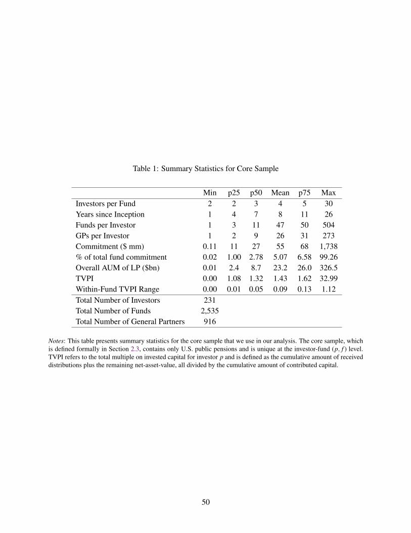
Table 1: Summary Statistics for Core Sample

Min p25 p50 Mean p75 MaxInvestors per Fund 2 2 3 4 5 30Years since Inception 1 4 7 8 11 26Funds per Investor 1 3 11 47 50 504GPs per Investor 1 2 9 26 31 273Commitment ($ mm) 0.11 11 27 55 68 1,738% of total fund commitment 0.02 1.00 2.78 5.07 6.58 99.26Overall AUM of LP ($bn) 0.01 2.4 8.7 23.2 26.0 326.5TVPI 0.00 1.08 1.32 1.43 1.62 32.99Within-Fund TVPI Range 0.00 0.01 0.05 0.09 0.13 1.12Total Number of Investors 231Total Number of Funds 2,535Total Number of General Partners 916

Notes: This table presents summary statistics for the core sample that we use in our analysis. The core sample, whichis defined formally in Section 2.3, contains only U.S. public pensions and is unique at the investor-fund (p, f ) level.TVPI refers to the total multiple on invested capital for investor p and is defined as the cumulative amount of receiveddistributions plus the remaining net-asset-value, all divided by the cumulative amount of contributed capital.

50

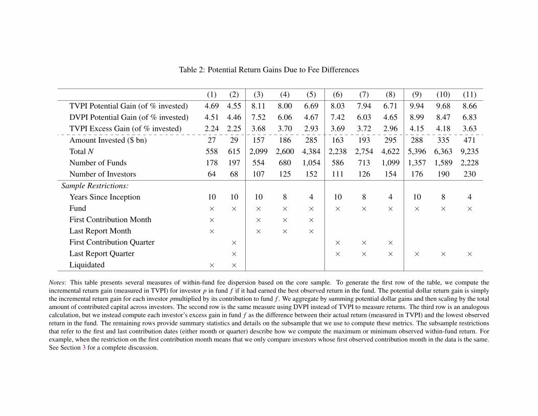
Table 2: Potential Return Gains Due to Fee Differences

(1) (2) (3) (4) (5) (6) (7) (8) (9) (10) (11)TVPI Potential Gain (of % invested) 4.69 4.55 8.11 8.00 6.69 8.03 7.94 6.71 9.94 9.68 8.66DVPI Potential Gain (of % invested) 4.51 4.46 7.52 6.06 4.67 7.42 6.03 4.65 8.99 8.47 6.83TVPI Excess Gain (of % invested) 2.24 2.25 3.68 3.70 2.93 3.69 3.72 2.96 4.15 4.18 3.63Amount Invested ($ bn) 27 29 157 186 285 163 193 295 288 335 471Total N 558 615 2,099 2,600 4,384 2,238 2,754 4,622 5,396 6,363 9,235Number of Funds 178 197 554 680 1,054 586 713 1,099 1,357 1,589 2,228Number of Investors 64 68 107 125 152 111 126 154 176 190 230

Sample Restrictions:Years Since Inception 10 10 10 8 4 10 8 4 10 8 4Fund × × × × × × × × × × ×First Contribution Month × × × ×Last Report Month × × × ×First Contribution Quarter × × × ×Last Report Quarter × × × × × × ×Liquidated × ×

Notes: This table presents several measures of within-fund fee dispersion based on the core sample. To generate the first row of the table, we compute theincremental return gain (measured in TVPI) for investor p in fund f if it had earned the best observed return in the fund. The potential dollar return gain is simplythe incremental return gain for each investor pmultiplied by its contribution to fund f . We aggregate by summing potential dollar gains and then scaling by the totalamount of contributed capital across investors. The second row is the same measure using DVPI instead of TVPI to measure returns. The third row is an analogouscalculation, but we instead compute each investor’s excess gain in fund f as the difference between their actual return (measured in TVPI) and the lowest observedreturn in the fund. The remaining rows provide summary statistics and details on the subsample that we use to compute these metrics. The subsample restrictionsthat refer to the first and last contribution dates (either month or quarter) describe how we compute the maximum or minimum observed within-fund return. Forexample, when the restriction on the first contribution month means that we only compare investors whose first observed contribution month in the data is the same.See Section 3 for a complete discussion.

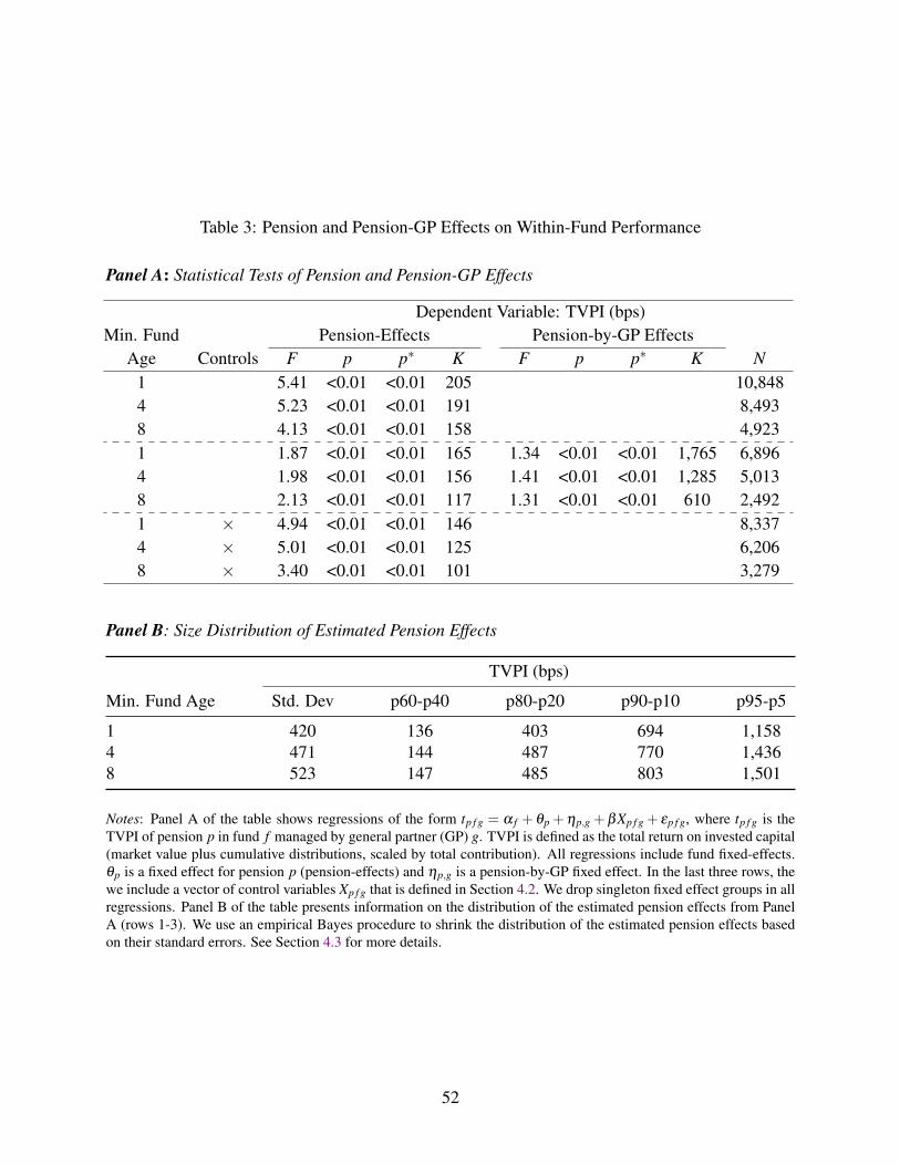
Table 3: Pension and Pension-GP Effects on Within-Fund Performance

Panel A: Statistical Tests of Pension and Pension-GP Effects

Dependent Variable: TVPI (bps)Min. Fund Pension-Effects Pension-by-GP Effects

Age Controls F p p∗ K F p p∗ K N1 5.41 <0.01 <0.01 205 10,8484 5.23 <0.01 <0.01 191 8,4938 4.13 <0.01 <0.01 158 4,9231 1.87 <0.01 <0.01 165 1.34 <0.01 <0.01 1,765 6,8964 1.98 <0.01 <0.01 156 1.41 <0.01 <0.01 1,285 5,0138 2.13 <0.01 <0.01 117 1.31 <0.01 <0.01 610 2,4921 × 4.94 <0.01 <0.01 146 8,3374 × 5.01 <0.01 <0.01 125 6,2068 × 3.40 <0.01 <0.01 101 3,279

Panel B: Size Distribution of Estimated Pension Effects

TVPI (bps)

Min. Fund Age Std. Dev p60-p40 p80-p20 p90-p10 p95-p5

1 420 136 403 694 1,1584 471 144 487 770 1,4368 523 147 485 803 1,501

Notes: Panel A of the table shows regressions of the form tp f g = α f + θp +ηp,g + βXp f g + εp f g, where tp f g is theTVPI of pension p in fund f managed by general partner (GP) g. TVPI is defined as the total return on invested capital(market value plus cumulative distributions, scaled by total contribution). All regressions include fund fixed-effects.θp is a fixed effect for pension p (pension-effects) and ηp,g is a pension-by-GP fixed effect. In the last three rows, thewe include a vector of control variables Xp f g that is defined in Section 4.2. We drop singleton fixed effect groups in allregressions. Panel B of the table presents information on the distribution of the estimated pension effects from PanelA (rows 1-3). We use an empirical Bayes procedure to shrink the distribution of the estimated pension effects basedon their standard errors. See Section 4.3 for more details.

52

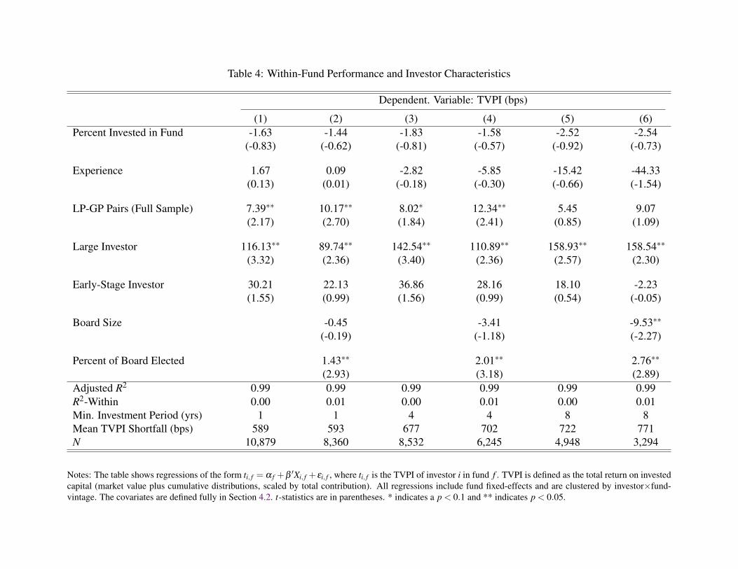
Table 4: Within-Fund Performance and Investor Characteristics

Dependent. Variable: TVPI (bps)

(1) (2) (3) (4) (5) (6)Percent Invested in Fund -1.63 -1.44 -1.83 -1.58 -2.52 -2.54

(-0.83) (-0.62) (-0.81) (-0.57) (-0.92) (-0.73)

Experience 1.67 0.09 -2.82 -5.85 -15.42 -44.33(0.13) (0.01) (-0.18) (-0.30) (-0.66) (-1.54)

LP-GP Pairs (Full Sample) 7.39∗∗ 10.17∗∗ 8.02∗ 12.34∗∗ 5.45 9.07(2.17) (2.70) (1.84) (2.41) (0.85) (1.09)

Large Investor 116.13∗∗ 89.74∗∗ 142.54∗∗ 110.89∗∗ 158.93∗∗ 158.54∗∗

(3.32) (2.36) (3.40) (2.36) (2.57) (2.30)

Early-Stage Investor 30.21 22.13 36.86 28.16 18.10 -2.23(1.55) (0.99) (1.56) (0.99) (0.54) (-0.05)

Board Size -0.45 -3.41 -9.53∗∗

(-0.19) (-1.18) (-2.27)

Percent of Board Elected 1.43∗∗ 2.01∗∗ 2.76∗∗

(2.93) (3.18) (2.89)Adjusted R2 0.99 0.99 0.99 0.99 0.99 0.99R2-Within 0.00 0.01 0.00 0.01 0.00 0.01Min. Investment Period (yrs) 1 1 4 4 8 8Mean TVPI Shortfall (bps) 589 593 677 702 722 771N 10,879 8,360 8,532 6,245 4,948 3,294

Notes: The table shows regressions of the form ti, f = α f +β ′Xi, f +εi, f , where ti, f is the TVPI of investor i in fund f . TVPI is defined as the total return on investedcapital (market value plus cumulative distributions, scaled by total contribution). All regressions include fund fixed-effects and are clustered by investor×fund-vintage. The covariates are defined fully in Section 4.2. t-statistics are in parentheses. * indicates a p < 0.1 and ** indicates p < 0.05.

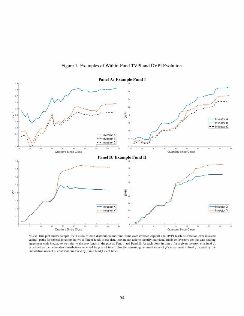
Figure 1: Examples of Within-Fund TVPI and DVPI Evolution

Panel A: Example Fund I

20 25 30 35 40 45 50 55 60 65

Quarters Since Close

1.9

2

2.1

2.2

2.3

2.4

2.5

2.6

2.7

2.8

2.9

TV

PI

Investor A

Investor B

Investor C

20 25 30 35 40 45 50 55 60 65

Quarters Since Close

1.2

1.4

1.6

1.8

2

2.2

2.4

2.6

2.8

DV

PI

Investor A

Investor B

Investor C

Panel B: Example Fund II

0 5 10 15 20 25 30 35 40 45

Quarters Since Close

1

1.1

1.2

1.3

1.4

1.5

1.6

1.7

1.8

TV

PI

Investor X

Investor Y

0 5 10 15 20 25 30 35 40 45

Quarters Since Close

0

0.2

0.4

0.6

0.8

1

1.2

1.4

1.6

1.8

DV

PI

Investor X

Investor Y

Notes: This plot shows sample TVPI (sum of cash distribution and fund value over invested capital) and DVPI (cash distribution over investedcapital) paths for several investors in two different funds in our data. We are not able to identify individual funds or investors per our data-sharingagreement with Preqin, so we refer to the two funds in the plot as Fund I and Fund II. At each point in time t for a given investor p in fund f ,is defined as the cumulative distributions received by p as of time t plus the remaining net-asset value of p’s investment in fund f , scaled by thecumulative amount of contributions made by p into fund f as of time t.

54

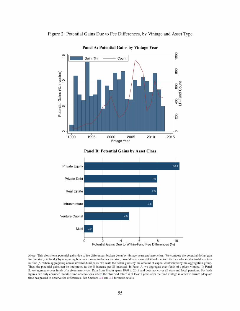
Figure 2: Potential Gains Due to Fee Differences, by Vintage and Asset Type

Panel A: Potential Gains by Vintage Year

020

040

060

080

010

00LP

-Fun

d C

ount

05

1015

Pote

ntia

l Gai

ns (%

inve

sted

)

1990 1995 2000 2005 2010 2015Vintage Year

Gain (%) Count

Panel B: Potential Gains by Asset Class

0.9

4.9

7.5

7.9

7.9

10.4

0 2 4 6 8 10Potential Gains Due to Within-Fund Fee Differences (%)

Multi

Venture Capital

Infrastructure

Real Estate

Private Debt

Private Equity

Notes: This plot shows potential gains due to fee differences, broken down by vintage years and asset class. We compute the potential dollar gainfor investor p in fund f by computing how much more in dollars investor p would have earned if it had received the best observed net-of-fee returnin fund f . When aggregating across investor-fund pairs, we scale the dollar gains by the amount of capital contributed by the aggregation group.Thus, the potential gains can be interpreted as the % increase per $1 invested. In Panel A, we aggregate over funds of a given vintage. In PanelB, we aggregate over funds of a given asset type. Data from Preqin spans 1990 to 2019 and does not cover all state and local pensions. For bothfigures, we only consider investor-fund observations where the observed return is at least 5 years after the fund vintage in order to ensure adequatetime has passed to observe fee differences. See Sections 3.1 and 3.2 for more details.

55

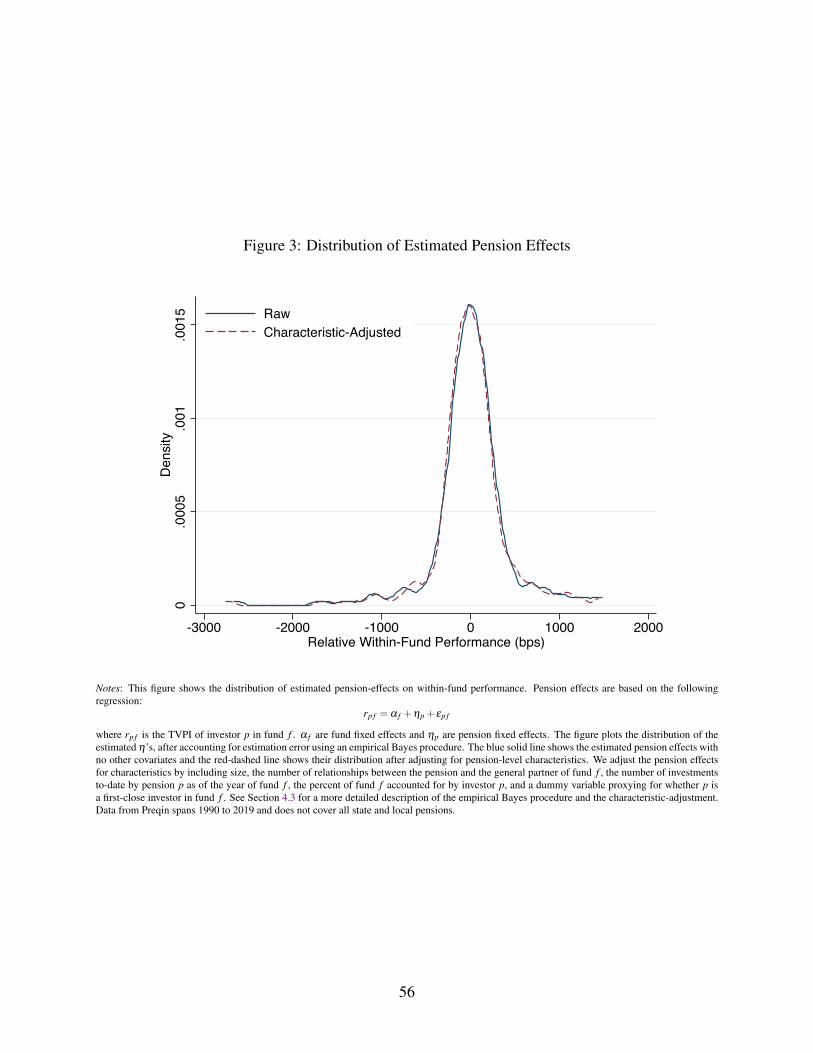
Figure 3: Distribution of Estimated Pension Effects

0.0

005

.001

.001

5D

ensi

ty

-3000 -2000 -1000 0 1000 2000Relative Within-Fund Performance (bps)

RawCharacteristic-Adjusted

Notes: This figure shows the distribution of estimated pension-effects on within-fund performance. Pension effects are based on the followingregression:

rp f = α f +ηp + εp f

where rp f is the TVPI of investor p in fund f . α f are fund fixed effects and ηp are pension fixed effects. The figure plots the distribution of theestimated η’s, after accounting for estimation error using an empirical Bayes procedure. The blue solid line shows the estimated pension effects withno other covariates and the red-dashed line shows their distribution after adjusting for pension-level characteristics. We adjust the pension effectsfor characteristics by including size, the number of relationships between the pension and the general partner of fund f , the number of investmentsto-date by pension p as of the year of fund f , the percent of fund f accounted for by investor p, and a dummy variable proxying for whether p isa first-close investor in fund f . See Section 4.3 for a more detailed description of the empirical Bayes procedure and the characteristic-adjustment.Data from Preqin spans 1990 to 2019 and does not cover all state and local pensions.

56

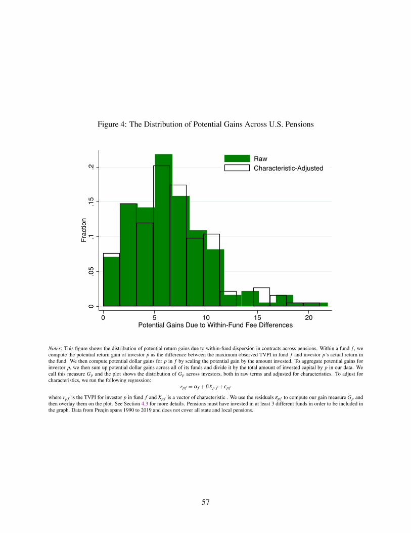
Figure 4: The Distribution of Potential Gains Across U.S. Pensions

0.0

5.1

.15

.2Fr

actio

n

0 5 10 15 20Potential Gains Due to Within-Fund Fee Differences

RawCharacteristic-Adjusted

Notes: This figure shows the distribution of potential return gains due to within-fund dispersion in contracts across pensions. Within a fund f , wecompute the potential return gain of investor p as the difference between the maximum observed TVPI in fund f and investor p’s actual return inthe fund. We then compute potential dollar gains for p in f by scaling the potential gain by the amount invested. To aggregate potential gains forinvestor p, we then sum up potential dollar gains across all of its funds and divide it by the total amount of invested capital by p in our data. Wecall this measure Gp and the plot shows the distribution of Gp across investors, both in raw terms and adjusted for characteristics. To adjust forcharacteristics, we run the following regression:

rp f = α f +βXp, f + εp f

where rp f is the TVPI for investor p in fund f and Xp f is a vector of characteristic . We use the residuals εp f to compute our gain measure Gp andthen overlay them on the plot. See Section 4.3 for more details. Pensions must have invested in at least 3 different funds in order to be included inthe graph. Data from Preqin spans 1990 to 2019 and does not cover all state and local pensions.

57

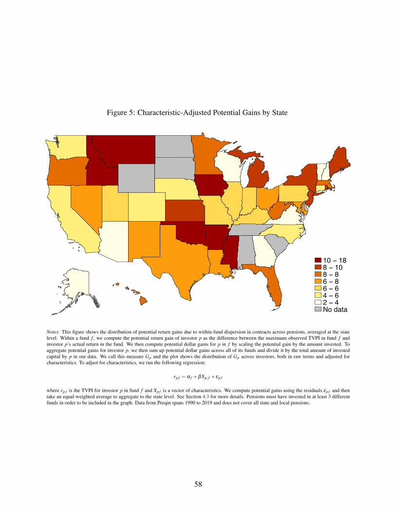
Figure 5: Characteristic-Adjusted Potential Gains by State

10 − 188 − 108 − 86 − 86 − 64 − 62 − 4No data

Notes: This figure shows the distribution of potential return gains due to within-fund dispersion in contracts across pensions, averaged at the statelevel. Within a fund f , we compute the potential return gain of investor p as the difference between the maximum observed TVPI in fund f andinvestor p’s actual return in the fund. We then compute potential dollar gains for p in f by scaling the potential gain by the amount invested. Toaggregate potential gains for investor p, we then sum up potential dollar gains across all of its funds and divide it by the total amount of investedcapital by p in our data. We call this measure Gp and the plot shows the distribution of Gp across investors, both in raw terms and adjusted forcharacteristics. To adjust for characteristics, we run the following regression:

rp f = α f +βXp, f + εp f

where rp f is the TVPI for investor p in fund f and Xp f is a vector of characteristics. We compute potential gains using the residuals εp f and thentake an equal-weighted average to aggregate to the state level. See Section 4.3 for more details. Pensions must have invested in at least 3 differentfunds in order to be included in the graph. Data from Preqin spans 1990 to 2019 and does not cover all state and local pensions.

58

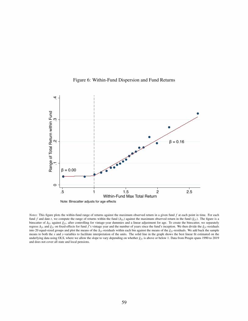
Figure 6: Within-Fund Dispersion and Fund Returns

β = 0.00

β = 0.16

0.1

.2.3

.4R

ange

of T

otal

Ret

urn

with

in F

und

.5 1 1.5 2 2.5Within-Fund Max Total Return

Note: Binscatter adjusts for age effects

Notes: This figure plots the within-fund range of returns against the maximum observed return in a given fund f at each point in time. For eachfund f and date t, we compute the range of returns within the fund (∆ f t ) against the maximum observed return in the fund (g f t ). The figure is abinscatter of ∆ f t against g f t , after controlling for vintage-year dummies and a linear adjustment for age. To create the binscatter, we separatelyregress ∆ f t and g f t on fixed-effects for fund f ’s vintage year and the number of years since the fund’s inception. We then divide the g f t -residualsinto 20 equal-sized groups and plot the means of the ∆ f t -residuals within each bin against the means of the g f t -residuals. We add back the samplemeans to both the x and y-variables to facilitate interpretation of the units. The solid line in the graph shows the best linear fit estimated on theunderlying data using OLS, where we allow the slope to vary depending on whether g f t is above or below 1. Data from Preqin spans 1990 to 2019and does not cover all state and local pensions.

59