Hopf Bifurcations of Functional Differential Equations with Dihedral Symmetries

File: DISTL2 342201 . By:CV . Date:20:05:98 . Time:09:42 LOP8M. V8.B. Page 01:01Codes: 3738 Signs: 1903 . Length: 50 pic 3 pts, 212 mm

Journal of Differential Equations � DE3422

journal of differential equations 146, 157�184 (1998)

Hopf Bifurcations of Functional Differential Equationswith Dihedral Symmetries

W. Krawcewicz and P. Vivi

Department of Mathematical Sciences, University of Alberta,Edmonton, Alberta, Canada T6G 2G1

and

J. Wu*

Department of Mathematics and Statistics, York University,North York, Ontario, Canada M3J 1P3

Received February 11, 1997; revised January 14, 1998

We discuss the joint impact of temporal delay and spatial dihedral symmetrieson the occurence and multiplicity of Hopf bifurcations for a system of FDEs. Byapplying the equivariant degree theory we establish a result on the existence ofmultiple branches of nonconstant periodic solutions and classify their symmetries.General results are illustrated by a ring of identical oscillators with identical couplingbetween adjacent cells. � 1998 Academic Press

1. INTRODUCTION

In this paper we develop a Hopf bifurcation theory for functional dif-ferential equations (FDEs) with dihedral symmetries via the equivariantdegree theory and present an orbit type classification of possible Hopfbifurcations. We also discuss the joint impact of the time delay and thespatial dihedral symmetry on the multiplicity of bifurcating solutions incoupled cells.

The advantage of using the equivariant degree lies in the fact that itprovides a local bifurcation invariant containing the full topological infor-mation on the `èssential'' types of bifurcated solutions and gives morecontrol over the global bifurcation phenomena.

In this paper we use only a simplified, but easier to compute, version ofthe equivariant degree, which is called the primary equivariant degree.

article no. DE983422

1570022-0396�98 �25.00

Copyright � 1998 by Academic PressAll rights of reproduction in any form reserved.

* Research supported by NSERC and by the Alexander von Humboldt Foundation.


However, this degree already gives us enough information to classify effec-tively the types of possible Hopf bifurcations with dihedral symmetry. Dueto the topological nature of the equivariant degree method, we can avoidseveral technical difficulties, such as symmetric generic approximations,encountered in Fiedler's approach (cf. [4]), which is based on a reductionof a system to a fixed point space with a cyclic group action. Nevertheless,his method may lead to the same results as ours for a system of coupledoscillators.

There are several advantages of using the equivariant degree method. Itcan be applied, without additional technicalities, to the study of Hopf bifur-cation problems for FDEs exactly in the same way as for ODEs, and it alsoprovides a local bifurcation invariant reflecting the true topological natureof the bifurcating branches of solutions (cf. [13, 19]). More precisely, a non-zero component of this local invariant indicates that ``generically'' there isa branch of solutions corresponding to the associated orbit type (possiblysubmaximal). The global Hopf bifurcation results are based on the fact thatfor a bounded branch of solutions the sum of local invariants must be zero.In our case the local bifurcation invariants take into account also sub-maximal orbit types and therefore the obtained relations may give bettercharacterizations of bounded branches. In this paper we present the fullclassification of the local bifurcation invariants, including the submaximalorbit types, which can also be used for the description of the globalbifurcations.

We should also mention that this method can be applied in a standardway to several Hopf bifurcation problems with more complicated sym-metries like SU(2) and O(3) (SU(n) or O(n), in general). However, theequivariant degree method is just one of many ways to study Hopf bifurca-tion problems and we do not claim that similar results can not be obtainedthrough another approach (for example, by using the equivariant singu-larity theory, cf. [8�10]). Still, we believe that equivariant degree methodis a standard and relatively simple technique and can be effectively used tostudy various symmetric bifurcation problems. We refer to the monographs[4, 8, 10, 12] for a detailed account of the subject for ordinary differentialequations and partial differential equations. As for FDEs, an analytic(local) Hopf bifurcation theorem was obtained in [31] as an analogy ofthe Golubitsky�Stewart theorem [9]. Moreover, a topological Hopf bifur-cation theory was developed in [18] for FDEs in the case where the spatialsymmetry group is the abelian group ZN or Z� :=S 1. While the problemof looking for local bifurcations of periodic solutions with prescribed sym-metries can always be reduced to one where the spatial symmetry group isZN or Z� (see [4, 9]), examining the global interaction of all bifurcatedperiodic solutions requires the consideration of the full symmetry group ofthe equation. Our results, especially the presented application to coupled

158 KRAWCEWICZ, VIVI, AND WU


cells arising from neural networks with memory [29, 30], illustrate that anonabelian action, due to the fact that its irreducible representations maycontain many different orbit types, can cause spontaneous bifurcations ofmultiple branches of periodic solutions with various symmetry properties.For example, if a coupled oscillators consist of N cells with N being aprime number, then at certain critical values of the parameter (usually thedelay) the system possess at least 2(N+1) distinct branches of nonconstantperiodic solutions with certain spatiotemporal patterns.

The rest of the paper is organized as follows: Section 2 summarizes someresults about the equivariant degree theory, Section 3 contains the generalresults on Hopf bifurcations of FDEs with dihedral group symmetry, andSection 4 presents some applications of the general results to coupled cells.

2. G-EQUIVARIANT DEGREE

Our main technical tool is the equivariant degree which was introducedby Ize et al. (cf. [13�15]). We use the standard notation following [25]and [16]. Let G be a compact Lie group, V a finite dimensional orthogonalrepresentation of G, and 0/V�Rn an open bounded invariant set. Weconsider an equivariant map f : V�Rn � V such that f (x){0 for x # �0.The equivariant degree degG( f, 0) of f in 0 is defined as an element of the``stabilized'' equivariant homotopy group of the representation sphereSV :=S(R�V )

6G :=Lim� k

6 GSR k�V�R n (S Rk�V ),

in the following way: Let ': V�Rn � [0, 1] be an invariant function suchthat '&1(0)=0� and '&1(0, 1) & f &1(0)=<. We put f' : [&1, 1]_V�Rn � R�V, f'(t, x)=(t+2'(x), f (x)) for t # [&1, 1] and x # V�Rn.The equivariant homotopy class [ f'] # 6 G

SV�R n (S V ) defines an elementdegG( f, 0) in 6G called the equivariant degree of f in 0. The equivariantdegree has all the standard properties like the existence, additivity, homo-topy, suspension, and excision.

Let 8n(G) denote the set of all the orbit types (H ) in V such that theWeyl group W(H)=N(H )�H of H is bi-orientable, i.e., W(H ) admits aninvariant (fixed) orientation with respect to left and right translations, anddim W(H )=n. Then the free Z-module An(G) :=Z[8n(G)] is a subgroup of6G (see [22] or [15]). We denote by G-Deg( f, 0) the image of degG( f, 0)under the natural projection 6G � An(G). We call G-Deg( f, 0) the primarydegree1 of f in 0. We will write G-Deg( f, 0)=�(H ) nH(H ), where the

159HOPF BIFURCATIONS OF FDEs

1 The primary degree is related to the primary orbit types (H ) in V, i.e., satisfyingdim W(H )=n.


summation is taken over all the primary orbit types in V. The primarydegree was introduced independently of the work of Ize et al. in [5] (seealso [21, 22]).

The primary degree of f : 0� � V can be expressed by an analytic formula:Approximate f by a regular normal map (i.e., a map satisfying certain nor-mality and transversality conditions, see [21] for more details) g: 0� � Vsuch that supx # 0 & f (x)& g(x)&<' with 2' :=infx # �0 & f (x)&. In par-ticular, for every orbit type (H ) in 0 the map gH := g |0H

: 0H � VH haszero as a regular value. Then

G-Deg( f, 0)= :(H ) # 8n(G)

nH (H ), (2.1)

and

nH= :W(H ) x/gH

&1(0)

sign det DgH (x) |Sx,

where Sx denotes the linear slice to the orbit W(H )x in the space VH�Rn

at x, i.e., the subspace of VH �Rn which is orthogonal to W(H )x at x. Wechoose bases in VH and Sx in such a way that the orientation of thetangent space TxW(H )x, induced by the chosen invariant orientation ofW(H ), followed by the orientation of Sx gives the orientation of VH

followed by the standard orientation of Rn.In the case where n=1 the computation of the primary degree can be be

reduced to the calculations of a related S1-degree (see [2] or [17] formore details, technical formulae and comprehensive examples).

Theorem 2.1. (Ulrich Type Formula for G-Degree, cf. [16].) Let Gbe a compact Lie group, V be an orthogonal representation of G, andf : V�R � V an equivariant map such that f (x){0 for all x # �0, where0/V�R is an open, invariant, and bounded subset. Then

nH=[IS 1(F H)Z1&IS1(F [H])Z1

]<}W(H )S1 } ,

where nH are the coefficients in (2.1), S 1/W(H ), IS 1 denotes the S 1-fixedpoint index corresponding to the primary S1-degree (see [16] for moredetails), and f :=Id&F : V�R � V.

In what follows we will denote by DN the dihedral group of order 2N.In the case G=DN_S 1, the primary G-degree has an additional importantproperty, called multiplicativity property (which is also true in more generalcase, cf. [16, Theorem 3.4]):



Proposition 2.2. Assume that V is an orthogonal G=DN_S 1-represen-tation and U is an orthogonal DN-representation. Let f : V�R � V (resp.g: U � U ) be an equivariant map such that f (x){0 for x # �0 (resp.g(x){0 for x # �U), where 0/V�R (resp. U/U) is an invariant openbounded subset. Then

G-Deg(g_ f, U_0)=DN -deg(g, U) } G-Deg( f, 0),

where A(DN)=A0(DN) denotes the Burnside ring of DN and A1(G) has anatural structure of an A(DN)-module.

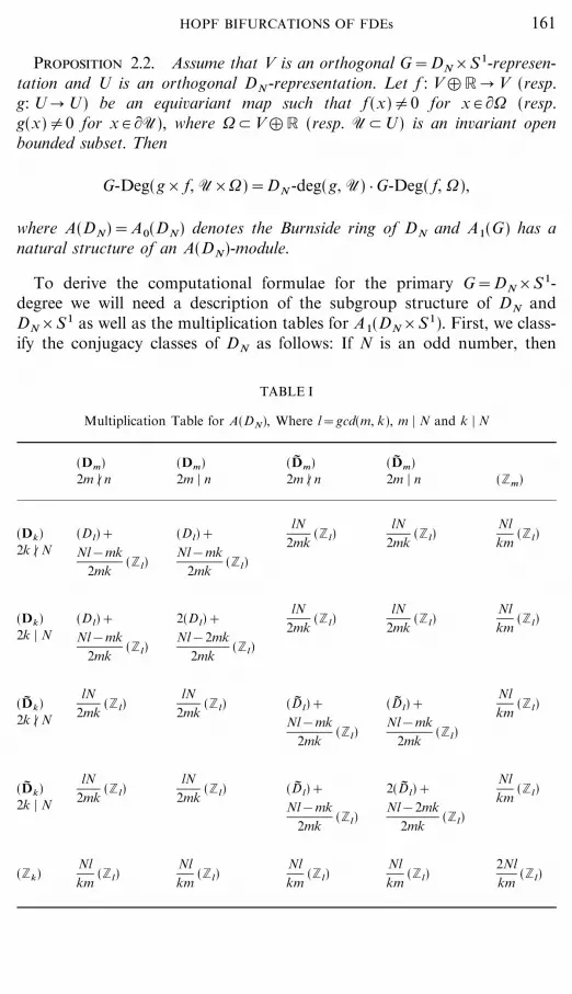
To derive the computational formulae for the primary G=DN_S 1-degree we will need a description of the subgroup structure of DN andDN_S1 as well as the multiplication tables for A1(DN_S1). First, we class-ify the conjugacy classes of DN as follows: If N is an odd number, then

TABLE I

Multiplication Table for A(DN), Where l=gcd(m, k), m | N and k | N

(Dm)2m |% n

(Dm)2m | n

(D� m)2m |% n

(D� m)2m | n (Zm)

(Dk)2k |% N

(D l)+Nl&mk

2mk(Zl)

(Dl)+Nl&mk

2mk(Zl)

lN2mk

(Z l)lN

2mk(Z l)

Nlkm

(Zl)

(Dk)2k | N

(D l)+Nl&mk

2mk(Zl)

2(D l)+Nl&2mk

2mk(Zl)

lN2mk

(Z l)lN

2mk(Z l)

Nlkm

(Zl)

(D� k)2k |% N

lN2mk

(Z l)lN

2mk(Z l) (D� l)+

Nl&mk2mk

(Zl)

(D� l)+Nl&mk

2mk(Zl)

Nlkm

(Zl)

(D� k)2k | N

lN2mk

(Z l)lN

2mk(Z l) (D� l)+

Nl&mk2mk

(Zl)

2(D� l)+Nl&2mk

2mk(Zl)

Nlkm

(Zl)

(Zk)Nlkm

(Zl)Nlkm

(Zl)Nlkm

(Zl)Nlkm

(Zl)2Nlkm

(Zl)



80(DN)=[(Dk), (Zk); k | N ]; and if N is even then 80(DN)=[(Dk), (D� k),(Zk); k | N ], where

D� k=Zk _ }!N Zk , !N=e2i?�N, and }=_10

0&1& .

We have Table I (see [16]) for the Burnside ring A(DN) :=A0(DN).All the generators of A1(DN_S1) are the m-folded %-twisted subgroups

K (%, m) :=[(#, z) # K_S1; %(#)=zm], where K is a subgroup of DN and% : K � S 1 a homomorphism (cf. [8]).

We next proceed with the classification (up to conjugacy classes) of thenontrivial l-folded %-twisted subgroups of DN_S 1: We have the subgroupsD(c, l )

k and D� (c, l )k , where c : Dk � Z2 is a homomorphism such that

ker c=Zk , and the subgroup D (d, l )k (when k is even), where d : Dk � Z2 is

a homomorphism such that ker d=Dk�2 . Moreover, if k is divisible by 4then there exists one more conjugacy class of the subgroup D(d� , l )

k , whereker d� =D� k�2 :=Zk�2 _ }!� k Zk�2 with !� k=e2i?�k. In the case of subgroups

TABLE II

Multiplication Table for A(Dn), Where l=gcd(m, k), m | n and k | n

(Dm)2m |% n

(Dm)2m | n

(D� m)2m |% n

(D� m)2m | n (Zm)

(Dk)2k |% n

(D l)+nl&mk

2mk(Zl)

(Dl)+nl&mk

2mk(Zl)

ln2mk

(Z l)ln

2mk(Z l)

nlkm

(Zl)

(Dk)2k | n

(D l)+nl&mk

2mk(Zl)

2(D l)+nl&2mk

2mk(Z l)

ln2mk

(Z l)ln

2mk(Z l)

nlkm

(Zl)

(D� k)2k |% n

ln2mk

(Z l)ln

2mk(Z l) (D� l)+

nl&mk2mk

(Zl)

(D� l)+nl&mk

2mk(Zl)

nlkm

(Zl)

(D� k)2k | n

ln2mk

(Z l)ln

2mk(Z l) (D� l)+

nl&mk2mk

(Zl)

2(D� l)+nl&2mk

2mk(Z l)

nlkm

(Zl)

(Zk)nl

km(Zl)

nlkm

(Zl)nl

km(Zl)

nlkm

(Zl)2nlkm

(Zl)



Table III

Multiplication Table, Where We Assume m=gcd(k, r) Is Such That 2m | N

(D (d, l )k ), 2 | k

2k |% N(D (d, l )

k ), 2 | k2k | N

(Dr), 2 | r2r |% N

Excluded 2(D (d, l )m )+

lm&2kr2kr

(Z (d, l )m )

(Dr), 2 | r2r | N

2(D (d, l )m )+

ml&2kr2kr

(Z (d, l )m ) 4(D (d, l )

m )+ml&4kr

2kr(Z (d, l )

m )

Z(.& , l )k , the homomorphism .& is given by .&(z)=z&, where & is an integer

and z # Zk/S 1/C. In the case where k is an even number, we havethe homomorphism d : Zk � Z2 such that ker d=Zk�2 , for which we havethe l-folded d-twisted subgroup Z (d, l )

k .We have Tables II and III for A(DN)_A1(DN_S 1) � A1(DN_S 1) (cf.

[16]).

3. HOPF DN -SYMMETRIC BIFURCATION THEOREMS

Let {�0 be a given constant, n a positive integer and Cn, { the Banachspace of continuous functions from [&{, 0] into Rn equipped with theusual supremum norm

&.&= sup&{�%�0

|.(%)|, . # Cn, { .

In what follows, if x : [&{, A] � Rn is a continuous function with A>0and if t # [0, A], then xt # Cn, { is defined by

xt(%)=x(t+%), % # [&{, 0].

Also, for any x # Rn we will use x� to denote the constant mapping from[&{, 0] into Rn with the value x # Rn.

Consider the following one parameter family of retarded functional dif-ferential equations

x* =f (xt , :), (3.1)

where x # Rn, : # R, f : Cn, {_R � Rn is a continuously differentiable andcompletely continuous mapping. Assume there is an orthogonal represen-tation 3 : 1 � O(n) of 1 :=DN , N>2, on Rn, which naturally induces an



isometric Banach representation of 1 on the space Cn, { with the action} : 1_Cn, { � Cn, { given by:

(#.)(%) :=3(#)(.(%)), # # 1, % # [&{, 0].

We make the following assumptions

(A1) The mapping f is 1-equivariant, i.e.,

f (#., :)=#f (., :), . # Cn, { , : # R, # # 1.

(A2) f (0, :)=0 for all : # R, i.e., (0, :) is a stationary solution of (3.1)for every : # R.

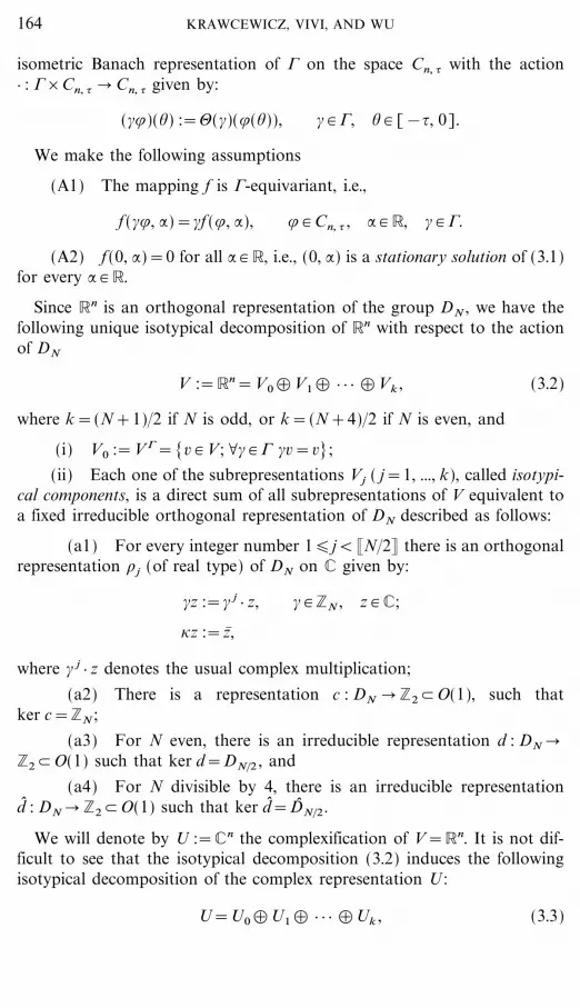
Since Rn is an orthogonal representation of the group DN , we have thefollowing unique isotypical decomposition of Rn with respect to the actionof DN

V :=Rn=V0�V1� } } } �Vk , (3.2)

where k=(N+1)�2 if N is odd, or k=(N+4)�2 if N is even, and

(i) V0 :=V1=[v # V; \# # 1 #v=v];

(ii) Each one of the subrepresentations Vj ( j=1, ..., k), called isotypi-cal components, is a direct sum of all subrepresentations of V equivalent toa fixed irreducible orthogonal representation of DN described as follows:

(a1) For every integer number 1�j<�N�2� there is an orthogonalrepresentation \j (of real type) of DN on C given by:

#z :=# j } z, # # ZN , z # C;

}z :=z� ,

where # j } z denotes the usual complex multiplication;

(a2) There is a representation c : DN � Z2/O(1), such thatker c=ZN ;

(a3) For N even, there is an irreducible representation d : DN �Z2/O(1) such that ker d=DN�2 , and

(a4) For N divisible by 4, there is an irreducible representationd� : DN � Z2/O(1) such that ker d� =D� N�2 .

We will denote by U :=Cn the complexification of V=Rn. It is not dif-ficult to see that the isotypical decomposition (3.2) induces the followingisotypical decomposition of the complex representation U :

U=U0�U1 � } } } �Uk , (3.3)



where U0 :=U 1 and each of the isotypical components Uj is characterizedby complex representation of the following types:

(b1) For 1< j��N�2� the representation 'j on C�C is given by

#(z1 , z2) :=(# j } z1 , #&j } z2), # # ZN , z1 , z2 # C,

}(z1 , z2) :=(z2 , z1);

(b2) The representation c : DN � Z2/U(1), such that ker c=ZN ;

(b3) In the case when N is even, the representation d : DN �Z2/U(1), such that ker d=DN�2 ; and

(b4) In the case when N is even, the representation d� : DN �Z2/U(1) such that ker d� =D� N�2 .

An element (x, :) # Rn_R is called a stationary solution of (3.1) iff (x� , :)=0. A complex number * # C is said to be a characteristic value ofthe stationary solution (x, :) if it is a root of the following characteristicequation

detC 2(x, :)(*)=0, (3.4)

where

2(x, :)(*) :=* Id&Dx f (x, :)(e* } Id).

A stationary solution (x0 , :0) is called nonsingular if *=0 is not acharacteristic value of (x0 , :0), and a nonsingular stationary point (x0 , :0)is called a center if it has a purely imaginary characteristic value. We willcall (x0 , :0) an isolated center if it is the only center in some neighborhoodof (x0 , :0) in Rn_R.

We now make the following assumption:

(A3) There is a stationary solution (0, :0) which is an isolated centersuch that *=i;0 , ;0>0, is a characteristic value of (0, :0).

Let 01 :=(0, b)_(;0&c, ;0+c)/C. Under assumption (A3), the con-stants b>0, c>0 and $>0 can be chosen such that the following condi-tion is satisfied:

(*) For every : # [:0&$, :0+$] if there is a characteristic valueu+iv # �01 of (0, :) then u+iv=i;0 and :=:0 .

Note that 2(0, :)(*) is analytic in * # C and continuous in : # [:0&$,:0+$]. It follows that detC 2(0, :0\$)(*){0 for * # �01 .



Since the mapping f is 1-equivariant, for every : # R and * # C theoperator 2(0, :)(*): Cn � Cn is 1-equivariant and consequently for every iso-typical component Uj of U=Cn we have 2(0, :)(*)(U j )�Uj for j=0, 1, ..., k.

We put

2:, j (*) :=2(0, :)(*)|Uj: Uj � Uj .

Solutions * # C of the equation

detC 2:, j (*)=0

where j=0, 1, ..., k, will be called the j th isotypical characteristic valuesof (0, :). It is clear that * is a characteristic value of the solution (0, :) ifand only if it is a j th isotypical characteristic value of (0, :) for somej=0, 1, ..., k.

Following the idea of a crossing number in a nonequivariant case (cf. [3,6, 17, 20]), we define

c1, j (:0 , ;0) :=degB(detC 2:0&$, j ( } ), 0)&degB(detC 2:0+$, j ( } ), 0)

for 0� j�k. The number c1, j (:0 , ;0) will be called the j th isotypical crossingnumber, for the isolated center (0, :0) corresponding to the characteristicvalue i;0 . The crossing number c1, j (:0 , ;0) indicates how many j th charac-teristic values (counted with algebraic multiplicity) of the stationary points(0, :) `èscape'' from the region 01 when : crosses the value :0 .

Since an integer multiple of i;0 can also be an j th isotypical charac-teristic value of (0, :0), we define for l>1

cl, j (:0 , ;0) :=degB(detC 2:0&$, j ( } ), 0l )&degB(detC 2:0+$, j ( } ), 0l )

where 0l :=(0, b)_(l;0&c, l;0+c)/C and the constants b>0, c>0 and$>0 can be chosen to be sufficiently small so that there are no charac-teristic values of (0, :) in �0l except perhaps il;0 for :=:0 . In other words,cl, j (:0 , ;0)=c1, j (:0 , l;0). If il; is not an j th isotypical characteristic valueof (0, :0) then clearly cl, j (:0 , ;0)=0.

In order to establish the existence of small amplitude periodic solutionsbifurcating from the stationary point (0, :0), i.e., the existence of Hopfbifurcations at the stationary point (0, :0), and to associate with (0, :0) alocal bifurcation invariant, we will use the standard degree-theoreticalapproach (cf. [3, 6, 17, 18, 20]). We reformulate the Hopf bifurcationproblem for equation (3.1) as an 1_S1-equivariant bifurcation problem(with two parameters) in an appropriate Hilbert isometric representationof G=1_S1. For this purpose we make the following change of variable



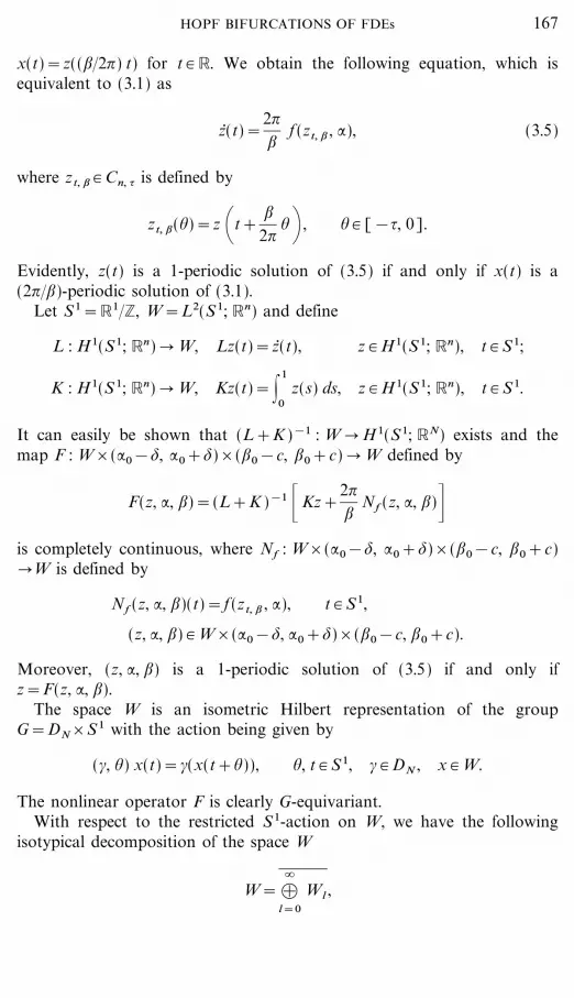
x(t)=z((;�2?) t) for t # R. We obtain the following equation, which isequivalent to (3.1) as

z* (t)=2?;

f (zt, ; , :), (3.5)

where zt, ; # Cn, { is defined by

zt, ;(%)=z \t+;

2?% + , % # [&{, 0].

Evidently, z(t) is a 1-periodic solution of (3.5) if and only if x(t) is a(2?�;)-periodic solution of (3.1).

Let S1=R1�Z, W=L2(S 1; Rn) and define

L : H1(S1; Rn) � W, Lz(t)=z* (t), z # H1(S 1; Rn), t # S1;

K : H1(S 1; Rn) � W, Kz(t)=|1

0z(s) ds, z # H1(S 1; Rn), t # S1.

It can easily be shown that (L+K )&1 : W � H 1(S1; RN) exists and themap F : W_(:0&$, :0+$)_(;0&c, ;0+c) � W defined by

F(z, :, ;)=(L+K )&1 _Kz+2?;

Nf (z, :, ;)&is completely continuous, where Nf : W_(:0&$, :0+$)_(;0&c, ;0+c)�W is defined by

Nf (z, :, ;)(t)=f (zt, ; , :), t # S1,

(z, :, ;) # W_(:0&$, :0+$)_(;0&c, ;0+c).

Moreover, (z, :, ;) is a 1-periodic solution of (3.5) if and only ifz=F(z, :, ;).

The space W is an isometric Hilbert representation of the groupG=DN_S 1 with the action being given by

(#, %) x(t)=#(x(t+%)), %, t # S1, # # DN , x # W.

The nonlinear operator F is clearly G-equivariant.With respect to the restricted S1-action on W, we have the following

isotypical decomposition of the space W

W=��

l=0

Wl ,



where W0 is the space of all constant mappings from S 1 into Rn, and Wl

with l>0 is the vector space of all mappings of the form x sin 2l? } +y cos 2l? } , x, y # Rn. For l>0, the subspace Wl can be endowed with acomplex structure by

i } (x sin 2l? } +y cos 2l? } )=x cos 2l? } &y sin 2l? } , x, y # Rn.

Since the above multiplication by i induces an operator J : Wl � Wl suchthat J2=&Id, it follows that Id+J is an 1-equivariant isomorphism andevery function in Wl can be uniquely represented as ei2l? } (x+iy), x, y # Rn.In particular, we notice that the above defined complex structure on Wl

coincides with the complex structure given by x+iy # Cn. In addition,the complex isomorphism Al : Wl � U :=Cn given by Al (ei2l? } (x+iy))=x+iy, x+iy # Cn is 1-equivariant. Thus, as a complex 1-representation,Wl is equivalent to U. Consequently, the isotypical 1-decomposition (3.3)of U induces the following isotypical 1-decomposition of Wl

Wl :=W0, l�W1, l � } } } �Wk, l ,

where the isotypical components Wj, l , l>0 can be described exactly by thesame conditions (b1)�(b4). On the other hand the component W0 isexactly the representation V=Rn, which admits the isotypical decomposi-tion (3.2). To unify the notations, we denote this isotypical decompositionby W0=W0, 0� } } } �Wk, 0 , where for every j we have Wj, 0 :=Vj . As thecomplex structure on Wj , with j>0 was defined using the S1-action and asall the subspaces Wj, l , with l>0 are complex 1-invariant subspaces, W j, l

with l>0 are also S1-invariant. Therefore, Wj, l are the isotypical G-com-ponents of the representation W.

For every j and l we define

aj, l (:, ;) :=Id&(L+K )&1 _K+2?;

Dz Nf (0, :, ;)&}Wj, l

,

where (:, ;) # (:0&$, :0+$)_(;0&c, ;0+c).We observe that

(L+K )&1 (ei2l? } (x+iy))=1

i2l?ei2l? } (x+iy) (3.6)

for every x, y # Rn, and since

aj, l (:, ;)=(L+K )&1 _L&2?;

Dz Nf (0, :, ;)&}Wj, l

,



we obtain

aj, l (:, ;) e i2l? } z=(L+K )&1 _i2l? ei2l? } z&2?;

ei2l? } Dx f (0, :)(eil; } ) z&=ei2l? } 1

il;2(0, :)(il;)(z).

Consequently,

aj, l (:, ;)=1

il;2:, j (il;).

The idea of using the topological degrees to study the existence of Hopfbifurcations, and the various symmetry properties of the solutions, is basedon the notion of a complementing function. More precisely, let *=:+i;=(:, ;) # R2=C and *0=:0+;0 . We define a special neighborhood U(r, \)of the solution (0, *0) # W_R2 by

U(r, \) :=[(z, *) # W_C; &z&<r, and |*&*0|<\].

By taking sufficiently small r>0 and \>0, we may assume that the equation

F(z, *)=0, z # W, * # C=R2, (3.7)

has no solution (z, *) such that (z, *) # �U(r, \), z{0 and |*&*0|=\.A G-invariant function ! : U(r, \) � R defined by

!(z, *) :=|*&*0| (&z&&r)+&z&

is called a complementing function with respect to U(r, \). Define the mappingF! : U(r, \) � W_R by F!(z, *) :=(F(z, *), !(z, *)), where (z, *) # U(r, \).The mapping F! is a compact G-equivariant field. It is well known that theG-equivariant degree G-Deg(F! , U(r, \)) does not depend on the numbersr>0 and \>0 (if r and \ are sufficiently small), thus the standard proper-ties of G-degree imply that if G-Deg(F! , U(r, \)){0 then (0, *0) is a bifur-cation point of (3.7), i.e., there exists a continuum C/U(r, \) of noncons-tant periodic solutions of (3.7) such that (0, *0) # C� . We can regard theG-degree G-Deg(F! , U(r, \)) as a local bifurcation invariant.

The computations in [16] provide us with a complete informationneeded to evaluate the exact value of G-Deg(F! , U(r, \)). To illustratethis point, we need a more detailed description of the G-isotypical com-ponents Wj, l .

For every isotypical component Wj, l , we denote by Yj, l the correspondingirreducible representation of G, (i.e., Yj, l is equivalent to every irreducible



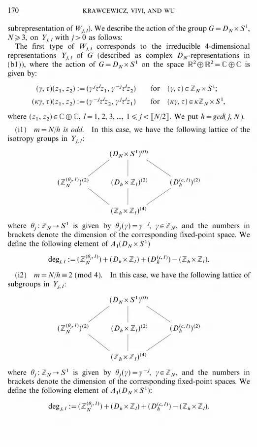
subrepresentation of Wj, l). We describe the action of the group G=DN_S 1,N�3, on Yj, l with j>0 as follows:

The first type of Wj, l corresponds to the irreducible 4-dimensionalrepresentations Yj, l of G (described as complex DN -representations in(b1)), where the action of G=DN_S 1 on the space R2�R2=C�C isgiven by:

(#, {)(z1 , z2) :=(# j{lz1 , #&j{lz2) for (#, {) # ZN_S 1;

(}#, {)(z1 , z2) :=(#&j{lz2 , # j{lz1) for (}#, {) # }ZN_S1,

where (z1 , z2) # C�C, l=1, 2, 3, ..., 1� j<�N�2�. We put h=gcd( j, N ).

(i1) m=N�h is odd. In this case, we have the following lattice of theisotropy groups in Yj, l :

(DN_S 1)(0)

(Z(%j , l )N ) (2) (Dh_Zl )

(2) (D (c, l )h ) (2)

(Zh_Zl )(4)

where %j : ZN � S1 is given by %j (#)=#&j, # # ZN , and the numbers inbrackets denote the dimension of the corresponding fixed-point space. Wedefine the following element of A1(DN_S 1)

degj, l :=(Z(%j , l )N )+(Dh_Zl )+(D (c, l )

h )&(Zh_Zl ).

(i2) m=N�h#2 (mod 4). In this case, we have the following lattice ofsubgroups in Yj, l :

(DN_S 1)(0)

(Z(%j , l )N ) (2) (Dh_Zl )

(2) (D (c, l )h ) (2)

(Zh_Zl )(4)

where %j : ZN � S1 is given by %j (#)=#&j, # # ZN , and the numbers inbrackets denote the dimension of the corresponding fixed-point spaces. Wedefine the following element of A1(DN_S 1):

deg j, l :=(Z(%j , l )N )+(Dh_Zl)+(D (c, l )

h )&(Zh_Zl).



(i2) m=N�h#2 (mod 4). In this case, we have the following lattice ofisotropy subgroups in Yj, l :

(DN_S 1) (0)

(Z (%j , l )N ) (2) (D (d, l)

2h ) (2) (D (d� , l )2h ) (2)

Z (d, l )2h ) (4)

and we define

deg j, l :=(Z(%j , l )N )+(D (d, l )

2h )+(D (d� , l )2h )&(Z (d, l )

2h ).

(i3) m=N�h#4 (mod 4). In this case, we have the following lattice ofisotropy subgroups in Yj, l

(DN_S 1) (0)

(Z (%j , l )N )(2) (D (d, l )

2h ) (2) (D� (d, l )2h ) (2)

Z (d, l )2h ) (4)

and we put

deg j, l :=(Z (%s , l )N )+(D (d, l )

2h )+(D� (d, l )2h )&(Z (d, l )

2h ).

(i4) For an isotypical component Wj, l corresponding to irreducibletwo-dimensional representation Yj, l on R2=C of DN_S1 which is givenby

(#, {) z={lz, (#, {) # ZN_S1;

(}#, {) z=&{lz, (}#, {) # }ZN_S 1,

where l=1, 2, 3, ... and we have the following lattice of the isotropy groupsin Yj, l

(DN_S 1)(0)

(D� (c, l )N ) (2).



We define

deg j, l :=(D� (c, l )N ).

(i5) If N is even then there is a two-dimensional irreducible representa-tion on Yj, l=R2=C of DN_S 1 given by

(g, {) z={lz, if (g, {) # DN�2_S1;

(g, {) z=&{lz, if (g, {) # (DN"DN�2)_S1.

We have the following lattice of the isotropy subgroups in Yj, l

(DN_S 1)(0)

(D� (d, l )N ) (2).

In this case we put

deg j, l :=(D� (d, l )N ).

(i6) Finally, for N even and j=N�2, there may also be an isotypicalcomponent WN�2, l corresponding to the two dimensional representation onYN�2, l :=R2=C of DN_S 1 given by

(#, {) z=#N�2{lz, where (#, {) # ZN_S1;

(}#, {) z= &#N�2{lz, where (}#, {) # }ZN_S 1.

In this case, we have the following lattice of the isotropy groups in YN�2, l

(DN_S 1)(0)

(D (d� , l )N ) (2)

and we define

deg j, l :=(D (d� , l )N ).

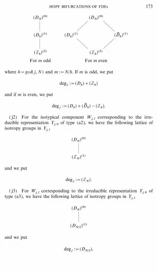
( j1) For the isotypical component corresponding to the type (a1) ofthe irreducible representations of DN , i.e., Wj, 0 :=Vj , where 1� j<�N�2� ,we have the following lattice of isotropy groups of Yj, 0



(DN) (0) (DN) (0)

(Dh) (1) (Dh) (1) (D� h) (1)

(Zh) (2) (Zh) (2)

For m odd For m even

where h=gcd( j, N ) and m :=N�h. If m is odd, we put

deg j :=(Dh)+(Zh)

and if m is even, we put

deg j :=(Dh)+(D� h)&(Zh).

( j2) For the isotypical component Wj, l corresponding to the irre-ducible representation Yj, 0 of type (a2), we have the following lattice ofisotropy groups in Yj, l

(DN) (0)

(ZN) (1)

and we put

deg j :=(ZN).

( j3) For Wj, l corresponding to the irreducible representation Yj, 0 oftype (a3), we have the following lattice of isotropy groups in Yj, l

(DN) (0)

(DN�2) (1)

and we put

deg j :=(DN�2).



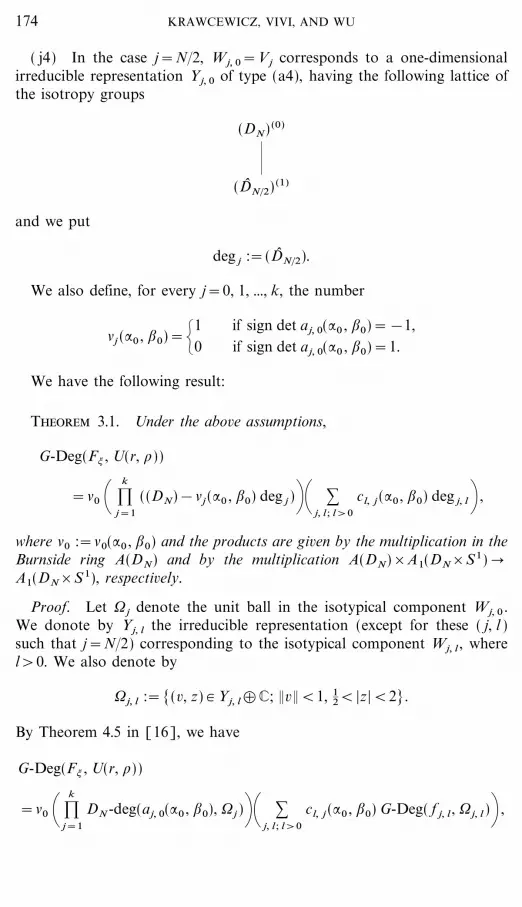
( j4) In the case j=N�2, Wj, 0=Vj corresponds to a one-dimensionalirreducible representation Yj, 0 of type (a4), having the following lattice ofthe isotropy groups

(DN) (0)

(D� N�2) (1)

and we put

deg j :=(D� N�2).

We also define, for every j=0, 1, ..., k, the number

&j (:0 , ;0)={10

if sign det a j, 0(:0 , ;0)=&1,if sign det a j, 0(:0 , ;0)=1.

We have the following result:

Theorem 3.1. Under the above assumptions,

G-Deg(F! , U(r, \))

=&0 \ `k

j=1

((DN)&&j (:0 , ;0) deg j )+\ :j, l ; l>0

cl, j (:0 , ;0) deg j, l+ ,

where &0 :=&0(:0 , ;0) and the products are given by the multiplication in theBurnside ring A(DN) and by the multiplication A(DN)_A1(DN_S1) �A1(DN_S 1), respectively.

Proof. Let 0j denote the unit ball in the isotypical component Wj, 0 .We donote by Yj, l the irreducible representation (except for these ( j, l )such that j=N�2) corresponding to the isotypical component Wj, l , wherel>0. We also denote by

0j, l :=[(v, z) # Yj, l�C; &v&<1, 12<|z|<2].

By Theorem 4.5 in [16], we have

G-Deg(F! , U(r, \))

=&0 \ `k

j=1

DN -deg(aj, 0(:0 , ;0), 0j )+\ :j, l ; l>0

cl, j (:0 , ;0) G-Deg( f j, l , 0j, l )+ ,



where f j, l : Yj, l�C � Yj, l�R is defined by

f j, l (v, z)=(z } v, |z| (&v&&1)+&v&+1).

The computations of G-Deg( f j, l , 0j, l ) were essentially done in Example 4.6in [16], where the Ulrich Type Formula (Theorem 2.2) was applied toshow that for every ( j, l ) such that l>0 we have G-Deg( f j, l , 0j, l )=deg j, l .In order to compute DN -deg(a j, 0(:0 , ;0), 0 j), we can use the propertiesof the Ulrich equivariant degree (the case n=0, see [27] or [17]) and thestandard computations based mostly on the evaluation of appropriate fixedpoint indices). In particular we can verify that DN -Deg(a j, 0(:0 , ;0))=(DN)&&(:0 , ;0) deg j . K

Theorem 3.2. Under the above assumptions, for every nonzero crossingnumber cl, j (:0 , ;0) there exist, bifurcating from (0, :0 , ;0), branches of non-constant periodic solutions of (3.5) such that :

(i1) if the corresponding to the index ( j, l ) element deg j, l is (Z (%j , l )N )+

(Dh_Zl )+(D (c, l )h )&(Zh_Zl ), i.e., m#1 (mod 2), then there are 2 branches

of periodic solutions with the orbit type (Z (%j , l )N ), m=N�h branches with the

orbit type (Dh_Zl ), and m=N�h branches with the orbit type (D (c, l )h );

(i2) if deg j, l=(Z (%j , l )N )+(D (d, l )

2h )+(D (d� , l )2h )&(Z (d, l )

2h ) (i.e., m#2(mod 4)), then there are 2 branches of periodic solutions with orbit type(Z (%j , l )

N ), N�2h branches with the orbit type (D (d, l )2h ), and N�2h branches with

the orbit type (D (d� , l )2h );

(i3) if deg j, l=(Z (%s , l )N )+(D (d, l )

2h )+(D� (d, l )2h )&(Z (d, l )

2h ) (i.e., m#0(mod 4)), then there are 2 branches of periodic solutions of type (Z

(%j , l )N ),

N�2h branches of orbit type (D (d, l )2h ), and N�2h branches of the orbit type

(D� (d, l )2h );

(i4) if deg j, l=(D� (c, l )N ), then there is one branch of periodic solutions of

the orbit type (D� (c, l )N );

(i5) if deg j, l=(D (d, l )N ), then there exists one branch of periodic solu-

tions of the orbit type (D (d, l )N );

(i6) if deg j, l=(D (d� , l )N ), then there exists one branch of periodic solu-

tions of the orbit type (D (d� , l )N ).

Proof. Using the fact that all the orbit types mentioned in Theorem 3.2are maximal, it follows from Theorem 3.1 that if the crossing numbercl, j (:0 , ;0) is nonzero, then there is a nonzero component cl, j (:0 , ;0) deg j, l

of the degree G-Deg(F! , U(r, \)). Consequently, from the existenceproperty of the G-degree, it follows that to every maximal orbit type (H )contained in deg j, l corresponds to at least |G�H | branches bifurcating



from (0, :0 , ;0) nonconstant periodic solutions of the orbit type exactlyequal to (H). K

Remark 3.3. Note that in Theorem 3.2, for a sequence of nonconstantperiodic solutions x(t) of (3.1) corresponding to the 1-periodic solutions(zk(t), :k , ;k) of (3.5) such that (zk(t), :k , ;k) � (0, :0 , ;0) in W�R2 ask � �, 2?�;k is not necessarly the minimal period of xk(t). However, byapplying the same idea as in [18], one can show that if pk is a minimalperiod of xk(t) such that limk � � pk=p0 then there exists an integer r suchthat 2?�;0=rp0 and ir;0 is a characteristic value of (0, :). In particular,if other purely imaginary characteristic values of (0, :0) are not integermultiples of \i;0 , then 2?�;k is the minimal period of xk(t).

Remark 3.4. We should emphasize that the computational formula forG-Deg(F! , U(r, \)) gives more information than what was used in theproof of Theorem 3.2. For example, we did not refer to the factor

&0 \ `k

j=1

((DN)&&j (:0 , ;0) deg j )+ # A(DN)

which provides additional information about the type of symmetriesinvolved in this Hopf bifurcation. At this stage, we are unable to predictthe existence of branches of periodic solutions corresponding to sub-maximal orbit types, but the computational formula for G-Deg(F! , U(r, \))indicates that there is a potential for this type of branches. It was shownin [19] that in the case of a finite dimensional symmetric bifurcation,a nonzero component of the equivariant degree corresponding to an orbittype (H ) (possibly submaximal), implies that the existence of a branch ofsolutions with the orbit type (H ) can be achieved using arbitrarily smallperturbations of the original mapping.

Remark 3.5. The degree G-Deg(F! , U(r, \)) is a local bifurcationinvariant characterizing the Hopf bifurcation from (0, :0 , ;0) which can beused to describe the global behavior of bifurcated branches of solutions.More precisely, assume that (3.1) has only isolated centers (0, :) and let S

be a bounded in H 1(S1; Rn)_R2 branch of nontrivial solutions of (3.1).Then the set of centers (0, :) belonging to S is finite, i.e., S & [0]_R2=[(0, :&1), ..., (0, :M)] and the corresponding sum of local bifurcationinvariants is zero, i.e.,

:M

s=1

G-Deg(F!s, U(rs , \s))=0, (3.1)

where U(rs , \s) is a special neighborhood of (0, :s , ;s) and !s is a corre-sponding complementing function near (0, :s , ;s). As the G-degree is fully



computable for the DN-symmetric Hopf bifurcation and the relations (3.8)take into account not only the maximal orbit types, but also the interactionbetween all the orbit types (including submaximal orbit types) of the bifur-cated solutions, this type of global bifurcation result provides a set of rela-tions which can be used to gain more information about the existence oflarge amplitude periodic solutions or even to prove the existence of multiplesolutions of (3.1). We refer to papers [17] and [18] for more details andexamples.

4. HOPF BIFURCATIONS IN A RING OFIDENTICAL OSCILLATORS

In this section we consider a ring of identical oscillators with identicalcoupling between adjacent cells. Such a ring was modeled by Turing (cf.[26]) and provides models for various situations in biology, chemistry,and electrical engineering. The local Hopf bifurcation of this Turing ringhas been extensively studied in the literature, see [1, 7, 11, 18, 24, 30] andreferences therein.

There are many reasons to emphasize the importance of temporal delaysin coupling between cells, for example, in many chemical or biologicaloscillators the time needed for transport or processing of chemical com-ponents or signals may be of considerable length (see [18]).

We will study how the temporal delay in the kinetics and in the couplingof cells together with the dihedral symmetries of the system may causevarious types of oscillations in the case where each cell is described by onlyone state variable. It has been shown in [8] that such oscillations can notoccur if the temporary delay is neglected.

We consider a ring of N identical cells coupled symmetrically by diffu-sion along the sides of an N-gon (see Fig. 1). Each cell may be regardedas a chemical system with m distinct chemical species. In what follows wewill assume, for the sake of simplicity, that m=1. However, our method,based on the use of the G-equivariant degree, can also be effectively appliedto more complex systems, in particular the case where m>1. We denote byu j (t) the concentration of the chemical species in the j th cell, 0� j�N&1.We assume that the coupling is ``nearest-neighbor'' and symmetric in thesense that the interaction between any neighboring pair of cells takes thesame form. For simplicity, we also assume that the coupling between adjacentcells is linear. Thus, we have the following system of retarded functionaldifferential equations

ddt

u j (t)= f (u jt , :)+K(:)(u j&1

t &2u jt +u j+1

t ), 0� j�N&1, (4.1)


File: 505J 342222 . By:XX . Date:14:05:98 . Time:15:34 LOP8M. V8.B. Page 01:01Codes: 2038 Signs: 1185 . Length: 45 pic 0 pts, 190 mm

FIGURE 1

where t # R denotes the time, : # R is a parameter, u jt (%)=u j (t+%),

0� j�N&1, f : C([&{, 0]; R) � R is continuously differentiable, andK(:) : C([&{, 0]; R) � R is a bounded linear operator and the mappingK : R � L(C([&{, 0]; R), R) is continuously differentiable. In (4.1) weassume that the integer j+1 has taken modulo N.

The function f describes the kinetic law obeyed by the concentrations u j

in every cell, and K(:) represents coupling strength, where the additionalterm

K(:)(u j&1t &u j

t )+K(:)(u j+1t &u j

t ), 0� j�N&1

in (4.1) is usually supported by the ordinary law of diffusion, i.e., thechemical substance moves from a region of greater concentration to aregion of less concentration, at a rate proportional to the gradient of theconcentration. We refer to [1, 26] for more details.

We assume that

f (0, :)=0. (4.2)

Then (0, 0, ..., 0, :) # RN_R is a stationary solution of (4.1) and thelinearization of (4.1) at (0, 0, ..., 0, :) is

ddt

x j (t)=Dx f (0, :) x jt +K(:)[x j&1

t &2x jt +x j+1

t ], 0� j�N&1. (4.3)

Therefore, a number * # C is a characteristic value of the stationary solu-tion (0, :) # RN_R if there exists a nonzero vector z=(z0 , ..., zN&1) # CN

such that

diag(* Id&Dx f (0, :)(e* } Id)) z+r(:, *) z=0,



where diag(* Id&Dx f (0, :)(e* } Id)) denotes the diagonal N_N matrixand r(:, *): CN � CN is defined by

[r(:, *) z]j=K(:)[e* } (zj&1&2z j+zj+1)]; 0� j�N&1.

We put [$z] j=zj&1&2zj+zj+1 , 0� j�N&1. The operator $ is the dis-cretized Laplacian. Therefore, a number * is a characteristic value if andonly if the matrix

2:(*)=diag(* Id&Dx f (0, :)(e* } Id))&r(:, *)

is singular, i.e., the following characteristic equation is satisfied:

detC 2:(*)=0.

We have the following

Proposition 4.1. A number * # C is a characteristic value of the station-ary solution if and only if

detC 2:(*)= `N&1

r=0_*&Dx f (0, :) e* } +4 sin2 ?r

NK(:) e* } &=0.

Proof. For every z # C and r # [0, 1, ..., N&1], we have

(2:(*)(1, !r, ..., !(N&1) r) z) j+1

=[*! jr&Dx f (0, :)(e* } ) ! jr&K(:) e* } (!( j+1) r&2! jr+!( j&1) r] z

=[*&Dx f (0, :) e* } &K(:) e* } (!r&2+!&r)] ! jrz

=[*&Dx f (0, :) e* } &K(:) e* } (2 Re !r&2)] ! jrz

=_*&Dx f (0, :) e* } &2 \cos2?rN

&1+ K(:) e* } & ! jrz

=_*&Dx f (0, :) e* } +4 sin2 ?rN

K(:) e* } & ! jrz. K

It is well-known (see [8]) that a Hopf bifurcation from a stationary solu-tion (0, :) cannot occur if Eq. (4.1) has no temporal delay. However, thetemporal delay in the coupling cells may cause various types of oscillationsin the system (4.1), as will be illustrated in the following.

It is clear that the system (4.1) is equivariant with respect to the actionof the dihedral group DN , where the subgroup ZN of rotations acts on RN



in such a way that the generator ! :=e2?i�N sends the j th coordinate of thevector x=(x0 , x1 , ..., xN&1) # RN to the j+1 (mod N ) coordinate, and theflip } sends the j th coordinate of x to the &j (mod N ) coordinate. Weassume that N>2 and denote this representation by 3 : DN � O(N ).

First, we consider the action of ZN on the complexification U :=CN ofthe representation 3. It is clear that the ZN -isotypical decomposition of Uis given by

U=U� 0�U� 1 � } } } �U� N&1 ,

where U� r :=[z(1, !r, !2r, ..., !(N&1) r); z # C]. Since the flip } sends U� r ontoU� &r , where &r is taken (mod N ), thus U0 :=U� 0 and Ur :=U� r�U� &r for0<r<�N�2� are the isotypical components of U with respect to the actionof DN . If N is even, there is one more isotypical component UN�2 :=U� N�2 .It is easy to see that the isotypical components Ur , 0<r<�N�2� ,correspond to the representations of DN on C�C of the type (b1) given by

#(z1 , z2)=(#r } z1 , #r } z2) if # # ZN ;

}(z1 , z2)=(z2 , z1),

where (z1 , z2) # C�C.If N is an even number, the isotypical component UN�2 is equivalent to

the DN -representation on C=R2 of the type (b3), where

gz={&zz

if g # DN"DN�2 ,if g # DN�2 .

We make the following hypothesis:

(H1) There exists (0, :0) # RN_R such that (0, :0) is an isolated centerof (4.1) such that detC 2(0, :0)(i;0)=0, ;0>0.

It is straightforward to obtain the next two technical results:

Corollary 4.2. A complex number * # C is a j th isotypical charac-teristic value of (0, :), where 0< j<�N�2� , if and only if

p:, j (*) :=*&Dx f (0, :) e* } +4 sin2 ?jN

K(:) e* } =0.

Corollary 4.3. Under the assumption (H1), the j th isotypical crossingnumber for the isolated center (0, :0) corresponding to the value il;0 is equalto



(i) for 0< j<�N�2� ,

cl, j (:0 , ;0)=2(degB( p:0&$, j ( } ), 0l )&degB( p:0+$, j ( } ), 0l ));

(ii) for j=0 or j=N�2 (if N is even),

cl, j (:0 , ;0)=degB( p:0&$, j ( } ), 0l )&degB( p:0+$, j ( } ), 0l ),

where 0l :=(0, b)_(l;0&c, l;0+c)/C and the constants b>0, c>0 and$>0 are sufficiently small.

Using Theorem 3.2, we can establish the following

Theorem 4.4. Assume the hypothesis (H1) is satisfied. If c1, j (:0 , ;0){0,then the stationary point (0, :0) is a bifurcation point of (4.1). Moreover,

(i) if 1< j<N�2, h=gcd( j, N ) and N�h is odd, then there are atleast 2 branches of periodic solutions corresponding to the orbit type (Z

(%j, 1)N ),

N�h branches of periodic solutions corresponding to the orbit type (Dh_Z1),and N�h branches of periodic solutions corresponding to the orbit type(D (c, 1)

h );

(ii) if 1< j<N�2, h=gcd( j, N ) and N�h#2 (mod 4), then there areat least 2 branches of periodic solution corresponding to the orbit type(Z (%j , 1)

N ), N�2h branches of periodic solutions corresponding to the orbit type(D (d, 1)

2h ), and N�2h branches of periodic solutions corresponding to the orbittype (D (d� , 1)

2h );

(iii) if 1< j<N�2, h=gcd( j, N ) and N�h#0 (mod 4), then there areat least 2 branches of periodic solution corresponding to the orbit type(Z (%j , 1)

N ), N�2h branches of periodic solutions corresponding to the orbit type(D (d, 1)

2h ), and N�2h branches of periodic solutions corresponding to the orbittype (D� (d, 1)

2h );

(iv) if j=N�2, then there exists at least one branch of periodic solu-tions corresponding to the orbit type (D (d� , l )

N );

(v) if j=0, then there exists at least one branch of periodic solutionscorresponding to the orbit type (DN_Z1).

Example 4.5. We consider the following system of retarded functionaldifferential equations (cf. [18])

x* j (t)=&:xj (t)+:h(xj (t))[ g(xj&1)&2g(x j (t&1))+g(x j+1(t&1))],

(4.4)

where 0� j�N&1 and we use the convention that j+1 is always taken(mod N ), :>0, h, g : R � R are continuously differentiable, h does not



vanish and g(0)=0, g$(0)>0. By using an appropriate change of variablesand rescaling the time, Eq. (4.4) can be transformed into an equation of thesame type as Eq. (4.1). In addition, we have

p:, j (*)=*+:+4 sin2 ?rN

:+e&*,

where +=h(0) g$(0). Assume that there exists j, 0< j<N�2, such that +>1�(4 sin2(?j�N )), then the number i;0, j , where ;0, j # (?�2, ?), is the uniquesolution of cos ;0, j= &1�(4 sin2(?j�N )) is a j th isotypical characteristicvalue corresponding to the stationary solution (0, :0, j), where :0, , j=&;0, j cot ;0, j . It can be computed (see [18]) that (0, :0, j) satisfies theassumption (H1) and we have c1, j (:0, j , ;0, j)<0. Consequently, byTheorem 4.4 we have

Proposition 4.6. Let h=gcd( j, N ). If there exists j, 0< j<N�2 suchthat +>1�(4 sin2(?j�N )), then the stationary solution (0, :0) is a bifurcationpoint for Eq. (4.4). In particular,

(i) if N�h is odd, then there are at least 2 branches of periodic solu-tion corresponding to the orbit type (Z (%j , 1)

N ), N�h branches of periodic solu-tions corresponding to the orbit type (Dh_Z1), and N�h branches of periodicsolutions corresponding to the orbit type (D (c, 1)

h ).

(ii) if N�h#2 (mod 4), then there are at least 2 branches of periodicsolution corresponding to the orbit type (Z (%j , 1)

N ), N�2h branches of periodicsolutions corresponding to the orbit type (D (d, 1)

2h ), and N�2h branches of peri-odic solutions corresponding to the orbit type (D (d� , 1)

2h );

(iii) if N�h#0 (mod 4), then there are at least 2 branches of periodicsolution corresponding to the orbit type (Z (%j , 1)

N ), N�2h branches of periodicsolutions corresponding to the orbit type (D (d, 1)

2h ), and N�2h branches of peri-odic solutions corresponding to the orbit type (D� (d, 1)

2h ).

Corollary 4.7. Assume that N is a prime number. If there exists j,0< j<N�2, such that +>1�(4 sin2(?j�N )), then there are at least 2(N+1)different branches of nonconstant periodic solutions of (4.4) bifurcating fromthe stationary solution (0, :0).

ACKNOWLEDGMENTS

The authors thank Zalman Balanov for his suggestions and discussions. We are also grate-ful to the referee for his critical remarks and comments.



REFERENCES

1. J. C. Alexander and G. Auchmuty, Global bifurcations of phase-locked oscillators, Arch.Rational Mech. Anal. 93 (1986), 253�270.

2. G. Dylawerski, K. Ge� ba, J. Jodel, and W. Marzantowicz, S1-equivariant degree and theFuller index, Ann. Polon. Math. 52 (1991), 243�280.

3. L. H. Erbe, K. Ge� ba, W. Krawcewicz, and J. Wu, S1-degree and global Hopf bifur-cation theory of functional differential equations, J. Differential Equations 97 (1992),227�239.

4. B. Fiedler, ``Global Bifurcation of Periodic Solutions with Symmetry,'' Lecture Notes inMath., Vol. 1309, Springer-Verlag, Berlin�New York, 1988.

5. K. Ge� ba, W. Krawcewicz, and J. Wu, An equivariant degree with applications to sym-metric bifurcation problems I: Construction of the segree, Bull. London Math. Soc. 69(1994), 377�398.

6. K. Ge� ba and W. Marzantowicz, Global bifurcation of periodic solutions, Top. Methods inNonlinear Anal. 1 (1991), 67�93.

7. S. A. van Gils and T. Valkering, Hopf bifurcation and symmetry: Standing and travellingwaves in a circular-chain, Japan J. Appl. Math. 3 (1986), 207�222.

8. M. Golubitsky, D. G. Schaeffer, and I. N. Stewart, ``Singularities and Group in Bifurca-tion Theory,'' Vol. II, Springer-Verlag, Berlin�New York, 1988.

9. M. Golubitsky and I. N. Stewart, Hopf bifurcation in the presence of symmetry, Arch.Rational Mech. Anal. 87 (1985), 107�165.

10. M. Golubitsky and I. N. Stewart, Hopf bifurcation with dihedral group symmetry:Coupled nonlinear oscillators, in ``Multiparameter Bifurcation Theory'' (M. Golubitskyand J. Guckenheimer, Eds.), Contemporary Math., Vol. 56, pp. 131�137, 1986.

11. L. N. Howard, Nonlinear oscillations, in `Òscillations in Biology'' (F. R. Hoppensteadt,Ed.), AMS Lecture Notes in Math., Vol. 17, pp. 1�69, 1979.

12. J. Ize, Topological bifurcation, Reportes de Invest. UNAM 34 (1993), 1�129.13. J. Ize, I. Massabo� , and V. Vignoli, Degree theory for equivariant maps, I, Trans. Amer.

Math. Soc. 315 (1989), 433�510.14. J. Ize, I. Massabo� , and V. Vignoli, Degree theory for equivariant maps, the general S1-action,

Mem. Amer. Math. Soc. 481 (1992).15. J. Ize, I. Massabo� , and V. Vignoli, Equivariant degree for abelian actions. Part I: Equiv-

ariant Homotopy Groups, Top. Methods in Nonlinear Anal. 2 (1993), 367�413.16. W. Krawcewicz, P. Vivi, and J. Wu, Computationa formulae of an equivariant degree

with applications to symmetric bifurcations, Nonlinear Studies 4 (1997), 89�120.17. W. Krawcewicz and J. Wu, ``Theory of Degrees with Applications to Bifurcations and

Differential Equations,'' CMS Series of Monographs, Wiley, New York, 1997.18. W. Krawcewicz and J. Wu, Theory and applications of Hopf bifurcations in symmetric

functional differential equations, Nonlinear Anal., to appear.19. W. Krawcewicz and P. Vivi, Normal bifurcation and equivariant degree, preprint, 1996.20. W. Krawcewicz, J. Wu, and H. Xia, Global Hopf bifurcation theory for condensing fields

and neutral equations with applications to lossless transmission problems, Canad. Appl.Math. Quart. 1 (1993), 167�220.

21. W. Krawcewicz and H. Xia, Analytic constructon of an equivariant degree, IzvestyaVuzov Matematika 6 (1996), 37�53 [in Russian]; and Russian Mathematics (Iz. Vuz.Matematika) 40 (1996), 34�49.

22. G. Peschke, Degree of certain equivariant maps into a representation sphere, TopologyAppl. 59 (1994), 137�156.

23. D. H. Sattinger, Bifurcation and symmetry breaking in applied mathematics, Bull. Amer.Math. Soc. 3 (1980), 779�89.



24. S. Smale, A mathematical model of two cells via Turing's equation, in ``Some Mathemati-cal Questions in Biology V'' (J. D. Cowan, Ed.), AMS Lecture Notes on Mathematics inthe Life Sciences, Amer. Math. Soc., Providence, RI, Vol. 6, pp. 15�26, 1974.

25. T. Dieck, ``Transformation Groups,'' de Gruyter, Berlin, 1987.26. A. Turing, The chemical basis of morphogenesis, Phil. Trans. Roy. Soc. B 237 (1952),

37�72.27. H. Ulrich, ``Fixed Point Theory of Parametrized Equivariant Maps,'' Lect. Notes in

Math., No. 1343, Springer-Verlag, Berlin�New York, 1980.28. A. Vanderbauwhede, ``Local Bifurcation and Symmetry,'' Research Notes in Math.,

Vol. 75, Pitman, Boston, 1982.29. J. Wu and W. Krawcewicz, Discrete waves and phase-locked oscillations in the growth of

a singular-species population over patch environment, Open Systems and InformationDynamics in Physics and Life Sciences 1 (1992), 127�147.

30. J. Wu, Symmetric differential equations and neutral networks with memory, Trans. Amer.Math. Soc., to appear.

31. X. Zou and J. Wu, Local existence and stability of periodic travelling waves of latticefunctional differential equations, preprint, 1996.

� � � � � � � � � �


Documents

Hopf Bifurcations of Functional Differential Equations with Dihedral Symmetries