arX

iv:1

009.

1019

v3 [

nlin

.CD

] 1

7 D

ec 2

010

Higher order statistics in the annulus square

billiard: transport and polyspectra

L Rebuzzini 1,2, R Artuso 1,3

1 Center for Nonlinear and Complex Systems and Dipartimento di Fisica eMatematica, Universita dell’Insubria, Via Valleggio 11, 22100 Como, Italy.2 Istituto Nazionale di Fisica Nucleare, Sezione di Pavia, Via Ugo Bassi 6, 27100Pavia, Italy.3 Istituto Nazionale di Fisica Nucleare, Sezione di Milano, Via Celoria 16, 20133Milano, Italy.

E-mail: laura.rebuzzini@uninsubria.it

Abstract. Classical transport in a doubly connected polygonal billiard, i.e. theannulus square billiard, is considered. Dynamical properties of the billiard flowwith a fixed initial direction are analyzed by means of the moments of arbitraryorder of the number of revolutions around the inner square, accumulated by theparticles during the evolution. An “anomalous” diffusion is found: the momentof order q exhibits an algebraic growth in time with an exponent different fromq/2, like in the normal case. Transport features are related to spectral propertiesof the system, which are reconstructed by Fourier transforming time correlationfunctions. An analytic estimate for the growth exponent of integer order momentsis derived as a function of the scaling index at zero frequency of the spectralmeasure, associated to the angle spanned by the particles. The n-th ordermoment is expressed in terms of a multiple-time correlation function, dependingon n−1 time intervals, which is shown to be linked to higher order density spectra(polyspectra), by a generalization of the Wiener-Khinchin Theorem. Analyticresults are confirmed by numerical simulations.

PACS numbers: 05.45.-a, 05.60.-k, 05.20.-y

Higher order statistics in the annulus square billiard 2

1. Introduction.

A fundamental problem in statistical mechanics is to understand how the reversiblemicroscopic dynamics of particles may produce macroscopic transport phenomena,which are described by irreversible laws such as diffusion equation or Fourier law.In particular, the last few years have witnessed a large debate whether chaos at amicroscopic level is a necessary ingredient to generate realistic macroscopic behaviour[1, 2]. In this paper we will be concerned with transport (diffusion) properties; forthis purpose, billiards represent a class of dynamical systems ideally suited, as theyallow both theoretical considerations and extensive numerical simulations: transportis typically studied by lifting the billiard table on the plane, like in the case of theperiodic Lorentz gas [1, 3, 4, 5, 6]. We also remark their physical significance assimplified models to study energy or mass transport in realistic systems, such asfluids, nanodevices, electromagnetic cavities, optical fibers and low density particlesin porous media [7, 8, 9, 10].

While the origin of normal diffusion (i.e. when the mean square displacement ofthe particles grows asymptotically linearly in time) is well understood in fully chaoticbilliards [3, 11], in recent years, great interest has focused on the study of transportin polygonal billiards, which are characterized by the absence of hyperbolicity anddynamical chaos, in the sense of exponential divergence of nearby initial trajectories.Indeed in polygonal billiards, all the Lyapunov exponents and Kolmogorov-Sinaientropy vanish and the dispersion of initially nearby orbits is polynomial. Neverthelesspolygonal billiards may give rise to a wide range of transport regimes, extending fromnormal to “anomalous” diffusion, in which the r.m.s. displays a non linear dependenceon time [12, 13, 14, 15, 16]. Some necessary conditions for the occurrence of normaltransport in periodical billiard chains have been singled out: vertex angles irrationallyrelated to π, absence of parallel scatterers, existence of an upper bound for the freepath length between collisions [17].

Particle dynamics in billiards can be described in terms of an invertible flow incontinuous time or, equivalently, of an invertible map connecting two collision points,which corresponds to a unitary evolution ruled by the Koopman operator. The mainfeatures of the dynamical transport are related to ergodic properties of the system,which can be formulated in terms of properties of the spectrum of the Koopmanoperator. Ergodic properties of polygonal billiards have been extensively tested bythe analysis of the decay of correlations, such as mixing in the triangle with irrationalangles [18] and weak-mixing as the maximal ergodic property in the right-trianglewith irrational acute angles [19]. The billiard flow in a typical polygon is ergodic,nevertheless the subset of rational polygonal billiards, in which all the angles betweenthe sides are rational multiples of π, possess weaker ergodic properties. Some exactresults are known for this subset: the billiard flow is not ergodic, because of a finitenumber of possible directions for a given initial condition, and it can be decomposedinto directional flows, which are ergodic but not mixing, for a generic choice of thedirection and for almost all initial conditions [20, 21].

The model considered in this paper is a doubly connected rational billiards, calledthe annulus square billiard, which was also studied in a quantum dynamical context[22, 23]. The billiard table, shown in figure 1, is formed by the plane region included inbetween two concentric squares with sides of different length. Arithmetical propertiesof the ratios between the sides of the two squares and between the components ofthe velocity vector of the particle determine different dynamical and spectral features,

Higher order statistics in the annulus square billiard 3

which allow a classification of the system into different subclasses [24], reviewed insection 2.2. We inspect the angle (and its absolute value), accumulated by a particlerevolving around the hole, and provide a complete characterization of the transportprocess by the analysis of moments of arbitrary order of this observable. The statisticalapproach is supported by a spectral analysis of the system: the interdependencebetween dynamical and spectral properties leads to a theoretical prediction for theexponents of moments of integer order. We restrict to the class of billiards in whichthe ratios of the sides and velocity components are both irrational; in this case, fortypical values of the parameters, the billiard flow, in a fixed direction, is weakly-mixing and not mixing, entailing the presence of a singular continuous component inthe spectrum, namely supported on a set of zero Lebesgue measure [24]. By assumingthat the singularities of the spectral measure are of Holder type [25, 26], we derive ananalytical relation connecting the exponents of the algebraic growth in time of integermoments with the scaling index at zero frequency of the spectral measure, associatedto the angle. The formula is exact for even-order moments, while it is an upper boundfor odd-order moments. This result generalizes the one obtained in [24] for the meansquare displacement (i.e. second order moment). Furthermore, analysis of higherorder statistics demands the introduction, in the context of dynamical system, ofbasic concepts as multiple-time correlation functions and polyspectra, which are ratherfamiliar in signal analysis [27]. The theoretical relation for integer order moments istested by numerical simulations, which moreover suggest that a similar estimate holdsfor moments of arbitrary order: the q-th order moment grows in time with an exponentνq; ν is a constant function of the scaling index of the spectral measure in 0, whichranges between ν = 1/2 (“normal” diffusion) and ν = 1 (“ballistic” transport).

A more detailed characterization of the anomalous diffusion process has recentlybeen considered in many papers about diffusion in periodical polygonal billiardchannel, in which the polygonal scatterers form a 1-dimensional periodical array[12, 13, 14, 16, 28]. These studies constitute a further motivation to the analysisof transport in the square annulus billiard; indeed, to examine the dynamics ofparticles winding around the inner square is equivalent to consider the transportin a “generalized Lorentz gas”, i.e. an extended system, obtained by periodicallyrepeating the elementary cell in both directions. In periodic channels, two differentbehaviours are identified: “weak” anomalous diffusion, when the exponent of thealgebraic growth of moment of order q is a linear function of the order, namely νqwith ν = const. 6= 1/2 for ∀q, and “strong” anomalous diffusion, when the exponentis a non trivial function of the order, i.e. ν(q)q [29, 30]. In some polygonal chains, atransition from normal to anomalous diffusion has been found in cases with an infinitehorizon, i.e. when the particle may travel without colliding with the walls, or, whenthe particle can propagate arbitrarily far by reflecting off only on parallels scatterers[15, 16]. A value qcr exists that discriminates between the two regimes with differentslopes of the exponent versus q. This phase transition physically corresponds to achange in the balance between the ballistic and diffusive trajectories in the ensembleaverages and infers the absence of a unique scaling law for the probability densityof particles, which does not relax at long times into a self-similar profile; this kindof processes are therefore classified as “ weak” self-similar processes. In some othercases, such as in the “zigzag model” [17, 29], the phase transition is not present; thisseems to be related to the geometry of the polygonal channel and, in particular, tothe number-theoretical properties of the angles.

The paper in organized as follows. The billiard model is described in section 2

Higher order statistics in the annulus square billiard 4

(s,ϕ)(s,-ϕ)

O

1

2

3

4

5

6

7

8

Figure 1. (Colour online) Billiard table for l1/l2 = π/2. A portion of a trajectoryof a particle with initial condition (s, ϕ), evolving under Bt

ϕ with t ≥ 0, is shown;(s,−ϕ) is the ”time reversed” initial condition.

and its basic spectral properties are reviewed. In section 3 we introduce the phaseobservable which identifies the diffusive process and we developed the spectral analysisof the signal produced by time evolution. We then consider arbitrary order momentsof the observable; the crucial issue is to get informations on the scaling function, whichdetermines the algebraic growth of the moments for long times. From the analyticpoint of view we restrict to integer order moments: higher order moments are expressedin terms of multiple-time correlation functions and polyspectra, which are introducedin section 4. The analytic relation between spectral and dynamical indexes is derivedin section 5 and numerically confirmed in section 6.

2. The model.

2.1. Description of the billiard table

We consider the dynamics of a classical point particle in a doubly connected rationalpolygonal billiard. The billiard table, shown in figure 1, is delimited by two concentricsquares with parallel sides of length l1 and l2 (l1 > l2). The particle moves freelyinside the billiard, colliding elastically with the boundary; the (preserved) modulus ofthe velocity is taken equal to 1. The accessible phase space is 3-dimensional and therepresentative point is (x, y, θ): (x, y) are the Cartesian coordinates of the particlesand θ is the angle of the velocity, measured counterclockwise from the positive x-axis.The billiard flow, denoted by T t, preserves the Lebesgue measure dxdydθ/(2π(l21−l22)).

We may also consider the discrete time dynamics, induced by successive collisions.Each collision point can be parametrized by a coordinate s along the boundary andan angle ϕ, between the outgoing direction and the inner normal to the boundary;

Higher order statistics in the annulus square billiard 5

we take ϕ positive if the outgoing velocity is given by a counterclockwise rotation tothe inner normal. By denoting L = 2(l1 + l2), the arclength s ∈ [−L,L) takes thevalue s = −L in the left corner of side 1 and increases by moving counterclockwisealong the sides of the billiard, labeled by increasing numbers (see figure 1). Thecorresponding phase space is called M = (s, ϕ); s ∈ [−L,L), ϕ ∈ [−π/2, π/2) andthe Birkhoff-Poincare map is denoted by Bt (t ∈ Z); the map Bt preserves the measuredΩ(z) = cosϕdϕ ds /(4L) on M.

Dynamics on such billiards is strongly influenced by number–theoreticalproperties of l2/l1 and of tanϕ; in particular we may distinguish three classes [24]:(i) class 1: l2/l1, tanϕ ∈ Q; (ii) class 2: l2/l1 ∈ Q, tanϕ ∈ R−Q; (iii) class 3:l2/l1 ∈ R−Q, tanϕ ∈ R−Q. In this paper we restrict to class 3.

2.2. Review on basic spectral properties

As all the internal angles are rational multiples of π, it is fairly easy to realize thatthe flow on the global phase space, or the mapping Bt on M, can never be ergodic.However T t can be decomposed into the one-parameter family of directional flows atfixed θ, T t

θ , whose dynamics is not trivial: in particular, T tθ is ergodic for almost all

θ ∈ [0, π/2) and never mixing [20, 21]. It is believed that the weak-mixing propertyshould be enjoyed by a “generic” subset of directional flows, and numerical evidencesfor class 3 are provided in [24].

Analogously to the billiard flow, the map Bt can be decomposed into a one-parameter family of components Bt

ϕ along the fixed direction ϕ (with 0 ≤ ϕ ≤ π/2).Once the initial outgoing angle is set, only the angles ±ϕ,±(π2 −ϕ) can be met alongthe trajectory, so the phase space for any fixed foliation, i.e. Mϕ, is a fourfold replicaof [−L,L): its points are denoted by z = (s,±ϕj) with ϕj = ϕ − jπ/2 and j = 0, 1.The phase average of an observable f : Mϕ → C can be written explicitly as:

∫

Mϕ

dΩ(z) f(z) =1

8L

∫ L

−L

ds

1∑

j=0

cosϕj f(s, ϕj) + f(s,−ϕj) . (1)

Spectral properties of the system can be formulated in terms of the asymptoticbehaviour of the correlation functions.

Ergodicity of Btϕ implies that the time-averaged correlation function of a generic

(real) phase function f : Mϕ → R:

Ctimef (t, z) = lim

T→+∞

1

2T

T−1∑

t′=−T

f(Bt′+tϕ z)f(Bt′

ϕz), (2)

and the phase-averaged correlation function:

Cphf (t) = 〈f |U tf〉 =

∫

Mϕ

dΩ(z) f(Btϕz)f(z), (3)

coincide for Ω-almost every z ∈ Mϕ. The unitary operator U in (3) is the Koopmanoperator, associated to the map Bt

ϕ.As directional flows or mappings are not mixing, correlation functions (of zero

mean observables) do not decay to zero in the asymptotic limit; while the (conjectured)weak-mixing property guarantees that integrated correlations:

Cintf (t) =

1

t

t−1∑

s=0

∣

∣

∣Cphf (s)

∣

∣

∣

2

(4)

Higher order statistics in the annulus square billiard 6

-4

-2

0

2

4 6 8 10 12 14t

Cin

t,Cph

(a)

-10

-5

0

-10 -5 0lnδ

χ 1,2

(b)

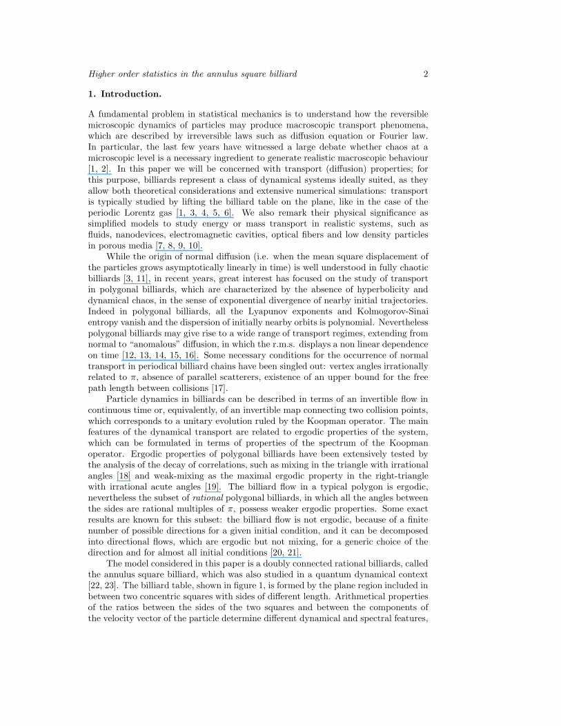
Figure 2. (Colour online) (a) Phase averaged (upper line) and integrated (lower)correlation functions of the angle ξ, spanned by the radius vector, as a functionof time t (measured in numbers of collisions). The billiard table belongs to class3 with parameters: l1/l2 = π/2 and tanϕ = π/4. The dotted line, which fitsCint(t), has a slope equal to −D2. (b) Estimates of generalized dimensions D1

(empty symbols) and D2 (full symbols) of the spectral measure, associated toξ, for the same parameters. The dimension estimates are given by the slopes ofstraight lines: D1 = 0.69 ± 0.01 and D2 = 0.42 ± 0.02. Details are explained insection 6.

vanish as t → ∞. Phase-averaged correlation function and integrated correlationfunction of the angle ξ, spanned by the radius vector of a particle between twosuccessive collision points, are shown in figure 2(a) for a generic billiard belongingto class 3: while Cph(t) 6→ 0 (upper line), Cint

f (t) decays to zero polynomially (lowerline).

By using the spectral decomposition of the Koopman operator U , we may rewrite(3) as

Cphf (t) =

1

2π

∫ π

−π

dµf (θ)eiθt, (5)

which provides a direct link between the autocorrelation function of an observable fand the associated spectral measure. If (in the complement of constant functions) thespectral measure is absolutely continuous, the system is mixing. On the other side,weak mixing is equivalent to an empty point spectrum, apart from the eigenvalue 1.Therefore, the weak mixing property, without the stronger mixing property, entailsthe presence of a singular continuous component of the spectrum of the Koopmanoperator.

Owing to the presence of a non empty point spectra, weakly mixing property isruled out in the almost integrable cases, namely for l1/l2 ∈ Q (class 1 and class 2);we will not consider such cases in the present work.

In [24], the occurrence of a singular continuous component of the spectrum inbilliards of class 3 was inferred by looking at scaling properties of the spectral measure,obtained by finer and finer numerical inversion of (5). In particular a multifractalanalysis yields a nontrivial spectrum of generalized dimensions, with a Hausdorff

Higher order statistics in the annulus square billiard 7

dimension D1 less than 1 and a correlation dimension D2 which rules the power-lawdecay of integrated correlations [31, 32]. An example is shown in figure 2(b), for thespectral measure associated to the angle ξ. As we will show in following sections, thelocal scaling properties of the spectral measure are even more relevant in connectionwith transport properties. For billiards in class 3, a nontrivial scaling of the spectralpeaks near the zero frequency is found (see figure 4(b)), in opposition to the almostintegrable case, in which a non empty pure point spectrum is marked by not scalingdeltalike peaks at different resolutions [24].

3. Higher order statistics

3.1. Dynamical quantities and spectral analysis

The dynamics inside the billiard table in figure 1 is equivalent to the dynamics of theparticles in a two-dimensional infinite periodic lattice with square obstacles, i.e. in ageneralized Lorentz gas, recently examined in [12, 13, 14, 16, 28]. The unfolded systemis obtained by reflecting the elementary cell and the segment of a trajectory at eachcollision point with the external square. Instead of considering particle diffusion alongthe channels of the extended system, we examine the transport generated by billiardtrajectories revolving around the inner square obstacle.

For this purpose, the natural observable is the angle ξ(z), spanned by the radiusvector, joining the center of the billiard O with the collision point z, when the particleis moving from z to Bϕz; it is assumed positive when counterclockwise. The totalangle accumulated by a single particle up to time t is:

Ξ(z, t) =

t−1∑

s=0

ξ(Bsϕz); (6)

Ξ(z, t)/(2π) gives the number of revolutions completed by a trajectory up to the timet.

In [24] the 2-nd order moment σ2(t) of Ξ(z, t), namely the r.m.s. number ofrevolutions, was examined; for generical values of the parameters in class 3, an“anomalous diffusion” was found, marked by an algebraic growth of σ2 in time withan exponent ranging between 1 (normal diffusion) and 2 (ballistic transport); thisexponent has shown to be related to the zero-frequency scaling index of the densitypower spectrum associated to the observable ξ(z). In this paper we extend the analysisto moments of arbitrary order.

Since ξ(Btϕz) is a “power signal”, i.e. ξ(Bt

ϕz)t∈Z 6∈ ℓ2(Z), as a function of

time t, but W = limT→∞12T

∑T−1t=−T ξ

2(Btϕz) ≡ Ctime

ξ (0; z) < +∞, we analyse thetrajectory of a particle on a finite time interval: −T ≤ t ≤ T (with T positive integer,i.e. T ∈ N+). Spectral analysis will involve Fourier transform of the signal ξ(Bt

ϕz) onfinite portions of trajectories.

Hence we call ξT the partial sum of the Fourier series of ξ(Btϕz):

ξT (θ; z) =(

kT ∗ ξ)

(θ; z) =

T−1∑

t=−T

ξ(Btϕz)e

−itθ = ρT (θ; z)eiφT (θ;z), (7)

where ∗ denotes convolution and kT (x) =∑T−1

t=−T e−ixt = ei

x2

(

sinTxsin x

2

)

. The upper

limit of the sum in (7) is determined by the fact that ξ(BTϕ z) is not defined.

Higher order statistics in the annulus square billiard 8

10

20

30

40

4 6 8 10 12 14lnt

ln(σ

4 )

Figure 3. (Colour online) Fourth order moment of Ξ(z, t) vs time in logarithmicscales, for the same data of figure 4. The slope of the straight line (= 3.4) is givenby the theoretical prediction (38) with n = 4 and α(0) = 0.3.

ξT (θ; z)

T∈N+

is a sequence of continuous, bounded and periodic complex

function of the frequency θ ∈ T; T = R/(2πZ) denotes the 1-dimensional torus.As ξ(Bt

ϕz) 6→ 0 for t → ∞, the limit T → ∞ of the sequence of partial sums maynot be a function in ordinary sense; as |ξ(t; z)| ≤ A ∀t ∈ Z and 0 < A < π, from the

theory of Fouries series, it follows that

ξT (θ; z)

T∈N+

converges weakly for T → ∞to a tempered distribution of period T.

Since ξ is a real-valued function, ξ∗T (θ; z) = ξT (−θ; z) and the absolute value and

the phase of ξT are respectively even and odd functions of θ (mod 2π) :

ρT (−θ; z) = ρT (θ; z) = ρT (|θ|; z) (8)

φT (−θ; z) = −φT (θ; z). (9)

In particular ξT (0; z) = ρT (0; z), φT (0; z) = 0; while, from periodicity and from (9),it follows that φT (−π; z) = φT (π; z) = 0.

By looking at forward trajectories starting at (s, ϕ) and their time reversal,generated by the “backward” (inverse) operator B−1

ϕ on (s,−ϕ), we can verify thatthe following identity holds:

ξ(Btϕ(s,−ϕ)) = −ξ(B−t−1

ϕ (s, ϕ)). (10)

This identity induces the following property of the partial sums:

ξT (θ; (s,−ϕ)) = −eiθ ξ∗T (θ; (s, ϕ)), (11)

which is equivalent to ρT (θ; (s,−ϕ)) = ρT (θ; (s, ϕ)) and φT (θ; (s,−ϕ)) = θ + π −φT (θ; (s, ϕ)) (mod (2π)).

Higher order statistics in the annulus square billiard 9

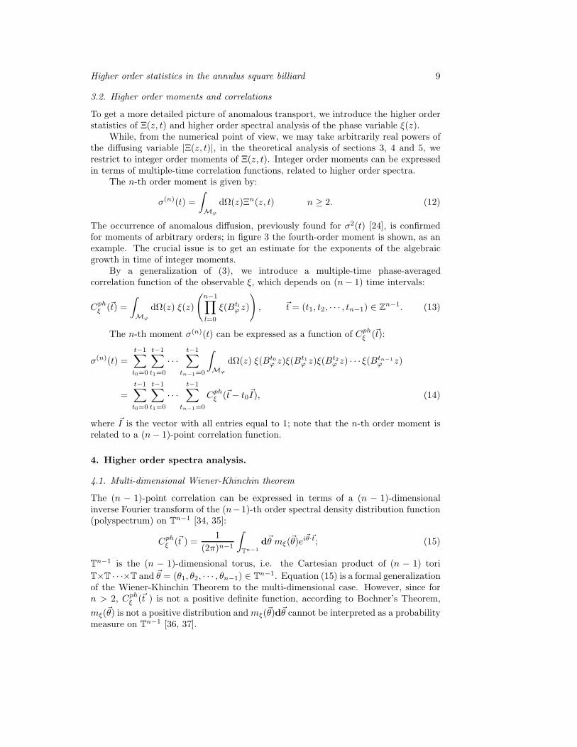
3.2. Higher order moments and correlations

To get a more detailed picture of anomalous transport, we introduce the higher orderstatistics of Ξ(z, t) and higher order spectral analysis of the phase variable ξ(z).

While, from the numerical point of view, we may take arbitrarily real powers ofthe diffusing variable |Ξ(z, t)|, in the theoretical analysis of sections 3, 4 and 5, werestrict to integer order moments of Ξ(z, t). Integer order moments can be expressedin terms of multiple-time correlation functions, related to higher order spectra.

The n-th order moment is given by:

σ(n)(t) =

∫

Mϕ

dΩ(z)Ξn(z, t) n ≥ 2. (12)

The occurrence of anomalous diffusion, previously found for σ2(t) [24], is confirmedfor moments of arbitrary orders; in figure 3 the fourth-order moment is shown, as anexample. The crucial issue is to get an estimate for the exponents of the algebraicgrowth in time of integer moments.

By a generalization of (3), we introduce a multiple-time phase-averagedcorrelation function of the observable ξ, which depends on (n− 1) time intervals:

Cphξ (~t) =

∫

Mϕ

dΩ(z) ξ(z)

(

n−1∏

l=0

ξ(Btlϕ z)

)

, ~t = (t1, t2, · · · , tn−1) ∈ Zn−1. (13)

The n-th moment σ(n)(t) can be expressed as a function of Cphξ (~t):

σ(n)(t) =

t−1∑

t0=0

t−1∑

t1=0

· · ·t−1∑

tn−1=0

∫

Mϕ

dΩ(z) ξ(Bt0ϕ z)ξ(B

t1ϕ z)ξ(B

t2ϕ z) · · · ξ(Btn−1

ϕ z)

=

t−1∑

t0=0

t−1∑

t1=0

· · ·t−1∑

tn−1=0

Cphξ (~t− t0~I), (14)

where ~I is the vector with all entries equal to 1; note that the n-th order moment isrelated to a (n− 1)-point correlation function.

4. Higher order spectra analysis.

4.1. Multi-dimensional Wiener-Khinchin theorem

The (n − 1)-point correlation can be expressed in terms of a (n − 1)-dimensionalinverse Fourier transform of the (n−1)-th order spectral density distribution function(polyspectrum) on Tn−1 [34, 35]:

Cphξ (~t ) =

1

(2π)n−1

∫

Tn−1

d~θ mξ(~θ)ei~θ·~t; (15)

Tn−1 is the (n − 1)-dimensional torus, i.e. the Cartesian product of (n − 1) tori

T×T · · ·×T and ~θ = (θ1, θ2, · · · , θn−1) ∈ Tn−1. Equation (15) is a formal generalizationof the Wiener-Khinchin Theorem to the multi-dimensional case. However, since forn > 2, Cph

ξ (~t ) is not a positive definite function, according to Bochner’s Theorem,

mξ(~θ) is not a positive distribution andmξ(~θ)d~θ cannot be interpreted as a probabilitymeasure on Tn−1 [36, 37].

Higher order statistics in the annulus square billiard 10

An alternative version of the theorem involves the time-averaged correlationfunction:

Ctimeξ (~t; z) ≡ lim

T→∞

1

2T

T−1∑

t=−T

ξ(Btϕz)

(

n∏

l=1

ξ(Bt+tlϕ z)

)

(16)

=1

(2π)n

∫

Tn−1

d~θ sξ(~θ; z)ei~θ·~t, (17)

with

mξ(~θ) =

∫

Mϕ

dΩ(z)sξ(~θ; z). (18)

If the system is ergodic, sξ(~θ; z) = mξ(~θ), for Ω-almost every z ∈ Mϕ.

4.2. Polyspectra

We may obtain mξ(~θ) in terms of partial sums of the Fourier series of ξ(Btϕz).

Firstly, we derive sξ(~θ; z) from (17). Since we consider the trajectory of aparticle on a finite time interval, each signal ξ(Bt+tl

ϕ z) in (16) is substituted byχIT

(t + tl) · ξ(Bt+tlϕ z), where χIT

is the characteristic function of the interval ofintegers IT ≡ t ∈ Z;−T ≤ t ≤ T − 1.

The square window of the signal is expressed by the Fourier transform

χIT(t)ξ(Btz) =

1

2π

∫ π

−π

dθ ξT (θ; z)eiθt, (19)

which is obtained by the Convolution Theorem from (7).

The polyspectra sξ(~θ; z) (and thus mξ(~θ)) is given as a limit of a sequence of

functions sT,ξ(~θ; z)T∈N+ , which converges to sξ(~θ; z) in a weak sense:

sξ(~θ; z) = limT→∞

sT,ξ(~θ; z) weakly. (20)

By inverting (17) and substituting (19), we get:

sT,ξ(~θ; z) =1

2T

T−1∑

t=−T

T−t−1∑

t1=−T−t

· · ·T−t−1∑

tn−1=−T−t

e−i~θ·~tχIT(t)ξ(Btz)

n−1∏

l=1

χIT(t+ tl)ξ(B

t+tlz)

=1

2T (2π)n

∫

T

dθ

∫

Tn−1

d~θ′ξT (θ; z)k∗T (θ +Θ(~θ))

n−1∏

l=1

ξT (θ′l; z)kT (θl − θ′l),

where Θ(~θ) =∑n−1

l=1 θl. By using that kT (x) (and k∗T (x)) is an approximate identity,

i.e. limT→∞

∫

TdθkT (θ − θ′)f(θ) = 2πf(θ′) for all continuous functions f on T, the

final expression of sξ(~θ; z) is obtained:

sξ(~θ; z) = limT→∞

1

2T

n−1∏

j=1

ξT (θj ; z)

ξ∗T

(

Θ(~θ); z)

. (21)

mξ(~θ) is derived by applying phase averages (18) to both sides of (21). The result isconsistent with analogous formulas in [34, 38].

We introduce the notation: ΓT (~θ; zs,l) =∏n−1

j=1 ρT (θj ; zs,l) and ΦT (~θ; zs,l) =∑n−1

j=1 φT (θj ; zs,l), with zs,l = (s, ϕl) and ϕl = ϕ− lπ/2 (l = 0, 1).

Higher order statistics in the annulus square billiard 11

By evaluating the phase average with (1) and by making use of the property (11),we get:

mξ(~θ) = limT→∞

mT,ξ(~θ) weakly

mT,ξ(~θ) =1

4L

∫ L

−L

ds1∑

l=0

cosϕl ·MT,ξ(~θ; zs,l); (22)

for n odd integer:

MT,ξ(~θ; zs,l) =i

2TΓT (~θ; zs,l)ρT (Θ(~θ); zs,l) sin

(

ΦT (~θ; zs,l)− φT (Θ(~θ); zs,l))

; (23)

for n even integer:

MT,ξ(~θ; zs,l) =1

2TΓT (~θ; zs,l)ρT (Θ(~θ); zs,l) cos

(

ΦT (~θ; zs,l)− φT (Θ(~θ); zs,l))

. (24)

Explicit formulas for the first few orders are given in Appendix A.Higher order spectra mξ(~θ) possess different symmetry properties.

From (21) and since ξ∗T (θ; z) = ξT (−θ; z), a conjugate symmetry property holds

for mξ(~θ):

m∗ξ(~θ) = mξ(−~θ); (25)

this condition guarantees the reality of multiple-time correlation Cphξ (~t), expressed by

(15).In particular, from (23), (24), (8) and (9), we get:

mξ(−~θ) = −mξ(~θ) for odd n (26)

mξ(−~θ) = mξ(~θ) for even n. (27)

For odd n (26) entails that the multiple integral ofmξ(~θ) on Tn−1 is null, because

the contributions of hyperoctants associated to ~θ and −~θ cancel each other. For evenn instead, owing to (27), these contributions are equal and the integration domain canbe reduced from 2n−1 hyperoctants to 2n−2 hyperoctants.

The multiple-time correlation function Cphξ (~t) posseses further symmetry

properties, which reflect to symmetries of mξ(~θ) and allow to further reducethe integration domain in (15) to the “so-called” principal domain [27, 39].These symmetry conditions are reviewed in Appendix A.1 for the bispectrum andtrispectrum, i.e. n = 3 and n = 4.

4.3. Single frequency case: small frequency asymptotics of the spectral measure

In section 5 we make use of the asymptotic behaviour of polyspectra for vanishingfrequencies. Since (21) and (22) are expressed in terms of products of one-variablefunctions, in this section we focus on the single frequency case, namely n = 2.

The correlation functions (15) and (17) are expressed by 1-dimensional integrals;sξ(θ; z) is the density power spectrum of the signal, obtained by a weak limit of thesequence of functions sT,ξ(θ; zT∈N+ :

sT,ξ(θ; z) =1

2TξT (θ; z) ξ

∗T (θ; z) =

1

2Tρ2T (θ; z). (28)

By comparing (15), for n = 2, with (5) we have

dµξ(θ) = mξ(θ)dθ, (29)

Higher order statistics in the annulus square billiard 12

-10

-8

-6

-4

-2 0 2θ

ln(m

ξ)

(a)

-10

-8

-6

-12 -10 -8 -6 -4ln(δ)

ln(µ

ξ)

(b)

Figure 4. (Colour online) (a) Numerical reconstruction of the density powerspectrum mξ(θ) associated to the angle ξ with a resolution ∆θ = 2π/214, forl1/l2 = π/2 and tanϕ = π/4. (b) Mass contained in small intervals of radius δcentered at 0 vs δ. The slope of the straight line gives the Holder exponent atθ = 0, i.e. α(0) = 0.30. Different symbols refer to different resolutions of mξ(θ),as explained in section 6.

which has to be interpreted in a strict distributional sense, as in our case mξ(θ) willbe a singular object. In billiards of class 3, as explained in section 2.2, the absence ofmixing excludes occurrence of purely absolute continuous spectrum and implies thatthe correlations do not decay to zero as t→ ∞; therefore, owing to Riemann-LebesgueLemma, mξ(θ) is not an integrable function of θ ∈ T.

In [24] it was pointed out that the singularity of the measure at θ = 0 is essential inorder to get an anomalous second moment of the transporting variable; in particularthe indices that quantify such singularities are the critical Holder exponents α(θ),which are defined for each point θ in the support of the measure as

lim supδ→0

µξ(Iδ(θ)) · δ−α =

0 α < α(θ)∞ α > α(θ)

, (30)

where Iδ(θ) = [θ − δ, θ + δ] is an interval of width 2δ, centered in θ. The measure isuniformly α-Holder continuous (UαH) in an interval I∆(θ), centered in a particular

point θ, if a positive constant c exists such that the mass µξ(Iδ(θ)) ≤ cδα(θ) for every

interval Iδ(θ) ⊂ I∆(θ).Smaller values of α correspond to stronger singularities of the spectral measure.

The more interesting case is when 0 ≤ α ≤ 1; in the following, we will consider α(θ)varying within this range. The values α = 0 and α ≥ 1 correspond to a discrete andabsolutely continuous component of the spectral measure, respectively; if α(θ) = 0,µξ(θ) > 0 and if α(θ) ≥ 1, the measure is continuous and differentiable in I∆(θ)and the derivative mξ(θ), being an integrable function on I∆(θ), is the density of themeasure, with respect to Lebesgue measure. According to numerical approximationsof the spectral measure, billiards belonging to class 3 are characterized by values of αin the range 0 < α < 1; in figure 4 a typical case is shown, in which α(0) = 0.3. Thisis consistent with the presence of a singular continuous component of the spectrum;

Higher order statistics in the annulus square billiard 13

however, an exponent α ∈ (0, 1) is not a sufficient condition to have either a continuous[24] or singular continuous part [25] of the measure.

In section 5 we will use a relationship which connects the Holder exponent of themeasure at some point θ to the asymptotic behaviour as T → +∞ of the sequencemT,ξ(θ)T∈N+ ; it is based on the equality mT,ξ(θ) = 1

2π

∫

Tdµξ(θ

′)KT (θ − θ′) withKT (x) = (sinTx/sin(x/2))2/2T . This relationship is derived in [25] and reviewed inAppendix B.

If the measure is UαH in an interval I∆(θ), then there exist a positive constantD and T = T (∆, θ) such that for T > T :

mT,ξ(θ) ≤ DT 1−α(θ) uniformly for θ ∈ I∆(θ). (31)

As we are dealing with an ergodic system, the bound (31) holds also for sT,ξ(θ; z),for Ω-a.e. z ∈ Mϕ, because the dependence on z in (18) is actually missing.‡

Consequently, it follows from (28) that, for Ω-a.e. z, the sequence of functionsρT (θ; z) as T → +∞ is bounded by:

ρT (θ; z) ≤ CT 1− α(θ)2 for θ ∈ I∆(θ), with C > 0; (32)

in particular, for instance, if θ = 0 and ∆ = 2π/T (with T ≥ 2), (32) holds in everyinterval Iδ(θ) with δ ≤ 2π/T .

5. Analytic estimate for the moments’ scaling function

An accurate study of moments’ asymptotic behaviour at large times is the centralpoint of the present paper. The moments’ scaling function γ(n) is defined as the realnumber γ(n) such that the discrete Mellin transform:

I(n)(β) =

+∞∑

t=1

1

t1+βσ(n)(t), (33)

converges for β > γ(n) and diverges for β < γ(n). This definition of γ(n), respectto other definitions based on the asymptotic behaviour of σ(n)(t) as t → ∞, has theadvantage that it does not take into account of possible subdominant contributions tothe transport process.

The moments’ scaling function may be written as γ(n) = ν(n)n. Normaltransport and weak anomalous transport fall in the category with ν(n) = ν0 = const.with ν0 = 1/2 and ν0 6= 1/2, respectively; at long times, the distribution of Ξ(z, t)relaxes to a self-similar function, which is a Gaussian distribution when ν0 = 1/2.Strong anomalous transport corresponds to the case where the distribution of Ξ doesnot collapse to a self-similar form, multiple scales exist and a phase transition isobserved, marked by a piecewise linear function ν(n) [29, 33].

For even moments of integer order ( n ≥ 2), we obtain an analytic relationship,linking the scaling function γ(n) with Holder exponent at θ = 0 of the spectral measureassociated to ξ(z). This relation extends to higher order moments the formula foundin [24] for the exponent γ(2) of the 2-nd moment.

‡ More precisely, accordingly to [25], the critical exponent 1− α(θ) in (31) is an upper bound for theexponent of sT,ξ(θ; z), for Ω-a.e. z ∈ Mϕ.

Higher order statistics in the annulus square billiard 14

By substituting (15) into (14), the moment of order n is expressed by the followingmultiple integral over the (n− 1)-dimensional torus Tn−1:

σ(n)(t) =1

(2π)n−1

∫

Tn−1

d~θ mξ(~θ )Dt

(

Θ(~θ))

n−1∏

j=1

Dt(θj), (34)

where Dt(x) denotes the kernel:

Dt(x) = e−i2x(t−1)

t−1∑

n=0

einx =sin(

x2 t)

sin(

x2

) . (35)

The conjungate symmetry property (25) of the polyspectrum guarantees that theexpression (34) is real. Moreover, since Dt(x) is an even function of x, the parity

transformation property of the integrand in (34) is determined by mξ(~θ). From (26),it follows that all moments of odd order are null. This is consistent with the fact thatthe angle Ξ(z, t), accumulated by a single particle, may assume positive or negativevalues; hence, in Appendix C, odd order moments of |Ξ(z, t)| are taken into account.

For even n, owing to symmetry (27), the integration domain of (34) can be reducedto half of the (n− 1)-dimensional hyperoctans.

By substituting (34) into (33), we get:

I(n)(β) =2

(2π)n−1

2n−2∑

l=1

I(n)l (β)

I(n)l (β) =

∫

Ln−1l

d ~θ mξ(~θ)S(β, ~θ) = limT→∞

∫

Ln−1l

d ~θ mT,ξ(~θ)ST (β, ~θ) (36)

ST (β, ~θ) =

T∑

t=1

1

t1+βDt

(

Θ(~θ))

n−1∏

j=1

Dt(θj) S(β, ~θ) = limT→∞

ST (β, ~θ)

The integration domains Ln−1l in (36) are Cartesian products of (n − 1) half tori,

T+ = [0, π] or T− =] − π, 0]. For instance for n = 4, L3l are the following octants:

L31 = T+×T+×T+, L

32 = T+×T+×T−, L

33 = T+×T−×T+ and L3

4 = T−×T+×T+.As shown below, the convergence of I(n)(β) is guaranteed under the condition

β > n

(

1− α(0)

2

)

; (37)

α(0) is the Holder exponent at 0 of the spectral measure, associated to ξ.Therefore, according to the definition of the moments’ scaling function γ(n)

defined via the discrete Mellin transform (33), we have:

γ(n) = n

(

1− α(0)

2

)

n positive even integer. (38)

As stated by (38), the spectrum of moments is governed by a single scale, and nostrong anomalous transport takes place.

5.1. Derivation of the convergence condition (37)

The argument (for even order moments) consists of two different steps. The first

step involves the second term appearing in (36), namely ST (β, ~θ), which constrainsan evaluation of (36) around the origin. Indeed, limt→∞Dt(x) = 0 uniformly

Higher order statistics in the annulus square billiard 15

for |x| ≥ δ > 0 and the dominant contribution to the integral (36) comes fromsimultaneous zeros of the denominators of Dt(θj), namely from θj = 0, ∀j = 1, · · ·n−1[40].

The kernel Dt(x) is an even function of x, whose smallest positive zero is givenby x = 2π/t; moreover, in the interval |x| ≤ 2π/t: 0 < Dt(x) ≤ t. It is sufficient to

choose |~θ| ≤ 2π/((n− 1)T ) to get all the arguments of the kernels in ST (β, ~θ) withinthe range |x| ≤ 2π/t.

Around the origin, we may thus write

ST (β, ~θ) ≤T∑

t=1

1

tβ+1tn ≡ s(1, T ), for |~θ| ≤ 2π

(n− 1)T. (39)

For β < n§, the partial sum is bounded by:

s(1, T ) ≤ c(β)T n−β, (40)

where c(β) is finite function for β 6= n.

By using T ≤ 2π/((n− 1)|~θ|), the final result for S(β, ~θ) is:

S(β, ~θ) ≤ s(1, T ) ≤ c1(β)|~θ|β−n (41)

where: c1(β) = (2π/(n− 1))n−βc(β).

Secondly, we derive the local scaling behaviour of mξ(~θ) near a singularity~θ

in frequency space Tn−1. As in 1-dimensional case, the scaling is related to theasymptotic growth of the sequence mT,ξ(~θ)T∈N+ as T → ∞. This link holds locallyin frequency space, inside a small (n− 1)-sphere centered at the singularity of radius

|δ~θ| = |~θ − ~θ| ≤ 2π/(T (n− 1)); then for large times, i.e. T → ∞, |δ~θ| → 0.The high-dimensional spectrum (22) is expressed by a phase average of the

contributions of different trajectories, i.e. MT,ξ(~θ; zs,l). Formula (24) gives MT,ξ as afunction of ρT and φT of a single variable θ, where θ means θj with j = 1, · · · , n− 1or Θ. By making use of the asymptotic behaviour (32) of the modulus ρT , valid forT → ∞, from (24) we get the bound:

|MT,ξ(θ1, · · · , θn−1; zs,l)| ≤ C′T n−1T−α(Θ)/2n−1∏

i=1

T−α(θi)/2, (42)

and, in particular, in a small (n− 1)-sphere centered at ~0,

mξ(~θ) ≤ C|~θ|n(α(0)2 −1)+1 for |~θ| ≤ 2π

(n− 1)T. (43)

In lhs of (43) we omit the absolute value because, as explained in section 3, for a fixedT , the modulus ρT and the phase φT are continuous functions of θ and in particular,since φT (θ = 0) = 0, φT → 0 for θ → 0. Hence the scaling behaviour in ~0 of the totalphase of MT,ξ, which is a sum of the single phases, is a trivial.

We finally derive condition (37), under which the integrals (36) converge.We consider a (n − 1)-sphere of radius 2π/((n − 1)T ), centered in the origin of

the frequency space, inside which the integrand function is bounded by (41) and (43).Dominant contributions to integrals (36) are restricted inside this (n− 1)-dimensionalsphere.

The integrals may be evaluated by (n− 1)-dimensional hyperpherical coordinates

r, ψ1, ψ2, · · ·ψn−2 [41]. The vector ~θ may be written as ~θ = r~ω; 0 ≤§ For β > n the integral (36) is always convergent in a small sphere around the origin.

Higher order statistics in the annulus square billiard 16

0

2

4

0 1 2 3 4 5

γ(q) (a)

0

2

4

6

0 1 2 3 4 5 6 7 8q

(b)

Figure 5. (Colour online) Scaling function γ(q) of the moments σ(q)(t), given

by (45), plotted vs the order q. Dotted straight lines have a slope q(

1− α(0)2

)

,

according to the theoretical prediction (38), extended to real values of q. Momentsof integer orders are marked by halos. (a) refers to same data of previous figures,for which the scaling exponent α(0) = 0.3 is derived in figure 4. The parametersof (b) are: l1/l2 = (

√5 + 1)/2, tanϕ = π/4 and α(0) = 0.47.

r ≤ 2π/((n − 1)T ) and ~ω is a unity vector with components: ω1 =cosψ1, ω2 = sinψ1 cosψ2; · · · ; ωn−2 = sinψ1 sinψ2 · · · sinψn−3 cosψn−2; ωn−1 =sinψ1 sinψ2 · · · sinψn−2 with 0 ≤ ψl ≤ π for l = 1, n − 3 and 0 ≤ ψn−2 ≤ 2π. TheJacobian of the coordinate transformation is J = rn−2 sinn−3 ψ1 sin

n−4 ψ2 · · · sinψn−3.The integration over variables r and ~ω can be carried on independently. From

(41) and (43), we may write:

I(n)l (β)

∣

∣

∣

|~θ|≤ 2π(n−1)T

≤ c2(β)

∫

sn−2

d~ω

∫ 2π(n−1)T

0

dr rβ−n(1− α(0)2 )−1 (44)

sn−2 is a (n−2)-dimensional hypersphere of unitary radius and c2(β) is a finite functionfor β 6= n.

The integral over the angles is trivial, while, the radial part is convergent under thecondition (37): β > n(1− α(0)/2), which finally yields the estimate for the exponentof even order moments.

6. Numerical simulations and conclusions

From the numerical point of view, we may extend the analysis to moments of thediffusive variable |Ξ(z, t)| of arbitrary positive real order. The q-th order moment is

σ(q)(t) =

∫

Mϕ

dΩ(z) |Ξ(z, t)|q , q ∈ R+; (45)

Higher order statistics in the annulus square billiard 17

the scaling function γ(q) is defined by (33), with σ(n) replaced by σ(q). Note that inspite of having introduced the absolute value respect to the definition (12), we keepthe same notation.

Numerical simulations, presented throughout the paper, refer to a billiard tablebelonging to class 3 with parameters l1/l2 = π/2 and vx/vy = tanϕ = π/4; a secondcase is shown in figure 5 (b), referring to l1/l2 = (

√5 + 1)/2.

The analytical expression for the exponent γ(n) of the algebraic growth of integerorder moments, given by (38), is numerically tested in figure 3, in which the 4-thorder moment is plotted as a function of time t in logarithmic scales. The straight linehas a slope γ(4) = 3.4, given by the formula with n = 4 and α(0) = 0.3. Numericalprocedure to derive α(0) is explained below.

Figure 5 displays the scaling function γ(q) of absolute moments of arbitrary realorder (45), for the two parameters’ pairs (l1/l2, tanϕ) specified above. Numericallyevaluated exponents are shown by dot symbols as a function of q; they are calculatedby a linear least-square fit of lnσ(q)(t) versus ln t.

Analytical estimates of the exponents of integer order moments are shown byhalos, surrounding the dots. Inside the inspected range, numerical data are consistentwith a linear dependence of γ(q) on q. The ratio γ(q)/q appears to be constant for fixedparameters (l1/l2, tanϕ) and to depend only on the spectral index α in θ = 0. Thisratio ranges between 1/2 (normal diffusion) and 1 (ballistic dispersion). Thereforethe square annulus billiard displays a so called “weak” anomalous diffusive (or strongself-similar) process [29, 30].

We finally provide a few further details on the numerical procedures.The discrete-time directional dynamics at fixed ϕ is evolved up to a time T = 220

and the number of initial conditions employed in phase averages ranges from 104 to106.

An approximation of the microcanonical measure inside the phase space Mϕ isobtained as follows. The phase average is evaluated by taking a uniform distribution ofthe particles inside the accessible region of the billiard and the sign of the componentsof the unity velocity vector ~v is assigned at random. The first collision points withthe boundaries of the billiard are taken as initial conditions of the Birkhoff mapping.

Spectral analysis of the signals is reconstructed numerically by employing theFast Fourier Transform algorithm (FFT), i.e. a finite discrete Fourier Transform forvectors in C2T . Two different methods have been tested to calculate the coarse-grained approximation of the (1-dimensional) average density power spectrum (18).According to (15), mξ(θ) may be approximated by a direct-FFT of the phase-averaged

correlation sequence Cphξ (t). Alternatively, according (18) and (28), we calculate the

square modulus of the direct-FFT of the signal ξ(Btz) of single trajectories and thenmake a phase average over the initial conditions. Owing to the finite time interval−T ≤ t ≤ T , we multiply time sequences, Cph

ξ (t) or ξ(Btz), by a proper windowingfunction [42]; to reduce the amount of negative values in the former method, we preferto use a triangular window function wt = 1 − |t|/T , instead of a square windowingfunction as in the theoretical treatment, because its partial Fourier series is a nonnegative function. In both methods, the resolution in frequency space is ∆θ = π/T .For the finest resolution, i.e. T = 220, the order of magnitude of negative values, inthe first method, is . 10−4. Apart from numerical errors, the two methods give thesame results, for a fixed resolution. By comparison of the two methods, we get thatless than the 1% of the total mass on the torus is affected by numerical errors. In

Higher order statistics in the annulus square billiard 18

figure 4 (a) a reconstruction ofmξ(θ) is shown, calculated with a resolution of π/(214).The first two generalized dimensions D1 (information dimension) and D2

(correlation dimension) [43] are calculated by making a sequence of dyadic partitionsof the coarse-grained approximation of mξ(θ). At step N , the interval (−π, π] isdivided into 2N sub-intervals IN,j (j = 1, · · · , 2N) of length δN = 2π/2N , each ofwhich contains a mass µ(IN,j). As N → ∞ (i.e. δN → 0), D1 and D2 are defined by:

χ1(N) =

2N∑

j=1

µ(IN,j) lnµ(IN,j) ∼ D1 ln δN

χ2(N) = ln

2N∑

j=1

µ2(IN,j) ∼ D2 ln δN .

We extrapolate D1 and D2 by a linear fitting in logarithmic scale with N ranging fromN = 2 to N = 20; an example is shown in figure 2 (b). A value of D1 < 1 is found,consistent with the presence of a singular continuous component of the spectrum. Asshown in figure 2 (a), the obtained value of D2 gives a satisfactory estimate of thepower law decay exponent of the integrated correlation function.

The scaling index α of the spectral measure in θ = 0 is also evaluated numerically.In figure 4 (b) the mass contained in the interval [−δ, δ] is shown as a function of δ.Intervals of different widths δM =M∆θ are considered, with a resolution ∆θ rangingfrom π/220 to π/26; different symbols refer to M = 0 (triangles), M = 1 (squares)

and M = 8 (circles). The mass is given by µ([−δM , δM ]) =∑M

j=−M mξ(j∆θ) and it

is supposed to scales as ∼ δα(0)M . The straight line, which fits the data in logarithmic

scales in the range −11 < lnδ < −7, has a slope of α(0) = 0.30±0.05. The data in theleft part of figure 4 (b) are not taken into account in the derivation of α(0) becausethe corresponding mass is close or below the numerical precision of the simulations.The same calculation in case l1/l2 = (

√5 + 1)/2 gives the value α(0) = 0.47 ± 0.05.

Note that the error on the numerical estimate of α(0) is not relevant when comparedwith data of figure 5.

We have thus provided analytic arguments and numerical support that polygonalbilliards may exhibit anomalous transport in a weak sense [29]: the distribution ofthe angle, accumulated by single particles at fixed time, is not gaussian and themoments’ asymptotic growth is governed by a single scale, which is related to theHolder exponent of the spectral measure at zero.

This work has been partially supported by MIUR-PRIN project “Nonlinearityand disorder in classical and quantum transport processes”.

Appendices

Appendix A. Power spectrum, bispectrum and trispectrum

For n = 2, namely for a single frequency θ ∈ T, the result (28) is retrieved from (24);the weak limit sξ(θ; z) of the sequence (28) is the density power spectrum of the signal.

For the first few orders, i.e. n = 3 and 4 (bispectrum and trispectrum), we havethe following explicit expressions, respectively:

MT,ξ(θ1, θ2; zs,l) =i

2TρT (θ1; zs,l)ρT (θ2; zs,l)ρT (θ1 + θ2; zs,l) ·· sin(φT (θ1; zs,l) + φT (θ2; zs,l)− φT (θ1 + θ2; zs,l)), (A.1)

Higher order statistics in the annulus square billiard 19

and

MT,ξ(θ1, θ2, θ3; zs,l) =1

2TρT (θ1; zs,l)ρT (θ2; zs,l)ρT (θ3; zs,l)ρT (θ1 + θ2 + θ3; zs,l) ·

· cos(φT (θ1; zs,l) + φT (θ2; zs,l) + φT (θ3; zs,l)− φT (θ1 + θ2 + θ3; zs,l)), (A.2)

with zs,l = (s, ϕl) and ϕl = ϕ− lπ/2 (l = 0, 1).

Appendix A.1. Symmetry properties

Owing to the symmetry properties of higher order spectra and of multiple-time phaseaveraged correlation functions (13), the integration domain in (15) can be reduced.Some properties, as (25), (26) and (27), follow directly from (21) and (8), (9) and havebeen used to restrict the domain in (36), as explained in section 5.

A general procedure to determine the principal domain of polyspectra, i.e. thenonredundant region of computation, is explained in [38, 39, 44]. The symmetryproperties of higher order spectra can be grouped into:

(i) invariance under permutation of any pair of frequencies;

(ii) the conjugate symmetry property (25), which implies the redundancy of half ofsome frequency axes;

(iii) periodicity of period 2π is each frequency variable; this is a consequence of thefact that the partial sums (7) are periodic functions of the frequencies θi ∈ T

(i = 1, · · · , n).In this appendix, we review some symmetry conditions for the 2- and 3- dimensionalcases [27].Two dimensional case. From the definition of 2-time phase-averaged correlation

function, i.e. (13) with n = 3, and the invariance of the measure dΩ(z) under Btϕ, we

get:

Cph(t1, t2) = Cph(t2, t1) = Cph(−t1, t2 − t1) = Cph(−t2, t1 − t2). (A.3)

From (A.1), (8) and (9), we have:

m(θ1, θ2) = m(θ2, θ1) = m∗(−θ1,−θ2) = m(θ1,−θ1 − θ2) = m(θ2,−θ1 − θ2). (A.4)

Owing to (A.4), the bispectrum is symmetric about the lines θ1 = θ2, θ1+2θ2 = 2πn1

and θ2 + 2θ1 = 2πn2 (n1, n2 ∈ Z). The principal domain is the triangle ofvertices A(0, 0), B(π, 0) and C(23π,

23π), i.e. 0 ≤ θ1 ≤ 2

3π, 0 ≤ θ2 ≤ θ1 and23π ≤ θ1 ≤ π, 0 ≤ θ2 ≤ −2θ1 + 2π.Three dimensional case. The 3-time phase-averaged correlation function satisfies:

Cph(t1, t2, t3) = Cph(t1, t3, t2) = Cph(−t1, t2 − t1, t3 − t1); (A.5)

and the trispectrum:

m(θ1, θ2, θ3) = m(θ1, θ3, θ2) = m(−θ1,−θ2,−θ3) = m(θ2, θ3,−θ1 − θ2 − θ3). (A.6)

Cyclic relations, obtained by permutations of (t1, t2, t3) in (A.5) and (θ1, θ2, θ3) in(A.6), hold. The trispectrum is symmetric about the plane 2θ1 + θ2 + θ3 = 2πn1 (andcyclic). The principal domain is a polyhedron with vertices A(0, 0, 0), B(π2 ,

π2 ,

π2 ),

C(π, 0, 0), D(23π,23π, 0), E(π, 0,−π

2 ) and F (π, π,−π) [39].

Higher order statistics in the annulus square billiard 20

Appendix B. Dynamical and spectral exponents.

In this appendix we sketch how to derive (31).We assume that the spectral measure dµξ(θ), associated to ξ, is uniformly α-

Holder continuous (UαH) in an interval I∆(θ) ≡ [θ − ∆, θ + ∆], namely a positiveconstant c exists such that

µξ(Iδ(θ)) ≡∫ θ+δ

θ−δ

dµξ(θ′) ≤ cδα(θ), ∀Iδ(θ) ⊂ I∆(θ). (B.1)

The sequence mT,ξ(θ)T∈N+ is defined by (18) and (28) as

mT,ξ(θ) =

∫

Mϕ

dΩ(z)sT,ξ(θ; z) (B.2)

=1

2T

∫

Mϕ

dΩ(z)ξT (θ; z)ξ∗T (θ; z).

By making use of (7) and then of (3), (15) and (29), we obtain

mT,ξ(θ) =1

2T

T−1∑

t=−T

T−1∑

t′=−T

Cphξ (t− t′)e−iθ(t−t′) =

1

2π

∫

T

dµξ(θ′)KT (θ − θ′) (B.3)

with

KT (x) =1

2T

T−1∑

t1=−T

T−1∑

t2=−T

eix(t1−t2) =1

2T

(

d2T (x)− 2dT (x) cosTx+ 1)

=

=1

2T

(

sinTx

sin x2

)2

; (B.4)

KT (x) is the Fejer kernel, up to a constant factor, and dT (x) is the Dirichlet Kernel:

dT (x) =

T∑

t=−T

eixt =sin[

(2T + 1)x2]

sin x2

. (B.5)

The kernel (B.4) is a positive, periodic even function of x ∈ T; moreover, it fulfills:

(i) KT (0) = 2T ;

(ii) limT→∞

KT (x) = 0 uniformly |x| ≥ δ > 0;

(iii) 0 ≤ KT (x) ≤ 2T |x| ≤ π

T;

(iv) 0 ≤ KT (x) ≤T

2k2kπ

T≤ |x| ≤ (k + 1)

π

Tand k ≥ 1.

(v)8T

π2≤ KT (x) ≤ 2T |x| ≤ π

2T.

By using the properties above, the proof of theorem 2.1 in [25] can be reproducedfor mT,ξ(θ). Note that mT,ξ(θ) corresponds to GT (θ), and β to 1− α in [25].

Let θ ∈ I∆(θ) and 0 < δ < π, we show that (31) holds in an arbitraryinterval Iδ(θ) ⊂ I∆(θ). Iδ(θ) can be covered by a finite sequence of intervals: (1)I(0) ≡ θ′ ∈ T/ |θ − θ′| ≤ π

T , in which (iii) holds, and (2) I(k) ≡ θ′ ∈ T/ k πT ≤

|θ − θ′| ≤ (k + 1) πT ≤ δ, in which (iv) holds.

Higher order statistics in the annulus square billiard 21

Moreover, assumption (B.1) implies that the mass in every interval of length π/T ,

included in I∆(θ), is bounded by µξ(I π2T

(θ)) ≤ DT−α(θ), with constant D > 0 and

T > T (∆, θ); T is chosen so that for T > T : I π2T

(θ) ⊂ I∆(θ).Therefore,

mT,ξ(θ)∣

∣

Iδ(θ) =1

2π

∫

I(0)

+∑

k

∫

I(k)

dµξ(θ′)KT (θ − θ′)

≤

C1 + C2

[δT/π]∑

k=1

1

k2

T−α(θ)T ≤ CT 1−α(θ); (B.6)

[.] denotes the integer part.

Appendix C. Upper bound for absolute moments of odd order

As mentioned in section 5, the moments of odd order of the observable Ξ(z, t) vanish

due to the symmetry property (26) of mξ(~θ); we therefore consider integer momentsof the absolute value of the observable Ξ(z, t):

σ(n)(t) =

∫

Mϕ

dΩ(z) |Ξ(z, t)|n . (C.1)

For even n (C.1) reduces to (12); we are interested to n odd integer (n > 1).

Since |Ξ(z, t)| ≤∑t−1

s=0

∣

∣ξ(Bsϕ; z)

∣

∣, the following bound holds:

σ(n)(t) ≤ σ(n)(t) =

∫

Mϕ

dΩ(z)

(

t−1∑

s=0

|ξ(Bsz)|)n

. (C.2)

Therefore, the exponent γ(n) of the algebraic growth of σ(n)(t) constitutes an upperbound for the exponent γ(n) of (C.1); γ(n) is again defined via a discrete Mellintransform (33), with σ replaced by σ.

We reproduce calculations in section 4, by starting from the new phase

observable ξ(Btz) ≡ |ξ(Btz)|. The partial sum of Fourier series, i.e. ˆξT (θ; z) =∑T−1

t=−T |ξ(Btz)|e−iθt, verifies the property (cf. (11)):

ˆξT (θ; (s,−ϕ)) = +eiθˆξ∗

T (θ; (s, ϕ)). (C.3)

By using (C.3) in the phase average, the following expression for MT,ξ is found (cf.(23) and (24)):

MT,ξ(~θ; zs,l) =1

2TΓT (~θ; zs,l)ρT (Θ(~θ); zs,l) cos

(

ΦT (~θ; zs,l)− φT (Θ(~θ); zs,l))

. (C.4)

MT,ξ is now an even function of ~θ and it shares the same symmetry properties of (24).For n = 3, in particular we have:

MT,ξ(θ1, θ2; zs,l) =1

2TρT (θ1; zs,l)ρT (θ2; zs,l)ρT (θ1 + θ2; zs,l) ·

· cos(φT (θ1; zs,l) + φT (θ2; zs,l)− φT (θ1 + θ2; zs,l)). (C.5)

The exponent γ(n) can be derived by proceeding as in section 5; by denoting ¯α(0)the Holder index of dµ|ξ| in 0, we get γ(n) = n(1− ¯α(0)/2).

Higher order statistics in the annulus square billiard 22

The mass associated to |ξ| in a small interval, centered in 0, is

µ|ξ|(Iδ(0)) = limT→∞

δ

T

∫

Mϕ

dΩ(z)

T−1∑

t=−T

T−1∑

t′=−T

|ξ(Btϕz)ξ(B

t′

ϕ z)| sinc(δ(t− t′)), (C.6)

with sinc(x) = sinx/x. If δ ≤ π/(2T ), µξ(Iδ(0)) ≤ µ|ξ|(Iδ(0)) and therefore¯α(0) ≤ α(0).

References

[1] Dettmann C P, Cohen E G D and Van Beijeren H 1999 Microscopic chaos from brownian motion?Nature 401 875–6

[2] Cecconi F, del-Castillo-Negrete D, Falcioni M and Vulpiani A 2003 The origin of diffusion: thecase of non-chaotic systems Physica D 180 129–39

[3] Alonso D, Artuso R, Casati G and Guarneri I 1999 Heat conductivity and dynamical instabilityPhys.Rev.Lett. 82 1859–62

[4] Lepri S, Rondoni L and Benettin G 2000 The Gallavotti–Cohen Fluctuation theorem for anonchaotic model J. Stat. Phys. 99 857–72

[5] Eckmann J -P and Mejia-Monasterio C 2006 Thermal rectification in billiard-like systems Phys.Rev. Lett. 97 094301–4

[6] Casati G, Mejia-Monasterio C and Prosen T 2007 Magnetically induced thermal rectificationPhys. Rev. Lett. 98 104302–5

[7] Jepps O G, Bhatia S K and Searles D J 2003 Wall mediated transport in confined spaces: exacttheory for low density Phys. Rev. Lett. 91 126102–5

[8] Friedman N, Kaplan A, Carasso D and Davidson N 2001 Observation of chaotic and regulardynamics in atom-optics billiards Phys. Rev. Lett. 86 1518–21

[9] Hentschel M and Richter K 2002 Quantum chaos in optical systems: the annular billiard Phys.Rev. E 66 056207–19

[10] Klages R 2007 Microscopic Chaos, Fractals and Transport in Nonequilibrium StatisticalMechanics Advanced Series in Nonlinear Dynamics vol 24 (World Scientific Co. Pte. Ltd.,Singapore)

[11] Borgonovi F, Casati G and Li B 1996 Diffusion and localization in chaotic billiards Phys. Rev.Lett. 77 4744–7

[12] Alonso D, Ruiz A and de Vega I 2002 Polygonal billiards and transport: diffusion and heatconduction Phys. Rev. E 66 066131–45

[13] Li B, Casati G and Wang J 2003 Heat conductivity in linear mixing systems Phys. Rev. E 67

021204–7[14] Alonso D, Ruiz A and de Vega I 2004 Transport in polygonal billiards Physica D 187 184–99[15] Jepps O G and Rondoni L 2006 Thermodynamics and complexity of simple transport phenomena

J. Phys. A: Math. Gen. 39 1311–37[16] Sanders D P and Larralde H 2006 Occurrence of normal and anomalous diffusion in polygonal

billiard channels Phys. Rev. E 73 026205–13[17] Sanders D P 2005 Deterministic diffusion in periodic billiard models PHD Thesis University of

Warwick, Coventry, CV4 7AL, U.K.[18] Casati G and Prosen T 1999 Mixing property of triangular billiards Phys. Rev. Lett. 83 4729–32[19] Artuso R, Casati G and Guarneri I 1997 Numerical study on ergodic properties of triangular

billiards Phys. Rev. E 55 6384–90[20] Gutkin E 1986 Billiards in polygons Physica D 19 311–33[21] Gutkin E 1996 Billiards in polygons: survey of recent results J. Stat. Phys. 83 7–26[22] Richens P J and Berry M V 1981 Pseudointegrable system in classical and quantum mechanics

Physica D 2 495–512[23] Liboff R L and Liu J 2000 The Sinai billiard, square torus, and field chaos Chaos 10 756–9[24] Artuso R, Guarneri I and Rebuzzini L 2000 Spectral properties and anomalous transport in a

polygonal billiard Chaos 10 189–94[25] Hof A 1997 On scaling in relation to singular spectra Comm. Math. Phys. 184 567–77

[26] Graczyk J and Swiatek G 1993 Singular measures in circle dynamics Commun. Math. Phys. 157213–30

[27] Nikias C L and Mendel J M 1993 Signal processing with higher-order spectra IEEE SignalProcessing Magazine 10–37

Higher order statistics in the annulus square billiard 23

[28] Armstead D N, Hunt B R and Ott E 2003 Anomalous diffusion in infinite horizon billiards Phys.Rev. E 67 021110–6

[29] Castiglione P, Mazzino A, Muratore-Ginanneschi P and Vulpiani A 1999 On strong anomalousdiffusion Physica D 134 75–93

[30] Ferrari F, Manfroi A J and Young W R 2001 Strongly and weakly self-similar diffusion PhysicaD 154 111–37

[31] Ketzmerick R, Petschel G and Geisel T 1992 Slow decay of temporal correlations in quantumsystems with Cantor spectra Phys. Rev. Lett. 69 695–8

[32] Holschneider M 1994 Fractal wavelet dimensions and localization Commun. Math. Phys. 160

457–73[33] Artuso R and Cristadoro G 2004 Periodic orbit theory of strongly anomalous transport J. Phys.

A: Math Gen. 37 85–103[34] Schreier P J and Scharf L L 2006 Higher-order spectral analysis of complex signals Signal

Processing 86 3321–33[35] Mendel J M 1991 Tutorial on higher-order statistics (spectra) in Signal Porcessing and system

theory: theoretical results and some applications Proceedings of the IEEE vol 79 n 3 278–305[36] Strichartz R S 2003 A guide to distribution theory and Fourier transforms (World Scientific Co.

Pte. Ltd., River Edge NJ)[37] Abrahamsen P 1997 A review of gaussian random fields and correlation functions Technical

report, Tech. Rep. 917 (Norwegian Computing Center)[38] Collis W B, White P R and Hammond J K 1998 Higher order spectra: the bispectrum and the

trispectrum Mechanical Systems and Signal Processing vol 12(3) 375–94[39] Chandran V and Elgar S 1994 A general procedure for the derivation of principal domains of

higher-order spectra IEEE Trans, on signal processing vol. 42 n 1 229–33[40] Dana I and Dorofeev D L 2006 General quantum resonances of the kicked particle Phys. Rev.

E 73 026206–11[41] Fan H and Fu L 2003 Normal ordering expansion of n-dimensional radial coordinate operators

gained by virtue of the IWOP technique J. Phys. A: Math Gen. 36 1531–6[42] Harris F J 1978 On the use of windows for harmonic analysis with the discrete Fourier transform

Proc. of IEEE 66 51–83[43] Hentschel H G E and Procaccia I 1983 The infinite number of generalized dimensions of fractals

and strange attractors Physica D 8 435–44[44] Chandran V 1994 On the computation and interpretation of auto- and cross-trispectra Proc. of

ICASSP94 (Adelaide) vol 4 (Australia) 445–8