Heuristics for 1D Rectilinear Partitioning as a Low Cost and High Quality Answer to Dynamic Load Balancing

Heuristics for 1D Rectilinear Partitioning as a Low Cost and High Quality Answer to Dynamic Load Balancing*

Serge Miguet Laboratoire E.R.I.C. Universit6 Lumi~re Lyon 2 5, av. Pierre Mendes France F-69676 BRON Cedex [email protected]

Jean-Marc Pierson Laboratoire LSIIT Universit6 Louis Pasteur 7, rue R. Descartes F-67084 STRASBOURG [email protected]"

A b s t r a c t . Several algorithms have been proposed for computing the optimal rectilinear partitioning of data to a linear array of processors. We introduce two fully parallel heuristics that compute sub-optimal partitions, in a more efficient way than the best known optimal algorithm. The goal of this paper is to compare our heuristics to an optimal partitioning, both in terms of execution time and accuracy of the partition. We give some very interesting theoritical bounds on the quality of our heuristics and we report results on numerical experiments and real applications.

Keywords : Dynamic Load Balancing, Rectilinear Partitioning

1 In troduc t i on

In many algorithms (e.g. linear algebra, image processing, finite elements, etc), the computa t ion of one data i tem uses the values of its neighbor- hood. In the f ramework of a parallel execution of these algorithms on a distr ibuted memory machine, a communicat ion will have to take place for each of the neighboring data that is located on a different processor. When the input da ta form a regular n-dimensional grid, an efficient way to minimize the communicat ion costs (in terms of number of communica- tions) is to use r e c t i l i n e a r p a r t i t i o n i n g [ I , 7]. When the computat ion costs of da ta i tems are not equal, we have fur thermore to handle load balancing problems. Moreover, when the cost associated with each i tem may change or is not known at compile time, the problem relates to dynamic load balancing. We have in t roduced in previous papers [5, 3], two parallel heuristics tha t compute an approximate partition, much more efficiently that the best known algorithms for computing the optimal rectilinear partition, in the framework of parallel image analysis and synthesis. We propose in this paper to give bounds on the cost of our heuristics as well as properties on

* This work was done while the authors were members of the LIP at ENS-Lyon

551

their quality. The outline of this paper is the following : we first introduce more formally the notat ions associated with rectilinear par t i t ion ing in section 2. Par t 3 presents briefly our two heuristics. Section 4 denotes the cost of computing our heuristics while section 5 discusses theoretical and experimental results on their quality.

2 N o t a t i o n s

We use the terminology introduced in [1, 7]. Assume we have M ordered da ta items, called modules, noted m0, m l , . . �9 , r e , M - 1 . The computa t ion associated to module mi is only dependent on modules mi-1 and mi+l, i C 1 , . . . , M - 2. We associate an elemental computational cost wi to each module mi, related to its execution time. Let PE0, P E I , , . . , PEP-1 be a P processors chain. We assume here tha t every processors have the same computat ional power. In other words, wi is supposed independant of the processor computing m i .

D e f i n i t i o n 1. A rectilinear partition of M modules into P intervals can be defined by a P + 1-uple 7~ = ( t o , r 1 , . . . , r p ) E N P+I with 0 = ro _< r l "~ . . . '~ r p - 1 < r p ---- M .

Processor PEp will be allocated all the modules rni such that rp _< i < rp+!. Let Ha P be the set of partit ions of all rectilinear partit ions of M modules into P intervals.

D e f i n i t i o n 2. The workload Wp associated to processor PEp is the sum of the weights wj of its modules. It represents the amount of t ime a processor consumes to handle its modules. We denote Wp(Tt) the work of the processor p with the part i t ion def ined with the vector ~ .

i=rp+ 1 --1

(1) w p ( u ) = w i

i=rp

D e f i n i t i o n 3. The bottleneck Bn of the partition T~ is then the maximum load among all the processors.

(2) B n = max p e { 0 . . . P - - 1 }

552

D e f i n i t i o n 4 . Eventually, among all the possible partitions, some of them have a minimal bottleneck, called the optimal bottleneck Bo. Such a partit ion (_9 is called the optimal partition.

(3) Bo = min Br~ 7"r E/ ' /~

Rectangular partit ioning can be generalized in any dimensions, and give rise to several interesting problems: Nicol has firstly shown in [7] that the problem of finding an optimal 3D partitioning is a NP-complete problem. More recently, Grigni and Manne [2] proved the NP-completeness in the 2D case. Olstad and Manne [8] proposed a 1D optimal partitioning scheme, based on dynamic programming, in O(P x (M - P)), which is the best known algorithm at the moment. This algorithm is very interesting in the framework of static load-balancing, when the number of modules, the number of processors and weights of the modules a r e

known at compile time. But it is intrinsically sequential, and is therefore difficult to use at run time, when these parameters evolve dynamically during the execution. Moreover, the sequentiality of the process makes it inefficient in a framework of a parallel and distributed memory architec- ture. Indeed, all the processors must have a global knowledge of the costs of all the modules to perform the computat ion of the optimal partitioning. We have thus proposed two heuristics that compute approximate parti t ions (in the sense that their bottleneck might be larger than the optimal bottleneck), in a distributed fashion.

3 P r e s e n t a t i o n o f our h e u r i s t i c s

The difficulty of our partitioning comes from the discrete nature of the modules. Indeed, if the modules were divisible, the problem could be solved in the following way : the load density f would be a integrable function of a continuous variable x. The repartition function F could be defined as F(x) = fo f(u)du. The total load of the partitioning problem is F(M). Each processor PEi has therefore to be allocated a sub-interval [xi, xi+l[ such that xi = F -1 (i F(---~y ). The key point of our heuristics is to simulate this partit ioning with a discrete variable. Let CWi be the cumulative workload, that is the sum of wj for j = 0 . . . i, and EW be the elementary workload, that is the ideal load each processor

should get (EW = cwv-1,) p

553

3.1 H e u r i s t i c 1

Note first that CWi is a non-decreasing function. Let lq be the first index such that CWzq exceeds the multiple of the elementary workload qEW. In this first heuristic, we choose mzq to be the first module allocated to PEq. The rectilinear partit ioning we use in this first heuristic is thus equal to ~1 = (0,11,... ,lp-1, M). It should be noted that every processor can achieve the computat ion with only local information, if EW is known since the destination processor of module i is [ c w , ] _ 1. This heuristic

I E W I was proposed in [5] for load balancing image processing algorithms.

3 .2 H e u r i s t i c 2

We believe that the bottleneck Brr of this first heuristic can be easily improved, using again only local information. Indeed, note that the cumulated load CWzq can be closer of qEW than CIYtq-1. In this case it seems natural to allocate module m~q to processor PEq-1 rather than to processor PEq. In other words, the destination processor of module i

/

I cwi+cw~_lI. This heuristic was first introduced in [3] for I

is now 2EW load [- .J

balancing a particle simulator.

3 .3 E x a m p l e

Figure 1 is an example of the partitions that are computed by our two heuristics, with 14 modules and 4 processors. The graph presents the cumulative workload of the modules. We can check that in this case the second heuristic gives a lower bottleneck than the first one.

. . . . . . . . . . . . . . . . . . . . . . . . . . . . . . . . . Total load

' i . . . . . . . . .

. . . . . . . . . EW

Modules : I

0',1 1',2 2 2 2 213 3 3 3 3 3 DestinafionprocessorwithHl

0 0 1 t 1 i 2 2 2 2!3 3 3 3 3 3 Destination processor w i t h H2

Fig. i. Example of partitioning

554

4 C o s t o f our p a r t i t i o n i n g

The cost of our two parti t ioning heuristics are approximately the same. Let us see what would occur in sequential. It is first necessary to pass through all the modules, in order to compute the cumulative workload, which gives a O ( M ) cost. There are P - 1 indexes to find, where the cost to find one is O(log M ) (with a dichotomy, since the cumulat ive workloads are ordered). In parallel, all the modules have also to be scanned. If they are well dis- t r ibuted among the processors, then o ( M ) modules have to be scanned on each one. This is true if we use a static allocation of modules giving [M] or [MJ modules to each processor. But we will show it is also true

in a dynamic case with a few restrictive asumption on the individual costs of the modules. Only a parallel prefix sum is then needed to obtain the e lementary workload and global cumulative workload. This leads to a global cost of O( M + log P) . This is the result we intend to prove in this part . Let us first demons t ra te a important lemma on the bot t leneck computed by our heuristics.

L e m m a 1 Let Tr be a part i t ion computed by one of our heuris t ics . We

have : Brr < E W + max we

P r o o f . Let q be the processor where the workload is maximum. Its load is precisely Bre. Let k be the index of the first module of this processor (k = rq), and l the index of its last module (1 = rq+l - 1). We have to split the proof according to the heuristic being used. F i r s t h e u r i s t i c : The set of modules allocated to q is mk u Eq where Eq = {raj I J > k, c w , < (q + 1)Ew}.

�9 I f E q = O t h e n B r c = w k < m a x w e < m a x w e + E W �9 If Eq :fi O.

B ~ can be rewri t ten as : BYe = wk + C W l - C W k . C W k >_ q E W

By definition, we know CW~ < (q + 1)Et/V

We can deduce BYe < E W + Wk, and thus B~z < E W + max we.

S e e o n d h e u r i s t i c : This proof is based on the fact that we can write the bot t leneck as the difference of the cumulated workload on the last module mz of the processor q and whose of the last module of the processor q - 1. We have BTz = CWz - C W k - 1 .

5 5 5

C W k - t - C W k _ 1 �9 If k = lq then mzq is allocated to q. We have 2 > q E W

and CWk = wk + CWk-1. Then we deduce tha t CWk-1 > q E W -

2 "

Otherwise, tha t is k = lq -t- 1, we have directly CWk-1 >_ q E W > q E W - ~k

2 "

�9 If 1 = lq+l then rnzq+l is allocated to q. By definition, cw,+cwt_12 - < (q + 1 ) E W and CWz = wz + CWt-1. We obtain in this case CWz < (q + 1 ) E W + ~_c

2 "

In the o ther case, l = lq+l - 1 , CW1 < (q+ I ) E W < (q+ I ) E W + ~--~' - - 2 "

Finally, C W I - C W k - 1 < E W + ~l+~ which gives BTz < E W + m a x w i 2 '

[]

As indicated previously, we have to make a small hypothesis noted 7t in the following, on the costs of the modules:

CWM-1 7/ : wi = O( M ) ,Vi

This asumpt ion is not too restrictive. It means that the cost of each individual module is not too far away (bounded by a constant multiplicative factor) from the average cost of all modules. Indeed, in real applications, for instance in image processing, this situation is common. In 2D image processing algorithms, the modules to partit ion are the lines of the image. Each pixel has a minimal consant cost, corresponding to the t ime to scan it. Each pixel also has a maxia cost corresponding to the maximal t ime the algorithm can spend on a given pixel, which is independant of the size of the image. A situation where the following results would thus not apply would be the possibility for some modules to have a null cost, where other modules would have arbitrarily large costs.

L e m m a 5. Under hypothesis 7/, our heuristics allocate O(M) modules to each processor.

P r o o f . Let x be the maximum number of modules present on a processor and j the index of the first module of this processor. The load of this processor is c where :

(4) c =

j + x - - 1

i = j

556

O( CWM_I The hypothesis on the cost of the modules (wi = v~ -~ ), Vi) means tha t all costs can be surrounded by two positive constants c~ et f~, mul- tiplied by the average cost of the modules, CWM_I

M

CWM-1 CWM-1 (5) /~ M _>w~_>~ M ,Vi

We apply now inequality (5) to each module of the considered processor and conclude from lemma 1 t h a t x < 1 x (M + fl) -- o ( M ) . The lower bound is obtained in a similar way, refer to [9] for more details. []

We are now ready to state the main result of this part which establishes the cost of our heuristics.

T h e o r e m 6 . Under hypothesis ~l, the cost of our heuristics is 0 ( M + log P) .

P r o o f . Each processor has to compute a local sum of the weights of its modules, for a cost of O ( M / P ) . In order to compute the e lementary workload E W , we need a parallel prefix sum whose cost is O(log P) . Indeed, all the "modern" architectures are able to simulate the hypercube algorithm for this cost (iterative faces exchange, dimension by dimension ). Once the new indexes rq computed, they have to be distr ibuted among the processors. The cost of this redistribution is related to the m ax i m um number of indexes one processor will have to redistribute. Indeed, a processor is likely to compute some indexes that does not concern him. We have to consider the worst case where a processor will have to redistr ibute the maximum of indexes to the others.

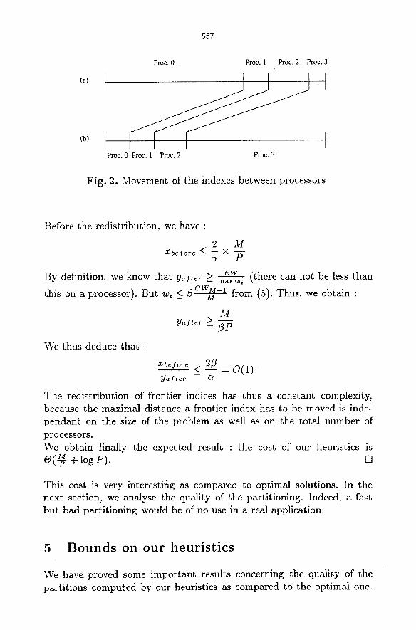
The figure 2(a) shows the processor 0, owning a lot of modules before the redistribution. Assume that the new arrangement of indexes after the redistribution is the one shown on figure 2(b). The processor 0 has computed new indexes, that have to be communicated to other processors. The number of indexes that will be comunicated is bounded by the ratio of the maximum number of modules on a processor before the redistribution (Xbe fore ) , to the ma.,dmum number after (yafter).

557

Proc. 0 Proc. 1 Proc. 2 Proc. 3

(b)

Proc. 0 Proc. I Proc. 2 Proc. 3

Fig . 2. Movement of the indexes between processors

Before the redistribution, we have :

2 M Z b e f o r e ~ - - X - -

--or P

By definition, we know that yafter :> EW (there can not be less than - - m a x 1s i

CWM-1 from (5). Thus, we obtain : this on a processor). But wi _ / 3 M

We thus deduce that :

M

xb jo, < 23 = o(1) y a f t e r Ol

The redistr ibution of frontier indices has thus a constant complexity, because the maximal distance a frontier index has to be moved is independant on the size of the problem as well as on the total number of pro cessors. We obtain finally the expected result : the cost of our heuristics is o ( M + l o g P) . []

This cost is very interesting as compared to optimal solutions. In the next section, we analyse the quality of the partitioning. Indeed, a fast bu t bad parti t ioning would be of no use in a real application.

5 B o u n d s o n o u r h e u r i s t i c s

We have proved some impor tant results concerning the quality of the part i t ions computed by our heuristics as compared to the optimal one.

558

In particular, we give some bounds for each of them as a function of the maximum of the workload of the modules. Let us first introduce a function to measure the quality of a given partition.

B{? D e f i n i t i o n 7. We define the quality factor of the part i t ion 7~ by p = BTe

(always smaller than 1).

The closest this factor to 1, the best the partition. The main result of 1 this section is to show that we always have p >_ 7"

Let us first introduce an intuitive lemma.

L e m m a 2 B o > E W

P r o o f . If Bo < E W , then the workload Wq of any processor q should verify Wq < E W . The total workload T W should verify T W < p E W , while by definition TI/V = p E W . We deduce that Bo >_ EI/V. []

T heor em 8. When all the modules have the same workload w, our strate- gies compute an optimal partition (such that p = 1)

M P r o o f . From lemma 1, we have Bze < -Fw + w. We also know that Bze

is a multiple of w. We can deduce that B n < r M ] w . From lemma 2,

Bo > E W . But E W = Mw, and B o is a multiple of w. So B o > [M] w. This leads to B o = Bze. []

L e m m a 3

Br< max{i=0... M--l} wi (6) B--T < 1 + E W

P r o o f . Let w = max{i=o...M-1} wi. From lemma 2, B o >_ E W . From lemma 1, we know that Bze < E W + w. The result is thus trivial. []

559

T h e o r e m 9. In the worst case, the bottlenecks of the parti t ions computed

by our heuristics are always smaller than twice the optimal bottleneck (i.e. p>_�89

P r o o f . We differentiate two cases accordingly to the value of w =

max{ i=o . . .M-1} wi.

�9 w > E W From lemma 1, B n < E W + w. Since we have B o >_ w, we obtain :

B o w P = > E W +

By asumption, w + E W < w + w. This leads to :

w 1 p >

w + w 2

�9 w < E W From lemma 3, we know tha t :

B o E W P = B~z > E W + w

By assumption, w + E W < E W + E W .

B o E W 1

P = Bra > E W + E W - 2

[]

We know how to quantify some bounds on the bottleneck of our heuristics as a function of the maximum of the workload of the modules. We have already obtained in lemma 1 that B n < E W + m a x w~, with 7~ computed by our heuristics. We give now a bet ter bound for the second heuristic.

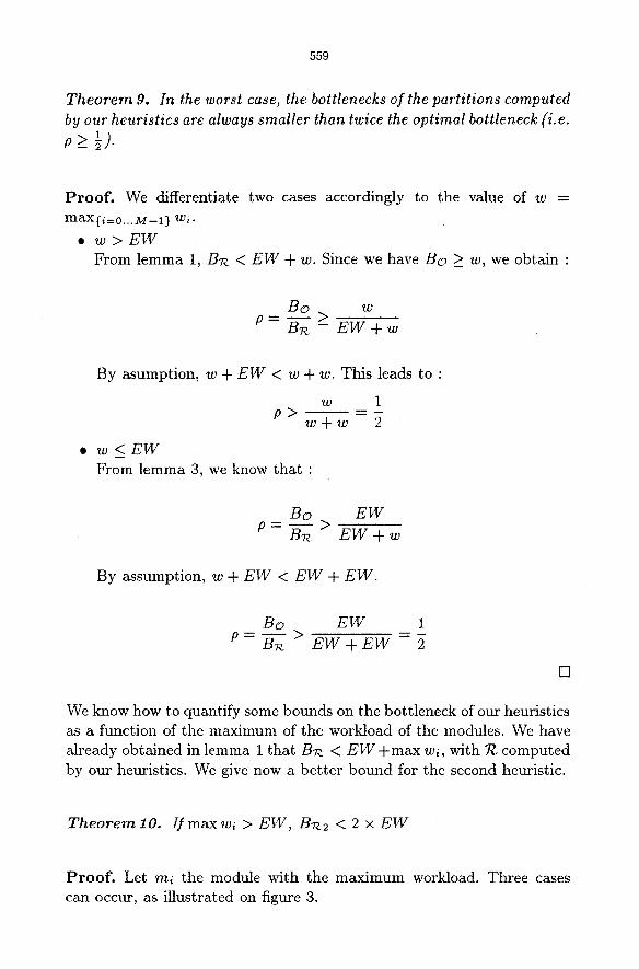
T h e o r e m 10. I f max w~ > E W , BT~2 < 2 x E W

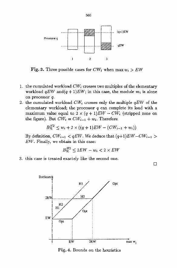
P r o o f . Let mi the module with the maximum workload. Three cases can occur, as illustrated on figure 3.

560

Processor q

1 2 3

Fig . 3. Three possible cases for CWi when max w~ > E W

1. the cumulated workload CWi crosses two multiples of the elementary workload q E W and(q + 1)EW; in this case, the module mi is alone on processor q.

2. the cumulated workload CWi crosses only the multiple q E W of the elementary workload; the processor q can complete its load with a max imum value equal to 2 • (q + 1 )EW - CWi (str ipped zone on the figure). But CW, = CWI-1 + wl. Therefore

B H2 <_ w, + 2 x ((q + 1)EW - (CWi-1 + wi))

By definition, CWi-1 < qEW. We deduce that ( q + I ) E W - C W i _ I > F_,W. Finally, we obtain in this case:

B H2 < 2 E W - w~ < 2 x E W

3. this case is t reated exactely fike the second one. []

Bottlenec

2E~

EW

HI

Opt

Opt

Fig . 4. Bounds on the heuristics

EW 2EW max w i

561

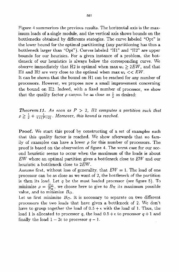
Figure 4 summerizes the previous results. The horizontal axis is the max-

imum loads of a single module, and the vertical axis shows bounds on the bottlenecks obtained by differents stategies. The curve labeled "Opt" is the lower bound for the optimal part i t ioning (any part i t ioning has thus a bott leneck larger than "Opt"). Curves labeled "HI" and "H2" are upper bounds for our heurisics. For a given instance of a problem, the bottleneck of our heuristics is always below the corresponding curve. We observe immediately that H2 is optimal when max wi > 2 E W , and tha t H1 and H2 are very close to the optimal when maxw~ < < E W . It can be shown tha t the bound on H1 can be reached for any number of processors. However, we propose now a small improvement concerning

the bound on H2. Indeed, with a fixed number of processor, we show 1 tha t the quality factor p ca .n:not be as close as ~ as desired:

T h e o r e m 1 1 . As soon as P > 2, H2 computes a partit ion such that 1 1

P ~-- 2- + 4 x ( P - 2 ) " Moreover, th i s b o u n d is reached .

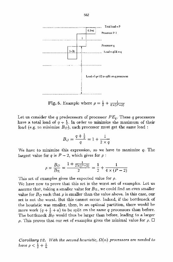
P r o o f . We s tar t this proof by constructing of a set of examples such tha t this quality factor is reached. We show afterwards tha t no fam- ily of examples can have a lower p for this number of processors. The proof is based on the observation of figure 4. The worst case for our second heuristic seems to occur when the maximum of the loads is about E W where an optimal parti t ion gives a bottleneck close to E W and our heuristic a bott leneck close to 2 E W .

Assume first, wi thout loss of generality, tha t E W - 1. The load of one processor can be as close as we want of 2, the bottleneck of the part i t ion is then its load. Let q be the most loaded processor (see figure 5). To

Bo we choose here to give to Bn its maximum possible minimize p = B~e' value, and to minimize B o . Let us first minimize B o . It is necessary to separate on two different processors the two loads tha t have given a bottleneck of 2. We don ' t have to group together the load of 0.5 + ~ with the load of 1. Thus, the load 1 is allocated to processor q, the toad 0.5 + e to processor q + 1 and finally the load 1 - 2e to processor q - 1.

562

Total h)ad = P

. . . . . . . . . . . . . . . . . . . . . . . . . . . . i ' " ] - ~ . . . . Processor P-I

- - - - - - - Processor q

Load = qCE = q

Load of q+l/2 to split on q processors

1 1 Fig . 5. Example where p = 7 + 4x(e-2)

Let us consider the q predecessors of processor PEq. These q processors 1 In order to minimize the maximum of their have a total load of q + 7"

load (e.g. to minimize Bo), each processor must get the same load :

1 1 Bo - q + g - 1 + ~

q 2 x q

We have to minimize this expression, so we have to maximize q. The largest value for q is P - 2, which gives for p :

1 Bo 1 + ~--g(P-2) 1 1

p - B7~ 2 2 + 4 x ( P - 2 )

This set of examples gives the expected value for p. We have now to prove that this set is the worst set of examples. Let us assume that , taking a smaller value for B a , we could find an even smaller value for Bo such that p is smaller than the value above. In this case, our set is not the worst. But this cannot occur. Indeed, if the bott leneck of the heuristic was smaller, then, in an optimal partition, there would be

a a) to be split the same q processors than before. more work (q + g + on The bottleneck Bo would thus be larger than before, leading to a larger p. This proves that our set of examples gives the minimal value for p. []

Corollary 12. With the second heuristic, Y2(n) processors are needed to 1 1 have p < ~ + -K

563

1 1 . I f w e w a n t < t 1 P r o o f . As we have just observed, p >_ $-~ 4x(P-2) P 2-'qt- n ' n

_ 1 that means P > u + 2. In other works, we need thus ~1 > 4•

P = f~(n). []

All these results seem to prove that the second heuristic is be t te r than the first one. Howerver, we can construct artificial examples where it is not the case. We have thus lead experiments on random da ta to confirm the average be t te r compor tment of H2 as compared to H1. We have also compared bottlenecks of our heuristics to the optimal one. These experiments show the following points (see [4] for details) :

- the second heuristic is almost always bet ter than the first one; 1 value of is very pessimistic for random data; the actual value - the ~ p

of p ahnost always larger than 0.8 in extreme cases; - the second heuristic gives a bott leneck very close to By, and even

identical in many cases; These results have been corroborated with real applications in the fields of image synthesis and analysis (parallel particle simulator [3], surface rendering and animation, image segmentation algorithm [6]). In these real applications, the quality of our heuristics was not worse than 8% of the optimal partition.

6 Conclus ion

We have analyzed the quality of heuristics for computing rectilinear partitions of da ta used for load-balancing the execution time of data-parallel algorithms. Our heuristics run in O(M/P +log P) on a P processors machine, instead of O(P(M - P)) for the best known optimal algorithm, much more difficult to parallelize. The quality of our partitioning schemes has been demons t ra ted theoritically as well as experimentally, on ran- domly chosen data. Other experiments have been done on real applications in image processing and image synthesis and will be published in a near future.

564

References

1. Shahid H. Bokhari. Partitioning Problems in Parallel, Pipelined, and Distributed Computing. IEEE Transactions on Computers, 37(1):48- 57, January 1988.

2. Michelangelo Grigni and Fredrik Marme. On the Complexity of the Generalized Block Distribution. In Ferreira, Rolim, Saad, and Yang, editors, Parallel Algorithms for Irregularly Structured Problems, number 1117 in Lecture Notes in Computer Science, pages 319-326. Springer, Santa Barbara, CA, USA, aug 1996. Proceedings of IR- REGULAR96.

3. Serge Miguet and Jean-Marc Pierson. Dynamic load balancing in a parallel particle simulation. In Proceedings of ttPCS'95, pages 420- 431, Montrfial, July 1995.

4. Serge Miguet and Jean-Marc Pierson. Heuristics for 1D rectilinear partitioning. In Denis Tristram and Jacques Chassin de Kergom- meaux, editors, Parallel Programming Environments for High Per- formance Computing, pages 111-115, Alpe d'Huez, April 1996. 2nd European School of Computer Science.

5. Serge Miguet and Yves Robert. Elastic load balancing for image processing algorithms. In H.P. Zima, editor, Parallel Computation, Lecture Notes in Computer Science, pages 438-451, Salzburg, Aus- tria, September 1991. 1st International ACPC Conference, Springer Verlag.

6. Jean-Marc Nicod. Extraction de surfaces en imagerie mddicale : ap- proches paral~les. Th~se, Ecole Normale Supfirieure de Lyon, January 1994.

7. D. M. Nicol. Rectilinear Partitioning of Irregular Data Parallel Com- putations. Journal of Parallel and Distributed Computing, 23:119- 134, 1994.

8. Bjorn Olstad and Fredrik Manne. Efficient Partitioning of Sequences. IEEE Transactions on Computers, 44(11):1322-1326, nov 1995.

9. Jean-Marc Pierson. Equilibrage de charge dirigd par les donndes : applications fi la synth~se d'images. Th~se, LIP-Ecole Normale Supfirieure de Lyon, 46 all~e d'Italie, 69364 Lyon cedex 07, France, october 1996.

Documents

Heuristics for 1D Rectilinear Partitioning as a Low Cost and High Quality Answer to Dynamic Load Balancing