heuristic rules for tardiness problems in flowshop with the intermediate due dates

1 23

The International Journal ofAdvanced Manufacturing Technology ISSN 0268-3768Volume 71Combined 1-4 Int J Adv Manuf Technol (2014)71:381-393DOI 10.1007/s00170-013-5478-8

Heuristic rules for tardiness problem inflow shop with intermediate due dates

Farhad Ghassemi Tari & Laya Olfat

1 23

Your article is protected by copyright and

all rights are held exclusively by Springer-

Verlag London. This e-offprint is for personal

use only and shall not be self-archived

in electronic repositories. If you wish to

self-archive your article, please use the

accepted manuscript version for posting on

your own website. You may further deposit

the accepted manuscript version in any

repository, provided it is only made publicly

available 12 months after official publication

or later and provided acknowledgement is

given to the original source of publication

and a link is inserted to the published article

on Springer's website. The link must be

accompanied by the following text: "The final

publication is available at link.springer.com”.

ORIGINAL ARTICLE

Heuristic rules for tardiness problem in flow shopwith intermediate due dates

Farhad Ghassemi Tari & Laya Olfat

Received: 4 April 2012 /Accepted: 5 November 2013 /Published online: 27 November 2013# Springer-Verlag London 2013

Abstract In this paper, the tardiness flow shop models withintermediate due date were considered. The flow shop modelsconsist of a set of jobs each having a number of operations,while each operation is performed in a single machine. All thejobs are considered having the same unidirectional precedenceorder. In the tardiness flow shopmodels with intermediate duedate, which we call the generalized tardiness flow shopmodels, there exist a due date associated with the completionof each operation, and we want to find a schedule whichminimizes the total tardiness of the jobs. This is a moregeneral version of tardiness flow shop in the sense that, byassigning a large value to each of the intermediate due dates,we can obtain the traditional flow shop models. Consideringthe generalized tardiness flow shop models as the NP-hardproblems, a set heuristic sequencing rules for finding the bestpermutation schedule for such problems is proposed. Weconducted an extensive computational experiment using ran-domly generated test problems for evaluating the efficiency ofthe proposed rules in obtaining a near-optimal solution. Theefficiency of the rules was evaluated, and those rules withbetter solutions were designated and reported.

Keywords Flow shop . Total tardiness . Permutationschedule . Heuristic rules . Intermediate due dates

1 Introduction

The performance measurer of meeting job due dates and, morespecifically, the tidiness penalty is one of the scheduling criteriamost frequently encountered in practical situations. The totaltardiness of jobs’ completion times is a typical quantification ofmeeting jobs due dates. However, in most of the product designand research/consulting projects, the outcomes are deliveredthrough predefined phases, and there is an associated due datefor each phase of the project deliverable tasks. The phases indifferent projects are carried out in a unidirectional precedencestructure and hence can be considered as a scheduling with theintermediate jobs due dates [8].

For discussion of intermediate due dates in flow shopmodels, a job is considered to be a collection of operationswhen there is a due date associated with the completion ofeach operation. This is a more general version of sequencingjobs in flow shop models with the criteria of minimizing sometardiness performance measures. Flow shop models address-ing tardiness as their performance measures are traditionallyconsidering a due date for each job, or more precisely, of thelast operation of each job. In fact, when all the intermediatedue dates are equal to the due date of the last operation, wewill have a traditional model as a special version of ourproposed generalized model.

Due to the combinatorial nature of the tardiness flow shopproblems, the exact solution approaches cannot provide theoptimal solution of the real-world problems [3, 4, 24]. For thisreason, research efforts are mainly focused on the develop-ment of heuristic and meta-heuristic approaches to tacklemore complex problems. In this category, there are severalclasses of algorithms such as simulated annealing, Tabusearch, evolutionary, genetic algorithms, and some other al-gorithmic classes [2, 6, 7, 10, 13]. As an example, Demirelet al. [5] investigated parallel machine scheduling problem inorder to minimize total tardiness and developed a genetic

F. Ghassemi Tari (*)Industrial Engineering, Sharif University of Technology, Azadi ave.,P.O. Box 11155–9414, Tehran, Irane-mail: [email protected]

L. OlfatDepartment of Management, Allameh Tabatabaei University,Tehran, Irane-mail: [email protected]

Int J Adv Manuf Technol (2014) 71:381–393DOI 10.1007/s00170-013-5478-8

Author's personal copy

algorithm solution procedure for their proposed problems.Among these classes, the simulated annealing was reportedby Vallada et al. [21] to be the best-performing class up to thereported date. However, since most of the heuristic classestackle some special type of the problem, the best-performedheuristic class has not been singled out.

There are other early heuristic approaches which use somepriority rules for constructing the heuristic algorithms. Al-though they were not presented a unified class, but some wereshown to be effective heuristic algorithms. Among those is thecost over time (COVERT) rule which is a dynamic rule andhas been proposed for the single machine and the job shopsequencing problems to minimize the total weighted tardinessof the jobs. The performance of COVERT is examined for avariety of tardiness measures. The results indicate thatCOVERT-based algorithms perform well as the other se-quencing rules and in most instances were superior to theother sequencing rules tested both directly and across varyingdegrees of due-date tightness [20]. Morton and Dharan [16]proposed two heuristics algorithms for the problem of mini-mizing the weighted flow time of n jobs on a single machine,and they claimed that their algorithms provided near-optimalsolutions. Isler, Toklu, and Çelik [9] considered the weightedabsolute deviation of earliness/tardiness (E/T) problem whiletotal tardiness criteria provides adaptation for due date. Theydeveloped several heuristic algorithms and conducted a com-putational experiment which its results revealed the appropri-ateness of their approaches for the large-sized problems.

Among the works considering sequencing rules in dynamicscheduling environments are the research efforts conducted byKim and Bobrowski [12]. This study classified and testedsome scheduling rules considering setup time and/or due dateinformation. These scheduling rules were then evaluated indynamic scheduling environments which were defined by duedate tightness, setup times, and cost structure. A simulationmodel of a nine-machine job shop was used in their experi-ment. Kianfar, Fatemi-Ghomi, and Karimi [11] studied theproblem of a flexible flow shop system with the dynamicarrival of jobs and the ability of acceptance and rejection ofnew jobs. They proposed four dispatching rules and conduct-ed a computational experiment. They concluded that theirproposed dispatching rules provided better performance underproblem assumptions. Vinod and Sridharan [23] presented adiscrete event simulation-based experimental study of sched-uling rules for scheduling a dynamic job shop in which thesetup times were sequence-dependent. Seven scheduling rulesfrom the literature and five new scheduling rules, developedby the authors, were incorporated in the simulation model.The results indicated that setup-oriented rules provide betterperformance than ordinary rules.

Rachamadugu and Morton [19] proposed the apparenttardiness cost (ATC) rule in which the index combines theweighted shortest processing time rule and the least slack rule.

Vepsalainen and Morton [22] extended the ATC rule for a jobshop sequencing problems. Lee et al. [14] and later Lee andPinedo [15] added the shortest setup rule to the ATC rule.Morton and Pentico [17] proposed the X-RM heuristic for thesingle machine scheduling problems. Apparent tardiness costwith setups and ready times was one of the most effectivedispatching rules to solve a dynamic problem with sequence-dependent setup in minimizing the total weighted tardiness,due to Pfund et al. [18]. They also proposed a new slack termand a new ready time term to the index, in a batch productionsystem, where several jobs are processed together at the sametime by a single machine. The next section describes theproposed problem. In Section 3, the developed heuristic ruleswill be explored. Section 4 is dedicated to the illustrations ofthe computational experiments. And finally, Section 5 con-cludes the results of this research study.

2 Problem statement

In real-world problems, however, there are considerable situ-ations in which there is a due date for each intermediateoperation of a job, and there exists a penalty associated withthe tardiness of each intermediate operation of a job. Themotivation of this study comes from these scheduling needsof the research and development, the product design, and theconsulting firms which have been conducting several deliver-able projects simultaneously. Usually, each project is carriedout through different phases, and there is an associated duedate for each phase. Different departments, in a unidirectionalprecedence structure, perform a set of tasks in each project.Considering each project as a job, the set of tasks to beperformed by each department as an operation, and eachdepartment as a machine, we have n jobs and m machinesflow shop in which an intermediate due date is defined forcompletion of each operation on each machine.

To answer this scheduling need, a new version offlow shop model, named as an intermediate due date’sflow shop (IDDF) model, with the total tardiness criteriawas defined. The computational time and memory re-quirements of obtaining an optimal solution of IDDFproblems with the tardiness criteria can be severe foreven moderate-sized problems. Even traditional case ofthe two-machine flow-shop problem with total tardinessas the scheduling criterion is NP-complete [13].

Heuristic procedures avoid these drawbacks, and hence, aset of heuristic procedures capable of solving a general versionof IDDF problems was developed. We then performed anextensive experimental study to compare efficiency of theproposed procedures in obtaining a good solution to IDDFproblems. Generally, problems of finding a sequence of jobsin a flow shop model consider two distinct schedules, namelypermutation schedule or non-permutation schedule. This

382 Int J Adv Manuf Technol (2014) 71:381–393


study addresses the permutation IDDF scheduling problemwith the objective of minimizing total tardiness. It is theproblem of scheduling n independent jobs, simultaneouslyavailable at time zero, on m sequential machines. All jobshave m operations with the same unidirectional precedencestructure, and each machine is capable of processing at mostone job at a time. Once an operation of a job is started,it must proceed to completion, and no machine break-down is considered. In addition, the processing time ofeach operation on each machine is known in advanceand is independent of the order in which operations arecarried out. There is a due date associated with thecompletion of each operation, and the objective is tofind a sequence of the n jobs such that the total tardi-ness of operations of all jobs is minimized

3 Development of the heuristic rules

In this section, a set of heuristic rules capable of for solvingIDDF scheduling problems with the total tardiness criteria isdeveloped. The fact that most of these heuristic rules haveperformed well in solving different scheduling problems mo-tivated us for modifying and applying them in solving ourproposed problem.

In order to have a more precise evaluation of the developedrules, they are classified in five groups, according to theirmechanism of generating jobs sequence. The followinggroups describe this classification:

1. Static procedures by which a single solution is obtained.2. Dynamic procedures by which a single solution is

obtained.3. Static procedures by which a set of solutions is obtained.4. Dynamic procedures by which a set of solutions is

obtained.5. Ranking rules.

By static rules we meanm-jobs-at-a-time sequencing rules.In contrast, the dynamic rules mean one-job-at-a-time se-quencing rules. In the latter case, information regarding com-pletion time of the scheduled jobs is used for selecting the nextjob to be sequenced.

The ranking rules are those by which a set of se-quence is initially generated, and according to the posi-tion of each job in each sequence, a score is assigned toeach job. The scores of each job are then summed up(rank of a job) and used as a base for determining thejob position in the final sequence.

For each group, several heuristic rules are developed.Table 1 presents the proposed rules in each group.Furthermore, different concepts for developing some ofthe rules are used and are named accordingly. The

following subsections will present the development ofdifferent rules.

Group # Group description Procedures

1 Static-single PD0, PD1, PD2, PD3, MDD1,SL1, CR1

2 Dynamic-single CR2, CR3, MDD2, MDD3, SL2

3 Static-multiple EDD, SPT, TSPT, CO1, CO2,AT1, AT2

4 Dynamic-multiple CO3, CO4, CO5, CO6, AT3, AT4,AT5, AT6, MDD4, MDD5

5 Ranking RSPT, RTSPT, REDD, RSPTEDD,RCO2, RAT2

The following notations are common in all the proposed rules:

n number of jobsm number of operations/machinespij processing time of job i on machine jd ij due date of job i on machine jA an ordered set of partially scheduled jobs (jobs’ order

shows their sequence)Aj an ordered set of partially scheduled jobs on machine jB a set of all other jobs not containing in A or Ajt the scheduling time (in the dynamic rules) the next job

is selected to be scheduledTPi total operations processing time of job i[k ] position of a job in k th sequencer i the time that job i is ready to be sequenced.

3.1 Processing time/due date rules

This section will present the rules based on a set of factorsconsisting of the job processing times, due dates, and combi-nation of the processing times and due dates. It is to be notedthat an extensive theoretical concept considers the job pro-cessing time and the job dates for the case of the singlemachine tardiness sequencing problem, but none haveemerged to a unique result [1]. To conclude the treatment ofthe single machine tardiness problem with some specializedresults concerning optimal sequences, the following are held.

& If the EDD sequence produces nomore than one tardy job,it yields the minimum of the tardiness value.

& If all jobs have the same due date, then their tardiness isminimized by SPT sequencing.

& If it is impossible for any job to be on time in anysequence, then tardiness is minimized by SPTsequencing.

& If SPT sequencing yields no jobs on time, then it mini-mizes the total tardiness.

In case of the traditional flow shop tardiness sequencingproblem, the problem is more complicated. The complicationsbecome more severe when one considers the tardiness

Int J Adv Manuf Technol (2014) 71:381–393 383


problem with the intermediate due dates. For shortening thediscussions, we therefore employed the results of these studiesand modified them for the flowshop with the intermediate duedate tardiness sequencing problems.

SPT rule: This rule determine the final sequence throughthe following steps:

Step 1. Let j =1.

Step 2. Schedule jobs in non-decreasing order of pij

(p [1] j≤p [2] j≤…≤p [n] j).Step 3. If j =m , go to step 4, otherwise let j =j +1, and go

to step 2.Step 4. Schedule jobs in non-decreasing order of TPi

(TP [1]≤TP [2]≤…≤TP [n]).Step 5. Choose the final schedule with the smallest

total tardiness among the m +1 schedulesand stop.

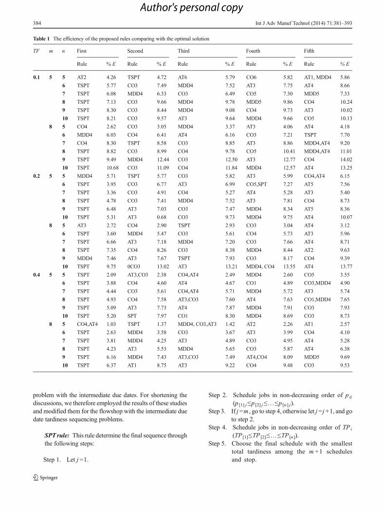
Table 1 The efficiency of the proposed rules comparing with the optimal solution

TF m n First Second Third Fourth Fifth

Rule % E Rule % E Rule % E Rule % E Rule % E

0.1 5 5 AT2 4.26 TSPT 4.72 AT6 5.79 CO6 5.82 AT1, MDD4 5.86

6 TSPT 5.77 CO3 7.49 MDD4 7.52 AT3 7.75 AT4 8.66

7 TSPT 6.08 MDD4 6.33 CO3 6.49 CO5 7.30 MDD5 7.33

8 TSPT 7.13 CO3 9.66 MDD4 9.78 MDD5 9.86 CO4 10.24

9 TSPT 8.30 CO3 8.44 MDD4 9.08 CO4 9.73 AT3 10.02

10 TSPT 8.21 CO3 9.57 AT3 9.64 MDD4 9.66 CO5 10.13

8 5 CO4 2.62 CO3 3.05 MDD4 3.37 AT3 4.06 AT4 4.18

6 MDD4 6.03 CO4 6.41 AT4 6.16 CO3 7.21 TSPT 7.70

7 CO4 8.30 TSPT 8.58 CO3 8.85 AT3 8.86 MDD4,AT4 9.20

8 TSPT 8.82 CO3 8.99 CO4 9.78 CO5 10.41 MDD4,AT4 11.01

9 TSPT 9.49 MDD4 12.44 CO3 12.50 AT3 12.77 CO4 14.02

10 TSPT 10.68 CO3 11.09 CO4 11.84 MDD4 12.57 AT4 13.25

0.2 5 5 MDD4 5.71 TSPT 5.77 CO3 5.82 AT3 5.99 CO4,AT4 6.15

6 TSPT 3.95 CO3 6.77 AT3 6.99 CO5,SPT 7.27 AT5 7.56

7 TSPT 3.36 CO3 4.91 CO4 5.27 AT4 5.28 AT3 5.40

8 TSPT 4.78 CO3 7.41 MDD4 7.52 AT3 7.81 CO4 8.73

9 TSPT 6.48 AT3 7.03 CO3 7.47 MDD4 8.34 AT5 8.36

10 TSPT 5.31 AT3 0.68 CO3 9.73 MDD4 9.75 AT4 10.07

8 5 AT3 2.72 CO4 2.90 TSPT 2.93 CO3 3.04 AT4 3.12

6 TSPT 3.60 MDD4 5.47 CO3 5.61 CO4 5.73 AT3 5.96

7 TSPT 6.66 AT3 7.18 MDD4 7.20 CO3 7.66 AT4 8.71

8 TSPT 7.35 CO4 8.26 CO3 8.38 MDD4 8.44 AT2 9.63

9 MDD4 7.46 AT3 7.67 TSPT 7.93 CO3 8.17 CO4 9.39

10 TSPT 9.75 0CO3 13.02 AT3 13.21 MDD4, CO4 13.55 AT4 13.77

0.4 5 5 TSPT 2.09 AT3,CO3 2.38 CO4,AT4 2.49 MDD4 2.60 CO5 3.55

6 TSPT 3.88 CO4 4.60 AT4 4.67 CO1 4.89 CO3,MDD4 4.90

7 TSPT 4.44 CO3 5.61 CO4,AT4 5.71 MDD4 5.72 AT3 5.74

8 TSPT 4.93 CO4 7.58 AT3,CO3 7.60 AT4 7.63 CO1,MDD4 7.65

9 TSPT 5.09 AT3 7.73 AT4 7.87 MDD4 7.91 CO3 7.93

10 TSPT 5.20 SPT 7.97 CO1 8.30 MDD4 8.69 CO3 8.73

8 5 CO4,AT4 1.03 TSPT 1.37 MDD4, CO3,AT3 1.42 AT2 2.26 AT1 2.57

6 TSPT 2.63 MDD4 3.58 CO3 3.67 AT3 3.99 CO4 4.10

7 TSPT 3.81 MDD4 4.25 AT3 4.89 CO3 4.95 AT4 5.28

8 TSPT 4.23 AT3 5.53 MDD4 5.65 CO3 5.87 AT4 6.38

9 TSPT 6.16 MDD4 7.43 AT3,CO3 7.49 AT4,CO4 8.09 MDD5 9.69

10 TSPT 6.37 AT1 8.75 AT3 9.22 CO4 9.48 CO3 9.53



EDD Rule - This rule determine the final sequencethrough the following steps:

Step 1. Let j = 1 .Step 2. Schedule jobs in non-decreasing order of dij

(d [1] j ≤ d [2] j ≤ … ≤ d [n] j ).Step 3. If j =m , go to step 4, otherwise let j = j + 1 , and

go to step 2.Step 4. Chose the final schedule with the smallest total

tardiness among the m schedules, and stop.

TSPT rule : This rule is similar to SPT, but for generatingthe firstm schedule, we consider the total processing timeof the jobs on each machine. The final schedule is deter-mined through the following steps:

Step 1. Let j =1, and SPi ¼ ∑k¼1

j

pik

Step 2. Schedule jobs in non-decreasing order of SPi

(SP [1]≤SP [2]≤…≤SP [n]).Step 3. If j =m , go to step 4, otherwise let j =j +1, and

go to step 2.Step 4. Choose the final schedule with the smallest total

tardiness among the m schedules and stop.

Combining processing time with due dates, four differentrules are developed based on these combination. To describethese rules let us first define the following indexes:

PD0i ¼ TPi � dim ð1Þ

PD1 ¼ TPi=dim ð2Þ

PD2i ¼Xj¼1

m

pij � dij ð3Þ

PD3ij ¼

Xk¼1

j

pik

dijð4Þ

PD0 rule: Sequence the jobs in non-decreasing order ofPD0i (PD0[1] ≤ PD0[2] ≤ … ≤ PD0[n])PD1 rule : Sequence the jobs in non-decreasing order ofPD1i (PD1[1]≤PD1[2]≤…≤PD1[n])PD2 rule : Sequence the jobs in non-decreasing order ofPD2i (PD2[1]≤PD2[2]≤…≤PD2[n])PD3 rule : This rule determines the final schedules by thefollowing steps:

Step 1. Let i =1.Step 2. Let, MPDi ¼ min

jPD3ij� �

Step 3a. (m is even). If the associated j of the minimumof MPDi occurs on machine one through m /2assign i in the first available position in se-quence, otherwise assign it to the last availableposition in sequence, go to step 4.

Step 3b. (m is odd). If the associated j of the minimumofMPDi occurs on median machine, position ion the median position in sequence, if j occursin the first portion of median assign i in the firstavailable position in sequence, otherwise as-sign it to the last available position in sequence,go to step 4.

Step 4. If I =n stop, otherwise let I =i +1, go to step 2.

3.2 Critical ratio rules

The critical ratio rules consist of a set of dynamic rulesdeveloped for IDDF problems. Since in dynamic rulesthe jobs sequence is determined one at a time, we use tas the time of sequencing the next job. A critical ratiois defined as:

CRi ¼ dim−t

LXj¼1

m

pij

ð5Þ

Where L is a factor for estimating the lead-time and its bestvalue can be determined experimentally.

Although the critical ratio is most appropriate for develop-ing dynamic rules, it can also be used for generating staticsequencing as well. Three rules are developed based on crit-ical ratio concept, one static rule and two dynamic rules, asfollows:

CR1 rule : In order to develop a static version of thecritical ratio rule let CR1i is defined as the criticalratio of i th job when t =0. Then we sequence thejobs by non-decreasing order of CR1i (CR1[1]≤CR1[2]≤…≤CR1[n ]).CR2 rule : In order to develop a dynamic version of thecritical ratio rule, let us defineCim as the completion timeof the last job in A on machine m . Then the followingsteps for one-at-a-time sequencing of the jobs is carried:

Step 1. Let t =0 , A=ϕ, B ={1, 2, …, n}.

Step 2. Let, CR2 ¼ mini∈B

dim−Cim

L ∑j¼1

mpij

8><>:

9>=>;

Step 3. Remove job i form B and place it in the lastposition of A .

Step 4. If B is empty stop, otherwise, go to step 2.



CR3 rule : This rule is similar to CR2 except the firstmachine for scheduling the jobs is selected. The follow-ing steps for one at a time sequencing of the jobs iscarried:

Step 1. Let t =0, A=ϕ, B ={1, 2, …, n}.

Step 2. Let, CR3 ¼ mini∈B

di1−Ci1L�pi1

n oStep 3. Remove job i form B and place it in the last

position of A .Step 4. If B is empty stop, otherwise, go to step 2.

3.3 Modified due date rules

Based on the theory of the SPT and EDD decision ruleconcepts, there is a choice between any pair of candidate jobi and j to be proceed each other. However, these rules cannotconclude whether jobs i and j should come early in theschedule or late in the schedule. Based on the followingtheorem, these decision rules the jobs are not sequencedunambiguously. Looking at the problem from anotherperspective, we can employ the modified due date pri-ority rule which is a dynamic rule, and it may changeas the time passes. Let us define the modified due dateof job j at time t to be d j ′=max{d j , t +p j} in which d j

and p j are due date and processing time of job j .Therefore, if one gives priority to the job with theearliest modified due date, then the choice between jobsi and j may be different early in the schedule than it islate in the schedule. The MDD rule is still weaker than suchrules as SPT and EDD for the single-machine tardiness prob-lem. However, it would be worthwhile to modify it and applyit to the flow shop sequencing problems. Putting it in anotherway, the MDD rule represents a necessary condition for opti-mality, but it is not a sufficient condition. The concepts of thisdynamic rule are used to develop five distinct schedulingrules, one static rule (MDD1) and four dynamic rules(MDD2–MDD5).

MDD1 rule : In order to develop a static version of theMDD, let us define D1i=max {di, t +pi} where t =0. Wethen determine the job sequence according to non-decreasing order of D1i (D1[1]≤D1[2]≤…≤D1[n]).MDD2 rule : In order to develop a dynamic version oftheMDD rule, let t =Cim, and then the following steps forone at a time sequencing of the jobs is carried:

Step 1. Let t =0, A=ϕ , B ={1, 2, …, n}.Step 2. Let, D2 ¼ min

i∈Bmax dim; t þ TPið Þf g


Step 4. If B is empty, stop, otherwise, let t =Cim, go tostep 2.

MDD3 rule : In this rule, letting Ci1 as the completiontime of the last job in A on the first machine, the followingsteps for one at a time sequencing of the jobs is carried:

Step 1. Let t =0, A=ϕ , B ={1, 2, …, n}.Step 2. Let, D3 ¼ min

i∈Bmax di1; t þ pi1ð Þf g


Step 4. If B is empty, stop, otherwise, let t =Ci1, go tostep 2.

MDD4 rule : By this rule, the jobs sequence in eachmachine is generated, and then the final sequence amongm generated sequences with the smallest total tardiness isselected. The steps to obtain the final schedule are:

Step 1. Let t =0, j =1.Step 2. Aj=ϕ , B ={1, 2, …, n}.Step 3. Let, D4 ¼ mini∈B max dij; t þ pij

� �n oStep 4. Remove job i form B and place it in the last

position of Aj, and then advance t by the com-pletion time of the last job in Aj.

Step 5. If B is empty, go to 6; otherwise, for all i S (asubset of B which their ready times are less thanor equal to t ), let ri ¼ 0; for j ¼ 1; andri ¼∑j−1

k¼1plk ; for j≥2; and then go to step 3:

Step 6. If j =m, select the schedule Aj with the smallesttotal tardiness, and then stop; otherwise let j =j +1, and then go to step 2.

MDD5 rule : This rule is the same asMDD4, except that,for selecting the next job to be scheduled, we consider allthe jobs in B (instead of a subset of B ).

3.4 Cost over time rules

The cost over time (COVERT) has been reported as an effi-cient index for dynamic sequencing of the jobs in a variety ofscheduling problems. Based on this index, six rules for sched-uling of IDDF problems are developed and are named asCO1through CO6 .

A general version of COVERT index for IDDF problems ismodified as follows:

COVERTij ¼ 1

pijdijmax 0; 1−

max 0; dij−pij−tn o

kbpij

8<:

9=;

24

35 ð6Þ

In the above formula, k is the adjustment factor of theworst-case scenario and b is the parameter of lead-time to beestimated experimentally. We first found that the best valuesfor k and b are both equal to 2.



Among these six rules, CO1 and CO2 are static rules andpursue the following identical algorithmic steps to obtain thefinal sequence:

Step 1. Let j =1, and t =0.Step 2. Sequence the jobs in non-increasing order ofCOVERTij.Step 3. If j =m , go to step 4, otherwise let j =j +1, and go to

step 2.Step 4. Let pij=TPi, and dij=dim. Then calculate the covert

index for these values (COVERTi) and find a sched-ule by sequencing the jobs in non-increasing order ofthe COVERTi.

Step 5. Chose the final schedule with the smallest totaltardiness among the m +1 schedules and stop.

CO1 rule : In this rule, we omit the dij's from the de-nominator of COVERT index, and we use the above-mentioned steps to determine the final schedule.CO2 rule : This rule is the same as CO1, except that welet due date (dij) remain in denominator for calculatingthe covert index.

All the other covert rules (CO3 through CO6) are dynamicprocedures. Letting r i be the ready time of the jobs in set B ,these rules then pursue the following identical algorithmicsteps to obtain the final sequence:

Step 1. Let t =0, j =1.Step 2. Aj i=ϕ, B ={1, 2, …, n}.Step 3. Let, COij ¼ max

i∈BCOVERTij

� �Step 4. Let i be the associated job number of COij ,

remove i from B and place it in the lastposition of A j , and then advance t by thecompletion time of the last job in Aj .

Step 5. If B is empty, go to 6; otherwise, for all i∈ B let

ri ¼ 0; for j ¼ 1; andri ¼ ∑j−1

k¼1plk ; for j≥2; and then

go to step 3:

Step 6. If j =m, select the schedule Aj with the smallest totaltardiness, and then stop; otherwise let j =j +1, and goto step 2.

Based on the above-mentioned general steps, four differentrules are developed as follows:

CO3 rule : In this rule, we omit the dij's from the de-nominator of COVERT index and calculate it only forthose jobs in the subset of B whose ready times are lessthan or equal to t .

CO4 rule : This rule is the same as CO3, except that welet due date (dij) remain in denominator for calculatingthe COVERT index.

CO5 rule : This rule is the same as CO3, except that, forselecting the next job to be scheduled, we calculate theCOVERT index for all the jobs in B .CO6 rule : This rule is the same asCO5, except that we letdij's remain in the denominator of the COVERT index.

3.5 Apparent tardiness cost rules

The apparent tardiness cost (ATC) is another index that hasbeen used for the dynamic sequencing rules in single-machinescheduling problems. Based on this index, six sequencingrules for the IDDF problems are proposed and are named asAT1 through AT6. A general version of ATC index for IDDFproblems is modified as follows:

ACTi tð Þ ¼ 1

dijpijexp −

max 0; dim−TPi−tð Þk

1

NB

Xj∈B

pij

0BBB@

1CCCA ð7Þ

Where k is a parameter for adjusting the slack time of thejobs and NB is the number of elements in set B . Through ourexperimental studies, the best value for k is found to be 2.Among these six rules, AT1 and AT2 are static rules andpursue the following identical algorithmic steps to obtain thefinal sequence:

Step 1. Let j =1, and t =0.Step 2. Schedule jobs in non-increasing order of ACTi(t ).Step 3. If j =m , go to step 4; otherwise let j =j +1, and go to

step 2.Step 4. Let pij=TPi, and dij=dim. Then calculate the covert

index for these values (ACTi(t)) and find a scheduleby sequencing the jobs in non-increasing order of theACTi(t ).

Step 5. Choose the final schedule with the smallest totaltardiness among the m +1 schedules and stop.

AT1 rule : In this rule, the dij's are omitted from thedenominator of ACTi(t ) index , and then the above-mentioned steps are carried to determine the finalschedule.AT2 rule : This rule is the same as AT1, except that thedue date (dij) remains in denominator for calculating thecovert index.

All the other ACT rules (AT3 through AT6) are dynamicprocedures. Again, letting r i to be the ready time of the jobs inset B , these rules pursue the following identical algorithmicsteps to obtain the final sequence:

Step 1. Let t =0, j =1.



Step 2. Let, Aj=ϕ, B ={1, 2, …,n}.Step 3. Let, AT j tð Þ ¼ max

i∈BACT j tð Þ� �

Step 4. Let i be the associated job number of ATj (t ), removei from B and place it in the last position of Aj, andthen advance t by the completion time of the last jobin Aj.

Step 5. If B is empty, go to 6; otherwise, for all i∈ B , let

ri ¼ 0; for j ¼ 1; andri ¼ ∑j−1

k¼1plk ; for j≥2; and then

go to step 3:Step 6. If j =m, select the schedule Aj with the smallest total

tardiness and then stop; otherwise let j =j +1, and goto step 2.

Based on the above-mentioned general steps, four differentrules are developed as follows:

AT3 rule : In this rule, we omit the dij's from the denom-inator of ACT index and calculate it only for those jobs inthe subset of B whose their ready times are less than orequal to t .AT4 rule : This rule is the same asAT3 , except that we letthe due date (dij) remain in denominator for calculatingthe ACT index.AT5 rule : This rule is the same as AT3 , except that forselecting the next job to be scheduled, the ACT index iscalculated for all the jobs in B .AT6 rule : This rule is the same as AT5, except that dij'sremain in the denominator of the ACT index.

3.6 Ranking rules

In this section, a set of rules will be proposed, which select theposition of each job in the final sequence by considering its totalranking score. To determine a rank for each job, firstm differentschedules on m machines based on some of the previouslyproposed rules are generated. Then a rank of Rij=k is assignedto the job i=[k] in schedule j (Rij is the rank of job which isappeared in position k of the sequence). The total rank of a job isthen determined as sum of its ranking score in all m schedules.

All the proposed ranking rules have following general steps:

Step 1. Let j =1.Step 2. Find a schedule in machine j according to rule Rulej

sequencing rule.Step 3. Let Rij=k for jobs I =[k ].

Step 4. Let, TRi ¼ ∑j¼1

mrij

Step 5. If j =m , go to step 6; otherwise, let j =j +1, and go tostep 2.

Step 6. Determine the final sequence by non-decreasingorder of TRi (TR [1]≤TR [2]≤…≤TR [n]).

RSPT rule : This rule employs the SPT sequencing rulefor Rulej.RTSPT rule : This rule employs the TSPT sequencingrule for Rulej.REDD rule : This rule employs the EDD sequencing rulefor Rulej.RSPTEDD rule : This rule employs both the SPT and theEDD sequencing rule for Rj and determines the total rankof each job by sum of its ranks among the 2m schedules.RAT2 rule : This rule employs the AT2 sequencing rulefor Rulej.RCO2 rule : This rule employs the CO2 sequencing rulefor Rulej.

3.7 Slack-based rules

Slack time is a measure of urgency for a given job and isdefined as the time its due date minus the time required toprocess it. In this section, two scheduling rules are proposedbased on the concept of slack time, called SL1 Rule, and SL2rule. The first rule uses slack time statically, and the secondrule uses slack time dynamically to produce the final schedule.The description of these two rules is as follows:

SL1 rule : Let SL1i be the slack time of the last operationof job i , determined as SL1i=d im–TPi, then the jobsequence is determined according to non-decreasing or-der of SL1i (SL1[1]≤SL1[2]≤…≤SL1[n]).SL2 rule : This rule determines the final schedule by thefollowing steps:

Step 1. Let t =0, j =1 , Aj=ϕ, and B ={1, 2, …, n}.

Step 2. Let, Slackij ¼ mini∈B

dij− ∑k¼1

j

pik þ t

!( )

Step 3. If j =m , go to step 4; otherwise let j =j +1, and goto step 2.

Step 4. Let, SL2i ¼ mini; j

Slackij� �

Step 5. Let i be the job number associated with SL2i,remove i form B and place it in the last positionof A , and then advance t by the completion timeof the last job in A .

Step 6. If B is empty, select the schedule A as the finalschedule, and then stop; otherwise let j =1, andthen go to step 2.

4 Computational experiments

We implement extensive numerical experiments to eval-uate the effectiveness of the proposed heuristic rules.To show the effectiveness of the proposed rules in



obtaining the optimal solution as well as comparingtheir relative effectiveness, computational experimentsare conducted with a variety of randomly generated testproblems. This section will describe the mechanism ofgenerating the test problems, and then will present theexperimental results.

4.1 Generation of the test problems

We employed the concepts of pseudo random genera-tion for developing the test problems. For each testproblem with the size of n jobs and m operations, weused a uniform distribution function with the rage[1–10] to generate p ij 's. The operations’ due dates aregenerated in two steps. First, the due date of the last

operation (d im) is generated using the following uni-form distribution:

dim∼U 1−TF−R=2ð Þ � C; 1−TF þ R=2ð Þ � C½ � ð8Þ

Where TF is the due date tightness parameter, R is therange adjusting parameter, and C is defined as follows:

C ¼ mini

Xm−1j¼1

pij

( )þXi¼1

n

pim ð9Þ

Then dim is used to generate all other dij’s as follows:

dij ¼ di jþ1ð Þ þ αipi jþ1ð Þ; ð10Þ

where α i=dim/TPi ⋅

Table 2 Relative efficiency ofthe proposed rules with TF =0.1 N Rank m =5 m =10 m=15 m =20

Rules % E Rules % E Rules % E Rules % E

5 Index MDD4 0.0 AT3, MDD4 0.0 TSPT 0.0 CO4 0.0

First TSPT 2.9 TSPT 0.3 CO4 0.4 TSPT 0.1

Second RSPTEDD 7.7 RSPTEDD 11.3 RSPTEDD 14.9 MDD2 15.6

Third MDD3 17.0 MDD3 18.2 MDD3 16.6 RSPTEDD 17.2

10 Index TSPT 0.0 TSPT 0.0 TSPT 0.0 TSPT 0.0

First CO3 2.2 CO4 1.9 CO4 1.7 CO3, MDD4 1.8

Second RSPTEDD 6.1 RSPTEDD 9.6 RSPTEDD 14.6 RSPTEDD 14.8

Third MDD3 13.1 MDD3 19.1 PD2 18.9 PD2 20.9


First MDD4 5.1 CO4 4.0 MDD4 1.5 MDD4 1.9

Second RSPTEDD 5.1 RSPTEDD 6.1 RSPTEDD 8.7 RSPTEDD 9.8

Third PD2 11.3 PD2 9.2 MDD3 19.0 MDD3 20.6


First RSPTEDD 3.9 CO4 4.3 MDD4 4.4 MDD4 3.7

Second CO3 4.6 RSPTEDD 5.6 RTSPT 9.1 RTSPT 11.0

Third PD2 9.3 PD2 11.4 PD0 16.7 PD0 19.9


First RSPTEDD 2.2 RTSPT 4.4 CO4 4.1 CO4 3.2

Second CO3 4.4 AT4 5.8 RTSPT 6.1 RTSPT 7.0

Third PD0 6.6 PD1 11.0 MDD3 13.9 PD0 15.5


First RSPTEDD 2.1 RTSPT 2.7 CO4 4.7 CO4 4.1

Second CO3 5.4 CO3 5.6 RTSPT 4.8 RTSPT 6.2

Third PD0 6.8 PD0 10.2 PD3 11.6 SL2 13.7


First RTSPT 2.8 RTSPT 3.9 AT4 6.1 CO4 4.3

Second AT3 6.8 CO4 5.6 RTSPT 6.2 RTSPT 5.9

Third PD1 6.1 PD2 9.1 PD3 10.5 PD0 11.8

40 Index TSPT 0.0 TSPT 0.0 TSPT 0.0 TSPT 0-.0

First RSPTEDD 1.8 RSPTEDD 4.2 RSPTEDD 5.7 CO4 5.3

Second PD1 5.3 CO4 6.7 CO4 5.8 RSPTEDD 7.1

Third CO3 6.0 PD1 8.6 PD3 9.8 PD3 12.0



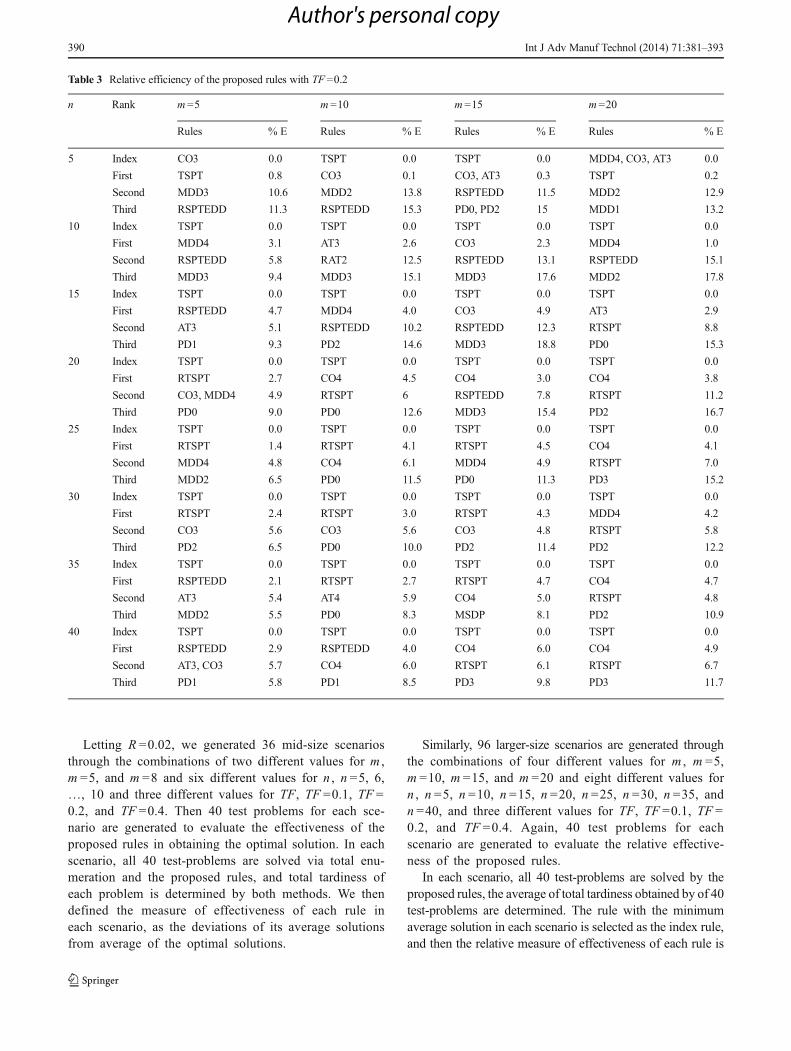
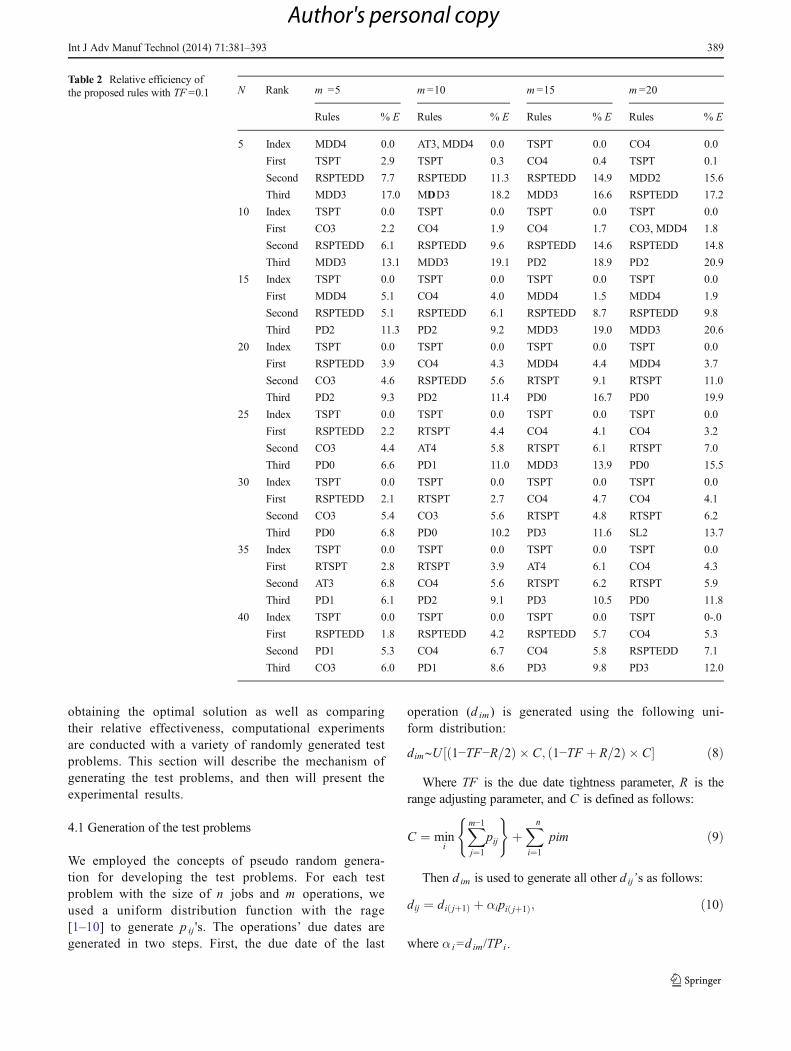
Letting R =0.02, we generated 36 mid-size scenariosthrough the combinations of two different values for m ,m =5, and m =8 and six different values for n , n =5, 6,…, 10 and three different values for TF, TF =0.1, TF =0.2, and TF =0.4. Then 40 test problems for each sce-nario are generated to evaluate the effectiveness of theproposed rules in obtaining the optimal solution. In eachscenario, all 40 test-problems are solved via total enu-meration and the proposed rules, and total tardiness ofeach problem is determined by both methods. We thendefined the measure of effectiveness of each rule ineach scenario, as the deviations of its average solutionsfrom average of the optimal solutions.

Similarly, 96 larger-size scenarios are generated throughthe combinations of four different values for m , m =5,m =10, m =15, and m =20 and eight different values forn , n =5, n =10, n =15, n =20, n =25, n =30, n =35, andn =40, and three different values for TF, TF =0.1, TF =0.2, and TF =0.4. Again, 40 test problems for eachscenario are generated to evaluate the relative effective-ness of the proposed rules.

In each scenario, all 40 test-problems are solved by theproposed rules, the average of total tardiness obtained by of 40test-problems are determined. The rule with the minimumaverage solution in each scenario is selected as the index rule,and then the relative measure of effectiveness of each rule is

Table 3 Relative efficiency of the proposed rules with TF =0.2

n Rank m=5 m=10 m=15 m=20


5 Index CO3 0.0 TSPT 0.0 TSPT 0.0 MDD4, CO3, AT3 0.0

First TSPT 0.8 CO3 0.1 CO3, AT3 0.3 TSPT 0.2

Second MDD3 10.6 MDD2 13.8 RSPTEDD 11.5 MDD2 12.9

Third RSPTEDD 11.3 RSPTEDD 15.3 PD0, PD2 15 MDD1 13.2


First MDD4 3.1 AT3 2.6 CO3 2.3 MDD4 1.0

Second RSPTEDD 5.8 RAT2 12.5 RSPTEDD 13.1 RSPTEDD 15.1

Third MDD3 9.4 MDD3 15.1 MDD3 17.6 MDD2 17.8


First RSPTEDD 4.7 MDD4 4.0 CO3 4.9 AT3 2.9

Second AT3 5.1 RSPTEDD 10.2 RSPTEDD 12.3 RTSPT 8.8

Third PD1 9.3 PD2 14.6 MDD3 18.8 PD0 15.3


First RTSPT 2.7 CO4 4.5 CO4 3.0 CO4 3.8

Second CO3, MDD4 4.9 RTSPT 6 RSPTEDD 7.8 RTSPT 11.2

Third PD0 9.0 PD0 12.6 MDD3 15.4 PD2 16.7


First RTSPT 1.4 RTSPT 4.1 RTSPT 4.5 CO4 4.1

Second MDD4 4.8 CO4 6.1 MDD4 4.9 RTSPT 7.0

Third MDD2 6.5 PD0 11.5 PD0 11.3 PD3 15.2


First RTSPT 2.4 RTSPT 3.0 RTSPT 4.3 MDD4 4.2

Second CO3 5.6 CO3 5.6 CO3 4.8 RTSPT 5.8

Third PD2 6.5 PD0 10.0 PD2 11.4 PD2 12.2


First RSPTEDD 2.1 RTSPT 2.7 RTSPT 4.7 CO4 4.7

Second AT3 5.4 AT4 5.9 CO4 5.0 RTSPT 4.8

Third MDD2 5.5 PD0 8.3 MSDP 8.1 PD2 10.9


First RSPTEDD 2.9 RSPTEDD 4.0 CO4 6.0 CO4 4.9

Second AT3, CO3 5.7 CO4 6.0 RTSPT 6.1 RTSPT 6.7

Third PD1 5.8 PD1 8.5 PD3 9.8 PD3 11.7



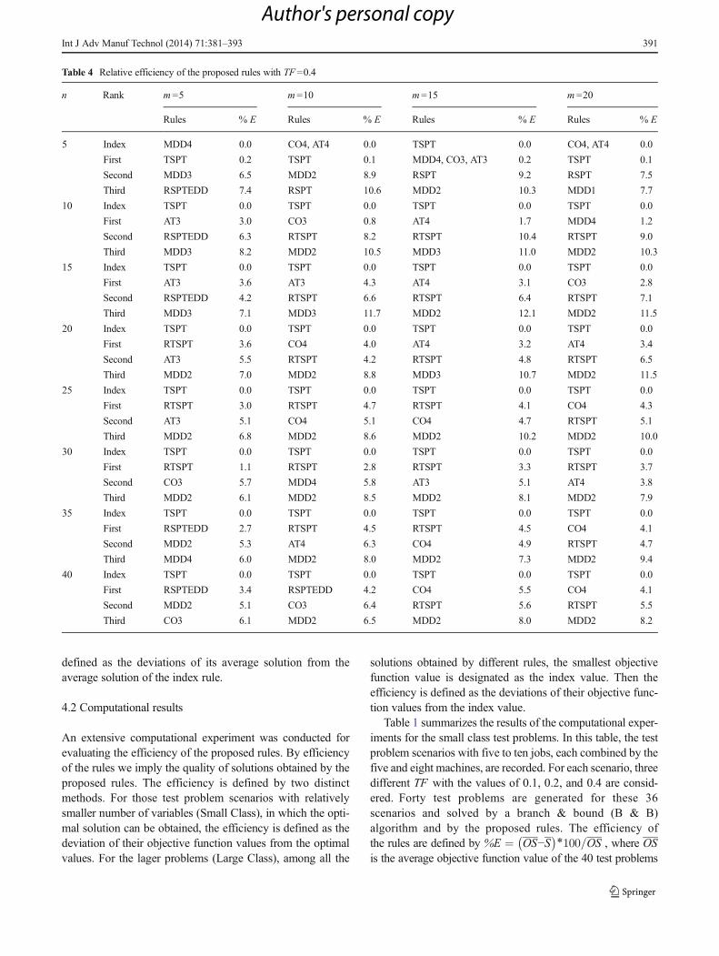
defined as the deviations of its average solution from theaverage solution of the index rule.

4.2 Computational results

An extensive computational experiment was conducted forevaluating the efficiency of the proposed rules. By efficiencyof the rules we imply the quality of solutions obtained by theproposed rules. The efficiency is defined by two distinctmethods. For those test problem scenarios with relativelysmaller number of variables (Small Class), in which the opti-mal solution can be obtained, the efficiency is defined as thedeviation of their objective function values from the optimalvalues. For the lager problems (Large Class), among all the

solutions obtained by different rules, the smallest objectivefunction value is designated as the index value. Then theefficiency is defined as the deviations of their objective func-tion values from the index value.

Table 1 summarizes the results of the computational exper-iments for the small class test problems. In this table, the testproblem scenarios with five to ten jobs, each combined by thefive and eight machines, are recorded. For each scenario, threedifferent TF with the values of 0.1, 0.2, and 0.4 are consid-ered. Forty test problems are generated for these 36scenarios and solved by a branch & bound (B & B)algorithm and by the proposed rules. The efficiency ofthe rules are defined by %E ¼ OS−S

� �∗100=OS , where OSis the average objective function value of the 40 test problems

Table 4 Relative efficiency of the proposed rules with TF =0.4

n Rank m=5 m =10 m=15 m=20


5 Index MDD4 0.0 CO4, AT4 0.0 TSPT 0.0 CO4, AT4 0.0

First TSPT 0.2 TSPT 0.1 MDD4, CO3, AT3 0.2 TSPT 0.1

Second MDD3 6.5 MDD2 8.9 RSPT 9.2 RSPT 7.5

Third RSPTEDD 7.4 RSPT 10.6 MDD2 10.3 MDD1 7.7


First AT3 3.0 CO3 0.8 AT4 1.7 MDD4 1.2

Second RSPTEDD 6.3 RTSPT 8.2 RTSPT 10.4 RTSPT 9.0



First AT3 3.6 AT3 4.3 AT4 3.1 CO3 2.8

Second RSPTEDD 4.2 RTSPT 6.6 RTSPT 6.4 RTSPT 7.1



First RTSPT 3.6 CO4 4.0 AT4 3.2 AT4 3.4

Second AT3 5.5 RTSPT 4.2 RTSPT 4.8 RTSPT 6.5



First RTSPT 3.0 RTSPT 4.7 RTSPT 4.1 CO4 4.3

Second AT3 5.1 CO4 5.1 CO4 4.7 RTSPT 5.1



First RTSPT 1.1 RTSPT 2.8 RTSPT 3.3 RTSPT 3.7

Second CO3 5.7 MDD4 5.8 AT3 5.1 AT4 3.8



First RSPTEDD 2.7 RTSPT 4.5 RTSPT 4.5 CO4 4.1

Second MDD2 5.3 AT4 6.3 CO4 4.9 RTSPT 4.7



First RSPTEDD 3.4 RSPTEDD 4.2 CO4 5.5 CO4 4.1

Second MDD2 5.1 CO3 6.4 RTSPT 5.6 RTSPT 5.5

Third CO3 6.1 MDD2 6.5 MDD2 8.0 MDD2 8.2



of each scenario, obtained by the B & B algorithm, S is theaverage objective function value of the forty test problems ofeach scenario, obtained by a proposed rule, and %E is theefficiency of the proposed rule. For each scenario, their effi-ciency is calculated, and the top five rules are listed in this table.

Tables 2 through 4 summarize the results of the computa-tional experiments for evaluating the relative efficiency of theproposed rules. In these tables, the test problem scenarios inlarge class are considered. The test problems scenarios with n =5, 10, 15, 20, 25, 30, 35, and 40, each combined by the m =5,10, 15, and 20 are evaluated. Table 2 records the results of thecomputational experiments for these scenarios with TF =0.1.Tables 3 and 4 record the results of the computational experi-ments for the same scenarios for TF =0.2 and TF =0.4, respec-tively. Again, 40 test problems are generated for these 96scenarios (eight different values for n , four different valuesfor m , and three different values of TF) and are solved by theproposed rules. The indexed rule, with the smallest averageobjective function value, is designated, and the relative efficien-cy of the other proposed rules is calculated. The efficiency ofthe rules are defined by %E ¼ IS−S

� �∗100=IS , where IS isthe average objective function value of the 40 test problems ofindex rule, S is the average objective function value of the 40test problems of each scenario, obtained by a proposed rule, and%E is the relative efficiency of the proposed rule. For eachscenario, their efficiency is calculated, and the top three rules inaddition to the index rule are listed in these tables.

The results of Table 1 reveal that rules which are modifiedbased on the some simple rules, such as shortest processingtime (TSPT), outperform other more complex rules. This isbased on the fact that in Table 1 the TSPT rule appeared as thefirst rule among the top 5 rules in 28 scenarios out of 36 testproblem scenarios. Due to the fact that, in Tables 2 to 4, theindex rule has been defined as the rule with the smallestaverage objective function value comparing to the other de-veloped rules, we will notice that the TSPT rule appeared asthe index rule in most of the test problem scenarios.

5 Conclusion

In this paper, a set of rules were modified and proposed forsolving the tardiness flow shop permutation scheduling prob-lems with intermediate due dates. In most of the productdesign and research/consulting projects, the outcomes aredelivered through predefined phases, and there is an associat-ed due date for each phase of the project deliverable tasks. Thephases in different projects are carried out in a unidirectionalprecedence structure and hence can be considered as a sched-uling with the intermediate jobs due dates [8].

Although an extensive theoretical concept considers the jobprocessing time and the job dates for case of the single machinetardiness sequencing problem, none have emerged to a unique

result. In case of the traditional flow shop tardiness sequencingproblem, the problem is more complicated. The complicationsbecome more severe when one considers the tardiness problemwith the intermediate due dates. We therefore employed theresults of these studies and modified them for the flow shopwith the intermediate due date tardiness sequencing problems.

Furthermore, an extensive computational experiment forevaluating the efficiency of the proposed rules is conducted.By efficiency of the rules we imply the quality of solutionsobtained by the proposed rules. The efficiency was defined bytwo distinct methods. For those test problem scenarios withrelatively smaller number of variables, for which the optimalsolution could be obtained, the efficiency was defined as thedeviation of their objective function values from the optimalvalues. For the lager problems, among all the solutions obtainedby different rules, the smallest objective function value wasdesignated as the index value. The efficiency was then definedas the deviations of their objective function values from theindex value. The rules were then ranked according to theirefficiencies and some of the top rules were designated and werereported. The results of these experiments revealed that ruleswhich are modified based on the some simple rules, such asshortest processing time, outperforms other more complex rules.

Considering this result, it will be worthwhile that simple rulesor modifications of these rules are employed in development ofmore efficient heuristic or meta-heuristic algorithms in the fur-ther research. The class of ranking rules is also very encourag-ing, because as with the number of jobs/machines, which deter-mine the number of decision variables increases, this class ofrules performsmuch better. Therefore, theywill be an interestingresearch subject to be explored more in further research.

References

1. Baker KR, Trietsch D (2009) Principles of sequencing and schedul-ing. John Wiley & Sons, Inc., Hoboken, NJ

2. Braglia M, Grassi A (2009) A new heuristic for the flow shopscheduling problem to minimize makespan and maximum tardiness.Int J Prod Res 47:273–288

3. Campbell HG, Richard A, Dudek RA, Smith ML (1970) A heuristicalgorithm for the n job, m machine sequencing problem. Manag Sci16(10):B630–B637

4. Deming L, Ping GX (2011) Variable neighborhood search for min-imizing tardiness objectives on flow shop with batch processingmachines. Int J Prod Res 49:519–529

5. Demirel T, Ozkir V, Demirel NC, Taşdelen B (2011) A geneticalgorithm approach for minimizing total tardiness in parallel machinescheduling problems. Proceedings of the World Congress onEngineering, July 6–8, 2011, London, UK

6. Dominic PDD, Kaliyamoorthy S, Saravana KM (2004) Efficientdispatching rules for dynamic job shop scheduling. Int J AdvManuf Technol 24:70–75

7. Figielska E (2009) A genetic algorithm and a simulated annealingalgorithm combined with column generation technique for solvingthe problem of scheduling in the hybrid flow shop with additionalresources. Comput Ind Eng 56:142–151



8. Ghassemi-Tari F, Olfat L (2004) Two COVERT based algorithms forsolving the generalized flowhop problems. Proceedings of the 34thInternational Conference on. Comput Ind Eng 34:29–37

9. Işler MC, Toklu B, Çelik V (2012) Scheduling in a two-machineflow-shop for earliness/tardiness under learning effect. Int J AdvManuf Technol 61(9):1129–1137

10. Khan BSH, Govindan K (2011) A multi-objective simulated anneal-ing algorithm for permutation flow shop scheduling problem. Int AdvOper Manag 3:88–100

11. Kianfar K, Fatmi-Ghomi SMT, Krimi B (2009) New dispatchingrules to minimize rejection and tardiness costs in a dynamic flexibleflow shop. Int J Adv Manuf Technol 45(7–8):759–771

12. Kim SC, Bobrowski PM (1994) Impact of sequence-dependent setuptime on job shop scheduling performance. Int J Prod Res 32(7):1503–1520

13. Koulamas C (1998) A guaranteed accuracy shifting bottleneck algo-rithm for the two-machine flow shop total tardiness problem. ComputOper Res 25:83–89

14. Lee YH, Bhaskaran K, Pinedo M (1997) A heuristic to minimize thetotal weighted tardiness with sequence-dependent setups. IIE Trans29:45–52

15. Lee YH, Pinedo M (1997) Scheduling job on parallel machines withsequence dependent setup time. Eur J Oper Res 100:464–474

16. Morton TE, Dharan BG (1978) Algoristics for single-machine se-quencing with precedence constraints. Manag Sci 24(10):1011–1020

17. Morton, T. E., and Pentico, D., 1993. Heuristic scheduling systems:with applications to production systems and project management.New York, NY, Wiley

18. Pfund ME, Fowler JW, Gadkari A, Chen Y (2008) Scheduling jobson parallel machines with setup times and ready time. Comput IndEng 54(4):764–782

19. Rachamadugu, RVand Morton, TE (1982) Myopic heuristics for thesingle machine weighted tardiness problem. Working Paper,Carnegie Mellon University, Pittsburgh, PA 30-82-83

20. Russell RS, Dar-El EM, Taylor BW (1987) A comparative analysis ofthe COVERT job sequencing rule using various shop performancemeasures. Int J Prod Res 25(10):1523–1540

21. Vallada E, Ruiz R, Minella G (2008) Minimizing total tardi-ness in the m-machine flow shop problem: a review andevaluation of heuristics and metaheuristics. Comput OperRes 35:1350–1373

22. Vepsalainen A, Morton TE (1987) Priority rules for job shops withweighted ardiness costs. Manag Sci 33:1035–1047

23. Vinod V, Sridharan R (2012) Dynamic job-shop scheduling withsequence-dependent setup times: simulation modeling and analysis.Int J Adv Manuf Technol 36(3):355–372

24. Yeung WK, Oguz C, Cheng TE (2009) Two-machine flowshop scheduling with common due window to minimizeweighted number of early and tardy jobs. Nav Res Logist 6:593–599



Documents

heuristic rules for tardiness problems in flowshop with the intermediate due dates