1

Heating and cooling building energy demand evaluation; a simplified model and a modified

degree days approach

Mattia De Rosa, Vincenzo Bianco, Federico Scarpa*, Luca A. Tagliafico

University of Genoa, DIME/TEC, Division of Thermal Energy and Environmental Conditioning

Via All'Opera Pia 15 A, 16145 Genoa, Italy

(*) corresponding author- e-mail: fscarpa@ditec.unige.it

To be published in the international journal Applied Energy

Abstract

Degree days represent a versatile climatic indicator which is commonly used in building energy performance analysis.

In this context, the present paper proposes a simple dynamic model to simulate heating/cooling energy consumption in

buildings. The model consists of several transient energy balance equations for external walls and internal air according

to a lumped-capacitance approach and it has been implemented utilizing the Matlab/Simulink® platform. Results are

validated by comparison to the outcomes of leading software packages, TRNSYS and Energy Plus.

By using the above mentioned model, energy consumption for heating/cooling is analyzed in different locations,

showing that for low degree days the inertia effect assumes a paramount importance, affecting the common linear

behavior of the building consumption against the standard degree days, especially for cooling energy demand.

Cooling energy demand at low cooling degree days (CDD) is deeply analyzed, highlighting that in this situation other

factors, such as solar irradiation, have an important role. To take into account these effects, a correction to CDD is

proposed, demonstrating that by considering all the contributions the linear relationship between energy consumption

and degree days is maintained.

Keywords: dynamic models; building, energy demand, modified degree days

*Manuscript cleanClick here to download Manuscript: manuscript_rev2_clean.doc Click here to view linked References

Acc

epte

d M

anus

crip

t

2

Nomenclature Roman letters a, b Forced convection coefficient C Thermal capacitance or Heat capacity (J K-1) Ct Natural convection coefficient (W m-2 K-4/3) CDD Cooling degree-days (°C) CDD* Modified cooling degree-days (°C) Dm Number of days in a month E Energy demand (kW m-2) E* Cooling energy demand calculated using CDD* (kW m-2) f Shadowing factor F1, F2 Brightening coefficient h Heat transfer coefficient (W m-2 K-1) H Building global heat transfer coefficient (W K-1) HDD Heating degree-days (°C) Ib,n Normal direct solar radiation (W m-2) Id,h Horizontal diffuse solar radiation (W m-2) Id,n Diffuse solar radiation on surface (W m-2) Ij,n Global solar radiation on surface j (W m-2) It0,y Total horizontal solar radiation in the year computed by CDD* model (W m-2) j Index of wall layers n Number of external walls. q Heat flux (W)

R Thermal resistance (K W-1) S Surface (m2) t Time (s, h) T Temperature (°C)

deT , Daily mean temperature (°C)

U Transmittance (W m-2 K-1) V Wind velocity (m s-1) Greek letters α Solar height angle / absorbance coefficient β Surface tilt angle (°) γ Surface azimuth (°) δ Declination angle (°) ε Emissivity ζ, χ Parameters for CDD* calculation θ Incidence angle between solar radiation and surface normal axis (°) ξr Tilt solar redirected radiation factor ρ Ground solar reflection factor σ Stefan Boltzmann’s constant (W m-2 K-4) τ Solar transmission coefficient ϕ Latitude (°) ω Hour angle (°) Subscripts b base temperature c Cooled cs Cooling system d days e External E East f Floor h hour

Acc

epte

d M

anus

crip

t

3

hs Heating system ht Heated i Internal is Internal sources j Wall index for vertical walls and roof m Month N North r Roof s Solar S South sg Solar gain tot Convective plus irradiative v Ventilation w Wall W West win Windows y Year

1. Introduction

Energy consumption of buildings has become a relevant international issue and different policy measures for energy

saving are under discussion in many countries. In the European Union (EU), buildings account for about the 40% of the

total energy consumption and they represent the largest sector in all end-users area, followed by transport with the 33%

[1]; whereas in terms of CO2 emission, buildings are responsible for about 36% of it. It is estimated that the residential

sector alone represents about 25% (in 2011) of the final energy consumption in EU [2]. Energy in household is

consumed for different purposes, such as hot water, cooking and appliances, but the dominant energy end-use in Europe

(responsible for around 70% of total consumption in households) is space heating [1]. Moreover, trend in energy

demand, both for heating and cooling purpose, assumes a relevant issue on the development of energy systems and

energy policies. Isaac and van Vuuren [3] highlight that energy demand for heating and cooling purposes tends to rise in

the 21th century, especially due to the increasing income in developing countries and to the climate change. In

particular, the climate change has a double effect: (i) it decreases the global heating energy demand by over a 30% and,

on the other hand, (ii) it increases cooling energy demand by about 70% [3]. An extended review on the impact of

climate change on energy use in building for different world locations was performed by Li et al. [4].

In order to achieve relevant saving of primary energy, several potential mitigation measures can be implemented

involving the building envelope, internal condition, heating/cooling systems, etc., as reported in Wan et al. [5].

In this context, the 91/2002 “Energy Performance of Buildings Directive” (EPBD) [6] has been emanated to introduce

several requirements for new and existent buildings within EU. Accordingly, designers and researchers must optimize

all the possible aspects (building envelope, shadowing, heating and cooling system components, regulation criteria,

Acc

epte

d M

anus

crip

t

4

etc.), starting from the earliest design phase with an optimization perspective, in order to respect the prescriptions of the

current directive and, at the same time, ensuring the thermal comfort for occupants [7, 8].

In this context, software able to predict the thermal energy demand for heating and cooling can contribute to find the

best solution to increase energy efficiency and this is the reason why several numerical models for buildings simulation

have been developed over the years.

Different basic approach can be adopted for building energy analysis tools, depending on the different level of building

description which could be useful for each different purpose. Generally, long term calculation with steady-state models,

without considering the inertia effect (or considering some correction factors), are commonly used for preliminary

building design and for scenario analyses. The degree-days method represents the simple way to obtain an idea of the

building energy consumption, performing very simple and fast calculations. Their base assumption is that for long term

calculation, the energy consumption is proportional to the difference between external and internal temperature.

Therefore, assuming a global building transmission coefficient H in W/K, the monthly energy consumption Eh,m can be

calculated as follows [9]:

cshs

hmm

tDDHE

/η××= (1)

where th is the heating time in a day (which can be assumed equal to 24h if a continuously heating/cooling is provided),

ηhs/cs is the efficiency of the equipment, and DDm is the total heating or cooling degree days of a month m. A simple

method to calculate the degree days is reported in Eq. (2) and Eq. (3) for heating (HDD) and cooling (CDD) calculation

respectively:

Heating: ( )∑= +−== mD

ddehsbmm TTHDDDD

1,, (2)

Cooling: ( )+=∑ −== mD

dcsbdemm TTCDDDD

1,, (3)

deT , represents the mean of the daily maximum and minimum external air temperature of a day d, while Tb,hs and Tb,cs

are the base temperatures for heating and cooling respectively, which represent the temperature set point of the inner

heated/cooled zones. The sign + indicates that only positive values are added. Different approaches can be adopted to

calculate the degree days, depending on the type of data available for the external temperature. A short review of the

different techniques is reported in [10], while a simple application can be found in [11]. Acc

epte

d M

anus

crip

t

5

Generally, steady state models are used in the common standards in order to obtain the energy performance of buildings

[12, 13]. Thanks to their fast calculations, this approach permits to conduct long-term analyses on different scenarios

involving several energy efficiency measures. As for instance, Yang et al. [14] study the effect of different building

envelope for different climate zones in China utilizing the OTTV approach [13].The main limitation of this approach is

represented by the fact that the inertia of the building envelop is completely neglected. To overcome this problem, the

common standards for calculation building energy consumption, as e.g. [12, 13], suggest implementing steady state

models in which inertia effects are approximated introducing several correction factors depending on the building

envelope characteristics. Furthermore, new technologies which exploit the building inertia effects, like free cooling [15,

16] and phase change materials [17, 18], cannot be analyzed under the steady state approach. In these cases, only

transient thermal models can be adopted to analyze innovative energy saving solutions, especially those in which

different systems are coupled together. Moreover, short time regulation criteria assume an important role in the global

energy performance of these integrated systems [19]. Thus, also in this context, dynamic models represent a powerful

and flexible tool for evaluating thermal performances of buildings/system coupled behavior.

In the last years several numerical approaches have been developed and tested (for a detailed classification and

description see [20]), and most of them have been implemented in software dedicated to building simulation such as

DOE-2, BLAST, EnergyPlus, TRNSYS, SPARK, etc. (an overview of their capabilities is reported in [21]). However,

the increase of the computer performance makes the use of mathematical packages, such as Matlab/Simulink, a good

option to perform dynamic simulations of buildings. In fact, simplified buildings models permit the evaluation of

thermal indoor environment and heating/cooling loads with a satisfactory level of accuracy and without excessive

computational costs.

In the present paper, a simplified thermal model is developed in order to obtain a simple tool able to predict the energy

performance of buildings. It can be built starting from the electrical network analogy (RC): thermal resistances R and

thermal capacitances C are introduced in an equivalent thermal network in which the connecting node potentials

represent actual temperatures. The model is quite simple and it can be implemented in all computational environments;

for this purpose, a detailed description of the model is reported in section 2.

For the present work, the simplified model has been implemented in a tool, called BEPS (Building Energy Performance

Simulator) which is based on the Matlab/Simulink software, which can be used to support the design of HVAC plants,

to perform energy diagnosis of buildings, to estimate energy consumption and so on. The use of Matlab/Simulink

allows users to extend by themselves the capabilities of the simulation package, for instance adding modules for the

evaluation of heating/cooling systems. In fact, its flexibility and robustness, combined with the low computational cost

Acc

epte

d M

anus

crip

t

6

in performing yearly simulations with short time discretization, allows performing combined building/system

simulations. BEPS has been tested and validated using consolidated simulators, especially TRNSYS and EnergyPlus in

order to check its performance.

Several simulations have been performed in order to observe the model behavior with different types of climatic

conditions in the European region. The building energy consumption, for both heating and cooling, is analyzed as

function of the HDD and CDD, assumed as standard climatic parameter of each locality. Moreover, considering that the

inertia effects assumes a paramount importance, especially in cooling energy demand calculation, the analyses are

extended to lower CDD conditions in order to observe and quantify the deviation caused by these effects.

Finally, a correction factor for the CDD formulation, based principally on the solar radiation of each locality, is

introduced in order to calculate new modified CDD with the aim to extend the validity of degree days description to

lower CDD localities.

2. Numerical model

In the last years, researchers have performed and compared a lot of dynamic numerical models, in order to analyze their

capability in predicting the energy demand of buildings. Boyer et al. [22] introduced the nodal analysis for determining

the thermal behavior of buildings: considering a one-dimensional conduction across the walls and introducing their

thermal capacities, each building component (wall, heating zone, etc.) is modeled as a node in which the energy

conservation law is applied.

Hudson and Underwood [23] tested a thermal model based on a lumped-capacity treatment of the building elements

adopting the electrical analogy. The model has been applied to a building with high thermal capacity, showing a good

agreement between numerical and experimental results. They concluded that there are no advantages in using a higher-

order description of walls if short-term transient analyses are considered. The same approach can be found in [24],

where the authors implemented a lumped model in Matlab/Simulink environment, performing several analyses

regarding the influence of different parameters on building indoor temperature and energy consumption.

Nielsen [25] developed a simple tool to evaluate building energy demand in a transient context. The equation system

consists in two differential equations, one for the internal air and the other for all the opaque structures grouped into a

single effective capacitance. Moreover, an algebraic equation is added to account for the conduction across the walls

and the solar contribution in the internal surfaces. As reported in the paper, this tool is useful in the early stage of the

building design to have a rough estimate of energy demand and thermal indoor environment. Acc

epte

d M

anus

crip

t

7

Starting from these past works, a thermal dynamic model based on the lumped capacitance approach [26], combined

with the electrical analogy [25], is developed. As suggested in [22], transient energy balance equations have been

written for each domain (floor, external walls, roof and internal air) and a lumped-thermal capacitance is taken into

account in order to consider the thermal inertia. Therefore, the entire building is described by a system of ordinary

differential equations, which is solved using standard numerical techniques [27].

2.1 Heating/cooling zone

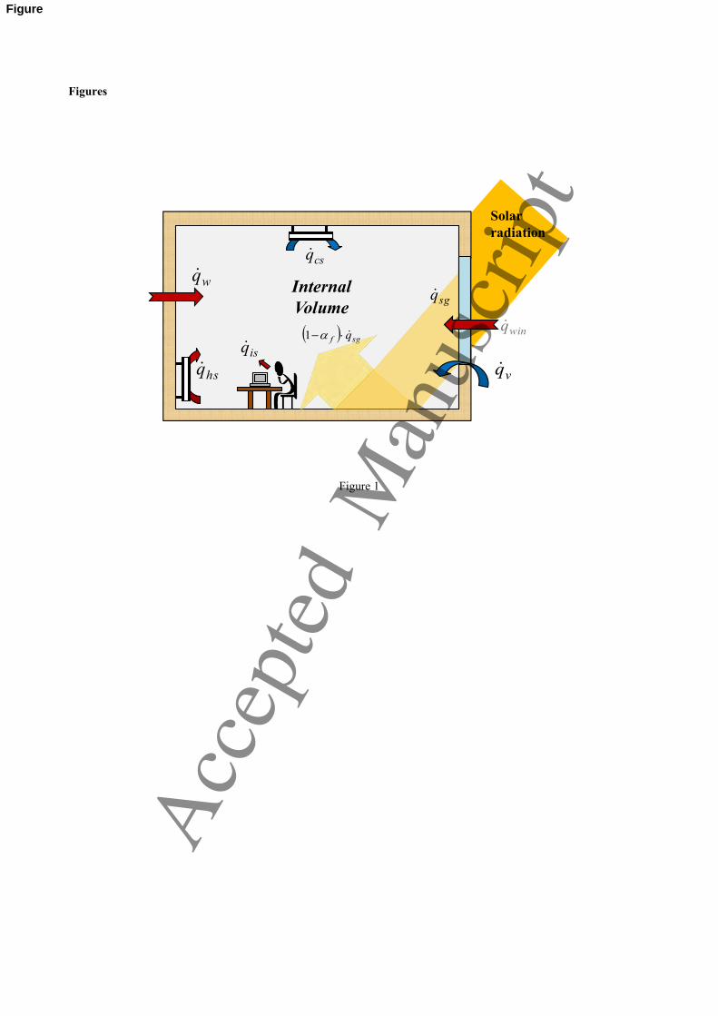
The building heated/cooled zones are modeled as a single isothermal air volume with a unique thermal capacitance

(Figure 1). This volume exchanges heat with the internal layer of the walls and with the external air across the windows

and it receives heat by the internal free gain due to persons and equipment. The heat transfers due to ventilation and

direct solar radiation across the windows is also taken into account.

The transient energy balance equation for the internal air node is written as follows:

winwviscshsi

i qqqqqdt

dTC ++++= /

(4)

in which the following contribution are taken into account:

- cshsq / is the heating/cooling input thermal power, which depends on external conditions, system configuration and

regulation criteria;

- isq represents the internal heat source due to persons and equipment. In the present analysis a global averaged

value of free gain is considered and it depends on the useful surface of the building and its intended use [12];

- vq refers to the heat transfer due to ventilation considering the minimum suitable value of air exchange, according

to [28];

- wq takes into account the heat transfer through the external walls and it is calculated by summing the contribution

of each wall, jiq , (Eq. (11)).

- winq considers heat transfer across the windows.

2.2 External walls

Each wall is modeled considering two different layers: the internal layer, which exchanges heat with the internal mass

of air, and the external one, which is subjected to the combined effect of external air convection and solar irradiation Acc

epte

d M

anus

crip

t

8

(Figure 2). The node capacitance point, which accounts for the entire wall, is normally located in the center of the wall,

but it is possible to move it depending on the characteristics of the wall.

The radiation coming from the windows is supposed to be absorbed by the floor according with its absorbance, whereas

the reflected part is assumed to be uniformly distributed on all interior surfaces, as described in section 2.4 [29].

The transient energy balance equations for opaque external walls (Figure 2) can be written as follows:

jewjiwjw

jw qqdt

dTC ,,

,, −− += (5)

where jwC , and jwT , represent the thermal capacitance and the node temperature of the wall respectively (Fig. 2a),

whereas jiwq ,− and jewq ,− represent the heat flux between the wall node and the internal/external wall surface. The

heat fluxes jiwq ,− and jewq ,− can be calculated as follows:

( )jiw

jwjwijiw R

TTq

,

,,,

−−

−= (6)

( )jew

jwjwejew R

TTq

,

,,,

−−

−= (7)

Similar contributions are also considered for modeling the floor, where the external heat flux is purely conductive and,

with respect to Eq. (7) and as shown in Eq. (8), it can be calculate directly considering the ground temperature T∞ as

function of the external temperature at a certain depth depending on the building foundation.

( )few

fwfew R

TTq

,

,,

−

∞−

−= (8)

jwiT , and jweT , in Eq. (6-7) are the internal and the external surface temperatures respectively and they can be

determined by considering the following energy balances:

jijsgjiw qqq ,,, =+− (9)

jejsjew qqq ,,, =+− (10)

where jiq , and jeq , are the heat flow rate on the internal and external wall surface respectively as defined in Eq. (11-

12), while the terms jsq , and jsgq , represent the solar contributions. In particular jsq , is the solar radiation normal to

the j-walls on the exterior surface, Eq. (16), while jsgq , is the solar heat transfer rate reflected from the floor, Eq. (19),

according to the hypothesis showed in section 2.4. Acc

epte

d M

anus

crip

t

9

( )ji

jwiiji R

TTq

,

,,

−= (11)

( )je

jweeje R

TTq

,

,,

−= (12)

The thermal resistances jiwR ,− and jewR ,− which appears in Eq. (7-8) are purely conductive and, as well known, they

depend on the thermal conductivity and on the thickness of each wall layer. On the contrary, thermal resistances jiR ,

and jeR , in Eq. (11-12) can be calculated as follows:

jwjtotje Sh

R,,

,

1

×= (13)

jwjiji Sh

R,,

,1

×= (14)

The term jwS , is the opaque external surface, while the internal heat transfer coefficient, hi,j, is calculated considering

only the natural convection term and assuming negligible the infrared irradiation between the internal surfaces. A

simply method to calculate the external convective heat transfer coefficient, jtoth , , is reported in Appendix A.

2.3 Windows

Heat transfer across the external windows, winq , is calculated as follows:

( ) ( )∑ ∑ −=×−=j

jjwin

iejwinjwiniewin R

TTSUTTq

,,, (15)

where jwinS , is the total windows surface at j-wall orientation and jwinU , is the transmittance of the windows which

depends on the glass characteristics and on the internal and external convective heat transfer coefficient.

2.4 Solar contributions

The heat contribution due to the solar radiation on the opaque surface of the external walls, which is represented by the

term jsq , in Eq. (10), can be calculated for each wall as follows:

njjwjwjs ISq ,,,, α= (16)

where jw,α is the absorbance coefficient of the wall external surface j.

Acc

epte

d M

anus

crip

t

10

The whole solar radiation transmitted across the windows can be calculated according to the following equation:

∑=j

njjwinjwinjsg ISfq ,,,τ (17)

in which jwin ,τ and jwinS , are the glass transmission coefficient and the total window surface at j-wall orientation

respectively. The term jf takes into account the presence of shadowing.

It is supposed that sgq is all absorbed by the floor according with its absorbance αf [29], as showed in Eq. (18), whereas

the reflected part is assumed to be uniformly distributed on all interior surfaces.

sgffsg qq ×=α, (18)

( ) sgf

jjw

jwjsg q

S

Sq ×−=∑ α1

,

,, (19)

The term njI , represents the global solar radiation normal to the wall, which can be calculated for each j-wall as

reported in Appendix B.

3. Benchmark test case

In order to validate the results furnished by BEPS, a benchmark test case of a standard residential building is analyzed

in comparison with consolidated simulators (TRNSYS and Energy Plus). This comparison is made in terms of heating

energy consumption, cooling energy demand and incident radiation. Calculation in TRNSYS and Energy Plus are taken

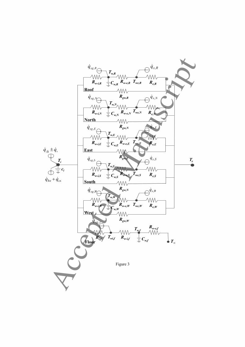
from [30] in which the same benchmark test case is adopted. A simplified schema of the thermal network adopted in the

present work is shown in Figure 3.

3.1 Building description

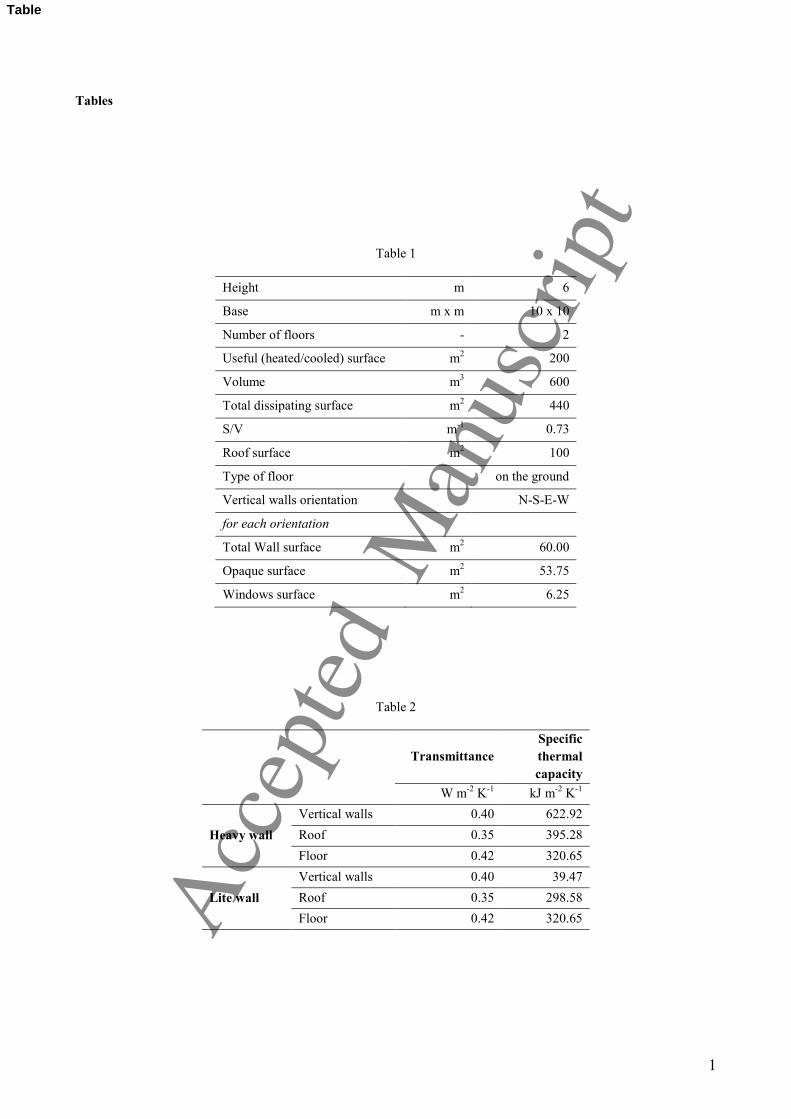
A standard building block of two floors is considered: it is represented by a parallelepiped with a squared floor of side

equal to 10 m and height of 6 m. The total internal volume is 600 m3 and the heated/cooled useful surface is 200 m2. All

the geometric data concerning the considered building are reported in Table 1.

In the present work, two different types of the wall structure are considered: heavy and light configuration. Preserving

the wall transmittances, the two configurations differ by the thermal capacitance and the superficial mass of vertical

walls and roof. Moreover, it is important to highlight that for both configuration an insulation substrate applied on the Acc

epte

d M

anus

crip

t

11

walls is already present, according to the usual Italian construction practice. The main characteristics of the walls are

reported in Table 2.

The glazed surfaces of the building are constituted by the same type of windows for all configurations. The glass

thermal transmittance is assumed equal to 2.465 W/(mK) and its transmission coefficient is equal to 0.571.

3.2 Climatic data

To perform detailed simulations about energy performance behavior of a building, several climatic data are necessary.

In the present model the hourly profiles of different climatic parameters are needed, particularly:

- external temperature;

- normal direct radiation and diffused horizontal radiation, which allow to determine the total value of the total

incident radiation on the surface;

- wind intensity and direction, necessary to determine the external convection coefficients for each surface.

Moreover, latitude and altitude of each considered location are necessary in order to calculate the global solar radiation.

All the climatic data considered in the present paper are taken from [31].

3.3 Model validation

In order to verify the validity of the results provided by BEPS, a comparison with consolidated simulators is proposed,

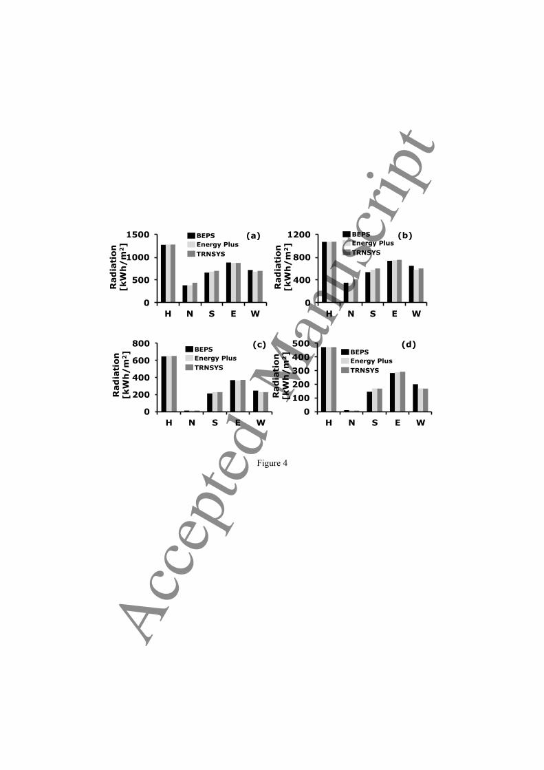
particularly TRNSYS and Energy Plus. The comparison is made in terms of the incident solar radiation on the building

external surface (Figure 4) and yearly heating and cooling demand for both building configuration (Figure 5).

Calculations in TRNSYS and Energy Plus are taken from [30], where the same benchmark is adopted.

The calculation of the solar radiation has an important role in the buildings thermal behavior, especially in determining

the cooling energy demand. In Figure 4 it is possible to see that both direct and global incident radiations calculated by

the three simulators are very close.

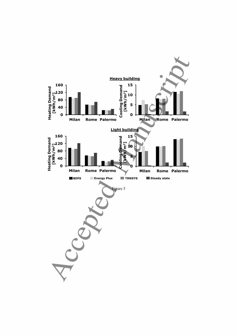
Figure 5 reports the estimation of heating and cooling demand for three Italian cities with different climates: cold in

Milan, moderate in Rome and warm in Palermo. The comparison shows that all the simulators predict similar heating

and cooling energy demand for all different climatic conditions. Particularly, the average deviation between BEPS and

TRSNYS in calculating heating energy demand is about 5.2% and 8.2% for heavy and light configuration respectively.

Similarly, the average deviation between BEPS and Energy Plus is about 4.6% for both wall configurations.

Considering the cooling energy demand, the average deviation between BEPS and TRSNYS is 4.3% and 5.6% for Acc

epte

d M

anus

crip

t

12

heavy and light configurations respectively, whereas Energy Plus shows a weak deviation compared to BEPS and

TRNSYS.

Finally, Figure 5 shows that the steady state approach is not able to reproduce the building energy demand: in particular

the heating energy demand is clearly overestimated while an underestimation in calculating the cooling energy demand

is reported. Moreover, the results of the static approach show a similar behavior in both heavy and light building wall

configuration. These effects can be explained by considering that the implemented steady state approach is derived from

the common standards [12], in which a monthly averaged temperature and radiation is assumed, neglecting all effects

due to the daily variation. Furthermore, a correction dynamic parameter is considered in order to take into account the

inertia of the building envelope, but this correction is not sufficient to reproduce the inertia effect, especially when they

assumes a paramount importance as is the case of cooling energy demand, where the effect of thermal storage of the

walls is relevant.

4. Results and discussion

Several simulations have been performed by using BEPS in order to extend the model testing for different types of

climatic conditions. The analysis have been conducted by using the heavy building configuration described in the

benchmark test case (see 3.1) and adopting an ON-OFF regulation system criterion operating for all 24 hours. The

internal temperature setting point is 18.3 °C (Tb,cs) in winter and 26.7 °C (Tb,hs) in summer with a dead-band setting of 2

°C in their surroundings. As in the previous analyses, the climatic data (external temperature, direct and diffuse solar

radiation, wind speed and direction) have been extracted from [31].

Several European cities have been analyzed in the present work in order to cover different climatic conditions typical

for this region. In order to perform these analyses heating (HDD) and cooling (CDD) degree days are introduced and,

according to the hourly method [10], they can be calculated as follows:

∑ ∑=

+

=

−= 365

1

24

1

,,

24d dh

hehsb TTHDD (20)

∑ ∑=

+

=

−= 365

1

24

1

,,

24d dh

csbhe TTCDD (21)

where Tb,hs and Tb,cs are the base temperature for heating and cooling respectively, which represent the temperature set

point of the inner heated/cooled zones. The superscript “+” means that the sum is extended only to positive terms. Acc

epte

d M

anus

crip

t

13

4.1 Standard CDD analysis

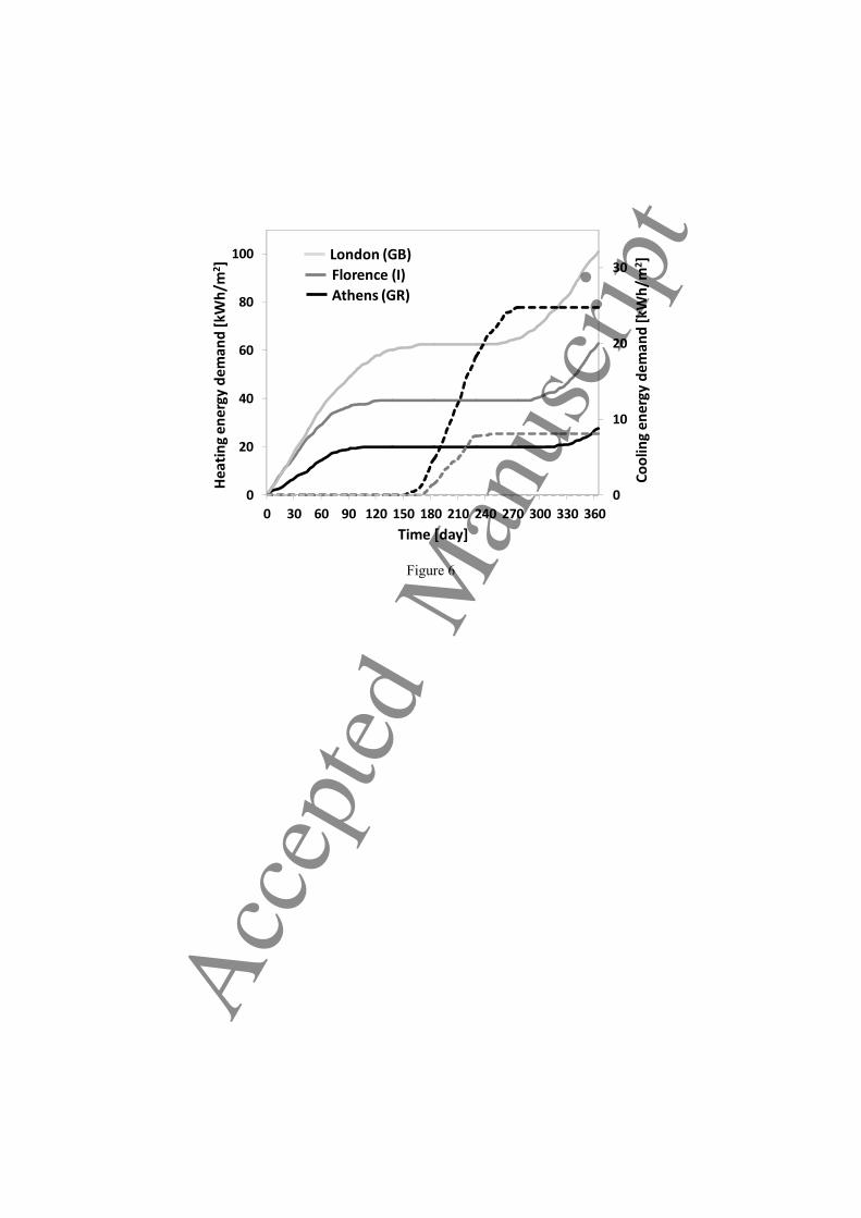
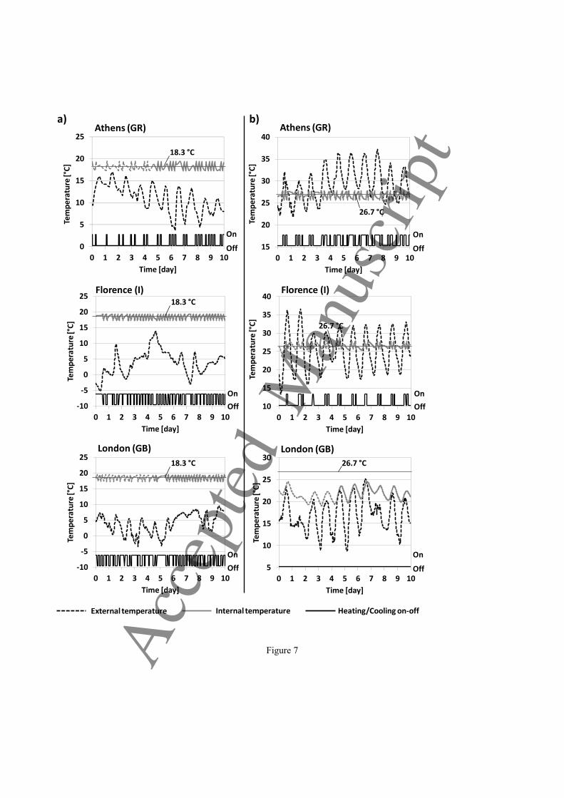
Three illustrative cases with different climatic conditions are analyzed as references. The warm climate is represented

by Athens (GR) with HDD = 1169 and CDD = 80, whereas Florence (I) is characterized by a moderate one, with HDD

= 1971 and CDD = 1. Finally London (GB) is taken as a typical cold climate with HDD = 2968 and CDD = 0. The

common profiles of the energy demand for heating (continuous lines) and cooling (dashed lines) are reported in Figure

6 as reference.

Figure 7 shows the trend of external and internal air temperature and the ON-OFF profile of heating/cooling system for

10 reference days in winter (Figure 7a) and in summer (Figure 7b). The internal temperature is constrained around the

set point temperature for both winter (18.3 °C) and summer (26.7 °C).

It is possible to note that in winter the internal temperature and, consequently, the ON-OFF cycle of the heating system

are governed by the external temperature profile which drives the building heat loss, as previously mentioned. Instead,

in summer (Figure 7b) the influence of solar irradiation and thermal inertia become more significant, especially if the

weather gets cold and the difference between the external and internal temperature is lower (or negative). Particularly,

the contribution of solar radiation can raise the internal temperature significantly, though Te < Ti as, e.g. in Florence.

The effect of the solar radiation becomes crucial in the London case to maintain the inlet temperature higher than the

external one. In fact, the external temperature reaches the internal one rarely and the cooling system is turned off

continuously. In this condition, the effect of building thermal inertia is highlighted by the damping and the phase shift

of the internal temperature profile compared with the external one.

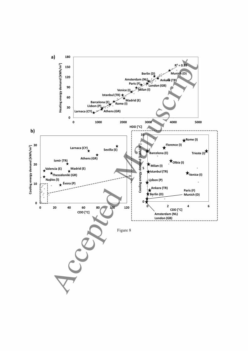
Figure 8 shows the consumption of the considered building for heating (a) and cooling (b) purposes as a function of

HDD and CDD. The figure highlights that energy consumption to heating purposes (Figure 8a) results to be a linear

function of HDD, thus it is possible to perform the analysis only for a few different values of HDD and then to get the

estimation of heating demand for different locations by performing a linear fitting of the calculated points, without

losing too much in terms of accuracy.

The cooling energy demand as a function of CDD shows a scattered trend (Figure 8b), which tends to decrease with

increasing of CDD. In fact, observing the degree-days definition, provided in Eq. (27-28), it is possible to note that it

depends only on the temperature difference between the external and internal ambient (or set point value). Since in

Europe the degree days are generally high in winter (HDD > 800), the building heat transfer is governed by this ∆T and,

consequently, the heating energy demand results to be a linear function of HDD, as shown in Figure 8a. Acc

epte

d M

anus

crip

t

14

On the contrary, in summer the cooling degree-days are generally low in Europe (CDD < 200) and the cooling energy

demand is also affected by other factors (e.g. solar irradiation, thermal inertia of the building envelope and the set-point

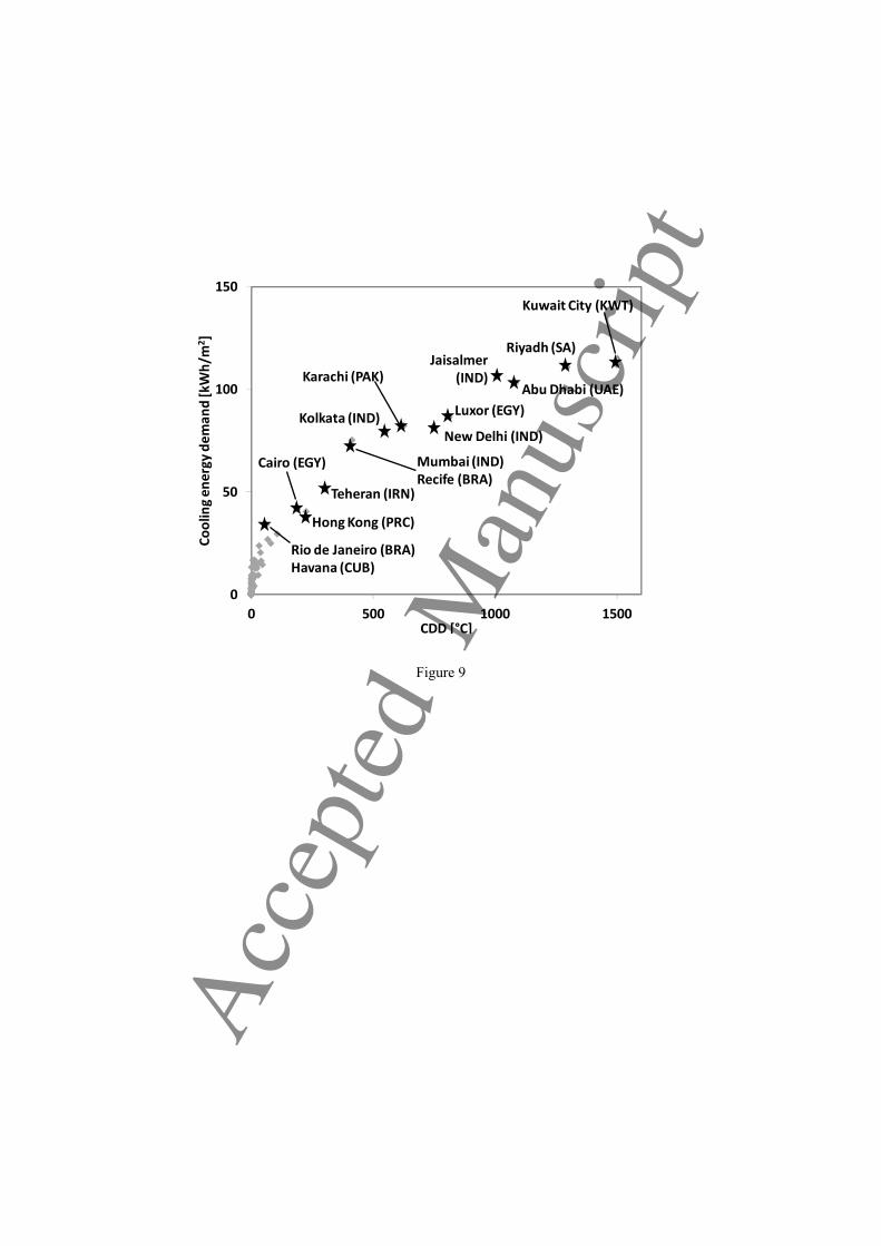
temperature) causing the scattering showed in Figure 8b. Extending the analysis to warmer localities outside of EU, it is

possible to observe that the scattering of the cooling energy demand tends to be reduced with the increase of the CDD

(Figure 9), thanks to the increase of the external temperature which makes the transmission phenomenon even more

relevant.

4.2 Low CDD analyses

Starting from the results provided in the previous section, several analyses have been conducted in order to underline

the behavior of the cooling energy consumption for lower CDDs. For each locality, it is possible to increase/decrease

the value of CDD by varying the base reference temperature with which CDDs are calculated (Eq. (21)).

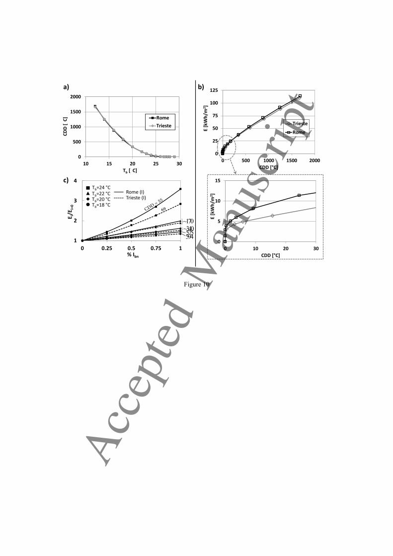
Several simulations have been performed considering two Italian cities with the similar CDD, Rome and Trieste, as

shown in Figure 10a. The profiles of the cooling energy demand obtained by BEPS are shown in Figure 10b, where the

same trend observed in Figure 9 is detected: for high CDDs the profiles assume a linear trend against CDDs with a very

low difference between the two cities, thanks to the quite similar values of CDDs, while for lower CDDs the deviation

becomes more consistent. This deviation is mainly due to the building inertia effects which are strictly connected with

the solar irradiation (which is quite different between the two cities). In Figure 10c, the impact of the solar radiation

(neglecting the diffuse contribution) on cooling energy demand of both cities for different CDDs is clearly highlighted.

Assuming as reference the case in which no solar irradiation is provided, the trends show that raising the solar radiation

tends to increase the gap in cooling energy demand between the two cities. Moreover, this phenomenon tends to be

pronounced with lower CDDs.

4.3 A simply correction factor for CDD formulation

In order to restore the validity of CDDs for low values, a simple correction is introduced. Starting from the standard

CDD, provided by Eq. (21), the novel cooling degree days (CDD*) are calculated taking into account the incident solar

radiation (both direct and diffuse) of each locality. The new formulation is shown in Eq. (22):

ytICDDCDD ,0* ×+= χ (22)

Acc

epte

d M

anus

crip

t

15

where It0,y is the total horizontal solar irradiation of each locality, computed by summing the daily values only when a

cooling demand is necessary, while χ is the correction factor, which is adjusted in order to minimize the deviation of the

linear regression. The criteria adopted in the present work to determine It0,y is shown in Eq. (23).

( )( ) 0,,

365

1

,0,,

→≤−=∆

→>−=∆ ∑=ζ

ζ

csbded

d d

dtcsbded

TTTt

ITTT

(23)

In Eq. (23) deT , is the daily external mean temperature, whereas It0,d and td are the total horizontal solar irradiation and

the total hours of light in the day d, which can be calculated as follows:

( )∑= += 24

1,0,,0 sin

hhdhibndt III α (24)

( )ϕδπ

tantancos24 ×= dd art (25)

where φ is the latitude of each locality, while α and δ are the hourly solar height angle and the daily declination angle.

The formulations of these two quantities are reported in Appendix B.

The parameter ζ have to be adjusted in order to consider that if the averaged external temperature is slightly lower than

the internal one (Td <0 and, therefore, CDDd =0), the solar radiation could raise sufficiently the internal temperature

causing the switching on of the cooling system. The value adopted in the present work is ζ=-2, equal to the dead-band

of the cooling system setting point.

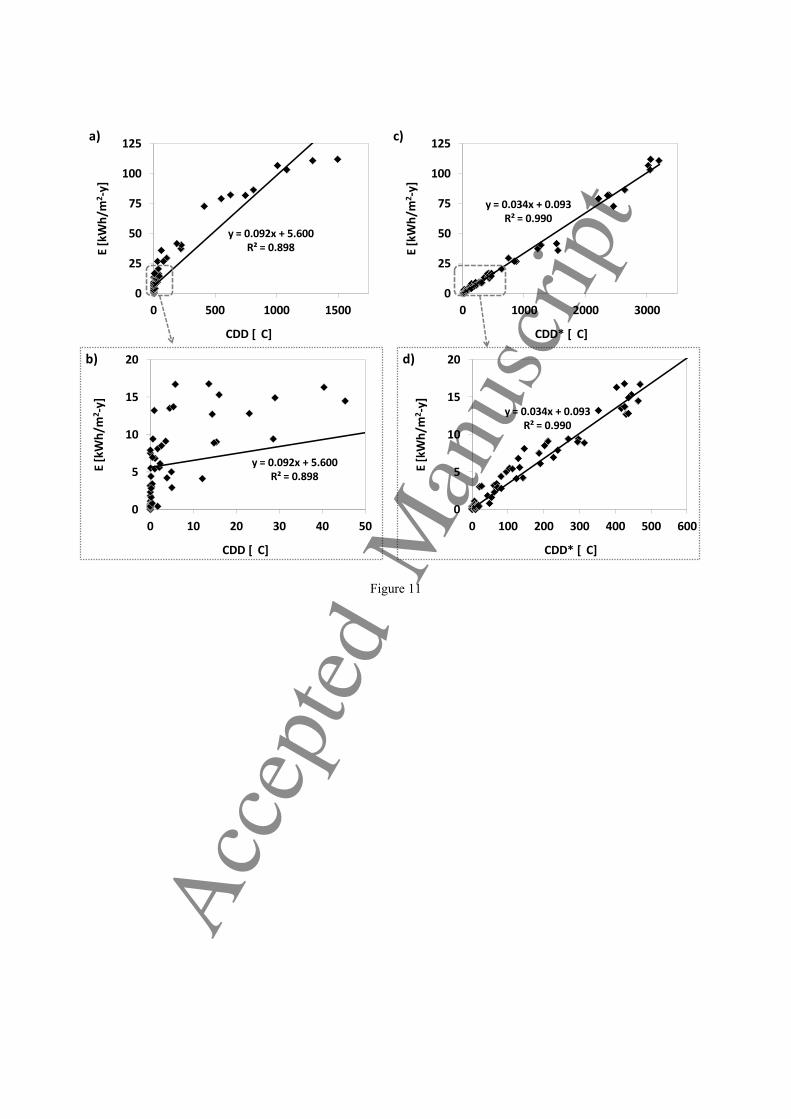
Figure 11 shows the results obtained with the novel formulation (CDD*), compared with the standard CDD. As a

reference, Figure 11a and Figure 11b show the same results of Figure 8b and Figure 9, realizing a very wide range of

case studies of localities around the world. As already shown in the previous sections, the standard CDDs are not able to

reproduce the cooling energy demand correctly when CDDs are low (Figure 11b). Instead, adopting the new CDD*

(Figure 11c,d) the profile of the energy consumption becomes quasi-linear, fitting the point at 99% and succeeding to

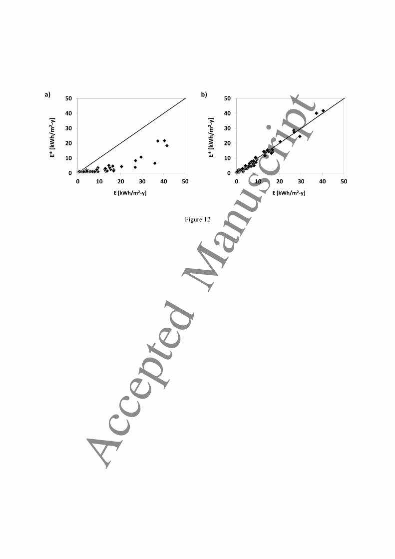
reproduce quite well the trend also for lower CDD* (Figure 11d). Moreover, Figure 12 provides the comparison of the

performances obtained by adopting the two formulations found by the linear regression of the data based on the CDD

(Figure 12a) and CDD* (Figure 12b) for low cooling energy demand cases. It is possible to observe that the new

formulation of CDD* is able to fit well the cooling energy consumption obtained by BEPS, while the CDD one

completely fails in this purpose (Figure 12a).

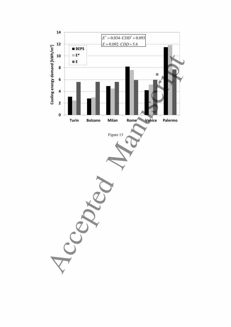
Finally, Figure 13 represents the comparison between the cooling energy demand obtained by using the two

formulations shown in Figure 11, taking as reference results provided by BEPS results for different Italian localities

Acc

epte

d M

anus

crip

t

16

with different climates. As it is possible to observe that, for all tested localities, the cooling energy demands calculated

by the new CDD* formulation provides better results in respect to the standard CDD formulation.

Conclusions

A simplified building dynamic model, based on the electrical analogy, has been developed and implemented in

Matlab/Simulink environment, in order to perform several analyses on heating and cooling energy demand in a wide

range of climatic conditions. A detailed description of this model is provided in section 2, while the validation is

performed by comparing the numerical results with the common commercial software (TRNSYS and Energy Plus).

The comparisons show that BEPS is able to predict the heating and cooling energy demand accurately for all tested

climatic conditions, guaranteeing a very high degree of flexibility and customization for the analysis of specific

problems.

Moreover, several European cities have been analyzed in the present work in order to cover a wide range of climatic

conditions. The analyses have been conducted introducing the heating (HDD) and cooling (CDD) degree days, as a

climate parameter of each locality. Studying the relationship between energy demand and degree days it was found that:

• Since in Europe the degree days is generally high in winter (HDD > 800), the heating demand is linearly correlated

with HDD, because the energy losses of a building are mainly driven by the difference between internal and

external temperature. Consequently, the ON-OFF cycle of the heating system follows the external temperature

profile. Thanks to this linearity, it is possible to perform analyses only for a few different values of HDD and then

to get the estimation of heating demand for different locations without losing too much in terms of accuracy.

• The cooling degree-days are generally low in Europe (CDD < 200) and the cooling energy demand can be affected

by other factors which lead to a scattered behavior of the cooling energy demand as function of CDD. In particular,

this deviation tends to be more pronounced with lower CDD values and it is mainly due to building inertia effects,

which are strictly connected with the solar irradiation. Extending the analysis to warmer localities outside of EU,

the observed cooling energy demand scattering tends to be reduced with the increase of the CDD, thanks to the

increase of the external temperature which makes the transmission phenomenon even more relevant.

• In order to restore the validity of CDDs assumption for low values, a novel formulation is introduced, which is

based on the correction of the standard CDD taking into account the incident solar radiation. The new CDD*s are

able to reestablish the linearity of the cooling energy consumption, fitting well the results obtained by BEPS..

Acc

epte

d M

anus

crip

t

17

References

[1] Buildings Performance Institute Europe (BPIE). Europe’s buildings under the microscope. 2011

[2] Data extracted from Eurostat: http://epp.eurostat.ec.europa.eu.

[3] Isaac M, van Vuuren DP. Modeling global residential sector energy demand for heating and air conditioning in the

context of climate change. Energ Policy. 2009; 37:507-21.

[4] Li DHW, Yang L, Lam JC. Impact of climate change on energy use in the built environment in different climate

zones – A review. Energ. 2012; 42: 103-12.

[5] Wan KKW, Li DHW, LAM JC. Assessment of climate change impact on building energy use and mitigation

measures in subtropical climates. Energ. 2011; 36: 1404-14.

[6] EU. On the energy performance of buildings. Directive 2002/91/EC of the European Parliament and of the Council,

Official Journal of the European Communities, Brussels; 2002.

[7] Nguyen A, Reiter S, Rigo P. A review on simulation-based optimization methods applied to building performance

analysis. Appl Energ. 2014; 113, 1043-58.

[8] Yang L, Haiyan Y, Lam JC. Thermal comfort and building energy consumption implications – A review. Appl

Energ. 2014; 115, 164-73.

[9] Al-Homoud M.S. Computer-aided building energy analysis techniques. Build Environ. 2001; 36,421-33.

[10] Mourshed M. Relationship between annual mean temperature and degree days. Energy and Build. 2012; 54, 418-

25.

[11] Büyükalaca O, Bulut H, Yilmaz T. Analysis of variable-base heating and cooling degree-days for Turkey. Appl

Energ. 2001; 69, 269-83.

[12] UNI EN ISO 13790:2008, Energy performance of buildings – Calculation of energy use for space heating and

cooling, CEN, UE 2008.

[13] ASHRAE Standard 90A-1980. Energy conservation in new building design. Atlanta: American Society of Heating

Refrigerating and Air Conditioning Engineers; 1980.

[14] Yang L, Lam JC, Tsang CL. Energy performance of building envelopes in different climate zones in China. App

Energ. 2008; 85:800-17.

[15] Brun A, Wurtz E, Hollmuller P, Quenard D. Summer comfort in a low-inertia building with a new free-cooling

system. Appl Energ. 2013; 112: 338-49.

[16] Rouault F, Bruneau D, Sebastian P, Lopez J. Numerical modelling of tube bundle thermal energy storage

for free-cooling of buildings. Appl Energ. 2013; 111: 1099-106.

[17] Zhou D, Zhao CY, Tian Y. Review on thermal energy storage with phase change materials (PCMs) in building

applications. Appl Energ. 2012; 92, 593-605.

[18] Alvarez S, Cabeza LF, Ruiz-Pardo A, Castell A, Tenorio JA. Building integration of PCM for natural cooling of

buildings. Appl Energ. 2013; 109, 514-22.

[19] Tagliafico L, Scarpa F, De Rosa M. Dynamic thermal models and CFD analysis for flat-plate thermal solar

collectors – A review. Renew Sustain Energy Rev. 2014; 30, 526-37.

[20] Kramer R, van Schijndel J, Schellen H. Simplified thermal and hygric building models: A literature review. Front.

Archit. Res. 2012; 1, 318-25. Acc

epte

d M

anus

crip

t

18

[21] Crawley D B, Hand J W, Kummert M, Griffith B T. Contrasting the capabilities of building energy performance

simulation programs. Build Environ. 2008; 43, 661-73.

[22] Boyer H, Chabriat J P, Grondin-Perez B, Tourrand C, Brau J. Thermal building simulation and computer

generation of nodal models. Build Environ. 1996; 31, 207-14.

[23] Hudson G, Underwood C P. A simple modeling procedure for Matlab/Simulink. Proceedings of the IBSPA

Building Simulation. Kyoto, 1999; 776-83.

[24] Mendes N, Oliveira G H C, de Araùjo H X. Building thermal performance analysis by using Matlab/Simulink. 7th

Int IBPSA Conf. Rio de Janeiro, 2001; 473-80.

[25] Nielsen T R. Simple tool to evaluate energy demand and indoor environment in the early stages of building design.

Sol Energy 2005; 78, 73-83.

[26] Crabb J, Murdoch N, Pennman J. A simplified thermal response model. Build Serv Eng Res T 1987; 8, 13-9.

[27] Dormand J R, Prince P J. A family of embedded Runge-Kutta formulae. J. Comp. Appl. Math, 1980; 6, 19-26.

[28] UNI EN 15251, "Indoor environmental input parameters for design and assessment of energy performance of

buildings addressing indoor air quality, thermal environment, lighting and acoustics," UNI, Italy, 2008.

[29] Energy Plus. The reference to EnergyPlus Calculations, 2012.

[30] Caputo P, Costa G, Zanotto V. Rapporto sulla validazione del modulo edificio Report ENEA RdS/2011/33 (2011)

(in Italian), ENEA. www.enea.it/it/Ricerca_sviluppo/documenti/ricerca-di-sistema-elettrico/efficienza-energetica-

servizi/rds-33.pdf (last time accessed: 12.21.2013).

[31] Wheather Data, U.S. Department of Energy,

http://apps1.eere.energy.gov/buildings/energyplus/weatherdata_about.cfm (last time accessed: 12.21.2013).

[32] Eiker U. Solar Technologies for Buildings. Chichester: John Wiley and Sons, 2003.

[33] Yazdanian M, Kelms J H. Measurement of the Exterior Convective Film Coefficient for Windows in Low-Rise

Buildings. ASHRAE Transactions 1994; 100, 1087.

[34] Booten C, Kruis N, Christensen C. Identifying and Resolving Issues in EnergyPlus and DOE-2 Window Heat

Transfer Calculations. National Renewable Energy Laboratory, Golden CO (USA), 2012. Technical Report NREL/TP-

5500-55787.

[35] Palyvos J A. A survey of wind convection coefficient correlations for building envelope energy systems’ modeling.

Appl Therm Eng, 2008; 28, 801-8.

[36] Nicol K. The energy balance of an exterior window surface, Inuvik, N.W.T., Canada. Build and Environ. 1977; 12,

215-19.

[37] Perez R, Ineichen P, Seals R, Michalsky J, Stewart R. Modeling daylight availability and irradiance components

from direct and global irradiance. Sol Energy. 1990; 44, 271,89.

Appendix A

Calculation of the convective heat transfer coefficient Acc

epte

d M

anus

crip

t

19

The external heat transfer coefficient can be calculated taking into account both radiation and convection terms

according to Eq. (A.1) [32]:

jirrjconvjtot hhh ,,, += (A.1)

The radiation term can be calculated as follows:

( )( )ejweejwejwjirr TTTTh ++= ,22

,,, σε (A.2)

whereas the convection term convh can be estimated as shown in Eq. (A.3) [33, 34], in which the first term represents

the natural convection and the second one represents the forced convection due to wind speed. A detailed review of the

different external convection algorithms used in buildings simulation is reported in [35].

( ) [ ]22

3

1

,b

jtjconv aVTCh +

∆= (A.3)

In order to consider the wind direction, each wall is classified thorough the definition of windward and leeward surface:

a wall is considered as windward if the angle of incidence between the normal to the wall surface and the wind direction

is less then ± 90° and leeward for all other directions [36]. Starting from this classification, the model coefficients which

can be adopted are reported in Table A.1.

Appendix B

Calculation of the solar radiation

The global solar radiation normal to the wall, njI , , can be calculated (for each j-wall) as follows:

( ) wrhdnbndjnbnj IsenIIII ,,,,,, cos ξαθ ×+++= (B.1)

where:

,b nI = normal direct solar radiation [W m-2];

hdI , = horizontal diffuse solar radiation [W m-2];

ndI , is the sky diffuse solar radiation on the surface which can be calculated according to Perez et al. [37].

rcircumsoladomehorizonnd IIII ++=, (B.2)

jhdhorizon FII βsin2,= (B.3)

( )( )2

cos11 1,

jhddome FII

β−−= (B.4)

Acc

epte

d M

anus

crip

t

20

αθ

sin

cos1,

jhdrcircumsola FII = (B.5)

where 1F and 2F are brightening coefficient functions of sky conditions (for details, see [37]).

The term jθ represents the angle of incidence between solar radiation and surface normal axis, Eq. (B.5), while α is

the solar height angle, Eq. (B.6).

( ) ( )ωγβδ

ωγβφβφδγβφβφδθsinsinsincos

coscossinsincoscoscoscossincoscossinsincos

jj

jjjjjjj

++−+−=

(B.5)

ωδφδφα coscoscossinsinsin += (B6)

The declination angle δ and the hour angle ω can be calculated as follows:

+×=365

284360sin45.23

dδ (B.7)

18015 −×= hω (B.8)

where d is the day number in the year (starting from 1st of January) and h is the hour of the day.

The term wr ,ξ in Eq. (B.1) is the tilt solar redirected radiation factor, which can be calculated using the following

equations:

2

cos1,

jwr

βρξ

−= (B.9)

where ρ is the ground reflectivity for which some typical values are reported in Table B.1.

Acc

epte

d M

anus

crip

t

1

Figure Captions

Figure 1: Schematic of heat transfer of the internal air volume.

Figure 2: Schematic of external walls model for: a) vertical walls and roof, b) floor.

Figure 3: Equivalent RC network of the model adopted in the present work.

Figure 4: Comparison of radiation values in kWh/m2 per year as a function of orientation (H: horizontal): global

incident radiation in Rome (a) and Milan (b); direct radiation in Rome (c) and Milan (d).

Figure 5: Comparison of estimation of heating and cooling energy demand of the two building wall structure

configurations in different Italian cities.

Figure 6: Heating (continuous line) and cooling (dashed line) thermal energy demand for three different European

cities.

Figure 7: External and internal temperature profiles obtained by BEPS for three different European cities in a) winter

(January) and b) summer (July-August).

Figure 8: Heating (a) and cooling (b) energy demand as a function of heating/cooling degree days (HDD-CDD). The

main cities (black star) are indicated in the plot, whereas the others are reported in light gray for the sake of clarity.

Figure 9: Cooling energy demand trend at higher cooling degree days (CDD). The main cities (black star) are indicated

in the plot, whereas the others are reported in light gray for the sake of clarity.

Figure 10: CDD analysis of two Italian cities (Rome and Trieste) considering the benchmark heavy building. In

particular: a) CDD trends for different base temperature; b) Cooling energy demand trends against CDD obtained by

BEPS; c) Effect of the direct solar irradiation on the cooling energy consumption for different values of CDD.

Figure 11: Cooling energy demand trend against CDD (a, b) and CDD* (c, d) for different world cities. Main parameter

values: Heavy wall configuration; Tb,cs = 26.7 ± 1°C; χ = 19.8 m2K/kWh, ζ= -2 °C.

Figure 12: Performance comparison of the cooling energy demand linear equation (E) based on CDD (a) and CDD* (b)

with the results obtained by BEPS (E) for low energy demand case.

Figure 13: Performance comparison of the cooling energy demand linear equation based on CDD and CDD* with the

results obtained by BEPS for several Italian localities with different climates.

Figure Captions

Acc

epte

d M

anus

crip

t

Table Captions

Table 1: Geometric data of the considered building [30]

Table 2: Wall structure adopted in the present work [30]

Table A.1: Convection coefficient for Eq. (11) [33, 34]

Table B.1: Estimates of common average ground reflectivity [36]

Table Captions

Acc

epte

d M

anus

crip

t

Figures

wq InternalVolume

csq

isq

vq

Solar radiation

sgf q1 winq

wq

hsq

sgq

Figure 1

Figure

Acc

epte

d M

anus

crip

t

T∞

Twi,f

Tw,fCw,f

fsgq ,

Tw, j

Re,jCw, j

Rw-e,jqs,j

Te

Twe,j

Ti

Tw, j TeTwe,jTi

jsq ,

jewq ,jiwq ,

jiq ,

jeq ,

Rw-e,f

Rw-i,f

a) b)

Rw-i,j

Ri,j

qsg,j

Twi,j

Twi,j

sgqTi

Ri,f

Figure 2

Acc

epte

d M

anus

crip

t

Cw,S

Tw,S

Rgw,N

Rw-e,SRw-i,S

South

Twe,S Re,S

Ti

ci

Te

cshs qq

vfg qq

Cw,fTwi,f Rw-i,fRi,f

Floor

Rw-e,f

fsgq ,

Tw,f

T∞

Cw,W

Tw,W

Rgw,W

Rw-e,WRw-i,W

West

Twe,W Re,W

Wsq ,Wsgq ,

Cw,E

Tw,E

Rgw,E

Rw-e,ERw-i,E

East

Twe,E Re,E

Ssq ,

Esq ,Esgq ,

Cw,R

Tw,R

Rgw,R

Rw-e,RRw-i,R

Roof

Twe,R Re,R

Rsq ,Rsgq ,

Cw,N

Tw,N

Rgw,N

Rw-e,NRw-i,N

North

Twe,N Re,N

Nsq ,Nsgq ,

Ssgq ,

Figure 3 A

ccep

ted

Man

uscr

ipt

Rad

iati

on

[kW

h/m

2]

0

500

1000

1500

H N S E W

BEPS

Energy Plus

TRNSYS

0

400

800

1200

H N S E W

BEPS

Energy Plus

TRNSYS

(a) (b)

0

200

400

600

800

H N S E W

BEPS

Energy Plus

TRNSYS

0

100

200

300

400

500

H N S E W

BEPS

Energy Plus

TRNSYS

(c) (d)

Rad

iati

on

[kW

h/m

2]

Rad

iati

on

[kW

h/m

2]

Rad

iati

on

[kW

h/m

2]

Figure 4

Acc

epte

d M

anus

crip

t

0

40

80

120

160

Milan Rome PalermoHeati

ng

Dem

an

d[kW

h/m

2]

0

5

10

15

Milan Rome PalermoC

ooli

ng

Dem

an

d[kW

h/m

2]

0

40

80

120

160

Milan Rome PalermoHeati

ng

Dem

an

d[kW

h/m

2]

Co

olin

gD

em

an

d[kW

h/m

2]

Light building

Heavy building

BEPS Energy Plus TRNSYS Steady state

0

5

10

15

Milan Rome Palermo

Figure 5

Acc

epte

d M

anus

crip

t

0

10

20

30

0

20

40

60

80

100

0 30 60 90 120 150 180 210 240 270 300 330 360

Co

olin

gen

ergy

dem

and

[kW

h/m

2 ]

Hea

tin

gen

ergy

dem

and

[kW

h/m

2]

Time [day]

London (GB)

Florence (I)

Athens (GR)

Figure 6

Acc

epte

d M

anus

crip

t

0

5

10

15

20

25

0 1 2 3 4 5 6 7 8 9 10

Tem

per

atu

re [°

C]

Time [day]

On

18.3 °C

15

20

25

30

35

40

0 1 2 3 4 5 6 7 8 9 10Te

mp

erat

ure

[°C

]

Time [day]

On

26.7 °C

Athens (GR)

-10

-5

0

5

10

15

20

25

0 1 2 3 4 5 6 7 8 9 10

Tem

per

atu

re [°

C]

Time [day]

On

18.3 °C

10

15

20

25

30

35

40

0 1 2 3 4 5 6 7 8 9 10

Tem

per

atu

re [°

C]

Time [day]

On

26.7 °C

-10

-5

0

5

10

15

20

25

0 1 2 3 4 5 6 7 8 9 10

Tem

per

atu

re [°

C]

Time [day]

On

18.3 °C

5

10

15

20

25

30

0 1 2 3 4 5 6 7 8 9 10

Tem

per

atu

re [°

C]

Time [day]

On

26.7 °C

Off

Off Off

Off Off

Off

a)

Florence (I) Florence (I)

Athens (GR)

London (GB) London (GB)

b)

External temperature Internal temperature Heating/Cooling on-off

Figure 7 A

ccep

ted

Man

uscr

ipt

R² = 0.99

0

30

60

90

120

150

180

0 1000 2000 3000 4000 5000

Hea

tin

gen

ergy

dem

and

[kW

h/m

2]

HDD [°C]

London (GB)

Berlin (D)

Madrid (E)

Paris (F)

Lisbon (P)

Munich (D)

Larnaca (CY)

Venice (I)

Istanbul (TR)

Amsterdam (NL) Ankara (TR)

Milan (I)

Barcelona (E) Rome (I)

Athens (GR)

a)

0

10

20

30

0 20 40 60 80 100 120

Co

olin

gen

ergy

dem

and

[kW

h/m

2]

CDD [°C]

Larnaca (CY)

Madrid (E)

Athens (GR)

Valencia (E)

Izmir (TR)

Naples (I)

Thessaloniki (GR)

Évora (P)

Sevilla (E)

0

5

10

0 2 4 6

Co

olin

gen

ergy

dem

and

[kW

h/m

2]

CDD [°C]

Paris (F)Munich (D)Berlin (D)

Ankara (TR)

Lisbon (P)

Istanbul (TR)

Milan (I)

Barcelona (E)

Florence (I)

Rome (I)

Venice (I)

Amsterdam (NL)London (GB)

Trieste (I)

b)

Olbia (I)

Figure 8

Acc

epte

d M

anus

crip

t

0

50

100

150

0 500 1000 1500

Co

olin

ge

ne

rgy

de

man

d[k

Wh

/m2 ]

CDD [°C]

Abu Dhabi (UAE)

Riyadh (SA)

Kuwait City (KWT)

Teheran (IRN)

Hong Kong (PRC)

Mumbai (IND)Recife (BRA)

Kolkata (IND)

Cairo (EGY)

Rio de Janeiro (BRA)Havana (CUB)

New Delhi (IND)

Luxor (EGY)

Jaisalmer(IND)Karachi (PAK)

Figure 9

Acc

epte

d M

anus

crip

t

0

5

10

15

0 10 20 30

E [k

Wh

/m2 ]

CDD [°C]

0

500

1000

1500

2000

10 15 20 25 30

CD

D [

C]

Tb [ C]

Rome

Trieste

1

2

3

4

0 0.25 0.5 0.75 1

E i/E

i=0

% Ibn

Tb=24 °C

Tb=22 °C

Tb=18 °CTb=20 °C

Rome (I)Trieste (I)

575

~170~340594

0

25

50

75

100

125

0 500 1000 1500 2000

E [k

Wh

/m2 ]

CDD [°C]

Trieste

Rome

a) b)

c)

Figure 10

Acc

epte

d M

anus

crip

t

y = 0.092x + 5.600R² = 0.898

0

5

10

15

20

0 10 20 30 40 50

E [k

Wh

/m2 -

y]

CDD [ C]

y = 0.034x + 0.093R² = 0.990

0

5

10

15

20

0 100 200 300 400 500 600

E [k

Wh

/m2 -

y]

CDD* [ C]

y = 0.092x + 5.600R² = 0.898

0

25

50

75

100

125

0 500 1000 1500

E [k

Wh

/m2-y

]

CDD [ C]

a)

y = 0.034x + 0.093R² = 0.990

0

25

50

75

100

125

0 1000 2000 3000

E [k

Wh

/m2-y

]

CDD* [ C]

c)

b) d)

Figure 11

Acc

epte

d M

anus

crip

t

0

10

20

30

40

50

0 10 20 30 40 50

E* [

kWh

/m2 -

y]

E [kWh/m2-y]

0

10

20

30

40

50

0 10 20 30 40 50

E* [

kWh

/m2 -

y]

E [kWh/m2-y]

a) b)

Figure 12

Acc

epte

d M

anus

crip

t

0

2

4

6

8

10

12

14

Turin Bolzano Milan Rome Venice Palermo

Co

olin

ge

ne

rgy

de

man

d[k

Wh

/m2]

BEPS

E*

E

6.5092.0093.0034.0 **

CDDECDDE

Figure 13

Acc

epte

d M

anus

crip

t

1

Tables

Table 1

Height m 6

Base m x m 10 x 10

Number of floors - 2

Useful (heated/cooled) surface m2 200

Volume m3 600

Total dissipating surface m2 440

S/V m-1 0.73

Roof surface m2 100

Type of floor on the ground

Vertical walls orientation N-S-E-W

for each orientation

Total Wall surface m2 60.00

Opaque surface m2 53.75

Windows surface m2 6.25

Table 2

Transmittance

Specific thermal capacity

W m-2 K-1 kJ m-2 K-1

Heavy wall Vertical walls 0.40 622.92 Roof 0.35 395.28 Floor 0.42 320.65

Lite wall Vertical walls 0.40 39.47 Roof 0.35 298.58 Floor 0.42 320.65

Table

Acc

epte

d M

anus

crip

t

2

Table A.1

Wind direction Ct a b Unit W/(m2K4/3) W/(m2K) (s/m)b -

Windward 0.84 3.26 0.89 Leeward 0.84 3.55 0.617

Table B.1

Ground cover Reflectivity Water (large incidence angles) 0.07 Coniferous forest (winter) 0.07 Bituminous and gravel roof 0.13 Dry bare ground 0.2 Weathered concrete 0.22 Green grass 0.26 Dry grassland 0.2-0.3 Desert sand 0.4 Light building surface 0.6

Acc

epte

d M

anus

crip

t