Harnessing forest automata for verification of heap

HAL Id: tel-00805794https://tel.archives-ouvertes.fr/tel-00805794v2

Submitted on 27 Jun 2017

HAL is a multi-disciplinary open accessarchive for the deposit and dissemination of sci-entific research documents, whether they are pub-lished or not. The documents may come fromteaching and research institutions in France orabroad, or from public or private research centers.

L’archive ouverte pluridisciplinaire HAL, estdestinée au dépôt et à la diffusion de documentsscientifiques de niveau recherche, publiés ou non,émanant des établissements d’enseignement et derecherche français ou étrangers, des laboratoirespublics ou privés.

Harnessing forest automata for verification of heapmanipulating programs

Jiri Simacek

To cite this version:Jiri Simacek. Harnessing forest automata for verification of heap manipulating programs. Systemsand Control [cs.SY]. Université de Grenoble; Brno University of Technology (MAIS), 2012. English.�NNT : 2012GRENM049�. �tel-00805794v2�

https://tel.archives-ouvertes.fr/tel-00805794v2

https://hal.archives-ouvertes.fr

��

��

�� !� "�#� $%��&��$�� "��'$��(��)��#� $��&��)��#� $%��

��

��

*�+$,-�.$#/0�1�2

!"#�� *��#/3��4��2��*�5��$��1"��"�2�� *��$)�2

�� 6�� $��!7�

� ��(�� !� "�#� $%��&��$�� "��'$��(��)��#� $��&��)��#� $%��

��$)$�� $��'��##��8�� #��9��

!"#��$��*�:;<=><:>=:�2%�� &��

��)��?��"�76��' ��

��)��!�4#-��@,� -��1A' ��

��)��7"#��44��$(��

��)��?� ��+��0��(��

��)��'��'��8$��!��$��9(��

��)��!$��B��1��

��

Abstract

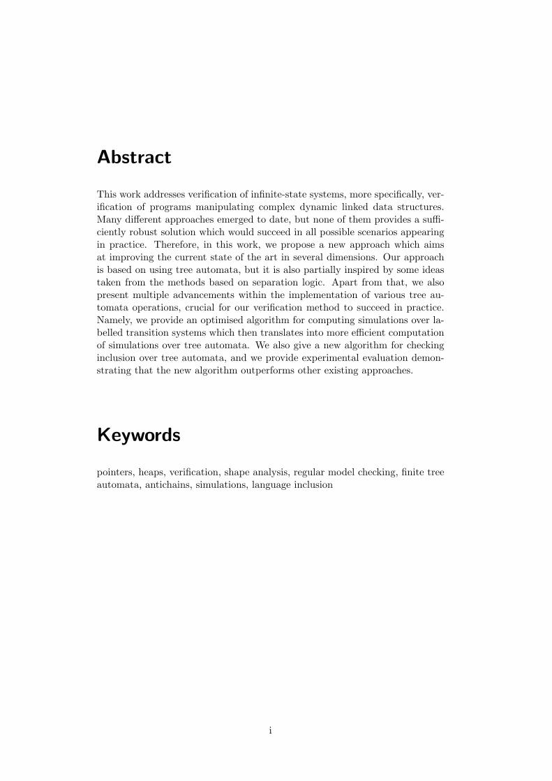
This work addresses verification of infinite-state systems, more specifically, ver-ification of programs manipulating complex dynamic linked data structures.Many different approaches emerged to date, but none of them provides a suffi-ciently robust solution which would succeed in all possible scenarios appearingin practice. Therefore, in this work, we propose a new approach which aimsat improving the current state of the art in several dimensions. Our approachis based on using tree automata, but it is also partially inspired by some ideastaken from the methods based on separation logic. Apart from that, we alsopresent multiple advancements within the implementation of various tree au-tomata operations, crucial for our verification method to succeed in practice.Namely, we provide an optimised algorithm for computing simulations over la-belled transition systems which then translates into more efficient computationof simulations over tree automata. We also give a new algorithm for checkinginclusion over tree automata, and we provide experimental evaluation demon-strating that the new algorithm outperforms other existing approaches.

Keywords

pointers, heaps, verification, shape analysis, regular model checking, finite treeautomata, antichains, simulations, language inclusion

i

Abstrakt

Tato prace se zabyva verifikacı nekonecne stavovych systemu, konkretne, ve-rifikacı programu vyuzıvajıch slozite dynamicky propojovane datove struktury.V minulosti se k resenı tohoto problemu objevilo mnoho ruznych prıstupu,avsak zadny z nich doposud nebyl natolik robustnı, aby fungoval ve vsech prı-padech, se kterymi se lze v praxi setkat. Ve snaze poskytnout vyssı urovenautomatizace a soucasne umoznit verifikaci programu se slozitejsımi datovymistrukturami v teto praci navrhujeme novy prıstup, ktery je zalozen zejmenana pouzitı stromovych automatu, ale je take castecne inspirovan nekterymimyslenkami, ktere jsou prevzaty z metod zalozenych na separacnı logice. Mimoto take predstavujeme nekolik vylepsenı v oblasti implementace operacı nadstromovymi automaty, ktere jsou klıcove pro praktickou vyuzitelnost navrho-vane verifikacnı metody. Konkretne uvadıme optimalizovany algoritmus provypocet simulacı pro prechodovy system s navestımi, pomocı ktereho lze efek-tivneji pocıtat simulace pro stromove automaty. Dale uvadıme novy algorit-mus pro testovanı inkluze stromovych automatu spolecne s experimenty, ktereukazujı, ze tento algoritmus prekonava jine existujıcı prıstupy.

ii

Resume

Les travaux decrits dans cette these portent sur le probleme de verification dessystemes avec espaces d’etats infinis, et, en particulier, avec des structures dedonnees chaınees. Plusieurs approches ont emerge, sans donner des solutionsconvenables et robustes, qui pourrait faire face aux situations rencontrees dansla pratique. Nos travaux proposent une approche nouvelle, qui combine lesavantages de deux approches tres prometteuses: la representation symboliquea base d’automates d’arbre, et la logique de separation. On presente egalementplusieurs ameliorations concernant l’implementation de differentes operationssur les automates d’arbre, requises pour le succes pratique de notre methode.En particulier, on propose un algorithme optimise pour le calcul des simulationssur les systemes de transitions etiquettes, qui se traduit dans un algorithmeefficace pour le calcul des simulations sur les automates d’arbre. En outre, onpresente un nouvel algorithme pour le probleme d’inclusion sur les automatesd’arbre. Un nombre important d’experimentes montre que cet algorithme estplus efficace que certaines des methodes existantes.

iii

Acknowledgements

I am deeply grateful to both of my supervisors Tomas Vojnar and Radu Iosif fortheir great guidance and help without which a successful completion of this workwould not be possible. I would also like to thank other coauthors, namely PeterHabermehl, Lukas Holık, Ondrej Lengal, and Adam Rogalewicz for their greatcooperation during our common research. Furthermore, I would like to thankLukas Holık and especially Tomas Vojnar once more for providing valuablecomments regarding this text. Also, I want to thank Kamil Dudka for creatinga plugin infrastructure which simplified the development of the verification toolpresented in this thesis. Finally, I am also grateful to my parents and the restof my family for the moral support that they always provided.

The work presented in this thesis was supported by the Czech Ministry of Edu-cation (project COST OC10009, Czech-French Barrande project MEB021023,the long-term institutional project MSM0021630528), the Czech Science Foun-dation (projects P103/10/0306, 102/09/H042, 201/09/P531), the EU/CzechIT4Innovations Centre of Excellence (project ED1.1.00/02.0070), the EuropeanScience Foundation (ESF COST action IC0901), the French National ResearchAgency (project ANR-09-SEGI-016 VERIDYC), and the Brno University ofTechnology (projects FIT-S-10-1, FIT-S-11-1, FIT-S-12-1).

iv

Contents

1 Introduction 11.1 Goals of the Work . . . . . . . . . . . . . . . . . . . . . . . . . . 21.2 An Overview of the Achieved Results . . . . . . . . . . . . . . . . 31.3 Plan of the Thesis . . . . . . . . . . . . . . . . . . . . . . . . . . 6

2 Preliminaries 72.1 Labelled Transition Systems . . . . . . . . . . . . . . . . . . . . . 72.2 Alphabets and Trees . . . . . . . . . . . . . . . . . . . . . . . . . 72.3 Tree Automata . . . . . . . . . . . . . . . . . . . . . . . . . . . . 72.4 Simulations over Tree Automata . . . . . . . . . . . . . . . . . . 82.5 Regular Tree Model Checking . . . . . . . . . . . . . . . . . . . . 8

3 Forest Automata 113.1 From Heaps to Forests . . . . . . . . . . . . . . . . . . . . . . . . 113.2 Hypergraphs and Their Representation . . . . . . . . . . . . . . . 14

3.2.1 Hypergraphs . . . . . . . . . . . . . . . . . . . . . . . . . 153.2.2 Forest Representation of Hypergraphs . . . . . . . . . . . 153.2.3 Minimal and Canonical Forests . . . . . . . . . . . . . . . 163.2.4 Root Interconnection Graphs . . . . . . . . . . . . . . . . 173.2.5 Manipulating the Forest Representation . . . . . . . . . . 17

3.3 Forest Automata . . . . . . . . . . . . . . . . . . . . . . . . . . . 183.3.1 Uniform and Canonicity Respecting FA . . . . . . . . . . 193.3.2 Transforming FA into Canonicity Respecting FA . . . . . 203.3.3 Sets of FA . . . . . . . . . . . . . . . . . . . . . . . . . . . 223.3.4 Testing Inclusion on Sets of FA . . . . . . . . . . . . . . . 23

3.4 Hierarchical Hypergraphs . . . . . . . . . . . . . . . . . . . . . . 233.4.1 Hierarchical Hypergraphs, Components, and Boxes . . . . 243.4.2 Semantics of Hierarchical Hypergraphs . . . . . . . . . . . 24

3.5 Hierarchical Forest Automata . . . . . . . . . . . . . . . . . . . . 253.5.1 On Well-Connectedness of Hierarchical FA . . . . . . . . 263.5.2 Properness and Box-Connectedness . . . . . . . . . . . . . 273.5.3 Checking Properness and Well-Connectedness . . . . . . . 273.5.4 On Inclusion of Hierarchical FA . . . . . . . . . . . . . . . 293.5.5 Canonicity Respecting Hierarchical FA . . . . . . . . . . . 303.5.6 Precise Inclusion on Hierarchical FA . . . . . . . . . . . . 313.5.7 Transforming Hierarchical FA into Canonicity Respecting

Hierarchical FA . . . . . . . . . . . . . . . . . . . . . . . . 323.6 Conclusions and Future Work . . . . . . . . . . . . . . . . . . . . 36

v

4 Forest Automata-based Verification 374.1 Symbolic Execution . . . . . . . . . . . . . . . . . . . . . . . . . 39

4.1.1 Executing C Statements on Hypergraphs . . . . . . . . . 394.1.2 Executing C Statements on FA . . . . . . . . . . . . . . . 404.1.3 Introduction of Auxiliary Roots . . . . . . . . . . . . . . . 434.1.4 Restricted Pointer Arithmetic . . . . . . . . . . . . . . . . 44

4.2 The Main Verification Loop . . . . . . . . . . . . . . . . . . . . . 464.3 Folding of Nested Forest Automata . . . . . . . . . . . . . . . . . 48

4.3.1 Cut-point Types . . . . . . . . . . . . . . . . . . . . . . . 494.3.2 Component Slicing . . . . . . . . . . . . . . . . . . . . . . 514.3.3 Cut-point Elimination . . . . . . . . . . . . . . . . . . . . 534.3.4 From Nested FA to Alphabet Symbols . . . . . . . . . . . 56

4.4 Abstraction . . . . . . . . . . . . . . . . . . . . . . . . . . . . . . 564.4.1 Automata Quotienting . . . . . . . . . . . . . . . . . . . . 574.4.2 Equivalence of Languages of Bounded Height . . . . . . . 574.4.3 Canonicity Preserving Equivalence . . . . . . . . . . . . . 594.4.4 Refined Canonicity Preserving Equivalence . . . . . . . . 604.4.5 Abstraction for Sets of FA . . . . . . . . . . . . . . . . . . 62

4.5 Towards Abstraction Refinement . . . . . . . . . . . . . . . . . . 644.5.1 Symbolic Execution Revisited . . . . . . . . . . . . . . . . 654.5.2 Backward Symbolic Execution . . . . . . . . . . . . . . . 66

4.6 Experimental Evaluation . . . . . . . . . . . . . . . . . . . . . . . 674.6.1 Comparison to Existing Tools . . . . . . . . . . . . . . . . 684.6.2 Folding of Nested FA . . . . . . . . . . . . . . . . . . . . . 694.6.3 Abstraction . . . . . . . . . . . . . . . . . . . . . . . . . . 704.6.4 Additional Experiments . . . . . . . . . . . . . . . . . . . 71

4.7 Related Work . . . . . . . . . . . . . . . . . . . . . . . . . . . . . 744.8 Conclusions and Future Work . . . . . . . . . . . . . . . . . . . . 75

5 Simulations over LTSs and Tree Automata 775.1 Preliminaries . . . . . . . . . . . . . . . . . . . . . . . . . . . . . 785.2 The Original LRT Algorithm . . . . . . . . . . . . . . . . . . . . 795.3 Optimisations of LRT . . . . . . . . . . . . . . . . . . . . . . . . 79

5.3.1 Data Structures . . . . . . . . . . . . . . . . . . . . . . . . 825.3.2 Complexity of Optimised LRT . . . . . . . . . . . . . . . 82

5.4 Tree Automata Simulations . . . . . . . . . . . . . . . . . . . . . 855.4.1 Complexity of Computing Simulations over TA . . . . . . 86

5.5 Experimental Results . . . . . . . . . . . . . . . . . . . . . . . . . 885.6 Conclusions and Future Work . . . . . . . . . . . . . . . . . . . . 90

6 Efficient Inclusion over Tree Automata 916.1 Downward Inclusion Checking . . . . . . . . . . . . . . . . . . . . 93

6.1.1 Basic Algorithm . . . . . . . . . . . . . . . . . . . . . . . 976.1.2 Antichains and Simulation . . . . . . . . . . . . . . . . . . 986.1.3 Caching Positive Pairs . . . . . . . . . . . . . . . . . . . . 100

6.2 Experimental Results . . . . . . . . . . . . . . . . . . . . . . . . . 1026.2.1 Explicit Encoding . . . . . . . . . . . . . . . . . . . . . . 102

vi

6.2.2 Semi-symbolic Encoding . . . . . . . . . . . . . . . . . . . 1046.3 Conclusions and Future Work . . . . . . . . . . . . . . . . . . . . 105

7 A Tree Automata Library 1067.1 Design of the Library . . . . . . . . . . . . . . . . . . . . . . . . . 107

7.1.1 Explicit Encoding . . . . . . . . . . . . . . . . . . . . . . 1087.1.2 Semi-Symbolic Encoding . . . . . . . . . . . . . . . . . . . 109

7.2 Supported Operations . . . . . . . . . . . . . . . . . . . . . . . . 1117.2.1 Downward and Upward Simulation . . . . . . . . . . . . . 1117.2.2 Simulation-based Size Reduction . . . . . . . . . . . . . . 1117.2.3 Bottom-up Inclusion . . . . . . . . . . . . . . . . . . . . . 1127.2.4 Top-down Inclusion . . . . . . . . . . . . . . . . . . . . . 1147.2.5 Computing Simulation over LTS . . . . . . . . . . . . . . 115

7.3 Experimental Evaluation . . . . . . . . . . . . . . . . . . . . . . . 1167.3.1 Explicit Encoding . . . . . . . . . . . . . . . . . . . . . . 1177.3.2 Semi-Symbolic Encoding . . . . . . . . . . . . . . . . . . . 117

7.4 Conclusions and Future Work . . . . . . . . . . . . . . . . . . . . 118

8 Conclusions and Future Directions 1198.1 A Summary of the Contributions . . . . . . . . . . . . . . . . . . 1198.2 Further Directions . . . . . . . . . . . . . . . . . . . . . . . . . . 1208.3 Publications and Tools Related to this Work . . . . . . . . . . . 121

References 123

vii

1 Introduction

Traditional approaches for ensuring quality of computer systems such as codereview or testing are nowadays reaching their inherent limitations due to thegrowing complexity of the current computer systems. That is why, there is anincreasing demand for more capable techniques. One of the ways how to dealwith this situation is to use suitable formal verification approaches.

In case of software, one especially critical area is that of ensuring safe mem-ory usage in programs using dynamic memory allocation. The development ofsuch programs is quite complicated, and many programming errors can easilyarise here. Worse yet, the bugs within memory manipulation often cause anunpredictable behaviour, and they are often very hard to find. Indeed, despitethe use of testing and other traditional means of quality assurance, many of thememory errors make it into the production versions of programs causing themto crash unexpectedly by breaking memory protection or to gradually wastemore and more memory (if the error causes memory leaks). Consequently,using formal verification is highly desirable in this area.Formal verification of programs with dynamically linked data structures is,

however, very demanding since these programs are infinite-state. One of themost promising ways of dealing with infinite state verification is to use symbolicverification in which infinite sets of reachable configurations are representedfinitely using a suitable formalism. In case of programs with dynamically linkeddata structures, the use of symbolic verification is complicated by the factthat their configurations are graphs, and representing infinite sets of graphs isparticularly complicated (compared to objects like words or trees).Many different verification approaches for programs manipulating dynami-

cally linked data structures have emerged so far. Some of them are based onlogics [MS01, SRW02, Rey02, BCC+07, GVA07, NDQC07, CRN07, ZKR08,YLB+08, CDOY09, MPQ11, DPV11], others are based on using automata[BHRV06b, BBH+11, DEG06], upward closed sets [ABC+08, ACV11], as wellas other formalisms. The approaches differ in their generality, efficiency, anddegree of automation. Among the fully automatic ones, the works [BCC+07,YLB+08] present an approach based on separation logic (see [Rey02]) that isquite scalable due to using local reasoning. However, their method is limitedto programs manipulating various kinds of lists. There are other works basedon separation logic which also consider trees or even more complex data struc-tures, but they either expect the input program to be in some special form (e.g.,[GVA07]) or they require some additional information about the data structureswhich are involved (as in [NDQC07, MTLT10]). Similarly, even the other exist-ing approaches that are not based on separation logic often suffer from the needof non-trivial user aid in order to successfully finish the verification task (see,e.g., [MS01, SRW02]). On the other hand, the work [BHRV06b] proposed an

1

automata-based method which is able to handle fully automatically quite com-plex data structures, but it suffers from several drawbacks such as a monolithicrepresentation of memory configurations which does not allow this approach toscale well.Another issue with many existing automata-based approaches for symbolic

verification of infinite-state systems (such as programs with dynamically linkeddata structures) is that they are based on using deterministic finite automata(DFA). This allows them to take advantage of the relatively simple and well-established algorithms for computing standard operations such as languageunion, language inclusion, minimisation, complementation, etc. However, someof these operations internally produce nondeterministic finite automata whichthen need to be immediately determinised. This is not difficult in theory, butin practice, the size of the automata for which the operation can be computedis very limited as the size of the corresponding deterministic automata can beexponential in the size of the original nondeterministic ones. As a result, veri-fication methods based on using DFA do not perform that well when they areforced to work with automata of bigger size.A use of nondeterministic finite automata (NFA) was proposed in [BHH+08]

in an effort to address the issues of scalability of symbolic automata-basedverification methods. Despite the fact that this approach cannot improve thetheoretical worst-case complexity, it turns out that the use of nondeterminis-tic automata can greatly improve the scalability of automata-based verificationapproaches in practice. However, in order to be able to efficiently use NFA inthe given context, one needs to have available suitable algorithms for certaincritical automata operations that will perform these operations without neces-sarily determinising the automata. This is in particular the case of languageinclusion, minimisation (or, more precisely, size reduction), and complementa-tion (if needed). Some of these algorithms have already been proposed (e.g.,[DWDHR06, BHH+08] use antichains to deal with the problem of languageinclusion), but there remained a significant space for improvement. In particu-lar, within the algorithms for language inclusion presented in [ACH+10, DR10](which further optimise the work of [DWDHR06, BHH+08]) and size reductionpresented in [ABH+08], one has to compute the maximal simulation relationover the set of states of an automaton. It turns out that the computation ofthe simulation relation often takes the majority of the time, especially in thecase of size reduction. Hence, efficient techniques for computing simulationsare needed. Moreover, the technique of [ACH+10] for antichain-based inclusionchecking of TA uses upward simulations which are especially costly to com-pute and often very sparse. Hence, there is also a need of still better inclusionchecking on NTA.

1.1 Goals of the Work

Above, we have argued that development of programs with dynamically linkeddata structures is difficult, error-prone, and the errors arising in this kind ofprograms are difficult to discover using traditional approaches for quality as-

2

surance. Hence, there is a strong need for formal verification approaches in thisarea. However, most of the existing formal verification techniques for programswith dynamically linked data structures are either not fully automatic, or theycan handle only a limited class of data structures. On the other hand, thosetechniques that can automatically handle complex data structures are usuallycomputationally very expensive. Therefore, our first goal is to develop an effi-cient and fully automatic approach for verification of this kind of programs. Thenew approach is intended to be able to verify programs manipulating more com-plex data structures than those that can be efficiently handled by existing fullyautomatic methods. We, in particular, focus on combining automata-based ap-proaches (which are rather general and which come with flexible and refinableabstraction) with some principles taken from the quite scalable methods basedon separation logic, which is especially the case of local reasoning.The second goal is to further improve the available algorithms implementing

the operations that one needs to perform over nondeterministic automata whenusing them in some method for symbolic verification of infinite-state systemssuch as the one proposed within the first goal. Concretely, our aim is to improvealgorithms for inclusion checking by considering the so-far neglected top-downapproach and to improve automata reduction by providing a better algorithmfor computing simulations.

1.2 An Overview of the Achieved Results

In this section, we summarise the contributions that we have achieved withinthe particular areas marked out by the goals of the work.

Verification of Heap Manipulating Programs. We propose a novel methodfor symbolic verification of heap manipulating programs. The main idea of ourapproach is the following. We represent heap graphs via their canonical treedecomposition. This can be done thanks to the observation that every heapgraph can be decomposed into a set of tree components when the leaves of thetree components are allowed to refer back to the roots of these components.Moreover, given a total ordering on program variables and pointer links (calledselectors), each heap graph may be decomposed into a tuple of tree componentsin a canonical way. In particular, one can first identify the so-called cut-points,i.e., nodes that are either pointed to by a program variable or that have sev-eral incoming edges. Next, the cut-points can be canonically numbered usinga depth-first traversal of the heap graph starting from nodes pointed to by pro-gram variables in the order derived from the order of the program variables andrespecting the order of selectors. Subsequently, one can split the heap graphinto tree components rooted at the particular cut-points. These componentsshould contain all the nodes reachable from their root while not passing throughany cut-point, plus a copy of each reachable cut-point, labelled by its number.Finally, the tree components can then be canonically ordered according to thenumbers of the cut-points representing their roots.

3

We introduce a new formalism of forest automata upon the described de-composition of heaps into tree components in order to be able to efficientlyrepresent sets of such decompositions (and hence sets of heaps). In particular,a forest automaton (FA) is basically a tuple of tree automata. Each of the treeautomata within the tuple accepts trees whose leaves may refer back to theroots of any of these trees. A forest automaton then represents exactly the setof heaps that may be obtained by taking a single tree from the language of eachof the component tree automata and by gluing the roots of the trees with theleaves referring to them.Further, we show that FA enjoy some nice properties, which are crucial for

our verification approach. In particular, we show that relevant C statements canbe easily symbolically executed over forest automata. Moreover, one can im-plement efficient abstraction on FA as well as decide language inclusion (whichis needed for fixpoint checking) The latter can in particular be implementedby an easy reduction to the well-known problem of language inclusion of treeautomata.Next, in order to extend the class of graphs that can be handled in our

framework, we extend FA to hierarchically nested FA by allowing their alpha-bet symbols to encode sets of subgraphs instead of plain hyperedges. Thesesets of subgraphs are again represented using hierarchically nested FA. For thehierarchical FA, we do not obtain the same nice theoretical properties, but weat least show that the needed operations (such as language inclusion checking)can be sufficiently precisely approximated (building on the results for plain FA).In our symbolic verification approach, a symbolic state is thus composed of

a finite number of program variable assignments, a forest automaton which isable to represent infinitely many heaps, and a program counter specifying whichinstruction of the verified code is to be executed in the next step. We haveimplemented the approach in a tool called Forester in order to experimentallyevaluate our method. The results show that the tool is very competitive whencompared to other existing tools for verification of dynamic data structureswhile being quite general and fully automatic.

Simulations over Labelled Transition Systems and Tree Automata. We ad-dress the problem of computing simulations over a labelled transition sys-tem (LTS) by designing an optimised version of the algorithm proposed in[ABH+08, AHKV08] (which is itself based on the algorithms for Kripke struc-tures from [HHK95, RT07]). Our optimisation is based on the observation thatin practice, we often work with LTSs in which transitions leading from particu-lar states are labelled by some subset of all alphabet symbols only. By a carefulanalysis of the original algorithm, we have identified that one can exploit thisirregular use of alphabet symbols in order to improve the performance of thecomputation.In particular, for two states p and q within an LTS, p can simulate q only if

for any transition leading from q labelled by some symbol a, there is a transitionleading from p labelled by a. Using this fact, we refine the initial estimationof the simulation relation within the first phase of the algorithm introduced in

4

[AHKV08], and we show that, thanks to the initial refinement, certain iterationsof the algorithm can be skipped without affecting its output. Furthermore, weshow that certain parts of the data structures used by the original algorithm areno longer needed when our optimisation is used. Hence, we obtain a reductionof the space requirements, too. For our optimised algorithm, we also derive itsworst-case time and space complexity.As shown in [AHKV08], simulations over tree automata can be efficiently

computed via a translation into LTSs. Therefore, we also derive the complexityof computing simulations over tree automata when our optimised algorithmis applied on LTSs produced during the translation. In this case, we achievea promising reduction of the asymptotic complexity. Moreover, we validatethe theoretical results by an experimental evaluation demonstrating significantsavings in terms of space as well as time on both LTSs and tree automata.

Language Inclusion Checking for Tree Automata. For the purposes of ourverification technique for programs manipulating dynamically linked data struc-tures, we also investigate new efficient methods for checking language inclusionon nondeterministic tree automata. Originally, we intended to build upon thebottom-up inclusion checking introduced in [ACH+10] which is based on com-bining antichains with upward simulation. However, during our experiments,we have realised that the particular combination does not yield the expectedimprovements in the efficiency of inclusion checking because the computationof upward simulation is often too costly. In reaction to this issue, we have de-signed a new top-down inclusion checking algorithm which is of a similar spiritas the one in [HVP05], but it is not limited to binary trees, and it is optimisedin several crucial ways as described below.Unlike the bottom-up approach which starts in the leaves and proceeds to-

wards the roots, the top-down inclusion starts in roots (represented via ac-cepting states) and continues towards the leaves. The approach is based ongenerating pairs in which the first component corresponds to a state of the firstautomaton, and the second component contains a set of states of the secondautomaton. During the computation, the algorithm maintains a set of thosepairs for which the inclusion has been shown not to hold. A fundamental prob-lem of this method is the fact that the number of successor pairs one needs toexplore grows exponentially with the level of the (top-down) nondeterminismof tree automata. Due to this, the construction may blow up and run out ofthe available time on certain automata pairs. We, however, show that it isoften possible to work around this issue by using the principle of antichains[DWDHR06]. Moreover, we further improve the approach by combining it witha use of downward simulation which greatly reduces the risk of the blow-up.Finally, we also present a sophisticated modification of the algorithm whichallows us to remember and to exploit the pairs for which the inclusion holds(apart from those in which it does not).We have implemented explicit and semi-symbolic variants of the various,

above mentioned language inclusion algorithms. Our experiments with thebottom-up and the top-down approaches for checking language inclusion of

5

tree automata show that the top-down inclusion checking dominates in most ofour benchmarks.

An Efficient Library for Dealing with NTA. The proposed algorithms for inclu-sion checking and simulation computation have been incorporated into a newlydesigned library (called VATA) for dealing with NTA, together with some fur-ther operations such as simulation-based reduction, union, intersection, etc.Various lower-level optimisations of the basic algorithms have been proposedwithin the implementation of the library to make it as efficient as possible. This,in particular, includes various improvements of the bottom up inclusion check-ing of [ACH+10] which make it more efficient in practice. Another significantimprovement introduced in the implementation of VATA is a substantial refine-ment of the internal representation of the data structures used in the algorithmfor computing simulations which further reduce its memory footprint.

1.3 Plan of the Thesis

Chapter 2 contains preliminaries on labelled transition systems, tree automata,and simulations. Chapter 3 proposes the notion of forest automata which servesas a theoretical basis for our verification technique for programs manipulatingdynamically linked data structures. In Chapter 4, we provide a detailed de-scription of the verification procedure as well as the experimental evaluation ofour prototype tool Forester based on it. Our optimised algorithm for comput-ing simulations on LTSs is presented in Chapter 5. Chapter 6 describes severalvariants of top-down inclusion checking algorithms. Essentials of our tree au-tomata library based on the proposed algorithms are discussed in Chapter 7,including various lower-level optimisations of the implementation of the algo-rithms discussed in Chapter 5 and Chapter 6. Finally, Chapter 8 concludes thethesis.

6

2 Preliminaries

In this chapter, we introduce preliminaries on labelled transition systems, al-phabets, trees, tree automata, and simulations that we build on in this work.

2.1 Labelled Transition Systems

A labeled transition system (LTS) is a tuple T = (S,Σ, {δa | a ∈ Σ}), where Sis a finite set of states, Σ is a finite set of labels, and for each a ∈ Σ, δa ⊆ S × Sis an a-labeled transition relation. We use δ to denote

⋃

a∈Σ δa.

2.2 Alphabets and Trees

A ranked alphabet Σ is a set of symbols together with a ranking function # :Σ → N. For a ∈ Σ, the value #a is called the rank of a. For any n ≥ 0, wedenote by Σn the set of all symbols of rank n from Σ. Let ε denote the emptysequence. A tree t over a ranked alphabet Σ is a partial mapping t : N∗ → Σ

that satisfies the following conditions: (1) dom(t) is a finite prefix-closed subsetof N∗ and (2) for each v ∈ dom(t), if #t(v) = n ≥ 0, then {i | vi ∈ dom(t)} ={1, . . . , n}. Each sequence v ∈ dom(t) is called a node of t. For a node v, wedefine the ith child of v to be the node vi, and the ith subtree of v to be thetree t′ such that t′(v′) = t(viv′) for all v′ ∈ N

∗. A leaf of t is a node v whichdoes not have any children, i.e., there is no i ∈ N with vi ∈ dom(t). We denoteby TΣ the set of all trees over the alphabet Σ.

2.3 Tree Automata

A (finite, non-deterministic) tree automaton (abbreviated sometimes as TA inthe following) is a quadruple A = (Q,Σ,∆, F) where Q is a finite set of states,F ⊆ Q is a set of final states, Σ is a ranked alphabet, and ∆ is a set of transi-tion rules. Each transition rule is a triple of the form ((q1, . . . , qn), a, q) whereq1, . . . , qn, q ∈ Q, a ∈ Σ, and #a = n. We use equivalently (q1, . . . , qn)

a−→ q

and qa−→ (q1, . . . , qn) to denote that ((q1, . . . , qn), a, q) ∈ ∆. The two notations

correspond to the bottom-up and top-down representation of tree automata,respectively. (Note that we can afford to work interchangeably with both ofthem since we work with non-deterministic tree automata, which are known tohave an equal expressive power in their bottom-up and top-down representa-tions.) In the special case when n = 0, we speak about the so-called leaf rules,which we sometimes abbreviate as

a−→ q or q

a−→.

For an automaton A = (Q,Σ,∆, F), we use Q# to denote the set of alltuples of states from Q with up to the maximum arity that some symbol in

7

Σ has, i.e., if r = maxa∈Σ #a, then Q# =⋃

0≤i≤r Qi. For p ∈ Q and a ∈

Σ, we use downa(p) to denote the set of tuples accessible from p over a inthe top-down manner; formally, downa(p) = {(p1, . . . , pn) | p

a−→ (p1, . . . , pn)}.

For a ∈ Σ and (p1, . . . , pn) ∈ Q#a, we denote by upa((p1, . . . , pn)) the set ofstates accessible from (p1, . . . , pn) over the symbol a in the bottom-up manner;formally, upa((p1, . . . , pn)) = {p | (p1, . . . , pn)

a−→ p}. We also extend these

notions to sets in the usual way, i.e., for a ∈ Σ, P ⊆ Q, and R ⊆ Q#a,downa(P ) =

⋃

p∈P downa(p) and upa(R) =⋃

(p1,...,pn)∈Rupa((p1, . . . , pn)).

Let A = (Q,Σ,∆, F) be a TA. A run of A over a tree t ∈ TΣ is a mappingπ : dom(t) → Q such that, for each node v ∈ dom(t) of rank #t(v) = n where

q = π(v), if qi = π(vi) for 1 ≤ i ≤ n, then ∆ has a rule (q1, . . . , qn)t(v)−−→ q.

We write tπ

=⇒ q to denote that π is a run of A over t such that π(ε) = q. Weuse t =⇒ q to denote that t

π=⇒ q for some run π. The language accepted by

a state q is defined by LA(q) = {t | t =⇒ q}, while the language of a set ofstates S ⊆ Q is defined as LA(S) =

⋃

q∈S LA(q). When it is clear which TAA we refer to, we only write L(q) or L(S). The language of A is defined asL(A) = LA(F ). We also extend the notion of a language to a tuple of states(q1, . . . , qn) ∈ Qn by letting L((q1, . . . , qn)) = L(q1)×· · ·×L(qn). The languageof a set of n-tuples of sets of states S ⊆ (2Q)

nis the union of languages of

elements of S, the set L(S) =⋃

E∈S L(E). We say that X accepts y to expressthat y ∈ L(X).

2.4 Simulations over Tree Automata

A downward simulation on TA A = (Q,Σ,∆, F) is a preorder relation (D⊆Q×Q such that if q (D p and (q1, . . . , qn)

a−→ q, then there are states p1, . . . , pn

such that (p1, . . . , pn)a−→ p and qi (D pi for each 1 ≤ i ≤ n. Given a TA

A = (Q,Σ,∆, F) and a downward simulation (D, an upward simulation (U⊆Q×Q induced by (D is a relation such that if q (U p and (q1, . . . , qn)

a−→ q′ with

qi = q, 1 ≤ i ≤ n, then there are states p1, . . . , pn, p′ such that (p1, . . . , pn)

a−→ p′

where pi = p, q′ (U p′, and qj (D pj for each j such that 1 ≤ j )= i ≤ n.Given two sets S, Q such that S ⊆ Q and a preorder (⊆ Q × Q, then S%

denotes the set {q ∈ S : ) ∃q′ ∈ S.q ( q′}.

2.5 Regular Tree Model Checking

(This section is borrowed from [Hol11] with the kind permission of the author.)

Regular tree model checking (RTMC) [Sha01, BT02, ALdR05, BHV04] isa general and uniform framework for verifying infinite-state systems. In RTMC,configurations of a system being verified are encoded by trees, sets of the con-figurations by tree automata, and transitions of the verified system by a termrewriting system (usually given as a tree transducer or a set of tree trans-ducers). Then, verification problems based on performing reachability analysiscorrespond to computing closures of regular languages under rewriting systems,i.e., given a term rewriting system τ and a regular tree language I, one needs

8

to compute τ∗(I) where τ∗ is the reflexive-transitive closure of τ . This com-putation is impossible in general. Therefore, the main issue in RTMC is tofind accurate and powerful fixpoint acceleration techniques helping the conver-gence of computing language closures. One of the most successful accelerationtechniques used in RTMC is abstraction whose use leads to the so-called ab-stract regular tree model checking (ARTMC) [BHRV06a, BHRV06b], on whichwe concentrate in this work.

Abstract Regular Tree Model Checking. We briefly recall the basic principlesof ARTMC in the way they were introduced in [BHRV06b]. Let Σ be a rankedalphabet and MΣ the set of all tree automata over Σ. Let I ∈ MΣ be a treeautomaton describing a set of initial configurations, τ a term rewriting systemdescribing the behaviour of a system, and B ∈ MΣ a tree automaton describ-ing a set of bad configurations. The safety verification problem can now beformulated as checking whether the following holds:

τ∗(L(I)) ∩ L(B) = ∅ (2.1)

In ARTMC, the precise set of reachable configurations τ∗(L(I)) is not computedto solve Problem (2.1). Instead, its overapproximation is computed by interleav-ing the application of τ and the union in L(I)∪ τ(L(I))∪ τ(τ(L(I)))∪ . . . withan application of an abstraction function α. The abstraction is applied on thetree automata encoding the so-far computed sets of reachable configurations.

An abstraction function is defined as a mapping α : MΣ → AΣ where AΣ ⊆MΣ and ∀A ∈ MΣ : L(A) ⊆ L(α(A)). An abstraction α′ is called a refinementof the abstraction α if ∀A ∈ MΣ : L(α′(A)) ⊆ L(α(A)). Given a term rewritingsystem τ and an abstraction α, a mapping τα : MΣ → MΣ is defined as ∀A ∈MΣ : τα(A) = τ(α(A)) where τ(A) is the minimal deterministic automatondescribing the language τ(L(A)). An abstraction α is finitary, if the set AΣ isfinite.For a given abstraction function α, one can compute iteratively the sequence

of automata (τ iα(I))i≥0. If the abstraction α is finitary, then there exists k ≥ 0such that τk+1

α (I) = τkα(I). The definition of the abstraction function α impliesthat L(τkα(I)) ⊇ τ∗(L(I)).

If L(τkα(I)) ∩ L(B) = ∅, then Problem (2.1) has a positive answer. If theintersection is non-empty, one must check whether a real or a spurious coun-terexample has been encountered. The spurious counterexample may be causedby the used abstraction (the counterexample is not reachable from the set ofinitial configurations). Assume that L(τkα(I)) ∩ L(B) )= ∅, which means thatthere is a symbolic path:

I, τα(I), τ2α(I), . . . , τ

n−1α (I), τnα (I) (2.2)

such that L(τnα (I)) ∩ L(B) )= ∅.Let Xn = L(τnα (I)) ∩ L(B). Now, for each l, 0 ≤ l < n, Xl = L(τ lα(I)) ∩

τ−1(Xl+1) is computed. Two possibilities may occur: (a) X0 )= ∅, which meansthat Problem (2.1) has a negative answer, and X0 ⊆ L(I) is a set of dangerousinitial configurations. (b) ∃m, 0 ≤ m < n,Xm+1 )= ∅ ∧ Xm = ∅ meaning

9

that the abstraction function is too rough—one needs to refine it and start theverification process again.In [BHRV06b], two general-purpose kinds of abstractions are proposed. Both

are based on automata state equivalences. Tree automata states are split intoseveral equivalence classes, and all states from one class are collapsed into onestate. An abstraction becomes finitary if the number of equivalence classesis finite. The refinement is done by refining the equivalence classes. Both ofthe proposed abstractions allow for an automatic refinement to exclude theencountered spurious counterexample.The first proposed abstraction is an abstraction based on languages of trees of

a finite height. It defines two states equivalent if their languages up to the givenheight n are equivalent. There is just a finite number of languages of heightn, therefore this abstraction is finitary. A refinement is done by an increaseof the height n. The second proposed abstraction is an abstraction based onpredicate languages. Let P = {P1, P2, . . . , Pn} be a set of predicates. Eachpredicate P ∈ P is a tree language represented by a tree automaton. Let A =(Q,Σ, F, q0, δ) be a tree automaton. Then, two states q1, q2 ∈ Q are equivalentif the languages L(Aq1) and L(Aq2) have a nonempty intersection with exactlythe same subset of predicates from the set P provided that Aq1 = (Q,Σ, F, q1, δ)and Aq2 = (Q,Σ, F, q2, δ). Since there is just a finite number of subsets of P,the abstraction is finitary. A refinement is done by adding new predicates, i.e.tree automata corresponding to the languages of all the states in the automatonof Xm+1 from the analysis of spurious counterexample (Xm = ∅).

10

3 Forest Automata

In this chapter, we introduce forest automata which is a new formalism forrepresenting sets of graphs. Our main motivation for creating this formalismhas been verification of programs manipulating dynamically linked data struc-tures. For this reason, in Section 3.1, we give an informal presentation of forestautomata in the context of heaps (which may be viewed as a special kind ofgraphs) instead of the context of plain graphs. The way heaps are representedby forests will then be presented in more detail in Section 4.1. In Section 3.2, weformally define the notion of hypergraphs and their representation using forests.In Section 3.3, we discuss the representation of sets of forests using forest au-tomata. Finally, Section 3.4 and Section 3.5 describe a hierarchical extensionsof hypergraphs and forest automata respectively.

3.1 From Heaps to Forests

Now, we outline in an informal way our proposal of hierarchical forest automataand the way how sets of heaps can be represented by them (the more precisedescription of the encoding will be given in Section 4.1). For the purpose of theexplanation, heaps may be viewed as oriented graphs whose nodes correspondto allocated memory cells and edges to pointer links between these cells. Thenodes may be labelled by non-pointer data stored in them (assumed to be froma finite data domain) and by program variables pointing to the nodes. Edgesmay be labelled by the corresponding selectors.In what follows, we restrict ourselves to garbage free heaps in which all mem-

ory cells are reachable from pointer variables by following pointer links. How-ever, this is not a restriction in practice since the emergence of garbage can bechecked for each executed program statement. If some garbage arises, an errormessage can be issued and the symbolic computation stopped. Alternatively,the garbage can be removed and the computation continued.It is easy to see that each heap graph can be decomposed into a set of tree

components when the leaves of the tree components are allowed to referenceback to the roots of these components. Moreover, given a total ordering onprogram variables and selectors, each heap graph may be decomposed intoa tuple of tree components in a canonical way as illustrated in Figure 3.1 (a)and (b). In particular, one can first identify the so-called cut-points, i.e., nodesthat are either pointed to by a program variable or that have several incomingedges. Next, the cut-points can be canonically numbered using a depth-firsttraversal of the heap graph starting from nodes pointed to by program variablesin the order derived from the order of the program variables and respectingthe order of selectors. Subsequently, one can split the heap graph into treecomponents rooted at particular cut-points. These components should contain

11

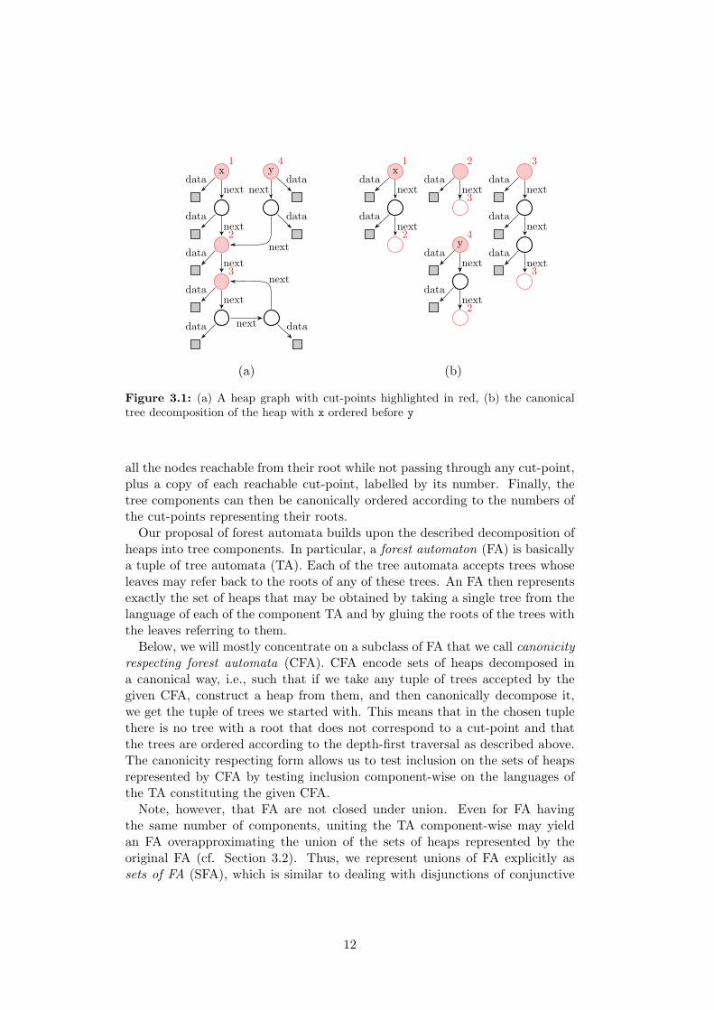
x1

2

3

y4

next

next

next

next

nextdata

data

data

data

data

data

data

datanext

next

next

x1

2

2

3

3

3

y4

2

next

next

next next

next

nextnext

next

data

data

data data

data

datadata

data

(a) (b)

Figure 3.1: (a) A heap graph with cut-points highlighted in red, (b) the canonicaltree decomposition of the heap with x ordered before y

all the nodes reachable from their root while not passing through any cut-point,plus a copy of each reachable cut-point, labelled by its number. Finally, thetree components can then be canonically ordered according to the numbers ofthe cut-points representing their roots.Our proposal of forest automata builds upon the described decomposition of

heaps into tree components. In particular, a forest automaton (FA) is basicallya tuple of tree automata (TA). Each of the tree automata accepts trees whoseleaves may refer back to the roots of any of these trees. An FA then representsexactly the set of heaps that may be obtained by taking a single tree from thelanguage of each of the component TA and by gluing the roots of the trees withthe leaves referring to them.Below, we will mostly concentrate on a subclass of FA that we call canonicity

respecting forest automata (CFA). CFA encode sets of heaps decomposed ina canonical way, i.e., such that if we take any tuple of trees accepted by thegiven CFA, construct a heap from them, and then canonically decompose it,we get the tuple of trees we started with. This means that in the chosen tuplethere is no tree with a root that does not correspond to a cut-point and thatthe trees are ordered according to the depth-first traversal as described above.The canonicity respecting form allows us to test inclusion on the sets of heapsrepresented by CFA by testing inclusion component-wise on the languages ofthe TA constituting the given CFA.Note, however, that FA are not closed under union. Even for FA having

the same number of components, uniting the TA component-wise may yieldan FA overapproximating the union of the sets of heaps represented by theoriginal FA (cf. Section 3.2). Thus, we represent unions of FA explicitly assets of FA (SFA), which is similar to dealing with disjunctions of conjunctive

12

next

prev

next

prev

next

prev

(a)

DLL DLL DLL

next

prev

(b)

Figure 3.2: (a) A part of a DLL, (b) a hierarchical encoding of the DLL

separation logic formulae. However, as we will see, inclusion on the sets of heapsrepresented by SFA is still easily decidable.The described encoding allows one to represent sets of heaps with a bounded

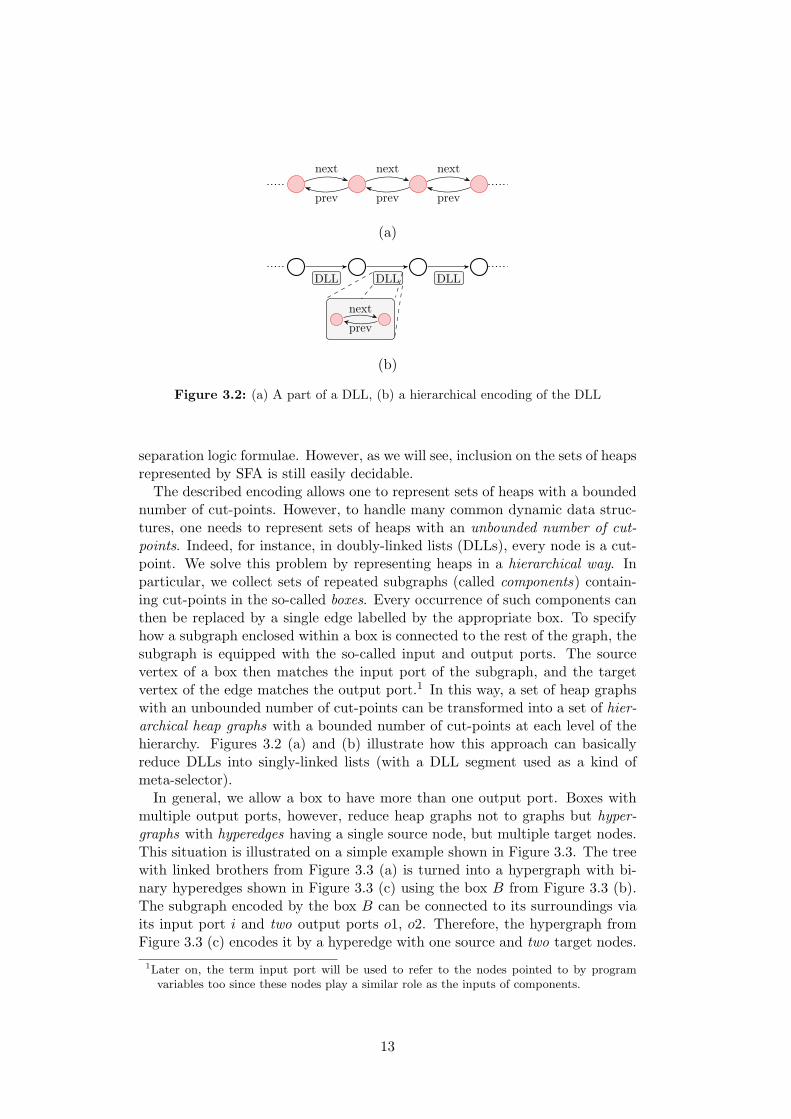
number of cut-points. However, to handle many common dynamic data struc-tures, one needs to represent sets of heaps with an unbounded number of cut-points. Indeed, for instance, in doubly-linked lists (DLLs), every node is a cut-point. We solve this problem by representing heaps in a hierarchical way. Inparticular, we collect sets of repeated subgraphs (called components) contain-ing cut-points in the so-called boxes. Every occurrence of such components canthen be replaced by a single edge labelled by the appropriate box. To specifyhow a subgraph enclosed within a box is connected to the rest of the graph, thesubgraph is equipped with the so-called input and output ports. The sourcevertex of a box then matches the input port of the subgraph, and the targetvertex of the edge matches the output port.1 In this way, a set of heap graphswith an unbounded number of cut-points can be transformed into a set of hier-archical heap graphs with a bounded number of cut-points at each level of thehierarchy. Figures 3.2 (a) and (b) illustrate how this approach can basicallyreduce DLLs into singly-linked lists (with a DLL segment used as a kind ofmeta-selector).In general, we allow a box to have more than one output port. Boxes with

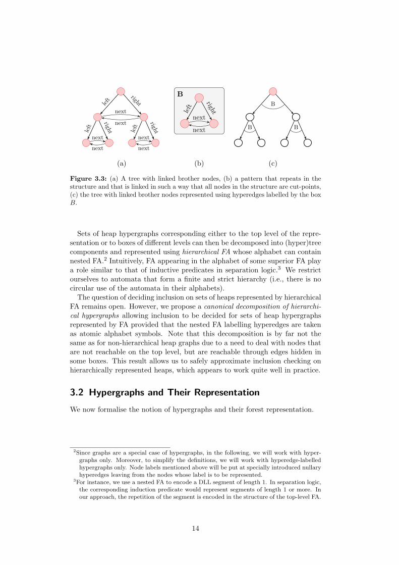
multiple output ports, however, reduce heap graphs not to graphs but hyper-graphs with hyperedges having a single source node, but multiple target nodes.This situation is illustrated on a simple example shown in Figure 3.3. The treewith linked brothers from Figure 3.3 (a) is turned into a hypergraph with bi-nary hyperedges shown in Figure 3.3 (c) using the box B from Figure 3.3 (b).The subgraph encoded by the box B can be connected to its surroundings viaits input port i and two output ports o1, o2. Therefore, the hypergraph fromFigure 3.3 (c) encodes it by a hyperedge with one source and two target nodes.

1Later on, the term input port will be used to refer to the nodes pointed to by programvariables too since these nodes play a similar role as the inputs of components.

13

left

right

next

next

left

right

next

next

left

right

next

next

B

left

right

next

next

B

B B

(a) (b) (c)

Figure 3.3: (a) A tree with linked brother nodes, (b) a pattern that repeats in thestructure and that is linked in such a way that all nodes in the structure are cut-points,(c) the tree with linked brother nodes represented using hyperedges labelled by the boxB.

Sets of heap hypergraphs corresponding either to the top level of the repre-sentation or to boxes of different levels can then be decomposed into (hyper)treecomponents and represented using hierarchical FA whose alphabet can containnested FA.2 Intuitively, FA appearing in the alphabet of some superior FA playa role similar to that of inductive predicates in separation logic.3 We restrictourselves to automata that form a finite and strict hierarchy (i.e., there is nocircular use of the automata in their alphabets).The question of deciding inclusion on sets of heaps represented by hierarchical

FA remains open. However, we propose a canonical decomposition of hierarchi-cal hypergraphs allowing inclusion to be decided for sets of heap hypergraphsrepresented by FA provided that the nested FA labelling hyperedges are takenas atomic alphabet symbols. Note that this decomposition is by far not thesame as for non-hierarchical heap graphs due to a need to deal with nodes thatare not reachable on the top level, but are reachable through edges hidden insome boxes. This result allows us to safely approximate inclusion checking onhierarchically represented heaps, which appears to work quite well in practice.

3.2 Hypergraphs and Their Representation

We now formalise the notion of hypergraphs and their forest representation.

2Since graphs are a special case of hypergraphs, in the following, we will work with hyper-graphs only. Moreover, to simplify the definitions, we will work with hyperedge-labelledhypergraphs only. Node labels mentioned above will be put at specially introduced nullaryhyperedges leaving from the nodes whose label is to be represented.

3For instance, we use a nested FA to encode a DLL segment of length 1. In separation logic,the corresponding induction predicate would represent segments of length 1 or more. Inour approach, the repetition of the segment is encoded in the structure of the top-level FA.

14

3.2.1 Hypergraphs

A ranked alphabet is a finite set Γ of symbols associated with a map # : Γ → N.The value #(a) is called the rank of a ∈ Γ. We use #(Γ) to denote the maximumrank of a symbol in Γ. A ranked alphabet Γ is a hypergraph alphabet if it isassociated with a total ordering (Γ on its symbols. For the rest of the section,we fix a hypergraph alphabet Γ.

An (oriented, Γ-labelled) hypergraph (with designated input/output ports) isa tuple G = (V,E, P ) where:

• V is a finite set of vertices.

• E is a finite set of hyperedges such that every hyperedge e ∈ E is of theform (v, a, (v1, . . . , vn)) where v ∈ V is the source of e, a ∈ Γ, n = #(a),and v1, . . . , vn ∈ V are targets of e and a-successors of v.

• P is the so-called port specification that consists of a set of input portsIP ⊆ V , a set of output ports OP ⊆ V , and a total ordering (P on IP∪OP .

We use v to denote a sequence v1, . . . , vn and v.i to denote its ith vertex vi. Forsymbols a ∈ Γ with #(a) = 0, we write (v, a) ∈ E to denote that (v, a, ()) ∈ E.Such hyperedges may simulate labels assigned to vertices.A path in a hypergraph G = (V,E, P ) is a sequence 〈v0, a1, v1, . . . , an, vn〉,

n ≥ 0, where for all 1 ≤ i ≤ n, vi is an ai-successor of vi−1. G is calleddeterministic iff ∀(v, a, v), (v, a′, v′) ∈ E: a = a′ =⇒ v = v′. G is calledwell-connected iff each node v ∈ V is reachable through some path from someinput port of G.As we have already mentioned in Section 3.1, in hypergraphs representing

heaps, input ports correspond to nodes pointed to by program variables or toinput nodes of components, and output ports correspond to output nodes ofcomponents. Figure 3.1 (a) shows a hypergraph with two input ports corre-sponding to the variables x and y. The hyperedges are labelled by selectorsdata and next. All the hyperedges are of arity 1. A simple example of a hy-pergraph with hyperedges of arity 2 is given in Figure 3.3 (c).

3.2.2 Forest Representation of Hypergraphs

We will now define the forest representation of hypergraphs. For that, wewill first define a notion of a tree as a basic building block of forests. We willdefine trees much like hypergraphs but with a restricted shape and withoutinput/output ports. The reason for the latter is that the ports of forests willbe defined on the level of the forests themselves, not on the level of the treesthat they are composed of.Formally, an (unordered, oriented, Γ-labelled) tree T = (V,E) consists of

a set of vertices and hyperedges defined as in the case of hypergraphs withthe following additional requirements: (1) V contains a single node with noincoming hyperedge (called the root of T and denoted root(T )). (2) All othernodes of T are reachable from root(T ) via some path. (3) Each node has atmost one incoming hyperedge. (4) Each node appears at most once among the

15

target nodes of its incoming hyperedge (if it has one). Given a tree, we call itsnodes with no successors leaves.Let us assume that Γ∩N = ∅. An (ordered, Γ-labelled) forest (with designated

input/output ports) is a tuple F = (T1, . . . , Tn, R) such that:

• For every i ∈ {1, . . . , n}, Ti = (Vi, Ei) is a tree that is labelled by thealphabet (Γ ∪ {1, . . . , n}).

• R is a (forest) port specification consisting of a set of input ports IR ⊆{1, . . . , n}, a set of output ports OR ⊆ {1, . . . , n}, and a total ordering (R

of IR ∪OR.

• For all i, j ∈ {1, . . . , n}, (1) if i )= j, then Vi ∩ Vj = ∅, (2) #(i) = 0, and(3) a vertex v with (v, i) ∈ Ej is not a source of any other edge (it isa leaf). We call such vertices root references and denote by rr(Ti, j) theset of all root references to Tj in Ti, i.e., rr(Ti, j) = {v ∈ Vi | (v, j) ∈ Ei}.We also define rr(Ti) =

⋃nj=1 rr(Ti, j).

A forest F = (T1, . . . , Tn, R) represents the hypergraph ⊗F obtained by unit-ing the trees T1, . . . , Tn and interconnecting their roots with the correspondingroot references. In particular, for every root reference v ∈ Vi, i ∈ {1, . . . , n},hyperedges leading to v are redirected to the root of Tj where (v, j) ∈ Ei, andv is removed. The sets IR and OR then contain indices of the trees whose rootsare to be input/output ports of ⊗F , respectively. Finally, their ordering (P

is defined by the (R-ordering of the indices of the trees whose roots they are.Formally, ⊗F = (V,E, P ) where:

• V =⋃n

i=1 Vi \ rr(Ti),

• E =⋃n

i=1{(v, a, v′) | a ∈ Γ ∧ ∃(v, a, v) ∈ Ei ∀1 ≤ j ≤ #(a) : if ∃(v.j, k) ∈

Ei with k ∈ {1, . . . , n}, then v′.j = root(Tk), else v′.j = v.j},

• IP = {root(Ti) | i ∈ IR},

• OP = {root(Ti) | i ∈ OR},

• ∀u, v ∈ IP ∪OP such that u = root(Ti) and v = root(Tj):

u (P v ⇐⇒ i (R j.

3.2.3 Minimal and Canonical Forests

We now define the canonical form of a forest which will be important laterfor deciding language inclusion on forest automata, acceptors of sets of hyper-graphs.We call a forest F = (T1, . . . , Tn, R) representing the well-connected hyper-

graph ⊗F minimal iff the roots of the trees T1, . . . , Tn correspond to the cut-points of ⊗F , i.e., those nodes that are either ports, have more than one incom-ing hyperedge in ⊗F , or appear more than once as a target of some hyperedge.A minimal forest representation of a hypergraph is unique up to permutationsof T1, . . . , Tn.

16

In order to get a truly unique canonical forest representation of a well-con-nected deterministic hypergraph G = (V,E, P ), it remains to canonically orderthe trees in the minimal forest representation of G. To do this, we use thetotal ordering (P on ports P and the total ordering (Γ on hyperedge labels Γof G. We then order the trees according to the order in which their roots arevisited in a depth-first traversal (DFT) of G. If all nodes are not reachable froma single port, a series of DFTs is used. The DFTs are started from the inputports in IP in the order given by (P . During the DFTs, a priority is given tothe hyperedges that are smaller in (Γ. A canonical representation is obtainedthis way since we consider G to be deterministic.

Figure 3.1 (b) shows a forest decomposition of the heap graph depicted inFigure 3.1 (a). The nodes pointed to by variables are input ports of the heapgraph. Assuming that the ports are ordered such that the port pointed by x

precedes the one pointed by y, then the forest of Figure 3.1 (b) is a canonicalrepresentation of the heap graph of Figure 3.1 (a).

3.2.4 Root Interconnection Graphs

Let F = (T1, . . . , Tn, R) be a forest. A root interconnection graph ⋆F = (V,E)is a (directed) graph in which the nodes V = {T1, . . . , Tn} represent the roots ofF , and the edges E ⊆ V × (N×{1, 2})×V represent the interconnection of thecomponents of F . In particular, an edge labelled by (k, 1) appears between Ti

and Tj in ⋆F if and only if the DFT of Ti started in its root visits a referenceto Tj after visiting k − 1 other root references (when not counting multipleoccurrences of the same roots), and a reference to Tj is not visited anymore inthe rest of the DFT. If a reference to Tj is visited after k − 1 other references(again not counting multiple occurrences of the same root), and it will be visitedat least once more in the rest of the DFT (i.e., the root of Tj can be reachedfrom the root of Ti via multiple paths, or, equivalently, |rr(Ti, j)| > 1), then,and only then ⋆F contains an edge connecting Ti and Tj labelled by (k, 2).

Using the root interconnection graph, one can immediately see whether thecorresponding forest is canonical or not. Indeed, a forest F = (T1, . . . , Tn, R)is minimal if and only if each node in ⋆F is in IP ∪ OP , has more than oneincoming edge, or it has an incoming edge labelled by (k, 2). Moreover, ifa series of DFTs on ⋆F (which start from the nodes corresponding to inputports in IP in the order given by (P , and in which an edge (k, i) is exploredbefore (l, j) iff k < l) visits the nodes of ⋆F in the order T1, T2, . . . , Tn, thenF is canonical.

3.2.5 Manipulating the Forest Representation

In practice, it is often the case that one needs to modify the number of treeswithin a forest representation of a hypergraph. For instance, we can have anarbitrary forest representation and want to obtain a canonical one. Apart fromchanging the order of the trees, we might also need to eliminate certain roots(which are not cut-points) by gluing them (together with the trees rooted atthem) with the leaves of other trees. For this reason, we define an additional

17

operation over forests which we call a concatenation. If a root of a tree Tj isreferenced exactly once from a different tree Ti inside the forest (i.e., |rr(Ti, j)| =1 and |rr(Tk, j)| = 0 for k )= i) and it corresponds to neither an input nor anoutput port (i.e., root(Tj) )∈ IR ∪ OR), then Tj can be concatenated to Ti byreplacing the leaf node referencing Tj in Ti by Tj . The concatenation of Tj toTi within F = (T1, . . . , Tn, R) is denoted by concat(F, i, j).Formally, let v ∈ Vi such that (v, j) ∈ Ei (i.e., v is a leaf of Ti representing the

root reference to Tj). Assuming (w.l.o.g.) that i < j, concat(F, i, j) is definedas

(T1, . . . , Ti−1, T′i , Ti+1, . . . , Tj−1, Tj+1, . . . , Tn, R)

where T ′i = (V ′

i , E′i) such that

• V ′i = (Vi \ {v}) ∪ Vj

• E′i = (Ei \ {(u, a, v) : u ∈ Vi ∧ a ∈ Γ} \ {(v, j)}) ∪ {(u, a,Root(Tj)) :

(u, a, v) ∈ Ei} ∪ Ej

The operation concat preserves the semantics of the forest, therefore it holdsthat ⊗concat(F, i, j) = ⊗F whenever such concatenation is possible.

3.3 Forest Automata

We will now define forest automata as tuples of tree automata extended bya port specification. Tree automata accept trees that are ordered and node-labelled. Therefore, in order to be able to use forest automata to encode sets offorests, we must define a conversion between ordered, node-labelled trees andour unordered, edge-labelled trees.We convert a deterministic Γ-labelled unordered tree T into a node-labelled

ordered tree ot(T ) by (1) transferring the information about labels of edgesof a node into the symbol associated with the node and by (2) ordering thesuccessors of the node. More concretely, we label each node of the ordered treeot(T ) by the set of labels of the hyperedges leading from the correspondingnode in the original tree T . Successors of the node in ot(T ) correspond tothe successors of the original node in T , and are ordered w.r.t. the order (Γ

of hyperedge labels through which the corresponding successors are reachablein T (while always keeping tuples of nodes reachable via the same hyperedgetogether, ordered in the same way as they were ordered within the hyperedge).The rank of the new node label is given by the sum of ranks of the originalhyperedge labels embedded into it. Below, we use ΣΓ to denote the rankednode alphabet obtained from Γ as described above.

A forest automaton over Γ (with designated input/output ports) is a tupleF = (A1, . . . ,An, R) where:

• For all 1 ≤ i ≤ n, Ai = (Qi,Σ,∆i, Fi) is a TA with Σ = ΣΓ ∪ {1, . . . , n}and #(i) = 0.

• R is defined as for forests, i.e., it consists of input and output portsIR, OR ⊆ {1, . . . , n} and a total ordering (R on IR ∪OR.

18

The forest language of F is the set of forests LF (F) = {(T1, . . . , Tn, R) | ∀1 ≤i ≤ n : ot(Ti) ∈ L(Ai)}, i.e., the forest language is obtained by taking theCartesian product of the tree languages, unordering the trees that appear in itselements, and extending them by the port specification. The forest language ofF in turn defines the hypergraph language of F which is the set of hypergraphsL(F) = {⊗F | F ∈ LF (F)}.

3.3.1 Uniform and Canonicity Respecting FA

An FA F is called uniform if and only if for each forest F ∈ LF (F), thehypergraph ⊗F is well-connected, and for any two F, F ′ ∈ LF (F), it holdsthat ⋆F = ⋆F ′. Since all forests within a uniform FA are required to havethe same root interconnection graph, the concatenation defined in Section 3.2.2can also be easily performed on language of uniform FA (note that if some Ti

does not correspond to a cut-point in F and it can be merged to Tj , then fromthe definition of uniform FA, any other F ′ is guaranteed to have some T ′

i andT ′j such that T ′

i can be merged into T ′j as well). Therefore, we can lift concat

from single forests to an entire language of FA F = (A1, . . . ,An, R) as follows:

concat(L(F), i, j) = {concat(F, i, j) : F ∈ L(F)}.

Moreover, an FA F ′ representing concat(L(F), i, j) can easily be obtained fromF . In particular, assuming the sets of states of components Ai and Aj to bedisjoint, we first replace each leaf transition in Ai labelled by the reference toj by all accepting transitions of Aj (we create new transitions by using theright-hand-side states of the leaf transitions of Ai and the symbol and the left-hand-side tuple of states of the accepting transitions of Aj ; in particullar, fora transition of 〈j〉 → r of Ai and a transition α(q1, . . . , qn) → q of Aj , we createa transition α(q1, . . . , qn) → r). Then, we add all transitions of Aj into Ai andremove Aj from the resulting FA.We say that an FA F respects canonicity4 iff for each forest F ∈ LF (F), the

hypergraph ⊗F is well-connected, and F is its canonical representation. Weabbreviate canonicity respecting FA as CFA. It is easy to see that comparing setsof hypergraphs represented by CFA can be done component-wise as describedin the below proposition.

Proposition 1 Let F = (A1, . . . ,An, R) and F ′ = (A′1, . . . ,A

′m, R′) be two

CFA. Then, L(F) ⊆ L(F ′) iff n = m, R = R′, and ∀1 ≤ i ≤ n : L(Ai) ⊆L(A′

i).

Obviously, any canonicity respecting FA is also uniform. On the other hand,any uniform FA F can be easily transformed into a canonicity respecting oneby first concatenating each redundant component5 with its parent component

4We intentionally use the term canonicity respecting FA instead of canonical FA to stressthat not all such FA are strictly canonical (this is due to the extensions that we willdescribe in Section 3.4 and Section 3.5). However, canonicity respecting FA can be treatedas canonical for many practical purposes.

5As we have already mentioned in Section 3.2.3, a redundant component can be identifiedby looking for roots which are referenced only once.

19

(i.e., the component that contains the only reference to the given root) suchthat the resulting FA contains the minimal number of components. Then, wereorder the remaining components according to the DFT performed on the rootinterconnection graph.

3.3.2 Transforming FA into Canonicity Respecting FA

In order to facilitate inclusion checking, each FA can be algorithmically trans-formed (split) into a finite set of CFA such that the union of their languagesequals the original language. As we have already mentioned in the Section 3.3,one can obtain a canonicity respecting FA from a uniform one. It remains toshow how to convert an arbitrary FA into a set of uniform FA. In the following,we describe the computation which allow us to reconstruct the root intercon-nection graph of a given FA and which, if it is needed, allows us to split the FAinto a set of uniform FA.First, we label the states of the component TA of the given FA by special

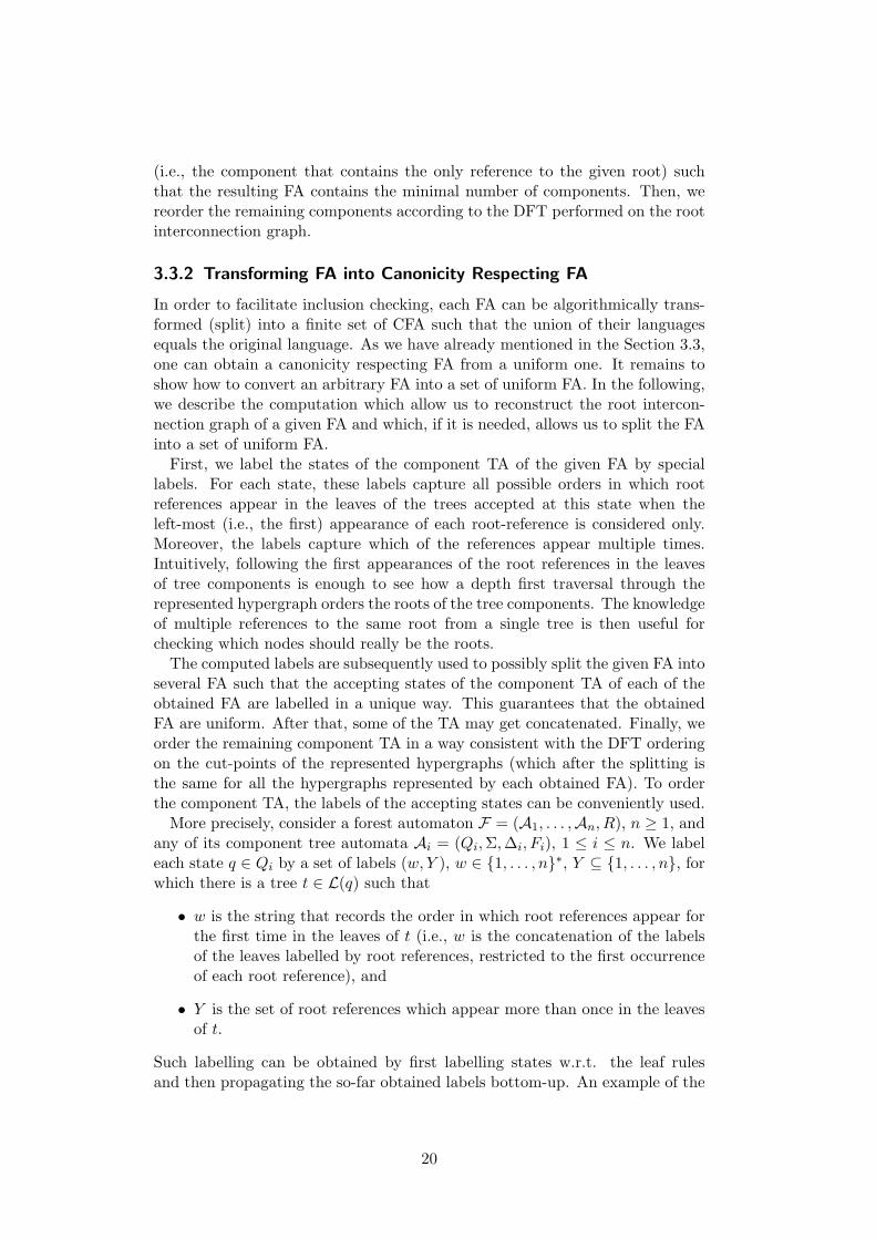
labels. For each state, these labels capture all possible orders in which rootreferences appear in the leaves of the trees accepted at this state when theleft-most (i.e., the first) appearance of each root-reference is considered only.Moreover, the labels capture which of the references appear multiple times.Intuitively, following the first appearances of the root references in the leavesof tree components is enough to see how a depth first traversal through therepresented hypergraph orders the roots of the tree components. The knowledgeof multiple references to the same root from a single tree is then useful forchecking which nodes should really be the roots.The computed labels are subsequently used to possibly split the given FA into

several FA such that the accepting states of the component TA of each of theobtained FA are labelled in a unique way. This guarantees that the obtainedFA are uniform. After that, some of the TA may get concatenated. Finally, weorder the remaining component TA in a way consistent with the DFT orderingon the cut-points of the represented hypergraphs (which after the splitting isthe same for all the hypergraphs represented by each obtained FA). To orderthe component TA, the labels of the accepting states can be conveniently used.More precisely, consider a forest automaton F = (A1, . . . ,An, R), n ≥ 1, and

any of its component tree automata Ai = (Qi,Σ,∆i, Fi), 1 ≤ i ≤ n. We labeleach state q ∈ Qi by a set of labels (w, Y ), w ∈ {1, . . . , n}∗, Y ⊆ {1, . . . , n}, forwhich there is a tree t ∈ L(q) such that

• w is the string that records the order in which root references appear forthe first time in the leaves of t (i.e., w is the concatenation of the labelsof the leaves labelled by root references, restricted to the first occurrenceof each root reference), and

• Y is the set of root references which appear more than once in the leavesof t.

Such labelling can be obtained by first labelling states w.r.t. the leaf rulesand then propagating the so-far obtained labels bottom-up. An example of the

20

∆: a(q, q) → q, a(r, q) → q, a(q, r) → q,a(s, s) → q, ref.1 → r, b → s

⇓

∆′: a(q(1,{1}), q(1,{1})) → q(1,{1}), a(q(1,∅), q(1,∅)) → q(1,{1}),

a(q(1,{1}), q(1,∅)) → q(1,{1}), a(q(1,∅), q(1,{1})) → q(1,{1}),

a(q(1,{1}), r(1,∅)) → q(1,{1}), a(r(1,∅), q(1,{1})) → q(1,{1}),

a(q(1,{1}), q(ε,∅)) → q(1,{1}), a(q(ε,∅), q(1,{1})) → q(1,{1}),

a(q(1,∅), r(1,∅)) → q(1,{1}), a(r(1,∅), q(1,∅)) → q(1,{1}),

a(q(1,∅), q(ε,∅)) → q(1,∅), a(q(ε,∅), q(1,∅)) → q(1,∅),

a(q(ε,∅), r(1,∅)) → q(1,∅), a(r(1,∅), q(ε,∅)) → q(1,∅),

a(q(ε,∅), q(ε,∅)) → q(ε,∅), a(s(ε,∅), s(ε,∅)) → q(ε,∅),

ref.1 → r(1,∅), b → s(ε,∅)

Figure 3.4: Example of labelling (w, Y ) obtained for a single component A =(Σ, Q,∆, {qf}) during the transformation into a canonicity respecting FA (in the pic-ture, labelled states are of the form q(w,Y )). The newly obtained TA contains 3 differentaccepting states (q(1,{1}), q(1,∅), and q(ε,∅)) suggesting that the component needs to besplit into 3. The language of q(1,{1}) contains trees with two or more references to root 1.Similarly q(1,∅) corresponds to trees having exactly one such a reference. Finally, treeswithin the language of q(ε,∅) do not contain any reference at all.

labelling is depicted in Figure 3.4. If the final states of Ai get labelled by severaldifferent labels, we make a copy of the automaton for each of these labels, andin each of them, we preserve only the transitions that allow trees with theappropriate label of the root to be accepted6. This way, all the componentautomata can be processed and then new forest automata can be created byconsidering all possible combinations of the transformed TA.Clearly, each of the FA created above represents a set of hypergraphs that

have the same number of cut-points (corresponding either to ports, nodes ref-erenced at least twice from a single component tree, or referenced from severalcomponent trees) that get ordered in the same way in the depth first traver-sal of the hypergraphs. However, it may be the case that some roots of theFA need not correspond to cut-points. This is easy to detect by looking fora root reference that does not appear in the set part of any label of some finalstate and that does not appear in the labels of two different component treeautomata. A useless root can then be eliminated by adding transition rules ofthe appropriate component tree automaton Ai to those of the tree automatonAj that refers to that root and by gluing final states of Ai with the states ofAj accepting the root reference i.

It remains to order the component TA within each of the obtained FA ina way consistent with the DFT ordering of the cut-points of the representedhypergraphs (which is now the same for all the hypergraphs represented by

6More technically, given a labelled TA, one can first make a separate copy of each statefor each of its labels, connect the states by transitions such that the obtained singletonlabelling is respected, then make a copy of the TA for each label of accepting states, andkeep the accepting status for a single labelling of accepting states in each of the copiesonly.

21

a single FA due to the performed splitting). To order the component TA of anyof the obtained FA, one can use the w-part of the labels of its accepting states.One can then perform a DFT on the component TA, considering the TA asatomic objects. One starts with the TA that accept trees whose roots representports and processes them w.r.t. the ordering of ports. When processing a TAA, one considers as its successors the TA that correspond to the root referencesthat appear in the w-part of the labels of the accepting states of A. Moreover,the successor TA are processed in the order in which they are referenced from thelabels. When the DFT is over, the component TA may get reordered accordingto the order in which they were visited.Subsequently, the port specification R and root references in leaves must be

updated to reflect the reordering. If the original sets IR or OR contain a porti, and the ith tree was moved to the jth position, then i must be substituted byj in IR, OR, and (R as well as in all root references. This finally leads to a setof canonicity respecting FA.Note that, in practice, it is not necessary to tightly follow the above described

process. Instead, one can arrange the symbolic execution of statements in sucha way that when starting with a CFA, one obtains an FA which already meetssome requirements for CFA. Most notably, the splitting of component TA—ifneeded—can be efficiently done already during the symbolic execution of theparticular statements. Therefore, transforming an FA obtained this way intothe corresponding CFA involves the elimination of redundant roots and the rootreordering only.

3.3.3 Sets of FA

The class of languages of FA (and even CFA) is not closed under union sincea forest language of a FA corresponds to the Cartesian product of the languagesof all its components, and not every union of Cartesian products may be ex-pressed as a single Cartesian product. For instance, consider two CFA F =(A,B, R) and F ′ = (A′,B′, R) such that LF (F) = {(a, b, R)} and LF (F

′) ={(c, d,R)} where a, b, c, d are distinct trees. The forest language of the FA(A ∪ A′,B ∪ B′, R) is {(x, y,R) | (x, y) ∈ {a, c} × {b, d}}), and there is no FAwith the hypergraph language equal to L(F) ∪ L(F ′).Due to the above, we cannot transform a set of CFA obtained by canonising

a given FA into a single CFA. Likewise, when we obtain several CFA when sym-bolically executing several program paths leading to the same program location,we cannot merge them into a single CFA without risking a loss of information.Consequently, we will explicitly work with finite sets of (canonicity-respecting)forest automata, S(C)FA for short, where the language L(S) of a finite set Sof FA is defined as the union of the languages of its elements. This, however,means that we need to be able to decide language inclusion on SFA.

22

3.3.4 Testing Inclusion on Sets of FA

The problem of checking inclusion on SFA, this is, checking whether L(S) ⊆L(S ′) where S,S ′ are SFA, can be reduced to a problem of checking inclusionon tree automata. We may w.l.o.g. assume that S and S ′ are SCFA.We will transform every FA F in S and S ′ into a TA AF which accepts the

language of trees where:

• The root of each of these trees is labelled by a special fresh symbol (pa-rameterised by n and the port specification of F).

• The root has n children, one for each tree automaton of F .

• For each 1 ≤ i ≤ n, the ith child of the root is the root of a tree acceptedby the ith tree automaton of F .

Trees accepted by AF are therefore unique encodings of hypergraphs in L(F).We will then test the inclusion L(S) ⊆ L(S ′) by testing the tree automatalanguage inclusion between the union of TA obtained from S and the union ofTA obtained from S ′.Formally, let F = (A1, . . . ,An, R) be an FA where Ai = (Σ, Qi,∆i, Fi) for

each 1 ≤ i ≤ n. Without a loss of generality, assume that Qi ∩Qj = ∅ for each1 ≤ i < j ≤ n. We define the TA AF = (Σ ∪ {"R

n }, Q,∆, {qtop}) where:

• "Rn )∈ Σ is a fresh symbol with #("R

n ) = n,

• qtop )∈⋃n

i=1Qi is a fresh accepting state,

• Q =⋃n

i=1Qi ∪ {qtop}, and

• ∆ =⋃n

i=1∆i ∪∆top where ∆

top contains the rule "Rn (q1, . . . , qn) → qtop

for each (q1, . . . , qn) ∈ F1 × · · · × Fn.

It is now easy to see that the following proposition holds (in the proposition,“∪” stands for the usual tree automata union).

Proposition 2 For SCFA S and S ′,

L(S) ⊆ L(S ′) ⇐⇒ L(⋃

F∈S

AF ) ⊆ L(⋃

F ′∈S′

AF ′

).

3.4 Hierarchical Hypergraphs

As discussed informally in Section 3.1, simple forest automata cannot expresssets of data structures with unbounded numbers of cut-points like, e.g., the setof all doubly-linked lists or the set of all trees with linked brothers (Figures 3.2and 3.3). To capture such data structures, we will enrich the expressive powerof forest automata by allowing them to be hierarchically nested. For the restof the section, we fix a hypergraph alphabet Γ.

23

3.4.1 Hierarchical Hypergraphs, Components, and Boxes

We first introduce hypergraphs with hyperedges labelled by the so-called boxeswhich are sets of hypergraphs (defined up to isomorphism7). A hypergraphG with hyperedges labelled by boxes encodes a set of hypergraphs. The hy-pergraphs encoded by G can be obtained by replacing every hyperedge of Glabelled by a box by some hypergraph from the box. The hypergraphs withinthe boxes may themselves have hyperedges labelled by boxes, which gives riseto a hierarchical structure (which we require to be of a finite depth).Let Υ be a hypergraph alphabet. First, we define an Υ-labelled component

as an Υ-labelled hypergraph C = (V,E, P ) which satisfies the requirement that|IP | = 1 and IP ∩ OP = ∅. Then, an Υ-labelled box is a non-empty set B ofΥ-labelled components such that all of them have the same number of outputports. This number is called the rank of the box B and denoted by #(B).Let B[Υ] be the ranked alphabet containing all Υ-labelled boxes such thatB[Υ] ∩Υ = ∅. The operator B gives rise to a hierarchy of alphabets Γ0,Γ1, . . .where:

• Γ0 = Γ is the set of plain symbols,

• for i ≥ 0, Γi+1 = Γi ∪ B[Γi] is the set of symbols of level i+ 1.

A Γi-labelled hypergraph H is then called a Γ-labelled (hierarchical) hypergraphof level i, and we refer to the Γi−1-labelled boxes appearing on edges of Has to nested boxes of H. A Γ-labelled hypergraph is sometimes called a plainΓ-labelled hypergraph.

3.4.2 Semantics of Hierarchical Hypergraphs

A Γ-labelled hierarchical hypergraph H encodes a set !H" of plain hypergraphs,called the semantics of H. For a set S of hierarchical hypergraphs, we use !S"to denote the union of semantics of its elements.If H is plain, then !H" contains just H itself. If H is of level j > 0, then

hypergraphs from !H" are obtained in such a way that hyperedges labelled byboxes B ∈ Γj are substituted in all possible ways by plain components from!B". The substitution is similar to an ordinary hyperedge replacement used ingraph grammars. When an edge e is substituted by a component C, the inputport of C is identified with the source node of e, and the output ports of C areidentified with the target nodes of e. The correspondence of the output portsof C and the target nodes of e is defined using the order of the target nodes ine and the ordering of ports of C. The edge e is finally removed from H.Formally, given a Γ-labelled hierarchical hypergraph H = (V,E, P ), a hyper-

edge e = (v, a, v) ∈ E, and a component C = (V ′, E′, P ′) where #(a) = |OP ′ | =k, the substitution of e by C in H results in the hypergraph H[C/e] definedas follows. Let o1 (P . . . (P ok be the ports of OP ordered by (P . W.l.o.g.,assume V ∩V ′ = ∅. C will be connected to H by identifying its ports with their

7Dealing with hypergraphs (and later also automata) defined up to isomorphism avoidsa need to deal with classes instead of sets. We will not repeat this fact later on.

24

matching vertices of e. We define for every vertex w ∈ V ′ its matching vertexmatch(w) such that (1) if w ∈ IP ′ , match(w) = v (the input port of C matchesthe source of e), (2) if w = oi, 1 ≤ i ≤ k, match(w) = v.i (the output ports of Cmatch the corresponding targets of e), and (3) match(w) = w otherwise (an in-ner node of C is not matched with any node of H). Then H[C/e] = (V ′′, E′′, P )where V ′′ = V ∪(V ′\(IP ′∪OP ′)) and E′′ = (E\{e})∪{(v′′, a′, v′′) | ∃(v′, a′, v′) ∈E′ : match(v′) = v′′ ∧ ∀1 ≤ i ≤ k : match(v′.i) = v′′.i}.We can now give an inductive definition of !H". Let e1 = (v1, B1, v1), . . . ,

en = (vn, Bn, vn) be all edges of H labelled by Γ-labelled boxes. Then, G ∈ !H"iff it is obtained from H by successively substituting every ei by a componentCi ∈ !Bi", i.e.,

!H" = {H[C1/e1] . . . [Cn/en] | C1 ∈ !B1", . . . , Cn ∈ !Bn"}.

Figure 3.2 (b) shows a hierarchical hypergraph of level 1 whose semantics isthe (hyper)graph of Figure 3.2 (a). Similarly, Figure 3.3 (c) shows a hierarchicalhypergraph of level 1 whose semantics is the (hyper)-graph of Figure 3.3 (a).

3.5 Hierarchical Forest Automata

We now define hierarchical forest automata that represent sets of hierarchicalhypergraphs. The hierarchical FA are FA whose alphabet can contain symbolswhich encode boxes appearing on edges of hierarchical hypergraphs. The boxesare themselves represented using hierarchical FA.To define an alphabet of hierarchical FA, we will take an approach similar

to the one used for the definition of hierarchical hypergraphs. First, we definean operator A which for a hypergraph alphabet Υ returns the ranked alphabetcontaining the set of all SFA S over (a finite subset of) Υ such that L(S) isan Υ-labelled box and such that A[Υ] ∩Υ = ∅. The rank of S in the alphabetA[Υ] is the rank of the box L(S). The operator A gives rise to a hierarchy ofalphabets Γ0,Γ1, . . . where:

• Γ0 = Γ is the set of plain symbols,

• for i ≥ 0, Γi+1 = Γi ∪ A[Γi] is the set of symbols of level i+ 1.

A hierarchical FA F over Γi is then called a Γ-labelled (hierarchical) FA oflevel i, and we refer to the hierarchical SFA over Γi−1 appearing within alphabetsymbols of F as to nested SFA of F .

Let F be a hierarchical FA. We now define an operator ♯ that translates anyΓi-labelled hypergraph G = (V,E, P ) ∈ L(F) to a Γ-labelled hierarchical hy-pergraph H of level i (i.e., it translates G by transforming the SFA that appearon its edges to the boxes they represent). Formally, G♯ is defined inductivelyas the Γ-labelled hierarchical hypergraph H = (V,E′, P ) of level i that is ob-tained from the hypergraph G by replacing every edge (v,S, v) ∈ E, labelled bya Γ-labelled hierarchical SFA S, by the edge (v,L(S)♯, v), labelled by the boxL(S)♯ where L(S)♯ denotes the set (box) {X♯ | X ∈ L(S)}. Then, we define

25

the semantics of a hierarchical FA F over Γ as the set of Γ-labelled (plain)hypergraphs !F" = !L(F)♯".Notice that a hierarchical SFA of any level has finitely many nested SFA

of a lower level only. Therefore, a hierarchical SFA is a finitely representableobject. Notice also that even though the maximum number of cut-points ofhypergraphs from L(S)♯ is fixed (SFA always accept hypergraphs with a fixedmaximum number of cut-points), the number of cut-points of hypergraphs in!S" may be unbounded. The reason is that hypergraphs from L(S)♯ may containan unbounded number of hyperedges labelled by boxes B such that hypergraphsfrom !B" contain cut-points too. These cut-points then appear in hypergraphsfrom !S", but they are not visible at the level of hypergraphs from L(S)♯.

Hierarchical SFA are therefore finite representations of sets of hypergraphswith possibly unbounded numbers of cut-points.

3.5.1 On Well-Connectedness of Hierarchical FA

In this section, we aim at checking well-connectedness and inclusion of sets ofhypergraphs represented by hierarchical FA. Since considering the full class ofhierarchical hypergraphs would unnecessarily complicate our task, we enforcea restricted form of hierarchical automata that rules out some rather artificialscenarios and that allows us to handle the automata hierarchically (i.e., usingsome pre-computed information for nested FA rather than having to unfold theentire hierarchy all the time). In particular, the restricted form guarantees that:

1. For a hierarchical hypergraph H, well-connectedness of hypergraphs in!H" is equivalent to the so-called box-connectedness of H. Box-connect-edness is a property introduced below that can be easily checked and thatbasically considers paths from input ports to output ports and vice versa,in the latter case through hyperedges hidden inside nested boxes.

2. Determinism of hypergraphs from !H" implies determinism of H.

The two above properties simplify checking well-connectedness and inclusionconsiderably since for a general hierarchical hypergraph H, well-connectednessof H is neither implied nor it implies well-connectedness of hypergraphs from!H". This holds also for determinism. The reason is that a component C ina nested box ofH may interconnect its ports in an arbitrary way. It may containpaths from output ports to both input and output ports (including paths froman output port to another output port not passing the input port), but it maybe missing paths from the input port to some of the output ports.Using the above restriction, we will show below a safe approximation of inclu-

sion checking on hierarchical SFA, and we will also show that this approximationis precise in some cases. Moreover, it turns out that in practice, an even moreaggressive approximation of inclusion checking in which nested boxes are takenas atomic symbols is often sufficient.

26

3.5.2 Properness and Box-Connectedness

Given a Γ-labelled component C of level 0, we define its backward reachabilityset br(C) as the set of indices i for which there is a path from the i-th outputport of C back to the input port of C. Given a box B over Γ, we inductivelydefine B to be proper iff all its nested boxes are proper, br(C1) = br(C2) forany C1, C2 ∈ !B", and the following holds for all components C ∈ !B":

1. C is well-connected.

2. If there is a path from the i-th to the j-th output port of C, i )= j, theni ∈ br(C).8

For a proper box B, we use br(B) to denote br(C) for C ∈ !B". A hierarchicalhypergraph H is called well-formed iff all its nested boxes are proper. In thatcase, the conditions above imply that either all or no hypergraphs from !H"are well-connected and that well-connectedness of hypergraphs in !H" may bejudged based only on the knowledge of br(B) for each nested box B of H,without a need to reason about the semantics of B (in particular, Point 2 inthe above definition of proper boxes guarantees that we do not have to takeinto account paths that interconnect output ports of B). This is formalised inthe following paragraph.Let H = (V,E, P ) be a well-formed Γ-labelled hierarchical hypergraph with

a set X of nested boxes. We define the backward reachability graph of H as theΓ ∪X ∪Xbr -labelled hypergraph Hbr = (V,E ∪ Ebr , P ) where Xbr = {(B, i) |B ∈ X ∧ i ∈ br(B)} and Ebr = {(vi, (B, i), (v)) | B ∈ X ∧ (v,B, (v1, . . . , vn)) ∈E ∧ i ∈ br(B)}. We say that H is box-connected iff Hbr is well-connected. Thebelow proposition clearly holds.

Proposition 3 If H is a well-formed hierarchical hypergraph, then the hyper-graphs from !H" are well-connected iff H is box-connected. Moreover, if hy-pergraphs from !H" are deterministic, then both H and Hbr are deterministichypergraphs.

We straightforwardly extend the above notions to hypergraphs with hyper-edges labelled by hierarchical SFA, treating these SFA-labels as if they were theboxes they represent. Particularly, we call a hierarchical SFA S proper iff itrepresents a proper box !S", we let br(S) = br(!S"), and for a Γ ∪ Y -labelledhypergraph G where Y is a set of proper SFA, its backward reachability hyper-graph Gbr is defined based on br in the same way as the backward reachabilityhypergraph of a hierarchical hypergraph above (just instead of boxes, we dealwith their SFA representations). We also say that G is box-connected iff Gbr iswell-connected.

3.5.3 Checking Properness and Well-Connectedness

We now outline algorithms for checking properness of nested SFA and well-connectedness of SFA.8Notice that this definition is correct since boxes of level 0 have no nested boxes, and therecursion stops at them.

27

Properness of nested SFA can be checked relatively easily since we can takeadvantage of the fact that nested SFA of a proper SFA must be proper as well.We start with nested SFA of level 0 which contain no nested SFA, we checktheir properness and compute the values of the backward reachability functionbr for them. To do this we can label TA states similarly to Section 3.3.2.A unique label of each root in the SFA representing the box guarantees thatthe br function will be equal for all hypergraphs hidden in the box. Then, weiteratively increase the level j and for each j, we check properness of the nestedSFA of level j and compute the values of the function br . For this, we use thevalues of br that we have computed for the nested SFA of level j − 1, and wecan also take advantage of the fact that the nested SFA of level j−1 have beenshown to be proper. We can again use the labels attached to all tree automatastates. The difference from level 0 is that we have to extend the labels in orderto capture also the backward reachability of the edges labelled by nested SFA.Now, given an FA F over Γ with proper nested SFA, we can check well-

connectedness of hypergraphs from !F" as follows: (1) for each nested SFAS of F , we compute like above (and cache for further use) the value br(S),and (2) using this value, we check box-connectedness of hypergraphs in L(F)without a need of reasoning about the inner structure of the nested SFA.Let us have a canonicity respecting SFA S of some level such that its nested

SFA are proper and we know the value of the function br for all of them.9 Weassume that S contains at least one FA, and that the languages of all F ∈ Sare nonempty.Moreover, to make the algorithms of checking properness and box-connect-

edness faster and simpler, we exploit the fact that the algorithm we describe inSection 3.5.7 in fact produces automata respecting canonicity in a somewhatstronger sense than described in Section 3.5.1. We define the stronger notionof respecting canonicity below.Given F = (A1, . . . ,An, R) ∈ S, a path in a tree t ∈ L(Ai) from v to w,

v, w ∈ dom(t), is a sequence v = v0, (a1, k1), v1 . . . , (am, km), vm = w, 0 ≤ m,where for each 1 ≤ i ≤ m, vi is the ki-th son of vi−1 and t(vi) = ai. The pathis backward passable iff for each 1 ≤ i ≤ m, the label ai is backward passable atthe ki-th position, which means that there is a proper nested SFA Si ∈ ai andj ∈ br(Si) such that j +

∑

{b∈ai|b%ΓSi,b)=Si}#(b) = ki.

For each 1 ≤ i ≤ n and each t ∈ L(Ai), we define the reachability relation10

ρti ⊆ {1, . . . , n} × {1, . . . , n} on the roots of F that contains a pair (j, k) iff oneof the following three conditions holds:

9Notice that even though respecting canonicity assumes properness of nested SFA and werequire here proper SFA to be canonicity respecting, this is not a circular dependency. Foran SFA to respect canonicity, we only require its nested SFA to be proper. So, for an SFAof level j to respect canonicity, we require properness of SFA of level j−1 only. Respectingcanonicity in an SFA of level 0 does not depend on the notion of properness since SFA oflevel 0 have no nested SFA. Properness on level j then depends on respecting canonicityon level j.

10Notice, that the reachability relation is related to the root interconnection graph which isdefined in Section 3.2.4. Unlike reachability relation, the root interconnection graph doesnot record backward passable paths. On the other hand, it also contains some informationabout the number of paths between nodes.

28

1. i = j and there is a leaf v of t with t(v) = k, or

2. i = k, there is a leaf v of t with t(v) = j, and the path from the root of tto v is backward passable, or

3. there are nodes u, v, w of t such that both v and w are leaves of the subtreerooted by u, t(v) = j, t(w) = k, and the path from u to v is backwardpassable.

We say that F is an FA with uniform reachability iff for each 1 ≤ i ≤ n, ρtiis the same for all t ∈ L(Ai). If it is the case, then we denote the reachabilityrelation as ρi. We further say that an SFA S strongly respects canonicity iff itrespects canonicity as defined in Section 3.5.1 and all its elements are FA withuniform reachability. In Section 3.5.7, we show the transformation of FA intoSFA that strongly respect canonicity and we also show how to compute therelation ρi.

If F is an FA with uniform reachability, we define the global reachabilityrelation ρ = (

⋃

1≤i≤n ρi)∗ on roots of F .11 Notice that (i, j) ∈ ρ iff for all

H ∈ !LH(F)" there are two nodes u and v that correspond to the i-th and j-throot of F , respectively, and such that there is a path from u to v in H.

Properness of an SFA representing some box and computing br on it is thendone as follows. First, a singleton SFA {F} with ι being the only input portof F is proper iff (1) for all 1 ≤ i ≤ n, (ι, i) ∈ ρ and (2) for all o, o′ ∈ OR,(o, o′) ∈ ρ =⇒ (o′, ι) ∈ ρ. If {F} is proper, then br({F}) equals the set{o ∈ OR | (o, ι) ∈ ρ}. Finally, assuming that an SFA S strongly respectscanonicity, S is proper iff all its elements agree on the values of IR and OR, andall the singleton SFA {F}, F ∈ S, are proper and agree on the value of br(F).This value then equals br(S).Box-connectedness of an SFA S that strongly respects canonicity and that has

proper nested SFA for which we know the values of br can be checked similarlyas properness, i.e., using the relation ρ. Particularly, S is box-connected if andonly if for all F = (A1, . . . ,An, R) ∈ S and for all 1 ≤ k ≤ n there is someι ∈ IR such that (ι, k) ∈ ρ.

3.5.4 On Inclusion of Hierarchical FA

Checking inclusion on hierarchical automata over Γ with nested boxes fromX, i.e., given two hierarchical FA F and F ′, checking whether !F" ⊆ !F ′",is a hard problem, even under the assumption that nested SFA of F and F ′

are proper. Its decidability is not known. In order to be able to use our inpractice (see Chapter 4), we choose a pragmatic approach and give only a semi-algorithm that is efficient and works well in practical cases. The idea is simple.Since the implications L(F) ⊆ L(F ′) =⇒ L(F)♯ ⊆ L(F ′)♯ =⇒ !F" ⊆ !F ′"obviously hold, we may safely approximate the solution of the inclusion problemby deciding whether L(F) ⊆ L(F ′) (i.e., we abstract away the semantics ofnested SFA of F and F ′ and treat them as ordinary labels).

11Here, the ∗ stands for the reflexive and transitive closure.

29

From now on, assume that our hierarchical FA represent only deterministicwell-connected hypergraphs, i.e., that !F" and !F ′" contain only well-connecteddeterministic hypergraphs. Note that this assumption is in particular fulfilledfor hierarchical FA representing garbage-free heaps.We cannot directly use the results on inclusion checking of Section 3.3, based

on a canonical forest representation and canonicity respecting FA, since theyrely on well-connectedness of hypergraphs from L(F) and L(F ′), which is nownot necessarily the case. The reason is that hypergraphs represented by a notwell-connected hierarchical hypergraphH can themselves still be well-connectedvia backward links hidden in boxes. However, by Proposition 3, every hyper-graph G from L(F) or L(F ′) is box-connected, and both G and Gbr are de-terministic. As we show below, these properties are still sufficient to definea canonical forest representation of G, which in turn yields a canonicity re-specting form of hierarchical FA.

3.5.5 Canonicity Respecting Hierarchical FA

Let Y be a set of proper SFA over Γ. We aim at a canonical forest representationF = (T1, . . . , Tn, R) of a Γ ∪ Y -labelled hypergraph G = ⊗F which is box-connected and such that both G and Gbr are deterministic. By extending theapproach used in Section 3.3, this will be achieved via an unambiguous definitionof the root-points of G, i.e., the nodes of G that correspond to the roots of thetrees T1, . . . , Tn, and their ordering.The root-points of G are defined as follows. First, every cut-point (port or

a node with more than one incoming edge) is a root-point of Type 1. Then,every node with no incoming edge is a root-point of Type 2. Root-points ofType 2 are entry points of parts of G such that they are not reachable fromroot-points of Type 1 (they are only backward reachable). However, not everysuch part of G has a unique entry point which is a root-point of Type 2. Instead,there might be a simple loop such that there are no edges leading into the loopfrom outside. To cover a part of G that is reachable from such a loop, wehave to choose exactly one node of the loop to be a root-point. To chooseone of them unambiguously, we define a total ordering (G on nodes of G andchoose the smallest node w.r.t. this ordering to be a root-point of Type 3. Afterunambiguously determining all root-points of G, we may order them accordingto (G, and we are done.A suitable total ordering (G on V can be defined taking advantage of the fact

that Gbr is well-connected and deterministic. Therefore, it is obviously possibleto define (G as the order in which the nodes are visited by a deterministicdepth-first traversal that starts at input ports. The details on how this maybe algorithmically done on the structure of forest automata may be found inSection 3.5.7.A hierarchical FA F over Γ with proper nested SFA and such that hyper-

graphs from !F" are deterministic and well-connected respects canonicity iffeach forest F ∈ LF (F) is a canonical representation of the hypergraph ⊗F . Weabbreviate canonicity respecting hierarchical FA as hierarchical CFA. Analogi-

30

cally as for ordinary CFA, respecting canonicity allows us to compare languagesof hierarchical CFA component-wise as described in the below proposition.

Proposition 4 Let F = (A1, . . . ,An, R) and F ′ = (A′1, . . . ,A

′m, R′) be hierar-

chical CFA. Then, L(F) ⊆ L(F ′) iff n = m, R = R′, and ∀1 ≤ i ≤ n : L(Ai) ⊆L(A′

i).

Proposition 4 allows us to safely approximate inclusion of the sets of hy-pergraphs encoded by hierarchical FA (i.e., to safely approximate the test!F" ⊆ !F ′" for hierarchical FA F , F ′). This turns out to be sufficient for all ourcase studies (cf. Section 4.6 in Chapter 4). Moreover, the described inclusionchecking is precise at least in some cases as discussed below. A generalisationof the result to sets of hierarchical CFA can be obtained as for ordinary SFA.Hierarchical FA that do not respect canonicity may be algorithmically splitinto several hierarchical CFA, similarly as ordinary CFA, as described in theSection 3.5.7.

3.5.6 Precise Inclusion on Hierarchical FA

In many practical cases, approximating the inclusion !F" ⊆ !F ′" by decidingL(F) ⊆ L(F ′) is actually precise. A condition that guarantees this is thefollowing:

Condition 1. ∀H ∈ L(F)♯ ∀H ′ ∈ L(F ′)♯ : H )= H ′ =⇒ !H"∩!H ′" = ∅. Intu-itively, this means that one cannot have two distinct hierarchical hypergraphsrepresenting the same plain hypergraph.

Clearly, Condition 1 holds if the following two more concrete conditions hold:

Condition 2. Nested SFA of F and F ′ represent a set of boxes X that do notoverlap.

Condition 3. Every H ∈ L(F)♯ ∪ L(F ′)♯ is maximally boxed by boxes fromX.

The notions of maximally boxed hypergraphs and non-overlapping boxes aredefined as follows. A hierarchical hypergraph H is maximally boxed by boxesfrom a set X iff all its nested boxes are from X, and no part of H can be“hidden” in a box from X, this is, there is no hypergraph G and no componentC ∈ B,B ∈ X such that G[C/e] = H for some edge e of G. Boxes from a set ofboxes X over Γ do not overlap iff for every hypergraph G over Γ, there is onlyone hierarchical hypergraph H over Γ which is maximally boxed by boxes fromX and such that G ∈ !H".We note that the boxes represented by the nested SFA that appear in the

case studies presented in the Chapter 4 satisfy Conditions 2 and 3, and soCondition 1 is satisfied too. Hence, inclusion tests performed within our casestudies are precise.

31

3.5.7 Transforming Hierarchical FA into Canonicity RespectingHierarchical FA

The labelling considered in Section 3.3.2 when transforming (non-hierarchical)FA into sets of canonicity respecting FA does not cover the cases when thenodes which are the roots of some tree components are reachable from nodespointed by program variables only when considering backward reachabilitythrough boxes. We solve this problem by extending the labelling from Sec-tion 3.3.2 as described below. Consider a hierarchical forest automaton F =(A1, . . . ,An, R), n ≥ 1, with a set X of nested SFA that are proper and its com-ponent tree automaton Ai = (Qi,Σ,∆i, Fi), 1 ≤ i ≤ n. We label each q ∈ Qi

by a set of extended labels (w, Y, Z1, Z2), w ∈ {1, . . . , n}∗, Y ⊆ {1, . . . , n},Z1 ⊆ {1, . . . , n} ×X ×N, and Z2 ⊆ {1, . . . , n} ×X ×N× {1, . . . , n}∗ for whichthere is a tree t ∈ L(q) such that

• w and Y are as in the non-hierarchical case.

• (r, S, i) ∈ Z1 iff there is a backward passable12 path from a leaf labelled bythe root reference r to the root of the tree t, and this leaf is an Si-successorof some node in the unordered tree t′ where ot(t′) = t.

• (r, S, i, w′) ∈ Z2 records the fact that in the tree t, there is a subtree t′

with the root labelled by (w′, Y ′, Z ′1, Z

′2) such that (r, S, i) ∈ Z ′

1. Thislabelling is used to resolve cases where there is a backward passable pathfrom a root reference into some intermediate node in the tree, but not tothe root of the tree t.

Such labelling can be obtained in a similar way as in the case of non-hierarchicalautomata—i.e., by first labelling states w.r.t. the leaf rules and then propagat-ing the so far obtained labels bottom-up. Elements of the Z1 sets are notpropagated when a transition rule reads an edge without backward reachabilityat the concerned position. If the final states of Ai get labelled by several dif-ferent labels, we make a copy of the automaton for each of these labels, and ineach of them, we preserve only the transitions that allow accepting trees withthe appropriate label of the root (in a similar way as in Section 3.3.2).The extended labels guarantee that each FA F obtained above is an FA with

uniform reachability (see Section 3.5.2). The relation ρi can be derived directlyfrom the label of the final states of Ai. Particularly, if the label is (w, Y, Z1, Z2),then (j, k) ∈ ρi iff:

1. i = j and k appears in w, or

2. i = k and (j, S, l) ∈ Z1 for some S and l, or

3. (j, S, l, w′) ∈ Z2 for some S and l such that k appears in w′.

Clearly, each of the FA created above represents a set of hierarchical hy-pergraphs that have the same number of roots. However, as in the case ofnon-hierarchical hypergraphs, some roots need not correspond to cut-points.This problem is solved in the same way as in non-hierarchical case.

12See Section 3.5.3 for the definition of a backward passable path.

32

Forward Traversal. In order to transform each FA F obtained above into the(strongly) canonicity respecting form, its component TA are subsequently or-dered according to the depth-first traversal on the root interconnection graphextended for hierarchical FA (see Section 3.2.4) such that nodes again corre-spond to the roots of the forest representation of the hypergraphs encoded byF , and edges represent the reachability relation

⋃

1≤i≤n ρi. The edges of theextended root interconnection graph are labelled by natural numbers using theextended labels as described below. Successors of nodes in the root interconnec-tion graph graph are then explored according to these numbers in the depth-firsttraversal on the graph.Let us denote by xA the node of the root interconnection graph corresponding

to a component TA A (i.e., to the roots of the trees accepted by A). For eachcomponent TA A, assuming that its final states are labelled by (w, Y, Z1, Z2),we label the edges leading from xA to the nodes corresponding to TA referencedfrom w by natural numbers assigned in the order given by w. Then, for eachcomponent TA A of F whose labelling of final states contains a Z1 triple (r, S, i)where r references a TA A′, we label the edge leading from xA′ to xA bya number assigned to the pair (S, i) in the lexicographic ordering on all suchpairs that appear in the Z1 triples of the labels of the component TA of F .(We use numbers greater than those used in the previous phase of numbering).Finally, for each label (r, S, i, w′) of the final states of some component TA A,the TA A′ referenced by r, and each TA A′′ referenced from w′, we label theedge leading from xA′ to xA′′ by a number obtained from the lexicographicordering of the triples (S, i, r′) where r′ ranges over references that appear inthe w′ parts of the Z2 labels. (We again use numbers greater than those used inthe previous phases of numbering.) If multiple numbers are assigned to a singleedge, the smallest is chosen.

Backward Traversal. The just described ordering of the component TA ofa given FA based on the root interconnection graph orders the component TAin a way consistent with the order (H that is induced on the root-points ofthe represented hypergraphs by the further described deterministic depth-firsttraversal on the corresponding backward reachability hypergraphs Hbr. In par-ticular, the corresponding DFT on the backward reachability hypergraphs startsfrom the input ports and it is driven by the fixed ordering on the input portsand the labels of hyperedges. The ordering of the inverted hyperedges (labelledby symbols from Xbr) is inherited from the ordering of the hyperedges on whichthey are based and from the number of the output port used. Moreover, theDFT normally explores first original hyperedges and only then the invertedhyperedges. However, the inverted hyperedges are prioritised whenever thetraversal comes to a node x using an inverted hyperedge and x is not a rootof some tree. In such a case, the DFT continues the search first by invertedhyperedges and only then by the regular hyperedges.The above described handling of the inverted hyperedges forces the DFT

on backward reachability hypergraphs to reach a root of a tree componentbefore alternating the direction of the DFT inside the tree component. We

33

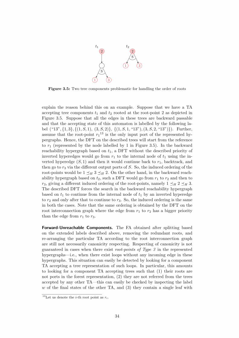
2

t1

1 3

S

2

t2

1 3

S

Figure 3.5: Two tree components problematic for handling the order of roots

explain the reason behind this on an example. Suppose that we have a TAaccepting tree components t1 and t2 rooted at the root-point 2 as depicted inFigure 3.5. Suppose that all the edges in these trees are backward passableand that the accepting state of this automaton is labelled by the following la-bel (“13”, {1, 3}, {(1, S, 1), (3, S, 2)}, {(1, S, 1, “13”), (3, S, 2, “13”)}). Further,assume that the root-point r1

13 is the only input port of the represented hy-pergraphs. Hence, the DFT on the described trees will start from the referenceto r1 (represented by the node labelled by 1 in Figure 3.5). In the backwardreachability hypergraph based on t1, a DFT without the described priority ofinverted hyperedges would go from r1 to the internal node of t1 using the in-verted hyperedge (S, 1) and then it would continue back to r1, backtrack, andthen go to r3 via the different output ports of S. So, the induced ordering of theroot-points would be 1 (H 3 (H 2. On the other hand, in the backward reach-ability hypergraph based on t2, such a DFT would go from r1 to r2 and then tor3, giving a different induced ordering of the root-points, namely 1 (H 2 (H 3.The described DFT forces the search in the backward reachability hypergraphbased on t1 to continue from the internal node of t1 by an inverted hyperedgeto r2 and only after that to continue to r3. So, the induced ordering is the samein both the cases. Note that the same ordering is obtained by the DFT on theroot interconnection graph where the edge from r1 to r2 has a bigger prioritythan the edge from r1 to r3.

Forward-Unreachable Components. The FA obtained after splitting basedon the extended labels described above, removing the redundant roots, andre-arranging the particular TA according to the root interconnection graphare still not necessarily canonicity respecting. Respecting of canonicity is notguaranteed in cases when there exist root-points of Type 3 in the representedhypergraphs—i.e., when there exist loops without any incoming edge in thesehypergraphs. This situation can easily be detected by looking for a componentTA accepting a tree representation of such loops. In particular, this amountsto looking for a component TA accepting trees such that (1) their roots arenot ports in the forest representation, (2) they are not referred from the treesaccepted by any other TA—this can easily be checked by inspecting the labelw of the final states of the other TA, and (3) they contain a single leaf with

13Let us denote the i-th root point as ri.

34

a root reference to itself—this can be checked by inspecting the labels w andY of the accepting states of the concerned TA. The canonisation procedurethen rearranges the concerned TA such that the root of each accepted tree isthe smallest node according to the above described depth-first traversal on Hbr

(i.e., the node that should be the canonically chosen root-point of Type 3). In-tuitively, this amounts to a rotation of the concerned backward reachable loopsrepresented by tree automata rules so that the nodes that are identified as theroot-points become the roots of the tree representation.More formally, let Ar be the TA that we need to rotate, r being the number

of Ar in the concerned FA, and let (wAr , Y Ar , ZAr

1 , ZAr

2 ) be the label associatedwith the accepting states of Ar. The states of Ar that accept the nodes thatshould become the new roots are identified as follows. Let k be the numberof the root-point from where the DFT on the represented hypergraphs comes(without passing through any other root-points) to the nodes corresponding tothe roots of the tree components represented by Ar. Identifying k is easy sincexAk

is the predecessor of xAr in the DFT performed on the root interconnectiongraph. The edge from xAk

to xAr exists in the root reference reachabilitygraph due to existence of a backward passable path from the root of each treerepresented by Ar to a root reference to k. Existence of this path is capturedby the label ZAr

1 , concretely by an element (x, S, i) ∈ ZAr

1 .14

Now, the TA Ar = (Qr,Σ,∆r, Fr) can be rotated as described in the fol-lowing. Let R = (. . . , qi1 , . . . , qi2 , . . .)

a→ q ∈ ∆ be a rule such that the w

label of qi1 contains r, and the Z1 label of qi2 contains (k, S, i).15 Such a ruleappears exactly once in each run of A since a reference to r may appear onlyonce at the leaf level (otherwise we would not be dealing with a root-pointof Type 3), and also Si can link with a single leaf only (otherwise we wouldobtain a nondeterministic hypergraph). If there are more rules like R in Ar,then we may split Ar to several automata containing a single rule of the de-scribed kind, and process each of the automata separately (which we assumeto be the case in the following). When we transform Ar to A′

r that acceptstrees in which the concerned loops are represented in the appropriately rotatedway, the rule R is redirected to a newly introduced accepting state, the rulesthat used to originally lead to accepting states are redirected to states origi-nally reading a reference to r, and reading a reference to r while going to q isallowed. Formally, for some qfin )∈ Qr, A

′r = (Qr ∪ {qfin},Σ,∆

′r, {qfin}) where

∆′ = (∆r \ ({R}∪ {

r→ q}))∪∆

′′. The set of the newly added rules is defined as

∆′′ = {(. . . , qi1 , . . . , qi2 , . . .)

a→ qfin} ∪ {(q1, . . . , qk)

b→ qr | (q1, . . . , qk)

b→ qf ∈

∆r, qf ∈ Fr,r→ qr ∈ ∆r} ∪ {

r→ q}.

As a consequence of the rotation, the final state of the rotated TA may havea different label (w, Y, Z1, Z2) than the original one.16 This may cause thatthe FA with the new TA inside has a different root interconnection graph and

14If there are more backward passable paths from the roots of the trees represented by Ar toa root reference to k, then each such path has a different record in Z

Ar

1 . In such a case,we choose the one with the smallest (S, i).

15Note that qi1 and qi2 can appear swapped on the left-hand side of the rule too.16The order of root references in the string w can be different, and in each (k, S, i, w′) ∈ Z2,

w′ can be ordered differently as well. Y and Z1 stay unchanged.

35

hence different ordering of the roots. Therefore after each TA rotation, werecompute the root reachability graph and reorder the forest. Note that theorder of the roots that are originally ordered before the root of the rotatedTA is not affected. Therefore, even if there are more root-points of Type 3, therotations on each of them will be done at most once, and hence the canonisationprocedure terminates.As we have already mentioned before, the described procedure yields FA that

strongly respect canonicity which allows us to check properness and box-con-nectedness by computing the reachability relation on the roots of the FA.

3.6 Conclusions and Future Work

With the aim of obtaining a formalism suitable for representing sets of heaps, wehave introduced forest automata as a formalism for representing sets of graphs,decomposed into tree components. We have discussed various properties of thisformalism. First of all, we have shown how one can obtain a canonical represen-tation of a given set of graphs. Furthermore, we have shown that the languageinclusion of canonical forest automata can be efficiently decided by translatingthem into tree automata. In addition, we have proposed a hierarchical extensionof forest automata, which on one hand greatly increases the expressive powerof our formalism, but on the other hand, certain operations—such as languageinclusion checking—become more complicated. For this reason, we have alsodemonstrated that these operations can be safely approximated. Experimentswith the verification approach based on FA that we present in the next chaptershow that the proposed notion of FA can be quite useful in practice. Theseresults also indicate that the approximate inclusion checking is sufficient inpractice.An interesting area for the future work which has not been investigated so

far is a characterisation of the class of graphs (heaps) which can be describedby hierarchical forest automata. Moreover, even though our experiments showthat the approximate inclusion checking on hierarchical FA that we have pro-posed is quite successful in practice, it would be interesting to know whether(precise) inclusion checking on FA is decidable (and efficiently implementable).A somewhat related problem, which we will come across in the next chapter, isthen the problem of computing intersections of FA (which we will also approxi-mate in Section 4.5). Finally, one can also consider extending FA by recursivelynested boxes. They would greatly increase the expressive power of the formal-ism, however, it is so far unclear how to implement the required algorithms oversuch an extension.

36

4 Forest Automata-based Verification

In this chapter, we build on the notion of forest automata, and we proposea forest-automata-based verification procedure for sequential programs manip-ulating complex dynamically linked data structures. We concentrate on pro-grams manipulating various forms of singly- and doubly-linked lists (SLL/DLL),possibly cyclic, shared, hierarchical, and/or having various additional selectors(e.g., head pointers, tail pointers, data, etc.), as well as various forms of trees.We, in particular, consider C pointer manipulation, but our approach can beeasily applied to any other similar language. We focus on safety properties ofthe considered programs, which includes generic properties like absence of nulldereferences, double free operations, dealing with dangling pointers, or memoryleakage. Furthermore, to check various shape properties of the involved datastructures, one can use testers, i.e., parts of code which, in case some desiredproperty is broken, lead the control flow to a designated error location.

As we have sketched already at the beginning of Chapter 3, in our forest-automata-based representation, a heap is split in a canonical way into severaltree components such that roots of the trees correspond to cut-points. The treecomponents can refer to the roots of each other. Using this decomposition, setsof heaps with a bounded number of cut-points are then represented by forestautomata. Moreover, we allow alphabets of FA to contain nested FA, allowingus to also represent sets of heaps with an unbounded number of cut-points,which is necessary in many practical cases (e.g., when one deals with sets ofDLLs). Finally, since FA are not closed under union, we work with sets of forestautomata.A fundamental property of our newly proposed formalism of forest automata

is that C program statements manipulating pointers can be easily encoded asoperations modifying FA. Due to this and due to the fact that FA are basedon tree automata, we can build on the concept of abstract regular tree modelchecking (see [BHRV06b] or Section 2.5) to obtain a new symbolic verificationprocedure for the considered class of programs. The procedure then works asfollows: The algorithm maintains a set of visited program configurations anda set of program configurations which need to be processed. At the begin-ning, the set of visited program configurations is empty, and the set of programconfigurations waiting to be processed contains the initial configuration of theprogram to be analysed which consists of the initial assignment of programvariables, the empty heap, and the program counter pointing to the first in-struction of the program. Then, the algorithm iteratively picks one waitingprogram configuration and performs a symbolic execution of the appropriateprogram statement. This essentially means that one takes a forest automatonrepresenting a set of heaps and transforms it into a new forest automaton. Theset of heaps represented by the newly obtained forest automaton reflects the

37

change within the heap caused by the execution of the given program state-ment. In addition to that, one can also apply abstraction in order to be ableto obtain sets of all reachable configurations, which are typically infinite, ina finite number of steps. In the next step, the algorithm checks whether thenewly created program configuration is covered by the set of already visitedprogram configurations by means of testing inclusion of languages representedby forest automata. If the newly obtained symbolic configuration is not coveredby the set of visited program configurations, it is inserted into the set of waitingprogram configurations. The process then continues by picking another waitingconfiguration. During the symbolic execution, the algorithm checks whether theverified code behaves properly, i.e., it does not dereference invalid pointers, itdoes not produce memory leaks, etc. If the program does not operate properly,the procedure is immediately terminated, and an error is reported. If the set ofwaiting configurations becomes empty, the procedure terminates and outputsthat the program is safe.When an error is encountered, it remains to find out whether it is reachable

within the original program, or it was encountered due to an excessive abstrac-tion. In order to check, whether the error is indeed reachable, one can executethe corresponding trace without the abstraction. If such trace cannot be exe-cuted, then the set of reachable program configurations is over-approximatedtoo much, and the abstraction needs to be refined. The refinement can be doneglobally which is, however, not very efficient. A better solution is to use thecounterexample-guided abstraction refinement as introduced in the frameworkof abstract regular tree model checking (see again [BHRV06b] or Section 2.5).For that to work, one needs to be able to execute the error trace backwardswhich is discussed later on.Our approach has been implemented in a prototype tool called Forester as

a gcc plug-in. This allows us to demonstrate that the proposed approach isvery promising as the tool can successfully handle multiple highly non-trivialcase studies (for some of which we are not aware of any other tool that couldhandle them fully automatically).

Plan of the Chapter. The rest of this chapter is organised as follows. In Sec-tion 4.1, we describe how we perform symbolic execution of C program state-ments over FA. Section 4.2 provides the main loop of our verification procedure.In Section 4.3, we present an algorithm for automatic discovery of nested FA.The problem of abstraction is described in Section 4.4. Section 4.5 discusseshow an error trace suspected to lead to an error can be executed backwards inorder to obtain an abstraction refinement if the error is spurious. In Section 4.6,we experimentally evaluate the performance of our prototype tool based on FA.Section 4.7 contains information about related work. Finally, Section 4.8 con-cludes the chapter.

38

4.1 Symbolic Execution

In this section, we make more precise the way we encode heaps using FA (refin-ing the main idea sketched in Section 3.1 when motivating the notion of FA),and we describe the symbolic execution of C programs over sets of hierarchicalFA, which is at the heart of our verification procedure. We consider sequential,non-recursive C programs manipulating dynamically linked data structures viathe following program statements:

• x = y,

• x = y->s,

• x = null,

• x->s = y,

• x->s = d where d is a constant of data domain,

• malloc(x), and

• free(x)

together with pointer and data equality tests and common control flow state-ments as discussed in more details below1. Each allocated cell may have severalnext pointer selectors and also selectors containing data from some finite do-main2. We use Sel to denote the set of all selectors and Data to denote the datadomain. The cells may be pointed by program variables whose set is denotedas Var below.

4.1.1 Executing C Statements on Hypergraphs

A single heap configuration can be viewed as a deterministic (Sel ∪Data∪Var)-labelled hypergraph with the ranking function being such that #e(x) = 1 ⇔ x ∈Sel and #e(x) = 0 ⇔ x ∈ Data ∪ Var . In the hypergraph, the nodes representallocated memory cells. Selectors are represented by the unary hyperedgeslabelled by elements of Sel . The nullary hyperedges labelled by elements ofData ∪ Var represent data values and program variables3. Input ports of thehypergraphs are nodes pointed to by program variables. Null and undefinedvalues are modelled as two special nodes null and undef.The symbolic computation of reachable heap configurations is done over the

control flow graph (CFG) obtained from the program under verification. A con-trol flow action a, corresponding to one of the supported statements, appliedto a hypergraph G (i.e., to a single configuration) returns a hypergraph a(G)that is obtained from G as follows:

1Most C statements for pointer manipulation can be translated the listed statements, in-cluding most type casts. The problem of restricted pointer arithmetic is discussed inSection 4.1.4.

2No abstraction for such data is considered.3Below, to simplify the informal description, we say that a node is labelled by a variableinstead of saying that the variable labels a nullary hyperedge leaving from that node.

39

• Non-destructive actions x = y, x = y->s, or x = null remove the x-labelfrom its current position and label with it the node pointed by y, thes-successor of that node, or the null node, respectively.

• The destructive action x->s = y replaces the edge (vx, s, v) by the edge(vx, s, vy) where vx and vy are the nodes pointed to by x and y, respec-tively. Further, malloc(x) moves the x-label to a newly created node,free(x) removes the node pointed to by x (and links x and all variablesaliased to x with undef), and x->s = dnew replaces the edge (vx, dold ) bythe edge (vx, dnew ).

• Evaluating a guard g applied on G amounts to a simple test of equalityof nodes or equality of data fields of nodes.

Dereferences of null and undef are of course detected (as an attempt to followa non-existing hyperedge), and an error is announced. Emergence of garbage isdetected iff a(G) is not well-connected.

4.1.2 Executing C Statements on FA

We, however, compute not on single hypergraphs representing particular heapsbut on sets of them represented by sets of canonicity respecting hierarchical FA(SCFA). Below, we first refine the description of the way we represent sets ofheaps via FA (sketched in Section 3.1). Then, we present the different stepsin which we symbolically execute C statements over FA. Next, we explain howpointer updates can be applied to it. Finally, we provide an example of thesymbolic execution.

Heap Encoding Details. As described in Chapter 3, in order to representsets of heaps using SCFA, we first decompose a (Sel ∪ Data ∪ Var)-labelledhypergraph into a forest of unordered, (Sel ∪Data ∪Var)-labelled trees. Then,the forest of unordered, (Sel ∪ Data ∪ Var)-labelled trees is transformed intoa forest of ordered, (Sel ∪ Data ∪ Var)∗-labelled trees in which the alphabet(Sel ∪ Data ∪ Var)∗ is ranked using the ranking function #v which is definedrecursively as follows:

#v(ε) = 0#v(xα) = #e(x) + #v(α)

In addition to that, we also decouple the selectors and their values (i.e., the val-ues are stored within dedicated nodes) in order to handle ordinary and pointerdata in a uniform way (selectors are always represented by a graph edge, nomatter what type of data they contain). As a result, we obtain a forest of treesin which a node can be labelled by:

• (Sel ∪ Var)∗ if it is a root,

• Sel∗ if it is an internal node, or

• Data if it is a leaf (we consider that the set Data also contains all possibleroot references).

40

Phases of Symbolic Execution. In order to be able to implement the sym-bolic execution on SCFA along the edges of a given CFG, we need to be ableto compute the following. For a given control flow action (or guard) x anda hierarchical SCFA S, we need to symbolically compute an SCFA x(S) s.t.!x(S)" equals {x(G) | G ∈ !S"} if x is an action and {G ∈ !S" | x(G)} if x isa guard.We derive the SCFA x(S) from S in several steps in which we process each

CFA F ∈ S separately. The first phase is materialisation where we unfoldnested SFA representing boxes that hide data values or pointers referred to byx. We note that we are unfolding only SFA in the closest neighbourhood ofthe involved pointer variables; thus, on the level of TA, we touch only nestedSFA adjacent to roots. In the next phase, we introduce auxiliary roots for everynode referred to by x (as discussed in Section 4.1.3) to the forest representation.Third, we perform the actual update, which due to the previous step amountsto manipulation with roots only. Last, we repeatedly fold (apply) boxes andnormalise (transform the obtained SFA into a canonicity respecting form) untilno further box can be applied, so that we end up with an SCFA. We notethat like the operation of unfolding, folding is also done only in the closestneighbourhood of roots.Unfolding is, loosely speaking, done by replacing a TA rule labelled by

a nested SFA by the nested SFA itself (plus the appropriate binding of statesof the top-level SFA to ports of the nested SFA). Conversely to unfolding, thefolding is done by replacing the part of the top-level SFA by a single rule la-belled by the nested SFA. More details on how we actually perform the foldingare provided in Section 4.3.

Pointer Updates. Before performing the actual update, we check whether theoperation tries to access the successors of null or undef nodes in which casewe have encountered a null or undefined pointer dereference. Otherwise, wecontinue by performing one of the following actions, depending on the particularstatement:

• x = y, x = null: x is removed from all labels in which it appears. Thenwe label by x each transition that is labelled by y (or by null, respec-tively).

• malloc(x): x is removed from all labels in which it appears. Then a newtree automaton accepting exactly a single tree encoding a single heapnode pointed by x and having undefined successors is added.

• x = y->s: x is removed from all labels in which it appears. Then the TAwhich accepts nodes pointed by y is split (as described in Section 4.1.3below) at the selector s, and the transitions of the newly created TAleading to its accepting state, at which y->s is accepted, are labelledby x.

• x->s = y: The TA that accepts nodes pointed by variable x is split at theselector s. Provided that qf is an accepting state and qs accepts a reference

41

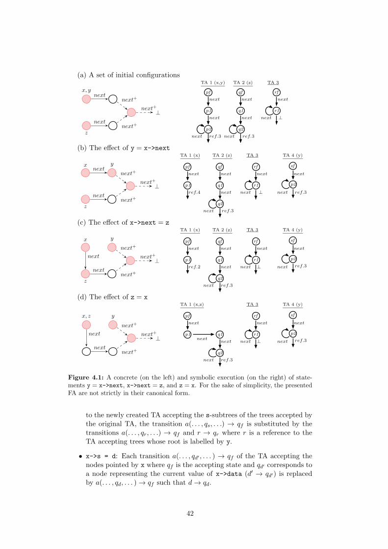
(a) A set of initial configurations

x, y

z

⊥

nextnext+

nextnext+

next+

next next

q1

qf

TA 2 (z) TA 3

next

r1

rfpf

p1

p2 q2

TA 1 (x,y)

next

ref.3

next

nextnext

ref.3

next

⊥

(b) The effect of y = x->next

x y

z

⊥

nextnext+

nextnext+

next+

next

qfpf

r1

rf

TA 1 (x) TA 2 (z) TA 3

p1

q2

q1

TA 4 (y)

p2

sf

next

next

ref.4

next

next

ref.3

next

⊥

next

ref.3

next

(c) The effect of x->next = z

x y

z

⊥next

next+

nextnext+

next+

next

qfpf

r1

rf

TA 1 (x) TA 2 (z) TA 3

p1

q2

q1 p2

sf

TA 4 (y)

ref.2

next next

next

ref.3

next

next ⊥

next

ref.3

next

(d) The effect of z = x

x, z y

⊥next

next+

nextnext+

next+

next

pf

r1

rf

TA 1 (x,z) TA 3

p1

q2

q1 p2

sf

TA 4 (y)

next

next

ref.3

next

next ⊥

next

ref.3next

next

Figure 4.1: A concrete (on the left) and symbolic execution (on the right) of state-ments y = x->next, x->next = z, and z = x. For the sake of simplicity, the presentedFA are not strictly in their canonical form.

to the newly created TA accepting the s-subtrees of the trees accepted bythe original TA, the transition a(. . . , qs, . . .) → qf is substituted by thetransitions a(. . . , qr, . . .) → qf and r → qr where r is a reference to theTA accepting trees whose root is labelled by y.

• x->s = d: Each transition a(. . . , qd′ , . . . ) → qf of the TA accepting thenodes pointed by x where qf is the accepting state and qd′ corresponds toa node representing the current value of x->data (d′ → qd′) is replacedby a(. . . , qd, . . . ) → qf such that d → qd.

42

• free(x): In the first phase, we split the TA that accepts nodes pointedby x to more TA such that all successors of the original root become rootsas well (i.e., the modified TA represents a set of single memory nodes).Then, the TA accepting nodes pointed by x is removed from the givenFA, and x is added to the label associated with the special undef node.

• Tests over pointer variables and data stored in cells pointed to by variablesare evaluated by examining labels of the rules leading to the acceptingstates of the TA that accept trees whose roots represent nodes pointedby the concerned pointer variables. These rules contain all the neededinformation (e.g., testing equality of pointer variables means that thesevariables should be associated with the same root node). After each test,the original SFA is split into two SFA—one of them accepts the trees thatsatisfy the tested condition, and the other one accepts the trees which donot satisfy it.

The execution of the particular program statement is followed by checkingwhether all TA components within a newly obtained CFA are reachable fromprogram variables. If an unreachable component is found we have encountereda memory leak.

Example of Symbolic Execution. A simplified example of a symbolic execu-tion is provided in Figure 4.1. In the left part of the figure, we provide concreteheaps (the dashed edges represent sequences of one or more edges linked intoa linked-list), and in the right part, we provide their forest automata repre-sentation (top-down tree automata are used within the example in order toimprove the readability). The initial configuration is depicted in Figure 4.1(a), and Figures 4.1 (b), (c), and (d) represent the sets of heaps obtained aftersuccessively applying the statements x = y->next, x->next = z, and z = x.

4.1.3 Introduction of Auxiliary Roots

In certain cases, one cannot execute the effect of a program statement directlyon the FA at hand. For example, consider an FA F and the statement y :=

x->s. Here, for any hypergraph represented by F , x points to a cut-pointthat corresponds to the roots of the trees accepted by some component TA ofF . We want y to point to the node which is reachable from the node pointedto by x via the selector s. After executing the statement, y will point toa cut-point. However, it may be the case that the node x->s (i.e., the nodethat is the successor of the node pointed to by x via the selector s) is currentlynot a cut-point, and it is accepted at an ordinary automaton state (not anaccepting state as in the case of the root). Therefore, the TA accepting treeswhose roots are pointed to by x has to be split into a new pair of TA such thatthe first automaton accepts trees that have a reference to the second automatonas the s-successors of their roots nodes, and the second automaton describesthe part of the heap starting at the x->s nodes in the trees accepted by theoriginal automaton (see Figures 4.1 (a) and (b)).

43

Note that it may happen that in some trees accepted by the given TA, a splitis needed whereas in the others not. This can happen when in the trees acceptedby the TA there is a tree where x->s is a root reference and another one wherex->s is an intermediate node (accepted at an ordinary state). As an example,there may be sequences of s-selectors below the node pointed by x of lengthone or more. This can be represented by a TA with a single accepting state q,and the transition function

∆ = {s(q) → q, s(r) → q, null → r}.

For length one, one does not need to introduce a new root since some root (nullin this case) is already reached via s, which is, however, not the case for theother lengths. In such a scenario, the TA has to be first divided into two TAsuch that the first one accepts trees which need to be split whereas the otheraccepts trees which do not need such a split (this can be done by inspecting thetransitions in the immediate neighbourhood of the accepting states), and thenthe split is done only in the latter case. In particular case of our example, wedivide ∆ into

∆1 = {s(r) → q′, null → r}∆2 = {s(q) → q′, s(q) → q, s(r) → q, null → r}

where q′ is the newly created accepting state.We now formalise the problem of adding auxiliary roots under the assump-

tion that the TA to be split contains a single transition leading to an acceptingstate only and that the accepting state does not appear inside any left handside of a rule of the TA. A general TA can easily be transformed into a set ofseveral TA such that they all satisfy these restrictions. Let A = (Q,Σ,∆, {qf})be the TA that we want to split, let a(. . . , qs, . . .) → qf ∈ ∆ be the only transi-tion that leads to qf , and let qs ∈ Q be the state at which the nodes accessiblevia the selector s from the roots of the trees accepted by A are accepted. Wereplace A by TA A1 and A2 such that A1 references A2 via s. Formally,A1 = (Q,Σ,∆′, {qf}), ∆

′ = ∆ \ {a(. . . , qs, . . .) → qf} ∪ {a(. . . , qr, . . .) →qf , r → qr} where r is a root reference to the newly created TA A2, andA2 = (Q,Σ,∆, {qs}). Since this transformation may cause that many statesof A1 and A2 become useless, the automata are subsequently reduced (by firstremoving useless states and subsequently by using, for instance, techniques forsimulation-based reduction of nondeterministic automata).

4.1.4 Restricted Pointer Arithmetic

In addition to the statements listed at the beginning of Section 4.1, we alsohandle a restricted pointer arithmetic arising from the use of the & C operator(an operator taking the address of an object in memory) and the operators +/-defined over pointers. Note that a support of this feature is crucial, e.g., fordealing with linked data structures in the form used in system software suchas the Linux kernel. There, one can, for instance, encounter data structureswhich are linked via embedded headers located at certain non-zero offset from

44

. . . . . .

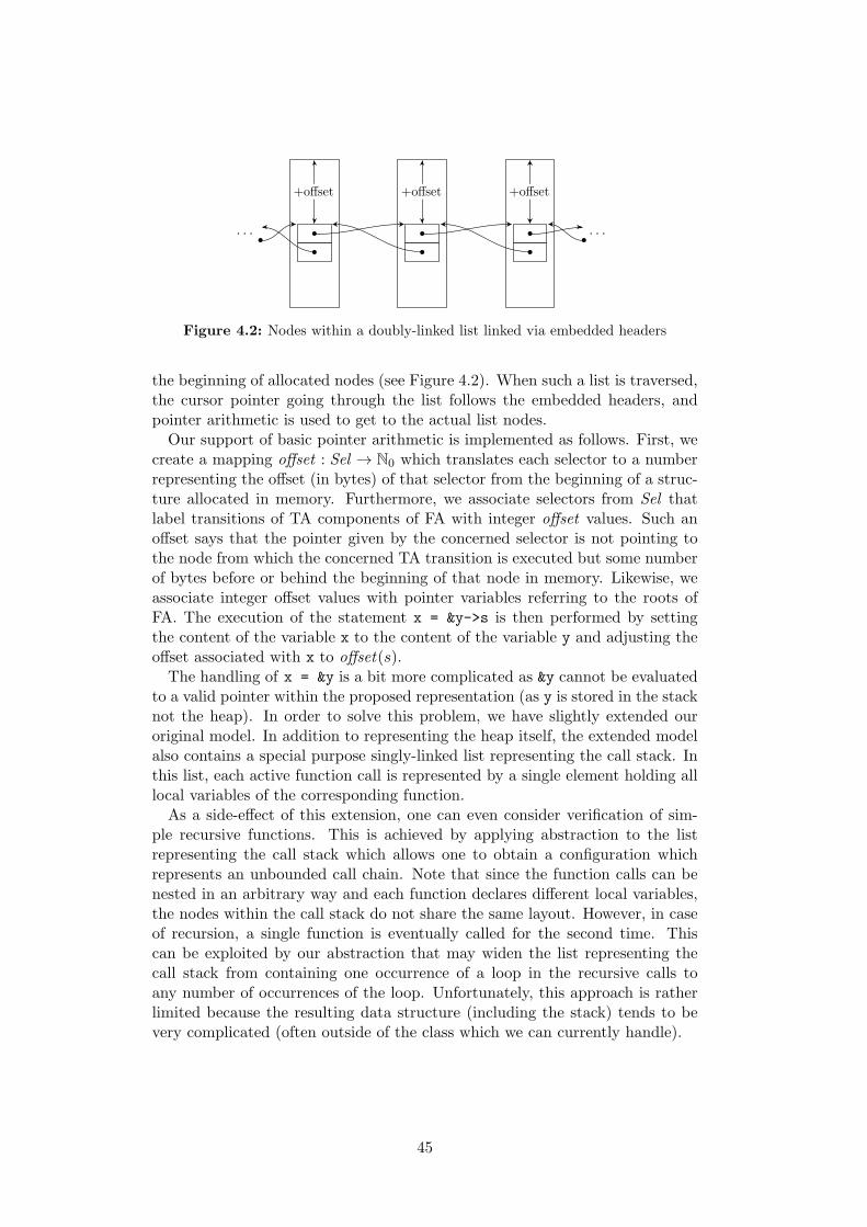
+offset +offset +offset

Figure 4.2: Nodes within a doubly-linked list linked via embedded headers

the beginning of allocated nodes (see Figure 4.2). When such a list is traversed,the cursor pointer going through the list follows the embedded headers, andpointer arithmetic is used to get to the actual list nodes.Our support of basic pointer arithmetic is implemented as follows. First, we

create a mapping offset : Sel → N0 which translates each selector to a numberrepresenting the offset (in bytes) of that selector from the beginning of a struc-ture allocated in memory. Furthermore, we associate selectors from Sel thatlabel transitions of TA components of FA with integer offset values. Such anoffset says that the pointer given by the concerned selector is not pointing tothe node from which the concerned TA transition is executed but some numberof bytes before or behind the beginning of that node in memory. Likewise, weassociate integer offset values with pointer variables referring to the roots ofFA. The execution of the statement x = &y->s is then performed by settingthe content of the variable x to the content of the variable y and adjusting theoffset associated with x to offset(s).

The handling of x = &y is a bit more complicated as &y cannot be evaluatedto a valid pointer within the proposed representation (as y is stored in the stacknot the heap). In order to solve this problem, we have slightly extended ouroriginal model. In addition to representing the heap itself, the extended modelalso contains a special purpose singly-linked list representing the call stack. Inthis list, each active function call is represented by a single element holding alllocal variables of the corresponding function.As a side-effect of this extension, one can even consider verification of sim-

ple recursive functions. This is achieved by applying abstraction to the listrepresenting the call stack which allows one to obtain a configuration whichrepresents an unbounded call chain. Note that since the function calls can benested in an arbitrary way and each function declares different local variables,the nodes within the call stack do not share the same layout. However, in caseof recursion, a single function is eventually called for the second time. Thiscan be exploited by our abstraction that may widen the list representing thecall stack from containing one occurrence of a loop in the recursive calls toany number of occurrences of the loop. Unfortunately, this approach is ratherlimited because the resulting data structure (including the stack) tends to bevery complicated (often outside of the class which we can currently handle).

45

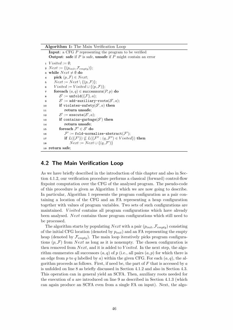
Algorithm 1: The Main Verification Loop

Input: a CFG P representing the program to be verifiedOutput: safe if P is safe, unsafe if P might contain an error

1 V isited := ∅;2 Next := {(pinit,Fempty)};3 while Next )= ∅ do4 pick (p,F) ∈ Next;5 Next := Next \ {(p,F)};6 V isited := V isited ∪ {(p,F)};7 foreach (a, q) ∈ successors(P, p) do8 S ′ := unfold({F}, a);9 S ′ := add-auxiliary-roots(S ′, a);

10 if violates-safety(S ′, a) then11 return unsafe;12 S ′ := execute(S ′, a);13 if contains-garbage(S ′) then14 return unsafe;15 foreach F ′ ∈ S ′ do16 F ′ := fold-normalise-abstract(F ′);17 if L({F ′}) )⊆ L({F ′′ : (q,F ′′) ∈ V isited}) then18 Next := Next ∪ {(q,F ′)}

19 return safe;

4.2 The Main Verification Loop

As we have briefly described in the introduction of this chapter and also in Sec-tion 4.1.2, our verification procedure performs a classical (forward) control-flowfixpoint computation over the CFG of the analysed program. The pseudo-codeof this procedure is given as Algorithm 1 which we are now going to describe.In particular, Algorithm 1 represents the program configuration as a pair con-taining a location of the CFG and an FA representing a heap configurationtogether with values of program variables. Two sets of such configurations aremaintained. V isited contains all program configurations which have alreadybeen analysed. Next contains those program configurations which still need tobe processed.The algorithm starts by populating Next with a pair (pinit,Fempty) consisting

of the initial CFG location (denoted by pinit) and an FA representing the emptyheap (denoted by Fempty). The main loop iteratively picks program configura-tions (p,F) from Next as long as it is nonempty. The chosen configuration isthen removed from Next, and it is added to V isited. In the next step, the algo-rithm enumerates all successors (a, q) of p (i.e., all pairs (a, p) for which there isan edge from p to q labelled by a) within the given CFG. For each (a, q), the al-gorithm proceeds as follows. First, if need be, the part of F that is accessed by ais unfolded on line 8 as briefly discussed in Section 4.1.2 and also in Section 4.3.This operation can in general yield an SCFA. Then, auxiliary roots needed forthe execution of a are introduced on line 9 as described in Section 4.1.3 (whichcan again produce an SCFA even from a single FA on input). Next, the algo-

46

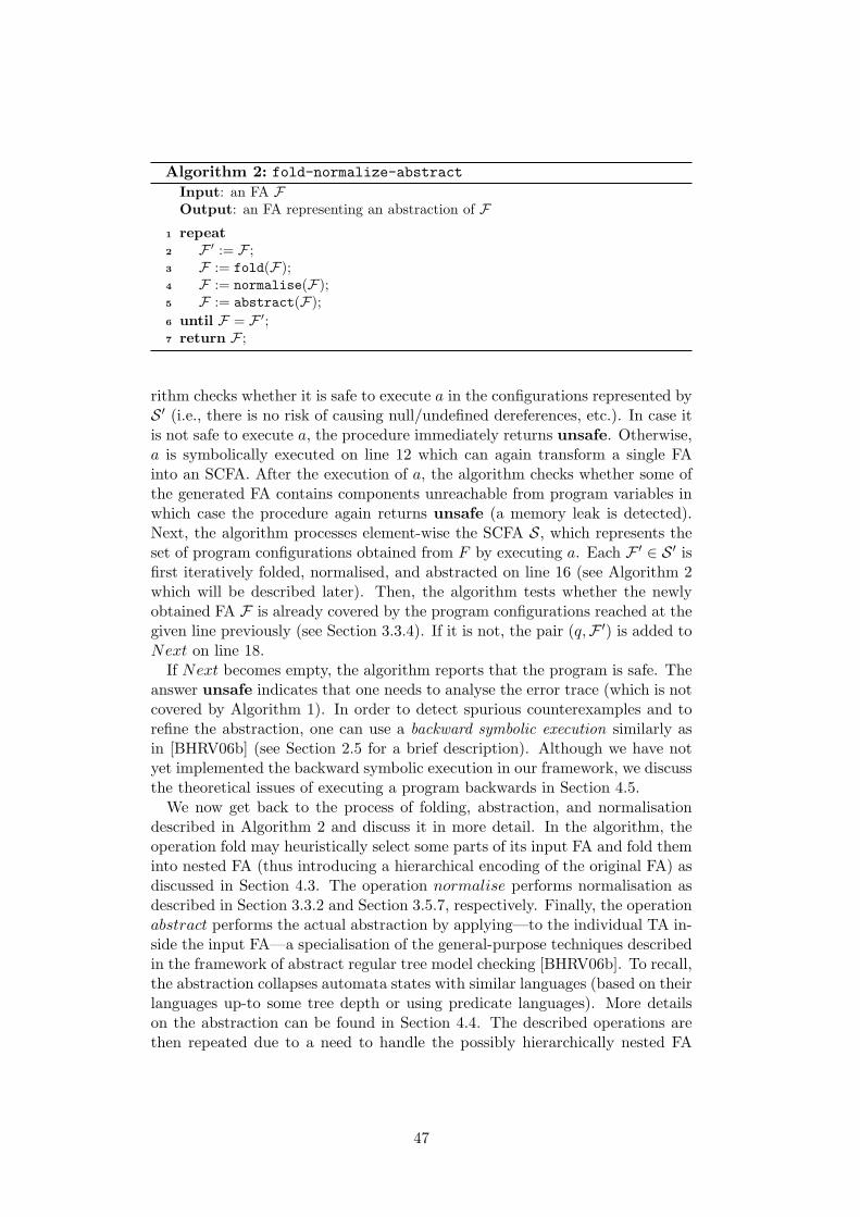
Algorithm 2: fold-normalize-abstract

Input: an FA FOutput: an FA representing an abstraction of F

1 repeat2 F ′ := F ;3 F := fold(F);4 F := normalise(F);5 F := abstract(F);

6 until F = F ′;7 return F ;

rithm checks whether it is safe to execute a in the configurations represented byS ′ (i.e., there is no risk of causing null/undefined dereferences, etc.). In case itis not safe to execute a, the procedure immediately returns unsafe. Otherwise,a is symbolically executed on line 12 which can again transform a single FAinto an SCFA. After the execution of a, the algorithm checks whether some ofthe generated FA contains components unreachable from program variables inwhich case the procedure again returns unsafe (a memory leak is detected).Next, the algorithm processes element-wise the SCFA S, which represents theset of program configurations obtained from F by executing a. Each F ′ ∈ S ′ isfirst iteratively folded, normalised, and abstracted on line 16 (see Algorithm 2which will be described later). Then, the algorithm tests whether the newlyobtained FA F is already covered by the program configurations reached at thegiven line previously (see Section 3.3.4). If it is not, the pair (q,F ′) is added toNext on line 18.If Next becomes empty, the algorithm reports that the program is safe. The

answer unsafe indicates that one needs to analyse the error trace (which is notcovered by Algorithm 1). In order to detect spurious counterexamples and torefine the abstraction, one can use a backward symbolic execution similarly asin [BHRV06b] (see Section 2.5 for a brief description). Although we have notyet implemented the backward symbolic execution in our framework, we discussthe theoretical issues of executing a program backwards in Section 4.5.We now get back to the process of folding, abstraction, and normalisation

described in Algorithm 2 and discuss it in more detail. In the algorithm, theoperation fold may heuristically select some parts of its input FA and fold theminto nested FA (thus introducing a hierarchical encoding of the original FA) asdiscussed in Section 4.3. The operation normalise performs normalisation asdescribed in Section 3.3.2 and Section 3.5.7, respectively. Finally, the operationabstract performs the actual abstraction by applying—to the individual TA in-side the input FA—a specialisation of the general-purpose techniques describedin the framework of abstract regular tree model checking [BHRV06b]. To recall,the abstraction collapses automata states with similar languages (based on theirlanguages up-to some tree depth or using predicate languages). More detailson the abstraction can be found in Section 4.4. The described operations arethen repeated due to a need to handle the possibly hierarchically nested FA

47

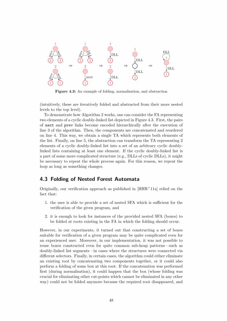
1

2 2

2

1 1

nextp

rev

nextp

rev

⇒

1

2 2

2

1

DLLp

rev

next

⇒

1

2

2

1

DLL

DLL

⇒

1

1

DLL

DLL

⇒

1

1

DLL

DLL

Figure 4.3: An example of folding, normalisation, and abstraction

(intuitively, these are iteratively folded and abstracted from their more nestedlevels to the top level).To demonstrate how Algorithm 2 works, one can consider the FA representing

two elements of a cyclic doubly-linked list depicted in Figure 4.3. First, the pairsof next and prev links become encoded hierarchically after the execution ofline 3 of the algorithm. Then, the components are concatenated and reorderedon line 4. This way, we obtain a single TA which represents both elements ofthe list. Finally, on line 5, the abstraction can transform the TA representing 2elements of a cyclic doubly-linked list into a set of an arbitrary cyclic doubly-linked lists containing at least one element. If the cyclic doubly-linked list isa part of some more complicated structure (e.g., DLLs of cyclic DLLs), it mightbe necessary to repeat the whole process again. For this reason, we repeat theloop as long as something changes.

4.3 Folding of Nested Forest Automata

Originally, our verification approach as published in [HHR+11a] relied on thefact that:

1. the user is able to provide a set of nested SFA which is sufficient for theverification of the given program, and

2. it is enough to look for instances of the provided nested SFA (boxes) tobe folded at roots existing in the FA in which the folding should occur.

However, in our experiments, it turned out that constructing a set of boxessuitable for verification of a given program may be quite complicated even foran experienced user. Moreover, in our implementation, it was not possible toreuse boxes constructed even for quite common sub-heap patterns—such asdoubly-linked list segments—in cases where the structures were connected viadifferent selectors. Finally, in certain cases, the algorithm could either eliminatean existing root by concatenating two components together, or it could alsoperform a folding of some box at this root. If the concatenation was performedfirst (during normalisation), it could happen that the box (whose folding wascrucial for eliminating other cut-points which cannot be eliminated in any otherway) could not be folded anymore because the required root disappeared, and

48

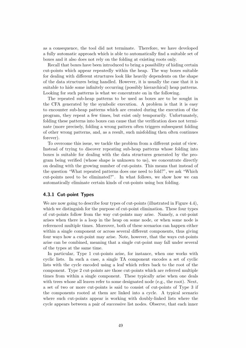
as a consequence, the tool did not terminate. Therefore, we have developeda fully automatic approach which is able to automatically find a suitable set ofboxes and it also does not rely on the folding at existing roots only.Recall that boxes have been introduced to bring a possibility of hiding certain

cut-points which appear repeatedly within the heap. The way boxes suitablefor dealing with different structures look like heavily dependents on the shapeof the data structures being handled. However, it is usually the case that it issuitable to hide some infinitely occurring (possibly hierarchical) heap patterns.Looking for such patterns is what we concentrate on in the following.The repeated sub-heap patterns to be used as boxes are to be sought in

the CFA generated by the symbolic execution. A problem is that it is easyto encounter sub-heap patterns which are created during the execution of theprogram, they repeat a few times, but exist only temporarily. Unfortunately,folding these patterns into boxes can cause that the verification does not termi-nate (more precisely, folding a wrong pattern often triggers subsequent foldingof other wrong patterns, and, as a result, such misfolding then often continuesforever).To overcome this issue, we tackle the problem from a different point of view.

Instead of trying to discover repeating sub-heap patterns whose folding intoboxes is suitable for dealing with the data structures generated by the pro-gram being verified (whose shape is unknown to us), we concentrate directlyon dealing with the growing number of cut-points. This means that instead ofthe question “What repeated patterns does one need to fold?”, we ask “Whichcut-points need to be eliminated?”. In what follows, we show how we canautomatically eliminate certain kinds of cut-points using box folding.

4.3.1 Cut-point Types

We are now going to describe four types of cut-points (illustrated in Figure 4.4),which we distinguish for the purpose of cut-point elimination. These four typesof cut-points follow from the way cut-points may arise. Namely, a cut-pointarises when there is a loop in the heap on some node, or when some node isreferenced multiple times. Moreover, both of these scenarios can happen eitherwithin a single component or across several different components, thus givingfour ways how a cut-point may arise. Note, however, that the ways cut-pointsarise can be combined, meaning that a single cut-point may fall under severalof the types at the same time.In particular, Type 1 cut-points arise, for instance, when one works with

cyclic lists. In such a case, a single TA component encodes a set of cycliclists with the cycle encoded using a leaf which refers back to the root of thecomponent. Type 2 cut-points are those cut-points which are referred multipletimes from within a single component. These typically arise when one dealswith trees whose all leaves refer to some designated node (e.g., the root). Next,a set of two or more cut-points is said to consist of cut-points of Type 3 ifthe components rooted at them are linked into a cycle. A typical scenariowhere such cut-points appear is working with doubly-linked lists where thecycle appears between a pair of successive list nodes. Observe, that each inner

49

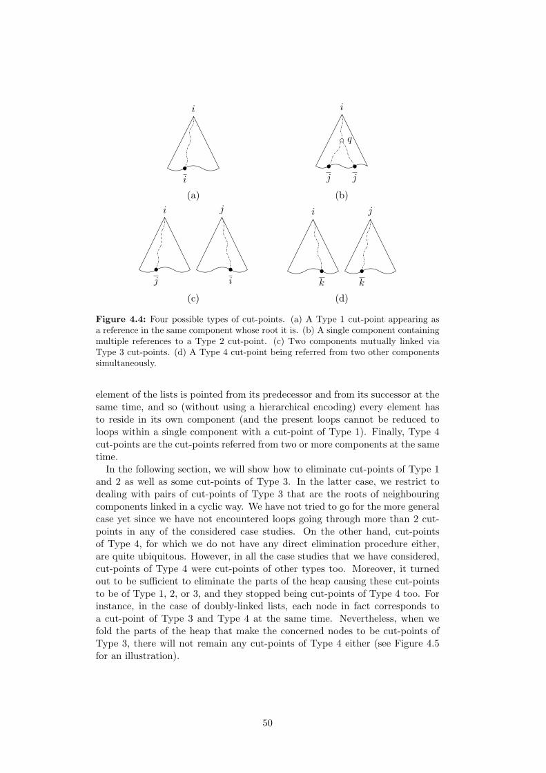
i

i

j j

i

q

(a) (b)

j

i

i

j

k

i

k

j

(c) (d)

Figure 4.4: Four possible types of cut-points. (a) A Type 1 cut-point appearing asa reference in the same component whose root it is. (b) A single component containingmultiple references to a Type 2 cut-point. (c) Two components mutually linked viaType 3 cut-points. (d) A Type 4 cut-point being referred from two other componentssimultaneously.

element of the lists is pointed from its predecessor and from its successor at thesame time, and so (without using a hierarchical encoding) every element hasto reside in its own component (and the present loops cannot be reduced toloops within a single component with a cut-point of Type 1). Finally, Type 4cut-points are the cut-points referred from two or more components at the sametime.In the following section, we will show how to eliminate cut-points of Type 1

and 2 as well as some cut-points of Type 3. In the latter case, we restrict todealing with pairs of cut-points of Type 3 that are the roots of neighbouringcomponents linked in a cyclic way. We have not tried to go for the more generalcase yet since we have not encountered loops going through more than 2 cut-points in any of the considered case studies. On the other hand, cut-pointsof Type 4, for which we do not have any direct elimination procedure either,are quite ubiquitous. However, in all the case studies that we have considered,cut-points of Type 4 were cut-points of other types too. Moreover, it turnedout to be sufficient to eliminate the parts of the heap causing these cut-pointsto be of Type 1, 2, or 3, and they stopped being cut-points of Type 4 too. Forinstance, in the case of doubly-linked lists, each node in fact corresponds toa cut-point of Type 3 and Type 4 at the same time. Nevertheless, when wefold the parts of the heap that make the concerned nodes to be cut-points ofType 3, there will not remain any cut-points of Type 4 either (see Figure 4.5for an illustration).

50

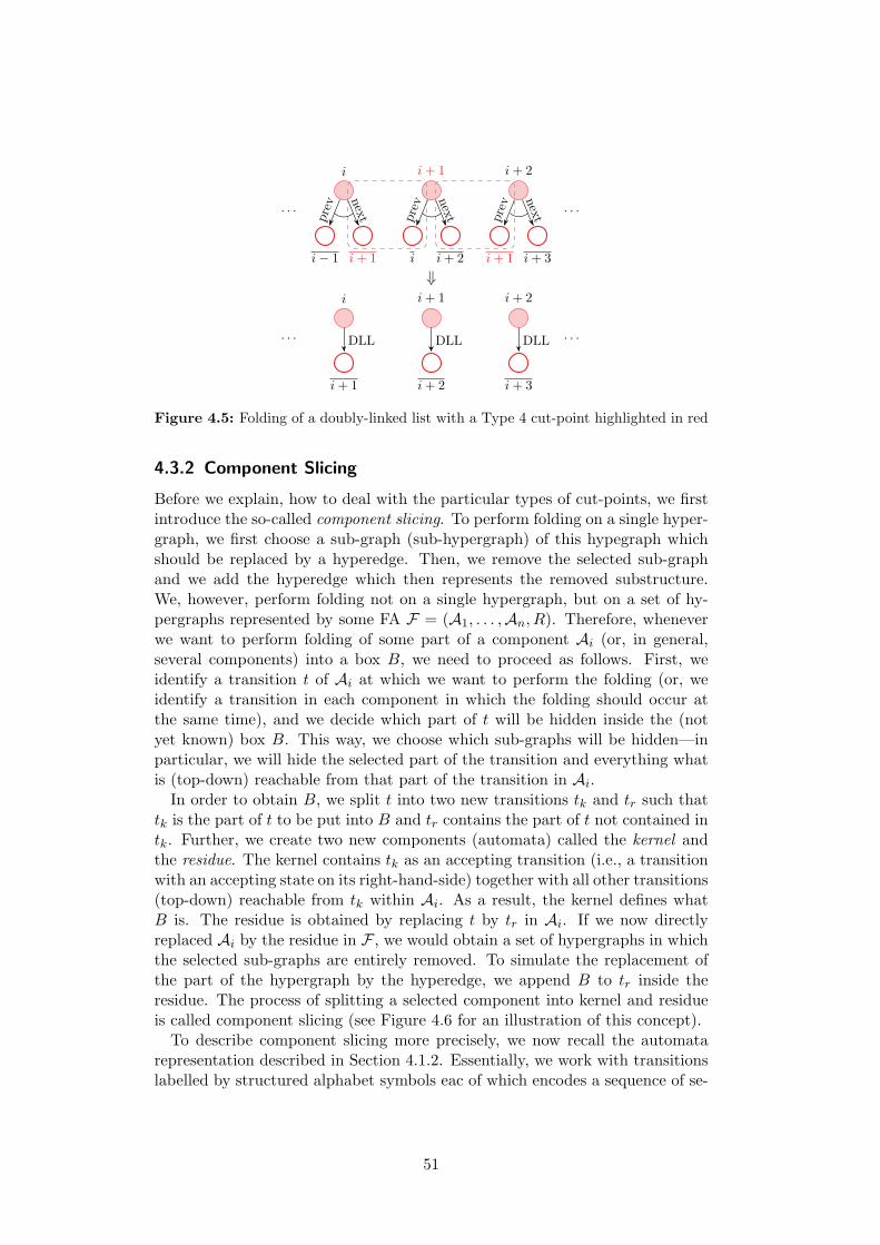
i

i− 1 i+ 1

i+ 1

i i+ 2

i+ 2

i+ 1 i+ 3

nextp

rev n

extprev n

extprev. . . . . .

⇓i

i+ 1

i+ 1

i+ 2

i+ 2

i+ 3

DLL DLL DLL. . . . . .

Figure 4.5: Folding of a doubly-linked list with a Type 4 cut-point highlighted in red

4.3.2 Component Slicing

Before we explain, how to deal with the particular types of cut-points, we firstintroduce the so-called component slicing. To perform folding on a single hyper-graph, we first choose a sub-graph (sub-hypergraph) of this hypegraph whichshould be replaced by a hyperedge. Then, we remove the selected sub-graphand we add the hyperedge which then represents the removed substructure.We, however, perform folding not on a single hypergraph, but on a set of hy-pergraphs represented by some FA F = (A1, . . . ,An, R). Therefore, wheneverwe want to perform folding of some part of a component Ai (or, in general,several components) into a box B, we need to proceed as follows. First, weidentify a transition t of Ai at which we want to perform the folding (or, weidentify a transition in each component in which the folding should occur atthe same time), and we decide which part of t will be hidden inside the (notyet known) box B. This way, we choose which sub-graphs will be hidden—inparticular, we will hide the selected part of the transition and everything whatis (top-down) reachable from that part of the transition in Ai.In order to obtain B, we split t into two new transitions tk and tr such that

tk is the part of t to be put into B and tr contains the part of t not contained intk. Further, we create two new components (automata) called the kernel andthe residue. The kernel contains tk as an accepting transition (i.e., a transitionwith an accepting state on its right-hand-side) together with all other transitions(top-down) reachable from tk within Ai. As a result, the kernel defines whatB is. The residue is obtained by replacing t by tr in Ai. If we now directlyreplaced Ai by the residue in F , we would obtain a set of hypergraphs in whichthe selected sub-graphs are entirely removed. To simulate the replacement ofthe part of the hypergraph by the hyperedge, we append B to tr inside theresidue. The process of splitting a selected component into kernel and residueis called component slicing (see Figure 4.6 for an illustration of this concept).To describe component slicing more precisely, we now recall the automata

representation described in Section 4.1.2. Essentially, we work with transitionslabelled by structured alphabet symbols eac of which encodes a sequence of se-

51

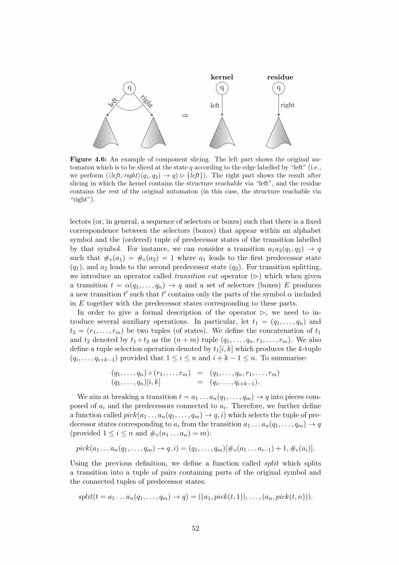
kernel residue

q

left

right

⇒

q

left

q

right

Figure 4.6: An example of component slicing. The left part shows the original au-tomaton which is to be sliced at the state q according to the edge labelled by “left” (i.e.,we perform (〈left , right〉(q1, q2) → q) ✄ {left}). The right part shows the result afterslicing in which the kernel contains the structure reachable via “left”, and the residuecontains the rest of the original automaton (in this case, the structure reachable via“right”).

lectors (or, in general, a sequence of selectors or boxes) such that there is a fixedcorrespondence between the selectors (boxes) that appear within an alphabetsymbol and the (ordered) tuple of predecessor states of the transition labelledby that symbol. For instance, we can consider a transition a1a2(q1, q2) → qsuch that #e(a1) = #e(a2) = 1 where a1 leads to the first predecessor state(q1), and a2 leads to the second predecessor state (q2). For transition splitting,we introduce an operator called transition cut operator (✄) which when givena transition t = α(q1, . . . , qn) → q and a set of selectors (boxes) E producesa new transition t′ such that t′ contains only the parts of the symbol α includedin E together with the predecessor states corresponding to these parts.In order to give a formal description of the operator ✄, we need to in-

troduce several auxiliary operations. In particular, let t1 = (q1, . . . , qn) andt2 = (r1, . . . , rm) be two tuples (of states). We define the concatenation of t1and t2 denoted by t1 ◦ t2 as the (n+m) tuple (q1, . . . , qn, r1, . . . , rm). We alsodefine a tuple selection operation denoted by t1[i, k] which produces the k-tuple(qi, . . . , qi+k−1) provided that 1 ≤ i ≤ n and i+ k − 1 ≤ n. To summarise:

(q1, . . . , qn) ◦ (r1, . . . , rm) = (q1, . . . , qn, r1, . . . , rm)(q1, . . . , qn)[i, k] = (qi, . . . , qi+k−1).

We aim at breaking a transition t = a1 . . . an(q1, . . . , qm) → q into pieces com-posed of ai and the predecessors connected to ai. Therefore, we further definea function called pick(a1 . . . an(q1, . . . , qm) → q, i) which selects the tuple of pre-decessor states corresponding to ai from the transition a1 . . . an(q1, . . . , qm) → q(provided 1 ≤ i ≤ n and #v(a1 . . . an) = m):

pick(a1 . . . an(q1, . . . , qm) → q, i) = (q1, . . . , qm)[#v(a1 . . . ai−1) + 1,#e(ai)].

Using the previous definition, we define a function called split which splitsa transition into a tuple of pairs containing parts of the original symbol andthe connected tuples of predecessor states:

split(t = a1 . . . an(q1, . . . , qm) → q) = ((a1, pick(t, 1)), . . . , (an, pick(t, n))).

52

In order to transform a tuple containing separated parts of the symbol andcorresponding tuples of states into a transition, we define a complementaryfunction to split called join which, given a tuple of pairs of the above form anda state, creates a new transition as follows ((s1 . . . sn) denotes the concatenationof tuples s1 ◦ s2 ◦ · · · ◦ sn):

join(((a1, s1), . . . , (an, sn)), q) = a1 . . . an(s1 . . . sn) → q

At this point, we are able to split a transition into pieces and then join thesepieces back together. We, however, do not intend to join all of the original piecesbut only some subset of them. Therefore, we also define a filtering function Φf ,which (depending on a Boolean function f) removes certain elements of thetuple it receives as the input:

Φf () = ()

Φf (x1, . . . , xn) =

{

(x1) · Φf (x2, . . . , xn) if f(x1)Φf (x2, . . . , xn) otherwise

Finally, we are ready to give the definition of the operator t✄E which first splitsthe given transition t, then it keeps only those pairs containing elements of theset E, and, in the last step, it joins the remaining pairs into a new transition:

(t = α(q1, . . . , qn) → q)✄ E = join(Φf (split(t)), q)

where f((a, s)) ⇐⇒ a ∈ E.Now, for a given state q, a fixed symbol α = a1 . . . an, and a given set of

selectors (boxes) E ⊆ {a1, . . . , an}, slicing of a component TA works as follows.We first create a kernel and a residue as two separate copies of the componentto be sliced. Then, in the kernel, we replace each transition t of the formα(q1, . . . , qm) → q by the transition t ✄ E. Contrary to that, we replace eachtransition t of the form α(q1, . . . , qm) → q by the transition t✄({a1, . . . , an}\E)in the residue.Note that all steps within our symbolic execution produce automata in which

all transitions of the form α(. . . ) → q are labelled by the same symbol α (i.e.,{α(. . . ) → q,α′(. . . ) → q} ⊆ ∆ ⇒ α = α′). Moreover, the abstraction nevercollapses states q1 and q2 if there exist transitions α(. . . ) → q1 and α′(. . . ) → q2such that α )= α′ (see Section 4.4). Hence, we assume that the symbol isalways specified implicitly by the state q, and we in the following parametrisecomponent slicing by a state and a set of selectors (boxes) only.

4.3.3 Cut-point Elimination

In this section, we discuss the automatic elimination of cut-points of type 1,2, and 3. As we have already mentioned, it might happen that some cut-pointis of more than one type which is solved by several applications of the foldingalgorithm. The heuristic, which currently seems to give the best results in ourexperiments, eliminates cut-points in the order 3, 2, and 1.

53

Type 1. A Type 1 cut-point (c.f. Figure 4.4 (a)) corresponds to a componentwhich contains references to its own root (these are called self-references in thefollowing). To eliminate such cut-point, we want to “hide” all the self-referencesinto a box. Therefore, we identify a set E of all selectors (or boxes) within theaccepting transitions which lie on some path going to some self-reference (forthis, we conveniently use labels introduced in Section 3.3.2). Then, we performslicing of the component parametrised by the appropriate accepting state andthe set E from the previous step to obtain a kernel containing all self-referencesand a residue containing the rest. Next, we perform a DFT on the kernel andwe rename all references R ⊆ {1, . . . , n} that appear in the kernel accordingto the order in which they are visited (such that the self-references are alwaysrelabelled to 0) to obtain a mapping f : R → {0, . . . , |R| − 1}. The relabelledkernel is transformed into a new box B such that #e(B) = |R|−1. All acceptingtransitions α(q1, . . . , qn) → q of the residue are modified to

αB(q1, . . . , qn, r1, . . . , r#e(B)) → q

where rj is a state representing a reference to a root u such that f(u) = j (i.e.,the additional predecessor states encode the mapping f and, as a result alsothe correspondence between the root references appearing inside the box andthe root references appearing on the level on which the box is used)4. As thelast step, we replace the original component by the modified residue.Note that the process of folding can easily be reversed whenever needed.

First, we extract the mapping f . Then, we relabel the root references insidethe box using f−1, and we replace the given box in some transition t by therelabelled component.

Type 2. A Type 2 cut-point arises when the reference to that cut-point appearsmultiple times within a single component (c.f. Figure 4.4 (b)). In this case, weare therefore interested in folding the smallest part of the component containingall the references inside a box which will then allow us to reduce the number ofreferences to the given cut-point to one whenever used. In order to perform thefolding as efficiently as possible, we first identify a state q whose subtrees containall the root references to the given cut-point and none of its predecessor stateshas this property (see Figure 4.4 (b)). If there are more such states, the foldingis performed separately for each of them. In the next step, we identify the set ofselectors (boxes) E lying on some path to the given cut-point reference startingat a node corresponding to q. Then, we perform slicing of the componentparametrised by q and E. The kernel of the slicing is transformed into a boxB which is then appended to the residue in the same manner as in the case ofcut-points of Type 1.

Type 3. To eliminate a pair of Type 3 cut-points i,j (i.e., the cut-points mutu-ally referring to each other—see Figure 4.4 (c)), we need to use a box encoding

4Here, for the sake of simplicity, we ignore the fact that the selectors and the boxes areordered, hence B should not be put simply behind α. However, the procedure can easilybe extended to respect the ordering.

54

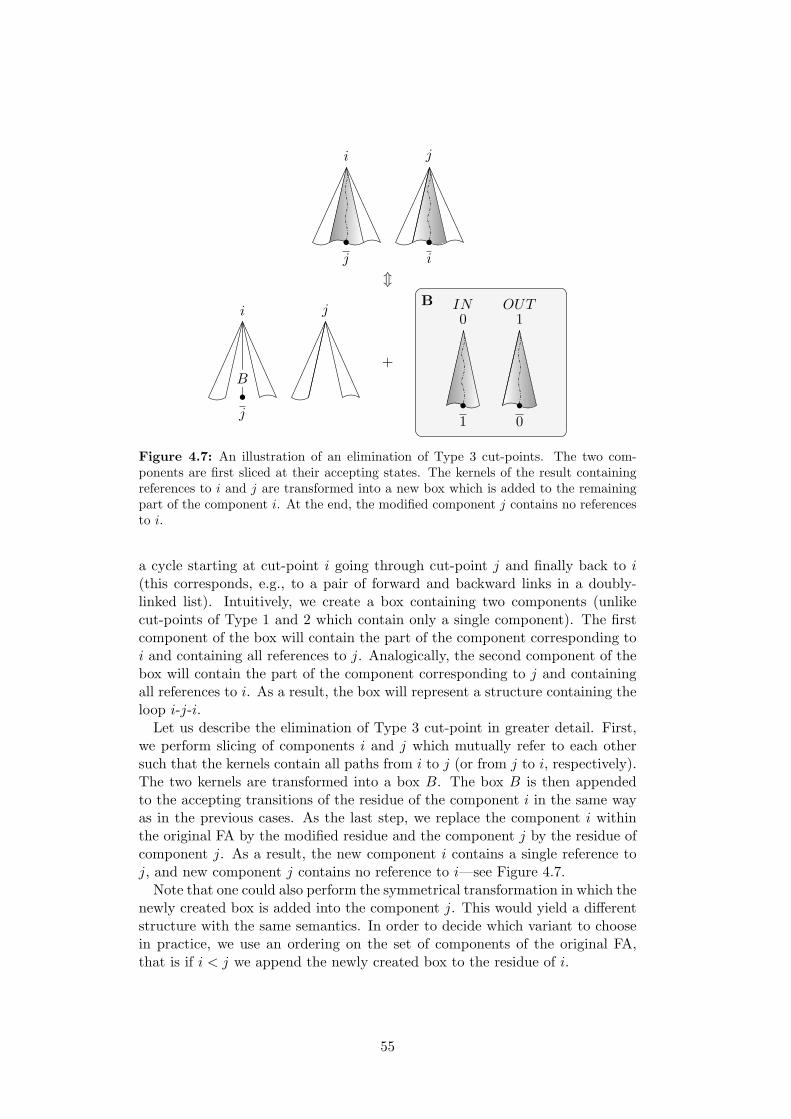
j

i

i

j

9

j

i

B

j

+

1

0IN

0

1OUTB

Figure 4.7: An illustration of an elimination of Type 3 cut-points. The two com-ponents are first sliced at their accepting states. The kernels of the result containingreferences to i and j are transformed into a new box which is added to the remainingpart of the component i. At the end, the modified component j contains no referencesto i.

a cycle starting at cut-point i going through cut-point j and finally back to i(this corresponds, e.g., to a pair of forward and backward links in a doubly-linked list). Intuitively, we create a box containing two components (unlikecut-points of Type 1 and 2 which contain only a single component). The firstcomponent of the box will contain the part of the component corresponding toi and containing all references to j. Analogically, the second component of thebox will contain the part of the component corresponding to j and containingall references to i. As a result, the box will represent a structure containing theloop i-j-i.Let us describe the elimination of Type 3 cut-point in greater detail. First,

we perform slicing of components i and j which mutually refer to each othersuch that the kernels contain all paths from i to j (or from j to i, respectively).The two kernels are transformed into a box B. The box B is then appendedto the accepting transitions of the residue of the component i in the same wayas in the previous cases. As the last step, we replace the component i withinthe original FA by the modified residue and the component j by the residue ofcomponent j. As a result, the new component i contains a single reference toj, and new component j contains no reference to i—see Figure 4.7.

Note that one could also perform the symmetrical transformation in which thenewly created box is added into the component j. This would yield a differentstructure with the same semantics. In order to decide which variant to choosein practice, we use an ordering on the set of components of the original FA,that is if i < j we append the newly created box to the residue of i.

55

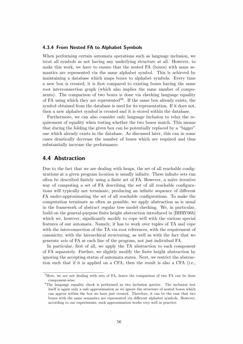
4.3.4 From Nested FA to Alphabet Symbols

When performing certain automata operations such as language inclusion, wetreat all symbols as not having any underlying structure at all. However, tomake this work, we have to ensure that the nested FA (boxes) with same se-mantics are represented via the same alphabet symbol. This is achieved bymaintaining a database which maps boxes to alphabet symbols. Every timea new box is created, it is first compared to existing boxes having the sameroot interconnection graph (which also implies the same number of compo-nents). The comparison of two boxes is done via checking language equalityof FA using which they are represented56. If the same box already exists, thesymbol obtained from the database is used for its representation. If it does not,then a new alphabet symbol is created and it is stored within the database.Furthermore, we can also consider only language inclusion to relax the re-

quirement of equality when testing whether the two boxes match. This meansthat during the folding the given box can be potentially replaced by a “bigger”one which already exists in the database. As discussed later, this can in somecases drastically decrease the number of boxes which are required and thussubstantially increase the performance.

4.4 Abstraction

Due to the fact that we are dealing with heaps, the set of all reachable config-urations at a given program location is usually infinite. These infinite sets canoften be described finitely using a finite set of FA. However, a naıve iterativeway of computing a set of FA describing the set of all reachable configura-tions will typically not terminate, producing an infinite sequence of differentFA under-approximating the set of all reachable configurations. To make thecomputation terminate as often as possible, we apply abstraction as is usualin the framework of abstract regular tree model checking. We, in particular,build on the general-purpose finite height abstraction introduced in [BHRV06b]which we, however, significantly modify to cope well with the various specialfeatures of our automata. Namely, it has to work over tuples of TA and copewith the interconnection of the TA via root references, with the requirement ofcanonicity, with the hierarchical structuring, as well as with the fact that wegenerate sets of FA at each line of the program, not just individual FA.In particular, first of all, we apply the TA abstraction to each component

of FA separately. Further, we slightly modify the finite height abstraction byignoring the accepting status of automata states. Next, we restrict the abstrac-tion such that if it is applied on a CFA, then the result is also a CFA (i.e.,

5Here, we are not dealing with sets of FA, hence the comparison of two FA can be donecomponent-wise.

6The language equality check is performed as two inclusion queries. The inclusion testitself is again only a safe approximation as we ignore the structure of nested boxes whichcan appear within the box we have just created. Therefore, it can be the case that twoboxes with the same semantics are represented via different alphabet symbols. However,according to our experiments, such approximation works very well in practice.

56

the abstraction preserves the canonicity respecting status). Subsequently, wepropose a further refinement of the abstraction based on more precise trackingof the paths between roots and root references even in cases when some of thesepaths are hidden in nested FA. Finally, we show how the abstract symbolic com-putation may be accelerated by enriching CFA that are generated at a certainline by the languages of the other CFA generated at the same line as a part ofa single SCFA.The rest of the section is organised as follows. We first introduce the prin-

ciple of quotienting automata w.r.t. an equivalence relation as a basis for ourabstraction. Next, we recall the equivalence based on languages of trees upto some height introduced as a general-purpose equivalence for abstracting au-tomata in the framework of abstract regular tree model checking (which weslightly modify by ignoring the accepting status of states). Subsequently, weintroduce our specialised abstraction which preserves canonicity, followed bycombining it with the basic finite height abstraction. Afterwards, we proposea further refinement of the abstraction which allows one to distinguish (to someextent) trees having different sets of paths (possibly hidden in nested FA) be-tween their roots and the particular root references. Finally, we show how onecan abstract SCFA in a better way than by separately abstracting each of theirCFA.

4.4.1 Automata Quotienting

We now formalise the notion of equivalence-based automata quotienting. LetA = (Q,Σ,∆, F ) be a tree automaton and ≈ be an equivalence on Q. Thequotient automaton A/≈ is obtained from A by collapsing its states accordingto ≈ (i.e., the set of states of A/≈ is obtained by taking the partition of Qinduced by ≈). Let [q] = {q′ ∈ Q : q′ ≈ q}. Then,

A/≈ = ({[q] : q ∈ Q},Σ,∆′, {[q] : q ∈ F})

where ∆′ = {a([q1], . . . , [qn]) → [q] : a(q1, . . . , qn) → q ∈ ∆}. We extend the

previous notion to a forest automaton F = (A1, . . . ,An, R) by creating quotient(tree) automata for each component separately:

F/≈ = (A1/≈, . . . ,An/≈, R).

Next, we need to clarify what relation ≈ we use in order to obtain the ab-straction. In fact, we use two relations over the set of states. Our abstractionis based on the equivalence of languages of bounded height (see [BHRV06b] orSection 2.5), but we also want to preserve the overall shape of the heap, andtherefore we also use a structure-preserving equivalence based on the reacha-bility of root references. We discuss both of the equivalences in the followingsubsections.

4.4.2 Equivalence of Languages of Bounded Height

Our equivalence of languages of bounded height is based on the idea of finiteheight abstraction from [BHRV06b], but instead of considering languages of

57

1 2 3next next

{1, 2} {3}

next

next

(a) (b)

Figure 4.8: An example of abstraction. (a) An automaton representing a list contain-ing 2 elements. (b) An abstracted automaton representing a set of lists containing atleast 1 element obtained using ≈1. For the sake of simplicity, we use word automatanotation here.

trees of some restricted height, it considers sets of all trees of height at most kthat can be read by the automata while getting to some state. This approachis, in fact, a generalisation of trace languages considered in [BHV04] for wordsto trees.Formally, let A = (Q,Σ,∆, F ) be a tree automaton and t be a tree over Σ.

The tree stub of t of height k (denoted by t|k) is the restriction of t defined as

t|k = t|⋃ki=0 N

i = {(p, a) : p ∈ dom(t) ∩k⋃

i=0

Ni ∧ t(p) = a}.

Then, for a state q, the language of height k denoted by L|k(q) is the set of alltree stubs of height n of trees which can be accepted by q:

L|k(q) = {t|k : t ∈ L(q)}.

Finally, we say that the states q1 and q2 are equivalent up to height k iff theyhave the same languages of height k:

q1 ≈k q2 ⇐⇒ L|k(q1) = L|k(q2).

In practice, we have obtained the best results with using the simplest ≈1

equivalence (refined by the below described specialised equivalences). The ef-fect of the abstraction based on the ≈1 equivalence is depicted in Figure 4.8.Using the ≈1 equivalence means that we allow the abstraction to treat memorynodes with the same layout of selectors (or, roughly speaking, memory nodes ofthe same type in the typing system of the C language) as equal no matter whatdata they contain7. Using this information together with the below introducedspecialised refinements turned out to be sufficient in all the considered casestudies. On the other hand, attempts to replace some of the specialised refine-ments by increasing the abstraction height were unsuccessful due to either notbeing precise enough or due to preventing too many states from being collapsedand thus causing an explosion in the size of the automata being handled.

7Indeed, the values of data are represented by separate child nodes. In order to make theabstraction data-aware, one needs to use at least ≈2.

58

4.4.3 Canonicity Preserving Equivalence

Given an FA F , the abstraction based on the equivalence of languages ofbounded height can in general produce some FA F/≈k which is not consistent,i.e., it might happen that one could pick a forest F from the correspondingcomponents of F/≈k such that ⊗F is not defined (one can, for example, ob-tain a forest in which one attempts to define the same selector multiple timesfor a single node). Moreover, we also want the abstraction to keep the basicshape of the heap unchanged, meaning that the abstraction should not touchthe interconnection among the components. In other words, if a certain root isreferenced only once before the abstraction, it should be referenced only onceafter the abstraction as well, no cut-point reference should suddenly appear ordisappear, etc. In order to better understand why this is important, one canimagine having a tree which contains a single root reference to some particularnode (represented as a root of a different component). Now, an unrestrictedabstraction could create a new tree containing many references to that par-ticular node which would essentially transform the tree into a directed acyclicgraph. This behaviour is, however, not desired in a large majority of cases as italmost always causes that the analysis immediately fails by reaching a spuriouscounterexample. Additionally, we also require that the abstraction applied ona canonical FA always produces an FA which is also canonical. To be precise,we want to ensure the following:

1. The order of roots visited during the depth first traversal of FA remainsunchanged.

2. If a given component contains exactly one reference to a certain rootbefore the abstraction, it also contains exactly one reference to that rootafter the abstraction.

3. The backward reachability relation remains unchanged.

To satisfy these requirements, we will take advantage of the labelling in-troduced in Section 3.5.7. Therefore, we first compute the labelling functionlabel(q) = (w, Y, Z1, Z2) introduced in Section 3.5.7 for each state q which caneasily be done assuming that we are working with canonicity respecting FA.Then, we define the so-called canonicity preserving equivalence ≈C using thelabelling function label:

q1 ≈C q2 ⇐⇒ label(q1) = label(q2).

It is not difficult to see that conditions (1), (2), and (3) from above are satisfiedunder≈C due to the fact that the equivalent states are required to have the samelabelling. Indeed, respecting the string w guarantees that the collapsed statesaccept trees with identical order of root references on the frontier. Moreover, wand Y together guarantee that the second condition is satisfied as well. Finally,respecting Z1 and Z2 preserves the backward reachability relation.

In practice, as already indicated, we combine the two above introduced equiv-alences, using finite height abstraction ≈1 based on the ≈1 equivalence. Thismeans that we use the ≈1 ∩≈C equivalence for collapsing states of the encoun-tered automata (apart from some exceptions discussed in the following section).

59

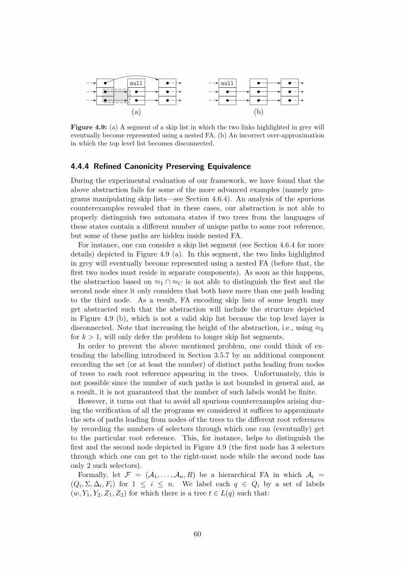
null null

(a) (b)

Figure 4.9: (a) A segment of a skip list in which the two links highlighted in grey willeventually become represented using a nested FA. (b) An incorrect over-approximationin which the top level list becomes disconnected.

4.4.4 Refined Canonicity Preserving Equivalence

During the experimental evaluation of our framework, we have found that theabove abstraction fails for some of the more advanced examples (namely pro-grams manipulating skip lists—see Section 4.6.4). An analysis of the spuriouscounterexamples revealed that in these cases, our abstraction is not able toproperly distinguish two automata states if two trees from the languages ofthese states contain a different number of unique paths to some root reference,but some of these paths are hidden inside nested FA.For instance, one can consider a skip list segment (see Section 4.6.4 for more

details) depicted in Figure 4.9 (a). In this segment, the two links highlightedin grey will eventually become represented using a nested FA (before that, thefirst two nodes must reside in separate components). As soon as this happens,the abstraction based on ≈1 ∩ ≈C is not able to distinguish the first and thesecond node since it only considers that both have more than one path leadingto the third node. As a result, FA encoding skip lists of some length mayget abstracted such that the abstraction will include the structure depictedin Figure 4.9 (b), which is not a valid skip list because the top level layer isdisconnected. Note that increasing the height of the abstraction, i.e., using ≈k

for k > 1, will only defer the problem to longer skip list segments.In order to prevent the above mentioned problem, one could think of ex-

tending the labelling introduced in Section 3.5.7 by an additional componentrecording the set (or at least the number) of distinct paths leading from nodesof trees to each root reference appearing in the trees. Unfortunately, this isnot possible since the number of such paths is not bounded in general and, asa result, it is not guaranteed that the number of such labels would be finite.

However, it turns out that to avoid all spurious counterexamples arising dur-ing the verification of all the programs we considered it suffices to approximatethe sets of paths leading from nodes of the trees to the different root referencesby recording the numbers of selectors through which one can (eventually) getto the particular root reference. This, for instance, helps to distinguish thefirst and the second node depicted in Figure 4.9 (the first node has 3 selectorsthrough which one can get to the right-most node while the second node hasonly 2 such selectors).Formally, let F = (A1, . . . ,An, R) be a hierarchical FA in which Ai =

(Qi,Σ,∆i, Fi) for 1 ≤ i ≤ n. We label each q ∈ Qi by a set of labels(w, Y1, Y2, Z1, Z2) for which there is a tree t ∈ L(q) such that:

60

• w,Z1, Z2 are as in Section 3.5.7.

• Y1 is the same as Y in Section 3.5.7.

• Y2 ⊆ {1, . . . , n}×N is a set such that (r, k) ∈ Y2 iff the root reference r canbe reached from the root of t via paths starting by k different selectors.

In order to compute the labelling, we again start by first labelling states w.r.t.the leaf rules, and then we propagate the so-far obtained labels bottom-up.The values of w, Y1, Z1, Z2 are computed as before, and Y2 is obtained asfollows. For a fixed reference r and a transition a1 . . . an(q1, . . . , qm) → q suchthat #v(a1, . . . an) = m, we compute

k =

n∑

i=1

#e(ai)∑

j=1

leadsto(#v(a1 . . . ai−1) + j) ∗ selectors(ai, j)

where leadsto(i) = 1 iff there exists k′ > 0 such that (r, k′) ∈ Y2(qi) orleadsto(i) = 0 otherwise, and selectors(ai, j) = l iff the output port j of aican be reached from the input port of ai via paths starting by l different se-lectors (or selectors(ai, j) = 1 iff ai corresponds to a plain selector). Then, weadd (r, k) to Y2(q). To obtain the number of different selectors that can appearat the beginning of the paths leading between the input and the output port ofsome nested FA, we use the Y2 labelling computed for the nested FA itself.

Next, we compute the labelling function label(q) = (w, Y1, Y2, Z1, Z2) foreach state q in a way mentioned above, and we define the refined canonicitypreserving equivalence ≈C↑ using the labelling function label:

q1 ≈C↑ q2 ⇐⇒ label(q1) = label(q2).

It immediately follows that two states can be collapsed using ≈C↑ iff they canbe collapsed using ≈C and, moreover, the corresponding trees have the samenumber of selectors that can appear at the beginning of the paths leading fromthe root to each of the different root references.

According to our experiments, the abstraction based on ≈1∩≈C↑ is sufficientfor the verification of all of the considered examples. However, if the abstrac-tion generates some counterexample in the future (which is for sure going tohappen, e.g., when one tries to enrich the technique for dealing with data-dependent data structures, such as red-black trees, or data dependent proper-ties, such as sortedness), it is possible to either adjust (increase) the height ofthe abstraction or to further refine the abstraction using predicate languages(see again [BHRV06a] or Section 2.5). Moreover, it would be also interesting tosee whether the predicate language abstraction could find the proposed refine-ment of the canonicity preserving equivalence automatically (even if this wouldcause some performance hit).A proper implementation of a fully automatic abstraction refinement based

on the predicate language abstraction remains an interesting subject for futureresearch. In Section 4.5, we will, however, make the first step towards thisgoal by proposing a way how the verified program can be executed backwardsalong a suspected counterexample trace, which is a necessary precondition forpredicate language abstraction.

61

struct Tree* buildTree() {1: struct Tree* root = NULL;

2: while (<cond>) {3: struct Tree** n = &root;

4: while (*n != NULL)

5: n = &(<cond>?(*n)->left:(*n)->right);

6: *n = newNode();

7: }8: return root;

}

Figure 4.10: A simple C function which constructs arbitrary binary trees. We assumethat Tree is a C structure containing left and right pointer fields (selectors). <cond>represents a condition which is abstracted away. newNode is a function which createsa new node and returns its address.

4.4.5 Abstraction for Sets of FA

According to our experiments, the approach presented above works quite wellfor many list-like data structures. One can observe that it is often sufficient tobuild a linked list containing 2 elements (assuming that one uses the height-1language abstraction) which is then abstracted to the set of lists containing oneor more cells. This usually amounts to symbolically executing 2 iterations ofeach loop within the program, which can be computed quite quickly. However,when one starts to deal with trees, the number of nodes, which has to beconstructed before the abstraction collapses enough states, grows considerably,especially for trees of higher arities.For instance, one can consider the function depicted in Figure 4.10. Here,

the statements on lines 2–7 are iteratively executed during the verification.Whenever the symbolic execution reaches a conditional statement or a loop

statement (as, e.g., on lines 2 and 5), and the involved condition does not evalu-ate to either true or false in the given symbolic configuration, the configurationis split into two configurations in which the condition either holds or does nothold (as described in Section 4.1.2). The symbolic execution then continues intoboth of the branches with one of the symbolic configurations arising from thesplit processed right away and the other one postponed. Now assume that theverification algorithm always first explores the left branch on line 5. Therefore,configurations representing trees consisting solely of a left branch of an increas-ing height are first generated. The generation of such trees of an increasingheight continues until the abstraction applies on line 4, producing a set of treesconsisting of an arbitrarily long left branch. At this point, the execution branchis not explored any further as it does not produce new configurations. Then,the algorithm switches back to some of the postponed branches, in which oneright successor is generated. After that, one starts to explore the left-mostbranch again, which eventually yields a set of trees in which the root has the

62

left successor or both successors, but those have left successors only. Eventu-ally, the algorithm inspects a branch which at the end yields the fixpoint of thewhile-loop in the form of a set of arbitrary binary trees (see Figure 4.11 for anillustration of the possible evolution of the set of reachable configurations inthe considered program). However, it is not difficult to see that this approachis far from optimal. Indeed, one would like to first explore the branch yield-ing the desired fixpoint. Then, while switching back the postponed branches,the verification procedure could quickly detect that no new configurations canbe generated. Unfortunately, it is not possible to efficiently decide beforehandwhich branch to take in order to reach the fixpoint sooner.In order to avoid the above problem, it would help to have a single CFA

representing all configurations reached at the given program location throughall explored execution branches. A symbolic execution from such a CFA wouldthen correspond to executing all the branches at the same time. Such a CFA,however, cannot be obtained since CFA are not closed under union even if theyhave the same number of components and the same root interconnection graph(see Section 3.3.3).Nevertheless, despite the fact that we are forced to work with SCFA, we will

now show that it is possible to use the information contained at least in all theCFA that have the same number of components and the same interconnectiongraph to improve the performance of the abstraction, especially in cases withmany execution branches (as above). This can be done as follows. Let Sbe an SCFA for the given program location. To compute an abstraction ofF = (A1, . . . ,An, R) ∈ S, we first select the subset S ′ of all the CFA of Sthat have n components and the specification R. Then, we unite the sets ofstates and transitions of the corresponding components of CFA in S ′ (assumingw.l.o.g. that these sets are disjoint) to obtain F ′ which itself inherits the setof final states from F . As a result, the languages of F and F ′ are equal, butF ′ can also contain states and transitions from the CFA in S ′ which may havebeen created in other execution branches than F . These additional states andtransitions do not lead to any any final state, but when F ′ is abstracted, it canhappen that some transitions which are unreachable in F ′ can become reachablein F ′/≈. This in turn means that the resulting language will be enriched bysome information from the other CFA. In particular, in our example, instead offirst generating trees with left branches only until the partial fixpoint is found,the extended abstraction will immediately take into account also the trees withnodes having some right successors, and hence the final fixpoint will be reachedin much fewer steps.Formally, we first define auxiliary sets Qk and ∆k for a fixed SCFA S, a fixed

number of components n, a fixed port specification R, and 1 ≤ k ≤ n:

Qk = {q ∈ Q′k : (A′

1, . . . ,A′n, R) ∈ S,A′

i = (Σ, Q′i,∆

′i, F

′i )} and

∆k = {t ∈ ∆′k : (A′

1, . . . ,A′n, R) ∈ S,A′

i = (Σ, Q′i,∆

′i, F

′i )}.

Intuitively, Qk contains union of states of all components with index k whichappear within FA having n components and specification R. Similarly ∆k

contains union of transitions of all such components. In the next step, for the

63

. . . . . . . . .

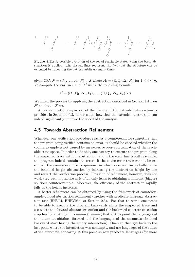
Figure 4.11: A possible evolution of the set of reachable states when the basic ab-straction is applied. The dashed lines represent the fact that the structure can beextended by repeating the pattern arbitrary many times.

given CFA F = (A1, . . . ,An, R) ∈ S where Ai = (Σ, Qi,∆i, Fi) for 1 ≤ i ≤ n,we compute the enriched CFA F ′ using the following formula:

F ′ = ((Σ,Q1,∆1, F1), . . . , (Σ,Qn,∆n, Fn), R).

We finish the process by applying the abstraction described in Section 4.4.1 onF ′ to obtain F ′/≈.An experimental comparison of the basic and the extended abstraction is

provided in Section 4.6.3. The results show that the extended abstraction canindeed significantly improve the speed of the analysis.

4.5 Towards Abstraction Refinement

Whenever our verification procedure reaches a counterexample suggesting thatthe program being verified contains an error, it should be checked whether thecounterexample is not caused by an excessive over-approximation of the reach-able state space. In order to do this, one can try to execute the program alongthe suspected trace without abstraction, and if the error line is still reachable,the program indeed contains an error. If the entire error trace cannot be ex-ecuted, the counterexample is spurious, in which case we can globally refinethe bounded height abstraction by increasing the abstraction height by oneand restart the verification process. This kind of refinement, however, does notwork very well in practice as it often only leads to obtaining a different (bigger)spurious counterexample. Moreover, the efficiency of the abstraction rapidlyfalls as the height increases.A better refinement can be obtained by using the framework of counterex-

ample-guided abstraction refinement together with predicate language abstrac-tion (see [BHV04, BHRV06b] or Section 2.5). For that to work, one needsto be able to execute the program backwards along the suspected trace andsee where the forward abstract execution and the backward concrete executionstop having anything in common (meaning that at this point the languages ofthe automata obtained forward and the languages of the automata obtainedbackward start having the empty intersection). One can then get back to thelast point where the intersection was nonempty, and use languages of the statesof the automata appearing at this point as new predicate languages (for more

64

details, see again [BHV04, BHRV06b])8. In what follows, we discuss how a pro-gram path suspected to lead to an error may be executed backwards in order tocheck whether it really leads to an error or whether it corresponds to a spuriouscounterexample (implying a need to refine the abstraction used).

4.5.1 Symbolic Execution Revisited

First, let us briefly recall some essentials of the (forward) symbolic executionof a program over FA as a basis for backward symbolic execution. The state-ments of the program are processed sequentially. The symbolic execution ofa statement over a set of configurations represented by a CFA can cause thecomputation to branch. This happens either due to several possible outcomesof the statement when it is executed over the given set of configurations and/ordue to the procedure of transforming an FA obtained as a result of the state-ment into an SCFA (which is then further processed element-wise, hence thebranching). The branching creates an execution tree whose nodes are labelledby CFA and the appropriate control line. The nodes of the tree where thecomputation can still continue are kept in memory together with some addi-tional information about the statements that generated the particular CFA.This additional information, which we will describe in more detail in the fol-lowing, allows us to reverse the effect of the corresponding statement duringthe backward symbolic execution. Once the forward symbolic execution hits anerroneous configuration, the program trace suspected to lead to an error canbe extracted by traversing the execution tree from the leaf node in which the(possible) error was detected towards the root.More precisely, assume that we have a suspected error trace—a branch of the

execution tree having the form F0, . . . ,Fn where for each 0 ≤ i ≤ n, Fi is a CFAencoding a set of possible configurations of the heap. Here, F0 represents theset of initial configurations (in our case, the empty heap), and Fn encodes a setof configurations that include some bad configurations. This means that thereis a nonempty set Bad ⊆ !Fn" of hypergraphs that are erroneous meaning thatthey, e.g., represent heaps with garbage, heaps where a value of a variable to bedereferenced is null or undef, heap configurations reached at a designated errorlocation, etc. Assume that we have a CFA FBad such that !FBad" ∩ Bad )= ∅.Such a CFA is obtained either as the result of symbolically executing a state-ment leading to a designated error line, or, in the case of generic pointer manip-ulation errors (such as null/undefined dereference, presence ofgarbage), as theresult of simply firing some pointer manipulating statement. In the latter case,the way, in which we symbolically execute pointer manipulating statements,guarantees that a CFA encoding all the configurations over which it is unsafeto execute the given statement gets generated. If an SCFA for the bad configu-rations is obtained, it can be processed element-wise. Further, we know that for

8Let us briefly recall that in case of predicate language abstraction, one has a set of predicatelanguages (represented using automata). A state is said to satisfy some predicate languageif the intersection of the language of this state and the the given predicate language isnonempty. Then, the abstraction allows one to collapse the states that satisfy the samepredicate languages.

65

every 1 ≤ i ≤ n, the CFA Fi was obtained from Fi−1 by symbolically executingsome program statement in the following four steps described in Section 4.1and also in Section 4.2:

1. materialisation (unfolding boxes represented by SCFA at the relevant FAtransitions),

2. introduction of auxiliary roots into the represented heaps (and hence com-ponent TA on the level of FA),

3. performing the actual update,

4. iterative folding, normalisation, and abstraction yielding an SCFA.

4.5.2 Backward Symbolic Execution

As usual in counterexample guided abstraction refinement, a backward execu-tion of a program trace computes a chain FBad = F ′

n,F′n−1, . . . ,F

′j of CFA

representing sets of configurations where j < n and either j ≥ 0 is the greatestindex such that !Fj" ∩ !F ′

j" = ∅ or j = 0 if there is no such index. For eachj < i ≤ n, F ′

i−1 is derived from F ′i by applying backwards the steps by which Fi

was obtained from Fi−1, but without abstraction. If j = 0 and !F ′0"∩ !F0" )= ∅,

then the backward execution reached the initial configurations which meansthat the error trace is feasible in the verified program. If !F ′

j" ∩ !Fj" = ∅ forsome j > 0, then the counterexample is spurious, and F ′

j+1 represents someconfigurations introduced by abstraction that caused the discovery of the spu-rious counterexample. In that case, we may use the pair F ′

j+1,Fj+1 to derivenew predicate languages to refine the abstraction to prevent this spurious errortrace from appearing in further verification as described in [BHV04, BHRV06a]and also briefly sketched in Section 2.5.To be able to revert Steps 1 to 4 of the symbolic execution of a program

statement in order to obtain F ′i from F ′

i+1, additional information is storedalong the computation path. More precisely, we remember where we performedfolding and unfolding (to revert Step 1 and Step 4). We also remember infor-mation needed to revert the actual update (Step 3) as described later on andthe actions which were taken in order to transform the obtained FA into CFA(Step 4). In particular, the following information is recorded for the differentsupported statements:

• x = y, x = null, x = y->s: We record the previous value of variable x

such that we can later restore its contents in the configuration obtainedduring the backward symbolic execution.

• x->s = y, x->s = d: We again keep the original value of the correspond-ing field x->s such that it can be restored if necessary.

• malloc(x): We remember the previous value of variable x. In addition,we record which component was created by malloc(x) such that it couldbe removed when computing backwards.

66

• free(x): In this case, we need to record the content of the whole nodewhich has been deleted by the statement. The reversal of this statement isthen similar to executing malloc(x), but the newly created node alreadycontains initialised fields.

Now, assume that we have computed F ′i+1 in the backward execution and we

want to revert the effect of the i-th statement. First of all, we have to revertfolding and normalisation performed as the last step of the forward execution.The folding is reverted by simply unfolding the corresponding box. The nor-malisation is reverted by splitting certain component TA (if it was recordedthat some component TA were removed during the forward execution) and byan inverse reordering of the component TA (the reordering is also recordedduring the forward execution). Next, we revert the effect of the actual updateas described above. Step 2 only introduces auxiliary roots which are redun-dant w.r.t. the canonical representation. Therefore, they can be removed byperforming the standard normalisation procedure which converts the given FAinto a CFA. Finally, the effect of unfolding performed in Step 1 is reverted byfolding if needed.

Checking Intersection of FA. Checking emptiness of the intersection !Fi" ∩!F ′

i" is an issue by itself. For two general hierarchical FA F = (A1, . . . ,An, R)and F ′ = (B1, . . . ,Bn, R), we do not know yet whether the intersection empti-ness problem is decidable. However, we can solve the problem of intersectionanalogically as in the case of checking language inclusion by using a safe approx-imation. For two FA F and F ′ having the same root interconnection graph,we can compute the automaton F ∩ F ′ = (A1 ∩ B1, . . . ,A2 ∩ B2, R) whereAi ∩ Bi is the usual intersection of two tree automata. It obviously holds that!F ∩ F ′" ⊆ !F" ∩ !F ′".Notice that by having a method that under-approximates the intersection,

the only thing that can happen is that emptiness of the intersection !Fi"∩ !F ′i"

is detected sooner during the backward execution (for a larger i) than it shouldbe, or it is detected in cases where it should not be detected at all. The onlypossible consequence of this is that we attempt to refine the abstraction insteadof signalling a real counterexample or that we refine the abstraction in a wrongway. Both of the cases can cause the computation not to terminate, but theycannot lead to introducing false positives nor false negatives.

4.6 Experimental Evaluation

We have implemented the proposed approach (up to a backward symbolic execu-tion and automatic abstraction refinement) in a prototype tool called Forester,having the form of a gcc plug-in. The core of the tool is our own library ofTA that uses the recent technology for handling nondeterministic automata(particularly, methods for reducing the size of TA and for testing language in-clusion on them [ABH+08, ACH+10], a part of that is also described later onin Chapter 5, Chapter 6, and Chapter 7).

67

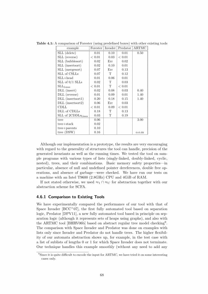
Table 4.1: A comparison of Forester (using predefined boxes) with other existing tools

example Forester Invader Predator ARTMC

SLL (delete) 0.01 < 0.10 0.01 < 0.50SLL (reverse) < 0.01 0.03 < 0.01SLL (bubblesort) 0.02 Err 0.02SLL (insertsort) 0.02 0.10 0.01SLL (mergesort) 0.07 Err 0.13SLL of CSLLs 0.07 T 0.12SLL+head 0.01 0.06 0.01SLL of 0/1 SLLs 0.02 T 0.03SLLLinux < 0.01 T < 0.01DLL (insert) 0.02 0.08 0.03 0.40DLL (reverse) 0.01 0.09 0.01 1.40DLL (insertsort1) 0.20 0.18 0.15 1.40DLL (insertsort2) 0.06 Err 0.03CDLL < 0.01 0.09 < 0.01DLL of CDLLs 0.18 T 0.13SLL of 2CDDLsLinux 0.03 T 0.19

tree 0.06 3.00tree+stack 0.02tree+parents 0.10tree (DSW) 0.16 o.o.m

Although our implementation is a prototype, the results are very encouragingwith regard to the generality of structures the tool can handle, precision of thegenerated invariants as well as the running times. We tested the tool on sam-ple programs with various types of lists (singly-linked, doubly-linked, cyclic,nested), trees, and their combinations. Basic memory safety properties—inparticular, absence of null and undefined pointer dereferences, double free op-erations, and absence of garbage—were checked. We have run our tests ona machine with an Intel T9600 (2.8GHz) CPU and 4GiB of RAM.If not stated otherwise, we used ≈1 ∩ ≈C for abstraction together with our

abstraction scheme for SCFA.

4.6.1 Comparison to Existing Tools

We have experimentally compared the performance of our tool with that ofSpace Invader [BCC+07], the first fully automated tool based on separationlogic, Predator [DPV11], a new fully automated tool based in principle on sep-aration logic (although it represents sets of heaps using graphs), and also withthe ARTMC tool [BHRV06b] based on abstract regular tree model checking9.The comparison with Space Invader and Predator was done on examples withlists only since Invader and Predator do not handle trees. The higher flexibil-ity of our automata abstraction shows up, for example, in the test case witha list of sublists of lengths 0 or 1 for which Space Invader does not terminate.Our technique handles this example smoothly (without any need to add any

9Since it is quite difficult to encode the input for ARTMC, we have tried it on some interestingcases only.

68

special inductive predicates that could decrease the performance or generatefalse alarms). Predator can also handle this test case, but to achieve that, thealgorithms implemented in it must have been manually extended to use a newkind of list segment of length 0 or 1, together with an appropriate modificationof the implementation of Predator’s join and abstraction operations10. On theother hand, the ARTMC tool can, in principle, handle more general structuresthan we can currently handle such as trees with linked leaves. However, therepresentation of heap configurations used in ARTMC is much heavier whichcauses ARTMC not to scale that well.Table 4.1 summarises running times (in seconds) of the four tools on our case

studies. The value T means that the running time exceeded 30 minutes, o.o.m.means that the tool ran out of memory, and the value Err stands for a failure ofsymbolic execution. The names of experiments in the table contain the nameof the data structure handled by the program. In particular, “SLL” stands forsingly-linked lists, “DLL” for doubly linked lists (the prefix “C” means cyclic),“tree” for binary trees, “tree+parents” for trees with parent pointers. Nestedvariants of SLL are named as “SLL of” and the type of the nested list. Inparticular, “SLL of 0/1 SLLs” stands for SLL of nested SLL of length 0 or 1.“SLL+head” stands for a list where each element points to the head of thelist, “SLL of 2CDLLs” stands for SLL whose implementation of lists used inthe Linux kernel with restricted pointer arithmetic [DPV11] which we can alsohandle. All experiments start with a random creation and end with a disposalof the specified structure. If some further operation is performed in betweenthe creation phase and the disposal phase, it is indicated in brackets. In theexperiment “tree+stack”, a randomly created tree is disposed using a stack ina top-down manner such that we always dispose a root of a subtree and saveits subtrees into the stack. “DSW” stands for the Deutsch-Schorr-Waite treetraversal (the Lindstrom variant). Forester has been provided a set of suitableboxes for each of the test cases for the comparison in Table 4.1.

4.6.2 Folding of Nested FA

In addition to the comparison of Forester and some of its competitors, we havealso compared the performance of two variants of Forester. In the first case, theuser has to provide the boxes which are required for the successful verification ofthe given program (this variant was used when comparing with other tools andoriginally published in [HHR+11a]). In the second case, the boxes are learntfully automatically using the approach presented in Section 4.3. Table 4.2 showsthe running times (in seconds) of the two variants as well as the number of boxeswhich were supplied (learnt).We can see that the overhead caused by the box discovery algorithm is quite

reasonable in most cases. Whenever no nested structures are required for suc-cessful verification, the slowdown is usually either not noticeable at all, or itamounts to a small fraction of the original running time. When simple nestedstructures such as those involved in DLLs are required then the slowdown is

10The operations were carefully tuned not to easily generate false alarms, but the risk ofgenerating them has anyway been increased.

69

Table 4.2: An evaluation of the performance of automatic box discovery

predef. boxes automaticexample time boxes time boxes

SLL (delete) 0.01 - 0.01 -SLL (reverse) < 0.01 - < 0.01 -SLL (bubblesort) 0.02 - 0.02 -SLL (insertsort) 0.02 - 0.02 -SLL (mergesort) 0.07 - 0.07 -SLL of CSLLs 0.07 3 0.64 4SLL+head 0.01 - 0.02 -SLL of 0/1 SLLs 0.02 - 0.02 -SLLLinux < 0.01 - < 0.01 -DLL (insert) 0.02 1 0.03 1DLL (reverse) 0.01 1 0.02 1DLL (insertsort1) 0.20 1 0.23 1DLL (insertsort2) 0.06 1 0.08 1CDLL < 0.01 1 0.01 1DLL of CDLLs 0.18 8 0.96 7SLL of 2CDDLsLinux 0.03 13 0.09 5

tree 0.06 - 0.10 -tree+stack 0.02 - 0.04 -tree+parents 0.10 2 0.16 2tree (DSW) 0.16 - 0.30 -

also relatively low. The only cases in which we obtained a significant slowdownare some of those which required us to learn hierarchically nested structures.However, according to our analysis, the slowdown in these cases is not causedby some fundamental limitation of the automatic discovery approach, but itis rather due to the heuristics which control when and what nested structuresare allowed to be folded. A further improvement of these heuristics is thus aninteresting subject of the future work.Table 4.2 also shows how many boxes (if any) were used for successful ver-

ification. We can see that in more complex settings, the automatic approachtends to use different (usually smaller) set of nested structures than what theuser typically provides manually. The main reason of this phenomenon is thefact that the user provides the nested structures in the light of what data struc-tures the program is supposed to work with. On the other hand, the discoveryheuristics work with the actual configurations appearing during the verificationrun, and these configurations are not always in a “nice” form as the user wouldexpect them to be.

4.6.3 Abstraction

We have also benchmarked the performance of our tool when different types ofabstraction are used. More precisely, we have compared the basic abstractionwhich processes each CFA within SCFA separately to the more advanced ab-straction for SCFA described in Section 4.4.5. The verification times obtainedwithin this comparison are shown in Table 4.3. One can immediately see that

70

Table 4.3: A comparison of the basic and the SCFA abstraction (time in seconds)

abstractionexample basic SCFA

SLL (delete) 0.01 0.01DLL (reverse) 0.01 0.02SLL of CSLLs 1.75 0.64DLL of CDLLs 4.31 0.96tree (DSW) 1.11 0.30

the SCFA abstraction indeed substantially helps in more complicated cases. Onthe other hand, for simple data structures—such as plain singly/doubly-linkedlists—the verification times remain unchanged, or the SCFA abstraction is a bitslower as its application incurs some overhead. The overhead is, however, sosmall that we by default use the SCFA abstraction in all further experiments.In addition, we have also tested the behaviour of our tool when ≈1 ∩ ≈C↑ is

used for abstraction (instead of ≈1 ∩ ≈C) even in benchmarks for which it isnot needed, however, the running times for the considered cases were identical.

4.6.4 Additional Experiments

On top of the programs considered in the paper [HHR+11a] on which this chap-ter is mostly based, we have later tried some additional challenging programs.In particular, we will now briefly discuss our experiments with skip lists to fur-ther highlight capabilities of our box discovery procedure. On this example,we also illustrate an improvement in scalability which can be achieved by usinglanguage inclusion instead of language equality when one matches a newly dis-covered box against the set of already existing boxes. We will also discuss ourinitial attempts on the verification of recursive programs.

Verification of Skip Lists. A skip list (see [Pug90]) is usually a randomiseddata structure which allows efficient insertion and retrieval of data such thatit provides an alternative to various balanced trees. A skip list can be seenas a multi-layered singly-linked list such that each element of the list containsmultiple next pointers. Each layer of the list forms a traditional singly-linkedlist such that elements present in the list of level i + 1 are also present in thelist of level i. The list of level 0 always contains all elements of the list. To finda key k in such a data structure, one proceeds as follows. First, one starts bytraversing the top-level list until one finds an element whose successor containsa key which is bigger than k. Then, one descends by one level and continuesthe traversal until one finds an element which is bigger than k. Then, onedescends again and repeats the whole process until level 0 is reached. At thatpoint, one has either found an element corresponding to k or such element isnot present within the skip list. During insertion of a new element, the skiplist is traversed in the same manner as in the case of a look-up. When thealgorithm finds a position at level 0 where the new element should be inserted,

71

Table 4.4: A comparison of the two box matching approaches

equivalence inclusionexample time boxes time boxes

skip list (2 levels) 0.65 s 3 0.30 s 2skip list (3 levels) 17.65 h 278 10.00 s 5

SLL of CSLLs 0.64 s 4 0.55 s 3DLL of CDLLs 0.96 s 7 0.92 s 7SLL of 2CDDLsLinux 0.09 s 5 0.09 s 5

it non-deterministically chooses up to what level i the element should be linkedand then links it into all levels 0, . . . , i.Formal verification of programs manipulating general skip lists is quite diffi-

cult. In our framework, a set of skip lists, in which the number of layers is notlimited, contains an unbounded number of cut-points which cannot be elimi-nated by our cut-point elimination procedure. To the best of our knowledge,however, no sufficiently automatic method for unbounded skip lists has beendeveloped so far. One can mention [MTLT10] and [CRN07], in which the au-thors consider a verification of skip lists with one layer of skipping (i.e., with2 levels altogether), and they both require that the user provides additionalinformation alongside the verified code.In order to verify a program working with skip lists (in particular, a program

performing repeated random insertion), we have also done certain modificationsto the original algorithm. First, we have fixed the number of levels to 2 and3 (in 2 different experiments), hence consisting of 1 or 2 layers of skipping,repectively. Moreover, we have slightly modified the original code such that thememory safety is no longer requiring the data stored in the skip lists be sortedwhich we currently do not handle11.

Table 4.4 shows the running times and the number of boxes which wererequired in order to successfully verify the considered program performing re-peated insertion of elements into skip lists with 2 or 3 levels (as we have alreadymentioned, 3 level skip lists required ≈1 ∩ ≈C↑). In addition, we also providesome selected benchmarks from Table 4.2. The column labelled by “equiva-lence” contains data for verification runs in which we only allowed a box to befolded when the set of substructures appearing within the given configurationmatches exactly the content of the box in the database. On the other hand, thecolumn labelled by “inclusion” lists data for the verification runs in which weallowed a box to be folded even if only a subset of the substructures representedby the box appears within the given configuration.First, we can see that we can verify 2 level skip lists quite efficiently no mat-

ter of what kind of matching we use. However, this is not the case when oneproceeds to skip lists with 3 levels. The variant with exact matching is substan-

11The skip list insertion/lookup algorithms rely on that the elements in the lowest level areordered. Due to that, a search/insertion on level i − 1 can never leave from within theselected segment of level i (delimited by two elements linked at level i one of which is smallerand the other one bigger than the element being sought/inserted). As a workaround, wehave modified the algorithm to explicitly check that the search on level i− 1 never leavesthe selected segment at level i.

72

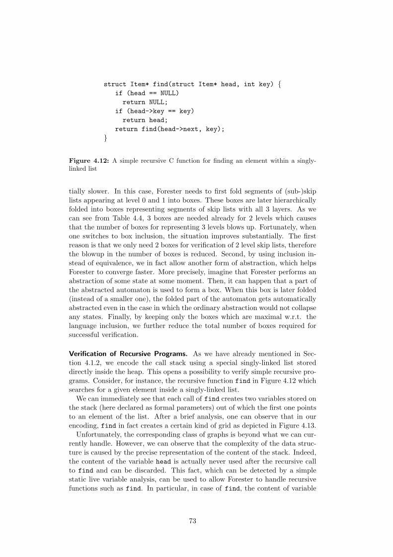
struct Item* find(struct Item* head, int key) {if (head == NULL)

return NULL;

if (head->key == key)

return head;

return find(head->next, key);

}

Figure 4.12: A simple recursive C function for finding an element within a singly-linked list

tially slower. In this case, Forester needs to first fold segments of (sub-)skiplists appearing at level 0 and 1 into boxes. These boxes are later hierarchicallyfolded into boxes representing segments of skip lists with all 3 layers. As wecan see from Table 4.4, 3 boxes are needed already for 2 levels which causesthat the number of boxes for representing 3 levels blows up. Fortunately, whenone switches to box inclusion, the situation improves substantially. The firstreason is that we only need 2 boxes for verification of 2 level skip lists, thereforethe blowup in the number of boxes is reduced. Second, by using inclusion in-stead of equivalence, we in fact allow another form of abstraction, which helpsForester to converge faster. More precisely, imagine that Forester performs anabstraction of some state at some moment. Then, it can happen that a part ofthe abstracted automaton is used to form a box. When this box is later folded(instead of a smaller one), the folded part of the automaton gets automaticallyabstracted even in the case in which the ordinary abstraction would not collapseany states. Finally, by keeping only the boxes which are maximal w.r.t. thelanguage inclusion, we further reduce the total number of boxes required forsuccessful verification.

Verification of Recursive Programs. As we have already mentioned in Sec-tion 4.1.2, we encode the call stack using a special singly-linked list storeddirectly inside the heap. This opens a possibility to verify simple recursive pro-grams. Consider, for instance, the recursive function find in Figure 4.12 whichsearches for a given element inside a singly-linked list.We can immediately see that each call of find creates two variables stored on

the stack (here declared as formal parameters) out of which the first one pointsto an element of the list. After a brief analysis, one can observe that in ourencoding, find in fact creates a certain kind of grid as depicted in Figure 4.13.Unfortunately, the corresponding class of graphs is beyond what we can cur-

rently handle. However, we can observe that the complexity of the data struc-ture is caused by the precise representation of the content of the stack. Indeed,the content of the variable head is actually never used after the recursive callto find and can be discarded. This fact, which can be detected by a simplestatic live variable analysis, can be used to allow Forester to handle recursivefunctions such as find. In particular, in case of find, the content of variable

73

. . . . . .

. . .

next next next next next

callcallcallcall

headheadheadhead

Figure 4.13: Heap configurations arising during the verification of find. The firstrow of nodes represents a singly-linked list which is to be traversed. The content of thecall stack is represented by the second row in which each node corresponds to a singlecall. The picture also demonstrates that each instantiation of the local variable head

points to a different element of the list.

head gets erased immediately after the value is passed into the recursive call(see the dashed links highlighted in red in Figure 4.13).Forester implements a traditional live variable analysis (see [NNH99]) which

is used to remove the content of dead variables as soon as possible. When usingthis extension, the verification of find takes about 0.02 s.In addition, removing the content of dead variables typically allows Forester

to reduce the number of generated FA (differing just in the values of deadvariables). Hence, the efficiency of Forester is improved even in cases in whichthere is no recursion at all.

4.7 Related Work

The area of verifying programs with dynamically linked data structures hasbeen a subject of intense research for quite some time. Many different ap-proaches based on the various kinds of logics, e.g., [MS01, SRW02, Rey02,BCC+07, GVA07, NDQC07, CRN07, ZKR08, YLB+08, CDOY09, MTLT10,MPQ11, DPV11], automata [BHRV06b, BBH+11, DEG06], upward closed sets[ABC+08, ACV11], and other formalisms have been proposed. These ap-proaches differ in their generality, efficiency, and degree of automation. Weconcentrate on a comparison with the two closest lines of work, namely, the useof automata as described in [BHRV06b] and the use of separation logic in theworks [BCC+07, YLB+08] linked with Space Invader and later Slayer and tosome extent Predator. In fact, as we have already noted earlier, the approachwe propose combines some features from these two lines of research.Compared to [BCC+07, YLB+08], our approach is more general in that it

allows one to deal with tree-like structures, too. We note that there are otherworks on separation logic, e.g., [NDQC07], that consider tree manipulation,but these are usually semi-automated only. An exception is [GVA07] whichautomatically handles even tree structures, but its mechanism of synthesisinginductive predicates seems quite dependent on the fact that the dynamic linkeddata structures are built in a “nice” way conforming to the structure of thepredicate to be learned (meaning, e.g., that lists are built by adding elementsat the end only12). An approach presented in [MTLT10] can also handle tree

12We did not find an available implementation of [GVA07], and so we could not try it outourselves.

74

structures, but their method requires substantial user aid in the form of recur-sive predicates in separation logic which are linked to the structure of the codeto be verified (in fact this is very close to providing inductive invariants of theprogram). Therefore, unlike in our case, the method is not fully automatic.Further, compared to [BCC+07, YLB+08], our approach comes with a more

flexible abstraction. We are not building on just using some inductive predi-cates, but we combine a use of our nested FA with an automatically refinableabstraction on the TA that appear in our representation. Thus our analysiscan more easily adjust to various cases arising in the programs being verified.An example is dealing with lists of lists where the sublists are of length 0 or 1,which is a quite practical situation [YLC+07]. In such cases, the abstractionused in [BCC+07, YLB+08] can fail, leading to an infinite computation (e.g.,when, by chance, a list of regularly interleaved lists of length 0 or 1 appears) orgenerate false alarms (when modified to abstract even pointer links of length 1to a list segment). For us, such a situation is easy to handle without any needto fine-tune the abstraction manually.Finally, compared with [BHRV06b], our newly proposed approach is a bit

less general. We cannot handle structures such as, e.g., trees with linked leaves.To handle these structures, we would have to introduce into our approach FAnested not just strictly hierarchically but in an arbitrary, possibly cyclic way,which is an interesting subject for future research. On the other hand, our newapproach is more scalable than that of [BHRV06b]. This is due to the factthat the heap representation in [BHRV06b] is monolithic, i.e., the whole heapis represented by a single tree skeleton over which additional pointer links areexpressed using the so-called routing expressions. The new encoding is muchmore structured, and so the different operations on the heap, correspondingto a symbolic execution of the verified program, typically influence only smallparts of the encoding and not all (or most) of it. The monolithic encoding of[BHRV06b] has also problems with deletion of elements inside data structuressince the routing expressions are built over a tree backbone that is assumed notto change (and hence deleted elements inside data structures are always kept,just marked as deleted). Moreover, the encoding of [BHRV06b] has troubleswith detection of memory leakage, which is in theory possible, but it is socomplex that it has never been implemented.


In this chapter, we have proposed a new method for verification of heap manip-ulating programs. In particular, we use forest automata proposed in Chapter 3to encode sets of heaps and exploit the fact that the set of C statements thatwe need to support can be easily symbolically executed over FA. Moreover, thefact that FA are built over tree automata allows us to build a verification proce-dure based on the framework of abstract regular tree model checking. For use inour setting, we have proposed specialisations of the general-purpose abstractionschemas, which have been introduced in ARTMC. Further, we have describedhow more complex data structures—such as doubly-linked lists—can be veri-

75

fied using hierarchically nested forest automata whose hierarchical structuringcan be discovered fully automatically. Finally, we have implemented the abovementioned approach in a prototype tool called Forester. We have performedan experimental evaluation on a set of benchmarks consisting of C programsmanipulating various dynamically allocated data structures in order to com-pare Forester to other similar tools. The obtained results confirmed that ourapproach is quite competitive in practice.As of what concerns the future work, one of the most interesting areas is an

implementation of the proposed but not yet implemented abstraction refinementwhich relies on the ability to perform a backward execution along the trace thatseems to lead to an error state. A part of this work should be an evaluationof whether the proposed under-approximation of intersection is sufficient inpractice, or whether some more precise approach is needed.Furthermore, it would also be interesting to extend our approach such that it

could track some information about the data stored within dynamically linkeddata structures. This would allow one to verify algorithms in which the memorysafety depends, for instance, on the fact that a certain sequence is sorted. As anexample, we can mention the algorithm for skip lists which we had to manuallymodify in order to remove the dependency on the data. Another example is thatof dealing with red-black trees in which case one needs to distinguish red andblack trees. Apart from that, tracking of the data stored inside the dynamicallylinked data structure would allow Forester to also check properties concerningthat data.Another line of research is a generalisation of our approach to concurrent

programs. Here, an especially interesting case is that of lockless concurrentdata structures, which are extremely difficult to understand and validate.Finally, some programs manipulating complex data structures—such as trees

with linked leaves—could be verified if one was able to work with recursivelynested boxes. Therefore, a generalisation of the algorithms proposed in thisthesis for such boxes is also an interesting topic for future work.

76

5 Simulations over LTSs and TreeAutomata

The approach of abstract regular (tree) model checking, which we use in a novelway also in our verification technique for programs with dynamic linked datastructures proposed in the previous chapter, crucially depends on the efficiencyof dealing with automata. AR(T)MC ([BHV04, BHRV06a]) was originally builtover deterministic finite tree automata. The need to determinise the automatain every step of the computation has, however, turned out to be a significantobstacle to practical applicability of the approach. That is why, in [BHH+08],it has been proposed to replace their use by nodeterministic tree automata(NTA). This, however, brings some problems to be solved. In particular, oneneeds to be able to perform inclusion checking (in order to see when a fixpointis reached) and to reduce the of the automata obtained in the computation.Unfortunately, both standard minimisation and inclusion checking algorithmsare based on first making the appropriate automata deterministic. Using de-terminisation as an intermediate step would, however, destroy the advantage ofworking with usually much smaller NTA. Hence, both of the operations are tobe done without determinisation. For checking inclusion, one can use methodsbased on antichains, possibly combined with simulation as discussed in Chap-ter 6 and in Chapter 7. For reducing the size of the automata, one can usequotienting w.r.t. a suitable, typically simulation-based equivalence relation(see [ABH+08]). For both of these problems, it is thus crucial to be able toefficiently compute simulations on NTA. One of the most efficient ways to ob-tain these equivalence simulation relations on NTA is via translating an NTAinto a labelled transition system (LTS) as described in [AHKV08] and thencomputing the simulation relation on this LTS.Apart form that, many other automated verification techniques—such as LTL

model checking—are also directly or indirectly dealing with LTSs and as suchthey are often limited by their size. One of the well-established approachesto cope with this problem is the reduction of an LTS using a suitable equiva-lence relation according to which the states of the LTS are collapsed. A goodcandidate for such a relation is again simulation equivalence. It strongly pre-serves logics like ACTL∗, ECTL∗, and LTL [DGG93, GL94, HHK95], and withrespect to its reduction power and computation cost, it offers a desirable com-promise among the other common candidates, such as bisimulation equivalence[PT87, SJ05] and language equivalence.The currently fastest LTS-simulation algorithm (below denoted as LRT—

i.e., labelled RT) has been published in [ABH+08]. It is a straightforwardmodification of the fastest algorithm (in the following denoted as RT, standingfor Ranzato-Tapparo) for computing simulations over Kripke structures [RT07],

77

which itself improves the algorithm from [HHK95]. The time complexity of RTamounts to O(|PSim ||δ|), the space complexity amounts to O(|PSim ||S|). In thecase of LRT, the time complexity is O(|PSim ||δ| + |Σ||PSim ||S|) and the spacecomplexity is O(|Σ||PSim ||S|). Here, S is the set of states of an LTS, δ is itstransition relation, Σ is its alphabet, and PSim is the partition of S accordingto the simulation equivalence. The space complexity blow-up of LRT is causedby indexing the data structures of RT by the symbols of the alphabet.In this chapter, we propose an optimised version of LRT (denoted OLRT)

that lowers the above described blow-up. We exploit the fact that not all statesof an LTS have incoming and outgoing transitions labelled by all symbols of thealphabet, which allows us to reduce the memory footprint of the data structuresused during the computation. Our experiments show that the optimisations wepropose lead to significant savings of space as well as of time in many practicalcases. Moreover, we have achieved a promising reduction of the asymptotic com-plexity of algorithms for computing tree-automata simulations from [ABH+08]using OLRT, too.

Plan of the Chapter. The text is organised as follows. In Section 5.1, weintroduce additional preliminaries used throughout the rest of this chapter.Section 5.2 presents the original algorithm upon which our optimisations arebuilt, In Section 5.3, we describe the proposed optimisations and we derive thecomplexity of our optimised algorithm. Section 5.4 discusses the complexity ofcomputing simulations over tree automata when our optimised algorithm is usedas a part of the procedure. The experimental evaluation of our optimisationsis provided in Section 5.5. Finally, Section 5.6 concludes the chapter.

5.1 Preliminaries

Given a binary relation ρ over a set X, we use ρ(x) to denote the set {y |(x, y) ∈ ρ}. Then, for a set Y ⊆ X, ρ(Y ) =

⋃

{ρ(y) | y ∈ Y }. A partition-relation pair over X is a pair 〈P,Rel〉 where P ⊆ 2X is a partition of X (wecall elements of P blocks) and Rel ⊆ P × P . A partition-relation pair 〈P,Rel〉induces the relation ρ =

⋃

(B,C)∈Rel B × C. We say that 〈P,Rel〉 is the coarsestpartition-relation pair inducing ρ if any two x, y ∈ X are in the same block ofP if and only if ρ(x) = ρ(y) and ρ−1(x) = ρ−1(y). Note that in the case whenρ is a preorder and 〈P,Rel〉 is coarsest, then P is the set of equivalence classesof ρ ∩ ρ−1 and Rel is a partial order.

For an LTS T = (S,Σ, {δa | a ∈ Σ}), a simulation over T is a binary relationρ on S such that if (u, v) ∈ ρ, then for all a ∈ Σ and u′ ∈ δa(u), there existsv′ ∈ δa(v) such that (u′, v′) ∈ ρ. It can be shown that for a given LTS T andan initial preorder I ⊆ S × S, there is a unique maximal simulation SimI on Tthat is a subset of I , and that SimI is a preorder (see [ABH+08]).

78

5.2 The Original LRT Algorithm

In this section, we describe the original version of the algorithm presented in[ABH+08], i.e., the algorithm that we denote as LRT (see Algorithm 3).The algorithm gradually refines a partition-relation pair 〈P,Rel〉, which is

initialised as the coarsest partition-relation pair inducing an initial preorder I .After its termination, 〈P,Rel〉 is the coarsest partition-relation pair inducingSimI . The basic invariant of the algorithm is that the relation induced by〈P,Rel〉 is always a superset of SimI .

The while-loop refines the partition P and then prunes the relation Rel ineach iteration of the while-loop. The role of the Remove sets can be explainedas follows: During the initialisation, every Removea(B) is filled by states vsuch that δa(v)∩

⋃

Rel(B) = ∅ (there is no a-transition leading from v “above”B w.r.t. Rel). During the computation phase, v is added into Removea(B)after δa(v) ∩

⋃

Rel(B) becomes empty (because of pruning Rel on line 19).Emptiness of δa(v) ∩ Rel(B) is tested on line 22 using counters Counta(v,B),which record the cardinality of δa(v)∩Rel(B). From the definition of simulation,and because the relation induced by 〈P,Rel〉 is always a superset of SimI ,δa(v) ∩

⋃

Rel(B) = ∅ implies that for all u ∈ δ−1a (B), (u, v) )∈ SimI (v cannot

simulate any u ∈ δ−1a (B)). To reflect this, the relation Rel is pruned each

time Removea(B) is processed. The code on lines 9–15 prepares the partition-relation pair and all the data structures. First, Split(P,Removea(B)) dividesevery block B′ into B′∩Removea(B) (which cannot simulate states from δ−1

a (B)as they have empty intersection with δ−1

a (Rel(B))), and B′\Removea(B). Morespecifically, for a set Remove ⊆ S, Split(P,Remove) returns a finer partitionP ′ = {B \ Remove | B ∈ P} ∪ {B ∩ Remove | B ∈ P}. After refining P bythe Split operation, the newly created blocks of P inherit the data structures(counters Count and Remove sets) from their “parents” (for a block B ∈ P ,its parent is the block Bprev ∈ Pprev such that B ⊆ Bprev). Rel is then updatedon line 19 by removing the pairs (C,D) such that C ∩ δ−1

a (B) )= ∅ and D ⊆Removea(B). The change of Rel causes that for some states u ∈ S and symbolsb ∈ Σ, δa(u) ∩

⋃

Rel(C) becomes empty. To propagate the change of therelation along the transition relation, u will be moved into Removeb(C) on line23, which will cause new changes of the relation in the following iterationsof the while-loop. If there is no nonempty Remove set, then 〈P,Rel〉 is thecoarsest partition-relation pair inducing SimI and the algorithm terminates.Correctness of LRT is stated by Theorem 1.

Theorem 1 ([ABH+08]) With an LTS T = (S,Σ, {δa | a ∈ Σ}) and thecoarsest partition-relation pair 〈PI ,Rel I 〉 inducing a preorder I ⊆ S ×S on theinput, LRT terminates with the coarsest partition-relation pair 〈P,Rel〉 inducingSimI .

5.3 Optimisations of LRT

The optimisation that we are now going to propose reduces the number ofcounters and the number and the size of Remove sets. The changes required

79

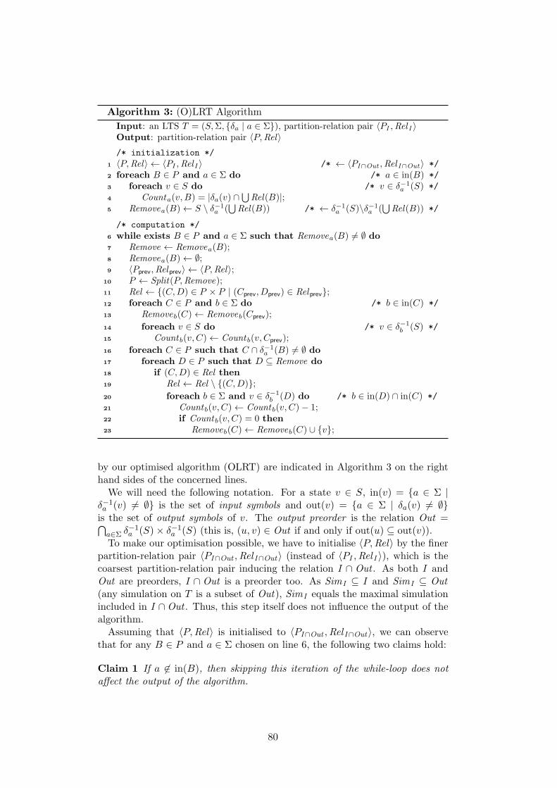
Algorithm 3: (O)LRT Algorithm

Input: an LTS T = (S,Σ, {δa | a ∈ Σ}), partition-relation pair 〈PI ,Rel I 〉Output: partition-relation pair 〈P,Rel〉

/* initialization */

1 〈P,Rel〉 ← 〈PI ,RelI〉 /* ← 〈PI∩Out ,Rel I∩Out 〉 */

2 foreach B ∈ P and a ∈ Σ do /* a ∈ in(B) */

3 foreach v ∈ S do /* v ∈ δ−1a (S) */

4 Counta(v,B) = |δa(v) ∩⋃

Rel(B)|;5 Removea(B) ← S \ δ−1

a (⋃

Rel(B)) /* ← δ−1a (S)\δ−1

a (⋃

Rel(B)) */

/* computation */

6 while exists B ∈ P and a ∈ Σ such that Removea(B) )= ∅ do7 Remove ← Removea(B);8 Removea(B) ← ∅;9 〈Pprev,Relprev〉 ← 〈P,Rel〉;

10 P ← Split(P,Remove);11 Rel ← {(C,D) ∈ P × P | (Cprev, Dprev) ∈ Relprev};12 foreach C ∈ P and b ∈ Σ do /* b ∈ in(C) */

13 Removeb(C) ← Removeb(Cprev);

14 foreach v ∈ S do /* v ∈ δ−1b (S) */

15 Countb(v, C) ← Countb(v, Cprev);

16 foreach C ∈ P such that C ∩ δ−1a (B) )= ∅ do

17 foreach D ∈ P such that D ⊆ Remove do18 if (C,D) ∈ Rel then19 Rel ← Rel \ {(C,D)};

20 foreach b ∈ Σ and v ∈ δ−1b (D) do /* b ∈ in(D) ∩ in(C) */

21 Countb(v, C) ← Countb(v, C)− 1;22 if Countb(v, C) = 0 then23 Removeb(C) ← Removeb(C) ∪ {v};

by our optimised algorithm (OLRT) are indicated in Algorithm 3 on the righthand sides of the concerned lines.We will need the following notation. For a state v ∈ S, in(v) = {a ∈ Σ |

δ−1a (v) )= ∅} is the set of input symbols and out(v) = {a ∈ Σ | δa(v) )= ∅}is the set of output symbols of v. The output preorder is the relation Out =⋂

a∈Σ δ−1a (S)× δ−1

a (S) (this is, (u, v) ∈ Out if and only if out(u) ⊆ out(v)).To make our optimisation possible, we have to initialise 〈P,Rel〉 by the finer

partition-relation pair 〈PI∩Out ,Rel I∩Out〉 (instead of 〈PI ,Rel I 〉), which is thecoarsest partition-relation pair inducing the relation I ∩ Out . As both I andOut are preorders, I ∩ Out is a preorder too. As SimI ⊆ I and SimI ⊆ Out(any simulation on T is a subset of Out), SimI equals the maximal simulationincluded in I ∩Out . Thus, this step itself does not influence the output of thealgorithm.Assuming that 〈P,Rel〉 is initialised to 〈PI∩Out ,Rel I∩Out〉, we can observe

that for any B ∈ P and a ∈ Σ chosen on line 6, the following two claims hold:

Claim 1 If a )∈ in(B), then skipping this iteration of the while-loop does notaffect the output of the algorithm.

80

Proof. In an iteration of the while-loop processing Removea(B) with a )∈ in(B),as there is no C ∈ P with δa(C) ∩ Rel(B) )= ∅, the for-loop on line 18 stopsimmediately. No pair (C,D) will be removed from Rel on line 19, no counterwill be decremented, and no state will be added into a Remove set. The onlything that can happen is that Split(P,Remove) refines P . However, in thiscase, this refinement of P would be done anyway in other iterations of thewhile-loop when processing sets Removeb(C) with b ∈ in(C). To see this,note that correctness of the algorithm does not depend on the order in whichnonempty Remove sets are processed. Therefore, we can postpone processing allthe nonempty Removea(B) sets with a )∈ in(B) to the end of the computation.Recall that processing no of these Remove sets can cause that an empty Removeset becomes nonempty. Thus, the algorithm terminates after processing the lastof the postponed Removea(B) sets. If processing some of these Removea(B)with a )∈ in(B) refines P , P will contain blocks C,D such that both (C,D) and(D,C) are in Rel (recall that when processing Removea(B), no pair of blockscan be removed from Rel on line 19). This means that the final 〈P,Rel〉 willnot be coarsest, which is a contradiction with Theorem 1. Thus, processingthe postponed Removea(B) sets can influence nor Rel neither P , and thereforethey do not have to be processed at all. #

Claim 2 It does not matter whether we assign Removea(B) or Removea(B) \(S \ δ−1

a (S)) to Remove on line 6.

Proof. Observe that v with a )∈ out(v) (i.e., v ∈ S \ δ−1a (S)) cannot be added

into Removea(B) on line 23, as this would mean that v has an a-transitionleading to D. Therefore, v can get into Removea(B) only during initialisationon line 5 together with all states from S\δ−1

a (S). After Removea(B) is processed(and emptied) for the first time, no state from S\δ−1

a (S) can appear there again.Thus, Removea(B) contains states from S \ δ−1

a (S) only when it is processedfor the first time and then it contains all of them. It can be shown that forany partition Q of a set X and any Y ⊆ X, if Split(Q, Y ) = Q, then alsofor any Z ⊆ X with Y ⊆ Z, Split(Q,Z) = Split(Q,Z \ Y ). As P refinesPI∩Out , Split(P, S \ δ−1

a (S)) = P . Therefore, as S \ δ−1a (S) ⊆ Removea(B),

Split(P,Removea(B)) = Split(P,Removea(B) \ (S \ δ−1a (S))). We have shown

that removing S \ δ−1a (S) from Remove does not influence the result of the

Split operation in this iteration of the while-loop (note that this implies thatall blocks from the new partition are included in or have empty intersectionwith S \ δ−1

a (S)). It remains to show that the change also does not influenceupdating Rel on line 19. Removing S \ δ−1

a (S) from Remove could only causethat the blocks D such that D ⊆ S \ δ−1

a (S) that were chosen on line 17 withthe original value of Remove will not be chosen with the restricted Remove.Thus, some of the pairs (C,D) removed from Rel with the original version ofRemove could stay in Rel with the restricted version of Remove. However, sucha pair (C,D) cannot exist because with the original value of Remove, if (C,D)is removed from Rel , then a ∈ out(C) (as δ(C) ∩ B )= ∅) and therefore alsoa ∈ out(D) (as Rel was initialised to Rel I∩Out on line 1 and (C,D) ∈ Rel).Thus, D∩ (S \ δ−1

a (S)) = ∅, which means that (C,D) is removed from Rel even

81

with the restricted Remove. Therefore, it is not important whether S \ δ−1a (S)

is a subset of or it has an empty intersection with Remove. #

As justified above, we can optimise LRT as follows. Sets Removea(B) arecomputed only if a ∈ in(B) and in that case we only add states q ∈ δ−1

a (S) toRemovea(B). As a result, we can reduce the number of required counters bymaintaining Counta(v,B) if and only if a ∈ in(B) and a ∈ out(v).

5.3.1 Data Structures

We now describe the essential data structures which are required by OLRT.The input LTS is represented as a list of records about its states. The recordabout each state v ∈ S contains a list of nonempty δ−1

a (v) sets1, each of themencoded as a list of its members. The partition P is encoded as a doubly-linkedlist (DLL) of blocks. Each block is represented as a DLL of (pointers to) statesof the block. Each block B contains for each a ∈ Σ a list of (pointers on) statesfrom Removea(B). Each time when any set Removea(B) becomes nonempty,block B is moved to the beginning of the list of blocks. Choosing the block Bon line 6 then means just scanning the head of the list of blocks.Each block B ∈ P and each state v ∈ S contains an Σ-indexed array contain-

ing a record B.a and v.a, respectively. The record B.a stores the informationwhether a ∈ in(B) (we need the test on a ∈ in(B) to take a constant time),If a ∈ in(B), then B.a also contains a reference to the set Removea(B), rep-resented as a list of states (with a constant time addition), and a reference toan array of counters B.a.Count containing the counter Counta(v,B) for eachv ∈ δ−1

a (S). Note that for two different symbols a, b ∈ Σ and some v ∈ S,the counter Counta(v,B) has different index in the array B.a.Count than thecounter Countb(v,B) in B.b.Count (as the sets δ−1

a (S) and δ−1b (S) are differ-

ent). Therefore, for each v ∈ S and a ∈ Σ, v.a contains an index va under whichfor each B ∈ P , the counter Counta(v,B) can be found in the array B.a.Count .Using the Σ-indexed arrays attached to symbols and blocks, every counter canbe found/updated in a constant time. For every v ∈ S, a ∈ Σ, v.a also storesa pointer to the list containing δ−1

a (v) or null if δ−1a (v) is empty. This allows

the constant time testing whether a ∈ in(v) and the constant time searchingfor the δ−1

a (v) list.

5.3.2 Complexity of Optimised LRT

Here, we provide a complexity analysis of our optimised algorithm. In order toimprove the readability, we fix IO = I ∩ Out for the rest of this section. TheSplit(P,X) operation can be implemented as follows: Iterate through all v ∈ X.If v ∈ B ∈ P , add v into a block Bchild (if Bchild does not exist yet, create itand add it into P ) and remove v from B. If B becomes empty, discard it. Thiscan be done in O(|X|) time.

1We use a list rather than an array having an entry for each a ∈ Σ in order to avoid a needto iterate over alphabet symbols for which there is no transition.

82

Complexity of Initialization Phase (lines 1–5). Computation of 〈PIO,Rel IO〉on line 1 can be done in time at most |Σ||PIO|

2 (starting with 〈PI ,Rel I 〉, andfor each a ∈ Σ, splitting P according to δ−1

a (S) and removing the relationbetween blocks containing states from δ−1

a (S) and those containing states fromS \ δ−1

a (S)). The initialisation of the Σ-indexed arrays attached to states andblocks can be done in O(|Σ||S|+ |δ|) time.

The Count counters are initialised by (1) allocating above described arraysof counters (attached to blocks), setting all the counters to 0, and then (2) forall B ∈ P , for all u ∈ IO(B), and for all a ∈ in(u), and for all v ∈ δ−1

a (u),incrementing Counta(v,B). This takes

O

∑

B∈PIO

∑

a∈in(B)

|δ−1a (S)|+

∑

B∈PIO

∑

v∈IO(B)

|δ−1(v)|

time. The Remove sets are initialised by iterating through all the counters and ifCounta(v,B) = 0, then adding (appending) v to Removea(B). This takes timeproportional to the number of counters, which is O(

∑

B∈PIO

∑

a∈in(B) |δ−1a (S)|).

Thus, the overall time complexity of the initialisation is

O

|Σ||PIO|2 + |Σ||S|+ |

∑

B∈PIO

∑

a∈in(B)

|δ−1a (S)|+

∑

B∈PIO

∑

v∈IO(B)

|δ−1(v)|

.

Complexity of Splitting (lines 10–15). The complexity analysis of lines 12–15 is based on the fact that it can happen at most |PIO| − |PSimI

| times thata block B is split on line 10. Moreover, the presented code can be optimised bynot having the lines 12–15 as a separate loop (this was chosen just for clarity ofthe presentation), but the inheritance of Rel , Remove, and the counters can bedone within the Split function, and only for those blocks that were really split(not for all the blocks every time). Whenever a block B is split into B1 andB2, we have to do the following: (1) allocate the Σ-indexed arrays containingthe record B1.a, B2.a for each a ∈ Σ, (the arrays of B can be reused for one ofthe new blocks); (2) for each a ∈ in(B), compute the sets in(B)1 and in(B)2and update the records B1.a and B2.a (saying whether a ∈ in(B1, B,2 )). Thistakes time O(

∑

v∈B |δ−1(v)|) for one block B, which gives time

O

∑

B∈PSimI

∑

v∈(IO∩IO−1)(B)

|δ−1(v)|+ |Σ|

overall; (3) for each Bi, i ∈ {1, 2} and each a ∈ in(Bi), copy the Removea(B)and the array of the counters B.a.Count and save them to the Bi.a record. Theoverall time needed for this copying is equal to the overall space taken by allRemove sets and all counters, which is O(

∑

B∈PSimI

∑

a∈in(B) |δ−1a (S)|); (4) add

a row and a column to the Rel matrix and copy the entries from those of theparent B. This operation takes O(|PSimI

|) time for one added block as the sizeof the rows and columns of the Rel -matrix is bounded by |PSimI

|. Thus, for allnewly generated blocks, we achieve the overall time complexity of O(|PSimI

|2).

83

The key observation, which the time complexity analysis of line 10 and lines16–18 is based on, is the following: For any two states u, v ∈ S and any symbola ∈ Σ, it can happen at most once that v is present in Removea(B) for someblock B with u ∈ B when Removea(B) is processed in the main while-loop (Band a is chosen on line 5). This also means that for every B ∈ PSimI

and a ∈ Σ,the sum of cardinalities of all Removea(B

′) sets with B ⊆ B′ (in the momentwhen a and B′ were chosen on line 5) is below |δ−1

a (S)|. Indeed, notice thatwhen v is being added into Removea(B) (either on line 5 or on line 23), thenδa(v) ∩ Rel(B) is empty. If v is added into Removea(B) in some iteration ofthe while-loop, then δa(v) ∩ Rel(B) was nonempty until (B,D) was removedfrom Rel on line 19 (in the same iteration). Once δa(v) ∩ Rel(B) is empty,δa(v) ∩ Rel(B′) can never get nonempty for any block B′ ⊆ B as Rel nevergrows, and thus v can never be added into some Removea(B

′) for B′ ⊆ B online 23.The above observation also implies that for a fixed block B ∈ PSimI

anda ∈ Σ, the sum of all cardinalities of the Removea(B

′) sets, where B ⊆ B′

according to which a Split is being done, is below |δ−1a (S)|. Therefore, the

overall time taken by splitting on line 10 is in

O

∑

B∈PSimI

∑

a∈in(B)

|δ−1a (S)|

.

Complexity of Refinement (lines 16–23). Lines 18 and 19 are O(1)-time (Relis a boolean matrix). Before we enter the for-loop on line 16, we compute a listRemoveLista(B) = {D ∈ P | D ⊆ Remove}. This is an O(|Remove|) operationand by almost the same argument as in the case of the overall time complexityof Split on line 10, we get also exactly the same overall time complexity forcomputing all the RemoveLista(B) lists. On line 16, the blocks C are listedby traversing all δ−1(v), v ∈ B. From the above it follows that for any twoB′, D′ ∈ PSimI

and any a ∈ Σ, it can happen at most once that a and someB with B′ ⊆ B are chosen on line 5 and at the same time D′ ⊆ Removea(B).Moreover, it holds that a ∈ in(B) and Removea(B) ⊆ δ−1

a (S). Thus, for a fixeda, the a-transition leading to a block B′ ∈ PSimI

can be traversed on line 16only |{D′ ∈ PSimI

| a ∈ out(D′)}| times and thus the time complexity of lines16–18 amounts to O(

∑

D∈PSimI

∑

a∈out(D) |δa|).

The analysis of lines 19–23 is based on the fact that if some (C,D) appearsonce on line 19, then no (C ′, D′) with C ′ ⊆ C,D′ ⊆ D can appear there again(as (C,D) is removed from Rel and Rel never grows). Moreover, (C,D) canappear on line 19 only if C × D ⊆ IO. For a fixed (C,D), the time spent inlines 19–23 is in O(

∑

v∈B |δ−1(v)|) and therefore the overall complexity of lines19–23 amounts to

O

∑

B∈PSimI

∑

v∈IO(B)

|δ−1(v)|

.

84

Overall Time Complexity. From the above it follows that the time complexityof OLRT is covered by the following six factors:

1. O(|Σ||PIO|2),

2. O(|Σ||S|),

3. O(|PSimI|2),

4. O(∑

B∈PSimI

∑

a∈in(B) |δ−1a (S)|),

5. O(∑

B∈PSimI

∑

a∈out(B) |δa|), and

6. O(∑

B∈PSimI

∑

v∈IO(B) |δ−1(v)|)).

In total, this gives:

O

|Σ||PIO|2 + |Σ||S|+ |PSimI

|2+

∑

B∈PSimI

∑

a∈in(B)

|δ−1a (S)|+

∑

a∈out(B)

|δa|+∑

v∈IO(B)

|δ−1(v)|

.

Space Comlexity. The space complexity of OLRT is determined by the numberof counters, the contents of the Remove sets, the size of the matrix encoding ofRel , and the Σ-indexed arrays attached to blocks and states. This is coveredby the above Factors 2,3 and 4, which gives:

O

|PSimI|2 + |Σ||S|+

∑

B∈PSimI

∑

a∈in(B)

|δ−1a (S)|

.

Observe that the improvement of both time and space complexity of LRT ismost significant for systems with large alphabets and a‘high diversity of setsof input and output symbols of states. Certain regular diversity of sets ofinput and output symbols is an inherent property of LTSs that arise when wecompute simulations over tree automata. We address the impact of employingOLRT within the procedures for computing tree automata simulation in thenext section.

5.4 Tree Automata Simulations

In [ABH+08], the authors propose methods for computing tree automata simu-lations via translating problems of computing simulations over tree-automatato problems of computing simulations over certain LTSs. In this section, weshow how replacing LRT by OLRT within these translation-based proceduresdecreases the overall complexity of computing tree-automata simulations. Forthe rest of this section, we fix a TA A = (Q,Σ,∆, F ). From now on, let Ddenote the maximal downward simulation on A and U the maximal upwardsimulation on A induced by D .

85

To define the translations from downward and upward simulation problems,we need the following notions. Given a transition t = ((q1, . . . , qn), f, q) ∈ ∆,(q1, . . . , qn) is its left-hand side and t(i) ∈ (Q∪{#})∗×Σ×Q is an environment—the tuple which arises from t by replacing state qi, 1 ≤ i ≤ n, at the ith positionof the left-hand side of t by the so called hole# )∈ Q. We use Lhs of to denote theset of all left-hand sides of A and Env to denote the set of all environments of A.

We translate the downward simulation problem on A to the simulation prob-lem on the LTS A• = (Q•,Σ•, {δ•a | a ∈ Σ

•}) where Q• = {q• | q ∈ Q}∪{l• | l ∈Lhs}, Σ• = Σ∪{1, . . . , rm}}, and for each ((q1, . . . , qn), f, q) ∈ ∆, (q•, q1 . . . q

•n) ∈

δ•f and (q1 . . . q•n, q

•i ) ∈ δ•i for each i : 1 ≤ i ≤ n. The initial relation is simply

I • = Q• × Q•. The upward simulation problem is then translated into a sim-ulation problem on LTS A⊙ = (Q⊙,Σ⊙, {δ⊙a | a ∈ Σ

⊙}), where Q⊙ = {q⊙ |q ∈ Q} ∪ {e⊙ | e ∈ Env}, Σ⊙ = Σ

•, and for each t = ((q1, . . . , qn), f, q) ∈ ∆,for each 1 ≤ i ≤ n, (q⊙i , t(i)

⊙) ∈ δ⊙i and (t(i)⊙, q⊙) ∈ δ⊙a . The initial rela-tion I⊙ ⊆ Q⊙ × Q⊙ contains all the pairs (q⊙, r⊙) such that q, r ∈ Q andr ∈ F =⇒ q ∈ F , and ((q1 . . . qn, f, q)(i)

⊙, (r1 . . . rn, f, r)(i)⊙) such that

(qj , rj) ∈ D for all j : 1 ≤ i )= j ≤ n. Let Sim• be the maximal simulation onA• included in I • and let Sim⊙ be the maximal simulation on A⊙ included inI⊙. The following theorem shows correctness of the translations.

Theorem 2 ([ABH+08]) For all q, r ∈ Q, we have (q•, r•) ∈ Sim• if andonly if (q, r) ∈ D and (q⊙, r⊙) ∈ Sim⊙ if and only if (q, r) ∈ U .

The states of the LTSs (A• as well as A⊙) can be classified into severalclasses according to the sets of input/output symbols. Particularly, Q• canbe classified into the classes {q• | q ∈ Q} and for each n : 1 ≤ n ≤ rm,{q1 . . . q

•n | q1 . . . qn ∈ Lhs}, and Q⊙ can be classified into {q⊙ | q ∈ Q} and for

each a ∈ Σ and i : 1 ≤ i ≤ r(a), {t(i)⊙ | t = ((q1, . . . , qn), a, q) ∈ ∆}. This turnsto a significant advantage when computing simulations on A• or on A⊙ usingOLRT instead of LRT. Moreover, we now propose another small optimisation,which is a specialised procedure for computing 〈PI∩OutRel I∩Out〉 for the bothof A⊙, A•. It is based on the simple observation that we need only a constanttime (not a time proportional to the size of the alphabet) to determine whethertwo left-hand sides or two environments are related by the particular Out (morespecifically, (e⊙1 , e

⊙2 ) ∈ Out if and only if the inner symbols of e1 and e2 are the

same, and (q1 . . . q•n, r1 . . . r

•m) ∈ Out if and only if n ≤ m).

5.4.1 Complexity of Computing Simulations over TA

In this section, we only point out the main differences between applicationof LRT [ABH+08] and OLRT on the LTSs that arise from the translationsdescribed above. For implementation details and full complexity analysis of theOLRT versions, see the Section 5.3.2.To be able to express the complexity of running OLRT on A• and A⊙, we

extend D to the set Lhs such that ((q1 . . . qn), (r1 . . . rn)) ∈ D if and only if

86

(qi, ri) ∈ D for each i : 1 ≤ i ≤ n, and we extend U to the set Env such that

((q1 . . . qn, f, q)(i), (r1 . . . rn, f, r)(i)) ∈ U⇐⇒

m = n ∧ i = j ∧ (q, r) ∈ U ∧ (∀k ∈ {1, ..., n}. k )= i =⇒ (qk, rk) ∈ D).

For a preorder ρ over a setX, we useX/ρ to denote the partition ofX accordingto the equivalence ρ ∩ ρ−1.The procedures for computing Sim• and Sim⊙ consist of (i) translating A

to the particular LTS (A• or A⊙) and computing the partition-relation pairinducing the initial preorder (I • or I⊙), and (ii) running a simulation algorithm(LRT or OLRT) on it. Below, we analyse the impact of replacing LRT by OLRTon the complexity of step (ii), which is the step with dominating complexity(as shown in [ABH+08] and also by our experiments; step (ii) is much morecomputationally demanding than step (i)).We will instantiate the six OLRT time complexity factors for A• and A⊙.

The first time complexity factor comes out from computing 〈PI∩Out ,Rel I∩Out〉.For A• and A⊙, this factor can be decreased exploiting special properties of thetransition systems. Bellow, we assume that |Q| ≤ |∆| and |Q| ≤ |Env|.

In the case of A•, 〈PI∩Out ,Rel I∩Out〉 can be computed separately for thestates Q•

1 = {q• | q ∈ Q} and Q•2 = {l• | l ∈ Lhs}. For the first set, for

each a ∈ Σ, we perform Split(P, δ−1a (Q•

2)) and remove from the relation all thepairs of blocks included in Q•

1 \ δ−1a (Q•

2)× δ−1a (Q•

2). Then, we partition Q•2 into

blocks Bn = {l• | l = q1 . . . qn ∈ Lhs} for each n ≤ rm and remove all relationon these blocks Bn, 1 ≤ n ≤ rm apart from the diagonal. Finally, we removeall relations between blocks included in Q•

1 and those in Q•2. Note that Q•

2 isinitially partitioned into rm blocks (one block for left-hand sides of each possiblelength up to rm). Overall, the procedure takes time in O(|Σ||Q/D |2 + r2

m).

In the case of A⊙, 〈PI∩Out ,Rel I∩Out〉 is computed separately for the statesQ⊙

1 = {q⊙ | q ∈ Q} and Q⊙2 = {e⊙ | e ∈ Env}. For the first set, for each i : 1 ≤

i ≤ rm, we perform Split(P, δ−1i (Q⊙

2 )) and remove from the relation all pairs ofblocks included in Q⊙

1 \ δ−1i (Q⊙

2 )× δ−1i (Q⊙

2 ). Then, for each a ∈ Σ, we performSplit(Q⊙

2 , δ−1a (Q⊙

1 )) and remove from the relation all pairs of blocks included inQ⊙

2 \ δ−1a (Q⊙

1 ) × δ−1a (Q⊙

1 ). Finally, we remove all the relations between blocksfrom Q⊙

1 and Q⊙2 . Overall, the procedure takes time O(|Σ||Q/U |2+ |Env/U |2).

We now derive the complexity of computing simulation on A• by OLRT. Theabove time complexity factors of OLRT are covered by the following factors(the first factor is the complexity of the specialised procedure for computing〈PI∩Out ,Rel I∩Out〉):

1. O(|Σ||Q/D |2 + r2m),

2. O((rm + |Σ|)|Lhs ∪Q|),

3. O(|Lhs ∪Q/D |2),

4. O(|Σ||Lhs/D ||Q|+ rm|Q/D ||Lhs |),

5. O(rm|Lhs/D ||Lhs |+ |Q/D ||∆|), and

87

6. O(|Lhs/D ||∆|+ rm|Q/D ||Lhs |).

The space complexity is the sum of the factors 2–4. This gives O(SpaceD),where SpaceD amounts to

(rm + |Σ|)|Lhs ∪Q|+ |Lhs ∪Q/D |2 + |Σ||Lhs/D ||Q|+ rm|Q/D ||Lhs |.

The time complexity can then be simplified to

O(

SpaceD + |Σ||Q/D |2 + rm|Lhs/D ||Lhs |+ |Q/D ||∆|+ |Lhs/D ||∆|)

.

In the case of A⊙, the space complexity of running OLRT on Sim⊙ and〈PI⊙ ,Rel I⊙〉 is O(SpaceU ), where SpaceU = (rm + |Σ|)|Env| + |Env/U |2 +|Env/U ||Q|+|Q/U ||Env|. The space complexity is again the sum of the Factors2–4 of the six time complexity factors that we instantiate bellow. The first factoris the complexity of the specialised procedure for computing 〈PI∩Out ,Rel I∩Out〉.We assume that Q ≤ Env, and thus also that Q/U ≤ Env/U :

1. O(|Σ||Q/U |2 + |Env/U |2),

2. O((rm + |Σ|)|Env|),

3. O(|Env/U |2),

4. O(|Env/U ||Q|+ |Q/U ||Env|),

5. O(|Env/U ||Env|+ |Q/U ||Env|), and

6. O(|Env/U ||δ|+ |Q/U ||Env|).

Finally, the time complexity of OLRT can be written as

O(SpaceU + |Σ||Q/U |2 + |Env/U ||Env|+ |Env/U ||δ|).

Now, let us compare the above complexities with the results obtained in[ABH+08], where LRT is used. In the case of A• and I •, LRT takes O(SpaceoldD )space where SpaceoldD = (|Σ| + rm)|Q ∪ Lhs||Q ∪ Lhs/D |, and O(SpaceoldD +|∆||Q ∪ Lhs/D |) time. When A⊙ and I⊙ are considered, we obtain space com-plexity O(SpaceoldU ) where SpaceoldU = |Σ||Env||Env/U | and time complexityO(SpaceoldU + rm|∆||Env/U |).

The biggest difference is in the space complexity (decreasing the factorsSpaceoldD and SpaceoldU ). However, the time complexity is better too, and ourexperiments show a significant improvement in space as well as in time.

5.5 Experimental Results

We implemented the original and the improved version of the algorithm ina uniform way in OCaml and experimentally compared their performance.The simulation algorithms were benchmarked using LTSs obtained from the

runs of the abstract regular model checking (ARMC) (see [BHMV05, BHV04])on several classic examples—producer-consumer (pc), readers-writers (rw), and

88

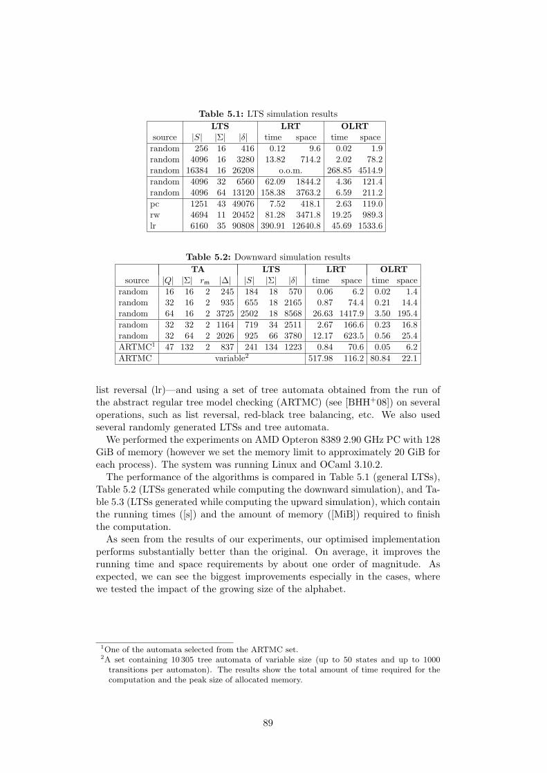
Table 5.1: LTS simulation results

LTS LRT OLRTsource |S| |Σ| |δ| time space time space

random 256 16 416 0.12 9.6 0.02 1.9random 4096 16 3280 13.82 714.2 2.02 78.2random 16384 16 26208 o.o.m. 268.85 4514.9

random 4096 32 6560 62.09 1844.2 4.36 121.4random 4096 64 13120 158.38 3763.2 6.59 211.2

pc 1251 43 49076 7.52 418.1 2.63 119.0rw 4694 11 20452 81.28 3471.8 19.25 989.3lr 6160 35 90808 390.91 12640.8 45.69 1533.6

Table 5.2: Downward simulation results

TA LTS LRT OLRTsource |Q| |Σ| rm |∆| |S| |Σ| |δ| time space time space

random 16 16 2 245 184 18 570 0.06 6.2 0.02 1.4random 32 16 2 935 655 18 2165 0.87 74.4 0.21 14.4random 64 16 2 3725 2502 18 8568 26.63 1417.9 3.50 195.4

random 32 32 2 1164 719 34 2511 2.67 166.6 0.23 16.8random 32 64 2 2026 925 66 3780 12.17 623.5 0.56 25.4

ARTMC1 47 132 2 837 241 134 1223 0.84 70.6 0.05 6.2

ARTMC variable2 517.98 116.2 80.84 22.1

list reversal (lr)—and using a set of tree automata obtained from the run ofthe abstract regular tree model checking (ARTMC) (see [BHH+08]) on severaloperations, such as list reversal, red-black tree balancing, etc. We also usedseveral randomly generated LTSs and tree automata.We performed the experiments on AMD Opteron 8389 2.90 GHz PC with 128

GiB of memory (however we set the memory limit to approximately 20 GiB foreach process). The system was running Linux and OCaml 3.10.2.The performance of the algorithms is compared in Table 5.1 (general LTSs),

Table 5.2 (LTSs generated while computing the downward simulation), and Ta-ble 5.3 (LTSs generated while computing the upward simulation), which containthe running times ([s]) and the amount of memory ([MiB]) required to finishthe computation.As seen from the results of our experiments, our optimised implementation

performs substantially better than the original. On average, it improves therunning time and space requirements by about one order of magnitude. Asexpected, we can see the biggest improvements especially in the cases, wherewe tested the impact of the growing size of the alphabet.

1One of the automata selected from the ARTMC set.2A set containing 10 305 tree automata of variable size (up to 50 states and up to 1000transitions per automaton). The results show the total amount of time required for thecomputation and the peak size of allocated memory.

89

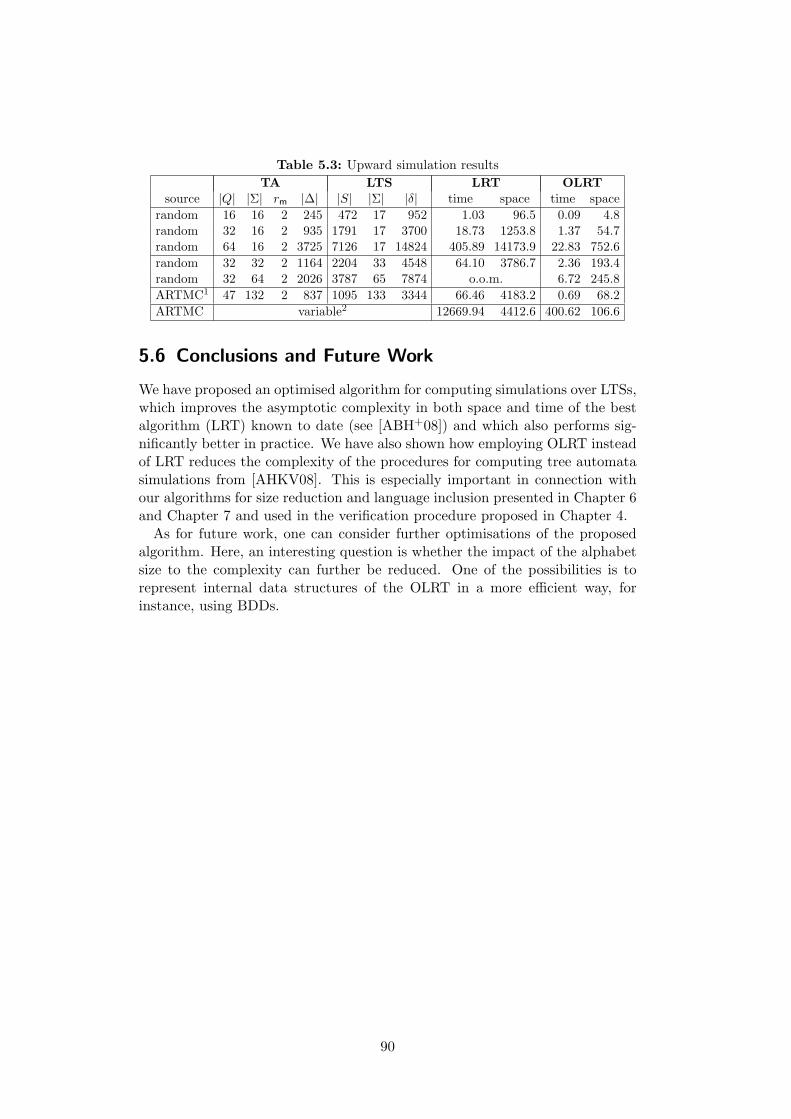
Table 5.3: Upward simulation results

TA LTS LRT OLRTsource |Q| |Σ| rm |∆| |S| |Σ| |δ| time space time space

random 16 16 2 245 472 17 952 1.03 96.5 0.09 4.8random 32 16 2 935 1791 17 3700 18.73 1253.8 1.37 54.7random 64 16 2 3725 7126 17 14824 405.89 14173.9 22.83 752.6

random 32 32 2 1164 2204 33 4548 64.10 3786.7 2.36 193.4random 32 64 2 2026 3787 65 7874 o.o.m. 6.72 245.8

ARTMC1 47 132 2 837 1095 133 3344 66.46 4183.2 0.69 68.2

ARTMC variable2 12669.94 4412.6 400.62 106.6


We have proposed an optimised algorithm for computing simulations over LTSs,which improves the asymptotic complexity in both space and time of the bestalgorithm (LRT) known to date (see [ABH+08]) and which also performs sig-nificantly better in practice. We have also shown how employing OLRT insteadof LRT reduces the complexity of the procedures for computing tree automatasimulations from [AHKV08]. This is especially important in connection withour algorithms for size reduction and language inclusion presented in Chapter 6and Chapter 7 and used in the verification procedure proposed in Chapter 4.As for future work, one can consider further optimisations of the proposed

algorithm. Here, an interesting question is whether the impact of the alphabetsize to the complexity can further be reduced. One of the possibilities is torepresent internal data structures of the OLRT in a more efficient way, forinstance, using BDDs.

90

6 Efficient Inclusion over TreeAutomata

As we have already mentioned, finite tree automata play a crucial role in sev-eral formal verification techniques, such as (abstract) regular tree model check-ing [AJMd02, BHRV06a], verification of programs with complex dynamic datastructures [BHRV06b], analysis of network firewalls [Bou11], and implementa-tion of decision procedures of logics such as WS2S or MSO [KMS01], whichthemselves have numerous applications. In the context of verification of pro-grams manipulating dynamically linked data structures, let us also mention(apart from our verification technique presented in Chapter 4, and many oth-ers) the work in [MPQ11] which deals with the verification of programs manip-ulating heap structures with data.In Chapter 5, we argued that in order to successfully use nondeterministic

finite automata, one needs efficient algorithms for handling them. This is no-tably the case of size reduction and language inclusion that are traditionallydone via determinisation. We have already said that determinisation-based sizereduction can be replaced by simulation quotienting and we have proposed thealgorithm for computing simulations to be used for this purpose. In this chapter,we concentrate on the other problem, i.e., the problem of inclusion checking.For that purpose, algorithms based on using antichains and antichains com-bined with simulations have been proposed in [BHH+08, ACH+10]. We furtherimprove the state of the art by proposing a new algorithm for inclusion checkingthat turns out to significantly outperform the existing algorithms in most of ourexperiments which we performed on two different automata representations. Inthe first case, the transition function of automata are encoded explicitly, in thesecond case, the transition function is encoded in a semi-symbolic way usingmulti-terminal binary decision diagrams (MTBDDs) such that the states stayexplicit.The classic textbook algorithm for checking inclusion L(AS) ⊆ L(AB) be-

tween two TA AS (Small) and AB (Big) first determinises AB, computes thecomplement automaton AB of AB, and then checks language emptiness of theproduct automaton accepting L(AS) ∩ L(AB). This approach has been opti-mised in [TH03, BHH+08, ACH+10] which describe variants of this algorithmthat try to avoid the construction of the whole product automaton (which canbe exponentially larger than AB and which is indeed extremely large in manypractical cases) by constructing some of its states and checking language empti-ness on the fly.By employing the antichain principle within the construction of the product

automaton which allows for the given set of states to discard all its supersets,the algorithm is often able to prove or refute inclusion by constructing a small

91

part of the product automaton only. The work of [TH03] does, in fact, notuse the terminology of antichains despite implementing them in a symbolic,BDD-based way. It specialises to binary tree automata only. A more gen-eral introduction of antichains within a lattice-theoretic framework appearedin the context of word automata in [DWDHR06]. Subsequently, [BHH+08]has generalised [DWDHR06] for explicit upward inclusion checking on TA andexperimentally advocated its use within abstract regular tree model checking.Additionally, the antichain algorithms can also be combined with using up-

ward simulation relations such as in [ACH+10] (see also [DR10] for other com-binations of antichains and simulations for word automata).

Upward Inclusion Checking. In general, we denote the above algorithms forTA as upward algorithms to reflect the direction in which they traverse au-tomata AS and AB (i.e., they start with leave transitions and continue upwardstowards the accepting states).The upward algorithms are sufficiently efficient in many practical cases. How-

ever, they have two drawbacks: (i) When generating the bottom-up post-imageof a set S of sets of states, all possible n-tuples of states from all possible prod-ucts S1×. . .×Sn, Si ∈ S need to be enumerated. (ii) Moreover, these algorithmsare known to be compatible with only upward simulations as a means of theirpossible optimisation, which is a disadvantage since downward simulations areoften much richer and also cheaper to compute.

Downward Inclusion Checking. The alternative downward approach to check-ing TA language inclusion was first proposed in [HVP05] in the context ofsubtyping of XML types. This algorithm is not derivable from the textbookapproach and has a more complex structure with its own weak points; neverthe-less, it does not suffer from the two issues of the upward algorithm mentionedabove. We generalise the algorithm of [HVP05] for automata over alphabetswith an arbitrary rank ([HVP05] considers rank at most two), and, most impor-tantly, we improve it significantly by using the antichain principle, empoweredby a use of the cheap and usually large downward simulation. In this way, we ob-tain an algorithm which is complementary to and highly competitive with theupward algorithm as shown by our experimental results (in which the newlyproposed algorithm significantly dominates in most of the considered cases).

Dealing with Semi-Symbolic Encoding. Certain important applications of TAsuch as formal verification of programs with complex dynamic data structuresor decision procedures of logics such as WS2S or MSO require handling verylarge alphabets. Here, the common choice is to use the MONA tree automatalibrary [KMS01] which is based on representing transitions of TA symbolicallyusing MTBDDs. However, the encoding used by MONA is restricted to deter-ministic automata only. This implies a necessity of immediate determinisationafter each operation over TA that introduces nondeterminism, which very eas-ily leads to a state space explosion. Despite the extensive engineering effort

92

spent to optimise the implementation of MONA, this fact significantly limitsits applicability.As a way to overcome this difficulty, we have participated on a proposal of

a semi-symbolic representation of nondeterministic TA which generalises theone used by MONA, and we have developed algorithms implementing the basicoperations on TA (such as union, intersection, etc.) as well as more involvedalgorithms for computing simulations and for checking inclusion (using simula-tions and antichains to optimise it) over the proposed representation. We havealso conducted experiments with a prototype implementation of our algorithmsshowing again a dominance of downward inclusion checking and justifying use-fulness of our symbolic encoding for TA with large alphabets. However, thesymbolic encoding is beyond the scope of this work. More details can be foundin [HLSV11a] or in [HLSV11b]. Here, we only present experimental evaluationin order to compare the inclusion algorithms.

Plan of the Chapter. The rest of this chapter is organised as follows. Sec-tion 6.1 describes the newly proposed downward inclusion checking algorithmand several extensions of its basic version which can greatly improve its perfor-mance. Section 6.2 provides an experimental evaluation of downward inclusionchecking in the explicit and the semi-symbolic setting. Section 6.3 then con-cludes the chapter.

6.1 Downward Inclusion Checking

Let us fix two tree automata AS = (QS ,Σ,∆S , FS) and AB = (QB,Σ,∆B, FB)for which we want to check whether L(AS) ⊆ L(AB) holds. If we try to answerthis query top-down and we proceed in a naıve way, we immediately realize thatthe fact that the top-down successors of particular states are tuples of statesleads us to checking inclusion of the languages of tuples of states. Subsequently,the need to compare the languages of each corresponding pair of states in thesetuples will again lead to comparing the languages of tuples of states, and hence,we end up comparing the languages of tuples of tuples of states, and the needto deal with more and more nested tuples of states never stops.For instance, given a transition q

a−→ (p1, p2) in AS , transitions r

a−→ (s1, s2)

and ra

−→ (t1, t2) in AB, and assuming that there are no further top-downtransitions from q and r, it holds that L(q) ⊆ L(r) if and only if L((p1, p2)) ⊆L((s1, s2)) ∪ L((t1, t2)). Note that the union L((s1, s2)) ∪ L((t1, t2)) cannot becomputed component-wise, this is, L((s1, s2)) ∪ L((t1, t2)) )= (L(s1) ∪ L(t1)) ×(L(s2) ∪ L(t2)). For instance, provided L(s1) = L(s2) = {b} and L(t1) =L(t2) = {c}, it holds that L((s1, s2)) ∪ L((t1, t2)) = {(b, b), (c, c)}, but thecomponent-wise union is

(L(s1) ∪ L(t1))× (L(s2) ∪ L(t2)) = {(b, b), (b, c), (c, b), (c, c)}.

Hence, we cannot simply check whether L(p1) ⊆ L(s1) ∪ L(t1) and L(p2) ⊆L(s2)∪L(t2) to answer the original query, and we have to proceed by checkinginclusion on the obtained tuples of states. However, exploring the top-down

93

transitions that lead from the states that appear in these tuples will lead us todealing with tuples of tuples of states, etc.Fortunately, there is a way out of the above trap. In particular, as first

observed in [HVP05] in the context of XML type checking, we can exploit thefollowing property of the Cartesian product of sets G,H ⊆ U :

G×H = (G× U) ∩ (U ×H). (6.1)

Continuing in our example, we can rewrite

L(p1)× L(p2) ⊆ (L((s1, s2)) ∪ L((t1, t2))) =

(L(s1)× L(s2)) ∪ (L(t1)× L(t2))(6.2)

as

L(p1)× L(p2) ⊆ ((L(s1)× TΣ) ∩ (TΣ × L(s2)))∪

((L(t1)× TΣ) ∩ (TΣ × L(t2))) ,(6.3)

This can further be rewritten, using the distributive laws in the (2TΣ×TΣ ,⊆)lattice, as

L(p1)× L(p2) ⊆ ((L(s1)× TΣ) ∪ (L(t1)× TΣ))∩

((L(s1)× TΣ) ∪ (TΣ × L(t2)))∩

((TΣ × L(s2)) ∪ (L(t1)× TΣ))∩

((TΣ × L(s2)) ∪ (TΣ × L(t2))) .

(6.4)

It is easy to see that the inclusion holds exactly if it holds for all componentsof the intersection, i.e., if and only if

L(p1)× L(p2) ⊆ ((L(s1)× TΣ) ∪ (L(t1)× TΣ))∧

L(p1)× L(p2) ⊆ ((L(s1)× TΣ) ∪ (TΣ × L(t2)))∧

L(p1)× L(p2) ⊆ ((TΣ × L(s2)) ∪ (L(t1)× TΣ))∧

L(p1)× L(p2) ⊆ ((TΣ × L(s2)) ∪ (TΣ × L(t2))) .

(6.5)

Two things should be noted in the previous equation.

1. If we are computing the union of languages of two tuples such that theyhave TΣ at all indices other than some index i, we can compute it com-ponent-wise, i.e.,

L(p1)× L(p2) ⊆ ((L(s1)× TΣ) ∪ (L(t1)× TΣ)) =

(L(s1) ∪ L(t1))× TΣ.(6.6)

The above clearly holds iff L(p1) ⊆ L(s1) ∪ L(t1).

2. If TΣ does not appear at the same positions as in the inclusion

L(p1)× L(p2) ⊆ ((L(s1)× TΣ) ∪ (TΣ × L(t2))) , (6.7)

it must hold that either

L(p1) ⊆ L(s1) or L(p2) ⊆ L(t2). (6.8)

94

Using the above observations, we can finally rewrite the equation L(p1) ×L(p2) ⊆ L((s1, s2))∪L((t1, t2)) into the following formula that does not containlanguages of tuples but of single states only:

L(p1) ⊆ L(s1) ∪ L(t1) ∧

(L(p1) ⊆ L(s1) ∨ L(p2) ⊆ L(t2)) ∧

(L(p1) ⊆ L(t1) ∨ L(p2) ⊆ L(s2)) ∧

L(p2) ⊆ L(s2) ∪ L(t2).

(6.9)

The above reasoning can be generalised to dealing with transitions of anyarity as shown in Theorem 3. In the theorem, we conveniently exploit thenotion of choice functions. Given PB ⊆ QB and a ∈ Σ, #a = n ≥ 1, wedenote by cf (PB, a) the set of all choice functions f that assign an index i,1 ≤ i ≤ n, to all n-tuples (q1, . . . , qn) ∈ Qn

B such that there exists a state inPB that can make a transition over a to (q1, . . . , qn); formally, cf (PB, a) = {f :downa(PB) → {1, . . . ,#a}}.

Theorem 3 Let AS = (QS ,Σ,∆S , FS) and AB = (QB,Σ,∆B, FB) be treeautomata. For sets PS ⊆ QS and PB ⊆ QB it holds that L(PS) ⊆ L(PB)if and only if ∀pS ∈ PS ∀a ∈ Σ : if pS

a−→ (r1, . . . , r#a), then it holds that

downa(PB) = {()} when #a = 0 and

∀f ∈ cf (PB, a) ∃1 ≤ i ≤ #a : L(ri) ⊆⋃

(u1,...,u#a)∈downa(PB)

f((u1,...,u#a))=i

L(ui)

when #a > 0.

Proof. For two sets PS ⊆ QS , PB ⊆ QB, it clearly holds that L(PS) ⊆ L(PB)if and only if ∀pS ∈ PS ∀a ∈ Σ :

pSa

−→ (r1, . . . , rn) =⇒ L((r1, . . . , rn)) ⊆⋃

u∈downa(PB)

L((u1, . . . , un)) (6.10)

where u = (u1, . . . , un). For the case when #a = 0, the above formula collapsesto pS

a−→ () =⇒ L(()) ⊆ ∪()∈downa(PB)L(()). Since downa(PB) ⊆ {()} for

#a = 0, the first part of the theorem is proven. We prove the second part(when #a > 0) in the following steps. Let us fix n = #a, u = u1, . . . , un:

L((r1, . . . , rn)) ⊆⋃

u∈downa(PB)

L((u1, . . . , un)) ⇐⇒

n∏

i=1

L(ri) ⊆⋃

u∈downa(PB)

n∏

i=1

L(ui),

(6.11)

where∏n

i=1 Si denotes the Cartesian product of a family of sets {S1, . . . , Sn}.We can further observe that for a set U and a family of sets {S1, . . . , Sn} : ∀1 ≤i ≤ n : Si ⊆ U it holds that

n∏

i=1

Si =

n⋂

i=1

U i−1 × Si × Un−i. (6.12)

95

Given the family of sets {L(u1), . . . ,L(un)} and the decomposition from Equa-tion 6.12 we can modify the formula from Equation 6.11 in the following way:

n∏

i=1

L(ri) ⊆⋃

u∈downa(PB)

n∏

i=1

L(ui) ⇐⇒

n∏

i=1

L(ri) ⊆⋃

u∈downa(PB)

n⋂

i=1

T i−1Σ

× L(ui)× Tn−iΣ

.

(6.13)

Since the power set lattice (2QB ,⊆) is a completely distributive lattice, we canexploit the fact that for any doubly indexed family {xj,k ∈ 2QB | j ∈ J, k ∈ Kj}it holds that

⋃

j∈J

⋂

k∈Kj

xj,k =⋂

f∈F

⋃

j∈J

xj,f(j) (6.14)

where F is the set of choice functions f choosing for each index j ∈ J someindex f(j) ∈ Kj . For our purpose, we introduce the set of choice functions:

F = {f : downa(PB) → {1, . . . , n}}. (6.15)

Therefore,n∏

i=1

L(ri) ⊆⋃

u∈downa(PB)

n⋂

i=1

T i−1Σ

× L(ui)× Tn−iΣ

⇐⇒

n∏

i=1

L(ri) ⊆⋂

f∈F

⋃

u∈downa(PB)

Tf(u)−1Σ

× L(uf(u))× Tn−f(u)Σ

.

(6.16)

Due to the fact that for a set S, its subset T ⊆ S and a family of its subsetsR ⊆ 2S it holds that

T ⊆⋂

U∈R

U ⇐⇒ ∀U ∈ R : T ⊆ U, (6.17)

we can simplify our case in the following way:n∏

i=1

L(ri) ⊆⋂

f∈F

⋃

u∈downa(PB)

Tf(u)−1Σ


⇐⇒

∀f ∈ F :

n∏

i=1

L(ri) ⊆⋃

u∈downa(PB)

Tf(u)−1Σ


(6.18)

For some fixed f , we can further rewrite the right-hand side of the inclusionquery to the following:

⋃

u∈downa(PB)

Tf(u)−1Σ


=

n⋃

i=1

⋃

u∈downa(PB)

f(u)=i

T i−1Σ

× L(ui)× Tn−iΣ

=

n⋃

i=1

T i−1Σ

×

⋃

u∈downa(PB)

f(u)=i

L(ui)

× Tn−i

Σ

(6.19)

96

It can be observed that for a set U and two families of sets {S1, . . . , Sn} and{S′

1, . . . , S′n} such that ∀1 ≤ i ≤ n : Si, S

′i ⊆ U it holds that

n∏

i=1

Si ⊆n⋃

i=1

U i−1 × S′i × Un−i ⇐⇒ ∃1 ≤ i ≤ n : Si ⊆ S′

i. (6.20)

Hence, we can now finally deduce that

∀f ∈ F :

n∏

i=1

L(ri) ⊆n⋃

i=1

T i−1Σ

×

⋃

u∈downa(PB)

f(u)=i

L(ui)

× Tn−i

Σ

⇐⇒

∀f ∈ F ∃1 ≤ i ≤ n : L(ri) ⊆⋃

u∈downa(PB)

f(u)=i

L(ui),

(6.21)

which concludes the proof. #

6.1.1 Basic Algorithm

We now construct a basic algorithm for downward inclusion checking on treeautomata AS = (QS ,Σ,∆S , FS) and AB = (QB,Σ,∆B, FB). The algorithmis shown as Algorithm 4. Its main idea relies on a recursive application ofTheorem 3 in function expand1. The function is given a pair (pS , PB) ∈ QS ×2QB for which we want to prove that L(pS) ⊆ L(PB)—initially, the functionis called for every pair (qS , FB) where qS ∈ FS . The function enumerates allpossible top-down transitions that AS can do from pS (lines 3–8). For eachsuch transition, the function either checks whether there is some transitionpB

a−→ for pB ∈ PB if #a = 0 (line 5), or it starts enumerating and recursively

checking queries L(p′S) ⊆ L(P ′B) on which the result of L(pS) ⊆ L(PB) depends

according to Theorem 3 (lines 9–16).The expand1 function keeps track of which inclusion queries are currently

being evaluated in the set workset (line 2). Encountering a query L(p′S) ⊆L(P ′

B) with (p′S , P′B) ∈ workset means that the result of L(p′S) ⊆ L(P ′

B) dependson the result of L(p′S) ⊆ L(P ′

B) itself. In this case, the function immediatelysuccessfully returns because the result of the query then depends only on theother branches of the call tree.Using Theorem 3 and noting that Algorithm 4 necessarily terminates because

all its loops are bounded, and the recursion in function expand1 is also boundeddue to the use of workset , it is not difficult to see that the following theoremholds.

Theorem 4 Let AS = (QS ,Σ,∆S , FS) and AB = (QB,Σ,∆B, FB) be two TA.Algorithm 4 terminates and returns true if and only if L(AS) ⊆ L(AB).

97

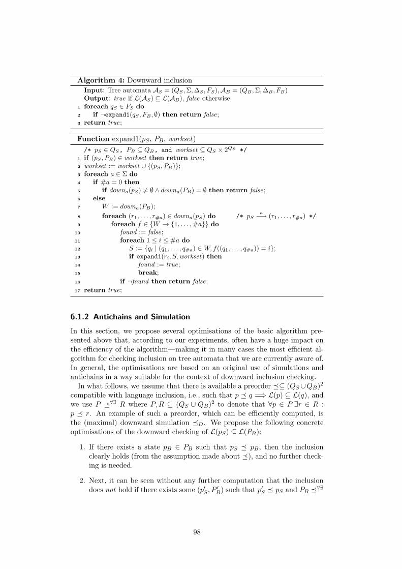
Algorithm 4: Downward inclusion

Input: Tree automata AS = (QS ,Σ,∆S , FS),AB = (QB ,Σ,∆B , FB)Output: true if L(AS) ⊆ L(AB), false otherwise

1 foreach qS ∈ FS do2 if ¬expand1(qS , FB , ∅) then return false;3 return true;

Function expand1(pS , PB, workset)

/* pS ∈ QS, PB ⊆ QB, and workset ⊆ QS × 2QB */

1 if (pS , PB) ∈ workset then return true;2 workset := workset ∪ {(pS , PB)};3 foreach a ∈ Σ do4 if #a = 0 then5 if downa(pS) )= ∅ ∧ downa(PB) = ∅ then return false;6 else7 W := downa(PB);

8 foreach (r1, . . . , r#a) ∈ downa(pS) do /* pSa

−→ (r1, . . . , r#a) */

9 foreach f ∈ {W → {1, . . . ,#a}} do10 found := false;11 foreach 1 ≤ i ≤ #a do12 S := {qi | (q1, . . . , q#a) ∈ W, f((q1, . . . , q#a)) = i};13 if expand1(ri, S,workset) then14 found := true;15 break;

16 if ¬found then return false;

17 return true;

6.1.2 Antichains and Simulation

In this section, we propose several optimisations of the basic algorithm pre-sented above that, according to our experiments, often have a huge impact onthe efficiency of the algorithm—making it in many cases the most efficient al-gorithm for checking inclusion on tree automata that we are currently aware of.In general, the optimisations are based on an original use of simulations andantichains in a way suitable for the context of downward inclusion checking.In what follows, we assume that there is available a preorder (⊆ (QS ∪QB)

2

compatible with language inclusion, i.e., such that p ( q =⇒ L(p) ⊆ L(q), andwe use P (∀∃ R where P,R ⊆ (QS ∪ QB)

2 to denote that ∀p ∈ P ∃r ∈ R :p ( r. An example of such a preorder, which can be efficiently computed, isthe (maximal) downward simulation (D. We propose the following concreteoptimisations of the downward checking of L(pS) ⊆ L(PB):

1. If there exists a state pB ∈ PB such that pS ( pB, then the inclusionclearly holds (from the assumption made about (), and no further check-ing is needed.

2. Next, it can be seen without any further computation that the inclusiondoes not hold if there exists some (p′S , P

′B) such that p′S ( pS and PB (∀∃

98

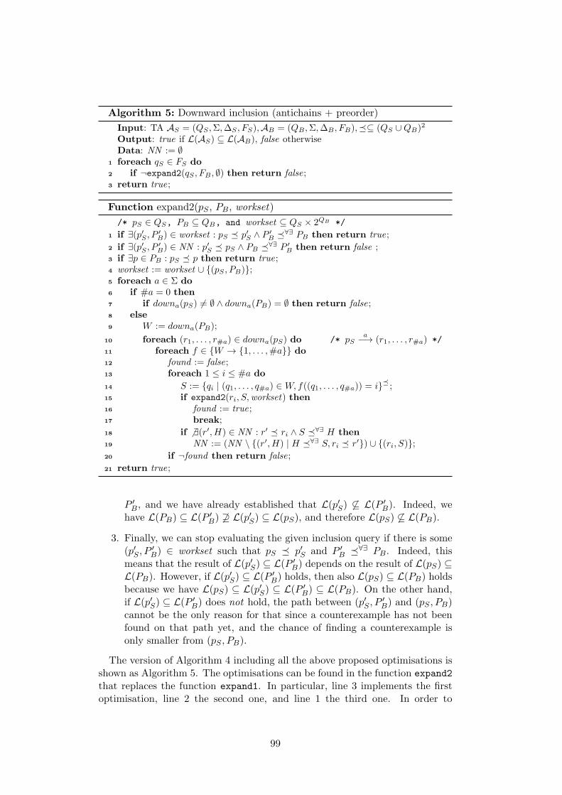
Algorithm 5: Downward inclusion (antichains + preorder)

Input: TA AS = (QS ,Σ,∆S , FS),AB = (QB ,Σ,∆B , FB),(⊆ (QS ∪QB)2

Output: true if L(AS) ⊆ L(AB), false otherwiseData: NN := ∅

1 foreach qS ∈ FS do2 if ¬expand2(qS , FB , ∅) then return false;3 return true;

Function expand2(pS , PB, workset)


1 if ∃(p′S , P′B) ∈ workset : pS ( p′S ∧ P ′

B (∀∃ PB then return true;

2 if ∃(p′S , P′B) ∈ NN : p′S ( pS ∧ PB (∀∃ P ′

B then return false ;3 if ∃p ∈ PB : pS ( p then return true;4 workset := workset ∪ {(pS , PB)};5 foreach a ∈ Σ do6 if #a = 0 then7 if downa(pS) )= ∅ ∧ downa(PB) = ∅ then return false;8 else9 W := downa(PB);


−→ (r1, . . . , r#a) */

11 foreach f ∈ {W → {1, . . . ,#a}} do12 found := false;13 foreach 1 ≤ i ≤ #a do

14 S := {qi | (q1, . . . , q#a) ∈ W, f((q1, . . . , q#a)) = i}(;

15 if expand2(ri, S,workset) then16 found := true;17 break;

18 if ) ∃(r′, H) ∈ NN : r′ ( ri ∧ S (∀∃ H then19 NN := (NN \ {(r′, H) | H (∀∃ S, ri ( r′}) ∪ {(ri, S)};

20 if ¬found then return false;

21 return true;

P ′B, and we have already established that L(p′S) )⊆ L(P ′

B). Indeed, wehave L(PB) ⊆ L(P ′

B) )⊇ L(p′S) ⊆ L(pS), and therefore L(pS) )⊆ L(PB).

3. Finally, we can stop evaluating the given inclusion query if there is some(p′S , P

′B) ∈ workset such that pS ( p′S and P ′

B (∀∃ PB. Indeed, thismeans that the result of L(p′S) ⊆ L(P ′

B) depends on the result of L(pS) ⊆L(PB). However, if L(p′S) ⊆ L(P ′

B) holds, then also L(pS) ⊆ L(PB) holdsbecause we have L(pS) ⊆ L(p′S) ⊆ L(P ′

B) ⊆ L(PB). On the other hand,if L(p′S) ⊆ L(P ′

B) does not hold, the path between (p′S , P′B) and (pS , PB)

cannot be the only reason for that since a counterexample has not beenfound on that path yet, and the chance of finding a counterexample isonly smaller from (pS , PB).

The version of Algorithm 4 including all the above proposed optimisations isshown as Algorithm 5. The optimisations can be found in the function expand2

that replaces the function expand1. In particular, line 3 implements the firstoptimisation, line 2 the second one, and line 1 the third one. In order to

99

implement the second optimisation, the algorithm maintains a new set NN .This set stores pairs (pS , PB) for which it has already been shown that theinclusion L(pS) ⊆ L(PB) does not hold.

As a further optimisation, the set NN is maintained as an antichain w.r.t.the preorder that compares the pairs stored in NN such that the states fromQS on the left are compared w.r.t. (, and the sets from 2QB on the right arecompared w.r.t. >∃∀ (line 19). Clearly, there is no need to store a pair (pS , PB)that is bigger in the described sense than some other pair (p′S , P

′B) since every

time (pS , PB) can be used to prune the search, (p′S , P′B) can also be used.

Taking into account Theorem 4 and the above presented facts, it is not diffi-cult to see that the following holds.


6.1.3 Caching Positive Pairs

The inclusion checking presented in the previous section can be optimised evenmore. Recall that the algorithm caches pairs for which the inclusion does nothold, i.e., pairs (pS , PB) such that L(pS) )⊆ L(PB), in the set NN (which ismaintained as an antichain). A natural question that arises is whether there isa similar option for pairs for which the inclusion does hold, i.e., pairs (pS , PB)such that L(pS) ⊆ L(PB). Such an option indeed exists and is presented in therest of this subsection.Let us denote the set of the above-mentioned pairs for which the inclusion

holds as IN . When checking the inclusion L(pS) ⊆ L(PB), we first try tofind a pair (p′S , P

′B) ∈ IN such that pS ( p′S and P ′

B (∀∃ PB. If such pairexists, then we immediately know that the checked inclusion holds becauseL(pS) ⊆ L(p′S) ⊆ L(P ′

B) ⊆ L(PB).The set IN can again be optimised as an antichain but with the opposite

ordering than NN . This means that there are no two pairs (pS , PB), (p′S , P

′B)

such that pS ( p′S and P ′B (∀∃ PB in IN . It is easy to understand that a pair

(pS , PB) does not have to be stored since whenever (pS , PB) can be used toprune the search, (p′S , P

′B) can also be used.

However, adding new pairs to IN is not as straightforward as for NN .Assume that we add a pair (pS , PB) to IN immediately when the functioncall expand2(pS , PB,workset) at line 15 of Algorithm 5 returns true for someworkset . This is not correct as shown in the following example.Suppose that when checking inclusion L(p′S) ⊆ L(P ′

B), a test for inclusionL(pS) ⊆ L(PB) where pS ( p′S and P ′

B (∀∃ PB is encountered somewheredeep in the recursive calls of expand2. As stated previously, the inclusionL(pS) ⊆ L(PB) does not need to be tested since if L(p′S) ⊆ L(P ′

B), then L(pS) ⊆L(PB), and if L(p′S) )⊆ L(P ′

B), then this cannot be caused solely by L(pS) )⊆L(PB). Hence, expand2(pS , PB,workset) returns true, and the result of thequery L(p′S) ⊆ L(P ′

B) will be given by other branches of the call tree generatedfor the L(p′S) ⊆ L(P ′

B) query. However, if we put the pair (pS , PB) into INand later proved that L(p′S) )⊆ L(P ′

B), then the set IN would become invalid.

100

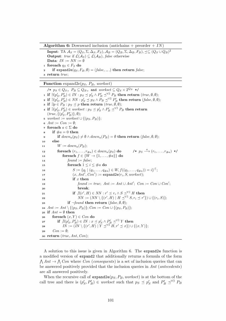
Algorithm 6: Downward inclusion (antichains + preorder + IN)

Input: TA AS = (QS ,Σ,∆S , FS),AB = (QB ,Σ,∆B , FB),(⊆ (QS ∪QB)2

Output: true if L(AS) ⊆ L(AB), false otherwiseData: IN := NN := ∅

1 foreach qS ∈ FS do2 if expand2e(qS , FB , ∅) = (false, , ) then return false;3 return true;

Function expand2e(pS , PB, workset)


1 if ∃(p′S , P′B) ∈ IN : pS ( p′S ∧ P ′

B (∀∃ PB then return (true, ∅, ∅);

2 if ∃(p′S , P′B) ∈ NN : p′S ( pS ∧ PB (∀∃ P ′

B then return (false, ∅, ∅);3 if ∃p ∈ PB : pS ( p then return (true, ∅, ∅);

4 if ∃(p′S , P′B) ∈ workset : pS ( p′S ∧ P ′

B (∀∃ PB then return(true, {(p′S , P

′B)}, ∅);

5 workset := workset ∪ {(pS , PB)};6 Ant := Con := ∅;7 foreach a ∈ Σ do8 if #a = 0 then9 if downa(pS) )= ∅ ∧ downa(PB) = ∅ then return (false, ∅, ∅);

10 else11 W := downa(PB);


−→ (r1, . . . , r#a) */

13 foreach f ∈ {W → {1, . . . ,#a}} do14 found := false;15 foreach 1 ≤ i ≤ #a do

16 S := {qi | (q1, . . . , q#a) ∈ W, f((q1, . . . , q#a)) = i}(;

17 (x,Ant ′,Con ′) := expand2e(ri, S,workset);18 if x then19 found := true; Ant := Ant ∪ Ant ′; Con := Con ∪ Con ′;20 break;

21 if ) ∃(r′, H) ∈ NN : r′ ( ri ∧ S (∀∃ H then22 NN := (NN \ {(r′, H) | H (∀∃ S, ri ( r′}) ∪ {(ri, S)};

23 if ¬found then return (false, ∅, ∅);24 Ant := Ant \ {(pS , PB)};Con := Con ∪ {(pS , PB)};25 if Ant = ∅ then26 foreach (x, Y ) ∈ Con do27 if ) ∃(p′S , P

′B) ∈ IN : x ( p′S ∧ P ′

B (∀∃ Y then28 IN := (IN \ {(r′, H) | Y (∀∃ H, r′ ( x}) ∪ {(x, Y )};

29 Con := ∅;30 return (true,Ant ,Con);

A solution to this issue is given in Algorithm 6. The expand2e function isa modified version of expand2 that additionally returns a formula of the form∧

Ant →∧

Con where Con (consequents) is a set of inclusion queries that canbe answered positively provided that the inclusion queries in Ant (antecedents)are all answered positively.When the recursive call of expand2e(pS , PB,workset) is at the bottom of the

call tree and there is (p′S , P′B) ∈ workset such that pS ( p′S and P ′

B (∀∃ PB

101

(line 4), then according to the above, the formula returned from expand2e alongwith true could be

∧

{L(p′S) ⊆ L(P ′B)} →

∧

{L(pS) ⊆ L(PB)} because L(pS) ⊆L(PB) cannot be considered guaranteed before L(p′S) ⊆ L(P ′

B) is positivelyanswered. This formula is, however, simplified to

∧

{L(p′S) ⊆ L(P ′B)} → ∅

since L(pS) ⊆ L(PB) can be forgotten as it is weaker than L(p′S) ⊆ L(P ′B).

A situation similar to what we have just discussed arises when the recursivecall of expand2e(pS , PB,workset) is at the bottom of the call tree and there is(p′S , P

′B) ∈ IN such that pS ( p′S and P ′

B (∀∃ PB (line 1). In this case,∧

∅ →∧

∅ is returned (along with true) since the validity of L(p′S) ⊆ L(P ′B) has already

been established. Next, if the recursive call of expand2e(pS , PB,workset) is atthe bottom of the call tree and there is p ∈ PB such that pS ( p (line 3),∧

∅ →∧

∅ is again returned since for any inclusion query L(p′S) ⊆ L(P ′B) such

that p′S ( pS and PB (∀∃ P ′B, it will be the case that there is p′ ∈ P ′

B suchthat p′S ( p′ (and hence the computation will be immediately stopped withouta need to use IN for this purpose). Finally, when expand2e returns false (line2), it is accompanied by the formula

∧

∅ →∧

∅, which, however, is not takeninto account in this case and is returned just to make the result of expand2eto have the same structure.For inner nodes of the call tree, this is, nodes that correspond to function

calls expand2e(pS , PB) that themselves call expand2e, all antecedents and con-sequents returned from successful nested calls are collected into sets Ant andCon. Then, the condition L(pS) ⊆ L(PB) is removed from Ant (if it is there)and added to Con since it has just been proved that L(pS) ⊆ L(PB) holds pro-vided that the elements from Ant \ {L(pS) ⊆ L(PB)} are later proved to alsohold. When the set Ant becomes empty, yielding the formula

∧

∅ →∧

Con, allelements of Con can be added to IN (while respecting the antichain propertyof IN) and the set Con cleared.

Taking into account Theorem 5 and the above presented facts, it can be seenthat the following holds.


6.2 Experimental Results

We have experimented with two tree automata encodings. The first one rep-resents the automata explicitly, i.e., the transition function is stored as a plainlist. The second encoding stores the automata in a semi-symbolic way usingMTBDDs allowing for a convenient representation of automata with large al-phabets.

6.2.1 Explicit Encoding

We have implemented three versions of downward inclusion for exlicitly en-coded tree automata. Algorithm 5 using an identity as an input preorder isdenoted by down, Algorithm 5 using the maximum downward simulation as theinput preorder is marked as down+s. Algorithm 6 is denoted by down+opt when

102

Table 6.1: A comparison of inclusion checking methods on explicit encoding

small TA (timeout 20 s) big TA (timeout 60 s)

winnerwinner(wo sim) timeout winner

winner(wo sim) timeout

up 25.52% - 0.00% 3.13% - 48.44%up+s 0.00% 81.82% 0.00% 0.00% 20.31% 48.44%down 16.21% - 25.08% 39.06% - 60.94%down+s 3.45% 18.18% 0.93% 14.06% 79.69% 9.38%down+opt 42.07% - 25.08% 0.00% - 60.94%down+opt+s 16.76% 0.00% 0.62% 56.25% 0.00% 1.56%

parametrised by identity. down+opt+s denotes the combination with maximumdownward simulation. We have also implemented the algorithm of upward in-clusion checking using antichains from [BHH+08] and its modification usingupward simulation proposed in [ACH+10] (these algorithms are marked as upand up+s below). We tested our approach on 387 tree automata pairs of differ-ent sizes generated from the intermediate steps of abstract regular tree modelchecking of the algorithm for rebalancing red-black trees after insertion or dele-tion of a leaf node [BHH+08]. The automata have been divided into two setsdepending on their size. The first set (denoted by “small TA”) contains 323automata of size ranging between 50 and 250 states. The second set (denotedby “big TA”) contains 64 automata of size ranging between 400 and 600 states.The results of the experiments with explicitly encoded automata are pre-

sented in Table 6.1 which compares the methods according to the percentageof the cases in which they were the fastest when checking inclusion on the sameautomata pair. The results are grouped into two sets according to the size ofthe automata measured in the number of states. Columns “winner (wo sim)”contain the percentage of the cases in which the method was the fastest with-out counting the time for computing simulation (in such cases they were alwaysfaster than the methods not using simulations). This comparison is motivatedby the observation that inclusion checking may be used as a part of a biggercomputation that anyway computes the simulation relations (which happens,e.g., in abstract regular model checking where the simulations are used for re-ducing the size of the encountered automata). Finally, the columns labelledby “timeout” summarise how often the particular methods exceeded the timeavailable for the computation of a single inclusion query.The results show that the overhead of computing upward simulation is too

high in all the cases that we have considered, causing upward inclusion checkingusing simulation to be the slowest when the time for computing the simulationused by the algorithm is included1. Next, it can be seen that for each of theremaining approaches there are cases in which they win in a significant way.However, the downward approaches are clearly dominating in significantly moreof our test cases (with the only exception being the case of small automata whenthe time of computing simulations is not included). Moreover, the dominance

1Note that up+s was winning over up in the experiments of [ACH+10] even with the timefor computing simulation included, which seems to be caused by a much less efficientimplementation of the antichains in the original algorithm.

103

Table 6.2: A comparison of inclusion checking methods on semi-symbolic encoding

winner timeout

symup 6.67% 22.68%symdown 90.67% 22.68%symdown+s 2.67% 73.92%

of the downward checking increases with the size of the automata that weconsidered in our test cases. Finally, one can observe that the down+opt+s cansolve almost all queries within the given timeout on both sets of automata eventhough it does not dominate on the set of smaller automata performance wise.

6.2.2 Semi-symbolic Encoding

In addition to experiments with explicitly encoded automata, we have alsobenchmarked our algorithms on automata represented in a semi-symbolic wayusing MTBDDs for storing transition functions. We have implemented some ofthe above mentioned algorithms on top of the MTBDD implementation foundin the CUDD library [Som11]. A detailed description of the algorithms modifiedfor the semi-symbolic setting can be found in [HLSV11b].

We have compared the upward inclusion checking algorithm from [BHH+08]adapted for semi-symbolically represented tree automata, which is given in[HLSV11b] (and marked as symup in the following), with the downward inclu-sion checking algorithm presented above. In the latter case, we let the algorithmuse either the identity relation, which corresponds to downward inclusion check-ing without using any simulation (this case is marked as symdown below), or themaximum downward simulation (which is marked as symdown+s in the results).We have not considered upward inclusion checking with upward simulation dueto its negative results in our experiments with explicitly encoded automata2.The implementation of downward inclusion checking with caching of positivepairs on top of the MTBDD package found in CUDD is also not available (seeChapter 7 for the version built on top of our own MTBDD library). For thecomparison, we used 97 pairs of tree automata with a large alphabet whichwe encoded into 12 bits. The size of the automata was between 50 and 150states and the timeout was set to 300 s. The automata were obtained by tak-ing the automata considered in Section 6.2.1 and labelling their transitions byrandomly generated sets of symbols from the considered large alphabet.The results that we have obtained are presented in Table 6.2. The first column

compares the methods according to the percentage of the cases in which theywere the fastest when checking inclusion on the same automata pair. The secondcolumn summarises how often each of the methods exceeded the time availablefor computation.When we compare the above experimental results with the results obtained on

the explicitly represented automata presented in Section 6.2.1, we may note that

2We, however, note that possibilities of implementing upward inclusion checking combinedwith upward simulations over semi-symbolically encoded TA and a further evaluation ofthis algorithm are still interesting subjects for the future.

104

(1) downward inclusion checking is again significantly dominating, but (2) theadvantage of exploiting downward simulation has decreased. According to theinformation we gathered from code profiling of our implementation, this is dueto the overhead of the CUDD library which is used as the underlying layer forstorage of shared MTBDDs of several data structures. This has indicated a needof a different MTBDD library to be used or perhaps of a specialised MTBDDlibrary to be developed. The issue is further briefly discussed in Chapter 7.Finally, we also evaluated performance of the implementation of the described

algorithms using a semi-symbolic encoding of TA with performance of the al-gorithms using an explicit encoding of TA considered in Section 6.1 on theautomata with the large alphabet. As we have expected, the symbolic versionwas on average about 8000 times faster than the explicit one in this case.


We have proposed a new algorithm for checking language inclusion over nonde-terministic TA (based on the one from [HVP05]) that traverses automata ina downward manner and uses both antichains and simulations to optimise itscomputation. This algorithm is, according to our experimental results, mostlysuperior to the known upward algorithms. We have further briefly presenteda semi symbolic MTBDD-based representation of nondeterministic TA gener-alising the one used by MONA. We have experimentally justified usefulness ofthe semi-symbolic encoding for nondeterministic TA with large alphabets.Furthermore, our experiments with downward inclusion show that the per-

formance of the algorithm is heavily dependent on the sequence in which oneevaluates successors of pairs of states. In the future, it would be interesting toexplore whether a more efficient order of exploring these successors exists.

105

7 A Tree Automata Library

This chapter describes the general-purpose tree automata library that was de-signed within our research. The library contains an efficient implementation ofmany important algorithms for use of TA in symbolic verification such as thealgorithm for computing simulations over TA presented in Chapter 5 or variousinclusion checking methods described in [ACH+10] or in Chapter 6.The main motivation behind the development of the library is to achieve

a better performance of the Forester verification tool presented in Chapter 4.Apart from this tool, as we have already discussedthere are other formal verifi-cation techniques relying on finite tree automata which often strongly dependson the performance of the underlying implementation of TA.Currently, there exist several available tree automata libraries, which are

mostly written in OCaml (e.g., Timbuk/Taml [Gen03]) or Java (e.g., LETHAL[CJH+09]), and they do not always use the most advanced algorithms knownto date. Therefore, they are not suitable for tasks which require that theavailable processing power is utilised as efficiently as possible. An exceptionfrom these libraries is MONA [KMS01] implementing decision procedures overWS1S/WS2S, which contains a highly optimised TA package written in C, but,alas, it supports only binary deterministic tree automata. As we have alreadymentioned, the determinisation is often a very significant bottleneck, and a lotof effort has therefore been invested into developing efficient algorithms forhandling nondeterministic tree automata without a need to ever determinisethem.In order to allow researchers focus on developing verification techniques rather

than reimplementing and optimising a TA package, we provide VATA1, aneasy-to-use open-source library for efficient manipulation of nondeterministicTA. VATA supports many of the operations commonly used in automata-basedformal verification techniques over two complementary encodings: explicit andsemi-symbolic. The explicit encoding is suitable for most applications that donot need to use alphabets with a large number of symbols. However, someformal verification approaches make use of such alphabets, e.g., the approachfor verification of programs with complex dynamic data structures [BHRV06a]or decision procedures of the MSO or WSkS logics [KMS01]. Therefore, inorder to address this issue, we also provide a semi-symbolic encoding of TA,which uses multi-terminal binary decision diagrams [CMZ+97] (MTBDDs), anextension of reduced ordered binary decision diagrams [Bry86] (BDDs), to storethe transition function of TA. In order to enable the widest possible range ofapplications of the library even for the semi-symbolic encoding, we provide bothbottom-up and top-down semi-symbolic representations.

1http://www.fit.vutbr.cz/research/groups/verifit/tools/libvata/

106

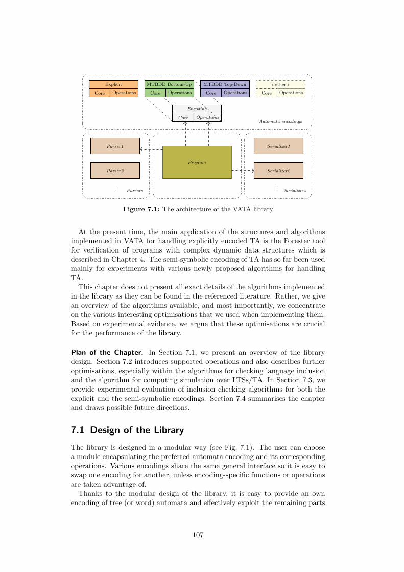
Encoding

Core Operations

Explicit

Core Operations

MTBDD Bottom-Up

Core Operations

MTBDD Top-Down

Core Operations

<other>

Core Operations

Automata encodings

Parser1

Parser2

.

.. Parsers

Serializer1

Serializer2

.

.. Serializers

Program

Figure 7.1: The architecture of the VATA library

At the present time, the main application of the structures and algorithmsimplemented in VATA for handling explicitly encoded TA is the Forester toolfor verification of programs with complex dynamic data structures which isdescribed in Chapter 4. The semi-symbolic encoding of TA has so far been usedmainly for experiments with various newly proposed algorithms for handlingTA.This chapter does not present all exact details of the algorithms implemented

in the library as they can be found in the referenced literature. Rather, we givean overview of the algorithms available, and most importantly, we concentrateon the various interesting optimisations that we used when implementing them.Based on experimental evidence, we argue that these optimisations are crucialfor the performance of the library.

Plan of the Chapter. In Section 7.1, we present an overview of the librarydesign. Section 7.2 introduces supported operations and also describes furtheroptimisations, especially within the algorithms for checking language inclusionand the algorithm for computing simulation over LTSs/TA. In Section 7.3, weprovide experimental evaluation of inclusion checking algorithms for both theexplicit and the semi-symbolic encodings. Section 7.4 summarises the chapterand draws possible future directions.

7.1 Design of the Library

The library is designed in a modular way (see Fig. 7.1). The user can choosea module encapsulating the preferred automata encoding and its correspondingoperations. Various encodings share the same general interface so it is easy toswap one encoding for another, unless encoding-specific functions or operationsare taken advantage of.Thanks to the modular design of the library, it is easy to provide an own

encoding of tree (or word) automata and effectively exploit the remaining parts

107

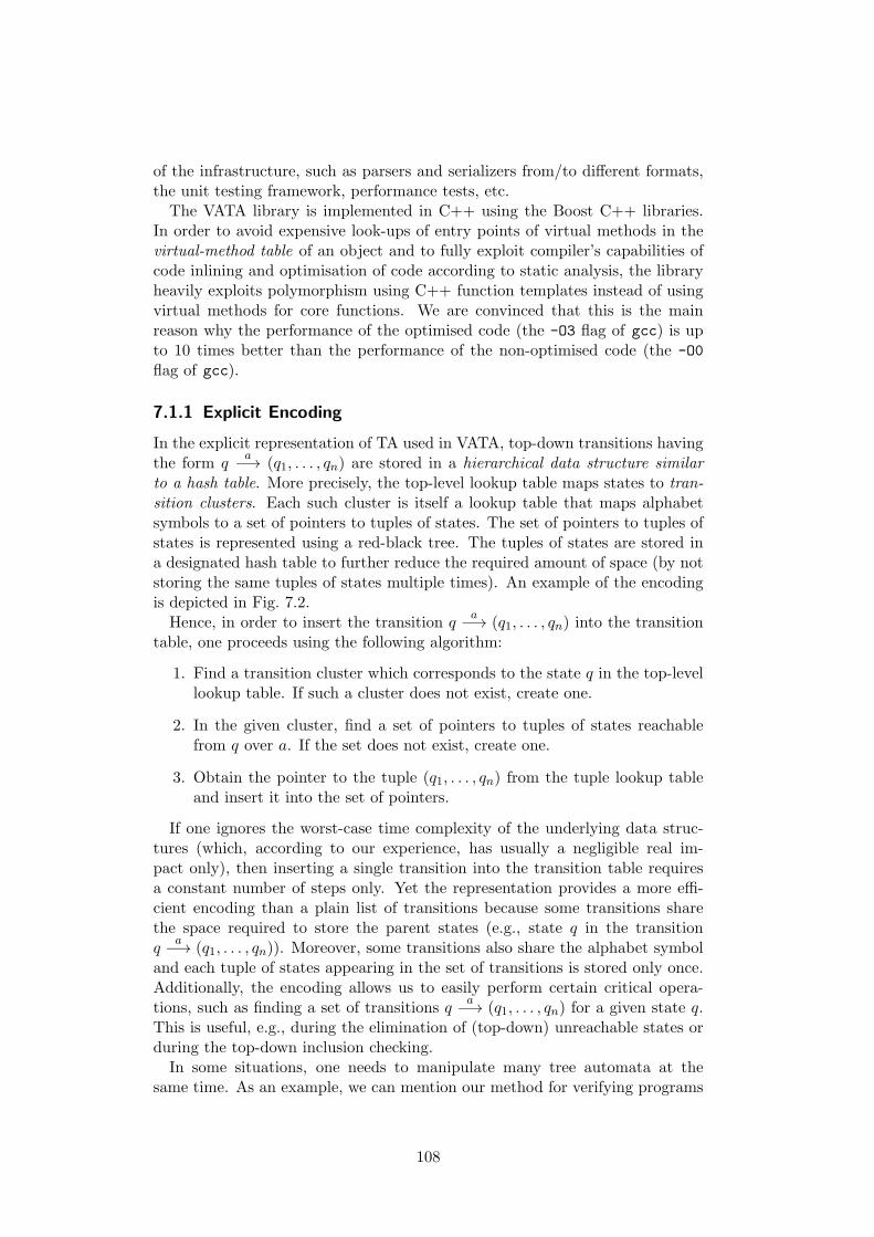
of the infrastructure, such as parsers and serializers from/to different formats,the unit testing framework, performance tests, etc.The VATA library is implemented in C++ using the Boost C++ libraries.

In order to avoid expensive look-ups of entry points of virtual methods in thevirtual-method table of an object and to fully exploit compiler’s capabilities ofcode inlining and optimisation of code according to static analysis, the libraryheavily exploits polymorphism using C++ function templates instead of usingvirtual methods for core functions. We are convinced that this is the mainreason why the performance of the optimised code (the -O3 flag of gcc) is upto 10 times better than the performance of the non-optimised code (the -O0

flag of gcc).


In the explicit representation of TA used in VATA, top-down transitions havingthe form q

a−→ (q1, . . . , qn) are stored in a hierarchical data structure similar

to a hash table. More precisely, the top-level lookup table maps states to tran-sition clusters. Each such cluster is itself a lookup table that maps alphabetsymbols to a set of pointers to tuples of states. The set of pointers to tuples ofstates is represented using a red-black tree. The tuples of states are stored ina designated hash table to further reduce the required amount of space (by notstoring the same tuples of states multiple times). An example of the encodingis depicted in Fig. 7.2.Hence, in order to insert the transition q

a−→ (q1, . . . , qn) into the transition

table, one proceeds using the following algorithm:

1. Find a transition cluster which corresponds to the state q in the top-levellookup table. If such a cluster does not exist, create one.

2. In the given cluster, find a set of pointers to tuples of states reachablefrom q over a. If the set does not exist, create one.

3. Obtain the pointer to the tuple (q1, . . . , qn) from the tuple lookup tableand insert it into the set of pointers.

If one ignores the worst-case time complexity of the underlying data struc-tures (which, according to our experience, has usually a negligible real im-pact only), then inserting a single transition into the transition table requiresa constant number of steps only. Yet the representation provides a more effi-cient encoding than a plain list of transitions because some transitions sharethe space required to store the parent states (e.g., state q in the transitionq

a−→ (q1, . . . , qn)). Moreover, some transitions also share the alphabet symbol

and each tuple of states appearing in the set of transitions is stored only once.Additionally, the encoding allows us to easily perform certain critical opera-tions, such as finding a set of transitions q

a−→ (q1, . . . , qn) for a given state q.

This is useful, e.g., during the elimination of (top-down) unreachable states orduring the top-down inclusion checking.In some situations, one needs to manipulate many tree automata at the

same time. As an example, we can mention our method for verifying programs

108

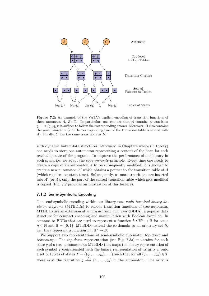
AutomataA B C

Top-levelLookup Tables

q1 q2 q3 q1 q2

Transition Clustersa b c e b c e

Sets ofPointers to Tuples

Tuples of States(q1, q1) (q1, q2) (q2, q2) (q3, q2)()

Figure 7.2: An example of the VATA’s explicit encoding of transition functions ofthree automata A, B, C. In particular, one can see that A contains a transitionq1

c−→ (q1, q2): it suffices to follow the corresponding arrows. Moreover, B also contains

the same transition (and the corresponding part of the transition table is shared withA). Finally, C has the same transitions as B.

with dynamic linked data structures introduced in Chapter4 where (in theory)one needs to store one automaton representing a content of the heap for eachreachable state of the program. To improve the performance of our library insuch scenarios, we adapt the copy-on-write principle. Every time one needs tocreate a copy of an automaton A to be subsequently modified, it is enough tocreate a new automaton A′ which obtains a pointer to the transition table of A(which requires constant time). Subsequently, as more transitions are insertedinto A′ (or A), only the part of the shared transition table which gets modifiedis copied (Fig. 7.2 provides an illustration of this feature).

7.1.2 Semi-Symbolic Encoding

The semi-symbolic encoding within our library uses multi-terminal binary de-cision diagrams (MTBDDs) to encode transition functions of tree automata.MTBDDs are an extension of binary decision diagrams (BDDs), a popular datastructure for compact encoding and manipulation with Boolean formulae. Incontrast to BDDs that are used to represent a function b : Bn → B for somen ∈ N and B = {0, 1}, MTBDDs extend the co-domain to an arbitrary set S,i.e., they represent a function m : Bn → S.

We support two representations of semi-symbolic automata: top-down andbottom-up. The top-down representation (see Fig. 7.3a) maintains for eachstate q of a tree automaton an MTBDD that maps the binary representation ofeach symbol f concatenated with the binary representation of its arity n ontoa set of tuples of states T = {(q1, . . . , qn), . . . } such that for all (q1, . . . , qn) ∈ T

there exist the transition qf

−→ (q1, . . . , qn) in the automaton. The arity is

109

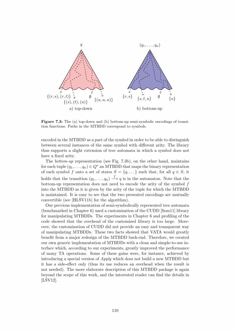
q

{(r, s), (r, t)}

{(s), (t), (u)}∅

{(u, u, u)}

a) top-down

(q1, . . . , qn)

{r, s}{s, t, u} ∅ {u}

b) bottom-up

Figure 7.3: The (a) top-down and (b) bottom-up semi-symbolic encodings of transi-tion functions. Paths in the MTBDD correspond to symbols.

encoded in the MTBDD as a part of the symbol in order to be able to distinguishbetween several instances of the same symbol with different arity. The librarythus supports a slight extension of tree automata in which a symbol does nothave a fixed arity.The bottom-up representation (see Fig. 7.3b), on the other hand, maintains

for each tuple (q1, . . . , qn) ∈ Q∗ an MTBDD that maps the binary representationof each symbol f onto a set of states S = {q, . . . } such that, for all q ∈ S, it

holds that the transition (q1, . . . , qn)f

−→ q is in the automaton. Note that thebottom-up representation does not need to encode the arity of the symbol finto the MTBDD as it is given by the arity of the tuple for which the MTBDDis maintained. It is easy to see that the two presented encodings are mutuallyconvertible (see [HLSV11b] for the algorithm).Our previous implementation of semi-symbolically represented tree automata

(benchmarked in Chapter 6) used a customisation of the CUDD [Som11] libraryfor manipulating MTBDDs. The experiments in Chapter 6 and profiling of thecode showed that the overhead of the customised library is too large. More-over, the customisation of CUDD did not provide an easy and transparent wayof manipulating MTBDDs. These two facts showed that VATA would greatlybenefit from a major redesign of the MTBDD back-end. Therefore, we createdour own generic implementation of MTBDDs with a clean and simple-to-use in-terface which, according to our experiments, greatly improved the performanceof many TA operations. Some of these gains were, for instance, achieved byintroducing a special version of Apply which does not build a new MTBDD butit has a side-effect only (thus its use reduces an overhead when the result isnot needed). The more elaborate description of this MTBDD package is againbeyond the scope of this work, and the interested reader can find the details in[LSV12].

110

7.2 Supported Operations

As we have described in the previous section, the VATA library allows a userto choose one of three available encodings: the explicit top-down, the semi-symbolic top-down, and the semi-symbolic bottom-up. Depending on the choiceof the encoding, certain TA operations may or may not be available. The fol-lowing operations are supported by at least one of the representations: union,intersection, elimination of (bottom-up, top-down) unreachable states, inclu-sion checking (bottom-up, top-down), computation of (maximum) simulationrelations (downward, upward), and language preserving size reduction basedon simulation equivalence. In some cases, multiple implementations of an op-eration are available, which is especially the case for language inclusion. Thisis because the different implementations are based on different heuristics thatmay work better for different applications as witnessed also by our experimentsdescribed in Section 7.3.Below, we do not discuss the relatively straightforward implementation of the

most basic operations on TA and we comment on the more advanced operationsonly.

7.2.1 Downward and Upward Simulation

Downward simulation relations can be computed over two tree automata rep-resentations in VATA: the explicit top-down and the semi-symbolic top-downencoding. The explicit variant first translates a tree automaton into a labelledtransition system (LTS) as described in [ABH+08]. Then the simulation rela-tion for this system is computed using an implementation of the state-of-the-artalgorithms for computing simulations on LTSs presented in [RT07] and also inChapter 5 with some further optimisations mentioned in Section 7.2.5. Finally,the result is projected back to the set of states of the original automaton.The semi-symbolic variant uses a simpler simulation algorithm based on

a generalisation of [INY04] to trees.Upward simulation can currently be computed over the explicit representation

only. The computation is again performed via a translation to an LTS (thedetails are in [ABH+08]), and the relation is computed using the engine forcomputing simulation relations on LTSs as above.

7.2.2 Simulation-based Size Reduction

In a typical setting, one often wants to use a representation of tree automatathat is as small as possible in order to reduce the memory consumption and/orspeed up operations on the automata (especially the potentially costly ones,such as inclusion testing). To achieve that, the classical approach is to usedeterminisation and minimisation. However, the minimal deterministic treeautomata can still be much bigger than the original nondeterministic ones.Therefore, VATA offers a possibility to reduce the size of tree automata withoutdeterminisation by their quotienting w.r.t. an equivalence relation—currently,

111

the library uses downward simulation simulation equivalence, but the user caneasily provide an arbitrary relation suitable for collapsing states.The procedure works as follows: first, the downward simulation relation (D

is computed for the automaton. Then, the symmetric fragment of (D (whichis an equivalence) is extracted, and each state appearing within the transi-tion function is replaced by a representative of the corresponding equivalenceclass. A further reduction is then based on the following observation: if anautomaton contains a transition q

a−→ (q1, . . . , qn), any additional transition

qa

−→ (r1, . . . , rn) where ri (D qi can be omitted since it does not contributeto the language of the result (recall that, for the downward simulation preorder(D, it holds that q (D r =⇒ L(q) ⊆ L(r)).

7.2.3 Bottom-up Inclusion

Bottom-up inclusion testing is implemented for the explicit top-down and thesemi-symbolic bottom-up representation in VATA. As its name suggests, thealgorithm naturally proceeds in the bottom-up way, therefore the top-downencoding is not very suitable here. In the case of the explicit representation,however, one can afford to build a temporary bottom-up encoding since theoverhead of such a translation is negligible compared to the complexity of fol-lowing operations.Both the explicit and semi-symbolic version of the bottom-up inclusion al-

gorithm are based on the approach introduced in [BHH+08]. Here, the mainprinciple used for checking whether L(A) ⊆ L(B) is to search for a tree whichis accepted by A and not by B (thus being a witness for L(A) )⊆ L(B)). Thisis done by simultaneously traversing both A and B from their leaf rules whilegenerating pairs (pA, PB) ∈ QA × 2QB where pA represents a state into whichA can get on some input tree and PB is the set of all states into which B canget over the same tree. The inclusion then does clearly not hold iff it is possi-ble to generate a pair consisting of an accepting state of A and of exclusivelynon-accepting states of B.

The algorithm collects the so far generated pairs (pA, PB) in a set calledV isited. Another set called Next is used to store the generated pairs whosesuccessors are still to be explored. One can then observe that whenever one canreach a counterexample to inclusion from (pA, PB), one can also reach a coun-terexample from any (pA, P

′B ⊆ PB) as P ′

B allows less runs than PB. Usingthis observation, both mentioned sets can be represented using antichains. Inparticular, one does not need to store and further explore any two elementscomparable w.r.t. (=,⊆), i.e., by equality on the first component and inclusionon the other component.In the following we describe several modifications of the existing bottom-up

inclusion algorithm (proposed in [BHH+08]) which according to experimentssubstantialy improve the performance of inclusion queries—see Algorithm 7.Clearly, the running time of the above algorithm strongly depends on the total

number of pairs (pA, PB) taken from Next for further processing. Indeed, thisis one of the reasons why the antichain-based optimisations helps. Accordingto our experience, the number of pairs which needs to be processed can further

112

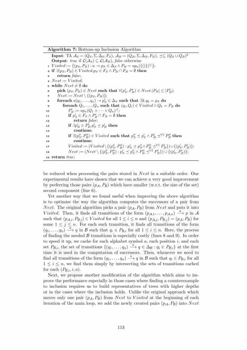
Algorithm 7: Bottom-up Inclusion Algorithm

Input: TA AS = (QS ,Σ,∆S , FS), AB = (QB ,Σ,∆B , FB), (⊆ (QS ∪QB)2

Output: true if L(AS) ⊆ L(AB), false otherwise1 V isited := {(pS , PB) : a → pS ∈ ∆S ∧ PB = upa({()})

(};2 if ∃(pS , PB) ∈ V isited.pS ∈ FS ∧ PB ∩ FB = ∅ then3 return false;4 Next := V isited;5 while Next )= ∅ do6 pick (pS , PB) ∈ Next such that ∀(p′S , P

′B) ∈ Next.|PB | ≤ |P ′

B |;7 Next := Next \ {(pS , PB)};8 foreach a(q1, . . . , qn) → p′S ∈ ∆S such that ∃k.qk = pS do9 foreach Q1, . . . , Qn such that (qi, Qi) ∈ V isited ∧Qk = PB do

10 P ′B := upa(Q1 × · · · ×Qn)

( ;11 if p′S ∈ FS ∧ P ′

B ∩ FB = ∅ then12 return false;13 if ∃p′B ∈ P ′

B .p′S ( p′B then

14 continue;

15 if ∃(p′′S , P′′B) ∈ V isited such that p′′S ( p′S ∧ P ′

B (∀∃ P ′′B then

16 continue;

17 V isited := (V isited\{(p′′S , P′′B) : p

′S ( p′′S ∧P ′′

B (∀∃ P ′B})∪{(p′S , P

′B)};

18 Next := (Next \ {(p′′S , P′′B) : p

′S ( p′′S ∧ P ′′

B (∀∃ P ′B}) ∪ {(p′S , P

′B)};

19 return true;

be reduced when processing the pairs stored in Next in a suitable order. Ourexperimental results have shown that we can achieve a very good improvementby preferring those pairs (pA, PB) which have smaller (w.r.t. the size of the set)second component (line 6).Yet another way that we found useful when improving the above algorithm

is to optimise the way the algorithm computes the successors of a pair fromNext. The original algorithm picks a pair (pA, PB) from Next and puts it intoV isited. Then, it finds all transitions of the form (pA,1, . . . , pA,n)

a−→ p in A

such that (pA,i, PB,i) ∈ V isited for all 1 ≤ i ≤ n and (pA,j , PB,j) = (pA, PB) forsome 1 ≤ j ≤ n. For each such transition, it finds all transitions of the form(q1, . . . , qn)

a−→ q in B such that qi ∈ PB,i for all 1 ≤ i ≤ n. Here, the process

of finding the needed B transitions is especially costly (lines 8 and 9). In orderto speed it up, we cache for each alphabet symbol a, each position i, and eachset PB,i, the set of transitions {(q1, . . . , qn)

a−→ q ∈ ∆B : qi ∈ PB,i} at the first

time it is used in the computation of successors. Then, whenever we need tofind all transitions of the form (q1, . . . , qn)

a−→ q in B such that qi ∈ PB,i for all

1 ≤ i ≤ n, we find them simply by intersecting the sets of transitions cachedfor each (PB,i, i, a).Next, we propose another modification of the algorithm which aims to im-

prove the performance especially in those cases where finding a counterexampleto inclusion requires us to build representatives of trees with higher depthsor in the cases where the inclusion holds. Unlike the original approach whichmoves only one pair (pA, PB) from Next to V isited at the beginning of eachiteration of the main loop, we add the newly created pairs (pA, PB) into Next

113

and V isited at the same time (immediately after they are generated). This,according to our experiments, allows V isited to converge faster towards thefixpoint (lines 17 and 18).Finally, another optimisation of the algorithm presented in [BHH+08] ap-

peared in [ACH+10]. This optimisation maintains the sets V isited and Nextas antichains w.r.t. ((U ,>∃∀

U )2. Hence, more pairs can be discarded from thesesets. Moreover, for pairs that cannot be discarded, one can at least reducethe sets on their right-hand side by removing states that are simulated bysome other state in these sets (this is based on the observation that any treeaccepted from an upward-simulation-smaller state is accepted from an upward-simulation-bigger state too). Finally, one can also use upward simulations be-tween states of the two automata being compared. Then, one can discard anypair (pA, PB) such that there is some pB ∈ PB that upward-simulates pA be-cause it is then clear that no tree can be accepted from pA that could not beaccepted from pB. All these optimisations are also available in VATA and canoptionally be used—they are not used by default since the computation of theupward simulation can be quite costly.

7.2.4 Top-down Inclusion

Top-down inclusion checking is supported by the explicit top-down and semi-symbolic top-down representations in VATA. As we have already discussedin Chapter 6, when one tries to solve inclusion of TA languages top-down ina naıve way, using a plain subset-construction-like approach, one immediatelyhits a problem due to the top-down successors of particular states are tuples ofstates. Hence, after one step of the construction, one needs to check inclusionon tuples of states, then tuples of tuples of states, etc. However, there is a wayhow to get out of this trap as shown in [HVP05] and also in Chapter 6. To recallfrom Chapter 6, the main idea of the approach resembles a conversion from thedisjunctive normal form (DNF) to the conjunctive normal form (CNF) takinginto account that top-down transitions of tree automata form a kind of and-or graphs (the disjunctions are between top-down transitions and conjunctionsamong the successors within particular transitions).VATA contains an implementation of the top-down inclusion checking algo-

rithm as presented in Chapter 6. This algorithm uses several optimisations,e.g., caching of results of auxiliary language inclusion queries between statesof the automata whose languages are being compared. More precisely, whenchecking whether L(A) ⊆ L(B) holds for two tree automata A and B, thealgorithm stores a set of pairs (pA, PB) ∈ QA × 2QB for which the languageinclusion L(pA) ⊆ L(PB) has been shown not to hold. As a further optimisa-tion, the set is stored as an antichain based on comparing the states w.r.t. thedownward simulation preorder. The use of the downward simulation is one ofthe main advantages of this approach compared with the bottom-up inclusionchecking since this preorder is cheaper to compute and usually richer than the

2One says that P $∃∀U Q holds iff ∀p ∈ P ∃q ∈ Q : p $U q. Note also that the upward

simulation must be parameterised by the identity in this case [ACH+10].

114

upward simulation. Indeed, as we have shown in Chapter 6, the top-down in-clusion checking is often—though not always—superior to bottom-up inclusionchecking.Moreover, VATA also imlements an optimized version of the top-down inclu-

sion checking algorithm that extends the previous version by caching even thepairs (pA, PB) ∈ QA × 2QB for which the language inclusion L(pA) ⊆ L(PB)has been shown to hold. This extension is far from trivial since the cachingmust be done very carefully in order to avoid a sort of circular reasoning whenanswering the various auxiliary language inclusion queries. A precise descrip-tion of this rather involved algorithm is again described in Chapter 6. As ourexperiments show, the caching positive pairs comes with some overhead, whichdoes not allow it to always win over the previous algorithm, but there are stillmany cases in which it performs significantly better.

7.2.5 Computing Simulation over LTS

The explicit part of VATA uses a highly optimised LTS simulation algorithmproposed in [RT07] together with the improvements presented in 5. The mainidea of the algorithm is to start with an overapproximation of the simulationpreorder (a possible initial approximation is the relation Q×Q) which is theniteratively pruned whenever it is discovered that the simulation relation cannothold for certain pairs of states. For a better efficiency, the algorithm representsthe current approximation R of the simulation being computed using a so-calledpartition-relation pair. The partition splits the set of states into subsets (calledblocks) whose elements are equivalent w.r.t. R, and a relation obtained by liftingR to blocks.In order to be able to deal with the partition-relation pair efficiently, the

algorithm needs to record for each block a matrix of counters of size |Q||Σ|where, for the given LTS, Q is the set of states and Σ is the set of labels. Thecounters are used to count how many transitions going from the given statevia a given symbol a lead to states in the given block (or blocks currentlyconsidered to be bigger w.r.t. the simulation). This information is then used tooptimise re-computation of the partition-relation pair when pruning the currentapproximation of the simulation relation being computed (for details see, e.g.,[RT07]). Since the number of blocks can (and often does) reach the number ofstates, the naıve solution requires |Q|2|Σ| counters in the worst case. It turnsout that this is one of the main barriers which prevents the algorithm fromscaling to systems with large alphabets and/or large sets of states.Working towards a remedy for the above problem, one can observe that the

mentioned algorithm actually works in several phases. At the beginning, it cre-ates an initial estimation of the partition-relation pair which typically containslarge equivalence classes. Then it initialises the counters for each element ofthe partition. Finally, it starts the iterative partition splitting. During thislast phase, the counters are only decremented or copied to the newly createdblocks. Moreover, the splitting of some block is itself triggered by decrementingsome set of counters to 0. In practice, late phases of the iteration often witness

115

a lot of small equivalence classes having very sparsely populated counters with0 being the most abundant value.This suggests that one could use sparse matrices containing only the non-

zero elements. Unfortunately, according to our experience, this turns out tobe the worst possible solution which strongly degrades the performance. Thereason is that the algorithm accesses the counters very frequently (the valuesof the counters are initialised at the beginning and then the algorithm keepsdecrementing them by one), hence any data structure with non-constant timeaccess causes the computation to stall. A somewhat better solution is to recordthe non-zero counters using a hash table, but the memory requirements of suchrepresentation are not yet reasonable.Instead, we are currently experimenting with storing the counters in blocks,

using a copy-on-write approach and a zeroed-block deallocation. In short, wedivide the matrix of counters into a list of blocks of some fixed size. Eachblock contains an additional counter (a block-level counter) which sums up allthe elements within the block. As soon as a block contains a single non-zerocounter only, it can safely be deallocated—the content of the non-zero counteris then recorded in the block-level counter.Our initial experiments show that, using the above approach, one can easily

reduce the memory consumption by the factor of 5 for very large instances ofthe problem compared to the array-based representation which was used forexperiments presented in Chapter 5. The best value to be used as the size ofblocks of counters is still to be studied—after some initial experiments, we arecurrently using blocks of size

√

|Q|.

7.3 Experimental Evaluation

In order to illustrate the level of optimisation that has been achieved in VATAand that can be exploited in its applications (like the Forester tool [HHR+11a]),we compared its performance against Timbuk and the prototype library con-sidered in Chapter 6, which—despite its prototype status—already containeda quite efficient TA implementation.The comparison of performance of VATA (using the explicit encoding) and

Timbuk was done for union and intersection of more than 3,000 pairs of TA. Onaverage, VATA was over 20,000 times faster on union and over 100,000 timesfaster on intersection.When comparing VATA with the implementation used in Chapter 6, we con-

centrated on language inclusion testing which is one of the most costly opera-tions on nondeterministic TA. In particular, we conducted a set of experimentsevaluating the performance of the VATA’s optimised TA language inclusion al-gorithms on pairs of TA obtained from abstract regular tree model checking ofthe algorithm for rebalancing red-black trees after insertion or deletion of a leafnode (which is the same test set that was used in Chapter 6).

116

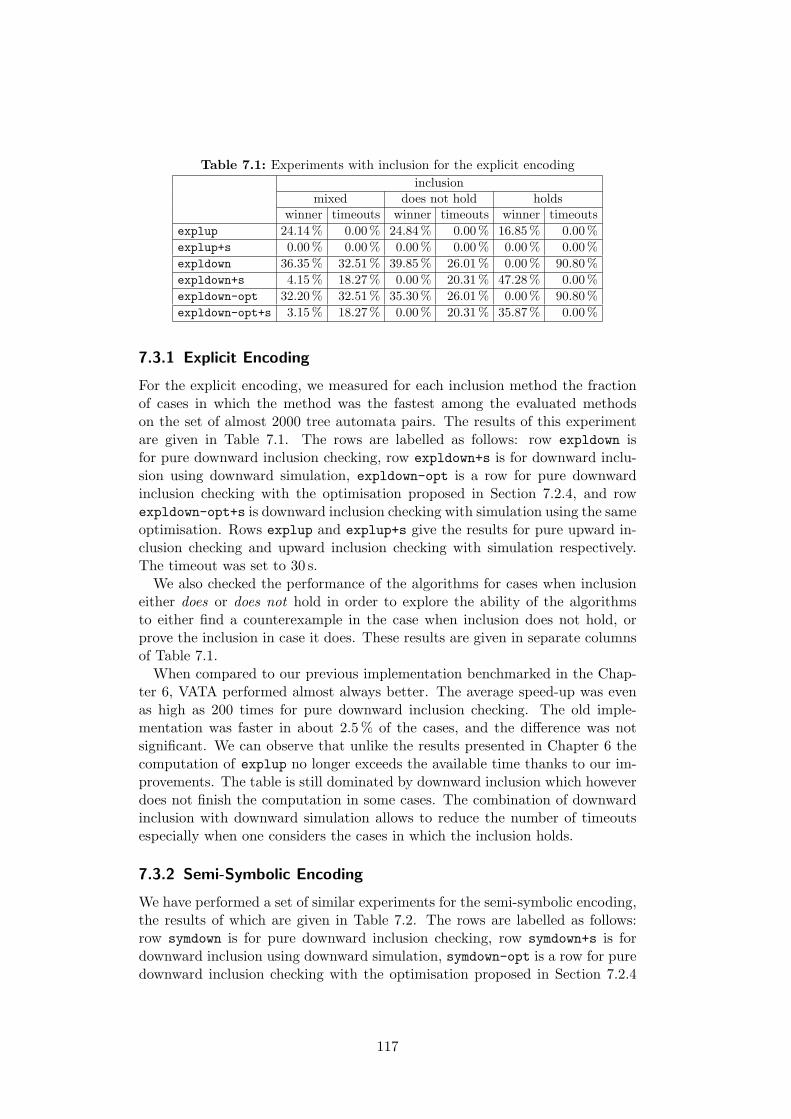
Table 7.1: Experiments with inclusion for the explicit encoding

inclusionmixed does not hold holds

winner timeouts winner timeouts winner timeouts

explup 24.14% 0.00% 24.84% 0.00% 16.85% 0.00%

explup+s 0.00% 0.00% 0.00% 0.00% 0.00% 0.00%

expldown 36.35% 32.51% 39.85% 26.01% 0.00% 90.80%

expldown+s 4.15% 18.27% 0.00% 20.31% 47.28% 0.00%

expldown-opt 32.20% 32.51% 35.30% 26.01% 0.00% 90.80%

expldown-opt+s 3.15% 18.27% 0.00% 20.31% 35.87% 0.00%


For the explicit encoding, we measured for each inclusion method the fractionof cases in which the method was the fastest among the evaluated methodson the set of almost 2000 tree automata pairs. The results of this experimentare given in Table 7.1. The rows are labelled as follows: row expldown isfor pure downward inclusion checking, row expldown+s is for downward inclu-sion using downward simulation, expldown-opt is a row for pure downwardinclusion checking with the optimisation proposed in Section 7.2.4, and rowexpldown-opt+s is downward inclusion checking with simulation using the sameoptimisation. Rows explup and explup+s give the results for pure upward in-clusion checking and upward inclusion checking with simulation respectively.The timeout was set to 30 s.We also checked the performance of the algorithms for cases when inclusion

either does or does not hold in order to explore the ability of the algorithmsto either find a counterexample in the case when inclusion does not hold, orprove the inclusion in case it does. These results are given in separate columnsof Table 7.1.When compared to our previous implementation benchmarked in the Chap-

ter 6, VATA performed almost always better. The average speed-up was evenas high as 200 times for pure downward inclusion checking. The old imple-mentation was faster in about 2.5% of the cases, and the difference was notsignificant. We can observe that unlike the results presented in Chapter 6 thecomputation of explup no longer exceeds the available time thanks to our im-provements. The table is still dominated by downward inclusion which howeverdoes not finish the computation in some cases. The combination of downwardinclusion with downward simulation allows to reduce the number of timeoutsespecially when one considers the cases in which the inclusion holds.

7.3.2 Semi-Symbolic Encoding

We have performed a set of similar experiments for the semi-symbolic encoding,the results of which are given in Table 7.2. The rows are labelled as follows:row symdown is for pure downward inclusion checking, row symdown+s is fordownward inclusion using downward simulation, symdown-opt is a row for puredownward inclusion checking with the optimisation proposed in Section 7.2.4

117

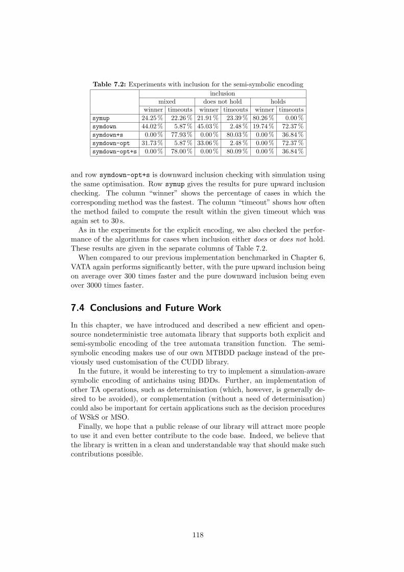
Table 7.2: Experiments with inclusion for the semi-symbolic encoding

inclusionmixed does not hold holds

winner timeouts winner timeouts winner timeouts

symup 24.25% 22.26% 21.91% 23.39% 80.26% 0.00%

symdown 44.02% 5.87% 45.03% 2.48% 19.74% 72.37%

symdown+s 0.00% 77.93% 0.00% 80.03% 0.00% 36.84%

symdown-opt 31.73% 5.87% 33.06% 2.48% 0.00% 72.37%

symdown-opt+s 0.00% 78.00% 0.00% 80.09% 0.00% 36.84%

and row symdown-opt+s is downward inclusion checking with simulation usingthe same optimisation. Row symup gives the results for pure upward inclusionchecking. The column “winner” shows the percentage of cases in which thecorresponding method was the fastest. The column “timeout” shows how oftenthe method failed to compute the result within the given timeout which wasagain set to 30 s.As in the experiments for the explicit encoding, we also checked the perfor-

mance of the algorithms for cases when inclusion either does or does not hold.These results are given in the separate columns of Table 7.2.When compared to our previous implementation benchmarked in Chapter 6,

VATA again performs significantly better, with the pure upward inclusion beingon average over 300 times faster and the pure downward inclusion being evenover 3000 times faster.


In this chapter, we have introduced and described a new efficient and open-source nondeterministic tree automata library that supports both explicit andsemi-symbolic encoding of the tree automata transition function. The semi-symbolic encoding makes use of our own MTBDD package instead of the pre-viously used customisation of the CUDD library.In the future, it would be interesting to try to implement a simulation-aware

symbolic encoding of antichains using BDDs. Further, an implementation ofother TA operations, such as determinisation (which, however, is generally de-sired to be avoided), or complementation (without a need of determinisation)could also be important for certain applications such as the decision proceduresof WSkS or MSO.Finally, we hope that a public release of our library will attract more people

to use it and even better contribute to the code base. Indeed, we believe thatthe library is written in a clean and understandable way that should make suchcontributions possible.

118

8 Conclusions and Future Directions

Detailed conclusions of each specific topic discussed in the thesis have been givenat the end of the corresponding chapters. Here, we summarise once more themain points and discuss possible future directions of the research from a broaderperspective.

8.1 A Summary of the Contributions

This thesis focuses on formal verification of programs manipulating complexdynamic data structures. Inspired by the existing techniques based on using treeautomata ([BHRV06b]) and also techniques based on separation logic ([Rey02]),we have developed a novel approach which tries to combine ideas from theselines of research.In particular, we have proposed an encoding of sets of heaps using an original

notion of forest automata. Essentially, a heap is split into a tuple of trees suchthat non-tree links can be represented via explicit references to the roots ofthe created trees. A forest automaton is then basically a tuple of ordinary treeautomata representing a set of heaps decomposed in this way. To obtain someconcrete heap out of this representation, one can pick a tuple of trees fromthe languages of the tree automata which an FA consists of and replace thenon-local references by gluing the corresponding nodes.Plain forest automata can represent sets of heaps which can be decomposed

into a finite number of tree components. In order to extend the expressive powerof the formalism, the original concept has been further extended by allowinghierarchically nested forest automata to appear within the alphabet. We haveshown that hierarchical forest automata can indeed represent some sets of heapswhich would normally require an unbounded number of tree components andthat are important in practice (e.g., DLLs).As the next step, we have developed a new symbolic verification method in

which we finitely represent infinite sets of heap configurations using forest au-tomata. During a verification run, program statements are interpreted directlyover forest automata such that we compute the effect of a particular programstatement on infinitely many configurations in one step.Our verification technique is based on the use of non-deterministic finite

tree automata, and the performance of the approach strongly depends on theefficiency of the tree automata operations used. Among them, size reductionand language inclusion are especially critical since they used to be traditionallyimplemented via determinisation and only recently started to be implementeddirectly on NTA (to avoid the exponential cost of determinisation as much aspossible). Therefore, we have also invested into improving the state-of-the-artalgorithms for these operations.

119

The size reduction algorithm that we use is based upon collapsing states of anautomaton according to a suitable preorder. We, in particular, use downwardsimulation which can be computed via a translation of a TA into a labelledtransition system. The original algorithm for computing simulation over LTSspresented in [ABH+08, AHKV08] is a straightforward extension of the algorithmfor Kripke structures presented in [HHK95, RT07]. We show that the increasein its complexity caused by the introduction of transition labels can be to a largedegree eliminated, which is supported by our experimental results.Furthermore, we have also intensively investigated methods for checking lan-

guage inclusion of tree automata which is indirectly used for checking inclusionof forest automata. The approach of [ACH+10] shows how one can combinesimulations and antichains for checking language inclusion of finite word andalso tree automata. This allows to achieve great computation speedups, es-pecially when finite word automata are considered. In the case of finite treeautomata, bottom-up inclusion is considered in [ACH+10]. This can only becombined with upward simulation which is quite expensive to compute andusually does not yield bigger gains in speed. In order to solve this problem, wehave generalised the top-down approach of [TH03] to tree automata of arbitraryarity. Moreover, we have extended the algorithm by using antichains combinedwith downward simulation which is cheaper to compute and allows for a betterspeedup.Finally, we have created a freely available tree automata library containing

an efficient implementation of many important general purpose algorithms forexplicitly and semi-symbolically represented tree automata. For this purpose,the basic versions of the data structures and algorithms described in the aboveworks have been carefully optimised, which we have also described in Chapter 7.

8.2 Further Directions

There are numerous directions of further work in the areas covered by thethesis. From the theoretical perspective, the expressive power of hierarchicalforest automata is an interesting question which has not yet been systematicallydiscussed. In connection to that, there arises a question of allowing recursivelynested FA which would extend the expressive power to other interesting setsof graphs. It is, however, not yet clear how such an extension should look likesuch that it allows for the needed automata operations to be implemented overit. Further, the proposed algorithm for backward symbolic execution should beimplemented and experimentally evaluated within the framework of predicatelanguage abstraction. One problem that could arise here is that of the precisionof the intersection under-approximation. If it appears problematic in somepractical cases, some more precise solution will have to be sought. Likewise,if the precision of the currently used algorithm for inclusion checking of FAappears insufficient on some examples (which has not yet happened), it mayturn out useful to increase its precision by taking into account the hierarchicalstructuring of FA. A related theoretical question is whether or not the inclusionis decidable (even if neglecting the cost of such a check).

120

A very broad area for further research is that of extending the proposedtechniques to be able to cope with data stored inside the dynamically linkeddata structures (which is crucial for verification of programs over red-black trees,unmodified skip lists, or various user-specific scenarios exploiting dynamicallylinked data structures) as well as for dealing with concurrency and/or recursion(without the restrictions imposed in Chapter 4).Next, concerning the problem of computing simulations for LTSs, it would be

interesting to study whether the memory requirements of the algorithm can befurther reduced by using some sophisticated data structure—such as BDDs—for storing internal data of the algorithm. Such an approach could perhapsreduce the impact of the alphabet size of the LTS even more. Moreover, aninteresting subject for further work is to go beyond reduction of automata basedon collapsing simulation equivalent states. Indeed, sometimes, it is useful tosplit some states allowing a subsequent collapsing to be much more productive.The problem of language inclusion of TA is also a possible subject of fur-

ther research focus. The bottom-up approach does not seem to benefit fromthe combination with upward simulation. Therefore, it would be interestingto see whether there exists a different (and possibly cheaper to compute) rela-tion which could improve the performance of upward inclusion checking. Onthe other hand, despite the optimisations that we proposed, the top-down ap-proach can suffer from an explosion of the number of downward successors ofa given macro state. Moreover, in many cases, not all the successors need tobe examined if one is able to explore them in a suitable order. Possibilities ofoptimising the sequence of successors are therefore also an interesting subjectof future work.The further development of our general purpose TA library involves imple-

mentation of so far missing operations such as determinisation, complementa-tion, general-purpose transduction, etc. Here, complementation is special inthat we are not aware of any existing efficient way how to implement it withoutdeterminisation (although some initial ideas have appeared, e.g., in [Hos10]).At the same time, complementation is crucial for some automata-based algo-rithms such as the decision procedures of WSkS or MSO. For that reason, itwould be nice to either find some efficient way how to complement automatawithout determinising them or to find ways how to avoid explicit complemen-tation as much as possible. Apart from that, specialized versions of algorithmsworking specifically with finite word automata (which are themselves a specialkind of TA) could be introduced in order to handle them more efficiently.

8.3 Publications and Tools Related to this Work

The verification technique for programs manipulating complex dynamic datastructures and the underlying formalism of forest automata presented in Chap-ter 3 and Chapter 4 were first introduced in [HHR+11a]. An extended versionof the original description appeared in [HHR+12]. The proposed improvementsof the in algorithm for computing simulations over labelled transition systemswere published in [HS09a]. An extended version then appeared in [HS10]. The

121

proposed top-down inclusion checking algorithm combined with antichains anddownward simulation was described in [HLSV11a]. Finally, our work on thegeneral purpose tree automata library (and the optimised data structures andalgorithms that it is based on) was presented in [LSV12].Apart from that, the full versions of some of the above mentioned papers

were published as technical reports [HHR+11b, HS09b, HLSV11b]. A detaileddescription of the algorithms for computing abstraction (Section 4.4) as well asthe automatic discovery of nested FA (Section 4.3) have not yet been published(and are planned to be published later on). The proposed techniques wereimplemented in the Forester tool and the VATA library publicly available overthe internet12.

1http://www.fit.vutbr.cz/research/groups/verifit/tools/forester/2http://www.fit.vutbr.cz/research/groups/verifit/tools/libvata/

122

References

[ABC+08] P.A. Abdulla, A. Bouajjani, J. Cederberg, F. Haziza, andA. Rezine. Monotonic Abstraction for Programs with DynamicMemory Heaps. In Proc. of CAV, volume 5123 of LNCS, pages341–354, Berlin, Heidelberg, 2008. Springer Verlag.

[ABH+08] P.A. Abdulla, A. Bouajjani, L. Holık, L. Kaati, and T. Voj-nar. Computing Simulations over Tree Automata: Efficient Tech-niques for Reducing Tree Automata. In Proc. of TACAS, number4963 in LNCS, pages 93–108, Berlin, Heidelberg, 2008. SpringerVerlag.

[ACH+10] P.A. Abdulla, Y.-F. Chen, L. Holık, R. Mayr, and T. Vojnar.When Simulation Meets Antichains (on Checking Language In-clusion of NFAs). In Proc. of TACAS’10, volume 6015 of LNCS,pages 158–174, Berlin, Heidelberg, 2010. Springer Verlag.

[ACV11] P.A. Abdulla, J. Cederberg, and T. Vojnar. Monotonic Abstrac-tion for Programs with Multiply-Linked Structures. In Proc. ofRP, volume 6945 of LNCS, pages 125–138, Berlin, Heidelberg,2011. Springer Verlag.

[AHKV08] P.A. Abdulla, L. Holık, L. Kaati, and T. Vojnar. A Uniform(Bi-)Simulation-Based Framework for Reducing Tree Automata.In Proc. of MEMICS, pages 3–11. Faculty of Informatics MU,2008.

[AJMd02] P.A. Abdulla, B. Jonsson, P. Mahata, and J. d’Orso. RegularTree Model Checking. In Proc. of CAV’02, volume 2404 of LNCS,Berlin, Heidelberg, 2002. Springer Verlag.

[ALdR05] P. A. Abdulla, A. Legay, J. d’Orso, and A. Rezine. Simulation-Based Iteration of Tree Transducers. In Proc. of TACAS, volume3440 of LNCS, pages 30–44, Berlin, Heidelberg, 2005. SpringerVerlag.

[BBH+11] Ahmed Bouajjani, Marius Bozga, Peter Habermehl, Radu Iosif,Pierre Moro, and Tomas Vojnar. Programs with Lists are CounterAutomata. Formal Methods in System Design, 38(2):158–192,April 2011.

[BCC+07] J. Berdine, C. Calcagno, B. Cook, D. Distefano, P.W. O’hearn,and H. Yang. Shape analysis for composite data structures. In

123

Proc. of CAV, pages 178–192, Berlin, Heidelberg, 2007. SpringerVerlag.

[BHH+08] A. Bouajjani, P. Habermehl, L. Holık, T. Touili, and T. Vojnar.Antichain-Based Universality and Inclusion Testing over Nonde-terministic Finite Tree Automata. In Proc. of CIAA’08, volume5148 of LNCS, Berlin, Heidelberg, 2008. Springer Verlag.

[BHMV05] A. Bouajjani, P. Habermehl, P. Moro, and T. Vojnar. VerifyingPrograms with Dynamic 1-Selector-Linked Structures in RegularModel Checking. In Proc. of TACAS’05, volume 3440 of LNCS,Berlin, Heidelberg, 2005. Springer Verlag.

[BHRV06a] A. Bouajjani, P. Habermehl, A. Rogalewicz, and T. Vojnar. Ab-stract Regular Tree Model Checking. ENTCS, 149:37–48, 2006.A preliminary version was presented at Infinity’05.

[BHRV06b] A. Bouajjani, P. Habermehl, A. Rogalewicz, and T. Vojnar. Ab-stract Regular Tree Model Checking of Complex Dynamic DataStructures. In Proc. of SAS’06, volume 4134 of LNCS, pages52–70, Berlin, Heidelberg, 2006. Springer Verlag.

[BHV04] A. Bouajjani, P. Habermehl, and T. Vojnar. Abstract RegularModel Checking. In Proc. of CAV, volume 3114 of LNCS, pages372–386, Berlin, Heidelberg, 2004. Springer Verlag.

[Bou11] T. Bourdier. Tree Automata-based Semantics of Firewalls. InProc. of SAR-SSI, pages 171–178, Washington, DC, USA, 2011.IEEE Computer Society.

[Bry86] R.E. Bryant. Graph-Based Algorithms for Boolean Function Ma-nipulation. IEEE Transactions on Computing, 35(8):677–691,1986.

[BT02] A. Bouajjani and T. Touili. Extrapolating Tree Transformations.In Proc. of CAV, volume 2404 of LNCS, pages 539–554, Berlin,Heidelberg, 2002. Springer Verlag.

[CDOY09] C. Calcagno, D. Distefano, P.W. O’Hearn, and H. Yang. Com-positional Shape Analysis by Means of Bi-abduction. In Proc.of PLDI, volume 44 of ACM SIGPLAN Notices, pages 289–300,New York, NY, USA, 2009. ACM Press.

[CJH+09] P. Claves, D. Jansen, S.J. Holtrup, M. Mohr, A. Reis, M. Schatz,and I. Thesing. The LETHAL Library.http://lethal.sourceforge.net/, 2009.

[CMZ+97] E. M. Clarke, K. L. Mcmillan, X. Zhao, M. Fujita, and J. Yang.Spectral Transforms for Large Boolean Functions withApplica-tions to Technology Mapping. Formal Methods in System Design,10(2-3):137–148, April 1997.

124

[CRN07] B.-Y. Chang, X. Rival, and G. Necula. Shape Analysis with Struc-tural Invariant Checkers. In Proc. of SAS, volume 4634 of LNCS,pages 384–401, Berlin, Heidelberg, 2007. Springer Verlag.

[DEG06] J.V. Deshmukh, E.A. Emerson, and P. Gupta. Automatic Veri-fication of Parameterized Data Structures. In Proc. of TACAS,volume 3920 of LNCS, pages 27–41, Berlin, Heidelberg, 2006.Springer Verlag.

[DGG93] D. Dams, O. Grumberg, and R. Gerth. Generation of ReducedModels for Checking Fragments of CTL. In Proc. of CAV, volume697 of LNCS, pages 479–490, Berlin, Heidelberg, 1993. SpringerVerlag.

[DPV11] K. Dudka, P. Peringer, and T. Vojnar. Predator: A PracticalTool for Checking Manipulation of Dynamic Data Structures us-ing Separation Logic. In Proc. of CAV, volume 6806 of LNCS,pages 372–378, Berlin, Heidelberg, 2011. Springer Verlag.

[DR10] L. Doyen and J.-F. Raskin. Antichain Algorithms for Finite Au-tomata. In Proc. of TACAS, volume 6015 of LNCS, pages 2–22,Berlin, Heidelberg, 2010. Springer Verlag.

[DWDHR06] M. De Wulf, L. Doyen, T. Henzinger, and J.-F. Raskin. An-tichains: A New Algorithm for Checking Universality of FiniteAutomata. In Proc. of CAV, volume 4144 of LNCS, pages 17–30,Berlin, Heidelberg, 2006. Springer Verlag.

[Gen03] T. Genet. Timbuk/Taml: A Tree Automata Library.http://www.irisa.fr/lande/genet/timbuk, 2003.

[GL94] O. Grumberg and D.E. Long. Model Checking and Modular Ver-ification. TOPLAS, 16(3):843–871, May 1994.

[GVA07] B. Guo, N. Vachharajani, and D.I. August. Shape Analysis withInductive Recursion Synthesis. In Proc. of PLDI, volume 42 ofACM SIGPLAN Notices, pages 256–265, New York, NY, USA,2007. ACM Press.

[HHK95] M. R. Henzinger, T. A. Henzinger, and P. W. Kopke. ComputingSimulations on Finite and Infinite Graphs. In Proc. of FOCS,pages 453–462, Washington, DC, USA, 1995. IEEE ComputerSociety.

[HHR+11a] P. Habermehl, L. Holık, A. Rogalewicz, J. Simacek, and T. Vo-jnar. Forest Automata for Verification of Heap Manipulation.In Proc. of CAV, volume 6806 of LNCS, pages 424–440, Berlin,Heidelberg, 2011. Springer Verlag.

[HHR+11b] P. Habermehl, L. Holık, A. Rogalewicz, J. Simacek, and T. Vo-jnar. Forest Automata for Verification of Heap Manipulation.Technical report, Faculty of Information Technology, BUT, 2011.

125

[HHR+12] P. Habermehl, L. Holık, A. Rogalewicz, J. Simacek, and T. Voj-nar. Forest automata for verification of heap manipulation. For-mal Methods in System Design, pages 1–24, 2012.

[HLSV11a] L. Holık, O. Lengal, J. Simacek, and T. Vojnar. Efficient Inclu-sion Checking on Explicit and Semi-symbolic Tree Automata. InProc. of ATVA, volume 6996 of LNCS, pages 243–258, Berlin,Heidelberg, 2011. Springer Verlag.

[HLSV11b] L. Holık, O. Lengal, J. Simacek, and T. Vojnar. Efficient In-clusion Checking on Explicit and Semi-Symbolic Tree Automata.Technical report, Faculty of Information Technology, BUT, 2011.

[Hol11] L. Holık. Simulations and Antichains for Efficient Handling ofFinite Automata. PhD thesis, Faculty of Information Technology,Brno University of Technology, 2011.

[Hos10] H. Hosoya. Foundations of XML Processing: The Tree-AutomataApproach. Cambridge University Press, 2010.

[HS09a] L. Holık and J. Simacek. Optimizing an LTS-Simulation Algo-rithm. In Proc. of MEMICS, pages 93–101. Faculty of InformaticsMU, 2009.

[HS09b] L. Holık and J. Simacek. Optimizing an LTS-Simulation Algo-rithm. Technical Report FIT-TR-2009-03, Brno University ofTechnology, 2009.

[HS10] L. Holık and J. Simacek. Optimizing an LTS-Simulation Algo-rithm. Computing and Informatics, 2010(7):1337–1348, 2010.

[HVP05] H. Hosoya, J. Vouillon, and B.C. Pierce. Regular ExpressionTypes for XML. TOPLAS, 27(1):46–90, January 2005.

[INY04] L. Ilie, G. Navarro, and S. Yu. On NFA Reductions. In TheoryIs Forever, volume 3113 of Lecture Notes in Computer Science,pages 112–124, Berlin, Heidelberg, 2004. Springer Verlag.

[KMS01] N. Klarlund, A. Møller, and M. Schwartzbach. MONA Implemen-tation Secrets. In Proc. of CIAA, volume 2088 of LNCS, pages182–194, Berlin, Heidelberg, 2001. Springer Verlag.

[LSV12] O. Lengal, J. Simacek, and T. Vojnar. VATA: A Library forEfficient Manipulation of Non-deterministic Tree Automata. InProc. of TACAS, volume 7214 of LNCS, pages 79–94, Berlin,Heidelberg, 2012. Springer Verlag.

[MPQ11] P. Madhusudan, G. Parlato, and X. Qiu. Decidable Logics Com-bining Heap Structures and Data. In Proc. of POPL, volume 46of ACM SIGPLAN Notices, pages 611–622, New York, NY, USA,2011. ACM Press.

126

[MS01] A. Møller and M.I. Schwartzbach. The Pointer Assertion LogicEngine. In Proc. of PLDI, volume 36 of ACM SIGPLAN Notices,pages 221–231, New York, NY, USA, 2001. ACM Press.

[MTLT10] S. Magill, M.-H. Tsai, P. Lee, and Y.-K. Tsay. Automatic Nu-meric Abstractions for Heap-manipulating Programs. In Proc.of POPL, volume 45 of ACM SIGPLAN Notices, pages 211–222,New York, NY, USA, 2010. ACM Press.

[NDQC07] H.H. Nguyen, C. David, S. Qin, and W.-N. Chin. AutomatedVerification of Shape and Size Properties via Separation Logic. InProc. of VMCAI, volume 4349 of LNCS, pages 251–266, Berlin,Heidelberg, 2007. Springer Verlag.

[NNH99] F. Nielson, H.R. Nielson, and C. Hankin. Principles of ProgramAnalysis. Springer Verlag New York, Inc., Secaucus, NJ, USA,1999.

[PT87] R. Paige and R.E. Tarjan. Three Partition Refinement Algo-rithms. SIAM Journal of Computing, 16(6):973–989, December1987.

[Pug90] W. Pugh. Skip Lists: A Probabilistic Alternative to BalancedTrees. Communications of the ACM, 33(6):668–676, June 1990.

[Rey02] J.C. Reynolds. Separation Logic: A Logic for Shared MutableData Structures. In Proc. of LICS, pages 55–74, Washington,DC, USA, 2002. IEEE Computer Society.

[RT07] F. Ranzato and F. Tapparo. A New Efficient Simulation Equiva-lence Algorithm. In Proc. of LICS, pages 171–180, Washington,DC, USA, 2007. IEEE Computer Society.

[Sha01] E. Shahar. Tools and Techniques for Verifying Parameterized Sys-tems. PhD thesis, Faculty of Mathematics and Computer Science,The Weizmann Inst. of Science, Rehovot, Israel, 2001.

[SJ05] Z. Sawa and P. Jancar. Behavioural Equivalences on Finite-State Systems are PTIME-hard. Computing and Informatics,24(5):513–528, 2005.

[Som11] F. Somenzi. CUDD: CU Decision Diagram Package Release 2.4.2.http://vlsi.colorado.edu/~fabio/CUDD/, 2011.

[SRW02] S. Sagiv, T.W. Reps, and R. Wilhelm. Parametric Shape Analysisvia 3-valued Logic. TOPLAS, 24(3), 2002.

[TH03] A. Tozawa and M. Hagiya. XML Schema Containment CheckingBased on Semi-implicit Techniques. In Proc. of CIAA, volume2759 of LNCS, pages 51–61, Berlin, Heidelberg, 2003. SpringerVerlag.

127

[YLB+08] H. Yang, O. Lee, J. Berdine, C. Calcagno, B. Cook, D. Distefano,and P.W. O’Hearn. Scalable Shape Analysis for Systems Code.In Proc. of CAV, volume 5123 of LNCS, pages 385–398, Berlin,Heidelberg, 2008. Springer-Verlag.

[YLC+07] H. Yang, O. Lee, C. Calcagno, D. Distefano, and P.W. O’Hearn.On Scalable Shape Analysis. Technical Report RR-07-10, QueenMary, University of London, 2007.

[ZKR08] K. Zee, V. Kuncak, and M. Rinard. Full Functional Verificationof Linked Data Structures. In Proc. of PLDI, volume 43 of ACMSIGPLAN Notices, pages 349–361, New York, NY, USA, 2008.ACM Press.

128

Documents

Harnessing forest automata for verification of heap