arX

iv:0

704.

1761

v3 [

hep-

th]

30

Aug

200

7

GLSM’s for Partial Flag Manifolds

Ron Donagi1, Eric Sharpe2

1 Department of MathematicsUniversity of PennsylvaniaDavid Rittenhouse Lab.

209 South 33rd St.Philadelphia, PA 19104-6395

2 Departments of Physics, MathematicsUniversity of Utah

Salt Lake City, UT 84112donagi@math.upenn.edu, ersharpe@math.utah.edu

In this paper we outline some aspects of nonabelian gauged linear sigma models. First, wereview how partial flag manifolds (generalizing Grassmannians) are described physically bynonabelian gauged linear sigma models, paying attention to realizations of tangent bundlesand other aspects pertinent to (0,2) models. Second, we review constructions of Calabi-Yaucomplete intersections within such flag manifolds, and properties of the gauged linear sigmamodels. We discuss a number of examples of nonabelian GLSM’s in which the Kahler phasesare not birational, and in which at least one phase is realized in some fashion other than as acomplete intersection, extending previous work of Hori-Tong. We also review an example ofan abelian GLSM exhibiting the same phenomenon. We tentatively identify the mathemati-cal relationship between such non-birational phases, as examples of Kuznetsov’s homologicalprojective duality. Finally, we discuss linear sigma model moduli spaces in these gaugedlinear sigma models. We argue that the moduli spaces being realized physically by theseGLSM’s are precisely Quot and hyperquot schemes, as one would expect mathematically.

April 2007

1

Contents

1 Introduction 4

2 Flag manifolds 5

2.1 Basics . . . . . . . . . . . . . . . . . . . . . . . . . . . . . . . . . . . . . . . 5

2.2 Plucker coordinates and baryons . . . . . . . . . . . . . . . . . . . . . . . . . 7

2.3 Presentation dependence . . . . . . . . . . . . . . . . . . . . . . . . . . . . . 9

2.4 Duality . . . . . . . . . . . . . . . . . . . . . . . . . . . . . . . . . . . . . . . 10

2.5 Weighted Grassmannians . . . . . . . . . . . . . . . . . . . . . . . . . . . . . 13

2.6 Mixed examples . . . . . . . . . . . . . . . . . . . . . . . . . . . . . . . . . . 15

2.6.1 P1 bundle over flag manifold . . . . . . . . . . . . . . . . . . . . . . 15

2.6.2 Gerbe on a flag manifold . . . . . . . . . . . . . . . . . . . . . . . . . 16

2.6.3 Grassmannian bundle over P1 . . . . . . . . . . . . . . . . . . . . . . 16

3 Bundles 17

3.1 Tangent bundles and the (2,2) locus . . . . . . . . . . . . . . . . . . . . . . . 17

3.2 Aside: homogeneous bundles . . . . . . . . . . . . . . . . . . . . . . . . . . . 21

3.3 More general bundles . . . . . . . . . . . . . . . . . . . . . . . . . . . . . . . 22

4 Complete intersections in flag manifolds 23

4.1 Calabi-Yau’s in flag manifolds . . . . . . . . . . . . . . . . . . . . . . . . . . 23

4.2 Non-birational derived equivalences in nonabelian GLSMs . . . . . . . . . . 25

4.2.1 Hori-Tong-Rodland example . . . . . . . . . . . . . . . . . . . . . . . 25

4.2.2 Aside: Pfaffian varieties . . . . . . . . . . . . . . . . . . . . . . . . . 26

4.2.3 A complete intersection in a G(2, 5) bundle . . . . . . . . . . . . . . . 30

4.2.4 A Fano example . . . . . . . . . . . . . . . . . . . . . . . . . . . . . . 31

2

4.2.5 A related non-Calabi-Yau example . . . . . . . . . . . . . . . . . . . 32

4.2.6 More non-Calabi-Yau examples . . . . . . . . . . . . . . . . . . . . . 33

4.2.7 Interpretation – Kuznetsov’s homological projective duality . . . . . . 33

4.2.8 Duals of G(2, N) with N even . . . . . . . . . . . . . . . . . . . . . . 35

4.3 Non-birational derived equivalences in abelian GLSMs . . . . . . . . . . . . . 38

5 Quantum cohomology 40

5.1 Basics . . . . . . . . . . . . . . . . . . . . . . . . . . . . . . . . . . . . . . . 41

5.2 One-loop effective action arguments . . . . . . . . . . . . . . . . . . . . . . . 44

5.3 Linear sigma model moduli spaces . . . . . . . . . . . . . . . . . . . . . . . . 47

5.3.1 Grassmannians . . . . . . . . . . . . . . . . . . . . . . . . . . . . . . 48

5.3.2 Balanced strata example . . . . . . . . . . . . . . . . . . . . . . . . . 49

5.3.3 Degree 1 maps example . . . . . . . . . . . . . . . . . . . . . . . . . 50

5.3.4 Degree two maps example . . . . . . . . . . . . . . . . . . . . . . . . 52

5.3.5 Interpretation – Quot and hyperquot schemes . . . . . . . . . . . . . 53

5.3.6 Flag manifolds . . . . . . . . . . . . . . . . . . . . . . . . . . . . . . 54

5.3.7 Flag manifold example . . . . . . . . . . . . . . . . . . . . . . . . . . 55

6 Conclusions 55

7 Acknowledgements 56

References 56

3

1 Introduction

Two-dimensional gauged linear sigma models [1] have proven to be an extremely powerfultool for describing a wide variety of spaces. Their primary original use was for describingtoric varieties and complete intersections therein. More recently [2] they have been used todescribe toric stacks and complete intersections therein.

In addition to toric manifolds, they have also been used to describe Grassmannians [1, 3],and although this application was comparatively obscure, recently it has been explored inmore depth [4]. In this paper we shall push this direction further by outlining basic aspectsof gauged linear sigma models for partial flag1 manifolds, which generalize Grassmannians.

We begin in section 2 with an overview of how flag manifolds are realized in physics vianonabelian gauged linear sigma models, also describing various dualities that exist amongthe flag manifolds, Plucker coordinates for flag manfiolds, and more complicated manifoldsand stacks realizable with gauged linear sigma models. In section 3 we describe how tangentbundles of flag manifolds are realized physically in gauged linear sigma models, a necessarystep for considering (0,2) theories.

Next, in section 4 we discuss Calabi-Yau complete intersections in flag manifolds. Asin [4], we also examine Kahler phases of some gauged linear sigma models, and describea number of examples in which the different Kahler phases have geometric interpretations,sometimes realized in novel fashions, but are not related by birational transformations. Inthe past, it was thought that geometric phases of gauged linear sigma models must be relatedby birational transformations, but recently in [5][section 12.2] and [4], counterexamples haveappeared. We interpret the different phases as being related by Kuznetsov’s homologicalprojective duality [6, 7, 8], an idea that will be explored much further in [9]. We use thatproposal that gauged linear sigma models realize Kuznetsov’s duality to make a proposalfor the physical interpretation of Calabi-Yau complete intersections in G(2, N) for N even,which has been mysterious previously. We also briefly outline how such non-birational phasephenomena can appear in abelian GLSM’s, reviewing an example that first appeared in[5][section 12.2] and which will be explored in greater detail (together with many otherexamples) in [9].

Finally, in section 5 we review how quantum cohomology of Grassmannians and flag man-ifolds is realized in corresponding GLSM’s, and describe linear sigma model moduli spacesin nonabelian GLSM’s. Physically, the computation of linear sigma model moduli spaces fornonabelian GLSM’s has not been clear, unlike the case of abelian GLSM’s. Mathematically,on the other hand, there are known candidates for what such spaces should be – Quot andhyperquot schemes, specifically – that have been used by mathematicians when studying

1In this paper, we shall use the terms “partial flag manifold” and “flag manifold” interchangeably. Inparticular, “flag manifold” should not be interpreted to mean only a complete flag manifold.

4

quantum cohomology rings of flag manifolds. In this paper, we show in examples that LSMmoduli spaces realized by nonabelian GLSM’s are precisely Quot and hyperquot schemes, asone would have expected naively, instead of, for example, some different spaces birationallyequivalent to Quot and hyperquot schemes.

2 Flag manifolds

2.1 Basics

A flag manifold is a manifold describing possible configurations of a series of nested vectorspaces. We will use the notation F (k1, k2, · · · , kn, N) to indicate configuration space of allk1-dimensional planes sitting inside k2-dimensional planes which themselves sit inside k3-dimensional planes, and so forth culminating in kn-dimensional planes sitting inside thevector space CN .

Grassmannians are a special case of flag manifolds. The Grassmannian of k-planes insideCN , denoted G(k,N), is the same as the flag manifold F (k,N). The space G(k,N) hascomplex dimension k(N − k), and Euler characteristic

(Nk

)=

N !

k!(N − k)!

As one special case, G(1, N) is the projective space PN−1, so Grassmannians themselvesgeneralize projective spaces.

Flag manifolds can be described as cosets as follows:

F (k1, k2, · · · , kn, N) =U(N)

U(k1) × U(k2 − k1) × · · ·U(kn − kn−1) × U(N − kn)(1)

which has complex dimension

n∑

i=1

(ki − ki−1) (N − ki) =n∑

i=1

ki (ki−1 − ki) + Nkn

in conventions where k0 = 0. In particular, as a special case,

G(k,N) =U(N)

U(k) × U(N − k)

which has complex dimension k(N − k).

5

The Euler characteristic of F (k1, · · · , kn, N) is given by the multinomial coefficient

N !

k1!(k2 − k1)! · · · (kn − kn−1)!(N − kn)!

Flag manifolds have only even-dimensional cohomology, with a basis given by Schubertclasses, which correspond to elements of W/WP (in a description of the flag manifold asG/P for P a parabolic subgroup of G). Thus, χ(G/P ) = |W |/|WP |.

There are natural projection maps to flag manifolds with fewer flags,

F (k1, · · · , kn, N) −→ F (k1, · · · , ki, · · · , kn, N)

(where ki denotes an omitted entry) defined by forgetting the intermediate flags. The pro-jection map above has fiber G(ki − ki−1, ki+1 − ki−1). For example, there is a map

F (1, 2, n) −→ F (1, n) = G(1, n)

with fiber G(1, n− 1).

These manifolds also have alternative descriptions which make it possible to describethem with gauged linear sigma models. The Grassmannian G(k,N) can be described as

G(k,N) = CkN//GL(k)

which corresponds physically to a two-dimensional U(k) gauge theory with N chiral fields inthe fundamental of U(k). The D-terms in the supersymmetric gauge theory have the form[1]

Dij =

N∑

s=1

φisφjs − rδij

We can interpret the sum above as the dot product of two vectors in CN , and so for r ≫ 0,we see that the vectors must be orthogonal and normalized. In other words, the D-termsforce the φ fields to describe a k-dimensional subspace of CN , exactly right to describe theGrassmannian of k planes in CN .

Similarly, flag manifolds can be described as

F (k1, k2, · · · , kn, N) =(Ck1k2 × Ck2k3 ×Ck3k4 × · · · × Ckn−1kn × CknN

)// (GL(k1) ×GL(k2) × · · · ×GL(kn))

which corresponds physically to a two-dimensional

U(k1) × U(k2) × · · · × U(kn)

gauge theory with bifundamentals.

6

The D-term analysis is similar to that for Grassmannians. The D-terms for the firstU(k1) factor are of the form

Dij =

k2∑

s=1

φisφjs − r1δij

identical to those for Grassmannians, and for r1 ≫ 0 the conclusion is the same: the φ’sdefine k1 orthogonal, normalized vectors in Ck2. A slightly more interesting case is a genericU(ki) factor. Here the D-terms are of the form

Dij = −

ki−1∑

s=1

φisφjs +ki+1∑

a=1

φaiφaj − riδij

where the φ’s are (ki−1,ki) bifundamentals and the φ’s are (ki,ki+1) bifundamentals. If wemake the inductive assumption that the φ’s define ki−1 orthogonal, normalized vectors inCki, then the first sum above is proportional to ri−1δ

ij for some i, j, and vanishes for others.

So long as both ri−1 ≫ 0 and ri ≫ 0, the result is the same: the D-terms give a constrainton the φ, which implies that they are orthogonal, normalized vectors in Cki+1. Proceedinginductively we see that so long as all the Fayet-Iliopoulos parameters are positive, we recoverthe flag manifold.

In this language, we can define the (forgetful) projection map

F (k1, k2, · · · , kn, N) −→ F (k1, · · · , ki, · · · , kn, N)

(where ki denotes an omitted entry) as follows. Let Bab denote the bifundamentals transform-

ing in the (ki−1,ki) representation of U(ki−1) × U(ki), and Cbc denote the bifundamentals

transforming in the (ki,ki+1) representation of U(ki) × U(ki+1), then the projection mapis defined by removing the U(ki) projection factor and replacing B, C with the factor BCwhere the internal U(ki) index is summed over.

For more information on flag manifolds and Grassmannians, see for example [10, 11].

2.2 Plucker coordinates and baryons

Grassmannians and flag manifolds can be embedded into projective spaces using “Pluckercoordinates,” which can be understood physically as baryons in the gauged linear sigmamodel. Let us first review how this works for Grassmann manifolds, then describe theconstruction for flag manifolds.

Describe a Grassmannian G(k,N) as a U(k) gauge theory with N chiral fields Ais trans-

forming in the fundamental representation of U(k). The SU(k) invariant field configurations(“baryons,” for mathematical readers) have the form

Ps1···sk= ǫi1···ikA

i1s1Ai2

s2· · ·Aik

sk

7

where i is a U(k) index and s ∈ {1, · · · , N}. This gives us

(Nk

)=

N !

k!(N − k)!

SU(k)-invariant composite fields. Since the gauge group is U(k) not SU(k), each of thesecomposite fields transforms with the same weight under the overall U(1), and the zero locusis disallowed by D-terms, we interpret each of these baryons as homogeneous coordinates ona projective space of dimension (

Nk

)− 1

We can follow a similar procedure to construct Plucker coordinates for flag manifolds.Consider the flag manifold constructed as the classical Higgs moduli space of a

U(k1) × U(k2) × · · · × U(kn)

gauge theory with bifundamentals in the (k1,k2) representation of U(k1) × U(k2), (k2,k3)representation of U(k2)×U(k3), and so forth, concluding with a bifundamental in the (kn,N)representation of U(kn) × U(N).

Let Aab denote the bifundamental of U(k1) × U(k2), B

bc denote the bifundamental of

U(k2) × U(k3), and Ccd denote the bifundamental of U(kn) × U(N). If we contract all

internal indices, then the productAB · · ·C

transforms as the (k1,N) of U(k1)×U(N), and by taking determinants of k1×k1 submatrices,just as for the Grassmannian G(k1, N), we can build one set of baryons, which we interpretas homogeneous coordinates on a projective space of dimension

(Nk1

)− 1.

Contracting internal indices, the product

B · · ·C

transforms as the (k2,N) representation of U(k2) × U(N), and by taking determinants ofk2 × k2 submatrices, just as for the Grassmannian G(k2, N), we can build another set ofbaryons, which we interpret as homogeneous coordinates on a projective space of dimension

(Nk2

)− 1

We can continue this process, which at the end will construct the last set of baryons asdeterminants of kn × kn submatrices of C.

8

More formally, each product of bifundamentals is defining a (forgetful) map

F (k1, k2, · · · , kn, N) −→ G(ki, N)

for some i. Constructing baryons from a product of bifundamentals is building Pluckercoordinates on the Grassmannians, and so ultimately mapping the flag manifold into aproduct of projective spaces:

F (k1, · · · , kn, N) −→n∏

i=1

PNi−1

where

Ni =

(Nki

)

2.3 Presentation dependence

In gauged sigma models, linear or nonlinear, there is often a question of, or assumptions madeconcerning, presentation-dependence, which is believed to be resolved by renormalizationgroup flow. For example, the Pn model can be alternately presented as either an ungaugednonlinear sigma model on Pn, or, a gauged linear sigma model with n + 1 matter fields allof charge 1. Mathematically, these are describing the same thing, but physically the twotheories are different. In this particular case, it has been checked by a variety of means thatthese two presentations are in the same universality class.

Such presentation-dependence assumptions in principle often appear in gauged linearsigma models: for example, the supersymmetric P1 model and a model describing a degree-two hypersurface in P2 are describing the same target space geometry, and so had betterbe in the same universality class, though we are not aware of any work specifically checkingthis.

In more complicated cases, presentation-dependence is a more important issue. Forexample, strings on stacks [2, 5, 12, 13, 14] are described concretely by universality classes ofgauged nonlinear sigma models, where the gauge group need be neither finite nor effectively-acting. Because several naive consistency checks fail, a great deal of effort was expended inespecially [2, 13] to verify that universality classes are independent of presentation. Also,presentation-dependence issues arise in the application of derived categories to physics [14],though there the presentations involve open strings, not gauged sigma models.

Here let us list some interesting examples of flag manifolds which can be presented bothwith nonabelian gauge theories and, alternately, with abelian gauge theories.

One example, discussed in [4], is the Grassmannian G(2, 4) of 2-planes in C4, which canbe understood as a hypersurface in P5, as follows: let φij = −φji, i ∈ {1, · · · , 4}, denote

9

homogeneous coordinates on P5, then G(2, 4) is given by the hypersurface

φ12φ34 − φ13φ24 + φ14φ23 = 0

In fact, this is just the Plucker embedding: each φij is a baryon on G(2, 4), and it is straight-forward to check that the equation above follows from the definition of Plucker coordinates.Furthermore, this result is invariant under duality transformations.

Another example is the flag manifold F (1, n−1, n), which is the degree (1, 1) hypersurfacein Pn−1 × Pn−1. This also can be understood as a Plucker embedding. Let A1

a, Bai , a ∈

{1, · · · , n−1}, i ∈ {1, · · · , n} denote the bifundamentals of the two-dimensional gauge theory,then define Plucker coordinates

p(AB)i1 = A1aB

ai1

p(B)i1···in−1= Ba1

i1· · ·Ban−1

in−1ǫa1···an−1

Define qi’s to be the dual of the p(B)’s:

qi =1

(n− 1)!ǫii1···in−1

p(B)i1···in−1

then the image of the Plucker embedding in Pn−1 × Pn−1 is the same as the degree (1, 1)hypersurface in Pn−1 × Pn−1 given by

∑

i

p(AB)iqi = 0

This follows from the identity that

∑

i

A1aB

ai B

a1

i1· · ·Ban−1

in−1ǫii1···in−1

ǫa1···an−1= 0

The reader should be careful to note that these examples are the exception, not therule: in general, although Plucker coordinates will define an embedding into a product ofprojective spaces, typically that embedding cannot be described as a complete intersectionof hypersurfaces in those projective spaces. For the embedding to be given globally as acomplete intersection, as in the examples above, is rare.

2.4 Duality

The Grassmannian of k-planes in CN is the same as the Grassmannian of N − k planes inCN :

G(k,N) ∼= G(N − k,N)

10

Physically, this is a duality between a two-dimensional U(k) field theory withN fundamentalsand a two-dimensional U(N − k) field theory with N fundamentals. Since both gaugetheories describe the same manifold, following the usual procedure for linear sigma modelsone assumes that the chiral rings of each theory match. This is very reminiscent of Seibergduality in four dimensions [15], which relates SU(k) gauge theories with N fundamentals andSU(N − k) gauge theories with N fundamentals, for which much of the original justificationcame from comparing chiral rings.

Let us briefly consider how Plucker coordinates behave under this duality. If we let pi1,···,ik

denote Plucker coordinates on G(k,N) (where p is antisymmmetric in its indices and all takevalues in {1, · · · , N}), and qi1,···,iN−k

denote Plucker coordinates on G(N − k,N), then it canbe shown [16][chapter II.VII.3, theorem 1] that they are related by

pi1,···,ik =1

(N − k)!ǫi1,···,iN qik+1,···,iN

This will be useful when relating Calabi-Yau complete intersections and bundles defined overdual Grassmannians.

For flag manifolds, there is an analogous duality: the manifold of k1-planes in k2-planesin k3-planes and so forth is diffeomorphic to the manifold of k1-planes in (k3−k2 +k1)-planesin k3 planes:

F (k1, k2, k3, · · · , N) ∼= F (k1, k3 − k2 + k1, k3, · · · , N)

More generally, any entry ki can be replaced by ki+1 − ki + ki−1, with the exception of k1

which dualizes to k2 − k1. It is straightforward to check that the coset representation (1)is symmetric under this duality. However, although this duality relates flag manifolds bydiffeomorphisms, the resulting flag manifolds need not be biholomorphic. In general, thisduality can be described explicitly using the metric. A flag of dimensions k1, · · · , kn isequivalent to a collection of mutually orthogonal subspaces of dimensions k1, k2 − k1, · · ·.The duality simply amounts to permuting the order of these subspaces and rearrangingthem into a new flag.

Let us consider a specific example of this duality in action. The flag manifold F (1, 2, n)is the projectivization of the total space of the tangent bundle to Pn−1, and F (1, n − 1, n)is the projectivization of the cotangent bundle to Pn−1. The projection to Pn−1 in bothcases is given by the forgetful map to F (1, n) = Pn−1, and the fibers of that projection areF (1, n− 1) and F (n− 2, n− 1), respectively, which are the projectivizations of the tangentand cotangent spaces. These two spaces are diffeomorphic: one can be written in the form

U(n)

U(1) × U(1) × U(n− 2)

and the other in the formU(n)

U(1) × U(n− 2) × U(1)

11

and there is certainly a diffeomorphism exchanging these two quotient spaces. We can per-form a consistency check of the existence of that diffeomorphism by calculating cohomologyrings. For a vector bundle E → M and rank n, the cohomology ring of the total space ofthe projectivization of E is given by [17][section 20]:

H∗(PE) = H∗(M)[x]/(xn + c1(E)xn−1 + · · · + cn(E))

The cohomology of the total spaces of the projectivization of the tangent and cotangentbundles are isomorphic, related in the notation above by sending x 7→ −x. There exists ananalogous diffeomorphism relating Hirzebruch surfaces of different degree, though there thediffeomorphism preserves a projectivized complex vector bundle structure, and so the diffeo-morphism can be understood by describing each Hirzebruch surface as the projectivizationof a vector bundle and arguing that the vector bundles are smoothly isomorphic, modulotensoring with an overall line bundle. In the present case, by contrast, the diffeomorphismdoes not preserve the projectivized complex vector bundle structure, and so no such argu-ment can apply. (In fact, such an argument necessarily cannot work. One would need a linebundle L such that TPn−1 ⊗ L ∼= T ∗Pn−1 as smooth bundles, but this implies

c1(TPn−1) + (n− 1)c1(L) = −c1(TPn−1)

or, more simply,(n− 1)c1(L) = −2c1(TPn−1) = −2n

but no such L can exist, except possibly when n− 1 = 2 or 1.)

By repeatedly applying the duality above, one can show that as a special case,

F (k1, · · · , kn, N) ∼= F (N − kn, N − kn−1, · · · , N − k2, N − k1, N)

Unlike the dualities above, this special case defines a biholomorphism, not just a diffeomor-phism.

It is straightforward to determine how Plucker coordinates behave under the biholomor-phic duality

F (k1, · · · , kn, N) ↔ F (N − kn, · · · , N − k1, N)

of flag manifolds. Letp(AB · · ·C)i1···ik1

p(B · · ·C)i1···ik2

p(C)i1···ikn

denote Plucker coordinates formed from the baryons AB · · ·C, B · · ·C, and C on the flagmanifold F (k1, · · · , kn, N) above. On the dual flag manifold, let

q(AB · · ·C)i1···iN−kn

q(B · · ·C)i1···iN−kn−1

q(C)i1···iN−k1

12

be their analogues. Then, essentially2 as a consequence of the relation between Pluckercoordinates on dual Grassmannians, the current sets of Plucker coordinates are related inthe form

p(AB · · ·C)i1···ik1=

1

(N − k1)!ǫi1···iN q(C)ik1+1···iN

In terms of the corresponding two-dimensional gauge theory, the general duality meansthat a given U(ki) factor can be replaced by a U(ki+1 − ki + ki−1) factor, at the same timethat bifundamentals are also replaced, and because the flag manifolds are the same, forconsistency of linear sigma model presentations one assumes that the chiral rings of thesetwo two-dimensional gauge theories also match.

This two-dimensional duality is very reminiscent of duality cascades in four-dimensionalgauge theories [18, 19]. In particular, in the two-dimensional gauge theory, the U(ki) factorhas ki+1 + ki−1 fundamentals, and so applying Seiberg duality on that factor would replacethe U(ki) by U(ki+1 − ki + ki−1). Here, however, the analogy with Seiberg duality begins tobreak down, because dualities on each individual i do not typically yield biholomorphisms,merely diffeomorphisms of the target space, and unlike biholomorphisms, diffeomorphismsneed not preserve the chiral ring.

2.5 Weighted Grassmannians

There exists a notion of ‘weighted Grassmannians’ [20], which generalizes both ordinaryGrassmannians and weighted projective spaces. Let us briefly review their construction andphysical realization.

Briefly, the idea is to either modify the group GL(k) (U(k)) appearing in the GIT (sym-plectic) quotient construction of the Grassmannian G(k,N) with another group, and/ormodify its action on the N fundamentals.

Before describing the weighted Grassmannian, let us describe the affine Grassmannian,as a simple prototype for these constructions. The affine Grassmannian corresponding tothe ordinary Grassmannian G(k,N) is defined by the GIT quotient

CkN//SL(k)

– in other words, we replace GL(k) by SL(k). The SL(k) acts by sending a k × N matrixA to SA, for S ∈ SL(k). Physically, this is realized by an SU(k) gauge theory with Nfundamentals, instead of a U(k) gauge theory with N fundamentals.

2Contractions such as AB · · ·C implicitly define projections to Grassmannians, so the duality describedhere for Plucker coordinates on flag manifolds is, in fact, an immediate consequence of the relation betweenPlucker coordinates for dual Grassmannians.

13

A weighted Grassmannian can be constructed as a C× quotient of the affine Grassman-nian. However, that C× action does not lift to an action on CkN – a weighted Grassmannianis not, CkN//(SL(k) × C×). Instead, to lift to an action on CkN , to describe the weightedGrassmannian as a quotient of CkN and so as a nonabelian gauge theory, we must work a bitharder. Specifically, we must replace C× by a cover of C×, call it C×, which will lift to anaction on CkN , and then we must quotient out a noneffectively-acting part of the SL(k)×C×

quotient.

The next step is to construct the group by which we will be quotienting CkN to recoverthe weighted Grassmannian, not just the ordinary Grassmannian. In fact, we will see thereare several closely related groups, all slightly different quotients of SL(k) × C×.

First, let us define C×. This is an extension of C× by Zk:

1 −→ Zk −→ C× −→ C× −→ 1

As a group, C× ∼= C×, but occasionally we need to distinguish them in order to preciselydescribe when a C× has a well-defined action and when we have to replace it by a cover. Tobe precise, and to hopefully help reduce confusion, we will distinguish the two groups.

Next, let us define the gauge group. This will be denoted Gu, and is defined by

Gu =SL(k) × C×

Zk

where the quotient is by the subgroup{(ζuI, ζ−1) ∈ SL(k) × C× | ζk = 1

}

for an integer u. For different integers, we get different groups. For example, when u = 0,G0 = SL(k) ×C×. For example, when u = 1, G1 = GL(k). These groups all have the sameLie algebra, but differ globally by finite group factors.

Next, we need to describe how the group Gu acts on CkN . To do so, we will describe howthe cover SL(k) × C× acts on CkN . That action will have a Zk kernel, and so will descendto an action of Gu. So, let A be a k × N matrix. Let S ∈ SL(k), and define a diagonalN × N matrix D to have entries µu+kwi on the diagonal, for µ ∈ C×. Then, SL(k) × C×

acts as follows:A 7→ SAD

This action has a Zk center – the action of the center of SL(k) is equivalent to multiplyingon the right by a diagonal matrix. In particular, for all u, this action descends to an actionof Gu.

The weighted Grassmannian with weights (u, w1, · · · , wN) is then the GIT quotient

CkN//Gu

14

with the Gu action above. In the case u = 1 and all wi = 0, the weighted Grassmannianreduces to the ordinary Grassmannian G(k,N). In the special case k = 1, the weightedGrassmannian is the same as the weighted projective stack PN−1

[u+w1,···,u+wN ].

Physically, this quotient is realized by a Gu gauge theory, where Gu is a quotient ofSU(k) × U(1) by a Zk center of the same form as for Gu. This gauge theory has N chiralsuperfields transforming in k-dimensional representations of Gu, defined by the group actiondefined above on CkN .

One can define baryons / Plucker coordinates in the same fashion described earlier,as SL(k)-invariant field combinations. Instead of defining an embedding into an ordinaryprojective space, Plucker coordinates on a weighted Grassmannian now define an embeddinginto a weighted projective space or stack, whose weights are given by u+

∑(wσ(i)), summing

over all combinations of k elements of the N basis elements of CN .

We can also now shed some light on some earlier comments. We claimed previously thata weighted Grassmannian is a C× quotient of an affine Grassmannian. That C× acts in sucha way that the Plucker coordinates have weights u+

∑wσ(i). To lift that action to an action

on CkN , each of the N sets of chiral superfields transforming as the k of SL(k) would haveto have weight (u/k) + wi under the C×. Unless u = 0 or is a multiple of k, that does notmake sense. Instead, we replace C× with a k-fold cover, whose weights are u+kwi, and thenone gets sensible results.

One can also define weighted flag manifolds in an analogous fashion, though we shall notdo so here.

2.6 Mixed examples

In this note we have studied gauged linear sigma models describing flag manifolds. It is alsopossible to mix flag manifolds and toric varieties and stacks. For completeness, we shall verybriefly outline a few examples here.

2.6.1 P1 bundle over flag manifold

Let us describe a P1 bundle over a flag manifold

F (k1, · · · , kn, N)

Begin with a gauged linear sigma model for the flag manifold above, i.e. a U(k1)×· · ·×U(kn)gauge theory with bifundamental matter, and add two more chiral superfields p0, p1. Let p1

be neutral under the determinants of each U(ki), but let p0 be charged under those same

15

determinants. Then, if we gauge an additional U(1) that rotates p0, p1 by the same phasefactors, then we have a P1 bundle over the flag manifold, built as a projectivization PE ofa rank two vector bundle E = O + L on the flag manifold.

Similarly, one can fiber other toric varieties and stacks over a flag manifold.

2.6.2 Gerbe on a flag manifold

Let us describe a Zk gerbe over the flag manifold F (k1, · · · , kn, N) above. Begin as abovewith a gauged linear sigma model for the flag manifold, then add one extra chiral superfieldp with charge qi under det U(ki). Now, gauge an additional U(1) that acts solely on p, withcharge m.

The D-term for the additional U(1) has the form

k|p|2 = r

and so when r ≫ 0, we see that p 6= 0, and so p is describing a C× bundle over theflag manifold. Gauging U(1) rotations (in the supersymmetric theory) removes all physicaldegrees of freedom along the fiber directions. Giving p charge m rather than charge 1 meansthat we are ‘overgauging’, gauging m rotations rather than a single rotation. This distinctionis nonperturbatively meaningful, as discussed in [2], and the resulting low-energy theory isa sigma model on a Zm gerbe over the flag manifold, with characteristic class

(q1 mod m, q2 mod m, · · · , qn mod m)

2.6.3 Grassmannian bundle over P1

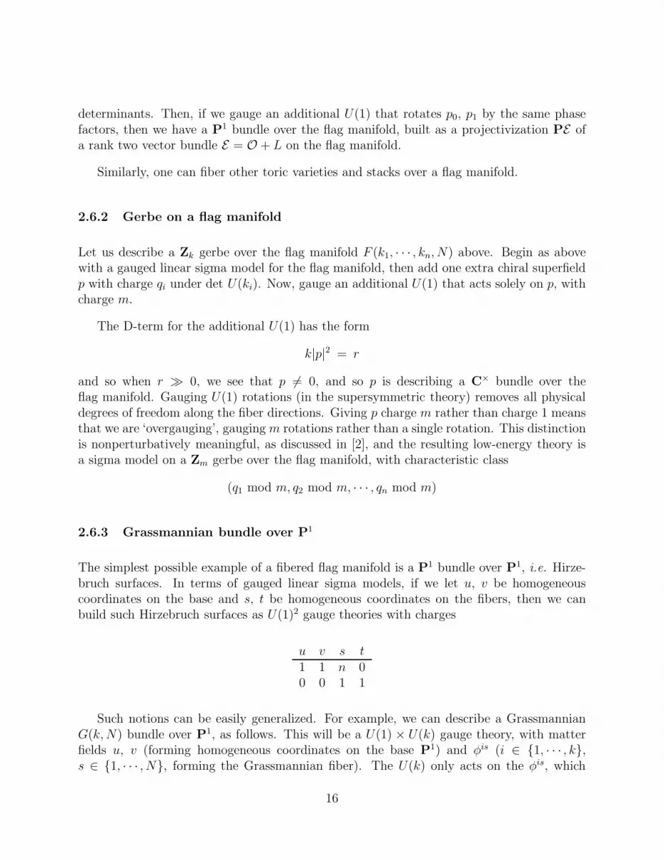
The simplest possible example of a fibered flag manifold is a P1 bundle over P1, i.e. Hirze-bruch surfaces. In terms of gauged linear sigma models, if we let u, v be homogeneouscoordinates on the base and s, t be homogeneous coordinates on the fibers, then we canbuild such Hirzebruch surfaces as U(1)2 gauge theories with charges

u v s t1 1 n 00 0 1 1

Such notions can be easily generalized. For example, we can describe a GrassmannianG(k,N) bundle over P1, as follows. This will be a U(1) × U(k) gauge theory, with matterfields u, v (forming homogeneous coordinates on the base P1) and φis (i ∈ {1, · · · , k},s ∈ {1, · · · , N}, forming the Grassmannian fiber). The U(k) only acts on the φis, which

16

transform in N copies of the fundamental representation. The U(1) acts on u, v with charge1, and also acts on the φis with weight ps, where ps is a sequence of N integers. (Thelocal U(k) gauge symmetry is preserved but the global U(N) symmetry is broken.) Moreinvariantly, we can think of this as a bundle with fibers G(k, E) where

E = ⊕Ns=1OP1(ps)

More general examples are also certainly possible, though this should suffice for illustrativepurposes.

3 Bundles

3.1 Tangent bundles and the (2,2) locus

First, let us recall how the tangent bundle is described by left-moving fermions in the linearsigma model for PN−1. Recall that PN−1 is described by a theory of N chiral fields in whicha U(1) action has been gauged. The action for the gauged linear sigma model has interactionterms of the form

φiψi−λ+ − φiψ

i+λ− + c.c.

where φ are the bosonic parts of the N chiral multiplets, ψ their superpartners, and λ part ofthe gauge multiplet. When φ has a nonzero vev, we see a linear combination of ψ’s and λ’sbecomes massive. To be specific, consider the term containing ψ+, and consider the subsetof ψi

+’s defined by ψi+ = ψφi for some Grassmann-valued parameter ψ. Using the D-term

condition ∑

i

|φi|2 = r

we see that the Yukawa coupling involving this particular ψi+ reduces to

φiψi+λ− = ψλ−|φi|2 = rψλ−

Thus, it is the ψφi combination that becomes massive. Put another way, identifying theψi

+’s with local sections of O(1)⊕N , we see that the remaining massless ψi+’s couple to the

cokernel T in the short exact sequence below:

0 −→ O ⊗φi−→ O(1)⊕N −→ T −→ 0

but that cokernel T is the tangent bundle of PN−1, so we see that the remaining masslessψi’s couple to the tangent bundle.

Mathematically, on PN−1 we have the “universal subbundle” (or “tautological bundle”)S, of rank one and c1(S) = −1, specifically O(−1), and the “universal quotient bundle” Q

17

of rank N − 1 and c1(Q) = +1. These are related by the short exact sequence

0 −→ S −→ ON −→ Q −→ 0

The tangent bundle of the projective space is given by S∨ ⊗ Q, and so fits into the shortexact sequence

0 −→ O −→ O(1)⊕N −→ TPN−1 −→ 0

known as the “Euler sequence.”

Projective spaces are special examples of Grassmannians – specifically,

PN−1 = G(1, N)

in our notation. Thus, it should not be surprising that the analysis above generalizes easilyto Grassmannians.

Let us begin our description of Grassmannians by working through the relevant math-ematics. On any Grassmannian G(k,N), we have the “universal subbundle” S, of rank kand c1(S) = −1, defined at any point on the Grassmannian to have fiber defined by thek-dimensional subspace of CN corresponding to that point. In addition, we have the “uni-versal quotient bundle” Q of rank N − k and c1(Q) = +1. Let V denote the trivial rank Nbundle on G(k,N), then these are related by the short exact sequence

0 −→ S −→ V −→ Q −→ 0

Under the duality operation G(k,N) ↔ G(N−k,N), the universal subbundle S is exchangedwith Q∨, the dual of the universal quotient bundle, and vice-versa. The tangent bundleT = Hom(S,Q) = S∨ ⊗Q, and so can be described as the cokernel

0 −→ S∨ ⊗ S −→ S∨ ⊗ V −→ T −→ 0

(For later use, note that using multiplicative properties of Chern characters (ch(T ) =ch(S∨)ch(Q)) one can immediately show c1(T ) = N .)

The analysis of the physics for Grassmannians also proceeds much as for projective spaces.The lagrangian of the corresponding nonabelian GLSM contains Yukawa couplings of theform

φisλi− jψ

js+

(plus complex conjugates and other chiralities) where i is a U(k) index and s ∈ {1, · · · , N}.Thus, some combination of λ−’s and ψ+’s will become massive. The ψ+’s that becomemassive can be understood by making the ansatz ψis

+ = ψφis, then applying the D-terms wesee

φisλi− jψ

js+ = φisλ

i− jφ

jsψ = rδjiλ

i− jψ = rλi

− iψ

18

and so we see that it is the ψφis combination of ψ+’s that becomes massive. Put anotherway, the remaining massless ψ+’s couple to the cokernel T of a short exact sequence of theform

0 −→ S∨ ⊗ S⊗φis−→ S∨ ⊗ V −→ T −→ 0

and so we realize the tangent bundle T of the Grassmannian in physics.

The tangent bundle of a partial flag manifold can be realized similarly. As for Grassman-nians, let us first describe the tangent bundle mathematically, then we shall describe how itis realized physically in the corresponding nonabelian GLSM.

Mathematically, the main difference between the tangent bundle of a Grassmannian andthat of a more general partial flag manifold is that instead of a single universal subbundleand universal quotient bundle, we now have a flag of both. First, over F (k1, · · · , kn, N) thereis a universal flag of subbundles

S1 → S2 → · · · → Sn → V

where the rank of Si is ki, and V is the trivial rank N bundle over the flag manifold.(The fibers of these subbundles are defined at any point on the flag manifold to be the flagcorresponding to that point.) In addition, there is a dual flag of quotient bundles

V −→ Q1 −→ Q2 −→ · · · −→ Qn

where each of the maps above is onto, and the Qi’s are defined by the short exact sequences

0 −→ Si −→ V −→ Qi −→ 0

Furthermore, the classical cohomology ring of the flag manifold is generated by the Chernclasses of the quotients Si/Si−1.

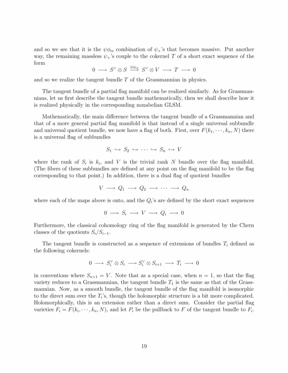
The tangent bundle is constructed as a sequence of extensions of bundles Ti defined asthe following cokernels:

0 −→ S∨i ⊗ Si −→ S∨

i ⊗ Si+1 −→ Ti −→ 0

in conventions where Sn+1 = V . Note that as a special case, when n = 1, so that the flagvariety reduces to a Grassmannian, the tangent bundle T1 is the same as that of the Grass-mannian. Now, as a smooth bundle, the tangent bundle of the flag manifold is isomorphicto the direct sum over the Ti’s, though the holomorphic structure is a bit more complicated.Holomorphically, this is an extension rather than a direct sum. Consider the partial flagvarieties Fi = F (ki, · · · , kn, N), and let Pi be the pullback to F of the tangent bundle to Fi.

19

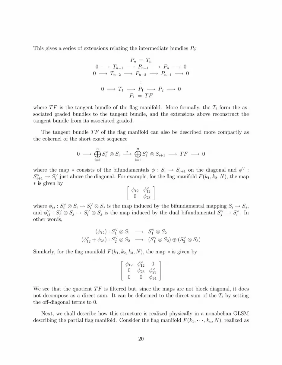
This gives a series of extensions relating the intermediate bundles Pi:

Pn = Tn

0 −→ Tn−1 −→ Pn−1 −→ Pn −→ 00 −→ Tn−2 −→ Pn−2 −→ Pn−1 −→ 0

...0 −→ T1 −→ P1 −→ P2 −→ 0

P1 = TF

where TF is the tangent bundle of the flag manifold. More formally, the Ti form the as-sociated graded bundles to the tangent bundle, and the extensions above reconstruct thetangent bundle from its associated graded.

The tangent bundle TF of the flag manifold can also be described more compactly asthe cokernel of the short exact sequence

0 −→n⊕

i=1

S∨i ⊗ Si

∗−→n⊕

i=1

S∨i ⊗ Si+1 −→ TF −→ 0

where the map ∗ consists of the bifundamentals φ : Si → Si+1 on the diagonal and φ∨ :S∨

i+1 → S∨i just above the diagonal. For example, for the flag manifold F (k1, k2, N), the map

∗ is given by [φ12 φ∨

12

0 φ23

]

where φij : S∨i ⊗ Si → S∨

i ⊗ Sj is the map induced by the bifundamental mapping Si → Sj ,and φ∨

ij : S∨j ⊗ Sj → S∨

i ⊗ Sj is the map induced by the dual bifundamental S∨j → S∨

i . Inother words,

(φ12) : S∨1 ⊗ S1 −→ S∨

1 ⊗ S2

(φ∨12 + φ23) : S∨

2 ⊗ S2 −→ (S∨1 ⊗ S2) ⊕ (S∨

2 ⊗ S3)

Similarly, for the flag manifold F (k1, k2, k3, N), the map ∗ is given by

φ12 φ∨

12 00 φ23 φ∨

23

0 0 φ34

We see that the quotient TF is filtered but, since the maps are not block diagonal, it doesnot decompose as a direct sum. It can be deformed to the direct sum of the Ti by settingthe off-diagonal terms to 0.

Next, we shall describe how this structure is realized physically in a nonabelian GLSMdescribing the partial flag manifold. Consider the flag manifold F (k1, · · · , kn, N), realized as

20

a two-dimensional U(k1)×· · ·×U(kn) gauge theory with bifundamentals. First consider theU(k1) factor. There are Yukawa couplings of the form

φisλi− jψ

js+

(where s is a U(k2) index), which can be analyzed in exactly the same way as those fora Grassmannian. The combination ψis

+ = ψφis becomes massive. Next, suppose ψis+ are

the fermionic components of a chiral superfield in the (ki−1,ki) representation of U(ki−1) ×U(ki), and ψai

+ are the corresponding components of a chiral superfield in the (ki,ki+1)representation of U(ki) × U(ki+1). Here, the Yukawa couplings involving the U(ki) λ−’s areof the form

−φisλi− jψ

js+ + φaiλ

i− jψ

aj

If we make the ansatz ψis+ = ψφis and ψai

+ = ψφai, for the same Grassmann parameter ψ inboth cases, then using the D-terms the Yukawa couplings above reduce to

(−φisφ

js + φaiφaj

)λi− jψ = riTr λ−ψ

Putting this together, we see that the remaining massless ψ+’s are described by the cokernelof the short exact sequence

0 −→n⊕

i=1

S∨i ⊗ Si

∗−→n⊕

i=1

S∨i ⊗ Si+1 −→ TF −→ 0

where the ⊕S∨i ⊗ Si factor is realized by the gauginos λ, the ⊕S∨

i ⊗ Si+1 factor is realizedby the fermionic parts ψ of the bifundamentals, and ∗ is the matrix with bifundamentals onand just above the diagonal described earlier. Thus, we see that the physical analysis of thefermions matches the mathematical picture of TF described earlier.

3.2 Aside: homogeneous bundles

For any parabolic subgroup P of a reductive algebraic group G, we can construct a largenumber of bundles on the coset space G/P by using a representation ρ of P . The total spaceof the bundle is G×ρ V , which has a natural projection to G/P , where V is the vector spaceon which the representation ρ acts. Such bundles are known as “homogeneous bundles.”

Grassmannians and flag manifolds can be described as coset spaces G/P , where in eachcase G = GL(N), and their tangent bundles are examples of homogeneous bundles. Therepresentations of the relevant parabolic P for a Grassmannian G(k,N) are the same as thoseof U(k)×U(N−k), so we merely need to find the relevant representation of U(k)×U(N−k).The universal subbundle S corresponds to the fundamental representation k of U(k), and theuniversal quotient bundle Q corresponds to the dual N − k of the fundamental representation

21

of U(N − k). Since the tangent bundle of G(k,N) is given by Hom(S,Q), we see that thetangent bundle is defined in this fashion by the representation (k,N− k) of U(k)×U(N−k).

The tangent bundle of the flag manifold can be described in an analogous fashion. Eachof the bundles Si can be described by the representation

(k1, 0, · · · , 0) ⊕ (0,k2 − k1, 0 · · · , 0) ⊕ (0, 0,k3 − k2, 0, · · · , 0) ⊕ (0, · · · , 0,ki − ki−1, 0, · · · , 0)

of U(k1) × U(k2 − k1) × · · · × U(N − kn). Call this representation ρSi. Similarly, each of

the bundles Ti that appeared in the construction of the tangent bundle is homogeneous, andfrom their definition it should be clear that they are defined by the representation

ρ∗Si⊗(0, · · · , 0,ki+1 − ki, 0, · · · , 0

)

=(k1, 0, · · · , 0,ki+1 − ki, 0, · · · , 0

)⊕ · · · ⊕

(0, · · · , 0,ki − ki−1,ki+1 − ki, 0, · · · , 0

)

However, typical bundles one works with in a (0,2) model will not be homogeneous, aswe shall see in the next section.

3.3 More general bundles

It is straightforward to describe other bundles in (0,2) GLSM’s over flag manifolds. Forexample, one common type of bundle described with (0,2) GLSM’s is given as the kernel Eof a short exact sequence:

0 −→ E −→ V1F−→ V2 −→ 0

The bundles V1 and V2 are determined by representations ρ1, ρ2 of the gauge group. Physi-cally, to describe V1 we introduce left-moving fermi multiplets Λ in the ρ1 representation ofthe gauge group, and right-moving chiral superfields p in the ρ∗2 representation of the gaugegroup. The map V1 → V2 is realized by a (0,2) superpotential

W =∫dθpFΛ

For example, one of the terms descending from that superpotential is

ψspλ

i−F

is(φ)

So long as the φ’s have nonzero vevs, a linear combination of ψp and λ− will become massive.The subset of λ− that remain massless are given by the kernel of the map defined by F ,hence this superpotential describes a kernel.

22

For example, consider a bundle on G(k,N) built as a kernel. Let ρ1 be k, and ρ2 beinvariant under SU(k), Take

F i =N∑

s=1

αsφis

for some arbitrary constants αi. With the superpotential∫dθpΛF , we have a (0,2) GLSM

on G(k,N) with bundle described by the kernel of F above. Note that this bundle is nothomogeneous, and cannot be described in terms of representation theory.

For another example, let us build a bundle on G(2, N) as a kernel. Take ρ1 to be the 2⊗2representation of U(2), and take ρ2 to be invariant under SU(2). Take the map F ij = ǫij .Then our bundle over G(2, N) is defined by the symmetric (3) representation of U(2).

Other standard (0,2) bundle constructions [21] are also possible, but we shall not discussthem further here.

4 Complete intersections in flag manifolds

4.1 Calabi-Yau’s in flag manifolds

We can add matter fields pα to describe hypersurfaces with gauge-invariant superpotentials,following [1, 4]. The condition for the intersection of those hypersurfaces to be Calabi-Yau can be described as the condition for the axial anomaly in the two-dimensional (2, 2)gauged linear sigma model to vanish. In effect, there will be n U(1) factors, correspondingto the determinants of the U(ki)’s, and so n conditions for the intersection to be Calabi-Yau.Following the analysis of [4] in the Grassmannian case, and given that our gauged linearsigma models for flag manifolds have bifundamental matter, it is straightforward to see thatthe Calabi-Yau condition can be stated as follows:

i Minus the sum of pα charges in det U(ki) (= −KF )1 k2

2 k3 − k1

3 k4 − k2

· · · · · ·n N − kn−1

The right column is determined as the difference between the number of fundamentals andantifundamentals charged under the corresponding U(ki). The right column can also beunderstood mathematically as minus the part of the canonical divisor corresponding to thatU(ki) factor.

23

A list of Calabi-Yau three-folds obtained as complete intersections in flag manifolds isprovided at the end of [22]. For completeness, we repeat that list here:

n F dim(F ) −KF

7 F (2, 7) 10 77 F (1, 2, 7) 11 (2, 6)7 F (1, 5, 7) 14 (5, 6)7 F (1, 2, 6, 7) 15 (2, 5, 5)∗

6 F (2, 6) 8 66 F (3, 6) 9 66 F (1, 2, 6) 9 (2, 5)6 F (1, 3, 6) 11 (3, 5)6 F (1, 4, 6) 11 (4, 5)6 F (1, 2, 5, 6) 12 (2, 4, 4)6 F (1, 3, 5, 6) 13 (3, 4, 3)5 F (2, 5) 6 55 F (1, 2, 5) 7 (2, 4)5 F (2, 3, 5) 8 (3, 3)5 F (1, 3, 5) 8 (3, 4)5 F (1, 2, 4, 5) 9 (2, 3, 3)5 F (1, 2, 3, 5) 9 (2, 2, 3)5 F (1, 2, 3, 4, 5) 10 (2, 2, 2, 2)4 F (2, 4) 4 44 F (1, 2, 4) 5 (2, 3)4 F (1, 2, 3, 4) 6 (2, 2, 2)

(*: This corrects a trivial typo in [22].)

Note that the Calabi-Yau’s built in Grassmannians listed in [4][table 2] and [23][section6.2] form a subset of the list above.

The observant reader will note that, according to our earlier description of dualities,

F (1, 3, 6) ∼= F (1, 4, 6)F (1, 3, 5) ∼= F (2, 3, 5)

F (1, 2, 4, 5) ∼= F (1, 2, 3, 5)

should be related by diffeomorphisms. However, although the manifolds are diffeomorphic,note that −KF differs. This is consistent because −KF is determined in part by the complexstructure, and the diffeomorphisms relating the special cases above do not preserve thecomplex structure. Put another way, c1(K) matches c1 of the holomorphic part of thecomplexified tangent bundle, but as Chern classes can only be defined for complexifiedtangent bundles, there is no reason why the c1’s need be invariant under non-holomorphic

24

diffeomorphisms. For a simpler example of this principle, the map z 7→ z defines a non-holomorphic diffeomorphism P1 → P1, which sends c1(K) 7→ −c1(K).

The analysis also easily extends to the weighted Grassmannians and flag manifolds de-scribed in section 2.5. For example, for a weighted Grassmannian modelled on G(k,N) withweights (u, w1, · · · , wN), the Calabi-Yau condition for a complete intersection is that the sumof the degrees of the hypersurfaces must equal

Nu + k∑

i

wi

For an ordinary Grassmannian G(k,N), u = 1 and all the wi = 0, and so the conditionreduces to the constraint that the sum of the degrees equal N .

4.2 Non-birational derived equivalences in nonabelian GLSMs

In [5][section 12.2] and [4], examples were given of GLSM’s in which

• one of the Kahler phases had a geometric interpretation, realized in a novel fashion,and

• geometric Kahler phases were not birational

in abelian and nonabelian GLSM’s, respectively. It has long been assumed that the geometricphases of GLSM’s were related by birational transformations, so examples contradicting thatbelief are of interest.

In this section we shall elaborate on this matter, by studying further examples of thisphenomenon in nonabelian GLSM’s, and reviewing an example of the phenomenon in abelianGLSM’s. We will also describe a tentative proposal for understanding the mathematicalrelationship between non-birational phases: we propose that they should be understood interms of Kuznetsov’s homological projective duality [6, 7, 8]. In this paper we will onlybegin to outline the relevance of Kuznetsov’s work – a much more thorough description, andfurther application to abelian GLSM’s, will appear in [9].

We shall begin by reviewing the example in [4], then discuss other examples in non-abelian GLSM’s before interpreting the results in terms of Kuznetsov’s work and outliningan analogous example in abelian GLSM’s.

4.2.1 Hori-Tong-Rodland example

In [4][section 5], an example of a gauged linear sigma model was analyzed which described,for r ≫ 0, a complete intersection of seven degree one hypersurfaces in the Grassmannian

25

G(2, 7), and for r ≪ 0, the “Pfaffian Calabi-Yau,” which is not a complete intersection. (See[24] for a corresponding mathematical discussion.) The superpotential terms each involve twoof the chiral fields Φa

i defining the Grassmannian and a single auxiliary field pi, introducedto describe members of the complete intersection, and so has the form

W ∝ Ajki p

iΦajΦ

bkǫab

for constants Ajki . In terms of the U(1) ⊂ U(2) given by matrices proportional to the identity,

the pi have charge 2 and the Φai have charge 1. For r ≫ 0, it is straightforward to check

that the gauged linear sigma model describes G(2, 7)[17]. For r ≪ 0, the D-terms forbid thepi from all vanishing, and so they form homogeneous coordinates on a P6. The U(2) gaugesymmetry is broken to SU(2) × Z2, where the Z2 subgroup of U(2) is given by matrices ofthe form diag(1, ζ), for ζ = ±1. That Z2 acts trivially on the pi but acts effectively on theΦa

i . The matrix Ajki p

i ≡ A(p)jk is a skew-symmetric 7 × 7 matrix with entries linear in thepi. Nondegeneracy of the original complete intersection forces A(p) to have rank either 4or 6 for all p. At p for which A(p) has rank 4, there are 7 − 4 = 3 massless Φ doublets;the rest are massive with masses proportional to |r|. At p for which A(p) has rank 6, thereis 7 − 6 = 1 massless Φ doublet. As discussed in [4], in the infrared limit all vacua in thenonabelian gauge theory on the rank 6 locus run to infinity, whereas on the rank 4 locus asingle vacuum remains. Thus, [4] identify the r ≪ 0 phase with a nonlinear sigma model onthe vanishing locus of the 6 × 6 Pfaffians of the matrix A(p) defined over P6.

4.2.2 Aside: Pfaffian varieties

As Pfaffian varieties are not commonly used in the physics community, let us take a momentto check certain basic properties of the previous example. (For a more complete description,see for example [11][section 3.5]. For other related information, see for example [25].)

First, let us establish some notation that will sometimes be used elsewhere in this paper.The Pfaffian variety Pf(N) for N odd is a space defined as follows. Let V be an N -dimensional vector space, and consider the locus in the space of two-forms in Λ2V ∗ whoserank is not maximal. The maximal possible rank is N − 1, and the next possible rank isN−3. So, for N odd, Pf(N) can be defined as the space of skew-symmetric N×N matricesof rank N − 3, i.e. whose (N − 1) × (N − 1) Pfaffians all vanish.

In particular, Pf(5) and G(2, 5) are the same space, but on dual vector spaces. Interms of Plucker coordinates, G(2, 5) describes the space of elements of Λ2V which have thesmallest possible nonzero rank, whereas Pf(5) describes the locus of elements of Λ2V ∗ ofsubmaximal rank, which is also 2 in this case. Alternatively, by identifying matrix entrieswith coordinates on the space of all skew-symmetric matrices and performing a linear changeof coordinates, we can describe Pf(5) (and hence G(2, 5)) as the vanishing locus in P9 (theprojectivized space of all skew-symmetric 5 × 5 matrices, using the fact that such matrices

26

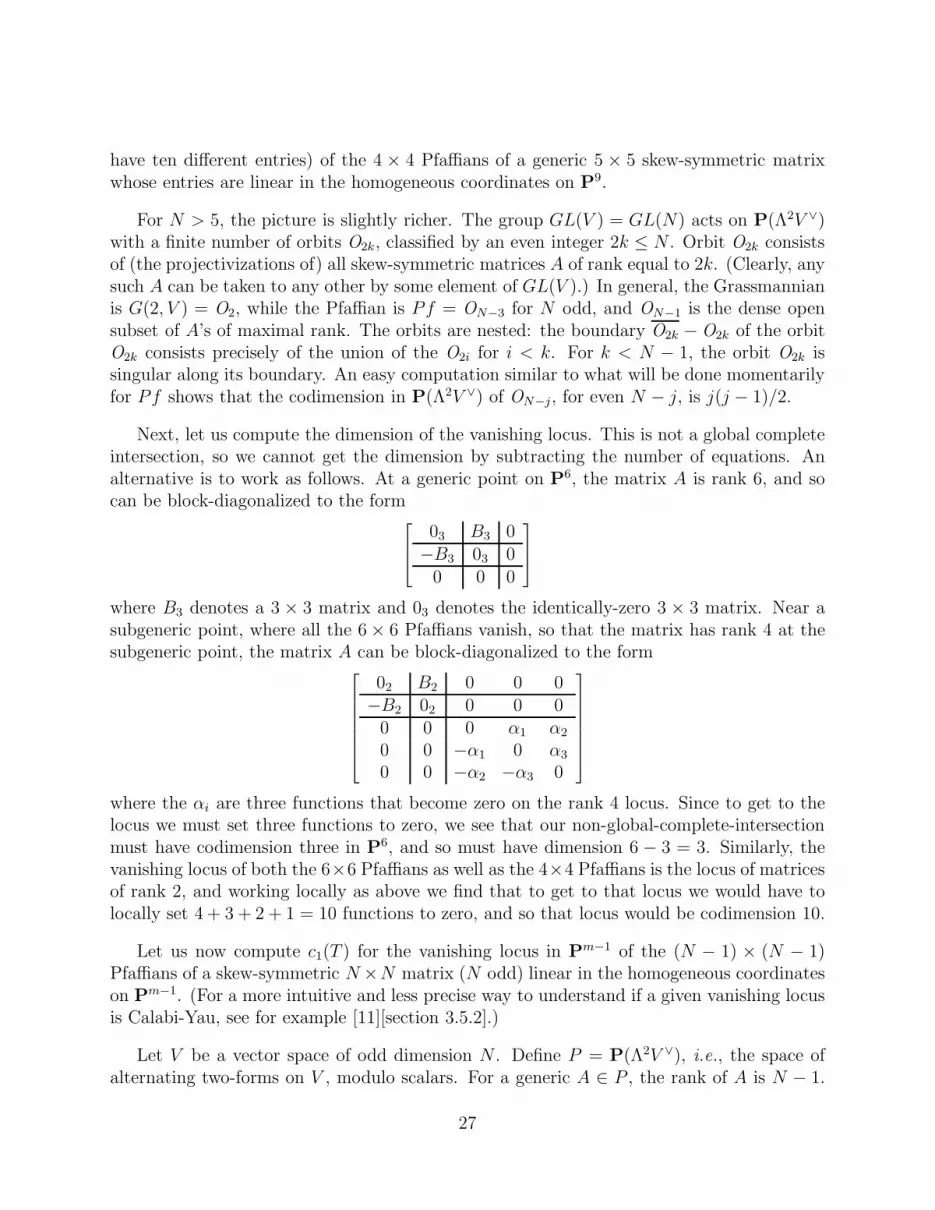
have ten different entries) of the 4 × 4 Pfaffians of a generic 5 × 5 skew-symmetric matrixwhose entries are linear in the homogeneous coordinates on P9.

For N > 5, the picture is slightly richer. The group GL(V ) = GL(N) acts on P(Λ2V ∨)with a finite number of orbits O2k, classified by an even integer 2k ≤ N . Orbit O2k consistsof (the projectivizations of) all skew-symmetric matrices A of rank equal to 2k. (Clearly, anysuch A can be taken to any other by some element of GL(V ).) In general, the Grassmannianis G(2, V ) = O2, while the Pfaffian is Pf = ON−3 for N odd, and ON−1 is the dense opensubset of A’s of maximal rank. The orbits are nested: the boundary O2k − O2k of the orbitO2k consists precisely of the union of the O2i for i < k. For k < N − 1, the orbit O2k issingular along its boundary. An easy computation similar to what will be done momentarilyfor Pf shows that the codimension in P(Λ2V ∨) of ON−j, for even N − j, is j(j − 1)/2.

Next, let us compute the dimension of the vanishing locus. This is not a global completeintersection, so we cannot get the dimension by subtracting the number of equations. Analternative is to work as follows. At a generic point on P6, the matrix A is rank 6, and socan be block-diagonalized to the form

03 B3 0−B3 03 0

0 0 0

where B3 denotes a 3 × 3 matrix and 03 denotes the identically-zero 3 × 3 matrix. Near asubgeneric point, where all the 6 × 6 Pfaffians vanish, so that the matrix has rank 4 at thesubgeneric point, the matrix A can be block-diagonalized to the form

02 B2 0 0 0−B2 02 0 0 0

0 0 0 α1 α2

0 0 −α1 0 α3

0 0 −α2 −α3 0

where the αi are three functions that become zero on the rank 4 locus. Since to get to thelocus we must set three functions to zero, we see that our non-global-complete-intersectionmust have codimension three in P6, and so must have dimension 6 − 3 = 3. Similarly, thevanishing locus of both the 6×6 Pfaffians as well as the 4×4 Pfaffians is the locus of matricesof rank 2, and working locally as above we find that to get to that locus we would have tolocally set 4 + 3 + 2 + 1 = 10 functions to zero, and so that locus would be codimension 10.

Let us now compute c1(T ) for the vanishing locus in Pm−1 of the (N − 1) × (N − 1)Pfaffians of a skew-symmetric N×N matrix (N odd) linear in the homogeneous coordinateson Pm−1. (For a more intuitive and less precise way to understand if a given vanishing locusis Calabi-Yau, see for example [11][section 3.5.2].)

Let V be a vector space of odd dimension N . Define P = P(Λ2V ∨), i.e., the space ofalternating two-forms on V , modulo scalars. For a generic A ∈ P , the rank of A is N − 1.

27

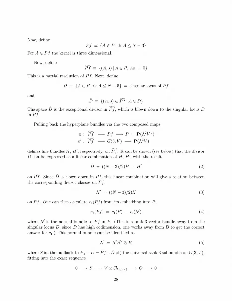
Now, definePf ≡ {A ∈ P | rk A ≤ N − 3}

For A ∈ Pf the kernel is three dimensional.

Now, defineP f ≡ {(A, s) |A ∈ P, As = 0}

This is a partial resolution of Pf . Next, define

D ≡ {A ∈ P | rk A ≤ N − 5} = singular locus of Pf

andD ≡ {(A, s) ∈ P f |A ∈ D}

The space D is the exceptional divisor in P f , which is blown down to the singular locus Din Pf .

Pulling back the hyperplane bundles via the two composed maps

π : P f −→ Pf −→ P = P(Λ2V ∨)

π′ : P f −→ G(3, V ) −→ P(Λ3V )

defines line bundles H , H ′, respectively, on P f . It can be shown (see below) that the divisorD can be expressed as a linear combination of H , H ′, with the result

D = ((N − 3)/2)H − H ′ (2)

on P f . Since D is blown down in Pf , this linear combination will give a relation betweenthe corresponding divisor classes on Pf :

H ′ = ((N − 3)/2)H (3)

on Pf . One can then calculate c1(Pf) from its embedding into P :

c1(Pf) = c1(P ) − c1(N ) (4)

where N is the normal bundle to Pf in P . (This is a rank 3 vector bundle away from thesingular locus D; since D has high codimension, one works away from D to get the correctanswer for c1.) This normal bundle can be identified as

N = Λ2S∨ ⊗H (5)

where S is (the pullback to Pf−D = P f−D of) the universal rank 3 subbundle on G(3, V ),fitting into the exact sequence

0 −→ S −→ V ⊗OG(3,V ) −→ Q −→ 0

28

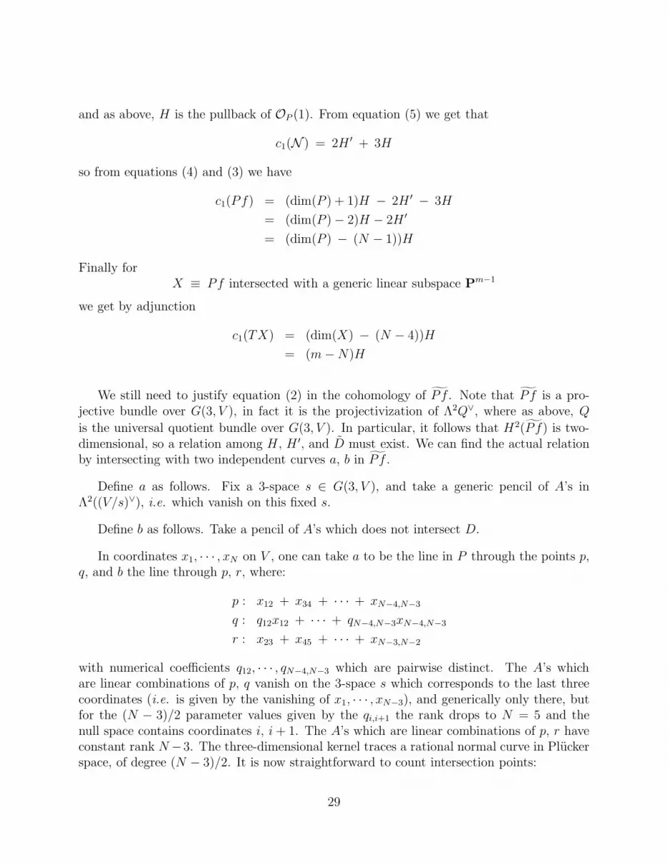
and as above, H is the pullback of OP (1). From equation (5) we get that

c1(N ) = 2H ′ + 3H

so from equations (4) and (3) we have

c1(Pf) = (dim(P ) + 1)H − 2H ′ − 3H

= (dim(P ) − 2)H − 2H ′

= (dim(P ) − (N − 1))H

Finally forX ≡ Pf intersected with a generic linear subspace Pm−1

we get by adjunction

c1(TX) = (dim(X) − (N − 4))H

= (m−N)H

We still need to justify equation (2) in the cohomology of P f . Note that P f is a pro-jective bundle over G(3, V ), in fact it is the projectivization of Λ2Q∨, where as above, Q

is the universal quotient bundle over G(3, V ). In particular, it follows that H2(P f) is two-dimensional, so a relation among H , H ′, and D must exist. We can find the actual relationby intersecting with two independent curves a, b in P f .

Define a as follows. Fix a 3-space s ∈ G(3, V ), and take a generic pencil of A’s inΛ2((V/s)∨), i.e. which vanish on this fixed s.

Define b as follows. Take a pencil of A’s which does not intersect D.

In coordinates x1, · · · , xN on V , one can take a to be the line in P through the points p,q, and b the line through p, r, where:

p : x12 + x34 + · · · + xN−4,N−3

q : q12x12 + · · · + qN−4,N−3xN−4,N−3

r : x23 + x45 + · · · + xN−3,N−2

with numerical coefficients q12, · · · , qN−4,N−3 which are pairwise distinct. The A’s whichare linear combinations of p, q vanish on the 3-space s which corresponds to the last threecoordinates (i.e. is given by the vanishing of x1, · · · , xN−3), and generically only there, butfor the (N − 3)/2 parameter values given by the qi,i+1 the rank drops to N = 5 and thenull space contains coordinates i, i+ 1. The A’s which are linear combinations of p, r haveconstant rank N−3. The three-dimensional kernel traces a rational normal curve in Pluckerspace, of degree (N − 3)/2. It is now straightforward to count intersection points:

29

a bH 1 1H ′ 0 (N − 3)/2

D (N − 3)/2 0

This establishes our claim that D = ((N − 3)/2)H − H ′, and completes the calculation ofc1(TX) = (m−N)H .

4.2.3 A complete intersection in a G(2, 5) bundle

Another analogous example can be built as follows. Let us consider a Calabi-Yau built asa complete intersection in the total space of a G(2, 5) bundle over P2. The G(2, 5) bundleis built by fibering the C5 as the vector bundle O(−1)⊕4 ⊕ O over P2. The gauged linearsigma model can be built from the fields x0, x1, x2, Φµ

i (µ ∈ {1, 2}, i ∈ {1, · · · , 5}) in whicha U(2) × U(1) action has been gauged. The U(2) acts on the Φµ

i as a set of five doublets,and leaves the xa invariant. The U(1) charges are as follows:

x0 x1 x2 Φµ1···4 Φµ

5

1 1 1 -1 0

Baryons (Plucker coordinates) naturally arrange themselves as

ǫµνΦµi Φν

j i, j ∈ {1, · · · , 4}ǫµνΦ

µi Φν

5 i ∈ {1, · · · , 4}

These baryons define an embedding of the total space of this Grassmannian bundle into thetotal space of the projective bundle

P(O(−2)⊕6 ⊕O(−1)⊕4

)−→ P2

We can build a Calabi-Yau by taking the complete intersection of five hypersurfaces, so weadd to the gauged linear sigma model five fields pi of charge −2 under det U(2) and charge+1 under the U(1). The superpotential then has the form

W = piBijk(x)ǫµνΦ

µj Φν

k = Aij(x, p)ǫµνΦµi Φν

j

The 5 × 5 matrix Aij is skew-symmetric. For i, j ≤ 4 it is degree (1, 1) in (x, p), and fori = 5, j ≤ 4 it is degree (0, 1) in (x, p).

The analysis of the Landau-Ginzburg point of this model is very similar to that in theprevious section. It is given by the vanishing locus of 4 × 4 Pfaffians of Aij on P2 × P4,where the P4 arises from the pi fields. Briefly, this is because, as in [4], on the rank 4 locus,

30

there is a single massless Φ doublet, and the vacua run to infinity, whereas on the rank 2locus (where the 4 × 4 Pfaffians vanish), there are three massless Φ doublets, and in the IRa single vacuum remains.

The geometry we have found at the Landau-Ginzburg point was discussed mathematicallyin [26][section 3.2], as an example of a genus-one-fibered Calabi-Yau threefold, fibered overP2, with an embedding into P2 × P4 of the form described above. It is not an ellipticfibration, as it does not have an ordinary section, but rather merely a 5-section.

The Landau-Ginzburg geometry above, is believed to have the same derived category ofcoherent sheaves [26] as the complete intersection in the G(2, 5) bundle3 on P2 that sits atthe large-radius point in the gauged linear sigma model above. Fiberwise [27], if G(2, 5) iscut by a codimension 5 plane, the result is an elliptic curve, and similarly if the Pfaffianmanifold Pf(5) (which can be understood as G(2, 5) again, but describing 2-planes in thedual 5-dimensional vector space) is cut by the dual linear space, the result is the sameelliptic curve. The two curves can be identified if one picks a point on each elliptic curve, oralternatively, the second elliptic curve can be identified naturally with Pic2 of the first curve.When this is done in families, the Grassmannian fibration can be understood as the relativePic2 of the Pfaffian fibration, and it is well-known that such pairs are derived equivalent.

Whether or not these two spaces are birational to one another, is not known at present.

4.2.4 A Fano example

In addition to Calabi-Yau examples, we can also consider non-Calabi-Yau examples. In thisand subsequent sections, we shall study several examples of nonabelian GLSM’s for Fanomanifolds. These GLSM’s will also possess nontrivial Landau-Ginzburg points. We shouldnote at the beginning, however, that there are some structural differences between GLSMKahler moduli spaces in Calabi-Yau and non-Calabi-Yau cases. For example, in Calabi-Yaucases the Kahler moduli space is complexified by the theta angle, but in non-Calabi-Yau casesan axial anomaly prevents that theta angle from being meaningful, so the Kahler modulispaces are real, not complex. In addition, the Kahler parameters will not be renormalization-group invariants in non-Calabi-Yau cases. In the examples below, we will consider somesimple nonabelian GLSM’s with a one-real-dimensional Kahler moduli “space.” Singularitiesnear the origin will break the Kahler moduli space into two disconnected components, andso as there is no way to smoothly deform the large-radius and Landau-Ginzburg points intoone another, Witten indices need not match.

Let us now consider our first example. A degree 5 del Pezzo can be described asG(2, 5)[1, 1, 1, 1]. At the Landau-Ginzburg point of the GLSM for G(2, 5)[1, 1, 1, 1], following

3In [26], the dual was described merely as relative Pic2 – the more explicit description as a G(2, 5) bundlewas not given there.

31

the same analysis as before we find the vanishing locus in P3 of 4 × 4 Pfaffians of a 5 × 5skew-symmetric matrix formed from a linear combination of the hyperplane equations.

Note that unlike the Calabi-Yau case, the large-radius and Landau-Ginzburg points nolonger describe spaces of the same dimension. The large radius space has complex dimension6 − 4 = 2, whereas the Landau-Ginzburg phase is codimension three in P3 and hence zero-dimension – a set of points with multiplicity.

4.2.5 A related non-Calabi-Yau example

Consider a GLSM describing the complete intersection of 6 hyperplanes in G(2, 5), i.e.,G(2, 5)[1, 1, 1, 1, 1, 1] (or, more compactly, G(2, 5)[16]). The Landau-Ginzburg point of thisGLSM can be determined using previous methods, and is given by the vanishing locus in P5

of the 4×4 Pfaffians of a skew-symmetric 5×5 matrix with entries linear in the homogeneouscoordinates on P5.

Here, the complete intersection in the Grassmannian G(2, 5) has dimension 0 – it is aset of points – whereas the Pfaffian variety has codimension 3 in P5, hence dimension 2, theopposite of the previous example.

This example is very closely related to the example in the previous section, as the degree5 del Pezzo G(2, 5)[1, 1, 1, 1] (the large-radius point of the previous example) has an alternatepresentation as the vanishing locus in P5 of the 4 × 4 Pfaffians of a skew-symmetric 5 × 5matrix with entries linear in the homogeneous coordinates on P5, the Landau-Ginzburg pointof the current example. This is a consequence of the equivalence described in section 4.2.2between G(2, 5) and the vanishing locus in P9 of the 4 × 4 Pfaffians of a generic 5 × 5skew-symmetric matrix – by intersecting both sides with four hyperplanes, we obtain theequivalence claimed here.

Not only are the dimension-two phases of this example and the previous one differentpresentations of the same thing, but so are the dimension-zero phases. Both G(2, 5)[16] andthe vanishing locus in P3 of the 4 × 4 Pfaffians of a 5 × 5 skew-symmetric matrix describethe same number of points (including multiplicity).

As a result, we believe the example in this subsection and that in the previous subsectionare actually different presentations of the same family of CFT’s, in which the interpretationas large-radius and Landau-Ginzburg points has been reversed.

32

4.2.6 More non-Calabi-Yau examples

Consider a gauged linear sigma model describing the complete intersection of m hyperplaneswith G(2, N) for N odd (using the restriction of [4]). Following reasoning that by now shouldbe routine, its Landau-Ginzburg point corresponds to the vanishing locus in Pm−1 of the(N − 1) × (N − 1) Pfaffians of a skew-symmetric N ×N matrix linear in the homogeneouscoordinates on Pm−1, where the N ×N matrix is formed by rewriting a linear combinationof the m hyperplanes, with coefficients given by the homogeneous coordinates on Pm−1.

The complete intersection in the Grassmannian G(2, N) has dimension 2(N − 2) − m,whereas the Pfaffian variety has codimension three in Pm−1, hence dimension m − 4. Thecanonical bundle of the complete intersection is O(m−N), whereas following the reasoningin section 4.2.2 the canonical bundle of the Pfaffian variety at the Landau-Ginzburg point isO(−m+N).

The fact that the canonical bundles of either end have c1’s of opposite sign gives us anothercheck on these results. After all, the renormalization of the Fayet-Iliopoulos parameter isdetermined by the gauge linear sigma model and is independent of the phase. If the large-radius phase shrinks under renormalization group flow, i.e., r → 0, then to be consistentthe theory at Landau-Ginzburg must expand to larger values of |r|, i.e. r → −∞, andconversely. A nonlinear sigma model on a positively-curved space will shrink under RG flow,and a nonlinear sigma model on a negatively-curved space will expand under RG flow, so wesee that if one phase of the GLSM is positively-curved, then in order for dr/dΛ as determinedby the GLSM to be consistent across both phases, the other phase must be negatively-curved,and vice-versa.

4.2.7 Interpretation – Kuznetsov’s homological projective duality

In the past, it has been thought that the geometric phases of a gauged linear sigma modelwere all birational. Here, however, we have seen several examples, both Calabi-Yau andnon-Calabi-Yau, of gauged linear sigma models with non-birational phases. One naturalquestion to ask then is, if these phases are not birational, then how precisely are they relatedmathematically?

In this paper and [9], we would like to propose that these non-birational phases arerelated by Kuznetsov’s “homological projective duality” [6, 7, 8]. Put another way, here andin [9] we propose that gauged linear sigma models implicitly give a physical realization ofKuznetsov’s homological projective duality.

The physical relevance of Kuznetsov’s work will be discussed in much greater detail in[9], together with more examples (including examples in abelian gauged linear sigma models)and more tests of corner cases.

33

Very briefly, two spaces are said to be homologically projectively dual if their derivedcategories of coherent sheaves have pieces in common, in a precise technical sense. Unfortu-nately, in general there is not a constructive method for producing examples of homologicalprojective duals – given one space, there is not yet an algorithm that will always produce adual.

However, much is known. For example, it is known that the examples discussed so far areall homologically projectively dual. In other words, the complete intersection of m hyper-planes in G(2, N) for N odd is known to be homologically projectively dual to the vanishinglocus in Pm−1 of the (N − 1) × (N − 1) Pfaffians of a skew-symmetric N ×N matrix linearin the homogeneous coordinates on Pm−1, where the N × N matrix is formed by rewrit-ing a linear combination of the m hyperplanes. In special cases, this can be understoodmore systematically. For example, the Grassmannian G(2, 5) itself is homologically projec-tively dual to a Pfaffian variety of 5 × 5 skew-symmetric matrices, the space of which liesin P(Λ2C5) = P9. Intersecting the Grassmannian with 4 hyperplanes is dual to intersectingthe Pfaffian variety with the dual of P9−4 in P9, which is P3.

More generally, we can understand this as follows [33]. Let M denote the dimension ofthe set of all skew-symmetric N × N matrices, N odd, choose M generic hyperplanes inG(2, N), and consider the vanishing locus in PM−1 of the (N − 1) × (N − 1) Pfaffians ofa skew-symmetric N × N matrix linear in the homogeneous coordinates on PM−1, wherethe N × N matrix is formed by rewriting a linear combination of the M hyperplanes, withcoefficients given by the homogeneous coordinates on PM−1. This variety, call it Y , ishomologically projectively dual to G(2, N). If we are given m hyperplanes in G(2, N), theygenerate Pm−1 ⊂ PM−1, and so the dual is Y ∩ Pm−1. In the language of section 4.2.2,this duality exchanges orbits O2 ↔ ON−3, as well as intersections: O2 intersected with acodimension m subspace A is dual to ON−3 intersected with A⊥, which is a Pm−1. Thegeneral result verifies not only the previous example but every example discussed so far,except for the G(2, 5) bundle model in section 4.2.3. For that model, it is believed [34] thatthe two geometries are homologically projectively dual, though a rigorous proof does not yetexist.

Strictly speaking, what often arises as the duals are not precisely ordinary nonlinearsigma models on spaces, but rather certain resolutions known technically as ‘noncommutativeresolutions.’ The term ‘noncommutative’ is a misnomer here, as it does not necessarily implythat there is any noncommutative algebra present, but rather is used as a generic term foranything on which one can do sheaf theory, and ‘noncommutative spaces’ are defined by theirsheaves. For example, via matrix factorization one can think of a Landau-Ginzburg modelas a ‘noncommutative space’ in this sense. In [9] we will closely examine some examples ofhomological projective duality in which noncommutative resolutions appear, and we will seehow those noncommutative resolutions arise within gauged linear sigma models.

So far we have outlined how non-birational phases of gauged linear sigma models can be

34

understood as examples of Kuznetsov’s homological projective duality, but we also conjecturethe same is true of birational phases also. It is known that some flops between Calabi-Yau’sare examples of homological projective duals, and it is conjectured that all flops are alsoexamples of homological projective duals.

However, although evidence suggests that all phases of gauged linear sigma models mightbe examples of homological projective duality, the converse may not be true – there areexamples of homological projective duals which might not be realizable within gauged linearsigma models. For example, Grassmannians themselves have homological projective duals,but a typical gauged linear sigma model for a Grassmannian has only one phase. Perhapsthere are alternate presentations, realizable within gauged linear sigma models, which havemultiple phases, or perhaps the duals reflect more subtle aspects of the original gauged linearsigma models.

In the next subsection, we shall consider a possible prediction of Kuznetsov’s work forcases in which the physics is more obscure.

4.2.8 Duals of G(2, N) with N even

The authors of [4] restricted to their analysis of duality in complete intersections in G(2, N)to the case N odd, because the physics in cases for which N is even is both different andmore difficult. However, there exist homological projective duals for cases in which N iseven, and so we can use homological projective duality to make predictions for such cases.

The duals of N even cases are slightly subtle, so we must proceed carefully. Let usfirst examine the case of G(2, 6)[16] in detail. Naively, the homological projective dual ofthe complete intersection G(2, 6)[16] is a ‘noncommutative resolution’ of a cubic 4-fold, ahypersurface in P5 defined by the Pfaffian of a skew-symmetric 6× 6 matrix determined bythe six hyperplanes in G(2, 6).

Given the match between homological projective duals and phases in previous examples,it is tempting to conjecture that the Landau-Ginzburg phases of G(2, 6)[16] might be thePfaffian variety above. On the other hand, although the complete intersection is Calabi-Yau,the Pfaffian variety is not. It is difficult to understand how a gauged linear sigma modelcould relate a Calabi-Yau space to a non-Calabi-Yau space, unless the non-Calabi-Yau spacehas a flux background present so as to preserve supersymmetry.

In fact, the correct answer here is slightly more subtle. The correct dual [6, 28] is a‘noncommutative4 space’ defined by a subcategory of the derived category of the cubic. Twospaces are dual in the relevant mathematical sense if, in essence, their derived categories

4As described earlier, but is well worth repeating, the word ‘noncommutative’ is used by mathematiciansin this context in a misleading fashion – it does not necessarily indicate the presence of any noncommutivity.

35

have a piece in common [8][theorem 2.9]. For G(2, N)[1N ] for N odd, the correspondingcomplete intersection in the Pfaffian variety is already a Calabi-Yau. The derived categoryof the complete intersection in the Pfaffian variety already matched5 that of the Calabi-Yau G(2, N)[1N ] (see e.g. [8, 24]), so there was no ‘noncommutative space’ to consider.However, for G(2, N)[1N ] for N even, the derived category of the original space matchesonly a subcategory of that of the hypersurface in the Pfaffian. So the correct dual in thecase of G(2, 6)[16] must be something slightly different from the cubic 4-fold described above,something defined by a subcategory of the derived category of the cubic 4-fold. We thenhave to find a physical theory whose D-branes are described by the pertinent subcategory.

It turns out that there is a very natural candidate for such a physical theory, that shouldrealize the ‘noncommutative space’ defined by a subcategory of the derived category of thecubic 4-fold. In particular, since the cubic is Fano, the category of matrix factorizations ofthe associated Landau-Ginzburg model is a subcategory [29], and is precisely the subcategorywe need to describe. That Landau-Ginzburg model is defined by a cubic superpotential insix variables, which up to finite group factors is a deformation of a Landau-Ginzburg modelfor an orbifold of a product of two elliptic curves – a K3, in other words. Assuming that thefinite group factors work out correctly, and that we have interpreted the structure of thatmodel and its deformations correctly, this finally gives us a physically consistent conjecturefor the form of the LG point in G(2, 6)[16] – namely, that it is a Landau-Ginzburg modelassociated to a K3 surface.

So, based on the mathematics of Kuznetsov’s homological projective duality, we propose(as suggested to us by [28]) that the Landau-Ginzburg point of the nonabelian GLSM forG(2, 6)[16] is a Landau-Ginzburg model corresponding to a K3 surface.

We will leave to future work a thorough verification that this is indeed the correct de-scription of the Landau-Ginzburg point of this model, although we will mention that it seemsvery plausible:

• As a consistency check, since G(2, 6)[16] is itself a K3, the only other geometries oneshould find as phases in a GLSM Kahler moduli space are other K3’s, so the result isphysically consistent.

• At the level of sheaf theory and D-branes [30, 31], both the derived category ofG(2, 6)[16] and the category of matrix factorizations of the Landau-Ginzburg model ap-pear [28] as subcategories of the derived category of the cubic fourfold in P5 defined asthe right orthogonal to O(k) for k = −1,−2,−3, i.e., F such that RHom(O(k),F) = 0for k = −1,−2,−3. So the derived categories of the large-radius limit and the proposedinterpretation of the Landau-Ginzburg point match on the nose, exactly as needed for

5We should be slightly careful. For N odd and N > 7, there is a technicality involving the constructionof a (noncommutative) resolution of the Pfaffian, so to be precise, these remarks ought to be limited to smallN , and considered to be conjectures for larger N .

36

consistency of the B twist of the gauged linear sigma model.

• Physically, this would mean that the fields fluctuate around a single vacuum at energycost determined by the Pfaffian of a skew-symmetric 6× 6 matrix, which is very plau-sibly a description of the Landau-Ginzburg point of this gauged linear sigma model.

In addition, we should also mention one other, related, geometry that appears in thiscontext. It is less clear to us what role it plays physically, but for completeness, it shouldbe mentioned. The space of lines in the cubic in P5 is another Calabi-Yau – in fact, ahyperKahler 4-fold given by the Hilbert scheme of pairs of points on the K3 G(2, 6)[16].Its derived category is nearly (but not quite) identical to that of G(2, 6)[16]. For moreinformation on this space and its relation to G(2, 6)[16] see for example [32].

Similarly, the dual of G(2, 8)[18] is a Landau-Ginzburg model defining a ‘noncommutativespace’ associated to a ‘noncommutative resolution’ of a degree four hypersurface in P7, wherethe hypersurface is defined by the Pfaffian of a skew-symmetric 8 × 8 matrix formed fromthe eight hyperplanes. The associated Landau-Ginzburg model is defined by a degree foursuperpotential in eight variables, which is related to an orbifold of the product of two K3surfaces. In this case we conjecture that the Landau-Ginzburg point of the GLSM forG(2, 8)[18] is an orbifold of a Landau-Ginzburg model with a quartic superpotential in eightvariables, associated to (K3 ×K3)/G for some G.

Technically [33], we can understand the duals as follows. The complete intersection in aPfaffian Y dual to G(2, N) for N even is (a certain resolution of) the set of all degenerateskew-symmetric matrices in PM−1, where M is the dimension of the set of all skew-symmetricN ×N matrices. Such Y can be described as a hypersurface in PM−1 of degree N/2, definedby the vanishing locus of the Pfaffian. The dual to a complete intersection of m hyperplanesin G(2, N) is the intersection Y ∩ Pm−1. Thus, for example, the variety dual to G(2, 6)[16]is a degree 6/2 = 3 hypersurface in P6−1 = P5.

However, these spaces are never Calabi-Yau, and so can not be the physically-realizedhomological projective duals to the Calabi-Yau’s G(2, N)[1N ]. More generally [33], a Calabi-Yau built as a complete intersection of N hyperplanes in G(2, N) odd will always have aCalabi-Yau homological projective dual; but for N even, the dual variety obtained as acomplete intersection in a Pfaffian variety will never be Calabi-Yau (leading us to work withrelated Landau-Ginzburg models).

Repeating the analysis above, we conjecture that the Landau-Ginzburg points of GLSM’sfor G(2, N)[1N ] for N even will always be the ‘correct’ homological projective duals, namelyLandau-Ginzburg models defined by degree N/2 superpotentials given by the Pfaffian of theskew-symmetric N × N matrix defined by the hyperplanes. The category of matrix factor-izations of these Landau-Ginzburg models will match the derived category of G(2, N)[1N ]for all even N , as needed for consistency of the B twist of the gauged linear sigma model,

37

and will also be a large distinguished subcategory of the derived category of the pertinentdegree N/2 hypersurface in PN−1.

As an aside, the reader might wonder whether G(2, N)[1N ] is hyperKahler for all evenN , since our duals above both at least naively appear hyperKahler, and G(2, N)[1N ] alwayshas even complex dimension. However, it can be shown that G(2, N)[1N ] cannot be hy-perKahler for N > 6. This is because, due to Lefschetz, h2,0 of the complete intersectionG(2, N)[1N ] matches that of the ambient space G(2, N), which vanishes, but on the otherhand, hyperKahler implies holomorphically symplectic which implies h2,0 = 1.

4.3 Non-birational derived equivalences in abelian GLSMs

Although the example in section 4.2.1 is sometimes advertised as the first example of a gaugedlinear sigma model involving (a) a Calabi-Yau not presented as a complete intersection, and(b) two non-birationally-equivalent Calabi-Yau’s, in fact an abelian gauged linear sigmamodel with both these properties appeared previously in [5][section 12.2]. There, the gaugedlinear sigma model described a complete intersection of four degree two hypersurfaces inP7 for r ≫ 0, and was associated with a double cover of P3 branched over a degree eighthypersurface (Clemens’ octic double solid) for r ≪ 0. The fact that they are not birationalfollows from the fact that [35] the complete intersection in P7 has no contractible curves,whereas the branched double cover has several ordinary double points. This is anotherexample of Kuznetsov’s homological projective duality [7, 9].

The double cover structure at the Landau-Ginzburg limit arises because generically theonly massless fields have nonminimal charges. After all, the superpotential

W =∑

i

piQi(x)

(where the Qi are quadric polynomials) can be equivalently rewritten in the form

W =∑

ij

xiAij(p)xj

where Aij is a symmetric matrix with entries linear in the p’s. Away from the locus where Adrops rank, i.e., away from the hypersurface det A = 0, the xi are all massive, leaving onlythe pi massless, which all have charge −2. A GLSM with nonminimal charges describes agerbe [12, 13, 2], and physically a string on a gerbe is isomorphic to a string on a disjointunion of spaces [5] (see [14] for a short review). Thus, away from the branch locus, we have adouble cover, and there is a Berry phase (see [9]) that interweaves the elements of the cover,thus giving precisely the right global structure.

Mathematically, the branched double cover will be singular when the branch locus issingular. (More generally, if the branch locus looks like f(x1, · · · , xn) = 0, then the double

38

cover is given by y2 = f(x1, · · · , xn), and it is straightforward to check that the doublecover y2 = f will be smooth precisely where the branch locus f = 0 is smooth.) Physically,however, there is no singularity in these models. After all, the F term conditions in thismodel can be written

∑

j

Aij(p)xj = 0

∑

ij

xi

∂Aij

∂pk

xj = 0

and it can be shown that these equations have no solution – the GLSM is smooth where thegeometry is singular. This is one indication that the Landau-Ginzburg point of this GLSMis actually describing a certain (‘noncommutative’) resolution of the branched double cover,matching the prediction of Kuznetsov’s homological projective duality, as will be describedin greater detail in [9].

Mathematically, the double cover can be understood as a moduli space of certain bundleson the complete intersection of quadrics [35]. (Each quadric in P7 carries two distinctspinor bundles which restrict to bundles on the complete intersection, and when the quadricdegenerates, the spinor bundles become isomorphic, hence giving the double cover of P3.)

Also, the twisted derived category of coherent sheaves of the double cover is expectedto be [35] isomorphic to the derived category of the complete intersection; such a derivedequivalence is to be expected for two geometries on the same GLSM Kahler moduli space.

The primary physical difference between the gauged linear sigma model in [4][section5], reviewed in section 4.2.1, and [5][section 12.2], reviewed here, is that in the former, atleast one φ always remains massless (and is removed by quantum corrections), whereas inthe latter all of the φ are generically massive. Thus, in the latter case one generically hasa nonminimally charged field, p, and so gerbes are relevant, whereas in the former there isnever a nonminimally-charged-field story.

Also, examples of this form generalize easily. The complete intersection of n quadrics inP2n−1 is related, in the same fashion as above, to a branched double cover of Pn−1, branchedover a determinantal hypersurface of degree 2n. These are Calabi-Yau, for the same reasonsas discussed in [5][section 12.2]. (In fact, when n = 2, the branched double cover is just thewell-known expression of certain elliptic curves as branched double covers of P1, branchedover a degree four locus. The fact that K3’s can be described as double covers branched oversextic curves, as realized here for n = 3, is described in [36][section 4.5], and the relationbetween the branched double cover and the complete intersection of quadrics is discussed in[37][p. 145].) This mathematical relationship can be described physically with gauged linearsigma models of essentially the same form as above.

These examples, and Kuznetsov’s homological projective duality, will be discussed ingreater detail in [9].

39

We should also point out that examples of this form indicate that gerbe structures aremuch more common in GLSM’s than previously thought. At minimum, we see that analysisof GLSM’s requires understanding the role stacks play in physics. Stacks were originallyintroduced to physics both to form potentially new string compactifications, and to betterunderstand physical characteristics of string orbifolds, which are described by special casesof strings on stacks. The initial drawbacks included the fact that string compactificationson stacks seemed to suffer from physical inconsistencies, including deformation theory in-consistencies and manifest violations of cluster decomposition, which might be a signal ofa potentially fatal presentation dependence. These issues were explored and resolved in[2, 5, 12, 13, 14]. In some sense, this paper and [9] represent a continuation of that work.

5 Quantum cohomology

In this section we collect some physical analyses pertinent to quantum cohomology rings ofGrassmannians and flag manifolds.

We begin in subsection 5.1 with a brief review of known results for quantum cohomologyrings of such spaces. Quantum cohomology of flag manifolds has been studied in a varietyof references; see for example6 [3, 38, 39, 40, 41, 42, 43, 44, 45, 46, 47, 48, 49]. In particular,[39] contains a more nearly physics-oriented discussion of nonlinear sigma models.

In subsection 5.2 we briefly outline how those results can be understood in terms ofone-loop effective actions in nonabelian gauged linear sigma models.

Finally, in subsection 5.3, we discuss ‘linear sigma model’ moduli spaces of maps fromP1 into Grassmannians and flag manifolds. These spaces, which are compactifications ofspaces of maps, figure prominently in physics discussions of quantum cohomology rings andrelated invariants. Although they are well-understood for toric varieties, they are less wellunderstood for Grassmannians and flag manifolds. More specifically, there is a natural math-ematical notion of what those spaces should be – namely Quot and hyperquot schemes – andthose mathematical notions have often been used in mathematical treatments of quantumcohomology rings of Grassmannians and flag manifolds. However, unlike the case of toric va-rieties, it has not been clear how to get those spaces from thinking about nonabelian gaugedlinear sigma models, and in fact it has not been completely obvious that the physicallyrelevant ‘linear sigma model’ moduli spaces really are the same as Quot’s and hyperquot’s,rather than some spaces birationally equivalent to them. In the last section we will performthe physical computation of the LSM moduli spaces in several examples, and demonstrateexplicitly that physics really does see precisely the same Quot’s and hyperquot’s that aremathematically relevant.

6This is merely a sample list of references – it is not intended to be complete or comprehensive.

40

5.1 Basics

In this subsection we shall briefly review known results for quantum cohomology rings forGrassmannians and flag manifolds.

The quantum cohomology ring of the Grassmannian G(k,N) can be very compactlyexpressed as follows [3][section 3.2]. Let S, Q be the universal subbundle, quotient bundleas described earlier, then the Chern classes of S generate the cohomology of G(k,N), andthe sole modification of quantum corrections is to change the classical constraint7

ck(S∨)cN−k(Q

∨) = 0

to the constraintck(S

∨)cN−k(Q∨) = q (6)

It is straightforward to check that the result above reproduces the well-known quan-tum cohomology ring of a projective space. Recall PN−1 = G(1, N), so in terms of theGrassmannian we have the constraint

c1(S∨)cN−1(Q

∨) = 1

Since the tangent bundle is S∨⊗Q and S is a line bundle, we have that Q∨ = S∨⊗T ∗PN−1.Let J denote the degree-two generator of the cohomology ring of PN−1. Then

cN−1(Q∨) = cN−1(T

∗PN−1) + c1(S∨)cN−2(T

∗PN−1) + c1(S∨)2cN−3(T

∗PN−1) +

· · · + c1(S∨)N−1

= (−)N−1

(N

N − 1

)JN−1 + (−)N−2

(N

N − 2

)JN−1 + · · · +

(N0

)JN−1

= (−)N−1JN−1

where we have used the fact that S∨ ∼= O(1) and ci(T∗PN−1) = (−)i

(Ni

). Thus, the

quantum relationck(S

∨)cN−k(Q∨) = q

reduces in the special case k = 1 to the relation

JN = (−)N−1q

which up to irrelevant signs is the quantum cohomology relation on PN−1.

7Given the short exact sequence relating S and Q, the total Chern classes are necessarily related byc(S∨)c(Q∨) = 1. The first N − k cohomology classes in the expansion can be used to solve for the Chernclasses of Q∨ in terms of those of S∨; the remaining ones are relations among the cohomology classes,including the one below at the last step.

41

For the flag manifold F (k1, · · · , kn, N), the quantum cohomology is somewhat more com-plicated to express [39][section 5]. The classical cohomology ring is generated by the Chern

classes of the bundles Si/Si−1. Let x(i)j denote the jth Chern class of Si/Si−1 (in conventions

where S0 = 0 and Sn+1 = O⊕N), then the classical cohomology of the flag manifold can beexpressed as the ring

C[x(1)1 , · · · , x(1)

k1, x

(2)1 , · · · , x(n+1)

N−kn]

modulo the ideal generated by the coefficients of the polynomial

P (λ) = λN −n+1∏

i=1

(λki−ki−1 + λki−ki−1−1x

(i)1 + · · · + x

(i)ki−ki−1

)

Let us check that this reproduces the classical cohomology ring of the GrassmannianG(k,N). Following the procedure above, the cohomology is given by the ring

C[x(1)1 , · · · , x(1)

k , x(2)1 , · · · , x(2)

N−k]

modulo the ideal generated by coefficients of the polynomial above, which in this case be-comes

λN −(λk + λk−1x

(1)1 + · · · + x

(1)k

) (λN−k + λN−k−1x

(2)1 + · · · + x

(2)N−k

)(7)

Multiplying this out, we find that the coefficient of λN is 0, the coefficient of λN−1 is

x(1)1 + x

(2)1

the coefficient of λN−2 isx

(1)2 + x

(1)1 x

(2)1 + x

(2)2

and so forth. Now, let us compare to the Grassmannian. The x(i)j are the Chern classes of

the universal subbundle S and quotient bundle Q:

x(1)i = ci(S), x

(2)i = ci(V/S) = ci(Q)

Because S and Q are related by the short exact sequence

0 −→ S −→ V −→ Q −→ 0

we have that c(S)c(Q) = 1, where c denotes the total Chern class. But

c(S)c(Q) = 1 + (c1(S) + c1(Q)) + (c2(S) + c1(S)c1(Q) + c2(Q)) + · · ·

and so we see the coefficients of c(S)c(Q) at any given order in cohomology are the same asthe coefficients of the polynomial P (λ) above. Thus, we recover the classical cohomology ringof the Grassmannian as a special case of the classical cohomology ring of the flag manifoldabove.

42

The quantum cohomology of the flag manifold is obtained by deforming the relations asfollows [39]. Introduce complex parameters q1, · · · , qn, and instead of taking the relationsto be defined by the coefficients of λ in the polynomial P (λ) above, take them to be thecoefficients of λ in the polynomial

λN − det(A + λI)

where A is the N ×N matrix defined by

x(1)1 · · · x

(1)k1

0 · · · −(−)k2−k1q1 · · · 0 · · · · · · 0 0−1 · · · 0 0 · · · 0 · · · 0 · · · · · · 0 0...

. . ....

.... . .

.... . .

.... . .

. . ....

...

0 · · · −1 x(2)1 · · · x

(2)k2−k1

· · · −(−)k3−k2q2 · · · · · · 0 0...

. . ....

.... . .

.... . .

. . .. . .

......

.... . .

......

. . ....

. . .. . .

. . ....

...

0 · · · 0 0 · · · 0 · · · · · · x(n+1)1 · · · x

(n+1)N−kn−1 x

(n+1)N−kn

0 · · · 0 0 · · · 0 · · · · · · −1 · · · 0 0...

. . ....

.... . .

.... . .

. . ....

. . ....

...0 · · · 0 0 · · · 0 · · · · · · 0 · · · −1 0

In the special case of the Grassmannian G(k,N), the matrix A + λI is given by

x(1)1 + λ x

(1)2 · · · x

(1)k−1 x

(1)k 0 0 · · · 0 −(−)N−kq

−1 λ · · · 0 0 0 0 · · · 0 0...

. . .. . .

......

...... · · · ...

...

0 0. . . λ 0 0 0 · · · 0 0

0 0 · · · −1 λ 0 0 · · · 0 0

0 0 · · · 0 −1 x(2)1 + λ x

(2)2 · · · x

(2)N−k−1 x

(2)N−k

0 0 · · · 0 0 −1 λ · · · 0 00 0 · · · 0 0 0 −1 · · · 0 0...

... · · · ......

......

. . ....

...0 0 · · · 0 0 0 0 · · · λ 00 0 · · · 0 0 0 0 · · · −1 λ

It can be shown that

det(A+ λI) =(λk + λk−1x

(1)1 + · · · + x

(1)k

) (λN−k + λN−k−1x

(2)1 + · · · + x

(2)N−k

)+ (−)N−k−1q

The relations in the polynomial ring are the coefficients of

λN − det(A + λI)

43

Comparing to equation (7) we see that the relations for the quantum cohomology ring arenearly identical to those for the classical cohomology ring, except for the one modification

x(1)k x

(2)N−k + (−)N−k−1q = 0

which the reader will recognize as the quantum cohomology relation for the Grassmanniandescribed earlier in equation (6), up to an irrelevant sign.

For the flag manifold F (k1, k2, N), it can be shown that

det(A+ λI) = Q1Q2Q3 + (−)N−k2−1q2Q1 − (−)k2−k1−1q1Q3

where

Q1 = λk1 + λk1−1x(1)1 + · · · + x

(1)k1

Q2 = λk2−k1 + λk2−k1−1x(2)1 + · · · + x

(2)k2−k1

Q3 = λN−k2 + λN−k2−1x(3)1 + · · · + x

(3)N−k2

As before, when q1 = q2 = 0, the quantum cohomology relations one derives from the abovereduce to the classical cohomology relations. For cohomology degrees lower than both k2

and N − k1, the relations one derives from the above are identical to the classical relations.However, in lower degrees there are quantum corrections. From the coefficient of λN−k2 weget the relation

x(1)k1x

(2)k2−k1

+ x(1)k1−1x

(2)k2−k1

x(3)1 + x

(1)k1x

(2)k2−k1−1x

(3)1 + · · ·

+ (−)k2−k1q1 + (−)N−k2−1q2x(1)k1+k2−N = 0

From the coefficient of λN−k2−1 we get the relation

x(1)k1x

(2)k2−k1

x(3)1 + x

(1)k1−1x

(2)k2−k1

x(3)2 + x

(1)k1x

(2)k2−k1−1x

(3)2 + · · ·

+ (−)k2−k1q1x(3)1 + (−)N−k2−1q2x

(1)k1+k2+1−N = 0

From the coefficient of λk1 we get the relation

x(2)k2−k1

x(3)N−k2

+ x(1)1 x

(2)k2−k1−1x

(3)N−k2

+ x(1)1 x

(2)k2−k1

x(3)N−k2−1 + · · ·

+ (−)N−k2−1q2 + (−)k2−k1q1x(3)N−k2−k1

= 0

and so forth. In each case, q1 acts like a cohomology class of degree k2, and q2 acts like acohomology class of degree N − k1.

5.2 One-loop effective action arguments

In [50], Batyrev’s conjecture for quantum cohomology rings of toric varieties was derivedphysically from the one-loop effective action for the two-dimensional gauged linear sigma

44

model. Those techniques were extended to toric stacks in [2], and in this subsection we shallbriefly outline some heuristics showing how analogous results arise in gauged linear sigmamodels for flag manifolds. We will not claim to have a derivation, but rather merely hopeto shed some insight into how the quantum cohomology ring of a flag manifold arises at thelevel of nonabelian gauged linear sigma models.

First, recall from [3][section 4.2] that in the gauged linear sigma model for a Grassman-nian, the field σ is identified in the low-energy theory with the curvature form for the U(k)gauge symmetry, which mathematically generates the cohomology of G(k,N). One way tosee this identification of σ involves the equations of motion for σ at low energies. The relevantpart of the action is

φis{σ, σ}ijφ

js +√

2ψ+isσijψ

js− + c.c.

At low energies the field φis have a vacuum expectation value, and plugging that in andcomputing equations of motion yields

σij ∝ 1

r

∑

s

ψ+jsψis−

The interpretation of σ in the low-energy theory follows from the fact that the ψ’s are tangentto the Grassmannian in that theory.

Now, using that interpretation of σ, let us give a very brief and heuristic outline of howto apply the methods of [50] to the present case. The superpotential in the one-loop effectiveaction for the Grassmannian was calculated in [4][equation (2.16)] along the Coulomb branch,and has the form

W = −tk∑

a=1

Σa −k∑

a=1

NΣa (log Σa − 1) .

The fields Σa are superfields whose lowest components are eigenvalues of σ. The vacua havethe form ΣN

a = exp(−t) for each a. Since σ is the curvature of the universal subbundleS, the Σa should be interpreted as Chern roots of the universal subbundle. Naively, thestatement above looks as if it might be interpreted as a quantum correction to cN(S), but nosuch Chern class exists for S. Instead, using the fact that the Chern classes of the universalquotient bundle Q are determined by those of S, a more sensible interpretation would be asa quantum correction to ck(S)cN−k(Q), which is the form of the quantum cohomology of theGrassmannian.

Again, this is not meant by any stretch to be a thorough derivation, but rather is onlyintended to be a brief heuristic argument linking the quantum cohomology of the Grassman-nian and the one-loop effective action, in the spirit of [50].

A similar heuristic argument can be applied in the case of more general flag manifolds.Here, the interpretation of the σ fields is more interesting. Let us apply the same argumentsas above to a σ field coupling to a U(ki) factor in the gauge group of a gauged linear sigma

45

model describing F (k1, · · · , kn, N). Relevant terms in the action are

−φis{σ, σ}ijφ

js + φia{σ, σ}ijφ

ja −√

2ψ+isσijψ

js− + c.c. +

√2ψ+iaσ

ijψ

ja− + c.c.

where φis, ψis are bifundamentals in the (ki−1,ki) representation of U(ki−1) × U(ki) andφia, ψia are bifundamentals in the (ki,ki+1) representation of U(ki) × U(ki+1). Plugging invacuum expectation values for the φ, φ, and applying D-terms, we find that we find that inthe low-energy theory the equations of motion for σ have the form

σij ∝ − 1

ri

∑

s

ψ+jsψis− +

1

ri

∑

a

ψ+jaψia− (8)

Instead of being the curvature of one universal subbundle Si, here the field σ should now havethe interpretation of being the difference in curvatures between two subbundles. Indeed, if

we proceed as in [3] and interpret the ψ+jsψis− term as the curvature of Si−1, and the ψ+jaψ

ia−

term as the curvature of Si, then we should interpret σ as the curvature of Si/Si−1.

Now, let us compute the one-loop effective action for the flag manifold F (k1, · · · , kn, N).As in [4], we shall work along the Coulomb branch in a region where every U(ki) gaugesymmetry has been Higgsed down to U(1)ki . In general terms, from [50][equ’n (3.36)], theone-loop effective superpotential in an abelian gauge theory with charged matter should havethe form

W =∑

a

Σa

[−ta −

∑

i

Qai

(log

(∑

b

QbiΣb

)− 1

)]

In the case of the Grassmannian G(k,N), there were N fundamentals of U(k), which becameN selectrons of charge 1 under each of the U(1)’s in U(1)k. In the case of the flag manifoldF (k1, · · · , kn, N), we have bifundamentals (ki,ki+1) which become a matrix of selectrons.The ijth entry in the matrix Ckiki+1 has charge +1 under the ith U(1) in U(1)ki, andcharge −1 under the jth U(1) in U(1)ki+1 . Putting this together, we get that the effectivesuperpotential should be given by

W =n∑

i=1

ki∑

a=1

Σia

−ti −

ki+1∑

s=1

(log(Σia − Σ(i+1)s) − 1

)+

ki−1∑

s=1

(log(Σ(i−1)s − Σia) − 1

)

with obvious modifications at the endpoints.

For example, in the special case F (k1, k2, N), the effective superpotential is given by

W =k1∑

a=1

Σ1a

−t1 −

k2∑

s=1

(log(Σ1a − Σ2s) − 1)

+k2∑

a=1

Σ2a

−t2 −

N∑

s=1

(log(Σ2a) − 1) +k1∑

s=1

[log(Σ1s − Σ2a) − 1)

46

The equations of motion for Σ1a are given by

k2∏

s=1

(Σ1a − Σ2s) = exp(−t1) ≡ q1 (9)

The equations of motion for Σ2a are given by

ΣN2a = exp(−t2)

k1∏

s=1

(Σ1s − Σ2a)

= q2

k1∏

s=1

(Σ1s − Σ2a)

where qi ≡ exp(−ti).

Now, let us compare to the quantum cohomology ring relations for F (k1, k2, N) computedearlier. We found, for example,

x(1)k1x

(2)k2−k1

+ x(1)k1−1x

(2)k2−k1

x(3)1 + x

(1)k1x

(2)k2−k1−1x

(3)1 + · · ·

+ (−)k2−k1q1 + (−)N−k2−1q2x(1)k1+k2−N = 0

and

x(2)k2−k1

x(3)N−k2

+ x(1)1 x

(2)k2−k1−1x

(3)N−k2

+ x(1)1 x

(2)k2−k1

x(3)N−k2−1 + · · ·

+ (−)N−k2−1q2 + (−)k2−k1q1x(3)N−k2−k1

= 0

where x(i)j = cj(Si/Si−1). The non-quantum-corrected ring relations allow us to solve for the

x(3)j in terms of the x

(1)j and x

(2)j . Note that in these polynomial equations, q1 appears as if

it were a cohomology class of degree k2, and q2 appears as if it were a cohomology class ofdegree N − k1.

Now, from equation (8), we identify Σ1a with the Chern roots of S1 and Σ2a with the

Chern roots of S2/S1, i.e. the x(1)j are built from the Σ1a and the x

(2)j are built from the Σ2a.

In both cases, we find that the qi are related to polynomials in the Chern classes – obtainedby expanding out the products

∏(Σ1a − Σ2s) in the equations of motion for Σ1a and Σ2a.

Furthermore, and more importantly, note that those same equations of motion are consistentwith q1 behaving as a class of degree k2 and q2 behaving as a class of degree N − k1.

As our purpose in this section was merely to heuristically outline how the quantumcohomology ring arises in nonabelian gauged linear sigma models, we shall not pursue thisdirection further.

5.3 Linear sigma model moduli spaces

In this subsection we shall discuss linear sigma model moduli spaces for Grassmannians andflag manifolds, which are relevant to some computations of quantum cohomology rings. Such

47

moduli spaces are well-understood physically for abelian gauged linear sigma models, but toour knowledge have not been worked out for nonabelian gauged linear sigma models, wherethe story is necessarily more complicated. There is a natural mathematical proposal for suchmoduli spaces – namely that they should be Quot schemes and hyperquot schemes – and weshall see explicitly in examples that the physical moduli spaces really are precisely the appro-priate Quot and hyperquot schemes, as one would have naively guessed from mathematics,and not some other related (possibly birational) spaces instead.

Before doing so, however, let us first review some basic facts regarding honest maps

P1 −→ F (k1, · · · , kn, N)

Such a map corresponds to a flag of bundles over P1:

E1 → E2 → · · · → En → O⊕NP1

where rank Ei = ki. Put simply, this is because a map from P1 into the flag manifold is givenby specifying, for each point on P1, a flag, which defines a point on the flag manifold. Thoseflags fit together to form a flag of bundles on P1. The multidegree of the map is defined bythe degrees of the bundles Ei above.

5.3.1 Grassmannians

What is the linear sigma model moduli space for target G(k,N)?

Recall the linear sigma model describes a GIT quotient of CkN by GL(k). The kN chiralsuperfields φis are naturally N copies of the fundamental representation of GL(k). The zeromodes of the φis are given as elements of

H0(P1, φ∗(S∨ ⊗ V )

)

In a nonlinear sigma model on a Grassmannian, to specify the degree of the map wewould need merely specify an integer, ultimately because H2(G(k,N),Z) = Z. In a linearsigma model, however, we must specify a partition of d into k integers ai. These integersspecify the splitting type on the P1 worldsheet:

φ∗S∨ = ⊕iO(ai)

where ∑

i

ai = d

In principle, all splitting types should contribute physically, but the gauged linear sigmamodel appears to provide a stratification of the full moduli space.

48

From Hirzebruch-Riemann-Roch,

χ (S∨ ⊗ V ) = c1 (S∨ ⊗ V ) + kN(1 − g)

= Nd + Nk

= N(k + d)

We can expand out the zero modes of each chiral superfield in the usual fashion. Notethat the original U(k) symmetry is broken by the choice of ai to some subset. Only whenall the ai are the same is the complete U(k) preserved.

Also note that we can recover an ordinary projective space in the case that k = 1, inwhich case the subtlety above does not arise.

We shall consider several examples next, and study the various strata appearing in thegauged linear sigma model moduli space. Then, after examining several examples, we willdiscuss how the complete moduli spaces can be understood, as Quot schemes and hyperquotschemes.

5.3.2 Balanced strata example

First, consider degree km maps from P1 into G(k,N), so that km = d, and use a partitionai = m for all i. In this case, the entire U(k) symmetry will be preserved. Each chiralsuperfield can be expanded

φis = φ0isu

m + φ1isu

m−1v + · · · φmisv

m

where u, v are homogeneous coordinates on the worldsheet. The coefficients φais transform in

the fundamental representation of U(k), which suggests that the linear sigma model modulispace is given by

C(m+1)kN//GL(k)

One example of such a quotient, depending upon the excluded set, is the GrassmannianG(k,N(m+ 1)), but we shall see that this stratum is not precisely a Grassmannian.

To completely determine this stratum, we need to specify the excluded set. In order forthe LSM moduli space to be given by the Grassmannian G(k,N(m + 1)), we would needthat for generic u, v, the k vectors (φi)

as = φa

is in CN(m+1) are orthonormal. Instead we havea slightly different condition. The D-terms in the original LSM say that the φis should formk orthonormal vectors in CN . Applying this constraint guarantees that for generic points onthe moduli space, we will be describing a flag of bundles on P1, which as discussed earlierdescribes a map into a flag manifold. In terms of zero modes, this implies that for generic

49

u, v,∑

s

(φ0

isum + φ1

isum−1v + · · ·

) (φ0

jsum + φ1

jsum−1v + · · ·

)

=∑

s

φ0isφ

0jsu

2m +∑

s

(φ0

isφ1js + φ1

isφ0is

)u2m−1v + · · ·

= δijr

More compactly, we can express this condition by saying that over every point on P1, thek×N matrix φis must be of rank k. To be in the Grassmannian G(k,N(m+1)), by contrast,a weaker condition need be satisfied, namely that the k vectors in CN(m+1) with coordinates(φi)

as = φa

is, must be linearly independent. To see that our condition is stronger, consider thefollowing example. Take any k and N , mk−2. If the φa

is are defined by, for s = 1, a degree mpolynomial with k different terms and, for s > 1, identically zero degree m polynomials, theresult is a perfectly good point of the Grassmannian but which does not satisfy our strongercondition, as the matrix φis is of rank 1 not rank k.

So, briefly, this component of the moduli space has the form U//GL(k) for U an opensubset of CkN(m+1), and is a proper subset of the Grassmannian G(k,N(m+ 1)).

In the special case that k = 1, this simplifies slightly, and the condition to be on the LSMmoduli space becomes identical to that for the Grassmannian, so the moduli space becomesG(1, N(m+1)) = PN(m+1)−1, reproducing the standard result for linear sigma model modulispaces of maps P1 → PN−1.

5.3.3 Degree 1 maps example

Next, let us consider degree one maps from P1 into G(2, N). We can partition as (1, 0) or(0, 1). Physics only sees unordered partitions, so, there is a single stratum. Here we runinto a subtlety: since the line bundles in the partition are no longer symmetric, we can notquotient precisely by GL(2).

One naive guess would be to restrict to a subgroup of GL(2) that preserves the stratifi-cation, such as (C×)2. One would get that the pieces of the moduli space look like

(CN//GL(1)

)×(C2N//GL(1)

)= PN−1 ×P2N−1

However, that naive guess is not quite right. Not only is the truncation of GL(2) to(C×)2 rather unnatural, but it also gives pieces of the wrong dimension. These modulispaces should be some sort of compactification of spaces of maps into Grassmannians, andthe space of maps of degree d from P1 into the Grassmannian G(k,N) has [48][theorem 2.1]dimension k(N−k)+dN . Here, we are considering degree 1 maps from P1 into G(2, N), andso our space should have dimension 2(N − 2) +N = 3N − 4. Instead, the naive guess above

50

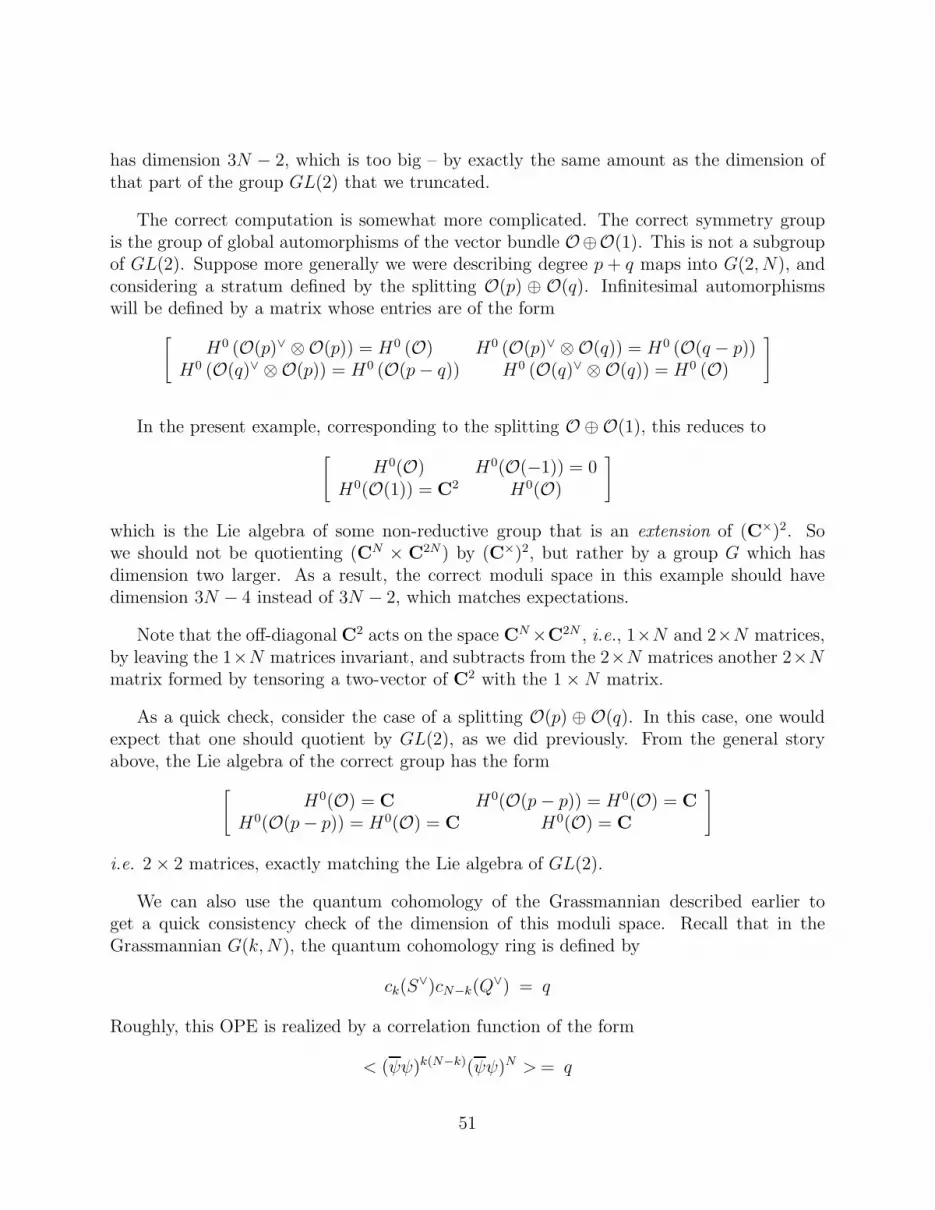
has dimension 3N − 2, which is too big – by exactly the same amount as the dimension ofthat part of the group GL(2) that we truncated.

The correct computation is somewhat more complicated. The correct symmetry groupis the group of global automorphisms of the vector bundle O⊕O(1). This is not a subgroupof GL(2). Suppose more generally we were describing degree p + q maps into G(2, N), andconsidering a stratum defined by the splitting O(p) ⊕ O(q). Infinitesimal automorphismswill be defined by a matrix whose entries are of the form

[H0 (O(p)∨ ⊗O(p)) = H0 (O) H0 (O(p)∨ ⊗O(q)) = H0 (O(q − p))

H0 (O(q)∨ ⊗O(p)) = H0 (O(p− q)) H0 (O(q)∨ ⊗O(q)) = H0 (O)

]

In the present example, corresponding to the splitting O ⊕O(1), this reduces to

[H0(O) H0(O(−1)) = 0

H0(O(1)) = C2 H0(O)

]

which is the Lie algebra of some non-reductive group that is an extension of (C×)2. Sowe should not be quotienting (CN × C2N) by (C×)2, but rather by a group G which hasdimension two larger. As a result, the correct moduli space in this example should havedimension 3N − 4 instead of 3N − 2, which matches expectations.

Note that the off-diagonal C2 acts on the space CN ×C2N , i.e., 1×N and 2×N matrices,by leaving the 1×N matrices invariant, and subtracts from the 2×N matrices another 2×Nmatrix formed by tensoring a two-vector of C2 with the 1 ×N matrix.

As a quick check, consider the case of a splitting O(p) ⊕ O(q). In this case, one wouldexpect that one should quotient by GL(2), as we did previously. From the general storyabove, the Lie algebra of the correct group has the form

[H0(O) = C H0(O(p− p)) = H0(O) = C

H0(O(p− p)) = H0(O) = C H0(O) = C

]

i.e. 2 × 2 matrices, exactly matching the Lie algebra of GL(2).

We can also use the quantum cohomology of the Grassmannian described earlier toget a quick consistency check of the dimension of this moduli space. Recall that in theGrassmannian G(k,N), the quantum cohomology ring is defined by

ck(S∨)cN−k(Q

∨) = q

Roughly, this OPE is realized by a correlation function of the form

< (ψψ)k(N−k)(ψψ)N >= q

51

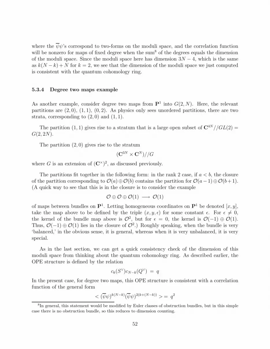
where the ψψ’s correspond to two-forms on the moduli space, and the correlation functionwill be nonzero for maps of fixed degree when the sum8 of the degrees equals the dimensionof the moduli space. Since the moduli space here has dimension 3N − 4, which is the sameas k(N − k) +N for k = 2, we see that the dimension of the moduli space we just computedis consistent with the quantum cohomology ring.

5.3.4 Degree two maps example

As another example, consider degree two maps from P1 into G(2, N). Here, the relevantpartitions are (2, 0), (1, 1), (0, 2). As physics only sees unordered partitions, there are twostrata, corresponding to (2, 0) and (1, 1).

The partition (1, 1) gives rise to a stratum that is a large open subset of C4N//GL(2) =G(2, 2N).

The partition (2, 0) gives rise to the stratum

(C3N ×CN)//G

where G is an extension of (C×)2, as discussed previously.

The partitions fit together in the following form: in the rank 2 case, if a < b, the closureof the partition corresponding to O(a)⊕O(b) contains the partition for O(a−1)⊕O(b+1).(A quick way to see that this is in the closure is to consider the example

O ⊕O ⊕O(1) −→ O(1)

of maps between bundles on P1. Letting homogeneous coordinates on P1 be denoted [x, y],take the map above to be defined by the triple (x, y, ǫ) for some constant ǫ. For ǫ 6= 0,the kernel of the bundle map above is O2, but for ǫ = 0, the kernel is O(−1) ⊕ O(1).Thus, O(−1) ⊕O(1) lies in the closure of O2.) Roughly speaking, when the bundle is very‘balanced,’ in the obvious sense, it is general, whereas when it is very unbalanced, it is veryspecial.

As in the last section, we can get a quick consistency check of the dimension of thismoduli space from thinking about the quantum cohomology ring. As described earlier, theOPE structure is defined by the relation

ck(S∨)cN−k(Q

∨) = q

In the present case, for degree two maps, this OPE structure is consistent with a correlationfunction of the general form

< (ψψ)k(N−k)(ψψ)2(k+(N−k)) >= q2

8In general, this statement would be modified by Euler classes of obstruction bundles, but in this simplecase there is no obstruction bundle, so this reduces to dimension counting.

52

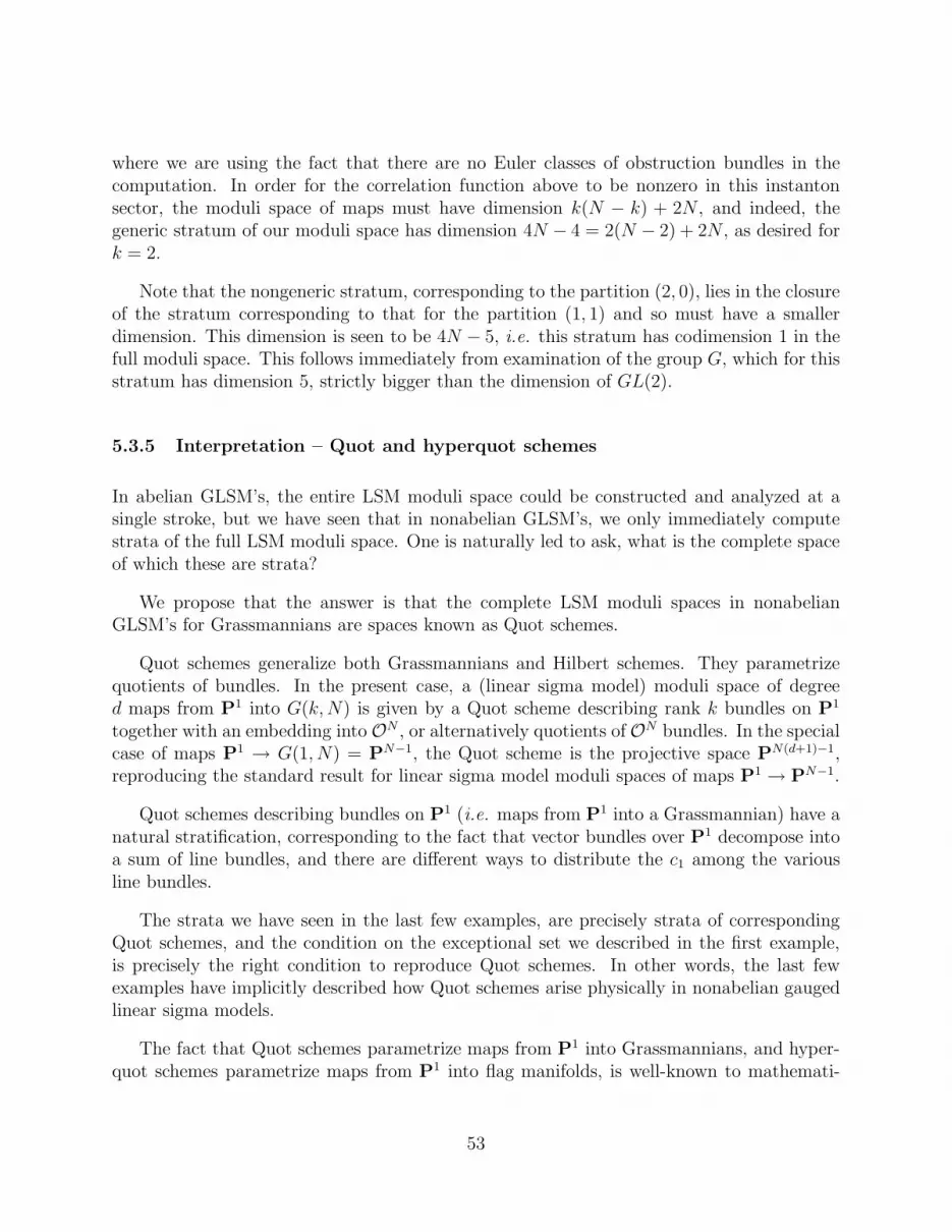
where we are using the fact that there are no Euler classes of obstruction bundles in thecomputation. In order for the correlation function above to be nonzero in this instantonsector, the moduli space of maps must have dimension k(N − k) + 2N , and indeed, thegeneric stratum of our moduli space has dimension 4N − 4 = 2(N − 2) + 2N , as desired fork = 2.

Note that the nongeneric stratum, corresponding to the partition (2, 0), lies in the closureof the stratum corresponding to that for the partition (1, 1) and so must have a smallerdimension. This dimension is seen to be 4N − 5, i.e. this stratum has codimension 1 in thefull moduli space. This follows immediately from examination of the group G, which for thisstratum has dimension 5, strictly bigger than the dimension of GL(2).

5.3.5 Interpretation – Quot and hyperquot schemes

In abelian GLSM’s, the entire LSM moduli space could be constructed and analyzed at asingle stroke, but we have seen that in nonabelian GLSM’s, we only immediately computestrata of the full LSM moduli space. One is naturally led to ask, what is the complete spaceof which these are strata?

We propose that the answer is that the complete LSM moduli spaces in nonabelianGLSM’s for Grassmannians are spaces known as Quot schemes.

Quot schemes generalize both Grassmannians and Hilbert schemes. They parametrizequotients of bundles. In the present case, a (linear sigma model) moduli space of degreed maps from P1 into G(k,N) is given by a Quot scheme describing rank k bundles on P1

together with an embedding into ON , or alternatively quotients of ON bundles. In the specialcase of maps P1 → G(1, N) = PN−1, the Quot scheme is the projective space PN(d+1)−1,reproducing the standard result for linear sigma model moduli spaces of maps P1 → PN−1.

Quot schemes describing bundles on P1 (i.e. maps from P1 into a Grassmannian) have anatural stratification, corresponding to the fact that vector bundles over P1 decompose intoa sum of line bundles, and there are different ways to distribute the c1 among the variousline bundles.

The strata we have seen in the last few examples, are precisely strata of correspondingQuot schemes, and the condition on the exceptional set we described in the first example,is precisely the right condition to reproduce Quot schemes. In other words, the last fewexamples have implicitly described how Quot schemes arise physically in nonabelian gaugedlinear sigma models.

The fact that Quot schemes parametrize maps from P1 into Grassmannians, and hyper-quot schemes parametrize maps from P1 into flag manifolds, is well-known to mathemati-

53

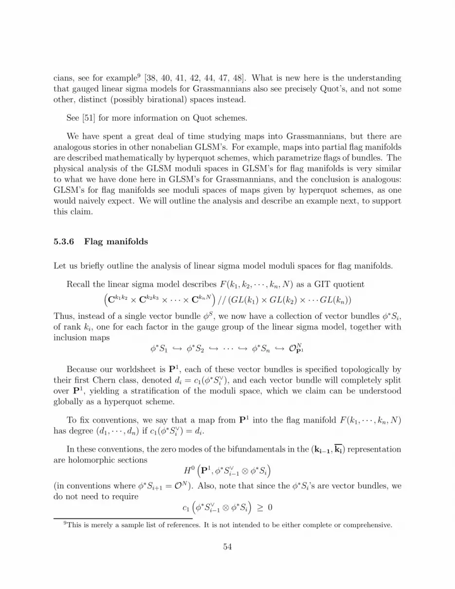
cians, see for example9 [38, 40, 41, 42, 44, 47, 48]. What is new here is the understandingthat gauged linear sigma models for Grassmannians also see precisely Quot’s, and not someother, distinct (possibly birational) spaces instead.

See [51] for more information on Quot schemes.

We have spent a great deal of time studying maps into Grassmannians, but there areanalogous stories in other nonabelian GLSM’s. For example, maps into partial flag manifoldsare described mathematically by hyperquot schemes, which parametrize flags of bundles. Thephysical analysis of the GLSM moduli spaces in GLSM’s for flag manifolds is very similarto what we have done here in GLSM’s for Grassmannians, and the conclusion is analogous:GLSM’s for flag manifolds see moduli spaces of maps given by hyperquot schemes, as onewould naively expect. We will outline the analysis and describe an example next, to supportthis claim.

5.3.6 Flag manifolds

Let us briefly outline the analysis of linear sigma model moduli spaces for flag manifolds.

Recall the linear sigma model describes F (k1, k2, · · · , kn, N) as a GIT quotient(Ck1k2 × Ck2k3 × · · · × CknN

)// (GL(k1) ×GL(k2) × · · ·GL(kn))

Thus, instead of a single vector bundle φS, we now have a collection of vector bundles φ∗Si,of rank ki, one for each factor in the gauge group of the linear sigma model, together withinclusion maps

φ∗S1 → φ∗S2 → · · · → φ∗Sn → ONP1

Because our worldsheet is P1, each of these vector bundles is specified topologically bytheir first Chern class, denoted di = c1(φ

∗S∨i ), and each vector bundle will completely split

over P1, yielding a stratification of the moduli space, which we claim can be understoodglobally as a hyperquot scheme.

To fix conventions, we say that a map from P1 into the flag manifold F (k1, · · · , kn, N)has degree (d1, · · · , dn) if c1(φ

∗S∨i ) = di.

In these conventions, the zero modes of the bifundamentals in the (ki−1,ki) representationare holomorphic sections

H0(P1, φ∗S∨

i−1 ⊗ φ∗Si

)

(in conventions where φ∗Si+1 = ON). Also, note that since the φ∗Si’s are vector bundles, wedo not need to require

c1(φ∗S∨

i−1 ⊗ φ∗Si

)≥ 0

9This is merely a sample list of references. It is not intended to be either complete or comprehensive.

54

for the moduli space to be nonempty.

5.3.7 Flag manifold example

Let us consider the example of maps of degree (2, 1) from P1 into F (1, 2, N). Such a mapis specified by two vector bundles over P1 φ∗S∨

1 , φ∗S∨2 of c1 equal to 2, 1, and ranks 1, 2,

respectively.

This information uniquely specifies φ∗S∨1 = O(2). Up to irrelevant ordering, this also

uniquely specifies that φ∗S∨2 = O(1) ⊕O.

The zero modes of the bifundamentals are given as follows. The bifundamentals in the(1, 2) representation of U(1) × U(2) have zero modes counted by

H0(P1,O(2 − 1) ⊕O(2 − 0)

)= H0

(P1,O(1) ⊕O(2)

)= C2 × C3 = C5

The remaining bifundamentals, in the (2,N) representation, have zero modes counted by

H0(P1, (O(1) ⊕O) ⊗ON

)= C2N ×CN = C3N

The linear sigma model moduli space will then be (C5 × C3N)//G for some G. In thepresent case, G will be a product of two factors, determined by the U(1) and U(2) factorsin the gauge group of the original linear sigma model. One of the factors in G will be allof GL(1), the automorphisms of O(2), which acts on the C5 in C5 × C3N with weight one.The other factor, determined by the U(2) of the linear sigma model gauge group, will be anon-reductive group defined as automorphisms of O(1) ⊕O(0), an extension of GL(1)2, asin section 5.3.3. This group, call it G′, acts on both the C5 and the C3N factors. So, thelinear sigma model moduli space has the form

(C5 × C3N

)// (GL(1) ×G′)

Moreover, this space is exactly the pertinent hyperquot scheme, giving us empirical confirma-tion of the claim that linear sigma model moduli spaces for maps from P1 into Grassmanniansand flag manifolds should be precisely Quot schemes and hyperquot schemes, respectively.

6 Conclusions

In this paper, we have described gauged linear sigma models for flag manifolds and theirproperties. In particular, we have accomplished three things. First, we have described the

55

gauged linear sigma models that describe partial flag manifolds, and outlined aspects relevantto (0,2) GLSM’s, which does not seem to have been in the literature previously.

Second, we have described properties of gauged linear sigma models for complete inter-sections in flag manifolds. After reviewing the Calabi-Yau conditions for a flag manifold, wehave discussed various examples of phenomena in which different geometric Kahler phases ofa given GLSM are not related by birational transformation. We have discussed both Calabi-Yau and non-Calabi-Yau examples of this phenomenon, and also proposed a mathematicalunderstanding that should be the right notion to replace ‘birational’ in this context, namely,Kuznetsov’s homological projective duality. Although nearly every example discussed in thispaper was a nonabelian GLSM, we also outline how similar phenomena happen in abelianGLSM’s, which will be studied in greater detail (together with Kuznetsov’s homologicalprojective duality) in [9].

Finally, we have outlined how quantum cohomology of flag manifolds arises within gaugedlinear sigma models. In particular, we describe linear sigma model moduli spaces of mapsinto Grassmannians and flag manifolds. The mathematically natural notion is that thosespaces are Quot and hyperquot schemes, and we describe how to see them explicitly in thephysics of nonabelian GLSM’s.

7 Acknowledgements

We would like to thank A. Bertram, T. Braden, A. Caldararu, L. Chen, I. Ciocan-Fontanine,J. Distler, M. Gross, S. Hellerman, S. Katz, and especially A. Knutson, A. Kuznetsov, andT. Pantev for useful conversations. This paper began as a project with A. Knutson, andlater grew in part out of the related work [9], done in collaboration with A. Caldararu,J. Distler, S. Hellerman, and T. Pantev. The work of R. Donagi was partially supported byNSF grants DMS-0612992 and Focused Research Grant DMS-0139799 for “The geometry ofsuperstrings.”

References

[1] E. Witten, “Phases of N=2 theories in two dimensions,” Nucl Phys. B403 (1993)159-222, hep-th/9301042.

[2] T. Pantev, E. Sharpe, “GLSM’s for gerbes (and other toric stacks),” Adv. Theor.Math. Phys. 10 (2006) 77-121, hep-th/0502053.

[3] E. Witten, “The Verlinde algebra and the cohomology of the Grassmannian,”hep-th/9312104.

56

[4] K. Hori, D. Tong, “Aspects of non-Abelian gauge dynamics in two-dimensional N =(2, 2) theories,” hep-th/0609032.

[5] S. Hellerman, A. Henriques, T. Pantev, E. Sharpe, M. Ando, “Cluster decomposition,T-duality, and gerby CFT’s,” hep-th/0606034.

[6] A. Kuznetsov, “Homological projective duality,” math.AG/0507292.

[7] A. Kuznetsov, “Derived categories of quadric fibrations and intersections of quadrics,”math.AG/0510670.

[8] A. Kuznetsov, “Homological projective duality for Grassmannians of lines,”math.AG/0610957.

[9] A. Caldararu, J. Distler, S. Hellerman, T. Pantev, and E. Sharpe, “Non-birationaltwisted derived equivalences in abelian GLSM’s,” to appear.

[10] Y. Manin, Gauge field theory and complex geometry, Springer-Verlag, 1988.

[11] T. Hubsch, Calabi-Yau manifolds: a bestiary for physicists, World Scientific, 1992.

[12] T. Pantev, E. Sharpe, “Notes on gauging noneffective group actions,” hep-th/0502027.

[13] T. Pantev, E. Sharpe, “String compactifications on Calabi-Yau stacks,” Nucl. Phys.B733 (2006) 233-296, hep-th/0502044.

[14] E. Sharpe, “Derived categories and stacks in physics,” hep-th/0608056.

[15] N. Seiberg, “Electric-magnetic duality in supersymmetric non-Abelian gauge theories,”hep-th/9411149.

[16] W. V. D. Hodge, D. Pedoe, Methods of Algebraic Geometry, volume 1, CambridgeUniversity Press, 1947.

[17] R. Bott, L. Tu, Differential forms in algebraic topology, Springer-Verlag, 1982.

[18] I. Klebanov, M. Strassler, “Supergravity and a confining gauge theory: duality cascadesand chiral-symmetry-breaking resolution of naked singularities,” hep-th/0007191.

[19] M. Strassler, “The duality cascade,” hep-th/0505153.

[20] A. Corti, M. Reid, “Weighted Grassmannians,” math.AG/0206011.

[21] J. Distler, “Notes on (0,2) superconformal field theories,” hep-th/9502012.

[22] V. Batyrev, I. Ciocan-Fontanine, B. Kim, D. van Straten, “Mirror symmetry and toricdegenerations of partial flag manifolds,” math.AG/9803108.

57

[23] V. Batyrev, I. Ciocan-Fontanine, B. Kim, D. van Straten, “Conifold transitions andmirror symmetry for Calabi-Yau complete intersections in Grassmannians,” Nucl.Phys. B514 (1998) 640-666, alg-geom/9710022.

[24] L. Borisov, A. Caldararu, “The Pfaffian-Grassmannian derived equivalence,”math.AG/0608404.

[25] J. Harris, L. Tu, “On symmetric and skew-symmetric determinantal varieties,” Topol-ogy 23 (1984) 71-84.

[26] A. Caldararu, “Derived categories of twisted sheaves on elliptic threefolds,”math.AG/0012083.

[27] A. Caldararu, private communication.

[28] T. Pantev, private communication.

[29] D. Orlov, “Derived categories of coherent sheaves and triangulated categories of sin-gularities,” math.AG/0503632.

[30] E. Sharpe, “D-branes, derived categories, and Grothendieck groups,” Nucl. Phys. B561(1999) 433-450, hep-th/9902116.

[31] M. Douglas, “D-branes, categories, and N = 1 supersymmetry,” J. Math. Phys. 42(2001) 004, hep-th/0104147.

[32] A. Beauville, R. Donagi, “La variete des droits d’une hypersurface cubique de dimen-sion 4,” C.R. Acad. Sci. Paris. Ser. I Math. 1985.

[33] A. Kuznetsov, private communication, March 10, 2007.

[34] A. Kuznetsov, private communication, April 3, 2007.

[35] M. Gross, private communication, September 27, 2006.

[36] P. Griffiths and J. Harris, Principles of Algebraic Geometry, John Wiley & Sons, NewYork, 1978.

[37] S. Mukai, “Moduli of vector bundles on K3 surfaces, and symplectic manifolds,” SugakuExpositions 1 (1988) 139-174.

[38] A. Bertram, G. Daskalopoulos, and R. Wentworth, “Gromov invariants for holomorphicmaps from Riemann surfaces to Grassmannians,” J. Amer. Math. Soc. 9 (1996) 529-571.

[39] A. Ashtashkevich, V. Sadov, “Quantum cohomology of partial flag manifolds Fn1···nk,”

Comm. Math. Phys. 170 (1995) 503-528.

58

[40] I. Ciocan-Fontanine, “On quantum cohomology rings of partial flag varieties,” DukeMath. J. 98 (1999) 485-524.

[41] I. Ciocan-Fontanine, “The quantum cohomology ring of flag varieties,” Trans. Amer.Math. Soc. 351 (1999) 2695-2729.

[42] I. Ciocan-Fontanine, “Quantum cohomology of flag varieties,” Int. Math. Res. Notices1995, no. 6, 263-277.

[43] B. Kim, “Quantum cohomology of partial flag manifolds and a residue formula fortheir intersection pairings,” Int. Math. Res. Notices 1995, no. 1, 1-16.

[44] B. Kim, “Quot schemes for flags and Gromov invariants for flag varieties,”alg-geom/9512003.

[45] A. Bertram, I. Ciocan-Fontanine, B. Kim, “Two proofs of a conjecture of Hori andVafa,” Duke Math. J. 126 (2005) 101-136, math.AG/0304403.

[46] A. Bertram, I. Ciocan-Fontanine, B. Kim, “Gromov-Witten invariants for abelian andnonabelian quotients,” math.AG/0407254.

[47] L. Chen, “Poincare polynomials of hyperquot schemes,” math.AG/0003077.

[48] S. A. Stromme, “On parametrized rational curves in Grassmann varieties,” pp. 251-272 in Space Curves, Lect. notes in math. 1266, ed. F. Ghione, C. Peskine, E. Sernesi,Springer-Verlag, 1987.

[49] B. Lian, C.-H. Liu, K. Liu, S.-T. Yau, “The S1 fixed points in Quot schemes and mirrorprinciple computations,” math/0111256.

[50] D. Morrison, R. Plesser, “Summing the instantons: quantum cohomology and mirrorsymmetry in toric varieties,” Nucl. Phys. B440 (1995) 279-354, hep-th/9412236.

[51] D. Huybrechts, M. Lehn, The geometry of moduli spaces of sheaves, Vieweg, 1997.

59