Abstract--The competitive market environment for the power

industry has resulted in new optimization problems that need to be solved such as bidding, pricing, risk management, and market clearing. These problems are complicated by the fact that power systems are nonlinear and some aspects of the problem are ill-formulated. In this paper, we report our formulation of a market clearing optimization problem that maximized the social welfare. The market 0ptimization is solved for cases where the market participants have private information about their generation costs. The proposed formulation incorporates the nonlinear nature of the MW power flows on the transmission grid. The IEEE 30-bus system is modified and used for testing of the proposed techniques.

Index Terms -- Power system economics, market optimization problem, sequential quadratic programming, market gaming.

I. INTRODUCTION raditional optimization problems in power systems deal with minimization of costs, system losses, violation of

operating constraints, etc. Well known optimization tools include Optimal Power Flow, Economic Dispatch and Unit Commitment [8]. These problems are, by nature, large-scale and non-linear with both continuous and discrete variables. However, various approximations allow linear programming and quadratic programming to play a significant role in their solution [1], [2].

In a competitive environment, market participants optimize their strategies for profits. On the other hand, from a societal point of view, optimization problems can be solved to increase the social welfare. Due to the new market structures, the nature of optimization problems is also changing. The participants bidding process in the energy market, handling of the ancillary services, information availability, and the market clearing process require new formulations and computational techniques. In the literature, some techniques that deal with

This work is partially supported by National Science Foundation Grant

No. ECS0217701 on transmission system economies. Y. Shen is with the Department of Industrial Engineering, University of

Washington Seattle, WA 98195 USA (e-mail: shyf@u.washington.edu) J. Lawarrée is with the Department of Economics, University of

Washington, Seattle, WA 98195 USA (e-mail: lawarree@u.washington.edu) C. C. Liu is with the Department of Electrical Engineering, University of

Washington, Seattle, WA 98195 USA (e-mail: liu@engr.washington.edu) Z. B. Zabinsky is with the Department of Industrial Engineering,

University of Washington Seattle, WA 98195 USA (e-mail: zelda@u.washington.edu)

much simplified versions of the market and supplier problems have been proposed, e.g., [3], [4]. The concept of efficient frontier requires the computation of the Pareto optimal trajectory on the space of expected profit vs. standard deviation [5]. To take into account the random nature of the state of the spot market, a Markov Decision optimization method was developed to optimize the profit for a supplier [6]. For the bilateral market, a necessary and sufficient condition was derived for the Nash Equilibrium, which leads to an optimization algorithm [7].

In this paper, our focus is on the formulation of a new market optimization problem (MOP) based on the power flow model. The objective of MOP is to maximize the social welfare, which is defined by the sum of the consumers' and producers' surplus. There are transmission system constraints based on the power flow model. Generators also have their capacity availability constraints and ramping constraints that limits the rate of power that can be increased. In order to gain insights into the non-linear and global nature of the problem, the nonlinear MW power flow model is used. It is well known that global optimization problems do not fall within a well-defined optimization method such as linear programming or quadratic programming. However, it is shown in this paper that the new MOP can be readily solved by sequential quadratic programming (SQP).

Furthermore, by using insights from the mechanism design literature in economics [9], we investigate how our optimization technique performs when a generator has private information about his cost function. Such generator may lie about its true cost and prevent the market designer from reaching the optimal solution. We explain how the optimization problem has to be modified.

II. MARKET OPTIMIZATION MODEL OF A 30-BUS POWER FLOW SYSTEM

In the 30-bus power flow system, five generators will generate power levels P1, P2, P3, P4 and P5 that feed into several lines, as depicted in Figure 1. The loads delivered to sixteen customers are L1, Ω, L16. Forty-one lines and thirty buses connect the generators with the customers. The angle differences of connected buses, such as (θ1 -θ2), (θ1 -θ3) and (θ2-θ5), reflect the power flow along each line. The reactance, e.g. x1_2, x1_3 and x2_5, are characteristics of the lines.

The optimization problem, stated below, is to find the optimal combination of the power generated, P1, …, P5, and

Global Optimization in an Electricity Market Environment

Yanfang Shen, Jacques Lawarrée, Chen-Ching Liu, Zelda B. Zabinsky

T

the load delivered, L1, Ω, L16, to maximize the social welfare (which simply reduces to utility minus cost when no price mechanism exists), while meeting constraints on the generation, load, line capacities and the balance equation of each bus. The mathematical model is stated below. Objective:

16,,1for U

5,,1for where

max

2

2

5

1

16

1

=+−=

=++=

−∑∑==

iLL

jPPC

CU

iiiiL

jjjjjP

jP

iL

i

j

ji

νυ

γβα

Constraints:

bounds on generators and loads ( )( )bounds 16,,1for 0

bounds 5,,1for

ii

jjjj

LiL

PjPPP

=≥

=≤≤

capacities of transmission lines ( )

( ) , , buses connected allfor

sin

_

kbkb

CAPx

CAP bkkb

kbbk

<

≤−

≤−θθ

balance equations for each bus

( ) 30,,1for 0sin)()(

bus toconnected

is bus : _=−+=

−∑ bLPx blbg

b

kk kb

kb θθ

where jα , jβ and jγ are the parameters of the generator j’s cost function, iυ , iν are the parameters of the load i ’s utility function, jP and jP represent the upper

and lower bounds of the jth generator, bkCAP is the capacity of the transmission

line that connects bus b and bus k, and kbx _ is the reactance of the line. The

values of those parameters, capacities and the reactance of each transmission line are given in tables A1, A2 and A3 in Appendix. In the balance equation constraints, ( )bg is the generator number connected to bus b and ( )bl is the load number connected to the bus. Note that if there is no any generator and load connected to the bus, the right-hand side of the balance equation equals zero.

Observe that in Table A1 of Appendix, one of the cost parameters β1 has two values, 1000 and 1100. We will later consider how the solution changes with different values of β1. We will also investigate the case where β1 is private information of the generator.

III. SOLVE THE MODEL A difficult step in the 30-bus MOP is to solve for θ1, θ2,

…, θ30 embedded within the optimization algorithm. Instead

of dealing with P1, …, P5 and L1, …, L16 as decision variables, our approach is to chose angles as decision variables. In the 30-bus problem, there are 21 decision variables. But since the angle differences determine the power flow, we can choose 20 angles as decision variables and put one of the remaining angles to zero. In our code, we set θ29=0±, and choose angles 1, 2, 3, 4, 5, 6, 7, 8, 9, 10, 11, 13, 14, 15, 17, 18, 20, 21, 23, 25 as the decision variables.

The 30-bus power system was solved using sequential quadratic programming (SQP) in Matlab. We considered two different values of β1: β1=1000 and β1=1100. For all

25, 23, 21, 20, 18, 17, 15, 14, 13, 11, 10, 9, 8, 7, 6, 5, 4, 3, 2, 1,∈b the search region was limited to -180±§θb§360±. When the initial starting point was θb=0±, the algorithm terminated at an optimal solution successfully. However, if the initial values are not chosen carefully the algorithm may not converge due to numerical error. It is also possible for the algorithm to

X5_7

L5 X9_10

q6

L1

X12_14

q1

L11

q10

q18

L9

X23_24

q16

X15_18

L8

X16_17

L13

q25

q24

X24_25

X25_27 q27 q28

q14

q12

q19

q26

q23 q15

q29 q30

q11

L6

L12

L14

L15 L16

q21

q4

q17 q8

q20

q22

q9

L3

L4 L7

L10

q5

q1

q3

q2

q7

L2

X1_2

X1_3

X3_4 X2_5

X2_4

X2_6

X4_6

X6_7

X6_ 8

X6_28

X9_11

X21_22

X10_ 21

X10_22

X10_17

X4_12

X12_13

X12_16

X14_15

X12_15

X15_23

X22_24

X6 10

X8_28

X27_28

X30_27

X27_29 X30_29

X18_19

X25_26

X6_9

X19_ 20

P4

P1

P3 P2

P5

X10_ 20

Fig. 1. 30-bus power flow system

TABLE 1 OPTIMAL SOLUTIONS OF 30-BUS MOP WITH DIFFERENT β1 VALUES

β1=1000 β1=1100

Values of Bus Angles

(Degree)

q=59.4765, 59.4705, 46.7379, 48.8027, 59.7189, 49.3162, 49.7569, 48.6651, 56.5516, 45.5058, 103.2706, 43.9340, 51.9818, 42.7883, 41.8942, 32.7001, 41.6054, 41.7551, 41.6729, 41.6296, 40.3881, 40.2271, 37.9562, 32.6894, 12.0078, -13.8177, 12.8877, 45.5631, 0, -14.0902

q=60.3015, 60.2955, 47.8231, 49.7359, 60.5397, 50.1412, 50.5767, 49.4801, 57.1697, 46.1262, 103.8887, 44.6671, 52.7149, 43.4866, 42.5655, 33.3990, 42.2496, 42.3801, 42.2705, 42.2128, 40.9537, 40.7909, 38.5469, 33.1721, 12.1923, -14.0296, 13.0909 46.3306, 0, -14.3131

Quantity

Binding Constraints Quantity

Binding Constraints

Generator 1 P1=2.3918 P1=2.3544 Generator 2 P2=1 P2=1 Generator 3 P3=1.5 P3=1.5 Generator 4 P4=3.5 P4=3.5 Generator 5 P5=1 P5=1

Load 1 L1=2.2854 L1=2.1887 Load 2 L2=1.3975 L2=1.3988 Load 3 L3=0 L3=0 Load 4 L4=1.1527 L4=1.1703 Load 5 L5=0 L5=0 Load 6 L6=0 L6=0 Load 7 L7=1.7854 L7=1.7835 Load 8 L8=0 L8=0 Load 9 L9=0 L9=0

Load 10 L10=0.3345 L10=0.3414 Load 11 L11=0 L11=0 Load 12 L12=0 L12=0 Load 13 L13=0 L13=0 Load 14 L14=1.1464 L14=1.1628 Load 15 L15=0 L15=0 Load 16 L16=1.2898

( )

1sin

6_2

62 ≤−

xθθ

( )

5.3sin

11_9

119 −≥−

xθθ

12 ≤P , 5.13 ≤P , 15 ≤P

03 ≥L , 05 ≥L , 06 ≥L

08 ≥L , 09 ≥L , 011 ≥L

012 ≥L , 013 ≥L , 015 ≥L

L16=1.309

( )

1sin

6_2

62 ≤−

xθθ

( )

5.3sin

11_9

119 −≥−

xθθ

12 ≤P , 5.13 ≤P , 15 ≤P

03 ≥L , 05 ≥L , 06 ≥L

08 ≥L , 09 ≥L , 011 ≥L

012 ≥L , 013 ≥L , 015 ≥L

Obj. Value Social Welfare = 21539 Social Welfare = 21301

converge to other local solution. For example if the initial values of θb are equal and in the range ]223,153[ , the algorithm converges to a solution worse than the one obtained with the starting point θb=0±. This result implies that the 30-bus MOP is a global problem.

The optimal solution corresponding to the initial point θb=0± with binding constraints is given in Table 1. The solution is very intuitive. If generator 1’s cost parameter β1 is lower (1000 vs. 1100), generator 1 is asked to produce more and the social welfare is higher.

IV. ECONOMICS ANALYSIS We now ask whether such optimal solution can be

implemented with an economic mechanism, i.e., whether we can find a set of prices inducing the participants to choose the optimal values. Let jq and ir denote the prices of generator j and load i respectively, where 5,,1=j and 16,,1=i . It is straightforward to find such set of prices by solving the first order conditions of each participant evaluated at the optimal values. In other words, we simply plug the optimal of Pj and Li values in the following first order conditions:

16,,1for 2

5,,1for 2

=+−=

=+=

iLr

jPq

iiii

jjjj

νυ

βα

The solutions are shown in appendix tables A4 and A5 for β1=1000 and β1=1100 respectively. We refer to this allocation as the first best solution. There are two noteworthy features to observe. First, the overall budget of such mechanism is in surplus. Indeed, one can compute that the five generators will receive $14006 while the sixteen loads will pay $31268 when β1=1000, generating a surplus of $17262 (when β1=1100, the surplus decreases to $17083.9). The reason for the existence of the surplus emerges from a simple supply-demand analysis. The optimal solution must balance supply and demand. If there are no transmission constraints binding, this equilibrium would occur when the price for the generators equal the price for the loads implying a balanced budget. Binding transmission constraints can only reduce the amount of power allowed to flow on the system. Therefore, with a decreasing demand function and an increasing supply function, the constrained equilibrium will always occur at a level where the price for the loads will be higher than the price for the generators, inducing a surplus.

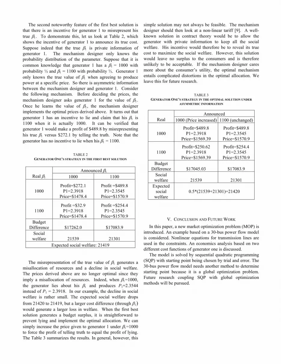
The second noteworthy feature of the first best solution is that there is an incentive for generator 1 to misrepresent his true β1. To demonstrate this, let us look at Table 2, which shows the incentive of generator 1 to announce its true cost. Suppose indeed that the true β1 is private information of generator 1. The mechanism designer only knows the probability distribution of the parameter. Suppose that it is common knowledge that generator 1 has a β1 = 1000 with probability ½ and β1 = 1100 with probability ½. Generator 1 only knows the true value of β1 when agreeing to produce power at a specific price. So there is asymmetric information between the mechanism designer and generator 1. Consider the following mechanism. Before deciding the prices, the mechanism designer asks generator 1 for the value of β1. Once he learns the value of β1, the mechanism designer implements the optimal prices derived above. It turns out that generator 1 has an incentive to lie and claim that his β1 is 1100 when it is actually 1000. It can be verified that generator 1 would make a profit of $489.8 by misrepresenting his true β1 versus $272.1 by telling the truth. Note that the generator has no incentive to lie when his β1 = 1100.

TABLE 2

GENERATOR ONE’S STRATEGY IN THE FIRST BEST SOLUTION

Announced β1 Real β1 1000 1100

1000

Profit=$272.1 P1=2.3918

Price=$1478.4

Profit =$489.8 P1=2.3545

Price=$1570.9

1100

Profit =$32.9 P1=2.3918

Price=$1478.4

Profit =$254.4 P1=2.3545

Price=$1570.9 Budget

Difference $17262.0 $17083.9 Social

welfare 21539 21301 Expected social welfare: 21419

The misrepresentation of the true value of β1 generates a

misallocation of resources and a decline in social welfare. The prices derived above are no longer optimal since they imply a misallocation of resources. Indeed, when β1=1000, the generator lies about his β1 and produces P1=2.3544 instead of P1 = 2.3918. In our example, the decline in social welfare is rather small. The expected social welfare drops from 21420 to 21419, but a larger cost difference (through β1) would generate a larger loss in welfare. When the first best solution generates a budget surplus, it is straightforward to prevent lying and implement the optimal allocation. We can simply increase the price given to generator 1 under β1=1000 to force the profit of telling truth to equal the profit of lying. The Table 3 summarizes the results. In general, however, this

simple solution may not always be feasible. The mechanism designer should then look at a non-linear tariff [9]. A well-known solution in contract theory would be to allow the generator with private information to keep all the social welfare. His incentive would therefore be to reveal its true cost to maximize the social welfare. However, this solution would leave no surplus to the consumers and is therefore unlikely to be acceptable. If the mechanism designer cares more about the consumer’s utility, the optimal mechanism entails complicated distortions in the optimal allocation. We leave this for future research.

TABLE 3 GENERATOR ONE’S STRATEGY IN THE OPTIMAL SOLUTION UNDER

ASYMMETRIC INFORMATION

Announced Real 1000 (Price increased) 1100 (unchanged)

1000

Profit=$489.8 P1=2.3918

Price=$1569.39

Profit=$489.8 P1=2.3545

Price=$1570.9

1100

Profit=$250.62 P1=2.3918

Price=$1569.39

Profit=$254.4 P1=2.3545

Price=$1570.9 Budget

Difference $17045.03 $17083.9 Social

welfare 21539 21301 Expected

social welfare

0.5*(21539+21301)=21420

V. CONCLUSION AND FUTURE WORK In this paper, a new market optimization problem (MOP) is

introduced. An example based on a 30-bus power flow model is considered. Nonlinear equations for transmission lines are used in the constraints. An economics analysis based on two different cost functions of generator one is discussed.

The model is solved by sequential quadratic programming (SQP) with starting point being chosen by trial and error. The 30-bus power flow model needs another method to determine starting point because it is a global optimization problem. Future research coupling SQP with global optimization methods will be pursued.

VI. APPENDIX

TABLE A1

PARAMETERS OF COST FUNCTIONS OF GENERATORS AND THE UPPER AND LOWER BOUNDS OF GENERATORS

Parameters of Cost

Function Generator

(P) Lower Bounds

( P )

Upper Bounds

( P ) α β γ

1

0

2.5 100

1000 or 1100

300

2 0 1 150 600 100 3 0 1.5 200 400 150 4 0 5 80 1500 350 5 0 1 180 500 150

TABLE A2 PARAMETERS OF UTILITY FUNCTIONS OF LOADS

Parameters of

Utility Function Parameters of

Utility Function Loads

(L) υ ν

Loads (L)

υ ν 1 160 3500 9 90 2500 2 200 4000 10 180 3600 3 150 3200 11 150 3400 4 220 4100 12 110 3350 5 120 3000 13 95 2800 6 100 2800 14 210 4050 7 250 4300 15 170 3550 8 130 3100 16 230 4200

TABLE A3 CAPACITIES AND REACTANCE OF TRANSMISSION LINES

Connected Buses Connected Buses Bus b Bus k

Capacity ( bkCAP )

Reactance ( kbx _ ) Bus b Bus k

Capacity ( bkCAP )

Reactance ( kbx _ )

1 2 3.5 0.0001 12 13 3.5 0.14 1 3 3.5 0.1652 12 14 3.5 0.2559 2 4 3.5 0.1737 12 15 3.5 0.1304 2 5 3.5 0.5 12 16 3.5 0.1987 2 6 1.0 0.1763 14 15 3.5 0.1997 3 4 3.5 0.0379 15 18 3.5 0.2185 4 6 0.84 0.0414 15 23 3.5 0.202 4 12 3.5 0.256 16 17 3.5 0.1923 5 7 3.5 0.116 18 19 3.5 0.1292 6 7 3.5 0.082 19 20 3.5 0.068 6 8 3.5 0.042 21 22 3.5 0.0236 6 9 3.5 0.208 22 24 3.5 0.179 6 10 3.5 0.556 23 24 3.5 0.27 6 28 3.5 0.0599 24 25 3.5 0.3292 8 28 3.5 0.2 25 26 3.5 0.38 9 10 3.5 0.11 25 27 3.5 0.2087 9 11 3.5 0.208 27 28 3.5 0.396

10 17 3.5 0.0845 27 29 3.5 0.4153 10 20 3.5 0.209 27 30 3.5 0.6027 10 21 3.5 0.749 29 30 3.5 0.4533 10 22 3.5 0.1499

Note: bkkb xx __ =

TABLE A4 FIRST BEST SOLUTION WHEN β1=1000

Quantity Price Profit Budget Total

Budget Budget

Difference Real

10001 =β Real

11001 =β

Generator 1

P1=2.3918

=1q 1478.4

272.1 32.9

3536.0

Generator 2 P2=1 =2q 900 50 900

Generator 3 P3=1.5 =3q 1000 300 1500

Generator 4 P4=3.5 =4q 2060 630 7210

Generator 5 P5=1 =5q 860 30 860

Generators: 14006.0

Load 1 L1=2.2854 =1r 2768.7 835.6 6327.6

Load 2 L2=1.3975 =2r 3441 390.6 4808.8

Load 3 L3=0 =3r 3200 0 0

Load 4 L4=1.1527 =4r 3592.8 292.3 4141.4

Load 5 L5=0 =5r 3000 0 0

Load 6 L6=0 =6r 2800 0 0

Load 7 L7=1.7854 =7r 3407.3 796.9 6083.4

Load 8 L8=0 =8r 3100 0 0

Load 9 L9=0 =9r 2500 0 0

Load 10 L10=0.3345 =10r 3479.6 20.1 1163.9

Load 11 L11=0 =11r 3400 0 0

Load 12 L12=0 =12r 3350 0 0

Load 13 L13=0 =13r 2800 0 0

Load 14 L14=1.1464 =14r 3568.5 276.0 4090.9

Load 15 L15=0 =15r 3550 0 0

Load 16 L16=1.2898 =16r 3606.7 382.6 4651.9

Loads: 31268.0

Loads –Generators =17262.0

Obj. Value Social Welfare = 21539

TABLE A5 FIRST BEST SOLUTION WHEN β1=1100

Quantity Price Profit Budget Total

Budget Budget

Difference Real

10001 =β Real

11001 =β

Generator 1

P1=2.3544

=1q 1570.9

489.8 254.4

3698.5

Generator 2 P2=1 =2q 900 50 900

Generator 3 P3=1.5 =3q 1000 300 1500

Generator 4 P4=3.5 =4q 2060 630 7210

Generator 5 P5=1 =5q 860 30 860

Generators: 14168.5

Load 1 L1=2.1887 =1r 2799.6 766.5 6127.5

Load 2 L2=1.3988 =2r 3440.5 391.3 4812.6

Load 3 L3=0 =3r 3200 0 0

Load 4 L4=1.1703 =4r 3585.1 301.3 4195.6

Load 5 L5=0 =5r 3000 0 0

Load 6 L6=0 =6r 2800 0 0

Load 7 L7=1.7835 =7r 3408.3 795.1 6078.7

Load 8 L8=0 =8r 3100 0 0

Load 9 L9=0 =9r 2500 0 0

Load 10 L10=0.3414 =10r 3477.1 21.0 1187.1

Load 11 L11=0 =11r 3400 0 0

Load 12 L12=0 =12r 3350 0 0

Load 13 L13=0 =13r 2800 0 0

Load 14 L14=1.1628 =14r 3561.6 284.0 4141.4

Load 15 L15=0 =15r 3550 0 0

Load 16 L16=1.309 =16r 3597.8 394.2 4709.5

Loads: 31252.4

Loads -Generators

=17083.9

Obj. Value Social Welfare = 21301

VII. REFERENCES Periodicals:

[1] D. Sun, et al., “Optimal Power Flow by Newton Approach,” IEEE Trans. Power Apparatus and Systems, pp. 2864-2880, Oct. 1984.

[2] O. Alsac, et al., “Further Developments in LP-Based Optimal Power Flow,” IEEE Trans. Power Systems, pp. 697-711, Aug. 1990.

[3] H. Song, C. C. Liu, J. Lawarree and R. Dahlgren, “Optimal Electricity Supply Bidding by Markov Decision Process,” IEEE Trans. Power Systems, pp. 618-624, May 2000.

[4] H. Song, C. C. Liu and J. Lawarree, ‘Decision Making of an Electricity Supplier’s Bid in a Spot Market,’ Proc. IEEE PES Summer Meeting, July 1999.

[5] R. Bjorgan, C. C. Liu and J. Lawarree, “Financial Risk Management in a Competitive Electricity Market”, IEEE Trans. Power Systems, pp. 1285-1291, Nov. 1999.

[6] H. Song, C. C. Liu, J. Lawarree and R. Dahlgren, “Optimal Electricity Supply Bidding by Markov Decision Process”, IEEE Trans. Power Systems, pp. 618-624. May 2000.

[7] H. Song, C. C. Liu, J. Lawarree, “Nash Equilibrium Bidding Strategies in a Bilateral Electricity Market”, IEEE Trans. Power Systems, pp. 73-79, Feb. 2002.

Books:

[8] A. Wood, and B. Wollenberg, Power Generation Operation and Control, 2nd Ed. John Wiley and Sons, 1996.

[9] J.-J. Laffont, and D. Martimort, The Theory of Incentives, Princeton University Press, 2002.

VIII. BIOGRAPHIES

Chen-Ching Liu (F'94) received the Ph.D. degree from the University of California, Berkeley. Currently, he is Professor of Electrical Engineering and Associate Dean of Engineering at the University of Washington, Seattle. He serves as Secretary of the Technical Committee on Power System Analysis, Computing and Economics. Dr. Liu is a Fellow of the IEEE.

Jacques Lawarrée received the Ph.D. degree from the University of California, Berkeley. Currently, he is Associate Professor of Economics at the University of Washington, Seattle. He specializes in game theory, contract theory, and industrial organization. Dr. Lawarre is a Member of the European Center for Advanced Research in Economics and Statistics, Brussels, Belgium.

Zelda B. Zabinsky received the Ph.D. degree from the University of Michigan. She is a Professor in Industrial Engineering at the University of Washington, Seattle. Her primary research is analysis and algorithms for global optimization, with applications to engineering design. She also uses operations research in air traffic management and supply chain management research. She is a member of INFORMS, Math Programming Society, and IIE.

Yanfang Shen received the M.S. degree from Tsinghua University, Beijing, China. Currently she is a Ph.D. candidate in Industrial Engineering at the University of Washington, Seattle. She is a member of INFORMS.