Generic thin-shell gravastars

arX

iv:1

112.

5253

v1 [

gr-q

c] 2

2 D

ec 2

011

Generic thin-shell gravastars

Prado Martin-Moruno1, Nadiezhda Montelongo Garcia2,3,

Francisco S. N. Lobo3, and Matt Visser1

1 School of Mathematics, Statistics, and Operations Research,

Victoria University of Wellington, PO Box 600, Wellington 6140, New Zealand2 Departamento de Fısica, Centro de Investigacion y Estudios avanzados del

I.P.N., A.P. 14-700,07000 Mexico, DF, Mexico3 Centro de Astronomia e Astrofısica da Universidade de Lisboa, Campo Grande,

Edifıcio C8 1749-016 Lisboa, Portugal

E-mail: [email protected], [email protected],

[email protected], [email protected]

Abstract. We construct generic spherically symmetric thin-shell gravastars by

using the cut-and-paste procedure. We take considerable effort to make the analysis

as general and unified as practicable; investigating both the internal physics of the

transition layer and its interaction with “external forces” arising due to interactions

between the transition layer and the bulk spacetime. Furthermore, we discuss both

the dynamic and static situations. In particular, we consider “bounded excursion”

dynamical configurations, and probe the stability of static configurations. For

gravastars there is always a particularly compelling configuration in which the

surface energy density is zero, while surface tension is nonzero.

PACS: 04.20.Cv, 04.20.Gz, 04.70.Bw

22 December 2011; LATEX-ed 23 December 2011.

http://arxiv.org/abs/1112.5253v1

Generic thin-shell gravastars 2

Contents

1 Introduction 3

2 General formalism 4

2.1 Bulk Einstein equations . . . . . . . . . . . . . . . . . . . . . . . . . 5

2.2 Null energy condition . . . . . . . . . . . . . . . . . . . . . . . . . . . 5

2.3 Transition layer . . . . . . . . . . . . . . . . . . . . . . . . . . . . . . 5

2.4 Lanczos equations: Surface stress-energy . . . . . . . . . . . . . . . . 7

2.5 Static gravastars . . . . . . . . . . . . . . . . . . . . . . . . . . . . . 9

2.6 Surface stress estimates . . . . . . . . . . . . . . . . . . . . . . . . . . 11

2.7 Conservation identity . . . . . . . . . . . . . . . . . . . . . . . . . . . 12

2.8 Integrability of the surface energy density . . . . . . . . . . . . . . . . 15

2.9 Equation of motion . . . . . . . . . . . . . . . . . . . . . . . . . . . . 17

2.10 Linearized equation of motion . . . . . . . . . . . . . . . . . . . . . . 18

2.11 The master equations . . . . . . . . . . . . . . . . . . . . . . . . . . . 20

3 Specific gravastar models 21

3.1 Schwarzschild exterior, de Sitter interior . . . . . . . . . . . . . . . . 21

3.2 Bounded excursion gravastars . . . . . . . . . . . . . . . . . . . . . . 23

3.3 Close to critical: Non-extremal . . . . . . . . . . . . . . . . . . . . . 25

3.4 Close to critical: Extremal . . . . . . . . . . . . . . . . . . . . . . . . 28

3.5 Charged dilatonic exterior, de Sitter interior . . . . . . . . . . . . . . 31

4 Summary and Discussion 32


1. Introduction

Gravastars (gravitational-vacuum stars) are hypothetical objects mooted as

alternatives to standard Schwarzschild black holes [1, 2]. Typically the interior is

some simple nonsingular spacetime geometry such as de Sitter space, the exterior

is some close approximation to the Schwarzschild geometry, and there is some

complicated transition layer near the location where the event horizon would

otherwise have been expected to form. Thus, in the traditional gravastar picture,

the transition layer replaces both the de Sitter and the Schwarzschild horizons, and

consequently the gravastar model has no singularity at the origin and no event

horizon, as its surface is located at a radius slightly greater than the Schwarzschild

radius. In this model, the quantum vacuum undergoes a phase transition at or near

the location where the event horizon is expected to form. Considerable attention has

been devoted to these objects, and to closely related “dark stars”, “quasi black holes”,

“monsters”, “black stars”, and the like [3, 4, 5, 6]. Some models use a continuous

distribution of stress-energy, which on rather general grounds must be anisotropic

in the transition layer [7, 8]. Other models idealize the transition layer to being

a thin shell [9] and apply a version of the Sen–Lanczos–Israel junction condition

formalism [10]. In fact, the latter approaches have been extensively analysed in the

literature, and applied to a wide variety of scenarios [11, 12]. Several criteria related

to potential observability have been explored [13].

The key point of the present paper is to develop an extremely general and

robust framework that can quickly be adapted to wide classes of generic thin-

shell gravastars. We shall consider standard general relativity, with gravastars that

are spherically symmetric, with the transition layer confined to a thin shell. The

bulk spacetimes (interior and exterior) on either side of the transition layer will

be spherically symmetric and static but otherwise arbitrary. (So the formalism

is simultaneously capable of dealing with gravastars embedded in Schwarzschild,

Reissner–Nordstrom, Kottler, or de Sitter spacetimes, or even “stringy” black hole

spacetimes. Similarly the gravastar interior will be kept as general as possible for as

long as possible.) The thin shell (transition layer) will be permitted to move freely

in the bulk spacetimes, permitting a fully dynamic analysis. This will then allow

us to perform a general stability analysis, where gravastar stability is related to the

properties of the matter residing in the thin-shell transition layer.

Many of the purely technical aspects of the analysis are very similar in


spirit to that encountered in a companion paper analyzing thin-shell traversable

wormholes [14] — mathematically there are a few strategic sign flips — but physically

the current framework is significantly different. Consequently we shall very rapidly

find our analysis diverging from the traversable wormhole case. Further afield, we

expect that the mathematical formalism developed herein will also prove useful when

considering spacetime “voids” (manifolds with boundary) [15].

This paper is organized in the following manner: In Section 2 we outline in

great detail the general formalism of generic dynamic spherically symmetric thin

shells, and provide a novel approach to the linearized stability analysis around a

static solution. In Section 3, we provide specific examples and consider a stability

analysis by applying the generic linearized stability formalism outlined in section 2.

Finally, in Section 4, we shall draw some general conclusions.

2. General formalism

To set the stage, consider two distinct spacetime manifolds, an exterior M+, and

an interior M−, that are eventually to be joined together across some surface layer

Σ. Let the two bulk spacetimes have metrics given by g+µν(xµ+) and g

−µν(x

µ−), in terms

of independently defined coordinate systems xµ+ and xµ−. In particular, consider two

generic static spherically symmetric spacetimes given by the following line elements:

ds2 = −e2Φ±(r±)

[

1− b±(r±)

r±

]

dt2± +

[

1− b±(r±)

r±

]−1

dr2± + r2±dΩ2±. (1)

Let us define

R+ = minr : b−(r) = r and R− = minr : b+(r) = r. (2)

Note the (at first glance) counter-intuitive placement of the ± on the quantities R±:

The conventions are chosen so that R+ is the furthest outwards one can extend the

interior geometry before hitting a horizon, whereas R− is the furthest inwards one

can extend the exterior geometry before hitting a horizon.

Since the whole point of a gravastar model is to avoid horizon formation we

certainly desire R− < R+. In particular, if the thin-shell transition layer Σ is located

at r = a(τ), then to avoid horizon formation we demand

R− < a(τ) < R+. (3)

The key issue of central interest in this article is the dynamics of this surface layer.


2.1. Bulk Einstein equations

Using the Einstein field equation, Gµν = 8π Tµν (with c = G = 1), the (orthonormal)

stress-energy tensor components in the bulk are given by

ρ(r) =1

8πr2b′, (4)

pr(r) = − 1

8πr2[2Φ′(b− r) + b′] , (5)

pt(r) = − 1

16πr2[(−b+ 3rb′ − 2r)Φ′ + 2r(b− r)(Φ′)2 + 2r(b− r)Φ′′ + b′′r] , (6)

where the prime denotes a derivative with respect to the radial coordinate. Here ρ(r)

is the energy density, pr(r) is the radial pressure, and pt(r) is the lateral pressure

measured in the orthogonal direction to the radial direction. The ± subscripts were

(temporarily) dropped so as not to overload the notation.

2.2. Null energy condition

Consider the null energy condition (NEC): Tµν kµ kν ≥ 0, where Tµν is the stress-

energy tensor and kµ any null vector. Then along the radial direction, with

kµ = (1,±1, 0, 0) in the orthonormal frame where Tµν = diag[ρ(r), pr(r), pt(r), pt(r)],

we have the particularly simple condition

Tµν kµ kν = ρ(r) + pr(r) =

(r − b)Φ′

4πr2≥ 0. (7)

By hypothesis r > b(r) in both the interior and exterior regions of the gravastar, so

the radial NEC reduces to Φ′(r) > 0. The NEC in the transverse direction, ρ+pt ≥ 0,

does not have any direct simple interpretation in terms of the metric components.

In most gravastar models the NEC is taken to be satisfied, though the status of the

NEC as fundamental physics is quite dubious [16].

2.3. Transition layer

The interior and exterior manifolds are bounded by isometric hypersurfaces Σ+ and

Σ−, with induced metrics g+ij and g−ij . By assumption g+ij(ξ) = g−ij(ξ) = gij(ξ), with

natural hypersurface coordinates ξi = (τ, θ, φ). A single manifold M is obtained by

gluing together M+ and M− at their boundaries. So M = M+ ∪ M−, with the

natural identification of the boundaries Σ = Σ+ = Σ−. The intrinsic metric on Σ is

ds2Σ = −dτ 2 + a(τ)2 (dθ2 + sin2 θ dφ2). (8)


The position of the junction surface is given by xµ(τ, θ, φ) = (t(τ), a(τ), θ, φ), and

the respective 4-velocities (as measured in the static coordinate systems on the two

sides of the junction) are

Uµ± =

e−Φ±(a)

√

1− b±(a)a

+ a2

1− b±(a)a

, a, 0, 0

. (9)

The overdot denotes a derivative with respect to τ , the proper time of an observer

comoving with the junction surface. The Israel formalism requires that the normals

point from M− to M+ [10]. The unit normals to the junction surface are

nµ± =

(

e−Φ±(a)

1− b±(a)a

a,

√

1− b±(a)

a+ a2, 0, 0

)

. (10)

In view of the spherical symmetry these results can easily be deduced from the

contractions UµUµ = −1, Uµnµ = 0, and nµnµ = +1. The extrinsic curvature, or the

second fundamental form, is defined as Kij = nµ;νeµ(i)e

ν(j). Differentiating nµe

µ(i) = 0

with respect to ξj, we have

nµ∂2xµ

∂ξi ∂ξj= −nµ,ν

∂xµ

∂ξi∂xν

∂ξj, (11)

so that general the extrinsic curvature is given by

K±ij = −nµ

(

∂2xµ

∂ξi ∂ξj+ Γµ±αβ

∂xα

∂ξi∂xβ

∂ξj

)

. (12)

For a thin shell Kij is not continuous across Σ. For notational convenience, the

discontinuity in the second fundamental form is defined as κij = K+ij − K−

ij . The

non-trivial components of the extrinsic curvature can easily be computed to be

Kθ ±θ =

1

a

√

1− b±(a)

a+ a2 , (13)

Kτ ±τ =

a +b±(a)−b′

±(a)a

2a2√

1− b±(a)a

+ a2+ Φ′

±(a)

√

1− b±(a)

a+ a2

, (14)

where the prime now denotes a derivative with respect to the coordinate a.

• Note that Kθ ±θ is independent of the quantities Φ±. This is most easily verified

by noting that in terms of the normal distance ℓ to the shell Σ the extrinsic

curvature can be written as Kij =12∂ℓgij =

12nµ∂µgij =

12nr∂rgij, where the last


step relies on the fact that the bulk spacetimes are static. Then since gθθ = r2,

differentiating and setting r → a we have Kθθ = a nr. Thus

Kθ ±θ =

nr

a, (15)

which is a particularly simple formula in terms of the radial component of the

normal vector, and which easily lets us verify (13).

• For Kττ there is an argument (easily extendable to the present context) in

reference [17] (see especially pages 181–183) to the effect that

Kτ ±τ = g± = (magnitude of the physical 4-acceleration of the throat).(16)

This gives a clear physical interpretation toKτ ±τ and rapidly allows one to verify

(14).

• There is also an important differential relationship between these extrinsic

curvature components

d

dτ

a eΦ± Kθ ±θ

= eΦ± Kτ ±τ a. (17)

The most direct way to verify this is to simply differentiate, using (13) and

(14) above. Geometrically, the existence of these relations between the extrinsic

curvature components is ultimately due to the fact that the bulk spacetimes

have been chosen to be static. By noting that

d

da

(

1

2a2)

=

(

d

daa

)

a = a, (18)

we can also write this differential relation as

d

da

a eΦ± Kθ ±θ

= eΦ± Kτ ±τ . (19)

2.4. Lanczos equations: Surface stress-energy

The Lanczos equations follow from the Einstein equations applied to the hypersurface

joining the bulk spacetimes, and are given by

Sij = − 1

8π(κij − δij κ

kk) . (20)

Here Sij is the surface stress-energy tensor on Σ. In particular, because of spherical

symmetry considerable simplifications occur, namely κij = diag(

κττ , κθθ, κ

θθ

)

. The

surface stress-energy tensor may be written in terms of the surface energy density,


σ, and the surface pressure, P, as Sij = diag(−σ,P,P). The Lanczos equations then

reduce to

σ = −κθθ

4π; P =

κττ + κθθ8π

; σ + 2P =κττ4π

. (21)

From equations (13)–(14), we see that:

σ = − 1

4πa

[√

1− b+(a)

a+ a2 −

√

1− b−(a)

a+ a2

]

, (22)

P =1

8πa

1 + a2 + aa− b+(a)+ab′+(a)

2a√

1− b+(a)a

+ a2+

√

1− b+(a)

a+ a2 aΦ′

+(a)

−1 + a2 + aa− b−(a)+ab′−(a)

2a√

1− b−(a)a

+ a2−√

1− b−(a)

a+ a2 aΦ′

−(a)

, (23)

and finally

σ + 2P =[g]

4π=

1

4π

a+b+(a)−ab′+(a)

2a2√

1− b+(a)a

+ a2+

√

1− b+(a)

a+ a2 Φ′

+(a)

− a+b−(a)−ab′

−(a)

2a2√

1− b−(a)a

+ a2−√

1− b−(a)

a+ a2 Φ′

−(a)

. (24)

Note that σ + 2P has a particularly simple physical interpretation in terms of [g],

the discontinuity in 4-acceleration. (This is ultimately related to the fact that the

quantity σ + 2P for a thin shell has properties remarkably similar to those of the

quantity ρ + 3p for a bulk spacetime.) Furthermore the surface energy density σ

is independent of the quantities Φ±. The surface mass of the thin shell is given by

ms = 4πa2σ.

Independent of the state of motion of the thin shell, we have σ(a) > 0 whenever

b+(a) > b−(a), and σ(a) < 0 whenever b+(a) < b−(a). The situation where σ = 0

corresponds to b−(a) = b+(a), and is precisely the case where all the discontinuities

are concentrated in Kττ while Kθ

θ is continuous. This phenomenon, the vanishing of

σ at certain specific shell radii given by b−(a) = b+(a), is generic to gravastars but

(because of a few key sign flips) cannot occur for the thin-shell traversable wormholes

considered in [14, 17, 18]. This is perhaps the most obvious of many properties


differentiating gravastars from the thin-shell traversable wormhole case, although

wormhole geometries surrounded by thin shells, similar to the cases explored in this

work, have also been analyzed in the literature [19, 20].

2.5. Static gravastars

Assume, for the sake of discussion, a static solution at some a0 ∈ (R−, R+). Then

σ(a0) = − 1

4πa0

√

1− b+(a0)

a0−√

1− b−(a0)

a0

, (25)

P(a0) =1

8πa0

1− b+(a0)+a0b′+(a0)

2a0√

1− b+(a0)a0

+

√

1− b+(a0)

a0a0Φ

′+(a0)

−1− b−(a0)+a0b′−(a0)

2a0√

1− b−(a0)a0

−√

1− b−(a0)

a0a0Φ

′−(a0)

, (26)

and finally

σ(a0) + 2P(a0) =[g0]

4π=

1

4π

b+(a)−ab′+(a)

2a2√

1− b+(a)a

+

√

1− b+(a)

aΦ′

+(a)

−b−(a)−ab′

−(a)

2a2√

1− b−(a)a

−√

1− b−(a)

aΦ′

−(a)

.

(27)

(See also equation (32) of [21].) Now taking a0 → R−, we have

σ(R−) = +1

4πR−

√

1− b−(R−)

R−> 0. (28)

However taking a0 → R+ we have

σ(R+) = − 1

4πR+

√

1− b+(R+)

R+< 0. (29)

That is:

σ(R±) = ∓ 1

4πR±

√

1− b±(R±)

R±. (30)


Applying the mean value theorem, for gravastars there will always be some R0 ∈(R−, R+), possibly many such R0, such that σ(R0) = 0. (This phenomenon cannot

occur for the thin-shell traversable wormholes considered in [14, 17, 18], because of

key sign flips — for thin-shell traversable wormholes we always have σ < 0.) The R0

such that σ(R0) = 0 is clearly a special place for gravastars. Explicitly this occurs

when

b+(R0) = b−(R0), (31)

and in fact for

R− < b+(R0) = b−(R0) < R+. (32)

At this special point the discontinuities are concentrated in Kττ while Kθ

θ is

continuous. That is

P(R0) =1

16πR0

b′−(R0)− b′+(R0)√

1− b±(R0)R0

+ 2

√

1− b±(R0)

R0R0[Φ

′+(R0)− Φ′

−(R0)]

, (33)

so that

P(R0) =[Kτ

τ ]

8π=

[g0]

8π. (34)

Even though σ = 0, one needs P 6= 0 because of the non-zero 4-acceleration g0.

If one also demands that the surface pressure at R0 also be zero, P(R0) = 0,

one must impose the additional condition

b′+ − b′− = 2 (R0 − b±)(

Φ′+ − Φ′

−

)

, (35)

which is equivalent to(

e2Φ+ [1− b+/a0])′∣

∣

∣

R0

=(

e2Φ− [1− b−/a0])′∣

∣

∣

R0

. (36)

If Φ±(R0) = 0, and Φ′±(R0), then not only does b+(R0) = b−(R0) but also

b′+(R0) = b′−(R0) — these two conditions give a zero pressure and zero density shell.

More specifically, in terms of standard nomenclature, if the surface stress-energy

terms are zero, the junction is denoted as a boundary surface; if surface stress terms

are present, the junction is called a thin shell.


2.6. Surface stress estimates

It is interesting to obtain some estimates of the surface stresses. For this purpose,

consider for simplicity an exterior geometry that is Schwarzschild-de Sitter spacetime,

so that

b+(r) = 2M +Λ

3r3 , Φ+(r) = 0 . (37)

An important quantity that will be play a fundamental role throughout this paper

is the surface mass of the thin shell, which is given by ms = 4πa2σ. For the exterior

Schwarzschild-de Sitter spacetime, and considering an arbitrary interior geometry,

the surface mass of the static thin shell is given by

ms(a0) = a0

√

1− b−(a0)

a0−√

1− 2M

a0− Λ

3a20

. (38)

Note that one may interpret M as the total mass of the system, as measured in an

asymptotic region of the spacetime. Solving for M , we have

M =b−(a0)

2+ms(a0)

√

1− b−(a0)

a0− ms(a0)

2a0

− Λ

6a30 . (39)

For the Schwarzschild–de Sitter spacetime Λ > 0. For the range 0 < 9ΛM2 < 1, the

factor g−1rr = −gtt = (1− 2M/r−Λr2/3) possesses two positive real roots, rb and rc,

corresponding to the black hole and the cosmological event horizons:

rb = 2Λ−1/2 cos(α/3) , (40)

rc = 2Λ−1/2 cos(α/3 + 4π/3) . (41)

Here cosα ≡ −3MΛ1/2, with π < α < 3π/2. In this domain we have 2M < rb < 3M

and rc > 3M [20].

Defining suitable dimensionless parameters, equations (25)–(26) take, for the

Schwarzschild-de Sitter solution, the form

µ(a0) = x

(

√

1− x b(x)−√

1− x− 4β

27x2

)

, (42)

Π(a0) = x

1− x2− 8β

27x2√

1− x− 4β27x2

− 1− 12

[

xb(x) + b′−]

√

1− xb(x)− ζ−

√

1− xb(x)

. (43)


Here we define: x = 2M/a, β = 9ΛM2, b(x) = b(a)/(2M), µ = 8πMσ, and set

Π = 16πMP. In the analysis that follows we shall assume that M is positive,

M > 0.

As a specific application, consider the standard gravastar picture, which consists

of a Schwarzschild exterior geometry and an interior de Sitter spacetime. Thus the

surface stresses, equations (42)–(43), are obtained by setting Λ = 0, (i.e., β = 0),

while b−(a0) = a30/R2 and Φ−(a0) = 0. Here we have defined R2 = 3/Λ−, for

simplicity. For this case the total mass of the system M is given by

M =a202R2

+ms(a0)

(√

1− a20R2

− ms

2a0

)

. (44)

Using the dimensionless parameters, x = 2M/a0 and y = 2M/R, while µ(a0) =

8πMσ(a0) and Π(a0) = 16πMP(a0), equations (42)–(43), take the form

µ(a0) = −x(

√1− x−

√

1− y2

x2

)

, (45)

Π(a0) = x

1− x2√

1− x− 1− 2 y

2

x2√

1− y2

x2

. (46)

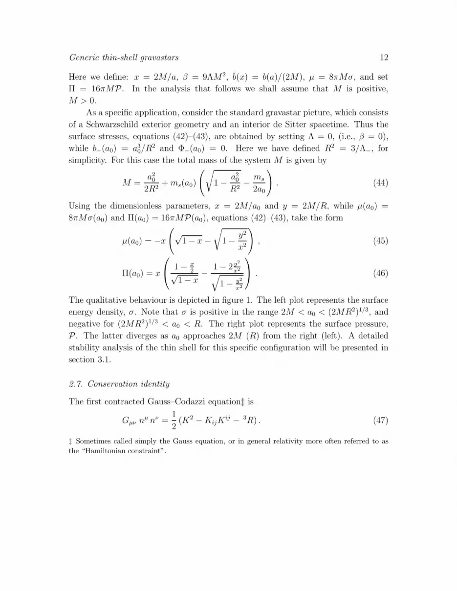
The qualitative behaviour is depicted in figure 1. The left plot represents the surface

energy density, σ. Note that σ is positive in the range 2M < a0 < (2MR2)1/3, and

negative for (2MR2)1/3 < a0 < R. The right plot represents the surface pressure,

P. The latter diverges as a0 approaches 2M (R) from the right (left). A detailed

stability analysis of the thin shell for this specific configuration will be presented in

section 3.1.

2.7. Conservation identity

The first contracted Gauss–Codazzi equation‡ is

Gµν nµ nν =

1

2(K2 −KijK

ij − 3R) . (47)

‡ Sometimes called simply the Gauss equation, or in general relativity more often referred to as

the “Hamiltonian constraint”.


Figure 1. Schwarzschild–de Sitter gravastar: These plots depict the qualitative

behaviour of the surface stresses of a gravastar with interior de Sitter and exterior

Schwarzschild spacetimes. We have considered the dimensionless parameters,

x = 2M/a0 and y = 2M/R, and µ(a0) = 8πMσ(a0) and Π(a0) = 16πMP(a0).

The left plot represents the surface energy density, σ. Note that σ is positive in

the range 2M < a0 < (2MR2)1/3, and negative in the range (2MR2)1/3 < a0 < R.

The right plot represents the surface pressure, P . The latter surface pressure

diverges as a0 approaches 2M (R) from the right (left). See the text for more

details.

The second contracted Gauss–Codazzi equation§ is

Gµνeµ(i)n

ν = Kji|j −K,i . (48)

Together with the Lanczos equations this provides the conservation identity

Sij|i =[

Tµν eµ(j)n

ν]+

−, (49)

where the convention [X ]+− ≡ X+|Σ − X−|Σ is used. When interpreting this

conservation identity, consider first the momentum flux defined by

[

Tµν eµ(τ) n

ν]+

−= [Tµν U

µ nν ]+− =

(Ttt + Trr)a√

1− b(a)a

+ a2

1− b(a)a

+

−

, (50)

where Ttt and Trr are the bulk stress-energy tensor components given in an

orthonormal basis. This flux term corresponds to the net discontinuity in the (bulk)

§ Sometimes called simply the Codazzi or the Codazzi–Mainardi equation, or in general relativity

more often referred to as the “ADM constraint” or “momentum constraint”.


momentum flux Fµ = Tµν Uν which impinges on the shell. Applying the (bulk)

Einstein equations we see

[

Tµν eµ(τ) n

ν]+

−=

a

4πa

[

Φ′+(a)

√

1− b+(a)

a+ a2 − Φ′

−(a)

√

1− b−(a)

a+ a2

]

. (51)

It is useful to define the quantity

Ξ =1

4πa

[

Φ′+(a)

√

1− b+(a)

a+ a2 − Φ′

−(a)

√

1− b−(a)

a+ a2

]

, (52)

and to let A = 4πa2 be the surface area of the thin shell. Then in the general case,

the conservation identity provides the following relationship

dσ

dτ+ (σ + P)

1

A

dA

dτ= Ξ a , (53)

or equivalently

d(σA)

dτ+ P dA

dτ= ΞA a . (54)

The first term represents the variation of the internal energy of the shell, the second

term is the work done by the shell’s internal force, and the third term represents the

work done by the external forces. Once could also brute force verify this equation

by explicitly differentiating (22) using (23) and the relations (17). If we assume that

the equations of motion can be integrated to determine the surface energy density

as a function of radius a, that is, assuming the existence of a suitable function σ(a),

then the conservation equation can be written as

σ′ = −2

a(σ + P) + Ξ , (55)

where σ′ = dσ/da. We shall carefully analyze the integrability conditions for σ(a)

in the next sub-section. For now, note that the flux term (external force term) Ξ is

automatically zero whenever Φ± = 0; this is actually a quite common occurrence, for

instance in either Schwarzschild or Reissner–Nordstrom geometries, or more generally

whenever ρ + pr = 0, so it is very easy for one to be mislead by those special

cases. In particular, in situations of vanishing flux Ξ = 0 one obtains the so-called

“transparency condition”, [Gµν Uµ nν ]+− = 0, see [22]. The conservation identity,

equation (49), then reduces to the simple relationship σ = −2 (σ + P)a/a. But in

general the “transparency condition” does not hold, and one needs the full version

of the conservation equation as given in equation (54).


2.8. Integrability of the surface energy density

When does it make sense to assert the existence of a function σ(a)? Let us start

with the situation in the absence of external forces (we will rapidly generalize this)

where the conservation equation,

σ = −2 (σ + P)a/a , (56)

can easily be rearranged to

σ

σ + P = −2a

a. (57)

Assuming a barotropic equation of state P(σ) for the matter in the gravastar

transition layer, this can be integrated to yield∫ σ

σ0

dσ

σ + P(σ)= −2

∫ a

a0

da

a= −2 ln(a/a0). (58)

This implies that a can be given as some function a(σ) of σ, and by the inverse

function theorem implies over suitable domains the existence of a function σ(a).

Now this barotropic equation of state is a rather strong assumption, albeit one that

is very often implicitly made when dealing with thin-shell gravastar (or thin-shell

wormholes, or other thin-shell objects). As a first generalization, consider what

happens if the surface pressure generalized is to be of the form P(a, σ), which is not

barotropic. Then the conservation equation can be rearranged to be

σ′ = −2[σ + P(a, σ)]

a. (59)

This is a first-order (albeit nonlinear and non-autonomous) ordinary differential

equation, which at least locally will have solutions σ(a). There is no particular

reason to be concerned about the question of global solutions to this ODE, since in

applications one is most typically dealing with linearization around a static solution.

If we now switch on external forces, one way of guaranteeing integrability

would be to demand that the external forces are of the form Ξ(a, σ), since then

the conservation equation would read

σ′ = −2[σ + P(a, σ)]

a+ Ξ(a, σ), (60)

which is again a first-order albeit nonlinear and non-autonomous ordinary differential

equation. But how general is this Ξ = Ξ(a, σ) assumption? There are at least two

nontrivial situations where this definitely holds:


• If Φ+(a) = Φ−(a) = Φ(a), then Ξ = −Φ′(a) σ, which is explicitly of the required

form.

• If b+(a) = b−(a) = b(a), but the Φ± are unequal, then σ ≡ 0 regardless of the

location and state of motion of the gravastar. Furthermore Ξ ≡ 2P/a. (This

would make for a somewhat unusual gravastar.)

• If both b+(a) = b−(a) = b(a) and Φ+(a) = Φ−(a) = Φ(a), then the situation is

vacuous. There is then no discontinuity in extrinsic curvatures and the thin shell

carries no stress-energy; so this in fact corresponds to a “continuum” gravastar

with b(r)/r < 1 for all r ∈ (0,∞).

But in general we will need a more complicated set of assumptions to assure

integrability, and the consequent existence of a function σ(a). A model that is always

sufficient (not necessary) to guarantee integrability is to view the exotic material on

the throat as a two-fluid system, characterized by σ± and P±, with two (possibly

independent) equations of state P±(σ±). Specifically, take

σ± = − 1

4π(K±)

θθ , (61)

P± =1

8π

(K±)ττ + (K±)

θθ

. (62)

In view of the differential identities

d

dτ

a eΦ± Kθ ±θ

= eΦ± Kτ ±τ a, (63)

each of these two fluids is independently subject to

d

dτ

eΦ± σ±

= −2eΦ±

aσ± + P± a, (64)

which is equivalent to

eΦ± σ±′

= −2eΦ±

aσ± + P±. (65)

With two equations of state P±(σ±) these are two nonlinear first-order ordinary

differential equations for σ±. These equations are integrable, implicitly defining

functions σ±(a), at least locally. Once this is done we define

σ(a) = σ+(a)− σ−(a), (66)

and

ms(a) = 4πσ(a) a2. (67)


While the argument is more complicated than one might have expected, the end

result is easy to interpret: We can simply choose σ(a), or equivalently ms(a), as an

arbitrarily specifiable function that encodes the (otherwise unknown) physics of the

specific form of matter residing on the gravastar transition layer.

2.9. Equation of motion

To qualitatively analyze the stability of the gravastar, assuming integrability of the

surface energy density, (that is, the existence of a function σ(a)), it is useful to

rearrange equation (22) into the form

1

2a2 + V (a) = 0 , (68)

where the potential V (a) is given by†

V (a) =1

2

1− b(a)

a−[

ms(a)

2a

]2

−[

∆(a)

ms(a)

]2

. (69)

Here ms(a) = 4πa2 σ(a) is the mass of the thin shell. The quantities b(a) and ∆(a)

are defined, for simplicity, as

b(a) =b+(a) + b−(a)

2, (70)

∆(a) =b+(a)− b−(a)

2, (71)

respectively. This gives the potential V (a) as a function of the surface mass ms(a).

By differentiating with respect to a, (using (18)), we see that the equation of motion

implies

a = −V ′(a). (72)

It is sometimes useful to reverse the logic flow and determine the surface mass as a

function of the potential. Following the techniques used in [9, 14], suitably modified

for the present context, a brief calculation yields

ms(a) = −a[√

1− b+(a)

a− 2V (a)−

√

1− b−(a)

a− 2V (a)

]

, (73)

† This equation only valid for σ 6≡ 0 due to a divide-by-zero problem. The σ ≡ 0 case is a special

one worth separate consideration:

V (a) =1

2

1− b(a)

a−(

8πPΦ′

+ − Φ′

−

)2

.


with the negative root now being necessary for compatibility with the Lanczos

equations. Note the logic here — assuming integrability of the surface energy density,

if we want a specific V (a) this tells us how much surface mass we need to put on

the transition layer (as a function of a), which is implicitly making demands on

the equation of state of the matter residing on the transition layer. In a completely

analogous manner, the assumption of integrability of σ(a) implies that after imposing

the equation of motion for the shell one has

σ(a) = − 1

4πa

[√

1− b+(a)

a− 2V (a)−

√

1− b−(a)

a− 2V (a)

]

, (74)

while

P =1

8πa

1− 2V (a)− aV ′(a)− b+(a)+ab′+(a)

2a√

1− b+(a)a

− 2V (a)+

√

1− b+(a)

a− 2V (a) aΦ′

+(a)

−1− 2V (a)− aV ′(a)− b−(a)+ab′−(a)

2a√

1− b−(a)a

− 2V (a)−√

1− b−(a)

a− 2V (a) aΦ′

−(a)

,

(75)

and

Ξ(a) =1

4πa

[

Φ′+(a)

√

1− b+(a)

a− 2V (a)− Φ′

−(a)

√

1− b−(a)

a− 2V (a)

]

. (76)

The three quantities σ(a),P(a),Ξ(a) (or equivalently ms(a),P(a),Ξ(a)) are

related by the differential conservation law, so at most two of them are functionally

independent.

2.10. Linearized equation of motion

Consider a linearization around an assumed static solution (at a0) to the equation

of motion 12a2 + V (a) = 0, and so also a solution of a = −V ′(a). Generally a Taylor

expansion of V (a) around a0 to second order yields

V (a) = V (a0) + V ′(a0)(a− a0) +1

2V ′′(a0)(a− a0)

2 +O[(a− a0)3] . (77)

But since we are expanding around a static solution a0 = a0 = 0, we automatically

have V (a0) = V ′(a0) = 0, so it is sufficient to consider

V (a) =1

2V ′′(a0)(a− a0)

2 +O[(a− a0)3] . (78)


The assumed static solution at a0 is stable if and only if V (a) has a local minimum

at a0, which requires V ′′(a0) > 0. This will be our primary criterion for gravastar

stability, though it will be useful to rephrase it in terms of more basic quantities.

For instance, it is extremely useful to express m′s(a) and m

′′s(a) by the following

expressions:

m′s(a) = +

ms(a)

a+a

2

(b+(a)/a)′ + 2V ′(a)

√

1− b+(a)/a− 2V (a)− (b−(a)/a)

′ + 2V ′(a)√

1− b−(a)/a− 2V (a)

, (79)

and

m′′s(a) =

(b+(a)/a)′ + 2V ′(a)

√

1− b+(a)/a− 2V (a)− (b−(a)/a)

′ + 2V ′(a)√

1− b−(a)/a− 2V (a)

+a

4

[(b+(a)/a)′ + 2V ′(a)]2

[1− b+(a)/a− 2V (a)]3/2− [(b−(a)/a)

′ + 2V ′(a)]2

[1− b−(a)/a− 2V (a)]3/2

+a

2

(b+(a)/a)′′ + 2V ′′(a)

√

1− b+(a)/a− 2V (a)− (b−(a)/a)

′′ + 2V ′′(a)√

1− b−(a)/a− 2V (a)

. (80)

Doing so allows us to easily study linearized stability, and to develop a simple

inequality on m′′s(a0) by using the constraint V ′′(a0) > 0. Similar formulae hold

for σ′(a), σ′′(a), for P ′(a), P ′′(a), and for Ξ′(a), Ξ′′(a). In view of the redundancies

coming from the relations ms(a) = 4πσ(a)a2 and the differential conservation law,

the only interesting quantities are Ξ′(a), Ξ′′(a).

It is similarly useful to consider

4π Ξ(a) a =

[

Φ′+(a)

√

1− b+(a)

a− 2V (a)− Φ′

−(a)

√

1− b−(a)

a− 2V (a)

]

. (81)

for which an easy computation yields:

[4π Ξ(a) a]′ = +

Φ′′+(a)

√

1− b+(a)/a− 2V (a)− Φ′′−(a)

√

1− b−(a)/a− 2V (a)

− 1

2

Φ′+(a)

(b+(a)/a)′ + 2V ′(a)

√

1− b+(a)/a − 2V (a)− Φ′

−(a)(b−(a)/a)

′ + 2V ′(a)√

1− b−(a)/a− 2V (a)

,

(82)

and

[4π Ξ(a) a]′′ =

Φ′′′+(a)

√

1− b+(a)/a− 2V (a)− Φ′′′−(a)

√

1− b−(a)/a − 2V (a)

−

Φ′′+(a)

(b+(a)/a)′ + 2V ′(a)

√

1− b+(a)/a− 2V (a)− Φ′′

−(a)(b−(a)/a)

′ + 2V ′(a)√

1− b−(a)/a− 2V (a)


− 1

4

Φ′+(a)

[(b+(a)/a)′ + 2V ′(a)]2

[1 − b+(a)/a− 2V (a)]3/2− Φ′

−(a)[(b−(a)/a)

′ + 2V ′(a)]2

[1 − b−(a)/a− 2V (a)]3/2

− 1

2

Φ′+(a)

(b+(a)/a)′′ + 2V ′′(a)

√

1− b+(a)/a − 2V (a)− Φ′

−(a)(b−(a)/a)

′′ + 2V ′′(a)√

1− b−(a)/a − 2V (a)

.

(83)

We shall now evaluate these quantities at the assumed stable solution a0.

2.11. The master equations

In view of the above, to have a stable static solution at a0 we must have:

ms(a0) = −a0

√

1− b+(a0)

a0−√

1− b−(a0)

a0

, (84)

while

m′s(a0) =

ms(a0)

2a0− 1

2

1− b′+(a0)√

1− b+(a0)/a0− 1− b′−(a0)√

1− b−(a0)/a0

. (85)

The inequality one derives for m′′s(a0) is now trickier since the relevant expression

contains two competing terms of opposite sign. Provided b+(a0) ≥ b−(a0), which is

equivalent to demanding σ(a0) ≥ 0, one derives

m′′s(a0) ≥ +

1

4a30

[b+(a0)− a0b′+(a0)]

2

[1− b+(a0)/a0]3/2− [b−(a0)− a0b

′−(a0)]

2

[1− b−(a0)/a0]3/2

+1

2

b′′+(a0)√

1− b+(a0)/a0− b′′−(a0)√

1− b−(a0)/a0

. (86)

However if b+(a0) ≤ b−(a0) the direction of the inequality is reversed. This last

formula in particular translates the stability condition V ′′(a0) ≥ 0 into a rather

explicit and not too complicated inequality on m′′s(a0), one that can in particular

cases be explicitly checked with a minimum of effort.

In the absence of external forces this inequality is the only stability constraint

one requires. However, once one has external forces (Ξ 6= 0 which requires Φ± 6= 0),

there is additional information:

[4π Ξ(a) a]′|a0 = +

Φ′′+(a)

√

1− b+(a)/a− Φ′′−(a)

√

1− b−(a)/a∣

∣

∣

a0

− 1

2

Φ′+(a)

(b+(a)/a)′

√

1− b+(a)/a− Φ′

−(a)(b−(a)/a)

′

√

1− b−(a)/a

∣

∣

∣

∣

∣

a0

. (87)


Provided Φ′+(a0)/

√

1− b+(a0)/a0 ≥ Φ′−(a0)/

√

1− b−(a0)/a0, we have

[4π Ξ(a) a]′′|a0 ≤

Φ′′′+(a)

√

1− b+(a)/a− Φ′′′−(a)

√

1− b−(a)/a∣

∣

∣

a0

−

Φ′′+(a)

(b+(a)/a)′

√

1− b+(a)/a− Φ′′

−(a)(b−(a)/a)

′

√

1− b−(a)/a

∣

∣

∣

∣

∣

a0

− 1

4

Φ′+(a)

[(b+(a)/a)′]2

[1− b+(a)/a]3/2− Φ′

−(a)[(b−(a)/a)

′]2

[1− b−(a)/a]3/2

∣

∣

∣

∣

a0

− 1

2

Φ′+(a)

(b+(a)/a)′′

√

1− b+(a)/a− Φ′

−(a)(b−(a)/a)

′′

√

1− b−(a)/a

∣

∣

∣

∣

∣

a0

. (88)

If Φ′+(a0)/

√

1− b+(a0)/a0 ≤ Φ′−(a0)/

√

1− b−(a0)/a0 then the direction of the

inequality is reversed. Note that these last two equations are entirely vacuous in

the absence of external forces, which is why they have not appeared in the literature

until now.

3. Specific gravastar models

In discussing specific gravastar models one now “merely” needs to apply the general

formalism described above. Up to this stage we have kept the formalism as general

as possible with a view to future applications, but we shall now focus on some more

specific situations.

3.1. Schwarzschild exterior, de Sitter interior

The traditional gravastar has a Schwarzschild exterior (with b+(r) = 2M and

Φ+(r) = 0) and a de Sitter interior (with b−(r) = r3/R2 and Φ−(r) = 0). The

parameters are chosen such that the transition layer is located at some 2M < a < R.

(So the transition layer is situated outside the region where the Schwarzschild event

horizon would normally form, and inside the region where the de Sitter cosmological

horizon would form). One normally is rather noncommittal regarding the physics of

the transition region, however, for the present case, the surface stresses of the thin

shell are given by

σ = − 1

4πa

[√

1− 2M

a+ a2 −

√

1− a2

R2+ a2

]

, (89)


P =1

8πa

1 + a2 + aa− Ma

√

1− 2Ma

+ a2− 1 + a2 + aa− 2 a

2

R2

√

1− a2

R2 + a2

. (90)

The external forces vanish (Ξ = 0), as Φ± = 0, and σ > 0 for a(τ) < (2MR2)1/3, as

can be readily verified from equation (89). To have a stable static solution at a0 we

must have:

σ(a0) = − 1

4πa0

[

√

1− 2M

a0−√

1− a20R2

]

, (91)

P(a0) =1

8πa0

1− Ma0

√

1− 2Ma0

− 1− 2a20

R2

√

1− a20

R2

, (92)

with 2M < a0 < R, a situation which has already been extensively analysed in

Section 2.6. As pointed out in the general discussion, σ takes finite values with

different signs in the endpoints of the range between 2M and R, being positive for

2M < a0 < (2MR2)1/3 and negative for (2MR2)1/3 < a0 < R. The surface pressure

P tends to +∞ when a0 approaches 2M (R) from the right (left). It can be seen

that P never vanishes in this interval, and that its derivative with respect to a0 tends

to −∞ (+∞) when a0 goes to 2M (R) from the right (left). That is, P (a0) evolves

from infinitely large values, to a minimum non-vanishing value, before then again

going to infinity.

Now consider the mass

ms(a0) = −a0

√

1− 2M

a0−√

1− a20R2

, (93)

while

m′s(a0) = −

1−M/a0√

1− 2M/a0− 1− 2a20/R

2

√

1− a20/R2

. (94)

The inequality one derives for m′′s(a0) is now trickier since the relevant expression

contains two competing terms of opposite sign. However, considering that the

physical solution should have σ > 0 (equivalent to a0 < (2MR2)1/3), one finds

that stability requires

m′′s(a0) ≥ +

1

4a30

[2M ]2

[1− 2M/a0]3/2− [2a30/R

2]2

[1− a20/R2]3/2

−

3a0/R2

√

1− a20/R2

. (95)


We can recast this as

a0m′′s(a0) ≥

(M/a0)2

[1− 2M/a0]3/2− (a0/R)

2 [3− 2 (a0/R)2]

[1− (a0/R)2]3/2

. (96)

In figure 2 we show the surface which is produced when this inequality saturates,

where the stability region are represented above this surface. It is interesting to

note that the possible positions of a static thin shell were studied in reference [9].

As those solutions, a0, were obtained by considering a particular equation of state

for the matter on the shell, and σ and P are independent of V ′′, then the solutions

would be the same for the zero potential as for the linearized potential. The only

difference between both models is that whereas if V = 0 then the solution would be

on the surface depicted in figure 2, if we consider the linearized potential then the

solutions should be in the region above the surface in order to assure stability of the

static solution (which is equivalent to demanding V ′′ (a0) > 0).

Figure 2. Schwarzschild-de Sitter gravastar: The function a0 m′′

s in the case that

V = 0. The surface is only defined for values of a0 < R and 2M < a0, as expected.

Models producing a function a0m′′

s above this surface would be in the stability

region.

3.2. Bounded excursion gravastars

On the other hand, once one obtains a static solution at a0 by requiring a specific

equation of state (for example, stiff matter on the shell σ = P), and verifies

the stability by checking that the second derivative of the mass of the thin shell


is in the stability region, it is easy to obtain dynamic “stable” solutions of the

‘bounded excursion’ type by deforming the linearized potential. Thus, considering

V (a) = γ2

2(a− a0)

2 − ǫ2

2, with ǫ sufficiently small, one can obtain the equation of

motion of the shell; this is

a(τ) = a0 +ǫ

γsin [γ (τ − τ0)] . (97)

Therefore, the shell expands from a minimum size with a1 = a0− ǫ/γ to a maximum

size corresponding to a2 = a0 + ǫ/γ. It then contracts to a1, starting a new cycle of

evolution after reaching this value. Now, it can be clearly understood what we mean

with ǫ sufficiently small, because this behavior makes sense for a stable gravastar

only if a1 > 2M and a2 < R, which implies ǫ < γ (a0 − 2M) and ǫ < γ (R − a0),

respectively. In figure 3 we show the behavior of the potential, which is related with

a through the equation of motion, as a function of a. This potential vanishes at a1and a2, where a = 0 but a = ±ǫγ, respectively. This acceleration imposes that the

shell rolls down the potential when it has reached both its minimum and maximum

sizes. The shell continues evolving when its radius takes the value a0 because at this

point a 6= 0.

Note that sincedτ

dt±=

1− b±(a)/a√

1− b±(a)/a+ a2, (98)

one would have, in general, a different equation of motion of the shell in terms

of the time coordinate of the exterior geometry and the time coordinate of the

interior geometry, that is a(t+) 6= a(t−). Nevertheless, as τ can be considered as

a parameter in both regions of the space, the shell radius would always be bounded

by a1 and a2. Thus, if a1 and a2 can be reached at a finite t±, then the shell would

be vibrating, although with a different kind of vibration as seen using t+ or t−. (See,

for instance, [23].)

Finally, we should comment on some features of the material on the shell.

Although we are deforming a solution corresponding to a particular kind of material

on the shell, that is with a given equation of state parameter relating σ and P,

the corresponding dynamic solution would not have a constant equation of state

parameter, at least in the general case, because the surface stresses, σ(a) and P(a),

have a different dependence on the trajectory (see equations (89)). Therefore, the

shell would be filled by material changing its behavior during the evolution of the

shell. Moreover, even if the original static solution corresponds to a material on the


Figure 3. Bounded excursion potential obtained by deforming the linearized

potential. V (a) vanishes at a1,2, with a1 < a0 < a2, being a0 the minimum of

the potential. The shell expands from a1 to a2, and then it contracts again due to

the nonvanishing acceleration at this point.

shell fulfilling the energy conditions, its dynamic generalization could easily violate

those conditions at some stage of the evolution of the shell. Thus, one should carefully

study that this is not the case in each particular model. In figure 4 we have depicted

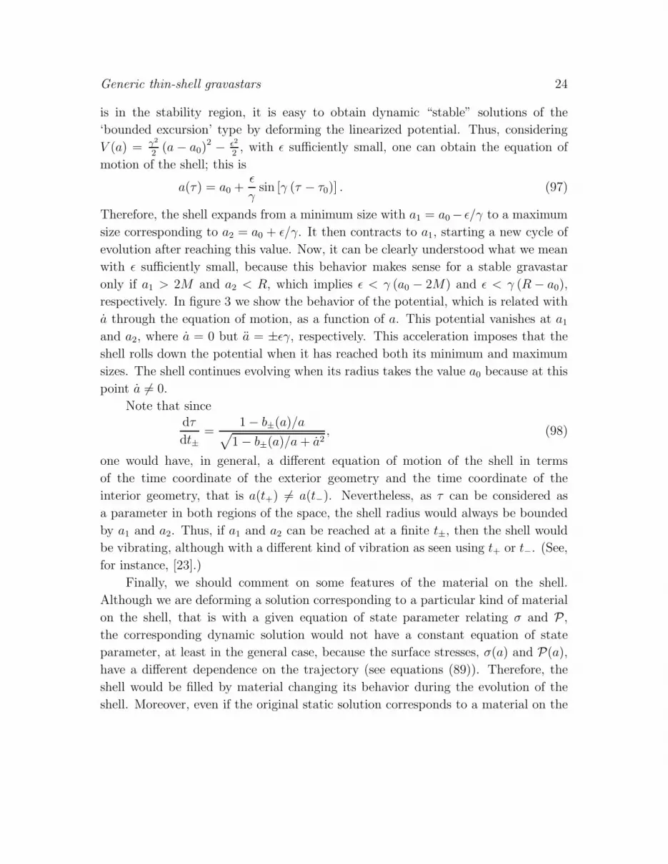
the equation of state parameter (w = P/σ) as a function of time, and the energy

density on the shell as a function of the pressure for a particular model obtained by

deforming a stable static solution with dust matter on the shell. It can be seen that

the pressure on the dynamic shell never vanishes, although the solution is obtained

by deforming one with P(a0) = 0.

3.3. Close to critical: Non-extremal

Another common feature of gravastars is that the transition layer is typically taken

to be “close” to horizon formation. That is b±(a)/a ≈ 1. In fact, it is useful to take

a linear approximation

b±(a)/a = 1∓ γ±(a− R∓) +O([a− R±]2) , (99)


Figure 4. Bounded excursion: We consider the deformation ǫ = 0.01 of a stable

static solution with dust matter on the shell, M = 1, a0 = 4.178821374980832,

R = 22.3607 and γ = 1. In the left figure we show the evolution of w in terms of

τ . It decreases from its maximum value to its minimum value from τ1 = τ(a = a1)

to τ2 = τ(a = a2) and then increases to its maximum value for the next cycle.

Evolution of the energy density in terms of the pressure is depicted in the right

figure. Consideration of more than one cycle would lead to the same graphic.

where R− is where the “black hole” horizon would have formed in the exterior

spacetime, R+ is where the “cosmological” horizon would have formed in the interior

spacetime. We take the transition layer to be at a position a such that R− < a < R+,

and γ± > 0 because we are (for now) avoiding “extremal” geometries. Dismissing

second order terms and considering vanishing external forces (Φ±(r) = 0), we have

σ ≃ − 1

4πa

[

√

γ+ (a−R−) + a2 −√

γ−(R+ − a) + a2]

, (100)

P ≃ 1

8πa

[

a2 + aa+ γ+ (3a/2− R−)√

γ+ (a−R−) + a2− a2 + aa + γ− (R+ − 3a/2)

√

γ− (R+ − a) + a2

]

. (101)

Therefore, σ(a) > 0 for a(τ) < (γ+R− + γ−R+) /(γ+ + γ−).

This “close to the horizon” approximation would be valid only if the trajectory

of the transition layer, which can be obtained from the equation of motion (or

equivalently considering some equation of state), is always in the region R− . a .

R+. In order to analyze the accuracy of this approximation, we consider a stable

static solution, implying

σ (a0) ≃ − 1

4πa0

[

√

γ+ (a0 − R−)−√

γ−(R+ − a0)]

, (102)


P (a0) ≃ 1

8πa0

[

γ+ (3a0/2− R−)√

γ+ (a0 −R−)− γ− (R+ − 3a0/2)√

γ− (R+ − a0)

]

. (103)

Consider stiff matter on the shell, σ (a0) = P (a0). Therefore, we have

γ1/2− (3R+ − 7a0/2)√

R+ − a0≃ γ

1/2+ (7a0/2− 3R−)√

a0 − R−

. (104)

Squaring both sides, and defining the dimensionless quantities α = a0/R−, β =

R−/R+, Γ+ = γ+R−, and Γ− = γ−R−, with α > 1 and 0 < β < 1, one has

49

4(Γ+ + Γ−)α

3 −[

49

4

(

Γ− +Γ+

β

)

+ 21

(

Γ−

β+ Γ+

)]

α2 (105)

+

[

21

β(Γ+ + Γ−) + 9

(

Γ−

β2+ Γ+

)]

α− 9

β

(

Γ−

β+ Γ+

)

≃ 0.

Thus, by considering the expansion of the background geometries close to where the

horizon would be formed, we have reduced the problem of finding static and stable

solutions (which usually involves some highly nontrivial equation) to solving a cubic,

which can be done analytically.

Nevertheless, some comments are in order. In the first place, as the RHS of

equation (104) is always positive, the solutions of equation (105) would correspond

to solutions of our problem only if R+ > 7a0/6, that is β < 6/7. In the second

place, one can consider that the approximation would not be accurate enough if

(a0 −R−) /R− < 1 and (R+ − a0) /a0 < 1 are not satisfied; thus, the solutions

would be reliable only if α < 2 and 1/4 < β. In summary, we should consider

1/4 < β < 6/7 to solve equation (105), and give physical meaning only to solutions

with 1 < α < 2, if any. In fact, one can see that the results that can be obtained by

using this approximation are compatible with those of a stiff matter gravastar with

a Schwarzschild exterior and a de Sitter interior when 1 < α < 2 (see equation (60)

of reference [9] for the equation that must be solved in that case).

On the other hand, we can study the stability of the static solutions. In this

case the inequality (86), for σ > 0, leads to

m′′s (a0) ≥ − γ2+ (3a0/4− R−)

[γ+ (a0 − R−)]3/2

− γ2− (R+ − 3a0/4)

[γ− (R+ − a0)]3/2

. (106)


It is more useful to consider m′′s (a0) /γ+, which can be written in terms of the

dimensionless quantities previously introduced, and is given by

m′′s (a0)

γ+≥ − 3α/4− 1

(α− 1)3/2−√

Γ−

Γ+

1/β − 3α/4

(1/β − α)3/2. (107)

In figure 5 we have drawn this function for the case that the inequality saturates for

two particular values of a0. Thus the region above the surface corresponds to the

stability region.

Figure 5. Close to critical (non-extremal): The left and right figures correspond

to a0 = 1.1R− and a0 = 1.5R−, respectively. It can be noticed that the function

is not defined for values of R+ < a0, since we must consider R− < a0 < R+.

3.4. Close to critical: Extremal

We now consider a gravastar with a transition layer “close” to where the horizon

would be expected to form, when both bulk geometries are “extremal”. This implies

that the coefficient of the first order term in the expansion (99) vanishes. Then,

assuming that the coefficient of the second order term is not vanishing, one has

b±(a)/a = 1− γ2±(a− R∓)2 +O([a− R±]

3) , (108)

with R− < a < R+, and γ± > 0. Note particularly that we now have a different

definition for γ±.


Again considering the situation Φ±(r) = 0, we can express the quantities related

to the thin-shell as

σ ≃ − 1

4πa

[

√

γ2+ (a− R−)2 + a2 −

√

γ2−(R+ − a)2 + a2]

, (109)

P ≃ 1

8πa

a2 + aa+ γ2+(

2a2 +R2− − 3R−a

)

√

γ2+ (a−R−)2 + a2

− a2 + aa + γ2−(

2a2 +R2+ − 3R+a

)

√

γ2− (R+ − a)2 + a2

.

(110)

Thus, we recover that a(τ) < (γ+R− + γ−R+) /(γ+ + γ−) for σ(a) > 0, although γ±would be different than in the former case analyzed. Considering a static solution,

one obtains

σ (a0) ≃ − 1

4πa0[γ+ (a0 −R−)− γ−(R+ − a0)] , (111)

P (a0) ≃ 1

8πa0

[

γ+(

2a20 +R2− − 3R−a0

)

a0 − R−

− γ−(

2a20 +R2+ − 3R+a0

)

R+ − a0

]

, (112)

where we have taken into account R− < a < R+, when simplifying. Following a

similar procedure to that considered in the non-extremal case, one can see that a

stiff matter shell must fulfil the equation

γ−(

4a20 + 3R2+ − 7R+a0

)

R+ − a0≃ γ+

(

4a20 + 3R2− − 7R−a0

)

a0 − R−, (113)

which, taking the same definition of Γ±, β and α introduced in the former case, leads

to

4 (Γ+ + Γ−)α3 −

[

4

(

Γ− +Γ+

β

)

+ 7

(

Γ−

β+ Γ+

)]

α2 (114)

+

[

7

β(Γ+ + Γ−) + 3

(

Γ−

β2+ Γ+

)]

α− 3

β

(

Γ−

β+ Γ+

)

≃ 0 .

This is again a cubic equation. However, whereas for non-extremal geometries

we have obtained equation (105) by squaring equation (104), in this case that

step was not necessary. Thus, all solutions of equation (114) are also solutions of

equation (113). Therefore, noticing the values of β and α for which the approximation

would be sufficiently accurate, we should solve equation (114) for 1/4 < β < 1 and

then consider only the solutions with 1 < α < 2.


A special characteristic of these static solutions can be seen when studying their

stability. Considering σ > 0, the inequality (86) can be simplify to obtain

m′′s

γ+≥ −2

(

1 +γ−γ+

)

, (115)

which is independent of a0. As the position a0 can be obtained by considering

a particular equation of state for the material on the shell, this implies that the

stability of the solution is independent of that equation of state†. In figure 6, we

show the behavior of this function.

Figure 6. Close to critical (extremal): We show the function m′′

sγ+ in the case

that V = 0. The stability region would be above this curve, independent of the

value of a0.

Finally, some comments about the case with one non-extremal and one extremal

background geometries are in order. In this case, for a stiff matter gravastar,

one would obtain an equation with the RHS of equation (104) and the LHS of

equation (113), or vice versa. Thus, after squaring, the analogue of equation (105)

or (114) would be a quintic. Therefore, the consideration of the close-to-horizon

approximation in this situation would generally not significantly simplify the problem

of obtaining static solutions, because we are only reducing the polynomial equation

by one degree (see also reference [9]).

† This interpretation could be reinforced by noticing that in this case m′′

s/γ+ depends only on the

geometry and on the potential, which, at the end of the day, implies a dependence on the geometry

and on σ (not on P), if σ 6= 0.


3.5. Charged dilatonic exterior, de Sitter interior

An interesting solution to consider is that of an interior de Sitter spacetime, (where

the metric functions are given by b−(r) = r3/R2 and Φ−(r) = 0), while the exterior

spacetime is given by the dilaton black hole solution, which corresponds to an

electric monopole. In Schwarzschild coordinates, this exterior solution is described

by [24, 25, 26],

ds2+ = −(

1− 2M

β +√

r2 + β2

)

dt2 +

(

1− 2M

β +√

r2 + β2

)−1r2

r2 + β2dr2

+ r2(dθ2 + sin2 θ dϕ2) . (116)

Here we have dropped the subscripts + for notational convenience. The Lagrangian

that describes this combined gravitational-electromagnetism-dilaton system is given

by [24, 25, 26]

L =√−g

−R/8π + 2(∇ψ)2 + F 2/4π

. (117)

Note that the non-zero component of the electromagnetic tensor is given by Ftr =

Q/r2, and the dilaton field is given by e2ψ = 1 − Q2/M(β +√

r2 + β2). The

parameter β is defined by β ≡ Q2/2M .

In terms of the formalism developed in this paper, the metric functions of the

exterior spacetime are

b+(r) = r

[

1−(

1 +β2

r2

)

(

1− 2M

β +√

r2 + β2

)]

, (118)

Φ+(r) = −1

2ln

(

1 +β2

r2

)

. (119)

An event horizon exists at rb = 2M√

1− β/M . Note that Φ′+(r) is given by

Φ′+(r) =

β2

a(β2 + a2), (120)

which is positive (and so satisfies the NEC) throughout the spacetime. Thus, taking

into account that Φ− = 0, we verify that the stability condition imposed by the

presence of the flux term is governed by inequality (88).

The thin shell is placed in the region rb < a < R∗, so that b+(a) ≥ b−(a) (and

consequently σ > 0) is satisfied. Consequently the stability regions are governed by


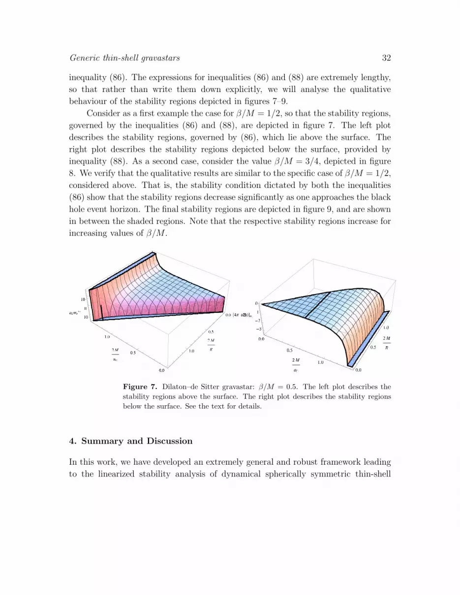
inequality (86). The expressions for inequalities (86) and (88) are extremely lengthy,

so that rather than write them down explicitly, we will analyse the qualitative

behaviour of the stability regions depicted in figures 7–9.

Consider as a first example the case for β/M = 1/2, so that the stability regions,

governed by the inequalities (86) and (88), are depicted in figure 7. The left plot

describes the stability regions, governed by (86), which lie above the surface. The

right plot describes the stability regions depicted below the surface, provided by

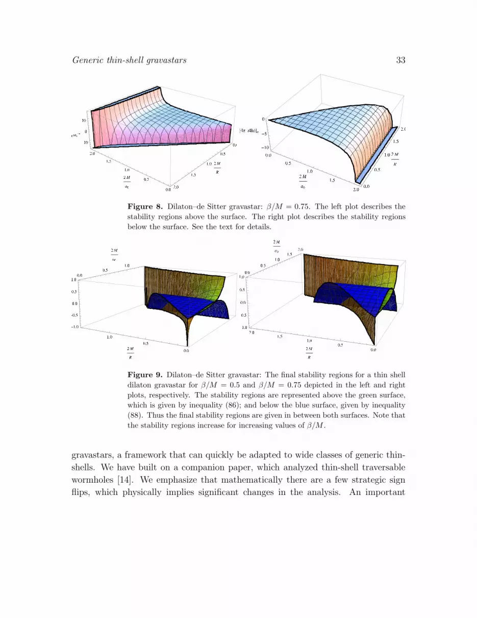
inequality (88). As a second case, consider the value β/M = 3/4, depicted in figure

8. We verify that the qualitative results are similar to the specific case of β/M = 1/2,

considered above. That is, the stability condition dictated by both the inequalities

(86) show that the stability regions decrease significantly as one approaches the black

hole event horizon. The final stability regions are depicted in figure 9, and are shown

in between the shaded regions. Note that the respective stability regions increase for

increasing values of β/M .

Figure 7. Dilaton–de Sitter gravastar: β/M = 0.5. The left plot describes the

stability regions above the surface. The right plot describes the stability regions

below the surface. See the text for details.

4. Summary and Discussion

In this work, we have developed an extremely general and robust framework leading

to the linearized stability analysis of dynamical spherically symmetric thin-shell


Figure 8. Dilaton–de Sitter gravastar: β/M = 0.75. The left plot describes the

stability regions above the surface. The right plot describes the stability regions

below the surface. See the text for details.

Figure 9. Dilaton–de Sitter gravastar: The final stability regions for a thin shell

dilaton gravastar for β/M = 0.5 and β/M = 0.75 depicted in the left and right

plots, respectively. The stability regions are represented above the green surface,

which is given by inequality (86); and below the blue surface, given by inequality

(88). Thus the final stability regions are given in between both surfaces. Note that

the stability regions increase for increasing values of β/M .

gravastars, a framework that can quickly be adapted to wide classes of generic thin-

shells. We have built on a companion paper, which analyzed thin-shell traversable

wormholes [14]. We emphasize that mathematically there are a few strategic sign

flips, which physically implies significant changes in the analysis. An important


difference is the possibility of a vanishing surface energy density at certain specific

shell radii, for the generic thin-shell gravastars considered in this work. Due to the

key sign flips, ultimately arising from the definition of the normals on the junction

interface, the surface energy density is always negative for the thin-shell traversable

wormholes considered in [14]. We have also explored static gravastar configurations

to some extent, and considered the generic qualitative behavior of the surface stresses.

Relative to the conservation law of the surface stresses, we have analysed in great

detail the most general case, widely ignored in the literature, namely, the presence

of a flux term, corresponding to the net discontinuity in the (bulk) momentum flux

which impinges on the shell. Physically, the latter flux term can be interpreted as

the work done by external forces on the thin shell.

In the context of the linearized stability analysis we have reversed the logic

flow typically considered in the literature and introduced a novel approach. More

specifically, we have considered the surface mass as a function of the potential, so that

specifying the latter tells us how much surface mass we need to put on the transition

layer. This procedure implicitly makes demands on the equation of state of the

matter residing on the transition layer and demonstrates in full generality that the

stability of the gravastar is equivalent to choosing suitable properties for the material

residing on the thin shell. We have applied the latter stability formalism to a number

of specific cases, namely, to the traditional gravastar picture, where the transition

layer separates an interior de Sitter space and an exterior Schwarschild geometry;

bounded excursion; close-to-horizon models, in both the extremal and non-extremal

regimes; and finally, to specific example of an interior de Sitter spacetime matched to

a charged dilatonic exterior. This latter case is particularly interesting, as it involves

the flux term.

In conclusion, by considering the matching of two generic static spherically

symmetric spacetimes using the cut-and-paste procedure, we have analyzed the

stability of thin-shell gravastars. The analysis provides a general and unified

framework for simultaneously addressing a large number of gravastar models

scattered throughout the literature. As such we hope it will serve to bring some

cohesion and focus to what is otherwise a rather disorganized and disparate collection

of results.


Acknowledgments

PMM acknowledges financial support from a FECYT postdoctoral mobility contract

of the Spanish Ministry of Education through National Programme No. 2008–2011.

NMG acknowledges financial support from CONACYT-Mexico. FSNL acknowledges

financial support of the Fundacao para a Ciencia e Tecnologia through Grants

PTDC/FIS/102742/2008 and CERN/FP/116398/2010. MV acknowledges financial

support from the Marsden Fund, administered by the Royal Society of New Zealand.

References

[1] G. Chapline, E. Hohlfeld, R. B. Laughlin and D. I. Santiago, “Quantum phase transitions

and the breakdown of classical general relativity”, Int. J. Mod. Phys. A 18, 3587 (2003)

[gr-qc/0012094].

[2] P. O. Mazur and E. Mottola, “Gravitational condensate stars: An alternative to black holes”,

gr-qc/0109035.

P. O. Mazur and E. Mottola, “Dark energy and condensate stars: Casimir energy in the

large”, gr-qc/0405111.

P. O. Mazur and E. Mottola, “Gravitational vacuum condensate stars”, Proc. Nat. Acad.

Sci. 101, 9545 (2004) [gr-qc/0407075].

[3] F. S. N. Lobo, “Stable dark energy stars”, Class. Quant. Grav. 23, 1525-1541 (2006).

[gr-qc/0508115].

S. S. Yazadjiev, “Exact dark energy star solutions”, Phys. Rev. D 83, 127501 (2011)

[arXiv:1104.1865 [gr-qc]].

R. Chan, M. F. A. da Silva and J. F. Villas da Rocha, “On Anisotropic Dark Energy Stars”,

Mod. Phys. Lett. A 24, 1137 (2009) [arXiv:0803.2508 [gr-qc]].

A. DeBenedictis, R. Garattini and F. S. N. Lobo, “Phantom stars and topology change”,

Phys. Rev. D 78, 104003 (2008) [arXiv:0808.0839 [gr-qc]].

[4] J. P. S. Lemos and O. B. Zaslavskii, “Entropy of quasiblack holes”, Phys. Rev. D 81 (2010)

064012 [arXiv:0904.1741 [gr-qc]];

J. P. S. Lemos and O. B. Zaslavskii, “Black hole mimickers: regular versus singular behavior”,

Phys. Rev. D 78 (2008) 024040 [arXiv:0806.0845 [gr-qc]].

[5] R. D. Sorkin, R. M. Wald and Z. J. Zhang, “Entropy of selfgravitating radiation”, Gen. Rel.

Grav. 13 (1981) 1127.

S. D. H. Hsu and D. Reeb, “Black hole entropy, curved space and monsters”, Phys. Lett. B

658 (2008) 244 [arXiv:0706.3239 [hep-th]];

S . D. H. Hsu and D. Reeb, “Monsters, black holes and the statistical mechanics of gravity”,

Mod. Phys. Lett. A 24 (2009) 1875 [arXiv:0908.1265 [gr-qc]].

[6] C. Barcelo, S. Liberati, S. Sonego and M. Visser, “Fate of gravitational collapse in semiclassical

gravity”, Phys. Rev. D 77 (2008) 044032 [arXiv:0712.1130 [gr-qc]];

C. Barcelo, S. Liberati, S. Sonego and M. Visser, “Revisiting the semiclassical gravity

http://arxiv.org/abs/gr-qc/0012094





http://arxiv.org/abs/1104.1865









scenario for gravitational collapse”, AIP Conf. Proc. 1122 (2009) 99 [arXiv: 0909.4157

[gr-qc]];

C. Barcelo, S. Liberati, S. Sonego and M. Visser, “Black stars, not holes”, Sci. Am. (Oct

2009) 8 pages;

M. Visser, C. Barcelo, S. Liberati and S. Sonego, “Small, dark, and heavy: But is it a black

hole?”, arXiv: 0902.0346 [gr-qc].

C. Barcelo, S. Liberati, S. Sonego and M. Visser, “Hawking-like radiation from evolving black

holes and compact horizonless objects,” JHEP 1102 (2011) 003 [arXiv:1011.5911 [gr-qc]].

C. Barcelo, S. Liberati, S. Sonego and M. Visser, “Minimal conditions for the existence of a

Hawking-like flux,” Phys. Rev. D 83 (2011) 041501 [arXiv:1011.5593 [gr-qc]].

M. Visser, “Black holes in general relativity,” arXiv:0901.4365 [gr-qc].

[7] C. Cattoen, T. Faber and M. Visser, “Gravastars must have anisotropic pressures”, Class.

Quant. Grav. 22, 4189 (2005) [gr-qc/0505137].

[8] A. DeBenedictis, D. Horvat, S. Ilijic, S. Kloster and K. S. Viswanathan, “Gravastar solutions

with continuous pressures and equation of state”, Class. Quant. Grav. 23, 2303 (2006)

[gr-qc/0511097].

[9] M. Visser, D. L. Wiltshire, “Stable gravastars: An alternative to black holes?”, Class. Quant.

Grav. 21 (2004) 1135-1152. [gr-qc/0310107].

[10] N. Sen, “Uber die grenzbedingungen des schwerefeldes an unsteig keitsflachen”, Ann. Phys.

(Leipzig) 73, 365 (1924);

K. Lanczos, “Flachenhafte verteiliung der materie in der Einsteinschen gravitationstheorie”,

Ann. Phys. (Leipzig) 74, 518 (1924);

G. Darmois, “Les equations de la gravitation einsteinienne”, in Memorial des sciences

mathematiques XXV. Fascicule XXV ch V (Gauthier-Villars, Paris, France, 1927);

S. O’Brien and J. L. Synge, “Jump conditions at discontinuity in general relativity.”,

Commun. Dublin Inst. Adv. Stud. Ser. A., no. 9 (1952) 1–20;

A. Lichnerowicz, Theories Relativistes de la Gravitation et de l’Electromagnetisme, Masson,

Paris (1955);

W. Israel, “Singular hypersurfaces and thin shells in general relativity”, Nuovo Cimento

44B, 1 (1966); and corrections in ibid. 48B, 463 (1966).

[11] N. Bilic, G. B. Tupper and R. D. Viollier, “Born-infeld phantom gravastars”, JCAP 0602, 013

(2006) [astro-ph/0503427].

B. M. N. Carter, “Stable gravastars with generalised exteriors”, Class. Quant. Grav. 22,

4551 (2005) [gr-qc/0509087].

F. S. N. Lobo, “Van der Waals quintessence stars”, Phys. Rev. D 75, 024023 (2007) [gr-

qc/0610118].

F. S. N. Lobo and A. V. B. Arellano, “Gravastars supported by nonlinear electrodynamics”,

Class. Quant. Grav. 24, 1069 (2007) [gr-qc/0611083].

F. S. N. Lobo, “Stable dark energy stars: An alternative to black holes?”, gr-qc/0612030.

D. Horvat and S. Ilijic, “Gravastar energy conditions revisited”, Class. Quant. Grav. 24,

5637 (2007) [arXiv:0707.1636 [gr-qc]].

R. Chan, M. F. A. da Silva and J. F. Villas da Rocha, “Star Models with Dark Energy”,







http://arxiv.org/abs/astro-ph/0503427






Gen. Rel. Grav. 41, 1835 (2009) [arXiv:0803.3064 [gr-qc]].

P. Rocha, A. Y. Miguelote, R. Chan, M. F. da Silva, N. O. Santos and A. Wang, “Bounded

excursion stable gravastars and black holes”, JCAP 0806, 025 (2008) [arXiv:0803.4200 [gr-

qc]].

D. Horvat, S. Ilijic and A. Marunovic, “Electrically charged gravastar configurations”, Class.

Quant. Grav. 26, 025003 (2009) [arXiv:0807.2051 [gr-qc]].

P. Rocha, R. Chan, M. F. A. da Silva and A. Wang, “Stable and ’bounded excursion’

gravastars, and black holes in Einstein’s theory of gravity”, JCAP 0811, 010 (2008)

[arXiv:0809.4879 [gr-qc]].

R. Chan, M. F. A. da Silva, P. Rocha and A. Wang, “Stable Gravastars of Phantom Energy”,

JCAP 0903, 010 (2009) [arXiv:0812.4924 [gr-qc]].

B. V. Turimov, B. J. Ahmedov and A. A. Abdujabbarov, “Electromagnetic Fields of Slowly

Rotating Magnetized Gravastars”, Mod. Phys. Lett. A 24, 733 (2009) [arXiv:0902.0217 [gr-

qc]].

R. Chan, M. F. A. da Silva and P. Rocha, “How the Cosmological Constant Affects the

Gravastar Formation”, JCAP 0912, 017 (2009) [arXiv:0910.2054 [gr-qc]].

F. S. N. Lobo and R. Garattini, “Linearized stability analysis of gravastars in

noncommutative geometry”, arXiv:1004.2520 [gr-qc].

R. Chan and M. F. A. da Silva, “How the Charge Can Affect the Formation of Gravastars”,

JCAP 1007, 029 (2010) [arXiv:1005.3703 [gr-qc]].

M. E. Gaspar and I. Racz, “Probing the stability of gravastars by dropping dust shells onto

them”, Class. Quant. Grav. 27, 185004 (2010) [arXiv:1008.0554 [gr-qc]].

E. Mottola, “New Horizons in Gravity: The Trace Anomaly, Dark Energy and Condensate

Stars”, Acta Phys. Polon. B 41, 2031 (2010) [arXiv:1008.5006 [gr-qc]].

R. Chan, M. F. A. da Silva and P. Rocha, “Gravastars and Black Holes of Anisotropic Dark

Energy”, Gen. Rel. Grav. 43, 2223 (2011) [arXiv:1009.4403 [gr-qc]].

A. A. Usmani, F. Rahaman, S. Ray, K. K. Nandi, P. K. F. Kuhfittig, S. .A. Rakib and

Z. Hasan, “Charged gravastars admitting conformal motion”, Phys. Lett. B 701, 388 (2011)

[arXiv:1012.5605 [gr-qc]].

D. Horvat, S. Ilijic and A. Marunovic, “Radial stability analysis of the continuous pressure

gravastar”, Class. Quant. Grav. 28, 195008 (2011) [arXiv:1104.3537 [gr-qc]].

R. Chan, M. F. A. da Silva, J. F. V. da Rocha and A. Wang, “Radiating Gravastars”, JCAP

1110, 013 (2011) [arXiv:1109.2062 [gr-qc]].

[12] C. Barrabes and W. Israel, “Thin shells in general relativity and cosmology: The lightlike

limit”, Phys. Rev. D 43, 1129 (1991);

R. Mansouri and M. Khorrami, “The equivalence of Darmois-Israel and distributional-

method for thin shells in general relativity”, J. Math. Phys. 37, 5672 (1996)

[arXiv:gr-qc/9608029];

P. Musgrave and K. Lake, “Junctions and thin shells in general relativity using

computer algebra I: The Darmois-Israel formalism”, Class. Quant. Grav. 13 1885 (1996)


V. P. Frolov, M. A. Markov and V. F. Mukhanov, “Black holes as possible sources of closed



















and semiclosed worlds”, Phys. Rev. D 41, 383 (1990);

J. Fraundiener, C. Hoenselaers and W. Konrad, “A shell around a black hole”, Class. Quant.

Grav. 7, 585 (1990);

P. R. Brady, J. Louko and E. Poisson, “Stability of a shell around a black hole”, Phys. Rev.

D 44, 1891 (1991).

[13] A. E. Broderick and R. Narayan, “Where are all the gravastars? Limits upon the gravastar

model from accreting black holes”, Class. Quant. Grav. 24, 659 (2007) [gr-qc/0701154

[GR-QC]].

C. B. M. H. Chirenti and L. Rezzolla, “How to tell a gravastar from a black hole”, Class.

Quant. Grav. 24, 4191 (2007) [arXiv:0706.1513 [gr-qc]].

J. P. S. Lemos and O. B. Zaslavskii, “Black hole mimickers: Regular versus singular

behavior”, Phys. Rev. D 78, 024040 (2008) [arXiv:0806.0845 [gr-qc]].

P. Pani, V. Cardoso, M. Cadoni and M. Cavaglia, “Ergoregion instability of black hole

mimickers”, arXiv:0901.0850 [gr-qc].

S. V. Sushkov and O. B. Zaslavskii, “Horizon closeness bounds for static black hole

mimickers”, Phys. Rev. D 79, 067502 (2009) [arXiv:0903.1510 [gr-qc]].

P. Pani, E. Berti, V. Cardoso, Y. Chen and R. Norte, “Gravitational wave signatures of the

absence of an event horizon. I. Nonradial oscillations of a thin-shell gravastar”, Phys. Rev.

D 80, 124047 (2009) [arXiv:0909.0287 [gr-qc]].

T. Harko, Z. Kovacs and F. S. N. Lobo, “Can accretion disk properties distinguish gravastars

from black holes?”, Class. Quant. Grav. 26, 215006 (2009) [arXiv:0905.1355 [gr-qc]].

[14] N. M. Garcia, F. S. N. Lobo and M. Visser “Generic spherically symmetric dynamic thin-shell

traversable wormholes in standard general relativity”, arXiv:1112.2057 [gr-qc].

[15] C. Barcelo and M. Visser, “Living on the edge: Cosmology on the boundary of Anti-de Sitter

space,” Phys. Lett. B 482 (2000) 183 [hep-th/0004056].

C. Barcel o and M. Visser, “Brane surgery: Energy conditions, traversable wormholes, and

voids,” Nucl. Phys. B 584 (2000) 415 [hep-th/0004022].

[16] C. Barcelo and M. Visser, “Twilight for the energy conditions?,” Int. J. Mod. Phys. D 11

(2002) 1553 [gr-qc/0205066].

M. Visser, “Gravitational vacuum polarization,” gr-qc/9710034.

M. Visser, “Gravitational vacuum polarization. 1: Energy conditions in the Hartle-Hawking

vacuum,” Phys. Rev. D 54 (1996) 5103 [gr-qc/9604007].

M. Visser, “Gravitational vacuum polarization. 2: Energy conditions in the Boulware

vacuum,” Phys. Rev. D 54 (1996) 5116 [gr-qc/9604008].

M. Visser, “Gravitational vacuum polarization. 3: Energy conditions in the (1+1)

Schwarzschild space-time,” Phys. Rev. D 54 (1996) 5123 [gr-qc/9604009].

M. Visser, “Gravitational vacuum polarization. 4: Energy conditions in the Unruh vacuum,”

Phys. Rev. D 56 (1997) 936 [gr-qc/9703001].

[17] M. Visser, Lorentzian Wormholes: From Einstein to Hawking, (American Institute of Physics,

New York, 1995).

[18] M. Visser, “Traversable wormholes: Some simple examples”, Phys. Rev. D 39 3182 (1989);

M. Visser, “Traversable wormholes from surgically modified Schwarzschild spacetimes”,









http://arxiv.org/abs/hep-th/0004056









Nucl. Phys. B 328 203 (1989);

M. Visser, “Quantum mechanical stabilization of Minkowski signature wormholes”, Phys.

Lett. B 242, 24 (1990);

E. Poisson and M. Visser, “Thin shell wormholes: Linearization stability”, Phys. Rev. D 52,

7318 (1995) [arXiv:gr-qc/9506083];

E. F. Eiroa and G. E. Romero “Linearized stability of charged thin-shell wormoles”, Gen.

Rel. Grav. 36 651-659 (2004) [arXiv:gr-qc/0303093];

F. S. N. Lobo and P. Crawford, “Linearized stability analysis of thin shell wormholes with

a cosmological constant”, Class. Quant. Grav. 21, 391 (2004) [arXiv:gr-qc/0311002];

J. P. S. Lemos and F. S. N. Lobo, “Plane symmetric thin-shell wormholes: Solutions and

stability,” Phys. Rev. D 78, 044030 (2008) [arXiv:0806.4459 [gr-qc]].

[19] J. P. S. Lemos, F. S. N. Lobo and S. Q. de Oliveira, “Morris-Thorne wormholes with a

cosmological constant”, Phys. Rev. D 68, 064004 (2003) [arXiv:gr-qc/0302049];

J. P. S. Lemos and F. S. N. Lobo, “Plane symmetric traversable wormholes in an anti-de

Sitter background”, Phys. Rev. D 69, 104007 (2004) [arXiv:gr-qc/0402099];

F. S. N. Lobo, “Energy conditions, traversable wormholes and dust shells”, Gen. Rel. Grav.

37 (2005) 2023 [arXiv:gr-qc/0410087];

F. S. N. Lobo, “Phantom energy traversable wormholes”, Phys. Rev. D 71, 084011 (2005)


F. S. N. Lobo, “Stability of phantom wormholes”, Phys. Rev. D71, 124022 (2005).

[gr-qc/0506001];

F. S. N. Lobo, P. Crawford, “Stability analysis of dynamic thin shells”, Class. Quant. Grav.

22, 4869-4886 (2005). [gr-qc/0507063];

F. S. N. Lobo, “Exotic solutions in General Relativity: Traversable wormholes and ’warp

drive’ spacetimes,” arXiv:0710.4474 [gr-qc].

[20] F. S. N. Lobo, “Surface stresses on a thin shell surrounding a traversable wormhole”, Class.

Quant. Grav. 21 4811 (2004) [arXiv:gr-qc/0409018].

[21] G. Abreu and M. Visser, “Tolman mass, generalized surface gravity, and entropy bounds,”

Phys. Rev. Lett. 105 (2010) 041302 [arXiv:1005.1132 [gr-qc]].

[22] M. Ishak and K. Lake, “Stability of transparent spherically symmetric thin shells and

wormholes”, Phys. Rev. D 65 044011 (2002) [arXiv:gr-qc/0108058].

[23] L. C. Barbado, C. Barcelo, L. J. Garay and G. Jannes, “The Trans-Planckian problem as a

guiding principle,” JHEP 1111 (2011) 112 [arXiv:1109.3593 [gr-qc]].

[24] M. Visser, “Dirty black holes: Thermodynamics and horizon structure”, Phys. Rev. D 46,

2445 (1992) [arXiv:hep-th/9203057 [hep-th]].

[25] G. W. Gibbons and K. -i. Maeda, “Black Holes and Membranes in Higher Dimensional Theories

with Dilaton Fields”, Nucl. Phys. B 298 (1988) 741.

[26] D. Garfinkle, G. T. Horowitz and A. Strominger, “Charged black holes in string theory”, Phys.

Rev. D 43 (1991) 3140 [Erratum-ibid. D 45 (1992) 3888].

















Documents

Generic thin-shell gravastars