General Network Lifetime and Cost Models for Evaluating Sensor Network Deployment Strategies

General Network Lifetime and Cost Modelsfor Evaluating Sensor Network

Deployment StrategiesZhao Cheng, Mark Perillo, and Wendi B. Heinzelman, Senior Member, IEEE

Abstract—In multihop wireless sensor networks that are often characterized by many-to-one (convergecast) traffic patterns, problems

related to energy imbalance among sensors often appear. Sensors closer to a data sink are usually required to forward a large amount

of traffic for sensors farther from the data sink. Therefore, these sensors tend to die early, leaving areas of the network completely

unmonitored and reducing the functional network lifetime. In our study, we explore possible sensor network deployment strategies that

maximize sensor network lifetime by mitigating the problem of the hot spot around the data sink. Strategies such as variable-range

transmission power control with optimal traffic distribution, mobile-data-sink deployment, multiple-data-sink deployment, nonuniform

initial energy assignment, and intelligent sensor/relay deployment are investigated. We suggest a general model to analyze and

evaluate these strategies. In this model, we not only discover how to maximize the network lifetime given certain network constraints

but also consider the factor of extra costs involved in more complex deployment strategies. This paper presents a comprehensive

analysis on the maximum achievable sensor network lifetime for different deployment strategies, and it also provides practical

cost-efficient sensor network deployment guidelines.

Index Terms—Wireless sensor networks, data dissemination, linear programming, deployment strategies.

Ç

1 INTRODUCTION

LARGE-SCALE wireless sensor networks are an emergingtechnology that has recently gained attention for their

potential use in many applications. Since sensors typicallyoperate on batteries and are thus limited in their activelifetime, the problem of designing protocols to achieveenergy efficiency to extend the network lifetime has becomea major concern for network designers. Much attention hasbeen given to the reduction of unnecessary energyconsumption of sensor nodes in areas such as hardwaredesign, collaborative signal processing, transmission powercontrol policies, and all levels of the network stack.However, reducing an individual sensor’s power consump-tion alone may not always allow networks to realize theirmaximum potential lifetime. In addition, it is important tomaintain a balance of energy consumption in the networkso that certain nodes do not die much earlier than others,leading to unmonitored areas in the network.

Previous research has shown that because of thecharacteristics of wireless channels, multihop forwardingbetween a data source and a data sink is often more energy-efficient than direct transmission. However, in sensornetworks, where many applications require a many-to-one(convergecast) traffic pattern in the network, multihopforwarding may cause energy imbalance as all the trafficmust be routed through the nodes near the data sink, thus

creating a hot spot around the data sink or base station.1

The nodes in this hot spot are required to forward adisproportionately high amount of traffic and typically dieat a very early stage. If we define the network lifetime as thetime when the first subregion of the environment (or asignificant portion of the environment) is left unmonitored,then the residual energy of the other sensors at this time canbe seen as wasted.

Despite the fact that many sensor deployment strategieshave been considered to extend the network lifetime, thereis no general framework to evaluate the maximum lifetimeprovided by these strategies and to evaluate their actualdeployment cost (that is, monetary cost). Thus, there is noeasy way to compare the advantages and disadvantages ofthese various deployment strategies. In this paper, weformulate the network lifetime problem and analyze thelimits of network lifetime for different types of sensornetwork scenarios and corresponding network deploymentstrategies. Since applying a more complex strategy mayintroduce extra costs, we also provide a simple yet effectivecost model to explore the cost trade-off for using advancedsolutions. The main contributions of this paper are thefollowing: 1) we propose a general framework for theanalysis of the network lifetime for several networkdeployment strategies, and 2) we consider the extra costsassociated with each deployment strategy to determine thebest overall strategy for a given scenario.

The rest of this paper is organized as follows: Section 2addresses related work. Section 3 presents several differentsensor network deployment strategies. Our models fornetwork lifetime and deployment cost are presented in

484 IEEE TRANSACTIONS ON MOBILE COMPUTING, VOL. 7, NO. 4, APRIL 2008

. The authors are with the Department of Electrical and ComputerEngineering, University of Rochester, Rochester, NY 14627.E-mail: {zhcheng, perillo, wheinzel}@ece.rochester.edu.

Manuscript received 22 Mar. 2006; revised 19 July 2007; accepted 17 Oct.2007; published online 12 Nov. 2007.For information on obtaining reprints of this article, please send e-mail to:[email protected], and reference IEEECS Log Number TMC-0083-0306.Digital Object Identifier no. 10.1109/TMC.2007.70784. 1. We do not differentiate between these terms in the rest of the paper.

1536-1233/08/$25.00 � 2008 IEEE Published by the IEEE CS, CASS, ComSoc, IES, & SPS

Section 4. Section 5 provides a detailed discussion of theoptimal lifetime for the simplest deployment strategy andreveals trends that are common to the different deploymentstrategies. Section 6 compares several different sensornetwork deployment strategies in terms of normalizedlifetime and cost for a target scenario. Finally, conclusionsare provided in Section 7.

2 RELATED WORK

The minimization of transmission energy in wireless sensornetworks and in wireless networks in general has beenstudied extensively. If the transmission power cannot beadjusted, power consumption can be minimized by mini-mizing the number of hops between the source anddestination. However, when the transmission power canbe set according to the distance over which data is beingtransmitted, because received energy typically falls off withdistance as 1=d2, it may be more energy efficient to senddata over many short hops rather than fewer long hops.Several works have noted this and shown how to minimizeenergy consumption by appropriately setting the transmis-sion power. Takagi and Kleinrock explored how to best setthe transmission power in order to minimize interferenceand maximize throughput [1]. The problem of setting thetransmission power to a minimal level that will allow anetwork to remain connected has been considered inseveral studies [2], [3]. In later work, some considered theimportance of a fixed energy consumption per bit,independent of the transmission distance. Because of thisoverhead, there exists an optimal nonzero transmissionrange, at which energy efficiency is optimized [4], [5].

In the above-cited works, the goal was to minimizeoverall energy consumption, and a fixed network-widetransmission range was assumed. However, using suchschemes may result in extremely unbalanced energyconsumption among the nodes in sensor networks char-acterized by many-to-one traffic patterns. In addition tominimizing energy consumption, it may also be beneficialto distribute the energy among the nodes and to favor usingthose with greater energy resources so that the networklifetime may be maximized. Note that the network lifetimemay be defined in a number of ways, including the timeuntil the first node dies, the time when the first region of asensor network is left unattended, etc. To accomplish thisgoal of lifetime maximization, load balancing through acombination of intelligent routing and transmission powercontrol was studied in [6], where several heuristic routingcosts were recommended for use in order to minimize and,at the same time, balance energy consumption. In [7],Chang and Tassiulas show how the optimal combination ofseveral routing costs allows the network lifetime to beextended. In [8], Efthymiou et al. show how energyconsumption can be balanced by distributing packets overseveral paths. The problem of finding the optimal routing toachieve the maximum network lifetime in a sensor networkwas studied as a constrained linear program optimizationin [9], [10], and [11]. In this work, the authors find themaximum lifetime that could be achieved by any routingcost or balancing scheme. In [12], Perillo et al. show howtransmission ranges can be optimally set and how traffic

can be optimally distributed specifically in a many-to-onesensor network.

Aside from transmission range optimization for balan-

cing energy across the sensors, several other sensor

deployment strategies have been proposed to extend the

network lifetime. For example, a mobile data sink roaming

within the network can be deployed to balance the energy

consumption. In [13], data mules are deployed in the

network to pick up the data once they are close to the data

source. Buffer requirements are the main focus of this study.

In [14], Kim et al. focus on minimizing the cost for topology

maintenance and communication between the mobile sinks

and the data sources. In [15], the optimal sink mobility

strategy is studied. Our generalized model is able to obtain

the optimal assignment of communication load for the

mobile-sink strategy, and our study focuses on the network

lifetime improvement from this strategy. Therefore, detailed

design considerations such as buffer size and the overhead

for network maintenance are not considered here.Multiple data sinks can also be deployed to collect data

over a certain subregion of the entire area. In [16], the optimalassignment of communication load to multiple sinks isfound using a method similar to electrostatic theory. In [17],an application using multiple Crossbow Stargates as virtualdata sinks is implemented. Further deployment strategiesthat integrate data aggregation have also been considered.In LEACH [18], each sensor can serve as a cluster head,where data from neighboring sensors is aggregated, andsensors rotate their roles to evenly distribute the energy load.This can be considered as a multiple-sink strategy with dataaggregation. We do not consider data aggregation in ourmodel since data aggregation is application specific.

The deployment of extra relay nodes around the datasink can also be helpful in solving energy imbalanceproblems. In [19], Ergen and Varaiya compare theminimum energy consumption when the relay nodes’locations are predetermined and when they can be placedin any location. The authors provide a heuristic method tosolve the latter problem. In [20], a similar mixed-integernonlinear programming solution is provided to discover theoptimal locations of relay nodes iteratively. In [21], Howittand Wang attempt to balance energy consumption byrequiring the sensors to send traffic to the next node along achain to the base station and spacing sensors nonuniformlyas a function of their distance to the data sink so that energyconsumption is uniform for all nodes. In our work, we lookat relay nodes simply as energy deposits. After we discoverthe optimal energy distribution map for the network, wecan easily determine where energy is insufficient and thusdetermine where relay nodes should be placed and howmuch energy they should carry. Therefore, our solution ismore general, and it is straightforward to apply.

Table 1 provides a summary of these different approachesfor balancing energy consumption and some representativeprotocols existing in the current literature. Despite themultitude of research investigating the aforementioneddeployment strategies, there is no cross comparison amongthese strategies for situations when multiple options areavailable. In this paper, we fill this void by proposing a

CHENG ET AL.: GENERAL NETWORK LIFETIME AND COST MODELS FOR EVALUATING SENSOR NETWORK DEPLOYMENT STRATEGIES 485

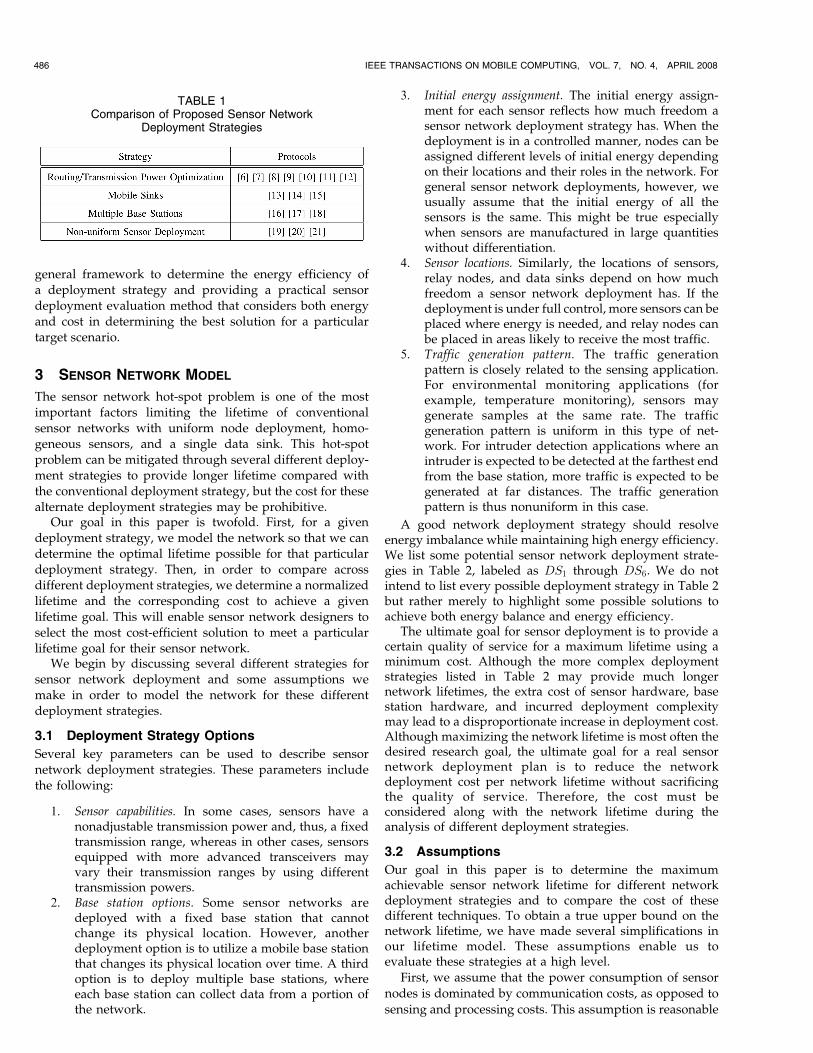
general framework to determine the energy efficiency ofa deployment strategy and providing a practical sensordeployment evaluation method that considers both energyand cost in determining the best solution for a particulartarget scenario.

3 SENSOR NETWORK MODEL

The sensor network hot-spot problem is one of the mostimportant factors limiting the lifetime of conventionalsensor networks with uniform node deployment, homo-geneous sensors, and a single data sink. This hot-spotproblem can be mitigated through several different deploy-ment strategies to provide longer lifetime compared withthe conventional deployment strategy, but the cost for thesealternate deployment strategies may be prohibitive.

Our goal in this paper is twofold. First, for a givendeployment strategy, we model the network so that we candetermine the optimal lifetime possible for that particulardeployment strategy. Then, in order to compare acrossdifferent deployment strategies, we determine a normalizedlifetime and the corresponding cost to achieve a givenlifetime goal. This will enable sensor network designers toselect the most cost-efficient solution to meet a particularlifetime goal for their sensor network.

We begin by discussing several different strategies forsensor network deployment and some assumptions wemake in order to model the network for these differentdeployment strategies.

3.1 Deployment Strategy Options

Several key parameters can be used to describe sensornetwork deployment strategies. These parameters includethe following:

1. Sensor capabilities. In some cases, sensors have anonadjustable transmission power and, thus, a fixedtransmission range, whereas in other cases, sensorsequipped with more advanced transceivers mayvary their transmission ranges by using differenttransmission powers.

2. Base station options. Some sensor networks aredeployed with a fixed base station that cannotchange its physical location. However, anotherdeployment option is to utilize a mobile base stationthat changes its physical location over time. A thirdoption is to deploy multiple base stations, whereeach base station can collect data from a portion ofthe network.

3. Initial energy assignment. The initial energy assign-ment for each sensor reflects how much freedom asensor network deployment strategy has. When thedeployment is in a controlled manner, nodes can beassigned different levels of initial energy dependingon their locations and their roles in the network. Forgeneral sensor network deployments, however, weusually assume that the initial energy of all thesensors is the same. This might be true especiallywhen sensors are manufactured in large quantitieswithout differentiation.

4. Sensor locations. Similarly, the locations of sensors,relay nodes, and data sinks depend on how muchfreedom a sensor network deployment has. If thedeployment is under full control, more sensors can beplaced where energy is needed, and relay nodes canbe placed in areas likely to receive the most traffic.

5. Traffic generation pattern. The traffic generationpattern is closely related to the sensing application.For environmental monitoring applications (forexample, temperature monitoring), sensors maygenerate samples at the same rate. The trafficgeneration pattern is uniform in this type of net-work. For intruder detection applications where anintruder is expected to be detected at the farthest endfrom the base station, more traffic is expected to begenerated at far distances. The traffic generationpattern is thus nonuniform in this case.

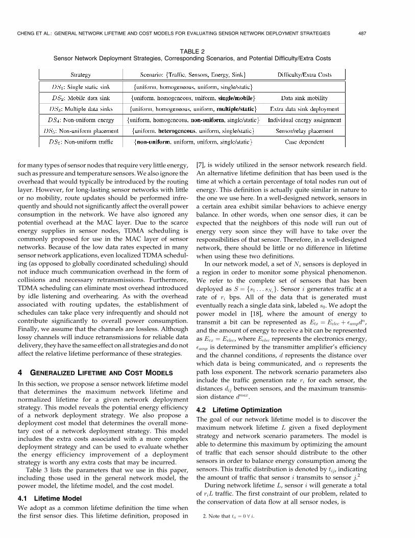
A good network deployment strategy should resolveenergy imbalance while maintaining high energy efficiency.We list some potential sensor network deployment strate-gies in Table 2, labeled as DS1 through DS6. We do notintend to list every possible deployment strategy in Table 2but rather merely to highlight some possible solutions toachieve both energy balance and energy efficiency.

The ultimate goal for sensor deployment is to provide acertain quality of service for a maximum lifetime using aminimum cost. Although the more complex deploymentstrategies listed in Table 2 may provide much longernetwork lifetimes, the extra cost of sensor hardware, basestation hardware, and incurred deployment complexitymay lead to a disproportionate increase in deployment cost.Although maximizing the network lifetime is most often thedesired research goal, the ultimate goal for a real sensornetwork deployment plan is to reduce the networkdeployment cost per network lifetime without sacrificingthe quality of service. Therefore, the cost must beconsidered along with the network lifetime during theanalysis of different deployment strategies.

3.2 Assumptions

Our goal in this paper is to determine the maximumachievable sensor network lifetime for different networkdeployment strategies and to compare the cost of thesedifferent techniques. To obtain a true upper bound on thenetwork lifetime, we have made several simplifications inour lifetime model. These assumptions enable us toevaluate these strategies at a high level.

First, we assume that the power consumption of sensor

nodes is dominated by communication costs, as opposed to

sensing and processing costs. This assumption is reasonable


TABLE 1Comparison of Proposed Sensor Network

Deployment Strategies

for many types of sensor nodes that require very little energy,

such as pressure and temperature sensors. We also ignore the

overhead that would typically be introduced by the routing

layer. However, for long-lasting sensor networks with little

or no mobility, route updates should be performed infre-

quently and should not significantly affect the overall power

consumption in the network. We have also ignored any

potential overhead at the MAC layer. Due to the scarce

energy supplies in sensor nodes, TDMA scheduling is

commonly proposed for use in the MAC layer of sensor

networks. Because of the low data rates expected in many

sensor network applications, even localized TDMA schedul-

ing (as opposed to globally coordinated scheduling) should

not induce much communication overhead in the form of

collisions and necessary retransmissions. Furthermore,

TDMA scheduling can eliminate most overhead introduced

by idle listening and overhearing. As with the overhead

associated with routing updates, the establishment of

schedules can take place very infrequently and should not

contribute significantly to overall power consumption.

Finally, we assume that the channels are lossless. Although

lossy channels will induce retransmissions for reliable data

delivery, they have the same effect on all strategies and do not

affect the relative lifetime performance of these strategies.

4 GENERALIZED LIFETIME AND COST MODELS

In this section, we propose a sensor network lifetime modelthat determines the maximum network lifetime andnormalized lifetime for a given network deploymentstrategy. This model reveals the potential energy efficiencyof a network deployment strategy. We also propose adeployment cost model that determines the overall mone-tary cost of a network deployment strategy. This modelincludes the extra costs associated with a more complexdeployment strategy and can be used to evaluate whetherthe energy efficiency improvement of a deploymentstrategy is worth any extra costs that may be incurred.

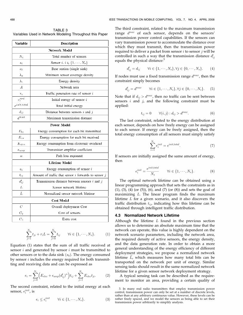
Table 3 lists the parameters that we use in this paper,including those used in the general network model, thepower model, the lifetime model, and the cost model.

4.1 Lifetime Model

We adopt as a common lifetime definition the time whenthe first sensor dies. This lifetime definition, proposed in

[7], is widely utilized in the sensor network research field.

An alternative lifetime definition that has been used is the

time at which a certain percentage of total nodes run out of

energy. This definition is actually quite similar in nature to

the one we use here. In a well-designed network, sensors in

a certain area exhibit similar behaviors to achieve energy

balance. In other words, when one sensor dies, it can be

expected that the neighbors of this node will run out of

energy very soon since they will have to take over the

responsibilities of that sensor. Therefore, in a well-designed

network, there should be little or no difference in lifetime

when using these two definitions.In our network model, a set of Ns sensors is deployed in

a region in order to monitor some physical phenomenon.

We refer to the complete set of sensors that has been

deployed as S ¼ fs1 . . . sNsg. Sensor i generates traffic at a

rate of ri bps. All of the data that is generated must

eventually reach a single data sink, labeled s0. We adopt the

power model in [18], where the amount of energy to

transmit a bit can be represented as Etx ¼ Eelec þ �ampd�,

and the amount of energy to receive a bit can be represented

as Erx ¼ Eelec, where Eelec represents the electronics energy,

�amp is determined by the transmitter amplifier’s efficiency

and the channel conditions, d represents the distance over

which data is being communicated, and � represents the

path loss exponent. The network scenario parameters also

include the traffic generation rate ri for each sensor, the

distances dij between sensors, and the maximum transmis-

sion distance dmax.

4.2 Lifetime Optimization

The goal of our network lifetime model is to discover the

maximum network lifetime L given a fixed deployment

strategy and network scenario parameters. The model is

able to determine this maximum by optimizing the amount

of traffic that each sensor should distribute to the other

sensors in order to balance energy consumption among the

sensors. This traffic distribution is denoted by tij, indicating

the amount of traffic that sensor i transmits to sensor j.2

During network lifetime L, sensor i will generate a total

of riL traffic. The first constraint of our problem, related to

the conservation of data flow at all sensor nodes, is


TABLE 2Sensor Network Deployment Strategies, Corresponding Scenarios, and Potential Difficulty/Extra Costs

2. Note that tii ¼ 0 8 i.

XNs

j¼1

tji þ riL ¼XNs

j¼0

tij 8i 2 f1; � � � ; Nsg: ð1Þ

Equation (1) states that the sum of all traffic received atsensor i and generated by sensor i must be transmitted toother sensors or to the data sink ðs0Þ. The energy consumedby sensor i includes the energy required for both transmit-ting and receiving data and can be expressed as

ei ¼XNs

j¼0

Eelec þ �ampðdtijÞ�

� �tij þ

XNs

j¼1

Eelectji: ð2Þ

The second constraint, related to the initial energy at eachsensor, einiti , is

ei � einiti 8i 2 f1; � � � ; Nsg: ð3Þ

The third constraint, related to the maximum transmissionrange dmax of each sensor, depends on the sensors’transmission power control capabilities. If the sensors canvary transmission power to accommodate the distance overwhich they must transmit, then the transmission powerrequired to deliver a packet from sensor i to sensor j will becontrolled in such a way that the transmission distance dtijequals the physical distance:3

dtij ¼ dij 8i 2 f1; � � � ; Nsg; 8j 2 f0; � � � ; Nsg: ð4Þ

If nodes must use a fixed transmission range dmax, then theconstraint simply becomes

dtij ¼ dmax 8i 2 f1; � � � ; Nsg; 8j 2 f0; � � � ; Nsg: ð5Þ

Note that if dij > dmax, then no traffic can be sent betweensensors i and j, and the following constraint must beapplied:

tij ¼ 0 8ði; jÞ : dij > dmax: ð6Þ

The last constraint, related to the energy distribution ateach sensor, depends on how freely energy can be assignedto each sensor. If energy can be freely assigned, then thetotal energy consumption of all sensors must simply satisfy

XNs

i¼1

einiti ¼ einit;total: ð7Þ

If sensors are initially assigned the same amount of energy,then

einiti ¼ einit;total

Ns8i 2 f1; � � � ; Nsg: ð8Þ

The optimal network lifetime can be obtained using alinear programming approach that sets the constraints as in(1), (3), (4) (or (5)), (6), and (7) (or (8)) and sets the goal ofmaximizing L. The linear program finds the maximumlifetime L for a given scenario, and it also discovers thetraffic distribution tij, indicating how this lifetime can beobtained through intelligent traffic distribution.

4.3 Normalized Network Lifetime

Although the lifetime L found in the previous sectionallows us to determine an absolute maximum time that thenetwork can operate, this value is highly dependent on thenetwork scenario parameters, including the network area,the required density of active sensors, the energy density,and the data generation rate. In order to obtain a moregeneral understanding of the energy efficiency of differentdeployment strategies, we propose a normalized networklifetime eL, which measures how many total bits can betransported on the network per unit of energy. Similarsensing tasks should result in the same normalized networklifetime for a given sensor network deployment strategy.

A typical sensing task can be described as the require-ment to monitor an area, providing a certain quality of


TABLE 3Variables Used in Network Modeling Throughout this Paper

3. In many real radio transmitters that employ transmission powercontrol, transmission power can only be set at a number of discrete levels,rather than at any arbitrary continuous value. However, these levels can berather finely spaced, and we model the sensors as being able to set theirtransmission power arbitrarily to simplify analysis.

service, for a certain period of time. For example, supposethat we want to monitor the temperature of a region forone year with a temperature sample rate of once per hour.The design parameters of this task include the averagetraffic generation rate among active sensors ð�rÞ, theminimum sensor coverage density �a, the initial energy

assigned to each node ð �einitÞ, and the monitoring period or

network lifetime ðLÞ. These parameters affect the absolute

lifetime, and they should be factored out during the

calculation of the normalized network lifetime. Note that

energy efficiency of each deployment strategy is dependent

on the area of the region being monitored, and so, we do not

attempt to remove this factor.In typical sensor networks, the network designer can

calculate the minimum number of sensors that are requiredto cover an area for a given application and required qualityof service. We denote this minimum sensor coveragedensity as �a. Sensors may be deployed more densely thanthe sensing application requires and allow their sensingactivity to be rotated while maintaining the same sensingcoverage goals [22], [23], [24], [25]. Once the network is fullycovered, the network lifetime can be arbitrarily increased bysimply putting more energy into the network. This can berealized by scaling up the deployed sensor density orincreasing the initial energy per sensor. The networklifetime can also be increased by reducing the trafficgeneration rate �r among active sensors. A normalizedlifetime eL that accounts for the total energy consumption byconsidering the above factors can be expressed as

eL ¼ L �r�a�e

� �; ð9Þ

where �a represents the minimum sensor coverage density,�r represents the average bit rate among active sensors,�e represents the energy density of the network (that is, howmuch energy is available per unit area), and L is the lifetimeachievable with the given scenario’s parameters.

In terms of units, L is measured in seconds, �r is measuredin bits per second, �a is measured in the number of sensorsper square meter, and �e is measured in Joules per squaremeter. eL is thus measured in terms of bits per Joule, whichexplicitly indicates the energy efficiency of a particulardeployment strategy for a given network scenario.

4.4 Cost Model

The normalized lifetime reflects the energy efficiency ofdifferent deployment plans. From the normalized lifetime,we can deduce the number of sensors that will need to bedeployed in order to meet the sensing requirements, givingsome indication of the cost to deploy the network. For aparticular deployment strategy DSi, given the sensingrequirements and a target network lifetime goal L, we cancalculate the number of required sensors Ns as follows:

NsðDSiÞ ¼minð�aA; L�r�aAeL �einit

Þ i ¼ 1; 2; 3; 5;

�aA i ¼ 4:

(ð10Þ

For deployment strategies DS1, DS2, DS3, and DS5, whereeach node has a uniform data generation rate �r and a uniforminitial energy �einit, (10) determines the number of sensors

that are needed based on the normalized lifetime eL, as wellas the application quality of service (sensing density). Fordeployment strategy DS4, (10) simply specifies that theminimum number of sensors that support the applicationquality of service (sensing density) should be deployed sinceunequal energy assignment can be used to ensure that thelifetime goal is met. In our cost analysis of strategies DS1,DS2, DS3, and DS5, we will assume that the applicationquality-of-service (sensing density) constraints are alwaysmet and that the network lifetime is the driving factor whendetermining how many sensors should be deployed.

More energy-efficient deployment strategies will have ahigher normalized lifetime (that is, they will carry moretraffic per unit of energy) and thus require a lower numberof sensors NsðDSiÞ to meet the target lifetime. Thus, thedeployment cost from sensors CsðDSiÞ is lowered. How-ever, these complex strategies may have higher extradeployment cost CeðDSiÞ. Our cost model explores theseextra costs that are often overlooked, and it enables theevaluation of different deployment strategies from amonetary cost perspective. The total cost for the sensorsis CsðDSiÞ ¼ csNsðDSiÞ, where cs represents the cost of anordinary microsensor, and the overall deployment costCðDSiÞ becomes

CðDSiÞ ¼ CeðDSiÞ þ CsðDSiÞ: ð11Þ

This cost model is a simple yet effective method forallowing a network designer to compare different deploy-ment strategies on an equal basis.

5 A CASE STUDY FOR THE SIMPLEST DEPLOYMENT

STRATEGY: DS1

We begin our study of the optimized network lifetime for

the simplest, most common sensor network deployment

scenario, DS1 in Table 2. For this deployment strategy, the

only option to reduce the effects of the hot-spot problem

and maximize the network lifetime is to employ intelligent

traffic distribution. Transmission power control can be used

along with the optimal traffic distribution to achieve both

energy efficiency and energy balance. Although it has been

shown that the ideal energy-efficient transmission range

for general ad hoc networks is dopt ¼ffiffiffiffiffiffiffiffiffiffiffiffiffiffiffiffi

2Eelecð��1Þ�amp

�

q[5], this

optimal transmission range is derived for networks in

which traffic flows are assumed to be randomly distributed

within the network rather than converging to a single base

station as in sensor networks. Thus, this fixed optimal

solution may not be suitable for many-to-one sensor

networks. In this section, we show how setting optimal

transmission ranges that vary with the sensors’ positions in

the network can help to balance energy consumption and

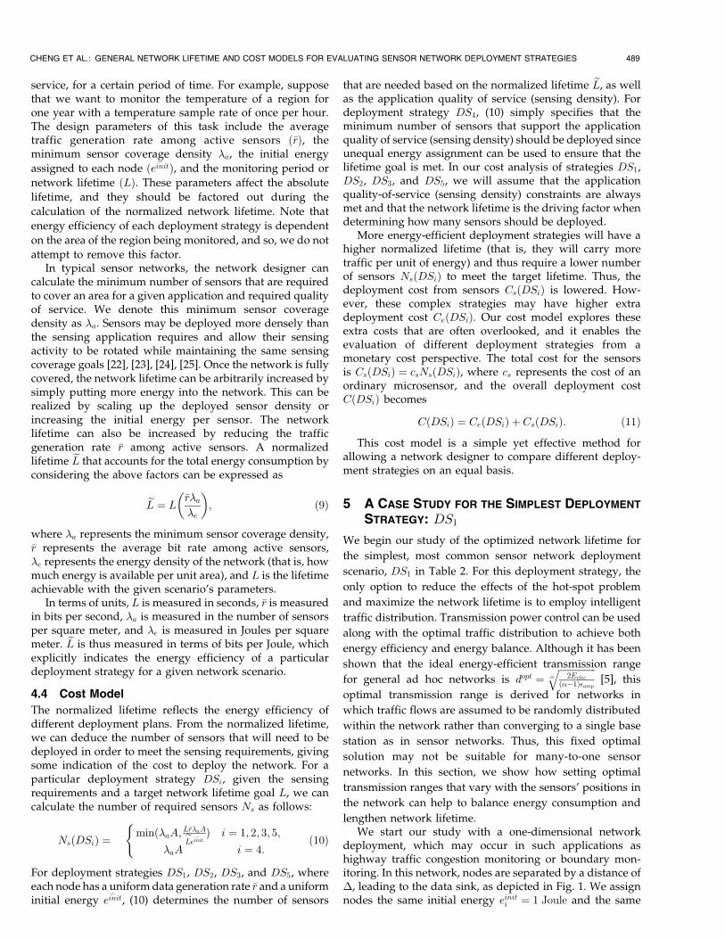
lengthen network lifetime.We start our study with a one-dimensional network

deployment, which may occur in such applications ashighway traffic congestion monitoring or boundary mon-itoring. In this network, nodes are separated by a distance of�, leading to the data sink, as depicted in Fig. 1. We assignnodes the same initial energy einiti ¼ 1 Joule and the same


traffic generation rate ri ¼ 1 bps. In all simulations andanalysis, we use values of Eelec ¼ 50 nJ=bit and �amp ¼100 pJ=bit=m2 [18].

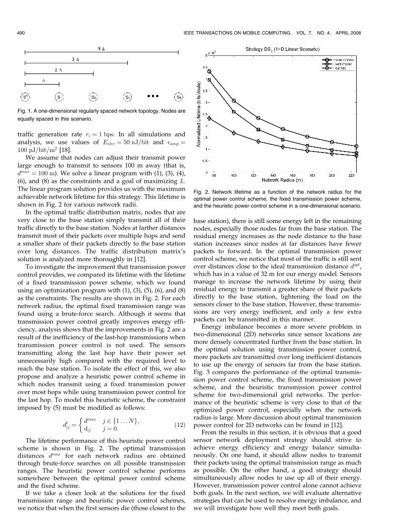
We assume that nodes can adjust their transmit powerlarge enough to transmit to sensors 100 m away (that is,dmax ¼ 100 m). We solve a linear program with (1), (3), (4),(6), and (8) as the constraints and a goal of maximizing L.The linear program solution provides us with the maximumachievable network lifetime for this strategy. This lifetime isshown in Fig. 2 for various network radii.

In the optimal traffic distribution matrix, nodes that arevery close to the base station simply transmit all of theirtraffic directly to the base station. Nodes at farther distancestransmit most of their packets over multiple hops and senda smaller share of their packets directly to the base stationover long distances. The traffic distribution matrix’ssolution is analyzed more thoroughly in [12].

To investigate the improvement that transmission powercontrol provides, we compared its lifetime with the lifetimeof a fixed transmission power scheme, which we foundusing an optimization program with (1), (3), (5), (6), and (8)as the constraints. The results are shown in Fig. 2. For eachnetwork radius, the optimal fixed transmission range wasfound using a brute-force search. Although it seems thattransmission power control greatly improves energy effi-ciency, analysis shows that the improvements in Fig. 2 are aresult of the inefficiency of the last-hop transmissions whentransmission power control is not used. The sensorstransmitting along the last hop have their power setunnecessarily high compared with the required level toreach the base station. To isolate the effect of this, we alsopropose and analyze a heuristic power control scheme inwhich nodes transmit using a fixed transmission powerover most hops while using transmission power control forthe last hop. To model this heuristic scheme, the constraintimposed by (5) must be modified as follows:

dtij ¼dmax j 2 f1 . . .Ng;dij j ¼ 0:

�ð12Þ

The lifetime performance of this heuristic power controlscheme is shown in Fig. 2. The optimal transmissiondistances dmax for each network radius are obtainedthrough brute-force searches on all possible transmissionranges. The heuristic power control scheme performssomewhere between the optimal power control schemeand the fixed scheme.

If we take a closer look at the solutions for the fixedtransmission range and heuristic power control schemes,we notice that when the first sensors die (those closest to the

base station), there is still some energy left in the remainingnodes, especially those nodes far from the base station. Theresidual energy increases as the node distance to the basestation increases since nodes at far distances have fewerpackets to forward. In the optimal transmission powercontrol scheme, we notice that most of the traffic is still sentover distances close to the ideal transmission distance dopt,which has in a value of 32 m for our energy model. Sensorsmanage to increase the network lifetime by using theirresidual energy to transmit a greater share of their packetsdirectly to the base station, lightening the load on thesensors closer to the base station. However, these transmis-sions are very energy inefficient, and only a few extrapackets can be transmitted in this manner.

Energy imbalance becomes a more severe problem intwo-dimensional (2D) networks since sensor locations aremore densely concentrated further from the base station. Inthe optimal solution using transmission power control,more packets are transmitted over long inefficient distancesto use up the energy of sensors far from the base station.Fig. 3 compares the performance of the optimal transmis-sion power control scheme, the fixed transmission powerscheme, and the heuristic transmission power controlscheme for two-dimensional grid networks. The perfor-mance of the heuristic scheme is very close to that of theoptimized power control, especially when the networkradius is large. More discussion about optimal transmissionpower control for 2D networks can be found in [12].

From the results in this section, it is obvious that a goodsensor network deployment strategy should strive toachieve energy efficiency and energy balance simulta-neously. On one hand, it should allow nodes to transmittheir packets using the optimal transmission range as muchas possible. On the other hand, a good strategy shouldsimultaneously allow nodes to use up all of their energy.However, transmission power control alone cannot achieveboth goals. In the next section, we will evaluate alternativestrategies that can be used to resolve energy imbalance, andwe will investigate how well they meet both goals.


Fig. 1. A one-dimensional regularly spaced network topology. Nodes are

equally spaced in this scenario.

Fig. 2. Network lifetime as a function of the network radius for the

optimal power control scheme, the fixed transmission power scheme,

and the heuristic power control scheme in a one-dimensional scenario.

6 COMPARISON OF DIFFERENT DEPLOYMENT

STRATEGIES

In the previous section, we showed that optimal traffic loaddistribution with transmission power control is not veryeffective in extending the network lifetime in somescenarios. However, for deployment strategy DS1, this isthe only option for extending the network lifetime. In thissection, we investigate how well each of the other strategieslisted in Table 2 improves the network lifetime. We willevaluate these strategies using the general normalizedlifetime and deployment cost models, defined in Section 4.

When determining the normalized lifetime for eachdeployment scenario, we use an arbitrary sample scenariothat is manageable in terms of memory and processingfor solving the linear programs. In the sample scenario,Ns ¼ 180 nodes are deployed in a disc with a radius of250 m, and sensors send traffic at a rate of �r ¼ 1 bps. Thetotal energy assigned to the sensors is 180 Joules. Thenetwork parameters for the sample scenario are summar-ized in Table 4. Once the values of eL have been determinedfor each deployment strategy via the analysis of thissample scenario, they can be used to compare the cost

efficiency of different deployment strategies for a largerscale target scenario. For each deployment strategy, we findthe normalized lifetime with and without transmissionpower control. For the scenarios without transmissionpower control, we perform a brute-force search over allpossible fixed transmission ranges so that we find an upperbound for that scenario using any transmission power.

6.1 Deployment Strategy DS1: Single Static Sink

The effectiveness of using transmission power control andoptimal traffic distribution with deployment strategy DS1

has been fully studied in Section 5. The normalized lifetimefor a 2D network utilizing the parameters in the samplescenario (Table 4) was found to be 4:69� 105 bits=J whenusing transmission power control and 1:62� 105 bits=Jwhen not using transmission power control.

6.2 Deployment Strategy DS2: Mobile Data Sink

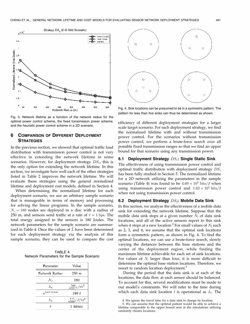
In this section, we analyze the effectiveness of a mobile datasink for extending the network lifetime. Suppose that themobile data sink stops at a given number Nl of data sinklocations, and all of the active sensors report to this sinkwhen it stops at a new location.4 For small values of Nl suchas 2, 3, and 4, we assume that the optimal sink locationsform a symmetric pattern, as shown in Fig. 4. To find theoptimal locations, we can use a brute-force search, slowlyvarying the distances between the base stations and thecenter of the deployment region, while finding themaximum lifetime achievable for each set of sink locations.For values of Nl larger than four, it is more difficult todetermine the optimal base station locations. Therefore, weresort to random location deployment.5

During the period that the data sink is at each of thelocations, the data flow at each sensor should be balanced.To account for this, several modifications must be made toour model’s constraints. We will refer to the time duringwhich each data sink location l is operational as Ll. The


4. We ignore the travel time for a data sink to change its location.5. We can assume that the optimal pattern would be able to achieve a

lifetime comparable to the upper bound seen in the simulations utilizingrandomly chosen locations.

Fig. 3. Network lifetime as a function of the network radius for the

optimal power control scheme, the fixed transmission power scheme,

and the heuristic power control scheme in a 2D scenario.

TABLE 4Network Parameters for the Sample Scenario

Fig. 4. Sink locations can be presumed to be in a symmetric pattern. The

pattern for less than five sinks can thus be determined as shown.

amount of traffic sent from sensor i to sensor j during thetime when sink location l is active will be denoted as tijl.The conservation of flow constraints become

XNs

j¼1

tijl þ riLl ¼XNs

j¼0

tijl 8i 2 f1; � � � ; Nsg; 8l 2 f1; � � � ; Nlg:

ð13Þ

Meanwhile, the energy consumption of each sensor shouldbe defined as

ei ¼XNs

j¼0

XNl

l¼1


� �tijl þ

XNs

j¼1

XNl

l¼1

Eelectjil: ð14Þ

The goal of the linear program is now to maximizePNl

l¼1 Ll.Note that sensors are required to send their traffic in a

timely manner. Although we do not consider packet delayin our analysis, we make a fundamental underlyingassumption that the data must reach its destination beforethe data sink moves to a new location. Otherwise, a nodecould simply hold the data until the base station movesto a nearby location, and the lifetime could be madearbitrarily high.

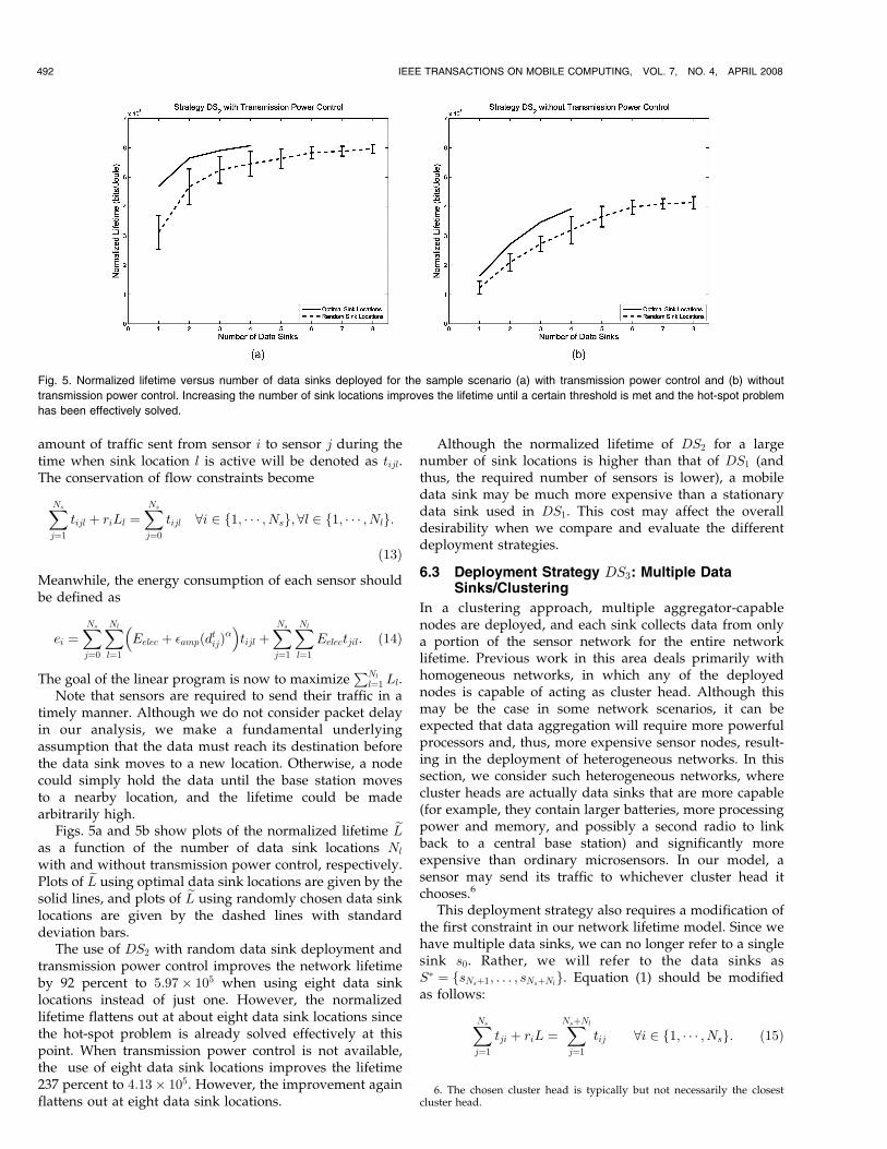
Figs. 5a and 5b show plots of the normalized lifetime eLas a function of the number of data sink locations Nl

with and without transmission power control, respectively.Plots of eL using optimal data sink locations are given by thesolid lines, and plots of eL using randomly chosen data sinklocations are given by the dashed lines with standarddeviation bars.

The use of DS2 with random data sink deployment andtransmission power control improves the network lifetimeby 92 percent to 5:97� 105 when using eight data sinklocations instead of just one. However, the normalizedlifetime flattens out at about eight data sink locations sincethe hot-spot problem is already solved effectively at thispoint. When transmission power control is not available,the use of eight data sink locations improves the lifetime237 percent to 4:13� 105. However, the improvement againflattens out at eight data sink locations.

Although the normalized lifetime of DS2 for a largenumber of sink locations is higher than that of DS1 (andthus, the required number of sensors is lower), a mobiledata sink may be much more expensive than a stationarydata sink used in DS1. This cost may affect the overalldesirability when we compare and evaluate the differentdeployment strategies.

6.3 Deployment Strategy DS3: Multiple DataSinks/Clustering

In a clustering approach, multiple aggregator-capablenodes are deployed, and each sink collects data from onlya portion of the sensor network for the entire networklifetime. Previous work in this area deals primarily withhomogeneous networks, in which any of the deployednodes is capable of acting as cluster head. Although thismay be the case in some network scenarios, it can beexpected that data aggregation will require more powerfulprocessors and, thus, more expensive sensor nodes, result-ing in the deployment of heterogeneous networks. In thissection, we consider such heterogeneous networks, wherecluster heads are actually data sinks that are more capable(for example, they contain larger batteries, more processingpower and memory, and possibly a second radio to linkback to a central base station) and significantly moreexpensive than ordinary microsensors. In our model, asensor may send its traffic to whichever cluster head itchooses.6

This deployment strategy also requires a modification ofthe first constraint in our network lifetime model. Since wehave multiple data sinks, we can no longer refer to a singlesink s0. Rather, we will refer to the data sinks asS� ¼ fsNsþ1; . . . ; sNsþNl

g. Equation (1) should be modifiedas follows:

XNs

j¼1

tji þ riL ¼XNsþNl

j¼1

tij 8i 2 f1; � � � ; Nsg: ð15Þ


Fig. 5. Normalized lifetime versus number of data sinks deployed for the sample scenario (a) with transmission power control and (b) without

transmission power control. Increasing the number of sink locations improves the lifetime until a certain threshold is met and the hot-spot problem

has been effectively solved.

6. The chosen cluster head is typically but not necessarily the closestcluster head.

The energy consumption of each sensor can be described as

ei ¼XNsþNl

j¼1


� �tij þ

XNs

j¼1

Eelectji: ð16Þ

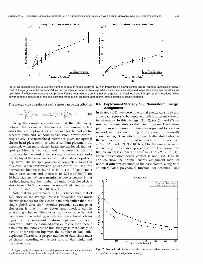
Using the sample scenario, we find the relationshipbetween the normalized lifetime and the number of datasinks that are deployed, as shown in Figs. 6a and 6b forschemes with and without transmission power control,respectively. The normalized lifetime is given for optimalcluster head placement,7 as well as random placement. Asexpected, when more cluster heads are deployed, the hot-spot problem is reduced, and the network lifetimeimproves. In the most extreme case, so many data sinksare deployed that every sensor can find a data sink just onehop away. The hot-spot problem is completely solved inthis case. When transmission power control is used, thenormalized lifetime is found to be 3:11� 105 bits=J for asingle base station and increases to 2:73� 106 bits=J for30 base stations. When transmission power control is notapplied, increasing the number of randomly deployed datasinks from 1 to 30 increases the normalized lifetime from1:19� 105 bits=J to 1:50� 106 bits=J.

Note that the performance of DS3 is better than that ofDS2 since on the average, traffic is forwarded over muchshorter distances (to the closest data sink rather than thesingle global data sink). Another potential advantage ofclustering is that it may better accommodate certainscheduling schemes. The cluster heads can serve as localcontrollers for scheduling, which brings additional advan-tages over the single-sink uniform deployment strategy.However, unlike the assumed fixed extra cost for a mobiledata sink, the extra cost of this strategy is more likely tohave a linear relationship with the number of data sinksdeployed. Therefore, a proper number of data sinks mustbe chosen according to the cost ratio of data sinks andnormal sensors.

6.4 Deployment Strategy DS4: Nonuniform EnergyAssignment

In strategy DS4, we loosen the initial energy constraint andallow each sensor to be deployed with a different value ofinitial energy. In this strategy, (1), (3), (4), (6), and (7) areused as the constraints for the linear program. The lifetimeperformance of nonuniform energy assignment for variousnetwork radii is shown in Fig. 7. Compared to the resultsshown in Fig. 3, in which optimal traffic distribution isthe only option, the normalized lifetime improves from4:69� 105 bits=J to 9:09� 105 bits=J for the sample scenariowhen using transmission power control. The normalizedlifetime increases from 1:62� 105 bit=J to 7:25� 105 bit=J

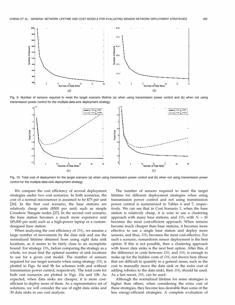
when transmission power control is not used. Figs. 8aand 8b show the optimal energy assignment map fornodes at different distances to the base station, along withan interpolated polynomial function, for schemes using


7. Again, optimal cluster head location patterns are only achievable for asmall number of cluster heads through brute-force searching.

Fig. 6. Normalized lifetime versus the number of cluster heads deployed (a) with transmission power control and (b) without transmission power

control. Large gains in the network lifetime can be achieved when even a few extra cluster heads are deployed, especially when their locations are

optimized. Random sink locations can provide lifetime improvement, but it is not as large as that obtained using the optimal sink locations. When

power control is unavailable, the gap between random sink locations and optimal sink locations is greatly reduced.

Fig. 7. Normalized lifetime as the network radius varies for the

nonuniform energy assignment strategy.

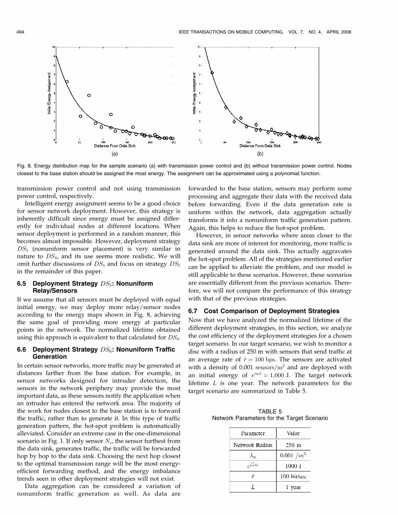
transmission power control and not using transmissionpower control, respectively.

Intelligent energy assignment seems to be a good choicefor sensor network deployment. However, this strategy isinherently difficult since energy must be assigned differ-ently for individual nodes at different locations. Whensensor deployment is performed in a random manner, thisbecomes almost impossible. However, deployment strategyDS5 (nonuniform sensor placement) is very similar innature to DS4, and its use seems more realistic. We willomit further discussions of DS4 and focus on strategy DS5

in the remainder of this paper.

6.5 Deployment Strategy DS5: NonuniformRelay/Sensors

If we assume that all sensors must be deployed with equalinitial energy, we may deploy more relay/sensor nodesaccording to the energy maps shown in Fig. 8, achievingthe same goal of providing more energy at particularpoints in the network. The normalized lifetime obtainedusing this approach is equivalent to that calculated for DS4.

6.6 Deployment Strategy DS6: Nonuniform TrafficGeneration

In certain sensor networks, more traffic may be generated atdistances farther from the base station. For example, insensor networks designed for intruder detection, thesensors in the network periphery may provide the mostimportant data, as these sensors notify the application whenan intruder has entered the network area. The majority ofthe work for nodes closest to the base station is to forwardthe traffic, rather than to generate it. In this type of trafficgeneration pattern, the hot-spot problem is automaticallyalleviated. Consider an extreme case in the one-dimensionalscenario in Fig. 1. If only sensor Ns, the sensor furthest fromthe data sink, generates traffic, the traffic will be forwardedhop by hop to the data sink. Choosing the next hop closestto the optimal transmission range will be the most energy-efficient forwarding method, and the energy imbalancetrends seen in other deployment strategies will not exist.

Data aggregation can be considered a variation ofnonuniform traffic generation as well. As data are

forwarded to the base station, sensors may perform some

processing and aggregate their data with the received data

before forwarding. Even if the data generation rate is

uniform within the network, data aggregation actually

transforms it into a nonuniform traffic generation pattern.

Again, this helps to reduce the hot-spot problem.However, in sensor networks where areas closer to the

data sink are more of interest for monitoring, more traffic is

generated around the data sink. This actually aggravates

the hot-spot problem. All of the strategies mentioned earlier

can be applied to alleviate the problem, and our model is

still applicable to these scenarios. However, these scenarios

are essentially different from the previous scenarios. There-

fore, we will not compare the performance of this strategy

with that of the previous strategies.

6.7 Cost Comparison of Deployment Strategies

Now that we have analyzed the normalized lifetime of the

different deployment strategies, in this section, we analyze

the cost efficiency of the deployment strategies for a chosen

target scenario. In our target scenario, we wish to monitor a

disc with a radius of 250 m with sensors that send traffic at

an average rate of �r ¼ 100 bps. The sensors are activated

with a density of 0.001 sensors=m2 and are deployed with

an initial energy of einit ¼ 1;000 J. The target network

lifetime L is one year. The network parameters for the

target scenario are summarized in Table 5.


Fig. 8. Energy distribution map for the sample scenario (a) with transmission power control and (b) without transmission power control. Nodes

closest to the base station should be assigned the most energy. The assignment can be approximated using a polynomial function.

TABLE 5Network Parameters for the Target Scenario

We compare the cost efficiency of several deploymentstrategies under two cost scenarios. In both scenarios, thecost of a normal microsensor is assumed to be $75 per unit[26]. In the first cost scenario, the base stations arerelatively cheap units ($500 per unit) such as simpleCrossbow Stargate nodes [27]. In the second cost scenario,the base station becomes a much more expensive unit($5,000 per unit) such as a high-power laptop or a custom-designed base station.

When analyzing the cost efficiency of DS2, we assume alarge number of movements by the data sink and use thenormalized lifetime obtained from using eight data sinklocations, as it seems to be fairly close to an asymptoticbound. For strategy DS3, before comparing the strategy as awhole, we must find the optimal number of sink locationsto use for a given cost model. The number of sensorsrequired for our target scenario when using strategy DS3 isplotted in Figs. 9a and 9b for schemes with and withouttransmission power control, respectively. The total costs forboth cost scenarios are plotted in Figs. 10a and 10b. Asexpected, when data sinks are cheaper, it is more cost-efficient to deploy more of them. As a representative set ofsolutions, we will consider the use of eight data sinks and30 data sinks in our cost analysis.

The number of sensors required to meet the targetlifetime for different deployment strategies when usingtransmission power control and not using transmissionpower control is summarized in Tables 6 and 7, respec-tively. We can see that in Cost Scenario 1, when the basestation is relatively cheap, it is wise to use a clusteringapproach with many base stations, and DS3 with Nl ¼ 30becomes the most cost-efficient approach. When sensorsbecome much cheaper than base stations, it becomes moreeffective to use a single base station and deploy moresensors, and thus, DS5 becomes the most cost-effective. Forsuch a scenario, nonuniform sensor deployment is the bestoption. If this is not possible, then a clustering approachwith fewer data sinks is the next best option. After this, ifthe difference in costs between DS1 and DS2 is enough tomake up for the hidden costs of DS2 not shown here (thosethat are difficult to quantify in a general sense, such as thecost to manually move the data sink or the extra cost ofadding robotics to the data sink), then DS2 should be used.As a last resort, DS1 can be used.

Although the normalized lifetime for some strategies ishigher than others, when considering the extra cost ofthese strategies, they become less desirable than some of theless energy-efficient strategies. A complete evaluation of


Fig. 9. Number of sensors required to meet the target scenario lifetime (a) when using transmission power control and (b) when not using

transmission power control for the multiple-data-sink deployment strategy.

Fig. 10. Total cost of deployment for the target scenario (a) when using transmission power control and (b) when not using transmission power

control for the multiple-data-sink deployment strategy.

different strategies should be performed from both anenergy and a cost perspective. Although these conclusionssound straightforward, our method provides a quantifica-tion on the overall cost, and thus, a clear method for making

a decision between several potential strategies.

7 CONCLUSIONS

In this paper, we proposed a general network lifetimemodel and a general deployment cost model to evaluatemultiple sensor network deployment strategies. In ourstudy, we have made the following observations:

1. Most sensor network deployment strategies can begeneralized and have their maximum achievablelifetime found using a linear programming model.Their differences lie in the freedom of deploymentparameters and the constraints on the networkparameters.

2. A good sensor network deployment strategy is onethat achieves both energy balance and energyefficiency.

3. Energy imbalance becomes worse when the networksize increases, and when the network goes from

one to two dimensions. The maximum achievablelifetime decreases accordingly.

4. Contrary to intuition, the strategy of transmissionpower control is not sufficient to resolve both energyimbalance and energy inefficiency. The limitedlifetime improvement from transmission powercontrol is mainly due to energy savings from nodesclose to the data sink.

5. A good strategy should allow sensors to send mostof their traffic at the general optimal transmissionrange (32 m in this paper).

6. The strategy of mobile-data-sink deployment hassome limitations on lifetime improvement, whereasthe strategy of deploying multiple data sinks cancontinue to improve the network lifetime as moresinks are added until the subnetworks becomeone-hop networks.

7. The strategy of nonuniform energy assignmentachieves both energy efficiency and energy balancesimultaneously. However, it is inherently difficultto apply in practice.

8. Although more intelligent strategies may have betterlifetime performance, the cost of these strategies


TABLE 6Cost Evaluation for the Two Cost Scenarios with Transmission Power Control

TABLE 7Cost Evaluation for the Two Cost Scenarios without Transmission Power Control

must be fully considered because once the qualityof service of a network is satisfied, the costbecomes the primary concern for a practical sensordeployment plan.

Thus, this paper has made the following contributions.

First, we propose a general lifetime model that can be

applied to many sensor network deployment strategies

with little or no modifications. Second, we reveal the

general lifetime trends for different deployment strategies.

Finally, we propose a general method to compare the

normalized lifetime and cost for different strategies, which

provides practical suggestions for real sensor deployment.

ACKNOWLEDGMENTS

This work was supported in part by the US Office of Naval

Research under Grant N00014-05-1-0626.

REFERENCES

[1] H. Takagi and L. Kleinrock, “Optimal Transmission Ranges forRandomly Distributed Packet Radio Terminals,” IEEE Trans.Comm., vol. 32, pp. 246-257, Mar. 1984.

[2] R. Ramanathan and R. Hain, “Topology Control of MultihopWireless Networks Using Transmit Power Adjustment,” Proc.IEEE INFOCOM, 2000.

[3] V. Rodoplu and T. Meng, “Minimum Energy Mobile WirelessNetworks,” Proc. IEEE Int’l Conf. Comm. (ICC), 1998.

[4] B. Calhoun, D. Daly, N. Verma, D. Finchelstein, D. Wentzloff,A. Wang, S. Cho, and A. Chandrakasan, “Design Considerationsfor Ultra-Low Energy Wireless Microsensor Nodes,” IEEE Trans.Computers, vol. 54, no. 6, pp. 727-740, June 2005.

[5] I. Stojmenovic and X. Lin, “Power-Aware Localized Routing inWireless Networks,” IEEE Trans. Parallel and Distributed Systems,vol. 12, no. 10, pp. 1122-1133, Oct. 2001.

[6] S. Singh, M. Woo, and C. Raghavendra, “Power-Aware Routing inMobile Ad Hoc Networks,” Proc. ACM MobiCom, 1998.

[7] J. Chang and L. Tassiulas, “Energy Conserving Routing inWireless Ad Hoc Networks,” Proc. IEEE INFOCOM, 2000.

[8] C. Efthymiou, S. Nikoletseas, and J. Rolim, “Energy Balanced DataPropagation in Wireless Sensor Networks,” Proc. 18th Int’l Paralleland Distributed Processing Symp. (IPDPS), 2004.

[9] M. Bhardwaj and A. Chandrakasan, “Bounding the Lifetime ofSensor Networks via Optimal Role Assignments,” Proc. IEEEINFOCOM, 2002.

[10] M. Perillo and W. Heinzelman, “Simple Approaches for ProvidingApplication QoS through Intelligent Sensor Management,”Elsevier Ad Hoc Networks J., vol. 1, no. 2-3, pp. 235-246, 2003.

[11] G. Zussman and A. Segall, “Energy Efficient Routing in Ad HocDisaster Recovery Networks,” Proc. IEEE INFOCOM, 2003.

[12] M. Perillo, Z. Cheng, and W. Heinzelman, “On the Problem ofUnbalanced Load Distribution in Wireless Sensor Networks,”Proc. Global Telecommunications Conf. (GLOBECOM ’04) WorkshopWireless Ad Hoc and Sensor Networks, 2004.

[13] R. Shah, S. Roy, S. Jain, and W. Brunette, “Data MULEs: Modelinga Three-Tier Architecture for Sparse Sensor Networks,” Proc.First IEEE Workshop Sensor Network Protocols and Applications(SNPA), 2003.

[14] H. Kim, T. Abdelzaher, and W. Kwon, “Minimum-EnergyAsynchronous Dissemination to Mobile Sinks in Wireless SensorNetworks,” Proc. First ACM Conf. Embedded Networked SensorSystems (SenSys), 2003.

[15] J. Luo and J. Hubaux, “Joint Mobility and Routing for LifetimeElongation in Wireless Sensor Networks,” Proc. IEEE INFOCOM,2005.

[16] M. Kalantari and M. Shayman, “Design Optimization of Multi-Sink Sensor Networks by Analogy to Electrostatic Theory,” Proc.IEEE Wireless Comm. and Networking Conf. (WCNC), 2006.

[17] C. Wan, S. Eisenman, A. Campbell, and J. Crowcroft, “Siphon:Overload Traffic Management Using Multi-Radio Virtual Sinks inSensor Networks,” Proc. Third ACM Conf. Embedded NetworkedSensor Systems (SenSys), 2005.

[18] W. Heinzelman, A. Chandrakasan, and H. Balakrishnan,“An Application-Specific Protocol Architecture for WirelessMicrosensor Networks,” IEEE Trans. Wireless Comm., vol. 1,pp. 660-670, Oct. 2002.

[19] S.C. Ergen and P. Varaiya, “Optimal Placement of Relay Nodes forEnergy Efficiency in Sensor Networks,” Proc. IEEE Int’l Conf.Comm. (ICC), 2006.

[20] Y.T. Hou, Y. Shi, H.D. Sherali, and S.F. Midkiff, “ProlongingSensor Network Lifetime with Energy Provisioning and RelayNode Placement,” Proc. Second Ann. IEEE Int’l Conf. Sensor andAd Hoc Comm. and Networks (SECON), 2005.

[21] I. Howitt and J. Wang, “Energy Balanced Chain in Wireless SensorNetworks,” Proc. IEEE Wireless Comm. and Networking Conf.(WCNC), 2004.

[22] X. Wang, G. Xing, Y. Zhang, C. Lu, R. Pless, and C. Gill,“Integrated Coverage and Connectivity Configuration in WirelessSensor Networks,” Proc. First ACM Conf. Embedded NetworkedSensor Systems (SenSys), 2003.

[23] F. Ye, G. Zhong, J. Cheng, S. Lu, and L. Zhang, “PEAS: ARobust Energy Conserving Protocol for Long-Lived SensorNetworks,” Proc. 23rd Int’l Conf. Distributed Computing Systems(ICDCS), 2003.

[24] J. Elson, L. Girod, and D. Estrin, “Fine-Grained Network TimeSynchronization Using Reference Broadcasts,” Proc. Fifth Symp.Operating Systems Design and Implementation (OSDI), 2002.

[25] M. Perillo and W. Heinzelman, “DAPR: A Protocol for WirelessSensor Networks Utilizing an Application-Based Routing Cost,”Proc. IEEE Wireless Comm. and Networking Conf. (WCNC), 2004.

[26] Moteiv Corp., http://www.moteiv.com, 2006.[27] Crossbow Technology, Inc., http://www.xbow.com, 2006.

Zhao Cheng received the BS degree in radioengineering from Southeast University, China, in2000 and the MS and PhD degrees in electricaland computer engineering from the University ofRochester in 2003 and 2006. His researchinterests include sensor networks, quality ofservice (QoS) and reliability for mobile ad hocnetworks, and efficient discovery strategies formobile ad hoc networks.

Mark Perillo received the BS and MS degreesin electrical and computer engineering from theUniversity of Rochester in 2000 and 2002,respectively. He is a PhD candidate in theDepartment of Electrical and Computer Engi-neering, University of Rochester. His researchinterests include wireless communications andad hoc and sensor networks.

Wendi B. Heinzelman received the BS degreein electrical engineering from Cornell Universityin 1995 and the MS and PhD degrees inelectrical engineering and computer sciencefrom the Massachusetts Institute of Technologyin 1997 and 2000, respectively. She is anassociate professor in the Department of Elec-trical and Computer Engineering, University ofRochester. Her current research interests in-clude wireless communications and networking,

mobile computing, and multimedia communication. She received theNSF CAREER Award in 2005 for her work on cross-layer architecturesfor wireless sensor networks and the ONR Young Investigator Award in2005 for her work on balancing resource utilization in wireless sensornetworks. She is a member of the ACM and a senior member of theIEEE.

. For more information on this or any other computing topic,please visit our Digital Library at www.computer.org/publications/dlib.


Documents

General Network Lifetime and Cost Models for Evaluating Sensor Network Deployment Strategies