arX

iv:h

ep-t

h/00

0523

5v1

25

May

200

0

Gauge Field Theory Coherent States (GCS) : IV.Infinite Tensor Product

and Thermodynamical Limit

T. Thiemann∗, O. Winkler†

MPI f. Gravitationsphysik, Albert-Einstein-Institut,

Am Muhlenberg 1, 14476 Golm near Potsdam, Germany

Preprint AEI-2000-030

Abstract

In the canonical approach to Lorentzian Quantum General Relativity in fourspacetime dimensions an important step forward has been made by Ashtekar, Ishamand Lewandowski some eight years ago through the introduction of a Hilbert spacestructure which was later proved to be a faithful representation of the canonicalcommutation and adjointness relations of the quantum field algebra of diffeomor-phism invariant gauge field theories by Ashtekar, Lewandowski, Marolf, Mourao andThiemann.

This Hilbert space, together with its generalization due to Baez and Sawin, isappropriate for semi-classical quantum general relativity if the spacetime is spatiallycompact. In the spatially non-compact case, however, an extension of the Hilbertspace is needed in order to approximate metrics that are macroscopically nowheredegenerate.

For this purpose, in this paper we apply the theory of the Infinite Tensor Product(ITP) of Hilbert Spaces, developed by von Neumann more than sixty years ago, toQuantum General Relativity. The cardinality of the number of tensor productfactors can take the value of any possible Cantor aleph, making this mathematicaltheory well suited to our problem in which a Hilbert space is attached to each edgeof an arbitrarily complicated, generally infinite graph.

The new framework opens a pandora’s box full of techniques, appropriate topose fascinating physical questions such as quantum topology change, semi-classicalquantum gravity, effective low energy physics etc. from the universal point of view ofthe ITP. In particular, the study of photons and gravitons propagating on fluctuatingquantum spacetimes is now in reach, the topic of the next paper in this series.

1 Introduction

Quantum General Relativity (QGR) has matured over the past decade to a mathemat-ically well-defined theory of quantum gravity. In contrast to string theory, by defini-tion QGR is a manifestly background independent, diffeomorphism invariant and non-perturbative theory. The obvious advantage is that one will never have to postulate the

∗thiemann@aei-potsdam.mpg.de†winkler@aei-potsdam.mpg.de

existence of a non-perturbative extension of the theory, which in string theory has beencalled the still unknown M(ystery)-Theory.

The disadvantage of a non-perturbative and background independent formulation is,of course, that one is faced with new and interesting mathematical problems so thatone cannot just go ahead and “start calculating scattering amplitudes”: As there is nobackground around which one could perturb, rather the full metric is fluctuating, oneis not doing quantum field theory on a spacetime but only on a differential manifold.Once there is no (Minkowski) metric at our disposal, one loses familiar notions such ascausality structure, locality, Poincare group and so forth, in other words, the theory is nota theory to which the Wightman axioms apply. Therefore, one must build an entirely newmathematical apparatus to treat the resulting quantum field theory which is drasticallydifferent from the Fock space picture to which particle physicists are used to.

As a consequence, the mathematical formulation of the theory was the main focusof research in the field over the past decade. The main achievements to date are thefollowing (more or less in chronological order) :

i) Kinematical FrameworkThe starting point was the introduction of new field variables [1] for the gravita-tional field which are better suited to a background independent formulation of thequantum theory than the ones employed until that time. In its original versionthese variables were complex valued, however, currently their real valued version,considered first in [2] for classical Euclidean gravity and later in [3] for classicalLorentzian gravity, is preferred because to date it seems that it is only with thesevariables that one can rigorously define the kinematics andf dynamics of Euclideanor Lorentzian quantum gravity [4].These variables are coordinates for the infinite dimensional phase space of an SU(2)gauge theory subject to further constraints besides the Gauss law, that is, a con-nection and a canonically conjugate electric field. As such, it is very natural tointroduce smeared functions of these variables, specifically Wilson loop and electricflux functions. (Notice that one does not need a metric to define these functions,that is, they are background independent). This had been done for ordinary gaugefields already before in [5] and was then reconsidered for gravity (see e.g. [6]).The next step was the choice of a representation of the canonical commutation rela-tions between the electric and magnetic degrees of freedom. This involves the choiceof a suitable space of distributional connections [7] and a faithful measure thereon [8]which, as one can show [9], is σ-additive. The corresponding L2 Hilbert space and itsgeneralization [10] will be henceforth called the Ashtekar-Isham-Lewandowski-Baez-Sawin (AILBS) Hilbert space. The proof that the AILBS Hilbert space indeed solvesthe adjointness relations induced by the reality structure of the classical theory aswell as the canonical commutation relations induced by the symplectic structure ofthe classical theory can be found in [11]. Independently, a second representationof the canonical commutation relations, called the loop representation, had beenadvocated (see e.g. [12] and especially [13] and references therein) but both repre-sentations were shown to be unitarily equivalent in [14] (see also [15] for a differentmethod of proof).This is then the first major achievement : The theory is based on a rigorouslydefined kinematical framework.

ii) Geometrical OperatorsThe second major achievement concerns the spectra of positive semi-definite, self-adjoint geometrical operators measuring lengths [16], areas [17, 18] and volumes[17, 19, 20, 21, 12] of curves, surfaces and regions in spacetime. These spectra

are pure point (discete) and imply a discrete Planck scale structure. It should bepointed out that the discreteness is, in contrast to other approaches to quantumgravity, not put in by hand but it is a prediction !

iii) Regularization- and Renormalization TechniquesThe third major achievement is that there is a new regularization and renormaliza-tion technique [22, 23] for diffeomorphism covariant, density-one-valued operators atour disposal which was successfully tested in model theories [24]. This technique canbe applied, in particular, to the standard model coupled to gravity [25, 26] and tothe Poincare generators at spatial infinity [27]. In particular, it works for Lorentziangravity while all earlier proposals could at best work in the Euclidean context only(see, e.g. [13] and references therein). The algebra of important operators of theresulting quantum field theories was shown to be consistent [28]. Most surprisingly,these operators are UV and IR finite ! Notice that, at least as far as these operatorsare concerned, this result is stronger than the believed but unproved finiteness ofscattering amplitudes order by order in perturbation theory of the five critical stringtheories, in a sense we claim that the perturbation series converges. The absenceof the divergences that usually plague interacting quantum fields propagating ona Minkowski background can be understood intuitively from the diffeomorphisminvariance of the theory : “short and long distances are gauge equivalent”. We willelaborate more on this point in future publications.

iv) Spin Foam ModelsAfter the construction of the densely defined Hamiltonian constraint operator of[22, 23], a formal, Euclidean functional integral was constructed in [29] and gaverise to the so-called spin foam models (a spin foam is a history of a graph with facesas the history of edges) [30]. Spin foam models are in close connection with causalspin-network evolutions [31], state sum models [32] and topological quantum fieldtheory, in particular BF theory [33]. To date most results are at a formal level andfor the Euclidean version of the theory only but the programme is exciting sinceit may restore manifest four-dimensional diffeomorphism invariance which in theHamiltonian formulation is somewhat hidden.

v) Finally, the fifth major achievement is the existence of a rigorous and satisfactoryframework [34, 35, 36, 37, 38, 39, 40] for the quantum statistical description of blackholes which reproduces the Bekenstein-Hawking Entropy-Area relation and applies,in particular, to physical Schwarzschild black holes while stringy black holes so farare under control only for extremal charged black holes.

Summarizing, the work of the past decade has now culminated in a promising startingpoint for a quantum theory of the gravitational field plus matter and the stage is set topose and answer physical questions.

The most basic and most important question that one should ask is : Does the theoryhave classical general relativity as its classical limit ? Notice that even if the answeris negative, the existence of a consistent, interacting, diffeomorphism invariant quantumfield theory in four dimensions is already a quite non-trivial result. However, we can claimto have a satisfactory quantum theory of Einstein’s theory only if the answer is positive.

In order to address this question with a mathematically well-defined procedure we havedeveloped in [41, 42] a theory of coherent states for the matter content of the standardmodel (with possible supersymmetric extensions) coupled to gravity. These states arelabelled by classical solutions to the field equations and have the property that a) theexpectation values of densely defined field operators with respect to these states take the

value prescribed by the classical solution and b) they saturate the Heisenberg uncertaintybound without quenching.

The way this has been achieved so far is the following : The degrees of freedom of, say,the gravitational field, are labelled by piecewise analytic (smooth) graphs (webs) composedof a finite number of edges (paths) only. For each such graph one finds a subspaceof the AILBS Hilbert space which is the finite tensor product of mutually isomorphicHilbert spaces, one for each edge (path) of the graph (web). The closure of finite linearcombinations of vectors from these subspaces labelled by graphs (webs), which turn outto be mutually orthogonal, is forms the AILBS Hilbert space. What has been done in[41, 42] is to develop a theory of coherent states for each of these Hilbert spaces labelledby a finite graph γ. More precisely, one constructs coherent states ψse for each of theHilbert spaces labelled by a single edge e of γ and the classicality parameter s (s → 0 isthe classical limit) and then the coherent state for the whole graph γ is simply the tensorproduct of those for each of its edges.

This framework is sufficient if the initial data hypersurface Σ is compact since onecan describe the quantum metric as precisely as one wishes in terms of finite graphs bytaking the graph to be finer and finer, filling Σ more and more densely. However, if Σ isnon-compact, say of the topology of R3 as required for Minkwoski space or the Kruskalextension of the Schwarzschild spacetime which in turn are the most important spacetimesif we want to make contact with the low energy physics of the standard model, scatteringtheory, Hawking radiation and thus the semiclassical approximation of quantum gravityby the theory of ordinary Quantum Field Theory on (curved) backgrounds, then the aboveframework is insufficient. What one needs in this case is an infinite graph no matter howcoarse the graph is, that is, no matter whether the lattice spacing is 1mm or of the orderof the Planck length, in order to fill Σ everywhere we need an infinite graph, no region ofΣ of infinite volume must be empty if we wish to approximate a non-degenerate metricas all the classical metrics are.

One may think that one can get away by taking an infinite superposition of stateslabelled by mutually different finite graphs. However, such states have infinite norm withrespect to the AILBS scalar product as the following simple example shows : Namely,let γ∞ be a cubic lattice, an infinte graph filling all of Σ := R3 as densely as we wishand construct the state ψs :=

∑e zeTe where the sum runs over all edges of γ∞, ze

are complex coefficients and Te is some linear combination of spin-network states overe. Obviously, this state is an infinite linear combination of states over finite graphs.Then, because of homogenity, this state produces the correct classical limit, correspondingto, say, Minkowski space, for each of the holonomy operators he at most if ze = z isindependent of e and Te(he) = T (he) is the same linear combination of spin-networkstates for each e. But then the norm of the state is formally |z|2||T ||2 ∑

e 1 = ∞ andbadly diverges.

On the other hand, we will show that one can give meaning to states of the formψsγ∞ := ⊗eψ

se where γ∞ is an infinite graph and if one defines the inner product to be the

product of the inner products of the tensor product factors, then ||ψsγ∞|| = 1 while thesemiclassical behaviour with respect to every possible operator over γ∞ is preserved andidentical to the one for finite tensor products. Notice that in our case the dimension ofthe Hilbert space over each edge is countably infinite. If γ∞ is countably infinite, the caseto which we restrict in this paper, then the direct sum Hilbert space is still separable.But even if the Hilbert space over each edge would be only two-dimensional then thecountably infinite tensor product Hilbert space is non-separable !

This article is organized as follows :

In section two we recall the basic kinematical structure of canonical Quantum GeneralRelativity.

In section three we list the essential properties of our family of coherent states forfinite tensor products as needed for the purpose of the present paper.

In section four we give an account of von Neumann’s theory of the Infinite TensorProduct [43] for the general case, in particular the occurance of von Neumann algebrasof different factor types induced by the operator algebras on each tensor product factor.

Section five contains the new results of this paper. We apply the general ITP theoryto our situation focussing on general and abstract properties only. We extend the quan-tum kinematical framework of Ashtekar, Isham and Lewandowski to piecewise analytical,infinite graphs, connect it with the (semi)classical analysis for canonical quantum fieldtheories over non-compact initial data hypersurfaces and finally discuss the transfer ofdynamical results as obtained earlier for finite graphs.

In particular, for any possible solution of the Einstein field equations we are able toidentify an element of the ITP Hilbert space, a so-called C0-vector Ω in von Neumann’sterminology, which in the theory of quantum fields propagating on curved backgroundspacetimes, plays the role of the vacuum or ground state and which can be constructedpurely in terms of our coherent states. Perturbations of this vacuum, which in von Neu-mann’s terminology lie in the subspace of the ITP Hilbert space generated by the strongequivalence class of the C0-vector Ω, can naturally be identified with the usual Fock statesof QFT on the curved background that Ω approximates. This opens the possibility tomake contact with the usual perturbation theory defined in terms of Fock states.

In fact, in [74] we show that it is possible to map a precisely defined subspace ofthe ITP Hilbert space for Einstein-Maxwell theory, to the Fock space defined in termsof, say, n−Photon states propagating on Minkowski spacetime up to corrections due topure quantum gravity effects caused by the fluctuating nature of the quantum metric andwhich one hopes to measure in experiment. More precisely, this subspace is generatedby the operator algebra of the Maxwell field acting on a C0-vector Ω of the Einstein-Maxwell ITP Hilbert space and which is cyclic for that subspace. This vector Ω is aminimal uncertainty vector for Einstein-Maxwell theory approximating the Minkowskimetric and vanishing electromagnetic field respectively. It should be noted, however, thatall the states so constructed are states of the fully interacting Einstein-Maxwell theoryand not only of the free Maxwell theory propagating on Minkowski space (an exampleof a free quantum field theory on a fixed curved background). The two sets of states soconstructed are in a one-to one and onto correspondence, leading to expectation values forphysical operators which coincide to lowest order in the Planck length. As far as quantumgravity corrections are concerned, however, these states are physically very different, thestates of the interacting theory give rise to the so-called γ−ray-burst effect [44] which isjust one way to measure the Poincare non-invariance of the present state of our universeat the fundamental level. In [45] we will explicitly compute the size of this effect fromfirst principles by a down-to-the-ground-computation, thereby significantly improving theresults of [46].

2 Kinematical Structure of Diffeomorphism Invari-

ant Quantum Gauge Theories

In this section we will recall the main ingredients of the mathematical formulation of(Lorentzian) diffeomorphism invariant classical and quantum field theories of connectionswith local degrees of freedom in any dimension and for any compact gauge group. See[41, 11] and references therein for more details.

2.1 Classical Theory

Let G be a compact gauge group, Σ a D−dimensional manifold and consider a principalG−bundle with connection over Σ. Let us denote the pull-back (by local sections) to Σof the connection by Aia where a, b, c, .. = 1, .., D denote tensorial indices and i, j, k, .. =1, .., dim(G) denote indices for the Lie algebra of G. Likewise, consider a vector bundleof electric fields, whose projection to Σ is a Lie algebra valued vector density of weightone. We will denote the set of generators of the rank N − 1 Lie algebra of G by τi whichare normalized according to tr(τiτj) = −Nδij and [τi, τj ] = 2fij

kτk defines the structureconstants of Lie(G).

Let F ai be a Lie algebra valued vector density test field of weight one and let f ia be a

Lie algebra valued covector test field. We consider the smeared quantities

F (A) :=∫

ΣdDxF a

i Aia and E(f) :=

∫

ΣdDxEa

i fia (2.1)

While both objects are diffeomorphism covariant, only the latter is gauge covariant, onereason to introduce the singular smearing discussed below. The choice of the space of pairsof test fields (F, f) ∈ S depends on the boundary conditions on the space of connectionsand electric fields which in turn depends on the topology of Σ and will not be specifiedin what follows.

Consider the set M of all pairs of smooth functions (A,E) on Σ such that (2.1) iswell defined for any (F, f) ∈ S. We define a topology on M through the globally definedmetric :

dρ,σ[(A,E), (A′, E ′)] (2.2)

:=

√√√√√− 1

N

∫

ΣdDx[

√det(ρ)ρabtr([Aa − A′

a][Ab − A′b]) +

[σabtr([Ea −Ea′][Eb − Eb′])√det(σ)

]

where ρab, σab are fiducial metrics on Σ of everywhere Euclidean signature. Their fall-offbehaviour has to be suited to the boundary conditions of the fields A,E at spatial infinity(if Σ is spatially non-compact). Notice that the metric (2.2) on M is gauge invariant.It can be used in the usual way to equip M with the structure of a smooth, infinitedimensional differential manifold modelled on a Banach (in fact Hilbert) space E whereS × S ⊂ E . (It is the weighted Sobolev space H2

0,ρ ×H20,σ−1 in the notation of [48]).

Finally, we equip M with the structure of an infinite dimensional symplectic manifoldthrough the following strong (in the sense of [49]) symplectic structure

Ω((f, F ), (f ′, F ′))m :=∫

ΣdDx[F a

i fi′a − F a′

i fia](x) (2.3)

for any (f, F ), (f ′, F ′) ∈ E . We have abused the notation by identifying the tangent spaceto M at m with E . To see that Ω is a strong symplectic structure one uses standardBanach space techniques. Computing the Hamiltonian vector fields (with respect to Ω)of the functions E(f), F (A) we obtain the following elementary Poisson brackets

E(f), E(f ′) = F (A), F ′(A) = 0, E(f), A(F ) = F (f) (2.4)

As a first step towards quantization of the symplectic manifold (M,Ω) one must choosea polarization. As usual in gauge theories, we will use connections as the configurationvariables and electric fields as canonically conjugate momenta. As a second step onemust decide on a complete set of coordinates of M which are to become the elementaryquantum operators. The analysis just outlined suggests to use the coordinates E(f), F (A).

However, the well-known immediate problem is that these coordinates are not gaugecovariant. Thus, we proceed as follows :

The idea is to construct the theory from smaller building blocks, labelled by graphsembedded into Σ. In the literature, two sets of graphs, labelling the so-called cylindricalfunctions, have been proposed : the set of finite piecewise analytical graphs Γω0 in [8] andin [10, 50] the restriction Γ∞

0 to so-called “webs” of the set of all piecewise smooth graphsΓ∞. (We do not discuss here a third alternative, the set of finite piecewise linear graphs[51]). Here we call a graph γ finite if its sets of oriented edges e and vertices v respectively,denoted by E(γ) and V (γ) respectively, have finite cardinality. A web is a special kindof a piecewise smooth graph which may not be finite but which can be obtained as theunion of a finite number of smooth curves with finite range (the diffeomorphic image in Σof a closed interval in R) and such that its vertex set has a finite number of accumulationpoints. (In fact, this is the essential difference between Γω0 and Γ∞

0 since a graph generatedby a finite number of analytical curves is a piecewise analytical, finite graph which cannothave any accumulation points). There are some additional restrictions on the commonintersections of the curves in a web which we do not need to explain here, see [10] forall details. It is not difficult to prove that both Γω0 ,Γ

∞0 are closed under forming finite

numbers of intersections and unions.In this paper we are going to extend the framework to truly infinite graphs. That

is, a priori, we do not impose any finiteness restriction neither on the number of edgesor vertices of a graph nor on the range of its edges. Various extensions are possible. Asimple possibility is the set Γω of piecewise analytic graphs with possibly a countablyinfinite number of edges. Such graphs can still have accumulation points of edges andvertices (e.g. the graph which looks like a ladder in a two-plane whose spokes are mutuallyparallel and come arbitrarily close to each other). An even simpler choice is the set Γωσ ofpiecewise analytic, σ-finite graphs which can be considered in locally compact manifoldsΣ (every point has a compact neighbourhood) which, of course, is satisfied for any finite-dimensional manifold that we have in mind here. They are characterized by the fact thatγ∪U ∈ Γω0 , i.e. the restriction of γ to any compact set is a piecewise analytic finite graphwhose number of edges is uniformly bounded. More precisely :

Definition 2.1 Let Σ be a locally compact manifold. A graph γ ∈ Γωσ is said to be apiecewise analytic, σ-finite graph, if for each compact subset U ⊂ Σ the restriction of thegraph is a finite graph, γ ∪ U ∈ Γω0 . Moreover, for any compact cover U of Σ the set|E(γ ∩ U)|; U ∈ U is bounded.

Clearly, truly infinite piecewise analytic graphs exist only if Σ is not compact and in thiscase Γω0 is a proper subset of Γω. In order to obtain maximally nice graphs we will makethe further restriction that Σ is paracompact, see section 5.1.

The next simple choice is the set Γ∞ of all piecewise smooth graphs with possiblya countable number of edges and possibly a countable number of accumulation points.More properly, we should call them the set of infinite webs, that is, the web γ is allowedto be generated by a countably infinite number of smooth curves such that for each accu-mulation point pi, i = 1, .., N ≤ ∞ there exists a neighbourhood Ui such that the Ui aremutually disjoint and such that γ restricted to Ui is an element of Γ∞

0 . It is a non-trivialtask to decide whether any of the three sets Γω,Γωσ ,Γ

∞ are closed under taking finiteunions and we will do this in this paper only for Γωσ , leaving the remaining cases for futurepublications.

Finally, we could consider Γ, the set of all piecewise smooth, oriented graphs γ em-bedded into Σ. That is, we do not impose any restriction on the cardinality of the setsE(γ), V (γ), or on the nature of the accumulation points. This set is trivially closed under

arbitrary unions but it is beyond present analytical control, furthermore, it is not clearwhether Γ and Γ∞ are really different and to analyze these questions is beyond the scopeof the present paper, too.

Suffice it to say that for the purposes that we have in mind, to take the classical limit,it is sufficient to work with the set Γωσ that is technically much easier to handle. Thus,from now on we will assume that γ ∈ Γωσ , the typical graph that we will need in ourapplications and that is good to have in mind as an example is a regular cubic lattice inR3.

Let γ be a graph and e an edge of γ. We denote by he(A) the holonomy of A along eand say that a function f on A is cylindrical with respect to γ if there exists a functionfγ on G|E(γ)| such that f = p∗γfγ = fγ pγ where pγ(A) = he(A)e∈E(γ). The set offunctions cylindrical over γ is denoted by Cylγ . Holonomies are invariant under reparam-eterizations of the edge and in this article we assume that the edges are always analyticitypreserving diffeomorphic images from [0, 1] to a one-dimensional submanifold of Σ if it hascompact range and from [0, 1), (0, 1], (0, 1) if it has semi-finite or infinite range. Gaugetransformations are functions g : Σ 7→ G; x 7→ g(x) and they act on holonomies ashe 7→ g(e(0))heg(e(1))−1 where in the (semi)finite case e(0) or e(1) or both are not pointsin Σ and we simply set g(e(0)) = 1 or g(e(1)) = 1, which is justified by the the boundaryconditions, restricting gauge transformations to be trivial at spatial infinity.

Next, given a graph γ we choose a polyhedronal decomposition Pγ of Σ dual to γ. Theprecise definition of a dual polyhedronal decomposition can be found in [47] but for thepurposes of the present paper it is sufficient to know that Pγ assigns to each edge e of γan open “face” Se (a polyhedron of codimension one embedded into Σ) with the followingproperties :(1) the surfaces Se are mutually non-intersecting,(2) only the edge e intersects Se, the intersection is transversal and consists only of onepoint which is an interiour point of both e and Se,(3) Se carries the normal orientation which agrees with the orientation of e.Furthermore, we choose a system Πγ of paths ρe(x) ⊂ Se, x ∈ Se, e ∈ E(γ) connectingthe intersection point pe = e∩Se with x. The paths vary smoothly with x and the triples(γ, Pγ,Πγ) have the property that if γ, γ′ are diffeomorphic, so are Pγ, Pγ′ and Πγ,Πγ′ .

With these structures we define the following function on (M,Ω)

P ei (A,E) := − 1

Ntr(τihe(0, 1/2)[

∫

Se

hρe(x) ∗ E(x)h−1ρe(x)]he(0, 1/2)−1) (2.5)

where he(s, t) denotes the holonomy of A along e between the parameter values s < t, ∗denotes the Hodge dual, that is, ∗E is a (D − 1)−form on Σ, Ea := Ea

i τi and we havechosen a parameterization of e such that pe = e(1/2).

Notice that in contrast to similar variables used earlier in the literature the functionP ei is gauge covariant. Namely, under gauge transformations it transforms as P e 7→g(e(0))P eg(e(0))−1, the price to pay being that P e depends on both A and E and notonly on E. The idea is therefore to use the variables he, P

ei for all possible graphs γ as

the coordinates of M .The problem with the functions he(A) and P e

i (A,E) on M is that they are not dif-ferentiable on M , that is, Dhe, DP

ei are nowhere bounded operators on E as one can

easily see. The reason for this is, of course, that these are functions on M which are notproperly smeared with functions from S, rather they are smeared with distributional testfunctions with support on e or Se respectively. Nevertheless, one would like to base thequantization of the theory on these functions as basic variables because of their gauge anddiffeomorphism covariance. Indeed, under diffeomorphisms he 7→ hϕ−1(e), P

ei 7→ P ϕ−1(e)

where we abuse notation since P e depends also on Se, ρe, see [47] for more details. Weproceed as follows.

Definition 2.2 By Mγ we denote the direct product [G×Lie(G)]|E(γ)|. The subset of Mγ

of pairs (he(A), P ei (A,E))e∈E(γ) as (A,E) varies over M will be denoted by (Mγ)|M . We

have a corresponding map pγ : M 7→ Mγ which maps M onto (Mγ)|M .

Notice that the set (Mγ)|M is, in general, a proper subset of Mγ , depending on theboundary conditions on (A,E), the topology of Σ and the “size” of e, Se. For instance,in the limit of e, Se → e ∩ Se but holding the number of edges fixed, (Mγ)|M will consistof only one point in Mγ. This follows from the smoothness of the (A,E).

We equip a subset Mγ of Mγ with the structure of a differentiable manifold modelledon the Banach space Eγ = R2 dim(G)|E(γ)| by using the natural direct product manifoldstructure of [G× Lie(G)]|E(γ)|. While Mγ is a kind of distributional phase space, Mγ hassuitable regularity properties similar to (2.2).

In order to proceed and to give Mγ a symplectic structure derived from (M,Ω) onemust regularize the elementary functions he, P

ei by writing them as limits (in which the

regulator vanishes) of functions which can be expressed in terms of the F (A), E(f). Thenone can compute their Poisson brackets with respect to the symplectic structure Ω at finiteregulator and then take the limit pointwise on M . The result is the following well-definedstrong symplectic structure Ωγ on Mγ .

he, he′γ = 0

P ei , he′γ = δee′

τi2he

P ei , P

e′

j γ = −δee′fij kP ek (2.6)

Since Ωγ is obviously block diagonal, each block standing for one copy of G× Lie(G), tocheck that Ωγ is non-degenerate and closed reduces to doing it for each factor togetherwith an appeal to well-known Hilbert space techniques to establish that Ωγ is a surjec-tion of Eγ. This is done in [47] where it is shown that each copy is isomorphic with thecotangent bundle T ∗G equipped with the symplectic structure (2.6) (choose e = e′ anddelete the label e).

Now that we have managed to assign to each graph γ a symplectic manifold (Mγ,Ωγ) wecan quantize it by using geometric quantization. This can be done in a well-defined waybecause the relations (2.6) show that the corresponding operators are non-distributional.This is therefore a clean starting point for the regularization of any operator of quantumgauge field theory which can always be written in terms of the he, P

e, e ∈ E(γ) if weapply this operator to a function which depends only on the he, e ∈ E(γ).

The question is what (Mγ ,Ωγ) has to do with (M,Ω). In [47] it is shown that thereexists a partial order ≺ on the set of triples (γ, Pγ,Πγ) and one can form a generalizedprojective limit M∞ of the Mγ (in particular, γ ≺ γ′ means γ ⊂ γ′). Moreover, the familyof symplectic structures Ωγ is self-consistent in the sense that if (γ, Pγ,Πγ) ≺ (γ′, Pγ′,Πγ′)then p∗γ′γf, gγ = p∗γ′γf, p∗γ′γgγ′ for any f, g ∈ C∞(Mγ) and pγ′γ : Mγ′ 7→ Mγ is anatural projection.

Now, via the maps pγ of definition 2.2 we can identify M with a subset of M∞.Moreover, in [47] it is shown that there is a generalized projective sequence (γn, Pγn

,Πγn)

such that limn→∞ p∗γnΩγn

= Ω pointwise in M . This displays (M,Ω) as embedded intoa generlized projective limit of the (Mγ ,Ωγ), intuitively speaking, as γ fills all of Σ, werecover (M,Ω) from the (Mγ ,Ωγ). On non-compact manifolds Σ this is possible only ifthe label set Γωσ contains infinite graphs.

It follows that quantization of (M,Ω), and conversely taking the classical limit, canbe studied purely in terms of Mγ,Ωγ for all γ. The quantum kinematical framework forthis will be given in the next subsection.

2.2 Quantum Theory

At this point there is a clash with the previous subsection because the quantum kinemat-ical structure has so far been defined only for the finite category of graphs Γω0 . We thushave to extend this framework which we will do in section 5.1. However, as the structurefrom Γω0 can be nicely embedded into the more general context, we will repeat here therelevant notions for finite, piecewise analytical graphs γ.

Let us denote the set of all smooth connections by A. This is our classical configurationspace and we will choose for its coordinates the holonomies he(A), e ∈ γ, γ ∈ Γω0 . A isnaturally equipped with a metric topology induced by (2.2).

Recall the notion of a function cylindrical over a graph from the previous subsection.A particularly useful set of cylindrical functions are the so-called spin-netwok functions[52, 53, 14] which so far have been introduced only for Γω0 , in fact, it is unclear whetherone can define spin-network functions for all elements of Γ∞

0 , see [50] for a discussion. Aswe will see in section 5, the spin-network bases proves to be of modest practical use inthe context of Γωσ only, to be replaced by what we will call von Neumann bases based onC0-vectors. To see what the problem is, we anyway have to introduce them here.

A spin-network function is labelled by a graph γ ∈ Γω0 , a set of non-trivial irre-ducible representations ~π = πee∈E(γ) (choose from each equivalence class of equivalentrepresentations once and for all a fixed representant), one for each edge of γ, and a set~c = cvv∈V (γ) of contraction matrices, one for each vertex of γ, which contract the indicesof the tensor product ⊗e∈E(γ)πe(he) in such a way that the resulting function is gauge in-variant. We denote spin-network functions as TI where I = γ, ~π,~c is a compound label.One can show that these functions are linearly independent. From now on we denoteby Φγ finite linear combinations of spin-network functions over γ, by Φγ the finite linearcombinations of elements from any possible Φγ′ , γ

′ ⊂ γ a subgraph of γ and by Φ thefinite linear combinations of spin-network functions from an arbitrary finite collection ofgraphs. Clearly Φγ is a subspace of Φγ which by itself is a proper subspace of the setCyl∞γ of smooth cylindrical functions over γ. To express this distinction we will say that

functions in Φγ are labelled by “coloured graphs” γ while functions in Φγ are labelledsimply by graphs γ, abusing the notation by using the same symbol γ.

The set Φ of finite linear combinations of spin-network functions forms an Abelian ∗

algebra of functions on A. By completing it with respect to the sup-norm topology itbecomes an Abelian C∗ algebra B (here the compactness of G is crucial). The spectrumA of this algebra, that is, the set of all algebraic homomorphisms B 7→ C is called thequantum configuration space. This space is equipped with the Gel’fand topology, thatis, the space of continuous functions C0(A) on A is given by the Gel’fand transforms ofelements of B. Recall that the Gel’fand transform is given by f(A) := A(f) ∀A ∈ A. It isa general result that A with this topology is a compact Hausdorff space. Obviously, theelements of A are contained in A and one can show that A is even dense [46]. Genericelements of A are, however, distributional.

The idea is now to construct a Hilbert space consisting of square integrable functionson A with respect to some measure µ. Recall that one can define a measure on a locallycompact Hausdorff space by prescribing a positive linear functional χµ on the space of

continuous functions thereon. The particular measure we choose is given by χµ0(TI) = 1

if I = p,~0,~1 and χµ0(TI) = 0 otherwise. Here p is any point in Σ, 0 denotes the

trivial representation and 1 the trivial contraction matrix. In other words, (Gel’fandtransforms of) spin-network functions play the same role for µ0 as Wick-polynomials dofor Gaussian measures and like those they form an orthonormal basis in the Hilbert spaceH := L2(A, dµ0) obtained by completing their finite linear span Φ.An equivalent definition of A, µ0 is as follows :A is in one to one correspondence, via the surjective map H defined below, with the setA′

:= Hom(X , G) of homomorphisms from the groupoid X of composable, holonomicallyindependent, analytical paths into the gauge group. The correspondence is explicitly givenby A ∋ A 7→ HA ∈ Hom(X , G) where X ∋ e 7→ HA(e) := A(he) = he(A) ∈ G and he isthe Gel’fand transform of the function A ∋ A 7→ he(A) ∈ G. Consider now the restrictionof X to Xγ , the groupoid of composable edges of the graph γ. One can then show that the

projective limit of the corresponding cylindrical sets A′γ := Hom(Xγ, G) coincides with

A′. Moreover, we have H(e)e∈E(γ); H ∈ A′

γ = HA(e)e∈E(γ); A ∈ A = G|E(γ)|.Let now f ∈ B be a function cylindrical over γ then

χµ0(f) =∫

Adµ0(A)f(A) =

∫

G|E(γ)|⊗e∈E(γ)dµH(he)fγ(hee∈E(γ))

where µH is the Haar measure onG. As usual, A turns out to be contained in a measurablesubset of A which has measure zero with respect to µ0. It turns out that it is this definitionof the measure which can be extended to the category of infinite graphs.

Let, as before, Φγ be the finite linear span of spin-network functions over γ or any of itssubgraphs and Hγ its completion with respect to µ0. Clearly, H itself is the completion ofthe finite linear span Φ of vectors from the mutually orthogonal Φγ . Our basic coordinatesof Mγ are promoted to operators on H with dense domain Φ. As he is group-valued andP e is real-valued we must check that the adjointness relations coming from these realityconditions as well as the Poisson brackets (2.6) are implemented on our H. This turns outto be precisely the case if we choose he to be a multiplication operator and P e

j = ihκXej /2

where κ is the gravitational constant, Xej = Xj(he) and Xj(h), h ∈ G is the vector field

on G generating left translations into the j − th coordinate direction of Lie(G) ≡ Th(G)(the tangent space of G at h can be identified with the Lie algebra of G) and κ is thecoupling constant of the theory. For details see [11, 41].

The question is now whether all of this structure can be extended to the infiniteanalytic category. In particular, in what sense does a spin-network function converge,what is the sup-norm for a function which is a finite linear combination of infinite productsof holonomy functions etc. Obviously, at this point one must invoke the theory of theInfinite Tensor Product. We therefore have to postpone the answer to these questions tosection 5.

3 Gauge Field Theory Coherent States

For a rather general idea of how to obtain coherent states for arbitrary canonically quan-tized quantum (field) theories and quantum gauge field theories in particular, see [41]which is based on [55]. Here we will stick with the heat kernel family initialized by themathematician Brian Hall [56] who proved that the associated Segal-Bargmann space isunitarily equivalent with the usual L2 space. These results were extended to the Hilbertspaces underlying cylindrical functions of section 2.2 in [57]. However, the semiclassicalproperties of these states were only later analyzed in [42].

3.1 Compact Group Coherent States

We will begin with only one copy ofG and consider the space of square integrable functionsover G with respect to the Haar measure dµH , that is, the Hilbert space HG = L2(G, dµH).Let s be a positive real number, π a (once and for all fixed, arbitrary representant fromits equivalence class) irreducible representation, χπ its character and dπ its dimension.Let ∆ be the Laplacian on G, then it is well known that the dim2

π functions πAB areeigenfunctions of −∆ with eigenvalue λπ ≥ 0 which vanishes if and only if π is the trivialrepresentation.

Let h ∈ G denote an element of G and g ∈ GC an element of its complexification (forinstance, if G = SU(2) then GC = SL(2,C)). Then the (non-normalized) coherent stateψsg at classicality parameter s and phase space point g (the reason for this notation willbe explained shortly) is defined by

ψsg(h) :=∑

π

dπe−sλπ/2χπ(gh

−1) = (es∆/2δh′)(h)|h′→g (3.1)

that is, it is given by heat kernel evolution with time parameter s of the δ-distribution onG followed by analytic continuation.

On HG we introduce multiplication and derivative operators on the dense domainD := C∞(G) by

(hABf)(h) := hABf(h) and (pjf)(h) =is

2(Xjf)(h) (3.2)

where hAB denote the matrix elements of the defining representation of G and i, j, k, .. =1, 2, .., dim(G) and Xj(h) = tr([τjh]

T∂/∂h) denotes the generator of right translations onG into the j’th coordinate direction of Lie(G), the Lie algebra of G. We choose a basis τjin Lie(G) with respect to which tr(τjτk) = −Nδjk, [τj , τk] = 2fjk

lτl where N − 1 is therank of G. The operators (3.2) enjoy the canonical commutation relations

[hAB, hCD] = 0, [pj, hAB] =is

2(τj h)AB, [pj , pk] = −isfjk lpl (3.3)

mirroring the classical Poisson brackets

hAB, hCD = 0, pj, hAB =1

2(τjh)AB, pj, pk = −fjk lpl (3.4)

on the phase space T ∗G, the cotangent bundle over G, where s plays the role of Planck’sconstant. It is easy to check that the CCR of (3.3) and the adjointness relations comingfrom pj = pj, hAB = fAB(h) are faithfully implemented on HG. Here, fAB depends onthe group, e.g. fAB(h) = (h−1)BA for G = SU(N), and pj is essentially self-adjoint withcore D.

We now consider G as a subgroup of some unitary group so that the τj are antiher-mitean. We then identify GC with T ∗G by the diffeomorphism

φ : T ∗G 7→ GC; (h, p) 7→ g := e−ipjτj/2h =: Hh (3.5)

where the inverse is simply given by the unique polar decomposition of g ∈ GC. One canshow that the symplectic structure (3.4) is compatible with the complex structure of GC,displaying the complex manifold GC as a Kahler manifold.

Next we define on D the annihilation and creation operators

gAB := es∆/2hABe−s∆/2 and (gAB)† := e−s∆/2f(h)ABe

s∆/2 (3.6)

Then, as one can show, g = eNs/4e−ipjτj h so that the operator g qualifies as a quantizationof the polar decomposition of g.

To call these operators annihilation and creation operators is justified by the followinglist of properties with respect to the coherent states (3.1).

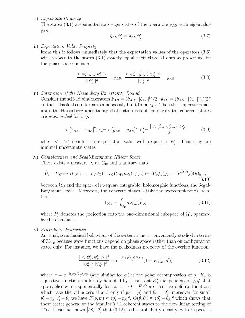
i) Eigenstate PropertyThe states (3.1) are simultaneous eigenstates of the operators gAB with eigenvaluegAB.

gABψsg = gABψ

sg (3.7)

ii) Expectation Value PropertyFrom this it follows immediately that the expectation values of the operators (3.6)with respect to the states (3.1) exactly equal their classical ones as prescribed bythe phase space point g.

< ψsg, gABψsg >

||ψsg||2= gAB,

< ψsg, (gAB)†ψsg >

||ψsg||2= gAB (3.8)

iii) Saturation of the Heisenberg Uncertainty BoundConsider the self-adjoint operators xAB = (gAB+[gAB]†)/2, yAB = (gAB−[gAB]†)/(2i)an their classical counterparts analogously built from gAB. Then these operators sat-urate the Heisenberg uncertainty obstruction bound, moreover, the coherent statesare unquenched for x, y.

< [xAB − xAB]2 >sg=< [yAB − yAB]2 >s

g=| < [xAB, yAB] >s

g |2

(3.9)

where < . >sg denotes the expectation value with respect to ψsg. Thus they are

minimal uncertainty states.

iv) Completeness and Segal-Bargmann Hilbert SpaceThere exists a measure νs on GC and a unitary map

Us : HG 7→ HGC := Hol(GC) ∩ L2(GC, dνs); f(h) 7→ (Usf)(g) := (es∆/2f)(h)h→g

(3.10)between HG and the space of νs-square integrable, holomorphic functions, the Segal-Bargmann space. Moreover, the coherent states satisfy the overcompleteness rela-tion

1HG=

∫

GC

dνs(g)Pψsg

(3.11)

where Pf denotes the projection onto the one-dimensional subspace of HG spannedby the element f .

v) Peakedness PropertiesAs usual, semiclassical behaviour of the system is most conveniently studied in termsof HGC

because wave functions depend on phase space rather than on configurationspace only. For instance, we have the peakedness property of the overlap function

| < ψsg, ψsg′ > |2

||ψsg||2||ψsg′ ||2= e−

F (p,p′)+G(θ,θ′)s (1 −Ks(g, g

′)) (3.12)

where g = e−ipjτj/2eθjτj (and similar for g′) is the polar decomposition of g. Ks isa positive function, uniformly bounded by a constant K ′

s independent of g, g′ thatapproaches zero exponentially fast as s → 0. F,G are positive definite functionswhich take the value zero if and only if pj = p′j and θj = θ′j , moreover for smallp′j − pj , θ

′j − θj we have F (p, p′) ≈ (p′j − pj)

2, G(θ, θ′) ≈ (θ′j − θj)2 which shows that

these states generalize the familiar T ∗R coherent states to the non-linear setting ofT ∗G. It can be shown [58, 42] that (3.12) is the probability density, with respect to

the Liouville measure on T ∗G, to find the system at the phase space point g′ if itis in the state ψsg and that density equals unity at g = g′ and is otherwise strongly,Gaussian suppressed as s → 0 with width

√s. Similar peakedness properties can

be established in the configuration or momentum representation.

vi) Ehrenfest TheoremsThe expectation value property holds for the operators gAB and g†AB at any valueof s. For the remaining operators one can show

lims→0

< hAB >sg= hAB and lim

s→0< pj >

sg= pj (3.13)

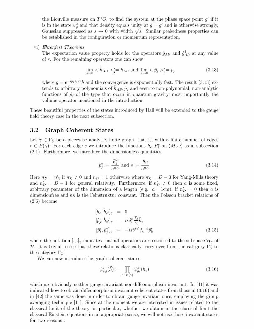
where g = e−ipjτj/2h and the convergence is exponentially fast. The result (3.13) ex-tends to arbitrary polynomials of hAB, pj and even to non-polynomial, non-analyticfunctions of pj of the type that occur in quantum gravity, most importantly thevolume operator mentioned in the introduction.

These beautiful properties of the states introduced by Hall will be extended to the gaugefield theory case in the next subsection.

3.2 Graph Coherent States

Let γ ∈ Γω0 be a piecewise analytic, finite graph, that is, with a finite number of edgese ∈ E(γ). For each edge e we introduce the functions he, P

ej on (M,ω) as in subsection

(2.1). Furthermore, we introduce the dimensionless quantities

pej :=P ej

anDand s :=

hκ

anD(3.14)

Here nD = n′D if n′

D 6= 0 and nD = 1 otherwise where n′D = D − 3 for Yang-Mills theory

and n′D = D − 1 for general relativity. Furthermore, if n′

D 6= 0 then a is some fixed,arbitrary parameter of the dimension of a length (e.g. a =1cm), if n′

D = 0 then a isdimensionfree and hκ is the Feinstruktur constant. Then the Poisson bracket relations of(2.6) become

[he, he′ ]γ = 0

[pej, he′ ]γ = isδee′τj2he

[pei , pe′

j ]γ = −isδee′fij kpek (3.15)

where the notation [., .]γ indicates that all operators are restricted to the subspace Hγ ofH. It is trivial to see that these relations classically carry over from the category Γω0 tothe category Γωσ .

We can now introduce the graph coherent states

ψsγ,~g(~h) :=

∏

e∈E(γ)

ψsge(he) (3.16)

which are obviously neither gauge invariant nor diffeomorphism invariant. In [41] it wasindicated how to obtain diffeomorphism invariant coherent states from those in (3.16) andin [42] the same was done in order to obtain gauge invariant ones, employing the groupaveraging technique [11]. Since at the moment we are interested in issues related to theclassical limit of the theory, in particular, whether we obtain in the classical limit theclassical Einstein equations in an appropriate sense, we will not use those invariant statesfor two reasons :

1) In order to check the correctness of the classical limit we must verify, in particular,whether the quantum constraint algebra of the the quantum theory becomes the Diracalgebra in the classical limit. However, one cannot check an algebra on its kernel, see [28]for a discussion.2) As far as the gauge – and diffeomorphism constraint are concerned, it is perfectlyfine to work with non-invariant coherent states because the corresponding gauge groupsare represented as unitarily on the Hilbert space. This implies that expectation valuesof gauge – and diffeomorphism invariant operators are automatically also gauge – anddiffeomorphism invariant and so qualify as expectation values of the reduced theory. Fa-mously, the time reparameterizations associated with the Hamiltonian constraint of thetheory cannot be unitarily represented and so the argument just given does not carryover to operators commuting with the Hamiltonian constraint. Presumably, the Hamil-tonian constraint cannot be exponentiated at all and one will then have to work with itsinfinitesimal version. To pass then to the reduced theory one would need to work withcoherent states that are annihilated by the Hamiltonian constraint (trivial representationof the “would be time reparameterization group”).

The coherent states (3.16) then form a valid starting point for adressing semiclassicalquestions in the case that Σ is compact, say, in some cosmological situations. To coverthe case that Σ is asymptotically flat we must blow up the framework and pass to theInfinite Tensor Product.

4 The Abstract Infinite Tensor Product

Bei Systemen mit N Teilchen ist der Hilbertraum das Tensorprodukt von denN Hilbertraumen der einzelnen Teilchen.

Das unendliche Tensorprodukt offnet die Tur zu den mathematischen Finessender Feldtheorie.

(Walter Thirring)

The Infinite Tensor Product (ITP) of Hilbert spaces is a standard construction instatistical physics (through the thermodynamic (or infinite volume) limit) as well as inOperator Theory (von Neumann Algebras). In fact, the first examples of von Neumannalgebras which are not of factor type In, I∞ (isomorphic to an algebra of bounded operatorson a (separable) Hilbert space) have been constructed by using the ITP.

On the other hand, since the concept of separable (Fock) Hilbert spaces plays such adominant role in high energy physics, presumably many theoretical physicists belongingto that community have never come across the concept of the Infinite Tensor Product(ITP) of Hilbert spaces which produces a non-separable Hilbert space in general. In fact,let us quote from Streater&Wightman, [59] p. 86, 87 in that respect :“...It is sometimes argued that in quantum field theory one is dealing with a system of aninfinite number of degrees of freedom and so must use a non-separable Hilbert space.....Our next task is to explain why this is wrong, or at best is grossly misleading.....All thesearguments make it clear that that there is no evidence that separable Hilbert spaces arenot the natural state spaces for quantum field theory....”

Because of this, we have decided to include here a rough account of the most importantconcepts associated with the abstract Infinite Tensor Product. As it will become clearshortly, the ITP decomposes into an uncountable direct sum of Hilbert spaces which inmost applications are separable. Each of these tiny subspaces of the complete ITP areisomorphic with the usual Fock spaces of quantum field theory on Minkowski space (orsome other background). Presumably, the fact that one can do with separable Hilbertspaces in ordinary QFT is directly related to the fact that one fixes the background sincethis fixes the vacuum. The necessity to deal with the full ITP in quantum gravity couldtherefore be based on the fact that, in a sense, one has to consider all possible backgroundsat once ! More precisely, the metric cannot be fixed to equal a given background but be-comes itself a fluctuating quantum operator.

We follow the beautiful and comprehensive exposition by von Neumann [43] who in-vented the Infinite Tensor Product (ITP) more than sixty years ago already. The readeris recommended to consult this work for more details.

4.1 Definition of the Infinite Tensor Product of Hilbert Spaces

Let I be some set of indices α. We will not restrict the cardinality |I|, rather for the sakeof maximal generality we will allow |I| to take any possible value in the set of Cantor’sAlephs [60]. The cardinality of the countably infinite sets is given by the non-standardnumber ℵ. Then the cardinality of any other infinite set can be written as a functionof ℵ (usually exponentials (of exponentials of..) ℵ), e.g. the set R has the cardinality2ℵ. The mathematical justification for this amount of generality is because, following vonNeumann [43],“...while the theory of enumerably infinite direct products ⊗∞

n=1Hn presents essentiallynew features, when compared with that of the finite ⊗N

n=1Hn, the passage from ⊗∞n=1Hn

to the general ⊗α∈IHα presents no further difficulties...., the generalizations of the directproduct lead to higher set-theoretical powers (G. Cantor’s “Alephs”), and to no measureproblems at all.”

Definition 4.1 Let zαα∈I be a collection of complex numbers. The infinite product

∏

α∈I

zα (4.1)

is said to converge to the number z ∈ C⇔ ∀ δ > 0 ∃ I0(δ) ⊂ I, |I0(δ)| <∞ ∋ |z − ∏

α∈J za| < δ ∀ I0(δ) ⊂ J ⊂ I, |J | <∞.

From the definition it is also straightforward to prove that if∏α zα,

∏α z

′α converge to z, z′

respectively then∏α zαz

′α converges to zz′.

Recall that a series∑α zα converges if and only if it converges absolutely which in

turn is the case if and only if zα = 0 for all but countably infinitely many α ∈ I. Thefollowing theorem gives a useful convergence criterion for infinite products.

Theorem 4.1

1)Let ρα ≥ 0.i) If ∃ α0 ∈ I ∋ ρα0 = 0 then

∏α ρα = 0.

ii) If ρα > 0 ∀α then∏α ρα converges if and only if

∑α max(ρα − 1, 0) converges.

iii) If ρα > 0 ∀α then∏α ρα converges to ρ > 0 if and only if

∑α |ρα − 1| converges.

2)Let zα = ραe

iϕα ∈ C where ρα = |zα|, ϕα ∈ [−π, π]. Then∏α zα converges if and only if

i) either∏α ρα converges to zero in which case

∏α zα = 0,

ii) or∏α ρα converges to ρ > 0 and

∑α |ϕα| converges in which case

∏α zα = ρei

∑αϕα.

In contrast to the case of an infinite series, absolute convergence of an infinite productdoes not imply convergence, the phases of the factors could fluctuate too wildly. Thismotivates the following definition.

Definition 4.2 Let zα ∈ C. We say that∏α zα is quasi-convergent if

∏α |zα| converges.

In this case we define the value of∏α zα to equal

∏α zα if

∏α zα is even convergent and

to equal zero otherwise.

This definition assigns a value to the infinite product of numbers which converge absolutelybut not necessarily non-absolutely. As a corollary of theorem 4.1 we have

Corollary 4.1 Quasi-convergence of∏α zα to a non-vanishing value is equivalent with

convergence to the same value. A necessary and sufficient criterion is that zα 6= 0 ∀α andthat

∑α |zα − 1| converges.

After having defined convergence for infinite products of complex numbers we are readyto turn to the ITP of Hilbert spaces.

Definition 4.3 Let Hα, α ∈ I be an arbitrary collection of Hilbert spaces. For a sequencef := fαα∈I , fα ∈ Hα the object

⊗f := ⊗αfα (4.2)

is called a C-vector provided that∏α ||fα||α converges, where ||.||α denotes the Hilbert

norm of Hα. The set of C-vectors will be called VC.

The following property holds for C-vectors, enabling us to compute their inner products.

Lemma 4.1 For two C-vectors ⊗f = ⊗αfα,⊗g = ⊗αgα the inner product

< ⊗f ,⊗g >:=∏

α

< fα, gα >α (4.3)

is a quasi-convergent product of the individual inner products < fα, gα >α on Hα.

There are C-vectors ⊗f such that∏α ||fα||α = 0 although ||fα||α > 0∀α. Thus, it is

conceivable that it happens that < Φf ,Φg > 6= 0 for some C-vector Φg. If that wouldbe the case, the Schwarz inequality would be violated for the inner product (4.3) onC-vectors. That this is not the case is the content of the following lemma.

Lemma 4.2 Let ⊗f be a C-sequence with∏α ||fα||α = 0. Then < ⊗f ,⊗g >= 0 for any

C-vector ⊗g.

To distinguish trivial C-vectors from non-trivial ones we define

Definition 4.4 A sequence (fα) defines a C0-vector ⊗f = ⊗αfα iff

∑

α

| ||fα||α − 1| (4.4)

converges. The set of C0-vectors will be denoted by V0.

It is easy to prove by means of theorem 4.1 that every C0-vector is a C-vector but onlythose C-vectors are C0-vectors for which < ⊗f , . >, considered as a linear functional on C-vectors, does not equal zero which by lemma 4.2 implies, in particular, that

∏α ||fα||α 6= 0.

It follows that the norm of a C0-vector does not vanish, as the following lemma reveals.

Lemma 4.3 For any complex numbers, the convergence of one of∑α | |zα|−1|, ∑

α | |zα|2−1| implies the convergence of the other.

Thus, since by definition of a C0-vector ⊗f and theorem 4.11)iii) zα = ||fα||α satisfiesthe assumption of lemma 4.3, by that lemma and again theorem 4.11iii) in the oppositedirection we find that || ⊗f || > 0.

Obviously we will construct the ITP Hilbert space from the linear span of C0-vectors(we can ignore the C−vectors which are not C0-vectors by lemma 4.2). For this it willbe useful to know how the Hilbert space decomposes into orthogonal subspaces. Thefollowing definition serves this purpose.

Definition 4.5 If ⊗f is a C0-vector, we will call the sequence f = fα a C0-sequence.We will call two C0-sequences f, g strongly equivalent, denoted f ≈ g, provided that

∑

α

| < fα, gα >α −1| (4.5)

converges.

Lemma 4.4 Strong equivalence of C0-sequences is an equivalence relation (reflexive, sym-metric, transitive).

This lemma motivates the following definition.

Definition 4.6 The strong eqivalence class of a C0 sequence f will be denoted by [f ].The set of strong equivalence classes of C0-sequences will be called S.

The subsequent theorem justifies the notion of strong equivalence.

Theorem 4.2 i) If f 0 ∈ [f ] 6= [g] ∋ g0 then < ⊗f0 ,⊗g0 >= 0.ii) If f 0, g0 ∈ [f ] then < ⊗f0 ,⊗g0 >= 0 if and only if there exists α ∈ I such that< fα, gα >α= 0.

So, C0-vectors from different strong equivalence classes are always orthogonal and thosefrom the same strong equivalence class are orthogonal if and only if they are orthogonalin at least one tensor product factor.

The following theorem gives two useful criteria for strong equivalence.

Theorem 4.3 i) [f ] = [g] if and only if∑α ||f 0

α−g0α||2α and

∑α |ℑ(< f 0

α, g0α >α)| converge

for some f 0 ∈ [f ], g0 ∈ [g].ii) If fα = gα for all but finitely many α then f ≈ g.

Obviously, it will be convenient to choose a representant f 0 ∈ [f ] which is normalized ineach tensor product factor. This is always possible.

Lemma 4.5 For each [f ] ∈ S there exists f 0 ≈ f such that ||f 0α||α = 1 for all α ∈ I.

The next lemma reveals that caution is due when trying to extend multilinearity fromthe finite to the infinite tensor product.

Lemma 4.6 Let∏α zα be quasi-convergent. Then

i) If f is a C-sequence, so is z · f with (z · f)α := zαfα.ii) If moreover

∑α ||zα| − 1| converges and f is a C0sequence, so is z · f .

iii) The product formula⊗z·f = [

∏

α

zα]⊗f (4.6)

fails to hold only if 1)∏α zα is not convergent and 2) < ⊗f , . > 6= 0 considered as a linear

functional on C-vectors. In that case, zα, f satisfy the assumptions of ii), moreoverzα 6= 0 ∀α.iv) If zα, f satisfy the assumptions of ii) then [z · f ] = [f ] iff

∑α |zα − 1| converges. If

even zα 6= 0 ∀α, the latter condition implies convergence of∏α zα.

An important conclusion that we can draw from this lemma is the following. If (4.6) failsthen, by iii), f, z · f are both C0-sequences while

∏α zα is only quasi-convergent. Thus,

both ⊗f ,⊗z·f 6= 0 while∏α zα = 0 by definition 4.2. Thus, [

∏α zα]⊗f = 0 6= ⊗z·f .

Next, since, also by iii), zα 6= 0 ∀α we have from collorary 4.1 that∑α |zα − 1| cannot

be convergent as otherwise∏α zα would be convergent which cannot be the case as

∏α zα

is only quasi-convergent. Thus, by iv) f, z · f lie in different strong equivalence classesand therefore by theorem 4.2 < ⊗f ,⊗z·f >= 0.

Definition 4.7 By HC we denote the completion of the complex vector space of finitelinear combinations of elements from VC equipped with the sesquilinear form < ., . >obtained by extending (4.3) from VC to HC by sesquilinearity.

Notice that for C-vectors which are not C0-vectors we have ⊗f = 0 as an element of HC .

Lemma 4.7 < ξ, ξ >≥ 0 ∀ξ ∈ HC and we define ||ξ||2 =< ξ, ξ >. In particular, < ., . >satisfies the Schwarz inequality and ||ξ|| = 0 if and only if ξ = 0.

We can now give the definition of the ITP.

Definition 4.8 We will denote by

H⊗ := ⊗αHα (4.7)

the Cauchy-completion of the pre-Hilbert space HC . It is called the complete ITP of theHα.

To analyze the structure H⊗ in more detail, the strong equivalence classes provide thebasic tool.

Definition 4.9 For a strong equivalence class [f ] ∈ S we define the closed subspace ofH⊗

H[f ] := N∑

k=1

zk⊗fk ; zk ∈ C, fk ∈ [f ], N <∞ (4.8)

by the closure of the finite linear combinations of ⊗f ′’s with f ′ ∈ [f ]. It is called the[f ]-adic incomplete ITP of the Hα’s.

Notice that we could absorb the zk in (4.8) into one of the fkα . Now we have the funda-mental theorem which splits H⊗ into simpler pieces.

Theorem 4.4 The complete ITP decomposes as the direct sum over strong equivalenceclasses [f ] of [f ]-adic ITP’s,

H⊗ = ⊗[f ]∈SH[f ] (4.9)

Also each [f ]-adic ITP can be given a simple description.

Lemma 4.8 For a given [f ] ∈ S, fix any f 0 ∈ [f ]. By lemma 4.5 we can choose an f 0

with ||f 0α||α = 1. Then H[f ] is the closure of the vector space of finite linear combinations

of ⊗f ′’s where f ′ ∈ [f ] and f ′α = f 0

α for all but finitely many α ∈ I.

It is easy to provide a complete orthonormal basis for an [f ]-adic ITP if we know one ineach Hα.

Lemma 4.9 Let f 0 ∈ [f ] ∈ S, ||f 0α||α = 1 ∀α. Let dα = dim(Hα) (takes the value of

some higher Cantor aleph if Hα is not separable). Let Jα, 0 ∈ Jα ∀ α ∈ I be a set ofindices of cardinality dα and choose a complete orthonormal basis eβα, β ∈ Jα such thate0α = f 0

α.Consider the set F of functions

β : I 7→ ×αJα; α 7→ β(α)α∈I (4.10)

such that 1) β(α) ∈ Jα and 2) β(α) 6= 0 for finitely many α only. Let

⊗eβ := ⊗αeβ(α)α (4.11)

Then eβ ∈ [f ] and the set of C0-vectors ⊗eβ ; β ∈ F forms a complete orthonormalbasis of H[f ], called a von Neumann basis.

The following corollary establishes that the [f ]-adic ITP’s are mutually isomorphic.

Corollary 4.2 Each [f ]-adic ITP is unitarily equivalent to the Hilbert space HF =L2(F , dν0) of square summable functions on F , ξ : F 7→ C; β 7→ ξ(β), where ν0 isthe counting measure. The unitary map is given by

U[f ] : HF 7→ H[f ]; ξ 7→∑

β∈F

ξ(β)⊗eβ (4.12)

The inverse map is given by

U−1[f ] : H[f ] 7→ HF ; ξ 7→ ξ(β) =< ⊗eβ , ξ > (4.13)

In particular, since each [f ]-adic ITP has a complete orthonormal basis labelled by Fand since the ITP is the direct sum of (the mutually isomorphic) [f ]-adic ITP’s we havedim(H⊗) = |F| · |S| where the appearing cardinalities will be aleph-valued in general(already in the simplest non-trivial case dim(Hα) = 2, I = N).

Notice that the index set I is not required to have any ordering structure, thus wehave identities of the form ⊗αfα = fα0 ⊗ [⊗α6=α0fα], these are just different notations forthe same object. However, is important to realize that the associative law genericallydoes not hold for the ITP. By this we mean the following :Let us decompose I into mutually disjoint index sets Il with l ∈ L then we can formthe following Hilbert spaces : H⊗ = ⊗α∈IHα and H⊗′ := ⊗l∈LHl where Hl := ⊗α∈Il

Hα.The C0-vectors of H⊗ are given by ⊗f = ⊗α∈Ifα while the C0-vectors of H⊗′ are givenby ⊗′

f = ⊗l∈Lf′l where f ′

l ∈ Hl is a (Cauchy limit of a) finite linear combination ofvectors of the form ⊗l

f = ⊗α∈Ilfα. Inner products between C0-vectors are computed

as < ⊗f ,⊗g >=∏α < fα, gα >α and < ⊗′

f ,⊗′g >=

∏α < fl, gl >l respectively where

< ⊗lf ,⊗l

g >l=∏α∈Il

< fα, gα >α.It is easy to see that if f = fαα∈I is a C0-sequence for H⊗ then f ′ = f ′

l := ⊗lfl∈L

is a C0-squence for H⊗′. However, the obvious map between C0-sequences given by

C : f 7→ f ′ (4.14)

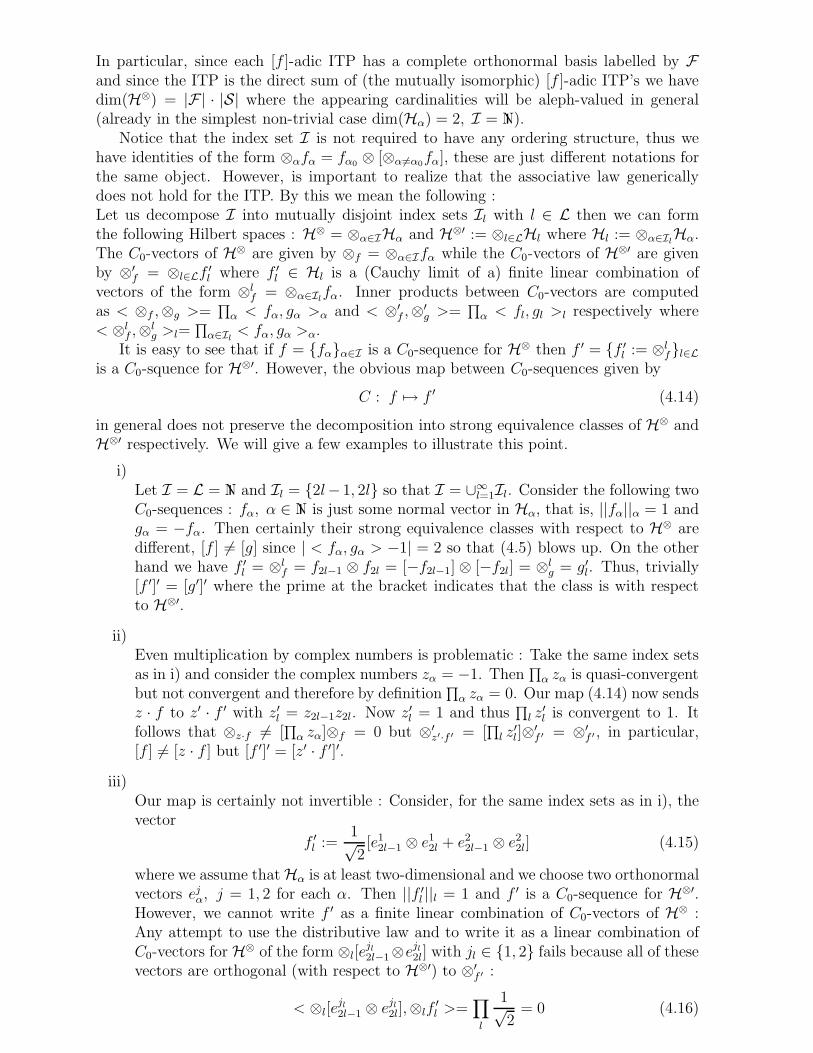
in general does not preserve the decomposition into strong equivalence classes of H⊗ andH⊗′ respectively. We will give a few examples to illustrate this point.

i)Let I = L = N and Il = 2l− 1, 2l so that I = ∪∞

l=1Il. Consider the following twoC0-sequences : fα, α ∈ N is just some normal vector in Hα, that is, ||fα||α = 1 andgα = −fα. Then certainly their strong equivalence classes with respect to H⊗ aredifferent, [f ] 6= [g] since | < fα, gα > −1| = 2 so that (4.5) blows up. On the otherhand we have f ′

l = ⊗lf = f2l−1 ⊗ f2l = [−f2l−1] ⊗ [−f2l] = ⊗l

g = g′l. Thus, trivially[f ′]′ = [g′]′ where the prime at the bracket indicates that the class is with respectto H⊗′.

ii)Even multiplication by complex numbers is problematic : Take the same index setsas in i) and consider the complex numbers zα = −1. Then

∏α zα is quasi-convergent

but not convergent and therefore by definition∏α zα = 0. Our map (4.14) now sends

z · f to z′ · f ′ with z′l = z2l−1z2l. Now z′l = 1 and thus∏l z

′l is convergent to 1. It

follows that ⊗z·f 6= [∏α zα]⊗f = 0 but ⊗′

z′·f ′ = [∏l z

′l]⊗′

f ′ = ⊗′f ′ , in particular,

[f ] 6= [z · f ] but [f ′]′ = [z′ · f ′]′.

iii)Our map is certainly not invertible : Consider, for the same index sets as in i), thevector

f ′l :=

1√2[e12l−1 ⊗ e12l + e22l−1 ⊗ e22l] (4.15)

where we assume that Hα is at least two-dimensional and we choose two orthonormalvectors ejα, j = 1, 2 for each α. Then ||f ′

l ||l = 1 and f ′ is a C0-sequence for H⊗′.However, we cannot write f ′ as a finite linear combination of C0-vectors of H⊗ :Any attempt to use the distributive law and to write it as a linear combination ofC0-vectors for H⊗ of the form ⊗l[e

jl2l−1⊗ejl2l] with jl ∈ 1, 2 fails because all of these

vectors are orthogonal (with respect to H⊗′) to ⊗′f ′ :

< ⊗l[ejl2l−1 ⊗ ejl2l],⊗lf

′l >=

∏

l

1√2

= 0 (4.16)

It is plausible and one can indeed show that these complications do not arise if |L| <∞.

4.2 Von Neumann Algebras on the Infinite Tensor Product

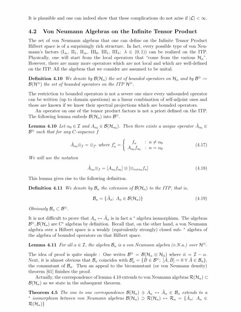
The set of von Neumann algebras that one can define on the Infinite Tensor ProductHilbert space is of a surprisingly rich structure. In fact, every possible type of von Neu-mann’s factors (I∞, II1, II∞, III0, III1, IIIλ; λ ∈ (0, 1)) can be realized on the ITP.Physically, one will start from the local operators that “come from the various Hα”.However, there are many more operators which are not local and which are well-definedon the ITP. All the algebras that we consider are assumed to be unital.

Definition 4.10 We denote by B(Hα) the set of bounded operators on Hα and by B⊗ :=B(H⊗) the set of bounded operators on the ITP H⊗.

The restriction to bounded operators is not a severe one since every unbounded operatorcan be written (up to domain questions) as a linear combination of self-adjoint ones andthose are known if we know their spectral projections which are bounded operators.

An operator on one of the tensor product factors is not a priori defined on the ITP.The following lemma embeds B(Hα) into B⊗.

Lemma 4.10 Let α0 ∈ I and Aα0 ∈ B(Hα0). Then there exists a unique operator Aα0 ∈B⊗ such that for any C-sequence f

Aα0⊗f = ⊗f ′ where f ′α =

fα : α 6= α0

Aα0fα0 : α = α0(4.17)

We will use the notation

Aα0⊗f = [Aα0fα0 ] ⊗ [⊗α6=α0fα] (4.18)

This lemma gives rise to the following definition.

Definition 4.11 We denote by Bα the extension of B(Hα) to the ITP, that is,

Bα = Aα; Aα ∈ B(Hα) (4.19)

Obviously Bα ⊂ B⊗.

It is not difficult to prove that Aα ↔ Aα is in fact a ∗ algebra isomorphism. The algebrasB⊗,B(Hα) are C∗ algebras by definition. Recall that, on the other hand, a von Neumannalgebra over a Hilbert space is a weakly (equivalently strongly) closed sub- ∗ algebra ofthe algebra of bounded operators on that Hilbert space.

Lemma 4.11 For all α ∈ I, the algebra Bα is a von Neumann algebra (v.N.a.) over H⊗.

The idea of proof is quite simple : One writes B⊗ = B(Hα ⊗ Hα) where α = I − α.Next, it is almost obvious that Bα coincides with B′

α = B ∈ B⊗; [A, B] = 0 ∀ A ∈ Bα,the commutant of Bα. Then an appeal to the bicommutant (or von Neumann density)theorem [61] finishes the proof.

Actually, the correspondence of lemma 4.10 extends to von Neumann algebras R(Hα) ⊂B(Hα) as we state in the subsequent theorem.

Theorem 4.5 The one to one correspondence B(Hα) ∋ Aα ↔ Aα ∈ Bα extends to a∗ isomorphism between von Neumann algebras B(Hα) ⊃ R(Hα) ↔ Rα = Aα; Aα ∈R(Hα)

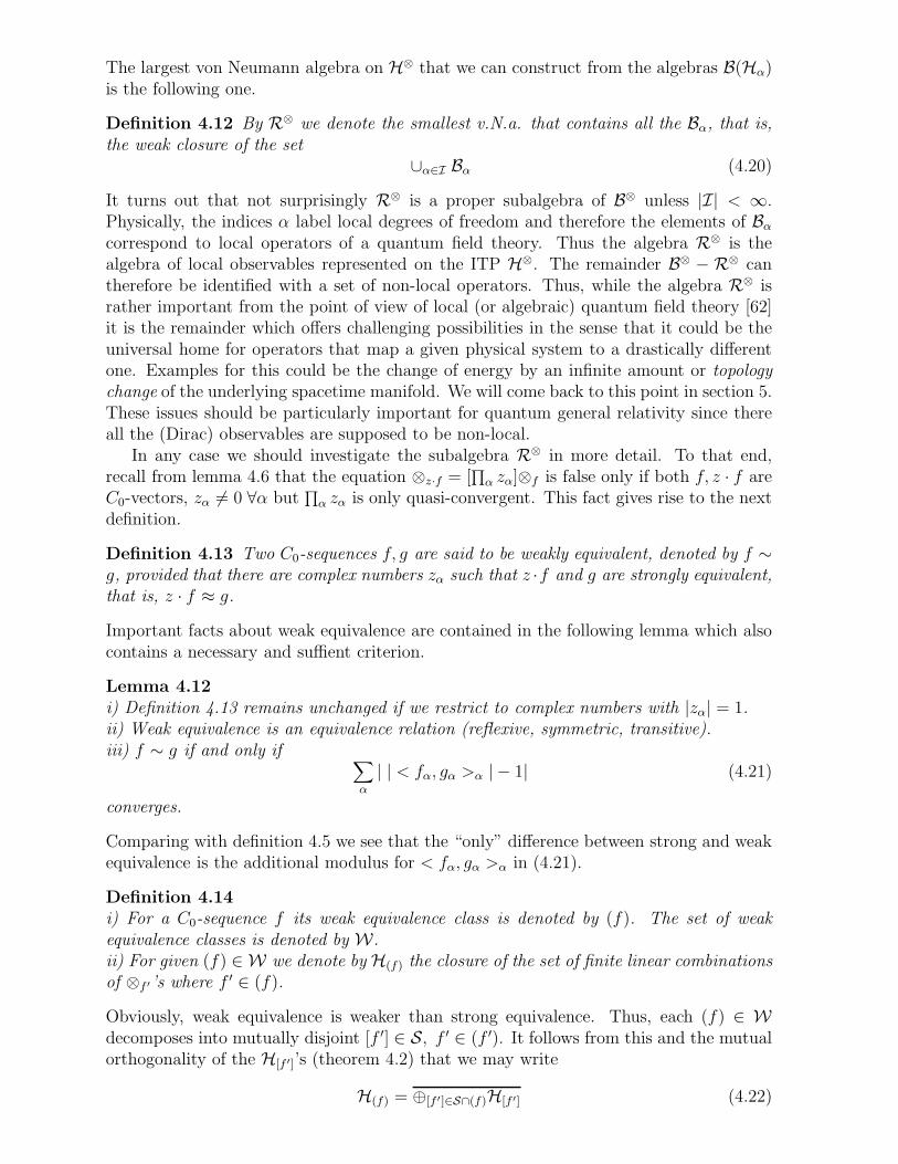
The largest von Neumann algebra on H⊗ that we can construct from the algebras B(Hα)is the following one.

Definition 4.12 By R⊗ we denote the smallest v.N.a. that contains all the Bα, that is,the weak closure of the set

∪α∈I Bα (4.20)

It turns out that not surprisingly R⊗ is a proper subalgebra of B⊗ unless |I| < ∞.Physically, the indices α label local degrees of freedom and therefore the elements of Bαcorrespond to local operators of a quantum field theory. Thus the algebra R⊗ is thealgebra of local observables represented on the ITP H⊗. The remainder B⊗ − R⊗ cantherefore be identified with a set of non-local operators. Thus, while the algebra R⊗ israther important from the point of view of local (or algebraic) quantum field theory [62]it is the remainder which offers challenging possibilities in the sense that it could be theuniversal home for operators that map a given physical system to a drastically differentone. Examples for this could be the change of energy by an infinite amount or topologychange of the underlying spacetime manifold. We will come back to this point in section 5.These issues should be particularly important for quantum general relativity since thereall the (Dirac) observables are supposed to be non-local.

In any case we should investigate the subalgebra R⊗ in more detail. To that end,recall from lemma 4.6 that the equation ⊗z·f = [

∏α zα]⊗f is false only if both f, z · f are

C0-vectors, zα 6= 0 ∀α but∏α zα is only quasi-convergent. This fact gives rise to the next

definition.

Definition 4.13 Two C0-sequences f, g are said to be weakly equivalent, denoted by f ∼g, provided that there are complex numbers zα such that z ·f and g are strongly equivalent,that is, z · f ≈ g.

Important facts about weak equivalence are contained in the following lemma which alsocontains a necessary and suffient criterion.

Lemma 4.12

i) Definition 4.13 remains unchanged if we restrict to complex numbers with |zα| = 1.ii) Weak equivalence is an equivalence relation (reflexive, symmetric, transitive).iii) f ∼ g if and only if ∑

α

| | < fα, gα >α | − 1| (4.21)

converges.

Comparing with definition 4.5 we see that the “only” difference between strong and weakequivalence is the additional modulus for < fα, gα >α in (4.21).

Definition 4.14

i) For a C0-sequence f its weak equivalence class is denoted by (f). The set of weakequivalence classes is denoted by W.ii) For given (f) ∈ W we denote by H(f) the closure of the set of finite linear combinationsof ⊗f ′’s where f ′ ∈ (f).

Obviously, weak equivalence is weaker than strong equivalence. Thus, each (f) ∈ Wdecomposes into mutually disjoint [f ′] ∈ S, f ′ ∈ (f ′). It follows from this and the mutualorthogonality of the H[f ′]’s (theorem 4.2) that we may write

H(f) = ⊕[f ′]∈S∩(f)H[f ′] (4.22)

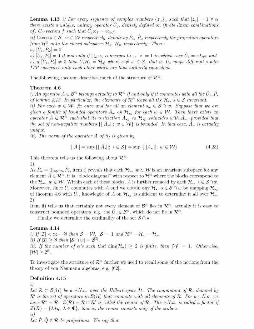
Lemma 4.13 i) For every sequence of complex numbers zαα such that |zα| = 1 ∀ αthere exists a unique, unitary operator Uz, densely defined on (finite linear combinationsof) C0-vectors f such that Uz⊗f = ⊗z·f .

ii) Given s ∈ S, w ∈ W respectively, denote by Ps, Pw respectively the projection operatorsfrom H⊗ onto the closed subspaces Hs, Hw respectively. Then :a) [Uz, Pw] = 0,b) [Uz, Ps] = 0 if and only if

∏α zα converges to z, |z| = 1 in which case Uz = z1H⊗ and

c) if [Uz, Ps] 6= 0 then UzHs = Hs′ where s 6= s′ ∈ S, that is, Uz maps different s-adicITP subspaces onto each other which are thus unitarily equivalent.

The following theorem describes much of the structure of R⊗.

Theorem 4.6

i) An operator A ∈ B⊗ belongs actually to R⊗ if and only if it commutes with all the Uz, Psof lemma 4.13. In particular, the elements of R⊗ leave all the Hs, s ∈ S invariant.ii) For each w ∈ W, fix once and for all an element sw ∈ S ∩ w. Suppose that we aregiven a family of bounded operators Aw on Hsw

for each w ∈ W. Then there exists anoperator A ∈ R⊗ such that its restriction Asw

to Hswcoincides with Aw, provided that

the set of non-negative numbers ||Aw||; w ∈ W is bounded. In that case, Aw is actuallyunique.iii) The norm of the operator A of ii) is given by

||A|| = sup ||As||; s ∈ S = sup ||Aw||; w ∈ W (4.23)

This theorem tells us the following about R⊗:1)As Pw = ⊕s∈S∩wPs, item i) reveals that each Hw, w ∈ W is an invariant subspace for anyelement A ∈ R⊗, it is “block diagonal” with respect to H⊗ where the blocks correspond tothe Hw, w ∈ W. Within each of these blocks, A is further reduced by each Hs, s ∈ S∩w.Moreover, since Uz commutes with A and we obtain any Hs, s ∈ S ∩w by mapping Hsw

of theorem 4.6 with Uz, knowlegde of A on Hswis sufficient to determine it all over Hw.

2)Item ii) tells us that certainly not every element of B⊗ lies in R⊗, actually it is easy toconstruct bounded operators, e.g. the Uz ∈ B⊗, which do not lie in R⊗.

Finally we determine the cardinality of the set S ∩ w.

Lemma 4.14

i) If |I| <∞ = ℵ then S = W, |S| = 1 and H⊗ = Hw = Hs.ii) If |I| ≥ ℵ then |S ∩ w| = 2|I|.iii) If the number of α’s such that dim(Hα) ≥ 2 is finite, then |W| = 1. Otherwise,|W| ≥ 2ℵ.

To investigate the structure of R⊗ further we need to recall some of the notions from thetheory of von Neumann algebras, e.g. [62].

Definition 4.15

i)Let R ⊂ B(H) be a v.N.a. over the Hilbert space H. The commutant of R, denoted byR′ is the set of operators in B(H) that commute with all elements of R. For a v.N.a. wehave R′′ = R. Z(R) = R∩R′ is called the center of R. The v.N.a. is called a factor ifZ(R) = λ1H; λ ∈ C, that is, the center consists only of the scalars.ii)Let P , Q ∈ R be projections. We say that

a) Q is a subprojection of P , denoted Q ≤ P , iff QH ⊂ PH.b) Q, P are equivalent, denoted Q ∼ P , iff there exists a partial isometry [64] with initialsubspace PH and final subspace QH.c) P 6= 0 is a minimal projection if there is no proper subprojection Q 6= 0 of P .d) P 6= 0 is an infinite projection if there is a proper subprojection Q 6= 0 of P to whichit is equivalent.iii)Let R be a factor. Then we call R of typeI : if R contains a minimal projection. If 1H is an infinite projection, then the type is I∞otherwise it is In where n = dim(H).III : every non-zero projection of R is infinite. A further systematic classification oftype III factors is due to Connes, see e.g. [65] and references therein. One distinguishesbetween type III0 (the Krieger factor [66]), type IIIλ, λ ∈ (0, 1) (the Powers factor [67])and III1 (the factor of Araki and Woods [68]).II : if R is neither of type I nor of type III. If 1H is an infinite projection, then R is calledtype II∞ otherwise type II1.

One can show that factors of type I are isomorphic to algebras of bounded operatorson some Hilbert space. Factors of type II∞ are generated by operators of the formA1 ⊗ 1H2 , 1H1 ⊗ A2 acting on the Hilbert space H1 ⊗ H2 where A1 belongs to a factorof type I∞ over H1 and A2 to one of type II1 over H2. For factors of type I and II itis possible to introduce a dimension function for projections, that is, a positive definitefunction dim(P ) ≥ 0 vanishing only if P = 0, uniquely determined by the two propertiesthat1) dim(P + Q) = dim(P ) + dim(Q) if P ⊥ Q and2) dim(P ) = dim(Q) if P ∼ Q.The range of that function is 0, 1, 2, .., n for type In, 0, 1, 2, ..,∞ for type I∞, [0, 1] for typeII1 and [0,∞] for type II∞. For type III a dimension function can be introduced but ittakes only the values 0,∞ and therefore cannot be used to obtain the finer subdivision oftype III factors outlined above for which the use of modular (or Tomita-Takesaki) theoryand the Connes invariant is necessary (a self-contained exposition aimed at mathematicalphyicists can be found in [69]).

We close this section by mentioning that the more unfamiliar factors of type II andIII are not only of academic interest. In fact, they appear already in systems as simpleas the infinite spin chain (see the second reference of [43]). If one represents the abstractCCR C∗algebra of spin 1/2 operators σjl ; j = 1, 2, 3; l = 1, 2, .., via the GNS theorem[61], for a state ωs (s ∈ [0, 1]) for which we get GNS data (Ω∞

s ,H∞s , π

∞s ) where the cyclic

vector is

Ω∞s = ⊗∞

l=1Ωs, Ωs = [

√1 + s

2e1 ⊗ e1 +

√1 − s

2e2 ⊗ e2],

the Hilbert space is the ITP H∞s = ⊗∞

l=1[C2⊗C2] corresponding to the index set I of pairs

α = (l, τ), τ = 1, 2, and the representation is π∞s (σjl ) acting only on the Hilbert C2 (with

standard orthonormal basis e1, e2) corresponding to α = (l, 1), then upon weak closurea factor of type I∞ or II1 or IIIs results for s = 1 or s = 0 or s ∈ (0, 1). The physicalinterpretation of the parameter s is that Ωs is the GNS datum for the mixed state

ωs(A) =tr(Aeβσ

3)

tr(eβσ3)

with s = th(β) on Hs = C4 = C2 ⊗C2, thus type I∞, II1 and IIIs respectively means zero,infinite or finite temperture respectively.

Finally, the type of local algebras R(O) appearing in algebraic quantum field theoryis the unique hyperfinite factor of type III1 for diamond regions O [62] (intersections ofpast and future light cones in the obvious way; this result can be extended to arbitraryO in case that the theory has a scaling limit (short distance conformal invariance) [63]).Here a v.N.a. is said to be hyperfinite if it is the inductive limit of finite dimensionalalgebras. This brings to the next topic.

4.3 Inductive Limits of Hilbert Spaces and von Neuman Alge-

bras

For the applications that we have in mind, specifically quantum gravity and quantumgauge theory coupled to gravity, the framework of the Infinite Tensor Product is notgeneral enough for the following reason. Recall from section 2 that the degrees of freedomof these field theories are labelled by graphs. Moreover, given a graph γ the degrees offreedom associated with it are labelled by the edges of that graph. Thus, it seems that weare in position to apply the theory outlined in sections 4.1 and 4.2 by choosing I = E(γ).While that is indeed true for the given graph γ, rather than working with a fixed, infinitegraph γ we are working with all of them because we do not have a lattice gauge fieldtheory but a continuum one. So we actually get an uncountably infinite family of ITP’s.That would not pose any problems if we could treat each of them independently, however,this is not the case, e.g. not if a graph is contained in a bigger one. The inductive limitconstruction is well suited to handle this problem.

Definition 4.16

0)Let ≺ be a partial order (that is, a reflexive, antisymmetric and transitive relation) onthe index set L. The index set is said to be directed if for any l, l′ there exists l′′ such thatl ≺ l′′ and l′ ≺ l′′.1i)Let Rll∈L be a family of C∗ algebras (v.N.a.’s) labelled by a directed index set L. Sup-pose that for all l, l′ with l ≺ l′ there is a ∗ monomorphism (injective homomorphism)Fll′ : Rl 7→ Rl′ satisfying1) Fll′(1Rl

) = 1Rl′and

2) Fll′ Fl′l′′ = Fll′′ for any l ≺ l′ ≺ l′′.Then the pair of families Rl, Fll′ is called a directed system of C∗ algebras (v.N.a.’s).1ii)Let Rll∈L be a family of C∗ algebras (v.N.a.’s) labelled by a directed index set L. A C∗

algebra (v.N.a.) R is said to be the C∗ (W ∗) inductive limit of the Rl provided there exist∗ monomorphisms Fl : Rl 7→ R such that1) Fl(1Rl

) = 1R and2) ∪lFl(Rl) is uniformly (weakly) dense in R.2i)Let Hll∈L be a family of Hilbert spaces labelled by a directed index set L. Suppose thatfor all l, l′ with l ≺ l′ there is an isometric monomorphism Ull′ : Hl 7→ Hl′ such thatUll′Ul′l′′ = Ull′′ for any l ≺ l′ ≺ l′′.Then the pair of families Hl, Ull′ is called a directed system of Hilbert spaces.2ii)Let Hll∈L be a family of Hilbert spaces labelled by a directed index set L. A Hilbert spaceH is said to be the inductive limit of the Hl provided there exist isometric monomorphismsUl : Hl 7→ H such that ∪lUlHl is dense in H.3i)

Given a directed system of Hilbert spaces Hl, suppose that we are given a family of oper-ators Al ∈ Rl ⊂ B(Hl) such that1) sup||Al||l; l ∈ L <∞ and2) there exists l0 ∈ L so that Ull′Al = Al′Ull′ for any l0 ≺ l ≺ l′.Then the family is called a directed system of operators.3ii)Given an inductive limit H of Hilbert spaces Hl together with a family of operatorsAl ∈ Rl ⊂ B(Hl), an operator A ∈ R ⊂ B(H) is called the inductive limit of the Alprovided that there exists l0 ∈ L so that UlAl = AUl for any l0 ≺ l.

The connection between ni) and nii), n = 1, 2, 3 is made through the following theorem.

Theorem 4.7

1)Given a directed system of C∗ algebras (v.N.a.’s) Rl, Fll′ there exists a unique (up to ∗

isomorphisms) C∗ (W ∗) inductive limit R of the Rl where the corresponding ∗ monomor-phisms Fl satisfy the compatibility condition Fl′ Fll′ = Fl.2)Given a directed system of Hilbert spaces Hl, Ull′ there exists a unique (up to unitarity)inductive limit H of the Hl where the corresponding isometric monomorphisms Ul satisfythe compatibility condition Ul′Ull′ = Ul.3)Given a directed system of operators Al on a directed system of Hilbert spaces Hl, thereexists a unique (up to unitarity) inductive limit operator A on the inductive limit Hilbertspace H.

The proof of this theorem can be found in the second volume of the first reference of[61]. Notice that inductive and projective limits (as used, e.g. in [8, 9]) are essentiallyidentical, just that the projective limit employs “projections downwards” a chain in thedirected system while the inductive limit employs “embeddings upwards” the chain.

The importance of the inductive limit for our purposes lies in the following construc-tion. Suppose we are given an index set I and consider the set L of all possible subsetsof I (notice that we allow the cardinality of l ∈ L to be infinite). Then L is a directed setwhere the partial order ≺ is given by the inclusion relation ⊂. For each l ∈ L we can formthe Infinite Tensor Product H⊗

l of the Hα, α ∈ l and the corresponding von Neumannalgebra R⊗

l . Moreover, we have for l ≺ l′ the obvious ∗ monomorphism Fll′ assigning toAl ∈ Rl the operator Al ⊗ [⊗α∈l′−l1Hα

] ∈ Rl′ . Finally, choose for each α ∈ I a fixedstandard unit vector Ωα ∈ Hα, then for l ≺ l′ we have isometric monomorphisms Ull′

mapping ξl ∈ Hl to ξl⊗ [⊗α∈l′−lΩα]. It is easy to see that Fll′, Ull′ satisfy the requirementsof definition 4.14 and so we can form the inductive limit von Neumann algebra R⊗

∞ andinductive limit Hilbert space H⊗

∞ respectively which are the universal objects from whichour various “lattice” algebras Rl and Hilbert spaces Hl respectively can be obtained bytheorem 4.7.

5 Infinite Tensor Products and Continuum Quantum

Gauge Theories

We will now apply the machinery of section 4 to quantum gauge field theories on globallyhyperbolic, spatially non-compact manifolds along the lines suggested by the expositionof section 2 and make contact with the semi-classical analysis machinery in connectionwith the coherent states as outlined in section 3. We proceed in several steps.

5.1 Kinematical Framework

In this subsection we carefully carry over the Ashtekar-Isham-Lewandowski kinematicalframework developed for the finite analytical category to the infinite analytical one.

5.1.1 Properties of Infinite Graphs

Notice that in order that γ ∈ Γωσ has an infinite number of edges, Σ must not be compactby the very definition of compactness.

Next, while Γωσ contains graphs with an infinite number of edges, the number of theseedges is at most countably infinite if Σ is paracompact as we assume here as otherwiseintegration theory cannot be employed. To see this, notice that since a finite dimensionalmanifold Σ is locally compact we can apply the theorem in [70] chapter I, paragraph 9which says that a (connected) locally compact space is paracompact if and only if it isthe countable union of compact sets. Assume now that γ has an uncountably infinitenumber of edges and let Un, n = 1, 2, .. be a countable compact cover of Σ. We concludethat at least one of the Un must contain an uncountably infinite number of edges of γbecause γ has an uncountable number of edges and the countable union of countable setsis countable. But this cannot happen if γ is piecewise analytic and σ-finite by definition.

We conclude that each element γ ∈ Γωσ is of a rather controllable form with at most acountable number of edges and vertices and no accumulation points as it would happen forwebs. They thus resemble maximally the lattices that one is used to from lattice gaugetheory and this is the form of graphs which are clearly most suitable for semiclassicalanalysis and the continuum limit. (The typical element of Γ∞

0 has at least one accumu-lation point of vertices and on such graphs one will certainly not approximate actions,Hamiltonians and the like).

Moreover, we have the following basic lemma and this is where analyticity comes in.

Lemma 5.1 The set Γωσ is a directed set by inclusion.

Proof of Lemma 5.1 :Notice that if γ, γ′ are two piecewise analytical, σ-finite graphs then γ′′ := γ ∪ γ′ is alsopiecewise analytic. We claim that it is also σ-finite. Suppose this was not the case. Then,either a) there exists a compact subset U ⊂ Σ such that γ′′ ∩U is an infinite graph or b)there exists a compact cover U such that the set |E(γ′′ ∩ U)|; U ∈ U is unbounded.

As for case a), we know that γ ∩ U, γ′ ∩ U are both finite graphs with finite numberof edges e, e′ respectively. Since γ′′ ∩U = [γ ∩U ] ∪ [γ′ ∩U ] the only way that γ′′ ∩U canpossibly be infinite is that there is at least one edge e of a γ and one edge e′ of γ′ suchthat e ∪ e′ intersect each other in an infinite number of isolated points. (The possibilitythat they overlap in a finite segment is excluded by analyticity as they would be analyticextensions of each other in this case and thus would make up a single analytical curve).However, two analytical curves that coincide in an infinite number of points are analyticalextensions of each other. Thus, case a) cannot occur.

As for case b), we find compact sets Un labelled by natural numbers n such that γ′′∩Unhas at least n edges. However, we know that there are natural numbers N,N ′ such that|E(γ ∩ Un)| < N, |E(γ′ ∩ Un)| < N ′ for all n. It follows that U∞ has the property of casea) which we excluded already. Thus, case b) can also not occur.2

That Γωσ is a directed set is of paramount importance for inductive limit constructions.

5.1.2 Quantum Configuration Space

Recall that in section 2.2 the quantum configuration space A arose as the Gel’fand spec-trum of the Abelian C∗ algebra generated by finite linear combinations of functions ofsmooth connections, restricted to finite graphs (cylindrical functions) and completed inthe supremum norm. It is natural to ask whether we can extend this construction tofunctions of smooth connections restricted to infinite graphs and to see if the size of thequantum configuration space is changed. The following simple example reveals that anaive transcription of this method is problematic :Take Σ = R3, G = SU(2) and let γ be the x-axis split into the countably infinite numberof intervals e of equal unit length. Thus, γ is a piecewise analytic, σ-finite graph. Let usconsider the following function of smooth connections

A 7→ f(A) :=∏

e

[kχj(he(A))] (5.1)

where k is a constant, χj(h) = tr(πj(h)) is the character of the spin j representation andthe convergence of (5.1) is meant in the sense of definition 4.1. By definition, the sup-normof that function is ||f || = supA∈A

∏e |kχj(he(A))|. Now the zero connection is certainly

an element of A, so ||f || ≥ supA∈A∏e |k(2j+1)| and this infinite product converges to 0 if

|k| < 1/(2j+1), to 1 if |k| = 1/(2j+1) and diverges otherwise. Now it is easy to see thatfor any h ∈ SU(2) we have in fact |χj(h)| ≤ 2j+1 and equality is reached for h = 1 so thatindeed ||f || = supA∈A

∏e |k(2j+1)|. It follows that in the only case that the norm is finite

and non-vanishing, we have that f(A) is non-vanishing iff∑e |kχj(he(A)) − 1| converges

which means that for each ǫ > 0 the set of e′s such that |kχj(he(A)) − 1| ≥ ǫ is finite.In other words, f(A) is almost given by

∏e δhe(A),1, an infinite product over Kronecker δ’s

rather than δ-distributions and it is almost granted that its support is of measure zerofor every reasonable measure even if we extend A to A. We will prove shortly that this isindeed the case with respect to the Ashtekar-Lewandowski measure which turns out to beextendible to our context. Thus, we face the problem that the (Gel’fand transforms of)functions of finite sup-norm (and thus all the elements of the Abelian C∗ algebra) seem tobe supported on measure zero subsets of interesting measures on the resulting spectrum.

On the other hand, it is physically plausible that the quantum configuration space asobtained from Γω0 should not change when we extend to Γωσ . The reason is that, by thevery definition of σ-finiteness, if we consider a function depending on the infinite numberof degrees of freedom labelled by the edges of γ ∈ Γωσ but restrict its dependence to a finitenumber of degrees of freedom by “freezing” all degrees of freedom labelled by γ − [γ ∩U ]for any compact set U ⊂ Σ then we get a function cylindrical over γ ∩ U ⊂ Γω0 whosebehaviour is certainly not different from the ones considered in section 2.2. In other words,functions over γ satisfy a locality property.

Thus, rather than deriving the spectrum A as the Gel’fand spectrum arising from anAbelian C∗ algebra of cylindrical functions over truly infinite graphs it is the characteri-zation of the Ashtekar-Isham spectrum derived in [7, 8] for finite graphs which we simplyextend to the infinite category ! This works as follows :We need the set W ω

0 that one obtains as the union of a finite number of, not necessarilycompactly supported anlytical paths. Since analytical paths of non-compact range canintersect each other in an infinite number of isolated points and since generic elementsof Γωσ cannot be otained as the union of a finite number of paths we see that we havethe proper inclusions Γω0 ⊂ W ω

0 ⊂ Γωσ . The set W ω0 is trivially directed by inclusion, in a

sense it is very similar to the set Γ∞0 . In fact, if one would blow up the neighbourhood of

the source of a tassel [10] by an infinite amount then one gets, apart from the differencebetween smooth and analytic paths, precisely the kind of objects that lie in W ω

0 . For thisreason, we will call them analytical webs. Notice that in contrast to smooth webs the

paths that determine an analytical web are obviously holonomically independent because1) they cannot overlap each other in a finite segment due to analyticity, they can onlyintersect each other in a possibly infinite number of isolated points and 2) because theyalways have a (non-overlapped) segment in the bulk of Σ where no fall-off conditions onA restrict the range of the holonomy along that segment.Let now A be the classical configuration space of section 2.1 where appropriate fall-offconditions at spatial infiniy are obeyed. Then the holonomy of A ∈ A along an ana-lytic path of infinite range is in fact well-defined precisely due to the fall-off conditionson A at spatial infinity. As in the context of Γω0 we can now consider the ∗algebra ofcylindrical functions of A ∈ A which are simply finite linear combinations of functions ofthe form f(A) = fw(he(A)e∈w) where w ∈ W ω

0 denotes the analytical web and fw is acomplex valued function on G|w|, |w| the number of paths that determine w. Now thecomplications that we observed above in the context of cylindrical functions over γ ∈ Γωσare out of the way because the cylindrical functions for webs depend on a finite numberof arguments only. We can therefore complete the ∗ algebra in the sup-norm just as insection 2.2, obtain a C∗ algebra and can follow exactly the same steps reviewed there forΓω0 to arrive at the Ashtekar-Isham spectrum A as the Gel-fand spectrum of that algebra.Finally, by following exactly the same proofs as in [7, 8, 50] we find A to be in one to onecorrespondence with the set of all homomorphisms from the groupoid X of (composable)analytic paths in Σ into the gauge group G. The isomorphism is the same as the one from[7, 8], that is,

A ∋ A 7→ HA ∈ Hom(X , G); (HA(e))mn := A((he)mn) = (he)mn(A) (5.2)

Here m,n are the indices of the matrix elements of the defining represenation of G and∧ denotes the Gel’fand transform. Notice that in contrast to [71] it was not necessaryto consider the one point compactification Σ of Σ. In fact, we refrained from doing thatbecause we now can consider the paths e ∈ X that determine an analytical web w alsoas possible edges of a truly infinite graph γ ∈ Γωσ . Clearly, considering the one pointcompactification Σ with an embedded generic element of Γωσ results in a highly singularobject and therefore we do not have the luxury to do this.

In summary, essentially we do not change the spectrum A as compared to [7, 8]except that the correspondence (5.2) is now extended to paths with non-compact rangeand therefore all the properties of A derived in the literature are preserved.

One could ask whether there is a more fundamental reason for this choice, trying todefine, as in the finite category, an Abelian C∗ algebra of cylindrical functions dependingon an infinite graph. This meets mathematical difficulties which are once more related tothe fact that the associative law does not hold in general for the ITP and boils down tosaying that one cannot really build an algebra of cylindrical functions over infinite graphs,only a vector space. We thus just adopt the above point of view with respect to definitionof A. However, an outline of these difficulties will be given in the subsequent digressionsince it is instructive and gives rise to some natural definitions.

A natural way to proceed with infinite graphs comes from the observation that the setΓω0 is a subset of Γωσ which consists of compactly supported graphs. This observationmotivates the following definition.

Definition 5.1 Let γ ∈ Γωσ .i)A function f on A is said to be a C function (not to be confused with the C vectors ofsection 4.1) over γ with values in C ∪ ∞ provided that for each e ∈ E(γ) there existfunctions fe on A of the form fe(A) = Fe(he(A)), where Fe is a complex valued function

on G, such thatf(A) =

∏

e∈E(γ)

fe(A) (5.3)

and convergence is defined as in definition 4.1 where we set f(A) = ∞ if∏e |fe(A)| = ∞

irrespective of the phases of the fe(A).ii)A function f on A is said to be cylindrical over γ if it is a finite linear combination of Cfunctions over γ. The set of cylindrical functions over γ is denoted by Cylγ.iii)A function f on A is said to be cylindrical if it is a finite linear combination of cylindricalfunctions over some graphs γ. The set of cylindrical functions is denoted Cyl.iv)An element 0 6= f =

∑Nn=1 zn

∏e∈E(γ) f

(n)e ∈ Cylγ, zn ∈ C is said to be σ-bounded if and

only if

||f ||γ := supU⊂Σ

supA∈A

|N∑

n=1

zn∏

e∩U 6=∅

f (n)e (A)| (5.4)

is finite where U runs over all compact subsets of Σ. For f = 0 we set ||f || = 0. Noticethat the argument of the modulus in (5.4) is a cylindrical function in the sense of section2.2. We will denote the set of σ-bounded, cylindrical functions by Cylbγ . Notice that Cylbγis not empty precisely due to the usual boundary conditions on smooth connections A fornon-compact Σ.

The norm (5.4) assigns a finite value to functions f even if there is A ∈ A such thatf(A) = ∞ which corresponds to our motivation to take over the structure from Γω0 .

Lemma 5.2 The space of σ-bounded cylindrical functions over γ forms a ∗ algebra withthe C∗ property.

Proof of Lemma 5.1 :That Cylbγ is closed under linear combination, multiplication by scalars and factor-wise

complex conjugation is obvious. Suppose now that f =∑Mm=1 um

∏e∈E(γ) f

(m)e , g =

∑Nn=1 vn

∏e∈E(γ) g

(n)e are given and we define

fg :=∑

m,n

umvn∏

e∈E(γ)

f (m)e g(n)

e (5.5)

simply by factorwise multiplication. Then

||fg||γ = supA,U

|∑

m,n

umvn∏

e∩U 6=∅

f (m)e (A)g(n)

e (A)|

= supA,U

|[M∑

m=1

um∏

e∩U 6=∅

f (m)e (A)][

N∑

n=1

vn∏

e∩U 6=∅

g(n)e (A)]|

≤ [supA,U

|M∑

m=1

um∏

e∩U 6=∅

f (m)e (A)|][sup

A,U|N∑

n=1

vn∏

e∩U 6=∅

g(n)e (A)|]

= ||f ||γ ||g||γ (5.6)

is also bounded. The C∗ property follows from |fU(A)| = |fU(A)| and supU,A |fU(A)|2 =(supU,A |fU(A)|)2.2

So far we have considered only one cylindrical algebra Cylbγ . Can we consider the al-gebra Cylb of finite linear combinations of elements of Cylbγ for some γ’s ? As we have

shown in lemma 5.1, Γωσ is a directed set so that for any finite collection γ1, .., γn thereexists a γ containing each of them. However, it may no longer be true that a givenfk ∈ Cylbγk

, k = 1, .., n can be written as a finite linear combination of C functions overγ, in fact, this will almost never be the case. Thus, while linear combinations pose noproblem, products do as we then can no longer multiply factor-wise without having toconsider infinite linear combinations of C functions. In other words, as soon as we al-low linear combinations of functions cylindrical over different infinite graphs, we end uphaving no algebra any more, products are ill-defined. The only exception is that for eachof γ1, .., γn only a finite number of edges have to be decomposed into a finite number ofsegments each of which is an edge of γ. In that case, each of fk can be considered alreadyas a function in Cylbγ so that nothing new is gained. Thus, the only way to proceed alongthe lines of [7, 8] is therefore to consider all the Cylbγ separately.

Once this is agreed on, the remainder is now standard. We complete the ∗ algebra Cylbγin the norm (5.4) and obtain an Abelian C∗ algebra Bγ which now depends on γ, in con-trast to section 2.2. By the Gel’fand theorem we obtain the spectrum Aγ of this algebra

and Bγ is, via the Gel’fand transform f 7→ f , isometrically isomorphic to the algebra ofcontinuous functions C0(Aγ) over the compact Hausdorff space Aγ. But now we meet thenext difficulty and this finishes our trial to proceed this way : Namely, the set A is nowno longer a subset of Aγ . Namely, let A0 ∈ A ∩Aγ then we have from isometricity

||f || = ||f || = supA∈Aγ

|f(A)| = supA∈Aγ

|A(f)| ≥ |A0(f)| = |f(A0)| (5.7)

which from the definition (5.4) can be true only if A0 has compact support. However, weare precisely interested in (distributional) connections which are supported everywhere inΣ as this corresponds to the intended physical application in connection with the clasicallimit for non-compact Σ. There is no claim that one could not introduce a different C∗

norm on cylindrical functions which would lead to the desired distributional extension ofA but there seems to be no obvious, natural candidate as the above discussion reveals.We leave the question on the existence of such a norm for future research. This terminatesour digression.

We thus will not use the norm (5.4) any further but simply consider the vector spaceCyl of arbitrary cylindrical functions of A without any convergence requirements, to be-gin with. As we will see, a subset of this space, extended to distributional connections,is dense in the Hilbert space which we are going to construct and although it is not analgebra, inner products can be computed even if we have linear combinations of functionsover different infinite graphs.

This extension works as follows : Since every cylindrical function is a finite linearcombination of C functions over some γ we can also extend any f ∈Cyl to a function fon A simply by the pull-back of the Gel’fand transform on C functions

f :=∏

e∈E(γ)

fe where fe(A) = Fe(A(he)) = Fe(he(A)) = (∧∗fe)(A) (5.8)

extended by linearity. The notation means that f is the Gel’fand transform of f =∏e fe, fe = Fe he extended from finite to infinite graphs. We will continue to call the

extensions f cylindrical functions.Although a general f ∈Cyl will take an infinite value on almost every point A ∈ A

it is still possible to equip Cyl with a topology which is weaker than the Hilbert spacetopology that we are going to construct, moreover, the Hilbert space measure is such

that these infinite values are integrable. This is important in order to have a frameworkfor solving quantum constraints via (analogs of) Gel’fand triples [11]. we postpone thedefinition of this topology to subsection 5.2.1.

5.1.3 Measure and Hilbert Space

Consider for a moment the set Cω of all possible oriented, analytic curves in Σ. Clearly, atmost countable collections of elements e ∈ Cωσ constitute an element γ ∈ Gωσ through theirunion if that union is σ-finite. The idea is now to construct the Infinite Tensor ProductHilbert spaces H⊗

γ associated with the Hilbert spaces He, e ∈ E(γ) of section 3.2, that is,

H⊗γ := ⊗e∈E(γ)He (5.9)

Using the notation of section 4.3 we would have index sets I = Cω and the set of arbitraryindex subsets L (or power set) of I of which Γωσ ⊂ L is a proper subset.

The reader may now wonder why we do not use the full power of the Infinite TensorProduct of being able to deal with index sets of arbitrary cardinality and rather stick withΓωσ . Indeed, an interesting observation is now the following : Consider instead of L theslightly smaller set P of arbitrary subsets C of Cω (not necessarily elements of Γωσ) suchthat no element e ∈ C can be written as a composition of elements of C − e and theirinverses. Then we say C ≺ C ′ if every element e ∈ C can be written as a compositionof elements e′ ∈ C ′ and their inverses which gives also P a partial order. For C ≺ C ′

we define C ∪ C ′ = C ′. Recall that a subset P ⊂ P is called a chain if all elementsC ∈ P are in relation ≺. Given a chain P , consider the element CP := ∪C∈PC whichis an element of P (not necessarily of P ), moreover, C ≺ CP ∀C ∈ P . In other words,every chain in P has an upper bound in P and by the lemma of Zorn we obtain that Phas a maximal element C∞, that is, C ≺ C∞ for all C ∈ P. Certainly, there are infinitelymany such maximal elements each of which we will call a “supergraph”. By construction,every element e ∈ C∞ is not composition of elements of C∞ − e and thus they areholonomically independent. (This construction can obviously be repeated for the smoothcategory of curves as well). Notice that the existence of C∞, while of theoretical interestsince it allows us to construct the universal ITP H⊗

∞ := ⊗e∈C∞He, universal in the sensethat every possible piecewise analytic graph γ can be written as composition of elementsof C∞, it is practically so far of modest interest only because 1) no one knows how todescribe C∞ explicitly and 2) even if one knew C∞ explicitly, given γ ∈ Γω, every edge eof γ would generically decompose into an infinite number of segments each of which is anelement of E(C∞). Thus, even a very simple function from the point of view of γ wouldlook very complicated from the point of view of C∞. In particular, as we have seen alreadyin section 4.1, the associative law fails for the ITP and it will in general happen that afunction on an incomplete ITP associated with some γ cannot be written as an element ofthe universal ITP. We are therefore forced to work with all the H⊗

γ simultaneously ratherthan with the single universal object H⊗

∞ only.However, the supergraph γ∞ allows us to give a simple proof of the existence of a

σ-additive, faithful, Borel measure on A with respect to which we can compute arbitraryinner products of cylindrical functions. This is a simple corollary of the Kolmogorovtheorem for the case of an uncountably infinite tensor product of probability measures[72] and works as follows in the present context :The supergraph C∞ ∈ P is a generating system of holonomically independent analyticcurves for every element P ∈ P, in particular, for every element γ ∈ Γωσ . Each element Aof the Ashtekar-Isham space A of generalized connections assigns to each curve e ∈ C∞ anelement A(he) = he(A) of G and as A varies, this map is onto (except if e is just a pointin which case A(he) = 1G). Given P ∈ P we consider the σ-algebra MP generated by

preimages of Borel subsets of G|P | under the map pP : A 7→ G|P |; A 7→ A(he)e∈P where|P | denotes the cardinality of the set P . Consider the σ-algebra M generated by all theMP displaying (A,M) as a measurable space. We say that a function f is measurable ifit is of the form f = F pP for some P ∈ P and some function F on G|P |. A measure onA can now be defined on measurable functions by

µ0(f) :=∫

G|P |⊗e∈PdµH(he)F (hee∈P ) (5.10)

where µH is the Haar measure on G. The normalization, right – and left invariance andthe invariance under inversion display this measure as a consistently defined measure onmeasurable functions, the proof is completely analogous to the one displayed in [8] so thatwe can omit it here. Notice, however, that in contrast to [8] we allow |P | = ∞. Beingconsistently defined, the measure qualifies as one to have a σ-additive extension to M.Rather than using the existence theorem of [9] we simply write it down :

µ0(.) :=∫

G|C∞|⊗e∈C∞dµH(he)(.) (5.11)

We will call it the extended Ashtekar-Lewandowski measure. Again, the remarkable prop-erties of the Haar measure on G reveal that (5.11) reduces to (5.10) for f = F pP andtheorem 12.1 in [72] guarantees that (5.11) has the required properties. Thus, althoughwe do not know the object C∞, its mere existence can be used to define µ0. Henceforthwe will denote H := L2(A, dµ0).

A more explicit construction of that Hilbert space is as follows and this provides a sim-ple way to embed the kinematical framework of section 2.2 for finite piecewise analyticalgraphs into the context of Γωσ of infinite piecewise analytical σ-finite graphs.

Given γ ∈ Γωσ we can use the inductive limit construction of section 4.3 to obtain H⊗γ

for infinite γ from the Hilbert spaces Hγ constructed in [8] for finite γ. Notice that weget this way a genuine extension of the so-called Ashtekar-Lewandowski Hilbert space

HAL := ∪γ∈Γω0Hγ (5.12)

as we will see in a moment. In fact, the Hilbert space that we will construct is defined by

H⊗ := ∪γ∈ΓωσH⊗γ (5.13)

Let us then proceed to the explicit construction. Recall that Hγ is the completion, withrespect to the Ashtekar-Lewandowski measure µ0 of section 2.2, of the space of cylindricalfunctions Cylγ over γ ∈ Γω0 . Since Cylγ can be replaced by the finite linear combinations of(non-coloured) spin-network functions over γ we see that Hγ can be equivalently describedas the closure of the finite linear combinations of C0-vectors of the finite tensor product

H⊗γ = ⊗e∈E(γ)He (5.14)

where each He is isometric isomorphic with L2(G, dµH) where µH is the Haar measure.Thus, Hγ = H⊗

γ for γ ∈ Γω0 .Indeed, as it is immediately obvious from the cylindrical consistency of the measure

µ0, it reduces on Hγ precisely to the tensor product Haar measure, corresponding to onecopy of G for each e ∈ γ and this is precisely the original definition of the Ashtekar-Lewandowski measure in terms of its cylindrical projections given in [8].

Let now γ ∈ Γωσ be given, then we find a sequence of elements γn ∈ Γω0 such thatγn ⊂ γ and γn ⊂ γn+1 for each n = 1, 2.., moreover ∪∞

n=1γn = γ. By means of theisometric monomorphisms defined on C0-vectors for m ≤ n

Uγmγn: H⊗

γm7→ H⊗

γn; ⊗e∈E(γm)fe 7→ [⊗e∈E(γm)fe] ⊗ [⊗e∈E(γn−γm)1] (5.15)

and extended by linearity, where 1(A) = 1 is the unit function, we display the system ofHilbert spaces Hγ ≃ H⊗

γ as a directed system. By theorem 4.7 the unique inductive limitof the Hγn

exists and can be identified with the Infinite Tensor Product for each γ ∈ Γωσ

H⊗γ = ⊗e∈E(γ)He (5.16)

and indeed the required isometric isomorphisms are given by

Uγn: H⊗

γn7→ H⊗

γ ; ⊗e∈E(γn)fe 7→ [⊗e∈E(γn)fe] ⊗ [⊗e∈E(γ−γn)1] (5.17)

Thus, for a truly infinite graph γ the Hilbert space H⊗γ is hyperfinite, that is, it is the

inductive limit of the finite dimensional Hilbert spaces H⊗γn

.Several remarks are in order :

A) From the point of view of H⊗γ the vectors of Hγn

≃ H⊗γn

lie in the strong equivalenceclass of the C0-sequence f 0 = f 0

e e∈E(γ) where f 0e = 1 for each e. This is an

immediate consequence of lemma 4.8. It follows that the Hilbert space (5.12) is justa tiny subspace of the Hilbert space (5.13) since every vector over γ which is notin the strong equivalence class of f 0 is orthogonal to all of the Hγn

and there areuncountably infinitely many different strong eqivalence classes even for fixed γ asfollows from lemma 4.14 since |E(γ)| = ℵ. To see this in more detail, notice that if ageneric element ξ ∈ H⊗

γ would be a Cauchy sequence of elements ξn ∈ HAL then forany ǫ > 0 we would find n0(ǫ) such that ||ξ− ξn|| < ǫ ∀ n > n0(ǫ). Now each ξn canbe chosen to be in some Hγn

with Γω0 ∋ γn ⊂ γ since any vector in the completion ofHAL can be approximated by vectors of that form and since any vector dependingon a coloured graph which is not contained in γ is automatically orthogonal to ξ.However, if we choose, e.g., ξ to be a linear combination of C0-vectors each of whichlies in a different strong equivalence class Hilbert space than the vector f 0 abovethen we get the contradiction ||ξ||2 < ||ξn||2 + ||ξ||2 < ǫ ∀ n > n0(ǫ).

B) While the Ashtekar-Lewandowski Hilbert space is just a tiny subspace of H⊗ in(5.5), the Ashtekar-Lewandowski measure is still the appropriate measure to use inour extended context.

Indeed, it has been identified already as the σ-additive extension of the cylindricallydefined measure of [8] to the projective (or inductive) limit of arbitrarily large andcomplicated, but finite piecewise analytic graphs in [9]. Therefore, it could be usedto date only in order to integrate special functions depending on an infinite numberdegrees of freedom (i.e. depending on infinite graphs) : Namely those which canbe written as infinite sums of functions each of which depends only on a finitegraph, an exception being [73] where some sort of infinite volume limit has beentaken. One contribution of the present paper is to show that the measure can beused to integrate more general functions depending on an infinite number of degreesof freedom : namely those which are infinite products of functions each of whichdepends only on a finite graph.

C) In the context of finite graphs we can (even for non-gauge-invariant states) writedown a complete orthonormal (with respect to the Ashtekar-Lewandowski measureµ0) basis, the so-called spin-network basis of section 2.2. It is frequently stressed thatthe Ashtekar-Lewandowski measure can then be dispensed with by just requiringthese functions to be orthogonal and to check that a positive definite sesquilinearform results in this way [12, 15]. Adopting this point of view, given arbitraryfunctions in HAL one can explicitly compute their inner products by writing them interms of spin-network functions and using sesquilinearity. This is no longer possible

in the context of the Infinite Tensor Product (spatially non-compact Σ), here theAshtekar-Lewandowski measure is the only way to calculate inner products ! To seethis we just need to display one simple example :Consider an infinite graph γ with a countable number of analytic edges e (say acubic lattice in Σ = R3). Consider the C0-sequence f := fe where (from now onwe drop the bar in A for a distributonal connection and we write he instead of theGel’fand transform he)

fe(A) := f 0(he(A)) :=1 + χj(he(A))√

2(5.18)

where χj is again the character in the spin j > 0 representation of SU(2). Usingthe extended Ashtekar Lewandowski measure (5.11), which on this infinite graphjust reduces to dµ0γ = ⊗e∈E(γ)dµH(he) we immediately verify that the norm of theC0-vector ⊗f equals unity. Suppose now we wanted to use only the knowledge thatthe set of functions

n∏

k=1

χj(hek) (5.19)

for finite n and mutually distinct e1, .., en ∈ E(γ) are mutually orthogonal spin-network functions. Then, in order to compute the norm of ⊗f we would need todecompose this vector into the latter set of functions which at least formally can bedone using the distributive law over and over again. However, it is easy to see thateach of these infinite number of terms comes with the coefficient (1/

√2)∞ and so our

attempt to compute the norm would result in the ill-defined expression 0 ·∞. Moreprecisely, this ill-defined result is due to the fact that the inner product between thevectors (5.18) and (5.19) for n→ ∞ equals zero.

Concluding, in the ITP or Γωσ category the spin-network functions no longer providea basis (a related observation has been made independently already in [10, 50] in thecontext of webs or Γ∞

0 ), simply because, even for a single γ ∈ Γωσ , the orthonormalset of functions given by

A 7→∏

e

[√

2je + 1πje(he(A))mene] (5.20)

where e ∈ E(γ); 2je = 0, 1, 2, ..;me, ne = −je,−je + 1, .., je and which from experi-ence with spin-network functions one might think to provide a basis, is not complete! For instance, the unit C0-vector

A 7→∏

e

χj(he(A)) (5.21)

is orthogonal to all of them for any j > 0, even if we choose je = j for all e since| < √

2j + 1πjmn, χj >L2(SU(2),dµH ) | ≤ 1/√

2j + 1 < 1. The ITP Hilbert space hasmany more orthogonal directions than one is used to due to its non-separability.A complete orthonormal bases on a single γ ∈ Γωσ is not given by spin-networkfunctions but rather by a von Neumann basis defined in lemma 4.9 and corollary4.2, one for each [f ]-adic Infinite Tensor Product subspace of Hγ . The only [f ]-adic ITP that has indeed a spin-network basis is the one given by the trivial strongequivalence class [f 0] where for any given γ ∈ Γωσ we have f 0

e = 1 for each e ∈ E(γ).

Our treatment is still incomplete because, while we can compute inner products betweenfinite linear combinations of C0 vectors over a single γ, nothing has so far been said aboutinner products between finite linear combinations of C0 vectors over different γ’s and this

is what we need if we wish to glue together the H⊗γ as displayed in (5.13). The idea is,

of course, to use the inductive limit construction once again, however, as far as innerproducts are concerned we have to go somewhat beyond von Neumann’s theory whichtells us only how to compute inner products between finite linear combinations of C0

vectors over the same γ.A concrete and natural definition can be given employing the extended Ashtekar-

Lewandowski measure. Let us derive it, proceeding formally to begin with :

Let γ, γ′ ∈ Γωσ and let fγ, gγ′ respectively be C0-sequences over γ, γ′ respectively. Considerthe graph γ′′ := γ∪γ′. The idea is to define the inner product between the correspondingC0-vectors ⊗fγ

,⊗gγ′by

< ⊗fγ,⊗gγ′

> :=∫

G|C∞|[⊗e′′∈C∞dµH(he′′)] [⊗fγ

] [⊗gγ′]

=∫

G|E(γ′′)|[⊗e′′∈E(γ′′)dµH(he′′)] [⊗fγ

] [⊗gγ′] (5.22)

where the second equality follows from cylindrical consistency. The problem, that by nowwe are already used to with these infinite tensor products, is that the associative law doesnot hold. In other words, the ITP

H⊗γ′′ := ⊗e′′∈E(γ′′)He′′ (5.23)

is in general quite different from the subdivisions

(⊗e∈E(γ)[⊗e′′∈E(γ′′)∩eHe′′ ]) ⊗ (⊗e′′∈E(γ′′)−γHe′′) and

(⊗e′∈E(γ′)[⊗e′′∈E(γ′′)∩e′He′′ ]) ⊗ (⊗e′′∈E(γ′′)−γ′He′′) (5.24)

to which fγ , gγ′ belong respectively. This is precisely the problem outlined at the endof section 4.1 : The correspondence with the notation there is that I = E(γ′′), L =E(γ) ∩ γ′′ − γ, Il = E(γ′′) ∩ e for l = e and Il = E(γ′′) − γ for l = γ′′ − γ and similarfor γ′. Here we have identified He with ⊗e′′∈E(γ′′)∩eHe′′ and similar for e′. Notice that ingeneral |E(γ′′) ∩ e|, |E(γ′′) ∩ e′| = ∞, an example being given by two graphs consisistingof a single edge only, γ = e, γ′ = e′, which however both have non-compact range andintersect each other an infinite number of times in isolated points. This is not excludedby piecewise analyticity since there is no accumulation point of intersection points (take,e.g. e = (x, 0) and e′ = (x, sin(x)) in R2).Step I)In order to proceed, we subdivide γ′′ into the mutually disjoint sets γ∗ := γ ∩ γ′, γ =γ′′ − γ, γ′ = γ′′ − γ′. Then we formally embed ⊗fγ

into Hγ′′ by identifying it with(⊗fγ

) ⊗ (⊗e′′∈E(γ′′)∩γ1) and similarly we identify ⊗gγ′with (⊗gγ′

) ⊗ (⊗e′′∈E(γ′′)∩γ′1).Clearly, we will now perform first the easy integrals corresponding to the tensor productsfactors of the unit function. In order to do this, for given e ∈ E(γ) we recall that wecan write fe(he) =

∑π f

mneπ πmn(he) by the Peter& Weyl theorem where the sum is over

a complete set of equivalence classes of irreducible representations of G, πmn denotesthe matrix elements of a group element in the representation π and fmneπ are the Fouriercoefficients of fe. Now suppose that e′′ ⊂ e and that e′′ 6⊂ γ′, that is, e′′ ∈ E(γ′′)∩ (e∩ γ′).Then we can write fe(he) =

∑π f

mneπ πmn(h

(1)e he′′h

(2)e ) where h(1)e, h

(2)e depend on e−e′′. In

other words, we can consider it as a function F of he′′ only and as far as the integral overhe′′ is concerned it reduces to evaluating < F, 1 >L2(G,dµH)= feπ0 =< fe, 1 >He

. It followsthat for any e ∈ E(γ) which is not fully overlapped by edges of E(γ′) we can replace fe by< fe, 1 > (we drop the index at the inner product). Likewise, for any e′ ∈ E(γ) which isnot fully overlapped by edges of E(γ) we can replace ge′ by < 1, ge′ >. This is the result

of performing the integral over all he′′ with e′′ ∈ E(γ′′) ∩ [γ ∪ γ′] = E(γ′′) ∩ [γ′′ − γ∗]. Itremains to perform the integral over the edges of E(γ′′) ∩ γ∗.Step II)Now notice that from ⊗e∈E(γ)fe only those factors are left corresponding to edges e fullyoverlapped by edges of E(γ′) and from ⊗e′∈E(γ′)ge′ only those factors are left correspondingto edges e′ fully overlapped by edges of E(γ). Let us denote the corresponding subsetsby E(γ)|γ∗ ⊂ E(γ), E(γ′)|γ∗ ⊂ E(γ′). The union of both sets of edges is contained in γ∗.Suppose now that e ∈ E(γ)|γ∗ is overlapped by a collection of edges e′ of E(γ′), that is,there is a countable number of edges e′10, .., e

′11 of E(γ′) so that the endpoint of one is the

starting point of the next, such that e is contained in their union and such that it is notany more contained if we remove e′10 or e′11 from the collection. It follows that e′10, .., e

′11

are analytical continuations of each other.Step III)Let us first focus on e′10. Now either, A) e′10 is also contained in e or, B) it is not. Incase B), if there are no other edges of E(γ) overlapping the remaining segment of e′10not contained in e then the edge e′10 does not appear any more in E(γ′)|γ∗ . By the sameargument as in Step I), if we now perform the integral over any he′′ with e′′ contained ine− e′10 then we can replace fe by < fe, 1 > and that factor also drops out of the integral.Thus, we can focus on the case that e′10 ∈ E(γ′)|γ∗ , that is, there are such other edgese0, .., e1 of E(γ) where e0 is adjacent to e, an endpoint of one is the starting point of thenext and if e1 is removed, the collection e, e0, .., e1 no longer overlaps e′10. We see thate, e0, .., e1 are analytical continuations of each other. Now either, A) e1 is also containedin e′10 or B), it is not. In case B), if there are no other edges of E(γ′) overlapping theremaining segment of e1 not contained in e′10 then e1 does not belong to E(γ)|γ∗ and so asin Step I) we can replace ge′10 by < 1, ge′10 > and so that factor drops out of the integral.

However, then as just explained also fe drops out of the integral. Thus, we may assumethat e1 ∈ E(γ)|γ∗ and there are new edges e′20, ..e

′21 with e′21 adjacent to e′01, the endpoint

of one is the starting point of the next and such that e1 is no longer overlapped if weremove e′20.

Let us now rename ee0..e1 by e and the collection e′20, .., e′21, e

′10, .., e

′11 by e′10, .., e

′11.

Then we are in the same situation as in the beginning of Step III). Iterating, we concludethat either we end up with case A) or with case B) but that e′10 is no longer overlapped.In case B) the whole chain collapses like a cardhouse and we can replace fe by < fe, 1 >.In case A) we see that we found a maximal analytical continuation of the original e, intothe direction of its starting point, by other edges of E(γ) all of which are overlapped byedges of E(γ′) and those edges are also contained in that maximal analytical continuationcontained in γ.Step IV)Now we focus on e′11 and proceed completely analogously. The end result is that fecan be replaced by < fe, 1 > unless there exists a maximal bothsided maximal analyticcontinuation e of e by edges of E(γ) completely overlapped by edges of E(γ′) and thoseedges of E(γ′) are also completely overlapped by e.Step V)As the argument is completely symmetric with respect to γ, γ′ we conclude that theremaining integral depends only on the graph γ consisting of analytical edges e whichcan be written simultaneously as compositions of edges of E(γ) alone and edges of E(γ′)alone. For all other edges e ∈ E(γ) − γ we can replace fe by < fe, 1 > and for all otheredges e′ ∈ E(γ′) − γ we can replace ge′ by < 1, ge′ >. We are thus left with

< ⊗fγ,⊗gγ′

> (5.25)

= [∏

e∈E(γ)−γ

< fe, 1 >] [∏

e′∈E(γ′)−γ

< 1, ge′ >] [∏

e∈E(γ)

< [⊗e∈E(γ)∩e fe], [⊗e′∈E(γ′)∩e ge′] >]

Step VI)It remains to compute the inner product labelled by e in (5.25). For each e ∈ γ considerits unique breakup into segments e′′ ∈ E(γ′′) defined by the breakpoints given by theunion of the endpoints of the E(γ) ∋ e ⊂ e and E(γ′) ∋ e′ ⊂ e respectively. Then thelast inner product in (5.25) is defined by

< ⊗e∈E(γ)∩efe,⊗e′∈E(γ′)∩ege′ > (5.26)

:=∫

G|e|[⊗e′′⊂e dµH(he′′)] [

∏

e∈E(γ)∩e

fe(∏

e′′⊂e

he′′)] [∏

e′∈E(γ′)∩e

ge′(∏

e′′⊂e′he′′)]

where we have symbolically written the holonomies along the edges e, e′ respectively asproducts of holonomies along the e′′. The integral (5.26) is already well-defined if thenumber of e′′ ⊂ e is finite, if not, then we proceed as follows :Since γ, γ′ are both σ-finite graphs, e must be an infinite curve in Σ with either A) oneor B) both ends at infinity, otherwise there would be an accumulation point. If only oneendpoint is at infinity, choose the other point as the starting point of e. If both endpointsare at infinity, choose an arbitrary breakpoint p on e and choose it as the startpoint of thethe resulting semi-infinite curves, that is, e = ([e(1)]−1 [e(2)])±1 is a choice of orientationof e. Since γ, γ′ are both σ-finite graphs, the number of e′′ ⊂ e is at most countableand we can label them by integers which are increasing into the direction of the orien-tation of e in case A) and of e(1,2) respectively in case B), that is, e = e′′1 e′′2 ... and

e(1,2) = e(1,2)′′1 e(1,2)′′2 ... respectively. The integral is then defined by performing the

integrals over the he′′n in case A) and over the pairs he1′′n, he2′′n

in case B) in both cases inthe order of increasing n. It is easy to see that the prescription in case B) is independentof the choice of breakpoint p because the two integrals differ by a change of the order of afinite number of integrations which is irrelevant by properties of the measure µ0 and thecompactness of G. Namely, all appearing functions are certainly absolutly integrable inany order and the assertion follows from Fubini’s theorem.

Steps I)-VI) provide the motivation for the following definition.

Definition 5.2 Let γ, γ′ ∈ Γωσ and let fγ , gγ′ respectively be C0-sequences over γ, γ′ re-spectively. Let γ′′ = γ∪γ′ and γ ⊂ γ∩γ′ be the piecewise analytic, σ-finite graph consistingof analytic edges e which can be written simultaneously as the (countable) composition ofedges of E(γ) alone and of edges E(γ′) alone. For e ∈ γ we define

< ⊗fγ,⊗gγ′

>e (5.27)

:=∫

G|e|[⊗e′′∈E(γ′′)∩edµH(he′′)] [

∏

e∈E(γ)∩e

fe(∏

e′′⊂e

he′′)] [∏

e′∈E(γ′)∩e

ge′(∏

e′′⊂e′he′′)]

where e, e′ have been written as their decompositions over γ′′ and the order of integrationsis defined in step VI) above. Then the scalar product between the C0 vectors over γ, γ′ isdefined by

< ⊗fγ,⊗gγ′

> (5.28)

:= [∏

e∈E(γ)−γ

< fe, 1 >] [∏

e′∈E(γ′)−γ

< 1, ge′ >] [∏

e∈E(γ)

< ⊗fγ,⊗gγ′

>e]

where the separate convergence of the infinite products in the square brackets is in thesense of definition 4.1.

In order to define a scalar product on finite linear combinations of C0 vectors over differentγ’s we extend definition 5.2 by sesquilinearity. Notice that the definition reduces to thescalar product on Hγ if both vectors are finite linear combinations of C0 vectors over γ.

Of course, in order to serve as a scalar product we must check that the scalar productis positive definite. However, this is obvious from the explicit measure theoretic expression(5.22) and can be verified by direct means as well.

Definition 5.3 The pre-Hilbert space of finite linear combinations of C0 vectors overgraphs γ ∈ Γωσ completed in the scalar product (5.28) defines the Hilbert space H⊗ of(5.13).

Why do we choose the Hilbert space H of definition 5.3 as our quantum mechanicalstarting point ? The reason is the same as in the case of the original Hilbert space HAL inwhich finite linear combinations of cylindrical functions over finite graphs were dense : thebasic operators of the theory are still the same local operators as in section 2.2. They canbe realized as operators on the infinite tensor product following the operator extensionprocedure of lemma 4.10 in section 4.2. Therefore, canonical commutation relations andadjointness relations are completely unchanged compared to the finite category.

5.2 Inductive Limit Structure

In the previous subsection we showed that any H⊗γ for γ ∈ Γωσ can be obtained as the

inductive limit of a sequence of Hilbert spaces H⊗γn

where γn ∈ Γω0 . It is therefore naturalto ask whether not all of H⊗ arises in turn as the inductive limit of the H⊗

γ for γ ∈ Γωσ .The answer turns out to be negative, however, there is an inductive substructure which

we now describe.Notice that if either 1) any of γ − γ, γ′ − γ is an infinite graph or 2) any e ∈ γ is a

composition of an infinite number of edges of γ or γ′, or 3) the number of those e, whichare compositions of more than one edge of γ or γ′ respectively, is infinite then almostalways the expression (5.28) will vanish, simply again because the associative law doesnot hold on the ITP. It follows that if γ ⊂ γ′ but one of the three cases 1), 2), 3) justlisted applies, a generic function fγ ∈ H⊗

γ cannot be written as a linear combination offunctions fγ′ ∈ H⊗

γ′ .This implies that, although Γωσ is a set directed by inclusion, we cannot simply define

H⊗ as the inductive limit of the H⊗γ . To see this, notice that given γ, γ′ ∈ Γωσ with γ ⊂ γ′

there is only one natural candidate for a unitary map Uγγ′ : Hγ 7→ Hγ′ :For any e ∈ E(γ), find its breakup e = e′n1

1 .. e′nN

N , N ≤ ∞ into edges of γ′ wherenk = ±1. We then consider the functon pγγ′ : Aγ 7→ Aγ′ ; he 7→ he′n1

1..he′nN

Nand then

defineUγγ′fγ := [p∗γγ′fγ] ⊗ [⊗e′∈E(γ′)−γ1] (5.29)

This map is unitary when considered as a map from H⊗γ into H⊗, with H⊗ as defined in

the previous section, since the extended Ashtekar Lewandowski measure is consistentlydefined. However, the right hand side of (5.29) will for a generic element fγ ∈ H⊗

γ simplynot define an element of H⊗

γ′ for the reason already explained.This state of affairs is in sharp contrast with the situation for the category Γω0 where

the Hilbert space could indeed be written as the inductive limit of the various Hγ ≡ H⊗γ .

For the category Γωσ the only way to define the Hilbert space structure is through (5.28).The inductive limit still has a limited application in the following sense :

First, we define a new partial order < on Γωσ , motivated by the conditions 1), 2) and 3)at the beginning of this subsection.

Definition 5.4 For γ, γ′ ∈ Γωσ we define γ < γ′ if and only if 1) γ ⊂ γ′ and 2) thereexist disjoint (up to common vertices) unions γ = γ ∪ γ1, γ

′ = γ ∪ γ′1 where γ ∈ Γωσ andγ1, γ

′1 ∈ Γω0 .

It is important to notice that condition and 2) is not equivalent with 2’) that γ′−γ ∈ Γω0 .This is because γ ⊂ γ′ only means that every edge e ∈ E(γ) is a countable compositionof edges e′ ∈ E(γ) and 2’) then does not exclude the existence of either a) at least oneedge of γ which is a countably infinite composition of edges of γ′ or b) an infinite numberof edges which are composed of at least two edges of γ′. Both possiblities a) and b) areexcluded by condition 2) which, in addition, implies 2’).

Lemma 5.3 The relation < of definition 5.4 is a partial order.

Proof of Lemma 5.3 :Only transitivity is nontrivial to prove. If γ < γ′ < γ′′ then first of all γ ⊂ γ′ ⊂ γ′′

so that γ ⊂ γ′′. Secondly, if γ = γ ∪ γ1, γ′ = γ ∪ γ′1 = γ′ ∪ γ′2, γ

′′ = γ′ ∪ γ′′1 are thecorresponding disjoint unions with γ, γ′ ∈ Γωσ and γ1, γ

′1, γ

′2, γ

′′1 ∈ Γω0 then we may define

γ′′ := γ′ − (γ′1 ∪ γ′2) = γ − γ′2 = γ′ − γ′1 which is obviously a subgraph of both γ, γ′ and anelement of Γωσ since γ′1 ∪ γ′2 ∈ Γω0 (recall that Γω0 is closed under unions due to piecewiseanalyticity and compact support of all its edges). It follows that there exist γ2, γ

′′2 ∈ Γω0

such that γ = γ′′ ∪ γ2 and γ′′ = γ′′ ∪ γ′′2 are disjoint unions.2

It is easy to see that Γωσ equipped with this partial order is not a directed set. Thismotivates to construct directed subsets.

Definition 5.5 Two graphs γ, γ′ ∈ Γωσ are said to be finitely related, γ ∼ γ′, providedthat γ, γ′ < γ ∪ γ′.

Lemma 5.4 Finite relatedness is an eqivalence relation.

Proof of Lemma 5.4 :Reflexivity and symmetry are trivial to check. To see transitivity notice that γ, γ′ < γ∪γ′implies the existence of γ, γ′ ∈ Γωσ and of γ1, γ

′′1 , γ

′1, γ

′′2 ∈ Γωσ such that we obtain disjoint

unions γ = γ∪γ1, γ′ = γ′∪γ′1, γ∪γ′ = γ∪γ′′1 = γ′∪γ′′2 . The last equality demonstrates that

we may write the disjoint union γ∪γ′ = γ′′∪ (γ′′1 ∪γ′′2 ) with Γωσ ∋ γ′′ = γ∪γ′− (γ′′1 ∪γ′′2 ) =γ − ∪γ′′2 = γ′ − γ′′1 . This in turn implies that we may actually write also disjoint unionsγ = γ′′ ∪ γ2, γ

′ = γ′′ ∪ γ′2 for some γ2, γ′2. In other words, γ ∼ γ′ guarantees property 2) of

definition 5.4. Transitivity now follows from the transitivity part of the proof of lemma5.3.2

We conclude that Γσω decomposes into equivalence classes (γ0), called clusters and labelledby representants γ0, called sources. Now, by construction, each cluster is directed by <.Moreover, since also by construction for any γ, γ′ ∈ (γ0) the three conditions 1), 2) and3) observed at the beginning of this subsection are not met, we find, in particular, thatthe operator (5.29) for γ < γ′ is now indeed a unitary operator which obviously satisfiesthe consistency condition Uγ′γ′′Uγγ′ = Uγγ′′ for γ < γ′ < γ′′. The general results of section4.3 now reveal the existence of the inductive limit Hilbert space H⊗

(γ0) for any cluster (γ0)

and corresponding unitarities Uγ : H⊗γ 7→ H⊗

(γ0) for any γ ∈ (γ0) such that Uγ = Uγ′Uγγ′ .It would be a very pretty result if one could establish that the Hilbert spaces H(γ0)

corresponding to different clusters are mutually orthogonal with respect to (5.28). But thisis certainly not the case, just take any γ ∈ (γ0) 6= (γ′0) ∋ γ′ and consider the C0-vectorsfγ := ⊗e∈E(γ)1 and fγ′ := ⊗e′∈E(γ′)1. Then trivially < ⊗fγ

,⊗fγ′>= 1.

Denote by Cωσ the set of clusters in Γωσ . Then we have the following equivalent definitionof the full Hilbert space

H⊗ = ∪(γ0)∈CωσH⊗

(γ0) (5.30)

which displays it as a kind of cluster decomposition. The decomposition is, however,not a direct sum decomposition. Obviously, the cluster Hilbert spaces H⊗

(γ0) are mutuallyisomorphic and therefore in particular isomorphic with the original Ashtekar LewandowskiHilbert space HAL ≡ H⊗

(∅) based on Γω0 obtained by choosing as the source the emptygraph. The fact that the cluster Hilbert spaces can be written as inductive limits is thennot any more surprising because they are isomorphic with HAL of which we knew alreadythat it is an inductive limit.

5.2.1 Rigging Triple Structures

Finally we can equip the space Cyl with a topology in analogy with the one defined in[28], the difference coming from the fact that we do not know an explicit orthonormalbasis for H.

Definition 5.6 Choose for any γ ∈ Γωσ once and for all a von Neumann basis Tγsβ overγ where s ∈ Sγ runs through the strong equivalence classes in Hγ and β through the setof functions Fγ defined in (4.10). Let f ∈Cyl be a cylindrical function.i)The family of Fourier semi-norms of f is defined by

|||f |||γ :=∑

sβ

| < Tsβ, f > | (5.31)

where the inner product in (5.31) is defined by (5.28). Notice that indeed |||f + g|||γ ≤|||f |||γ + |||g|||γ, |||zf |||γ = |z| |||f |||γ for all γ ∈ Γωσ , z ∈ C, f, g ∈Cyl. Obviouslythe family separates the points of Cyl since |||f |||γ < ∞ for all γ implies f ∈ H and|||f |||γ = 0 for all γ implies ||f || = 0, that is, f is the zero C0 sequence and so f = 0, thezero C function in Cyl.ii)Consider the subspace Φ of Cyl consisting of elements which are finite linear combinationsof C functions f with the property that

|||f ||| := supγ

|||f |||γ <∞ (5.32)

iii)Item i) displays Φ as a locally convex vector space. Upon equipping it with the naturaltopology (the weakest topology such that all the |||.|||γ and addition are continuous) it be-comes a topological vector space Φ.

An alternative choice for a topology for Φ, upon which it would become a normed (butnot necessarily complete, Banach) topological vector space, is given by the norm (5.32).The natural topology defined in iii) is not generated by a countable set of seminorms,therefore it is not metrizable [64] and (upon completion) cannot be a Frechet space. Onthe other hand, the norm |||.||| certainly defines a metric. The two topologies are thereforenot equivalent, clearly the natural topology is weaker than the norm topology.

Lemma 5.5 We have Φ ⊂ H and Φ is dense in H.

Proof of Lemma 5.5 :To see this, consider an arbitrary element f =

∑Nn=1 fγn

where fγnis a C function over

γnin Φ and N < ∞. Therefore, |||fγn|||γ < ∞ for any γ, n = 1, .., N . In particular,

|||fγn|||γn

<∞ for any γ. Thus,

|||fγn|||γn

=∑

s,β

| < Tγsβ, fγn> | <∞

and therefore||fγn

||2 =∑

s,β

| < Tγsβ, fγn> |2 < (|||fγn

|||γn)2 <∞

from which we see that fγnis a C0 vector. It follows that f is a finite linear combinations

of C0 vectors and thus an element of H. As the finite linear combinations of C0 vectorsform a dense subset of H which we just showed to be contained in Φ, we conclude that Φis dense in H.2

With the natural topology on Φ we are equipped with the rigging triple Φ ⊂ H ⊂ Φ′ andcan take over the framework of [11] to solve constraints also in the context of the ITP.

5.3 Contact with Semiclassical Analysis

In this subsection we will make contact with the semi-classical states of section 3.

Let γ ∈ Γωσ be an infinite graph, filling all of Σ arbitrarily densely (in the absence ofa background metric by this we mean simply that for an arbitrary choice of neighbour-hoods of each point of Σ, γ can be chosen to intersect all of them). Suppose we aregiven a solution of the classical field equations (say the Einstein equations in the absenceof matter or the Einstein-Yang-Mills equations in the presence of matter, in the lattercase G is the direct product of the gravitational SU(2) with the SU(3) × SU(2) × U(1)of the standard model), that is, for each time slice Σt, t ∈ R we have an initial dataset (A0

t (x), E0t (x)), x ∈ Σ satisfying the field equations and in particular the constraint

equations. Moreover, we will have to choose a certain gauge to write down the solutionexplicitly. Then, with the techniques of section 3, for each edge e ∈ E(γ) and givenclassicality parameter s we obtain a normalized coherent state

ξsgte(A

0,E0) :=ψsgt

e(A0,E0)

||ψsgte(A

0,E0)||He

(5.33)

where gte((A0, E0)) = exp(−iτjP e

j (E0t , A

0t )/(2a

2))he(A0t ) for pure general relativity. Fi-

nally, we consider the C0-vector over γ given by

ξsγ,(A0t ,E

0t ) := ⊗e∈E(γ)ξ

sgt

e(A0,E0) (5.34)

These states comprise a preferred set of coherent states over the infinite graph γ andprovide the basic tool with which to address the following list of fascinating physicalproblems :

i) Given one and the same graph γ and classicality parameter s, when are the strongand weak equivalence classes of the states (5.34) equal to each other ? What is thephysical significance of strong and weak equivalence anyway ? From experience withmodel systems one expects that two different weak equivalence classes correspond todrastically different physical situations such as an infinite difference in ground stateenergies or topologically different situations while the general analysis of section 4.1

(lemma 4.14) states that two incomplete ITP’s corresponding to different strongequivalence classes within the same weak one are unitarily equivalent.

Of course, different topological situations can be described within the same com-plete ITP only if we get rid off the embedding spacetime that one classically startedwith. One way to do this would be roughly as follows :Consider γ ∈ Γωσ not as an embedded graph but merely as a countable, combinator-ical one. A countable combinatorical graph is simply a countable collection of edges(which are analytic curves when embedded into any given Σ), and vertices togetherwith its connectivity relations, that is, information telling us at which vertices agiven edge ends. Now recall that the spectrum specΣ(O) of important operatorsO of the theory such as the area operator (see [20]), as obtained on the Hilbertspaces corresponding to graphs embedded in a concrete Σ, depends on the topologyof Σ and it should be true that a complete set of operators encodes full informationabout the topology of Σ via the range of their respective spectra. We can now definethe universal operator O acting on Hilbert spaces over combinatorical graphs by anew kind of summming over topologies, namely, one allows the spectrum of O totake all possible values, that is, spec(O) = ∪ΣspecΣ(O). One would then say that agiven closed subspace of the Hilbert space, carrying a representation of the operatoralgebra describes a concrete topology of Σ provided the spectra of the operators Oresricted to that subspace are compatible with th spectra specΣ(O).

Now the Infinite Tensor Product Hilbert space as obtained from combinatoricalgraphs space comes in as follows. It is expected that closed [f ]-adic subspaces ofthat ITP corresponding to different topologies of Σ in the way just described alsocorrespond to strong equivalence classes within different weak equivalence classes.Now while elementary operators of the theory will leave these subspaces invariant,there are densely defined operators on the complete ITP which mediate between thetwo. Thus, the ITP might be used to describe topology change in Quantum GeneralRelativity and would then wipe away one of the main criticisms directed towardsthe whole programme.

A related interesting question is, whether classical states (C0-vectors) correspondingto Minkowski and Kruskal spacetime respectively are orthogonal, more generally,whether one can superimpose classical states corresponding to globally differentspacetimes within the same strong equivalence class. Interestingly, all this can beanalyzed by performing relatively straightforward calculations of the type outlinedin [41, 42].

ii) Given one and the same graph γ and solution (A0t , E

0t ), are the C0 vectors (5.34) for

different values of s in the same weak equivalence class for non-compact Σ ? Sincethe parameter s plays a role similar to a mass parameter in free scalar field theory onMinkowski space one might expect this not to be the case as the Fock representationsover Minkowski space with different mass are not unitarily equivalent. Indeed, itis easy to see that for Minkowski space in the gauge Aja = 0, Ea

j = δaj we have

< ξse , ξs′

e >= | < ξse , ξs′

e > | = q < 1 for s 6= s′ so that we obtain different weakeqivalence classes.

iii) Given one and the same (A0t , E

0t ) and s, what happens under refinements of the

graph γ ? Again, since under refinements of an infinite graph we perform an infinitechange on the graph, from expression (5.28) we expect the corresponding C0 vectorsto be orthogonal. This turns out to be correct.

iv) Given a C0 vector ξ of the type (5.34) we know from lemma 4.8 that any other vec-tor in the [ξ]-adic incomplete ITP can be obtained as a (Cauchy sequence of) linearcombinations of C0 vectors each of which differs from ξ in only a finite number ofentries e ∈ E(γ). Now consider a deformation of a classical solution (A0

t , E0t ), say

the Minkowski metric plus a graviton or photon. A plane wave graviton is every-where excited over Σ, that is, differs everywhere significantly from the Minkowskibackground, and therefore will not lie in the closure of the states just described. Inthe case of the electromagnetic field this is expected because plane wave solutionshave infinite energy. But the anyway more physical graviton wave packets, althoughalso everywhere excited, are Gaussian damped and thus have a chance to lie in that[ξ]-adic strong equivalence class of Minkowski space (or any other background).We expect that there is a unitary map between the usual Fock space descriptionof gravitons and the coherent state Gaussian wave packet gravitons of the presentframework. If that turns out to be correct, we can also describe Einstein-Maxwell-Theory this way and consider photons propagating on quantum spacetimes. Theseissues will be examined in [74].

The same analysis can, of course, be performed on any background and this is theway we will try to describe the Hawking effect in this approach [81].

v) Related to this is the question if we can recover the spectacular results of QuantumField Theory on Curved Backgrounds anyway [76]. The philosophy of that approachis that if the backreaction of matter to geometry can be safely neglected then treatingthe metric as a given, classical background should be a good approximation to thephysics of the system. Recently, [77] there has been a quantum leap in this fieldof research due to a precise formulation of the microlocal spectrum condition onarbitrary, globally hyperbolic but not necessarily stationary backgrounds.

It is to be expected, and an important consistency check, that to zeroth order in thePlanck length the full quantum gravity calculation should agree with the predictionsof Quantum Field Theory on curved backgrounds, in other words, QFT on curvedbackgrounds is a semi-classical limit of quantum gravity. The way to check thisexpectation is of course the following : The total Hilbert space of the system matterplus geometry is the tensor product of the Hilbert spaces for the matter sectorand the gravity sector respectively. Given a classical background metric, we willchoose states ψtotal which are tensor products of arbitrary states ψmatter from thematter Hilbert space with one fixed state ψ0

grav from the gravity Hilbert space,namely the coherent C0 vector for the metric to be approximated, symbolicallyψtotal = ψmatter ⊗ ψ0

grav. The matter Hamiltonian operator of, say, bosonic mattercoupled to quantum gravity is roughly a linear combination of operators of the formHtotal = AmatterAgrav. Thus we find for the matrix elements of that operator

< ψtotal, Htotalψ′total >total=< ψmatter , Amatterψ

′matter >matter< ψ0

grav, Agravψ0grav >grav

which shows that we obtain an effective matter Hamiltonian given by Hefftotal =

Amatter < ψ0grav, Agravψ

0grav >grav which by the properties of the operator of [25]

is finite ! The corrections to the classical background metric are of course containedin the difference < ψ0

grav, Agravψ0grav >grav −Aclassgrav where Aclassgrav is the classical limit

of the gravity operator evaluated for the given classical background. This quantityis certainly at least of order ℓp. However, this is not the only correction to QuantumField Theory on curved backgrounds. A second correction comes from the fact thatour theory is non-perturbative which means, in particular, that the matter Hilbertspace is not the usual perturbative Fock space. Therefore it is not at all obvious

that the spectrum of the operator Amatter on the non-perturbative Hilbert spacecoincides with the spectrum of the usual matter Hamiltonian on the usual pertur-bative Fock space. The spectra better agree, at least modulo corrections of order atleast ℓp, in order that we can claim to have quantized a theory which has generalrelativity plus standard matter as the classical limit.

vi) A first application of this procedure to discover new physical effects due to quantumgravity is the exact treatment of the so-called γ-ray-burst effect [44] which we willdo in [45].

To date the exact astrophysical explanation or source for high energetic γ-photons(up to TeV !) is unclear but what is important for us is that these photons were cre-ated billions of years ago, they can come from distances comparable to the Hubbleradius. The idea is that these photons on their way to us constantly are influencedby the vacuum fluctuations of the gravitational field and although the influenceis very, very, very small, it can accumulate due to the long travelling time of thephotons. Now the higher energetic the photon, the more it should probe the smallscale discreteness of quantum geometry and we thus expect an energy-dependentdispersion law. The dispersion law being energy and therefore (Minkowski) framedependent, it violates Poincare invariance. The effect therefore cannot come fromany perturbative theory (interacting QFT on Minkowski space, perturbative quan-tum (super)gravity, perturbative string theory) all of whose S-matrix elements orn-point functions are by definition (or (Wightman) axiom) Poincare invariant. Forobservational purposes it is convenient that the intensity peak of the burst can havea time width as small as of the order of 1ms. The idea is then to calibrate thedetector to detect events at energies E2 > E1 at times t2 > t1 due to the energydependence of the speed of light which according to [44] is speculated to be of theform c(E)/c(0) = 1−k(E/Eeff)α. Here k is a coefficient of the order of 1, Eeff is theeffective quantum gravity scale and α is a power which is hopefully of the order 1 forthe effect to be detectable. For α = 1 one finds t2 − t1 = k[(E2 −E1)/Eeff ] [L/c(0)]where L is the distance of the source inside a galaxy and so can be determined fromits redshift. Inserting the numbers for a burst which is a billion lightyears away andE2 − E1 = 1TeV we get t2 − t1 of the order of a second (!) if we set Eeff = mp

which is large enough compared to the width of the signal. Thus, for α = 1 theeffect could be indeed observable, say by a Cerenkov observatory [78] (but not forα = 2), at least in principle, however, experimentally it is a highly non-trivial taskto take into account all possible errors (dark matter, gravitational lensing, dust,atmosphere, ...) and to make sure that the measured intensities really came fromthe same burst.

Our aim in [45] will be to compute k and α, or more generally, the precise dis-persion law, exactly along the lines outlined in item v). It is important to realize,that the effect is an inevitable theoretical prediction of quantum general relativityin the present formulation due to the Heisenberg Uncertainty Obstruction. Namely,the quantum metric depends on magnetic (connection A) and electric (conjugatemomentum E) degrees of freedom which upon quantization become noncommuta-tive operators as we have seen in section 2.2 and therefore cannot be simultaneouslydiagonalized. Thus, the best we can do is to write down a best approximation eigen-state of the metric operator, that is, a coherent state which saturates the Heisenberguncertainty bound. As we showed in [41, 42], our states of section 3 have preciselythese semiclassical properties. However, while a best approximation state, it is notan exact eigenstate and thus cannot be Poincare invariant.

It is also important to see that our analysis is more ambitious than the pioneeringwork [46] for three reasons : First of all, instead of coherent states only weaves[80] were used, however, these approximate only half of the degrees of freedomand are more similar to momentum eigenstates than semiclassical states. Secondly,the matter field was treated classically and one was computing only the dispersionlaw coming from the changed d’Alembert operator, an option which we also have.Thirdly, in contrast to our coherent states, the weave with the assumed semi-classicalbehaviour was not proved to exist as a normalizable state of the Hilbert space.

vii) The results of [22, 23, 24, 25, 26, 27, 28] are a small indication that quantum gravityplus quantum matter combine to a finite quantum field theory. An elementary parti-cle physicist who computes Feynman diagrammes and has to renormalize divergentquantities all the time will rightfully ask what happened to the ultraviolet diver-gencies of his everyday life. A short answer seems to be, that in a diffeomorphisminvariant, background independent theory there is no room for UV divergencies sincethere is no difference between “large” and “small” distances, the renormalizationgroup gets “absorbed” into the diffeomorphism group. While plausible, to the bestof our knowledge nobody has so far investigated these speculations in detail. Thiswill be the topic of [75].

viii) The result of [22, 25] shows that the geometry and matter Hamiltonian (constraints)are densely defined operators on the unextended Ashtekar-Lewandowski Hilbertspace. How does the situation change with the huge extension of the Hilbert spaceperformed in section 5.1 ? The answer, investigated in detail in [82] is that, notunexpectedly, these operators are not densely defined on all of H, however, theyare on physical [f ]-adic Hilbert spaces for f a coherent C0-vector. Here we calla coherent C0-vector physical if it is labelled by classical field configuration thatobeys the fall-off conditions at spatial infinity. To see how this roughly comes aboutsuppose we have a coherent C0 vector ⊗f = ⊗efe over some infinite graph γ. The

Hamiltonian constraint operators applied to ⊗f are of the form H⊗f = [∑v Hv]⊗f

where the sum is over all vertices of γ and Hv influences only those fe for which itsedge e is incident at v, that is, it is a local operator. Our first observation is thattherefore Hv⊗f ∈ H[f ] as guaranteed again by lemma 4.8. So H⊗f is a countablyinfinite sum of vectors in H[f ] and the question is whether it is convergent, that is,

whether ||H ⊗f ||2 < ∞. Suppose now that fe = ξsgte(A

0,E0) and ⊗f is a coherent C0

vector peaked at A0t , E

0t . Then we have by the Ehrenfest theorem of [42]

||H ⊗f ||2 =< ⊗f , H†H⊗f >= |

∑

v

Hv(A0t , E

0t )|2[1 +O(s)]

where Hv(A0t , E

0t ) is by construction a dicretization of an integral over a small region

in Σt of the classical Hamiltonian density H(A0t , E

0t ) and the sum over vertices is a

Riemann sum for the integral∫Σtd3xH(A0

t , E0t ). It follows that the norm exists if

and only if the field configuration A0t , E

0t satisfies the fall-off conditions, that is, if

it is a point in the classical phase space (no constraints or field equations yet beingimposed). Next, again from lemma 4.8 we see that for such coherent C0 sequences fthe Hamiltonian constraint is densely defined on the [f ]-adic Hilbert space because adense domain is given by the vector space of finite linear combinations of C0-vectorsdiffering from ⊗f in at most a finite number of entries fe and the convergence proofjust outlined certainly goes through since the finite number of changes made affecta finite number of vertices only and these are of d3x measure zero in the limit ofinfinitely fine graphs.

This result is rather pretty because it tells us that the classical theory still hassome effect on the quantum theory, not every [.]-adic incomplete ITP carries arepresentation of the operator algebra. The set of C0 vectors whose [.]-adic ITP’sdo carry a representation includes the physical coherent C0 vectors but excludes thenon-physical ones. Since coherent states form an overcomplete basis on the completeITP, this statement seems to give a rather complete classification of [.]-adic ITP’scarrying a representation.

However, there are also other [.]-adic ITP’s which are not of that form : An exampleis provided by the Ashtekar-Lewandowski state ωAL which on the complete ITP H⊗

is given by the GNS cyclic vector ΩAL = ⊗e∈C∞1 where as before C∞ denotes asupergraph. Now it is easy to check, using the overcompleteness of Hall’s coherentstates, that 1 = 1e =

∫GC dνs(ge)ψ

sge

where νt is Hall’s measure [56], that is, theAshtekar-Lewandowski C0-vector is an infinite-fold superposition of all coherentstates formally given by the (kind of functional integral)

ΩAL =∫

[⊗edνs(ge)] ⊗e ψsge

and so includes non-physical coherent C0-vectors which, however, come with theappropriate weight enabling it to carry a representation of the observable algebra.This way to write ΩAL makes it obvious that it is not peaked on a particular meticat all although it is annihilated by all momentum operators which might lead oneto assume that ΩAL approximates the zero metric ! This is clearly not the case.

Another way to write ΩAL is ΩAL = lims→∞⊗e∈C∞ψsge

which displays it as a C0-vector, but only in the anticlassical limit s→ ∞ ! Both ways to write ΩAL reaffirmone more time the impression that in the spatially non-compact case the [1]-adicincomplete ITP, or, in other words, the original, unextended Ashtekar-LewandowskiHilbert space is a pure quantum representation of the observable algebra which seemsto have no obvious semi-classical correspondence. All the solutions found in [23] are(diffeomorphism invariant versions of) states in that Hilbert space and thus havepresumably no (semi)classical relevance, as speculated by many, it is indeed correctthat not only infinite linear combinations but indeed infinite products are necessaryto catch the physically relevant sector of the complete ITP. This could also explainthe discrepancy with respect to the number of degrees of freedom in 2+1 gravitypointed out in [24] : There the [1]-adic incomplete ITP was used and gave rise toan infinite number of physical states each of which describes zero volume almosteverywhere. As in that case Σ was assumed to be compact, the [1]-adic incompleteITP coincides in fact with H⊗, however, the true physical states are only obtainedas infinite linear combinations of zero volume states which presumably builds up an[f ]-adic incomplete ITP describing an everywhere non-degenerate metric. We willcome back to this in a future publication [79].

ix) A heuristic method to use the coherent states in order to derive a Hamiltonianconstraint operator with the correct classical limit is as follows : We choose a point(A0

t=0(x), E0t=0(x)), x ∈ Σ on the constraint surface of the phase space of, say,

general relativity in some gauge (that is, a field configuration on Σ0) and obtainits trajectory under the Einstein evolution to first order in the time parametert as A0

t (x) = A00(x) + tH0(N), A0

0(x) (that is, a field configuration on Σt) andlikewise for Et(x). Here, H0(N) is the Hamiltonian constraint on Σ0. We thusobtain coherent states as in (5.34) over any γ ∈ Γωσ and now define a family ofoperators Hγ(N), each of which is densely defined on the [.]-adic incomplete ITP

corresponding to the strong equivalence class of the C0-sequence associated with thecoherent C0-vector (5.34) by the definition

Hγ(N)ξsγ,(A00,E

00) :=

1

i(d

dt)t=0ξ

sγ,(A0

t ,E0t ) (5.35)

Notice that time evolution preserves the kinematical constraints of the phase space,in particular, the fall-off conditions and so the strong equivalence classes of theC0 sequences defined by the C0-vectors ξsγ,(A0

0,E00), ξ

sγ,(A0

t ,E0t ) are equal to each other.

Since the map t 7→ (A0t , E

0t ) is smooth on the continuum phase space M , it induces a

smooth map on the subset Mγ|M of the graph phase space of section 2.1. Therefore,t 7→ ξsγ,(A0

t ,E0t ) is strongly continuous since ||ξsγ,(A0

t ,E0t ) − ξsγ,(A0

0,E00)|| depends smoothly

on Mγ|M . If we could verify also that ||ξsγ,(A0t ,E

0t )|| = ||ξsγ,(A0

0,E00)|| up to terms of order

t2 then time evolution would be given to first order in t by a one-parameter groupof unitary operators and the existence of Hγ(N) would follow from Stone’s theorem[64]. However, due to the complicated classical constraint algebra H(N), H(M) =∫d3x(MN,a −M,aN)qabVb 6= 0, where Vb is the infinitesimal generator of the vector

constraint, the quantum evolution is better not unitary in order that it has thecorrect classical limit. Therefore, Stone’s theorem will not apply and if we interprete(5.35) as a strong limit then it might be ill-defined.

x) A great surprise of quantum theory was the resolution of a classical paradoxon, theexplanation for the stability of atoms. According to classical electrodynamics theelectrons orbiting the nucleus should emit radiation and fall into it after a finitetime. The discreteness of the bound state energy spectrum bounded from belowprevents this from happening and displays a mechanism for the avoidance of aclassical singularity. It is an interesting speculation that something like this couldalso happen in quantum gravity, that the classical singularities predicted by thesingularity theorems of Hawking and Penrose [83] are actually absent in quantumgravity, providing a resolution of the information paradox. This question can also benaturally adressed within the framework of coherent states : given a classical blackhole spacetime with its singularity, say the Kruskal spacetime, we could compute theexpectation value, with respect to a coherent state for that black hole spacetime, ofan operator whose classical counterpart becomes singular there. If the singularity isquantum mechanically absent, then the operator should be bounded from above andthe expectation value should be finite. From the point of view of the Bargmann-Segal Hilbert space, the coherent state is peaked at the singular spacetime butthere is a non-zero probability to be away from it just in the right way to be squareintegrable. This is in analogy with the eigenstates of the electron energy operatorof the hydrogenium atom whose probability density at the origin is finite and whichare also square integrable (notice that coherent states are approximate eigenstates ofany operator). More generally, one would like to treat quantum black holes with thenew semi-classical input provided by coherent states which come out of the quantumtheory and are not a purely classical input such as classically encoding the presenceof an isolated horizon into the topology of Σ, thus inducing corresponding boundaryconditions, in quantum general relativity [35, 36, 37, 38, 39, 40] or the identificationof classical supergravity black hole solutions with D-brane configurations protectedagainst quantum corrections due to the BPS nature of the corresponding states instring theory (see, e.g. [84] and references therein). These and related questionswill be examined in [81].

xi) The coherent state framework of [41, 42] so far is worked out in full detail only forthe compact groups of rank one and direct products of those. As argued there, the

extension to groups of higher rank should be straightforward given the strategy forU(1), SU(2) but it is yet a lot of work. It would be important to give the full detailsat least for the physically important case of SU(3). The analysis will be given in[85].

xii) The exposition in section 4.2 underlines the relevance of von Neumann algebras andoperator theory for the Infinite Tensor Product. This provides a pretty interfacewith the methods of Algebraic Quantum Field Theory. In particular, it would beinteresting to work out the Tomita Takesaki Theory for the appearing operatoralgebras as it was done for scalar field theory on Minkowski space for diamondregions (the Bisognano Wichmann theorem) where the challenge in our context isthat we have only a spacetime background topology and differentiable structure butnot a spacetime background metric. Modular theory is the basic tool to determinethe precise type of the type III factors which from experience with scalar field theoryseem to be the most relevant types of factors in quantum field theory and will bestudied in [86].

At this point the careful reader will wonder how we can apply the theory outlinedin section (4.2) which was geared only at bounded operators. However, our basicoperators are he, p

ei , e ∈ E(γ) and the latter is unbounded although essentially self-

adjoint on He, a property which trivially extends to the ITP. This mismatch can becured by considering instead of pei the Weyl kind of operator

He := eτj pej/2 (5.36)

which takes values in the set of group valued bounded operators and transformsas He 7→ Adge(0)He under gauge transformations. Its boundedness, for instance forG = SU(2), is evident from the formula

He =eis∆e/2hee

−is∆e/2 (he)−1

eis(5.37)

which can be proved from a similar formula in the first reference of [42] by analyticalcontinuation of the classicality parameter s. Here, ∆e is the Laplacian on the copyof G corresponding to he. Formula (5.37) displays He as a product of four boundedoperators. Taking the operator adjoint of (5.37) one finds that the operators He, heobey the kind of Weyl algebra

Hehe = e−2isǫ(he−1He−1)T (5.38)

where (.)T denotes transposition, ǫ is the skew symmetric spinor of second rank ofunit determinant and He−1 = (He)

−1 = ((He)†)T (matrix and operator inverse but

only operator adjoint) clarifies the adjointness relations. Notice that one could alsoconsider the objects Hj

e := eipej which satisfy the simpler Weyl algebra

Hje he = e−sτj/2heH

jeǫ

−1

but the Hje do not transform covariantly under gauge transformations.

Although it is slightly inconvenient to work with He in place of pje since physicaloperators are more easily expressed in terms of the latter, it can be done and will beuseful to prove abstract theorems. In that respect it is worthwhile mentioning thatone could also try to work directly with the unbounded operators but the generaltheory for this does not yet exist due to complications associated with the fact that

domains do not interact with the linear structure, efforts have, to the best of ourknowledge, so far been restricted to the discussion of essential self-adjointness of(infinite) sums of operators restricted to one [f ]-adic Hilbert space, where [f ] is astrong eqivalence class [87].

xiii) The present framework could also be employed to make contact with the so-calledspin foam models [29, 30, 31, 32, 33]. These are a class of state sum models includingthe one that one obtains by studying the transition amplitudes associated with theHamiltonian constraint constructed in [22] and which since then have attracted alarge amount of researchers. The procedure will be to exploit the fact that coherentstates are the most convenient (over)complete bases to construct a formal Feynmanpath integral (see e.g. [88] and references therein). Certainly, a lot of work will benecessary to make that formal path integral rigorous but coherent states provide adefinite starting point. The coherent state path integral should then be equivalentto a spin foam model which can be considered as a path integral using “momentumeigenstate bases”. These issues will be worked out in [89].

xiv) Finally, the coherent states that we have constructed are coherent over a fixedgraph only, they are pure states. However, our techniques readily combine withthe random lattice approach developed in [90] to produce mixed coherent states,that is, trace class operators on H (in physical terms : density matrices). We canoutline some of the ideas already here : Given a density parameter λ, an infinitevolume cut-off parameter r and a spatial metric qab, to be approximated by a mixedcoherent state ρsλrA0,E0, we choose a number of 1 ≪ N r < ∞ points at random in Σr

where Σr is a compact subset of Σ which tends to Σ as r → ∞. This is done insuch a way that the density of points as measured by qab is roughly constant andequal to λ. More precisely, a region R ⊂ Σr is macroscopic if its volume satisfies

VR(q) =∫R d

3x√

det(q(x)) ≫ ℓ3p. Then we find approximately NR(q) = λVR(q)

points inside this region (it will be convenient to choose λ = 1/a3 where a is thelength parameter of equation (3.14)). We will also set V r := VΣr(q). It follows that

dµrq(x) :=

√det(q)(x)

V rd3x (5.39)

is a probability measure on Σr (the necessity for the cut-off r is evident). The proba-

bility to find the N r = λV r points pk in the infinitesimal volumes√

det(q)(pk)d3pk is

given by∏Nr

k=1 dµrq(pk). For each such random distribution of points we can construct

a four-valent lattice γqp1,..,pNrby the generalized Dirichlet-Voronoi construction [91]

which depends on q. Automatically, also a dual lattice is generated which we can usefor the polyhedronal decomposition of Σr dual to γqp1,..,pNr

and which goes into the

definition of the momenta pej , e ∈ E(γqp1,..,pNr). For this lattice, let P sλr

γqp1,..,pNr

(A0, E0)

be the one-dimensional projector on the coherent C0-vector ξsγqp1,..,pNr ,(A0,E0)

as in

(5.34). Then, the task is to show that for the following operator, (which is traceclass at r <∞),

ρsλrA0,E0 :=∫

(Σr)Nr

Nr∏

k=1

dµqr(xk)Psλrγq

p1,..,pNr(A0, E0) (5.40)

the limit r → ∞ exists as a trace class operator on H which can presumably beproved by invoking inductive limit methods. That (5.40) is trace class at finite rfollows from

tr[P sλrγq

p1,..,pNr(A0, E0)] = ||ξsγq

p1,..,pNr ,(A0,E0)||2 = 1

by construction so that actually tr(ρsλrA0,E0) = 1 for all r as it should be for a mixedstate. This is a strong indication that the limit within the trace class ideal of the setof bounded operators exists. Practically, it might even be unnecessary to actuallyperform the limit as long as one measures only local operators : if the surfacesand paths with respect to which the operator is smeared lie within Σr0 then themeasurement should be the same for all r > r0.

This state is an average over a huge class of graphs and should have an improvedsemi-classical behaviour as compared to the pure ones. Notice that it is here thatthe possibility to compute inner products between C0 vectors over different graphsbecomes important. The details of this construction will appear in [92].

As the above list reveals there exists a plethora of fascinating and challenging open ques-tion and a huge programme is to be performed. In particular, the formalism is expectedlyrather complicated as far as computations are concerned. The development of approx-imation techniques and error estimates as outlined in [42] will become important. Thecoherent states together with the Infinite Tensor Product beautifully combine three mainresearch streams in general relativity :A) Quantum Gravity, since these are states of a quantum theory of general relativity,B) Classical Mathematical General Relativity, since the states are labelled by classicalsolutions of Einstein’s equations andC) Numerical Relativity, since the computations will need the help of supercomputers,the stage is prepared for numerical canonical quantum general relativity. In fact, sincethe graphs that we are using are not too different from the grids employed in numericalgeneral relativity and lattice gauge theory, some codes in classical numerical relativity orlattice gauge theory might be easily adaptable to our purposes, although many new codeshave to be written as well, for instance a fast diagonalization code for the volume operator.

Remark :In [93] the authors observe that the quantum fluctuations for the holonomy operator of amacroscopic loop, being the product of a large number of holonomies along “plaquettes”or elementary loops, are always large and it seems that there is no state that can approx-imate such holonomy operators. First of all, this “problem” is not tied to, say, latticegauge theories but applies to any theory in which operators that are products of a large(or infinite) number of elementary operators play a role. Next, while the observation iscertainly correct, given a large loop α on a graph γ we can trade it for a single plaquetteloop β while keeping the number of holonomically independent loops constant. With thisrelabelling of our degrees of freedom over γ the loop α is now elementary and we can writedown a coherent state which approximates it arbitrarily well. From the point of view ofthe ITP, while the coherent states with either α or β considered as elementary are definedover the same γ, they correspond to different regroupings of Hilbert spaces labelled byedges in the infinite tensor product. Thus, we see once more that the observation of [93]is directly related to the fact that the associative law is generally wrong for the infinitetensor product of Hilbert spaces.

5.4 Dynamical Framework

So far our discussion has not touched the question whether it is possible to constructcoherent states which are at the same time physical, that is, annihilated by the constraintoperators in an appropriate (generalized) sense. At least with respect to the gauge – anddiffeomorphism constraint one might think that the answer should be given by the groupaveraging proposal applied in [11] to finite graphs. This section is intended to point out

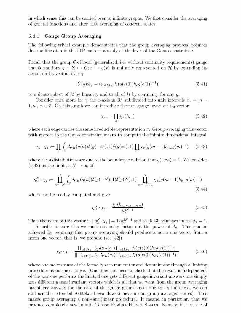
in which sense this can be carried over to infinite graphs. We first consider the averagingof general functions and after that averaging of coherent states.

5.4.1 Gauge Group Averaging

The following trivial example demonstrates that the group averaging proposal requiresdue modification in the ITP context already at the level of the Gauss constraint :

Recall that the group G of local (generalized, i.e. without continuity requirements) gaugetransformations g : Σ 7→ G; x 7→ g(x) is unitarily represented on H by extending itsaction on C0-vectors over γ

U(g)⊗f = ⊗e∈E(γ)fe(g(e(0))heg(e(1))−1) (5.41)

to a dense subset of H by linearity and to all of H by continuity for any g.Consider once more for γ the x-axis in R3 subdivided into unit intervals en = [n −

1, n], n ∈ Z. On this graph we can introduce the non-gauge invariant C0-vector

χπ :=∏

n

χπ(hen) (5.42)

where each edge carries the same irreducible representation π. Group averaging this vectorwith respect to the Gauss constraint means to compute the infinite dimensional integral

ηG · χj :=∏

n

∫

GdµH(g(n))δ(g(−∞), 1)δ(g(∞), 1)

∏

m

χπ(g(m− 1)hemg(m)−1) (5.43)

where the δ distributions are due to the boundary condition that g(±∞) = 1. We consider(5.43) as the limit as N → ∞ of

ηNG · χj :=N∏

n=−N

∫

GdµH(g(n))δ(g(−N), 1)δ(g(N), 1)

N∏

m=−N+1

χπ(g(m− 1)hemg(m)−1)

(5.44)which can be readily computed and gives

ηNG · χj =χj(he−N+1..eN

)

d2N−1π

(5.45)

Thus the norm of this vector is ||ηNG ·χj|| = 1/d2N−1π and so (5.43) vanishes unless dπ = 1.

In order to cure this we must obviously factor out the power of dπ. This can beachieved by requiring that group averaging should produce a norm one vector from anorm one vector, that is, we propose (see [42])

χG · f =

∏v∈V (γ)

∫G dµH(gv)

∏e∈E(γ) fe(g(e(0))heg(e(1))−1)

||∏v∈V (γ)

∫G dµH(gv)

∏e∈E(γ) fe(g(e(0))heg(e(1))−1)|| (5.46)

where one makes sense of the formally zero numerator and denominator through a limitingprocedure as outlined above. (One does not need to check that the result is independentof the way one performs the limit, if one gets different gauge invariant answers one simplygets different gauge invariant vectors which is all that we want from the group averagingmachinery anyway for the case of the gauge group since, due to its finiteness, we canstill use the extended Ashtekar-Lewandowski measure on group averaged states). Thismakes group averaging a non-(anti)linear procedure. It means, in particular, that weproduce completely new Infinite Tensor Product Hilbert Spaces. Namely, in the case of

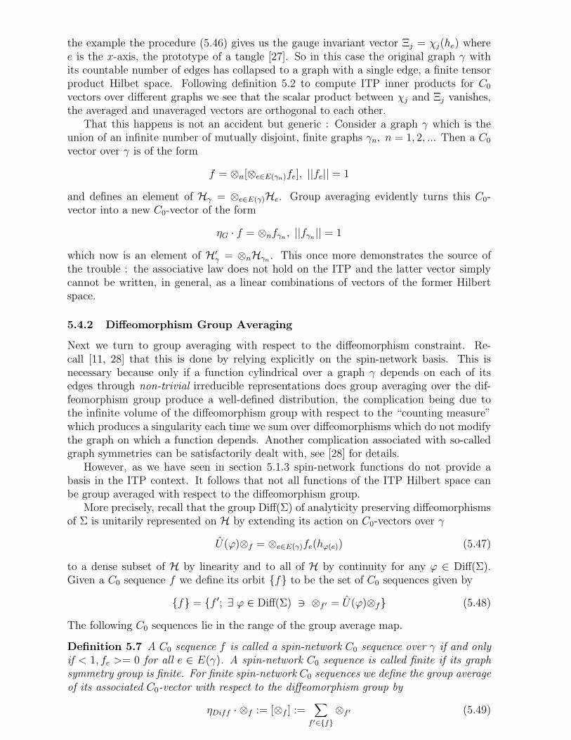
the example the procedure (5.46) gives us the gauge invariant vector Ξj = χj(he) wheree is the x-axis, the prototype of a tangle [27]. So in this case the original graph γ withits countable number of edges has collapsed to a graph with a single edge, a finite tensorproduct Hilbet space. Following definition 5.2 to compute ITP inner products for C0

vectors over different graphs we see that the scalar product between χj and Ξj vanishes,the averaged and unaveraged vectors are orthogonal to each other.

That this happens is not an accident but generic : Consider a graph γ which is theunion of an infinite number of mutually disjoint, finite graphs γn, n = 1, 2, ... Then a C0

vector over γ is of the form

f = ⊗n[⊗e∈E(γn)fe], ||fe|| = 1

and defines an element of Hγ = ⊗e∈E(γ)He. Group averaging evidently turns this C0-vector into a new C0-vector of the form

ηG · f = ⊗nfγn, ||fγn

|| = 1

which now is an element of H′γ = ⊗nHγn

. This once more demonstrates the source ofthe trouble : the associative law does not hold on the ITP and the latter vector simplycannot be written, in general, as a linear combinations of vectors of the former Hilbertspace.

5.4.2 Diffeomorphism Group Averaging

Next we turn to group averaging with respect to the diffeomorphism constraint. Re-call [11, 28] that this is done by relying explicitly on the spin-network basis. This isnecessary because only if a function cylindrical over a graph γ depends on each of itsedges through non-trivial irreducible representations does group averaging over the dif-feomorphism group produce a well-defined distribution, the complication being due tothe infinite volume of the diffeomorphism group with respect to the “counting measure”which produces a singularity each time we sum over diffeomorphisms which do not modifythe graph on which a function depends. Another complication associated with so-calledgraph symmetries can be satisfactorily dealt with, see [28] for details.

However, as we have seen in section 5.1.3 spin-network functions do not provide abasis in the ITP context. It follows that not all functions of the ITP Hilbert space canbe group averaged with respect to the diffeomorphism group.

More precisely, recall that the group Diff(Σ) of analyticity preserving diffeomorphismsof Σ is unitarily represented on H by extending its action on C0-vectors over γ

U(ϕ)⊗f = ⊗e∈E(γ)fe(hϕ(e)) (5.47)

to a dense subset of H by linearity and to all of H by continuity for any ϕ ∈ Diff(Σ).Given a C0 sequence f we define its orbit f to be the set of C0 sequences given by

f = f ′; ∃ ϕ ∈ Diff(Σ) ∋ ⊗f ′ = U(ϕ)⊗f (5.48)

The following C0 sequences lie in the range of the group average map.

Definition 5.7 A C0 sequence f is called a spin-network C0 sequence over γ if and onlyif < 1, fe >= 0 for all e ∈ E(γ). A spin-network C0 sequence is called finite if its graphsymmetry group is finite. For finite spin-network C0 sequences we define the group averageof its associated C0-vector with respect to the diffeomorphism group by

ηDiff · ⊗f := [⊗f ] :=∑

f ′∈f

⊗f ′ (5.49)

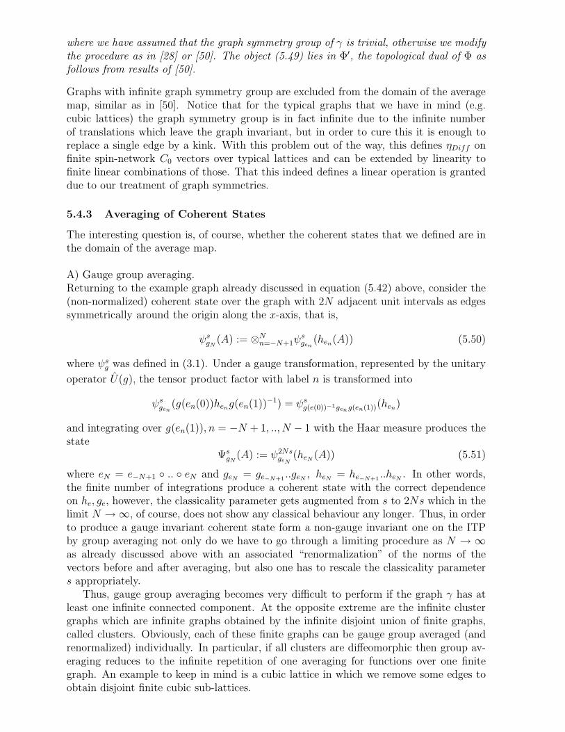
where we have assumed that the graph symmetry group of γ is trivial, otherwise we modifythe procedure as in [28] or [50]. The object (5.49) lies in Φ′, the topological dual of Φ asfollows from results of [50].

Graphs with infinite graph symmetry group are excluded from the domain of the averagemap, similar as in [50]. Notice that for the typical graphs that we have in mind (e.g.cubic lattices) the graph symmetry group is in fact infinite due to the infinite numberof translations which leave the graph invariant, but in order to cure this it is enough toreplace a single edge by a kink. With this problem out of the way, this defines ηDiff onfinite spin-network C0 vectors over typical lattices and can be extended by linearity tofinite linear combinations of those. That this indeed defines a linear operation is granteddue to our treatment of graph symmetries.

5.4.3 Averaging of Coherent States

The interesting question is, of course, whether the coherent states that we defined are inthe domain of the average map.

A) Gauge group averaging.Returning to the example graph already discussed in equation (5.42) above, consider the(non-normalized) coherent state over the graph with 2N adjacent unit intervals as edgessymmetrically around the origin along the x-axis, that is,

ψsgN(A) := ⊗N

n=−N+1ψsgen

(hen(A)) (5.50)

where ψsg was defined in (3.1). Under a gauge transformation, represented by the unitary

operator U(g), the tensor product factor with label n is transformed into

ψsgen(g(en(0))hen

g(en(1))−1) = ψsg(e(0))−1geng(en(1))(hen)

and integrating over g(en(1)), n = −N + 1, .., N − 1 with the Haar measure produces thestate

ΨsgN

(A) := ψ2NsgeN

(heN(A)) (5.51)

where eN = e−N+1 .. eN and geN= ge−N+1

..geN, heN

= he−N+1..heN

. In other words,the finite number of integrations produce a coherent state with the correct dependenceon he, ge, however, the classicality parameter gets augmented from s to 2Ns which in thelimit N → ∞, of course, does not show any classical behaviour any longer. Thus, in orderto produce a gauge invariant coherent state form a non-gauge invariant one on the ITPby group averaging not only do we have to go through a limiting procedure as N → ∞as already discussed above with an associated “renormalization” of the norms of thevectors before and after averaging, but also one has to rescale the classicality parameters appropriately.

Thus, gauge group averaging becomes very difficult to perform if the graph γ has atleast one infinite connected component. At the opposite extreme are the infinite clustergraphs which are infinite graphs obtained by the infinite disjoint union of finite graphs,called clusters. Obviously, each of these finite graphs can be gauge group averaged (andrenormalized) individually. In particular, if all clusters are diffeomorphic then group av-eraging reduces to the infinite repetition of one averaging for functions over one finitegraph. An example to keep in mind is a cubic lattice in which we remove some edges toobtain disjoint finite cubic sub-lattices.

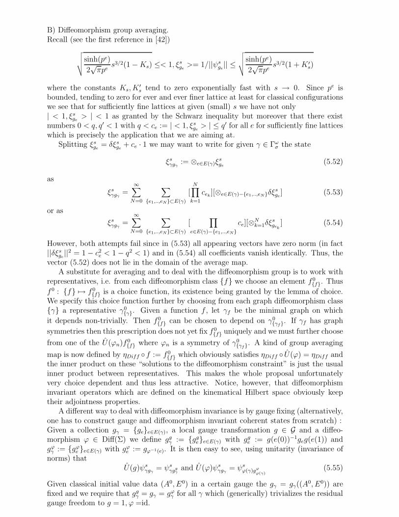
B) Diffeomorphism group averaging.Recall (see the first reference in [42])

√√√√sinh(pe)

2√πpe

s3/2(1 −Ks) ≤< 1, ξsge>= 1/||ψsge

|| ≤√√√√sinh(pe)

2√πpe

s3/2(1 +K ′s)

where the constants Ks, K′s tend to zero exponentially fast with s → 0. Since pe is

bounded, tending to zero for ever and ever finer lattice at least for classical configurationswe see that for sufficiently fine lattices at given (small) s we have not only| < 1, ξsge

> | < 1 as granted by the Schwarz inequality but moreover that there existnumbers 0 < q, q′ < 1 with q < ce := | < 1, ξsge

> | ≤ q′ for all e for sufficiently fine latticeswhich is precisely the application that we are aiming at.

Splitting ξsge= δξsge

+ ce · 1 we may want to write for given γ ∈ Γωσ the state

ξsγgγ:= ⊗e∈E(γ)ξ

sge

(5.52)

as

ξsγgγ=

∞∑

N=0

∑

e1,..,eN⊂E(γ)

[N∏

k=1

cek][⊗e∈E(γ)−e1,..,eNδξ

sge

] (5.53)

or as

ξsγgγ=

∞∑

N=0

∑

e1,..,eN⊂E(γ)

[∏

e∈E(γ)−e1,..,eN

ce][⊗Nk=1δξ

sgek

] (5.54)

However, both attempts fail since in (5.53) all appearing vectors have zero norm (in fact||δξsge

||2 = 1 − c2e < 1 − q2 < 1) and in (5.54) all coefficients vanish identically. Thus, thevector (5.52) does not lie in the domain of the average map.

A substitute for averaging and to deal with the diffeomorphism group is to work withrepresentatives, i.e. from each diffeomorphism class f we choose an element f 0

f. Thus

f 0 : f 7→ f 0f is a choice function, its existence being granted by the lemma of choice.

We specify this choice function further by choosing from each graph diffeomorphism classγ a representative γ0

γ. Given a function f , let γf be the minimal graph on which

it depends non-trivially. Then f 0f can be chosen to depend on γ0

γf. If γf has graph

symmetries then this prescription does not yet fix f 0f uniquely and we must further choose

from one of the U(ϕn)f0f where ϕn is a symmetry of γ0

γf. A kind of group averaging

map is now defined by ηDiff f := f 0f which obviously satisfies ηDiff U(ϕ) = ηDiff and

the inner product on these “solutions to the diffeomorphism constraint” is just the usualinner product between representatives. This makes the whole proposal unfortunatelyvery choice dependent and thus less attractive. Notice, however, that diffeomorphisminvariant operators which are defined on the kinematical Hilbert space obviously keeptheir adjointness properties.

A different way to deal with diffeomorphism invariance is by gauge fixing (alternatively,one has to construct gauge and diffeomorphism invariant coherent states from scratch) :Given a collection gγ = gee∈E(γ), a local gauge transformation g ∈ G and a diffeo-morphism ϕ ∈ Diff(Σ) we define ggγ := ggee∈E(γ) with gge := g(e(0))−1geg(e(1)) andgϕγ := gϕe e∈E(γ) with gϕe := gϕ−1(e). It is then easy to see, using unitarity (invariance ofnorms) that

U(g)ψsγgγ= ψsγgg

γand U(ϕ)ψsγgγ

= ψsϕ(γ)gϕ

ϕ(γ)(5.55)

Given classical initial value data (A0, E0) in a certain gauge the gγ = gγ((A0, E0)) are

fixed and we require that ggγ = gγ = gϕγ for all γ which (generically) trivializes the residualgauge freedom to g = 1, ϕ =id.

Thus, as far as the gauge and diffeomorphism constraints are concerned, we can fix agauge to take care of gauge and diffeomorphism invariance. The issue lies much harderwith respect to the Hamiltonian constraint because its action [22] is much more compli-cated than the action of the kinematical constraints, and almost no Hamiltonian invariantobservables are known with respect to which one would need to construct the invariantcoherent states. Fortunately, there are certain “simple” solutions to the Hamiltonian con-straint [22] corresponding to states whose underlying graph is out of the range of graphsthat the Hamiltonian constraint produces. If we build (non-distributional) coherent stateson such graphs, then they lie in the kernel of the Hamiltonian constraint in the sense ofgeneralized eigenvectors with eigenvalue zero. Thus, at least for these simple solutions,together with fixing of gauge and diffeomorphism freedom, we can incorporate the quan-tum dynamics of general relativity.

All these observations reveal that group averaging non-gauge and/or non-diffeomorphisminvariant coherent states over the gauge or diffeomorphism group is a non-trivial task, atleast not if Σ is non-compact and applied naively without some sort of renormalizationleads to meaningless results. More work is needed in order to construct rigorous solutionsto all constraints which at the same time behave semi-classically. However, at the mo-ment we are not so much interested in obtaining semi-classical solutions to all constraints.Rather, besides the applications already mentioned in section 5.3, it is of paramount im-portance to test the consistency of a quantum representation of the classical constraintalgebra and the verification of its correct classical limit [82]. In order to do this one ob-viously must not have semi-classical states which solve the constraints.

Acknowledgements

O. W. thanks the “Studienstiftung des Deutschen Volkes” for financial support.

References

[1] A. Ashtekar, Phys. Rev. Lett. 57 (1986) 2244, Phys. Rev. D36 (1987) 1587[2] A. Ashtekar, in “Mathematics and General Relativity”, American Mathematical

Society, Providence, Rhode Island, 1987[3] F. Barbero, Phys. Rev. D51 (1995) 5507

F. Barbero, Phys. Rev. D51 (1995) 5498[4] T. Thiemann, Physics Letters B 380 (1996) 257-264, gr-qc/960688[5] R. Gambini, A. Trias, Phys. Rev. D22 (1980) 1380

C. Di Bartolo, F. Nori, R. Gambini, A. Trias, Lett. Nuov. Cim. 38 (1983) 497R. Gambini, A. Trias, Nucl. Phys. B278 (1986) 436

[6] C. Rovelli, L. Smolin, Nucl. Phys. B331 (1990) 80[7] A. Ashtekar and C.J. Isham, Class. Quantum Grav. 9 (1992) 1433[8] A. Ashtekar, J. Lewandowski, “Representation theory of analytic holonomy C⋆ al-

gebras”, in “Knots and Quantum Gravity”, J. Baez (ed), Oxford University Press,Oxford, 1994A. Ashtekar, J. Lewandowski, Journ. Geo. Physics 17 (1995) 191A. Ashtekar and J. Lewandowski, J. Math. Phys. 36, (1995) 2170

[9] D. Marolf and J. M. Mourao, Commun. Math. Phys. 170 (1995) 583-606

[10] J. Baez, S. Sawin, “Functional Integration on Spaces of Connections”, q-alg/9507023J. Baez, S. Sawin, “Diffeomorphism Invariant Spin-Network States”, q-alg/9708005

[11] A. Ashtekar, J. Lewandowski, D. Marolf, J.Mourao, T. Thiemann, Journ. Math.Phys. 36 (1995) 6456-6493, gr-qc/9504018

[12] R. De Pietri, C. Rovelli, Phys. Rev. D54 (1996) 2664[13] R. Gambini, J. Pullin, “Loops, Knots, Gauge Theories and Quantum Gravity”,

Cambridge University Press, Cambridge, 1996[14] T. Thiemann, Journ. Math. Phys. 39 (1998) 1236-48, hep-th/9601105[15] R. De Pietri, Class. Quantum Grav. 14 (1997) 53[16] T. Thiemann, Journ. Math. Phys. 39 (1998) 3372-92, gr-qc/9606092[17] C. Rovelli, L. Smolin, Nucl. Phys. B 442 (1995) 593; Erratum : Nucl. Phys. B 456

(1995) 734[18] A. Ashtekar, J. Lewandowski, Class. Quantum Grav. 14 A55-81 (1997)[19] R. Loll, Nucl. Phys. B460 (1996) 143

R. Loll, Class. Quantum Grav. 14 (1997) 1725R. Loll, Nucl. Phys. B500 (1997) 405

[20] A. Ashtekar, J. Lewandowski, Adv. Theo. Math. Phys. 1 (1997) 388-429[21] T. Thiemann, Journ. Math. Phys. 39 (1998) 3347-71, gr-qc/9606091[22] T. Thiemann, Class. Quantum Grav. 15 (1998) 839-73, gr-qc/9606089[23] T. Thiemann, Class. Quantum Grav. 15 (1998) 875-905, gr-qc/9606090[24] T. Thiemann, Class. Quantum Grav. 15 (1998) 1249-80, gr-qc/9705018[25] T. Thiemann, Class. Quantum Grav. 15 (1998) 1281-1314, gr-qc/9705019[26] T. Thiemann, Class. Quantum Grav. 15 (1998) 1487-1512, gr-qc/9705021[27] T. Thiemann, Class. Quantum Grav. 15 (1998) 1463-85, gr-qc/9705020[28] T. Thiemann, Class. Quantum Gravity 15 (1998) 1207-47, gr-qc/9705017[29] M. Reisenberger, C. Rovelli, Phys. Rev. D56 (1997) 3490-3508[30] J. Baez, Class. Quantum Grav. 15 (1998) 1827-58[31] F. Markopoulou, L. Smolin, Phys. Rev. D58 (1998) 084032[32] J. W. Barret, L. Crane, Class. Quantum Grav. 14 (1997) 2113[33] L. Freidel, K. Krasnov, Adv. Theor. Math. Phys. 2 (1999) 1183[34] K. Krasnov, Gen. Rel. Grav. 30 (1998) 53-68[35] A. Ashtekar, C. Beetle, S. Fairhurst, Class. Quantum Grav. 17 (2000) 1317[36] A. Ashtekar, A. Corichi, K. Krasnov, “Isolated horizons : The classical phase space”,

gr-qc/9905089[37] A. Ashtekar, C. Beetle, S. Fairhurst, Class. Quantum Grav. 16 (1999) L1-L7[38] A. Ashtekar, K. Krasnov, “Quantum Geometry and Black Holes, gr-qc/9804039[39] A. Ashtekar, J. Baez, A. Corichi, K. Krasnov, Phys. Rev. Lett. 80:904-907, 1998[40] A. Ashtekar, “Interface of General Relativity, Quantum Physics amd Statistical

Mechanics : Some Recent Developments”, gr-qc/9910101[41] T. Thiemann, “Gauge Field Theory Coherent States (GCS) : I. General Properties”,

hep-th/0005233[42] T. Thiemann, O. Winkler, “Gauge Field Theory Coherent States (GCS) : II. Peaked-

ness Properties”, hep-th/0005237T. Thiemann, O. Winkler, “Gauge Field Theory Coherent States (GCS) : III. Ehren-fest Theorems”, hep-th/0005234T. Thiemann, “Gauge Field Theory Coherent States (GCS) : V. Extension to HiggsFields and Fermions”, to appear

[43] J. von Neumann, Comp. Math. 6 (1938) 1-77W. Thirring, “Lehrbuch der Mathematischen Physik”, vol. 4, Springer-Verlag, Wien,1994

[44] G. Amelino-Camelia et al, “Tests of quantum gravity from observations of γ−raybursts”, Nature 393 (1998) 763

[45] H. Sahlmann, T. Thiemann, O. Winkler, “Gauge Field Theory Coherent States(GCS) : VII. The Non-Perturbative γ-Ray Burst Effect”, to appear

[46] R. Gambini, J. Pullin, “Non-standard optics from quantum spacetime, Phys. Rev.D59 (1999) 124021

[47] T. Thiemann, “Quantum Spin Dynamics (QSD) : VII. Symplectic Structures andContinuum Lattice Formulations of Gauge Field Theories”, hep-th/0005232

[48] E. Hebey, “Sobolev Spaces on Riemannian Manifolds”, Lecture Notes in Mathemat-ics 1635, Springer Verlag, Berlin, 1996

[49] S. Lang, “Differential Manifolds”, Addison Wesley, Reading, Massachusetts, 1972[50] J. Lewandowski, T. Thiemann, Class. Quantum Grav. 16 (1999) 2299-2322, gr-

qc/9901015[51] J.-A. Zapata, Journ. Math. Phys. 38 (1997) 5663

J.-A. Zapata, Gen. Rel. Grav. 30 (1998) 1229[52] C. Rovelli, L. Smolin, “Spin networks and quantum gravity” pre-print CGPG-95/4-

1, Phys. Rev. D52 (1995) 5743[53] J. Baez, Adv. Math. 117 (1996) 253-272[54] A. Rendall, Class. Quantum Grav. 10 (1993) 605

A. Rendall, “Adjointness Relations as a Criterion for Choosing an Inner Product”,gr-qc/9403001

[55] T. Thiemann, Class. Quantum Gravity 13 (1996) 1383-1403, gr-qc/9511057T. Thiemann, Acta Cosmologica 21 (1995), 145-167, gr-qc/9511049 T. Thiemann,in : “Symplectic Singularities and Geometry of Gauge Fields”, Banach Center Pub-lications, 39 389-403 (1996), hep-th/9511122

[56] B. C. Hall, Journ. Funct. Analysis 122 (1994) 103[57] A. Ashtekar, J. Lewandowski, D. Marolf, J. Mourao, T. Thiemann, Journ. Funct.

Analysis 135 (1996) 519-551, gr-qc/9412014[58] B. C. Hall, Comm. Math. Phys. 184 (1997) 233[59] R. F. Streater, A. S. Wightman, “PCT, Spin and Statistics, and all that”, Benjamin,

New York, 1964[60] M. D. Potter, “Mengentheorie”, ch. 5, Spektrum Akademischer Verlag, Berlin, 1990

P. J. Cameron, “Sets, Logic and Categories”, Springer Verlag, Berlin, 1999[61] R. V. Kadison, J. R. Ringrose, “Fundamentals of the Theory of Operator Algebras”,

vol. 1 and 2, Academic Press, London, 1983O. Bratteli, D. W. Robinson, “Operator Algebrs and Quantum Statistical Mechan-ics”, vol. 1 and 2, Springer Verlag, Berlin, 1997

[62] R. Haag, “Local Quantum Physics”, 2nd ed., Springer Verlag, Berlin, 1996[63] K. Fredenhagen, Comm. Math. Phys. 97 (1985) 79[64] M. Reed, B. Simon “Methods of Modern Mathematical Physics”, vol. 1 and 2,

Academic Press, New York, 1975[65] A. Connes, “Noncommutative Geometry”, Academic Press, 1994[66] W. Krieger, Math. Ann. 223 (1976) 19[67] R. T. Powers, Ann. Math. 86 (1967) 138[68] H. Araki, E.J. Woods, Publ. Res. Inst. Math. Sci. Ser. A4 (1968) 51[69] H. Baumgartel, M. Wollenberg, “Causal Nets of Operator Algebras”, Akademie

Verlag, Berlin, 1992[70] N. Bourbaki, “General Topology”, vol. 1 and 2, Hermann, Paris, 1966[71] M. Arnsdorf, R. S. Garcia, Class. Quantum Grav. 16 (1999) 3405[72] Y. Yamasaki, “Measures on Infinite Dimensional Spaces”, World Scientific, Singa-

pore, 1985

[73] A. Ashtekar, J. Lewandowski, D. Marolf, J. Mourao, T. Thiemann, Journ. Math.Phys. 38 (1997) 5453-82, hep-th/9605128

[74] H. Sahlmann, T. Thiemann, O. Winkler, “Gauge Field Theory Coherent States(GCS) : VI. Photons and Gravitatons Propagating on Quantum Spacetimes”, toappear

[75] H. Sahlmann, T. Thiemann, O. Winkler, “Gauge Field Theory Coherent States(GCS) : VIII. Perturbation Theory Results from Non-Perturbative CoherentStates”, in preparationH. Sahlmann, T. Thiemann, O. Winkler, “Gauge Field Theory Coherent States(GCS) : IX. Renormalization Group and Diffeomorphism Invariance”, in prepara-tion

[76] S. A. Fulling, “Aspects of Quantum Field Theory in Curved Space-Time”, Cam-bridge University Press, Cambridge, 1989

[77] M. J. Radzikowski, “The Hadamard Condition and Kay’s Conjecture in (Axiomatic)Quantum Field Theory on Curved Space-Time”, PhD Thesis, Princeton University,October 1992R. Brunetti, K. Fredenhagen, Comm. Math. Phys. 180 (1996) 312W. Junker, Rev. Math. Phys. 8 (1996) 1091

[78] S. D. Biller et al, Phys. Rev. Lett. 83 (1999) 2108[79] O. Winkler, “Infinite Tensor Product and Metric Non-Degeneracy Condition in 2+1

Gravity”, in preparation[80] A. Ashtekar, C. Rovelli, L. Smolin, Phys. Rev. Lett. 69 (1992) 237[81] H. Sahlmann, T. Thiemann, O. Winkler “Gauge Field Theory Coherent States

(GCS) : X. Quantum Black Holes, Hawking Effect and Singularity Theorems”, inpreparation

[82] T. Thiemann, “Quantum Spin Dynamics (QSD) : VIII. The Classical Limit”, toappear

[83] S.W. Hawking, G.F.R. Ellis, “The large scale structure of space-time”, CambridgeUniversity Press, Cambridge, 1989

[84] A. Sen, “An Introduction to Non-perturbative String Theory”, hep-th/9802051[85] H. Sahlmann, T. Thiemann, O. Winkler, “Gauge Field Theory Coherent States

(GCS) : XI. Coherent States for Groups of Higher Rank”, in preparation[86] H. Sahlmann, T. Thiemann, O. Winkler, “Gauge Field Theory Coherent States

(GCS) : XII. Modular Theory and von Neumann Agebra Factor Types”, in prepa-ration

[87] M. C. Reed, Journ. Funct. Analysis 5 (1970) 94[88] J. R. Klauder, B.-S. Skagerstam, “Coherent Sates”, World Scientific, Singapore,

1985[89] H. Sahlmann, T. Thiemann, O. Winkler, “Gauge Field Theory Coherent States

(GCS) : XIII. Coherent State Path Integral for Quantum General Relativity”, inpreparation

[90] L. Bombelli, “Statistical Lorentzian Geometry and the Closeness of Lorentzian Man-ifolds”, gr-qc/0002053A. Ashtekar, L. Bombelli, “Weaves and Random Lattices”, in preparation

[91] C. Itzykson, J.-M. Drouffe, “Statistical Field Theory”, vol. 2, Cambridge UniversityPress, Cambridge, 1997

[92] A. Ashtekar, L. Bombelli, H. Sahlmann, T. Thiemann, O. Winkler, “Gauge FieldTheory Coherent States (GCS) : XIV. Random Coherent States for Quantum Gen-eral Relativity”, in preparation

[93] M. Varadarajan, J.-A. Zapata, “A proposal for Analyzing the Classical Limit ofKinematic Loop Quantum Gravity”, gr-qc/0001040