Computing Laboratory

GAME-BASED PROBABILISTIC PREDICATE ABSTRACTIONWITH PRISM

M. Kattenbelt M. Kwiatkowska G. Norman D. Parker

CL-RR-08-01

�Oxford University Computing Laboratory

Wolfson Building, Parks Road, Oxford OX1 3QD

Abstract

Modelling and verification of systems such as communication, network and se-curity protocols, which exhibit both probabilistic and non-deterministic behaviour,typically use Markov Decision Processes (MDPs). For large, complex systems, ab-straction techniques are essential. This paper builds on a promising approach forabstraction of MDPs based on stochastic two-player games which provides distinctlower and upper bounds for minimum and maximum probabilistic reachability prop-erties. Existing implementations work at the model level, limiting their scalability. Inthis paper, we develop language-level abstraction techniques that build game-basedabstractions of MDPs directly from high-level descriptions in the PRISM modellinglanguage, using predicate abstraction and SMT solvers. For efficiency, we developa compositional framework for abstraction. We have applied our techniques to arange of case studies, successfully verifying models larger than was possible with ex-isting implementations. We are also able to demonstrate the benefits of adopting acompositional approach.

1 Introduction

Verification of systems that exhibit both non-deterministic and probabilistic behaviourhas proved to be very useful in domains such as communication and network protocols,security protocols, and randomised distributed algorithms. Markov Decision Processes(MDPs) are a natural model for such systems and several tools, such as PRISM [13]and LiQuor [4], implement efficient solution methods for these models. As in the fieldof non-probabilistic model checking, however, the state space explosion problem tends tolimit the scalability of these approaches and techniques to counter this are an importantarea of research.

Of particular current interest are the development of abstraction techniques for theverification of MDPs [6, 8, 17, 21]. In this paper, we use the abstraction approach of[17], which is based on stochastic two-player games. The key idea is to separate thenon-determinism that is introduced by the abstraction from the non-determinism presentin the original MDP. This results in abstract models that provide distinct upper andlower bounds on minimum and maximum reachability probabilities. This is in contrastto alternative abstraction methods [6], where only an upper bound on the maximum prob-ability and a lower bound on the minimum probability can be extracted. Besides being amore informative abstraction, these bounds also provide a measure of the quality of theabstraction. This information is potentially very useful when considering refinement.

A limitation of the existing implementation in [17] is that abstractions are performedat the model level, i.e. the full concrete model (MDP) is constructed and then reduced tothe corresponding stochastic game. In this paper, we develop techniques to construct theabstraction directly from a high-level description of the MDP (in this case the modellinglanguage of PRISM) using predicate abstraction [12, 1, 5], which has been very successfulin the non-probabilistic setting.

Predicate abstraction for PRISM models was recently considered in [21], but using theabstraction technique of [6] which represents abstractions as MDPs. Applying predicateabstraction to the approach of [17] provides the additional benefits of the game-based

1

approach but proves to be more involved. This is because the game-based abstractionpreserves additional information which is non-trivial to extract from language-level de-scriptions of PRISM models.

We present a compositional variant of game-based abstraction of MDPs, explain howto apply it at the level of the PRISM modelling language, and describe an implementationof these techniques using SMT solvers and ‘on-the-fly’ abstraction. We illustrate itsapplicability on several examples, successfully analysing models larger than is possiblewith the implementation of [17] and improving performance on others. We also analysethe benefits of employing a compositional approach.

The remainder of this paper is structured as follows. Section 2 provides backgroundmaterial, including the PRISM modelling language and its semantics. In Section 3 wepresent a compositional variant of the game-based abstraction method of [17]. In Sec-tion 4, we give a game-based variant of PRISM called A–PRISM and describe a predicateabstraction procedure for PRISM models that results in A–PRISM models. Sections 5and 6 describe our implementation and present experimental results from several casestudies. We conclude with a discussion of related work and ideas for future development.

2 Background

We assume a set of typed variables V . A valuation of V is a function s mapping eachvariable in V to a value in its domain. We let val(V ) denote the set of all valuations ofV and, for any s ∈ val(V ) and V ′ ⊆ V , let sdV ′ denote the restriction of s to the domainV ′. Furthermore, if s1 ∈ val(V1), s2 ∈ val(V2) and V1 ∩ V2 = ∅, we let s1 ‖ s2 denote thevaluation of V1 ∪ V2 where (s1 ‖ s2)dV1= s1 and (s1 ‖ s2)dV2= s2. We will often refer tovaluations as states. We also assume a finite set Act of actions and an additional ‘silent’action τ 6∈ Act .

A probability distribution over a finite set S is a function µ : S → [0, 1] such that∑s∈S µ(s) = 1. Let Dist(S) denote the set of all distributions over S. For any s ∈ S,

let ηs denote the point distribution at s. If µ1 ∈ Dist(val(V1)), µ2 ∈ Dist(val(V2)) andV1 ∩ V2 = ∅, let µ1 ‖µ2 denote the distribution over val(V1 ∪ V2) such that (µ1 ‖µ2)(s) =µ1(sdV1) · µ2(sdV2) for all s ∈ val(V1 ∪ V2).

Definition 1 Let V, V ′ be sets of variables such that V ′ ⊆ V. A transition from V to V ′‘is a tuple 〈s, step〉 where s ∈ val(V ) and step ⊆ (Act ∪ {τ})× Dist(val(V ′)).

A transition 〈s, step〉 consists of a source state s and non-deterministic choice step betweenpairs comprising an action and a distribution over target states. We now define (standardCSP-style) parallel composition of transitions.

Definition 2 Suppose V1, V2 ⊆ V are disjoint sets of variables, 〈s, stepi〉 is a transitionfrom V to Vi for i ∈ {1, 2} and A ⊆ Act . Let 〈s, step1〉 |[A]| 〈s, step2〉 denote the transition〈s, step〉 from V to V1∪V2 where 〈a, µ〉 ∈ step if and only if one of the following conditionsholds:

1. a 6∈ A and µ = µ1 ‖ η(sdV2) for some 〈a, µ1〉 ∈ step1;

2

2. a 6∈ A and µ = η(sdV1) ‖µ2 for some 〈a, µ2〉 ∈ step2;

3. a ∈ A and µ = µ1 ‖µ2 for some 〈a, µ1〉 ∈ step1 and 〈a, µ2〉 ∈ step2.

2.1 Controlled Markov Decision Processes

The techniques introduced in this paper are for Markov Decision Processes (MDPs).However, in order to adopt a compositional approach, we use a variant called ControlledMarkov Decision Processes which represent components of an MDP. These are similar tothe probabilistic modules of [7].

Definition 3 A Controlled Markov Decision Process (CMDP) is a tuple C =〈V, V ctrl, V ext,Act , sinit,Steps 〉 where:

• V is a finite set of typed variables;

• V ctrl and V ext partition V into controlled and external variables;

• Act is a finite set of actions;

• sinit ∈ val(V ctrl) is the initial valuation;

• Steps : val(V ) → P((Act ∪ {τ})× Dist(val(V ctrl))) is the transition function.

A CMDP specifies the initial values of its controlled variables and how these variablesare updated. These updates depend on the values of both its controlled variables andthe external variables, which are assumed to be under the control of other componentsin the system. Given a valuation of all variables s ∈ val(V) the set of action-distributionpairs Steps (s) represents a non-deterministic choice between several behaviours. If the〈a, µ〉 is chosen, then the CMDP performs action a and then probabilistically selects anew valuation of its controlled variables according to µ. The transition function canequivalently be defined as the set {〈s,Steps (s)〉 | s ∈ val(V )} of transitions from V to V ctrl.

We now describe the parallel composition of CMDPs. CMDPs can only be combinedin parallel when they agree on the total set of variables and their control variables aredisjoint. We call such CMDPs composable. Let Ci = 〈V, V ctrl

i , V exti ,Act i, s

initi ,Steps i〉 for

i ∈ {1, 2}.

Definition 4 The parallel composition of two composable CMDPs C1 and C2 is the CMDPC1 |[A]| C2 = 〈V, V ctrl, V ext,Act , sinit,Steps 〉 where:

• V ctrl = V ctrl1 ∪ V ctrl

2 ;

• V ext = (V ext1 ∪ V ext

2 ) \ (V ctrl1 ∪ V ctrl

2 );

• Act = Act 1 ∪Act 2;

• sinit = sinit1 ‖ sinit

2 ;

• if s ∈ val(V ), then 〈s,Steps (s)〉 = 〈s,Steps 1(s)〉 |[A]| 〈s,Steps 2(s)〉.

3

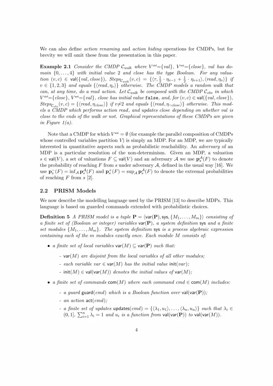
We can also define action renaming and action hiding operations for CMDPs, but forbrevity we will omit these from the presentation in this paper.

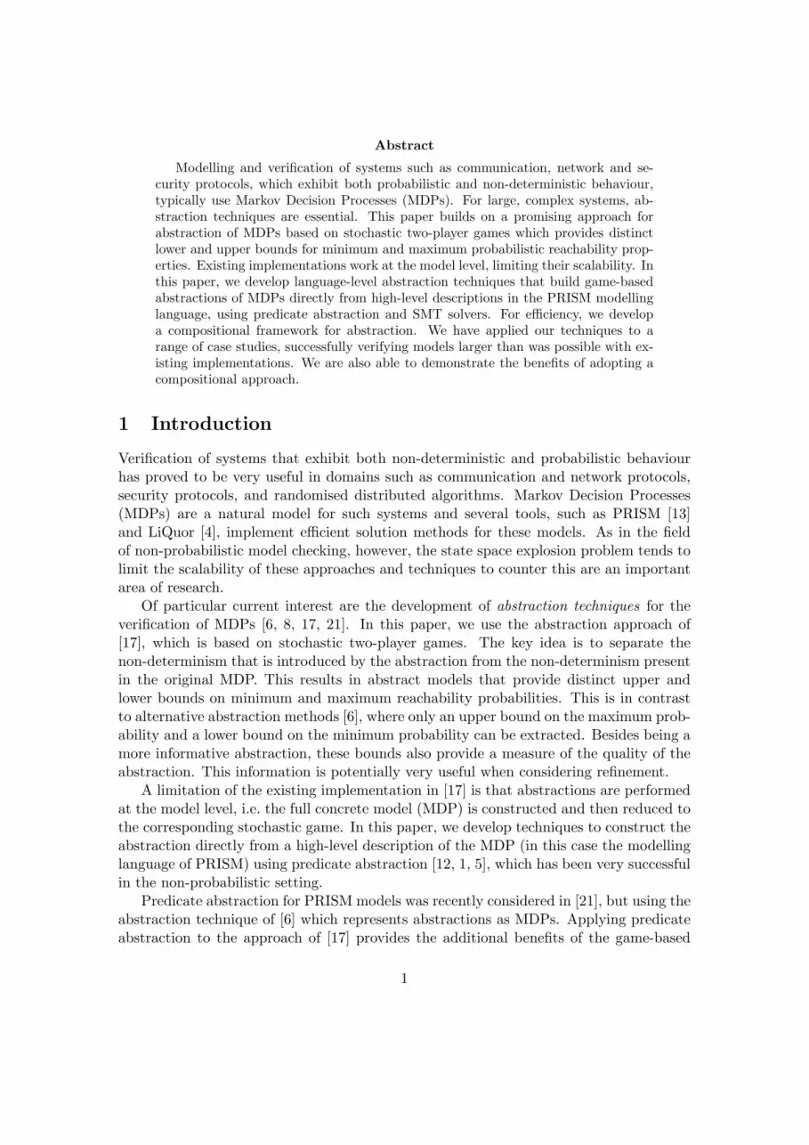
Example 2.1 Consider the CMDP Cwalk where V ctrl={val}, V ext={close}, val has do-main {0, . . . , 4} with initial value 2 and close has the type Boolean. For any valua-tion (v, c) ∈ val({val , close}), StepsCwalk

(v, c) = {〈τ, 12 · ηv−1 + 1

2 · ηv+1〉, 〈read , ηv〉} ifv ∈ {1, 2, 3} and equals {〈read , ηv〉} otherwise. The CMDP models a random walk thatcan, at any time, do a read action. Let Cwalk be composed with the CMDP Cobs in whichV ctrl={close}, V ext={val}, close has initial value false, and, for (v, c) ∈ val({val , close}),StepsCobs

(v, c) = {〈read , ηclose〉} if v 6=2 and equals {〈read , η¬close〉} otherwise. This mod-els a CMDP which performs action read, and updates close depending on whether val isclose to the ends of the walk or not. Graphical representations of these CMDPs are givenin Figure 1(a).

Note that a CMDP for which V ext = ∅ (for example the parallel composition of CMDPswhose controlled variables partition V) is simply an MDP. For an MDP, we are typicallyinterested in quantitative aspects such as probabilistic reachability. An adversary of anMDP is a particular resolution of the non-determinism. Given an MDP, a valuations ∈ val(V ), a set of valuations F ⊆ val(V ) and an adversary A we use pAs (F ) to denotethe probability of reaching F from s under adversary A, defined in the usual way [16]. Weuse p−s (F ) = infA pAs (F ) and p+

s (F ) = supA pAs (F ) to denote the extremal probabilitiesof reaching F from s [2].

2.2 PRISM Models

We now describe the modelling language used by the PRISM [13] to describe MDPs. Thislanguage is based on guarded commands extended with probabilistic choices.

Definition 5 A PRISM model is a tuple P = 〈var(P), sys, {M1, . . . ,Mm}〉 consisting ofa finite set of (Boolean or integer) variables var(P), a system definition sys and a finiteset modules {M1, . . . ,Mm}. The system definition sys is a process algebraic expressioncontaining each of the m modules exactly once. Each module M consists of:

• a finite set of local variables var(M) ⊆ var(P) such that:

- var(M) are disjoint from the local variables of all other modules;

- each variable var ∈ var(M) has the initial value init(var);

- init(M) ∈ val(var(M)) denotes the initial values of var(M);

• a finite set of commands com(M) where each command cmd ∈ com(M) includes:

- a guard guard(cmd) which is a Boolean function over val(var(P));

- an action act(cmd);

- a finite set of updates updates(cmd) = {〈λ1, u1〉, . . . , 〈λn, un〉} such that λi ∈(0, 1],

∑ni=1 λi = 1 and ui is a function from val(var(P)) to val(var(M)).

4

val=0

val=4

close

¬close

0.5

0.5

0.5

0.5

0.5

τval=1

τ val=2

τval=3

read

read

1.0read

1.0

1.0read

1.0

1.0 val 6=2

1.0

1.0read1.0

readval 6=2

read

read

0.5

val=2

1.0read

(a) CMDPs.

module walk

val : [0..4] init 2;

[] (0<val<4) → 0.5 : (val ′=val−1) + 0.5 : (val ′=val+1);[read ] true → 1.0 : true;

endmodule

module obs

close : bool init false;

[read ] (val 6=2) → 1.0 : (close′=true);[read ] (val=2) → 1.0 : (close′=false);

endmodule

system walk |[read ]| obs endsystem

(b) PRISM syntax.

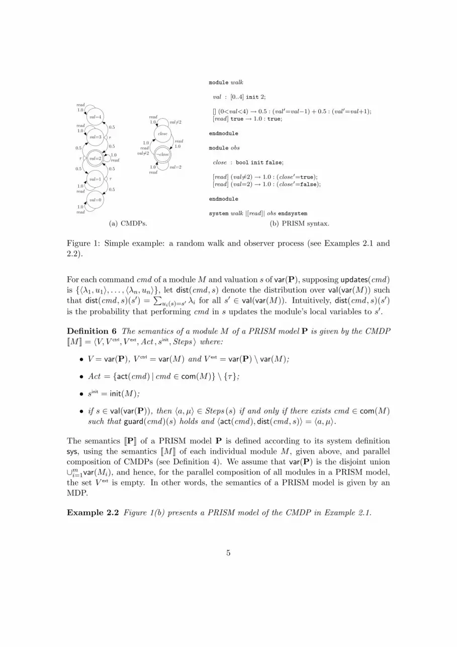
Figure 1: Simple example: a random walk and observer process (see Examples 2.1 and2.2).

For each command cmd of a module M and valuation s of var(P), supposing updates(cmd)is {〈λ1, u1〉, . . . , 〈λn, un〉}, let dist(cmd , s) denote the distribution over val(var(M)) suchthat dist(cmd , s)(s′) =

∑ui(s)=s′ λi for all s′ ∈ val(var(M)). Intuitively, dist(cmd , s)(s′)

is the probability that performing cmd in s updates the module’s local variables to s′.

Definition 6 The semantics of a module M of a PRISM model P is given by the CMDP[[M ]] = 〈V, V ctrl, V ext,Act , sinit,Steps 〉 where:

• V = var(P), V ctrl = var(M) and V ext = var(P) \ var(M);

• Act = {act(cmd) | cmd ∈ com(M)} \ {τ};

• sinit = init(M);

• if s ∈ val(var(P)), then 〈a, µ〉 ∈ Steps (s) if and only if there exists cmd ∈ com(M)such that guard(cmd)(s) holds and 〈act(cmd), dist(cmd , s)〉 = 〈a, µ〉.

The semantics [[P]] of a PRISM model P is defined according to its system definitionsys, using the semantics [[M ]] of each individual module M , given above, and parallelcomposition of CMDPs (see Definition 4). We assume that var(P) is the disjoint union∪m

i=1var(Mi), and hence, for the parallel composition of all modules in a PRISM model,the set V ext is empty. In other words, the semantics of a PRISM model is given by anMDP.

Example 2.2 Figure 1(b) presents a PRISM model of the CMDP in Example 2.1.

5

3 Abstraction of CMDPs

In this section we introduce abstractions of CMDPs, using the stochastic two-player gameapproach of [17] and predicates. A predicate ϕ is over variables V if all valuations of Vuniquely determine the truth value of ϕ and we write ϕ(s) to denote the value of ϕ for avaluation s of V . Given a set of predicates Φ, let bool(Φ) be the set of Boolean variablesindexed by the predicates in Φ, i.e. the set {bϕ |ϕ ∈ Φ}. Furthermore, for abstractionof a particular CMDP using Φ, we will require that every predicate is either over onlycontrolled variables or only external variables of this component. This partitions thepredicates into Φctrl and Φext.

3.1 Abstract Controlled Markov Decision Processes

In order to present a compositional variant of game-based MDP abstraction, we introduceAbstract Controlled Markov Decision Processes (ACMDPs) which are a variant of theclass of stochastic two-player games used in [17].

Definition 7 An Abstract Controlled Markov Decision Process (ACMDP) is a tupleA = 〈V , V ctrl, V ext,Act , sinit,Steps 〉 where:

• V is a set of typed variables;

• V ctrl and V ext partition V into controlled and external variables;

• Act is a finite set of actions;

• sinit ∈ val(V ctrl) is the initial valuation;

• Steps : val(V ) → P(P((Act ∪ {τ})× Dist(val(V ctrl)))) is the transition function.

The crucial difference between CMDPs and ACMDPs is that the transition function nowreturns sets of sets of action-distribution pairs. This means ACMDPs capture two levelsof non-determinism: the choice of a set of action-distribution pairs, and then the choiceof an element in this set. This two-level non-determinism is equivalent to that of thestochastic two-player games used in [17], where first player 1 makes a choice, then player2 does, followed by a probabilistic choice.

We now describe the parallel composition of ACMDPs. As for CMDPs, ACMDPs canonly be combined when they agree on the total set of variables and their control variablesare disjoint. We call such ACMDPs composable. Let Ai = 〈V , V ctrl

i , V exti ,Act i, sinit

i ,Steps i〉for i ∈ {1, 2}.

Definition 8 The parallel composition of two composable ACMDPs A1 and A2 is theACMDP A1 |[A]| A2 = 〈V , V ctrl, V ext,Act , sinit,Steps 〉 where

• V ctrl = V ctrl1 ∪ V ctrl

2 ;

• V ext = (V ext1 ∪ V ext

2 ) \ (V ctrl1 ∪ V ctrl

2 );

6

• Act = Act 1 ∪Act 2;

• sinit = sinit1 ‖ sinit

2 ;

• if s ∈ val(V ), then step ∈ Steps (s) if and only if 〈s, step〉 = 〈s, step1〉 |[A]| 〈s, step2〉for some step1 ∈ Steps 1(s) and step2 ∈ Steps 2(s).

Like the relation between CMDPs and MDPs, an ACMDP for which V ext = ∅ is equiva-lent to a stochastic two-player game from [17]. A player 1 strategy in such an ACMDP isa particular resolution of the first non-deterministic choice of transitions in the ACMDP,whereas a player 2 strategy resolves the second non-deterministic choice. Given a valua-tion s ∈ val(V ), a set of valuations F ⊆ val(V ) and strategy pair σ1, σ2, we use pσ1,σ2

s (F )to denote the probability of reaching F from s under the strategies σ1, σ2. Like for MDPs,we define extremal values as:

p−−s (F ) = infσ1

infσ2

pσ1,σ2s (F ) p+−

s (F ) = supσ1

infσ2

pσ1,σ2s (F )

p−+s (F ) = inf

σ1

supσ2

pσ1,σ2s (F ) p++

s (F ) = supσ1

supσ2

pσ1,σ2s (F )

3.2 Predicate Abstraction for CMDPs

In this section we introduce a compositional and predicate-based extension of the ab-straction procedure described in [17]. Like in non-probabilistic predicate abstraction [1],we will represent an abstract state using Boolean variables bool(Φ) indexed by a set ofpredicates Φ. We will denote abstractions with respect to Φ by α( · ,Φ), which we nowdefine for states, distributions, transitions and then CMDPs.

Definition 9 Given a set of variables V and predicates Φ over V , the abstractions of avaluation s ∈ val(V ) and distribution µ ∈ Dist(val(V )) with respect to Φ are defined asfollows:

• α(s,Φ) is the valuation of bool(Φ) where α(s,Φ)(bϕ)=ϕ(s) for all ϕ ∈ Φ;

• α(µ,Φ) is the distribution over val(bool(Φ)) where α(µ,Φ)(s) =∑

α(s,Φ)=s µ(s) forall s ∈ val(bool(Φ)).

Definition 10 Given a set of variables V, subset V ′ ⊆ V and sets of predicates Φ andΦ′ ⊆ Φ over V and V ′, the abstraction of a transition 〈s, step〉 from V to V ′ with respect toΦ, denoted α(〈s, step〉,Φ), is given by the transition 〈α(s,Φ), {〈a, α(µ,Φ′)〉 | 〈a, µ〉 ∈ step}〉from bool(Φ) to bool(Φ′).

We now define an abstraction function over CMDPs. For the remainder of Section 3, wefix a CMDP C = 〈V, V ctrl, V ext,Act , sinit,Steps 〉 and set of predicates Φ over V .

Definition 11 The abstraction of CMDP C with respect to the predicates Φ is the ACMDPα(C,Φ) = 〈V , V ctrl, V ext,Act , sinit,Steps 〉 where:

• V = bool(Φ);

7

• V ctrl = bool(Φctrl);

• V ext = bool(Φext);

• sinit = α(sinit,Φctrl);

• if s ∈ val(V ), then step ∈ Steps (s) if and only if there exists s ∈ val(V ) such thatα(〈s,Steps (s)〉,Φ) = 〈s, step〉.

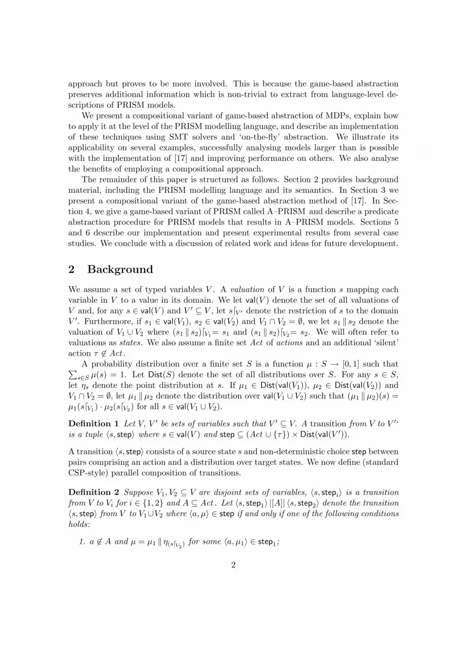
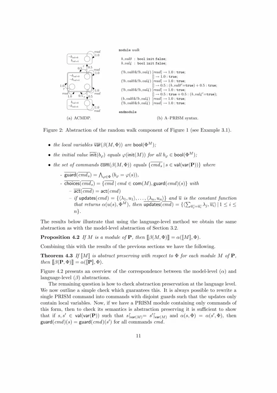
Example 3.1 Consider the CMDP Cwalk of Example 2.1 and set of predicates Φ ={(val=0), (val=4), (close)}. Applying Definition 11, we obtain the ACMDP depicted inFigure 2(a) with V ctrl = {bval=0, bval=4} and V ext = {bclose}. The states of the ACMDP areshown as rectangles and the initial state as a double rectangle. The first non-deterministicchoice is represented by the circles within a state, and the second non-deterministic choiceby outgoing distributions from a circle. Since the external variables have no influence,they are omitted.

It is straightforward to show that applying Definition 11 to a CMDP for which V ext = ∅yields an ACMDP (with V ext = ∅) equivalent to the stochastic two-player game derivedfrom the abstraction procedure described in [17]. Therefore the results of [17] carry overto this setting; in particular, by analysing the ACMDP α(C,Φ) we can obtain upper andlower bounds for both minimum and maximum reachability probabilities of the CMDPC. More formally, given a CMDP C = 〈V, V ctrl, V ext,Act , sinit,Steps 〉, valuation s ∈ val(V)and reachability objective F ⊆ val(V ), letting s = α(s,Φ) and F = {α(s′,Φ) | s′ ∈ F} wehave:

p−−s (F ) ≤ p−s (F ) ≤ p+−s (F )

p−+s (F ) ≤ p+

s (F ) ≤ p++s (F )

3.3 Compositional Abstraction of CMDPs

The abstraction of Definition 11 can be applied to any CMDP but, as the followingexample demonstrates, parallel composition and abstraction do not commute.

Example 3.2 Consider again Example 2.1 (Figure 1(a)) and set of predicates Φ ={(val=0), (val=4), (close)}. For the abstract valuation s = (¬bval=0,¬bval=4, bclose) fromDefinition 11 it follows that {〈τ, η(¬bval=0,¬bval=4)〉, 〈read , η(¬bval=0,¬bval=4)〉} and {〈read,ηbclose 〉} are in Steps α(Cobs ,Φ)(s). Therefore, by Definition 8, it follows that {〈τ, ηs〉, 〈read,ηs〉} is in Steps α(Cwalk ,Φ) |[read ]|α(Cobs ,Φ)(s). However, no valuation (v, c) abstracts to sand induces this transition in α(Cwalk |[read ]| Cobs ,Φ). More precisely, if the τ transitionabstracts to a self-loop, then v=2, and if the read transition sets close to true, then v 6=2.

As this example illustrates, a compositional abstraction may introduce spurious transi-tions, resulting in an over-approximation of the non-compositional abstraction and thusless precise lower and upper bounds for probabilistic reachability. Although such ab-stractions may still lead to useful results, we now introduce the notion of abstraction

8

preserving CMDPs, for which compositional abstraction is precise (i.e. equivalent to thenon-compositional abstraction).

Definition 12 The CMDP C is called abstraction preserving with respect to the predi-cates Φ if for any s, s′ ∈ val(V ) such that sdV ctrl= s′dV ctrl and α(s,Φext) = α(s′,Φext), thenα(〈s,Steps (s)〉,Φ) = α(〈s′,Steps (s′)〉,Φ).

Intuitively, this states that any valuations which agree on control variables and satisfythe same external predicates yield the same abstract transitions. As the following tworesults show, this property is both preserved under parallel composition and ensures aprecise abstraction under parallel composition.

Proposition 3.3 Let C1 and C2 be composable CMDPs and A be a set of actions. If C1

and C2 are abstraction preserving with respect to the predicates Φ, then their compositionC1 |[A]| C2 is also abstraction preserving with respect to Φ.

Proposition 3.4 Let C1 and C2 be composable CMDPs and A be a set of actions. If C1

and C2 are abstraction preserving with respect to the predicates Φ, then:

α(C1,Φ) |[A]|α(C2,Φ) = α(C1 |[A]| C2,Φ) .

From Proposition 3.3 and Proposition 3.4, we can infer that a compositional abstractionis precise if each individual component is abstraction preserving.

Example 3.5 Consider the CMDP Cobs from Example 2.1 and set of predicates Φ ={(val=0), (val=4), (close)}. This CMDP is not abstraction preserving with respect toΦ. For example, the valuations s = (2, true) and s′ = (3, true) agree on the value ofclose and α(s,Φext) = α(s′,Φext) = (¬bval=0 ,¬bval=4 ). However, α(〈s,Steps Cobs

(s)〉,Φ) =〈α(s,Φ), {〈read , η¬bclose 〉}〉 while α(〈s′,Steps Cobs

(s′)〉,Φ) = 〈α(s′,Φ), {〈read , ηbclose 〉}〉. Ifwe extend Φ with the predicate (val=2), then Cobs is abstraction preserving.

4 Abstraction of PRISM Models

Suppose we wish to abstract a PRISM model. One possibility is to (compositionally ornon-compositionally) apply the abstraction method of Section 3 to its CMDP semantics.In either case, the disadvantage of such a method is that the concrete CMDPs have tobe constructed, limiting the applicability of the approach. In this section we define alanguage-level abstraction method to remedy the situation.

4.1 A–PRISM Models

For our language-level abstraction, we introduce the A–PRISM language, an extensionof the PRISM language with an additional element of choice.

Definition 13 An A–PRISM model is a tuple A = 〈var(A), sys, {M1, . . . ,Mm}〉. Theonly difference between this and a PRISM model is the definition of the commandscom(M) for each module M . Each command cmd ∈ com(M) includes:

9

• a guard guard(cmd) which is a Boolean function over val(var(A));

• a finite set of choices choices(cmd) where each chc ∈ choices(cmd) consists of anaction act(chc) and a finite set of updates updates(chc) = {〈λ1, u1〉, . . . , 〈λn, un〉}such that λi ∈ (0, 1],

∑ni=1 λi = 1 and ui is a function from var(A) to var(M).

For a choice chc of a command and valuation s ∈ val(var(A)), supposing updates(chc) ={〈λ1, u1〉, . . . , 〈λn, un〉}, let dist(chc, s) denote the distribution over var(M) such thatdist(chc, s)(s′) =

∑ui(s)=s′ λi for all s′ ∈ val(var(M)).

Definition 14 The semantics of a module M of A–PRISM model A is given by theACMDP [[[M ]]] = 〈V , V ctrl, V ext,Act , sinit,Steps 〉, where:

• V = var(A), V ctrl = var(M) and V ext = var(A) \ var(M);

• Act = {act(chc) | cmd ∈ com(M), chc ∈ choices(cmd)} \ {τ};

• sinit = init(M);

• if s ∈ val(var(A)), then step ∈ Steps (s) if and only if there exists a commandcmd ∈ com(M) such that step = {〈act(chc), dist(chc, s)〉 | chc ∈ choices(cmd)} andguard(cmd)(s) holds.

The semantics [[[A]]] of an A–PRISM model A is defined according to its system definitionsys, using the semantics [[[M ]]] of each individual module M , given above, and parallelcomposition of ACMDPs (see Definition 8).

The ‘first’ non-deterministic choices of [[[M ]]] are caused by overlaps between the guardsof commands, whereas the ‘second’ non-deterministic choices are induced by the choiceswithin commands.

Example 4.1 Figure 2 shows an A–PRISM module and its ACMDP semantics.

4.2 Language-level Abstraction of PRISM Models

In this section we introduce a language-level abstraction method for PRISM. We as-sume a fixed PRISM model P = 〈var(P), sys, {M1, . . . ,Mm}〉 and a set of predicates Φwhich is partitioned into subsets ΦM1 , . . . ,ΦMm over the local variables of the modulesM1, . . . ,Mm. The abstraction of P is defined as the A–PRISM model:

β(P,Φ) = 〈bool(Φ), β(sys), {β(M1,Φ), . . . , β(Mm,Φ)}〉

where the system definition β(sys) is a syntactic copy of sys and each module M is replacedby the language-level abstraction β(M,Φ), defined below.

Definition 15 The language-level abstraction of a module M of P is the A–PRISMmodule β(M,Φ) where:

10

¬bval=0

¬bval=0

¬bval=4

0.5

τ 0.5

τ

0.5

0.5

read

¬bval=4 1.0

1.0read

1.0read

1.0read

1.0τ

1.0read

bval=4

bval=0

(a) ACMDP.

module walk

b val0 : bool init false;b val4 : bool init false;

(!b val0&!b val4 ) [read ] → 1.0 : true;[] → 1.0 : true;

(!b val0&!b val4 ) [read ] → 1.0 : true;[] → 0.5 : (b val0 ′=true) + 0.5 : true;

(!b val0&!b val4 ) [read ] → 1.0 : true;[] → 0.5 : true + 0.5 : (b val4 ′=true);

(b val0&!b val4 ) [read ] → 1.0 : true;(!b val0&b val4 ) [read ] → 1.0 : true;

endmodule

(b) A–PRISM syntax.

Figure 2: Abstraction of the random walk component of Figure 1 (see Example 3.1).

• the local variables var(β(M,Φ)) are bool(ΦM );

• the initial value init(bϕ) equals ϕ(init(M)) for all bϕ ∈ bool(ΦM );

• the set of commands com(β(M,Φ)) equals {cmds | s ∈ val(var(P))} where

- guard(cmds) =∧

ϕ∈Φ (bϕ = ϕ(s)),

- choices(cmds) = {cmd | cmd ∈ com(M), guard(cmd)(s)} with– act(cmd) = act(cmd)– if updates(cmd) = {〈λ1, u1〉, . . . , 〈λn, un〉} and u is the constant function

that returns α(u(s),ΦM ), then updates(cmd) = {〈∑

uj=uiλj , ui〉 | 1 ≤ i ≤

n}.

The results below illustrate that using the language-level method we obtain the sameabstraction as with the model-level abstraction of Section 3.2.

Proposition 4.2 If M is a module of P, then [[[β(M,Φ)]]] = α([[M ]],Φ).

Combining this with the results of the previous sections we have the following.

Theorem 4.3 If [[M ]] is abstract preserving with respect to Φ for each module M of P,then [[[β(P,Φ)]]] = α([[P]],Φ).

Figure 4.2 presents an overview of the correspondence between the model-level (α) andlanguage-level (β) abstractions.

The remaining question is how to check abstraction preservation at the language level.We now outline a simple check which guarantees this. It is always possible to rewrite asingle PRISM command into commands with disjoint guards such that the updates onlycontain local variables. Now, if we have a PRISM module containing only commands ofthis form, then to check its semantics is abstraction preserving it is sufficient to showthat if s, s′ ∈ val(var(P)) such that sdvar(M)= s′dvar(M) and α(s,Φ) = α(s′,Φ), thenguard(cmd)(s) = guard(cmd)(s′) for all commands cmd .

11

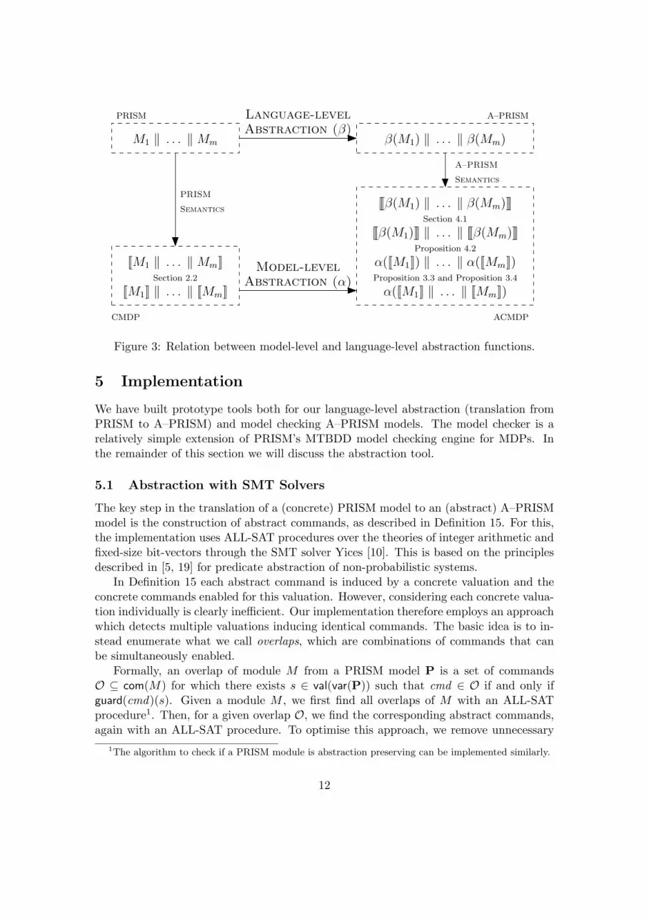
[[[β(M1) ‖ . . . ‖ β(Mm)]]]Section 4.1

[[[β(M1)]]] ‖ . . . ‖ [[[β(Mm)]]]Proposition 4.2

α([[M1]]) ‖ . . . ‖ α([[Mm]])Proposition 3.3 and Proposition 3.4

ACMDP

A–PRISM

Semantics

β(M1) ‖ . . . ‖ β(Mm)

A–PRISMLanguage-levelAbstraction (β)

Model-level

α([[M1]] ‖ . . . ‖ [[Mm]])Abstraction (α)

[[M1]] ‖ . . . ‖ [[Mm]]

[[M1 ‖ . . . ‖ Mm]]Section 2.2

CMDP

PRISM

M1 ‖ . . . ‖ Mm

Semantics

PRISM

Figure 3: Relation between model-level and language-level abstraction functions.

5 Implementation

We have built prototype tools both for our language-level abstraction (translation fromPRISM to A–PRISM) and model checking A–PRISM models. The model checker is arelatively simple extension of PRISM’s MTBDD model checking engine for MDPs. Inthe remainder of this section we will discuss the abstraction tool.

5.1 Abstraction with SMT Solvers

The key step in the translation of a (concrete) PRISM model to an (abstract) A–PRISMmodel is the construction of abstract commands, as described in Definition 15. For this,the implementation uses ALL-SAT procedures over the theories of integer arithmetic andfixed-size bit-vectors through the SMT solver Yices [10]. This is based on the principlesdescribed in [5, 19] for predicate abstraction of non-probabilistic systems.

In Definition 15 each abstract command is induced by a concrete valuation and theconcrete commands enabled for this valuation. However, considering each concrete valua-tion individually is clearly inefficient. Our implementation therefore employs an approachwhich detects multiple valuations inducing identical commands. The basic idea is to in-stead enumerate what we call overlaps, which are combinations of commands that canbe simultaneously enabled.

Formally, an overlap of module M from a PRISM model P is a set of commandsO ⊆ com(M) for which there exists s ∈ val(var(P)) such that cmd ∈ O if and only ifguard(cmd)(s). Given a module M , we first find all overlaps of M with an ALL-SATprocedure1. Then, for a given overlap O, we find the corresponding abstract commands,again with an ALL-SAT procedure. To optimise this approach, we remove unnecessary

1The algorithm to check if a PRISM module is abstraction preserving can be implemented similarly.

12

predicates both from the guards and updates of abstract commands. For example, we donot include any predicates in an abstract update if the corresponding concrete updatesdo not influence their values.

5.2 ‘On-the-Fly’ Abstraction

During prototyping, our implementation would often find a large number of overlaps,making the ALL-SAT procedures infeasible. However, further investigation revealed thatthe majority of these overlaps were induced by unreachable concrete valuations. There-fore, the prototype was extended with an ‘on-the-fly’ abstraction method to overcomethis problem. Like in explicit-state model checking, this is achieved by keeping a stack ofreachable abstract valuations of bool(ΦM ). Initially, this stack only contains the elementα(sinit,ΦM ). The method takes individual abstract valuations off the stack, constructs theabstract commands for this valuation and adds any new abstract valuations that are thetarget of this command to the stack. Note that, since the tool now constructs abstractcommands for each abstract state s separately, only commands that are enabled for somevaluation s such that α(s,ΦM ) = s need be considered when searching for overlaps ofthese commands.

Although this ‘on-the-fly’ abstraction method does perform reachability over abstractstates, it is important to stress that, unlike [17], it does not require the construction of thereachable concrete state space or take into account whether concrete states are reachable.

6 Experimental Results

We have tested the performance of our implementation on three case studies:2

• An extension of the sliding window protocol of [20] where channels lose messagesprobabilistically instead of non-deterministically and a notion of timeout is included.We fix the window size of the sender (2) and receiver (1), buffer size of the channels(2) and sequence numbers (modulo 4) while varying the number of data frames(D) in the source. We analyse ‘the maximum probability of sending D data frameswithout a timeout ’ using an abstraction that removes the values of the data frames.In the compositional approach, we abstract the sender and data channel separatelyfrom the receiver and acknowledgement channel.

• IPv4 Zeroconf protocol [3], as described in [17], parameterised by the number ofconfigured hosts (N) and with 64 IP addresses. We encode the abstraction of[17] into predicates and consider ‘the minimum probability that the host eventuallysecures an IP address’. In the compositional approach, the configuring host isabstracted separately from the channel and configured hosts.

• Israeli and Jalfon’s self-stabilisation protocol [15] for a ring with N processes. Weencode the abstraction of [9] into predicates and analyse ‘the minimum probability

2Files for the case studies are available from http://www.prismmodelchecker.org/files/qapl08/.

13

Concrete Model Abstract ModelsNon-compositional Compositional

Num. Num. Check Abstr. Num. Abstr. Num. Num. Checkcomm. states time time Comm. time Comm. states time

Slid

ing

Win

.(D

) 8 19 189,952 30.2 96.7 540 220 3,260 742 0.2110 19 987,136 153 126 706 336 4,870 964 0.4312 19 – – 155 872 473 6,545 1,186 0.6914 19 – – 200 1,038 630 8,225 1,408 1.2316 19 – – 237 1,204 819 9,905 1,630 1.6818 19 – – 285 1,370 962 11,585 1,852 2.4720 19 – – 334 1,536 1,201 13,265 2,074 3.45

Zer

ocon

f(N

) 4 89 50,377 206 1,110 2,349 106 362 1,325 1045 109 113,217 355 1,480 2,523 183 396 1,421 1346 129 282,185 678 2,480 2,695 262 431 1,517 1617 149 426,529 952 3,630 2,762 434 444 1,549 1758 169 838,905 1,400 6,370 2,804 785 453 1,581 209

Isra

eli&

Jalfo

n(N

) 8 8 255 0.01 13.4 28 n/a n/a 22 <0.0110 10 1,023 0.03 95.2 68 n/a n/a 42 <0.0112 12 4,095 0.08 727 168 n/a n/a 77 <0.0114 14 16,383 0.22 4,210 415 n/a n/a 135 <0.0116 16 65,535 0.75 28,000 1,025 n/a n/a 231 <0.0118 18 262,143 2.27 136,000 2,505 n/a n/a 385 <0.0120 20 1,048,575 8.51 1,090,000 6,056 n/a n/a 627 0.02

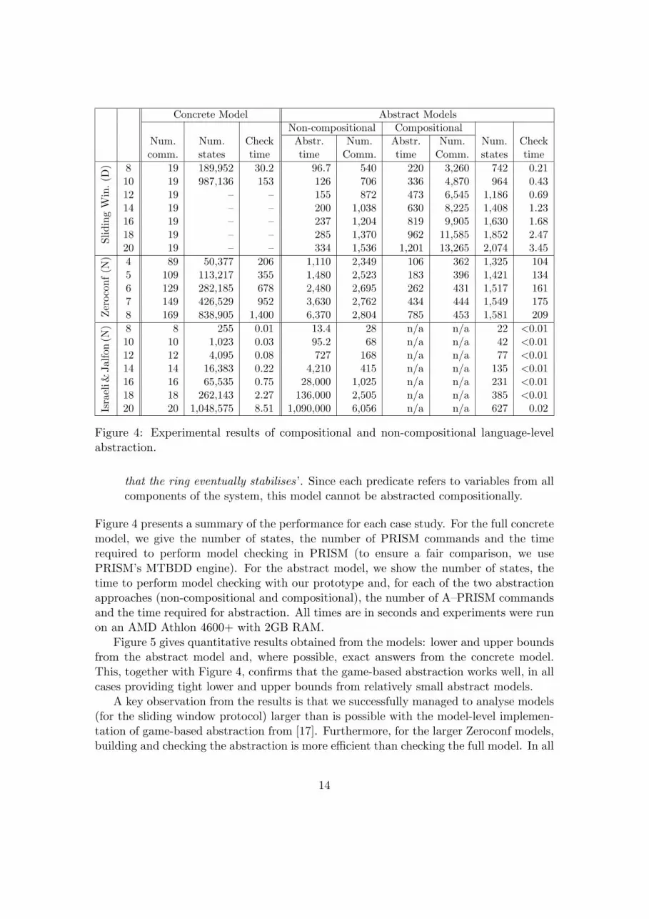
Figure 4: Experimental results of compositional and non-compositional language-levelabstraction.

that the ring eventually stabilises’. Since each predicate refers to variables from allcomponents of the system, this model cannot be abstracted compositionally.

Figure 4 presents a summary of the performance for each case study. For the full concretemodel, we give the number of states, the number of PRISM commands and the timerequired to perform model checking in PRISM (to ensure a fair comparison, we usePRISM’s MTBDD engine). For the abstract model, we show the number of states, thetime to perform model checking with our prototype and, for each of the two abstractionapproaches (non-compositional and compositional), the number of A–PRISM commandsand the time required for abstraction. All times are in seconds and experiments were runon an AMD Athlon 4600+ with 2GB RAM.

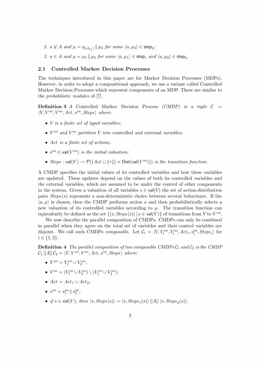
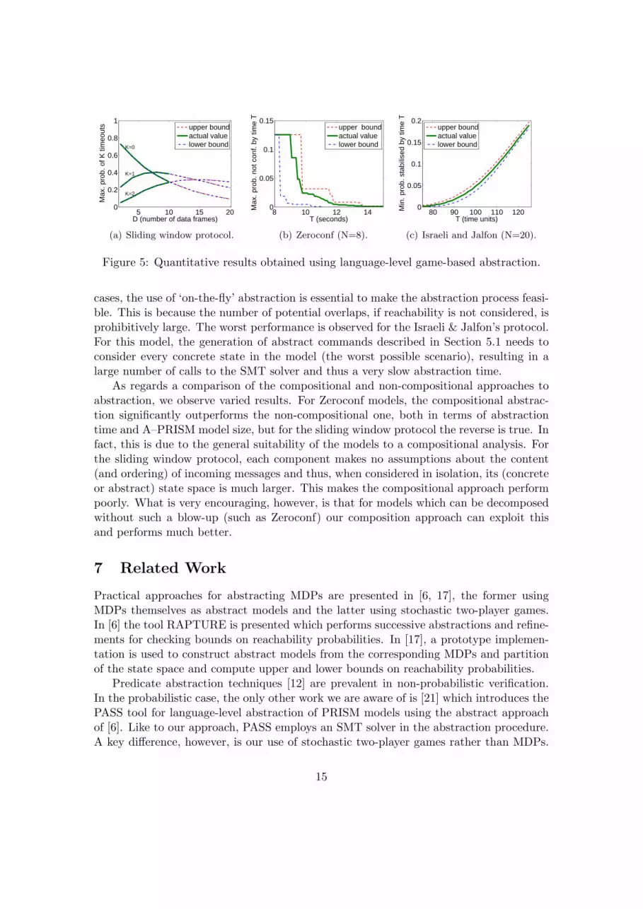
Figure 5 gives quantitative results obtained from the models: lower and upper boundsfrom the abstract model and, where possible, exact answers from the concrete model.This, together with Figure 4, confirms that the game-based abstraction works well, in allcases providing tight lower and upper bounds from relatively small abstract models.

A key observation from the results is that we successfully managed to analyse models(for the sliding window protocol) larger than is possible with the model-level implemen-tation of game-based abstraction from [17]. Furthermore, for the larger Zeroconf models,building and checking the abstraction is more efficient than checking the full model. In all

14

5 10 15 200

0.2

0.4

0.6

0.8

1

D (number of data frames)

Max

. pro

b. o

f K ti

meo

uts

upper boundactual valuelower boundK=0

K=1

K=2

(a) Sliding window protocol.

8 10 12 140

0.05

0.1

0.15

T (seconds)

Max

. pro

b. n

ot c

onf.

by ti

me

T

upper boundactual valuelower bound

(b) Zeroconf (N=8).

80 90 100 110 1200

0.05

0.1

0.15

0.2

T (time units)

Min

. pro

b. s

tabi

lised

by

time

T

upper boundactual valuelower bound

(c) Israeli and Jalfon (N=20).

Figure 5: Quantitative results obtained using language-level game-based abstraction.

cases, the use of ‘on-the-fly’ abstraction is essential to make the abstraction process feasi-ble. This is because the number of potential overlaps, if reachability is not considered, isprohibitively large. The worst performance is observed for the Israeli & Jalfon’s protocol.For this model, the generation of abstract commands described in Section 5.1 needs toconsider every concrete state in the model (the worst possible scenario), resulting in alarge number of calls to the SMT solver and thus a very slow abstraction time.

As regards a comparison of the compositional and non-compositional approaches toabstraction, we observe varied results. For Zeroconf models, the compositional abstrac-tion significantly outperforms the non-compositional one, both in terms of abstractiontime and A–PRISM model size, but for the sliding window protocol the reverse is true. Infact, this is due to the general suitability of the models to a compositional analysis. Forthe sliding window protocol, each component makes no assumptions about the content(and ordering) of incoming messages and thus, when considered in isolation, its (concreteor abstract) state space is much larger. This makes the compositional approach performpoorly. What is very encouraging, however, is that for models which can be decomposedwithout such a blow-up (such as Zeroconf) our composition approach can exploit thisand performs much better.

7 Related Work

Practical approaches for abstracting MDPs are presented in [6, 17], the former usingMDPs themselves as abstract models and the latter using stochastic two-player games.In [6] the tool RAPTURE is presented which performs successive abstractions and refine-ments for checking bounds on reachability probabilities. In [17], a prototype implemen-tation is used to construct abstract models from the corresponding MDPs and partitionof the state space and compute upper and lower bounds on reachability probabilities.

Predicate abstraction techniques [12] are prevalent in non-probabilistic verification.In the probabilistic case, the only other work we are aware of is [21] which introduces thePASS tool for language-level abstraction of PRISM models using the abstract approachof [6]. Like to our approach, PASS employs an SMT solver in the abstraction procedure.A key difference, however, is our use of stochastic two-player games rather than MDPs.

15

While this will in general provide a more useful abstraction, it is also more difficultto apply to predicate abstraction. In [21] each command of a PRISM module can beabstracted separately. Here, as described in Section 5, we must consider overlaps betweencommands in order to distinguish between the two types of non-determinism. To improveefficiency, we also adopt a compositional approach to abstraction and use ‘on-the-fly’techniques.

Also relevant is the ‘magnifying-lens abstraction’ (MLA) approach of [8], which com-putes lower and upper bounds for PCTL formulae on MDPs. This is done by partitioningthe state space into regions and analysing each region separately. It is still necessary tobuild the full MDP, however. Finally, approaches have also been proposed for abstractingdiscrete-time Markov chains [11, 14], using interval-based extensions of Markov chains,but no implementations or results were presented.

8 Conclusions

We have introduced a method to obtain stochastic two-player game abstractions of MDPs,directly from high-level model descriptions in the PRISM language. Our approach isbased on a compositional reformulation of the abstraction techniques from [17] and theuse of predicate abstraction. Although a compositional abstraction is potentially an over-approximation (compared to the non-compositional version), we provide conditions whichguarantee a precise abstraction. We have developed an implementation of our techniquesbased on the SMT solver Yices and present experimental results from a range of casestudies, illustrating how our work can generate game-based abstractions for larger modelsthan was previously possible. We also highlight the benefits of adopting a compositionalapproach.

In the future, we hope to improve the performance of our tool chain using symbolicdecision procedures [18]. We also plan to integrate this with ongoing work to develop anabstraction-refinement loop for MDP verification. Finally, we also intend to extend thecurrent method to imperative programming languages.

References

[1] T. Ball, T. Millstein, and S. K. Rajamani. Automatic predicate abstraction of Cprograms. SIGPLAN Notices, 36(5):203–213, 2001.

[2] A. Bianco and L. de Alfaro. Model checking of probabilistic and nondeterministicsystems. In P. S. Thiagarajan, editor, Proc. 15th Conf. on Foundations of SoftwareTechnology and Theoretical Computer Science (FSTTC‘95), volume 1026 of LNCS,pages 499–513. Springer, 1995.

[3] S. Cheshire, B. Adoba, and E. Gutterman. Dynamic configuration of IPv4 link localaddresses. Available from http://www.ietf.org/rfc/rfc3927.txt.

16

[4] F. Ciesinski and C. Baier. LiQuor: A tool for qualitative and quantitative lineartime analysis of reactive systems. In Proc. 3rd Int. Conf. Quantitative Evaluation ofSystems (QEST‘06), pages 131–132. IEEE CS, 2006.

[5] E. Clarke, D. Kroening, N. Sharygina, and K. Yorav. Predicate abstraction of ANSI-C programs using SAT. Formal Methods in System Design, 25:105–127, 2004.

[6] P. D’Argenio, B. Jeannet, H. Jensen, and K. Larsen. Reachability analysis of prob-abilistic systems by successive refinements. In L. de Alfaro and S. Gilmore, editors,Proc. 1st Joint Int. Workshop on Process Algebra and Probabilistic Methods, Per-formance Modeling and Verification (PAPM/PROBMIV‘01), volume 2165 of LNCS,pages 39–56. Springer, 2001.

[7] L. de Alfaro, T. Henzinger, and R. Jhala. Compositional methods for probabilisticsystems. In K. Larsen and M. Nielsen, editors, Proc. 12th Int. Conf. ConcurrencyTheory (CONCUR‘01), volume 2154 of LNCS, pages 351–365. Springer, 2001.

[8] L. de Alfaro and P. Roy. Magnifying-lens abstraction for Markov decision processes.In W. Damm and H. Hermanns, editors, Proc. 19th Int. Conf. Computer AidedVerification (CAV‘07), volume 4590 of LNCS, pages 325–338. Springer, 2007.

[9] M. Duflot, L. Fribourg, and C. Picaronny. Randomized finite-state distributed al-gorithms as Markov chains. In J. Welch, editor, Proc. 15th Int. Conf. DistributedComputing (DISC‘01), volume 2180 of LNCS, pages 240–254. Springer, 2001.

[10] B. Dutertre and L. de Moura. A fast linear-arithmetic solver for DPLL(T). In T. Balland R. Jones, editors, Proc. 18th Int. Conf. Computer Aided Verification (CAV‘06),volume 4114 of LNCS, pages 81–94. Springer, 2006.

[11] H. Fecher, M. Leucker, and V. Wolf. Don’t know in probabilistic systems. In A. Val-mari, editor, Proc. 13th Int. SPIN Workshop (SPIN‘06), volume 3925 of LNCS,pages 71–88. Springer, 2006.

[12] S. Graf and H. Saıdi. Construction of abstract state graphs with PVS. In O. Grum-berg, editor, Proc. 9th Int. Conf. Computer Aided Verification (CAV‘97), volume1254 of LNCS, pages 72–83. Springer, 1997.

[13] A. Hinton, M. Kwiatkowska, G. Norman, and D. Parker. PRISM: A tool for auto-matic verification of probabilistic systems. In H. Hermanns and J. Palsberg, editors,Proc. 12th Int. Conf. Tools and Algorithms for the Construction and Analysis ofSystems (TACAS‘06), volume 3920 of LNCS, pages 441–444. Springer, 2006.

[14] M. Huth. On finite-state approximants for probabilistic computation tree logic.Theoretical Computer Science, 346(1):113–134, 2005.

[15] A. Israeli and M. Jalfon. Token management schemes and random walks yield self-stabilizing mutual exclusion. In Proc. 9th ACM Symp. Principles of DistributedComputing (PODC‘90), pages 119–131. ACM, 1990.

17

[16] J. G. Kemeny, J. L. Snell, and A. W. Knapp. Denumerable Markov Chains. Springer-Verlag, 2 edition, 1976.

[17] M. Kwiatkowska, G. Norman, and D. Parker. Game-based abstraction for Markovdecision processes. In Proc. 3rd Int. Conf. Quantitative Evaluation of Systems(QEST‘06), pages 157–166. IEEE CS, 2006.

[18] S. Lahiri, T. Ball, and B. Cook. Predicate abstraction via symbolic decision proce-dures. In K. Etessami and S. Rajamani, editors, Proc. 17th Int. Conf. on ComputerAided Verification (CAV‘05), volume 3576 of LNCS, pages 24–38. Springer, 2005.

[19] S. K. Lahiri, R. Nieuwenhuis, and A. Oliveras. SMT techniques for fast predicateabstraction. In T. Ball and R. B. Jones, editors, Proc. 18th Int. Conf. ComputerAided Verification (CAV‘06), volume 4144 of LNCS, pages 424–437. Springer, 2006.

[20] K. Stahl, K. Baukus, Y. Lakhnech, and M. Steffen. Divide, abstract, and model-check. In D. Dams, R. Gerth, S. Leue, and M. Massink, editors, Proc. 5th and6th Int. SPIN Workshops (SPIN‘99), volume 1680 of LNCS, pages 57–76. Springer,1999.

[21] B. Wachter, L. Zhang, and H. Hermanns. Probabilistic model checking modulotheories. In Proc. 4th Int. Conf. Quantitative Evaluation of Systems (QEST‘07),pages 119–128. IEEE CS, 2007.

18

Appendices

A Proofs of Section 3.3

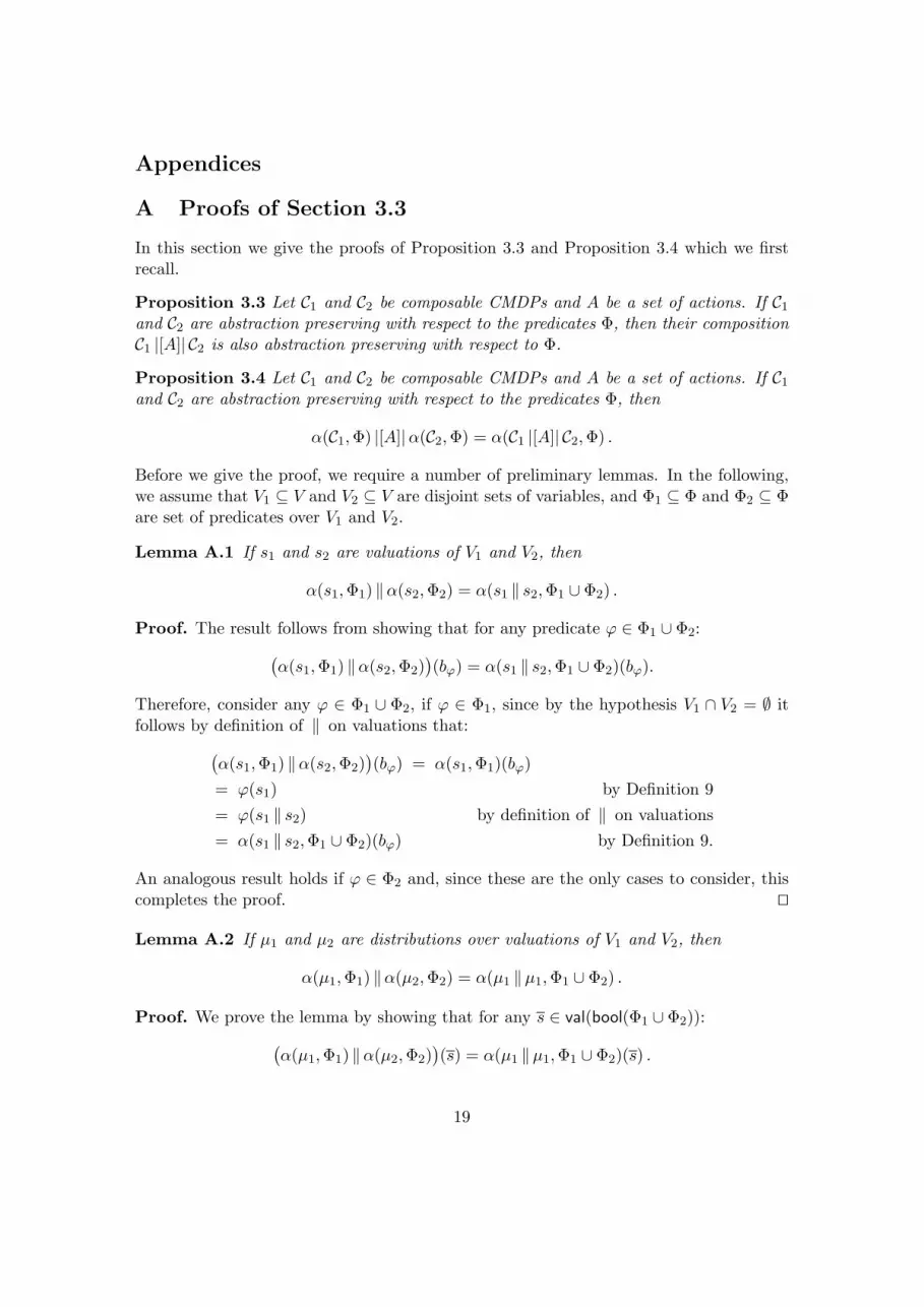
In this section we give the proofs of Proposition 3.3 and Proposition 3.4 which we firstrecall.

Proposition 3.3 Let C1 and C2 be composable CMDPs and A be a set of actions. If C1

and C2 are abstraction preserving with respect to the predicates Φ, then their compositionC1 |[A]| C2 is also abstraction preserving with respect to Φ.

Proposition 3.4 Let C1 and C2 be composable CMDPs and A be a set of actions. If C1

and C2 are abstraction preserving with respect to the predicates Φ, then

α(C1,Φ) |[A]|α(C2,Φ) = α(C1 |[A]| C2,Φ) .

Before we give the proof, we require a number of preliminary lemmas. In the following,we assume that V1 ⊆ V and V2 ⊆ V are disjoint sets of variables, and Φ1 ⊆ Φ and Φ2 ⊆ Φare set of predicates over V1 and V2.

Lemma A.1 If s1 and s2 are valuations of V1 and V2, then

α(s1,Φ1) ‖α(s2,Φ2) = α(s1 ‖ s2,Φ1 ∪ Φ2) .

Proof. The result follows from showing that for any predicate ϕ ∈ Φ1 ∪ Φ2:(α(s1,Φ1) ‖α(s2,Φ2)

)(bϕ) = α(s1 ‖ s2,Φ1 ∪ Φ2)(bϕ).

Therefore, consider any ϕ ∈ Φ1 ∪ Φ2, if ϕ ∈ Φ1, since by the hypothesis V1 ∩ V2 = ∅ itfollows by definition of ‖ on valuations that:(

α(s1,Φ1) ‖α(s2,Φ2))(bϕ) = α(s1,Φ1)(bϕ)

= ϕ(s1) by Definition 9= ϕ(s1 ‖ s2) by definition of ‖ on valuations= α(s1 ‖ s2,Φ1 ∪ Φ2)(bϕ) by Definition 9.

An analogous result holds if ϕ ∈ Φ2 and, since these are the only cases to consider, thiscompletes the proof. ut

Lemma A.2 If µ1 and µ2 are distributions over valuations of V1 and V2, then

α(µ1,Φ1) ‖α(µ2,Φ2) = α(µ1 ‖µ1,Φ1 ∪ Φ2) .

Proof. We prove the lemma by showing that for any s ∈ val(bool(Φ1 ∪ Φ2)):(α(µ1,Φ1) ‖α(µ2,Φ2)

)(s) = α(µ1 ‖µ1,Φ1 ∪ Φ2)(s) .

19

Therefore consider any s ∈ val(bool(Φ1 ∪ Φ2)), by the hypothesis Φ1 and Φ2 are predicatesover V1 and V2 and V1∩V2 = ∅, and hence we can write s as s1 ‖ s2 where s1 ∈ val(bool(Φ1))and s2 ∈ val(bool(Φ2)). By definition of ‖ on distributions it follows that:(

α(µ1,Φ1) ‖α(µ2,Φ2))(s) = α(µ1,Φ1)(s1) · α(µ2,Φ2)(s2)

=

∑α(s1,Φ1)=s1

µ1(s1)

·

∑α(s2,Φ2)=s2

µ2(s2)

by Definition 9

=∑

α(s1,Φ1)=s1

∑α(s2,Φ2)=s2

µ1(s1) · µ2(s2) rearranging

=∑

α(s1,Φ1) ‖α(s2,Φ2)=s1 ‖ s2

(µ1 ‖µ2)(s1 ‖ s2) by definition of ‖ on distributions

=∑

α(s1 ‖ s2,Φ1∪Φ2)=s1 ‖ s2

(µ1 ‖µ2)(s1 ‖ s2) by Lemma A.1

= α(µ1 ‖µ1,Φ1 ∪ Φ2)(s1 ‖ s2) by Definition 9= α(µ1 ‖µ1,Φ1 ∪ Φ2)(s) by construction of s1 ‖ s2.

Hence, since s ∈ val(bool(Φ1 ∪ Φ2)) was arbitrary, the lemma holds. ut

Lemma A.3 If 〈s, step1〉 and 〈s, step2〉 are transitions from V to V1 and V2 respectively,then for any set of actions A:

α(〈s, step1〉,Φ) |[A]|α(〈s, step2〉,Φ) = α(〈s, step1〉 |[A]| 〈s, step2〉,Φ

).

Proof. Let 〈sα(‖), stepα(‖)〉 = α(〈s, step1〉,Φ) |[A]|α(〈s, step2〉,Φ) and 〈sα‖α, stepα‖α〉 =α(〈s, step1〉 |[A]| 〈s, step2〉,Φ). Using Lemma A.1 it follows that sα‖α = sα(‖) = α(s,Φ),and hence is remains to show that stepα‖α = stepα(‖). Therefore consider any 〈act , µ〉 ∈stepα‖α by the hypothesis, Definition 4 and Definition 11 one of the following cases musthold:

• act 6∈ A and µ = α(µ1 ‖ ηsdV2,Φ) and 〈act , µ1〉 ∈ step1;

• act 6∈ A and µ = α(ηsdV1‖µ2,Φ) and 〈act , µ2〉 ∈ step2;

• act ∈ A and µ = α(µ1 ‖µ2,Φ) and 〈act , µi〉 ∈ stepi for i ∈ {1, 2}.

On the other hand, for any 〈act , µ〉 ∈ stepα(‖), by the hypothesis, Definition 8 andDefinition 11 one of the following cases must hold:

• act 6∈ A and µ = α(µ1,Φ1) ‖ ηα(s,Φ)dbool(V2)and 〈act , µ1〉 ∈ step1;

• act 6∈ A and µ = ηα(s,Φ)dbool(V1)‖α(µ2,Φ2) and 〈act , µ2〉 ∈ step2;

• act ∈ A and µ = α(µ1,Φ1) ‖α(µ2,Φ2) and 〈act , µi〉 ∈ stepi for i ∈ {1, 2}.

20

Now, since ηα(s,Φ)dbool(Vi)= α(ηsdVi

,Φ) for i ∈ {1, 2}, it follows from Lemma A.2 that thecases are equivalent, and hence stepα‖α = stepα(‖) as required. ut

We are now in a position to present the proofs of Proposition 3.3 and Proposition 3.4.

Proof of Proposition 3.3. Let Ci = 〈V, V ctrli , V ext

i ,Act i, sinit,Steps i〉 for i ∈ {1, 2}

and C1 |[A]| C2 = 〈V, V ctrl, V ext,Act , sinit,Steps 〉. Consider any s, s′ ∈ val(V ) such thatsdV ctrl= s′dV ctrl and α(s,Φext) = α(s′,Φext). Now by Definition 4 we have 〈s,Steps (s)〉 =〈s,Steps 1(s)〉 |[A]| 〈s,Steps 2(s)〉 and using Lemma A.3 it follows that:

α(〈s,Steps (s)〉,Φ) = α(〈s,Steps 1(s)〉,Φ) |[A]|α(〈s,Steps 2(s)〉,Φ2) .

Similarly, we have:

α(〈s′,Steps (s′)〉,Φ) = α(〈s′,Steps 1(s′)〉,Φ) |[A]|α(〈s′,Steps 2(s

′)〉,Φ) .

By the hypothesis C1 and C2 are abstraction preserving, therefore by construction of sand s′ we have α(〈s,Steps i(s)〉,Φ) = α(〈s′,Steps i(s′)〉,Φ) for i ∈ {1, 2}. Combining theseresults gives α(〈s,Steps (s)〉,Φ) = α(〈s′,Steps (s′)〉,Φ), and hence C1 |[A]| C2 is abstractionpreserving as required. ut

Proof of Proposition 3.4. Let Ci = 〈V, V ctrli , V ext

i ,Act i, sinit,Steps i〉 for i ∈ {1, 2}. By

construction the controlled variables, external variables, actions and initial valuations ofα(C1,Φ) |[A]|α(C2,Φ) and α(C1 |[A]| C2,Φ) are equal. To complete the proof it thereforeremains to show that the transition functions of the two ACMDPs are the same. To easenotation let Steps α‖α denote the transition function of α(C1,Φ) |[A]|α(C2,Φ), Steps α(‖)the transition function of α(C1 |[A]| C2,Φ) and α(Ci,Φ) = 〈V , V ctrl

i , V exti ,Act i, sinit,Steps i〉

for i ∈ {1, 2}. We split the proof into two parts by showing that for any s ∈ val(V ):

1. if step ∈ Steps α‖α(s), then step ∈ Steps α(‖)(s);

2. if step ∈ Steps α(‖)(s), then step ∈ Steps α‖α(s).

Therefore consider any s ∈ val(V ).

1. If step ∈ Steps α‖α(s), then from Definition 8 there exists step1 ∈ Steps 1(s) andstep2 ∈ Steps 2(s) such that 〈s, step〉 = 〈s, step1〉 |[A]| 〈s, step2〉. Now, since step1 ∈Steps 1(s) and step2 ∈ Steps 2(s), it follows from Definition 11 there exist valua-tions s1, s2 ∈ val(V ) such that α(s1,Φ) = α(s2,Φ) = s and α(〈s1,Steps 1(s1)〉,Φ) =〈s1, step1〉 and α(〈s2,Steps 2(s2),Φ) = 〈s2, step2〉. Letting s = s1d(V \V ctrl

2 ) ‖ s2dV ctrl2

,we have sdV ctrl

1= s1dV ctrl

1, sdV ctrl

2= s2dV ctrl

2and α(s,Φ) = s, since C1 and C2 are abstrac-

tion preserving, we have:

α(〈s,Steps i(s)〉,Φ) = α(〈si,Steps i(si)〉,Φ) for i ∈ {1, 2},

and therefore

〈s, step〉 = α(〈s,Steps 1(s)〉,Φ) |[A]|α(〈s,Steps 2(s)〉,Φ)= α(〈s,Steps 1(s)〉 |[A]| 〈s,Steps 2(s)〉,Φ) by Lemma A.3.

21

From Definition 11 and Definition 4 it follows that step is the element of Steps α(‖)(s),induced by s, as required.

2. If step ∈ Steps α(‖)(s), then by Definition 11 there exists s ∈ val(V ) such thatα(s,Φ) = s and

〈s, step〉 = α(〈s,Steps 1(s)〉 |[A]| 〈s,Steps 2(s)〉,Φ)= α(〈s,Steps 1(s)〉,Φ) |[A]|α(〈s,Steps 2(s)〉,Φ) by Lemma A.3.

It then follows from Definition 8 that step ∈ Steps α‖α(s) as required.

Thus the transition functions of the two ACMDPs are the same which completes theproof of Proposition 3.4. ut

B Proofs of Section 4.2

As in Section 4.2 we assume a fixed PRISM model P = 〈var(P), sys, {M1, . . . ,Mm}〉 and aset of predicates Φ which is partitioned into subsets ΦM1 , . . . ,ΦMm over the local variablesof the modules M1, . . . ,Mm. Before presenting the proofs we first recall Proposition 4.2and Theorem 4.3.

Proposition 4.2 If M is a module of P, then [[[β(M,Φ)]]] = α([[M ]],Φ).

Theorem 4.3 If [[M ]] is abstract preserving with respect to Φ for each module M of P,then [[[β(P,Φ)]]] = α([[P]],Φ).

Proof of Proposition 4.2. By construction the controlled variables, external vari-ables, actions and initial valuations of [[[β(M,Φ)]]] and α([[M ]],Φ) are equal. To com-plete the proof it therefore remains to show that the transition functions of the twoACMDPs are the same. Let Steps [[[β(M,Φ)]]] denote the transition function of [[[β(M,Φ)]]]and Steps α([[M ]],Φ) the transition function of α([[M ]],Φ), to complete the proof we will showthat Steps [[[β(M,Φ)]]](s) = Steps α([[M ]],Φ)(s) for all s ∈ val(bool(Φ)). Therefore consider anys ∈ val(bool(Φ)).

• If step[[[β(M,Φ)]]] ∈ Steps [[[β(M,Φ)]]](s), then by Definition 14 there exists a commandcmd of β(M,ΦM ) such that:

step[[[β(M,Φ)]]] ={〈act(chc), dist(chc, s)〉 | chc ∈ choices(cmd)

}and guard(cmd)(s) holds. By Definition 15, there exists a valuation s ∈ val(var(P))such that:

step[[[β(M,Φ)]]] ={〈act(cmd), dist(cmd , s)〉 | cmd ∈ com(M) ∧ guard(cmd)(s)

}and α(s,Φ) = s.

22

• On the other hand, if stepα([[M ]],Φ) ∈ Steps α([[M ]],Φ)(s), then from Definition 11 itfollows that there exists a valuation s ∈ val(var(P)) such that 〈s, stepα([[M ]],Φ)〉 =α(〈s, stepα([[M ]],Φ)〉,Φ) where 〈s, stepα([[M ]],Φ)〉 is a transition of [[M ]]. By Definition 6it follows that stepα([[M ]],Φ) equals

α({〈act(cmd), dist(cmd , s)〉 | cmd ∈ com(M) ∧ guard(cmd)(s)} ,ΦM

)=

{〈act(cmd), α(dist(cmd , s),ΦM )〉 | cmd ∈ com(M) ∧ guard(cmd)(s)

}by Definition 11.

Combining these results and since act(cmd) = act(cmd), it follows that it is sufficient toshow that

α(dist(cmd , s),ΦM ) = dist(cmd , s) for all cmd ∈ com(M) .

Therefore consider any cmd ∈ com(M) where updates(cmd) = {〈λ1, u1〉, . . . , 〈λn, un〉}and s′ ∈ val(bool(ΦM )), from Definition 9 we have:

α(dist(cmd , s),ΦM )(s′)=∑

α(s′,ΦM )=s′

dist(cmd , s)(s′)

=∑

α(s′,ΦM )=s′

∑1≤i≤n∧ui(s)=s′

λi

by definition of dist(·, ·)

=∑

1≤i≤n∧α(ui(s),Φ

M )=s′

λi rearranging

=∑

1≤i≤n∧ui(s)=s′

λi by Definition 15

=∑

u∈{ui | 1≤i≤n}∧u(s)=s′

∑1≤i≤n∧ui=u

λi

rearranging

=∑

〈λ,u〉∈updates(cmd)∧u(s)=s′

λ by Definition 15

= dist(cmd , s)(s′) by definition of dist(·, ·).

Therefore, since s′ ∈ val(bool(ΦM )) and cmd ∈ com(M) were arbitrary, it follows thatα(dist(cmd , s),ΦM ) = dist(cmd , s) for all cmd ∈ com(M) as required. ut

Proof of Theorem 4.3. The proof is by induction on the structure of sys. In the basecase, sys = M for some module M and hence [[[β(P,Φ)]]] = [[[β(M,Φ)]]] = α([[M ]],Φ) byProposition 4.2 as required.

For the inductive step we have that sys = sys1 |[A]| sys2 for some process-algebraicexpressions sys1 and sys2 over the modules of P. First note that, since [[M ]] is abstract

23

preserving with respect to Φ for each module M of P, applying Proposition 3.3 it followsthat [[sys1]] and [[sys2]] are abstract preserving, and hence from Proposition 3.4 we have:

α([[sys1]],Φ) |[A]|α([[sys2]],Φ) = α([[sys1]] |[A]| [[sys2]],Φ) . (1)

Now by definition of [[[·]]]:

[[[β(P,Φ)]]] = [[[β(sys1),Φ]]] |[A]| [[[β(sys2),Φ]]]= α([[sys1]],Φ) |[A]|α([[sys2]],Φ) by induction= α([[sys1]] |[A]| [[sys2]],Φ) by (1)= α([[sys1 |[A]| sys2]],Φ) by definition of [[·]]= α([[P]],Φ) by definition of P,

and hence the theorem holds by induction on the structure of sys. ut

24