Embed Size (px)
Citation preview

Computer Science Journal of Moldova, vol.10, no.1(28), 2002
Fuzzy Sets-based Control Rules for
Terminating Algorithms
Jose L. VERDEGAY, Edmundo VERGARA-MORENO
Abstract
In this paper some problems arising in the interface betweentwo different areas, Decision Support Systems and Fuzzy Setsand Systems, are considered. The Model-Base Management Sys-tem of a Decision Support System which involves some fuzzinessis considered, and in that context the questions on the manage-ment of the fuzziness in some optimisation models, and then ofusing fuzzy rules for terminating conventional algorithms are pre-sented, discussed and analyzed. Finally, for the concrete case ofthe Travelling Salesman Problem, and as an illustration of deter-mination, management and using the fuzzy rules, a new algorithmeasy to implement in the Model-Base Management System of anyoriented Decision Support System is shown.
Keywords: Decision Support System, Fuzzy Rules,Travelling Salesman Problem, Algorithm.
1 Introduction
From a broad point of view the interface between two different areas,Decision Support Systems and Fuzzy Sets and Systems, is consideredin this paper. On the one hand, the term Decision Support System(DSS) was coined at the beginning of the 70s to feature the computerprograms that could support a user in making decisions when facingill-structured problems. Nowadays, software for supporting decision-making is available for almost any management problem. On the otherhand, in the early sixties, based on the fact that classical logic doesnot reflect, to the extent that it should, the omnipresent imprecision
c©2002 by J.L. Verdegay, E. Vergara-Moreno
9
J.L. Verdegay, E. Vergara-Moreno
in the real world, L. A. Zadeh proposed the Theory of Fuzzy Sets andFuzzy Logic. Nowadays Fuzzy Logic is employed with great success inthe conception, design, construction and utilisation of a wide range ofproducts and systems whose functioning is directly based on the wayshuman beings reason.
But, in spite of the high levels achieved in these two fields, thereis a gap in the interface between them, i.e., Fuzzy Logic-Based DSShas been not so widely exploited, although in this interface contextthere are a number of important problems to be solved. Amongthem, and for the sake of the interest that for the authors of thispaper this kind of problems exists, the following questions are to bepointed out: the practical determination of membership functions,which will be not considered here (interested readers are invited toconsult 3,7,8,12,13,15,16,17,19), the numerical accuracy need in thatfuzzy environment, the use of new algorithms to find good enough so-lutions, instead of optimal ones, etc. Consequently the primary aimof this paper is to describe briefly some of these problems as well astheir solution ways in a DSS framework, in order to bridge the abovementioned gap and help to produce more effective and friendship FuzzyLogic-based DSS.
In order to structure the contents of the paper, let us considerfirst of all the concept of DSS. In a very general meaning a DSS isa system that supports technological and managerial decision mak-ing by assisting in the organisation of knowledge about ill-structured,semi-structured or unstructured issues, and its main components area Data-Base Management System, a Model-Base Management Systemand a Dialog Generation and Management System [10]. ConsequentlyDSS are especially useful in areas providing problems with an unfa-miliar structure, and much more specifically, in situations where theknowledge available from experts has a human nature, i.e., it is eitherimprecise or vague. At this juncture, as is well known, the Theory ofFuzzy Sets and Fuzzy Logic is the most appropriate tool for dealingwith this kind of lack of precision. Amongst the three components de-scribed for a DSS, all with an equal level of importance, for the sake ofconvenience here only the second one will be considered. Therefore as
10

Fuzzy Sets-based Control Rules for . . .
follows, the Model-Base Management System (MBMS) will be focusedon, and an imprecise framework assumed.
Consequently, in Section 2 the management of the correspondingand omnipresent fuzziness in the existing models in the MBMS is tobe considered. Among all the possible development areas that couldbe approached, only that one considering optimisation problems, inparticular Linear Programming (LP) problems, will be discussed. Thereason for this is twofold. On the one hand, it is well known that inthe framework of DSS, LP provides a very powerful context that hasbeen used in a range of different applications, and has a documentedhistory of success [14]. On the other hand, LP problems assuming fuzzyparameters, i.e., Fuzzy Linear Programming (FLP) problems is one ofthe best studied topics in the field of Fuzzy Sets and Fuzzy Logic [2,5]. Finally, as a matter of illustration showing the relevance of thepresented way to manage the fuzziness in the previous section, andbridging the announced gap between DSS and Fuzzy Sets and Systems,in Section 3 the Travelling Salesman Problem will be considered, and anew algorithm proving the efficiency of using fuzzy rules as terminationcriteria and being able of implementation in some oriented DSS will beprovided.
2 Managing the lack of precision in the MBMS
It is absolutely clear that in real applications, and hence in the MBMSof any DSS, the perfect knowledge of the exact data taking part into theinvolved models is almost impossible, and then it is usual to approxi-mate those values, data and/or models in different ways: for instanceby using heuristic algorithms instead of conventional and experiencedones. From this last point of view amongst the many reasons thatmight justify the use of FLP in DSS [1, 13], and more specifically inthe MBMS, here we are going to concentrate on the following two:
1) Because FLP is useful for accurately modelling the inherentvagueness in the data which the user often has available, and
2) Because it may help to find solutions for problems in which tofind an optimum solution is not easy.
11
J.L. Verdegay, E. Vergara-Moreno
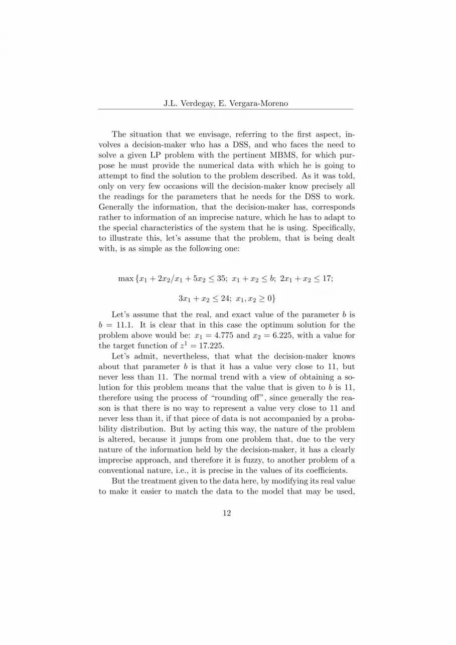
The situation that we envisage, referring to the first aspect, in-volves a decision-maker who has a DSS, and who faces the need tosolve a given LP problem with the pertinent MBMS, for which pur-pose he must provide the numerical data with which he is going toattempt to find the solution to the problem described. As it was told,only on very few occasions will the decision-maker know precisely allthe readings for the parameters that he needs for the DSS to work.Generally the information, that the decision-maker has, correspondsrather to information of an imprecise nature, which he has to adapt tothe special characteristics of the system that he is using. Specifically,to illustrate this, let’s assume that the problem, that is being dealtwith, is as simple as the following one:
max {x1 + 2x2/x1 + 5x2 ≤ 35; x1 + x2 ≤ b; 2x1 + x2 ≤ 17;
3x1 + x2 ≤ 24; x1, x2 ≥ 0}Let’s assume that the real, and exact value of the parameter b is
b = 11.1. It is clear that in this case the optimum solution for theproblem above would be: x1 = 4.775 and x2 = 6.225, with a value forthe target function of z1 = 17.225.
Let’s admit, nevertheless, that what the decision-maker knowsabout that parameter b is that it has a value very close to 11, butnever less than 11. The normal trend with a view of obtaining a so-lution for this problem means that the value that is given to b is 11,therefore using the process of “rounding off”, since generally the rea-son is that there is no way to represent a value very close to 11 andnever less than it, if that piece of data is not accompanied by a proba-bility distribution. But by acting this way, the nature of the problemis altered, because it jumps from one problem that, due to the verynature of the information held by the decision-maker, it has a clearlyimprecise approach, and therefore it is fuzzy, to another problem of aconventional nature, i.e., it is precise in the values of its coefficients.
But the treatment given to the data here, by modifying its real valueto make it easier to match the data to the model that may be used,
12

Fuzzy Sets-based Control Rules for . . .
(i.e. the one that is available in the MBMS, though making it simplerto solve the problem) it may really cause serious problems, since it maylead us to propose the application of solution that are very far removedfrom the authentic, optimum policies that should correspond to theproblem in question, if it had been approached in its original fuzzyterms. It is clear that such action may lead to serious consequencesdepending on the context that is being dealt with (economics, health,etc..).
In particular, in the example that is being used to illustrate thisargument, the fact of forcing parameter b to take the value b = 11,means that the optimum solution to the problem would be: x1 = 5and x2 = 6, with a value for the target function of z2 = 17, which isclearly much lower than (it is really just a question of scales) the oneobtained for the real problem.
The models and techniques offered by the FLP allow these miss-function to be solved without any difficulty. In fact, the modelling ofthe imprecision in the values of the parameters may be approached fromthe viewpoint that the latter are fuzzy numbers. In this sense, regard-less of the wide range of different models that may be considered forimplementing in an MBMS (fuzzy constraints, fuzzy objectives, etc.)the above mentioned problem could be dealt with using the followingmodel:
max{cx/Afx ≤f bf , x ≥ 0}where Af an bf refer to the fact that we are considering fuzzy numbersin the coefficients that define the restrictions (thereby allowing, as atrivial case, there also to be real numbers when there are no ambigui-ties), and symbol ≤f means that the way of comparing both membersin the inequality, due to formal coherence, must be done by using arelationship for ordering the fuzzy numbers. This comparison relation≤f may be any one from the extensive list available [19], which in turnwould also allow the decision-maker to have a greater degree of freedomwhen it comes to establishing preferences. In more specific terms, inorder to provide that theoretical model with a way for operating, let’sbriefly refer back to the different indices for comparing fuzzy numbers
13
J.L. Verdegay, E. Vergara-Moreno
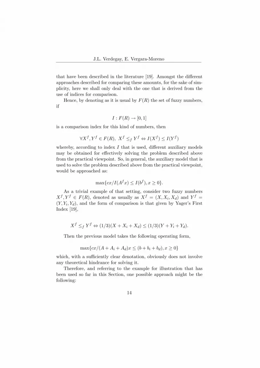
that have been described in the literature [19]. Amongst the differentapproaches described for comparing these amounts, for the sake of sim-plicity, here we shall only deal with the one that is derived from theuse of indices for comparison.
Hence, by denoting as it is usual by F (R) the set of fuzzy numbers,if
I : F (R) → [0, 1]
is a comparison index for this kind of numbers, then
∀Xf , Y f ∈ F (R), Xf ≤f Y f ⇔ I(Xf ) ≤ I(Y f )
whereby, according to index I that is used, different auxiliary modelsmay be obtained for effectively solving the problem described abovefrom the practical viewpoint. So, in general, the auxiliary model that isused to solve the problem described above from the practical viewpoint,would be approached as:
max{cx/I(Afx) ≤ I(bf ), x ≥ 0}.As a trivial example of that setting, consider two fuzzy numbers
Xf , Y f ∈ F (R), denoted as usually as Xf = (X,Xi, Xd) and Y f =(Y, Yi, Yd), and the form of comparison is that given by Yager’s FirstIndex [19],
Xf ≤f Y f ⇔ (1/3)(X + Xi + Xd) ≤ (1/3)(Y + Yi + Yd).
Then the previous model takes the following operating form,
max{cx/(A + Ai + Ad)x ≤ (b + bi + bd), x ≥ 0}which, with a sufficiently clear denotation, obviously does not involveany theoretical hindrance for solving it.
Therefore, and referring to the example for illustration that hasbeen used so far in this Section, one possible approach might be thefollowing:
14

Fuzzy Sets-based Control Rules for . . .
max{x1 + 2x2/x1 + 5x2 ≤ 35; x1 + x2 ≤f 11f ; 2x1 + x2 ≤ 17;
3x1 + x2 ≤ 24; x1, x2 ≥ 0} .
Assuming the simplest case, i.e., that 11f is a triangular numberwith a membership function (11, 11, 11.3), we may obtain a whole rangeof auxiliary problems that solve the previous example by providingdifferent solutions. Specifically, by means of an example, the auxiliarymodel that would be obtained would be:
max {x1 + 2x2/x1 + 5x2 ≤ 35; x1 + x2 ≤f 11.1
2x1 + x2 ≤ 17; 3x1 + x2 ≤ 24; x1, x2 ≥ 0} .
From which we would obviously obtain the optimum solution to theproblem in question.
With regards to the second reason that we use in this article to jus-tify the use of the FLP models in DSS, i.e., its help in finding solutionsfor those in which it is not easy to find their optimum solution, thequestion posed is the following.
As it is well known, there are a lot of NP problems (Knapsack,Travelling Salesman, etc.) which cannot effectively be solved in allcases, but which are of the utmost importance in a number of differentDSS. In these problems the decision-maker must usually accept approx-imate solutions instead of optimum ones. At this point the aim hereis to show how the FLP can help classical MP models and techniquesby providing approximate (fuzzy) solutions that may be used by thedecision-maker as help to quickly obtain a good enough solution forthese problems.
Let‘s justify this fact as follows. As it is well known, an algo-rithm for solving a general classical optimisation problem can be viewedas an iterative process that produces a sequence of points accordingto a prescribed set of instructions, together with a termination crite-rion. Usually we are interested in algorithms that generate a sequencex1, x2, ..., xN that converges to an overall, optimum solution. But in
15

J.L. Verdegay, E. Vergara-Moreno
many cases however, and because of the difficulties in the problem, wemay have to be satisfied with less favorable solutions. Then the iter-ative procedure may stop either 1) if a point belonging to a prefixedset (the solution set) is reached, or 2) if some prefixed condition forsatisfaction is verified.
But, the conditions for satisfaction are not to be meant as universalones. In fact they depend on several factors such as the decision-maker,the features of the problem, the nature of the information available, ...In any case, assuming that a solution set is prefixed, the algorithm willstop if a point in that solution set is reached. Frequently, however,the convergence to a point in the solution set is not easy because, forexample, of the existence of local optimum points, and hence we mustredefine some rules for terminating the iterative procedure.
Roughly speaking, the possible criteria to be taken into account forterminating the algorithms are no more than control rules. From thispoint of view, the control rules of the algorithms for optimisation prob-lems can be associated to the two above points: the solution set, andthe criteria for terminating the algorithm. As it is clear, fuzziness canbe introduced in both points, not assuming it as inherent in the prob-lem, but as help for obtaining, in a more effective way, some solutionfor satisfying the decision-maker’s wishes. This is meant so that thedecision-maker might be more comfortable when obtaining a solutionexpressed in terms of satisfaction instead of optimisation, as is the casewhen fuzzy control rules are applied to the control processes.
Therefore, and in the particular case of optimisation problems [4,18], it makes sense to consider fuzziness
a) In the Solution Set, i.e., there is a membership function givingthe degree with which a point belongs to that set, and
b) On the conditions for satisfaction, and hence Fuzzy Control ruleson the criteria for terminating the algorithm.
In the particular and easy case of Linear Programming problems,and hence of the very well known Simplex Algorithm, if a conventionalproblem is assumed
16
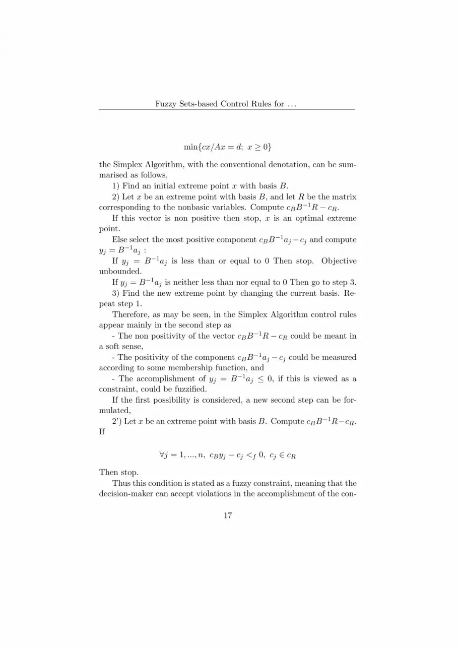
Fuzzy Sets-based Control Rules for . . .
min{cx/Ax = d; x ≥ 0}the Simplex Algorithm, with the conventional denotation, can be sum-marised as follows,
1) Find an initial extreme point x with basis B.2) Let x be an extreme point with basis B, and let R be the matrix
corresponding to the nonbasic variables. Compute cBB−1R− cR.If this vector is non positive then stop, x is an optimal extreme
point.Else select the most positive component cBB−1aj−cj and compute
yj = B−1aj :If yj = B−1aj is less than or equal to 0 Then stop. Objective
unbounded.If yj = B−1aj is neither less than nor equal to 0 Then go to step 3.3) Find the new extreme point by changing the current basis. Re-
peat step 1.Therefore, as may be seen, in the Simplex Algorithm control rules
appear mainly in the second step as- The non positivity of the vector cBB−1R− cR could be meant in
a soft sense,- The positivity of the component cBB−1aj − cj could be measured
according to some membership function, and- The accomplishment of yj = B−1aj ≤ 0, if this is viewed as a
constraint, could be fuzzified.If the first possibility is considered, a new second step can be for-
mulated,2’) Let x be an extreme point with basis B. Compute cBB−1R−cR.
If
∀j = 1, ..., n, cByj − cj <f 0, cj ∈ cR
Then stop.Thus this condition is stated as a fuzzy constraint, meaning that the
decision-maker can accept violations in the accomplishment of the con-
17
J.L. Verdegay, E. Vergara-Moreno
trol rules, cByj − cj < 0, to obtain a near, and therefore approximate,optimal solution instead of a full optimal one.
3 Using fuzzy rules for terminating algorithmsin MBMS.
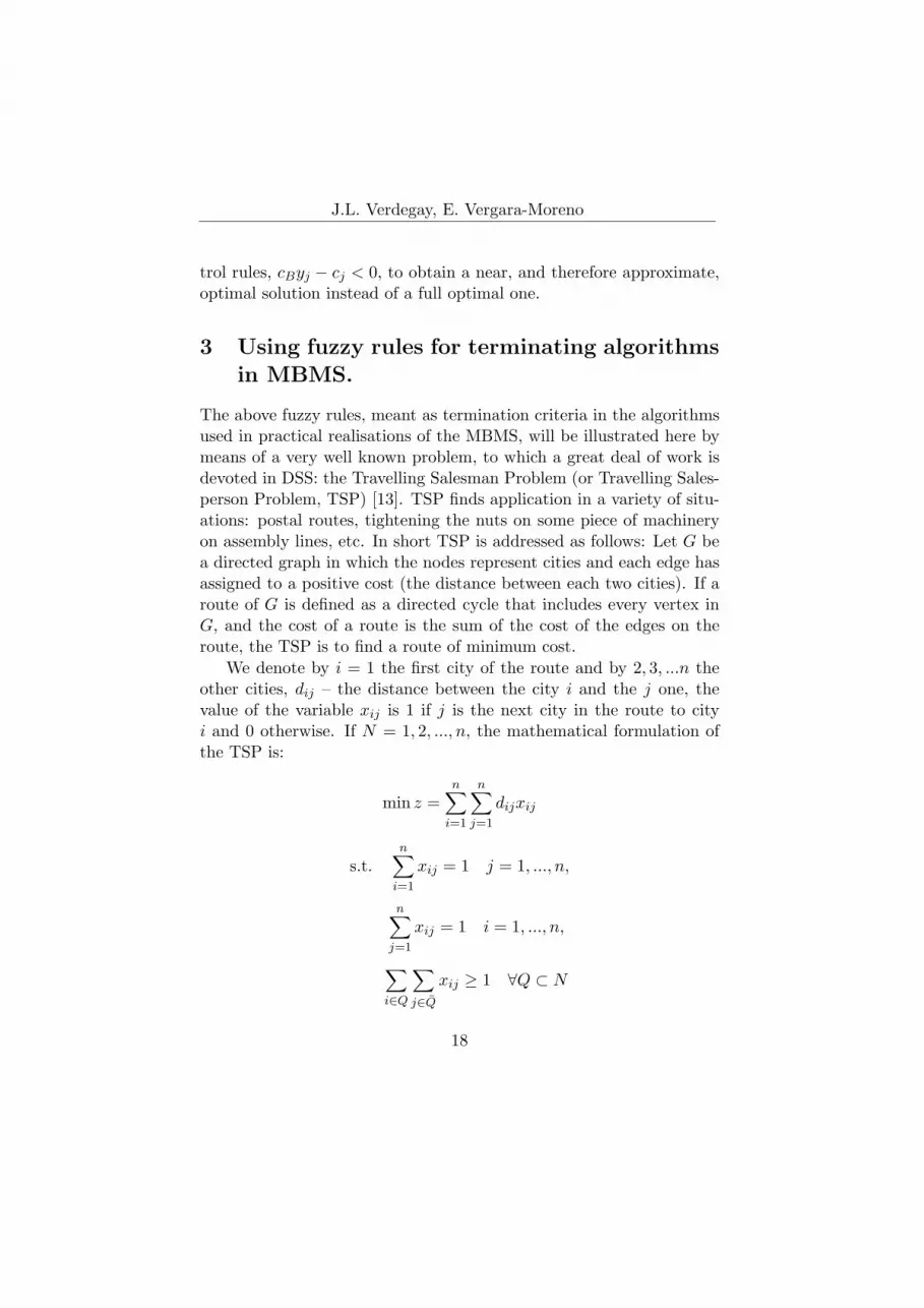
The above fuzzy rules, meant as termination criteria in the algorithmsused in practical realisations of the MBMS, will be illustrated here bymeans of a very well known problem, to which a great deal of work isdevoted in DSS: the Travelling Salesman Problem (or Travelling Sales-person Problem, TSP) [13]. TSP finds application in a variety of situ-ations: postal routes, tightening the nuts on some piece of machineryon assembly lines, etc. In short TSP is addressed as follows: Let G bea directed graph in which the nodes represent cities and each edge hasassigned to a positive cost (the distance between each two cities). If aroute of G is defined as a directed cycle that includes every vertex inG, and the cost of a route is the sum of the cost of the edges on theroute, the TSP is to find a route of minimum cost.
We denote by i = 1 the first city of the route and by 2, 3, ...n theother cities, dij – the distance between the city i and the j one, thevalue of the variable xij is 1 if j is the next city in the route to cityi and 0 otherwise. If N = 1, 2, ..., n, the mathematical formulation ofthe TSP is:
min z =n∑
i=1
n∑
j=1
dijxij
s.t.n∑
i=1
xij = 1 j = 1, ..., n,
n∑
j=1
xij = 1 i = 1, ..., n,
∑
i∈Q
∑
j∈Q
xij ≥ 1 ∀Q ⊂ N
18
Fuzzy Sets-based Control Rules for . . .
xij ∈ 0, 1 i, j = 1, 2, ..., n.
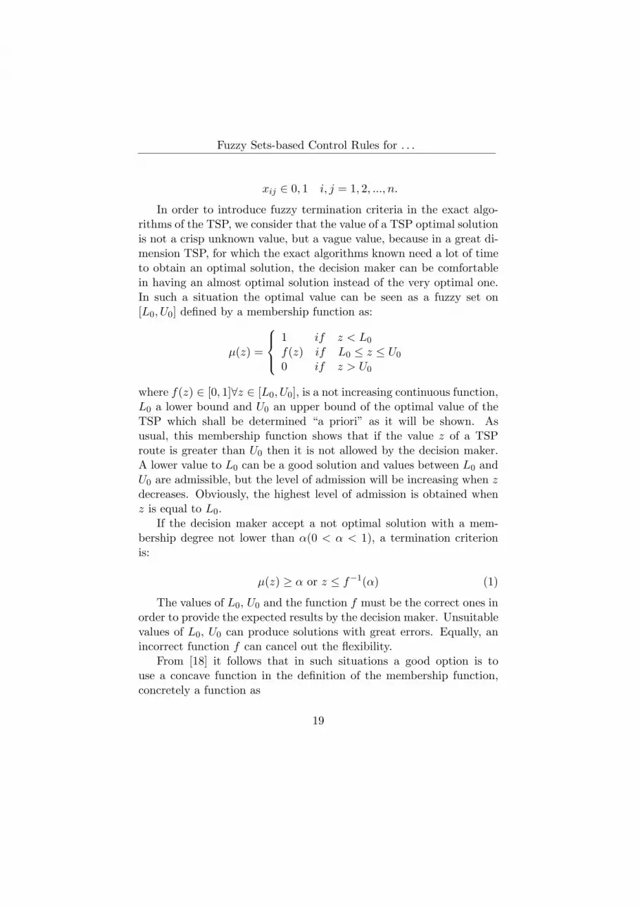
In order to introduce fuzzy termination criteria in the exact algo-rithms of the TSP, we consider that the value of a TSP optimal solutionis not a crisp unknown value, but a vague value, because in a great di-mension TSP, for which the exact algorithms known need a lot of timeto obtain an optimal solution, the decision maker can be comfortablein having an almost optimal solution instead of the very optimal one.In such a situation the optimal value can be seen as a fuzzy set on[L0, U0] defined by a membership function as:
µ(z) =
1 if z < L0
f(z) if L0 ≤ z ≤ U0
0 if z > U0
where f(z) ∈ [0, 1]∀z ∈ [L0, U0], is a not increasing continuous function,L0 a lower bound and U0 an upper bound of the optimal value of theTSP which shall be determined “a priori” as it will be shown. Asusual, this membership function shows that if the value z of a TSProute is greater than U0 then it is not allowed by the decision maker.A lower value to L0 can be a good solution and values between L0 andU0 are admissible, but the level of admission will be increasing when zdecreases. Obviously, the highest level of admission is obtained whenz is equal to L0.
If the decision maker accept a not optimal solution with a mem-bership degree not lower than α(0 < α < 1), a termination criterionis:
µ(z) ≥ α or z ≤ f−1(α) (1)
The values of L0, U0 and the function f must be the correct ones inorder to provide the expected results by the decision maker. Unsuitablevalues of L0, U0 can produce solutions with great errors. Equally, anincorrect function f can cancel out the flexibility.
From [18] it follows that in such situations a good option is touse a concave function in the definition of the membership function,concretely a function as
19
J.L. Verdegay, E. Vergara-Moreno
f(z) = n
√U0 − z
U0 − L0(2)
for which the bounds L0 and U0 can be computed by suitable efficientexisting algorithms.
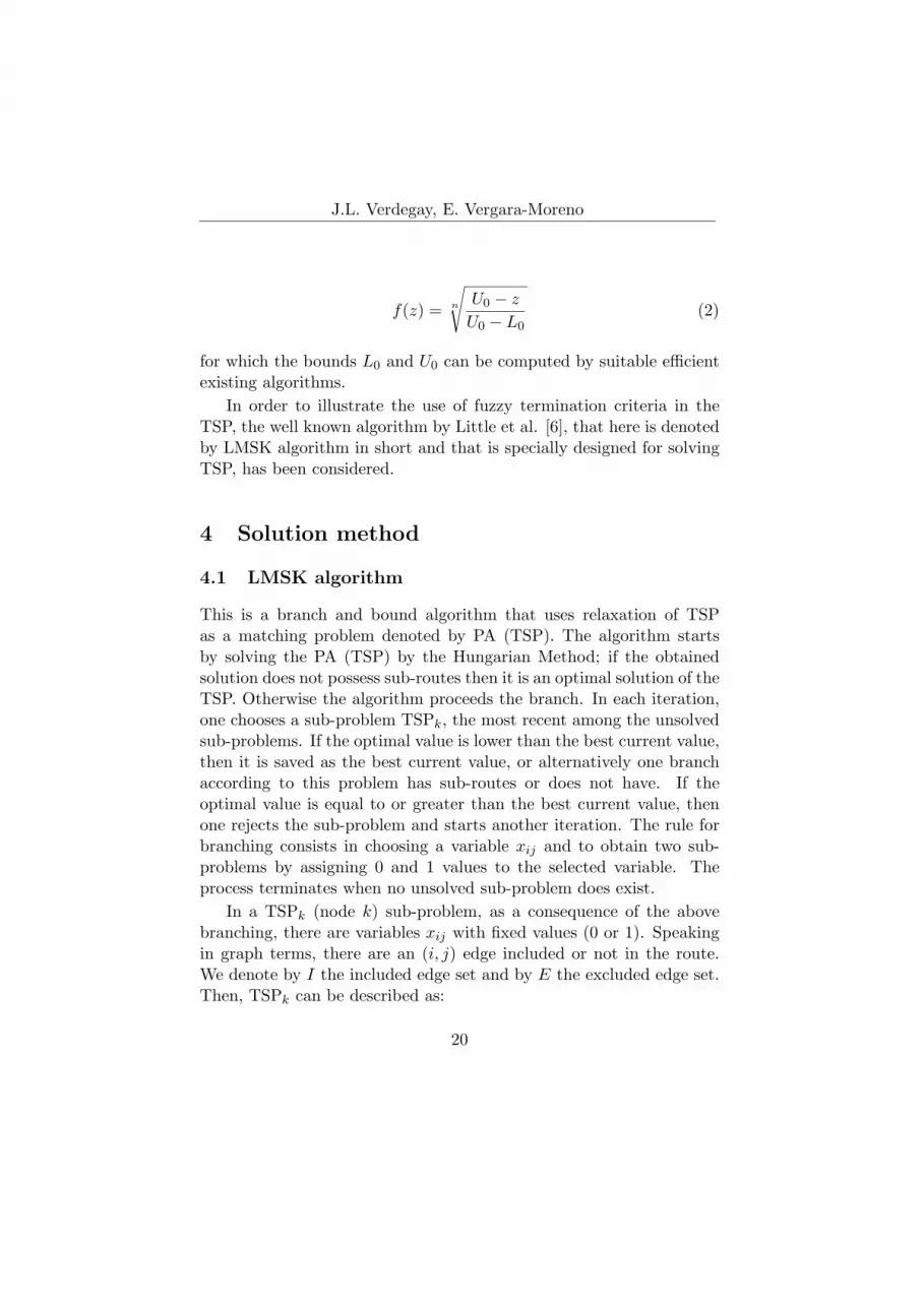
In order to illustrate the use of fuzzy termination criteria in theTSP, the well known algorithm by Little et al. [6], that here is denotedby LMSK algorithm in short and that is specially designed for solvingTSP, has been considered.
4 Solution method
4.1 LMSK algorithm
This is a branch and bound algorithm that uses relaxation of TSPas a matching problem denoted by PA (TSP). The algorithm startsby solving the PA (TSP) by the Hungarian Method; if the obtainedsolution does not possess sub-routes then it is an optimal solution of theTSP. Otherwise the algorithm proceeds the branch. In each iteration,one chooses a sub-problem TSPk, the most recent among the unsolvedsub-problems. If the optimal value is lower than the best current value,then it is saved as the best current value, or alternatively one branchaccording to this problem has sub-routes or does not have. If theoptimal value is equal to or greater than the best current value, thenone rejects the sub-problem and starts another iteration. The rule forbranching consists in choosing a variable xij and to obtain two sub-problems by assigning 0 and 1 values to the selected variable. Theprocess terminates when no unsolved sub-problem does exist.
In a TSPk (node k) sub-problem, as a consequence of the abovebranching, there are variables xij with fixed values (0 or 1). Speakingin graph terms, there are an (i, j) edge included or not in the route.We denote by I the included edge set and by E the excluded edge set.Then, TSPk can be described as:
20

Fuzzy Sets-based Control Rules for . . .
min∑
(i,j)∈I
dij +∑
i∈S
∑
j∈T
d′ijxij
s.a.∑
i∈S
xij = 1, ∀j ∈ T,
∑
j∈T
xij = 1, ∀i ∈ S,
xij ∈ 0, 1, ∀(i, j), i ∈ S, j ∈ T
where:
S = {i/(i, j) /∈ I ∀j} , T = {j/(i, j) /∈ I ∀i} ,
d′ij =
{dij (i, j) /∈ E∞ (i, j) ∈ E
furthermore dij are the coefficients of the matrix of reduced distance ofprevious node, that is to say, the matrix that rests after the obtainingthe optimum assignation in the previous node.
This sub-problem is solved by using the Hungarian Method. If theobtained solution has sub-routes one proceeds the branch. A rule forbranching is to choose a variable xrs where r ∈ S and s ∈ T , and tomake two nodes assigning value 1 or 0 each one. Little et al [6] suggestto select a variable xrs with value 0 if this variable has the maximalpotential of increasing in the objective function of the sub-problem. Inorder to make it, let
{dij
}i ∈ S, j ∈ T
be the reduced cost of the optimum solution of the sub-problem. Then,for each edge (i, j), i ∈ S, j ∈ T with reduced cost 0, we compute:
pij = min{dik/h ∈ T − j
}+ min
{dhj/h ∈ S − i
}
which is the minimum amount to increase the optimum value of theassignation to the subproblem, if the chosen variable is fixed to 0.Therefore we can choose xrs such that:
21

J.L. Verdegay, E. Vergara-Moreno
prs = max{pij/i ∈ S, j ∈ T, dij = 0
}(3)
when the variable of branching xrs is chosen, all the new nodes can beobtained making xrs = 1 and xrs = 0. In the first new node, I has theedge (r, s) as new element, and in the second new node, E has the edge(r, s) as new element.
Steps of LMSK algorithm
Step 1: [Starting] Let U = ∞ (best bound and real value) andL = TSP (subproblem list).
Step 2: [Selecting a sub-problem] If L = Φ then one terminates theprocess, because the route associated to U is an optimal one (if U = ∞, the TSP has not solution).
If L 6= Φ, one chooses the more recent sub-problem TSPi, and oneremoves it from the list L. Go to step 3.
Step 3: [Upper bound determination] Solve PA(TSPi) by means ofthe Hungarian Method. Let Zi be the obtained value.
If Zi ≥ U , go to step 2.If Zi < U and the solution is a route for TSP (there are no sub-
routes) then make U = Zi.If Zi < U and the solution is not a route for TSP (there are sub-
routes) go to step 4.Step 4: [Branching] Choose xrs according to (3) and generate two
new sub-problems TSPi1 and TSPi2 by fixing xrs = 0 and xrs = 1.Let L = L ∪ TSPi1, TSPi2.
Go to step 2.Remark: Note that the termination criterion of this algorithm is
L 6= Φ.
4.2 Fuzzy termination criteria in the LMSK algorithm
To introduce a fuzzy termination criterion in the LMSK algorithm, wemake a change at the starting step in order to determinate the boundsL0 and U0. L0 is computed by using the method proposed in [11], and
22

Fuzzy Sets-based Control Rules for . . .
the upper bound U0 is computed by means of the process described in[9]. In the same starting step, the decision maker will choose and fix α(the lowest level of admission). Finally, at step 2 one must include thefuzzy termination condition (1). Therefore the following new algorithmis obtained:
Step 1: [Starting] Let U = ∞ (best bound and real value) andL = TSP (subproblem list). Solve by means of the Hungarian MethodPA(TSP). If optimum matching is a route of TSP go to step 2. Else,go to 1’.
Step 1’: Find L0 and U0, then make U = U0 (best real bound) andgo to step 1”;
Step 1”: Fix α(0 < α ≤ 1). If 0 < α < 1 let z0 = f−1(α) (boundfor the admissible solution, where f is as in (2)). If L 6= Φ go to step2. Else, go to step 4.
If α = 1 (the decision maker do not want to improve an admissiblesolution), let L = Φ and go to step 2.
Step 2: [Selecting a sub-problem] If L = Φ or U ≤ z0 stop theprocess, as the associated route with U is admissible; if L 6= Φ go tostep 1”. Otherwise stop.
If L 6= Φ and U > z0, select the more recent problem TSPi, removeit from the list L and go to step 3.
Step 3: [Upper bound determination] Solve PA(TSPi) by means ofthe Hungarian Method. Let Zi be the obtained value.
If Zi ≥ U , go to step 2.If Zi < U and the solution is a route for TSP (there are no sub-
routes) then let U = Zi.If Zi < U and the solution is not a route for TSP (there are sub-
routes) go to step 4.Step 4: [Branching] Choose xrs according to (3) and generate two
new sub-problems TSPi1 and TSPi2 by fixing xrs = 0 and xrs = 1.Take L = L ∪ TSPi1, TSPi2.
Go to step 2.The introduction of the fuzzy termination criterion on the algo-
rithm has made it more flexible. Now, the decision maker can controlthe iterations because at step 1” he can introduce little values for α
23

J.L. Verdegay, E. Vergara-Moreno
and to increase them if he want to improve the admissible solution.Consequently the decision maker will take into account the time usedfor obtaining admissible solutions.
For the sake of illustration, let us consider finally the following TSPfor 10 cities, with a distance matrix given by:
(dij) =
− 1 62 56 54 27 30 27 55 6090 − 66 77 52 98 12 55 7 6430 41 − 60 59 17 72 82 76 2157 33 33 − 64 78 62 24 70 7295 32 69 74 − 97 94 92 96 5529 25 40 61 25 − 27 81 57 9498 52 8 11 89 61 − 55 91 3752 50 90 33 64 86 37 − 91 8845 83 31 79 70 22 46 18 − 9196 62 88 9 2 67 64 43 85 −
We consider the diagonal elements of the matrix and the distancesof excluded edges in the iterations with a value M = 10 × (max dij).Then, dii = M and dij = M if the edge (i, j) is excluded of a possibleroute. Then solving the problem with the exact algorithm LMSK, oneobtains the optimal route
1 → 2 → 9 → 6 → 5 → 10 → 4 → 8 → 7 → 3 → 1
with a total distance z = 218, after solving 15 sub-problems (originalproblem included).
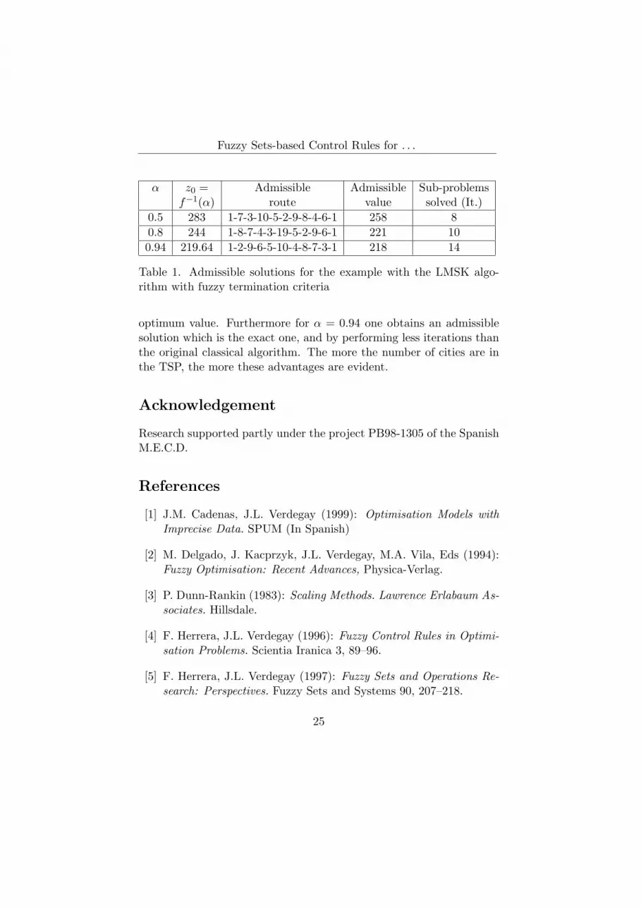
On the other hand when using the LMSK algorithm with a fuzzytermination criterion, a function f as (2), n = 2, and bounds L0 = 208and U0 = 308 (at the starting step 1’), the admissible solutions for thedifferent values of α is shown in the following table:
One can observe that for α = 0.8, an admissible solution is obtainedby solving only the 66% of all the sub-problems that the classical al-gorithm solves. However, the admissible value obtained is very closeto the optimum. It is then evident that the saving in time is upper incomparison with the difference between the admissible value and the
24
Fuzzy Sets-based Control Rules for . . .
α z0 = Admissible Admissible Sub-problemsf−1(α) route value solved (It.)
0.5 283 1-7-3-10-5-2-9-8-4-6-1 258 80.8 244 1-8-7-4-3-19-5-2-9-6-1 221 100.94 219.64 1-2-9-6-5-10-4-8-7-3-1 218 14
Table 1. Admissible solutions for the example with the LMSK algo-rithm with fuzzy termination criteria
optimum value. Furthermore for α = 0.94 one obtains an admissiblesolution which is the exact one, and by performing less iterations thanthe original classical algorithm. The more the number of cities are inthe TSP, the more these advantages are evident.
Acknowledgement
Research supported partly under the project PB98-1305 of the SpanishM.E.C.D.
References
[1] J.M. Cadenas, J.L. Verdegay (1999): Optimisation Models withImprecise Data. SPUM (In Spanish)
[2] M. Delgado, J. Kacprzyk, J.L. Verdegay, M.A. Vila, Eds (1994):Fuzzy Optimisation: Recent Advances, Physica-Verlag.
[3] P. Dunn-Rankin (1983): Scaling Methods. Lawrence Erlabaum As-sociates. Hillsdale.
[4] F. Herrera, J.L. Verdegay (1996): Fuzzy Control Rules in Optimi-sation Problems. Scientia Iranica 3, 89–96.
[5] F. Herrera, J.L. Verdegay (1997): Fuzzy Sets and Operations Re-search: Perspectives. Fuzzy Sets and Systems 90, 207–218.
25

J.L. Verdegay, E. Vergara-Moreno
[6] J.D.C. Little, K.G. Murty, D.W. Sweeney y C. Karel (1963): Analgorithm for the traveling salesman problem, Operations research11, 972–989.
[7] J.L. Melia (1990): One dimension Scaling Methods. Valencia (inSpanish).
[8] G.A. Miller (1967): The Magical Number Seven Plus or MinusTwo: Some Limits on our Capacity for Processing Information.The Psychology of Communication. Penguin Books Inc.
[9] D.J. Rosenkrantz., R.E. Stearns y P.M. Lewis II (1977): An anal-ysis of several heuristics for the traveling salesman problem. SIAMJ. Computing 6, 563–581.
[10] A.P. Sage (1991): Decision Support Systems Engineering. WileySeries in Systems Engineering. John Wiley and Sons
[11] H.M. Salkin and K. Mathur (1989): Foundations of integer pro-gramming, North-Holland, New York.
[12] A. Sancho and J.L. Verdegay (1999): Methods for the Construc-tion of Membership Functions. International Journal of IntelligentSystems 14, 1213–1230.
[13] A. Sancho-Royo, J.L. Verdegay y E. Vergara-Moreno: Some Prac-tical Problems in Fuzzy Sets-based Decision Support Systems.MathWare and Soft Computing VI, 2-3 (1999), 173–187.
[14] E.Turban (1988): Decision Support and Expert Systems (Man-agerial Perspectives). Macmillan Series in Information Systems.Macmillan Publishing Company.
[15] B. Turksen (1991): Measurement of Membership Functions andtheir Acquisition. Fuzzy Sets and Systems 40, 5–38.
[16] B. Turksen and A. Wilson (1994): A Fuzzy Set Preference Modelfor Consumer Choice. Fuzzy Sets and Systems 68, 253–266.
26

Fuzzy Sets-based Control Rules for . . .
[17] B. Turksen and A. Wilson (1995): A Fuzzy Set Model for MarketShare and Preference Prediction. European Journal of OperativeResearch 82, 39–52.
[18] E.R. Vergara (1999): New Termination Criteria for Optimisa-tion Algorithms. Ph. D. Dissertation. Universidad de Granada (inSpanish).
[19] X. Wang, E. Kerre (1996): On the Classification and the Depen-dencies of the Ordering Methods. In D. Ruan (Ed.): Fuzzy LogicFoundation and Industrial Applications. International Series in In-telligent Technologies. Kluwer 73–90
J.L. Verdegay, E. Vergara-Moreno, Received November 16, 2001
Jose L. VERDEGAY1,Depto. de Ciencias de la Computacion eInteligencia Artificial.Universidad de Granada.18071 Granada, SPAIN
Edmundo VERGARA-MORENO,Depto. de Matematicas.Universidad Nacional de Trujillo.Trujillo, PERU
27


