Embed Size (px)
Citation preview
FUNDAMENTALS OF
DatabaseSystemsSIXTH EDITION
15.6 Multivalued Dependency and Fourth Normal Form 53115.7 Join Dependencies and Fifth Normal Form 53415.8 Summary 535Review Questions 536Exercises 537Laboratory Exercises 542Selected Bibliography 542
chapter 16 Relational Database Design Algorithms and Further Dependencies 543
16.1 Further Topics in Functional Dependencies: Inference Rules,Equivalence, and Minimal Cover 545
16.2 Properties of Relational Decompositions 55116.3 Algorithms for Relational Database Schema Design 55716.4 About Nulls, Dangling Tuples, and Alternative Relational
Designs 56316.5 Further Discussion of Multivalued Dependencies and 4NF 56716.6 Other Dependencies and Normal Forms 57116.7 Summary 575Review Questions 576Exercises 576Laboratory Exercises 578Selected Bibliography 579
■ part 7File Structures, Indexing, and Hashing ■
chapter 17 Disk Storage, Basic File Structures, and Hashing 583
17.1 Introduction 58417.2 Secondary Storage Devices 58717.3 Buffering of Blocks 59317.4 Placing File Records on Disk 59417.5 Operations on Files 59917.6 Files of Unordered Records (Heap Files) 60117.7 Files of Ordered Records (Sorted Files) 60317.8 Hashing Techniques 606
Contents xxi
17.9 Other Primary File Organizations 61617.10 Parallelizing Disk Access Using RAID Technology 61717.11 New Storage Systems 62117.12 Summary 624Review Questions 625Exercises 626Selected Bibliography 630
chapter 18 Indexing Structures for Files 63118.1 Types of Single-Level Ordered Indexes 63218.2 Multilevel Indexes 64318.3 Dynamic Multilevel Indexes Using B-Trees and B+-Trees 64618.4 Indexes on Multiple Keys 66018.5 Other Types of Indexes 66318.6 Some General Issues Concerning Indexing 66818.7 Summary 670Review Questions 671Exercises 672Selected Bibliography 674
■ part 8Query Processing and Optimization, and Database Tuning ■
chapter 19 Algorithms for Query Processing and Optimization 679
19.1 Translating SQL Queries into Relational Algebra 68119.2 Algorithms for External Sorting 68219.3 Algorithms for SELECT and JOIN Operations 68519.4 Algorithms for PROJECT and Set Operations 69619.5 Implementing Aggregate Operations and OUTER JOINs 69819.6 Combining Operations Using Pipelining 70019.7 Using Heuristics in Query Optimization 70019.8 Using Selectivity and Cost Estimates in Query Optimization 71019.9 Overview of Query Optimization in Oracle 72119.10 Semantic Query Optimization 72219.11 Summary 723
xxii Contents
Review Questions 723Exercises 724Selected Bibliography 725
chapter 20 Physical Database Design and Tuning 72720.1 Physical Database Design in Relational Databases 72720.2 An Overview of Database Tuning in Relational Systems 73320.3 Summary 739Review Questions 739Selected Bibliography 740
■ part 9Transaction Processing, Concurrency Control, and Recovery ■
chapter 21 Introduction to Transaction Processing Concepts and Theory 743
21.1 Introduction to Transaction Processing 74421.2 Transaction and System Concepts 75121.3 Desirable Properties of Transactions 75421.4 Characterizing Schedules Based on Recoverability 75521.5 Characterizing Schedules Based on Serializability 75921.6 Transaction Support in SQL 77021.7 Summary 772Review Questions 772Exercises 773Selected Bibliography 775
chapter 22 Concurrency Control Techniques 77722.1 Two-Phase Locking Techniques for Concurrency Control 77822.2 Concurrency Control Based on Timestamp Ordering 78822.3 Multiversion Concurrency Control Techniques 79122.4 Validation (Optimistic) Concurrency Control Techniques 79422.5 Granularity of Data Items and Multiple Granularity Locking 79522.6 Using Locks for Concurrency Control in Indexes 79822.7 Other Concurrency Control Issues 800
Contents xxiii
xxiv Contents
22.8 Summary 802Review Questions 803Exercises 804Selected Bibliography 804
chapter 23 Database Recovery Techniques 80723.1 Recovery Concepts 80823.2 NO-UNDO/REDO Recovery Based on Deferred Update 81523.3 Recovery Techniques Based on Immediate Update 81723.4 Shadow Paging 82023.5 The ARIES Recovery Algorithm 82123.6 Recovery in Multidatabase Systems 82523.7 Database Backup and Recovery from Catastrophic Failures 82623.8 Summary 827Review Questions 828Exercises 829Selected Bibliography 832
■ part 10Additional Database Topics: Security and Distribution ■
chapter 24 Database Security 83524.1 Introduction to Database Security Issues 83624.2 Discretionary Access Control Based on Granting
and Revoking Privileges 84224.3 Mandatory Access Control and Role-Based Access Control
for Multilevel Security 84724.4 SQL Injection 85524.5 Introduction to Statistical Database Security 85924.6 Introduction to Flow Control 86024.7 Encryption and Public Key Infrastructures 86224.8 Privacy Issues and Preservation 86624.9 Challenges of Database Security 86724.10 Oracle Label-Based Security 86824.11 Summary 870
Contents xxv
Review Questions 872Exercises 873Selected Bibliography 874
chapter 25 Distributed Databases 87725.1 Distributed Database Concepts 87825.2 Types of Distributed Database Systems 88325.3 Distributed Database Architectures 88725.4 Data Fragmentation, Replication, and Allocation Techniques for
Distributed Database Design 89425.5 Query Processing and Optimization in Distributed Databases 90125.6 Overview of Transaction Management in Distributed Databases 90725.7 Overview of Concurrency Control and Recovery in Distributed
Databases 90925.8 Distributed Catalog Management 91325.9 Current Trends in Distributed Databases 91425.10 Distributed Databases in Oracle 91525.11 Summary 919Review Questions 921Exercises 922 Selected Bibliography 924
■ part 11Advanced Database Models, Systems, and Applications ■
chapter 26 Enhanced Data Models for Advanced Applications 931
26.1 Active Database Concepts and Triggers 93326.2 Temporal Database Concepts 94326.3 Spatial Database Concepts 95726.4 Multimedia Database Concepts 96526.5 Introduction to Deductive Databases 97026.6 Summary 983Review Questions 985Exercises 986Selected Bibliography 989
xxvi Contents
chapter 27 Introduction to Information Retrieval and Web Search 993
27.1 Information Retrieval (IR) Concepts 99427.2 Retrieval Models 100127.3 Types of Queries in IR Systems 100727.4 Text Preprocessing 100927.5 Inverted Indexing 101227.6 Evaluation Measures of Search Relevance 101427.7 Web Search and Analysis 101827.8 Trends in Information Retrieval 102827.9 Summary 1030Review Questions 1031Selected Bibliography 1033
chapter 28 Data Mining Concepts 103528.1 Overview of Data Mining Technology 103628.2 Association Rules 103928.3 Classification 105128.4 Clustering 105428.5 Approaches to Other Data Mining Problems 105728.6 Applications of Data Mining 106028.7 Commercial Data Mining Tools 106028.8 Summary 1063Review Questions 1063Exercises 1064Selected Bibliography 1065
chapter 29 Overview of Data Warehousing and OLAP 1067
29.1 Introduction, Definitions, and Terminology 106729.2 Characteristics of Data Warehouses 106929.3 Data Modeling for Data Warehouses 107029.4 Building a Data Warehouse 107529.5 Typical Functionality of a Data Warehouse 107829.6 Data Warehouse versus Views 107929.7 Difficulties of Implementing Data Warehouses 1080
29.8 Summary 1081Review Questions 1081Selected Bibliography 1082
appendix A Alternative Diagrammatic Notations for ER Models 1083
appendix B Parameters of Disks 1087
appendix C Overview of the QBE Language 1091C.1 Basic Retrievals in QBE 1091C.2 Grouping, Aggregation, and Database
Modification in QBE 1095
appendix D Overview of the Hierarchical Data Model(located on the Companion Website athttp://www.aw.com/elmasri)
appendix E Overview of the Network Data Model(located on the Companion Website athttp://www.aw.com/elmasri)
Selected Bibliography 1099
Index 1133
Contents xxvii
part7File Structures, Indexing,
and Hashing
583
Disk Storage, Basic FileStructures, and Hashing
Databases are stored physically as files of records,which are typically stored on magnetic disks. This
chapter and the next deal with the organization of databases in storage and the tech-niques for accessing them efficiently using various algorithms, some of whichrequire auxiliary data structures called indexes. These structures are often referredto as physical database file structures, and are at the physical level of the three-schema architecture described in Chapter 2. We start in Section 17.1 by introducingthe concepts of computer storage hierarchies and how they are used in database sys-tems. Section 17.2 is devoted to a description of magnetic disk storage devices andtheir characteristics, and we also briefly describe magnetic tape storage devices.After discussing different storage technologies, we turn our attention to the meth-ods for physically organizing data on disks. Section 17.3 covers the technique ofdouble buffering, which is used to speed retrieval of multiple disk blocks. In Section17.4 we discuss various ways of formatting and storing file records on disk. Section17.5 discusses the various types of operations that are typically applied to filerecords. We present three primary methods for organizing file records on disk:unordered records, in Section 17.6; ordered records, in Section 17.7; and hashedrecords, in Section 17.8.
Section 17.9 briefly introduces files of mixed records and other primary methodsfor organizing records, such as B-trees. These are particularly relevant for storage ofobject-oriented databases, which we discussed in Chapter 11. Section 17.10describes RAID (Redundant Arrays of Inexpensive (or Independent) Disks)—adata storage system architecture that is commonly used in large organizations forbetter reliability and performance. Finally, in Section 17.11 we describe three devel-opments in the storage systems area: storage area networks (SAN), network-
17chapter 17
584 Chapter 17 Disk Storage, Basic File Structures, and Hashing
attached storage (NAS), and iSCSI (Internet SCSI—Small Computer SystemInterface), the latest technology, which makes storage area networks more afford-able without the use of the Fiber Channel infrastructure and hence is getting verywide acceptance in industry. Section 17.12 summarizes the chapter. In Chapter 18we discuss techniques for creating auxiliary data structures, called indexes, whichspeed up the search for and retrieval of records. These techniques involve storage ofauxiliary data, called index files, in addition to the file records themselves.
Chapters 17 and 18 may be browsed through or even omitted by readers who havealready studied file organizations and indexing in a separate course. The materialcovered here, in particular Sections 17.1 through 17.8, is necessary for understand-ing Chapters 19 and 20, which deal with query processing and optimization, anddatabase tuning for improving performance of queries.
17.1 IntroductionThe collection of data that makes up a computerized database must be stored phys-ically on some computer storage medium. The DBMS software can then retrieve,update, and process this data as needed. Computer storage media form a storagehierarchy that includes two main categories:
■ Primary storage. This category includes storage media that can be operatedon directly by the computer’s central processing unit (CPU), such as the com-puter’s main memory and smaller but faster cache memories. Primary stor-age usually provides fast access to data but is of limited storage capacity.Although main memory capacities have been growing rapidly in recentyears, they are still more expensive and have less storage capacity than sec-ondary and tertiary storage devices.
■ Secondary and tertiary storage. This category includes magnetic disks,optical disks (CD-ROMs, DVDs, and other similar storage media), andtapes. Hard-disk drives are classified as secondary storage, whereas remov-able media such as optical disks and tapes are considered tertiary storage.These devices usually have a larger capacity, cost less, and provide sloweraccess to data than do primary storage devices. Data in secondary or tertiarystorage cannot be processed directly by the CPU; first it must be copied intoprimary storage and then processed by the CPU.
We first give an overview of the various storage devices used for primary and sec-ondary storage in Section 17.1.1 and then discuss how databases are typically han-dled in the storage hierarchy in Section 17.1.2.
17.1.1 Memory Hierarchies and Storage DevicesIn a modern computer system, data resides and is transported throughout a hierar-chy of storage media. The highest-speed memory is the most expensive and is there-fore available with the least capacity. The lowest-speed memory is offline tapestorage, which is essentially available in indefinite storage capacity.
17.1 Introduction 585
At the primary storage level, the memory hierarchy includes at the most expensiveend, cache memory, which is a static RAM (Random Access Memory). Cache mem-ory is typically used by the CPU to speed up execution of program instructionsusing techniques such as prefetching and pipelining. The next level of primary stor-age is DRAM (Dynamic RAM), which provides the main work area for the CPU forkeeping program instructions and data. It is popularly called main memory. Theadvantage of DRAM is its low cost, which continues to decrease; the drawback is itsvolatility1 and lower speed compared with static RAM. At the secondary and tertiarystorage level, the hierarchy includes magnetic disks, as well as mass storage in theform of CD-ROM (Compact Disk–Read-Only Memory) and DVD (Digital VideoDisk or Digital Versatile Disk) devices, and finally tapes at the least expensive end ofthe hierarchy. The storage capacity is measured in kilobytes (Kbyte or 1000 bytes),megabytes (MB or 1 million bytes), gigabytes (GB or 1 billion bytes), and even ter-abytes (1000 GB). The word petabyte (1000 terabytes or 10**15 bytes) is nowbecoming relevant in the context of very large repositories of data in physics,astronomy, earth sciences, and other scientific applications.
Programs reside and execute in DRAM. Generally, large permanent databases resideon secondary storage, (magnetic disks), and portions of the database are read intoand written from buffers in main memory as needed. Nowadays, personal comput-ers and workstations have large main memories of hundreds of megabytes of RAMand DRAM, so it is becoming possible to load a large part of the database into mainmemory. Eight to 16 GB of main memory on a single server is becoming common-place. In some cases, entire databases can be kept in main memory (with a backupcopy on magnetic disk), leading to main memory databases; these are particularlyuseful in real-time applications that require extremely fast response times. Anexample is telephone switching applications, which store databases that containrouting and line information in main memory.
Between DRAM and magnetic disk storage, another form of memory, flash mem-ory, is becoming common, particularly because it is nonvolatile. Flash memories arehigh-density, high-performance memories using EEPROM (Electrically ErasableProgrammable Read-Only Memory) technology. The advantage of flash memory isthe fast access speed; the disadvantage is that an entire block must be erased andwritten over simultaneously. Flash memory cards are appearing as the data storagemedium in appliances with capacities ranging from a few megabytes to a few giga-bytes. These are appearing in cameras, MP3 players, cell phones, PDAs, and so on.USB (Universal Serial Bus) flash drives have become the most portable medium forcarrying data between personal computers; they have a flash memory storage deviceintegrated with a USB interface.
CD-ROM (Compact Disk – Read Only Memory) disks store data optically and areread by a laser. CD-ROMs contain prerecorded data that cannot be overwritten.WORM (Write-Once-Read-Many) disks are a form of optical storage used for
1Volatile memory typically loses its contents in case of a power outage, whereas nonvolatile memorydoes not.
586 Chapter 17 Disk Storage, Basic File Structures, and Hashing
archiving data; they allow data to be written once and read any number of timeswithout the possibility of erasing. They hold about half a gigabyte of data per diskand last much longer than magnetic disks.2 Optical jukebox memories use an arrayof CD-ROM platters, which are loaded onto drives on demand. Although opticaljukeboxes have capacities in the hundreds of gigabytes, their retrieval times are inthe hundreds of milliseconds, quite a bit slower than magnetic disks. This type ofstorage is continuing to decline because of the rapid decrease in cost and increase incapacities of magnetic disks. The DVD is another standard for optical disks allowing4.5 to 15 GB of storage per disk. Most personal computer disk drives now read CD-ROM and DVD disks. Typically, drives are CD-R (Compact Disk Recordable) thatcan create CD-ROMs and audio CDs (Compact Disks), as well as record on DVDs.
Finally, magnetic tapes are used for archiving and backup storage of data. Tapejukeboxes—which contain a bank of tapes that are catalogued and can be automat-ically loaded onto tape drives—are becoming popular as tertiary storage to holdterabytes of data. For example, NASA’s EOS (Earth Observation Satellite) systemstores archived databases in this fashion.
Many large organizations are already finding it normal to have terabyte-sized data-bases. The term very large database can no longer be precisely defined because diskstorage capacities are on the rise and costs are declining. Very soon the term may bereserved for databases containing tens of terabytes.
17.1.2 Storage of DatabasesDatabases typically store large amounts of data that must persist over long periodsof time, and hence is often referred to as persistent data. Parts of this data areaccessed and processed repeatedly during this period. This contrasts with the notionof transient data that persist for only a limited time during program execution.Most databases are stored permanently (or persistently) on magnetic disk secondarystorage, for the following reasons:
■ Generally, databases are too large to fit entirely in main memory.
■ The circumstances that cause permanent loss of stored data arise less fre-quently for disk secondary storage than for primary storage. Hence, we referto disk—and other secondary storage devices—as nonvolatile storage,whereas main memory is often called volatile storage.
■ The cost of storage per unit of data is an order of magnitude less for disk sec-ondary storage than for primary storage.
Some of the newer technologies—such as optical disks, DVDs, and tape juke-boxes—are likely to provide viable alternatives to the use of magnetic disks. In thefuture, databases may therefore reside at different levels of the memory hierarchyfrom those described in Section 17.1.1. However, it is anticipated that magnetic
2Their rotational speeds are lower (around 400 rpm), giving higher latency delays and low transfer rates(around 100 to 200 KB/second).
17.2 Secondary Storage Devices 587
disks will continue to be the primary medium of choice for large databases for yearsto come. Hence, it is important to study and understand the properties and charac-teristics of magnetic disks and the way data files can be organized on disk in order todesign effective databases with acceptable performance.
Magnetic tapes are frequently used as a storage medium for backing up databasesbecause storage on tape costs even less than storage on disk. However, access to dataon tape is quite slow. Data stored on tapes is offline; that is, some intervention by anoperator—or an automatic loading device—to load a tape is needed before the databecomes available. In contrast, disks are online devices that can be accessed directlyat any time.
The techniques used to store large amounts of structured data on disk are impor-tant for database designers, the DBA, and implementers of a DBMS. Databasedesigners and the DBA must know the advantages and disadvantages of each stor-age technique when they design, implement, and operate a database on a specificDBMS. Usually, the DBMS has several options available for organizing the data. Theprocess of physical database design involves choosing the particular data organiza-tion techniques that best suit the given application requirements from among theoptions. DBMS system implementers must study data organization techniques sothat they can implement them efficiently and thus provide the DBA and users of theDBMS with sufficient options.
Typical database applications need only a small portion of the database at a time forprocessing. Whenever a certain portion of the data is needed, it must be located ondisk, copied to main memory for processing, and then rewritten to the disk if thedata is changed. The data stored on disk is organized as files of records. Each recordis a collection of data values that can be interpreted as facts about entities, theirattributes, and their relationships. Records should be stored on disk in a mannerthat makes it possible to locate them efficiently when they are needed.
There are several primary file organizations, which determine how the file recordsare physically placed on the disk, and hence how the records can be accessed. A heap file(or unordered file) places the records on disk in no particular order by appendingnew records at the end of the file, whereas a sorted file (or sequential file) keeps therecords ordered by the value of a particular field (called the sort key). A hashed fileuses a hash function applied to a particular field (called the hash key) to determinea record’s placement on disk. Other primary file organizations, such as B-trees, usetree structures. We discuss primary file organizations in Sections 17.6 through 17.9.A secondary organization or auxiliary access structure allows efficient access tofile records based on alternate fields than those that have been used for the primaryfile organization. Most of these exist as indexes and will be discussed in Chapter 18.
17.2 Secondary Storage DevicesIn this section we describe some characteristics of magnetic disk and magnetic tapestorage devices. Readers who have already studied these devices may simply browsethrough this section.
588 Chapter 17 Disk Storage, Basic File Structures, and Hashing
Actuator movement
Track
ArmActuatorRead/write
head Spindle Disk rotation
Cylinderof tracks(imaginary)
(a)
(b)
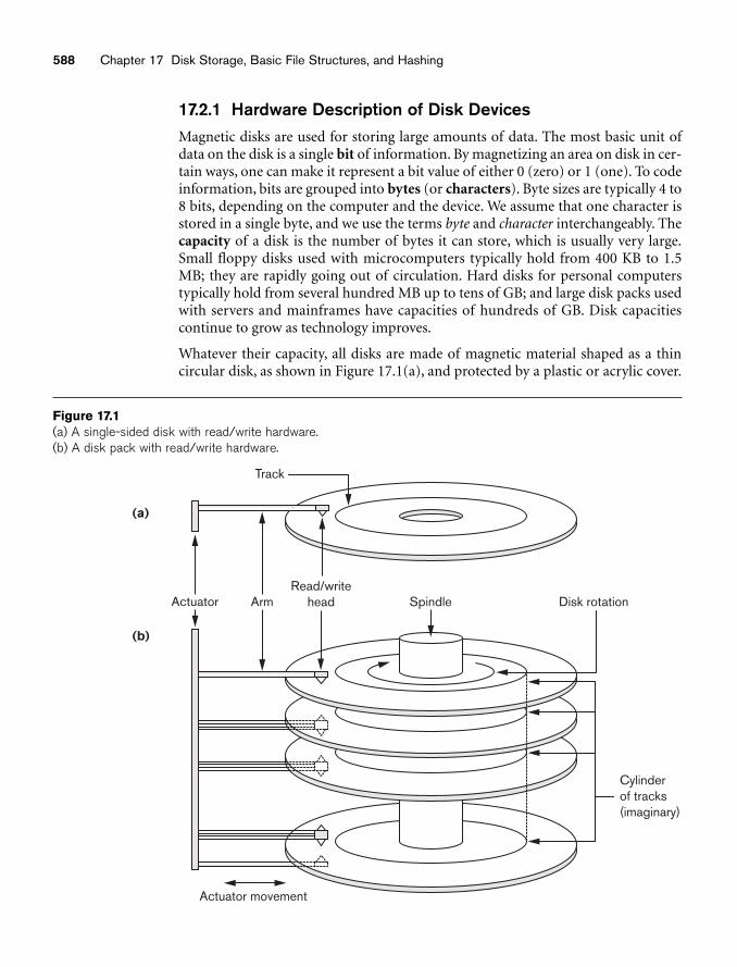
Figure 17.1(a) A single-sided disk with read/write hardware.(b) A disk pack with read/write hardware.
17.2.1 Hardware Description of Disk DevicesMagnetic disks are used for storing large amounts of data. The most basic unit ofdata on the disk is a single bit of information. By magnetizing an area on disk in cer-tain ways, one can make it represent a bit value of either 0 (zero) or 1 (one). To codeinformation, bits are grouped into bytes (or characters). Byte sizes are typically 4 to8 bits, depending on the computer and the device. We assume that one character isstored in a single byte, and we use the terms byte and character interchangeably. Thecapacity of a disk is the number of bytes it can store, which is usually very large.Small floppy disks used with microcomputers typically hold from 400 KB to 1.5MB; they are rapidly going out of circulation. Hard disks for personal computerstypically hold from several hundred MB up to tens of GB; and large disk packs usedwith servers and mainframes have capacities of hundreds of GB. Disk capacitiescontinue to grow as technology improves.
Whatever their capacity, all disks are made of magnetic material shaped as a thincircular disk, as shown in Figure 17.1(a), and protected by a plastic or acrylic cover.
17.2 Secondary Storage Devices 589
Track(a) Sector (arc of track)
(b)
Three sectors
Two sectorsOne sector
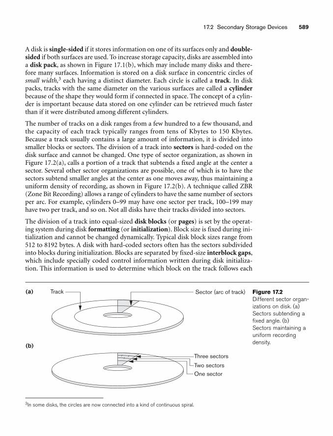
Figure 17.2Different sector organ-izations on disk. (a)Sectors subtending afixed angle. (b)Sectors maintaining auniform recording density.
A disk is single-sided if it stores information on one of its surfaces only and double-sided if both surfaces are used. To increase storage capacity, disks are assembled intoa disk pack, as shown in Figure 17.1(b), which may include many disks and there-fore many surfaces. Information is stored on a disk surface in concentric circles ofsmall width,3 each having a distinct diameter. Each circle is called a track. In diskpacks, tracks with the same diameter on the various surfaces are called a cylinderbecause of the shape they would form if connected in space. The concept of a cylin-der is important because data stored on one cylinder can be retrieved much fasterthan if it were distributed among different cylinders.
The number of tracks on a disk ranges from a few hundred to a few thousand, andthe capacity of each track typically ranges from tens of Kbytes to 150 Kbytes.Because a track usually contains a large amount of information, it is divided intosmaller blocks or sectors. The division of a track into sectors is hard-coded on thedisk surface and cannot be changed. One type of sector organization, as shown inFigure 17.2(a), calls a portion of a track that subtends a fixed angle at the center asector. Several other sector organizations are possible, one of which is to have thesectors subtend smaller angles at the center as one moves away, thus maintaining auniform density of recording, as shown in Figure 17.2(b). A technique called ZBR(Zone Bit Recording) allows a range of cylinders to have the same number of sectorsper arc. For example, cylinders 0–99 may have one sector per track, 100–199 mayhave two per track, and so on. Not all disks have their tracks divided into sectors.
The division of a track into equal-sized disk blocks (or pages) is set by the operat-ing system during disk formatting (or initialization). Block size is fixed during ini-tialization and cannot be changed dynamically. Typical disk block sizes range from512 to 8192 bytes. A disk with hard-coded sectors often has the sectors subdividedinto blocks during initialization. Blocks are separated by fixed-size interblock gaps,which include specially coded control information written during disk initializa-tion. This information is used to determine which block on the track follows each
3In some disks, the circles are now connected into a kind of continuous spiral.
590 Chapter 17 Disk Storage, Basic File Structures, and Hashing
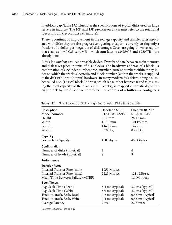
Table 17.1 Specifications of Typical High-End Cheetah Disks from Seagate
Description Cheetah 15K.6 Cheetah NS 10KModel Number ST3450856SS/FC ST3400755FCHeight 25.4 mm 26.11 mmWidth 101.6 mm 101.85 mmLength 146.05 mm 147 mmWeight 0.709 kg 0.771 kg
CapacityFormatted Capacity 450 Gbytes 400 Gbytes
ConfigurationNumber of disks (physical) 4 4Number of heads (physical) 8 8
Performance
Transfer RatesInternal Transfer Rate (min) 1051 Mb/secInternal Transfer Rate (max) 2225 Mb/sec 1211 Mb/secMean Time Between Failure (MTBF) 1.4 M hours
Seek TimesAvg. Seek Time (Read) 3.4 ms (typical) 3.9 ms (typical)Avg. Seek Time (Write) 3.9 ms (typical) 4.2 ms (typical)Track-to-track, Seek, Read 0.2 ms (typical) 0.35 ms (typical)Track-to-track, Seek, Write 0.4 ms (typical) 0.35 ms (typical)Average Latency 2 ms 2.98 msec
Courtesy Seagate Technology
interblock gap. Table 17.1 illustrates the specifications of typical disks used on largeservers in industry. The 10K and 15K prefixes on disk names refer to the rotationalspeeds in rpm (revolutions per minute).
There is continuous improvement in the storage capacity and transfer rates associ-ated with disks; they are also progressively getting cheaper—currently costing only afraction of a dollar per megabyte of disk storage. Costs are going down so rapidlythat costs as low 0.025 cent/MB—which translates to $0.25/GB and $250/TB—arealready here.
A disk is a random access addressable device. Transfer of data between main memoryand disk takes place in units of disk blocks. The hardware address of a block—acombination of a cylinder number, track number (surface number within the cylin-der on which the track is located), and block number (within the track) is suppliedto the disk I/O (input/output) hardware. In many modern disk drives, a single num-ber called LBA (Logical Block Address), which is a number between 0 and n (assum-ing the total capacity of the disk is n + 1 blocks), is mapped automatically to theright block by the disk drive controller. The address of a buffer—a contiguous
reserved area in main storage that holds one disk block—is also provided. For aread command, the disk block is copied into the buffer; whereas for a write com-mand, the contents of the buffer are copied into the disk block. Sometimes severalcontiguous blocks, called a cluster, may be transferred as a unit. In this case, thebuffer size is adjusted to match the number of bytes in the cluster.
The actual hardware mechanism that reads or writes a block is the disk read/writehead, which is part of a system called a disk drive. A disk or disk pack is mounted inthe disk drive, which includes a motor that rotates the disks. A read/write headincludes an electronic component attached to a mechanical arm. Disk packs withmultiple surfaces are controlled by several read/write heads—one for each surface,as shown in Figure 17.1(b). All arms are connected to an actuator attached toanother electrical motor, which moves the read/write heads in unison and positionsthem precisely over the cylinder of tracks specified in a block address.
Disk drives for hard disks rotate the disk pack continuously at a constant speed(typically ranging between 5,400 and 15,000 rpm). Once the read/write head ispositioned on the right track and the block specified in the block address movesunder the read/write head, the electronic component of the read/write head is acti-vated to transfer the data. Some disk units have fixed read/write heads, with as manyheads as there are tracks. These are called fixed-head disks, whereas disk units withan actuator are called movable-head disks. For fixed-head disks, a track or cylinderis selected by electronically switching to the appropriate read/write head rather thanby actual mechanical movement; consequently, it is much faster. However, the costof the additional read/write heads is quite high, so fixed-head disks are not com-monly used.
A disk controller, typically embedded in the disk drive, controls the disk drive andinterfaces it to the computer system. One of the standard interfaces used today fordisk drives on PCs and workstations is called SCSI (Small Computer SystemInterface). The controller accepts high-level I/O commands and takes appropriateaction to position the arm and causes the read/write action to take place. To transfera disk block, given its address, the disk controller must first mechanically positionthe read/write head on the correct track. The time required to do this is called theseek time. Typical seek times are 5 to 10 msec on desktops and 3 to 8 msecs onservers. Following that, there is another delay—called the rotational delay orlatency—while the beginning of the desired block rotates into position under theread/write head. It depends on the rpm of the disk. For example, at 15,000 rpm, thetime per rotation is 4 msec and the average rotational delay is the time per half rev-olution, or 2 msec. At 10,000 rpm the average rotational delay increases to 3 msec.Finally, some additional time is needed to transfer the data; this is called the blocktransfer time. Hence, the total time needed to locate and transfer an arbitraryblock, given its address, is the sum of the seek time, rotational delay, and blocktransfer time. The seek time and rotational delay are usually much larger than theblock transfer time. To make the transfer of multiple blocks more efficient, it iscommon to transfer several consecutive blocks on the same track or cylinder. Thiseliminates the seek time and rotational delay for all but the first block and can result
17.2 Secondary Storage Devices 591
592 Chapter 17 Disk Storage, Basic File Structures, and Hashing
in a substantial saving of time when numerous contiguous blocks are transferred.Usually, the disk manufacturer provides a bulk transfer rate for calculating the timerequired to transfer consecutive blocks. Appendix B contains a discussion of theseand other disk parameters.
The time needed to locate and transfer a disk block is in the order of milliseconds,usually ranging from 9 to 60 msec. For contiguous blocks, locating the first blocktakes from 9 to 60 msec, but transferring subsequent blocks may take only 0.4 to 2msec each. Many search techniques take advantage of consecutive retrieval of blockswhen searching for data on disk. In any case, a transfer time in the order of millisec-onds is considered quite high compared with the time required to process data inmain memory by current CPUs. Hence, locating data on disk is a major bottleneck indatabase applications. The file structures we discuss here and in Chapter 18 attemptto minimize the number of block transfers needed to locate and transfer the requireddata from disk to main memory. Placing “related information” on contiguousblocks is the basic goal of any storage organization on disk.
17.2.2 Magnetic Tape Storage DevicesDisks are random access secondary storage devices because an arbitrary disk blockmay be accessed at random once we specify its address. Magnetic tapes are sequen-tial access devices; to access the nth block on tape, first we must scan the precedingn – 1 blocks. Data is stored on reels of high-capacity magnetic tape, somewhat sim-ilar to audiotapes or videotapes. A tape drive is required to read the data from orwrite the data to a tape reel. Usually, each group of bits that forms a byte is storedacross the tape, and the bytes themselves are stored consecutively on the tape.
A read/write head is used to read or write data on tape. Data records on tape are alsostored in blocks—although the blocks may be substantially larger than those fordisks, and interblock gaps are also quite large. With typical tape densities of 1600 to6250 bytes per inch, a typical interblock gap4 of 0.6 inch corresponds to 960 to 3750bytes of wasted storage space. It is customary to group many records together in oneblock for better space utilization.
The main characteristic of a tape is its requirement that we access the data blocks insequential order. To get to a block in the middle of a reel of tape, the tape ismounted and then scanned until the required block gets under the read/write head.For this reason, tape access can be slow and tapes are not used to store online data,except for some specialized applications. However, tapes serve a very importantfunction—backing up the database. One reason for backup is to keep copies of diskfiles in case the data is lost due to a disk crash, which can happen if the diskread/write head touches the disk surface because of mechanical malfunction. Forthis reason, disk files are copied periodically to tape. For many online critical appli-cations, such as airline reservation systems, to avoid any downtime, mirrored sys-tems are used to keep three sets of identical disks—two in online operation and one
4Called interrecord gaps in tape terminology.
17.3 Buffering of Blocks 593
as backup. Here, offline disks become a backup device. The three are rotated so thatthey can be switched in case there is a failure on one of the live disk drives. Tapes canalso be used to store excessively large database files. Database files that are seldomused or are outdated but required for historical record keeping can be archived ontape. Originally, half-inch reel tape drives were used for data storage employing theso-called 9 track tapes. Later, smaller 8-mm magnetic tapes (similar to those used incamcorders) that can store up to 50 GB, as well as 4-mm helical scan data cartridgesand writable CDs and DVDs, became popular media for backing up data files fromPCs and workstations. They are also used for storing images and system libraries.
Backing up enterprise databases so that no transaction information is lost is a majorundertaking. Currently, tape libraries with slots for several hundred cartridges areused with Digital and Superdigital Linear Tapes (DLTs and SDLTs) having capacitiesin hundreds of gigabytes that record data on linear tracks. Robotic arms are used towrite on multiple cartridges in parallel using multiple tape drives with automaticlabeling software to identify the backup cartridges. An example of a giant library isthe SL8500 model of Sun Storage Technology that can store up to 70 petabytes(petabyte = 1000 TB) of data using up to 448 drives with a maximum throughputrate of 193.2 TB/hour. We defer the discussion of disk storage technology calledRAID, and of storage area networks, network-attached storage, and iSCSI storagesystems to the end of the chapter.
17.3 Buffering of BlocksWhen several blocks need to be transferred from disk to main memory and all theblock addresses are known, several buffers can be reserved in main memory tospeed up the transfer. While one buffer is being read or written, the CPU canprocess data in the other buffer because an independent disk I/O processor (con-troller) exists that, once started, can proceed to transfer a data block between mem-ory and disk independent of and in parallel to CPU processing.
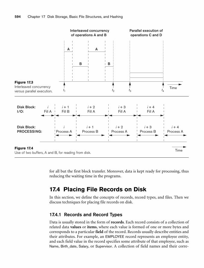
Figure 17.3 illustrates how two processes can proceed in parallel. Processes A and Bare running concurrently in an interleaved fashion, whereas processes C and D arerunning concurrently in a parallel fashion. When a single CPU controls multipleprocesses, parallel execution is not possible. However, the processes can still runconcurrently in an interleaved way. Buffering is most useful when processes can runconcurrently in a parallel fashion, either because a separate disk I/O processor isavailable or because multiple CPU processors exist.
Figure 17.4 illustrates how reading and processing can proceed in parallel when thetime required to process a disk block in memory is less than the time required toread the next block and fill a buffer. The CPU can start processing a block once itstransfer to main memory is completed; at the same time, the disk I/O processor canbe reading and transferring the next block into a different buffer. This technique iscalled double buffering and can also be used to read a continuous stream of blocksfrom disk to memory. Double buffering permits continuous reading or writing ofdata on consecutive disk blocks, which eliminates the seek time and rotational delay
594 Chapter 17 Disk Storage, Basic File Structures, and Hashing
Interleaved concurrency of operations A and B
Parallel execution of operations C and D
t1
A A
B B
t2 t3 t4Time
Figure 17.3Interleaved concurrencyversus parallel execution.
i + 1Process B
i + 2Fill A
Time
iProcess A
i + 1Fill B
Disk Block:I/O:
Disk Block:PROCESSING:
iFill A
i + 2Process A
i + 3Fill A
i + 4Process A
i + 3Process B
i + 4Fill A
Figure 17.4Use of two buffers, A and B, for reading from disk.
for all but the first block transfer. Moreover, data is kept ready for processing, thusreducing the waiting time in the programs.
17.4 Placing File Records on DiskIn this section, we define the concepts of records, record types, and files. Then wediscuss techniques for placing file records on disk.
17.4.1 Records and Record TypesData is usually stored in the form of records. Each record consists of a collection ofrelated data values or items, where each value is formed of one or more bytes andcorresponds to a particular field of the record. Records usually describe entities andtheir attributes. For example, an EMPLOYEE record represents an employee entity,and each field value in the record specifies some attribute of that employee, such asName, Birth_date, Salary, or Supervisor. A collection of field names and their corre-
17.4 Placing File Records on Disk 595
sponding data types constitutes a record type or record format definition. A datatype, associated with each field, specifies the types of values a field can take.
The data type of a field is usually one of the standard data types used in program-ming. These include numeric (integer, long integer, or floating point), string ofcharacters (fixed-length or varying), Boolean (having 0 and 1 or TRUE and FALSEvalues only), and sometimes specially coded date and time data types. The numberof bytes required for each data type is fixed for a given computer system. An integermay require 4 bytes, a long integer 8 bytes, a real number 4 bytes, a Boolean 1 byte,a date 10 bytes (assuming a format of YYYY-MM-DD), and a fixed-length string ofk characters k bytes. Variable-length strings may require as many bytes as there arecharacters in each field value. For example, an EMPLOYEE record type may bedefined—using the C programming language notation—as the following structure:
struct employee{char name[30];char ssn[9];int salary;int job_code;char department[20];
} ;
In some database applications, the need may arise for storing data items that consistof large unstructured objects, which represent images, digitized video or audiostreams, or free text. These are referred to as BLOBs (binary large objects). A BLOBdata item is typically stored separately from its record in a pool of disk blocks, and apointer to the BLOB is included in the record.
17.4.2 Files, Fixed-Length Records, and Variable-Length Records
A file is a sequence of records. In many cases, all records in a file are of the samerecord type. If every record in the file has exactly the same size (in bytes), the file issaid to be made up of fixed-length records. If different records in the file have dif-ferent sizes, the file is said to be made up of variable-length records. A file may havevariable-length records for several reasons:
■ The file records are of the same record type, but one or more of the fields areof varying size (variable-length fields). For example, the Name field ofEMPLOYEE can be a variable-length field.
■ The file records are of the same record type, but one or more of the fieldsmay have multiple values for individual records; such a field is called arepeating field and a group of values for the field is often called a repeatinggroup.
■ The file records are of the same record type, but one or more of the fields areoptional; that is, they may have values for some but not all of the file records(optional fields).
Name = Smith, John Ssn = 123456789 DEPARTMENT = Computer
Smith, John
Name
1
(a)
(b)
(c)
1 12 21 25 29
Name Ssn Salary Job_code Department Hire_date
31 40 44 48 68
Ssn Salary Job_code Department
Separator Characters123456789 XXXX XXXX Computer
Separator Characters
Separates field name from field value
Separates fields
Terminates record
=
596 Chapter 17 Disk Storage, Basic File Structures, and Hashing
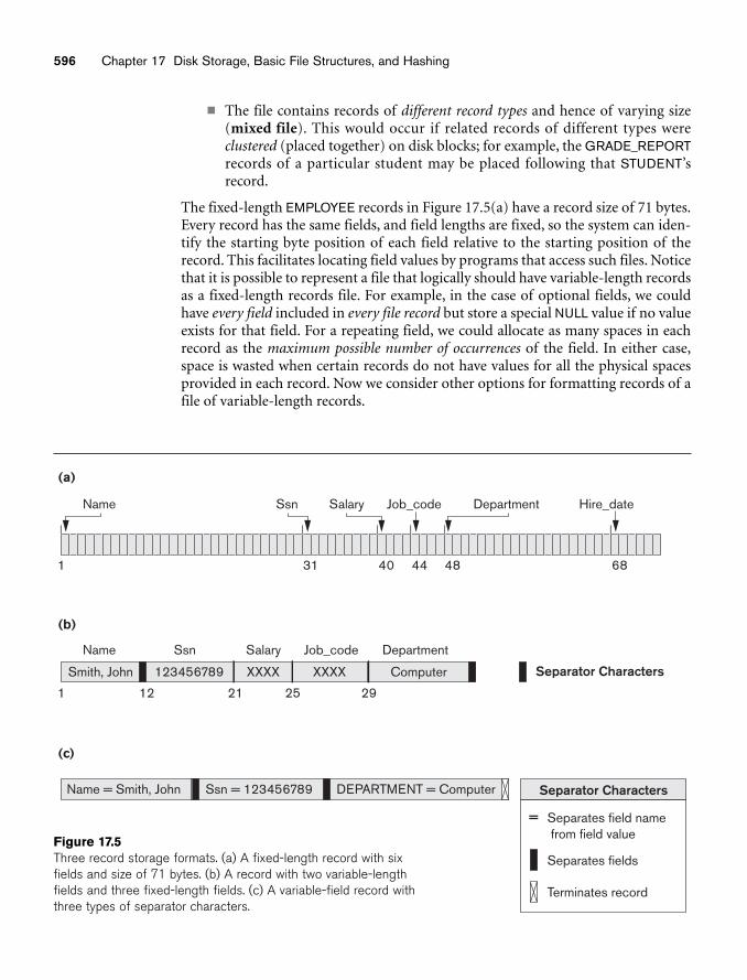
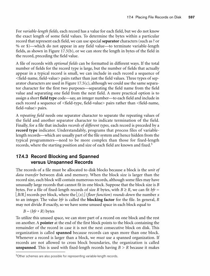
Figure 17.5Three record storage formats. (a) A fixed-length record with sixfields and size of 71 bytes. (b) A record with two variable-lengthfields and three fixed-length fields. (c) A variable-field record withthree types of separator characters.
■ The file contains records of different record types and hence of varying size(mixed file). This would occur if related records of different types wereclustered (placed together) on disk blocks; for example, the GRADE_REPORTrecords of a particular student may be placed following that STUDENT’srecord.
The fixed-length EMPLOYEE records in Figure 17.5(a) have a record size of 71 bytes.Every record has the same fields, and field lengths are fixed, so the system can iden-tify the starting byte position of each field relative to the starting position of therecord. This facilitates locating field values by programs that access such files. Noticethat it is possible to represent a file that logically should have variable-length recordsas a fixed-length records file. For example, in the case of optional fields, we couldhave every field included in every file record but store a special NULL value if no valueexists for that field. For a repeating field, we could allocate as many spaces in eachrecord as the maximum possible number of occurrences of the field. In either case,space is wasted when certain records do not have values for all the physical spacesprovided in each record. Now we consider other options for formatting records of afile of variable-length records.
17.4 Placing File Records on Disk 597
For variable-length fields, each record has a value for each field, but we do not knowthe exact length of some field values. To determine the bytes within a particularrecord that represent each field, we can use special separator characters (such as ? or% or $)—which do not appear in any field value—to terminate variable-lengthfields, as shown in Figure 17.5(b), or we can store the length in bytes of the field inthe record, preceding the field value.
A file of records with optional fields can be formatted in different ways. If the totalnumber of fields for the record type is large, but the number of fields that actuallyappear in a typical record is small, we can include in each record a sequence of<field-name, field-value> pairs rather than just the field values. Three types of sep-arator characters are used in Figure 17.5(c), although we could use the same separa-tor character for the first two purposes—separating the field name from the fieldvalue and separating one field from the next field. A more practical option is toassign a short field type code—say, an integer number—to each field and include ineach record a sequence of <field-type, field-value> pairs rather than <field-name,field-value> pairs.
A repeating field needs one separator character to separate the repeating values ofthe field and another separator character to indicate termination of the field.Finally, for a file that includes records of different types, each record is preceded by arecord type indicator. Understandably, programs that process files of variable-length records—which are usually part of the file system and hence hidden from thetypical programmers—need to be more complex than those for fixed-lengthrecords, where the starting position and size of each field are known and fixed.5
17.4.3 Record Blocking and Spanned versus Unspanned Records
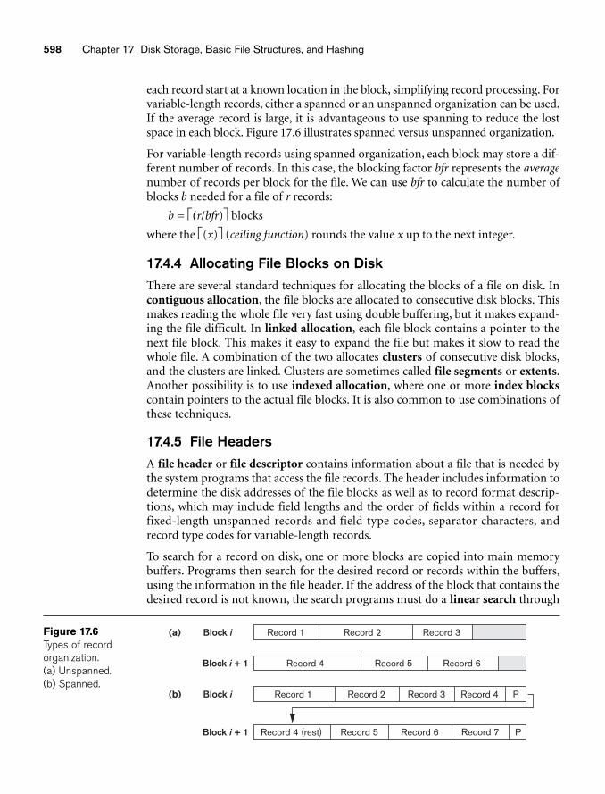
The records of a file must be allocated to disk blocks because a block is the unit ofdata transfer between disk and memory. When the block size is larger than therecord size, each block will contain numerous records, although some files may haveunusually large records that cannot fit in one block. Suppose that the block size is Bbytes. For a file of fixed-length records of size R bytes, with B ≥ R, we can fit bfr =⎣B/R⎦ records per block, where the ⎣(x)⎦ (floor function) rounds down the number xto an integer. The value bfr is called the blocking factor for the file. In general, Rmay not divide B exactly, so we have some unused space in each block equal to
B − (bfr * R) bytes
To utilize this unused space, we can store part of a record on one block and the reston another. A pointer at the end of the first block points to the block containing theremainder of the record in case it is not the next consecutive block on disk. Thisorganization is called spanned because records can span more than one block.Whenever a record is larger than a block, we must use a spanned organization. Ifrecords are not allowed to cross block boundaries, the organization is calledunspanned. This is used with fixed-length records having B > R because it makes
5Other schemes are also possible for representing variable-length records.
598 Chapter 17 Disk Storage, Basic File Structures, and Hashing
Record 1Block i Record 2 Record 3 Record 4 P
Record 4 (rest)Block i + 1 Record 5 Record 6 Record 7 P
Record 1Block i
(b)
(a) Record 2 Record 3
Record 4Block i + 1 Record 5 Record 6
Figure 17.6Types of record organization.(a) Unspanned. (b) Spanned.
each record start at a known location in the block, simplifying record processing. Forvariable-length records, either a spanned or an unspanned organization can be used.If the average record is large, it is advantageous to use spanning to reduce the lostspace in each block. Figure 17.6 illustrates spanned versus unspanned organization.
For variable-length records using spanned organization, each block may store a dif-ferent number of records. In this case, the blocking factor bfr represents the averagenumber of records per block for the file. We can use bfr to calculate the number ofblocks b needed for a file of r records:
b = ⎡(r/bfr)⎤ blocks
where the ⎡(x)⎤ (ceiling function) rounds the value x up to the next integer.
17.4.4 Allocating File Blocks on DiskThere are several standard techniques for allocating the blocks of a file on disk. Incontiguous allocation, the file blocks are allocated to consecutive disk blocks. Thismakes reading the whole file very fast using double buffering, but it makes expand-ing the file difficult. In linked allocation, each file block contains a pointer to thenext file block. This makes it easy to expand the file but makes it slow to read thewhole file. A combination of the two allocates clusters of consecutive disk blocks,and the clusters are linked. Clusters are sometimes called file segments or extents.Another possibility is to use indexed allocation, where one or more index blockscontain pointers to the actual file blocks. It is also common to use combinations ofthese techniques.
17.4.5 File HeadersA file header or file descriptor contains information about a file that is needed bythe system programs that access the file records. The header includes information todetermine the disk addresses of the file blocks as well as to record format descrip-tions, which may include field lengths and the order of fields within a record forfixed-length unspanned records and field type codes, separator characters, andrecord type codes for variable-length records.
To search for a record on disk, one or more blocks are copied into main memorybuffers. Programs then search for the desired record or records within the buffers,using the information in the file header. If the address of the block that contains thedesired record is not known, the search programs must do a linear search through
17.5 Operations on Files 599
the file blocks. Each file block is copied into a buffer and searched until the record islocated or all the file blocks have been searched unsuccessfully. This can be verytime-consuming for a large file. The goal of a good file organization is to locate theblock that contains a desired record with a minimal number of block transfers.
17.5 Operations on FilesOperations on files are usually grouped into retrieval operations and update oper-ations. The former do not change any data in the file, but only locate certain recordsso that their field values can be examined and processed. The latter change the fileby insertion or deletion of records or by modification of field values. In either case,we may have to select one or more records for retrieval, deletion, or modificationbased on a selection condition (or filtering condition), which specifies criteria thatthe desired record or records must satisfy.
Consider an EMPLOYEE file with fields Name, Ssn, Salary, Job_code, and Department.A simple selection condition may involve an equality comparison on some fieldvalue—for example, (Ssn = ‘123456789’) or (Department = ‘Research’). More com-plex conditions can involve other types of comparison operators, such as > or ≥; anexample is (Salary ≥ 30000). The general case is to have an arbitrary Boolean expres-sion on the fields of the file as the selection condition.
Search operations on files are generally based on simple selection conditions. Acomplex condition must be decomposed by the DBMS (or the programmer) toextract a simple condition that can be used to locate the records on disk. Eachlocated record is then checked to determine whether it satisfies the full selectioncondition. For example, we may extract the simple condition (Department =‘Research’) from the complex condition ((Salary ≥ 30000) AND (Department =‘Research’)); each record satisfying (Department = ‘Research’) is located and thentested to see if it also satisfies (Salary ≥ 30000).
When several file records satisfy a search condition, the first record—with respect tothe physical sequence of file records—is initially located and designated the currentrecord. Subsequent search operations commence from this record and locate thenext record in the file that satisfies the condition.
Actual operations for locating and accessing file records vary from system to system.Below, we present a set of representative operations. Typically, high-level programs,such as DBMS software programs, access records by using these commands, so wesometimes refer to program variables in the following descriptions:
■ Open. Prepares the file for reading or writing. Allocates appropriate buffers(typically at least two) to hold file blocks from disk, and retrieves the fileheader. Sets the file pointer to the beginning of the file.
■ Reset. Sets the file pointer of an open file to the beginning of the file.■ Find (or Locate). Searches for the first record that satisfies a search condi-
tion. Transfers the block containing that record into a main memory buffer(if it is not already there). The file pointer points to the record in the buffer
600 Chapter 17 Disk Storage, Basic File Structures, and Hashing
and it becomes the current record. Sometimes, different verbs are used toindicate whether the located record is to be retrieved or updated.
■ Read (or Get). Copies the current record from the buffer to a program vari-able in the user program. This command may also advance the currentrecord pointer to the next record in the file, which may necessitate readingthe next file block from disk.
■ FindNext. Searches for the next record in the file that satisfies the searchcondition. Transfers the block containing that record into a main memorybuffer (if it is not already there). The record is located in the buffer andbecomes the current record. Various forms of FindNext (for example, FindNext record within a current parent record, Find Next record of a given type,or Find Next record where a complex condition is met) are available inlegacy DBMSs based on the hierarchical and network models.
■ Delete. Deletes the current record and (eventually) updates the file on diskto reflect the deletion.
■ Modify. Modifies some field values for the current record and (eventually)updates the file on disk to reflect the modification.
■ Insert. Inserts a new record in the file by locating the block where the recordis to be inserted, transferring that block into a main memory buffer (if it isnot already there), writing the record into the buffer, and (eventually) writ-ing the buffer to disk to reflect the insertion.
■ Close. Completes the file access by releasing the buffers and performing anyother needed cleanup operations.
The preceding (except for Open and Close) are called record-at-a-time operationsbecause each operation applies to a single record. It is possible to streamline theoperations Find, FindNext, and Read into a single operation, Scan, whose descrip-tion is as follows:
■ Scan. If the file has just been opened or reset, Scan returns the first record;otherwise it returns the next record. If a condition is specified with the oper-ation, the returned record is the first or next record satisfying the condition.
In database systems, additional set-at-a-time higher-level operations may beapplied to a file. Examples of these are as follows:
■ FindAll. Locates all the records in the file that satisfy a search condition.
■ Find (or Locate) n. Searches for the first record that satisfies a search condi-tion and then continues to locate the next n – 1 records satisfying the samecondition. Transfers the blocks containing the n records to the main memorybuffer (if not already there).
■ FindOrdered. Retrieves all the records in the file in some specified order.
■ Reorganize. Starts the reorganization process. As we shall see, some fileorganizations require periodic reorganization. An example is to reorder thefile records by sorting them on a specified field.
17.6 Files of Unordered Records (Heap Files) 601
At this point, it is worthwhile to note the difference between the terms file organiza-tion and access method. A file organization refers to the organization of the data ofa file into records, blocks, and access structures; this includes the way records andblocks are placed on the storage medium and interlinked. An access method, on theother hand, provides a group of operations—such as those listed earlier—that canbe applied to a file. In general, it is possible to apply several access methods to a fileorganization. Some access methods, though, can be applied only to files organizedin certain ways. For example, we cannot apply an indexed access method to a filewithout an index (see Chapter 18).
Usually, we expect to use some search conditions more than others. Some files maybe static, meaning that update operations are rarely performed; other, moredynamic files may change frequently, so update operations are constantly applied tothem. A successful file organization should perform as efficiently as possible theoperations we expect to apply frequently to the file. For example, consider theEMPLOYEE file, as shown in Figure 17.5(a), which stores the records for currentemployees in a company. We expect to insert records (when employees are hired),delete records (when employees leave the company), and modify records (for exam-ple, when an employee’s salary or job is changed). Deleting or modifying a recordrequires a selection condition to identify a particular record or set of records.Retrieving one or more records also requires a selection condition.
If users expect mainly to apply a search condition based on Ssn, the designer mustchoose a file organization that facilitates locating a record given its Ssn value. Thismay involve physically ordering the records by Ssn value or defining an index onSsn (see Chapter 18). Suppose that a second application uses the file to generateemployees’ paychecks and requires that paychecks are grouped by department. Forthis application, it is best to order employee records by department and then byname within each department. The clustering of records into blocks and the organ-ization of blocks on cylinders would now be different than before. However, thisarrangement conflicts with ordering the records by Ssn values. If both applicationsare important, the designer should choose an organization that allows both opera-tions to be done efficiently. Unfortunately, in many cases a single organization doesnot allow all needed operations on a file to be implemented efficiently. This requiresthat a compromise must be chosen that takes into account the expected importanceand mix of retrieval and update operations.
In the following sections and in Chapter 18, we discuss methods for organizingrecords of a file on disk. Several general techniques, such as ordering, hashing, andindexing, are used to create access methods. Additionally, various general tech-niques for handling insertions and deletions work with many file organizations.
17.6 Files of Unordered Records (Heap Files)In this simplest and most basic type of organization, records are placed in the file inthe order in which they are inserted, so new records are inserted at the end of the
602 Chapter 17 Disk Storage, Basic File Structures, and Hashing
file. Such an organization is called a heap or pile file.6 This organization is oftenused with additional access paths, such as the secondary indexes discussed inChapter 18. It is also used to collect and store data records for future use.
Inserting a new record is very efficient. The last disk block of the file is copied into abuffer, the new record is added, and the block is then rewritten back to disk. Theaddress of the last file block is kept in the file header. However, searching for arecord using any search condition involves a linear search through the file block byblock—an expensive procedure. If only one record satisfies the search condition,then, on the average, a program will read into memory and search half the fileblocks before it finds the record. For a file of b blocks, this requires searching (b/2)blocks, on average. If no records or several records satisfy the search condition, theprogram must read and search all b blocks in the file.
To delete a record, a program must first find its block, copy the block into a buffer,delete the record from the buffer, and finally rewrite the block back to the disk. Thisleaves unused space in the disk block. Deleting a large number of records in this wayresults in wasted storage space. Another technique used for record deletion is tohave an extra byte or bit, called a deletion marker, stored with each record. A recordis deleted by setting the deletion marker to a certain value. A different value for themarker indicates a valid (not deleted) record. Search programs consider only validrecords in a block when conducting their search. Both of these deletion techniquesrequire periodic reorganization of the file to reclaim the unused space of deletedrecords. During reorganization, the file blocks are accessed consecutively, andrecords are packed by removing deleted records. After such a reorganization, theblocks are filled to capacity once more. Another possibility is to use the space ofdeleted records when inserting new records, although this requires extra bookkeep-ing to keep track of empty locations.
We can use either spanned or unspanned organization for an unordered file, and itmay be used with either fixed-length or variable-length records. Modifying a vari-able-length record may require deleting the old record and inserting a modifiedrecord because the modified record may not fit in its old space on disk.
To read all records in order of the values of some field, we create a sorted copy of thefile. Sorting is an expensive operation for a large disk file, and special techniques forexternal sorting are used (see Chapter 19).
For a file of unordered fixed-length records using unspanned blocks and contiguousallocation, it is straightforward to access any record by its position in the file. If thefile records are numbered 0, 1, 2, ..., r − 1 and the records in each block are num-bered 0, 1, ..., bfr − 1, where bfr is the blocking factor, then the ith record of the fileis located in block ⎣(i/bfr)⎦ and is the (i mod bfr)th record in that block. Such a fileis often called a relative or direct file because records can easily be accessed directlyby their relative positions. Accessing a record by its position does not help locate arecord based on a search condition; however, it facilitates the construction of accesspaths on the file, such as the indexes discussed in Chapter 18.
6Sometimes this organization is called a sequential file.
17.7 Files of Ordered Records (Sorted Files) 603
17.7 Files of Ordered Records (Sorted Files)We can physically order the records of a file on disk based on the values of one oftheir fields—called the ordering field. This leads to an ordered or sequential file.7
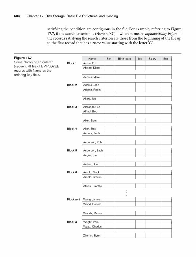
If the ordering field is also a key field of the file—a field guaranteed to have aunique value in each record—then the field is called the ordering key for the file.Figure 17.7 shows an ordered file with Name as the ordering key field (assuming thatemployees have distinct names).
Ordered records have some advantages over unordered files. First, reading the recordsin order of the ordering key values becomes extremely efficient because no sorting isrequired. Second, finding the next record from the current one in order of the order-ing key usually requires no additional block accesses because the next record is in thesame block as the current one (unless the current record is the last one in the block).Third, using a search condition based on the value of an ordering key field results infaster access when the binary search technique is used, which constitutes an improve-ment over linear searches, although it is not often used for disk files. Ordered files areblocked and stored on contiguous cylinders to minimize the seek time.
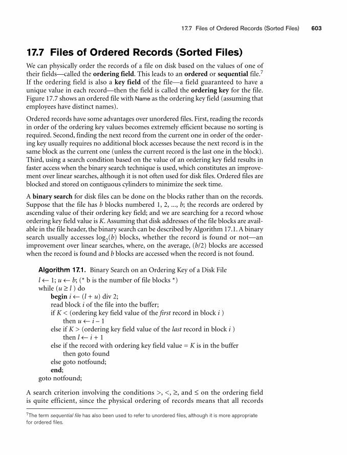
A binary search for disk files can be done on the blocks rather than on the records.Suppose that the file has b blocks numbered 1, 2, ..., b; the records are ordered byascending value of their ordering key field; and we are searching for a record whoseordering key field value is K. Assuming that disk addresses of the file blocks are avail-able in the file header, the binary search can be described by Algorithm 17.1. A binarysearch usually accesses log2(b) blocks, whether the record is found or not—animprovement over linear searches, where, on the average, (b/2) blocks are accessedwhen the record is found and b blocks are accessed when the record is not found.
Algorithm 17.1. Binary Search on an Ordering Key of a Disk File
l ← 1; u ← b; (* b is the number of file blocks *)while (u ≥ l ) do
begin i ← (l + u) div 2;read block i of the file into the buffer;if K < (ordering key field value of the first record in block i )
then u ← i – 1else if K > (ordering key field value of the last record in block i )
then l ← i + 1else if the record with ordering key field value = K is in the buffer
then goto foundelse goto notfound;end;
goto notfound;
A search criterion involving the conditions >, <, ≥, and ≤ on the ordering field is quite efficient, since the physical ordering of records means that all records
7The term sequential file has also been used to refer to unordered files, although it is more appropriatefor ordered files.
604 Chapter 17 Disk Storage, Basic File Structures, and Hashing
Name
Aaron, Ed
Abbott, Diane
Block 1
Acosta, Marc
Ssn Birth_date
...
Job Salary Sex
...
Adams, John
Adams, Robin
Block 2
Akers, Jan
...
Alexander, Ed
Alfred, Bob
Block 3
Allen, Sam
...
Allen, Troy
Anders, Keith
Block 4
Anderson, Rob
...
Anderson, Zach
Angeli, Joe
Block 5
Archer, Sue
...
Arnold, Mack
Arnold, Steven
Block 6
Atkins, Timothy
Wong, James
Wood, Donald
Block n–1
Woods, Manny
...
Wright, Pam
Wyatt, Charles
Block n
Zimmer, Byron
...
Figure 17.7Some blocks of an ordered(sequential) file of EMPLOYEErecords with Name as theordering key field.
satisfying the condition are contiguous in the file. For example, referring to Figure17.7, if the search criterion is (Name < ‘G’)—where < means alphabetically before—the records satisfying the search criterion are those from the beginning of the file upto the first record that has a Name value starting with the letter ‘G’.
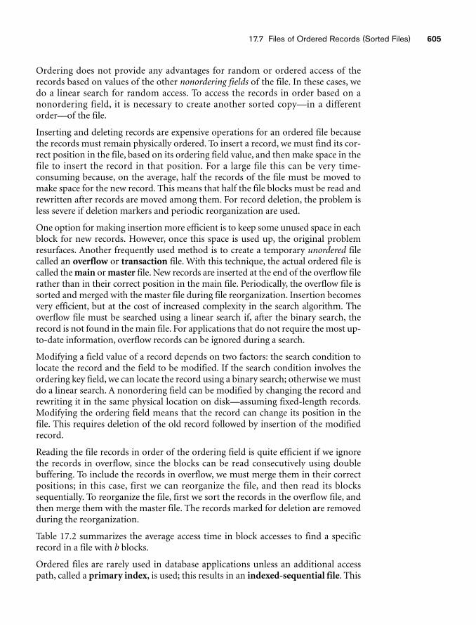
17.7 Files of Ordered Records (Sorted Files) 605
Ordering does not provide any advantages for random or ordered access of therecords based on values of the other nonordering fields of the file. In these cases, wedo a linear search for random access. To access the records in order based on anonordering field, it is necessary to create another sorted copy—in a differentorder—of the file.
Inserting and deleting records are expensive operations for an ordered file becausethe records must remain physically ordered. To insert a record, we must find its cor-rect position in the file, based on its ordering field value, and then make space in thefile to insert the record in that position. For a large file this can be very time-consuming because, on the average, half the records of the file must be moved tomake space for the new record. This means that half the file blocks must be read andrewritten after records are moved among them. For record deletion, the problem isless severe if deletion markers and periodic reorganization are used.
One option for making insertion more efficient is to keep some unused space in eachblock for new records. However, once this space is used up, the original problemresurfaces. Another frequently used method is to create a temporary unordered filecalled an overflow or transaction file. With this technique, the actual ordered file iscalled the main or master file. New records are inserted at the end of the overflow filerather than in their correct position in the main file. Periodically, the overflow file issorted and merged with the master file during file reorganization. Insertion becomesvery efficient, but at the cost of increased complexity in the search algorithm. Theoverflow file must be searched using a linear search if, after the binary search, therecord is not found in the main file. For applications that do not require the most up-to-date information, overflow records can be ignored during a search.
Modifying a field value of a record depends on two factors: the search condition tolocate the record and the field to be modified. If the search condition involves theordering key field, we can locate the record using a binary search; otherwise we mustdo a linear search. A nonordering field can be modified by changing the record andrewriting it in the same physical location on disk—assuming fixed-length records.Modifying the ordering field means that the record can change its position in thefile. This requires deletion of the old record followed by insertion of the modifiedrecord.
Reading the file records in order of the ordering field is quite efficient if we ignorethe records in overflow, since the blocks can be read consecutively using doublebuffering. To include the records in overflow, we must merge them in their correctpositions; in this case, first we can reorganize the file, and then read its blockssequentially. To reorganize the file, first we sort the records in the overflow file, andthen merge them with the master file. The records marked for deletion are removedduring the reorganization.
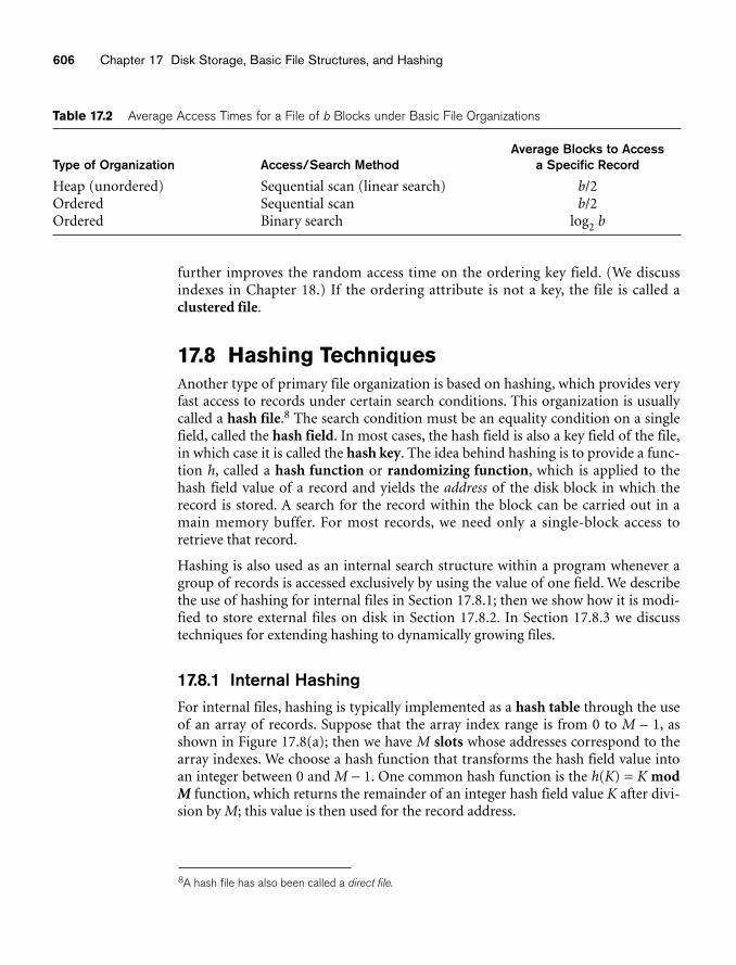
Table 17.2 summarizes the average access time in block accesses to find a specificrecord in a file with b blocks.
Ordered files are rarely used in database applications unless an additional accesspath, called a primary index, is used; this results in an indexed-sequential file. This
606 Chapter 17 Disk Storage, Basic File Structures, and Hashing
Table 17.2 Average Access Times for a File of b Blocks under Basic File Organizations
Average Blocks to AccessType of Organization Access/Search Method a Specific Record
Heap (unordered) Sequential scan (linear search) b/2Ordered Sequential scan b/2Ordered Binary search log2 b
further improves the random access time on the ordering key field. (We discussindexes in Chapter 18.) If the ordering attribute is not a key, the file is called aclustered file.
17.8 Hashing TechniquesAnother type of primary file organization is based on hashing, which provides veryfast access to records under certain search conditions. This organization is usuallycalled a hash file.8 The search condition must be an equality condition on a singlefield, called the hash field. In most cases, the hash field is also a key field of the file,in which case it is called the hash key. The idea behind hashing is to provide a func-tion h, called a hash function or randomizing function, which is applied to thehash field value of a record and yields the address of the disk block in which therecord is stored. A search for the record within the block can be carried out in amain memory buffer. For most records, we need only a single-block access toretrieve that record.
Hashing is also used as an internal search structure within a program whenever agroup of records is accessed exclusively by using the value of one field. We describethe use of hashing for internal files in Section 17.8.1; then we show how it is modi-fied to store external files on disk in Section 17.8.2. In Section 17.8.3 we discusstechniques for extending hashing to dynamically growing files.
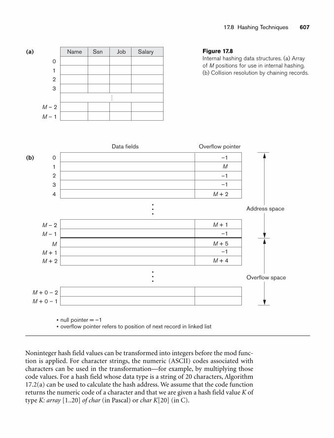
17.8.1 Internal HashingFor internal files, hashing is typically implemented as a hash table through the useof an array of records. Suppose that the array index range is from 0 to M – 1, asshown in Figure 17.8(a); then we have M slots whose addresses correspond to thearray indexes. We choose a hash function that transforms the hash field value intoan integer between 0 and M − 1. One common hash function is the h(K) = K modM function, which returns the remainder of an integer hash field value K after divi-sion by M; this value is then used for the record address.
8A hash file has also been called a direct file.
17.8 Hashing Techniques 607
Noninteger hash field values can be transformed into integers before the mod func-tion is applied. For character strings, the numeric (ASCII) codes associated withcharacters can be used in the transformation—for example, by multiplying thosecode values. For a hash field whose data type is a string of 20 characters, Algorithm17.2(a) can be used to calculate the hash address. We assume that the code functionreturns the numeric code of a character and that we are given a hash field value K oftype K: array [1..20] of char (in Pascal) or char K[20] (in C).
(a)
–1
–1–1
M + 2
M
0
12
3
M – 2
M – 1
Data fields Overflow pointer
Address space
Overflow space
M + 1
M + 5–1
M + 4
–1
M + 0 – 2M + 0 – 1
null pointer = –1overflow pointer refers to position of next record in linked list
M – 2
MM + 1M + 2
M – 1
Name Ssn Job Salary
(b) 0
12
3
4
...
Figure 17.8Internal hashing data structures. (a) Arrayof M positions for use in internal hashing.(b) Collision resolution by chaining records.
608 Chapter 17 Disk Storage, Basic File Structures, and Hashing
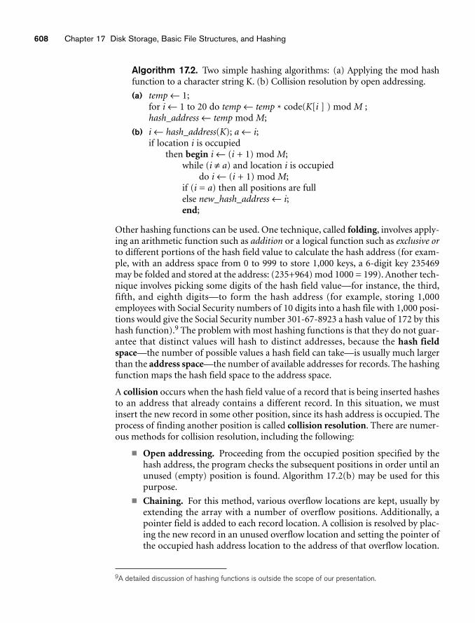
Algorithm 17.2. Two simple hashing algorithms: (a) Applying the mod hashfunction to a character string K. (b) Collision resolution by open addressing.
(a) temp ← 1;for i ← 1 to 20 do temp ← temp * code(K[i ] ) mod M ;hash_address ← temp mod M;
(b) i ← hash_address(K); a ← i;if location i is occupied
then begin i ← (i + 1) mod M;while (i ≠ a) and location i is occupied
do i ← (i + 1) mod M;if (i = a) then all positions are fullelse new_hash_address ← i;end;
Other hashing functions can be used. One technique, called folding, involves apply-ing an arithmetic function such as addition or a logical function such as exclusive orto different portions of the hash field value to calculate the hash address (for exam-ple, with an address space from 0 to 999 to store 1,000 keys, a 6-digit key 235469may be folded and stored at the address: (235+964) mod 1000 = 199). Another tech-nique involves picking some digits of the hash field value—for instance, the third,fifth, and eighth digits—to form the hash address (for example, storing 1,000employees with Social Security numbers of 10 digits into a hash file with 1,000 posi-tions would give the Social Security number 301-67-8923 a hash value of 172 by thishash function).9 The problem with most hashing functions is that they do not guar-antee that distinct values will hash to distinct addresses, because the hash fieldspace—the number of possible values a hash field can take—is usually much largerthan the address space—the number of available addresses for records. The hashingfunction maps the hash field space to the address space.
A collision occurs when the hash field value of a record that is being inserted hashesto an address that already contains a different record. In this situation, we mustinsert the new record in some other position, since its hash address is occupied. Theprocess of finding another position is called collision resolution. There are numer-ous methods for collision resolution, including the following:
■ Open addressing. Proceeding from the occupied position specified by thehash address, the program checks the subsequent positions in order until anunused (empty) position is found. Algorithm 17.2(b) may be used for thispurpose.
■ Chaining. For this method, various overflow locations are kept, usually byextending the array with a number of overflow positions. Additionally, apointer field is added to each record location. A collision is resolved by plac-ing the new record in an unused overflow location and setting the pointer ofthe occupied hash address location to the address of that overflow location.
9A detailed discussion of hashing functions is outside the scope of our presentation.
17.8 Hashing Techniques 609
A linked list of overflow records for each hash address is thus maintained, asshown in Figure 17.8(b).
■ Multiple hashing. The program applies a second hash function if the firstresults in a collision. If another collision results, the program uses openaddressing or applies a third hash function and then uses open addressing ifnecessary.
Each collision resolution method requires its own algorithms for insertion,retrieval, and deletion of records. The algorithms for chaining are the simplest.Deletion algorithms for open addressing are rather tricky. Data structures textbooksdiscuss internal hashing algorithms in more detail.
The goal of a good hashing function is to distribute the records uniformly over theaddress space so as to minimize collisions while not leaving many unused locations.Simulation and analysis studies have shown that it is usually best to keep a hashtable between 70 and 90 percent full so that the number of collisions remains lowand we do not waste too much space. Hence, if we expect to have r records to storein the table, we should choose M locations for the address space such that (r/M) isbetween 0.7 and 0.9. It may also be useful to choose a prime number for M, since ithas been demonstrated that this distributes the hash addresses better over theaddress space when the mod hashing function is used. Other hash functions mayrequire M to be a power of 2.
17.8.2 External Hashing for Disk FilesHashing for disk files is called external hashing. To suit the characteristics of diskstorage, the target address space is made of buckets, each of which holds multiplerecords. A bucket is either one disk block or a cluster of contiguous disk blocks. Thehashing function maps a key into a relative bucket number, rather than assigning anabsolute block address to the bucket. A table maintained in the file header convertsthe bucket number into the corresponding disk block address, as illustrated inFigure 17.9.
The collision problem is less severe with buckets, because as many records as will fitin a bucket can hash to the same bucket without causing problems. However, wemust make provisions for the case where a bucket is filled to capacity and a newrecord being inserted hashes to that bucket. We can use a variation of chaining inwhich a pointer is maintained in each bucket to a linked list of overflow records forthe bucket, as shown in Figure 17.10. The pointers in the linked list should berecord pointers, which include both a block address and a relative record positionwithin the block.
Hashing provides the fastest possible access for retrieving an arbitrary record giventhe value of its hash field. Although most good hash functions do not maintainrecords in order of hash field values, some functions—called order preserving—do. A simple example of an order preserving hash function is to take the leftmostthree digits of an invoice number field that yields a bucket address as the hashaddress and keep the records sorted by invoice number within each bucket. Another
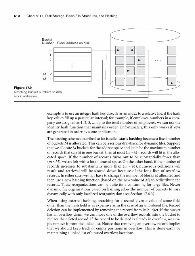
610 Chapter 17 Disk Storage, Basic File Structures, and Hashing
012
M – 2M – 1
Bucket Number Block address on disk
Figure 17.9Matching bucket numbers to diskblock addresses.
example is to use an integer hash key directly as an index to a relative file, if the hashkey values fill up a particular interval; for example, if employee numbers in a com-pany are assigned as 1, 2, 3, ... up to the total number of employees, we can use theidentity hash function that maintains order. Unfortunately, this only works if keysare generated in order by some application.
The hashing scheme described so far is called static hashing because a fixed numberof buckets M is allocated. This can be a serious drawback for dynamic files. Supposethat we allocate M buckets for the address space and let m be the maximum numberof records that can fit in one bucket; then at most (m * M) records will fit in the allo-cated space. If the number of records turns out to be substantially fewer than (m * M), we are left with a lot of unused space. On the other hand, if the number ofrecords increases to substantially more than (m * M), numerous collisions willresult and retrieval will be slowed down because of the long lists of overflowrecords. In either case, we may have to change the number of blocks M allocated andthen use a new hashing function (based on the new value of M) to redistribute therecords. These reorganizations can be quite time-consuming for large files. Newerdynamic file organizations based on hashing allow the number of buckets to varydynamically with only localized reorganization (see Section 17.8.3).
When using external hashing, searching for a record given a value of some fieldother than the hash field is as expensive as in the case of an unordered file. Recorddeletion can be implemented by removing the record from its bucket. If the buckethas an overflow chain, we can move one of the overflow records into the bucket toreplace the deleted record. If the record to be deleted is already in overflow, we sim-ply remove it from the linked list. Notice that removing an overflow record impliesthat we should keep track of empty positions in overflow. This is done easily bymaintaining a linked list of unused overflow locations.
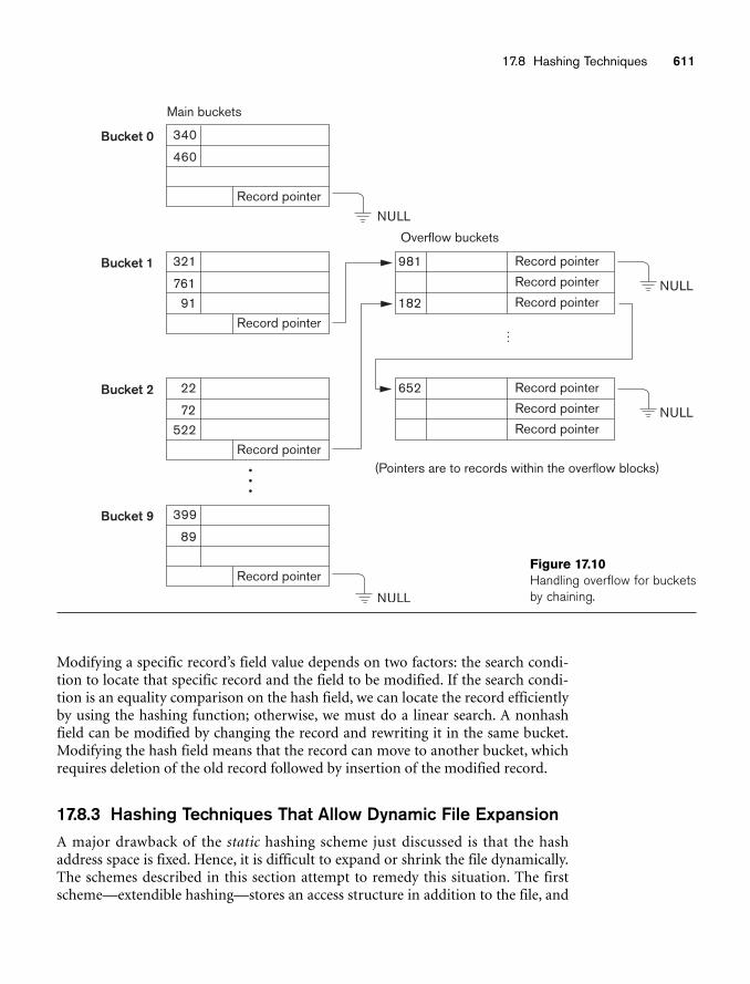
17.8 Hashing Techniques 611
Bucket 0
Main buckets
Overflow buckets
340
460
Record pointer
NULL
NULL
NULL
Bucket 1 321
76191
Record pointer
981
182
Record pointer
(Pointers are to records within the overflow blocks)
Record pointer
Record pointer
652 Record pointer
Record pointer
Record pointer
Bucket 2 22
72
522Record pointer
Bucket 9 399
89
Record pointer
NULL
...
Figure 17.10Handling overflow for bucketsby chaining.
Modifying a specific record’s field value depends on two factors: the search condi-tion to locate that specific record and the field to be modified. If the search condi-tion is an equality comparison on the hash field, we can locate the record efficientlyby using the hashing function; otherwise, we must do a linear search. A nonhashfield can be modified by changing the record and rewriting it in the same bucket.Modifying the hash field means that the record can move to another bucket, whichrequires deletion of the old record followed by insertion of the modified record.
17.8.3 Hashing Techniques That Allow Dynamic File ExpansionA major drawback of the static hashing scheme just discussed is that the hashaddress space is fixed. Hence, it is difficult to expand or shrink the file dynamically.The schemes described in this section attempt to remedy this situation. The firstscheme—extendible hashing—stores an access structure in addition to the file, and
612 Chapter 17 Disk Storage, Basic File Structures, and Hashing
hence is somewhat similar to indexing (see Chapter 18). The main difference is thatthe access structure is based on the values that result after application of the hashfunction to the search field. In indexing, the access structure is based on the valuesof the search field itself. The second technique, called linear hashing, does notrequire additional access structures. Another scheme, called dynamic hashing, usesan access structure based on binary tree data structures..
These hashing schemes take advantage of the fact that the result of applying a hash-ing function is a nonnegative integer and hence can be represented as a binary num-ber. The access structure is built on the binary representation of the hashingfunction result, which is a string of bits. We call this the hash value of a record.Records are distributed among buckets based on the values of the leading bits intheir hash values.
Extendible Hashing. In extendible hashing, a type of directory—an array of 2d
bucket addresses—is maintained, where d is called the global depth of the direc-tory. The integer value corresponding to the first (high-order) d bits of a hash valueis used as an index to the array to determine a directory entry, and the address inthat entry determines the bucket in which the corresponding records are stored.However, there does not have to be a distinct bucket for each of the 2d directorylocations. Several directory locations with the same first d� bits for their hash valuesmay contain the same bucket address if all the records that hash to these locations fitin a single bucket. A local depth d�—stored with each bucket—specifies the numberof bits on which the bucket contents are based. Figure 17.11 shows a directory withglobal depth d = 3.
The value of d can be increased or decreased by one at a time, thus doubling or halv-ing the number of entries in the directory array. Doubling is needed if a bucket,whose local depth d� is equal to the global depth d, overflows. Halving occurs if d >d� for all the buckets after some deletions occur. Most record retrievals require twoblock accesses—one to the directory and the other to the bucket.
To illustrate bucket splitting, suppose that a new inserted record causes overflow inthe bucket whose hash values start with 01—the third bucket in Figure 17.11. Therecords will be distributed between two buckets: the first contains all records whosehash values start with 010, and the second all those whose hash values start with011. Now the two directory locations for 010 and 011 point to the two new distinctbuckets. Before the split, they pointed to the same bucket. The local depth d� of thetwo new buckets is 3, which is one more than the local depth of the old bucket.
If a bucket that overflows and is split used to have a local depth d�equal to the globaldepth d of the directory, then the size of the directory must now be doubled so thatwe can use an extra bit to distinguish the two new buckets. For example, if thebucket for records whose hash values start with 111 in Figure 17.11 overflows, thetwo new buckets need a directory with global depth d = 4, because the two bucketsare now labeled 1110 and 1111, and hence their local depths are both 4. The direc-tory size is hence doubled, and each of the other original locations in the directory
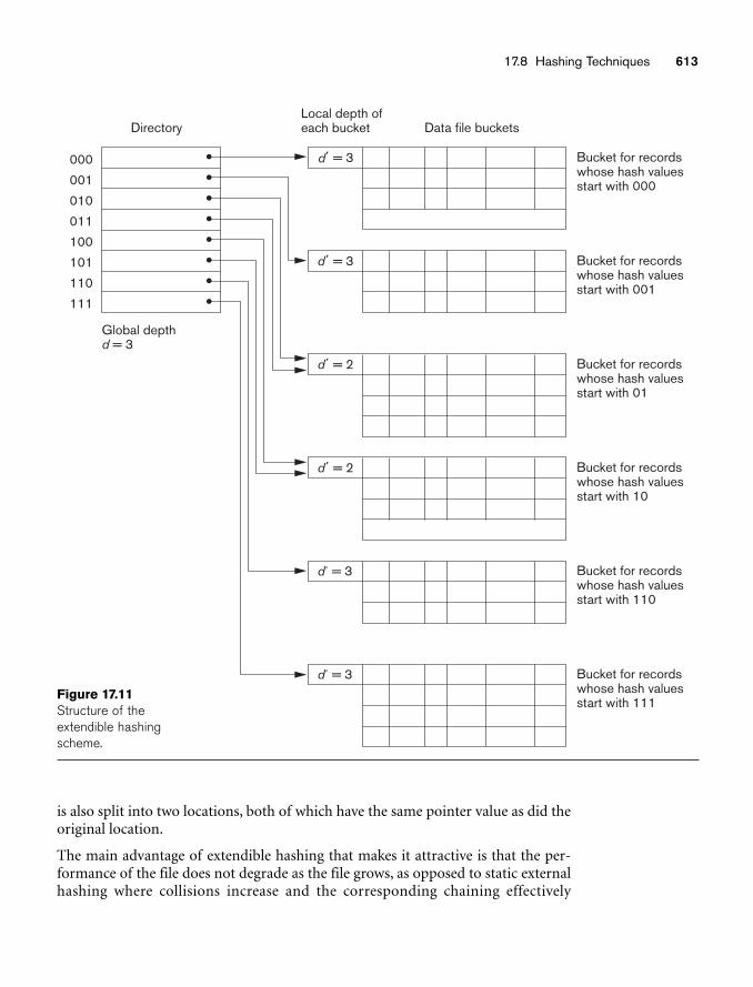
17.8 Hashing Techniques 613
Global depthd = 3
000
001
010
011
100
101
110
111
d´ = 3 Bucket for recordswhose hash values start with 000
Directory Data file bucketsLocal depth ofeach bucket
d´ = 3 Bucket for recordswhose hash values start with 001
d´ = 2 Bucket for recordswhose hash values start with 01
d´ = 2 Bucket for recordswhose hash values start with 10
d´ = 3 Bucket for recordswhose hash values start with 110
d´ = 3 Bucket for recordswhose hash values start with 111
Figure 17.11Structure of theextendible hashingscheme.
is also split into two locations, both of which have the same pointer value as did theoriginal location.
The main advantage of extendible hashing that makes it attractive is that the per-formance of the file does not degrade as the file grows, as opposed to static externalhashing where collisions increase and the corresponding chaining effectively
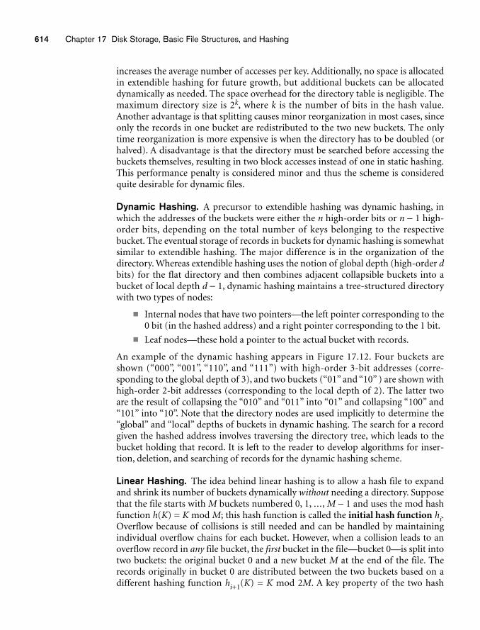
614 Chapter 17 Disk Storage, Basic File Structures, and Hashing
increases the average number of accesses per key. Additionally, no space is allocatedin extendible hashing for future growth, but additional buckets can be allocateddynamically as needed. The space overhead for the directory table is negligible. Themaximum directory size is 2k, where k is the number of bits in the hash value.Another advantage is that splitting causes minor reorganization in most cases, sinceonly the records in one bucket are redistributed to the two new buckets. The onlytime reorganization is more expensive is when the directory has to be doubled (orhalved). A disadvantage is that the directory must be searched before accessing thebuckets themselves, resulting in two block accesses instead of one in static hashing.This performance penalty is considered minor and thus the scheme is consideredquite desirable for dynamic files.
Dynamic Hashing. A precursor to extendible hashing was dynamic hashing, inwhich the addresses of the buckets were either the n high-order bits or n − 1 high-order bits, depending on the total number of keys belonging to the respectivebucket. The eventual storage of records in buckets for dynamic hashing is somewhatsimilar to extendible hashing. The major difference is in the organization of thedirectory. Whereas extendible hashing uses the notion of global depth (high-order dbits) for the flat directory and then combines adjacent collapsible buckets into abucket of local depth d − 1, dynamic hashing maintains a tree-structured directorywith two types of nodes:
■ Internal nodes that have two pointers—the left pointer corresponding to the0 bit (in the hashed address) and a right pointer corresponding to the 1 bit.
■ Leaf nodes—these hold a pointer to the actual bucket with records.
An example of the dynamic hashing appears in Figure 17.12. Four buckets areshown (“000”, “001”, “110”, and “111”) with high-order 3-bit addresses (corre-sponding to the global depth of 3), and two buckets (“01” and “10” ) are shown withhigh-order 2-bit addresses (corresponding to the local depth of 2). The latter twoare the result of collapsing the “010” and “011” into “01” and collapsing “100” and“101” into “10”. Note that the directory nodes are used implicitly to determine the“global” and “local” depths of buckets in dynamic hashing. The search for a recordgiven the hashed address involves traversing the directory tree, which leads to thebucket holding that record. It is left to the reader to develop algorithms for inser-tion, deletion, and searching of records for the dynamic hashing scheme.
Linear Hashing. The idea behind linear hashing is to allow a hash file to expandand shrink its number of buckets dynamically without needing a directory. Supposethat the file starts with M buckets numbered 0, 1, ..., M − 1 and uses the mod hashfunction h(K) = K mod M; this hash function is called the initial hash function hi.Overflow because of collisions is still needed and can be handled by maintainingindividual overflow chains for each bucket. However, when a collision leads to anoverflow record in any file bucket, the first bucket in the file—bucket 0—is split intotwo buckets: the original bucket 0 and a new bucket M at the end of the file. Therecords originally in bucket 0 are distributed between the two buckets based on adifferent hashing function hi+1(K) = K mod 2M. A key property of the two hash
17.8 Hashing Techniques 615
Data File Buckets
Bucket for recordswhose hash valuesstart with 000
Bucket for recordswhose hash valuesstart with 001
Bucket for recordswhose hash valuesstart with 01
Bucket for recordswhose hash valuesstart with 10
Bucket for recordswhose hash valuesstart with 110
Bucket for recordswhose hash valuesstart with 111
Directory0
1
0
1
0
1
0
1
0
1
internal directory node
leaf directory node
Figure 17.12Structure of the dynamic hashing scheme.
functions hi and hi+1 is that any records that hashed to bucket 0 based on hi will hashto either bucket 0 or bucket M based on hi+1; this is necessary for linear hashing towork.
As further collisions lead to overflow records, additional buckets are split in thelinear order 1, 2, 3, .... If enough overflows occur, all the original file buckets 0, 1, ...,M − 1 will have been split, so the file now has 2M instead of M buckets, and all buck-ets use the hash function hi+1. Hence, the records in overflow are eventually redis-tributed into regular buckets, using the function hi+1 via a delayed split of theirbuckets. There is no directory; only a value n—which is initially set to 0 and is incre-mented by 1 whenever a split occurs—is needed to determine which buckets havebeen split. To retrieve a record with hash key value K, first apply the function hi to K;if hi(K) < n, then apply the function hi+1 on K because the bucket is already split.Initially, n = 0, indicating that the function hi applies to all buckets; n grows linearlyas buckets are split.
616 Chapter 17 Disk Storage, Basic File Structures, and Hashing
When n = M after being incremented, this signifies that all the original buckets havebeen split and the hash function hi+1 applies to all records in the file. At this point, nis reset to 0 (zero), and any new collisions that cause overflow lead to the use of anew hashing function hi+2(K) = K mod 4M. In general, a sequence of hashing func-tions hi+j(K) = K mod (2jM) is used, where j = 0, 1, 2, ...; a new hashing functionhi+j+1 is needed whenever all the buckets 0, 1, ..., (2jM) − 1 have been split and n isreset to 0. The search for a record with hash key value K is given by Algorithm 17.3.
Splitting can be controlled by monitoring the file load factor instead of by splittingwhenever an overflow occurs. In general, the file load factor l can be defined as l =r/(bfr * N), where r is the current number of file records, bfr is the maximum num-ber of records that can fit in a bucket, and N is the current number of file buckets.Buckets that have been split can also be recombined if the load factor of the file fallsbelow a certain threshold. Blocks are combined linearly, and N is decrementedappropriately. The file load can be used to trigger both splits and combinations; inthis manner the file load can be kept within a desired range. Splits can be triggeredwhen the load exceeds a certain threshold—say, 0.9—and combinations can be trig-gered when the load falls below another threshold—say, 0.7. The main advantagesof linear hashing are that it maintains the load factor fairly constantly while the filegrows and shrinks, and it does not require a directory.10
Algorithm 17.3. The Search Procedure for Linear Hashing
if n = 0then m ← hj (K) (* m is the hash value of record with hash key K *)else begin
m ← hj (K);if m < n then m ← hj+1 (K)end;
search the bucket whose hash value is m (and its overflow, if any);
17.9 Other Primary File Organizations
17.9.1 Files of Mixed RecordsThe file organizations we have studied so far assume that all records of a particularfile are of the same record type. The records could be of EMPLOYEEs, PROJECTs,STUDENTs, or DEPARTMENTs, but each file contains records of only one type. Inmost database applications, we encounter situations in which numerous types ofentities are interrelated in various ways, as we saw in Chapter 7. Relationshipsamong records in various files can be represented by connecting fields.11 For exam-ple, a STUDENT record can have a connecting field Major_dept whose value gives the
10For details of insertion and deletion into Linear hashed files, refer to Litwin (1980) and Salzberg(1988).11The concept of foreign keys in the relational data model (Chapter 3) and references among objects inobject-oriented models (Chapter 11) are examples of connecting fields.
17.10 Parallelizing Disk Access Using RAID Technology 617
name of the DEPARTMENT in which the student is majoring. This Major_dept fieldrefers to a DEPARTMENT entity, which should be represented by a record of its ownin the DEPARTMENT file. If we want to retrieve field values from two related records,we must retrieve one of the records first. Then we can use its connecting field valueto retrieve the related record in the other file. Hence, relationships are implementedby logical field references among the records in distinct files.
File organizations in object DBMSs, as well as legacy systems such as hierarchicaland network DBMSs, often implement relationships among records as physicalrelationships realized by physical contiguity (or clustering) of related records or byphysical pointers. These file organizations typically assign an area of the disk tohold records of more than one type so that records of different types can bephysically clustered on disk. If a particular relationship is expected to be used fre-quently, implementing the relationship physically can increase the system’s effi-ciency at retrieving related records. For example, if the query to retrieve aDEPARTMENT record and all records for STUDENTs majoring in that department isfrequent, it would be desirable to place each DEPARTMENT record and its cluster ofSTUDENT records contiguously on disk in a mixed file. The concept of physicalclustering of object types is used in object DBMSs to store related objects togetherin a mixed file.
To distinguish the records in a mixed file, each record has—in addition to its fieldvalues—a record type field, which specifies the type of record. This is typically thefirst field in each record and is used by the system software to determine the type ofrecord it is about to process. Using the catalog information, the DBMS can deter-mine the fields of that record type and their sizes, in order to interpret the data val-ues in the record.
17.9.2 B-Trees and Other Data Structures as Primary Organization
Other data structures can be used for primary file organizations. For example, if boththe record size and the number of records in a file are small, some DBMSs offer theoption of a B-tree data structure as the primary file organization. We will describe B-trees in Section 18.3.1, when we discuss the use of the B-tree data structure for index-ing. In general, any data structure that can be adapted to the characteristics of diskdevices can be used as a primary file organization for record placement on disk.Recently, column-based storage of data has been proposed as a primary method forstorage of relations in relational databases. We will briefly introduce it in Chapter 18as a possible alternative storage scheme for relational databases.
17.10 Parallelizing Disk Access Using RAID Technology
With the exponential growth in the performance and capacity of semiconductordevices and memories, faster microprocessors with larger and larger primary mem-ories are continually becoming available. To match this growth, it is natural to
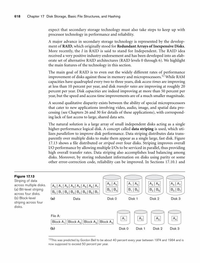
618 Chapter 17 Disk Storage, Basic File Structures, and Hashing
(a) Disk 0
A0 | A4
B0 | B4
Disk 1
A1 | A5
B1 | B5
Disk 2
A2 | A6
B2 | B6
Disk 3
A3 | A7
B3 | B7
Disk 0
A1
Disk 1
A2
Disk 2
A3
Disk 3
A4
A0 | A1 | A2 | A3 | A4 | A5 | A6 | A7
B0 | B1 | B2 | B3 | B4 | B5 | B6 | B7
Data
Block A1
File A:
(b)
Block A2 Block A3 Block A4
Figure 17.13Striping of dataacross multiple disks.(a) Bit-level stripingacross four disks. (b) Block-level striping across fourdisks.
expect that secondary storage technology must also take steps to keep up withprocessor technology in performance and reliability.
A major advance in secondary storage technology is represented by the develop-ment of RAID, which originally stood for Redundant Arrays of Inexpensive Disks.More recently, the I in RAID is said to stand for Independent. The RAID ideareceived a very positive industry endorsement and has been developed into an elab-orate set of alternative RAID architectures (RAID levels 0 through 6). We highlightthe main features of the technology in this section.
The main goal of RAID is to even out the widely different rates of performanceimprovement of disks against those in memory and microprocessors.12 While RAMcapacities have quadrupled every two to three years, disk access times are improvingat less than 10 percent per year, and disk transfer rates are improving at roughly 20percent per year. Disk capacities are indeed improving at more than 50 percent peryear, but the speed and access time improvements are of a much smaller magnitude.
A second qualitative disparity exists between the ability of special microprocessorsthat cater to new applications involving video, audio, image, and spatial data pro-cessing (see Chapters 26 and 30 for details of these applications), with correspond-ing lack of fast access to large, shared data sets.
The natural solution is a large array of small independent disks acting as a singlehigher-performance logical disk. A concept called data striping is used, which uti-lizes parallelism to improve disk performance. Data striping distributes data trans-parently over multiple disks to make them appear as a single large, fast disk. Figure17.13 shows a file distributed or striped over four disks. Striping improves overallI/O performance by allowing multiple I/Os to be serviced in parallel, thus providinghigh overall transfer rates. Data striping also accomplishes load balancing amongdisks. Moreover, by storing redundant information on disks using parity or someother error-correction code, reliability can be improved. In Sections 17.10.1 and
12This was predicted by Gordon Bell to be about 40 percent every year between 1974 and 1984 and isnow supposed to exceed 50 percent per year.
17.10 Parallelizing Disk Access Using RAID Technology 619
17.10.2, we discuss how RAID achieves the two important objectives of improvedreliability and higher performance. Section 17.10.3 discusses RAID organizationsand levels.
17.10.1 Improving Reliability with RAIDFor an array of n disks, the likelihood of failure is n times as much as that for onedisk. Hence, if the MTBF (Mean Time Between Failures) of a disk drive is assumed tobe 200,000 hours or about 22.8 years (for the disk drive in Table 17.1 called CheetahNS, it is 1.4 million hours), the MTBF for a bank of 100 disk drives becomes only2,000 hours or 83.3 days (for 1,000 Cheetah NS disks it would be 1,400 hours or58.33 days). Keeping a single copy of data in such an array of disks will cause a signif-icant loss of reliability. An obvious solution is to employ redundancy of data so thatdisk failures can be tolerated. The disadvantages are many: additional I/O operationsfor write, extra computation to maintain redundancy and to do recovery fromerrors, and additional disk capacity to store redundant information.
One technique for introducing redundancy is called mirroring or shadowing. Datais written redundantly to two identical physical disks that are treated as one logicaldisk. When data is read, it can be retrieved from the disk with shorter queuing, seek,and rotational delays. If a disk fails, the other disk is used until the first is repaired.Suppose the mean time to repair is 24 hours, then the mean time to data loss of amirrored disk system using 100 disks with MTBF of 200,000 hours each is(200,000)2/(2 * 24) = 8.33 * 108 hours, which is 95,028 years.13 Disk mirroring alsodoubles the rate at which read requests are handled, since a read can go to either disk.The transfer rate of each read, however, remains the same as that for a single disk.
Another solution to the problem of reliability is to store extra information that is notnormally needed but that can be used to reconstruct the lost information in case ofdisk failure. The incorporation of redundancy must consider two problems: selectinga technique for computing the redundant information, and selecting a method ofdistributing the redundant information across the disk array. The first problem isaddressed by using error-correcting codes involving parity bits, or specialized codessuch as Hamming codes. Under the parity scheme, a redundant disk may be consid-ered as having the sum of all the data in the other disks. When a disk fails, the miss-ing information can be constructed by a process similar to subtraction.
For the second problem, the two major approaches are either to store the redundantinformation on a small number of disks or to distribute it uniformly across all disks.The latter results in better load balancing. The different levels of RAID choose acombination of these options to implement redundancy and improve reliability.
17.10.2 Improving Performance with RAIDThe disk arrays employ the technique of data striping to achieve higher transfer rates.Note that data can be read or written only one block at a time, so a typical transfercontains 512 to 8192 bytes. Disk striping may be applied at a finer granularity by
13The formulas for MTBF calculations appear in Chen et al. (1994).
620 Chapter 17 Disk Storage, Basic File Structures, and Hashing
breaking up a byte of data into bits and spreading the bits to different disks. Thus,bit-level data striping consists of splitting a byte of data and writing bit j to the jthdisk. With 8-bit bytes, eight physical disks may be considered as one logical disk withan eightfold increase in the data transfer rate. Each disk participates in each I/Orequest and the total amount of data read per request is eight times as much. Bit-levelstriping can be generalized to a number of disks that is either a multiple or a factor ofeight. Thus, in a four-disk array, bit n goes to the disk which is (n mod 4). Figure17.13(a) shows bit-level striping of data.
The granularity of data interleaving can be higher than a bit; for example, blocks ofa file can be striped across disks, giving rise to block-level striping. Figure 17.13(b)shows block-level data striping assuming the data file contains four blocks. Withblock-level striping, multiple independent requests that access single blocks (smallrequests) can be serviced in parallel by separate disks, thus decreasing the queuingtime of I/O requests. Requests that access multiple blocks (large requests) can beparallelized, thus reducing their response time. In general, the more the number ofdisks in an array, the larger the potential performance benefit. However, assumingindependent failures, the disk array of 100 disks collectively has 1/100th the reliabil-ity of a single disk. Thus, redundancy via error-correcting codes and disk mirroringis necessary to provide reliability along with high performance.
17.10.3 RAID Organizations and LevelsDifferent RAID organizations were defined based on different combinations of thetwo factors of granularity of data interleaving (striping) and pattern used to com-pute redundant information. In the initial proposal, levels 1 through 5 of RAIDwere proposed, and two additional levels—0 and 6—were added later.
RAID level 0 uses data striping, has no redundant data, and hence has the best writeperformance since updates do not have to be duplicated. It splits data evenly acrosstwo or more disks. However, its read performance is not as good as RAID level 1,which uses mirrored disks. In the latter, performance improvement is possible byscheduling a read request to the disk with shortest expected seek and rotationaldelay. RAID level 2 uses memory-style redundancy by using Hamming codes, whichcontain parity bits for distinct overlapping subsets of components. Thus, in oneparticular version of this level, three redundant disks suffice for four original disks,whereas with mirroring—as in level 1—four would be required. Level 2 includesboth error detection and correction, although detection is generally not requiredbecause broken disks identify themselves.
RAID level 3 uses a single parity disk relying on the disk controller to figure outwhich disk has failed. Levels 4 and 5 use block-level data striping, with level 5 dis-tributing data and parity information across all disks. Figure 17.14(b) shows anillustration of RAID level 5, where parity is shown with subscript p. If one disk fails,the missing data is calculated based on the parity available from the remainingdisks. Finally, RAID level 6 applies the so-called P + Q redundancy scheme usingReed-Soloman codes to protect against up to two disk failures by using just tworedundant disks.
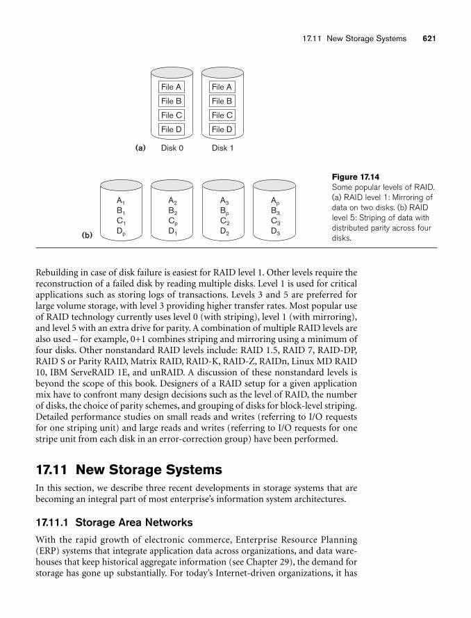
17.11 New Storage Systems 621
Disk 0 Disk 1
A1
B1
C1
Dp
A2
B2
Cp
D1
A3
Bp
C2
D2
Ap
B3
C3
D3
(a)
(b)
File A
File B
File C
File D
File A
File B
File C
File D
Figure 17.14Some popular levels of RAID.(a) RAID level 1: Mirroring ofdata on two disks. (b) RAIDlevel 5: Striping of data withdistributed parity across fourdisks.
Rebuilding in case of disk failure is easiest for RAID level 1. Other levels require thereconstruction of a failed disk by reading multiple disks. Level 1 is used for criticalapplications such as storing logs of transactions. Levels 3 and 5 are preferred forlarge volume storage, with level 3 providing higher transfer rates. Most popular useof RAID technology currently uses level 0 (with striping), level 1 (with mirroring),and level 5 with an extra drive for parity. A combination of multiple RAID levels arealso used – for example, 0+1 combines striping and mirroring using a minimum offour disks. Other nonstandard RAID levels include: RAID 1.5, RAID 7, RAID-DP,RAID S or Parity RAID, Matrix RAID, RAID-K, RAID-Z, RAIDn, Linux MD RAID10, IBM ServeRAID 1E, and unRAID. A discussion of these nonstandard levels isbeyond the scope of this book. Designers of a RAID setup for a given applicationmix have to confront many design decisions such as the level of RAID, the numberof disks, the choice of parity schemes, and grouping of disks for block-level striping.Detailed performance studies on small reads and writes (referring to I/O requestsfor one striping unit) and large reads and writes (referring to I/O requests for onestripe unit from each disk in an error-correction group) have been performed.
17.11 New Storage SystemsIn this section, we describe three recent developments in storage systems that arebecoming an integral part of most enterprise’s information system architectures.
17.11.1 Storage Area NetworksWith the rapid growth of electronic commerce, Enterprise Resource Planning(ERP) systems that integrate application data across organizations, and data ware-houses that keep historical aggregate information (see Chapter 29), the demand forstorage has gone up substantially. For today’s Internet-driven organizations, it has
622 Chapter 17 Disk Storage, Basic File Structures, and Hashing
become necessary to move from a static fixed data center-oriented operation to amore flexible and dynamic infrastructure for their information processing require-ments. The total cost of managing all data is growing so rapidly that in manyinstances the cost of managing server-attached storage exceeds the cost of the serveritself. Furthermore, the procurement cost of storage is only a small fraction—typi-cally, only 10 to 15 percent of the overall cost of storage management. Many users ofRAID systems cannot use the capacity effectively because it has to be attached in afixed manner to one or more servers. Therefore, most large organizations havemoved to a concept called storage area networks (SANs). In a SAN, online storageperipherals are configured as nodes on a high-speed network and can be attachedand detached from servers in a very flexible manner. Several companies haveemerged as SAN providers and supply their own proprietary topologies. They allowstorage systems to be placed at longer distances from the servers and provide differ-ent performance and connectivity options. Existing storage management applica-tions can be ported into SAN configurations using Fiber Channel networks thatencapsulate the legacy SCSI protocol. As a result, the SAN-attached devices appearas SCSI devices.
Current architectural alternatives for SAN include the following: point-to-pointconnections between servers and storage systems via fiber channel; use of a fiberchannel switch to connect multiple RAID systems, tape libraries, and so on toservers; and the use of fiber channel hubs and switches to connect servers and stor-age systems in different configurations. Organizations can slowly move up fromsimpler topologies to more complex ones by adding servers and storage devices asneeded. We do not provide further details here because they vary among SAN ven-dors. The main advantages claimed include:
■ Flexible many-to-many connectivity among servers and storage devicesusing fiber channel hubs and switches
■ Up to 10 km separation between a server and a storage system using appro-priate fiber optic cables
■ Better isolation capabilities allowing nondisruptive addition of new periph-erals and servers
SANs are growing very rapidly, but are still faced with many problems, such as com-bining storage options from multiple vendors and dealing with evolving standardsof storage management software and hardware. Most major companies are evaluat-ing SANs as a viable option for database storage.
17.11.2 Network-Attached StorageWith the phenomenal growth in digital data, particularly generated from multime-dia and other enterprise applications, the need for high-performance storage solu-tions at low cost has become extremely important. Network-attached storage(NAS) devices are among the storage devices being used for this purpose. Thesedevices are, in fact, servers that do not provide any of the common server services,but simply allow the addition of storage for file sharing. NAS devices allow vast
17.11 New Storage Systems 623
amounts of hard-disk storage space to be added to a network and can make thatspace available to multiple servers without shutting them down for maintenanceand upgrades. NAS devices can reside anywhere on a local area network (LAN) andmay be combined in different configurations. A single hardware device, often calledthe NAS box or NAS head, acts as the interface between the NAS system and net-work clients. These NAS devices require no monitor, keyboard, or mouse. One ormore disk or tape drives can be attached to many NAS systems to increase totalcapacity. Clients connect to the NAS head rather than to the individual storagedevices. An NAS can store any data that appears in the form of files, such as e-mailboxes, Web content, remote system backups, and so on. In that sense, NAS devicesare being deployed as a replacement for traditional file servers.
NAS systems strive for reliable operation and easy administration. They includebuilt-in features such as secure authentication, or the automatic sending of e-mailalerts in case of error on the device. The NAS devices (or appliances, as some ven-dors refer to them) are being offered with a high degree of scalability, reliability,flexibility, and performance. Such devices typically support RAID levels 0, 1, and 5.Traditional storage area networks (SANs) differ from NAS in several ways.Specifically, SANs often utilize Fiber Channel rather than Ethernet, and a SAN oftenincorporates multiple network devices or endpoints on a self-contained or privateLAN, whereas NAS relies on individual devices connected directly to the existingpublic LAN. Whereas Windows, UNIX, and NetWare file servers each demand spe-cific protocol support on the client side, NAS systems claim greater operating sys-tem independence of clients.
17.11.3 iSCSI Storage SystemsA new protocol called iSCSI (Internet SCSI) has been proposed recently. It allowsclients (called initiators) to send SCSI commands to SCSI storage devices on remotechannels. The main advantage of iSCSI is that it does not require the special cablingneeded by Fiber Channel and it can run over longer distances using existing networkinfrastructure. By carrying SCSI commands over IP networks, iSCSI facilitates datatransfers over intranets and manages storage over long distances. It can transfer dataover local area networks (LANs), wide area networks (WANs), or the Internet.
iSCSI works as follows. When a DBMS needs to access data, the operating systemgenerates the appropriate SCSI commands and data request, which then go throughencapsulation and, if necessary, encryption procedures. A packet header is addedbefore the resulting IP packets are transmitted over an Ethernet connection. When apacket is received, it is decrypted (if it was encrypted before transmission) and dis-assembled, separating the SCSI commands and request. The SCSI commands go viathe SCSI controller to the SCSI storage device. Because iSCSI is bidirectional, theprotocol can also be used to return data in response to the original request. Ciscoand IBM have marketed switches and routers based on this technology.
iSCSI storage has mainly impacted small- and medium-sized businesses because ofits combination of simplicity, low cost, and the functionality of iSCSI devices. Itallows them not to learn the ins and outs of Fiber Channel (FC) technology and
624 Chapter 17 Disk Storage, Basic File Structures, and Hashing
instead benefit from their familiarity with the IP protocol and Ethernet hardware.iSCSI implementations in the data centers of very large enterprise businesses areslow in development due to their prior investment in Fiber Channel-based SANs.
iSCSI is one of two main approaches to storage data transmission over IP networks.The other method, Fiber Channel over IP (FCIP), translates Fiber Channel controlcodes and data into IP packets for transmission between geographically distantFiber Channel storage area networks. This protocol, known also as Fiber Channeltunneling or storage tunneling, can only be used in conjunction with Fiber Channeltechnology, whereas iSCSI can run over existing Ethernet networks.
The latest idea to enter the enterprise IP storage race is Fiber Channel overEthernet (FCoE), which can be thought of as iSCSI without the IP. It uses many ele-ments of SCSI and FC (just like iSCSI), but it does not include TCP/IP components.This promises excellent performance, especially on 10 Gigabit Ethernet (10GbE),and is relatively easy for vendors to add to their products.
17.12 SummaryWe began this chapter by discussing the characteristics of memory hierarchies andthen concentrated on secondary storage devices. In particular, we focused on mag-netic disks because they are used most often to store online database files.
Data on disk is stored in blocks; accessing a disk block is expensive because of theseek time, rotational delay, and block transfer time. To reduce the average blockaccess time, double buffering can be used when accessing consecutive disk blocks.(Other disk parameters are discussed in Appendix B.) We presented different waysof storing file records on disk. File records are grouped into disk blocks and can befixed length or variable length, spanned or unspanned, and of the same record typeor mixed types. We discussed the file header, which describes the record formats andkeeps track of the disk addresses of the file blocks. Information in the file header isused by system software accessing the file records.
Then we presented a set of typical commands for accessing individual file recordsand discussed the concept of the current record of a file. We discussed how complexrecord search conditions are transformed into simple search conditions that areused to locate records in the file.
Three primary file organizations were then discussed: unordered, ordered, andhashed. Unordered files require a linear search to locate records, but record inser-tion is very simple. We discussed the deletion problem and the use of deletionmarkers.
Ordered files shorten the time required to read records in order of the ordering field.The time required to search for an arbitrary record, given the value of its orderingkey field, is also reduced if a binary search is used. However, maintaining the recordsin order makes insertion very expensive; thus the technique of using an unorderedoverflow file to reduce the cost of record insertion was discussed. Overflow recordsare merged with the master file periodically during file reorganization.
Review Questions 625
Hashing provides very fast access to an arbitrary record of a file, given the value ofits hash key. The most suitable method for external hashing is the bucket technique,with one or more contiguous blocks corresponding to each bucket. Collisions caus-ing bucket overflow are handled by chaining. Access on any nonhash field is slow,and so is ordered access of the records on any field. We discussed three hashing tech-niques for files that grow and shrink in the number of records dynamically:extendible, dynamic, and linear hashing. The first two use the higher-order bits ofthe hash address to organize a directory. Linear hashing is geared to keep the loadfactor of the file within a given range and adds new buckets linearly.
We briefly discussed other possibilities for primary file organizations, such as B-trees, and files of mixed records, which implement relationships among records ofdifferent types physically as part of the storage structure. We reviewed the recentadvances in disk technology represented by RAID (Redundant Arrays ofInexpensive (or Independent) Disks), which has become a standard technique inlarge enterprises to provide better reliability and fault tolerance features in storage.Finally, we reviewed three currently popular options in enterprise storage systems:storage area networks (SANs), network-attached storage (NAS), and iSCSI storagesystems.
Review Questions17.1. What is the difference between primary and secondary storage?
17.2. Why are disks, not tapes, used to store online database files?
17.3. Define the following terms: disk, disk pack, track, block, cylinder, sector,interblock gap, read/write head.
17.4. Discuss the process of disk initialization.
17.5. Discuss the mechanism used to read data from or write data to the disk.
17.6. What are the components of a disk block address?
17.7. Why is accessing a disk block expensive? Discuss the time componentsinvolved in accessing a disk block.
17.8. How does double buffering improve block access time?
17.9. What are the reasons for having variable-length records? What types of sep-arator characters are needed for each?
17.10. Discuss the techniques for allocating file blocks on disk.
17.11. What is the difference between a file organization and an access method?
17.12. What is the difference between static and dynamic files?
17.13. What are the typical record-at-a-time operations for accessing a file? Whichof these depend on the current file record?
17.14. Discuss the techniques for record deletion.
626 Chapter 17 Disk Storage, Basic File Structures, and Hashing
17.15. Discuss the advantages and disadvantages of using (a) an unordered file, (b)an ordered file, and (c) a static hash file with buckets and chaining. Whichoperations can be performed efficiently on each of these organizations, andwhich operations are expensive?
17.16. Discuss the techniques for allowing a hash file to expand and shrink dynam-ically. What are the advantages and disadvantages of each?
17.17. What is the difference between the directories of extendible and dynamichashing?
17.18. What are mixed files used for? What are other types of primary file organiza-tions?
17.19. Describe the mismatch between processor and disk technologies.
17.20. What are the main goals of the RAID technology? How does it achieve them?
17.21. How does disk mirroring help improve reliability? Give a quantitative example.
17.22. What characterizes the levels in RAID organization?
17.23. What are the highlights of the popular RAID levels 0, 1, and 5?
17.24. What are storage area networks? What flexibility and advantages do theyoffer?
17.25. Describe the main features of network-attached storage as an enterprisestorage solution.
17.26. How have new iSCSI systems improved the applicability of storage area net-works?
Exercises17.27. Consider a disk with the following characteristics (these are not parameters
of any particular disk unit): block size B = 512 bytes; interblock gap size G =128 bytes; number of blocks per track = 20; number of tracks per surface =400. A disk pack consists of 15 double-sided disks.
a. What is the total capacity of a track, and what is its useful capacity(excluding interblock gaps)?
b. How many cylinders are there?
c. What are the total capacity and the useful capacity of a cylinder?
d. What are the total capacity and the useful capacity of a disk pack?
e. Suppose that the disk drive rotates the disk pack at a speed of 2400 rpm(revolutions per minute); what are the transfer rate (tr) in bytes/msec andthe block transfer time (btt) in msec? What is the average rotational delay(rd) in msec? What is the bulk transfer rate? (See Appendix B.)
f. Suppose that the average seek time is 30 msec. How much time does ittake (on the average) in msec to locate and transfer a single block, givenits block address?
Exercises 627
g. Calculate the average time it would take to transfer 20 random blocks,and compare this with the time it would take to transfer 20 consecutiveblocks using double buffering to save seek time and rotational delay.
17.28. A file has r = 20,000 STUDENT records of fixed length. Each record has thefollowing fields: Name (30 bytes), Ssn (9 bytes), Address (40 bytes), PHONE(10 bytes), Birth_date (8 bytes), Sex (1 byte), Major_dept_code (4 bytes),Minor_dept_code (4 bytes), Class_code (4 bytes, integer), and Degree_program(3 bytes). An additional byte is used as a deletion marker. The file is stored onthe disk whose parameters are given in Exercise 17.27.
a. Calculate the record size R in bytes.
b. Calculate the blocking factor bfr and the number of file blocks b, assum-ing an unspanned organization.
c. Calculate the average time it takes to find a record by doing a linear searchon the file if (i) the file blocks are stored contiguously, and double buffer-ing is used; (ii) the file blocks are not stored contiguously.
d. Assume that the file is ordered by Ssn; by doing a binary search, calculatethe time it takes to search for a record given its Ssn value.
17.29. Suppose that only 80 percent of the STUDENT records from Exercise 17.28have a value for Phone, 85 percent for Major_dept_code, 15 percent forMinor_dept_code, and 90 percent for Degree_program; and suppose that weuse a variable-length record file. Each record has a 1-byte field type for eachfield in the record, plus the 1-byte deletion marker and a 1-byte end-of-record marker. Suppose that we use a spanned record organization, whereeach block has a 5-byte pointer to the next block (this space is not used forrecord storage).
a. Calculate the average record length R in bytes.
b. Calculate the number of blocks needed for the file.
17.30. Suppose that a disk unit has the following parameters: seek time s = 20 msec;rotational delay rd = 10 msec; block transfer time btt = 1 msec; block size B =2400 bytes; interblock gap size G = 600 bytes. An EMPLOYEE file has the fol-lowing fields: Ssn, 9 bytes; Last_name, 20 bytes; First_name, 20 bytes;Middle_init, 1 byte; Birth_date, 10 bytes; Address, 35 bytes; Phone, 12 bytes;Supervisor_ssn, 9 bytes; Department, 4 bytes; Job_code, 4 bytes; deletionmarker, 1 byte. The EMPLOYEE file has r = 30,000 records, fixed-length for-mat, and unspanned blocking. Write appropriate formulas and calculate thefollowing values for the above EMPLOYEE file:
a. The record size R (including the deletion marker), the blocking factor bfr,and the number of disk blocks b.
b. Calculate the wasted space in each disk block because of the unspannedorganization.
c. Calculate the transfer rate tr and the bulk transfer rate btr for this diskunit (see Appendix B for definitions of tr and btr).
628 Chapter 17 Disk Storage, Basic File Structures, and Hashing
d. Calculate the average number of block accesses needed to search for anarbitrary record in the file, using linear search.
e. Calculate in msec the average time needed to search for an arbitraryrecord in the file, using linear search, if the file blocks are stored on con-secutive disk blocks and double buffering is used.
f. Calculate in msec the average time needed to search for an arbitraryrecord in the file, using linear search, if the file blocks are not stored onconsecutive disk blocks.
g. Assume that the records are ordered via some key field. Calculate theaverage number of block accesses and the average time needed to search foran arbitrary record in the file, using binary search.
17.31. A PARTS file with Part# as the hash key includes records with the followingPart# values: 2369, 3760, 4692, 4871, 5659, 1821, 1074, 7115, 1620, 2428, 3943,4750, 6975, 4981, and 9208. The file uses eight buckets, numbered 0 to 7. Eachbucket is one disk block and holds two records. Load these records into thefile in the given order, using the hash function h(K) = K mod 8. Calculate theaverage number of block accesses for a random retrieval on Part#.
17.32. Load the records of Exercise 17.31 into expandable hash files based onextendible hashing. Show the structure of the directory at each step, and theglobal and local depths. Use the hash function h(K) = K mod 128.
17.33. Load the records of Exercise 17.31 into an expandable hash file, using linearhashing. Start with a single disk block, using the hash function h0 = K mod20, and show how the file grows and how the hash functions change as therecords are inserted. Assume that blocks are split whenever an overflowoccurs, and show the value of n at each stage.
17.34. Compare the file commands listed in Section 17.5 to those available on a fileaccess method you are familiar with.
17.35. Suppose that we have an unordered file of fixed-length records that uses anunspanned record organization. Outline algorithms for insertion, deletion,and modification of a file record. State any assumptions you make.
17.36. Suppose that we have an ordered file of fixed-length records and anunordered overflow file to handle insertion. Both files use unspannedrecords. Outline algorithms for insertion, deletion, and modification of a filerecord and for reorganizing the file. State any assumptions you make.
17.37. Can you think of techniques other than an unordered overflow file that canbe used to make insertions in an ordered file more efficient?
17.38. Suppose that we have a hash file of fixed-length records, and suppose thatoverflow is handled by chaining. Outline algorithms for insertion, deletion,and modification of a file record. State any assumptions you make.
Exercises 629
17.39. Can you think of techniques other than chaining to handle bucket overflowin external hashing?
17.40. Write pseudocode for the insertion algorithms for linear hashing and forextendible hashing.
17.41. Write program code to access individual fields of records under each of thefollowing circumstances. For each case, state the assumptions you make con-cerning pointers, separator characters, and so on. Determine the type ofinformation needed in the file header in order for your code to be general ineach case.
a. Fixed-length records with unspanned blocking
b. Fixed-length records with spanned blocking
c. Variable-length records with variable-length fields and spanned blocking
d. Variable-length records with repeating groups and spanned blocking
e. Variable-length records with optional fields and spanned blocking
f. Variable-length records that allow all three cases in parts c, d, and e
17.42. Suppose that a file initially contains r = 120,000 records of R = 200 byteseach in an unsorted (heap) file. The block size B = 2400 bytes, the averageseek time s = 16 ms, the average rotational latency rd = 8.3 ms, and the blocktransfer time btt = 0.8 ms. Assume that 1 record is deleted for every 2 recordsadded until the total number of active records is 240,000.
a. How many block transfers are needed to reorganize the file?
b. How long does it take to find a record right before reorganization?
c. How long does it take to find a record right after reorganization?
17.43. Suppose we have a sequential (ordered) file of 100,000 records where eachrecord is 240 bytes. Assume that B = 2400 bytes, s = 16 ms, rd = 8.3 ms, andbtt = 0.8 ms. Suppose we want to make X independent random record readsfrom the file. We could make X random block reads or we could perform oneexhaustive read of the entire file looking for those X records. The question isto decide when it would be more efficient to perform one exhaustive read ofthe entire file than to perform X individual random reads. That is, what isthe value for X when an exhaustive read of the file is more efficient than ran-dom X reads? Develop this as a function of X.
17.44. Suppose that a static hash file initially has 600 buckets in the primary areaand that records are inserted that create an overflow area of 600 buckets. Ifwe reorganize the hash file, we can assume that most of the overflow is elim-inated. If the cost of reorganizing the file is the cost of the bucket transfers(reading and writing all of the buckets) and the only periodic file operationis the fetch operation, then how many times would we have to perform afetch (successfully) to make the reorganization cost effective? That is, thereorganization cost and subsequent search cost are less than the search costbefore reorganization. Support your answer. Assume s = 16 ms, rd = 8.3 ms,and btt = 1 ms.
630 Chapter 17 Disk Storage, Basic File Structures, and Hashing
17.45. Suppose we want to create a linear hash file with a file load factor of 0.7 anda blocking factor of 20 records per bucket, which is to contain 112,000records initially.
a. How many buckets should we allocate in the primary area?
b. What should be the number of bits used for bucket addresses?
Selected BibliographyWiederhold (1987) has a detailed discussion and analysis of secondary storagedevices and file organizations as a part of database design. Optical disks aredescribed in Berg and Roth (1989) and analyzed in Ford and Christodoulakis(1991). Flash memory is discussed by Dipert and Levy (1993). Ruemmler andWilkes (1994) present a survey of the magnetic-disk technology. Most textbooks ondatabases include discussions of the material presented here. Most data structurestextbooks, including Knuth (1998), discuss static hashing in more detail; Knuth hasa complete discussion of hash functions and collision resolution techniques, as wellas of their performance comparison. Knuth also offers a detailed discussion of tech-niques for sorting external files. Textbooks on file structures include Claybrook(1992), Smith and Barnes (1987), and Salzberg (1988); they discuss additional fileorganizations including tree-structured files, and have detailed algorithms for oper-ations on files. Salzberg et al. (1990) describe a distributed external sorting algo-rithm. File organizations with a high degree of fault tolerance are described byBitton and Gray (1988) and by Gray et al. (1990). Disk striping was proposed inSalem and Garcia Molina (1986). The first paper on redundant arrays of inexpen-sive disks (RAID) is by Patterson et al. (1988). Chen and Patterson (1990) and theexcellent survey of RAID by Chen et al. (1994) are additional references.Grochowski and Hoyt (1996) discuss future trends in disk drives. Various formulasfor the RAID architecture appear in Chen et al. (1994).
Morris (1968) is an early paper on hashing. Extendible hashing is described in Faginet al. (1979). Linear hashing is described by Litwin (1980). Algorithms for insertionand deletion for linear hashing are discussed with illustrations in Salzberg (1988).Dynamic hashing, which we briefly introduced, was proposed by Larson (1978).There are many proposed variations for extendible and linear hashing; for exam-ples, see Cesarini and Soda (1991), Du and Tong (1991), and Hachem and Berra(1992).
Details of disk storage devices can be found at manufacturer sites (for example,http://www.seagate.com, http://www.ibm.com, http://www.emc.com, http://www.hp.com, http://www.storagetek.com,. IBM has a storage technology research centerat IBM Almaden (http://www.almaden.ibm.com/).
631
Indexing Structures for Files
In this chapter we assume that a file already exists withsome primary organization such as the unordered,
ordered, or hashed organizations that were described in Chapter 17. We willdescribe additional auxiliary access structures called indexes, which are used tospeed up the retrieval of records in response to certain search conditions. The indexstructures are additional files on disk that provide secondary access paths, whichprovide alternative ways to access the records without affecting the physical place-ment of records in the primary data file on disk. They enable efficient access torecords based on the indexing fields that are used to construct the index. Basically,any field of the file can be used to create an index, and multiple indexes on differentfields—as well as indexes on multiple fields—can be constructed on the same file. Avariety of indexes are possible; each of them uses a particular data structure to speedup the search. To find a record or records in the data file based on a search conditionon an indexing field, the index is searched, which leads to pointers to one or moredisk blocks in the data file where the required records are located. The most preva-lent types of indexes are based on ordered files (single-level indexes) and tree datastructures (multilevel indexes, B+-trees). Indexes can also be constructed based onhashing or other search data structures. We also discuss indexes that are vectors ofbits called bitmap indexes.
We describe different types of single-level ordered indexes—primary, secondary,and clustering—in Section 18.1. By viewing a single-level index as an ordered file,one can develop additional indexes for it, giving rise to the concept of multilevelindexes. A popular indexing scheme called ISAM (Indexed Sequential AccessMethod) is based on this idea. We discuss multilevel tree-structured indexes inSection 18.2. In Section 18.3 we describe B-trees and B+-trees, which are data struc-tures that are commonly used in DBMSs to implement dynamically changing mul-tilevel indexes. B+-trees have become a commonly accepted default structure for
18chapter 18
632 Chapter 18 Indexing Structures for Files
generating indexes on demand in most relational DBMSs. Section 18.4 is devoted toalternative ways to access data based on a combination of multiple keys. In Section18.5 we discuss hash indexes and introduce the concept of logical indexes, whichgive an additional level of indirection from physical indexes, allowing for the physi-cal index to be flexible and extensible in its organization. In Section 18.6 we discussmultikey indexing and bitmap indexes used for searching on one or more keys.Section 18.7 summarizes the chapter.
18.1 Types of Single-Level Ordered IndexesThe idea behind an ordered index is similar to that behind the index used in a text-book, which lists important terms at the end of the book in alphabetical order alongwith a list of page numbers where the term appears in the book. We can search thebook index for a certain term in the textbook to find a list of addresses—page num-bers in this case—and use these addresses to locate the specified pages first and thensearch for the term on each specified page. The alternative, if no other guidance isgiven, would be to sift slowly through the whole textbook word by word to find theterm we are interested in; this corresponds to doing a linear search, which scans thewhole file. Of course, most books do have additional information, such as chapterand section titles, which help us find a term without having to search through thewhole book. However, the index is the only exact indication of the pages where eachterm occurs in the book.
For a file with a given record structure consisting of several fields (or attributes), anindex access structure is usually defined on a single field of a file, called an indexingfield (or indexing attribute).1 The index typically stores each value of the indexfield along with a list of pointers to all disk blocks that contain records with thatfield value. The values in the index are ordered so that we can do a binary search onthe index. If both the data file and the index file are ordered, and since the index fileis typically much smaller than the data file, searching the index using a binarysearch is a better option. Tree-structured multilevel indexes (see Section 18.2)implement an extension of the binary search idea that reduces the search space by 2-way partitioning at each search step, thereby creating a more efficient approach thatdivides the search space in the file n-ways at each stage.
There are several types of ordered indexes. A primary index is specified on theordering key field of an ordered file of records. Recall from Section 17.7 that anordering key field is used to physically order the file records on disk, and every recordhas a unique value for that field. If the ordering field is not a key field—that is, ifnumerous records in the file can have the same value for the ordering field—another type of index, called a clustering index, can be used. The data file is called aclustered file in this latter case. Notice that a file can have at most one physicalordering field, so it can have at most one primary index or one clustering index, butnot both. A third type of index, called a secondary index, can be specified on any
1We use the terms field and attribute interchangeably in this chapter.
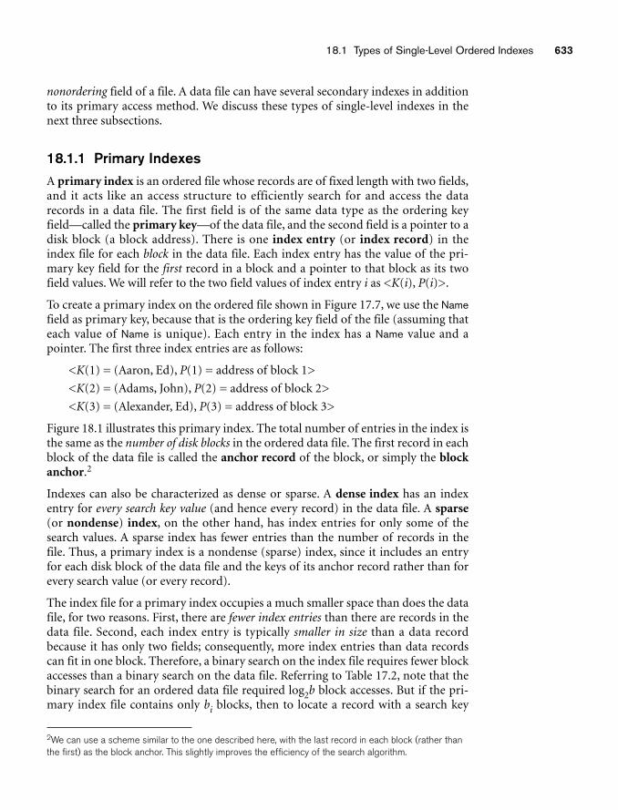
18.1 Types of Single-Level Ordered Indexes 633
nonordering field of a file. A data file can have several secondary indexes in additionto its primary access method. We discuss these types of single-level indexes in thenext three subsections.
18.1.1 Primary IndexesA primary index is an ordered file whose records are of fixed length with two fields,and it acts like an access structure to efficiently search for and access the datarecords in a data file. The first field is of the same data type as the ordering keyfield—called the primary key—of the data file, and the second field is a pointer to adisk block (a block address). There is one index entry (or index record) in theindex file for each block in the data file. Each index entry has the value of the pri-mary key field for the first record in a block and a pointer to that block as its twofield values. We will refer to the two field values of index entry i as <K(i), P(i)>.
To create a primary index on the ordered file shown in Figure 17.7, we use the Namefield as primary key, because that is the ordering key field of the file (assuming thateach value of Name is unique). Each entry in the index has a Name value and apointer. The first three index entries are as follows:
<K(1) = (Aaron, Ed), P(1) = address of block 1>
<K(2) = (Adams, John), P(2) = address of block 2>
<K(3) = (Alexander, Ed), P(3) = address of block 3>
Figure 18.1 illustrates this primary index. The total number of entries in the index isthe same as the number of disk blocks in the ordered data file. The first record in eachblock of the data file is called the anchor record of the block, or simply the blockanchor.2
Indexes can also be characterized as dense or sparse. A dense index has an indexentry for every search key value (and hence every record) in the data file. A sparse(or nondense) index, on the other hand, has index entries for only some of thesearch values. A sparse index has fewer entries than the number of records in thefile. Thus, a primary index is a nondense (sparse) index, since it includes an entryfor each disk block of the data file and the keys of its anchor record rather than forevery search value (or every record).
The index file for a primary index occupies a much smaller space than does the datafile, for two reasons. First, there are fewer index entries than there are records in thedata file. Second, each index entry is typically smaller in size than a data recordbecause it has only two fields; consequently, more index entries than data recordscan fit in one block. Therefore, a binary search on the index file requires fewer blockaccesses than a binary search on the data file. Referring to Table 17.2, note that thebinary search for an ordered data file required log2b block accesses. But if the pri-mary index file contains only bi blocks, then to locate a record with a search key
2We can use a scheme similar to the one described here, with the last record in each block (rather thanthe first) as the block anchor. This slightly improves the efficiency of the search algorithm.
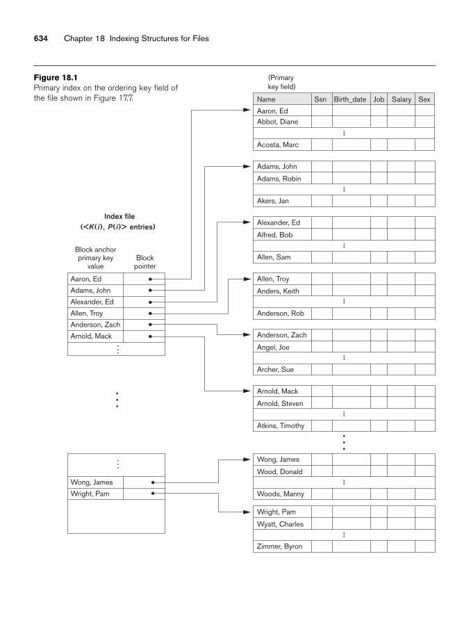
634 Chapter 18 Indexing Structures for Files
Index file(<K(i), P( i)> entries)
Block anchorprimary key
valueBlock
pointer
(Primarykey field)
Name
Aaron, EdAbbot, Diane
...
...
...
...
...
Acosta, Marc
Adams, John
Adams, Robin
Akers, Jan
Alexander, Ed
Alfred, Bob
Allen, Sam
Allen, Troy
Anders, Keith
Anderson, Rob
Anderson, Zach
Angel, Joe
Archer, Sue
Arnold, Mack
Arnold, Steven
Atkins, Timothy
Wong, James
Wood, Donald
Woods, Manny
Wright, Pam
Wyatt, Charles
Zimmer, Byron
Aaron, Ed
Adams, John
Alexander, Ed
Allen, Troy
Anderson, Zach
Arnold, Mack
Wong, James
Wright, Pam
...
...
...
. . .
. . .
Ssn Birth_date Job Salary Sex
Figure 18.1Primary index on the ordering key field ofthe file shown in Figure 17.7.
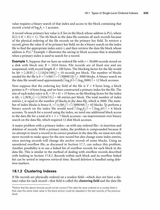
18.1 Types of Single-Level Ordered Indexes 635
value requires a binary search of that index and access to the block containing thatrecord: a total of log2bi + 1 accesses.
A record whose primary key value is K lies in the block whose address is P(i), whereK(i) ≤ K < K(i + 1). The ith block in the data file contains all such records becauseof the physical ordering of the file records on the primary key field. To retrieve arecord, given the value K of its primary key field, we do a binary search on the indexfile to find the appropriate index entry i, and then retrieve the data file block whoseaddress is P(i).3 Example 1 illustrates the saving in block accesses that is attainablewhen a primary index is used to search for a record.
Example 1. Suppose that we have an ordered file with r = 30,000 records stored ona disk with block size B = 1024 bytes. File records are of fixed size and areunspanned, with record length R = 100 bytes. The blocking factor for the file wouldbe bfr = ⎣(B/R)⎦ = ⎣(1024/100)⎦ = 10 records per block. The number of blocksneeded for the file is b = ⎡(r/bfr)⎤ = ⎡(30000/10)⎤ = 3000 blocks. A binary search onthe data file would need approximately ⎡log2b⎤= ⎡(log23000)⎤ = 12 block accesses.
Now suppose that the ordering key field of the file is V = 9 bytes long, a blockpointer is P = 6 bytes long, and we have constructed a primary index for the file. Thesize of each index entry is Ri = (9 + 6) = 15 bytes, so the blocking factor for the indexis bfri = ⎣(B/Ri)⎦ = ⎣(1024/15)⎦ = 68 entries per block. The total number of indexentries ri is equal to the number of blocks in the data file, which is 3000. The num-ber of index blocks is hence bi = ⎡(ri/bfri)⎤ = ⎡(3000/68)⎤ = 45 blocks. To perform abinary search on the index file would need ⎡(log2bi)⎤ = ⎡(log245)⎤ = 6 blockaccesses. To search for a record using the index, we need one additional block accessto the data file for a total of 6 + 1 = 7 block accesses—an improvement over binarysearch on the data file, which required 12 disk block accesses.
A major problem with a primary index—as with any ordered file—is insertion anddeletion of records. With a primary index, the problem is compounded because ifwe attempt to insert a record in its correct position in the data file, we must not onlymove records to make space for the new record but also change some index entries,since moving records will change the anchor records of some blocks. Using anunordered overflow file, as discussed in Section 17.7, can reduce this problem.Another possibility is to use a linked list of overflow records for each block in thedata file. This is similar to the method of dealing with overflow records describedwith hashing in Section 17.8.2. Records within each block and its overflow linkedlist can be sorted to improve retrieval time. Record deletion is handled using dele-tion markers.
18.1.2 Clustering IndexesIf file records are physically ordered on a nonkey field—which does not have a dis-tinct value for each record—that field is called the clustering field and the data file
3Notice that the above formula would not be correct if the data file were ordered on a nonkey field; inthat case the same index value in the block anchor could be repeated in the last records of the previousblock.
636 Chapter 18 Indexing Structures for Files
is called a clustered file. We can create a different type of index, called a clusteringindex, to speed up retrieval of all the records that have the same value for the clus-tering field. This differs from a primary index, which requires that the ordering fieldof the data file have a distinct value for each record.
A clustering index is also an ordered file with two fields; the first field is of the sametype as the clustering field of the data file, and the second field is a disk blockpointer. There is one entry in the clustering index for each distinct value of the clus-tering field, and it contains the value and a pointer to the first block in the data filethat has a record with that value for its clustering field. Figure 18.2 shows an exam-ple. Notice that record insertion and deletion still cause problems because the datarecords are physically ordered. To alleviate the problem of insertion, it is common toreserve a whole block (or a cluster of contiguous blocks) for each value of the clus-tering field; all records with that value are placed in the block (or block cluster). Thismakes insertion and deletion relatively straightforward. Figure 18.3 shows thisscheme.
A clustering index is another example of a nondense index because it has an entryfor every distinct value of the indexing field, which is a nonkey by definition andhence has duplicate values rather than a unique value for every record in the file.There is some similarity between Figures 18.1, 18.2, and 18.3 and Figures 17.11 and17.12. An index is somewhat similar to dynamic hashing (described in Section17.8.3) and to the directory structures used for extendible hashing. Both aresearched to find a pointer to the data block containing the desired record. A maindifference is that an index search uses the values of the search field itself, whereas ahash directory search uses the binary hash value that is calculated by applying thehash function to the search field.
18.1.3 Secondary IndexesA secondary index provides a secondary means of accessing a data file for whichsome primary access already exists. The data file records could be ordered,unordered, or hashed. The secondary index may be created on a field that is a can-didate key and has a unique value in every record, or on a nonkey field with dupli-cate values. The index is again an ordered file with two fields. The first field is of thesame data type as some nonordering field of the data file that is an indexing field.The second field is either a block pointer or a record pointer. Many secondaryindexes (and hence, indexing fields) can be created for the same file—each repre-sents an additional means of accessing that file based on some specific field.
First we consider a secondary index access structure on a key (unique) field that hasa distinct value for every record. Such a field is sometimes called a secondary key; inthe relational model, this would correspond to any UNIQUE key attribute or to theprimary key attribute of a table. In this case there is one index entry for each recordin the data file, which contains the value of the field for the record and a pointereither to the block in which the record is stored or to the record itself. Hence, suchan index is dense.
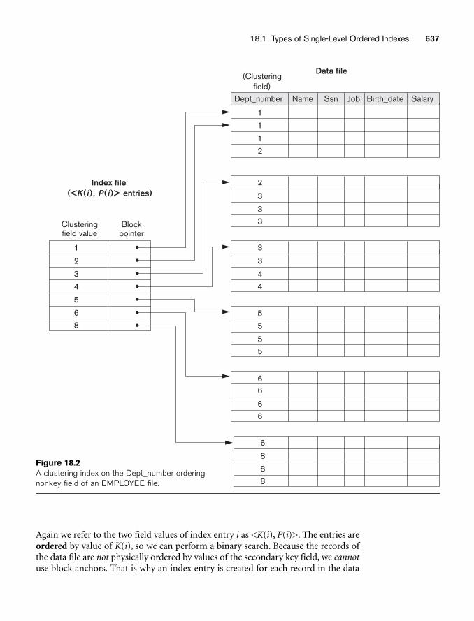
18.1 Types of Single-Level Ordered Indexes 637
Data file(Clustering
field)Dept_number
1
1
12
Name Ssn Birth_date SalaryJob
2
3
33
3
3
44
5
5
55
66
66
6
8
88
1
2
3
4
5
68
Index file(<K(i), P( i)> entries)
Clusteringfield value
Blockpointer
Figure 18.2A clustering index on the Dept_number orderingnonkey field of an EMPLOYEE file.
Again we refer to the two field values of index entry i as <K(i), P(i)>. The entries areordered by value of K(i), so we can perform a binary search. Because the records ofthe data file are not physically ordered by values of the secondary key field, we cannotuse block anchors. That is why an index entry is created for each record in the data
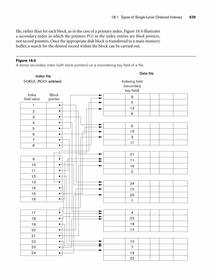
18.1 Types of Single-Level Ordered Indexes 639
Data file
Indexing field(secondarykey field)
615
3
17
95
138
21
11
162
24
10
201
4
23
1814
12
7
1922
1
2
3
4
5
6
7
8
9
10
11
12
13
14
1516
17
18
19
20
21
2223
24
Index file(<K(i), P( i)> entries)
Indexfield value
Blockpointer
Figure 18.4A dense secondary index (with block pointers) on a nonordering key field of a file.
file, rather than for each block, as in the case of a primary index. Figure 18.4 illustratesa secondary index in which the pointers P(i) in the index entries are block pointers,not record pointers. Once the appropriate disk block is transferred to a main memorybuffer, a search for the desired record within the block can be carried out.
640 Chapter 18 Indexing Structures for Files
A secondary index usually needs more storage space and longer search time thandoes a primary index, because of its larger number of entries. However, theimprovement in search time for an arbitrary record is much greater for a secondaryindex than for a primary index, since we would have to do a linear search on the datafile if the secondary index did not exist. For a primary index, we could still use abinary search on the main file, even if the index did not exist. Example 2 illustratesthe improvement in number of blocks accessed.
Example 2. Consider the file of Example 1 with r = 30,000 fixed-length records ofsize R = 100 bytes stored on a disk with block size B = 1024 bytes. The file has b =3000 blocks, as calculated in Example 1. Suppose we want to search for a record witha specific value for the secondary key—a nonordering key field of the file that is V =9 bytes long. Without the secondary index, to do a linear search on the file wouldrequire b/2 = 3000/2 = 1500 block accesses on the average. Suppose that we con-struct a secondary index on that nonordering key field of the file. As in Example 1, ablock pointer is P = 6 bytes long, so each index entry is Ri = (9 + 6) = 15 bytes, andthe blocking factor for the index is bfri = ⎣(B/Ri)⎦ = ⎣(1024/15)⎦ = 68 entries perblock. In a dense secondary index such as this, the total number of index entries ri isequal to the number of records in the data file, which is 30,000. The number of blocksneeded for the index is hence bi = ⎡(ri /bfri)⎤ = ⎡(3000/68)⎤ = 442 blocks.
A binary search on this secondary index needs ⎡(log2bi)⎤ = ⎡(log2442)⎤ = 9 blockaccesses. To search for a record using the index, we need an additional block accessto the data file for a total of 9 + 1 = 10 block accesses—a vast improvement over the1500 block accesses needed on the average for a linear search, but slightly worse thanthe 7 block accesses required for the primary index. This difference arose becausethe primary index was nondense and hence shorter, with only 45 blocks in length.
We can also create a secondary index on a nonkey, nonordering field of a file. In thiscase, numerous records in the data file can have the same value for the indexingfield. There are several options for implementing such an index:
■ Option 1 is to include duplicate index entries with the same K(i) value—onefor each record. This would be a dense index.
■ Option 2 is to have variable-length records for the index entries, with arepeating field for the pointer. We keep a list of pointers <P(i, 1), ..., P(i, k)>in the index entry for K(i)—one pointer to each block that contains a recordwhose indexing field value equals K(i). In either option 1 or option 2, thebinary search algorithm on the index must be modified appropriately toaccount for a variable number of index entries per index key value.
■ Option 3, which is more commonly used, is to keep the index entries them-selves at a fixed length and have a single entry for each index field value, butto create an extra level of indirection to handle the multiple pointers. In thisnondense scheme, the pointer P(i) in index entry <K(i), P(i)> points to adisk block, which contains a set of record pointers; each record pointer in thatdisk block points to one of the data file records with value K(i) for the index-ing field. If some value K(i) occurs in too many records, so that their recordpointers cannot fit in a single disk block, a cluster or linked list of blocks is
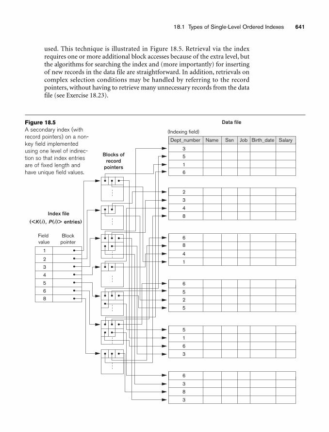
18.1 Types of Single-Level Ordered Indexes 641
Data file
(Indexing field)
Dept_number
3
5
16
Name Ssn Birth_date SalaryJob
2
3
4
8
68
4
1
6
5
2
5
5
1
6
3
6
3
8
3
1
2
3
4
5
68
Blocks ofrecord
pointers
Index file
(<K(i), P(i)> entries)
Fieldvalue
Blockpointer
Figure 18.5A secondary index (withrecord pointers) on a non-key field implementedusing one level of indirec-tion so that index entriesare of fixed length andhave unique field values.
used. This technique is illustrated in Figure 18.5. Retrieval via the indexrequires one or more additional block accesses because of the extra level, butthe algorithms for searching the index and (more importantly) for insertingof new records in the data file are straightforward. In addition, retrievals oncomplex selection conditions may be handled by referring to the recordpointers, without having to retrieve many unnecessary records from the datafile (see Exercise 18.23).
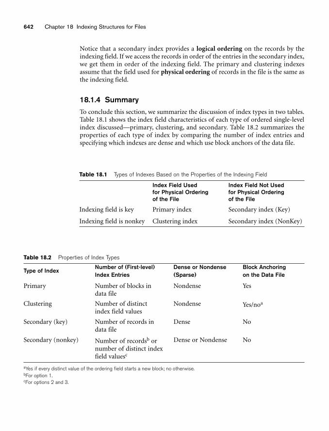
642 Chapter 18 Indexing Structures for Files
Notice that a secondary index provides a logical ordering on the records by theindexing field. If we access the records in order of the entries in the secondary index,we get them in order of the indexing field. The primary and clustering indexesassume that the field used for physical ordering of records in the file is the same asthe indexing field.
18.1.4 SummaryTo conclude this section, we summarize the discussion of index types in two tables.Table 18.1 shows the index field characteristics of each type of ordered single-levelindex discussed—primary, clustering, and secondary. Table 18.2 summarizes theproperties of each type of index by comparing the number of index entries andspecifying which indexes are dense and which use block anchors of the data file.
Table 18.1 Types of Indexes Based on the Properties of the Indexing Field
Index Field Used for Physical Ordering of the File
Index Field Not Used for Physical Ordering of the File
Indexing field is key Primary index Secondary index (Key)
Indexing field is nonkey Clustering index Secondary index (NonKey)
Table 18.2 Properties of Index Types
Type of IndexNumber of (First-level) Index Entries
Dense or Nondense(Sparse)
Block Anchoring on the Data File
Primary Number of blocks in data file
Nondense Yes
Clustering Number of distinct index field values
Nondense Yes/noa
Secondary (key) Number of records in data file
Dense No
Secondary (nonkey) Number of recordsb ornumber of distinct indexfield valuesc
Dense or Nondense No
aYes if every distinct value of the ordering field starts a new block; no otherwise.bFor option 1.cFor options 2 and 3.
18.2 Multilevel Indexes 643
18.2 Multilevel IndexesThe indexing schemes we have described thus far involve an ordered index file. Abinary search is applied to the index to locate pointers to a disk block or to a record(or records) in the file having a specific index field value. A binary search requiresapproximately (log2bi) block accesses for an index with bi blocks because each stepof the algorithm reduces the part of the index file that we continue to search by afactor of 2. This is why we take the log function to the base 2. The idea behind amultilevel index is to reduce the part of the index that we continue to search by bfri,the blocking factor for the index, which is larger than 2. Hence, the search space isreduced much faster. The value bfri is called the fan-out of the multilevel index, andwe will refer to it by the symbol fo. Whereas we divide the record search space intotwo halves at each step during a binary search, we divide it n-ways (where n = thefan-out) at each search step using the multilevel index. Searching a multilevel indexrequires approximately (logfobi) block accesses, which is a substantially smallernumber than for a binary search if the fan-out is larger than 2. In most cases, thefan-out is much larger than 2.
A multilevel index considers the index file, which we will now refer to as the first (orbase) level of a multilevel index, as an ordered file with a distinct value for each K(i).Therefore, by considering the first-level index file as a sorted data file, we can createa primary index for the first level; this index to the first level is called the secondlevel of the multilevel index. Because the second level is a primary index, we can useblock anchors so that the second level has one entry for each block of the first level.The blocking factor bfri for the second level—and for all subsequent levels—is thesame as that for the first-level index because all index entries are the same size; eachhas one field value and one block address. If the first level has r1 entries, and theblocking factor—which is also the fan-out—for the index is bfri = fo, then the firstlevel needs ⎡(r1/fo)⎤ blocks, which is therefore the number of entries r2 needed at thesecond level of the index.
We can repeat this process for the second level. The third level, which is a primaryindex for the second level, has an entry for each second-level block, so the numberof third-level entries is r3 = ⎡(r2/fo)⎤. Notice that we require a second level only if thefirst level needs more than one block of disk storage, and, similarly, we require athird level only if the second level needs more than one block. We can repeat thepreceding process until all the entries of some index level t fit in a single block. Thisblock at the tth level is called the top index level.4 Each level reduces the number ofentries at the previous level by a factor of fo—the index fan-out—so we can use theformula 1 ≤ (r1/((fo)t)) to calculate t. Hence, a multilevel index with r1 first-levelentries will have approximately t levels, where t = ⎡(logfo(r1))⎤. When searching the
4The numbering scheme for index levels used here is the reverse of the way levels are commonlydefined for tree data structures. In tree data structures, t is referred to as level 0 (zero), t – 1 is level 1,and so on.
644 Chapter 18 Indexing Structures for Files
index, a single disk block is retrieved at each level. Hence, t disk blocks are accessedfor an index search, where t is the number of index levels.
The multilevel scheme described here can be used on any type of index—whether itis primary, clustering, or secondary—as long as the first-level index has distinct val-ues for K(i) and fixed-length entries. Figure 18.6 shows a multilevel index built over aprimary index. Example 3 illustrates the improvement in number of blocks accessedwhen a multilevel index is used to search for a record.
Example 3. Suppose that the dense secondary index of Example 2 is converted intoa multilevel index. We calculated the index blocking factor bfri = 68 index entriesper block, which is also the fan-out fo for the multilevel index; the number of first-level blocks b1 = 442 blocks was also calculated. The number of second-level blockswill be b2 = ⎡(b1/fo)⎤ = ⎡(442/68)⎤ = 7 blocks, and the number of third-level blockswill be b3 = ⎡(b2/fo)⎤ = ⎡(7/68)⎤ = 1 block. Hence, the third level is the top level ofthe index, and t = 3. To access a record by searching the multilevel index, we mustaccess one block at each level plus one block from the data file, so we need t + 1 = 3+ 1 = 4 block accesses. Compare this to Example 2, where 10 block accesses wereneeded when a single-level index and binary search were used.
Notice that we could also have a multilevel primary index, which would be non-dense. Exercise 18.18(c) illustrates this case, where we must access the data blockfrom the file before we can determine whether the record being searched for is inthe file. For a dense index, this can be determined by accessing the first index level(without having to access a data block), since there is an index entry for every recordin the file.
A common file organization used in business data processing is an ordered file witha multilevel primary index on its ordering key field. Such an organization is calledan indexed sequential file and was used in a large number of early IBM systems.IBM’s ISAM organization incorporates a two-level index that is closely related tothe organization of the disk in terms of cylinders and tracks (see Section 17.2.1).The first level is a cylinder index, which has the key value of an anchor record foreach cylinder of a disk pack occupied by the file and a pointer to the track index forthe cylinder. The track index has the key value of an anchor record for each track inthe cylinder and a pointer to the track. The track can then be searched sequentiallyfor the desired record or block. Insertion is handled by some form of overflow filethat is merged periodically with the data file. The index is recreated during file reor-ganization.
Algorithm 18.1 outlines the search procedure for a record in a data file that uses anondense multilevel primary index with t levels. We refer to entry i at level j of theindex as <Kj(i), Pj(i)>, and we search for a record whose primary key value is K. Weassume that any overflow records are ignored. If the record is in the file, there mustbe some entry at level 1 with K1(i) K < K1(i + 1) and the record will be in the blockof the data file whose address is P1(i). Exercise 18.23 discusses modifying the searchalgorithm for other types of indexes.
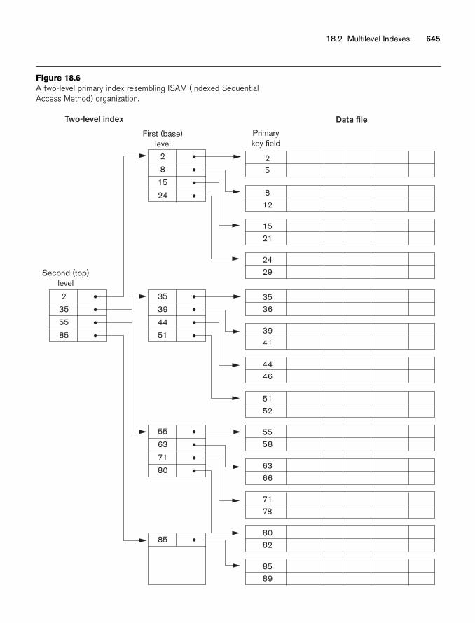
18.2 Multilevel Indexes 645
Data file
Primarykey field
Second (top)level
Two-level index
25
812
1521
2429
3536
3941
4446
5152
5558
6366
7178
8082
8589
2
35
55
85
First (base)level
2
8
15
24
35
39
44
51
55
63
71
80
85
Figure 18.6A two-level primary index resembling ISAM (Indexed SequentialAccess Method) organization.
646 Chapter 18 Indexing Structures for Files
Algorithm 18.1. Searching a Nondense Multilevel Primary Index with t Levels
(* We assume the index entry to be a block anchor that is the first key per block. *)p ← address of top-level block of index;for j ← t step – 1 to 1 do
beginread the index block (at jth index level) whose address is p;search block p for entry i such that Kj (i) ≤ K < Kj(i + 1)
(* if Kj(i)is the last entry in the block, it is sufficient to satisfy Kj(i) ≤ K *);p ← Pj(i ) (* picks appropriate pointer at jth index level *)
end;read the data file block whose address is p;search block p for record with key = K;
As we have seen, a multilevel index reduces the number of blocks accessed whensearching for a record, given its indexing field value. We are still faced with the prob-lems of dealing with index insertions and deletions, because all index levels arephysically ordered files. To retain the benefits of using multilevel indexing whilereducing index insertion and deletion problems, designers adopted a multilevelindex called a dynamic multilevel index that leaves some space in each of its blocksfor inserting new entries and uses appropriate insertion/deletion algorithms for cre-ating and deleting new index blocks when the data file grows and shrinks. It is oftenimplemented by using data structures called B-trees and B+-trees, which wedescribe in the next section.
18.3 Dynamic Multilevel Indexes Using B-Trees and B+-Trees
B-trees and B+-trees are special cases of the well-known search data structureknown as a tree. We briefly introduce the terminology used in discussing tree datastructures. A tree is formed of nodes. Each node in the tree, except for a specialnode called the root, has one parent node and zero or more child nodes. The rootnode has no parent. A node that does not have any child nodes is called a leaf node;a nonleaf node is called an internal node. The level of a node is always one morethan the level of its parent, with the level of the root node being zero.5 A subtree ofa node consists of that node and all its descendant nodes—its child nodes, the childnodes of its child nodes, and so on. A precise recursive definition of a subtree is thatit consists of a node n and the subtrees of all the child nodes of n. Figure 18.7 illus-trates a tree data structure. In this figure the root node is A, and its child nodes areB, C, and D. Nodes E, J, C, G, H, and K are leaf nodes. Since the leaf nodes are at dif-ferent levels of the tree, this tree is called unbalanced.
5This standard definition of the level of a tree node, which we use throughout Section 18.3, is differentfrom the one we gave for multilevel indexes in Section 18.2.
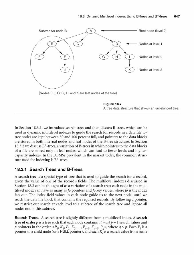
18.3 Dynamic Multilevel Indexes Using B-Trees and B+-Trees 647
A
CB
Subtree for node B
(Nodes E, J, C, G, H, and K are leaf nodes of the tree)
Root node (level 0)
Nodes at level 1D
Nodes at level 2DF I
Nodes at level 3I
HG
J
E
K
Figure 18.7A tree data structure that shows an unbalanced tree.
In Section 18.3.1, we introduce search trees and then discuss B-trees, which can beused as dynamic multilevel indexes to guide the search for records in a data file. B-tree nodes are kept between 50 and 100 percent full, and pointers to the data blocksare stored in both internal nodes and leaf nodes of the B-tree structure. In Section18.3.2 we discuss B+-trees, a variation of B-trees in which pointers to the data blocksof a file are stored only in leaf nodes, which can lead to fewer levels and higher-capacity indexes. In the DBMSs prevalent in the market today, the common struc-ture used for indexing is B+-trees.
18.3.1 Search Trees and B-TreesA search tree is a special type of tree that is used to guide the search for a record,given the value of one of the record’s fields. The multilevel indexes discussed inSection 18.2 can be thought of as a variation of a search tree; each node in the mul-tilevel index can have as many as fo pointers and fo key values, where fo is the indexfan-out. The index field values in each node guide us to the next node, until wereach the data file block that contains the required records. By following a pointer,we restrict our search at each level to a subtree of the search tree and ignore allnodes not in this subtree.
Search Trees. A search tree is slightly different from a multilevel index. A searchtree of order p is a tree such that each node contains at most p − 1 search values andp pointers in the order <P1, K1, P2, K2, ..., Pq−1, Kq−1, Pq>, where q ≤ p. Each Pi is apointer to a child node (or a NULL pointer), and each Ki is a search value from some
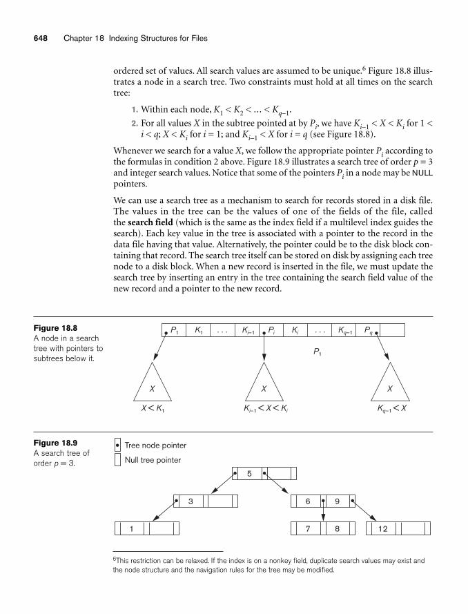
648 Chapter 18 Indexing Structures for Files
P1
P1
K1 Ki–1
Kq–1 < X
X
Ki–1 < X < Ki
X
X < K1
X
Pi Ki Kq–1 Pq. . . . . .Figure 18.8A node in a searchtree with pointers tosubtrees below it.
5
3
Tree node pointer
Null tree pointer
6 9
7 8 121
Figure 18.9A search tree oforder p = 3.
ordered set of values. All search values are assumed to be unique.6 Figure 18.8 illus-trates a node in a search tree. Two constraints must hold at all times on the searchtree:
1. Within each node, K1 < K2 < ... < Kq−1.
2. For all values X in the subtree pointed at by Pi, we have Ki−1 < X < Ki for 1 <i < q; X < Ki for i = 1; and Ki−1 < X for i = q (see Figure 18.8).
Whenever we search for a value X, we follow the appropriate pointer Pi according tothe formulas in condition 2 above. Figure 18.9 illustrates a search tree of order p = 3and integer search values. Notice that some of the pointers Pi in a node may be NULLpointers.
We can use a search tree as a mechanism to search for records stored in a disk file.The values in the tree can be the values of one of the fields of the file, called the search field (which is the same as the index field if a multilevel index guides thesearch). Each key value in the tree is associated with a pointer to the record in thedata file having that value. Alternatively, the pointer could be to the disk block con-taining that record. The search tree itself can be stored on disk by assigning each treenode to a disk block. When a new record is inserted in the file, we must update thesearch tree by inserting an entry in the tree containing the search field value of thenew record and a pointer to the new record.
6This restriction can be relaxed. If the index is on a nonkey field, duplicate search values may exist andthe node structure and the navigation rules for the tree may be modified.
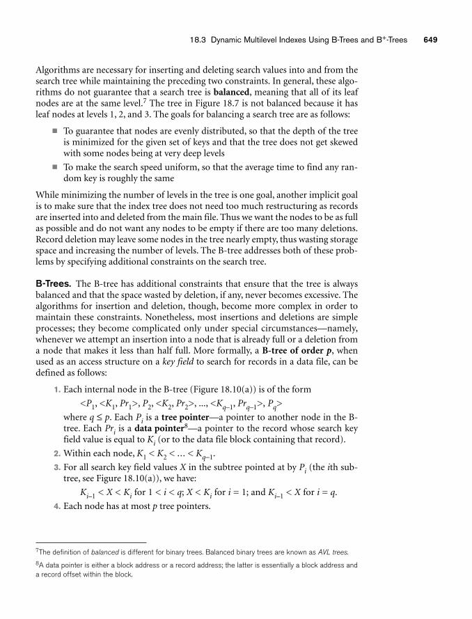
18.3 Dynamic Multilevel Indexes Using B-Trees and B+-Trees 649
Algorithms are necessary for inserting and deleting search values into and from thesearch tree while maintaining the preceding two constraints. In general, these algo-rithms do not guarantee that a search tree is balanced, meaning that all of its leafnodes are at the same level.7 The tree in Figure 18.7 is not balanced because it hasleaf nodes at levels 1, 2, and 3. The goals for balancing a search tree are as follows:
■ To guarantee that nodes are evenly distributed, so that the depth of the treeis minimized for the given set of keys and that the tree does not get skewedwith some nodes being at very deep levels
■ To make the search speed uniform, so that the average time to find any ran-dom key is roughly the same
While minimizing the number of levels in the tree is one goal, another implicit goalis to make sure that the index tree does not need too much restructuring as recordsare inserted into and deleted from the main file. Thus we want the nodes to be as fullas possible and do not want any nodes to be empty if there are too many deletions.Record deletion may leave some nodes in the tree nearly empty, thus wasting storagespace and increasing the number of levels. The B-tree addresses both of these prob-lems by specifying additional constraints on the search tree.
B-Trees. The B-tree has additional constraints that ensure that the tree is alwaysbalanced and that the space wasted by deletion, if any, never becomes excessive. Thealgorithms for insertion and deletion, though, become more complex in order tomaintain these constraints. Nonetheless, most insertions and deletions are simpleprocesses; they become complicated only under special circumstances—namely,whenever we attempt an insertion into a node that is already full or a deletion froma node that makes it less than half full. More formally, a B-tree of order p, whenused as an access structure on a key field to search for records in a data file, can bedefined as follows:
1. Each internal node in the B-tree (Figure 18.10(a)) is of the form
<P1, <K1, Pr1>, P2, <K2, Pr2>, ..., <Kq–1, Prq–1>, Pq>
where q ≤ p. Each Pi is a tree pointer—a pointer to another node in the B-tree. Each Pri is a data pointer8—a pointer to the record whose search keyfield value is equal to Ki (or to the data file block containing that record).
2. Within each node, K1 < K2 < ... < Kq−1.
3. For all search key field values X in the subtree pointed at by Pi (the ith sub-tree, see Figure 18.10(a)), we have:
Ki–1 < X < Ki for 1 < i < q; X < Ki for i = 1; and Ki–1 < X for i = q.
4. Each node has at most p tree pointers.
7The definition of balanced is different for binary trees. Balanced binary trees are known as AVL trees.8A data pointer is either a block address or a record address; the latter is essentially a block address anda record offset within the block.
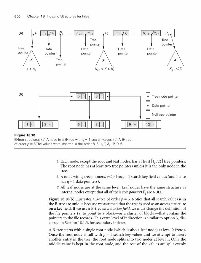
650 Chapter 18 Indexing Structures for Files
X Treepointer
Treepointer
Treepointer
(a)
(b)
P2
X
Datapointer
Datapointer
Datapointer
5 o 8 Tree node pointero
6 o 7 o 9 o 12 o
Data pointer
Null tree pointer
1 o 3 o
Datapointer
P1 Pr1K1 Ki–1 Prq–1Kq–1
X
Kq–1 < XKi–1 < X < KiX < K1
Pi Pq. . . . . .Pri–1 Ki Pri
Treepointer
o
Figure 18.10B-tree structures. (a) A node in a B-tree with q – 1 search values. (b) A B-treeof order p = 3.The values were inserted in the order 8, 5, 1, 7, 3, 12, 9, 6.
5. Each node, except the root and leaf nodes, has at least ⎡(p/2)⎤ tree pointers.The root node has at least two tree pointers unless it is the only node in thetree.
6. A node with q tree pointers, q ≤ p, has q – 1 search key field values (and hencehas q – 1 data pointers).
7. All leaf nodes are at the same level. Leaf nodes have the same structure asinternal nodes except that all of their tree pointers Pi are NULL.
Figure 18.10(b) illustrates a B-tree of order p = 3. Notice that all search values K inthe B-tree are unique because we assumed that the tree is used as an access structureon a key field. If we use a B-tree on a nonkey field, we must change the definition ofthe file pointers Pri to point to a block—or a cluster of blocks—that contain thepointers to the file records. This extra level of indirection is similar to option 3, dis-cussed in Section 18.1.3, for secondary indexes.
A B-tree starts with a single root node (which is also a leaf node) at level 0 (zero).Once the root node is full with p – 1 search key values and we attempt to insertanother entry in the tree, the root node splits into two nodes at level 1. Only themiddle value is kept in the root node, and the rest of the values are split evenly
18.3 Dynamic Multilevel Indexes Using B-Trees and B+-Trees 651
between the other two nodes. When a nonroot node is full and a new entry isinserted into it, that node is split into two nodes at the same level, and the middleentry is moved to the parent node along with two pointers to the new split nodes. Ifthe parent node is full, it is also split. Splitting can propagate all the way to the rootnode, creating a new level if the root is split. We do not discuss algorithms for B-trees in detail in this book,9 but we outline search and insertion procedures for B+-trees in the next section.
If deletion of a value causes a node to be less than half full, it is combined with itsneighboring nodes, and this can also propagate all the way to the root. Hence, dele-tion can reduce the number of tree levels. It has been shown by analysis and simula-tion that, after numerous random insertions and deletions on a B-tree, the nodesare approximately 69 percent full when the number of values in the tree stabilizes.This is also true of B+-trees. If this happens, node splitting and combining willoccur only rarely, so insertion and deletion become quite efficient. If the number ofvalues grows, the tree will expand without a problem—although splitting of nodesmay occur, so some insertions will take more time. Each B-tree node can have atmost p tree pointers, p – 1 data pointers, and p – 1 search key field values (see Figure18.10(a)).
In general, a B-tree node may contain additional information needed by the algo-rithms that manipulate the tree, such as the number of entries q in the node and apointer to the parent node. Next, we illustrate how to calculate the number of blocksand levels for a B-tree.
Example 4. Suppose that the search field is a nonordering key field, and we con-struct a B-tree on this field with p = 23. Assume that each node of the B-tree is 69percent full. Each node, on the average, will have p * 0.69 = 23 * 0.69 or approxi-mately 16 pointers and, hence, 15 search key field values. The average fan-out fo =16. We can start at the root and see how many values and pointers can exist, on theaverage, at each subsequent level:
Root: 1 node 15 key entries 16 pointersLevel 1: 16 nodes 240 key entries 256 pointersLevel 2: 256 nodes 3840 key entries 4096 pointersLevel 3: 4096 nodes 61,440 key entries
At each level, we calculated the number of key entries by multiplying the total num-ber of pointers at the previous level by 15, the average number of entries in eachnode. Hence, for the given block size, pointer size, and search key field size, a two-level B-tree holds 3840 + 240 + 15 = 4095 entries on the average; a three-level B-treeholds 65,535 entries on the average.
B-trees are sometimes used as primary file organizations. In this case, whole recordsare stored within the B-tree nodes rather than just the <search key, record pointer>entries. This works well for files with a relatively small number of records and a small
9For details on insertion and deletion algorithms for B-trees, consult Ramakrishnan and Gehrke [2003].
652 Chapter 18 Indexing Structures for Files
record size. Otherwise, the fan-out and the number of levels become too great topermit efficient access.
In summary, B-trees provide a multilevel access structure that is a balanced treestructure in which each node is at least half full. Each node in a B-tree of order p canhave at most p − 1 search values.
18.3.2 B+-TreesMost implementations of a dynamic multilevel index use a variation of the B-treedata structure called a B+-tree. In a B-tree, every value of the search field appearsonce at some level in the tree, along with a data pointer. In a B+-tree, data pointersare stored only at the leaf nodes of the tree; hence, the structure of leaf nodes differsfrom the structure of internal nodes. The leaf nodes have an entry for every value ofthe search field, along with a data pointer to the record (or to the block that containsthis record) if the search field is a key field. For a nonkey search field, the pointerpoints to a block containing pointers to the data file records, creating an extra levelof indirection.
The leaf nodes of the B+-tree are usually linked to provide ordered access on thesearch field to the records. These leaf nodes are similar to the first (base) level of anindex. Internal nodes of the B+-tree correspond to the other levels of a multilevelindex. Some search field values from the leaf nodes are repeated in the internalnodes of the B+-tree to guide the search. The structure of the internal nodes of a B+-tree of order p (Figure 18.11(a)) is as follows:
1. Each internal node is of the form
<P1, K1, P2, K2, ..., Pq – 1, Kq –1, Pq>
where q ≤ p and each Pi is a tree pointer.
2. Within each internal node, K1 < K2 < ... < Kq−1.
3. For all search field values X in the subtree pointed at by Pi, we have Ki−1 < X≤ Ki for 1 < i < q; X ≤ Ki for i = 1; and Ki−1 < X for i = q (see Figure18.11(a)).10
4. Each internal node has at most p tree pointers.
5. Each internal node, except the root, has at least ⎡(p/2)⎤ tree pointers. Theroot node has at least two tree pointers if it is an internal node.
6. An internal node with q pointers, q ≤ p, has q − 1 search field values.
The structure of the leaf nodes of a B+-tree of order p (Figure 18.11(b)) is as follows:
1. Each leaf node is of the form
<<K1, Pr1>, <K2, Pr2>, ..., <Kq–1, Prq–1>, Pnext>
where q ≤ p, each Pri is a data pointer, and Pnext points to the next leaf node ofthe B+-tree.
10Our definition follows Knuth (1998). One can define a B+-tree differently by exchanging the < and symbols (Ki−1 X < Ki; Kq−1 ≤ X), but the principles remain the same.
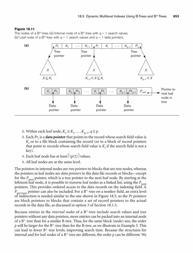
18.3 Dynamic Multilevel Indexes Using B-Trees and B+-Trees 653
(b) Pointer to next leaf node intree
Datapointer
Datapointer
Datapointer
Datapointer
Pr1K1 Pr2K2 Pri Prq–1 PnextKi Kq–1. . . . . .
(a) P1 K1 Ki–1
Kq–1 < X
XX
X < K1
X
Pi Ki Kq–1 Pq. . . . . .
Treepointer
Treepointer
Treepointer
Ki–1 < X < Ki
Figure 18.11The nodes of a B+-tree. (a) Internal node of a B+-tree with q – 1 search values.(b) Leaf node of a B+-tree with q – 1 search values and q – 1 data pointers.
2. Within each leaf node, K1 ≤ K2 ... , Kq−1, q ≤ p.
3. Each Pri is a data pointer that points to the record whose search field value isKi or to a file block containing the record (or to a block of record pointersthat point to records whose search field value is Ki if the search field is not akey).
4. Each leaf node has at least ⎡(p/2)⎤ values.
5. All leaf nodes are at the same level.
The pointers in internal nodes are tree pointers to blocks that are tree nodes, whereasthe pointers in leaf nodes are data pointers to the data file records or blocks—exceptfor the Pnext pointer, which is a tree pointer to the next leaf node. By starting at theleftmost leaf node, it is possible to traverse leaf nodes as a linked list, using the Pnextpointers. This provides ordered access to the data records on the indexing field. APprevious pointer can also be included. For a B+-tree on a nonkey field, an extra levelof indirection is needed similar to the one shown in Figure 18.5, so the Pr pointersare block pointers to blocks that contain a set of record pointers to the actualrecords in the data file, as discussed in option 3 of Section 18.1.3.
Because entries in the internal nodes of a B+-tree include search values and treepointers without any data pointers, more entries can be packed into an internal nodeof a B+-tree than for a similar B-tree. Thus, for the same block (node) size, the orderp will be larger for the B+-tree than for the B-tree, as we illustrate in Example 5. Thiscan lead to fewer B+-tree levels, improving search time. Because the structures forinternal and for leaf nodes of a B+-tree are different, the order p can be different. We
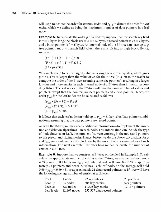
654 Chapter 18 Indexing Structures for Files
will use p to denote the order for internal nodes and pleaf to denote the order for leafnodes, which we define as being the maximum number of data pointers in a leafnode.
Example 5. To calculate the order p of a B+-tree, suppose that the search key fieldis V = 9 bytes long, the block size is B = 512 bytes, a record pointer is Pr = 7 bytes,and a block pointer is P = 6 bytes. An internal node of the B+-tree can have up to ptree pointers and p – 1 search field values; these must fit into a single block. Hence,we have:
(p * P) + ((p – 1) * V) ≤ B
(P * 6) + ((P − 1) * 9) ≤ 512
(15 * p) ≤ 521
We can choose p to be the largest value satisfying the above inequality, which gives p = 34. This is larger than the value of 23 for the B-tree (it is left to the reader tocompute the order of the B-tree assuming same size pointers), resulting in a largerfan-out and more entries in each internal node of a B+-tree than in the correspon-ding B-tree. The leaf nodes of the B+-tree will have the same number of values andpointers, except that the pointers are data pointers and a next pointer. Hence, theorder pleaf for the leaf nodes can be calculated as follows:
(pleaf * (Pr + V)) + P ≤ B
(pleaf * (7 + 9)) + 6 ≤ 512
(16 * pleaf) ≤ 506
It follows that each leaf node can hold up to pleaf = 31 key value/data pointer combi-nations, assuming that the data pointers are record pointers.
As with the B-tree, we may need additional information—to implement the inser-tion and deletion algorithms—in each node. This information can include the typeof node (internal or leaf), the number of current entries q in the node, and pointersto the parent and sibling nodes. Hence, before we do the above calculations for pand pleaf, we should reduce the block size by the amount of space needed for all suchinformation. The next example illustrates how we can calculate the number ofentries in a B+-tree.
Example 6. Suppose that we construct a B+-tree on the field in Example 5. To cal-culate the approximate number of entries in the B+-tree, we assume that each nodeis 69 percent full. On the average, each internal node will have 34 * 0.69 or approxi-mately 23 pointers, and hence 22 values. Each leaf node, on the average, will hold0.69 * pleaf = 0.69 * 31 or approximately 21 data record pointers. A B+-tree will havethe following average number of entries at each level:
Root: 1 node 22 key entries 23 pointersLevel 1: 23 nodes 506 key entries 529 pointersLevel 2: 529 nodes 11,638 key entries 12,167 pointersLeaf level: 12,167 nodes 255,507 data record pointers
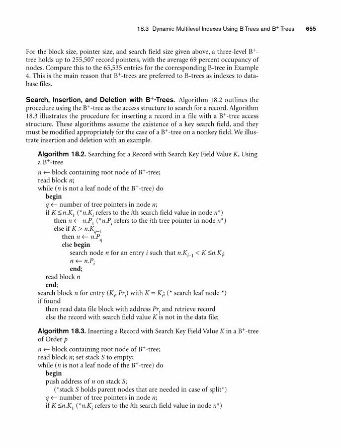
18.3 Dynamic Multilevel Indexes Using B-Trees and B+-Trees 655
For the block size, pointer size, and search field size given above, a three-level B+-tree holds up to 255,507 record pointers, with the average 69 percent occupancy ofnodes. Compare this to the 65,535 entries for the corresponding B-tree in Example4. This is the main reason that B+-trees are preferred to B-trees as indexes to data-base files.
Search, Insertion, and Deletion with B+-Trees. Algorithm 18.2 outlines theprocedure using the B+-tree as the access structure to search for a record. Algorithm18.3 illustrates the procedure for inserting a record in a file with a B+-tree accessstructure. These algorithms assume the existence of a key search field, and theymust be modified appropriately for the case of a B+-tree on a nonkey field. We illus-trate insertion and deletion with an example.
Algorithm 18.2. Searching for a Record with Search Key Field Value K, Usinga B+-tree
n ← block containing root node of B+-tree;read block n;while (n is not a leaf node of the B+-tree) do
beginq ← number of tree pointers in node n;if K ≤ n.K1 (*n.Ki refers to the ith search field value in node n*)
then n ← n.P1 (*n.Pi refers to the ith tree pointer in node n*)else if K > n.Kq−1
then n ← n.Pqelse begin
search node n for an entry i such that n.Ki−1 < K ≤n.Ki;n ← n.Piend;
read block nend;
search block n for entry (Ki, Pri) with K = Ki; (* search leaf node *)if found
then read data file block with address Pri and retrieve recordelse the record with search field value K is not in the data file;
Algorithm 18.3. Inserting a Record with Search Key Field Value K in a B+-treeof Order p
n ← block containing root node of B+-tree;read block n; set stack S to empty;while (n is not a leaf node of the B+-tree) do
beginpush address of n on stack S;
(*stack S holds parent nodes that are needed in case of split*)q ← number of tree pointers in node n;if K ≤n.K1 (*n.Ki refers to the ith search field value in node n*)
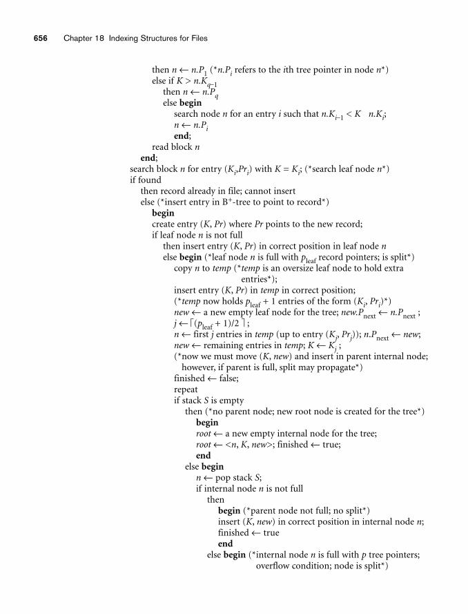
656 Chapter 18 Indexing Structures for Files
then n ← n.P1 (*n.Pi refers to the ith tree pointer in node n*)else if K > n.Kq−1
then n ← n.Pqelse begin
search node n for an entry i such that n.Ki−1 < K n.Ki;n ← n.Piend;
read block nend;
search block n for entry (Ki,Pri) with K = Ki; (*search leaf node n*)if found
then record already in file; cannot insertelse (*insert entry in B+-tree to point to record*)
begincreate entry (K, Pr) where Pr points to the new record;if leaf node n is not full
then insert entry (K, Pr) in correct position in leaf node nelse begin (*leaf node n is full with pleaf record pointers; is split*)
copy n to temp (*temp is an oversize leaf node to hold extraentries*);
insert entry (K, Pr) in temp in correct position;(*temp now holds pleaf + 1 entries of the form (Ki, Pri)*)new ← a new empty leaf node for the tree; new.Pnext ← n.Pnext ;j ← ⎡(pleaf + 1)/2 ⎤ ;n ← first j entries in temp (up to entry (Kj, Prj)); n.Pnext ← new;new ← remaining entries in temp; K ← Kj ;(*now we must move (K, new) and insert in parent internal node;
however, if parent is full, split may propagate*)finished ← false;repeatif stack S is empty
then (*no parent node; new root node is created for the tree*)beginroot ← a new empty internal node for the tree;root ← <n, K, new>; finished ← true;end
else beginn ← pop stack S;if internal node n is not full
thenbegin (*parent node not full; no split*)insert (K, new) in correct position in internal node n;finished ← trueend
else begin (*internal node n is full with p tree pointers;overflow condition; node is split*)
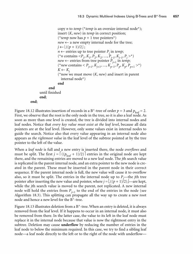
18.3 Dynamic Multilevel Indexes Using B-Trees and B+-Trees 657
copy n to temp (*temp is an oversize internal node*);insert (K, new) in temp in correct position;(*temp now has p + 1 tree pointers*)new ← a new empty internal node for the tree;j ← ⎣((p + 1)/2⎦ ;n ← entries up to tree pointer Pj in temp;(*n contains <P1, K1, P2, K2, ..., Pj−1, Kj−1, Pj >*)new ← entries from tree pointer Pj+1 in temp;(*new contains < Pj+1, Kj+1, ..., Kp−1, Pp, Kp, Pp+1 >*)K ← Kj(*now we must move (K, new) and insert in parent
internal node*)end
enduntil finishedend;
end;
Figure 18.12 illustrates insertion of records in a B+-tree of order p = 3 and pleaf = 2.First, we observe that the root is the only node in the tree, so it is also a leaf node. Assoon as more than one level is created, the tree is divided into internal nodes andleaf nodes. Notice that every key value must exist at the leaf level, because all datapointers are at the leaf level. However, only some values exist in internal nodes toguide the search. Notice also that every value appearing in an internal node alsoappears as the rightmost value in the leaf level of the subtree pointed at by the treepointer to the left of the value.
When a leaf node is full and a new entry is inserted there, the node overflows andmust be split. The first j = ⎡((pleaf + 1)/2)⎤ entries in the original node are keptthere, and the remaining entries are moved to a new leaf node. The jth search valueis replicated in the parent internal node, and an extra pointer to the new node is cre-ated in the parent. These must be inserted in the parent node in their correctsequence. If the parent internal node is full, the new value will cause it to overflowalso, so it must be split. The entries in the internal node up to Pj—the jth treepointer after inserting the new value and pointer, where j = ⎣((p + 1)/2)⎦—are kept,while the jth search value is moved to the parent, not replicated. A new internalnode will hold the entries from Pj+1 to the end of the entries in the node (seeAlgorithm 18.3). This splitting can propagate all the way up to create a new rootnode and hence a new level for the B+-tree.
Figure 18.13 illustrates deletion from a B+-tree. When an entry is deleted, it is alwaysremoved from the leaf level. If it happens to occur in an internal node, it must alsobe removed from there. In the latter case, the value to its left in the leaf node mustreplace it in the internal node because that value is now the rightmost entry in thesubtree. Deletion may cause underflow by reducing the number of entries in theleaf node to below the minimum required. In this case, we try to find a sibling leafnode—a leaf node directly to the left or to the right of the node with underflow—
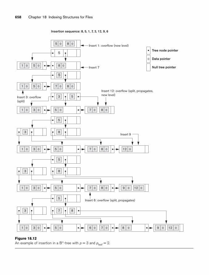
658 Chapter 18 Indexing Structures for Files
5 0 8 Insert 1: overflow (new level)0
5
1 0 5 0 8 0
5
3 5
5
3
3
8
3 7 8
8
Tree node pointer
Data pointer
Null tree pointerInsert 7
Insert 9
Insert 6: overflow (split, propagates)
Insert 3: overflow(split)
Insert 12: overflow (split, propagates,new level)
1 0 5 0 7 0 8 0
1 0 5 0
5 0 12 0
3 0
1 0 3 0
5 01 0 3 0
7 0 8 0
7 0 8 0
12 09 07 0 8 0
5
5
5 01 0 3 0 8 0 12 09 06 0 7 0
Insertion sequence: 8, 5, 1, 7, 3, 12, 9, 6
0
Figure 18.12An example of insertion in a B+-tree with p = 3 and pleaf = 2.
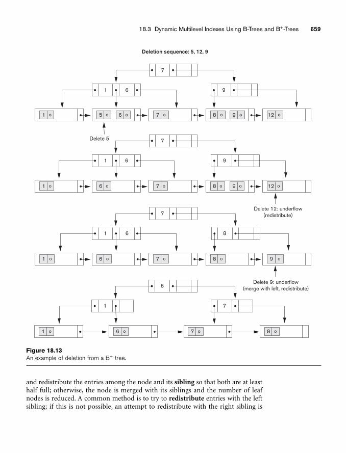
18.3 Dynamic Multilevel Indexes Using B-Trees and B+-Trees 659
7
1 6
7
1 6 9
Deletion sequence: 5, 12, 9
1 o 5 o 6
Delete 5
o 8 o 9 o 12 o7 o
1 o 6 o 8 o 9 o 12 o7 o
9
7
1 6 8
1 o 6 o 8 o 9 o7 o
Delete 12: underflow(redistribute)
Delete 9: underflow(merge with left, redistribute)6
1 7
1 o 6 o 8 o7 o
Figure 18.13An example of deletion from a B+-tree.
and redistribute the entries among the node and its sibling so that both are at leasthalf full; otherwise, the node is merged with its siblings and the number of leafnodes is reduced. A common method is to try to redistribute entries with the leftsibling; if this is not possible, an attempt to redistribute with the right sibling is
660 Chapter 18 Indexing Structures for Files
made. If this is also not possible, the three nodes are merged into two leaf nodes. Insuch a case, underflow may propagate to internal nodes because one fewer treepointer and search value are needed. This can propagate and reduce the tree levels.
Notice that implementing the insertion and deletion algorithms may require parentand sibling pointers for each node, or the use of a stack as in Algorithm 18.3. Eachnode should also include the number of entries in it and its type (leaf or internal).Another alternative is to implement insertion and deletion as recursiveprocedures.11
Variations of B-Trees and B+-Trees. To conclude this section, we briefly men-tion some variations of B-trees and B+-trees. In some cases, constraint 5 on the B-tree (or for the internal nodes of the B+–tree, except the root node), which requireseach node to be at least half full, can be changed to require each node to be at leasttwo-thirds full. In this case the B-tree has been called a B*-tree. In general, somesystems allow the user to choose a fill factor between 0.5 and 1.0, where the lattermeans that the B-tree (index) nodes are to be completely full. It is also possible tospecify two fill factors for a B+-tree: one for the leaf level and one for the internalnodes of the tree. When the index is first constructed, each node is filled up toapproximately the fill factors specified. Some investigators have suggested relaxingthe requirement that a node be half full, and instead allow a node to become com-pletely empty before merging, to simplify the deletion algorithm. Simulation studiesshow that this does not waste too much additional space under randomly distrib-uted insertions and deletions.
18.4 Indexes on Multiple KeysIn our discussion so far, we have assumed that the primary or secondary keys onwhich files were accessed were single attributes (fields). In many retrieval andupdate requests, multiple attributes are involved. If a certain combination of attrib-utes is used frequently, it is advantageous to set up an access structure to provideefficient access by a key value that is a combination of those attributes.
For example, consider an EMPLOYEE file containing attributes Dno (departmentnumber), Age, Street, City, Zip_code, Salary and Skill_code, with the key of Ssn (SocialSecurity number). Consider the query: List the employees in department number 4whose age is 59. Note that both Dno and Age are nonkey attributes, which means thata search value for either of these will point to multiple records. The following alter-native search strategies may be considered:
1. Assuming Dno has an index, but Age does not, access the records having Dno = 4 using the index, and then select from among them those records thatsatisfy Age = 59.
11For more details on insertion and deletion algorithms for B+ trees, consult Ramakrishnan and Gehrke[2003].
18.4 Indexes on Multiple Keys 661
2. Alternately, if Age is indexed but Dno is not, access the records having Age =59 using the index, and then select from among them those records that sat-isfy Dno = 4.
3. If indexes have been created on both Dno and Age, both indexes may be used;each gives a set of records or a set of pointers (to blocks or records). An inter-section of these sets of records or pointers yields those records or pointersthat satisfy both conditions.
All of these alternatives eventually give the correct result. However, if the set ofrecords that meet each condition (Dno = 4 or Age = 59) individually are large, yetonly a few records satisfy the combined condition, then none of the above is an effi-cient technique for the given search request. A number of possibilities exist thatwould treat the combination < Dno, Age> or < Age, Dno> as a search key made up ofmultiple attributes. We briefly outline these techniques in the following sections. Wewill refer to keys containing multiple attributes as composite keys.
18.4.1 Ordered Index on Multiple AttributesAll the discussion in this chapter so far still applies if we create an index on a searchkey field that is a combination of <Dno, Age>. The search key is a pair of values <4,59> in the above example. In general, if an index is created on attributes <A1, A2, ...,An>, the search key values are tuples with n values: <v1, v2, ..., vn>.
A lexicographic ordering of these tuple values establishes an order on this compos-ite search key. For our example, all of the department keys for department number3 precede those for department number 4. Thus <3, n> precedes <4, m> for any val-ues of m and n. The ascending key order for keys with Dno = 4 would be <4, 18>, <4,19>, <4, 20>, and so on. Lexicographic ordering works similarly to ordering ofcharacter strings. An index on a composite key of n attributes works similarly to anyindex discussed in this chapter so far.
18.4.2 Partitioned HashingPartitioned hashing is an extension of static external hashing (Section 17.8.2) thatallows access on multiple keys. It is suitable only for equality comparisons; rangequeries are not supported. In partitioned hashing, for a key consisting of n compo-nents, the hash function is designed to produce a result with n separate hashaddresses. The bucket address is a concatenation of these n addresses. It is then pos-sible to search for the required composite search key by looking up the appropriatebuckets that match the parts of the address in which we are interested.
For example, consider the composite search key <Dno, Age>. If Dno and Age arehashed into a 3-bit and 5-bit address respectively, we get an 8-bit bucket address.Suppose that Dno = 4 has a hash address ‘100’ and Age = 59 has hash address ‘10101’.Then to search for the combined search value, Dno = 4 and Age = 59, one goes tobucket address 100 10101; just to search for all employees with Age = 59, all buckets(eight of them) will be searched whose addresses are ‘000 10101’, ‘001 10101’, ... and
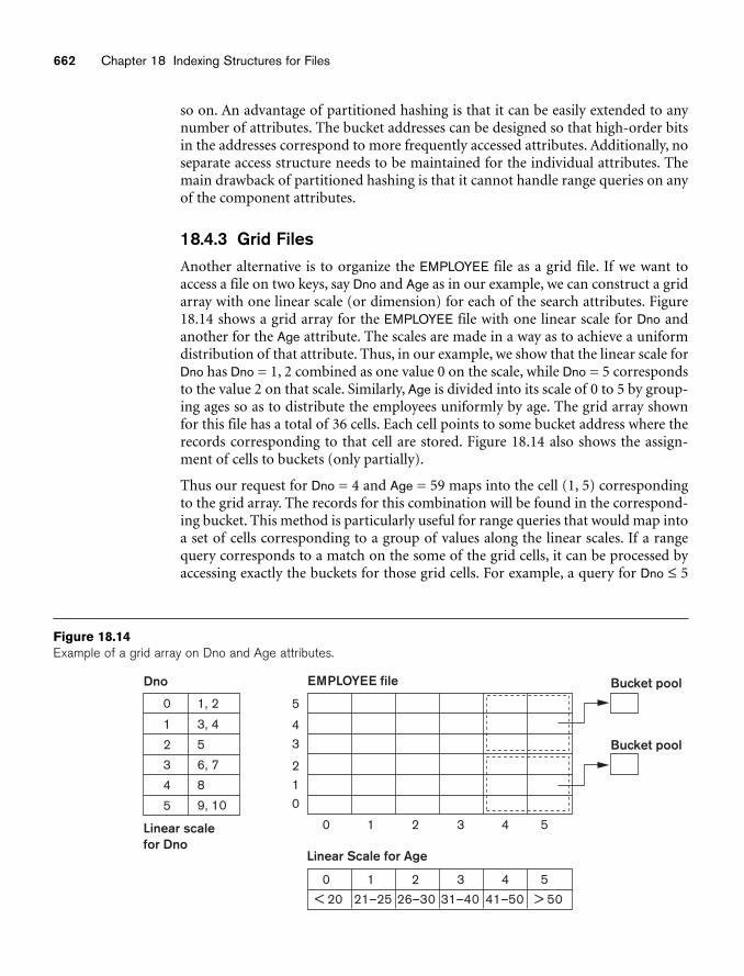
662 Chapter 18 Indexing Structures for Files
Linear Scale for Age
EMPLOYEE file Bucket pool
Bucket pool
4
5
3
210
0 1 2 3 4 5
< 20 21–25 26–30 31–40 41–50 > 50
0 1 2 3 4 5
Dno
Linear scalefor Dno
0 1, 2
3, 4
5
6, 7
8
9, 10
1
2
3
4
5
Figure 18.14Example of a grid array on Dno and Age attributes.
so on. An advantage of partitioned hashing is that it can be easily extended to anynumber of attributes. The bucket addresses can be designed so that high-order bitsin the addresses correspond to more frequently accessed attributes. Additionally, noseparate access structure needs to be maintained for the individual attributes. Themain drawback of partitioned hashing is that it cannot handle range queries on anyof the component attributes.
18.4.3 Grid FilesAnother alternative is to organize the EMPLOYEE file as a grid file. If we want toaccess a file on two keys, say Dno and Age as in our example, we can construct a gridarray with one linear scale (or dimension) for each of the search attributes. Figure18.14 shows a grid array for the EMPLOYEE file with one linear scale for Dno andanother for the Age attribute. The scales are made in a way as to achieve a uniformdistribution of that attribute. Thus, in our example, we show that the linear scale forDno has Dno = 1, 2 combined as one value 0 on the scale, while Dno = 5 correspondsto the value 2 on that scale. Similarly, Age is divided into its scale of 0 to 5 by group-ing ages so as to distribute the employees uniformly by age. The grid array shownfor this file has a total of 36 cells. Each cell points to some bucket address where therecords corresponding to that cell are stored. Figure 18.14 also shows the assign-ment of cells to buckets (only partially).
Thus our request for Dno = 4 and Age = 59 maps into the cell (1, 5) correspondingto the grid array. The records for this combination will be found in the correspond-ing bucket. This method is particularly useful for range queries that would map intoa set of cells corresponding to a group of values along the linear scales. If a rangequery corresponds to a match on the some of the grid cells, it can be processed byaccessing exactly the buckets for those grid cells. For example, a query for Dno ≤ 5
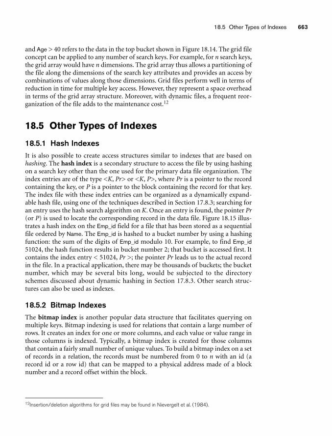
18.5 Other Types of Indexes 663
and Age > 40 refers to the data in the top bucket shown in Figure 18.14. The grid fileconcept can be applied to any number of search keys. For example, for n search keys,the grid array would have n dimensions. The grid array thus allows a partitioning ofthe file along the dimensions of the search key attributes and provides an access bycombinations of values along those dimensions. Grid files perform well in terms ofreduction in time for multiple key access. However, they represent a space overheadin terms of the grid array structure. Moreover, with dynamic files, a frequent reor-ganization of the file adds to the maintenance cost.12
18.5 Other Types of Indexes
18.5.1 Hash IndexesIt is also possible to create access structures similar to indexes that are based onhashing. The hash index is a secondary structure to access the file by using hashingon a search key other than the one used for the primary data file organization. Theindex entries are of the type <K, Pr> or <K, P>, where Pr is a pointer to the recordcontaining the key, or P is a pointer to the block containing the record for that key.The index file with these index entries can be organized as a dynamically expand-able hash file, using one of the techniques described in Section 17.8.3; searching foran entry uses the hash search algorithm on K. Once an entry is found, the pointer Pr(or P) is used to locate the corresponding record in the data file. Figure 18.15 illus-trates a hash index on the Emp_id field for a file that has been stored as a sequentialfile ordered by Name. The Emp_id is hashed to a bucket number by using a hashingfunction: the sum of the digits of Emp_id modulo 10. For example, to find Emp_id51024, the hash function results in bucket number 2; that bucket is accessed first. Itcontains the index entry < 51024, Pr >; the pointer Pr leads us to the actual recordin the file. In a practical application, there may be thousands of buckets; the bucketnumber, which may be several bits long, would be subjected to the directoryschemes discussed about dynamic hashing in Section 17.8.3. Other search struc-tures can also be used as indexes.
18.5.2 Bitmap IndexesThe bitmap index is another popular data structure that facilitates querying onmultiple keys. Bitmap indexing is used for relations that contain a large number ofrows. It creates an index for one or more columns, and each value or value range inthose columns is indexed. Typically, a bitmap index is created for those columnsthat contain a fairly small number of unique values. To build a bitmap index on a setof records in a relation, the records must be numbered from 0 to n with an id (arecord id or a row id) that can be mapped to a physical address made of a blocknumber and a record offset within the block.
12Insertion/deletion algorithms for grid files may be found in Nievergelt et al. (1984).
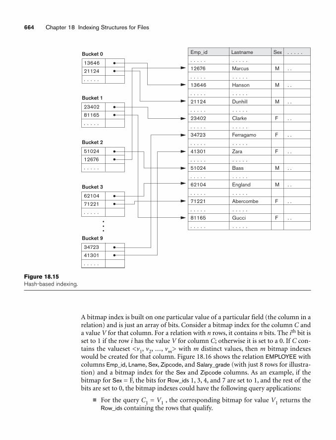
664 Chapter 18 Indexing Structures for Files
Bucket 0 Emp_id
. . . . . . . . . .
12676 Marcus M . .
. . . . . . . . . .
13646 Hanson M . .
. . . . . . . . . .
21124 Dunhill M . .
. . . . . . . . . .
23402 Clarke F . .
. . . . . . . . . .
34723 Ferragamo F . .
. . . . . . . . . .
41301 Zara F . .
. . . . . . . . . .
51024 Bass M . .
. . . . . . . . . .
62104 England M . .
. . . . . . . . . .
71221 Abercombe F . .
. . . . . . . . . .
81165 Gucci F . .
. . . . . . . . . .
13646
21124
. . . . .
Lastname Sex . . . . .
Bucket 1
23402
81165
. . . . .
Bucket 2
51024
12676
. . . . .
Bucket 3
62104
71221
. . . . .
Bucket 9
34723
41301
. . . . .
Figure 18.15Hash-based indexing.
A bitmap index is built on one particular value of a particular field (the column in arelation) and is just an array of bits. Consider a bitmap index for the column C anda value V for that column. For a relation with n rows, it contains n bits. The ith bit isset to 1 if the row i has the value V for column C; otherwise it is set to a 0. If C con-tains the valueset <v1, v2, ..., vm> with m distinct values, then m bitmap indexeswould be created for that column. Figure 18.16 shows the relation EMPLOYEE withcolumns Emp_id, Lname, Sex, Zipcode, and Salary_grade (with just 8 rows for illustra-tion) and a bitmap index for the Sex and Zipcode columns. As an example, if thebitmap for Sex = F, the bits for Row_ids 1, 3, 4, and 7 are set to 1, and the rest of thebits are set to 0, the bitmap indexes could have the following query applications:
■ For the query C1 = V1 , the corresponding bitmap for value V1 returns theRow_ids containing the rows that qualify.
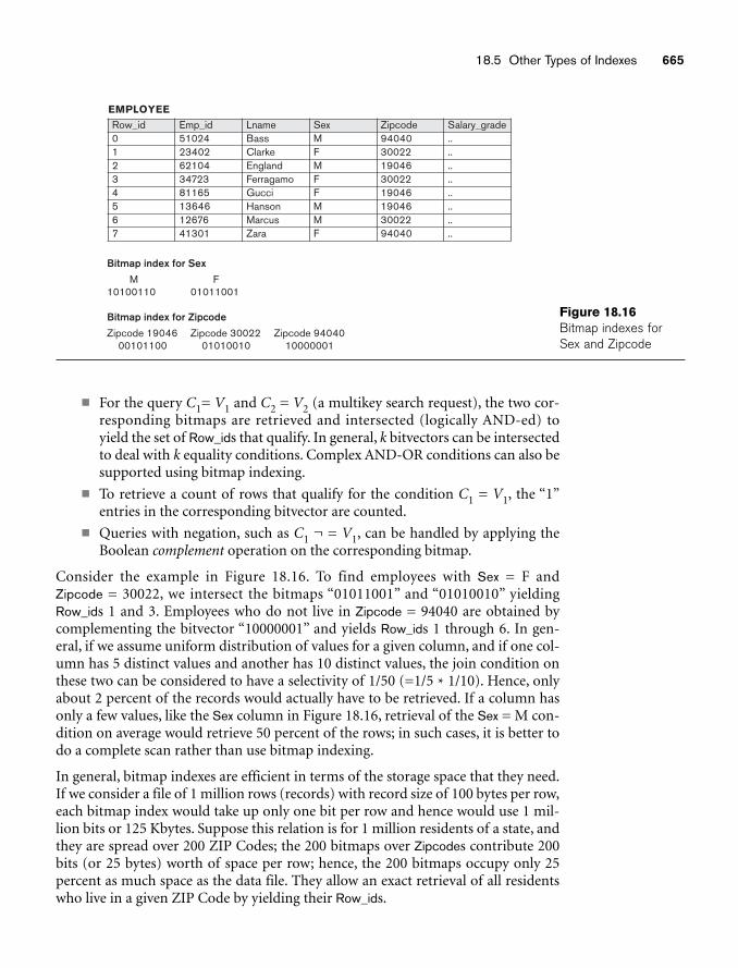
18.5 Other Types of Indexes 665
EMPLOYEE
Row_id Emp_id Lname Sex Zipcode Salary_grade0 51024 Bass M 94040 ..1 23402 Clarke F 30022 ..2 62104 England M 19046 ..3 34723 Ferragamo F 30022 ..4 81165 Gucci F 19046 ..5 13646 Hanson M 19046 ..6 12676 Marcus M 30022 ..7 41301 Zara F 94040 ..
Bitmap index for Sex
M F10100110 01011001
Bitmap index for Zipcode
Zipcode 19046 Zipcode 30022 Zipcode 94040 00101100 01010010 10000001
Figure 18.16Bitmap indexes forSex and Zipcode
■ For the query C1= V1 and C2 = V2 (a multikey search request), the two cor-responding bitmaps are retrieved and intersected (logically AND-ed) toyield the set of Row_ids that qualify. In general, k bitvectors can be intersectedto deal with k equality conditions. Complex AND-OR conditions can also besupported using bitmap indexing.
■ To retrieve a count of rows that qualify for the condition C1 = V1, the “1”entries in the corresponding bitvector are counted.
■ Queries with negation, such as C1 ¬ = V1, can be handled by applying theBoolean complement operation on the corresponding bitmap.
Consider the example in Figure 18.16. To find employees with Sex = F and Zipcode = 30022, we intersect the bitmaps “01011001” and “01010010” yieldingRow_ids 1 and 3. Employees who do not live in Zipcode = 94040 are obtained bycomplementing the bitvector “10000001” and yields Row_ids 1 through 6. In gen-eral, if we assume uniform distribution of values for a given column, and if one col-umn has 5 distinct values and another has 10 distinct values, the join condition onthese two can be considered to have a selectivity of 1/50 (=1/5 * 1/10). Hence, onlyabout 2 percent of the records would actually have to be retrieved. If a column hasonly a few values, like the Sex column in Figure 18.16, retrieval of the Sex = M con-dition on average would retrieve 50 percent of the rows; in such cases, it is better todo a complete scan rather than use bitmap indexing.
In general, bitmap indexes are efficient in terms of the storage space that they need.If we consider a file of 1 million rows (records) with record size of 100 bytes per row,each bitmap index would take up only one bit per row and hence would use 1 mil-lion bits or 125 Kbytes. Suppose this relation is for 1 million residents of a state, andthey are spread over 200 ZIP Codes; the 200 bitmaps over Zipcodes contribute 200bits (or 25 bytes) worth of space per row; hence, the 200 bitmaps occupy only 25percent as much space as the data file. They allow an exact retrieval of all residentswho live in a given ZIP Code by yielding their Row_ids.
666 Chapter 18 Indexing Structures for Files
When records are deleted, renumbering rows and shifting bits in bitmaps becomesexpensive. Another bitmap, called the existence bitmap, can be used to avoid thisexpense. This bitmap has a 0 bit for the rows that have been deleted but are stillpresent and a 1 bit for rows that actually exist. Whenever a row is inserted in therelation, an entry must be made in all the bitmaps of all the columns that have abitmap index; rows typically are appended to the relation or may replace deletedrows. This process represents an indexing overhead.
Large bitvectors are handled by treating them as a series of 32-bit or 64-bit vectors,and corresponding AND, OR, and NOT operators are used from the instruction setto deal with 32- or 64-bit input vectors in a single instruction. This makes bitvectoroperations computationally very efficient.
Bitmaps for B+-Tree Leaf Nodes. Bitmaps can be used on the leaf nodes ofB+-tree indexes as well as to point to the set of records that contain each specificvalue of the indexed field in the leaf node. When the B+-tree is built on a nonkeysearch field, the leaf record must contain a list of record pointers alongside eachvalue of the indexed attribute. For values that occur very frequently, that is, in alarge percentage of the relation, a bitmap index may be stored instead of the point-ers. As an example, for a relation with n rows, suppose a value occurs in 10 percentof the file records. A bitvector would have n bits, having the “1” bit for those Row_idsthat contain that search value, which is n/8 or 0.125n bytes in size. If the recordpointer takes up 4 bytes (32 bits), then the n/10 record pointers would take up 4 * n/10 or 0.4n bytes. Since 0.4n is more than 3 times larger than 0.125n, it is betterto store the bitmap index rather than the record pointers. Hence for search valuesthat occur more frequently than a certain ratio (in this case that would be 1/32), it isbeneficial to use bitmaps as a compressed storage mechanism for representing therecord pointers in B+-trees that index a nonkey field.
18.5.3 Function-Based IndexingIn this section we discuss a new type of indexing, called function-based indexing,that has been introduced in the Oracle relational DBMS as well as in some othercommercial products.13
The idea behind function-based indexing is to create an index such that the valuethat results from applying some function on a field or a collection of fields becomesthe key to the index. The following examples show how to create and use function-based indexes.
Example 1. The following statement creates a function-based index on theEMPLOYEE table based on an uppercase representation of the Lname column, whichcan be entered in many ways but is always queried by its uppercase representation.
CREATE INDEX upper_ix ON Employee (UPPER(Lname));
13Rafi Ahmed contributed most of this section.
18.5 Other Types of Indexes 667
This statement will create an index based on the function UPPER(Lname), whichreturns the last name in uppercase letters; for example, UPPER('Smith') willreturn ‘SMITH’.
Function-based indexes ensure that Oracle Database system will use the indexrather than perform a full table scan, even when a function is used in the searchpredicate of a query. For example, the following query will use the index:
SELECT First_name, LnameFROM EmployeeWHERE UPPER(Lname)= "SMITH".
Without the function-based index, an Oracle Database might perform a full tablescan, since a B+-tree index is searched only by using the column value directly; theuse of any function on a column prevents such an index from being used.
Example 2. In this example, the EMPLOYEE table is supposed to contain twofields—salary and commission_pct (commission percentage)—and an index is beingcreated on the sum of salary and commission based on the commission_pct.
CREATE INDEX income_ixON Employee(Salary + (Salary*Commission_pct));
The following query uses the income_ix index even though the fields salary andcommission_pct are occurring in the reverse order in the query when compared tothe index definition.
SELECT First_name, LnameFROM EmployeeWHERE ((Salary*Commission_pct) + Salary ) > 15000;
Example 3. This is a more advanced example of using function-based indexing todefine conditional uniqueness. The following statement creates a unique function-based index on the ORDERS table that prevents a customer from taking advantage ofa promotion id (“blowout sale”) more than once. It creates a composite index on theCustomer_id and Promotion_id fields together, and it allows only one entry in the indexfor a given Customer_id with the Promotion_id of “2” by declaring it as a unique index.
CREATE UNIQUE INDEX promo_ix ON Orders(CASE WHEN Promotion_id = 2 THEN Customer_id ELSE NULL END,CASE WHEN Promotion_id = 2 THEN Promotion_id ELSE NULL END);
Note that by using the CASE statement, the objective is to remove from the index anyrows where Promotion_id is not equal to 2. Oracle Database does not store in the B+-tree index any rows where all the keys are NULL. Therefore, in this example, we mapboth Customer_id and Promotion_id to NULL unless Promotion_id is equal to 2. Theresult is that the index constraint is violated only if Promotion_id is equal to 2, for two(attempted insertions of) rows with the same Customer_id value.
668 Chapter 18 Indexing Structures for Files
18.6 Some General Issues Concerning Indexing
18.6.1 Logical versus Physical IndexesIn the earlier discussion, we have assumed that the index entries <K, Pr> (or <K,P>) always include a physical pointer Pr (or P) that specifies the physical recordaddress on disk as a block number and offset. This is sometimes called a physicalindex, and it has the disadvantage that the pointer must be changed if the record ismoved to another disk location. For example, suppose that a primary file organiza-tion is based on linear hashing or extendible hashing; then, each time a bucket issplit, some records are allocated to new buckets and hence have new physicaladdresses. If there was a secondary index on the file, the pointers to those recordswould have to be found and updated, which is a difficult task.
To remedy this situation, we can use a structure called a logical index, whose indexentries are of the form <K, Kp>. Each entry has one value K for the secondary index-ing field matched with the value Kp of the field used for the primary file organiza-tion. By searching the secondary index on the value of K, a program can locate thecorresponding value of Kp and use this to access the record through the primary fileorganization. Logical indexes thus introduce an additional level of indirectionbetween the access structure and the data. They are used when physical recordaddresses are expected to change frequently. The cost of this indirection is the extrasearch based on the primary file organization.
18.6.2 DiscussionIn many systems, an index is not an integral part of the data file but can be createdand discarded dynamically. That is why it is often called an access structure.Whenever we expect to access a file frequently based on some search conditioninvolving a particular field, we can request the DBMS to create an index on thatfield. Usually, a secondary index is created to avoid physical ordering of the recordsin the data file on disk.
The main advantage of secondary indexes is that—theoretically, at least—they canbe created in conjunction with virtually any primary record organization. Hence, asecondary index could be used to complement other primary access methods suchas ordering or hashing, or it could even be used with mixed files. To create a B+-treesecondary index on some field of a file, we must go through all records in the file tocreate the entries at the leaf level of the tree. These entries are then sorted and filledaccording to the specified fill factor; simultaneously, the other index levels are cre-ated. It is more expensive and much harder to create primary indexes and clusteringindexes dynamically, because the records of the data file must be physically sortedon disk in order of the indexing field. However, some systems allow users to createthese indexes dynamically on their files by sorting the file during index creation.
It is common to use an index to enforce a key constraint on an attribute. Whilesearching the index to insert a new record, it is straightforward to check at the same
18.6 Some General Issues Concerning Indexing 669
time whether another record in the file—and hence in the index tree—has the samekey attribute value as the new record. If so, the insertion can be rejected.
If an index is created on a nonkey field, duplicates occur; handling of these dupli-cates is an issue the DBMS product vendors have to deal with and affects data stor-age as well as index creation and management. Data records for the duplicate keymay be contained in the same block or may span multiple blocks where many dupli-cates are possible. Some systems add a row id to the record so that records withduplicate keys have their own unique identifiers. In such cases, the B+-tree indexmay regard a <key, Row_id> combination as the de facto key for the index, turningthe index into a unique index with no duplicates. The deletion of a key K from suchan index would involve deleting all occurrences of that key K—hence the deletionalgorithm has to account for this.
In actual DBMS products, deletion from B+-tree indexes is also handled in variousways to improve performance and response times. Deleted records may be markedas deleted and the corresponding index entries may also not be removed until agarbage collection process reclaims the space in the data file; the index is rebuiltonline after garbage collection.
A file that has a secondary index on every one of its fields is often called a fullyinverted file. Because all indexes are secondary, new records are inserted at the endof the file; therefore, the data file itself is an unordered (heap) file. The indexes areusually implemented as B+-trees, so they are updated dynamically to reflect inser-tion or deletion of records. Some commercial DBMSs, such as Software AG’sAdabas, use this method extensively.
We referred to the popular IBM file organization called ISAM in Section 18.2.Another IBM method, the virtual storage access method (VSAM), is somewhat sim-ilar to the B+–tree access structure and is still being used in many commercial systems.
18.6.3 Column-Based Storage of RelationsThere has been a recent trend to consider a column-based storage of relations as analternative to the traditional way of storing relations row by row. Commercial rela-tional DBMSs have offered B+-tree indexing on primary as well as secondary keys asan efficient mechanism to support access to data by various search criteria and theability to write a row or a set of rows to disk at a time to produce write-optimizedsystems. For data warehouses (to be discussed in Chapter 29), which are read-onlydatabases, the column-based storage offers particular advantages for read-onlyqueries. Typically, the column-store RDBMSs consider storing each column of dataindividually and afford performance advantages in the following areas:
■ Vertically partitioning the table column by column, so that a two-columntable can be constructed for every attribute and thus only the neededcolumns can be accessed
■ Use of column-wise indexes (similar to the bitmap indexes discussed inSection 18.5.2) and join indexes on multiple tables to answer queries with-out having to access the data tables
670 Chapter 18 Indexing Structures for Files
■ Use of materialized views (see Chapter 5) to support queries on multiplecolumns
Column-wise storage of data affords additional freedom in the creation of indexes,such as the bitmap indexes discussed earlier. The same column may be present inmultiple projections of a table and indexes may be created on each projection. Tostore the values in the same column, strategies for data compression, null-value sup-pression, dictionary encoding techniques (where distinct values in the column areassigned shorter codes), and run-length encoding techniques have been devised.MonetDB/X100, C-Store, and Vertica are examples of such systems. Further discus-sion on column-store DBMSs can be found in the references mentioned in thischapter’s Selected Bibliography.
18.7 SummaryIn this chapter we presented file organizations that involve additional access struc-tures, called indexes, to improve the efficiency of retrieval of records from a data file.These access structures may be used in conjunction with the primary file organiza-tions discussed in Chapter 17, which are used to organize the file records themselveson disk.
Three types of ordered single-level indexes were introduced: primary, clustering, andsecondary. Each index is specified on a field of the file. Primary and clusteringindexes are constructed on the physical ordering field of a file, whereas secondaryindexes are specified on nonordering fields as additional access structures to improveperformance of queries and transactions. The field for a primary index must also bea key of the file, whereas it is a nonkey field for a clustering index. A single-level indexis an ordered file and is searched using a binary search. We showed how multilevelindexes can be constructed to improve the efficiency of searching an index.
Next we showed how multilevel indexes can be implemented as B-trees and B+-trees, which are dynamic structures that allow an index to expand and shrinkdynamically. The nodes (blocks) of these index structures are kept between half fulland completely full by the insertion and deletion algorithms. Nodes eventually sta-bilize at an average occupancy of 69 percent full, allowing space for insertions with-out requiring reorganization of the index for the majority of insertions. B+-treescan generally hold more entries in their internal nodes than can B-trees, so they mayhave fewer levels or hold more entries than does a corresponding B-tree.
We gave an overview of multiple key access methods, and showed how an index canbe constructed based on hash data structures. We discussed the hash index in somedetail—it is a secondary structure to access the file by using hashing on a search keyother than that used for the primary organization. Bitmap indexing is anotherimportant type of indexing used for querying by multiple keys and is particularlyapplicable on fields with a small number of unique values. Bitmaps can also be usedat the leaf nodes of B+ tree indexes as well. We also discussed function-based index-ing, which is being provided by relational vendors to allow special indexes on afunction of one or more attributes.
Review Questions 671
We introduced the concept of a logical index and compared it with the physicalindexes we described before. They allow an additional level of indirection in index-ing in order to permit greater freedom for movement of actual record locations ondisk. We also reviewed some general issues related to indexing, and commented oncolumn-based storage of relations, which has particular advantages for read-onlydatabases. Finally, we discussed how combinations of the above organizations canbe used. For example, secondary indexes are often used with mixed files, as well aswith unordered and ordered files.
Review Questions18.1. Define the following terms: indexing field, primary key field, clustering field,
secondary key field, block anchor, dense index, and nondense (sparse) index.
18.2. What are the differences among primary, secondary, and clustering indexes?How do these differences affect the ways in which these indexes are imple-mented? Which of the indexes are dense, and which are not?
18.3. Why can we have at most one primary or clustering index on a file, but sev-eral secondary indexes?
18.4. How does multilevel indexing improve the efficiency of searching an indexfile?
18.5. What is the order p of a B-tree? Describe the structure of B-tree nodes.
18.6. What is the order p of a B+-tree? Describe the structure of both internal andleaf nodes of a B+-tree.
18.7. How does a B-tree differ from a B+-tree? Why is a B+-tree usually preferredas an access structure to a data file?
18.8. Explain what alternative choices exist for accessing a file based on multiplesearch keys.
18.9. What is partitioned hashing? How does it work? What are its limitations?
18.10. What is a grid file? What are its advantages and disadvantages?
18.11. Show an example of constructing a grid array on two attributes on some file.
18.12. What is a fully inverted file? What is an indexed sequential file?
18.13. How can hashing be used to construct an index?
18.14. What is bitmap indexing? Create a relation with two columns and sixteentuples and show an example of a bitmap index on one or both.
18.15. What is the concept of function-based indexing? What additional purposedoes it serve?
18.16. What is the difference between a logical index and a physical index?
18.17. What is column-based storage of a relational database?
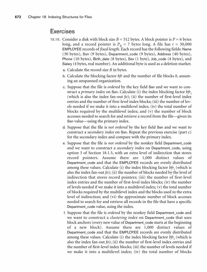
672 Chapter 18 Indexing Structures for Files
Exercises18.18. Consider a disk with block size B = 512 bytes. A block pointer is P = 6 bytes
long, and a record pointer is PR = 7 bytes long. A file has r = 30,000EMPLOYEE records of fixed length. Each record has the following fields: Name(30 bytes), Ssn (9 bytes), Department_code (9 bytes), Address (40 bytes),Phone (10 bytes), Birth_date (8 bytes), Sex (1 byte), Job_code (4 bytes), andSalary (4 bytes, real number). An additional byte is used as a deletion marker.
a. Calculate the record size R in bytes.
b. Calculate the blocking factor bfr and the number of file blocks b, assum-ing an unspanned organization.
c. Suppose that the file is ordered by the key field Ssn and we want to con-struct a primary index on Ssn. Calculate (i) the index blocking factor bfri(which is also the index fan-out fo); (ii) the number of first-level indexentries and the number of first-level index blocks; (iii) the number of lev-els needed if we make it into a multilevel index; (iv) the total number ofblocks required by the multilevel index; and (v) the number of blockaccesses needed to search for and retrieve a record from the file—given itsSsn value—using the primary index.
d. Suppose that the file is not ordered by the key field Ssn and we want toconstruct a secondary index on Ssn. Repeat the previous exercise (part c)for the secondary index and compare with the primary index.
e. Suppose that the file is not ordered by the nonkey field Department_codeand we want to construct a secondary index on Department_code, usingoption 3 of Section 18.1.3, with an extra level of indirection that storesrecord pointers. Assume there are 1,000 distinct values ofDepartment_code and that the EMPLOYEE records are evenly distributedamong these values. Calculate (i) the index blocking factor bfri (which isalso the index fan-out fo); (ii) the number of blocks needed by the level ofindirection that stores record pointers; (iii) the number of first-levelindex entries and the number of first-level index blocks; (iv) the numberof levels needed if we make it into a multilevel index; (v) the total numberof blocks required by the multilevel index and the blocks used in the extralevel of indirection; and (vi) the approximate number of block accessesneeded to search for and retrieve all records in the file that have a specificDepartment_code value, using the index.
f. Suppose that the file is ordered by the nonkey field Department_code andwe want to construct a clustering index on Department_code that usesblock anchors (every new value of Department_code starts at the beginningof a new block). Assume there are 1,000 distinct values ofDepartment_code and that the EMPLOYEE records are evenly distributedamong these values. Calculate (i) the index blocking factor bfri (which isalso the index fan-out fo); (ii) the number of first-level index entries andthe number of first-level index blocks; (iii) the number of levels needed ifwe make it into a multilevel index; (iv) the total number of blocks
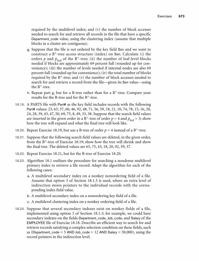
Exercises 673
required by the multilevel index; and (v) the number of block accessesneeded to search for and retrieve all records in the file that have a specificDepartment_code value, using the clustering index (assume that multipleblocks in a cluster are contiguous).
g. Suppose that the file is not ordered by the key field Ssn and we want toconstruct a B+-tree access structure (index) on Ssn. Calculate (i) theorders p and pleaf of the B+-tree; (ii) the number of leaf-level blocksneeded if blocks are approximately 69 percent full (rounded up for con-venience); (iii) the number of levels needed if internal nodes are also 69percent full (rounded up for convenience); (iv) the total number of blocksrequired by the B+-tree; and (v) the number of block accesses needed tosearch for and retrieve a record from the file—given its Ssn value—usingthe B+-tree.
h. Repeat part g, but for a B-tree rather than for a B+-tree. Compare yourresults for the B-tree and for the B+-tree.
18.19. A PARTS file with Part# as the key field includes records with the followingPart# values: 23, 65, 37, 60, 46, 92, 48, 71, 56, 59, 18, 21, 10, 74, 78, 15, 16, 20,24, 28, 39, 43, 47, 50, 69, 75, 8, 49, 33, 38. Suppose that the search field valuesare inserted in the given order in a B+-tree of order p = 4 and pleaf = 3; showhow the tree will expand and what the final tree will look like.
18.20. Repeat Exercise 18.19, but use a B-tree of order p = 4 instead of a B+-tree.
18.21. Suppose that the following search field values are deleted, in the given order,from the B+-tree of Exercise 18.19; show how the tree will shrink and showthe final tree. The deleted values are 65, 75, 43, 18, 20, 92, 59, 37.
18.22. Repeat Exercise 18.21, but for the B-tree of Exercise 18.20.
18.23. Algorithm 18.1 outlines the procedure for searching a nondense multilevelprimary index to retrieve a file record. Adapt the algorithm for each of thefollowing cases:
a. A multilevel secondary index on a nonkey nonordering field of a file.Assume that option 3 of Section 18.1.3 is used, where an extra level ofindirection stores pointers to the individual records with the corres-ponding index field value.
b. A multilevel secondary index on a nonordering key field of a file.
c. A multilevel clustering index on a nonkey ordering field of a file.
18.24. Suppose that several secondary indexes exist on nonkey fields of a file,implemented using option 3 of Section 18.1.3; for example, we could havesecondary indexes on the fields Department_code, Job_code, and Salary of theEMPLOYEE file of Exercise 18.18. Describe an efficient way to search for andretrieve records satisfying a complex selection condition on these fields, suchas (Department_code = 5 AND Job_code = 12 AND Salary = 50,000), using therecord pointers in the indirection level.
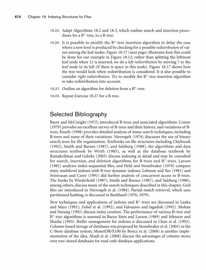
674 Chapter 18 Indexing Structures for Files
18.25. Adapt Algorithms 18.2 and 18.3, which outline search and insertion proce-dures for a B+-tree, to a B-tree.
18.26. It is possible to modify the B+-tree insertion algorithm to delay the casewhere a new level is produced by checking for a possible redistribution of val-ues among the leaf nodes. Figure 18.17 (next page) illustrates how this couldbe done for our example in Figure 18.12; rather than splitting the leftmostleaf node when 12 is inserted, we do a left redistribution by moving 7 to theleaf node to its left (if there is space in this node). Figure 18.17 shows howthe tree would look when redistribution is considered. It is also possible toconsider right redistribution. Try to modify the B+-tree insertion algorithmto take redistribution into account.
18.27. Outline an algorithm for deletion from a B+-tree.
18.28. Repeat Exercise 18.27 for a B-tree.
Selected BibliographyBayer and McCreight (1972) introduced B-trees and associated algorithms. Comer(1979) provides an excellent survey of B-trees and their history, and variations of B-trees. Knuth (1998) provides detailed analysis of many search techniques, includingB-trees and some of their variations. Nievergelt (1974) discusses the use of binarysearch trees for file organization. Textbooks on file structures including Claybrook(1992), Smith and Barnes (1987), and Salzberg (1988), the algorithms and datastructures textbook by Wirth (1985), as well as the database textbook byRamakrihnan and Gehrke (2003) discuss indexing in detail and may be consultedfor search, insertion, and deletion algorithms for B-trees and B+-trees. Larson(1981) analyzes index-sequential files, and Held and Stonebraker (1978) comparestatic multilevel indexes with B-tree dynamic indexes. Lehman and Yao (1981) andSrinivasan and Carey (1991) did further analysis of concurrent access to B-trees.The books by Wiederhold (1987), Smith and Barnes (1987), and Salzberg (1988),among others, discuss many of the search techniques described in this chapter. Gridfiles are introduced in Nievergelt et al. (1984). Partial-match retrieval, which usespartitioned hashing, is discussed in Burkhard (1976, 1979).
New techniques and applications of indexes and B+-trees are discussed in Lankaand Mays (1991), Zobel et al. (1992), and Faloutsos and Jagadish (1992). Mohanand Narang (1992) discuss index creation. The performance of various B–tree andB+-tree algorithms is assessed in Baeza-Yates and Larson (1989) and Johnson andShasha (1993). Buffer management for indexes is discussed in Chan et al. (1992).Column-based storage of databases was proposed by Stonebraker et al. (2005) in theC-Store database system; MonetDB/X100 by Boncz et al. (2008) is another imple-mentation of the idea. Abadi et al. (2008) discuss the advantages of column storesover row-stored databases for read-only database applications.
Selected Bibliography 675
1 0 3 0 5 0 7 0 8 0
3 5
Insert 12: overflow (leftredistribution)
Insert 9: overflow (new level)
Insert 6: overflow (split)
1 0 3 0 5 0 7 0 8 0 12 0
1 0 3 0 5 0 7 0 8 0 9 0 12 0
12 0
3 7
3 9
7
1 0 3 0 5 0 6 0 7 0 8 0 9 0
3 6 9
7
Figure 18.17B+-tree insertion with left redistribution.
Query Processing andOptimization, and Database Tuning
part8
679
Algorithms for Query Processing and Optimization
In this chapter we discuss the techniques used inter-nally by a DBMS to process, optimize, and execute
high-level queries. A query expressed in a high-level query language such as SQLmust first be scanned, parsed, and validated.1 The scanner identifies the querytokens—such as SQL keywords, attribute names, and relation names—that appearin the text of the query, whereas the parser checks the query syntax to determinewhether it is formulated according to the syntax rules (rules of grammar) of thequery language. The query must also be validated by checking that all attribute andrelation names are valid and semantically meaningful names in the schema of theparticular database being queried. An internal representation of the query is thencreated, usually as a tree data structure called a query tree. It is also possible to rep-resent the query using a graph data structure called a query graph. The DBMS mustthen devise an execution strategy or query plan for retrieving the results of thequery from the database files. A query typically has many possible execution strate-gies, and the process of choosing a suitable one for processing a query is known asquery optimization.
Figure 19.1 shows the different steps of processing a high-level query. The queryoptimizer module has the task of producing a good execution plan, and the codegenerator generates the code to execute that plan. The runtime database processorhas the task of running (executing) the query code, whether in compiled or inter-preted mode, to produce the query result. If a runtime error results, an error mes-sage is generated by the runtime database processor.
19chapter 19
1We will not discuss the parsing and syntax-checking phase of query processing here; this material isdiscussed in compiler textbooks.
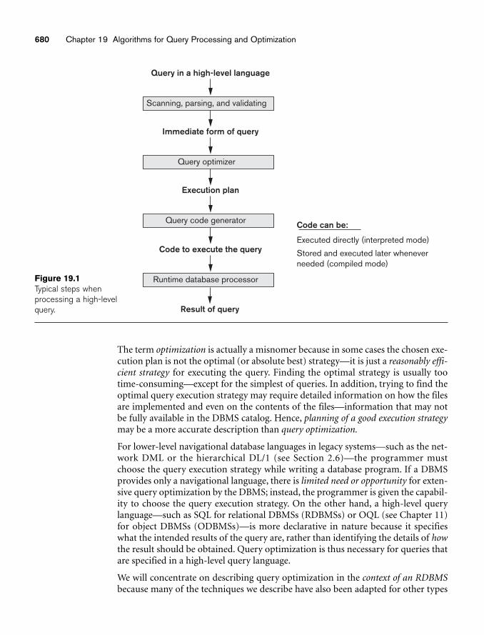
680 Chapter 19 Algorithms for Query Processing and Optimization
The term optimization is actually a misnomer because in some cases the chosen exe-cution plan is not the optimal (or absolute best) strategy—it is just a reasonably effi-cient strategy for executing the query. Finding the optimal strategy is usually tootime-consuming—except for the simplest of queries. In addition, trying to find theoptimal query execution strategy may require detailed information on how the filesare implemented and even on the contents of the files—information that may notbe fully available in the DBMS catalog. Hence, planning of a good execution strategymay be a more accurate description than query optimization.
For lower-level navigational database languages in legacy systems—such as the net-work DML or the hierarchical DL/1 (see Section 2.6)—the programmer mustchoose the query execution strategy while writing a database program. If a DBMSprovides only a navigational language, there is limited need or opportunity for exten-sive query optimization by the DBMS; instead, the programmer is given the capabil-ity to choose the query execution strategy. On the other hand, a high-level querylanguage—such as SQL for relational DBMSs (RDBMSs) or OQL (see Chapter 11)for object DBMSs (ODBMSs)—is more declarative in nature because it specifieswhat the intended results of the query are, rather than identifying the details of howthe result should be obtained. Query optimization is thus necessary for queries thatare specified in a high-level query language.
We will concentrate on describing query optimization in the context of an RDBMSbecause many of the techniques we describe have also been adapted for other types
Query in a high-level language
Scanning, parsing, and validating
Immediate form of query
Query optimizer
Execution plan
Query code generator
Code to execute the query
Runtime database processor
Code can be:
Executed directly (interpreted mode)
Stored and executed later wheneverneeded (compiled mode)
Result of query
Figure 19.1Typical steps when processing a high-levelquery.
19.1 Translating SQL Queries into Relational Algebra 681
2There are some query optimization problems and techniques that are pertinent only to ODBMSs.However, we do not discuss them here because we give only an introduction to query optimization.
of database management systems, such as ODBMSs.2 A relational DBMS must sys-tematically evaluate alternative query execution strategies and choose a reasonablyefficient or near-optimal strategy. Each DBMS typically has a number of generaldatabase access algorithms that implement relational algebra operations such asSELECT or JOIN (see Chapter 6) or combinations of these operations. Only execu-tion strategies that can be implemented by the DBMS access algorithms and thatapply to the particular query, as well as to the particular physical database design, canbe considered by the query optimization module.
This chapter starts with a general discussion of how SQL queries are typically trans-lated into relational algebra queries and then optimized in Section 19.1. Then wediscuss algorithms for implementing relational algebra operations in Sections 19.2through 19.6. Following this, we give an overview of query optimization strategies.There are two main techniques that are employed during query optimization. Thefirst technique is based on heuristic rules for ordering the operations in a queryexecution strategy. A heuristic is a rule that works well in most cases but is not guar-anteed to work well in every case. The rules typically reorder the operations in aquery tree. The second technique involves systematically estimating the cost of dif-ferent execution strategies and choosing the execution plan with the lowest cost esti-mate. These techniques are usually combined in a query optimizer. We discussheuristic optimization in Section 19.7 and cost estimation in Section 19.8. Then weprovide a brief overview of the factors considered during query optimization in theOracle commercial RDBMS in Section 19.9. Section 19.10 introduces the topic ofsemantic query optimization, in which known constraints are used as an aid todevising efficient query execution strategies.
The topics covered in this chapter require that the reader be familiar with the mate-rial presented in several earlier chapters. In particular, the chapters on SQL(Chapters 4 and 5), relational algebra (Chapter 6), and file structures and indexing(Chapters 17 and 18) are a prerequisite to this chapter. Also, it is important to notethat the topic of query processing and optimization is vast, and we can only give anintroduction to the basic principles and techniques in this chapter.
19.1 Translating SQL Queries into RelationalAlgebra
In practice, SQL is the query language that is used in most commercial RDBMSs. AnSQL query is first translated into an equivalent extended relational algebra expres-sion—represented as a query tree data structure—that is then optimized. Typically,SQL queries are decomposed into query blocks, which form the basic units that canbe translated into the algebraic operators and optimized. A query block contains asingle SELECT-FROM-WHERE expression, as well as GROUP BY and HAVING clausesif these are part of the block. Hence, nested queries within a query are identified as
682 Chapter 19 Algorithms for Query Processing and Optimization
separate query blocks. Because SQL includes aggregate operators—such as MAX,MIN, SUM, and COUNT—these operators must also be included in the extendedalgebra, as we discussed in Section 6.4.
Consider the following SQL query on the EMPLOYEE relation in Figure 3.5:
SELECT Lname, FnameFROM EMPLOYEEWHERE Salary > ( SELECT MAX (Salary)
FROM EMPLOYEEWHERE Dno=5 );
This query retrieves the names of employees (from any department in the com-pany) who earn a salary that is greater than the highest salary in department 5. Thequery includes a nested subquery and hence would be decomposed into two blocks.The inner block is:
( SELECT MAX (Salary)FROM EMPLOYEEWHERE Dno=5 )
This retrieves the highest salary in department 5. The outer query block is:
SELECT Lname, FnameFROM EMPLOYEEWHERE Salary > c
where c represents the result returned from the inner block. The inner block couldbe translated into the following extended relational algebra expression:
ℑMAX Salary(σDno=5(EMPLOYEE))
and the outer block into the expression:
πLname,Fname(σSalary>c(EMPLOYEE))
The query optimizer would then choose an execution plan for each query block.Notice that in the above example, the inner block needs to be evaluated only once toproduce the maximum salary of employees in department 5, which is then used—asthe constant c—by the outer block. We called this a nested query (without correlationwith the outer query) in Section 5.1.2. It is much harder to optimize the more com-plex correlated nested queries (see Section 5.1.3), where a tuple variable from theouter query block appears in the WHERE-clause of the inner query block.
19.2 Algorithms for External SortingSorting is one of the primary algorithms used in query processing. For example,whenever an SQL query specifies an ORDER BY-clause, the query result must besorted. Sorting is also a key component in sort-merge algorithms used for JOIN andother operations (such as UNION and INTERSECTION), and in duplicate eliminationalgorithms for the PROJECT operation (when an SQL query specifies the DISTINCT
19.2 Algorithms for External Sorting 683
option in the SELECT clause). We will discuss one of these algorithms in this sec-tion. Note that sorting of a particular file may be avoided if an appropriate index—such as a primary or clustering index (see Chapter 18)—exists on the desired fileattribute to allow ordered access to the records of the file.
External sorting refers to sorting algorithms that are suitable for large files ofrecords stored on disk that do not fit entirely in main memory, such as most data-base files.3 The typical external sorting algorithm uses a sort-merge strategy, whichstarts by sorting small subfiles—called runs—of the main file and then merges thesorted runs, creating larger sorted subfiles that are merged in turn. The sort-mergealgorithm, like other database algorithms, requires buffer space in main memory,where the actual sorting and merging of the runs is performed. The basic algorithm,outlined in Figure 19.2, consists of two phases: the sorting phase and the mergingphase. The buffer space in main memory is part of the DBMS cache—an area in thecomputer’s main memory that is controlled by the DBMS. The buffer space isdivided into individual buffers, where each buffer is the same size in bytes as the sizeof one disk block. Thus, one buffer can hold the contents of exactly one disk block.
In the sorting phase, runs (portions or pieces) of the file that can fit in the availablebuffer space are read into main memory, sorted using an internal sorting algorithm,and written back to disk as temporary sorted subfiles (or runs). The size of each runand the number of initial runs (nR) are dictated by the number of file blocks (b)and the available buffer space (nB). For example, if the number of available mainmemory buffers nB = 5 disk blocks and the size of the file b = 1024 disk blocks, thennR= ⎡(b/nB)⎤ or 205 initial runs each of size 5 blocks (except the last run which willhave only 4 blocks). Hence, after the sorting phase, 205 sorted runs (or 205 sortedsubfiles of the original file) are stored as temporary subfiles on disk.
In the merging phase, the sorted runs are merged during one or more mergepasses. Each merge pass can have one or more merge steps. The degree of merging(dM) is the number of sorted subfiles that can be merged in each merge step. Duringeach merge step, one buffer block is needed to hold one disk block from each of thesorted subfiles being merged, and one additional buffer is needed for containingone disk block of the merge result, which will produce a larger sorted file that is theresult of merging several smaller sorted subfiles. Hence, dM is the smaller of (nB − 1)and nR, and the number of merge passes is ⎡(logdM(nR))⎤. In our example where nB =5, dM = 4 (four-way merging), so the 205 initial sorted runs would be merged 4 at atime in each step into 52 larger sorted subfiles at the end of the first merge pass.These 52 sorted files are then merged 4 at a time into 13 sorted files, which are thenmerged into 4 sorted files, and then finally into 1 fully sorted file, which means thatfour passes are needed.
3Internal sorting algorithms are suitable for sorting data structures, such as tables and lists, that can fitentirely in main memory. These algorithms are described in detail in data structures and algorithmsbooks, and include techniques such as quick sort, heap sort, bubble sort, and many others. We do notdiscuss these here.
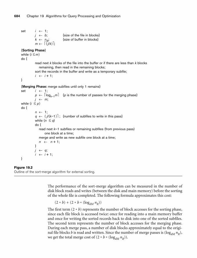
684 Chapter 19 Algorithms for Query Processing and Optimization
set i ← 1;j ← b; {size of the file in blocks}k ← nB; {size of buffer in blocks}m ← ⎡( j/k)⎤;
{Sorting Phase}while (i ≤ m)do {
read next k blocks of the file into the buffer or if there are less than k blocksremaining, then read in the remaining blocks;
sort the records in the buffer and write as a temporary subfile;i ← i + 1;
}
{Merging Phase: merge subfiles until only 1 remains}set i ← 1;
p ← ⎡logk–1m⎤ {p is the number of passes for the merging phase}j ← m;
while (i ≤ p)do {
n ← 1;q ← ( j/(k–1)⎤ ; {number of subfiles to write in this pass}while (n ≤ q)do {
read next k–1 subfiles or remaining subfiles (from previous pass)one block at a time;
merge and write as new subfile one block at a time;n ← n + 1;
}j ← q;i ← i + 1;
}
Figure 19.2Outline of the sort-merge algorithm for external sorting.
The performance of the sort-merge algorithm can be measured in the number ofdisk block reads and writes (between the disk and main memory) before the sortingof the whole file is completed. The following formula approximates this cost:
(2 * b) + (2 * b * (logdM nR))
The first term (2 * b) represents the number of block accesses for the sorting phase,since each file block is accessed twice: once for reading into a main memory bufferand once for writing the sorted records back to disk into one of the sorted subfiles.The second term represents the number of block accesses for the merging phase.During each merge pass, a number of disk blocks approximately equal to the origi-nal file blocks b is read and written. Since the number of merge passes is (logdM nR),we get the total merge cost of (2 * b * (logdM nR)).
19.3 Algorithms for SELECT and JOIN Operations 685
The minimum number of main memory buffers needed is nB = 3, which gives a dMof 2 and an nR of ⎡(b/3)⎤. The minimum dM of 2 gives the worst-case performanceof the algorithm, which is:
(2 * b) + (2 * (b * (log2 nR))).
The following sections discuss the various algorithms for the operations of the rela-tional algebra (see Chapter 6).
19.3 Algorithms for SELECT and JOINOperations
19.3.1 Implementing the SELECT OperationThere are many algorithms for executing a SELECT operation, which is basically asearch operation to locate the records in a disk file that satisfy a certain condition.Some of the search algorithms depend on the file having specific access paths, andthey may apply only to certain types of selection conditions. We discuss some of thealgorithms for implementing SELECT in this section. We will use the followingoperations, specified on the relational database in Figure 3.5, to illustrate our dis-cussion:
OP1: σSsn = ‘123456789’ (EMPLOYEE)
OP2: σDnumber > 5 (DEPARTMENT)
OP3: σDno = 5 (EMPLOYEE)
OP4: σDno = 5 AND Salary > 30000 AND Sex = ‘F’ (EMPLOYEE)
OP5: σEssn=‘123456789’ AND Pno =10(WORKS_ON)
Search Methods for Simple Selection. A number of search algorithms are pos-sible for selecting records from a file. These are also known as file scans, becausethey scan the records of a file to search for and retrieve records that satisfy a selec-tion condition.4 If the search algorithm involves the use of an index, the indexsearch is called an index scan. The following search methods (S1 through S6) areexamples of some of the search algorithms that can be used to implement a selectoperation:
■ S1—Linear search (brute force algorithm). Retrieve every record in the file,and test whether its attribute values satisfy the selection condition. Since therecords are grouped into disk blocks, each disk block is read into a mainmemory buffer, and then a search through the records within the disk blockis conducted in main memory.
4A selection operation is sometimes called a filter, since it filters out the records in the file that do not
satisfy the selection condition.
686 Chapter 19 Algorithms for Query Processing and Optimization
■ S2—Binary search. If the selection condition involves an equality compari-son on a key attribute on which the file is ordered, binary search—which ismore efficient than linear search—can be used. An example is OP1 if Ssn isthe ordering attribute for the EMPLOYEE file.5
■ S3a—Using a primary index. If the selection condition involves an equalitycomparison on a key attribute with a primary index—for example, Ssn =‘123456789’ in OP1—use the primary index to retrieve the record. Note thatthis condition retrieves a single record (at most).
■ S3b—Using a hash key. If the selection condition involves an equality com-parison on a key attribute with a hash key—for example, Ssn = ‘123456789’in OP1—use the hash key to retrieve the record. Note that this conditionretrieves a single record (at most).
■ S4—Using a primary index to retrieve multiple records. If the comparisoncondition is >, >=, <, or <= on a key field with a primary index—for exam-ple, Dnumber > 5 in OP2—use the index to find the record satisfying the cor-responding equality condition (Dnumber = 5), then retrieve all subsequentrecords in the (ordered) file. For the condition Dnumber < 5, retrieve all thepreceding records.
■ S5—Using a clustering index to retrieve multiple records. If the selectioncondition involves an equality comparison on a nonkey attribute with aclustering index—for example, Dno = 5 in OP3—use the index to retrieve allthe records satisfying the condition.
■ S6—Using a secondary (B+-tree) index on an equality comparison. Thissearch method can be used to retrieve a single record if the indexing field is akey (has unique values) or to retrieve multiple records if the indexing field isnot a key. This can also be used for comparisons involving >, >=, <, or <=.
In Section 19.8, we discuss how to develop formulas that estimate the access cost ofthese search methods in terms of the number of block accesses and access time.Method S1 (linear search) applies to any file, but all the other methods depend onhaving the appropriate access path on the attribute used in the selection condition.Method S2 (binary search) requires the file to be sorted on the search attribute. Themethods that use an index (S3a, S4, S5, and S6) are generally referred to as indexsearches, and they require the appropriate index to exist on the search attribute.Methods S4 and S6 can be used to retrieve records in a certain range—for example,30000 <= Salary <= 35000. Queries involving such conditions are called rangequeries.
Search Methods for Complex Selection. If a condition of a SELECT operationis a conjunctive condition—that is, if it is made up of several simple conditions
5Generally, binary search is not used in database searches because ordered files are not used unlessthey also have a corresponding primary index.
19.3 Algorithms for SELECT and JOIN Operations 687
connected with the AND logical connective such as OP4 above—the DBMS can usethe following additional methods to implement the operation:
■ S7—Conjunctive selection using an individual index. If an attributeinvolved in any single simple condition in the conjunctive select conditionhas an access path that permits the use of one of the methods S2 to S6, usethat condition to retrieve the records and then check whether each retrievedrecord satisfies the remaining simple conditions in the conjunctive select condition.
■ S8—Conjunctive selection using a composite index. If two or more attrib-utes are involved in equality conditions in the conjunctive select conditionand a composite index (or hash structure) exists on the combined fields—for example, if an index has been created on the composite key (Essn, Pno) ofthe WORKS_ON file for OP5—we can use the index directly.
■ S9—Conjunctive selection by intersection of record pointers.6 If second-ary indexes (or other access paths) are available on more than one of thefields involved in simple conditions in the conjunctive select condition, andif the indexes include record pointers (rather than block pointers), then eachindex can be used to retrieve the set of record pointers that satisfy the indi-vidual condition. The intersection of these sets of record pointers gives therecord pointers that satisfy the conjunctive select condition, which are thenused to retrieve those records directly. If only some of the conditions havesecondary indexes, each retrieved record is further tested to determinewhether it satisfies the remaining conditions.7 In general, method S9assumes that each of the indexes is on a nonkey field of the file, because if oneof the conditions is an equality condition on a key field, only one record willsatisfy the whole condition.
Whenever a single condition specifies the selection—such as OP1, OP2, or OP3—the DBMS can only check whether or not an access path exists on the attributeinvolved in that condition. If an access path (such as index or hash key or sorted file)exists, the method corresponding to that access path is used; otherwise, the bruteforce, linear search approach of method S1 can be used. Query optimization for aSELECT operation is needed mostly for conjunctive select conditions whenevermore than one of the attributes involved in the conditions have an access path. Theoptimizer should choose the access path that retrieves the fewest records in the mostefficient way by estimating the different costs (see Section 19.8) and choosing themethod with the least estimated cost.
Selectivity of a Condition. When the optimizer is choosing between multiplesimple conditions in a conjunctive select condition, it typically considers the
6A record pointer uniquely identifies a record and provides the address of the record on disk; hence, it isalso called the record identifier or record id.7The technique can have many variations—for example, if the indexes are logical indexes that store pri-mary key values instead of record pointers.
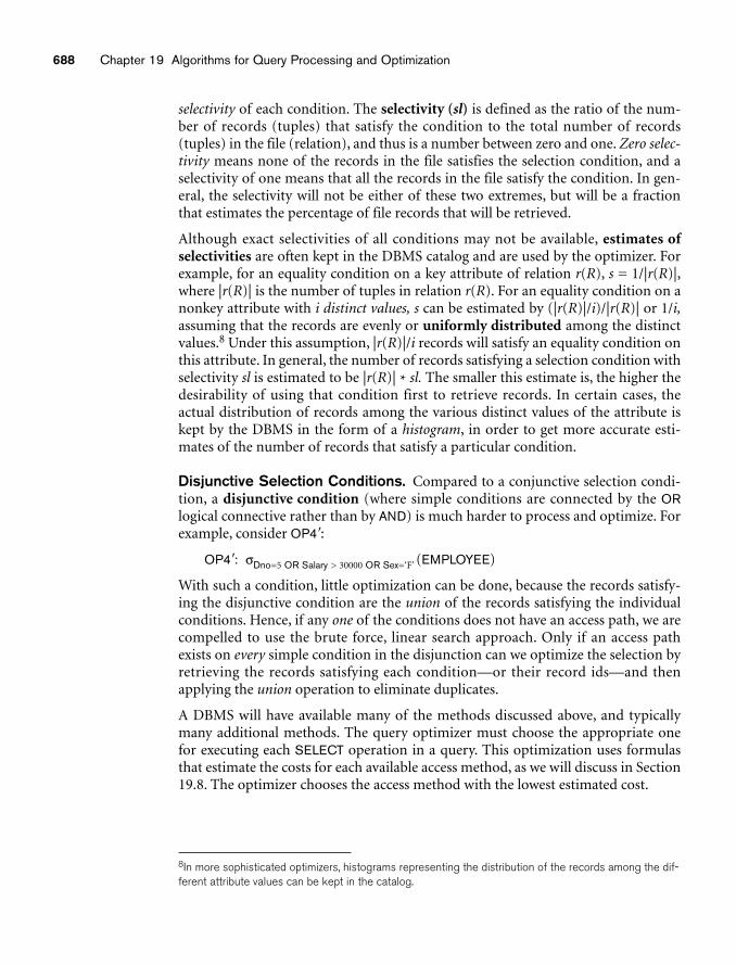
688 Chapter 19 Algorithms for Query Processing and Optimization
selectivity of each condition. The selectivity (sl) is defined as the ratio of the num-ber of records (tuples) that satisfy the condition to the total number of records(tuples) in the file (relation), and thus is a number between zero and one. Zero selec-tivity means none of the records in the file satisfies the selection condition, and aselectivity of one means that all the records in the file satisfy the condition. In gen-eral, the selectivity will not be either of these two extremes, but will be a fractionthat estimates the percentage of file records that will be retrieved.
Although exact selectivities of all conditions may not be available, estimates ofselectivities are often kept in the DBMS catalog and are used by the optimizer. Forexample, for an equality condition on a key attribute of relation r(R), s = 1/|r(R)|,where |r(R)| is the number of tuples in relation r(R). For an equality condition on anonkey attribute with i distinct values, s can be estimated by (|r(R)|/i)/|r(R)| or 1/i,assuming that the records are evenly or uniformly distributed among the distinctvalues.8 Under this assumption, |r(R)|/i records will satisfy an equality condition onthis attribute. In general, the number of records satisfying a selection condition withselectivity sl is estimated to be |r(R)| * sl. The smaller this estimate is, the higher thedesirability of using that condition first to retrieve records. In certain cases, theactual distribution of records among the various distinct values of the attribute iskept by the DBMS in the form of a histogram, in order to get more accurate esti-mates of the number of records that satisfy a particular condition.
Disjunctive Selection Conditions. Compared to a conjunctive selection condi-tion, a disjunctive condition (where simple conditions are connected by the ORlogical connective rather than by AND) is much harder to process and optimize. Forexample, consider OP4�:
OP4�: σDno=5 OR Salary > 30000 OR Sex=‘F’ (EMPLOYEE)
With such a condition, little optimization can be done, because the records satisfy-ing the disjunctive condition are the union of the records satisfying the individualconditions. Hence, if any one of the conditions does not have an access path, we arecompelled to use the brute force, linear search approach. Only if an access pathexists on every simple condition in the disjunction can we optimize the selection byretrieving the records satisfying each condition—or their record ids—and thenapplying the union operation to eliminate duplicates.
A DBMS will have available many of the methods discussed above, and typicallymany additional methods. The query optimizer must choose the appropriate onefor executing each SELECT operation in a query. This optimization uses formulasthat estimate the costs for each available access method, as we will discuss in Section19.8. The optimizer chooses the access method with the lowest estimated cost.
8In more sophisticated optimizers, histograms representing the distribution of the records among the dif-ferent attribute values can be kept in the catalog.
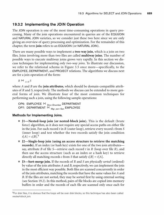
19.3 Algorithms for SELECT and JOIN Operations 689
19.3.2 Implementing the JOIN OperationThe JOIN operation is one of the most time-consuming operations in query pro-cessing. Many of the join operations encountered in queries are of the EQUIJOINand NATURAL JOIN varieties, so we consider just these two here since we are onlygiving an overview of query processing and optimization. For the remainder of thischapter, the term join refers to an EQUIJOIN (or NATURAL JOIN).
There are many possible ways to implement a two-way join, which is a join on twofiles. Joins involving more than two files are called multiway joins. The number ofpossible ways to execute multiway joins grows very rapidly. In this section we dis-cuss techniques for implementing only two-way joins. To illustrate our discussion,we refer to the relational schema in Figure 3.5 once more—specifically, to theEMPLOYEE, DEPARTMENT, and PROJECT relations. The algorithms we discuss nextare for a join operation of the form:
R A=B S
where A and B are the join attributes, which should be domain-compatible attrib-utes of R and S, respectively. The methods we discuss can be extended to more gen-eral forms of join. We illustrate four of the most common techniques forperforming such a join, using the following sample operations:
OP6: EMPLOYEE Dno=Dnumber DEPARTMENTOP7: DEPARTMENT Mgr_ssn=Ssn EMPLOYEE
Methods for Implementing Joins.
■ J1—Nested-loop join (or nested-block join). This is the default (bruteforce) algorithm, as it does not require any special access paths on either filein the join. For each record t in R (outer loop), retrieve every record s from S(inner loop) and test whether the two records satisfy the join condition t[A] = s[B].9
■ J2—Single-loop join (using an access structure to retrieve the matchingrecords). If an index (or hash key) exists for one of the two join attributes—say, attribute B of file S—retrieve each record t in R (loop over file R), andthen use the access structure (such as an index or a hash key) to retrievedirectly all matching records s from S that satisfy s[B] = t[A].
■ J3—Sort-merge join. If the records of R and S are physically sorted (ordered)by value of the join attributes A and B, respectively, we can implement the joinin the most efficient way possible. Both files are scanned concurrently in orderof the join attributes, matching the records that have the same values for A andB. If the files are not sorted, they may be sorted first by using external sorting(see Section 19.2). In this method, pairs of file blocks are copied into memorybuffers in order and the records of each file are scanned only once each for
9For disk files, it is obvious that the loops will be over disk blocks, so this technique has also been callednested-block join.
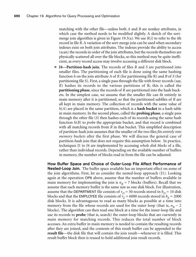
690 Chapter 19 Algorithms for Query Processing and Optimization
matching with the other file—unless both A and B are nonkey attributes, inwhich case the method needs to be modified slightly. A sketch of the sort-merge join algorithm is given in Figure 19.3(a). We use R(i) to refer to the ithrecord in file R. A variation of the sort-merge join can be used when secondaryindexes exist on both join attributes. The indexes provide the ability to access(scan) the records in order of the join attributes, but the records themselves arephysically scattered all over the file blocks, so this method may be quite ineffi-cient, as every record access may involve accessing a different disk block.
■ J4—Partition-hash join. The records of files R and S are partitioned intosmaller files. The partitioning of each file is done using the same hashingfunction h on the join attribute A of R (for partitioning file R) and B of S (forpartitioning file S). First, a single pass through the file with fewer records (say,R) hashes its records to the various partitions of R; this is called thepartitioning phase, since the records of R are partitioned into the hash buck-ets. In the simplest case, we assume that the smaller file can fit entirely inmain memory after it is partitioned, so that the partitioned subfiles of R areall kept in main memory. The collection of records with the same value ofh(A) are placed in the same partition, which is a hash bucket in a hash tablein main memory. In the second phase, called the probing phase, a single passthrough the other file (S) then hashes each of its records using the same hashfunction h(B) to probe the appropriate bucket, and that record is combinedwith all matching records from R in that bucket. This simplified descriptionof partition-hash join assumes that the smaller of the two files fits entirely intomemory buckets after the first phase. We will discuss the general case ofpartition-hash join that does not require this assumption below. In practice,techniques J1 to J4 are implemented by accessing whole disk blocks of a file,rather than individual records. Depending on the available number of buffersin memory, the number of blocks read in from the file can be adjusted.
How Buffer Space and Choice of Outer-Loop File Affect Performance ofNested-Loop Join. The buffer space available has an important effect on some ofthe join algorithms. First, let us consider the nested-loop approach (J1). Lookingagain at the operation OP6 above, assume that the number of buffers available inmain memory for implementing the join is nB = 7 blocks (buffers). Recall that weassume that each memory buffer is the same size as one disk block. For illustration,assume that the DEPARTMENT file consists of rD = 50 records stored in bD = 10 diskblocks and that the EMPLOYEE file consists of rE = 6000 records stored in bE = 2000disk blocks. It is advantageous to read as many blocks as possible at a time intomemory from the file whose records are used for the outer loop (that is, nB − 2blocks). The algorithm can then read one block at a time for the inner-loop file anduse its records to probe (that is, search) the outer-loop blocks that are currently inmain memory for matching records. This reduces the total number of blockaccesses. An extra buffer in main memory is needed to contain the resulting recordsafter they are joined, and the contents of this result buffer can be appended to theresult file—the disk file that will contain the join result—whenever it is filled. Thisresult buffer block then is reused to hold additional join result records.
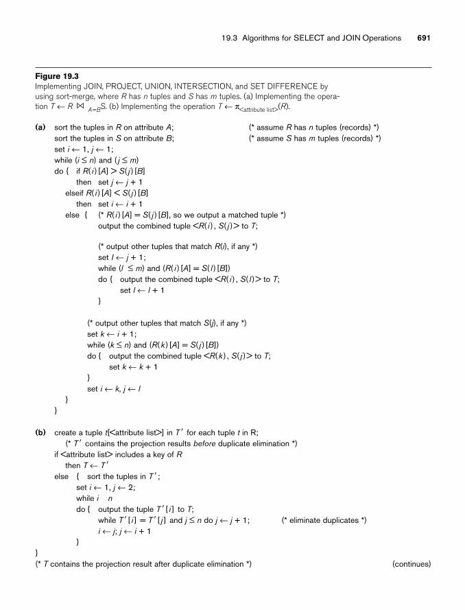
(a) sort the tuples in R on attribute A; (* assume R has n tuples (records) *)sort the tuples in S on attribute B; (* assume S has m tuples (records) *)set i ← 1, j ← 1;while (i ≤ n) and ( j ≤ m)do { if R( i ) [A] > S( j ) [B]
then set j ← j + 1elseif R( i ) [A] < S( j ) [B]
then set i ← i + 1else { (* R( i ) [A] = S( j ) [B], so we output a matched tuple *)
output the combined tuple <R( i ) , S( j )> to T;
(* output other tuples that match R(i), if any *)set I ← j + 1;while (l ≤ m) and (R( i ) [A] = S( l ) [B])do { output the combined tuple <R( i ) , S( l )> to T;
set l ← l + 1}
(* output other tuples that match S(j), if any *)set k ← i + 1;while (k ≤ n) and (R(k ) [A] = S( j ) [B])do { output the combined tuple <R(k ) , S( j )> to T;
set k ← k + 1}set i ← k, j ← l
}}
(b) create a tuple t[<attribute list>] in T� for each tuple t in R;(* T� contains the projection results before duplicate elimination *)
if <attribute list> includes a key of Rthen T ← T�
else { sort the tuples in T �;set i ← 1, j ← 2;while i ndo { output the tuple T�[ i ] to T;
while T�[ i ] = T �[ j ] and j ≤ n do j ← j + 1; (* eliminate duplicates *)i ← j; j ← i + 1
}}(* T contains the projection result after duplicate elimination *) (continues)
19.3 Algorithms for SELECT and JOIN Operations 691
Figure 19.3Implementing JOIN, PROJECT, UNION, INTERSECTION, and SET DIFFERENCE byusing sort-merge, where R has n tuples and S has m tuples. (a) Implementing the opera-tion T ← R A=BS. (b) Implementing the operation T ← π<attribute list>(R).
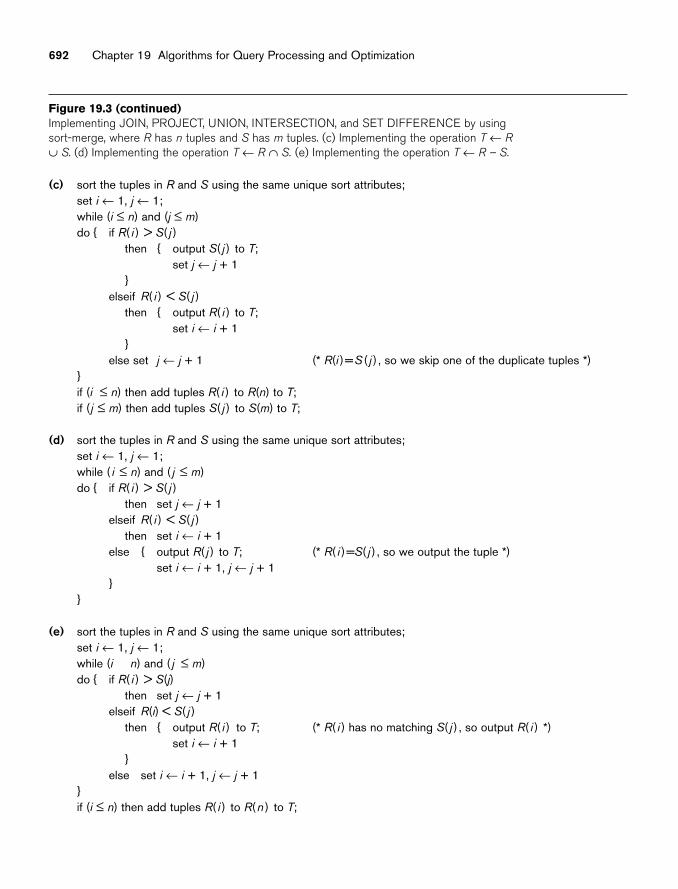
(c) sort the tuples in R and S using the same unique sort attributes;set i ← 1, j ← 1;while (i ≤ n) and (j ≤ m)do { if R( i ) > S( j )
then { output S( j ) to T;set j ← j + 1
}elseif R( i ) < S( j )
then { output R( i ) to T;set i ← i + 1
}else set j ← j + 1 (* R(i )=S ( j ) , so we skip one of the duplicate tuples *)
}if (i ≤ n) then add tuples R( i ) to R(n) to T;if (j ≤ m) then add tuples S( j ) to S(m) to T;
(d) sort the tuples in R and S using the same unique sort attributes;set i ← 1, j ← 1;while ( i ≤ n) and ( j ≤ m)do { if R( i ) > S( j )
then set j ← j + 1elseif R( i ) < S( j )
then set i ← i + 1else { output R( j ) to T; (* R( i )=S( j ) , so we output the tuple *)
set i ← i + 1, j ← j + 1}
}
(e) sort the tuples in R and S using the same unique sort attributes;set i ← 1, j ← 1;while (i n) and ( j ≤ m)do { if R( i ) > S(j)
then set j ← j + 1elseif R(i) < S( j )
then { output R( i ) to T; (* R( i ) has no matching S( j ) , so output R( i ) *)set i ← i + 1
}else set i ← i + 1, j ← j + 1
}if (i ≤ n) then add tuples R( i ) to R(n ) to T;
692 Chapter 19 Algorithms for Query Processing and Optimization
Figure 19.3 (continued)Implementing JOIN, PROJECT, UNION, INTERSECTION, and SET DIFFERENCE by usingsort-merge, where R has n tuples and S has m tuples. (c) Implementing the operation T ← R
∪ S. (d) Implementing the operation T ← R ∩ S. (e) Implementing the operation T ← R – S.
19.3 Algorithms for SELECT and JOIN Operations 693
In the nested-loop join, it makes a difference which file is chosen for the outer loopand which for the inner loop. If EMPLOYEE is used for the outer loop, each block ofEMPLOYEE is read once, and the entire DEPARTMENT file (each of its blocks) is readonce for each time we read in (nB – 2) blocks of the EMPLOYEE file. We get the follow-ing formulas for the number of disk blocks that are read from disk to main memory:
Total number of blocks accessed (read) for outer-loop file = bE
Number of times (nB − 2) blocks of outer file are loaded into main memory = ⎡bE/(nB – 2)⎤
Total number of blocks accessed (read) for inner-loop file = bD * ⎡bE/(nB – 2)⎤
Hence, we get the following total number of block read accesses:
bE + ( ⎡bE/(nB – 2)⎤ * bD) = 2000 + ( ⎡(2000/5)⎤ * 10) = 6000 block accesses
On the other hand, if we use the DEPARTMENT records in the outer loop, by symme-try we get the following total number of block accesses:
bD + ( ⎡bD/(nB – 2)⎤ * bE) = 10 + ( ⎡(10/5)⎤ * 2000) = 4010 block accesses
The join algorithm uses a buffer to hold the joined records of the result file. Oncethe buffer is filled, it is written to disk and its contents are appended to the resultfile, and then refilled with join result records.10
If the result file of the join operation has bRES disk blocks, each block is written onceto disk, so an additional bRES block accesses (writes) should be added to the preced-ing formulas in order to estimate the total cost of the join operation. The sameholds for the formulas developed later for other join algorithms. As this exampleshows, it is advantageous to use the file with fewer blocks as the outer-loop file in thenested-loop join.
How the Join Selection Factor Affects Join Performance. Another factor thataffects the performance of a join, particularly the single-loop method J2, is the frac-tion of records in one file that will be joined with records in the other file. We callthis the join selection factor11 of a file with respect to an equijoin condition withanother file. This factor depends on the particular equijoin condition between thetwo files. To illustrate this, consider the operation OP7, which joins eachDEPARTMENT record with the EMPLOYEE record for the manager of that depart-ment. Here, each DEPARTMENT record (there are 50 such records in our example)will be joined with a single EMPLOYEE record, but many EMPLOYEE records (the5,950 of them that do not manage a department) will not be joined with any recordfrom DEPARTMENT.
Suppose that secondary indexes exist on both the attributes Ssn of EMPLOYEE andMgr_ssn of DEPARTMENT, with the number of index levels xSsn = 4 and xMgr_ssn= 2,
10If we reserve two buffers for the result file, double buffering can be used to speed the algorithm (seeSection 17.3).11This is different from the join selectivity, which we will discuss in Section 19.8.
694 Chapter 19 Algorithms for Query Processing and Optimization
respectively. We have two options for implementing method J2. The first retrieveseach EMPLOYEE record and then uses the index on Mgr_ssn of DEPARTMENT to finda matching DEPARTMENT record. In this case, no matching record will be found foremployees who do not manage a department. The number of block accesses for thiscase is approximately:
bE + (rE * (xMgr_ssn + 1)) = 2000 + (6000 * 3) = 20,000 block accesses
The second option retrieves each DEPARTMENT record and then uses the index onSsn of EMPLOYEE to find a matching manager EMPLOYEE record. In this case, everyDEPARTMENT record will have one matching EMPLOYEE record. The number ofblock accesses for this case is approximately:
bD + (rD * (xSsn + 1)) = 10 + (50 * 5) = 260 block accesses
The second option is more efficient because the join selection factor ofDEPARTMENT with respect to the join condition Ssn = Mgr_ssn is 1 (every record inDEPARTMENT will be joined), whereas the join selection factor of EMPLOYEE withrespect to the same join condition is (50/6000), or 0.008 (only 0.8 percent of therecords in EMPLOYEE will be joined). For method J2, either the smaller file or thefile that has a match for every record (that is, the file with the high join selection fac-tor) should be used in the (single) join loop. It is also possible to create an indexspecifically for performing the join operation if one does not already exist.
The sort-merge join J3 is quite efficient if both files are already sorted by their joinattribute. Only a single pass is made through each file. Hence, the number of blocksaccessed is equal to the sum of the numbers of blocks in both files. For this method,both OP6 and OP7 would need bE + bD = 2000 + 10 = 2010 block accesses. However,both files are required to be ordered by the join attributes; if one or both are not, asorted copy of each file must be created specifically for performing the join opera-tion. If we roughly estimate the cost of sorting an external file by (b log2b) blockaccesses, and if both files need to be sorted, the total cost of a sort-merge join can beestimated by (bE + bD + bE log2bE + bD log2bD).12
General Case for Partition-Hash Join. The hash-join method J4 is also quiteefficient. In this case only a single pass is made through each file, whether or not thefiles are ordered. If the hash table for the smaller of the two files can be kept entirelyin main memory after hashing (partitioning) on its join attribute, the implementa-tion is straightforward. If, however, the partitions of both files must be stored ondisk, the method becomes more complex, and a number of variations to improvethe efficiency have been proposed. We discuss two techniques: the general case ofpartition-hash join and a variation called hybrid hash-join algorithm, which has beenshown to be quite efficient.
In the general case of partition-hash join, each file is first partitioned into M parti-tions using the same partitioning hash function on the join attributes. Then, each
12We can use the more accurate formulas from Section 19.2 if we know the number of available buffersfor sorting.
19.3 Algorithms for SELECT and JOIN Operations 695
pair of corresponding partitions is joined. For example, suppose we are joining rela-tions R and S on the join attributes R.A and S.B:
R A=B S
In the partitioning phase, R is partitioned into the M partitions R1, R2, ..., RM, andS into the M partitions S1, S2, ..., SM. The property of each pair of correspondingpartitions Ri, Si with respect to the join operation is that records in Ri only need to bejoined with records in Si, and vice versa. This property is ensured by using the samehash function to partition both files on their join attributes—attribute A for R andattribute B for S. The minimum number of in-memory buffers needed for thepartitioning phase is M + 1. Each of the files R and S are partitioned separately.During partitioning of a file, M in-memory buffers are allocated to store the recordsthat hash to each partition, and one additional buffer is needed to hold one block ata time of the input file being partitioned. Whenever the in-memory buffer for a par-tition gets filled, its contents are appended to a disk subfile that stores the partition.The partitioning phase has two iterations. After the first iteration, the first file R ispartitioned into the subfiles R1, R2, ..., RM, where all the records that hashed to thesame buffer are in the same partition. After the second iteration, the second file S issimilarly partitioned.
In the second phase, called the joining or probing phase, M iterations are needed.During iteration i, two corresponding partitions Ri and Si are joined. The minimumnumber of buffers needed for iteration i is the number of blocks in the smaller ofthe two partitions, say Ri, plus two additional buffers. If we use a nested-loop joinduring iteration i, the records from the smaller of the two partitions Ri are copiedinto memory buffers; then all blocks from the other partition Si are read—one at atime—and each record is used to probe (that is, search) partition Ri for matchingrecord(s). Any matching records are joined and written into the result file. Toimprove the efficiency of in-memory probing, it is common to use an in-memoryhash table for storing the records in partition Ri by using a different hash functionfrom the partitioning hash function.13
We can approximate the cost of this partition hash-join as 3 * (bR + bS) + bRES forour example, since each record is read once and written back to disk once during thepartitioning phase. During the joining (probing) phase, each record is read a secondtime to perform the join. The main difficulty of this algorithm is to ensure that thepartitioning hash function is uniform—that is, the partition sizes are nearly equalin size. If the partitioning function is skewed (nonuniform), then some partitionsmay be too large to fit in the available memory space for the second joining phase.
Notice that if the available in-memory buffer space nB > (bR + 2), where bR is thenumber of blocks for the smaller of the two files being joined, say R, then there is noreason to do partitioning since in this case the join can be performed entirely inmemory using some variation of the nested-loop join based on hashing and probing.
13If the hash function used for partitioning is used again, all records in a partition will hash to the samebucket again.
696 Chapter 19 Algorithms for Query Processing and Optimization
For illustration, assume we are performing the join operation OP6, repeated below:
OP6: EMPLOYEE Dno=Dnumber DEPARTMENT
In this example, the smaller file is the DEPARTMENT file; hence, if the number ofavailable memory buffers nB > (bD + 2), the whole DEPARTMENT file can be readinto main memory and organized into a hash table on the join attribute. EachEMPLOYEE block is then read into a buffer, and each EMPLOYEE record in the bufferis hashed on its join attribute and is used to probe the corresponding in-memorybucket in the DEPARTMENT hash table. If a matching record is found, the recordsare joined, and the result record(s) are written to the result buffer and eventually tothe result file on disk. The cost in terms of block accesses is hence (bD + bE), plusbRES—the cost of writing the result file.
Hybrid Hash-Join. The hybrid hash-join algorithm is a variation of partitionhash-join, where the joining phase for one of the partitions is included in thepartitioning phase. To illustrate this, let us assume that the size of a memory bufferis one disk block; that nB such buffers are available; and that the partitioning hashfunction used is h(K) = K mod M, so that M partitions are being created, where M< nB. For illustration, assume we are performing the join operation OP6. In the firstpass of the partitioning phase, when the hybrid hash-join algorithm is partitioningthe smaller of the two files (DEPARTMENT in OP6), the algorithm divides the bufferspace among the M partitions such that all the blocks of the first partition ofDEPARTMENT completely reside in main memory. For each of the other partitions,only a single in-memory buffer—whose size is one disk block—is allocated; theremainder of the partition is written to disk as in the regular partition-hash join.Hence, at the end of the first pass of the partitioning phase, the first partition ofDEPARTMENT resides wholly in main memory, whereas each of the other partitionsof DEPARTMENT resides in a disk subfile.
For the second pass of the partitioning phase, the records of the second file beingjoined—the larger file, EMPLOYEE in OP6—are being partitioned. If a recordhashes to the first partition, it is joined with the matching record in DEPARTMENTand the joined records are written to the result buffer (and eventually to disk). If anEMPLOYEE record hashes to a partition other than the first, it is partitioned nor-mally and stored to disk. Hence, at the end of the second pass of the partitioningphase, all records that hash to the first partition have been joined. At this point,there are M − 1 pairs of partitions on disk. Therefore, during the second joining orprobing phase, M − 1 iterations are needed instead of M. The goal is to join as manyrecords during the partitioning phase so as to save the cost of storing those recordson disk and then rereading them a second time during the joining phase.
19.4 Algorithms for PROJECT and SetOperations
A PROJECT operation π<attribute list>(R) is straightforward to implement if <attributelist> includes a key of relation R, because in this case the result of the operation will
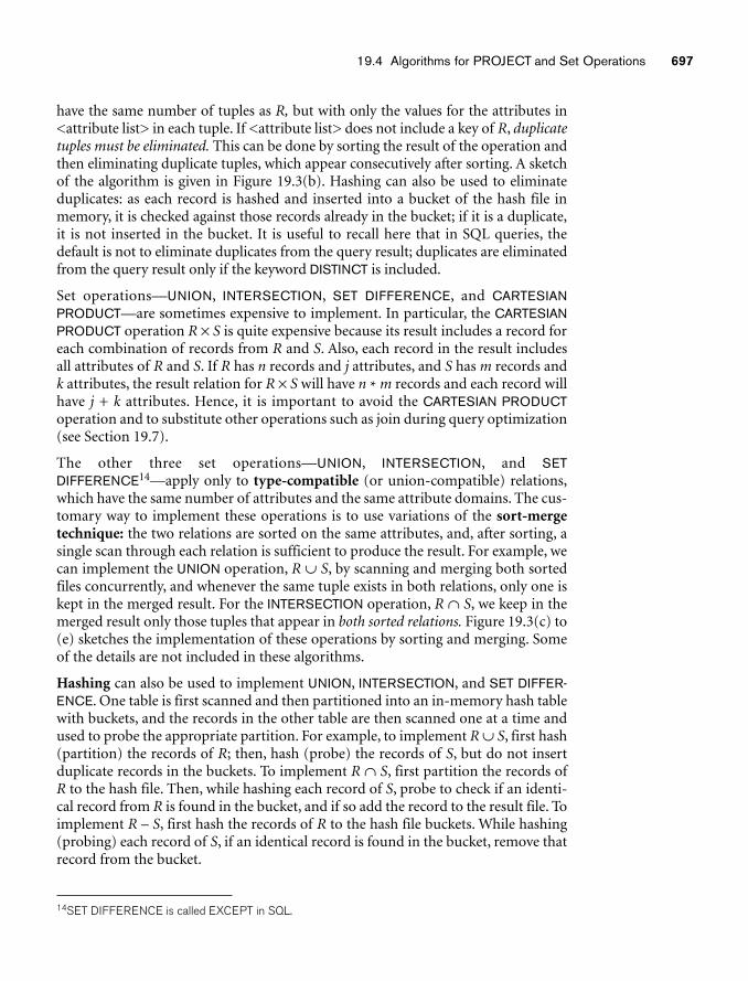
19.4 Algorithms for PROJECT and Set Operations 697
have the same number of tuples as R, but with only the values for the attributes in<attribute list> in each tuple. If <attribute list> does not include a key of R, duplicatetuples must be eliminated. This can be done by sorting the result of the operation andthen eliminating duplicate tuples, which appear consecutively after sorting. A sketchof the algorithm is given in Figure 19.3(b). Hashing can also be used to eliminateduplicates: as each record is hashed and inserted into a bucket of the hash file inmemory, it is checked against those records already in the bucket; if it is a duplicate,it is not inserted in the bucket. It is useful to recall here that in SQL queries, thedefault is not to eliminate duplicates from the query result; duplicates are eliminatedfrom the query result only if the keyword DISTINCT is included.
Set operations—UNION, INTERSECTION, SET DIFFERENCE, and CARTESIANPRODUCT—are sometimes expensive to implement. In particular, the CARTESIANPRODUCT operation R × S is quite expensive because its result includes a record foreach combination of records from R and S. Also, each record in the result includesall attributes of R and S. If R has n records and j attributes, and S has m records andk attributes, the result relation for R × S will have n * m records and each record willhave j + k attributes. Hence, it is important to avoid the CARTESIAN PRODUCToperation and to substitute other operations such as join during query optimization(see Section 19.7).
The other three set operations—UNION, INTERSECTION, and SETDIFFERENCE14—apply only to type-compatible (or union-compatible) relations,which have the same number of attributes and the same attribute domains. The cus-tomary way to implement these operations is to use variations of the sort-mergetechnique: the two relations are sorted on the same attributes, and, after sorting, asingle scan through each relation is sufficient to produce the result. For example, wecan implement the UNION operation, R ∪ S, by scanning and merging both sortedfiles concurrently, and whenever the same tuple exists in both relations, only one iskept in the merged result. For the INTERSECTION operation, R ∩ S, we keep in themerged result only those tuples that appear in both sorted relations. Figure 19.3(c) to(e) sketches the implementation of these operations by sorting and merging. Someof the details are not included in these algorithms.
Hashing can also be used to implement UNION, INTERSECTION, and SET DIFFER-ENCE. One table is first scanned and then partitioned into an in-memory hash tablewith buckets, and the records in the other table are then scanned one at a time andused to probe the appropriate partition. For example, to implement R ∪ S, first hash(partition) the records of R; then, hash (probe) the records of S, but do not insertduplicate records in the buckets. To implement R ∩ S, first partition the records ofR to the hash file. Then, while hashing each record of S, probe to check if an identi-cal record from R is found in the bucket, and if so add the record to the result file. Toimplement R – S, first hash the records of R to the hash file buckets. While hashing(probing) each record of S, if an identical record is found in the bucket, remove thatrecord from the bucket.
14SET DIFFERENCE is called EXCEPT in SQL.
698 Chapter 19 Algorithms for Query Processing and Optimization
In SQL, there are two variations of these set operations. The operations UNION,INTERSECTION, and EXCEPT (the SQL keyword for the SET DIFFERENCE opera-tion) apply to traditional sets, where no duplicate records exist in the result. Theoperations UNION ALL, INTERSECTION ALL, and EXCEPT ALL apply to multisets (orbags), and duplicates are fully considered. Variations of the above algorithms can beused for the multiset operations in SQL. We leave these as an exercise for the reader.
19.5 Implementing Aggregate Operations and OUTER JOINs
19.5.1 Implementing Aggregate OperationsThe aggregate operators (MIN, MAX, COUNT, AVERAGE, SUM), when applied to anentire table, can be computed by a table scan or by using an appropriate index, ifavailable. For example, consider the following SQL query:
SELECT MAX(Salary)FROM EMPLOYEE;
If an (ascending) B+-tree index on Salary exists for the EMPLOYEE relation, then theoptimizer can decide on using the Salary index to search for the largest Salary valuein the index by following the rightmost pointer in each index node from the root tothe rightmost leaf. That node would include the largest Salary value as its last entry.In most cases, this would be more efficient than a full table scan of EMPLOYEE, sinceno actual records need to be retrieved. The MIN function can be handled in a similarmanner, except that the leftmost pointer in the index is followed from the root toleftmost leaf. That node would include the smallest Salary value as its first entry.
The index could also be used for the AVERAGE and SUM aggregate functions, butonly if it is a dense index—that is, if there is an index entry for every record in themain file. In this case, the associated computation would be applied to the values inthe index. For a nondense index, the actual number of records associated with eachindex value must be used for a correct computation. This can be done if the numberof records associated with each value in the index is stored in each index entry. For theCOUNT aggregate function, the number of values can be also computed from theindex in a similar manner. If a COUNT(*) function is applied to a whole relation, thenumber of records currently in each relation are typically stored in the catalog, andso the result can be retrieved directly from the catalog.
When a GROUP BY clause is used in a query, the aggregate operator must be appliedseparately to each group of tuples as partitioned by the grouping attribute. Hence,the table must first be partitioned into subsets of tuples, where each partition(group) has the same value for the grouping attributes. In this case, the computa-tion is more complex. Consider the following query:
SELECT Dno, AVG(Salary)FROM EMPLOYEEGROUP BY Dno;
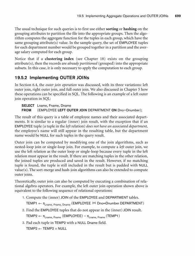
19.5 Implementing Aggregate Operations and OUTER JOINs 699
The usual technique for such queries is to first use either sorting or hashing on thegrouping attributes to partition the file into the appropriate groups. Then the algo-rithm computes the aggregate function for the tuples in each group, which have thesame grouping attribute(s) value. In the sample query, the set of EMPLOYEE tuplesfor each department number would be grouped together in a partition and the aver-age salary computed for each group.
Notice that if a clustering index (see Chapter 18) exists on the groupingattribute(s), then the records are already partitioned (grouped) into the appropriatesubsets. In this case, it is only necessary to apply the computation to each group.
19.5.2 Implementing OUTER JOINsIn Section 6.4, the outer join operation was discussed, with its three variations: leftouter join, right outer join, and full outer join. We also discussed in Chapter 5 howthese operations can be specified in SQL. The following is an example of a left outerjoin operation in SQL:
SELECT Lname, Fname, DnameFROM (EMPLOYEE LEFT OUTER JOIN DEPARTMENT ON Dno=Dnumber);
The result of this query is a table of employee names and their associated depart-ments. It is similar to a regular (inner) join result, with the exception that if anEMPLOYEE tuple (a tuple in the left relation) does not have an associated department,the employee’s name will still appear in the resulting table, but the departmentname would be NULL for such tuples in the query result.
Outer join can be computed by modifying one of the join algorithms, such asnested-loop join or single-loop join. For example, to compute a left outer join, weuse the left relation as the outer loop or single-loop because every tuple in the leftrelation must appear in the result. If there are matching tuples in the other relation,the joined tuples are produced and saved in the result. However, if no matchingtuple is found, the tuple is still included in the result but is padded with NULLvalue(s). The sort-merge and hash-join algorithms can also be extended to computeouter joins.
Theoretically, outer join can also be computed by executing a combination of rela-tional algebra operators. For example, the left outer join operation shown above isequivalent to the following sequence of relational operations:
1. Compute the (inner) JOIN of the EMPLOYEE and DEPARTMENT tables.
TEMP1 ← πLname, Fname, Dname (EMPLOYEE Dno=Dnumber DEPARTMENT)
2. Find the EMPLOYEE tuples that do not appear in the (inner) JOIN result.
TEMP2 ← πLname, Fname (EMPLOYEE) – πLname, Fname (TEMP1)
3. Pad each tuple in TEMP2 with a NULL Dname field.
TEMP2 ← TEMP2 × NULL
700 Chapter 19 Algorithms for Query Processing and Optimization
4. Apply the UNION operation to TEMP1, TEMP2 to produce the LEFT OUTERJOIN result.
RESULT ← TEMP1 ∪ TEMP2
The cost of the outer join as computed above would be the sum of the costs of theassociated steps (inner join, projections, set difference, and union). However, notethat step 3 can be done as the temporary relation is being constructed in step 2; thatis, we can simply pad each resulting tuple with a NULL. In addition, in step 4, weknow that the two operands of the union are disjoint (no common tuples), so thereis no need for duplicate elimination.
19.6 Combining Operations Using PipeliningA query specified in SQL will typically be translated into a relational algebra expres-sion that is a sequence of relational operations. If we execute a single operation at atime, we must generate temporary files on disk to hold the results of these tempo-rary operations, creating excessive overhead. Generating and storing large tempo-rary files on disk is time-consuming and can be unnecessary in many cases, sincethese files will immediately be used as input to the next operation. To reduce thenumber of temporary files, it is common to generate query execution code that cor-responds to algorithms for combinations of operations in a query.
For example, rather than being implemented separately, a JOIN can be combinedwith two SELECT operations on the input files and a final PROJECT operation onthe resulting file; all this is implemented by one algorithm with two input files and asingle output file. Rather than creating four temporary files, we apply the algorithmdirectly and get just one result file. In Section 19.7.2, we discuss how heuristic rela-tional algebra optimization can group operations together for execution. This iscalled pipelining or stream-based processing.
It is common to create the query execution code dynamically to implement multipleoperations. The generated code for producing the query combines several algo-rithms that correspond to individual operations. As the result tuples from one oper-ation are produced, they are provided as input for subsequent operations. Forexample, if a join operation follows two select operations on base relations, thetuples resulting from each select are provided as input for the join algorithm in astream or pipeline as they are produced.
19.7 Using Heuristics in Query OptimizationIn this section we discuss optimization techniques that apply heuristic rules tomodify the internal representation of a query—which is usually in the form of aquery tree or a query graph data structure—to improve its expected performance.The scanner and parser of an SQL query first generate a data structure that corre-sponds to an initial query representation, which is then optimized according toheuristic rules. This leads to an optimized query representation, which correspondsto the query execution strategy. Following that, a query execution plan is generated
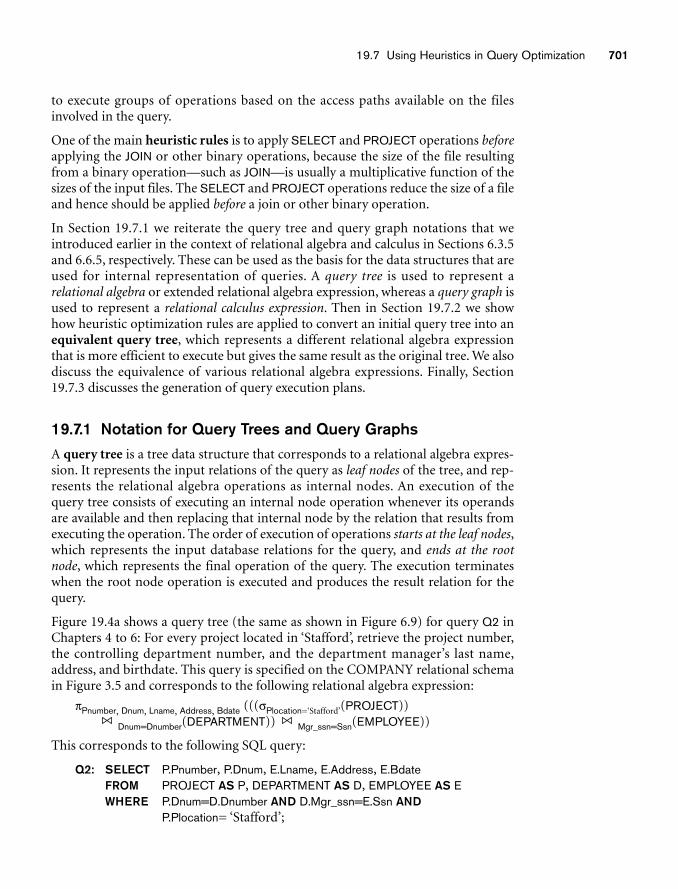
19.7 Using Heuristics in Query Optimization 701
to execute groups of operations based on the access paths available on the filesinvolved in the query.
One of the main heuristic rules is to apply SELECT and PROJECT operations beforeapplying the JOIN or other binary operations, because the size of the file resultingfrom a binary operation—such as JOIN—is usually a multiplicative function of thesizes of the input files. The SELECT and PROJECT operations reduce the size of a fileand hence should be applied before a join or other binary operation.
In Section 19.7.1 we reiterate the query tree and query graph notations that weintroduced earlier in the context of relational algebra and calculus in Sections 6.3.5and 6.6.5, respectively. These can be used as the basis for the data structures that areused for internal representation of queries. A query tree is used to represent arelational algebra or extended relational algebra expression, whereas a query graph isused to represent a relational calculus expression. Then in Section 19.7.2 we showhow heuristic optimization rules are applied to convert an initial query tree into anequivalent query tree, which represents a different relational algebra expressionthat is more efficient to execute but gives the same result as the original tree. We alsodiscuss the equivalence of various relational algebra expressions. Finally, Section19.7.3 discusses the generation of query execution plans.
19.7.1 Notation for Query Trees and Query GraphsA query tree is a tree data structure that corresponds to a relational algebra expres-sion. It represents the input relations of the query as leaf nodes of the tree, and rep-resents the relational algebra operations as internal nodes. An execution of thequery tree consists of executing an internal node operation whenever its operandsare available and then replacing that internal node by the relation that results fromexecuting the operation. The order of execution of operations starts at the leaf nodes,which represents the input database relations for the query, and ends at the rootnode, which represents the final operation of the query. The execution terminateswhen the root node operation is executed and produces the result relation for thequery.
Figure 19.4a shows a query tree (the same as shown in Figure 6.9) for query Q2 inChapters 4 to 6: For every project located in ‘Stafford’, retrieve the project number,the controlling department number, and the department manager’s last name,address, and birthdate. This query is specified on the COMPANY relational schemain Figure 3.5 and corresponds to the following relational algebra expression:
πPnumber, Dnum, Lname, Address, Bdate (((σPlocation=‘Stafford’(PROJECT))
Dnum=Dnumber(DEPARTMENT)) Mgr_ssn=Ssn(EMPLOYEE))
This corresponds to the following SQL query:
Q2: SELECT P.Pnumber, P.Dnum, E.Lname, E.Address, E.BdateFROM PROJECT AS P, DEPARTMENT AS D, EMPLOYEE AS EWHERE P.Dnum=D.Dnumber AND D.Mgr_ssn=E.Ssn AND
P.Plocation= ‘Stafford’;
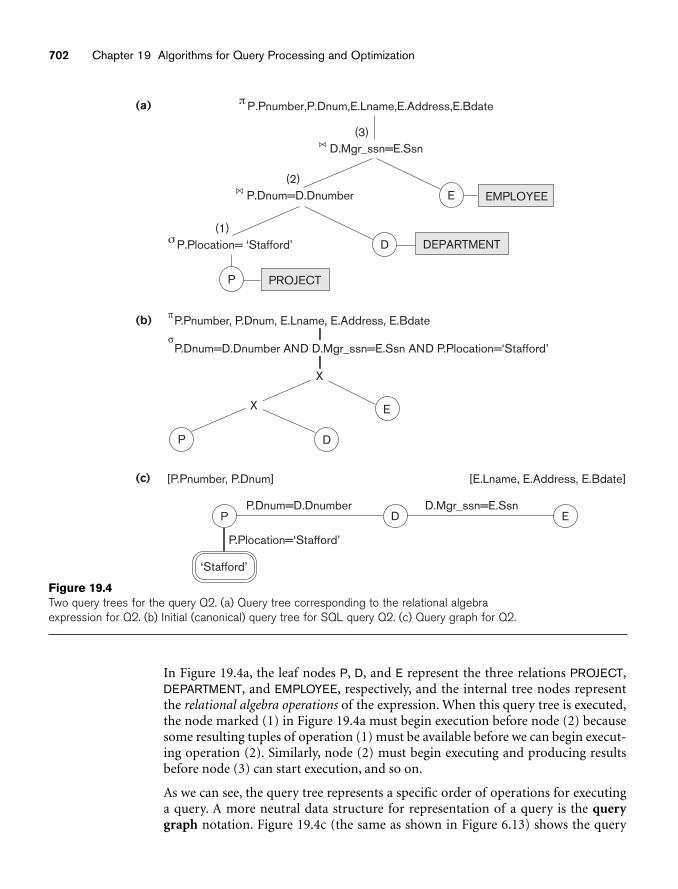
702 Chapter 19 Algorithms for Query Processing and Optimization
(b)
(a)
E
DP
P.Pnumber, P.Dnum, E.Lname, E.Address, E.Bdateπ
P.Dnum=D.Dnumber AND D.Mgr_ssn=E.Ssn AND P.Plocation=‘Stafford’σ
(c)
EDP
[P.Pnumber, P.Dnum] [E.Lname, E.Address, E.Bdate]
P.Dnum=D.Dnumber
P.Plocation=‘Stafford’
D.Mgr_ssn=E.Ssn
‘Stafford’
XX
XX
(1)
(2)
(3)
P.Pnumber,P.Dnum,E.Lname,E.Address,E.Bdateπ
D.Mgr_ssn=E.Ssn
P.Dnum=D.Dnumber
σ P.Plocation= ‘Stafford’
E
D
P
EMPLOYEE
DEPARTMENT
PROJECT
Figure 19.4Two query trees for the query Q2. (a) Query tree corresponding to the relational algebraexpression for Q2. (b) Initial (canonical) query tree for SQL query Q2. (c) Query graph for Q2.
In Figure 19.4a, the leaf nodes P, D, and E represent the three relations PROJECT,DEPARTMENT, and EMPLOYEE, respectively, and the internal tree nodes representthe relational algebra operations of the expression. When this query tree is executed,the node marked (1) in Figure 19.4a must begin execution before node (2) becausesome resulting tuples of operation (1) must be available before we can begin execut-ing operation (2). Similarly, node (2) must begin executing and producing resultsbefore node (3) can start execution, and so on.
As we can see, the query tree represents a specific order of operations for executinga query. A more neutral data structure for representation of a query is the querygraph notation. Figure 19.4c (the same as shown in Figure 6.13) shows the query
19.7 Using Heuristics in Query Optimization 703
graph for query Q2. Relations in the query are represented by relation nodes, whichare displayed as single circles. Constant values, typically from the query selectionconditions, are represented by constant nodes, which are displayed as double circlesor ovals. Selection and join conditions are represented by the graph edges, as shownin Figure 19.4c. Finally, the attributes to be retrieved from each relation are dis-played in square brackets above each relation.
The query graph representation does not indicate an order on which operations toperform first. There is only a single graph corresponding to each query.15 Althoughsome optimization techniques were based on query graphs, it is now generallyaccepted that query trees are preferable because, in practice, the query optimizerneeds to show the order of operations for query execution, which is not possible inquery graphs.
19.7.2 Heuristic Optimization of Query TreesIn general, many different relational algebra expressions—and hence many differentquery trees—can be equivalent; that is, they can represent the same query.16
The query parser will typically generate a standard initial query tree to correspondto an SQL query, without doing any optimization. For example, for a SELECT-PROJECT-JOIN query, such as Q2, the initial tree is shown in Figure 19.4(b). TheCARTESIAN PRODUCT of the relations specified in the FROM clause is first applied;then the selection and join conditions of the WHERE clause are applied, followed bythe projection on the SELECT clause attributes. Such a canonical query tree repre-sents a relational algebra expression that is very inefficient if executed directly,because of the CARTESIAN PRODUCT (×) operations. For example, if the PROJECT,DEPARTMENT, and EMPLOYEE relations had record sizes of 100, 50, and 150 bytesand contained 100, 20, and 5,000 tuples, respectively, the result of the CARTESIANPRODUCT would contain 10 million tuples of record size 300 bytes each. However,the initial query tree in Figure 19.4(b) is in a simple standard form that can be eas-ily created from the SQL query. It will never be executed. The heuristic query opti-mizer will transform this initial query tree into an equivalent final query tree that isefficient to execute.
The optimizer must include rules for equivalence among relational algebra expres-sions that can be applied to transform the initial tree into the final, optimized querytree. First we discuss informally how a query tree is transformed by using heuristics,and then we discuss general transformation rules and show how they can be used inan algebraic heuristic optimizer.
Example of Transforming a Query. Consider the following query Q on the data-base in Figure 3.5: Find the last names of employees born after 1957 who work on aproject named ‘Aquarius’. This query can be specified in SQL as follows:
15Hence, a query graph corresponds to a relational calculus expression as shown in Section 6.6.5.16The same query may also be stated in various ways in a high-level query language such as SQL (seeChapters 4 and 5).
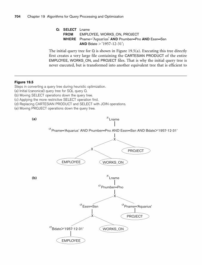
704 Chapter 19 Algorithms for Query Processing and Optimization
Q: SELECT LnameFROM EMPLOYEE, WORKS_ON, PROJECTWHERE Pname=‘Aquarius’ AND Pnumber=Pno AND Essn=Ssn
AND Bdate > ‘1957-12-31’;
The initial query tree for Q is shown in Figure 19.5(a). Executing this tree directlyfirst creates a very large file containing the CARTESIAN PRODUCT of the entireEMPLOYEE, WORKS_ON, and PROJECT files. That is why the initial query tree isnever executed, but is transformed into another equivalent tree that is efficient to
(a) Lname
Pname=‘Aquarius’ AND Pnumber=Pno AND Essn=Ssn AND Bdate>‘1957-12-31’
PROJECT
WORKS_ONEMPLOYEE
(b) Lname
Pnumber=Pno
Bdate>‘1957-12-31’
Pname=‘Aquarius’Essn=Ssn
π
π
σ
σ
σσ
σ
EMPLOYEE
PROJECT
WORKS_ON
X
X
X
X
Figure 19.5Steps in converting a query tree during heuristic optimization.(a) Initial (canonical) query tree for SQL query Q.(b) Moving SELECT operations down the query tree.(c) Applying the more restrictive SELECT operation first.(d) Replacing CARTESIAN PRODUCT and SELECT with JOIN operations.(e) Moving PROJECT operations down the query tree.
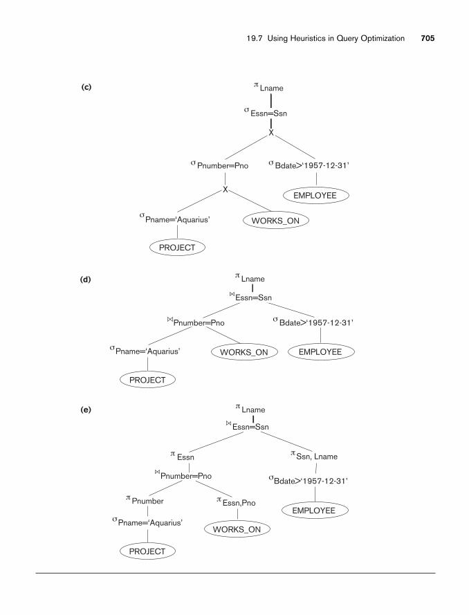
19.7 Using Heuristics in Query Optimization 705
(e) π Lname
σBdate>‘1957-12-31’
σPname=‘Aquarius’
π Pnumber π Essn,Pno
π Essn πSsn, Lname
EMPLOYEE
WORKS_ON
PROJECT
(d) π Lname
σ Bdate>‘1957-12-31’
σPname=‘Aquarius’ EMPLOYEEWORKS_ON
PROJECT
Essn=Ssn
Pnumber=Pno
Pnumber=Pno
Essn=Ssn
(c)
σ Essn=Ssn
π Lname
σ Pnumber=Pno σ Bdate>‘1957-12-31’
σPname=‘Aquarius’
EMPLOYEE
WORKS_ON
PROJECT
X
X
execute. This particular query needs only one record from the PROJECT relation—for the ‘Aquarius’ project—and only the EMPLOYEE records for those whose date ofbirth is after ‘1957-12-31’. Figure 19.5(b) shows an improved query tree that firstapplies the SELECT operations to reduce the number of tuples that appear in theCARTESIAN PRODUCT.
A further improvement is achieved by switching the positions of the EMPLOYEE andPROJECT relations in the tree, as shown in Figure 19.5(c). This uses the informationthat Pnumber is a key attribute of the PROJECT relation, and hence the SELECToperation on the PROJECT relation will retrieve a single record only. We can furtherimprove the query tree by replacing any CARTESIAN PRODUCT operation that isfollowed by a join condition with a JOIN operation, as shown in Figure 19.5(d).Another improvement is to keep only the attributes needed by subsequent opera-tions in the intermediate relations, by including PROJECT (π) operations as early aspossible in the query tree, as shown in Figure 19.5(e). This reduces the attributes(columns) of the intermediate relations, whereas the SELECT operations reduce thenumber of tuples (records).
As the preceding example demonstrates, a query tree can be transformed step bystep into an equivalent query tree that is more efficient to execute. However, wemust make sure that the transformation steps always lead to an equivalent querytree. To do this, the query optimizer must know which transformation rules preservethis equivalence. We discuss some of these transformation rules next.
General Transformation Rules for Relational Algebra Operations. There aremany rules for transforming relational algebra operations into equivalent ones. Forquery optimization purposes, we are interested in the meaning of the operationsand the resulting relations. Hence, if two relations have the same set of attributes ina different order but the two relations represent the same information, we considerthe relations to be equivalent. In Section 3.1.2 we gave an alternative definition ofrelation that makes the order of attributes unimportant; we will use this definitionhere. We will state some transformation rules that are useful in query optimization,without proving them:
1. Cascade of σ A conjunctive selection condition can be broken up into a cas-cade (that is, a sequence) of individual σ operations:
σc1 AND c2 AND . . . AND cn(R)� σc1
(σc2(...(σcn
(R))...))
2. Commutativity of σ. The σ operation is commutative:
σc1(σc2
(R)) � σc2(σc1
(R))
3. Cascade of π. In a cascade (sequence) of π operations, all but the last one canbe ignored:
πList1(πList2
(...(πListn(R))...)) � πList1
(R)
4. Commuting σ with π. If the selection condition c involves only those attrib-utes A1, . . . , An in the projection list, the two operations can be commuted:
πA1, A2, ..., An(σc (R)) � σc (πA1, A2, ..., An
(R))
706 Chapter 19 Algorithms for Query Processing and Optimization
19.7 Using Heuristics in Query Optimization 707
5. Commutativity of (and ×). The join operation is commutative, as is the× operation:
R c S ≡ S c R
R × S ≡ S × R
Notice that although the order of attributes may not be the same in the rela-tions resulting from the two joins (or two Cartesian products), the meaningis the same because the order of attributes is not important in the alternativedefinition of relation.
6. Commuting σ with (or ×). If all the attributes in the selection conditionc involve only the attributes of one of the relations being joined—say, R—thetwo operations can be commuted as follows:
σc (R S) ≡ (σc (R)) S
Alternatively, if the selection condition c can be written as (c1 AND c2), wherecondition c1 involves only the attributes of R and condition c2 involves onlythe attributes of S, the operations commute as follows:
σc (R S) � (σc1(R)) (σc2
(S))
The same rules apply if the is replaced by a × operation.
7. Commuting π with (or ×). Suppose that the projection list is L = {A1, ...,An, B1, ..., Bm} , where A1, ..., An are attributes of R and B1, ..., Bm are attrib-utes of S. If the join condition c involves only attributes in L, the two opera-tions can be commuted as follows:
πL (R c S) � (πA1, ..., An(R)) c (πB1, ..., Bm
(S))
If the join condition c contains additional attributes not in L, these must beadded to the projection list, and a final π operation is needed. For example, ifattributes An+1, ..., An+k of R and Bm+1, ..., Bm+p of S are involved in the joincondition c but are not in the projection list L, the operations commute asfollows:
πL (R c S) � πL ((πA1, ..., An, An+1, ..., An+k(R)) c (πB1, ..., Bm, Bm+1, ..., Bm+p
(S)))
For ×, there is no condition c, so the first transformation rule always appliesby replacing c with ×.
8. Commutativity of set operations. The set operations ∪ and ∩ are commu-tative but − is not.
9. Associativity of , ×, ∪, and ∩. These four operations are individuallyassociative; that is, if θ stands for any one of these four operations (through-out the expression), we have:
(R θ S) θ T ≡ R θ (S θ T)
10. Commuting σ with set operations. The σ operation commutes with ∪, ∩,and −. If θ stands for any one of these three operations (throughout theexpression), we have:
σc (R θ S) ≡ (σc (R)) θ (σc (S))
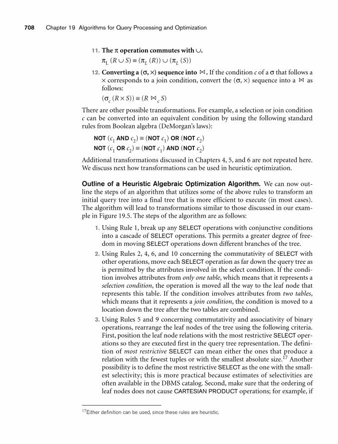
708 Chapter 19 Algorithms for Query Processing and Optimization
11. The π operation commutes with ∪.
πL (R ∪ S) ≡ (πL (R)) ∪ (πL (S))
12. Converting a (σ, ×) sequence into . If the condition c of a σ that follows a× corresponds to a join condition, convert the (σ, ×) sequence into a asfollows:
(σc (R × S)) ≡ (R c S)
There are other possible transformations. For example, a selection or join conditionc can be converted into an equivalent condition by using the following standardrules from Boolean algebra (DeMorgan’s laws):
NOT (c1 AND c2) ≡ (NOT c1) OR (NOT c2)
NOT (c1 OR c2) ≡ (NOT c1) AND (NOT c2)
Additional transformations discussed in Chapters 4, 5, and 6 are not repeated here.We discuss next how transformations can be used in heuristic optimization.
Outline of a Heuristic Algebraic Optimization Algorithm. We can now out-line the steps of an algorithm that utilizes some of the above rules to transform aninitial query tree into a final tree that is more efficient to execute (in most cases).The algorithm will lead to transformations similar to those discussed in our exam-ple in Figure 19.5. The steps of the algorithm are as follows:
1. Using Rule 1, break up any SELECT operations with conjunctive conditionsinto a cascade of SELECT operations. This permits a greater degree of free-dom in moving SELECT operations down different branches of the tree.
2. Using Rules 2, 4, 6, and 10 concerning the commutativity of SELECT withother operations, move each SELECT operation as far down the query tree asis permitted by the attributes involved in the select condition. If the condi-tion involves attributes from only one table, which means that it represents aselection condition, the operation is moved all the way to the leaf node thatrepresents this table. If the condition involves attributes from two tables,which means that it represents a join condition, the condition is moved to alocation down the tree after the two tables are combined.
3. Using Rules 5 and 9 concerning commutativity and associativity of binaryoperations, rearrange the leaf nodes of the tree using the following criteria.First, position the leaf node relations with the most restrictive SELECT oper-ations so they are executed first in the query tree representation. The defini-tion of most restrictive SELECT can mean either the ones that produce arelation with the fewest tuples or with the smallest absolute size.17 Anotherpossibility is to define the most restrictive SELECT as the one with the small-est selectivity; this is more practical because estimates of selectivities areoften available in the DBMS catalog. Second, make sure that the ordering ofleaf nodes does not cause CARTESIAN PRODUCT operations; for example, if
17Either definition can be used, since these rules are heuristic.
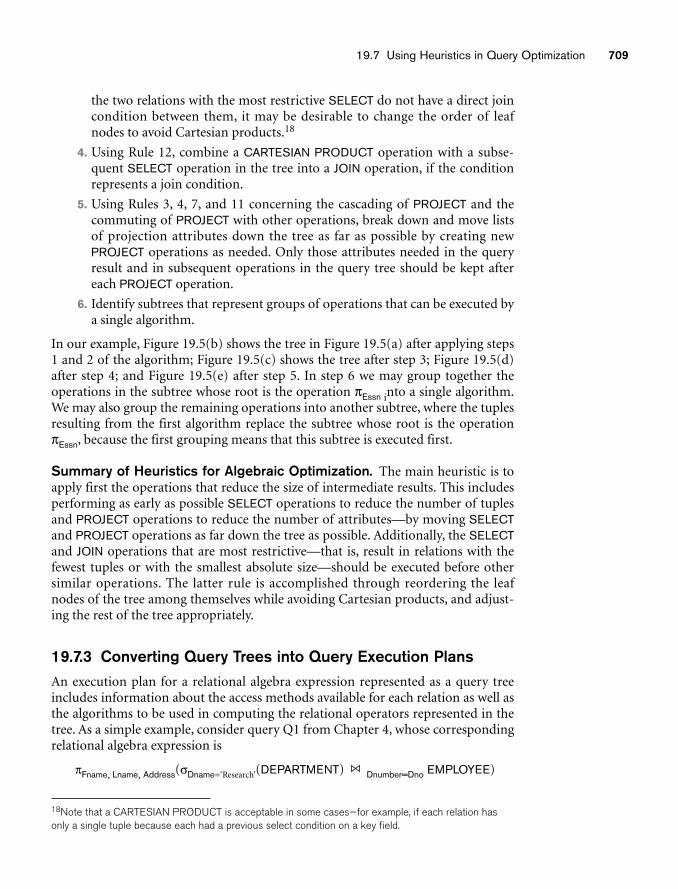
19.7 Using Heuristics in Query Optimization 709
the two relations with the most restrictive SELECT do not have a direct joincondition between them, it may be desirable to change the order of leafnodes to avoid Cartesian products.18
4. Using Rule 12, combine a CARTESIAN PRODUCT operation with a subse-quent SELECT operation in the tree into a JOIN operation, if the conditionrepresents a join condition.
5. Using Rules 3, 4, 7, and 11 concerning the cascading of PROJECT and thecommuting of PROJECT with other operations, break down and move listsof projection attributes down the tree as far as possible by creating newPROJECT operations as needed. Only those attributes needed in the queryresult and in subsequent operations in the query tree should be kept aftereach PROJECT operation.
6. Identify subtrees that represent groups of operations that can be executed bya single algorithm.
In our example, Figure 19.5(b) shows the tree in Figure 19.5(a) after applying steps1 and 2 of the algorithm; Figure 19.5(c) shows the tree after step 3; Figure 19.5(d)after step 4; and Figure 19.5(e) after step 5. In step 6 we may group together theoperations in the subtree whose root is the operation πEssn into a single algorithm.We may also group the remaining operations into another subtree, where the tuplesresulting from the first algorithm replace the subtree whose root is the operationπEssn, because the first grouping means that this subtree is executed first.
Summary of Heuristics for Algebraic Optimization. The main heuristic is toapply first the operations that reduce the size of intermediate results. This includesperforming as early as possible SELECT operations to reduce the number of tuplesand PROJECT operations to reduce the number of attributes—by moving SELECTand PROJECT operations as far down the tree as possible. Additionally, the SELECTand JOIN operations that are most restrictive—that is, result in relations with thefewest tuples or with the smallest absolute size—should be executed before othersimilar operations. The latter rule is accomplished through reordering the leafnodes of the tree among themselves while avoiding Cartesian products, and adjust-ing the rest of the tree appropriately.
19.7.3 Converting Query Trees into Query Execution PlansAn execution plan for a relational algebra expression represented as a query treeincludes information about the access methods available for each relation as well asthe algorithms to be used in computing the relational operators represented in thetree. As a simple example, consider query Q1 from Chapter 4, whose correspondingrelational algebra expression is
πFname, Lname, Address(σDname=‘Research’(DEPARTMENT) Dnumber=Dno EMPLOYEE)
18Note that a CARTESIAN PRODUCT is acceptable in some cases—for example, if each relation hasonly a single tuple because each had a previous select condition on a key field.
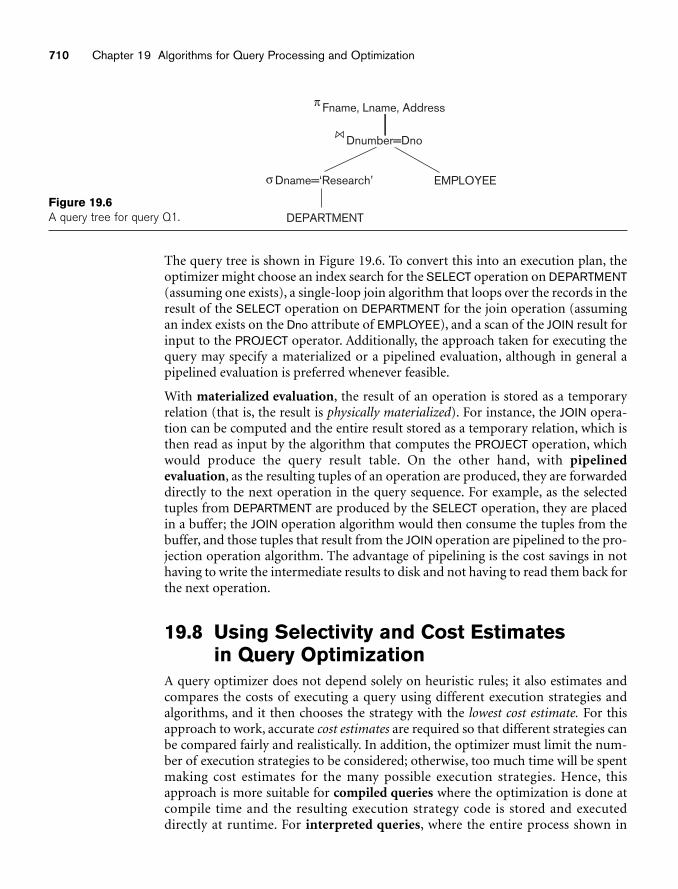
710 Chapter 19 Algorithms for Query Processing and Optimization
π Fname, Lname, Address
σ Dname=‘Research’
DEPARTMENT
EMPLOYEE
Dnumber=Dno
Figure 19.6A query tree for query Q1.
The query tree is shown in Figure 19.6. To convert this into an execution plan, theoptimizer might choose an index search for the SELECT operation on DEPARTMENT(assuming one exists), a single-loop join algorithm that loops over the records in theresult of the SELECT operation on DEPARTMENT for the join operation (assumingan index exists on the Dno attribute of EMPLOYEE), and a scan of the JOIN result forinput to the PROJECT operator. Additionally, the approach taken for executing thequery may specify a materialized or a pipelined evaluation, although in general apipelined evaluation is preferred whenever feasible.
With materialized evaluation, the result of an operation is stored as a temporaryrelation (that is, the result is physically materialized). For instance, the JOIN opera-tion can be computed and the entire result stored as a temporary relation, which isthen read as input by the algorithm that computes the PROJECT operation, whichwould produce the query result table. On the other hand, with pipelinedevaluation, as the resulting tuples of an operation are produced, they are forwardeddirectly to the next operation in the query sequence. For example, as the selectedtuples from DEPARTMENT are produced by the SELECT operation, they are placedin a buffer; the JOIN operation algorithm would then consume the tuples from thebuffer, and those tuples that result from the JOIN operation are pipelined to the pro-jection operation algorithm. The advantage of pipelining is the cost savings in nothaving to write the intermediate results to disk and not having to read them back forthe next operation.
19.8 Using Selectivity and Cost Estimates in Query Optimization
A query optimizer does not depend solely on heuristic rules; it also estimates andcompares the costs of executing a query using different execution strategies andalgorithms, and it then chooses the strategy with the lowest cost estimate. For thisapproach to work, accurate cost estimates are required so that different strategies canbe compared fairly and realistically. In addition, the optimizer must limit the num-ber of execution strategies to be considered; otherwise, too much time will be spentmaking cost estimates for the many possible execution strategies. Hence, thisapproach is more suitable for compiled queries where the optimization is done atcompile time and the resulting execution strategy code is stored and executeddirectly at runtime. For interpreted queries, where the entire process shown in
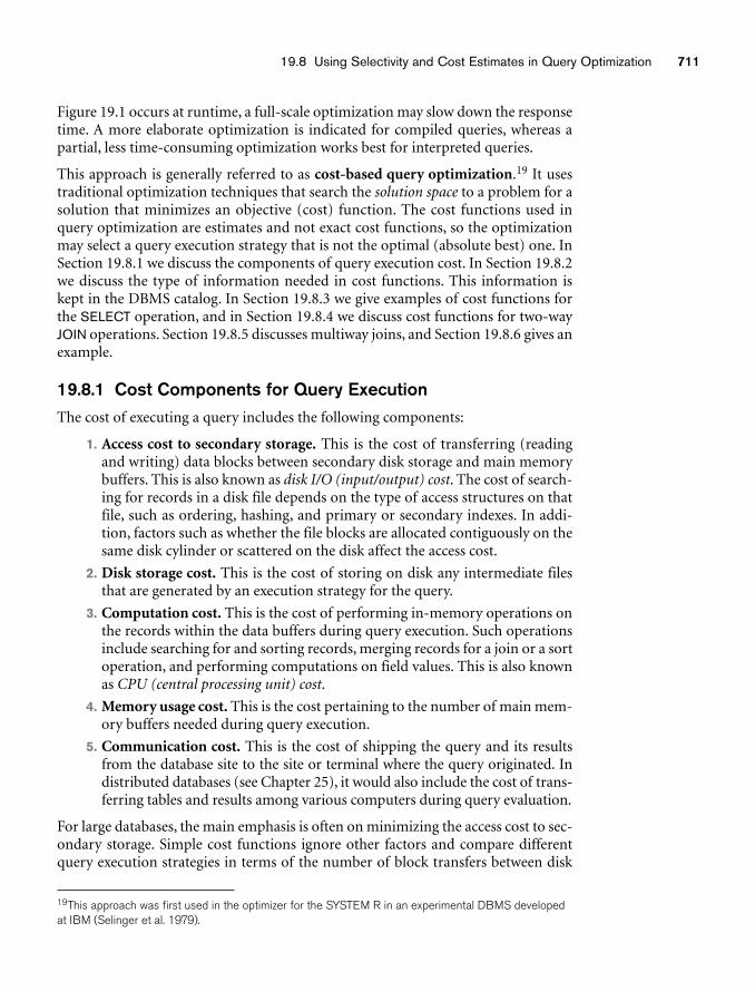
19.8 Using Selectivity and Cost Estimates in Query Optimization 711
Figure 19.1 occurs at runtime, a full-scale optimization may slow down the responsetime. A more elaborate optimization is indicated for compiled queries, whereas apartial, less time-consuming optimization works best for interpreted queries.
This approach is generally referred to as cost-based query optimization.19 It usestraditional optimization techniques that search the solution space to a problem for asolution that minimizes an objective (cost) function. The cost functions used inquery optimization are estimates and not exact cost functions, so the optimizationmay select a query execution strategy that is not the optimal (absolute best) one. InSection 19.8.1 we discuss the components of query execution cost. In Section 19.8.2we discuss the type of information needed in cost functions. This information iskept in the DBMS catalog. In Section 19.8.3 we give examples of cost functions forthe SELECT operation, and in Section 19.8.4 we discuss cost functions for two-wayJOIN operations. Section 19.8.5 discusses multiway joins, and Section 19.8.6 gives anexample.
19.8.1 Cost Components for Query ExecutionThe cost of executing a query includes the following components:
1. Access cost to secondary storage. This is the cost of transferring (readingand writing) data blocks between secondary disk storage and main memorybuffers. This is also known as disk I/O (input/output) cost. The cost of search-ing for records in a disk file depends on the type of access structures on thatfile, such as ordering, hashing, and primary or secondary indexes. In addi-tion, factors such as whether the file blocks are allocated contiguously on thesame disk cylinder or scattered on the disk affect the access cost.
2. Disk storage cost. This is the cost of storing on disk any intermediate filesthat are generated by an execution strategy for the query.
3. Computation cost. This is the cost of performing in-memory operations onthe records within the data buffers during query execution. Such operationsinclude searching for and sorting records, merging records for a join or a sortoperation, and performing computations on field values. This is also knownas CPU (central processing unit) cost.
4. Memory usage cost. This is the cost pertaining to the number of main mem-ory buffers needed during query execution.
5. Communication cost. This is the cost of shipping the query and its resultsfrom the database site to the site or terminal where the query originated. Indistributed databases (see Chapter 25), it would also include the cost of trans-ferring tables and results among various computers during query evaluation.
For large databases, the main emphasis is often on minimizing the access cost to sec-ondary storage. Simple cost functions ignore other factors and compare differentquery execution strategies in terms of the number of block transfers between disk
19This approach was first used in the optimizer for the SYSTEM R in an experimental DBMS developedat IBM (Selinger et al. 1979).
712 Chapter 19 Algorithms for Query Processing and Optimization
and main memory buffers. For smaller databases, where most of the data in the filesinvolved in the query can be completely stored in memory, the emphasis is on min-imizing computation cost. In distributed databases, where many sites are involved(see Chapter 25), communication cost must be minimized also. It is difficult toinclude all the cost components in a (weighted) cost function because of the diffi-culty of assigning suitable weights to the cost components. That is why some costfunctions consider a single factor only—disk access. In the next section we discusssome of the information that is needed for formulating cost functions.
19.8.2 Catalog Information Used in Cost FunctionsTo estimate the costs of various execution strategies, we must keep track of anyinformation that is needed for the cost functions. This information may be stored inthe DBMS catalog, where it is accessed by the query optimizer. First, we must knowthe size of each file. For a file whose records are all of the same type, the number ofrecords (tuples) (r), the (average) record size (R), and the number of file blocks (b)(or close estimates of them) are needed. The blocking factor (bfr) for the file mayalso be needed. We must also keep track of the primary file organization for each file.The primary file organization records may be unordered, ordered by an attributewith or without a primary or clustering index, or hashed (static hashing or one ofthe dynamic hashing methods) on a key attribute. Information is also kept on allprimary, secondary, or clustering indexes and their indexing attributes. The numberof levels (x) of each multilevel index (primary, secondary, or clustering) is neededfor cost functions that estimate the number of block accesses that occur duringquery execution. In some cost functions the number of first-level index blocks(bI1) is needed.
Another important parameter is the number of distinct values (d) of an attributeand the attribute selectivity (sl), which is the fraction of records satisfying an equal-ity condition on the attribute. This allows estimation of the selection cardinality (s= sl*r) of an attribute, which is the average number of records that will satisfy anequality selection condition on that attribute. For a key attribute, d = r, sl = 1/r and s= 1. For a nonkey attribute, by making an assumption that the d distinct values areuniformly distributed among the records, we estimate sl = (1/d) and so s = (r/d).20
Information such as the number of index levels is easy to maintain because it doesnot change very often. However, other information may change frequently; forexample, the number of records r in a file changes every time a record is inserted ordeleted. The query optimizer will need reasonably close but not necessarily com-pletely up-to-the-minute values of these parameters for use in estimating the cost ofvarious execution strategies.
For a nonkey attribute with d distinct values, it is often the case that the records arenot uniformly distributed among these values. For example, suppose that a com-pany has 5 departments numbered 1 through 5, and 200 employees who are distrib-
20More accurate optimizers store histograms of the distribution of records over the data values for anattribute.
19.8 Using Selectivity and Cost Estimates in Query Optimization 713
uted among the departments as follows: (1, 5), (2, 25), (3, 70), (4, 40), (5, 60). Insuch cases, the optimizer can store a histogram that reflects the distribution ofemployee records over different departments in a table with the two attributes (Dno,Selectivity), which would contain the following values for our example: (1, 0.025), (2,0.125), (3, 0.35), (4, 0.2), (5, 0.3). The selectivity values stored in the histogram canalso be estimates if the employee table changes frequently.
In the next two sections we examine how some of these parameters are used in costfunctions for a cost-based query optimizer.
19.8.3 Examples of Cost Functions for SELECTWe now give cost functions for the selection algorithms S1 to S8 discussed inSection 19.3.1 in terms of number of block transfers between memory and disk.Algorithm S9 involves an intersection of record pointers after they have beenretrieved by some other means, such as algorithm S6, and so the cost function willbe based on the cost for S6. These cost functions are estimates that ignore compu-tation time, storage cost, and other factors. The cost for method Si is referred to asCSi block accesses.
■ S1—Linear search (brute force) approach. We search all the file blocks toretrieve all records satisfying the selection condition; hence, CS1a = b. For anequality condition on a key attribute, only half the file blocks are searched onthe average before finding the record, so a rough estimate for CS1b = (b/2) ifthe record is found; if no record is found that satisfies the condition, CS1b = b.
■ S2—Binary search. This search accesses approximately CS2 = log2b +⎡(s/bfr)⎤ − 1 file blocks. This reduces to log2b if the equality condition is on aunique (key) attribute, because s = 1 in this case.
■ S3a—Using a primary index to retrieve a single record. For a primaryindex, retrieve one disk block at each index level, plus one disk block fromthe data file. Hence, the cost is one more disk block than the number ofindex levels: CS3a = x + 1.
■ S3b—Using a hash key to retrieve a single record. For hashing, only onedisk block needs to be accessed in most cases. The cost function is approxi-mately CS3b = 1 for static hashing or linear hashing, and it is 2 disk blockaccesses for extendible hashing (see Section 17.8).
■ S4—Using an ordering index to retrieve multiple records. If the compari-son condition is >, >=, <, or <= on a key field with an ordering index,roughly half the file records will satisfy the condition. This gives a cost func-tion of CS4 = x + (b/2). This is a very rough estimate, and although it may becorrect on the average, it may be quite inaccurate in individual cases. A moreaccurate estimate is possible if the distribution of records is stored in a his-togram.
■ S5—Using a clustering index to retrieve multiple records. One disk blockis accessed at each index level, which gives the address of the first file diskblock in the cluster. Given an equality condition on the indexing attribute, s
714 Chapter 19 Algorithms for Query Processing and Optimization
records will satisfy the condition, where s is the selection cardinality of theindexing attribute. This means that ⎡(s/bfr)⎤ file blocks will be in the clusterof file blocks that hold all the selected records, giving CS5 = x + ⎡(s/bfr)⎤.
■ S6—Using a secondary (B+-tree) index. For a secondary index on a key(unique) attribute, the cost is x + 1 disk block accesses. For a secondary indexon a nonkey (nonunique) attribute, s records will satisfy an equality condi-tion, where s is the selection cardinality of the indexing attribute. However,because the index is nonclustering, each of the records may reside on a differ-ent disk block, so the (worst case) cost estimate is CS6a = x + 1 + s. The addi-tional 1 is to account for the disk block that contains the record pointers afterthe index is searched (see Figure 18.5). If the comparison condition is >, >=,<, or <= and half the file records are assumed to satisfy the condition, then(very roughly) half the first-level index blocks are accessed, plus half the filerecords via the index. The cost estimate for this case, approximately, is CS6b =x + (bI1/2) + (r/2). The r/2 factor can be refined if better selectivity estimatesare available through a histogram. The latter method CS6b can be very costly.
■ S7—Conjunctive selection. We can use either S1 or one of the methods S2to S6 discussed above. In the latter case, we use one condition to retrieve therecords and then check in the main memory buffers whether each retrievedrecord satisfies the remaining conditions in the conjunction. If multipleindexes exist, the search of each index can produce a set of record pointers(record ids) in the main memory buffers. The intersection of the sets ofrecord pointers (referred to in S9) can be computed in main memory, andthen the resulting records are retrieved based on their record ids.
■ S8—Conjunctive selection using a composite index. Same as S3a, S5, orS6a, depending on the type of index.
Example of Using the Cost Functions. In a query optimizer, it is common toenumerate the various possible strategies for executing a query and to estimate thecosts for different strategies. An optimization technique, such as dynamic program-ming, may be used to find the optimal (least) cost estimate efficiently, without hav-ing to consider all possible execution strategies. We do not discuss optimizationalgorithms here; rather, we use a simple example to illustrate how cost estimatesmay be used. Suppose that the EMPLOYEE file in Figure 3.5 has rE = 10,000 recordsstored in bE = 2000 disk blocks with blocking factor bfrE = 5 records/block and thefollowing access paths:
1. A clustering index on Salary, with levels xSalary = 3 and average selection car-dinality sSalary = 20. (This corresponds to a selectivity of slSalary = 0.002).
2. A secondary index on the key attribute Ssn, with xSsn = 4 (sSsn = 1, slSsn =0.0001).
3. A secondary index on the nonkey attribute Dno, with xDno = 2 and first-levelindex blocks bI1Dno = 4. There are dDno = 125 distinct values for Dno, so theselectivity of Dno is slDno = (1/dDno) = 0.008, and the selection cardinality issDno = (rE * slDno) = (rE/dDno) = 80.
19.8 Using Selectivity and Cost Estimates in Query Optimization 715
4. A secondary index on Sex, with xSex = 1. There are dSex = 2 values for the Sexattribute, so the average selection cardinality is sSex = (rE/dSex) = 5000. (Notethat in this case, a histogram giving the percentage of male and femaleemployees may be useful, unless they are approximately equal.)
We illustrate the use of cost functions with the following examples:
OP1: σSsn=‘123456789’(EMPLOYEE)
OP2: σDno>5(EMPLOYEE)
OP3: σDno=5(EMPLOYEE)
OP4: σDno=5 AND SALARY>30000 AND Sex=‘F’(EMPLOYEE)
The cost of the brute force (linear search or file scan) option S1 will be estimated asCS1a = bE = 2000 (for a selection on a nonkey attribute) or CS1b = (bE/2) = 1000(average cost for a selection on a key attribute). For OP1 we can use either methodS1 or method S6a; the cost estimate for S6a is CS6a = xSsn + 1 = 4 + 1 = 5, and it ischosen over method S1, whose average cost is CS1b = 1000. For OP2 we can useeither method S1 (with estimated cost CS1a = 2000) or method S6b (with estimatedcost CS6b = xDno + (bI1Dno/2) + (rE /2) = 2 + (4/2) + (10,000/2) = 5004), so we choosethe linear search approach for OP2. For OP3 we can use either method S1 (with esti-mated cost CS1a = 2000) or method S6a (with estimated cost CS6a = xDno + sDno = 2+ 80 = 82), so we choose method S6a.
Finally, consider OP4, which has a conjunctive selection condition. We need to esti-mate the cost of using any one of the three components of the selection condition toretrieve the records, plus the linear search approach. The latter gives cost estimateCS1a = 2000. Using the condition (Dno = 5) first gives the cost estimate CS6a = 82.Using the condition (Salary > 30,000) first gives a cost estimate CS4 = xSalary + (bE/2)= 3 + (2000/2) = 1003. Using the condition (Sex = ‘F’) first gives a cost estimate CS6a= xSex + sSex = 1 + 5000 = 5001. The optimizer would then choose method S6a onthe secondary index on Dno because it has the lowest cost estimate. The condition(Dno = 5) is used to retrieve the records, and the remaining part of the conjunctivecondition (Salary > 30,000 AND Sex = ‘F’) is checked for each selected record after itis retrieved into memory. Only the records that satisfy these additional conditionsare included in the result of the operation.
19.8.4 Examples of Cost Functions for JOINTo develop reasonably accurate cost functions for JOIN operations, we need to havean estimate for the size (number of tuples) of the file that results after the JOIN oper-ation. This is usually kept as a ratio of the size (number of tuples) of the resultingjoin file to the size of the CARTESIAN PRODUCT file, if both are applied to the sameinput files, and it is called the join selectivity ( js). If we denote the number of tuplesof a relation R by |R|, we have:
js = |(R c S)| / |(R × S)| = |(R c S)| / (|R| * |S|)
If there is no join condition c, then js = 1 and the join is the same as the CARTESIANPRODUCT. If no tuples from the relations satisfy the join condition, then js = 0. In
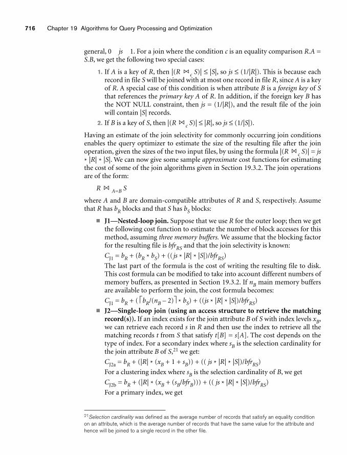
716 Chapter 19 Algorithms for Query Processing and Optimization
general, 0 js 1. For a join where the condition c is an equality comparison R.A =S.B, we get the following two special cases:
1. If A is a key of R, then |(R c S)| ≤ |S|, so js ≤ (1/|R|). This is because eachrecord in file S will be joined with at most one record in file R, since A is a keyof R. A special case of this condition is when attribute B is a foreign key of Sthat references the primary key A of R. In addition, if the foreign key B hasthe NOT NULL constraint, then js = (1/|R|), and the result file of the joinwill contain |S| records.
2. If B is a key of S, then |(R c S)| ≤ |R|, so js ≤ (1/|S|).
Having an estimate of the join selectivity for commonly occurring join conditionsenables the query optimizer to estimate the size of the resulting file after the joinoperation, given the sizes of the two input files, by using the formula |(R c S)| = js
* |R| * |S|. We can now give some sample approximate cost functions for estimatingthe cost of some of the join algorithms given in Section 19.3.2. The join operationsare of the form:
R A=B S
where A and B are domain-compatible attributes of R and S, respectively. Assumethat R has bR blocks and that S has bS blocks:
■ J1—Nested-loop join. Suppose that we use R for the outer loop; then we getthe following cost function to estimate the number of block accesses for thismethod, assuming three memory buffers. We assume that the blocking factorfor the resulting file is bfrRS and that the join selectivity is known:
CJ1 = bR + (bR * bS) + (( js * |R| * |S|)/bfrRS)
The last part of the formula is the cost of writing the resulting file to disk.This cost formula can be modified to take into account different numbers ofmemory buffers, as presented in Section 19.3.2. If nB main memory buffersare available to perform the join, the cost formula becomes:
CJ1 = bR + ( ⎡bR/(nB – 2)⎤ * bS) + ((js * |R| * |S|)/bfrRS)
■ J2—Single-loop join (using an access structure to retrieve the matchingrecord(s)). If an index exists for the join attribute B of S with index levels xB,we can retrieve each record s in R and then use the index to retrieve all thematching records t from S that satisfy t[B] = s[A]. The cost depends on thetype of index. For a secondary index where sB is the selection cardinality forthe join attribute B of S,21 we get:
CJ2a = bR + (|R| * (xB + 1 + sB)) + (( js * |R| * |S|)/bfrRS)
For a clustering index where sB is the selection cardinality of B, we get
CJ2b = bR + (|R| * (xB + (sB/bfrB))) + (( js * |R| * |S|)/bfrRS)
For a primary index, we get
21Selection cardinality was defined as the average number of records that satisfy an equality conditionon an attribute, which is the average number of records that have the same value for the attribute andhence will be joined to a single record in the other file.
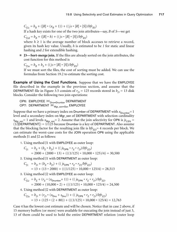
19.8 Using Selectivity and Cost Estimates in Query Optimization 717
CJ2c = bR + (|R| * (xB + 1)) + (( j s * |R| * |S|)/bfrRS)
If a hash key exists for one of the two join attributes—say, B of S—we get
CJ2d = bR + (|R| * h) + (( j s * |R| * |S|)/bfrRS)
where h ≥ 1 is the average number of block accesses to retrieve a record,given its hash key value. Usually, h is estimated to be 1 for static and linearhashing and 2 for extendible hashing.
■ J3—Sort-merge join. If the files are already sorted on the join attributes, thecost function for this method is
CJ3a = bR + bS + (( j s * |R| * |S|)/bfrRS)
If we must sort the files, the cost of sorting must be added. We can use theformulas from Section 19.2 to estimate the sorting cost.
Example of Using the Cost Functions. Suppose that we have the EMPLOYEEfile described in the example in the previous section, and assume that theDEPARTMENT file in Figure 3.5 consists of rD = 125 records stored in bD = 13 diskblocks. Consider the following two join operations:
OP6: EMPLOYEE Dno=Dnumber DEPARTMENTOP7: DEPARTMENT Mgr_ssn=Ssn EMPLOYEE
Suppose that we have a primary index on Dnumber of DEPARTMENT with xDnumber= 1level and a secondary index on Mgr_ssn of DEPARTMENT with selection cardinalitysMgr_ssn= 1 and levels xMgr_ssn= 2. Assume that the join selectivity for OP6 is jsOP6 =(1/|DEPARTMENT|) = 1/125 because Dnumber is a key of DEPARTMENT. Also assumethat the blocking factor for the resulting join file is bfrED= 4 records per block. Wecan estimate the worst-case costs for the JOIN operation OP6 using the applicablemethods J1 and J2 as follows:
1. Using method J1 with EMPLOYEE as outer loop:
CJ1 = bE + (bE * bD) + (( jsOP6 * rE * rD)/bfrED)
= 2000 + (2000 * 13) + (((1/125) * 10,000 * 125)/4) = 30,500
2. Using method J1 with DEPARTMENT as outer loop:
CJ1 = bD + (bE * bD) + (( jsOP6 * rE * rD)/bfrED)
= 13 + (13 * 2000) + (((1/125) * 10,000 * 125/4) = 28,513
3. Using method J2 with EMPLOYEE as outer loop:
CJ2c = bE + (rE * (xDnumber+ 1)) + (( jsOP6 * rE * rD)/bfrED
= 2000 + (10,000 * 2) + (((1/125) * 10,000 * 125/4) = 24,500
4. Using method J2 with DEPARTMENT as outer loop:
CJ2a = bD + (rD * (xDno + sDno)) + (( jsOP6 * rE * rD)/bfrED)
= 13 + (125 * (2 + 80)) + (((1/125) * 10,000 * 125/4) = 12,763
Case 4 has the lowest cost estimate and will be chosen. Notice that in case 2 above, if15 memory buffers (or more) were available for executing the join instead of just 3,13 of them could be used to hold the entire DEPARTMENT relation (outer loop
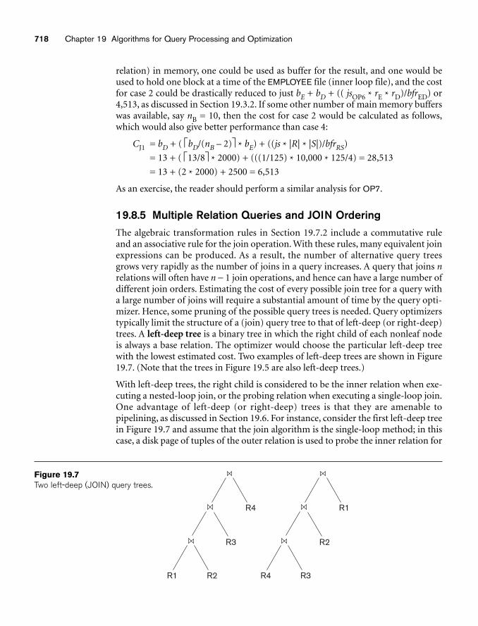
718 Chapter 19 Algorithms for Query Processing and Optimization
R1 R2
R3
R4
R4 R3
R2
R1
Figure 19.7Two left-deep (JOIN) query trees.
relation) in memory, one could be used as buffer for the result, and one would beused to hold one block at a time of the EMPLOYEE file (inner loop file), and the costfor case 2 could be drastically reduced to just bE + bD + (( jsOP6 * rE * rD)/bfrED) or4,513, as discussed in Section 19.3.2. If some other number of main memory bufferswas available, say nB = 10, then the cost for case 2 would be calculated as follows,which would also give better performance than case 4:
CJ1 = bD + ( ⎡bD/(nB – 2)⎤ * bE) + ((js * |R| * |S|)/bfrRS)
= 13 + ( ⎡13/8⎤ * 2000) + (((1/125) * 10,000 * 125/4) = 28,513
= 13 + (2 * 2000) + 2500 = 6,513
As an exercise, the reader should perform a similar analysis for OP7.
19.8.5 Multiple Relation Queries and JOIN OrderingThe algebraic transformation rules in Section 19.7.2 include a commutative ruleand an associative rule for the join operation. With these rules, many equivalent joinexpressions can be produced. As a result, the number of alternative query treesgrows very rapidly as the number of joins in a query increases. A query that joins nrelations will often have n − 1 join operations, and hence can have a large number ofdifferent join orders. Estimating the cost of every possible join tree for a query witha large number of joins will require a substantial amount of time by the query opti-mizer. Hence, some pruning of the possible query trees is needed. Query optimizerstypically limit the structure of a (join) query tree to that of left-deep (or right-deep)trees. A left-deep tree is a binary tree in which the right child of each nonleaf nodeis always a base relation. The optimizer would choose the particular left-deep treewith the lowest estimated cost. Two examples of left-deep trees are shown in Figure19.7. (Note that the trees in Figure 19.5 are also left-deep trees.)
With left-deep trees, the right child is considered to be the inner relation when exe-cuting a nested-loop join, or the probing relation when executing a single-loop join.One advantage of left-deep (or right-deep) trees is that they are amenable topipelining, as discussed in Section 19.6. For instance, consider the first left-deep treein Figure 19.7 and assume that the join algorithm is the single-loop method; in thiscase, a disk page of tuples of the outer relation is used to probe the inner relation for
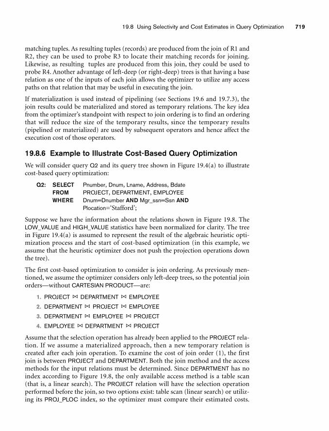
19.8 Using Selectivity and Cost Estimates in Query Optimization 719
matching tuples. As resulting tuples (records) are produced from the join of R1 andR2, they can be used to probe R3 to locate their matching records for joining.Likewise, as resulting tuples are produced from this join, they could be used toprobe R4. Another advantage of left-deep (or right-deep) trees is that having a baserelation as one of the inputs of each join allows the optimizer to utilize any accesspaths on that relation that may be useful in executing the join.
If materialization is used instead of pipelining (see Sections 19.6 and 19.7.3), thejoin results could be materialized and stored as temporary relations. The key ideafrom the optimizer’s standpoint with respect to join ordering is to find an orderingthat will reduce the size of the temporary results, since the temporary results(pipelined or materialized) are used by subsequent operators and hence affect theexecution cost of those operators.
19.8.6 Example to Illustrate Cost-Based Query OptimizationWe will consider query Q2 and its query tree shown in Figure 19.4(a) to illustratecost-based query optimization:
Q2: SELECT Pnumber, Dnum, Lname, Address, BdateFROM PROJECT, DEPARTMENT, EMPLOYEEWHERE Dnum=Dnumber AND Mgr_ssn=Ssn AND
Plocation=‘Stafford’;
Suppose we have the information about the relations shown in Figure 19.8. TheLOW_VALUE and HIGH_VALUE statistics have been normalized for clarity. The treein Figure 19.4(a) is assumed to represent the result of the algebraic heuristic opti-mization process and the start of cost-based optimization (in this example, weassume that the heuristic optimizer does not push the projection operations downthe tree).
The first cost-based optimization to consider is join ordering. As previously men-tioned, we assume the optimizer considers only left-deep trees, so the potential joinorders—without CARTESIAN PRODUCT—are:
1. PROJECT DEPARTMENT EMPLOYEE
2. DEPARTMENT PROJECT EMPLOYEE
3. DEPARTMENT EMPLOYEE PROJECT
4. EMPLOYEE DEPARTMENT PROJECT
Assume that the selection operation has already been applied to the PROJECT rela-tion. If we assume a materialized approach, then a new temporary relation is created after each join operation. To examine the cost of join order (1), the firstjoin is between PROJECT and DEPARTMENT. Both the join method and the accessmethods for the input relations must be determined. Since DEPARTMENT has noindex according to Figure 19.8, the only available access method is a table scan(that is, a linear search). The PROJECT relation will have the selection operationperformed before the join, so two options exist: table scan (linear search) or utiliz-ing its PROJ_PLOC index, so the optimizer must compare their estimated costs.
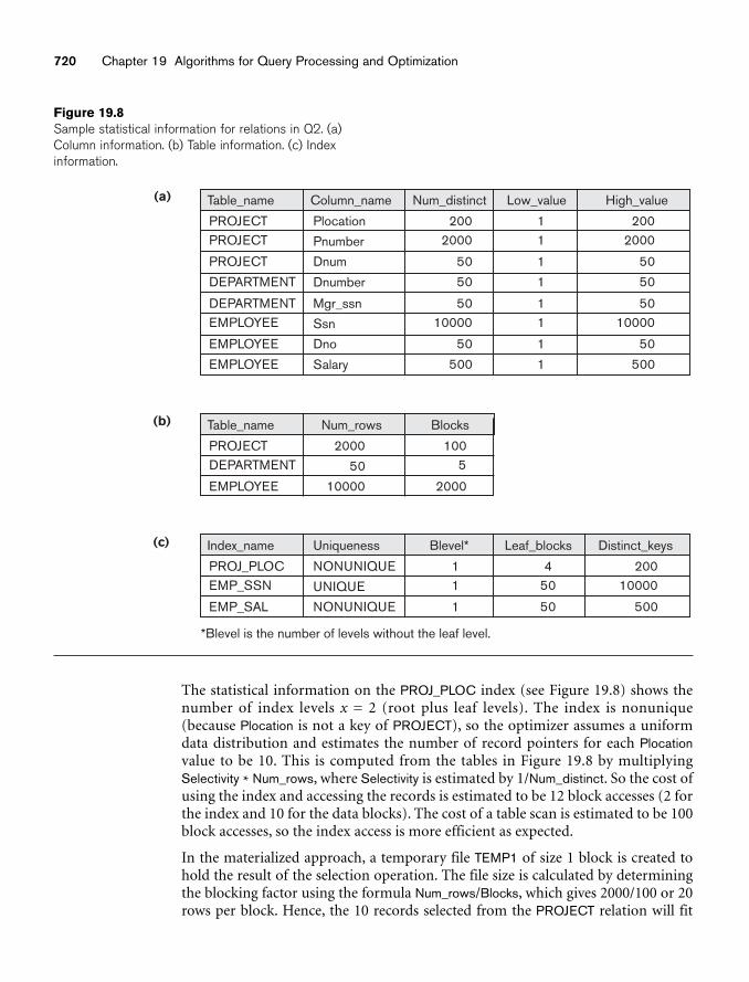
720 Chapter 19 Algorithms for Query Processing and Optimization
(a) Table_name
PROJECTPROJECT
PROJECT
DEPARTMENT
DEPARTMENTEMPLOYEE
EMPLOYEE
EMPLOYEE
2002000
50
50
5010000
50
500
11
1
1
11
1
1
2002000
50
50
5010000
50
500
Dnum
Dnumber
Plocation
Pnumber
Dno
Salary
Mgr_ssn
Ssn
Column_name Num_distinct Low_value High_value
(c) Index_name
*Blevel is the number of levels without the leaf level.
PROJ_PLOCEMP_SSN
EMP_SAL
11
1
450
50
20010000
500NONUNIQUE
NONUNIQUE
UNIQUE
Uniqueness Blevel* Leaf_blocks Distinct_keys
(b) Table_name
PROJECTDEPARTMENT
EMPLOYEE
1005
200010000
2000
50
Num_rows Blocks
Figure 19.8Sample statistical information for relations in Q2. (a)Column information. (b) Table information. (c) Indexinformation.
The statistical information on the PROJ_PLOC index (see Figure 19.8) shows thenumber of index levels x = 2 (root plus leaf levels). The index is nonunique(because Plocation is not a key of PROJECT), so the optimizer assumes a uniformdata distribution and estimates the number of record pointers for each Plocationvalue to be 10. This is computed from the tables in Figure 19.8 by multiplyingSelectivity * Num_rows, where Selectivity is estimated by 1/Num_distinct. So the cost ofusing the index and accessing the records is estimated to be 12 block accesses (2 forthe index and 10 for the data blocks). The cost of a table scan is estimated to be 100block accesses, so the index access is more efficient as expected.
In the materialized approach, a temporary file TEMP1 of size 1 block is created tohold the result of the selection operation. The file size is calculated by determiningthe blocking factor using the formula Num_rows/Blocks, which gives 2000/100 or 20rows per block. Hence, the 10 records selected from the PROJECT relation will fit
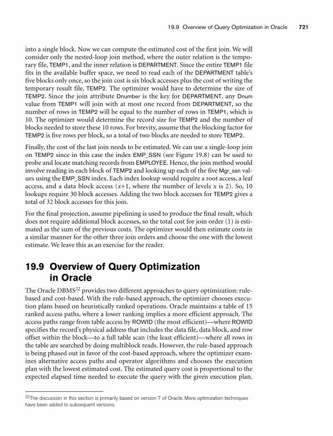
19.9 Overview of Query Optimization in Oracle 721
into a single block. Now we can compute the estimated cost of the first join. We willconsider only the nested-loop join method, where the outer relation is the tempo-rary file, TEMP1, and the inner relation is DEPARTMENT. Since the entire TEMP1 filefits in the available buffer space, we need to read each of the DEPARTMENT table’sfive blocks only once, so the join cost is six block accesses plus the cost of writing thetemporary result file, TEMP2. The optimizer would have to determine the size ofTEMP2. Since the join attribute Dnumber is the key for DEPARTMENT, any Dnumvalue from TEMP1 will join with at most one record from DEPARTMENT, so thenumber of rows in TEMP2 will be equal to the number of rows in TEMP1, which is10. The optimizer would determine the record size for TEMP2 and the number ofblocks needed to store these 10 rows. For brevity, assume that the blocking factor forTEMP2 is five rows per block, so a total of two blocks are needed to store TEMP2.
Finally, the cost of the last join needs to be estimated. We can use a single-loop joinon TEMP2 since in this case the index EMP_SSN (see Figure 19.8) can be used toprobe and locate matching records from EMPLOYEE. Hence, the join method wouldinvolve reading in each block of TEMP2 and looking up each of the five Mgr_ssn val-ues using the EMP_SSN index. Each index lookup would require a root access, a leafaccess, and a data block access (x+1, where the number of levels x is 2). So, 10lookups require 30 block accesses. Adding the two block accesses for TEMP2 gives atotal of 32 block accesses for this join.
For the final projection, assume pipelining is used to produce the final result, whichdoes not require additional block accesses, so the total cost for join order (1) is esti-mated as the sum of the previous costs. The optimizer would then estimate costs ina similar manner for the other three join orders and choose the one with the lowestestimate. We leave this as an exercise for the reader.
19.9 Overview of Query Optimization in Oracle
The Oracle DBMS22 provides two different approaches to query optimization: rule-based and cost-based. With the rule-based approach, the optimizer chooses execu-tion plans based on heuristically ranked operations. Oracle maintains a table of 15ranked access paths, where a lower ranking implies a more efficient approach. Theaccess paths range from table access by ROWID (the most efficient)—where ROWIDspecifies the record’s physical address that includes the data file, data block, and rowoffset within the block—to a full table scan (the least efficient)—where all rows inthe table are searched by doing multiblock reads. However, the rule-based approachis being phased out in favor of the cost-based approach, where the optimizer exam-ines alternative access paths and operator algorithms and chooses the executionplan with the lowest estimated cost. The estimated query cost is proportional to theexpected elapsed time needed to execute the query with the given execution plan.
22The discussion in this section is primarily based on version 7 of Oracle. More optimization techniqueshave been added to subsequent versions.
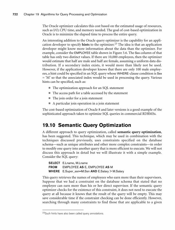
722 Chapter 19 Algorithms for Query Processing and Optimization
The Oracle optimizer calculates this cost based on the estimated usage of resources,such as I/O, CPU time, and memory needed. The goal of cost-based optimization inOracle is to minimize the elapsed time to process the entire query.
An interesting addition to the Oracle query optimizer is the capability for an appli-cation developer to specify hints to the optimizer.23 The idea is that an applicationdeveloper might know more information about the data than the optimizer. Forexample, consider the EMPLOYEE table shown in Figure 3.6. The Sex column of thattable has only two distinct values. If there are 10,000 employees, then the optimizerwould estimate that half are male and half are female, assuming a uniform data dis-tribution. If a secondary index exists, it would more than likely not be used.However, if the application developer knows that there are only 100 male employ-ees, a hint could be specified in an SQL query whose WHERE-clause condition is Sex= ‘M’ so that the associated index would be used in processing the query. Varioushints can be specified, such as:
■ The optimization approach for an SQL statement
■ The access path for a table accessed by the statement
■ The join order for a join statement
■ A particular join operation in a join statement
The cost-based optimization of Oracle 8 and later versions is a good example of thesophisticated approach taken to optimize SQL queries in commercial RDBMSs.
19.10 Semantic Query OptimizationA different approach to query optimization, called semantic query optimization,has been suggested. This technique, which may be used in combination with thetechniques discussed previously, uses constraints specified on the databaseschema—such as unique attributes and other more complex constraints—in orderto modify one query into another query that is more efficient to execute. We will notdiscuss this approach in detail but we will illustrate it with a simple example.Consider the SQL query:
SELECT E.Lname, M.LnameFROM EMPLOYEE AS E, EMPLOYEE AS MWHERE E.Super_ssn=M.Ssn AND E.Salary > M.Salary
This query retrieves the names of employees who earn more than their supervisors.Suppose that we had a constraint on the database schema that stated that noemployee can earn more than his or her direct supervisor. If the semantic queryoptimizer checks for the existence of this constraint, it does not need to execute thequery at all because it knows that the result of the query will be empty. This maysave considerable time if the constraint checking can be done efficiently. However,searching through many constraints to find those that are applicable to a given
23Such hints have also been called query annotations.
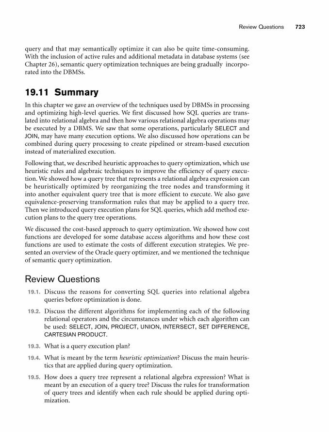
Review Questions 723
query and that may semantically optimize it can also be quite time-consuming.With the inclusion of active rules and additional metadata in database systems (seeChapter 26), semantic query optimization techniques are being gradually incorpo-rated into the DBMSs.
19.11 SummaryIn this chapter we gave an overview of the techniques used by DBMSs in processingand optimizing high-level queries. We first discussed how SQL queries are trans-lated into relational algebra and then how various relational algebra operations maybe executed by a DBMS. We saw that some operations, particularly SELECT andJOIN, may have many execution options. We also discussed how operations can becombined during query processing to create pipelined or stream-based executioninstead of materialized execution.
Following that, we described heuristic approaches to query optimization, which useheuristic rules and algebraic techniques to improve the efficiency of query execu-tion. We showed how a query tree that represents a relational algebra expression canbe heuristically optimized by reorganizing the tree nodes and transforming it into another equivalent query tree that is more efficient to execute. We also gaveequivalence-preserving transformation rules that may be applied to a query tree.Then we introduced query execution plans for SQL queries, which add method exe-cution plans to the query tree operations.
We discussed the cost-based approach to query optimization. We showed how costfunctions are developed for some database access algorithms and how these costfunctions are used to estimate the costs of different execution strategies. We pre-sented an overview of the Oracle query optimizer, and we mentioned the techniqueof semantic query optimization.
Review Questions19.1. Discuss the reasons for converting SQL queries into relational algebra
queries before optimization is done.
19.2. Discuss the different algorithms for implementing each of the followingrelational operators and the circumstances under which each algorithm canbe used: SELECT, JOIN, PROJECT, UNION, INTERSECT, SET DIFFERENCE,CARTESIAN PRODUCT.
19.3. What is a query execution plan?
19.4. What is meant by the term heuristic optimization? Discuss the main heuris-tics that are applied during query optimization.
19.5. How does a query tree represent a relational algebra expression? What ismeant by an execution of a query tree? Discuss the rules for transformationof query trees and identify when each rule should be applied during opti-mization.
724 Chapter 19 Algorithms for Query Processing and Optimization
19.6. How many different join orders are there for a query that joins 10 relations?
19.7. What is meant by cost-based query optimization?
19.8. What is the difference between pipelining and materialization?
19.9. Discuss the cost components for a cost function that is used to estimatequery execution cost. Which cost components are used most often as thebasis for cost functions?
19.10. Discuss the different types of parameters that are used in cost functions.Where is this information kept?
19.11. List the cost functions for the SELECT and JOIN methods discussed inSection 19.8.
19.12. What is meant by semantic query optimization? How does it differ fromother query optimization techniques?
Exercises19.13. Consider SQL queries Q1, Q8, Q1B, and Q4 in Chapter 4 and Q27 in
Chapter 5.
a. Draw at least two query trees that can represent each of these queries.Under what circumstances would you use each of your query trees?
b. Draw the initial query tree for each of these queries, and then show howthe query tree is optimized by the algorithm outlined in Section 19.7.
c. For each query, compare your own query trees of part (a) and the initialand final query trees of part (b).
19.14. A file of 4096 blocks is to be sorted with an available buffer space of 64blocks. How many passes will be needed in the merge phase of the externalsort-merge algorithm?
19.15. Develop cost functions for the PROJECT, UNION, INTERSECTION, SET DIF-FERENCE, and CARTESIAN PRODUCT algorithms discussed in Section 19.4.
19.16. Develop cost functions for an algorithm that consists of two SELECTs, aJOIN, and a final PROJECT, in terms of the cost functions for the individualoperations.
19.17. Can a nondense index be used in the implementation of an aggregate opera-tor? Why or why not?
19.18. Calculate the cost functions for different options of executing the JOIN oper-ation OP7 discussed in Section 19.3.2.
19.19. Develop formulas for the hybrid hash-join algorithm for calculating the sizeof the buffer for the first bucket. Develop more accurate cost estimation for-mulas for the algorithm.
Selected Bibliography 725
19.20. Estimate the cost of operations OP6 and OP7, using the formulas developedin Exercise 19.9.
19.21. Extend the sort-merge join algorithm to implement the LEFT OUTER JOINoperation.
19.22. Compare the cost of two different query plans for the following query:
σSalary > 40000(EMPLOYEE Dno=DnumberDEPARTMENT)
Use the database statistics in Figure 19.8.
Selected BibliographyA detailed algorithm for relational algebra optimization is given by Smith andChang (1975). The Ph.D. thesis of Kooi (1980) provides a foundation for query pro-cessing techniques. A survey paper by Jarke and Koch (1984) gives a taxonomy ofquery optimization and includes a bibliography of work in this area. A survey byGraefe (1993) discusses query execution in database systems and includes an exten-sive bibliography.
Whang (1985) discusses query optimization in OBE (Office-By-Example), which isa system based on the language QBE. Cost-based optimization was introduced inthe SYSTEM R experimental DBMS and is discussed in Astrahan et al. (1976).Selinger et al. (1979) is a classic paper that discussed cost-based optimization ofmultiway joins in SYSTEM R. Join algorithms are discussed in Gotlieb (1975),Blasgen and Eswaran (1976), and Whang et al. (1982). Hashing algorithms forimplementing joins are described and analyzed in DeWitt et al. (1984),Bratbergsengen (1984), Shapiro (1986), Kitsuregawa et al. (1989), and Blakeley andMartin (1990), among others. Approaches to finding a good join order are pre-sented in Ioannidis and Kang (1990) and in Swami and Gupta (1989). A discussionof the implications of left-deep and bushy join trees is presented in Ioannidis andKang (1991). Kim (1982) discusses transformations of nested SQL queries intocanonical representations. Optimization of aggregate functions is discussed in Klug(1982) and Muralikrishna (1992). Salzberg et al. (1990) describe a fast external sort-ing algorithm. Estimating the size of temporary relations is crucial for query opti-mization. Sampling-based estimation schemes are presented in Haas et al. (1995)and in Haas and Swami (1995). Lipton et al. (1990) also discuss selectivity estima-tion. Having the database system store and use more detailed statistics in the formof histograms is the topic of Muralikrishna and DeWitt (1988) and Poosala et al.(1996).
Kim et al. (1985) discuss advanced topics in query optimization. Semantic queryoptimization is discussed in King (1981) and Malley and Zdonick (1986). Work onsemantic query optimization is reported in Chakravarthy et al. (1990), Shenoy andOzsoyoglu (1989), and Siegel et al. (1992).
727
Physical Database Design and Tuning
In the last chapter we discussed various techniques bywhich queries can be processed efficiently by the
DBMS. These techniques are mostly internal to the DBMS and invisible to the pro-grammer. In this chapter we discuss additional issues that affect the performance ofan application running on a DBMS. In particular, we discuss some of the optionsavailable to database administrators and programmers for storing databases, andsome of the heuristics, rules, and techniques that they can use to tune the databasefor performance improvement. First, in Section 20.1, we discuss the issues that arisein physical database design dealing with storage and access of data. Then, in Section20.2, we discuss how to improve database performance through tuning, indexing ofdata, database design, and the queries themselves.
20.1 Physical Database Design in Relational Databases
In this section, we begin by discussing the physical design factors that affect the per-formance of applications and transactions, and then we comment on the specificguidelines for RDBMSs.
20.1.1 Factors That Influence Physical Database DesignPhysical design is an activity where the goal is not only to create the appropriatestructuring of data in storage, but also to do so in a way that guarantees good per-formance. For a given conceptual schema, there are many physical design alterna-tives in a given DBMS. It is not possible to make meaningful physical design
20chapter 20
728 Chapter 20 Physical Database Design and Tuning
decisions and performance analyses until the database designer knows the mix ofqueries, transactions, and applications that are expected to run on the database.This is called the job mix for the particular set of database system applications. Thedatabase administrators/designers must analyze these applications, their expectedfrequencies of invocation, any timing constraints on their execution speed, theexpected frequency of update operations, and any unique constraints on attributes.We discuss each of these factors next.
A. Analyzing the Database Queries and Transactions. Before undertakingthe physical database design, we must have a good idea of the intended use of thedatabase by defining in a high-level form the queries and transactions that areexpected to run on the database. For each retrieval query, the following informa-tion about the query would be needed:
1. The files that will be accessed by the query.1
2. The attributes on which any selection conditions for the query are specified.
3. Whether the selection condition is an equality, inequality, or a range condi-tion.
4. The attributes on which any join conditions or conditions to link multipletables or objects for the query are specified.
5. The attributes whose values will be retrieved by the query.
The attributes listed in items 2 and 4 above are candidates for the definition ofaccess structures, such as indexes, hash keys, or sorting of the file.
For each update operation or update transaction, the following informationwould be needed:
1. The files that will be updated.
2. The type of operation on each file (insert, update, or delete).
3. The attributes on which selection conditions for a delete or update are spec-ified.
4. The attributes whose values will be changed by an update operation.
Again, the attributes listed in item 3 are candidates for access structures on the files,because they would be used to locate the records that will be updated or deleted. Onthe other hand, the attributes listed in item 4 are candidates for avoiding an accessstructure, since modifying them will require updating the access structures.
B. Analyzing the Expected Frequency of Invocation of Queries andTransactions. Besides identifying the characteristics of expected retrieval queriesand update transactions, we must consider their expected rates of invocation. Thisfrequency information, along with the attribute information collected on eachquery and transaction, is used to compile a cumulative list of the expected fre-quency of use for all queries and transactions. This is expressed as the expected fre-quency of using each attribute in each file as a selection attribute or a join attribute,
1For simplicity we use the term files here, but this can also mean tables or relations.
20.1 Physical Database Design in Relational Databases 729
over all the queries and transactions. Generally, for large volumes of processing, theinformal 80–20 rule can be used: approximately 80 percent of the processing isaccounted for by only 20 percent of the queries and transactions. Therefore, in prac-tical situations, it is rarely necessary to collect exhaustive statistics and invocationrates on all the queries and transactions; it is sufficient to determine the 20 percentor so most important ones.
C. Analyzing the Time Constraints of Queries and Transactions. Somequeries and transactions may have stringent performance constraints. For example,a transaction may have the constraint that it should terminate within 5 seconds on95 percent of the occasions when it is invoked, and that it should never take morethan 20 seconds. Such timing constraints place further priorities on the attributesthat are candidates for access paths. The selection attributes used by queries andtransactions with time constraints become higher-priority candidates for primaryaccess structures for the files, because the primary access structures are generally themost efficient for locating records in a file.
D. Analyzing the Expected Frequencies of Update Operations. A minimumnumber of access paths should be specified for a file that is frequently updated,because updating the access paths themselves slows down the update operations. Forexample, if a file that has frequent record insertions has 10 indexes on 10 differentattributes, each of these indexes must be updated whenever a new record is inserted.The overhead for updating 10 indexes can slow down the insert operations.
E. Analyzing the Uniqueness Constraints on Attributes. Access paths shouldbe specified on all candidate key attributes—or sets of attributes—that are either theprimary key of a file or unique attributes. The existence of an index (or other accesspath) makes it sufficient to only search the index when checking this uniquenessconstraint, since all values of the attribute will exist in the leaf nodes of the index.For example, when inserting a new record, if a key attribute value of the new recordalready exists in the index, the insertion of the new record should be rejected, since itwould violate the uniqueness constraint on the attribute.
Once the preceding information is compiled, it is possible to address the physicaldatabase design decisions, which consist mainly of deciding on the storage struc-tures and access paths for the database files.
20.1.2 Physical Database Design DecisionsMost relational systems represent each base relation as a physical database file. Theaccess path options include specifying the type of primary file organization for eachrelation and the attributes of which indexes that should be defined. At most, one ofthe indexes on each file may be a primary or a clustering index. Any number ofadditional secondary indexes can be created.2
2The reader should review the various types of indexes described in Section 18.1. For a clearer under-standing of this discussion, it is also helpful to be familiar with the algorithms for query processing dis-cussed in Chapter 19.
730 Chapter 20 Physical Database Design and Tuning
Design Decisions about Indexing. The attributes whose values are required inequality or range conditions (selection operation) are those that are keys or thatparticipate in join conditions (join operation) requiring access paths, such asindexes.
The performance of queries largely depends upon what indexes or hashing schemesexist to expedite the processing of selections and joins. On the other hand, duringinsert, delete, or update operations, the existence of indexes adds to the overhead.This overhead must be justified in terms of the gain in efficiency by expeditingqueries and transactions.
The physical design decisions for indexing fall into the following categories:
1. Whether to index an attribute. The general rules for creating an index on anattribute are that the attribute must either be a key (unique), or there mustbe some query that uses that attribute either in a selection condition (equal-ity or range of values) or in a join condition. One reason for creating multi-ple indexes is that some operations can be processed by just scanning theindexes, without having to access the actual data file (see Section 19.5).
2. What attribute or attributes to index on. An index can be constructed on asingle attribute, or on more than one attribute if it is a composite index. Ifmultiple attributes from one relation are involved together in several queries,(for example, (Garment_style_#, Color) in a garment inventory database), amultiattribute (composite) index is warranted. The ordering of attributeswithin a multiattribute index must correspond to the queries. For instance,the above index assumes that queries would be based on an ordering of col-ors within a Garment_style_# rather than vice versa.
3. Whether to set up a clustered index. At most, one index per table can be aprimary or clustering index, because this implies that the file be physicallyordered on that attribute. In most RDBMSs, this is specified by the keywordCLUSTER. (If the attribute is a key, a primary index is created, whereas aclustering index is created if the attribute is not a key—see Section 18.1.) If atable requires several indexes, the decision about which one should be theprimary or clustering index depends upon whether keeping the tableordered on that attribute is needed. Range queries benefit a great deal fromclustering. If several attributes require range queries, relative benefits mustbe evaluated before deciding which attribute to cluster on. If a query is to beanswered by doing an index search only (without retrieving data records),the corresponding index should not be clustered, since the main benefit ofclustering is achieved when retrieving the records themselves. A clusteringindex may be set up as a multiattribute index if range retrieval by that com-posite key is useful in report creation (for example, an index on Zip_code,Store_id, and Product_id may be a clustering index for sales data).
4. Whether to use a hash index over a tree index. In general, RDBMSs use B+-trees for indexing. However, ISAM and hash indexes are also provided insome systems (see Chapter 18). B+-trees support both equality and rangequeries on the attribute used as the search key. Hash indexes work well with
20.1 Physical Database Design in Relational Databases 731
equality conditions, particularly during joins to find a matching record(s),but they do not support range queries.
5. Whether to use dynamic hashing for the file. For files that are veryvolatile—that is, those that grow and shrink continuously—one of thedynamic hashing schemes discussed in Section 17.9 would be suitable.Currently, they are not offered by many commercial RDBMSs.
How to Create an Index. Many RDBMSs have a similar type of command forcreating an index, although it is not part of the SQL standard. The general form ofthis command is:
CREATE [ UNIQUE ] INDEX <index name>ON <table name> ( <column name> [ <order> ] { , <column name> [ <order> ] } )[ CLUSTER ] ;
The keywords UNIQUE and CLUSTER are optional. The keyword CLUSTER is usedwhen the index to be created should also sort the data file records on the indexingattribute. Thus, specifying CLUSTER on a key (unique) attribute would create somevariation of a primary index, whereas specifying CLUSTER on a nonkey(nonunique) attribute would create some variation of a clustering index. The valuefor <order> can be either ASC (ascending) or DESC (descending), and specifieswhether the data file should be ordered in ascending or descending values of theindexing attribute. The default is ASC. For example, the following would create aclustering (ascending) index on the nonkey attribute Dno of the EMPLOYEE file:
CREATE INDEX DnoIndexON EMPLOYEE (Dno)CLUSTER ;
Denormalization as a Design Decision for Speeding Up Queries. The ulti-mate goal during normalization (see Chapters 15 and 16) is to separate attributesinto tables to minimize redundancy, and thereby avoid the update anomalies thatlead to an extra processing overhead to maintain consistency in the database. Theideals that are typically followed are the third or Boyce-Codd normal forms (seeChapter 15).
The above ideals are sometimes sacrificed in favor of faster execution of frequentlyoccurring queries and transactions. This process of storing the logical databasedesign (which may be in BCNF or 4NF) in a weaker normal form, say 2NF or 1NF,is called denormalization. Typically, the designer includes certain attributes from atable S into another table R. The reason is that the attributes from S that areincluded in R are frequently needed—along with other attributes in R—for answer-ing queries or producing reports. By including these attributes, a join of R with S isavoided for these frequently occurring queries and reports. This reintroducesredundancy in the base tables by including the same attributes in both tables R andS. A partial functional dependency or a transitive dependency now exists in the tableR, thereby creating the associated redundancy problems (see Chapter 15). A tradeoffexists between the additional updating needed for maintaining consistency of
732 Chapter 20 Physical Database Design and Tuning
redundant attributes versus the effort needed to perform a join to incorporate theadditional attributes needed in the result. For example, consider the following rela-tion:
ASSIGN (Emp_id, Proj_id, Emp_name, Emp_job_title, Percent_assigned, Proj_name,Proj_mgr_id, Proj_mgr_name),
which corresponds exactly to the headers in a report called The EmployeeAssignment Roster.
This relation is only in 1NF because of the following functional dependencies:
Proj_id → Proj_name, Proj_mgr_idProj_mgr_id → Proj_mgr_nameEmp_id → Emp_name, Emp_job_title
This relation may be preferred over the design in 2NF (and 3NF) consisting of thefollowing three relations:
EMP (Emp_id, Emp_name, Emp_job_title)PROJ (Proj_id, Proj_name, Proj_mgr_id)EMP_PROJ (Emp_id, Proj_id, Percent_assigned)
This is because to produce the The Employee Assignment Roster report (with allfields shown in ASSIGN above), the latter multirelation design requires twoNATURAL JOIN (indicated with *) operations (between EMP and EMP_PROJ, andbetween PROJ and EMP_PROJ), plus a final JOIN between PROJ and EMP to retrievethe Proj_mgr_name from the Proj_mgr_id. Thus the following JOINs would be needed(the final join would also require renaming (aliasing) of the last EMP table, which isnot shown):
((EMP_PROJ * EMP) * PROJ) PROJ.Proj_mgr_id = EMP.Emp_id EMP
It is also possible to create a view for the ASSIGN table. This does not mean that thejoin operations will be avoided, but that the user need not specify the joins. If theview table is materialized, the joins would be avoided, but if the virtual view table isnot stored as a materialized file, the join computations would still be necessary.Other forms of denormalization consist of storing extra tables to maintain originalfunctional dependencies that are lost during BCNF decomposition. For example,Figure 15.14 shows the TEACH(Student, Course, Instructor) relation with the func-tional dependencies {{Student, Course} → Instructor, Instructor → Course}. A losslessdecomposition of TEACH into T1(Student, Instructor) and T2(Instructor, Course) doesnot allow queries of the form what course did student Smith take from instructorNavathe to be answered without joining T1 and T2. Therefore, storing T1, T2, andTEACH may be a possible solution, which reduces the design from BCNF to 3NF.Here, TEACH is a materialized join of the other two tables, representing an extremeredundancy. Any updates to T1 and T2 would have to be applied to TEACH. An alter-nate strategy is to create T1 and T2 as updatable base tables, and to create TEACH asa view (virtual table) on T1 and T2 that can only be queried.
20.2 An Overview of Database Tuning in Relational Systems 733
20.2 An Overview of Database Tuning in Relational Systems
After a database is deployed and is in operation, actual use of the applications, trans-actions, queries, and views reveals factors and problem areas that may not have beenaccounted for during the initial physical design. The inputs to physical design listedin Section 20.1.1 can be revised by gathering actual statistics about usage patterns.Resource utilization as well as internal DBMS processing—such as query optimiza-tion—can be monitored to reveal bottlenecks, such as contention for the same dataor devices. Volumes of activity and sizes of data can be better estimated. Therefore, itis necessary to monitor and revise the physical database design constantly—an activ-ity referred to as database tuning. The goals of tuning are as follows:
■ To make applications run faster.
■ To improve (lower) the response time of queries and transactions.
■ To improve the overall throughput of transactions.
The dividing line between physical design and tuning is very thin. The same designdecisions that we discussed in Section 20.1.2 are revisited during database tuning,which is a continual adjustment of the physical design. We give a brief overview ofthe tuning process below.3 The inputs to the tuning process include statistics relatedto the same factors mentioned in Section 20.1.1. In particular, DBMSs can internallycollect the following statistics:
■ Sizes of individual tables.
■ Number of distinct values in a column.
■ The number of times a particular query or transaction is submitted and exe-cuted in an interval of time.
■ The times required for different phases of query and transaction processing(for a given set of queries or transactions).
These and other statistics create a profile of the contents and use of the database.Other information obtained from monitoring the database system activities andprocesses includes the following:
■ Storage statistics. Data about allocation of storage into tablespaces, index-spaces, and buffer pools.
■ I/O and device performance statistics. Total read/write activity (paging) ondisk extents and disk hot spots.
■ Query/transaction processing statistics. Execution times of queries andtransactions, and optimization times during query optimization.
3Interested readers should consult Shasha and Bonnet (2002) for a detailed discussion of tuning.
734 Chapter 20 Physical Database Design and Tuning
■ Locking/logging related statistics. Rates of issuing different types of locks,transaction throughput rates, and log records activity.4
■ Index statistics. Number of levels in an index, number of noncontiguousleaf pages, and so on.
Some of the above statistics relate to transactions, concurrency control, and recov-ery, which are discussed in Chapters 21 through 23. Tuning a database involves deal-ing with the following types of problems:
■ How to avoid excessive lock contention, thereby increasing concurrencyamong transactions.
■ How to minimize the overhead of logging and unnecessary dumping of data.
■ How to optimize the buffer size and scheduling of processes.
■ How to allocate resources such as disks, RAM, and processes for most effi-cient utilization.
Most of the previously mentioned problems can be solved by the DBA by settingappropriate physical DBMS parameters, changing configurations of devices, chang-ing operating system parameters, and other similar activities. The solutions tend tobe closely tied to specific systems. The DBAs are typically trained to handle thesetuning problems for the specific DBMS. We briefly discuss the tuning of variousphysical database design decisions below.
20.2.1 Tuning IndexesThe initial choice of indexes may have to be revised for the following reasons:
■ Certain queries may take too long to run for lack of an index.
■ Certain indexes may not get utilized at all.
■ Certain indexes may undergo too much updating because the index is on anattribute that undergoes frequent changes.
Most DBMSs have a command or trace facility, which can be used by the DBA to askthe system to show how a query was executed—what operations were performed inwhat order and what secondary access structures (indexes) were used. By analyzingthese execution plans, it is possible to diagnose the causes of the above problems.Some indexes may be dropped and some new indexes may be created based on thetuning analysis.
The goal of tuning is to dynamically evaluate the requirements, which sometimesfluctuate seasonally or during different times of the month or week, and to reorgan-ize the indexes and file organizations to yield the best overall performance.Dropping and building new indexes is an overhead that can be justified in terms ofperformance improvements. Updating of a table is generally suspended while an
4The reader should preview Chapters 21–23 for an explanation of these terms.
20.2 An Overview of Database Tuning in Relational Systems 735
index is dropped or created; this loss of service must be accounted for. Besides drop-ping or creating indexes and changing from a nonclustered to a clustered index andvice versa, rebuilding the index may improve performance. Most RDBMSs use B+-trees for an index. If there are many deletions on the index key, index pages maycontain wasted space, which can be claimed during a rebuild operation. Similarly,too many insertions may cause overflows in a clustered index that affect perfor-mance. Rebuilding a clustered index amounts to reorganizing the entire tableordered on that key.
The available options for indexing and the way they are defined, created, and reor-ganized varies from system to system. As an illustration, consider the sparse anddense indexes in Chapter 18. A sparse index such as a primary index (see Section18.1) will have one index pointer for each page (disk block) in the data file; a denseindex such as a unique secondary index will have an index pointer for each record.Sybase provides clustering indexes as sparse indexes in the form of B+-trees, whereasINGRES provides sparse clustering indexes as ISAM files and dense clusteringindexes as B+-trees. In some versions of Oracle and DB2, the option of setting up aclustering index is limited to a dense index (with many more index entries), and theDBA has to work with this limitation.
20.2.2 Tuning the Database DesignIn Section 20.1.2, we discussed the need for a possible denormalization, which is adeparture from keeping all tables as BCNF relations. If a given physical databasedesign does not meet the expected objectives, the DBA may revert to the logicaldatabase design, make adjustments such as denormalizations to the logical schema,and remap it to a new set of physical tables and indexes.
As discussed, the entire database design has to be driven by the processing require-ments as much as by data requirements. If the processing requirements are dynam-ically changing, the design needs to respond by making changes to the conceptualschema if necessary and to reflect those changes into the logical schema and physi-cal design. These changes may be of the following nature:
■ Existing tables may be joined (denormalized) because certain attributesfrom two or more tables are frequently needed together: This reduces thenormalization level from BCNF to 3NF, 2NF, or 1NF.5
■ For the given set of tables, there may be alternative design choices, all ofwhich achieve 3NF or BCNF. We illustrated alternative equivalent designs inChapter 16. One normalized design may be replaced by another.
■ A relation of the form R(K,A, B, C, D, ...)—with K as a set of key attributes—that is in BCNF can be stored in multiple tables that are also in BCNF—forexample, R1(K, A, B), R2(K, C, D, ), R3(K, ...)—by replicating the key K in eachtable. Such a process is known as vertical partitioning. Each table groups
5Note that 3NF and 2NF address different types of problem dependencies that are independent ofeach other; hence, the normalization (or denormalization) order between them is arbitrary.
736 Chapter 20 Physical Database Design and Tuning
sets of attributes that are accessed together. For example, the tableEMPLOYEE(Ssn, Name, Phone, Grade, Salary) may be split into two tables:EMP1(Ssn, Name, Phone) and EMP2(Ssn, Grade, Salary). If the original tablehas a large number of rows (say 100,000) and queries about phone numbersand salary information are totally distinct and occur with very different fre-quencies, then this separation of tables may work better.
■ Attribute(s) from one table may be repeated in another even though this cre-ates redundancy and a potential anomaly. For example, Part_name may bereplicated in tables wherever the Part# appears (as foreign key), but theremay be one master table called PART_MASTER(Part#, Part_name, ...) wherethe Partname is guaranteed to be up-to-date.
■ Just as vertical partitioning splits a table vertically into multiple tables,horizontal partitioning takes horizontal slices of a table and stores them asdistinct tables. For example, product sales data may be separated into tentables based on ten product lines. Each table has the same set of columns(attributes) but contains a distinct set of products (tuples). If a query ortransaction applies to all product data, it may have to run against all thetables and the results may have to be combined.
These types of adjustments designed to meet the high volume of queries or transac-tions, with or without sacrificing the normal forms, are commonplace in practice.
20.2.3 Tuning QueriesWe already discussed how query performance is dependent upon the appropriateselection of indexes, and how indexes may have to be tuned after analyzing queriesthat give poor performance by using the commands in the RDBMS that show theexecution plan of the query. There are mainly two indications that suggest thatquery tuning may be needed:
1. A query issues too many disk accesses (for example, an exact match queryscans an entire table).
2. The query plan shows that relevant indexes are not being used.
Some typical instances of situations prompting query tuning include the following:
1. Many query optimizers do not use indexes in the presence of arithmeticexpressions (such as Salary/365 > 10.50), numerical comparisons of attrib-utes of different sizes and precision (such as Aqty = Bqty where Aqty is of typeINTEGER and Bqty is of type SMALLINTEGER), NULL comparisons (such asBdate IS NULL), and substring comparisons (such as Lname LIKE ‘%mann’).
2. Indexes are often not used for nested queries using IN; for example, the fol-lowing query:
SELECT Ssn FROM EMPLOYEEWHERE Dno IN ( SELECT Dnumber FROM DEPARTMENT
WHERE Mgr_ssn = ‘333445555’ );
20.2 An Overview of Database Tuning in Relational Systems 737
may not use the index on Dno in EMPLOYEE, whereas using Dno = Dnumberin the WHERE-clause with a single block query may cause the index to beused.
3. Some DISTINCTs may be redundant and can be avoided without changingthe result. A DISTINCT often causes a sort operation and must be avoided asmuch as possible.
4. Unnecessary use of temporary result tables can be avoided by collapsingmultiple queries into a single query unless the temporary relation is neededfor some intermediate processing.
5. In some situations involving the use of correlated queries, temporaries areuseful. Consider the following query, which retrieves the highest paidemployee in each department:
SELECT SsnFROM EMPLOYEE EWHERE Salary = SELECT MAX (Salary)
FROM EMPLOYEE AS MWHERE M.Dno = E.Dno;
This has the potential danger of searching all of the inner EMPLOYEE table Mfor each tuple from the outer EMPLOYEE table E. To make the executionmore efficient, the process can be broken into two queries, where the firstquery just computes the maximum salary in each department as follows:
SELECT MAX (Salary) AS High_salary, Dno INTO TEMPFROM EMPLOYEEGROUP BY Dno;SELECT EMPLOYEE.SsnFROM EMPLOYEE, TEMPWHERE EMPLOYEE.Salary = TEMP.High_salary
AND EMPLOYEE.Dno = TEMP.Dno;
6. If multiple options for a join condition are possible, choose one that uses aclustering index and avoid those that contain string comparisons. For exam-ple, assuming that the Name attribute is a candidate key in EMPLOYEE andSTUDENT, it is better to use EMPLOYEE.Ssn = STUDENT.Ssn as a join condi-tion rather than EMPLOYEE.Name = STUDENT.Name if Ssn has a clusteringindex in one or both tables.
7. One idiosyncrasy with some query optimizers is that the order of tables inthe FROM-clause may affect the join processing. If that is the case, one mayhave to switch this order so that the smaller of the two relations is scannedand the larger relation is used with an appropriate index.
8. Some query optimizers perform worse on nested queries compared to theirequivalent unnested counterparts. There are four types of nested queries:
■ Uncorrelated subqueries with aggregates in an inner query.
■ Uncorrelated subqueries without aggregates.
■ Correlated subqueries with aggregates in an inner query.
738 Chapter 20 Physical Database Design and Tuning
■ Correlated subqueries without aggregates.
Of the four types above, the first one typically presents no problem, sincemost query optimizers evaluate the inner query once. However, for a queryof the second type, such as the example in item 2, most query optimizersmay not use an index on Dno in EMPLOYEE. However, the same optimizersmay do so if the query is written as an unnested query. Transformation ofcorrelated subqueries may involve setting temporary tables. Detailed exam-ples are outside our scope here.6
9. Finally, many applications are based on views that define the data of interestto those applications. Sometimes, these views become overkill, because aquery may be posed directly against a base table, rather than going through aview that is defined by a JOIN.
20.2.4 Additional Query Tuning GuidelinesAdditional techniques for improving queries apply in certain situations as follows:
1. A query with multiple selection conditions that are connected via OR maynot be prompting the query optimizer to use any index. Such a query may besplit up and expressed as a union of queries, each with a condition on anattribute that causes an index to be used. For example,
SELECT Fname, Lname, Salary, Age7
FROM EMPLOYEEWHERE Age > 45 OR Salary < 50000;
may be executed using sequential scan giving poor performance. Splitting itup as
SELECT Fname, Lname, Salary, AgeFROM EMPLOYEEWHERE Age > 45UNIONSELECT Fname, Lname, Salary, AgeFROM EMPLOYEEWHERE Salary < 50000;
may utilize indexes on Age as well as on Salary.
2. To help expedite a query, the following transformations may be tried:
■ NOT condition may be transformed into a positive expression.
■ Embedded SELECT blocks using IN, = ALL, = ANY, and = SOME may bereplaced by joins.
■ If an equality join is set up between two tables, the range predicate (selec-tion condition) on the joining attribute set up in one table may berepeated for the other table.
6For further details, see Shasha and Bonnet (2002).7We modified the schema and used Age in EMPLOYEE instead of Bdate.
Review Questions 739
3. WHERE conditions may be rewritten to utilize the indexes on multiplecolumns. For example,
SELECT Region#, Prod_type, Month, SalesFROM SALES_STATISTICSWHERE Region# = 3 AND ((Prod_type BETWEEN 1 AND 3) OR (Prod_type
BETWEEN 8 AND 10));
may use an index only on Region# and search through all leaf pages of theindex for a match on Prod_type. Instead, using
SELECT Region#, Prod_type, Month, SalesFROM SALES_STATISTICSWHERE (Region# = 3 AND (Prod_type BETWEEN 1 AND 3))
OR (Region# = 3 AND (Prod_type BETWEEN 8 AND 10));
may use a composite index on (Region#, Prod_type) and work much moreefficiently.
In this section, we have covered many of the common instances where the ineffi-ciency of a query may be fixed by some simple corrective action such as using a tem-porary table, avoiding certain types of query constructs, or avoiding the use ofviews. The goal is to have the RDBMS use existing single attribute or compositeattribute indexes as much as possible. This avoids full scans of data blocks or entirescanning of index leaf nodes. Redundant processes like sorting must be avoided atany cost. The problems and the remedies will depend upon the workings of a queryoptimizer within an RDBMS. Detailed literature exists in database tuning guidelinesfor database administration by the RDBMS vendors. Major relational DBMS ven-dors like Oracle, IBM and Microsoft encourage their large customers to share ideasof tuning at the annual expos and other forums so that the entire industry benefitsby using performance enhancement techniques. These techniques are typicallyavailable in trade literature and on various Web sites.
20.3 SummaryIn this chapter, we discussed the factors that affect physical database design deci-sions and provided guidelines for choosing among physical design alternatives. Wediscussed changes to logical design such as denormalization, as well as modifica-tions of indexes, and changes to queries to illustrate different techniques for data-base performance tuning. These are only a representative sample of a large numberof measures and techniques adopted in the design of large commercial applicationsof relational DBMSs.
Review Questions20.1. What are the important factors that influence physical database design?
20.2. Discuss the decisions made during physical database design.
20.3. Discuss the guidelines for physical database design in RDBMSs.
740 Chapter 20 Physical Database Design and Tuning
20.4. Discuss the types of modifications that may be applied to the logical data-base design of a relational database.
20.5. Under what situations would denormalization of a database schema beused? Give examples of denormalization.
20.6. Discuss the tuning of indexes for relational databases.
20.7. Discuss the considerations for reevaluating and modifying SQL queries.
20.8. Illustrate the types of changes to SQL queries that may be worth consideringfor improving the performance during database tuning.
Selected BibliographyWiederhold (1987) covers issues related to physical design. O’Neil and O’Neil(2001) has a detailed discussion of physical design and transaction issues in refer-ence to commercial RDBMSs. Navathe and Kerschberg (1986) discuss all phases ofdatabase design and point out the role of data dictionaries. Rozen and Shasha(1991) and Carlis and March (1984) present different models for the problem ofphysical database design. Shasha and Bonnet (2002) has an elaborate discussion ofguidelines for database tuning. Niemiec (2008) is one among several books availablefor Oracle database administration and tuning; Schneider (2006) is focused ondesigning and tuning MySQL databases.
part9Transaction Processing,
Concurrency Control, and Recovery
743
Introduction to TransactionProcessing Concepts
and Theory
The concept of transaction provides a mechanismfor describing logical units of database processing.
Transaction processing systems are systems with large databases and hundreds ofconcurrent users executing database transactions. Examples of such systems includeairline reservations, banking, credit card processing, online retail purchasing, stockmarkets, supermarket checkouts, and many other applications. These systemsrequire high availability and fast response time for hundreds of concurrent users. Inthis chapter we present the concepts that are needed in transaction processing sys-tems. We define the concept of a transaction, which is used to represent a logicalunit of database processing that must be completed in its entirety to ensure correct-ness. A transaction is typically implemented by a computer program, whichincludes database commands such as retrievals, insertions, deletions, and updates.We introduced some of the basic techniques for database programming in Chapters13 and 14.
In this chapter, we focus on the basic concepts and theory that are needed to ensurethe correct executions of transactions. We discuss the concurrency control problem,which occurs when multiple transactions submitted by various users interfere withone another in a way that produces incorrect results. We also discuss the problemsthat can occur when transactions fail, and how the database system can recoverfrom various types of failures.
This chapter is organized as follows. Section 21.1 informally discusses why concur-rency control and recovery are necessary in a database system. Section 21.2 definesthe term transaction and discusses additional concepts related to transaction pro-cessing in database systems. Section 21.3 presents the important properties of atom-icity, consistency preservation, isolation, and durability or permanency—called the
21chapter 21
744 Chapter 21 Introduction to Transaction Processing Concepts and Theory
ACID properties—that are considered desirable in transaction processing systems.Section 21.4 introduces the concept of schedules (or histories) of executing transac-tions and characterizes the recoverability of schedules. Section 21.5 discusses thenotion of serializability of concurrent transaction execution, which can be used todefine correct execution sequences (or schedules) of concurrent transactions. InSection 21.6, we present some of the commands that support the transaction con-cept in SQL. Section 21.7 summarizes the chapter.
The two following chapters continue with more details on the actual methods andtechniques used to support transaction processing. Chapter 22 gives an overview of the basic concurrency control protocols and Chapter 23 introduces recovery techniques.
21.1 Introduction to Transaction ProcessingIn this section we discuss the concepts of concurrent execution of transactions andrecovery from transaction failures. Section 21.1.1 compares single-user and multi-user database systems and demonstrates how concurrent execution of transactionscan take place in multiuser systems. Section 21.1.2 defines the concept of transac-tion and presents a simple model of transaction execution based on read and writedatabase operations. This model is used as the basis for defining and formalizingconcurrency control and recovery concepts. Section 21.1.3 uses informal examplesto show why concurrency control techniques are needed in multiuser systems.Finally, Section 21.1.4 discusses why techniques are needed to handle recovery fromsystem and transaction failures by discussing the different ways in which transac-tions can fail while executing.
21.1.1 Single-User versus Multiuser SystemsOne criterion for classifying a database system is according to the number of userswho can use the system concurrently. A DBMS is single-user if at most one user ata time can use the system, and it is multiuser if many users can use the system—andhence access the database—concurrently. Single-user DBMSs are mostly restrictedto personal computer systems; most other DBMSs are multiuser. For example, anairline reservations system is used by hundreds of travel agents and reservationclerks concurrently. Database systems used in banks, insurance agencies, stockexchanges, supermarkets, and many other applications are multiuser systems. Inthese systems, hundreds or thousands of users are typically operating on the data-base by submitting transactions concurrently to the system.
Multiple users can access databases—and use computer systems—simultaneouslybecause of the concept of multiprogramming, which allows the operating systemof the computer to execute multiple programs—or processes—at the same time. Asingle central processing unit (CPU) can only execute at most one process at a time.However, multiprogramming operating systems execute some commands fromone process, then suspend that process and execute some commands from the next
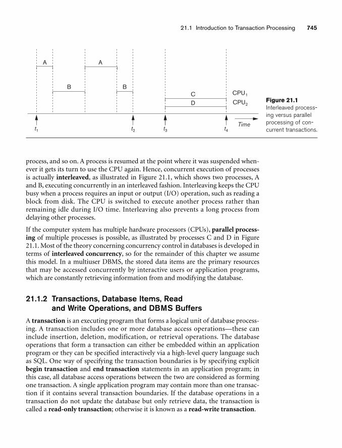
21.1 Introduction to Transaction Processing 745
A A
B BCD
CPU1
CPU2
t1 t2 t3 t4Time
Figure 21.1Interleaved process-ing versus parallelprocessing of con-current transactions.
process, and so on. A process is resumed at the point where it was suspended when-ever it gets its turn to use the CPU again. Hence, concurrent execution of processesis actually interleaved, as illustrated in Figure 21.1, which shows two processes, Aand B, executing concurrently in an interleaved fashion. Interleaving keeps the CPUbusy when a process requires an input or output (I/O) operation, such as reading ablock from disk. The CPU is switched to execute another process rather thanremaining idle during I/O time. Interleaving also prevents a long process fromdelaying other processes.
If the computer system has multiple hardware processors (CPUs), parallel process-ing of multiple processes is possible, as illustrated by processes C and D in Figure21.1. Most of the theory concerning concurrency control in databases is developed interms of interleaved concurrency, so for the remainder of this chapter we assumethis model. In a multiuser DBMS, the stored data items are the primary resourcesthat may be accessed concurrently by interactive users or application programs,which are constantly retrieving information from and modifying the database.
21.1.2 Transactions, Database Items, Read and Write Operations, and DBMS Buffers
A transaction is an executing program that forms a logical unit of database process-ing. A transaction includes one or more database access operations—these caninclude insertion, deletion, modification, or retrieval operations. The databaseoperations that form a transaction can either be embedded within an applicationprogram or they can be specified interactively via a high-level query language suchas SQL. One way of specifying the transaction boundaries is by specifying explicitbegin transaction and end transaction statements in an application program; inthis case, all database access operations between the two are considered as formingone transaction. A single application program may contain more than one transac-tion if it contains several transaction boundaries. If the database operations in atransaction do not update the database but only retrieve data, the transaction iscalled a read-only transaction; otherwise it is known as a read-write transaction.
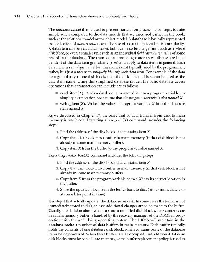
746 Chapter 21 Introduction to Transaction Processing Concepts and Theory
The database model that is used to present transaction processing concepts is quitesimple when compared to the data models that we discussed earlier in the book,such as the relational model or the object model. A database is basically representedas a collection of named data items. The size of a data item is called its granularity.A data item can be a database record, but it can also be a larger unit such as a wholedisk block, or even a smaller unit such as an individual field (attribute) value of somerecord in the database. The transaction processing concepts we discuss are inde-pendent of the data item granularity (size) and apply to data items in general. Eachdata item has a unique name, but this name is not typically used by the programmer;rather, it is just a means to uniquely identify each data item. For example, if the dataitem granularity is one disk block, then the disk block address can be used as thedata item name. Using this simplified database model, the basic database accessoperations that a transaction can include are as follows:
■ read_item(X). Reads a database item named X into a program variable. Tosimplify our notation, we assume that the program variable is also named X.
■ write_item(X). Writes the value of program variable X into the databaseitem named X.
As we discussed in Chapter 17, the basic unit of data transfer from disk to mainmemory is one block. Executing a read_item(X) command includes the followingsteps:
1. Find the address of the disk block that contains item X.
2. Copy that disk block into a buffer in main memory (if that disk block is notalready in some main memory buffer).
3. Copy item X from the buffer to the program variable named X.
Executing a write_item(X) command includes the following steps:
1. Find the address of the disk block that contains item X.
2. Copy that disk block into a buffer in main memory (if that disk block is notalready in some main memory buffer).
3. Copy item X from the program variable named X into its correct location inthe buffer.
4. Store the updated block from the buffer back to disk (either immediately orat some later point in time).
It is step 4 that actually updates the database on disk. In some cases the buffer is notimmediately stored to disk, in case additional changes are to be made to the buffer.Usually, the decision about when to store a modified disk block whose contents arein a main memory buffer is handled by the recovery manager of the DBMS in coop-eration with the underlying operating system. The DBMS will maintain in thedatabase cache a number of data buffers in main memory. Each buffer typicallyholds the contents of one database disk block, which contains some of the databaseitems being processed. When these buffers are all occupied, and additional databasedisk blocks must be copied into memory, some buffer replacement policy is used to
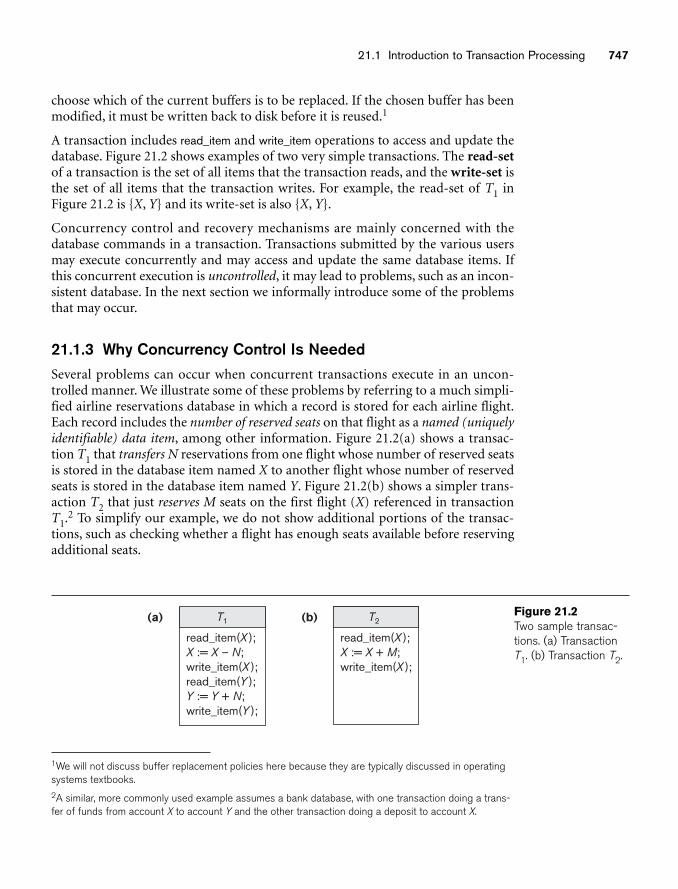
21.1 Introduction to Transaction Processing 747
(a)
read_item(X );X := X – N;write_item(X );read_item(Y );Y := Y + N;write_item(Y );
(b)
read_item(X );X := X + M;write_item(X );
T1 T2Figure 21.2Two sample transac-tions. (a) TransactionT1. (b) Transaction T2.
choose which of the current buffers is to be replaced. If the chosen buffer has beenmodified, it must be written back to disk before it is reused.1
A transaction includes read_item and write_item operations to access and update thedatabase. Figure 21.2 shows examples of two very simple transactions. The read-setof a transaction is the set of all items that the transaction reads, and the write-set isthe set of all items that the transaction writes. For example, the read-set of T1 inFigure 21.2 is {X, Y} and its write-set is also {X, Y}.
Concurrency control and recovery mechanisms are mainly concerned with thedatabase commands in a transaction. Transactions submitted by the various usersmay execute concurrently and may access and update the same database items. Ifthis concurrent execution is uncontrolled, it may lead to problems, such as an incon-sistent database. In the next section we informally introduce some of the problemsthat may occur.
21.1.3 Why Concurrency Control Is NeededSeveral problems can occur when concurrent transactions execute in an uncon-trolled manner. We illustrate some of these problems by referring to a much simpli-fied airline reservations database in which a record is stored for each airline flight.Each record includes the number of reserved seats on that flight as a named (uniquelyidentifiable) data item, among other information. Figure 21.2(a) shows a transac-tion T1 that transfers N reservations from one flight whose number of reserved seatsis stored in the database item named X to another flight whose number of reservedseats is stored in the database item named Y. Figure 21.2(b) shows a simpler trans-action T2 that just reserves M seats on the first flight (X) referenced in transactionT1.2 To simplify our example, we do not show additional portions of the transac-tions, such as checking whether a flight has enough seats available before reservingadditional seats.
1We will not discuss buffer replacement policies here because they are typically discussed in operatingsystems textbooks.2A similar, more commonly used example assumes a bank database, with one transaction doing a trans-fer of funds from account X to account Y and the other transaction doing a deposit to account X.
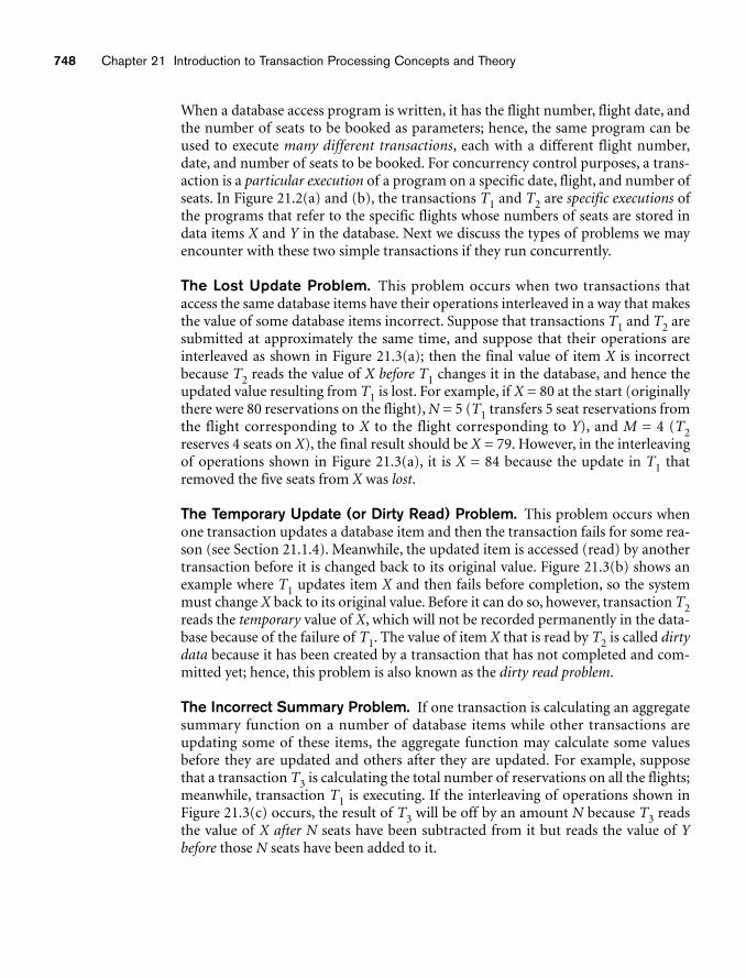
748 Chapter 21 Introduction to Transaction Processing Concepts and Theory
When a database access program is written, it has the flight number, flight date, andthe number of seats to be booked as parameters; hence, the same program can beused to execute many different transactions, each with a different flight number,date, and number of seats to be booked. For concurrency control purposes, a trans-action is a particular execution of a program on a specific date, flight, and number ofseats. In Figure 21.2(a) and (b), the transactions T1 and T2 are specific executions ofthe programs that refer to the specific flights whose numbers of seats are stored indata items X and Y in the database. Next we discuss the types of problems we mayencounter with these two simple transactions if they run concurrently.
The Lost Update Problem. This problem occurs when two transactions thataccess the same database items have their operations interleaved in a way that makesthe value of some database items incorrect. Suppose that transactions T1 and T2 aresubmitted at approximately the same time, and suppose that their operations areinterleaved as shown in Figure 21.3(a); then the final value of item X is incorrectbecause T2 reads the value of X before T1 changes it in the database, and hence theupdated value resulting from T1 is lost. For example, if X = 80 at the start (originallythere were 80 reservations on the flight), N = 5 (T1 transfers 5 seat reservations fromthe flight corresponding to X to the flight corresponding to Y), and M = 4 (T2reserves 4 seats on X), the final result should be X = 79. However, in the interleavingof operations shown in Figure 21.3(a), it is X = 84 because the update in T1 thatremoved the five seats from X was lost.
The Temporary Update (or Dirty Read) Problem. This problem occurs whenone transaction updates a database item and then the transaction fails for some rea-son (see Section 21.1.4). Meanwhile, the updated item is accessed (read) by anothertransaction before it is changed back to its original value. Figure 21.3(b) shows anexample where T1 updates item X and then fails before completion, so the systemmust change X back to its original value. Before it can do so, however, transaction T2reads the temporary value of X, which will not be recorded permanently in the data-base because of the failure of T1. The value of item X that is read by T2 is called dirtydata because it has been created by a transaction that has not completed and com-mitted yet; hence, this problem is also known as the dirty read problem.
The Incorrect Summary Problem. If one transaction is calculating an aggregatesummary function on a number of database items while other transactions areupdating some of these items, the aggregate function may calculate some valuesbefore they are updated and others after they are updated. For example, supposethat a transaction T3 is calculating the total number of reservations on all the flights;meanwhile, transaction T1 is executing. If the interleaving of operations shown inFigure 21.3(c) occurs, the result of T3 will be off by an amount N because T3 readsthe value of X after N seats have been subtracted from it but reads the value of Ybefore those N seats have been added to it.
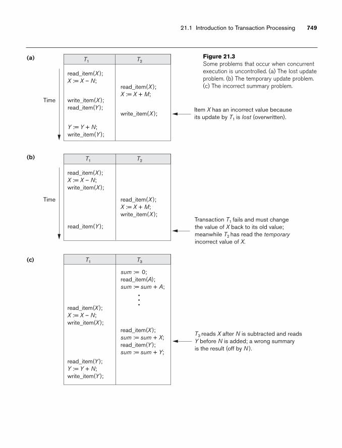
21.1 Introduction to Transaction Processing 749
(a)
read_item(X );X := X – N;
write_item(X );read_item(Y );
read_item(X );X := X + M;
write_item(X );
Time
Item X has an incorrect value becauseits update by T1 is lost (overwritten).
Y := Y + N;write_item(Y );
(b)
read_item(X );X := X – N;write_item(X );
read_item(X );X := X + M;write_item(X );
Time
Transaction T1 fails and must changethe value of X back to its old value;meanwhile T2 has read the temporaryincorrect value of X.
read_item(Y );
T1
T1
(c)
read_item(X );X := X – N;write_item(X );
read_item(Y );Y := Y + N;write_item(Y );
read_item(X );sum := sum + X;read_item(Y );sum := sum + Y;
T3 reads X after N is subtracted and readsY before N is added; a wrong summaryis the result (off by N ).
T3
T2
sum := 0;read_item(A);sum := sum + A;
T1 T2Figure 21.3Some problems that occur when concurrentexecution is uncontrolled. (a) The lost updateproblem. (b) The temporary update problem.(c) The incorrect summary problem.
750 Chapter 21 Introduction to Transaction Processing Concepts and Theory
The Unrepeatable Read Problem. Another problem that may occur is calledunrepeatable read, where a transaction T reads the same item twice and the item ischanged by another transaction T� between the two reads. Hence, T receivesdifferent values for its two reads of the same item. This may occur, for example, ifduring an airline reservation transaction, a customer inquires about seat availabilityon several flights. When the customer decides on a particular flight, the transactionthen reads the number of seats on that flight a second time before completing thereservation, and it may end up reading a different value for the item.
21.1.4 Why Recovery Is NeededWhenever a transaction is submitted to a DBMS for execution, the system is respon-sible for making sure that either all the operations in the transaction are completedsuccessfully and their effect is recorded permanently in the database, or that thetransaction does not have any effect on the database or any other transactions. Inthe first case, the transaction is said to be committed, whereas in the second case,the transaction is aborted. The DBMS must not permit some operations of a trans-action T to be applied to the database while other operations of T are not, becausethe whole transaction is a logical unit of database processing. If a transaction failsafter executing some of its operations but before executing all of them, the opera-tions already executed must be undone and have no lasting effect.
Types of Failures. Failures are generally classified as transaction, system, andmedia failures. There are several possible reasons for a transaction to fail in the mid-dle of execution:
1. A computer failure (system crash). A hardware, software, or network erroroccurs in the computer system during transaction execution. Hardwarecrashes are usually media failures—for example, main memory failure.
2. A transaction or system error. Some operation in the transaction may causeit to fail, such as integer overflow or division by zero. Transaction failure mayalso occur because of erroneous parameter values or because of a logicalprogramming error.3 Additionally, the user may interrupt the transactionduring its execution.
3. Local errors or exception conditions detected by the transaction. Duringtransaction execution, certain conditions may occur that necessitate cancel-lation of the transaction. For example, data for the transaction may not befound. An exception condition,4 such as insufficient account balance in abanking database, may cause a transaction, such as a fund withdrawal, to becanceled. This exception could be programmed in the transaction itself, andin such a case would not be considered as a transaction failure.
3In general, a transaction should be thoroughly tested to ensure that it does not have any bugs (logicalprogramming errors).4Exception conditions, if programmed correctly, do not constitute transaction failures.
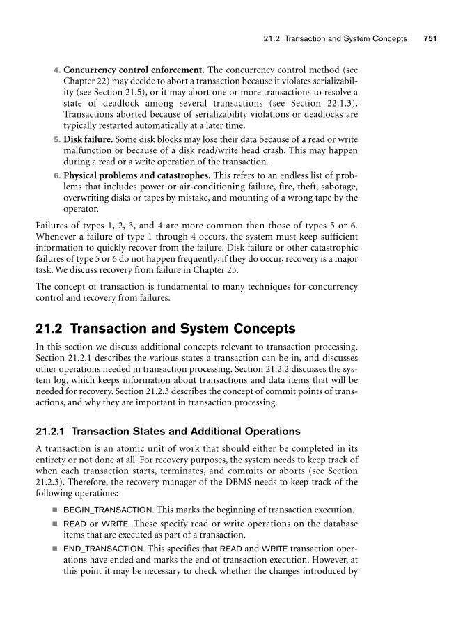
21.2 Transaction and System Concepts 751
4. Concurrency control enforcement. The concurrency control method (seeChapter 22) may decide to abort a transaction because it violates serializabil-ity (see Section 21.5), or it may abort one or more transactions to resolve astate of deadlock among several transactions (see Section 22.1.3).Transactions aborted because of serializability violations or deadlocks aretypically restarted automatically at a later time.
5. Disk failure. Some disk blocks may lose their data because of a read or writemalfunction or because of a disk read/write head crash. This may happenduring a read or a write operation of the transaction.
6. Physical problems and catastrophes. This refers to an endless list of prob-lems that includes power or air-conditioning failure, fire, theft, sabotage,overwriting disks or tapes by mistake, and mounting of a wrong tape by theoperator.
Failures of types 1, 2, 3, and 4 are more common than those of types 5 or 6.Whenever a failure of type 1 through 4 occurs, the system must keep sufficientinformation to quickly recover from the failure. Disk failure or other catastrophicfailures of type 5 or 6 do not happen frequently; if they do occur, recovery is a majortask. We discuss recovery from failure in Chapter 23.
The concept of transaction is fundamental to many techniques for concurrencycontrol and recovery from failures.
21.2 Transaction and System ConceptsIn this section we discuss additional concepts relevant to transaction processing.Section 21.2.1 describes the various states a transaction can be in, and discussesother operations needed in transaction processing. Section 21.2.2 discusses the sys-tem log, which keeps information about transactions and data items that will beneeded for recovery. Section 21.2.3 describes the concept of commit points of trans-actions, and why they are important in transaction processing.
21.2.1 Transaction States and Additional OperationsA transaction is an atomic unit of work that should either be completed in itsentirety or not done at all. For recovery purposes, the system needs to keep track ofwhen each transaction starts, terminates, and commits or aborts (see Section21.2.3). Therefore, the recovery manager of the DBMS needs to keep track of thefollowing operations:
■ BEGIN_TRANSACTION. This marks the beginning of transaction execution.
■ READ or WRITE. These specify read or write operations on the databaseitems that are executed as part of a transaction.
■ END_TRANSACTION. This specifies that READ and WRITE transaction oper-ations have ended and marks the end of transaction execution. However, atthis point it may be necessary to check whether the changes introduced by
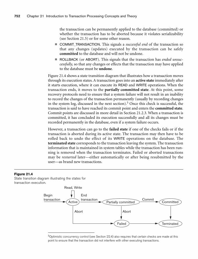
752 Chapter 21 Introduction to Transaction Processing Concepts and Theory
Active
Begintransaction
Endtransaction Commit
AbortAbort
Read, Write
Partially committed
Failed Terminated
Committed
Figure 21.4State transition diagram illustrating the states fortransaction execution.
the transaction can be permanently applied to the database (committed) orwhether the transaction has to be aborted because it violates serializability(see Section 21.5) or for some other reason.
■ COMMIT_TRANSACTION. This signals a successful end of the transaction sothat any changes (updates) executed by the transaction can be safelycommitted to the database and will not be undone.
■ ROLLBACK (or ABORT). This signals that the transaction has ended unsuc-cessfully, so that any changes or effects that the transaction may have appliedto the database must be undone.
Figure 21.4 shows a state transition diagram that illustrates how a transaction movesthrough its execution states. A transaction goes into an active state immediately afterit starts execution, where it can execute its READ and WRITE operations. When thetransaction ends, it moves to the partially committed state. At this point, somerecovery protocols need to ensure that a system failure will not result in an inabilityto record the changes of the transaction permanently (usually by recording changesin the system log, discussed in the next section).5 Once this check is successful, thetransaction is said to have reached its commit point and enters the committed state.Commit points are discussed in more detail in Section 21.2.3. When a transaction iscommitted, it has concluded its execution successfully and all its changes must berecorded permanently in the database, even if a system failure occurs.
However, a transaction can go to the failed state if one of the checks fails or if thetransaction is aborted during its active state. The transaction may then have to berolled back to undo the effect of its WRITE operations on the database. Theterminated state corresponds to the transaction leaving the system. The transactioninformation that is maintained in system tables while the transaction has been run-ning is removed when the transaction terminates. Failed or aborted transactionsmay be restarted later—either automatically or after being resubmitted by theuser—as brand new transactions.
5Optimistic concurrency control (see Section 22.4) also requires that certain checks are made at thispoint to ensure that the transaction did not interfere with other executing transactions.
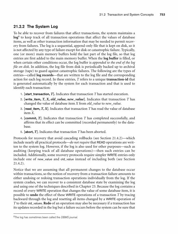
21.2 Transaction and System Concepts 753
21.2.2 The System LogTo be able to recover from failures that affect transactions, the system maintains alog6 to keep track of all transaction operations that affect the values of databaseitems, as well as other transaction information that may be needed to permit recov-ery from failures. The log is a sequential, append-only file that is kept on disk, so itis not affected by any type of failure except for disk or catastrophic failure. Typically,one (or more) main memory buffers hold the last part of the log file, so that logentries are first added to the main memory buffer. When the log buffer is filled, orwhen certain other conditions occur, the log buffer is appended to the end of the logfile on disk. In addition, the log file from disk is periodically backed up to archivalstorage (tape) to guard against catastrophic failures. The following are the types ofentries—called log records—that are written to the log file and the correspondingaction for each log record. In these entries, T refers to a unique transaction-id thatis generated automatically by the system for each transaction and that is used toidentify each transaction:
1. [start_transaction, T]. Indicates that transaction T has started execution.
2. [write_item, T, X, old_value, new_value]. Indicates that transaction T haschanged the value of database item X from old_value to new_value.
3. [read_item, T, X]. Indicates that transaction T has read the value of databaseitem X.
4. [commit, T]. Indicates that transaction T has completed successfully, andaffirms that its effect can be committed (recorded permanently) to the data-base.
5. [abort, T]. Indicates that transaction T has been aborted.
Protocols for recovery that avoid cascading rollbacks (see Section 21.4.2)—whichinclude nearly all practical protocols—do not require that READ operations are writ-ten to the system log. However, if the log is also used for other purposes—such asauditing (keeping track of all database operations)—then such entries can beincluded. Additionally, some recovery protocols require simpler WRITE entries onlyinclude one of new_value and old_value instead of including both (see Section21.4.2).
Notice that we are assuming that all permanent changes to the database occurwithin transactions, so the notion of recovery from a transaction failure amounts toeither undoing or redoing transaction operations individually from the log. If thesystem crashes, we can recover to a consistent database state by examining the logand using one of the techniques described in Chapter 23. Because the log contains arecord of every WRITE operation that changes the value of some database item, it ispossible to undo the effect of these WRITE operations of a transaction T by tracingbackward through the log and resetting all items changed by a WRITE operation ofT to their old_values. Redo of an operation may also be necessary if a transaction hasits updates recorded in the log but a failure occurs before the system can be sure that
6The log has sometimes been called the DBMS journal.
754 Chapter 21 Introduction to Transaction Processing Concepts and Theory
all these new_values have been written to the actual database on disk from the mainmemory buffers.7
21.2.3 Commit Point of a TransactionA transaction T reaches its commit point when all its operations that access thedatabase have been executed successfully and the effect of all the transaction opera-tions on the database have been recorded in the log. Beyond the commit point, thetransaction is said to be committed, and its effect must be permanently recorded inthe database. The transaction then writes a commit record [commit, T] into the log.If a system failure occurs, we can search back in the log for all transactions T thathave written a [start_transaction, T] record into the log but have not written their[commit, T] record yet; these transactions may have to be rolled back to undo theireffect on the database during the recovery process. Transactions that have writtentheir commit record in the log must also have recorded all their WRITE operations inthe log, so their effect on the database can be redone from the log records.
Notice that the log file must be kept on disk. As discussed in Chapter 17, updating adisk file involves copying the appropriate block of the file from disk to a buffer inmain memory, updating the buffer in main memory, and copying the buffer to disk.It is common to keep one or more blocks of the log file in main memory buffers,called the log buffer, until they are filled with log entries and then to write themback to disk only once, rather than writing to disk every time a log entry is added.This saves the overhead of multiple disk writes of the same log file buffer. At thetime of a system crash, only the log entries that have been written back to disk areconsidered in the recovery process because the contents of main memory may belost. Hence, before a transaction reaches its commit point, any portion of the logthat has not been written to the disk yet must now be written to the disk. Thisprocess is called force-writing the log buffer before committing a transaction.
21.3 Desirable Properties of TransactionsTransactions should possess several properties, often called the ACID properties;they should be enforced by the concurrency control and recovery methods of theDBMS. The following are the ACID properties:
■ Atomicity. A transaction is an atomic unit of processing; it should either beperformed in its entirety or not performed at all.
■ Consistency preservation. A transaction should be consistency preserving,meaning that if it is completely executed from beginning to end withoutinterference from other transactions, it should take the database from oneconsistent state to another.
■ Isolation. A transaction should appear as though it is being executed in iso-lation from other transactions, even though many transactions are executing
7Undo and redo are discussed more fully in Chapter 23.
21.4 Characterizing Schedules Based on Recoverability 755
concurrently. That is, the execution of a transaction should not be interferedwith by any other transactions executing concurrently.
■ Durability or permanency. The changes applied to the database by a com-mitted transaction must persist in the database. These changes must not belost because of any failure.
The atomicity property requires that we execute a transaction to completion. It is theresponsibility of the transaction recovery subsystem of a DBMS to ensure atomicity.If a transaction fails to complete for some reason, such as a system crash in themidst of transaction execution, the recovery technique must undo any effects of thetransaction on the database. On the other hand, write operations of a committedtransaction must be eventually written to disk.
The preservation of consistency is generally considered to be the responsibility of theprogrammers who write the database programs or of the DBMS module thatenforces integrity constraints. Recall that a database state is a collection of all thestored data items (values) in the database at a given point in time. A consistent stateof the database satisfies the constraints specified in the schema as well as any otherconstraints on the database that should hold. A database program should be writtenin a way that guarantees that, if the database is in a consistent state before executingthe transaction, it will be in a consistent state after the complete execution of thetransaction, assuming that no interference with other transactions occurs.
The isolation property is enforced by the concurrency control subsystem of theDBMS.8 If every transaction does not make its updates (write operations) visible toother transactions until it is committed, one form of isolation is enforced that solvesthe temporary update problem and eliminates cascading rollbacks (see Chapter 23)but does not eliminate all other problems. There have been attempts to define thelevel of isolation of a transaction. A transaction is said to have level 0 (zero) isola-tion if it does not overwrite the dirty reads of higher-level transactions. Level 1(one) isolation has no lost updates, and level 2 isolation has no lost updates and nodirty reads. Finally, level 3 isolation (also called true isolation) has, in addition tolevel 2 properties, repeatable reads.9
And last, the durability property is the responsibility of the recovery subsystem of theDBMS. We will introduce how recovery protocols enforce durability and atomicityin the next section and then discuss this in more detail in Chapter 23.
21.4 Characterizing Schedules Based on Recoverability
When transactions are executing concurrently in an interleaved fashion, then theorder of execution of operations from all the various transactions is known as aschedule (or history). In this section, first we define the concept of schedules, and
8We will discuss concurrency control protocols in Chapter 22.9The SQL syntax for isolation level discussed later in Section 21.6 is closely related to these levels.
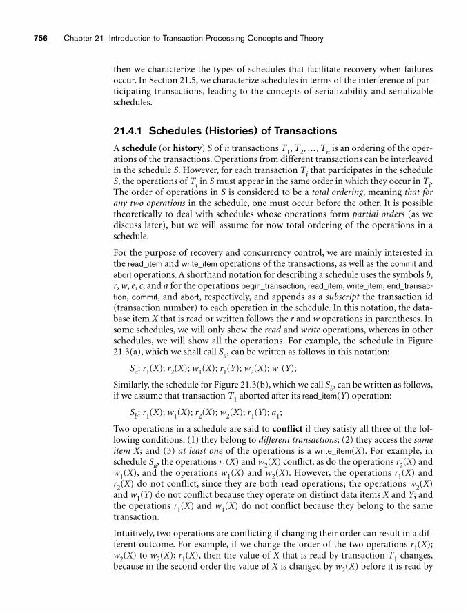
756 Chapter 21 Introduction to Transaction Processing Concepts and Theory
then we characterize the types of schedules that facilitate recovery when failuresoccur. In Section 21.5, we characterize schedules in terms of the interference of par-ticipating transactions, leading to the concepts of serializability and serializableschedules.
21.4.1 Schedules (Histories) of TransactionsA schedule (or history) S of n transactions T1, T2, ..., Tn is an ordering of the oper-ations of the transactions. Operations from different transactions can be interleavedin the schedule S. However, for each transaction Ti that participates in the scheduleS, the operations of Ti in S must appear in the same order in which they occur in Ti.The order of operations in S is considered to be a total ordering, meaning that forany two operations in the schedule, one must occur before the other. It is possibletheoretically to deal with schedules whose operations form partial orders (as we discuss later), but we will assume for now total ordering of the operations in a schedule.
For the purpose of recovery and concurrency control, we are mainly interested inthe read_item and write_item operations of the transactions, as well as the commit andabort operations. A shorthand notation for describing a schedule uses the symbols b,r, w, e, c, and a for the operations begin_transaction, read_item, write_item, end_transac-tion, commit, and abort, respectively, and appends as a subscript the transaction id(transaction number) to each operation in the schedule. In this notation, the data-base item X that is read or written follows the r and w operations in parentheses. Insome schedules, we will only show the read and write operations, whereas in otherschedules, we will show all the operations. For example, the schedule in Figure21.3(a), which we shall call Sa, can be written as follows in this notation:
Sa: r1(X); r2(X); w1(X); r1(Y); w2(X); w1(Y);
Similarly, the schedule for Figure 21.3(b), which we call Sb, can be written as follows,if we assume that transaction T1 aborted after its read_item(Y) operation:
Sb: r1(X); w1(X); r2(X); w2(X); r1(Y); a1;
Two operations in a schedule are said to conflict if they satisfy all three of the fol-lowing conditions: (1) they belong to different transactions; (2) they access the sameitem X; and (3) at least one of the operations is a write_item(X). For example, inschedule Sa, the operations r1(X) and w2(X) conflict, as do the operations r2(X) andw1(X), and the operations w1(X) and w2(X). However, the operations r1(X) andr2(X) do not conflict, since they are both read operations; the operations w2(X)and w1(Y) do not conflict because they operate on distinct data items X and Y; andthe operations r1(X) and w1(X) do not conflict because they belong to the sametransaction.
Intuitively, two operations are conflicting if changing their order can result in a dif-ferent outcome. For example, if we change the order of the two operations r1(X);w2(X) to w2(X); r1(X), then the value of X that is read by transaction T1 changes,because in the second order the value of X is changed by w2(X) before it is read by
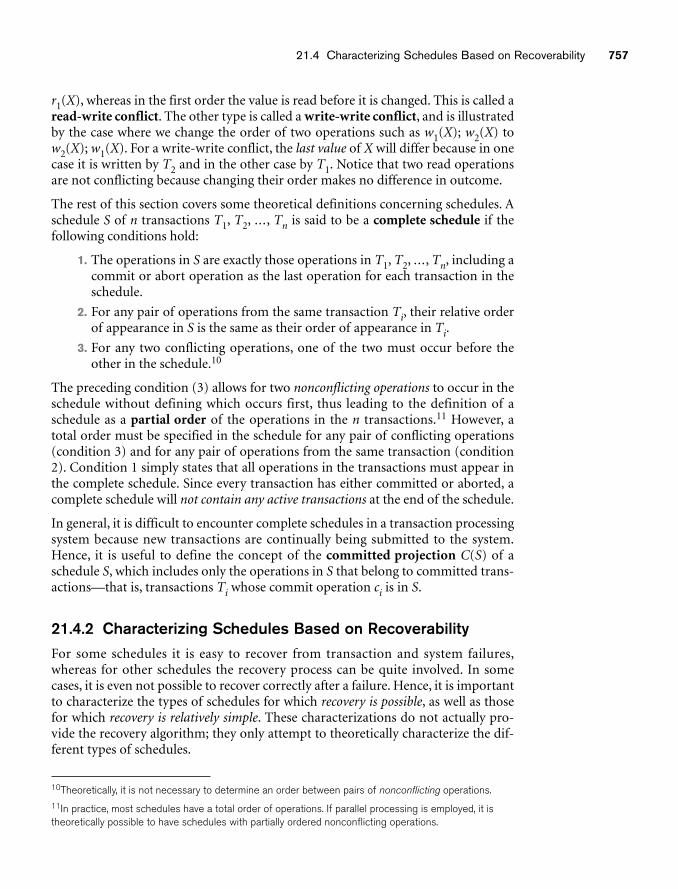
21.4 Characterizing Schedules Based on Recoverability 757
r1(X), whereas in the first order the value is read before it is changed. This is called aread-write conflict. The other type is called a write-write conflict, and is illustratedby the case where we change the order of two operations such as w1(X); w2(X) tow2(X); w1(X). For a write-write conflict, the last value of X will differ because in onecase it is written by T2 and in the other case by T1. Notice that two read operationsare not conflicting because changing their order makes no difference in outcome.
The rest of this section covers some theoretical definitions concerning schedules. Aschedule S of n transactions T1, T2, ..., Tn is said to be a complete schedule if thefollowing conditions hold:
1. The operations in S are exactly those operations in T1, T2, ..., Tn, including acommit or abort operation as the last operation for each transaction in theschedule.
2. For any pair of operations from the same transaction Ti, their relative orderof appearance in S is the same as their order of appearance in Ti.
3. For any two conflicting operations, one of the two must occur before theother in the schedule.10
The preceding condition (3) allows for two nonconflicting operations to occur in theschedule without defining which occurs first, thus leading to the definition of aschedule as a partial order of the operations in the n transactions.11 However, atotal order must be specified in the schedule for any pair of conflicting operations(condition 3) and for any pair of operations from the same transaction (condition2). Condition 1 simply states that all operations in the transactions must appear inthe complete schedule. Since every transaction has either committed or aborted, acomplete schedule will not contain any active transactions at the end of the schedule.
In general, it is difficult to encounter complete schedules in a transaction processingsystem because new transactions are continually being submitted to the system.Hence, it is useful to define the concept of the committed projection C(S) of aschedule S, which includes only the operations in S that belong to committed trans-actions—that is, transactions Ti whose commit operation ci is in S.
21.4.2 Characterizing Schedules Based on RecoverabilityFor some schedules it is easy to recover from transaction and system failures,whereas for other schedules the recovery process can be quite involved. In somecases, it is even not possible to recover correctly after a failure. Hence, it is importantto characterize the types of schedules for which recovery is possible, as well as thosefor which recovery is relatively simple. These characterizations do not actually pro-vide the recovery algorithm; they only attempt to theoretically characterize the dif-ferent types of schedules.
10Theoretically, it is not necessary to determine an order between pairs of nonconflicting operations.11In practice, most schedules have a total order of operations. If parallel processing is employed, it istheoretically possible to have schedules with partially ordered nonconflicting operations.
758 Chapter 21 Introduction to Transaction Processing Concepts and Theory
First, we would like to ensure that, once a transaction T is committed, it shouldnever be necessary to roll back T. This ensures that the durability property of trans-actions is not violated (see Section 21.3). The schedules that theoretically meet thiscriterion are called recoverable schedules; those that do not are callednonrecoverable and hence should not be permitted by the DBMS. The definition ofrecoverable schedule is as follows: A schedule S is recoverable if no transaction T inS commits until all transactions T� that have written some item X that T reads havecommitted. A transaction T reads from transaction T� in a schedule S if some itemX is first written by T� and later read by T. In addition, T� should not have beenaborted before T reads item X, and there should be no transactions that write X afterT� writes it and before T reads it (unless those transactions, if any, have abortedbefore T reads X).
Some recoverable schedules may require a complex recovery process as we shall see,but if sufficient information is kept (in the log), a recovery algorithm can be devisedfor any recoverable schedule. The (partial) schedules Sa and Sb from the precedingsection are both recoverable, since they satisfy the above definition. Consider theschedule Sa� given below, which is the same as schedule Sa except that two commitoperations have been added to Sa:
Sa�: r1(X); r2(X); w1(X); r1(Y); w2(X); c2; w1(Y); c1;
Sa� is recoverable, even though it suffers from the lost update problem; this problemis handled by serializability theory (see Section 21.5). However, consider the two(partial) schedules Sc and Sd that follow:
Sc: r1(X); w1(X); r2(X); r1(Y); w2(X); c2; a1;
Sd: r1(X); w1(X); r2(X); r1(Y); w2(X); w1(Y); c1; c2;
Se: r1(X); w1(X); r2(X); r1(Y); w2(X); w1(Y); a1; a2;
Sc is not recoverable because T2 reads item X from T1, but T2 commits before T1commits. The problem occurs if T1 aborts after the c2 operation in Sc, then the valueof X that T2 read is no longer valid and T2 must be aborted after it is committed,leading to a schedule that is not recoverable. For the schedule to be recoverable, the c2operation in Sc must be postponed until after T1 commits, as shown in Sd. If T1aborts instead of committing, then T2 should also abort as shown in Se, because thevalue of X it read is no longer valid. In Se, aborting T2 is acceptable since it has notcommitted yet, which is not the case for the nonrecoverable schedule Sc.
In a recoverable schedule, no committed transaction ever needs to be rolled back,and so the definition of committed transaction as durable is not violated. However,it is possible for a phenomenon known as cascading rollback (or cascading abort)to occur in some recoverable schedules, where an uncommitted transaction has to berolled back because it read an item from a transaction that failed. This is illustratedin schedule Se, where transaction T2 has to be rolled back because it read item Xfrom T1, and T1 then aborted.
Because cascading rollback can be quite time-consuming—since numerous transac-tions can be rolled back (see Chapter 23)—it is important to characterize the sched-
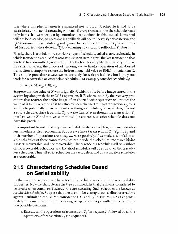
21.5 Characterizing Schedules Based on Serializability 759
ules where this phenomenon is guaranteed not to occur. A schedule is said to becascadeless, or to avoid cascading rollback, if every transaction in the schedule readsonly items that were written by committed transactions. In this case, all items readwill not be discarded, so no cascading rollback will occur. To satisfy this criterion, ther2(X) command in schedules Sd and Se must be postponed until after T1 has commit-ted (or aborted), thus delaying T2 but ensuring no cascading rollback if T1 aborts.
Finally, there is a third, more restrictive type of schedule, called a strict schedule, inwhich transactions can neither read nor write an item X until the last transaction thatwrote X has committed (or aborted). Strict schedules simplify the recovery process.In a strict schedule, the process of undoing a write_item(X) operation of an abortedtransaction is simply to restore the before image (old_value or BFIM) of data item X.This simple procedure always works correctly for strict schedules, but it may notwork for recoverable or cascadeless schedules. For example, consider schedule Sf :
Sf : w1(X, 5); w2(X, 8); a1;
Suppose that the value of X was originally 9, which is the before image stored in thesystem log along with the w1(X, 5) operation. If T1 aborts, as in Sf , the recovery pro-cedure that restores the before image of an aborted write operation will restore thevalue of X to 9, even though it has already been changed to 8 by transaction T2, thusleading to potentially incorrect results. Although schedule Sf is cascadeless, it is nota strict schedule, since it permits T2 to write item X even though the transaction T1that last wrote X had not yet committed (or aborted). A strict schedule does nothave this problem.
It is important to note that any strict schedule is also cascadeless, and any cascade-less schedule is also recoverable. Suppose we have i transactions T1, T2, ..., Ti, andtheir number of operations are n1, n2, ..., ni, respectively. If we make a set of all pos-sible schedules of these transactions, we can divide the schedules into two disjointsubsets: recoverable and nonrecoverable. The cascadeless schedules will be a subsetof the recoverable schedules, and the strict schedules will be a subset of the cascade-less schedules. Thus, all strict schedules are cascadeless, and all cascadeless schedulesare recoverable.
21.5 Characterizing Schedules Based on Serializability
In the previous section, we characterized schedules based on their recoverabilityproperties. Now we characterize the types of schedules that are always considered tobe correct when concurrent transactions are executing. Such schedules are known asserializable schedules. Suppose that two users—for example, two airline reservationsagents—submit to the DBMS transactions T1 and T2 in Figure 21.2 at approxi-mately the same time. If no interleaving of operations is permitted, there are onlytwo possible outcomes:
1. Execute all the operations of transaction T1 (in sequence) followed by all theoperations of transaction T2 (in sequence).
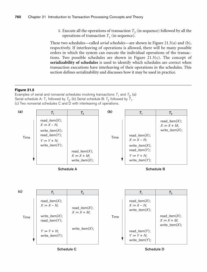
(a)
Schedule A Schedule B
read_item(X );X := X – N;
write_item(X );read_item(Y );
read_item(X );X := X + M;write_item(X );
TimeY := Y + N;write_item(Y );
(b)
read_item(X );X := X + M;write_item(X );
Time read_item(X );X := X – N;
write_item(X );read_item(Y );
Y := Y + N;write_item(Y );
(c) T1 T2
Schedule C Schedule D
read_item(X );X := X – N;
write_item(X );read_item(Y );
read_item(X );X := X + M;
write_item(X );
Time
Y := Y + N;write_item(Y );
read_item(X );X := X + M;write_item(X );
read_item(X );X := X – N;write_item(X );
read_item(Y );Y := Y + N;write_item(Y );
T1 T2
T1 T2 T1 T2
Time
760 Chapter 21 Introduction to Transaction Processing Concepts and Theory
Figure 21.5Examples of serial and nonserial schedules involving transactions T1 and T2. (a)Serial schedule A: T1 followed by T2. (b) Serial schedule B: T2 followed by T1.(c) Two nonserial schedules C and D with interleaving of operations.
2. Execute all the operations of transaction T2 (in sequence) followed by all theoperations of transaction T1 (in sequence).
These two schedules—called serial schedules—are shown in Figure 21.5(a) and (b),respectively. If interleaving of operations is allowed, there will be many possibleorders in which the system can execute the individual operations of the transac-tions. Two possible schedules are shown in Figure 21.5(c). The concept ofserializability of schedules is used to identify which schedules are correct whentransaction executions have interleaving of their operations in the schedules. Thissection defines serializability and discusses how it may be used in practice.
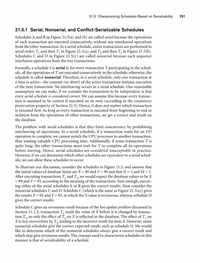
21.5 Characterizing Schedules Based on Serializability 761
21.5.1 Serial, Nonserial, and Conflict-Serializable SchedulesSchedules A and B in Figure 21.5(a) and (b) are called serial because the operationsof each transaction are executed consecutively, without any interleaved operationsfrom the other transaction. In a serial schedule, entire transactions are performed inserial order: T1 and then T2 in Figure 21.5(a), and T2 and then T1 in Figure 21.5(b).Schedules C and D in Figure 21.5(c) are called nonserial because each sequenceinterleaves operations from the two transactions.
Formally, a schedule S is serial if, for every transaction T participating in the sched-ule, all the operations of T are executed consecutively in the schedule; otherwise, theschedule is called nonserial. Therefore, in a serial schedule, only one transaction ata time is active—the commit (or abort) of the active transaction initiates executionof the next transaction. No interleaving occurs in a serial schedule. One reasonableassumption we can make, if we consider the transactions to be independent, is thatevery serial schedule is considered correct. We can assume this because every transac-tion is assumed to be correct if executed on its own (according to the consistencypreservation property of Section 21.3). Hence, it does not matter which transactionis executed first. As long as every transaction is executed from beginning to end inisolation from the operations of other transactions, we get a correct end result onthe database.
The problem with serial schedules is that they limit concurrency by prohibitinginterleaving of operations. In a serial schedule, if a transaction waits for an I/Ooperation to complete, we cannot switch the CPU processor to another transaction,thus wasting valuable CPU processing time. Additionally, if some transaction T isquite long, the other transactions must wait for T to complete all its operationsbefore starting. Hence, serial schedules are considered unacceptable in practice.However, if we can determine which other schedules are equivalent to a serial sched-ule, we can allow these schedules to occur.
To illustrate our discussion, consider the schedules in Figure 21.5, and assume thatthe initial values of database items are X = 90 and Y = 90 and that N = 3 and M = 2.After executing transactions T1 and T2, we would expect the database values to be X= 89 and Y = 93, according to the meaning of the transactions. Sure enough, execut-ing either of the serial schedules A or B gives the correct results. Now consider thenonserial schedules C and D. Schedule C (which is the same as Figure 21.3(a)) givesthe results X = 92 and Y = 93, in which the X value is erroneous, whereas schedule Dgives the correct results.
Schedule C gives an erroneous result because of the lost update problem discussed inSection 21.1.3; transaction T2 reads the value of X before it is changed by transac-tion T1, so only the effect of T2 on X is reflected in the database. The effect of T1 onX is lost, overwritten by T2, leading to the incorrect result for item X. However, somenonserial schedules give the correct expected result, such as schedule D. We wouldlike to determine which of the nonserial schedules always give a correct result andwhich may give erroneous results. The concept used to characterize schedules in thismanner is that of serializability of a schedule.
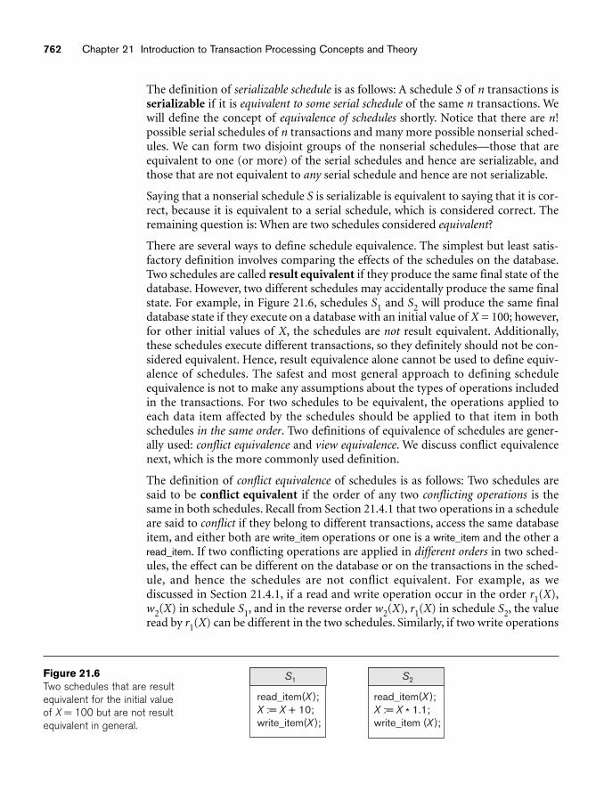
762 Chapter 21 Introduction to Transaction Processing Concepts and Theory
S1
read_item(X );X := X + 10;write_item(X );
S2
read_item(X );X := X * 1.1;write_item (X );
Figure 21.6Two schedules that are resultequivalent for the initial valueof X = 100 but are not resultequivalent in general.
The definition of serializable schedule is as follows: A schedule S of n transactions isserializable if it is equivalent to some serial schedule of the same n transactions. Wewill define the concept of equivalence of schedules shortly. Notice that there are n!possible serial schedules of n transactions and many more possible nonserial sched-ules. We can form two disjoint groups of the nonserial schedules—those that areequivalent to one (or more) of the serial schedules and hence are serializable, andthose that are not equivalent to any serial schedule and hence are not serializable.
Saying that a nonserial schedule S is serializable is equivalent to saying that it is cor-rect, because it is equivalent to a serial schedule, which is considered correct. Theremaining question is: When are two schedules considered equivalent?
There are several ways to define schedule equivalence. The simplest but least satis-factory definition involves comparing the effects of the schedules on the database.Two schedules are called result equivalent if they produce the same final state of thedatabase. However, two different schedules may accidentally produce the same finalstate. For example, in Figure 21.6, schedules S1 and S2 will produce the same finaldatabase state if they execute on a database with an initial value of X = 100; however,for other initial values of X, the schedules are not result equivalent. Additionally,these schedules execute different transactions, so they definitely should not be con-sidered equivalent. Hence, result equivalence alone cannot be used to define equiv-alence of schedules. The safest and most general approach to defining scheduleequivalence is not to make any assumptions about the types of operations includedin the transactions. For two schedules to be equivalent, the operations applied toeach data item affected by the schedules should be applied to that item in bothschedules in the same order. Two definitions of equivalence of schedules are gener-ally used: conflict equivalence and view equivalence. We discuss conflict equivalencenext, which is the more commonly used definition.
The definition of conflict equivalence of schedules is as follows: Two schedules aresaid to be conflict equivalent if the order of any two conflicting operations is thesame in both schedules. Recall from Section 21.4.1 that two operations in a scheduleare said to conflict if they belong to different transactions, access the same databaseitem, and either both are write_item operations or one is a write_item and the other aread_item. If two conflicting operations are applied in different orders in two sched-ules, the effect can be different on the database or on the transactions in the sched-ule, and hence the schedules are not conflict equivalent. For example, as wediscussed in Section 21.4.1, if a read and write operation occur in the order r1(X),w2(X) in schedule S1, and in the reverse order w2(X), r1(X) in schedule S2, the valueread by r1(X) can be different in the two schedules. Similarly, if two write operations
21.5 Characterizing Schedules Based on Serializability 763
occur in the order w1(X), w2(X) in S1, and in the reverse order w2(X), w1(X) in S2,the next r(X) operation in the two schedules will read potentially different values; orif these are the last operations writing item X in the schedules, the final value of itemX in the database will be different.
Using the notion of conflict equivalence, we define a schedule S to be conflict seri-alizable12 if it is (conflict) equivalent to some serial schedule S�. In such a case, wecan reorder the nonconflicting operations in S until we form the equivalent serialschedule S�. According to this definition, schedule D in Figure 21.5(c) is equivalentto the serial schedule A in Figure 21.5(a). In both schedules, the read_item(X) of T2reads the value of X written by T1, while the other read_item operations read thedatabase values from the initial database state. Additionally, T1 is the last transactionto write Y, and T2 is the last transaction to write X in both schedules. Because A is aserial schedule and schedule D is equivalent to A, D is a serializable schedule. Noticethat the operations r1(Y) and w1(Y) of schedule D do not conflict with the opera-tions r2(X) and w2(X), since they access different data items. Therefore, we can mover1(Y), w1(Y) before r2(X), w2(X), leading to the equivalent serial schedule T1, T2.
Schedule C in Figure 21.5(c) is not equivalent to either of the two possible serialschedules A and B, and hence is not serializable. Trying to reorder the operations ofschedule C to find an equivalent serial schedule fails because r2(X) and w1(X) con-flict, which means that we cannot move r2(X) down to get the equivalent serialschedule T1, T2. Similarly, because w1(X) and w2(X) conflict, we cannot move w1(X)down to get the equivalent serial schedule T2, T1.
Another, more complex definition of equivalence—called view equivalence, whichleads to the concept of view serializability—is discussed in Section 21.5.4.
21.5.2 Testing for Conflict Serializability of a ScheduleThere is a simple algorithm for determining whether a particular schedule is con-flict serializable or not. Most concurrency control methods do not actually test forserializability. Rather protocols, or rules, are developed that guarantee that anyschedule that follows these rules will be serializable. We discuss the algorithm fortesting conflict serializability of schedules here to gain a better understanding ofthese concurrency control protocols, which are discussed in Chapter 22.
Algorithm 21.1 can be used to test a schedule for conflict serializability. The algo-rithm looks at only the read_item and write_item operations in a schedule to constructa precedence graph (or serialization graph), which is a directed graph G = (N, E)that consists of a set of nodes N = {T1, T2, ..., Tn } and a set of directed edges E = {e1,e2, ..., em }. There is one node in the graph for each transaction Ti in the schedule.Each edge ei in the graph is of the form (Tj → Tk ), 1 ≤ j ≤ n, 1 ≤ k n, where Tj is thestarting node of ei and Tk is the ending node of ei. Such an edge from node Tj to
12We will use serializable to mean conflict serializable. Another definition of serializable used in practice(see Section 21.6) is to have repeatable reads, no dirty reads, and no phantom records (see Section22.7.1 for a discussion on phantoms).
764 Chapter 21 Introduction to Transaction Processing Concepts and Theory
node Tk is created by the algorithm if one of the operations in Tj appears in theschedule before some conflicting operation in Tk.
Algorithm 21.1. Testing Conflict Serializability of a Schedule S
1. For each transaction Ti participating in schedule S, create a node labeled Tiin the precedence graph.
2. For each case in S where Tj executes a read_item(X) after Ti executes awrite_item(X), create an edge (Ti → Tj) in the precedence graph.
3. For each case in S where Tj executes a write_item(X) after Ti executes aread_item(X), create an edge (Ti → Tj) in the precedence graph.
4. For each case in S where Tj executes a write_item(X) after Ti executes awrite_item(X), create an edge (Ti → Tj) in the precedence graph.
5. The schedule S is serializable if and only if the precedence graph has nocycles.
The precedence graph is constructed as described in Algorithm 21.1. If there is acycle in the precedence graph, schedule S is not (conflict) serializable; if there is nocycle, S is serializable. A cycle in a directed graph is a sequence of edges C = ((Tj →Tk), (Tk → Tp), ..., (Ti → Tj)) with the property that the starting node of eachedge—except the first edge—is the same as the ending node of the previous edge,and the starting node of the first edge is the same as the ending node of the last edge(the sequence starts and ends at the same node).
In the precedence graph, an edge from Ti to Tj means that transaction Ti must comebefore transaction Tj in any serial schedule that is equivalent to S, because two con-flicting operations appear in the schedule in that order. If there is no cycle in theprecedence graph, we can create an equivalent serial schedule S� that is equivalentto S, by ordering the transactions that participate in S as follows: Whenever an edgeexists in the precedence graph from Ti to Tj, Ti must appear before Tj in the equiva-lent serial schedule S�.13 Notice that the edges (Ti → Tj) in a precedence graph canoptionally be labeled by the name(s) of the data item(s) that led to creating theedge. Figure 21.7 shows such labels on the edges.
In general, several serial schedules can be equivalent to S if the precedence graph forS has no cycle. However, if the precedence graph has a cycle, it is easy to show thatwe cannot create any equivalent serial schedule, so S is not serializable. The prece-dence graphs created for schedules A to D, respectively, in Figure 21.5 appear inFigure 21.7(a) to (d). The graph for schedule C has a cycle, so it is not serializable.The graph for schedule D has no cycle, so it is serializable, and the equivalent serialschedule is T1 followed by T2. The graphs for schedules A and B have no cycles, asexpected, because the schedules are serial and hence serializable.
Another example, in which three transactions participate, is shown in Figure 21.8.Figure 21.8(a) shows the read_item and write_item operations in each transaction.Two schedules E and F for these transactions are shown in Figure 21.8(b) and (c),
13This process of ordering the nodes of an acrylic graph is known as topological sorting.
21.5 Characterizing Schedules Based on Serializability 765
T1(a)
(c)
(b)
(d)
T2
T1
X
X
X
X
T2
T1 T2
T1 T2
X
Figure 21.7Constructing the precedence graphs for schedules A to D from Figure 21.5 to testfor conflict serializability. (a) Precedence graph for serial schedule A. (b) Precedencegraph for serial schedule B. (c) Precedence graph for schedule C (not serializable).(d) Precedence graph for schedule D (serializable, equivalent to schedule A).
respectively, and the precedence graphs for schedules E and F are shown in parts (d)and (e). Schedule E is not serializable because the corresponding precedence graphhas cycles. Schedule F is serializable, and the serial schedule equivalent to F is shownin Figure 21.8(e). Although only one equivalent serial schedule exists for F, in gen-eral there may be more than one equivalent serial schedule for a serializable sched-ule. Figure 21.8(f) shows a precedence graph representing a schedule that has twoequivalent serial schedules. To find an equivalent serial schedule, start with a nodethat does not have any incoming edges, and then make sure that the node order forevery edge is not violated.
21.5.3 How Serializability Is Used for Concurrency ControlAs we discussed earlier, saying that a schedule S is (conflict) serializable—that is, S is(conflict) equivalent to a serial schedule—is tantamount to saying that S is correct.Being serializable is distinct from being serial, however. A serial schedule representsinefficient processing because no interleaving of operations from different transac-tions is permitted. This can lead to low CPU utilization while a transaction waits fordisk I/O, or for another transaction to terminate, thus slowing down processingconsiderably. A serializable schedule gives the benefits of concurrent executionwithout giving up any correctness. In practice, it is quite difficult to test for the seri-alizability of a schedule. The interleaving of operations from concurrent transac-tions—which are usually executed as processes by the operating system—istypically determined by the operating system scheduler, which allocates resources to
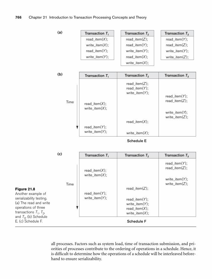
766 Chapter 21 Introduction to Transaction Processing Concepts and Theory
Transaction T1
read_item(X );
write_item(X );
read_item(Y );
write_item(Y );
read_item(X );write_item(X );
read_item(Y );write_item(Y );
Transaction T3
read_item(Y );
read_item(Z );
write_item(Y );
write_item(Z );
read_item(Y );read_item(Z );
write_item(Y);write_item(Z );
Transaction T2
read_item(Z );
read_item(Y );
write_item(Y );
read_item(X );
write_item(X );
read_item(Z );read_item(Y );write_item(Y );
read_item(X );
write_item(X );
(b)
(a)
Schedule E
Time
read_item(X );write_item(X );
read_item(Y );write_item(Y );
read_item(Y );read_item(Z );
write_item(Y );write_item(Z );
read_item(Z );
read_item(Y );write_item(Y );read_item(X );write_item(X );
(c)
Schedule F
Time
Transaction T1 Transaction T2 Transaction T3
Transaction T1 Transaction T2 Transaction T3
Figure 21.8Another example ofserializability testing.(a) The read and writeoperations of threetransactions T1, T2,and T3. (b) ScheduleE. (c) Schedule F.
all processes. Factors such as system load, time of transaction submission, and pri-orities of processes contribute to the ordering of operations in a schedule. Hence, itis difficult to determine how the operations of a schedule will be interleaved before-hand to ensure serializability.
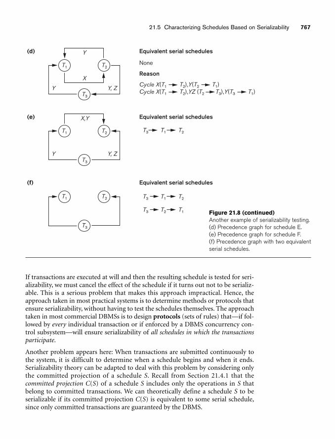
21.5 Characterizing Schedules Based on Serializability 767
(d)
X
Y
Y Y, Z
T1
Equivalent serial schedules
None
Reason
Cycle X(T1 T2),Y(T2 T1)Cycle X(T1 T2),YZ (T2 T3),Y(T3 T1)
(e) X,Y
Y Y, Z
Equivalent serial schedules
(f) Equivalent serial schedules
T2
T3
T1 T2
T3
T1 T2
T3
T2T3 T1
T2T3 T1
T1T3 T2
If transactions are executed at will and then the resulting schedule is tested for seri-alizability, we must cancel the effect of the schedule if it turns out not to be serializ-able. This is a serious problem that makes this approach impractical. Hence, theapproach taken in most practical systems is to determine methods or protocols thatensure serializability, without having to test the schedules themselves. The approachtaken in most commercial DBMSs is to design protocols (sets of rules) that—if fol-lowed by every individual transaction or if enforced by a DBMS concurrency con-trol subsystem—will ensure serializability of all schedules in which the transactionsparticipate.
Another problem appears here: When transactions are submitted continuously tothe system, it is difficult to determine when a schedule begins and when it ends.Serializability theory can be adapted to deal with this problem by considering onlythe committed projection of a schedule S. Recall from Section 21.4.1 that thecommitted projection C(S) of a schedule S includes only the operations in S thatbelong to committed transactions. We can theoretically define a schedule S to beserializable if its committed projection C(S) is equivalent to some serial schedule,since only committed transactions are guaranteed by the DBMS.
Figure 21.8 (continued)Another example of serializability testing.(d) Precedence graph for schedule E. (e) Precedence graph for schedule F. (f) Precedence graph with two equivalentserial schedules.
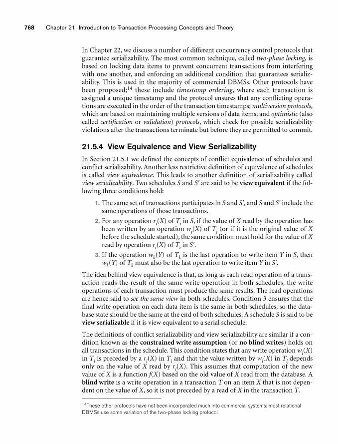
768 Chapter 21 Introduction to Transaction Processing Concepts and Theory
In Chapter 22, we discuss a number of different concurrency control protocols thatguarantee serializability. The most common technique, called two-phase locking, isbased on locking data items to prevent concurrent transactions from interferingwith one another, and enforcing an additional condition that guarantees serializ-ability. This is used in the majority of commercial DBMSs. Other protocols havebeen proposed;14 these include timestamp ordering, where each transaction isassigned a unique timestamp and the protocol ensures that any conflicting opera-tions are executed in the order of the transaction timestamps; multiversion protocols,which are based on maintaining multiple versions of data items; and optimistic (alsocalled certification or validation) protocols, which check for possible serializabilityviolations after the transactions terminate but before they are permitted to commit.
21.5.4 View Equivalence and View SerializabilityIn Section 21.5.1 we defined the concepts of conflict equivalence of schedules andconflict serializability. Another less restrictive definition of equivalence of schedulesis called view equivalence. This leads to another definition of serializability calledview serializability. Two schedules S and S� are said to be view equivalent if the fol-lowing three conditions hold:
1. The same set of transactions participates in S and S�, and S and S� include thesame operations of those transactions.
2. For any operation ri(X) of Ti in S, if the value of X read by the operation hasbeen written by an operation wj(X) of Tj (or if it is the original value of Xbefore the schedule started), the same condition must hold for the value of Xread by operation ri(X) of Ti in S�.
3. If the operation wk(Y) of Tk is the last operation to write item Y in S, thenwk(Y) of Tk must also be the last operation to write item Y in S�.
The idea behind view equivalence is that, as long as each read operation of a trans-action reads the result of the same write operation in both schedules, the writeoperations of each transaction must produce the same results. The read operationsare hence said to see the same view in both schedules. Condition 3 ensures that thefinal write operation on each data item is the same in both schedules, so the data-base state should be the same at the end of both schedules. A schedule S is said to beview serializable if it is view equivalent to a serial schedule.
The definitions of conflict serializability and view serializability are similar if a con-dition known as the constrained write assumption (or no blind writes) holds onall transactions in the schedule. This condition states that any write operation wi(X)in Ti is preceded by a ri(X) in Ti and that the value written by wi(X) in Ti dependsonly on the value of X read by ri(X). This assumes that computation of the newvalue of X is a function f(X) based on the old value of X read from the database. Ablind write is a write operation in a transaction T on an item X that is not depen-dent on the value of X, so it is not preceded by a read of X in the transaction T.
14These other protocols have not been incorporated much into commercial systems; most relationalDBMSs use some variation of the two-phase locking protocol.
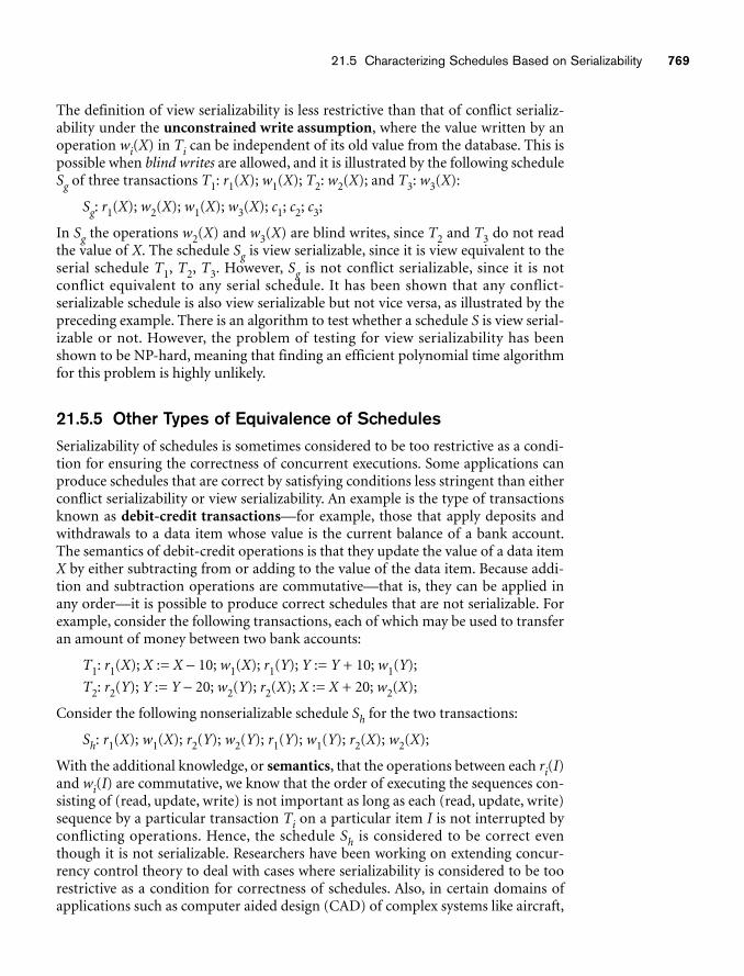
21.5 Characterizing Schedules Based on Serializability 769
The definition of view serializability is less restrictive than that of conflict serializ-ability under the unconstrained write assumption, where the value written by anoperation wi(X) in Ti can be independent of its old value from the database. This ispossible when blind writes are allowed, and it is illustrated by the following scheduleSg of three transactions T1: r1(X); w1(X); T2: w2(X); and T3: w3(X):
Sg: r1(X); w2(X); w1(X); w3(X); c1; c2; c3;
In Sg the operations w2(X) and w3(X) are blind writes, since T2 and T3 do not readthe value of X. The schedule Sg is view serializable, since it is view equivalent to theserial schedule T1, T2, T3. However, Sg is not conflict serializable, since it is not conflict equivalent to any serial schedule. It has been shown that any conflict-serializable schedule is also view serializable but not vice versa, as illustrated by thepreceding example. There is an algorithm to test whether a schedule S is view serial-izable or not. However, the problem of testing for view serializability has beenshown to be NP-hard, meaning that finding an efficient polynomial time algorithmfor this problem is highly unlikely.
21.5.5 Other Types of Equivalence of SchedulesSerializability of schedules is sometimes considered to be too restrictive as a condi-tion for ensuring the correctness of concurrent executions. Some applications canproduce schedules that are correct by satisfying conditions less stringent than eitherconflict serializability or view serializability. An example is the type of transactionsknown as debit-credit transactions—for example, those that apply deposits andwithdrawals to a data item whose value is the current balance of a bank account.The semantics of debit-credit operations is that they update the value of a data itemX by either subtracting from or adding to the value of the data item. Because addi-tion and subtraction operations are commutative—that is, they can be applied inany order—it is possible to produce correct schedules that are not serializable. Forexample, consider the following transactions, each of which may be used to transferan amount of money between two bank accounts:
T1: r1(X); X := X − 10; w1(X); r1(Y); Y := Y + 10; w1(Y);
T2: r2(Y); Y := Y − 20; w2(Y); r2(X); X := X + 20; w2(X);
Consider the following nonserializable schedule Sh for the two transactions:
Sh: r1(X); w1(X); r2(Y); w2(Y); r1(Y); w1(Y); r2(X); w2(X);
With the additional knowledge, or semantics, that the operations between each ri(I)and wi(I) are commutative, we know that the order of executing the sequences con-sisting of (read, update, write) is not important as long as each (read, update, write)sequence by a particular transaction Ti on a particular item I is not interrupted byconflicting operations. Hence, the schedule Sh is considered to be correct eventhough it is not serializable. Researchers have been working on extending concur-rency control theory to deal with cases where serializability is considered to be toorestrictive as a condition for correctness of schedules. Also, in certain domains ofapplications such as computer aided design (CAD) of complex systems like aircraft,
770 Chapter 21 Introduction to Transaction Processing Concepts and Theory
design transactions last over a long time period. In such applications, more relaxedschemes of concurrency control have been proposed to maintain consistency of thedatabase.
21.6 Transaction Support in SQLIn this section, we give a brief introduction to transaction support in SQL. There aremany more details, and the newer standards have more commands for transactionprocessing. The basic definition of an SQL transaction is similar to our alreadydefined concept of a transaction. That is, it is a logical unit of work and is guaran-teed to be atomic. A single SQL statement is always considered to be atomic—eitherit completes execution without an error or it fails and leaves the databaseunchanged.
With SQL, there is no explicit Begin_Transaction statement. Transaction initiation isdone implicitly when particular SQL statements are encountered. However, everytransaction must have an explicit end statement, which is either a COMMIT or aROLLBACK. Every transaction has certain characteristics attributed to it. Thesecharacteristics are specified by a SET TRANSACTION statement in SQL. The charac-teristics are the access mode, the diagnostic area size, and the isolation level.
The access mode can be specified as READ ONLY or READ WRITE. The default isREAD WRITE, unless the isolation level of READ UNCOMMITTED is specified (seebelow), in which case READ ONLY is assumed. A mode of READ WRITE allows select,update, insert, delete, and create commands to be executed. A mode of READ ONLY,as the name implies, is simply for data retrieval.
The diagnostic area size option, DIAGNOSTIC SIZE n, specifies an integer value n,which indicates the number of conditions that can be held simultaneously in thediagnostic area. These conditions supply feedback information (errors or excep-tions) to the user or program on the n most recently executed SQL statement.
The isolation level option is specified using the statement ISOLATION LEVEL <isolation>, where the value for <isolation> can be READ UNCOMMITTED, READCOMMITTED, REPEATABLE READ, or SERIALIZABLE.15 The default isolation level isSERIALIZABLE, although some systems use READ COMMITTED as their default. Theuse of the term SERIALIZABLE here is based on not allowing violations that causedirty read, unrepeatable read, and phantoms,16 and it is thus not identical to the wayserializability was defined earlier in Section 21.5. If a transaction executes at a lowerisolation level than SERIALIZABLE, then one or more of the following three viola-tions may occur:
1. Dirty read. A transaction T1 may read the update of a transaction T2, whichhas not yet committed. If T2 fails and is aborted, then T1 would have read avalue that does not exist and is incorrect.
15These are similar to the isolation levels discussed briefly at the end of Section 21.3.16The dirty read and unrepeatable read problems were discussed in Section 21.1.3. Phantoms are dis-cussed in Section 22.7.1.
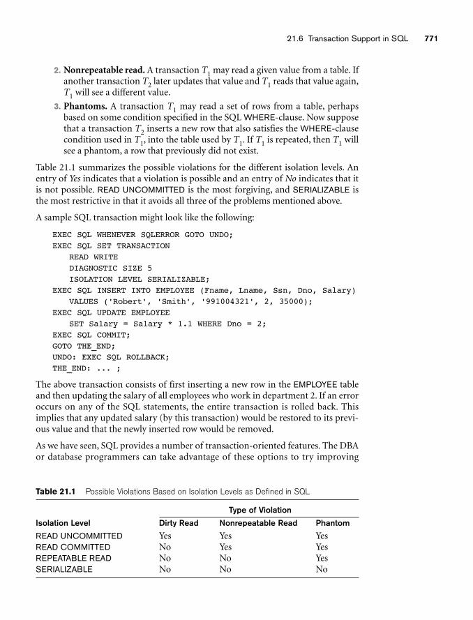
21.6 Transaction Support in SQL 771
Table 21.1 Possible Violations Based on Isolation Levels as Defined in SQL
Type of Violation
Isolation Level Dirty Read Nonrepeatable Read Phantom
READ UNCOMMITTED Yes Yes YesREAD COMMITTED No Yes YesREPEATABLE READ No No YesSERIALIZABLE No No No
2. Nonrepeatable read. A transaction T1 may read a given value from a table. Ifanother transaction T2 later updates that value and T1 reads that value again,T1 will see a different value.
3. Phantoms. A transaction T1 may read a set of rows from a table, perhapsbased on some condition specified in the SQL WHERE-clause. Now supposethat a transaction T2 inserts a new row that also satisfies the WHERE-clausecondition used in T1, into the table used by T1. If T1 is repeated, then T1 willsee a phantom, a row that previously did not exist.
Table 21.1 summarizes the possible violations for the different isolation levels. Anentry of Yes indicates that a violation is possible and an entry of No indicates that itis not possible. READ UNCOMMITTED is the most forgiving, and SERIALIZABLE isthe most restrictive in that it avoids all three of the problems mentioned above.
A sample SQL transaction might look like the following:
EXEC SQL WHENEVER SQLERROR GOTO UNDO;EXEC SQL SET TRANSACTION
READ WRITEDIAGNOSTIC SIZE 5ISOLATION LEVEL SERIALIZABLE;
EXEC SQL INSERT INTO EMPLOYEE (Fname, Lname, Ssn, Dno, Salary)VALUES ('Robert', 'Smith', '991004321', 2, 35000);
EXEC SQL UPDATE EMPLOYEESET Salary = Salary * 1.1 WHERE Dno = 2;
EXEC SQL COMMIT;GOTO THE_END;UNDO: EXEC SQL ROLLBACK;THE_END: ... ;
The above transaction consists of first inserting a new row in the EMPLOYEE tableand then updating the salary of all employees who work in department 2. If an erroroccurs on any of the SQL statements, the entire transaction is rolled back. Thisimplies that any updated salary (by this transaction) would be restored to its previ-ous value and that the newly inserted row would be removed.
As we have seen, SQL provides a number of transaction-oriented features. The DBAor database programmers can take advantage of these options to try improving
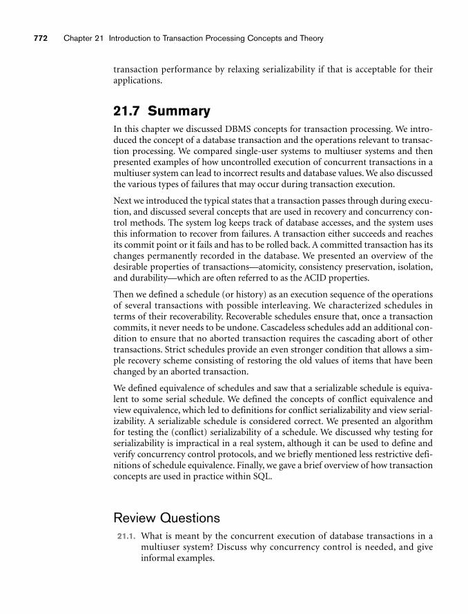
772 Chapter 21 Introduction to Transaction Processing Concepts and Theory
transaction performance by relaxing serializability if that is acceptable for theirapplications.
21.7 SummaryIn this chapter we discussed DBMS concepts for transaction processing. We intro-duced the concept of a database transaction and the operations relevant to transac-tion processing. We compared single-user systems to multiuser systems and thenpresented examples of how uncontrolled execution of concurrent transactions in amultiuser system can lead to incorrect results and database values. We also discussedthe various types of failures that may occur during transaction execution.
Next we introduced the typical states that a transaction passes through during execu-tion, and discussed several concepts that are used in recovery and concurrency con-trol methods. The system log keeps track of database accesses, and the system usesthis information to recover from failures. A transaction either succeeds and reachesits commit point or it fails and has to be rolled back. A committed transaction has itschanges permanently recorded in the database. We presented an overview of thedesirable properties of transactions—atomicity, consistency preservation, isolation,and durability—which are often referred to as the ACID properties.
Then we defined a schedule (or history) as an execution sequence of the operationsof several transactions with possible interleaving. We characterized schedules interms of their recoverability. Recoverable schedules ensure that, once a transactioncommits, it never needs to be undone. Cascadeless schedules add an additional con-dition to ensure that no aborted transaction requires the cascading abort of othertransactions. Strict schedules provide an even stronger condition that allows a sim-ple recovery scheme consisting of restoring the old values of items that have beenchanged by an aborted transaction.
We defined equivalence of schedules and saw that a serializable schedule is equiva-lent to some serial schedule. We defined the concepts of conflict equivalence andview equivalence, which led to definitions for conflict serializability and view serial-izability. A serializable schedule is considered correct. We presented an algorithmfor testing the (conflict) serializability of a schedule. We discussed why testing forserializability is impractical in a real system, although it can be used to define andverify concurrency control protocols, and we briefly mentioned less restrictive defi-nitions of schedule equivalence. Finally, we gave a brief overview of how transactionconcepts are used in practice within SQL.
Review Questions21.1. What is meant by the concurrent execution of database transactions in a
multiuser system? Discuss why concurrency control is needed, and giveinformal examples.
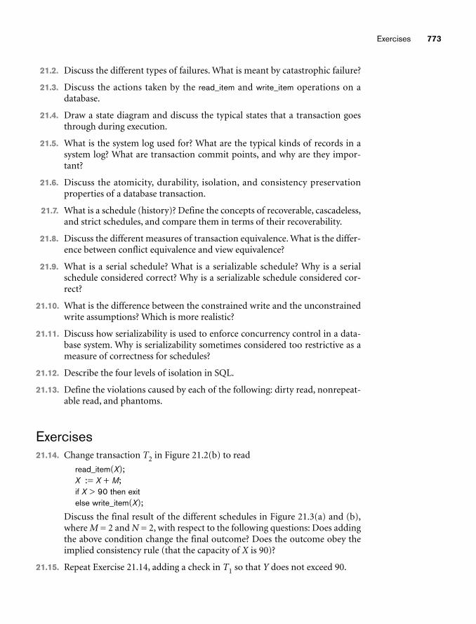
Exercises 773
21.2. Discuss the different types of failures. What is meant by catastrophic failure?
21.3. Discuss the actions taken by the read_item and write_item operations on adatabase.
21.4. Draw a state diagram and discuss the typical states that a transaction goesthrough during execution.
21.5. What is the system log used for? What are the typical kinds of records in asystem log? What are transaction commit points, and why are they impor-tant?
21.6. Discuss the atomicity, durability, isolation, and consistency preservationproperties of a database transaction.
21.7. What is a schedule (history)? Define the concepts of recoverable, cascadeless,and strict schedules, and compare them in terms of their recoverability.
21.8. Discuss the different measures of transaction equivalence. What is the differ-ence between conflict equivalence and view equivalence?
21.9. What is a serial schedule? What is a serializable schedule? Why is a serialschedule considered correct? Why is a serializable schedule considered cor-rect?
21.10. What is the difference between the constrained write and the unconstrainedwrite assumptions? Which is more realistic?
21.11. Discuss how serializability is used to enforce concurrency control in a data-base system. Why is serializability sometimes considered too restrictive as ameasure of correctness for schedules?
21.12. Describe the four levels of isolation in SQL.
21.13. Define the violations caused by each of the following: dirty read, nonrepeat-able read, and phantoms.
Exercises21.14. Change transaction T2 in Figure 21.2(b) to read
read_item(X);X := X + M;if X > 90 then exitelse write_item(X);
Discuss the final result of the different schedules in Figure 21.3(a) and (b),where M = 2 and N = 2, with respect to the following questions: Does addingthe above condition change the final outcome? Does the outcome obey theimplied consistency rule (that the capacity of X is 90)?
21.15. Repeat Exercise 21.14, adding a check in T1 so that Y does not exceed 90.
774 Chapter 21 Introduction to Transaction Processing Concepts and Theory
21.16. Add the operation commit at the end of each of the transactions T1 and T2 inFigure 21.2, and then list all possible schedules for the modified transactions.Determine which of the schedules are recoverable, which are cascadeless,and which are strict.
21.17. List all possible schedules for transactions T1 and T2 in Figure 21.2, anddetermine which are conflict serializable (correct) and which are not.
21.18. How many serial schedules exist for the three transactions in Figure 21.8(a)?What are they? What is the total number of possible schedules?
21.19. Write a program to create all possible schedules for the three transactions inFigure 21.8(a), and to determine which of those schedules are conflict serial-izable and which are not. For each conflict-serializable schedule, your pro-gram should print the schedule and list all equivalent serial schedules.
21.20. Why is an explicit transaction end statement needed in SQL but not anexplicit begin statement?
21.21. Describe situations where each of the different isolation levels would be use-ful for transaction processing.
21.22. Which of the following schedules is (conflict) serializable? For each serializ-able schedule, determine the equivalent serial schedules.
a. r1(X); r3(X); w1(X); r2(X); w3(X);
b. r1(X); r3(X); w3(X); w1(X); r2(X);
c. r3(X); r2(X); w3(X); r1(X); w1(X);
d. r3(X); r2(X); r1(X); w3(X); w1(X);
21.23. Consider the three transactions T1, T2, and T3, and the schedules S1 and S2given below. Draw the serializability (precedence) graphs for S1 and S2, andstate whether each schedule is serializable or not. If a schedule is serializable,write down the equivalent serial schedule(s).
T1: r1 (X); r1 (Z); w1 (X);T2: r2 (Z); r2 (Y); w2 (Z); w2 (Y);T3: r3 (X); r3 (Y); w3 (Y);S1: r1 (X); r2 (Z); r1 (Z); r3 (X); r3 (Y); w1 (X); w3 (Y); r2 (Y); w2 (Z); w2 (Y);S2: r1 (X); r2 (Z); r3 (X); r1 (Z); r2 (Y); r3 (Y); w1 (X); w2 (Z); w3 (Y); w2 (Y);
21.24. Consider schedules S3, S4, and S5 below. Determine whether each schedule isstrict, cascadeless, recoverable, or nonrecoverable. (Determine the strictestrecoverability condition that each schedule satisfies.)
S3: r1 (X); r2 (Z); r1 (Z); r3 (X); r3 (Y); w1 (X); c1; w3 (Y); c3; r2 (Y); w2 (Z);w2 (Y); c2;
S4: r1 (X); r2 (Z); r1 (Z); r3 (X); r3 (Y); w1 (X); w3 (Y); r2 (Y); w2 (Z); w2 (Y); c1;c2; c3;
S5: r1 (X); r2 (Z); r3 (X); r1 (Z); r2 (Y); r3 (Y); w1 (X); c1; w2 (Z); w3 (Y); w2 (Y);c3; c2;
Selected BibliographyThe concept of serializability and related ideas to maintain consistency in a databasewere introduced in Gray et al. (1975). The concept of the database transaction wasfirst discussed in Gray (1981). Gray won the coveted ACM Turing Award in 1998 forhis work on database transactions and implementation of transactions in relationalDBMSs. Bernstein, Hadzilacos, and Goodman (1988) focus on concurrency controland recovery techniques in both centralized and distributed database systems; it isan excellent reference. Papadimitriou (1986) offers a more theoretical perspective. Alarge reference book of more than a thousand pages by Gray and Reuter (1993)offers a more practical perspective of transaction processing concepts and tech-niques. Elmagarmid (1992) offers collections of research papers on transaction pro-cessing for advanced applications. Transaction support in SQL is described in Dateand Darwen (1997). View serializability is defined in Yannakakis (1984).Recoverability of schedules and reliability in databases is discussed in Hadzilacos(1983, 1988).
Selected Bibliography 775
777
Concurrency Control Techniques
In this chapter we discuss a number of concurrencycontrol techniques that are used to ensure the nonin-
terference or isolation property of concurrently executing transactions. Most ofthese techniques ensure serializability of schedules—which we defined in Section21.5—using concurrency control protocols (sets of rules) that guarantee serializ-ability. One important set of protocols—known as two-phase locking protocols—employ the technique of locking data items to prevent multiple transactions fromaccessing the items concurrently; a number of locking protocols are described inSections 22.1 and 22.3.2. Locking protocols are used in most commercial DBMSs.Another set of concurrency control protocols use timestamps. A timestamp is aunique identifier for each transaction, generated by the system. Timestamps valuesare generated in the same order as the transaction start times. Concurrency controlprotocols that use timestamp ordering to ensure serializability are introduced inSection 22.2. In Section 22.3 we discuss multiversion concurrency control proto-cols that use multiple versions of a data item. One multiversion protocol extendstimestamp order to multiversion timestamp ordering (Section 22.3.1), and anotherextends two-phase locking (Section 22.3.2). In Section 22.4 we present a protocolbased on the concept of validation or certification of a transaction after it executesits operations; these are sometimes called optimistic protocols, and also assumethat multiple versions of a data item can exist.
Another factor that affects concurrency control is the granularity of the dataitems—that is, what portion of the database a data item represents. An item can beas small as a single attribute (field) value or as large as a disk block, or even a wholefile or the entire database. We discuss granularity of items and a multiple granular-ity concurrency control protocol, which is an extension of two-phase locking, inSection 22.5. In Section 22.6 we describe concurrency control issues that arise when
22chapter 22
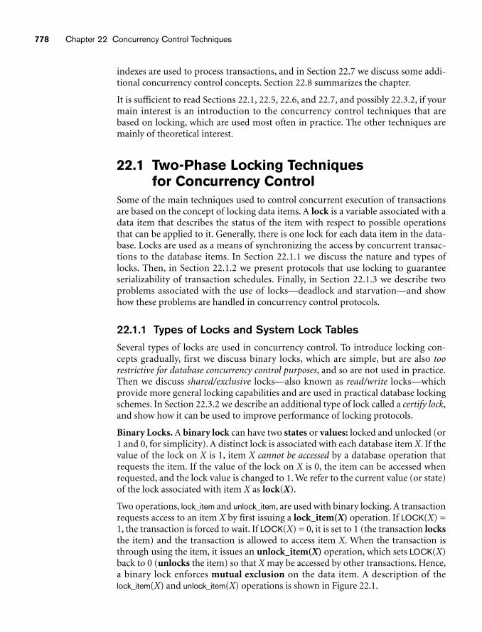
778 Chapter 22 Concurrency Control Techniques
indexes are used to process transactions, and in Section 22.7 we discuss some addi-tional concurrency control concepts. Section 22.8 summarizes the chapter.
It is sufficient to read Sections 22.1, 22.5, 22.6, and 22.7, and possibly 22.3.2, if yourmain interest is an introduction to the concurrency control techniques that arebased on locking, which are used most often in practice. The other techniques aremainly of theoretical interest.
22.1 Two-Phase Locking Techniques for Concurrency Control
Some of the main techniques used to control concurrent execution of transactionsare based on the concept of locking data items. A lock is a variable associated with adata item that describes the status of the item with respect to possible operationsthat can be applied to it. Generally, there is one lock for each data item in the data-base. Locks are used as a means of synchronizing the access by concurrent transac-tions to the database items. In Section 22.1.1 we discuss the nature and types oflocks. Then, in Section 22.1.2 we present protocols that use locking to guaranteeserializability of transaction schedules. Finally, in Section 22.1.3 we describe twoproblems associated with the use of locks—deadlock and starvation—and showhow these problems are handled in concurrency control protocols.
22.1.1 Types of Locks and System Lock TablesSeveral types of locks are used in concurrency control. To introduce locking con-cepts gradually, first we discuss binary locks, which are simple, but are also toorestrictive for database concurrency control purposes, and so are not used in practice.Then we discuss shared/exclusive locks—also known as read/write locks—whichprovide more general locking capabilities and are used in practical database lockingschemes. In Section 22.3.2 we describe an additional type of lock called a certify lock,and show how it can be used to improve performance of locking protocols.
Binary Locks. A binary lock can have two states or values: locked and unlocked (or1 and 0, for simplicity). A distinct lock is associated with each database item X. If thevalue of the lock on X is 1, item X cannot be accessed by a database operation thatrequests the item. If the value of the lock on X is 0, the item can be accessed whenrequested, and the lock value is changed to 1. We refer to the current value (or state)of the lock associated with item X as lock(X).
Two operations, lock_item and unlock_item, are used with binary locking. A transactionrequests access to an item X by first issuing a lock_item(X) operation. If LOCK(X) =1, the transaction is forced to wait. If LOCK(X) = 0, it is set to 1 (the transaction locksthe item) and the transaction is allowed to access item X. When the transaction isthrough using the item, it issues an unlock_item(X) operation, which sets LOCK(X)back to 0 (unlocks the item) so that X may be accessed by other transactions. Hence,a binary lock enforces mutual exclusion on the data item. A description of thelock_item(X) and unlock_item(X) operations is shown in Figure 22.1.
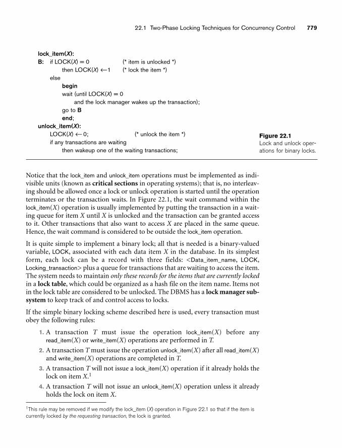
22.1 Two-Phase Locking Techniques for Concurrency Control 779
lock_item(X):B: if LOCK(X) = 0 (* item is unlocked *)
then LOCK(X) ←1 (* lock the item *)else
beginwait (until LOCK(X) = 0
and the lock manager wakes up the transaction);go to Bend;
unlock_item(X):LOCK(X) ← 0; (* unlock the item *)if any transactions are waiting
then wakeup one of the waiting transactions;
Figure 22.1Lock and unlock oper-ations for binary locks.
Notice that the lock_item and unlock_item operations must be implemented as indi-visible units (known as critical sections in operating systems); that is, no interleav-ing should be allowed once a lock or unlock operation is started until the operationterminates or the transaction waits. In Figure 22.1, the wait command within thelock_item(X) operation is usually implemented by putting the transaction in a wait-ing queue for item X until X is unlocked and the transaction can be granted accessto it. Other transactions that also want to access X are placed in the same queue.Hence, the wait command is considered to be outside the lock_item operation.
It is quite simple to implement a binary lock; all that is needed is a binary-valuedvariable, LOCK, associated with each data item X in the database. In its simplestform, each lock can be a record with three fields: <Data_item_name, LOCK,Locking_transaction> plus a queue for transactions that are waiting to access the item.The system needs to maintain only these records for the items that are currently lockedin a lock table, which could be organized as a hash file on the item name. Items notin the lock table are considered to be unlocked. The DBMS has a lock manager sub-system to keep track of and control access to locks.
If the simple binary locking scheme described here is used, every transaction mustobey the following rules:
1. A transaction T must issue the operation lock_item(X) before anyread_item(X) or write_item(X) operations are performed in T.
2. A transaction T must issue the operation unlock_item(X) after all read_item(X)and write_item(X) operations are completed in T.
3. A transaction T will not issue a lock_item(X) operation if it already holds thelock on item X.1
4. A transaction T will not issue an unlock_item(X) operation unless it alreadyholds the lock on item X.
1This rule may be removed if we modify the lock_item (X) operation in Figure 22.1 so that if the item iscurrently locked by the requesting transaction, the lock is granted.
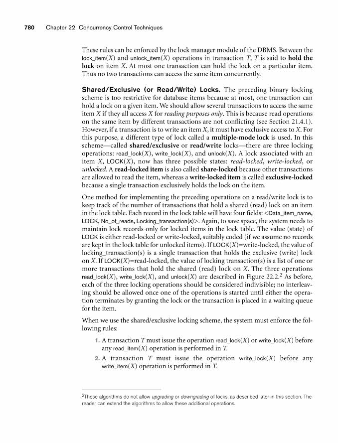
780 Chapter 22 Concurrency Control Techniques
These rules can be enforced by the lock manager module of the DBMS. Between thelock_item(X) and unlock_item(X) operations in transaction T, T is said to hold thelock on item X. At most one transaction can hold the lock on a particular item.Thus no two transactions can access the same item concurrently.
Shared/Exclusive (or Read/Write) Locks. The preceding binary lockingscheme is too restrictive for database items because at most, one transaction canhold a lock on a given item. We should allow several transactions to access the sameitem X if they all access X for reading purposes only. This is because read operationson the same item by different transactions are not conflicting (see Section 21.4.1).However, if a transaction is to write an item X, it must have exclusive access to X. Forthis purpose, a different type of lock called a multiple-mode lock is used. In thisscheme—called shared/exclusive or read/write locks—there are three lockingoperations: read_lock(X), write_lock(X), and unlock(X). A lock associated with anitem X, LOCK(X), now has three possible states: read-locked, write-locked, orunlocked. A read-locked item is also called share-locked because other transactionsare allowed to read the item, whereas a write-locked item is called exclusive-lockedbecause a single transaction exclusively holds the lock on the item.
One method for implementing the preceding operations on a read/write lock is tokeep track of the number of transactions that hold a shared (read) lock on an itemin the lock table. Each record in the lock table will have four fields: <Data_item_name,LOCK, No_of_reads, Locking_transaction(s)>. Again, to save space, the system needs tomaintain lock records only for locked items in the lock table. The value (state) ofLOCK is either read-locked or write-locked, suitably coded (if we assume no recordsare kept in the lock table for unlocked items). If LOCK(X)=write-locked, the value oflocking_transaction(s) is a single transaction that holds the exclusive (write) lockon X. If LOCK(X)=read-locked, the value of locking transaction(s) is a list of one ormore transactions that hold the shared (read) lock on X. The three operationsread_lock(X), write_lock(X), and unlock(X) are described in Figure 22.2.2 As before,each of the three locking operations should be considered indivisible; no interleav-ing should be allowed once one of the operations is started until either the opera-tion terminates by granting the lock or the transaction is placed in a waiting queuefor the item.
When we use the shared/exclusive locking scheme, the system must enforce the fol-lowing rules:
1. A transaction T must issue the operation read_lock(X) or write_lock(X) beforeany read_item(X) operation is performed in T.
2. A transaction T must issue the operation write_lock(X) before anywrite_item(X) operation is performed in T.
2These algorithms do not allow upgrading or downgrading of locks, as described later in this section. Thereader can extend the algorithms to allow these additional operations.
read_lock(X):B: if LOCK(X) = “unlocked”
then begin LOCK(X) ← “read-locked”;no_of_reads(X) ← 1end
else if LOCK(X) = “read-locked”then no_of_reads(X) ← no_of_reads(X) + 1
else beginwait (until LOCK(X) = “unlocked”
and the lock manager wakes up the transaction);go to Bend;
write_lock(X):B: if LOCK(X) = “unlocked”
then LOCK(X) ← “write-locked”else begin
wait (until LOCK(X) = “unlocked”and the lock manager wakes up the transaction);
go to Bend;
unlock (X):if LOCK(X) = “write-locked”
then begin LOCK(X) ← “unlocked”;wakeup one of the waiting transactions, if anyend
else it LOCK(X) = “read-locked”then begin
no_of_reads(X) ← no_of_reads(X) −1;if no_of_reads(X) = 0
then begin LOCK(X) = “unlocked”;wakeup one of the waiting transactions, if anyend
end;
22.1 Two-Phase Locking Techniques for Concurrency Control 781
Figure 22.2Locking and unlockingoperations for two-mode (read-write orshared-exclusive)locks.
3. A transaction T must issue the operation unlock(X) after all read_item(X) andwrite_item(X) operations are completed in T.3
4. A transaction T will not issue a read_lock(X) operation if it already holds aread (shared) lock or a write (exclusive) lock on item X. This rule may berelaxed, as we discuss shortly.
3This rule may be relaxed to allow a transaction to unlock an item, then lock it again later.
782 Chapter 22 Concurrency Control Techniques
5. A transaction T will not issue a write_lock(X) operation if it already holds aread (shared) lock or write (exclusive) lock on item X. This rule may also berelaxed, as we discuss shortly.
6. A transaction T will not issue an unlock(X) operation unless it already holdsa read (shared) lock or a write (exclusive) lock on item X.
Conversion of Locks. Sometimes it is desirable to relax conditions 4 and 5 in thepreceding list in order to allow lock conversion; that is, a transaction that alreadyholds a lock on item X is allowed under certain conditions to convert the lock fromone locked state to another. For example, it is possible for a transaction T to issue aread_lock(X) and then later to upgrade the lock by issuing a write_lock(X) operation.If T is the only transaction holding a read lock on X at the time it issues thewrite_lock(X) operation, the lock can be upgraded; otherwise, the transaction mustwait. It is also possible for a transaction T to issue a write_lock(X) and then later todowngrade the lock by issuing a read_lock(X) operation. When upgrading anddowngrading of locks is used, the lock table must include transaction identifiers inthe record structure for each lock (in the locking_transaction(s) field) to store theinformation on which transactions hold locks on the item. The descriptions of theread_lock(X) and write_lock(X) operations in Figure 22.2 must be changed appropri-ately to allow for lock upgrading and downgrading. We leave this as an exercise forthe reader.
Using binary locks or read/write locks in transactions, as described earlier, does notguarantee serializability of schedules on its own. Figure 22.3 shows an examplewhere the preceding locking rules are followed but a nonserializable schedule mayresult. This is because in Figure 22.3(a) the items Y in T1 and X in T2 were unlockedtoo early. This allows a schedule such as the one shown in Figure 22.3(c) to occur,which is not a serializable schedule and hence gives incorrect results. To guaranteeserializability, we must follow an additional protocol concerning the positioning oflocking and unlocking operations in every transaction. The best-known protocol,two-phase locking, is described in the next section.
22.1.2 Guaranteeing Serializability by Two-Phase LockingA transaction is said to follow the two-phase locking protocol if all locking opera-tions (read_lock, write_lock) precede the first unlock operation in the transaction.4
Such a transaction can be divided into two phases: an expanding or growing (first)phase, during which new locks on items can be acquired but none can be released;and a shrinking (second) phase, during which existing locks can be released but nonew locks can be acquired. If lock conversion is allowed, then upgrading of locks(from read-locked to write-locked) must be done during the expanding phase, anddowngrading of locks (from write-locked to read-locked) must be done in the
4This is unrelated to the two-phase commit protocol for recovery in distributed databases (see Chapter25).
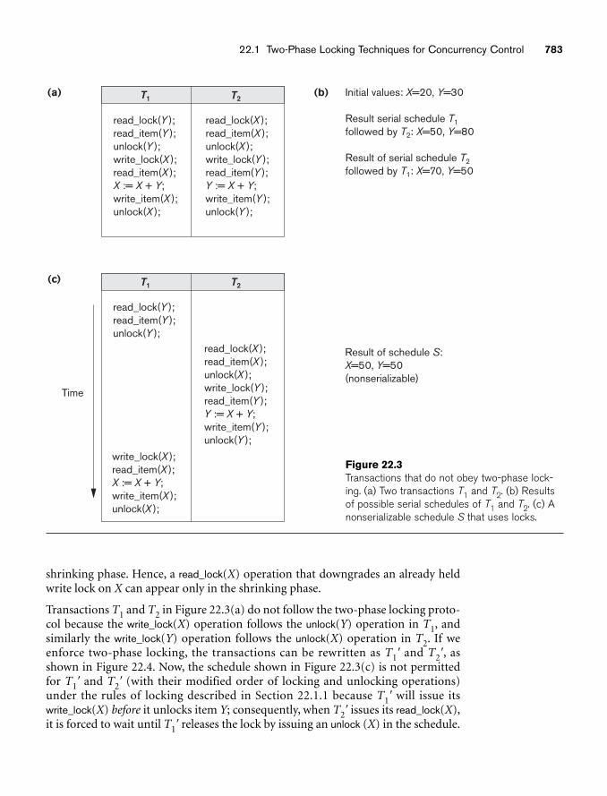
22.1 Two-Phase Locking Techniques for Concurrency Control 783
(a) T1Initial values: X=20, Y=30
Result serial schedule T1
followed by T2: X=50, Y=80
Result of serial schedule T2
followed by T1: X=70, Y=50
read_lock(Y );read_item(Y );unlock(Y );write_lock(X );read_item(X );X := X + Y;write_item(X );unlock(X );
write_lock(X );read_item(X );X := X + Y;write_item(X );unlock(X );
read_lock(X );read_item(X );unlock(X );write_lock(Y );read_item(Y );Y := X + Y;write_item(Y );unlock(Y );
read_lock(X );read_item(X );unlock(X );write_lock(Y );read_item(Y );Y := X + Y;write_item(Y );unlock(Y );
(b)
(c)
Time
read_lock(Y );read_item(Y );unlock(Y );
Result of schedule S:X=50, Y=50(nonserializable)
T2
T1 T2
Figure 22.3Transactions that do not obey two-phase lock-ing. (a) Two transactions T1 and T2. (b) Resultsof possible serial schedules of T1 and T2. (c) Anonserializable schedule S that uses locks.
shrinking phase. Hence, a read_lock(X) operation that downgrades an already heldwrite lock on X can appear only in the shrinking phase.
Transactions T1 and T2 in Figure 22.3(a) do not follow the two-phase locking proto-col because the write_lock(X) operation follows the unlock(Y) operation in T1, andsimilarly the write_lock(Y) operation follows the unlock(X) operation in T2. If weenforce two-phase locking, the transactions can be rewritten as T1� and T2�, asshown in Figure 22.4. Now, the schedule shown in Figure 22.3(c) is not permittedfor T1� and T2� (with their modified order of locking and unlocking operations)under the rules of locking described in Section 22.1.1 because T1� will issue itswrite_lock(X) before it unlocks item Y; consequently, when T2� issues its read_lock(X),it is forced to wait until T1� releases the lock by issuing an unlock (X) in the schedule.
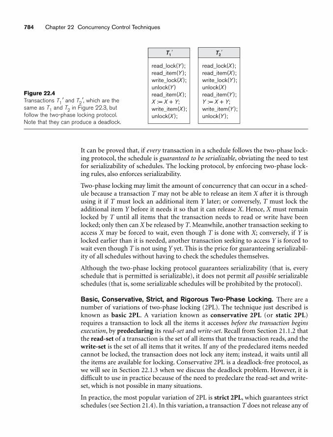
784 Chapter 22 Concurrency Control Techniques
read_lock(Y );read_item(Y );write_lock(X );unlock(Y )read_item(X );X := X + Y;write_item(X );unlock(X );
read_lock(X );read_item(X );write_lock(Y );unlock(X )read_item(Y );Y := X + Y;write_item(Y );unlock(Y );
T1� T2�
Figure 22.4Transactions T1� and T2�, which are thesame as T1 and T2 in Figure 22.3, butfollow the two-phase locking protocol.Note that they can produce a deadlock.
It can be proved that, if every transaction in a schedule follows the two-phase lock-ing protocol, the schedule is guaranteed to be serializable, obviating the need to testfor serializability of schedules. The locking protocol, by enforcing two-phase lock-ing rules, also enforces serializability.
Two-phase locking may limit the amount of concurrency that can occur in a sched-ule because a transaction T may not be able to release an item X after it is throughusing it if T must lock an additional item Y later; or conversely, T must lock theadditional item Y before it needs it so that it can release X. Hence, X must remainlocked by T until all items that the transaction needs to read or write have beenlocked; only then can X be released by T. Meanwhile, another transaction seeking toaccess X may be forced to wait, even though T is done with X; conversely, if Y islocked earlier than it is needed, another transaction seeking to access Y is forced towait even though T is not using Y yet. This is the price for guaranteeing serializabil-ity of all schedules without having to check the schedules themselves.
Although the two-phase locking protocol guarantees serializability (that is, everyschedule that is permitted is serializable), it does not permit all possible serializableschedules (that is, some serializable schedules will be prohibited by the protocol).
Basic, Conservative, Strict, and Rigorous Two-Phase Locking. There are anumber of variations of two-phase locking (2PL). The technique just described isknown as basic 2PL. A variation known as conservative 2PL (or static 2PL)requires a transaction to lock all the items it accesses before the transaction beginsexecution, by predeclaring its read-set and write-set. Recall from Section 21.1.2 thatthe read-set of a transaction is the set of all items that the transaction reads, and thewrite-set is the set of all items that it writes. If any of the predeclared items neededcannot be locked, the transaction does not lock any item; instead, it waits until allthe items are available for locking. Conservative 2PL is a deadlock-free protocol, aswe will see in Section 22.1.3 when we discuss the deadlock problem. However, it isdifficult to use in practice because of the need to predeclare the read-set and write-set, which is not possible in many situations.
In practice, the most popular variation of 2PL is strict 2PL, which guarantees strictschedules (see Section 21.4). In this variation, a transaction T does not release any of
22.1 Two-Phase Locking Techniques for Concurrency Control 785
its exclusive (write) locks until after it commits or aborts. Hence, no other transac-tion can read or write an item that is written by T unless T has committed, leadingto a strict schedule for recoverability. Strict 2PL is not deadlock-free. A more restric-tive variation of strict 2PL is rigorous 2PL, which also guarantees strict schedules.In this variation, a transaction T does not release any of its locks (exclusive orshared) until after it commits or aborts, and so it is easier to implement than strict2PL. Notice the difference between conservative and rigorous 2PL: the former mustlock all its items before it starts, so once the transaction starts it is in its shrinkingphase; the latter does not unlock any of its items until after it terminates (by com-mitting or aborting), so the transaction is in its expanding phase until it ends.
In many cases, the concurrency control subsystem itself is responsible for generat-ing the read_lock and write_lock requests. For example, suppose the system is toenforce the strict 2PL protocol. Then, whenever transaction T issues a read_item(X),the system calls the read_lock(X) operation on behalf of T. If the state of LOCK(X) iswrite_locked by some other transaction T�, the system places T in the waiting queuefor item X; otherwise, it grants the read_lock(X) request and permits theread_item(X) operation of T to execute. On the other hand, if transaction T issues awrite_item(X), the system calls the write_lock(X) operation on behalf of T. If the stateof LOCK(X) is write_locked or read_locked by some other transaction T�, the systemplaces T in the waiting queue for item X; if the state of LOCK(X) is read_locked andT itself is the only transaction holding the read lock on X, the system upgrades thelock to write_locked and permits the write_item(X) operation by T. Finally, if thestate of LOCK(X) is unlocked, the system grants the write_lock(X) request and per-mits the write_item(X) operation to execute. After each action, the system mustupdate its lock table appropriately.
The use of locks can cause two additional problems: deadlock and starvation. Wediscuss these problems and their solutions in the next section.
22.1.3 Dealing with Deadlock and StarvationDeadlock occurs when each transaction T in a set of two or more transactions iswaiting for some item that is locked by some other transaction T� in the set. Hence,each transaction in the set is in a waiting queue, waiting for one of the other trans-actions in the set to release the lock on an item. But because the other transaction isalso waiting, it will never release the lock. A simple example is shown in Figure22.5(a), where the two transactions T1�and T2�are deadlocked in a partial schedule;T1� is in the waiting queue for X, which is locked by T2�, while T2� is in the waitingqueue for Y, which is locked by T1�. Meanwhile, neither T1� nor T2� nor any othertransaction can access items X and Y.
Deadlock Prevention Protocols. One way to prevent deadlock is to use adeadlock prevention protocol.5 One deadlock prevention protocol, which is used
5These protocols are not generally used in practice, either because of unrealistic assumptions orbecause of their possible overhead. Deadlock detection and timeouts (covered in the following sections)are more practical.
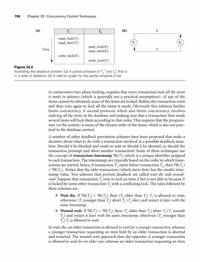
786 Chapter 22 Concurrency Control Techniques
(a) T1� (b)
read_lock(Y );read_item(Y );
Time
write_lock(X );
read_lock(X );read_item(X );
write_lock(Y );
T2�
T2�T1�
X
Y
Figure 22.5Illustrating the deadlock problem. (a) A partial schedule of T1� and T2� that isin a state of deadlock. (b) A wait-for graph for the partial schedule in (a).
in conservative two-phase locking, requires that every transaction lock all the itemsit needs in advance (which is generally not a practical assumption)—if any of theitems cannot be obtained, none of the items are locked. Rather, the transaction waitsand then tries again to lock all the items it needs. Obviously this solution furtherlimits concurrency. A second protocol, which also limits concurrency, involvesordering all the items in the database and making sure that a transaction that needsseveral items will lock them according to that order. This requires that the program-mer (or the system) is aware of the chosen order of the items, which is also not prac-tical in the database context.
A number of other deadlock prevention schemes have been proposed that make adecision about what to do with a transaction involved in a possible deadlock situa-tion: Should it be blocked and made to wait or should it be aborted, or should thetransaction preempt and abort another transaction? Some of these techniques usethe concept of transaction timestamp TS(T), which is a unique identifier assignedto each transaction. The timestamps are typically based on the order in which trans-actions are started; hence, if transaction T1 starts before transaction T2, then TS(T1)< TS(T2). Notice that the older transaction (which starts first) has the smaller time-stamp value. Two schemes that prevent deadlock are called wait-die and wound-wait. Suppose that transaction Ti tries to lock an item X but is not able to because Xis locked by some other transaction Tj with a conflicting lock. The rules followed bythese schemes are:
■ Wait-die. If TS(Ti) < TS(Tj), then (Ti older than Tj) Ti is allowed to wait;otherwise (Ti younger than Tj) abort Ti (Ti dies) and restart it later with thesame timestamp.
■ Wound-wait. If TS(Ti) < TS(Tj), then (Ti older than Tj) abort Tj (Ti woundsTj) and restart it later with the same timestamp; otherwise (Ti younger thanTj) Ti is allowed to wait.
In wait-die, an older transaction is allowed to wait for a younger transaction, whereasa younger transaction requesting an item held by an older transaction is abortedand restarted. The wound-wait approach does the opposite: A younger transactionis allowed to wait for an older one, whereas an older transaction requesting an item
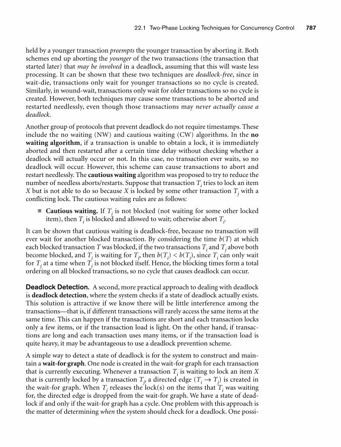
22.1 Two-Phase Locking Techniques for Concurrency Control 787
held by a younger transaction preempts the younger transaction by aborting it. Bothschemes end up aborting the younger of the two transactions (the transaction thatstarted later) that may be involved in a deadlock, assuming that this will waste lessprocessing. It can be shown that these two techniques are deadlock-free, since inwait-die, transactions only wait for younger transactions so no cycle is created.Similarly, in wound-wait, transactions only wait for older transactions so no cycle iscreated. However, both techniques may cause some transactions to be aborted andrestarted needlessly, even though those transactions may never actually cause adeadlock.
Another group of protocols that prevent deadlock do not require timestamps. Theseinclude the no waiting (NW) and cautious waiting (CW) algorithms. In the nowaiting algorithm, if a transaction is unable to obtain a lock, it is immediatelyaborted and then restarted after a certain time delay without checking whether adeadlock will actually occur or not. In this case, no transaction ever waits, so nodeadlock will occur. However, this scheme can cause transactions to abort andrestart needlessly. The cautious waiting algorithm was proposed to try to reduce thenumber of needless aborts/restarts. Suppose that transaction Ti tries to lock an itemX but is not able to do so because X is locked by some other transaction Tj with aconflicting lock. The cautious waiting rules are as follows:
■ Cautious waiting. If Tj is not blocked (not waiting for some other lockeditem), then Ti is blocked and allowed to wait; otherwise abort Ti.
It can be shown that cautious waiting is deadlock-free, because no transaction willever wait for another blocked transaction. By considering the time b(T) at whicheach blocked transaction T was blocked, if the two transactions Ti and Tj above bothbecome blocked, and Ti is waiting for Tj, then b(Ti) < b(Tj), since Ti can only waitfor Tj at a time when Tj is not blocked itself. Hence, the blocking times form a totalordering on all blocked transactions, so no cycle that causes deadlock can occur.
Deadlock Detection. A second, more practical approach to dealing with deadlockis deadlock detection, where the system checks if a state of deadlock actually exists.This solution is attractive if we know there will be little interference among thetransactions—that is, if different transactions will rarely access the same items at thesame time. This can happen if the transactions are short and each transaction locksonly a few items, or if the transaction load is light. On the other hand, if transac-tions are long and each transaction uses many items, or if the transaction load isquite heavy, it may be advantageous to use a deadlock prevention scheme.
A simple way to detect a state of deadlock is for the system to construct and main-tain a wait-for graph. One node is created in the wait-for graph for each transactionthat is currently executing. Whenever a transaction Ti is waiting to lock an item Xthat is currently locked by a transaction Tj, a directed edge (Ti → Tj) is created inthe wait-for graph. When Tj releases the lock(s) on the items that Ti was waitingfor, the directed edge is dropped from the wait-for graph. We have a state of dead-lock if and only if the wait-for graph has a cycle. One problem with this approach isthe matter of determining when the system should check for a deadlock. One possi-
788 Chapter 22 Concurrency Control Techniques
bility is to check for a cycle every time an edge is added to the wait-for graph, butthis may cause excessive overhead. Criteria such as the number of currently execut-ing transactions or the period of time several transactions have been waiting to lockitems may be used instead to check for a cycle. Figure 22.5(b) shows the wait-forgraph for the (partial) schedule shown in Figure 22.5(a).
If the system is in a state of deadlock, some of the transactions causing the deadlockmust be aborted. Choosing which transactions to abort is known as victim selec-tion. The algorithm for victim selection should generally avoid selecting transac-tions that have been running for a long time and that have performed manyupdates, and it should try instead to select transactions that have not made manychanges (younger transactions).
Timeouts. Another simple scheme to deal with deadlock is the use of timeouts.This method is practical because of its low overhead and simplicity. In this method,if a transaction waits for a period longer than a system-defined timeout period, thesystem assumes that the transaction may be deadlocked and aborts it—regardless ofwhether a deadlock actually exists or not.
Starvation. Another problem that may occur when we use locking is starvation,which occurs when a transaction cannot proceed for an indefinite period of timewhile other transactions in the system continue normally. This may occur if thewaiting scheme for locked items is unfair, giving priority to some transactions overothers. One solution for starvation is to have a fair waiting scheme, such as using afirst-come-first-served queue; transactions are enabled to lock an item in the orderin which they originally requested the lock. Another scheme allows some transac-tions to have priority over others but increases the priority of a transaction thelonger it waits, until it eventually gets the highest priority and proceeds. Starvationcan also occur because of victim selection if the algorithm selects the same transac-tion as victim repeatedly, thus causing it to abort and never finish execution. Thealgorithm can use higher priorities for transactions that have been aborted multipletimes to avoid this problem. The wait-die and wound-wait schemes discussed previ-ously avoid starvation, because they restart a transaction that has been aborted withits same original timestamp, so the possibility that the same transaction is abortedrepeatedly is slim.
22.2 Concurrency Control Based on Timestamp Ordering
The use of locks, combined with the 2PL protocol, guarantees serializability ofschedules. The serializable schedules produced by 2PL have their equivalent serialschedules based on the order in which executing transactions lock the items theyacquire. If a transaction needs an item that is already locked, it may be forced to waituntil the item is released. Some transactions may be aborted and restarted becauseof the deadlock problem. A different approach that guarantees serializabilityinvolves using transaction timestamps to order transaction execution for an equiva-
22.2 Concurrency Control Based on Timestamp Ordering 789
lent serial schedule. In Section 22.2.1 we discuss timestamps, and in Section 22.2.2we discuss how serializability is enforced by ordering transactions based on theirtimestamps.
22.2.1 TimestampsRecall that a timestamp is a unique identifier created by the DBMS to identify atransaction. Typically, timestamp values are assigned in the order in which thetransactions are submitted to the system, so a timestamp can be thought of as thetransaction start time. We will refer to the timestamp of transaction T as TS(T).Concurrency control techniques based on timestamp ordering do not use locks;hence, deadlocks cannot occur.
Timestamps can be generated in several ways. One possibility is to use a counter thatis incremented each time its value is assigned to a transaction. The transaction time-stamps are numbered 1, 2, 3, ... in this scheme. A computer counter has a finite max-imum value, so the system must periodically reset the counter to zero when notransactions are executing for some short period of time. Another way to implementtimestamps is to use the current date/time value of the system clock and ensure thatno two timestamp values are generated during the same tick of the clock.
22.2.2 The Timestamp Ordering AlgorithmThe idea for this scheme is to order the transactions based on their timestamps. Aschedule in which the transactions participate is then serializable, and the onlyequivalent serial schedule permitted has the transactions in order of their timestampvalues. This is called timestamp ordering (TO). Notice how this differs from 2PL,where a schedule is serializable by being equivalent to some serial schedule allowedby the locking protocols. In timestamp ordering, however, the schedule is equivalentto the particular serial order corresponding to the order of the transaction time-stamps. The algorithm must ensure that, for each item accessed by conflicting opera-tions in the schedule, the order in which the item is accessed does not violate thetimestamp order. To do this, the algorithm associates with each database item X twotimestamp (TS) values:
1. read_TS(X). The read timestamp of item X is the largest timestamp amongall the timestamps of transactions that have successfully read item X—thatis, read_TS(X) = TS(T), where T is the youngest transaction that has read Xsuccessfully.
2. write_TS(X). The write timestamp of item X is the largest of all the time-stamps of transactions that have successfully written item X—that is,write_TS(X) = TS(T), where T is the youngest transaction that has written Xsuccessfully.
Basic Timestamp Ordering (TO). Whenever some transaction T tries to issue aread_item(X) or a write_item(X) operation, the basic TO algorithm compares thetimestamp of T with read_TS(X) and write_TS(X) to ensure that the timestamp
790 Chapter 22 Concurrency Control Techniques
order of transaction execution is not violated. If this order is violated, then transac-tion T is aborted and resubmitted to the system as a new transaction with a newtimestamp. If T is aborted and rolled back, any transaction T1 that may have used avalue written by T must also be rolled back. Similarly, any transaction T2 that mayhave used a value written by T1 must also be rolled back, and so on. This effect isknown as cascading rollback and is one of the problems associated with basic TO,since the schedules produced are not guaranteed to be recoverable. An additionalprotocol must be enforced to ensure that the schedules are recoverable, cascadeless,or strict. We first describe the basic TO algorithm here. The concurrency controlalgorithm must check whether conflicting operations violate the timestamp order-ing in the following two cases:
1. Whenever a transaction T issues a write_item(X) operation, the following ischecked:
a. If read_TS(X) > TS(T) or if write_TS(X) > TS(T), then abort and roll backT and reject the operation. This should be done because some youngertransaction with a timestamp greater than TS(T)—and hence after T inthe timestamp ordering—has already read or written the value of item Xbefore T had a chance to write X, thus violating the timestamp ordering.
b. If the condition in part (a) does not occur, then execute the write_item(X)operation of T and set write_TS(X) to TS(T).
2. Whenever a transaction T issues a read_item(X) operation, the following ischecked:
a. If write_TS(X) > TS(T), then abort and roll back T and reject the opera-tion. This should be done because some younger transaction with time-stamp greater than TS(T)—and hence after T in the timestampordering—has already written the value of item X before T had a chanceto read X.
b. If write_TS(X) ≤ TS(T), then execute the read_item(X) operation of T andset read_TS(X) to the larger of TS(T) and the current read_TS(X).
Whenever the basic TO algorithm detects two conflicting operations that occur in theincorrect order, it rejects the later of the two operations by aborting the transactionthat issued it. The schedules produced by basic TO are hence guaranteed to beconflict serializable, like the 2PL protocol. However, some schedules are possibleunder each protocol that are not allowed under the other. Thus, neither protocolallows all possible serializable schedules. As mentioned earlier, deadlock does notoccur with timestamp ordering. However, cyclic restart (and hence starvation) mayoccur if a transaction is continually aborted and restarted.
Strict Timestamp Ordering (TO). A variation of basic TO called strict TOensures that the schedules are both strict (for easy recoverability) and (conflict)serializable. In this variation, a transaction T that issues a read_item(X) orwrite_item(X) such that TS(T) > write_TS(X) has its read or write operation delayeduntil the transaction T� that wrote the value of X (hence TS(T�) = write_TS(X)) hascommitted or aborted. To implement this algorithm, it is necessary to simulate the
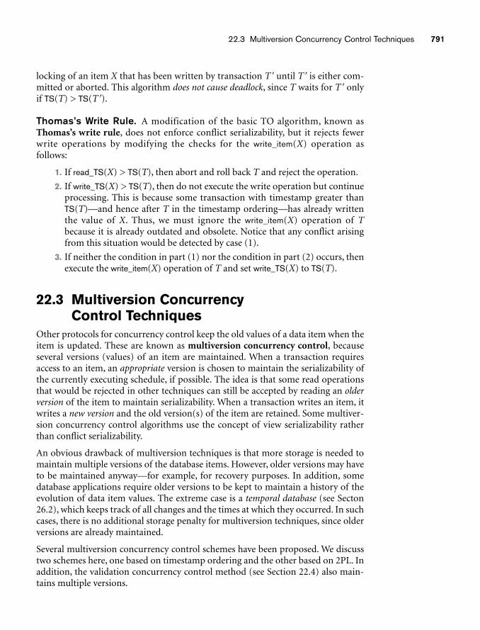
22.3 Multiversion Concurrency Control Techniques 791
locking of an item X that has been written by transaction T� until T� is either com-mitted or aborted. This algorithm does not cause deadlock, since T waits for T� onlyif TS(T) > TS(T�).
Thomas’s Write Rule. A modification of the basic TO algorithm, known asThomas’s write rule, does not enforce conflict serializability, but it rejects fewerwrite operations by modifying the checks for the write_item(X) operation as follows:
1. If read_TS(X) > TS(T), then abort and roll back T and reject the operation.
2. If write_TS(X) > TS(T), then do not execute the write operation but continueprocessing. This is because some transaction with timestamp greater thanTS(T)—and hence after T in the timestamp ordering—has already writtenthe value of X. Thus, we must ignore the write_item(X) operation of Tbecause it is already outdated and obsolete. Notice that any conflict arisingfrom this situation would be detected by case (1).
3. If neither the condition in part (1) nor the condition in part (2) occurs, thenexecute the write_item(X) operation of T and set write_TS(X) to TS(T).
22.3 Multiversion Concurrency Control Techniques
Other protocols for concurrency control keep the old values of a data item when theitem is updated. These are known as multiversion concurrency control, becauseseveral versions (values) of an item are maintained. When a transaction requiresaccess to an item, an appropriate version is chosen to maintain the serializability ofthe currently executing schedule, if possible. The idea is that some read operationsthat would be rejected in other techniques can still be accepted by reading an olderversion of the item to maintain serializability. When a transaction writes an item, itwrites a new version and the old version(s) of the item are retained. Some multiver-sion concurrency control algorithms use the concept of view serializability ratherthan conflict serializability.
An obvious drawback of multiversion techniques is that more storage is needed tomaintain multiple versions of the database items. However, older versions may haveto be maintained anyway—for example, for recovery purposes. In addition, somedatabase applications require older versions to be kept to maintain a history of theevolution of data item values. The extreme case is a temporal database (see Secton26.2), which keeps track of all changes and the times at which they occurred. In suchcases, there is no additional storage penalty for multiversion techniques, since olderversions are already maintained.
Several multiversion concurrency control schemes have been proposed. We discusstwo schemes here, one based on timestamp ordering and the other based on 2PL. Inaddition, the validation concurrency control method (see Section 22.4) also main-tains multiple versions.
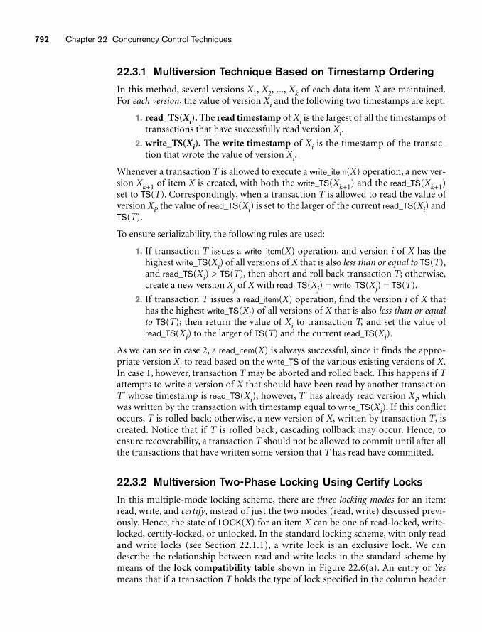
792 Chapter 22 Concurrency Control Techniques
22.3.1 Multiversion Technique Based on Timestamp OrderingIn this method, several versions X1, X2, ..., Xk of each data item X are maintained.For each version, the value of version Xi and the following two timestamps are kept:
1. read_TS(Xi). The read timestamp of Xi is the largest of all the timestamps oftransactions that have successfully read version Xi.
2. write_TS(Xi). The write timestamp of Xi is the timestamp of the transac-tion that wrote the value of version Xi.
Whenever a transaction T is allowed to execute a write_item(X) operation, a new ver-sion Xk+1 of item X is created, with both the write_TS(Xk+1) and the read_TS(Xk+1)set to TS(T). Correspondingly, when a transaction T is allowed to read the value ofversion Xi, the value of read_TS(Xi) is set to the larger of the current read_TS(Xi) andTS(T).
To ensure serializability, the following rules are used:
1. If transaction T issues a write_item(X) operation, and version i of X has thehighest write_TS(Xi) of all versions of X that is also less than or equal to TS(T),and read_TS(Xi) > TS(T), then abort and roll back transaction T; otherwise,create a new version Xj of X with read_TS(Xj) = write_TS(Xj) = TS(T).
2. If transaction T issues a read_item(X) operation, find the version i of X thathas the highest write_TS(Xi) of all versions of X that is also less than or equalto TS(T); then return the value of Xi to transaction T, and set the value ofread_TS(Xi) to the larger of TS(T) and the current read_TS(Xi).
As we can see in case 2, a read_item(X) is always successful, since it finds the appro-priate version Xi to read based on the write_TS of the various existing versions of X.In case 1, however, transaction T may be aborted and rolled back. This happens if Tattempts to write a version of X that should have been read by another transactionT� whose timestamp is read_TS(Xi); however, T� has already read version Xi, whichwas written by the transaction with timestamp equal to write_TS(Xi). If this conflictoccurs, T is rolled back; otherwise, a new version of X, written by transaction T, iscreated. Notice that if T is rolled back, cascading rollback may occur. Hence, toensure recoverability, a transaction T should not be allowed to commit until after allthe transactions that have written some version that T has read have committed.
22.3.2 Multiversion Two-Phase Locking Using Certify LocksIn this multiple-mode locking scheme, there are three locking modes for an item:read, write, and certify, instead of just the two modes (read, write) discussed previ-ously. Hence, the state of LOCK(X) for an item X can be one of read-locked, write-locked, certify-locked, or unlocked. In the standard locking scheme, with only readand write locks (see Section 22.1.1), a write lock is an exclusive lock. We candescribe the relationship between read and write locks in the standard scheme bymeans of the lock compatibility table shown in Figure 22.6(a). An entry of Yesmeans that if a transaction T holds the type of lock specified in the column header
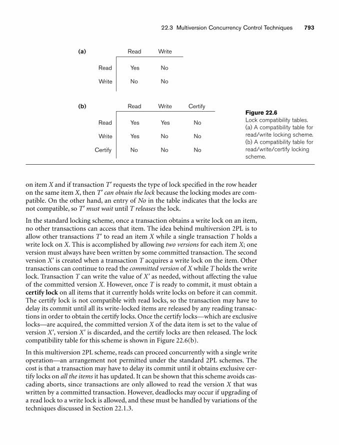
22.3 Multiversion Concurrency Control Techniques 793
(b) Read Write
Read
Write
Certify
Yes No No
No No No
Yes Yes No
Certify
(a) Read Write
Read
Write No No
Yes No
Figure 22.6Lock compatibility tables.(a) A compatibility table forread/write locking scheme.(b) A compatibility table forread/write/certify lockingscheme.
on item X and if transaction T� requests the type of lock specified in the row headeron the same item X, then T� can obtain the lock because the locking modes are com-patible. On the other hand, an entry of No in the table indicates that the locks arenot compatible, so T� must wait until T releases the lock.
In the standard locking scheme, once a transaction obtains a write lock on an item,no other transactions can access that item. The idea behind multiversion 2PL is toallow other transactions T� to read an item X while a single transaction T holds awrite lock on X. This is accomplished by allowing two versions for each item X; oneversion must always have been written by some committed transaction. The secondversion X� is created when a transaction T acquires a write lock on the item. Othertransactions can continue to read the committed version of X while T holds the writelock. Transaction T can write the value of X� as needed, without affecting the valueof the committed version X. However, once T is ready to commit, it must obtain acertify lock on all items that it currently holds write locks on before it can commit.The certify lock is not compatible with read locks, so the transaction may have todelay its commit until all its write-locked items are released by any reading transac-tions in order to obtain the certify locks. Once the certify locks—which are exclusivelocks—are acquired, the committed version X of the data item is set to the value ofversion X�, version X� is discarded, and the certify locks are then released. The lockcompatibility table for this scheme is shown in Figure 22.6(b).
In this multiversion 2PL scheme, reads can proceed concurrently with a single writeoperation—an arrangement not permitted under the standard 2PL schemes. Thecost is that a transaction may have to delay its commit until it obtains exclusive cer-tify locks on all the items it has updated. It can be shown that this scheme avoids cas-cading aborts, since transactions are only allowed to read the version X that waswritten by a committed transaction. However, deadlocks may occur if upgrading ofa read lock to a write lock is allowed, and these must be handled by variations of thetechniques discussed in Section 22.1.3.
794 Chapter 22 Concurrency Control Techniques
22.4 Validation (Optimistic) ConcurrencyControl Techniques
In all the concurrency control techniques we have discussed so far, a certain degreeof checking is done before a database operation can be executed. For example, inlocking, a check is done to determine whether the item being accessed is locked. Intimestamp ordering, the transaction timestamp is checked against the read andwrite timestamps of the item. Such checking represents overhead during transac-tion execution, with the effect of slowing down the transactions.
In optimistic concurrency control techniques, also known as validation orcertification techniques, no checking is done while the transaction is executing.Several theoretical concurrency control methods are based on the validation tech-nique. We will describe only one scheme here. In this scheme, updates in the trans-action are not applied directly to the database items until the transaction reaches itsend. During transaction execution, all updates are applied to local copies of the dataitems that are kept for the transaction.6 At the end of transaction execution, avalidation phase checks whether any of the transaction’s updates violate serializ-ability. Certain information needed by the validation phase must be kept by the sys-tem. If serializability is not violated, the transaction is committed and the databaseis updated from the local copies; otherwise, the transaction is aborted and thenrestarted later.
There are three phases for this concurrency control protocol:
1. Read phase. A transaction can read values of committed data items from thedatabase. However, updates are applied only to local copies (versions) of thedata items kept in the transaction workspace.
2. Validation phase. Checking is performed to ensure that serializability willnot be violated if the transaction updates are applied to the database.
3. Write phase. If the validation phase is successful, the transaction updates areapplied to the database; otherwise, the updates are discarded and the trans-action is restarted.
The idea behind optimistic concurrency control is to do all the checks at once;hence, transaction execution proceeds with a minimum of overhead until the vali-dation phase is reached. If there is little interference among transactions, most willbe validated successfully. However, if there is much interference, many transactionsthat execute to completion will have their results discarded and must be restartedlater. Under these circumstances, optimistic techniques do not work well. The tech-niques are called optimistic because they assume that little interference will occurand hence that there is no need to do checking during transaction execution.
The optimistic protocol we describe uses transaction timestamps and also requiresthat the write_sets and read_sets of the transactions be kept by the system.Additionally, start and end times for some of the three phases need to be kept for
6Note that this can be considered as keeping multiple versions of items!
22.5 Granularity of Data Items and Multiple Granularity Locking 795
each transaction. Recall that the write_set of a transaction is the set of items it writes,and the read_set is the set of items it reads. In the validation phase for transaction Ti,the protocol checks that Ti does not interfere with any committed transactions orwith any other transactions currently in their validation phase. The validation phasefor Ti checks that, for each such transaction Tj that is either committed or is in itsvalidation phase, one of the following conditions holds:
1. Transaction Tj completes its write phase before Ti starts its read phase.
2. Ti starts its write phase after Tj completes its write phase, and the read_setof Ti has no items in common with the write_set of Tj.
3. Both the read_set and write_set of Ti have no items in common with thewrite_set of Tj, and Tj completes its read phase before Ti completes its readphase.
When validating transaction Ti, the first condition is checked first for each transac-tion Tj, since (1) is the simplest condition to check. Only if condition 1 is false iscondition 2 checked, and only if (2) is false is condition 3—the most complex toevaluate—checked. If any one of these three conditions holds, there is no interfer-ence and Ti is validated successfully. If none of these three conditions holds, the val-idation of transaction Ti fails and it is aborted and restarted later becauseinterference may have occurred.
22.5 Granularity of Data Items and MultipleGranularity Locking
All concurrency control techniques assume that the database is formed of a numberof named data items. A database item could be chosen to be one of the following:
■ A database record
■ A field value of a database record
■ A disk block
■ A whole file
■ The whole database
The granularity can affect the performance of concurrency control and recovery. InSection 22.5.1, we discuss some of the tradeoffs with regard to choosing the granu-larity level used for locking, and in Section 22.5.2 we discuss a multiple granularitylocking scheme, where the granularity level (size of the data item) may be changeddynamically.
22.5.1 Granularity Level Considerations for LockingThe size of data items is often called the data item granularity. Fine granularityrefers to small item sizes, whereas coarse granularity refers to large item sizes. Severaltradeoffs must be considered in choosing the data item size. We will discuss dataitem size in the context of locking, although similar arguments can be made forother concurrency control techniques.
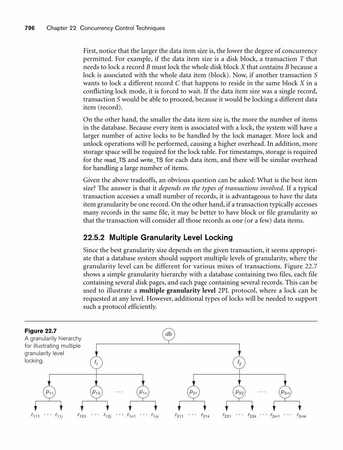
796 Chapter 22 Concurrency Control Techniques
db
r111 r11j r121 r12j r1n1 r1nj r211 r21k r221 r22k r2m1 r2mk. . . . . . . . .
. . .
. . . . . . . . . . . .
. . .
. . .
p11 p12
f1
p1n p21 p22 p2m
f2
Figure 22.7A granularity hierarchyfor illustrating multiplegranularity level locking.
First, notice that the larger the data item size is, the lower the degree of concurrencypermitted. For example, if the data item size is a disk block, a transaction T thatneeds to lock a record B must lock the whole disk block X that contains B because alock is associated with the whole data item (block). Now, if another transaction Swants to lock a different record C that happens to reside in the same block X in aconflicting lock mode, it is forced to wait. If the data item size was a single record,transaction S would be able to proceed, because it would be locking a different dataitem (record).
On the other hand, the smaller the data item size is, the more the number of itemsin the database. Because every item is associated with a lock, the system will have alarger number of active locks to be handled by the lock manager. More lock andunlock operations will be performed, causing a higher overhead. In addition, morestorage space will be required for the lock table. For timestamps, storage is requiredfor the read_TS and write_TS for each data item, and there will be similar overheadfor handling a large number of items.
Given the above tradeoffs, an obvious question can be asked: What is the best itemsize? The answer is that it depends on the types of transactions involved. If a typicaltransaction accesses a small number of records, it is advantageous to have the dataitem granularity be one record. On the other hand, if a transaction typically accessesmany records in the same file, it may be better to have block or file granularity sothat the transaction will consider all those records as one (or a few) data items.
22.5.2 Multiple Granularity Level LockingSince the best granularity size depends on the given transaction, it seems appropri-ate that a database system should support multiple levels of granularity, where thegranularity level can be different for various mixes of transactions. Figure 22.7shows a simple granularity hierarchy with a database containing two files, each filecontaining several disk pages, and each page containing several records. This can beused to illustrate a multiple granularity level 2PL protocol, where a lock can berequested at any level. However, additional types of locks will be needed to supportsuch a protocol efficiently.
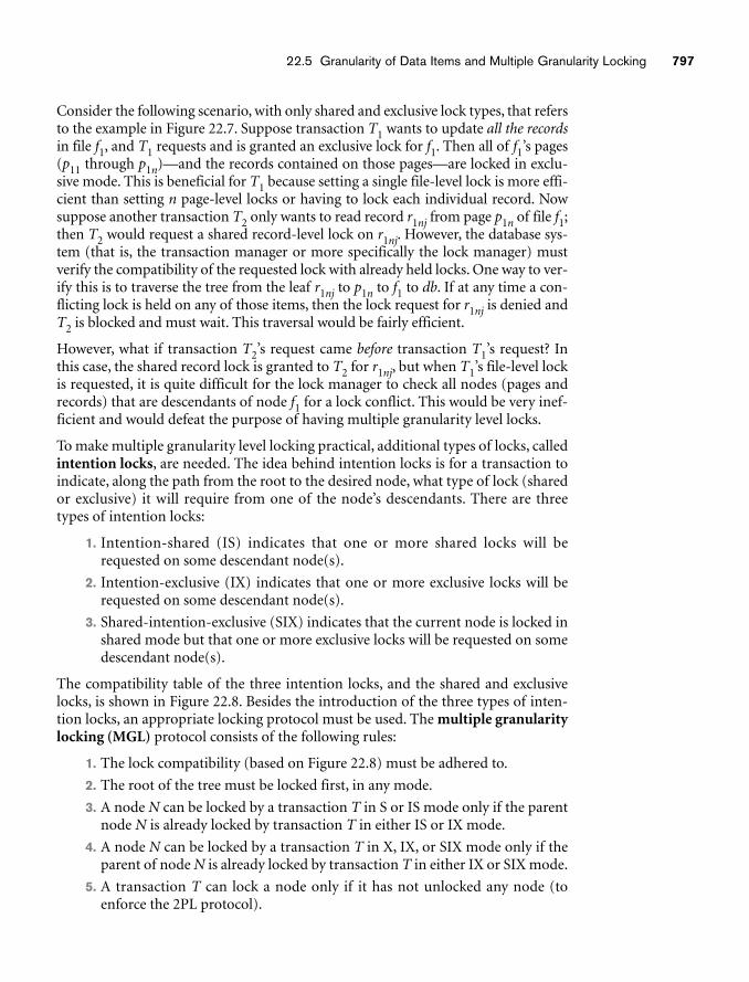
22.5 Granularity of Data Items and Multiple Granularity Locking 797
Consider the following scenario, with only shared and exclusive lock types, that refersto the example in Figure 22.7. Suppose transaction T1 wants to update all the recordsin file f1, and T1 requests and is granted an exclusive lock for f1. Then all of f1’s pages(p11 through p1n)—and the records contained on those pages—are locked in exclu-sive mode. This is beneficial for T1 because setting a single file-level lock is more effi-cient than setting n page-level locks or having to lock each individual record. Nowsuppose another transaction T2 only wants to read record r1nj from page p1n of file f1;then T2 would request a shared record-level lock on r1nj. However, the database sys-tem (that is, the transaction manager or more specifically the lock manager) mustverify the compatibility of the requested lock with already held locks. One way to ver-ify this is to traverse the tree from the leaf r1nj to p1n to f1 to db. If at any time a con-flicting lock is held on any of those items, then the lock request for r1nj is denied andT2 is blocked and must wait. This traversal would be fairly efficient.
However, what if transaction T2’s request came before transaction T1’s request? Inthis case, the shared record lock is granted to T2 for r1nj, but when T1’s file-level lockis requested, it is quite difficult for the lock manager to check all nodes (pages andrecords) that are descendants of node f1 for a lock conflict. This would be very inef-ficient and would defeat the purpose of having multiple granularity level locks.
To make multiple granularity level locking practical, additional types of locks, calledintention locks, are needed. The idea behind intention locks is for a transaction toindicate, along the path from the root to the desired node, what type of lock (sharedor exclusive) it will require from one of the node’s descendants. There are threetypes of intention locks:
1. Intention-shared (IS) indicates that one or more shared locks will berequested on some descendant node(s).
2. Intention-exclusive (IX) indicates that one or more exclusive locks will berequested on some descendant node(s).
3. Shared-intention-exclusive (SIX) indicates that the current node is locked inshared mode but that one or more exclusive locks will be requested on somedescendant node(s).
The compatibility table of the three intention locks, and the shared and exclusivelocks, is shown in Figure 22.8. Besides the introduction of the three types of inten-tion locks, an appropriate locking protocol must be used. The multiple granularitylocking (MGL) protocol consists of the following rules:
1. The lock compatibility (based on Figure 22.8) must be adhered to.
2. The root of the tree must be locked first, in any mode.
3. A node N can be locked by a transaction T in S or IS mode only if the parentnode N is already locked by transaction T in either IS or IX mode.
4. A node N can be locked by a transaction T in X, IX, or SIX mode only if theparent of node N is already locked by transaction T in either IX or SIX mode.
5. A transaction T can lock a node only if it has not unlocked any node (toenforce the 2PL protocol).
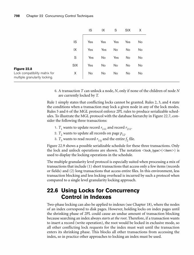
798 Chapter 22 Concurrency Control Techniques
IS
IX
S
SIX
X
IS
Yes
Yes
Yes
Yes
No
IX
Yes
No
Yes
No
No
S
No
Yes
Yes
No
No
SIX
No
No
Yes
No
No
X
No
No
No
No
NoFigure 22.8Lock compatibility matrix formultiple granularity locking.
6. A transaction T can unlock a node, N, only if none of the children of node Nare currently locked by T.
Rule 1 simply states that conflicting locks cannot be granted. Rules 2, 3, and 4 statethe conditions when a transaction may lock a given node in any of the lock modes.Rules 5 and 6 of the MGL protocol enforce 2PL rules to produce serializable sched-ules. To illustrate the MGL protocol with the database hierarchy in Figure 22.7, con-sider the following three transactions:
1. T1 wants to update record r111 and record r211.
2. T2 wants to update all records on page p12.
3. T3 wants to read record r11j and the entire f2 file.
Figure 22.9 shows a possible serializable schedule for these three transactions. Onlythe lock and unlock operations are shown. The notation <lock_type>(<item>) isused to display the locking operations in the schedule.
The multiple granularity level protocol is especially suited when processing a mix oftransactions that include (1) short transactions that access only a few items (recordsor fields) and (2) long transactions that access entire files. In this environment, lesstransaction blocking and less locking overhead is incurred by such a protocol whencompared to a single level granularity locking approach.
22.6 Using Locks for Concurrency Control in Indexes
Two-phase locking can also be applied to indexes (see Chapter 18), where the nodesof an index correspond to disk pages. However, holding locks on index pages untilthe shrinking phase of 2PL could cause an undue amount of transaction blockingbecause searching an index always starts at the root. Therefore, if a transaction wantsto insert a record (write operation), the root would be locked in exclusive mode, soall other conflicting lock requests for the index must wait until the transactionenters its shrinking phase. This blocks all other transactions from accessing theindex, so in practice other approaches to locking an index must be used.
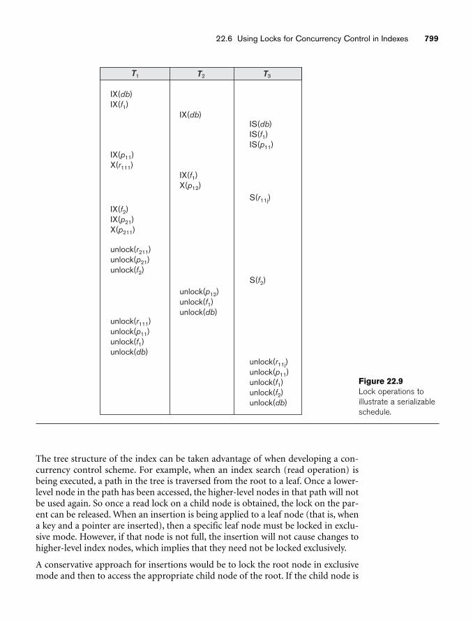
22.6 Using Locks for Concurrency Control in Indexes 799
IX(db)IX(f1)
T1
IX(p11)X(r111)
IX(f2)IX(p21)X(p211)
unlock(r211)unlock(p21)unlock(f2)
unlock(r111)unlock(p11)unlock(f1)unlock(db)
T3
IS(db)IS(f1)IS(p11)
S(r11j)
S(f2)
unlock(r11j)unlock(p11)unlock(f1)unlock(f2)unlock(db)
IX(db)
T2
IX(f1)X(p12)
unlock(p12)unlock(f1)unlock(db)
Figure 22.9Lock operations toillustrate a serializableschedule.
The tree structure of the index can be taken advantage of when developing a con-currency control scheme. For example, when an index search (read operation) isbeing executed, a path in the tree is traversed from the root to a leaf. Once a lower-level node in the path has been accessed, the higher-level nodes in that path will notbe used again. So once a read lock on a child node is obtained, the lock on the par-ent can be released. When an insertion is being applied to a leaf node (that is, whena key and a pointer are inserted), then a specific leaf node must be locked in exclu-sive mode. However, if that node is not full, the insertion will not cause changes tohigher-level index nodes, which implies that they need not be locked exclusively.
A conservative approach for insertions would be to lock the root node in exclusivemode and then to access the appropriate child node of the root. If the child node is
800 Chapter 22 Concurrency Control Techniques
not full, then the lock on the root node can be released. This approach can beapplied all the way down the tree to the leaf, which is typically three or four levelsfrom the root. Although exclusive locks are held, they are soon released. An alterna-tive, more optimistic approach would be to request and hold shared locks on thenodes leading to the leaf node, with an exclusive lock on the leaf. If the insertioncauses the leaf to split, insertion will propagate to one or more higher-level nodes.Then, the locks on the higher-level nodes can be upgraded to exclusive mode.
Another approach to index locking is to use a variant of the B+-tree, called the B-link tree. In a B-link tree, sibling nodes on the same level are linked at every level.This allows shared locks to be used when requesting a page and requires that thelock be released before accessing the child node. For an insert operation, the sharedlock on a node would be upgraded to exclusive mode. If a split occurs, the parentnode must be relocked in exclusive mode. One complication is for search operationsexecuted concurrently with the update. Suppose that a concurrent update operationfollows the same path as the search, and inserts a new entry into the leaf node.Additionally, suppose that the insert causes that leaf node to split. When the insert isdone, the search process resumes, following the pointer to the desired leaf, only tofind that the key it is looking for is not present because the split has moved that keyinto a new leaf node, which would be the right sibling of the original leaf node.However, the search process can still succeed if it follows the pointer (link) in theoriginal leaf node to its right sibling, where the desired key has been moved.
Handling the deletion case, where two or more nodes from the index tree merge, isalso part of the B-link tree concurrency protocol. In this case, locks on the nodes tobe merged are held as well as a lock on the parent of the two nodes to be merged.
22.7 Other Concurrency Control IssuesIn this section we discuss some other issues relevant to concurrency control. InSection 22.7.1, we discuss problems associated with insertion and deletion ofrecords and the so-called phantom problem, which may occur when records areinserted. This problem was described as a potential problem requiring a concur-rency control measure in Section 21.6. In Section 22.7.2 we discuss problems thatmay occur when a transaction outputs some data to a monitor before it commits,and then the transaction is later aborted.
22.7.1 Insertion, Deletion, and Phantom RecordsWhen a new data item is inserted in the database, it obviously cannot be accesseduntil after the item is created and the insert operation is completed. In a lockingenvironment, a lock for the item can be created and set to exclusive (write) mode;the lock can be released at the same time as other write locks would be released,based on the concurrency control protocol being used. For a timestamp-based pro-tocol, the read and write timestamps of the new item are set to the timestamp of thecreating transaction.
22.7 Other Concurrency Control Issues 801
Next, consider a deletion operation that is applied on an existing data item. Forlocking protocols, again an exclusive (write) lock must be obtained before the trans-action can delete the item. For timestamp ordering, the protocol must ensure that nolater transaction has read or written the item before allowing the item to be deleted.
A situation known as the phantom problem can occur when a new record that isbeing inserted by some transaction T satisfies a condition that a set of recordsaccessed by another transaction T� must satisfy. For example, suppose that transac-tion T is inserting a new EMPLOYEE record whose Dno = 5, while transaction T� isaccessing all EMPLOYEE records whose Dno = 5 (say, to add up all their Salary valuesto calculate the personnel budget for department 5). If the equivalent serial order isT followed by T�, then T�must read the new EMPLOYEE record and include its Salaryin the sum calculation. For the equivalent serial order T� followed by T, the newsalary should not be included. Notice that although the transactions logically con-flict, in the latter case there is really no record (data item) in common between thetwo transactions, since T� may have locked all the records with Dno = 5 before Tinserted the new record. This is because the record that causes the conflict is aphantom record that has suddenly appeared in the database on being inserted. Ifother operations in the two transactions conflict, the conflict due to the phantomrecord may not be recognized by the concurrency control protocol.
One solution to the phantom record problem is to use index locking, as discussedin Section 22.6. Recall from Chapter 18 that an index includes entries that have anattribute value, plus a set of pointers to all records in the file with that value. Forexample, an index on Dno of EMPLOYEE would include an entry for each distinctDno value, plus a set of pointers to all EMPLOYEE records with that value. If theindex entry is locked before the record itself can be accessed, then the conflict on thephantom record can be detected, because transaction T� would request a read lockon the index entry for Dno = 5, and T would request a write lock on the same entrybefore they could place the locks on the actual records. Since the index locks conflict,the phantom conflict would be detected.
A more general technique, called predicate locking, would lock access to all recordsthat satisfy an arbitrary predicate (condition) in a similar manner; however, predi-cate locks have proved to be difficult to implement efficiently.
22.7.2 Interactive TransactionsAnother problem occurs when interactive transactions read input and write outputto an interactive device, such as a monitor screen, before they are committed. Theproblem is that a user can input a value of a data item to a transaction T that isbased on some value written to the screen by transaction T�, which may not havecommitted. This dependency between T and T� cannot be modeled by the systemconcurrency control method, since it is only based on the user interacting with thetwo transactions.
An approach to dealing with this problem is to postpone output of transactions tothe screen until they have committed.
802 Chapter 22 Concurrency Control Techniques
22.7.3 LatchesLocks held for a short duration are typically called latches. Latches do not follow theusual concurrency control protocol such as two-phase locking. For example, a latchcan be used to guarantee the physical integrity of a page when that page is beingwritten from the buffer to disk. A latch would be acquired for the page, the pagewritten to disk, and then the latch released.
22.8 SummaryIn this chapter we discussed DBMS techniques for concurrency control. We startedby discussing lock-based protocols, which are by far the most commonly used inpractice. We described the two-phase locking (2PL) protocol and a number of itsvariations: basic 2PL, strict 2PL, conservative 2PL, and rigorous 2PL. The strict andrigorous variations are more common because of their better recoverability proper-ties. We introduced the concepts of shared (read) and exclusive (write) locks, andshowed how locking can guarantee serializability when used in conjunction withthe two-phase locking rule. We also presented various techniques for dealing withthe deadlock problem, which can occur with locking. In practice, it is common touse timeouts and deadlock detection (wait-for graphs).
We presented other concurrency control protocols that are not used often in prac-tice but are important for the theoretical alternatives they show for solving thisproblem. These include the timestamp ordering protocol, which ensures serializ-ability based on the order of transaction timestamps. Timestamps are unique,system-generated transaction identifiers. We discussed Thomas’s write rule, whichimproves performance but does not guarantee conflict serializability. The stricttimestamp ordering protocol was also presented. We discussed two multiversionprotocols, which assume that older versions of data items can be kept in the data-base. One technique, called multiversion two-phase locking (which has been used inpractice), assumes that two versions can exist for an item and attempts to increaseconcurrency by making write and read locks compatible (at the cost of introducingan additional certify lock mode). We also presented a multiversion protocol basedon timestamp ordering, and an example of an optimistic protocol, which is alsoknown as a certification or validation protocol.
Then we turned our attention to the important practical issue of data item granu-larity. We described a multigranularity locking protocol that allows the change ofgranularity (item size) based on the current transaction mix, with the goal ofimproving the performance of concurrency control. An important practical issuewas then presented, which is to develop locking protocols for indexes so that indexesdo not become a hindrance to concurrent access. Finally, we introduced the phan-tom problem and problems with interactive transactions, and briefly described theconcept of latches and how it differs from locks.
Review Questions 803
Review Questions22.1. What is the two-phase locking protocol? How does it guarantee serializabil-
ity?
22.2. What are some variations of the two-phase locking protocol? Why is strict orrigorous two-phase locking often preferred?
22.3. Discuss the problems of deadlock and starvation, and the differentapproaches to dealing with these problems.
22.4. Compare binary locks to exclusive/shared locks. Why is the latter type oflocks preferable?
22.5. Describe the wait-die and wound-wait protocols for deadlock prevention.
22.6. Describe the cautious waiting, no waiting, and timeout protocols for dead-lock prevention.
22.7. What is a timestamp? How does the system generate timestamps?
22.8. Discuss the timestamp ordering protocol for concurrency control. How doesstrict timestamp ordering differ from basic timestamp ordering?
22.9. Discuss two multiversion techniques for concurrency control.
22.10. What is a certify lock? What are the advantages and disadvantages of usingcertify locks?
22.11. How do optimistic concurrency control techniques differ from other con-currency control techniques? Why are they also called validation or certifica-tion techniques? Discuss the typical phases of an optimistic concurrencycontrol method.
22.12. How does the granularity of data items affect the performance of concur-rency control? What factors affect selection of granularity size for data items?
22.13. What type of lock is needed for insert and delete operations?
22.14. What is multiple granularity locking? Under what circumstances is it used?
22.15. What are intention locks?
22.16. When are latches used?
22.17. What is a phantom record? Discuss the problem that a phantom record cancause for concurrency control.
22.18. How does index locking resolve the phantom problem?
22.19. What is a predicate lock?
804 Chapter 22 Concurrency Control Techniques
Exercises22.20. Prove that the basic two-phase locking protocol guarantees conflict serializ-
ability of schedules. (Hint: Show that if a serializability graph for a schedulehas a cycle, then at least one of the transactions participating in the scheduledoes not obey the two-phase locking protocol.)
22.21. Modify the data structures for multiple-mode locks and the algorithms forread_lock(X), write_lock(X), and unlock(X) so that upgrading and downgrad-ing of locks are possible. (Hint: The lock needs to check the transaction id(s)that hold the lock, if any.)
22.22. Prove that strict two-phase locking guarantees strict schedules.
22.23. Prove that the wait-die and wound-wait protocols avoid deadlock and star-vation.
22.24. Prove that cautious waiting avoids deadlock.
22.25. Apply the timestamp ordering algorithm to the schedules in Figure 21.8(b)and (c), and determine whether the algorithm will allow the execution of theschedules.
22.26. Repeat Exercise 22.25, but use the multiversion timestamp ordering method.
22.27. Why is two-phase locking not used as a concurrency control method forindexes such as B+-trees?
22.28. The compatibility matrix in Figure 22.8 shows that IS and IX locks are com-patible. Explain why this is valid.
22.29. The MGL protocol states that a transaction T can unlock a node N, only ifnone of the children of node N are still locked by transaction T. Show thatwithout this condition, the MGL protocol would be incorrect.
Selected BibliographyThe two-phase locking protocol and the concept of predicate locks were first pro-posed by Eswaran et al. (1976). Bernstein et al. (1987), Gray and Reuter (1993), andPapadimitriou (1986) focus on concurrency control and recovery. Kumar (1996)focuses on performance of concurrency control methods. Locking is discussed inGray et al. (1975), Lien and Weinberger (1978), Kedem and Silbershatz (1980), andKorth (1983). Deadlocks and wait-for graphs were formalized by Holt (1972), andthe wait-wound and wound-die schemes are presented in Rosenkrantz et al. (1978).Cautious waiting is discussed in Hsu and Zhang (1992). Helal et al. (1993) com-pares various locking approaches. Timestamp-based concurrency control tech-niques are discussed in Bernstein and Goodman (1980) and Reed (1983).Optimistic concurrency control is discussed in Kung and Robinson (1981) andBassiouni (1988). Papadimitriou and Kanellakis (1979) and Bernstein and
Selected Bibliography 805
Goodman (1983) discuss multiversion techniques. Multiversion timestamp order-ing was proposed in Reed (1979, 1983), and multiversion two-phase locking is dis-cussed in Lai and Wilkinson (1984). A method for multiple locking granularitieswas proposed in Gray et al. (1975), and the effects of locking granularities are ana-lyzed in Ries and Stonebraker (1977). Bhargava and Reidl (1988) presents anapproach for dynamically choosing among various concurrency control and recov-ery methods. Concurrency control methods for indexes are presented in Lehmanand Yao (1981) and in Shasha and Goodman (1988). A performance study of vari-ous B+-tree concurrency control algorithms is presented in Srinivasan and Carey(1991).
Other work on concurrency control includes semantic-based concurrency control(Badrinath and Ramamritham, 1992), transaction models for long-running activi-ties (Dayal et al., 1991), and multilevel transaction management (Hasse andWeikum, 1991).
807
Database Recovery Techniques
In this chapter we discuss some of the techniques thatcan be used for database recovery from failures. In
Section 21.1.4 we discussed the different causes of failure, such as system crashesand transaction errors. Also, in Section 21.2, we covered many of the concepts thatare used by recovery processes, such as the system log and commit points.
This chapter presents additional concepts that are relevant to recovery protocols,and provides an overview of the various database recovery algorithms We start inSection 23.1 with an outline of a typical recovery procedure and a categorization ofrecovery algorithms, and then we discuss several recovery concepts, including write-ahead logging, in-place versus shadow updates, and the process of rolling back(undoing) the effect of an incomplete or failed transaction. In Section 23.2 we pre-sent recovery techniques based on deferred update, also known as the NO-UNDO/REDO technique, where the data on disk is not updated until after atransaction commits. In Section 23.3 we discuss recovery techniques based onimmediate update, where data can be updated on disk during transaction execution;these include the UNDO/REDO and UNDO/NO-REDO algorithms. We discuss thetechnique known as shadowing or shadow paging, which can be categorized as aNO-UNDO/NO-REDO algorithm in Section 23.4. An example of a practical DBMSrecovery scheme, called ARIES, is presented in Section 23.5. Recovery in multidata-bases is briefly discussed in Section 23.6. Finally, techniques for recovery from cata-strophic failure are discussed in Section 23.7. Section 23.8 summarizes the chapter.
Our emphasis is on conceptually describing several different approaches to recov-ery. For descriptions of recovery features in specific systems, the reader should con-sult the bibliographic notes at the end of the chapter and the online and printeduser manuals for those systems. Recovery techniques are often intertwined with the
23chapter 23
808 Chapter 23 Database Recovery Techniques
concurrency control mechanisms. Certain recovery techniques are best used withspecific concurrency control methods. We will discuss recovery concepts indepen-dently of concurrency control mechanisms, but we will discuss the circumstancesunder which a particular recovery mechanism is best used with a certain concur-rency control protocol.
23.1 Recovery Concepts
23.1.1 Recovery Outline and Categorization of Recovery Algorithms
Recovery from transaction failures usually means that the database is restored to themost recent consistent state just before the time of failure. To do this, the systemmust keep information about the changes that were applied to data items by thevarious transactions. This information is typically kept in the system log, as we dis-cussed in Section 21.2.2. A typical strategy for recovery may be summarized infor-mally as follows:
1. If there is extensive damage to a wide portion of the database due to cata-strophic failure, such as a disk crash, the recovery method restores a pastcopy of the database that was backed up to archival storage (typically tape orother large capacity offline storage media) and reconstructs a more currentstate by reapplying or redoing the operations of committed transactionsfrom the backed up log, up to the time of failure.
2. When the database on disk is not physically damaged, and a noncatastrophicfailure of types 1 through 4 in Section 21.1.4 has occurred, the recoverystrategy is to identify any changes that may cause an inconsistency in thedatabase. For example, a transaction that has updated some database itemson disk but has not been committed needs to have its changes reversed byundoing its write operations. It may also be necessary to redo some opera-tions in order to restore a consistent state of the database; for example, if atransaction has committed but some of its write operations have not yetbeen written to disk. For noncatastrophic failure, the recovery protocol doesnot need a complete archival copy of the database. Rather, the entries kept inthe online system log on disk are analyzed to determine the appropriateactions for recovery.
Conceptually, we can distinguish two main techniques for recovery from noncata-strophic transaction failures: deferred update and immediate update. The deferredupdate techniques do not physically update the database on disk until after a trans-action reaches its commit point; then the updates are recorded in the database.Before reaching commit, all transaction updates are recorded in the local transac-tion workspace or in the main memory buffers that the DBMS maintains (theDBMS main memory cache). Before commit, the updates are recorded persistentlyin the log, and then after commit, the updates are written to the database on disk.If a transaction fails before reaching its commit point, it will not have changed the
23.1 Recovery Concepts 809
database in any way, so UNDO is not needed. It may be necessary to REDO theeffect of the operations of a committed transaction from the log, because theireffect may not yet have been recorded in the database on disk. Hence, deferredupdate is also known as the NO-UNDO/REDO algorithm. We discuss this tech-nique in Section 23.2.
In the immediate update techniques, the database may be updated by some opera-tions of a transaction before the transaction reaches its commit point. However,these operations must also be recorded in the log on disk by force-writing before theyare applied to the database on disk, making recovery still possible. If a transactionfails after recording some changes in the database on disk but before reaching itscommit point, the effect of its operations on the database must be undone; that is,the transaction must be rolled back. In the general case of immediate update, bothundo and redo may be required during recovery. This technique, known as theUNDO/REDO algorithm, requires both operations during recovery, and is usedmost often in practice. A variation of the algorithm where all updates are requiredto be recorded in the database on disk before a transaction commits requires undoonly, so it is known as the UNDO/NO-REDO algorithm. We discuss these techniquesin Section 23.3.
The UNDO and REDO operations are required to be idempotent—that is, executingan operation multiple times is equivalent to executing it just once. In fact, the wholerecovery process should be idempotent because if the system were to fail during therecovery process, the next recovery attempt might UNDO and REDO certainwrite_item operations that had already been executed during the first recoveryprocess. The result of recovery from a system crash during recovery should be thesame as the result of recovering when there is no crash during recovery!
23.1.2 Caching (Buffering) of Disk BlocksThe recovery process is often closely intertwined with operating system functions—in particular, the buffering of database disk pages in the DBMS main memorycache. Typically, multiple disk pages that include the data items to be updated arecached into main memory buffers and then updated in memory before being writ-ten back to disk. The caching of disk pages is traditionally an operating system func-tion, but because of its importance to the efficiency of recovery procedures, it ishandled by the DBMS by calling low-level operating systems routines.
In general, it is convenient to consider recovery in terms of the database disk pages(blocks). Typically a collection of in-memory buffers, called the DBMS cache, iskept under the control of the DBMS for the purpose of holding these buffers. Adirectory for the cache is used to keep track of which database items are in thebuffers.1 This can be a table of <Disk_page_address, Buffer_location, ... > entries.When the DBMS requests action on some item, first it checks the cache directory todetermine whether the disk page containing the item is in the DBMS cache. If it is
1This is somewhat similar to the concept of page tables used by the operating system.
810 Chapter 23 Database Recovery Techniques
not, the item must be located on disk, and the appropriate disk pages are copied intothe cache. It may be necessary to replace (or flush) some of the cache buffers tomake space available for the new item. Some page replacement strategy similar tothese used in operating systems, such as least recently used (LRU) or first-in-first-out (FIFO), or a new strategy that is DBMS-specific can be used to select the buffersfor replacement, such as DBMIN or Least-Likely-to-Use (see bibliographic notes).
The entries in the DBMS cache directory hold additional information relevant tobuffer management. Associated with each buffer in the cache is a dirty bit, whichcan be included in the directory entry, to indicate whether or not the buffer hasbeen modified. When a page is first read from the database disk into a cache buffer,a new entry is inserted in the cache directory with the new disk page address, andthe dirty bit is set to 0 (zero). As soon as the buffer is modified, the dirty bit for thecorresponding directory entry is set to 1 (one). Additional information, such as thetransaction id(s) of the transaction(s) that modified the buffer can also be kept inthe directory. When the buffer contents are replaced (flushed) from the cache, thecontents must first be written back to the corresponding disk page only if its dirty bitis 1. Another bit, called the pin-unpin bit, is also needed—a page in the cache ispinned (bit value 1 (one)) if it cannot be written back to disk as yet. For example,the recovery protocol may restrict certain buffer pages from being written back tothe disk until the transactions that changed this buffer have committed.
Two main strategies can be employed when flushing a modified buffer back to disk.The first strategy, known as in-place updating, writes the buffer to the same originaldisk location, thus overwriting the old value of any changed data items on disk.2
Hence, a single copy of each database disk block is maintained. The second strategy,known as shadowing, writes an updated buffer at a different disk location, so mul-tiple versions of data items can be maintained, but this approach is not typicallyused in practice.
In general, the old value of the data item before updating is called the before image(BFIM), and the new value after updating is called the after image (AFIM). If shad-owing is used, both the BFIM and the AFIM can be kept on disk; hence, it is notstrictly necessary to maintain a log for recovering. We briefly discuss recovery basedon shadowing in Section 23.4.
23.1.3 Write-Ahead Logging, Steal/No-Steal, and Force/No-Force
When in-place updating is used, it is necessary to use a log for recovery (see Section21.2.2). In this case, the recovery mechanism must ensure that the BFIM of the dataitem is recorded in the appropriate log entry and that the log entry is flushed to diskbefore the BFIM is overwritten with the AFIM in the database on disk. This processis generally known as write-ahead logging, and is necessary to be able to UNDO theoperation if this is required during recovery. Before we can describe a protocol for
2In-place updating is used in most systems in practice.
23.1 Recovery Concepts 811
write-ahead logging, we need to distinguish between two types of log entry infor-mation included for a write command: the information needed for UNDO and theinformation needed for REDO. A REDO-type log entry includes the new value(AFIM) of the item written by the operation since this is needed to redo the effect ofthe operation from the log (by setting the item value in the database on disk to itsAFIM). The UNDO-type log entries include the old value (BFIM) of the item sincethis is needed to undo the effect of the operation from the log (by setting the itemvalue in the database back to its BFIM). In an UNDO/REDO algorithm, both types oflog entries are combined. Additionally, when cascading rollback is possible,read_item entries in the log are considered to be UNDO-type entries (see Section23.1.5).
As mentioned, the DBMS cache holds the cached database disk blocks in mainmemory buffers, which include not only data blocks, but also index blocks and logblocks from the disk. When a log record is written, it is stored in the current logbuffer in the DBMS cache. The log is simply a sequential (append-only) disk file,and the DBMS cache may contain several log blocks in main memory buffers (typi-cally, the last n log blocks of the log file). When an update to a data block—stored inthe DBMS cache—is made, an associated log record is written to the last log bufferin the DBMS cache. With the write-ahead logging approach, the log buffers (blocks)that contain the associated log records for a particular data block update must firstbe written to disk before the data block itself can be written back to disk from itsmain memory buffer.
Standard DBMS recovery terminology includes the terms steal/no-steal andforce/no-force, which specify the rules that govern when a page from the databasecan be written to disk from the cache:
1. If a cache buffer page updated by a transaction cannot be written to diskbefore the transaction commits, the recovery method is called a no-stealapproach. The pin-unpin bit will be used to indicate if a page cannot bewritten back to disk. On the other hand, if the recovery protocol allows writ-ing an updated buffer before the transaction commits, it is called steal. Stealis used when the DBMS cache (buffer) manager needs a buffer frame foranother transaction and the buffer manager replaces an existing page thathad been updated but whose transaction has not committed. The no-stealrule means that UNDO will never be needed during recovery, since a commit-ted transaction will not have any of its updates on disk before it commits.
2. If all pages updated by a transaction are immediately written to disk beforethe transaction commits, it is called a force approach. Otherwise, it is calledno-force. The force rule means that REDO will never be needed during recov-ery, since any committed transaction will have all its updates on disk beforeit is committed.
The deferred update (NO-UNDO) recovery scheme discussed in Section 23.2 followsa no-steal approach. However, typical database systems employ a steal/no-force strat-egy. The advantage of steal is that it avoids the need for a very large buffer space tostore all updated pages in memory. The advantage of no-force is that an updated
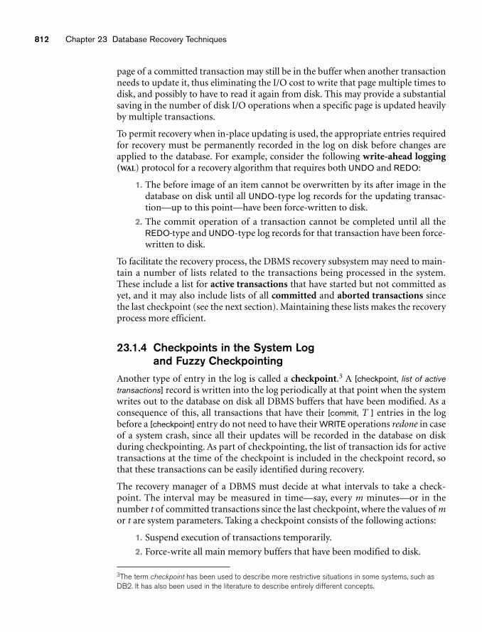
812 Chapter 23 Database Recovery Techniques
page of a committed transaction may still be in the buffer when another transactionneeds to update it, thus eliminating the I/O cost to write that page multiple times todisk, and possibly to have to read it again from disk. This may provide a substantialsaving in the number of disk I/O operations when a specific page is updated heavilyby multiple transactions.
To permit recovery when in-place updating is used, the appropriate entries requiredfor recovery must be permanently recorded in the log on disk before changes areapplied to the database. For example, consider the following write-ahead logging(WAL) protocol for a recovery algorithm that requires both UNDO and REDO:
1. The before image of an item cannot be overwritten by its after image in thedatabase on disk until all UNDO-type log records for the updating transac-tion—up to this point—have been force-written to disk.
2. The commit operation of a transaction cannot be completed until all theREDO-type and UNDO-type log records for that transaction have been force-written to disk.
To facilitate the recovery process, the DBMS recovery subsystem may need to main-tain a number of lists related to the transactions being processed in the system.These include a list for active transactions that have started but not committed asyet, and it may also include lists of all committed and aborted transactions sincethe last checkpoint (see the next section). Maintaining these lists makes the recoveryprocess more efficient.
23.1.4 Checkpoints in the System Log and Fuzzy Checkpointing
Another type of entry in the log is called a checkpoint.3 A [checkpoint, list of activetransactions] record is written into the log periodically at that point when the systemwrites out to the database on disk all DBMS buffers that have been modified. As aconsequence of this, all transactions that have their [commit, T ] entries in the logbefore a [checkpoint] entry do not need to have their WRITE operations redone in caseof a system crash, since all their updates will be recorded in the database on diskduring checkpointing. As part of checkpointing, the list of transaction ids for activetransactions at the time of the checkpoint is included in the checkpoint record, sothat these transactions can be easily identified during recovery.
The recovery manager of a DBMS must decide at what intervals to take a check-point. The interval may be measured in time—say, every m minutes—or in thenumber t of committed transactions since the last checkpoint, where the values of mor t are system parameters. Taking a checkpoint consists of the following actions:
1. Suspend execution of transactions temporarily.
2. Force-write all main memory buffers that have been modified to disk.
3The term checkpoint has been used to describe more restrictive situations in some systems, such asDB2. It has also been used in the literature to describe entirely different concepts.
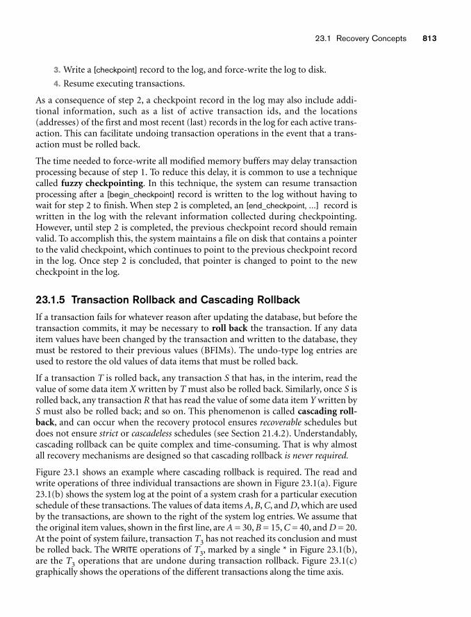
23.1 Recovery Concepts 813
3. Write a [checkpoint] record to the log, and force-write the log to disk.
4. Resume executing transactions.
As a consequence of step 2, a checkpoint record in the log may also include addi-tional information, such as a list of active transaction ids, and the locations(addresses) of the first and most recent (last) records in the log for each active trans-action. This can facilitate undoing transaction operations in the event that a trans-action must be rolled back.
The time needed to force-write all modified memory buffers may delay transactionprocessing because of step 1. To reduce this delay, it is common to use a techniquecalled fuzzy checkpointing. In this technique, the system can resume transactionprocessing after a [begin_checkpoint] record is written to the log without having towait for step 2 to finish. When step 2 is completed, an [end_checkpoint, ...] record iswritten in the log with the relevant information collected during checkpointing.However, until step 2 is completed, the previous checkpoint record should remainvalid. To accomplish this, the system maintains a file on disk that contains a pointerto the valid checkpoint, which continues to point to the previous checkpoint recordin the log. Once step 2 is concluded, that pointer is changed to point to the newcheckpoint in the log.
23.1.5 Transaction Rollback and Cascading RollbackIf a transaction fails for whatever reason after updating the database, but before thetransaction commits, it may be necessary to roll back the transaction. If any dataitem values have been changed by the transaction and written to the database, theymust be restored to their previous values (BFIMs). The undo-type log entries areused to restore the old values of data items that must be rolled back.
If a transaction T is rolled back, any transaction S that has, in the interim, read thevalue of some data item X written by T must also be rolled back. Similarly, once S isrolled back, any transaction R that has read the value of some data item Y written byS must also be rolled back; and so on. This phenomenon is called cascading roll-back, and can occur when the recovery protocol ensures recoverable schedules butdoes not ensure strict or cascadeless schedules (see Section 21.4.2). Understandably,cascading rollback can be quite complex and time-consuming. That is why almostall recovery mechanisms are designed so that cascading rollback is never required.
Figure 23.1 shows an example where cascading rollback is required. The read andwrite operations of three individual transactions are shown in Figure 23.1(a). Figure23.1(b) shows the system log at the point of a system crash for a particular executionschedule of these transactions. The values of data items A, B, C, and D, which are usedby the transactions, are shown to the right of the system log entries. We assume thatthe original item values, shown in the first line, are A = 30, B = 15, C = 40, and D = 20.At the point of system failure, transaction T3 has not reached its conclusion and mustbe rolled back. The WRITE operations of T3, marked by a single * in Figure 23.1(b),are the T3 operations that are undone during transaction rollback. Figure 23.1(c)graphically shows the operations of the different transactions along the time axis.
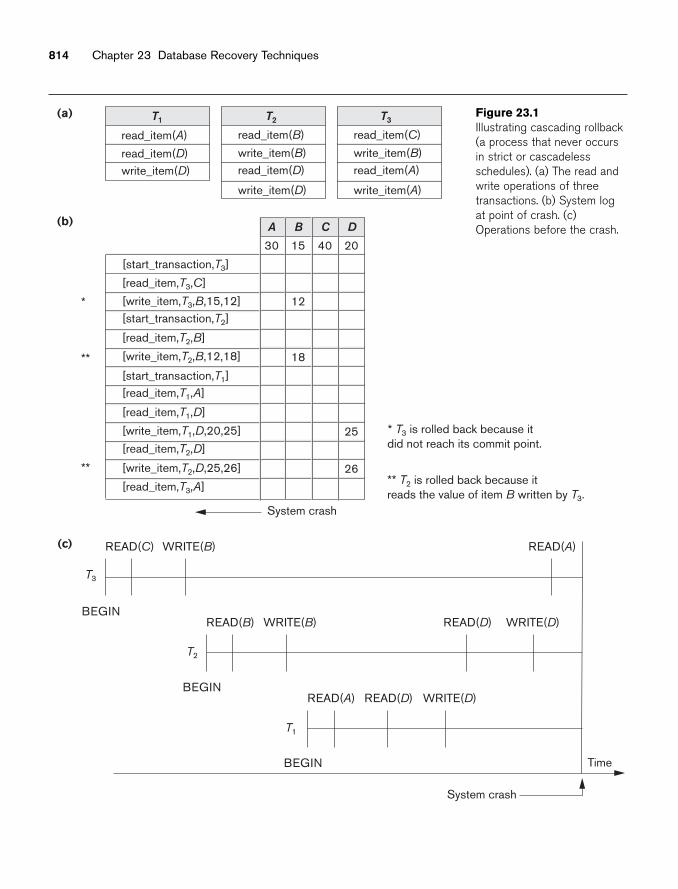
814 Chapter 23 Database Recovery Techniques
(a)
(b)
*
**
**
[start_transaction,T3]
[read_item,T3,C]
[write_item,T3,B,15,12][start_transaction,T2]
[read_item,T2,B]
[write_item,T2,B,12,18]
[write_item,T1,D,20,25]
[write_item,T2,D,25,26]
[start_transaction,T1][read_item,T1,A]
[read_item,T1,D]
[read_item,T2,D]
[read_item,T3,A]
* T3 is rolled back because it did not reach its commit point.
** T2 is rolled back because it reads the value of item B written by T3.
read_item(A)
read_item(D)write_item(D)
read_item(B)
write_item(B)read_item(D)
write_item(D)
System crash
T3T2T1
read_item(C)
write_item(B)read_item(A)
write_item(A)
A
30
B
15
12
18
C
40
D
20
25
26
(c) READ(C)
BEGIN
READ(A)WRITE(B)
T3
READ(B)
BEGIN
WRITE(D)READ(D)WRITE(B)
READ(A)
BEGIN
System crash
Time
READ(D) WRITE(D)
T2
T1
Figure 23.1Illustrating cascading rollback(a process that never occursin strict or cascadelessschedules). (a) The read andwrite operations of threetransactions. (b) System logat point of crash. (c)Operations before the crash.
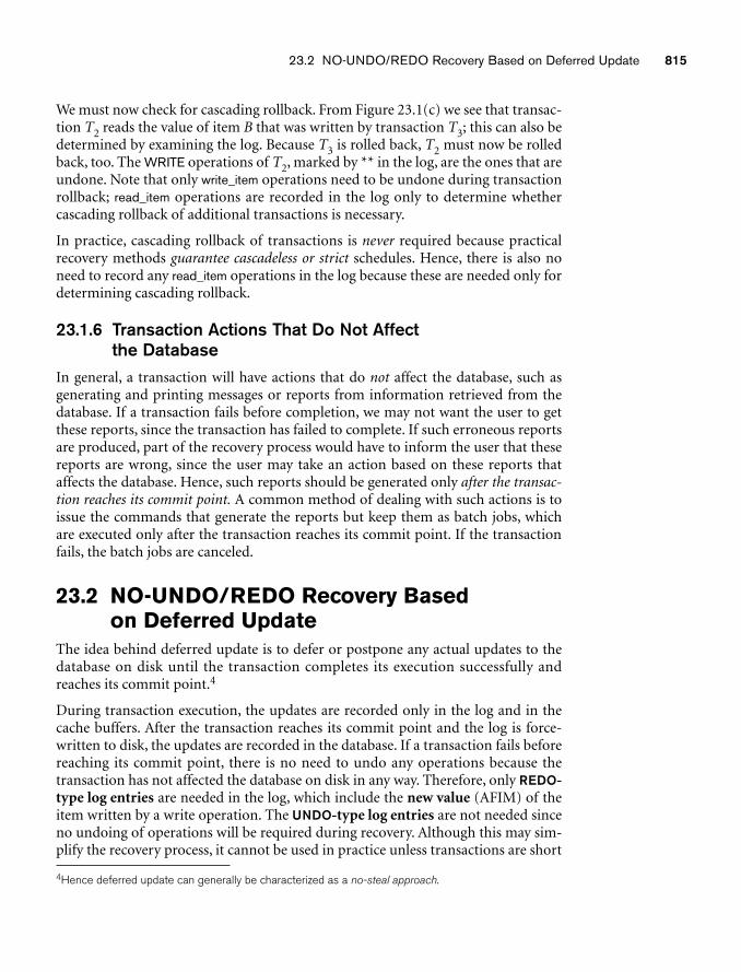
23.2 NO-UNDO/REDO Recovery Based on Deferred Update 815
We must now check for cascading rollback. From Figure 23.1(c) we see that transac-tion T2 reads the value of item B that was written by transaction T3; this can also bedetermined by examining the log. Because T3 is rolled back, T2 must now be rolledback, too. The WRITE operations of T2, marked by ** in the log, are the ones that areundone. Note that only write_item operations need to be undone during transactionrollback; read_item operations are recorded in the log only to determine whethercascading rollback of additional transactions is necessary.
In practice, cascading rollback of transactions is never required because practicalrecovery methods guarantee cascadeless or strict schedules. Hence, there is also noneed to record any read_item operations in the log because these are needed only fordetermining cascading rollback.
23.1.6 Transaction Actions That Do Not Affect the Database
In general, a transaction will have actions that do not affect the database, such asgenerating and printing messages or reports from information retrieved from thedatabase. If a transaction fails before completion, we may not want the user to getthese reports, since the transaction has failed to complete. If such erroneous reportsare produced, part of the recovery process would have to inform the user that thesereports are wrong, since the user may take an action based on these reports thataffects the database. Hence, such reports should be generated only after the transac-tion reaches its commit point. A common method of dealing with such actions is toissue the commands that generate the reports but keep them as batch jobs, whichare executed only after the transaction reaches its commit point. If the transactionfails, the batch jobs are canceled.
23.2 NO-UNDO/REDO Recovery Based on Deferred Update
The idea behind deferred update is to defer or postpone any actual updates to thedatabase on disk until the transaction completes its execution successfully andreaches its commit point.4
During transaction execution, the updates are recorded only in the log and in thecache buffers. After the transaction reaches its commit point and the log is force-written to disk, the updates are recorded in the database. If a transaction fails beforereaching its commit point, there is no need to undo any operations because thetransaction has not affected the database on disk in any way. Therefore, only REDO-type log entries are needed in the log, which include the new value (AFIM) of theitem written by a write operation. The UNDO-type log entries are not needed sinceno undoing of operations will be required during recovery. Although this may sim-plify the recovery process, it cannot be used in practice unless transactions are short
4Hence deferred update can generally be characterized as a no-steal approach.
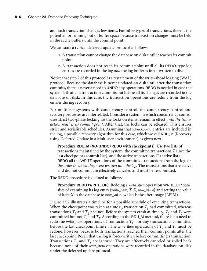
816 Chapter 23 Database Recovery Techniques
and each transaction changes few items. For other types of transactions, there is thepotential for running out of buffer space because transaction changes must be heldin the cache buffers until the commit point.
We can state a typical deferred update protocol as follows:
1. A transaction cannot change the database on disk until it reaches its commitpoint.
2. A transaction does not reach its commit point until all its REDO-type logentries are recorded in the log and the log buffer is force-written to disk.
Notice that step 2 of this protocol is a restatement of the write-ahead logging (WAL)protocol. Because the database is never updated on disk until after the transactioncommits, there is never a need to UNDO any operations. REDO is needed in case thesystem fails after a transaction commits but before all its changes are recorded in thedatabase on disk. In this case, the transaction operations are redone from the logentries during recovery.
For multiuser systems with concurrency control, the concurrency control andrecovery processes are interrelated. Consider a system in which concurrency controluses strict two-phase locking, so the locks on items remain in effect until the trans-action reaches its commit point. After that, the locks can be released. This ensuresstrict and serializable schedules. Assuming that [checkpoint] entries are included inthe log, a possible recovery algorithm for this case, which we call RDU_M (Recoveryusing Deferred Update in a Multiuser environment), is given next.
Procedure RDU_M (NO-UNDO/REDO with checkpoints). Use two lists oftransactions maintained by the system: the committed transactions T since thelast checkpoint (commit list), and the active transactions T� (active list).REDO all the WRITE operations of the committed transactions from the log, inthe order in which they were written into the log. The transactions that are activeand did not commit are effectively canceled and must be resubmitted.
The REDO procedure is defined as follows:
Procedure REDO (WRITE_OP). Redoing a write_item operation WRITE_OP con-sists of examining its log entry [write_item, T, X, new_value] and setting the valueof item X in the database to new_value, which is the after image (AFIM).
Figure 23.2 illustrates a timeline for a possible schedule of executing transactions.When the checkpoint was taken at time t1, transaction T1 had committed, whereastransactions T3 and T4 had not. Before the system crash at time t2, T3 and T2 werecommitted but not T4 and T5. According to the RDU_M method, there is no need toredo the write_item operations of transaction T1—or any transactions committedbefore the last checkpoint time t1. The write_item operations of T2 and T3 must beredone, however, because both transactions reached their commit points after thelast checkpoint. Recall that the log is force-written before committing a transaction.Transactions T4 and T5 are ignored: They are effectively canceled or rolled backbecause none of their write_item operations were recorded in the database on diskunder the deferred update protocol.
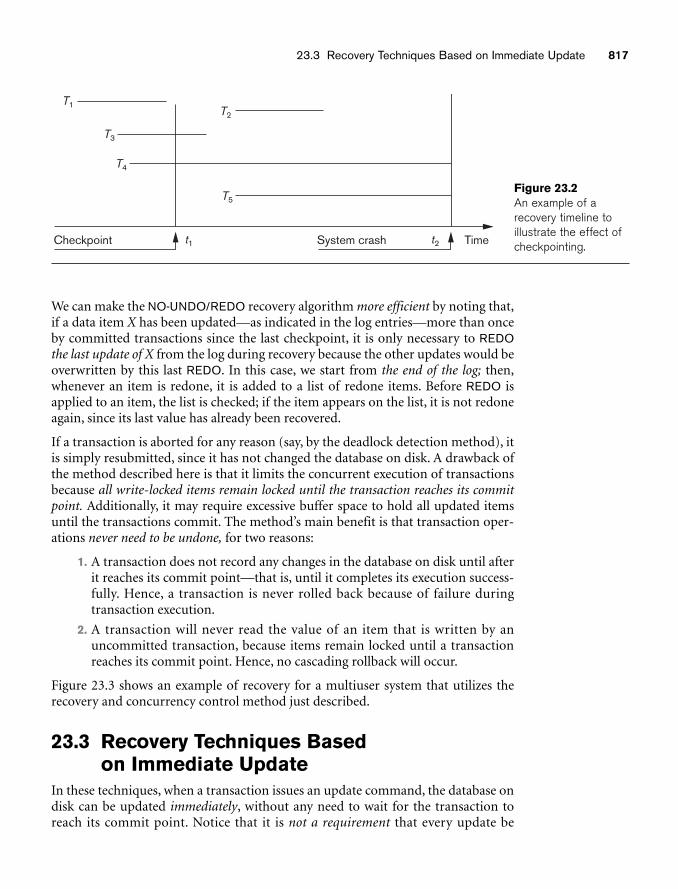
23.3 Recovery Techniques Based on Immediate Update 817
System crash TimeCheckpoint
T2
T1
T3
T5
T4
t1 t2
Figure 23.2An example of arecovery timeline toillustrate the effect ofcheckpointing.
We can make the NO-UNDO/REDO recovery algorithm more efficient by noting that,if a data item X has been updated—as indicated in the log entries—more than onceby committed transactions since the last checkpoint, it is only necessary to REDOthe last update of X from the log during recovery because the other updates would beoverwritten by this last REDO. In this case, we start from the end of the log; then,whenever an item is redone, it is added to a list of redone items. Before REDO isapplied to an item, the list is checked; if the item appears on the list, it is not redoneagain, since its last value has already been recovered.
If a transaction is aborted for any reason (say, by the deadlock detection method), itis simply resubmitted, since it has not changed the database on disk. A drawback ofthe method described here is that it limits the concurrent execution of transactionsbecause all write-locked items remain locked until the transaction reaches its commitpoint. Additionally, it may require excessive buffer space to hold all updated itemsuntil the transactions commit. The method’s main benefit is that transaction oper-ations never need to be undone, for two reasons:
1. A transaction does not record any changes in the database on disk until afterit reaches its commit point—that is, until it completes its execution success-fully. Hence, a transaction is never rolled back because of failure duringtransaction execution.
2. A transaction will never read the value of an item that is written by anuncommitted transaction, because items remain locked until a transactionreaches its commit point. Hence, no cascading rollback will occur.
Figure 23.3 shows an example of recovery for a multiuser system that utilizes therecovery and concurrency control method just described.
23.3 Recovery Techniques Based on Immediate Update
In these techniques, when a transaction issues an update command, the database ondisk can be updated immediately, without any need to wait for the transaction toreach its commit point. Notice that it is not a requirement that every update be
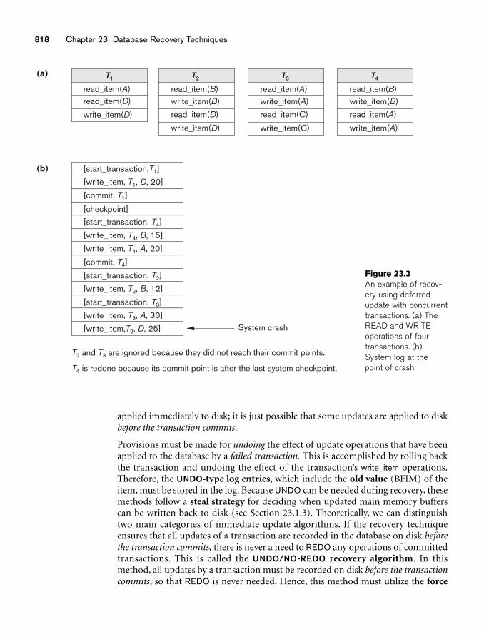
818 Chapter 23 Database Recovery Techniques
(a) T1
read_item(A)read_item(D)
write_item(D)
[checkpoint]
(b)
read_item(B)write_item(B)
read_item(D)
write_item(D)
read_item(A)write_item(A)
read_item(C)
write_item(C)
read_item(B)write_item(B)
read_item(A)
write_item(A)
[start_transaction,T1]
[start_transaction, T2]
[write_item, T1, D, 20]
[commit, T1]
[commit, T4]
[start_transaction, T4]
[start_transaction, T3]
[write_item, T4, B, 15]
[write_item, T2, B, 12]
[write_item, T4, A, 20]
[write_item, T3, A, 30]
[write_item,T2, D, 25]
T2 and T3 are ignored because they did not reach their commit points.
T4 is redone because its commit point is after the last system checkpoint.
System crash
T2 T3 T4
Figure 23.3An example of recov-ery using deferredupdate with concurrenttransactions. (a) TheREAD and WRITEoperations of fourtransactions. (b)System log at thepoint of crash.
applied immediately to disk; it is just possible that some updates are applied to diskbefore the transaction commits.
Provisions must be made for undoing the effect of update operations that have beenapplied to the database by a failed transaction. This is accomplished by rolling backthe transaction and undoing the effect of the transaction’s write_item operations.Therefore, the UNDO-type log entries, which include the old value (BFIM) of theitem, must be stored in the log. Because UNDO can be needed during recovery, thesemethods follow a steal strategy for deciding when updated main memory bufferscan be written back to disk (see Section 23.1.3). Theoretically, we can distinguishtwo main categories of immediate update algorithms. If the recovery techniqueensures that all updates of a transaction are recorded in the database on disk beforethe transaction commits, there is never a need to REDO any operations of committedtransactions. This is called the UNDO/NO-REDO recovery algorithm. In thismethod, all updates by a transaction must be recorded on disk before the transactioncommits, so that REDO is never needed. Hence, this method must utilize the force
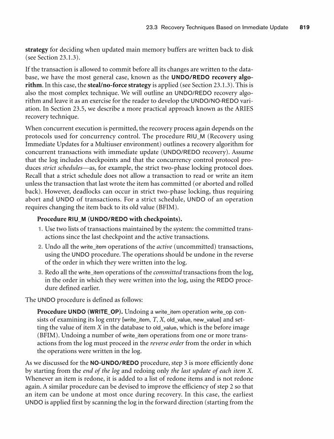
23.3 Recovery Techniques Based on Immediate Update 819
strategy for deciding when updated main memory buffers are written back to disk(see Section 23.1.3).
If the transaction is allowed to commit before all its changes are written to the data-base, we have the most general case, known as the UNDO/REDO recovery algo-rithm. In this case, the steal/no-force strategy is applied (see Section 23.1.3). This isalso the most complex technique. We will outline an UNDO/REDO recovery algo-rithm and leave it as an exercise for the reader to develop the UNDO/NO-REDO vari-ation. In Section 23.5, we describe a more practical approach known as the ARIESrecovery technique.
When concurrent execution is permitted, the recovery process again depends on theprotocols used for concurrency control. The procedure RIU_M (Recovery usingImmediate Updates for a Multiuser environment) outlines a recovery algorithm forconcurrent transactions with immediate update (UNDO/REDO recovery). Assumethat the log includes checkpoints and that the concurrency control protocol pro-duces strict schedules—as, for example, the strict two-phase locking protocol does.Recall that a strict schedule does not allow a transaction to read or write an itemunless the transaction that last wrote the item has committed (or aborted and rolledback). However, deadlocks can occur in strict two-phase locking, thus requiringabort and UNDO of transactions. For a strict schedule, UNDO of an operationrequires changing the item back to its old value (BFIM).
Procedure RIU_M (UNDO/REDO with checkpoints).
1. Use two lists of transactions maintained by the system: the committed trans-actions since the last checkpoint and the active transactions.
2. Undo all the write_item operations of the active (uncommitted) transactions,using the UNDO procedure. The operations should be undone in the reverseof the order in which they were written into the log.
3. Redo all the write_item operations of the committed transactions from the log,in the order in which they were written into the log, using the REDO proce-dure defined earlier.
The UNDO procedure is defined as follows:
Procedure UNDO (WRITE_OP). Undoing a write_item operation write_op con-sists of examining its log entry [write_item, T, X, old_value, new_value] and set-ting the value of item X in the database to old_value, which is the before image(BFIM). Undoing a number of write_item operations from one or more trans-actions from the log must proceed in the reverse order from the order in whichthe operations were written in the log.
As we discussed for the NO-UNDO/REDO procedure, step 3 is more efficiently doneby starting from the end of the log and redoing only the last update of each item X.Whenever an item is redone, it is added to a list of redone items and is not redoneagain. A similar procedure can be devised to improve the efficiency of step 2 so thatan item can be undone at most once during recovery. In this case, the earliest UNDO is applied first by scanning the log in the forward direction (starting from the
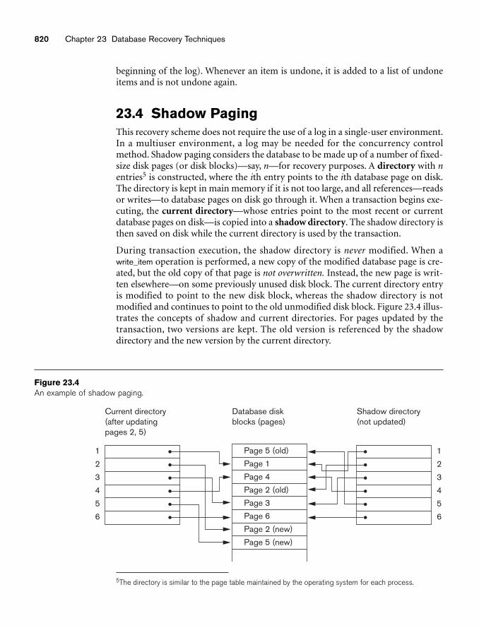
820 Chapter 23 Database Recovery Techniques
Current directory(after updatingpages 2, 5)
Database disk blocks (pages)
Shadow directory(not updated)
Page 5 (old)
Page 1
Page 4
Page 2 (old)
Page 3
Page 6
Page 2 (new)
Page 5 (new)
1
2
3
4
5
6
1
2
3
4
5
6
Figure 23.4An example of shadow paging.
beginning of the log). Whenever an item is undone, it is added to a list of undoneitems and is not undone again.
23.4 Shadow PagingThis recovery scheme does not require the use of a log in a single-user environment.In a multiuser environment, a log may be needed for the concurrency controlmethod. Shadow paging considers the database to be made up of a number of fixed-size disk pages (or disk blocks)—say, n—for recovery purposes. A directory with nentries5 is constructed, where the ith entry points to the ith database page on disk.The directory is kept in main memory if it is not too large, and all references—readsor writes—to database pages on disk go through it. When a transaction begins exe-cuting, the current directory—whose entries point to the most recent or currentdatabase pages on disk—is copied into a shadow directory. The shadow directory isthen saved on disk while the current directory is used by the transaction.
During transaction execution, the shadow directory is never modified. When awrite_item operation is performed, a new copy of the modified database page is cre-ated, but the old copy of that page is not overwritten. Instead, the new page is writ-ten elsewhere—on some previously unused disk block. The current directory entryis modified to point to the new disk block, whereas the shadow directory is notmodified and continues to point to the old unmodified disk block. Figure 23.4 illus-trates the concepts of shadow and current directories. For pages updated by thetransaction, two versions are kept. The old version is referenced by the shadowdirectory and the new version by the current directory.
5The directory is similar to the page table maintained by the operating system for each process.
23.5 The ARIES Recovery Algorithm 821
To recover from a failure during transaction execution, it is sufficient to free themodified database pages and to discard the current directory. The state of the data-base before transaction execution is available through the shadow directory, andthat state is recovered by reinstating the shadow directory. The database thus isreturned to its state prior to the transaction that was executing when the crashoccurred, and any modified pages are discarded. Committing a transaction corre-sponds to discarding the previous shadow directory. Since recovery involves neitherundoing nor redoing data items, this technique can be categorized as a NO-UNDO/NO-REDO technique for recovery.
In a multiuser environment with concurrent transactions, logs and checkpoints mustbe incorporated into the shadow paging technique. One disadvantage of shadowpaging is that the updated database pages change location on disk. This makes it dif-ficult to keep related database pages close together on disk without complex storagemanagement strategies. Furthermore, if the directory is large, the overhead of writ-ing shadow directories to disk as transactions commit is significant. A further com-plication is how to handle garbage collection when a transaction commits. The oldpages referenced by the shadow directory that have been updated must be releasedand added to a list of free pages for future use. These pages are no longer needed afterthe transaction commits. Another issue is that the operation to migrate between cur-rent and shadow directories must be implemented as an atomic operation.
23.5 The ARIES Recovery AlgorithmWe now describe the ARIES algorithm as an example of a recovery algorithm usedin database systems. It is used in many relational database-related products of IBM.ARIES uses a steal/no-force approach for writing, and it is based on three concepts:write-ahead logging, repeating history during redo, and logging changes duringundo. We discussed write-ahead logging in Section 23.1.3. The second concept,repeating history, means that ARIES will retrace all actions of the database systemprior to the crash to reconstruct the database state when the crash occurred.Transactions that were uncommitted at the time of the crash (active transactions)are undone. The third concept, logging during undo, will prevent ARIES fromrepeating the completed undo operations if a failure occurs during recovery, whichcauses a restart of the recovery process.
The ARIES recovery procedure consists of three main steps: analysis, REDO, andUNDO. The analysis step identifies the dirty (updated) pages in the buffer6 and theset of transactions active at the time of the crash. The appropriate point in the logwhere the REDO operation should start is also determined. The REDO phase actu-ally reapplies updates from the log to the database. Generally, the REDO operation isapplied only to committed transactions. However, this is not the case in ARIES.Certain information in the ARIES log will provide the start point for REDO, from
6The actual buffers may be lost during a crash, since they are in main memory. Additional tables storedin the log during checkpointing (Dirty Page Table, Transaction Table) allows ARIES to identify this infor-mation (as discussed later in this section).
822 Chapter 23 Database Recovery Techniques
which REDO operations are applied until the end of the log is reached. Additionally,information stored by ARIES and in the data pages will allow ARIES to determinewhether the operation to be redone has actually been applied to the database andtherefore does not need to be reapplied. Thus, only the necessary REDO operationsare applied during recovery. Finally, during the UNDO phase, the log is scannedbackward and the operations of transactions that were active at the time of the crashare undone in reverse order. The information needed for ARIES to accomplish itsrecovery procedure includes the log, the Transaction Table, and the Dirty PageTable. Additionally, checkpointing is used. These tables are maintained by the trans-action manager and written to the log during checkpointing.
In ARIES, every log record has an associated log sequence number (LSN) that ismonotonically increasing and indicates the address of the log record on disk. EachLSN corresponds to a specific change (action) of some transaction. Also, each datapage will store the LSN of the latest log record corresponding to a change for that page.A log record is written for any of the following actions: updating a page (write),committing a transaction (commit), aborting a transaction (abort), undoing anupdate (undo), and ending a transaction (end). The need for including the firstthree actions in the log has been discussed, but the last two need some explanation.When an update is undone, a compensation log record is written in the log. When atransaction ends, whether by committing or aborting, an end log record is written.
Common fields in all log records include the previous LSN for that transaction, thetransaction ID, and the type of log record. The previous LSN is important because itlinks the log records (in reverse order) for each transaction. For an update (write)action, additional fields in the log record include the page ID for the page that con-tains the item, the length of the updated item, its offset from the beginning of thepage, the before image of the item, and its after image.
Besides the log, two tables are needed for efficient recovery: the Transaction Tableand the Dirty Page Table, which are maintained by the transaction manager. Whena crash occurs, these tables are rebuilt in the analysis phase of recovery. TheTransaction Table contains an entry for each active transaction, with informationsuch as the transaction ID, transaction status, and the LSN of the most recent logrecord for the transaction. The Dirty Page Table contains an entry for each dirtypage in the buffer, which includes the page ID and the LSN corresponding to theearliest update to that page.
Checkpointing in ARIES consists of the following: writing a begin_checkpoint recordto the log, writing an end_checkpoint record to the log, and writing the LSN of thebegin_checkpoint record to a special file. This special file is accessed during recoveryto locate the last checkpoint information. With the end_checkpoint record, the con-tents of both the Transaction Table and Dirty Page Table are appended to the end ofthe log. To reduce the cost, fuzzy checkpointing is used so that the DBMS can con-tinue to execute transactions during checkpointing (see Section 23.1.4).Additionally, the contents of the DBMS cache do not have to be flushed to disk dur-ing checkpoint, since the Transaction Table and Dirty Page Table—which areappended to the log on disk—contain the information needed for recovery. Note
23.5 The ARIES Recovery Algorithm 823
that if a crash occurs during checkpointing, the special file will refer to the previouscheckpoint, which is used for recovery.
After a crash, the ARIES recovery manager takes over. Information from the lastcheckpoint is first accessed through the special file. The analysis phase starts at thebegin_checkpoint record and proceeds to the end of the log. When the end_checkpointrecord is encountered, the Transaction Table and Dirty Page Table are accessed(recall that these tables were written in the log during checkpointing). Duringanalysis, the log records being analyzed may cause modifications to these two tables.For instance, if an end log record was encountered for a transaction T in theTransaction Table, then the entry for T is deleted from that table. If some other typeof log record is encountered for a transaction T�, then an entry for T� is inserted intothe Transaction Table, if not already present, and the last LSN field is modified. Ifthe log record corresponds to a change for page P, then an entry would be made forpage P (if not present in the table) and the associated LSN field would be modified.When the analysis phase is complete, the necessary information for REDO andUNDO has been compiled in the tables.
The REDO phase follows next. To reduce the amount of unnecessary work, ARIESstarts redoing at a point in the log where it knows (for sure) that previous changesto dirty pages have already been applied to the database on disk. It can determine thisby finding the smallest LSN, M, of all the dirty pages in the Dirty Page Table, whichindicates the log position where ARIES needs to start the REDO phase. Any changescorresponding to an LSN < M, for redoable transactions, must have already beenpropagated to disk or already been overwritten in the buffer; otherwise, those dirtypages with that LSN would be in the buffer (and the Dirty Page Table). So, REDOstarts at the log record with LSN = M and scans forward to the end of the log. Foreach change recorded in the log, the REDO algorithm would verify whether or notthe change has to be reapplied. For example, if a change recorded in the log pertainsto page P that is not in the Dirty Page Table, then this change is already on disk anddoes not need to be reapplied. Or, if a change recorded in the log (with LSN = N,say) pertains to page P and the Dirty Page Table contains an entry for P with LSNgreater than N, then the change is already present. If neither of these two conditionshold, page P is read from disk and the LSN stored on that page, LSN(P), is comparedwith N. If N < LSN(P), then the change has been applied and the page does not needto be rewritten to disk.
Once the REDO phase is finished, the database is in the exact state that it was inwhen the crash occurred. The set of active transactions—called the undo_set—hasbeen identified in the Transaction Table during the analysis phase. Now, the UNDOphase proceeds by scanning backward from the end of the log and undoing theappropriate actions. A compensating log record is written for each action that isundone. The UNDO reads backward in the log until every action of the set of trans-actions in the undo_set has been undone. When this is completed, the recoveryprocess is finished and normal processing can begin again.
Consider the recovery example shown in Figure 23.5. There are three transactions:T1, T2, and T3. T1 updates page C, T2 updates pages B and C, and T3 updates page A.
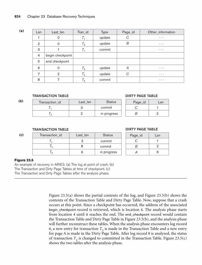
824 Chapter 23 Database Recovery Techniques
TRANSACTION TABLE
Last_lsn Status(b)
(c)
(a) Lsn
1
Last_lsn Tran_id Type Page_id Other_information
Transaction_id
TRANSACTION TABLE DIRTY PAGE TABLE
Transaction_id
T1 3
Last_lsn
commit
Status Page_id
C
Lsn
1
T3
T2 8
6 in progress
commit
A
B
6
2
T2
T1
DIRTY PAGE TABLE
Page_id
C
Lsn
1
B 22
3 commit
in progress
8
7
6
5
4
3
2
0
7
2
0
end checkpoint
begin checkpoint
1
0
T1
T2
T1
T3
T2
T2
update
commit
update
update
commit
update B
C
A
C . . .
. . .
. . .
. . .
. . .
. . .
Figure 23.5An example of recovery in ARIES. (a) The log at point of crash. (b)The Transaction and Dirty Page Tables at time of checkpoint. (c)The Transaction and Dirty Page Tables after the analysis phase.
Figure 23.5(a) shows the partial contents of the log, and Figure 23.5(b) shows thecontents of the Transaction Table and Dirty Page Table. Now, suppose that a crashoccurs at this point. Since a checkpoint has occurred, the address of the associatedbegin_checkpoint record is retrieved, which is location 4. The analysis phase startsfrom location 4 until it reaches the end. The end_checkpoint record would containthe Transaction Table and Dirty Page Table in Figure 23.5(b), and the analysis phasewill further reconstruct these tables. When the analysis phase encounters log record6, a new entry for transaction T3 is made in the Transaction Table and a new entryfor page A is made in the Dirty Page Table. After log record 8 is analyzed, the statusof transaction T2 is changed to committed in the Transaction Table. Figure 23.5(c)shows the two tables after the analysis phase.
23.6 Recovery in Multidatabase Systems 825
For the REDO phase, the smallest LSN in the Dirty Page Table is 1. Hence the REDOwill start at log record 1 and proceed with the REDO of updates. The LSNs {1, 2, 6,7} corresponding to the updates for pages C, B, A, and C, respectively, are not lessthan the LSNs of those pages (as shown in the Dirty Page Table). So those data pageswill be read again and the updates reapplied from the log (assuming the actual LSNsstored on those data pages are less then the corresponding log entry). At this point,the REDO phase is finished and the UNDO phase starts. From the Transaction Table(Figure 23.5(c)), UNDO is applied only to the active transaction T3. The UNDOphase starts at log entry 6 (the last update for T3) and proceeds backward in the log.The backward chain of updates for transaction T3 (only log record 6 in this exam-ple) is followed and undone.
23.6 Recovery in Multidatabase SystemsSo far, we have implicitly assumed that a transaction accesses a single database. Insome cases, a single transaction, called a multidatabase transaction, may requireaccess to multiple databases. These databases may even be stored on different typesof DBMSs; for example, some DBMSs may be relational, whereas others are object-oriented, hierarchical, or network DBMSs. In such a case, each DBMS involved inthe multidatabase transaction may have its own recovery technique and transactionmanager separate from those of the other DBMSs. This situation is somewhat simi-lar to the case of a distributed database management system (see Chapter 25), whereparts of the database reside at different sites that are connected by a communicationnetwork.
To maintain the atomicity of a multidatabase transaction, it is necessary to have atwo-level recovery mechanism. A global recovery manager, or coordinator, isneeded to maintain information needed for recovery, in addition to the local recov-ery managers and the information they maintain (log, tables). The coordinator usu-ally follows a protocol called the two-phase commit protocol, whose two phasescan be stated as follows:
■ Phase 1. When all participating databases signal the coordinator that thepart of the multidatabase transaction involving each has concluded, thecoordinator sends a message prepare for commit to each participant to getready for committing the transaction. Each participating database receivingthat message will force-write all log records and needed information forlocal recovery to disk and then send a ready to commit or OK signal to thecoordinator. If the force-writing to disk fails or the local transaction cannotcommit for some reason, the participating database sends a cannot commitor not OK signal to the coordinator. If the coordinator does not receive areply from the database within a certain time out interval, it assumes a notOK response.
■ Phase 2. If all participating databases reply OK, and the coordinator’s vote isalso OK, the transaction is successful, and the coordinator sends a commitsignal for the transaction to the participating databases. Because all the local
826 Chapter 23 Database Recovery Techniques
effects of the transaction and information needed for local recovery havebeen recorded in the logs of the participating databases, recovery from fail-ure is now possible. Each participating database completes transaction com-mit by writing a [commit] entry for the transaction in the log andpermanently updating the database if needed. On the other hand, if one ormore of the participating databases or the coordinator have a not OKresponse, the transaction has failed, and the coordinator sends a message toroll back or UNDO the local effect of the transaction to each participatingdatabase. This is done by undoing the transaction operations, using the log.
The net effect of the two-phase commit protocol is that either all participating data-bases commit the effect of the transaction or none of them do. In case any of theparticipants—or the coordinator—fails, it is always possible to recover to a statewhere either the transaction is committed or it is rolled back. A failure during orbefore Phase 1 usually requires the transaction to be rolled back, whereas a failureduring Phase 2 means that a successful transaction can recover and commit.
23.7 Database Backup and Recovery from Catastrophic Failures
So far, all the techniques we have discussed apply to noncatastrophic failures. A keyassumption has been that the system log is maintained on the disk and is not lost asa result of the failure. Similarly, the shadow directory must be stored on disk toallow recovery when shadow paging is used. The recovery techniques we have dis-cussed use the entries in the system log or the shadow directory to recover from fail-ure by bringing the database back to a consistent state.
The recovery manager of a DBMS must also be equipped to handle more cata-strophic failures such as disk crashes. The main technique used to handle suchcrashes is a database backup, in which the whole database and the log are periodi-cally copied onto a cheap storage medium such as magnetic tapes or other largecapacity offline storage devices. In case of a catastrophic system failure, the latestbackup copy can be reloaded from the tape to the disk, and the system can berestarted.
Data from critical applications such as banking, insurance, stock market, and otherdatabases is periodically backed up in its entirety and moved to physically separatesafe locations. Subterranean storage vaults have been used to protect such data fromflood, storm, earthquake, or fire damage. Events like the 9/11 terrorist attack in NewYork (in 2001) and the Katrina hurricane disaster in New Orleans (in 2005) havecreated a greater awareness of disaster recovery of business-critical databases.
To avoid losing all the effects of transactions that have been executed since the lastbackup, it is customary to back up the system log at more frequent intervals thanfull database backup by periodically copying it to magnetic tape. The system log isusually substantially smaller than the database itself and hence can be backed upmore frequently. Therefore, users do not lose all transactions they have performed
23.8 Summary 827
since the last database backup. All committed transactions recorded in the portionof the system log that has been backed up to tape can have their effect on the data-base redone. A new log is started after each database backup. Hence, to recover fromdisk failure, the database is first recreated on disk from its latest backup copy ontape. Following that, the effects of all the committed transactions whose operationshave been recorded in the backed-up copies of the system log are reconstructed.
23.8 SummaryIn this chapter we discussed the techniques for recovery from transaction failures.The main goal of recovery is to ensure the atomicity property of a transaction. If atransaction fails before completing its execution, the recovery mechanism has tomake sure that the transaction has no lasting effects on the database. First we gavean informal outline for a recovery process and then we discussed system conceptsfor recovery. These included a discussion of caching, in-place updating versus shad-owing, before and after images of a data item, UNDO versus REDO recovery opera-tions, steal/no-steal and force/no-force policies, system checkpointing, and thewrite-ahead logging protocol.
Next we discussed two different approaches to recovery: deferred update and imme-diate update. Deferred update techniques postpone any actual updating of the data-base on disk until a transaction reaches its commit point. The transactionforce-writes the log to disk before recording the updates in the database. Thisapproach, when used with certain concurrency control methods, is designed neverto require transaction rollback, and recovery simply consists of redoing the opera-tions of transactions committed after the last checkpoint from the log. The disad-vantage is that too much buffer space may be needed, since updates are kept in thebuffers and are not applied to disk until a transaction commits. Deferred update canlead to a recovery algorithm known as NO-UNDO/REDO. Immediate update tech-niques may apply changes to the database on disk before the transaction reaches asuccessful conclusion. Any changes applied to the database must first be recorded inthe log and force-written to disk so that these operations can be undone if neces-sary. We also gave an overview of a recovery algorithm for immediate update knownas UNDO/REDO. Another algorithm, known as UNDO/NO-REDO, can also be devel-oped for immediate update if all transaction actions are recorded in the databasebefore commit.
We discussed the shadow paging technique for recovery, which keeps track of olddatabase pages by using a shadow directory. This technique, which is classified asNO-UNDO/NO-REDO, does not require a log in single-user systems but still needsthe log for multiuser systems. We also presented ARIES, a specific recovery schemeused in many of IBM’s relational database products. Then we discussed the two-phase commit protocol, which is used for recovery from failures involving multi-database transactions. Finally, we discussed recovery from catastrophic failures,which is typically done by backing up the database and the log to tape. The log canbe backed up more frequently than the database, and the backup log can be used toredo operations starting from the last database backup.
828 Chapter 23 Database Recovery Techniques
Review Questions23.1. Discuss the different types of transaction failures. What is meant by cata-
strophic failure?
23.2. Discuss the actions taken by the read_item and write_item operations on adatabase.
23.3. What is the system log used for? What are the typical kinds of entries in asystem log? What are checkpoints, and why are they important? What aretransaction commit points, and why are they important?
23.4. How are buffering and caching techniques used by the recovery subsystem?
23.5. What are the before image (BFIM) and after image (AFIM) of a data item?What is the difference between in-place updating and shadowing, withrespect to their handling of BFIM and AFIM?
23.6. What are UNDO-type and REDO-type log entries?
23.7. Describe the write-ahead logging protocol.
23.8. Identify three typical lists of transactions that are maintained by the recoverysubsystem.
23.9. What is meant by transaction rollback? What is meant by cascading rollback?Why do practical recovery methods use protocols that do not permit cascad-ing rollback? Which recovery techniques do not require any rollback?
23.10. Discuss the UNDO and REDO operations and the recovery techniques thatuse each.
23.11. Discuss the deferred update technique of recovery. What are the advantagesand disadvantages of this technique? Why is it called the NO-UNDO/REDOmethod?
23.12. How can recovery handle transaction operations that do not affect the data-base, such as the printing of reports by a transaction?
23.13. Discuss the immediate update recovery technique in both single-user andmultiuser environments. What are the advantages and disadvantages ofimmediate update?
23.14. What is the difference between the UNDO/REDO and the UNDO/NO-REDOalgorithms for recovery with immediate update? Develop the outline for anUNDO/NO-REDO algorithm.
23.15. Describe the shadow paging recovery technique. Under what circumstancesdoes it not require a log?
23.16. Describe the three phases of the ARIES recovery method.
23.17. What are log sequence numbers (LSNs) in ARIES? How are they used? Whatinformation do the Dirty Page Table and Transaction Table contain?Describe how fuzzy checkpointing is used in ARIES.
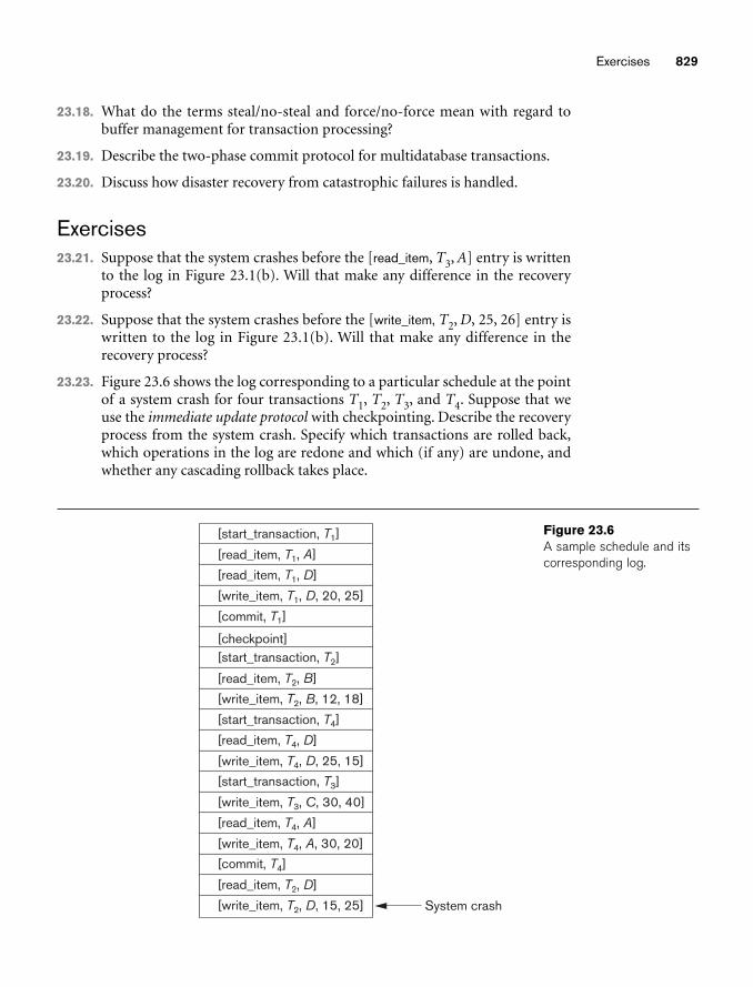
Exercises 829
[checkpoint]
[start_transaction, T1]
[start_transaction, T2]
[start_transaction, T3]
[read_item, T1, A]
[read_item, T1, D]
[read_item, T4, D]
[read_item, T2, D]
[read_item, T2, B]
[write_item, T1, D, 20, 25]
[write_item, T2, B, 12, 18]
[read_item, T4, A]
[write_item, T4, D, 25, 15]
[write_item, T3, C, 30, 40]
[write_item, T2, D, 15, 25]
[write_item, T4, A, 30, 20]
[commit, T1]
[commit, T4]
[start_transaction, T4]
System crash
Figure 23.6A sample schedule and itscorresponding log.
23.18. What do the terms steal/no-steal and force/no-force mean with regard tobuffer management for transaction processing?
23.19. Describe the two-phase commit protocol for multidatabase transactions.
23.20. Discuss how disaster recovery from catastrophic failures is handled.
Exercises23.21. Suppose that the system crashes before the [read_item, T3, A] entry is written
to the log in Figure 23.1(b). Will that make any difference in the recoveryprocess?
23.22. Suppose that the system crashes before the [write_item, T2, D, 25, 26] entry iswritten to the log in Figure 23.1(b). Will that make any difference in therecovery process?
23.23. Figure 23.6 shows the log corresponding to a particular schedule at the pointof a system crash for four transactions T1, T2, T3, and T4. Suppose that weuse the immediate update protocol with checkpointing. Describe the recoveryprocess from the system crash. Specify which transactions are rolled back,which operations in the log are redone and which (if any) are undone, andwhether any cascading rollback takes place.
830 Chapter 23 Database Recovery Techniques
23.24. Suppose that we use the deferred update protocol for the example in Figure23.6. Show how the log would be different in the case of deferred update byremoving the unnecessary log entries; then describe the recovery process,using your modified log. Assume that only REDO operations are applied,and specify which operations in the log are redone and which are ignored.
23.25. How does checkpointing in ARIES differ from checkpointing as described inSection 23.1.4?
23.26. How are log sequence numbers used by ARIES to reduce the amount ofREDO work needed for recovery? Illustrate with an example using the infor-mation shown in Figure 23.5. You can make your own assumptions as towhen a page is written to disk.
23.27. What implications would a no-steal/force buffer management policy haveon checkpointing and recovery?
Choose the correct answer for each of the following multiple-choice questions:
23.28. Incremental logging with deferred updates implies that the recovery systemmust necessarily
a. store the old value of the updated item in the log.
b. store the new value of the updated item in the log.
c. store both the old and new value of the updated item in the log.
d. store only the Begin Transaction and Commit Transaction records in thelog.
23.29. The write-ahead logging (WAL) protocol simply means that
a. writing of a data item should be done ahead of any logging operation.
b. the log record for an operation should be written before the actual data iswritten.
c. all log records should be written before a new transaction begins execu-tion.
d. the log never needs to be written to disk.
23.30. In case of transaction failure under a deferred update incremental loggingscheme, which of the following will be needed?
a. an undo operation
b. a redo operation
c. an undo and redo operation
d. none of the above
23.31. For incremental logging with immediate updates, a log record for a transac-tion would contain
a. a transaction name, a data item name, and the old and new value of theitem.
Exercises 831
b. a transaction name, a data item name, and the old value of the item.
c. a transaction name, a data item name, and the new value of the item.
d. a transaction name and a data item name.
23.32. For correct behavior during recovery, undo and redo operations must be
a. commutative.
b. associative.
c. idempotent.
d. distributive.
23.33. When a failure occurs, the log is consulted and each operation is eitherundone or redone. This is a problem because
a. searching the entire log is time consuming.
b. many redos are unnecessary.
c. both (a) and (b).
d. none of the above.
23.34. When using a log-based recovery scheme, it might improve performance aswell as providing a recovery mechanism by
a. writing the log records to disk when each transaction commits.
b. writing the appropriate log records to disk during the transaction’s execu-tion.
c. waiting to write the log records until multiple transactions commit andwriting them as a batch.
d. never writing the log records to disk.
23.35. There is a possibility of a cascading rollback when
a. a transaction writes items that have been written only by a committedtransaction.
b. a transaction writes an item that is previously written by an uncommittedtransaction.
c. a transaction reads an item that is previously written by an uncommittedtransaction.
d. both (b) and (c).
23.36. To cope with media (disk) failures, it is necessary
a. for the DBMS to only execute transactions in a single user environment.
b. to keep a redundant copy of the database.
c. to never abort a transaction.
d. all of the above.
23.37. If the shadowing approach is used for flushing a data item back to disk, then
a. the item is written to disk only after the transaction commits.
b. the item is written to a different location on disk.
c. the item is written to disk before the transaction commits.
d. the item is written to the same disk location from which it was read.
Selected BibliographyThe books by Bernstein et al. (1987) and Papadimitriou (1986) are devoted to thetheory and principles of concurrency control and recovery. The book by Gray andReuter (1993) is an encyclopedic work on concurrency control, recovery, and othertransaction-processing issues.
Verhofstad (1978) presents a tutorial and survey of recovery techniques in databasesystems. Categorizing algorithms based on their UNDO/REDO characteristics is dis-cussed in Haerder and Reuter (1983) and in Bernstein et al. (1983). Gray (1978) dis-cusses recovery, along with other system aspects of implementing operating systemsfor databases. The shadow paging technique is discussed in Lorie (1977), Verhofstad(1978), and Reuter (1980). Gray et al. (1981) discuss the recovery mechanism inSYSTEM R. Lockemann and Knutsen (1968), Davies (1973), and Bjork (1973) areearly papers that discuss recovery. Chandy et al. (1975) discuss transaction rollback.Lilien and Bhargava (1985) discuss the concept of integrity block and its use toimprove the efficiency of recovery.
Recovery using write-ahead logging is analyzed in Jhingran and Khedkar (1992)and is used in the ARIES system (Mohan et al. 1992). More recent work on recoveryincludes compensating transactions (Korth et al. 1990) and main memory databaserecovery (Kumar 1991). The ARIES recovery algorithms (Mohan et al. 1992) havebeen quite successful in practice. Franklin et al. (1992) discusses recovery in theEXODUS system. Two books by Kumar and Hsu (1998) and Kumar and Song(1998) discuss recovery in detail and contain descriptions of recovery methods usedin a number of existing relational database products. Examples of page replacementstrategies that are specific for databases are discussed in Chou and DeWitt (1985)and Pazos et al. (2006).
832 Chapter 23 Database Recovery Techniques
part10Additional Database Topics:
Security and Distribution
835
Database Security
This chapter discusses techniques for securing data-bases against a variety of threats. It also presents
schemes of providing access privileges to authorized users. Some of the securitythreats to databases—such as SQL Injection—will be presented. At the end of thechapter we also summarize how a commercial RDBMS—specifically, the Oracle sys-tem—provides different types of security. We start in Section 24.1 with an introduc-tion to security issues and the threats to databases, and we give an overview of thecontrol measures that are covered in the rest of this chapter. We also comment onthe relationship between data security and privacy as it applies to personal informa-tion. Section 24.2 discusses the mechanisms used to grant and revoke privileges inrelational database systems and in SQL, mechanisms that are often referred to asdiscretionary access control. In Section 24.3, we present an overview of the mech-anisms for enforcing multiple levels of security—a particular concern in databasesystem security that is known as mandatory access control. Section 24.3 also intro-duces the more recently developed strategies of role-based access control, andlabel-based and row-based security. Section 24.3 also provides a brief discussion ofXML access control. Section 24.4 discusses a major threat to databases called SQLInjection, and discusses some of the proposed preventive measures against it.Section 24.5 briefly discusses the security problem in statistical databases. Section24.6 introduces the topic of flow control and mentions problems associated withcovert channels. Section 24.7 provides a brief summary of encryption and symmet-ric key and asymmetric (public) key infrastructure schemes. It also discusses digitalcertificates. Section 24.8 introduces privacy-preserving techniques, and Section 24.9presents the current challenges to database security. In Section 24.10, we discussOracle label-based security. Finally, Section 24.11 summarizes the chapter. Readerswho are interested only in basic database security mechanisms will find it sufficientto cover the material in Sections 24.1 and 24.2.
24chapter 24
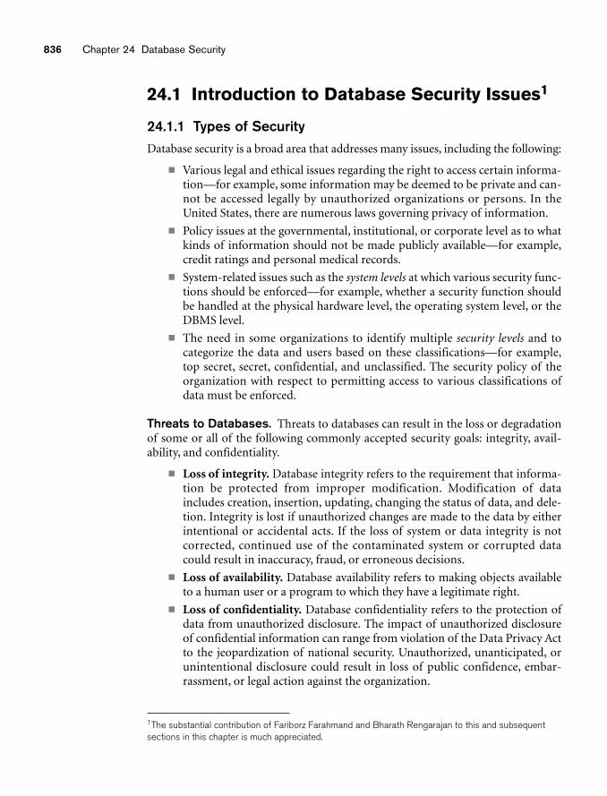
836 Chapter 24 Database Security
24.1 Introduction to Database Security Issues1
24.1.1 Types of SecurityDatabase security is a broad area that addresses many issues, including the following:
■ Various legal and ethical issues regarding the right to access certain informa-tion—for example, some information may be deemed to be private and can-not be accessed legally by unauthorized organizations or persons. In theUnited States, there are numerous laws governing privacy of information.
■ Policy issues at the governmental, institutional, or corporate level as to whatkinds of information should not be made publicly available—for example,credit ratings and personal medical records.
■ System-related issues such as the system levels at which various security func-tions should be enforced—for example, whether a security function shouldbe handled at the physical hardware level, the operating system level, or theDBMS level.
■ The need in some organizations to identify multiple security levels and tocategorize the data and users based on these classifications—for example,top secret, secret, confidential, and unclassified. The security policy of theorganization with respect to permitting access to various classifications ofdata must be enforced.
Threats to Databases. Threats to databases can result in the loss or degradationof some or all of the following commonly accepted security goals: integrity, avail-ability, and confidentiality.
■ Loss of integrity. Database integrity refers to the requirement that informa-tion be protected from improper modification. Modification of dataincludes creation, insertion, updating, changing the status of data, and dele-tion. Integrity is lost if unauthorized changes are made to the data by eitherintentional or accidental acts. If the loss of system or data integrity is notcorrected, continued use of the contaminated system or corrupted datacould result in inaccuracy, fraud, or erroneous decisions.
■ Loss of availability. Database availability refers to making objects availableto a human user or a program to which they have a legitimate right.
■ Loss of confidentiality. Database confidentiality refers to the protection ofdata from unauthorized disclosure. The impact of unauthorized disclosureof confidential information can range from violation of the Data Privacy Actto the jeopardization of national security. Unauthorized, unanticipated, orunintentional disclosure could result in loss of public confidence, embar-rassment, or legal action against the organization.
1The substantial contribution of Fariborz Farahmand and Bharath Rengarajan to this and subsequentsections in this chapter is much appreciated.
24.1 Introduction to Database Security Issues 837
To protect databases against these types of threats, it is common to implement fourkinds of control measures: access control, inference control, flow control, and encryp-tion. We discuss each of these in this chapter.
In a multiuser database system, the DBMS must provide techniques to enable cer-tain users or user groups to access selected portions of a database without gainingaccess to the rest of the database. This is particularly important when a large inte-grated database is to be used by many different users within the same organization.For example, sensitive information such as employee salaries or performancereviews should be kept confidential from most of the database system’s users. ADBMS typically includes a database security and authorization subsystem that isresponsible for ensuring the security of portions of a database against unauthorizedaccess. It is now customary to refer to two types of database security mechanisms:
■ Discretionary security mechanisms. These are used to grant privileges tousers, including the capability to access specific data files, records, or fields ina specified mode (such as read, insert, delete, or update).
■ Mandatory security mechanisms. These are used to enforce multilevelsecurity by classifying the data and users into various security classes (or lev-els) and then implementing the appropriate security policy of the organiza-tion. For example, a typical security policy is to permit users at a certainclassification (or clearance) level to see only the data items classified at theuser’s own (or lower) classification level. An extension of this is role-basedsecurity, which enforces policies and privileges based on the concept of orga-nizational roles.
We discuss discretionary security in Section 24.2 and mandatory and role-basedsecurity in Section 24.3.
24.1.2 Control MeasuresFour main control measures are used to provide security of data in databases:
■ Access control
■ Inference control
■ Flow control
■ Data encryption
A security problem common to computer systems is that of preventing unautho-rized persons from accessing the system itself, either to obtain information or tomake malicious changes in a portion of the database. The security mechanism of aDBMS must include provisions for restricting access to the database system as awhole. This function, called access control, is handled by creating user accounts andpasswords to control the login process by the DBMS. We discuss access control tech-niques in Section 24.1.3.
Statistical databases are used to provide statistical information or summaries ofvalues based on various criteria. For example, a database for population statistics
838 Chapter 24 Database Security
may provide statistics based on age groups, income levels, household size, educationlevels, and other criteria. Statistical database users such as government statisticiansor market research firms are allowed to access the database to retrieve statisticalinformation about a population but not to access the detailed confidential informa-tion about specific individuals. Security for statistical databases must ensure thatinformation about individuals cannot be accessed. It is sometimes possible todeduce or infer certain facts concerning individuals from queries that involve onlysummary statistics on groups; consequently, this must not be permitted either. Thisproblem, called statistical database security, is discussed briefly in Section 24.4.The corresponding control measures are called inference control measures.
Another security issue is that of flow control, which prevents information fromflowing in such a way that it reaches unauthorized users. It is discussed in Section24.6. Channels that are pathways for information to flow implicitly in ways that vio-late the security policy of an organization are called covert channels. We briefly dis-cuss some issues related to covert channels in Section 24.6.1.
A final control measure is data encryption, which is used to protect sensitive data(such as credit card numbers) that is transmitted via some type of communicationsnetwork. Encryption can be used to provide additional protection for sensitive por-tions of a database as well. The data is encoded using some coding algorithm. Anunauthorized user who accesses encoded data will have difficulty deciphering it, butauthorized users are given decoding or decrypting algorithms (or keys) to decipherthe data. Encrypting techniques that are very difficult to decode without a key havebeen developed for military applications. Section 24.7 briefly discusses encryptiontechniques, including popular techniques such as public key encryption, which isheavily used to support Web-based transactions against databases, and digital signa-tures, which are used in personal communications.
A comprehensive discussion of security in computer systems and databases is out-side the scope of this textbook. We give only a brief overview of database securitytechniques here. The interested reader can refer to several of the references dis-cussed in the Selected Bibliography at the end of this chapter for a more compre-hensive discussion.
24.1.3 Database Security and the DBAAs we discussed in Chapter 1, the database administrator (DBA) is the centralauthority for managing a database system. The DBA’s responsibilities include grant-ing privileges to users who need to use the system and classifying users and data inaccordance with the policy of the organization. The DBA has a DBA account in theDBMS, sometimes called a system or superuser account, which provides powerfulcapabilities that are not made available to regular database accounts and users.2
DBA-privileged commands include commands for granting and revoking privileges
2This account is similar to the root or superuser accounts that are given to computer system administra-tors, which allow access to restricted operating system commands.
24.1 Introduction to Database Security Issues 839
to individual accounts, users, or user groups and for performing the following typesof actions:
1. Account creation. This action creates a new account and password for a useror a group of users to enable access to the DBMS.
2. Privilege granting. This action permits the DBA to grant certain privilegesto certain accounts.
3. Privilege revocation. This action permits the DBA to revoke (cancel) certainprivileges that were previously given to certain accounts.
4. Security level assignment. This action consists of assigning user accounts tothe appropriate security clearance level.
The DBA is responsible for the overall security of the database system. Action 1 inthe preceding list is used to control access to the DBMS as a whole, whereas actions2 and 3 are used to control discretionary database authorization, and action 4 is usedto control mandatory authorization.
24.1.4 Access Control, User Accounts, and Database AuditsWhenever a person or a group of persons needs to access a database system, theindividual or group must first apply for a user account. The DBA will then create anew account number and password for the user if there is a legitimate need toaccess the database. The user must log in to the DBMS by entering the accountnumber and password whenever database access is needed. The DBMS checks thatthe account number and password are valid; if they are, the user is permitted to usethe DBMS and to access the database. Application programs can also be consideredusers and are required to log in to the database (see Chapter 13).
It is straightforward to keep track of database users and their accounts and pass-words by creating an encrypted table or file with two fields: AccountNumber andPassword. This table can easily be maintained by the DBMS. Whenever a newaccount is created, a new record is inserted into the table. When an account is can-celed, the corresponding record must be deleted from the table.
The database system must also keep track of all operations on the database that areapplied by a certain user throughout each login session, which consists of thesequence of database interactions that a user performs from the time of logging into the time of logging off. When a user logs in, the DBMS can record the user’saccount number and associate it with the computer or device from which the userlogged in. All operations applied from that computer or device are attributed to theuser’s account until the user logs off. It is particularly important to keep track ofupdate operations that are applied to the database so that, if the database is tam-pered with, the DBA can determine which user did the tampering.
To keep a record of all updates applied to the database and of particular users whoapplied each update, we can modify the system log. Recall from Chapters 21 and 23that the system log includes an entry for each operation applied to the database thatmay be required for recovery from a transaction failure or system crash. We can
840 Chapter 24 Database Security
expand the log entries so that they also include the account number of the user andthe online computer or device ID that applied each operation recorded in the log. Ifany tampering with the database is suspected, a database audit is performed, whichconsists of reviewing the log to examine all accesses and operations applied to thedatabase during a certain time period. When an illegal or unauthorized operation isfound, the DBA can determine the account number used to perform the operation.Database audits are particularly important for sensitive databases that are updatedby many transactions and users, such as a banking database that is updated by manybank tellers. A database log that is used mainly for security purposes is sometimescalled an audit trail.
24.1.5 Sensitive Data and Types of DisclosuresSensitivity of data is a measure of the importance assigned to the data by its owner,for the purpose of denoting its need for protection. Some databases contain onlysensitive data while other databases may contain no sensitive data at all. Handlingdatabases that fall at these two extremes is relatively easy, because these can be cov-ered by access control, which is explained in the next section. The situation becomestricky when some of the data is sensitive while other data is not.
Several factors can cause data to be classified as sensitive:
1. Inherently sensitive. The value of the data itself may be so revealing or con-fidential that it becomes sensitive—for example, a person’s salary or that apatient has HIV/AIDS.
2. From a sensitive source. The source of the data may indicate a need forsecrecy—for example, an informer whose identity must be kept secret.
3. Declared sensitive. The owner of the data may have explicitly declared it assensitive.
4. A sensitive attribute or sensitive record. The particular attribute or recordmay have been declared sensitive—for example, the salary attribute of anemployee or the salary history record in a personnel database.
5. Sensitive in relation to previously disclosed data. Some data may not besensitive by itself but will become sensitive in the presence of some otherdata—for example, the exact latitude and longitude information for a loca-tion where some previously recorded event happened that was later deemedsensitive.
It is the responsibility of the database administrator and security administrator tocollectively enforce the security policies of an organization. This dictates whetheraccess should be permitted to a certain database attribute (also known as a table col-umn or a data element) or not for individual users or for categories of users. Severalfactors need to be considered before deciding whether it is safe to reveal the data.The three most important factors are data availability, access acceptability, andauthenticity assurance.
1. Data availability. If a user is updating a field, then this field becomes inac-cessible and other users should not be able to view this data. This blocking is
24.1 Introduction to Database Security Issues 841
only temporary and only to ensure that no user sees any inaccurate data.This is typically handled by the concurrency control mechanism (seeChapter 22).
2. Access acceptability. Data should only be revealed to authorized users. Adatabase administrator may also deny access to a user request even if therequest does not directly access a sensitive data item, on the grounds that therequested data may reveal information about the sensitive data that the useris not authorized to have.
3. Authenticity assurance. Before granting access, certain external characteris-tics about the user may also be considered. For example, a user may only bepermitted access during working hours. The system may track previousqueries to ensure that a combination of queries does not reveal sensitivedata. The latter is particularly relevant to statistical database queries (seeSection 24.5).
The term precision, when used in the security area, refers to allowing as much aspossible of the data to be available, subject to protecting exactly the subset of datathat is sensitive. The definitions of security versus precision are as follows:
■ Security: Means of ensuring that data is kept safe from corruption and thataccess to it is suitably controlled. To provide security means to disclose onlynonsensitive data, and reject any query that references a sensitive field.
■ Precision: To protect all sensitive data while disclosing as much nonsensitivedata as possible.
The ideal combination is to maintain perfect security with maximum precision. Ifwe want to maintain security, some sacrifice has to be made with precision. Hencethere is typically a tradeoff between security and precision.
24.1.6 Relationship between Information Security versus Information Privacy
The rapid advancement of the use of information technology (IT) in industry, gov-ernment, and academia raises challenging questions and problems regarding theprotection and use of personal information. Questions of who has what rights toinformation about individuals for which purposes become more important as wemove toward a world in which it is technically possible to know just about anythingabout anyone.
Deciding how to design privacy considerations in technology for the future includesphilosophical, legal, and practical dimensions. There is a considerable overlapbetween issues related to access to resources (security) and issues related to appro-priate use of information (privacy). We now define the difference between securityversus privacy.
Security in information technology refers to many aspects of protecting a systemfrom unauthorized use, including authentication of users, information encryption,access control, firewall policies, and intrusion detection. For our purposes here, we
842 Chapter 24 Database Security
will limit our treatment of security to the concepts associated with how well a sys-tem can protect access to information it contains. The concept of privacy goesbeyond security. Privacy examines how well the use of personal information thatthe system acquires about a user conforms to the explicit or implicit assumptionsregarding that use. From an end user perspective, privacy can be considered fromtwo different perspectives: preventing storage of personal information versusensuring appropriate use of personal information.
For the purposes of this chapter, a simple but useful definition of privacy is the abil-ity of individuals to control the terms under which their personal information isacquired and used. In summary, security involves technology to ensure that informa-tion is appropriately protected. Security is a required building block for privacy toexist. Privacy involves mechanisms to support compliance with some basic principlesand other explicitly stated policies. One basic principle is that people should beinformed about information collection, told in advance what will be done with theirinformation, and given a reasonable opportunity to approve of such use of the infor-mation. A related concept, trust, relates to both security and privacy, and is seen asincreasing when it is perceived that both security and privacy are provided for.
24.2 Discretionary Access Control Based on Granting and Revoking Privileges
The typical method of enforcing discretionary access control in a database systemis based on the granting and revoking of privileges. Let us consider privileges in thecontext of a relational DBMS. In particular, we will discuss a system of privilegessomewhat similar to the one originally developed for the SQL language (seeChapters 4 and 5). Many current relational DBMSs use some variation of this tech-nique. The main idea is to include statements in the query language that allow theDBA and selected users to grant and revoke privileges.
24.2.1 Types of Discretionary PrivilegesIn SQL2 and later versions,3 the concept of an authorization identifier is used torefer, roughly speaking, to a user account (or group of user accounts). For simplic-ity, we will use the words user or account interchangeably in place of authorizationidentifier. The DBMS must provide selective access to each relation in the databasebased on specific accounts. Operations may also be controlled; thus, having anaccount does not necessarily entitle the account holder to all the functionality pro-vided by the DBMS. Informally, there are two levels for assigning privileges to usethe database system:
■ The account level. At this level, the DBA specifies the particular privilegesthat each account holds independently of the relations in the database.
■ The relation (or table) level. At this level, the DBA can control the privilegeto access each individual relation or view in the database.
3Discretionary privileges were incorporated into SQL2 and are applicable to later versions of SQL.
24.2 Discretionary Access Control Based on Granting and Revoking Privileges 843
The privileges at the account level apply to the capabilities provided to the accountitself and can include the CREATE SCHEMA or CREATE TABLE privilege, to create aschema or base relation; the CREATE VIEW privilege; the ALTER privilege, to applyschema changes such as adding or removing attributes from relations; the DROPprivilege, to delete relations or views; the MODIFY privilege, to insert, delete, orupdate tuples; and the SELECT privilege, to retrieve information from the databaseby using a SELECT query. Notice that these account privileges apply to the accountin general. If a certain account does not have the CREATE TABLE privilege, no rela-tions can be created from that account. Account-level privileges are not defined aspart of SQL2; they are left to the DBMS implementers to define. In earlier versionsof SQL, a CREATETAB privilege existed to give an account the privilege to createtables (relations).
The second level of privileges applies to the relation level, whether they are baserelations or virtual (view) relations. These privileges are defined for SQL2. In thefollowing discussion, the term relation may refer either to a base relation or to aview, unless we explicitly specify one or the other. Privileges at the relation levelspecify for each user the individual relations on which each type of command canbe applied. Some privileges also refer to individual columns (attributes) of relations.SQL2 commands provide privileges at the relation and attribute level only. Althoughthis is quite general, it makes it difficult to create accounts with limited privileges.The granting and revoking of privileges generally follow an authorization model fordiscretionary privileges known as the access matrix model, where the rows of amatrix M represent subjects (users, accounts, programs) and the columns representobjects (relations, records, columns, views, operations). Each position M(i, j) in thematrix represents the types of privileges (read, write, update) that subject i holds onobject j.
To control the granting and revoking of relation privileges, each relation R in a data-base is assigned an owner account, which is typically the account that was usedwhen the relation was created in the first place. The owner of a relation is given allprivileges on that relation. In SQL2, the DBA can assign an owner to a wholeschema by creating the schema and associating the appropriate authorization iden-tifier with that schema, using the CREATE SCHEMA command (see Section 4.1.1).The owner account holder can pass privileges on any of the owned relations to otherusers by granting privileges to their accounts. In SQL the following types of privi-leges can be granted on each individual relation R:
■ SELECT (retrieval or read) privilege on R. Gives the account retrieval privi-lege. In SQL this gives the account the privilege to use the SELECT statementto retrieve tuples from R.
■ Modification privileges on R. This gives the account the capability to mod-ify the tuples of R. In SQL this includes three privileges: UPDATE, DELETE,and INSERT. These correspond to the three SQL commands (see Section 4.4)for modifying a table R. Additionally, both the INSERT and UPDATE privi-leges can specify that only certain attributes of R can be modified by theaccount.

844 Chapter 24 Database Security
■ References privilege on R. This gives the account the capability to reference(or refer to) a relation R when specifying integrity constraints. This privilegecan also be restricted to specific attributes of R.
Notice that to create a view, the account must have the SELECT privilege on all rela-tions involved in the view definition in order to specify the query that correspondsto the view.
24.2.2 Specifying Privileges through the Use of ViewsThe mechanism of views is an important discretionary authorization mechanism inits own right. For example, if the owner A of a relation R wants another account B tobe able to retrieve only some fields of R, then A can create a view V of R thatincludes only those attributes and then grant SELECT on V to B. The same applies tolimiting B to retrieving only certain tuples of R; a view V�can be created by definingthe view by means of a query that selects only those tuples from R that A wants toallow B to access. We will illustrate this discussion with the example given in Section24.2.5.
24.2.3 Revoking of PrivilegesIn some cases it is desirable to grant a privilege to a user temporarily. For example,the owner of a relation may want to grant the SELECT privilege to a user for a spe-cific task and then revoke that privilege once the task is completed. Hence, a mech-anism for revoking privileges is needed. In SQL a REVOKE command is included forthe purpose of canceling privileges. We will see how the REVOKE command is usedin the example in Section 24.2.5.
24.2.4 Propagation of Privileges Using the GRANT OPTIONWhenever the owner A of a relation R grants a privilege on R to another account B,the privilege can be given to B with or without the GRANT OPTION. If the GRANTOPTION is given, this means that B can also grant that privilege on R to otheraccounts. Suppose that B is given the GRANT OPTION by A and that B then grantsthe privilege on R to a third account C, also with the GRANT OPTION. In this way,privileges on R can propagate to other accounts without the knowledge of theowner of R. If the owner account A now revokes the privilege granted to B, all theprivileges that B propagated based on that privilege should automatically be revokedby the system.
It is possible for a user to receive a certain privilege from two or more sources. Forexample, A4 may receive a certain UPDATE R privilege from both A2 and A3. In sucha case, if A2 revokes this privilege from A4, A4 will still continue to have the privilegeby virtue of having been granted it from A3. If A3 later revokes the privilege fromA4, A4 totally loses the privilege. Hence, a DBMS that allows propagation of privi-leges must keep track of how all the privileges were granted so that revoking of priv-ileges can be done correctly and completely.
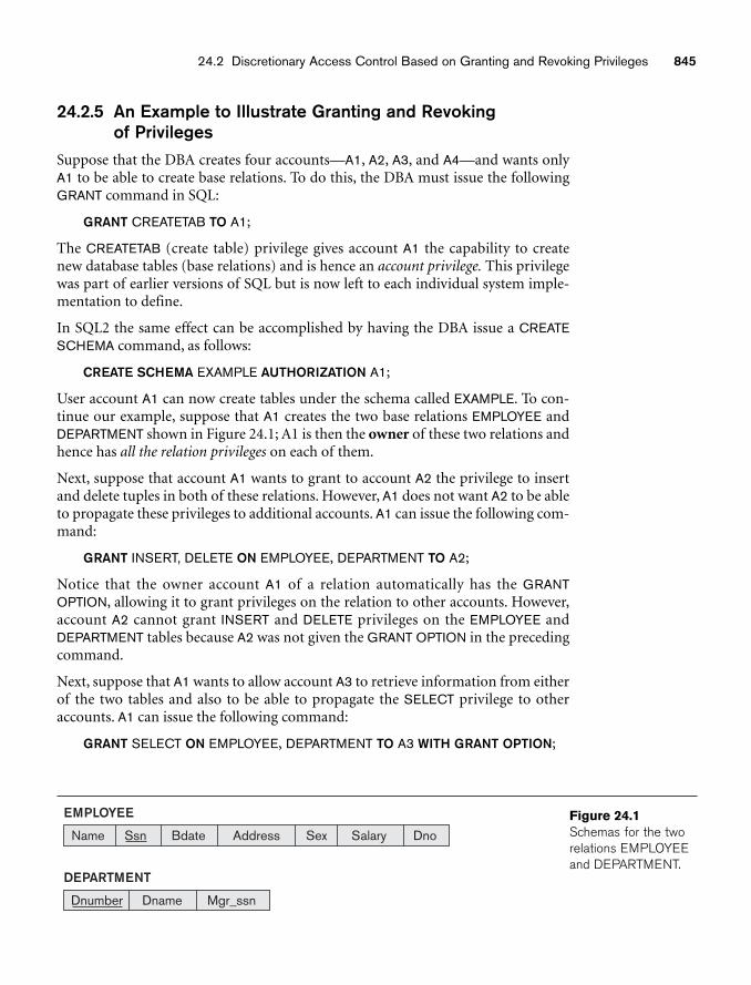
24.2 Discretionary Access Control Based on Granting and Revoking Privileges 845
24.2.5 An Example to Illustrate Granting and Revoking of Privileges
Suppose that the DBA creates four accounts—A1, A2, A3, and A4—and wants onlyA1 to be able to create base relations. To do this, the DBA must issue the followingGRANT command in SQL:
GRANT CREATETAB TO A1;
The CREATETAB (create table) privilege gives account A1 the capability to createnew database tables (base relations) and is hence an account privilege. This privilegewas part of earlier versions of SQL but is now left to each individual system imple-mentation to define.
In SQL2 the same effect can be accomplished by having the DBA issue a CREATESCHEMA command, as follows:
CREATE SCHEMA EXAMPLE AUTHORIZATION A1;
User account A1 can now create tables under the schema called EXAMPLE. To con-tinue our example, suppose that A1 creates the two base relations EMPLOYEE andDEPARTMENT shown in Figure 24.1; A1 is then the owner of these two relations andhence has all the relation privileges on each of them.
Next, suppose that account A1 wants to grant to account A2 the privilege to insertand delete tuples in both of these relations. However, A1 does not want A2 to be ableto propagate these privileges to additional accounts. A1 can issue the following com-mand:
GRANT INSERT, DELETE ON EMPLOYEE, DEPARTMENT TO A2;
Notice that the owner account A1 of a relation automatically has the GRANTOPTION, allowing it to grant privileges on the relation to other accounts. However,account A2 cannot grant INSERT and DELETE privileges on the EMPLOYEE andDEPARTMENT tables because A2 was not given the GRANT OPTION in the precedingcommand.
Next, suppose that A1 wants to allow account A3 to retrieve information from eitherof the two tables and also to be able to propagate the SELECT privilege to otheraccounts. A1 can issue the following command:
GRANT SELECT ON EMPLOYEE, DEPARTMENT TO A3 WITH GRANT OPTION;
DEPARTMENT
DnameDnumber Mgr_ssn
Name Bdate Address Sex Salary Dno
EMPLOYEE
Ssn
Figure 24.1Schemas for the tworelations EMPLOYEEand DEPARTMENT.
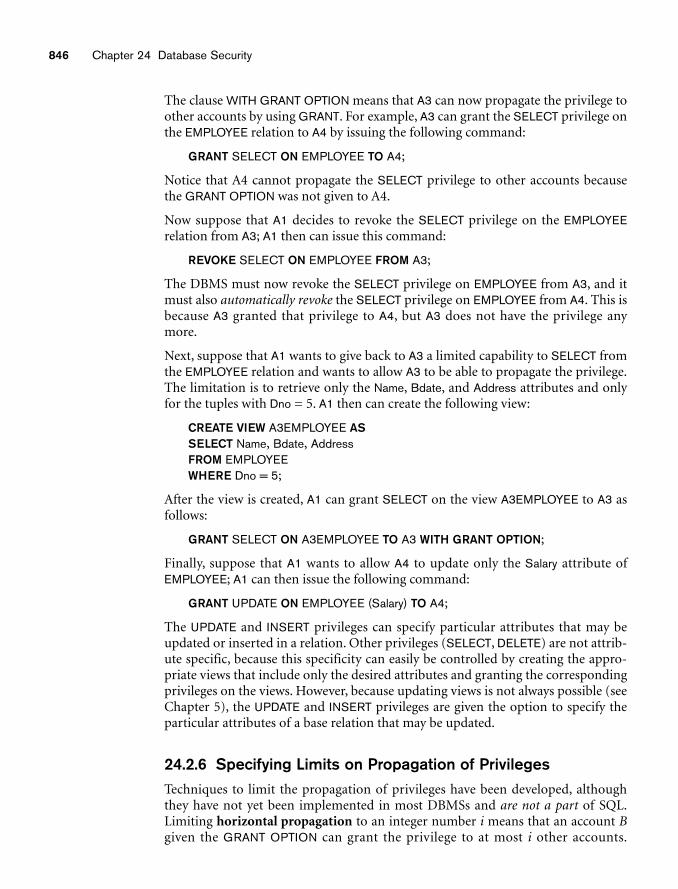
846 Chapter 24 Database Security
The clause WITH GRANT OPTION means that A3 can now propagate the privilege toother accounts by using GRANT. For example, A3 can grant the SELECT privilege onthe EMPLOYEE relation to A4 by issuing the following command:
GRANT SELECT ON EMPLOYEE TO A4;
Notice that A4 cannot propagate the SELECT privilege to other accounts becausethe GRANT OPTION was not given to A4.
Now suppose that A1 decides to revoke the SELECT privilege on the EMPLOYEErelation from A3; A1 then can issue this command:
REVOKE SELECT ON EMPLOYEE FROM A3;
The DBMS must now revoke the SELECT privilege on EMPLOYEE from A3, and itmust also automatically revoke the SELECT privilege on EMPLOYEE from A4. This isbecause A3 granted that privilege to A4, but A3 does not have the privilege anymore.
Next, suppose that A1 wants to give back to A3 a limited capability to SELECT fromthe EMPLOYEE relation and wants to allow A3 to be able to propagate the privilege.The limitation is to retrieve only the Name, Bdate, and Address attributes and onlyfor the tuples with Dno = 5. A1 then can create the following view:
CREATE VIEW A3EMPLOYEE ASSELECT Name, Bdate, AddressFROM EMPLOYEEWHERE Dno = 5;
After the view is created, A1 can grant SELECT on the view A3EMPLOYEE to A3 asfollows:
GRANT SELECT ON A3EMPLOYEE TO A3 WITH GRANT OPTION;
Finally, suppose that A1 wants to allow A4 to update only the Salary attribute ofEMPLOYEE; A1 can then issue the following command:
GRANT UPDATE ON EMPLOYEE (Salary) TO A4;
The UPDATE and INSERT privileges can specify particular attributes that may beupdated or inserted in a relation. Other privileges (SELECT, DELETE) are not attrib-ute specific, because this specificity can easily be controlled by creating the appro-priate views that include only the desired attributes and granting the correspondingprivileges on the views. However, because updating views is not always possible (seeChapter 5), the UPDATE and INSERT privileges are given the option to specify theparticular attributes of a base relation that may be updated.
24.2.6 Specifying Limits on Propagation of PrivilegesTechniques to limit the propagation of privileges have been developed, althoughthey have not yet been implemented in most DBMSs and are not a part of SQL.Limiting horizontal propagation to an integer number i means that an account Bgiven the GRANT OPTION can grant the privilege to at most i other accounts.
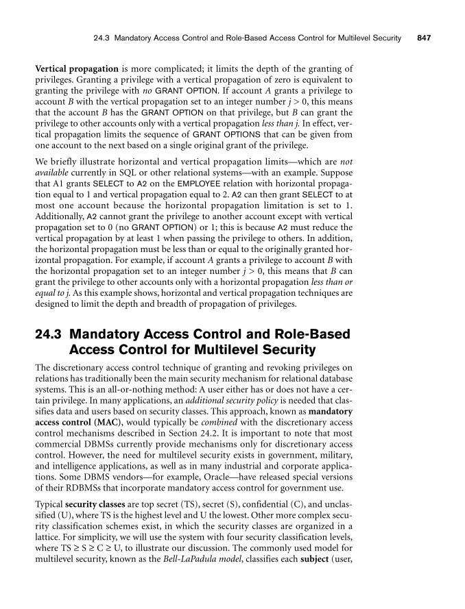
24.3 Mandatory Access Control and Role-Based Access Control for Multilevel Security 847
Vertical propagation is more complicated; it limits the depth of the granting ofprivileges. Granting a privilege with a vertical propagation of zero is equivalent togranting the privilege with no GRANT OPTION. If account A grants a privilege toaccount B with the vertical propagation set to an integer number j > 0, this meansthat the account B has the GRANT OPTION on that privilege, but B can grant theprivilege to other accounts only with a vertical propagation less than j. In effect, ver-tical propagation limits the sequence of GRANT OPTIONS that can be given fromone account to the next based on a single original grant of the privilege.
We briefly illustrate horizontal and vertical propagation limits—which are notavailable currently in SQL or other relational systems—with an example. Supposethat A1 grants SELECT to A2 on the EMPLOYEE relation with horizontal propaga-tion equal to 1 and vertical propagation equal to 2. A2 can then grant SELECT to atmost one account because the horizontal propagation limitation is set to 1.Additionally, A2 cannot grant the privilege to another account except with verticalpropagation set to 0 (no GRANT OPTION) or 1; this is because A2 must reduce thevertical propagation by at least 1 when passing the privilege to others. In addition,the horizontal propagation must be less than or equal to the originally granted hor-izontal propagation. For example, if account A grants a privilege to account B withthe horizontal propagation set to an integer number j > 0, this means that B cangrant the privilege to other accounts only with a horizontal propagation less than orequal to j. As this example shows, horizontal and vertical propagation techniques aredesigned to limit the depth and breadth of propagation of privileges.
24.3 Mandatory Access Control and Role-BasedAccess Control for Multilevel Security
The discretionary access control technique of granting and revoking privileges onrelations has traditionally been the main security mechanism for relational databasesystems. This is an all-or-nothing method: A user either has or does not have a cer-tain privilege. In many applications, an additional security policy is needed that clas-sifies data and users based on security classes. This approach, known as mandatoryaccess control (MAC), would typically be combined with the discretionary accesscontrol mechanisms described in Section 24.2. It is important to note that mostcommercial DBMSs currently provide mechanisms only for discretionary accesscontrol. However, the need for multilevel security exists in government, military,and intelligence applications, as well as in many industrial and corporate applica-tions. Some DBMS vendors—for example, Oracle—have released special versionsof their RDBMSs that incorporate mandatory access control for government use.
Typical security classes are top secret (TS), secret (S), confidential (C), and unclas-sified (U), where TS is the highest level and U the lowest. Other more complex secu-rity classification schemes exist, in which the security classes are organized in alattice. For simplicity, we will use the system with four security classification levels,where TS ≥ S ≥ C ≥ U, to illustrate our discussion. The commonly used model formultilevel security, known as the Bell-LaPadula model, classifies each subject (user,
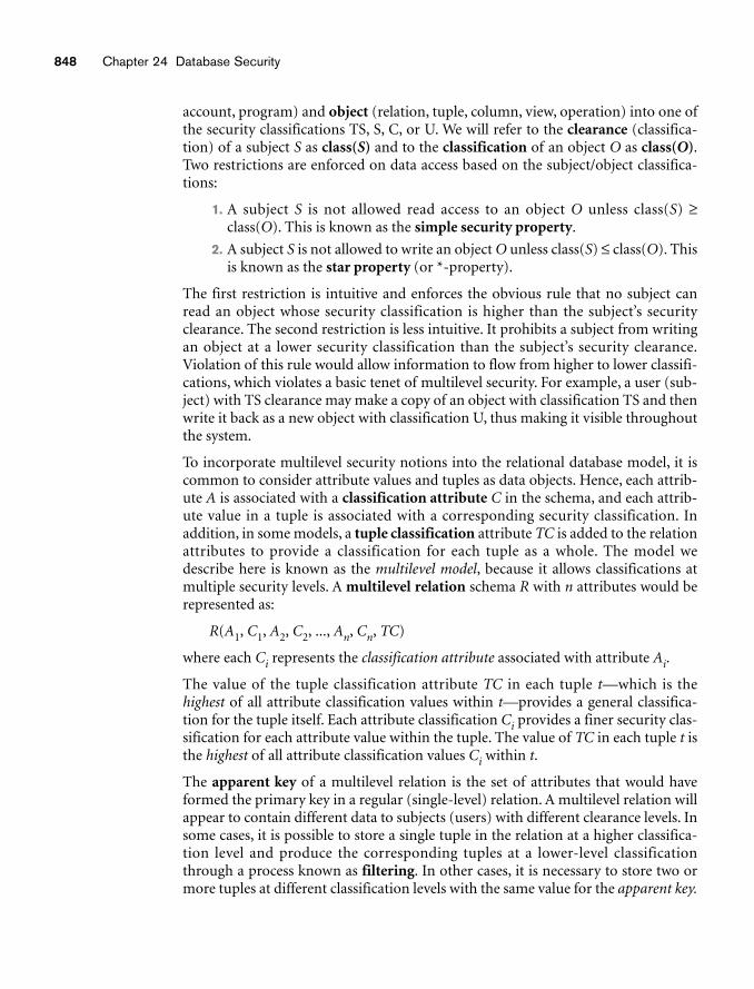
848 Chapter 24 Database Security
account, program) and object (relation, tuple, column, view, operation) into one ofthe security classifications TS, S, C, or U. We will refer to the clearance (classifica-tion) of a subject S as class(S) and to the classification of an object O as class(O).Two restrictions are enforced on data access based on the subject/object classifica-tions:
1. A subject S is not allowed read access to an object O unless class(S) ≥class(O). This is known as the simple security property.
2. A subject S is not allowed to write an object O unless class(S) ≤ class(O). Thisis known as the star property (or *-property).
The first restriction is intuitive and enforces the obvious rule that no subject canread an object whose security classification is higher than the subject’s securityclearance. The second restriction is less intuitive. It prohibits a subject from writingan object at a lower security classification than the subject’s security clearance.Violation of this rule would allow information to flow from higher to lower classifi-cations, which violates a basic tenet of multilevel security. For example, a user (sub-ject) with TS clearance may make a copy of an object with classification TS and thenwrite it back as a new object with classification U, thus making it visible throughoutthe system.
To incorporate multilevel security notions into the relational database model, it iscommon to consider attribute values and tuples as data objects. Hence, each attrib-ute A is associated with a classification attribute C in the schema, and each attrib-ute value in a tuple is associated with a corresponding security classification. Inaddition, in some models, a tuple classification attribute TC is added to the relationattributes to provide a classification for each tuple as a whole. The model wedescribe here is known as the multilevel model, because it allows classifications atmultiple security levels. A multilevel relation schema R with n attributes would berepresented as:
R(A1, C1, A2, C2, ..., An, Cn, TC)
where each Ci represents the classification attribute associated with attribute Ai.
The value of the tuple classification attribute TC in each tuple t—which is thehighest of all attribute classification values within t—provides a general classifica-tion for the tuple itself. Each attribute classification Ci provides a finer security clas-sification for each attribute value within the tuple. The value of TC in each tuple t isthe highest of all attribute classification values Ci within t.
The apparent key of a multilevel relation is the set of attributes that would haveformed the primary key in a regular (single-level) relation. A multilevel relation willappear to contain different data to subjects (users) with different clearance levels. Insome cases, it is possible to store a single tuple in the relation at a higher classifica-tion level and produce the corresponding tuples at a lower-level classificationthrough a process known as filtering. In other cases, it is necessary to store two ormore tuples at different classification levels with the same value for the apparent key.
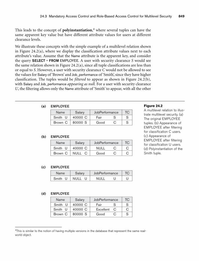
24.3 Mandatory Access Control and Role-Based Access Control for Multilevel Security 849
This leads to the concept of polyinstantiation,4 where several tuples can have thesame apparent key value but have different attribute values for users at differentclearance levels.
We illustrate these concepts with the simple example of a multilevel relation shownin Figure 24.2(a), where we display the classification attribute values next to eachattribute’s value. Assume that the Name attribute is the apparent key, and considerthe query SELECT * FROM EMPLOYEE. A user with security clearance S would seethe same relation shown in Figure 24.2(a), since all tuple classifications are less thanor equal to S. However, a user with security clearance C would not be allowed to seethe values for Salary of ‘Brown’ and Job_performance of ‘Smith’, since they have higherclassification. The tuples would be filtered to appear as shown in Figure 24.2(b),with Salary and Job_performance appearing as null. For a user with security clearanceU, the filtering allows only the Name attribute of ‘Smith’ to appear, with all the other
Name Salary JobPerformance TCSmith U C40000 SFair SSmith U C40000 CExcellent CBrown C S80000 CGood S
EMPLOYEE(d)
Name Salary JobPerformance TCSmith U C40000 SFair SBrown C S80000 CGood S
EMPLOYEE(a)
Name Salary JobPerformance TC
Smith U C40000 CNULL CBrown C CNULL CGood C
EMPLOYEE(b)
Name Salary JobPerformance TC
Smith U UNULL UNULL U
EMPLOYEE(c)
Figure 24.2A multilevel relation to illus-trate multilevel security. (a)The original EMPLOYEEtuples. (b) Appearance ofEMPLOYEE after filteringfor classification C users.(c) Appearance ofEMPLOYEE after filteringfor classification U users.(d) Polyinstantiation of theSmith tuple.
4This is similar to the notion of having multiple versions in the database that represent the same real-world object.
850 Chapter 24 Database Security
attributes appearing as null (Figure 24.2(c)). Thus, filtering introduces null valuesfor attribute values whose security classification is higher than the user’s securityclearance.
In general, the entity integrity rule for multilevel relations states that all attributesthat are members of the apparent key must not be null and must have the samesecurity classification within each individual tuple. Additionally, all other attributevalues in the tuple must have a security classification greater than or equal to that ofthe apparent key. This constraint ensures that a user can see the key if the user ispermitted to see any part of the tuple. Other integrity rules, called null integrityand interinstance integrity, informally ensure that if a tuple value at some securitylevel can be filtered (derived) from a higher-classified tuple, then it is sufficient tostore the higher-classified tuple in the multilevel relation.
To illustrate polyinstantiation further, suppose that a user with security clearance Ctries to update the value of Job_performance of ‘Smith’ in Figure 24.2 to ‘Excellent’;this corresponds to the following SQL update being submitted by that user:
UPDATE EMPLOYEESET Job_performance = ‘Excellent’WHERE Name = ‘Smith’;
Since the view provided to users with security clearance C (see Figure 24.2(b)) per-mits such an update, the system should not reject it; otherwise, the user could inferthat some nonnull value exists for the Job_performance attribute of ‘Smith’ ratherthan the null value that appears. This is an example of inferring informationthrough what is known as a covert channel, which should not be permitted inhighly secure systems (see Section 24.6.1). However, the user should not be allowedto overwrite the existing value of Job_performance at the higher classification level.The solution is to create a polyinstantiation for the ‘Smith’ tuple at the lower classi-fication level C, as shown in Figure 24.2(d). This is necessary since the new tuplecannot be filtered from the existing tuple at classification S.
The basic update operations of the relational model (INSERT, DELETE, UPDATE)must be modified to handle this and similar situations, but this aspect of the prob-lem is outside the scope of our presentation. We refer the interested reader to theSelected Bibliography at the end of this chapter for further details.
24.3.1 Comparing Discretionary Access Control and Mandatory Access Control
Discretionary access control (DAC) policies are characterized by a high degree offlexibility, which makes them suitable for a large variety of application domains.The main drawback of DAC models is their vulnerability to malicious attacks, suchas Trojan horses embedded in application programs. The reason is that discre-tionary authorization models do not impose any control on how information ispropagated and used once it has been accessed by users authorized to do so. By con-trast, mandatory policies ensure a high degree of protection—in a way, they prevent
24.3 Mandatory Access Control and Role-Based Access Control for Multilevel Security 851
any illegal flow of information. Therefore, they are suitable for military and highsecurity types of applications, which require a higher degree of protection.However, mandatory policies have the drawback of being too rigid in that theyrequire a strict classification of subjects and objects into security levels, and there-fore they are applicable to few environments. In many practical situations, discre-tionary policies are preferred because they offer a better tradeoff between securityand applicability.
24.3.2 Role-Based Access ControlRole-based access control (RBAC) emerged rapidly in the 1990s as a proven tech-nology for managing and enforcing security in large-scale enterprise-wide systems.Its basic notion is that privileges and other permissions are associated with organi-zational roles, rather than individual users. Individual users are then assigned toappropriate roles. Roles can be created using the CREATE ROLE and DESTROYROLE commands. The GRANT and REVOKE commands discussed in Section 24.2can then be used to assign and revoke privileges from roles, as well as for individualusers when needed. For example, a company may have roles such as sales accountmanager, purchasing agent, mailroom clerk, department manager, and so on.Multiple individuals can be assigned to each role. Security privileges that are com-mon to a role are granted to the role name, and any individual assigned to this rolewould automatically have those privileges granted.
RBAC can be used with traditional discretionary and mandatory access controls; itensures that only authorized users in their specified roles are given access to certaindata or resources. Users create sessions during which they may activate a subset ofroles to which they belong. Each session can be assigned to several roles, but it mapsto one user or a single subject only. Many DBMSs have allowed the concept of roles,where privileges can be assigned to roles.
Separation of duties is another important requirement in various commercialDBMSs. It is needed to prevent one user from doing work that requires the involve-ment of two or more people, thus preventing collusion. One method in which sepa-ration of duties can be successfully implemented is with mutual exclusion of roles.Two roles are said to be mutually exclusive if both the roles cannot be used simul-taneously by the user. Mutual exclusion of roles can be categorized into two types,namely authorization time exclusion (static) and runtime exclusion (dynamic). Inauthorization time exclusion, two roles that have been specified as mutually exclu-sive cannot be part of a user’s authorization at the same time. In runtime exclusion,both these roles can be authorized to one user but cannot be activated by the user atthe same time. Another variation in mutual exclusion of roles is that of completeand partial exclusion.
The role hierarchy in RBAC is a natural way to organize roles to reflect the organi-zation’s lines of authority and responsibility. By convention, junior roles at the bottom are connected to progressively senior roles as one moves up the hierarchy.The hierarchic diagrams are partial orders, so they are reflexive, transitive, and
852 Chapter 24 Database Security
antisymmetric. In other words, if a user has one role, the user automatically hasroles lower in the hierarchy. Defining a role hierarchy involves choosing the type ofhierarchy and the roles, and then implementing the hierarchy by granting roles toother roles. Role hierarchy can be implemented in the following manner:
GRANT ROLE full_time TO employee_type1GRANT ROLE intern TO employee_type2
The above are examples of granting the roles full_time and intern to two types ofemployees.
Another issue related to security is identity management. Identity refers to a uniquename of an individual person. Since the legal names of persons are not necessarilyunique, the identity of a person must include sufficient additional information tomake the complete name unique. Authorizing this identity and managing theschema of these identities is called Identity Management. Identity Managementaddresses how organizations can effectively authenticate people and manage theiraccess to confidential information. It has become more visible as a business require-ment across all industries affecting organizations of all sizes. Identity Managementadministrators constantly need to satisfy application owners while keeping expendi-tures under control and increasing IT efficiency.
Another important consideration in RBAC systems is the possible temporal con-straints that may exist on roles, such as the time and duration of role activations,and timed triggering of a role by an activation of another role. Using an RBACmodel is a highly desirable goal for addressing the key security requirements ofWeb-based applications. Roles can be assigned to workflow tasks so that a user withany of the roles related to a task may be authorized to execute it and may play a cer-tain role only for a certain duration.
RBAC models have several desirable features, such as flexibility, policy neutrality,better support for security management and administration, and other aspects thatmake them attractive candidates for developing secure Web-based applications.These features are lacking in DAC and MAC models. In addition, RBAC modelsinclude the capabilities available in traditional DAC and MAC policies.Furthermore, an RBAC model provides mechanisms for addressing the securityissues related to the execution of tasks and workflows, and for specifying user-defined and organization-specific policies. Easier deployment over the Internet hasbeen another reason for the success of RBAC models.
24.3.3 Label-Based Security and Row-Level Access ControlMany commercial DBMSs currently use the concept of row-level access control,where sophisticated access control rules can be implemented by considering thedata row by row. In row-level access control, each data row is given a label, which isused to store information about data sensitivity. Row-level access control providesfiner granularity of data security by allowing the permissions to be set for each rowand not just for the table or column. Initially the user is given a default session labelby the database administrator. Levels correspond to a hierarchy of data-sensitivity
24.3 Mandatory Access Control and Role-Based Access Control for Multilevel Security 853
levels to exposure or corruption, with the goal of maintaining privacy or security.Labels are used to prevent unauthorized users from viewing or altering certain data.A user having a low authorization level, usually represented by a low number, isdenied access to data having a higher-level number. If no such label is given to a row,a row label is automatically assigned to it depending upon the user’s session label.
A policy defined by an administrator is called a Label Security policy. Wheneverdata affected by the policy is accessed or queried through an application, the policyis automatically invoked. When a policy is implemented, a new column is added toeach row in the schema. The added column contains the label for each row thatreflects the sensitivity of the row as per the policy. Similar to MAC, where each userhas a security clearance, each user has an identity in label-based security. This user’sidentity is compared to the label assigned to each row to determine whether the userhas access to view the contents of that row. However, the user can write the labelvalue himself, within certain restrictions and guidelines for that specific row. Thislabel can be set to a value that is between the user’s current session label and theuser’s minimum level. The DBA has the privilege to set an initial default row label.
The Label Security requirements are applied on top of the DAC requirements foreach user. Hence, the user must satisfy the DAC requirements and then the labelsecurity requirements to access a row. The DAC requirements make sure that theuser is legally authorized to carry on that operation on the schema. In most applica-tions, only some of the tables need label-based security. For the majority of theapplication tables, the protection provided by DAC is sufficient.
Security policies are generally created by managers and human resources personnel.The policies are high-level, technology neutral, and relate to risks. Policies are aresult of management instructions to specify organizational procedures, guidingprinciples, and courses of action that are considered to be expedient, prudent, oradvantageous. Policies are typically accompanied by a definition of penalties andcountermeasures if the policy is transgressed. These policies are then interpretedand converted to a set of label-oriented policies by the Label Security administra-tor, who defines the security labels for data and authorizations for users; these labelsand authorizations govern access to specified protected objects.
Suppose a user has SELECT privileges on a table. When the user executes a SELECTstatement on that table, Label Security will automatically evaluate each rowreturned by the query to determine whether the user has rights to view the data. Forexample, if the user has a sensitivity of 20, then the user can view all rows having asecurity level of 20 or lower. The level determines the sensitivity of the informationcontained in a row; the more sensitive the row, the higher its security label value.Such Label Security can be configured to perform security checks on UPDATE,DELETE, and INSERT statements as well.
24.3.4 XML Access ControlWith the worldwide use of XML in commercial and scientific applications, effortsare under way to develop security standards. Among these efforts are digital
854 Chapter 24 Database Security
signatures and encryption standards for XML. The XML Signature Syntax andProcessing specification describes an XML syntax for representing the associationsbetween cryptographic signatures and XML documents or other electronicresources. The specification also includes procedures for computing and verifyingXML signatures. An XML digital signature differs from other protocols for messagesigning, such as PGP (Pretty Good Privacy—a confidentiality and authenticationservice that can be used for electronic mail and file storage application), in its sup-port for signing only specific portions of the XML tree (see Chapter 12) rather thanthe complete document. Additionally, the XML signature specification definesmechanisms for countersigning and transformations—so-called canonicalization toensure that two instances of the same text produce the same digest for signing evenif their representations differ slightly, for example, in typographic white space.
The XML Encryption Syntax and Processing specification defines XML vocabularyand processing rules for protecting confidentiality of XML documents in whole orin part and of non-XML data as well. The encrypted content and additional pro-cessing information for the recipient are represented in well-formed XML so thatthe result can be further processed using XML tools. In contrast to other commonlyused technologies for confidentiality such as SSL (Secure Sockets Layer—a leadingInternet security protocol), and virtual private networks, XML encryption alsoapplies to parts of documents and to documents in persistent storage.
24.3.5 Access Control Policies for E-Commerce and the WebElectronic commerce (e-commerce) environments are characterized by any trans-actions that are done electronically. They require elaborate access control policiesthat go beyond traditional DBMSs. In conventional database environments, accesscontrol is usually performed using a set of authorizations stated by security officersor users according to some security policies. Such a simple paradigm is not well suited for a dynamic environment like e-commerce. Furthermore, in an e-commerce environment the resources to be protected are not only traditional databut also knowledge and experience. Such peculiarities call for more flexibility inspecifying access control policies. The access control mechanism must be flexibleenough to support a wide spectrum of heterogeneous protection objects.
A second related requirement is the support for content-based access control.Content-based access control allows one to express access control policies that takethe protection object content into account. In order to support content-based accesscontrol, access control policies must allow inclusion of conditions based on theobject content.
A third requirement is related to the heterogeneity of subjects, which requires accesscontrol policies based on user characteristics and qualifications rather than on spe-cific and individual characteristics (for example, user IDs). A possible solution, tobetter take into account user profiles in the formulation of access control policies, isto support the notion of credentials. A credential is a set of properties concerning auser that are relevant for security purposes (for example, age or position or role
24.4 SQL Injection 855
within an organization). For instance, by using credentials, one can simply formu-late policies such as Only permanent staff with five or more years of service can accessdocuments related to the internals of the system.
It is believed that the XML is expected to play a key role in access control for e-commerce applications5 because XML is becoming the common representationlanguage for document interchange over the Web, and is also becoming the lan-guage for e-commerce. Thus, on the one hand there is the need to make XML repre-sentations secure, by providing access control mechanisms specifically tailored tothe protection of XML documents. On the other hand, access control information(that is, access control policies and user credentials) can be expressed using XMLitself. The Directory Services Markup Language (DSML) is a representation ofdirectory service information in XML syntax. It provides a foundation for a stan-dard for communicating with the directory services that will be responsible for pro-viding and authenticating user credentials. The uniform presentation of bothprotection objects and access control policies can be applied to policies and creden-tials themselves. For instance, some credential properties (such as the user name)may be accessible to everyone, whereas other properties may be visible only to arestricted class of users. Additionally, the use of an XML-based language for specify-ing credentials and access control policies facilitates secure credential submissionand export of access control policies.
24.4 SQL InjectionSQL Injection is one of the most common threats to a database system. We will dis-cuss it in detail later in this section. Some of the other attacks on databases that arequite frequent are:
■ Unauthorized privilege escalation. This attack is characterized by an indi-vidual attempting to elevate his or her privilege by attacking vulnerablepoints in the database systems.
■ Privilege abuse. While the previous attack is done by an unauthorized user,this attack is performed by a privileged user. For example, an administratorwho is allowed to change student information can use this privilege toupdate student grades without the instructor’s permission.
■ Denial of service. A Denial of Service (DOS) attack is an attempt to makeresources unavailable to its intended users. It is a general attack category inwhich access to network applications or data is denied to intended users byoverflowing the buffer or consuming resources.
■ Weak Authentication. If the user authentication scheme is weak, an attackercan impersonate the identity of a legitimate user by obtaining their logincredentials.
5See Thuraisingham et al. (2001).
856 Chapter 24 Database Security
24.4.1 SQL Injection MethodsAs we discussed in Chapter 14, Web programs and applications that access a data-base can send commands and data to the database, as well as display data retrievedfrom the database through the Web browser. In an SQL Injection attack, theattacker injects a string input through the application, which changes or manipu-lates the SQL statement to the attacker’s advantage. An SQL Injection attack canharm the database in various ways, such as unauthorized manipulation of the data-base, or retrieval of sensitive data. It can also be used to execute system level com-mands that may cause the system to deny service to the application. This sectiondescribes types of injection attacks.
SQL Manipulation. A manipulation attack, which is the most common type ofinjection attack, changes an SQL command in the application—for example, byadding conditions to the WHERE-clause of a query, or by expanding a query withadditional query components using set operations such as UNION, INTERSECT, orMINUS. Other types of manipulation attacks are also possible. A typical manipula-tion attack occurs during database login. For example, suppose that a simplisticauthentication procedure issues the following query and checks to see if any rowswere returned:
SELECT * FROM users WHERE username = ‘jake’ and PASSWORD =‘jakespasswd’.
The attacker can try to change (or manipulate) the SQL statement, by changing it asfollows:
SELECT * FROM users WHERE username = ‘jake’ and (PASSWORD =‘jakespasswd’ or ‘x’ = ‘x’)
As a result, the attacker who knows that ‘jake’ is a valid login of some user is able tolog into the database system as ‘jake’ without knowing his password and is able to doeverything that ‘jake’ may be authorized to do to the database system.
Code Injection. This type of attack attempts to add additional SQL statements orcommands to the existing SQL statement by exploiting a computer bug, which iscaused by processing invalid data. The attacker can inject or introduce code into acomputer program to change the course of execution. Code injection is a populartechnique for system hacking or cracking to gain information.
Function Call Injection. In this kind of attack, a database function or operatingsystem function call is inserted into a vulnerable SQL statement to manipulate thedata or make a privileged system call. For example, it is possible to exploit a functionthat performs some aspect related to network communication. In addition, func-tions that are contained in a customized database package, or any custom databasefunction, can be executed as part of an SQL query. In particular, dynamically cre-ated SQL queries (see Chapter 13) can be exploited since they are constructed at runtime.
24.4 SQL Injection 857
For example, the dual table is used in the FROM clause of SQL in Oracle when a userneeds to run SQL that does not logically have a table name. To get today’s date, wecan use:
SELECT SYSDATE FROM dual;
The following example demonstrates that even the simplest SQL statements can bevulnerable.
SELECT TRANSLATE (‘user input’, ‘from_string’, ‘to_string’) FROM dual;
Here, TRANSLATE is used to replace a string of characters with another string ofcharacters. The TRANSLATE function above will replace the characters of the‘from_string’ with the characters in the ‘to_string’ one by one. This means that the fwill be replaced with the t, the r with the o, the o with the _, and so on.
This type of SQL statement can be subjected to a function injection attack. Considerthe following example:
SELECT TRANSLATE (“ || UTL_HTTP.REQUEST (‘http://129.107.2.1/’) || ’’,‘98765432’, ‘9876’) FROM dual;
The user can input the string (“ || UTL_HTTP.REQUEST (‘http://129.107.2.1/’) || ’’), where || is the concatenate operator, thus requesting a page from a Web server.UTL_HTTP makes Hypertext Transfer Protocol (HTTP) callouts from SQL. TheREQUEST object takes a URL (‘http://129.107.2.1/’ in this example) as a parameter,contacts that site, and returns the data (typically HTML) obtained from that site.The attacker could manipulate the string he inputs, as well as the URL, to includeother functions and do other illegal operations. We just used a dummy example toshow conversion of ‘98765432’ to ‘9876’, but the user’s intent would be to access theURL and get sensitive information. The attacker can then retrieve useful informa-tion from the database server—located at the URL that is passed as a parameter—and send it to the Web server (that calls the TRANSLATE function).
24.4.2 Risks Associated with SQL InjectionSQL injection is harmful and the risks associated with it provide motivation forattackers. Some of the risks associated with SQL injection attacks are explainedbelow.
■ Database Fingerprinting. The attacker can determine the type of databasebeing used in the backend so that he can use database-specific attacks thatcorrespond to weaknesses in a particular DBMS.
■ Denial of Service. The attacker can flood the server with requests, thusdenying service to valid users, or they can delete some data.
■ Bypassing Authentication. This is one of the most common risks, in whichthe attacker can gain access to the database as an authorized user and per-form all the desired tasks.
858 Chapter 24 Database Security
■ Identifying Injectable Parameters. In this type of attack, the attacker gath-ers important information about the type and structure of the back-enddatabase of a Web application. This attack is made possible by the fact that the default error page returned by application servers is often overlydescriptive.
■ Executing Remote Commands. This provides attackers with a tool to exe-cute arbitrary commands on the database. For example, a remote user canexecute stored database procedures and functions from a remote SQL inter-active interface.
■ Performing Privilege Escalation. This type of attack takes advantage of log-ical flaws within the database to upgrade the access level.
24.4.3 Protection Techniques against SQL InjectionProtection against SQL injection attacks can be achieved by applying certain pro-gramming rules to all Web-accessible procedures and functions. This sectiondescribes some of these techniques.
Bind Variables (Using Parameterized Statements). The use of bind variables(also known as parameters; see Chapter 13) protects against injection attacks andalso improves performance.
Consider the following example using Java and JDBC:
PreparedStatement stmt = conn.prepareStatement( “SELECT * FROMEMPLOYEE WHERE EMPLOYEE_ID=? AND PASSWORD=?”);
stmt.setString(1, employee_id);
stmt.setString(2, password);
Instead of embedding the user input into the statement, the input should be boundto a parameter. In this example, the input ‘1’ is assigned (bound) to a bind variable‘employee_id’ and input ‘2’ to the bind variable ‘password’ instead of directly pass-ing string parameters.
Filtering Input (Input Validation). This technique can be used to remove escapecharacters from input strings by using the SQL Replace function. For example, thedelimiter single quote (‘) can be replaced by two single quotes (‘’). Some SQLManipulation attacks can be prevented by using this technique, since escape charac-ters can be used to inject manipulation attacks. However, because there can be alarge number of escape characters, this technique is not reliable.
Function Security. Database functions, both standard and custom, should berestricted, as they can be exploited in the SQL function injection attacks.
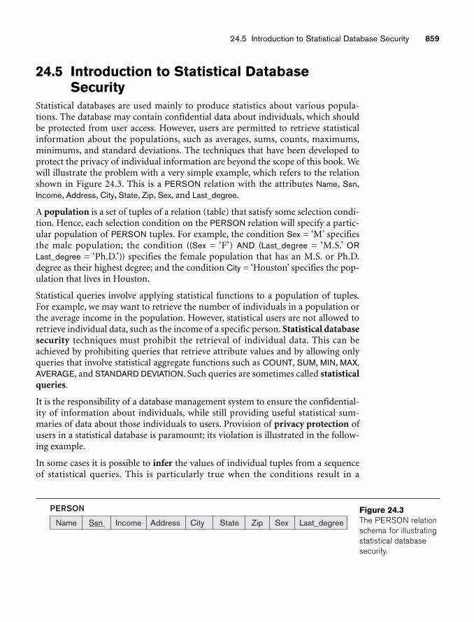
24.5 Introduction to Statistical Database Security 859
24.5 Introduction to Statistical DatabaseSecurity
Statistical databases are used mainly to produce statistics about various popula-tions. The database may contain confidential data about individuals, which shouldbe protected from user access. However, users are permitted to retrieve statisticalinformation about the populations, such as averages, sums, counts, maximums,minimums, and standard deviations. The techniques that have been developed toprotect the privacy of individual information are beyond the scope of this book. Wewill illustrate the problem with a very simple example, which refers to the relationshown in Figure 24.3. This is a PERSON relation with the attributes Name, Ssn,Income, Address, City, State, Zip, Sex, and Last_degree.
A population is a set of tuples of a relation (table) that satisfy some selection condi-tion. Hence, each selection condition on the PERSON relation will specify a partic-ular population of PERSON tuples. For example, the condition Sex = ‘M’ specifiesthe male population; the condition ((Sex = ‘F’) AND (Last_degree = ‘M.S.’ ORLast_degree = ‘Ph.D.’)) specifies the female population that has an M.S. or Ph.D.degree as their highest degree; and the condition City = ‘Houston’ specifies the pop-ulation that lives in Houston.
Statistical queries involve applying statistical functions to a population of tuples.For example, we may want to retrieve the number of individuals in a population orthe average income in the population. However, statistical users are not allowed toretrieve individual data, such as the income of a specific person. Statistical databasesecurity techniques must prohibit the retrieval of individual data. This can beachieved by prohibiting queries that retrieve attribute values and by allowing onlyqueries that involve statistical aggregate functions such as COUNT, SUM, MIN, MAX,AVERAGE, and STANDARD DEVIATION. Such queries are sometimes called statisticalqueries.
It is the responsibility of a database management system to ensure the confidential-ity of information about individuals, while still providing useful statistical sum-maries of data about those individuals to users. Provision of privacy protection ofusers in a statistical database is paramount; its violation is illustrated in the follow-ing example.
In some cases it is possible to infer the values of individual tuples from a sequenceof statistical queries. This is particularly true when the conditions result in a
Name Ssn Income Address City State Zip Sex Last_degree
PERSON Figure 24.3The PERSON relationschema for illustratingstatistical databasesecurity.
860 Chapter 24 Database Security
population consisting of a small number of tuples. As an illustration, consider thefollowing statistical queries:
Q1: SELECT COUNT (*) FROM PERSONWHERE <condition>;
Q2: SELECT AVG (Income) FROM PERSONWHERE <condition>;
Now suppose that we are interested in finding the Salary of Jane Smith, and we knowthat she has a Ph.D. degree and that she lives in the city of Bellaire, Texas. We issuethe statistical query Q1 with the following condition:
(Last_degree=‘Ph.D.’ AND Sex=‘F’ AND City=‘Bellaire’ AND State=‘Texas’)
If we get a result of 1 for this query, we can issue Q2 with the same condition andfind the Salary of Jane Smith. Even if the result of Q1 on the preceding condition isnot 1 but is a small number—say 2 or 3—we can issue statistical queries using thefunctions MAX, MIN, and AVERAGE to identify the possible range of values for theSalary of Jane Smith.
The possibility of inferring individual information from statistical queries isreduced if no statistical queries are permitted whenever the number of tuples in thepopulation specified by the selection condition falls below some threshold. Anothertechnique for prohibiting retrieval of individual information is to prohibitsequences of queries that refer repeatedly to the same population of tuples. It is alsopossible to introduce slight inaccuracies or noise into the results of statistical queriesdeliberately, to make it difficult to deduce individual information from the results.Another technique is partitioning of the database. Partitioning implies that recordsare stored in groups of some minimum size; queries can refer to any complete groupor set of groups, but never to subsets of records within a group. The interestedreader is referred to the bibliography at the end of this chapter for a discussion ofthese techniques.
24.6 Introduction to Flow ControlFlow control regulates the distribution or flow of information among accessibleobjects. A flow between object X and object Y occurs when a program reads valuesfrom X and writes values into Y. Flow controls check that information contained insome objects does not flow explicitly or implicitly into less protected objects. Thus, auser cannot get indirectly in Y what he or she cannot get directly in X. Active flowcontrol began in the early 1970s. Most flow controls employ some concept of securityclass; the transfer of information from a sender to a receiver is allowed only if thereceiver’s security class is at least as privileged as the sender’s. Examples of a flow con-trol include preventing a service program from leaking a customer’s confidentialdata, and blocking the transmission of secret military data to an unknown classifieduser.
A flow policy specifies the channels along which information is allowed to move.The simplest flow policy specifies just two classes of information—confidential (C)
24.6 Introduction to Flow Control 861
and nonconfidential (N)—and allows all flows except those from class C to class N.This policy can solve the confinement problem that arises when a service programhandles data such as customer information, some of which may be confidential.For example, an income-tax computing service might be allowed to retain a cus-tomer’s address and the bill for services rendered, but not a customer’s income ordeductions.
Access control mechanisms are responsible for checking users’ authorizations forresource access: Only granted operations are executed. Flow controls can beenforced by an extended access control mechanism, which involves assigning a secu-rity class (usually called the clearance) to each running program. The program isallowed to read a particular memory segment only if its security class is as high asthat of the segment. It is allowed to write in a segment only if its class is as low asthat of the segment. This automatically ensures that no information transmitted bythe person can move from a higher to a lower class. For example, a military programwith a secret clearance can only read from objects that are unclassified and confi-dential and can only write into objects that are secret or top secret.
Two types of flow can be distinguished: explicit flows, occurring as a consequence ofassignment instructions, such as Y:= f(X1,Xn,), and implicit flows generated by con-ditional instructions, such as if f(Xm+1, ..., Xn) then Y:= f (X1,Xm).
Flow control mechanisms must verify that only authorized flows, both explicit andimplicit, are executed. A set of rules must be satisfied to ensure secure informationflows. Rules can be expressed using flow relations among classes and assigned toinformation, stating the authorized flows within a system. (An information flowfrom A to B occurs when information associated with A affects the value of infor-mation associated with B. The flow results from operations that cause informationtransfer from one object to another.) These relations can define, for a class, the set ofclasses where information (classified in that class) can flow, or can state the specificrelations to be verified between two classes to allow information to flow from one tothe other. In general, flow control mechanisms implement the controls by assigninga label to each object and by specifying the security class of the object. Labels arethen used to verify the flow relations defined in the model.
24.6.1 Covert ChannelsA covert channel allows a transfer of information that violates the security or thepolicy. Specifically, a covert channel allows information to pass from a higher clas-sification level to a lower classification level through improper means. Covert chan-nels can be classified into two broad categories: timing channels and storage. Thedistinguishing feature between the two is that in a timing channel the informationis conveyed by the timing of events or processes, whereas storage channels do notrequire any temporal synchronization, in that information is conveyed by accessingsystem information or what is otherwise inaccessible to the user.
In a simple example of a covert channel, consider a distributed database system inwhich two nodes have user security levels of secret (S) and unclassified (U). In order
862 Chapter 24 Database Security
for a transaction to commit, both nodes must agree to commit. They mutually canonly do operations that are consistent with the *-property, which states that in anytransaction, the S site cannot write or pass information to the U site. However, ifthese two sites collude to set up a covert channel between them, a transactioninvolving secret data may be committed unconditionally by the U site, but the S sitemay do so in some predefined agreed-upon way so that certain information may bepassed from the S site to the U site, violating the *-property. This may be achievedwhere the transaction runs repeatedly, but the actions taken by the S site implicitlyconvey information to the U site. Measures such as locking, which we discussed inChapters 22 and 23, prevent concurrent writing of the information by users withdifferent security levels into the same objects, preventing the storage-type covertchannels. Operating systems and distributed databases provide control over themultiprogramming of operations that allows a sharing of resources without thepossibility of encroachment of one program or process into another’s memory orother resources in the system, thus preventing timing-oriented covert channels. Ingeneral, covert channels are not a major problem in well-implemented robust data-base implementations. However, certain schemes may be contrived by clever usersthat implicitly transfer information.
Some security experts believe that one way to avoid covert channels is to disallowprogrammers to actually gain access to sensitive data that a program will processafter the program has been put into operation. For example, a programmer for abank has no need to access the names or balances in depositors’ accounts.Programmers for brokerage firms do not need to know what buy and sell ordersexist for clients. During program testing, access to a form of real data or some sam-ple test data may be justifiable, but not after the program has been accepted for reg-ular use.
24.7 Encryption and Public Key Infrastructures
The previous methods of access and flow control, despite being strong controlmeasures, may not be able to protect databases from some threats. Suppose we com-municate data, but our data falls into the hands of a nonlegitimate user. In this situ-ation, by using encryption we can disguise the message so that even if thetransmission is diverted, the message will not be revealed. Encryption is the conver-sion of data into a form, called a ciphertext, which cannot be easily understood byunauthorized persons. It enhances security and privacy when access controls arebypassed, because in cases of data loss or theft, encrypted data cannot be easilyunderstood by unauthorized persons.
With this background, we adhere to following standard definitions:6
■ Ciphertext: Encrypted (enciphered) data.
6These definitions are from NIST (National Institute of Standards and Technology) from http://csrc.nist.gov/publications/nistpubs/800-67/SP800-67.pdf.
24.7 Encryption and Public Key Infrastructures 863
■ Plaintext (or cleartext): Intelligible data that has meaning and can be read oracted upon without the application of decryption.
■ Encryption: The process of transforming plaintext into ciphertext.
■ Decryption: The process of transforming ciphertext back into plaintext.
Encryption consists of applying an encryption algorithm to data using some pre-specified encryption key. The resulting data has to be decrypted using adecryption key to recover the original data.
24.7.1 The Data Encryption and Advanced Encryption Standards
The Data Encryption Standard (DES) is a system developed by the U.S. govern-ment for use by the general public. It has been widely accepted as a cryptographicstandard both in the United States and abroad. DES can provide end-to-endencryption on the channel between sender A and receiver B. The DES algorithm is acareful and complex combination of two of the fundamental building blocks ofencryption: substitution and permutation (transposition). The algorithm derives itsstrength from repeated application of these two techniques for a total of 16 cycles.Plaintext (the original form of the message) is encrypted as blocks of 64 bits.Although the key is 64 bits long, in effect the key can be any 56-bit number. Afterquestioning the adequacy of DES, the NIST introduced the Advanced EncryptionStandard (AES). This algorithm has a block size of 128 bits, compared with DES’s56-block size, and can use keys of 128, 192, or 256 bits, compared with DES’s 56-bitkey. AES introduces more possible keys, compared with DES, and thus takes a muchlonger time to crack.
24.7.2 Symmetric Key AlgorithmsA symmetric key is one key that is used for both encryption and decryption. Byusing a symmetric key, fast encryption and decryption is possible for routine usewith sensitive data in the database. A message encrypted with a secret key can bedecrypted only with the same secret key. Algorithms used for symmetric key encryption are called secret-key algorithms. Since secret-key algorithms aremostly used for encrypting the content of a message, they are also called content-encryption algorithms.
The major liability associated with secret-key algorithms is the need for sharing thesecret key. A possible method is to derive the secret key from a user-supplied passwordstring by applying the same function to the string at both the sender and receiver; thisis known as a password-based encryption algorithm. The strength of the symmetric keyencryption depends on the size of the key used. For the same algorithm, encryptingusing a longer key is tougher to break than the one using a shorter key.
24.7.3 Public (Asymmetric) Key Encryption In 1976, Diffie and Hellman proposed a new kind of cryptosystem, which theycalled public key encryption. Public key algorithms are based on mathematical
864 Chapter 24 Database Security
functions rather than operations on bit patterns. They address one drawback ofsymmetric key encryption, namely that both sender and recipient must exchangethe common key in a secure manner. In public key systems, two keys are used forencryption/decryption. The public key can be transmitted in a non-secure way,whereas the private key is not transmitted at all. These algorithms—which use tworelated keys, a public key and a private key, to perform complementary operations(encryption and decryption)—are known as asymmetric key encryption algo-rithms. The use of two keys can have profound consequences in the areas of confi-dentiality, key distribution, and authentication. The two keys used for public keyencryption are referred to as the public key and the private key. The private key iskept secret, but it is referred to as a private key rather than a secret key (the key usedin conventional encryption) to avoid confusion with conventional encryption. Thetwo keys are mathematically related, since one of the keys is used to performencryption and the other to perform decryption. However, it is very difficult toderive the private key from the public key.
A public key encryption scheme, or infrastructure, has six ingredients:
1. Plaintext. This is the data or readable message that is fed into the algorithmas input.
2. Encryption algorithm. This algorithm performs various transformationson the plaintext.
3. and 4. Public and private keys. These are a pair of keys that have beenselected so that if one is used for encryption, the other is used for decryp-tion. The exact transformations performed by the encryption algorithmdepend on the public or private key that is provided as input. For example, ifa message is encrypted using the public key, it can only be decrypted usingthe private key.
5. Ciphertext. This is the scrambled message produced as output. It dependson the plaintext and the key. For a given message, two different keys will pro-duce two different ciphertexts.
6. Decryption algorithm. This algorithm accepts the ciphertext and thematching key and produces the original plaintext.
As the name suggests, the public key of the pair is made public for others to use,whereas the private key is known only to its owner. A general-purpose public keycryptographic algorithm relies on one key for encryption and a different but relatedkey for decryption. The essential steps are as follows:
1. Each user generates a pair of keys to be used for the encryption and decryp-tion of messages.
2. Each user places one of the two keys in a public register or other accessiblefile. This is the public key. The companion key is kept private.
3. If a sender wishes to send a private message to a receiver, the sender encryptsthe message using the receiver’s public key.
24.7 Encryption and Public Key Infrastructures 865
4. When the receiver receives the message, he or she decrypts it using thereceiver’s private key. No other recipient can decrypt the message becauseonly the receiver knows his or her private key.
The RSA Public Key Encryption Algorithm. One of the first public key schemeswas introduced in 1978 by Ron Rivest, Adi Shamir, and Len Adleman at MIT and isnamed after them as the RSA scheme. The RSA scheme has since then reignedsupreme as the most widely accepted and implemented approach to public keyencryption. The RSA encryption algorithm incorporates results from number the-ory, combined with the difficulty of determining the prime factors of a target. TheRSA algorithm also operates with modular arithmetic—mod n.
Two keys, d and e, are used for decryption and encryption. An important property isthat they can be interchanged. n is chosen as a large integer that is a product of twolarge distinct prime numbers, a and b, n = a × b. The encryption key e is a randomlychosen number between 1 and n that is relatively prime to (a – 1) × (b – 1). Theplaintext block P is encrypted as Pe where Pe = P mod n. Because the exponentiationis performed mod n, factoring Pe to uncover the encrypted plaintext is difficult.However, the decrypting key d is carefully chosen so that (Pe)d mod n = P. Thedecryption key d can be computed from the condition that d × e = 1 mod ((a – 1) ×(b – 1)). Thus, the legitimate receiver who knows d simply computes (Pe)d mod n =P and recovers P without having to factor Pe.
24.7.4 Digital SignaturesA digital signature is an example of using encryption techniques to provide authen-tication services in electronic commerce applications. Like a handwritten signature,a digital signature is a means of associating a mark unique to an individual with abody of text. The mark should be unforgettable, meaning that others should be ableto check that the signature comes from the originator.
A digital signature consists of a string of symbols. If a person’s digital signature werealways the same for each message, then one could easily counterfeit it by simplycopying the string of symbols. Thus, signatures must be different for each use. Thiscan be achieved by making each digital signature a function of the message that it issigning, together with a timestamp. To be unique to each signer and counterfeit-proof, each digital signature must also depend on some secret number that isunique to the signer. Thus, in general, a counterfeitproof digital signature mustdepend on the message and a unique secret number of the signer. The verifier of thesignature, however, should not need to know any secret number. Public key tech-niques are the best means of creating digital signatures with these properties.
24.7.5 Digital CertificatesA digital certificate is used to combine the value of a public key with the identity ofthe person or service that holds the corresponding private key into a digitally signed
866 Chapter 24 Database Security
statement. Certificates are issued and signed by a certification authority (CA). Theentity receiving this certificate from a CA is the subject of that certificate. Instead ofrequiring each participant in an application to authenticate every user, third-partyauthentication relies on the use of digital certificates.
The digital certificate itself contains various types of information. For example,both the certification authority and the certificate owner information are included.The following list describes all the information included in the certificate:
1. The certificate owner information, which is represented by a unique identi-fier known as the distinguished name (DN) of the owner. This includes theowner’s name, as well as the owner’s organization and other informationabout the owner.
2. The certificate also includes the public key of the owner.
3. The date of issue of the certificate is also included.
4. The validity period is specified by ‘Valid From’ and ‘Valid To’ dates, which areincluded in each certificate.
5. Issuer identifier information is included in the certificate.
6. Finally, the digital signature of the issuing CA for the certificate is included.All the information listed is encoded through a message-digest function,which creates the digital signature. The digital signature basically certifiesthat the association between the certificate owner and public key is valid.
24.8 Privacy Issues and PreservationPreserving data privacy is a growing challenge for database security and privacyexperts. In some perspectives, to preserve data privacy we should even limit per-forming large-scale data mining and analysis. The most commonly used techniquesto address this concern are to avoid building mammoth central warehouses as a sin-gle repository of vital information. Another possible measure is to intentionallymodify or perturb data.
If all data were available at a single warehouse, violating only a single repository’ssecurity could expose all data. Avoiding central warehouses and using distributeddata mining algorithms minimizes the exchange of data needed to develop globallyvalid models. By modifying, perturbing, and anonymizing data, we can also miti-gate privacy risks associated with data mining. This can be done by removing iden-tity information from the released data and injecting noise into the data. However,by using these techniques, we should pay attention to the quality of the resultingdata in the database, which may undergo too many modifications. We must be ableto estimate the errors that may be introduced by these modifications.
Privacy is an important area of ongoing research in database management. It iscomplicated due to its multidisciplinary nature and the issues related to the subjec-tivity in the interpretation of privacy, trust, and so on. As an example, considermedical and legal records and transactions, which must maintain certain privacy
24.9 Challenges of Database Security 867
requirements while they are being defined and enforced. Providing access controland privacy for mobile devices is also receiving increased attention. DBMSs needrobust techniques for efficient storage of security-relevant information on smalldevices, as well as trust negotiation techniques. Where to keep information relatedto user identities, profiles, credentials, and permissions and how to use it for reliableuser identification remains an important problem. Because large-sized streams ofdata are generated in such environments, efficient techniques for access controlmust be devised and integrated with processing techniques for continuous queries.Finally, the privacy of user location data, acquired from sensors and communica-tion networks, must be ensured.
24.9 Challenges of Database SecurityConsidering the vast growth in volume and speed of threats to databases and infor-mation assets, research efforts need to be devoted to the following issues: data qual-ity, intellectual property rights, and database survivability. These are only some ofthe main challenges that researchers in database security are trying to address.
24.9.1 Data QualityThe database community needs techniques and organizational solutions to assessand attest the quality of data. These techniques may include simple mechanismssuch as quality stamps that are posted on Web sites. We also need techniques thatprovide more effective integrity semantics verification and tools for the assessmentof data quality, based on techniques such as record linkage. Application-level recov-ery techniques are also needed for automatically repairing incorrect data. The ETL(extract, transform, load) tools widely used to load data in data warehouses (seeSection 29.4) are presently grappling with these issues.
24.9.2 Intellectual Property RightsWith the widespread use of the Internet and intranets, legal and informationalaspects of data are becoming major concerns of organizations. To address theseconcerns, watermarking techniques for relational data have been proposed. Themain purpose of digital watermarking is to protect content from unauthorizedduplication and distribution by enabling provable ownership of the content. It hastraditionally relied upon the availability of a large noise domain within which theobject can be altered while retaining its essential properties. However, research isneeded to assess the robustness of such techniques and to investigate differentapproaches aimed at preventing intellectual property rights violations.
24.9.3 Database SurvivabilityDatabase systems need to operate and continue their functions, even with reducedcapabilities, despite disruptive events such as information warfare attacks. A DBMS,
868 Chapter 24 Database Security
in addition to making every effort to prevent an attack and detecting one in theevent of occurrence, should be able to do the following:
■ Confinement. Take immediate action to eliminate the attacker’s access to thesystem and to isolate or contain the problem to prevent further spread.
■ Damage assessment. Determine the extent of the problem, including failedfunctions and corrupted data.
■ Reconfiguration. Reconfigure to allow operation to continue in a degradedmode while recovery proceeds.
■ Repair. Recover corrupted or lost data and repair or reinstall failed systemfunctions to reestablish a normal level of operation.
■ Fault treatment. To the extent possible, identify the weaknesses exploited inthe attack and take steps to prevent a recurrence.
The goal of the information warfare attacker is to damage the organization’s opera-tion and fulfillment of its mission through disruption of its information systems.The specific target of an attack may be the system itself or its data. While attacks thatbring the system down outright are severe and dramatic, they must also be welltimed to achieve the attacker’s goal, since attacks will receive immediate and con-centrated attention in order to bring the system back to operational condition, diag-nose how the attack took place, and install preventive measures.
To date, issues related to database survivability have not been sufficiently investi-gated. Much more research needs to be devoted to techniques and methodologiesthat ensure database system survivability.
24.10 Oracle Label-Based Security Restricting access to entire tables or isolating sensitive data into separate databases isa costly operation to administer. Oracle Label Security overcomes the need for suchmeasures by enabling row-level access control. It is available in Oracle Database 11gRelease 1 (11.1) Enterprise Edition at the time of writing. Each database table orview has a security policy associated with it. This policy executes every time thetable or view is queried or altered. Developers can readily add label-based accesscontrol to their Oracle Database applications. Label-based security provides anadaptable way of controlling access to sensitive data. Both users and data have labelsassociated with them. Oracle Label Security uses these labels to provide security.
24.10.1 Virtual Private Database (VPD) TechnologyVirtual Private Databases (VPDs) is a feature of the Oracle Enterprise Edition thatadds predicates to user statements to limit their access in a transparent manner tothe user and the application. The VPD concept allows server-enforced, fine-grainedaccess control for a secure application.
VPD provides access control based on policies. These VPD policies enforce object-level access control or row-level security. It provides an application programming
24.10 Oracle Label-Based Security 869
interface (API) that allows security policies to be attached to database tables orviews. Using PL/SQL, a host programming language used in Oracle applications,developers and security administrators can implement security policies with thehelp of stored procedures.7 VPD policies allow developers to remove access securitymechanisms from applications and centralize them within the Oracle Database.
VPD is enabled by associating a security “policy” with a table, view, or synonym. Anadministrator uses the supplied PL/SQL package, DBMS_RLS, to bind a policyfunction with a database object. When an object having a security policy associatedwith it is accessed, the function implementing this policy is consulted. The policyfunction returns a predicate (a WHERE clause) which is then appended to the user’sSQL statement, thus transparently and dynamically modifying the user’s data access.Oracle Label Security is a technique of enforcing row-level security in the form of asecurity policy.
24.10.2 Label Security ArchitectureOracle Label Security is built on the VPD technology delivered in the OracleDatabase 11.1 Enterprise Edition. Figure 24.4 illustrates how data is accessed underOracle Label Security, showing the sequence of DAC and label security checks.
Figure 24.4 shows the sequence of discretionary access control (DAC) and labelsecurity checks. The left part of the figure shows an application user in an OracleDatabase 11g Release 1 (11.1) session sending out an SQL request. The OracleDBMS checks the DAC privileges of the user, making sure that he or she has SELECTprivileges on the table. Then it checks whether the table has a Virtual PrivateDatabase (VPD) policy associated with it to determine if the table is protected usingOracle Label Security. If it is, the VPD SQL modification (WHERE clause) is addedto the original SQL statement to find the set of accessible rows for the user to view.Then Oracle Label Security checks the labels on each row, to determine the subset ofrows to which the user has access (as explained in the next section). This modifiedquery gets processed, optimized, and executed.
24.10.3 How Data Labels and User Labels Work TogetherA user’s label indicates the information the user is permitted to access. It also deter-mines the type of access (read or write) that the user has on that information. Arow’s label shows the sensitivity of the information that the row contains as well asthe ownership of the information. When a table in the database has a label-basedaccess associated with it, a row can be accessed only if the user’s label meet certaincriteria defined in the policy definitions. Access is granted or denied based on theresult of comparing the data label and the session label of the user.
Compartments allow a finer classification of sensitivity of the labeled data. All datarelated to the same project can be labeled with the same compartment.Compartments are optional; a label can contain zero or more compartments.
7Stored procedures are discussed in Section 5.2.2.
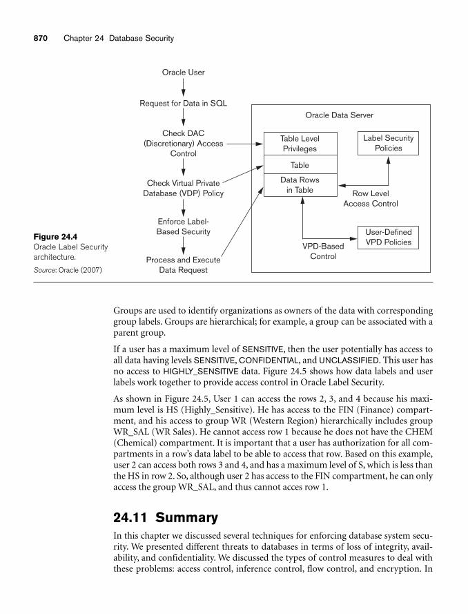
870 Chapter 24 Database Security
Oracle User
Request for Data in SQL
Check DAC(Discretionary) Access
Control
Check Virtual PrivateDatabase (VDP) Policy
Process and ExecuteData Request
Enforce Label-Based Security
Oracle Data Server
Table LevelPrivileges
Table
Data Rowsin Table
Label SecurityPolicies
Row LevelAccess Control
VPD-BasedControl
User-DefinedVPD Policies
Figure 24.4Oracle Label Securityarchitecture.
Source: Oracle (2007)
Groups are used to identify organizations as owners of the data with correspondinggroup labels. Groups are hierarchical; for example, a group can be associated with aparent group.
If a user has a maximum level of SENSITIVE, then the user potentially has access toall data having levels SENSITIVE, CONFIDENTIAL, and UNCLASSIFIED. This user hasno access to HIGHLY_SENSITIVE data. Figure 24.5 shows how data labels and userlabels work together to provide access control in Oracle Label Security.
As shown in Figure 24.5, User 1 can access the rows 2, 3, and 4 because his maxi-mum level is HS (Highly_Sensitive). He has access to the FIN (Finance) compart-ment, and his access to group WR (Western Region) hierarchically includes groupWR_SAL (WR Sales). He cannot access row 1 because he does not have the CHEM(Chemical) compartment. It is important that a user has authorization for all com-partments in a row’s data label to be able to access that row. Based on this example,user 2 can access both rows 3 and 4, and has a maximum level of S, which is less thanthe HS in row 2. So, although user 2 has access to the FIN compartment, he can onlyaccess the group WR_SAL, and thus cannot acces row 1.
24.11 SummaryIn this chapter we discussed several techniques for enforcing database system secu-rity. We presented different threats to databases in terms of loss of integrity, avail-ability, and confidentiality. We discussed the types of control measures to deal withthese problems: access control, inference control, flow control, and encryption. In
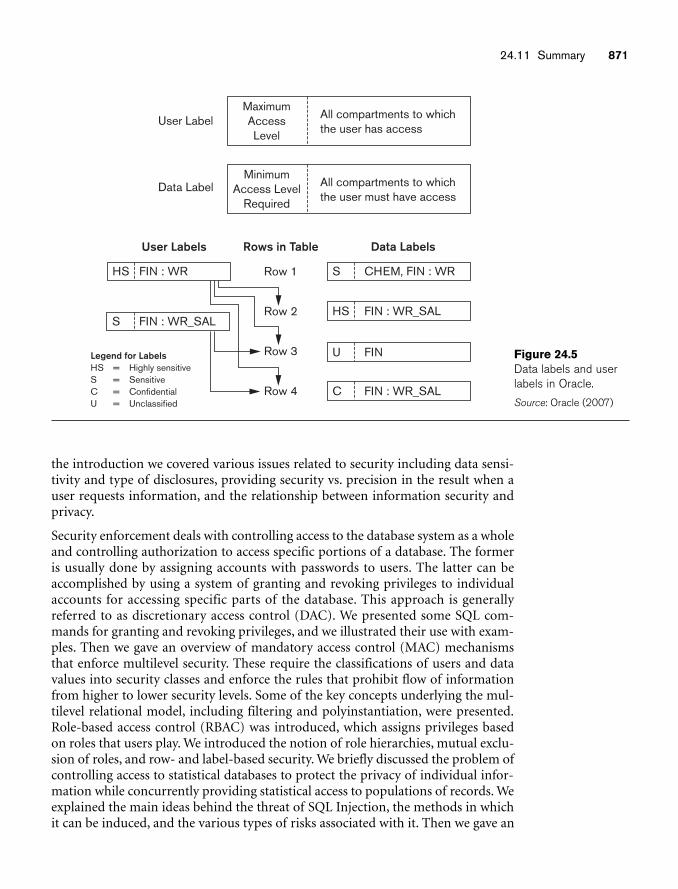
24.11 Summary 871
User Labels
HS FIN : WR
S FIN : WR_SAL
Legend for LabelsHS = Highly sensitiveS = SensitiveC = ConfidentialU = Unclassified
MaximumAccessLevel
All compartments to which the user has access
MinimumAccess Level
Required
All compartments to which the user must have access
User Label
Data Label
Rows in Table Data Labels
Row 1
Row 2
Row 3
Row 4
S CHEM, FIN : WR
HS FIN : WR_SAL
U FIN
C FIN : WR_SAL
Figure 24.5Data labels and userlabels in Oracle.
Source: Oracle (2007)
the introduction we covered various issues related to security including data sensi-tivity and type of disclosures, providing security vs. precision in the result when auser requests information, and the relationship between information security andprivacy.
Security enforcement deals with controlling access to the database system as a wholeand controlling authorization to access specific portions of a database. The formeris usually done by assigning accounts with passwords to users. The latter can beaccomplished by using a system of granting and revoking privileges to individualaccounts for accessing specific parts of the database. This approach is generallyreferred to as discretionary access control (DAC). We presented some SQL com-mands for granting and revoking privileges, and we illustrated their use with exam-ples. Then we gave an overview of mandatory access control (MAC) mechanismsthat enforce multilevel security. These require the classifications of users and datavalues into security classes and enforce the rules that prohibit flow of informationfrom higher to lower security levels. Some of the key concepts underlying the mul-tilevel relational model, including filtering and polyinstantiation, were presented.Role-based access control (RBAC) was introduced, which assigns privileges basedon roles that users play. We introduced the notion of role hierarchies, mutual exclu-sion of roles, and row- and label-based security. We briefly discussed the problem ofcontrolling access to statistical databases to protect the privacy of individual infor-mation while concurrently providing statistical access to populations of records. Weexplained the main ideas behind the threat of SQL Injection, the methods in whichit can be induced, and the various types of risks associated with it. Then we gave an
872 Chapter 24 Database Security
idea of the various ways SQL injection can be prevented. The issues related to flowcontrol and the problems associated with covert channels were discussed next, aswell as encryption and public-private key-based infrastructures. The idea of sym-metric key algorithms and the use of the popular asymmetric key-based public keyinfrastructure (PKI) scheme was explained. We also covered the concepts of digitalsignatures and digital certificates. We highlighted the importance of privacy issuesand hinted at some privacy preservation techniques. We discussed a variety of chal-lenges to security including data quality, intellectual property rights, and data sur-vivability. We ended the chapter by introducing the implementation of securitypolicies by using a combination of label-based security and virtual private databasesin Oracle 11g.
Review Questions24.1. Discuss what is meant by each of the following terms: database authoriza-
tion, access control, data encryption, privileged (system) account, databaseaudit, audit trail.
24.2. Which account is designated as the owner of a relation? What privileges doesthe owner of a relation have?
24.3. How is the view mechanism used as an authorization mechanism?
24.4. Discuss the types of privileges at the account level and those at the relationlevel.
24.5. What is meant by granting a privilege? What is meant by revoking a privilege?
24.6. Discuss the system of propagation of privileges and the restraints imposedby horizontal and vertical propagation limits.
24.7. List the types of privileges available in SQL.
24.8. What is the difference between discretionary and mandatory access control?
24.9. What are the typical security classifications? Discuss the simple securityproperty and the *-property, and explain the justification behind these rulesfor enforcing multilevel security.
24.10. Describe the multilevel relational data model. Define the following terms:apparent key, polyinstantiation, filtering.
24.11. What are the relative merits of using DAC or MAC?
24.12. What is role-based access control? In what ways is it superior to DAC andMAC?
24.13. What are the two types of mutual exclusion in role-based access control?
24.14. What is meant by row-level access control?
24.15. What is label security? How does an administrator enforce it?
Exercises 873
24.16. What are the different types of SQL injection attacks?
24.17. What risks are associated with SQL injection attacks?
24.18. What preventive measures are possible against SQL injection attacks?
24.19. What is a statistical database? Discuss the problem of statistical databasesecurity.
24.20. How is privacy related to statistical database security? What measures can betaken to ensure some degree of privacy in statistical databases?
24.21. What is flow control as a security measure? What types of flow control exist?
24.22. What are covert channels? Give an example of a covert channel.
24.23. What is the goal of encryption? What process is involved in encrypting dataand then recovering it at the other end?
24.24. Give an example of an encryption algorithm and explain how it works.
24.25. Repeat the previous question for the popular RSA algorithm.
24.26. What is a symmetric key algorithm for key-based security?
24.27. What is the public key infrastructure scheme? How does it provide security?
24.28. What are digital signatures? How do they work?
24.29. What type of information does a digital certificate include?
Exercises24.30. How can privacy of data be preserved in a database?
24.31. What are some of the current outstanding challenges for database security?
24.32. Consider the relational database schema in Figure 3.5. Suppose that all therelations were created by (and hence are owned by) user X, who wants togrant the following privileges to user accounts A, B, C, D, and E:
a. Account A can retrieve or modify any relation except DEPENDENT andcan grant any of these privileges to other users.
b. Account B can retrieve all the attributes of EMPLOYEE and DEPARTMENTexcept for Salary, Mgr_ssn, and Mgr_start_date.
c. Account C can retrieve or modify WORKS_ON but can only retrieve theFname, Minit, Lname, and Ssn attributes of EMPLOYEE and the Pname andPnumber attributes of PROJECT.
d. Account D can retrieve any attribute of EMPLOYEE or DEPENDENT andcan modify DEPENDENT.
e. Account E can retrieve any attribute of EMPLOYEE but only forEMPLOYEE tuples that have Dno = 3.
f. Write SQL statements to grant these privileges. Use views where appropriate.
874 Chapter 24 Database Security
24.33. Suppose that privilege (a) of Exercise 24.32 is to be given with GRANTOPTION but only so that account A can grant it to at most five accounts, andeach of these accounts can propagate the privilege to other accounts butwithout the GRANT OPTION privilege. What would the horizontal and verti-cal propagation limits be in this case?
24.34. Consider the relation shown in Figure 24.2(d). How would it appear to auser with classification U? Suppose that a classification U user tries to updatethe salary of ‘Smith’ to $50,000; what would be the result of this action?
Selected BibliographyAuthorization based on granting and revoking privileges was proposed for the SYSTEM R experimental DBMS and is presented in Griffiths and Wade (1976).Several books discuss security in databases and computer systems in general,including the books by Leiss (1982a) and Fernandez et al. (1981), and Fugini et al.(1995). Natan (2005) is a practical book on security and auditing implementationissues in all major RDBMSs.
Many papers discuss different techniques for the design and protection of statisticaldatabases. They include McLeish (1989), Chin and Ozsoyoglu (1981), Leiss (1982),Wong (1984), and Denning (1980). Ghosh (1984) discusses the use of statisticaldatabases for quality control. There are also many papers discussing cryptographyand data encryption, including Diffie and Hellman (1979), Rivest et al. (1978), Akl(1983), Pfleeger and Pfleeger (2007), Omura et al. (1990), Stallings (2000), and Iyerat al. (2004).
Halfond et al. (2006) helps understand the concepts of SQL injection attacks andthe various threats imposed by them. The white paper Oracle (2007a) explains howOracle is less prone to SQL injection attack as compared to SQL Server. It also givesa brief explanation as to how these attacks can be prevented from occurring.Further proposed frameworks are discussed in Boyd and Keromytis (2004), Halfondand Orso (2005), and McClure and Krüger (2005).
Multilevel security is discussed in Jajodia and Sandhu (1991), Denning et al. (1987),Smith and Winslett (1992), Stachour and Thuraisingham (1990), Lunt et al. (1990),and Bertino et al. (2001). Overviews of research issues in database security are givenby Lunt and Fernandez (1990), Jajodia and Sandhu (1991), Bertino (1998), Castanoet al. (1995), and Thuraisingham et al. (2001). The effects of multilevel security onconcurrency control are discussed in Atluri et al. (1997). Security in next-generation,semantic, and object-oriented databases is discussed in Rabbiti et al. (1991), Jajodiaand Kogan (1990), and Smith (1990). Oh (1999) presents a model for both discre-tionary and mandatory security. Security models for Web-based applications androle-based access control are discussed in Joshi et al. (2001). Security issues for man-agers in the context of e-commerce applications and the need for risk assessmentmodels for selection of appropriate security control measures are discussed in
Selected Bibliography 875
Farahmand et al. (2005). Row-level access control is explained in detail in Oracle(2007b) and Sybase (2005). The latter also provides details on role hierarchy andmutual exclusion. Oracle (2009) explains how Oracle uses the concept of identitymanagement.
Recent advances as well as future challenges for security and privacy of databases arediscussed in Bertino and Sandhu (2005). U.S. Govt. (1978), OECD (1980), and NRC(2003) are good references on the view of privacy by important government bodies.Karat et al. (2009) discusses a policy framework for security and privacy. XML andaccess control are discussed in Naedele (2003). More details can be found on privacypreserving techniques in Vaidya and Clifton (2004), intellectual property rights inSion et al. (2004), and database survivability in Jajodia et al. (1999). Oracle’s VPDtechnology and label-based security is discussed in more detail in Oracle (2007b).
877
Distributed Databases
In this chapter we turn our attention to distributeddatabases (DDBs), distributed database management
systems (DDBMSs), and how the client-server architecture is used as a platform fordatabase application development. Distributed databases bring the advantages ofdistributed computing to the database management domain. A distributed com-puting system consists of a number of processing elements, not necessarily homo-geneous, that are interconnected by a computer network, and that cooperate inperforming certain assigned tasks. As a general goal, distributed computing systemspartition a big, unmanageable problem into smaller pieces and solve it efficiently ina coordinated manner. The economic viability of this approach stems from two rea-sons: more computing power is harnessed to solve a complex task, and eachautonomous processing element can be managed independently to develop its ownapplications.
DDB technology resulted from a merger of two technologies: database technology,and network and data communication technology. Computer networks allow dis-tributed processing of data. Traditional databases, on the other hand, focus on pro-viding centralized, controlled access to data. Distributed databases allow anintegration of information and its processing by applications that may themselvesbe centralized or distributed.
Several distributed database prototype systems were developed in the 1980s toaddress the issues of data distribution, distributed query and transaction process-ing, distributed database metadata management, and other topics. However, a full-scale comprehensive DDBMS that implements the functionality and techniquesproposed in DDB research never emerged as a commercially viable product. Mostmajor vendors redirected their efforts from developing a pure DDBMS product intodeveloping systems based on client-server concepts, or toward developing technolo-gies for accessing distributed heterogeneous data sources.
25chapter 25
878 Chapter 25 Distributed Databases
Organizations continue to be interested in the decentralization of processing (at thesystem level) while achieving an integration of the information resources (at the log-ical level) within their geographically distributed systems of databases, applications,and users. There is now a general endorsement of the client-server approach toapplication development, and the three-tier approach to Web applications develop-ment (see Section 2.5).
In this chapter we discuss distributed databases, their architectural variations, andconcepts central to data distribution and the management of distributed data.Details of the advances in communication technologies facilitating the develop-ment of DDBs are outside the scope of this book; see the texts on data communica-tions and networking listed in the Selected Bibliography at the end of this chapter.
Section 25.1 introduces distributed database management and related concepts.Sections 25.2 and 25.3 introduce different types of distributed database systems andtheir architectures, including federated and multidatabase systems. The problems ofheterogeneity and the needs of autonomy in federated database systems are alsohighlighted. Detailed issues of distributed database design, involving fragmenting ofdata and distributing it over multiple sites with possible replication, are discussed inSection 25.4. Sections 25.5 and 25.6 introduce distributed database query and trans-action processing techniques, respectively. Section 25.7 gives an overview of theconcurrency control and recovery in distributed databases. Section 25.8 discussescatalog management schemes in distributed databases. In Section 25.9, we brieflydiscuss current trends in distributed databases such as cloud computing and peer-to-peer databases. Section 25.10 discusses distributed database features of theOracle RDBMS. Section 25.11 summarizes the chapter.
For a short introduction to the topic of distributed databases, Sections 25.1, 25.2,and 25.3 may be covered.
25.1 Distributed Database Concepts1
We can define a distributed database (DDB) as a collection of multiple logicallyinterrelated databases distributed over a computer network, and a distributed data-base management system (DDBMS) as a software system that manages a distrib-uted database while making the distribution transparent to the user.2
Distributed databases are different from Internet Web files. Web pages are basicallya very large collection of files stored on different nodes in a network—theInternet—with interrelationships among the files represented via hyperlinks. Thecommon functions of database management, including uniform query processingand transaction processing, do not apply to this scenario yet. The technology is,however, moving in a direction such that distributed World Wide Web (WWW)databases will become a reality in the future. We have discussed some of the issues of
1The substantial contribution of Narasimhan Srinivasan to this and several other sections in this chapteris appreciated.2This definition and discussions in this section are based largely on Ozsu and Valduriez (1999).
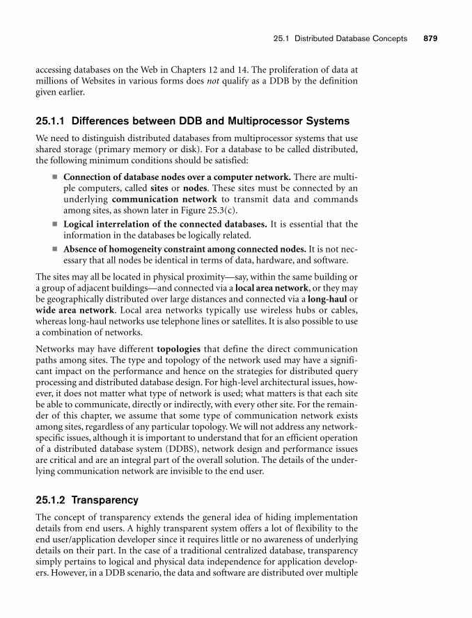
25.1 Distributed Database Concepts 879
accessing databases on the Web in Chapters 12 and 14. The proliferation of data atmillions of Websites in various forms does not qualify as a DDB by the definitiongiven earlier.
25.1.1 Differences between DDB and Multiprocessor SystemsWe need to distinguish distributed databases from multiprocessor systems that useshared storage (primary memory or disk). For a database to be called distributed,the following minimum conditions should be satisfied:
■ Connection of database nodes over a computer network. There are multi-ple computers, called sites or nodes. These sites must be connected by anunderlying communication network to transmit data and commandsamong sites, as shown later in Figure 25.3(c).
■ Logical interrelation of the connected databases. It is essential that theinformation in the databases be logically related.
■ Absence of homogeneity constraint among connected nodes. It is not nec-essary that all nodes be identical in terms of data, hardware, and software.
The sites may all be located in physical proximity—say, within the same building ora group of adjacent buildings—and connected via a local area network, or they maybe geographically distributed over large distances and connected via a long-haul orwide area network. Local area networks typically use wireless hubs or cables,whereas long-haul networks use telephone lines or satellites. It is also possible to usea combination of networks.
Networks may have different topologies that define the direct communicationpaths among sites. The type and topology of the network used may have a signifi-cant impact on the performance and hence on the strategies for distributed queryprocessing and distributed database design. For high-level architectural issues, how-ever, it does not matter what type of network is used; what matters is that each sitebe able to communicate, directly or indirectly, with every other site. For the remain-der of this chapter, we assume that some type of communication network existsamong sites, regardless of any particular topology. We will not address any network-specific issues, although it is important to understand that for an efficient operationof a distributed database system (DDBS), network design and performance issuesare critical and are an integral part of the overall solution. The details of the under-lying communication network are invisible to the end user.
25.1.2 TransparencyThe concept of transparency extends the general idea of hiding implementationdetails from end users. A highly transparent system offers a lot of flexibility to theend user/application developer since it requires little or no awareness of underlyingdetails on their part. In the case of a traditional centralized database, transparencysimply pertains to logical and physical data independence for application develop-ers. However, in a DDB scenario, the data and software are distributed over multiple
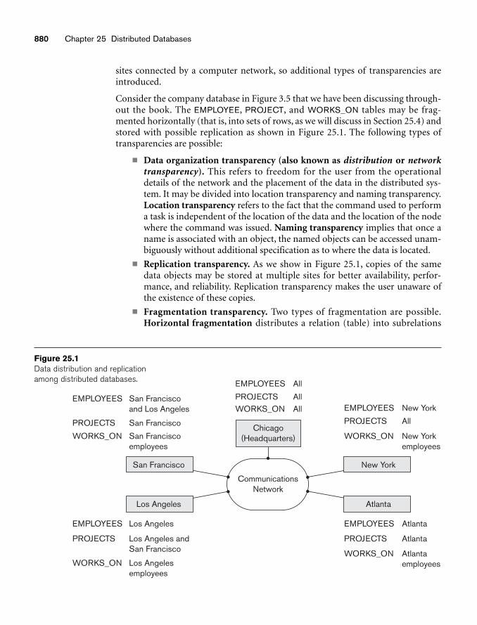
880 Chapter 25 Distributed Databases
sites connected by a computer network, so additional types of transparencies areintroduced.
Consider the company database in Figure 3.5 that we have been discussing through-out the book. The EMPLOYEE, PROJECT, and WORKS_ON tables may be frag-mented horizontally (that is, into sets of rows, as we will discuss in Section 25.4) andstored with possible replication as shown in Figure 25.1. The following types oftransparencies are possible:
■ Data organization transparency (also known as distribution or networktransparency). This refers to freedom for the user from the operationaldetails of the network and the placement of the data in the distributed sys-tem. It may be divided into location transparency and naming transparency.Location transparency refers to the fact that the command used to performa task is independent of the location of the data and the location of the nodewhere the command was issued. Naming transparency implies that once aname is associated with an object, the named objects can be accessed unam-biguously without additional specification as to where the data is located.
■ Replication transparency. As we show in Figure 25.1, copies of the samedata objects may be stored at multiple sites for better availability, perfor-mance, and reliability. Replication transparency makes the user unaware ofthe existence of these copies.
■ Fragmentation transparency. Two types of fragmentation are possible.Horizontal fragmentation distributes a relation (table) into subrelations
EMPLOYEES
PROJECTS WORKS_ON
All
AllAll
EMPLOYEES
PROJECTS
WORKS_ON
San Franciscoand Los Angeles
San Francisco
San Franciscoemployees
EMPLOYEES
PROJECTS
WORKS_ON
Los Angeles
Los Angeles andSan Francisco
Los Angelesemployees
EMPLOYEES
PROJECTS
WORKS_ON
New York
All
New Yorkemployees
EMPLOYEES
PROJECTS
WORKS_ON
Atlanta
Atlanta
Atlanta employees
Chicago(Headquarters)
New York
Los Angeles Atlanta
San Francisco
CommunicationsNetwork
Figure 25.1Data distribution and replicationamong distributed databases.
25.1 Distributed Database Concepts 881
that are subsets of the tuples (rows) in the original relation. Vertical frag-mentation distributes a relation into subrelations where each subrelation isdefined by a subset of the columns of the original relation. A global query bythe user must be transformed into several fragment queries. Fragmentationtransparency makes the user unaware of the existence of fragments.
■ Other transparencies include design transparency and execution trans-parency—referring to freedom from knowing how the distributed databaseis designed and where a transaction executes.
25.1.3 AutonomyAutonomy determines the extent to which individual nodes or DBs in a connectedDDB can operate independently. A high degree of autonomy is desirable forincreased flexibility and customized maintenance of an individual node. Autonomycan be applied to design, communication, and execution. Design autonomy refersto independence of data model usage and transaction management techniquesamong nodes. Communication autonomy determines the extent to which eachnode can decide on sharing of information with other nodes. Execution autonomyrefers to independence of users to act as they please.
25.1.4 Reliability and AvailabilityReliability and availability are two of the most common potential advantages citedfor distributed databases. Reliability is broadly defined as the probability that a sys-tem is running (not down) at a certain time point, whereas availability is the prob-ability that the system is continuously available during a time interval. We candirectly relate reliability and availability of the database to the faults, errors, and fail-ures associated with it. A failure can be described as a deviation of a system’s behav-ior from that which is specified in order to ensure correct execution of operations.Errors constitute that subset of system states that causes the failure. Fault is thecause of an error.
To construct a system that is reliable, we can adopt several approaches. One com-mon approach stresses fault tolerance; it recognizes that faults will occur, anddesigns mechanisms that can detect and remove faults before they can result in asystem failure. Another more stringent approach attempts to ensure that the finalsystem does not contain any faults. This is done through an exhaustive designprocess followed by extensive quality control and testing. A reliable DDBMS toler-ates failures of underlying components and processes user requests so long as data-base consistency is not violated. A DDBMS recovery manager has to deal withfailures arising from transactions, hardware, and communication networks.Hardware failures can either be those that result in loss of main memory contents orloss of secondary storage contents. Communication failures occur due to errorsassociated with messages and line failures. Message errors can include their loss,corruption, or out-of-order arrival at destination.
882 Chapter 25 Distributed Databases
25.1.5 Advantages of Distributed DatabasesOrganizations resort to distributed database management for various reasons.Some important advantages are listed below.
1. Improved ease and flexibility of application development. Developing andmaintaining applications at geographically distributed sites of an organiza-tion is facilitated owing to transparency of data distribution and control.
2. Increased reliability and availability. This is achieved by the isolation offaults to their site of origin without affecting the other databases connectedto the network. When the data and DDBMS software are distributed overseveral sites, one site may fail while other sites continue to operate. Only thedata and software that exist at the failed site cannot be accessed. Thisimproves both reliability and availability. Further improvement is achievedby judiciously replicating data and software at more than one site. In a cen-tralized system, failure at a single site makes the whole system unavailable toall users. In a distributed database, some of the data may be unreachable, butusers may still be able to access other parts of the database. If the data in thefailed site had been replicated at another site prior to the failure, then theuser will not be affected at all.
3. Improved performance. A distributed DBMS fragments the database bykeeping the data closer to where it is needed most. Data localization reducesthe contention for CPU and I/O services and simultaneously reduces accessdelays involved in wide area networks. When a large database is distributedover multiple sites, smaller databases exist at each site. As a result, localqueries and transactions accessing data at a single site have better perfor-mance because of the smaller local databases. In addition, each site has asmaller number of transactions executing than if all transactions are submit-ted to a single centralized database. Moreover, interquery and intraqueryparallelism can be achieved by executing multiple queries at different sites,or by breaking up a query into a number of subqueries that execute in paral-lel. This contributes to improved performance.
4. Easier expansion. In a distributed environment, expansion of the system interms of adding more data, increasing database sizes, or adding more proces-sors is much easier.
The transparencies we discussed in Section 25.1.2 lead to a compromise betweenease of use and the overhead cost of providing transparency. Total transparencyprovides the global user with a view of the entire DDBS as if it is a single centralizedsystem. Transparency is provided as a complement to autonomy, which gives theusers tighter control over local databases. Transparency features may be imple-mented as a part of the user language, which may translate the required services intoappropriate operations. Additionally, transparency impacts the features that mustbe provided by the operating system and the DBMS.
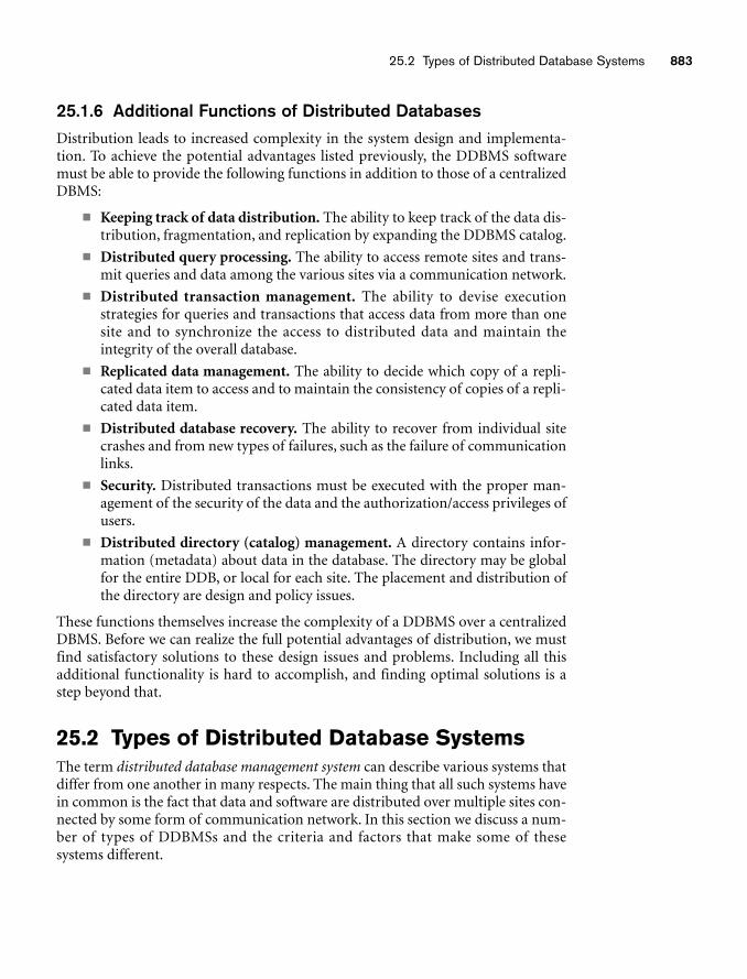
25.2 Types of Distributed Database Systems 883
25.1.6 Additional Functions of Distributed DatabasesDistribution leads to increased complexity in the system design and implementa-tion. To achieve the potential advantages listed previously, the DDBMS softwaremust be able to provide the following functions in addition to those of a centralizedDBMS:
■ Keeping track of data distribution. The ability to keep track of the data dis-tribution, fragmentation, and replication by expanding the DDBMS catalog.
■ Distributed query processing. The ability to access remote sites and trans-mit queries and data among the various sites via a communication network.
■ Distributed transaction management. The ability to devise executionstrategies for queries and transactions that access data from more than onesite and to synchronize the access to distributed data and maintain theintegrity of the overall database.
■ Replicated data management. The ability to decide which copy of a repli-cated data item to access and to maintain the consistency of copies of a repli-cated data item.
■ Distributed database recovery. The ability to recover from individual sitecrashes and from new types of failures, such as the failure of communicationlinks.
■ Security. Distributed transactions must be executed with the proper man-agement of the security of the data and the authorization/access privileges ofusers.
■ Distributed directory (catalog) management. A directory contains infor-mation (metadata) about data in the database. The directory may be globalfor the entire DDB, or local for each site. The placement and distribution ofthe directory are design and policy issues.
These functions themselves increase the complexity of a DDBMS over a centralizedDBMS. Before we can realize the full potential advantages of distribution, we mustfind satisfactory solutions to these design issues and problems. Including all thisadditional functionality is hard to accomplish, and finding optimal solutions is astep beyond that.
25.2 Types of Distributed Database SystemsThe term distributed database management system can describe various systems thatdiffer from one another in many respects. The main thing that all such systems havein common is the fact that data and software are distributed over multiple sites con-nected by some form of communication network. In this section we discuss a num-ber of types of DDBMSs and the criteria and factors that make some of thesesystems different.
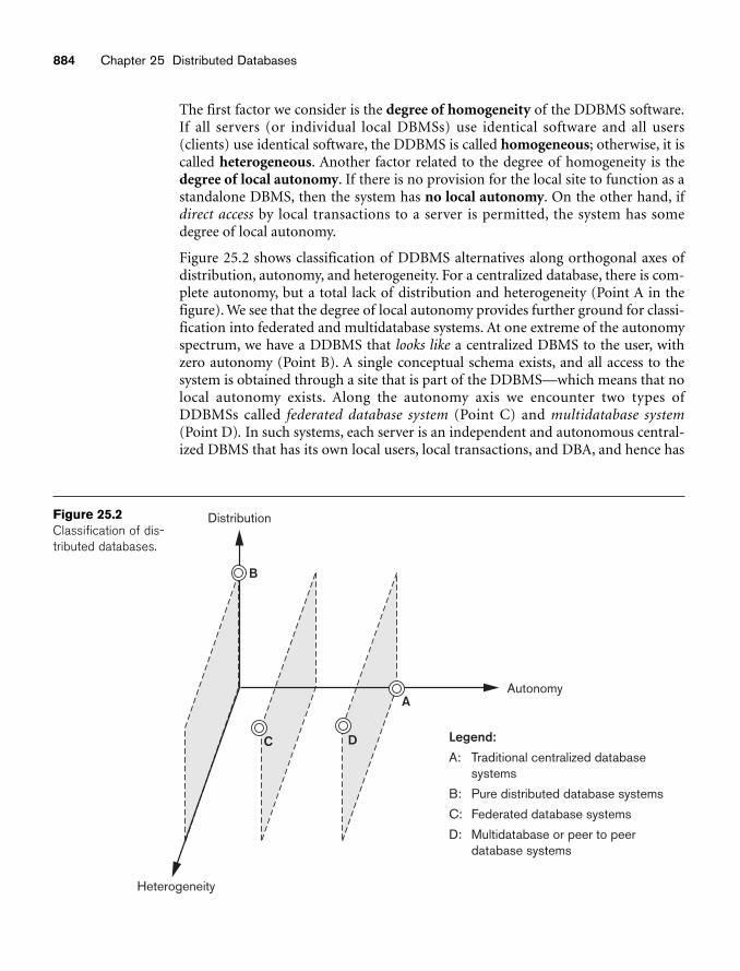
884 Chapter 25 Distributed Databases
The first factor we consider is the degree of homogeneity of the DDBMS software.If all servers (or individual local DBMSs) use identical software and all users(clients) use identical software, the DDBMS is called homogeneous; otherwise, it iscalled heterogeneous. Another factor related to the degree of homogeneity is thedegree of local autonomy. If there is no provision for the local site to function as astandalone DBMS, then the system has no local autonomy. On the other hand, ifdirect access by local transactions to a server is permitted, the system has somedegree of local autonomy.
Figure 25.2 shows classification of DDBMS alternatives along orthogonal axes ofdistribution, autonomy, and heterogeneity. For a centralized database, there is com-plete autonomy, but a total lack of distribution and heterogeneity (Point A in thefigure). We see that the degree of local autonomy provides further ground for classi-fication into federated and multidatabase systems. At one extreme of the autonomyspectrum, we have a DDBMS that looks like a centralized DBMS to the user, withzero autonomy (Point B). A single conceptual schema exists, and all access to thesystem is obtained through a site that is part of the DDBMS—which means that nolocal autonomy exists. Along the autonomy axis we encounter two types ofDDBMSs called federated database system (Point C) and multidatabase system(Point D). In such systems, each server is an independent and autonomous central-ized DBMS that has its own local users, local transactions, and DBA, and hence has
B
Distribution
Heterogeneity
Legend:
A: Traditional centralized database systems
B: Pure distributed database systems
C: Federated database systems
D: Multidatabase or peer to peer database systems
C D
AAutonomy
Figure 25.2Classification of dis-tributed databases.
25.2 Types of Distributed Database Systems 885
a very high degree of local autonomy. The term federated database system (FDBS)is used when there is some global view or schema of the federation of databases thatis shared by the applications (Point C). On the other hand, a multidatabase systemhas full local autonomy in that it does not have a global schema but interactivelyconstructs one as needed by the application (Point D).3 Both systems are hybridsbetween distributed and centralized systems, and the distinction we made betweenthem is not strictly followed. We will refer to them as FDBSs in a generic sense. PointD in the diagram may also stand for a system with full local autonomy and full het-erogeneity—this could be a peer-to-peer database system (see Section 25.9.2). In aheterogeneous FDBS, one server may be a relational DBMS, another a networkDBMS (such as Computer Associates’ IDMS or HP’S IMAGE/3000), and a third anobject DBMS (such as Object Design’s ObjectStore) or hierarchical DBMS (such asIBM’s IMS); in such a case, it is necessary to have a canonical system language andto include language translators to translate subqueries from the canonical languageto the language of each server.
We briefly discuss the issues affecting the design of FDBSs next.
25.2.1 Federated Database Management Systems IssuesThe type of heterogeneity present in FDBSs may arise from several sources. We dis-cuss these sources first and then point out how the different types of autonomiescontribute to a semantic heterogeneity that must be resolved in a heterogeneousFDBS.
■ Differences in data models. Databases in an organization come from a vari-ety of data models, including the so-called legacy models (hierarchical andnetwork, see Web Appendixes D and E), the relational data model, the objectdata model, and even files. The modeling capabilities of the models vary.Hence, to deal with them uniformly via a single global schema or to processthem in a single language is challenging. Even if two databases are both fromthe RDBMS environment, the same information may be represented as anattribute name, as a relation name, or as a value in different databases. Thiscalls for an intelligent query-processing mechanism that can relate informa-tion based on metadata.
■ Differences in constraints. Constraint facilities for specification and imple-mentation vary from system to system. There are comparable features thatmust be reconciled in the construction of a global schema. For example, therelationships from ER models are represented as referential integrity con-straints in the relational model. Triggers may have to be used to implementcertain constraints in the relational model. The global schema must also dealwith potential conflicts among constraints.
3The term multidatabase system is not easily applicable to most enterprise IT environments. The notionof constructing a global schema as and when the need arises is not very feasible in practice for enter-prise databases.
886 Chapter 25 Distributed Databases
■ Differences in query languages. Even with the same data model, the lan-guages and their versions vary. For example, SQL has multiple versions likeSQL-89, SQL-92, SQL-99, and SQL:2008, and each system has its own set ofdata types, comparison operators, string manipulation features, and so on.
Semantic Heterogeneity. Semantic heterogeneity occurs when there are differ-ences in the meaning, interpretation, and intended use of the same or related data.Semantic heterogeneity among component database systems (DBSs) creates thebiggest hurdle in designing global schemas of heterogeneous databases. The designautonomy of component DBSs refers to their freedom of choosing the followingdesign parameters, which in turn affect the eventual complexity of the FDBS:
■ The universe of discourse from which the data is drawn. For example, fortwo customer accounts, databases in the federation may be from the UnitedStates and Japan and have entirely different sets of attributes about customeraccounts required by the accounting practices. Currency rate fluctuationswould also present a problem. Hence, relations in these two databases thathave identical names—CUSTOMER or ACCOUNT—may have some com-mon and some entirely distinct information.
■ Representation and naming. The representation and naming of data ele-ments and the structure of the data model may be prespecified for each localdatabase.
■ The understanding, meaning, and subjective interpretation of data. This isa chief contributor to semantic heterogeneity.
■ Transaction and policy constraints. These deal with serializability criteria,compensating transactions, and other transaction policies.
■ Derivation of summaries. Aggregation, summarization, and other data-processing features and operations supported by the system.
The above problems related to semantic heterogeneity are being faced by all majormultinational and governmental organizations in all application areas. In today’scommercial environment, most enterprises are resorting to heterogeneous FDBSs,having heavily invested in the development of individual database systems usingdiverse data models on different platforms over the last 20 to 30 years. Enterprisesare using various forms of software—typically called the middleware, or Web-based packages called application servers (for example, WebLogic or WebSphere)and even generic systems, called Enterprise Resource Planning (ERP) systems (forexample, SAP, J. D. Edwards ERP)—to manage the transport of queries and transac-tions from the global application to individual databases (with possible additionalprocessing for business rules) and the data from the heterogeneous database serversto the global application. Detailed discussion of these types of software systems isoutside the scope of this book.
Just as providing the ultimate transparency is the goal of any distributed databasearchitecture, local component databases strive to preserve autonomy.Communication autonomy of a component DBS refers to its ability to decidewhether to communicate with another component DBS. Execution autonomy
25.3 Distributed Database Architectures 887
refers to the ability of a component DBS to execute local operations without inter-ference from external operations by other component DBSs and its ability to decidethe order in which to execute them. The association autonomy of a componentDBS implies that it has the ability to decide whether and how much to share itsfunctionality (operations it supports) and resources (data it manages) with othercomponent DBSs. The major challenge of designing FDBSs is to let componentDBSs interoperate while still providing the above types of autonomies to them.
25.3 Distributed Database ArchitecturesIn this section, we first briefly point out the distinction between parallel and distrib-uted database architectures. While both are prevalent in industry today, there arevarious manifestations of the distributed architectures that are continuously evolv-ing among large enterprises. The parallel architecture is more common in high-performance computing, where there is a need for multiprocessor architectures tocope with the volume of data undergoing transaction processing and warehousingapplications. We then introduce a generic architecture of a distributed database.This is followed by discussions on the architecture of three-tier client-server andfederated database systems.
25.3.1 Parallel versus Distributed ArchitecturesThere are two main types of multiprocessor system architectures that are common-place:
■ Shared memory (tightly coupled) architecture. Multiple processors sharesecondary (disk) storage and also share primary memory.
■ Shared disk (loosely coupled) architecture. Multiple processors share sec-ondary (disk) storage but each has their own primary memory.
These architectures enable processors to communicate without the overhead ofexchanging messages over a network.4 Database management systems developedusing the above types of architectures are termed parallel database managementsystems rather than DDBMSs, since they utilize parallel processor technology.Another type of multiprocessor architecture is called shared nothing architecture.In this architecture, every processor has its own primary and secondary (disk)memory, no common memory exists, and the processors communicate over a high-speed interconnection network (bus or switch). Although the shared nothing archi-tecture resembles a distributed database computing environment, major differencesexist in the mode of operation. In shared nothing multiprocessor systems, there issymmetry and homogeneity of nodes; this is not true of the distributed databaseenvironment where heterogeneity of hardware and operating system at each node isvery common. Shared nothing architecture is also considered as an environment for
4If both primary and secondary memories are shared, the architecture is also known as shared everything
architecture.
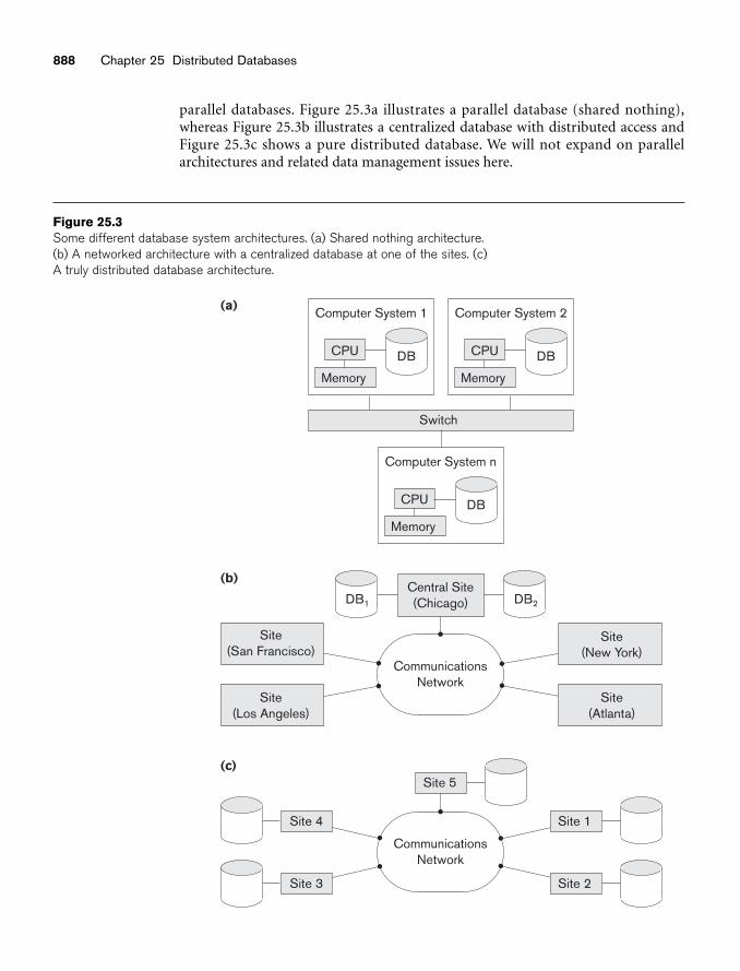
888 Chapter 25 Distributed Databases
parallel databases. Figure 25.3a illustrates a parallel database (shared nothing),whereas Figure 25.3b illustrates a centralized database with distributed access andFigure 25.3c shows a pure distributed database. We will not expand on parallelarchitectures and related data management issues here.
(a)
(b)
Switch
CPU
Computer System 1
Memory
DB CPU
Computer System 2
Memory
DB
CPU
Memory
DB
Computer System n
Central Site(Chicago)
Site(New York)
Site(Los Angeles)
Site(Atlanta)
Site(San Francisco)
DB1 DB2
CommunicationsNetwork
(c)Site 5
Site 1
Site 2
Site 4
Site 3
CommunicationsNetwork
Figure 25.3Some different database system architectures. (a) Shared nothing architecture.(b) A networked architecture with a centralized database at one of the sites. (c)A truly distributed database architecture.
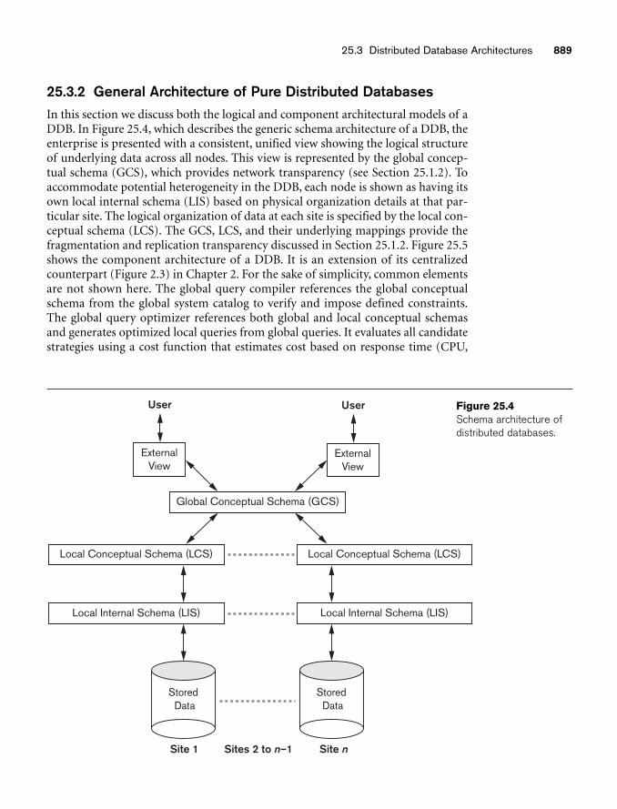
25.3 Distributed Database Architectures 889
User
StoredData
Global Conceptual Schema (GCS)
ExternalView
User
ExternalView
Local Conceptual Schema (LCS) Local Conceptual Schema (LCS)
Local Internal Schema (LIS) Local Internal Schema (LIS)
StoredData
Site 1 Site nSites 2 to n–1
Figure 25.4Schema architecture ofdistributed databases.
25.3.2 General Architecture of Pure Distributed DatabasesIn this section we discuss both the logical and component architectural models of aDDB. In Figure 25.4, which describes the generic schema architecture of a DDB, theenterprise is presented with a consistent, unified view showing the logical structureof underlying data across all nodes. This view is represented by the global concep-tual schema (GCS), which provides network transparency (see Section 25.1.2). Toaccommodate potential heterogeneity in the DDB, each node is shown as having itsown local internal schema (LIS) based on physical organization details at that par-ticular site. The logical organization of data at each site is specified by the local con-ceptual schema (LCS). The GCS, LCS, and their underlying mappings provide thefragmentation and replication transparency discussed in Section 25.1.2. Figure 25.5shows the component architecture of a DDB. It is an extension of its centralizedcounterpart (Figure 2.3) in Chapter 2. For the sake of simplicity, common elementsare not shown here. The global query compiler references the global conceptualschema from the global system catalog to verify and impose defined constraints.The global query optimizer references both global and local conceptual schemasand generates optimized local queries from global queries. It evaluates all candidatestrategies using a cost function that estimates cost based on response time (CPU,
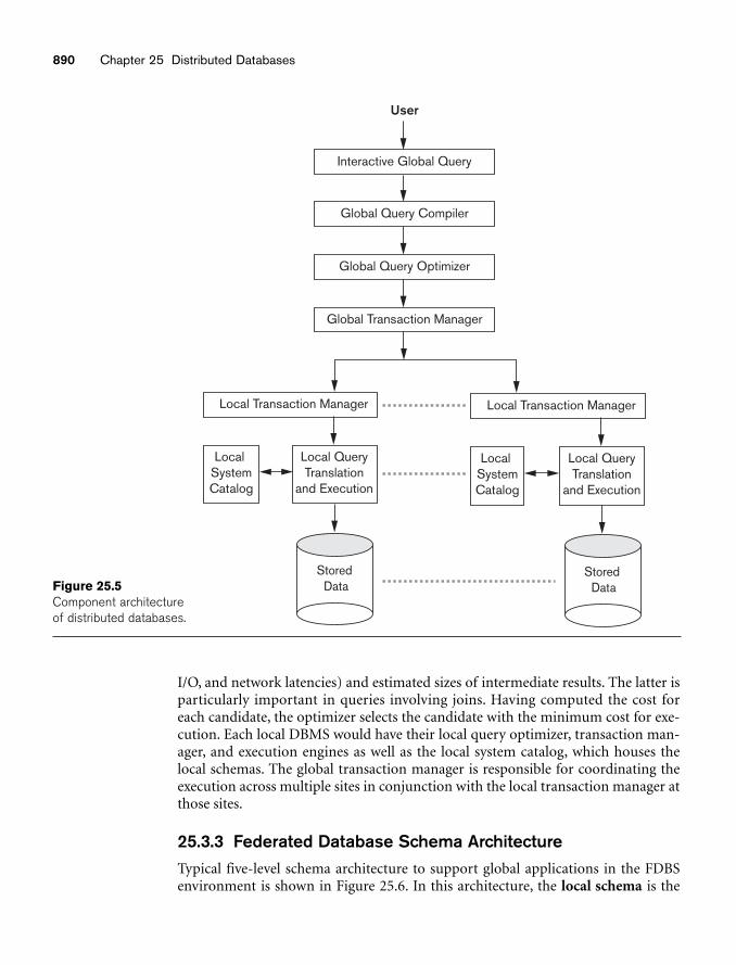
890 Chapter 25 Distributed Databases
User
Interactive Global Query
StoredData
Global Query Compiler
Global Query Optimizer
Global Transaction Manager
Local Transaction Manager
Local QueryTranslation
and Execution
LocalSystemCatalog
StoredData
Local Transaction Manager
Local QueryTranslation
and Execution
LocalSystemCatalog
Figure 25.5Component architectureof distributed databases.
I/O, and network latencies) and estimated sizes of intermediate results. The latter isparticularly important in queries involving joins. Having computed the cost foreach candidate, the optimizer selects the candidate with the minimum cost for exe-cution. Each local DBMS would have their local query optimizer, transaction man-ager, and execution engines as well as the local system catalog, which houses thelocal schemas. The global transaction manager is responsible for coordinating theexecution across multiple sites in conjunction with the local transaction manager atthose sites.
25.3.3 Federated Database Schema ArchitectureTypical five-level schema architecture to support global applications in the FDBSenvironment is shown in Figure 25.6. In this architecture, the local schema is the
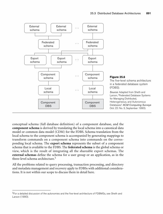
Externalschema
Federatedschema
. . .
. . .
. . .
. . .
. . .
Componentschema
Localschema
ComponentDBS
Externalschema
Externalschema
Federatedschema
Exportschema
Componentschema
Localschema
ComponentDBS
Exportschema
Exportschema
25.3 Distributed Database Architectures 891
Figure 25.6The five-level schema architecturein a federated database system(FDBS).
Source: Adapted from Sheth andLarson, “Federated Database Systemsfor Managing Distributed,Heterogeneous, and AutonomousDatabases.” ACM Computing Surveys(Vol. 22: No. 3, September 1990).
conceptual schema (full database definition) of a component database, and thecomponent schema is derived by translating the local schema into a canonical datamodel or common data model (CDM) for the FDBS. Schema translation from thelocal schema to the component schema is accompanied by generating mappings totransform commands on a component schema into commands on the corres-ponding local schema. The export schema represents the subset of a componentschema that is available to the FDBS. The federated schema is the global schema orview, which is the result of integrating all the shareable export schemas. Theexternal schemas define the schema for a user group or an application, as in thethree-level schema architecture.5
All the problems related to query processing, transaction processing, and directoryand metadata management and recovery apply to FDBSs with additional considera-tions. It is not within our scope to discuss them in detail here.
5For a detailed discussion of the autonomies and the five-level architecture of FDBMSs, see Sheth andLarson (1990).
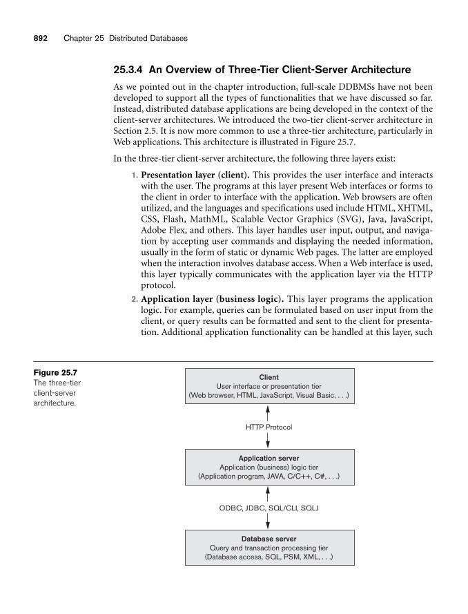
892 Chapter 25 Distributed Databases
ClientUser interface or presentation tier
(Web browser, HTML, JavaScript, Visual Basic, . . .)
HTTP Protocol
Application serverApplication (business) logic tier
(Application program, JAVA, C/C++, C#, . . .)
Database serverQuery and transaction processing tier
(Database access, SQL, PSM, XML, . . .)
ODBC, JDBC, SQL/CLI, SQLJ
Figure 25.7The three-tierclient-serverarchitecture.
25.3.4 An Overview of Three-Tier Client-Server ArchitectureAs we pointed out in the chapter introduction, full-scale DDBMSs have not beendeveloped to support all the types of functionalities that we have discussed so far.Instead, distributed database applications are being developed in the context of theclient-server architectures. We introduced the two-tier client-server architecture inSection 2.5. It is now more common to use a three-tier architecture, particularly inWeb applications. This architecture is illustrated in Figure 25.7.
In the three-tier client-server architecture, the following three layers exist:
1. Presentation layer (client). This provides the user interface and interactswith the user. The programs at this layer present Web interfaces or forms tothe client in order to interface with the application. Web browsers are oftenutilized, and the languages and specifications used include HTML, XHTML,CSS, Flash, MathML, Scalable Vector Graphics (SVG), Java, JavaScript,Adobe Flex, and others. This layer handles user input, output, and naviga-tion by accepting user commands and displaying the needed information,usually in the form of static or dynamic Web pages. The latter are employedwhen the interaction involves database access. When a Web interface is used,this layer typically communicates with the application layer via the HTTPprotocol.
2. Application layer (business logic). This layer programs the applicationlogic. For example, queries can be formulated based on user input from theclient, or query results can be formatted and sent to the client for presenta-tion. Additional application functionality can be handled at this layer, such
25.3 Distributed Database Architectures 893
as security checks, identity verification, and other functions. The applicationlayer can interact with one or more databases or data sources as needed byconnecting to the database using ODBC, JDBC, SQL/CLI, or other databaseaccess techniques.
3. Database server. This layer handles query and update requests from theapplication layer, processes the requests, and sends the results. Usually SQL isused to access the database if it is relational or object-relational and storeddatabase procedures may also be invoked. Query results (and queries) maybe formatted into XML (see Chapter 12) when transmitted between theapplication server and the database server.
Exactly how to divide the DBMS functionality between the client, applicationserver, and database server may vary. The common approach is to include the func-tionality of a centralized DBMS at the database server level. A number of relationalDBMS products have taken this approach, where an SQL server is provided. Theapplication server must then formulate the appropriate SQL queries and connect tothe database server when needed. The client provides the processing for user inter-face interactions. Since SQL is a relational standard, various SQL servers, possiblyprovided by different vendors, can accept SQL commands through standards suchas ODBC, JDBC, and SQL/CLI (see Chapter 13).
In this architecture, the application server may also refer to a data dictionary thatincludes information on the distribution of data among the various SQL servers, aswell as modules for decomposing a global query into a number of local queries thatcan be executed at the various sites. Interaction between an application server anddatabase server might proceed as follows during the processing of an SQL query:
1. The application server formulates a user query based on input from theclient layer and decomposes it into a number of independent site queries.Each site query is sent to the appropriate database server site.
2. Each database server processes the local query and sends the results to theapplication server site. Increasingly, XML is being touted as the standard fordata exchange (see Chapter 12), so the database server may format the queryresult into XML before sending it to the application server.
3. The application server combines the results of the subqueries to produce theresult of the originally required query, formats it into HTML or some otherform accepted by the client, and sends it to the client site for display.
The application server is responsible for generating a distributed execution plan fora multisite query or transaction and for supervising distributed execution by send-ing commands to servers. These commands include local queries and transactionsto be executed, as well as commands to transmit data to other clients or servers.Another function controlled by the application server (or coordinator) is that ofensuring consistency of replicated copies of a data item by employing distributed(or global) concurrency control techniques. The application server must also ensurethe atomicity of global transactions by performing global recovery when certainsites fail.
894 Chapter 25 Distributed Databases
If the DDBMS has the capability to hide the details of data distribution from theapplication server, then it enables the application server to execute global queriesand transactions as though the database were centralized, without having to specifythe sites at which the data referenced in the query or transaction resides. This prop-erty is called distribution transparency. Some DDBMSs do not provide distribu-tion transparency, instead requiring that applications are aware of the details of datadistribution.
25.4 Data Fragmentation, Replication, and Allocation Techniques for DistributedDatabase Design
In this section we discuss techniques that are used to break up the database into log-ical units, called fragments, which may be assigned for storage at the various sites.We also discuss the use of data replication, which permits certain data to be storedin more than one site, and the process of allocating fragments—or replicas of frag-ments—for storage at the various sites. These techniques are used during theprocess of distributed database design. The information concerning data fragmen-tation, allocation, and replication is stored in a global directory that is accessed bythe DDBS applications as needed.
25.4.1 Data FragmentationIn a DDB, decisions must be made regarding which site should be used to storewhich portions of the database. For now, we will assume that there is no replication;that is, each relation—or portion of a relation—is stored at one site only. We discussreplication and its effects later in this section. We also use the terminology of rela-tional databases, but similar concepts apply to other data models. We assume thatwe are starting with a relational database schema and must decide on how to dis-tribute the relations over the various sites. To illustrate our discussion, we use therelational database schema in Figure 3.5.
Before we decide on how to distribute the data, we must determine the logical unitsof the database that are to be distributed. The simplest logical units are the relationsthemselves; that is, each whole relation is to be stored at a particular site. In ourexample, we must decide on a site to store each of the relations EMPLOYEE,DEPARTMENT, PROJECT, WORKS_ON, and DEPENDENT in Figure 3.5. In manycases, however, a relation can be divided into smaller logical units for distribution.For example, consider the company database shown in Figure 3.6, and assume thereare three computer sites—one for each department in the company.6
We may want to store the database information relating to each department at thecomputer site for that department. A technique called horizontal fragmentation canbe used to partition each relation by department.
6Of course, in an actual situation, there will be many more tuples in the relation than those shown inFigure 3.6.
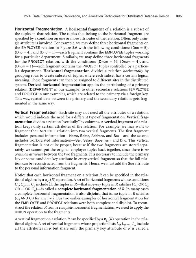
25.4 Data Fragmentation, Replication, and Allocation Techniques for Distributed Database Design 895
Horizontal Fragmentation. A horizontal fragment of a relation is a subset ofthe tuples in that relation. The tuples that belong to the horizontal fragment arespecified by a condition on one or more attributes of the relation. Often, only a sin-gle attribute is involved. For example, we may define three horizontal fragments on the EMPLOYEE relation in Figure 3.6 with the following conditions: (Dno = 5),(Dno = 4), and (Dno = 1)—each fragment contains the EMPLOYEE tuples workingfor a particular department. Similarly, we may define three horizontal fragmentsfor the PROJECT relation, with the conditions (Dnum = 5), (Dnum = 4), and (Dnum = 1)—each fragment contains the PROJECT tuples controlled by a particu-lar department. Horizontal fragmentation divides a relation horizontally bygrouping rows to create subsets of tuples, where each subset has a certain logicalmeaning. These fragments can then be assigned to different sites in the distributedsystem. Derived horizontal fragmentation applies the partitioning of a primaryrelation (DEPARTMENT in our example) to other secondary relations (EMPLOYEEand PROJECT in our example), which are related to the primary via a foreign key.This way, related data between the primary and the secondary relations gets frag-mented in the same way.
Vertical Fragmentation. Each site may not need all the attributes of a relation,which would indicate the need for a different type of fragmentation. Vertical frag-mentation divides a relation “vertically” by columns. A vertical fragment of a rela-tion keeps only certain attributes of the relation. For example, we may want tofragment the EMPLOYEE relation into two vertical fragments. The first fragmentincludes personal information—Name, Bdate, Address, and Sex—and the secondincludes work-related information—Ssn, Salary, Super_ssn, and Dno. This verticalfragmentation is not quite proper, because if the two fragments are stored sepa-rately, we cannot put the original employee tuples back together, since there is nocommon attribute between the two fragments. It is necessary to include the primarykey or some candidate key attribute in every vertical fragment so that the full rela-tion can be reconstructed from the fragments. Hence, we must add the Ssn attributeto the personal information fragment.
Notice that each horizontal fragment on a relation R can be specified in the rela-tional algebra by a σCi
(R) operation. A set of horizontal fragments whose conditionsC1, C2, ..., Cn include all the tuples in R—that is, every tuple in R satisfies (C1 OR C2OR ... OR Cn)—is called a complete horizontal fragmentation of R. In many casesa complete horizontal fragmentation is also disjoint; that is, no tuple in R satisfies(Ci AND Cj) for any i ≠ j. Our two earlier examples of horizontal fragmentation forthe EMPLOYEE and PROJECT relations were both complete and disjoint. To recon-struct the relation R from a complete horizontal fragmentation, we need to apply theUNION operation to the fragments.
A vertical fragment on a relation R can be specified by a πLi(R) operation in the rela-
tional algebra. A set of vertical fragments whose projection lists L1, L2, ..., Ln includeall the attributes in R but share only the primary key attribute of R is called a
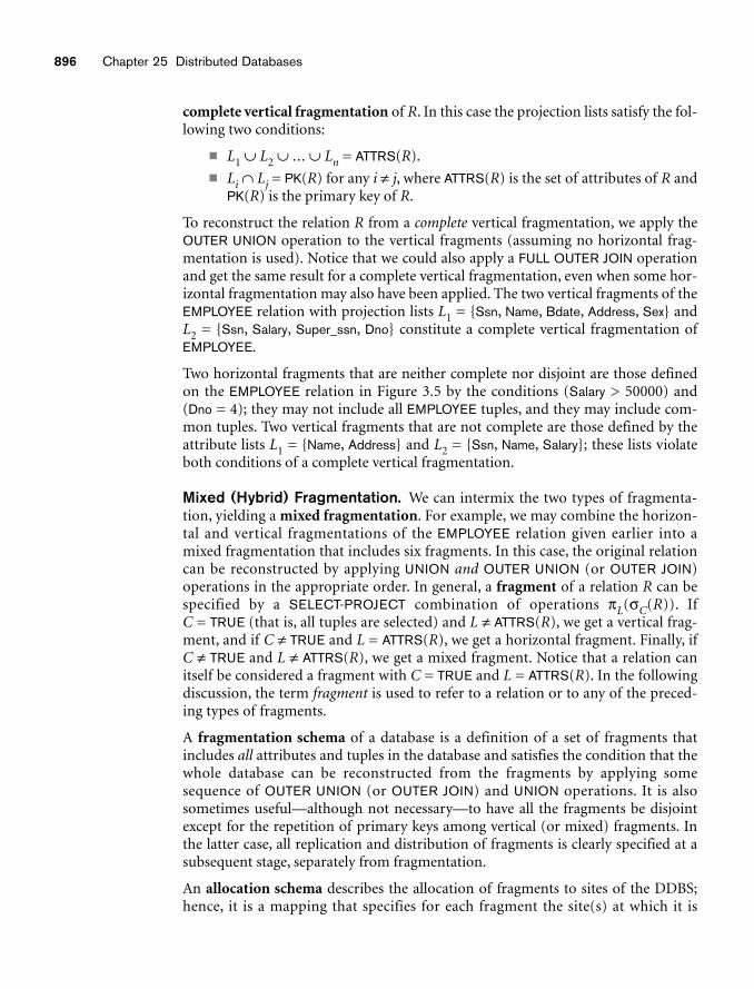
896 Chapter 25 Distributed Databases
complete vertical fragmentation of R. In this case the projection lists satisfy the fol-lowing two conditions:
■ L1 ∪ L2 ∪ ... ∪ Ln = ATTRS(R).
■ Li ∩ Lj = PK(R) for any i ≠ j, where ATTRS(R) is the set of attributes of R andPK(R) is the primary key of R.
To reconstruct the relation R from a complete vertical fragmentation, we apply theOUTER UNION operation to the vertical fragments (assuming no horizontal frag-mentation is used). Notice that we could also apply a FULL OUTER JOIN operationand get the same result for a complete vertical fragmentation, even when some hor-izontal fragmentation may also have been applied. The two vertical fragments of theEMPLOYEE relation with projection lists L1 = {Ssn, Name, Bdate, Address, Sex} andL2 = {Ssn, Salary, Super_ssn, Dno} constitute a complete vertical fragmentation ofEMPLOYEE.
Two horizontal fragments that are neither complete nor disjoint are those definedon the EMPLOYEE relation in Figure 3.5 by the conditions (Salary > 50000) and (Dno = 4); they may not include all EMPLOYEE tuples, and they may include com-mon tuples. Two vertical fragments that are not complete are those defined by theattribute lists L1 = {Name, Address} and L2 = {Ssn, Name, Salary}; these lists violateboth conditions of a complete vertical fragmentation.
Mixed (Hybrid) Fragmentation. We can intermix the two types of fragmenta-tion, yielding a mixed fragmentation. For example, we may combine the horizon-tal and vertical fragmentations of the EMPLOYEE relation given earlier into amixed fragmentation that includes six fragments. In this case, the original relationcan be reconstructed by applying UNION and OUTER UNION (or OUTER JOIN)operations in the appropriate order. In general, a fragment of a relation R can bespecified by a SELECT-PROJECT combination of operations πL(σC(R)). IfC = TRUE (that is, all tuples are selected) and L ≠ ATTRS(R), we get a vertical frag-ment, and if C ≠ TRUE and L = ATTRS(R), we get a horizontal fragment. Finally, ifC ≠ TRUE and L ≠ ATTRS(R), we get a mixed fragment. Notice that a relation canitself be considered a fragment with C = TRUE and L = ATTRS(R). In the followingdiscussion, the term fragment is used to refer to a relation or to any of the preced-ing types of fragments.
A fragmentation schema of a database is a definition of a set of fragments thatincludes all attributes and tuples in the database and satisfies the condition that thewhole database can be reconstructed from the fragments by applying somesequence of OUTER UNION (or OUTER JOIN) and UNION operations. It is alsosometimes useful—although not necessary—to have all the fragments be disjointexcept for the repetition of primary keys among vertical (or mixed) fragments. Inthe latter case, all replication and distribution of fragments is clearly specified at asubsequent stage, separately from fragmentation.
An allocation schema describes the allocation of fragments to sites of the DDBS;hence, it is a mapping that specifies for each fragment the site(s) at which it is
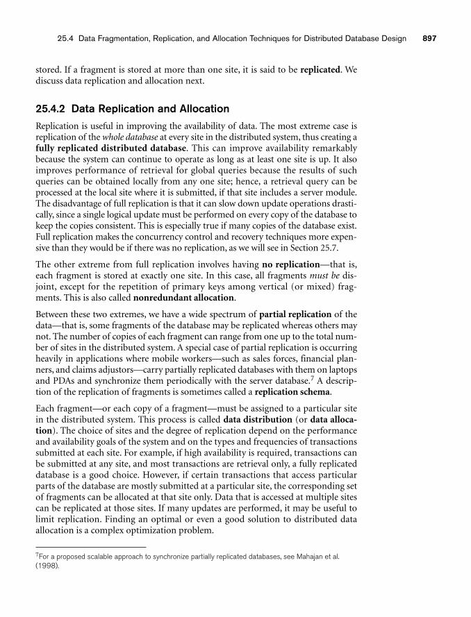
25.4 Data Fragmentation, Replication, and Allocation Techniques for Distributed Database Design 897
stored. If a fragment is stored at more than one site, it is said to be replicated. Wediscuss data replication and allocation next.
25.4.2 Data Replication and AllocationReplication is useful in improving the availability of data. The most extreme case isreplication of the whole database at every site in the distributed system, thus creating afully replicated distributed database. This can improve availability remarkablybecause the system can continue to operate as long as at least one site is up. It alsoimproves performance of retrieval for global queries because the results of suchqueries can be obtained locally from any one site; hence, a retrieval query can beprocessed at the local site where it is submitted, if that site includes a server module.The disadvantage of full replication is that it can slow down update operations drasti-cally, since a single logical update must be performed on every copy of the database tokeep the copies consistent. This is especially true if many copies of the database exist.Full replication makes the concurrency control and recovery techniques more expen-sive than they would be if there was no replication, as we will see in Section 25.7.
The other extreme from full replication involves having no replication—that is,each fragment is stored at exactly one site. In this case, all fragments must be dis-joint, except for the repetition of primary keys among vertical (or mixed) frag-ments. This is also called nonredundant allocation.
Between these two extremes, we have a wide spectrum of partial replication of thedata—that is, some fragments of the database may be replicated whereas others maynot. The number of copies of each fragment can range from one up to the total num-ber of sites in the distributed system. A special case of partial replication is occurringheavily in applications where mobile workers—such as sales forces, financial plan-ners, and claims adjustors—carry partially replicated databases with them on laptopsand PDAs and synchronize them periodically with the server database.7 A descrip-tion of the replication of fragments is sometimes called a replication schema.
Each fragment—or each copy of a fragment—must be assigned to a particular sitein the distributed system. This process is called data distribution (or data alloca-tion). The choice of sites and the degree of replication depend on the performanceand availability goals of the system and on the types and frequencies of transactionssubmitted at each site. For example, if high availability is required, transactions canbe submitted at any site, and most transactions are retrieval only, a fully replicateddatabase is a good choice. However, if certain transactions that access particularparts of the database are mostly submitted at a particular site, the corresponding setof fragments can be allocated at that site only. Data that is accessed at multiple sitescan be replicated at those sites. If many updates are performed, it may be useful tolimit replication. Finding an optimal or even a good solution to distributed dataallocation is a complex optimization problem.
7For a proposed scalable approach to synchronize partially replicated databases, see Mahajan et al.(1998).
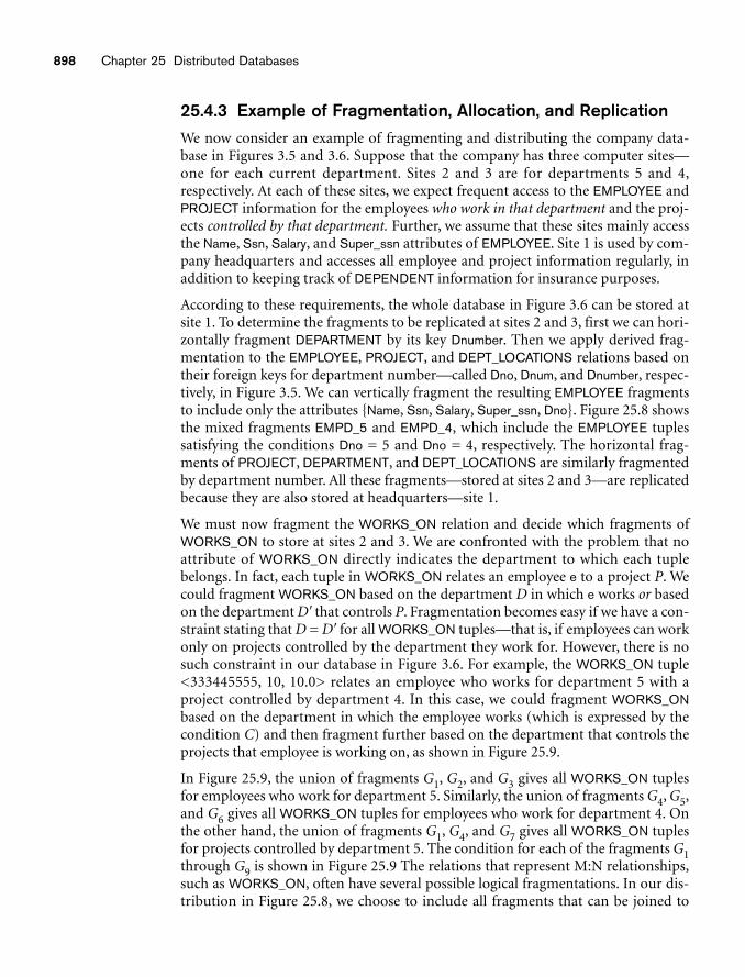
898 Chapter 25 Distributed Databases
25.4.3 Example of Fragmentation, Allocation, and ReplicationWe now consider an example of fragmenting and distributing the company data-base in Figures 3.5 and 3.6. Suppose that the company has three computer sites—one for each current department. Sites 2 and 3 are for departments 5 and 4,respectively. At each of these sites, we expect frequent access to the EMPLOYEE andPROJECT information for the employees who work in that department and the proj-ects controlled by that department. Further, we assume that these sites mainly accessthe Name, Ssn, Salary, and Super_ssn attributes of EMPLOYEE. Site 1 is used by com-pany headquarters and accesses all employee and project information regularly, inaddition to keeping track of DEPENDENT information for insurance purposes.
According to these requirements, the whole database in Figure 3.6 can be stored atsite 1. To determine the fragments to be replicated at sites 2 and 3, first we can hori-zontally fragment DEPARTMENT by its key Dnumber. Then we apply derived frag-mentation to the EMPLOYEE, PROJECT, and DEPT_LOCATIONS relations based ontheir foreign keys for department number—called Dno, Dnum, and Dnumber, respec-tively, in Figure 3.5. We can vertically fragment the resulting EMPLOYEE fragmentsto include only the attributes {Name, Ssn, Salary, Super_ssn, Dno}. Figure 25.8 showsthe mixed fragments EMPD_5 and EMPD_4, which include the EMPLOYEE tuplessatisfying the conditions Dno = 5 and Dno = 4, respectively. The horizontal frag-ments of PROJECT, DEPARTMENT, and DEPT_LOCATIONS are similarly fragmentedby department number. All these fragments—stored at sites 2 and 3—are replicatedbecause they are also stored at headquarters—site 1.
We must now fragment the WORKS_ON relation and decide which fragments ofWORKS_ON to store at sites 2 and 3. We are confronted with the problem that noattribute of WORKS_ON directly indicates the department to which each tuplebelongs. In fact, each tuple in WORKS_ON relates an employee e to a project P. Wecould fragment WORKS_ON based on the department D in which e works or basedon the department D� that controls P. Fragmentation becomes easy if we have a con-straint stating that D = D� for all WORKS_ON tuples—that is, if employees can workonly on projects controlled by the department they work for. However, there is nosuch constraint in our database in Figure 3.6. For example, the WORKS_ON tuple<333445555, 10, 10.0> relates an employee who works for department 5 with aproject controlled by department 4. In this case, we could fragment WORKS_ONbased on the department in which the employee works (which is expressed by thecondition C) and then fragment further based on the department that controls theprojects that employee is working on, as shown in Figure 25.9.
In Figure 25.9, the union of fragments G1, G2, and G3 gives all WORKS_ON tuplesfor employees who work for department 5. Similarly, the union of fragments G4, G5,and G6 gives all WORKS_ON tuples for employees who work for department 4. Onthe other hand, the union of fragments G1, G4, and G7 gives all WORKS_ON tuplesfor projects controlled by department 5. The condition for each of the fragments G1through G9 is shown in Figure 25.9 The relations that represent M:N relationships,such as WORKS_ON, often have several possible logical fragmentations. In our dis-tribution in Figure 25.8, we choose to include all fragments that can be joined to
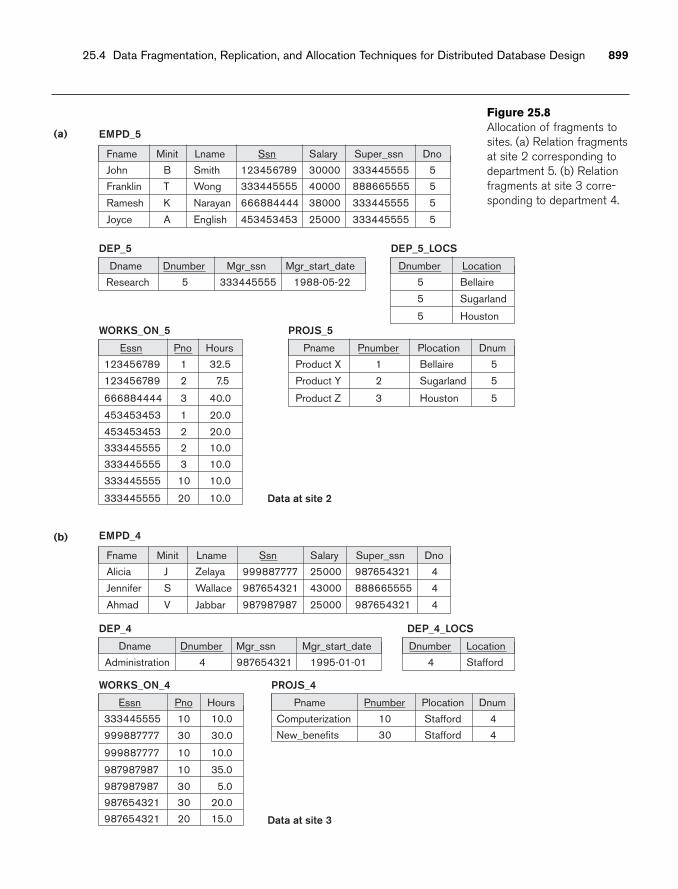
25.4 Data Fragmentation, Replication, and Allocation Techniques for Distributed Database Design 899
(a)
(b)
Fname
John B Smith 123456789 30000 333445555 5
Franklin T Wong 333445555 40000 888665555 5
K Narayan 666884444 38000 333445555 5
A English 453453453 25000 333445555 5
Ramesh
Joyce
EMPD_5
Minit Lname Ssn Salary Super_ssn Dno
Data at site 2
Data at site 3
Fname
Alicia J Zelaya 999887777 25000 987654321 4
Jennifer S Wallace 987654321 43000 888665555 4
V Jabbar 987987987 25000 987654321 4Ahmad
EMPD_4
Minit Lname Ssn Salary Super_ssn Dno
Dname
Research 5 333445555 1988-05-22
DEP_5
Dnumber Mgr_ssn Mgr_start_date Dnumber
5 Bellaire
5 Sugarland
5 Houston
DEP_5_LOCS
Location
Dname
Administration 4 987654321 1995-01-01
DEP_4
Dnumber Mgr_ssn Mgr_start_date
Essn
123456789 1
123456789 2
666884444
453453453
453453453
333445555
333445555
333445555
333445555
1
2
2
3
10
20
3
32.5
7.5
20.0
20.0
10.0
10.0
10.0
10.0
40.0
WORKS_ON_5
Pno Hours Pname
Product X 1
Product Y 2
Product Z 3
Bellaire
Sugarland
Houston
PROJS_5
Pnumber Plocation
5
5
5
Dnum
Essn
333445555 10
999887777 30
999887777
987987987
987987987
987654321
987654321
10
30
30
20
10
10.0
30.0
35.0
5.0
20.0
15.0
10.0
WORKS_ON_4
Pno Hours Pname
Computerization 10
New_benefits 30
Stafford
Stafford
PROJS_4
Pnumber Plocation
4
4
Dnum
Dnumber
4 Stafford
DEP_4_LOCS
Location
Figure 25.8Allocation of fragments tosites. (a) Relation fragmentsat site 2 corresponding todepartment 5. (b) Relationfragments at site 3 corre-sponding to department 4.
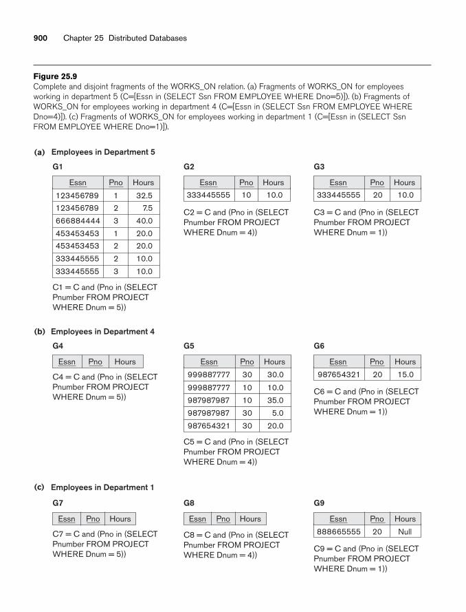
900 Chapter 25 Distributed Databases
Essn
123456789 1 32.5
123456789 2 7.5
3 40.0
1 20.0
2 20.0
2 10.0
3 10.0
666884444
453453453
453453453
333445555
333445555
G1
1C = C and (Pno in (SELECT Pnumber FROM PROJECTWHERE Dnum = 5))
Employees in Department 5
Pno Hours Essn
333445555 10 10.0
G2
C2 = C and (Pno in (SELECT Pnumber FROM PROJECTWHERE Dnum = 4))
Pno Hours Essn
333445555 20 10.0
G3
C3 = C and (Pno in (SELECT Pnumber FROM PROJECTWHERE Dnum = 1))
Pno Hours
Essn
G4
(b)
(c)
(a)
C4 = C and (Pno in (SELECT Pnumber FROM PROJECTWHERE Dnum = 5))
Employees in Department 4
Pno Hours Essn
999887777 30 30.0
999887777 10 10.0
987987987 10 35.0
987987987 30 5.0
987654321 30 20.0
G5
C5 = C and (Pno in (SELECT Pnumber FROM PROJECTWHERE Dnum = 4))
Pno Hours Essn
987654321 20 15.0
G6
C6 = C and (Pno in (SELECT Pnumber FROM PROJECTWHERE Dnum = 1))
Pno Hours
Essn
G7
C7 = C and (Pno in (SELECT Pnumber FROM PROJECTWHERE Dnum = 5))
Employees in Department 1
Pno Hours Essn
G8
C8 = C and (Pno in (SELECT Pnumber FROM PROJECTWHERE Dnum = 4))
Pno Hours Essn
888665555 20 Null
G9
C9 = C and (Pno in (SELECT Pnumber FROM PROJECTWHERE Dnum = 1))
Pno Hours
Figure 25.9Complete and disjoint fragments of the WORKS_ON relation. (a) Fragments of WORKS_ON for employeesworking in department 5 (C=[Essn in (SELECT Ssn FROM EMPLOYEE WHERE Dno=5)]). (b) Fragments ofWORKS_ON for employees working in department 4 (C=[Essn in (SELECT Ssn FROM EMPLOYEE WHEREDno=4)]). (c) Fragments of WORKS_ON for employees working in department 1 (C=[Essn in (SELECT SsnFROM EMPLOYEE WHERE Dno=1)]).
25.5 Query Processing and Optimization in Distributed Databases 901
either an EMPLOYEE tuple or a PROJECT tuple at sites 2 and 3. Hence, we place theunion of fragments G1, G2, G3, G4, and G7 at site 2 and the union of fragments G4,G5, G6, G2, and G8 at site 3. Notice that fragments G2 and G4 are replicated at bothsites. This allocation strategy permits the join between the local EMPLOYEE orPROJECT fragments at site 2 or site 3 and the local WORKS_ON fragment to be per-formed completely locally. This clearly demonstrates how complex the problem ofdatabase fragmentation and allocation is for large databases. The SelectedBibliography at the end of this chapter discusses some of the work done in this area.
25.5 Query Processing and Optimization inDistributed Databases
Now we give an overview of how a DDBMS processes and optimizes a query. Firstwe discuss the steps involved in query processing and then elaborate on the commu-nication costs of processing a distributed query. Finally we discuss a special opera-tion, called a semijoin, which is used to optimize some types of queries in a DDBMS.A detailed discussion about optimization algorithms is beyond the scope of thisbook. We attempt to illustrate optimization principles using suitable examples.8
25.5.1 Distributed Query ProcessingA distributed database query is processed in stages as follows:
1. Query Mapping. The input query on distributed data is specified formallyusing a query language. It is then translated into an algebraic query on globalrelations. This translation is done by referring to the global conceptualschema and does not take into account the actual distribution and replica-tion of data. Hence, this translation is largely identical to the one performedin a centralized DBMS. It is first normalized, analyzed for semantic errors,simplified, and finally restructured into an algebraic query.
2. Localization. In a distributed database, fragmentation results in relationsbeing stored in separate sites, with some fragments possibly being replicated.This stage maps the distributed query on the global schema to separatequeries on individual fragments using data distribution and replicationinformation.
3. Global Query Optimization. Optimization consists of selecting a strategyfrom a list of candidates that is closest to optimal. A list of candidate queriescan be obtained by permuting the ordering of operations within a fragmentquery generated by the previous stage. Time is the preferred unit for measur-ing cost. The total cost is a weighted combination of costs such as CPU cost,I/O costs, and communication costs. Since DDBs are connected by a net-work, often the communication costs over the network are the most signifi-cant. This is especially true when the sites are connected through a wide areanetwork (WAN).
8For a detailed discussion of optimization algorithms, see Ozsu and Valduriez (1999).
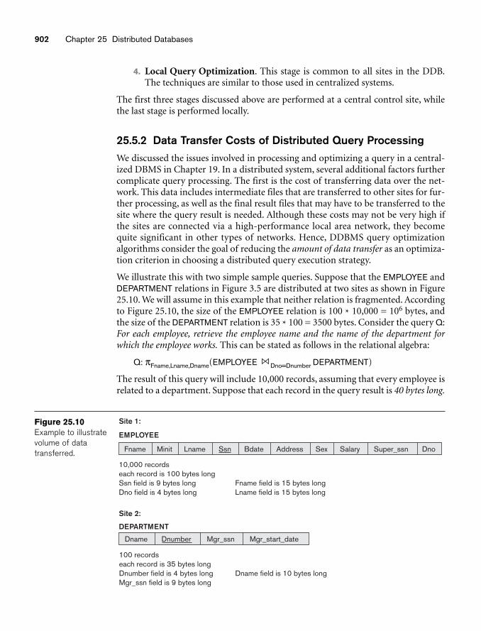
902 Chapter 25 Distributed Databases
4. Local Query Optimization. This stage is common to all sites in the DDB.The techniques are similar to those used in centralized systems.
The first three stages discussed above are performed at a central control site, whilethe last stage is performed locally.
25.5.2 Data Transfer Costs of Distributed Query ProcessingWe discussed the issues involved in processing and optimizing a query in a central-ized DBMS in Chapter 19. In a distributed system, several additional factors furthercomplicate query processing. The first is the cost of transferring data over the net-work. This data includes intermediate files that are transferred to other sites for fur-ther processing, as well as the final result files that may have to be transferred to thesite where the query result is needed. Although these costs may not be very high ifthe sites are connected via a high-performance local area network, they becomequite significant in other types of networks. Hence, DDBMS query optimizationalgorithms consider the goal of reducing the amount of data transfer as an optimiza-tion criterion in choosing a distributed query execution strategy.
We illustrate this with two simple sample queries. Suppose that the EMPLOYEE andDEPARTMENT relations in Figure 3.5 are distributed at two sites as shown in Figure25.10. We will assume in this example that neither relation is fragmented. Accordingto Figure 25.10, the size of the EMPLOYEE relation is 100 * 10,000 = 106 bytes, andthe size of the DEPARTMENT relation is 35 * 100 = 3500 bytes. Consider the query Q:For each employee, retrieve the employee name and the name of the department forwhich the employee works. This can be stated as follows in the relational algebra:
Q: πFname,Lname,Dname(EMPLOYEE Dno=Dnumber DEPARTMENT)
The result of this query will include 10,000 records, assuming that every employee isrelated to a department. Suppose that each record in the query result is 40 bytes long.
Fname
EMPLOYEE
Site 1:
10,000 recordseach record is 100 bytes longSsn field is 9 bytes longDno field is 4 bytes long
Site 2:
Minit Lname Ssn Salary Super_ssn DnoBdate Address Sex
Dname
DEPARTMENT
Dnumber Mgr_ssn Mgr_start_date
Fname field is 15 bytes longLname field is 15 bytes long
100 recordseach record is 35 bytes longDnumber field is 4 bytes longMgr_ssn field is 9 bytes long
Dname field is 10 bytes long
Figure 25.10Example to illustratevolume of datatransferred.
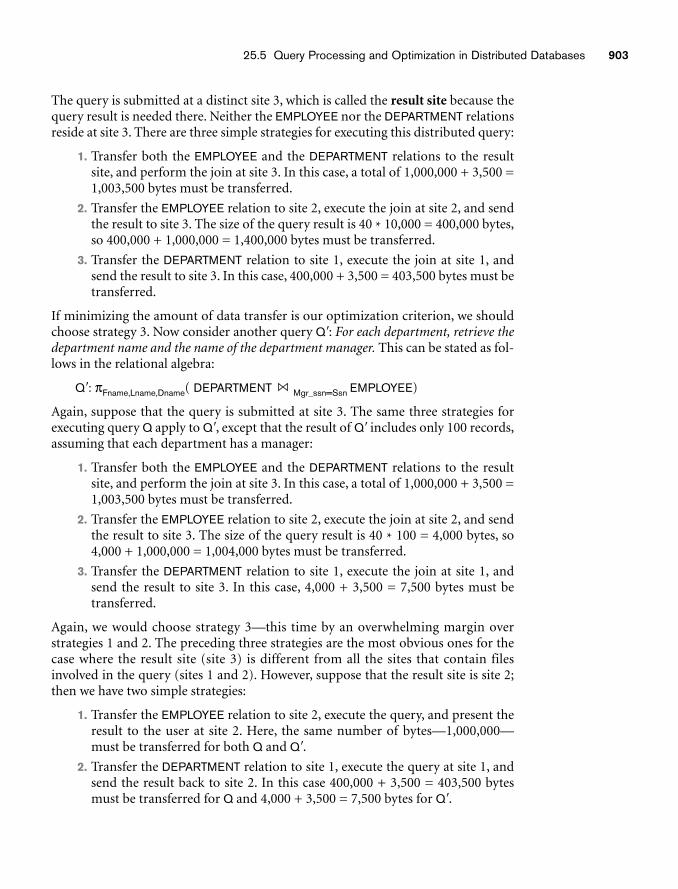
25.5 Query Processing and Optimization in Distributed Databases 903
The query is submitted at a distinct site 3, which is called the result site because thequery result is needed there. Neither the EMPLOYEE nor the DEPARTMENT relationsreside at site 3. There are three simple strategies for executing this distributed query:
1. Transfer both the EMPLOYEE and the DEPARTMENT relations to the resultsite, and perform the join at site 3. In this case, a total of 1,000,000 + 3,500 =1,003,500 bytes must be transferred.
2. Transfer the EMPLOYEE relation to site 2, execute the join at site 2, and sendthe result to site 3. The size of the query result is 40 * 10,000 = 400,000 bytes,so 400,000 + 1,000,000 = 1,400,000 bytes must be transferred.
3. Transfer the DEPARTMENT relation to site 1, execute the join at site 1, andsend the result to site 3. In this case, 400,000 + 3,500 = 403,500 bytes must betransferred.
If minimizing the amount of data transfer is our optimization criterion, we shouldchoose strategy 3. Now consider another query Q�: For each department, retrieve thedepartment name and the name of the department manager. This can be stated as fol-lows in the relational algebra:
Q�: πFname,Lname,Dname( DEPARTMENT Mgr_ssn=Ssn EMPLOYEE)
Again, suppose that the query is submitted at site 3. The same three strategies forexecuting query Q apply to Q�, except that the result of Q� includes only 100 records,assuming that each department has a manager:
1. Transfer both the EMPLOYEE and the DEPARTMENT relations to the resultsite, and perform the join at site 3. In this case, a total of 1,000,000 + 3,500 =1,003,500 bytes must be transferred.
2. Transfer the EMPLOYEE relation to site 2, execute the join at site 2, and sendthe result to site 3. The size of the query result is 40 * 100 = 4,000 bytes, so4,000 + 1,000,000 = 1,004,000 bytes must be transferred.
3. Transfer the DEPARTMENT relation to site 1, execute the join at site 1, andsend the result to site 3. In this case, 4,000 + 3,500 = 7,500 bytes must betransferred.
Again, we would choose strategy 3—this time by an overwhelming margin overstrategies 1 and 2. The preceding three strategies are the most obvious ones for thecase where the result site (site 3) is different from all the sites that contain filesinvolved in the query (sites 1 and 2). However, suppose that the result site is site 2;then we have two simple strategies:
1. Transfer the EMPLOYEE relation to site 2, execute the query, and present theresult to the user at site 2. Here, the same number of bytes—1,000,000—must be transferred for both Q and Q�.
2. Transfer the DEPARTMENT relation to site 1, execute the query at site 1, andsend the result back to site 2. In this case 400,000 + 3,500 = 403,500 bytesmust be transferred for Q and 4,000 + 3,500 = 7,500 bytes for Q�.
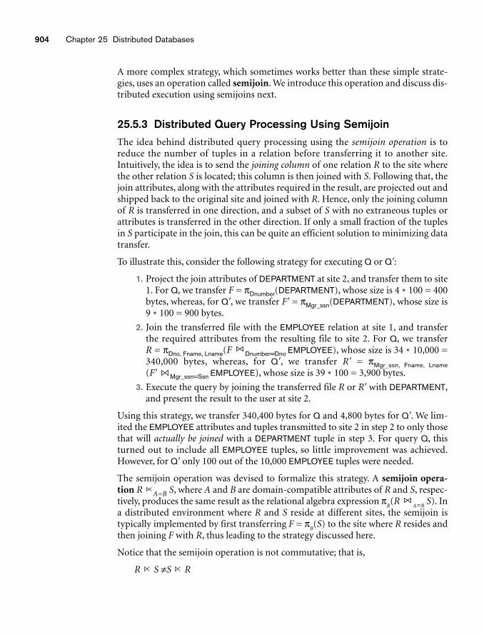
904 Chapter 25 Distributed Databases
A more complex strategy, which sometimes works better than these simple strate-gies, uses an operation called semijoin. We introduce this operation and discuss dis-tributed execution using semijoins next.
25.5.3 Distributed Query Processing Using SemijoinThe idea behind distributed query processing using the semijoin operation is toreduce the number of tuples in a relation before transferring it to another site.Intuitively, the idea is to send the joining column of one relation R to the site wherethe other relation S is located; this column is then joined with S. Following that, thejoin attributes, along with the attributes required in the result, are projected out andshipped back to the original site and joined with R. Hence, only the joining columnof R is transferred in one direction, and a subset of S with no extraneous tuples orattributes is transferred in the other direction. If only a small fraction of the tuplesin S participate in the join, this can be quite an efficient solution to minimizing datatransfer.
To illustrate this, consider the following strategy for executing Q or Q�:
1. Project the join attributes of DEPARTMENT at site 2, and transfer them to site1. For Q, we transfer F = πDnumber(DEPARTMENT), whose size is 4 * 100 = 400bytes, whereas, for Q�, we transfer F� = πMgr_ssn(DEPARTMENT), whose size is9 * 100 = 900 bytes.
2. Join the transferred file with the EMPLOYEE relation at site 1, and transferthe required attributes from the resulting file to site 2. For Q, we transfer R = πDno, Fname, Lname(F Dnumber=Dno EMPLOYEE), whose size is 34 * 10,000 =340,000 bytes, whereas, for Q�, we transfer R� = πMgr_ssn, Fname, Lname(F� Mgr_ssn=Ssn EMPLOYEE), whose size is 39 * 100 = 3,900 bytes.
3. Execute the query by joining the transferred file R or R� with DEPARTMENT,and present the result to the user at site 2.
Using this strategy, we transfer 340,400 bytes for Q and 4,800 bytes for Q�. We lim-ited the EMPLOYEE attributes and tuples transmitted to site 2 in step 2 to only thosethat will actually be joined with a DEPARTMENT tuple in step 3. For query Q, thisturned out to include all EMPLOYEE tuples, so little improvement was achieved.However, for Q� only 100 out of the 10,000 EMPLOYEE tuples were needed.
The semijoin operation was devised to formalize this strategy. A semijoin opera-tion R A=B S, where A and B are domain-compatible attributes of R and S, respec-tively, produces the same result as the relational algebra expression π
R(R
A=BS). In
a distributed environment where R and S reside at different sites, the semijoin istypically implemented by first transferring F = π
B(S) to the site where R resides and
then joining F with R, thus leading to the strategy discussed here.
Notice that the semijoin operation is not commutative; that is,
R S ≠S R
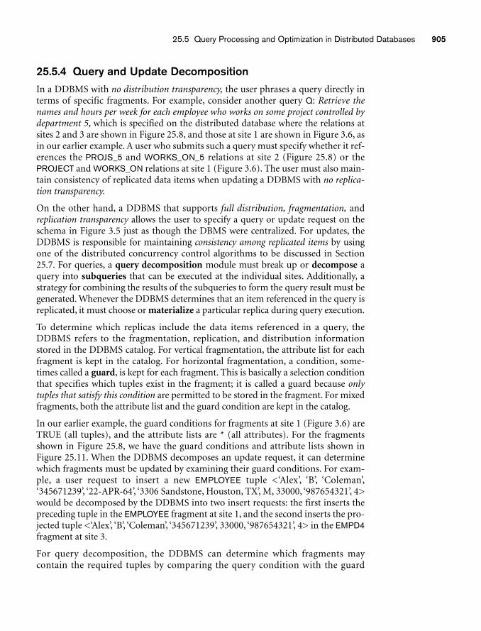
25.5 Query Processing and Optimization in Distributed Databases 905
25.5.4 Query and Update DecompositionIn a DDBMS with no distribution transparency, the user phrases a query directly interms of specific fragments. For example, consider another query Q: Retrieve thenames and hours per week for each employee who works on some project controlled bydepartment 5, which is specified on the distributed database where the relations atsites 2 and 3 are shown in Figure 25.8, and those at site 1 are shown in Figure 3.6, asin our earlier example. A user who submits such a query must specify whether it ref-erences the PROJS_5 and WORKS_ON_5 relations at site 2 (Figure 25.8) or thePROJECT and WORKS_ON relations at site 1 (Figure 3.6). The user must also main-tain consistency of replicated data items when updating a DDBMS with no replica-tion transparency.
On the other hand, a DDBMS that supports full distribution, fragmentation, andreplication transparency allows the user to specify a query or update request on theschema in Figure 3.5 just as though the DBMS were centralized. For updates, theDDBMS is responsible for maintaining consistency among replicated items by usingone of the distributed concurrency control algorithms to be discussed in Section25.7. For queries, a query decomposition module must break up or decompose aquery into subqueries that can be executed at the individual sites. Additionally, astrategy for combining the results of the subqueries to form the query result must begenerated. Whenever the DDBMS determines that an item referenced in the query isreplicated, it must choose or materialize a particular replica during query execution.
To determine which replicas include the data items referenced in a query, theDDBMS refers to the fragmentation, replication, and distribution informationstored in the DDBMS catalog. For vertical fragmentation, the attribute list for eachfragment is kept in the catalog. For horizontal fragmentation, a condition, some-times called a guard, is kept for each fragment. This is basically a selection conditionthat specifies which tuples exist in the fragment; it is called a guard because onlytuples that satisfy this condition are permitted to be stored in the fragment. For mixedfragments, both the attribute list and the guard condition are kept in the catalog.
In our earlier example, the guard conditions for fragments at site 1 (Figure 3.6) areTRUE (all tuples), and the attribute lists are * (all attributes). For the fragmentsshown in Figure 25.8, we have the guard conditions and attribute lists shown inFigure 25.11. When the DDBMS decomposes an update request, it can determinewhich fragments must be updated by examining their guard conditions. For exam-ple, a user request to insert a new EMPLOYEE tuple <‘Alex’, ‘B’, ‘Coleman’,‘345671239’, ‘22-APR-64’, ‘3306 Sandstone, Houston, TX’, M, 33000, ‘987654321’, 4>would be decomposed by the DDBMS into two insert requests: the first inserts thepreceding tuple in the EMPLOYEE fragment at site 1, and the second inserts the pro-jected tuple <‘Alex’, ‘B’, ‘Coleman’, ‘345671239’, 33000, ‘987654321’, 4> in the EMPD4fragment at site 3.
For query decomposition, the DDBMS can determine which fragments may contain the required tuples by comparing the query condition with the guard
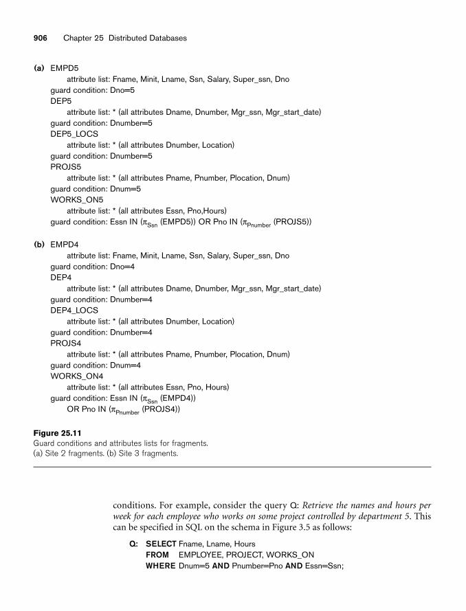
906 Chapter 25 Distributed Databases
(a) EMPD5attribute list: Fname, Minit, Lname, Ssn, Salary, Super_ssn, Dno
guard condition: Dno=5DEP5
attribute list: * (all attributes Dname, Dnumber, Mgr_ssn, Mgr_start_date)guard condition: Dnumber=5DEP5_LOCS
attribute list: * (all attributes Dnumber, Location)guard condition: Dnumber=5PROJS5
attribute list: * (all attributes Pname, Pnumber, Plocation, Dnum)guard condition: Dnum=5WORKS_ON5
attribute list: * (all attributes Essn, Pno,Hours)guard condition: Essn IN (πSsn (EMPD5)) OR Pno IN (πPnumber (PROJS5))
(b) EMPD4attribute list: Fname, Minit, Lname, Ssn, Salary, Super_ssn, Dno
guard condition: Dno=4DEP4
attribute list: * (all attributes Dname, Dnumber, Mgr_ssn, Mgr_start_date)guard condition: Dnumber=4DEP4_LOCS
attribute list: * (all attributes Dnumber, Location)guard condition: Dnumber=4PROJS4
attribute list: * (all attributes Pname, Pnumber, Plocation, Dnum)guard condition: Dnum=4WORKS_ON4
attribute list: * (all attributes Essn, Pno, Hours)guard condition: Essn IN (πSsn (EMPD4))
OR Pno IN (πPnumber (PROJS4))
Figure 25.11Guard conditions and attributes lists for fragments.(a) Site 2 fragments. (b) Site 3 fragments.
conditions. For example, consider the query Q: Retrieve the names and hours perweek for each employee who works on some project controlled by department 5. Thiscan be specified in SQL on the schema in Figure 3.5 as follows:
Q: SELECT Fname, Lname, HoursFROM EMPLOYEE, PROJECT, WORKS_ONWHERE Dnum=5 AND Pnumber=Pno AND Essn=Ssn;
25.6 Overview of Transaction Management in Distributed Databases 907
Suppose that the query is submitted at site 2, which is where the query result will beneeded. The DDBMS can determine from the guard condition on PROJS5 andWORKS_ON5 that all tuples satisfying the conditions (Dnum = 5 AND Pnumber =Pno) reside at site 2. Hence, it may decompose the query into the following rela-tional algebra subqueries:
T1 ← πEssn(PROJS5 Pnumber=PnoWORKS_ON5)
T2 ← πEssn, Fname, Lname(T1 Essn=SsnEMPLOYEE)
RESULT ← πFname, Lname, Hours(T2 * WORKS_ON5)
This decomposition can be used to execute the query by using a semijoin strategy.The DDBMS knows from the guard conditions that PROJS5 contains exactly thosetuples satisfying (Dnum = 5) and that WORKS_ON5 contains all tuples to be joinedwith PROJS5; hence, subquery T1 can be executed at site 2, and the projected columnEssn can be sent to site 1. Subquery T2 can then be executed at site 1, and the resultcan be sent back to site 2, where the final query result is calculated and displayed tothe user. An alternative strategy would be to send the query Q itself to site 1, whichincludes all the database tuples, where it would be executed locally and from whichthe result would be sent back to site 2. The query optimizer would estimate the costsof both strategies and would choose the one with the lower cost estimate.
25.6 Overview of Transaction Management in Distributed Databases
The global and local transaction management software modules, along with theconcurrency control and recovery manager of a DDBMS, collectively guarantee theACID properties of transactions (see Chapter 21). We discuss distributed transac-tion management in this section and explore concurrency control in Section 25.7.
As can be seen in Figure 25.5, an additional component called the global transac-tion manager is introduced for supporting distributed transactions. The site wherethe transaction originated can temporarily assume the role of global transactionmanager and coordinate the execution of database operations with transactionmanagers across multiple sites. Transaction managers export their functionality asan interface to the application programs. The operations exported by this interfaceare similar to those covered in Section 21.2.1, namely BEGIN_TRANSACTION, READor WRITE, END_TRANSACTION, COMMIT_TRANSACTION, and ROLLBACK (orABORT). The manager stores bookkeeping information related to each transaction,such as a unique identifier, originating site, name, and so on. For READ operations,it returns a local copy if valid and available. For WRITE operations, it ensures thatupdates are visible across all sites containing copies (replicas) of the data item. ForABORT operations, the manager ensures that no effects of the transaction arereflected in any site of the distributed database. For COMMIT operations, it ensuresthat the effects of a write are persistently recorded on all databases containing copiesof the data item. Atomic termination (COMMIT/ ABORT) of distributed transactionsis commonly implemented using the two-phase commit protocol. We give moredetails of this protocol in the following section.
908 Chapter 25 Distributed Databases
The transaction manager passes to the concurrency controller the database opera-tion and associated information. The controller is responsible for acquisition andrelease of associated locks. If the transaction requires access to a locked resource, itis delayed until the lock is acquired. Once the lock is acquired, the operation is sentto the runtime processor, which handles the actual execution of the database opera-tion. Once the operation is completed, locks are released and the transaction man-ager is updated with the result of the operation. We discuss commonly useddistributed concurrency methods in Section 25.7.
25.6.1 Two-Phase Commit ProtocolIn Section 23.6, we described the two-phase commit protocol (2PC), which requires aglobal recovery manager, or coordinator, to maintain information needed forrecovery, in addition to the local recovery managers and the information they main-tain (log, tables) The two-phase commit protocol has certain drawbacks that led tothe development of the three-phase commit protocol, which we discuss next.
25.6.2 Three-Phase Commit ProtocolThe biggest drawback of 2PC is that it is a blocking protocol. Failure of the coordi-nator blocks all participating sites, causing them to wait until the coordinator recov-ers. This can cause performance degradation, especially if participants are holdinglocks to shared resources. Another problematic scenario is when both the coordina-tor and a participant that has committed crash together. In the two-phase commitprotocol, a participant has no way to ensure that all participants got the commitmessage in the second phase. Hence once a decision to commit has been made bythe coordinator in the first phase, participants will commit their transactions in thesecond phase independent of receipt of a global commit message by other partici-pants. Thus, in the situation that both the coordinator and a committed participantcrash together, the result of the transaction becomes uncertain or nondeterministic.Since the transaction has already been committed by one participant, it cannot beaborted on recovery by the coordinator. Also, the transaction cannot be optimisti-cally committed on recovery since the original vote of the coordinator may havebeen to abort.
These problems are solved by the three-phase commit (3PC) protocol, which essen-tially divides the second commit phase into two subphases called prepare-to-commit and commit. The prepare-to-commit phase is used to communicate theresult of the vote phase to all participants. If all participants vote yes, then the coordi-nator instructs them to move into the prepare-to-commit state. The commit subphaseis identical to its two-phase counterpart. Now, if the coordinator crashes during thissubphase, another participant can see the transaction through to completion. It cansimply ask a crashed participant if it received a prepare-to-commit message. If it didnot, then it safely assumes to abort. Thus the state of the protocol can be recoveredirrespective of which participant crashes. Also, by limiting the time required for atransaction to commit or abort to a maximum time-out period, the protocol ensuresthat a transaction attempting to commit via 3PC releases locks on time-out.
25.7 Overview of Concurrency Control and Recovery in Distributed Databases 909
The main idea is to limit the wait time for participants who have committed and arewaiting for a global commit or abort from the coordinator. When a participantreceives a precommit message, it knows that the rest of the participants have votedto commit. If a precommit message has not been received, then the participant willabort and release all locks.
25.6.3 Operating System Support for Transaction Management
The following are the main benefits of operating system (OS)-supported transac-tion management:
■ Typically, DBMSs use their own semaphores9 to guarantee mutually exclu-sive access to shared resources. Since these semaphores are implemented inuserspace at the level of the DBMS application software, the OS has noknowledge about them. Hence if the OS deactivates a DBMS process holdinga lock, other DBMS processes wanting this lock resource get queued. Such asituation can cause serious performance degradation. OS-level knowledge ofsemaphores can help eliminate such situations.
■ Specialized hardware support for locking can be exploited to reduce associ-ated costs. This can be of great importance, since locking is one of the mostcommon DBMS operations.
■ Providing a set of common transaction support operations though the ker-nel allows application developers to focus on adding new features to theirproducts as opposed to reimplementing the common functionality for eachapplication. For example, if different DDBMSs are to coexist on the samemachine and they chose the two-phase commit protocol, then it is morebeneficial to have this protocol implemented as part of the kernel so that the DDBMS developers can focus more on adding new features to their products.
25.7 Overview of Concurrency Control and Recovery in Distributed Databases
For concurrency control and recovery purposes, numerous problems arise in a dis-tributed DBMS environment that are not encountered in a centralized DBMS envi-ronment. These include the following:
■ Dealing with multiple copies of the data items. The concurrency controlmethod is responsible for maintaining consistency among these copies. Therecovery method is responsible for making a copy consistent with othercopies if the site on which the copy is stored fails and recovers later.
9Semaphores are data structures used for synchronized and exclusive access to shared resources forpreventing race conditions in a parallel computing system.
910 Chapter 25 Distributed Databases
■ Failure of individual sites. The DDBMS should continue to operate with itsrunning sites, if possible, when one or more individual sites fail. When a siterecovers, its local database must be brought up-to-date with the rest of thesites before it rejoins the system.
■ Failure of communication links. The system must be able to deal with thefailure of one or more of the communication links that connect the sites. Anextreme case of this problem is that network partitioning may occur. Thisbreaks up the sites into two or more partitions, where the sites within eachpartition can communicate only with one another and not with sites in otherpartitions.
■ Distributed commit. Problems can arise with committing a transaction thatis accessing databases stored on multiple sites if some sites fail during thecommit process. The two-phase commit protocol (see Section 23.6) is oftenused to deal with this problem.
■ Distributed deadlock. Deadlock may occur among several sites, so tech-niques for dealing with deadlocks must be extended to take this intoaccount.
Distributed concurrency control and recovery techniques must deal with these andother problems. In the following subsections, we review some of the techniques thathave been suggested to deal with recovery and concurrency control in DDBMSs.
25.7.1 Distributed Concurrency Control Based on a Distinguished Copy of a Data Item
To deal with replicated data items in a distributed database, a number of concur-rency control methods have been proposed that extend the concurrency controltechniques for centralized databases. We discuss these techniques in the context ofextending centralized locking. Similar extensions apply to other concurrency controltechniques. The idea is to designate a particular copy of each data item as adistinguished copy. The locks for this data item are associated with the distin-guished copy, and all locking and unlocking requests are sent to the site that containsthat copy.
A number of different methods are based on this idea, but they differ in theirmethod of choosing the distinguished copies. In the primary site technique, all dis-tinguished copies are kept at the same site. A modification of this approach is theprimary site with a backup site. Another approach is the primary copy method,where the distinguished copies of the various data items can be stored in differentsites. A site that includes a distinguished copy of a data item basically acts as thecoordinator site for concurrency control on that item. We discuss these techniquesnext.
Primary Site Technique. In this method a single primary site is designated to bethe coordinator site for all database items. Hence, all locks are kept at that site, andall requests for locking or unlocking are sent there. This method is thus an extension
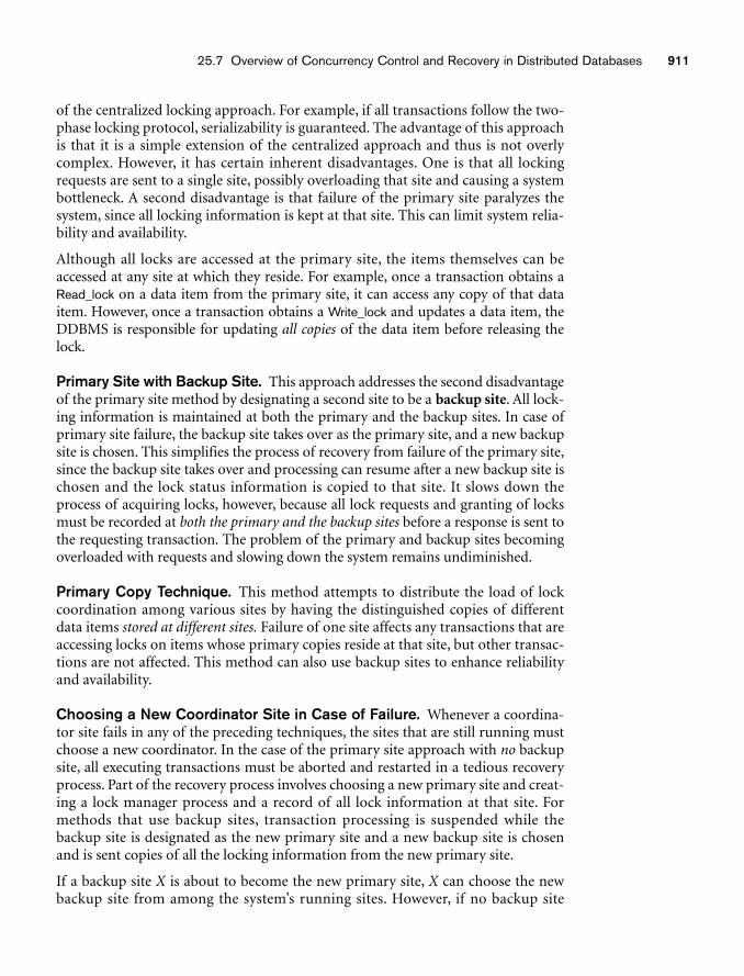
25.7 Overview of Concurrency Control and Recovery in Distributed Databases 911
of the centralized locking approach. For example, if all transactions follow the two-phase locking protocol, serializability is guaranteed. The advantage of this approachis that it is a simple extension of the centralized approach and thus is not overlycomplex. However, it has certain inherent disadvantages. One is that all lockingrequests are sent to a single site, possibly overloading that site and causing a systembottleneck. A second disadvantage is that failure of the primary site paralyzes thesystem, since all locking information is kept at that site. This can limit system relia-bility and availability.
Although all locks are accessed at the primary site, the items themselves can beaccessed at any site at which they reside. For example, once a transaction obtains aRead_lock on a data item from the primary site, it can access any copy of that dataitem. However, once a transaction obtains a Write_lock and updates a data item, theDDBMS is responsible for updating all copies of the data item before releasing thelock.
Primary Site with Backup Site. This approach addresses the second disadvantageof the primary site method by designating a second site to be a backup site. All lock-ing information is maintained at both the primary and the backup sites. In case ofprimary site failure, the backup site takes over as the primary site, and a new backupsite is chosen. This simplifies the process of recovery from failure of the primary site,since the backup site takes over and processing can resume after a new backup site ischosen and the lock status information is copied to that site. It slows down theprocess of acquiring locks, however, because all lock requests and granting of locksmust be recorded at both the primary and the backup sites before a response is sent tothe requesting transaction. The problem of the primary and backup sites becomingoverloaded with requests and slowing down the system remains undiminished.
Primary Copy Technique. This method attempts to distribute the load of lockcoordination among various sites by having the distinguished copies of differentdata items stored at different sites. Failure of one site affects any transactions that areaccessing locks on items whose primary copies reside at that site, but other transac-tions are not affected. This method can also use backup sites to enhance reliabilityand availability.
Choosing a New Coordinator Site in Case of Failure. Whenever a coordina-tor site fails in any of the preceding techniques, the sites that are still running mustchoose a new coordinator. In the case of the primary site approach with no backupsite, all executing transactions must be aborted and restarted in a tedious recoveryprocess. Part of the recovery process involves choosing a new primary site and creat-ing a lock manager process and a record of all lock information at that site. Formethods that use backup sites, transaction processing is suspended while thebackup site is designated as the new primary site and a new backup site is chosenand is sent copies of all the locking information from the new primary site.
If a backup site X is about to become the new primary site, X can choose the newbackup site from among the system’s running sites. However, if no backup site
912 Chapter 25 Distributed Databases
existed, or if both the primary and the backup sites are down, a process calledelection can be used to choose the new coordinator site. In this process, any site Ythat attempts to communicate with the coordinator site repeatedly and fails to do socan assume that the coordinator is down and can start the election process by send-ing a message to all running sites proposing that Y become the new coordinator. Assoon as Y receives a majority of yes votes, Y can declare that it is the new coordina-tor. The election algorithm itself is quite complex, but this is the main idea behindthe election method. The algorithm also resolves any attempt by two or more sitesto become coordinator at the same time. The references in the Selected Bibliographyat the end of this chapter discuss the process in detail.
25.7.2 Distributed Concurrency Control Based on VotingThe concurrency control methods for replicated items discussed earlier all use theidea of a distinguished copy that maintains the locks for that item. In the votingmethod, there is no distinguished copy; rather, a lock request is sent to all sites thatincludes a copy of the data item. Each copy maintains its own lock and can grant ordeny the request for it. If a transaction that requests a lock is granted that lock by amajority of the copies, it holds the lock and informs all copies that it has beengranted the lock. If a transaction does not receive a majority of votes granting it alock within a certain time-out period, it cancels its request and informs all sites ofthe cancellation.
The voting method is considered a truly distributed concurrency control method,since the responsibility for a decision resides with all the sites involved. Simulationstudies have shown that voting has higher message traffic among sites than do thedistinguished copy methods. If the algorithm takes into account possible site fail-ures during the voting process, it becomes extremely complex.
25.7.3 Distributed RecoveryThe recovery process in distributed databases is quite involved. We give only a verybrief idea of some of the issues here. In some cases it is quite difficult even to deter-mine whether a site is down without exchanging numerous messages with othersites. For example, suppose that site X sends a message to site Y and expects aresponse from Y but does not receive it. There are several possible explanations:
■ The message was not delivered to Y because of communication failure.
■ Site Y is down and could not respond.
■ Site Y is running and sent a response, but the response was not delivered.
Without additional information or the sending of additional messages, it is difficultto determine what actually happened.
Another problem with distributed recovery is distributed commit. When a transac-tion is updating data at several sites, it cannot commit until it is sure that the effectof the transaction on every site cannot be lost. This means that every site must first
25.8 Distributed Catalog Management 913
have recorded the local effects of the transactions permanently in the local site logon disk. The two-phase commit protocol is often used to ensure the correctness ofdistributed commit (see Section 23.6).
25.8 Distributed Catalog ManagementEfficient catalog management in distributed databases is critical to ensure satisfac-tory performance related to site autonomy, view management, and data distributionand replication. Catalogs are databases themselves containing metadata about thedistributed database system.
Three popular management schemes for distributed catalogs are centralized cata-logs, fully replicated catalogs, and partitioned catalogs. The choice of the schemedepends on the database itself as well as the access patterns of the applications to theunderlying data.
Centralized Catalogs. In this scheme, the entire catalog is stored in one singlesite. Owing to its central nature, it is easy to implement. On the other hand, theadvantages of reliability, availability, autonomy, and distribution of processing loadare adversely impacted. For read operations from noncentral sites, the requestedcatalog data is locked at the central site and is then sent to the requesting site. Oncompletion of the read operation, an acknowledgement is sent to the central site,which in turn unlocks this data. All update operations must be processed throughthe central site. This can quickly become a performance bottleneck for write-intensive applications.
Fully Replicated Catalogs. In this scheme, identical copies of the complete cata-log are present at each site. This scheme facilitates faster reads by allowing them tobe answered locally. However, all updates must be broadcast to all sites. Updates aretreated as transactions and a centralized two-phase commit scheme is employed toensure catalog consitency. As with the centralized scheme, write-intensive applica-tions may cause increased network traffic due to the broadcast associated with thewrites.
Partially Replicated Catalogs. The centralized and fully replicated schemesrestrict site autonomy since they must ensure a consistent global view of the catalog.Under the partially replicated scheme, each site maintains complete catalog infor-mation on data stored locally at that site. Each site is also permitted to cache entriesretrieved from remote sites. However, there are no guarantees that these cachedcopies will be the most recent and updated. The system tracks catalog entries forsites where the object was created and for sites that contain copies of this object. Anychanges to copies are propagated immediately to the original (birth) site. Retrievingupdated copies to replace stale data may be delayed until an access to this dataoccurs. In general, fragments of relations across sites should be uniquely accessible.Also, to ensure data distribution transparency, users should be allowed to createsynonyms for remote objects and use these synonyms for subsequent referrals.
914 Chapter 25 Distributed Databases
25.9 Current Trends in Distributed DatabasesCurrent trends in distributed data management are centered on the Internet, inwhich petabytes of data can be managed in a scalable, dynamic, and reliable fashion.Two important areas in this direction are cloud computing and peer-to-peer data-bases.
25.9.1 Cloud ComputingCloud computing is the paradigm of offering computer infrastructure, platforms,and software as services over the Internet. It offers significant economic advantagesby limiting both up-front capital investments toward computer infrastructure aswell as total cost of ownership. It has introduced a new challenge of managingpetabytes of data in a scalable fashion. Traditional database systems for managingenterprise data proved to be inadequate in handling this challenge, which hasresulted in a major architectural revision. The Claremont report10 by a group ofsenior database researchers envisions that future research in cloud computing willresult in the emergence of new data management architectures and the interplay ofstructured and unstructured data as well as other developments.
Performance costs associated with partial failures and global synchronization werekey performance bottlenecks of traditional database solutions. The key insight isthat the hash-value nature of the underlying datasets used by these organizationslends itself naturally to partitioning. For instance, search queries essentially involvea recursive process of mapping keywords to a set of related documents, which canbenefit from such a partitioning. Also, the partitions can be treated independently,thereby eliminating the need for a coordinated commit. Another problem with tra-ditional DDBMSs is the lack of support for efficient dynamic partitioning of data,which limited scalability and resource utilization. Traditional systems treated sys-tem metadata and application data alike, with the system data requiring strict con-sistency and availability guarantees. But application data has variable requirementson these characteristics, depending on its nature. For example, while a search enginecan afford weaker consistency guarantees, an online text editor like Google Docs,which allows concurrent users, has strict consistency requirements.
The metadata of a distributed database system should be decoupled from its actualdata in order to ensure scalability. This decoupling can be used to develop innova-tive solutions to manage the actual data by exploiting their inherent suitability topartitioning and using traditional database solutions to manage critical systemmetadata. Since metadata is only a fraction of the total data set, it does not prove tobe a performance bottleneck. Single object semantics of these implementationsenables higher tolerance to nonavailability of certain sections of data. Access to datais typically by a single object in an atomic fashion. Hence, transaction support tosuch data is not as stringent as for traditional databases.11 There is a varied set of
10“The Claremont Report on Database Research” is available at http://db.cs.berkeley.edu/claremont/claremontreport08.pdf.11Readers may refer to the work done by Das et al. (2008) for further details.
25.10 Distributed Databases in Oracle 915
cloud services available today, including application services (salesforce.com), stor-age services (Amazon Simple Storage Service, or Amazon S3), compute services(Google App Engine, Amazon Elastic Compute Cloud—Amazon EC2), and dataservices (Amazon SimpleDB, Microsoft SQL Server Data Services, Google’sDatastore). More and more data-centric applications are expected to leverage dataservices in the cloud. While most current cloud services are data-analysis intensive,it is expected that business logic will eventually be migrated to the cloud. The keychallenge in this migration would be to ensure the scalability advantages for multi-ple object semantics inherent to business logic. For a detailed treatment of cloudcomputing, refer to the relevant bibliographic references in this chapter’s SelectedBibliography.
25.9.2 Peer-to-Peer Database SystemsA peer-to-peer database system (PDBS) aims to integrate advantages of P2P (peer-to-peer) computing, such as scalability, attack resilience, and self-organization, withthe features of decentralized data management. Nodes are autonomous and arelinked only to a small number of peers individually. It is permissible for a node tobehave purely as a collection of files without offering a complete set of traditionalDBMS functionality. While FDBS and MDBS mandate the existence of mappingsbetween local and global federated schemas, PDBSs attempt to avoid a globalschema by providing mappings between pairs of information sources. In PDBS,each peer potentially models semantically related data in a manner different fromother peers, and hence the task of constructing a central mediated schema can bevery challenging. PDBSs aim to decentralize data sharing. Each peer has a schemaassociated with its domain-specific stored data. The PDBS constructs a semanticpath12 of mappings between peer schemas. Using this path, a peer to which a queryhas been submitted can obtain information from any relevant peer connectedthrough this path. In multidatabase systems, a separate global query processor isused, whereas in a P2P system a query is shipped from one peer to another until it isprocessed completely. A query submitted to a node may be forwarded to othersbased on the mapping graph of semantic paths. Edutella and Piazza are examples ofPDBSs. Details of these systems can be found from the sources mentioned in thischapter’s Selected Bibliography.
25.10 Distributed Databases in Oracle13
Oracle provides support for homogeneous, heterogeneous, and client server archi-tectures of distributed databases. In a homogeneous architecture, a minimum oftwo Oracle databases reside on at least one machine. Although the location andplatform of the databases are transparent to client applications, they would need to
12A semantic path describes the higher-level relationship between two domains that are dissimilar butnot unrelated. 13The discussion is based on available documentation at http://docs.oracle.com.
916 Chapter 25 Distributed Databases
distinguish between local and remote objects semantically. Using synonyms, thisneed can be overcome wherein users can access the remote objects with the samesyntax as local objects. Different versions of DBMSs can be used, although it mustbe noted that Oracle offers backward compatibility but not forward compatibilitybetween its versions. For example, it is possible that some of the SQL extensions thatwere incorporated into Oracle 11i may not be understood by Oracle 9.
In a heterogeneous architecture, at least one of the databases in the network is anon-Oracle system. The Oracle database local to the application hides the underly-ing heterogeneity and offers the view of a single local, underlying Oracle database.Connectivity is handled by use of an ODBC- or OLE-DB-compliant protocol or byOracle’s Heterogeneous Services and Transparent Gateway agent components. Adiscussion of the Heterogeneous Services and Transparent Gateway agents isbeyond the scope of this book, and the reader is advised to consult the online Oracledocumentation.
In the client-server architecture, the Oracle database system is divided into twoparts: a front end as the client portion, and a back end as the server portion. Theclient portion is the front-end database application that interacts with the user. Theclient has no data access responsibility and merely handles the requesting, process-ing, and presentation of data managed by the server. The server portion runs Oracleand handles the functions related to concurrent shared access. It accepts SQL andPL/SQL statements originating from client applications, processes them, and sendsthe results back to the client. Oracle client-server applications provide locationtransparency by making the location of data transparent to users; several featureslike views, synonyms, and procedures contribute to this. Global naming is achievedby using <TABLE_NAME@DATABASE_NAME> to refer to tables uniquely.
Oracle uses a two-phase commit protocol to deal with concurrent distributed trans-actions. The COMMIT statement triggers the two-phase commit mechanism. TheRECO (recoverer) background process automatically resolves the outcome of thosedistributed transactions in which the commit was interrupted. The RECO of eachlocal Oracle server automatically commits or rolls back any in-doubt distributedtransactions consistently on all involved nodes. For long-term failures, Oracleallows each local DBA to manually commit or roll back any in-doubt transactionsand free up resources. Global consistency can be maintained by restoring the data-base at each site to a predetermined fixed point in the past.
Oracle’s distributed database architecture is shown in Figure 25.12. A node in a dis-tributed database system can act as a client, as a server, or both, depending on the sit-uation. The figure shows two sites where databases called HQ (headquarters) andSales are kept. For example, in the application shown running at the headquarters,for an SQL statement issued against local data (for example, DELETE FROM DEPT ...),the HQ computer acts as a server, whereas for a statement against remote data (forexample, INSERT INTO EMP@SALES), the HQ computer acts as a client.
Communication in such a distributed heterogeneous environment is facilitatedthrough Oracle Net Services, which supports standard network protocols and APIs.Under Oracle’s client-server implementation of distributed databases, Net Services
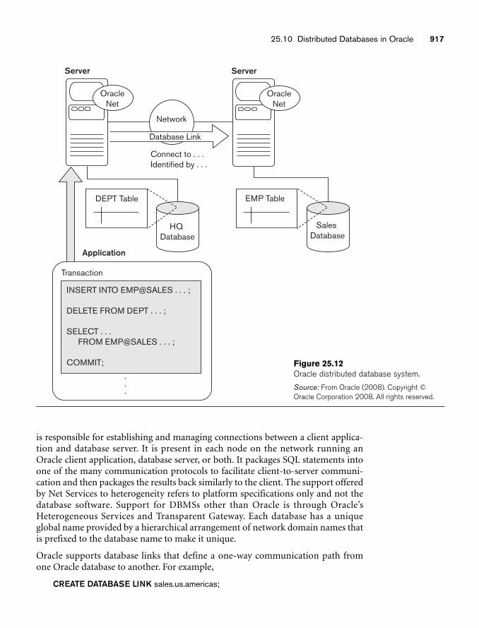
25.10 Distributed Databases in Oracle 917
Server
DEPT Table
Application
HQ Database
Connect to . . .Identified by . . .
OracleNet
EMP Table
Sales Database
Transaction
.
.
.
Network
INSERT INTO EMP@SALES . . . ;
DELETE FROM DEPT . . . ;
SELECT . . . FROM EMP@SALES . . . ;
COMMIT;
Server
OracleNet
Database Link
Figure 25.12Oracle distributed database system.
Source: From Oracle (2008). Copyright ©Oracle Corporation 2008. All rights reserved.
is responsible for establishing and managing connections between a client applica-tion and database server. It is present in each node on the network running anOracle client application, database server, or both. It packages SQL statements intoone of the many communication protocols to facilitate client-to-server communi-cation and then packages the results back similarly to the client. The support offeredby Net Services to heterogeneity refers to platform specifications only and not thedatabase software. Support for DBMSs other than Oracle is through Oracle’sHeterogeneous Services and Transparent Gateway. Each database has a uniqueglobal name provided by a hierarchical arrangement of network domain names thatis prefixed to the database name to make it unique.
Oracle supports database links that define a one-way communication path fromone Oracle database to another. For example,
CREATE DATABASE LINK sales.us.americas;
918 Chapter 25 Distributed Databases
establishes a connection to the sales database in Figure 25.12 under the networkdomain us that comes under domain americas. Using links, a user can access aremote object on another database subject to ownership rights without the need forbeing a user on the remote database.
Data in an Oracle DDBS can be replicated using snapshots or replicated mastertables. Replication is provided at the following levels:
■ Basic replication. Replicas of tables are managed for read-only access. Forupdates, data must be accessed at a single primary site.
■ Advanced (symmetric) replication. This extends beyond basic replicationby allowing applications to update table replicas throughout a replicatedDDBS. Data can be read and updated at any site. This requires additionalsoftware called Oracle’s advanced replication option. A snapshot generates acopy of a part of the table by means of a query called the snapshot definingquery. A simple snapshot definition looks like this:
CREATE SNAPSHOT SALES_ORDERS ASSELECT * FROM [email protected];
Oracle groups snapshots into refresh groups. By specifying a refresh interval, thesnapshot is automatically refreshed periodically at that interval by up to tenSnapshot Refresh Processes (SNPs). If the defining query of a snapshot contains adistinct or aggregate function, a GROUP BY or CONNECT BY clause, or join or setoperations, the snapshot is termed a complex snapshot and requires additionalprocessing. Oracle (up to version 7.3) also supports ROWID snapshots that arebased on physical row identifiers of rows in the master table.
Heterogeneous Databases in Oracle. In a heterogeneous DDBS, at least onedatabase is a non-Oracle system. Oracle Open Gateways provides access to a non-Oracle database from an Oracle server, which uses a database link to access data orto execute remote procedures in the non-Oracle system. The Open Gateways featureincludes the following:
■ Distributed transactions. Under the two-phase commit mechanism, trans-actions may span Oracle and non-Oracle systems.
■ Transparent SQL access. SQL statements issued by an application are trans-parently transformed into SQL statements understood by the non-Oraclesystem.
■ Pass-through SQL and stored procedures. An application can directlyaccess a non-Oracle system using that system’s version of SQL. Stored proce-dures in a non-Oracle SQL-based system are treated as if they were PL/SQLremote procedures.
■ Global query optimization. Cardinality information, indexes, and so on atthe non-Oracle system are accounted for by the Oracle server query opti-mizer to perform global query optimization.
■ Procedural access. Procedural systems like messaging or queuing systemsare accessed by the Oracle server using PL/SQL remote procedure calls.
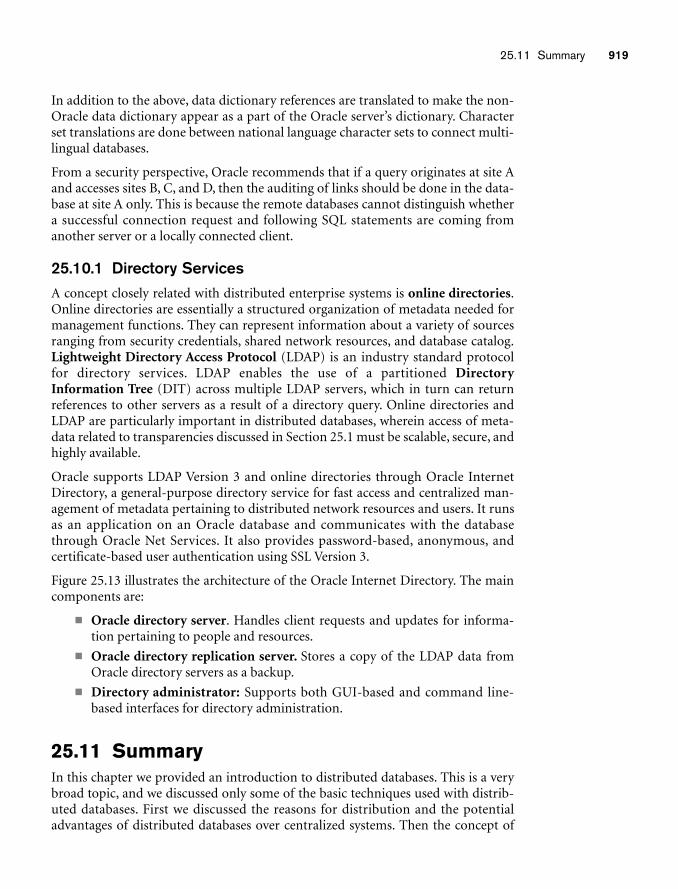
25.11 Summary 919
In addition to the above, data dictionary references are translated to make the non-Oracle data dictionary appear as a part of the Oracle server’s dictionary. Characterset translations are done between national language character sets to connect multi-lingual databases.
From a security perspective, Oracle recommends that if a query originates at site Aand accesses sites B, C, and D, then the auditing of links should be done in the data-base at site A only. This is because the remote databases cannot distinguish whethera successful connection request and following SQL statements are coming fromanother server or a locally connected client.
25.10.1 Directory ServicesA concept closely related with distributed enterprise systems is online directories.Online directories are essentially a structured organization of metadata needed formanagement functions. They can represent information about a variety of sourcesranging from security credentials, shared network resources, and database catalog.Lightweight Directory Access Protocol (LDAP) is an industry standard protocolfor directory services. LDAP enables the use of a partitioned DirectoryInformation Tree (DIT) across multiple LDAP servers, which in turn can returnreferences to other servers as a result of a directory query. Online directories andLDAP are particularly important in distributed databases, wherein access of meta-data related to transparencies discussed in Section 25.1 must be scalable, secure, andhighly available.
Oracle supports LDAP Version 3 and online directories through Oracle InternetDirectory, a general-purpose directory service for fast access and centralized man-agement of metadata pertaining to distributed network resources and users. It runsas an application on an Oracle database and communicates with the databasethrough Oracle Net Services. It also provides password-based, anonymous, and certificate-based user authentication using SSL Version 3.
Figure 25.13 illustrates the architecture of the Oracle Internet Directory. The maincomponents are:
■ Oracle directory server. Handles client requests and updates for informa-tion pertaining to people and resources.
■ Oracle directory replication server. Stores a copy of the LDAP data fromOracle directory servers as a backup.
■ Directory administrator: Supports both GUI-based and command line-based interfaces for directory administration.
25.11 SummaryIn this chapter we provided an introduction to distributed databases. This is a verybroad topic, and we discussed only some of the basic techniques used with distrib-uted databases. First we discussed the reasons for distribution and the potentialadvantages of distributed databases over centralized systems. Then the concept of
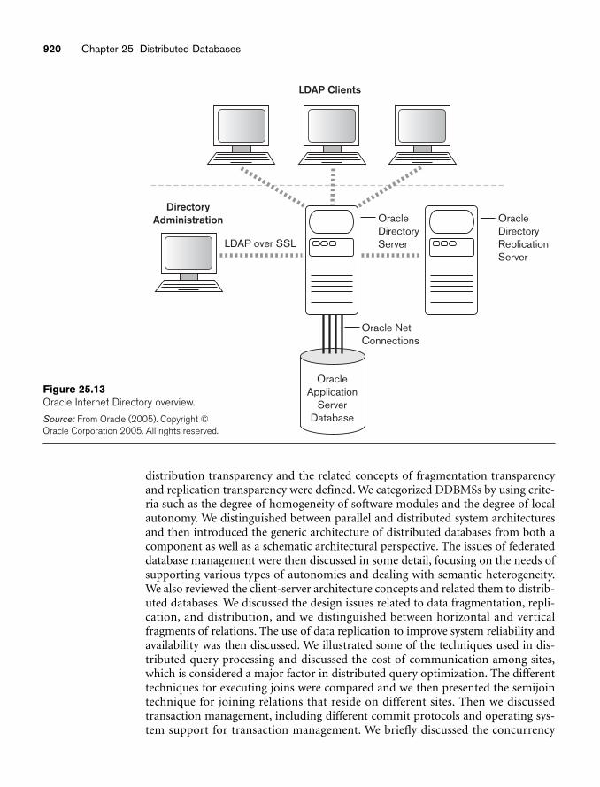
920 Chapter 25 Distributed Databases
OracleApplication
ServerDatabase
Oracle NetConnections
OracleDirectoryReplicationServer
OracleDirectoryServerLDAP over SSL
LDAP Clients
DirectoryAdministration
Figure 25.13Oracle Internet Directory overview.
Source: From Oracle (2005). Copyright ©Oracle Corporation 2005. All rights reserved.
distribution transparency and the related concepts of fragmentation transparencyand replication transparency were defined. We categorized DDBMSs by using crite-ria such as the degree of homogeneity of software modules and the degree of localautonomy. We distinguished between parallel and distributed system architecturesand then introduced the generic architecture of distributed databases from both acomponent as well as a schematic architectural perspective. The issues of federateddatabase management were then discussed in some detail, focusing on the needs ofsupporting various types of autonomies and dealing with semantic heterogeneity.We also reviewed the client-server architecture concepts and related them to distrib-uted databases. We discussed the design issues related to data fragmentation, repli-cation, and distribution, and we distinguished between horizontal and verticalfragments of relations. The use of data replication to improve system reliability andavailability was then discussed. We illustrated some of the techniques used in dis-tributed query processing and discussed the cost of communication among sites,which is considered a major factor in distributed query optimization. The differenttechniques for executing joins were compared and we then presented the semijointechnique for joining relations that reside on different sites. Then we discussedtransaction management, including different commit protocols and operating sys-tem support for transaction management. We briefly discussed the concurrency
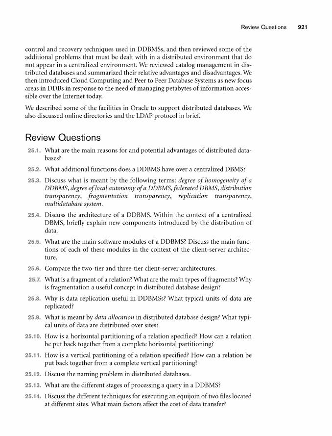
Review Questions 921
control and recovery techniques used in DDBMSs, and then reviewed some of theadditional problems that must be dealt with in a distributed environment that donot appear in a centralized environment. We reviewed catalog management in dis-tributed databases and summarized their relative advantages and disadvantages. Wethen introduced Cloud Computing and Peer to Peer Database Systems as new focusareas in DDBs in response to the need of managing petabytes of information acces-sible over the Internet today.
We described some of the facilities in Oracle to support distributed databases. Wealso discussed online directories and the LDAP protocol in brief.
Review Questions25.1. What are the main reasons for and potential advantages of distributed data-
bases?
25.2. What additional functions does a DDBMS have over a centralized DBMS?
25.3. Discuss what is meant by the following terms: degree of homogeneity of aDDBMS, degree of local autonomy of a DDBMS, federated DBMS, distributiontransparency, fragmentation transparency, replication transparency,multidatabase system.
25.4. Discuss the architecture of a DDBMS. Within the context of a centralizedDBMS, briefly explain new components introduced by the distribution ofdata.
25.5. What are the main software modules of a DDBMS? Discuss the main func-tions of each of these modules in the context of the client-server architec-ture.
25.6. Compare the two-tier and three-tier client-server architectures.
25.7. What is a fragment of a relation? What are the main types of fragments? Whyis fragmentation a useful concept in distributed database design?
25.8. Why is data replication useful in DDBMSs? What typical units of data arereplicated?
25.9. What is meant by data allocation in distributed database design? What typi-cal units of data are distributed over sites?
25.10. How is a horizontal partitioning of a relation specified? How can a relationbe put back together from a complete horizontal partitioning?
25.11. How is a vertical partitioning of a relation specified? How can a relation beput back together from a complete vertical partitioning?
25.12. Discuss the naming problem in distributed databases.
25.13. What are the different stages of processing a query in a DDBMS?
25.14. Discuss the different techniques for executing an equijoin of two files locatedat different sites. What main factors affect the cost of data transfer?
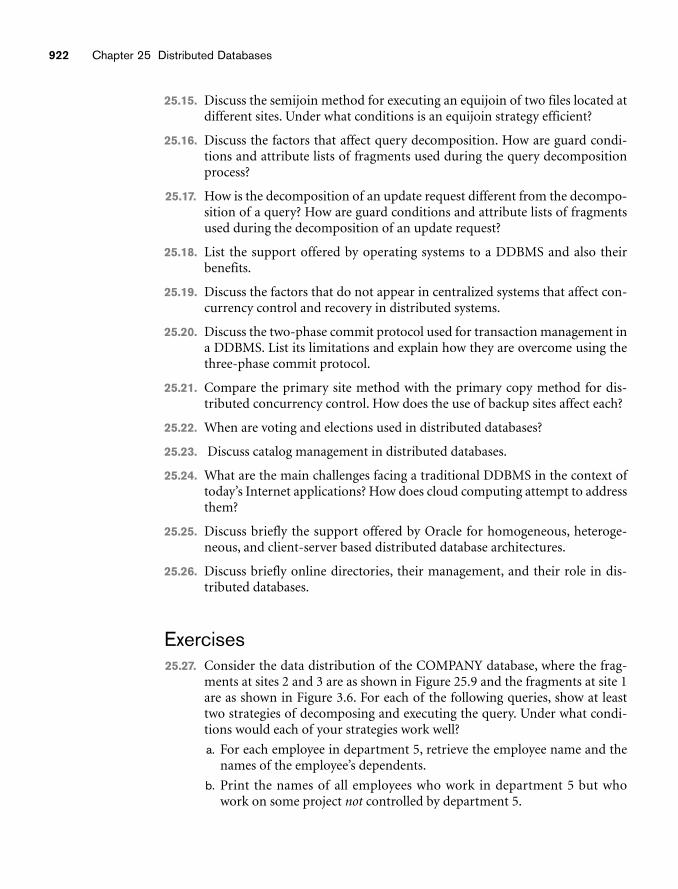
922 Chapter 25 Distributed Databases
25.15. Discuss the semijoin method for executing an equijoin of two files located atdifferent sites. Under what conditions is an equijoin strategy efficient?
25.16. Discuss the factors that affect query decomposition. How are guard condi-tions and attribute lists of fragments used during the query decompositionprocess?
25.17. How is the decomposition of an update request different from the decompo-sition of a query? How are guard conditions and attribute lists of fragmentsused during the decomposition of an update request?
25.18. List the support offered by operating systems to a DDBMS and also theirbenefits.
25.19. Discuss the factors that do not appear in centralized systems that affect con-currency control and recovery in distributed systems.
25.20. Discuss the two-phase commit protocol used for transaction management ina DDBMS. List its limitations and explain how they are overcome using thethree-phase commit protocol.
25.21. Compare the primary site method with the primary copy method for dis-tributed concurrency control. How does the use of backup sites affect each?
25.22. When are voting and elections used in distributed databases?
25.23. Discuss catalog management in distributed databases.
25.24. What are the main challenges facing a traditional DDBMS in the context oftoday’s Internet applications? How does cloud computing attempt to addressthem?
25.25. Discuss briefly the support offered by Oracle for homogeneous, heteroge-neous, and client-server based distributed database architectures.
25.26. Discuss briefly online directories, their management, and their role in dis-tributed databases.
Exercises25.27. Consider the data distribution of the COMPANY database, where the frag-
ments at sites 2 and 3 are as shown in Figure 25.9 and the fragments at site 1are as shown in Figure 3.6. For each of the following queries, show at leasttwo strategies of decomposing and executing the query. Under what condi-tions would each of your strategies work well?
a. For each employee in department 5, retrieve the employee name and thenames of the employee’s dependents.
b. Print the names of all employees who work in department 5 but whowork on some project not controlled by department 5.
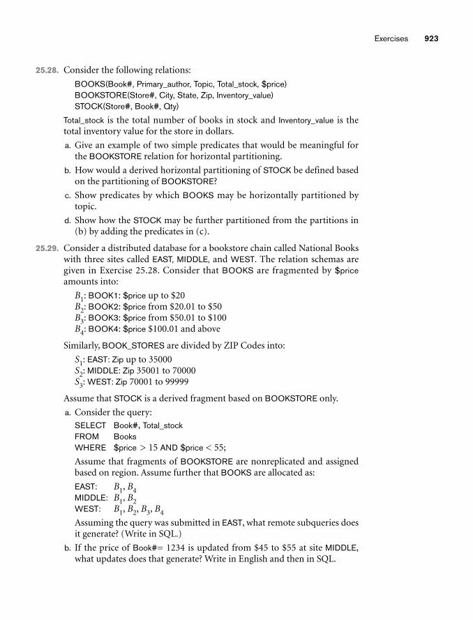
Exercises 923
25.28. Consider the following relations:
BOOKS(Book#, Primary_author, Topic, Total_stock, $price)BOOKSTORE(Store#, City, State, Zip, Inventory_value)STOCK(Store#, Book#, Qty)
Total_stock is the total number of books in stock and Inventory_value is thetotal inventory value for the store in dollars.
a. Give an example of two simple predicates that would be meaningful forthe BOOKSTORE relation for horizontal partitioning.
b. How would a derived horizontal partitioning of STOCK be defined basedon the partitioning of BOOKSTORE?
c. Show predicates by which BOOKS may be horizontally partitioned bytopic.
d. Show how the STOCK may be further partitioned from the partitions in(b) by adding the predicates in (c).
25.29. Consider a distributed database for a bookstore chain called National Bookswith three sites called EAST, MIDDLE, and WEST. The relation schemas aregiven in Exercise 25.28. Consider that BOOKS are fragmented by $priceamounts into:
B1: BOOK1: $price up to $20B2: BOOK2: $price from $20.01 to $50B3: BOOK3: $price from $50.01 to $100B4: BOOK4: $price $100.01 and above
Similarly, BOOK_STORES are divided by ZIP Codes into:
S1: EAST: Zip up to 35000S2: MIDDLE: Zip 35001 to 70000S3: WEST: Zip 70001 to 99999
Assume that STOCK is a derived fragment based on BOOKSTORE only.
a. Consider the query:
SELECT Book#, Total_stockFROM BooksWHERE $price > 15 AND $price < 55;
Assume that fragments of BOOKSTORE are nonreplicated and assignedbased on region. Assume further that BOOKS are allocated as:
EAST: B1, B4MIDDLE: B1, B2WEST: B1, B2, B3, B4
Assuming the query was submitted in EAST, what remote subqueries doesit generate? (Write in SQL.)
b. If the price of Book#= 1234 is updated from $45 to $55 at site MIDDLE,what updates does that generate? Write in English and then in SQL.
924 Chapter 25 Distributed Databases
c. Give a sample query issued at WEST that will generate a subquery forMIDDLE.
d. Write a query involving selection and projection on the above relationsand show two possible query trees that denote different ways of execu-tion.
25.30. Consider that you have been asked to propose a database architecture in alarge organization (General Motors, for example) to consolidate all dataincluding legacy databases (from hierarchical and network models, whichare explained in the Web Appendices D and E; no specific knowledge of thesemodels is needed) as well as relational databases, which are geographicallydistributed so that global applications can be supported. Assume that alter-native one is to keep all databases as they are, while alternative two is to firstconvert them to relational and then support the applications over a distrib-uted integrated database.
a. Draw two schematic diagrams for the above alternatives showing the link-ages among appropriate schemas. For alternative one, choose theapproach of providing export schemas for each database and construct-ing unified schemas for each application.
b. List the steps that you would have to go through under each alternativefrom the present situation until global applications are viable.
c. Compare these from the issues of:i. design time considerations
ii. runtime considerations
Selected BibliographyThe textbooks by Ceri and Pelagatti (1984a) and Ozsu and Valduriez (1999) aredevoted to distributed databases. Peterson and Davie (2008), Tannenbaum (2003),and Stallings (2007) cover data communications and computer networks. Comer(2008) discusses networks and internets. Ozsu et al. (1994) has a collection ofpapers on distributed object management.
Most of the research on distributed database design, query processing, and opti-mization occurred in the 1980s and 1990s; we quickly review the important refer-ences here. Distributed database design has been addressed in terms of horizontaland vertical fragmentation, allocation, and replication. Ceri et al. (1982) defined theconcept of minterm horizontal fragments. Ceri et al. (1983) developed an integerprogramming-based optimization model for horizontal fragmentation and alloca-tion. Navathe et al. (1984) developed algorithms for vertical fragmentation based onattribute affinity and showed a variety of contexts for vertical fragment allocation.Wilson and Navathe (1986) present an analytical model for optimal allocation offragments. Elmasri et al. (1987) discuss fragmentation for the ECR model;Karlapalem et al. (1996) discuss issues for distributed design of object databases.Navathe et al. (1996) discuss mixed fragmentation by combining horizontal and
Selected Bibliography 925
vertical fragmentation; Karlapalem et al. (1996) present a model for redesign of dis-tributed databases.
Distributed query processing, optimization, and decomposition are discussed inHevner and Yao (1979), Kerschberg et al. (1982), Apers et al. (1983), Ceri andPelagatti (1984), and Bodorick et al. (1992). Bernstein and Goodman (1981) discussthe theory behind semijoin processing. Wong (1983) discusses the use of relation-ships in relation fragmentation. Concurrency control and recovery schemes are dis-cussed in Bernstein and Goodman (1981a). Kumar and Hsu (1998) compiles somearticles related to recovery in distributed databases. Elections in distributed systemsare discussed in Garcia-Molina (1982). Lamport (1978) discusses problems withgenerating unique timestamps in a distributed system. Rahimi and Haug (2007)discuss a more flexible way to construct query critical metadata for P2P databases.Ouzzani and Bouguettaya (2004) outline fundamental problems in distributedquery processing over Web-based data sources.
A concurrency control technique for replicated data that is based on voting is pre-sented by Thomas (1979). Gifford (1979) proposes the use of weighted voting, andParis (1986) describes a method called voting with witnesses. Jajodia and Mutchler(1990) discuss dynamic voting. A technique called available copy is proposed byBernstein and Goodman (1984), and one that uses the idea of a group is presentedin ElAbbadi and Toueg (1988). Other work that discusses replicated data includesGladney (1989), Agrawal and ElAbbadi (1990), ElAbbadi and Toueg (1989), Kumarand Segev (1993), Mukkamala (1989), and Wolfson and Milo (1991). Bassiouni(1988) discusses optimistic protocols for DDB concurrency control. Garcia-Molina(1983) and Kumar and Stonebraker (1987) discuss techniques that use the seman-tics of the transactions. Distributed concurrency control techniques based on lock-ing and distinguished copies are presented by Menasce et al. (1980) and Minouraand Wiederhold (1982). Obermark (1982) presents algorithms for distributeddeadlock detection. In more recent work, Vadivelu et al. (2008) propose usingbackup mechanism and multilevel security to develop algorithms for improvingconcurrency. Madria et al. (2007) propose a mechanism based on a multiversiontwo-phase locking scheme and timestamping to address concurrency issues specificto mobile database systems. Boukerche and Tuck (2001) propose a technique thatallows transactions to be out of order to a limited extent. They attempt to ease theload on the application developer by exploiting the network environment and pro-ducing a schedule equivalent to a temporally ordered serial schedule. Han et al.(2004) propose a deadlock-free and serializable extended Petri net model for Web-based distributed real-time databases.
A survey of recovery techniques in distributed systems is given by Kohler (1981).Reed (1983) discusses atomic actions on distributed data. Bhargava (1987) presentsan edited compilation of various approaches and techniques for concurrency andreliability in distributed systems.
Federated database systems were first defined in McLeod and Heimbigner (1985).Techniques for schema integration in federated databases are presented by Elmasriet al. (1986), Batini et al. (1987), Hayne and Ram (1990), and Motro (1987).
926 Chapter 25 Distributed Databases
Elmagarmid and Helal (1988) and Gamal-Eldin et al. (1988) discuss the updateproblem in heterogeneous DDBSs. Heterogeneous distributed database issues arediscussed in Hsiao and Kamel (1989). Sheth and Larson (1990) present an exhaus-tive survey of federated database management.
Since late 1980s multidatabase systems and interoperability have become importanttopics. Techniques for dealing with semantic incompatibilities among multipledatabases are examined in DeMichiel (1989), Siegel and Madnick (1991),Krishnamurthy et al. (1991), and Wang and Madnick (1989). Castano et al. (1998)present an excellent survey of techniques for analysis of schemas. Pitoura et al.(1995) discuss object orientation in multidatabase systems. Xiao et al. (2003) pro-pose an XML-based model for a common data model for multidatabase systemsand present a new approach for schema mapping based on this model. Lakshmananet al. (2001) propose extending SQL for interoperability and describe the architec-ture and algorithms for achieving the same.
Transaction processing in multidatabases is discussed in Mehrotra et al. (1992),Georgakopoulos et al. (1991), Elmagarmid et al. (1990), and Brietbart et al. (1990),among others. Elmagarmid (1992) discuss transaction processing for advancedapplications, including engineering applications discussed in Heiler et al. (1992).
The workflow systems, which are becoming popular to manage information in com-plex organizations, use multilevel and nested transactions in conjunction with dis-tributed databases. Weikum (1991) discusses multilevel transaction management.Alonso et al. (1997) discuss limitations of current workflow systems. Lopes et al.(2009) propose that users define and execute their own workflows using a client-side Web browser. They attempt to leverage Web 2.0 trends to simplify the user’swork for workflow management. Jung and Yeom (2008) exploit data workflow todevelop an improved transaction management system that provides simultaneous,transparent access to the heterogeneous storages that constitute the HVEMDataGrid. Deelman and Chervanak (2008) list the challenges in data-intensive sci-entific workflows. Specifically, they look at automated management of data, effi-cient mapping techniques, and user feedback issues in workflow mapping. Theyalso argue for data reuse as an efficient means to manage data and present the chal-lenges therein.
A number of experimental distributed DBMSs have been implemented. Theseinclude distributed INGRES by Epstein et al., (1978), DDTS by Devor andWeeldreyer, (1980), SDD-1 by Rothnie et al., (1980), System R* by Lindsay et al.,(1984), SIRIUS-DELTA by Ferrier and Stangret, (1982), and MULTIBASE by Smithet al., (1981). The OMNIBASE system by Rusinkiewicz et al. (1988) and theFederated Information Base developed using the Candide data model by Navathe etal. (1994) are examples of federated DDBMSs. Pitoura et al. (1995) present a com-parative survey of the federated database system prototypes. Most commercialDBMS vendors have products using the client-server approach and offer distributedversions of their systems. Some system issues concerning client-server DBMS archi-tectures are discussed in Carey et al. (1991), DeWitt et al. (1990), and Wang andRowe (1991). Khoshafian et al. (1992) discuss design issues for relational DBMSs in

the client-server environment. Client-server management issues are discussed inmany books, such as Zantinge and Adriaans (1996). Di Stefano (2005) discussesdata distribution issues specific to grid computing. A major part of this discussionmay also apply to cloud computing.
Selected Bibliography 927
part11Advanced Database Models,
Systems, and Applications
931
Enhanced Data Models for Advanced Applications
As the use of database systems has grown, users havedemanded additional functionality from these
software packages, with the purpose of making it easier to implement moreadvanced and complex user applications. Object-oriented databases and object-relational systems do provide features that allow users to extend their systems byspecifying additional abstract data types for each application. However, it is quiteuseful to identify certain common features for some of these advanced applicationsand to create models that can represent them. Additionally, specialized storagestructures and indexing methods can be implemented to improve the performanceof these common features. Then the features can be implemented as abstract datatypes or class libraries and purchased separately from the basic DBMS softwarepackage. The term data blade has been used in Informix and cartridge in Oracle torefer to such optional submodules that can be included in a DBMS package. Userscan utilize these features directly if they are suitable for their applications, withouthaving to reinvent, reimplement, and reprogram such common features.
This chapter introduces database concepts for some of the common features thatare needed by advanced applications and are being used widely. We will cover activerules that are used in active database applications, temporal concepts that are used intemporal database applications, and, briefly, some of the issues involving spatialdatabases and multimedia databases. We will also discuss deductive databases. It isimportant to note that each of these topics is very broad, and we give only a briefintroduction to each. In fact, each of these areas can serve as the sole topic of a com-plete book.
In Section 26.1 we introduce the topic of active databases, which provide additionalfunctionality for specifying active rules. These rules can be automatically triggered
26chapter 26
932 Chapter 26 Enhanced Data Models for Advanced Applications
by events that occur, such as database updates or certain times being reached, andcan initiate certain actions that have been specified in the rule declaration to occurif certain conditions are met. Many commercial packages include some of the func-tionality provided by active databases in the form of triggers. Triggers are now partof the SQL-99 and later standards.
In Section 26.2 we introduce the concepts of temporal databases, which permit thedatabase system to store a history of changes, and allow users to query both currentand past states of the database. Some temporal database models also allow users tostore future expected information, such as planned schedules. It is important tonote that many database applications are temporal, but they are often implementedwithout having much temporal support from the DBMS package—that is, the tem-poral concepts are implemented in the application programs that access the data-base.
Section 26.3 gives a brief overview of spatial database concepts. We discuss types ofspatial data, different kinds of spatial analyses, operations on spatial data, types ofspatial queries, spatial data indexing, spatial data mining, and applications of spatialdatabases.
Section 26.4 is devoted to multimedia database concepts. Multimedia databasesprovide features that allow users to store and query different types of multimediainformation, which includes images (such as pictures and drawings), video clips(such as movies, newsreels, and home videos), audio clips (such as songs, phonemessages, and speeches), and documents (such as books and articles). We discussautomatic analysis of images, object recognition in images, and semantic tagging ofimages,
In Section 26.5 we discuss deductive databases,1 an area that is at the intersection ofdatabases, logic, and artificial intelligence or knowledge bases. A deductive data-base system includes capabilities to define (deductive) rules, which can deduce orinfer additional information from the facts that are stored in a database. Becausepart of the theoretical foundation for some deductive database systems is mathe-matical logic, such rules are often referred to as logic databases. Other types of sys-tems, referred to as expert database systems or knowledge-based systems, alsoincorporate reasoning and inferencing capabilities; such systems use techniquesthat were developed in the field of artificial intelligence, including semantic networks, frames, production systems, or rules for capturing domain-specificknowledge. Section 26.6 summarizes the chapter.
Readers may choose to peruse the particular topics they are interested in, as the sec-tions in this chapter are practically independent of one another.
1Section 26.5 is a summary of Deductive Databases. The full chapter from the third edition, which pro-vides a more comprehensive introduction, is available on the book’s Web site.
26.1 Active Database Concepts and Triggers 933
26.1 Active Database Concepts and TriggersRules that specify actions that are automatically triggered by certain events havebeen considered important enhancements to database systems for quite some time.In fact, the concept of triggers—a technique for specifying certain types of activerules—has existed in early versions of the SQL specification for relational databasesand triggers are now part of the SQL-99 and later standards. Commercial relationalDBMSs—such as Oracle, DB2, and Microsoft SQLServer—have various versions oftriggers available. However, much research into what a general model for activedatabases should look like has been done since the early models of triggers wereproposed. In Section 26.1.1 we will present the general concepts that have been pro-posed for specifying rules for active databases. We will use the syntax of the Oraclecommercial relational DBMS to illustrate these concepts with specific examples,since Oracle triggers are close to the way rules are specified in the SQL standard.Section 26.1.2 will discuss some general design and implementation issues for activedatabases. We give examples of how active databases are implemented in the STAR-BURST experimental DBMS in Section 26.1.3, since STARBURST provides formany of the concepts of generalized active databases within its framework. Section26.1.4 discusses possible applications of active databases. Finally, Section 26.1.5describes how triggers are declared in the SQL-99 standard.
26.1.1 Generalized Model for Active Databases and Oracle Triggers
The model that has been used to specify active database rules is referred to as theEvent-Condition-Action (ECA) model. A rule in the ECA model has three compo-nents:
1. The event(s) that triggers the rule: These events are usually database updateoperations that are explicitly applied to the database. However, in the generalmodel, they could also be temporal events2 or other kinds of external events.
2. The condition that determines whether the rule action should be executed:Once the triggering event has occurred, an optional condition may be evalu-ated. If no condition is specified, the action will be executed once the eventoccurs. If a condition is specified, it is first evaluated, and only if it evaluatesto true will the rule action be executed.
3. The action to be taken: The action is usually a sequence of SQL statements,but it could also be a database transaction or an external program that willbe automatically executed.
Let us consider some examples to illustrate these concepts. The examples are basedon a much simplified variation of the COMPANY database application from Figure3.5 and is shown in Figure 26.1, with each employee having a name (Name), Social
2An example would be a temporal event specified as a periodic time, such as: Trigger this rule every dayat 5:30 A.M.
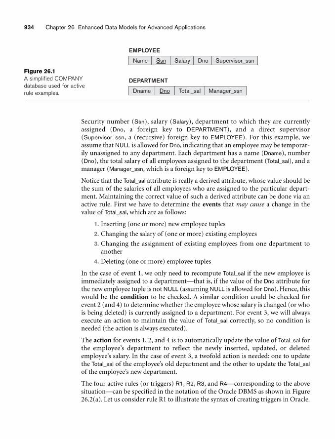
934 Chapter 26 Enhanced Data Models for Advanced Applications
Name Ssn Salary Dno Supervisor_ssn
EMPLOYEE
Dname Dno Total_sal Manager_ssn
DEPARTMENT
Figure 26.1A simplified COMPANYdatabase used for activerule examples.
Security number (Ssn), salary (Salary), department to which they are currentlyassigned (Dno, a foreign key to DEPARTMENT), and a direct supervisor(Supervisor_ssn, a (recursive) foreign key to EMPLOYEE). For this example, weassume that NULL is allowed for Dno, indicating that an employee may be temporar-ily unassigned to any department. Each department has a name (Dname), number(Dno), the total salary of all employees assigned to the department (Total_sal), and amanager (Manager_ssn, which is a foreign key to EMPLOYEE).
Notice that the Total_sal attribute is really a derived attribute, whose value should bethe sum of the salaries of all employees who are assigned to the particular depart-ment. Maintaining the correct value of such a derived attribute can be done via anactive rule. First we have to determine the events that may cause a change in thevalue of Total_sal, which are as follows:
1. Inserting (one or more) new employee tuples
2. Changing the salary of (one or more) existing employees
3. Changing the assignment of existing employees from one department toanother
4. Deleting (one or more) employee tuples
In the case of event 1, we only need to recompute Total_sal if the new employee isimmediately assigned to a department—that is, if the value of the Dno attribute forthe new employee tuple is not NULL (assuming NULL is allowed for Dno). Hence, thiswould be the condition to be checked. A similar condition could be checked forevent 2 (and 4) to determine whether the employee whose salary is changed (or whois being deleted) is currently assigned to a department. For event 3, we will alwaysexecute an action to maintain the value of Total_sal correctly, so no condition isneeded (the action is always executed).
The action for events 1, 2, and 4 is to automatically update the value of Total_sal forthe employee’s department to reflect the newly inserted, updated, or deletedemployee’s salary. In the case of event 3, a twofold action is needed: one to updatethe Total_sal of the employee’s old department and the other to update the Total_salof the employee’s new department.
The four active rules (or triggers) R1, R2, R3, and R4—corresponding to the abovesituation—can be specified in the notation of the Oracle DBMS as shown in Figure26.2(a). Let us consider rule R1 to illustrate the syntax of creating triggers in Oracle.
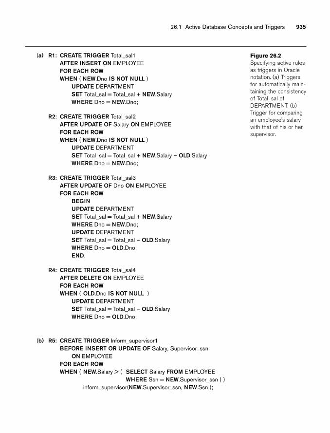
26.1 Active Database Concepts and Triggers 935
(a) R1: CREATE TRIGGER Total_sal1AFTER INSERT ON EMPLOYEEFOR EACH ROWWHEN ( NEW.Dno IS NOT NULL )
UPDATE DEPARTMENTSET Total_sal = Total_sal + NEW.SalaryWHERE Dno = NEW.Dno;
R2: CREATE TRIGGER Total_sal2AFTER UPDATE OF Salary ON EMPLOYEEFOR EACH ROWWHEN ( NEW.Dno IS NOT NULL )
UPDATE DEPARTMENTSET Total_sal = Total_sal + NEW.Salary – OLD.SalaryWHERE Dno = NEW.Dno;
R3: CREATE TRIGGER Total_sal3AFTER UPDATE OF Dno ON EMPLOYEEFOR EACH ROW
BEGINUPDATE DEPARTMENTSET Total_sal = Total_sal + NEW.SalaryWHERE Dno = NEW.Dno;UPDATE DEPARTMENTSET Total_sal = Total_sal – OLD.SalaryWHERE Dno = OLD.Dno;END;
R4: CREATE TRIGGER Total_sal4AFTER DELETE ON EMPLOYEEFOR EACH ROWWHEN ( OLD.Dno IS NOT NULL )
UPDATE DEPARTMENTSET Total_sal = Total_sal – OLD.SalaryWHERE Dno = OLD.Dno;
(b) R5: CREATE TRIGGER Inform_supervisor1BEFORE INSERT OR UPDATE OF Salary, Supervisor_ssn
ON EMPLOYEEFOR EACH ROWWHEN ( NEW.Salary > ( SELECT Salary FROM EMPLOYEE
WHERE Ssn = NEW.Supervisor_ssn ) )inform_supervisor(NEW.Supervisor_ssn, NEW.Ssn );
Figure 26.2Specifying active rulesas triggers in Oraclenotation. (a) Triggersfor automatically main-taining the consistencyof Total_sal ofDEPARTMENT. (b)Trigger for comparingan employee’s salarywith that of his or hersupervisor.
936 Chapter 26 Enhanced Data Models for Advanced Applications
The CREATE TRIGGER statement specifies a trigger (or active rule) name—Total_sal1 for R1. The AFTER clause specifies that the rule will be triggered after theevents that trigger the rule occur. The triggering events—an insert of a newemployee in this example—are specified following the AFTER keyword.3
The ON clause specifies the relation on which the rule is specified—EMPLOYEE forR1. The optional keywords FOR EACH ROW specify that the rule will be triggeredonce for each row that is affected by the triggering event.4
The optional WHEN clause is used to specify any conditions that need to be checkedafter the rule is triggered, but before the action is executed. Finally, the action(s) tobe taken is (are) specified as a PL/SQL block, which typically contains one or moreSQL statements or calls to execute external procedures.
The four triggers (active rules) R1, R2, R3, and R4 illustrate a number of features ofactive rules. First, the basic events that can be specified for triggering the rules arethe standard SQL update commands: INSERT, DELETE, and UPDATE. They are spec-ified by the keywords INSERT, DELETE, and UPDATE in Oracle notation. In the caseof UPDATE, one may specify the attributes to be updated—for example, by writingUPDATE OF Salary, Dno. Second, the rule designer needs to have a way to refer to thetuples that have been inserted, deleted, or modified by the triggering event. The key-words NEW and OLD are used in Oracle notation; NEW is used to refer to a newlyinserted or newly updated tuple, whereas OLD is used to refer to a deleted tuple or toa tuple before it was updated.
Thus, rule R1 is triggered after an INSERT operation is applied to the EMPLOYEErelation. In R1, the condition (NEW.Dno IS NOT NULL) is checked, and if it evaluatesto true, meaning that the newly inserted employee tuple is related to a department,then the action is executed. The action updates the DEPARTMENT tuple(s) related tothe newly inserted employee by adding their salary (NEW.Salary) to the Total_salattribute of their related department.
Rule R2 is similar to R1, but it is triggered by an UPDATE operation that updates theSALARY of an employee rather than by an INSERT. Rule R3 is triggered by an updateto the Dno attribute of EMPLOYEE, which signifies changing an employee’s assign-ment from one department to another. There is no condition to check in R3, so theaction is executed whenever the triggering event occurs. The action updates boththe old department and new department of the reassigned employees by addingtheir salary to Total_sal of their new department and subtracting their salary fromTotal_sal of their old department. Note that this should work even if the value of Dnois NULL, because in this case no department will be selected for the rule action.5
3As we will see, it is also possible to specify BEFORE instead of AFTER, which indicates that the rule istriggered before the triggering event is executed.
4Again, we will see that an alternative is to trigger the rule only once even if multiple rows (tuples) areaffected by the triggering event.5R1, R2, and R4 can also be written without a condition. However, it may be more efficient to executethem with the condition since the action is not invoked unless it is required.
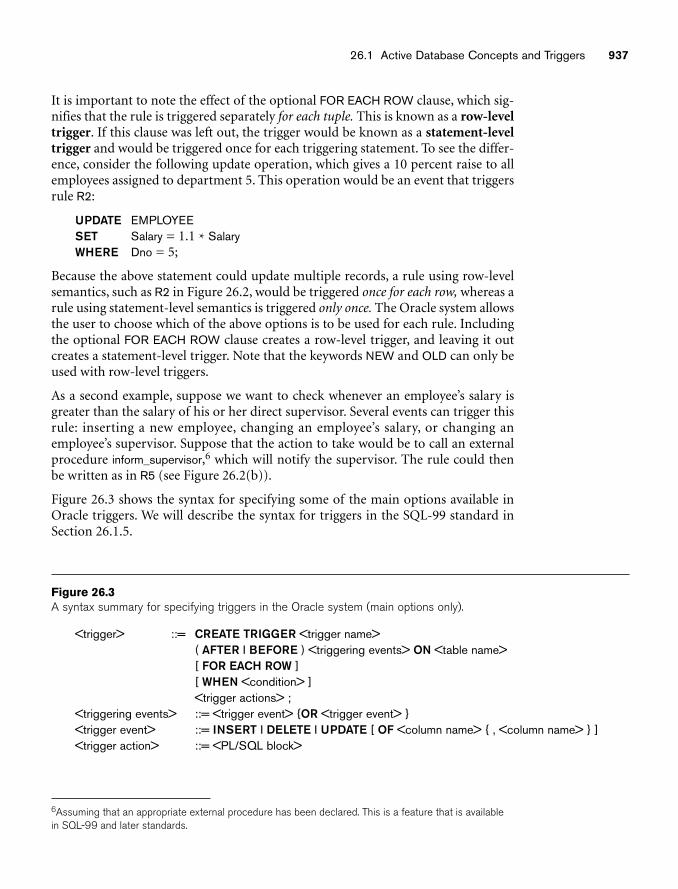
26.1 Active Database Concepts and Triggers 937
<trigger> ::= CREATE TRIGGER <trigger name>( AFTER I BEFORE ) <triggering events> ON <table name>[ FOR EACH ROW ][ WHEN <condition> ]<trigger actions> ;
<triggering events> ::= <trigger event> {OR <trigger event> }<trigger event> ::= INSERT I DELETE I UPDATE [ OF <column name> { , <column name> } ]<trigger action> ::= <PL/SQL block>
Figure 26.3A syntax summary for specifying triggers in the Oracle system (main options only).
It is important to note the effect of the optional FOR EACH ROW clause, which sig-nifies that the rule is triggered separately for each tuple. This is known as a row-leveltrigger. If this clause was left out, the trigger would be known as a statement-leveltrigger and would be triggered once for each triggering statement. To see the differ-ence, consider the following update operation, which gives a 10 percent raise to allemployees assigned to department 5. This operation would be an event that triggersrule R2:
UPDATE EMPLOYEESET Salary = 1.1 * SalaryWHERE Dno = 5;
Because the above statement could update multiple records, a rule using row-levelsemantics, such as R2 in Figure 26.2, would be triggered once for each row, whereas arule using statement-level semantics is triggered only once. The Oracle system allowsthe user to choose which of the above options is to be used for each rule. Includingthe optional FOR EACH ROW clause creates a row-level trigger, and leaving it outcreates a statement-level trigger. Note that the keywords NEW and OLD can only beused with row-level triggers.
As a second example, suppose we want to check whenever an employee’s salary isgreater than the salary of his or her direct supervisor. Several events can trigger thisrule: inserting a new employee, changing an employee’s salary, or changing anemployee’s supervisor. Suppose that the action to take would be to call an externalprocedure inform_supervisor,6 which will notify the supervisor. The rule could thenbe written as in R5 (see Figure 26.2(b)).
Figure 26.3 shows the syntax for specifying some of the main options available inOracle triggers. We will describe the syntax for triggers in the SQL-99 standard inSection 26.1.5.
6Assuming that an appropriate external procedure has been declared. This is a feature that is availablein SQL-99 and later standards.
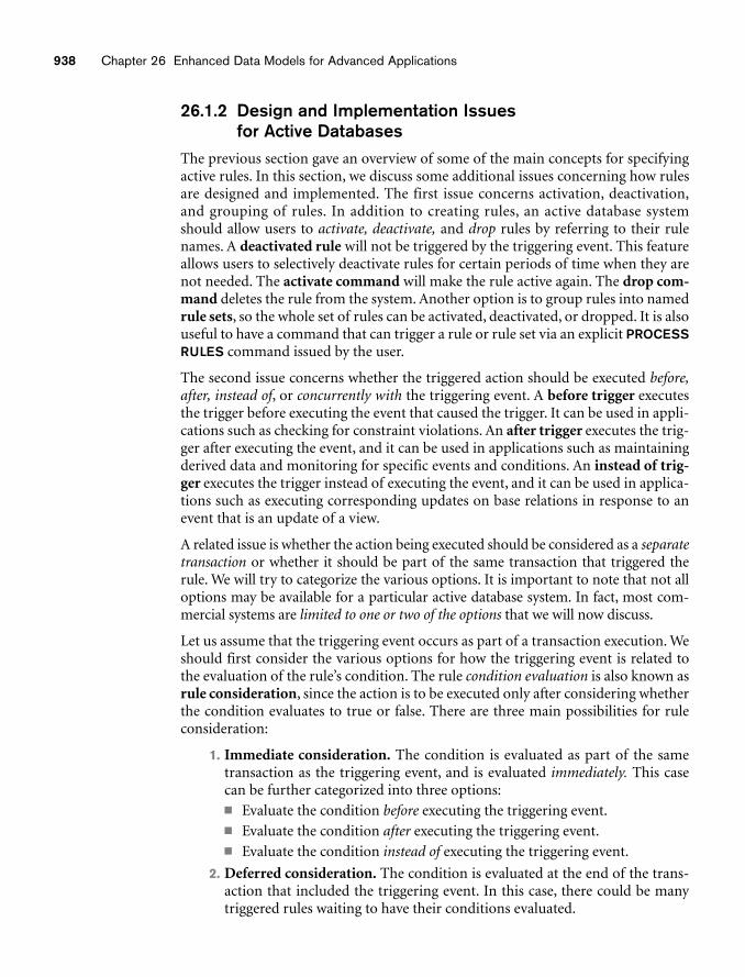
938 Chapter 26 Enhanced Data Models for Advanced Applications
26.1.2 Design and Implementation Issues for Active Databases
The previous section gave an overview of some of the main concepts for specifyingactive rules. In this section, we discuss some additional issues concerning how rulesare designed and implemented. The first issue concerns activation, deactivation,and grouping of rules. In addition to creating rules, an active database systemshould allow users to activate, deactivate, and drop rules by referring to their rulenames. A deactivated rule will not be triggered by the triggering event. This featureallows users to selectively deactivate rules for certain periods of time when they arenot needed. The activate command will make the rule active again. The drop com-mand deletes the rule from the system. Another option is to group rules into namedrule sets, so the whole set of rules can be activated, deactivated, or dropped. It is alsouseful to have a command that can trigger a rule or rule set via an explicit PROCESSRULES command issued by the user.
The second issue concerns whether the triggered action should be executed before,after, instead of, or concurrently with the triggering event. A before trigger executesthe trigger before executing the event that caused the trigger. It can be used in appli-cations such as checking for constraint violations. An after trigger executes the trig-ger after executing the event, and it can be used in applications such as maintainingderived data and monitoring for specific events and conditions. An instead of trig-ger executes the trigger instead of executing the event, and it can be used in applica-tions such as executing corresponding updates on base relations in response to anevent that is an update of a view.
A related issue is whether the action being executed should be considered as a separatetransaction or whether it should be part of the same transaction that triggered therule. We will try to categorize the various options. It is important to note that not alloptions may be available for a particular active database system. In fact, most com-mercial systems are limited to one or two of the options that we will now discuss.
Let us assume that the triggering event occurs as part of a transaction execution. Weshould first consider the various options for how the triggering event is related tothe evaluation of the rule’s condition. The rule condition evaluation is also known asrule consideration, since the action is to be executed only after considering whetherthe condition evaluates to true or false. There are three main possibilities for ruleconsideration:
1. Immediate consideration. The condition is evaluated as part of the sametransaction as the triggering event, and is evaluated immediately. This casecan be further categorized into three options:■ Evaluate the condition before executing the triggering event.■ Evaluate the condition after executing the triggering event.■ Evaluate the condition instead of executing the triggering event.
2. Deferred consideration. The condition is evaluated at the end of the trans-action that included the triggering event. In this case, there could be manytriggered rules waiting to have their conditions evaluated.
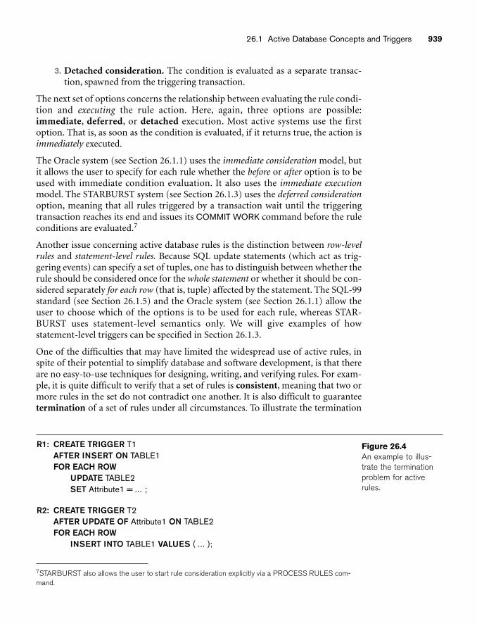
26.1 Active Database Concepts and Triggers 939
3. Detached consideration. The condition is evaluated as a separate transac-tion, spawned from the triggering transaction.
The next set of options concerns the relationship between evaluating the rule condi-tion and executing the rule action. Here, again, three options are possible:immediate, deferred, or detached execution. Most active systems use the firstoption. That is, as soon as the condition is evaluated, if it returns true, the action isimmediately executed.
The Oracle system (see Section 26.1.1) uses the immediate consideration model, butit allows the user to specify for each rule whether the before or after option is to beused with immediate condition evaluation. It also uses the immediate executionmodel. The STARBURST system (see Section 26.1.3) uses the deferred considerationoption, meaning that all rules triggered by a transaction wait until the triggeringtransaction reaches its end and issues its COMMIT WORK command before the ruleconditions are evaluated.7
Another issue concerning active database rules is the distinction between row-levelrules and statement-level rules. Because SQL update statements (which act as trig-gering events) can specify a set of tuples, one has to distinguish between whether therule should be considered once for the whole statement or whether it should be con-sidered separately for each row (that is, tuple) affected by the statement. The SQL-99standard (see Section 26.1.5) and the Oracle system (see Section 26.1.1) allow theuser to choose which of the options is to be used for each rule, whereas STAR-BURST uses statement-level semantics only. We will give examples of how statement-level triggers can be specified in Section 26.1.3.
One of the difficulties that may have limited the widespread use of active rules, inspite of their potential to simplify database and software development, is that thereare no easy-to-use techniques for designing, writing, and verifying rules. For exam-ple, it is quite difficult to verify that a set of rules is consistent, meaning that two ormore rules in the set do not contradict one another. It is also difficult to guaranteetermination of a set of rules under all circumstances. To illustrate the termination
R1: CREATE TRIGGER T1AFTER INSERT ON TABLE1FOR EACH ROW
UPDATE TABLE2SET Attribute1 = ... ;
R2: CREATE TRIGGER T2AFTER UPDATE OF Attribute1 ON TABLE2FOR EACH ROW
INSERT INTO TABLE1 VALUES ( ... );
Figure 26.4An example to illus-trate the terminationproblem for activerules.
7STARBURST also allows the user to start rule consideration explicitly via a PROCESS RULES com-mand.
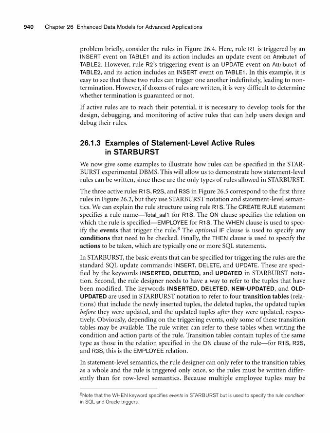
940 Chapter 26 Enhanced Data Models for Advanced Applications
problem briefly, consider the rules in Figure 26.4. Here, rule R1 is triggered by anINSERT event on TABLE1 and its action includes an update event on Attribute1 ofTABLE2. However, rule R2’s triggering event is an UPDATE event on Attribute1 ofTABLE2, and its action includes an INSERT event on TABLE1. In this example, it iseasy to see that these two rules can trigger one another indefinitely, leading to non-termination. However, if dozens of rules are written, it is very difficult to determinewhether termination is guaranteed or not.
If active rules are to reach their potential, it is necessary to develop tools for thedesign, debugging, and monitoring of active rules that can help users design anddebug their rules.
26.1.3 Examples of Statement-Level Active Rules in STARBURST
We now give some examples to illustrate how rules can be specified in the STAR-BURST experimental DBMS. This will allow us to demonstrate how statement-levelrules can be written, since these are the only types of rules allowed in STARBURST.
The three active rules R1S, R2S, and R3S in Figure 26.5 correspond to the first threerules in Figure 26.2, but they use STARBURST notation and statement-level seman-tics. We can explain the rule structure using rule R1S. The CREATE RULE statementspecifies a rule name—Total_sal1 for R1S. The ON clause specifies the relation onwhich the rule is specified—EMPLOYEE for R1S. The WHEN clause is used to spec-ify the events that trigger the rule.8 The optional IF clause is used to specify anyconditions that need to be checked. Finally, the THEN clause is used to specify theactions to be taken, which are typically one or more SQL statements.
In STARBURST, the basic events that can be specified for triggering the rules are thestandard SQL update commands: INSERT, DELETE, and UPDATE. These are speci-fied by the keywords INSERTED, DELETED, and UPDATED in STARBURST nota-tion. Second, the rule designer needs to have a way to refer to the tuples that havebeen modified. The keywords INSERTED, DELETED, NEW-UPDATED, and OLD-UPDATED are used in STARBURST notation to refer to four transition tables (rela-tions) that include the newly inserted tuples, the deleted tuples, the updated tuplesbefore they were updated, and the updated tuples after they were updated, respec-tively. Obviously, depending on the triggering events, only some of these transitiontables may be available. The rule writer can refer to these tables when writing thecondition and action parts of the rule. Transition tables contain tuples of the sametype as those in the relation specified in the ON clause of the rule—for R1S, R2S,and R3S, this is the EMPLOYEE relation.
In statement-level semantics, the rule designer can only refer to the transition tablesas a whole and the rule is triggered only once, so the rules must be written differ-ently than for row-level semantics. Because multiple employee tuples may be
8Note that the WHEN keyword specifies events in STARBURST but is used to specify the rule condition
in SQL and Oracle triggers.
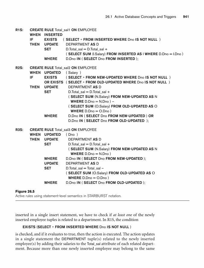
26.1 Active Database Concepts and Triggers 941
R1S: CREATE RULE Total_sal1 ON EMPLOYEEWHEN INSERTEDIF EXISTS ( SELECT * FROM INSERTED WHERE Dno IS NOT NULL )THEN UPDATE DEPARTMENT AS D
SET D.Total_sal = D.Total_sal +( SELECT SUM (I.Salary) FROM INSERTED AS I WHERE D.Dno = I.Dno )
WHERE D.Dno IN ( SELECT Dno FROM INSERTED );
R2S: CREATE RULE Total_sal2 ON EMPLOYEEWHEN UPDATED ( Salary )IF EXISTS ( SELECT * FROM NEW-UPDATED WHERE Dno IS NOT NULL )
OR EXISTS ( SELECT * FROM OLD-UPDATED WHERE Dno IS NOT NULL )THEN UPDATE DEPARTMENT AS D
SET D.Total_sal = D.Total_sal +( SELECT SUM (N.Salary) FROM NEW-UPDATED AS N
WHERE D.Dno = N.Dno ) –( SELECT SUM (O.Salary) FROM OLD-UPDATED AS O
WHERE D.Dno = O.Dno )WHERE D.Dno IN ( SELECT Dno FROM NEW-UPDATED ) OR
D.Dno IN ( SELECT Dno FROM OLD-UPDATED );
R3S: CREATE RULE Total_sal3 ON EMPLOYEEWHEN UPDATED ( Dno )THEN UPDATE DEPARTMENT AS D
SET D.Total_sal = D.Total_sal +( SELECT SUM (N.Salary) FROM NEW-UPDATED AS N
WHERE D.Dno = N.Dno )WHERE D.Dno IN ( SELECT Dno FROM NEW-UPDATED );UPDATE DEPARTMENT AS DSET D.Total_sal = Total_sal –
( SELECT SUM (O.Salary) FROM OLD-UPDATED AS OWHERE D.Dno = O.Dno )
WHERE D.Dno IN ( SELECT Dno FROM OLD-UPDATED );
Figure 26.5Active rules using statement-level semantics in STARBURST notation.
inserted in a single insert statement, we have to check if at least one of the newlyinserted employee tuples is related to a department. In R1S, the condition
EXISTS (SELECT * FROM INSERTED WHERE Dno IS NOT NULL )
is checked, and if it evaluates to true, then the action is executed. The action updatesin a single statement the DEPARTMENT tuple(s) related to the newly insertedemployee(s) by adding their salaries to the Total_sal attribute of each related depart-ment. Because more than one newly inserted employee may belong to the same
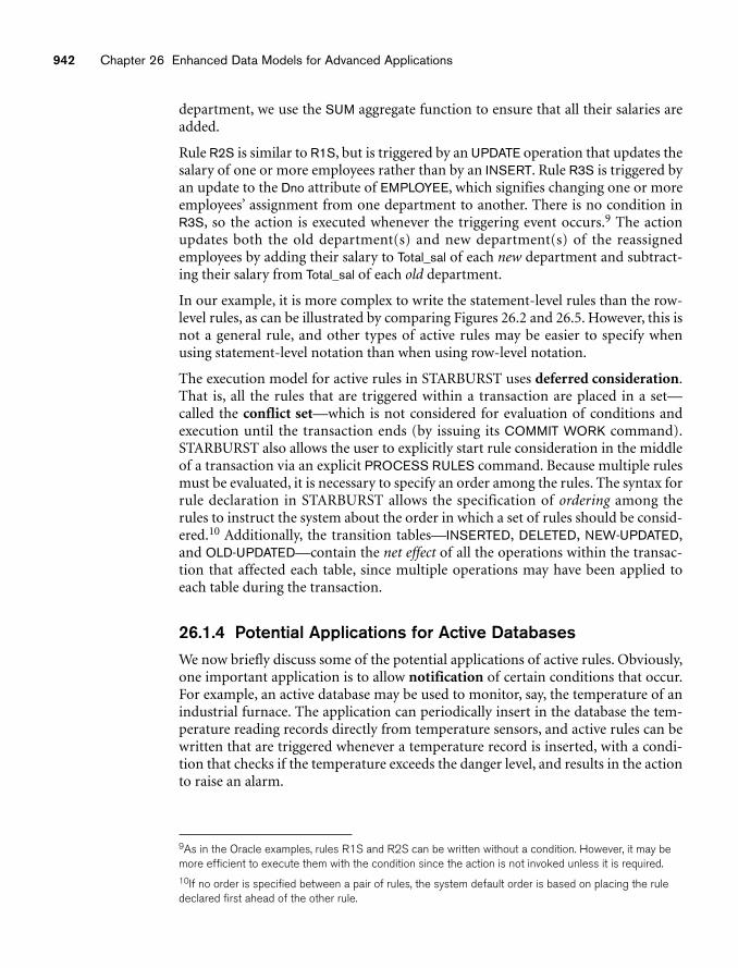
942 Chapter 26 Enhanced Data Models for Advanced Applications
department, we use the SUM aggregate function to ensure that all their salaries areadded.
Rule R2S is similar to R1S, but is triggered by an UPDATE operation that updates thesalary of one or more employees rather than by an INSERT. Rule R3S is triggered byan update to the Dno attribute of EMPLOYEE, which signifies changing one or moreemployees’ assignment from one department to another. There is no condition inR3S, so the action is executed whenever the triggering event occurs.9 The actionupdates both the old department(s) and new department(s) of the reassignedemployees by adding their salary to Total_sal of each new department and subtract-ing their salary from Total_sal of each old department.
In our example, it is more complex to write the statement-level rules than the row-level rules, as can be illustrated by comparing Figures 26.2 and 26.5. However, this isnot a general rule, and other types of active rules may be easier to specify whenusing statement-level notation than when using row-level notation.
The execution model for active rules in STARBURST uses deferred consideration.That is, all the rules that are triggered within a transaction are placed in a set—called the conflict set—which is not considered for evaluation of conditions andexecution until the transaction ends (by issuing its COMMIT WORK command).STARBURST also allows the user to explicitly start rule consideration in the middleof a transaction via an explicit PROCESS RULES command. Because multiple rulesmust be evaluated, it is necessary to specify an order among the rules. The syntax forrule declaration in STARBURST allows the specification of ordering among therules to instruct the system about the order in which a set of rules should be consid-ered.10 Additionally, the transition tables—INSERTED, DELETED, NEW-UPDATED,and OLD-UPDATED—contain the net effect of all the operations within the transac-tion that affected each table, since multiple operations may have been applied toeach table during the transaction.
26.1.4 Potential Applications for Active DatabasesWe now briefly discuss some of the potential applications of active rules. Obviously,one important application is to allow notification of certain conditions that occur.For example, an active database may be used to monitor, say, the temperature of anindustrial furnace. The application can periodically insert in the database the tem-perature reading records directly from temperature sensors, and active rules can bewritten that are triggered whenever a temperature record is inserted, with a condi-tion that checks if the temperature exceeds the danger level, and results in the actionto raise an alarm.
9As in the Oracle examples, rules R1S and R2S can be written without a condition. However, it may bemore efficient to execute them with the condition since the action is not invoked unless it is required.10If no order is specified between a pair of rules, the system default order is based on placing the ruledeclared first ahead of the other rule.
26.2 Temporal Database Concepts 943
Active rules can also be used to enforce integrity constraints by specifying the typesof events that may cause the constraints to be violated and then evaluating appro-priate conditions that check whether the constraints are actually violated by theevent or not. Hence, complex application constraints, often known as businessrules, may be enforced that way. For example, in the UNIVERSITY database applica-tion, one rule may monitor the GPA of students whenever a new grade is entered,and it may alert the advisor if the GPA of a student falls below a certain threshold;another rule may check that course prerequisites are satisfied before allowing a stu-dent to enroll in a course; and so on.
Other applications include the automatic maintenance of derived data, such as theexamples of rules R1 through R4 that maintain the derived attribute Total_sal when-ever individual employee tuples are changed. A similar application is to use activerules to maintain the consistency of materialized views (see Section 5.3) wheneverthe base relations are modified. Alternately, an update operation specified on a viewcan be a triggering event, which can be converted to updates on the base relations byusing an instead of trigger. These applications are also relevant to the new data ware-housing technologies (see Chapter 29). A related application maintains thatreplicated tables are consistent by specifying rules that modify the replicas when-ever the master table is modified.
26.1.5 Triggers in SQL-99Triggers in the SQL-99 and later standards are quite similar to the examples we dis-cussed in Section 26.1.1, with some minor syntactic differences. The basic eventsthat can be specified for triggering the rules are the standard SQL update com-mands: INSERT, DELETE, and UPDATE. In the case of UPDATE, one may specify theattributes to be updated. Both row-level and statement-level triggers are allowed,indicated in the trigger by the clauses FOR EACH ROW and FOR EACH STATEMENT,respectively. One syntactic difference is that the trigger may specify particular tuplevariable names for the old and new tuples instead of using the keywords NEW andOLD, as shown in Figure 26.1. Trigger T1 in Figure 26.6 shows how the row-leveltrigger R2 from Figure 26.1(a) may be specified in SQL-99. Inside theREFERENCING clause, we named tuple variables (aliases) O and N to refer to theOLD tuple (before modification) and NEW tuple (after modification), respectively.Trigger T2 in Figure 26.6 shows how the statement-level trigger R2S from Figure26.5 may be specified in SQL-99. For a statement-level trigger, the REFERENCINGclause is used to refer to the table of all new tuples (newly inserted or newlyupdated) as N, whereas the table of all old tuples (deleted tuples or tuples beforethey were updated) is referred to as O.
26.2 Temporal Database ConceptsTemporal databases, in the broadest sense, encompass all database applications thatrequire some aspect of time when organizing their information. Hence, they provide a good example to illustrate the need for developing a set of unifying con-cepts for application developers to use. Temporal database applications have been
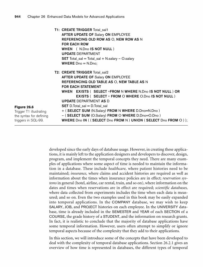
944 Chapter 26 Enhanced Data Models for Advanced Applications
developed since the early days of database usage. However, in creating these applica-tions, it is mainly left to the application designers and developers to discover, design,program, and implement the temporal concepts they need. There are many exam-ples of applications where some aspect of time is needed to maintain the informa-tion in a database. These include healthcare, where patient histories need to bemaintained; insurance, where claims and accident histories are required as well asinformation about the times when insurance policies are in effect; reservation sys-tems in general (hotel, airline, car rental, train, and so on), where information on thedates and times when reservations are in effect are required; scientific databases,where data collected from experiments includes the time when each data is meas-ured; and so on. Even the two examples used in this book may be easily expandedinto temporal applications. In the COMPANY database, we may wish to keepSALARY, JOB, and PROJECT histories on each employee. In the UNIVERSITY data-base, time is already included in the SEMESTER and YEAR of each SECTION of aCOURSE, the grade history of a STUDENT, and the information on research grants.In fact, it is realistic to conclude that the majority of database applications havesome temporal information. However, users often attempt to simplify or ignoretemporal aspects because of the complexity that they add to their applications.
In this section, we will introduce some of the concepts that have been developed todeal with the complexity of temporal database applications. Section 26.2.1 gives anoverview of how time is represented in databases, the different types of temporal
T1: CREATE TRIGGER Total_sal1AFTER UPDATE OF Salary ON EMPLOYEEREFERENCING OLD ROW AS O, NEW ROW AS NFOR EACH ROWWHEN ( N.Dno IS NOT NULL )UPDATE DEPARTMENTSET Total_sal = Total_sal + N.salary – O.salaryWHERE Dno = N.Dno;
T2: CREATE TRIGGER Total_sal2AFTER UPDATE OF Salary ON EMPLOYEEREFERENCING OLD TABLE AS O, NEW TABLE AS NFOR EACH STATEMENTWHEN EXISTS ( SELECT *FROM N WHERE N.Dno IS NOT NULL ) OR
EXISTS ( SELECT * FROM O WHERE O.Dno IS NOT NULL )UPDATE DEPARTMENT AS DSET D.Total_sal = D.Total_sal+ ( SELECT SUM (N.Salary) FROM N WHERE D.Dno=N.Dno )– ( SELECT SUM (O.Salary) FROM O WHERE D.Dno=O.Dno )WHERE Dno IN ( ( SELECT Dno FROM N ) UNION ( SELECT Dno FROM O ) );
Figure 26.6Trigger T1 illustratingthe syntax for definingtriggers in SQL-99.
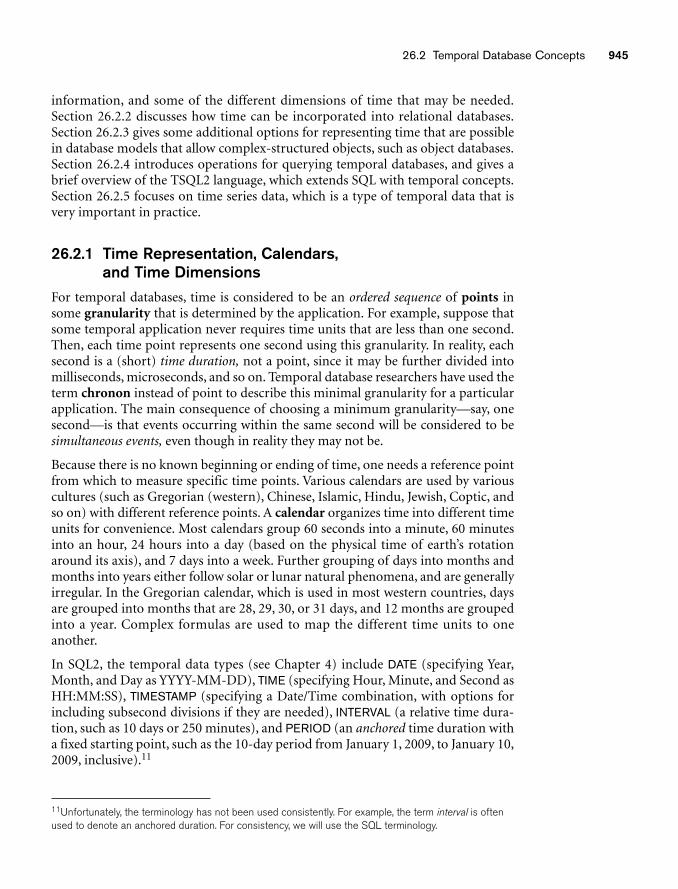
26.2 Temporal Database Concepts 945
information, and some of the different dimensions of time that may be needed.Section 26.2.2 discusses how time can be incorporated into relational databases.Section 26.2.3 gives some additional options for representing time that are possiblein database models that allow complex-structured objects, such as object databases.Section 26.2.4 introduces operations for querying temporal databases, and gives abrief overview of the TSQL2 language, which extends SQL with temporal concepts.Section 26.2.5 focuses on time series data, which is a type of temporal data that isvery important in practice.
26.2.1 Time Representation, Calendars, and Time Dimensions
For temporal databases, time is considered to be an ordered sequence of points insome granularity that is determined by the application. For example, suppose thatsome temporal application never requires time units that are less than one second.Then, each time point represents one second using this granularity. In reality, eachsecond is a (short) time duration, not a point, since it may be further divided intomilliseconds, microseconds, and so on. Temporal database researchers have used theterm chronon instead of point to describe this minimal granularity for a particularapplication. The main consequence of choosing a minimum granularity—say, onesecond—is that events occurring within the same second will be considered to besimultaneous events, even though in reality they may not be.
Because there is no known beginning or ending of time, one needs a reference pointfrom which to measure specific time points. Various calendars are used by variouscultures (such as Gregorian (western), Chinese, Islamic, Hindu, Jewish, Coptic, andso on) with different reference points. A calendar organizes time into different timeunits for convenience. Most calendars group 60 seconds into a minute, 60 minutesinto an hour, 24 hours into a day (based on the physical time of earth’s rotationaround its axis), and 7 days into a week. Further grouping of days into months andmonths into years either follow solar or lunar natural phenomena, and are generallyirregular. In the Gregorian calendar, which is used in most western countries, daysare grouped into months that are 28, 29, 30, or 31 days, and 12 months are groupedinto a year. Complex formulas are used to map the different time units to oneanother.
In SQL2, the temporal data types (see Chapter 4) include DATE (specifying Year,Month, and Day as YYYY-MM-DD), TIME (specifying Hour, Minute, and Second asHH:MM:SS), TIMESTAMP (specifying a Date/Time combination, with options forincluding subsecond divisions if they are needed), INTERVAL (a relative time dura-tion, such as 10 days or 250 minutes), and PERIOD (an anchored time duration witha fixed starting point, such as the 10-day period from January 1, 2009, to January 10,2009, inclusive).11
11Unfortunately, the terminology has not been used consistently. For example, the term interval is oftenused to denote an anchored duration. For consistency, we will use the SQL terminology.
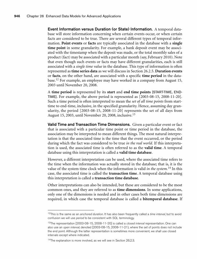
946 Chapter 26 Enhanced Data Models for Advanced Applications
Event Information versus Duration (or State) Information. A temporal data-base will store information concerning when certain events occur, or when certainfacts are considered to be true. There are several different types of temporal infor-mation. Point events or facts are typically associated in the database with a singletime point in some granularity. For example, a bank deposit event may be associ-ated with the timestamp when the deposit was made, or the total monthly sales of aproduct (fact) may be associated with a particular month (say, February 2010). Notethat even though such events or facts may have different granularities, each is stillassociated with a single time value in the database. This type of information is oftenrepresented as time series data as we will discuss in Section 26.2.5. Duration eventsor facts, on the other hand, are associated with a specific time period in the data-base.12 For example, an employee may have worked in a company from August 15,2003 until November 20, 2008.
A time period is represented by its start and end time points [START-TIME, END-TIME]. For example, the above period is represented as [2003-08-15, 2008-11-20].Such a time period is often interpreted to mean the set of all time points from start-time to end-time, inclusive, in the specified granularity. Hence, assuming day gran-ularity, the period [2003-08-15, 2008-11-20] represents the set of all days fromAugust 15, 2003, until November 20, 2008, inclusive.13
Valid Time and Transaction Time Dimensions. Given a particular event or factthat is associated with a particular time point or time period in the database, theassociation may be interpreted to mean different things. The most natural interpre-tation is that the associated time is the time that the event occurred, or the periodduring which the fact was considered to be true in the real world. If this interpreta-tion is used, the associated time is often referred to as the valid time. A temporaldatabase using this interpretation is called a valid time database.
However, a different interpretation can be used, where the associated time refers tothe time when the information was actually stored in the database; that is, it is thevalue of the system time clock when the information is valid in the system.14 In thiscase, the associated time is called the transaction time. A temporal database usingthis interpretation is called a transaction time database.
Other interpretations can also be intended, but these are considered to be the mostcommon ones, and they are referred to as time dimensions. In some applications,only one of the dimensions is needed and in other cases both time dimensions arerequired, in which case the temporal database is called a bitemporal database. If
12This is the same as an anchored duration. It has also been frequently called a time interval, but to avoidconfusion we will use period to be consistent with SQL terminology.13The representation [2003-08-15, 2008-11-20] is called a closed interval representation. One canalso use an open interval, denoted [2003-08-15, 2008-11-21), where the set of points does not includethe end point. Although the latter representation is sometimes more convenient, we shall use closedintervals except where indicated.14The explanation is more involved, as we will see in Section 26.2.3.
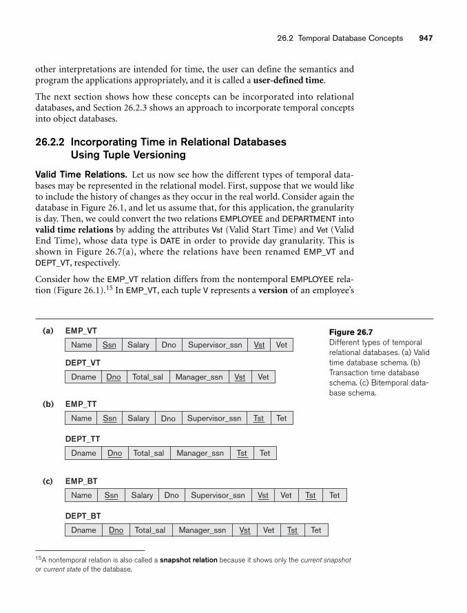
26.2 Temporal Database Concepts 947
(a)
Name
EMP_VT
Salary DnoSsn Supervisor_ssn Vst Vet
Name Salary Supervisor_ssnSsn Tst Tet
(b)
(c)
Dname
DEPT_VT
EMP_TT
Dname Total_sal Manager_ssnDno
Dno
Tst Tet
DEPT_TT
Total_salDno Manager_ssn Vst Vet
Name Salary Supervisor_ssnSsn Dno Tst Tet
EMP_BT
Dname Total_sal Manager_ssnDno Tst Tet
DEPT_BT
Vst Vet
Vst Vet
Figure 26.7Different types of temporalrelational databases. (a) Validtime database schema. (b)Transaction time databaseschema. (c) Bitemporal data-base schema.
other interpretations are intended for time, the user can define the semantics andprogram the applications appropriately, and it is called a user-defined time.
The next section shows how these concepts can be incorporated into relationaldatabases, and Section 26.2.3 shows an approach to incorporate temporal conceptsinto object databases.
26.2.2 Incorporating Time in Relational Databases Using Tuple Versioning
Valid Time Relations. Let us now see how the different types of temporal data-bases may be represented in the relational model. First, suppose that we would liketo include the history of changes as they occur in the real world. Consider again thedatabase in Figure 26.1, and let us assume that, for this application, the granularityis day. Then, we could convert the two relations EMPLOYEE and DEPARTMENT intovalid time relations by adding the attributes Vst (Valid Start Time) and Vet (ValidEnd Time), whose data type is DATE in order to provide day granularity. This isshown in Figure 26.7(a), where the relations have been renamed EMP_VT andDEPT_VT, respectively.
Consider how the EMP_VT relation differs from the nontemporal EMPLOYEE rela-tion (Figure 26.1).15 In EMP_VT, each tuple V represents a version of an employee’s
15A nontemporal relation is also called a snapshot relation because it shows only the current snapshot
or current state of the database.
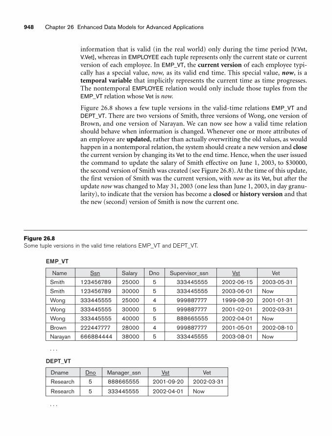
948 Chapter 26 Enhanced Data Models for Advanced Applications
Name
Smith 123456789 25000 5 333445555 2002-06-15 2003-05-31
Smith 123456789 30000 5 333445555 2003-06-01 Now
333445555 25000 4 999887777 1999-08-20 2001-01-31
333445555 30000 5 999887777 2001-02-01 2002-03-31
333445555 40000 5 888665555 2002-04-01 Now
222447777 28000 4 999887777 2001-05-01 2002-08-10
666884444 38000 5 333445555 2003-08-01 Now
Wong
Wong
Wong
Brown
Narayan
. . .
. . .
EMP_VT
Ssn Salary Dno Supervisor_ssn Vst Vet
Dname
Research
Research
DEPT_VT
5 888665555 2002-03-312001-09-20
333445555 2002-04-015 Now
Dno Manager_ssn Vst Vet
Figure 26.8Some tuple versions in the valid time relations EMP_VT and DEPT_VT.
information that is valid (in the real world) only during the time period [V.Vst,V.Vet], whereas in EMPLOYEE each tuple represents only the current state or currentversion of each employee. In EMP_VT, the current version of each employee typi-cally has a special value, now, as its valid end time. This special value, now, is atemporal variable that implicitly represents the current time as time progresses.The nontemporal EMPLOYEE relation would only include those tuples from theEMP_VT relation whose Vet is now.
Figure 26.8 shows a few tuple versions in the valid-time relations EMP_VT andDEPT_VT. There are two versions of Smith, three versions of Wong, one version ofBrown, and one version of Narayan. We can now see how a valid time relationshould behave when information is changed. Whenever one or more attributes ofan employee are updated, rather than actually overwriting the old values, as wouldhappen in a nontemporal relation, the system should create a new version and closethe current version by changing its Vet to the end time. Hence, when the user issuedthe command to update the salary of Smith effective on June 1, 2003, to $30000,the second version of Smith was created (see Figure 26.8). At the time of this update,the first version of Smith was the current version, with now as its Vet, but after theupdate now was changed to May 31, 2003 (one less than June 1, 2003, in day granu-larity), to indicate that the version has become a closed or history version and thatthe new (second) version of Smith is now the current one.
26.2 Temporal Database Concepts 949
It is important to note that in a valid time relation, the user must generally providethe valid time of an update. For example, the salary update of Smith may have beenentered in the database on May 15, 2003, at 8:52:12 A.M., say, even though the salarychange in the real world is effective on June 1, 2003. This is called a proactiveupdate, since it is applied to the database before it becomes effective in the realworld. If the update is applied to the database after it becomes effective in the realworld, it is called a retroactive update. An update that is applied at the same time asit becomes effective is called a simultaneous update.
The action that corresponds to deleting an employee in a nontemporal databasewould typically be applied to a valid time database by closing the current version ofthe employee being deleted. For example, if Smith leaves the company effectiveJanuary 19, 2004, then this would be applied by changing Vet of the current versionof Smith from now to 2004-01-19. In Figure 26.8, there is no current version forBrown, because he presumably left the company on 2002-08-10 and was logicallydeleted. However, because the database is temporal, the old information on Brown isstill there.
The operation to insert a new employee would correspond to creating the first tupleversion for that employee, and making it the current version, with the Vst being theeffective (real world) time when the employee starts work. In Figure 26.7, the tupleon Narayan illustrates this, since the first version has not been updated yet.
Notice that in a valid time relation, the nontemporal key, such as Ssn in EMPLOYEE,is no longer unique in each tuple (version). The new relation key for EMP_VT is acombination of the nontemporal key and the valid start time attribute Vst,16 so weuse (Ssn, Vst) as primary key. This is because, at any point in time, there should be atmost one valid version of each entity. Hence, the constraint that any two tuple ver-sions representing the same entity should have nonintersecting valid time periodsshould hold on valid time relations. Notice that if the nontemporal primary keyvalue may change over time, it is important to have a unique surrogate key attrib-ute, whose value never changes for each real-world entity, in order to relate all ver-sions of the same real-world entity.
Valid time relations basically keep track of the history of changes as they becomeeffective in the real world. Hence, if all real-world changes are applied, the databasekeeps a history of the real-world states that are represented. However, becauseupdates, insertions, and deletions may be applied retroactively or proactively, there isno record of the actual database state at any point in time. If the actual database statesare important to an application, then one should use transaction time relations.
Transaction Time Relations. In a transaction time database, whenever a changeis applied to the database, the actual timestamp of the transaction that applied thechange (insert, delete, or update) is recorded. Such a database is most useful whenchanges are applied simultaneously in the majority of cases—for example, real-timestock trading or banking transactions. If we convert the nontemporal database in
16A combination of the nontemporal key and the valid end time attribute Vet could also be used.
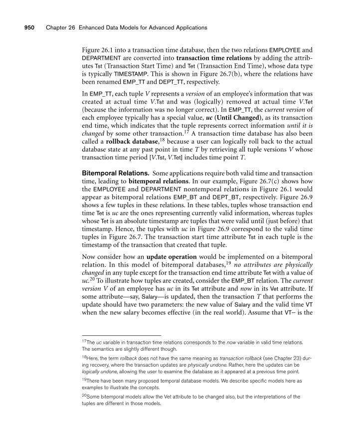
950 Chapter 26 Enhanced Data Models for Advanced Applications
Figure 26.1 into a transaction time database, then the two relations EMPLOYEE andDEPARTMENT are converted into transaction time relations by adding the attrib-utes Tst (Transaction Start Time) and Tet (Transaction End Time), whose data typeis typically TIMESTAMP. This is shown in Figure 26.7(b), where the relations havebeen renamed EMP_TT and DEPT_TT, respectively.
In EMP_TT, each tuple V represents a version of an employee’s information that wascreated at actual time V.Tst and was (logically) removed at actual time V.Tet(because the information was no longer correct). In EMP_TT, the current version ofeach employee typically has a special value, uc (Until Changed), as its transactionend time, which indicates that the tuple represents correct information until it ischanged by some other transaction.17 A transaction time database has also beencalled a rollback database,18 because a user can logically roll back to the actualdatabase state at any past point in time T by retrieving all tuple versions V whosetransaction time period [V.Tst, V.Tet] includes time point T.
Bitemporal Relations. Some applications require both valid time and transactiontime, leading to bitemporal relations. In our example, Figure 26.7(c) shows howthe EMPLOYEE and DEPARTMENT nontemporal relations in Figure 26.1 wouldappear as bitemporal relations EMP_BT and DEPT_BT, respectively. Figure 26.9shows a few tuples in these relations. In these tables, tuples whose transaction endtime Tet is uc are the ones representing currently valid information, whereas tupleswhose Tet is an absolute timestamp are tuples that were valid until (just before) thattimestamp. Hence, the tuples with uc in Figure 26.9 correspond to the valid timetuples in Figure 26.7. The transaction start time attribute Tst in each tuple is thetimestamp of the transaction that created that tuple.
Now consider how an update operation would be implemented on a bitemporalrelation. In this model of bitemporal databases,19 no attributes are physicallychanged in any tuple except for the transaction end time attribute Tet with a value ofuc.20 To illustrate how tuples are created, consider the EMP_BT relation. The currentversion V of an employee has uc in its Tet attribute and now in its Vet attribute. Ifsome attribute—say, Salary—is updated, then the transaction T that performs theupdate should have two parameters: the new value of Salary and the valid time VTwhen the new salary becomes effective (in the real world). Assume that VT− is the
17The uc variable in transaction time relations corresponds to the now variable in valid time relations.The semantics are slightly different though.18Here, the term rollback does not have the same meaning as transaction rollback (see Chapter 23) dur-ing recovery, where the transaction updates are physically undone. Rather, here the updates can belogically undone, allowing the user to examine the database as it appeared at a previous time point.19There have been many proposed temporal database models. We describe specific models here asexamples to illustrate the concepts.20Some bitemporal models allow the Vet attribute to be changed also, but the interpretations of thetuples are different in those models.
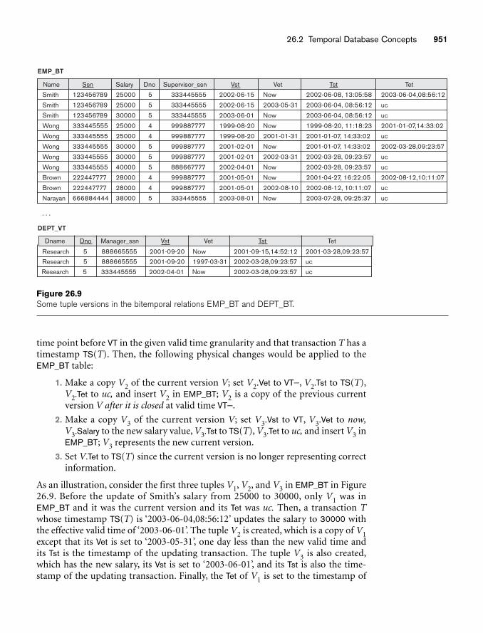
26.2 Temporal Database Concepts 951
Name
Smith 123456789 25000 5 333445555 2002-06-15
Smith 123456789 25000 5 333445555 2002-06-15
123456789 30000 5 333445555 2003-06-01
333445555 25000 4 999887777 1999-08-20
333445555 25000 4 999887777 1999-08-20
333445555 30000 5 999887777 2001-02-01
333445555 30000 5
5
4
4
5
999887777
888667777
999887777
999887777
333445555
2001-02-01
2002-04-01
2001-05-01
2001-05-01
2003-08-01
2002-06-08, 13:05:58
2003-06-04, 08:56:12
2003-06-04, 08:56:12
1999-08-20, 11:18:23
2001-01-07, 14:33:02
2001-01-07, 14:33:02
2002-03-28, 09:23:57
2002-03-28, 09:23:57
2001-04-27, 16:22:05
2002-08-12, 10:11:07
2003-07-28, 09:25:37
2003-06-04,08:56:12
uc
uc
2001-01-07,14:33:02
uc
2002-03-28,09:23:57
uc
uc
2002-08-12,10:11:07
uc
uc
Now
2003-05-31
Now
Now
2001-01-31
Now
2002-03-31
Now
Now
2002-08-10
Now
Smith
Wong
Wong
Wong
Wong
Wong 333445555
Brown 222447777
Brown 222447777
Narayan
. . .
40000
28000
28000
38000666884444
EMP_BT
Ssn Salary Dno Supervisor_ssn Vst Vet Tst Tet
Dname
Research
Research
DEPT_VT
5 888665555 Now2001-09-20
888665555 2001-09-205 1997-03-31
Dno Manager_ssn Vst Vet
2001-09-15,14:52:12
2002-03-28,09:23:57
Tst
2001-03-28,09:23:57
uc
Research 333445555 2002-04-015 Now 2002-03-28,09:23:57 uc
Tet
Figure 26.9Some tuple versions in the bitemporal relations EMP_BT and DEPT_BT.
time point before VT in the given valid time granularity and that transaction T has atimestamp TS(T). Then, the following physical changes would be applied to theEMP_BT table:
1. Make a copy V2 of the current version V; set V2.Vet to VT−, V2.Tst to TS(T),V2.Tet to uc, and insert V2 in EMP_BT; V2 is a copy of the previous currentversion V after it is closed at valid time VT−.
2. Make a copy V3 of the current version V; set V3.Vst to VT, V3.Vet to now,V3.Salary to the new salary value, V3.Tst to TS(T), V3.Tet to uc, and insert V3 inEMP_BT; V3 represents the new current version.
3. Set V.Tet to TS(T) since the current version is no longer representing correctinformation.
As an illustration, consider the first three tuples V1, V2, and V3 in EMP_BT in Figure26.9. Before the update of Smith’s salary from 25000 to 30000, only V1 was inEMP_BT and it was the current version and its Tet was uc. Then, a transaction Twhose timestamp TS(T) is ‘2003-06-04,08:56:12’ updates the salary to 30000 withthe effective valid time of ‘2003-06-01’. The tuple V2 is created, which is a copy of V1except that its Vet is set to ‘2003-05-31’, one day less than the new valid time and its Tst is the timestamp of the updating transaction. The tuple V3 is also created,which has the new salary, its Vst is set to ‘2003-06-01’, and its Tst is also the time-stamp of the updating transaction. Finally, the Tet of V1 is set to the timestamp of
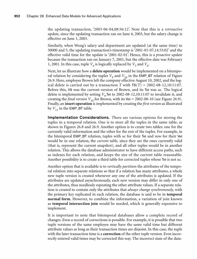
952 Chapter 26 Enhanced Data Models for Advanced Applications
the updating transaction, ‘2003-06-04,08:56:12’. Note that this is a retroactiveupdate, since the updating transaction ran on June 4, 2003, but the salary change iseffective on June 1, 2003.
Similarly, when Wong’s salary and department are updated (at the same time) to30000 and 5, the updating transaction’s timestamp is ‘2001-01-07,14:33:02’ and theeffective valid time for the update is ‘2001-02-01’. Hence, this is a proactive updatebecause the transaction ran on January 7, 2001, but the effective date was February1, 2001. In this case, tuple V4 is logically replaced by V5 and V6.
Next, let us illustrate how a delete operation would be implemented on a bitempo-ral relation by considering the tuples V9 and V10 in the EMP_BT relation of Figure26.9. Here, employee Brown left the company effective August 10, 2002, and the log-ical delete is carried out by a transaction T with TS(T) = 2002-08-12,10:11:07.Before this, V9 was the current version of Brown, and its Tet was uc. The logicaldelete is implemented by setting V9.Tet to 2002-08-12,10:11:07 to invalidate it, andcreating the final version V10 for Brown, with its Vet = 2002-08-10 (see Figure 26.9).Finally, an insert operation is implemented by creating the first version as illustratedby V11 in the EMP_BT table.
Implementation Considerations. There are various options for storing thetuples in a temporal relation. One is to store all the tuples in the same table, asshown in Figures 26.8 and 26.9. Another option is to create two tables: one for thecurrently valid information and the other for the rest of the tuples. For example, inthe bitemporal EMP_BT relation, tuples with uc for their Tet and now for their Vetwould be in one relation, the current table, since they are the ones currently valid(that is, represent the current snapshot), and all other tuples would be in anotherrelation. This allows the database administrator to have different access paths, suchas indexes for each relation, and keeps the size of the current table reasonable.Another possibility is to create a third table for corrected tuples whose Tet is not uc.
Another option that is available is to vertically partition the attributes of the tempo-ral relation into separate relations so that if a relation has many attributes, a wholenew tuple version is created whenever any one of the attributes is updated. If theattributes are updated asynchronously, each new version may differ in only one ofthe attributes, thus needlessly repeating the other attribute values. If a separate rela-tion is created to contain only the attributes that always change synchronously, withthe primary key replicated in each relation, the database is said to be in temporalnormal form. However, to combine the information, a variation of join known as temporal intersection join would be needed, which is generally expensive toimplement.
It is important to note that bitemporal databases allow a complete record ofchanges. Even a record of corrections is possible. For example, it is possible that twotuple versions of the same employee may have the same valid time but differentattribute values as long as their transaction times are disjoint. In this case, the tuplewith the later transaction time is a correction of the other tuple version. Even incor-rectly entered valid times may be corrected this way. The incorrect state of the data-
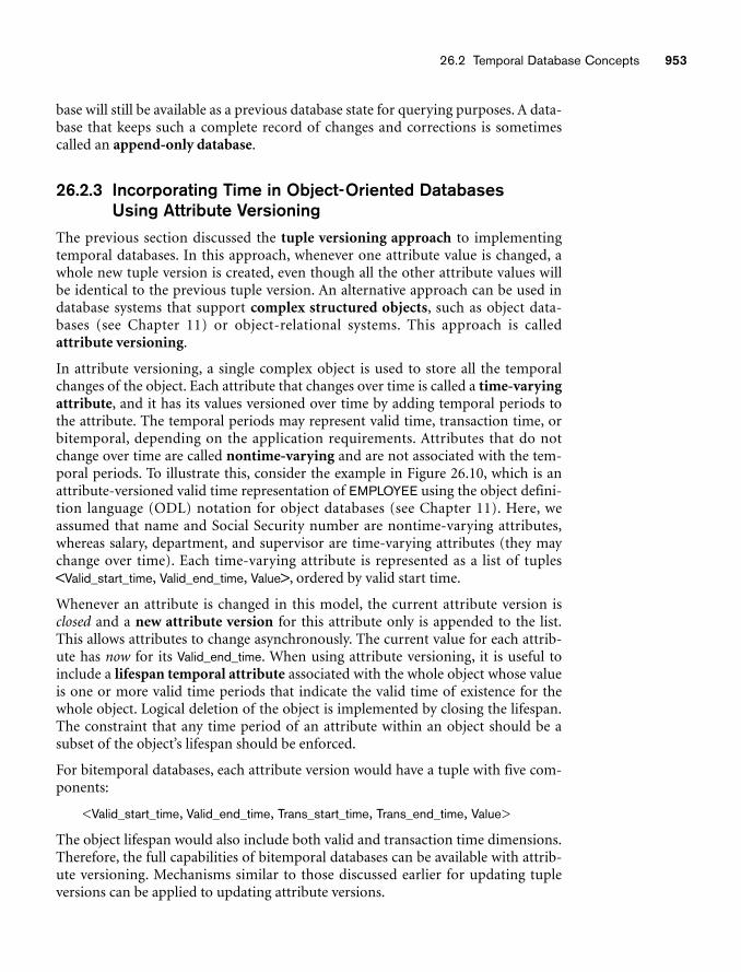
26.2 Temporal Database Concepts 953
base will still be available as a previous database state for querying purposes. A data-base that keeps such a complete record of changes and corrections is sometimescalled an append-only database.
26.2.3 Incorporating Time in Object-Oriented Databases Using Attribute Versioning
The previous section discussed the tuple versioning approach to implementingtemporal databases. In this approach, whenever one attribute value is changed, awhole new tuple version is created, even though all the other attribute values willbe identical to the previous tuple version. An alternative approach can be used indatabase systems that support complex structured objects, such as object data-bases (see Chapter 11) or object-relational systems. This approach is calledattribute versioning.
In attribute versioning, a single complex object is used to store all the temporalchanges of the object. Each attribute that changes over time is called a time-varyingattribute, and it has its values versioned over time by adding temporal periods tothe attribute. The temporal periods may represent valid time, transaction time, orbitemporal, depending on the application requirements. Attributes that do notchange over time are called nontime-varying and are not associated with the tem-poral periods. To illustrate this, consider the example in Figure 26.10, which is anattribute-versioned valid time representation of EMPLOYEE using the object defini-tion language (ODL) notation for object databases (see Chapter 11). Here, weassumed that name and Social Security number are nontime-varying attributes,whereas salary, department, and supervisor are time-varying attributes (they maychange over time). Each time-varying attribute is represented as a list of tuples<Valid_start_time, Valid_end_time, Value>, ordered by valid start time.
Whenever an attribute is changed in this model, the current attribute version isclosed and a new attribute version for this attribute only is appended to the list.This allows attributes to change asynchronously. The current value for each attrib-ute has now for its Valid_end_time. When using attribute versioning, it is useful toinclude a lifespan temporal attribute associated with the whole object whose valueis one or more valid time periods that indicate the valid time of existence for thewhole object. Logical deletion of the object is implemented by closing the lifespan.The constraint that any time period of an attribute within an object should be asubset of the object’s lifespan should be enforced.
For bitemporal databases, each attribute version would have a tuple with five com-ponents:
<Valid_start_time, Valid_end_time, Trans_start_time, Trans_end_time, Value>
The object lifespan would also include both valid and transaction time dimensions.Therefore, the full capabilities of bitemporal databases can be available with attrib-ute versioning. Mechanisms similar to those discussed earlier for updating tupleversions can be applied to updating attribute versions.
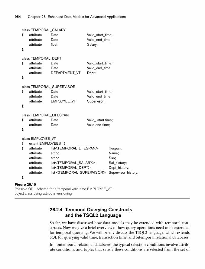
954 Chapter 26 Enhanced Data Models for Advanced Applications
class TEMPORAL_SALARY{ attribute Date Valid_start_time;
attribute Date Valid_end_time;attribute float Salary;
};
class TEMPORAL_DEPT{ attribute Date Valid_start_time;
attribute Date Valid_end_time;attribute DEPARTMENT_VT Dept;
};
class TEMPORAL_SUPERVISOR{ attribute Date Valid_start_time;
attribute Date Valid_end_time;attribute EMPLOYEE_VT Supervisor;
};
class TEMPORAL_LIFESPAN{ attribute Date Valid_ start time;
attribute Date Valid end time;};
class EMPLOYEE_VT( extent EMPLOYEES ){ attribute list<TEMPORAL_LIFESPAN> lifespan;
attribute string Name;attribute string Ssn;attribute list<TEMPORAL_SALARY> Sal_history;attribute list<TEMPORAL_DEPT> Dept_history;attribute list <TEMPORAL_SUPERVISOR> Supervisor_history;
};
Figure 26.10Possible ODL schema for a temporal valid time EMPLOYEE_VTobject class using attribute versioning.
26.2.4 Temporal Querying Constructs and the TSQL2 Language
So far, we have discussed how data models may be extended with temporal con-structs. Now we give a brief overview of how query operations need to be extendedfor temporal querying. We will briefly discuss the TSQL2 language, which extendsSQL for querying valid time, transaction time, and bitemporal relational databases.
In nontemporal relational databases, the typical selection conditions involve attrib-ute conditions, and tuples that satisfy these conditions are selected from the set of
26.2 Temporal Database Concepts 955
current tuples. Following that, the attributes of interest to the query are specified bya projection operation (see Chapter 6). For example, in the query to retrieve thenames of all employees working in department 5 whose salary is greater than 30000,the selection condition would be as follows:
((Salary > 30000) AND (Dno = 5))
The projected attribute would be Name. In a temporal database, the conditions mayinvolve time in addition to attributes. A pure time condition involves only time—for example, to select all employee tuple versions that were valid on a certain timepoint T or that were valid during a certain time period [T1, T2]. In this case, the spec-ified time period is compared with the valid time period of each tuple version [T.Vst,T.Vet], and only those tuples that satisfy the condition are selected. In these opera-tions, a period is considered to be equivalent to the set of time points from T1 to T2inclusive, so the standard set comparison operations can be used. Additional opera-tions, such as whether one time period ends before another starts are also needed.21
Some of the more common operations used in queries are as follows:
[T.Vst, T.Vet] INCLUDES [T1, T2] Equivalent to T1 ≥ T.Vst AND T2 ≤ T.Vet
[T.Vst, T.Vet] INCLUDED_IN [T1, T2] Equivalent to T1 ≤ T.Vst AND T2 ≥ T.Vet
[T.Vst, T.Vet] OVERLAPS [T1, T2] Equivalent to (T1 ≤ T.Vet AND T2 ≥ T.Vst)22
[T.Vst, T.Vet] BEFORE [T1, T2] Equivalent to T1 ≥ T.Vet
[T.Vst, T.Vet] AFTER [T1, T2] Equivalent to T2 ≤ T.Vst
[T.Vst, T.Vet] MEETS_BEFORE [T1, T2] Equivalent to T1 = T.Vet + 123
[T.Vst, T.Vet] MEETS_AFTER [T1, T2] Equivalent to T2 + 1 = T.Vst
Additionally, operations are needed to manipulate time periods, such as computingthe union or intersection of two time periods. The results of these operations maynot themselves be periods, but rather temporal elements—a collection of one ormore disjoint time periods such that no two time periods in a temporal element aredirectly adjacent. That is, for any two time periods [T1, T2] and [T3, T4] in a tempo-ral element, the following three conditions must hold:
■ [T1, T2] intersection [T3, T4] is empty.
■ T3 is not the time point following T2 in the given granularity.
■ T1 is not the time point following T4 in the given granularity.
The latter conditions are necessary to ensure unique representations of temporalelements. If two time periods [T1, T2] and [T3, T4] are adjacent, they are combined
21A complete set of operations, known as Allen’s algebra (Allen, 1983), has been defined for compar-ing time periods.22This operation returns true if the intersection of the two periods is not empty; it has also been calledINTERSECTS_WITH.23Here, 1 refers to one time point in the specified granularity. The MEETS operations basically specify ifone period starts immediately after another period ends.
956 Chapter 26 Enhanced Data Models for Advanced Applications
into a single time period [T1, T4]. This is called coalescing of time periods.Coalescing also combines intersecting time periods.
To illustrate how pure time conditions can be used, suppose a user wants to select allemployee versions that were valid at any point during 2002. The appropriate selec-tion condition applied to the relation in Figure 26.8 would be
[T.Vst, T.Vet] OVERLAPS [2002-01-01, 2002-12-31]
Typically, most temporal selections are applied to the valid time dimension. For abitemporal database, one usually applies the conditions to the currently correcttuples with uc as their transaction end times. However, if the query needs to beapplied to a previous database state, an AS_OF T clause is appended to the query,which means that the query is applied to the valid time tuples that were correct inthe database at time T.
In addition to pure time conditions, other selections involve attribute and timeconditions. For example, suppose we wish to retrieve all EMP_VT tuple versions Tfor employees who worked in department 5 at any time during 2002. In this case,the condition is
[T.Vst, T.Vet]OVERLAPS [2002-01-01, 2002-12-31] AND (T.Dno = 5)
Finally, we give a brief overview of the TSQL2 query language, which extends SQLwith constructs for temporal databases. The main idea behind TSQL2 is to allowusers to specify whether a relation is nontemporal (that is, a standard SQL relation)or temporal. The CREATE TABLE statement is extended with an optional AS clause toallow users to declare different temporal options. The following options are avail-able:
■ <AS VALID STATE <GRANULARITY> (valid time relation with valid timeperiod)
■ <AS VALID EVENT <GRANULARITY> (valid time relation with valid timepoint)
■ <AS TRANSACTION (transaction time relation with transaction time period)
■ <AS VALID STATE <GRANULARITY> AND TRANSACTION (bitemporal rela-tion, valid time period)
■ <AS VALID EVENT <GRANULARITY> AND TRANSACTION (bitemporal rela-tion, valid time point)
The keywords STATE and EVENT are used to specify whether a time period or timepoint is associated with the valid time dimension. In TSQL2, rather than have theuser actually see how the temporal tables are implemented (as we discussed in theprevious sections), the TSQL2 language adds query language constructs to specifyvarious types of temporal selections, temporal projections, temporal aggregations,transformation among granularities, and many other concepts. The book bySnodgrass et al. (1995) describes the language.
26.3 Spatial Database Concepts 957
26.2.5 Time Series DataTime series data is used very often in financial, sales, and economics applications.They involve data values that are recorded according to a specific predefinedsequence of time points. Therefore, they are a special type of valid event data, wherethe event time points are predetermined according to a fixed calendar. Consider theexample of closing daily stock prices of a particular company on the New York StockExchange. The granularity here is day, but the days that the stock market is open areknown (nonholiday weekdays). Hence, it has been common to specify a computa-tional procedure that calculates the particular calendar associated with a timeseries. Typical queries on time series involve temporal aggregation over highergranularity intervals—for example, finding the average or maximum weekly closingstock price or the maximum and minimum monthly closing stock price from thedaily information.
As another example, consider the daily sales dollar amount at each store of a chainof stores owned by a particular company. Again, typical temporal aggregates wouldbe retrieving the weekly, monthly, or yearly sales from the daily sales information(using the sum aggregate function), or comparing same store monthly sales withprevious monthly sales, and so on.
Because of the specialized nature of time series data and the lack of support for it inolder DBMSs, it has been common to use specialized time series management sys-tems rather than general-purpose DBMSs for managing such information. In suchsystems, it has been common to store time series values in sequential order in a file,and apply specialized time series procedures to analyze the information. The prob-lem with this approach is that the full power of high-level querying in languagessuch as SQL will not be available in such systems.
More recently, some commercial DBMS packages are offering time series exten-sions, such as the Oracle time cartridge and the time series data blade of InformixUniversal Server. In addition, the TSQL2 language provides some support for timeseries in the form of event tables.
26.3 Spatial Database Concepts24
26.3.1 Introduction to Spatial DatabasesSpatial databases incorporate functionality that provides support for databases thatkeep track of objects in a multidimensional space. For example, cartographic data-bases that store maps include two-dimensional spatial descriptions of theirobjects—from countries and states to rivers, cities, roads, seas, and so on. The sys-tems that manage geographic data and related applications are known as
24The contribution of Pranesh Parimala Ranganathan to this section is appreciated.
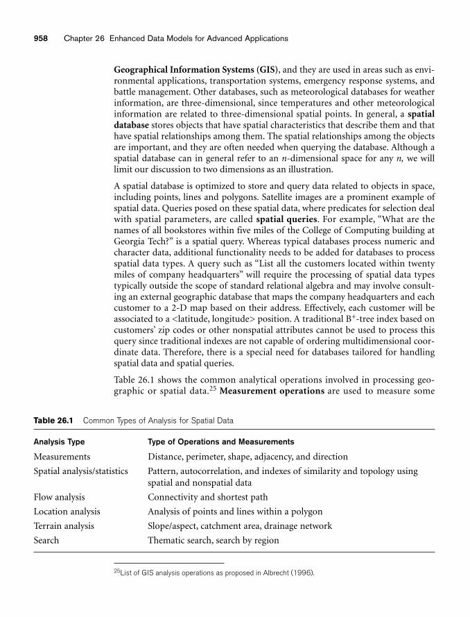
958 Chapter 26 Enhanced Data Models for Advanced Applications
Table 26.1 Common Types of Analysis for Spatial Data
Analysis Type Type of Operations and Measurements
Measurements Distance, perimeter, shape, adjacency, and direction
Spatial analysis/statistics Pattern, autocorrelation, and indexes of similarity and topology usingspatial and nonspatial data
Flow analysis Connectivity and shortest path
Location analysis Analysis of points and lines within a polygon
Terrain analysis Slope/aspect, catchment area, drainage network
Search Thematic search, search by region
Geographical Information Systems (GIS), and they are used in areas such as envi-ronmental applications, transportation systems, emergency response systems, andbattle management. Other databases, such as meteorological databases for weatherinformation, are three-dimensional, since temperatures and other meteorologicalinformation are related to three-dimensional spatial points. In general, a spatialdatabase stores objects that have spatial characteristics that describe them and thathave spatial relationships among them. The spatial relationships among the objectsare important, and they are often needed when querying the database. Although aspatial database can in general refer to an n-dimensional space for any n, we willlimit our discussion to two dimensions as an illustration.
A spatial database is optimized to store and query data related to objects in space,including points, lines and polygons. Satellite images are a prominent example ofspatial data. Queries posed on these spatial data, where predicates for selection dealwith spatial parameters, are called spatial queries. For example, “What are thenames of all bookstores within five miles of the College of Computing building atGeorgia Tech?” is a spatial query. Whereas typical databases process numeric andcharacter data, additional functionality needs to be added for databases to processspatial data types. A query such as “List all the customers located within twentymiles of company headquarters” will require the processing of spatial data typestypically outside the scope of standard relational algebra and may involve consult-ing an external geographic database that maps the company headquarters and eachcustomer to a 2-D map based on their address. Effectively, each customer will beassociated to a <latitude, longitude> position. A traditional B+-tree index based oncustomers’ zip codes or other nonspatial attributes cannot be used to process thisquery since traditional indexes are not capable of ordering multidimensional coor-dinate data. Therefore, there is a special need for databases tailored for handlingspatial data and spatial queries.
Table 26.1 shows the common analytical operations involved in processing geo-graphic or spatial data.25 Measurement operations are used to measure some
25List of GIS analysis operations as proposed in Albrecht (1996).
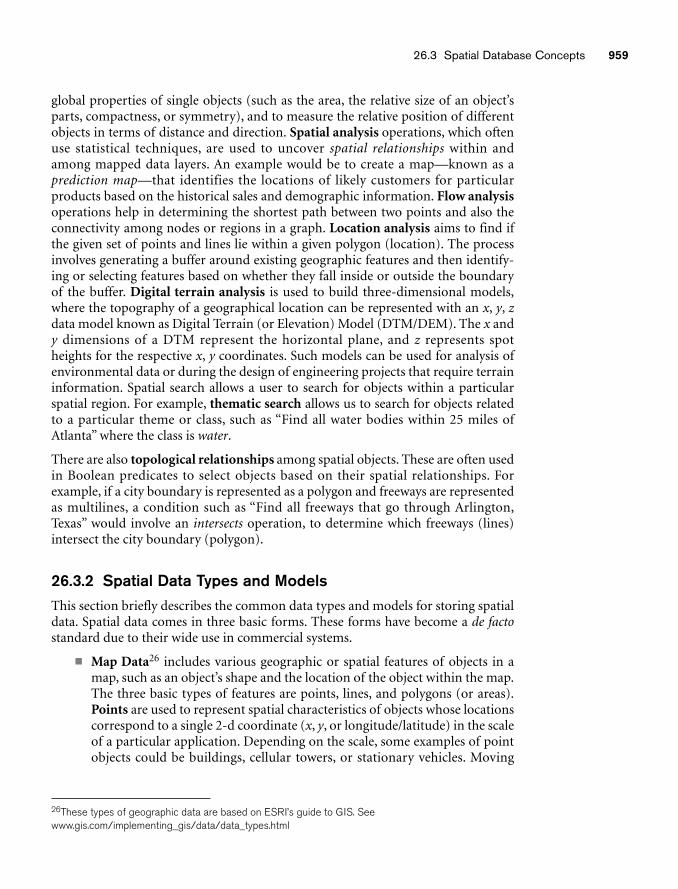
26.3 Spatial Database Concepts 959
global properties of single objects (such as the area, the relative size of an object’sparts, compactness, or symmetry), and to measure the relative position of differentobjects in terms of distance and direction. Spatial analysis operations, which oftenuse statistical techniques, are used to uncover spatial relationships within andamong mapped data layers. An example would be to create a map—known as aprediction map—that identifies the locations of likely customers for particularproducts based on the historical sales and demographic information. Flow analysisoperations help in determining the shortest path between two points and also theconnectivity among nodes or regions in a graph. Location analysis aims to find ifthe given set of points and lines lie within a given polygon (location). The processinvolves generating a buffer around existing geographic features and then identify-ing or selecting features based on whether they fall inside or outside the boundaryof the buffer. Digital terrain analysis is used to build three-dimensional models,where the topography of a geographical location can be represented with an x, y, zdata model known as Digital Terrain (or Elevation) Model (DTM/DEM). The x andy dimensions of a DTM represent the horizontal plane, and z represents spotheights for the respective x, y coordinates. Such models can be used for analysis ofenvironmental data or during the design of engineering projects that require terraininformation. Spatial search allows a user to search for objects within a particularspatial region. For example, thematic search allows us to search for objects relatedto a particular theme or class, such as “Find all water bodies within 25 miles ofAtlanta” where the class is water.
There are also topological relationships among spatial objects. These are often usedin Boolean predicates to select objects based on their spatial relationships. Forexample, if a city boundary is represented as a polygon and freeways are representedas multilines, a condition such as “Find all freeways that go through Arlington,Texas” would involve an intersects operation, to determine which freeways (lines)intersect the city boundary (polygon).
26.3.2 Spatial Data Types and ModelsThis section briefly describes the common data types and models for storing spatialdata. Spatial data comes in three basic forms. These forms have become a de factostandard due to their wide use in commercial systems.
■ Map Data26 includes various geographic or spatial features of objects in amap, such as an object’s shape and the location of the object within the map.The three basic types of features are points, lines, and polygons (or areas).Points are used to represent spatial characteristics of objects whose locationscorrespond to a single 2-d coordinate (x, y, or longitude/latitude) in the scaleof a particular application. Depending on the scale, some examples of pointobjects could be buildings, cellular towers, or stationary vehicles. Moving
26These types of geographic data are based on ESRI’s guide to GIS. Seewww.gis.com/implementing_gis/data/data_types.html
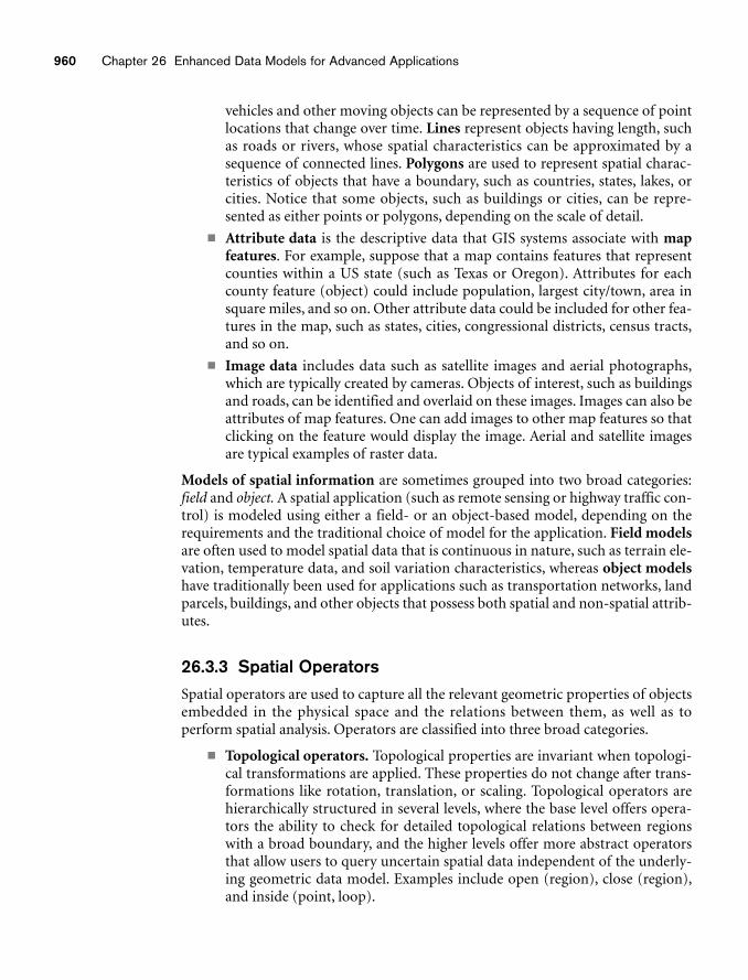
960 Chapter 26 Enhanced Data Models for Advanced Applications
vehicles and other moving objects can be represented by a sequence of pointlocations that change over time. Lines represent objects having length, suchas roads or rivers, whose spatial characteristics can be approximated by asequence of connected lines. Polygons are used to represent spatial charac-teristics of objects that have a boundary, such as countries, states, lakes, orcities. Notice that some objects, such as buildings or cities, can be repre-sented as either points or polygons, depending on the scale of detail.
■ Attribute data is the descriptive data that GIS systems associate with mapfeatures. For example, suppose that a map contains features that representcounties within a US state (such as Texas or Oregon). Attributes for eachcounty feature (object) could include population, largest city/town, area insquare miles, and so on. Other attribute data could be included for other fea-tures in the map, such as states, cities, congressional districts, census tracts,and so on.
■ Image data includes data such as satellite images and aerial photographs,which are typically created by cameras. Objects of interest, such as buildingsand roads, can be identified and overlaid on these images. Images can also beattributes of map features. One can add images to other map features so thatclicking on the feature would display the image. Aerial and satellite imagesare typical examples of raster data.
Models of spatial information are sometimes grouped into two broad categories:field and object. A spatial application (such as remote sensing or highway traffic con-trol) is modeled using either a field- or an object-based model, depending on therequirements and the traditional choice of model for the application. Field modelsare often used to model spatial data that is continuous in nature, such as terrain ele-vation, temperature data, and soil variation characteristics, whereas object modelshave traditionally been used for applications such as transportation networks, landparcels, buildings, and other objects that possess both spatial and non-spatial attrib-utes.
26.3.3 Spatial OperatorsSpatial operators are used to capture all the relevant geometric properties of objectsembedded in the physical space and the relations between them, as well as to perform spatial analysis. Operators are classified into three broad categories.
■ Topological operators. Topological properties are invariant when topologi-cal transformations are applied. These properties do not change after trans-formations like rotation, translation, or scaling. Topological operators arehierarchically structured in several levels, where the base level offers opera-tors the ability to check for detailed topological relations between regionswith a broad boundary, and the higher levels offer more abstract operatorsthat allow users to query uncertain spatial data independent of the underly-ing geometric data model. Examples include open (region), close (region),and inside (point, loop).
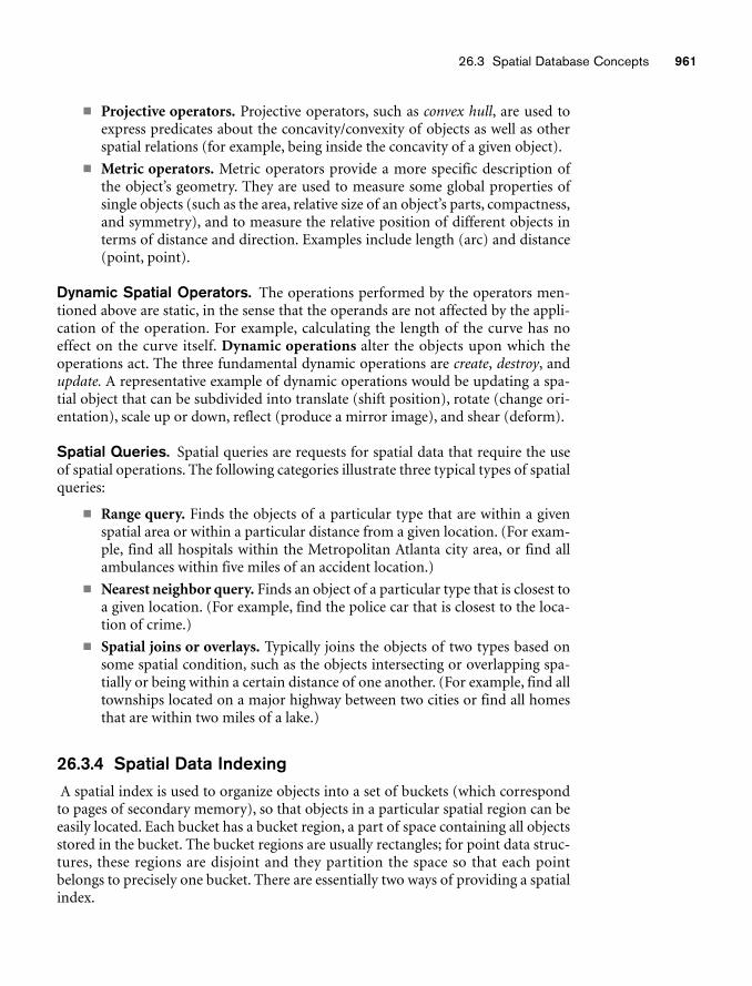
26.3 Spatial Database Concepts 961
■ Projective operators. Projective operators, such as convex hull, are used toexpress predicates about the concavity/convexity of objects as well as otherspatial relations (for example, being inside the concavity of a given object).
■ Metric operators. Metric operators provide a more specific description ofthe object’s geometry. They are used to measure some global properties ofsingle objects (such as the area, relative size of an object’s parts, compactness,and symmetry), and to measure the relative position of different objects interms of distance and direction. Examples include length (arc) and distance(point, point).
Dynamic Spatial Operators. The operations performed by the operators men-tioned above are static, in the sense that the operands are not affected by the appli-cation of the operation. For example, calculating the length of the curve has noeffect on the curve itself. Dynamic operations alter the objects upon which theoperations act. The three fundamental dynamic operations are create, destroy, andupdate. A representative example of dynamic operations would be updating a spa-tial object that can be subdivided into translate (shift position), rotate (change ori-entation), scale up or down, reflect (produce a mirror image), and shear (deform).
Spatial Queries. Spatial queries are requests for spatial data that require the useof spatial operations. The following categories illustrate three typical types of spatialqueries:
■ Range query. Finds the objects of a particular type that are within a givenspatial area or within a particular distance from a given location. (For exam-ple, find all hospitals within the Metropolitan Atlanta city area, or find allambulances within five miles of an accident location.)
■ Nearest neighbor query. Finds an object of a particular type that is closest toa given location. (For example, find the police car that is closest to the loca-tion of crime.)
■ Spatial joins or overlays. Typically joins the objects of two types based onsome spatial condition, such as the objects intersecting or overlapping spa-tially or being within a certain distance of one another. (For example, find alltownships located on a major highway between two cities or find all homesthat are within two miles of a lake.)
26.3.4 Spatial Data IndexingA spatial index is used to organize objects into a set of buckets (which correspond
to pages of secondary memory), so that objects in a particular spatial region can beeasily located. Each bucket has a bucket region, a part of space containing all objectsstored in the bucket. The bucket regions are usually rectangles; for point data struc-tures, these regions are disjoint and they partition the space so that each pointbelongs to precisely one bucket. There are essentially two ways of providing a spatialindex.
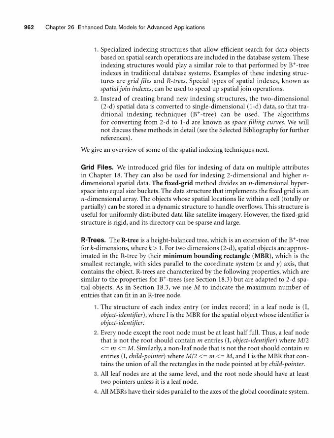
962 Chapter 26 Enhanced Data Models for Advanced Applications
1. Specialized indexing structures that allow efficient search for data objectsbased on spatial search operations are included in the database system. Theseindexing structures would play a similar role to that performed by B+-treeindexes in traditional database systems. Examples of these indexing struc-tures are grid files and R-trees. Special types of spatial indexes, known asspatial join indexes, can be used to speed up spatial join operations.
2. Instead of creating brand new indexing structures, the two-dimensional (2-d) spatial data is converted to single-dimensional (1-d) data, so that tra-ditional indexing techniques (B+-tree) can be used. The algorithms for converting from 2-d to 1-d are known as space filling curves. We will not discuss these methods in detail (see the Selected Bibliography for further references).
We give an overview of some of the spatial indexing techniques next.
Grid Files. We introduced grid files for indexing of data on multiple attributes in Chapter 18. They can also be used for indexing 2-dimensional and higher n-dimensional spatial data. The fixed-grid method divides an n-dimensional hyper-space into equal size buckets. The data structure that implements the fixed grid is ann-dimensional array. The objects whose spatial locations lie within a cell (totally orpartially) can be stored in a dynamic structure to handle overflows. This structure isuseful for uniformly distributed data like satellite imagery. However, the fixed-gridstructure is rigid, and its directory can be sparse and large.
R-Trees. The R-tree is a height-balanced tree, which is an extension of the B+-treefor k-dimensions, where k > 1. For two dimensions (2-d), spatial objects are approx-imated in the R-tree by their minimum bounding rectangle (MBR), which is thesmallest rectangle, with sides parallel to the coordinate system (x and y) axis, thatcontains the object. R-trees are characterized by the following properties, which aresimilar to the properties for B+-trees (see Section 18.3) but are adapted to 2-d spa-tial objects. As in Section 18.3, we use M to indicate the maximum number ofentries that can fit in an R-tree node.
1. The structure of each index entry (or index record) in a leaf node is (I,object-identifier), where I is the MBR for the spatial object whose identifier isobject-identifier.
2. Every node except the root node must be at least half full. Thus, a leaf nodethat is not the root should contain m entries (I, object-identifier) where M/2<= m <= M. Similarly, a non-leaf node that is not the root should contain mentries (I, child-pointer) where M/2 <= m <= M, and I is the MBR that con-tains the union of all the rectangles in the node pointed at by child-pointer.
3. All leaf nodes are at the same level, and the root node should have at leasttwo pointers unless it is a leaf node.
4. All MBRs have their sides parallel to the axes of the global coordinate system.
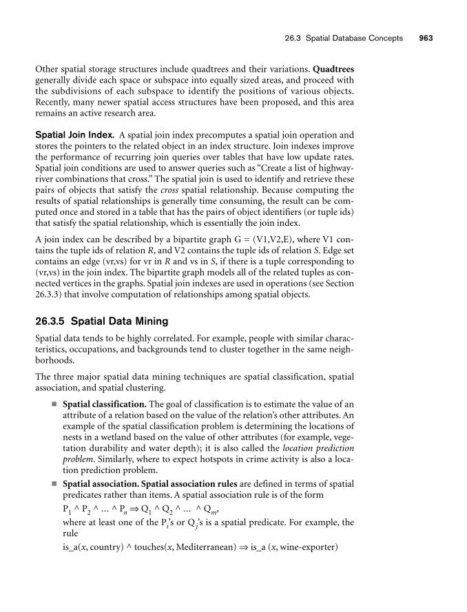
26.3 Spatial Database Concepts 963
Other spatial storage structures include quadtrees and their variations. Quadtreesgenerally divide each space or subspace into equally sized areas, and proceed withthe subdivisions of each subspace to identify the positions of various objects.Recently, many newer spatial access structures have been proposed, and this arearemains an active research area.
Spatial Join Index. A spatial join index precomputes a spatial join operation andstores the pointers to the related object in an index structure. Join indexes improvethe performance of recurring join queries over tables that have low update rates.Spatial join conditions are used to answer queries such as “Create a list of highway-river combinations that cross.” The spatial join is used to identify and retrieve thesepairs of objects that satisfy the cross spatial relationship. Because computing theresults of spatial relationships is generally time consuming, the result can be com-puted once and stored in a table that has the pairs of object identifiers (or tuple ids)that satisfy the spatial relationship, which is essentially the join index.
A join index can be described by a bipartite graph G = (V1,V2,E), where V1 con-tains the tuple ids of relation R, and V2 contains the tuple ids of relation S. Edge setcontains an edge (vr,vs) for vr in R and vs in S, if there is a tuple corresponding to(vr,vs) in the join index. The bipartite graph models all of the related tuples as con-nected vertices in the graphs. Spatial join indexes are used in operations (see Section26.3.3) that involve computation of relationships among spatial objects.
26.3.5 Spatial Data MiningSpatial data tends to be highly correlated. For example, people with similar charac-teristics, occupations, and backgrounds tend to cluster together in the same neigh-borhoods.
The three major spatial data mining techniques are spatial classification, spatialassociation, and spatial clustering.
■ Spatial classification. The goal of classification is to estimate the value of anattribute of a relation based on the value of the relation’s other attributes. Anexample of the spatial classification problem is determining the locations ofnests in a wetland based on the value of other attributes (for example, vege-tation durability and water depth); it is also called the location predictionproblem. Similarly, where to expect hotspots in crime activity is also a loca-tion prediction problem.
■ Spatial association. Spatial association rules are defined in terms of spatialpredicates rather than items. A spatial association rule is of the form
P1 ^ P2 ^ ... ^ Pn ⇒ Q1 ^ Q2 ^ ... ^ Qm,
where at least one of the Pi’s or Q j’s is a spatial predicate. For example, therule
is_a(x, country) ^ touches(x, Mediterranean) ⇒ is_a (x, wine-exporter)
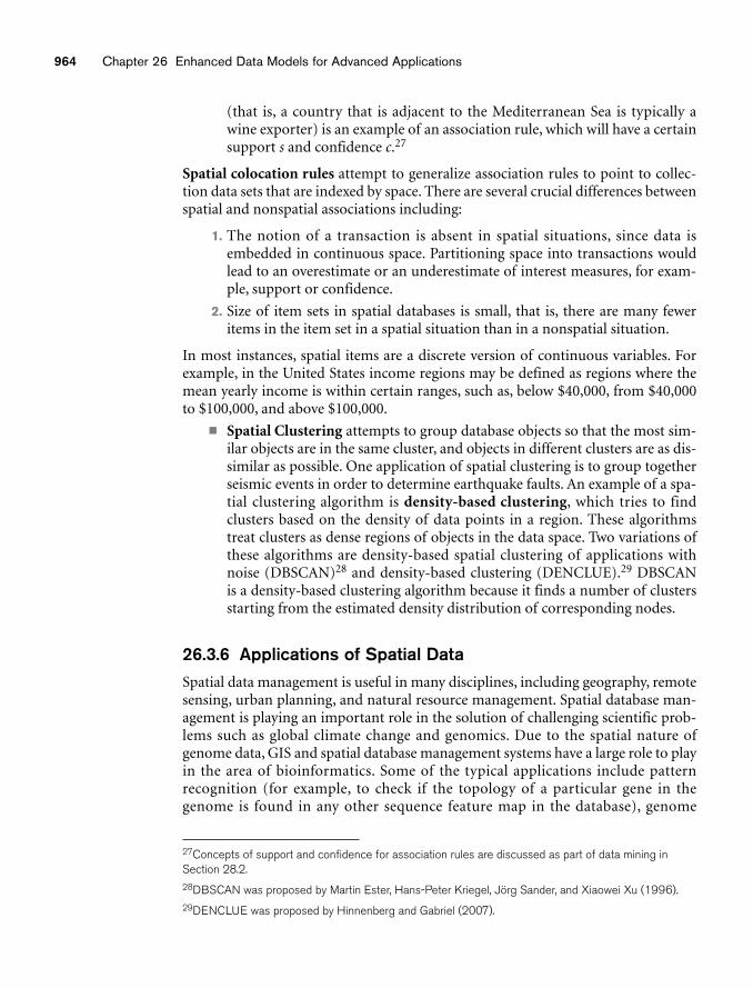
964 Chapter 26 Enhanced Data Models for Advanced Applications
(that is, a country that is adjacent to the Mediterranean Sea is typically awine exporter) is an example of an association rule, which will have a certainsupport s and confidence c.27
Spatial colocation rules attempt to generalize association rules to point to collec-tion data sets that are indexed by space. There are several crucial differences betweenspatial and nonspatial associations including:
1. The notion of a transaction is absent in spatial situations, since data isembedded in continuous space. Partitioning space into transactions wouldlead to an overestimate or an underestimate of interest measures, for exam-ple, support or confidence.
2. Size of item sets in spatial databases is small, that is, there are many feweritems in the item set in a spatial situation than in a nonspatial situation.
In most instances, spatial items are a discrete version of continuous variables. Forexample, in the United States income regions may be defined as regions where themean yearly income is within certain ranges, such as, below $40,000, from $40,000to $100,000, and above $100,000.
■ Spatial Clustering attempts to group database objects so that the most sim-ilar objects are in the same cluster, and objects in different clusters are as dis-similar as possible. One application of spatial clustering is to group togetherseismic events in order to determine earthquake faults. An example of a spa-tial clustering algorithm is density-based clustering, which tries to findclusters based on the density of data points in a region. These algorithmstreat clusters as dense regions of objects in the data space. Two variations ofthese algorithms are density-based spatial clustering of applications withnoise (DBSCAN)28 and density-based clustering (DENCLUE).29 DBSCANis a density-based clustering algorithm because it finds a number of clustersstarting from the estimated density distribution of corresponding nodes.
26.3.6 Applications of Spatial DataSpatial data management is useful in many disciplines, including geography, remotesensing, urban planning, and natural resource management. Spatial database man-agement is playing an important role in the solution of challenging scientific prob-lems such as global climate change and genomics. Due to the spatial nature ofgenome data, GIS and spatial database management systems have a large role to playin the area of bioinformatics. Some of the typical applications include patternrecognition (for example, to check if the topology of a particular gene in thegenome is found in any other sequence feature map in the database), genome
27Concepts of support and confidence for association rules are discussed as part of data mining inSection 28.2.28DBSCAN was proposed by Martin Ester, Hans-Peter Kriegel, Jörg Sander, and Xiaowei Xu (1996).29DENCLUE was proposed by Hinnenberg and Gabriel (2007).
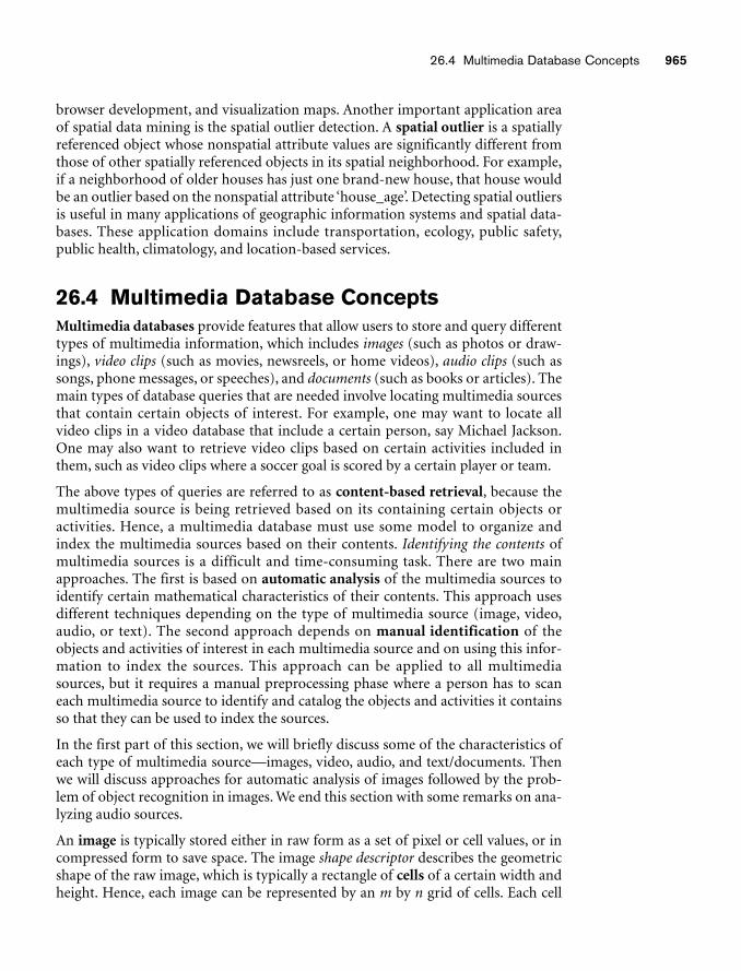
26.4 Multimedia Database Concepts 965
browser development, and visualization maps. Another important application areaof spatial data mining is the spatial outlier detection. A spatial outlier is a spatiallyreferenced object whose nonspatial attribute values are significantly different fromthose of other spatially referenced objects in its spatial neighborhood. For example,if a neighborhood of older houses has just one brand-new house, that house wouldbe an outlier based on the nonspatial attribute ‘house_age’. Detecting spatial outliersis useful in many applications of geographic information systems and spatial data-bases. These application domains include transportation, ecology, public safety,public health, climatology, and location-based services.
26.4 Multimedia Database ConceptsMultimedia databases provide features that allow users to store and query differenttypes of multimedia information, which includes images (such as photos or draw-ings), video clips (such as movies, newsreels, or home videos), audio clips (such assongs, phone messages, or speeches), and documents (such as books or articles). Themain types of database queries that are needed involve locating multimedia sourcesthat contain certain objects of interest. For example, one may want to locate allvideo clips in a video database that include a certain person, say Michael Jackson.One may also want to retrieve video clips based on certain activities included inthem, such as video clips where a soccer goal is scored by a certain player or team.
The above types of queries are referred to as content-based retrieval, because themultimedia source is being retrieved based on its containing certain objects oractivities. Hence, a multimedia database must use some model to organize andindex the multimedia sources based on their contents. Identifying the contents ofmultimedia sources is a difficult and time-consuming task. There are two mainapproaches. The first is based on automatic analysis of the multimedia sources toidentify certain mathematical characteristics of their contents. This approach usesdifferent techniques depending on the type of multimedia source (image, video,audio, or text). The second approach depends on manual identification of theobjects and activities of interest in each multimedia source and on using this infor-mation to index the sources. This approach can be applied to all multimediasources, but it requires a manual preprocessing phase where a person has to scaneach multimedia source to identify and catalog the objects and activities it containsso that they can be used to index the sources.
In the first part of this section, we will briefly discuss some of the characteristics ofeach type of multimedia source—images, video, audio, and text/documents. Thenwe will discuss approaches for automatic analysis of images followed by the prob-lem of object recognition in images. We end this section with some remarks on ana-lyzing audio sources.
An image is typically stored either in raw form as a set of pixel or cell values, or incompressed form to save space. The image shape descriptor describes the geometricshape of the raw image, which is typically a rectangle of cells of a certain width andheight. Hence, each image can be represented by an m by n grid of cells. Each cell
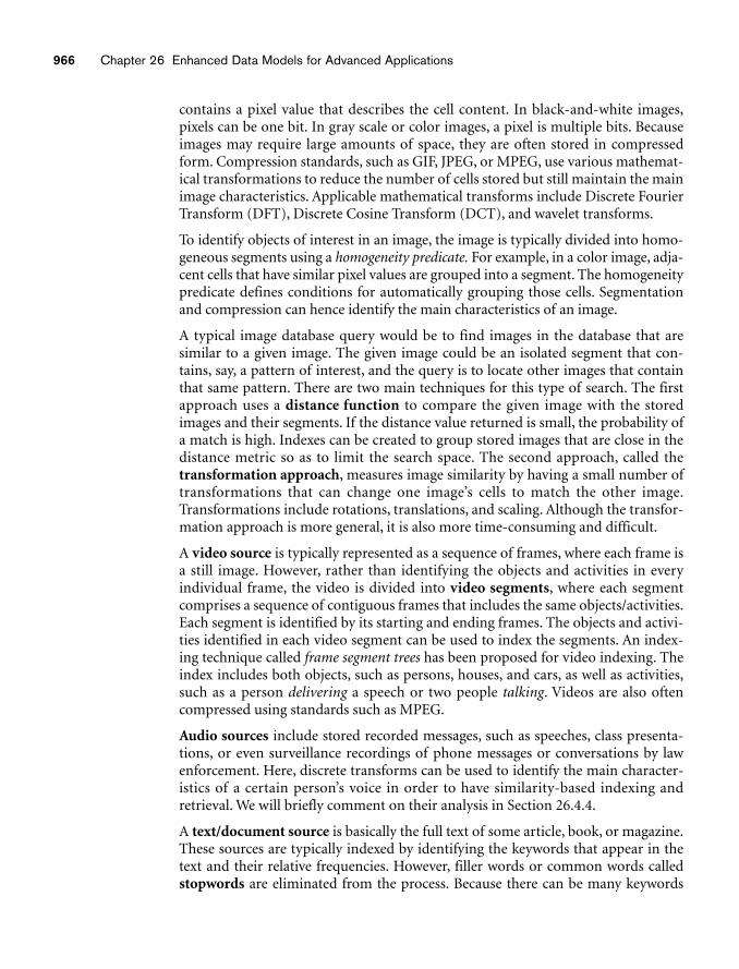
966 Chapter 26 Enhanced Data Models for Advanced Applications
contains a pixel value that describes the cell content. In black-and-white images,pixels can be one bit. In gray scale or color images, a pixel is multiple bits. Becauseimages may require large amounts of space, they are often stored in compressedform. Compression standards, such as GIF, JPEG, or MPEG, use various mathemat-ical transformations to reduce the number of cells stored but still maintain the mainimage characteristics. Applicable mathematical transforms include Discrete FourierTransform (DFT), Discrete Cosine Transform (DCT), and wavelet transforms.
To identify objects of interest in an image, the image is typically divided into homo-geneous segments using a homogeneity predicate. For example, in a color image, adja-cent cells that have similar pixel values are grouped into a segment. The homogeneitypredicate defines conditions for automatically grouping those cells. Segmentationand compression can hence identify the main characteristics of an image.
A typical image database query would be to find images in the database that aresimilar to a given image. The given image could be an isolated segment that con-tains, say, a pattern of interest, and the query is to locate other images that containthat same pattern. There are two main techniques for this type of search. The firstapproach uses a distance function to compare the given image with the storedimages and their segments. If the distance value returned is small, the probability ofa match is high. Indexes can be created to group stored images that are close in thedistance metric so as to limit the search space. The second approach, called thetransformation approach, measures image similarity by having a small number oftransformations that can change one image’s cells to match the other image.Transformations include rotations, translations, and scaling. Although the transfor-mation approach is more general, it is also more time-consuming and difficult.
A video source is typically represented as a sequence of frames, where each frame isa still image. However, rather than identifying the objects and activities in everyindividual frame, the video is divided into video segments, where each segmentcomprises a sequence of contiguous frames that includes the same objects/activities.Each segment is identified by its starting and ending frames. The objects and activi-ties identified in each video segment can be used to index the segments. An index-ing technique called frame segment trees has been proposed for video indexing. Theindex includes both objects, such as persons, houses, and cars, as well as activities,such as a person delivering a speech or two people talking. Videos are also oftencompressed using standards such as MPEG.
Audio sources include stored recorded messages, such as speeches, class presenta-tions, or even surveillance recordings of phone messages or conversations by lawenforcement. Here, discrete transforms can be used to identify the main character-istics of a certain person’s voice in order to have similarity-based indexing andretrieval. We will briefly comment on their analysis in Section 26.4.4.
A text/document source is basically the full text of some article, book, or magazine.These sources are typically indexed by identifying the keywords that appear in thetext and their relative frequencies. However, filler words or common words calledstopwords are eliminated from the process. Because there can be many keywords
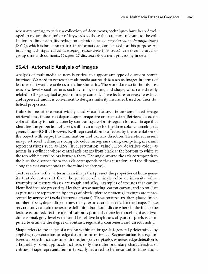
26.4 Multimedia Database Concepts 967
when attempting to index a collection of documents, techniques have been devel-oped to reduce the number of keywords to those that are most relevant to the col-lection. A dimensionality reduction technique called singular value decompositions(SVD), which is based on matrix transformations, can be used for this purpose. Anindexing technique called telescoping vector trees (TV-trees), can then be used togroup similar documents. Chapter 27 discusses document processing in detail.
26.4.1 Automatic Analysis of ImagesAnalysis of multimedia sources is critical to support any type of query or searchinterface. We need to represent multimedia source data such as images in terms offeatures that would enable us to define similarity. The work done so far in this areauses low-level visual features such as color, texture, and shape, which are directlyrelated to the perceptual aspects of image content. These features are easy to extractand represent, and it is convenient to design similarity measures based on their sta-tistical properties.
Color is one of the most widely used visual features in content-based imageretrieval since it does not depend upon image size or orientation. Retrieval based oncolor similarity is mainly done by computing a color histogram for each image thatidentifies the proportion of pixels within an image for the three color channels (red,green, blue—RGB). However, RGB representation is affected by the orientation ofthe object with respect to illumination and camera direction. Therefore, currentimage retrieval techniques compute color histograms using competing invariantrepresentations such as HSV (hue, saturation, value). HSV describes colors aspoints in a cylinder whose central axis ranges from black at the bottom to white atthe top with neutral colors between them. The angle around the axis corresponds tothe hue, the distance from the axis corresponds to the saturation, and the distancealong the axis corresponds to the value (brightness).
Texture refers to the patterns in an image that present the properties of homogene-ity that do not result from the presence of a single color or intensity value.Examples of texture classes are rough and silky. Examples of textures that can beidentified include pressed calf leather, straw matting, cotton canvas, and so on. Justas pictures are represented by arrays of pixels (picture elements), textures are repre-sented by arrays of texels (texture elements). These textures are then placed into anumber of sets, depending on how many textures are identified in the image. Thesesets not only contain the texture definition but also indicate where in the image thetexture is located. Texture identification is primarily done by modeling it as a two-dimensional, gray-level variation. The relative brightness of pairs of pixels is com-puted to estimate the degree of contrast, regularity, coarseness, and directionality.
Shape refers to the shape of a region within an image. It is generally determined byapplying segmentation or edge detection to an image. Segmentation is a region-based approach that uses an entire region (sets of pixels), whereas edge detection isa boundary-based approach that uses only the outer boundary characteristics ofentities. Shape representation is typically required to be invariant to translation,
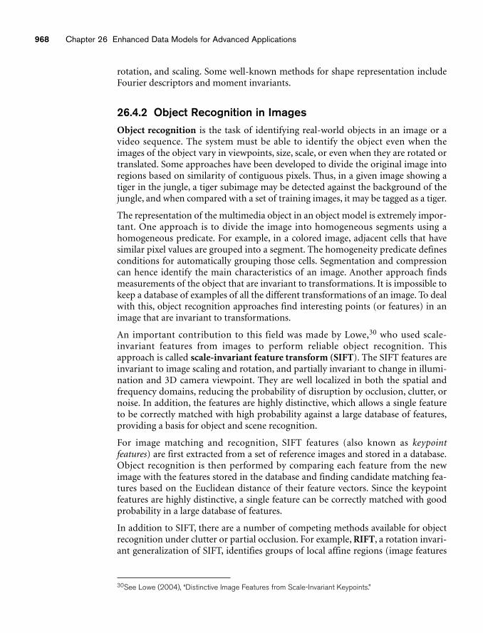
968 Chapter 26 Enhanced Data Models for Advanced Applications
rotation, and scaling. Some well-known methods for shape representation includeFourier descriptors and moment invariants.
26.4.2 Object Recognition in ImagesObject recognition is the task of identifying real-world objects in an image or avideo sequence. The system must be able to identify the object even when theimages of the object vary in viewpoints, size, scale, or even when they are rotated ortranslated. Some approaches have been developed to divide the original image intoregions based on similarity of contiguous pixels. Thus, in a given image showing atiger in the jungle, a tiger subimage may be detected against the background of thejungle, and when compared with a set of training images, it may be tagged as a tiger.
The representation of the multimedia object in an object model is extremely impor-tant. One approach is to divide the image into homogeneous segments using ahomogeneous predicate. For example, in a colored image, adjacent cells that havesimilar pixel values are grouped into a segment. The homogeneity predicate definesconditions for automatically grouping those cells. Segmentation and compressioncan hence identify the main characteristics of an image. Another approach findsmeasurements of the object that are invariant to transformations. It is impossible tokeep a database of examples of all the different transformations of an image. To dealwith this, object recognition approaches find interesting points (or features) in animage that are invariant to transformations.
An important contribution to this field was made by Lowe,30 who used scale-invariant features from images to perform reliable object recognition. Thisapproach is called scale-invariant feature transform (SIFT). The SIFT features areinvariant to image scaling and rotation, and partially invariant to change in illumi-nation and 3D camera viewpoint. They are well localized in both the spatial andfrequency domains, reducing the probability of disruption by occlusion, clutter, ornoise. In addition, the features are highly distinctive, which allows a single featureto be correctly matched with high probability against a large database of features,providing a basis for object and scene recognition.
For image matching and recognition, SIFT features (also known as keypointfeatures) are first extracted from a set of reference images and stored in a database.Object recognition is then performed by comparing each feature from the newimage with the features stored in the database and finding candidate matching fea-tures based on the Euclidean distance of their feature vectors. Since the keypointfeatures are highly distinctive, a single feature can be correctly matched with goodprobability in a large database of features.
In addition to SIFT, there are a number of competing methods available for objectrecognition under clutter or partial occlusion. For example, RIFT, a rotation invari-ant generalization of SIFT, identifies groups of local affine regions (image features
30See Lowe (2004), “Distinctive Image Features from Scale-Invariant Keypoints.”
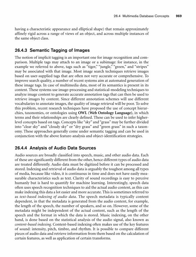
26.4 Multimedia Database Concepts 969
having a characteristic appearance and elliptical shape) that remain approximatelyaffinely rigid across a range of views of an object, and across multiple instances ofthe same object class.
26.4.3 Semantic Tagging of ImagesThe notion of implicit tagging is an important one for image recognition and com-parison. Multiple tags may attach to an image or a subimage: for instance, in theexample we referred to above, tags such as “tiger,” “jungle,” “green,” and “stripes”may be associated with that image. Most image search techniques retrieve imagesbased on user-supplied tags that are often not very accurate or comprehensive. Toimprove search quality, a number of recent systems aim at automated generation ofthese image tags. In case of multimedia data, most of its semantics is present in itscontent. These systems use image-processing and statistical-modeling techniques toanalyze image content to generate accurate annotation tags that can then be used toretrieve images by content. Since different annotation schemes will use differentvocabularies to annotate images, the quality of image retrieval will be poor. To solvethis problem, recent research techniques have proposed the use of concept hierar-chies, taxonomies, or ontologies using OWL (Web Ontology Language), in whichterms and their relationships are clearly defined. These can be used to infer higher-level concepts based on tags. Concepts like “sky” and “grass” may be further dividedinto “clear sky” and “cloudy sky” or “dry grass” and “green grass” in such a taxon-omy. These approaches generally come under semantic tagging and can be used inconjunction with the above feature-analysis and object-identification strategies.
26.4.4 Analysis of Audio Data SourcesAudio sources are broadly classified into speech, music, and other audio data. Eachof these are significantly different from the other, hence different types of audio dataare treated differently. Audio data must be digitized before it can be processed andstored. Indexing and retrieval of audio data is arguably the toughest among all typesof media, because like video, it is continuous in time and does not have easily mea-surable characteristics such as text. Clarity of sound recordings is easy to perceivehumanly but is hard to quantify for machine learning. Interestingly, speech dataoften uses speech recognition techniques to aid the actual audio content, as this canmake indexing this data a lot easier and more accurate. This is sometimes referred toas text-based indexing of audio data. The speech metadata is typically contentdependent, in that the metadata is generated from the audio content, for example,the length of the speech, the number of speakers, and so on. However, some of themetadata might be independent of the actual content, such as the length of thespeech and the format in which the data is stored. Music indexing, on the otherhand, is done based on the statistical analysis of the audio signal, also known ascontent-based indexing. Content-based indexing often makes use of the key featuresof sound: intensity, pitch, timbre, and rhythm. It is possible to compare differentpieces of audio data and retrieve information from them based on the calculation ofcertain features, as well as application of certain transforms.
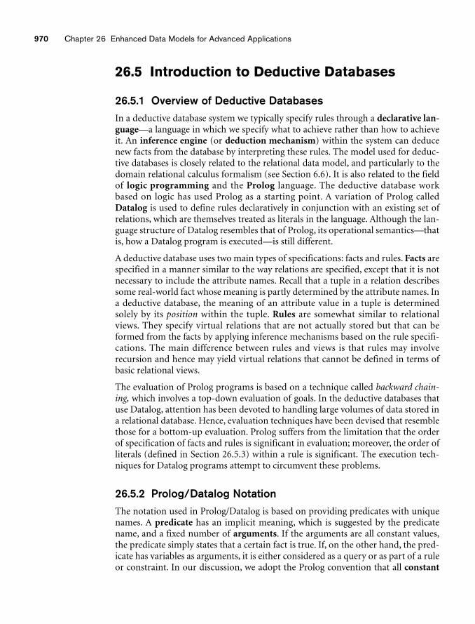
970 Chapter 26 Enhanced Data Models for Advanced Applications
26.5 Introduction to Deductive Databases
26.5.1 Overview of Deductive DatabasesIn a deductive database system we typically specify rules through a declarative lan-guage—a language in which we specify what to achieve rather than how to achieveit. An inference engine (or deduction mechanism) within the system can deducenew facts from the database by interpreting these rules. The model used for deduc-tive databases is closely related to the relational data model, and particularly to thedomain relational calculus formalism (see Section 6.6). It is also related to the fieldof logic programming and the Prolog language. The deductive database workbased on logic has used Prolog as a starting point. A variation of Prolog calledDatalog is used to define rules declaratively in conjunction with an existing set ofrelations, which are themselves treated as literals in the language. Although the lan-guage structure of Datalog resembles that of Prolog, its operational semantics—thatis, how a Datalog program is executed—is still different.
A deductive database uses two main types of specifications: facts and rules. Facts arespecified in a manner similar to the way relations are specified, except that it is notnecessary to include the attribute names. Recall that a tuple in a relation describessome real-world fact whose meaning is partly determined by the attribute names. Ina deductive database, the meaning of an attribute value in a tuple is determinedsolely by its position within the tuple. Rules are somewhat similar to relationalviews. They specify virtual relations that are not actually stored but that can beformed from the facts by applying inference mechanisms based on the rule specifi-cations. The main difference between rules and views is that rules may involverecursion and hence may yield virtual relations that cannot be defined in terms ofbasic relational views.
The evaluation of Prolog programs is based on a technique called backward chain-ing, which involves a top-down evaluation of goals. In the deductive databases thatuse Datalog, attention has been devoted to handling large volumes of data stored ina relational database. Hence, evaluation techniques have been devised that resemblethose for a bottom-up evaluation. Prolog suffers from the limitation that the orderof specification of facts and rules is significant in evaluation; moreover, the order ofliterals (defined in Section 26.5.3) within a rule is significant. The execution tech-niques for Datalog programs attempt to circumvent these problems.
26.5.2 Prolog/Datalog NotationThe notation used in Prolog/Datalog is based on providing predicates with uniquenames. A predicate has an implicit meaning, which is suggested by the predicatename, and a fixed number of arguments. If the arguments are all constant values,the predicate simply states that a certain fact is true. If, on the other hand, the pred-icate has variables as arguments, it is either considered as a query or as part of a ruleor constraint. In our discussion, we adopt the Prolog convention that all constant
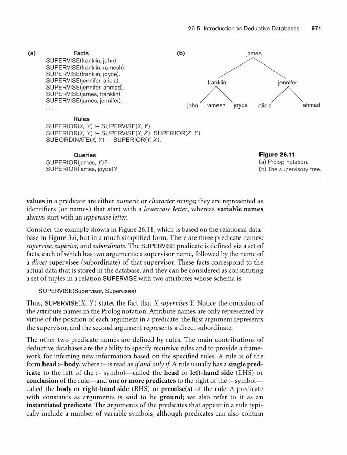
26.5 Introduction to Deductive Databases 971
FactsSUPERVISE(franklin, john).SUPERVISE(franklin, ramesh).SUPERVISE(franklin, joyce).SUPERVISE(jennifer, alicia).SUPERVISE(jennifer, ahmad).SUPERVISE(james, franklin).SUPERVISE(james, jennifer).. . .
RulesSUPERIOR(X, Y ) :– SUPERVISE(X, Y ).SUPERIOR(X, Y ) :– SUPERVISE(X, Z ), SUPERIOR(Z, Y ).SUBORDINATE(X, Y ) :– SUPERIOR(Y, X ).
QueriesSUPERIOR(james, Y )?SUPERIOR(james, joyce)?
joyceramesh
franklin
james(b)(a)
john ahmad
jennifer
alicia
Figure 26.11(a) Prolog notation. (b) The supervisory tree.
values in a predicate are either numeric or character strings; they are represented asidentifiers (or names) that start with a lowercase letter, whereas variable namesalways start with an uppercase letter.
Consider the example shown in Figure 26.11, which is based on the relational data-base in Figure 3.6, but in a much simplified form. There are three predicate names:supervise, superior, and subordinate. The SUPERVISE predicate is defined via a set offacts, each of which has two arguments: a supervisor name, followed by the name ofa direct supervisee (subordinate) of that supervisor. These facts correspond to theactual data that is stored in the database, and they can be considered as constitutinga set of tuples in a relation SUPERVISE with two attributes whose schema is
SUPERVISE(Supervisor, Supervisee)
Thus, SUPERVISE(X, Y ) states the fact that X supervises Y. Notice the omission ofthe attribute names in the Prolog notation. Attribute names are only represented byvirtue of the position of each argument in a predicate: the first argument representsthe supervisor, and the second argument represents a direct subordinate.
The other two predicate names are defined by rules. The main contributions ofdeductive databases are the ability to specify recursive rules and to provide a frame-work for inferring new information based on the specified rules. A rule is of theform head :– body, where :– is read as if and only if. A rule usually has a single pred-icate to the left of the :– symbol—called the head or left-hand side (LHS) orconclusion of the rule—and one or more predicates to the right of the :– symbol—called the body or right-hand side (RHS) or premise(s) of the rule. A predicatewith constants as arguments is said to be ground; we also refer to it as aninstantiated predicate. The arguments of the predicates that appear in a rule typi-cally include a number of variable symbols, although predicates can also contain
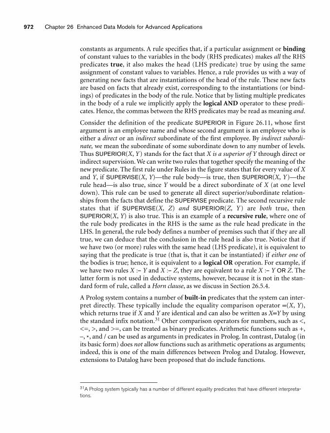
972 Chapter 26 Enhanced Data Models for Advanced Applications
constants as arguments. A rule specifies that, if a particular assignment or bindingof constant values to the variables in the body (RHS predicates) makes all the RHSpredicates true, it also makes the head (LHS predicate) true by using the sameassignment of constant values to variables. Hence, a rule provides us with a way ofgenerating new facts that are instantiations of the head of the rule. These new factsare based on facts that already exist, corresponding to the instantiations (or bind-ings) of predicates in the body of the rule. Notice that by listing multiple predicatesin the body of a rule we implicitly apply the logical AND operator to these predi-cates. Hence, the commas between the RHS predicates may be read as meaning and.
Consider the definition of the predicate SUPERIOR in Figure 26.11, whose firstargument is an employee name and whose second argument is an employee who iseither a direct or an indirect subordinate of the first employee. By indirect subordi-nate, we mean the subordinate of some subordinate down to any number of levels.Thus SUPERIOR(X, Y) stands for the fact that X is a superior of Y through direct orindirect supervision. We can write two rules that together specify the meaning of thenew predicate. The first rule under Rules in the figure states that for every value of Xand Y, if SUPERVISE(X, Y)—the rule body—is true, then SUPERIOR(X, Y)—therule head—is also true, since Y would be a direct subordinate of X (at one leveldown). This rule can be used to generate all direct superior/subordinate relation-ships from the facts that define the SUPERVISE predicate. The second recursive rulestates that if SUPERVISE(X, Z) and SUPERIOR(Z, Y ) are both true, thenSUPERIOR(X, Y) is also true. This is an example of a recursive rule, where one ofthe rule body predicates in the RHS is the same as the rule head predicate in theLHS. In general, the rule body defines a number of premises such that if they are alltrue, we can deduce that the conclusion in the rule head is also true. Notice that ifwe have two (or more) rules with the same head (LHS predicate), it is equivalent tosaying that the predicate is true (that is, that it can be instantiated) if either one ofthe bodies is true; hence, it is equivalent to a logical OR operation. For example, ifwe have two rules X :– Y and X :– Z, they are equivalent to a rule X :– Y OR Z. Thelatter form is not used in deductive systems, however, because it is not in the stan-dard form of rule, called a Horn clause, as we discuss in Section 26.5.4.
A Prolog system contains a number of built-in predicates that the system can inter-pret directly. These typically include the equality comparison operator =(X, Y),which returns true if X and Y are identical and can also be written as X=Y by usingthe standard infix notation.31 Other comparison operators for numbers, such as <,<=, >, and >=, can be treated as binary predicates. Arithmetic functions such as +,–, *, and / can be used as arguments in predicates in Prolog. In contrast, Datalog (inits basic form) does not allow functions such as arithmetic operations as arguments;indeed, this is one of the main differences between Prolog and Datalog. However,extensions to Datalog have been proposed that do include functions.
31A Prolog system typically has a number of different equality predicates that have different interpreta-tions.
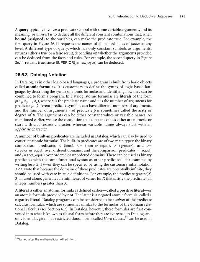
26.5 Introduction to Deductive Databases 973
A query typically involves a predicate symbol with some variable arguments, and itsmeaning (or answer) is to deduce all the different constant combinations that, whenbound (assigned) to the variables, can make the predicate true. For example, thefirst query in Figure 26.11 requests the names of all subordinates of james at anylevel. A different type of query, which has only constant symbols as arguments,returns either a true or a false result, depending on whether the arguments providedcan be deduced from the facts and rules. For example, the second query in Figure26.11 returns true, since SUPERIOR(james, joyce) can be deduced.
26.5.3 Datalog NotationIn Datalog, as in other logic-based languages, a program is built from basic objectscalled atomic formulas. It is customary to define the syntax of logic-based lan-guages by describing the syntax of atomic formulas and identifying how they can becombined to form a program. In Datalog, atomic formulas are literals of the formp(a1, a2, ..., an), where p is the predicate name and n is the number of arguments forpredicate p. Different predicate symbols can have different numbers of arguments,and the number of arguments n of predicate p is sometimes called the arity ordegree of p. The arguments can be either constant values or variable names. Asmentioned earlier, we use the convention that constant values either are numeric orstart with a lowercase character, whereas variable names always start with anuppercase character.
A number of built-in predicates are included in Datalog, which can also be used toconstruct atomic formulas. The built-in predicates are of two main types: the binarycomparison predicates < (less), <= (less_or_equal), > (greater), and >=(greater_or_equal) over ordered domains; and the comparison predicates = (equal)and /= (not_equal) over ordered or unordered domains. These can be used as binarypredicates with the same functional syntax as other predicates—for example, bywriting less(X, 3)—or they can be specified by using the customary infix notationX<3. Note that because the domains of these predicates are potentially infinite, theyshould be used with care in rule definitions. For example, the predicate greater(X,3), if used alone, generates an infinite set of values for X that satisfy the predicate (allinteger numbers greater than 3).
A literal is either an atomic formula as defined earlier—called a positive literal—oran atomic formula preceded by not. The latter is a negated atomic formula, called anegative literal. Datalog programs can be considered to be a subset of the predicatecalculus formulas, which are somewhat similar to the formulas of the domain rela-tional calculus (see Section 6.7). In Datalog, however, these formulas are first con-verted into what is known as clausal form before they are expressed in Datalog, andonly formulas given in a restricted clausal form, called Horn clauses,32 can be used inDatalog.
32Named after the mathematician Alfred Horn.
974 Chapter 26 Enhanced Data Models for Advanced Applications
26.5.4 Clausal Form and Horn ClausesRecall from Section 6.6 that a formula in the relational calculus is a condition thatincludes predicates called atoms (based on relation names). Additionally, a formulacan have quantifiers—namely, the universal quantifier (for all) and the existentialquantifier (there exists). In clausal form, a formula must be transformed intoanother formula with the following characteristics:
■ All variables in the formula are universally quantified. Hence, it is not neces-sary to include the universal quantifiers (for all) explicitly; the quantifiers areremoved, and all variables in the formula are implicitly quantified by the uni-versal quantifier.
■ In clausal form, the formula is made up of a number of clauses, where eachclause is composed of a number of literals connected by OR logical connec-tives only. Hence, each clause is a disjunction of literals.
■ The clauses themselves are connected by AND logical connectives only, toform a formula. Hence, the clausal form of a formula is a conjunction ofclauses.
It can be shown that any formula can be converted into clausal form. For our pur-poses, we are mainly interested in the form of the individual clauses, each of whichis a disjunction of literals. Recall that literals can be positive literals or negative liter-als. Consider a clause of the form:
NOT(P1) OR NOT(P2) OR ... OR NOT(Pn) OR Q1 OR Q2 OR ... OR Qm (1)
This clause has n negative literals and m positive literals. Such a clause can be trans-formed into the following equivalent logical formula:
P1 AND P2 AND ... AND Pn ⇒ Q1 OR Q2 OR ... OR Qm (2)
where ⇒ is the implies symbol. The formulas (1) and (2) are equivalent, meaningthat their truth values are always the same. This is the case because if all the Pi liter-als (i = 1, 2, ..., n) are true, the formula (2) is true only if at least one of the Qi’s istrue, which is the meaning of the ⇒ (implies) symbol. For formula (1), if all the Piliterals (i = 1, 2, ..., n) are true, their negations are all false; so in this case formula(1) is true only if at least one of the Qi’s is true. In Datalog, rules are expressed as arestricted form of clauses called Horn clauses, in which a clause can contain at mostone positive literal. Hence, a Horn clause is either of the form
NOT (P1) OR NOT(P2) OR ... OR NOT(Pn) OR Q (3)
or of the form
NOT (P1) OR NOT(P2) OR ... OR NOT(Pn) (4)
The Horn clause in (3) can be transformed into the clause
P1 AND P2 AND ... AND Pn ⇒ Q (5)
which is written in Datalog as the following rule:
Q :– P1, P2, ..., Pn. (6)
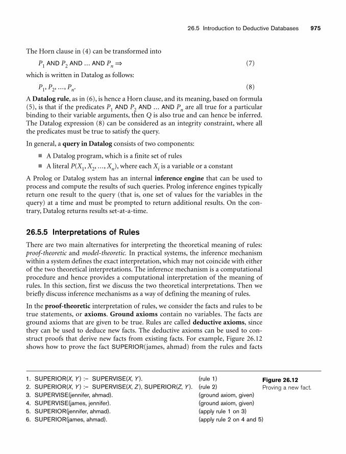
26.5 Introduction to Deductive Databases 975
1. SUPERIOR(X, Y ) :– SUPERVISE(X, Y ). (rule 1)2. SUPERIOR(X, Y ) :– SUPERVISE(X, Z ), SUPERIOR(Z, Y ). (rule 2)3. SUPERVISE(jennifer, ahmad). (ground axiom, given)4. SUPERVISE(james, jennifer). (ground axiom, given)5. SUPERIOR(jennifer, ahmad). (apply rule 1 on 3)6. SUPERIOR(james, ahmad). (apply rule 2 on 4 and 5)
Figure 26.12Proving a new fact.
The Horn clause in (4) can be transformed into
P1 AND P2 AND ... AND Pn ⇒ (7)
which is written in Datalog as follows:
P1, P2, ..., Pn. (8)
A Datalog rule, as in (6), is hence a Horn clause, and its meaning, based on formula(5), is that if the predicates P1 AND P2 AND ... AND Pn are all true for a particularbinding to their variable arguments, then Q is also true and can hence be inferred.The Datalog expression (8) can be considered as an integrity constraint, where allthe predicates must be true to satisfy the query.
In general, a query in Datalog consists of two components:
■ A Datalog program, which is a finite set of rules
■ A literal P(X1, X2, ..., Xn), where each Xi is a variable or a constant
A Prolog or Datalog system has an internal inference engine that can be used toprocess and compute the results of such queries. Prolog inference engines typicallyreturn one result to the query (that is, one set of values for the variables in thequery) at a time and must be prompted to return additional results. On the con-trary, Datalog returns results set-at-a-time.
26.5.5 Interpretations of RulesThere are two main alternatives for interpreting the theoretical meaning of rules:proof-theoretic and model-theoretic. In practical systems, the inference mechanismwithin a system defines the exact interpretation, which may not coincide with eitherof the two theoretical interpretations. The inference mechanism is a computationalprocedure and hence provides a computational interpretation of the meaning ofrules. In this section, first we discuss the two theoretical interpretations. Then webriefly discuss inference mechanisms as a way of defining the meaning of rules.
In the proof-theoretic interpretation of rules, we consider the facts and rules to betrue statements, or axioms. Ground axioms contain no variables. The facts areground axioms that are given to be true. Rules are called deductive axioms, sincethey can be used to deduce new facts. The deductive axioms can be used to con-struct proofs that derive new facts from existing facts. For example, Figure 26.12shows how to prove the fact SUPERIOR(james, ahmad) from the rules and facts
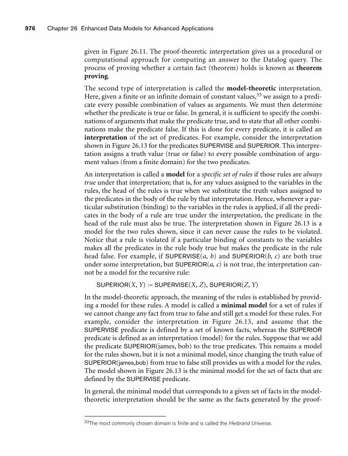
976 Chapter 26 Enhanced Data Models for Advanced Applications
given in Figure 26.11. The proof-theoretic interpretation gives us a procedural orcomputational approach for computing an answer to the Datalog query. Theprocess of proving whether a certain fact (theorem) holds is known as theoremproving.
The second type of interpretation is called the model-theoretic interpretation.Here, given a finite or an infinite domain of constant values,33 we assign to a predi-cate every possible combination of values as arguments. We must then determinewhether the predicate is true or false. In general, it is sufficient to specify the combi-nations of arguments that make the predicate true, and to state that all other combi-nations make the predicate false. If this is done for every predicate, it is called aninterpretation of the set of predicates. For example, consider the interpretationshown in Figure 26.13 for the predicates SUPERVISE and SUPERIOR. This interpre-tation assigns a truth value (true or false) to every possible combination of argu-ment values (from a finite domain) for the two predicates.
An interpretation is called a model for a specific set of rules if those rules are alwaystrue under that interpretation; that is, for any values assigned to the variables in therules, the head of the rules is true when we substitute the truth values assigned tothe predicates in the body of the rule by that interpretation. Hence, whenever a par-ticular substitution (binding) to the variables in the rules is applied, if all the predi-cates in the body of a rule are true under the interpretation, the predicate in thehead of the rule must also be true. The interpretation shown in Figure 26.13 is amodel for the two rules shown, since it can never cause the rules to be violated.Notice that a rule is violated if a particular binding of constants to the variablesmakes all the predicates in the rule body true but makes the predicate in the rulehead false. For example, if SUPERVISE(a, b) and SUPERIOR(b, c) are both trueunder some interpretation, but SUPERIOR(a, c) is not true, the interpretation can-not be a model for the recursive rule:
SUPERIOR(X, Y) :– SUPERVISE(X, Z), SUPERIOR(Z, Y)
In the model-theoretic approach, the meaning of the rules is established by provid-ing a model for these rules. A model is called a minimal model for a set of rules ifwe cannot change any fact from true to false and still get a model for these rules. Forexample, consider the interpretation in Figure 26.13, and assume that theSUPERVISE predicate is defined by a set of known facts, whereas the SUPERIORpredicate is defined as an interpretation (model) for the rules. Suppose that we addthe predicate SUPERIOR(james, bob) to the true predicates. This remains a modelfor the rules shown, but it is not a minimal model, since changing the truth value ofSUPERIOR(james,bob) from true to false still provides us with a model for the rules.The model shown in Figure 26.13 is the minimal model for the set of facts that aredefined by the SUPERVISE predicate.
In general, the minimal model that corresponds to a given set of facts in the model-theoretic interpretation should be the same as the facts generated by the proof-
33The most commonly chosen domain is finite and is called the Herbrand Universe.
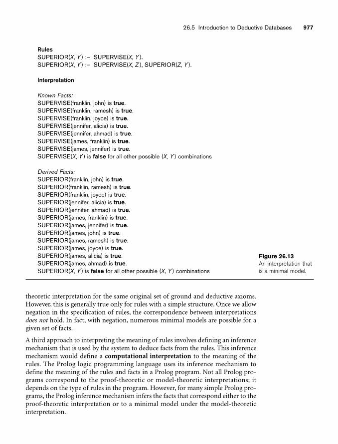
26.5 Introduction to Deductive Databases 977
RulesSUPERIOR(X, Y ) :– SUPERVISE(X, Y ).SUPERIOR(X, Y ) :– SUPERVISE(X, Z ), SUPERIOR(Z, Y ).
Interpretation
Known Facts:SUPERVISE(franklin, john) is true.SUPERVISE(franklin, ramesh) is true.SUPERVISE(franklin, joyce) is true.SUPERVISE(jennifer, alicia) is true.SUPERVISE(jennifer, ahmad) is true.SUPERVISE(james, franklin) is true.SUPERVISE(james, jennifer) is true.SUPERVISE(X, Y ) is false for all other possible (X, Y ) combinations
Derived Facts:SUPERIOR(franklin, john) is true.SUPERIOR(franklin, ramesh) is true.SUPERIOR(franklin, joyce) is true.SUPERIOR(jennifer, alicia) is true.SUPERIOR(jennifer, ahmad) is true.SUPERIOR(james, franklin) is true.SUPERIOR(james, jennifer) is true.SUPERIOR(james, john) is true.SUPERIOR(james, ramesh) is true.SUPERIOR(james, joyce) is true.SUPERIOR(james, alicia) is true.SUPERIOR(james, ahmad) is true.SUPERIOR(X, Y ) is false for all other possible (X, Y ) combinations
Figure 26.13An interpretation thatis a minimal model.
theoretic interpretation for the same original set of ground and deductive axioms.However, this is generally true only for rules with a simple structure. Once we allownegation in the specification of rules, the correspondence between interpretationsdoes not hold. In fact, with negation, numerous minimal models are possible for agiven set of facts.
A third approach to interpreting the meaning of rules involves defining an inferencemechanism that is used by the system to deduce facts from the rules. This inferencemechanism would define a computational interpretation to the meaning of therules. The Prolog logic programming language uses its inference mechanism todefine the meaning of the rules and facts in a Prolog program. Not all Prolog pro-grams correspond to the proof-theoretic or model-theoretic interpretations; itdepends on the type of rules in the program. However, for many simple Prolog pro-grams, the Prolog inference mechanism infers the facts that correspond either to theproof-theoretic interpretation or to a minimal model under the model-theoreticinterpretation.
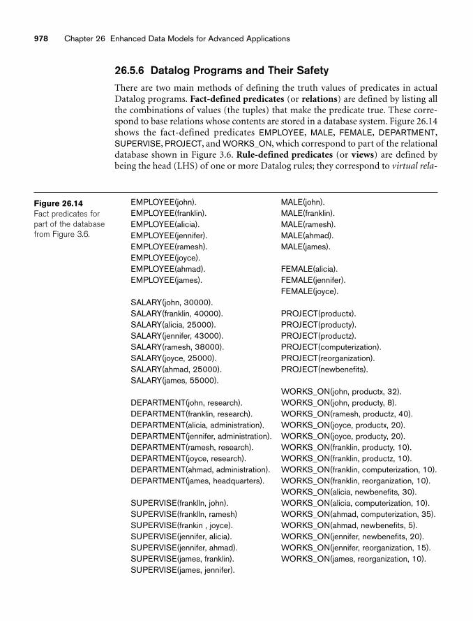
978 Chapter 26 Enhanced Data Models for Advanced Applications
EMPLOYEE(john). MALE(john).EMPLOYEE(franklin). MALE(franklin).EMPLOYEE(aIicia). MALE(ramesh).EMPLOYEE(jennifer). MALE(ahmad).EMPLOYEE(ramesh). MALE(james).EMPLOYEE(joyce).EMPLOYEE(ahmad). FEMALE(alicia).EMPLOYEE(james). FEMALE(jennifer).
FEMALE(joyce).SALARY(john, 30000).SALARY(franklin, 40000). PROJECT(productx).SALARY(alicia, 25000). PROJECT(producty).SALARY(jennifer, 43000). PROJECT(productz).SALARY(ramesh, 38000). PROJECT(computerization).SALARY(joyce, 25000). PROJECT(reorganization).SALARY(ahmad, 25000). PROJECT(newbenefits).SALARY(james, 55000).
WORKS_ON(john, productx, 32).DEPARTMENT(john, research). WORKS_ON(john, producty, 8).DEPARTMENT(franklin, research). WORKS_ON(ramesh, productz, 40).DEPARTMENT(alicia, administration). WORKS_ON(joyce, productx, 20).DEPARTMENT(jennifer, administration). WORKS_ON(joyce, producty, 20).DEPARTMENT(ramesh, research). WORKS_ON(franklin, producty, 10).DEPARTMENT(joyce, research). WORKS_ON(franklin, productz, 10).DEPARTMENT(ahmad, administration). WORKS_ON(franklin, computerization, 10).DEPARTMENT(james, headquarters). WORKS_ON(franklin, reorganization, 10).
WORKS_ON(alicia, newbenefits, 30).SUPERVISE(franklln, john). WORKS_ON(alicia, computerization, 10).SUPERVISE(franklln, ramesh) WORKS_ON(ahmad, computerization, 35).SUPERVISE(frankin , joyce). WORKS_ON(ahmad, newbenefits, 5).SUPERVISE(jennifer, aIicia). WORKS_ON(jennifer, newbenefits, 20).SUPERVISE(jennifer, ahmad). WORKS_ON(jennifer, reorganization, 15).SUPERVISE(james, franklin). WORKS_ON(james, reorganization, 10).SUPERVISE(james, jennifer).
Figure 26.14Fact predicates forpart of the databasefrom Figure 3.6.
26.5.6 Datalog Programs and Their SafetyThere are two main methods of defining the truth values of predicates in actualDatalog programs. Fact-defined predicates (or relations) are defined by listing allthe combinations of values (the tuples) that make the predicate true. These corre-spond to base relations whose contents are stored in a database system. Figure 26.14shows the fact-defined predicates EMPLOYEE, MALE, FEMALE, DEPARTMENT,SUPERVISE, PROJECT, and WORKS_ON, which correspond to part of the relationaldatabase shown in Figure 3.6. Rule-defined predicates (or views) are defined bybeing the head (LHS) of one or more Datalog rules; they correspond to virtual rela-
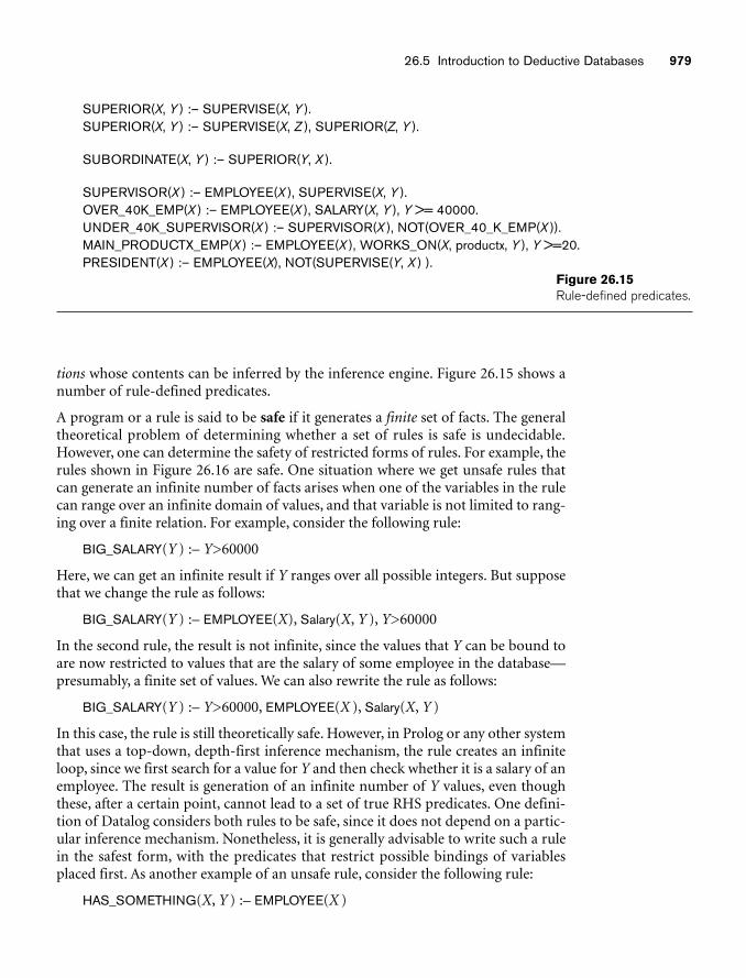
26.5 Introduction to Deductive Databases 979
SUPERIOR(X, Y ) :– SUPERVISE(X, Y ).SUPERIOR(X, Y ) :– SUPERVISE(X, Z ), SUPERIOR(Z, Y ).
SUBORDINATE(X, Y ) :– SUPERIOR(Y, X ).
SUPERVISOR(X ) :– EMPLOYEE(X ), SUPERVISE(X, Y ).OVER_40K_EMP(X ) :– EMPLOYEE(X ), SALARY(X, Y ), Y >= 40000.UNDER_40K_SUPERVISOR(X ) :– SUPERVISOR(X ), NOT(OVER_40_K_EMP(X )).MAIN_PRODUCTX_EMP(X ) :– EMPLOYEE(X ), WORKS_ON(X, productx, Y ), Y >=20.PRESIDENT(X ) :– EMPLOYEE(X), NOT(SUPERVISE(Y, X ) ).
Figure 26.15Rule-defined predicates.
tions whose contents can be inferred by the inference engine. Figure 26.15 shows anumber of rule-defined predicates.
A program or a rule is said to be safe if it generates a finite set of facts. The generaltheoretical problem of determining whether a set of rules is safe is undecidable.However, one can determine the safety of restricted forms of rules. For example, therules shown in Figure 26.16 are safe. One situation where we get unsafe rules thatcan generate an infinite number of facts arises when one of the variables in the rulecan range over an infinite domain of values, and that variable is not limited to rang-ing over a finite relation. For example, consider the following rule:
BIG_SALARY(Y ) :– Y>60000
Here, we can get an infinite result if Y ranges over all possible integers. But supposethat we change the rule as follows:
BIG_SALARY(Y ) :– EMPLOYEE(X), Salary(X, Y ), Y>60000
In the second rule, the result is not infinite, since the values that Y can be bound toare now restricted to values that are the salary of some employee in the database—presumably, a finite set of values. We can also rewrite the rule as follows:
BIG_SALARY(Y ) :– Y>60000, EMPLOYEE(X ), Salary(X, Y )
In this case, the rule is still theoretically safe. However, in Prolog or any other systemthat uses a top-down, depth-first inference mechanism, the rule creates an infiniteloop, since we first search for a value for Y and then check whether it is a salary of anemployee. The result is generation of an infinite number of Y values, even thoughthese, after a certain point, cannot lead to a set of true RHS predicates. One defini-tion of Datalog considers both rules to be safe, since it does not depend on a partic-ular inference mechanism. Nonetheless, it is generally advisable to write such a rulein the safest form, with the predicates that restrict possible bindings of variablesplaced first. As another example of an unsafe rule, consider the following rule:
HAS_SOMETHING(X, Y ) :– EMPLOYEE(X )
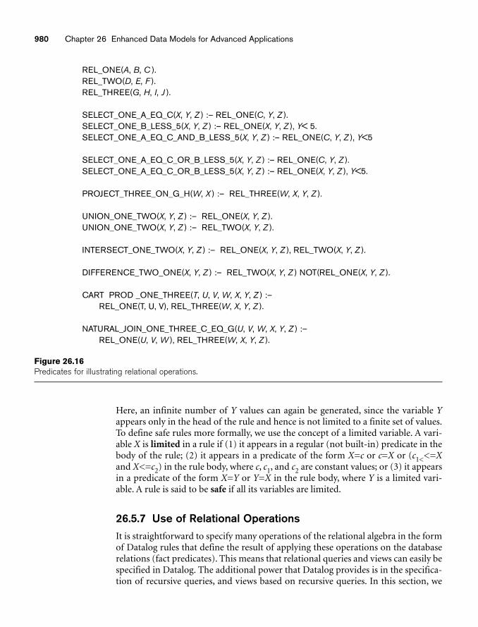
980 Chapter 26 Enhanced Data Models for Advanced Applications
REL_ONE(A, B, C ).REL_TWO(D, E, F ).REL_THREE(G, H, I, J ).
SELECT_ONE_A_EQ_C(X, Y, Z ) :– REL_ONE(C, Y, Z ).SELECT_ONE_B_LESS_5(X, Y, Z ) :– REL_ONE(X, Y, Z ), Y< 5.SELECT_ONE_A_EQ_C_AND_B_LESS_5(X, Y, Z ) :– REL_ONE(C, Y, Z ), Y<5
SELECT_ONE_A_EQ_C_OR_B_LESS_5(X, Y, Z ) :– REL_ONE(C, Y, Z ).SELECT_ONE_A_EQ_C_OR_B_LESS_5(X, Y, Z ) :– REL_ONE(X, Y, Z ), Y<5.
PROJECT_THREE_ON_G_H(W, X ) :– REL_THREE(W, X, Y, Z ).
UNION_ONE_TWO(X, Y, Z ) :– REL_ONE(X, Y, Z ).UNION_ONE_TWO(X, Y, Z ) :– REL_TWO(X, Y, Z ).
INTERSECT_ONE_TWO(X, Y, Z ) :– REL_ONE(X, Y, Z ), REL_TWO(X, Y, Z ).
DIFFERENCE_TWO_ONE(X, Y, Z ) :– REL_TWO(X, Y, Z ) NOT(REL_ONE(X, Y, Z ).
CART PROD _ONE_THREE(T, U, V, W, X, Y, Z ) :–REL_ONE(T, U, V), REL_THREE(W, X, Y, Z ).
NATURAL_JOIN_ONE_THREE_C_EQ_G(U, V, W, X, Y, Z ) :–REL_ONE(U, V, W ), REL_THREE(W, X, Y, Z ).
Figure 26.16Predicates for illustrating relational operations.
Here, an infinite number of Y values can again be generated, since the variable Yappears only in the head of the rule and hence is not limited to a finite set of values.To define safe rules more formally, we use the concept of a limited variable. A vari-able X is limited in a rule if (1) it appears in a regular (not built-in) predicate in thebody of the rule; (2) it appears in a predicate of the form X=c or c=X or (c1<<=Xand X<=c2) in the rule body, where c, c1, and c2 are constant values; or (3) it appearsin a predicate of the form X=Y or Y=X in the rule body, where Y is a limited vari-able. A rule is said to be safe if all its variables are limited.
26.5.7 Use of Relational OperationsIt is straightforward to specify many operations of the relational algebra in the formof Datalog rules that define the result of applying these operations on the databaserelations (fact predicates). This means that relational queries and views can easily bespecified in Datalog. The additional power that Datalog provides is in the specifica-tion of recursive queries, and views based on recursive queries. In this section, we
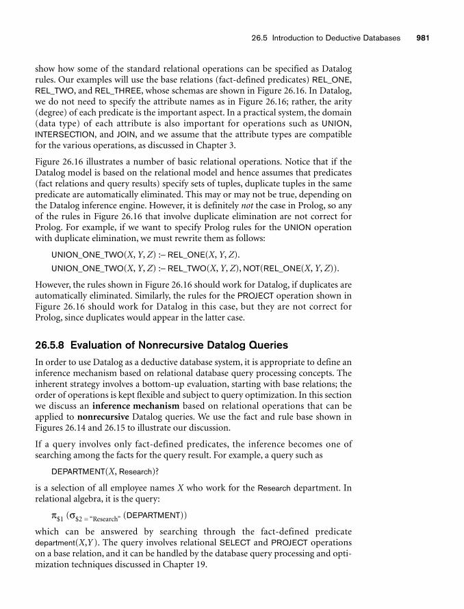
26.5 Introduction to Deductive Databases 981
show how some of the standard relational operations can be specified as Datalogrules. Our examples will use the base relations (fact-defined predicates) REL_ONE,REL_TWO, and REL_THREE, whose schemas are shown in Figure 26.16. In Datalog,we do not need to specify the attribute names as in Figure 26.16; rather, the arity(degree) of each predicate is the important aspect. In a practical system, the domain(data type) of each attribute is also important for operations such as UNION,INTERSECTION, and JOIN, and we assume that the attribute types are compatiblefor the various operations, as discussed in Chapter 3.
Figure 26.16 illustrates a number of basic relational operations. Notice that if theDatalog model is based on the relational model and hence assumes that predicates(fact relations and query results) specify sets of tuples, duplicate tuples in the samepredicate are automatically eliminated. This may or may not be true, depending onthe Datalog inference engine. However, it is definitely not the case in Prolog, so anyof the rules in Figure 26.16 that involve duplicate elimination are not correct forProlog. For example, if we want to specify Prolog rules for the UNION operationwith duplicate elimination, we must rewrite them as follows:
UNION_ONE_TWO(X, Y, Z) :– REL_ONE(X, Y, Z).
UNION_ONE_TWO(X, Y, Z) :– REL_TWO(X, Y, Z), NOT(REL_ONE(X, Y, Z)).
However, the rules shown in Figure 26.16 should work for Datalog, if duplicates areautomatically eliminated. Similarly, the rules for the PROJECT operation shown inFigure 26.16 should work for Datalog in this case, but they are not correct forProlog, since duplicates would appear in the latter case.
26.5.8 Evaluation of Nonrecursive Datalog QueriesIn order to use Datalog as a deductive database system, it is appropriate to define aninference mechanism based on relational database query processing concepts. Theinherent strategy involves a bottom-up evaluation, starting with base relations; theorder of operations is kept flexible and subject to query optimization. In this sectionwe discuss an inference mechanism based on relational operations that can beapplied to nonrecursive Datalog queries. We use the fact and rule base shown inFigures 26.14 and 26.15 to illustrate our discussion.
If a query involves only fact-defined predicates, the inference becomes one ofsearching among the facts for the query result. For example, a query such as
DEPARTMENT(X, Research)?
is a selection of all employee names X who work for the Research department. Inrelational algebra, it is the query:
π$1 (σ$2 = “Research” (DEPARTMENT))
which can be answered by searching through the fact-defined predicatedepartment(X,Y ). The query involves relational SELECT and PROJECT operationson a base relation, and it can be handled by the database query processing and opti-mization techniques discussed in Chapter 19.
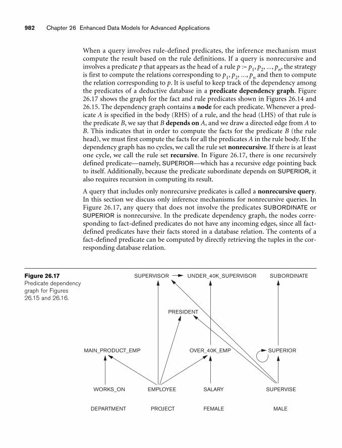
982 Chapter 26 Enhanced Data Models for Advanced Applications
SUPERVISOR UNDER_40K_SUPERVISOR
OVER_40K_EMP
PRESIDENT
MAIN_PRODUCT_EMP
WORKS_ON EMPLOYEE SALARY SUPERVISE
DEPARTMENT PROJECT FEMALE MALE
SUBORDINATE
SUPERIOR
Figure 26.17Predicate dependencygraph for Figures26.15 and 26.16.
When a query involves rule-defined predicates, the inference mechanism mustcompute the result based on the rule definitions. If a query is nonrecursive andinvolves a predicate p that appears as the head of a rule p :– p1, p2, ..., pn, the strategyis first to compute the relations corresponding to p1, p2, ..., pn and then to computethe relation corresponding to p. It is useful to keep track of the dependency amongthe predicates of a deductive database in a predicate dependency graph. Figure26.17 shows the graph for the fact and rule predicates shown in Figures 26.14 and26.15. The dependency graph contains a node for each predicate. Whenever a pred-icate A is specified in the body (RHS) of a rule, and the head (LHS) of that rule isthe predicate B, we say that B depends on A, and we draw a directed edge from A toB. This indicates that in order to compute the facts for the predicate B (the rulehead), we must first compute the facts for all the predicates A in the rule body. If thedependency graph has no cycles, we call the rule set nonrecursive. If there is at leastone cycle, we call the rule set recursive. In Figure 26.17, there is one recursivelydefined predicate—namely, SUPERIOR—which has a recursive edge pointing backto itself. Additionally, because the predicate subordinate depends on SUPERIOR, italso requires recursion in computing its result.
A query that includes only nonrecursive predicates is called a nonrecursive query.In this section we discuss only inference mechanisms for nonrecursive queries. InFigure 26.17, any query that does not involve the predicates SUBORDINATE orSUPERIOR is nonrecursive. In the predicate dependency graph, the nodes corre-sponding to fact-defined predicates do not have any incoming edges, since all fact-defined predicates have their facts stored in a database relation. The contents of afact-defined predicate can be computed by directly retrieving the tuples in the cor-responding database relation.
26.6 Summary 983
The main function of an inference mechanism is to compute the facts that corre-spond to query predicates. This can be accomplished by generating a relationalexpression involving relational operators as SELECT, PROJECT, JOIN, UNION, andSET DIFFERENCE (with appropriate provision for dealing with safety issues) that,when executed, provides the query result. The query can then be executed by utiliz-ing the internal query processing and optimization operations of a relational data-base management system. Whenever the inference mechanism needs to computethe fact set corresponding to a nonrecursive rule-defined predicate p, it first locatesall the rules that have p as their head. The idea is to compute the fact set for eachsuch rule and then to apply the UNION operation to the results, since UNION corre-sponds to a logical OR operation. The dependency graph indicates all predicates qon which each p depends, and since we assume that the predicate is nonrecursive,we can always determine a partial order among such predicates q. Before computingthe fact set for p, first we compute the fact sets for all predicates q on which pdepends, based on their partial order. For example, if a query involves the predicateUNDER_40K_SUPERVISOR, we must first compute both SUPERVISOR andOVER_40K_EMP. Since the latter two depend only on the fact-defined predicatesEMPLOYEE, SALARY, and SUPERVISE, they can be computed directly from thestored database relations.
This concludes our introduction to deductive databases. Additional material may befound at the book’s Website, where the complete Chapter 25 from the third editionis available. This includes a discussion on algorithms for recursive query processing.We have included an extensive bibliography of work in deductive databases, recur-sive query processing, magic sets, combination of relational databases with deduc-tive rules, and GLUE-NAIL! System at the end of this chapter.
26.6 SummaryIn this chapter we introduced database concepts for some of the common featuresthat are needed by advanced applications: active databases, temporal databases, spa-tial databases, multimedia databases, and deductive databases. It is important tonote that each of these is a broad topic and warrants a complete textbook.
First we introduced the topic of active databases, which provide additional func-tionality for specifying active rules. We introduced the Event-Condition-Action(ECA) model for active databases. The rules can be automatically triggered byevents that occur—such as a database update—and they can initiate certain actionsthat have been specified in the rule declaration if certain conditions are true. Manycommercial packages have some of the functionality provided by active databases inthe form of triggers. We discussed the different options for specifying rules, such asrow-level versus statement-level, before versus after, and immediate versus deferred.We gave examples of row-level triggers in the Oracle commercial system, and statement-level rules in the STARBURST experimental system. The syntax for trig-gers in the SQL-99 standard was also discussed. We briefly discussed some designissues and some possible applications for active databases.
984 Chapter 26 Enhanced Data Models for Advanced Applications
Next we introduced some of the concepts of temporal databases, which permit thedatabase system to store a history of changes and allow users to query both currentand past states of the database. We discussed how time is represented and distin-guished between the valid time and transaction time dimensions. We discussed howvalid time, transaction time, and bitemporal relations can be implemented usingtuple versioning in the relational model, with examples to illustrate how updates,inserts, and deletes are implemented. We also showed how complex objects can beused to implement temporal databases using attribute versioning. We looked atsome of the querying operations for temporal relational databases and gave a briefintroduction to the TSQL2 language.
Then we turned to spatial databases. Spatial databases provide concepts for data-bases that keep track of objects that have spatial characteristics. We discussed thetypes of spatial data, types of operators for processing spatial data, types of spatialqueries, and spatial indexing techniques, including the popular R-trees. Then wediscussed some spatial data mining techniques and applications of spatial data.
We discussed some basic types of multimedia databases and their important char-acteristics. Multimedia databases provide features that allow users to store andquery different types of multimedia information, which includes images (such aspictures and drawings), video clips (such as movies, newsreels, and home videos),audio clips (such as songs, phone messages, and speeches), and documents (such asbooks and articles). We provided a brief overview of the various types of mediasources and how multimedia sources may be indexed. Images are an extremely com-mon type of data among databases today and are likely to occupy a large proportionof stored data in databases. We therefore provided a more detailed treatment ofimages: their automatic analysis, recognition of objects within images, and theirsemantic tagging—all of which contribute to developing better systems to retrieveimages by content, which still remains a challenging problem. We also commentedon the analysis of audio data sources.
We concluded the chapter with an introduction to deductive databases. We gave anoverview of Prolog and Datalog notation. We discussed the clausal form of formu-las. Datalog rules are restricted to Horn clauses, which contain at most one positiveliteral. We discussed the proof-theoretic and model-theoretic interpretation ofrules. We briefly discussed Datalog rules and their safety and the ways of expressingrelational operators using Datalog rules. Finally, we discussed an inference mecha-nism based on relational operations that can be used to evaluate nonrecursiveDatalog queries using relational query optimization techniques. While Datalog hasbeen a popular language with many applications, unfortunately, implementationsof deductive database systems such as LDL or VALIDITY have not become widelycommercially available.
Review Questions 985
Review Questions26.1. What are the differences between row-level and statement-level active rules?
26.2. What are the differences among immediate, deferred, and detachedconsideration of active rule conditions?
26.3. What are the differences among immediate, deferred, and detachedexecution of active rule actions?
26.4. Briefly discuss the consistency and termination problems when designing aset of active rules.
26.5. Discuss some applications of active databases.
26.6. Discuss how time is represented in temporal databases and compare the dif-ferent time dimensions.
26.7. What are the differences between valid time, transaction time, and bitempo-ral relations?
26.8. Describe how the insert, delete, and update commands should be imple-mented on a valid time relation.
26.9. Describe how the insert, delete, and update commands should be imple-mented on a bitemporal relation.
26.10. Describe how the insert, delete, and update commands should be imple-mented on a transaction time relation.
26.11. What are the main differences between tuple versioning and attribute ver-sioning?
26.12. How do spatial databases differ from regular databases?
26.13. What are the different types of spatial data?
26.14. Name the main types of spatial operators and different classes of spatialqueries.
26.15. What are the properties of R-trees that act as an index for spatial data?
26.16. Describe how a spatial join index between spatial objects can be constructed.
26.17. What are the different types of spatial data mining?
26.18. State the general form of a spatial association rule. Give an example of a spa-tial association rule.
26.19. What are the different types of multimedia sources?
26.20. How are multimedia sources indexed for content-based retrieval?
986 Chapter 26 Enhanced Data Models for Advanced Applications
26.21. What important features of images are used to compare them?
26.22. What are the different approaches to recognizing objects in images?
26.23. How is semantic tagging of images used?
26.24. What are the difficulties in analyzing audio sources?
26.25. What are deductive databases?
26.26. Write sample rules in Prolog to define that courses with course numberabove CS5000 are graduate courses and that DBgrads are those graduate stu-dents who enroll in CS6400 and CS8803.
26.27. Define clausal form of formulas and Horn clauses.
26.28. What is theorem proving and what is proof-theoretic interpretation of rules?
26.29. What is model-theoretic interpretation and how does it differ from proof-theoretic interpretation?
26.30. What are fact-defined predicates and rule-defined predicates?
26.31. What is a safe rule?
26.32. Give examples of rules that can define relational operations SELECT,PROJECT, JOIN, and SET operations.
26.33. Discuss the inference mechanism based on relational operations that can beapplied to evaluate nonrecursive Datalog queries.
Exercises26.34. Consider the COMPANY database described in Figure 3.6. Using the syntax
of Oracle triggers, write active rules to do the following:
a. Whenever an employee’s project assignments are changed, check if thetotal hours per week spent on the employee’s projects are less than 30 orgreater than 40; if so, notify the employee’s direct supervisor.
b. Whenever an employee is deleted, delete the PROJECT tuples andDEPENDENT tuples related to that employee, and if the employee man-ages a department or supervises employees, set the Mgr_ssn for thatdepartment to NULL and set the Super_ssn for those employees to NULL.
26.35. Repeat 26.34 but use the syntax of STARBURST active rules.
26.36. Consider the relational schema shown in Figure 26.18. Write active rules forkeeping the Sum_commissions attribute of SALES_PERSON equal to the sumof the Commission attribute in SALES for each sales person. Your rules shouldalso check if the Sum_commissions exceeds 100000; if it does, call a procedureNotify_manager(S_id). Write both statement-level rules in STARBURST nota-tion and row-level rules in Oracle.
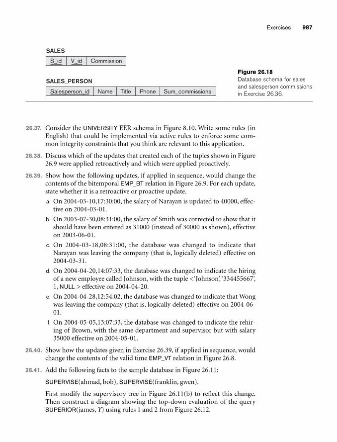
Exercises 987
S_id V_id Commission
SALES
Salesperson_id Name Title Phone Sum_commissions
SALES_PERSON
Figure 26.18Database schema for salesand salesperson commissionsin Exercise 26.36.
26.37. Consider the UNIVERSITY EER schema in Figure 8.10. Write some rules (inEnglish) that could be implemented via active rules to enforce some com-mon integrity constraints that you think are relevant to this application.
26.38. Discuss which of the updates that created each of the tuples shown in Figure26.9 were applied retroactively and which were applied proactively.
26.39. Show how the following updates, if applied in sequence, would change thecontents of the bitemporal EMP_BT relation in Figure 26.9. For each update,state whether it is a retroactive or proactive update.
a. On 2004-03-10,17:30:00, the salary of Narayan is updated to 40000, effec-tive on 2004-03-01.
b. On 2003-07-30,08:31:00, the salary of Smith was corrected to show that itshould have been entered as 31000 (instead of 30000 as shown), effectiveon 2003-06-01.
c. On 2004-03-18,08:31:00, the database was changed to indicate thatNarayan was leaving the company (that is, logically deleted) effective on2004-03-31.
d. On 2004-04-20,14:07:33, the database was changed to indicate the hiringof a new employee called Johnson, with the tuple <‘Johnson’, ‘334455667’,1, NULL > effective on 2004-04-20.
e. On 2004-04-28,12:54:02, the database was changed to indicate that Wongwas leaving the company (that is, logically deleted) effective on 2004-06-01.
f. On 2004-05-05,13:07:33, the database was changed to indicate the rehir-ing of Brown, with the same department and supervisor but with salary35000 effective on 2004-05-01.
26.40. Show how the updates given in Exercise 26.39, if applied in sequence, wouldchange the contents of the valid time EMP_VT relation in Figure 26.8.
26.41. Add the following facts to the sample database in Figure 26.11:
SUPERVISE(ahmad, bob), SUPERVISE(franklin, gwen).
First modify the supervisory tree in Figure 26.11(b) to reflect this change.Then construct a diagram showing the top-down evaluation of the querySUPERIOR(james, Y) using rules 1 and 2 from Figure 26.12.
988 Chapter 26 Enhanced Data Models for Advanced Applications
26.42. Consider the following set of facts for the relation PARENT(X, Y), where Y isthe parent of X:
PARENT(a, aa), PARENT(a, ab), PARENT(aa, aaa), PARENT(aa, aab),PARENT(aaa, aaaa), PARENT(aaa, aaab).
Consider the rules
r1: ANCESTOR(X, Y) :– PARENT(X, Y)r2: ANCESTOR(X, Y) :– PARENT(X, Z), ANCESTOR(Z, Y)
which define ancestor Y of X as above.
a. Show how to solve the Datalog query
ANCESTOR(aa, X)?
and show your work at each step.
b. Show the same query by computing only the changes in the ancestor rela-tion and using that in rule 2 each time.
[This question is derived from Bancilhon and Ramakrishnan (1986).]
26.43. Consider a deductive database with the following rules:
ANCESTOR(X, Y) :– FATHER(X, Y)ANCESTOR(X, Y) :– FATHER(X, Z), ANCESTOR(Z, Y)
Notice that FATHER(X, Y) means that Y is the father of X; ANCESTOR(X, Y)means that Y is the ancestor of X.
Consider the following fact base:
FATHER(Harry, Issac), FATHER(Issac, John), FATHER(John, Kurt).
a. Construct a model-theoretic interpretation of the above rules using thegiven facts.
b. Consider that a database contains the above relations FATHER(X, Y ),another relation BROTHER(X, Y ), and a third relation BIRTH(X, B ),where B is the birth date of person X. State a rule that computes the firstcousins of the following variety: their fathers must be brothers.
c. Show a complete Datalog program with fact-based and rule-based literalsthat computes the following relation: list of pairs of cousins, where thefirst person is born after 1960 and the second after 1970. You may usegreater than as a built-in predicate. (Note: Sample facts for brother, birth,and person must also be shown.)
26.44. Consider the following rules:
REACHABLE(X, Y) :– FLIGHT(X, Y)REACHABLE(X, Y) :– FLIGHT(X, Z), REACHABLE(Z, Y)
where REACHABLE(X, Y) means that city Y can be reached from city X, andFLIGHT(X, Y) means that there is a flight to city Y from city X.
Selected Bibliography 989
a. Construct fact predicates that describe the following:
i. Los Angeles, New York, Chicago, Atlanta, Frankfurt, Paris, Singapore,Sydney are cities.
ii. The following flights exist: LA to NY, NY to Atlanta, Atlanta toFrankfurt, Frankfurt to Atlanta, Frankfurt to Singapore, andSingapore to Sydney. (Note: No flight in reverse direction can be auto-matically assumed.)
b. Is the given data cyclic? If so, in what sense?
c. Construct a model-theoretic interpretation (that is, an interpretationsimilar to the one shown in Figure 26.13) of the above facts and rules.
d. Consider the query
REACHABLE(Atlanta, Sydney)?
How will this query be executed? List the series of steps it will go through.
e. Consider the following rule-defined predicates:
ROUND-TRIP-REACHABLE(X, Y) :–REACHABLE(X, Y), REACHABLE(Y, X)
DURATION(X, Y, Z)
Draw a predicate dependency graph for the above predicates. (Note:DURATION(X, Y, Z) means that you can take a flight from X to Y in Zhours.)
f. Consider the following query: What cities are reachable in 12 hours fromAtlanta? Show how to express it in Datalog. Assume built-in predicateslike greater-than(X, Y). Can this be converted into a relational algebrastatement in a straightforward way? Why or why not?
g. Consider the predicate population(X, Y), where Y is the population ofcity X. Consider the following query: List all possible bindings of thepredicate pair (X, Y), where Y is a city that can be reached in two flightsfrom city X, which has over 1 million people. Show this query in Datalog.Draw a corresponding query tree in relational algebraic terms.
Selected BibliographyThe book by Zaniolo et al. (1997) consists of several parts, each describing anadvanced database concept such as active, temporal, and spatial/text/multimediadatabases. Widom and Ceri (1996) and Ceri and Fraternali (1997) focus on activedatabase concepts and systems. Snodgrass (1995) describes the TSQL2 languageand data model. Khoshafian and Baker (1996), Faloutsos (1996), andSubrahmanian (1998) describe multimedia database concepts. Tansel et al. (1993) isa collection of chapters on temporal databases.
STARBURST rules are described in Widom and Finkelstein (1990). Early work onactive databases includes the HiPAC project, discussed in Chakravarthy et al. (1989)
990 Chapter 26 Enhanced Data Models for Advanced Applications
and Chakravarthy (1990). A glossary for temporal databases is given in Jensen et al.(1994). Snodgrass (1987) focuses on TQuel, an early temporal query language.
Temporal normalization is defined in Navathe and Ahmed (1989). Paton (1999)and Paton and Diaz (1999) survey active databases. Chakravarthy et al. (1994)describe SENTINEL and object-based active systems. Lee et al. (1998) discuss timeseries management.
The book by Shekhar and Chawla (2003) consists of all aspects of spatial databasesincluding spatial data models, spatial storage and indexing, and spatial data mining.Scholl et al. (2001) is another textbook on spatial data management. Albrecht(1996) describes in detail the various GIS analysis operations. Clementini and DiFelice (1993) give a detailed description of the spatial operators. Güting (1994)describes the spatial data structures and querying languages for spatial database sys-tems. Guttman (1984) proposed R-trees for spatial data indexing. Manolopoulos etal. (2005) is a book on the theory and applications of R-trees. Papadias et al. (2003)discuss query processing using R-trees for spatial networks. Ester et al. (2001) pro-vide a comprehensive discussion on the algorithms and applications of spatial datamining. Koperski and Han (1995) discuss association rule discovery from geo-graphic databases. Brinkhoff et al. (1993) provide a comprehensive overview of theusage of R-trees for efficient processing of spatial joins. Rotem (1991) describes spa-tial join indexes comprehensively. Shekhar and Xiong (2008) is a compilation ofvarious sources that discuss different aspects of spatial database management sys-tems and GIS. The density-based clustering algorithms DBSCAN and DENCLUEare proposed by Ester et al. (1996) and Hinnenberg and Gabriel (2007) respectively.
Multimedia database modeling has a vast amount of literature—it is difficult topoint to all important references here. IBM’s QBIC (Query By Image Content) sys-tem described in Niblack et al. (1998) was one of the first comprehensive approachesfor querying images based on content. It is now available as a part of IBM’s DB2database image extender. Zhao and Grosky (2002) discuss content-based imageretrieval. Carneiro and Vasconselos (2005) present a database-centric view of seman-tic image annotation and retrieval. Content-based retrieval of subimages is discussedby Luo and Nascimento (2004). Tuceryan and Jain (1998) discuss various aspects oftexture analysis. Object recognition using SIFT is discussed in Lowe (2004). Lazebniket al. (2004) describe the use of local affine regions to model 3D objects (RIFT).Among other object recognition approaches, G-RIF is described in Kim et al. (2006),Bay et al. (2006) discuss SURF, Ke and Sukthankar (2004) present PCA-SIFT, andMikolajczyk and Schmid (2005) describe GLOH. Fan et al. (2004) present a tech-nique for automatic image annotation by using concept-sensitive objects. Fotouhi etal. (2007) was the first international workshop on many faces of multimedia seman-tics, which is continuing annually. Thuraisingham (2001) classifies audio data intodifferent categories, and by treating each of these categories differently, elaborates onthe use of metadata for audio. Prabhakaran (1996) has also discussed how speechprocessing techniques can add valuable metadata information to the audio piece.
The early developments of the logic and database approach are surveyed by Gallaireet al. (1984). Reiter (1984) provides a reconstruction of relational database theory,
while Levesque (1984) provides a discussion of incomplete knowledge in light oflogic. Gallaire and Minker (1978) provide an early book on this topic. A detailedtreatment of logic and databases appears in Ullman (1989, Volume 2), and there is arelated chapter in Volume 1 (1988). Ceri, Gottlob, and Tanca (1990) present a com-prehensive yet concise treatment of logic and databases. Das (1992) is a comprehen-sive book on deductive databases and logic programming. The early history ofDatalog is covered in Maier and Warren (1988). Clocksin and Mellish (2003) is anexcellent reference on Prolog language.
Aho and Ullman (1979) provide an early algorithm for dealing with recursivequeries, using the least fixed-point operator. Bancilhon and Ramakrishnan (1986)give an excellent and detailed description of the approaches to recursive query pro-cessing, with detailed examples of the naive and seminaive approaches. Excellentsurvey articles on deductive databases and recursive query processing includeWarren (1992) and Ramakrishnan and Ullman (1995). A complete description ofthe seminaive approach based on relational algebra is given in Bancilhon (1985).Other approaches to recursive query processing include the recursive query/sub-query strategy of Vieille (1986), which is a top-down interpreted strategy, and theHenschen-Naqvi (1984) top-down compiled iterative strategy. Balbin andRamamohanrao (1987) discuss an extension of the seminaive differential approachfor multiple predicates.
The original paper on magic sets is by Bancilhon et al. (1986). Beeri andRamakrishnan (1987) extend it. Mumick et al. (1990a) show the applicability ofmagic sets to nonrecursive nested SQL queries. Other approaches to optimizing ruleswithout rewriting them appear in Vieille (1986, 1987). Kifer and Lozinskii (1986)propose a different technique. Bry (1990) discusses how the top-down and bottom-up approaches can be reconciled. Whang and Navathe (1992) describe an extendeddisjunctive normal form technique to deal with recursion in relational algebraexpressions for providing an expert system interface over a relational DBMS.
Chang (1981) describes an early system for combining deductive rules with rela-tional databases. The LDL system prototype is described in Chimenti et al. (1990).Krishnamurthy and Naqvi (1989) introduce the choice notion in LDL. Zaniolo(1988) discusses the language issues for the LDL system. A language overview ofCORAL is provided in Ramakrishnan et al. (1992), and the implementation isdescribed in Ramakrishnan et al. (1993). An extension to support object-orientedfeatures, called CORAL++, is described in Srivastava et al. (1993). Ullman (1985)provides the basis for the NAIL! system, which is described in Morris et al. (1987).Phipps et al. (1991) describe the GLUE-NAIL! deductive database system.
Zaniolo (1990) reviews the theoretical background and the practical importance ofdeductive databases. Nicolas (1997) gives an excellent history of the developmentsleading up to Deductive Object-Oriented Database (DOOD) systems. Falcone et al.(1997) survey the DOOD landscape. References on the VALIDITY system includeFriesen et al. (1995), Vieille (1998), and Dietrich et al. (1999).
Selected Bibliography 991
1035
Data Mining Concepts
Over the last three decades, many organizationshave generated a large amount of machine-
readable data in the form of files and databases. To process this data, we have thedatabase technology available that supports query languages like SQL. The problemwith SQL is that it is a structured language that assumes the user is aware of thedatabase schema. SQL supports operations of relational algebra that allow a user toselect rows and columns of data from tables or join-related information from tablesbased on common fields. In the next chapter, we will see that data warehousing tech-nology affords several types of functionality: that of consolidation, aggregation, andsummarization of data. Data warehouses let us view the same information alongmultiple dimensions. In this chapter, we will focus our attention on another verypopular area of interest known as data mining. As the term connotes, data miningrefers to the mining or discovery of new information in terms of patterns or rulesfrom vast amounts of data. To be practically useful, data mining must be carried outefficiently on large files and databases. Although some data mining features arebeing provided in RDBMSs, data mining is not well-integrated with database man-agement systems.
We will briefly review the state of the art of this rather extensive field of data min-ing, which uses techniques from such areas as machine learning, statistics, neuralnetworks, and genetic algorithms. We will highlight the nature of the informationthat is discovered, the types of problems faced when trying to mine databases, andthe types of applications of data mining. We will also survey the state of the art of alarge number of commercial tools available (see Section 28.7) and describe a num-ber of research advances that are needed to make this area viable.
28chapter 28
1036 Chapter 28 Data Mining Concepts
28.1 Overview of Data Mining TechnologyIn reports such as the very popular Gartner Report,1 data mining has been hailed asone of the top technologies for the near future. In this section we relate data miningto the broader area called knowledge discovery and contrast the two by means of anillustrative example.
28.1.1 Data Mining versus Data WarehousingThe goal of a data warehouse (see Chapter 29) is to support decision making withdata. Data mining can be used in conjunction with a data warehouse to help with certain types of decisions. Data mining can be applied to operational databaseswith individual transactions. To make data mining more efficient, the data ware-house should have an aggregated or summarized collection of data. Data mininghelps in extracting meaningful new patterns that cannot necessarily be found bymerely querying or processing data or metadata in the data warehouse. Therefore,data mining applications should be strongly considered early, during the design of adata warehouse. Also, data mining tools should be designed to facilitate their use inconjunction with data warehouses. In fact, for very large databases running into ter-abytes and even petabytes of data, successful use of data mining applications willdepend first on the construction of a data warehouse.
28.1.2 Data Mining as a Part of the Knowledge Discovery Process
Knowledge Discovery in Databases, frequently abbreviated as KDD, typicallyencompasses more than data mining. The knowledge discovery process comprisessix phases:2 data selection, data cleansing, enrichment, data transformation orencoding, data mining, and the reporting and display of the discovered information.
As an example, consider a transaction database maintained by a specialty consumergoods retailer. Suppose the client data includes a customer name, ZIP Code, phonenumber, date of purchase, item code, price, quantity, and total amount. A variety ofnew knowledge can be discovered by KDD processing on this client database.During data selection, data about specific items or categories of items, or from storesin a specific region or area of the country, may be selected. The data cleansingprocess then may correct invalid ZIP Codes or eliminate records with incorrectphone prefixes. Enrichment typically enhances the data with additional sources ofinformation. For example, given the client names and phone numbers, the storemay purchase other data about age, income, and credit rating and append them toeach record. Data transformation and encoding may be done to reduce the amount
1The Gartner Report is one example of the many technology survey publications that corporate man-agers rely on to make their technology selection discussions.2This discussion is largely based on Adriaans and Zantinge (1996).
28.1 Overview of Data Mining Technology 1037
of data. For instance, item codes may be grouped in terms of product categories intoaudio, video, supplies, electronic gadgets, camera, accessories, and so on. ZIP Codesmay be aggregated into geographic regions, incomes may be divided into ranges,and so on. In Figure 29.1, we will show a step called cleaning as a precursor to thedata warehouse creation. If data mining is based on an existing warehouse for thisretail store chain, we would expect that the cleaning has already been applied. It isonly after such preprocessing that data mining techniques are used to mine differentrules and patterns.
The result of mining may be to discover the following type of new information:
■ Association rules—for example, whenever a customer buys video equip-ment, he or she also buys another electronic gadget.
■ Sequential patterns—for example, suppose a customer buys a camera, andwithin three months he or she buys photographic supplies, then within sixmonths he is likely to buy an accessory item. This defines a sequential pat-tern of transactions. A customer who buys more than twice in lean periodsmay be likely to buy at least once during the Christmas period.
■ Classification trees—for example, customers may be classified by frequencyof visits, types of financing used, amount of purchase, or affinity for types ofitems; some revealing statistics may be generated for such classes.
We can see that many possibilities exist for discovering new knowledge about buy-ing patterns, relating factors such as age, income group, place of residence, to whatand how much the customers purchase. This information can then be utilized toplan additional store locations based on demographics, run store promotions, com-bine items in advertisements, or plan seasonal marketing strategies. As this retailstore example shows, data mining must be preceded by significant data preparationbefore it can yield useful information that can directly influence business decisions.
The results of data mining may be reported in a variety of formats, such as listings,graphic outputs, summary tables, or visualizations.
28.1.3 Goals of Data Mining and Knowledge DiscoveryData mining is typically carried out with some end goals or applications. Broadlyspeaking, these goals fall into the following classes: prediction, identification, classi-fication, and optimization.
■ Prediction. Data mining can show how certain attributes within the datawill behave in the future. Examples of predictive data mining include theanalysis of buying transactions to predict what consumers will buy undercertain discounts, how much sales volume a store will generate in a givenperiod, and whether deleting a product line will yield more profits. In suchapplications, business logic is used coupled with data mining. In a scientificcontext, certain seismic wave patterns may predict an earthquake with highprobability.
1038 Chapter 28 Data Mining Concepts
■ Identification. Data patterns can be used to identify the existence of an item,an event, or an activity. For example, intruders trying to break a system maybe identified by the programs executed, files accessed, and CPU time per ses-sion. In biological applications, existence of a gene may be identified by cer-tain sequences of nucleotide symbols in the DNA sequence. The area knownas authentication is a form of identification. It ascertains whether a user isindeed a specific user or one from an authorized class, and involves a com-parison of parameters or images or signals against a database.
■ Classification. Data mining can partition the data so that different classesor categories can be identified based on combinations of parameters. Forexample, customers in a supermarket can be categorized into discount-seeking shoppers, shoppers in a rush, loyal regular shoppers, shoppersattached to name brands, and infrequent shoppers. This classification maybe used in different analyses of customer buying transactions as a post-mining activity. Sometimes classification based on common domainknowledge is used as an input to decompose the mining problem and makeit simpler. For instance, health foods, party foods, or school lunch foods aredistinct categories in the supermarket business. It makes sense to analyzerelationships within and across categories as separate problems. Such cate-gorization may be used to encode the data appropriately before subjecting itto further data mining.
■ Optimization. One eventual goal of data mining may be to optimize the useof limited resources such as time, space, money, or materials and to maxi-mize output variables such as sales or profits under a given set of constraints.As such, this goal of data mining resembles the objective function used in operations research problems that deals with optimization under constraints.
The term data mining is popularly used in a very broad sense. In some situations itincludes statistical analysis and constrained optimization as well as machine learn-ing. There is no sharp line separating data mining from these disciplines. It isbeyond our scope, therefore, to discuss in detail the entire range of applications thatmake up this vast body of work. For a detailed understanding of the topic, readersare referred to specialized books devoted to data mining.
28.1.4 Types of Knowledge Discovered during Data Mining
The term knowledge is broadly interpreted as involving some degree of intelligence.There is a progression from raw data to information to knowledge as we go throughadditional processing. Knowledge is often classified as inductive versus deductive.Deductive knowledge deduces new information based on applying prespecified log-ical rules of deduction on the given data. Data mining addresses inductive knowl-edge, which discovers new rules and patterns from the supplied data. Knowledgecan be represented in many forms: In an unstructured sense, it can be representedby rules or propositional logic. In a structured form, it may be represented in deci-
28.2 Association Rules 1039
sion trees, semantic networks, neural networks, or hierarchies of classes or frames. Itis common to describe the knowledge discovered during data mining as follows:
■ Association rules. These rules correlate the presence of a set of items withanother range of values for another set of variables. Examples: (1) When afemale retail shopper buys a handbag, she is likely to buy shoes. (2) An X-rayimage containing characteristics a and b is likely to also exhibit characteristic c.
■ Classification hierarchies. The goal is to work from an existing set of eventsor transactions to create a hierarchy of classes. Examples: (1) A populationmay be divided into five ranges of credit worthiness based on a history ofprevious credit transactions. (2) A model may be developed for the factorsthat determine the desirability of a store location on a 1–10 scale. (3) Mutualfunds may be classified based on performance data using characteristics suchas growth, income, and stability.
■ Sequential patterns. A sequence of actions or events is sought. Example: If apatient underwent cardiac bypass surgery for blocked arteries and ananeurysm and later developed high blood urea within a year of surgery, he orshe is likely to suffer from kidney failure within the next 18 months.Detection of sequential patterns is equivalent to detecting associationsamong events with certain temporal relationships.
■ Patterns within time series. Similarities can be detected within positions ofa time series of data, which is a sequence of data taken at regular intervals,such as daily sales or daily closing stock prices. Examples: (1) Stocks of a util-ity company, ABC Power, and a financial company, XYZ Securities, showedthe same pattern during 2009 in terms of closing stock prices. (2) Two prod-ucts show the same selling pattern in summer but a different one in winter.(3) A pattern in solar magnetic wind may be used to predict changes inEarth’s atmospheric conditions.
■ Clustering. A given population of events or items can be partitioned (seg-mented) into sets of “similar” elements. Examples: (1) An entire populationof treatment data on a disease may be divided into groups based on the sim-ilarity of side effects produced. (2) The adult population in the United Statesmay be categorized into five groups from most likely to buy to least likely tobuy a new product. (3) The Web accesses made by a collection of usersagainst a set of documents (say, in a digital library) may be analyzed in termsof the keywords of documents to reveal clusters or categories of users.
For most applications, the desired knowledge is a combination of the above types.We expand on each of the above knowledge types in the following sections.
28.2 Association Rules
28.2.1 Market-Basket Model, Support, and ConfidenceOne of the major technologies in data mining involves the discovery of associationrules. The database is regarded as a collection of transactions, each involving a set of
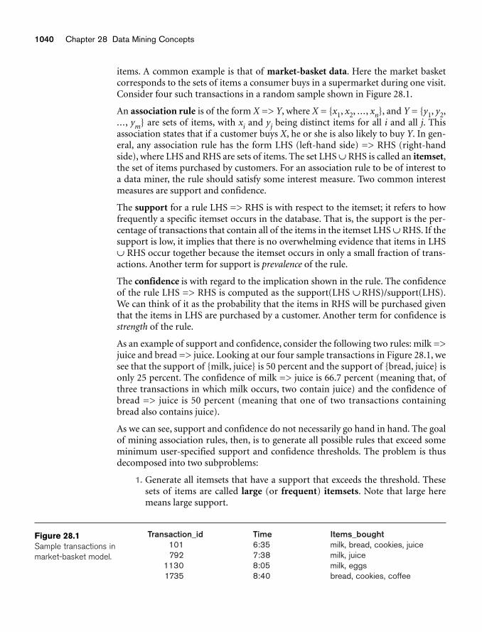
1040 Chapter 28 Data Mining Concepts
items. A common example is that of market-basket data. Here the market basketcorresponds to the sets of items a consumer buys in a supermarket during one visit.Consider four such transactions in a random sample shown in Figure 28.1.
An association rule is of the form X => Y, where X = {x1, x2, ..., xn}, and Y = {y1, y2,..., ym} are sets of items, with xi and yj being distinct items for all i and all j. Thisassociation states that if a customer buys X, he or she is also likely to buy Y. In gen-eral, any association rule has the form LHS (left-hand side) => RHS (right-handside), where LHS and RHS are sets of items. The set LHS ∪ RHS is called an itemset,the set of items purchased by customers. For an association rule to be of interest toa data miner, the rule should satisfy some interest measure. Two common interestmeasures are support and confidence.
The support for a rule LHS => RHS is with respect to the itemset; it refers to howfrequently a specific itemset occurs in the database. That is, the support is the per-centage of transactions that contain all of the items in the itemset LHS ∪ RHS. If thesupport is low, it implies that there is no overwhelming evidence that items in LHS∪ RHS occur together because the itemset occurs in only a small fraction of trans-actions. Another term for support is prevalence of the rule.
The confidence is with regard to the implication shown in the rule. The confidenceof the rule LHS => RHS is computed as the support(LHS ∪ RHS)/support(LHS).We can think of it as the probability that the items in RHS will be purchased giventhat the items in LHS are purchased by a customer. Another term for confidence isstrength of the rule.
As an example of support and confidence, consider the following two rules: milk =>juice and bread => juice. Looking at our four sample transactions in Figure 28.1, wesee that the support of {milk, juice} is 50 percent and the support of {bread, juice} isonly 25 percent. The confidence of milk => juice is 66.7 percent (meaning that, ofthree transactions in which milk occurs, two contain juice) and the confidence ofbread => juice is 50 percent (meaning that one of two transactions containingbread also contains juice).
As we can see, support and confidence do not necessarily go hand in hand. The goalof mining association rules, then, is to generate all possible rules that exceed someminimum user-specified support and confidence thresholds. The problem is thusdecomposed into two subproblems:
1. Generate all itemsets that have a support that exceeds the threshold. Thesesets of items are called large (or frequent) itemsets. Note that large heremeans large support.
Transaction_id Time Items_bought101 6:35 milk, bread, cookies, juice792 7:38 milk, juice
1130 8:05 milk, eggs1735 8:40 bread, cookies, coffee
Figure 28.1Sample transactions inmarket-basket model.
28.2 Association Rules 1041
2. For each large itemset, all the rules that have a minimum confidence are gen-erated as follows: For a large itemset X and Y ⊂ X, let Z = X – Y; then if sup-port(X)/support(Z) > minimum confidence, the rule Z => Y (that is, X – Y=> Y) is a valid rule.
Generating rules by using all large itemsets and their supports is relatively straight-forward. However, discovering all large itemsets together with the value for theirsupport is a major problem if the cardinality of the set of items is very high. A typi-cal supermarket has thousands of items. The number of distinct itemsets is 2m,where m is the number of items, and counting support for all possible itemsetsbecomes very computation intensive. To reduce the combinatorial search space,algorithms for finding association rules utilize the following properties:
■ A subset of a large itemset must also be large (that is, each subset of a largeitemset exceeds the minimum required support).
■ Conversely, a superset of a small itemset is also small (implying that it doesnot have enough support).
The first property is referred to as downward closure. The second property, calledthe antimonotonicity property, helps to reduce the search space of possible solu-tions. That is, once an itemset is found to be small (not a large itemset), then anyextension to that itemset, formed by adding one or more items to the set, will alsoyield a small itemset.
28.2.2 Apriori AlgorithmThe first algorithm to use the downward closure and antimontonicity propertieswas the Apriori algorithm, shown as Algorithm 28.1.
We illustrate Algorithm 28.1 using the transaction data in Figure 28.1 using a mini-mum support of 0.5. The candidate 1-itemsets are {milk, bread, juice, cookies, eggs,coffee} and their respective supports are 0.75, 0.5, 0.5, 0.5, 0.25, and 0.25. The firstfour items qualify for L1 since each support is greater than or equal to 0.5. In the firstiteration of the repeat-loop, we extend the frequent 1-itemsets to create the candi-date frequent 2-itemsets, C2. C2 contains {milk, bread}, {milk, juice}, {bread, juice},{milk, cookies}, {bread, cookies}, and {juice, cookies}. Notice, for example, that{milk, eggs} does not appear in C2 since {eggs} is small (by the antimonotonicityproperty) and does not appear in L1. The supports for the six sets contained in C2are 0.25, 0.5, 0.25, 0.25, 0.5, and 0.25 and are computed by scanning the set of trans-actions. Only the second 2-itemset {milk, juice} and the fifth 2-itemset {bread,cookies} have support greater than or equal to 0.5. These two 2-itemsets form thefrequent 2-itemsets, L2.
Algorithm 28.1. Apriori Algorithm for Finding Frequent (Large) Itemsets
Input: Database of m transactions, D, and a minimum support, mins, represented asa fraction of m.
1042 Chapter 28 Data Mining Concepts
Output: Frequent itemsets, L1, L2, ..., Lk
Begin /* steps or statements are numbered for better readability */
1. Compute support(ij) = count(ij)/m for each individual item, i1, i2, ..., in byscanning the database once and counting the number of transactions thatitem ij appears in (that is, count(ij));
2. The candidate frequent 1-itemset, C1, will be the set of items i1, i2, ..., in;
3. The subset of items containing ij from C1 where support(ij) >= minsbecomes the frequent
1-itemset, L1;
4. k = 1;
termination = false;
repeat
1. Lk+1 = ;
2. Create the candidate frequent (k+1)-itemset, Ck+1, by combining membersof Lk that have k–1 items in common (this forms candidate frequent (k+1)-itemsets by selectively extending frequent k-itemsets by one item);
3. In addition, only consider as elements of Ck+1 those k+1 items such thatevery subset of size k appears in Lk;
4. Scan the database once and compute the support for each member of Ck+1; ifthe support for a member of Ck+1 >= mins then add that member to Lk+1;
5. If Lk+1 is empty then termination = true
else k = k + 1;
until termination;
End;
In the next iteration of the repeat-loop, we construct candidate frequent 3-itemsetsby adding additional items to sets in L2. However, for no extension of itemsets in L2will all 2-item subsets be contained in L2. For example, consider {milk, juice, bread};the 2-itemset {milk, bread} is not in L2, hence {milk, juice, bread} cannot be a fre-quent 3-itemset by the downward closure property. At this point the algorithm ter-minates with L1 equal to {{milk}, {bread}, {juice}, {cookies}} and L2 equal to {{milk,juice}, {bread, cookies}}.
Several other algorithms have been proposed to mine association rules. They varymainly in terms of how the candidate itemsets are generated, and how the supportsfor the candidate itemsets are counted. Some algorithms use such data structures asbitmaps and hashtrees to keep information about itemsets. Several algorithms havebeen proposed that use multiple scans of the database because the potential numberof itemsets, 2m, can be too large to set up counters during a single scan. We willexamine three improved algorithms (compared to the Apriori algorithm) for asso-ciation rule mining: the Sampling algorithm, the Frequent-Pattern Tree algorithm,and the Partition algorithm.
28.2 Association Rules 1043
28.2.3 Sampling AlgorithmThe main idea for the Sampling algorithm is to select a small sample, one that fitsin main memory, of the database of transactions and to determine the frequentitemsets from that sample. If those frequent itemsets form a superset of the frequentitemsets for the entire database, then we can determine the real frequent itemsets byscanning the remainder of the database in order to compute the exact support val-ues for the superset itemsets. A superset of the frequent itemsets can usually befound from the sample by using, for example, the Apriori algorithm, with a loweredminimum support.
In some rare cases, some frequent itemsets may be missed and a second scan of thedatabase is needed. To decide whether any frequent itemsets have been missed, theconcept of the negative border is used. The negative border with respect to a fre-quent itemset, S, and set of items, I, is the minimal itemsets contained inPowerSet(I) and not in S. The basic idea is that the negative border of a set of fre-quent itemsets contains the closest itemsets that could also be frequent. Considerthe case where a set X is not contained in the frequent itemsets. If all subsets of X arecontained in the set of frequent itemsets, then X would be in the negative border.
We illustrate this with the following example. Consider the set of items I = {A, B, C,D, E} and let the combined frequent itemsets of size 1 to 3 be S = {{A}, {B}, {C}, {D},{AB}, {AC}, {BC}, {AD}, {CD}, {ABC}}. The negative border is {{E}, {BD}, {ACD}}.The set {E} is the only 1-itemset not contained in S, {BD} is the only 2-itemset not in S but whose 1-itemset subsets are, and {ACD} is the only 3-itemset whose 2-itemset subsets are all in S. The negative border is important since it is necessaryto determine the support for those itemsets in the negative border to ensure that nolarge itemsets are missed from analyzing the sample data.
Support for the negative border is determined when the remainder of the databaseis scanned. If we find that an itemset, X, in the negative border belongs in the set ofall frequent itemsets, then there is a potential for a superset of X to also be frequent.If this happens, then a second pass over the database is needed to make sure that allfrequent itemsets are found.
28.2.4 Frequent-Pattern (FP) Tree and FP-Growth AlgorithmThe Frequent-Pattern Tree (FP-tree) is motivated by the fact that Apriori-basedalgorithms may generate and test a very large number of candidate itemsets.For example, with 1000 frequent 1-itemsets, the Apriori algorithm would have togenerate
or 499,500 candidate 2-itemsets. The FP-Growth algorithm is one approach thateliminates the generation of a large number of candidate itemsets.
1000
2
⎛⎝⎜
⎞⎠⎟
1044 Chapter 28 Data Mining Concepts
The algorithm first produces a compressed version of the database in terms of anFP-tree (frequent-pattern tree). The FP-tree stores relevant itemset information andallows for the efficient discovery of frequent itemsets. The actual mining processadopts a divide-and-conquer strategy where the mining process is decomposed intoa set of smaller tasks that each operates on a conditional FP-tree, a subset (projec-tion) of the original tree. To start with, we examine how the FP-tree is constructed.The database is first scanned and the frequent 1-itemsets along with their supportare computed. With this algorithm, the support is the count of transactions contain-ing the item rather than the fraction of transactions containing the item. The fre-quent 1-itemsets are then sorted in nonincreasing order of their support. Next, theroot of the FP-tree is created with a NULL label. The database is scanned a secondtime and for each transaction T in the database, the frequent 1-itemsets in T areplaced in order as was done with the frequent 1-itemsets. We can designate thissorted list for T as consisting of a first item, the head, and the remaining items, thetail. The itemset information (head, tail) is inserted into the FP-tree recursively,starting at the root node, as follows:
1. If the current node, N, of the FP-tree has a child with an item name = head,then increment the count associated with node N by 1, else create a newnode, N, with a count of 1, link N to its parent and link N with the itemheader table (used for efficient tree traversal).
2. If the tail is nonempty, then repeat step (1) using as the sorted list only thetail, that is, the old head is removed and the new head is the first item fromthe tail and the remaining items become the new tail.
The item header table, created during the process of building the FP-tree, containsthree fields per entry for each frequent item: item identifier, support count, andnode link. The item identifier and support count are self-explanatory. The node linkis a pointer to an occurrence of that item in the FP-tree. Since multiple occurrencesof a single item may appear in the FP-tree, these items are linked together as a listwhere the start of the list is pointed to by the node link in the item header table. Weillustrate the building of the FP-tree using the transaction data in Figure 28.1. Let ususe a minimum support of 2. One pass over the four transactions yields the follow-ing frequent 1-itemsets with associated support: {{(milk, 3)}, {(bread, 2)}, {(cookies,2)}, {(juice, 2)}}. The database is scanned a second time and each transaction will beprocessed again.
For the first transaction, we create the sorted list, T = {milk, bread, cookies, juice}.The items in T are the frequent 1-itemsets from the first transaction. The items areordered based on the nonincreasing ordering of the count of the 1-itemsets foundin pass 1 (that is, milk first, bread second, and so on). We create a NULL root nodefor the FP-tree and insert milk as a child of the root, bread as a child of milk, cookiesas a child of bread, and juice as a child of cookies. We adjust the entries for the fre-quent items in the item header table.
For the second transaction, we have the sorted list {milk, juice}. Starting at the root,we see that a child node with label milk exists, so we move to that node and update
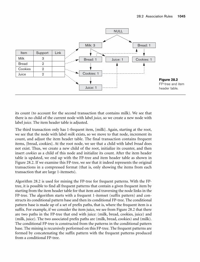
28.2 Association Rules 1045
its count (to account for the second transaction that contains milk). We see thatthere is no child of the current node with label juice, so we create a new node withlabel juice. The item header table is adjusted.
The third transaction only has 1-frequent item, {milk}. Again, starting at the root,we see that the node with label milk exists, so we move to that node, increment itscount, and adjust the item header table. The final transaction contains frequentitems, {bread, cookies}. At the root node, we see that a child with label bread doesnot exist. Thus, we create a new child of the root, initialize its counter, and theninsert cookies as a child of this node and initialize its count. After the item headertable is updated, we end up with the FP-tree and item header table as shown inFigure 28.2. If we examine this FP-tree, we see that it indeed represents the originaltransactions in a compressed format (that is, only showing the items from eachtransaction that are large 1-itemsets).
Algorithm 28.2 is used for mining the FP-tree for frequent patterns. With the FP-tree, it is possible to find all frequent patterns that contain a given frequent item bystarting from the item header table for that item and traversing the node links in theFP-tree. The algorithm starts with a frequent 1-itemset (suffix pattern) and con-structs its conditional pattern base and then its conditional FP-tree. The conditionalpattern base is made up of a set of prefix paths, that is, where the frequent item is asuffix. For example, if we consider the item juice, we see from Figure 28.2 that thereare two paths in the FP-tree that end with juice: (milk, bread, cookies, juice) and(milk, juice). The two associated prefix paths are (milk, bread, cookies) and (milk).The conditional FP-tree is constructed from the patterns in the conditional patternbase. The mining is recursively performed on this FP-tree. The frequent patterns areformed by concatenating the suffix pattern with the frequent patterns producedfrom a conditional FP-tree.
Item Support Link
Milk 3
Bread 2
Cookies 2
Juice 2
Bread: 1Milk: 3
Bread: 1
Cookies: 1
Juice: 1
Juice: 1 Cookies: 1
NULL
Figure 28.2FP-tree and itemheader table.
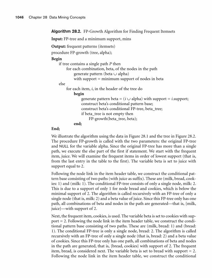
1046 Chapter 28 Data Mining Concepts
Algorithm 28.2. FP-Growth Algorithm for Finding Frequent Itemsets
Input: FP-tree and a minimum support, mins
Output: frequent patterns (itemsets)
procedure FP-growth (tree, alpha);
Beginif tree contains a single path P then
for each combination, beta, of the nodes in the pathgenerate pattern (beta ∪ alpha)with support = minimum support of nodes in beta
elsefor each item, i, in the header of the tree do
begingenerate pattern beta = (i ∪ alpha) with support = i.support;construct beta’s conditional pattern base;construct beta’s conditional FP-tree, beta_tree;if beta_tree is not empty then
FP-growth(beta_tree, beta);end;
End;
We illustrate the algorithm using the data in Figure 28.1 and the tree in Figure 28.2.The procedure FP-growth is called with the two parameters: the original FP-treeand NULL for the variable alpha. Since the original FP-tree has more than a singlepath, we execute the else part of the first if statement. We start with the frequentitem, juice. We will examine the frequent items in order of lowest support (that is,from the last entry in the table to the first). The variable beta is set to juice with support equal to 2.
Following the node link in the item header table, we construct the conditional pat-tern base consisting of two paths (with juice as suffix). These are (milk, bread, cook-ies: 1) and (milk: 1). The conditional FP-tree consists of only a single node, milk: 2.This is due to a support of only 1 for node bread and cookies, which is below theminimal support of 2. The algorithm is called recursively with an FP-tree of only asingle node (that is, milk: 2) and a beta value of juice. Since this FP-tree only has onepath, all combinations of beta and nodes in the path are generated—that is, {milk,juice}—with support of 2.
Next, the frequent item, cookies, is used. The variable beta is set to cookies with sup-port = 2. Following the node link in the item header table, we construct the condi-tional pattern base consisting of two paths. These are (milk, bread: 1) and (bread:1). The conditional FP-tree is only a single node, bread: 2. The algorithm is calledrecursively with an FP-tree of only a single node (that is, bread: 2) and a beta valueof cookies. Since this FP-tree only has one path, all combinations of beta and nodesin the path are generated, that is, {bread, cookies} with support of 2. The frequentitem, bread, is considered next. The variable beta is set to bread with support = 2.Following the node link in the item header table, we construct the conditional
28.2 Association Rules 1047
pattern base consisting of one path, which is (milk: 1). The conditional FP-tree isempty since the count is less than the minimum support. Since the conditional FP-tree is empty, no frequent patterns will be generated.
The last frequent item to consider is milk. This is the top item in the item headertable and as such has an empty conditional pattern base and empty conditional FP-tree. As a result, no frequent patterns are added. The result of executing the algo-rithm is the following frequent patterns (or itemsets) with their support: {{milk: 3},{bread: 2}, {cookies: 2}, {juice: 2}, {milk, juice: 2}, {bread, cookies: 2}}.
28.2.5 Partition AlgorithmAnother algorithm, called the Partition algorithm,3 is summarized below. If we aregiven a database with a small number of potential large itemsets, say, a few thou-sand, then the support for all of them can be tested in one scan by using a partition-ing technique. Partitioning divides the database into nonoverlapping subsets; theseare individually considered as separate databases and all large itemsets for that par-tition, called local frequent itemsets, are generated in one pass. The Apriori algorithmcan then be used efficiently on each partition if it fits entirely in main memory.Partitions are chosen in such a way that each partition can be accommodated inmain memory. As such, a partition is read only once in each pass. The only caveatwith the partition method is that the minimum support used for each partition hasa slightly different meaning from the original value. The minimum support is basedon the size of the partition rather than the size of the database for determining localfrequent (large) itemsets. The actual support threshold value is the same as givenearlier, but the support is computed only for a partition.
At the end of pass one, we take the union of all frequent itemsets from each parti-tion. This forms the global candidate frequent itemsets for the entire database.When these lists are merged, they may contain some false positives. That is, some ofthe itemsets that are frequent (large) in one partition may not qualify in severalother partitions and hence may not exceed the minimum support when the originaldatabase is considered. Note that there are no false negatives; no large itemsets willbe missed. The global candidate large itemsets identified in pass one are verified inpass two; that is, their actual support is measured for the entire database. At the endof phase two, all global large itemsets are identified. The Partition algorithm lendsitself naturally to a parallel or distributed implementation for better efficiency.Further improvements to this algorithm have been suggested.4
28.2.6 Other Types of Association Rules
Association Rules among Hierarchies. There are certain types of associationsthat are particularly interesting for a special reason. These associations occur among
3See Savasere et al. (1995) for details of the algorithm, the data structures used to implement it, and itsperformance comparisons.4See Cheung et al. (1996) and Lin and Dunham (1998).
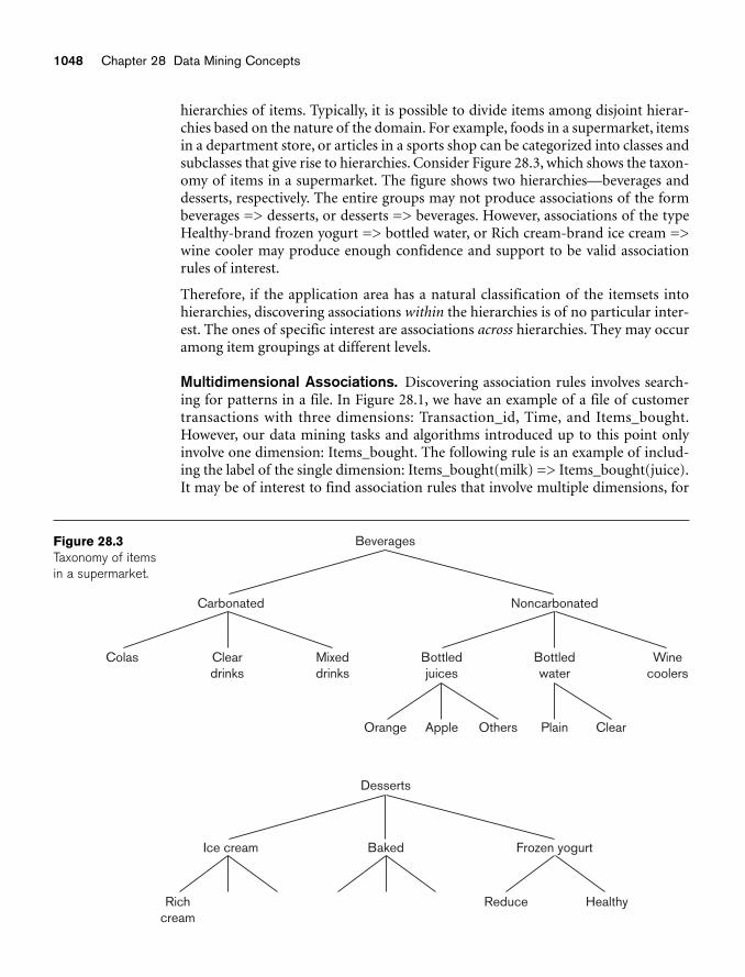
1048 Chapter 28 Data Mining Concepts
Beverages
Carbonated Noncarbonated
Orange Apple Others Plain Clear
Colas Cleardrinks
Mixeddrinks
Bottledjuices
Bottledwater
Winecoolers
Desserts
Ice cream Baked Frozen yogurt
Richcream
Reduce Healthy
Figure 28.3Taxonomy of itemsin a supermarket.
hierarchies of items. Typically, it is possible to divide items among disjoint hierar-chies based on the nature of the domain. For example, foods in a supermarket, itemsin a department store, or articles in a sports shop can be categorized into classes andsubclasses that give rise to hierarchies. Consider Figure 28.3, which shows the taxon-omy of items in a supermarket. The figure shows two hierarchies—beverages anddesserts, respectively. The entire groups may not produce associations of the formbeverages => desserts, or desserts => beverages. However, associations of the typeHealthy-brand frozen yogurt => bottled water, or Rich cream-brand ice cream =>wine cooler may produce enough confidence and support to be valid associationrules of interest.
Therefore, if the application area has a natural classification of the itemsets intohierarchies, discovering associations within the hierarchies is of no particular inter-est. The ones of specific interest are associations across hierarchies. They may occuramong item groupings at different levels.
Multidimensional Associations. Discovering association rules involves search-ing for patterns in a file. In Figure 28.1, we have an example of a file of customertransactions with three dimensions: Transaction_id, Time, and Items_bought.However, our data mining tasks and algorithms introduced up to this point onlyinvolve one dimension: Items_bought. The following rule is an example of includ-ing the label of the single dimension: Items_bought(milk) => Items_bought(juice).It may be of interest to find association rules that involve multiple dimensions, for
28.2 Association Rules 1049
example, Time(6:30...8:00) => Items_bought(milk). Rules like these are calledmultidimensional association rules. The dimensions represent attributes of recordsof a file or, in terms of relations, columns of rows of a relation, and can be categori-cal or quantitative. Categorical attributes have a finite set of values that display noordering relationship. Quantitative attributes are numeric and their values displayan ordering relationship, for example, <. Items_bought is an example of a categori-cal attribute and Transaction_id and Time are quantitative.
One approach to handling a quantitative attribute is to partition its values intononoverlapping intervals that are assigned labels. This can be done in a static man-ner based on domain-specific knowledge. For example, a concept hierarchy maygroup values for Salary into three distinct classes: low income (0 < Salary < 29,999),middle income (30,000 < Salary < 74,999), and high income (Salary > 75,000). Fromhere, the typical Apriori-type algorithm or one of its variants can be used for therule mining since the quantitative attributes now look like categorical attributes.Another approach to partitioning is to group attribute values based on data distri-bution, for example, equi-depth partitioning, and to assign integer values to eachpartition. The partitioning at this stage may be relatively fine, that is, a larger num-ber of intervals. Then during the mining process, these partitions may combinewith other adjacent partitions if their support is less than some predefined maxi-mum value. An Apriori-type algorithm can be used here as well for the data mining.
Negative Associations. The problem of discovering a negative association isharder than that of discovering a positive association. A negative association is ofthe following type: 60 percent of customers who buy potato chips do not buy bottledwater. (Here, the 60 percent refers to the confidence for the negative associationrule.) In a database with 10,000 items, there are 210,000 possible combinations ofitems, a majority of which do not appear even once in the database. If the absence ofa certain item combination is taken to mean a negative association, then we poten-tially have millions and millions of negative association rules with RHSs that are ofno interest at all. The problem, then, is to find only interesting negative rules. In gen-eral, we are interested in cases in which two specific sets of items appear very rarelyin the same transaction. This poses two problems.
1. For a total item inventory of 10,000 items, the probability of any two beingbought together is (1/10,000) * (1/10,000) = 10–8. If we find the actual sup-port for these two occurring together to be zero, that does not represent asignificant departure from expectation and hence is not an interesting (neg-ative) association.
2. The other problem is more serious. We are looking for item combinationswith very low support, and there are millions and millions with low or evenzero support. For example, a data set of 10 million transactions has most ofthe 2.5 billion pairwise combinations of 10,000 items missing. This wouldgenerate billions of useless rules.
Therefore, to make negative association rules interesting, we must use prior knowl-edge about the itemsets. One approach is to use hierarchies. Suppose we use thehierarchies of soft drinks and chips shown in Figure 28.4.
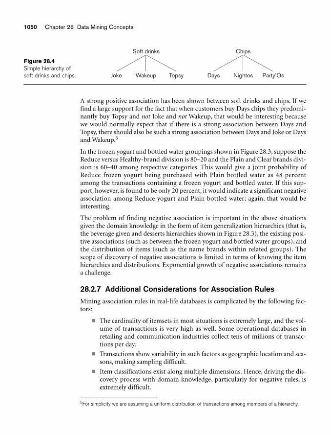
1050 Chapter 28 Data Mining Concepts
Soft drinks
Joke Wakeup Topsy
Chips
Days Nightos Party’Os
Figure 28.4Simple hierarchy ofsoft drinks and chips.
A strong positive association has been shown between soft drinks and chips. If wefind a large support for the fact that when customers buy Days chips they predomi-nantly buy Topsy and not Joke and not Wakeup, that would be interesting becausewe would normally expect that if there is a strong association between Days andTopsy, there should also be such a strong association between Days and Joke or Daysand Wakeup.5
In the frozen yogurt and bottled water groupings shown in Figure 28.3, suppose theReduce versus Healthy-brand division is 80–20 and the Plain and Clear brands divi-sion is 60–40 among respective categories. This would give a joint probability ofReduce frozen yogurt being purchased with Plain bottled water as 48 percentamong the transactions containing a frozen yogurt and bottled water. If this sup-port, however, is found to be only 20 percent, it would indicate a significant negativeassociation among Reduce yogurt and Plain bottled water; again, that would beinteresting.
The problem of finding negative association is important in the above situationsgiven the domain knowledge in the form of item generalization hierarchies (that is,the beverage given and desserts hierarchies shown in Figure 28.3), the existing posi-tive associations (such as between the frozen yogurt and bottled water groups), andthe distribution of items (such as the name brands within related groups). Thescope of discovery of negative associations is limited in terms of knowing the itemhierarchies and distributions. Exponential growth of negative associations remainsa challenge.
28.2.7 Additional Considerations for Association RulesMining association rules in real-life databases is complicated by the following fac-tors:
■ The cardinality of itemsets in most situations is extremely large, and the vol-ume of transactions is very high as well. Some operational databases inretailing and communication industries collect tens of millions of transac-tions per day.
■ Transactions show variability in such factors as geographic location and sea-sons, making sampling difficult.
■ Item classifications exist along multiple dimensions. Hence, driving the dis-covery process with domain knowledge, particularly for negative rules, isextremely difficult.
5For simplicity we are assuming a uniform distribution of transactions among members of a hierarchy.
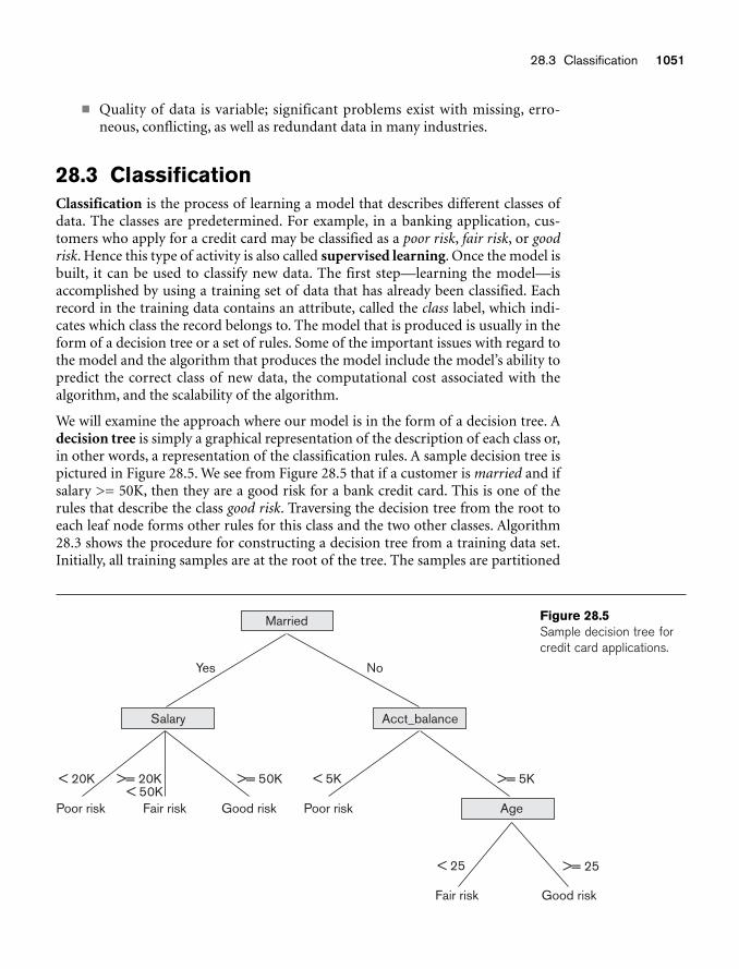
28.3 Classification 1051
■ Quality of data is variable; significant problems exist with missing, erro-neous, conflicting, as well as redundant data in many industries.
28.3 ClassificationClassification is the process of learning a model that describes different classes ofdata. The classes are predetermined. For example, in a banking application, cus-tomers who apply for a credit card may be classified as a poor risk, fair risk, or goodrisk. Hence this type of activity is also called supervised learning. Once the model isbuilt, it can be used to classify new data. The first step—learning the model—isaccomplished by using a training set of data that has already been classified. Eachrecord in the training data contains an attribute, called the class label, which indi-cates which class the record belongs to. The model that is produced is usually in theform of a decision tree or a set of rules. Some of the important issues with regard tothe model and the algorithm that produces the model include the model’s ability topredict the correct class of new data, the computational cost associated with thealgorithm, and the scalability of the algorithm.
We will examine the approach where our model is in the form of a decision tree. Adecision tree is simply a graphical representation of the description of each class or,in other words, a representation of the classification rules. A sample decision tree ispictured in Figure 28.5. We see from Figure 28.5 that if a customer is married and ifsalary >= 50K, then they are a good risk for a bank credit card. This is one of therules that describe the class good risk. Traversing the decision tree from the root toeach leaf node forms other rules for this class and the two other classes. Algorithm28.3 shows the procedure for constructing a decision tree from a training data set.Initially, all training samples are at the root of the tree. The samples are partitioned
Married
Salary Acct_balance
Fair risk Good risk
Poor risk
< 20K >= 20K >= 50K < 5K >= 5K
< 25 >= 25
< 50K
NoYes
Fair risk Good risk Poor risk Age
Figure 28.5Sample decision tree forcredit card applications.
1052 Chapter 28 Data Mining Concepts
recursively based on selected attributes. The attribute used at a node to partition thesamples is the one with the best splitting criterion, for example, the one that maxi-mizes the information gain measure.
Algorithm 28.3. Algorithm for Decision Tree Induction
Input: Set of training data records: R1, R2, ..., Rm and set of attributes: A1, A2, ..., An
Output: Decision tree
procedure Build_tree (records, attributes);Begin
create a node N;if all records belong to the same class, C then
return N as a leaf node with class label C;if attributes is empty then
return N as a leaf node with class label C, such that the majority ofrecords belong to it;
select attribute Ai (with the highest information gain) from attributes;label node N with Ai;for each known value, vj, of Ai do
beginadd a branch from node N for the condition Ai = vj;Sj = subset of records where Ai = vj;if Sj is empty then
add a leaf, L, with class label C, such that the majority ofrecords belong to it and return L
else add the node returned by Build_tree(Sj, attributes – Ai);end;
End;
Before we illustrate Algorithm 28.3, we will explain the information gain measurein more detail. The use of entropy as the information gain measure is motivated bythe goal of minimizing the information needed to classify the sample data in theresulting partitions and thus minimizing the expected number of conditional testsneeded to classify a new record. The expected information needed to classify train-ing data of s samples, where the Class attribute has n values (v1, ..., vn) and si is thenumber of samples belonging to class label vi, is given by
where pi is the probability that a random sample belongs to the class with label vi.An estimate for pi is si/s. Consider an attribute A with values {v1, ..., vm} used as thetest attribute for splitting in the decision tree. Attribute A partitions the samplesinto the subsets S1, ..., Sm where samples in each Sj have a value of vj for attribute A.Each Sj may contain samples that belong to any of the classes. The number of
I S S S p pn i ii
n
1 2 21
, , ..., log( ) = −=
∑
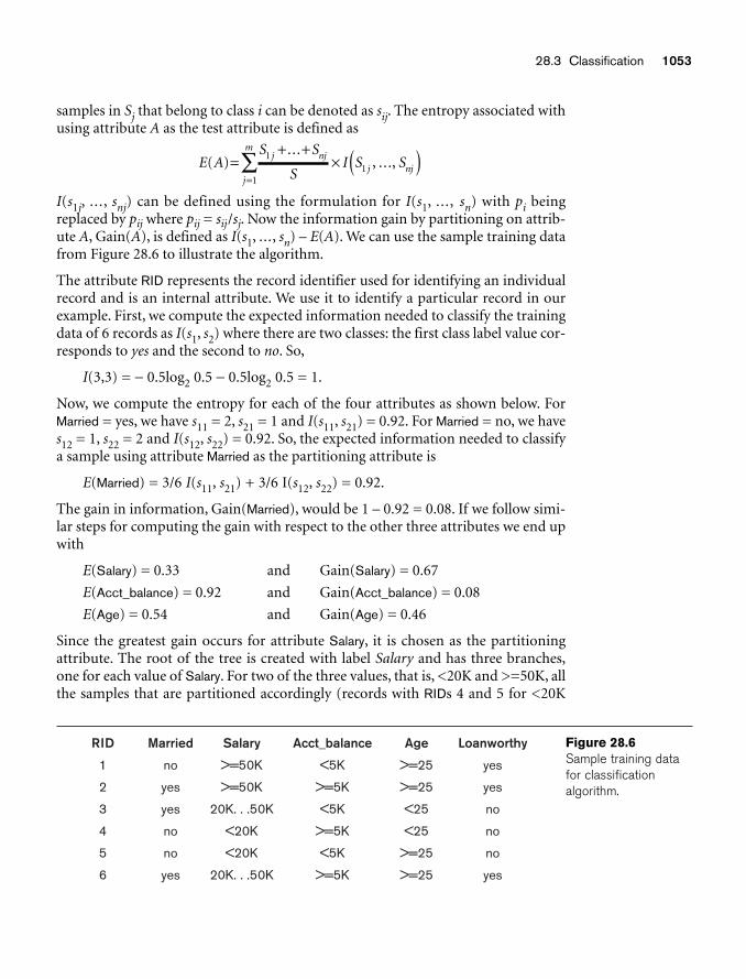
28.3 Classification 1053
samples in Sj that belong to class i can be denoted as sij. The entropy associated withusing attribute A as the test attribute is defined as
I(s1j, ..., snj) can be defined using the formulation for I(s1, ..., sn) with pi beingreplaced by pij where pij = sij/sj. Now the information gain by partitioning on attrib-ute A, Gain(A), is defined as I(s1, ..., sn) – E(A). We can use the sample training datafrom Figure 28.6 to illustrate the algorithm.
The attribute RID represents the record identifier used for identifying an individualrecord and is an internal attribute. We use it to identify a particular record in ourexample. First, we compute the expected information needed to classify the trainingdata of 6 records as I(s1, s2) where there are two classes: the first class label value cor-responds to yes and the second to no. So,
I(3,3) = − 0.5log2 0.5 − 0.5log2 0.5 = 1.
Now, we compute the entropy for each of the four attributes as shown below. ForMarried = yes, we have s11 = 2, s21 = 1 and I(s11, s21) = 0.92. For Married = no, we haves12 = 1, s22 = 2 and I(s12, s22) = 0.92. So, the expected information needed to classifya sample using attribute Married as the partitioning attribute is
E(Married) = 3/6 I(s11, s21) + 3/6 I(s12, s22) = 0.92.
The gain in information, Gain(Married), would be 1 – 0.92 = 0.08. If we follow simi-lar steps for computing the gain with respect to the other three attributes we end upwith
E(Salary) = 0.33 and Gain(Salary) = 0.67
E(Acct_balance) = 0.92 and Gain(Acct_balance) = 0.08
E(Age) = 0.54 and Gain(Age) = 0.46
Since the greatest gain occurs for attribute Salary, it is chosen as the partitioningattribute. The root of the tree is created with label Salary and has three branches,one for each value of Salary. For two of the three values, that is, <20K and >=50K, allthe samples that are partitioned accordingly (records with RIDs 4 and 5 for <20K
E AS S
SI S S
j nj
j
m
j nj( )...
, ...,=+ +
× ( )=
∑ 1
11
RID Married Salary Acct_balance Age Loanworthy
1 no >=50K <5K >=25 yes
2 yes >=50K >=5K >=25 yes
3 yes 20K. . .50K <5K <25 no
4 no <20K >=5K <25 no
5 no <20K <5K >=25 no
6 yes 20K. . .50K >=5K >=25 yes
Figure 28.6Sample training datafor classification algorithm.
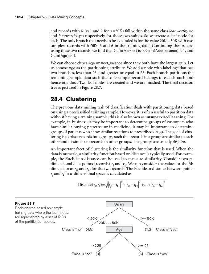
1054 Chapter 28 Data Mining Concepts
Salary
{3} {6}
{4,5}
Class is “no”
Class is “no”
Class is “yes”
Class is “yes”
< 20K20K . . . 50K
>= 50K
< 25 >= 25
{1,2}Age
Figure 28.7Decision tree based on sampletraining data where the leaf nodesare represented by a set of RIDsof the partitioned records.
and records with RIDs 1 and 2 for >=50K) fall within the same class loanworthy noand loanworthy yes respectively for those two values. So we create a leaf node foreach. The only branch that needs to be expanded is for the value 20K...50K with twosamples, records with RIDs 3 and 6 in the training data. Continuing the processusing these two records, we find that Gain(Married) is 0, Gain(Acct_balance) is 1, andGain(Age) is 1.
We can choose either Age or Acct_balance since they both have the largest gain. Letus choose Age as the partitioning attribute. We add a node with label Age that hastwo branches, less than 25, and greater or equal to 25. Each branch partitions theremaining sample data such that one sample record belongs to each branch andhence one class. Two leaf nodes are created and we are finished. The final decisiontree is pictured in Figure 28.7.
28.4 ClusteringThe previous data mining task of classification deals with partitioning data basedon using a preclassified training sample. However, it is often useful to partition datawithout having a training sample; this is also known as unsupervised learning. Forexample, in business, it may be important to determine groups of customers whohave similar buying patterns, or in medicine, it may be important to determinegroups of patients who show similar reactions to prescribed drugs. The goal of clus-tering is to place records into groups, such that records in a group are similar to eachother and dissimilar to records in other groups. The groups are usually disjoint.
An important facet of clustering is the similarity function that is used. When thedata is numeric, a similarity function based on distance is typically used. For exam-ple, the Euclidean distance can be used to measure similarity. Consider two n-dimensional data points (records) rj and rk. We can consider the value for the ithdimension as rji and rki for the two records. The Euclidean distance between pointsrj and rk in n-dimensional space is calculated as:
Distance( , ) ...r r r r r r r rj k j k j k jn kn= − + − + + −1 1
2
2 2
2 2
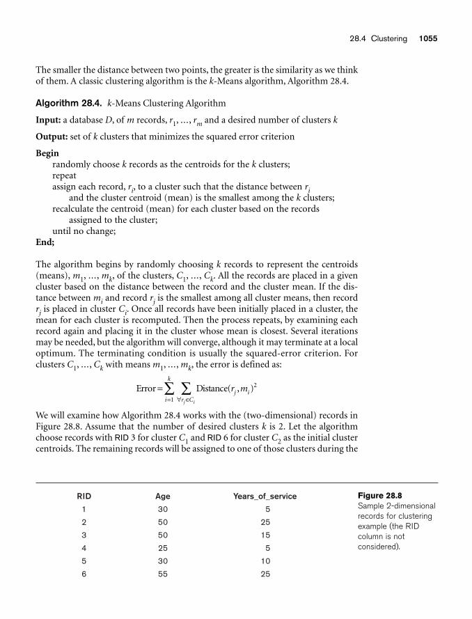
28.4 Clustering 1055
The smaller the distance between two points, the greater is the similarity as we thinkof them. A classic clustering algorithm is the k-Means algorithm, Algorithm 28.4.
Algorithm 28.4. k-Means Clustering Algorithm
Input: a database D, of m records, r1, ..., rm and a desired number of clusters k
Output: set of k clusters that minimizes the squared error criterion
Beginrandomly choose k records as the centroids for the k clusters;repeatassign each record, ri, to a cluster such that the distance between ri
and the cluster centroid (mean) is the smallest among the k clusters;recalculate the centroid (mean) for each cluster based on the records
assigned to the cluster;until no change;
End;
The algorithm begins by randomly choosing k records to represent the centroids(means), m1, ..., mk, of the clusters, C1, ..., Ck. All the records are placed in a givencluster based on the distance between the record and the cluster mean. If the dis-tance between mi and record rj is the smallest among all cluster means, then recordrj is placed in cluster Ci. Once all records have been initially placed in a cluster, themean for each cluster is recomputed. Then the process repeats, by examining eachrecord again and placing it in the cluster whose mean is closest. Several iterationsmay be needed, but the algorithm will converge, although it may terminate at a localoptimum. The terminating condition is usually the squared-error criterion. Forclusters C1, ..., Ck with means m1, ..., mk, the error is defined as:
We will examine how Algorithm 28.4 works with the (two-dimensional) records inFigure 28.8. Assume that the number of desired clusters k is 2. Let the algorithmchoose records with RID 3 for cluster C1 and RID 6 for cluster C2 as the initial clustercentroids. The remaining records will be assigned to one of those clusters during the
Error Distance=∀ ∈=
∑∑ ( , )r mj ir Ci
k
j i
2
1
RID Age Years_of_service
5031
52052
51053
5524
01035
52556
Figure 28.8Sample 2-dimensionalrecords for clusteringexample (the RID column is not considered).
1056 Chapter 28 Data Mining Concepts
first iteration of the repeat loop. The record with RID 1 has a distance from C1 of22.4 and a distance from C2 of 32.0, so it joins cluster C1. The record with RID 2 hasa distance from C1 of 10.0 and a distance from C2 of 5.0, so it joins cluster C2. Therecord with RID 4 has a distance from C1 of 25.5 and a distance from C2 of 36.6, soit joins cluster C1. The record with RID 5 has a distance from C1 of 20.6 and a dis-tance from C2 of 29.2, so it joins cluster C1. Now, the new means (centroids) for thetwo clusters are computed. The mean for a cluster, Ci, with n records of m dimen-sions is the vector:
The new mean for C1 is (33.75, 8.75) and the new mean for C2 is (52.5, 25). A sec-ond iteration proceeds and the six records are placed into the two clusters as follows:records with RIDs 1, 4, 5 are placed in C1 and records with RIDs 2, 3, 6 are placed inC2. The mean for C1 and C2 is recomputed as (28.3, 6.7) and (51.7, 21.7), respec-tively. In the next iteration, all records stay in their previous clusters and the algo-rithm terminates.
Traditionally, clustering algorithms assume that the entire data set fits in mainmemory. More recently, researchers have developed algorithms that are efficient andare scalable for very large databases. One such algorithm is called BIRCH. BIRCH isa hybrid approach that uses both a hierarchical clustering approach, which builds atree representation of the data, as well as additional clustering methods, which areapplied to the leaf nodes of the tree. Two input parameters are used by the BIRCHalgorithm. One specifies the amount of available main memory and the other is aninitial threshold for the radius of any cluster. Main memory is used to store descrip-tive cluster information such as the center (mean) of a cluster and the radius of thecluster (clusters are assumed to be spherical in shape). The radius threshold affectsthe number of clusters that are produced. For example, if the radius threshold valueis large, then few clusters of many records will be formed. The algorithm tries tomaintain the number of clusters such that their radius is below the radius threshold.If available memory is insufficient, then the radius threshold is increased.
The BIRCH algorithm reads the data records sequentially and inserts them into anin-memory tree structure, which tries to preserve the clustering structure of thedata. The records are inserted into the appropriate leaf nodes (potential clusters)based on the distance between the record and the cluster center. The leaf nodewhere the insertion happens may have to split, depending upon the updated centerand radius of the cluster and the radius threshold parameter. Additionally, whensplitting, extra cluster information is stored, and if memory becomes insufficient,then the radius threshold will be increased. Increasing the radius threshold mayactually produce a side effect of reducing the number of clusters since some nodesmay be merged.
Overall, BIRCH is an efficient clustering method with a linear computational com-plexity in terms of the number of records to be clustered.
Cn
rn
ri jir C
jmr Cj i j i
=⎛
⎝⎜⎜
⎞
⎠⎟⎟∀ ∈ ∀ ∈
∑ ∑1 1,...,
28.5 Approaches to Other Data Mining Problems 1057
28.5 Approaches to Other Data Mining Problems
28.5.1 Discovery of Sequential PatternsThe discovery of sequential patterns is based on the concept of a sequence of item-sets. We assume that transactions such as the supermarket-basket transactions wediscussed previously are ordered by time of purchase. That ordering yields asequence of itemsets. For example, {milk, bread, juice}, {bread, eggs}, {cookies, milk,coffee} may be such a sequence of itemsets based on three visits by the same cus-tomer to the store. The support for a sequence S of itemsets is the percentage of thegiven set U of sequences of which S is a subsequence. In this example, {milk, bread,juice} {bread, eggs} and {bread, eggs} {cookies, milk, coffee} are consideredsubsequences. The problem of identifying sequential patterns, then, is to find allsubsequences from the given sets of sequences that have a user-defined minimumsupport. The sequence S1, S2, S3, ... is a predictor of the fact that a customer whobuys itemset S1 is likely to buy itemset S2 and then S3, and so on. This prediction isbased on the frequency (support) of this sequence in the past. Various algorithmshave been investigated for sequence detection.
28.5.2 Discovery of Patterns in Time SeriesTime series are sequences of events; each event may be a given fixed type of a trans-action. For example, the closing price of a stock or a fund is an event that occursevery weekday for each stock and fund. The sequence of these values per stock orfund constitutes a time series. For a time series, one may look for a variety of pat-terns by analyzing sequences and subsequences as we did above. For example, wemight find the period during which the stock rose or held steady for n days, or wemight find the longest period over which the stock had a fluctuation of no morethan 1 percent over the previous closing price, or we might find the quarter duringwhich the stock had the most percentage gain or percentage loss. Time series may becompared by establishing measures of similarity to identify companies whose stocksbehave in a similar fashion. Analysis and mining of time series is an extended func-tionality of temporal data management (see Chapter 26).
28.5.3 RegressionRegression is a special application of the classification rule. If a classification rule isregarded as a function over the variables that maps these variables into a target classvariable, the rule is called a regression rule. A general application of regressionoccurs when, instead of mapping a tuple of data from a relation to a specific class,the value of a variable is predicted based on that tuple. For example, consider a relation
LAB_TESTS (patient ID, test 1, test 2, ..., test n)
1058 Chapter 28 Data Mining Concepts
which contains values that are results from a series of n tests for one patient. Thetarget variable that we wish to predict is P, the probability of survival of the patient.Then the rule for regression takes the form:
(test 1 in range1) and (test 2 in range2) and ... (test n in rangen) ⇒ P = x,or x < P ≤ y
The choice depends on whether we can predict a unique value of P or a range of val-ues for P. If we regard P as a function:
P = f (test 1, test 2, ..., test n)
the function is called a regression function to predict P. In general, if the functionappears as
Y = f (X1, X2, ..., Xn),
and f is linear in the domain variables xi, the process of deriving f from a given set oftuples for <X1, X2, ..., Xn, y> is called linear regression. Linear regression is a com-monly used statistical technique for fitting a set of observations or points in ndimensions with the target variable y.
Regression analysis is a very common tool for analysis of data in many researchdomains. The discovery of the function to predict the target variable is equivalent toa data mining operation.
28.5.4 Neural NetworksA neural network is a technique derived from artificial intelligence research thatuses generalized regression and provides an iterative method to carry it out. Neuralnetworks use the curve-fitting approach to infer a function from a set of samples.This technique provides a learning approach; it is driven by a test sample that is usedfor the initial inference and learning. With this kind of learning method, responsesto new inputs may be able to be interpolated from the known samples. This interpo-lation, however, depends on the world model (internal representation of the prob-lem domain) developed by the learning method.
Neural networks can be broadly classified into two categories: supervised and unsu-pervised networks. Adaptive methods that attempt to reduce the output error aresupervised learning methods, whereas those that develop internal representationswithout sample outputs are called unsupervised learning methods.
Neural networks self-adapt; that is, they learn from information about a specificproblem. They perform well on classification tasks and are therefore useful in datamining. Yet, they are not without problems. Although they learn, they do not pro-vide a good representation of what they have learned. Their outputs are highlyquantitative and not easy to understand. As another limitation, the internal repre-sentations developed by neural networks are not unique. Also, in general, neuralnetworks have trouble modeling time series data. Despite these shortcomings, theyare popular and frequently used by several commercial vendors.
28.5 Approaches to Other Data Mining Problems 1059
28.5.5 Genetic AlgorithmsGenetic algorithms (GAs) are a class of randomized search procedures capable ofadaptive and robust search over a wide range of search space topologies. Modeledafter the adaptive emergence of biological species from evolutionary mechanisms,and introduced by Holland,6 GAs have been successfully applied in such diversefields as image analysis, scheduling, and engineering design.
Genetic algorithms extend the idea from human genetics of the four-letter alphabet(based on the A,C,T,G nucleotides) of the human DNA code. The construction of agenetic algorithm involves devising an alphabet that encodes the solutions to thedecision problem in terms of strings of that alphabet. Strings are equivalent to indi-viduals. A fitness function defines which solutions can survive and which cannot.The ways in which solutions can be combined are patterned after the cross-overoperation of cutting and combining strings from a father and a mother. An initialpopulation of a well-varied population is provided, and a game of evolution isplayed in which mutations occur among strings. They combine to produce a newgeneration of individuals; the fittest individuals survive and mutate until a family ofsuccessful solutions develops.
The solutions produced by GAs are distinguished from most other search tech-niques by the following characteristics:
■ A GA search uses a set of solutions during each generation rather than a sin-gle solution.
■ The search in the string-space represents a much larger parallel search in thespace of encoded solutions.
■ The memory of the search done is represented solely by the set of solutionsavailable for a generation.
■ A genetic algorithm is a randomized algorithm since search mechanisms useprobabilistic operators.
■ While progressing from one generation to the next, a GA finds near-optimalbalance between knowledge acquisition and exploitation by manipulatingencoded solutions.
Genetic algorithms are used for problem solving and clustering problems. Theirability to solve problems in parallel provides a powerful tool for data mining. Thedrawbacks of GAs include the large overproduction of individual solutions, the ran-dom character of the searching process, and the high demand on computer process-ing. In general, substantial computing power is required to achieve anything ofsignificance with genetic algorithms.
6Holland’s seminal work (1975) entitled Adaptation in Natural and Artificial Systems introduced the ideaof genetic algorithms.
1060 Chapter 28 Data Mining Concepts
28.6 Applications of Data MiningData mining technologies can be applied to a large variety of decision-making con-texts in business. In particular, areas of significant payoffs are expected to includethe following:
■ Marketing. Applications include analysis of consumer behavior based onbuying patterns; determination of marketing strategies including advertis-ing, store location, and targeted mailing; segmentation of customers, stores,or products; and design of catalogs, store layouts, and advertising cam-paigns.
■ Finance. Applications include analysis of creditworthiness of clients, seg-mentation of account receivables, performance analysis of finance invest-ments like stocks, bonds, and mutual funds; evaluation of financing options;and fraud detection.
■ Manufacturing. Applications involve optimization of resources likemachines, manpower, and materials; and optimal design of manufacturingprocesses, shop-floor layouts, and product design, such as for automobilesbased on customer requirements.
■ Health Care. Applications include discovery of patterns in radiologicalimages, analysis of microarray (gene-chip) experimental data to cluster genesand to relate to symptoms or diseases, analysis of side effects of drugs andeffectiveness of certain treatments, optimization of processes within a hospi-tal, and the relationship of patient wellness data with doctor qualifications.
28.7 Commercial Data Mining ToolsCurrently, commercial data mining tools use several common techniques to extractknowledge. These include association rules, clustering, neural networks, sequenc-ing, and statistical analysis. We discussed these earlier. Also used are decision trees,which are a representation of the rules used in classification or clustering, and statis-tical analyses, which may include regression and many other techniques. Othercommercial products use advanced techniques such as genetic algorithms, case-based reasoning, Bayesian networks, nonlinear regression, combinatorial optimiza-tion, pattern matching, and fuzzy logic. In this chapter we have already discussedsome of these.
Most data mining tools use the ODBC (Open Database Connectivity) interface.ODBC is an industry standard that works with databases; it enables access to data inmost of the popular database programs such as Access, dBASE, Informix, Oracle,and SQL Server. Some of these software packages provide interfaces to specific data-base programs; the most common are Oracle, Access, and SQL Server. Most of thetools work in the Microsoft Windows environment and a few work in the UNIXoperating system. The trend is for all products to operate under the MicrosoftWindows environment. One tool, Data Surveyor, mentions ODMG compliance; seeChapter 11 where we discuss the ODMG object-oriented standard.
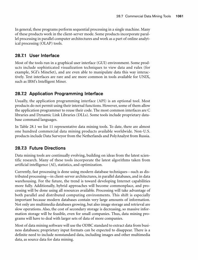
28.7 Commercial Data Mining Tools 1061
In general, these programs perform sequential processing in a single machine. Manyof these products work in the client-server mode. Some products incorporate paral-lel processing in parallel computer architectures and work as a part of online analyt-ical processing (OLAP) tools.
28.7.1 User InterfaceMost of the tools run in a graphical user interface (GUI) environment. Some prod-ucts include sophisticated visualization techniques to view data and rules (forexample, SGI’s MineSet), and are even able to manipulate data this way interac-tively. Text interfaces are rare and are more common in tools available for UNIX,such as IBM’s Intelligent Miner.
28.7.2 Application Programming InterfaceUsually, the application programming interface (API) is an optional tool. Mostproducts do not permit using their internal functions. However, some of them allowthe application programmer to reuse their code. The most common interfaces are Clibraries and Dynamic Link Libraries (DLLs). Some tools include proprietary data-base command languages.
In Table 28.1 we list 11 representative data mining tools. To date, there are almostone hundred commercial data mining products available worldwide. Non-U.S.products include Data Surveyor from the Netherlands and PolyAnalyst from Russia.
28.7.3 Future DirectionsData mining tools are continually evolving, building on ideas from the latest scien-tific research. Many of these tools incorporate the latest algorithms taken from artificial intelligence (AI), statistics, and optimization.
Currently, fast processing is done using modern database techniques—such as dis-tributed processing—in client-server architectures, in parallel databases, and in datawarehousing. For the future, the trend is toward developing Internet capabilitiesmore fully. Additionally, hybrid approaches will become commonplace, and pro-cessing will be done using all resources available. Processing will take advantage ofboth parallel and distributed computing environments. This shift is especiallyimportant because modern databases contain very large amounts of information.Not only are multimedia databases growing, but also image storage and retrieval areslow operations. Also, the cost of secondary storage is decreasing, so massive infor-mation storage will be feasible, even for small companies. Thus, data mining pro-grams will have to deal with larger sets of data of more companies.
Most of data mining software will use the ODBC standard to extract data from busi-ness databases; proprietary input formats can be expected to disappear. There is adefinite need to include nonstandard data, including images and other multimediadata, as source data for data mining.
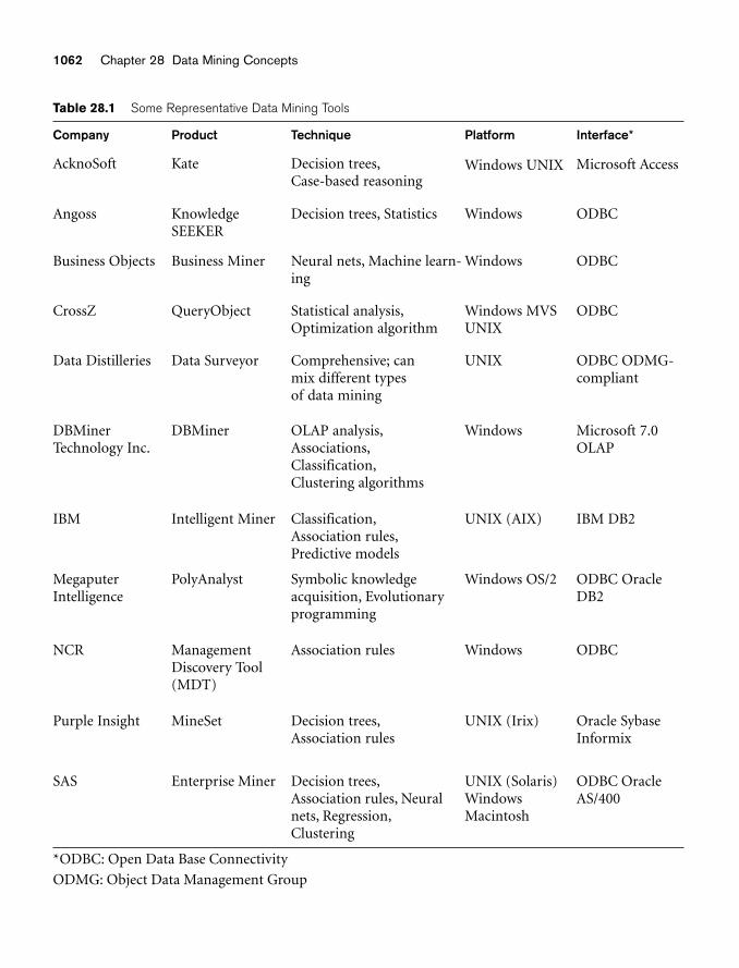
Table 28.1 Some Representative Data Mining Tools
Company Product Technique Platform Interface*
AcknoSoft Kate Decision trees,Case-based reasoning
Windows UNIX Microsoft Access
Angoss Knowledge SEEKER
Decision trees, Statistics Windows ODBC
Business Objects Business Miner Neural nets, Machine learn-ing
Windows ODBC
CrossZ QueryObject Statistical analysis,Optimization algorithm
Windows MVSUNIX
ODBC
Data Distilleries Data Surveyor Comprehensive; can mix different types of data mining
UNIX ODBC ODMG-compliant
DBMinerTechnology Inc.
DBMiner OLAP analysis,Associations,Classification,Clustering algorithms
Windows Microsoft 7.0OLAP
IBM Intelligent Miner Classification,Association rules,Predictive models
UNIX (AIX) IBM DB2
MegaputerIntelligence
PolyAnalyst Symbolic knowledge acquisition, Evolutionaryprogramming
Windows OS/2 ODBC OracleDB2
NCR ManagementDiscovery Tool(MDT)
Association rules Windows ODBC
Purple Insight MineSet Decision trees,Association rules
UNIX (Irix) Oracle SybaseInformix
SAS Enterprise Miner Decision trees,Association rules, Neuralnets, Regression,Clustering
UNIX (Solaris)WindowsMacintosh
ODBC OracleAS/400
*ODBC: Open Data Base Connectivity
ODMG: Object Data Management Group
1062 Chapter 28 Data Mining Concepts
28.8 SummaryIn this chapter we surveyed the important discipline of data mining, which usesdatabase technology to discover additional knowledge or patterns in the data. Wegave an illustrative example of knowledge discovery in databases, which has a widerscope than data mining. For data mining, among the various techniques, we focusedon the details of association rule mining, classification, and clustering. We presentedalgorithms in each of these areas and illustrated with examples of how those algo-rithms work.
A variety of other techniques, including the AI-based neural networks and geneticalgorithms, were also briefly discussed. Active research is ongoing in data miningand we have outlined some of the expected research directions. In the future data-base technology products market, a great deal of data mining activity is expected.We summarized 11 out of nearly one hundred data mining tools available; futureresearch is expected to extend the number and functionality significantly.
Review Questions28.1. What are the different phases of the knowledge discovery from databases?
Describe a complete application scenario in which new knowledge may bemined from an existing database of transactions.
28.2. What are the goals or tasks that data mining attempts to facilitate?
28.3. What are the five types of knowledge produced from data mining?
28.4. What are association rules as a type of knowledge? Give a definition of sup-port and confidence and use them to define an association rule.
28.5. What is the downward closure property? How does it aid in developing anefficient algorithm for finding association rules, that is, with regard to find-ing large itemsets?
28.6. What was the motivating factor for the development of the FP-tree algo-rithm for association rule mining?
28.7. Describe an association rule among hierarchies with an example.
28.8. What is a negative association rule in the context of the hierarchy in Figure28.3?
28.9. What are the difficulties of mining association rules from large databases?
28.10. What are classification rules and how are decision trees related to them?
28.11. What is entropy and how is it used in building decision trees?
28.12. How does clustering differ from classification?
28.13. Describe neural networks and genetic algorithms as techniques for datamining. What are the main difficulties in using these techniques?
Review Questions 1063
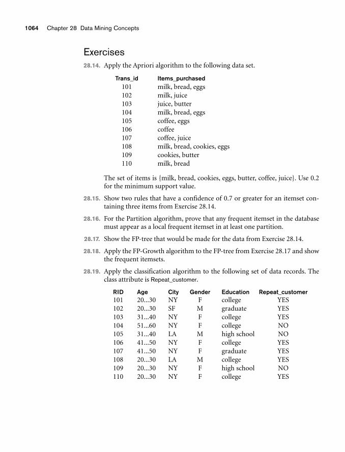
1064 Chapter 28 Data Mining Concepts
Trans_id Items_purchased101 milk, bread, eggs102 milk, juice103 juice, butter104 milk, bread, eggs105 coffee, eggs106 coffee107 coffee, juice108 milk, bread, cookies, eggs109 cookies, butter110 milk, bread
RID Age City Gender Education Repeat_customer101 20...30 NY F college YES102 20...30 SF M graduate YES103 31...40 NY F college YES104 51...60 NY F college NO105 31...40 LA M high school NO106 41...50 NY F college YES107 41...50 NY F graduate YES108 20...30 LA M college YES109 20...30 NY F high school NO110 20...30 NY F college YES
Exercises28.14. Apply the Apriori algorithm to the following data set.
The set of items is {milk, bread, cookies, eggs, butter, coffee, juice}. Use 0.2for the minimum support value.
28.15. Show two rules that have a confidence of 0.7 or greater for an itemset con-taining three items from Exercise 28.14.
28.16. For the Partition algorithm, prove that any frequent itemset in the databasemust appear as a local frequent itemset in at least one partition.
28.17. Show the FP-tree that would be made for the data from Exercise 28.14.
28.18. Apply the FP-Growth algorithm to the FP-tree from Exercise 28.17 and showthe frequent itemsets.
28.19. Apply the classification algorithm to the following set of data records. Theclass attribute is Repeat_customer.
28.20. Consider the following set of two-dimensional records:
Selected Bibliography 1065
RID Dimension1 Dimension21 8 42 5 43 2 44 2 65 2 86 8 6
Also consider two different clustering schemes: (1) where Cluster1 containsrecords {1,2,3} and Cluster2 contains records {4,5,6} and (2) where Cluster1contains records {1,6} and Cluster2 contains records {2,3,4,5}. Which schemeis better and why?
28.21. Use the k-Means algorithm to cluster the data from Exercise 28.20. We canuse a value of 3 for K and we can assume that the records with RIDs 1, 3, and5 are used for the initial cluster centroids (means).
28.22. The k-Means algorithm uses a similarity metric of distance between a recordand a cluster centroid. If the attributes of the records are not quantitative butcategorical in nature, such as Income_level with values {low, medium, high}or Married with values {Yes, No} or State_of_residence with values {Alabama,Alaska, ..., Wyoming}, then the distance metric is not meaningful. Define amore suitable similarity metric that can be used for clustering data recordsthat contain categorical data.
Selected BibliographyLiterature on data mining comes from several fields, including statistics, mathemat-ical optimization, machine learning, and artificial intelligence. Chen et al. (1996)give a good summary of the database perspective on data mining. The book by Hanand Kamber (2001) is an excellent text, describing in detail the different algorithmsand techniques used in the data mining area. Work at IBM Almaden research hasproduced a large number of early concepts and algorithms as well as results fromsome performance studies. Agrawal et al. (1993) report the first major study onassociation rules. Their Apriori algorithm for market basket data in Agrawal andSrikant (1994) is improved by using partitioning in Savasere et al. (1995); Toivonen(1996) proposes sampling as a way to reduce the processing effort. Cheung et al.(1996) extends the partitioning to distributed environments; Lin and Dunham(1998) propose techniques to overcome problems with data skew. Agrawal et al.(1993b) discuss the performance perspective on association rules. Mannila et al.(1994), Park et al. (1995), and Amir et al. (1997) present additional efficient algo-rithms related to association rules. Han et al. (2000) present the FP-tree algorithm
1066 Chapter 28 Data Mining Concepts
discussed in this chapter. Srikant and Agrawal(1995) proposes mining generalizedrules. Savasere et al. (1998) present the first approach to mining negative associa-tions. Agrawal et al. (1996) describe the Quest system at IBM. Sarawagi et al. (1998)describe an implementation where association rules are integrated with a relationaldatabase management system. Piatesky-Shapiro and Frawley (1992) have con-tributed papers from a wide range of topics related to knowledge discovery. Zhanget al. (1996) present the BIRCH algorithm for clustering large databases.Information about decision tree learning and the classification algorithm presentedin this chapter can be found in Mitchell (1997).
Adriaans and Zantinge (1996), Fayyad et al. (1997), and Weiss and Indurkhya(1998) are books devoted to the different aspects of data mining and its use in pre-diction. The idea of genetic algorithms was proposed by Holland (1975); a goodsurvey of genetic algorithms appears in Srinivas and Patnaik (1994). Neural net-works have a vast literature; a comprehensive introduction is available in Lippman(1987).
Tan et al. (2006) provides a comprehensive introduction to data mining and has adetailed set of references. Readers are also advised to consult proceedings of twoprominent annual conferences in data mining: the Knowledge Discovery and DataMining Conference (KDD), which has been running since 1995, and the SIAMInternational Conference on Data Mining (SDM), which has been running since2001. Links to past conferences may be found at http://dblp.uni-trier.de.
1067
Overview of Data Warehousing and OLAP
The increasing processing power and sophisticationof analytical tools and techniques have resulted in
the development of what are known as data warehouses. These data warehousesprovide storage, functionality, and responsiveness to queries beyond the capabilitiesof transaction-oriented databases. Accompanying this ever-increasing power is agreat demand to improve the data access performance of databases. As we have seenthroughout this book, traditional databases balance the requirement of data accesswith the need to ensure data integrity. In modern organizations, users of data areoften completely removed from the data sources. Many people only need read-access to data, but still need fast access to a larger volume of data than can conve-niently be downloaded to the desktop. Often such data comes from multipledatabases. Because many of the analyses performed are recurrent and predictable,software vendors and systems support staff are designing systems to support thesefunctions. Presently there is a great need to provide decision makers from middlemanagement upward with information at the correct level of detail to support deci-sion making. Data warehousing, online analytical processing (OLAP), and data min-ing provide this functionality. We gave an introduction to data mining techniques inChapter 28. In this chapter we give a broad overview of data warehousing andOLAP technologies.
29.1 Introduction, Definitions, and TerminologyIn Chapter 1 we defined a database as a collection of related data and a database sys-tem as a database and database software together. A data warehouse is also a collec-tion of information as well as a supporting system. However, a clear distinction
29chapter 29
1068 Chapter 29 Overview of Data Warehousing and OLAP
exists. Traditional databases are transactional (relational, object-oriented, network,or hierarchical). Data warehouses have the distinguishing characteristic that they aremainly intended for decision-support applications. They are optimized for dataretrieval, not routine transaction processing.
Because data warehouses have been developed in numerous organizations to meetparticular needs, there is no single, canonical definition of the term data warehouse.Professional magazine articles and books in the popular press have elaborated onthe meaning in a variety of ways. Vendors have capitalized on the popularity of theterm to help market a variety of related products, and consultants have provided alarge variety of services, all under the data warehousing banner. However, datawarehouses are quite distinct from traditional databases in their structure, func-tioning, performance, and purpose.
W. H. Inmon1 characterized a data warehouse as a subject-oriented, integrated, non-volatile, time-variant collection of data in support of management’s decisions. Datawarehouses provide access to data for complex analysis, knowledge discovery, anddecision making. They support high-performance demands on an organization’sdata and information. Several types of applications—OLAP, DSS, and data miningapplications—are supported. We define each of these next.
OLAP (online analytical processing) is a term used to describe the analysis of com-plex data from the data warehouse. In the hands of skilled knowledge workers,OLAP tools use distributed computing capabilities for analyses that require morestorage and processing power than can be economically and efficiently located onan individual desktop.
DSS (decision-support systems), also known as EIS—executive information sys-tems; not to be confused with enterprise integration systems—support an organiza-tion’s leading decision makers with higher-level data for complex and importantdecisions. Data mining (which we discussed in Chapter 28) is used for knowledgediscovery, the process of searching data for unanticipated new knowledge.
Traditional databases support online transaction processing (OLTP), whichincludes insertions, updates, and deletions, while also supporting informationquery requirements. Traditional relational databases are optimized to processqueries that may touch a small part of the database and transactions that deal withinsertions or updates of a few tuples per relation to process. Thus, they cannot beoptimized for OLAP, DSS, or data mining. By contrast, data warehouses aredesigned precisely to support efficient extraction, processing, and presentation foranalytic and decision-making purposes. In comparison to traditional databases,data warehouses generally contain very large amounts of data from multiple sourcesthat may include databases from different data models and sometimes files acquiredfrom independent systems and platforms.
1Inmon (1992) is credited with initially using the term warehouse. The latest edition of his work is Inmon(2005).
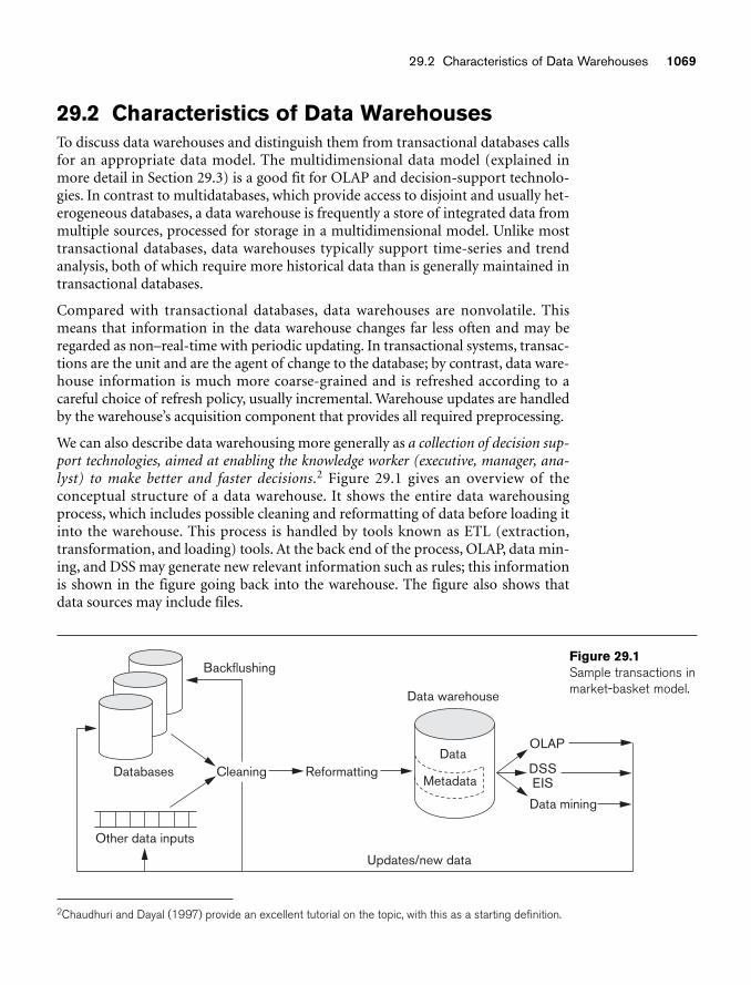
29.2 Characteristics of Data Warehouses 1069
Databases Cleaning
Backflushing
Reformatting
Data mining
DSSEIS
OLAP
Other data inputs
Updates/new data
Metadata
Data
Data warehouse
Figure 29.1Sample transactions inmarket-basket model.
29.2 Characteristics of Data WarehousesTo discuss data warehouses and distinguish them from transactional databases callsfor an appropriate data model. The multidimensional data model (explained inmore detail in Section 29.3) is a good fit for OLAP and decision-support technolo-gies. In contrast to multidatabases, which provide access to disjoint and usually het-erogeneous databases, a data warehouse is frequently a store of integrated data frommultiple sources, processed for storage in a multidimensional model. Unlike mosttransactional databases, data warehouses typically support time-series and trendanalysis, both of which require more historical data than is generally maintained intransactional databases.
Compared with transactional databases, data warehouses are nonvolatile. Thismeans that information in the data warehouse changes far less often and may beregarded as non–real-time with periodic updating. In transactional systems, transac-tions are the unit and are the agent of change to the database; by contrast, data ware-house information is much more coarse-grained and is refreshed according to acareful choice of refresh policy, usually incremental. Warehouse updates are handledby the warehouse’s acquisition component that provides all required preprocessing.
We can also describe data warehousing more generally as a collection of decision sup-port technologies, aimed at enabling the knowledge worker (executive, manager, ana-lyst) to make better and faster decisions.2 Figure 29.1 gives an overview of theconceptual structure of a data warehouse. It shows the entire data warehousingprocess, which includes possible cleaning and reformatting of data before loading itinto the warehouse. This process is handled by tools known as ETL (extraction,transformation, and loading) tools. At the back end of the process, OLAP, data min-ing, and DSS may generate new relevant information such as rules; this informationis shown in the figure going back into the warehouse. The figure also shows thatdata sources may include files.
2Chaudhuri and Dayal (1997) provide an excellent tutorial on the topic, with this as a starting definition.
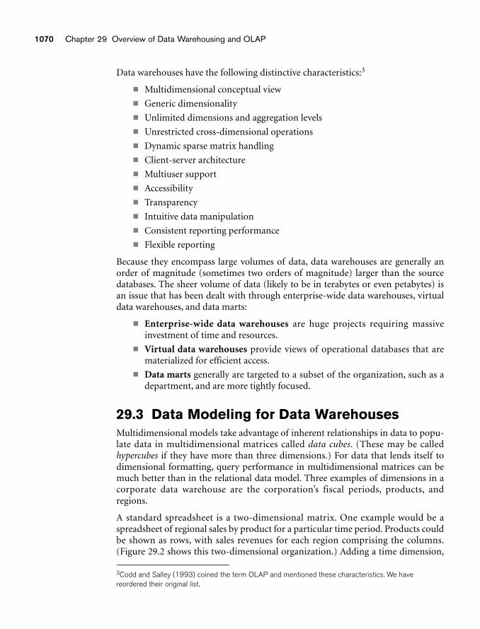
1070 Chapter 29 Overview of Data Warehousing and OLAP
Data warehouses have the following distinctive characteristics:3
■ Multidimensional conceptual view
■ Generic dimensionality
■ Unlimited dimensions and aggregation levels
■ Unrestricted cross-dimensional operations
■ Dynamic sparse matrix handling
■ Client-server architecture
■ Multiuser support
■ Accessibility
■ Transparency
■ Intuitive data manipulation
■ Consistent reporting performance
■ Flexible reporting
Because they encompass large volumes of data, data warehouses are generally anorder of magnitude (sometimes two orders of magnitude) larger than the sourcedatabases. The sheer volume of data (likely to be in terabytes or even petabytes) isan issue that has been dealt with through enterprise-wide data warehouses, virtualdata warehouses, and data marts:
■ Enterprise-wide data warehouses are huge projects requiring massiveinvestment of time and resources.
■ Virtual data warehouses provide views of operational databases that arematerialized for efficient access.
■ Data marts generally are targeted to a subset of the organization, such as adepartment, and are more tightly focused.
29.3 Data Modeling for Data WarehousesMultidimensional models take advantage of inherent relationships in data to popu-late data in multidimensional matrices called data cubes. (These may be calledhypercubes if they have more than three dimensions.) For data that lends itself todimensional formatting, query performance in multidimensional matrices can bemuch better than in the relational data model. Three examples of dimensions in acorporate data warehouse are the corporation’s fiscal periods, products, andregions.
A standard spreadsheet is a two-dimensional matrix. One example would be aspreadsheet of regional sales by product for a particular time period. Products couldbe shown as rows, with sales revenues for each region comprising the columns.(Figure 29.2 shows this two-dimensional organization.) Adding a time dimension,
3Codd and Salley (1993) coined the term OLAP and mentioned these characteristics. We havereordered their original list.
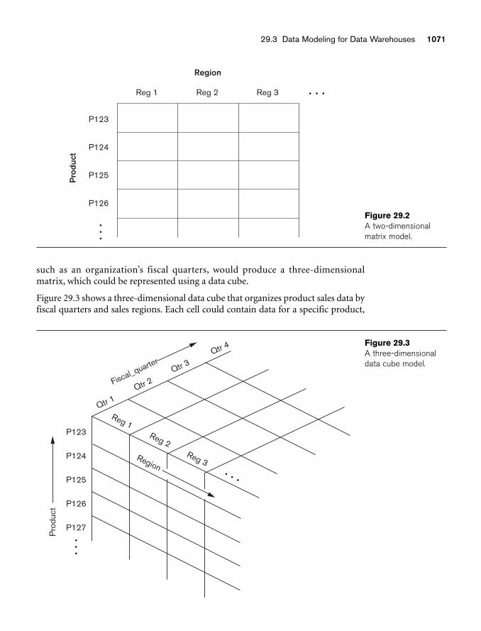
29.3 Data Modeling for Data Warehouses 1071
Reg 1
P123
P124
P125
P126
RegionP
rodu
ct
Reg 2 Reg 3
Figure 29.2A two-dimensionalmatrix model.
such as an organization’s fiscal quarters, would produce a three-dimensionalmatrix, which could be represented using a data cube.
Figure 29.3 shows a three-dimensional data cube that organizes product sales data byfiscal quarters and sales regions. Each cell could contain data for a specific product,
P126
P127
Pro
duct
P125
P124
P123
Reg 1Reg 2
RegionReg 3
Qtr 1Qtr 2Fiscal_quarter
Qtr 3Qtr 4
Figure 29.3A three-dimensionaldata cube model.
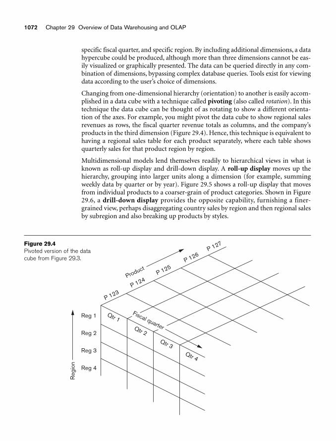
1072 Chapter 29 Overview of Data Warehousing and OLAP
Reg 4
Reg
ion
Reg 3
Reg 2
Reg 1 Qtr 1
Qtr 2
Fiscal quarter
Qtr 3Qtr 4
P 123P 124
ProductP 125
P 126P 127Figure 29.4
Pivoted version of the datacube from Figure 29.3.
specific fiscal quarter, and specific region. By including additional dimensions, a datahypercube could be produced, although more than three dimensions cannot be eas-ily visualized or graphically presented. The data can be queried directly in any com-bination of dimensions, bypassing complex database queries. Tools exist for viewingdata according to the user’s choice of dimensions.
Changing from one-dimensional hierarchy (orientation) to another is easily accom-plished in a data cube with a technique called pivoting (also called rotation). In thistechnique the data cube can be thought of as rotating to show a different orienta-tion of the axes. For example, you might pivot the data cube to show regional salesrevenues as rows, the fiscal quarter revenue totals as columns, and the company’sproducts in the third dimension (Figure 29.4). Hence, this technique is equivalent tohaving a regional sales table for each product separately, where each table showsquarterly sales for that product region by region.
Multidimensional models lend themselves readily to hierarchical views in what isknown as roll-up display and drill-down display. A roll-up display moves up thehierarchy, grouping into larger units along a dimension (for example, summingweekly data by quarter or by year). Figure 29.5 shows a roll-up display that movesfrom individual products to a coarser-grain of product categories. Shown in Figure29.6, a drill-down display provides the opposite capability, furnishing a finer-grained view, perhaps disaggregating country sales by region and then regional salesby subregion and also breaking up products by styles.
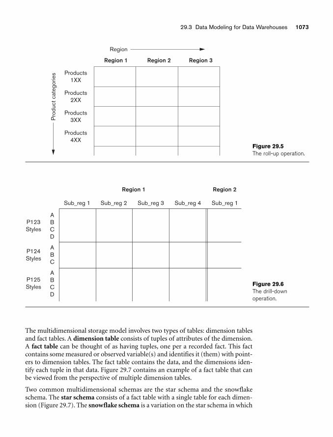
29.3 Data Modeling for Data Warehouses 1073
Products1XX
Products2XX
Products3XX
Products4XX
RegionP
rodu
ct c
ateg
orie
sRegion 1 Region 2 Region 3
Figure 29.5The roll-up operation.
The multidimensional storage model involves two types of tables: dimension tablesand fact tables. A dimension table consists of tuples of attributes of the dimension.A fact table can be thought of as having tuples, one per a recorded fact. This factcontains some measured or observed variable(s) and identifies it (them) with point-ers to dimension tables. The fact table contains the data, and the dimensions iden-tify each tuple in that data. Figure 29.7 contains an example of a fact table that canbe viewed from the perspective of multiple dimension tables.
Two common multidimensional schemas are the star schema and the snowflakeschema. The star schema consists of a fact table with a single table for each dimen-sion (Figure 29.7). The snowflake schema is a variation on the star schema in which
ABCD
P123Styles
P124Styles
P125Styles
ABC
ABCD
Sub_reg 1 Sub_reg 2
Region 1 Region 2
Sub_reg 3 Sub_reg 4 Sub_reg 1
Figure 29.6The drill-down operation.
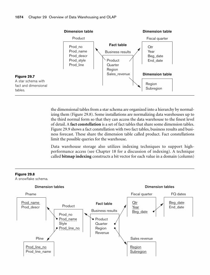
1074 Chapter 29 Overview of Data Warehousing and OLAP
Dimension table
Product
Prod_noProd_nameProd_descrProd_styleProd_line
Fact table
Business results
ProductQuarterRegionSales_revenue
Dimension table
Fiscal quarter
QtrYearBeg_dateEnd_date
Dimension table
RegionSubregion
Figure 29.7A star schema withfact and dimensionaltables.
Dimension tables
Pname
Prod_nameProd_descr Product
Prod_noProd_nameStyleProd_line_no
Fact table
Business results
ProductQuarterRegionRevenue
Pline
Prod_line_noProd_line_name
Dimension tables
Fiscal quarter
QtrYearBeg_date
FQ dates
Beg_dateEnd_date
Sales revenue
RegionSubregion
Figure 29.8A snowflake schema.
the dimensional tables from a star schema are organized into a hierarchy by normal-izing them (Figure 29.8). Some installations are normalizing data warehouses up tothe third normal form so that they can access the data warehouse to the finest levelof detail. A fact constellation is a set of fact tables that share some dimension tables.Figure 29.9 shows a fact constellation with two fact tables, business results and busi-ness forecast. These share the dimension table called product. Fact constellationslimit the possible queries for the warehouse.
Data warehouse storage also utilizes indexing techniques to support high-performance access (see Chapter 18 for a discussion of indexing). A techniquecalled bitmap indexing constructs a bit vector for each value in a domain (column)
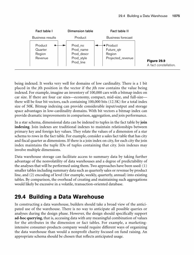
29.4 Building a Data Warehouse 1075
Fact table I
Business results
Prod_noProd_nameProd_descrProd_styleProd_line
Dimension table
Product
ProductQuarterRegionRevenue
Fact table II
Business forecast
ProductFuture_qtrRegionProjected_revenue
Figure 29.9A fact constellation.
being indexed. It works very well for domains of low cardinality. There is a 1 bitplaced in the jth position in the vector if the jth row contains the value beingindexed. For example, imagine an inventory of 100,000 cars with a bitmap index oncar size. If there are four car sizes—economy, compact, mid-size, and full-size—there will be four bit vectors, each containing 100,000 bits (12.5K) for a total indexsize of 50K. Bitmap indexing can provide considerable input/output and storagespace advantages in low-cardinality domains. With bit vectors a bitmap index canprovide dramatic improvements in comparison, aggregation, and join performance.
In a star schema, dimensional data can be indexed to tuples in the fact table by joinindexing. Join indexes are traditional indexes to maintain relationships betweenprimary key and foreign key values. They relate the values of a dimension of a starschema to rows in the fact table. For example, consider a sales fact table that has cityand fiscal quarter as dimensions. If there is a join index on city, for each city the joinindex maintains the tuple IDs of tuples containing that city. Join indexes mayinvolve multiple dimensions.
Data warehouse storage can facilitate access to summary data by taking furtheradvantage of the nonvolatility of data warehouses and a degree of predictability ofthe analyses that will be performed using them. Two approaches have been used: (1)smaller tables including summary data such as quarterly sales or revenue by productline, and (2) encoding of level (for example, weekly, quarterly, annual) into existingtables. By comparison, the overhead of creating and maintaining such aggregationswould likely be excessive in a volatile, transaction-oriented database.
29.4 Building a Data WarehouseIn constructing a data warehouse, builders should take a broad view of the antici-pated use of the warehouse. There is no way to anticipate all possible queries oranalyses during the design phase. However, the design should specifically supportad-hoc querying, that is, accessing data with any meaningful combination of valuesfor the attributes in the dimension or fact tables. For example, a marketing-intensive consumer-products company would require different ways of organizingthe data warehouse than would a nonprofit charity focused on fund raising. Anappropriate schema should be chosen that reflects anticipated usage.
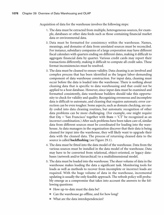
1076 Chapter 29 Overview of Data Warehousing and OLAP
Acquisition of data for the warehouse involves the following steps:
1. The data must be extracted from multiple, heterogeneous sources, for exam-ple, databases or other data feeds such as those containing financial marketdata or environmental data.
2. Data must be formatted for consistency within the warehouse. Names,meanings, and domains of data from unrelated sources must be reconciled.For instance, subsidiary companies of a large corporation may have differentfiscal calendars with quarters ending on different dates, making it difficult toaggregate financial data by quarter. Various credit cards may report theirtransactions differently, making it difficult to compute all credit sales. Theseformat inconsistencies must be resolved.
3. The data must be cleaned to ensure validity. Data cleaning is an involved andcomplex process that has been identified as the largest labor-demandingcomponent of data warehouse construction. For input data, cleaning mustoccur before the data is loaded into the warehouse. There is nothing aboutcleaning data that is specific to data warehousing and that could not beapplied to a host database. However, since input data must be examined andformatted consistently, data warehouse builders should take this opportu-nity to check for validity and quality. Recognizing erroneous and incompletedata is difficult to automate, and cleaning that requires automatic error cor-rection can be even tougher. Some aspects, such as domain checking, are eas-ily coded into data cleaning routines, but automatic recognition of otherdata problems can be more challenging. (For example, one might requirethat City = ‘San Francisco’ together with State = ‘CT’ be recognized as anincorrect combination.) After such problems have been taken care of, similardata from different sources must be coordinated for loading into the ware-house. As data managers in the organization discover that their data is beingcleaned for input into the warehouse, they will likely want to upgrade theirdata with the cleaned data. The process of returning cleaned data to thesource is called backflushing (see Figure 29.1).
4. The data must be fitted into the data model of the warehouse. Data from thevarious sources must be installed in the data model of the warehouse. Datamay have to be converted from relational, object-oriented, or legacy data-bases (network and/or hierarchical) to a multidimensional model.
5. The data must be loaded into the warehouse. The sheer volume of data in thewarehouse makes loading the data a significant task. Monitoring tools forloads as well as methods to recover from incomplete or incorrect loads arerequired. With the huge volume of data in the warehouse, incrementalupdating is usually the only feasible approach. The refresh policy will proba-bly emerge as a compromise that takes into account the answers to the fol-lowing questions:
■ How up-to-date must the data be?
■ Can the warehouse go offline, and for how long?
■ What are the data interdependencies?
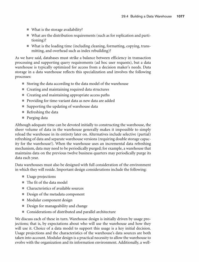
29.4 Building a Data Warehouse 1077
■ What is the storage availability?
■ What are the distribution requirements (such as for replication and parti-tioning)?
■ What is the loading time (including cleaning, formatting, copying, trans-mitting, and overhead such as index rebuilding)?
As we have said, databases must strike a balance between efficiency in transactionprocessing and supporting query requirements (ad hoc user requests), but a datawarehouse is typically optimized for access from a decision maker’s needs. Datastorage in a data warehouse reflects this specialization and involves the followingprocesses:
■ Storing the data according to the data model of the warehouse■ Creating and maintaining required data structures■ Creating and maintaining appropriate access paths■ Providing for time-variant data as new data are added■ Supporting the updating of warehouse data■ Refreshing the data■ Purging data
Although adequate time can be devoted initially to constructing the warehouse, thesheer volume of data in the warehouse generally makes it impossible to simplyreload the warehouse in its entirety later on. Alternatives include selective (partial)refreshing of data and separate warehouse versions (requiring double storage capac-ity for the warehouse!). When the warehouse uses an incremental data refreshingmechanism, data may need to be periodically purged; for example, a warehouse thatmaintains data on the previous twelve business quarters may periodically purge itsdata each year.
Data warehouses must also be designed with full consideration of the environmentin which they will reside. Important design considerations include the following:
■ Usage projections
■ The fit of the data model
■ Characteristics of available sources
■ Design of the metadata component
■ Modular component design
■ Design for manageability and change
■ Considerations of distributed and parallel architecture
We discuss each of these in turn. Warehouse design is initially driven by usage pro-jections; that is, by expectations about who will use the warehouse and how theywill use it. Choice of a data model to support this usage is a key initial decision.Usage projections and the characteristics of the warehouse’s data sources are bothtaken into account. Modular design is a practical necessity to allow the warehouse toevolve with the organization and its information environment. Additionally, a well-
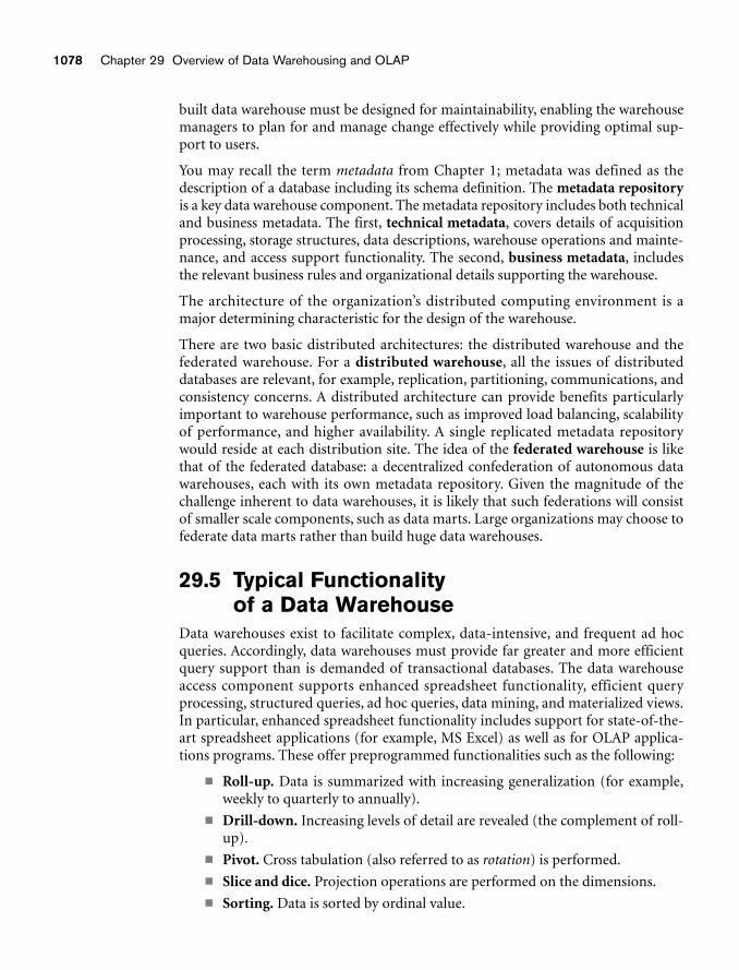
1078 Chapter 29 Overview of Data Warehousing and OLAP
built data warehouse must be designed for maintainability, enabling the warehousemanagers to plan for and manage change effectively while providing optimal sup-port to users.
You may recall the term metadata from Chapter 1; metadata was defined as thedescription of a database including its schema definition. The metadata repositoryis a key data warehouse component. The metadata repository includes both technicaland business metadata. The first, technical metadata, covers details of acquisitionprocessing, storage structures, data descriptions, warehouse operations and mainte-nance, and access support functionality. The second, business metadata, includesthe relevant business rules and organizational details supporting the warehouse.
The architecture of the organization’s distributed computing environment is amajor determining characteristic for the design of the warehouse.
There are two basic distributed architectures: the distributed warehouse and thefederated warehouse. For a distributed warehouse, all the issues of distributeddatabases are relevant, for example, replication, partitioning, communications, andconsistency concerns. A distributed architecture can provide benefits particularlyimportant to warehouse performance, such as improved load balancing, scalabilityof performance, and higher availability. A single replicated metadata repositorywould reside at each distribution site. The idea of the federated warehouse is likethat of the federated database: a decentralized confederation of autonomous datawarehouses, each with its own metadata repository. Given the magnitude of thechallenge inherent to data warehouses, it is likely that such federations will consistof smaller scale components, such as data marts. Large organizations may choose tofederate data marts rather than build huge data warehouses.
29.5 Typical Functionality of a Data Warehouse
Data warehouses exist to facilitate complex, data-intensive, and frequent ad hocqueries. Accordingly, data warehouses must provide far greater and more efficientquery support than is demanded of transactional databases. The data warehouseaccess component supports enhanced spreadsheet functionality, efficient queryprocessing, structured queries, ad hoc queries, data mining, and materialized views.In particular, enhanced spreadsheet functionality includes support for state-of-the-art spreadsheet applications (for example, MS Excel) as well as for OLAP applica-tions programs. These offer preprogrammed functionalities such as the following:
■ Roll-up. Data is summarized with increasing generalization (for example,weekly to quarterly to annually).
■ Drill-down. Increasing levels of detail are revealed (the complement of roll-up).
■ Pivot. Cross tabulation (also referred to as rotation) is performed.
■ Slice and dice. Projection operations are performed on the dimensions.
■ Sorting. Data is sorted by ordinal value.
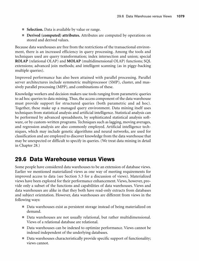
29.6 Data Warehouse versus Views 1079
■ Selection. Data is available by value or range.
■ Derived (computed) attributes. Attributes are computed by operations onstored and derived values.
Because data warehouses are free from the restrictions of the transactional environ-ment, there is an increased efficiency in query processing. Among the tools andtechniques used are query transformation; index intersection and union; specialROLAP (relational OLAP) and MOLAP (multidimensional OLAP) functions; SQLextensions; advanced join methods; and intelligent scanning (as in piggy-backingmultiple queries).
Improved performance has also been attained with parallel processing. Parallelserver architectures include symmetric multiprocessor (SMP), cluster, and mas-sively parallel processing (MPP), and combinations of these.
Knowledge workers and decision makers use tools ranging from parametric queriesto ad hoc queries to data mining. Thus, the access component of the data warehousemust provide support for structured queries (both parametric and ad hoc).Together, these make up a managed query environment. Data mining itself usestechniques from statistical analysis and artificial intelligence. Statistical analysis canbe performed by advanced spreadsheets, by sophisticated statistical analysis soft-ware, or by custom-written programs. Techniques such as lagging, moving averages,and regression analysis are also commonly employed. Artificial intelligence tech-niques, which may include genetic algorithms and neural networks, are used forclassification and are employed to discover knowledge from the data warehouse thatmay be unexpected or difficult to specify in queries. (We treat data mining in detailin Chapter 28.)
29.6 Data Warehouse versus ViewsSome people have considered data warehouses to be an extension of database views.Earlier we mentioned materialized views as one way of meeting requirements forimproved access to data (see Section 5.3 for a discussion of views). Materializedviews have been explored for their performance enhancement. Views, however, pro-vide only a subset of the functions and capabilities of data warehouses. Views anddata warehouses are alike in that they both have read-only extracts from databasesand subject orientation. However, data warehouses are different from views in thefollowing ways:
■ Data warehouses exist as persistent storage instead of being materialized ondemand.
■ Data warehouses are not usually relational, but rather multidimensional.Views of a relational database are relational.
■ Data warehouses can be indexed to optimize performance. Views cannot beindexed independent of the underlying databases.
■ Data warehouses characteristically provide specific support of functionality;views cannot.
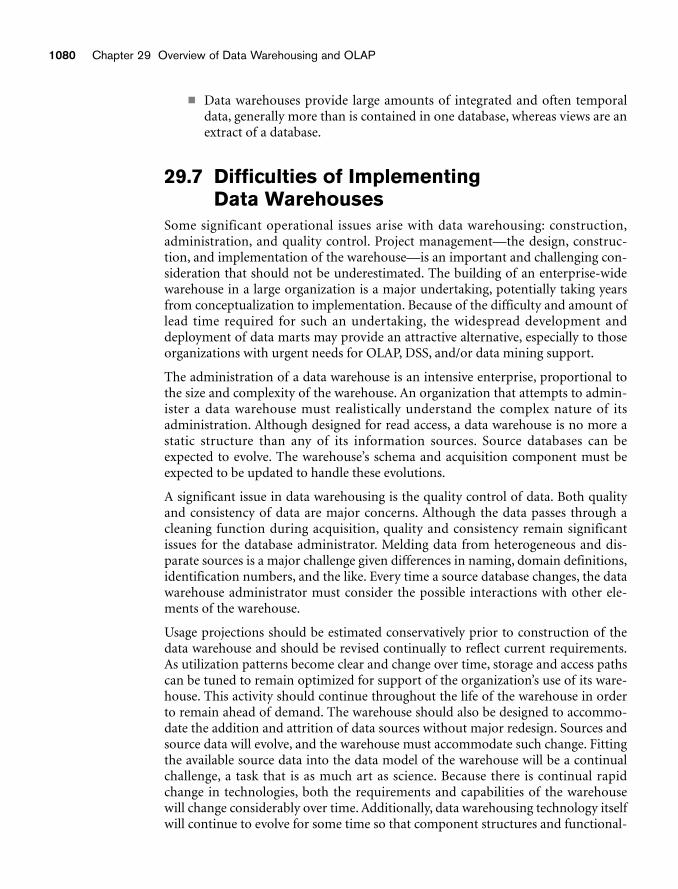
1080 Chapter 29 Overview of Data Warehousing and OLAP
■ Data warehouses provide large amounts of integrated and often temporaldata, generally more than is contained in one database, whereas views are anextract of a database.
29.7 Difficulties of Implementing Data Warehouses
Some significant operational issues arise with data warehousing: construction,administration, and quality control. Project management—the design, construc-tion, and implementation of the warehouse—is an important and challenging con-sideration that should not be underestimated. The building of an enterprise-widewarehouse in a large organization is a major undertaking, potentially taking yearsfrom conceptualization to implementation. Because of the difficulty and amount oflead time required for such an undertaking, the widespread development anddeployment of data marts may provide an attractive alternative, especially to thoseorganizations with urgent needs for OLAP, DSS, and/or data mining support.
The administration of a data warehouse is an intensive enterprise, proportional tothe size and complexity of the warehouse. An organization that attempts to admin-ister a data warehouse must realistically understand the complex nature of itsadministration. Although designed for read access, a data warehouse is no more astatic structure than any of its information sources. Source databases can beexpected to evolve. The warehouse’s schema and acquisition component must beexpected to be updated to handle these evolutions.
A significant issue in data warehousing is the quality control of data. Both qualityand consistency of data are major concerns. Although the data passes through acleaning function during acquisition, quality and consistency remain significantissues for the database administrator. Melding data from heterogeneous and dis-parate sources is a major challenge given differences in naming, domain definitions,identification numbers, and the like. Every time a source database changes, the datawarehouse administrator must consider the possible interactions with other ele-ments of the warehouse.
Usage projections should be estimated conservatively prior to construction of thedata warehouse and should be revised continually to reflect current requirements.As utilization patterns become clear and change over time, storage and access pathscan be tuned to remain optimized for support of the organization’s use of its ware-house. This activity should continue throughout the life of the warehouse in orderto remain ahead of demand. The warehouse should also be designed to accommo-date the addition and attrition of data sources without major redesign. Sources andsource data will evolve, and the warehouse must accommodate such change. Fittingthe available source data into the data model of the warehouse will be a continualchallenge, a task that is as much art as science. Because there is continual rapidchange in technologies, both the requirements and capabilities of the warehousewill change considerably over time. Additionally, data warehousing technology itselfwill continue to evolve for some time so that component structures and functional-
Review Questions 1081
ities will continually be upgraded. This certain change is excellent motivation forhaving fully modular design of components.
Administration of a data warehouse will require far broader skills than are neededfor traditional database administration. A team of highly skilled technical expertswith overlapping areas of expertise will likely be needed, rather than a single indi-vidual. Like database administration, data warehouse administration is only partlytechnical; a large part of the responsibility requires working effectively with all themembers of the organization with an interest in the data warehouse. However diffi-cult that can be at times for database administrators, it is that much more challeng-ing for data warehouse administrators, as the scope of their responsibilities isconsiderably broader.
Design of the management function and selection of the management team for adatabase warehouse are crucial. Managing the data warehouse in a large organizationwill surely be a major task. Many commercial tools are available to support manage-ment functions. Effective data warehouse management will certainly be a team func-tion, requiring a wide set of technical skills, careful coordination, and effectiveleadership. Just as we must prepare for the evolution of the warehouse, we must alsorecognize that the skills of the management team will, of necessity, evolve with it.
29.8 SummaryIn this chapter we surveyed the field known as data warehousing. Data warehousingcan be seen as a process that requires a variety of activities to precede it. In contrast,data mining (see Chapter 28) may be thought of as an activity that draws knowledgefrom an existing data warehouse. We introduced key concepts related to data ware-housing and we discussed the special functionality associated with a multidimen-sional view of data. We also discussed the ways in which data warehouses supplydecision makers with information at the correct level of detail, based on an appro-priate organization and perspective.
Review Questions29.1. What is a data warehouse? How does it differ from a database?
29.2. Define the terms: OLAP (online analytical processing), ROLAP (relationalOLAP), MOLAP (multidimensional OLAP), and DSS (decision-support systems).
29.3. Describe the characteristics of a data warehouse. Divide them into function-ality of a warehouse and advantages users derive from it.
29.4. What is the multidimensional data model? How is it used in data ware-housing?
29.5. Define the following terms: star schema, snowflake schema, fact constella-tion, data marts.
1082 Chapter 29 Overview of Data Warehousing and OLAP
29.6. What types of indexes are built for a warehouse? Illustrate the uses for eachwith an example.
29.7. Describe the steps of building a warehouse.
29.8. What considerations play a major role in the design of a warehouse?
29.9. Describe the functions a user can perform on a data warehouse and illustratethe results of these functions on a sample multidimensional data warehouse.
29.10. How is the concept of a relational view related to a data warehouse and datamarts? In what way are they different?
29.11. List the difficulties in implementing a data warehouse.
29.12. List the open issues and research problems in data warehousing.
Selected BibliographyInmon (1992, 2005) is credited for giving the term wide acceptance. Codd andSalley (1993) popularized the term online analytical processing (OLAP) anddefined a set of characteristics for data warehouses to support OLAP. Kimball(1996) is known for his contribution to the development of the data warehousingfield. Mattison (1996) is one of the several books on data warehousing that gives acomprehensive analysis of techniques available in data warehouses and the strate-gies companies should use in deploying them. Ponniah (2002) gives a very goodpractical overview of the data warehouse building process from requirements collection to deployment maintenance. Bischoff and Alexander (1997) is a compila-tion of advice from experts. Chaudhuri and Dayal (1997) give an excellent tutorialon the topic, while Widom (1995) points to a number of outstanding research problems.
1083
Alternative DiagrammaticNotations for ER Models
Figure A.1 shows a number of different diagram-matic notations for representing ER and EER
model concepts. Unfortunately, there is no standard notation: different databasedesign practitioners prefer different notations. Similarly, various CASE (computer-aided software engineering) tools and OOA (object-oriented analysis) methodolo-gies use various notations. Some notations are associated with models that haveadditional concepts and constraints beyond those of the ER and EER modelsdescribed in Chapters 7 through 9, while other models have fewer concepts andconstraints. The notation we used in Chapter 7 is quite close to the original notationfor ER diagrams, which is still widely used. We discuss some alternate notationshere.
Figure A.1(a) shows different notations for displaying entity types/classes, attrib-utes, and relationships. In Chapters 7 through 9, we used the symbols marked (i) inFigure A.1(a)—namely, rectangle, oval, and diamond. Notice that symbol (ii) forentity types/classes, symbol (ii) for attributes, and symbol (ii) for relationships aresimilar, but they are used by different methodologies to represent three differentconcepts. The straight line symbol (iii) for representing relationships is used by sev-eral tools and methodologies.
Figure A.1(b) shows some notations for attaching attributes to entity types. We usednotation (i). Notation (ii) uses the third notation (iii) for attributes from FigureA.1(a). The last two notations in Figure A.1(b)—(iii) and (iv)—are popular in OOAmethodologies and in some CASE tools. In particular, the last notation displaysboth the attributes and the methods of a class, separated by a horizontal line.
Aappendix A
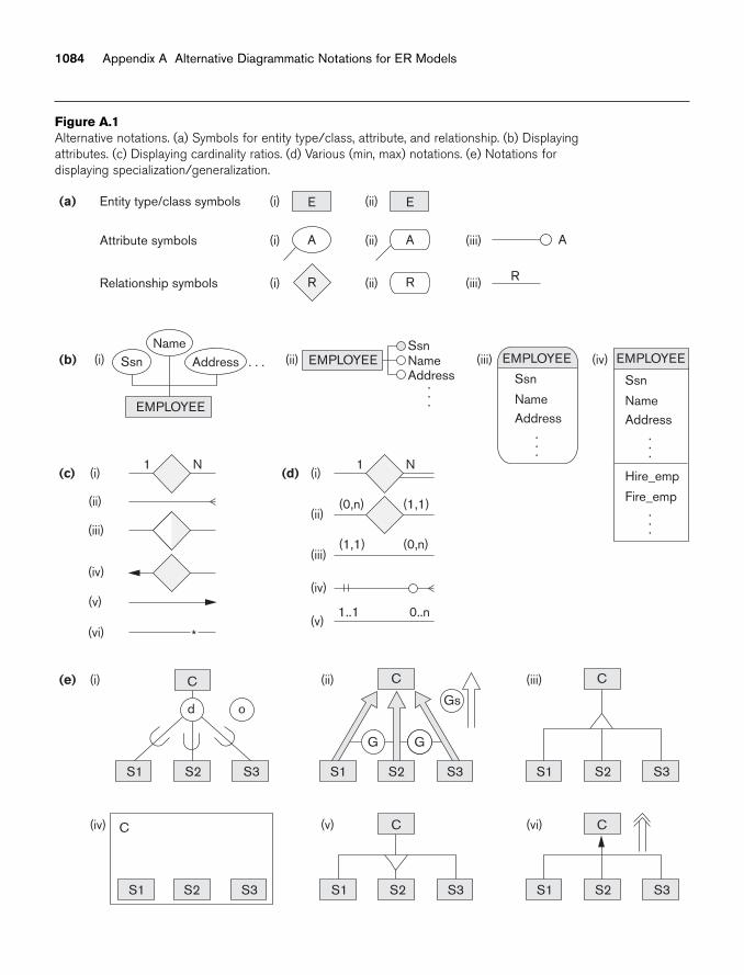
1084 Appendix A Alternative Diagrammatic Notations for ER Models
Entity type/class symbols E(i) E(ii)
Attribute symbols (i) (ii)
Relationship symbols (i) (ii)
(iii)
(iii)
(a)
A
R
A A
R R
(b)SsnNameAddress
.
.
.
EMPLOYEE(ii)
EMPLOYEE
Ssn(i)Name
Address . . .
.
.
.
(iii)Ssn
NameAddress
EMPLOYEE
.
.
.
.
.
.
(iv)
Ssn
NameAddress
Hire_emp
Fire_emp
EMPLOYEE
(c) (i)
(ii)
1 N
(iii)
(iv)
(v)
(vi) *
(d) (i)
(ii)
1 N
(0,n) (1,1)
(0,n)(1,1)(iii)
(iv)
(e) (i)
(iv) C
(ii) (iii)C
S2S1 S3
d o
S2S1 S3
G
Gs
C
S2S1 S3
C
S2S1 S3
(v) (vi)C
S2S1 S3
C
S2S1 S3
G
(v) 0..n1..1
Figure A.1Alternative notations. (a) Symbols for entity type/class, attribute, and relationship. (b) Displayingattributes. (c) Displaying cardinality ratios. (d) Various (min, max) notations. (e) Notations for displaying specialization/generalization.
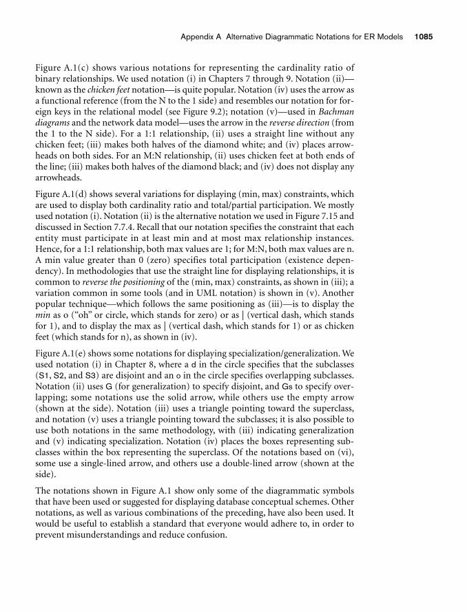
Appendix A Alternative Diagrammatic Notations for ER Models 1085
Figure A.1(c) shows various notations for representing the cardinality ratio ofbinary relationships. We used notation (i) in Chapters 7 through 9. Notation (ii)—known as the chicken feet notation—is quite popular. Notation (iv) uses the arrow asa functional reference (from the N to the 1 side) and resembles our notation for for-eign keys in the relational model (see Figure 9.2); notation (v)—used in Bachmandiagrams and the network data model—uses the arrow in the reverse direction (fromthe 1 to the N side). For a 1:1 relationship, (ii) uses a straight line without anychicken feet; (iii) makes both halves of the diamond white; and (iv) places arrow-heads on both sides. For an M:N relationship, (ii) uses chicken feet at both ends ofthe line; (iii) makes both halves of the diamond black; and (iv) does not display anyarrowheads.
Figure A.1(d) shows several variations for displaying (min, max) constraints, whichare used to display both cardinality ratio and total/partial participation. We mostlyused notation (i). Notation (ii) is the alternative notation we used in Figure 7.15 anddiscussed in Section 7.7.4. Recall that our notation specifies the constraint that eachentity must participate in at least min and at most max relationship instances.Hence, for a 1:1 relationship, both max values are 1; for M:N, both max values are n.A min value greater than 0 (zero) specifies total participation (existence depen-dency). In methodologies that use the straight line for displaying relationships, it iscommon to reverse the positioning of the (min, max) constraints, as shown in (iii); avariation common in some tools (and in UML notation) is shown in (v). Anotherpopular technique—which follows the same positioning as (iii)—is to display themin as o (“oh” or circle, which stands for zero) or as | (vertical dash, which standsfor 1), and to display the max as | (vertical dash, which stands for 1) or as chickenfeet (which stands for n), as shown in (iv).
Figure A.1(e) shows some notations for displaying specialization/generalization. Weused notation (i) in Chapter 8, where a d in the circle specifies that the subclasses(S1, S2, and S3) are disjoint and an o in the circle specifies overlapping subclasses.Notation (ii) uses G (for generalization) to specify disjoint, and Gs to specify over-lapping; some notations use the solid arrow, while others use the empty arrow(shown at the side). Notation (iii) uses a triangle pointing toward the superclass,and notation (v) uses a triangle pointing toward the subclasses; it is also possible touse both notations in the same methodology, with (iii) indicating generalizationand (v) indicating specialization. Notation (iv) places the boxes representing sub-classes within the box representing the superclass. Of the notations based on (vi),some use a single-lined arrow, and others use a double-lined arrow (shown at theside).
The notations shown in Figure A.1 show only some of the diagrammatic symbolsthat have been used or suggested for displaying database conceptual schemes. Othernotations, as well as various combinations of the preceding, have also been used. Itwould be useful to establish a standard that everyone would adhere to, in order toprevent misunderstandings and reduce confusion.
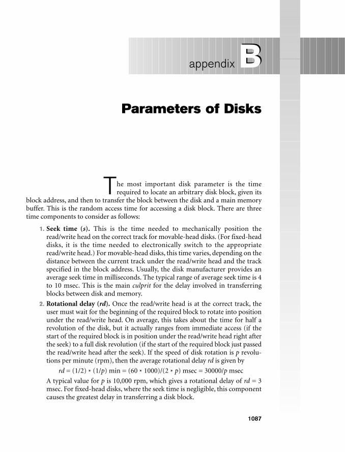
1087
Parameters of Disks
The most important disk parameter is the timerequired to locate an arbitrary disk block, given its
block address, and then to transfer the block between the disk and a main memorybuffer. This is the random access time for accessing a disk block. There are threetime components to consider as follows:
1. Seek time (s). This is the time needed to mechanically position theread/write head on the correct track for movable-head disks. (For fixed-headdisks, it is the time needed to electronically switch to the appropriateread/write head.) For movable-head disks, this time varies, depending on thedistance between the current track under the read/write head and the trackspecified in the block address. Usually, the disk manufacturer provides anaverage seek time in milliseconds. The typical range of average seek time is 4to 10 msec. This is the main culprit for the delay involved in transferringblocks between disk and memory.
2. Rotational delay (rd). Once the read/write head is at the correct track, theuser must wait for the beginning of the required block to rotate into positionunder the read/write head. On average, this takes about the time for half arevolution of the disk, but it actually ranges from immediate access (if thestart of the required block is in position under the read/write head right afterthe seek) to a full disk revolution (if the start of the required block just passedthe read/write head after the seek). If the speed of disk rotation is p revolu-tions per minute (rpm), then the average rotational delay rd is given by
rd = (1/2) * (1/p) min = (60 * 1000)/(2 * p) msec = 30000/p msec
A typical value for p is 10,000 rpm, which gives a rotational delay of rd = 3msec. For fixed-head disks, where the seek time is negligible, this componentcauses the greatest delay in transferring a disk block.
Bappendix B

1088 Appendix B Parameters of Disks
3. Block transfer time (btt). Once the read/write head is at the beginning ofthe required block, some time is needed to transfer the data in the block.This block transfer time depends on the block size, track size, and rotationalspeed. If the transfer rate for the disk is tr bytes/msec and the block size is Bbytes, then
btt = B/tr msec
If we have a track size of 50 Kbytes and p is 3600 rpm, then the transfer ratein bytes/msec is
tr = (50 * 1000)/(60 * 1000/3600) = 3000 bytes/msec
In this case, btt = B/3000 msec, where B is the block size in bytes.
The average time (s) needed to find and transfer a block, given its block address, isestimated by
(s + rd + btt) msec
This holds for either reading or writing a block. The principal method of reducingthis time is to transfer several blocks that are stored on one or more tracks of thesame cylinder; then the seek time is required for the first block only. To transfer con-secutively k noncontiguous blocks that are on the same cylinder, we need approxi-mately
s + (k * (rd + btt)) msec
In this case, we need two or more buffers in main storage because we are continu-ously reading or writing the k blocks, as we discussed in Chapter 17. The transfertime per block is reduced even further when consecutive blocks on the same track orcylinder are transferred. This eliminates the rotational delay for all but the firstblock, so the estimate for transferring k consecutive blocks is
s + rd + (k * btt) msec
A more accurate estimate for transferring consecutive blocks takes into account theinterblock gap (see Section 17.2.1), which includes the information that enables theread/write head to determine which block it is about to read. Usually, the disk man-ufacturer provides a bulk transfer rate (btr) that takes the gap size into accountwhen reading consecutively stored blocks. If the gap size is G bytes, then
btr = (B/(B + G)) * tr bytes/msec
The bulk transfer rate is the rate of transferring useful bytes in the data blocks. Thedisk read/write head must go over all bytes on a track as the disk rotates, includingthe bytes in the interblock gaps, which store control information but not real data.When the bulk transfer rate is used, the time needed to transfer the useful data inone block out of several consecutive blocks is B/btr. Hence, the estimated time toread k blocks consecutively stored on the same cylinder becomes
s + rd + (k * (B/btr)) msec
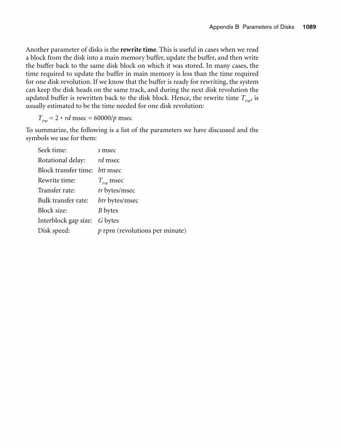
Appendix B Parameters of Disks 1089
Another parameter of disks is the rewrite time. This is useful in cases when we reada block from the disk into a main memory buffer, update the buffer, and then writethe buffer back to the same disk block on which it was stored. In many cases, thetime required to update the buffer in main memory is less than the time requiredfor one disk revolution. If we know that the buffer is ready for rewriting, the systemcan keep the disk heads on the same track, and during the next disk revolution theupdated buffer is rewritten back to the disk block. Hence, the rewrite time Trw, isusually estimated to be the time needed for one disk revolution:
Trw = 2 * rd msec = 60000/p msec
To summarize, the following is a list of the parameters we have discussed and thesymbols we use for them:
Seek time: s msec
Rotational delay: rd msec
Block transfer time: btt msec
Rewrite time: Trw msec
Transfer rate: tr bytes/msec
Bulk transfer rate: btr bytes/msec
Block size: B bytes
Interblock gap size: G bytes
Disk speed: p rpm (revolutions per minute)
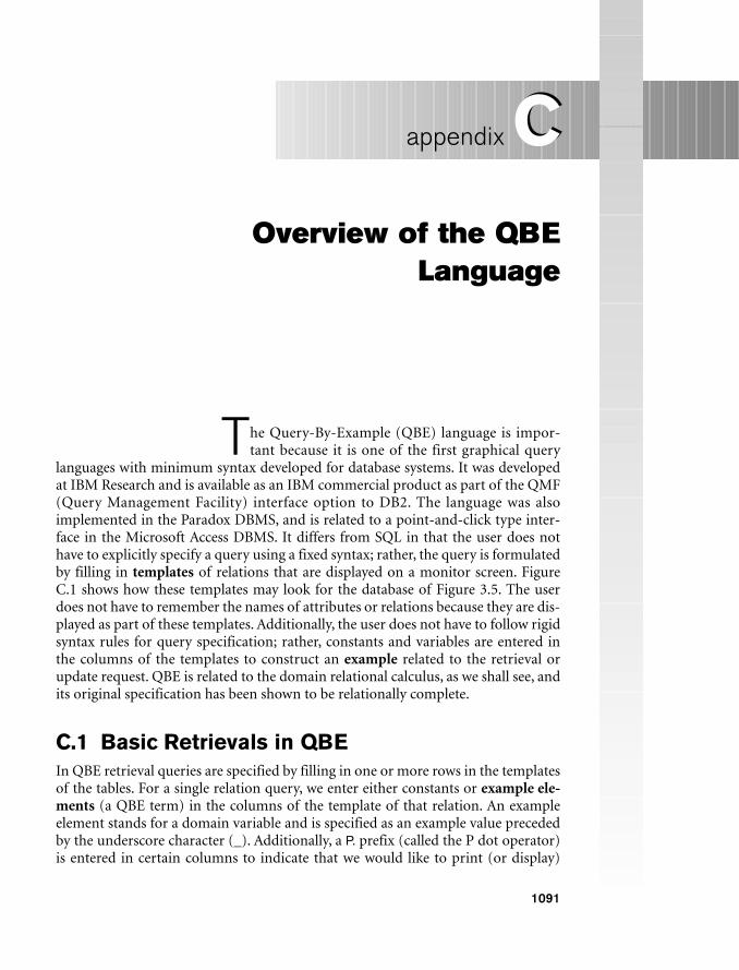
1091
Overview of the QBE Language
The Query-By-Example (QBE) language is impor-tant because it is one of the first graphical query
languages with minimum syntax developed for database systems. It was developedat IBM Research and is available as an IBM commercial product as part of the QMF(Query Management Facility) interface option to DB2. The language was alsoimplemented in the Paradox DBMS, and is related to a point-and-click type inter-face in the Microsoft Access DBMS. It differs from SQL in that the user does nothave to explicitly specify a query using a fixed syntax; rather, the query is formulatedby filling in templates of relations that are displayed on a monitor screen. FigureC.1 shows how these templates may look for the database of Figure 3.5. The userdoes not have to remember the names of attributes or relations because they are dis-played as part of these templates. Additionally, the user does not have to follow rigidsyntax rules for query specification; rather, constants and variables are entered inthe columns of the templates to construct an example related to the retrieval orupdate request. QBE is related to the domain relational calculus, as we shall see, andits original specification has been shown to be relationally complete.
C.1 Basic Retrievals in QBEIn QBE retrieval queries are specified by filling in one or more rows in the templatesof the tables. For a single relation query, we enter either constants or example ele-ments (a QBE term) in the columns of the template of that relation. An exampleelement stands for a domain variable and is specified as an example value precededby the underscore character (_). Additionally, a P. prefix (called the P dot operator)is entered in certain columns to indicate that we would like to print (or display)
Cappendix C
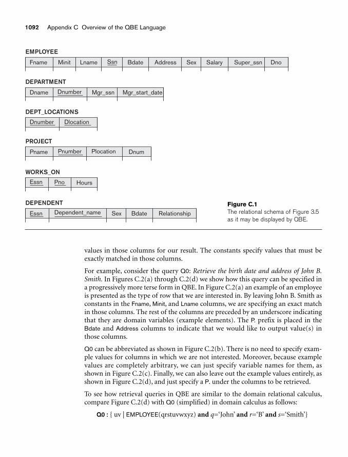
1092 Appendix C Overview of the QBE Language
values in those columns for our result. The constants specify values that must beexactly matched in those columns.
For example, consider the query Q0: Retrieve the birth date and address of John B.Smith. In Figures C.2(a) through C.2(d) we show how this query can be specified ina progressively more terse form in QBE. In Figure C.2(a) an example of an employeeis presented as the type of row that we are interested in. By leaving John B. Smith asconstants in the Fname, Minit, and Lname columns, we are specifying an exact matchin those columns. The rest of the columns are preceded by an underscore indicatingthat they are domain variables (example elements). The P. prefix is placed in theBdate and Address columns to indicate that we would like to output value(s) inthose columns.
Q0 can be abbreviated as shown in Figure C.2(b). There is no need to specify exam-ple values for columns in which we are not interested. Moreover, because examplevalues are completely arbitrary, we can just specify variable names for them, asshown in Figure C.2(c). Finally, we can also leave out the example values entirely, asshown in Figure C.2(d), and just specify a P. under the columns to be retrieved.
To see how retrieval queries in QBE are similar to the domain relational calculus,compare Figure C.2(d) with Q0 (simplified) in domain calculus as follows:
Q0 : { uv | EMPLOYEE(qrstuvwxyz) and q=‘John’ and r=‘B’ and s=‘Smith’}
DEPARTMENT
Fname Minit Lname Ssn Bdate Address Sex Salary Super_ssn Dno
EMPLOYEE
DEPT_LOCATIONS
Dnumber Dlocation
PROJECT
Pname Pnumber Plocation Dnum
WORKS_ON
Essn Pno Hours
DEPENDENT
Essn Dependent_name Sex Bdate Relationship
Dname Dnumber Mgr_ssn Mgr_start_date
Figure C.1The relational schema of Figure 3.5as it may be displayed by QBE.
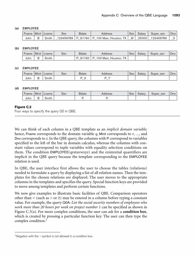
Appendix C Overview of the QBE Language 1093
EMPLOYEE(a)
(b)
(c)
(d)
Fname Minit Lname Ssn Bdate Address Sex Salary Super_ssn Dno
John B Smith _123456789 P._9/1/60 P._100 Main, Houston, TX _M _25000 _123456789 _3
EMPLOYEE
Fname Minit Lname Ssn Bdate Address Sex Salary Super_ssn Dno
John B Smith P._9/1/60 P._100 Main, Houston, TX
EMPLOYEE
Fname Minit Lname Ssn Bdate Address Sex Salary Super_ssn Dno
John B Smith P._X P._Y
EMPLOYEE
Fname Minit Lname Ssn Bdate Address Sex Salary Super_ssn Dno
John B Smith P. P.
Figure C.2Four ways to specify the query Q0 in QBE.
We can think of each column in a QBE template as an implicit domain variable;hence, Fname corresponds to the domain variable q, Minit corresponds to r, ..., andDno corresponds to z. In the QBE query, the columns with P. correspond to variablesspecified to the left of the bar in domain calculus, whereas the columns with con-stant values correspond to tuple variables with equality selection conditions onthem. The condition EMPLOYEE(qrstuvwxyz) and the existential quantifiers areimplicit in the QBE query because the template corresponding to the EMPLOYEErelation is used.
In QBE, the user interface first allows the user to choose the tables (relations)needed to formulate a query by displaying a list of all relation names. Then the tem-plates for the chosen relations are displayed. The user moves to the appropriatecolumns in the templates and specifies the query. Special function keys are providedto move among templates and perform certain functions.
We now give examples to illustrate basic facilities of QBE. Comparison operatorsother than = (such as > or ≥) may be entered in a column before typing a constantvalue. For example, the query Q0A: List the social security numbers of employees whowork more than 20 hours per week on project number 1 can be specified as shown inFigure C.3(a). For more complex conditions, the user can ask for a condition box,which is created by pressing a particular function key. The user can then type thecomplex condition.1
1Negation with the ¬ symbol is not allowed in a condition box.
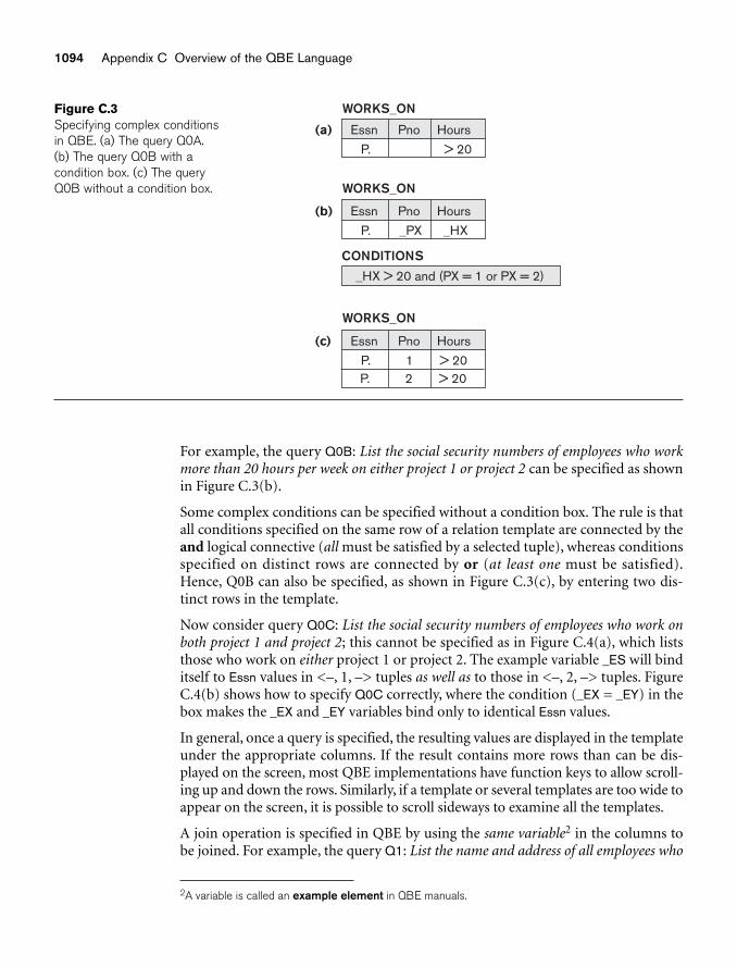
1094 Appendix C Overview of the QBE Language
For example, the query Q0B: List the social security numbers of employees who workmore than 20 hours per week on either project 1 or project 2 can be specified as shownin Figure C.3(b).
Some complex conditions can be specified without a condition box. The rule is thatall conditions specified on the same row of a relation template are connected by theand logical connective (all must be satisfied by a selected tuple), whereas conditionsspecified on distinct rows are connected by or (at least one must be satisfied).Hence, Q0B can also be specified, as shown in Figure C.3(c), by entering two dis-tinct rows in the template.
Now consider query Q0C: List the social security numbers of employees who work onboth project 1 and project 2; this cannot be specified as in Figure C.4(a), which liststhose who work on either project 1 or project 2. The example variable _ES will binditself to Essn values in <–, 1, –> tuples as well as to those in <–, 2, –> tuples. FigureC.4(b) shows how to specify Q0C correctly, where the condition (_EX = _EY) in thebox makes the _EX and _EY variables bind only to identical Essn values.
In general, once a query is specified, the resulting values are displayed in the templateunder the appropriate columns. If the result contains more rows than can be dis-played on the screen, most QBE implementations have function keys to allow scroll-ing up and down the rows. Similarly, if a template or several templates are too wide toappear on the screen, it is possible to scroll sideways to examine all the templates.
A join operation is specified in QBE by using the same variable2 in the columns tobe joined. For example, the query Q1: List the name and address of all employees who
2A variable is called an example element in QBE manuals.
WORKS_ON
(a) Essn Pno Hours
P. > 20
WORKS_ON
(b) Essn Pno Hours
P. _PX _HX
_HX > 20 and (PX = 1 or PX = 2)
CONDITIONS
WORKS_ON
(c) Essn Pno Hours
P. > 201P. > 202
Figure C.3Specifying complex conditionsin QBE. (a) The query Q0A. (b) The query Q0B with a condition box. (c) The queryQ0B without a condition box.
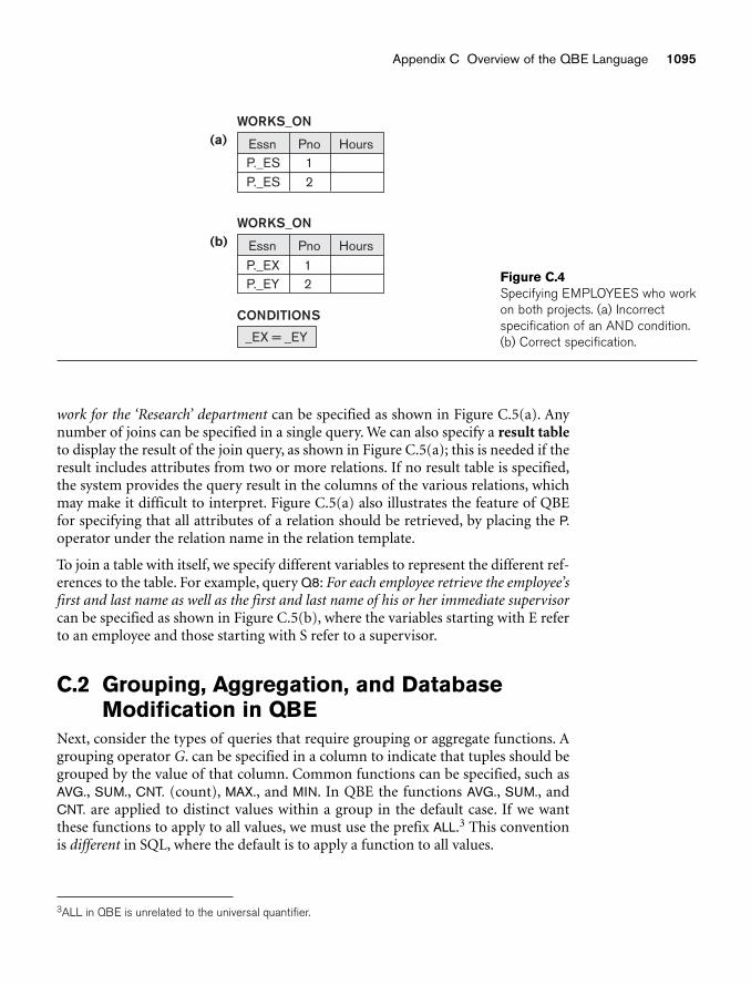
Appendix C Overview of the QBE Language 1095
WORKS_ON(a) Essn Pno Hours
P._ES 1P._ES 2
WORKS_ON(b) Essn Pno Hours
P._EX 1P._EY 2
_EX = _EY
CONDITIONS
Figure C.4Specifying EMPLOYEES who workon both projects. (a) Incorrectspecification of an AND condition.(b) Correct specification.
work for the ‘Research’ department can be specified as shown in Figure C.5(a). Anynumber of joins can be specified in a single query. We can also specify a result tableto display the result of the join query, as shown in Figure C.5(a); this is needed if theresult includes attributes from two or more relations. If no result table is specified,the system provides the query result in the columns of the various relations, whichmay make it difficult to interpret. Figure C.5(a) also illustrates the feature of QBEfor specifying that all attributes of a relation should be retrieved, by placing the P.operator under the relation name in the relation template.
To join a table with itself, we specify different variables to represent the different ref-erences to the table. For example, query Q8: For each employee retrieve the employee’sfirst and last name as well as the first and last name of his or her immediate supervisorcan be specified as shown in Figure C.5(b), where the variables starting with E referto an employee and those starting with S refer to a supervisor.
C.2 Grouping, Aggregation, and DatabaseModification in QBE
Next, consider the types of queries that require grouping or aggregate functions. Agrouping operator G. can be specified in a column to indicate that tuples should begrouped by the value of that column. Common functions can be specified, such asAVG., SUM., CNT. (count), MAX., and MIN. In QBE the functions AVG., SUM., andCNT. are applied to distinct values within a group in the default case. If we wantthese functions to apply to all values, we must use the prefix ALL.3 This conventionis different in SQL, where the default is to apply a function to all values.
3ALL in QBE is unrelated to the universal quantifier.
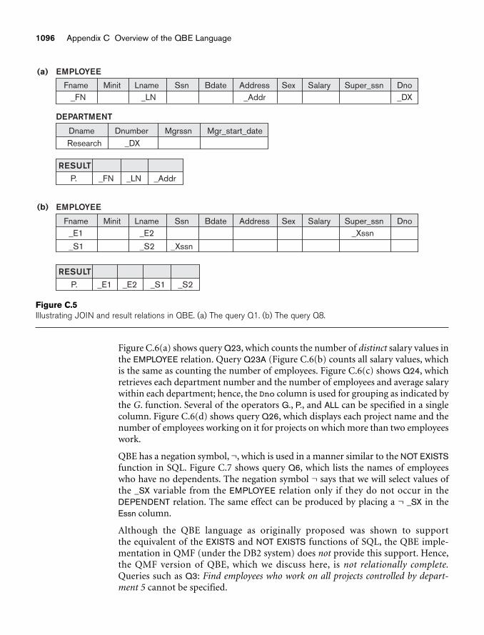
1096 Appendix C Overview of the QBE Language
Figure C.6(a) shows query Q23, which counts the number of distinct salary values inthe EMPLOYEE relation. Query Q23A (Figure C.6(b) counts all salary values, whichis the same as counting the number of employees. Figure C.6(c) shows Q24, whichretrieves each department number and the number of employees and average salarywithin each department; hence, the Dno column is used for grouping as indicated bythe G. function. Several of the operators G., P., and ALL can be specified in a singlecolumn. Figure C.6(d) shows query Q26, which displays each project name and thenumber of employees working on it for projects on which more than two employeeswork.
QBE has a negation symbol, ¬, which is used in a manner similar to the NOT EXISTSfunction in SQL. Figure C.7 shows query Q6, which lists the names of employeeswho have no dependents. The negation symbol ¬ says that we will select values ofthe _SX variable from the EMPLOYEE relation only if they do not occur in theDEPENDENT relation. The same effect can be produced by placing a ¬ _SX in theEssn column.
Although the QBE language as originally proposed was shown to support the equivalent of the EXISTS and NOT EXISTS functions of SQL, the QBE imple-mentation in QMF (under the DB2 system) does not provide this support. Hence,the QMF version of QBE, which we discuss here, is not relationally complete.Queries such as Q3: Find employees who work on all projects controlled by depart-ment 5 cannot be specified.
EMPLOYEE(a)
(b)
Fname Minit Lname Ssn Bdate Address Sex Salary Super_ssn Dno_FN
Research
P. _FN _LN _Addr
_DX
_LN _Addr _DX
DEPARTMENT
Dname Dnumber Mgrssn Mgr_start_date
RESULT
P. _E1 _E2 _S1
RESULT_S2
EMPLOYEE
Fname Minit Lname Ssn Bdate Address Sex Salary Super_ssn Dno_E1 _E2 _Xssn
_S1 _S2 _Xssn
Figure C.5Illustrating JOIN and result relations in QBE. (a) The query Q1. (b) The query Q8.
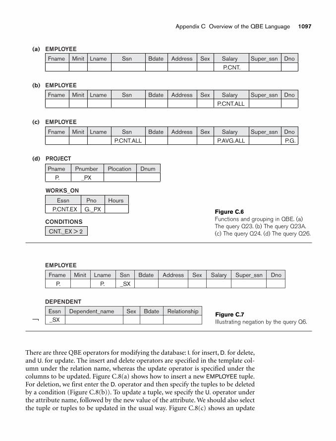
Appendix C Overview of the QBE Language 1097
EMPLOYEE(a)
Fname Minit Lname Ssn Bdate Address Sex Salary Super_ssn Dno
P.CNT.
EMPLOYEE(b)
Fname Minit Lname Ssn Bdate Address Sex Salary Super_ssn Dno
P.CNT.ALL
EMPLOYEE(c)
Fname Minit Lname Ssn Bdate Address Sex Salary Super_ssn Dno
P.AVG.ALL P.G.P.CNT.ALL
PROJECT(d)
Pname Pnumber Plocation
_PXP.
Dnum
WORKS_ON
Essn Pno Hours
P.CNT.EX G._PX
CNT._EX > 2
CONDITIONS
Figure C.6Functions and grouping in QBE. (a)The query Q23. (b) The query Q23A.(c) The query Q24. (d) The query Q26.
There are three QBE operators for modifying the database: I. for insert, D. for delete,and U. for update. The insert and delete operators are specified in the template col-umn under the relation name, whereas the update operator is specified under thecolumns to be updated. Figure C.8(a) shows how to insert a new EMPLOYEE tuple.For deletion, we first enter the D. operator and then specify the tuples to be deletedby a condition (Figure C.8(b)). To update a tuple, we specify the U. operator underthe attribute name, followed by the new value of the attribute. We should also selectthe tuple or tuples to be updated in the usual way. Figure C.8(c) shows an update
EMPLOYEE
Fname Minit Lname Ssn Bdate Address Sex Salary Super_ssn Dno
P. P. _SX
DEPENDENT
Essn Dependent_name Sex Bdate Relationship_SX
Figure C.7Illustrating negation by the query Q6.
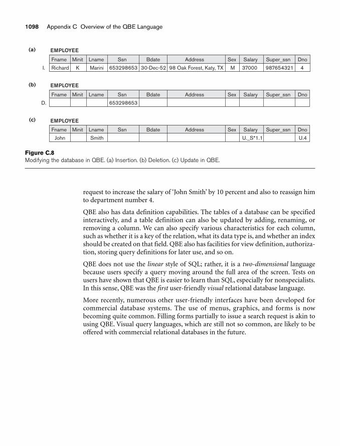
1098 Appendix C Overview of the QBE Language
EMPLOYEE(a)
Fname Minit Lname Ssn Bdate Address Sex Salary Super_ssn Dno
RichardI. MariniK M 37000 987654321 4653298653 30-Dec-52 98 Oak Forest, Katy, TX
EMPLOYEE(b)
Fname Minit Lname Ssn Bdate Address Sex Salary Super_ssn Dno
D. 653298653
EMPLOYEE(c)
Fname Minit Lname Ssn Bdate Address Sex Salary Super_ssn Dno
John Smith U._S*1.1 U.4
Figure C.8Modifying the database in QBE. (a) Insertion. (b) Deletion. (c) Update in QBE.
request to increase the salary of ‘John Smith’ by 10 percent and also to reassign himto department number 4.
QBE also has data definition capabilities. The tables of a database can be specifiedinteractively, and a table definition can also be updated by adding, renaming, orremoving a column. We can also specify various characteristics for each column,such as whether it is a key of the relation, what its data type is, and whether an indexshould be created on that field. QBE also has facilities for view definition, authoriza-tion, storing query definitions for later use, and so on.
QBE does not use the linear style of SQL; rather, it is a two-dimensional languagebecause users specify a query moving around the full area of the screen. Tests onusers have shown that QBE is easier to learn than SQL, especially for nonspecialists.In this sense, QBE was the first user-friendly visual relational database language.
More recently, numerous other user-friendly interfaces have been developed forcommercial database systems. The use of menus, graphics, and forms is nowbecoming quite common. Filling forms partially to issue a search request is akin tousing QBE. Visual query languages, which are still not so common, are likely to beoffered with commercial relational databases in the future.


